Fuel Consumption and Pollutant Emissions of Spark Ignition Engines

During Cold-Started Drive Cycles

Nicholas Julian Darnton

Thesis submitted to the University of Nottingham for the degree of Doctor of Philosophy,

June 1997

Contents List

Abstract Acknowledgements Abbreviations Nomenclature

Chapter 1 Introduction

1.1 Background to Thesis 1.1.1 European Emissions Legislation 1.1.2 The New European Drive Cycle (NEDC) 1.1.3 Fuel Consumption and Emissions During Cold-Start and

Warm-up 1.2 Aims of Work 1.3 Thesis Content

1.3.1 Engine Mapping 1.3.2 Predicting Cold-Start Fuel Consumption and Emissions 1.3.3 Assessment of Model Performance

1.4 Contribution of Thesis to Engine Development

Chapter 2 Characterising Engine Mapping Data Using Neural Networks

2.1 Introduction 2.2 Engine Map Characteristics 2.3 Neural Network Description and Application

2.3.1 Network Configuration to Predict Fuel and Emissions Flow Rates

2.4 Discussion and Conclusions

Chapter 3 Fuel Consumption and Emissions Studies: Literature and Test Facility Description

3.1 Introduction 3.2 Fuel Consumption and Emissions Literature 3.3 Experimental Test Set-up and Procedure

3.3.1 Test Engine and Management System 3.3.2 Engine Monitoring and Control Equipment 3.3.3 Engine Data Acquisition

3.4 Conclusions

Chapter 4 Predicting Fuel Consumption From FuUy-Warm Data

4.1 Introduction

4.2 4.3

4.4

Chapter 5

5.1 5.2 5.3 5.4

Effect of Coolant Temperature on isfc 'Unaccounted For' Fuel During Warm-up 4.3.1 Characterising 'Unaccounted For' Fuel Discussion and Conclusions

Predicting Emissions From Hot Test Bed Data

Introduction Experimental Test Set-up and Procedure Predicting the Effect of ECT on Indicated Specific Emissions Predicting the Effect of Engine Start-up Transients on HC Emissions

5.5 Discussion 5.6 Conclusions

Chapter 6

6.1 6.2

6.3 6.4

Chapter 7

7.1 7.2 7.3

7.4

Chapter 8

8.1 8.2 8.3 8.4 8.5 8.6

Engine Thermal Model to Predict Friction Characteristics

Introduction Modelling Engine Friction Using PROMETS 6.2.1 Friction Power Losses During Steady-State 6.2.2 Friction Power Losses During Warm-up Validation of Friction Model Discussion

Application to Cold Start Drive Cycles to Predict Fuel Consumption and Emissions

Introduction Predicting Drive Cycle Fuel Consumption and Emissions Prediction Accuracy and Sources of Error 7.3.1 Treatment of Idle and Over-Run Conditions 7.3.2 Overall Prediction Accuracy Discussion

Illustration of Factors Influencing Drive Cycle Fuel Consumption and Emissions Performance

Introduction Increased Engine Friction During Warm-Up Poor Mixture Preparation During Warm-Up AFR Mixture Excursions During Throttle Transients Cold-Start Transient Contributions Discussion

Chapter 9 Model Exploitation

9.1 Intoduction 9.2 Case 1: Drive Cycle Definition Effects 9.3 Case 2: Vehicle Effects 9.4 Case 3: Cold-Start Temperature Effects 9.5 Case 4: Engine Calibration Effects 9.6 Case 5: Tail-Pipe After-Treatment Effects 9.7 Discussion

Chapter 10 Discussion and Conclusions

10.1 Discussion 10.2 Further Work 10.3 Conclusions

References Tables Figures

Appendix A ECT Correction Factor Modelling Appendix B Steady-State Friction Model Equations

Abstract

"Fuel Consumption and Pollutant Emissions of Spark Ignition Engines

During Cold-Started Drive Cycles", N J Darnton

This thesis details the development and evaluation of a procedure to predict the

fuel consumption and pollutant emissions of spark ignition engines during

cold-started drive cycles. Such predictions are of use in the early development

and optimisation of an engine and vehicle combination with regard to legislated

limits on vehicle performance over defined drive cycles. Although levels of

pollutant emissions are the main focus of legislation, reducing fuel consumption

is also of interest and drive cycle fuel consumption figures provide a useful

benchmark of vehicle performance appraisals.

The procedure makes use of a combination of engine friction models and

experimentally defined correction functions to enable the application of

fully-warm engine test bed data to cold-start conditions. This accounts for the

effects of engine temperature on friction levels, mixture preparation and start-up

transient behaviour. Experimental data to support the models and assumptions

used are presented and discussed. Although not an essential part of the procedure,

neural networks have been used to characterise the fully-warm engine mapping

data. These are shown to provide an effective way of interpolating between

engine mapping points. To facilitate the prediction of tail-pipe emissions, a

simple catalyst efficiency model has been included and the complete procedure

incorporated into a single software package enabling second-by-second fuel and

emissions flow rates to be predicted for a given engine and vehicle combination

over a defined drive cycle. This package is called CECSP or the Cold Emissions

Cycle Simulation Program. The program has been designed to run on PC

machines.

1

The procedure has been validated by application to a typical 1.8 litre medium

sized vehicle driven over the ECE+EUDC drive cycle and the predictions found

to be within the target accuracy of +/-5% for fuel consumption and +/-10% for

engine-out emissions. Envisaged applications of the procedure to rank the sources

of increased fuel consumption and emissions due to cold-starting and engine and

vehicle details are outlined.

11

Acknowledgements

I would like to express my thanks to Professor Paul Shayler for his advice and

guidance throughout my research work and during the writing of this thesis.

Thanks also go to John McGhee for maintaining the rig and his help throughout

the project and to the rest of the Engines Group, past and present, for their

assistance and humour.

The research has been generously supported by Ford Motor Company and I

would like to thank Dr Tom Ma for his enthusiasm and interest in this research.

Finally, thanks go to my family and friends for their support and encouragement

during my education and, in particular, during the writing of this thesis.

111

Abbreviations

AFR

bmep

CCC

CECSP

co cO2

DOHC

Air/fuel ratio by mass (measured using a UEGO sensor)

Brake mean effective pressure

Close-coupled catalyst

Cold Emissions Cycle Simulation Program

Carbon monoxide

Carbon dioxide

Double overhead camshaft

EC European Community

ECE+EUDC European drive cycle (also termed NEDC)

ECT Engine coolant temperature

EECIV

EGR

EHC

FID

fmep

FTP

HC

HE GO

HO

IMechE

Imep

ISCO

isfc

ishc

LEV

MAP

Electronic engine control unit, version 4

Exhaust gas recirculation

Electrically heated catalyst

Flame ionisation detector

Friction mean effective pressure

Federal test procedure

Hydrocarbons

Heated exhaust gas oxygen

High output

Institute of Mechanical Engineers

Indicated mean effective pressure

Indicated specific carbon monoxide emissions

Indicated specific fuel consumption

Indicated specific hydrocarbon emissions

Indicated specific nitrous oxide emissions

Low emission vehicles

Manifold absolute pressure

IV

MBT Minimum advance for best torque

NEDC New European Drive Cycle

NOx Nitrous oxides

PC Personal computer

RON Research octane number

RPM Revolutions per minute

TDC Top dead centre

TLEV Transitional low emission vehicles

UBC Underbody catalyst

UEGO Universal exhaust gas oxygen

ULEV Ultra low emission vehicles

ZEV Zero emission vehicles

v

Nomenclature

D Catalyst dead time (s)

F Initial friction correction factor

L Catalyst light-off time (s)

Mengine Engine brake torque (Nm)

rna Mass of air induced (kg)

me Mass of recycled exhaust gas (kg)

minj Mass of fuel injected per stroke (kg)

rilf Combusted fuel mass flow rate (g/hr)

rilinj Injected fuel mass flow rate (kg/s)

riloverall Overall fuel mass flow rate (kg/s)

rilunaccounted for Unaccounted for fuel mass flow rate (kg/ s)

N Engine speed (rpm)

nR Number of revolutions per cycle

P Pressure (N/m2)

P Power(W)

Plndicated Indicated power (k W)

Pa Accessory friction power loss (W)

P friction Predicted friction power loss (W)

PKE

Power required to increase vehicle kinetic energy (W)

Pprf Total friction power loss (W)

Prf Rubbing friction power loss (W)

Prl Road load power (W)

RFDR Final drive ratio

R Gear ratio gear

rwheel Driving wheel radius (m)

T Start temperature (OC)

V Volume (m3)

VI

vveh

y

'llcat

'llt

'lltrans

v

Displaced volume per cylinder (m3)

Engine swept volume (m3)

Vehicle speed (km/hr)

Net indicated work (J)

Friction correction factor

Delta HC constant

Fully-warm catalyst conversion efficiency

Catalyst conversion efficiency at time t

Transmission efficiency

Kinematic viscosity (m2/s)

.. VB

Chapter 1

Introduction

1.1 Background to Thesis

Pollution of the environment by emissions from road traffic and competitive

pressures to improve fuel economy are maj or concerns during research and

development efforts on spark ignition engines. With regard to levels of emissions,

vehicle performance is assessed over a drive cycle of operating conditions for

which maximum limits on the masses of particular pollutants have been set by

legislation. These limits have been revised downwards through a series of

amendments to the legislation since the 1970's. In some cases, the test procedure

and drive cycle details have also been revised over the same period. Most

recently, revisions designed to give due weight to the early period of engine

operation, when the engine is not fully-warm and when post-combustion systems

for emissions control may not be operating efficiently, have been debated and

will be fully implemented before the turn of the century.

The current European ECE+EUDC and USA FTP-75 drive cycles are designed

to represent typical patterns of vehicle operation on these continents. For this

reason, and because vehicles must pass tests on emission limits based on these

cycles before introduction to the market, they are particularly important sets of

operating conditions which manufacturers focus attention on during engine and

vehicle development programs. In addition to emissions-related developments,

the same cycles are used to benchmark fuel economy values. However, it is

relatively late in a vehicle development program that final specifications are

available for evaluation, and many critical engineering decisions must be made

prior to this stage.

1

A technique to predict vehicle performance over drive cycles given information

available relatively early on in a development programme has been investigated.

This has major practical applications in, for example, screening possible design

variants for potential impact on vehicle performance. At the outset of the

investigation, no system was available to provide this facility. Of particular

interest has been the problem of predicting the performance of vehicles during the

early part of a drive cycle before the engine is fully-warm. In general terms, the

objective ofthe investigation has been to provide a computer based system for the

prediction of fuel consumption and pollutant emissions, for any specified engine,

transmission and vehicle combination. The computer software which has been

produced is termed CECSP (Cold Emissions Cycle Simulation Program). The

experimental and theoretical studies carried out to develop CECSP, and

applications of this, form the main body of the work described in the thesis.

1.1.1 European Emissions Legislation

The three main pollutant emissions produced by the spark ignition engine are:

Carbon monoxide (CO). This is a colour free, odour free highly poisonous

gas which is readily absorbed into the blood reducing its ability to supply

oxygen around the body. A volumetric concentration of 0.3% can result

in death in humans within 30 minutes.

Unburned Hydrocarbons (HC). These are present as both unburned fuel

and partially reacted fuel components, some of which are known to be

carcinogenic. In certain conditions they react with low level ozone and

nitrogen oxides to form photochemical smog.

Nitrogen Oxides (NO and N02). Generally referred to collectively as NOx

since NO is readily oxidised in air to form N02• N02 is in itself a

poisonous gas but, in addition, it is readily soluble in water forming nitric

acid. Thus, NOx emissions are believed to cause acid rain which is

2

thought to cause damage to both vegetation and buildings.

The bulk of the exhaust gases are made up of nitrogen, carbon dioxide and water.

Although non-poisonous, carbon dioxide emissions are believed to contribute to

the "green-house effect". These may become the focus of future emissions

legislation. However, the strictest legislation deals with emissions ofHC, CO and

NOx and requires manufacturers to ensure tail-pipe emissions of vehicles are no

more than a prescribed limit for a carefully defined vehicle operating regime or

drive cycle. The legislation defines the exact drive cycle for the vehicle

performance to be assessed over and certain conditions which must apply to

enable test results to be representative for different vehicles and manufacturers.

Vehicle exhaust emissions have been the focus of European legislation ever since

the 1970's when a British Standard to limit 'visible' emissions was incorporated

into an EC Directive [1.1]. As road traffic has increased the legislation has been

tightened in response to environmental concerns and with the aim of bringing

European legislation in line with the more stringent US standards. In 1985, the

so-called 'Luxembourg Agreement' marked a significant step in European

emissions legislation as it effectively ensured that catalytic convertors would be

required to meet future emissions standards in Europe, as had been the case in the

USA for several years. The agreement culminated in the adoption ofEC Directive

911441IEEC [1.2]. This directive finally brought European legislation in line with

US 1983 emissions standards. US legislation has typically been led by the State

of California and in September 1990, the California Air Resources Board

(CARB) introduced further legislation cutting the allowed emissions of new

vehicles substantially in a series of stages, as shown in Table 1.1. In Europe, new

legislation and proposals aimed at tightening the regulations defined in EC

Directive 911441IEEC have already been introduced, as shown in Table 1.2. The

proposed stages 3 and 4 of the European legislation, to be introduced in 2000 and

2005, are expected to bring European requirements in line with the Californian

ULEV standard to be introduced in 1997. Different approaches are used to

3

determine the emissions levels from actual motor vehicles for comparison with

the allowed limits in the United States and Europe. In the US, the Federal Test

Procedure (FTP) is used while in Europe emissions are evaluated using the New

European Drive Cycle (NEDC) also known as the ECE+EUDC drive cycle.

Although different in detail, these two cycles both define a series of engine idling

and loading repeated in a manner to define a vehicle speed characteristic

representative of the typical driving behaviour experienced by production

vehicles. In addition to the drive cycle profile, the start-up temperature of the

engine and allowed conditioning time before emission sampling begins is

carefully defined with the intention of producing a repeatable test procedure

which accurately represents the relative performance of a wide range of vehicles

from different manufacturers. For the purpose of this work, the NEDC has been

used in accordance with current and proposed European emissions legislation

already discussed.

1.1.2 The New European Drive Cycle (NED C)

The NEDC consists of an elementary urban cycle repeated four times followed

by the extra-urban cycle as shown in Figure 1.1. Each of the elementary cycles

last 195 seconds and the extra-urban cycle lasts 400 seconds giving a total cycle

length of 1180 seconds. The cycle is defined as a series of vehicle speed and gear

number points with gear changes defined at appropriate points in the cycle,

according to EC Directive 9114411EEC. Suitable tolerances are defined in the

legislation for both vehicle speed and time from start to ensure cycle repeatability

is maintained to as high an accuracy as possible. Current European legislation

(EC Stage 2) defines a start/soak temperature of between 20°C and 30°C and

permits a period of 40 seconds of engine idling before emission sampling begins,

as illustrated in Figure 1.1. Possible changes to this procedure are currently under

consideration and could include the removal of the initial conditioning period and

a reduction ofthe start/soak temperature [1.4]. CARB have already adopted cold­

start CO legislation at a test temperature of -7°C for current technology vehicles

although it is not yet known if the ULEV legislation will require this test

4

temperature. In Europe, it is thought more likely that the start/soak temperature

will eventually be reduced to between O°C and 5°C to reflect patterns of vehicle

use and operating conditions in northern Europe more accurately without

imposing the additional costs on industry of sub-zero test temperatures. Current

proposals, however, suggest that test cycle modifications will be limited to the

elimination of the 40 second conditioning period [1.5]. In addition, individual

targets for HC and NOx are to be introduced from Stage 3 onwards instead of a

single target for HC+NOx'

1.1.3 Fuel Consumption and Emissions During Cold-Start and Warm-up

The current European drive cycle includes a cold-start from a soak temperature

of between 20°C and 30°C and as such is designed to represent a typical urban

journey starting with a cold engine. The vehicle speed and gear number profile

adopted for all light-duty vehicles does not account for variations in driving style

and the different manner in which vehicles of varying performance are likely to

be driven, as discussed by Andre et al [1.6]. Work done as part of the EC DRIVE

program may result in a modified drive cycle format, but currently the

ECE+EUDC drive cycle is believed to provide the most representative emissions

performance comparisons between vehicles and as such is used extensively in the

work presented in this thesis. Given that all European vehicles are assessed over

the same drive cycle under the same operating conditions, techniques for reducing

total emissions production over this drive cycle are of paramount interest to

manufacturers. Whilst pollutant emissions are of primary importance, fuel

consumption is of increasing interest and provides a useful benchmark for vehicle

performance appraisals. Work done at the University of Melbourne [1.7] indicates

that for hot-start operation the main influences on fuel consumption and exhaust

emissions are vehicle acceleration and speed, revealing the importance of overall

vehicle mass and choice of transmission ratios when applied to the fixed vehicle

speed profile of the ECE+EUDC drive cycle. However, the primary area of

concern in the current drive cycle is the initial period following the cold-start

when various effects combine to give both poor fuel economy and increased

5

emission levels. This period contributes significantly to actual overall vehicle

pollution in northern Europe. It has long been established that vehicle exhaust

emissions from vehicles fitted with catalytic convertors are at their highest in the

period immediately following a ,cold-start before catalyst light-off occurs, and

that the driving conditions which yield the greatest adverse effects on emissions

are at low ambient temperature and during urban driving [1.8]. Results from the

United States Department of Energy show that vehicles used for short cold-start

trips consume fuel at a much higher average rate than during long trips, and that

the effect is magnified with decreasing ambient temperatures [1.9]. Furthermore,

averaged over weekday trips in the 100 largest metropolitan areas in the United

States, fuel consumption is between 13% and 17% higher than it would be if fuel

consumption rates during engine warm-up were those of fully-warm vehicles

[1.10]. Approximately one third of all motor vehicle travel in the United States

consists of trips no more than ten miles in length [1.11]. A similar picture exists

in Europe, where the bulk of weekday travel occurs in urban areas and starts with

a cold engine. In fact, according to Andre, approximately one third of all journeys

start with a cold engine (coolant and oil temperatures below 30°C) and a similar

proportion are completed before the engine is fully-warm [1.12]. Thus the

cold-start element of the European drive cycle is of vital significance to the

overall fuel consumption and emissions produced over the cycle period, since the

relative contribution of pollutants emitted during vehicle warm-up has been

magnified due to the outstanding performance of modem catalytic convertors

nearly eliminating pollutants emitted from fully-warm engines. This is most

important when considering tail-pipe exhaust emissions, particularly those ofHC,

as more than 80 per cent of these are generated in the warm-up phase before the

catalytic convertor has reached its normal operating temperature [1.13]. The

principle sources of HC emissions in the exhaust pipe have been reviewed by

Heywood et al [1.14]. These can be summarised as follows:

Release ofHC from narrow crevice volumes within the cylinder where

the combustible mixture escapes burning because the flame cannot

penetrate into these narrow volumes.

6

Flame quenching by the cold cylinder walls, resulting in the appearance

of a thin layer of unburned mixture adjacent to the relatively cold surfaces

in the combustion chamber.

Absorption of fuel hydrocarbon components into thin oil layers in certain

parts of the cylinder before combustion takes place and subsequent

desorption at a later stage in the cycle.

Leakage past the exhaust valve between compression and combustion.

This effect is particularly significant in high mileage vehicles where worn

valves and valve seats can lead to significant leakage.

Presence of liquid fuel on the combustion chamber walls during early

seconds of engine operation after a cold-start escaping combustion and

passing directly into the exhaust stream. Further work by Heywood [1.15]

suggests that liquid fuel films around the inlet valve can last for periods

in the region of 60 seconds after a 20°C start.

Work by Shayler et al [1.16] suggests that poor mixture preparation in the

inlet manifold due to injector location and intake geometry can lead to a

degree of mixture stratification in the cylinder resulting in some fuel rich

mixture escaping combustion and entering the exhaust pipe.

Each of the above mechanisms have a different effect on total HC emissions

depending on the operating conditions and state of the engine with the result that

HC emissions are poorly understood and difficult to predict, particularly in the

period immediately following a cold-start.

1.2 Aims of Work

The aims of developing CECSP and the associated procedures to apply this are

to predict fuel and engine-out emission mass flow rates on a second-by-second

basis for the ECE+EUDC drive cycle and other patterns of operating conditions

which might be specified. The procedure was to require only fully-warm engine

mapping data to characterise the engine under consideration and the vehicle was

to be defined by inputing appropriate definition parameters. As such, the

procedure was intended to provide a means of determining to within a target

7

accuracy of 10% both the expected fuel consumption and engine-out (also tenned

feedgas) emission levels expected for a given engine/vehicle combination and the

effects on these values of changing the various engine, vehicle and drive cycle

variables modelled.

For a cold-start drive cycle, fuel consumption and engine-out emISSIOns,

particularly those ofHC, are influenced by the increased friction levels and fuel

enrichment associated with the cold-start and warm-up process. Engine-out

emission production mechanisms, particularly those for HC emissions, are

involved and complex. Tail-pipe emissions are influenced by the time taken for

the catalyst to reach its normal operating temperature and by the conversion

efficiency of the catalyst itself. In addition, actual vehicle and drive cycle details,

such as total weight, transmission ratios and aerodynamics, will influence the

total fuel consumption and emission levels. Thus, improvements in vehicle drive

cycle emission performance can come from many different areas of both engine

and vehicle design. The prediction procedure was intended primarily to enable the

effects on total fuel consumption and engine-out emissions ofHC, CO and NOx

of changing various vehicle and drive cycle parameters to be examined for both

a fully-wann and cold-started drive cycle. Once engine-out emissions have been

predicted, tail-pipe values can be calculated from basic knowledge of catalyst

light-off and conversion performance.

CECSP uses fully-wann steady-state dynamometer data to characterise the engine

fuel and emissions perfonnance for the required operating conditions imposed by

the drive cycle under consideration. In general, engine maps are produced for

fully-warm operating conditions, which are most easily controlled and provide

the bulk of the infonnation needed for engine development. In addition, these

maps are usually available at an early stage of engine development and so

predicting drive cycle performance from such maps will enable drive cycle

perfonnance of pre-production vehicles to be assessed early in their development

period. Figure 1.2 shows a brief outline of the procedure. A simple road load

8

model is used to deduce engine speed and brake load from a given vehicle and

drive cycle description. An engine thermal model is used to predict engine

friction levels on a second-by-second basis throughout the drive cycle for both a

fully-warm start and a cold-start enabling indicated loads to be calculated, and

then the fully-warm indicated engine map is used to deduce instantaneous fuel

and emission mass flow rates. The emissions mass flow rates then need to be

adjusted to account for the expected changes during engine warm-up and both the

fuel and emissions flow rates adjusted to account for the transient effects

associated with a cold-start. This procedure relies on several assumptions and

engine models derived from experimental data. Figure 1.3 shows the inputs

required and a brief summary of the route to achieve the desired outputs.

1.3 Thesis Content

This thesis deals with the various concepts and models which need to be

combined to produce the final drive cycle prediction procedure. The following

sections detail each of these and how this thesis covers the work done in

developing the procedure.

1.3.1 Engine Mapping

The prediction procedure outlined in Figure 1.2 is based on the assumption that

fully-warm engine mapping data will be used to characterise the engine under

consideration. Fully-warm data is generally available even at an early stage in

engine development. In order to use this to determine fuel and emissions mass

flow rates at non-fully warm operating conditions the effects of differences

between fully-warm and warm-up conditions on performance must be accounted

for. A key step towards this is to recast the engine data, based on the rationale

given in Chapter 4, into indicated operating conditions. The indicated mean

effective pressure (imep), defined as the total work done by the engine is

calculated from the brake mean effective pressure as:

9

hnep = bmep + frnep (1.1)

where finep is the friction mean effective pressure. Thus, if the finep at each point

in the cold-start drive cycle is determined, it should be possible to infer the fuel

and emissions flow rates from the fully-warm engine map, providing the effect

of engine temperature on the relationship between indicated operating conditions

and exhaust flow rates can be defmed. Although not essential, in this application

a neural network has been used as a simple way of characterising the engine map

and interpolating between the fixed fully-warm engine mapping points to

determine fuel and emissions mass flow rates at each point in the drive cycle.

Chapter 2 deals with the engine mapping data processing and details the

application and optimisation of the neural network to characterise the engine map.

1.3.2 Predicting Cold-Start Fuel Consumption and Emissions

In order to apply the fully-warm indicated operating map to the indicated load

profile of the cold-start drive cycle, the effect of both engine operating

temperature and the transient effects of start-up on the indicated engine operating

map has to be established. Chapter 4 deals with the influence of engine coolant

temperature on fuel consumption and the development of a model to predict the

increase in fuel consumption during and immediately following a cold-start.

Chapter 5 deals with the corresponding effect on engine-out exhaust emissions

with particular attention being paid to the increase in HC emissions during the

early minutes of engine operation. When applying the fully-warm engine map to

the cold-started drive cycle, the engine management calibrations for parameters

such as spark timing and EGR rate are, for simplicity, assumed to be identical to

the fully-warm calibration.

Predicting the increased engine friction and engine temperature distribution

during the cold-started drive cycle is achieved by using a program for modelling

engine thermal systems called PROMETS [1.17] previously developed at the

University of Nottingham. Chapter 6 details the basic structure and validation of

10

this model and its application to the drive cycle prediction procedure. Chapter 7

outlines the combination of the various elements of the prediction procedure that

comprise CECSP.

1.3.3 Assessment of Model Performance

Chapters 8 and 9 detail applications of the CECSP software. The flexibility of the

prediction software is investigated and its application to various possible

engine/vehicle development programs illustrated. The effect of changes to

engine/vehicle details such as total vehicle mass, transmission ratios and engine

management strategy are discussed and possible future applications of the

procedure suggested. Initially developed to predict engine-out emissions, the

extension to predict tail-pipe emissions and account for appropriate

after-treatment considerations is considered and the implication of the various

proposed drive cycle changes investigated. The use of the software to prioritise

the principle sources of emissions during the ECE+EUDC drive cycle, and

possible areas of emissions reduction, is demonstrated.

1.4 Contribution of Thesis to Engine Development

The main objective of the work presented in this thesis was to develop a simple

prediction procedure, based on fully-warm dynamometer test-bed data, to predict

to within a target accuracy of 10% the total fuel consumption and engine-out

emissions produced for a typical drive cycle. The work has resulted in the

production of a software package (CECSP) which predicts fuel and emissions

mass flow rates at each point in a defined drive cycle for given engine fully-warm

mapping data and defined vehicle characteristics. The procedure requires no cold

engine data and assumes that fully-warm engine calibration settings apply

throughout the drive cycle, and as such provides a useful approximation of

expected drive cycle performance for a loosely defined engine and vehicle

combination. The procedure enables the relative effects of changing many engine

and vehicle parameters to be examined and as such could be used to prioritise

areas of performance improvement during vehicle development. In addition, the

11

requirement of fully-warm engine mapping data only means that the procedure

can be used at an early stage of engine development to predict expected drive

cycle results before engine and vehicle design parameters are fixed and before

experimental measurements can be taken.

12

Chapter 2

Characterising Engine Mapping Data Using

Neural Networks

2.1 Introduction

Details of how fully-warm engine performance maps have been exploited in the

modelling of cold-started drive cycle conditions will be described in later

chapters. As a precursor to this, general trends in fully-warm steady-state engine

behaviour and how these can be characterised in a suitable form are described

here. In particular, the use of neural networks to relate independent and dependent

engine state variables is considered. Although this is not an essential part of the

model representing the physical processes involved, this form of data handling

plays an important role in enabling efficient use of the model.

The major operating variables that influence spark ignition engine performance

are engine speed, load, air/fuel ratio (AFR) , spark timing and exhaust gas

recirculation rate (EGR) [2.1]. The engine mapping data used in the work

presented here has been derived from engines mapped with production engine

management strategies. Hence the spark timing and EGR rate for a given engine

speed, load and AFR during fully-warm operation are fixed by the strategy and

so the engine variables of interest are limited to these three. The maj or part of this

chapter deals with characterising engine mapping data in terms of just engine

speed, load and APR and assumes that the spark timing and EGR rate are

determined by the engine management strategy, since engine data in this format

was readily available. However, in order to provide a more complete picture of

engine map characterisation, the effect of changing the spark timing and EGR rate

calibrations is also be considered here. This requires a much larger and more

13

complex engine map database but such an engine map could then be used to

enable the effects of changing spark timing and EGR rate during a cold-started

drive cycle to be assessed.

Previous work carried out by Bacon [2.2, 2.3] has demonstrated that providing

patterns exist within a sequence of data values, neural networks can be used to

associate these with a corresponding set of input values. Neural network

computing was originally conceived as a model for the brain and, as such, neural

networks comprise several interconnected processing units connected in parallel.

In essence, a neural network 'learns' the relationship between input and output

parameters in a process called 'training'. The trained neural network can then be

used to generate output values for input patterns not included in the training data.

Bacon used a neural network to emulate certain elements of a current engine

control strategy and found the interpolation and extrapolation accuracy to be high.

In particular, the neural network approach was found to provide a significant time

saving when compared to the standard control algorithm development times.

Work by Stevens et al [2.4] demonstrated the use of neural networks to determine

relationships between engine-out emissions and engine state variables and

concluded that very accurate predictions of engine performance could be made

providing the engine database was sufficiently large to characterise the engine

performance map. Hence, neural networks provide a simple, time saving,

alternative to regression analysis to characterise engine mapping data. In the work

presented in this thesis a neural network has been optimised to predict fuel

consumption and emissions as a function of engine speed, load and APR. In

addition, work has been carried out to investigate the possibility of using a neural

network to simulate a complete engine map with engine speed, load, APR, spark

timing and EGR rate as the inputs. The characteristics of the engine maps used

are given below. In addition, a brief description of neural networks and an

overview of their application to engine mapping is given. A comprehensive

introduction to the theory and application of neural network processing

techniques can be found in publications by Rumelhart and McClelland [2.5-2.7].

14

2.2 Engine Map Characteristics

The engine mapping data are generally available as a series of steady-state

fully-warm brake load sweeps at a range of engine speeds and AFRs. The engine

performance parameters of interest here are fuel, HC, CO and NOx

mass flow

rates. In order to keep the amount of data to be handled to a minimum the range

of engine speeds and loads covered by the mapping data was restricted to that

imposed by the ECE+EUDC drive cycle. By way of illustration, the results used

in this chapter are taken from a 1.8 litre Ford Zetec engine. This 4-valve per

cylinder engine is representative of engines currently in service and is designed

to operate at stoichiometric mixture setting at most operating conditions. First,

the influence of operating conditions for fixed tail-pipe AFR mixture calibration

is considered. Figures 2.1 and 2.2 show a typical dataset plotting fuel and

emissions against engine speed and brake load for stoichiometric AFR operation

and with spark timing set to MBT (Minimum advance for Best Torque). Fuel

mass flow rates increase with both engine speed and load in proportion to air

mass flow rate increases, to maintain a constant stoichiometric tail-pipe AFR.

Similarly, CO mass flow rates increase uniformly with both engine speed and

load because CO concentrations are effectively dependent only on the AFR,

which is constant. HC and NOx emissions behave less uniformly due to the

variation in volumetric concentration with both engine speed and load.

Consequently, the HC and NOx mass flow rates do not follow the fuel mass flow

rate variations as closely as the CO flow rates.

A more detailed picture of the effect of operating conditions on engine-out

emissions can be obtained by considering emission concentrations. Again

considering only stoichiometric mixture settings, the effect of engine speed and

indicated load on HC emissions concentrations is shown in Figure 2.3. The HC

formation mechanisms, discussed in Chapter 1, are sensitive to both engine speed

and load. Whilst the way engine speed and load effect the various formation

mechanisms is difficult to describe in quantitative terms the observed trends are

attributable to a trade-off between combustion temperature and in-cylinder and

15

exhaust residence times [2.1]. Increasing engine speed at constant indicated load

results in increased gas temperatures in both the expansion and exhaust strokes

due to the reduced significance of heat transfer from the cylinder. This results in

more oxidation of unbumt HC which more than offsets the reduced residence

time in the cylinder and exhaust system. Consequently, unbumt HC emissions

decrease with increasing engine speed. Similarly, when increasing indicated load

at constant engine speed, gas temperature increases offset the effect of reduced

residence time resulting in a slight decrease in HC emissions.

Figure 2.4 shows the effect of engine speed and brake load on NOx emissions and

shows it to be the opposite of that for HC emissions. NOx concentrations increase

both with increasing engine speed and indicated load. As discussed above,

increasing both engine speed and indicated load results in increased combustion

temperature due to the reduced significance of heat transfer. In addition, increases

in in-cylinder pressure result in increased combustion temperature and these

effects combine to have a direct effect on NOx emissions which are extremely

sensitive to combustion temperature.

The engIne data presented in Figures 2.1 to 2.4 were all obtained with a

stoichiometric tail-pipe AFR. The third and fmal engine variable of interest in the

engine maps to be characterised here is AFR, since emission concentrations are

particularly sensitive to this parameter. Figure 2.5 [2.1] shows (not to scale) the

variation ofHC, CO and NOx emissions of a typical spark ignition engine with

AFR. HC emissions decrease as the AFR is progressively increased and more and

more of the injected fuel is oxidised. However, eventually the mixture becomes

too lean to bum and partial misfiring occurs causing the HC emissions to rise

again. CO emissions also reduce with increasing AFR as combustion becomes

increasingly complete and the carbon in the fuel is increasingly oxidised to CO2.

This effect is particularly significant when the AFR is richer than stoichiometric

as oxidation is limited by lack of oxygen and so any increase in oxygen levels

will significantly affect the completeness of combustion. As mentioned above,

16

NOx emissions are governed by combustion temperature and so peak when the

AFR is just lean of stoichiometric when the combustion temperature is at its

highest. NOx emissions then reduce uniformly with AFR either side of this peak.

The combined effects of engine speed, load and AFR on the emissions produced

by a spark-ignition engine is that engine emissions performance maps are more

complex than the fuel consumption map. In order to characterise these engine

performance variations with engine speed, load and AFR a neural network has

been used to 'learn' the experimental engine data and enable the interpolation of

fuel and emissions flow rates at points within the boundaries defined by the

experimental data.

The engine data considered so far has been obtained with MBT spark timing and

no exhaust gas recirculation. Both these variables, like AFR, are generally fixed

by the engine management strategy. However, if a complete engine map is to be

simulated the effect of all the engine operating variables on fuel and emissions

flow rates must be considered.

The spark timing in an engine cylinder determines at what point in the engine

cycle combustion begins. If combustion starts too early the work transfer from the

piston at the end of the compression stroke on the combusting gases is too large,

and results in an excessively high in-cylinder gas temperature causing

pre-ignition of the remaining air/fuel mixture in a phenomenon often called

'knock'. If combustion starts too late, the peak cylinder pressure is reduced and

the expansion stroke work transfer from the gas to the piston decreases [2.1]

resulting in reduced brake torque. Consequently, MBT spark timing gives the

maximum brake power and minimum brake specific fuel consumption.

Deviations from MBT spark timing influence fuel consumption and emissions

performance through changes in combustion gas temperature and exhaust gas

temperature. Retarding spark timing from the optimum (reducing the spark

advance relative to TDC) results in lower combustion temperatures and higher

17

exhaust gas temperatures because combustion takes place later in the expansion

stroke of the engine. Therefore, retarding spark timing relative to MBT reduces

NOx emissions (due to reduced combustion temperature) and also reduces He

emissions (due to increased exhaust gas temperatures).

Exhaust gas recirculation (EGR) is used to reduce NOx emissions. The system

involves recycling a fraction (typically up to 30%) of the exhaust gases from the

exhaust to the intake system. This gas then acts, along with the normal residual

gas fraction from the previous engine cycle, as a diluent resulting in reduced

combustion temperature without significantly affecting the combustion AFR.

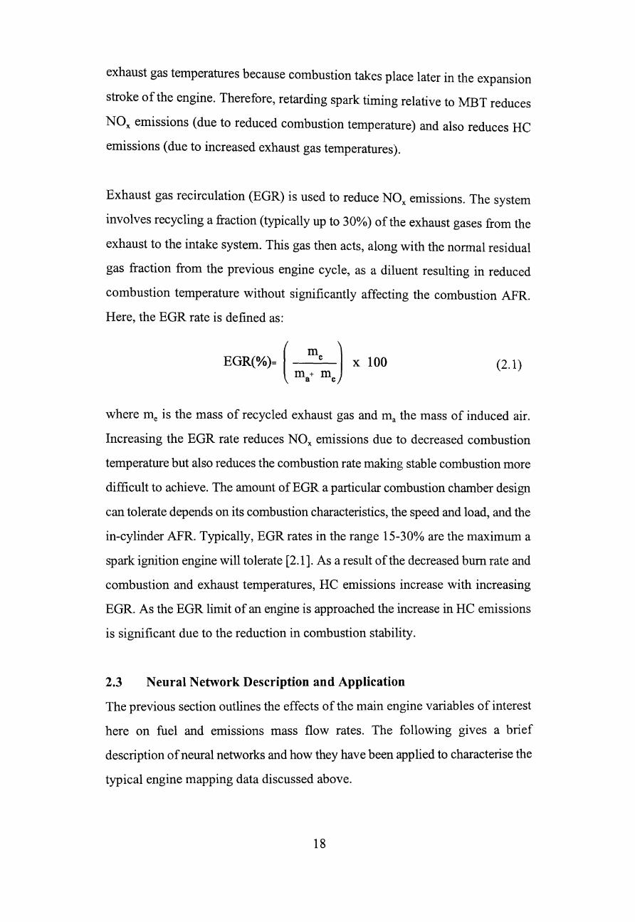
Here, the EGR rate is defined as:

EGR(%)= ( me ) X 100 m+ m a e

(2.1)

where me is the mass of recycled exhaust gas and rna the mass of induced air.

Increasing the EGR rate reduces NOx emissions due to decreased combustion

temperature but also reduces the combustion rate making stable combustion more

difficult to achieve. The amount of EGR a particular combustion chamber design

can tolerate depends on its combustion characteristics, the speed and load, and the

in-cylinder AFR. Typically, EGR rates in the range 15-30% are the maximum a

spark ignition engine will tolerate [2.1]. As a result of the decreased bum rate and

combustion and exhaust temperatures, He emissions increase with increasing

EGR. As the EGR limit of an engine is approached the increase in He emissions

is significant due to the reduction in combustion stability.

2.3 Neural Network Description and Application

The previous section outlines the effects of the main engine variables of interest

here on fuel and emissions mass flow rates. The following gives a brief

description of neural networks and how they have been applied to characterise the

typical engine mapping data discussed above.

18

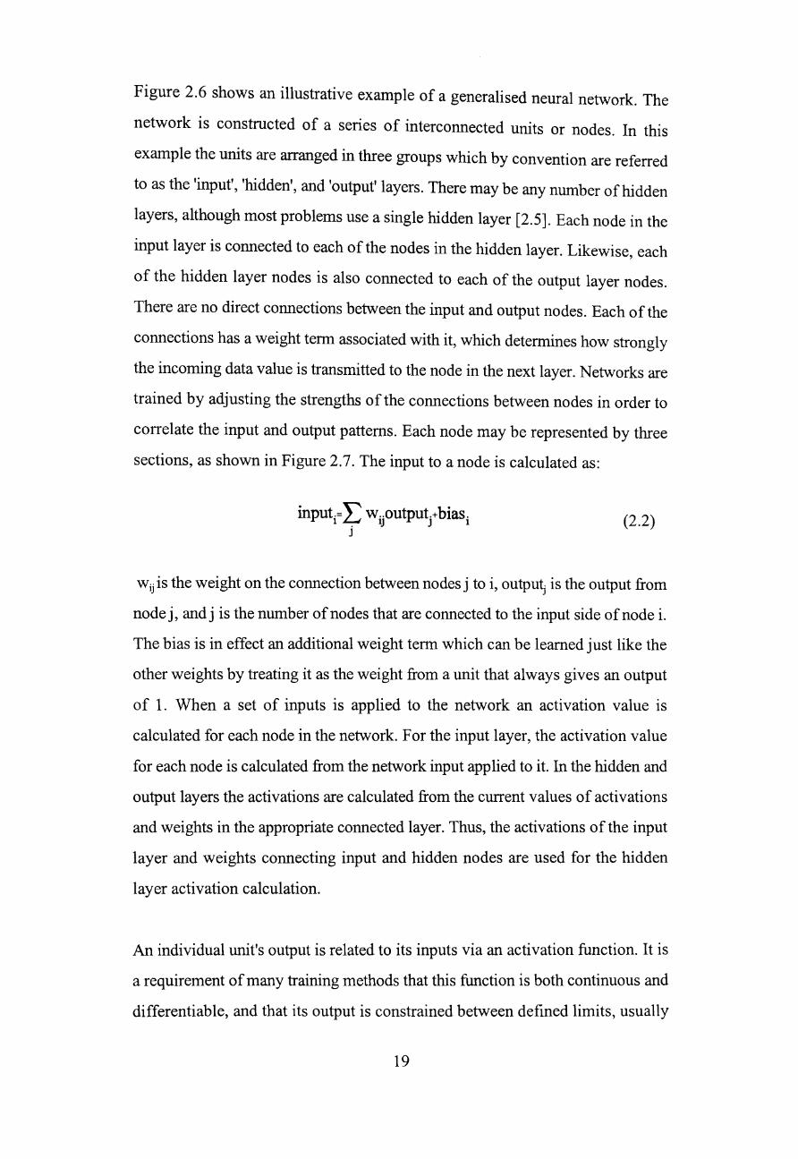
Figure 2.6 shows an illustrative example of a generalised neural network. The

network is constructed of a series of interconnected units or nodes. In this

example the units are arranged in three groups which by convention are referred

to as the 'input', 'hidden', and 'output' layers. There may be any number of hidden

layers, although most problems use a single hidden layer [2.5]. Each node in the

input layer is connected to each of the nodes in the hidden layer. Likewise, each

of the hidden layer nodes is also connected to each of the output layer nodes.

There are no direct connections between the input and output nodes. Each of the

connections has a weight term associated with it, which determines how strongly

the incoming data value is transmitted to the node in the next layer. Networks are

trained by adjusting the strengths of the connections between nodes in order to

correlate the input and output patterns. Each node may be represented by three

sections, as shown in Figure 2.7. The input to a node is calculated as:

input.= ~ w .. output.+bias. 1 L.; IJ J 1

j (2.2)

Wij is the weight on the connection between nodes j to i, outpu~ is the output from

node j, and j is the number of nodes that are connected to the input side of node i.

The bias is in effect an additional weight term which can be learned just like the

other weights by treating it as the weight from a unit that always gives an output

of 1. When a set of inputs is applied to the network an activation value is

calculated for each node in the network. For the input layer, the activation value

for each node is calculated from the network input applied to it. In the hidden and

output layers the activations are calculated from the current values of activations

and weights in the appropriate connected layer. Thus, the activations of the input

layer and weights connecting input and hidden nodes are used for the hidden

layer activation calculation.

An individual unit's output is related to its inputs via an activation function. It is

a requirement of many training methods that this function is both continuous and

differentiable, and that its output is constrained between defined limits, usually

19

o and 1. For these reasons the sigmoid function is normally employed, and the

activation a; is thus:

1

(l + e -inputi ) (2.3)

The calculation of the output proceeds through all the units of each layer

simultaneously, starting with the input layer and finishing with the output layer.

The activation is computed for each unit in the input layer and the activations for

the next layer are then calculated from the known connection weights and

activations of the previous layer. This process is carried out for each layer until

the output layer is reached and the network outputs calculated. Providing each

layer is fully calculated before the next layer is started, this method of

propagating the signals forward through the network mimics the desired parallel

processmg.

During the training process, the network learns to associate the required outputs

with the defined inputs in the training data. Details of the training process used

are given by Bacon [2.2] and summarised in Table 2.1. Several procedures are

available for modifying the weights during network training. The most common

of these, and the one used here, is the 'Back Propagation' or BP method. This

method adjusts the weights that contribute significantly to the error calculated

between the desired and actual output values in order to reduce the error. The

training patterns are presented to the network randomly and each complete pass

of the training samples is called an epoch. The number of iterations, or epochs,

used during training can be set to an absolute number or, alternatively, the

process may be set to iterate until the total error for all the input patterns in the

training set is below a pre-defined threshold value. This total error is calculated

as the sum of the squared errors in each of the outputs for all the patterns in the

training dataset. Once the error threshold is reached, the weight values represent

an optimised solution ofthe relationship between the input and output pairs in the

training data. The accuracy of the solution can then be assessed by direct

20

comparison of the desired and actual output values for each input pattern.

2.3.1 Network Configuration to Predict Fuel and Emissions Flow Rates

The network configuration to predict fuel consumption, HC, CO and NOx

emissions from engine speed, imep and AFR inputs requires a three node input

layer and a four node output layer. The network inputs were limited to these three

because the bulk of the engine data available were obtained with MET spark

timing and calibrated EGR rates. It is generally accepted that a certain degree of

trial and error is required when selecting a neural network configuration for a

particUlar problem [2.6]. Of particular interest here was the size of the hidden

layer and the number of training epochs to use in order to provide the most

accurate solution. The training time is sensitive to both hidden layer size and the

number of training epochs and so a trade-off exists between network accuracy

and network training time.

In order to determine the optimum size of the hidden layer and the minimum

number of training epochs to provide the desired training accuracy, a series of

network configurations were examined. Figure 2.8 shows the effects of hidden

layer size and number of training epochs on the correlation coefficient between

predicted and target outputs. The engine data used were for a 1.8 litre Ford Zetec

engine, as shown in Figures 2.1 and 2.2, and consisted of around one hundred

input patterns covering the range of engine speeds from idle to 4000 rpm in steps

of 500 rpm, and brake loads from 0 to 120 Nm in steps of 10 Nm, all at

stoichiometric AFR. To determine the accuracy of output values, for data

examples used during training, and separately for other examples not used during

training, the dataset was split into two sets of cases. The training data set

consisted of around 800/0 of the total number of input and output pattern pairs and

was used to train the neural network. The remaining data patterns were not used

to train the network but were used after training to confirm the accuracy of the

network predictions at 'unseen' data points. The prediction accuracy at these

points was of particular interest because these represent the drive cycle operating

21

conditions at which fuel and emission flow rates need to be inferred from the

training data. The training data was scaled to lie in the range 0.1 to 0.9 as the

network can only manipulate input and output values within a range of 0 to 1.

Scaling the data between 0.1 and 0.9 avoids the network having to predict values

at the extreme limits of 0 and 1 which would require extreme connection weights

between nodes. Simple linear regression analysis was then used to determine the

correlation coefficient between predicted and target output values. All the

network preparation and results processing together with the network training

have been carried out on an IBM compatible 486 PC. The results for fuel mass

flow rates are given in Figure 2.8 and indicate that, for this database

configuration, the optimum hidden layer size is 20 nodes and the best training

accuracy is obtained after 10,000 training epochs. Predicted and target scaled fuel

and emission mass flow rates for the training and validation data are shown in

Figures 2.9 to 2.12. The closest agreement between target and predicted values

can be seen to occur for fuel mass flow rates but in all cases the prediction

accuracy is within +/- 10%. The prediction accuracy at the 'unseen' validation

points is as good as that at data points used to train the network.

Additional work has been carried out to investigate if the neural network

approach used here could be extended to account for changes in the spark timing

and EGR calibrations used on the test engine. This involved training a neural

network with five inputs, instead of three, on a much bigger database. The engine

data used were for a 1.6 litre Zetec engine and, although the data did not cover the

complete range of values required during engine calibration, it did enable the

possibility of using a neural network to predict the effect of spark timing and

EGR rate on engine emissions performance to be examined. The network used

had five input nodes and a hidden layer size of 80. The engine database consisted

of around 1600 data points, all of which were used to train the neural network.

The results of the network training are shown for HC and NOx emissions in

Figures 2.13 and 2.14 respectively. The prediction accuracy is generally within

+/-100/0, as for the simpler engine map, which suggests that a neural network is

22

capable of characterising the more complex engine map successfully. The trained

neural network was then used to demonstrate the effect of both EGR rate

(Figure 2.15) and spark timing relative to MBT (Figure 2.16) on HC and NOx

emissions. The predictions reflect the expected trends (discussed above) in engine

performance.

2.4 Discussion and Conclusions

Before fuel consumption and emission mass flow rates at each point in the

ECE+EUDC drive cycle can be determined, a full engine map covering all

possible operating conditions has to be inferred from a much smaller set of

fully-warm engine data. For the work in this thesis, the engine operating variables

of interest are engine speed, brake and hence indicated load, and AFR. Other

engine variables, such as spark timing and EGR rate, are determined by the

engine mapping data and are fixed by the control strategy on the test engine.

Initially, fuel and emissions flow rates have been predicted from engine speed,

load and AFR information for fully-warm engine mapping data with a fixed spark

timing and EGR rate calibration.

In order to characterise the engine mapping data, a neural network has been used

to 'learn' the engine map and enable fuel and emissions flow rates to be

determined at all points within the boundaries of the engine mapping data. A

degree of trial and error is required when optimising the configuration of a

network to obtain the best training performance and this resulted in the selection

of a 20 node hidden layer and a minimum of 10,000 training epochs for this

application. Such a network is capable of predicting fuel and emissions flow rates

to within +/-10% of the training data using engine speed, load and AFR as inputs.

The network prediction accuracy at operating conditions from within the range

of engine speeds and loads covered by the training data is equally good. This

suggests that fuel and emissions mass flow rates can be predicted to within

+/-100/0 for all operating conditions bounded by the data used to train the neural

network.

23

The possibility of extending the neural network approach to a more complicated

engine map, using spark timing and EGR rate as additional input variables, has

been investigated. A single engine map of this type was available and this data

did not include the complete range of operating conditions likely to be

experienced over a cold-started drive cycle. This has limited the scope of the

investigation. However, the results obtained are encouraging. A modified neural

network appears to be capable of predicting the expected trends within the

database. This suggests that the technique of characterising engine performance

data with neural networks could be used successfully to account for deviations

from the fully-warm spark timing and EGR rates during a cold-started drive

cycle. However, before such an extension to the envisaged drive cycle prediction

procedure can be achieved, further work is required to optimise the neural

network set-up and more engine data for network training and validation

required. Increasing the number of inputs to the neural network is likely to require

a larger hidden layer to enable the network to learn the more complicated engine

map and consequently increases the processing time needed to train and

interrogate the network. Furthermore, the effect of increasing the complexity of

the engine map is likely to result in a reduction in prediction accuracy and may

result in the advantages of using a neural network, compared to regression

analysis, being negated.

24

Chapter 3

Fuel Consumption and Emissions Studies:

Literature and Test Facility Description

3.1 Introduction

The effect of reduced engine operating temperature on indicated specific fuel

consumption and emissions is important. When the engine is operating at

conditions other than fully-warm, indicated operating conditions will differ for

a given brake operating condition. This is due primarily to higher engine friction

loads during engine warm-up. In addition, reduced engine temperatures will

adversely affect mixture preparation conditions in the inlet port. These will

influence emissions levels particularly, but may also have a small effect on fuel

consumption. These influences need to be taken into account when applying

fully-warm engine data to warm-up operating conditions. Examining how this

should be done is the subject of this and the subsequent three chapters. Here, a

review of the relevant literature is presented, the implications are described, and

the associated needs for experimental work defined. The experimental facilities

used in the subsequent investigation are described later in the chapter.

3.2 Fuel Consumption and Emissions Literature

The starting point for fuel consumption predictions during engine warm-up is the

corresponding point on the fully-warm indicated operating engine map. During

the period immediately following a cold-start there is a difference between the

amount of fuel injected and the amount of fuel burned, as accounted for by

exhaust gas analysis. Indeed, current engine strategies inject approximately five

times the required fuel during the first one or two cycles at room temperature to

get the engine started as soon as possible [3.1]. According to Shayler et al [3.2]

25

only 25-30% of the injected fuel is in vapor fonn inside the engine cylinder

during the first few cycles of engine cranking. During the subsequent wann-up

period a degree of fuel enrichment is used to ensure sufficient fuel vaporizes to

facilitate stable combustion. This additional fuel causes accordingly large

amounts of liquid fuel to be deposited on the intake port walls and in the engine

cylinder. In addition, it has been shown [3.3] that hydrocarbons present in the

gasoline are observed in the crankcase oil and that fuel related hydrocarbons in

the sump oil can reach 1.35% by mass [3.4]. Hence, in additional to any mixture

preparation effects on indicated specific fuel consumption during wann-up this

additional 'lost' fuel has to be accounted for when predicting cold-start fuel

consumption.

Pollutant emissions are more sensitive than fuel consumption to changes in

mixture preparation. Previous work by Shayler et al [3.5] investigated the

influence of fuel injection system details on exhaust emissions at fully-wann

steady-state operation. They concluded that system detail changes influenced

emissions by affecting mixture preparation. In particular, mixture inhomogeneity

in the cylinder at the start of combustion is believed to result in a degree of

stratification of the air/fuel mixture. Much other work at fully-warm steady-state

operating conditions has investigated the influence of various injector designs,

locations and injection timing strategies on mixture preparation, including

techniques to detennine droplet sizes using laser imaging [3.6]. Most spark

ignition engines have individual solenoid controlled valves (injectors) which

deliver fuel into the engine inlet of each cylinder. This arrangement for fuel

delivery is known as multi-point injection. Early mUlti-point injection systems

operated all injectors simultaneously. Later systems with computer controlled

injection use sequential injection timing, meaning that injection can be timed to

occur at the same point in the cycle for each cylinder. Such systems have fonned

the basis for work investigating the effect of fuel injection parameters on mixture

preparation and the associated effects on pollutant emissions. For example, Nogi

et al [3.7] concluded that reducing the diameter of spray droplets and preventing

26

fuel from concentrating in the intake valve promotes vaporisation, reduces fuel

concentration on cylinder walls, and prevents reductions in engine performance.

However, the bulk of the literature available has concentrated on fully-warm

steady-state operation and not on the vital warm-up phase of interest here, where

mixture preparation variations are believed to be more significant. The bulk ofthe

literature available concentrates on the sources of emissions of unburnt

hydrocarbons. These sources are: crevice volumes, oil layer absorption and

desorption, incomplete combustion, flame quenching and air fuel ratio

abnormalities [3.8]. During engine starting and warm-up, these mechanisms can

produce particUlarly high levels ofHC emissions. Of particular importance is the

influence of poor mixture preparation under these conditions. Work resulting

from a collaborative research project investigating the sources of unburnt

hydrocarbon emissions [3.9] in cold engines has also shown the importance of

minimising in-cylinder crevice volumes and optimising valve timing. In addition,

work to investigate the effect of varying coolant flow to vary engine warm-up,

inparticular cylinder liner warm-up time, suggested that coolant flow should be

minimised to enhance warm-up and reduce wall quench effects. Andrews et al

[3.10, 3.11] have shown that coolant and lubricant temperatures influence HC

emissions significantly. Work by Guillemot and Gatellier [3.12] investigated the

influence of coolant temperature on HC emissions, employing a dual system

cooling the cylinder head and block independently. Their results indicated that

the cylinder head temperature influences the HC emissions. They also concluded

that mixture preparation, absorption/desorption and crevice volume effects were

greatly reduced with increasing coolant temperature. The effect of coolant

temperature on emissions formation mechanisms is still not fully understood. HC

emissions have been shown to be dependent on engine coolant temperature, but

the effect on CO and NOx emissions is less well documented. However,

additional work by Andrews et al [3.13] investigating the transient warm-up

behaviour of two Ford engines, detected a strong dependence of NO x emissions

on engine coolant temperature concluding that NOx emissions increased during

engine warm-up due to the appreciable time taken for the combustion process to

27

achieve its maximum flame temperature. Likewise, Lee [3.14] observed similar

qualitative trends in emission levels with coolant temperature, using a single

cylinder engine operating at constant speed and part throttle operation. Lee

concluded that increasing coolant temperature from 65°C to 100°C decreased HC

emissions by around 10%, increased NOx emissions by around 10% and increased

CO emissions by around 5%. Hence, knowledge of the variation of steady-state

emission levels with engine coolant temperature during engine warm-up is

required when using fully-warm emissions data to predict emissions levels at

lower engine temperatures.

In addition to the variation of steady-state emission levels with engine coolant

temperature, the effect of the initial engine start-up transient on each of the three

emissions needs to be considered. Both CO and NOx emissions are closely related

to the actual air/fuel mixture burnt in the combustion process whereas HC

emissions result primarily from the air/fuel mixture left unburned at the end of

each expansion stroke. As such, HC emissions are particularly sensitive to the

fuelling strategy during engine start-up. HC emissions increase during

cold-starting because the fuel vaporisation is insufficient [3.15]. As a result,

excessive amounts of fuel need to be injected to enable sufficient fuel to vaporise

to form a combustible mixture at the spark plug. Indeed, according to Shayler et

al [3.2], at 16°C only 25-30% of the injected fuel is in vapour form inside the

cylinder during the first few cycles of cranking. This extra fuel causes accordingy

large amounts of liquid fuel to be layered on the surfaces of both the intake port

and the engine cylinder [3.16]. Hence, although the combustible mixture may be

close to the desired stoichiometric air/fuel ratio in the period immediately

following a cold start, the HC emissions are much higher than would be

associated with this mixture strength due to the large amounts of liquid fuel

which do not take part in the combustion process. Much work has been carried

out to both attempt to visualise the behaviour of the liquid fuel deposited on the

engine intake and combustion surfaces [3.17] and to reduce the amount of liquid

fuel that does not take part in the combustion process. Takeda et al [3.18]

28

investigated general fuel behaviour during cold-start and wann-up and concluded

that to reduce engine-out He emissions it is important to reduce intake port

wall-wetting and cylinder wall-wetting simultaneously. Injection system details

are important if wall-wetting is to be minimised and various studies have been

carried out to determine the effect of both injection timing and injector type on

wall-wetting and engine-out He emissions [3.19-3.22]. However, the

investigation into engine hardware configurations is beyond the scope of the work

presented in this thesis. This has made use of standard production engines and

fuelling strategies.

3.3 Experimetal Test Set-up and Procedure

Engine data presented in the subsequent two chapters of this thesis were acquired

using an engine test facility built for a previous research project. The installation

consists of three main parts: the engine and management system, the monitoring

and control equipment, and the engine data acquisition system. It is convenient

to desribe these at this point in the thesis for future reference.

3.3.1 Test Engine and Management System

The test engine used in this work was a 1989-specification Ford 2.0 litre DOHe

8V engine, details of which are given in Table 3.1. This engine is a standard

production four cylinder with multi-point fuel injection as used initially by the

Ford Sierra and Granada ranges and currently by certain models in the Ford

Scorpio range. The test engine was mounted at its original points onto a steel

frame via rubber vibration dampers, the frame being mounted onto steel rails

sunk into the concrete base of the engine test bed. Figure 3.1 shows the general

layout of the test rig within the test laboratory. Fuelling and spark timing were

controlled using the Ford EEeIV engine management system, shown

schematically in Figure 3.2. The system uses a hot wire anemometer to determine

air mass flow rate, an Electronic Distributorless Ignition System CEDIS) and

sequential fuel injection with conventional single spray solenoid injectors. A

standard Ford EEerV calibration console connected to the engine management

29

system enabled changes to the calibrated AFR and spark timing strategy to be

made and various management signals to be logged on the PC based engine

controller. Standard 95 RON unleaded gasoline was used throughout the engine

testing. Measurements of AFR were made using an NTK MO-1 000 AFR meter ,

the UEGO sensor of which was mounted in the exhaust downpipe approximately

1 m from the exhaust ports.

3.3.2 Engine Monitoring and Control Equipment

The engine was coupled to a Froude EC38TA eddy-current dynamometer via a

Ford MT-75 five-speed gearbox, fourth gear of which gave a 1:1 gear ratio.

Dynamometer load was determined by a Froude HD70B control module enabling

the engine to be run at either constant speed or constant brake torque. In all tests,

the dynamometer control was used to set engine speed with brake torque being

adjusted by means of a stepper motor connected to the throttle linkage.

The rig cooling system enables the engine to be cooled to temperatures as low as

-10°C and the engine coolant as low as -25°C. The engine oil and coolant circuit

is shown schematically in Figure 3.3. Oil and coolant flow was directed either

through the heat exchangers activated by computer controlled solenoid valves or

to the Drakes refrigerated water chiller.

When soaking-down the engine the gate valves to the coolant heat exchanger

were closed and those to the chiller opened. Refrigerated coolant, a 50/50 mixture

of water and glycol antifreeze, was then circulated through the engine. As shown

in Figure 3.3, the engine could be covered by a removable insulating blanket

manufactured to fit over a steel frame enclosing the complete engine. The

refrigerated coolant is pumped by the chiller pump through a standard automotive

radiator and then through the engine block and cylinder head through the standard

water jacket and thermostat bypass loop. The radiator was used to chill the air

enclosed by the insulating blanket drawn up through the radiator by the fan

mounted above the radiator. A second parallel path allowed coolant to circulate

30

through a fabricated copper coil located in the sump to cool the engine oil. Using

this configuration, the engine oil and coolant temperatures could be reduced to

-10°C from ambient temperature in around 3-4 hours.

When the engine was at the desired temperature, the insulating blanket was

removed and the gate valves to the heat exchanger opened and those to the chiller

closed. In this configuration, the engine water pump was used to circulate the

coolant through the thermostat bypass during warm-up and through the coolant

heat exchanger once the thermostat was open. Cooling water was circulated

through the heat exchanger and the dynamometer and returned by a centrifugal

pump to a Carter fan-assisted cooling tower in the service yard outside the test

laboratory. Before running for long periods at fully-warm operating conditions

an oil heat exchanger was fitted to the oil filter inlet to prevent overheating,

cooling water again coming from the external cooling tower.

Certain engine tests (detailed in chapter 5) required steady-state running at

non-fully-warm operating conditions. This was achieved by removing the

thermostat and thermostat bypass loop. This enabled the engine to be

force-cooled using either the chiller circuit (for coolant temperatures below

ambient) or the heat exchanger circuit (for coolant temperatures between ambient

and fully-warm).

A schematic of the engine test facility monitoring and control system is shown

in Figure 3.4. A list of the equipment used in the control and monitoring system

is given in Table 3.2. The digital input/output card was used to switch the relays

for the oil and coolant solenoid valves, and to index the throttle stepper motor.

Table 3.3 lists the various temperatures monitored using the calibrated

thermocouple board together with the analogue signals logged using the ADC

board. Engine-out emissions concentrations measurements were made using an

Horiba MEXA-324 GE analyser for CO emissions and Signal Series 3000 and

4000 analysers for HC and NOx emissions respectively, the sample lines being

31

located in the exhaust downpipe alongside the NTK AFR sensor.

3.3.3 Engine Data Acquisition

Engine data acquisition was carried out on two separate PC systems. The first

system uses the rig control PC to log specified engine parameters selected from

the temperatures and analogue signals displayed by the rig control and monitoring

system. The second system was used to capture cylinder pressure data from

cylinder number one and calculate imep.

The imep system is based on an Amplicon PC226 data acquisition card installed

in an IBM-compatible 486-33 PC. The PC226 card was triggered using a one

degree crank angle signal obtained from a Hohner Series 3000 optical shaft

encoder, mounted on the engine block connected to the crankshaft via a flexible

coupling.

In addition to the one degree trigger signal, the shaft encoder also produced a

once-per-revolution marker pulse. This marker pulse was aligned to cylinder one

TDC using the polytropic exponent method described by Douaud and Eyzat

[3.23]. Compression TDC was determined by comparing pressure data at

successive TDC samples.

Cylinder pressure from cylinder one was acquired usmg a Kistler 6121

piezo-electric pressure transducer, flush mounted in the cylinder head. The

transducer signal was amplified using a Kistler 5007 charge amplifier with a

standard 180kHz filter. As the cylinder pressure signal obtained from the pressure

transducer was not absolute a reference procedure was required. This involved

offsetting the cylinder pressure data between the exhaust and induction strokes

when both the inlet and exhaust valves are open to the manifold absolute

pressure. Manifold absolute pressure was measured using a Setra 280E absolute

pressure transducer connected to the inlet manifold using 4mm diameter

polypropylene tube. In order to suppress any fluctuations in the pressure, the tube

32

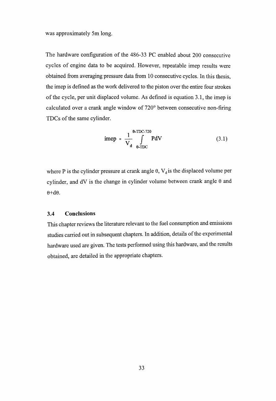
was approximately Sm long.

The hardware configuration of the 486-33 PC enabled about 200 consecutive

cycles of engine data to be acquired. However, repeatable imep results were

obtained from averaging pressure data from 10 consecutive cycles. In this thesis,

the imep is defined as the work delivered to the piston over the entire four strokes

of the cycle, per unit displaced volume. As defined is equation 3.1, the imep is

calculated over a crank angle window of 7200 between consecutive non-firing

TDCs of the same cylinder.

6=TDC+720

nnep ~ J PdV d 6=TDC

(3.1)

where P is the cylinder pressure at crank angle 8, V d is the displaced volume per

cylinder, and dV is the change in cylinder volume between crank angle 8 and

8+d8.

3.4 Conclusions

This chapter reviews the literature relevant to the fuel consumption and emissions

studies carried out in subsequent chapters. In addition, details of the experimental

hardware used are given. The tests performed using this hardware, and the results

obtained, are detailed in the appropriate chapters.

33

Chapter 4

Predicting Fuel Consumption From Fully-Warm

Data

4.1 Introduction

In this chapter, consideration is given to how fuel consumption can be detennined

from engine data taken at fully-wann operating conditions. Two aspects of this

are covered in the following. The first concerns the relationship between

indicated specific fuel consumption and indicated operating conditions. The

assumption made is that this will be independent of differences between wann-up

and fully-wann engine thennal states, and experimental studies have been carried

out to examine and support this. This second concerns the differences between

the amount of fuel injected and fuel combusted. This difference can be significant

during cold engine operation. The amount of fuel injected is the appropriate value

for fuel consumption calculations but it is the fuel combusted that is relevant to

considerations of indicated perfonnance.

Fully-wann engine mapping data are generally obtained at constant tail-pipe

AFR. At fully-wann steady-state operation, the tail-pipe AFR gives an accurate

measure of the overall in-cylinder AFR since all the fuel in the cylinder is

vaporised. However, in the period immediately following a cold-start the tail-pipe

fuel mass flow rate does not account for any liquid fuel stored in the engine

cylinder and lubricating oil. During the wann-up period the overall fuel mass

flow rate is thus:

rhoverall isfc.P indicated + ~accounted for (4.1)

34

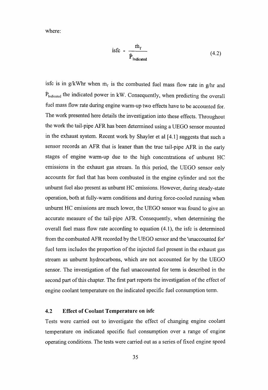
where:

isfc

P Indicated (4.2)

isfc is in g/k Whr when rilr is the combusted fuel mass flow rate in g/hr and

Plndicated the indicated power in kW. Consequently, when predicting the overall

fuel mass flow rate during engine warm-up two effects have to be accounted for.

The work presented here details the investigation into these effects. Throughout

the work the tail-pipe AFR has been determined using a UEGO sensor mounted

in the exhaust system. Recent work by Shayler et al [4.1] suggests that such a

sensor records an AFR that is leaner than the true tail-pipe AFR in the early

stages of engine warm-up due to the high concentrations of unbumt HC

emissions in the exhaust gas stream. In this period, the UEGO sensor only

accounts for fuel that has been combusted in the engine cylinder and not the

unbumt fuel also present as unbumt HC emissions. However, during steady-state

operation, both at fully-warm conditions and during force-cooled running when

unbumt HC emissions are much lower, the UEGO sensor was found to give an

accurate measure of the tail-pipe AFR. Consequently, when determining the

overall fuel mass flow rate according to equation (4.1), the isfc is determined

from the combusted AFR recorded by the UEGO sensor and the 'unaccounted for'

fuel term includes the proportion of the injected fuel present in the exhaust gas

stream as unbumt hydrocarbons, which are not accounted for by the UEGO

sensor. The investigation of the fuel unaccounted for term is described in the

second part of this chapter. The first part reports the investigation of the effect of

engine coolant temperature on the indicated specific fuel consumption term.

4.2 Effect of Coolant Temperature on isfc

Tests were carried out to investigate the effect of changing engine coolant

temperature on indicated specific fuel consumption over a range of engine

operating conditions. The tests were carried out as a series of fixed engine speed

35

and throttle position warm-up runs, with engme data logged on a

second-by-second basis throughout the warm-up. The experimental data were

obtained using the engine test rig described in Chapter 3. Before each test the

engine was run at fully-warm temperatures and the engine speed and brake load

fixed using the dynamometer and throttle stepper motor controls. The engine was

then stopped, with the engine speed and throttle position fixed, and allowed to

cool down to 20DC. The coolant control valves were then switched to allow

coolant from the chiller to be circulated around the engine and the engine coolant

brought down to _2SDC. The insulating blanket was used to aid the cooling

process and left in position until the oil sump temperature fell to -10DC. Once

cool, the insulating blanket was removed and the coolant control valves switched

to allow the engine water pump to circulate coolant through the heat exchanger

once the thermostat opened. Cylinder pressure data were acquired at regular

intervals during the warm-up and corresponding imep values calculated by the

acquisition software. Imep values were produced at approximately SO second

intervals due to the need to average cylinder pressure data over several cycles and

because the imep calculations require intensive use of the 486 PC's processor.

Table 4.1 shows the test conditions used and Table 4.2 lists the imep readings and

corresponding time from start of test for one test condition. Two

second-by-second fuel mass flow rates were recorded for each test. Fuel injected

was determined from EECIV fuel injector pulsewidth from the calibration

console and fuel combusted from the UEGO sensor tail-pipe AFR and EECIV

measured air mass flow rate.

The observed effect of engine coolant temperature on isfc is shown in Figure 4.1.

The results show isfc plotted against imep at engine coolant temperatures

between -10DC and 80DC at engine speeds of 17S0rpm and 2400rpm. At each test

point, isfc is calculated from the measured imep and the tail-pipe detected fuel

mass flow rate from the measured airflow and UEGO AFR. During each warm-up

test the fully-warm tail-pipe AFR was set at stoichiometric using the EECIY

calibration console. Initial data immediately following the engine start-up was

36

discarded as in this period accurate control of the tail-pipe AFR was not possible.

This essentially replicates a cold-start in a current production vehicle where a

HEGO sensor, operating on the same principle as a UEGO sensor, provides

feedback to the engine management system to maintain a stoichiometric AFR in

a process known as closed loop fuelling. According to Figure 4.2, the input isfc,

calculated from the mass of fuel injected, decreases rapidly and converges to the

UEGO sensor determined tail-pipe isfc value as the engine warms-up and the

input AFR tends towards the stoichiometric tail-pipe AFR. The tests indicate that,

by careful control of engine fuelling, a near stoichiometric tail-pipe AFR can be

maintained once the coolant temperature has reached -10°C. From this point

onwards, isfc calculated from the combusted fuel mass flow rate using a UEGO

sensor remains approximately constant independent of coolant temperature. The

scatter in the isfc data in Figure 4.1 is of the order of2% and within this scatter

there is no definable trend in isfc with ECT.

4.3 'Unaccounted For' Fuel During Warm-Up

In addition to the constant AFR warm-up tests, tests were carried out using the

standard EECIV cold-start fuelling strategy to vary the AFR during engine

warm-up. As before, a series of fixed engine speeds and throttle positions were

used (Table 4.3) and cylinder imep measurements were recorded during the

warm-up period to enable indicated specific fuel consumption (isfc) values to be

calculated. These tests were used to investigate the relationship between fuel

injected and fuel burnt during the warm-up process, and so the same injected and

UEGO detected fuel flow rate measurements as for the constant AFR tests were

recorded to enable 'unaccounted for' fuel during warm-up to be calculated.

The data presented above suggest that tail-pipe isfc is only weakly dependent on

ECT during engine warm-up. However, Figure 4.2 indicates that a substantial

difference between fuel injected and fuel burnt exists in the period immediately

following engine start-up. This difference is due to fuel being deposited on the

combustion chamber surfaces and being absorbed into the lubricating oil during

37

the early stages of engine warm-up. In addition, in the period immediately

following start-up the UEGO sensor used to detect the AFR of the exhaust gases

fails to account fully for unbumt fuel in the form of HC emissions present in the

tail-pipe. Consequently, when determining fuel consumption during engine

warm-up from fully-warm engine data, knowledge of the additional fuel required

to maintain a stoichiometric AFR as detected by the UEGO sensor is important.

The second set of engine warm-up tests, using the standard fuelling strategy, were

used to investigate the behaviour of this 'unaccounted for' fuel during engine

warm-up. Figure 4.3 shows a typical warm-up test result for AFR and fuel mass

flow rate during engine warm-up and the resulting 'unaccounted for' fuel

calculated as the difference between fuel injected and fuel detected by the UEGO

sensor in the tail-pipe. At fully-warm conditions, any residual difference between

fuel supply and exhaust fuel flow rate was attributed to calibration errors and

zeroed by adjusting the air mass flow rate calibration. The results appear to show

a near exponential decrease of 'unaccounted for' fuel from an initial peak. As

reported elsewhere, a proportion of this fuel is believed to be due to in-cylinder

storage of fuel on cold combustion chamber surfaces [4.2,4.3]. Recent work by

Shayler et al [4.1] has investigated the behaviour of 'unaccounted for' fuel during

the warm-up period and attempted to define the relative proportions of fuel lost

to the lubricating oil and stored in fuel films in the engine cylinder, but such an

investigation was beyond the scope of the work presented here.

4.3.1 Characterising 'Unaccounted For' Fuel

In order to predict fuel consumption during engine warm-up and the period

immediately after start-up from fully-warm data, characterising the behaviour of

the observed 'unaccounted for' fuel detailed above is important. Work to

investigate the behaviour of this fuel under cold-start conditions has resulted in

the development of a simple exponential function to simulate the observed

experimental behaviour [4.4]. The tests were carried out on a Ford 1.8 litre 16V

Zetec engine over a wide range of operating conditions. The amount of

'unaccounted for' fuel at any point in the warm-up period as a percentage of the

38

fuel supplied can be expressed as:

Unaccounted For Fuel = A.ex~ aE~T) x 100 (4.3)

where .L\ECT is the difference between the instantaneous EeT and the initial

coolant start temperature.

The A value defines the initial peak of the 'unaccounted for' fuel and has been

found to depend on the following:

i) Initial start temperature

Tests have indicated that a reduction in engine start temperature increases

the magnitude of A. This is thought to be due to the increased amount of

liquid fuel entering the combustion chamber as a result of reduced

vaporisation within the intake port. Wall wetting in the combustion

chamber will be more significant due to the combination of increased

amounts ofliquid fuel entering and the lower wall temperatures. This fuel

behaviour has been observed photographically elsewhere [4.5] and the

liquid fuel films found to remain in the cylinder for a considerable portion

of the warm-up [4.6].

ii) Fuel Injected

The amount of fuel injected per stroke is a function of air charge and

AFR. Increasing the amount of fuel injected increases the magnitude of

A as the increased fuel mass in the intake port is believed to result in

more liquid fuel entering the cylinder.

iii) Engine Speed

Increasing the engine speed has been found to reduce the magnitude of A.

This is thought to be due to increased air mass flow rates resulting in

better air/fuel mixing and fuel atomization and consequently reducing the

39

amount of wall wetting in the engine cylinder.

A mathematical expression for A has been defined from experimental data and

is a function of engine speed, fuel injected per stroke and start temperature, as

shown below.

A = minl-0.2N + 1300 - 6T? (4.4)

where N is the engine speed in rpm, T the initial start temperature in °C and minj

the fuel injected per stroke in kg.

The p value is defined as the 'unaccounted for' fuel temperature constant and has

been found to depend on the following two parameters:

i) S tart temperature

Decreasing the start temperature was found to decrease the p value. A

lower start temperature is believed to result in a larger quantity of liquid

fuel in the cylinder and consequently more time is needed for the coolant

and wall temperature to rise sufficiently to vaporise this fuel.

ii) Fuel injected per stroke

The amount of fuel injected is believed to strongly influence the amount

of liquid fuel in the cylinder. Consequently, a longer time is required to

heat up the coolant and cylinder walls to vaporise this fuel resulting in a

larger p value with increased fuel injected per stroke.

Once again, experimental data were used to derive a function to define p as

shown below [4.4]:

~ 1 +(120000m .. ) (4.5) = [0.Sl+(0.012T)+(-0.00011T2)] ill]

40

Using equations (4.3)-(4.5) an 'unaccounted for' fuel fraction can be determined

during a warm-up test. Figure 4.4 shows measured and predicted 'unaccounted

for' fuel curves for two warm-up tests from -15°C on the 2 litre DORC 8V engine

with different engine speeds, brake loads and AFR control during warm-up.

Whilst, in both cases, the fully-warm AFR was 14.2:1 the AFR strategy during

warm-up was different. The test in Figure 4.4a was run using the standard EECIV

determined cold-start AFR strategy while the data in Figure 4.4b was obtained

with constant tail-pipe AFR during warm-up. These tests illustrate the

significance of the 'fuel injected' term in the model as with the standard EECIV

fuel enrichment strategy the 'unaccounted for' fuel fraction is much more

significant.

4.4 Discussion and Conclusions

The data presented in this chapter suggest that the relationship between isfc and

imep is only very weakly dependent on ECT when fuel mass flow rates are

calculated from exhaust gas analysis. Assuming this weak dependence to be

negligible enables fully-warm fuel mass flow rate data to be applied to

non-fully-warm operating conditions, providing indicated operating conditions

are used to correlate cold operating conditions with fully-warm conditions. In this

way engine friction considerations are accounted for. If fully-warm and cold-start

engine indicated operating conditions are not available, an engine friction model

is required to recast the engine brake operating conditions into indicated

operating conditions. Such an engine model and its application is discussed in

Chapter 6 of this thesis.

The above assumption only applies to fuel flow rates calculated from tail-pipe

AFRs which closely represent the fuel involved in combustion and do not always

equate to the fuel mass injected. Thus, in order to determine the total fuel mass

flow rate during non-fully-warm conditions, the difference between fuel injected

and fuel detected by exhaust gas analysis in the period following a cold start has

to be accounted for. A simple model has been developed at Nottingham

41

University to characterise this 'unaccounted for' fuel fraction [4.4]. This has been

found to depend upon engine start temperature, mass of fuel injected per stroke

and engine speed and decays exponentially with increasing ECT.

The 'unaccounted for' fuel fraction can be more accurately described as the

fraction of fuel supplied which is not accounted for by the UEGO sensor in the

exhaust, and is believed to be due to a combination of several engine warm-up

effects. Liquid fuel films have been shown to form in the intake port and on the

intake valves and liquid fuel may be temporarily stored within the combustion

chamber. Several studies [4.2, 4.3, 4.5] have shown this occurs in the period

immediately following engine start-up. The in-cylinder films have been observed

to last for several minutes after engine start-up, but do eventually vaporise as the

cylinder wall temperature rises. In addition, liquid fuel has been shown to pass

the piston rings and mix into the engine lubricating oil [4.7] and up to 1 % of the

fuel injected during the first 20 minutes of a light-load warm-up test from room

temperature was detected in the lubricating oil. This fuel is then believed to return

to the cylinder via the crankcase breather system at a near undetectable rate. A

further fraction of the liquid fuel in the cylinder is thought to pass directly into the

exhaust system as unburnt hydrocarbons. After combustion has been completed

and the in-cylinder pressure decreases during the exhaust stroke, some of the fuel

wall-wetting in the cylinder is vaporised as unbumt hydrocarbons [4.8] with the

result that the cold-start HC emissions are greatly increased in the period when

liquid fuel is present in the engine cylinder. Shayler et al [4.1] have shown that

in this period the UEGO sensor does not fully account for these hydrocarbons and

records an AFR that is lean of the true tail-pipe AFR. As a result, the

'unaccounted for' fuel fraction includes a proportion of the inj ected fuel that

passes undetected down the exhaust tail-pipe. The relationship between

'unaccounted for' fuel and the unburnt hydrocarbon emissions during cold-starting

is considered in the following chapter of this thesis and is of particular

importance when applying fully-warm HC emissions data to cold-start indicated

operating conditions.

42

In conclusion, it can be seen that fully-watm fuel flow rate data can be recast to

represent cold-start conditions and engine wann-up. This requires a combination

of accounting for engine friction changes during engine Watm-up by using

indicated operating conditions, and predicting the 'unaccounted for' fuel in the

period immediately following engine start-up. In order to predict the percentage

of injected fuel that is unaccounted for in the exhaust system, knowledge of the

overall injected fuel mass flow rate is required. When applying predictions to

fully-watm engine data to detennine the percentage increase in fuel consumption

associated with 'unaccounted for' fuel, the overall injected fuel mass is not

known. Consequently, an iterative approach has to be applied with the initial

'unaccounted for' fuel percentage being calculated by assuming that the fuel

injected is the same as the fuel detected in the exhaust pipe. A new fuel injected

mass flow rate can then be calculated and the procedure repeated. After two such

iterations the change in predicted instantaneous 'unaccounted for' fuel as a

percentage of fuel injected is less than 0.5%, and the 'unaccounted for' fuel

percentage assumed to have converged.

43

Chapter 5

Predicting Emissions From Hot Test Bed Data

5.1 Introduction

Indicated specific engine-out emissions are more sensitive than fuel consumption

to changes in air/fuel mixture preparation and in-cylinder temperature variations

during engine warm-up, as discussed in Chapter 3. In addition, for a period after

cold start-up, HC emissions are further influenced by the consequences of poor

fuel utilisation [5.1]. This chapter deals with how the treatment of fuel

consumption, described in the previous chapter, can be adapted to enable the

prediction of emission levels during cold running. Firstly, the effect of reduced

engine coolant temperature on the steady-state engine-out indicated specific

emission levels is examined and then the additional effect of engine start-up

transients on engine-out HC emissions is considered. The objective of the work

has been to develop a simple technique for scaling fully-warm engine-out

emission levels to account for changes in mixture preparation during warm-up

and the effect of engine start-up transients in the period immediately following

a cold-start. As such, the individual sources of the three pollutant emissions under

consideration at fully-warm operating conditions are not of primary importance

but the likely mechanisms that influence changes during warm-up are. The

possibility of predicting the effect of engine coolant temperature changes on HC,

CO and NOx emissions during steady-state operating conditions and the

additional effect on HC emissions of the transient period immediately following

a cold start have been investigated. Of particular interest was the possible link

between the increase in HC emissions due to engine start-up and the observed

discrepancy between the amount of fuel injected and the amount of fuel burnt as

accounted for by exhaust gas analysis described in the previous chapter.

44

5.2 Experimental Test Set-up and Procedure

Engine test data have been obtained from a 2 litre DOHC 8V engine installed on

the test rig described in Chapter 3, and from a Ford 1.8 litre HO Zetec engine

installed on an identical test facility. Two sets of experiments have been carried

out. The first to establish how mixture preparation effects arise under relatively

stable thermal conditions produced by force-cooling the engine. The second was

to investigate the link between 'unaccounted for' fuel and HC emissions in the

transient period immediately following engine start-up.

The effect of ECT on indicated specific emissions has been investigated under

stable thermal conditions maintained by force-cooling to limit the rate of engine

warm-up. This enables steady-state emissions data to be taken at coolant

temperatures down to O°C. Force-cooling entailed removing the engine

thermostat and continuously circulating refrigerated coolant through the engine.

By careful control of coolant flow rates and chiller temperature settings, ECT

could be held at any temperature between O°C and 85°C for up to 10 minutes.

Before an emission reading at each temperature was finalised, the emissions data

were allowed to settle to a steady-state value after each step change in

temperature. This ensured that any transient effects due to sudden temperature

changes and cold-starting did not influence the results, and took about 5 minutes

to achieve. At a given test temperature engine data were logged on a 5 second

interval basis and imep readings recorded to enable indicated specific emissions

(in g/kWhr) to be calculated. Each warm-up test was carried out with a fixed

throttle position and VEGO sensor measured tail-pipe AFR giving an

approximately constant imep during warm-up. Table 5.1 shows the range of

operating conditions tested for the 2 litre DOHe 8V engine and the additional

tests carried out on the 1.8 litre HO Zetec engine.

5.3 Predicting the Effect of ECT on Indicated Specific Emissions

To examine if the effects of mixture preparation on engine-out emission levels

could be characterised by a relatively simple function ofECT, the experimental

45

indicated specific emissions data were plotted against ECT in Figure 5.1. At each

ECT value, the absolute emission value is divided by the corresponding

fully-warm value to give an ECT Correction Factor. The data presented in

Figure 5.1 are from the full range of test conditions defined in Table 5.1, and

demonstrate that, when normalised to values obtained at fully-warm operating

conditions, the indicated specific emissions are strongly correlated to ECT. For

each of the pollutants of interest, a simple function of ECT has been defined to

characterise the correction factor required to define indicated specific emissions

to within +/-5% of the observed values. This function is independent of engine

speed, indicated load and AFR to within this level of accuracy and experimental

repeatability. The three ECT Correction Functions for the three indicated specific

emissions are defined in Appendix A.

Previous work by Shayler et al [5.2] described studies of the relationship between

emissions and operating conditions and fuel inj ection system details. They

showed how many of the effects on emissions could be explained on the basis of

mixture inhomogeneity within the cylinder at the time of combustion. In the work

presented here, ECT is believed to provide a direct indication of mixture

preparation conditions in the intake port, which in tum give rise to varying

degrees of mixture inhomogeneity within the cylinder and consequently to

variations in emissions from values at the corresponding fully-warm engine state.

Emission concentrations for the 2 litre DORC 8V engine against AFR for one

operating condition are shown in Figure 5.2. With reference to this, the lower isco

emissions observed during warm-up are believed to be due to the bulk of the

cylinder mixture being leaner than the overall AFR during the warm-up period.

Figure 5.1 suggests that CO emissions at 20°C are between 5%-10% lower than

those for the corresponding fully-warm operating conditions, irrespective of

engine speed, load and tail-pipe AFR when normalised.

Ishc emissions are relatively high during the warm-up period. Figure 5.1 shows

46

that ishc emissions are approximately 30% higher when the coolant temperature

is 20DC, compared to the fully-warm case.

Isnox emISSIOns were found to be around 30% lower at 20DC than at the

corresponding fully-warm condition, again independently of engine speed,

indicated load and overall tail-pipe AFR. Figure 5.2 indicates that the NO x

emissions are influenced by the AFR of the lean part of the stratified mixture, but

the changes in NOx emissions cannot be entirely due to this, since the same

dependence on ECT was observed regardless of whether the engine was run lean

or rich of the AFR producing peak NOx' It is likely that the reduction in NOx

emissions is more significantly influenced by the lower combustion temperatures

during engine warm-up than by mixture stratification.

The mechanisms that produce these trends are likely to arise in any engine but

whether or not the simple ECT correction functions presented here are adequately

representative is an open issue and requires further work. However, additional

data were obtained from a Ford 1.8 litre RO Zetec engine to confirm that the

above functions were representative for this engine, since data from this engine

were to be used in the drive cycle evaluation procedure, described in Chapter 7.

Figure 5.3 shows experimental data from the Zetec engine plotted in the same

ECT correction factor format as for the 2 litre DORC 8V engine data. Figure 5.3

also shows the model predicted correction factors obtained from the DORC data

and indicates that the same trends in emissions occur on the Zetec engine. The

Zetec data were derived from only three tests all at an engine speed of 2000 rpm

and imep of 8.3 bar at tail-pipe AFRs of 12:1, 14.7:1 and 17:1. Despite the

limited amount of data available, the general agreement with the ECT Correction

Functions derived from the DORC data is generally good suggesting that the

trends observed and modelled are generic to other engine types.

5.4 Predicting the Effect of Engine Start-Up Transients on He Emissions

In addition to the force-cooled tests, experiments were carried out to investigate

47

the relationship between 'unaccounted for' fuel in the period immediately

following cold start-up and the increased HC emissions in this period. These tests

were carried out using the standard EECIV cold-start fuelling strategy. Once

again, a series of fixed engine speeds and throttle positions were used (Table 5.2)

and cylinder imep measurements recorded during engine warm-up. The coolant

circuit was the standard production circuit with the standard thermostat unit

fitted.

Figure 5.4 shows HC mass flow rates during two fixed throttle warm-up tests.

The measured HC mass flow rate is that determined from exhaust concentrations

and fuel and air mass flow rates logged throughout the test period. The predicted

HC mass flow rate is calculated from the fully-warm steady-state value at the end

of the warm-up test and is corrected to account for mixture preparation effects,

using the ECT functions described above, and for changes in tail-pipe AFR

during warm-up by interpolation using fully-warm AFR data. Since each test was

carried out at near constant indicated load, the HC mass flow rate at each point

in the warm-up, neglecting mixture preparation effects, could be calculated from

the fully-warm HC mass flow rate scaled according to AFR. This was done using

simple linear interpolation based on fully-warm engine data at corresponding

indicated operating conditions and a range of tail-pipe AFRs. This HC mass flow

rate was then scaled according to ECT to account for mixture preparation changes

to give the predicted HC mass flow rate during engine warm-up. This mass flow

rate can be seen to be significantly lower than the measured HC mass flow rate

in the early seconds after engine start-up.

The difference between the measured and predicted HC mass flow rates, termed

the 'Delta HC Flow Rate', is closely related to the 'unaccounted for' fuel behaviour

described in Chapter 4, as shown in Figures 5.5 and 5.6. Figure 5.5 shows the

results from three warm-up tests at an engine speed of 1750 rpm and a range of

fully-warm engine brake loads with a start temperature of -15°C. The relationship

between Delta HC and 'unaccounted for' fuel is relatively insensitive to engine

48

load, engine speed and start temperature as indicated by Figure 5.6. This shows

the results for a series of warm-up tests with a range of engine speeds, engine

loads and start temperatures, detailed in Table 5.2. Linear regression on these data

gIves:

(5.1)

where y has a value of 0.33. mini is the fuel mass flow rate inJ·ected and ri1 the " exh

fuel mass flow rate determined by exhaust gas analysis with the UEGO sensor.

Similar engine data obtained at Nottingham University from a Ford 1.S litre 16V

HO Zetec engine demonstrate the same linear relationship [5.3]. However, in this

case the value of y was found to be 0.5 which suggests that y is dependent on

engine type. The DOHC engine data correlation has been used to predict total HC

mass flow rates during engine warm-up and the methodology detailed below. The

details and implications of the work using the Zetec engine data [5.3] are

discussed later in the chapter.

For the 2 litre DOHC SV engine examined, equation (5.1) gives a good first

approximation to the increase in HC emissions during the period immediately

following engine start-up, believed to be primarily due to liquid fuel films in the

engine intake and cylinder. Using this relationship and the 'unaccounted for' fuel

model described in Chapter 4, an additional HC mass flow rate during engine

warm-up due to cold-starting was predicted for each of the warm-up tests carried

out. The total HC mass flow rate at any point during the warm-up was predicted

by summing the fully-warm value at the corresponding AFR corrected for

mixture preparation effects and an additional 'Delta HC' term, calculated from

equation (5.1). Figure 5.7 shows the results of two such tests, which correspond

to the data presented in Figure 5.4. These tests demonstrate that the simple linear

correlation with 'unaccounted for' fuel enables a good approximation to the actual

HC mass flow rate in the early seconds of engine warm-up to be made from the

fully-warm HC mass flow rate for the engine examined.

49

5.5 Discussion

The experimental data presented in this chapter were obtained to illustrate the

effects of reduced engine temperature on indicated specific emissions under

steady-state conditions and the additional effect of engine start-up transients on

HC emissions. These two phenomena are essentially coupled together as, in

reality, both occur simultaneously during the standard engine start and wann-up.

However, in order to predict the engine-out emissions at non-fully-warm

operating conditions from fully-wann data the two effects have been separated

and examined independently.

The effect of mixture preparation on the engine-out indicated specific emissions

have been characterised by three functions defining a correction factor to scale

fully-wann emission values for engine coolant temperatures down to O°C.

Indicated specific emissions have been used in order to compensate for the effect

of increased engine friction at lower engine temperatures. The three functions

were obtained by curve fitting to experimental data obtained from the 2 litre

DOHC 8V engine test rig. The data indicate that the effect ofECT on each of the

indicated specific emissions is independent of engine speed, indicated load and

tail-pipe AFR when the emissions are nonnalised to the corresponding indicated

operating conditions at fully-warm. Indicated specific CO emissions were found

to be around 5%-10% lower at 20°C than at fully-warm and to increase linearly

with ECT despite the tail-pipe AFR remaining the same at all ECT values.

Conversely, indicated specific HC emissions decreased with increasing ECT and

were in the region of 30% higher at 20°C than at fully-wann. Indicated specific

NOx emissions increased with increasing ECT and were around 30% lower at

20°C than at fully-warm. This behaviour is believed to be due to a degree of

charge stratification in the cylinder due to mixture preparation changes in the

intake system. Mixture preparation conditions in the intake port and HC

emissions particularly are known to be very sensitive to ECT [5.4, 5.5] but the

mechanisms governing the effects ofECT on emissions are less well understood.

The tests presented here were carried out with a constant tail-pipe AFR measured

50

by a VEGO sensor which is believed to give an accurate measure of the overall

in-cylinder AFR during steady-state operating conditions under force-cooled

running [5.6]. Hence, even with a constant overall in-cylinder AFR, the degree

of charge stratification decreases and the combustion AFR becomes progressively

richer as mixture preparation improves with increasing ECT. This results in the

observed increase in CO emissions and the corresponding decrease in HC

emissions as the unbumt mixture fraction decreases. Figure 5.8 shows HC and

NOx correction factors plotted against CO correction factor during the warm-up

phase with typical experimental data points, and shows HC emissions decreasing

and NOx emissions increasing during engine warm-up. Similar trends in HC and

CO emissions have been observed qualitatively elsewhere [5.7, 5.8]. Lee's results

are particularly interesting as he found that increasing ECT from 65°C to 100°C

decreased HC emissions by around 10%, increased NOx emissions by 10% and

decreased CO emissions by less than 5%.

While the charge stratification theory outlined initially by Shayler et al [5.2]

appears to hold for both CO and HC emissions, the behaviour of NO x emissions

is less clear. CO emissions are, in effect, a direct measure of the combusted AFR

and HC emissions are primarily due to the remaining uncombusted and poorly

oxidised fuel. NOx emissions, like CO emissions, are heavily influenced by the

combustion AFR and as such would be expected to either increase or decrease

according to whether the combusted AFR was rich or lean of the peak NOx AFR.

However, the additional effect of changing combustion temperature during

warm-up is believed to out-weigh any effect of charge stratification, since NOx

emissions were always observed to increase during warm-up independently of

AFR. Similar trends in NOx emissions have been observed by Andrews et al [5.8]

and Russ et al [5.9] and explained in terms of increasing combustion temperature.

Both CO and NOx emissions are directly linked to the AFR of the combusted

in-cylinder mixture at all times in the warm-up process. Thus, isco and isnox at

all points in the warm-up can be determined by scaling the fully-warm indicated

51

specific emISSIOns to account for mixture preparation as described above.

However, HC emissions arise primarily from fuel that does not take part in

combustion and as such are particularly sensitive to any additional fuelling

needed in the period immediately following a cold start. Consequently, an

additional increase in HC emissions occurs over and above that associated with

mixture preparation changes during this transient period.

The additional increase in HC emissions is believed to be due to liquid fuel films

existing in the engine cylinder in the early seconds after engine start-up. The

build-up of these fuel films and additional absorption of fuel into the lubricating

oil [S.1 0] contributes to the 'unaccounted for' fuel behaviour described in

Chapter 4 of this thesis. Various studies [S.I1-S.13] have shown the existence of

liquid fuel films in the engine cylinder and a significant fraction of this fuel is

believed to pass directly into the exhaust system as unburnt hydrocarbons [S .14].

After combustion has been completed and the in-cylinder pressure decreases

during the exhaust stroke, a proportion of the fuel wall-wetting in the cylinder is

vaporised as unbumt hydrocarbons. The data for the 2 litre DOHC 8V engine

presented in this chapter suggest that around 33% of the fuel 'unaccounted for'

based on exhaust measurements made with a UEGO sensor is actually present as

unbumt hydrocarbons in the exhaust system but passes the sensor undetected.

Similar work on a Ford 1.8 litre HO Zetec engine [S.3] suggests that, for this

engine, the additional HC emissions account for SO% of the UEGO 'unaccounted

for' fuel fraction. Additional work on this engine [S.6] has attempted to identify

the various sources of apparent fuel loss which result in the overall 'unaccounted

for' fuel observed. Three sources of 'unaccounted for' fuel can be identified.

Firstly, the UEGO sensor is demonstrated to record an AFR which is lean of the

overall in-cylinder AFR during engine warm-up. This is because the UEGO

sensor fails to fully account for the high proportion of unbumt hydrocarbons

present in the period immediately following a cold start. As the warm-up

proceeds and the HC concentration decreases, the UEGO sensor records an AFR

which is progressively closer to the overall in-cylinder AFR. For the Zetec engine

S2

examined, Shayler et al defined a UEGO sensor correction factor to scale the

UEGO AFR to that calculated by analysis of all the exhaust gas products of

combustion. This correction factor is specific to the engine examined and the

same procedure cannot be applied to the DOHC engine data presented in this

chapter since the rig instrumentation did not enable measurements of the carbon

dioxide and oxygen concentrations in the exhaust gases needed to calculate the

exhaust AFR. Consequently, for the DOHC engine data, the contribution of

UEGO sensor errors to the total 'unaccounted for' fuel cannot be accurately

defined and the 'unaccounted for' fuel, characterised from experimental data in

Chapter 4, includes fuel, in the form of unbumt HC, undetected by the UEGO

sensor.

Predicting the amount of fuel stored temporarily in the engine cylinder and

absorbed into the lubricating oil is difficult. After correcting the UEGO sensor

AFR during warm-up, Shayler et al [5.6] estimate the relative proportions of fuel

stored and fuel lost by analysis of the HC and UEGO corrected 'unaccounted for'

fuel curves during warm-up, but once again, the lack of an accurate UEGO

correction function for the DOHC engine prevents a similar analysis here.

However, the fact that the additional HC contributes 33% of the total

'unaccounted for' fuel on the DOHC engine and that this fraction is around 50%

on the Zetec engine, given that the additional HC mass flow rate is similar for

both engines, suggests that the proportion of fuel lost to the lubricating oil is

greater for the DOHC engine. This is believed to be consistent with the

comparitively more modem design and construction of the Zetec engine.

Because the UEGO sensor does not provide an accurate overall AFR during the

early period of engine warm-up, the 'unaccounted for' fuel predicted by the

exponential functions detailed in Chapter 4 will give an over estimation of the

additional fuel required when predicting cold-start fuel consumption from

fully-warm engine data. However, using the UEGO sensor to determine the

'unaccounted for' fuel is consistent with current vehicle technology which relies

53

on a similar sensor, the HEGO sensor, to maintain an assumed stoichiometric

APR during both warm-up and fully-warm operation. In reality, such a sensor

will maintain a tail-pipe APR that is slightly rich, in the region of one air/fuel

ratio, of stoichiometric in the period when the exhaust hydrocarbons are high and

not fully-accounted for by the exhaust mounted sensor. In addition, using such

a sensor here enables the definition of a simple function to relate excess exhaust

hydrocarbons during warm-up to the UEGO predicted 'unaccounted for' fuel

detailed in Chapter 4.

5.6 Conclusions

In order to investigate the possibility of predicting engine-out emissions during

cold-starting and engine warm-up two sets of warm-up tests have been carried

out. The first set of tests involved force-cooling the engine to establish near

steady-state engine conditions at non-fully warm temperatures and constant

tail-pipe AFR. These tests suggest that, unlike indicated specific fuel

consumption, indicated specific emissions are strongly dependent on ECT. The

data suggest that fully-warm indicated HC, CO and NOx emissions can be scaled

by a simple ECT Correction Function to account for changes in mixture

preparation due to reduced coolant temperatures during engine warm-up.

Indicated specific emissions were used to remove the effect of increased engine

friction at lower engine temperatures enabling the effect of mixture preparation

to be assessed independently.

Changes in emISSIOns with ECT have been explained in terms of charge

stratification due to poor vaporisation in the intake system and reduced

combustion temperatures due to reduced in-cylinder metal temperatures.

The relationship between the additional HC emissions immediately following

start-up and the 'unaccounted for' fuel in this period has been investigated.

Experimental data indicate that a simple linear relationship exists between the

additional HC over that predicted by poor mixture preparation and 'unaccounted

54

for' fuel measured using a UEGO sensor, such that the additional He is around

33% of the 'unaccounted for' fuel at any time during the warm-up.

Similar work at Nottingham University [5.6] suggests that, in the period

immediately following a cold start, the UEGO sensor does not fully-account for

unbumt hydrocarbons in the exhaust pipe resulting in a measured AFR that is

lean of the actual tail-pipe AFR. Consequently, the 'unaccounted for' fuel

predicted based on UEGO measurements provides an over-estimate of the fuel

stored in the engine cylinder and absorbed in the lubricating oil. Experimental

data suggest that, for the engine examined, around 33% of the fuel unaccounted

for by the UEGO sensor is actually present as unbumt hydrocarbons in the

exhaust pipe.

55

Chapter 6

Engine Thermal Model to Predict Friction

Characteristics

6.1 Introduction

Both fuel consumption and emISSIOns are affected by changes in thermal

conditions during engine warm-up. In order to apply the developments and results

described in the preceding chapters, a means of predicting how thermal

conditions vary from engine start-up onwards is required. This involves the use

of an engine thermal model developed at the University of Nottingham called

PROMETS which, amongst other things, provides the facility to predict engine

frictional losses and oil and coolant temperature variations. The indicated mean

effective pressure (imep), defined as the total work delivered to the piston over

the entire four strokes of the engine cycle per unit displaced volume, is calculated

from the brake mean effective pressure as:

imep = bmep + fmep (6.1)

where fmep is the friction mean effective pressure due to rubbing friction in the

engine and ancillary friction losses such as the water and oil pumps. This chapter

gives a brief description of the thermal model employed and details its

application to the work presented in this thesis. A more detailed description is

given elsewhere [6.1].

Increased frictional losses are responsible for a significant part of the increase in

fuel consumption of a cold engine. Sorrell and Stone [6.2] found that combustion

chamber wall temperatures rose rapidly to their steady-state values, indicating

that reduced thermal efficiency due to cold cylinder walls is not a significant

56

cause of increased fuel consumption during warm-up. Work by Raahtela et al

[6.3] investigated the warm-up behaviour of a 1.3 litre engine starting at -100C.

Figure 6.l(a) shows the measured motoring frictional losses as a function of oil

temperature. The excess motoring losses were attributed to the increased viscosity

of the cold engine oil. Figure 6.1 (b) shows that the effect of oil temperature on

frictional losses is different for various engine components. Temperature was

found to have the greatest influence on the crankshaft group, which includes the

crankshaft, connecting rod, piston and rings. It was also estimated that the fuel

flow rate required at -10°C is 85% higher than that required by a fully-warm

engine. Much work has been done to investigate the effect of engine oil viscosity

on engine cranking, starting and warm-up fuel economy [6.4-6.7], but little work

relates to the prediction of frictional losses during the period between start-up and

fully-warm.

6.2 Modelling Engine Friction Using PROMETS

The PROMETS software package enables engine oil, coolant and metal warm-up

rates to be predicted for a defined set of engine operating conditions. Thermal

analysis of the engine structure is based on the lumped capacity approach. The

engine is divided into elements, each of which has a spatially uniform

temperature, a given thermal capacity, and is thermally coupled to adjacent

elements and to any adjacent heat sinks. Energy balance equations are formed for

each element and temperatures obtained by solving appropriate sets of

simultaneous equations. In the version ofPROMETS used here, 36 elements are

used to represent the engine structure around one cylinder of the 1.8 litre Zetec

engine and 30 elements for the 2 litre DORC 8V engine. The additional six

elements in the Zetec case are used to define the additional intake and exhaust

valves in this engine configuration.

The friction model in PROMETS is used to predict the increase in imep caused

by higher friction losses during engine warm-up. In determining friction losses,

it is important to clarify the component sources that are included in the

57

calculation. In this thesis, imep is defined as the net imep or the work delivered

to the piston over the entire four strokes of the cycle, per unit displaced volume.

As such, it follows that:

imep = bmep + rfinep + amep (6.2)

where rfinep is the rubbing friction mean effective pressure and amep the

accessory mean effective pressure.

The friction model developed by Patton et al [6.8] is used to predict the rubbing

friction and accessory mean effective pressure terms for fully-warm engine states.

The effect of the bore, the stroke, the number of cylinders, the number and size

of bearings and the valve train configuration are accounted for. The bearings

group includes friction from the main bearings, con-rod bearings and camshaft

bearings. The piston groups includes friction from piston and piston rings and the

valve train group is made up of friction from the cam followers and valve actuator

mechanisms. The accessory friction is the sum of oil pump, water pump and

alternator friction. The correlations used to define these terms are given for

reference in Appendix B.

In the implementation of the friction model used by PROMETS, the net indicated

work, Wc,i' is determined over the whole engine cycle as:

w . = f P.dV C,l (6.3)

and imep is calculated as:

unep (6.4)

where Vs is the swept volume. Consistent with these definitions, the total friction

losses described hereafter are only the sum of the rubbing friction loss and

accessory friction loss and are independent of pumping losses during the

58

induction and exhaust strokes of the cycle.

Power and mean effective pressure (mep) are related by:

(6.5)

where nR is the number of revolutions per cycle and N the engine speed in

revolutions per second. In the following, the total friction power loss is denoted

by Pprf , the rubbing friction loss by P rf , and the accessory friction power loss by

1\. These terms are related by:

Pf=Pf+P pr r a (6.6)

6.2.1 Friction Power Losses During Steady-State

The total friction power loss, Pfriction predicted using the Patton et al model [6.8],

is split into four components so that the frictional generated heat can be

distributed as heat sources within the thermal analysis of the engine.

P friction = a(a+h+c+d)P prf (6.7)

where:

(6.8)

where the coefficients a to d represent the proportions of the steady-state friction

losses for the valve train, the bearings, the piston, and the accessory components

respectively. The factor a is used to compensate for discrepancies between

measured friction losses and the friction losses predicted by the model.

Experience of applying the model [6.9] indicates that a is typically l.34 for a four

cylinder engine. Table 6.1 lists the predicted friction losses for each component

source of the 2 litre DORe 8V engine running at 3000 rpm and 30 Nm brake

59

load. It can be seen that piston friction accounts for the largest proportion of the

total friction losses, and is dependent on gas pressure.

6.2.2 Friction Power Losses During Warm-Up

For other than fully-warm running conditions, the effect of oil temperature on

viscosity and hence friction losses is taken into account by introducing a

correction factor. This is used to scale the instantaneous friction loss in proportion

to values at the same running condition for fully-warmed up conditions. The

correction is given by:

( )

n . v· p =-warm-up V Pf

ref

(6.9)

where the reference viscosity is for a temperature of 90°C and v is the viscosity

at any time during warm-up, whose dependence on absolute temperature Tabs is

calculated using the Walther equation [6.10]:

(6.10)

where C1 and C2 are constants determined from the oil viscosity specification. The

reference oil temperature is that at the inlet to the oil pump and is taken as being

representative of the mean sump oil temperature. The index n has been

determined experimentally to be typically 0.19-0.24 [6.9]. Not all of the friction

loss dissipated as heat goes into the lubricating oil. The majority is transferred to

adjacent parts of the engine structure or piston. During the development of

PROMETS the split between the proportion transferred to the surrounding

structure and the proportion which heats the oil directly has been established by

trial and error to best match measured temperature characteristics on a number of

engines. Typically, about 10% of the friction power is dissipated directly to the

oil.

In the version of PROMETS used here, heat transfer from the gas side to the

engine structure is described by a model which partly utilises the Taylor and

60

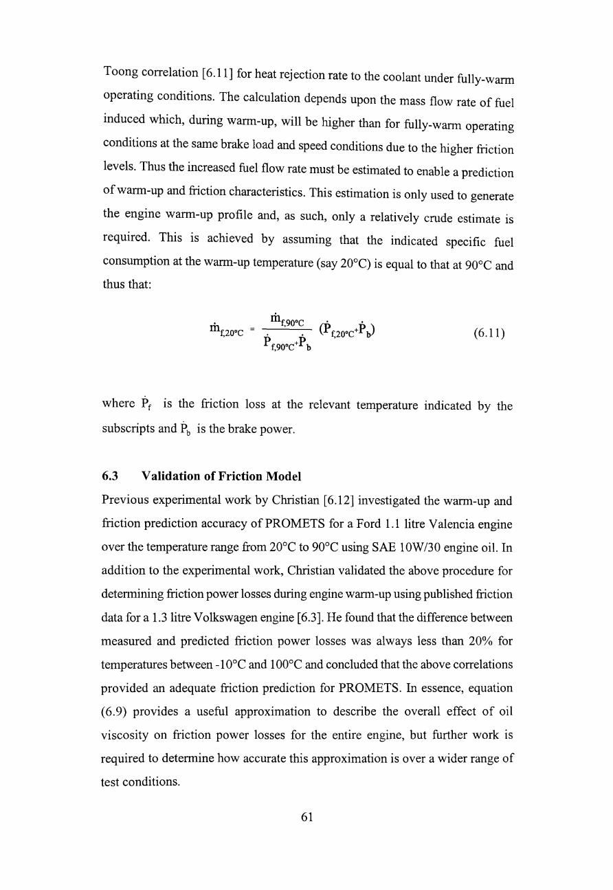
Toong correlation [6.11] for heat rejection rate to the coolant under fully-warm

operating conditions. The calculation depends upon the mass flow rate of fuel

induced which, during warm-up, will be higher than for fully-warm operating

conditions at the same brake load and speed conditions due to the higher friction

levels. Thus the increased fuel flow rate must be estimated to enable a prediction

of warm-up and friction characteristics. This estimation is only used to generate

the engine warm-up profile and, as such, only a relatively crude estimate is

required. This is achieved by assuming that the indicated specific fuel

consumption at the warm-up temperature (say 20°C) is equal to that at 90°C and

thus that:

(6.11)

where Pf is the friction loss at the relevant temperature indicated by the

subscripts and 1\ is the brake power.

6.3 Validation of Friction Model

Previous experimental work by Christian [6.12] investigated the warm-up and

friction prediction accuracy of PROMETS for a Ford 1.1 litre Valencia engine

over the temperature range from 20°C to 90°C using SAE 10W/30 engine oil. In

addition to the experimental work, Christian validated the above procedure for

determining friction power losses during engine warm-up using published friction

data for a 1.3 litre Volkswagen engine [6.3]. He found that the difference between

measured and predicted friction power losses was always less than 20% for

temperatures between -10°C and 100°C and concluded that the above correlations

provided an adequate friction prediction for PROMETS. In essence, equation

(6.9) provides a useful approximation to describe the overall effect of oil

viscosity on friction power losses for the entire engine, but further work is

required to determine how accurate this approximation is over a wider range of

test conditions.

61

In order to detennine if the above relationships are valid over wider temperature

and viscosity ranges additional tests were carried out using the 2 litre DORe 8V

engine test rig described in Chapter 3 of this thesis. The test facilities enabled

start/soak temperatures down to -10°C to be used giving a much wider range of

oil viscosity. To further extend this viscosity range, a series of tests were carried

out with SAE 20W/50 oil and the effect of the value of the index n observed. The

oil viscosity variation with absolute temperature was calculated using

equation (6.10) and the variation for the two test oils is shown in Figure 6.2. The

tests were carried out as fixed throttle free wann-up tests with start/soak

temperatures of -10°C and +20oe with constant stoichiometric input AFR.

Table 6.2 shows the range of operating conditions and start/soak temperatures

used.

Figures 6.3 and 6.4 show measured and predicted friction power losses and

measured and predicted oil and coolant wann-up temperatures for two typical

tests with start/soak temperature of 20°C and -10°C respectively, and demonstrate

close agreement between measured and predicted values. Of particular interest are

the friction power losses in the period immediately following engine start-up.

During this period the friction is much higher and reduces more rapidly than is

predicted by equation (6.9). Such behaviour indicates that the viscosity of the oil

at pump inlet temperature does not fully account for friction level changes

immediately following start-up. In the version ofPROMETS used here, a linear

drop in friction power has been incorporated into the friction power loss

representation. The friction power loss at engine start-up is assumed to be 1.5

times the value predicted by equation (6.9). After 50 seconds, the friction power

losses are assumed to be fully-dependent on oil viscosity and are then calculated

directly from equation (6.9). While the linear drop in friction representation

provides a good approximation to the friction behaviour for the 20°C start the

approximation is less accurate for the -10°C start where the initial friction factor

(F) is greater than 1.5 times the value predicted by equation (6.9) and takes longer

than the allowed 50 seconds to decay. In order to develop a more representative

62

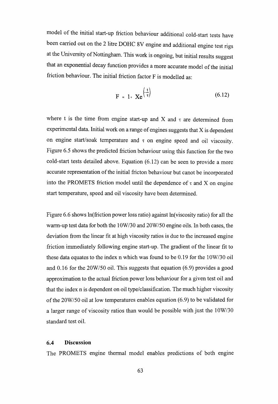
model of the initial start-up friction behaviour additional cold-start tests have

been carried out on the 2 litre DORe 8V engine and additional engine test rigs

at the University of Nottingham. This work is ongoing, but initial results suggest

that an exponential decay function provides a more accurate model of the initial

friction behaviour. The initial friction factor F is modelled as:

(6.12)

where t is the time from engine start-up and X and 1" are determined from

experimental data. Initial work on a range of engines suggests that X is dependent

on engine start/soak temperature and 1" on engine speed and oil viscosity.

Figure 6.5 shows the predicted friction behaviour using this function for the two

cold-start tests detailed above. Equation (6.12) can be seen to provide a more

accurate representation of the initial fricton behaviour but canot be incorporated

into the PROMETS friction model until the dependence of 1" and X on engine

start temperature, speed and oil viscosity have been determined.

Figure 6.6 shows In(friction power loss ratio) against In(viscosity ratio) for all the

warm-up test data for both the lOW /30 and 20W /50 engine oils. In both cases, the

deviation from the linear fit at high viscosity ratios is due to the increased engine

friction immediately following engine start-up. The gradient of the linear fit to

these data equates to the index n which was found to be 0.19 for the lOW /30 oil

and 0.16 for the 20W/50 oil. This suggests that equation (6.9) provides a good

approximation to the actual friction power loss behaviour for a given test oil and

that the index n is dependent on oil type/classification. The much higher viscosity

of the 20W/50 oil at low temperatures enables equation (6.9) to be validated for

a larger range of viscosity ratios than would be possible with just the lOW /30

standard test oil.

6.4 Discussion

The PROMETS engine thermal model enables predictions of both engme

63

temperature and friction power losses to be made. The correlations used to

calculate fully-warm engine friction levels are derived from the Patton et al model

[6.S] and reflect the importance of basic design variables and generate a

distribution of frictional dissipation throughout the whole engine.

Comparisons between measured and predicted friction power losses during

engine warm-up for a Ford Valencia and, as presented here, for a Ford 2 litre

DOHC SV engine give high confidence in the technique used to scale fully-warm

engine friction levels according to oil viscosity. The experimental work presented

in this chapter confirms the validity of this scaling over a wider range of oil

temperatures and with two different test oil specifications.

Predicting friction power losses in the period immediately following a cold-start

requires an additional modification to the fully-warm friction levels over and

above that described by equation (6.9). During this period, friction levels are

higher than predicted by equation (6.9) and decay more rapidly, suggesting that

friction levels immediately after start-up are not entirely governed by the bulk oil

viscosity. Christian [6.12] suggested a linear correction function to predict this

start-up friction, and the test data presented here suggests that this provides an

adequate approximation to the measured friction behaviour. He postulated that

the apparent independence of engine friction on oil viscosity in the first 50

seconds of engine operation was due to a lack of oil on the rubbing surfaces and

the time taken to fully develop flow conditions in the engine. The exact

lubrication mechanisms that result in the observed behaviour are not fully

understood. Work by Hashizume and Kumada [6.13] has investigated the effect

of oil flow rate on bearing temperature and it is possible that the start-up friction

behaviour could be explained by differences in the oil temperature at the bearing

surfaces and in the oil galleries. Additional cold-start test data from the DOHC

engine test rig suggests that the start-up friction behaviour is more accurately

modelled by an exponential decay function and is influenced by engine start/soak

temperature and engine speed. This is believed to be due to the effects of the

64

initial bearing temperatures and the time taken for the bearing oil temperatures

to stabilise, governed by the rate at which fresh oil is supplied to the bearing

surfaces. However, further work is required to determine the way these effects

combine to determine start-up friction behaviour and is currently being

undertaken. Consequently, the original linear friction correction model used in

PROMETS was adopted for the work presented here as it provides a good

approximation to the friction behaviour, particularly when start temperatures of

20DC or higher are of interest.

65

Chapter 7

Application to Cold-Started Drive Cycles to

Predict Fuel Consumption and Emissions

7.1 Introduction

The Cold Emission Cycle Simulation Program (CECSP) draws on the various

models and results described in previous chapters and further components of the

prediction scheme described in this chapter. The complete CECSP package

enables second-by-second fuel and emissions flow rates to be predicted for a

given drive cycle from a cold-start initial condition. A combination of engine

friction models and mixture preparation compensation functions enable the

application of fully-warm engine test bed data to cold-start conditions. Neural

networks are used to characterise the fully-warm engine mapping data as

described in Chapter 2.

To demonstrate the complete procedure, CECSP has been applied to the

ECE+EUDC drive cycle with a 20°C start temperature and with the currently

allowed 40 second idle conditioning period before emission sampling begins. A

neural network is used to map fully-warm fuel and emissions mass flow rates as

a function of engine speed, indicated load and AFR for the engine under

consideration which is then used to interpolate fuel and emission flow rates at

each point in the drive cycle. In order to predict cold-start fuel and emissions flow

rates from fully-warm mapping data the PROMETS friction model is used to

calculate the increased engine friction during warm-up and hence the new

indicated load profile. The correlations derived in Chapter 5 are used to correct

the predicted emissions values for the effect of changes in mixture preparation at

low engine coolant temperatures.

66

In addition to predictions of engine-out emissions, tail-pipe emISSIOns are

predicted using a simple catalyst model. This enables experimental catalyst

efficiencies for a given drive cycle to be used, if available, or more generally, the

definition of catalyst light-off times and conversion efficiencies. When predicting

tail-pipe emissions, particularly those ofHC, the prediction accuracy in the early

part of the drive cycle is of paramount importance as it is this period, before

catalyst light-off occurs, that contributes the bulk of the total drive cycle

emissions. The increased HC emissions immediately following start-up have been

closely linked to differences in fuel injected and fuel combusted and to the

corresponding liquid fuel puddles believed to exist in the engine cylinder during

this period.

CECSP enables the user to select different combinations of engines and vehicles

and to change various vehicle characteristics such as transmission ratios, wheel

radius and total vehicle mass. The drive cycle to be used is defined as a series of

second-by-second vehicle speed and gear number points and the start/soak

temperature defined in the PROMETS friction model module of the software. The

ECE + EUDC has been used during the development of CECSP. The complete

vehicle speed profile for this cycle is shown in Figure 7.1 and consists of two

parts, the elementary urban cycle (repeated four times) and the extra-urban cycle.

For a given vehicle and drive cycle specification, engine speed variations can be

defined from knowledge of rolling tyre radius and transmission ratios. The engine

speed N is defined as:

N V vehRgearRFDR

0.37699rwhee1

(7.1)

where Vveh is the vehicle speed(km/hr), Rgear the gear ratio, RFDR the final drive

ratio and rwheel the driving wheel radius(m). The engine brake torque (Mengine) is

then calculated by dividing the engine brake power requirement by the engine

speed at each point in the cycle. Thus:

67

M. engme

where:

60(i> rl+ i> ICE)

2nN 11 trans (7.2)

(7.3)

F 0, F 1 and F 2 are coefficients determined by experiment. PKE is the power required

at the road wheels to increase the kinetic energy of the vehicle during

acceleration. This term is set to zero when decelerating, as under these conditions

energy is dissipated through the vehicle brakes and the engine is motored. This

simple vehicle model enables the vehicle performance during a drive cycle to be

translated into required engine performance at the engine flywheel. Figure 7.2

shows a typical example ofthe variations in engine brake torque and speed during

the ECE+EUDC drive cycle for a medium sized vehicle. It is assumed that the

over-run periods when the engine is motored can be treated as zero load points

at the appropriate engine speed. Once the required engine performance over the

drive cycle has been determined in this way, fuel consumption and emissions

mass flow rates are inferred from fully-warm engine data modified to account for

cold-start effects.

7.2 Predicting Drive Cycle Fuel Consumption and Emissions

Although not an essential part of the procedure, using neural networks to

characterise engine fuel consumption and emissions performance as a function

of operating conditions and calibration details has proved to be both effective and

efficient, as detailed in Chapter 2. Fuel and emissions flow rates are determined

by a neural network which maps fuel and emissions flow rates as a function of

engine speed, indicated load and AFR. This same network can then be used to

predict cold-started fuel consumption once the cold-started friction values have

been calculated for each point in the drive cycle. Details of the neural network

68

configuration used and the training procedure employed are also detailed in

Chapter 2 of this thesis. Two neural networks are used. The first maps fuel and

emissions flow rates as a function of engine speed, bmep and AFR and the second

uses engine speed, imep and AFR as inputs. In order to train the second network ,

the fully-warm mapping data has to be recast to express brake operating

conditions as indicated operating conditions. This is done using the fully-warm

component of the PROMETS engine friction model which is detailed III

Chapter 6. Indicated mean effective pressure (imep) is calculated as:

1lllep = bmep + finep (7.4)

Figure 7.3 shows the steps in the prediction procedure to enable fully-warm fuel

consumption and emissions values to be determined. In order to predict friction

power losses at each point in the fully-warm drive cycle, approximate fuel mass

flow rate values at each point are needed. Hence, the first network trained on

brake operating conditions is used to determine this fuel flow rate data, enabling

friction power losses to be predicted and indicated operating conditions to be

defined. The second neural network is then used to determine new fuel mass flow

rates and emissions mass flow rates over the drive cycle. These new fuel mass

flow rates are then used to re-calculate engine friction power losses and hence

indicated loads, and the network used to predict new fuel consumption and

emissions values. This process is repeated until the change in predicted total drive

cycle fuel used is less than 0.5%, as indicated in Figure 7.3. Generally, not more

than three iterations are required to achieve this level of prediction accuracy.

Applying the procedure to a cold-started drive cycle entails the prediction of

engine friction at each point in the drive cycle as the engine warms up in parallel

with a time marching calculation of fuel consumption from the corresponding

indicated operating conditions, as shown in Figure 7.4. The rate at which the

engine structure and lubricating oil warm-up influences friction losses over the

cycle, because these depend upon oil viscosity which in tum depends upon

69

temperature. The warm-up behaviour of the engine over the drive cycle is

determined using the PROMETS engine thermal model. For each time step

through the drive cycle, an iterative procedure is used to obtain a self-consistent

variation of friction, indicated operating conditions and oil warm-up

characteristics. Once the indicated operating conditions for the cold-started drive

cycle have been determined the same neural network used to predict fully-warm

fuel and emissions mass flow rates from indicated operating conditions is used

to predict the cold-start values. However, in the cold-start case the values

predicted by the network are not the final drive cycle flow rates, as the effects of

poor mixture preparation during warm-up and initial start-up transient behaviour

have to be accounted for. This is done by applying the 'unaccounted for' fuel and

mixture preparation correcting functions described in chapters 4 and 5

respectively. The corrected fuel and emissions mass flow rates are then summed

over the drive cycle to give the total fuel consumption and emissions produced.

To extend the prediction procedure to include predictions of tail-pipe emissions

a simple catalytic convertor model has been included in the CECSP program. The

model uses second-by-second catalyst conversion efficiencies for each of the

three exhaust emissions to convert the predicted engine-out, or feedgas, emission

mass flow rates to tail-pipe flow rates. The inputs to the catalyst model are the

catalyst light-off and fully-warm conversion efficiency characteristics. After

catalyst light-off, the conversion efficiency is assumed to remain constant

throughout the remainder of the drive cycle.

The catalyst conversion efficiency at time t in the period between the time when

the catalyst starts to become active, referred to here as the 'dead' time D, and the

catalyst reaching its fully-warm efficiency, referred to here as the light-off time

L, is modelled by the following function:

(7.5)

70

where:

't= -6( t- D) L- D (7.6)

T]cat is the fully-wann catalyst efficiency and t is the time elapsed from the start

of the drive cycle. The above relationships were derived to fit the experimental

data for the catalyst perfonnance of three catalyst types and locations for a

particular vehicle. Consequently, the model requires the knowledge of catalyst

light-off times and conversion efficiencies for each engine/vehicle/drive cycle

combination, and is not a complete model of catalyst behaviour.

7.3 Prediction Accuracy and Sources of Error

The prediction accuracy achieved by CECSP for any gIven application is

dependent on the magnitude of various error sources from the various stages of

the procedure. These can be classified as known and unknown sources of error

and the way in which these combine to influence the final results can only be

detennined by comparisons with experimental data. The main known sources of

error are the neural network/friction model characterisation of the fully-warm

engine map (Chapter 2) and the temperature correction functions used to

compensate for mixture preparation effects on emission levels during engine

wann-up (Chapter 5). In each case, accuracy was discussed in the relevant

chapter. Additional unknown errors are believed to arise as a result of engine

management system details which cannot be generalised and are of concern

during over-run conditions, AFR variations during throttle transients, start-up

transients, and changes in engine calibration details at non-fully-wann operating

conditions. This section deals with the overall prediction accuracy despite the

engine management assumptions made in CECSP, by application to a Ford 1.8

litre Zetec engine in a Mondeo driven over the ECE+EUDC drive cycle in

accordance with EC Stage 2 legislation requirements.

71

7.3.1 Treatment of Idle and Over-Run Conditions

CECSP assumes that all the over-run periods in the drive cycle can be treated as

zero load idle points at the appropriate engine speeds. Fuel and emissions flow

rates during over-run are thus predicted by inputing the appropriate engine speed,

imep and AFR values to the neural network. The AFR during over-run is

assumed to remain unchanged from the stoichiometric baseline and, as such, the

over-run predictions are a simplification of the actual conditions.

In order to model over-run conditions more accurately, detailed knowledge of the

fueling strategy would be required. Fueling during over-run influences HC

emissions particularly, as in this period the engine is prone to poor combustion

stabili ty and misfire. Work by Boam et al [7.1] looked at HC emissions during

over-run periods of the ECE+EUDC drive cycle and explained the observed

behaviour in terms of features of the engine management strategy. Different

engine fuelling strategies employ varying degrees of fuel cut-off during

deceleration (Decel Fuel Cut-Off or DFCO) and so HC behaviour during periods

of deceleration is difficult to predict. DFCO is beneficial in terms of reducing fuel

consumption, CO and NOx emissions but not HC emissions, as liquid fuel films

in the inlet port cause high HC concentrations due to either a partially or

completely incombustible mixture entering the cylinder. During long periods of

deceleration with complete fuel cut-off, wall film dryout may occur when all the

liquid fuel in the intake system has evaporated. This phenomenon results in

extremely low HC emissions during this period. However, when the engine is

restarted a significant proportion of the injected fuel is needed to restore the

intake port wall fuel films resulting in a lean mixture entering the cylinder and

possible misfire once again until the wall films are fully restored. Hence, HC

emissions during over-run may be sensitive to fuelling strategy details, which are

beyond the scope of this work.

Figure 7.5 shows experimental and predicted HC flow rate data for the 1.8 litre

Zetec Mondeo application during the final and longest over-run in the

72

ECE+EUDC drive cycle. The predicted data, based on no-load idle conditions ,

provides a good basic approximation to the HC behaviour, but does not model the

extremes believed to be caused by misfire and port wall dryout described above.

Figure 7.6 indicates that only around 17% of the ECE+EUDC drive cycle is

periods of deceleration and so any errors in the predictions during these periods

are less significant than at all other operating conditions. This, combined with the

generalised approximation of fast idle to deceleration conditions, results in the

deceleration prediction performance illustrated in Figure 7.7, where deceleration

fuel consumption and emissions are all predicted close to the target +/-10%

accuracy.

7.3.2 Overall Prediction Accuracy

Prediction errors within CECSP come from neural network predictions,

PROMETS friction model predictions and the mixture preparation compensation

assumptions discussed in previous chapters. In addition, errors from the over-run

and constant AFR during throttle transient assumptions are believed to exist, as

well as errors resulting from the assumption that identical spark timing and EGR

rates apply at both cold-start and fully-warm conditions. The errors due to both

neural network engine map characterisation and mixture preparation

compensation have been shown to be entirely random within the boundaries

described in Chapters 2 and 5, and so predicting the error at any given point in the

drive cycle is not possible. The overall prediction accuracy can be assessed by

comparison with experimental data taken using a chassis dynamometer or 'rolling

road'. However, such experimental data do not provide a direct comparison with

predicted data due to several assumptions made in the predictions. In CECSP it

is assumed that perfect mixture control maintains stoichiometric conditions

throughout the drive cycle and that during over-run periods fuel and emissions

mass flow rates for no-load apply at a given engine speed. Furthermore, during

warm-up CECSP assumes that the same spark timing and EGR rate settings as

at fully-warm apply. The only experimental data available for comparison for the

engine and vehicle under consideration included a degree of fuel enrichment in

73

the first 50 seconds of the drive cycle and additional deviations from the desired

stoichiometric AFR of around +/-0.5 AFRs at transient points in the cycle.

Despite these differences, comparisons between experimental and predicted data

for the 1.8 litre Zetec Mondeo indicate that both fuel and emissions drive cycle

totals can be predicted to within the target accuracies of +/-5% for fuel and +/_

10% for emissions. Although these target accuracy tolerances appear to be quite

large, experimental fuel and emissions results are only obtainable to similar

degrees of repeatability. Generally, from a range of experimental results supplied

by Ford Motor Company for various engine and vehicle combinations, emissions

totals varied by up to 10% and fuel consumption by up to 4% from test to test. In

order to confirm that the prediction accuracies obtained when considering drive

cycle totals exist over the range of conditions imposed over the drive cycle, the

cumulative fuel and emissions results can be broken down into four categories:

accelerations, decelerations, idles and cruises. These results are shown for fuel

and HC mass flow rates in Figure 7.8 and for CO and NOx mass flow rates in

Figure 7.9. In all cases, predicted values lie within the target accuracy bands

suggesting that the assumptions made do not compromise the overall prediction

accuracy for this application.

7.4 Discussion

CECSP has been developed to predict fuel consumption and emissions flow rates

for both fully-warm and cold-started drive cycles using a combination of neural

networks and engine friction models. The data input to the procedure is

fully-warm dynamometer engine mapping data covering the range of engine

speeds, loads and AFRs imposed by the drive cycle. Other calibration details,

such as EGR rates and spark timings, are currently determined by the form of the

fully-warm data. The drive cycle is supplied as a series of vehicle speed and gear

number points from which the engine speed and brake load profiles are calculated

from various input parameters to define the vehicle under consideration. Thus the

effect of changing both the vehicle and the engine can be investigated by

changing the vehicle definition parameters or the engine mapping data. In

74

addition, the engine start/soak temperature at the beginning of the drive cycle can

be varied. Tail-pipe emissions can be calculated from engine-out emissions using

a simple catalyst efficiency model from defined catalyst conversion efficiency

and light-off behaviour details for the particular engine/vehicle combination.

In order to predict cold-start fuel and emissions flow rates from fully-warm

mapping data account has to be taken of the increased engine friction due to

increased oil viscosity, poor mixture preparation in the intake port during engine

warm-up and the initial transient behaviour of the engine in the period

immediately following a cold-start. In addition, two important assumptions made

in the prediction procedure are that APR excursions during transient points in the

drive cycle do not influence fuel consumption and emissions, and that zero load

fuel and emission mass flow rates apply during over-run conditions. Comparisons

with experimental data indicate that these assumptions allow predictions to be

made to within the target accuracies of +/- 5% for fuel consumption and +/- 10%

for engine-out emissions. Tail-pipe emissions can also be predicted by application

of a simple catalytic convertor efficiency model enabling catalyst light-off times

and conversion efficiencies to be defined. Consequently, the procedure outlined

here provides the facility to investigate the likely influence of various vehicle,

engine and drive cycle specification parameters on the instantaneous and

cumulative drive cycle fuel and emissions mass flow rates. Furthermore, it

enables possible routes to improve fuel consumption and emISSIOns over

cold-started drive cycles to be prioritised. The following chapter deals with ways

in which the procedure has been used to determine these priorities.

75

Chapter 8

Illustration of Factors Influencing Drive Cycle

Fuel Consumption and Emissions Performance

8.1 Introduction

The predictions of fuel and emissions flow rates detailed in Chapter 7 were

computed using the assumptions that start-up effects on emissions are negligible,

that mixture control is perfect and maintains stoichiometric conditions throughout

the drive cycle, and that during the over-run periods of the cycle, fuel and

emissions mass flow rates for no-load apply at a given engine speed. In this

chapter, the extent to which these and other factors influence fuel consumption

and emissions and their relative importance is investigated. As in the previous

chapter, the vehicle data used were derived from a 1.8 litre Ford Zetec engine

installed in a Mondeo vehicle. The data were obtained by driving the vehicle on

a chassis roll dynamometer over the ECE+EUDC drive cycle with the initial 40

second conditioning period and a 20°C start temperature. The effect on the

predictions made of changing various aspects of the engine/vehicle/drive cycle

application used are considered. This approach has been used to rank the various

sources of increased fuel consumption and emissions over the ECE+EUDC drive

cycle and demonstrate the suitability of the procedure to other

engine/vehicle/drive cycle combinations. Both engine-out and tail-pipe emissions

are considered. Total tail-pipe emissions are particularly sensitive to emission

levels in the early seconds of engine operation before the catalytic convertor

becomes effective. The factors investigated are increased engine friction due to

reduced engine temperature, poor mixture preparation during engine warm-up,

possible AFR mixture excursions during throttle transients and cold-start transient

contributions due to poor fuel utilisation immediately following a cold start.

76

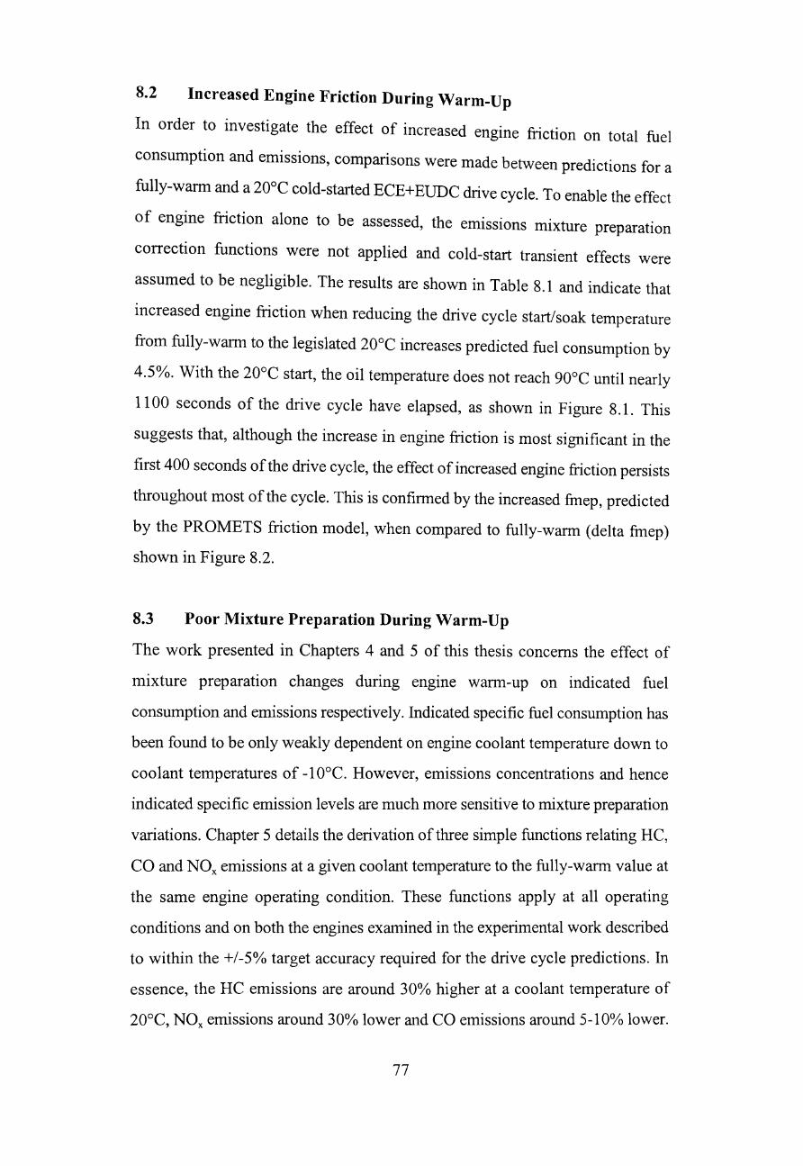
8.2 Increased Engine Friction During Warm-Up

In order to investigate the effect of increased engine friction on total fuel

consumption and emissions, comparisons were made between predictions for a

fully-warm and a 20°C cold-started ECE+EUDC drive cycle. To enable the effect

of engine friction alone to be assessed, the emissions mixture preparation

correction functions were not applied and cold-start transient effects were

assumed to be negligible. The results are shown in Table 8.1 and indicate that

increased engine friction when reducing the drive cycle start/soak temperature

from fully-warm to the legislated 20°C increases predicted fuel consumption by

4.5%. With the 20°C start, the oil temperature does not reach 90°C until nearly

1100 seconds of the drive cycle have elapsed, as shown in Figure 8.1. This

suggests that, although the increase in engine friction is most significant in the

first 400 seconds of the drive cycle, the effect of increased engine friction persists

throughout most of the cycle. This is confirmed by the increased finep, predicted

by the PROMETS friction model, when compared to fully-warm (delta finep)

shown in Figure 8.2.

8.3 Poor Mixture Preparation During Warm-Up

The work presented in Chapters 4 and 5 of this thesis concerns the effect of

mixture preparation changes during engine warm-up on indicated fuel

consumption and emissions respectively. Indicated specific fuel consumption has

been found to be only weakly dependent on engine coolant temperature down to

coolant temperatures of -10°C. However, emissions concentrations and hence

indicated specific emission levels are much more sensitive to mixture preparation

variations. Chapter 5 details the derivation of three simple functions relating HC,

CO and NOx emissions at a given coolant temperature to the fully-warm value at

the same engine operating condition. These functions apply at all operating

condi tions and on both the engines examined in the experimental work described

to within the +/-5% target accuracy required for the drive cycle predictions. In

essence, the HC emissions are around 30% higher at a coolant temperature of

20°C, NOx emissions around 30% lower and CO emissions around 5-10% lower.

77

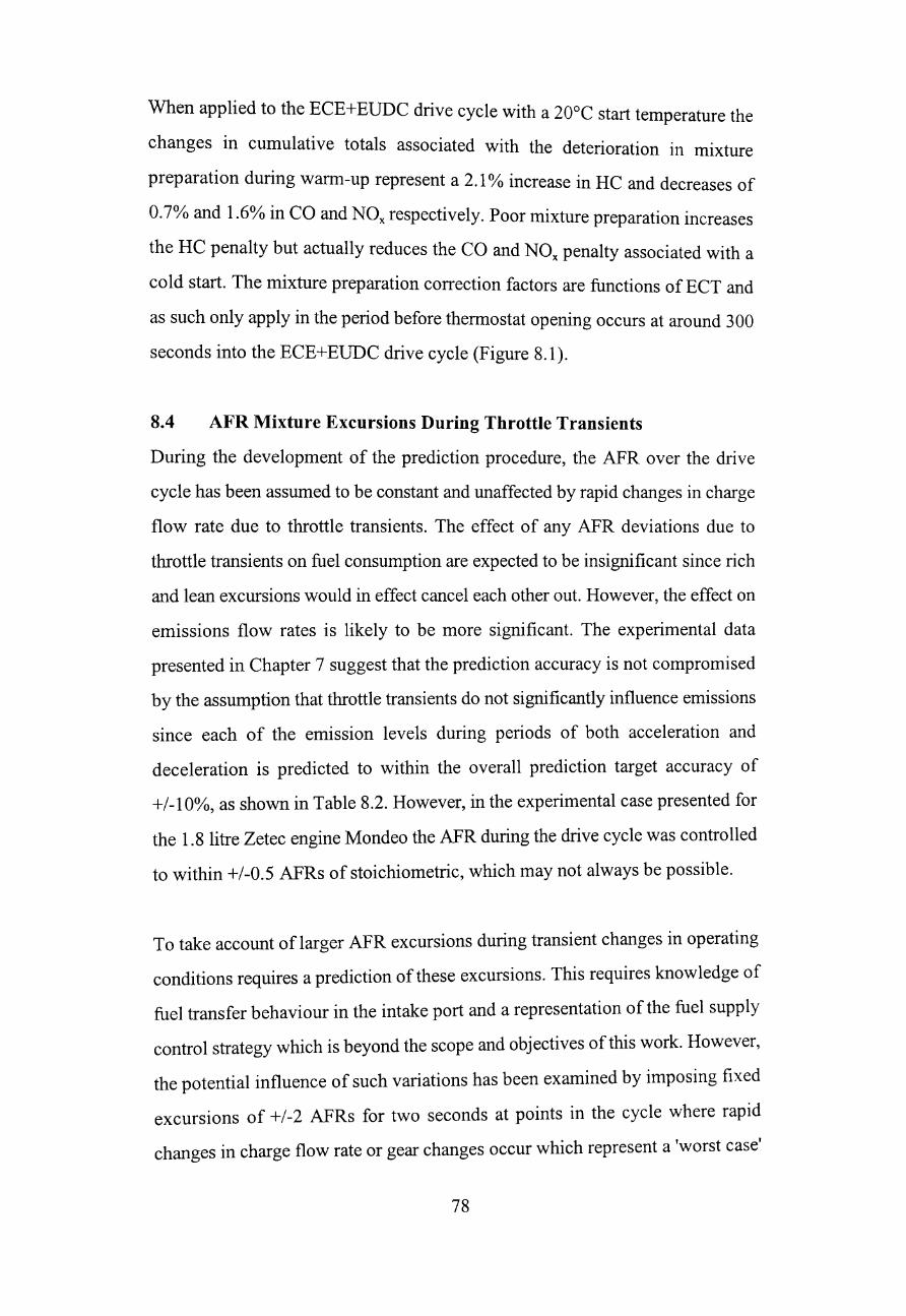
When applied to the ECE+EUDC drive cycle with a 20c C start temperature the

changes in cumulative totals associated with the deterioration in mixture

preparation during warm-up represent a 2.1 % increase in HC and decreases of

0.7% and 1.6% in CO and NOx respectively. Poor mixture preparation increases

the HC penalty but actually reduces the CO and NOx penalty associated with a

cold start. The mixture preparation correction factors are functions of ECT and

as such only apply in the period before thermostat opening occurs at around 300

seconds into the ECE+EUDC drive cycle (Figure 8.1).

8.4 AFR Mixture Excursions During Throttle Transients

During the development of the prediction procedure, the APR over the drive

cycle has been assumed to be constant and unaffected by rapid changes in charge

flow rate due to throttle transients. The effect of any APR deviations due to

throttle transients on fuel consumption are expected to be insignificant since rich

and lean excursions would in effect cancel each other out. However, the effect on

emissions flow rates is likely to be more significant. The experimental data

presented in Chapter 7 suggest that the prediction accuracy is not compromised

by the assumption that throttle transients do not significantly influence emissions

since each of the emission levels during periods of both acceleration and

deceleration is predicted to within the overall prediction target accuracy of

+/-10%, as shown in Table 8.2. However, in the experimental case presented for

the 1.8 litre Zetec engine Mondeo the APR during the drive cycle was controlled

to within +/-0.5 APRs of stoichiometric, which may not always be possible.

To take account of larger APR excursions during transient changes in operating

conditions requires a prediction of these excursions. This requires knowledge of

fuel transfer behaviour in the intake port and a representation of the fuel supply

control strategy which is beyond the scope and objectives of this work. However,

the potential influence of such variations has been examined by imposing fixed

excursions of +/-2 APRs for two seconds at points in the cycle where rapid

changes in charge flow rate or gear changes occur which represent a 'worst case'

78

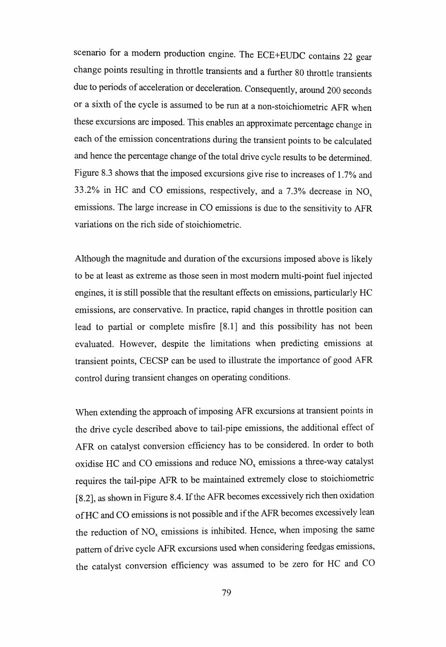
scenario for a modem production engine. The ECE+EUDC contains 22 gear

change points resulting in throttle transients and a further 80 throttle transients

due to periods of acceleration or deceleration. Consequently, around 200 seconds

or a sixth of the cycle is assumed to be run at a non-stoichiometric AFR when

these excursions are imposed. This enables an approximate percentage change in

each of the emission concentrations during the transient points to be calculated

and hence the percentage change of the total drive cycle results to be determined.

Figure 8.3 shows that the imposed excursions give rise to increases of 1.7% and

33.2% in HC and CO emissions, respectively, and a 7.3% decrease in NOx

emissions. The large increase in CO emissions is due to the sensitivity to AFR

variations on the rich side of stoichiometric.

Although the magnitude and duration of the excursions imposed above is likely

to be at least as extreme as those seen in most modem multi-point fuel injected

engines, it is still possible that the resultant effects on emissions, particularly HC

emissions, are conservative. In practice, rapid changes in throttle position can

lead to partial or complete misfire [8.1] and this possibility has not been

evaluated. However, despite the limitations when predicting emissions at

transient points, CECSP can be used to illustrate the importance of good APR

control during transient changes on operating conditions.

When extending the approach of imposing AFR excursions at transient points in

the drive cycle described above to tail-pipe emissions, the additional effect of

AFR on catalyst conversion efficiency has to be considered. In order to both

oxidise HC and CO emissions and reduce NOx emissions a three-way catalyst

requires the tail-pipe AFR to be maintained extremely close to stoichiometric

[8.2], as shown in Figure 8.4. If the AFR becomes excessively rich then oxidation

ofHC and CO emissions is not possible and ifthe AFR becomes excessively lean

the reduction of NOx emissions is inhibited. Hence, when imposing the same

pattern of drive cycle AFR excursions used when considering feedgas emissions,

the catalyst conversion efficiency was assumed to be zero for HC and CO

79

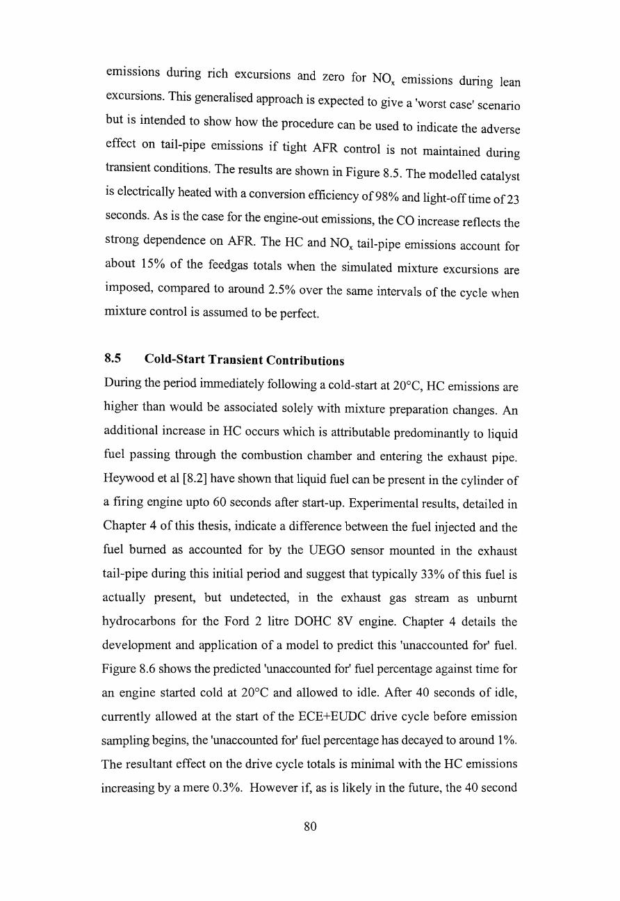
emISSIOns during rich excursions and zero for NOx

emISSIOns during lean

excursions. This generalised approach is expected to give a 'worst case' scenario

but is intended to show how the procedure can be used to indicate the adverse

effect on tail-pipe emissions if tight AFR control is not maintained during

transient conditions. The results are shown in Figure 8.5. The modelled catalyst

is electrically heated with a conversion efficiency of98% and light-off time of23

seconds. As is the case for the engine-out emissions, the CO increase reflects the

strong dependence on AFR. The HC and NOx tail-pipe emissions account for

about 15% of the feedgas totals when the simulated mixture excursions are

imposed, compared to around 2.5% over the same intervals of the cycle when

mixture control is assumed to be perfect.

8.S Cold-Start Transient Contributions

During the period immediately following a cold-start at 20°C, HC emissions are

higher than would be associated solely with mixture preparation changes. An

additional increase in HC occurs which is attributable predominantly to liquid

fuel passing through the combustion chamber and entering the exhaust pipe.

Heywood et al [8.2] have shown that liquid fuel can be present in the cylinder of

a firing engine upto 60 seconds after start-up. Experimental results, detailed in

Chapter 4 of this thesis, indicate a difference between the fuel inj ected and the

fuel burned as accounted for by the VEGO sensor mounted in the exhaust

tail-pipe during this initial period and suggest that typically 33% of this fuel is

actually present, but undetected, in the exhaust gas stream as unburnt

hydrocarbons for the Ford 2 litre DOHC 8V engine. Chapter 4 details the

development and application of a model to predict this 'unaccounted for' fuel.

Figure 8.6 shows the predicted 'unaccounted for' fuel percentage against time for

an engine started cold at 20°C and allowed to idle. After 40 seconds of idle,

currently allowed at the start of the ECE+EUDC drive cycle before emission

sampling begins, the 'unaccounted for' fuel percentage has decayed to around 1 %.

The resultant effect on the drive cycle totals is minimal with the HC emissions

increasing by a mere 0.3%. However if, as is likely in the future, the 40 second

80

conditioning period is removed the 'unaccounted for' fuel effect is more

significant. Figure 8.7 shows the 'unaccounted for' fuel percentage and coolant

temperature against time from start of the drive cycle when the conditioning

period is removed and Figure 8.8 the increase in engine-out HC emissions

associated with this 'unaccounted for' fuel prediction for the first 100 seconds

after start-up. The total drive cycle fuel consumption increases by 0.1 % and the

HC emissions by a more significant 2.2%.

The increase in HC emISSIOns occurs during the first 60 seconds of the

ECE+EUDC drive cycle. Consequently, the effect on tail-pipe emissions is much

more significant than on engine-out values because the catalytic convertor has not

reached its peak conversion efficiency. To illustrate these effects, computations

were carried out with a catalyst with an assumed efficiency of 98% and light-off

times typical of various catalyst types and locations. These times were assumed

to be 23 seconds for an electrically-heated catalyst (ERC), 70 seconds for a

close-coupled catalyst (CCC), and 130 seconds for an underbody catalyst location

(UBC). Figure 8.9 shows that in the best case, and including the effect of start-up

transients on HC emissions, tail-pipe emissions are reduced to around 2.7% ofthe

feedgas totals. Including the start-up transient HC emissions increases the best

case from 2.7% to 3.5% representing a 30% increase in tail-pipe HC emissions.

This clearly demonstrates the importance of transient phenomena immediately

following engine start-up and shows how the catalyst model in CECSP can be

used to illustrate their importance over a drive cycle.

8.6 Discussion

CECSP has been used to assess the importance to both fuel and emissions totals

over the ECE+EUDC drive cycle of the various factors influencing drive cycle

results. While some of these factors were shown to be of little importance when

predicting engine-out emissions for the initial engine/vehicle combination

examined, they are believed to be more significant when extending the

predictions to other engine/vehicle applications and particularly when predicting

81

tail-pipe emissions.

As described in Chapter 7, CECSP predicts feedgas emissions initially and these

can then be converted to tail-pipe emissions using the catalyst model described.

Factors which appear to have insignificant influences on feedgas emissions

cannot be disregarded when predictions of tail-pipe emissions are also required.

CECSP has been used to demonstrate the significance of these effects when

predicting both feedgas and tail-pipe emissions and to prioritise the factors that

influence both feedgas and tail-pipe emissions over the ECE+EUDC drive cycle

most significantly.

The extent to which cold-start and warm-up affects the pattern of fuel

consumption and emissions is shown schematically in Figure 8.10. The relative

importance of higher engine friction during warm-up, poor mixture preparation

penalties and start-up transient effects due to poor fuel utilisation are summarised

in Table 8.1. The baseline for comparison here is ECE+EUDC drive cycle results

generated assuming the engine is fully-warm from key-on and that cold-start

transient effects are zero. All results are for the Ford 1.8 litre Zetec engine

installed in a Mondeo. The results indicate that increased engine friction is the

main source of increased fuel consumption and feedgas emissions and that poor

mixture preparation and cold-start transient effects only influence He emissions

detrimentally, and even then only by around 2%. Mixture ratio excursions

throughout the drive cycle during transient changes in operating conditions have

been shown to have a potentially large influence on HC and, partiCUlarly, on CO

emlsslOns.

When tail-pipe emissions are considered, poor mixture preparation and cold-start

phenomena prior to catalyst light-off have substantial effects on cumulative

emissions, particularly ofHC. Mixture ratio excursions have a more significant

effect on emissions levels than for feedgas emissions due to the sensitivity of the

catalytic convertor to AFR deviations from the stoichiometric baseline. The

82

sensitivity of tail-pipe emissions to engine calibration details makes absolute

values difficult to predict accurately, and hence the application of CECSP

presented here is intended to demonstrate the significance of the various factors

influencing tail-pipe emissions rather than provide absolute predictions to within

the accuracy possible with feedgas emissions. Table 8.3 shows the effects

demonstrated to be of primary significance to tail-pipe emissions totals over the

ECE+EUDC drive cycle together with suggested actions to limit these effects.

In conclusion, this chapter demonstrates the application of CECSP to examine the

influence of cold-start and engine management strategy implications on drive

cycle fuel consumption, and both feedgas and tail-pipe emission levels. The

illustration presented demonstrates the need to reduce engine friction levels and

warm-up times to be of principal importance to minimise drive cycle fuel

consumption and feedgas emissions. However, when tail-pipe emissions are

considered, these priorities are overshadowed by the need for rapid catalyst

light-off and good fuelling control to minimise excess fuel supply and maintain

tight control of AFR excursions during transients. The following chapter goes on

to detail the additional applications the CECSP prediction procedure has been

used for and the appropriate changes to the model required for these applications.

83

Chapter 9

Model Exploitation

9.1 Introduction

In the work presented so far, CECSP has been applied to a single engine/vehicle

combination driven through the ECE+EUDC drive cycle from a cold-start

condition. In this chapter, other applications of CECSP are considered.

Essentially, the prediction procedure developed can be used in two ways. Firstly,

predictions of the effect on drive cycle performance of changing various

engine/vehicle parameters for different drive cycles can be made and the likely

performance of new engine/vehicle combinations in the early stages of

development assessed. Such predictions require assumptions or knowledge of

likely exhaust gas after-treatment performance to enable tail-pipe emissions to be

predicted. Secondly, predictions of feedgas emissions can be compared with

desired tail-pipe values to enable target catalytic convertor characteristics and the

associated exhaust gas after-treatment system development costs to be evaluated.

In both cases, the prediction of feedgas emissions is influenced by various

characteristics of the complete engine/vehicle/drive cycle package and the

prediction procedure can be used to investigate the effect of these characteristics

on the drive cycle performance. The following details five applications of

CECSP, the interpretation of results and the implications of these.

9.2 Case 1: Drive Cycle Definition Effects

In this case, CECSP is used to demonstrate the effect on fuel consumption and

emission levels of the drive cycle used. The software was developed using the

ECE+EUDC drive cycle, also termed the New European Drive Cycle (NEDC).

However, because engine fuel consumption and emissions performance is

influenced by the characteristics of the drive cycle used to determine fuel and

84

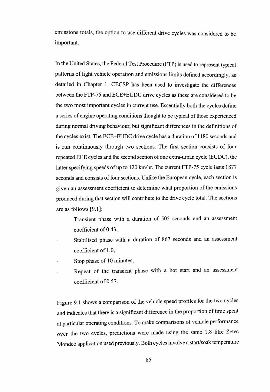
emissions totals, the option to use different drive cycles was considered to be

important.

In the United States, the Federal Test Procedure (FTP) is used to represent typical

patterns of light vehicle operation and emissions limits defined accordingly, as

detailed in Chapter 1. CECSP has been used to investigate the differences

between the FTP-75 and ECE+EUDC drive cycles as these are considered to be

the two most important cycles in current use. Essentially both the cycles define

a series of engine operating conditions thought to be typical of those experienced

during normal driving behaviour, but significant differences in the definitions of

the cycles exist. The ECE+EUDC drive cycle has a duration of 1180 seconds and

is run continuously through two sections. The first section consists of four

repeated ECE cycles and the second section of one extra-urban cycle (EUDC), the

latter specifying speeds of up to 120 kmIhr. The current FTP-75 cycle lasts 1877

seconds and consists of four sections. Unlike the European cycle, each section is

given an assessment coefficient to determine what proportion of the emissions

produced during that section will contribute to the drive cycle total. The sections

are as follows [9.1]:

Transient phase with a duration of 505 seconds and an assessment

coefficient of 0.43,

Stabilised phase with a duration of 867 seconds and an assessment

coefficient of 1.0,

Stop phase of 10 minutes,

Repeat of the transient phase with a hot start and an assessment

coefficient of 0.57.

Figure 9.1 shows a comparison of the vehicle speed profiles for the two cycles

and indicates that there is a significant difference in the proportion of time spent

at particular operating conditions. To make comparisons of vehicle performance

over the two cycles, predictions were made using the same 1.8 litre Zetec

Mondeo application used previously. Both cycles involve a start/soak temperature

85

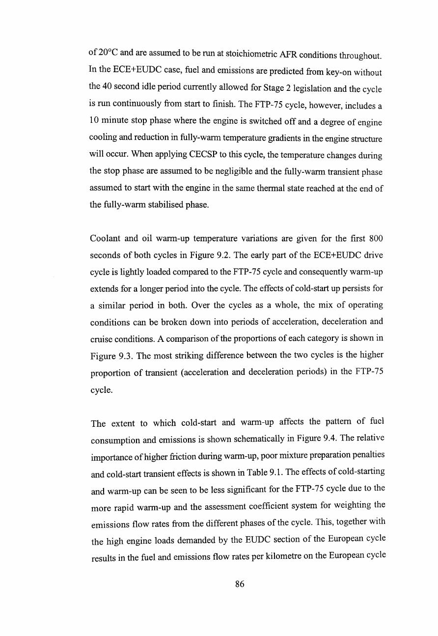
of 20°C and are assumed to be run at stoichiometric AFR conditions throughout.

In the ECE+EUDC case, fuel and emissions are predicted from key-on without

the 40 second idle period currently allowed for Stage 2 legislation and the cycle

is run continuously from start to finish. The FTP-75 cycle, however, includes a

10 minute stop phase where the engine is switched off and a degree of engine

cooling and reduction in fully-warm temperature gradients in the engine structure

will occur. When applying CECSP to this cycle, the temperature changes during

the stop phase are assumed to be negligible and the fully-warm transient phase

assumed to start with the engine in the same thermal state reached at the end of

the fully-warm stabilised phase.

Coolant and oil warm-up temperature variations are given for the first 800

seconds of both cycles in Figure 9.2. The early part of the ECE+EUDC drive

cycle is lightly loaded compared to the FTP-75 cycle and consequently warm-up

extends for a longer period into the cycle. The effects of cold-start up persists for

a similar period in both. Over the cycles as a whole, the mix of operating

conditions can be broken down into periods of acceleration, deceleration and

cruise conditions. A comparison of the proportions of each category is shown in

Figure 9.3. The most striking difference between the two cycles is the higher

proportion of transient (acceleration and deceleration periods) in the FTP-75

cycle.

The extent to which cold-start and warm-up affects the pattern of fuel

consumption and emissions is shown schematically in Figure 9.4. The relative

importance of higher friction during warm-up, poor mixture preparation penalties

and cold-start transient effects is shown in Table 9.1. The effects of cold-starting

and warm-up can be seen to be less significant for the FTP-75 cycle due to the

more rapid warm-up and the assessment coefficient system for weighting the

emissions flow rates from the different phases of the cycle. This, together with

the high engine loads demanded by the EUDC section of the European cycle

results in the fuel and emissions flow rates per kilometre on the European cycle

86

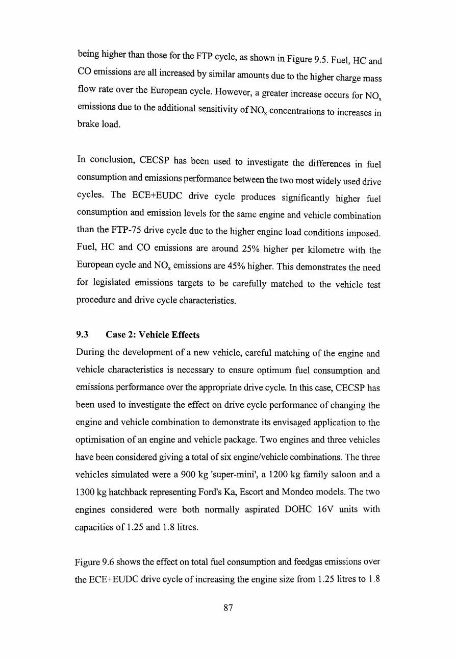
being higher than those for the FTP cycle, as shown in Figure 9.5. Fuel, HC and

CO emissions are all increased by similar amounts due to the higher charge mass

flow rate over the European cycle. However, a greater increase occurs for NO x

emissions due to the additional sensitivity of NO x concentrations to increases in

brake load.

In conclusion, CECSP has been used to investigate the differences in fuel

consumption and emissions performance between the two most widely used drive

cycles. The ECE+EUDC drive cycle produces significantly higher fuel

consumption and emission levels for the same engine and vehicle combination

than the FTP-75 drive cycle due to the higher engine load conditions imposed.

Fuel, HC and CO emissions are around 25% higher per kilometre with the

European cycle and NOx emissions are 45% higher. This demonstrates the need

for legislated emissions targets to be carefully matched to the vehicle test

procedure and drive cycle characteristics.

9.3 Case 2: Vehicle Effects

During the development of a new vehicle, careful matching of the engine and

vehicle characteristics is necessary to ensure optimum fuel consumption and

emissions performance over the appropriate drive cycle. In this case, CECSP has

been used to investigate the effect on drive cycle performance of changing the

engine and vehicle combination to demonstrate its envisaged application to the

optimisation of an engine and vehicle package. Two engines and three vehicles

have been considered giving a total of six engine/vehicle combinations. The three

vehicles simulated were a 900 kg 'super-mini', a 1200 kg family saloon and a

1300 kg hatchback representing Ford's Ka, Escort and Mondeo models. The two

engines considered were both normally aspirated DOHC 16V units with

capacities of 1.25 and 1.8 litres.

Figure 9.6 shows the effect on total fuel consumption and feedgas emissions over

the ECE+EUDC drive cycle of increasing the engine size from 1.25 litres to 1.8

87

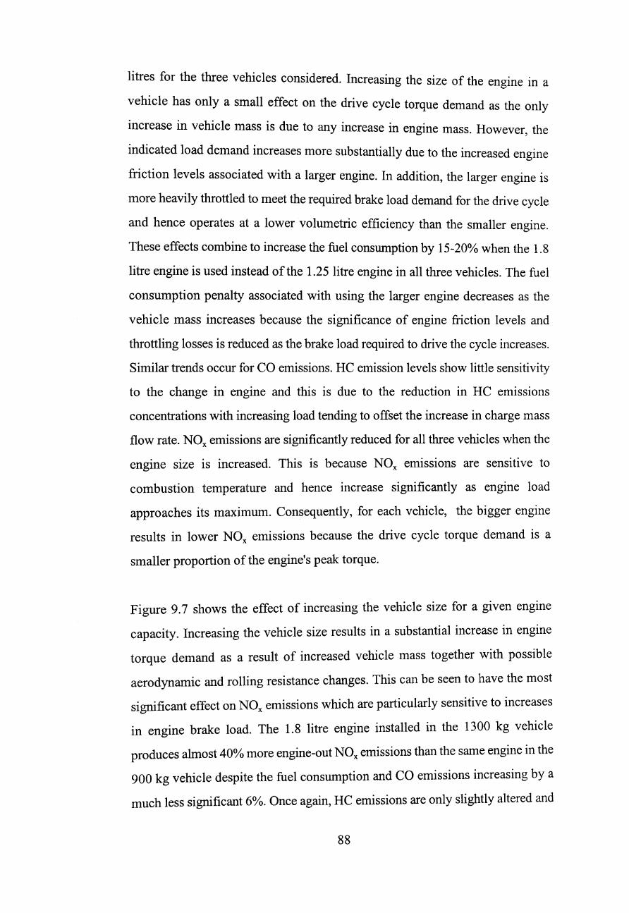
litres for the three vehicles considered. Increasing the size of the engine in a

vehicle has only a small effect on the drive cycle torque demand as the only

increase in vehicle mass is due to any increase in engine mass. However, the

indicated load demand increases more substantially due to the increased engine

friction levels associated with a larger engine. In addition, the larger engine is

more heavily throttled to meet the required brake load demand for the drive cycle

and hence operates at a lower volumetric efficiency than the smaller engine.

These effects combine to increase the fuel consumption by 15-20% when the 1.8

litre engine is used instead of the 1.25 litre engine in all three vehicles. The fuel

consumption penalty associated with using the larger engine decreases as the

vehicle mass increases because the significance of engine friction levels and

throttling losses is reduced as the brake load required to drive the cycle increases.

Similar trends occur for CO emissions. HC emission levels show little sensitivity

to the change in engine and this is due to the reduction in HC emissions

concentrations with increasing load tending to offset the increase in charge mass

flow rate. NOx emissions are significantly reduced for all three vehicles when the

engine size is increased. This is because NOx emissions are sensitive to

combustion temperature and hence increase significantly as engine load

approaches its maximum. Consequently, for each vehicle, the bigger engine

results in lower NOx emissions because the drive cycle torque demand is a

smaller proportion of the engine's peak torque.

Figure 9.7 shows the effect of increasing the vehicle size for a given engine

capacity. Increasing the vehicle size results in a substantial increase in engine

torque demand as a result of increased vehicle mass together with possible

aerodynamic and rolling resistance changes. This can be seen to have the most

significant effect on NOx emissions which are particularly sensitive to increases

in engine brake load. The 1.8 litre engine installed in the 1300 kg vehicle

produces almost 40% more engine-out NOx emissions than the same engine in the

900 kg vehicle despite the fuel consumption and CO emissions increasing by a

much less significant 6%. Once again, HC emissions are only slightly altered and

88

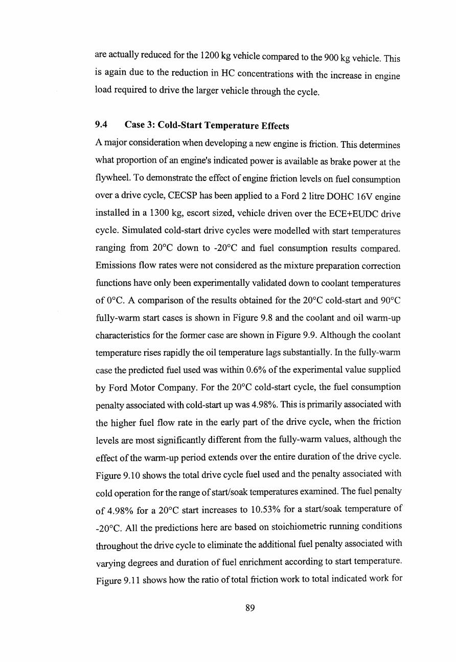
are actually reduced for the 1200 kg vehicle compared to the 900 kg vehicle. This

is again due to the reduction in HC concentrations with the increase in engine

load required to drive the larger vehicle through the cycle.

9.4 Case 3: Cold-Start Temperature Effects

A major consideration when developing a new engine is friction. This detennines

what proportion of an engine's indicated power is available as brake power at the

flywheel. To demonstrate the effect of engine friction levels on fuel consumption

over a drive cycle, CECSP has been applied to a Ford 2 litre DOHC 16V engine

installed in a 1300 kg, escort sized, vehicle driven over the ECE+EUDC drive

cycle. Simulated cold-start drive cycles were modelled with start temperatures

ranging from 20°C down to -20°C and fuel consumption results compared.

Emissions flow rates were not considered as the mixture preparation correction

functions have only been experimentally validated down to coolant temperatures

of O°C. A comparison of the results obtained for the 20°C cold-start and 90°C

fully-warm start cases is shown in Figure 9.8 and the coolant and oil warm-up

characteristics for the fonner case are shown in Figure 9.9. Although the coolant

temperature rises rapidly the oil temperature lags substantially. In the fully-warm

case the predicted fuel used was within 0.6% of the experimental value supplied

by Ford Motor Company. For the 20°C cold-start cycle, the fuel consumption

penalty associated with cold-start up was 4.98%. This is primarily associated with

the higher fuel flow rate in the early part of the drive cycle, when the friction

levels are most significantly different from the fully-warm values, although the

effect of the warm-up period extends over the entire duration of the drive cycle.

Figure 9.10 shows the total drive cycle fuel used and the penalty associated with

cold operation for the range of start/soak temperatures examined. The fuel penalty

of 4.98% for a 20°C start increases to 10.53% for a start/soak temperature of

-20°C. All the predictions here are based on stoichiometric running conditions

throughout the drive cycle to eliminate the additional fuel penalty associated with

varying degrees and duration of fuel enrichment according to start temperature.

Figure 9.11 shows how the ratio of total friction work to total indicated work for

89

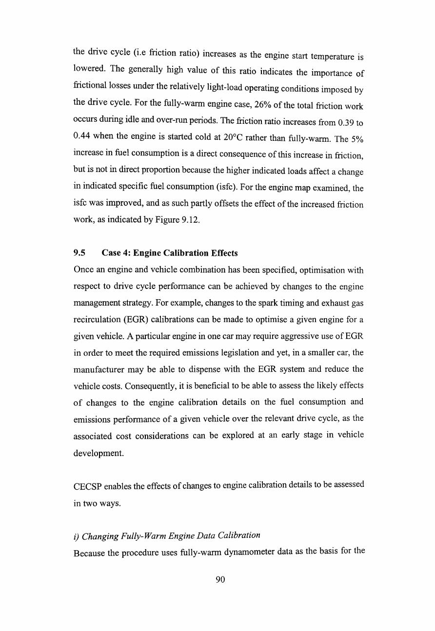
the drive cycle (i.e friction ratio) increases as the engine start temperature is

lowered. The generally high value of this ratio indicates the importance of

frictional losses under the relatively light-load operating conditions imposed by

the drive cycle. For the fully-warm engine case, 26% of the total friction work

occurs during idle and over-run periods. The friction ratio increases from 0.39 to

0.44 when the engine is started cold at 20°C rather than fully-warm. The 5%

increase in fuel consumption is a direct consequence of this increase in friction,

but is not in direct proportion because the higher indicated loads affect a change

in indicated specific fuel consumption (isfc). For the engine map examined, the

isfc was improved, and as such partly offsets the effect of the increased friction

work, as indicated by Figure 9.12.

9.5 Case 4: Engine Calibration Effects

Once an engine and vehicle combination has been specified, optimisation with

respect to drive cycle performance can be achieved by changes to the engine

management strategy. For example, changes to the spark timing and exhaust gas

recirculation (EGR) calibrations can be made to optimise a given engine for a

given vehicle. A partiCUlar engine in one car may require aggressive use of EGR

in order to meet the required emissions legislation and yet, in a smaller car, the

manufacturer may be able to dispense with the EGR system and reduce the

vehicle costs. Consequently, it is beneficial to be able to assess the likely effects

of changes to the engine calibration details on the fuel consumption and

emissions performance of a given vehicle over the relevant drive cycle, as the

associated cost considerations can be explored at an early stage in vehicle

development.

CECSP enables the effects of changes to engine calibration details to be assessed

in two ways.

i) Changing Fully- Warm Engine Data Calibration

Because the procedure uses fully-warm dynamometer data as the basis for the

90

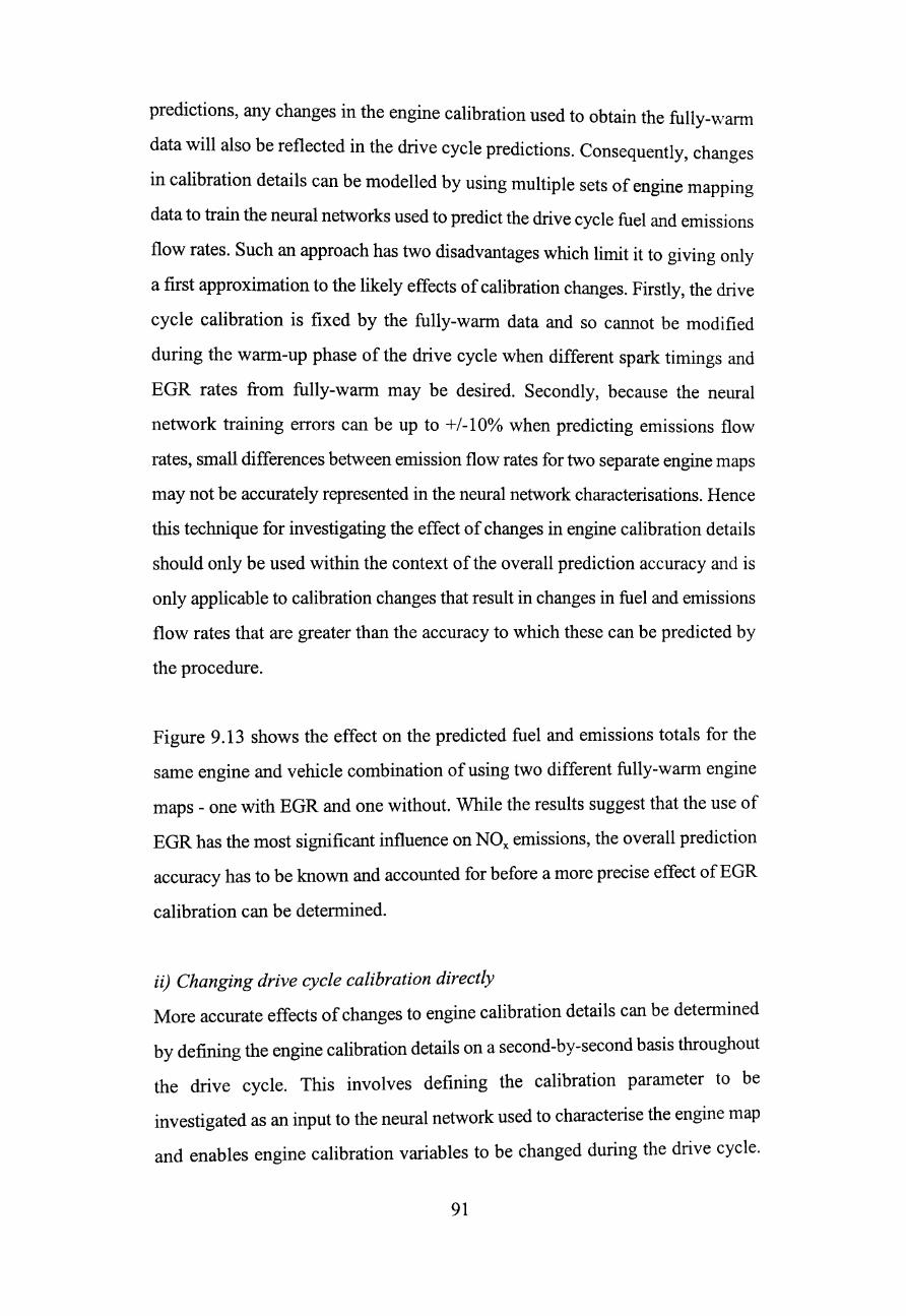
predictions, any changes in the engine calibration used to obtain the fully-wann

data will also be reflected in the drive cycle predictions. Consequently, changes

in calibration details can be modelled by using multiple sets of engine mapping

data to train the neural networks used to predict the drive cycle fuel and emissions

flow rates. Such an approach has two disadvantages which limit it to giving only

a first approximation to the likely effects of calibration changes. Firstly, the drive

cycle calibration is fixed by the fully-wann data and so cannot be modified

during the warm-up phase of the drive cycle when different spark timings and

EGR rates from fully-warm may be desired. Secondly, because the neural

network training errors can be up to +1-10% when predicting emissions flow

rates, small differences between emission flow rates for two separate engine maps

may not be accurately represented in the neural network characterisations. Hence

this technique for investigating the effect of changes in engine calibration details

should only be used within the context of the overall prediction accuracy and is

only applicable to calibration changes that result in changes in fuel and emissions

flow rates that are greater than the accuracy to which these can be predicted by

the procedure.

Figure 9.13 shows the effect on the predicted fuel and emissions totals for the

same engine and vehicle combination of using two different fully-warm engine

maps - one with EGR and one without. While the results suggest that the use of

EGR has the most significant influence on NOx emissions, the overall prediction

accuracy has to be known and accounted for before a more precise effect of EGR

calibration can be determined.

ii) Changing drive cycle calibration directly

More accurate effects of changes to engine calibration details can be determined

by defining the engine calibration details on a second-by-second basis throughout

the drive cycle. This involves defining the calibration parameter to be

investigated as an input to the neural network used to characterise the engine map

and enables engine calibration variables to be changed during the drive cycle.

91

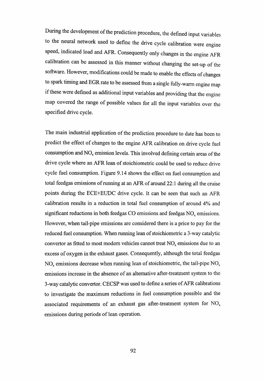
During the development of the prediction procedure, the defined input variables

to the neural network used to define the drive cycle calibration were engine

speed, indicated load and AFR. Consequently only changes in the engine AFR

calibration can be assessed in this manner without changing the set-up of the

software. However, modifications could be made to enable the effects of changes

to spark timing and EGR rate to be assessed from a single fully-warm engine map

if these were defined as additional input variables and providing that the engine

map covered the range of possible values for all the input variables over the

specified drive cycle.

The main industrial application of the prediction procedure to date has been to

predict the effect of changes to the engine AFR calibration on drive cycle fuel

consumption and NOx emission levels. This involved defining certain areas of the

drive cycle where an AFR lean of stoichiometric could be used to reduce drive

cycle fuel consumption. Figure 9.14 shows the effect on fuel consumption and

total feedgas emissions of running at an AFR of around 22: 1 during all the cruise

points during the ECE+EUDC drive cycle. It can be seen that such an AFR

calibration results in a reduction in total fuel consumption of around 4% and

significant reductions in both feedgas CO emissions and feedgas NOx emissions.

However, when tail-pipe emissions are considered there is a price to pay for the

reduced fuel consumption. When running lean of stoichiometric a 3-way catalytic

convertor as fitted to most modem vehicles cannot treat NOx emissions due to an

excess of oxygen in the exhaust gases. Consequently, although the total feedgas

NOx emissions decrease when running lean of stoichiometric, the tail-pipe NOx

emissions increase in the absence of an alternative after-treatment system to the

3-way catalytic convertor. CECSP was used to define a series of AFR calibrations

to investigate the maximum reductions in fuel consumption possible and the

associated requirements of an exhaust gas after-treatment system for NOx

emissions during periods of lean operation.

92

9.6 Case 5: Tail-Pipe After-Treatment Effects

Initially developed to predict fuel consumption and feedgas emissions, CECSP

enables the definition of exhaust gas after-treatment characteristics to enable

predictions of tail-pipe emissions to be made. In order to predict accurate tail-pipe

emissions the catalyst model in CECSP requires catalyst data specific to the

engine/vehicle/drive cycle combination which would not be available until the

actual vehicle drive cycle performance could be measured. Consequently, the

catalyst model is intended primarily to facilitate the investigation of the effects

on tail-pipe emissions of imposed catalyst characteristics. These may be known

characteristics or target values which may not yet be achievable with current

catalyst technology. In the industrial application discussed above, CECSP was

used to determine the required lean NOx conversion efficiency to achieve future

emissions legislation whilst achieving the maximum reduction in drive cycle fuel

consumption by use of a hybrid stoichiometric/lean AFR engine calibration. A

simple extension of this application of CECSP would be to determine the

required after-treatment performance for a vehicle under development. This could

involve engine data from engines in the early stages of production or even from

simulated engine performance programs which are now becoming increasingly

available.

9.7 Discussion

CECSP is intended to provide a research tool to enable the prediction of drive

cycle fuel and emissions performance at an early stage in vehicle development.

A wide range of possible applications are envisaged for the software in the

development and evaluation of proposed solutions in the ongoing quest for

reduced fuel consumption and improved emissions performance from new

light-duty road vehicles. Current and future emissions legislation worldwide

provide many challenges for new vehicle design engineers and result in

manufacturers adapting engine/vehicle specifications to suit the intended market.

Factors such as the drive cycle used to determine fuel consumption and emissions

performance and the associated range of engine options that can be offered in a

93

given vehicle need to be considered to ensure that new vehicles comply with

legislated requirements. For a given market using a given drive cycle and test

procedure fuel and emissions performance can essentially be optimised in two

ways: by changing the vehicle characteristics or by changing the engine and

exhaust after-treatment characteristics. In CECSP, vehicle characteristics can be

altered by changing parameters such as transmission ratios, vehicle aerodynamics

and vehicle mass. Different engines can be mated with different vehicles to assess

the significance of engine performance and the effect of both engine friction

levels and engine management calibration details. Finally, a major factor

influencing drive cycle emissions performance is exhaust gas after-treatment. The

efficiency and location of a catalytic convertor on a vehicle significantly

influences the tail-pipe emissions produced throughout a drive cycle. Initially

developed to predict engine-out emissions, CECSP can be used to assess the

effect of, or requirement for, exhaust gas after-treatment performance for a given

engine/vehicle/drive cycle combination.

The case studies detailed above provide a brief summary of the applications

considered to date and illustrate some of the important issues that need to be

considered during modem engine and vehicle development. Further development

work, detailed in the following chapter, will extend the scope of the existing

CECSP software to cover more engineering problems.

94

Chapter 10

Discussion and Conclusions

10.1 Discussion

This thesis details the development and exploitation of a PC based prediction

procedure, called CECSP. The aim has been to facilitate predictions of fuel

consumption and emissions during cold-started drive cycles. CECSP enables the

relative effects of changing several engine and vehicle parameters to be examined

and so can be used to prioritise areas of performance improvement during both

engine and vehicle development. Because the procedure only requires fully-warm

engine mapping data it can be used at an early stage in the development process

to predict expected drive cycle results before engine and vehicle design

parameters are finalised. Engine development teams generally now have access

to thermodynamic performance simulation codes which have been developed

in-house or which are commercially available. Also early test work on prototype

engines rapidly generates engine performance maps. Both simulation and

experimental data tend to be for fully-warm steady-state operating conditions, and

CECSP makes use of such data to predict how a given engine/vehicle

combination would perform over a defined drive cycle.

CECSP has been validated by comparison with experimental data for a typical

production vehicle driven over the ECE+EUDC drive cycle and the prediction

accuracy found to be within the target +/-5% for fuel consumption and +/-10%

for feedgas emissions. The application of CECSP to investigate and prioritise the

various external factors influencing fuel consumption and emissions over drive

cycles has been considered and the results and assumptions made justified and

discussed. Additional applications have been considered in an attempt to illustrate

95

the contribution of the procedure to real engme and vehicle development

situations.

10.2 Further Work

At various points in this thesis the requirement for further work to extend both the

accuracy and the scope of the work presented has been highlighted. These

requirements are now summarised in the context of the overall prediction

procedure and the original objectives of the work.

The first area for further work concerns the use of neural networks. These have

been found to provide a simple and effective way of characterising engine

mapping data for use over the range of operating conditions imposed by a typical

drive cycle, and have been used in preference to regression analysis. However,

the neural networks used extensively here use only engine speed, load and APR

as inputs to define fuel and emissions mass flow rates as outputs. This is

consistent with the original objective of the work to provide an initial prediction

of the fuel consumption and emissions performance of a given engine and vehicle

package over a defined drive cycle. Consequently, the drive cycle is defined in

terms of a series of engine speed, indicated load and APR conditions. Such a

configuration has been shown to be capable of predicting fuel mass flow rates to

within +/- 5% and emissions flow rates to within +/- 10% of experimental data

but imposes fixed spark timing and EGR rate settings throughout the drive cycle.

Chapter 2 shows that the neural network characterisation procedure can, in

principle, be extended to map fuel and emissions flow rates as functions of spark

timing and EGR rate in addition to engine speed, load and APR, but that further

work is required to determine the effect this extension has on both the prediction

accuracy and the data processing time. Such an extension would enable the

effects of spark timing and EGR rate changes on drive cycle performance to be

investigated. Increasing the number of inputs to the neural network increases the

size of the required database on which to train the neural network and

consequently increases the processing time required. Since the optimisation of a

96

neural network setup for a given database has been found to involve a certain

degree of trial and error, a significant amount of further work is required to

determine the optimum network configuration for such an extension to the

prediction procedure, together with the effects on the prediction accuracy that

could be expected. More fundamentally, CECSP currently uses experimental

engine mapping data to characterise engine performance. Ultimately, it may be

possible to use a complete engine combustion model to accurately model fuel

consumption and emissions and negate the current need for empirical engine data.

Such engine simulation software is becoming increasingly available and provides

a possibility for future development of CECSP.

The second major area of interest for further work is the period immediately

following engine start-up. During the first 100 seconds after a cold-start various

phenomena combine to provide uncertainty in the predictions of fuel and

emissions mass flow rates. This is particularly important for emissions flow rates,

as it is in this period when the bulk of the drive cycle total emissions are

produced, while the catalytic convertor efficiency is low. As detailed in Chapters

4 and 5 of this thesis, a significant amount of the fuel injected into the engine

intake system is not accounted for in exhaust gas analysis using a UEGO sensor,

and is believed to pass undetected into both the engine lubricating oil and the

exhaust system, resulting in extremely high HC emissions immediately following

a cold-start. Further work is required to determine more accurately the

proportions of the fuel injected that pass directly into the lubricating oil and

exhaust stream and the mechanisms by which these phenomena occur. While the

work presented in Chapters 7 and 8 suggests that these considerations are of little

significance to the total fuel consumption and engine-out emissions predictions

over a typical drive cycle, they are likely to be of much greater significance to

both the instantaneous mass flow rate predictions in this period and the drive

cycle tail-pipe emissions predictions.

In addition to these two areas of envisaged development, the addition of a full

97

catalytic convertor model to the procedure would further extend the scope of the

existing software package. It is envisaged that such a model could use exhaust gas

temperature predictions made by a sub-model of the PROMETS package to

predict catalyst light-off behaviour for a given engine/vehicle/drive cycle

combination, enabling catalyst performance and warm-up behaviour to be more

accurately modelled.

The above areas of proposed further work will, it is believed, further extend the

contribution of the work presented in this thesis to both engine and vehicle

developent. CECSP will never ultimately be capable of modelling exactly the fuel

consumption and emissions performance of an engine and vehicle combination

but it is believed to provide a useful tool for predicting expected drive cycle

performance to positively influence the development and optimisation of road

vehicles in the future.

10.3 Conclusions

CECSP has been developed to predict fuel consumption and emissions over drive

cycles starting with the engine at cold-soak temperatures. CECSP requires

fully-warm test bed data to be available for the engine under consideration over

the range of indicated loads and speeds imposed by the drive cycle.

Experimental data support the assumptions made when applying fully-warm data

to a cold-start situation. Indicated specific fuel consumption is a function of

indicated operating conditions independent of engine coolant temperature.

Indicated specific emissions ofHC, CO and NOx during warm-up can be related

to the corresponding fully-warm values using simple functions of engine coolant

temperature to account for the deterioration in mixture preparation.

An engine friction model is used to infer indicated operating conditions from

brake operating conditions. Experimental data confirm that warm-up friction

power losses can be predicted by scaling fully-warm friction levels according to

98

oil viscosity.

CECSP has been used to investigate and illustrate the factors that influence drive

cycle fuel consumption and emissions performance with the following

conclusions:

Cold-start effects

• Fuel consumption and engine-out emissions, particularly of HC, are

influen?ed most by increased engine friction levels during warm-up and

poor mixture preparation.

• Cold-start transient effects due to poor fuel utilisation represent a

negligible increase in fuel consumption and a very small increase in

engine-out HC emissions of around 2% over the European drive cycle.

• Poor mixture ratio control during transient operating points have a

potentially large influence on engine-out HC and CO emissions.

• Tail-pipe emissions are most sensitive to changes in emission levels in the

period before catalyst light-off occurs immediately following a cold-start.

Reductions in tail-pipe emissions are best achieved by rapid catalyst

light-off and good fuel utilisation through engine calibration.

• Mixture ratio excurSIOns influence tail-pipe emISSIOns more than

engine-out emissions due to reduced catalyst performance at APRs rich

or lean of stoichiometric. Close control of APR during transient operating

points can significantly reduce this effect.

Drive cycle effects

• Comparisons between the US FTP-75 and European ECE+EUDC drive

cycles have been made. The FTP-75 cycle results are less sensitive to

99

changes in cold-start engme friction, poor mixture preparation and

cold-start transient effects due to faster engine warm-up. In addition, the

cold and hot parts of the FTP-75 cycle are weighted so that the majority

of the cycle totals come from fully-warm operating conditions.

• Mixture ratio excursions have a more significant effect on the FTP-75

cycle due to a larger proportion of transient operating conditions.

Vehicle effects

• Increasing vehicle mass results in significant increases in drive cycle fuel

consumption and emissions. NOx emissions increase the most due to their

sensitivity to the resulting increases in indicated load.

• Increasing engine size in a given vehicle increases fuel consumption due

to increased engine friction and reduced volumetric efficiency resulting

from a larger engine working at a smaller proportion of its maximum

power output. NOx emissions, however, may be reduced due to the

reduction in the proportion of the engine's maximum indicated load

required to drive the vehicle.

100

References

Chapter 1

1.1

1.2

1.3

Dunne J M and Greening P J, "European emission standards to the year

2000", !MechE Seminar on Worldwide Engine Emissions Standards and

How to Meet Them, London, 25-26 May 1993.

EC Directive 9114411EEC, OJ, L242, 1.

"Proposed Regulations for Low-Emission Vehicles and Clean Fuels" ,

California Air Resources Board, August 13, 1990.

1.4 Hadded 0, Stokes J and Grigg D W, "Low emission vehicle technology

for ULEV and European stage 3 emission standards", lMechE paper

C462/181126, Autotech '93, 1993.

1.5 Dunne J M, "Status of Emissions Legislation", IMechE Seminar on

Application of Powertrain and Fuel Technologies to Meet Emissions

Standards, 3rd lnt Seminar on Worldwide Engine Emissions Standards

and How to Meet Them, 24-26 June 1996.

1.6 Andre M, Hickman A J, Hassel D and Joumard R, "Driving cycles for

emissions measurements under European conditions", SAE paper no.

950926.

1.7 Watson H C, "Effects of a wide range of drive cycles on the emissions

from vehicles of three levels of technology", SAE paper no. 950221.

1.8 Marshall W F and Eccleston B H, "Emissions at off-ambient

temperature", SAE paper no. 800512.

1.9 Eccleston B H and Hum R W, "Ambient temperature and trip length _

influences on automotive fuel economy and emissions", SAE paper no.

780613.

1.10 Horowitz A and Tobin R L, "The influence of urban trip characteristics

on vehicle warm-up - implication for urban automobile fuel

consumption", SAE paper no. 790656.

1.11 Austin T C and Hellman K H, "Passenger car fuel economy as influenced

by trip length", SAE paper no. 750004.

1.12 Andre M, "In actual use car testing: 70,000 kilometres and 10,000 trips

by 55 French cars under real conditions", SAE paper no. 910039.

1.13 Langen P, Theissen M, Mallog J and Zielinski R, "Heated catalytic

convertor competing technologies to meet LEV emission standards", SAE

paper no. 940470.

1.14 Cheng W K, Hamrin D, Heywood J B, Hochgreb S, Min K and Norris M,

"An overview of hydrocarbon emissions mechanisms in spark-ignition

engines", SAE paper no. 932708.

1.15 Shin Y, Cheng W K and Heywood J B, "Liquid gasolene behaviour in the

engine cylinder of an SI engine", SAE paper no. 941872.

1.16 Shayler P J, Marshall W D P and Turner J, "Exhaust emissions: the

influence of fuel injection system details", IMechE paper C394/015,

IMechE Int Conf on Automotive Power Systems, Chester, 10-12

September 1990.

1.17 Shayler P J, Christian S J and Ma T, "A model for the investigation of

temperature, heat flow and friction characteristics during engine

warm-up", SAEpaperno. 931153.

Chapter 2

2.1 Heywood J B, "Internal Combustion Engine Fundamentals", published by

McGraw-Hill Book Company, ISBN 0-07-100499-8, 1988.

2.2 Bacon A, "Fault Diagnosis Techniques for Spark Ignition Engines", PhD

Thesis, University of Nottingham, 1991.

2.3 Bacon A, Shay1er P J, Ma T, "Potential for engine control using neural

networks", IMechE paper C448/057, 1992.

2.4 Stevens S P, Shayler P J, Ma T, "Experimental data processing techniques

to map the performance of a spark ignition engine", Proc IMechE, vol

290,1995.

2.5 McClelland J L, Rumelhart D E, "Explorations in Parallel Distributed

Processing: A Handbook of Models, Programs and Exercises", IT Press,

ISBN 0-262-63113-X, 1988.

2.6 McClelland J L, Rumelhart D E, "Parallel Distributed Processing,

Volume 1", IT Press, ISBN 0-262-68053-X, 1986

2.7 McClelland J L, Rumelhart D E, "Parallel Distributed Processing,

Volume 2", IT Press, ISBN 0-262-63110-5, 1986

Chapter 3

3.1 Sampson A J and Heywood J B, "Analysis of fuel behaviour in the

spark-ignition engine start-up process", SAE paper no. 950678.

3.2 Shayler P J, Isaacs R M and Ma T, "The variation of in-cylinder mixture

ratios during engine cranking at low ambient temperatures", IMechE,

Journal of Automobile Engineering, 1992.

3.3 Murakami Y and Aihara H, "Analysis of mechanism intermixing

combustion products in engine oil", JSME Int. 1, Series II, vol. 34, No.

4, pp.548-556 (1991).

3.4 Frottier V, Heywood J Band Hochgreb S, "Measurement of gasolene

absorption into engine lubricating oil", SAE paper no. 961229.

3.5 Shay1er P J, Marshall W D P and Turner J, "Exhaust emissions: the

influence of fuel injection system details", IMechE paper C394/015,

IMechE Int Conf on Automotive Power Systems, Chester, 10-12

September 1990.

3.6 Johansson B, Neij H, Alden M and Juhlin G, "Investigations of the

influence of mixture preparation on cyclic variations in a SI engine, using

laser induced fluorescence", SAE paper no. 950108.

3.7 Nogi T, Ohyama Y, Yamauchi T and Kuroiwa H, "Mixture formation of

fuel injection systems in gasoline engines", SAE paper no. 880558.

3.8 Fox J W, Min K D, Cheng W K and Heywood J B, "Mixture preparation

in an SI engine with port fuel injection during starting and warm-up",

SAE paper no. 922170.

3.9 Boam D J et al,"The sources of unburnt hydrocarbon emissions from

spark ignition engines during warm-up", !MechE paper C448/064, 1992.

3.10 Andrews G E et aI, "The role of cooling water and lubricating oil

temperatures on transient emissions during SI engine warm-up", !MechE

paper C382/015, 1989.

3.11 Andrews G E, Harris J R and Ounzain A, "SI engine warm-up: Water and

lubricating oil temperature influences", SAE paper no. 892103.

3.12 Guillemot P, Gatellier Band Rouveirolles P, "The influence of coolant

temperature on unburned hydrocarbon emissions from spark ignition

engine", SAE paper no. 941962.

3.13 Andrews G E, Harris J R and Ounzain A, "Transient heating and

emissions of an SI engine during the warm-up period", SAE paper no.

880264.

3.14 Lee R C, "Effect of compression ratio, mixture strength, spark timing and

coolant temperature upon exhaust emissions and power", SAE paper no.

710832.

3.15 Ohyama Y, Yamauchi T and Ohsuga M, "Mixture formation during cold

starting and warm-up in spark ignition engines", SAE paper no. 960065.

3.16 Campbell S, Clasen E, Chang C and Rhee K T, "Flames and liquid fuel

in an SI engine cylinder during cold start", SAE paper no. 961153.

3.17 Shin Y, Cheng W K and Heywood J B, "Liquid gasolene behaviour in the

engine cylinder of an SI engine", SAE paper no. 941872.

3.18 Takeda K, Yaegashi T, Sekiguchi K, Saito K and Imatake N, "Mixture

preparation and He emissions of a 4-valve engine with port fuel injection

during cold starting and warm-up", SAE paper no. 950074.

3.19 Yang J, Kaiser E, Siegl Wand Anderson R, "Effects of port-injection

timing and fuel droplet size on total and speciated exhaust hydrocarbon

emissions", SAE paper no. 930711.

3.20 Menne R J, Heuser G and Morris G D, "Potential of the new Ford Zetec

SE engine to meet future emissions standards", IMechE Seminar on

Application of Powertrain and Fuel Technologies to Meet Emissions

Standards, 3rd Int Seminar on Worldwide Engine Emissions Standards

and How to Meet Them, 24-26 June 1996.

3.21 Quader A A, "How injector, engine and fuel variables impact smoke and

hydrocarbon emissions with port fuel injection", SAE paper no. 890623.

3.22 Kashiwaya M, Kosuge T, Nakagawa K and Okamoto Y, "The effect of

atomisation of fuel injectors on engine performance", SAE paper no.

900261.

3.23 Douaud A and Eyzat P, "DIGITAP- An on-line acquisition and

processing system for instantaneous engine data-applications", SAE paper

no. 770218.

Chapter 4

4.1 Shayler P J, Davies M T and Scarisbrick A, "An audit of fuel utilisation

during the warm-up ofSI engines", SAE paper no. 971656.

4.2 Campbell S, Clasen E, Chang C and Rhee K T, "Flames and liquid fuel

in an SI engine cylinder during cold start", SAE paper no. 961153.

4.3 Shin Y, Cheng W K and Heywood J B, "Liquid gasolene behaviour in the

engine cylinder of an SI engine", SAE paper no. 941872.

4.4 Shayler P J, Duggleby P and Scarisbrick A, "Combustion stability

mapping during warm-up for spark timing and mixture ratio calibrations" ,

6th Int EAEC Congress, Conference II, "Energy Saving and Emissions",

2-4 July 1997.

4.5 Saito K, Sekiguchi K, Imatake N, Takeda K and Yaegashi T, "A new

method to analyze fuel behaviour in a spark ignition engine", SAE paper

no. 950044.

4.6 Sampson A J and Heywood J B, "Analysis of fuel behaviour in the

spark-ignition engine start-up process", SAE paper no. 950678.

4.7 Frottier V, Heywood J Band Hochgreb S, "Measurement of gasolene

absorption into engine lubricating oil", SAE paper no. 961229.

4.8 Takeda K, Yaegashi T, Sekiguchi K, Saito K and Imatake N, "Mixture

preparation and HC emissions of a 4-valve engine with port fuel injection

during cold starting and warm-up", SAE paper no. 950074.

Chapter 5

5.1 Ohyama Y, Yamauchi T and Ohsuga M, "Mixture formation during cold

starting and warm-up in spark ignition engines", SAE paper no. 960065.

5.2 P J Shayler, J Turner, K Ford, "Exhaust emissions: the influence of fuel

injection system details", IMechE Paper C394/015, September 1990.

5.3 Davies M T, Personal Communications, University of Nottingham,

5.4

September 1996 - December 1996.

Andrews G E et aI, "The role of cooling water and lubricating oil

temperatures on transient emissions during S1 engine wann-up", IMechE

paper C382/015, 1989.

5.5 Andrews G E, Harris J Rand Ounzain A, "Transient heating and

emissions of an S1 engine during the wann-up period", SAE paper no.

880264.

5.6 Shayler P J, Davies M T and Scarisbrick A, "An audit of fuel utilisation

during the warm-up ofS1 engines", SAE paper no. 971656.

5.7 Guillemot P, Gatellier Band Rouveirolles P, "The influence of coolant

temperature on unburned hydrocarbon emissions from spark ignition

engine", SAE paper no. 941962.

5.8 Lee R C, "Effect of compression ratio, mixture strength, spark timing and

coolant temperature upon exhaust emissions and power", SAE paper no.

710832.

5.9 Russ S G, Kaiser E W, Siegl W 0, Podsiadlik and Barrett K M,

"Compression ratio and coolant temperature effects on He emissions

from a spark-ignition engine", SAE paper no. 950163

5.10 Frottier V, Heywood J B and Hochgreb S, "Measurement of gaso1ene

absorption into engine lubricating oil", SAE paper no. 961229.

5.11 Campbell S, Clasen E, Chang C and Rhee K T, "Flames and liquid fuel

in an S1 engine cylinder during cold start", SAE paper no. 961153.

5.12 Shin Y, Cheng W K and Heywood J B, "Liquid gasolene behaviour in the

engine cylinder of an SI engine", SAE paper no. 941872.

5.13 Saito K, Sekiguchi K, Imatake N, Takeda K and Yaegashi T, "A new

method to analyze fuel behaviour in a spark ignition engine", SAE paper

no. 950044.

5.14 Takeda K, Yaegashi T, Sekiguchi K, Saito K and Imatake N, "Mixture

preparation and HC emissions of a 4-valve engine with port fuel injection

during cold starting and warm-up", SAE paper no. 950074.

Chapter 6

6.1 Shayler P J, Christian S J and Ma T, "A model for the investigation of

temperature, heat flow and friction characteristics during engine warm­

up", SAEpaperno. 931153.

6.2 Sorrell A J and Stone C R, "Spark-ignition engine performance during

warm-up", SAE paper no. 890567.

6.3 Haahtela 0 and Decker G, "Present and future fuels and lubricants in cold

climate operation", SAE paper no. 890032.

6.4 May C J and Smith C R, "The importance of lubricant low temperature

performance to vehicle operation or 'Will it still go when it's 30 below?"',

SAE paper no. 920024.

6.5 Henderson K 0, "Low temperature performance of commercial SAE

5W-30 oils in engines and their correlation with bench tests", SAE paper

no. 920650.

6.6 Caracciolo F and McMillan M L, "Effect of engine oil viscosity on low

temperature cranking, starting and fuel economy", SAE paper no. 790728.

6.7 Kyto M, "Engine lubrication in cold start-up", SAE paper no. 890033.

6.8 Patton K J, Nitschke R G and Heywood J B, "Development and

evaluation of a friction model for spark ignition engines", SAE paper no.

890836.

6.9 Yuen H C R, "An Investigation of Thermal Conditions in Spark Ignition

Engines", PhD Thesis, University of Nottingham, 1995.

6.10 Schilling A, "Motor Oils and Engine Lubrication", Scientific Publications

(GB) Limited, 2nd edition, 1968.

6.11 Taylor C F, Toong T Y, "Heat transfer in internal combustion engines",

ASME paper 57-HT-17, 1957.

6.12 Christian S J, "A Spark Ignition Engine Model for Heat Flow and Friction

Characteristics", PhD Theis, University of Nottingham, 1992.

6.13 Hashizume K and Kumada Y, "A study of oil flow and temperature in

journal bearings", SAE paper no. 910160.

Chapter 7

7.1 Boam D J, Clark T and Hobbs K E, "The influence of fuel management

on unburnt hydrocarbon emissions during the ECE 15 and US FTP drive

cycles", SAE paper no. 950930.

Chapter 8

8.1 Boam D J, Clark T and Hobbs K E, "The influence of fuel management

on unburnt hydrocarbon emissions during the EeE 15 and US FTP drive

cycles", SAE paper no. 950930.

8.2 Shin Y, Cheng W K, Heywood J B, "Liquid gasolene behaviour in the

engine cylinder of a SI engine", SAE Paper 941872.

8.3 Heywood J B, "Internal Combustion Engine Fundamentals", published by

McGraw-Hill Book Company, ISBN 0-07-100499-8, 1988.

Chapter 9

9.1 Schafer F, van Basshuysen R, "Reduced emissions and fuel consumption

in automobile engines", published by Springer-Verlag Wien, ISBN

3-211-82718-8, 1995.

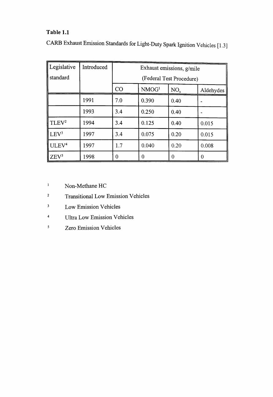
Table 1.1

CARB Exhaust Emission Standards for Light-Duty Spark Ignition Vehicles [1.3]

Legislative Introduced Exhaust emissions, glmile

standard (F ederal Test Procedure)

CO NMOG1 NOx Aldehydes

1991 7.0 0.390 0.40 -

1993 3.4 0.250 0.40 -

TLEy2 1994 3.4 0.125 0.40 0.015

LEy3 1997 3.4 0.075 0.20 0.015

ULEy4 1997 1.7 0.040 0.20 0.008

ZEy5 1998 0 0 0 0

Non-Methane HC

2 Transitional Low Emission Vehicles

3 Low Emission Vehicles

4 Ultra Low Emission Vehicles

5 Zero Emission Vehicles

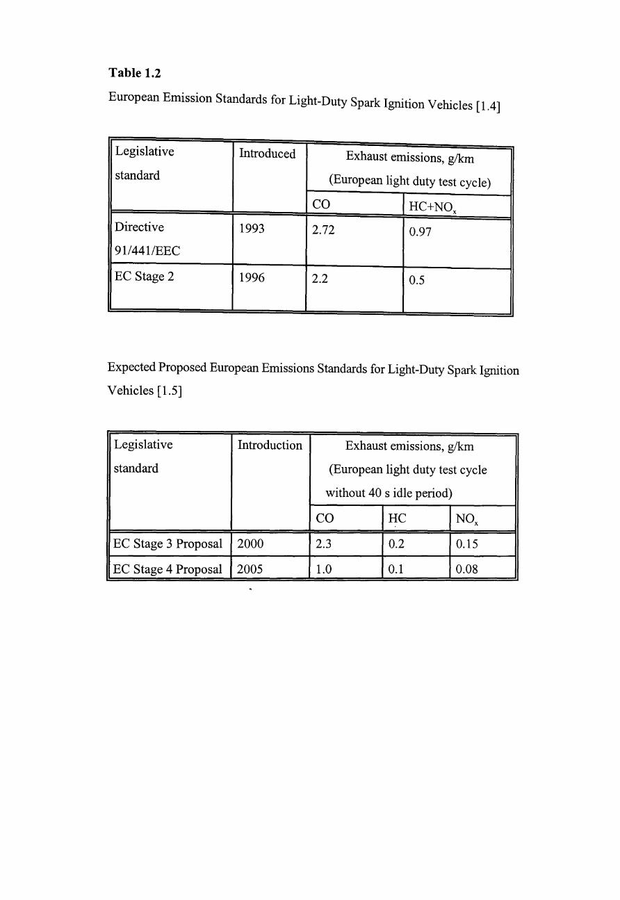
Table 1.2

European Emission Standards for Light-Duty Spark Ignition Vehicles [1.4]

Legislative Introduced Exhaust emissions, g/km

standard (European light duty test cycle)

CO HC+NOx

Directive 1993 2.72 0.97

9114411EEC

EC Stage 2 1996 2.2 0.5

Expected Proposed European Emissions Standards for Light-Duty Spark Ignition

Vehicles [1.5]

Legislative Introduction Exhaust emissions, g/km

standard (European light duty test cycle

without 40 s idle period)

CO HC NOx

EC Stage 3 Proposal 2000 2.3 0.2 0.15

EC Stage 4 Proposal 2005 1.0 0.1 0.08

Table 2.1

Summary of Neural Network Training Procedure (from Bacon [2.2])

Step Task

Number

1 Set all the weights in the network to random values

2 Take each input pattern in tum and, for each one, carry out steps

2(a) to 2(d)

2(a) Apply each element of the input pattern as an input to the

corresponding input unit

2(b) Calculate the activation of the output units by progressing the

activation values through the network

2(c) Compare the actual output value or pattern with the desired

output value or pattern

2(d) Adjust the weights in the network to bring the actual output

closer to the target

3 Starting again at the first input pattern, repeat step 2 until a

measure of the errors in the outputs is below a defined level or

until the weights values have converged to a constant value

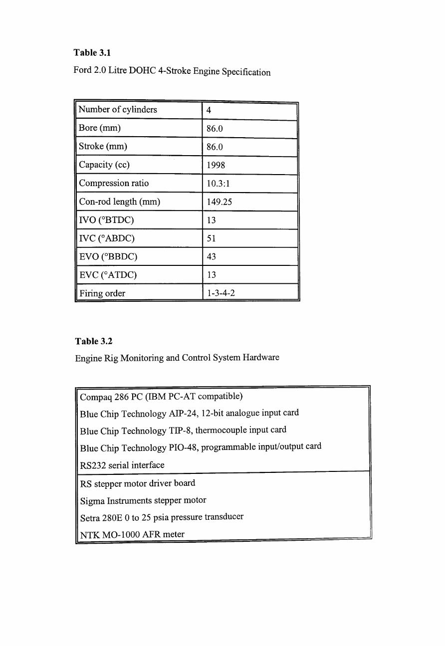
Table 3.1

Ford 2.0 Litre DOHC 4-Stroke Engine Specification

Number of cylinders 4

Bore (mm) 86.0

Stroke (mm) 86.0

Capacity (cc) 1998

Compression ratio 10.3:1

Con-rod length (mm) 149.25

IVO COBTDC) 13

IVC (oABDC) 51

EVO COBBDC) 43

EVC (OATDC) 13

Firing order 1-3-4-2

Table 3.2

Engine Rig Monitoring and Control System Hardware

Compaq 286 PC (mM PC-AT compatible)

Blue Chip Technology AIP-24, 12-bit analogue input card

Blue Chip Technology TIP-8, thermocouple input card

Blue Chip Technology PIO-48, programmable input/output card

RS232 serial interface

RS stepper motor driver board

Sigma Instruments stepper motor

Setra 280E 0 to 25 psia pressure transducer

NTK MO-1 000 AFR meter

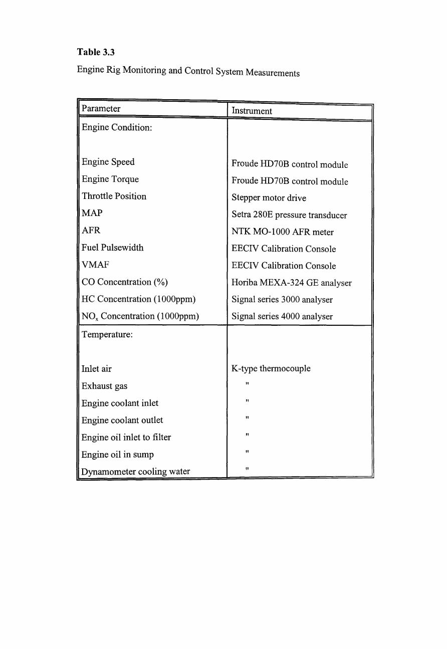
Table 3.3

Engine Rig Monitoring and Control System Measurements

Parameter Instrument

Engine Condition:

Engine Speed Froude HD70B control module

Engine Torque Froude HD70B control module

Throttle Position Stepper motor drive

MAP Setra 280E pressure transducer

APR NTK MO-l 000 APR meter

Fuel Pulsewidth EECIV Calibration Console

VMAP EECIV Calibration Console

CO Concentration (%) Horiba MEXA-324 GE analyser

HC Concentration (1000ppm) Signal series 3000 analyser

NOx Concentration (1000ppm) Signal series 4000 analyser

Temperature:

Inlet air K-type thermocouple

Exhaust gas "

Engine coolant inlet "

Engine coolant outlet "

Engine oil inlet to filter "

Engine oil in sump "

Dynamometer cooling water "

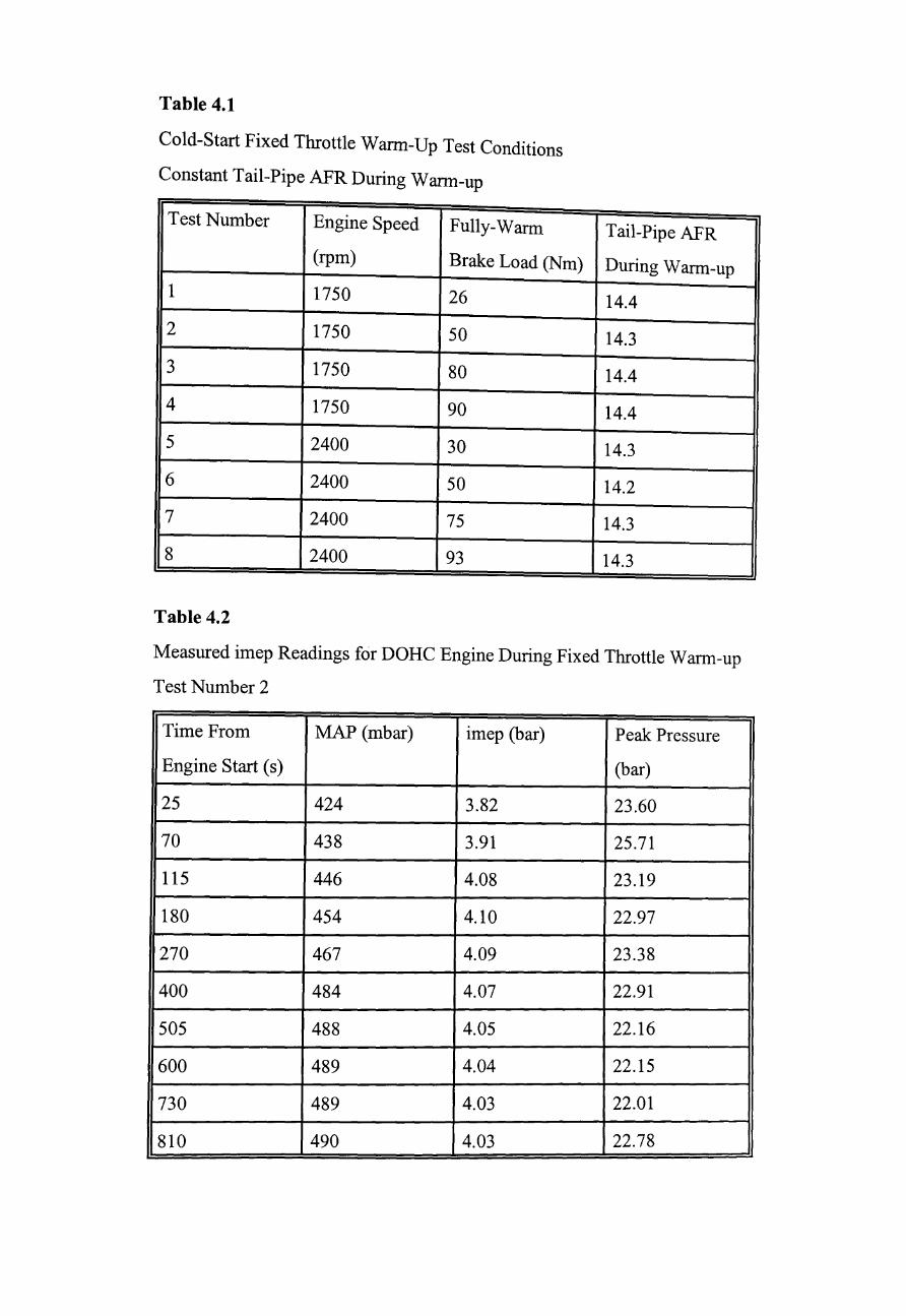
Table 4.1

Cold-Start Fixed Throttle Warm-Up Test Conditions

Constant Tail-Pipe AFR During Wann-up

Test Number Engine Speed Fully-Warm

(rpm) Brake Load (Nm)

1 1750 26

2 1750 50

3 1750 80

4 1750 90

5 2400 30

6 2400 50

7 2400 75

8 2400 93

Table 4.2

Tail-Pipe APR

During Warm-up

14.4

14.3

14.4

14.4

14.3

14.2

14.3

14.3

Measured imep Readings for DORC Engine During Fixed Throttle Warm-up

Test Number 2

Time From MAP (mbar) imep (bar) Peak Pressure

Engine Start (s) (bar)

25 424 3.82 23.60

70 438 3.91 25.71

115 446 4.08 23.19

180 454 4.10 22.97

270 467 4.09 23.38

400 484 4.07 22.91

505 488 4.05 22.16

600 489 4.04 22.15

730 489 4.03 22.01

810 490 4.03 22.78

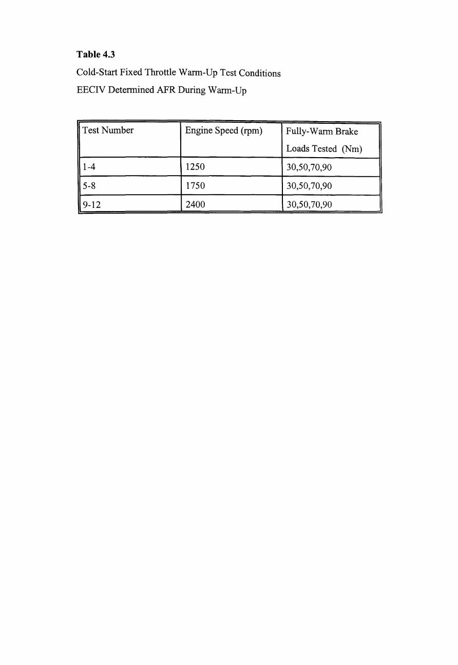
Table 4.3

Cold-Start Fixed Throttle Warm-Up Test Conditions

EECIV Determined APR During Warm-Up

Test Number Engine Speed (rpm)

1-4 1250

5-8 1750

9-12 2400

Fully-W ann Brake

Loads Tested (Nm)

30,50,70,90

30,50,70,90

30,50,70,90

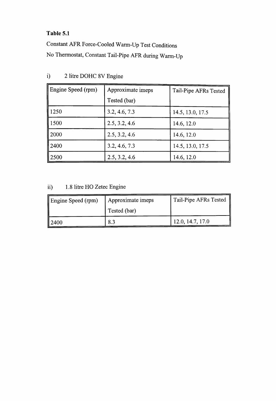
Table 5.1

Constant AFR Force-Cooled Wann-Up Test Conditions

No Thennostat, Constant Tail-Pipe AFR during Wann-Up

i) 2 litre DORC SV Engine

Engine Speed (rpm) Approximate imeps Tail-Pipe AFRs Tested

Tested (bar)

1250 3.2,4.6, 7.3 14.5, 13.0, 17.5

1500 2.5, 3.2, 4.6 14.6, 12.0

2000 2.5, 3.2, 4.6 14.6, 12.0

2400 3.2,4.6, 7.3 14.5, 13.0, 17.5

2500 2.5, 3.2, 4.6 14.6, 12.0

ii) 1.S litre RO Zetec Engine

Engine Speed (rpm) Approximate imeps Tail-Pipe AFRs Tested

Tested (bar)

2400 S.3 12.0, 14.7, 17.0

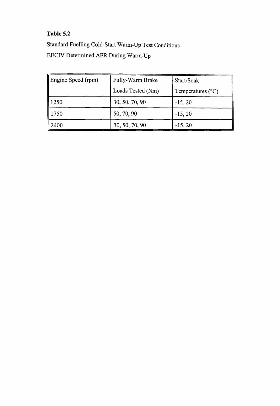
Table 5.2

Standard Fuelling Cold-Start Warm-Up Test Conditions

EECIV Determined AFR During Wann-Up

Engine Speed (rpm) Fully-W ann Brake Start/Soak

Loads Tested (Nm) Temperatures (OC)

1250 30,50,70,90 -15,20

1750 50,70,90 -15, 20

2400 30,50,70,90 -15,20

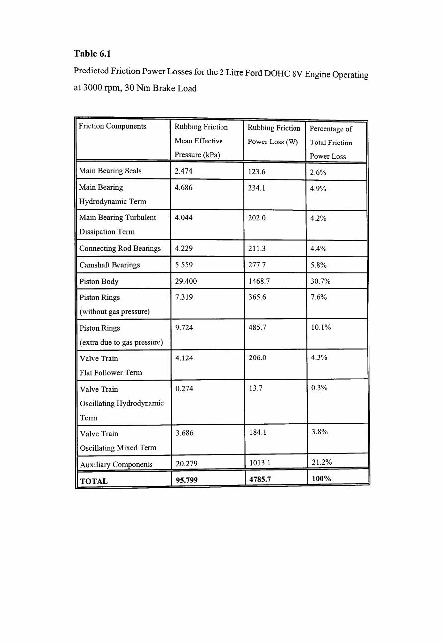
Table 6.1

Predicted Friction Power Losses for the 2 Litre Ford DORe 8V Engine Operating

at 3000 rpm, 30 Nm Brake Load

Friction Components Rubbing Friction Rubbing Friction Percentage of

Mean Effective Power Loss (W) Total Friction

Pressure (kPa) Power Loss

Main Bearing Seals 2.474 123.6 2.6%

Main Bearing 4.686 234.1 4.9%

Hydrodynamic Term

Main Bearing Turbulent 4.044 202.0 4.2%

Dissipation Term

Connecting Rod Bearings 4.229 211.3 4.4%

Camshaft Bearings 5.559 277.7 5.8%

Piston Body 29.400 1468.7 30.7%

Piston Rings 7.319 365.6 7.6%

(without gas pressure)

Piston Rings 9.724 485.7 10.1%

(extra due to gas pressure)

Valve Train 4.124 206.0 4.3%

Flat Follower Term

Valve Train 0.274 13.7 0.3%

Oscillating Hydrodynamic

Term

Valve Train 3.686 184.1 3.8%

Oscillating Mixed Term

Auxiliary Components 20.279 1013.1 21.2%

TOTAL 95.799 4785.7 100%

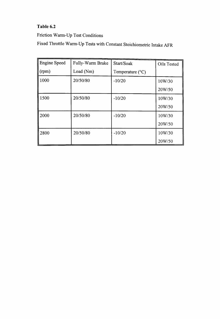
Table 6.2

Friction Warm-Up Test Conditions

Fixed Throttle Warm-Up Tests with Constant Stoichiometric Intake APR

Engine Speed Fully-Warm Brake Start/Soak Oils Tested

(rpm) Load (Nm) Temperature (OC)

1000 20/50/80 -10/20 10W/30

20W/50

1500 20/50/80 -10/20 10W/30

20W/50

2000 20/50/80 -10/20 10W/30

20W/50

2800 20/50/80 -10/20 IOW/30

20W/50

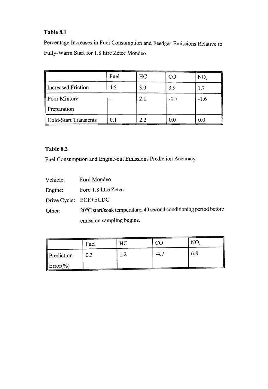
Table 8.1

Percentage Increases in Fuel Consumption and Feedgas Emissions Relative to

Fully-Warm Start for 1.8 litre Zetec Mondeo

Fuel HC CO NOx

Increased Friction 4.5 3.0 3.9 l.7

Poor Mixture - 2.1 -0.7 -l.6

Preparation

Cold-Start Transients 0.1 2.2 0.0 0.0

Table 8.2

Fuel Consumption and Engine-out Emissions Prediction Accuracy

Vehicle: Ford Mondeo

Engine: Ford 1.8 litre Zetec

Drive Cycle: ECE+EUDC

Other:

Prediction

Error(%)

20°C start/soak temperature, 40 second conditioning period before

emission sampling begins.

Fuel HC CO NOx

0.3 1.2 -4.7 6.8

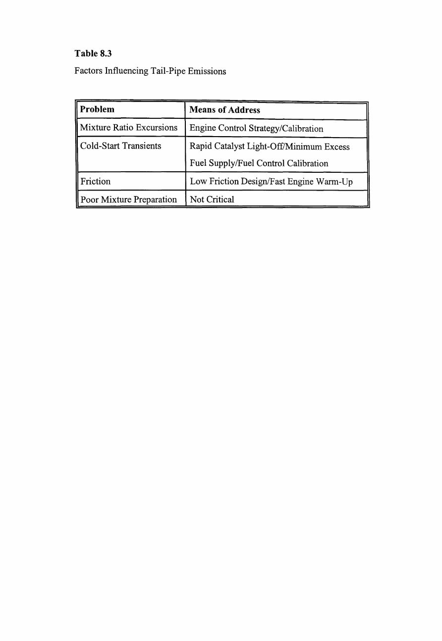
Table 8.3

Factors Influencing Tail-Pipe Emissions

Problem Means of Address

Mixture Ratio Excursions Engine Control Strategy/Calibration

Cold-Start Transients Rapid Catalyst Light-OfflMinimum Excess

Fuel Supply/Fuel Control Calibration

Friction Low Friction DesignlFast Engine Warm-Up

Poor Mixture Preparation Not Critical

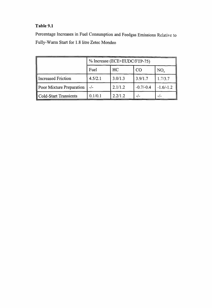
Table 9.1

Percentage Increases in Fuel Consumption and Feedgas Emissions Relative to

Fully-Warm Start for 1.8 litre Zetec Mondeo

% Increase (ECE+EUDCIFTP-75)

Fuel HC CO NOx

Increased Friction 4.5/2.1 3.0/1.3 3.9/1.7 1. 7/3.7

Poor Mixture Preparation -/- 2.111.2 -0.7/-0.4 -1.6/-1.2

Cold-Start Transients 0.110.1 2.2/1.2 -/- -/-

140 .r-----------------------------~

_120 .... .s:: -E 100 ...!iiI:: -"C 80 cu cu 9i 60

(J

.s:: ~ 20

o 200 400 600 800 1000 1200 Time From Start (sees)

Drive Cycle Breakdown

Time(secs)

0-195 196-390 391-585 586-780 781-1180

Phase

Elementary Urban Cycle No.1 Elementary Urban Cycle No.2 Elementary Urban Cycle NO.3 Elementary Urban Cycle No.4 Extra-Urban Drive Cycle

Figure 1.1 NEDC or ECE +EUDC vehicle speed vs time description

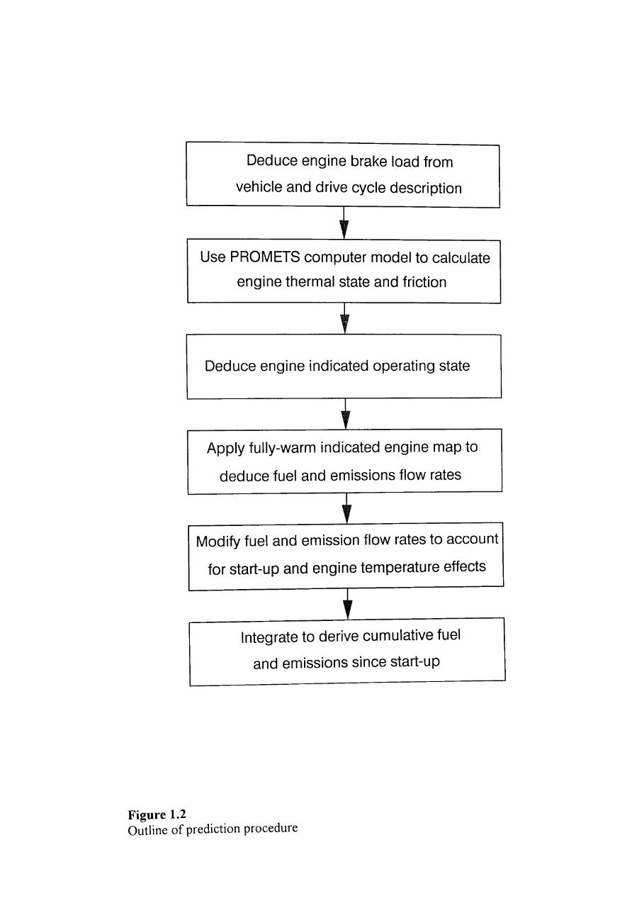
Deduce engine brake load from

vehicle and drive cycle description

~r

Use PROMETS computer model to calculate

engine thermal state and friction

" Deduce engine indicated operating state

"

Apply fully-warm indicated engine map to

deduce fuel and emissions flow rates

~,

Modify fuel and emission flow rates to account

for start-up and engine temperature effects

" Integrate to derive cumulative fuel

and emissions since start-up

Figure 1.2 Outline of prediction procedure

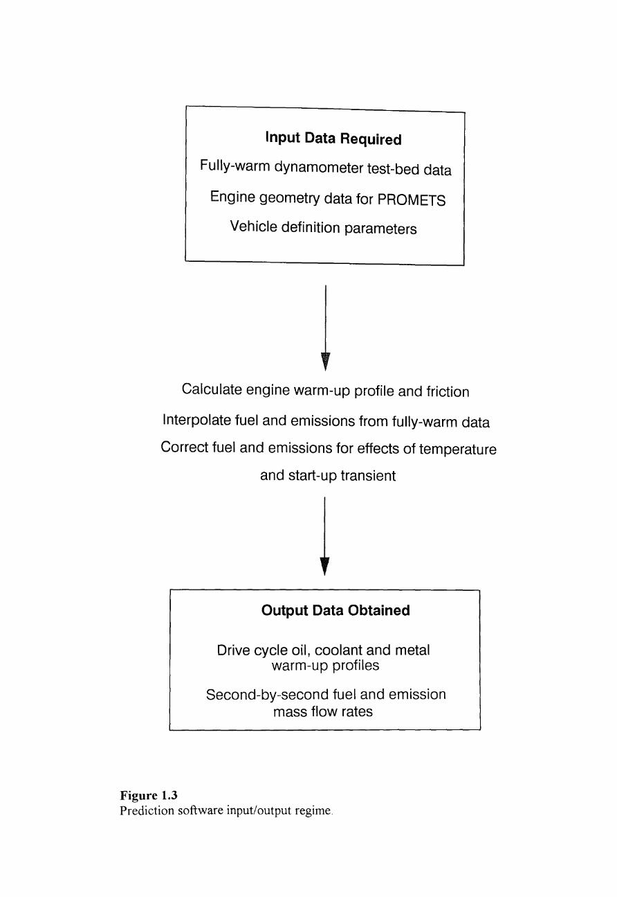
Input Data Required

Fully-warm dynamometer test-bed data

Engine geometry data for PROMETS

Vehicle definition parameters

Calculate engine warm-up profile and friction

Interpolate fuel and emissions from fully-warm data

Correct fuel and emissions for effects of temperature

and start-up transient

Figure 1.3

Output Data Obtained

Drive cycle oil, coolant and metal warm-up profiles

Second-by-second fuel and emission mass flow rates

Prediction software input/output regime.

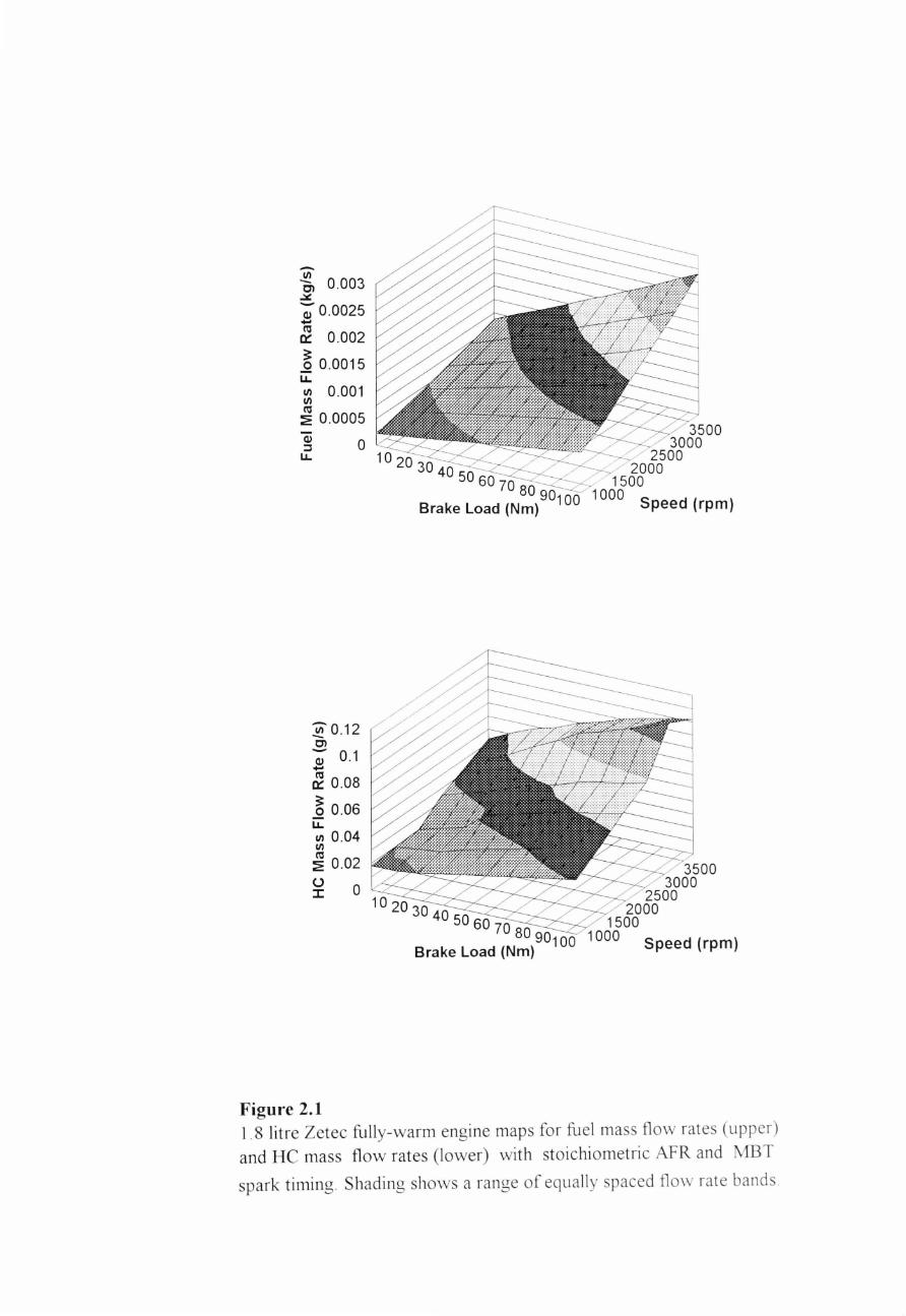
-VI 0, 0.003 .:::t:.

-; 0.0025 -co 0:: 0.002 ::

..Q 0.0015 LL VI 0 .001 VI co ~ 0.0005

o

~0 . 12 Cl -; 0.1 -& 0.08

~ 0.06 LL VI 0.04 VI co ~ 0.02

~ 0

Figure 2.1

1020 30 4050 60 7080 90 Brake Load (Nm) 100

1020 30 4050 60 70 80901

Brake Load (Nm)

3500 3000

2500 2000

1500 1000

Speed (rpm)

3500 3000

2500 2000

1500 1000 Speed (rpm)

1.8 li tre Zetec fu lly-warm engine maps for fuel mass flow rates (upper) and He mass flow rates (lower) with stoichiometric AFR and MBT

spark timing. Shading shovvs a range of equally spaced fl ow rate band

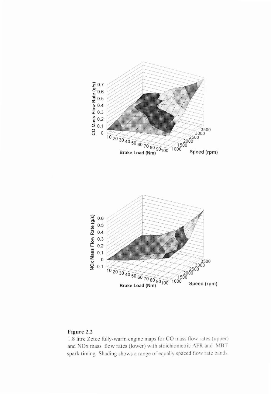
~0.7 C)

-;0 .6 -~ 0.5

3: 0.4 o

iL: 0.3 VI VI 0.2 I'tI

:2: 0.1

8 0

--a, 0.6

-; 0.5 -~ 0.4 3: 0.3

.Q LL 0.2 VI

~ 0.1 ~ x 0 ~ -0 .1

Figure 2.2

1020 30 4050 60 7080 90 Brake Load (Nm) 100

1020 30 4050 60 7080901

Brake Load (Nm)

3500 3000

2500 2000

1500 1000

Speed (rpm)

3500 3000

2500 2000

1500 1000 Speed (rpm)

1.8 litre Zetec fully-warm engine maps for CO mass fl ow rates (upper) and NOx mass flow rates (lower) with stoichiometric AFR and MET

spark timing. Shading shows a range of equally spaced fl ow rate bands

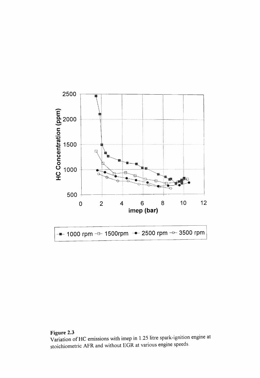
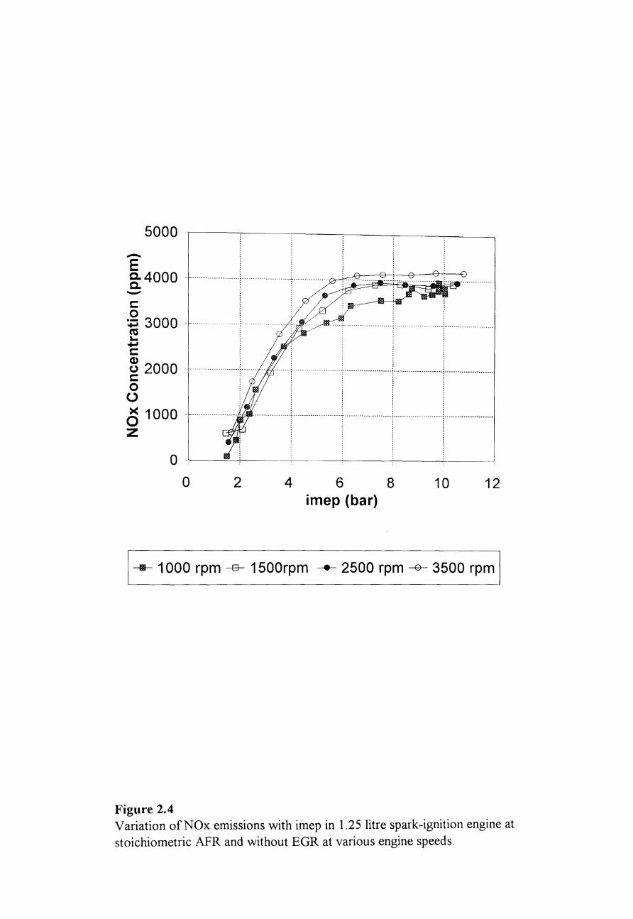
5000

-E 8: 4000 -c: 0 ~ 3000 co L. +I c: B 2000 c: 0 ()

~ 1000 z

0

0

---.-- ____ • _________ 4 _____________ ••• _. ___ 0 ___ _

· . · . · . · . -----------------------------r-------------------r--------------·------·------------.--.. ------

: : : :

... ___ . ___ ." ___________________ ... ____ .________ ! i -----T-----------------r-------------------'1'-----·················

2

i !

468 imep (bar)

10 12

1---- 1 000 rpm -B- 1500rpm ---- 2500 rpm --G- 3500 rpm 1

Figure 2.4 Variation of NO x emissions with imep in 1.25 litre spark-ignition engine at stoichiometric AFR and without EGR at various engine speeds.

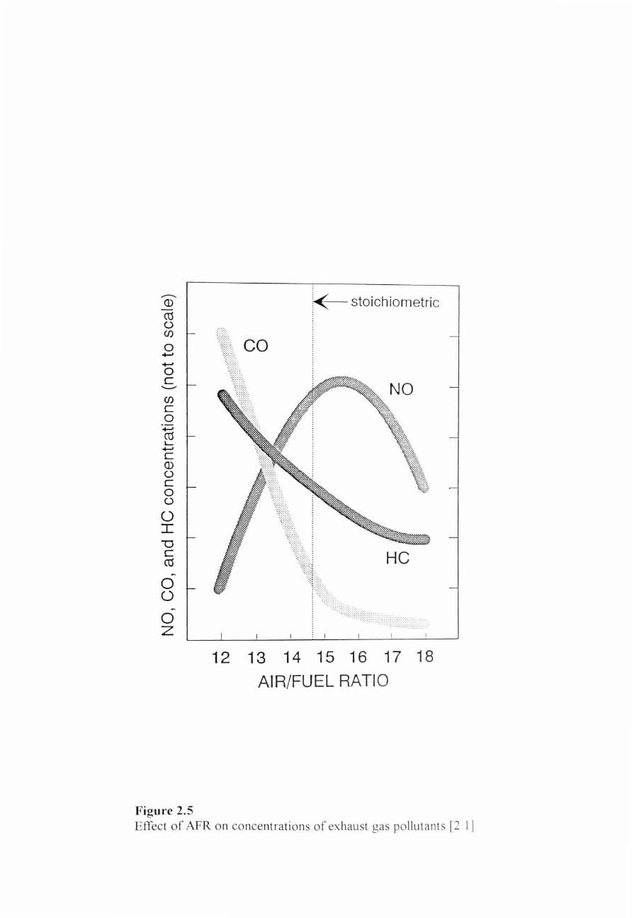
en c o al L +-' C ill o C o o o I -0 C co -o

o o z

Figure 2.5

< stoichiometric

co

NO

He

12 13 14 15 16 17 18

AIR/FUEL RATIO

Effect of AFR on concentrations of exhaust gas pollutants [2 .1 ]

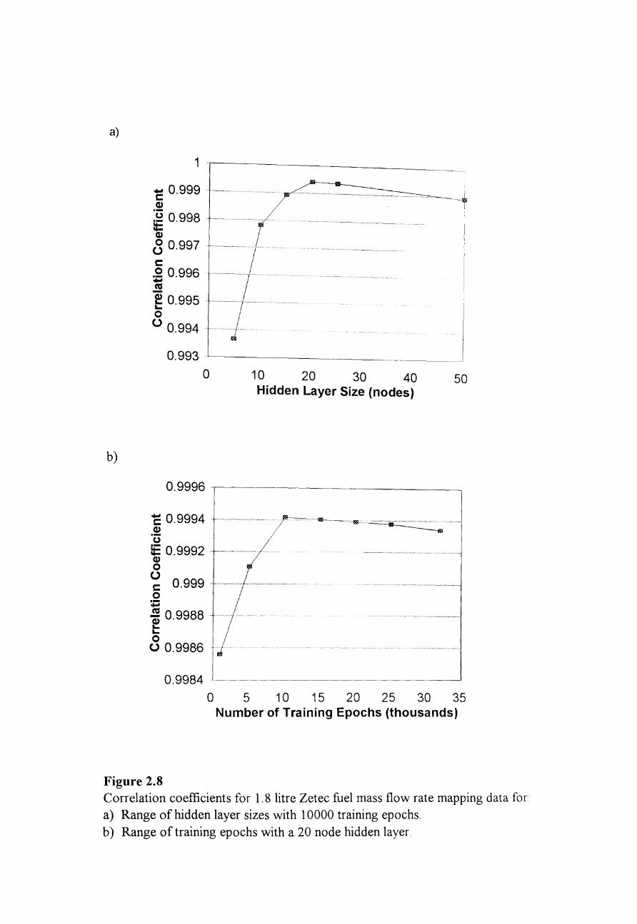
a)

b)

1 .r-----------------------~ 0.999 .9! .~ 0.998 .. tt: Q)

<3 0.997 . c .2 0.996 ........ . -.!!! e 0.995 .......... . ... o () 0.994 .

. ...................... _-_ ... __ .... _----_ ....••.....

0.993 .~-----------_ _____.J

o 10 20 30 40 50 Hidden Layer Size (nodes)

0.9996 .r-------------_

~ 0.9994 ................. . . 9! (,)

IE 0.9992 ......... . Q) o () c 0.999 .................... . o :;; ~ 0.9988 . ... ... o () 0.9986 .

0.9984

o 5

~~-~~.:.:a: ....... = ............................... .

10 15 20 25 30 35 Number of Training Epochs (thousands)

Figure 2.8 Correlation coefficients for 1.8 litre Zetec fuel mass flow rate mapping data for. a) Range of hidden layer sizes with 10000 training epochs. b) Range of training epochs with a 20 node hidden layer.

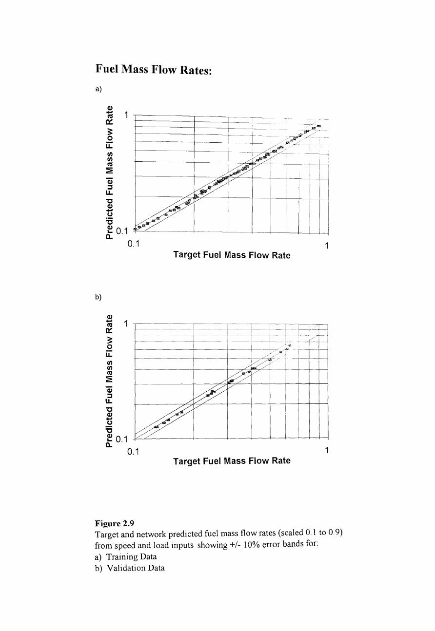
Fuel Mass Flow Rates:

a)

-r------+-------+-~ ~.-"- ~~~~

t-----l------+- --= ~~~~/~

b)

Q)

::::J U. "C Q) -u .-"C f! 0 1 a.'

-Q)

::::J U.

0.1

IY~T~I ---- . -~~--_____i , I

1 Target Fuel Mass Flow Rate

FT r-

·~--l--- -+ .. ~ -~=+~ , ' /

-- -_.-t---~--- ~ ,) '?'

l-~/~/f " - -t

~./,/' I

W V J

./

W V

./

"C Q) -(.) .-"C f! 0.1 a. ~

V

0.1 1 Target Fuel Mass Flow Rate

Figure 2.9 Target and network predicted fuel mass flow rates (scaled 0" 1 to 0.9) from speed and load inputs showing +/- 10% error bands for:

a) Training Data b) Validation Data

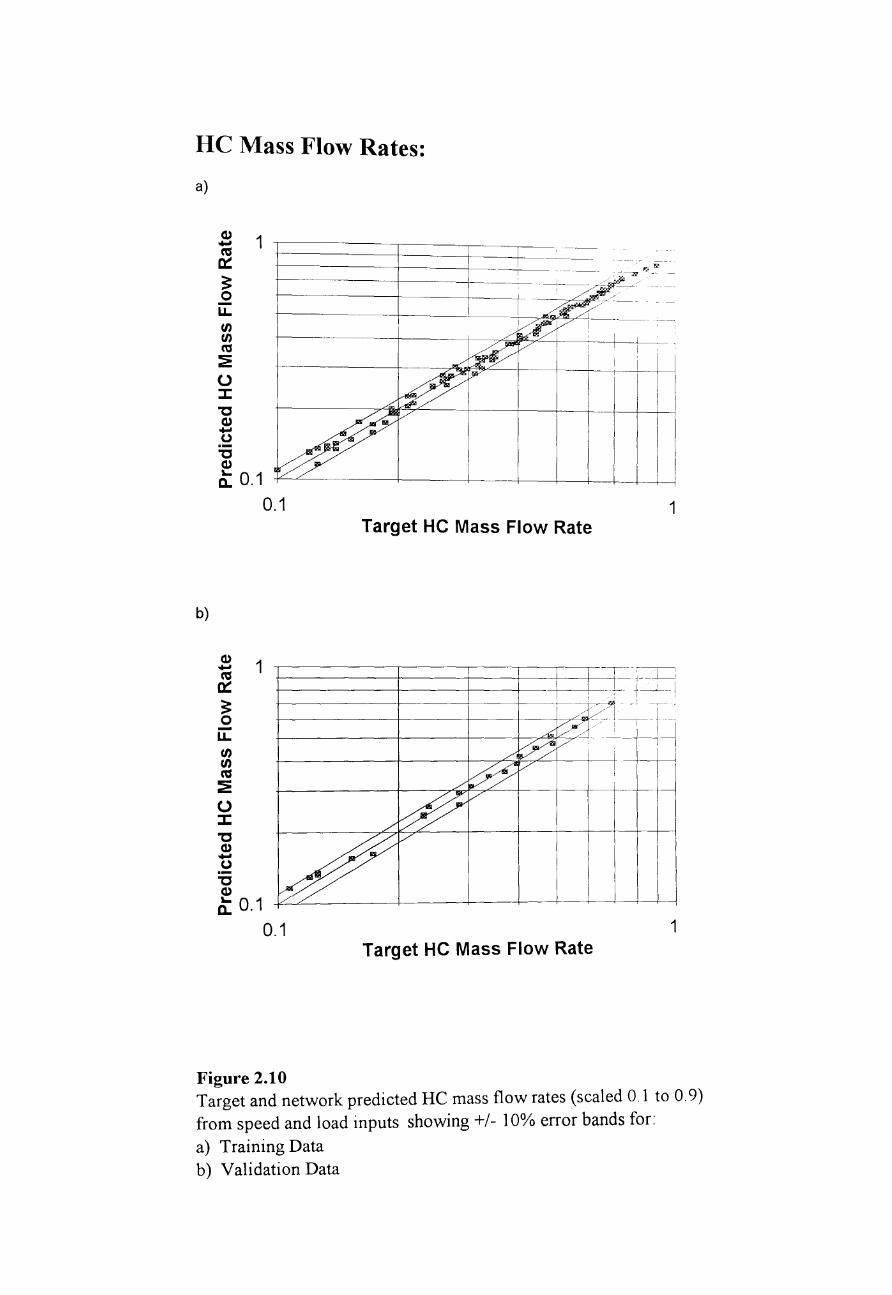
He Mass Flow Rates:

a)

~ 1 ctS 0::: 3: o u.. en en ctS ~ (J ::z:: "C cu -(.) .-"C cu c: 0.1 -j"--"'------~~~--+~~~l________~__+_~+_____+_J_1J-

0.1 1 Target HC Mass Flow Rate

b)

cu 1 -ctS 0::: 3: 0 u.. (/) en n:s ~ (J ::z::

-~-~;-:==

I r-- ;--L

, -;- +~' -I ! __ - // I - -1---- -

//~,,~I-~l--/' ~V---l~ '/ .. I

» v --t I /' ;

~ V

1--

/ "C cu -(.) .-"C cu c: 0.1 /

v

0.1 1 Target HC Mass Flow Rate

Figure 2.10 Target and network predicted He mass flow rates (scaled 0.1 to 0.9) from speed and load inputs showing +/- 10% error bands for:

a) Training Data b) Validation Data

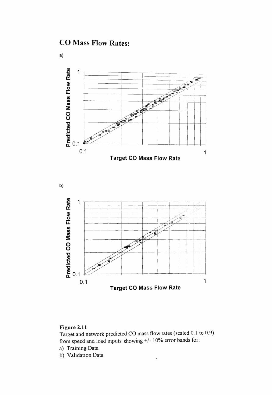
CO Mass Flow Rates:

a)

b)

~ 1 ~ ~----------r-----~--~--

0::: ~ o -LL U) fn cu :2: o (J

"C c:u ...., (.) .-"C (1)

D: 0.1

(1)

'"

0.1 Target CO Mass Flow Rate

1

1 ...., ~

0::: ~

.~ //-~ -~--- - l

0 LL

./~'

./ ~v~- .--:

U) fn cu :2: 0 (J

"C (1) ...., (.) .-"C (1) a: 0.1

./

/ 0.1

./ ~ ~ V

/'

~ ~

v

Target CO Mass Flow Rate

Figure 2.11

1

Target and network predicted CO mass flow rates (scaled 0.1 to 0.9) from speed and load inputs showing +/- 10% error bands for:

a) Training Data b) Validation Data

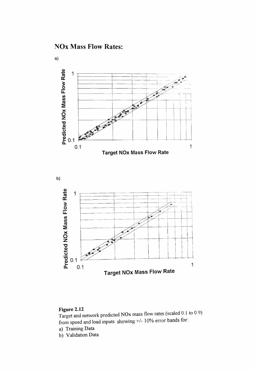
NOx Mass Flow Rates:

a)

cu .. 1 ~ ~ o -u. rn rn cu :2: >< o Z "C J!! CJ .-"C

---1~ r--------t---+---TS$:~+-------,--' i I '~----. I

! I I

£ 0.1 -r"""---"-----------1---+------+--+------+--l------t--u

0.1 1 Target NOx Mass Flow Rate

b)

Cl) .. 1 cu 0::: ~ 0

-=-1] ~~ '--;-~

I

u. tI) tI)

+--_____ ----1- ~ __ _+-~~~---l---- - -

cu :2: >< 0 Z 'C CI) .. 0 .--g 0.1 '-a.. 0.1 1

Target NOx Mass Flow Rate

Figure 2.12 Target and network predicted NOx mass flow rates (scaled 0.1 to 0.9)

from speed and load inputs showing +/- 10% error bands for:

a) Training Data b) Validation Data

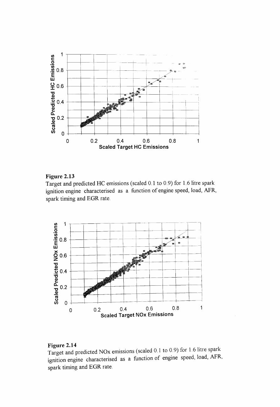
en c

,52 en

1 ,--------,----~--~-

---1---+ -,!!! 0.8 -t---t----+----l--- -i . . -- a?Z _ !T/'.

• 'I // E W b--t--+--+--~-~-~-~'~/~ I ----r-

~ 0.6 +--+---t-----L r---r----~"'-----+-----..

"C CI> -:5 0.4 -t---t----+---I----~ p--t--t--+----+--+---

~ a. "C 0.2 +---+---.!!!. ~

0+--4--~--+--+--~--~-+--+-~-~

o 0.2 0.4 0.6 0.8 1 Scaled Target He Emissions

Figure 2.13 Target and predicted He emissions (scaled 0.1 to 0.9) for 1.6 litre spark ignition engine characterised as a function of engine speed, load, AFR,

spark timing and EGR rate.

en 1 ~-~-~.- --

c 0 en en 'E 0.8 w >< 00.6 z "C

CI>

~ 0.4 "C CI> '-a. "C 0.2

CI> cu ()

CJ) 0 0 0.2 0.4 0.6 0.8 1

Scaled Target NOx Emissions

Figure 2.14 Target and predicted NOx emissions (scaled 0.1 to 0.9) for 1.6 litre spark ignition engine characterised as a function of engine speed, load, AFR,

spark timing and EGR rate.

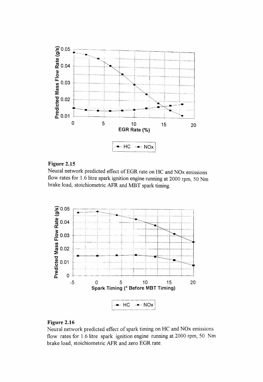
~0.05 C) -C1) -(}, 0.04 . .- ... f-·· ........ ·r .. 3: o ...... ,. --------- .. -.-...... ~ ..

u. I/) 0.03 ·--··i .. ··· .. -- ..... ~

I/) CIS ~

.......... ; . ----_ ........ - .- .~. -.... ..-........... ••••••••• -_ ......... _._, ._-+.

"C ' SO.02 . ···············i .... .... , ................. .-...... -.. (,)

"C ~ a. 0.01

o

Figure 2.15

. ' •

5 10 EGR Rate (%)

1-- HC - Noxl

15 20

Neural network predicted effect ofEGR rate on HC and NOx emissions flow rates for 1.6 litre spark ignition engine running at 2000 rpm, 50 Nm brake load, stoichiometric AFR and MBT spark timing.

~0.05 C) -C1) 1; 0.04 .. ""!-, .:.:;: ..... -.. + ................ -;-............... -i- .......... .

0::: : . . j .. . ·············i······ .... _·_···t·······"'-<· ".-.. , .......... - ...... , ........ -.... ./

i ::::_-.... --':-... -............... I---~----I~~~.-~.···-~···_'_t:=-=-:_=:1;::::l-~~~-: ~ 0.01 : ............... :.- .............. : ......... - .. _ ... __ ....... .

"C .-.--...•... -.-~ .. ---

~ a. 0 .~--~--~--~--+---~--+---~--~--~~

-5 o 5 10 15 20 Spark Timing (0 Before MBT Timing)

1-- HC - NOX\

Figure 2.16 Neural network predicted effect of spark timing on HC and NOx emissions flow rates for 1.6 litre spark ignition engine running at 2000 rpm, 50 Nm brake load, stoichiometric AFR and zero EGR rate.

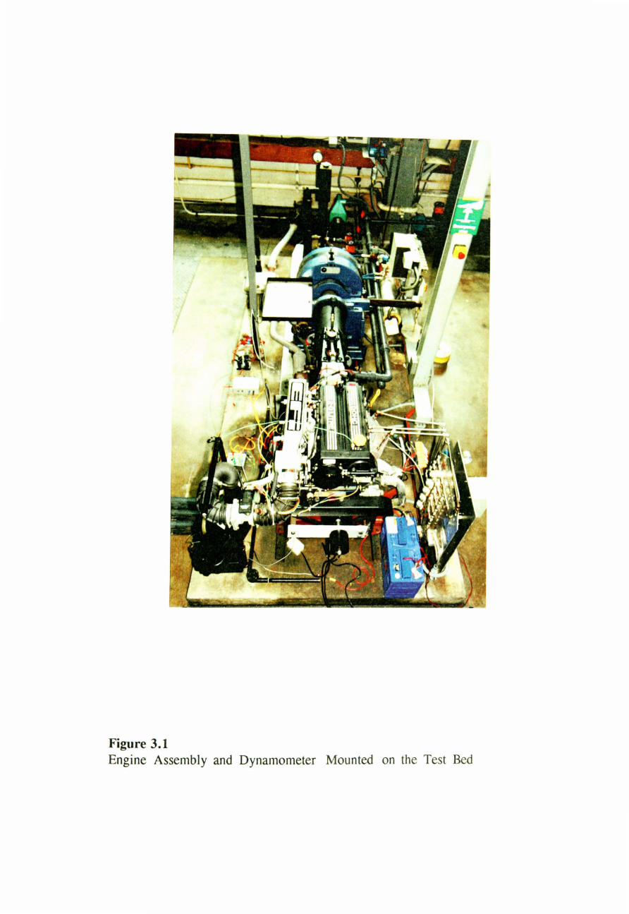
Figure 3.1 Engine Assembly and Dynamometer Mounted on the Test Bed

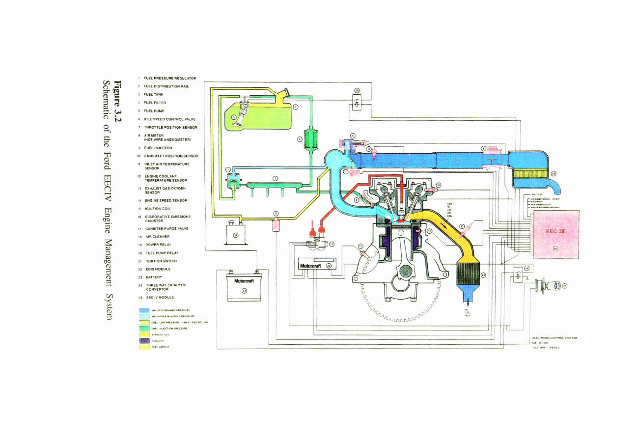
C/1~ n _. ::r!JC:I (D C 3 ., ~ ~ c. ~ n •

N o """t)

....... ::r (D

'Tl o ...., 0..

tTl tTl n -<: tTl ::l

(T'Q .... . ::l (1)

~ ~ ::l ~

(T'Q (D

3 (D ::l ......

C/1 '< Vl ...... (D

3

, FUEL PRESSURE REGUL.~TOR

2 FUEL OISTRI BUTION RAIL

FUEL TANK

• FUEL FILTER

FUEL PUMP

IDLE SPEED CONTROL VALVE

7 THROTTLE POSITION SENSOR

AIR METER (HOT WIRE ANEMOMETER)

FUEL iNJECTOR

10 CAMSHAFT POSITION SENSOR

11 INLET AIR TEMPERATURE SENSOR

12 ENGINE COOLANT TEMPERATURE SENSOR

13 EXHAUST GAS OXYGEN SENSOR

' . ENGINE SPEED SENSOR

, 5 IGNITION COIL

, 6 EVAPORATIVE EMISSION S CANISTER

17 CAN!STER pu I=tGE VALVE

18 AIR CLEANER

19 POWER RELAY

20 FUEL PUMP RELAY

2' IGNITION SW ITCH

22 EDIS MODULE

23 BATTERY

l ' THREE WAY CATALVT IC CONVERTOR

25 EEC IV MODULE

Alit ATMOSPHE R IC PR(SSUA!

~ .., 11=1 l"Il'Altl ..... ,'u "Ol.O .,qESS Uq(

==:J FUEL LOW " tlt ESSUA! - .NU T "NO AElVA",

o FUEl IPO(C""Ot\l~SSURE - 1 ( J; OOj.LlJST(LA "I

I COOL;} ""

1 "U lE llf"~UA

@

~},J!" ---10

J 0) l

MD1Drcnrft

@

.,0

0)

EEe Ill:

e

Hf.C1'tltONIC CO""TAOl I'!'STUd

GIS IS 1 110

JUlY 1~ lSS Ut ~

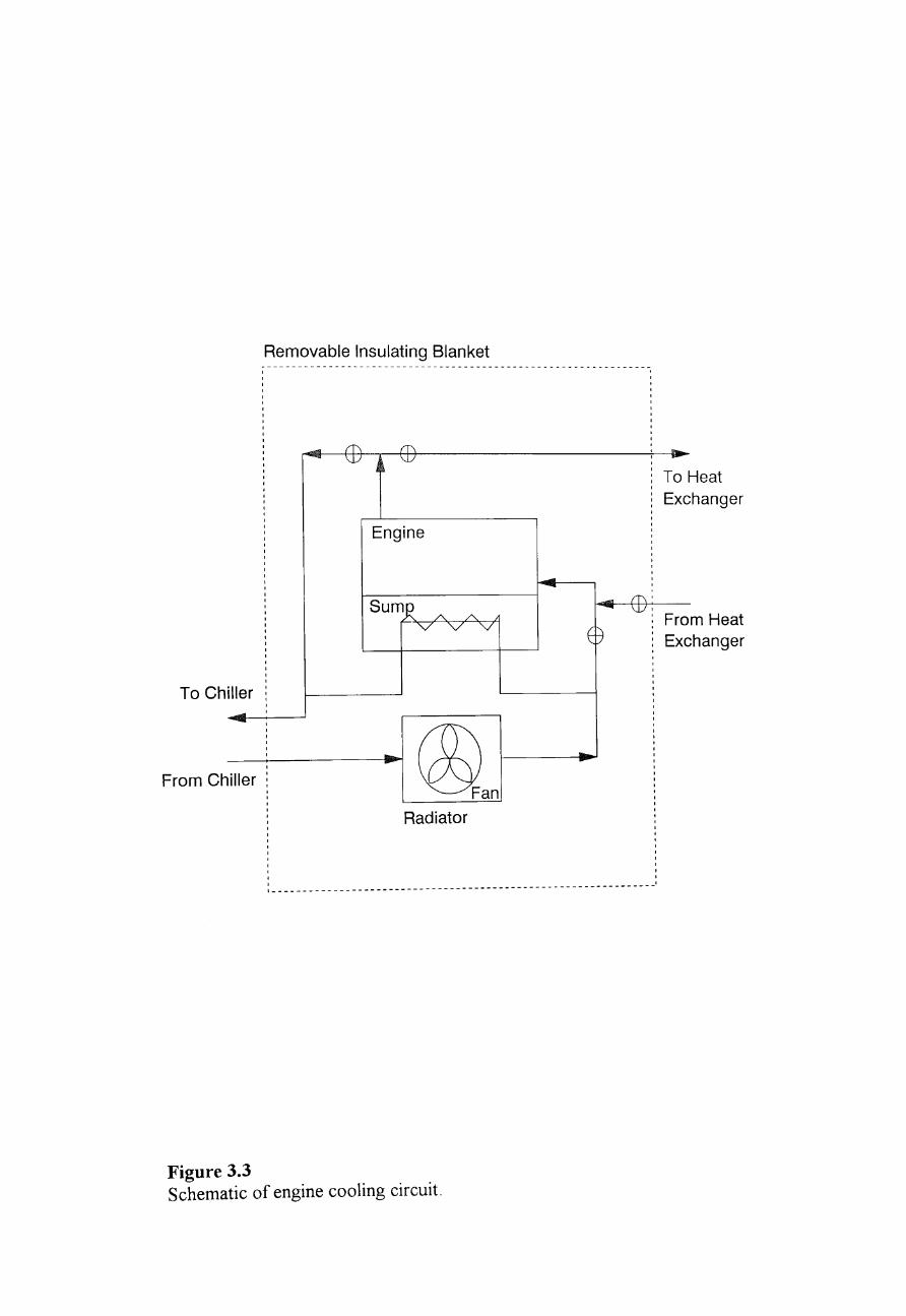
To Ch iller ..... -

From Ch iller

Removable Insulating Blanket ~ - -- - - - - - - - - - - - - - - - - - - - --I --------------------------------, , , , , , , , , , , , , , , , , , , , , , , , , , , , , , , , , , , , , , , , , , , , , , , , , , , , , , , , , , , , , , , , , , , ,

... f1\ \lJ

(1\

~ \J./

Engine

-... SumR

.... A A -

v v v E&

@an - ... ~- ---

Radiator

, ,

, , , , (1\: \J.),

, , , , , , , , , , , , , , , , , , , , , , , , , ,

1_--------------------------------------------------------------

Figure 3.3 Schematic of engine cooling circuit.

.. ... To Heat

hanger Exc

Fro m Heat hanger Exc

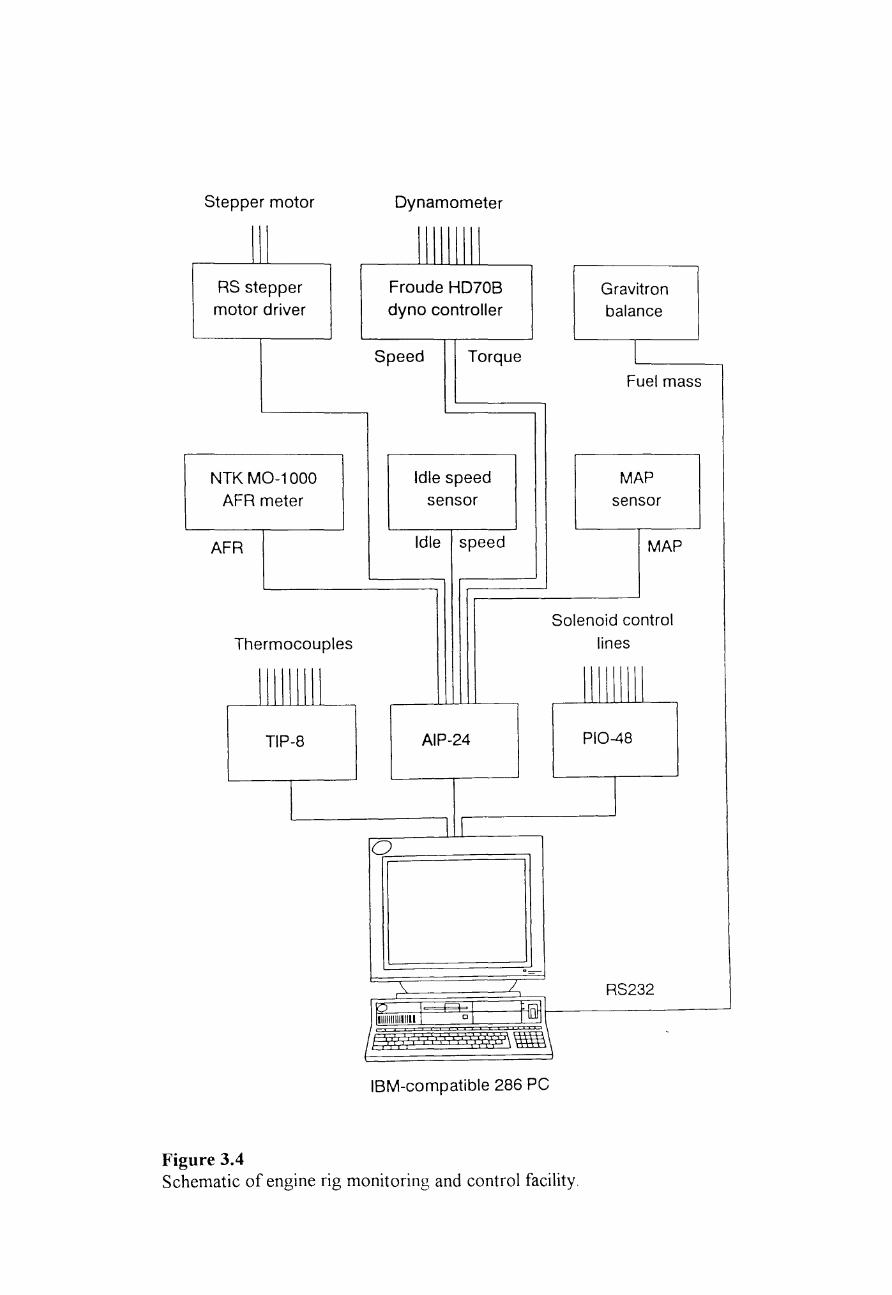
Stepper motor

\ \ \

RS stepper motor driver

NTK MO-1000

AFR meter

AFR

Thermocouples

111111111

TIP-8

Figure 3.4

Dynamometer

111111 \ \ \

Froude HD70B dyno controller

Speed Torque

o

Idle speed sensor

Idle speed

AIP-24

[

\ L

l~11I1I1I11I1I1 Dol f@l,

Gravitron balance

I Fuel mass

MAP sensor

MAP

Solenoid control

lines

1IIII11U PI0-48

RS232

• 1 : 1 1 [ " : : I' l;Tl< ~\ } ,',-:',1 J \1 'S'{'_';1_ I { 11: I 1 I I 1 I i r l { ( "\

IBM-compatible 286 PC

Schematic of engine rig monitoring and control facility.

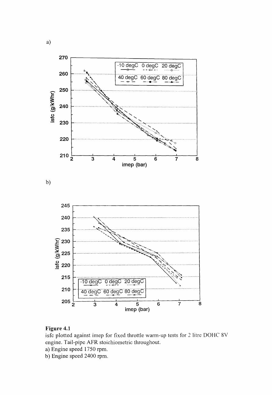
a)

270 r---------------------------------~

260

_ 250 ... .I:.

~ - 240 C) -u -.~ 230

220

b)

-1 0 degC 0 degC 20 degC ...... ~\ .......................... ~ .......... ~.~. ~~.~.: .............. ~ .................... .

}... \. 40 degC 60 degC 80 degC ' .. '-.." - .... - - ...... - - ...... -":~:.'-..\.

•.••••.••••..• "Ii_'~ .............................................................. .

\".'~ ........................ :"'.::

" ....... ........ ~ .......

" ....... ", .... ....... . . . . . . . . . . . . . . . . . .. .. .. . . . .. .. . .. . ... .. :." .. ~ ... :.: ~ .. ~ ............................... ..

.. ~"" ....... , . .:-... ..... J, ". "'" ............................................................ -.~::..~ ........ . """",. ,"0

"~-.~

3 4 5 6 7 8 imep (bar)

245 ~---------------------------------------

240

235

-1: 230 ;: ~ 225 C) -u :m 220

215

210

Figure 4.1

............ ~.'s~.:~ ............................................................ . ' .... "',.,

" ... '" .......................... '~'~.":"":: ~.:.:..:.:.:' ........................................... . ........ . ........ , ....... ;:-... .........

...................................... ~ .... :~~: .. -:-... ............................. . ""''''''''~. ....... ',

......... "'. .......................................................... ' ...... ,,~ ...................... . "<., '-.

' .... " ~ . . ," "::--'" ................................................................... ': .. ~.~'. .............. .

-10 degC 0 degC 20 degC .... ' iii - - ~- - ••••• $....... "()

. '4c),(jeg'C"6CfdegC'scYde'g'C' ...................................... . - -+- - _ ........ - -- ........ --

3 456 imep (bar)

7 8

isfc plotted against imep for fixed throttle warm-up tests for 2 litre DOHC 8V engine. Tail-pipe APR stoichiometric throughout. a) Engine speed 1750 rpm. b) Engine speed 2400 rpm.

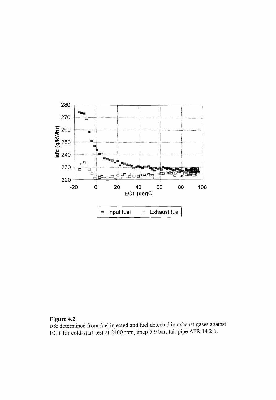
280.r----:----:----:----~--~~--~ IlliHaIa i

270 ........... ~ ..... + ............... L ....... ---~-- .. --.--- -. --- -_ .. - -_ .............. _ .. _.- ------

~ 260 ..~ .... : ... ,. . . ··········T·········· ...... -1-···· ......... (

~ 250 iRIl • ~ Ia:·· ..................... j ...................... j ...................... j ..................... . o. :: ~ 240 ... ·D~i"'~~~[··············lT············L.··················

:::6\C~=I~~MU -20 o 20 40 60 80 100

ECT (degC)

~ Input fuel o Exhaust fuel \

Figure 4.2 isfc determined from fuel injected and fuel detected in exhaust gases against ECT for cold-start test at 2400 rpm, imep 5.9 bar, tail-pipe AFR 14.2: 1.

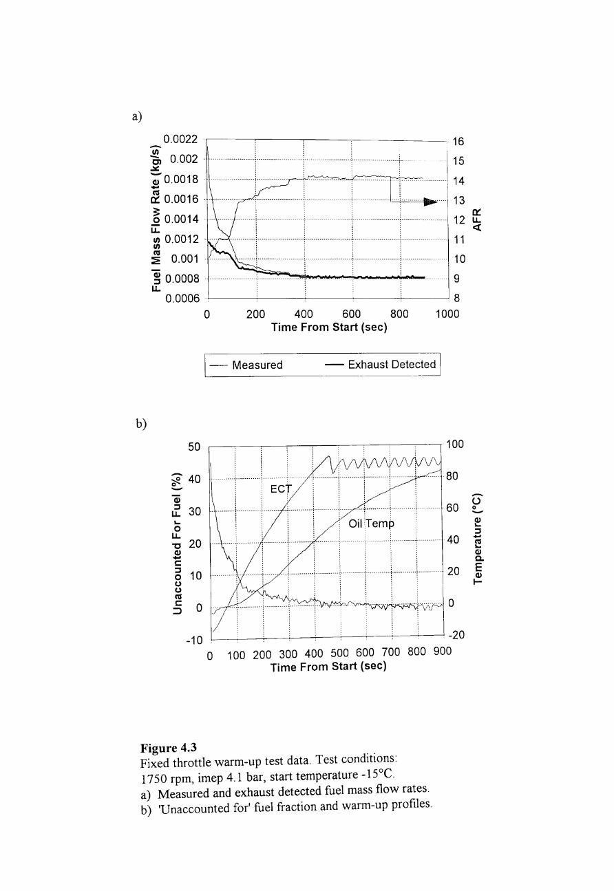
a)

0.0022 -r--------r-------r-----.------

~ OO~~~! .1'- ....... ... I ::

-:u ! .. ,,1 14

~ 0.0016 --oo-- -----oo - roooo.-.oo .. -oo.m--!""----m----m --- --,- - -- moo oooo,-- ----- -...- - 13

---------------,-------- 12 e: <t

11

10 - ------ - - -- 9

0.0006, : ' ,8

o 200 400 600 800 1000 Time From Start (sec)

1- Measured - Exhaust Detected I

b)

50 ~-,--:-~~~--~~--~--~-.100

, , '

~ 40 Q

I : : :

-CU :J 30 u.

---------j------- ECT-- -:----------T----------r-----------'---- 80

.[Lti!:.:, 60 E : : : : : 01'1 'Temp' : E L..

0 : : : : : : . U. "C 20

l l 1 ~ . ~ -_. ----- f---- -------i----------- '---- _.- -- --i-----·· -_. -.~ ------- _ .. -;-_._- --------- -40

CU -c: :! :

:J 10 0 20

() ()

C'tS c: 0 :J

o

-10 0 100 200 300 400 500 600 700 800 900

Time From Start (sec)

Figure 4.3 Fixed throttle warm-up test data. Test conditions: 1750 rpm, imep 4.1 bar, start temperature -15°C. a) Measured and exhaust detected fuel mass flow rates. b) 'Unaccounted for' fuel fraction and warm-up profiles.

:J -E cu a. E cu I-

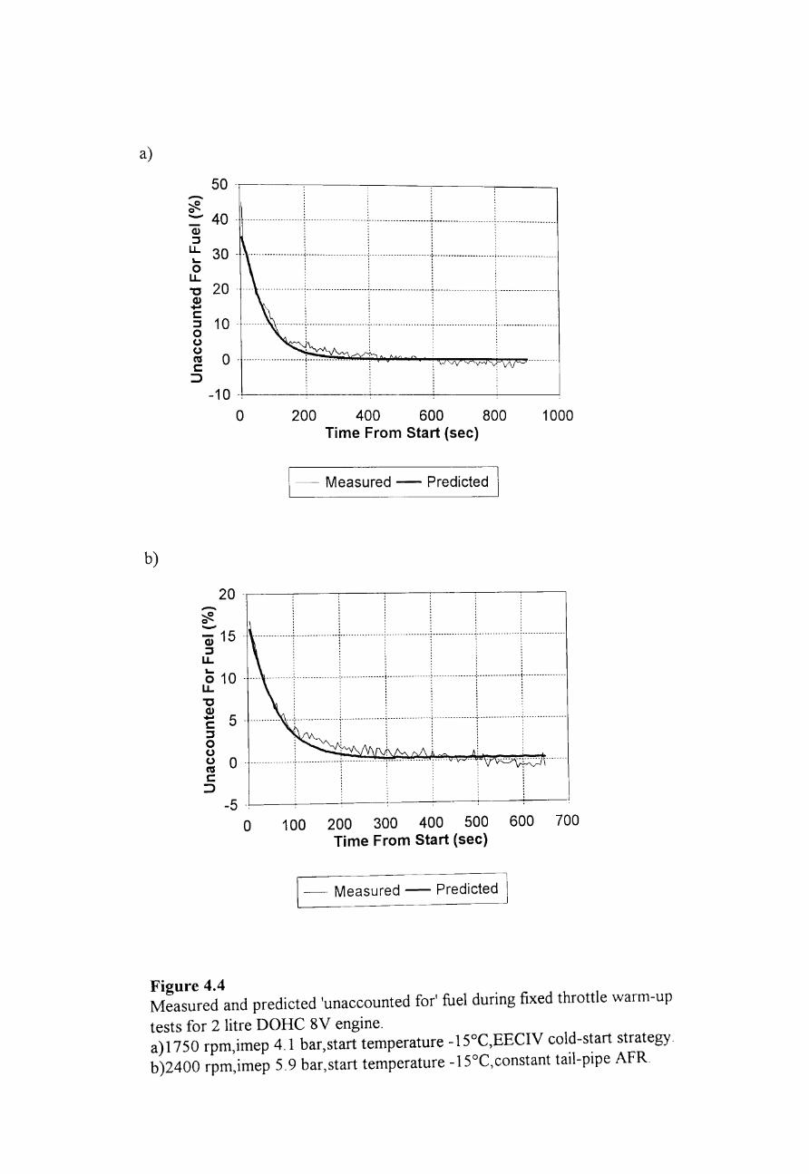
a)

b)

- 50-r---~----~----:---~----~

~ :::- 40 - --- ---- ....... -------- ------.--- -. ------.... ' ~ ·r·······-------··----:·-------·······-···-·-

~ 30 . ....:+\' ~ 20 - - ... -- -----------T··-·····-·----·-····t····------------··-- -~ ...... .

g 1 0 ------- .. -(-.- .... --.----------~---.------- ----------.------------- -------.-- .......... --.------. (.) (.) cu c: ::J

o -------------------·--i~----~----·:..,;;,---·~---~~----~~~~

-10 -, o 200 400 600 800 1000

Time From Start (sec)

\- --- Measured - Predicted

20 -,---~--~----~--~--------------~ -Cii 15 - ----.--.------.-------. ------------,-----------.--.-,----------, ------------------:J ' :: ----- ,----

~ 1: •••••..•..•••..•• ' ••••••••••••••• , ••••••••••••....• ; ••••••••••••••• \ ••• · .•••••••••• 1 •••••••• ·······\········· ...... . :J ,,:,

:: : o ,: , (.) ,; i (.) 0 ' ' cu -----r--------------,----------------:---------- --c: ,i ::J "

-5 -~--~--~----~--~----~--~--~

o 100 200 300 400 500 600 700 Time From Start (sec)

\- Measured - Predicted \

Figure 4.4 Measured and predicted 'unaccounted for' fuel during fixed throttle warm-up

tests for 2 litre DOHC 8V engine. a)1750 rpm,imep 4.1 bar,start temperature -15°C,EECIV cold-start strategy. b)2400 rpm,imep 5.9 bar,start temperature -15°C,constant tail-pipe AFR_

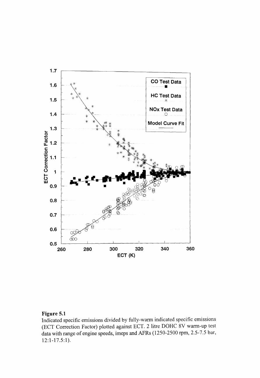
1.7

1.6 * CO Test Data

• 1.5 *

HC Test Data

* NOx Test Data

1.4 0

* * t Model Curve Fit 1.3

* .... 0 * '0 .f 1.2 r::: 0 ~ g 1.1 .... .... 0 0 1 I-0 w

0.9

0.8

0.7

0.6

C§X)

0.5 260 280 300 320 340 360

ECT (K)

Figure 5.1 Indicated specific emissions divided by fully-wann indicated specific emissions (ECT Correction Factor) plotted against ECT. 2 litre DOHC 8V wann-up test data with range of engine speeds, imeps and AFRs (1250-2500 rpm, 2.5-7.5 bar, 12:1-17.5:1).

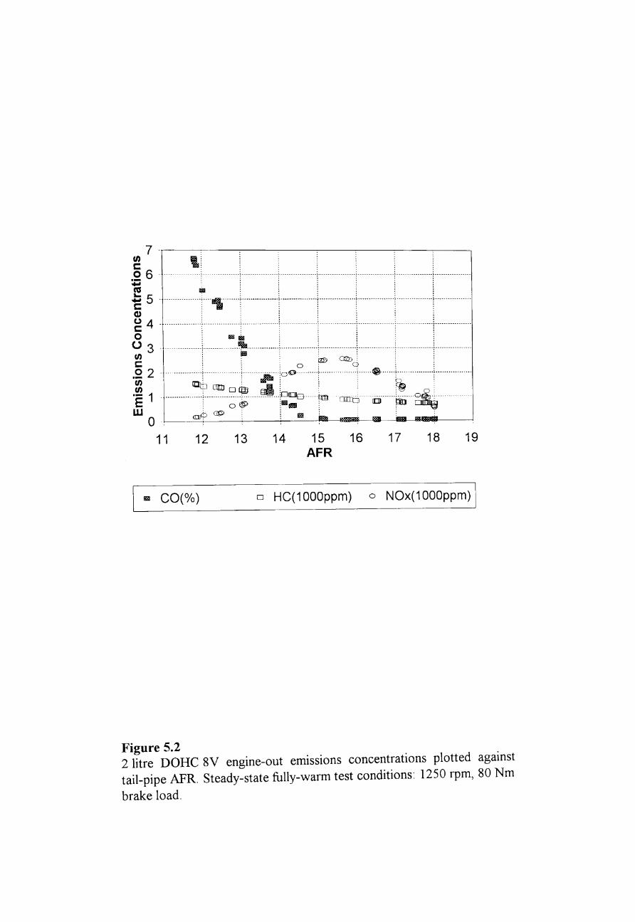
7·r-~~~--:---:---~--~--~-------~ , t : ••............•• ~···~· •••• ·.l···.····...]················I ••••• · ••••••• I.· ••• • •••••• • ••• i.·· ..........' ••••••••••••••••

~ 3 ..............•........ ··~·l····i ... ~~~J .............. l........' ........... . . 2 2 ··············t··········~·······~··:oo ........ +...... .. ; .... ~ .... ,..... . ...................... . . ~tnE 1 . m"T'L"'[]'i".p_imm~ ~ .. .

! 0 ~ lR. : 0Jt:ttj!Ill lID ' Wo ~@) ;mi..........",.;,_i....._........i.

11 12 13 14 15 16 AFR

17 18 19

R CO(%) o HC(1000ppm) 0 NOx(1000ppm)

Figure 5.2 2 litre DORe 8V engine-out emISSIons concentrations plotted against tail-pipe AFR. Steady-state fully-warm test conditions: 1250 rpm, 80 Nm

brake load,

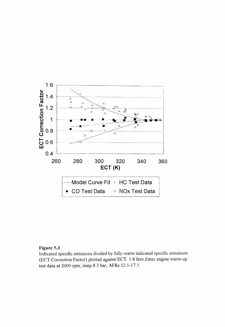
1.6 ~

o x t) 1.4 - ------- --------------------- -- -------- ._. ---

co u. c: 1.2 o t1 1 Q) ~ ~

8 0.8

..... () 0.6 w

0.4 260

Figure 5.3

-------------- -- ---._---------. -- - - - -- ---x x x x

x

.----... ---.~.~-=~=~~~~a==iFl~ o

----------------------------- . • ----------- ----------------------0--------------0 -- ---------- •.••.••.•......... _. ___ .. _ .. _ ....... ___ _ o

o

--.-0.-------------------------

280 300 320 EeT (K)

340

- Model Curve Fit x HC Test Data

• CO Test Data o NOx Test Data

360

Indicated specific emissions divided by fully-warm indicated specific emissions (ECT Correction F actor) plotted against ECT. 1.8 litre Zetec engine warm-up

test data at 2000 rpm, imep 8. 3 bar, AFRs 12: 1-17: 1.

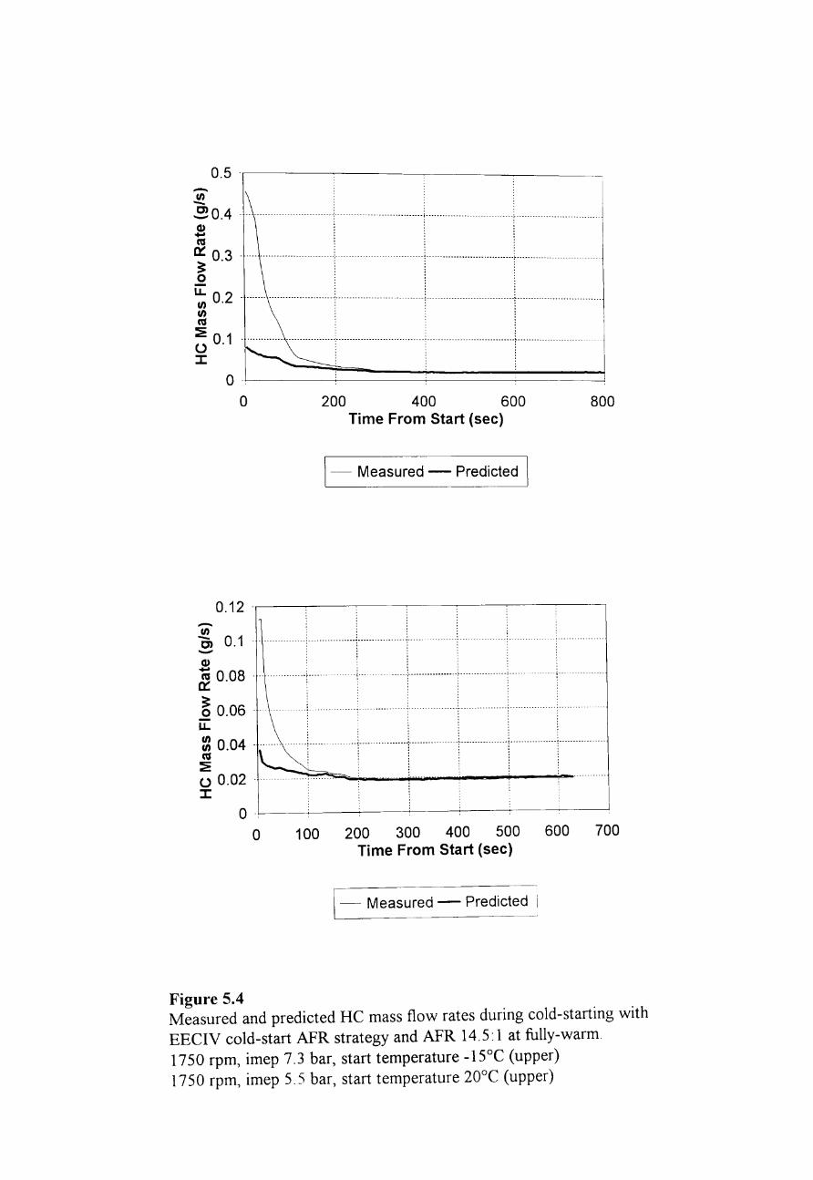
0.5 .r---------:---~---------~0.4 ·················· ............ ··i··········· ................... , ............................... , ................. . m : - :

~ 0.3 ............................... L .......................... .L. ............................. 1.. ...... . 0;> ::

~ 0.2 ............................... ; ............................. :·······························r······················ ........ .

~ : : o 1: : u ................................ j........................... . ............................ + ........................... . :c : : · . · . · .

o .~. --------~------~-----------------o 200 400 600 800

Time From Start (sec)

1- Measured - Predicted 1

0.12 . .------~-----------------

-en C, 0.1 -m -~ 0.08 ...

~ 0.06 . u-~ 0.04 ...... . cu ~ u 0.02 . :c

o .~-~--~-~--~-~--~-~ o 100 200 300 400 500 600 700

Time From Start (sec)

1- Measured - Predicted i

Figure 5.4 Measured and predicted HC mass flow rates during cold-starting with EECIV cold-start AFR strategy and AFR 14.5: 1 at fully-warm. 1750 rpm, imep 7.3 bar, start temperature -15°C (upper) 1750 rpm, imep 5.5 bar, start temperature 20°C (upper)

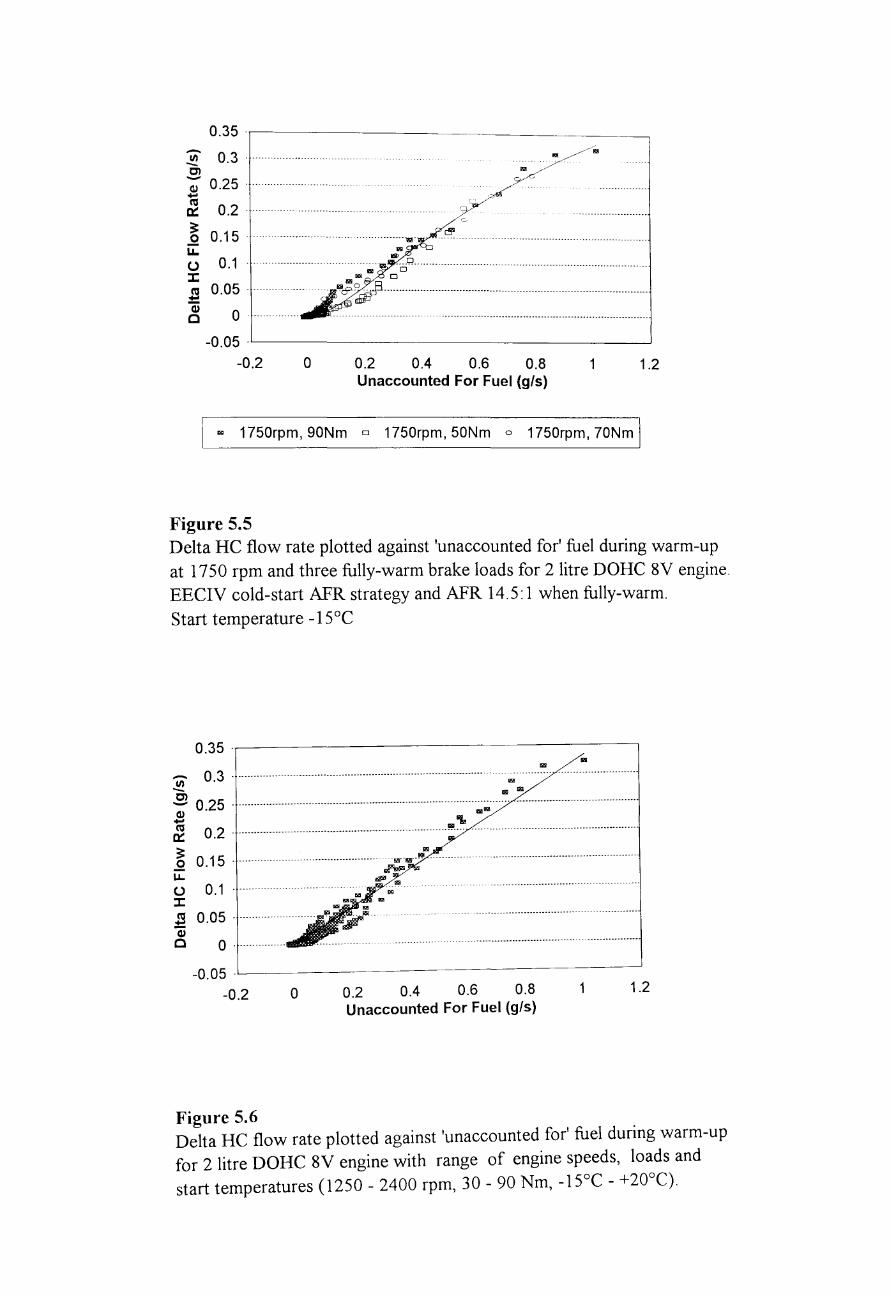
0.35 .,-------------

~ 0.3 101

Cl .. -; 0.25 . -C'tS ~ 0.2 -------- .. -- ........ ---

~ 0.15' ........ ----.---.. . L&.. u 0.1 - .... ------.-.--.-- .. J: .a 0.05 - .... -...... ----

~ 0 .... .

-0.05 -L----______________ ---.-J

-0.2 o 0.2 0.4 0.6 0.8 Unaccounted For Fuel (g/5)

.. 1750rpm,90Nm 0 1750rpm,50Nm 0 1750rpm,70Nm

Figure 5.5

1.2

Delta HC flow rate plotted against 'unaccounted for' fuel during warm-up at 1750 rpm and three fully-warm brake loads for 2 litre DOHC 8Y engine. EECry cold-start AFR strategy and AFR 14.5: 1 when fully-warm.

Start temperature -15°C

0.35 .,-------------------~

'" Cii 0.3 - --- ... ---- ... ------------.. ------------------------------------------.-------.---.. .. -Cl .. - 0.25 - ------------------------------------.------------------------------- .. ----- .. -.. -- ..... --/--------.... ------------.. ---------------~ M"" - ~ ~ 0.2 - ---------------.. --- .. ---- .. ---------------------.. ----------- .... ~ ..

~ 0.15 - .. --- .. -...... -- .. - .. -- .. ---- .. --- .. ---.... \.L. u 0.1' -........ -... -...... J: .a 0.05 ........... -.. .. -; o 0· .. -- .... -- ..

-0.05 _L-_________________ -----'

-0.2 o 0.2 0.4 0.6 0.8 Unaccounted For Fuel (g/5)

1 1.2

Figure 5.6 Delta HC flow rate plotted against 'unaccounted for' fuel during warm-up for 2 litre DOHC 8Y engine with range of engine speeds, loads and start temperatures (1250 - 2400 rpm, 30 - 90 Nm, -15°C - +20°C).

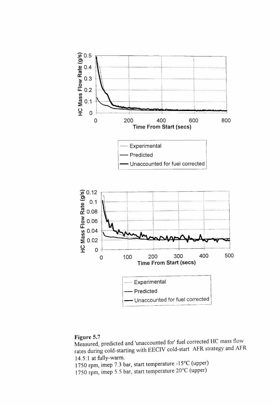
~ 0.5 .r----:-----~----,----­C) -~ 0.4· ~ ........ ---------~--.-.---------.---C'G ............. , ........................... < .....•

0:: ~ 0.3 •• _------------- ••• -:-----_ •• _----------- --------- -< ... - ------- .... ----:-- ... ------

o ~ 0.2 . ...... . ....................... > •••••••••••••••••••••••••••••••••• ~ ••••••••••••••••••••••••••••••• , ••••

en ------ --------- ~ ----- -_. _. - . ~ 0.1 ..

~ 0 .L---==:::::===::::::~~~~~~~~d o 200 400 600 800

Time From Start (sees)

- Experimental

- Predicted

- Unaccounted for fuel corrected

~ 0.12 .r-------:------:-------:---------­C) -;- 0.1 - -------------._,--------... ----.- --- ... -.. -.------------ ... __ .... _-_ .. +" &. 0.08 . .... . ................................. .

; ~:~: . ........... ..,[' .. ::::::::::::::::::::.:: ......... . en C'G ~ 0.02 . u :::c

o 100 200 300 400 500 Time From Start (sees)

- Experimental

- Predicted

_ Unaccounted for fuel corrected

Figure 5.7 Measured, predicted and 'unaccounted for' fuel corrected HC mass flow rates during cold-starting with EECrV cold-start AFR strategy and AFR

14.5: 1 at fully-warm. 1750 rpm, imep 7.3 bar, start temperature -15°C (upper) 1750 rpm, imep 5.5 bar, start temperature 20°C (upper)

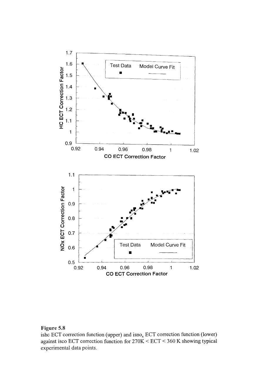
1.7

1.6 .... 0 -~ 1.5 LL

.Q 1.4 -0 ~ 1.3 .... 0 0 I- 1.2 0 w o 1.1 :r:

1

0.9 0.92

1.1

o 1 U co LL c 0.9 o U Q)

t: 0.8 o o I-o 0.7 w >< o Z 0.6

Figure 5.8

0.5 0.92

•

Test Data Model Curve Fit

•

• • • •

~ • • • • • • •

0.94 0.96 0.98 1 CO ECT Correction Factor

.... • • • rfII •

• ••• ••

Test Data Model Curve Fit

• 0.94 0.96 0.98 1

CO ECT Correction Factor

1.02

1.02

ishc EeT correction function (upper) and isnox EeT correction function (lower) against isco EeT correction function for 270K < EeT < 360 K showing typical experimental data points.

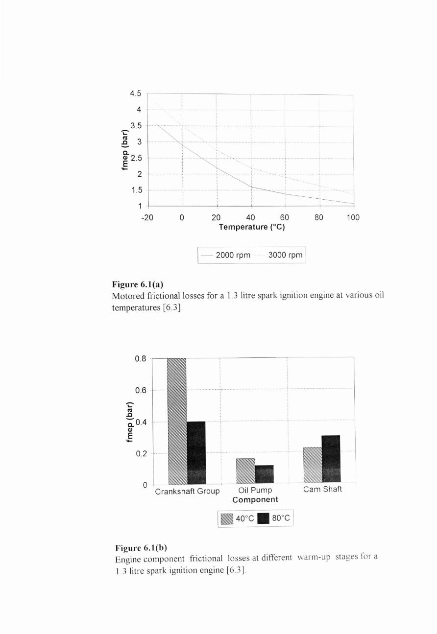
-L-

4.5

4

3.5

~ 3 -Co E 2.5 - 2 ·

1.5 .

1

-20

Figure 6.1(a)

o 20 40 60 80 100 Temperature (OC)

\ - 2000 rpm .... 3000 rpm \

Motored frictional losses for a 1.3 litre spark ignition engine at various oil

temperatures [6.3] .

-L-eu .c

0.8 .

0.6 .

~0.4 Q)

E -0.2 .

o Crankshaft Group Oil Pump Cam Shaft

Component

Figure 6.1(b) Engine component frictional losses at different warm-up stages for a

1. 3 litre spark ignition engine [6.3].

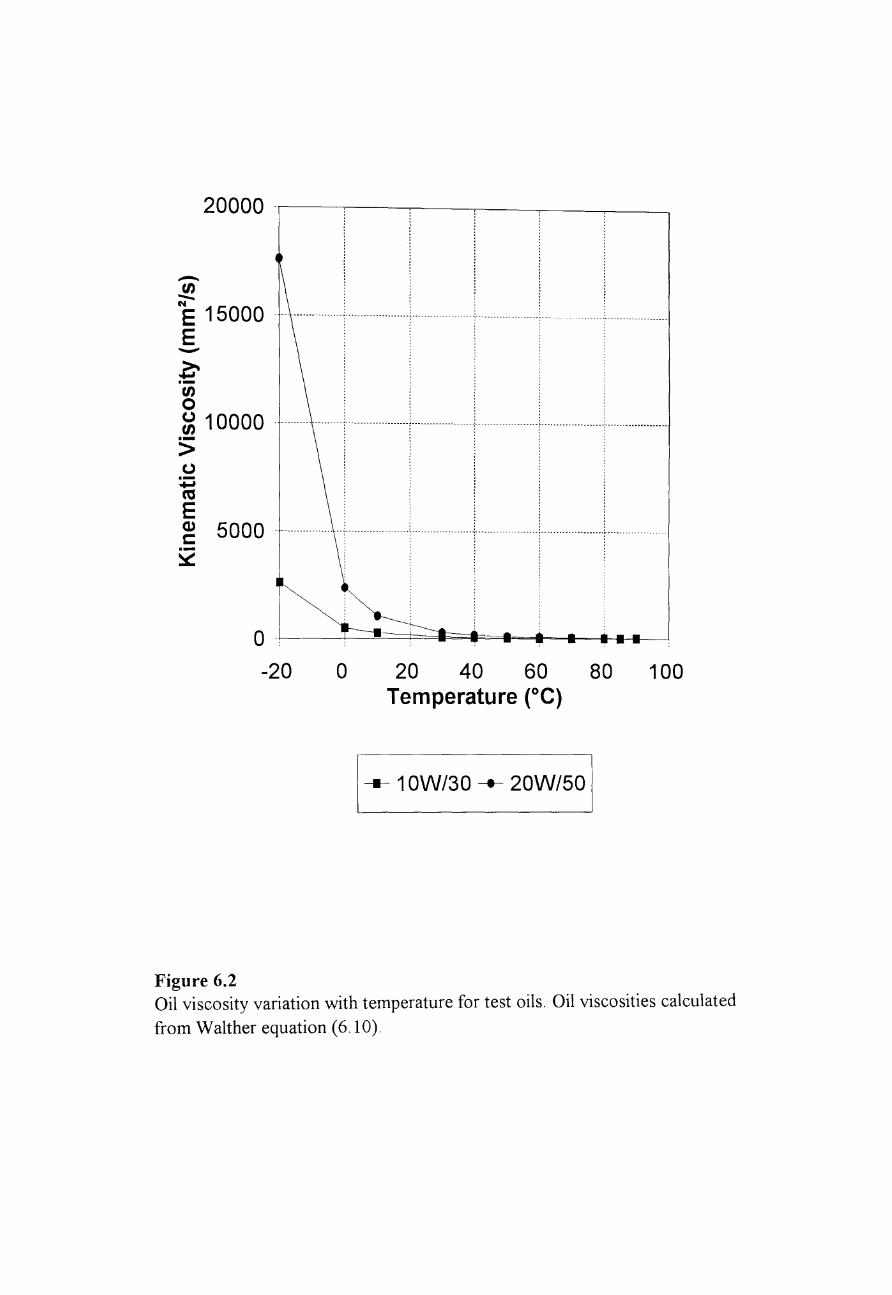
20000 .r----:-----:----:---~-~--

-~ E 15000 E -~ .-

•• -.------ •• ~-------- •• _.- .-.----~---- •• ---_.- - --- __ A - _. - - _._. ,_. _____ ~. __ • __

en . ::

~ 10000 ........... ·········1····················,····················,·· .................. [ .................... i .................. -~ co E Q) 5000 ._ ....... . c .-~

----------i- .. ·_·_--------------f--------------------_L----.... : :

! :

o .k: --~~C=~~~~~~-4~~

-20 o 20 40 60 80 100 Temperature (OC)

1--- 1 OW/3D --- 20W/SO 1

Figure 6.2 Oil viscosity variation with temperature for test oils. Oil viscosities calculated

from Walther equation (6.10).

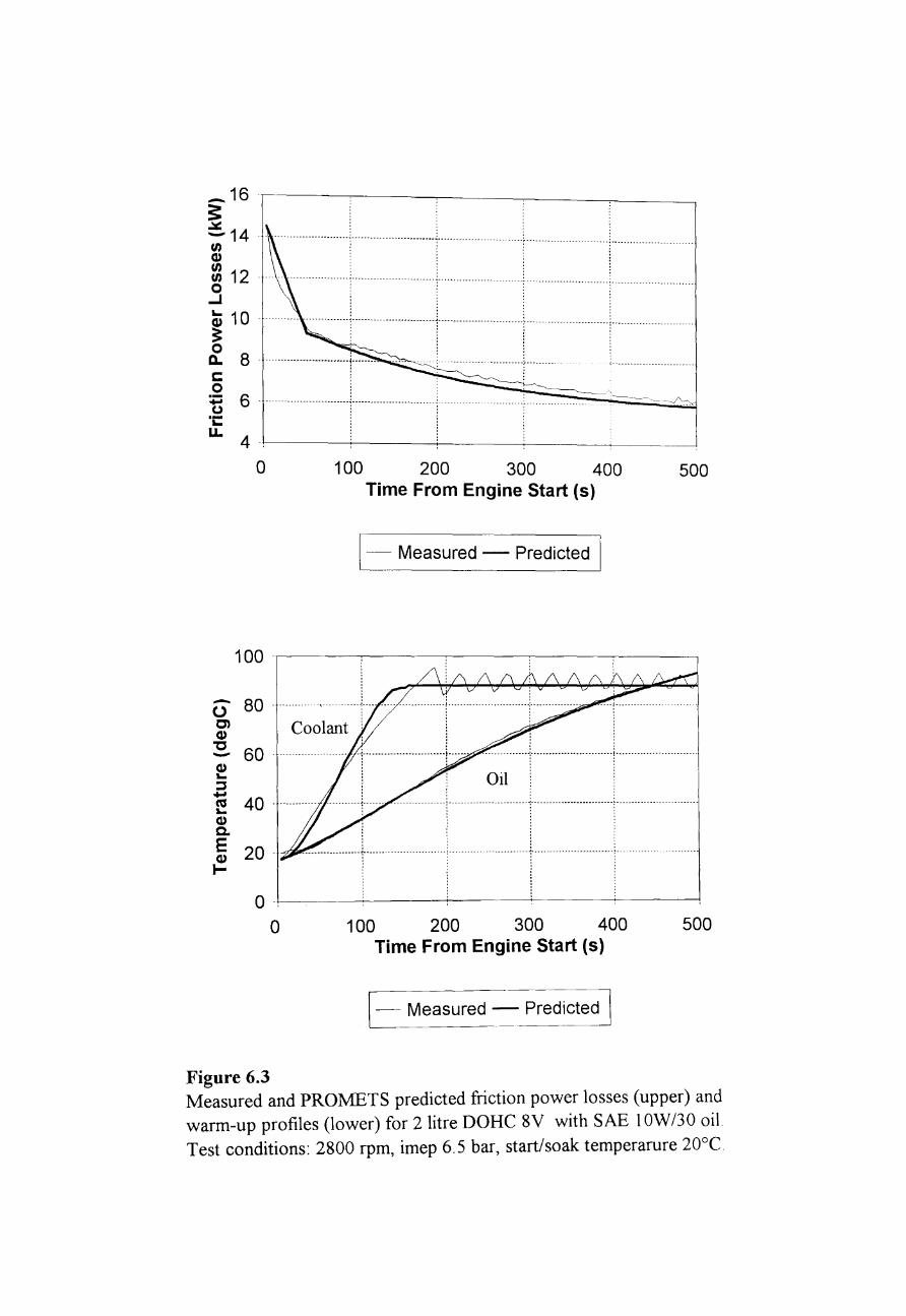
_16~---:-----:----~ ____ ~ __ ~ 3: :£ 14 ~ ---------------T----------------------····r-···-------------

~ 12 o ...J

~ 10 ~

--------- -.-. - --- ------ ---- --_ .. ----~- -.. -

-- -------:---- .................. + .. . , ~

- --- --- ------ -

o ~ 8 -----.--.... -............... j ........ --.-. -········-----------------------f--·----.--

o ~ 6 --.-------.---------.------L---------.-- ____________ ~---.

~ 4 _. i i

-- - - -------

o 100 200 300 400 Time From Engine Start (5)

1- Measured - Predicted I

-... -... _-- .....

500

100 -r----~----~-----~----~---~

o 80-C) cu

"C -~ :::s ..... n:I 40· ----- .. -----'­cu Co

, : ·····_----------:----_·····-----------------1---------._._."---------

Oil ----_._--------:------------_ ............. _;--_ ... _------

· . · . · . · . : : E cu t-

20 - ---_ .. ---------.. --1- -.----- . _. _. ---_. _. _ .. --L - - - - • _ •• - - - - - - - - - - - - - - --:- - -- - -- - - - - - - - - - - - -- - - - _. _. ~ -. --

o -,~.~----~------~------~----~-------o 100 200 300 400 500

Time From Engine Start (5)

1- Measured - Predicted I Figure 6.3 Measured and PROMETS predicted friction power losses (upper) and warm-up profiles (lower) for 2 litre DORC 8V with SAE I OW/30 oil. Test conditions: 2800 rpm, imep 6.5 bar, start/soak temperarure 20°C.

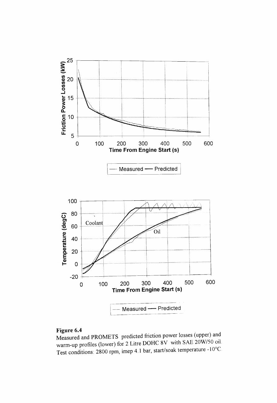
- 25 ·i--;--------r----:------:------~ -

•••••••••••• oooo.oojooooo.ooo.ooooooooooooorooooooooo.oooooo.o.oooo:oooooooooooooooooooooooroooooooo.oo 00 0 0 000,0 0000 0 0

, , , ,

"I: u.. 5.,

o

, , , , , , , , , , , ,

: : ______ -t - --- -- - -- ________ • __ Jo_ ----------. __________ ~----.- ••• -------------~--.----_--- __

- - - - - - - - eo __ ~, __________________ eo __ j:, eo _____________ • ______ ~, __ •• _ - ------------:--------------- --

100 200 300 400 500 Time From Engine Start (5)

[- Measured - Predicted I

.. - -_. -- .. --- _. -- -_. -_ .. -. -- ---- ~

, , , , ....... 0000.01'00 .... 00.000000000.0-:--00000000.0

600

_. - - ----------" --_. ---_. - --_. ------~ -------------_. -------~. -----_. -_. -- -_ .. -_ ... ----------------. -----

-20 .~, ----~------~----+-----~----~-----

o 100 200 300 400 500 Time From Engine Start (5)

600

Figure 6.4 Measured and PROMETS predicted friction power losses (upper) and warm-up profiles (lower) for 2 Litre DORe 8V with SAE 20W/SO oil. Test conditions: 2800 rpm, imep 4,1 bar, start/soak temperature -10°C

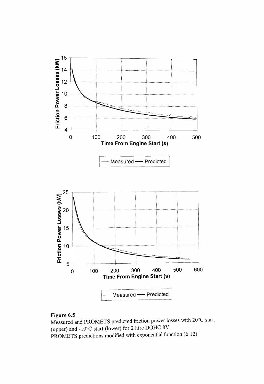
_16'~----;-----:-----~----~--~ 3: =-14 . tn ......................... j ............................................... ~ ..... . . .... __ ._------:..-----------------------Q) , . tn : : tn 12 ........................ ..: ........................... L ... .. o ' . ...J : :

----------------:--- ------- -------------- -.- -~---_.- -- --- - -- .. _-

~ 1: ••••••••••••..••••••••••••• , ••••••• ····· •••• ··· •••••• 1 •••••••••••••••••••••••••• r ••••• ·· ••••••••••••••••• , ••••........ o ~ 6· ........ · 13 .......................................... ; ............... . . ~ u. 4 .!----~---+_---.;...---l----

o 100 200 300 400 500 Time From Engine Start (5)

1- Measured - Predicted I

_25 .r--~--~--~--~--~-~

~ -~ 20 tn tn o

----r-·· ----_ ... -;---_. - ·_--_···------r· .. --------··----------;---------_·_--·· ___ A_A.

...J :: ;; 15 ..................... ;:':: ........................ i:.: ...................... ;':"'"'' • : ;: · .. ···· ...... ·[······ .... ···· .. · .... ·r .... ·· .. · .. ···· o i i Q. i i ~ 10 . ............................. .. .......... t ...................... ( ..................... \...... .. ..... + ........ . U : : .~

U. 5 .~. ____ ~------~----~----~----~-----

o 100 200 300 400 500 Time From Engine Start (5)

1- Measured - Predicted I

600

Figure 6.5 Measured and PROMETS predicted friction power losses with 20°C start (upper) and -10°C start (lower) for 2 litre DORC 8V. PROMETS predictions modified with exponential function (6.12).

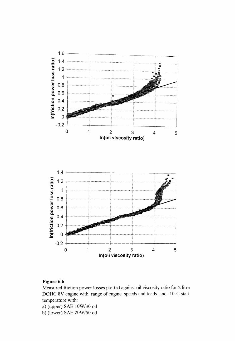
1.6 ·I-------:-----r---~----~-0' 1.4················· ......... -..................................... .

. .. -'- ••. 1I!l

!!II !!II

:;; f! tn tn o

1.2

1 ... ~ 0.8

&. 0.6 .

§ 0.4 :;; (.) 'i: 'to-- 0.2

. . . . ·······------t--·--·-----------···· _. -1--

. -_ .. -' .. -.~ .. _. '. - --. -- --r------------------_·_---_··-----_·_----------

,-.-- ... , .. -,-., . --------:---------------------------1---------------------------r---------

-"'-'-"r""-' ... ······························1····················

....................... ; ..................... ( ............ . C o ............................................... , .......................... , ........................ .

-0.2 .~--~------:----~--~-----J

o 1 2 3 4 5 In( oil viscosity ratio)

1.4 .,------;------~------------~----__ III!

- ~III! :8 1.2· ................... ······0······· .. ········· ...... , ......................... ~ ........................ ~ ......... .

f! :: 1 ··· .............. ·· .. ·· .. ·i .. · .. ·· .. ·· .............. ·: .... · .. · .. ······ ......... ~ .......................... , .. tn tn o ... (1)

0.8

~ 0.6 o

. . . . - - - - - 0- __ • ___ ._. ___ ._ •• ___ :.. 0. _______________ ••• _. _ •• _; _ _ ••• _. ____________ • ___ ~_ •

-------------------------+----_ .. __ ..... _---_ ... _---j--.- .. -.-- .. --.---------.--~- ..

Q. § 0.4' ......................... _ .......... = .. ~ ..• ····111··'···· .. ·· ",,-~ ....................... _ ....................... .

~ 0.2 :s c 0 --0.2 .l---------<-----4------~----1__--___._j

o 1 2 3 4 5 In( oil viscosity ratio)

Figure 6.6 Measured friction power losses plotted against oil viscosity ratio for 2 litre DOHC 8V engine with range of engine speeds and loads and -10°C start

temperature with: a) (upper) SAE lOW/30 oil b) (lower) SAE 20W/SO oil

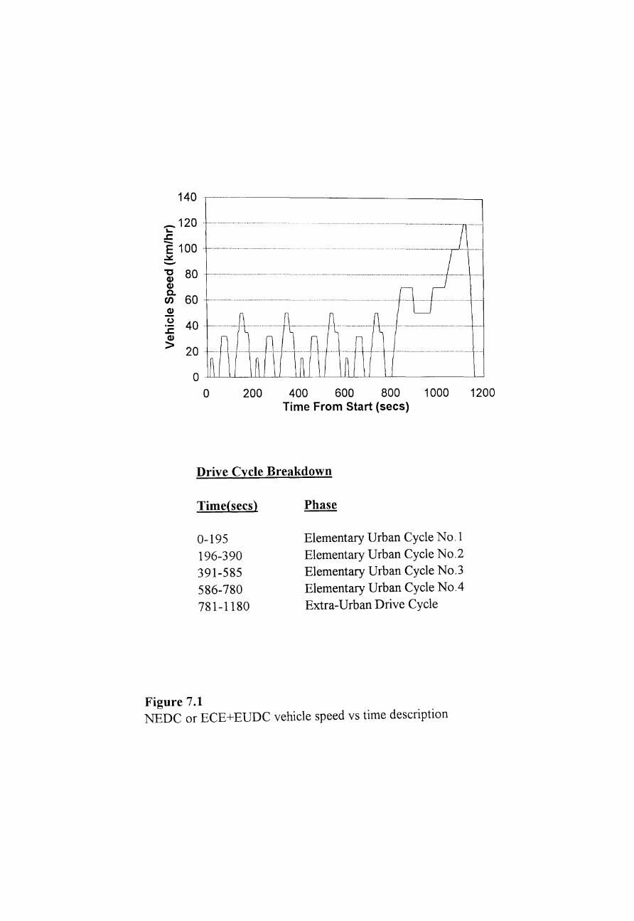
140 .r------------------------------­

_120 .... '­.r:. -E 100 .................... . .::.:: -"C 80 (1) (1) a. en 60 .......................... .

o 40 . .............................................. . .r:. (1)

> 20 ....... .

o .. ~-U~~-U~ilL~~llL~~L-________ ~

o 200 400 600 800 1000 1200 Time From Start (sees)

Drive Cycle Breakdown

Time(secs)

0-195 196-390 391-585 586-780 781-1180

Phase

Elementary Urban Cycle No.1 Elementary Urban Cycle No.2 Elementary Urban Cycle No.3 Elementary Urban Cycle NO.4 Extra-Urban Drive Cycle

Figure 7.1 NEDC or ECE+EUDC vehicle speed vs time description

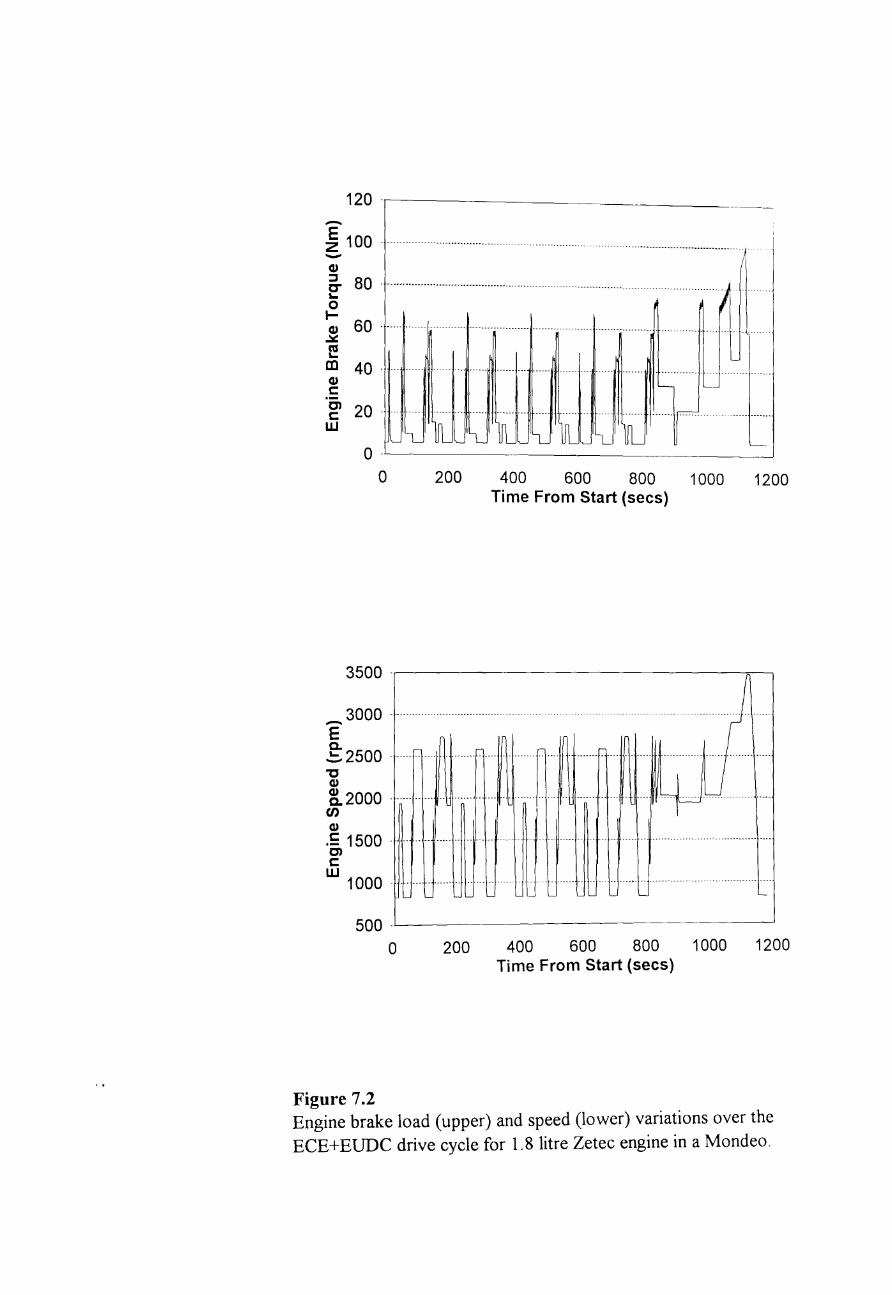
120 .,-------_______ _

-E :2: 100 .-................................ . -Q) e- 80 .-.......................................................................................... . o I-Q) 60· ..... " ...... '.,,,, .. ,, ................................................................ . ~

e OJ Q) c:

40 ........ .

g' 20· .. · w

o·~-----------------------------

o 200 400 600 800 1000 1200 Time From Start (sees)

3500 .,-----------------------------~-

3000 .-.......... ",,, .. ,, .. ,,,,., .. ,, -[ r .!:.. 2500 . -......... . "C Q)

~ 2000 . -.......... . .~ ....... . lL--

en Q) .=: 1500 . .. . .................. '.". C') c: w 1000 ............. ' .......... .

L.L. L.~ L.L. L...

500 .L-________________________________ _

o 200 400 600 800 1000 1200 Time From Start (sees)

Figure 7.2 Engine brake load (upper) and speed (lower) variations over the ECE+EUDC drive cycle for 1.8 litre Zetec engine in a Mondeo.

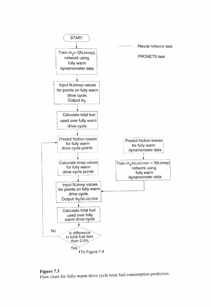
( START )

~ Train nl f= f(N,bmep)

network using fully warm

dynamometer data

l Input N,bmep values

for points on fully warm drive cycle. Output Iilf

~ Calculate total fuel

used over fully warm drive cycle.

...... ______ L Predict friction losses:

.------:.. for fully warm drive cycle points

-J-- ----

: Calculate imep value~ ; for fully warm : ! drive cycle points : ....... _--_ ... -_ ..... _--_.-- -------_ .. -._------- .....

Input N,imep values for points on fully warm

drive cycle. Output mf,hc,co,nox

Calculate total fuel used over fully

warm drive cycle

:Neural network task

:PROMETS task

Predict friction losses for fully warm

dynamometer data

Train nif'hc,co,nox = f(N,imep) network using

fully warm dynamometer data

~----------------'

Figure 7.3 Flow chart for fully-warm drive cycle total fuel consumption prediction.

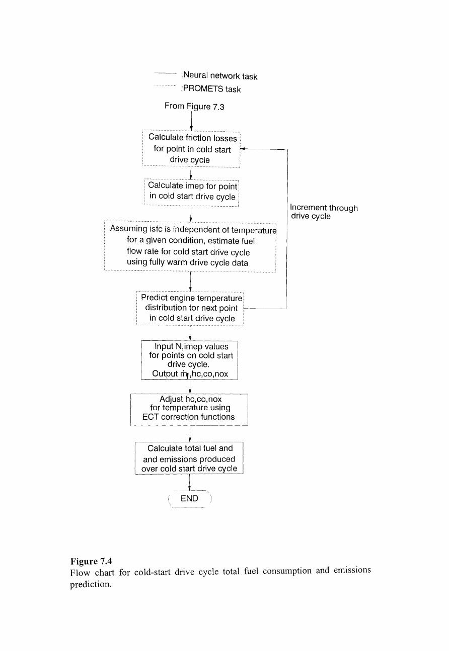
:Neural network task

:PROMETS task

From Figure 7.3

------------------- ___________ 1 _________ _ Calculate friction -i-~-~·~~~--:

for point in cold start drive cycle

, :::::::::::::::::1:::::::::::::::::-:::::-::::; : Calculate imep for point: , in cold start drive cycle'

--------------_-_-_-_-_-_-~_-_-~-_-~_-_-_J_-_ ---------------------------,

Assuming isfc is independent of te~p~~~t~-~~ for a given condition, estimate fuel flow rate for cold start drive cycle using fully warm drive cycle data

r········· ..... . :---Predict-~~-gine temperature : distribution for next point : in cold start drive cycle L ~ ____ -.. _---- -- ---l

Input N,imep values for points on cold start

drive cycle. Output rilt,hc,co,nox

~ Adjust hc,co,nox

for temperature using ECT correction functions

1 Calculate total fuel and

and emissions produced over cold start drive cycle

1 -

( END

Increment through drive cycle

Figure 7.4 Flow chart for cold-start drive cycle total fuel consumption and emissions

prediction.

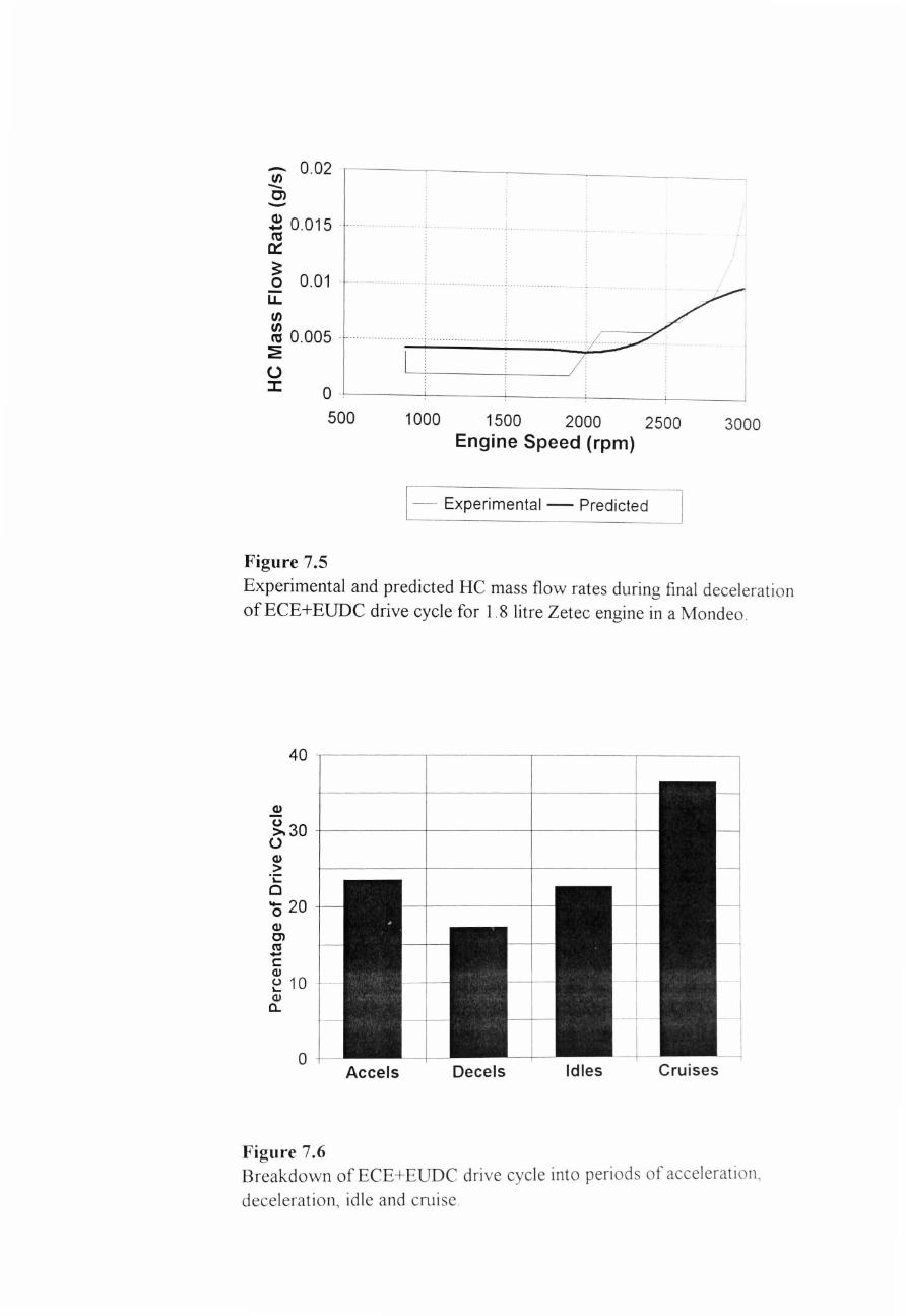
en 0.02 -0') -~ 0.015 ra ~

~ 0.01 ·-u. U) U) ra 0.005 .

::2: U :c o .~----~------~------~ ______ ~ ____ ~

500 1000 1500 2000 2500 3000 Engine Speed (rpm)

[ - Experimental - Predicted

Figure 7.S

Experimental and predicted HC mass flow rates during final deceleration ofECE+EUDC drive cycle for 1.8 litre Zetec engine in a Mondeo .

40 ~--------~-------,---------,--------,

cv

~30 +---------+---------~--------~-u cv > ·c o '0 20 cv 0) n:I -c: cv ~ 10 (l)

a..

o Accels Decels Idles Cruises

Figure 7.6 . Breakdown of ECE+EUDC drive cycle into periods of acceleratIon ,

deceleration, idle and cruise .

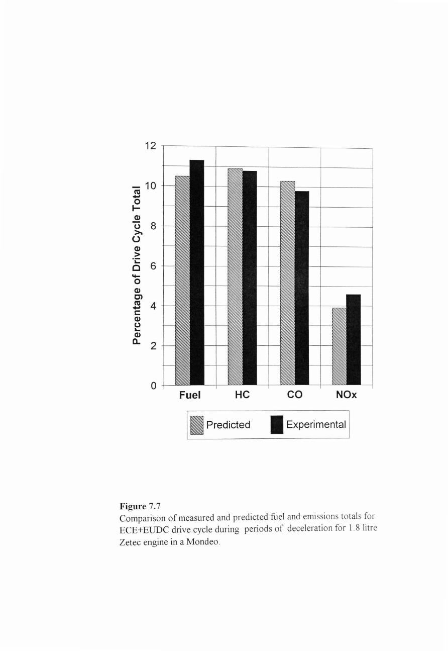
12

10 co +' 0 t-Q)

0 8 ~ () Q)

> 0;: 6 0

'to-0 Q) C) co 4 +' c: Q) 0 .... Q)

Q. 2

o Fuel HC co NOx

Predicted • Experimental

Figure 7.7 Comparison of measured and predicted fuel and emissions totals for ECE+EUDC drive cycle during periods of deceleration for 1.8 litre

Zetec engine in a Mondeo .

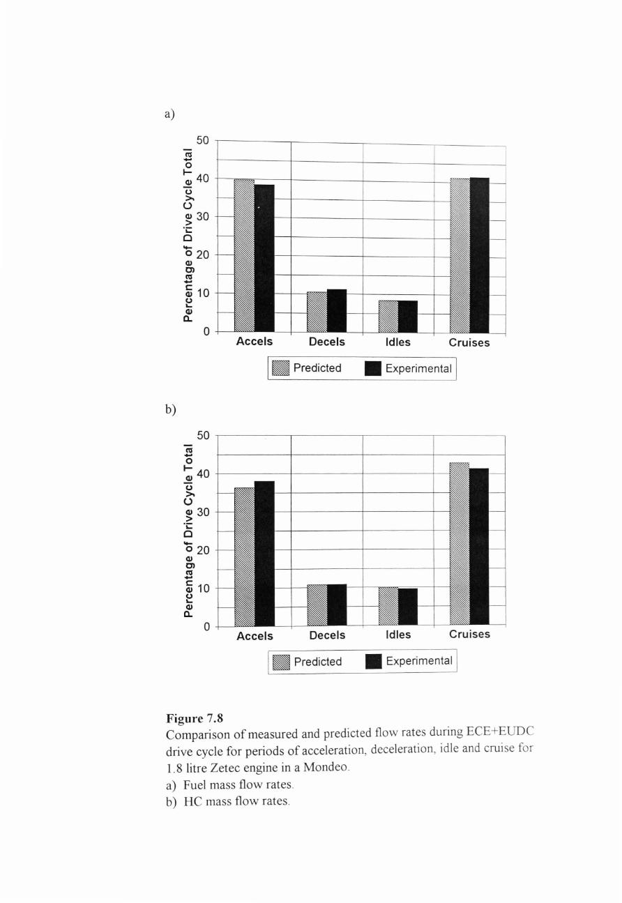
Idles Cruises

_ Experimental I

Idles Cruises

1_ Predicted _ Experimental I

Figure 7.8 Comparison of measured and predicted flow rates during ECE+EUDC drive cycle for periods of acceleration, deceleration, idle and cruise for

1.8 litre Zetec engine in a Mondeo .

a) Fuel mass flow rates. b) HC mass flow rates.

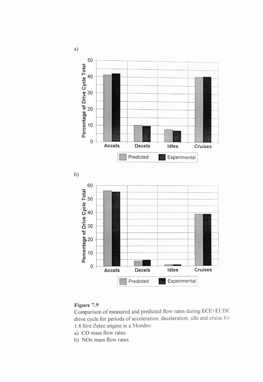
Idles Cruises

II Experimental I

Idles Cruises

1_ Predicted II Experimental I

Figure 7.9 Comparison of measured and predicted flow rates during ECE+EUDC drive cycle for periods of acceleration, deceleration, idle and cruise for

1 .8 litre Zetec engine in a Mondeo .

a) CO mass flow rates . b) NOx mass flow rates .

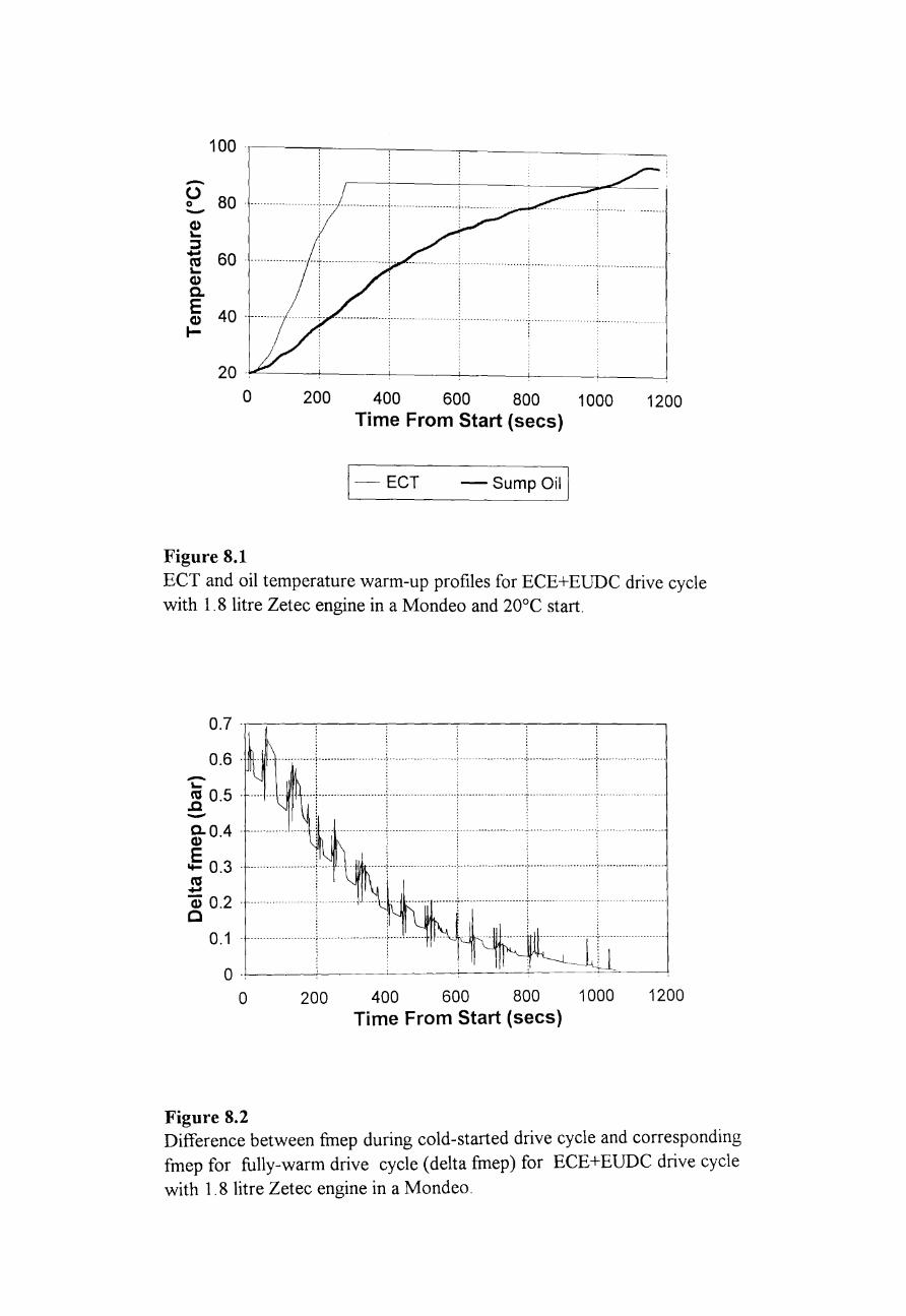
-~ 80 -~ ::l ... ~ CI) c. ~ 40 -------------....

20 -~, ----~----+-----~--~--__ ~--__ ~

o 200 400 600 800 1000 1200 Time From Start (sees)

1-- EeT -sumpoilj

Figure 8.1 ECT and oil temperature warm-up profiles for ECE+EUDC drive cycle with 1.8 litre Zetec engine in a Mondeo and 20°C start.

0.7 -~,---~----~----~----~----~----~ , , , ,

0.6 - -- -- -----------+--......... ---------+-------------- ------~-------- ... --- .... -- .. : ......... -.-------.... _r ... -------------------

--------.--------

(i) 0.2 - ------------ --:------- -- ----- -- --- --.............. ; ... _____ .. ___ .. __ .... _L .. __ .. _____ --------------------

o :,: 0.1 - ---------------------[-----------------.----(-.---.---. -

o -~, ----~,------~----~--~~-----=~--~ o 200 400 600 800 1000 1200

Time From Start (sees)

Figure 8.2 Difference between fmep during cold-started drive cycle and corresponding fmep for fully-warm drive cycle (delta fmep) for ECE+EUDC drive cycle with 1.8 litre Zetec engine in a Mondeo_

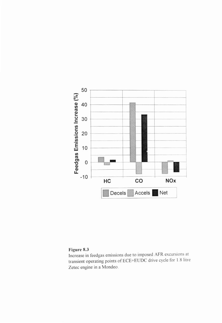
50 r--------,--------~---------~ -Q.)40 -r-------+­en cu Q.) '­o c: en c:

30 --t--------+--

o 20 --t--------+--en en .-~ 10 +----------4-

en cu ~ 0 Q.) Q.) u.

-10 +--____ +--____ +--___ ----1

HC CO NOx

I_ Deeeis _ Aeeeis • Net

Figure 8.3 Increase in feedgas emissions due to imposed AFR excursions at transient operating points of ECE +EUDC drive cycle for 1. 8 litre

Zetec engine in a Mondeo .

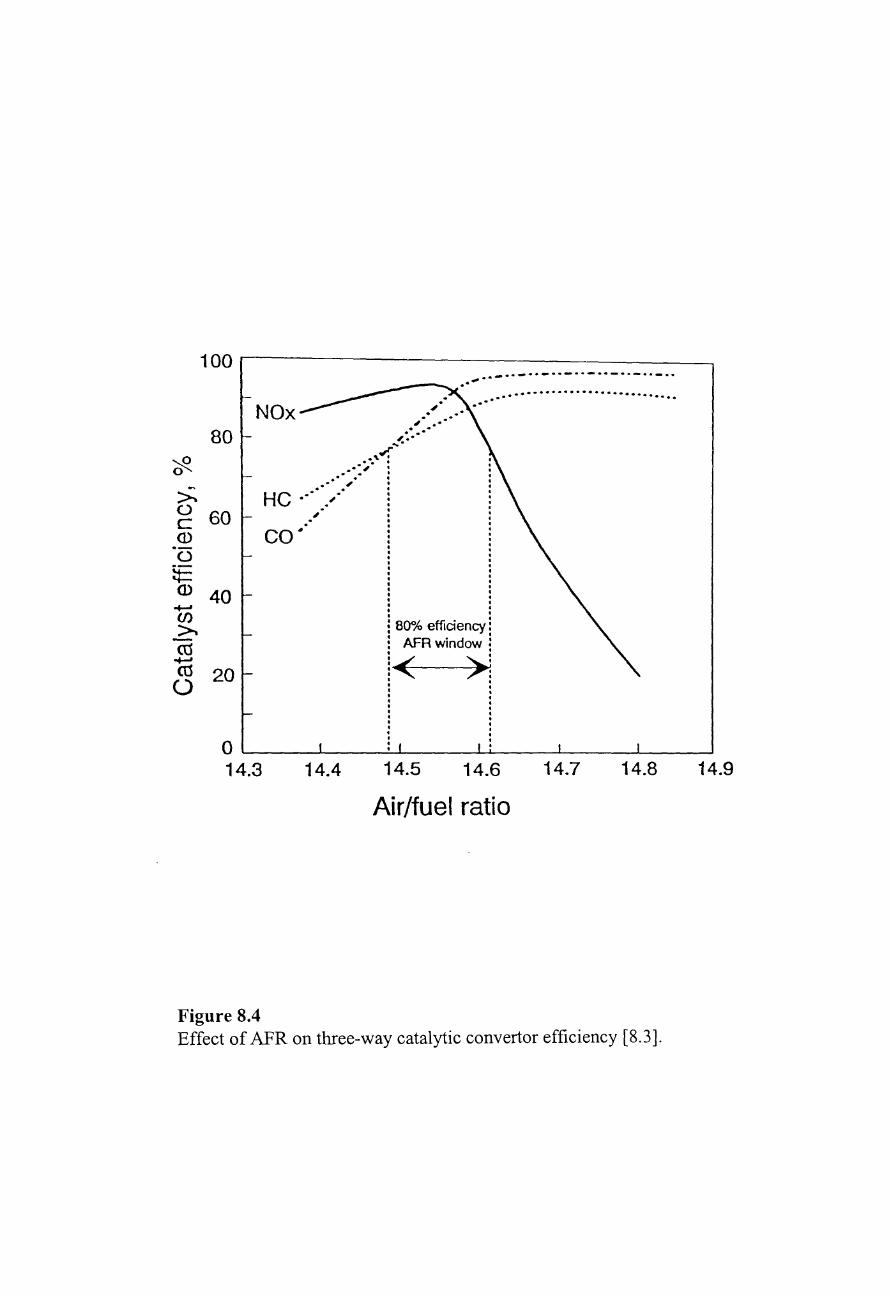
100.-------------------------------~ .. - .. - .. _ .. - .. - .. _ .. - .. - .. ...............................

NOx ~. . . , ..... . . ... 80

>-g 60 ill o ~ ill 40 ....... en >­CO ....... CO 20 o

, .. . ,.,,; ... .. :,. : .-. . .... ,. :

He ..... : ., . . . co ..

. . , . · · · • · • · · · · · · • • • • · • ~ BOO~ efficiency l AFR window.

1< >1 . o ~ ____ ~ ____ ~ ______ ~ ____ -J ______ ~ ____ ~

14.3 14.4 14.5 14.6 14.7 14.8 14.9

Air/fuel ratio

Figure 8.4 Effect of AFR on three-way catalytic convertor efficiency [8.3].

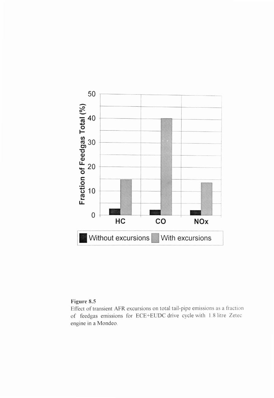
50

-~ 0 -- 40 m ..... 0 ..... ~ 30 C)

"'C Q) Q)

!: 20 0 c: 0 .-..... 10 (.) m a... U-

0 HC co NOx

• Without excursions I With excursions

Figure 8.5 Effect of transient AFR excursions on total tail-pipe emissions as a fracti on

of feedgas emissions for ECE+EUDC drive cycle with 1.8 litre Zetec

engine in a Mondeo .

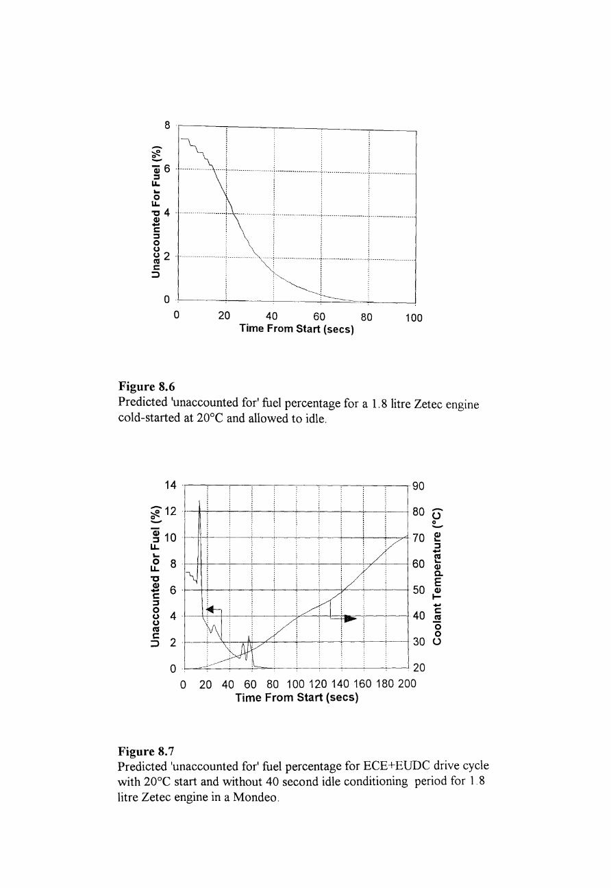
8~---;--~:-____ ~ __ ~ ____ ~

-~ : i 6 ..................... , .................... , ........... ·········i·····················,·················

~4 ..................... + .................... , ...................... } ...................... , .................... . C ' ' , :::s : : o ' , ~ 2 . .......... ...~ ............. , ...... ; .................... ) ...................... ; .................... . c ':

~ I o .~----~----~----~~~==~ ____ ~

o 20 40 60 80 100 Time From Start (sees)

Figure 8.6 Predicted 'unaccounted for' fuel percentage for a 1.8 litre Zetec engine cold-started at 20°C and allowed to idle.

90

~ 12 ----t--+-~-__;_--.:---~---:--~---;--:---+ 80 -.... 0 8 L1.

I~ "C (1)

6· -c :::s 0

4· (J (J cu c

2· :::>

0

0

Figure 8.7

70

60

50

40

30

+- ,14: h' xj:: :,',"'" : ::

: ,I:;:

20

20 40 60 80 100 120 140 160 180 200 Time From Start (sees)

-u 0 -e :::s -cu .... (1) Co E (1)

I---c ~ 0 0 U

Predicted 'unaccounted for' fuel percentage for ECE +EUDC drive cycle with 20°C start and without 40 second idle conditioning period for 1,8 litre Zetec engine in a Mondeo.

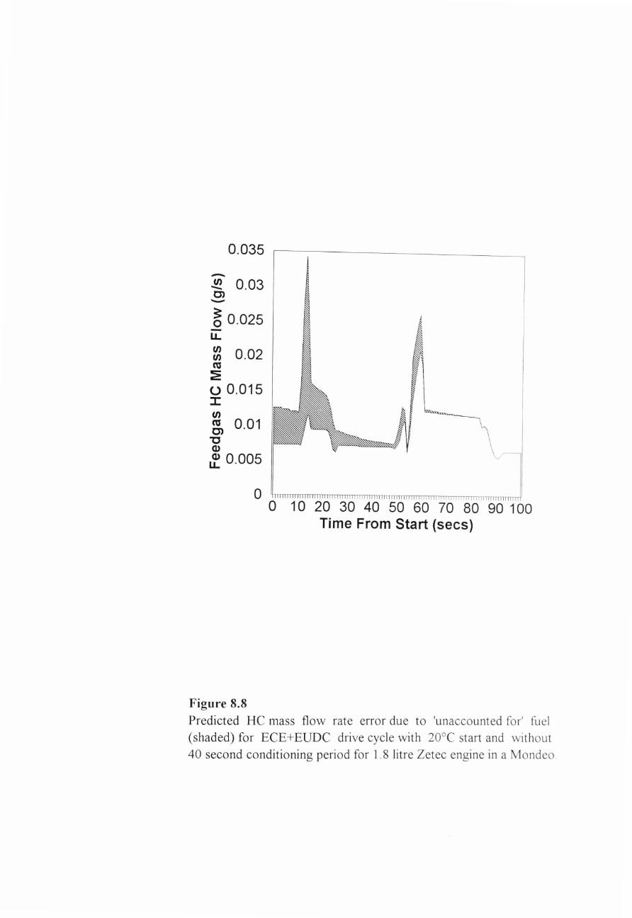
0.035

-.!!! 0.03 0) -~ 0.025

LL

~ 0.02 co :a: (J 0.015 :::r: t/)

~ 0.01 '0 Q)

.T. 0.005

o

Figure 8.8

o 10 20 30 40 50 60 70 80 90 100 Time From Start (sees)

Predicted HC mass flow rate error due to 'unaccounted for ' fuel

(shaded) for ECE+EUDC drive cycle with 20°C start and without

40 second conditioning period for 1. 8 litre Zetec engine in a Mondeo .

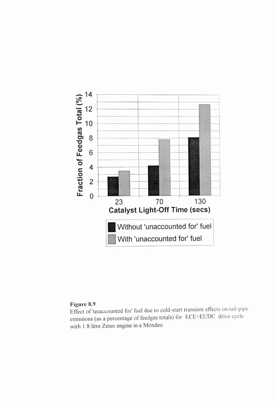
-14 ~ o -co 12 +-' o I- 10 U) co ~ 8 !---------~--~----~-

"'C Q)

~ 6 't-

o 4 c T---------~-

o .-t) 2 co L.

LL o 23 70 130

Catalyst Light-Off Time (sees)

• Without 'unaccounted for' fuel

• With 'unaccounted for' fuel

Figure 8.9 Effect of 'unaccounted for' fuel due to cold-start transient effects on tail -pipe emissions (as a percentage offeedgas totals) for ECE+EUDC drive cycle

with 1.8 litre Zetec engine in a Mondeo .

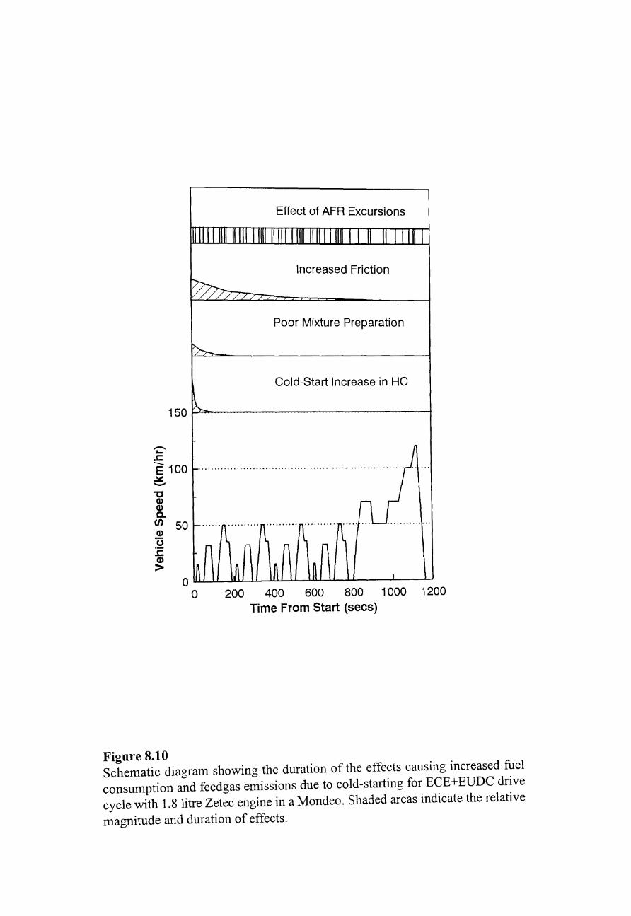
C .c

Effect of AFR Excursions

Increased Friction

Poor Mixture Preparation

Cold-Start Increase in HC

150~--~-----------------------J

-E 100 ............................................................... . ~ -"C Q) Q) 0-W 50 Q)

.~

.c Q)

> O~~~~U-~~L-UU~~L---~----U

o 200 400 600 800 1 000 1200 Time From Start (sees)

Figure 8.10 Schematic diagram showing the duration of the effects causing increased fuel consumption and feedgas emissions due to cold-starting for ECE+EUDC drive cycle with 1.8 litre Zetec engine in a Mondeo. Shaded areas indicate the relative

magnitude and duration of effects.

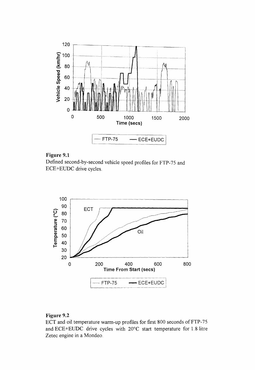
120

- ' ..c 100 . ..............................................[,1- ........................................ .

EN: : • =- 80 ............. r:·\ .......... ··j· .... ·· .......... ··.............. .... ...... .............. ~ ................... . -g :,.,,J: ~ 60 .............................. j ......................... ,.;, ...................... f ................... r:., ...... ..

] 40j~ ..... J '~~ili' ......... . ~ 20 . "II' '. . ... ' ......... ":" " ...... .... ,. .......... .. . ........ .

o. lD IDI ~ : o

Figure 9.1

500 1000 Time (sees)

1500

\- FTP-75 -ECE+EUDC I

2000

Defined second-by-second vehicle speed profiles for FTP-75 and ECE+EUDC drive cycles.

100 90 -U 80 0 -Q) 70 '-::s - 60 e

Q) 50 c.

E 40 Q) I-

30 20

0 200 400 600 800 Time From Start (sees)

1- FTP-75 -ECE+EUDC I

Figure 9.2 ECT and oil temperature warm-up profiles for first 800 seconds ofFTP-75 and ECE+EUDC drive cycles with 20°C start temperature for 1.8 litre Zetec engine in a Mondeo.

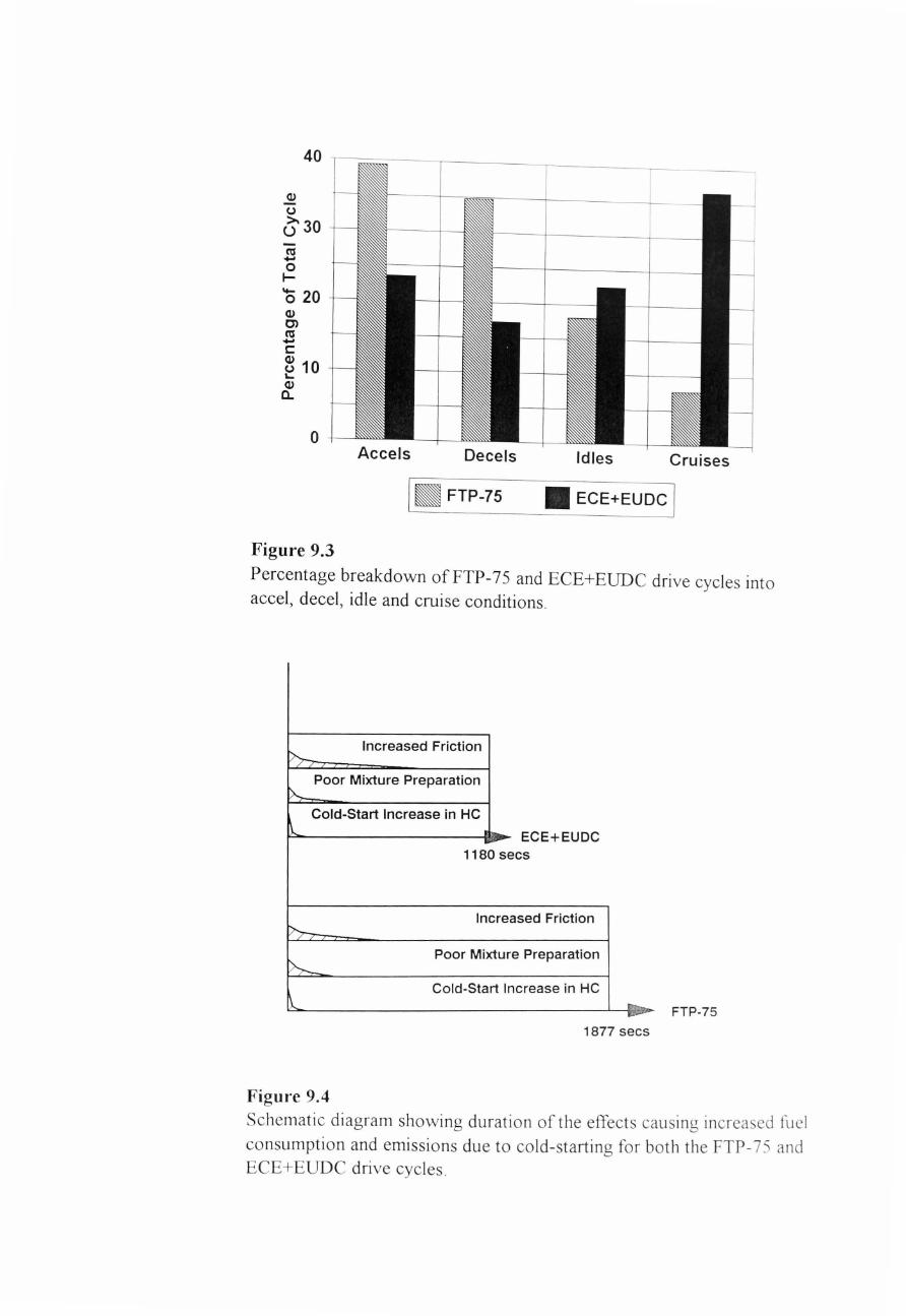
40 ~~~--~ ________ ~ ______ ~ ______ __

a> (.)

0' 30 CI3 -o l-

'020 a> Ol CI3 -C

~ 10 L-a> a.

o Accels Decels Idles Cruises

1_ FTP-75 _ ECE+EUDC I

Figure 9.3

Percentage breakdown ofFTP-75 and ECE+EUDC drive cycles into accel, decel, idle and cruise conditions.

~ Increased Friction

(>.., Poor Mixture Preparation

Cold-Start Increase in HC ~ .k- ECE+EUDC -.-

1180 secs

Increased Friction t>..

~ Poor Mixture Preparation

~ Cold-Start Increase in He

rt._. ..... FTP-75

1877 sees

Figure 9.4 Schematic diagram showing duration of the effects causing increased fuel

consumption and emissions due to cold-starting for both the FTP-75 and ECE+EUDC drive cycles .

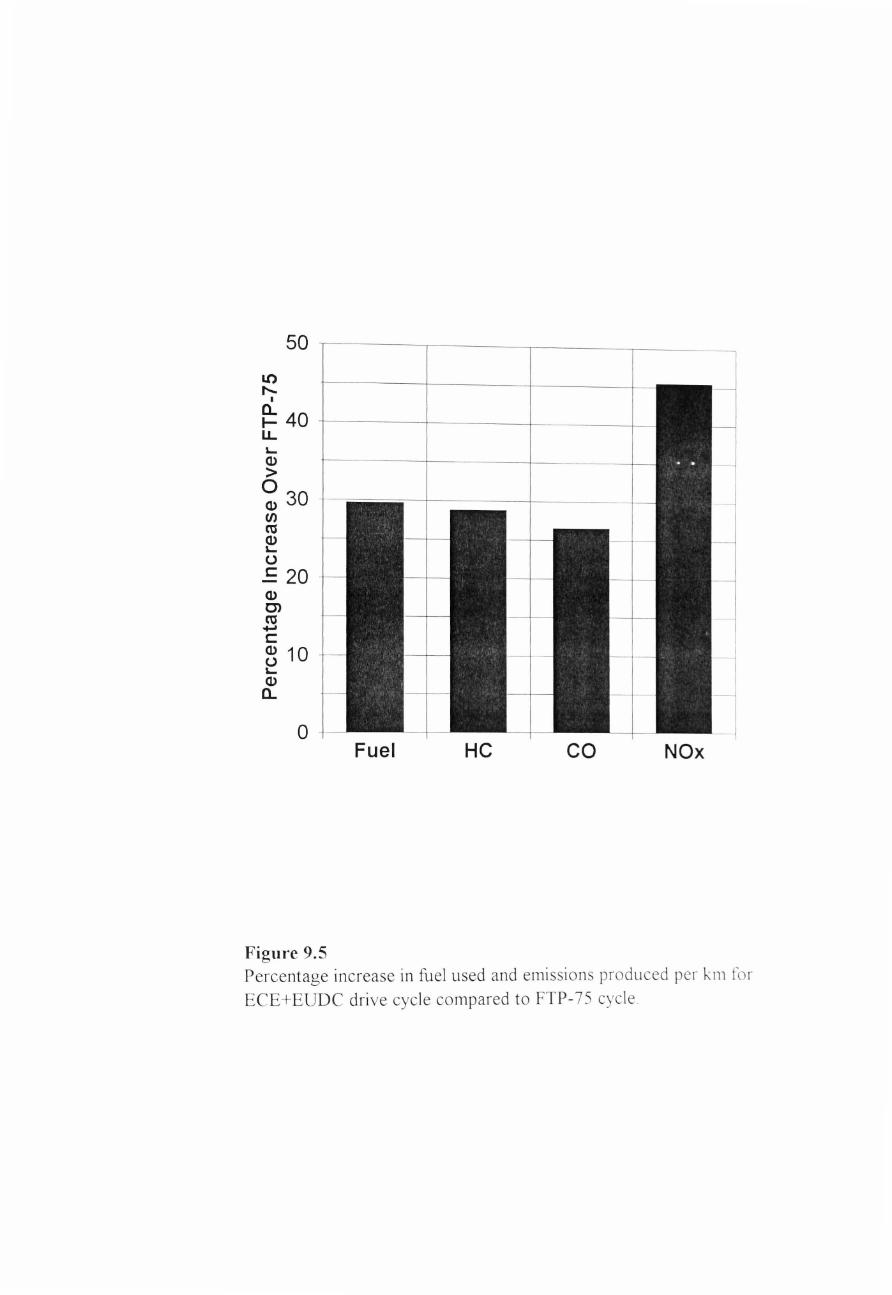
LO r---

I

50

g: 40 u.. s.... Q)

> 0

30 Q) (/) C'tS Q) s.... u .!: 20 Q)

C> C'tS ~

C Q) 10 u s.... Q)

a..

o

Figure 9.5

Fuel HC co NOx

Percentage increase in fue l used and emissions produced per km for ECE+EUDC drive cycle compared to FTP-75 cycle.

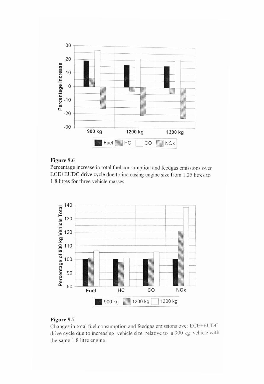
30 ~--------~ __________ ~ ________ _

20 +----.j ClI VI (U

~ 10 o c:

ClI 0 0> (U -c: ~ -10 -t------'­ClI a..

-20 -r-------+----~

-30 +-----------+-----------~--------~ 900 kg 1200 kg 1300 kg

1_ Fuel _ HC D co _ NOx 1

Figure 9.6 Percentage increase in total fuel consumption and feedgas emissions over ECE+EUDC drive cycle due to increasing engine size from 1.25 litres to 1.8 litres for three vehicle masses .

- 140 ,------,-------~------,------_, (U -o I­ClI 130 +-----+-----~----_r--~ o .c: ~ 120 +------t-------t-----t---

0> ~

g 110 -f------j------t-------j---m -o 100 ClI 0> (U -@ 90 o '­ClI

a.. 80

Figure 9.7

Fuel HC co NOx

1_ 900 kg _ 1200 kg D 1300 kg I

Changes in total fuel consumption and feedgas emissions over ECE+EUDC drive cycle due to increasing vehicle size relative to a 900 kg vehicle with the same 1.8 litre engine

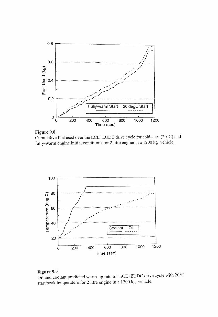
0.8 1------------------.

0.6 -Ol ~ --"C (])

0.4 (J)

:::> (])

:J u..

0.2

, I

I

I

I

.................................................................................................................................... . ;,./~ .................. ..

~-

~ ,

................................................................ ,~ .................... _ .................. .. ,

I Fully-warm Start 20 degC Start

o ~ ____ ~ ____ ~ ____ ~ ____ ~ ____ -L ____ ~

o 200 400 600 800 1000 1200 Time (sec)

Figure 9.8 Cumulative fuel used over the ECE+EUDC drive cycle for cold-start (20°C) and fully-warm engine initial conditions for 2 litre engine in a 1200 kg vehicle.

100 ~----------------------------------~

-80 o Ol (]) "C --(]) 60 .... :J co .... (])

a. 40 E (])

I-

..........................................................................................

---.............................. -.............. ;.,;-~."'::' .................................. .

, ,

--

...... ••••••••••••• .J" ......................................... ••••••••••••••••••••••••• , I Coolant - _?~I- _\

20 -:: ....................................................................... .

o 200 400 600 800 1000 1200

Time (sec)

Figure 9.9 Oil and coolant predicted warm-up rate for ECE+EUDC drive cycle with 20

0 e start/soak temperature for 2 litre engine in a 1200 kg vehicle.

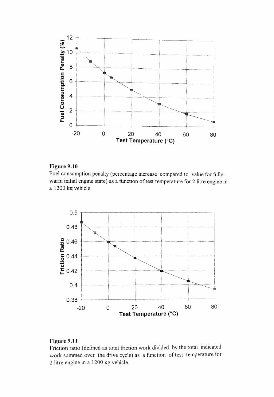
12 -~ o -~10 . ..... .. ~ .................. .L .. . ~ .: tt. 8· ............. ~ .. ~ ......................... -i- ..................... ..... , ..................... : ........................... ..

c::::

:[ 6 ............................. j .............. · ...... · .... ·i .. · ............ · ............................................ ; ............ . E i : :J II) 4· ...... ~ ............................. ~ ......................................... .. 8 : i ................ . 7. 2 · ........................... , ....................... '::............... .. .......... .. ..., • "--- ._---i---------

:J U. o .~----~------~------~------~ ______ ~

-20 o 20 40 60 80 Test Temperature (OC)

Figure 9.10 Fuel consumption penalty (percentage increase compared to value for fully­warm initial engine state) as a function of test temperature for 2 litre engine in a 1200 kg vehicle.

0.5 .~------------~------~------~------

. . 0.48· .. ·'1·· ················r····

:8 0.46 . .......................... .. ........................ -: ........................... , ............................ ; ......................... . ca ~ 5 0.44 ........................... , .......................... : ......................... < .......................... ,

+i (J

;t 0.42

0.4 .

----------.--_._--------------- ----------.------- ----.. ----------

................. ..; ........................ : ............................ j--..................... ] .. ..

L-------'----~------;------:-- ___ J 0.38

-20 o 20 40 60 80 Test Temperature (OC)

Figure 9.11 Friction ratio (defined as total friction work divided by the total indicated work summed over the drive cycle) as a function of test temperature for 2 litre engine in a 1200 kg vehicle.

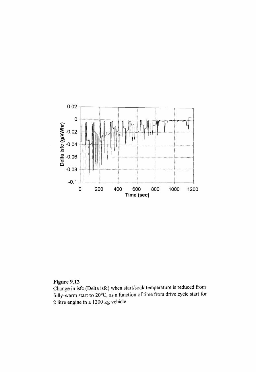
O. 02 ·.r-----,----,----------;---,----~--

'C' 0 ............... L ...... ,! ntldM~~

1-0.02 .... v···: ~ .; II~.~ I' ~.. r" ..... 'fLJi l

~ -0.04 . T? .. ..... . ..... ································r···················

.f! -0.06 .. ...... .~. . .... .. . ..... . ................. , ... . _ ..... --------~ -_. -.. --_. -------_. --CI)

o -0.08 ... . _.- -~-- ------- .... --------~---------

: :

! i ································r···················

-0.1 .!-, ---+---+------i----+------i----J

o 200 400 600 800 1000 1200 Time (sec)

Figure 9.12 Change in isfc (Delta isfc) when start/soak temperature is reduced from fully-warm start to 20°C, as a function of time from drive cycle start for

2 litre engine in a 1200 kg vehicle.

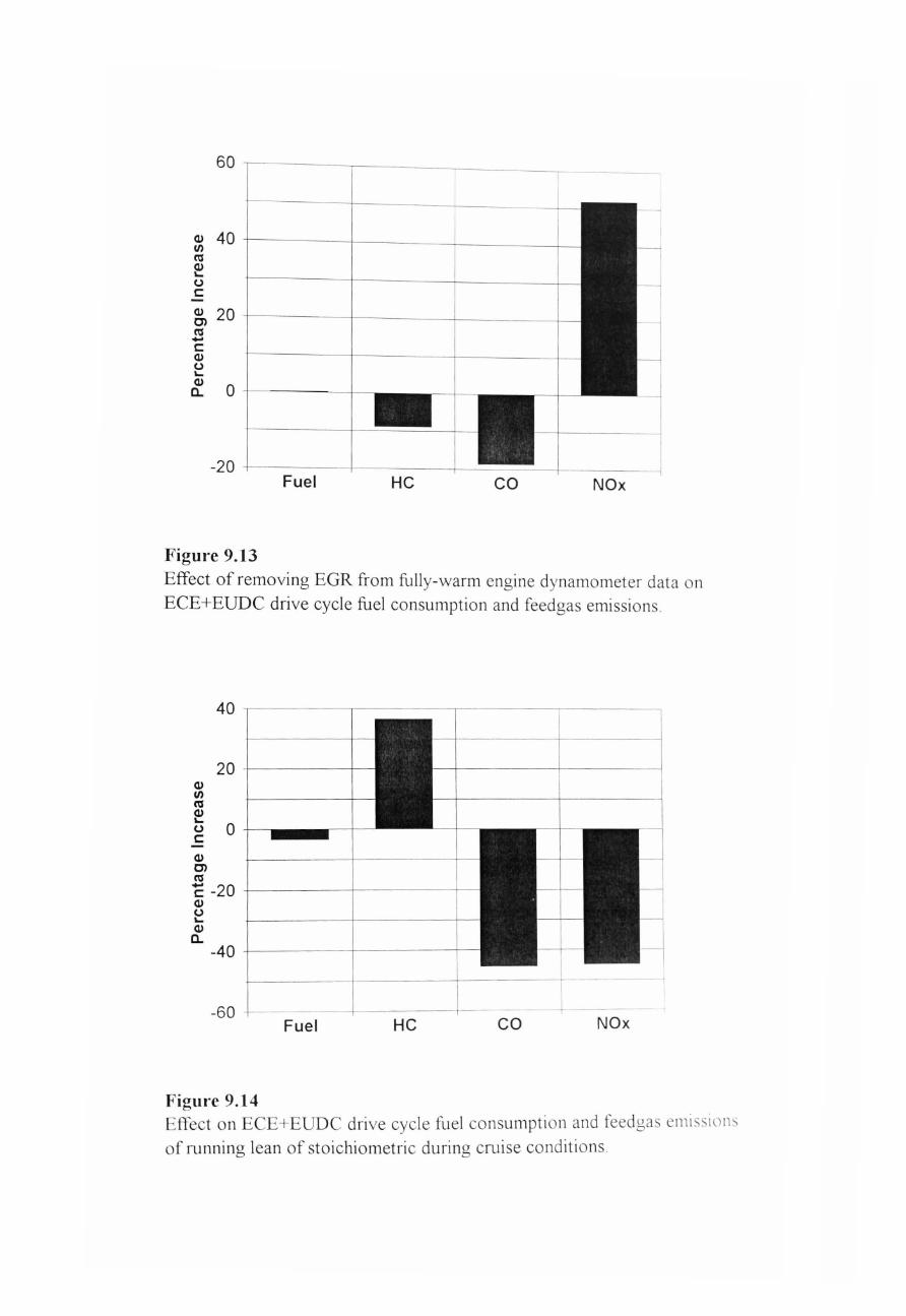
60 ~------~ ______ ~ ________ __

CLI I/)

40 ru CLI L. (,)

s:: CLI 20 01 ru -s:: CLI (,) L. CLI 0 a..

-20 +----~----~~-~~+_-----Fuel HC co NOx

Figure 9.13 Effect of removing EGR from fully -warm engine dynamometer data on

ECE+EUDC drive cycle fuel consumption and feedgas emissions

CLI I/) ru e

40 ~---~----~----,-----,

20 +------~-

g 0 r -------r-CLI 01 ru 1: -20 -1------+------1-

CLI (,) L. CLI a..

-40 -1-----+-----1--

Fuel -60 +------1--------j--- -----+--

HC CO NOx

Figure 9.14 Effect on ECE+EUDC drive cycle fuel consumption and feedgas emi ssio n '

of running lean of stoichiometric during cruise conditions .

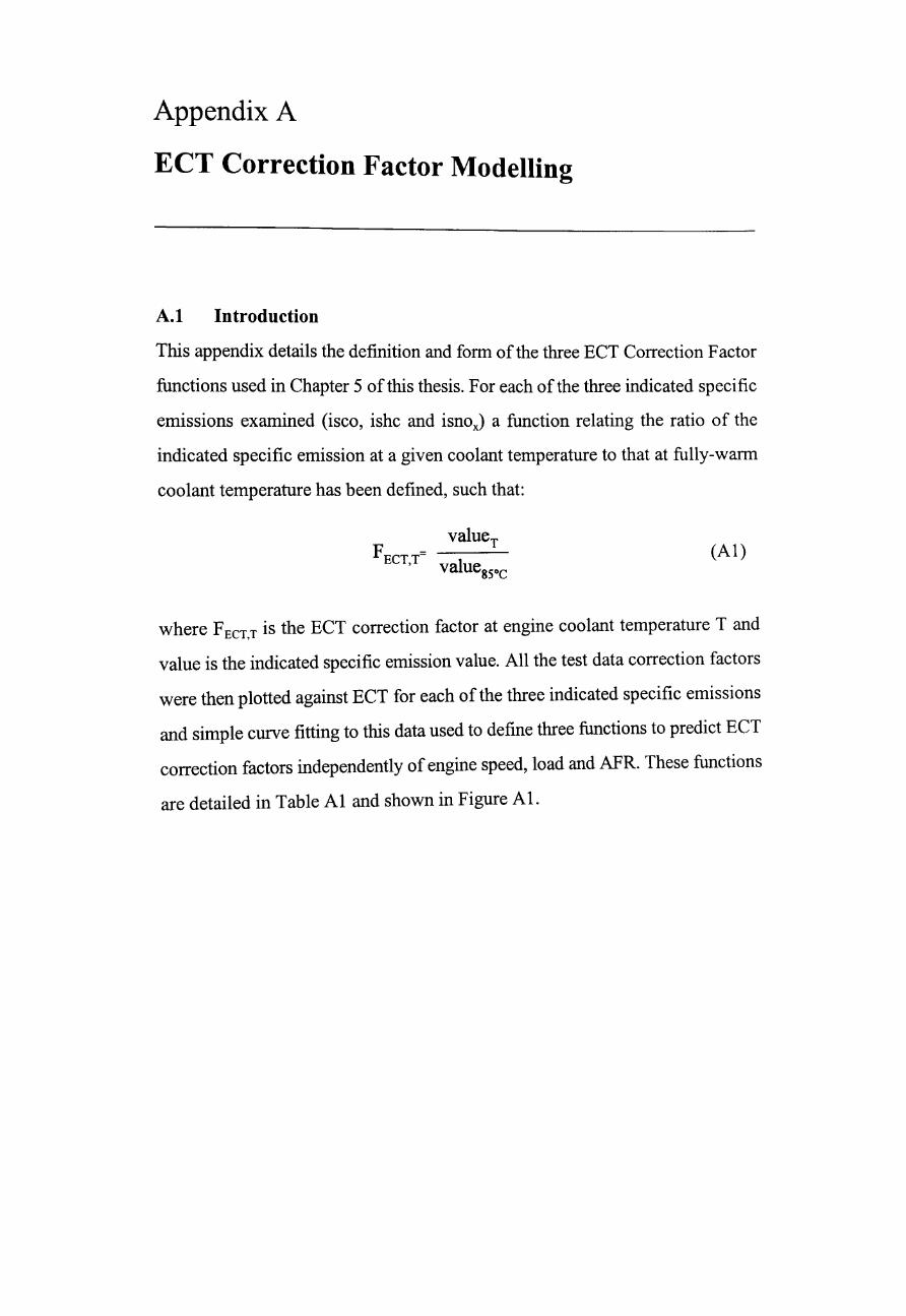
Appendix A

ECT Correction Factor Modelling

A.I Introduction

This appendix details the defInition and form of the three ECT Correction Factor

functions used in Chapter 5 of this thesis. For each of the three indicated specifIc

emissions examined (isco, ishc and isnox) a function relating the ratio of the

indicated specifIc emission at a given coolant temperature to that at fully-warm

coolant temperature has been defIned, such that:

(AI)

where F ECT,T is the ECT correction factor at engine coolant temperature T and

value is the indicated specifIc emission value. All the test data correction factors

were then plotted against ECT for each of the three indicated specifIc emissions

and simple curve fItting to this data used to defIne three functions to predict ECT

correction factors independently of engine speed, load and AFR. These functions

are detailed in Table Al and shown in Figure AI.

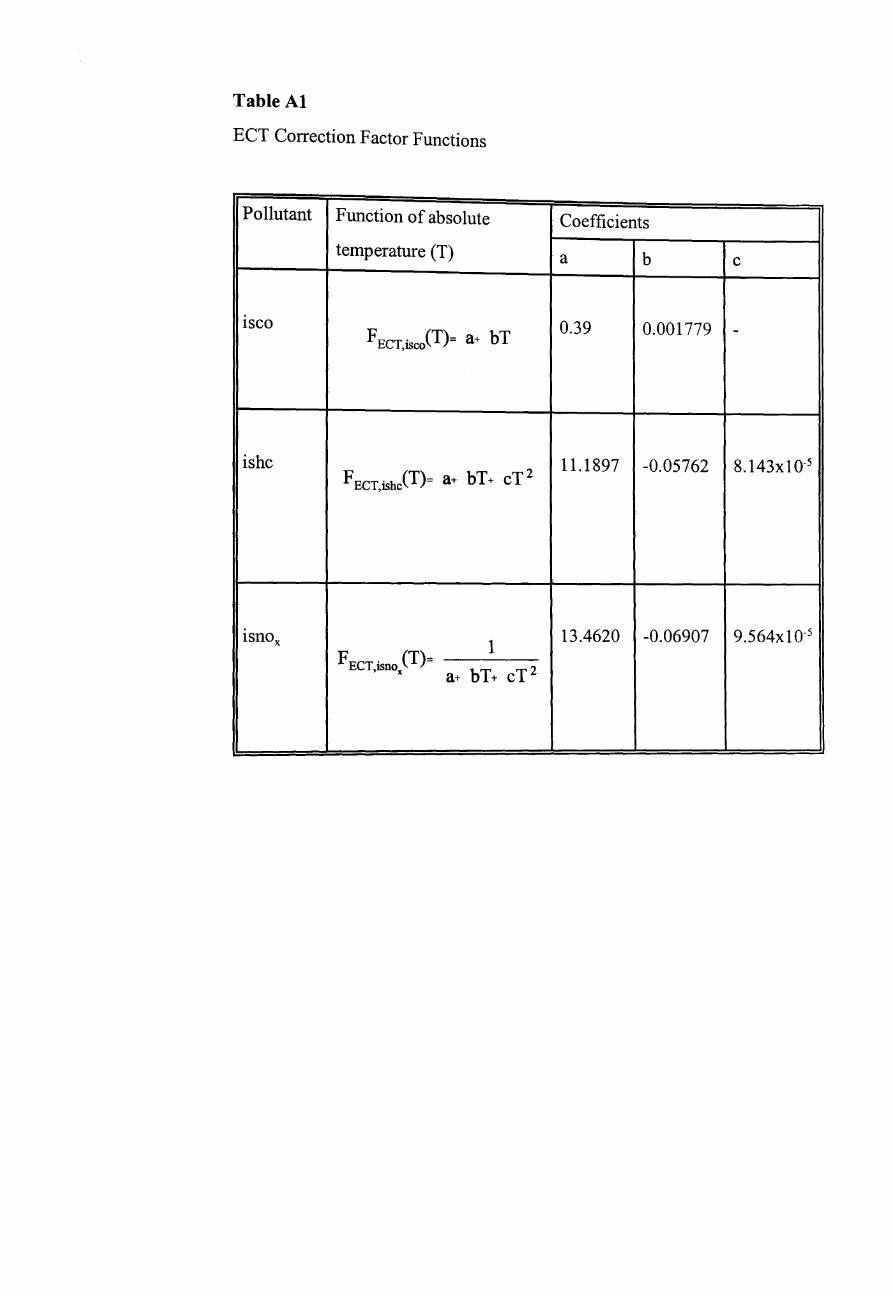
Table At

ECT Correction Factor Functions

Pollutant Function of absolute Coefficients

temperature (T) a b c

ISCO 0.39 0.001779 -FECT,isco(T)= a+ bT

ishc 11.1897 -0.05762 8.143x10-5 F ECT,ishcCT)= a+ bT + cT 2

13.4620 -0.06907 9.564x10-5 Isnox 1 F ECT isno (T)=

a+ bT+ cT2 ' x

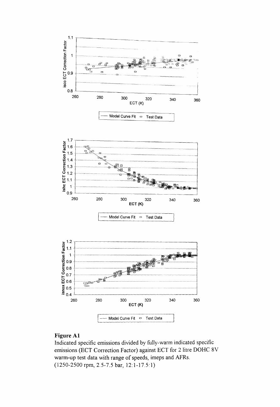
o 1.1 ·I---------------~. -0 ro u. c o t5 ~ o ()

-.. -... --O·--D----g~--~ __ D

t) 0.9 ............... c:J. D -...... ~ .. -

W o o

.!Q

D

D

. -- ----.... -~. __ ....... _-_ .... -... _ .. -

0.8 .~--____________ ~

260 280 300 320 ECT (K)

340 360

1- Model Curve Fit D Test Data

o 1.7·r-----------------------______________ ~ u 1.6· ....... Q .......................................... . IU .•..........•.....•••.•••......................................... U. D c 1.5 ........... 0 ....... .... Q .... . ---...... -----._------_ .... ---------------_._-- .. ---- ------------_ ... . 2 D U 1.4" ...................... ' .. " .......................................................................... . Qj 0 0

t: 1.3 . ····························· .... ·0 .. · c:JJl... .... ~.............. . ..................... . o § ...................... .

~ 1.2 ... ·· .. ·· .. · .. ······················ .. ······ .. ·0 .... · ... !S' .. ~;;;;; ....................................................... . hl1.1 .................................................... c:J.~c. .. g .. .

,g 1· ............................ . VI .- 0.9 .L-...------___________ -.-J

260 280 300 320 340 360 ECT (K)

1- Model Curve Fit 0 Test Data

~1.2·r_----------------------------------------~ .s ~ 1.1 ................................................................................................................................ ..

u..

~ 0.: : :.:::::::.':::::::::::::::::::"::::::::::::::::::::::::::::::::::::::::: ... :.: ......... ~.~~ ............................ . Qj 0 ~ ~ 0.8' .............................................................. 'l2l .... IIJl ......................................... .. u =~ D I- 0.7 ......................................... E!i=J.. .. .. -'91. ................................ ..

U W 0.6 · ...... · .. 0 .. · .... >< DO g 0.5' .................................................................... .. . !!! 0.4 .L..-________________________________________ ---l

260 280 300 320 340 360 ECT (K)

1- Model Curve Fit D Test Data

Figure Al Indicated specific emissions divided by fully-warm indicated specific emissions (ECT Correction Factor) against ECT for 2 litre DOHC 8V warm-up test data with range of speeds, imeps and AFRs. (1250-2500 rpm, 2.5-7.5 bar, 12:1-17.5:1)

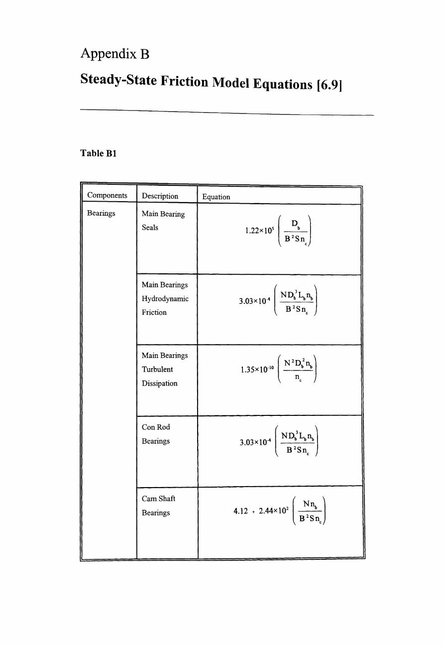
Appendix B

Steady-State Friction Model Equations [6.9]

Table Bl

Components Description Equation

Bearings Main Bearing

1.22x10' ( Db ) Seals

B 2 Sn e

Main Bearings

(ND'L ) Hydrodynamic 3.03xlO-4 b b~ B 2 Sn Friction e

Main Bearings

(N'D' ) Turbulent 1.35xlO-1o ncb ~ Dissipation

Con Rod ( , ) NDb Lb~ Bearings 3.03xlO-4

B 2 Sn e

Cam Shaft

4.12 • 2.44x10' ( ~n,. ) Bearings B Sne

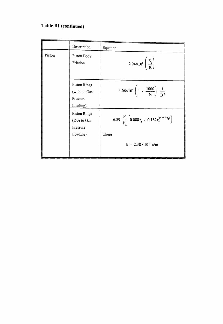
Table Bl (continued)

Description Equation

Piston Piston Body

2.94xl~ ( ;) Friction

Piston Rings

4.06x104 ( 1 • l~OO) 1

(without Gas -B2

Pressure

Loading)

Piston Rings P. [ (1.33 - kS,> ]

(Due to Gas 6.89 'f O.088rc + O. 182rc

a Pressure

Loading) where

k = 2.38 X 10-2 slm

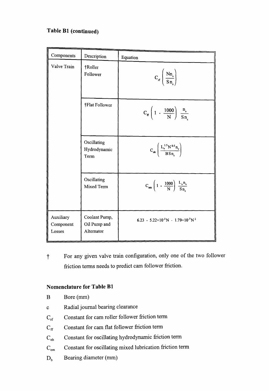
Table B1 (continued)

Components Description Equation

Valve Train tRoller

Follower Cn ( ~::)

tFlat Follower

C. ( 1 • l~O) n v -Sn c

Oscillating [ L "No, 1 Hydrodynamic C v I\,

Term 011 BSn

c

Oscillating

Com ( 1 + l~O) LvI\, Mixed Term -

Snc

Auxiliary Coolant Pump, 6.23 + S.22xlO-3 N - 1.79xlO-7 N 2

Component Oil Pump and

Losses Alternator

t For any given valve train configuration, only one of the two follower

friction terms needs to predict cam follower friction.

Nomenclature for Table B1

B Bore (mm)

c Radial journal bearing clearance

Crf Constant for cam roller follower friction term

CfT Constant for cam flat follower friction term

Coh Constant for oscillating hydrodynamic friction term

Com Constant for oscillating mixed lubrication friction term

Db Bearing diameter (mm)

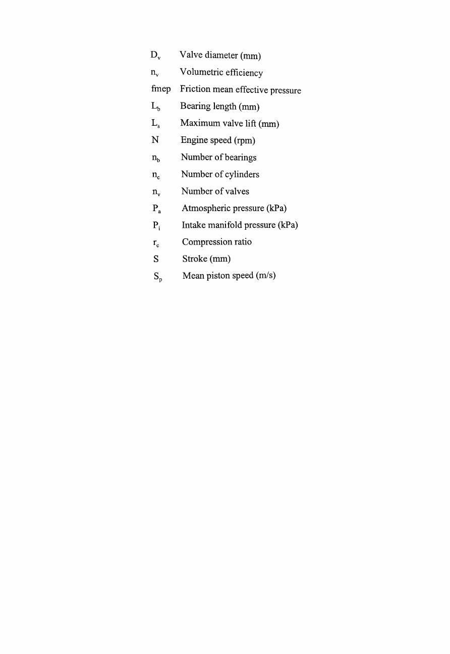
Dv Valve diameter (mm)

l1y Volumetric efficiency

fmep Friction mean effective pressure

~ Bearing length (mm)

Ls Maximum valve lift (mm)

N Engine speed (rpm)

nb Number of bearings

ne Number of cylinders

l1y Number of valves

Pa Atmospheric pressure (kPa)

Pi Intake manifold pressure (kPa)

re Compression ratio

S Stroke (mm)

Sp Mean piston speed (m/s)