Embed Size (px)
Citation preview
Fundamentals of Neural Networks
Fundamentals of Neural Networks
Soft Computing
Neural network, topics : Introduction, biological neuron model, artificial
neuron model, neuron equation. Artificial neuron : basic elements,
activation and threshold function, piecewise linear and sigmoidal
function. Neural network architectures : single layer feed- forward
network, multi layer feed-forward network, recurrent networks. Learning
methods in neural networks : unsupervised Learning - Hebbian learning,
competitive learning; Supervised learning - stochastic learning, gradient
descent learning; Reinforced learning. Taxonomy of neural network
systems : popular neural network systems, classification of neural
network systems as per learning methods and architecture. Single-layer
NN system : single layer perceptron, learning algorithm for training
perceptron, linearly separable task, XOR problem, ADAptive LINear
Element (ADALINE) - architecture, and training. Applications of neural
networks: clustering, classification, pattern recognition, function
approximation, prediction systems.

Fundamentals of Neural Networks
Soft Computing
Topics
1. Introduction
Why neural network ?, Research History, Biological Neuron model, Artificial
Neuron model, Notations, Neuron equation.
2. Model of Artificial Neuron
Artificial neuron - basic elements, Activation functions – Threshold function,
Piecewise linear function, Sigmoidal function, Example.
3. Neural Network Architectures
Single layer Feed-forward network, Multi layer Feed-forward network, Recurrent
networks.
4. Learning Methods in Neural Networks
Learning algorithms: Unsupervised Learning - Hebbian Learning, Competitive
learning; Supervised Learning : Stochastic learning, Grant descent learning;
Reinforced Learning;
24-29
5. Taxonomy Of Neural Network Systems
Popular neural network systems; Classification of neural network
systems with respect to learning methods and architecture types.
6. Single-Layer NN System
Single layer perceptron : Learning algorithm for training Perceptron, Linearly
separable task, XOR Problem; ADAptive LINear Element (ADALINE) :
Architecture, Training.

SC - Neural Network – Introduction
.
What is Neural Net ?
• A neural net is an artificial representation of the human brain that tries to
simulate its learning process. An artificial neural network
(ANN) is often called a "Neural Network" or simply Neural Net (NN).
• Traditionally, the word neural network is referred to a network of biological neurons
in the nervous system that process and transmit information.
• Artificial neural network is an interconnected group of artificial neurons
that uses a mathematical model or computational model for information processing
based on a connectionist approach to computation.
• The artificial neural networks are made of interconnecting artificial
neurons which may share some properties of biological neural networks.
• Artificial Neural network is a network of simple processing elements
(neurons) which can exhibit complex global behavior, determined by the
connections between the processing elements and element parameters.
1. Introduction
Neural Computers mimic certain processing capabilities of the human brain.
- Neural Computing is an information processing paradigm, inspired by biological
system, composed of a large number of highly interconnected processing elements
(neurons) working in unison to solve specific problems.
- Artificial Neural Networks (ANNs), like people, learn by example.
- An ANN is configured for a specific application, such as pattern recognition or data
classification, through a learning process.
- Learning in biological systems involves adjustments to the synaptic connections that
exist between the neurons. This is true of ANNs as well.

SC - Neural Network – Introduction
Why Neural Network
Neural Networks follow a different paradigm for computing.
■ The conventional computers are good for - fast arithmetic and does what
programmer programs, ask them to do.
■ The conventional computers are not so good for - interacting with noisy data or
data from the environment, massive parallelism, fault tolerance, and adapting to
circumstances.
■ The neural network systems help where we can not formulate an algorithmic
solution or where we can get lots of examples of the behavior we require.
■ Neural Networks follow different paradigm for computing.
The von Neumann machines are based on the processing/memory abstraction of
human information processing.
The neural networks are based on the parallel architecture of
biological brains.
■ Neural networks are a form of multiprocessor computer system, with
- simple processing elements ,
- a high degree of interconnection,
- simple scalar messages, and
- adaptive interaction between elements.
Research History
The history is relevant because for nearly two decades the future of Neural network
remained uncertain.
McCulloch and Pitts (1943) are generally recognized as the designers of the first neural
network. They combined many simple processing units together that could lead to an
overall increase in computational power. They suggested many ideas like : a neuron
has a threshold level and once that level is reached the neuron fires. It is still the
fundamental way in which ANNs operate. The McCulloch and Pitts's network had a
fixed set of weights.
Hebb (1949) developed the first learning rule, that is if two neurons are active at the
same time then the strength between them should be increased.

SC - Neural Network – Introduction
In the 1950 and 60's, many researchers (Block, Minsky, Papert, and Rosenblatt
worked on perceptron. The neural network model could be proved to converge to the
correct weights, that will solve the problem. The weight adjustment (learning
algorithm) used in the perceptron was found more powerful than the learning rules
used by Hebb. The perceptron caused great excitement. It was thought to produce
programs that could think.
Minsky & Papert (1969) showed that perceptron could not learn those functions
which are not linearly separable.
The neural networks research declined throughout the 1970 and until mid 80's
because the perceptron could not learn certain important functions.
Neural network regained importance in 1985-86. The researchers, Parker and LeCun
discovered a learning algorithm for multi-layer networks called back propagation that
could solve problems that were not linearly separable.
Biological Neuron Model
The human brain consists of a large number, more than a billion of neural cells that
process information. Each cell works like a simple processor. The massive interaction
between all cells and their parallel processing only makes the brain's abilities possible.
Dendrites are branching fibers that
extend from the cell body or soma.
Soma or cell body of a neuron contains
the nucleus and other structures, support
chemical processing and production of
neurotransmitters.
Axon is a singular fiber carries
information away from the soma to the
synaptic sites of other neurons (dendrites
and somas), muscles, or glands.
Axon hillock is the site of summation
for incoming information. At any
moment, the collective influence of all
neurons that conduct impulses to a given
neuron will determine whether or not an

SC - Neural Network – Introduction
Fig. Structure of Neuron
axon hillock and propagated along the axon.
action potential will be initiated at the
Myelin Sheath consists of fat-containing cells that insulate the axon from electrical
activity. This insulation acts to increase the rate of transmission of signals. A gap
exists between each myelin sheath cell along the axon. Since fat inhibits the
propagation of electricity, the signals jump from one gap to the next.
Nodes of Ranvier are the gaps (about 1 m) between myelin sheath cells long axons
are Since fat serves as a good insulator, the myelin sheaths speed the rate of
transmission of an electrical impulse along the axon.
Synapse is the point of connection between two neurons or a neuron and a muscle or
a gland. Electrochemical communication between neurons takes place at these
junctions.
Terminal Buttons of a neuron are the small knobs at the end of an axon that release
chemicals called neurotransmitters.
SC - Neural Network – Introduction
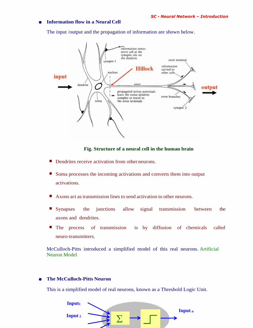
• Information flow in a Neural Cell
The input /output and the propagation of information are shown below.
Fig. Structure of a neural cell in the human brain
■ Dendrites receive activation from other neurons.
■ Soma processes the incoming activations and converts them into output
activations.
■ Axons act as transmission lines to send activation to other neurons.
■ Synapses the junctions allow signal transmission between the
axons and dendrites.
■ The process of transmission is by diffusion of chemicals called
neuro-transmitters.
McCulloch-Pitts introduced a simplified model of this real neurons. Artificial
Neuron Model
• The McCulloch-Pitts Neuron
This is a simplified model of real neurons, known as a Threshold Logic Unit.
Input1
Input 2
Input n

SC - Neural Network – Introduction
O
u
t
p
u
t

SC - Neural Network – Introduction
■ A set of input connections brings in activations from other neurons.
■ A processing unit sums the inputs, and then applies a non-linear activation
function (i.e. squashing / transfer / threshold function).
■ An output line transmits the result to other neurons.
In other words ,
- The input to a neuron arrives in the form of signals.
- The signals build up in the cell.
- Finally the cell discharges (cell fires) through the output .
- The cell can start building up signals again.
Notations
Recaps : Scalar, Vectors, Matrices and Functions
Scalar : The number xi can be added up to give a scalar number. n
s = x1 + x2 + x3 + . . . . + xn = xi i=1
Vectors : An ordered sets of related numbers. Row Vectors (1 x n)
X = ( x1 , x2 , x3 , . . ., xn ) , Y = ( y1 , y2 , y3 , . . ., yn )
Add : Two vectors of same length added to give another vector.
Z = X + Y = (x1 + y1 , x2 + y2 , ....................... , xn + yn)
Multiply: Two vectors of same length multiplied to give a scalar.
n
p = X . Y = x1 y1 + x2 y2 + . . . . + xnyn =
i=1
xi yi

SC - Neural Network – Introduction
Matrices : m x n matrix , row no = m , column no = n
w11 w11 . . . . w1n
w21 w21 . . . . w21
W = . . . . . . .
. . . . . . .
wm1 w11 .......................... wmn
Add or Subtract : Matrices of the same size are added or subtracted
component by component. A + B = C , cij = aij + bij
a11 a12 b11 b12 c11 = a11+b11 c12 = a12+b12
a21 a22 +
b21 b22 =
C21 = a21+b21 C22 = a22 +b22
Multiply : matrix A multiplied by matrix B gives matrix C.
(m x n) (n x p) (m x p)
n elements cij =
k=1 aik bkj
a11 a12 b11 b12 c11 c12
a21 a22 x
b21 b22 = c21 c22

SC - Neural Network – Introduction
c11 = (a11 x b11) + (a12 x B21) c12 =
(a11 x b12) + (a12 x B22) C21 = (a21 x
b11) + (a22 x B21) C22 = (a21 x b12) + (a22 x
B22)
Functions
The Function y= f(x) describes a relationship, an input-output mapping,
from x to y.
■ Threshold or Sign function : sgn(x) defined as
sgn (x) =
1 if x 0
0 if x 0
Sign(x)
1
.8
.6
.4
.2
0
-4 -3 -2 -1 0 1 2 3 4 I/P
■ Threshold or Sign function : sigmoid(x) defined as a smoothed
(differentiable) form of the threshold function
sigmoid (x) =
1
1 + e -x
Sign(x)
1
.8
.6
.2
0
O/P
O/P

SC - Neural Network –Artificial Neuron Model
-4 -3 -2 -1 0 1 2 3 4 I/P
2. Model of Artificial Neuron
A very simplified model of real neurons is known as a Threshold Logic Unit
(TLU). The model is said to have :
- A set of synapses (connections) brings in activations from other neurons.
- A processing unit sums the inputs, and then applies a non-linear activation function (i.e.
squashing / transfer / threshold function).
- An output line transmits the result to other neurons.
McCulloch-Pitts (M-P) Neuron Equation
McCulloch-Pitts neuron is a simplified model of real biological neuron.
Input 1
Input 2
Input n
Simplified Model of Real Neuron
(Threshold Logic Unit)
Output
The equation for the output of a McCulloch-Pitts neuron as a function of 1 to n
inputs is written as
n
Output = sgn ( i=1
Input i - )
where is the neuron’s activation threshold. n
If i=1 n
If i=1
Input i then Output = 1
Input i then Output = 0
In this McCulloch-Pitts neuron model, the missing features are :
- Non-binary input and output,
- Non-linear summation,
- Smooth thresholding,
- Stochastic, and
- Temporal information processing.

SC - Neural Network –Artificial Neuron Model
Artificial Neuron - Basic Elements
Neuron consists of three basic components - weights, thresholds, and a single activation
function.
x1
x2
y
xn
Fig Basic Elements of an Artificial Linear Neuron
■ Weighting Factors w
The values w1 , w2 , . . . wn are weights to determine the strength of input vector
X = [x1 , x2 , . . . , xn]T. Each input is multiplied by the associated weight of the
neuron connection XT W. The +ve weight
excites and the -ve weight inhibits the node output.
I = XT.W = x1 w1 + x2 w2 + . . . . + xnwn =
n
i=1 xi wi
■ Threshold
The node’s internal threshold is the magnitude offset. It affects the activation of
the node output y as: n
Y = f (I) = f { i=1
xi wi - k }
W1 Activation Function
W2
i=1
Wn
Synaptic Weights
Threshold

SC - Neural Network –Artificial Neuron Model
To generate the final output Y , the sum is passed on to a non-linear filter f called
Activation Function or Transfer function or Squash function which releases the
output Y.
■ Threshold for a Neuron
In practice, neurons generally do not fire (produce an output) unless their total
input goes above a threshold value.
The total input for each neuron is the sum of the weighted inputs to the neuron
minus its threshold value. This is then passed through the sigmoid function. The
equation for the transition in a neuron is :
a = 1/(1 + exp(- x)) where
x = i
ai wi - Q
a is the activation for the neuron ai is
the activation for neuron i wi is the
weight
Q is the threshold subtracted
■ Activation Function
An activation function f performs a mathematical operation on the signal output.
The most common activation functions are:
- Linear Function,
- Piecewise Linear Function,
- Tangent hyperbolic function
- Threshold Function,
- Sigmoidal (S shaped) function,
The activation functions are chosen depending upon the type of problem to be
solved by the network.

SC - Neural Network –Artificial Neuron Model
Activation Functions f - Types
Over the years, researches tried several functions to convert the input into an outputs.
The most commonly used functions are described below.
- I/P Horizontal axis shows sum of inputs .
- O/P Vertical axis shows the value the function produces ie output.
- All functions f are designed to produce values between 0 and 1.
• Threshold Function
A threshold (hard-limiter) activation function is either a binary type or a
bipolar type as shown below.
binary threshold
O/p
I/P
Output of a binary threshold function produces :
1 if the weighted sum of the inputs is +ve,
0 if the weighted sum of the inputs is -ve.
1 if I 0
Y = f (I) =
0 if I 0
bipolar threshold
O/p
I/P
Output of a bipolar threshold function produces :
1 if the weighted sum of the inputs is +ve,
-1 if the weighted sum of the inputs is -ve.
1 if I 0
Y = f (I) = -1
1
1

SC - Neural Network –Artificial Neuron Model
Neuron with hard limiter activation function is called McCulloch-Pitts model.
• Piecewise Linear Function
This activation function is also called saturating linear function and can have either a
binary or bipolar range for the saturation limits of the output. The mathematical model
for a symmetric saturation function is described below.
Piecewise Linear
O/p
I/P
This is a sloping function that produces :
-1 for a -ve weighted sum of inputs,
1 for a +ve weighted sum of inputs.
I proportional to input for values between +1
and -1 weighted sum,
1 if I 0
Y = f (I) = I if -1 I 1
-1 if I 0
+1
-1

SC - Neural Network –Artificial Neuron Model
• Sigmoidal Function (S-shape function)
The nonlinear curved S-shape function is called the sigmoid function. This is most
common type of activation used to construct the neural networks. It is mathematically
well behaved, differentiable and strictly increasing function.
Sigmoidal function A sigmoidal transfer function can be
written in the form:
1
Y = f (I) =
1 + e
-
I
, 0 f(I) 1
The sigmoidal
function is
= 1/(1 + exp(- I)) , 0 f(I) 1
This is explained as
0 for large -ve input values,
1 for large +ve values, with
a smooth transition between the two.
is slope parameter also called shape
parameter; symbol the is also used to
represented this parameter.
achieved using exponential equation.
1 O/P
= 2.0
0.5
-4 -2 0 1 2
I/P
= 1.0
= 0.5

SC - Neural Network –Artificial Neuron Model
By varying different shapes of the function can be obtained which adjusts the
abruptness of the function as it changes between the two asymptotic values.
• Example :
The neuron shown consists of four inputs with the weights.
x1=1
x2=2
X3=5
xn=8
+1
+1
-1
+2
Synaptic
Weights
I
Summing
Junction
Activation
Function
y
= 0
Threshold
Fig Neuron Structure of Example
The output I of the network, prior to the activation function stage, is
+1
+1 I = XT. W = 1 2 5 8 = 14
-1
+2
= (1 x 1) + (2 x 1) + (5 x -1) + (8 x 2) = 14
With a binary activation function the outputs of the neuron is:
y (threshold) = 1;

SC - Neural Network – Architecture
3. Neural Network Architectures
An Artificial Neural Network (ANN) is a data processing system, consisting large number
of simple highly interconnected processing elements as artificial neuron in a network
structure that can be represented using a directed graph G, an ordered 2-tuple (V, E) ,
consisting a set V of vertices and a set E of edges.
- The vertices may represent neurons (input/output) and
- The edges may represent synaptic links labeled by the weights attached. Example :
Fig. Directed Graph
Vertices V = { v1 , v2 , v3 , v4, v5 } Edges
E = { e1 , e2 , e3 , e4, e5 }
Single Layer Feed-forward Network
The Single Layer Feed-forward Network consists of a single layer of weights , where
the inputs are directly connected to the outputs, via a series of weights. The synaptic
links carrying weights connect every input to every output , but not other way. This
way it is considered a network of feed-forward type. The sum of the products of the
weights and the inputs is calculated in each neuron node, and if the value is above
some threshold (typically 0) the neuron fires and takes the activated value (typically
1); otherwise it takes the deactivated value (typically -1).
V1 e5
V3
V5
e2 e4
e5
V2 e3
V4

SC - Neural Network – Architecture
w11
w12 w21
w22
w2m
wn1 w1m
wn2
wnm
input xi weights wij
x1
x2
output yj
y1
y2
xn ym
Single layer Neurons
Fig. Single Layer Feed-forward Network

SC - Neural Network – Architecture
x 1
Input
hidden layer
weights vij
v11
Output
hidden layer
weights wjk w11
y 1
v21 y1
x2 v1m
w12
w11
y2
v2m y3
vn1 w1m
Vℓm ym
xℓ
Input Layer
neurons xi
Hidden Layer
neurons yj y n
Output Layer
neurons zk
Multi Layer Feed-forward Network
The name suggests, it consists of multiple layers. The architecture of this class of
network, besides having the input and the output layers, also have one or more
intermediary layers called hidden layers. The computational units of the hidden layer
are known as hidden neurons.
Fig. Multilayer feed-forward network in (ℓ – m – n) configuration.
- The hidden layer does intermediate computation before directing the input to
output layer.
- The input layer neurons are linked to the hidden layer neurons; the weights on
these links are referred to as input-hidden layer weights.
- The hidden layer neurons and the corresponding weights are referred to as output-
hidden layer weights.
- A multi-layer feed-forward network with ℓ input neurons, m1 neurons in the first
hidden layers, m2 neurons in the second hidden layers, and n output neurons in the
output layers is written as (ℓ - m1 - m2 – n ).
The Fig. above illustrates a multilayer feed-forward network with a configuration (ℓ -
m – n).

SC - Neural Network –Learning methods
Recurrent Networks
The Recurrent Networks differ from feed-forward architecture. A Recurrent network
has at least one feed back loop.
Example :
Feedback
links
Fig Recurrent Neural Network
There could be neurons with self-feedback links; that is the output of a
neuron is fed back into it self as input.
4. Learning Methods in Neural Networks
The learning methods in neural networks are classified into three basic types :
- Supervised Learning,
- Unsupervised Learning and
- Reinforced Learning
These three types are classified based on :
- presence or absence of teacher and
- the information provided for the system to learn.
These are further categorized, based on the rules used, as
- Hebbian,
y1
x1
y1 y2
x2
ym Yn
Xℓ
Input Layer
neurons xi
Hidden Layer
neurons yj Output Layer
neurons zk

SC - Neural Network –Learning methods
- Gradient descent,
- Competitive and
- Stochastic learning.

SC - Neural Network –Learning methods
Error Correction
Gradient descent
Supervised Learning
(Error based)
Stochastic
Reinforced Learning
(Output based)
Unsupervised Learning
Competitive Hebbian
• Classification of Learning Algorithms
Fig. below indicate the hierarchical representation of the algorithms mentioned in the
previous slide. These algorithms are explained in subsequent slides.
Fig. Classification of learning algorithms
• Supervised Learning
- A teacher is present during learning process and presents expected output.
- Every input pattern is used to train the network.
- Learning process is based on comparison, between network's computed output and
the correct expected output, generating "error".
- The "error" generated is used to change network parameters that result improved
performance.
• Unsupervised Learning
- No teacher is present.
- The expected or desired output is not presented to the network.
- The system learns of it own by discovering and adapting to the structural features in
the input patterns.
• Reinforced learning
- A teacher is present but does not present the expected or desired output but only
indicated if the computed output is correct or incorrect.
- The information provided helps the network in its learning process.
- A reward is given for correct answer computed and a penalty for a wrong answer.
Neural Network
Learning algorithms
Back
Propagation
Least Mean Square

SC - Neural Network –Learning methods
Note : The Supervised and Unsupervised learning methods are most popular forms of
learning compared to Reinforced learning.
• Hebbian Learning
Hebb proposed a rule based on correlative weight adjustment.
In this rule, the input-output pattern pairs (Xi , Yi) are associated by
the weight matrix W, known as correlation matrix computed as
n W =
i=1
Xi YiT

SC - Neural Network –Systems
where YiT is the transpose of the associated output vector Yi
There are many variations of this rule proposed by the other
researchers (Kosko, Anderson, Lippman) .
• Gradient descent Learning
This is based on the minimization of errors E defined in terms of weights and the
activation function of the network.
- Here, the activation function of the network is required to be differentiable,
because the updates of weight is dependent on the gradient of the error E.
- If Wij is the weight update of the link connecting the i th and the j th
neuron of the two neighboring layers, then Wij is defined as
Wij = ( E / Wij )
where is the learning rate parameters and ( E / Wij ) is error gradient
with reference to the weight Wij .
Note : The Hoffs Delta rule and Back-propagation learning rule are the examples
of Gradient descent learning.
• Competitive Learning
- In this method, those neurons which respond strongly to the input stimuli have
their weights updated.
- When an input pattern is presented, all neurons in the layer compete, and the
winning neuron undergoes weight adjustment .
- This strategy is called "winner-takes-all".
• Stochastic Learning
- In this method the weights are adjusted in a probabilistic fashion.
- Example : Simulated annealing which is a learning mechanism
employed by Boltzmann and Cauchy machines.
5. Taxonomy Of Neural Network Systems
In the previous sections, the Neural Network Architectures and the Learning methods

SC - Neural Network –Systems
have been discussed. Here the popular neural network systems are listed. The grouping of
these systems in terms of architectures and the learning methods are presented in the next
slide.
• Neural Network Systems
– ADALINE (Adaptive Linear Neural Element)
– ART (Adaptive Resonance Theory)
– AM (Associative Memory)
– BAM (Bidirectional Associative Memory)
– Boltzmann machines
– BSB ( Brain-State-in-a-Box)
– Cauchy machines
– Hopfield Network
– LVQ (Learning Vector Quantization)
– Neoconition
– Perceptron
– RBF ( Radial Basis Function)
– RNN (Recurrent Neural Network)
– SOFM (Self-organizing Feature Map)
• Classification of Neural Network
A taxonomy of neural network systems based on Architectural types
and the Learning methods is illustrated below.
Learning Methods
Gradient
descent
Hebbian Competitive Stochastic
Single-layer
feed-forward
ADALINE,
Hopfield,
Percepton,
AM, Hopfield,
LVQ,
SOFM
-

SC - Neural Network –Systems
Multi-layer
feed- forward
CC
M,
MLF
F,
RBF
Neocognition
Recurrent
Networks
RNN BAM
,
BSB, Hopfield,
ART Boltzmann and
Cauchy
machines
Table : Classification of Neural Network Systems with respect to learning
methods and Architecture types

SC - Neural Network –Single Layer learning
w11
w12 w21
w22
w2m
wn1 w1m
wn2
wnm
6. Single-Layer NN Systems
Here, a simple Perceptron Model and an ADALINE Network Model is presented.
Single layer Perceptron
Definition : An arrangement of one input layer of neurons feed forward to one
output layer of neurons is known as Single Layer Perceptron.
input xi weights wij
x1
x2
output yj
y1
y2
xn ym
Single layer
Perceptron
Fig. Simple Perceptron Model
1 if net j 0
y j = f (net j) = where net j =
0 if net j 0
n
i=1
xi wij

SC - Neural Network –Single Layer learning
• Learning Algorithm : Training Perceptron
The training of Perceptron is a supervised learning algorithm where weights are
adjusted to minimize error when ever the output does not match the desired
output.
− If the output is correct then no adjustment of weights is done.
i.e. K+1
Wi j
=
K
Wi j
− If the output is 1 but should have been 0 then the weights are decreased
on the active input link
i.e. K+1
Wi j
=
K
Wi j
− . xi
− If the output is 0 but should have been 1 then the weights are increased on
the active input link
i.e.
Where
K+1 W
i j =
K+1
K
Wi j
+ . xi
K
Wi j
is the new adjusted weight, Wi j
is the old weight

SC - Neural Network –Single Layer learning
• (1, 1)
•
S2 S1 S1
S2
• Perceptron and Linearly Separable Task
Perceptron can not handle tasks which are not separable.
- Definition : Sets of points in 2-D space are linearly separable if the sets can be
separated by a straight line.
- Generalizing, a set of points in n-dimensional space are linearly separable if there
is a hyper plane of (n-1) dimensions separates the sets.
Example
(a) Linearly separable patterns (b) Not Linearly separable patterns
Note : Perceptron cannot find weights for classification problems that are not
linearly separable.
• XOR Problem :
Exclusive OR operation
X2
XOR
truth table
Even parity
Odd parity
(0, 1)
(0, 0) X1
(0, 1)
Fig. Output of XOR in
X1 , x2 plane
Input x1 Input x2 Output
0 0 0
1 1 0
0 1 1
1 0 1
SC - Neural Network –Single Layer learning
Even parity is, even number of 1 bits in the input Odd parity
is, odd number of 1 bits in the input
- There is no way to draw a single straight line so that the circles are on one side of
the line and the dots on the other side.
- Perceptron is unable to find a line separating even parity input
patterns from odd parity input patterns.
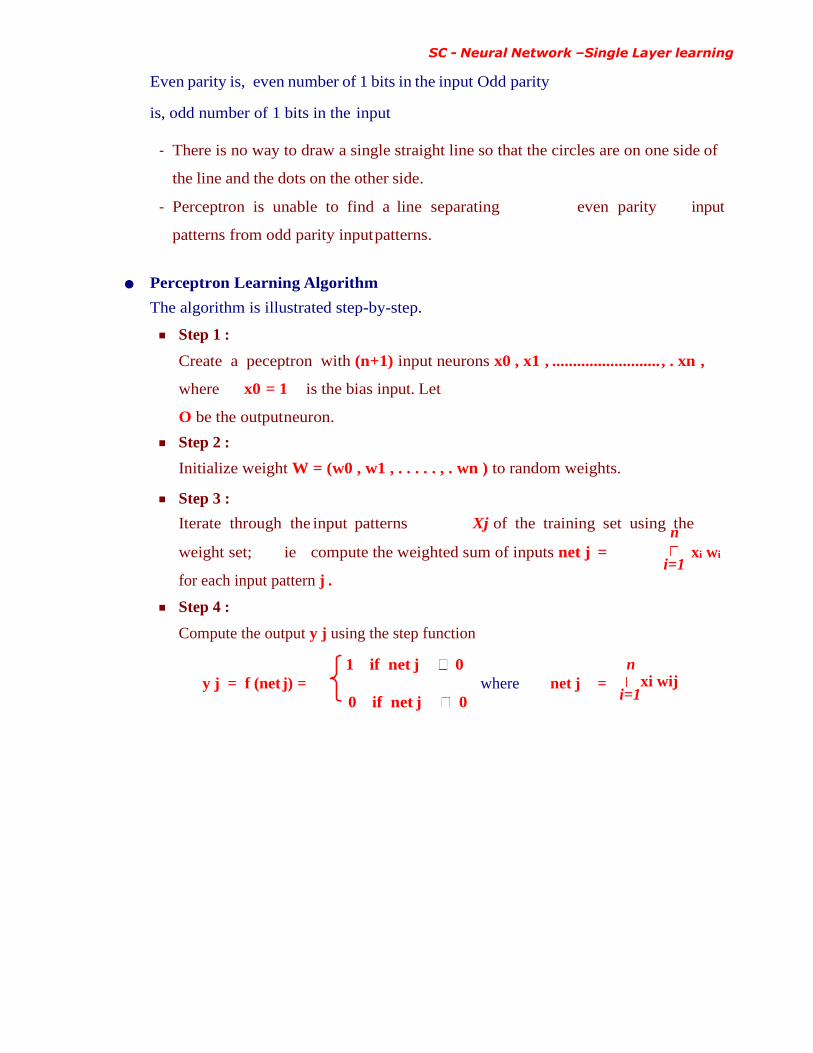
• Perceptron Learning Algorithm
The algorithm is illustrated step-by-step.
■ Step 1 :
Create a peceptron with (n+1) input neurons x0 , x1 , .......................... , . xn ,
where x0 = 1 is the bias input. Let
O be the output neuron.
■ Step 2 :
Initialize weight W = (w0 , w1 , . . . . . , . wn ) to random weights.
■ Step 3 :
Iterate through the input patterns Xj of the training set using the n
weight set; ie compute the weighted sum of inputs net j =
for each input pattern j .
■ Step 4 :
Compute the output y j using the step function
i=1
xi wi
1 if net j 0
y j = f (net j) = where net j =
0 if net j 0
n
xi wij i=1

SC - Neural Network –ADALINE
W1
W2
Neuron
Output
Wn
– Error
+
■ Step 5 :
Compare the computed output yj with the target output yj for
each input pattern j .
If all the input patterns have been classified correctly, then output (read) the
weights and exit.
■ Step 6 :
Otherwise, update the weights as given below :
If the computed outputs yj is 1 but should have been 0,
Then wi = wi - xi , i= 0, 1, 2, ............ , n
If the computed outputs yj is 0 but should have been 1,
Then wi = wi + xi , i= 0, 1, 2, ............. , n
where is the learning parameter and is constant.
■ Step 7 :
goto step 3
■ END
ADAptive LINear Element (ADALINE)
An ADALINE consists of a single neuron of the McCulloch-Pitts type, where its
weights are determined by the normalized least mean square (LMS) training law.
The LMS learning rule is also referred to as delta rule. It is a well-established
supervised training method that has been used over a wide range of diverse
applications.
• Architecture of a simple ADALINE
x1
x2
xn

SC - Neural Network –ADALINE
Desired Output
The basic structure of an ADALINE is similar to a neuron with a linear
activation function and a feedback loop. During the training phase of ADALINE,
the input vector as well as the desired output are presented to the network.
[The complete training mechanism has been explained in the next slide. ]
• ADALINE Training Mechanism
(Ref. Fig. in the previous slide - Architecture of a simple ADALINE)
■ The basic structure of an ADALINE is similar to a linear neuron
with an extra feedback loop.
■ During the training phase of ADALINE, the input vector
X = [x1 , x2 , . . . , xn]T as well as desired output are presented to the
network.
■ The weights are adaptively adjusted based on delta rule.
■ After the ADALINE is trained, an input vector presented to the network with
fixed weights will result in a scalar output.
■ Thus, the network performs an n dimensional mapping to a scalar value.
■ The activation function is not used during the training phase. Once the
weights are properly adjusted, the response of the trained unit can be tested by
applying various inputs, which are not in the training set. If the network
produces consistent responses to a high degree with the test inputs, it is
said that the network could generalize. The process of training and
generalization are two important attributes of this network.
Usage of ADLINE :
In practice, an ADALINE is used to
- Make binary decisions; the output is sent through a binary threshold.
- Realizations of logic gates such as AND, NOT and OR .
- Realize only those logic functions that are linearly separable.
SC - Neural Network –ADALINE
Applications of Neural Network
Neural Network Applications can be grouped in following categories:
■ Clustering:
A clustering algorithm explores the similarity between patterns and places similar
patterns in a cluster. Best known applications include data compression and data
mining.
■ Classification/Pattern recognition:
The task of pattern recognition is to assign an input pattern (like handwritten
symbol) to one of many classes. This category includes algorithmic
implementations such as associative memory.
■ Function approximation :
The tasks of function approximation is to find an estimate of the unknown function
subject to noise. Various engineering and scientific disciplines require function
approximation.
■ Prediction Systems:
The task is to forecast some future values of a time-sequenced data. Prediction
has a significant impact on decision support systems. Prediction differs from function
approximation by considering time factor. System may be dynamic and may produce
different results for the same input data based on system state (time).
Back Propagation Network
Soft Computing
Back-Propagation Network, topics : Background, what is back-prop
network ? learning AND function, simple learning machines - Error
measure , Perceptron learning rule, Hidden Layer, XOR problem. Back-
Propagation Learning : learning by example, multi-layer feed-forward
back-propagation network, computation in input, hidden and output
layers, error calculation. Back-propagation algorithm for training
network - basic loop structure, step-by-step procedure, numerical
example.

SC - Neural Network –ADALINE
1. Back-Propagation Learning - learning by example
Multi-layer Feed-forward Back-propagation network; Computation of Input, Hidden and
Output layers ; Calculation of Error.
2. Back-Propagation Algorithm
Algorithm for training Network - Basic loop structure, Step-by-step procedure; Example:
Training Back-prop network, Numerical example.
Back-Propagation Network
What is BPN ?
• A single-layer neural network has many restrictions. This network can
accomplish very limited classes of tasks.
Minsky and Papert (1969) showed that a two layer feed-forward network can
overcome many restrictions, but they did not present a solution to the problem
as "how to adjust the weights from input to hidden layer" ?
• An answer to this question was presented by Rumelhart, Hinton and Williams
in 1986. The central idea behind this solution is that the errors for the units of the
hidden layer are determined by back-propagating the errors of the units of the
output layer.
This method is often called the Back-propagation learning rule.
Back-propagation can also be considered as a generalization of the delta rule for
non-linear activation functions and multi-layer networks.
• Back-propagation is a systematic method of training multi-layer artificial neural
networks.

SC - NN - BPN – Background
1. Back-Propagation Network – Background
Real world is faced with a situations where data is incomplete or noisy. To make
reasonable predictions about what is missing from the information available is a difficult
task when there is no a good theory available that may to help reconstruct the missing
data. It is in such situations the Back-propagation (Back-Prop) networks may provide some
answers.
• A BackProp network consists of at least three layers of units :
- an input layer,
- at least one intermediate hidden layer, and
- an output layer.
• Typically, units are connected in a feed-forward fashion with input units fully
connected to units in the hidden layer and hidden units fully connected to units in
the output layer.
• When a BackProp network is cycled, an input pattern is propagated forward to the
output units through the intervening input-to-hidden and hidden-to-output
weights.
• The output of a BackProp network is interpreted as a classification decision.
• With BackProp networks, learning occurs during a training phase. The steps
followed during learning are :
− each input pattern in a training set is applied to the input units and then propagated
forward.
− the pattern of activation arriving at the output layer is compared with the correct
(associated) output pattern to calculate an error signal.
− the error signal for each such target output pattern is then back-propagated from
the outputs to the inputs in order to appropriately adjust the weights in each layer
of the network.
− after a BackProp network has learned the correct classification for a set of
inputs, it can be tested on a second set of inputs to see how well it classifies

SC - NN - BPN – Background
untrained patterns.
• An important consideration in applying BackProp learning is how
well the network generalizes.
Learning :
AND function
Implementation of AND function in the neural network.
W1
Input I1 A
W2
Input I2 B
Output O
C
AND
X1 X2 Y
0 0 0
0 1 0
1 0 0
1 1 1

SC - NN - BPN – Background
AND function implementation
− there are 4 inequalities in the AND function and they must be satisfied.
w10 + w2 0 < θ , w1 0 + w2 1 < θ ,
w11 + w2 0 < θ , w1 1 + w2 1 > θ
− one possible solution :
if both weights are set to 1 and the threshold is set to 1.5, then
(1)(0) + (1)(0) < 1.5 assign 0 , (1)(0) + (1)(1) < 1.5 assign 0
(1)(1) + (1)(0) < 1.5 assign 0 , (1)(1) + (1)(1) > 1.5 assign 1
Although it is straightforward to explicitly calculate a solution to the AND function
problem, but the question is "how the network can learn such a solution". That
is, given random values for the weights can we define an incremental procedure
which will cover a set of weights which implements AND function.
• Example 1
AND Problem
Consider a simple neural network made up of two inputs connected to a single
output unit.
Input I1
Input I2
W1
A
W2 C
B
Output O
AND
X1 X2 Y
0 0 0
0 1 0
1 0 0
1 1 1

SC - NN - BPN – Background
Fig A simple two-layer network applied to the AND problem
the output of the network is determined by calculating a weighted sum of its two
inputs and comparing this value with a threshold θ.
if the net input (net) is greater than the threshold, then the output is 1, else it is
0.
mathematically, the computation performed by the output unit is
net = w1 I1 + w2 I2 if net > θ then O = 1, otherwise O = 0.
• Example 2
Marital status and occupation
In the above example 1
the input characteristics may be : marital Status (single or married)
and their occupation (pusher or bookie).
this information is presented to the network as a 2-D binary input vector where 1st
element indicates marital status (single = 0, married = 1) and 2nd element
indicates occupation ( pusher = 0, bookie = 1 ).
the output, comprise "class 0" and "class 1".
by applying the AND operator to the inputs, we classify an individual as a
member of the "class 0" only if they are both married and a bookie; that is the
output is 1 only when both of the inputs are 1.
Simple Learning Machines
Rosenblatt (late 1950's) proposed learning networks called Perceptron. The task
was to discover a set of connection weights which correctly classified a set of binary
input vectors. The basic architecture of the perceptron is similar to the simple AND
network in the previous example.
A perceptron consists of a set of input units and a single output unit.
As in the AND network, the output of the perceptron is calculated n
by comparing the net input net = i=1
wi Ii and a threshold θ.

SC - NN - BPN – Background
If the net input is greater than the threshold θ , then the output unit is turned on ,
otherwise it is turned off.
To address the learning question, Rosenblatt solved two problems.
− first, defined a cost function which measured error.
− second, defined a procedure or a rule which reduced that error by appropriately
adjusting each of the weights in the network.
However, the procedure (or learning rule) required to assesses the relative
contribution of each weight to the total error.
The learning rule that Roseblatt developed, is based on determining the difference
between the actual output of the network with the target output (0 or 1), called
"error measure" which is explained in the next slide.
• Error Measure ( learning rule )
Mentioned in the previous slide, the error measure is the difference between actual
output of the network with the target output (0 or 1).
― If the input vector is correctly classified (i.e., zero error), then the
weights are left unchanged, and
the next input vector is presented.
― If the input vector is incorrectly classified (i.e., not zero error), then
there are two cases to consider :
Case 1 : If the output unit is 1 but need to be 0 then
◊ the threshold is incremented by 1 (to make it less likely that the output unit
would be turned on if the same input vector was presented again).
◊ If the input Ii is 0, then the corresponding weight Wi is left unchanged.
◊ If the input Ii is 1, then the corresponding weight Wi is
decreased by 1.
Case 2 : If output unit is 0 but need to be 1 then the opposite changes are made.

SC - NN - BPN – Background
― ― ―
+ + + + +
― + + +
― + + ―
― ― ― ― ― ― ― ― ―
―
The perceptron learning rules are govern by two equations,
− one that defines the change in the threshold and
− the other that defines change in the weights, The
change in the threshold is given by
θ = - (tp - op) = - dp
where p specifies the presented input pattern,
op actual output of the input pattern Ipi
tp specifies the correct classification of the input pattern ie target,
dp is the difference between the target and actual outputs.
The change in the weights are given by
wi = (tp - op) Ipi = - dp Ipi
Hidden Layer
Back-propagation is simply a way to determine the error values in hidden layers.
This needs be done in order to update the weights.
The best example to explain where back-propagation can be used is the XOR
problem.
Consider a simple graph shown below.
− all points on the right side of the line are +ve, therefore the output of the neuron
should be +ve.
− all points on the left side of the line are –ve, therefore the output of
the neuron should be –ve.
With this graph, one can make a simple table of X2
inputs and outputs as shown below.
AND X1 X2 Y
X1 1 1 1
― 1 0 0 0 1 0 0 0 0
Training a network to operate as
an AND switch can be done
easily through only one neuron
(see previous slides)

SC - NN - BPN – Background
But a XOR problem can't be solved using only one neuron.
If we want to train an XOR, we need 3 neurons, fully-connected in a feed-forward
network as shown below.
XOR X1 X2 Y 1 1 0 1 0 1 0 1 1 0 0 0
X1 A
X2
X2 B
X1
C Y

SC - NN – Back Propagation Network
II1 1 OI1
V11 IH1 1 OH1 W11 IO1
1 OO1
V21 W21
II2 2 OI2 IH2 2
OH2 IO2 2 OO2
Vl1 Wm1
IIℓ ℓ OIℓ IHm
m OHm IOn n
OOn
Vij Wij
2. Back Propagation Network
Learning By Example
Consider the Multi-layer feed-forward back-propagation network below. The
subscripts I, H, O denotes input, hidden and output neurons.
The weight of the arc between i th input neuron to j th hidden layer is Vij .
The weight of the arc between i th hidden neuron to j th out layer is Wij
Input Layer
i - nodes Hidden
Layer m-
nodes
Output Layer
n - nodes
Fig Multi-layer feed-forward back-propagation network
The table below indicates an 'nset' of input and out put data. It shows ℓ
inputs and the corresponding n output data.
Table : 'nset' of input and output data
No Input Ouput
I1 I2 . . . . Iℓ O1 O2 . . . . On
1 0.3 0.4 . . . . 0.8 0.1 0.56 .................... 0.82
2
:
nset
In this section, over a three layer network the computation in the input, hidden and output
layers are explained while the step-by-step implementation of the BPN algorithm by solving
an example is illustrated in the next section.

SC - NN – Back Propagation Network
Computation of Input, Hidden and Output Layers
(Ref.Previous slide, Fig. Multi-layer feed-forward back-propagation network)
• Input Layer Computation
Consider linear activation function.
If the output of the input layer is the input of the input layer and the transfer
function is 1, then
{ O }I = { I }I
ℓ x 1 ℓ x 1 (denotes matrix row, column size)
The hidden neurons are connected by synapses to the input neurons.
- Let Vij be the weight of the arc between i th input neuron to
j th hidden layer.
- The input to the hidden neuron is the weighted sum of the outputs of the input
neurons. Thus the equation
IHp = V1p OI1 + V2p OI2 + . . . . + V1p OIℓ where (p =1, 2, 3 . . , m)
denotes weight matrix or connectivity matrix between input neurons and a hidden
neurons as [ V ].
we can get an input to the hidden neuron as ℓ x m
{ I }H = [ V ] T { O }I
m x 1 m x ℓ ℓ x 1 (denotes matrix row, column size)
Hidden Layer Computation
Shown below the pth neuron of the hidden layer. It has input from the output of the
input neurons layers. If we consider transfer function as
sigmoidal function then the output of the pth hidden neuron is given by
1
OHp = ( 1 + e - (IHP – θHP))
where OHp is the output of the pth hidden neuron, IHp
is the input of the pth hidden neuron, and θHP is the
threshold of the pth neuron;

SC - NN – Back Propagation Network
Note : a non zero threshold neuron, is computationally equivalent to an input that is
always held at -1 and the non-zero threshold becomes the connecting weight value as
shown in Fig. below.
IIO = -1
O OIO = -1
Note : the threshold is not treated as
shown in the Fig (left); the outputs of the
hidden neuron are given by the
Fig. Example of Treating threshold in
hidden layer
above equation.
Treating each component of the input of the hidden neuron separately, we get the
outputs of the hidden neuron as given by above equation .
The input to the output neuron is the weighted sum of the outputs of the hidden
neurons. Accordingly, Ioq the input to the qth output neuron is given by the equation
Ioq = W1q OH1 + W2q OH2 + . . . . + Wmq OHm , where (q =1, 2, 3 . . , n)
It denotes weight matrix or connectivity matrix between hidden neurons and output
neurons as [ W ], we can get input to output neuron as
{ I }O = [ W] T { O }H
n x 1 n x m m x 1 (denotes matrix row, column size)
{ O }H =
p
– –
1
( 1 + e - (IHP – θHP))
– –
II1 1 OI1
II2 2 OI2
II3 3
OI3
IIℓ ℓ
OIℓ θHP
V3p
Vℓp
V1p V2p

SC - NN – Back Propagation Network
• Output Layer Computation
Shown below the qth neuron of the output layer. It has input from the output of
the hidden neurons layers.
If we consider transfer function as sigmoidal function then the output of the qth
output neuron is given by
1
OOq = ( 1 + e - (IOq – θOq))
where OOq is the output of the qth output neuron,
IOq is the input to the qth output neuron, and
θOq is the threshold of the qth neuron;
Note : A non zero threshold neuron, is computationally equivalent to an input that
is always held at -1 and the non-zero threshold becomes the connecting weight value
as shown in Fig. below.
Note : Here again the threshold may be tackled by considering extra Oth neuron
in the hidden layer with output of -1 and the threshold value θOq becomes the
connecting weight value as shown in Fig. below.
IHO = -1
O OHO = -1
Note : here again the threshold is not
treated as shown in the Fig (left); the
Outputs of the output neurons given by
Fig. Example of Treating threshold
in output layer the above equation.
{ O }O =
q OOq
– –
1
( 1 + e - (IOq – θOq))
– –
IH1 1 OH1
IH2 2 OH2
IH3 3
OH3
IHm m OHm
θOq
W3q
Wmq
W1q w2q

SC - NN – Back Propagation Network
Calculation of Error
(refer the earlier slides - Fig. "Multi-layer feed-forward back-propagation network"
and a table indicating an 'nset' of input and out put data for the purpose of training)
Consider any r th output neuron. For the target out value T, mentioned in the table-
'nset' of input and output data" for the purpose of training, calculate output O .
The error norm in output for the r th output neuron is
E1r = (1/2) e2r = (1/2) (T –O)2
where E1r is 1/2 of the second norm of the error er in the r th neuron for the given
training pattern.
e2r is the square of the error, considered to make it independent of sign +ve
or –ve , ie consider only the absolute value.
The Euclidean norm of error E1 for the first training pattern is given by
E1 = (1/2)
n
r=1 (Tor - Oor )2
This error function is for one training pattern. If we use the same technique for all
the training pattern, we get
nset
E (V, W) = r=1
E j (V, W, I)
SC - NN - BPN – Algorithm
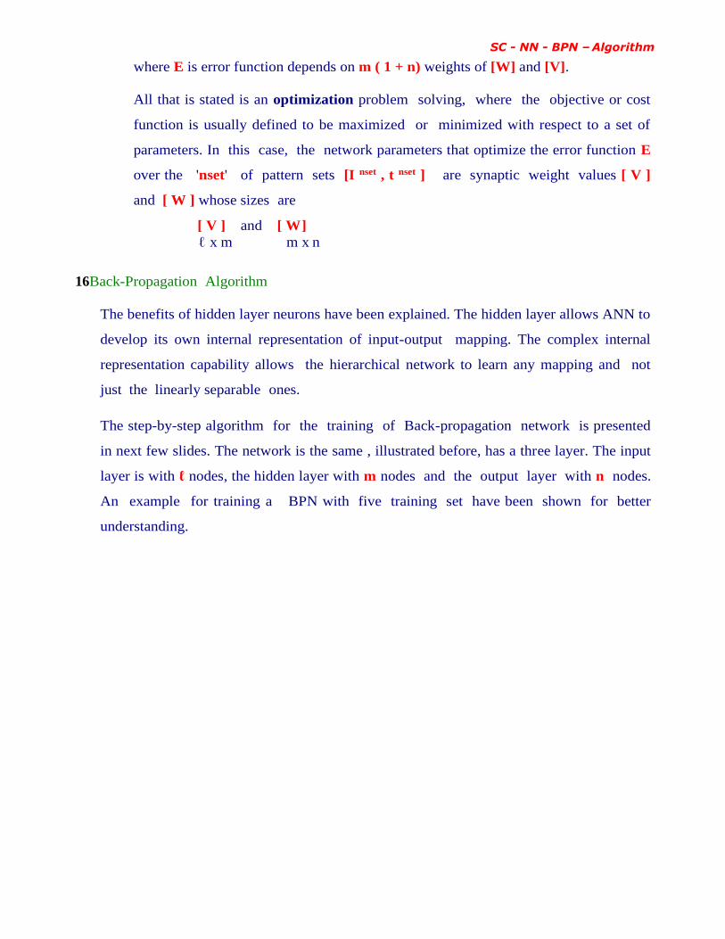
where E is error function depends on m ( 1 + n) weights of [W] and [V].
All that is stated is an optimization problem solving, where the objective or cost
function is usually defined to be maximized or minimized with respect to a set of
parameters. In this case, the network parameters that optimize the error function E
over the 'nset' of pattern sets [I nset , t nset ] are synaptic weight values [ V ]
and [ W ] whose sizes are
[ V ] and [ W ]
ℓ x m m x n
16Back-Propagation Algorithm
The benefits of hidden layer neurons have been explained. The hidden layer allows ANN to
develop its own internal representation of input-output mapping. The complex internal
representation capability allows the hierarchical network to learn any mapping and not
just the linearly separable ones.
The step-by-step algorithm for the training of Back-propagation network is presented
in next few slides. The network is the same , illustrated before, has a three layer. The input
layer is with ℓ nodes, the hidden layer with m nodes and the output layer with n nodes.
An example for training a BPN with five training set have been shown for better
understanding.

SC - NN - BPN – Algorithm
Algorithm for Training Network
The basic algorithm loop structure, and the step by step procedure of Back-
propagation algorithm are illustrated in next few slides.
• Basic algorithm loop structure
Initialize the weights Repeat
For each training pattern
"Train on that pattern"
End
Until the error is acceptably low.

SC - NN - BPN – Algorithm
• Back-Propagation Algorithm - Step-by-step procedure
■ Step 1 :
Normalize the I/P and O/P with respect to their maximum values.
For each training pair, assume that in normalized form there are
ℓ inputs given by { I }I and
ℓ x 1
n outputs given by { O}O
n x 1
■ Step 2 :
Assume that the number of neurons in the hidden layers lie
between 1 < m < 21

SC - NN - BPN – Algorithm
Step 3 : ■
Let [ V ] represents the weights of synapses connecting input
neuron and hidden neuron
Let [ W ] represents the weights of synapses connecting hidden
neuron and output neuron
Initialize the weights to small random values usually from -1 to +1;
[ V ] 0 = [ random weights ] [ W
] 0 = [ random weights ] [ V ] 0
= [ W ] 0 = [ 0 ]
For general problems can be assumed as 1 and threshold value as 0.

SC - NN - BPN – Algorithm
Step 4 : ■
For training data, we need to present one set of inputs and outputs. Present the pattern
as inputs to the input layer { I }I .
then by using linear activation function, the output of the input layer may be
evaluated as
{ O }I = { I }I
ℓ x 1 ℓ x 1
■ Step 5 :
Compute the inputs to the hidden layers by multiplying corresponding weights of
synapses as
{ I }H = [ V] T { O }I
m x 1 m x ℓ ℓ x 1
■ Step 6 :
Let the hidden layer units, evaluate the output using the
sigmoidal function as
{ O }H =
m x 1
– –
1
( 1 + e - (IHi))
– –

SC - NN - BPN – Algorithm
Step 9 : ■
Compute the inputs to the output layers by multiplying corresponding weights of
synapses as
{ I }O = [ W] T { O }H
n x 1 n x m m x 1
■ Step 8 :
Let the output layer units, evaluate the output using sigmoidal
function as
{ O }O =
Note : This output is the network output
Calculate the error using the difference between the network output and the
desired output as for the j th training set as
EP =
(Tj - Ooj )2
n
■ Step 10 :
Find a term { d } as
–
–
{ d } = (Tk – OOk) OOk (1 – OOk )
–
– n x 1
– –
1
( 1 + e - (IOj))
– –

SC - NN - BPN – Algorithm
Step 11 : ■
Find [ Y ] matrix as
[ Y ] = { O }H d
m x n m x 1 1 x n
■ Step 12 :
Find [ W ] t +1
= [ W ] t
+ [ Y ]
m x n m x n m x n
■ Step 13 :
Find { e } = [ W ] { d }
m x 1 m x n n x 1
–
–
{ d* } = (OHi) (1 – OHi )
ei
–
–
m x 1 m x 1
Find [ X ] matrix as
[ X ] = { O }I d* = { I }I d*
1 x m ℓ x 1 1 x m ℓ x 1 1 x m

SC - NN - BPN – Algorithm
■ Step 14 :
Find [ V ] t +1
= [ V ] t
+ [ X ]
1 x m 1 x m 1 x m
■ Step 15 :
Find [ V ] t +1
= [V ] t
+ [ V ] t +1
[ W ] t +1
= [W ] t
+ [ W ] t +1
■ Step 16 :
Find error rate as
error rate =
Ep
nset
■ Step 17 :
Repeat steps 4 to 16 until the convergence in the error rate is less than the
tolerance value
■ End of Algorithm
Note : The implementation of this algorithm, step-by-step 1 to 17, assuming one
example for training BackProp Network is illustrated in the next section.

SC - NN - BPN – Algorithm
0.4 0.1
0.2
0.4 -0.2 TO = 0.1
-0.7 -0.5
0.2
Example : Training Back-Prop Network
• Problem :
Consider a typical problem where there are 5 training sets.
Table : Training sets
S. No. Input Output
I1 I2 O
1 0.4 -0.7 0.1
2 0.3 -0.5 0.05
3 0.6 0.1 0.3
4 0.2 0.4 0.25
5 0.1 -0.2 0.12
In this problem,
- there are two inputs and one output.
- the values lie between -1 and +1 i.e., no need to normalize the values.
- assume two neurons in the hidden layers.
- the NN architecture is shown in the Fig. below.
Input
layer
Hidden
layer
Output
layer
Fig. Multi layer feed forward neural network (MFNN) architecture with
data of the first training set
The solution to problem are stated step-by-step in the subsequent
slides.
SC - NN - BPN – Algorithm
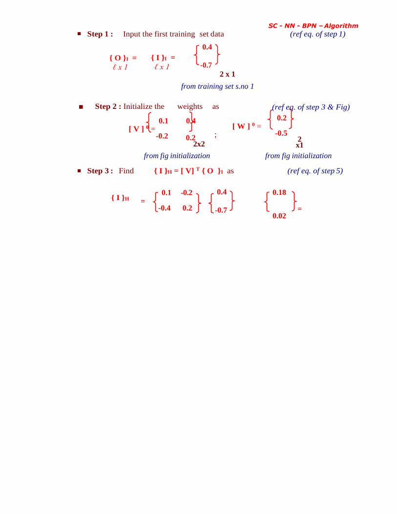
■ Step 1 : Input the first training set data (ref eq. of step 1)
0.4
{ O }I =
ℓ x 1
{ I }I =
ℓ x 1
-0.7
2 x 1
from training set s.no 1
■ Step 2 : Initialize the weights as (ref eq. of step 3 & Fig)
0.1
[ V ] 0 = -0.2
0.4
0.2
2x2
;
0.2 [ W ] 0 =
-0.5 2 x1
from fig initialization from fig initialization
■ Step 3 : Find { I }H = [ V] T { O }I as (ref eq. of step 5)
{ I }H 0.1 -0.2
= -0.4 0.2
0.4
-0.7
0.18
= 0.02

SC - NN - BPN – Algorithm
(ref eq. of step 6) Step 4 : ■
Values from step
1 & 2
{ O }H =
1
( 1 + e - (0.18))
1
( 1 + e - (0.02))
0.5448
= 0.505

SC - NN - BPN – Algorithm
(ref eq. of step 7) Step 5 : ■
Values from step 3 values
{ I }O = [ W] T { O }H = ( 0.2 - 0.5 ) 0.5448
0.505
= - 0.14354
Values from step 2 , from step 4
■ Step 6 : (ref eq. of step 8)
{ O }O = 1
( 1 + e - (0.14354))
= 0.4642
Values from step 5
■ Step 7 : (ref eq. of step 9)
Error = (TO – OO1 )2 = (0.1 – 0.4642)2 = 0.13264
table first training set o/p from step 6

SC - NN - BPN – Algorithm
(ref eq. of step 10) Step 8 : ■
–0.02958
–0.02742
–0.018116
–0.04529
d = (TO – OO1 ) ( OO1 ) (1 – OO1 )
= (0.1 – 0.4642) (0.4642) ( 0.5358) = – 0.09058
Training o/p all from step 6
[ Y ] = { O }H (d ) =
0.5448
0.505
(ref eq. of step 11)
(– 0.09058) =
from values at step 4 from values at step 8 above
■ Step 9 : (ref eq. of step 12)
[ W ] 1
= [ W ] 0
+ [ Y ] assume =0.6
=
from values at step 2 & step 8 above
■ Step 10 : (ref eq. of step 13)
0.2 { e } = [ W ] { d } = (– 0.09058) =
-0.5
from values at step 8 above from values at step 2
–0.0493
–0.0457

SC - NN - BPN – Algorithm
(ref eq. of step 13) Step 11 : ■
(–0.018116) (0.5448) (1- 0.5448) { d* } = =
(0.04529) (0.505) ( 1 – 0.505)
–0.00449
–0.01132
from values at step 10 at step 4 at step 8
■ Step 12 : (ref eq. of step 13)
[ X ] = { O }I ( d* ) = 0.4
-0.7
( – 0.00449 0.01132)
from values at step 1 from values at step 11 above
– 0.001796 0.004528
= 0.003143 –0.007924
■ Step 13 : (ref eq. of step 14)
[ V ] 1
= [ V ] 0
+ [ X ] =
– 0.001077 0.002716
0.001885 –0.004754
from values at step 2 & step 8 above

SC - NN - BPN – Algorithm
(ref eq. of step 15) ■ Step 14 :
0.1 0.4
[ V ] 1
= + -0.2 0.2
– 0.001077 0.002716
0.001885 –0.004754
from values at step 2 from values at step 13
– 0.0989 0.04027
= 0.1981 –0.19524
0.2 –0.02958 0.17042 [ W ]
1 = + =
-0.5
–0.02742 –0.52742

SC - NN - BPN – Algorithm
(ref eq. of step 15) ■ Step 14 :
from values at step 2, from values at step 9
■ Step 15 :
With the updated weights [ V ] and [ W ] , error is calculated again and
next training set is taken and the error will then get adjusted.
■ Step 16 :
Iterations are carried out till we get the error less than the tolerance.
■ Step 17 :
Once the weights are adjusted the network is ready
for inferencing new objects .
Fuzzy Set Theory
Soft Computing
Introduction to fuzzy set, topics : classical set theory, fuzzy set theory,
crisp and non-crisp Sets representation, capturing uncertainty, examples.
Fuzzy membership and graphic interpretation of fuzzy sets - small, prime
numbers, universal, finite, infinite, empty space; Fuzzy Operations -
inclusion, comparability, equality, complement, union, intersection,
difference; Fuzzy properties related to union, intersection, distributivity,
law of excluded middle, law of contradiction, and cartesian product.
Fuzzy relations : definition, examples, forming fuzzy relations,
projections of fuzzy relations, max-min and min-max compositions.

Fuzzy Set Theory
Soft Computing
Topics
1. Introduction to fuzzy Set
What is Fuzzy set? Classical set theory; Fuzzy set theory; Crisp and
Non-crisp Sets : Representation; Capturing uncertainty, Examples
2. Fuzzy set
Fuzzy Membership; Graphic interpretation of fuzzy sets : small, prime numbers, universal,
finite, infinite, empty space;
Fuzzy Operations : Inclusion, Comparability, Equality, Complement, Union,
Intersection, Difference;
Fuzzy Properties : Related to union – Identity, Idempotence, Associativity,
Commutativity ; Related to Intersection – Absorption, Identity, Idempotence,
Commutativity, Associativity; Additional properties - Distributivity, Law of excluded
middle, Law of contradiction; Cartesian product .
3. Fuzzy Relations
Definition of Fuzzy Relation, examples;
Forming Fuzzy Relations – Membership matrix, Graphical form; Projections of
Fuzzy Relations – first, second and global; Max-Min and Min-Max compositions.

Fuzzy Set Theory
What is Fuzzy Set ?
• The word "fuzzy" means "vagueness". Fuzziness occurs when the boundary of a piece
of information is not clear-cut.
• Fuzzy sets have been introduced by Lotfi A. Zadeh (1965) as an extension of the
classical notion of set.
• Classical set theory allows the membership of the elements in the set in binary
terms, a bivalent condition - an element either belongs or does not belong to the
set.
Fuzzy set theory permits the gradual assessment of the membership of elements in
a set, described with the aid of a membership function valued in the real unit interval
[0, 1].
• Example:
Words like young, tall, good, or high are fuzzy.
− There is no single quantitative value which defines the term young.
− For some people, age 25 is young, and for others, age 35 is young.
− The concept young has no clean boundary.
− Age 1 is definitely young and age 100 is definitely not young;
− Age 35 has some possibility of being young and usually depends on the
context in which it is being considered.

SC - Fuzzy set theory - Introduction
1. Introduction
In real world, there exists much fuzzy knowledge;
Knowledge that is vague, imprecise, uncertain, ambiguous, inexact, or probabilistic in
nature.
Human thinking and reasoning frequently involve fuzzy information, originating from
inherently inexact human concepts. Humans, can give satisfactory answers, which are
probably true.
However, our systems are unable to answer many questions. The reason is, most
systems are designed based upon classical set theory and two-valued logic which is
unable to cope with unreliable and incomplete information and give expert opinions.
We want, our systems should also be able to cope with unreliable and incomplete
information and give expert opinions. Fuzzy sets have been able provide solutions to
many real world problems.
Fuzzy Set theory is an extension of classical set theory where elements have degrees of
membership.
• Classical Set Theory
A Set is any well defined collection of objects. An object in a set is called an
element or member of that set.
− Sets are defined by a simple statement describing whether a particular element
having a certain property belongs to that particular set.
− Classical set theory enumerates all its elements using
A = { a1 , a2 , a3 , a4 , ........................ an }
If the elements ai (i = 1, 2, 3, . . . n) of a set A are subset of universal set X,
then set A can be represented for all elements x X by its characteristic
function
1 if x X
A (x) =
0 otherwise

SC - Fuzzy set theory – Fuzzy Operation
− A set A is well described by a function called characteristic
function.
This function, defined on the universal space X, assumes :
a value of 1 for those elements x that belong to set A, and
a value of 0 for those elements x that do not belong to set A.
The notations used to express these mathematically are
Α : Χ [0, 1]
A(x) = 1 , x is a member of A Eq.(1)
A(x) = 0 , x is not a member of A
Alternatively, the set A can be represented for all elements x X
by its characteristic function A (x) defined as
1 if x X
A (x) = Eq.(2)
0 otherwise
− Thus in classical set theory A (x) has only the values 0 ('false')
and 1 ('true''). Such sets are called crisp sets.
• Fuzzy Set Theory
Fuzzy set theory is an extension of classical set theory where elements have
varying degrees of membership. A logic based on the two truth values, True and
False, is sometimes inadequate when describing human reasoning. Fuzzy logic uses
the whole interval between 0 (false) and 1 (true) to describe human reasoning.
− A Fuzzy Set is any set that allows its members to have different degree of
membership, called membership function, in the interval [0 , 1].
− The degree of membership or truth is not same as probability;
fuzzy truth is not likelihood of some event or condition.
fuzzy truth represents membership in vaguely defined sets;
− Fuzzy logic is derived from fuzzy set theory dealing with reasoning that is
approximate rather than precisely deduced from classical predicate logic.
− Fuzzy logic is capable of handling inherently imprecise concepts.

SC - Fuzzy set theory – Fuzzy Operation
Degree or grade of truth
Not Tall Tall
1
0 1.8 m Height x
Degree or grade of truth
Not Tall Tall
1
0 1.8 m Height x
− Fuzzy logic allows in linguistic form the set membership values to imprecise
concepts like "slightly", "quite" and "very".
− Fuzzy set theory defines Fuzzy Operators on Fuzzy Sets.
• Crisp and Non-Crisp Set
− As said before, in classical set theory, the characteristic function
A(x) of Eq.(2) has only values 0 ('false') and 1 ('true''). Such sets
are crisp sets.
− For Non-crisp sets the characteristic function A(x) can be defined.
The characteristic function A(x) of Eq. (2) for the crisp set is
generalized for the Non-crisp sets.
This generalized characteristic function A(x) of Eq.(2) is called
membership function.
Such Non-crisp sets are called Fuzzy Sets.
− Crisp set theory is not capable of representing descriptions and classifications in
many cases; In fact, Crisp set does not provide adequate representation for most
cases.
− The proposition of Fuzzy Sets are motivated by the need to capture and represent
real world data with uncertainty due to imprecise measurement.
− The uncertainties are also caused by vagueness in the language.
• Representation of Crisp and Non-Crisp Set Example :
Classify students for a basketball team This example
explains the grade of truth value.
- tall students qualify and not tall students do not qualify
- if students 1.8 m tall are to be qualified, then should we
exclude a student who is 1/10" less? or should we exclude
a student who is 1" shorter?
■ Non-Crisp Representation to represent the notion of a tall person.

SC - Fuzzy set theory – Fuzzy Operation
1
c (x)
C
F (x)
F 0.5
0 x
Crisp logic Non-crisp logic
Fig. 1 Set Representation – Degree or grade of truth
A student of height 1.79m would belong to both tall and not tall sets with a
particular degree of membership.
As the height increases the membership grade within the tall set would increase
whilst the membership grade within the not-tall set would decrease.
• Capturing Uncertainty
Instead of avoiding or ignoring uncertainty, Lotfi Zadeh introduced Fuzzy Set theory
that captures uncertainty.
■ A fuzzy set is described by a membership function A (x) of A.
This membership function associates to each element x X a
number as A (x ) in the closed unit interval [0, 1].
The number A (x ) represents the degree of membership of x in A.
■ The notation used for membership function A (x) of a fuzzy set A is
Α : Χ [0, 1]
■ Each membership function maps elements of a given universal base set X , which
is itself a crisp set, into real numbers in [0, 1] .
■ Example
Fig. 2 Membership function of a Crisp set C and Fuzzy set F
■ In the case of Crisp Sets the members of a set are :
either out of the set, with membership of degree " 0 ", or in the
set, with membership of degree " 1 ",

SC - Fuzzy set theory – Fuzzy Operation
Therefore, Crisp Sets ⊆ Fuzzy Sets
In other words, Crisp Sets are Special cases of Fuzzy Sets.
• Examples of Crisp and Non-Crisp Set
Example 1: Set of prime numbers ( a crisp set)
If we consider space X consisting of natural numbers 12
ie X = {1, 2, 3, 4, 5, 6, 7, 8, 9, 10, 11, 12}
Then, the set of prime numbers could be described as follows.
PRIME = {x contained in X | x is a prime number} = {2, 3, 5, 6, 7, 11}
Example 2: Set of SMALL ( as non-crisp set)
A Set X that consists of SMALL cannot be described;
for example 1 is a member of SMALL and 12 is not a member of SMALL.
Set A, as SMALL, has un-sharp boundaries, can be characterized by a function that
assigns a real number from the closed interval from 0 to 1 to each element x in the set
X.
A Fuzzy Set is any set that allows its members to have different degree of
membership, called membership function, in the interval [0 , 1].
• Definition of Fuzzy set
A fuzzy set A, defined in the universal space X, is a function defined in
X which assumes values in the range [0, 1].
A fuzzy set A is written as a set of pairs {x, A(x)} as
A = {{x , A(x)}} , x in the set X
where x is an element of the universal space X, and
A(x) is the value of the function A for this element.
The value A(x) is the membership grade of the element x in a
fuzzy set A.
Example : Set SMALL in set X consisting of natural numbers to 12. Assume:
SMALL(1) = 1, SMALL(2) = 1, SMALL(3) = 0.9, SMALL(4) = 0.6,
SMALL(5) = 0.4, SMALL(6) = 0.3, SMALL(7) = 0.2, SMALL(8) =
0.1, SMALL(u) = 0 for u >= 9.

SC - Fuzzy set theory – Fuzzy Operation
Then, following the notations described in the definition above :
Set SMALL = {{1, 1 }, {2, 1 }, {3, 0.9}, {4, 0.6}, {5, 0.4}, {6, 0.3}, {7, 0.2},
{8, 0.1}, {9, 0 }, {10, 0 }, {11, 0}, {12, 0}}
Note that a fuzzy set can be defined precisely by associating with each x , its
grade of membership in SMALL.
• Definition of Universal Space
Originally the universal space for fuzzy sets in fuzzy logic was defined only on the
integers. Now, the universal space for fuzzy sets and fuzzy relations is defined with
three numbers.
The first two numbers specify the start and end of the universal space, and the third
argument specifies the increment between elements. This gives the user more
flexibility in choosing the universal space.
Example : The fuzzy set of numbers, defined in the universal space
X = { xi } = {1, 2, 3, 4, 5, 6, 7, 8, 9, 10, 11, 12} is presented as
SetOption [FuzzySet, UniversalSpace {1, 12, 1}]
Fuzzy Membership
A fuzzy set A defined in the universal space X is a function defined in X which
assumes values in the range [0, 1].
A fuzzy set A is written as a set of pairs {x, A(x)}.
A = {{x , A(x)}} , x in the set X
where x is an element of the universal space X, and
A(x) is the value of the function A for this element.
The value A(x) is the degree of membership of the element x
in a fuzzy set A.
The Graphic Interpretation of fuzzy membership for the fuzzy sets : Small, Prime
Numbers, Universal-space, Finite and Infinite UniversalSpace, and Empty are
illustrated in the next few slides.
• Graphic Interpretation of Fuzzy Sets SMALL

SC - Fuzzy set theory – Fuzzy Operation
The fuzzy set SMALL of small numbers, defined in the universal space
X = { xi } = {1, 2, 3, 4, 5, 6, 7, 8, 9, 10, 11, 12} is presented as
SetOption [FuzzySet, UniversalSpace {1, 12, 1}]
The Set SMALL in set X is :
SMALL = FuzzySet {{1, 1 }, {2, 1 }, {3, 0.9}, {4, 0.6}, {5, 0.4}, {6, 0.3},
{7, 0.2}, {8, 0.1}, {9, 0 }, {10, 0 }, {11, 0}, {12, 0}}
Therefore SetSmall is represented as
SetSmall = FuzzySet [{{1,1},{2,1}, {3,0.9}, {4,0.6}, {5,0.4},{6,0.3}, {7,0.2},
{8, 0.1}, {9, 0}, {10, 0}, {11, 0}, {12, 0}} , UniversalSpace {1, 12, 1}]
FuzzyPlot [ SMALL, AxesLable {"X", "SMALL"}]
SMALL
1
.8
.6
.4
.2
0 0 1 2 3 4 5 6 7 8 9 10 11 12 X
Fig Graphic Interpretation of Fuzzy Sets SMALL
• Graphic Interpretation of Fuzzy Sets PRIME Numbers The
fuzzy set PRIME numbers, defined in the universal space X = { xi } = {1,
2, 3, 4, 5, 6, 7, 8, 9, 10, 11, 12} is presented as
SetOption [FuzzySet, UniversalSpace {1, 12, 1}]
The Set PRIME in set X is :
PRIME = FuzzySet {{1, 0}, {2, 1}, {3, 1}, {4, 0}, {5, 1}, {6, 0}, {7, 1}, {8, 0},
{9, 0}, {10, 0}, {11, 1}, {12, 0}}
Therefore SetPrime is represented as
SetPrime = FuzzySet [{{1,0},{2,1}, {3,1}, {4,0}, {5,1},{6,0}, {7,1},
{8, 0}, {9, 0}, {10, 0}, {11, 1}, {12, 0}} , UniversalSpace {1, 12, 1}]
FuzzyPlot [ PRIME, AxesLable {"X", "PRIME"}]
PRIME
1

SC - Fuzzy set theory – Fuzzy Operation
.8
.6
.4
.2
0 0 1 2 3 4 5 6 7 8 9 10 11 12 X
Fig Graphic Interpretation of Fuzzy Sets PRIME
• Graphic Interpretation of Fuzzy Sets UNIVERSALSPACE
In any application of sets or fuzzy sets theory, all sets are subsets of a fixed set
called universal space or universe of discourse denoted by X. Universal space X as a
fuzzy set is a function equal to 1 for all elements.
The fuzzy set UNIVERSALSPACE numbers, defined in the universal space
X = { xi } = {1, 2, 3, 4, 5, 6, 7, 8, 9, 10, 11, 12} is presented as
SetOption [FuzzySet, UniversalSpace {1, 12, 1}]
The Set UNIVERSALSPACE in set X is :
UNIVERSALSPACE = FuzzySet {{1, 1}, {2, 1}, {3, 1}, {4, 1}, {5, 1}, {6, 1},
{7, 1}, {8, 1}, {9, 1}, {10, 1}, {11, 1}, {12, 1}}
Therefore SetUniversal is represented as
SetUniversal = FuzzySet [{{1,1},{2,1}, {3,1}, {4,1}, {5,1},{6,1}, {7,1},
{8, 1}, {9, 1}, {10, 1}, {11, 1}, {12, 1}} , UniversalSpace {1, 12, 1}]

SC - Fuzzy set theory – Fuzzy Operation
FuzzyPlot [ UNIVERSALSPACE, AxesLable {"X", " UNIVERSAL SPACE "}]
UNIVERSAL SPACE
1
.8
.6
.4
.2
0 0 1 2 3 4 5 6 7 8 9 10 11 12 X
Fig Graphic Interpretation of Fuzzy Set UNIVERSALSPACE
• Finite and Infinite Universal Space
Universal sets can be finite or infinite.
Any universal set is finite if it consists of a specific number of different elements, that
is, if in counting the different elements of the set, the counting can come to an end,
else the set is infinite.
Examples:
1. Let N be the universal space of the days of the week.
N = {Mo, Tu, We, Th, Fr, Sa, Su}. N is finite. 2.
Let M = {1, 3, 5, 7, 9, ...}. M is infinite.
3. Let L = {u | u is a lake in a city }. L is finite.
(Although it may be difficult to count the number of lakes in a city,
but L is still a finite universal set.)
• Graphic Interpretation of Fuzzy Sets EMPTY
An empty set is a set that contains only elements with a grade of membership equal to
0.
Example: Let EMPTY be a set of people, in Minnesota, older than 120. The Empty
set is also called the Null set.
The fuzzy set EMPTY , defined in the universal space
X = { xi } = {1, 2, 3, 4, 5, 6, 7, 8, 9, 10, 11, 12} is presented as
SetOption [FuzzySet, UniversalSpace {1, 12, 1}]

SC - Fuzzy set theory – Fuzzy Operation
The Set EMPTY in set X is :
EMPTY = FuzzySet {{1, 0}, {2, 0}, {3, 0}, {4, 0}, {5, 0}, {6, 0}, {7, 0},
{8, 0}, {9, 0}, {10, 0}, {11, 0}, {12, 0}}
Therefore SetEmpty is represented as
SetEmpty = FuzzySet [{{1,0},{2,0}, {3,0}, {4,0}, {5,0},{6,0}, {7,0},
{8, 0}, {9, 0}, {10, 0}, {11, 0}, {12, 0}} , UniversalSpace {1, 12, 1}]
FuzzyPlot [ EMPTY, AxesLable {"X", " UNIVERSAL SPACE "}]
EMPT
Y 1
.8
.6
.4
.2
0 0 1 2 3 4 5 6 7 8 9 10 11 12 X
Fig Graphic Interpretation of Fuzzy Set EMPTY
Fuzzy Operations
A fuzzy set operations are the operations on fuzzy sets. The fuzzy set operations are
generalization of crisp set operations. Zadeh [1965] formulated the fuzzy set theory in
the terms of standard operations: Complement, Union, Intersection, and Difference.
In this section, the graphical interpretation of the following standard fuzzy set terms
and the Fuzzy Logic operations are illustrated:
Inclusion : FuzzyInclude [VERYSMALL, SMALL]
Equality : FuzzyEQUALITY [SMALL, STILLSMALL]
Complement : FuzzyNOTSMALL = FuzzyCompliment
[Small] Union : FuzzyUNION = [SMALL MEDIUM]
Intersection : FUZZYINTERSECTON = [SMALL
MEDIUM]
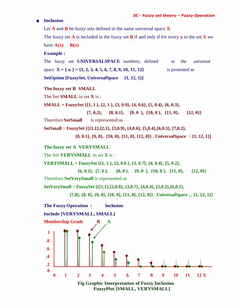
SC - Fuzzy set theory – Fuzzy Operation
• Inclusion
Let A and B be fuzzy sets defined in the same universal space X.
The fuzzy set A is included in the fuzzy set B if and only if for every x in the set X we
have A(x) B(x)
Example :
The fuzzy set UNIVERSALSPACE numbers, defined in the universal
space X = { xi } = {1, 2, 3, 4, 5, 6, 7, 8, 9, 10, 11, 12} is presented as
SetOption [FuzzySet, UniversalSpace {1, 12, 1}]
The fuzzy set B SMALL
The Set SMALL in set X is :
SMALL = FuzzySet {{1, 1 }, {2, 1 }, {3, 0.9}, {4, 0.6}, {5, 0.4}, {6, 0.3},
{7, 0.2}, {8, 0.1}, {9, 0 }, {10, 0 }, {11, 0}, {12, 0}}
Therefore SetSmall is represented as
SetSmall = FuzzySet [{{1,1},{2,1}, {3,0.9}, {4,0.6}, {5,0.4},{6,0.3}, {7,0.2},
{8, 0.1}, {9, 0}, {10, 0}, {11, 0}, {12, 0}} , UniversalSpace {1, 12, 1}]
The fuzzy set A VERYSMALL
The Set VERYSMALL in set X is :
VERYSMALL = FuzzySet {{1, 1 }, {2, 0.8 }, {3, 0.7}, {4, 0.4}, {5, 0.2},
{6, 0.1}, {7, 0 }, {8, 0 }, {9, 0 }, {10, 0 }, {11, 0}, {12, 0}}
Therefore SetVerySmall is represented as
SetVerySmall = FuzzySet [{{1,1},{2,0.8}, {3,0.7}, {4,0.4}, {5,0.2},{6,0.1},
{7,0}, {8, 0}, {9, 0}, {10, 0}, {11, 0}, {12, 0}} , UniversalSpace {1, 12, 1}]
The Fuzzy Operation : Inclusion
Include [VERYSMALL, SMALL]
Membership Grade B A
1
.8
.6
.4
.2
0 0 1 2 3 4 5 6 7 8 9 10 11 12 X
Fig Graphic Interpretation of Fuzzy Inclusion
FuzzyPlot [SMALL, VERYSMALL]

SC - Fuzzy set theory – Fuzzy Properties
• Comparability
Two fuzzy sets A and B are comparable if the
condition A B or B A holds, ie,
if one of the fuzzy sets is a subset of the other set, they are comparable.
Two fuzzy sets A and B are incomparable If the
condition A B or B A holds.
Example 1:
Let A = {{a, 1}, {b, 1}, {c, 0}} and
B = {{a, 1}, {b, 1}, {c, 1}}.
Then A is comparable to B, since A is a subset of B.
Example 2 :
Let C = {{a, 1}, {b, 1}, {c, 0.5}} and
D = {{a, 1}, {b, 0.9}, {c, 0.6}}.
Then C and D are not comparable since
C is not a subset of D and
D is not a subset of C.
Property Related to Inclusion :
for all x in the set X, if A(x) B(x) C(x), then accordingly A C.
• Equality
Let A and B be fuzzy sets defined in the same space X.
Then A and B are equal, which is denoted X = Y
if and only if for all x in the set X, A(x) = B(x).
Example.
The fuzzy set B SMALL
SMALL = FuzzySet {{1, 1 }, {2, 1 }, {3, 0.9}, {4, 0.6}, {5, 0.4}, {6, 0.3},
{7, 0.2}, {8, 0.1}, {9, 0 }, {10, 0 }, {11, 0}, {12, 0}}
The fuzzy set A STILLSMALL
STILLSMALL = FuzzySet {{1, 1 }, {2, 1 }, {3, 0.9}, {4, 0.6}, {5, 0.4},
{6, 0.3}, {7, 0.2}, {8, 0.1}, {9, 0 }, {10, 0 }, {11, 0}, {12, 0}}

SC - Fuzzy set theory – Fuzzy Properties
The Fuzzy Operation : Equality
Equality [SMALL, STILLSMALL]
Membership Grade B A
1
.8
.6
.4
.2
0 0 1 2 3 4 5 6 7 8 9 10 11 12 X
Fig Graphic Interpretation of Fuzzy Equality
FuzzyPlot [SMALL, STILLSMALL]
Note : If equality A(x) = B(x) is not satisfied even for one element x in
the set X, then we say that A is not equal to B.
• Complement
Let A be a fuzzy set defined in the space X.
Then the fuzzy set B is a complement of the fuzzy set A, if and only if, for all x in
the set X, B(x) = 1 - A(x).
The complement of the fuzzy set A is often denoted by A' or Ac or A
Fuzzy Complement : Ac(x) = 1 – A(x)
Example 1.
The fuzzy set A SMALL
SMALL = FuzzySet {{1, 1 }, {2, 1 }, {3, 0.9}, {4, 0.6}, {5, 0.4}, {6, 0.3},
{7, 0.2}, {8, 0.1}, {9, 0 }, {10, 0 }, {11, 0}, {12, 0}}
The fuzzy set Ac NOTSMALL
NOTSMALL = FuzzySet {{1, 0 }, {2, 0 }, {3, 0.1}, {4, 0.4}, {5, 0.6}, {6, 0.7},
{7, 0.8}, {8, 0.9}, {9, 1 }, {10, 1 }, {11, 1}, {12, 1}}
The Fuzzy Operation : Compliment
NOTSMALL = Compliment [SMALL]

SC - Fuzzy set theory – Fuzzy Properties
Membership Grade A Ac
1
.8
.6
.4
.2
0 0 1 2 3 4 5 6 7 8 9 10 11 12 X
Fig Graphic Interpretation of Fuzzy Compliment
FuzzyPlot [SMALL, NOTSMALL]
Example 2.
The empty set and the universal set X, as fuzzy sets, are
complements of one another.
' = X , X' =
The fuzzy set B EMPTY
Empty = FuzzySet {{1, 0 }, {2, 0 }, {3, 0}, {4, 0}, {5, 0}, {6, 0},
{7, 0}, {8, 0}, {9, 0 }, {10, 0 }, {11, 0}, {12, 0}}
The fuzzy set A UNIVERSAL
Universal = FuzzySet {{1, 1 }, {2, 1 }, {3, 1}, {4, 1}, {5, 1}, {6, 1},
{7, 1}, {8, 1}, {9, 1 }, {10, 1 }, {11, 1}, {12, 1}}
The fuzzy operation : Compliment
EMPTY = Compliment [UNIVERSALSPACE]
Membership Grade B A
1
.8
.6

SC - Fuzzy set theory – Fuzzy Properties
.4
.2
0 0 1 2 3 4 5 6 7 8 9 10 11 12 X
Fig Graphic Interpretation of Fuzzy Compliment
FuzzyPlot [EMPTY, UNIVERSALSPACE]
• Union
Let A and B be fuzzy sets defined in the space X.
The union is defined as the smallest fuzzy set that contains both A and B. The union of
A and B is denoted by A B.
The following relation must be satisfied for the union operation :
for all x in the set X, (A B)(x) = Max (A(x), B(x)).
Fuzzy Union : (A B)(x) = max [A(x), B(x)] for all x X
Example 1 : Union of Fuzzy A and B
A(x) = 0.6 and B(x) = 0.4 (A B)(x) = max [0.6, 0.4] = 0.6
Example 2 : Union of SMALL and MEDIUM
The fuzzy set A SMALL
SMALL = FuzzySet {{1, 1 }, {2, 1 }, {3, 0.9}, {4, 0.6}, {5, 0.4}, {6, 0.3},
{7, 0.2}, {8, 0.1}, {9, 0 }, {10, 0 }, {11, 0}, {12, 0}}
The fuzzy set B MEDIUM
MEDIUM = FuzzySet {{1, 0 }, {2, 0 }, {3, 0}, {4, 0.2}, {5, 0.5}, {6, 0.8},
{7, 1}, {8, 1}, {9, 0.7 }, {10, 0.4 }, {11, 0.1}, {12, 0}}
The fuzzy operation : Union
FUZZYUNION = [SMALL MEDIUM]
SetSmallUNIONMedium = FuzzySet [{{1,1},{2,1}, {3,0.9}, {4,0.6}, {5,0.5},
{6,0.8}, {7,1}, {8, 1}, {9, 0.7}, {10, 0.4}, {11, 0.1}, {12, 0}} ,
UniversalSpace {1, 12, 1}]
Membership Grade FUZZYUNION = [SMALL MEDIUM]
1
.8
.6
.4
.2
0 0 1 2 3 4 5 6 7 8 9 10 11 12 X

SC - Fuzzy set theory – Fuzzy Properties
Fig Graphic Interpretation of Fuzzy Union
FuzzyPlot [UNION]
The notion of the union is closely related to that of the connective "or". Let A is a
class of "Young" men, B is a class of "Bald" men.
If "David is Young" or "David is Bald," then David is associated with the
union of A and B. Implies David is a member of A B.
• Intersection
Let A and B be fuzzy sets defined in the space X. Intersection is defined as the
greatest fuzzy set that include both A and B. Intersection of A and B is denoted by A
B. The following relation must be satisfied for the intersection operation :
for all x in the set X, (A B)(x) = Min (A(x), B(x)).
Fuzzy Intersection : (A B)(x) = min [A(x), B(x)] for all x X Example 1 :
Intersection of Fuzzy A and B
A(x) = 0.6 and B(x) = 0.4 (A B)(x) = min [0.6, 0.4] = 0.4
Example 2 : Union of SMALL and MEDIUM
The fuzzy set A SMALL
SMALL = FuzzySet {{1, 1 }, {2, 1 }, {3, 0.9}, {4, 0.6}, {5, 0.4}, {6, 0.3},
{7, 0.2}, {8, 0.1}, {9, 0 }, {10, 0 }, {11, 0}, {12, 0}}
The fuzzy set B MEDIUM
MEDIUM = FuzzySet {{1, 0 }, {2, 0 }, {3, 0}, {4, 0.2}, {5, 0.5}, {6, 0.8},
{7, 1}, {8, 1}, {9, 0.7 }, {10, 0.4 }, {11, 0.1}, {12, 0}}
The fuzzy operation : Intersection
FUZZYINTERSECTION = min [SMALL MEDIUM]
SetSmallINTERSECTIONMedium = FuzzySet [{{1,0},{2,0}, {3,0}, {4,0.2},
{5,0.4}, {6,0.3}, {7,0.2}, {8, 0.1}, {9, 0},
{10, 0}, {11, 0}, {12, 0}} , UniversalSpace {1, 12, 1}]
Membership Grade FUZZYINTERSECTON = [SMALL MEDIUM]
1
.8
.6
.4

SC - Fuzzy set theory – Fuzzy Properties
.2
0 0 1 2 3 4 5 6 7 8 9 10 11 12 X
Fig Graphic Interpretation of Fuzzy Union
FuzzyPlot [INTERSECTION]
• Difference
Let A and B be fuzzy sets defined in the space X. The
difference of A and B is denoted by A B'.
Fuzzy Difference : (A - B)(x) = min [A(x), 1- B(x)] for all x X
Example : Difference of MEDIUM and SMALL
The fuzzy set A MEDIUM
MEDIUM = FuzzySet {{1, 0 }, {2, 0 }, {3, 0}, {4, 0.2}, {5, 0.5}, {6, 0.8}, {7, 1}, {8, 1}, {9, 0.7 }, {10, 0.4 }, {11, 0.1}, {12, 0}}
The fuzzy set B SMALL
MEDIUM = FuzzySet {{1, 1 }, {2, 1 }, {3, 0.9}, {4, 0.6}, {5, 0.4}, {6, 0.3},
{7, 0.2}, {8, 0.1}, {9, 0.7 }, {10, 0.4 }, {11, 0}, {12, 0}}
Fuzzy Complement : Bc(x) = 1 – B(x)
The fuzzy set Bc NOTSMALL
NOTSMALL = FuzzySet {{1, 0 }, {2, 0 }, {3, 0.1}, {4, 0.4}, {5, 0.6}, {6, 0.7},
{7, 0.8}, {8, 0.9}, {9, 1 }, {10, 1 }, {11, 1}, {12, 1}}
The fuzzy operation : Difference by the definition of Difference
FUZZYDIFFERENCE = [MEDIUM SMALL']
SetMediumDIFFERECESmall = FuzzySet [{{1,0},{2,0}, {3,0}, {4,0.2},
{5,0.5}, {6,0.7}, {7,0.8}, {8, 0.9}, {9, 0.7},
{10, 0.4}, {11, 0.1}, {12, 0}} , UniversalSpace {1, 12, 1}]
Membership Grade FUZZYDIFFERENCE = [MEDIUM SMALL' ]
1
.8
.6
.4
.2
0 0 1 2 3 4 5 6 7 8 9 10 11 12 X
Fig Graphic Interpretation of Fuzzy Union
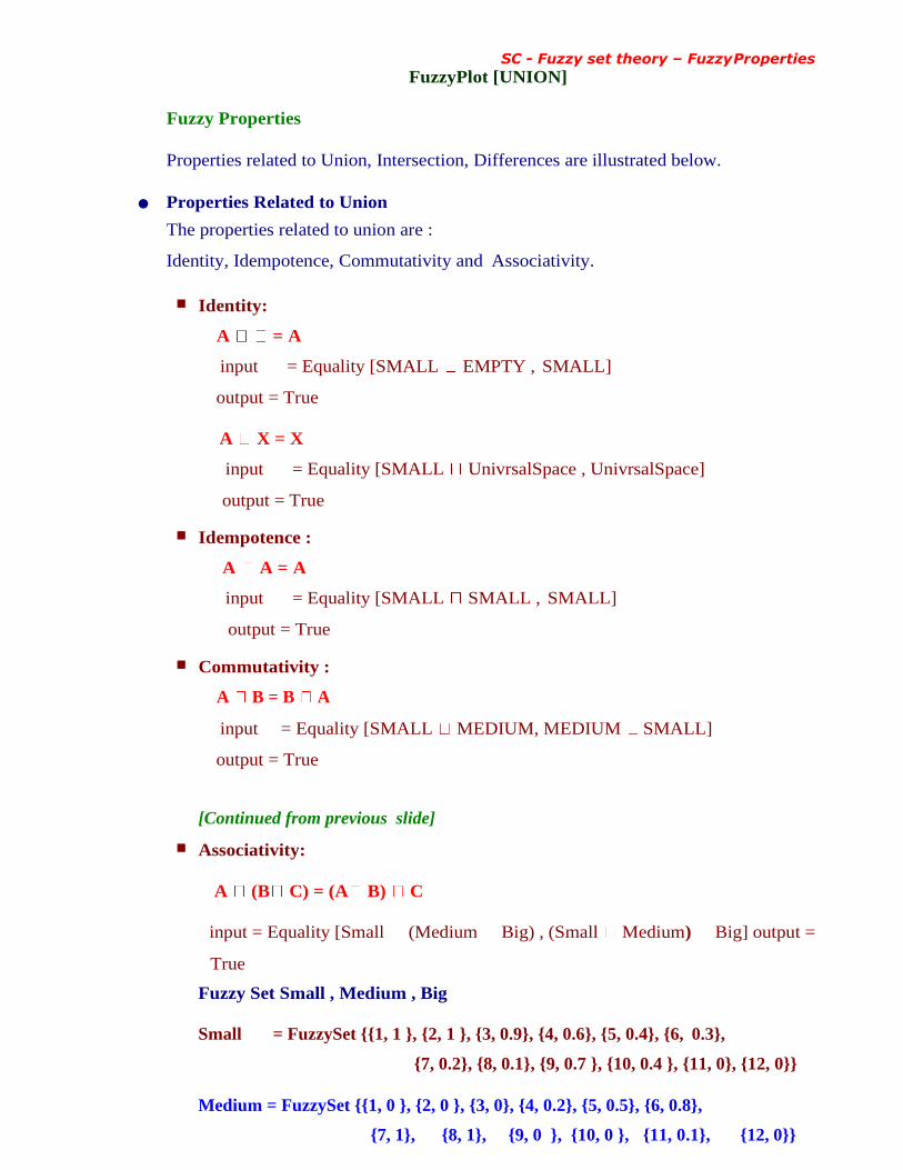
SC - Fuzzy set theory – Fuzzy Properties
FuzzyPlot [UNION]
Fuzzy Properties
Properties related to Union, Intersection, Differences are illustrated below.
• Properties Related to Union
The properties related to union are :
Identity, Idempotence, Commutativity and Associativity.
■ Identity:
A = A
input = Equality [SMALL EMPTY , SMALL]
output = True
A X = X
input = Equality [SMALL UnivrsalSpace , UnivrsalSpace]
output = True
■ Idempotence :
A A = A
input = Equality [SMALL SMALL , SMALL]
output = True
■ Commutativity :
A B = B A
input = Equality [SMALL MEDIUM, MEDIUM SMALL]
output = True
[Continued from previous slide]
■ Associativity:
A (B C) = (A B) C
input = Equality [Small (Medium Big) , (Small Medium) Big] output =
True
Fuzzy Set Small , Medium , Big
Small = FuzzySet {{1, 1 }, {2, 1 }, {3, 0.9}, {4, 0.6}, {5, 0.4}, {6, 0.3},
{7, 0.2}, {8, 0.1}, {9, 0.7 }, {10, 0.4 }, {11, 0}, {12, 0}}
Medium = FuzzySet {{1, 0 }, {2, 0 }, {3, 0}, {4, 0.2}, {5, 0.5}, {6, 0.8},
{7, 1}, {8, 1}, {9, 0 }, {10, 0 }, {11, 0.1}, {12, 0}}

SC - Fuzzy set theory – Fuzzy Properties
Big = FuzzySet [{{1,0}, {2,0}, {3,0}, {4,0}, {5,0}, {6,0.1},
{7,0.2}, {8,0.4}, {9,0.6}, {10,0.8}, {11,1}, {12,1}}]
Calculate Fuzzy relations :
(1) Medium Big = FuzzySet [{1,0},{2,0}, {3,0}, {4,0.2}, {5,0.5},
{6,0.8},{7,1}, {8, 1}, {9, 0.6}, {10, 0.8}, {11, 1}, {12, 1}]
(2) Small Medium = FuzzySet [{1,1},{2,1}, {3,0.9}, {4,0.6}, {5,0.5},
{6,0.8}, {7,1}, {8, 1}, {9, 0.7}, {10, 0.4}, {11, 0.1}, {12, 0}]
(3) Small (Medium Big) = FuzzySet [{1,1},{2,1}, {3,0.9}, {4,0.6},
{5,0.5}, {6,0.8}, {7,1}, {8, 1}, {9, 0.7}, {10, 0.8}, {11, 1}, {12, 1}]
(4) (Small Medium) Big] = FuzzySet [{1,1},{2,1}, {3,0.9}, {4,0.6},
{5,0.5}, {6,0.8}, {7,1}, {8, 1}, {9, 0.7},{10, 0.8}, {11, 1},{12, 1}]
Fuzzy set (3) and (4) proves Associativity relation

SC - Fuzzy set theory – Fuzzy Properties
• Properties Related to Intersection
Absorption, Identity, Idempotence, Commutativity, Associativity.
■ Absorption by Empty Set :
A =
input = Equality [Small Empty , Empty]
output = True
■ Identity :
A X = A
input = Equality [Small UnivrsalSpace , Small]
output = True
■ Idempotence :
A A = A
input = Equality [Small Small , Small]
output = True
■ Commutativity :
A B = B A
input = Equality [Small Big , Big Small]
output = True
■ Associativity :
A (B C) = (A B) C
input = Equality [Small (Medium Big), (Small Medium) Big] output =
True

SC - Fuzzy set theory – Fuzzy Properties
• Additional Properties
Related to Intersection and Union
■ Distributivity:
A (B C) = (A B) (A C)
input = Equality [Small (Medium Big) ,
(Small Medium) (Small Big)]
output = True
■ Distributivity:
A (B C) = (A B) (A C)
input = Equality [Small (Medium Big) ,
(Small Medium) (Small Big)]
output = True
■ Law of excluded middle :
A A' = X
input = Equality [Small NotSmall , UnivrsalSpace ] output =
True
■ Law of contradiction
A A' =
input = Equality [Small NotSmall , EmptySpace ] output =
True
• Cartesian Product Of Two Fuzzy Sets
■ Cartesian Product of two Crisp Sets
Let A and B be two crisp sets in the universe of discourse X and Y.. The
Cartesian product of A and B is denoted by A x B
Defined as A x B = { (a , b) │ a A , b B }
Note : Generally A x B ≠ B x A
Example :
Let A = {a, b, c} and B = {1, 2}
then A x B = { (a , 1) , (a , 2) ,
(b , 1) , (b , 2) ,
(c , 1) , (c , 2) }
Graphic representation of A x B
B
2
1
A

SC - Fuzzy set theory – Fuzzy Properties
a b c

SC - Fuzzy set theory – Fuzzy Relations
■ Cartesian product of two Fuzzy Sets
Let A and B be two fuzzy sets in the universe of discourse X and Y. The
Cartesian product of A and B is denoted by A x B
Defined by their membership function A (x) and B (y) as
A x B (x , y) = min [ A (x) , B (y) ] = A (x) B (y)
or A x B (x , y) = A (x) B (y)
for all x X and y Y
Thus the Cartesian product A x B is a fuzzy set of ordered pair (x , y) for all
x X and y Y, with grade membership of (x , y) in X x Y given by the
above equations .
In a sense Cartesian product of two Fuzzy sets is a Fuzzy Relation.
2. Fuzzy Relations
Fuzzy Relations describe the degree of association of the elements; Example :
“x is approximately equal to y”.
− Fuzzy relations offer the capability to capture the uncertainty and vagueness in relations
between sets and elements of a set.
− Fuzzy Relations make the description of a concept possible.
− Fuzzy Relations were introduced to supersede classical crisp relations; It
describes the total presence or absence of association of elements.
In this section, first the fuzzy relation is defined and then expressing fuzzy relations in
terms of matrices and graphical visualizations. Later the properties of fuzzy relations and
operations that can be performed with fuzzy relations are illustrated.
Definition of Fuzzy Relation
Fuzzy relation is a generalization of the definition of fuzzy set
from 2-D space to 3-D space.
• Fuzzy relation definition
Consider a Cartesian product

SC - Fuzzy set theory – Fuzzy Relations
A x B = { (x , y) | x A, y B }
where A and B are subsets of universal sets U1 and U2.
Fuzzy relation on A x B is denoted by R or R(x , y) is defined as the set
R = { ((x , y) , R (x , y)) | (x , y) A x B , R (x , y) [0,1] }
where R (x , y) is a function in two variables called membership function.
It gives the degree of membership of the ordered pair (x , y) in R associating with
each pair (x , y) in A x B a real number in the interval [0 , 1].
The degree of membership indicates the degree to which x is in relation to y.
Note :
Definition of fuzzy relation is a generalization of the definition of fuzzy set from
the 2-D space (x , , R (x)) to 3-D space ((x , y) , R (x , y)).
Cartesian product A x B is a relation by itself between x and y .
A fuzzy relation R is a sub set of R3 namely
{ ((x , y) , R (x , y)) | A x B x [0,1] U1 x U2 x [0,1] }
• Example of Fuzzy Relation
R = { ((x1 , y1) , 0)) , ((x1 , y2) , 0.1)) , ((x1 , y3) , 0.2)) ,
((x2 , y1) , 0.7)) , ((x2 , y2) , 0.2)) , ((x2 , y3) , 0.3)) ,
((x3 , y1) , 1)) , ((x3 , y2) , 0.6)) , ((x3 , y3) , 0.2)) ,
The relation can be written in matrix form as
R
where symbol means ' is defined as' and
the values in the matrix are the values of membership function:
R (x1 , y1) = 0 R (x1 , y2) = 0.1 R (x1 , y3) = 0.2
R (x2 , y1) = 0.7 R (x2, y2) = 0.2 R (x2 , y3) = 0.3
R (x3 , y1) = 1 R (x3 , y2) = 0.6 R (x3 , y3) = 0.2
Assuming x1 = 1 , x2 = 2 , x3 = 3 and y1 = 1 , y2= 2 , y3= 3 ,
the relation can be graphically represented by points in 3-D space
(X, Y, ) as :
y x
y1 Y2 Y3
x1 0 0.1 0.2
X2 0.7 0.2 0.3
X3 1 0.6 0.2

SC - Fuzzy set theory – Fuzzy Relations
Fig Fuzzy Relation R describing
x greater than y
Note : Since the values of the membership function 0.7, 1, 0.6 are in the direction of x below
the major diagonal (0, 0.2, 0.2) in the matrix are grater than those 0.1, 0.2, 0.3 in the
direction of y, we therefore say that the relation R describes x is grater than y.
Forming Fuzzy Relations
Assume that V and W are two collections of objects.
A fuzzy relation is characterized in the same way as it is in a fuzzy set.
− The first item is a list containing element and membership grade pairs,
{{v1, w1}, R11}, {{ v1, w2}, R12}, ... , {{ vn, wm}, Rnm}}.
where { v1, w1}, { v1, w2}, ... , { vn, wm} are the elements of the relation are defined
as ordered pairs, and { R11 , R12 , ... , Rnm} are the membership grades of the
elements of the relation that range from 0 to 1, inclusive.
− The second item is the universal space; for relations, the universal space consists of
a pair of ordered pairs,
{{ Vmin, Vmax, C1}, { Wmin, Wmax, C2}}.
where the first pair defines the universal space for the first set and the second pair
defines the universal space for the second set.
Example showing how fuzzy relations are represented
Let V = {1, 2, 3} and W = {1, 2, 3, 4}.
A fuzzy relation R is, a function defined in the space V x W, which takes values from
the interval [0, 1] , expressed as R : V x W [0, 1]
1
.8
.6
.4
.2
0
1 2 3 y
1
2
3
x

SC - Fuzzy set theory – Fuzzy Relations
R = FuzzyRelation [{{{1, 1}, 1}, {{1, 2}, 0.2}, {{1, 3}, 0.7}, {{1, 4}, 0}, {{2, 1}, 0.7}, {{2, 2}, 1}, {{2, 3}, 0.4}, {{2, 4}, 0.8}, {{3, 1}, 0}, {{3, 2}, 0.6}, {{3, 3}, 0.3}, {{3, 4}, 0.5}, UniversalSpace {{1, 3, 1}, {1, 4, 1}}]
This relation can be represented in the following two forms shown below
Membership matrix form 1 Graph form
.8 w w1 w2 w3 w4 .6
v .4
v1 1 0.2 0.7 0 .2
v2 0.7 1 0.4 0.8 0 1 2 3 4
v3 0 0.6 0.3 0.5 1

SC - Fuzzy set theory – Fuzzy Relations
R w
2
3 v
Vertical lines represent membership grades
Elements of fuzzy relation are ordered pairs {vi , wj}, where vi is first and wj is second
element. The membership grades of the elements are represented by the heights of the
vertical lines.
Projections of Fuzzy Relations
Definition : A fuzzy relation on A x B is denoted by R or R(x , y) is defined as the
set
R = { ((x , y) , R (x , y)) | (x , y) A x B , R (x , y) [0,1] }
where R (x , y) is a function in two variables called membership function. The first,
the second and the total projections of fuzzy relations are stated below.
• First Projection of R : defined as
R(1) = {(x) , R(1) (x , y))}
= {(x) , max R (x , y)) | (x , y) A x B }
Y
• Second Projection of R : defined as
R(2) = {(y) , R(2) (x , y))}
= {(y) ,
max
X
R (x , y)) | (x , y) A x B }
• Total Projection of R : defined as
R(T) = max
X max
Y
{ R (x , y) | (x , y) A x B }
Note : In all these three expression

SC - Fuzzy set theory – Fuzzy Relations
max
Y
max
X
means max with respect to y while x is considered fixed means max
with respect to x while y is considered fixed

SC - Fuzzy set theory – Fuzzy Relations
y y1 y2 y3
x
The Total Projection is also known as Global projection
• Example : Fuzzy Projections
The Fuzzy Relation R together with First, Second and Total Projection of R are
shown below.
x1
x2 R
x3
R(2
)
y4 Y5 R(1)
0.1 0.3 1 0.5 0.3 1
0.2 0.5 0.7 0.9 0.6 0.9
0.3 0.6 1 0.8 0.2 1
0.3
0.6
1
0.9
0.6
1
= R(T)
Note :
For R(1) select
For R(2) select
max
Y
max
x
means max with respect to y while x is considered fixed means
max with respect to x while y is considered fixed

SC - Fuzzy set theory – Fuzzy Relations
y y1 y2 y3
x
x1 0.1 0.3 0
x2 0.8 1 0.3
R(1)
1
.8
.6
.4
.2
0 x
1 2 3 4 5
R(2)
1
.8
.6
.4
.2
0 y
1 2 3 4 5
For R(T) select max with respect to R(1) and R(2)
The Fuzzy plot of these projections are shown below.
Fig Fuzzy plot of 1st projection R(1) Fig Fuzzy plot of 2nd projection R(2)
Max-Min and Min-Max Composition
The operation composition combines the fuzzy relations in different
variables, say (x , y) and (y , z) ; x A , y B , z C .
Consider the relations :
R1(x , y) = { ((x , y) , R1 (x , y)) | (x , y) A x B }
R2(y , z) = { ((y , y) , R1 (y , z)) | (y , z) B x C }
The domain of R1 is A x B and the domain of R2 is B x C
• Max-Min Composition
Definition : The Max-Min composition denoted by R1 R2 with membership
function R1 R2 defined as
R1 R2 = { ((x , z) , max(min ( R1 (x , y) , R2 (y , z))))} , Y
(x , z) A x C , y B
Thus R1 R2 is relation in the domain A x C
An example of the composition is shown in the next slide.
• Example : Max-Min Composition
Consider the relations R1(x , y) and R2(y , z) as given below.
R1 R2
Note : Number of columns in the first table and second table are equal. Compute max-
z z1 z2 z3
y
y1 0.8 0.2 0
y2 0.2 1 0.6
y3 0.5 0 0.4

SC - Fuzzy set theory – Fuzzy Relations
min composition denoted by R1 R2 :
Step -1 Compute min operation (definition in previous slide). Consider row
x1 and column z1 , means the pair (x1 , z1) for all yj , j = 1, 2, 3, and perform
min operation
min ( R1 (x1 , y1) , R2 (y1 , z1)) = min (0.1, 0.8) = 0.1,
min ( R1 (x1 , y2) , R2 (y2 , z1)) = min (0.3, 0.2) = 0.2,
min ( R1 (x1 , y3) , R2 (y3 , z1)) = min ( 0, 0.5) = 0,
Step -2 Compute max operation (definition in previous slide).
For x = x1 , z = z1 , y = yj , j = 1, 2, 3,
Calculate the grade membership of the pair (x1 , z1) as
{ (x1 , z1) , max ( (min (0.1, 0.8), min (0.3, 0.2), min (0, 0.5) )
i.e. { (x1 , z1) , max(0.1, 0.2, 0) }
i.e. { (x1 , z1) , 0.2 }
Hence the grade membership of the pair (x1 , z1) is 0.2 .
Similarly, find all the grade membership of the pairs
(x1 , z2) , (x1 , z3) , (x2 , z1) , (x2 , z2) , (x2 , z3)
The final result is
R1 R2 =
Note : If tables R1 and R2 are considered as matrices, the operation composition resembles
the operation multiplication in matrix calculus linking row by columns. After each cell is
occupied max-min value (the product is replaced by min, the sum is replaced by max).
• Example : Min-Max Composition
The min-max composition is similar to max-min composition with the difference that
the roll of max and min are interchanged.
Definition : The max-min composition denoted by R1 ◻ R2 with membership function
R1 ◻ R2 is defined by
R1 ◻ R2 = { ((x , z) , mi
n
y
(max ( R1 (x , y) , R2 (y , z))))} , (x ,
z) A x C , y B
x
z z1 z2 z3
x1 0.1 0.3 0
x2 0.8 1 0.3

SC - Neural Network –Applications
y y1 y2 y3
x
x1
x2
0.1 0.3 0
Thus R1 ◻ R2 is relation in the domain A x C
Consider the relations R1(x , y) and R2(y , z) as given by the same
relation of previous example of max-min composition, that is
R1 R
After computation in similar way as done in the case of max-min
composition, the final result is
R1 ◻ R2 =
• Relation between Max-Min and Min-Max Compositions
The Max-Min and Min-Max Compositions are related by the formula
R1 R2 = R1 ◻ R2
z z1 z2 z3
y
y1 0.8 0.2 0
0.8 1 2
0.3 y2 0.2 1 0.6
y3 0.5 0 0.4
x
z z1 z2 z3
x1 0.3 0 0.1
x2 0.5 0.4 0.4

SC - Neural Network –Applications


