Unit -1. Introduction of algorithms:

Definition: An algorithm is a finite set of instructions which, if followed, accomplish a particular task. In addition every algorithm must satisfy the following criteria:

(i) Input: there are zero or more quantities which are externally supplied;

(ii) Output: at least one quantity is produced;

(iii) Definiteness: each instruction must be clear and unambiguous;

(iv) Finiteness: if we trace out the instructions of an algorithm, then for all cases the algorithm will

terminate after a finite number of steps;

(v) Effectiveness: every instruction must be sufficiently basic that it can in principle be carried out by

a person using only pencil and paper. It is not enough that each operation be definite as in (iii),

but it must also be feasible.

Analysis of algorithms— Analyzing an algorithm has come to mean predicting the resources that the algorithm

requires. Occasionally, resources such as memory, communication bandwidth, or computer hardware are of

primary concern, but most often it is computational time that we want to measure. Generally, by analyzing

several candidate algorithms for a problem, we can identify a most efficient one. Such analysis may indicate more

than one viable candidate, but we can often discard several inferior algorithms in the process.

Array: An Array is a Linear data structure which is a collection of data items having similar data types stored in

contiguous memory locations.

Arrays and its representation is given below.

• Element − Each item stored in an array is called an element.

• Index − Each location of an element in an array has a numerical index, which is used to identify the element.

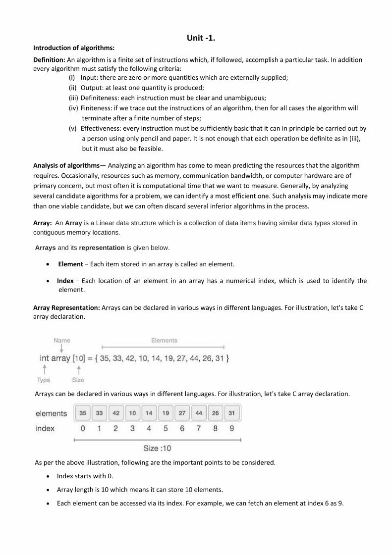
Array Representation: Arrays can be declared in various ways in different languages. For illustration, let's take C array declaration.

Arrays can be declared in various ways in different languages. For illustration, let's take C array declaration.

As per the above illustration, following are the important points to be considered.

• Index starts with 0.

• Array length is 10 which means it can store 10 elements.

• Each element can be accessed via its index. For example, we can fetch an element at index 6 as 9.

Basic Array Operations

Following are the basic operations supported by an array.

• Traverse − print all the array elements one by one.

• Insertion − Adds an element at the given index.

• Deletion − Deletes an element at the given index.

• Search − Searches an element using the given index or by the value.

• Update − Updates an element at the given index.

Stacks: A stack is an Abstract Data Type (ADT), commonly used in most programming languages. It is named

stack as it behaves like a real-world stack, for example – a deck of cards or a pile of plates, etc.

Definition: Stack is a linear data structure which follows a particular order in which the operations are performed. The order may be LIFO(Last In First Out) or FILO(First In Last Out).

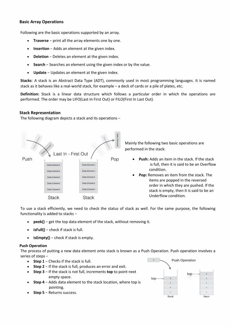
Stack Representation The following diagram depicts a stack and its operations −

Mainly the following two basic operations are

performed in the stack:

• Push: Adds an item in the stack. If the stack is full, then it is said to be an Overflow condition.

• Pop: Removes an item from the stack. The items are popped in the reversed order in which they are pushed. If the stack is empty, then it is said to be an Underflow condition.

To use a stack efficiently, we need to check the status of stack as well. For the same purpose, the following functionality is added to stacks −

• peek() − get the top data element of the stack, without removing it.

• isFull() − check if stack is full.

• isEmpty() − check if stack is empty.

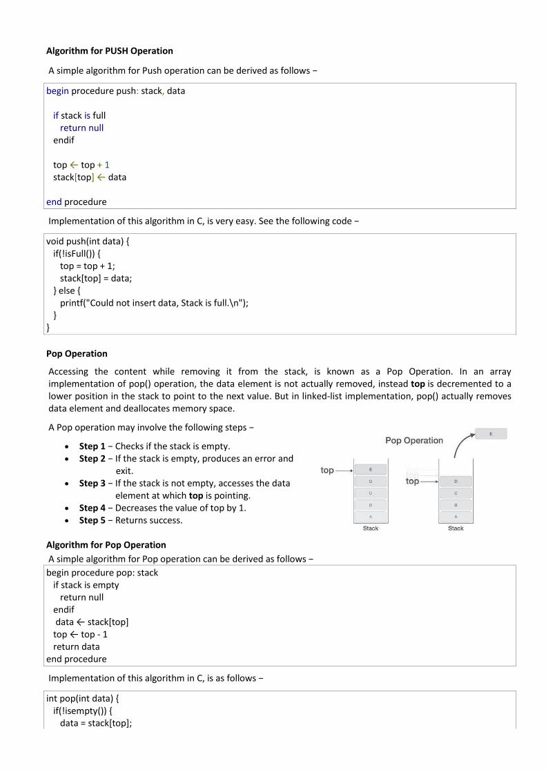
Push Operation The process of putting a new data element onto stack is known as a Push Operation. Push operation involves a series of steps −

• Step 1 − Checks if the stack is full. • Step 2 − If the stack is full, produces an error and exit. • Step 3 − If the stack is not full, increments top to point next empty space. • Step 4 − Adds data element to the stack location, where top is

pointing. • Step 5 − Returns success.

Algorithm for PUSH Operation

A simple algorithm for Push operation can be derived as follows −

begin procedure push: stack, data if stack is full return null endif top ← top + 1 stack[top] ← data end procedure

Implementation of this algorithm in C, is very easy. See the following code −

void push(int data) { if(!isFull()) { top = top + 1; stack[top] = data; } else { printf("Could not insert data, Stack is full.\n"); } }

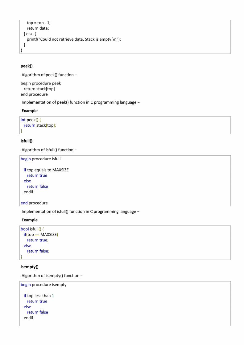
Pop Operation

Accessing the content while removing it from the stack, is known as a Pop Operation. In an array implementation of pop() operation, the data element is not actually removed, instead top is decremented to a lower position in the stack to point to the next value. But in linked-list implementation, pop() actually removes data element and deallocates memory space.

A Pop operation may involve the following steps −

• Step 1 − Checks if the stack is empty. • Step 2 − If the stack is empty, produces an error and

exit. • Step 3 − If the stack is not empty, accesses the data element at which top is pointing. • Step 4 − Decreases the value of top by 1. • Step 5 − Returns success.

Algorithm for Pop Operation

A simple algorithm for Pop operation can be derived as follows −

begin procedure pop: stack if stack is empty return null endif data ← stack[top] top ← top - 1 return data end procedure

Implementation of this algorithm in C, is as follows −

int pop(int data) { if(!isempty()) { data = stack[top];

top = top - 1; return data; } else { printf("Could not retrieve data, Stack is empty.\n"); } }

peek()

Algorithm of peek() function −

begin procedure peek return stack[top] end procedure

Implementation of peek() function in C programming language −

Example

int peek() { return stack[top]; }

isfull()

Algorithm of isfull() function −

begin procedure isfull if top equals to MAXSIZE return true else return false endif end procedure

Implementation of isfull() function in C programming language −

Example

bool isfull() { if(top == MAXSIZE) return true; else return false; }

isempty()

Algorithm of isempty() function −

begin procedure isempty if top less than 1 return true else return false endif

end procedure

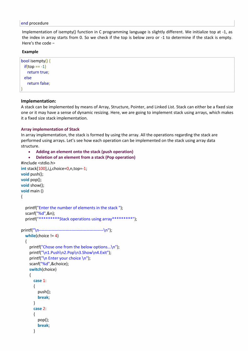
Implementation of isempty() function in C programming language is slightly different. We initialize top at -1, as the index in array starts from 0. So we check if the top is below zero or -1 to determine if the stack is empty. Here's the code −

Example

bool isempty() { if(top == -1) return true; else return false; }

Implementation: A stack can be implemented by means of Array, Structure, Pointer, and Linked List. Stack can either be a fixed size one or it may have a sense of dynamic resizing. Here, we are going to implement stack using arrays, which makes it a fixed size stack implementation. Array implementation of Stack In array implementation, the stack is formed by using the array. All the operations regarding the stack are performed using arrays. Let’s see how each operation can be implemented on the stack using array data structure.

• Adding an element onto the stack (push operation) • Deletion of an element from a stack (Pop operation)

#include <stdio.h> int stack[100],i,j,choice=0,n,top=-1; void push(); void pop(); void show(); void main () { printf("Enter the number of elements in the stack "); scanf("%d",&n); printf("*********Stack operations using array*********"); printf("\n----------------------------------------------\n"); while(choice != 4) { printf("Chose one from the below options...\n"); printf("\n1.Push\n2.Pop\n3.Show\n4.Exit"); printf("\n Enter your choice \n"); scanf("%d",&choice); switch(choice) { case 1: { push(); break; } case 2: { pop(); break; }

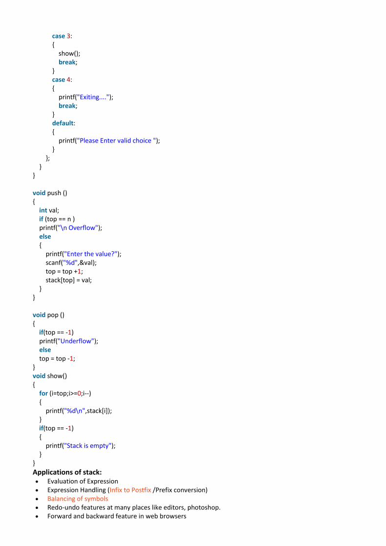
case 3: { show(); break; } case 4: { printf("Exiting...."); break; } default: { printf("Please Enter valid choice "); } }; } } void push () { int val; if (top == n ) printf("\n Overflow"); else { printf("Enter the value?"); scanf("%d",&val); top = top +1; stack[top] = val; } } void pop () { if(top == -1) printf("Underflow"); else top = top -1; } void show() { for (i=top;i>=0;i--) { printf("%d\n",stack[i]); } if(top == -1) { printf("Stack is empty"); } }

Applications of stack: • Evaluation of Expression • Expression Handling (Infix to Postfix /Prefix conversion) • Balancing of symbols • Redo-undo features at many places like editors, photoshop. • Forward and backward feature in web browsers

• Used in many algorithms like Tower of Hanoi, tree traversals, stock span problem, histogram problem. • Other applications can be Backtracking, Knight tour problem, rat in a maze, N queen problem and sudoku

solver • In Graph Algorithms like Topological Sorting and Strongly Connected Components

Evaluation of Expression Stack is used to evaluate prefix, postfix and infix expressions.

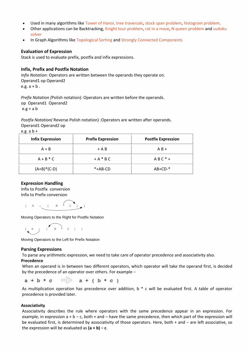
Infix, Prefix and Postfix Notation Infix Notation: Operators are written between the operands they operate on. Operand1 op Operand2 e.g. a + b . Prefix Notation (Polish notation): Operators are written before the operands. op Operand1 Operand2 e.g + a b Postfix Notation( Reverse Polish notation) :Operators are written after operands. Operand1 Operand2 op e.g a b +

Infix Expression Prefix Expression Postfix Expression

A + B + A B A B +

A + B * C + A * B C A B C * +

(A+B)*(C-D) *+AB-CD AB+CD-*

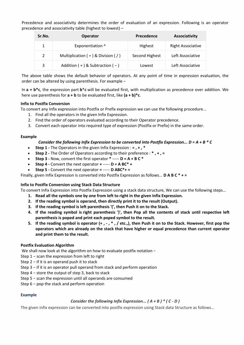
Expression Handling Infix to Postfix conversion Infix to Prefix conversion

Moving Operators to the Right for Postfix Notation

Moving Operators to the Left for Prefix Notation

Parsing Expressions To parse any arithmetic expression, we need to take care of operator precedence and associativity also. Precedence When an operand is in between two different operators, which operator will take the operand first, is decided by the precedence of an operator over others. For example −

As multiplication operation has precedence over addition, b * c will be evaluated first. A table of operator precedence is provided later. Associativity Associativity describes the rule where operators with the same precedence appear in an expression. For example, in expression a + b − c, both + and – have the same precedence, then which part of the expression will be evaluated first, is determined by associativity of those operators. Here, both + and − are left associative, so the expression will be evaluated as (a + b) − c.

Precedence and associativity determines the order of evaluation of an expression. Following is an operator precedence and associativity table (highest to lowest) –

Sr.No. Operator Precedence Associativity

1 Exponentiation ^ Highest Right Associative

2 Multiplication ( ∗ ) & Division ( / ) Second Highest Left Associative

3 Addition ( + ) & Subtraction ( − ) Lowest Left Associative

The above table shows the default behavior of operators. At any point of time in expression evaluation, the order can be altered by using parenthesis. For example −

In a + b*c, the expression part b*c will be evaluated first, with multiplication as precedence over addition. We here use parenthesis for a + b to be evaluated first, like (a + b)*c.

Infix to Postfix Conversion To convert any Infix expression into Postfix or Prefix expression we can use the following procedure...

1. Find all the operators in the given Infix Expression. 2. Find the order of operators evaluated according to their Operator precedence. 3. Convert each operator into required type of expression (Postfix or Prefix) in the same order.

Example

Consider the following Infix Expression to be converted into Postfix Expression... D = A + B * C • Step 1 - The Operators in the given Infix Expression : = , + , * • Step 2 - The Order of Operators according to their preference : * , + , = • Step 3 - Now, convert the first operator * ----- D = A + B C * • Step 4 - Convert the next operator + ----- D = A BC* + • Step 5 - Convert the next operator = ----- D ABC*+ =

Finally, given Infix Expression is converted into Postfix Expression as follows... D A B C * + =

Infix to Postfix Conversion using Stack Data Structure To convert Infix Expression into Postfix Expression using a stack data structure, We can use the following steps...

1. Read all the symbols one by one from left to right in the given Infix Expression. 2. If the reading symbol is operand, then directly print it to the result (Output). 3. If the reading symbol is left parenthesis '(', then Push it on to the Stack. 4. If the reading symbol is right parenthesis ')', then Pop all the contents of stack until respective left

parenthesis is poped and print each poped symbol to the result. 5. If the reading symbol is operator (+ , - , * , / etc.,), then Push it on to the Stack. However, first pop the

operators which are already on the stack that have higher or equal precedence than current operator and print them to the result.

Postfix Evaluation Algorithm We shall now look at the algorithm on how to evaluate postfix notation − Step 1 − scan the expression from left to right Step 2 − if it is an operand push it to stack Step 3 − if it is an operator pull operand from stack and perform operation Step 4 − store the output of step 3, back to stack Step 5 − scan the expression until all operands are consumed Step 6 − pop the stack and perform operation Example

Consider the following Infix Expression... ( A + B ) * ( C - D )

The given infix expression can be converted into postfix expression using Stack data Structure as follows...

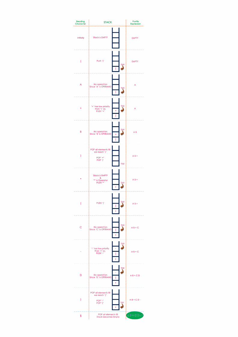
The final Postfix Expression is as follows... A B + C D - *

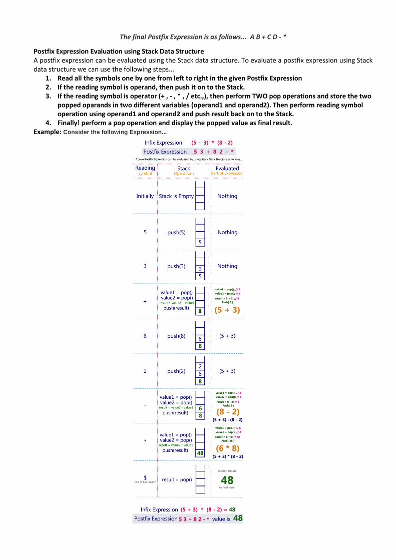
Postfix Expression Evaluation using Stack Data Structure A postfix expression can be evaluated using the Stack data structure. To evaluate a postfix expression using Stack data structure we can use the following steps...

1. Read all the symbols one by one from left to right in the given Postfix Expression 2. If the reading symbol is operand, then push it on to the Stack. 3. If the reading symbol is operator (+ , - , * , / etc.,), then perform TWO pop operations and store the two

popped oparands in two different variables (operand1 and operand2). Then perform reading symbol operation using operand1 and operand2 and push result back on to the Stack.

4. Finally! perform a pop operation and display the popped value as final result. Example: Consider the following Expression...

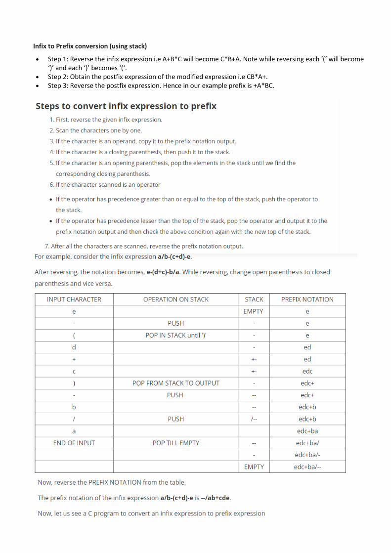
Infix to Prefix conversion (using stack)

• Step 1: Reverse the infix expression i.e A+B*C will become C*B+A. Note while reversing each ‘(‘ will become ‘)’ and each ‘)’ becomes ‘(‘.

• Step 2: Obtain the postfix expression of the modified expression i.e CB*A+. • Step 3: Reverse the postfix expression. Hence in our example prefix is +A*BC.

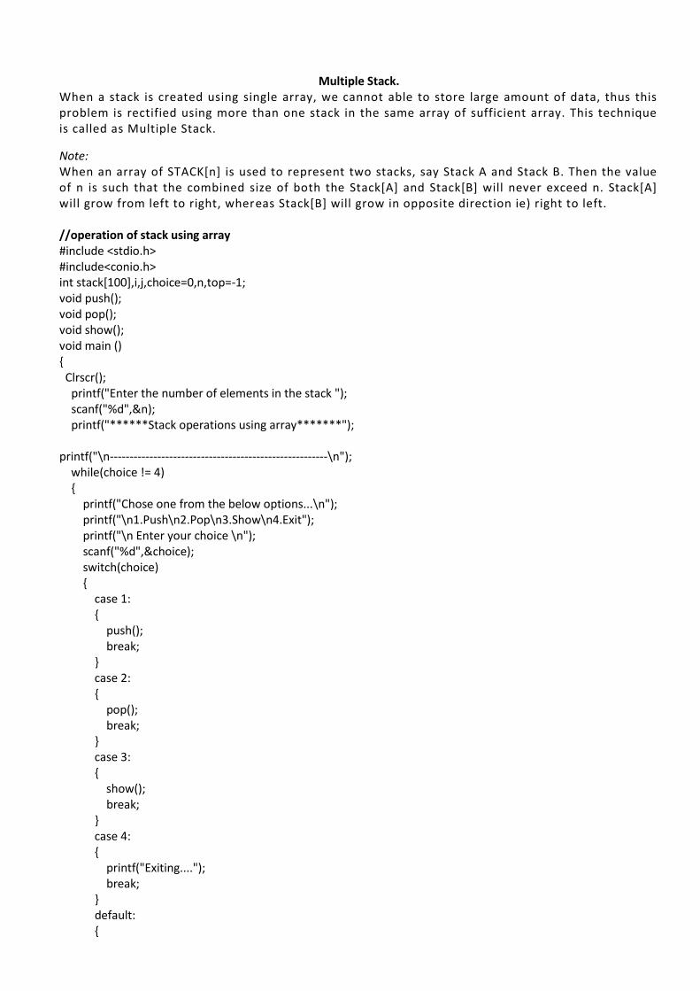
Multiple Stack.

When a stack is created using single array, we cannot able to store large amount of data, thus this problem is rectified using more than one stack in the same array of sufficient array. This technique is called as Multiple Stack.

Note: When an array of STACK[n] is used to represent two stacks, say Stack A and Stack B. Then the value of n is such that the combined size of both the Stack[A] and Stack[B] will never exceed n. Stack[A] will grow from left to right, whereas Stack[B] will grow in opposite direction ie) right to left. //operation of stack using array #include <stdio.h> #include<conio.h> int stack[100],i,j,choice=0,n,top=-1; void push(); void pop(); void show(); void main () { Clrscr(); printf("Enter the number of elements in the stack "); scanf("%d",&n); printf("******Stack operations using array*******"); printf("\n-------------------------------------------------------\n"); while(choice != 4) { printf("Chose one from the below options...\n"); printf("\n1.Push\n2.Pop\n3.Show\n4.Exit"); printf("\n Enter your choice \n"); scanf("%d",&choice); switch(choice) { case 1: { push(); break; } case 2: { pop(); break; } case 3: { show(); break; } case 4: { printf("Exiting...."); break; } default: {

printf("Please Enter valid choice "); } }; } } void push () { int val; if (top == n ) printf("\n Overflow"); else { printf("Enter the value?"); scanf("%d",&val); top = top +1; stack[top] = val; } } void pop () { if(top == -1) printf("Underflow"); else top = top -1; } void show() { for (i=top;i>=0;i--) { printf("%d\n",stack[i]); } if(top == -1) { printf("Stack is empty"); } } //infix to postfix conversion #include<stdio.h> #include<conio.h> char stack[20]; int top = -1; void push(char x) { stack[++top] = x; } char pop() { if(top == -1) return -1; else return stack[top--]; } int priority(char x) { if(x == '(')

return 0; if(x == '+' || x == '-') return 1; if(x == '*' || x == '/') return 2; } void main() { char exp[20]; char *e, x; clrscr(); printf("Enter the expression :: "); scanf("%s",exp); e = exp; while(*e != '\0') { if(isalnum(*e)) printf("%c",*e); else if(*e == '(') push(*e); else if(*e == ')') { while((x = pop()) != '(') printf("%c", x); } else { while(priority(stack[top]) >= priority(*e)) printf("%c",pop()); push(*e); } e++; } while(top != -1) { printf("%c",pop()); } getch(); }

Queue What is Queue?

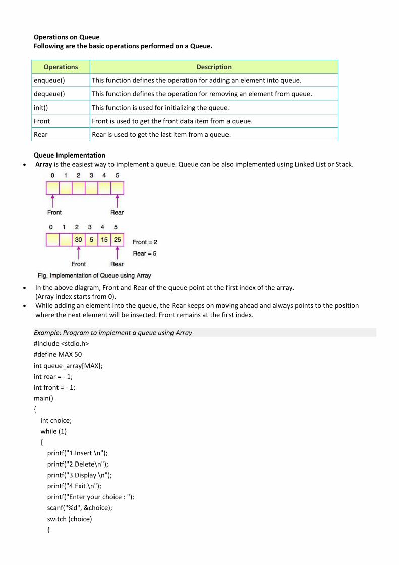
• Queue is a linear data structure where the first element is inserted from one end called REAR and deleted from the other end called as FRONT.

• Front points to the beginning of the queue and Rear points to the end of the queue. • Queue follows the FIFO (First - In - First Out) structure. • According to its FIFO structure, element inserted first will also be removed first. • In a queue, one end is always used to insert data (enqueue) and the other is used to delete data (dequeue),

because queue is open at both its ends. • The enqueue() and dequeue() are two important functions used in a queue.

Operations on Queue Following are the basic operations performed on a Queue.

Operations Description

enqueue() This function defines the operation for adding an element into queue.

dequeue() This function defines the operation for removing an element from queue.

init() This function is used for initializing the queue.

Front Front is used to get the front data item from a queue.

Rear Rear is used to get the last item from a queue.

Queue Implementation

• Array is the easiest way to implement a queue. Queue can be also implemented using Linked List or Stack.

• In the above diagram, Front and Rear of the queue point at the first index of the array.

(Array index starts from 0). • While adding an element into the queue, the Rear keeps on moving ahead and always points to the position

where the next element will be inserted. Front remains at the first index. Example: Program to implement a queue using Array

#include <stdio.h>

#define MAX 50

int queue_array[MAX];

int rear = - 1;

int front = - 1;

main()

{

int choice;

while (1)

{

printf("1.Insert \n");

printf("2.Delete\n");

printf("3.Display \n");

printf("4.Exit \n");

printf("Enter your choice : ");

scanf("%d", &choice);

switch (choice)

{

case 1:

insert();

break;

case 2:

delete();

break;

case 3:

display();

break;

case 4:

exit(1);

default:

printf("Inavlid choice \n");

} /*End of switch*/

} /*End of while*/

} /*End of main()*/

insert()

{

int add_item;

if (rear == MAX - 1)

printf("Queue Overflow \n");

else

{

if (front == - 1)

/*If queue is initially empty */

front = 0;

printf("Inset the element in queue : ");

scanf("%d", &add_item);

rear = rear + 1;

queue_array[rear] = add_item;

}

} /*End of insert()*/

delete()

{

if (front == - 1 || front > rear)

{

printf("Queue Underflow \n");

return ;

}

else

{

printf("Deleted Element is : %d\n", queue_array[front]);

front = front + 1;

}

} /*End of delete() */

display()

{

int i;

if (front == - 1)

printf("Queue is empty \n");

else

{

printf("Queue is : \n");

for (i = front; i <= rear; i++)

printf("%d ", queue_array[i]);

printf("\n");

}

} /*End of display() */

Sl.No. STACKS QUEUES

1 Stacks are based on the LIFO Queues are based on the FIFO

2 Insertion and deletion in stacks takes place only from one end of the list called the top.

Insertion and deletion in queues takes place from the opposite ends of the list. The insertion takes place at the rear of the list and the deletion takes place from the front of the list.

3 Insert operation is called push operation. Insert operation is called enqueue operation.

4 Delete operation is called pop operation. Delete operation is called dequeue operation

Sparse Matrix

What is Sparse Matrix?

In computer programming, a matrix can be defined with a 2-dimensional array. Any array with ‘m’ columns and ‘n’ rows represents a mXn matrix. There may be a situation in which a matrix contains more number of ZERO values than NON-ZERO values. Such matrix is known as sparse matrix.

Sparse matrix is a matrix which contains very few non-zero elements.

When a sparse matrix is represented with 2-dimensional array, we waste lot of space to represent that matrix. For example, consider a matrix of size 100 X 100 containing only 10 non-zero elements.

In this matrix, only 10 spaces are filled with non-zero values and remaining spaces of matrix are filled with zero. That means, totally we allocate 100 X 100 X 2 = 20000 bytes of space to store this integer matrix. And to access these 10 non-zero elements we have to make scanning for 10000 times.

Sparse Matrix Representations

A sparse matrix can be represented by using TWO representations, those are as follows…

1. Triplet Representation 2. Linked Representation

Triplet Representation (Array Representation)

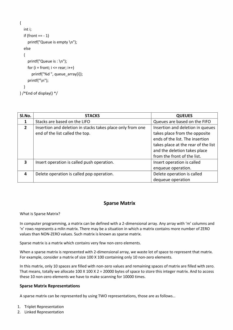
In this representation, we consider only non-zero values along with their row and column index values. In this representation, the 0th row stores the total number of rows, total number of columns and the total number of non-zero values in the sparse matrix. For example, consider a matrix of size 5 X 6 containing 6 number of non-zero values. This matrix can be represented as shown in the image...

In above example matrix, there are only 6 non-zero elements (those are 9, 8, 4, 2, 5 & 2) and matrix size is 5 X 6. We represent this matrix as shown in the above image. Here the first row in the right side table is filled with values 5, 6 & 6 which indicate that it is a sparse matrix with 5 rows, 6 columns & 6 non-zero values. The second row is filled with 0, 4, & 9 which indicate the non-zero value 9 is at the 0th-row 4th column in the Sparse matrix. In the same way, the remaining non-zero values also follow a similar pattern.

Linked Representation

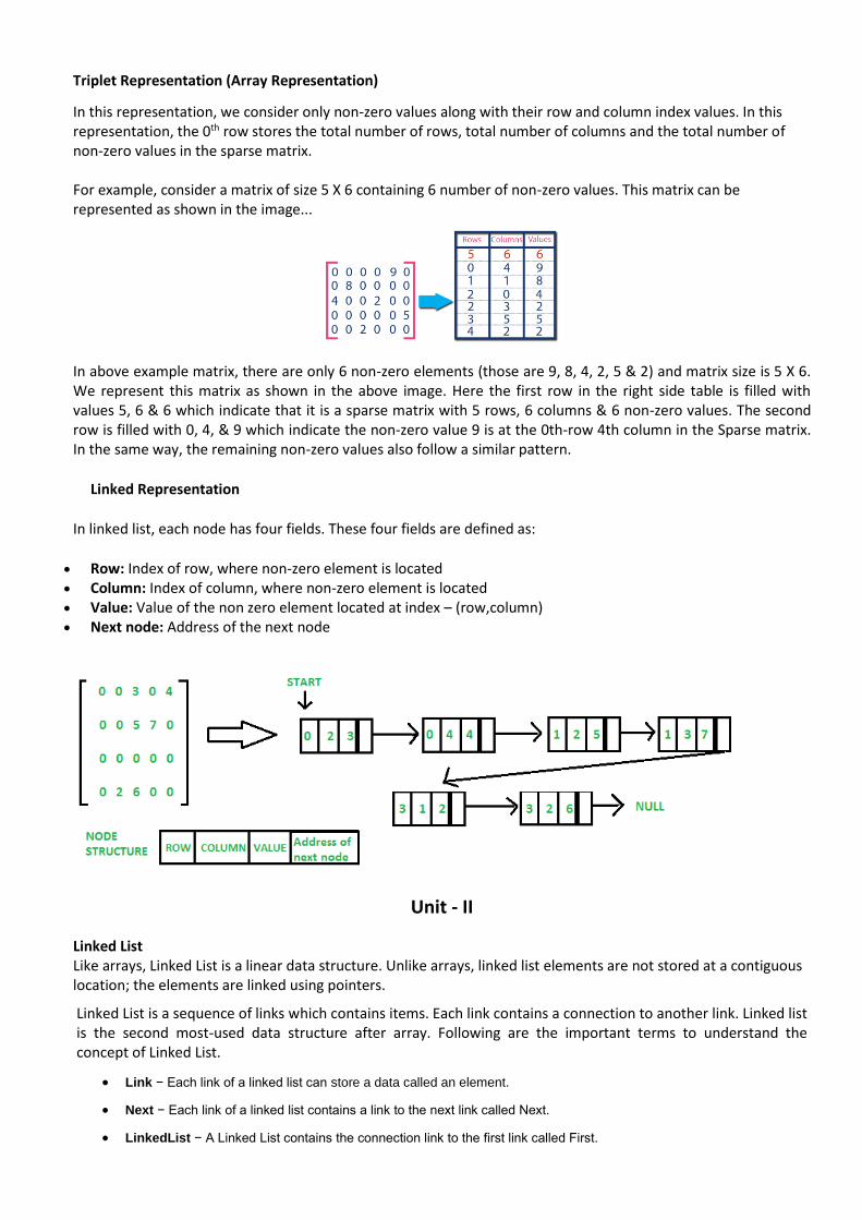
In linked list, each node has four fields. These four fields are defined as:

• Row: Index of row, where non-zero element is located • Column: Index of column, where non-zero element is located • Value: Value of the non zero element located at index – (row,column) • Next node: Address of the next node

Unit - II

Linked List Like arrays, Linked List is a linear data structure. Unlike arrays, linked list elements are not stored at a contiguous location; the elements are linked using pointers.

Linked List is a sequence of links which contains items. Each link contains a connection to another link. Linked list is the second most-used data structure after array. Following are the important terms to understand the concept of Linked List.

• Link − Each link of a linked list can store a data called an element.

• Next − Each link of a linked list contains a link to the next link called Next.

• LinkedList − A Linked List contains the connection link to the first link called First.

Why Linked List? Arrays can be used to store linear data of similar types, but arrays have the following limitations. 1) The size of the arrays is fixed: So we must know the upper limit on the number of elements in advance. Also, generally, the allocated memory is equal to the upper limit irrespective of the usage. 2) Inserting a new element in an array of elements is expensive because the room has to be created for the new elements and to create room existing elements have to be shifted.

For example, in a system, if we maintain a sorted list of IDs in an array id[]. id[] = [1000, 1010, 1050, 2000, 2040]. And if we want to insert a new ID 1005, then to maintain the sorted order, we have to move all the elements after 1000 (excluding 1000). Deletion is also expensive with arrays until unless some special techniques are used. For example, to delete 1010 in id[], everything after 1010 has to be moved.

Advantages over arrays 1) Dynamic size 2) Ease of insertion/deletion Drawbacks: 1) Random access is not allowed. We have to access elements sequentially starting from the first node. So we cannot do binary search with linked lists efficiently with its default implementation. Read about it here. 2) Extra memory space for a pointer is required with each element of the list. 3) Not cache friendly. Since array elements are contiguous locations, there is locality of reference which is not there in case of linked lists. Linked List Representation: A linked list is represented by a pointer to the first node of the linked list. The first node is called the head. If the linked list is empty, then the value of the head is NULL. Each node in a list consists of at least two parts: 1) data 2) Pointer (Or Reference) to the next node

Types of Linked List

Following are the various types of linked list.

• Simple Linked List(Singly Linked List) − Item navigation is forward only.

• Doubly Linked List − Items can be navigated forward and backward.

• Circular Linked List − Last item contains link of the first element as next and the first element has a link to the last element as previous.

Simple Linked List(Singly Linked List)

Basic Operations Following are the basic operations supported by a list.

• Insertion − Adds an element at the beginning of the list. • Deletion − Deletes an element at the beginning of the list. • Display − Displays the complete list. • Search − Searches an element using the given key. • Delete − Deletes an element using the given key.

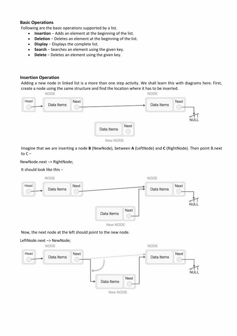
Insertion Operation Adding a new node in linked list is a more than one step activity. We shall learn this with diagrams here. First, create a node using the same structure and find the location where it has to be inserted.

Imagine that we are inserting a node B (NewNode), between A (LeftNode) and C (RightNode). Then point B.next to C −

NewNode.next −> RightNode;

It should look like this −

Now, the next node at the left should point to the new node.

LeftNode.next −> NewNode;

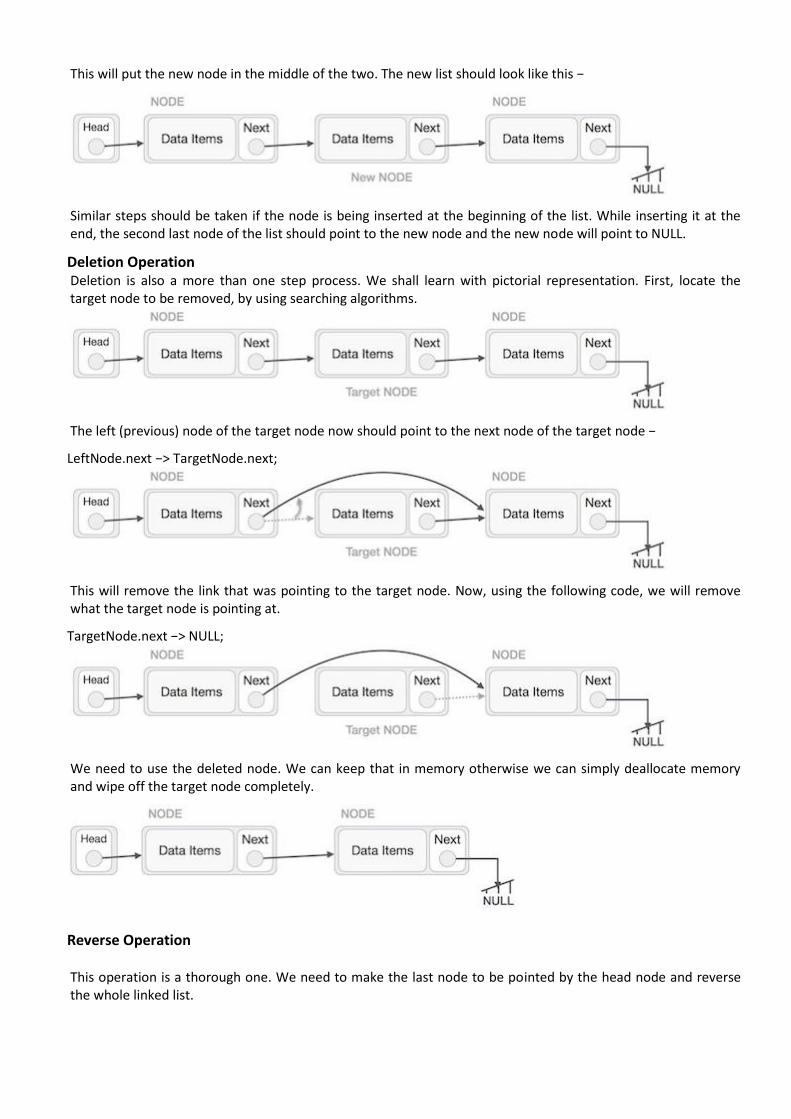
This will put the new node in the middle of the two. The new list should look like this −

Similar steps should be taken if the node is being inserted at the beginning of the list. While inserting it at the end, the second last node of the list should point to the new node and the new node will point to NULL.

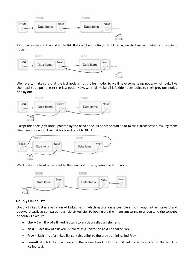
Deletion Operation Deletion is also a more than one step process. We shall learn with pictorial representation. First, locate the target node to be removed, by using searching algorithms.

The left (previous) node of the target node now should point to the next node of the target node −

LeftNode.next −> TargetNode.next;

This will remove the link that was pointing to the target node. Now, using the following code, we will remove what the target node is pointing at.

TargetNode.next −> NULL;

We need to use the deleted node. We can keep that in memory otherwise we can simply deallocate memory and wipe off the target node completely.

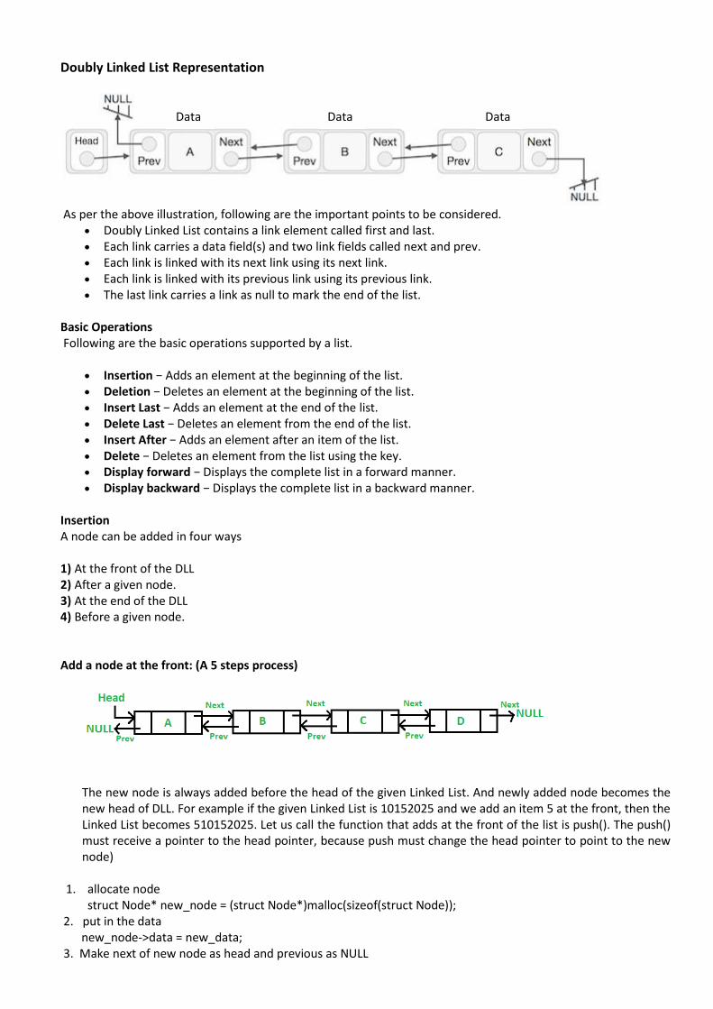
Reverse Operation

This operation is a thorough one. We need to make the last node to be pointed by the head node and reverse the whole linked list.

First, we traverse to the end of the list. It should be pointing to NULL. Now, we shall make it point to its previous node −

We have to make sure that the last node is not the lost node. So we'll have some temp node, which looks like the head node pointing to the last node. Now, we shall make all left side nodes point to their previous nodes one by one.

Except the node (first node) pointed by the head node, all nodes should point to their predecessor, making them their new successor. The first node will point to NULL.

We'll make the head node point to the new first node by using the temp node.

Doubly Linked List

Doubly Linked List is a variation of Linked list in which navigation is possible in both ways, either forward and backward easily as compared to Single Linked List. Following are the important terms to understand the concept of doubly linked list.

• Link − Each link of a linked list can store a data called an element.

• Next − Each link of a linked list contains a link to the next link called Next.

• Prev − Each link of a linked list contains a link to the previous link called Prev.

• LinkedList − A Linked List contains the connection link to the first link called First and to the last link called Last.

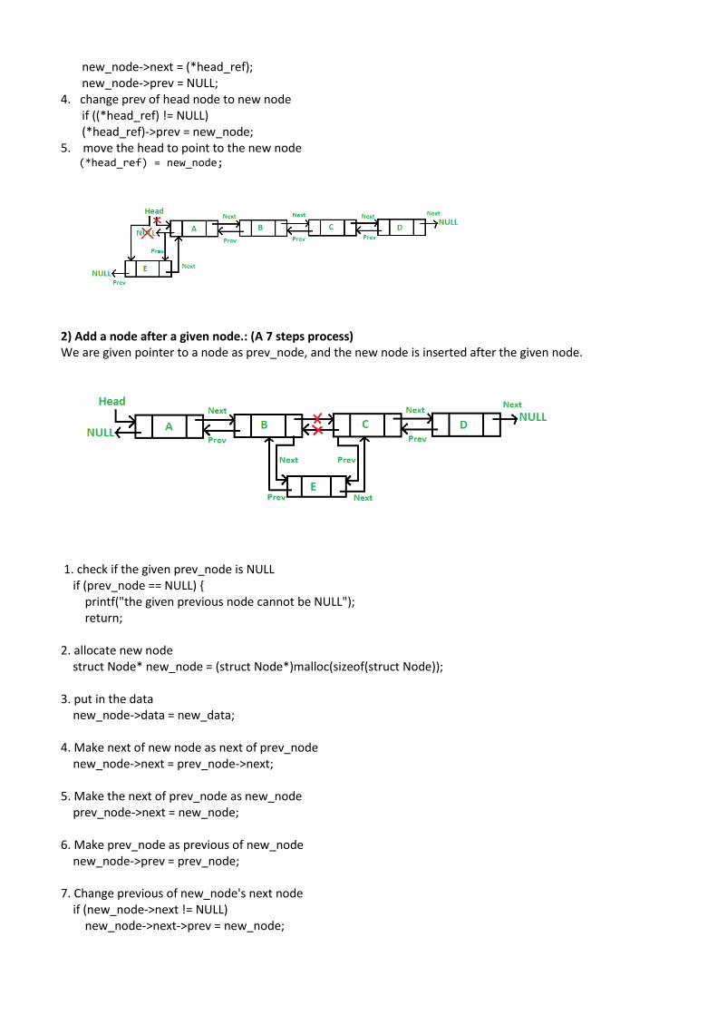
Doubly Linked List Representation

As per the above illustration, following are the important points to be considered.

• Doubly Linked List contains a link element called first and last. • Each link carries a data field(s) and two link fields called next and prev. • Each link is linked with its next link using its next link. • Each link is linked with its previous link using its previous link. • The last link carries a link as null to mark the end of the list.

Basic Operations Following are the basic operations supported by a list.

• Insertion − Adds an element at the beginning of the list. • Deletion − Deletes an element at the beginning of the list. • Insert Last − Adds an element at the end of the list. • Delete Last − Deletes an element from the end of the list. • Insert After − Adds an element after an item of the list. • Delete − Deletes an element from the list using the key. • Display forward − Displays the complete list in a forward manner. • Display backward − Displays the complete list in a backward manner.

Insertion A node can be added in four ways 1) At the front of the DLL 2) After a given node. 3) At the end of the DLL 4) Before a given node. Add a node at the front: (A 5 steps process)

The new node is always added before the head of the given Linked List. And newly added node becomes the new head of DLL. For example if the given Linked List is 10152025 and we add an item 5 at the front, then the Linked List becomes 510152025. Let us call the function that adds at the front of the list is push(). The push() must receive a pointer to the head pointer, because push must change the head pointer to point to the new node)

1. allocate node struct Node* new_node = (struct Node*)malloc(sizeof(struct Node));

2. put in the data new_node->data = new_data; 3. Make next of new node as head and previous as NULL

Data Data Data

new_node->next = (*head_ref); new_node->prev = NULL; 4. change prev of head node to new node if ((*head_ref) != NULL) (*head_ref)->prev = new_node; 5. move the head to point to the new node (*head_ref) = new_node;

2) Add a node after a given node.: (A 7 steps process) We are given pointer to a node as prev_node, and the new node is inserted after the given node.

1. check if the given prev_node is NULL if (prev_node == NULL) { printf("the given previous node cannot be NULL"); return; 2. allocate new node struct Node* new_node = (struct Node*)malloc(sizeof(struct Node)); 3. put in the data new_node->data = new_data; 4. Make next of new node as next of prev_node new_node->next = prev_node->next; 5. Make the next of prev_node as new_node prev_node->next = new_node; 6. Make prev_node as previous of new_node new_node->prev = prev_node; 7. Change previous of new_node's next node if (new_node->next != NULL) new_node->next->prev = new_node;

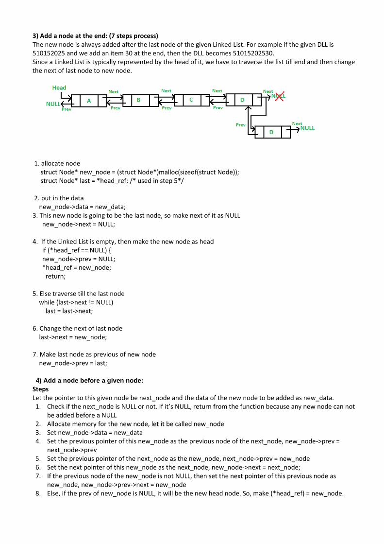
3) Add a node at the end: (7 steps process) The new node is always added after the last node of the given Linked List. For example if the given DLL is 510152025 and we add an item 30 at the end, then the DLL becomes 51015202530. Since a Linked List is typically represented by the head of it, we have to traverse the list till end and then change the next of last node to new node.

1. allocate node struct Node* new_node = (struct Node*)malloc(sizeof(struct Node)); struct Node* last = *head_ref; /* used in step 5*/ 2. put in the data new_node->data = new_data; 3. This new node is going to be the last node, so make next of it as NULL new_node->next = NULL; 4. If the Linked List is empty, then make the new node as head if (*head_ref == NULL) { new_node->prev = NULL; *head_ref = new_node; return; 5. Else traverse till the last node while (last->next != NULL) last = last->next; 6. Change the next of last node last->next = new_node; 7. Make last node as previous of new node new_node->prev = last; 4) Add a node before a given node:

Steps Let the pointer to this given node be next_node and the data of the new node to be added as new_data. 1. Check if the next_node is NULL or not. If it’s NULL, return from the function because any new node can not

be added before a NULL 2. Allocate memory for the new node, let it be called new_node 3. Set new_node->data = new_data 4. Set the previous pointer of this new_node as the previous node of the next_node, new_node->prev =

next_node->prev 5. Set the previous pointer of the next_node as the new_node, next_node->prev = new_node 6. Set the next pointer of this new_node as the next_node, new_node->next = next_node; 7. If the previous node of the new_node is not NULL, then set the next pointer of this previous node as

new_node, new_node->prev->next = new_node 8. Else, if the prev of new_node is NULL, it will be the new head node. So, make (*head_ref) = new_node.

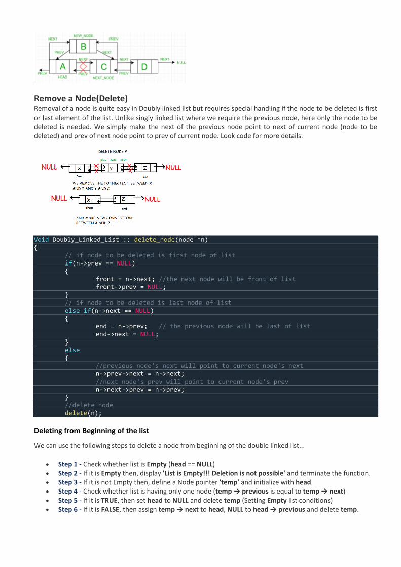
Remove a Node(Delete) Removal of a node is quite easy in Doubly linked list but requires special handling if the node to be deleted is first or last element of the list. Unlike singly linked list where we require the previous node, here only the node to be deleted is needed. We simply make the next of the previous node point to next of current node (node to be deleted) and prev of next node point to prev of current node. Look code for more details.

Void Doubly_Linked_List :: delete_node(node *n) { // if node to be deleted is first node of list if(n->prev == NULL) { front = n->next; //the next node will be front of list front->prev = NULL; } // if node to be deleted is last node of list else if(n->next == NULL) { end = n->prev; // the previous node will be last of list end->next = NULL; } else { //previous node's next will point to current node's next n->prev->next = n->next; //next node's prev will point to current node's prev n->next->prev = n->prev; } //delete node delete(n);

Deleting from Beginning of the list

We can use the following steps to delete a node from beginning of the double linked list...

• Step 1 - Check whether list is Empty (head == NULL) • Step 2 - If it is Empty then, display 'List is Empty!!! Deletion is not possible' and terminate the function. • Step 3 - If it is not Empty then, define a Node pointer 'temp' and initialize with head. • Step 4 - Check whether list is having only one node (temp → previous is equal to temp → next) • Step 5 - If it is TRUE, then set head to NULL and delete temp (Setting Empty list conditions) • Step 6 - If it is FALSE, then assign temp → next to head, NULL to head → previous and delete temp.

Deleting from End of the list

We can use the following steps to delete a node from end of the double linked list...

• Step 1 - Check whether list is Empty (head == NULL) • Step 2 - If it is Empty, then display 'List is Empty!!! Deletion is not possible' and terminate the function. • Step 3 - If it is not Empty then, define a Node pointer 'temp' and initialize with head. • Step 4 - Check whether list has only one Node (temp → previous and temp → next both are NULL) • Step 5 - If it is TRUE, then assign NULL to head and delete temp. And terminate from the function.

(Setting Empty list condition) • Step 6 - If it is FALSE, then keep moving temp until it reaches to the last node in the list. (until temp →

next is equal to NULL) • Step 7 - Assign NULL to temp → previous → next and delete temp.

Deleting a Specific Node from the list

We can use the following steps to delete a specific node from the double linked list...

• Step 1 - Check whether list is Empty (head == NULL) • Step 2 - If it is Empty then, display 'List is Empty!!! Deletion is not possible' and terminate the function. • Step 3 - If it is not Empty, then define a Node pointer 'temp' and initialize with head. • Step 4 - Keep moving the temp until it reaches to the exact node to be deleted or to the last node. • Step 5 - If it is reached to the last node, then display 'Given node not found in the list! Deletion not

possible!!!' and terminate the fuction. • Step 6 - If it is reached to the exact node which we want to delete, then check whether list is having only

one node or not • Step 7 - If list has only one node and that is the node which is to be deleted then set head to NULL and

delete temp (free(temp)). • Step 8 - If list contains multiple nodes, then check whether temp is the first node in the list (temp ==

head). • Step 9 - If temp is the first node, then move the head to the next node (head = head → next),

set head of previous to NULL (head → previous = NULL) and delete temp. • Step 10 - If temp is not the first node, then check whether it is the last node in the list (temp → next ==

NULL). • Step 11 - If temp is the last node then set temp of previous of next to NULL (temp → previous → next =

NULL) and delete temp (free(temp)). • Step 12 - If temp is not the first node and not the last node, then

set temp of previous of next to temp of next (temp → previous → next = temp → next), temp of next of previous to temp of previous (temp → next → previous = temp → previous) and delete temp (free(temp)).

Forward Traversal

Start with the front node and visit all the nodes untill the node becomes NULL.

void Doubly_Linked_List :: forward_traverse() { node *trav; trav = front; while(trav != NULL) { cout<<trav->data<<endl; trav = trav->next; } }

Backward Traversal

Start with the end node and visit all the nodes until the node becomes NULL.

void Doubly_Linked_List :: backward_traverse() { node *trav; trav = end; while(trav != NULL) { cout<<trav->data<<endl; trav = trav->prev; } }

Implementing Stack Using a Linked List Stack can be implemented using both arrays and linked lists. The limitation, in the case of an array, is that we need to define the size at the beginning of the implementation. This makes our stack static. It can also result in “stack overflow” if we try to add elements after the array is full. So, to alleviate this problem, we use a linked list to implement the stack so that it can grow in real time. First, we will create our Node class which will form our linked list. We will be using this same Node class to also implement the queue in the later part of this article. internal class Node { internal int data; internal Node next; // Constructor to create a new node.Next is by default initialized as null public Node(int d) { data = d; next = null; } } Now, we will create our stack class. We will define a pointer, top, and initialize it to null. So, our LinkedListStack class will be: internal class LinkListStack { Node top; public LinkListStack() { this.top = null; } } Push an Element Onto a Stack Now, our stack and Node class is ready. So, we will proceed to push the operation onto the stack. We will add a new element at the top of the stack. Algorithm

• Create a new node with the value to be inserted. • If the stack is empty, set the next of the new node to null. • If the stack is not empty, set the next of the new node to top. • Finally, increment the top to point to the new node.

The time complexity for the Push operation is O(1). The method for push will look like this: internal void Push(int value) { Node newNode = new Node(value); if (top == null) {

newNode.next = null; } else { newNode.next = top; } top = newNode; Console.WriteLine("{0} pushed to stack", value); } Pop an Element From the Stack We will remove the top element from the stack. Algorithm

• If the stack is empty, terminate the method as it is stack underflow. • If the stack is not empty, increment the top to point to the next node. • Hence the element pointed to by the top earlier is now removed.

The time complexity for Pop operation is O(1). The method for pop will look like the following: internal void Pop() { if (top == null) { Console.WriteLine("Stack Underflow. Deletion not possible"); return; } Console.WriteLine("Item popped is {0}", top.data); top = top.next; }

Implementing Queue Functionalities Using Linked List

Similar to stack, the queue can also be implemented using both arrays and linked lists. But it also has the same drawback of limited size. Hence, we will be using a linked list to implement the queue. The Node class will be the same as defined above in the stack implementation. We will define the LinkedListQueue class as below: internal class LinkListQueue { Node front; Node rear; public LinkListQueue() { this.front = this.rear = null; } } Here, we have taken two pointers – rear and front – to refer to the rear and the front end of the queue respectively, and will initialize it to null. Enqueue of an Element We will add a new element to our queue from the rear end. Algorithm

• Create a new node with the value to be inserted. • If the queue is empty, then set both front and rear to point to newNode. • If the queue is not empty, then set next to the rear of the new node and the rear to point to the new

node. The time complexity for Enqueue operation is O(1). The method for Enqueue will look like the following: internal void Enqueue(int item) { Node newNode = new Node(item);

// If queue is empty, then new node is front and rear both if (this.rear == null) { this.front = this.rear = newNode; } else { // Add the new node at the end of queue and change rear this.rear.next = newNode; this.rear = newNode; } Console.WriteLine("{0} inserted into Queue", item); } Dequeue of an Element We will delete the existing element from the queue from the front end. Algorithm

• If the queue is empty, terminate the method. • If the queue is not empty, increment the front to point to the next node. • Finally, check if the front is null, then set rear to null also. This signifies an empty queue.

The time complexity for Dequeue operation is O(1). The method for Dequeue will look like the following: internal void Dequeue() { // If queue is empty, return NULL. if (this.front == null) { Console.WriteLine("The Queue is empty"); return; } // Store previous front and move front one node ahead Node temp = this.front; this.front = this.front.next; // If front becomes NULL, then change rear also as NULL if (this.front == null) { this.rear = null; } Console.WriteLine("Item deleted is {0}", temp.data); }

What is Polynomial A polynomial p(x) is the expression in variable x which is in the form (axn + bxn-1 + …. + jx+ k), where a, b, c …., k fall in the category of real numbers and 'n' is non negative integer, which is called the degree of polynomial. An essential characteristic of the polynomial is that each term in the polynomial expression consists of two parts:

• one is the coefficient • other is the exponent

Example: 10x2 + 26x, here 10 and 26 are coefficients and 2, 1 is its exponential value. Points to keep in Mind while working with Polynomials:

• The sign of each coefficient and exponent is stored within the coefficient and the exponent itself • Additional terms having equal exponent is possible one

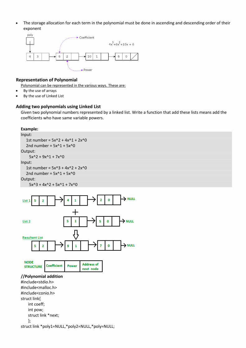
• The storage allocation for each term in the polynomial must be done in ascending and descending order of their exponent

Representation of Polynomial

Polynomial can be represented in the various ways. These are:

• By the use of arrays

• By the use of Linked List

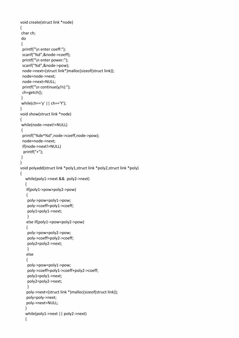
Adding two polynomials using Linked List

Given two polynomial numbers represented by a linked list. Write a function that add these lists means add the coefficients who have same variable powers. Example: Input: 1st number = 5x^2 + 4x^1 + 2x^0 2nd number = 5x^1 + 5x^0 Output: 5x^2 + 9x^1 + 7x^0 Input: 1st number = 5x^3 + 4x^2 + 2x^0 2nd number = 5x^1 + 5x^0 Output: 5x^3 + 4x^2 + 5x^1 + 7x^0

//Polynomial addition #include<stdio.h> #include<malloc.h> #include<conio.h> struct link{ int coeff; int pow; struct link *next; }; struct link *poly1=NULL,*poly2=NULL,*poly=NULL;

void create(struct link *node) { char ch; do { printf("\n enter coeff:"); scanf("%d",&node->coeff); printf("\n enter power:"); scanf("%d",&node->pow); node->next=(struct link*)malloc(sizeof(struct link)); node=node->next; node->next=NULL; printf("\n continue(y/n):"); ch=getch(); } while(ch=='y' || ch=='Y'); } void show(struct link *node) { while(node->next!=NULL) { printf("%dx^%d",node->coeff,node->pow); node=node->next; if(node->next!=NULL) printf("+"); } } void polyadd(struct link *poly1,struct link *poly2,struct link *poly) { while(poly1->next && poly2->next) { if(poly1->pow>poly2->pow) { poly->pow=poly1->pow; poly->coeff=poly1->coeff; poly1=poly1->next; } else if(poly1->pow<poly2->pow) { poly->pow=poly2->pow; poly->coeff=poly2->coeff; poly2=poly2->next; } else { poly->pow=poly1->pow; poly->coeff=poly1->coeff+poly2->coeff; poly1=poly1->next; poly2=poly2->next; } poly->next=(struct link *)malloc(sizeof(struct link)); poly=poly->next; poly->next=NULL; } while(poly1->next || poly2->next) {

if(poly1->next) { poly->pow=poly1->pow; poly->coeff=poly1->coeff; poly1=poly1->next; } if(poly2->next) { poly->pow=poly2->pow; poly->coeff=poly2->coeff; poly2=poly2->next; } poly->next=(struct link *)malloc(sizeof(struct link)); poly=poly->next; poly->next=NULL; } } main() { char ch; do{ poly1=(struct link *)malloc(sizeof(struct link)); poly2=(struct link *)malloc(sizeof(struct link)); poly=(struct link *)malloc(sizeof(struct link)); printf("\nenter 1st number:"); create(poly1); printf("\nenter 2nd number:"); create(poly2); printf("\n1st Number:"); show(poly1); printf("\n2nd Number:"); show(poly2); polyadd(poly1,poly2,poly); printf("\nAdded polynomial:"); show(poly); printf("\n add two more numbers:"); ch=getch(); } while(ch=='y' || ch=='Y'); }

Garbage Collection and Compaction garbage collection is the process of collecting all unused nodes and returning them to available space.

This process is carried out in essentially two phases. In the first phase, known as the marking phase, all nodes in use are marked. In the second phase all unmarked nodes are returned to the available space list. This second phase is trivial when all nodes are of a fixed size. In this case, the second phase requires only the examination of each node to see whether or not it has been marked. If there are a total of n nodes, then the second phase of garbage collection can be carried out in O(n) steps. In this situation it is only the first or marking phase that is of any interest in designing an algorithm. When variable size nodes are in use, it is desirable to compact memory so that all free nodes form a contiguous block of memory. In this case the second phase is referred to as memory compaction. Compaction of disk space to reduce average retrieval time is desirable even for fixed size nodes.

Marking

In order to be able to carry out the marking, we need a mark bit in each node. It will be assumed that this mark bit can be changed at any time by the marking algorithm. Marking algorithms mark all directly accessible

nodes (i.e., nodes accessible through program variables referred to as pointer variables) and also all indirectly accessible nodes (i.e., nodes accessible through link fields of nodes in accessible lists). It is assumed that a certain set of variables has been specified as pointer variables and that these variables at all times are either zero (i.e., point to nothing) or are valid pointers to lists. It is also assumed that the link fields of nodes always contain valid link information.

Knowing which variables are pointer variables, it is easy to mark all directly accessible nodes. The indirectly accessible nodes are marked by systematically examining all nodes reachable from these directly accessible nodes. Before examining the marking algorithms let us review the node structure in use. Each node regardless of its usage will have a one bit mark field, MARK, as well as a one bit tag field, TAG. The tag bit of a node will be zero if it contains atomic information. The tag bit is one otherwise. A node with a tag of one has two link fields DLINK and RLINK. Atomic information can be stored only in a node with tag 0. Such nodes are called atomic nodes. All other nodes are list nodes. This node structure is slightly different from the one used in the previous section where a node with tag 0 contained atomic information as well as a RLINK. It is usually the case that the DLINK field is too small for the atomic information and an entire node is required.

MARK(i) = 0 for all nodes i) . In addition they will require MARK(0) = 1 and TAG(0) = 0. This will enable us

to handle end conditions (such as end of list or empty list) easily. Instead of writing the code for this in both algorithms we shall instead write a driver algorithm to do this. Having initialized all the mark bits as well as TAG(0), this driver will then repeatedly call a marking algorithm to mark all nodes accessible from each of the pointer variables being used. The driver algorithm is fairly simple and we shall just state it without further explanation. In line 7 the algorithm invokes MARK1. In case the second marking algorithm is to be used this can be changed to call MARK2. Both marking algorithms are written so as to work on collections of lists.

Storage Compaction

When all requests for storage are of a fixed size, it is enough to just link all unmarked (i.e., free) nodes together into an available space list. However, when storage requests may be for blocks of varying sizes, it is desirable to compact storage so that all the free space forms one contiguous block. Consider the memory configuration of figure 4.30. Nodes in use have a MARK bit = 1 while free nodes have their MARK bit = 0. The nodes are labeled 1 through 8, with ni, 1 i 8 being the size of the ith node.

The free nodes could be linked together to obtain the available space list of figure 4.31. While the total amount of memory available is n1 + n3 + n5 + n8, a request for this much memory cannot be met since the memory is fragmented into 4 nonadjacent nodes. Further, with more and more use of these nodes, the size of free nodes will get smaller and smaller.

//Insert a new node at the end of a Singly Linked List

#include <stdio.h> #include <stdlib.h> struct node { int num; //Data of the node struct node *nextptr; //Address of the node }*stnode; void createNodeList(int n); //function to create the list void NodeInsertatEnd(int num); //function to insert node at the end void displayList(); //function to display the list int main() { int n,num; printf("\n\n Linked List : Insert a new node at the end of a Singly Linked List :\n"); printf("-------------------------------------------------------------------------\n"); printf(" Input the number of nodes : ");

scanf("%d", &n); createNodeList(n); printf("\n Data entered in the list are : \n"); displayList(); printf("\n Input data to insert at the end of the list : "); scanf("%d", &num); NodeInsertatEnd(num); printf("\n Data, after inserted in the list are : \n"); displayList(); return 0; } void createNodeList(int n) { struct node *fnNode, *tmp; int num, i; stnode = (struct node *)malloc(sizeof(struct node)); if(stnode == NULL) //check whether the stnode is NULL and if so no memory allocation { printf(" Memory can not be allocated."); } else { // reads data for the node through keyboard printf(" Input data for node 1 : "); scanf("%d", &num); stnode-> num = num; stnode-> nextptr = NULL; //Links the address field to NULL tmp = stnode; //Creates n nodes and adds to linked list for(i=2; i<=n; i++) { fnNode = (struct node *)malloc(sizeof(struct node)); if(fnNode == NULL) //check whether the fnnode is NULL and if so no memory allocation { printf(" Memory can not be allocated."); break; } else { printf(" Input data for node %d : ", i); scanf(" %d", &num); fnNode->num = num; // links the num field of fnNode with num fnNode->nextptr = NULL; // links the address field of fnNode with NULL tmp->nextptr = fnNode; // links previous node i.e. tmp to the fnNode tmp = tmp->nextptr; } } } } void NodeInsertatEnd(int num) { struct node *fnNode, *tmp; fnNode = (struct node*)malloc(sizeof(struct node)); if(fnNode == NULL)

{ printf(" Memory can not be allocated."); } else { fnNode->num = num; //Links the data part fnNode->nextptr = NULL; tmp = stnode; while(tmp->nextptr != NULL) tmp = tmp->nextptr; tmp->nextptr = fnNode; //Links the address part } } void displayList() { struct node *tmp; if(stnode == NULL) { printf(" No data found in the empty list."); } else { tmp = stnode; while(tmp != NULL) { printf(" Data = %d\n", tmp->num); // prints the data of current node tmp = tmp->nextptr; // advances the position of current node } } }

Sample Output:

Linked List : Insert a new node at the end of a Singly Linked List :

-------------------------------------------------------------------------

Input the number of nodes : 3

Input data for node 1 : 5

Input data for node 2 : 6

Input data for node 3 : 7

Data entered in the list are :

Data = 5

Data = 6

Data = 7

Input data to insert at the end of the list : 8

Data, after inserted in the list are :

Data = 5

Data = 6

Data = 7

Data = 8

Unit - III

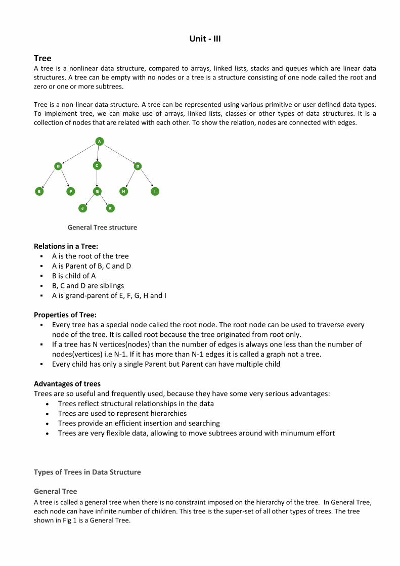
Tree A tree is a nonlinear data structure, compared to arrays, linked lists, stacks and queues which are linear data structures. A tree can be empty with no nodes or a tree is a structure consisting of one node called the root and zero or one or more subtrees. Tree is a non-linear data structure. A tree can be represented using various primitive or user defined data types. To implement tree, we can make use of arrays, linked lists, classes or other types of data structures. It is a collection of nodes that are related with each other. To show the relation, nodes are connected with edges.

General Tree structure

Relations in a Tree: ▪ A is the root of the tree ▪ A is Parent of B, C and D ▪ B is child of A ▪ B, C and D are siblings ▪ A is grand-parent of E, F, G, H and I

Properties of Tree: ▪ Every tree has a special node called the root node. The root node can be used to traverse every

node of the tree. It is called root because the tree originated from root only. ▪ If a tree has N vertices(nodes) than the number of edges is always one less than the number of

nodes(vertices) i.e N-1. If it has more than N-1 edges it is called a graph not a tree. ▪ Every child has only a single Parent but Parent can have multiple child

Advantages of trees Trees are so useful and frequently used, because they have some very serious advantages:

• Trees reflect structural relationships in the data • Trees are used to represent hierarchies • Trees provide an efficient insertion and searching • Trees are very flexible data, allowing to move subtrees around with minumum effort

Types of Trees in Data Structure

General Tree

A tree is called a general tree when there is no constraint imposed on the hierarchy of the tree. In General Tree, each node can have infinite number of children. This tree is the super-set of all other types of trees. The tree shown in Fig 1 is a General Tree.

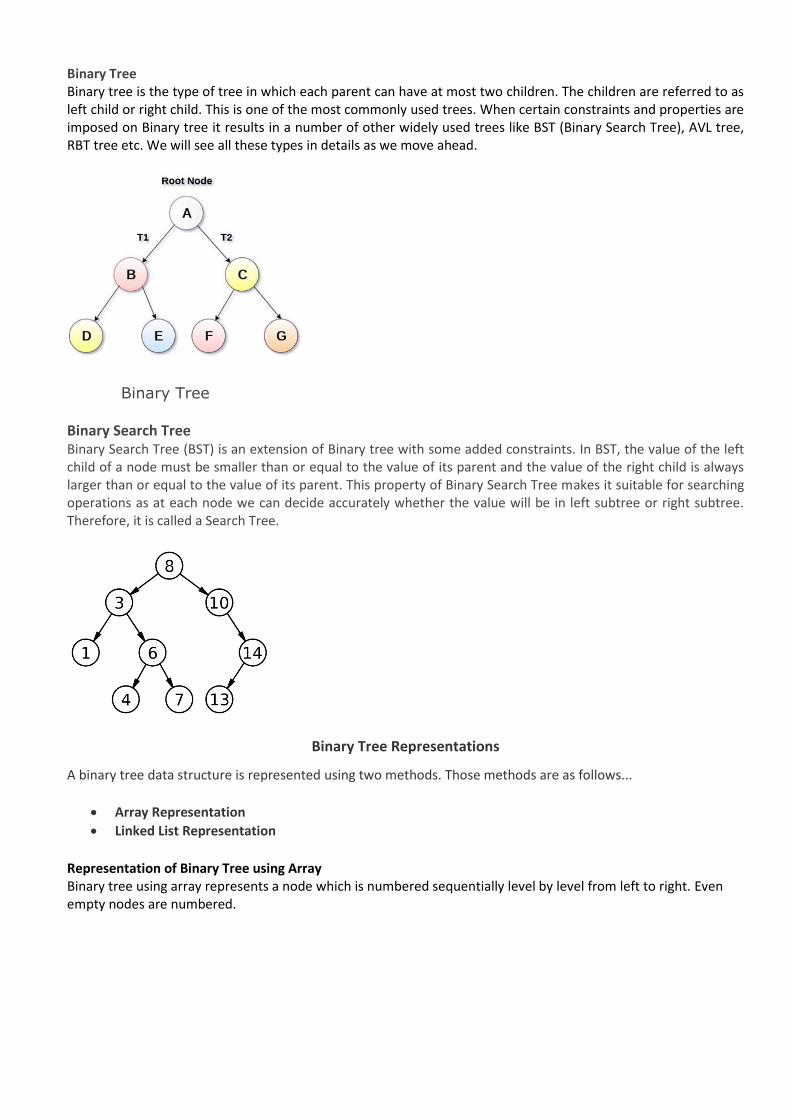
Binary Tree Binary tree is the type of tree in which each parent can have at most two children. The children are referred to as left child or right child. This is one of the most commonly used trees. When certain constraints and properties are imposed on Binary tree it results in a number of other widely used trees like BST (Binary Search Tree), AVL tree, RBT tree etc. We will see all these types in details as we move ahead.

Binary Tree

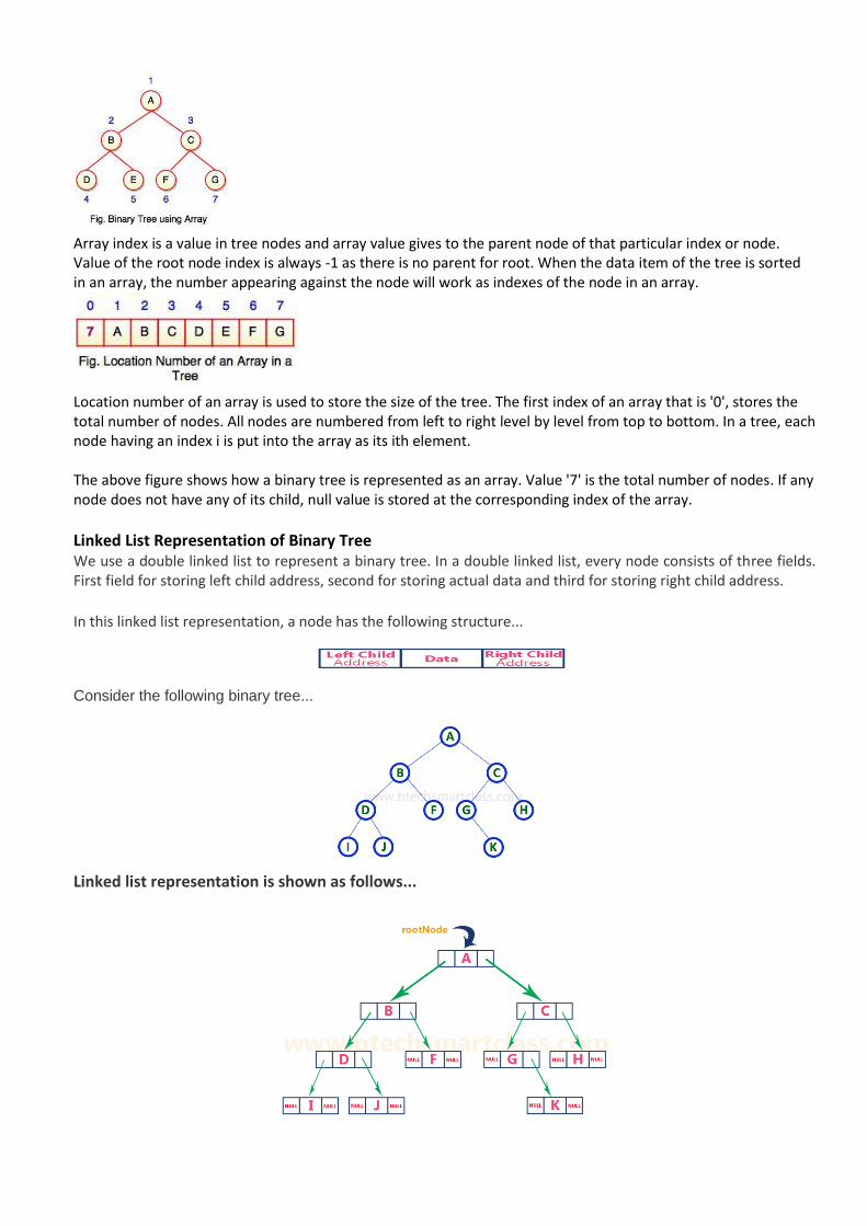
Binary Search Tree Binary Search Tree (BST) is an extension of Binary tree with some added constraints. In BST, the value of the left child of a node must be smaller than or equal to the value of its parent and the value of the right child is always larger than or equal to the value of its parent. This property of Binary Search Tree makes it suitable for searching operations as at each node we can decide accurately whether the value will be in left subtree or right subtree. Therefore, it is called a Search Tree.

Binary Tree Representations

A binary tree data structure is represented using two methods. Those methods are as follows...

• Array Representation

• Linked List Representation

Representation of Binary Tree using Array Binary tree using array represents a node which is numbered sequentially level by level from left to right. Even empty nodes are numbered.

Array index is a value in tree nodes and array value gives to the parent node of that particular index or node. Value of the root node index is always -1 as there is no parent for root. When the data item of the tree is sorted in an array, the number appearing against the node will work as indexes of the node in an array.

Location number of an array is used to store the size of the tree. The first index of an array that is '0', stores the total number of nodes. All nodes are numbered from left to right level by level from top to bottom. In a tree, each node having an index i is put into the array as its ith element. The above figure shows how a binary tree is represented as an array. Value '7' is the total number of nodes. If any node does not have any of its child, null value is stored at the corresponding index of the array.

Linked List Representation of Binary Tree We use a double linked list to represent a binary tree. In a double linked list, every node consists of three fields. First field for storing left child address, second for storing actual data and third for storing right child address.

In this linked list representation, a node has the following structure...

Consider the following binary tree...

Linked list representation is shown as follows...

Binary Tree: Common Terminologies

• Root: Topmost node in a tree. • Parent: Every node (excluding a root) in a tree is connected by a directed edge from exactly one

other node. This node is called a parent. • Child: A node directly connected to another node when moving away from the root. • Leaf/External node: Node with no children. • Internal node: Node with atleast one children. • Depth of a node: Number of edges from root to the node. • Height of a node: Number of edges from the node to the deepest leaf. Height of the tree is the

height of the root.

Types of Binary Trees (Based on Structure) • Rooted binary tree: It has a root node and every node has atmost two children. • Full binary tree: It is a tree in which every node in the tree has either 0 or 2 children.

o The number of nodes, n, in a full binary tree is atleast n = 2h – 1, and atmost n = 2h+1 – 1, where h is the height of the tree.

o The number of leaf nodes l, in a full binary tree is number, L of internal nodes + 1, i.e, l = L+1.

• Perfect binary tree: It is a binary tree in which all interior nodes have two children and all leaves have the same depth or same level.

o A perfect binary tree with l leaves has n = 2l-1 nodes. o In perfect full binary tree, l = 2h and n = 2h+1 - 1 where, n is number of nodes, h is height of tree

and l is number of leaf nodes

• Complete binary tree: It is a binary tree in which every level, except possibly the last, is completely filled, and all nodes are as far left as possible.

o The number of internal nodes in a complete binary tree of n nodes is floor(n/2).

• Balanced binary tree: A binary tree is height balanced if it satisfies the following constraints: 1. The left and right subtrees' heights differ by at most one, AND 2. The left subtree is balanced, AND 3. The right subtree is balanced

An empty tree is height balanced.

o The height of a balanced binary tree is O(Log n) where n is number of nodes.

Degenarate tree: It is a tree is where each parent node has only one child node. It behaves like a linked list.

The threaded Binary tree is the tree which is represented using pointers the empty subtrees are set to NULL, i.e.

'left' pointer of the node whose left child is empty subtree is normally set to NULL. These large numbers of

pointer sets are used in different ways.

Binary Tree Traversal

Traversal is a process to visit all the nodes of a tree and may print their values too. Because, all nodes are connected via edges (links) we always start from the root (head) node. That is, we cannot randomly access a node in a tree. There are three ways which we use to traverse a tree – (a) Inorder (Left, Root, Right) (b) Preorder (Root, Left, Right) (c) Postorder (Left, Right, Root) Generally, we traverse a tree to search or locate a given item or key in the tree or to print all the values it contains.

In-order Traversal

In this traversal method, the left subtree is visited first, then the root and later the right sub-tree. We should always remember that every node may represent a subtree itself.

If a binary tree is traversed in-order, the output will produce sorted key values in an ascending order.

We start from A, and following in-order traversal, we move to its left subtree B. B is also traversed in-order. The process goes on until all the nodes are visited. The output of inorder traversal of this tree will be −

D → B → E → A → F → C → G

Algorithm

Until all nodes are traversed − Step 1 − Recursively traverse left subtree. Step 2 − Visit root node. Step 3 − Recursively traverse right subtree.

Pre-order Traversal

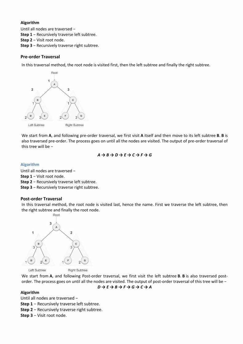
In this traversal method, the root node is visited first, then the left subtree and finally the right subtree.

We start from A, and following pre-order traversal, we first visit A itself and then move to its left subtree B. B is also traversed pre-order. The process goes on until all the nodes are visited. The output of pre-order traversal of this tree will be −

A → B → D → E → C → F → G

Algorithm

Until all nodes are traversed − Step 1 − Visit root node. Step 2 − Recursively traverse left subtree. Step 3 − Recursively traverse right subtree.

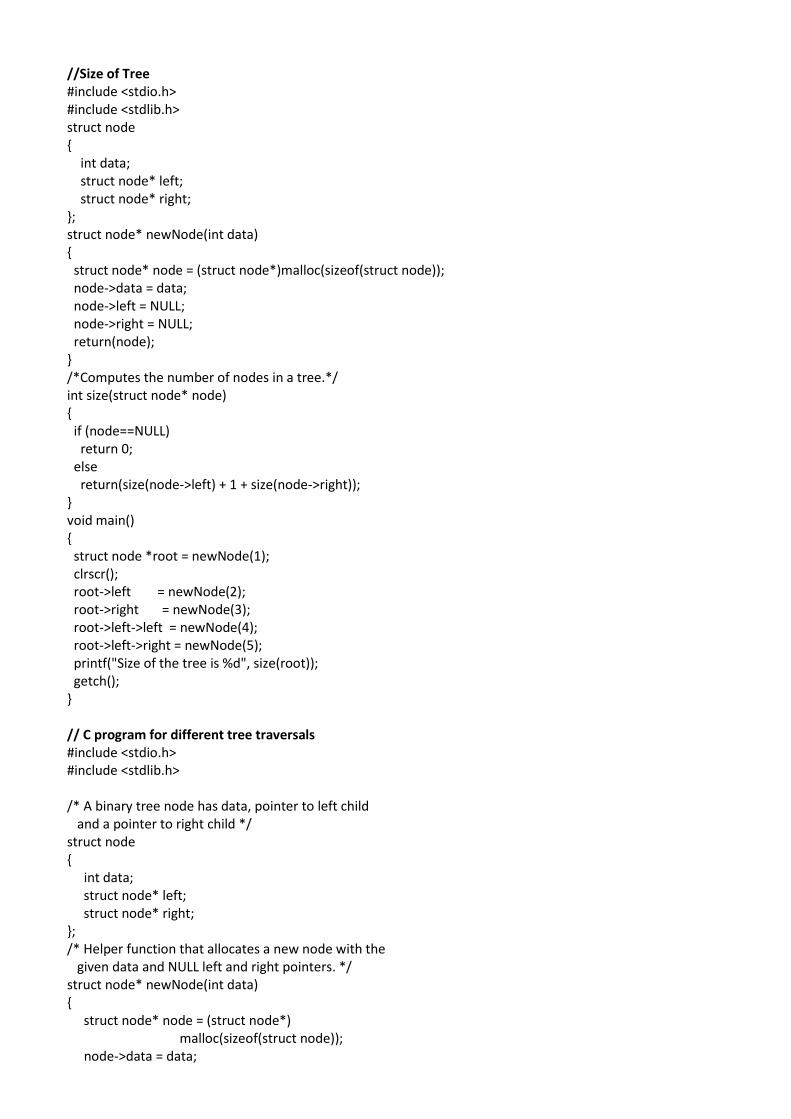
Post-order Traversal In this traversal method, the root node is visited last, hence the name. First we traverse the left subtree, then the right subtree and finally the root node.

We start from A, and following Post-order traversal, we first visit the left subtree B. B is also traversed post-order. The process goes on until all the nodes are visited. The output of post-order traversal of this tree will be −

D → E → B → F → G → C → A Algorithm

Until all nodes are traversed − Step 1 − Recursively traverse left subtree. Step 2 − Recursively traverse right subtree. Step 3 − Visit root node.

//Size of Tree #include <stdio.h> #include <stdlib.h> struct node { int data; struct node* left; struct node* right; }; struct node* newNode(int data) { struct node* node = (struct node*)malloc(sizeof(struct node)); node->data = data; node->left = NULL; node->right = NULL; return(node); } /*Computes the number of nodes in a tree.*/ int size(struct node* node) { if (node==NULL) return 0; else return(size(node->left) + 1 + size(node->right)); } void main() { struct node *root = newNode(1); clrscr(); root->left = newNode(2); root->right = newNode(3); root->left->left = newNode(4); root->left->right = newNode(5); printf("Size of the tree is %d", size(root)); getch(); } // C program for different tree traversals #include <stdio.h> #include <stdlib.h> /* A binary tree node has data, pointer to left child and a pointer to right child */ struct node { int data; struct node* left; struct node* right; }; /* Helper function that allocates a new node with the given data and NULL left and right pointers. */ struct node* newNode(int data) { struct node* node = (struct node*) malloc(sizeof(struct node)); node->data = data;

node->left = NULL; node->right = NULL; return(node); } /* Given a binary tree, print its nodes according to the "bottom-up" postorder traversal. */ void printPostorder(struct node* node) { if (node == NULL) return; // first recur on left subtree printPostorder(node->left); // then recur on right subtree printPostorder(node->right); // now deal with the node printf("%d ", node->data); } /* Given a binary tree, print its nodes in inorder*/ void printInorder(struct node* node) { if (node == NULL) return; /* first recur on left child */ printInorder(node->left); /* then print the data of node */ printf("%d ", node->data); /* now recur on right child */ printInorder(node->right); } /* Given a binary tree, print its nodes in preorder*/ void printPreorder(struct node* node) { if (node == NULL) return; /* first print data of node */ printf("%d ", node->data); /* then recur on left sutree */ printPreorder(node->left); /* now recur on right subtree */ printPreorder(node->right); } /* Driver program to test above functions*/ int main() { struct node *root = newNode(1); root->left = newNode(2); root->right = newNode(3); root->left->left = newNode(4); root->left->right = newNode(5); printf("\nPreorder traversal of binary tree is \n"); printPreorder(root); printf("\nInorder traversal of binary tree is \n"); printInorder(root); printf("\nPostorder traversal of binary tree is \n");

printPostorder(root); getch(); return 0; }

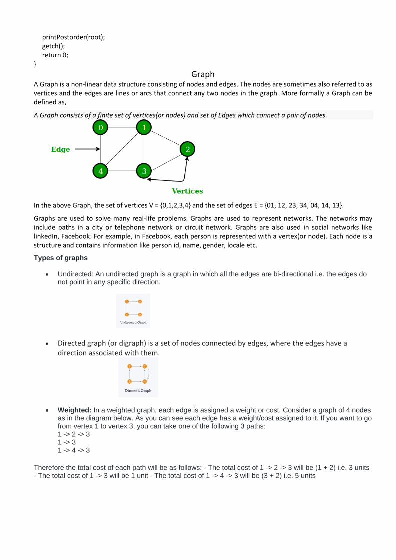
Graph A Graph is a non-linear data structure consisting of nodes and edges. The nodes are sometimes also referred to as vertices and the edges are lines or arcs that connect any two nodes in the graph. More formally a Graph can be defined as,

A Graph consists of a finite set of vertices(or nodes) and set of Edges which connect a pair of nodes.

In the above Graph, the set of vertices V = {0,1,2,3,4} and the set of edges E = {01, 12, 23, 34, 04, 14, 13}.

Graphs are used to solve many real-life problems. Graphs are used to represent networks. The networks may include paths in a city or telephone network or circuit network. Graphs are also used in social networks like linkedIn, Facebook. For example, in Facebook, each person is represented with a vertex(or node). Each node is a structure and contains information like person id, name, gender, locale etc.

Types of graphs

• Undirected: An undirected graph is a graph in which all the edges are bi-directional i.e. the edges do not point in any specific direction.

• Directed graph (or digraph) is a set of nodes connected by edges, where the edges have a direction associated with them.

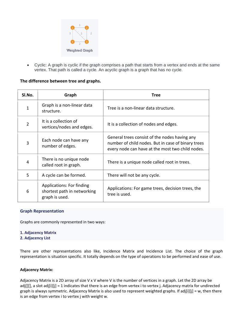
• Weighted: In a weighted graph, each edge is assigned a weight or cost. Consider a graph of 4 nodes as in the diagram below. As you can see each edge has a weight/cost assigned to it. If you want to go from vertex 1 to vertex 3, you can take one of the following 3 paths: 1 -> 2 -> 3 1 -> 3 1 -> 4 -> 3

Therefore the total cost of each path will be as follows: - The total cost of 1 -> 2 -> 3 will be (1 + 2) i.e. 3 units - The total cost of 1 -> 3 will be 1 unit - The total cost of 1 -> 4 -> 3 will be (3 + 2) i.e. 5 units

• Cyclic: A graph is cyclic if the graph comprises a path that starts from a vertex and ends at the same vertex. That path is called a cycle. An acyclic graph is a graph that has no cycle.

The difference between tree and graphs.

Sl.No. Graph Tree

1 Graph is a non-linear data structure.

Tree is a non-linear data structure.

2 It is a collection of vertices/nodes and edges.

It is a collection of nodes and edges.

3 Each node can have any number of edges.

General trees consist of the nodes having any number of child nodes. But in case of binary trees every node can have at the most two child nodes.

4 There is no unique node called root in graph.

There is a unique node called root in trees.

5 A cycle can be formed. There will not be any cycle.

6 Applications: For finding shortest path in networking graph is used.

Applications: For game trees, decision trees, the tree is used.

Graph Representation Graphs are commonly represented in two ways: 1. Adjacency Matrix 2. Adjacency List

There are other representations also like, Incidence Matrix and Incidence List. The choice of the graph representation is situation specific. It totally depends on the type of operations to be performed and ease of use.

Adjacency Matrix: Adjacency Matrix is a 2D array of size V x V where V is the number of vertices in a graph. Let the 2D array be adj[][], a slot adj[i][j] = 1 indicates that there is an edge from vertex i to vertex j. Adjacency matrix for undirected graph is always symmetric. Adjacency Matrix is also used to represent weighted graphs. If adj[i][j] = w, then there is an edge from vertex i to vertex j with weight w.

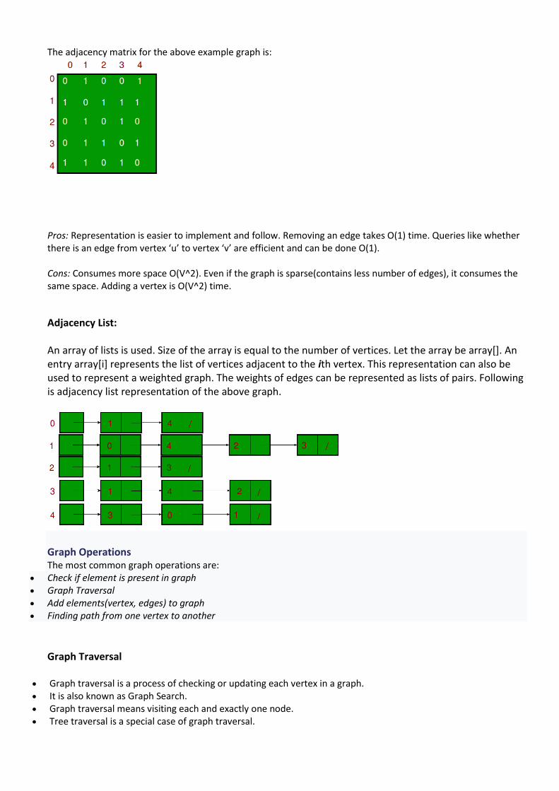
The adjacency matrix for the above example graph is:

Pros: Representation is easier to implement and follow. Removing an edge takes O(1) time. Queries like whether there is an edge from vertex ‘u’ to vertex ‘v’ are efficient and can be done O(1). Cons: Consumes more space O(V^2). Even if the graph is sparse(contains less number of edges), it consumes the same space. Adding a vertex is O(V^2) time.

Adjacency List: An array of lists is used. Size of the array is equal to the number of vertices. Let the array be array[]. An entry array[i] represents the list of vertices adjacent to the ith vertex. This representation can also be used to represent a weighted graph. The weights of edges can be represented as lists of pairs. Following is adjacency list representation of the above graph.

Graph Operations The most common graph operations are:

• Check if element is present in graph • Graph Traversal • Add elements(vertex, edges) to graph • Finding path from one vertex to another

Graph Traversal

• Graph traversal is a process of checking or updating each vertex in a graph. • It is also known as Graph Search. • Graph traversal means visiting each and exactly one node. • Tree traversal is a special case of graph traversal.

There are two techniques used in graph traversal: 1. Depth First Search 2. Breadth First Search

BFS (Breadth First Search)

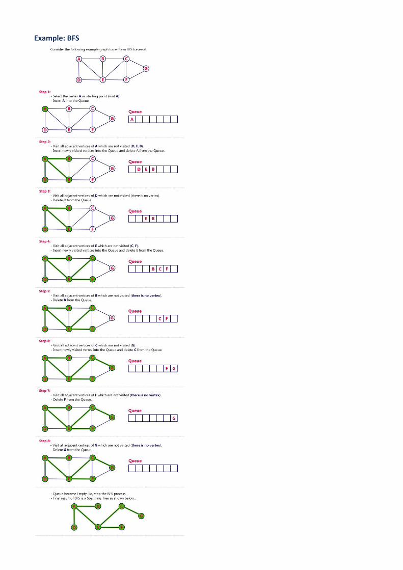
BFS traversal of a graph produces a spanning tree as final result. Spanning Tree is a graph without loops. We use Queue data structure with maximum size of total number of vertices in the graph to implement BFS traversal. We use the following steps to implement BFS traversal...

• Step 1 - Define a Queue of size total number of vertices in the graph. • Step 2 - Select any vertex as starting point for traversal. Visit that vertex and insert it into the Queue. • Step 3 - Visit all the non-visited adjacent vertices of the vertex which is at front of the Queue and insert

them into the Queue. • Step 4 - When there is no new vertex to be visited from the vertex which is at front of the Queue then

delete that vertex. • Step 5 - Repeat steps 3 and 4 until queue becomes empty. • Step 6 - When queue becomes empty, then produce final spanning tree by removing unused edges from

the graph

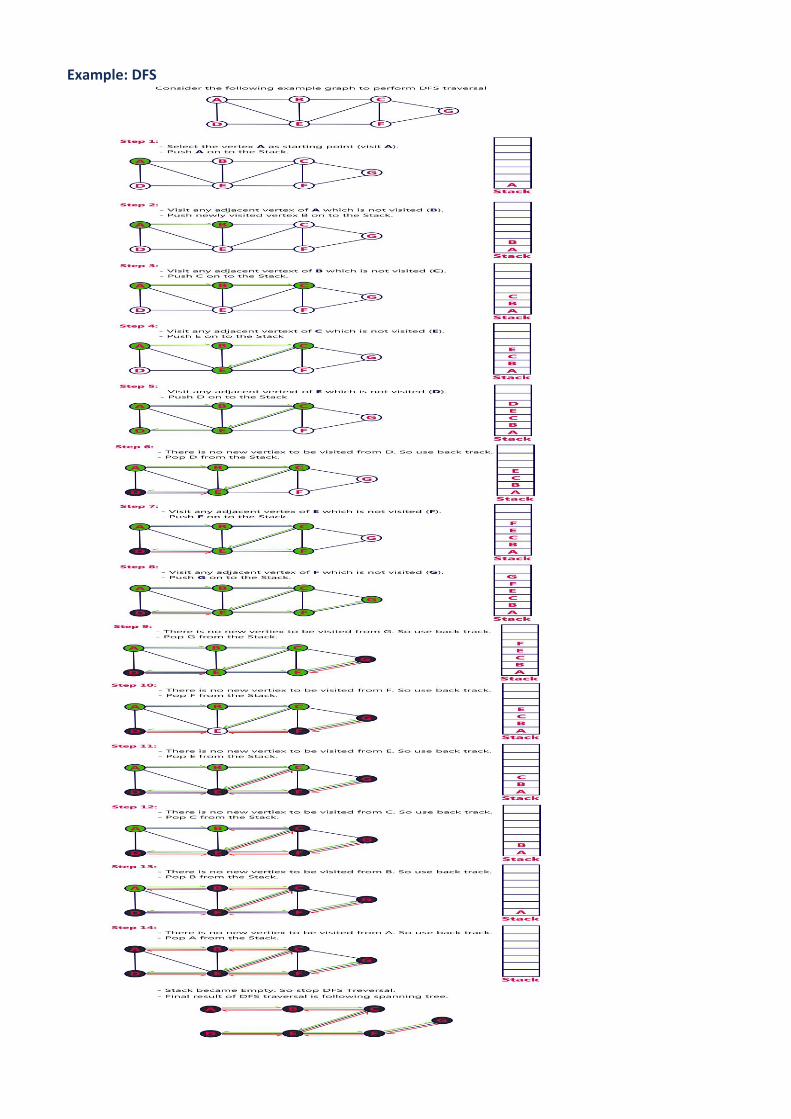
DFS (Depth First Search)

DFS traversal of a graph produces a spanning tree as final result. Spanning Tree is a graph without loops. We use Stack data structure with maximum size of total number of vertices in the graph to implement DFS traversal.

We use the following steps to implement DFS traversal...

• Step 1 - Define a Stack of size total number of vertices in the graph. • Step 2 - Select any vertex as starting point for traversal. Visit that vertex and push it on to the Stack. • Step 3 - Visit any one of the non-visited adjacent vertices of a vertex which is at the top of stack and push

it on to the stack. • Step 4 - Repeat step 3 until there is no new vertex to be visited from the vertex which is at the top of the

stack. • Step 5 - When there is no new vertex to visit then use back tracking and pop one vertex from the stack. • Step 6 - Repeat steps 3, 4 and 5 until stack becomes Empty. • Step 7 - When stack becomes Empty, then produce final spanning tree by removing unused edges from

the graph.

• Back tracking is coming back to the vertex from which we reached the current vertex.

Example: BFS

Example: DFS

Sr. No.

Key BFS DFS

1 Definition BFS, stands for Breadth First

Search. DFS, stands for Depth First Search.

2 Data structure

BFS uses Queue to find the shortest path.

DFS uses Stack to find the shortest path.

3 Source BFS is better when target is

closer to Source. DFS is better when target is far from source.

4

Suitablity for decision tree

As BFS considers all neighbour so it is not suitable for decision tree used in puzzle games.

DFS is more suitable for decision tree. As with one decision, we need to traverse further to augment the decision. If we reach the conclusion, we won.

5 Speed BFS is slower than DFS. DFS is faster than BFS.

6 Time Complexity

Time Complexity of BFS = O(V+E) where V is vertices and E is edges.

Time Complexity of DFS is also O(V+E) where V is vertices and E is edges.

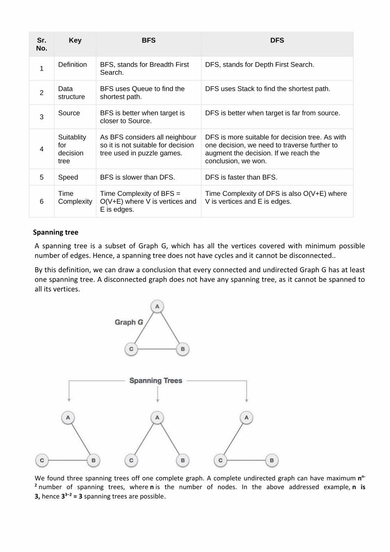
Spanning tree

A spanning tree is a subset of Graph G, which has all the vertices covered with minimum possible number of edges. Hence, a spanning tree does not have cycles and it cannot be disconnected..

By this definition, we can draw a conclusion that every connected and undirected Graph G has at least one spanning tree. A disconnected graph does not have any spanning tree, as it cannot be spanned to all its vertices.

We found three spanning trees off one complete graph. A complete undirected graph can have maximum nn-

2 number of spanning trees, where n is the number of nodes. In the above addressed example, n is

3, hence 33−2 = 3 spanning trees are possible.

General Properties of Spanning Tree We now understand that one graph can have more than one spanning tree. Following are a few properties of the spanning tree connected to graph G −

• A connected graph G can have more than one spanning tree.

• All possible spanning trees of graph G, have the same number of edges and vertices.

• The spanning tree does not have any cycle (loops).

• Removing one edge from the spanning tree will make the graph disconnected, i.e. the spanning tree is minimally connected.

• Adding one edge to the spanning tree will create a circuit or loop, i.e. the spanning tree is maximally acyclic.

Mathematical Properties of Spanning Tree

• Spanning tree has n-1 edges, where n is the number of nodes (vertices).

• From a complete graph, by removing maximum e - n + 1 edges, we can construct a spanning tree.

• A complete graph can have maximum nn-2 number of spanning trees.

Thus, we can conclude that spanning trees are a subset of connected Graph G and disconnected graphs do not have spanning tree.

Application of Spanning Tree

Spanning tree is basically used to find a minimum path to connect all nodes in a graph. Common application of spanning trees are −

• Civil Network Planning

• Computer Network Routing Protocol

• Cluster Analysis

Minimum Spanning Tree (MST)

In a weighted graph, a minimum spanning tree is a spanning tree that has minimum weight than all other spanning trees of the same graph. In real-world situations, this weight can be measured as distance, congestion, traffic load or any arbitrary value denoted to the edges.

Minimum Spanning-Tree Algorithm

We shall learn about two most important spanning tree algorithms here −

• Kruskal's Algorithm

• Prim's Algorithm

Kruskal's Spanning Tree Algorithm

Kruskal's algorithm to find the minimum cost spanning tree uses the greedy approach. This algorithm treats the graph as a forest and every node it has as an individual tree. A tree connects to another only and only if, it has the least cost among all available options and does not violate MST properties.

To understand Kruskal's algorithm let us consider the following example −

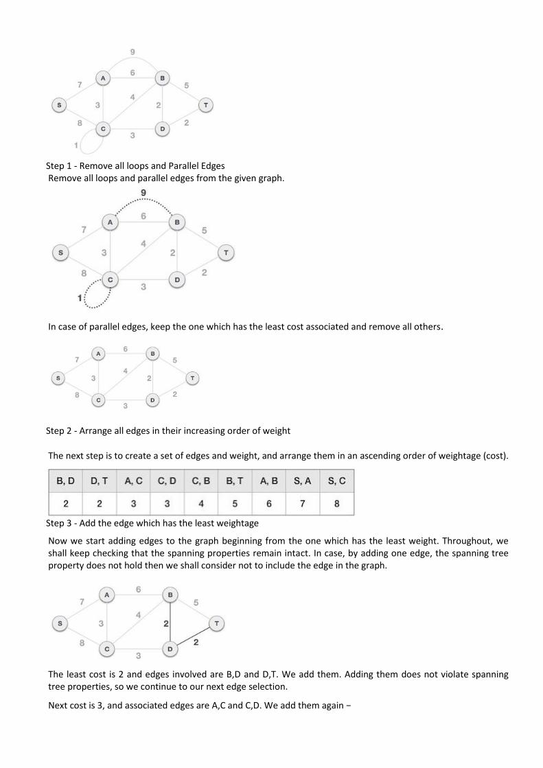
Step 1 - Remove all loops and Parallel Edges Remove all loops and parallel edges from the given graph.

In case of parallel edges, keep the one which has the least cost associated and remove all others.

Step 2 - Arrange all edges in their increasing order of weight

The next step is to create a set of edges and weight, and arrange them in an ascending order of weightage (cost).

Step 3 - Add the edge which has the least weightage

Now we start adding edges to the graph beginning from the one which has the least weight. Throughout, we shall keep checking that the spanning properties remain intact. In case, by adding one edge, the spanning tree property does not hold then we shall consider not to include the edge in the graph.

The least cost is 2 and edges involved are B,D and D,T. We add them. Adding them does not violate spanning tree properties, so we continue to our next edge selection.

Next cost is 3, and associated edges are A,C and C,D. We add them again −

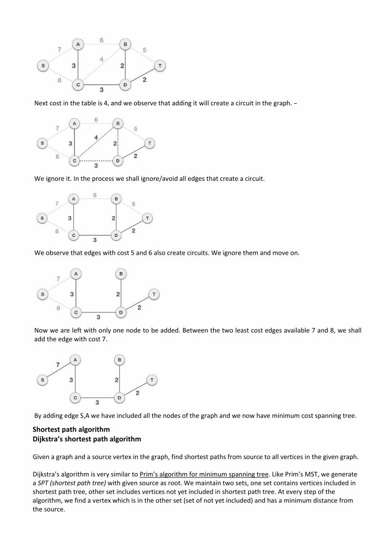
Next cost in the table is 4, and we observe that adding it will create a circuit in the graph. −

We ignore it. In the process we shall ignore/avoid all edges that create a circuit.

We observe that edges with cost 5 and 6 also create circuits. We ignore them and move on.

Now we are left with only one node to be added. Between the two least cost edges available 7 and 8, we shall add the edge with cost 7.

By adding edge S,A we have included all the nodes of the graph and we now have minimum cost spanning tree.

Shortest path algorithm Dijkstra’s shortest path algorithm

Given a graph and a source vertex in the graph, find shortest paths from source to all vertices in the given graph. Dijkstra’s algorithm is very similar to Prim’s algorithm for minimum spanning tree. Like Prim’s MST, we generate a SPT (shortest path tree) with given source as root. We maintain two sets, one set contains vertices included in shortest path tree, other set includes vertices not yet included in shortest path tree. At every step of the algorithm, we find a vertex which is in the other set (set of not yet included) and has a minimum distance from the source.

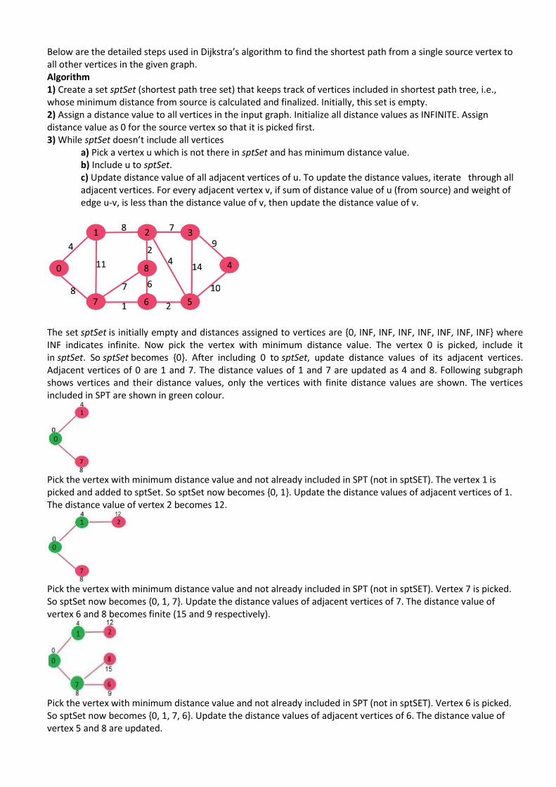
Below are the detailed steps used in Dijkstra’s algorithm to find the shortest path from a single source vertex to all other vertices in the given graph. Algorithm 1) Create a set sptSet (shortest path tree set) that keeps track of vertices included in shortest path tree, i.e., whose minimum distance from source is calculated and finalized. Initially, this set is empty. 2) Assign a distance value to all vertices in the input graph. Initialize all distance values as INFINITE. Assign distance value as 0 for the source vertex so that it is picked first. 3) While sptSet doesn’t include all vertices

a) Pick a vertex u which is not there in sptSet and has minimum distance value. b) Include u to sptSet. c) Update distance value of all adjacent vertices of u. To update the distance values, iterate through all adjacent vertices. For every adjacent vertex v, if sum of distance value of u (from source) and weight of edge u-v, is less than the distance value of v, then update the distance value of v.

The set sptSet is initially empty and distances assigned to vertices are {0, INF, INF, INF, INF, INF, INF, INF} where INF indicates infinite. Now pick the vertex with minimum distance value. The vertex 0 is picked, include it in sptSet. So sptSet becomes {0}. After including 0 to sptSet, update distance values of its adjacent vertices. Adjacent vertices of 0 are 1 and 7. The distance values of 1 and 7 are updated as 4 and 8. Following subgraph shows vertices and their distance values, only the vertices with finite distance values are shown. The vertices included in SPT are shown in green colour.

Pick the vertex with minimum distance value and not already included in SPT (not in sptSET). The vertex 1 is picked and added to sptSet. So sptSet now becomes {0, 1}. Update the distance values of adjacent vertices of 1. The distance value of vertex 2 becomes 12.

Pick the vertex with minimum distance value and not already included in SPT (not in sptSET). Vertex 7 is picked. So sptSet now becomes {0, 1, 7}. Update the distance values of adjacent vertices of 7. The distance value of vertex 6 and 8 becomes finite (15 and 9 respectively).

Pick the vertex with minimum distance value and not already included in SPT (not in sptSET). Vertex 6 is picked. So sptSet now becomes {0, 1, 7, 6}. Update the distance values of adjacent vertices of 6. The distance value of vertex 5 and 8 are updated.

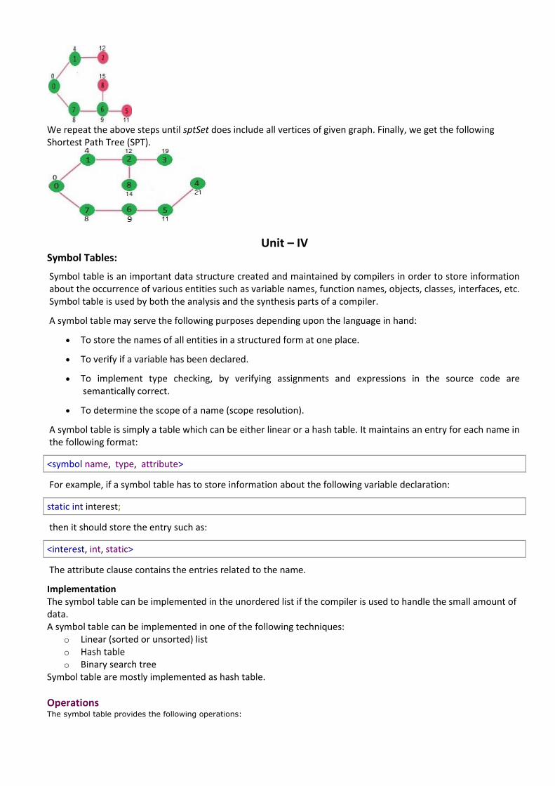
We repeat the above steps until sptSet does include all vertices of given graph. Finally, we get the following Shortest Path Tree (SPT).

Unit – IV Symbol Tables:

Symbol table is an important data structure created and maintained by compilers in order to store information about the occurrence of various entities such as variable names, function names, objects, classes, interfaces, etc. Symbol table is used by both the analysis and the synthesis parts of a compiler.

A symbol table may serve the following purposes depending upon the language in hand:

• To store the names of all entities in a structured form at one place.

• To verify if a variable has been declared.

• To implement type checking, by verifying assignments and expressions in the source code are semantically correct.

• To determine the scope of a name (scope resolution).

A symbol table is simply a table which can be either linear or a hash table. It maintains an entry for each name in the following format:

<symbol name, type, attribute>

For example, if a symbol table has to store information about the following variable declaration:

static int interest;

then it should store the entry such as:

<interest, int, static>

The attribute clause contains the entries related to the name.

Implementation The symbol table can be implemented in the unordered list if the compiler is used to handle the small amount of data. A symbol table can be implemented in one of the following techniques:

o Linear (sorted or unsorted) list o Hash table o Binary search tree

Symbol table are mostly implemented as hash table.

Operations The symbol table provides the following operations:

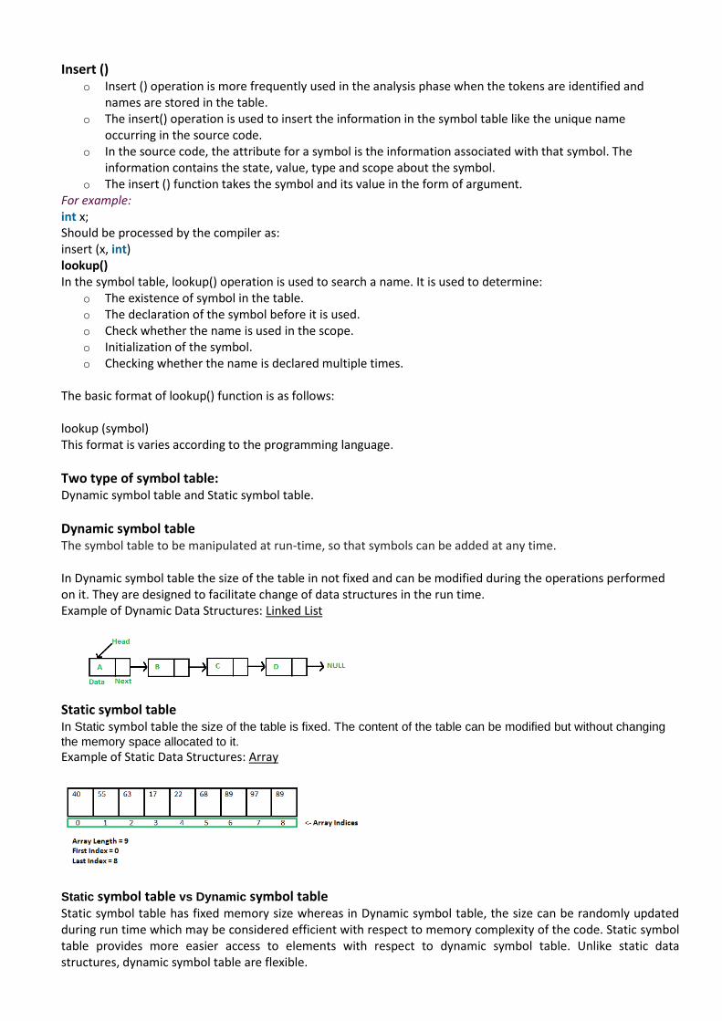
Insert () o Insert () operation is more frequently used in the analysis phase when the tokens are identified and

names are stored in the table. o The insert() operation is used to insert the information in the symbol table like the unique name

occurring in the source code. o In the source code, the attribute for a symbol is the information associated with that symbol. The

information contains the state, value, type and scope about the symbol. o The insert () function takes the symbol and its value in the form of argument.

For example: int x; Should be processed by the compiler as: insert (x, int) lookup() In the symbol table, lookup() operation is used to search a name. It is used to determine:

o The existence of symbol in the table. o The declaration of the symbol before it is used. o Check whether the name is used in the scope. o Initialization of the symbol. o Checking whether the name is declared multiple times.

The basic format of lookup() function is as follows: lookup (symbol) This format is varies according to the programming language.

Two type of symbol table: Dynamic symbol table and Static symbol table.

Dynamic symbol table The symbol table to be manipulated at run-time, so that symbols can be added at any time. In Dynamic symbol table the size of the table in not fixed and can be modified during the operations performed on it. They are designed to facilitate change of data structures in the run time. Example of Dynamic Data Structures: Linked List

Static symbol table In Static symbol table the size of the table is fixed. The content of the table can be modified but without changing

the memory space allocated to it.

Example of Static Data Structures: Array

Static symbol table vs Dynamic symbol table

Static symbol table has fixed memory size whereas in Dynamic symbol table, the size can be randomly updated during run time which may be considered efficient with respect to memory complexity of the code. Static symbol table provides more easier access to elements with respect to dynamic symbol table. Unlike static data structures, dynamic symbol table are flexible.

Hash table:

Hash Table is a data structure which stores data in an associative manner. In a hash table, data is stored in an array format, where each data value has its own unique index value. Access of data becomes very fast if we know the index of the desired data.

Thus, it becomes a data structure in which insertion and search operations are very fast irrespective of the size of the data. Hash Table uses an array as a storage medium and uses hash technique to generate an index where an element is to be inserted or is to be located from.

Hashing is an important Data Structure which is designed to use a special function called the hash function which is used to map a given value with a particular key for faster access of elements. Hashing function A hash function takes a group of characters (called a key) and maps it to a value of a certain length (called a hash value or hash). The hash value is representative of the original string of characters, but is normally smaller than the original.

Hashing is done for indexing and locating items in databases because it is easier to find the shorter hash value than the longer string. Hashing is also used in encryption. A hash function maps an identifier name into a table index A hash function, h(name), should depend solely on name h(name) should be computed quickly h should be uniform and randomizing in distributing names All table indices should be mapped with equal probability Similar names should not cluster to the same table index Hash functions can be defined in many ways . . . A string can be treated as a sequence of integer words Several characters are fit into an integer word Strings longer than one word are folded using exclusive-or or addition Hash value is obtained by taking integer word modulo TableSize. We can also compute a hash value character by character: h(name) = (c0 + c1 + … + cn–1) mod TableSize, where n is name length h(name) = (c0 * c1 * … * cn–1) mod TableSize h(name) = (cn–1 + cn–2 + … + c1 + c0))) mod TableSize h(name) = (c0 * cn–1 * n) mod TableSize Importance of hashing. Hash functions are important and ubiquitous cryptography building block. They are relatively simple to understand and to use. Most cryptographic hash functions are designed to take a string of any length as input and produce a fixed-length hash value.

Basic Operations Following are the basic primary operations of a hash table.

• Search − Searches an element in a hash table.

• Insert − inserts an element in a hash table.

• delete − Deletes an element from a hash table.

Overflow Handling in hash function. An overflow occurs at the time of the home bucket for a new pair (key, element) is full. We may tackle overflows by Search the hash table in some systematic manner for a bucket that is not full.

• Linear probing (linear open addressing). • Quadratic probing. • Random probing.

Eliminate overflows by allowing each bucket to keep a list of all pairs for which it is the home bucket. • Array linear list. • Chain.

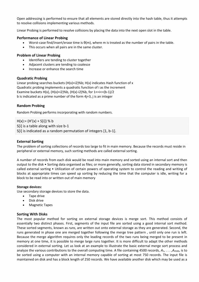
Open addressing is performed to ensure that all elements are stored directly into the hash table, thus it attempts to resolve collisions implementing various methods.

Linear Probing is performed to resolve collisions by placing the data into the next open slot in the table.

Performance of Linear Probing • Worst-case find/insert/erase time is θ(m), where m is treated as the number of pairs in the table. • This occurs when all pairs are in the same cluster.

Problem of Linear Probing • Identifiers are tending to cluster together • Adjacent clusters are tending to coalesce • Increase or enhance the search time

Quadratic Probing Linear probing searches buckets (H(x)+i2)%b; H(x) indicates Hash function of x Quadratic probing implements a quadratic function of i as the increment Examine buckets H(x), (H(x)+i2)%b, (H(x)-i2)%b, for 1<=i<=(b-1)/2 b is indicated as a prime number of the form 4j+3, j is an integer

Random Probing

Random Probing performs incorporating with random numbers.

H(x):= (H’(x) + S[i]) % b S[i] is a table along with size b-1 S[i] is indicated as a random permutation of integers [1, b-1].

External Sorting The problem of sorting collections of records too large to fit in main memory. Because the records must reside in peripheral or external memory, such sorting methods are called external sorting. A number of records from each disk would be read into main memory and sorted using an internal sort and then output to the disk • Sorting data organised as files; or more generally, sorting data stored in secondary memory is called external sorting • Utilization of certain powers of operating system to control the reading and writing of blocks at appropriate times can speed up sorting by reducing the time that the computer is idle, writing for a block to be read into or written out of main memory Storage devices: Use secondary storage devices to store the data.

• Tape drive • Disk drive • Magnetic Tapes

Sorting With Disks The most popular method for sorting on external storage devices is merge sort. This method consists of essentially two distinct phases. First, segments of the input file are sorted using a good internal sort method. These sorted segments, known as runs, are written out onto external storage as they are generated. Second, the runs generated in phase one are merged together following the merge tree pattern , until only one run is left. Because the merge algorithm requires only the leading records of the two runs being merged to be present in memory at one time, it is possible to merge large runs together. It is more difficult to adapt the other methods considered in external sorting. Let us look at an example to illustrate the basic external merge sort process and analyze the various contributions to the overall computing time. A file containing 4500 records, A1, . . . ,A4500, is to be sorted using a computer with an internal memory capable of sorting at most 750 records. The input file is maintained on disk and has a block length of 250 records. We have available another disk which may be used as a

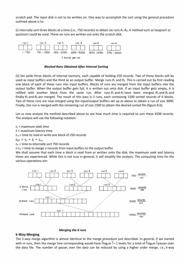
scratch pad. The input disk is not to be written on. One way to accomplish the sort using the general procedure outlined above is to:

(i) Internally sort three blocks at a time (i.e., 750 records) to obtain six runs R1-R6. A method such as heapsort or quicksort could be used. These six runs are written out onto the scratch disk.

Blocked Runs Obtained After Internal Sorting

(ii) Set aside three blocks of internal memory, each capable of holding 250 records. Two of these blocks will be used as input buffers and the third as an output buffer. Merge runs R1 and R2. This is carried out by first reading one block of each of these runs into input buffers. Blocks of runs are merged from the input buffers into the output buffer. When the output buffer gets full, it is written out onto disk. If an input buffer gets empty, it is refilled with another block from the same run. After runs R1 and R2 have been merged, R3 and R4 and finally R5 and R6 are merged. The result of this pass is 3 runs, each containing 1500 sorted records of 6 blocks. Two of these runs are now merged using the input/output buffers set up as above to obtain a run of size 3000. Finally, this run is merged with the remaining run of size 1500 to obtain the desired sorted file (figure 8.6).

Let us now analyze the method described above to see how much time is required to sort these 4500 records. The analysis will use the following notation:

ts = maximum seek time tl = maximum latency time trw = time to read or write one block of 250 records

tIO = ts + tl + trw tIS = time to internally sort 750 records n tm = time to merge n records from input buffers to the output buffer We shall assume that each time a block is read from or written onto the disk, the maximum seek and latency times are experienced. While this is not true in general, it will simplify the analysis. The computing time for the various operations are:

Merging the 6 runs

k-Way Merging The 2-way merge algorithm is almost identical to the merge procedure just described. In general, if we started

with m runs, then the merge tree corresponding would have log2m + 1 levels for a total of log2m passes over the data file. The number of passes over the data can be reduced by using a higher order merge, i.e., k-way

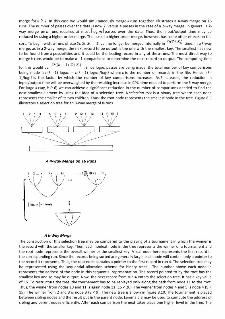
merge for k 2. In this case we would simultaneously merge k runs together. Illustrates a 4-way merge on 16 runs. The number of passes over the data is now 2, versus 4 passes in the case of a 2-way merge. In general, a k-

way merge on m runs requires at most logkm passes over the data. Thus, the input/output time may be reduced by using a higher order merge. The use of a higher order merge, however, has some other effects on the

sort. To begin with, k-runs of size S1, S2, S3, ...,Sk can no longer be merged internally in time. In a k-way merge, as in a 2-way merge, the next record to be output is the one with the smallest key. The smallest has now to be found from k possibilities and it could be the leading record in any of the k-runs. The most direct way to merge k-runs would be to make k - 1 comparisons to determine the next record to output. The computing time

for this would be . Since logkm passes are being made, the total number of key comparisons being made is n(k - 1) logkm = n(k - 1) log2m/log2k where n is the number of records in the file. Hence, (k - 1)/log2k is the factor by which the number of key comparisons increases. As k increases, the reduction in input/output time will be overweighed by the resulting increase in CPU time needed to perform the k-way merge. For large k (say, k 6) we can achieve a significant reduction in the number of comparisons needed to find the next smallest element by using the idea of a selection tree. A selection tree is a binary tree where each node represents the smaller of its two children. Thus, the root node represents the smallest node in the tree. Figure 8.9 illustrates a selection tree for an 8-way merge of 8-runs.

A 4-way Merge on 16 Runs

A k-Way Merge

The construction of this selection tree may be compared to the playing of a tournament in which the winner is the record with the smaller key. Then, each nonleaf node in the tree represents the winner of a tournament and the root node represents the overall winner or the smallest key. A leaf node here represents the first record in the corresponding run. Since the records being sorted are generally large, each node will contain only a pointer to the record it represents. Thus, the root node contains a pointer to the first record in run 4. The selection tree may be represented using the sequential allocation scheme for binary trees. The number above each node in represents the address of the node in this sequential representation. The record pointed to by the root has the smallest key and so may be output. Now, the next record from run 4 enters the selection tree. It has a key value of 15. To restructure the tree, the tournament has to be replayed only along the path from node 11 to the root. Thus, the winner from nodes 10 and 11 is again node 11 (15 < 20). The winner from nodes 4 and 5 is node 4 (9 < 15). The winner from 2 and 3 is node 3 (8 < 9). The new tree is shown in figure 8.10. The tournament is played between sibling nodes and the result put in the parent node. Lemma 5.3 may be used to compute the address of sibling and parent nodes efficiently. After each comparison the next takes place one higher level in the tree. The

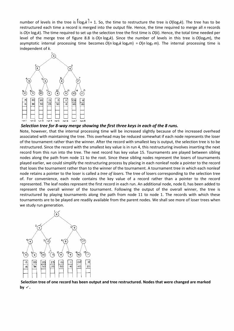
number of levels in the tree is log2k + 1. So, the time to restructure the tree is O(log2k). The tree has to be restructured each time a record is merged into the output file. Hence, the time required to merge all n records is O(n log2k). The time required to set up the selection tree the first time is O(k). Hence, the total time needed per level of the merge tree of figure 8.8 is O(n log2k). Since the number of levels in this tree is O(logkm), the asymptotic internal processing time becomes O(n log2k logkm) = O(n log2 m). The internal processing time is independent of k.

Selection tree for 8-way merge showing the first three keys in each of the 8 runs. Note, however, that the internal processing time will be increased slightly because of the increased overhead associated with maintaining the tree. This overhead may be reduced somewhat if each node represents the loser of the tournament rather than the winner. After the record with smallest key is output, the selection tree is to be restructured. Since the record with the smallest key value is in run 4, this restructuring involves inserting the next record from this run into the tree. The next record has key value 15. Tournaments are played between sibling nodes along the path from node 11 to the root. Since these sibling nodes represent the losers of tournaments played earlier, we could simplify the restructuring process by placing in each nonleaf node a pointer to the record that loses the tournament rather than to the winner of the tournament. A tournament tree in which each nonleaf node retains a pointer to the loser is called a tree of losers. The tree of losers corresponding to the selection tree of. For convenience, each node contains the key value of a record rather than a pointer to the record represented. The leaf nodes represent the first record in each run. An additional node, node 0, has been added to represent the overall winner of the tournament. Following the output of the overall winner, the tree is restructured by playing tournaments along the path from node 11 to node 1. The records with which these tournaments are to be played are readily available from the parent nodes. We shall see more of loser trees when we study run generation.

Selection tree of one record has been output and tree restructured. Nodes that were changed are marked by .

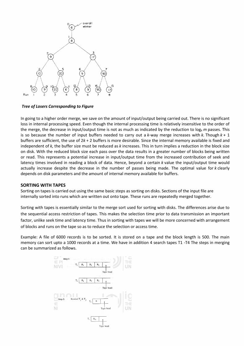
Tree of Losers Corresponding to Figure

In going to a higher order merge, we save on the amount of input/output being carried out. There is no significant loss in internal processing speed. Even though the internal processing time is relatively insensitive to the order of the merge, the decrease in input/output time is not as much as indicated by the reduction to logk m passes. This is so because the number of input buffers needed to carry out a k-way merge increases with k. Though k + 1 buffers are sufficient, the use of 2k + 2 buffers is more desirable. Since the internal memory available is fixed and independent of k, the buffer size must be reduced as k increases. This in turn implies a reduction in the block size on disk. With the reduced block size each pass over the data results in a greater number of blocks being written or read. This represents a potential increase in input/output time from the increased contribution of seek and latency times involved in reading a block of data. Hence, beyond a certain k value the input/output time would actually increase despite the decrease in the number of passes being made. The optimal value for k clearly depends on disk parameters and the amount of internal memory available for buffers.

SORTING WITH TAPES Sorting on tapes is carried out using the same basic steps as sorting on disks. Sections of the input file are internally sorted into runs which are written out onto tape. These runs are repeatedly merged together. Sorting with tapes is essentially similar to the merge sort used for sorting with disks. The differences arise due to

the sequential access restriction of tapes. This makes the selection time prior to data transmission an important

factor, unlike seek time and latency time. Thus in sorting with tapes we will be more concerned with arrangement

of blocks and runs on the tape so as to reduce the selection or access time.

Example: A file of 6000 records is to be sorted. It is stored on a tape and the block length is 500. The main memory can sort upto a 1000 records at a time. We have in addition 4 search tapes T1 -T4 The steps in merging can be summarized as follows.

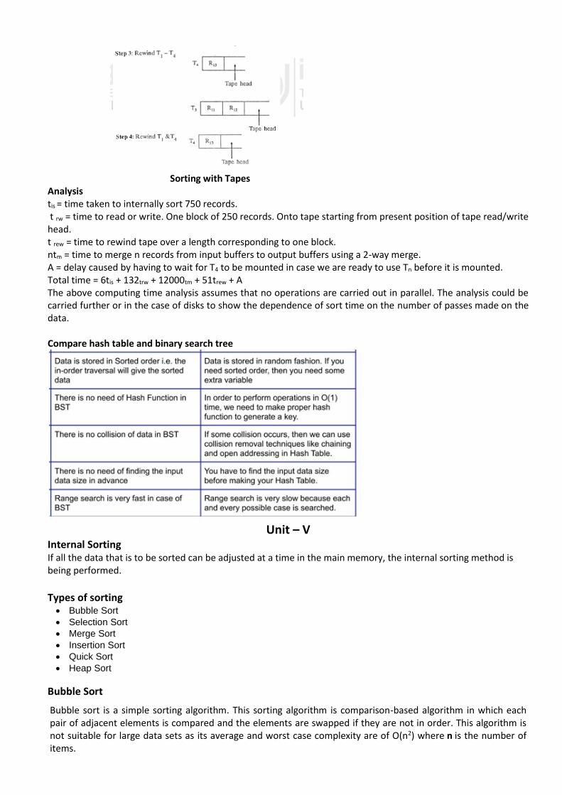
Sorting with Tapes Analysis tis = time taken to internally sort 750 records. t rw = time to read or write. One block of 250 records. Onto tape starting from present position of tape read/write head. t rew = time to rewind tape over a length corresponding to one block. ntm = time to merge n records from input buffers to output buffers using a 2-way merge. A = delay caused by having to wait for T4 to be mounted in case we are ready to use Tn before it is mounted. Total time = 6tis + 132trw + 12000tm + 51trew + A The above computing time analysis assumes that no operations are carried out in parallel. The analysis could be carried further or in the case of disks to show the dependence of sort time on the number of passes made on the data. Compare hash table and binary search tree

Unit – V

Internal Sorting If all the data that is to be sorted can be adjusted at a time in the main memory, the internal sorting method is being performed.

Types of sorting • Bubble Sort

• Selection Sort

• Merge Sort

• Insertion Sort

• Quick Sort

• Heap Sort

Bubble Sort

Bubble sort is a simple sorting algorithm. This sorting algorithm is comparison-based algorithm in which each pair of adjacent elements is compared and the elements are swapped if they are not in order. This algorithm is not suitable for large data sets as its average and worst case complexity are of Ο(n2) where n is the number of items.

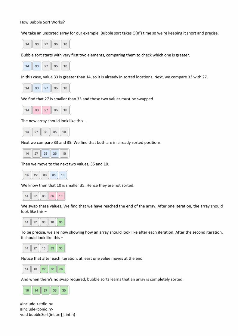
How Bubble Sort Works?

We take an unsorted array for our example. Bubble sort takes Ο(n2) time so we're keeping it short and precise.

Bubble sort starts with very first two elements, comparing them to check which one is greater.

In this case, value 33 is greater than 14, so it is already in sorted locations. Next, we compare 33 with 27.

We find that 27 is smaller than 33 and these two values must be swapped.

The new array should look like this −

Next we compare 33 and 35. We find that both are in already sorted positions.

Then we move to the next two values, 35 and 10.

We know then that 10 is smaller 35. Hence they are not sorted.

We swap these values. We find that we have reached the end of the array. After one iteration, the array should look like this −

To be precise, we are now showing how an array should look like after each iteration. After the second iteration, it should look like this −

Notice that after each iteration, at least one value moves at the end.

And when there's no swap required, bubble sorts learns that an array is completely sorted.

#include <stdio.h> #include<conio.h> void bubbleSort(int arr[], int n)

{ int i, j, temp; for(i = 0; i &lt; n; i++) { for(j = 0; j &lt; n-i-1; j++) { if( arr[j] &gt; arr[j+1]) { // swap the elements temp = arr[j]; arr[j] = arr[j+1]; arr[j+1] = temp; } } } // print the sorted array printf(&quot;Sorted Array: &quot;); for(i = 0; i &lt; n; i++) { printf(&quot;%d &quot;, arr[i]); } } void main() { int arr[100], i, n, step, temp; // ask user for number of elements to be sorted clrscr(); printf(&quot;Enter the number of elements to be sorted: &quot;); scanf(&quot;%d&quot;, &amp;n); // input elements if the array for(i = 0; i &lt; n; i++) { printf(&quot;Enter element no. %d: &quot;, i+1); scanf(&quot;%d&quot;, &amp;arr[i]); } // call the function bubbleSort bubbleSort(arr, n); getch(); } Output: Enter the number of elements to be sorted:5 Enter element no. %d:98 Enter element no. %d:56 Enter element no. %d:78 Enter element no. %d:45 Enter element no. %d:32 Sorted Array:32 45 56 78 98

Selection Sort

Selection sort is a simple sorting algorithm. This sorting algorithm is an in-place comparison-based algorithm in which the list is divided into two parts, the sorted part at the left end and the unsorted part at the right end. Initially, the sorted part is empty and the unsorted part is the entire list.

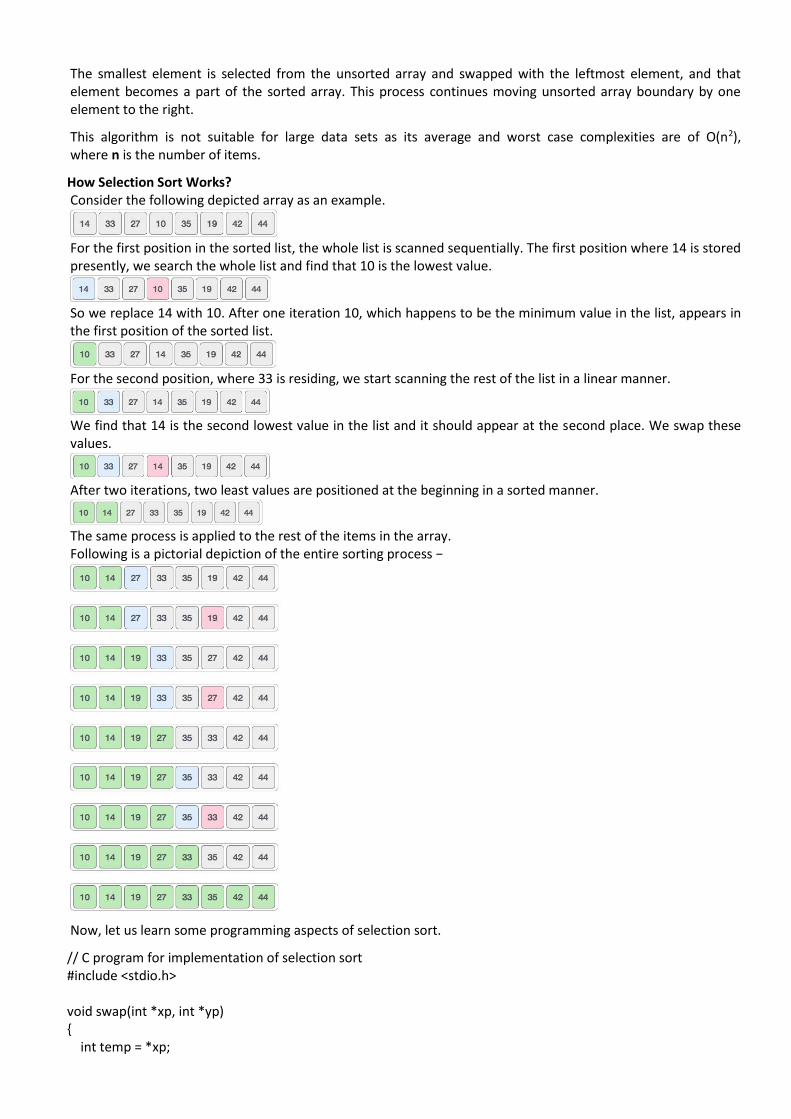
The smallest element is selected from the unsorted array and swapped with the leftmost element, and that element becomes a part of the sorted array. This process continues moving unsorted array boundary by one element to the right.

This algorithm is not suitable for large data sets as its average and worst case complexities are of Ο(n2), where n is the number of items.

How Selection Sort Works? Consider the following depicted array as an example.

For the first position in the sorted list, the whole list is scanned sequentially. The first position where 14 is stored presently, we search the whole list and find that 10 is the lowest value.

So we replace 14 with 10. After one iteration 10, which happens to be the minimum value in the list, appears in the first position of the sorted list.

For the second position, where 33 is residing, we start scanning the rest of the list in a linear manner.

We find that 14 is the second lowest value in the list and it should appear at the second place. We swap these values.

After two iterations, two least values are positioned at the beginning in a sorted manner.

The same process is applied to the rest of the items in the array. Following is a pictorial depiction of the entire sorting process −

Now, let us learn some programming aspects of selection sort.

// C program for implementation of selection sort #include <stdio.h> void swap(int *xp, int *yp) { int temp = *xp;

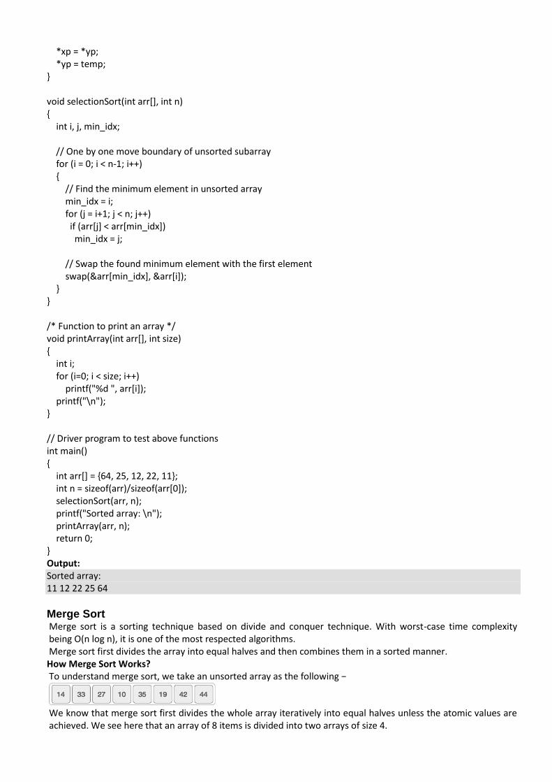
*xp = *yp; *yp = temp; } void selectionSort(int arr[], int n) { int i, j, min_idx; // One by one move boundary of unsorted subarray for (i = 0; i < n-1; i++) { // Find the minimum element in unsorted array min_idx = i; for (j = i+1; j < n; j++) if (arr[j] < arr[min_idx]) min_idx = j; // Swap the found minimum element with the first element swap(&arr[min_idx], &arr[i]); } } /* Function to print an array */ void printArray(int arr[], int size) { int i; for (i=0; i < size; i++) printf("%d ", arr[i]); printf("\n"); } // Driver program to test above functions int main() { int arr[] = {64, 25, 12, 22, 11}; int n = sizeof(arr)/sizeof(arr[0]); selectionSort(arr, n); printf("Sorted array: \n"); printArray(arr, n); return 0; } Output: Sorted array: 11 12 22 25 64

Merge Sort Merge sort is a sorting technique based on divide and conquer technique. With worst-case time complexity being Ο(n log n), it is one of the most respected algorithms. Merge sort first divides the array into equal halves and then combines them in a sorted manner. How Merge Sort Works? To understand merge sort, we take an unsorted array as the following −

We know that merge sort first divides the whole array iteratively into equal halves unless the atomic values are achieved. We see here that an array of 8 items is divided into two arrays of size 4.

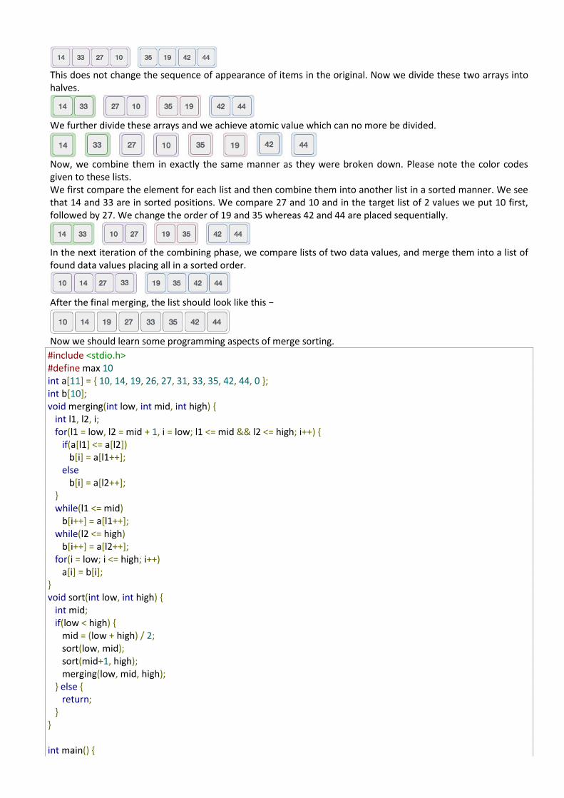
This does not change the sequence of appearance of items in the original. Now we divide these two arrays into halves.

We further divide these arrays and we achieve atomic value which can no more be divided.

Now, we combine them in exactly the same manner as they were broken down. Please note the color codes given to these lists. We first compare the element for each list and then combine them into another list in a sorted manner. We see that 14 and 33 are in sorted positions. We compare 27 and 10 and in the target list of 2 values we put 10 first, followed by 27. We change the order of 19 and 35 whereas 42 and 44 are placed sequentially.

In the next iteration of the combining phase, we compare lists of two data values, and merge them into a list of found data values placing all in a sorted order.

After the final merging, the list should look like this −

Now we should learn some programming aspects of merge sorting.

#include <stdio.h> #define max 10 int a[11] = { 10, 14, 19, 26, 27, 31, 33, 35, 42, 44, 0 }; int b[10]; void merging(int low, int mid, int high) { int l1, l2, i; for(l1 = low, l2 = mid + 1, i = low; l1 <= mid && l2 <= high; i++) { if(a[l1] <= a[l2]) b[i] = a[l1++]; else b[i] = a[l2++]; } while(l1 <= mid) b[i++] = a[l1++]; while(l2 <= high) b[i++] = a[l2++]; for(i = low; i <= high; i++) a[i] = b[i]; } void sort(int low, int high) { int mid; if(low < high) { mid = (low + high) / 2; sort(low, mid); sort(mid+1, high); merging(low, mid, high); } else { return; } } int main() {

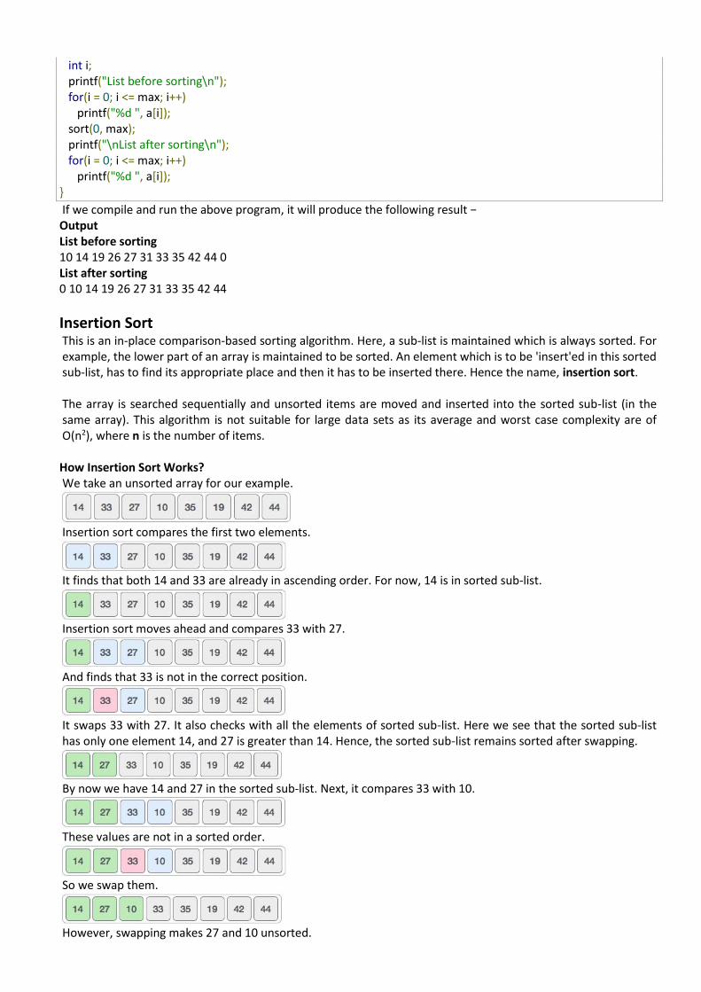
int i; printf("List before sorting\n"); for(i = 0; i <= max; i++) printf("%d ", a[i]); sort(0, max); printf("\nList after sorting\n"); for(i = 0; i <= max; i++) printf("%d ", a[i]); }

If we compile and run the above program, it will produce the following result − Output List before sorting 10 14 19 26 27 31 33 35 42 44 0 List after sorting 0 10 14 19 26 27 31 33 35 42 44

Insertion Sort This is an in-place comparison-based sorting algorithm. Here, a sub-list is maintained which is always sorted. For example, the lower part of an array is maintained to be sorted. An element which is to be 'insert'ed in this sorted sub-list, has to find its appropriate place and then it has to be inserted there. Hence the name, insertion sort. The array is searched sequentially and unsorted items are moved and inserted into the sorted sub-list (in the same array). This algorithm is not suitable for large data sets as its average and worst case complexity are of Ο(n2), where n is the number of items. How Insertion Sort Works? We take an unsorted array for our example.

Insertion sort compares the first two elements.

It finds that both 14 and 33 are already in ascending order. For now, 14 is in sorted sub-list.

Insertion sort moves ahead and compares 33 with 27.

And finds that 33 is not in the correct position.

It swaps 33 with 27. It also checks with all the elements of sorted sub-list. Here we see that the sorted sub-list has only one element 14, and 27 is greater than 14. Hence, the sorted sub-list remains sorted after swapping.

By now we have 14 and 27 in the sorted sub-list. Next, it compares 33 with 10.

These values are not in a sorted order.

So we swap them.

However, swapping makes 27 and 10 unsorted.

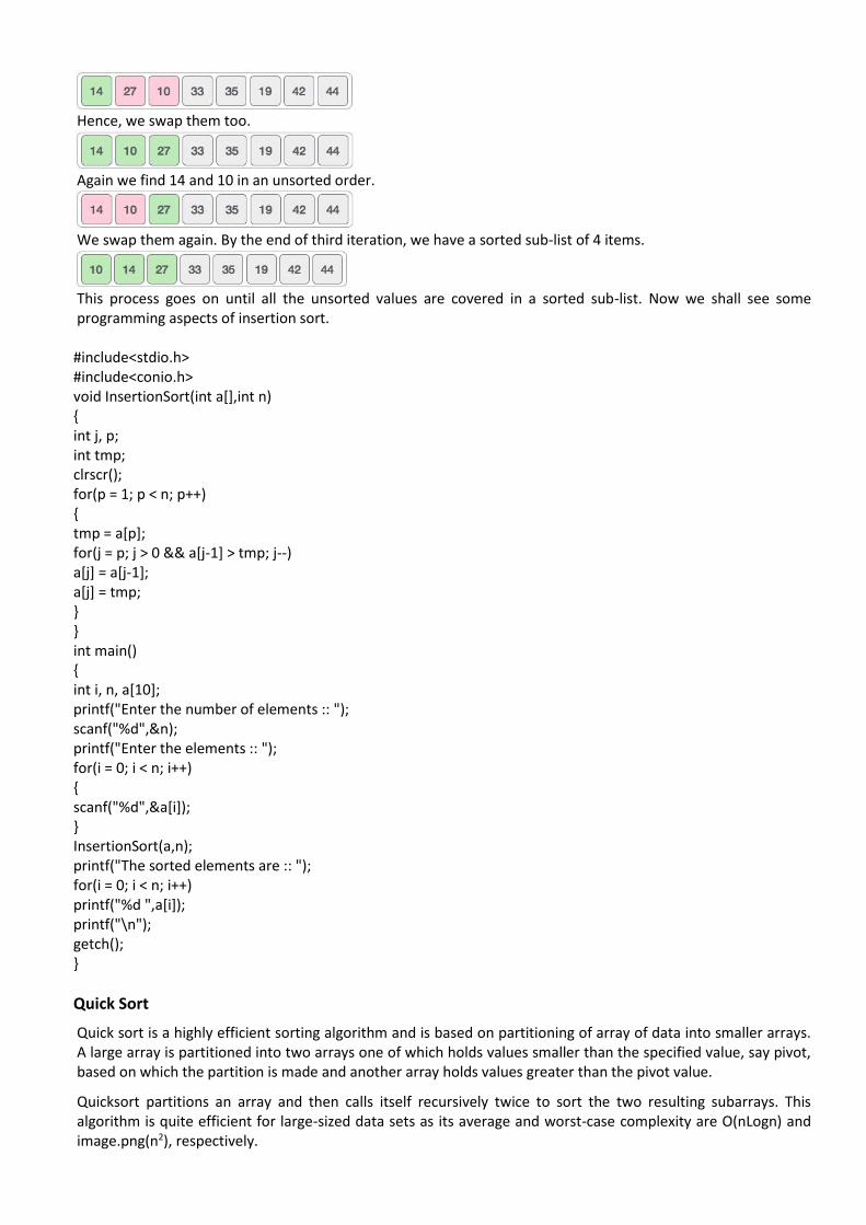
Hence, we swap them too.

Again we find 14 and 10 in an unsorted order.

We swap them again. By the end of third iteration, we have a sorted sub-list of 4 items.

This process goes on until all the unsorted values are covered in a sorted sub-list. Now we shall see some programming aspects of insertion sort. #include<stdio.h> #include<conio.h> void InsertionSort(int a[],int n) { int j, p; int tmp; clrscr(); for(p = 1; p < n; p++) { tmp = a[p]; for(j = p; j > 0 && a[j-1] > tmp; j--) a[j] = a[j-1]; a[j] = tmp; } } int main() { int i, n, a[10]; printf("Enter the number of elements :: "); scanf("%d",&n); printf("Enter the elements :: "); for(i = 0; i < n; i++) { scanf("%d",&a[i]); } InsertionSort(a,n); printf("The sorted elements are :: "); for(i = 0; i < n; i++) printf("%d ",a[i]); printf("\n"); getch(); }

Quick Sort

Quick sort is a highly efficient sorting algorithm and is based on partitioning of array of data into smaller arrays. A large array is partitioned into two arrays one of which holds values smaller than the specified value, say pivot, based on which the partition is made and another array holds values greater than the pivot value.

Quicksort partitions an array and then calls itself recursively twice to sort the two resulting subarrays. This algorithm is quite efficient for large-sized data sets as its average and worst-case complexity are O(nLogn) and image.png(n2), respectively.

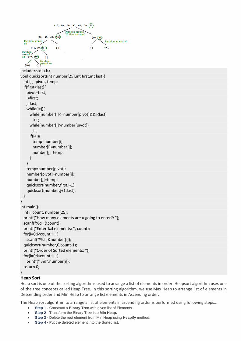
include<stdio.h> void quicksort(int number[25],int first,int last){ int i, j, pivot, temp; if(first<last){ pivot=first; i=first; j=last; while(i<j){ while(number[i]<=number[pivot]&&i<last) i++; while(number[j]>number[pivot]) j--; if(i<j){ temp=number[i]; number[i]=number[j]; number[j]=temp; } } temp=number[pivot]; number[pivot]=number[j]; number[j]=temp; quicksort(number,first,j-1); quicksort(number,j+1,last); } } int main(){ int i, count, number[25]; printf("How many elements are u going to enter?: "); scanf("%d",&count); printf("Enter %d elements: ", count); for(i=0;i<count;i++) scanf("%d",&number[i]); quicksort(number,0,count-1); printf("Order of Sorted elements: "); for(i=0;i<count;i++) printf(" %d",number[i]); return 0; }

Heap Sort Heap sort is one of the sorting algorithms used to arrange a list of elements in order. Heapsort algorithm uses one of the tree concepts called Heap Tree. In this sorting algorithm, we use Max Heap to arrange list of elements in Descending order and Min Heap to arrange list elements in Ascending order.

The Heap sort algorithm to arrange a list of elements in ascending order is performed using following steps... • Step 1 - Construct a Binary Tree with given list of Elements.

• Step 2 - Transform the Binary Tree into Min Heap.

• Step 3 - Delete the root element from Min Heap using Heapify method.

• Step 4 - Put the deleted element into the Sorted list.

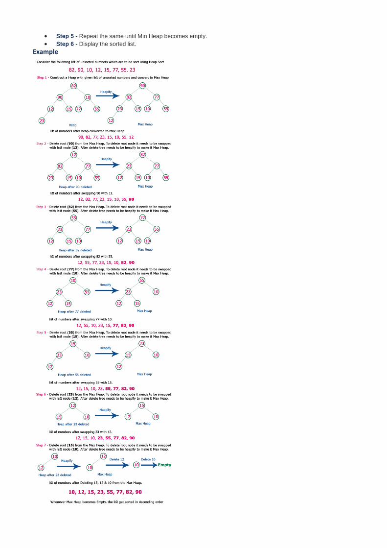
• Step 5 - Repeat the same until Min Heap becomes empty.

• Step 6 - Display the sorted list.

Example

#include<stdio.h> #include <conio.h> void heapify_function(int arr[]) { int i,n; n=arr[0]; for(i=n/2;i>=1;i--) adjust(arr,i); } void adjust(int arr[],int i) { int j,temp,n,k=1; n=arr[0]; while(2*i<=n && k==1) { j=2*i; if(j+1<=n && arr[j+1] > arr[j]) j=j+1; if( arr[j] < arr[i]) k=0; else { temp=arr[i]; arr[i]=arr[j]; arr[j]=temp; i=j; } } } void main() { int arr[100],n,temp,last,i; clrscr(); printf("How many Numbers you want to enter in your array: \n"); scanf("%d",&n); printf("Enter Elements in array:\n"); for(i=1;i<=n;i++) scanf("%d",&arr[i]); arr[0]=n; heapify_function(arr); while(arr[0] > 1) { last=arr[0]; temp=arr[1]; arr[1]=arr[last]; arr[last]=temp; arr[0]--; adjust(arr,1); }

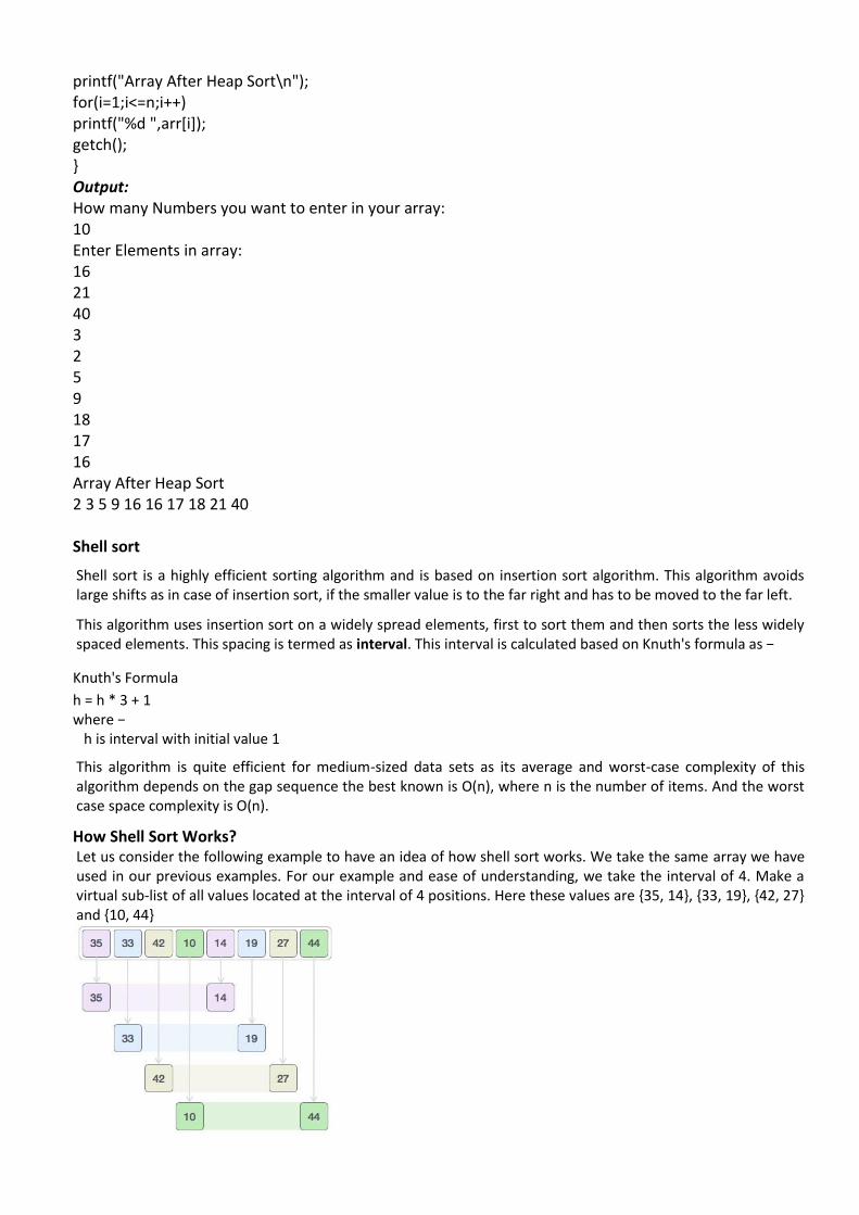
printf("Array After Heap Sort\n"); for(i=1;i<=n;i++) printf("%d ",arr[i]); getch(); } Output: How many Numbers you want to enter in your array: 10 Enter Elements in array: 16 21 40 3 2 5 9 18 17 16 Array After Heap Sort 2 3 5 9 16 16 17 18 21 40 Shell sort

Shell sort is a highly efficient sorting algorithm and is based on insertion sort algorithm. This algorithm avoids large shifts as in case of insertion sort, if the smaller value is to the far right and has to be moved to the far left.

This algorithm uses insertion sort on a widely spread elements, first to sort them and then sorts the less widely spaced elements. This spacing is termed as interval. This interval is calculated based on Knuth's formula as −

Knuth's Formula

h = h * 3 + 1 where − h is interval with initial value 1

This algorithm is quite efficient for medium-sized data sets as its average and worst-case complexity of this algorithm depends on the gap sequence the best known is Ο(n), where n is the number of items. And the worst case space complexity is O(n).

How Shell Sort Works? Let us consider the following example to have an idea of how shell sort works. We take the same array we have used in our previous examples. For our example and ease of understanding, we take the interval of 4. Make a virtual sub-list of all values located at the interval of 4 positions. Here these values are {35, 14}, {33, 19}, {42, 27} and {10, 44}

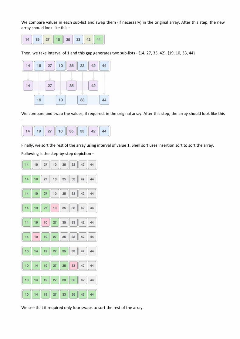
We compare values in each sub-list and swap them (if necessary) in the original array. After this step, the new array should look like this −

Then, we take interval of 1 and this gap generates two sub-lists - {14, 27, 35, 42}, {19, 10, 33, 44}

We compare and swap the values, if required, in the original array. After this step, the array should look like this −

Finally, we sort the rest of the array using interval of value 1. Shell sort uses insertion sort to sort the array.

Following is the step-by-step depiction −

We see that it required only four swaps to sort the rest of the array.

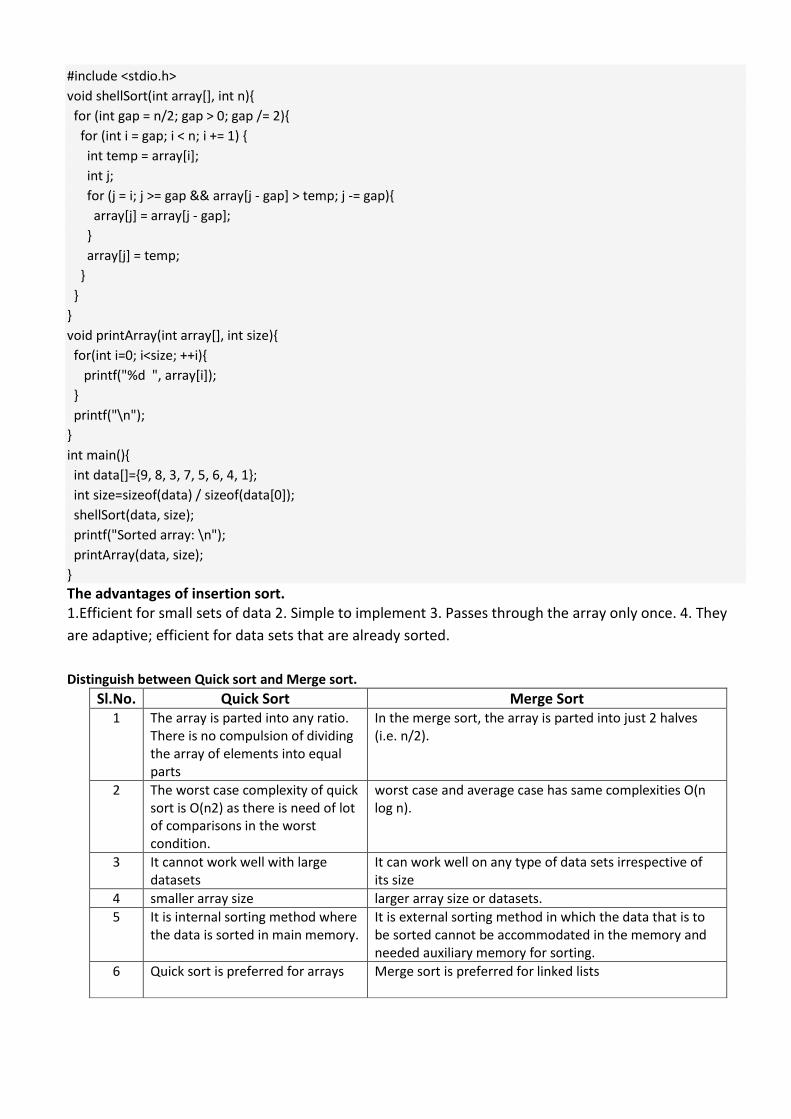
#include <stdio.h>

void shellSort(int array[], int n){

for (int gap = n/2; gap > 0; gap /= 2){

for (int i = gap; i < n; i += 1) {

int temp = array[i];

int j;

for (j = i; j >= gap && array[j - gap] > temp; j -= gap){

array[j] = array[j - gap];

}

array[j] = temp;

}

}

}

void printArray(int array[], int size){

for(int i=0; i<size; ++i){

printf("%d ", array[i]);

}

printf("\n");

}

int main(){

int data[]={9, 8, 3, 7, 5, 6, 4, 1};

int size=sizeof(data) / sizeof(data[0]);

shellSort(data, size);

printf("Sorted array: \n");

printArray(data, size);

}

The advantages of insertion sort. 1.Efficient for small sets of data 2. Simple to implement 3. Passes through the array only once. 4. They

are adaptive; efficient for data sets that are already sorted.

Distinguish between Quick sort and Merge sort.

Sl.No. Quick Sort Merge Sort 1 The array is parted into any ratio.

There is no compulsion of dividing the array of elements into equal parts

In the merge sort, the array is parted into just 2 halves (i.e. n/2).

2 The worst case complexity of quick sort is O(n2) as there is need of lot of comparisons in the worst condition.

worst case and average case has same complexities O(n log n).

3 It cannot work well with large datasets

It can work well on any type of data sets irrespective of its size

4 smaller array size larger array size or datasets.

5 It is internal sorting method where the data is sorted in main memory.

It is external sorting method in which the data that is to be sorted cannot be accommodated in the memory and needed auxiliary memory for sorting.

6 Quick sort is preferred for arrays

Merge sort is preferred for linked lists

What is File? File is a collection of records related to each other. The file size is limited by the size of memory and storage medium. There are two important features of file: 1. File Activity 2. File Volatility File activity specifies percent of actual records which proceed in a single run. File volatility addresses the properties of record changes. It helps to increase the efficiency of disk design than tape. File Organization File organization ensures that records are available for processing. It is used to determine an efficient file organization for each base relation. For example, if we want to retrieve employee records in alphabetical order of name. Sorting the file by employee name is a good file organization. However, if we want to retrieve all employees whose marks are in a certain range, a file is ordered by employee name would not be a good file organization.

Types of File Organization There are three types of organizing the file: 1. Sequential access file organization 2. Direct access file organization 3. Indexed sequential access file organization

1. Sequential access file organization

• Storing and sorting in contiguous block within files on tape or disk is called as sequential access file

organization.

• In sequential access file organization, all records are stored in a sequential order. The records are arranged in

the ascending or descending order of a key field.

• Sequential file search starts from the beginning of the file and the records can be added at the end of the file.

• In sequential file, it is not possible to add a record in the middle of the file without rewriting the file.

Advantages of sequential file

• It is simple to program and easy to design.

• Sequential file is best use if storage space.

Disadvantages of sequential file

• Sequential file is time consuming process.

• It has high data redundancy.

• Random searching is not possible.

2. Direct access file organization

• Direct access file is also known as random access or relative file organization.

• In direct access file, all records are stored in direct access storage device (DASD), such as hard disk. The records

are randomly placed throughout the file.

• The records does not need to be in sequence because they are updated directly and rewritten back in the same

location.

• This file organization is useful for immediate access to large amount of information. It is used in accessing large

databases.

• It is also called as hashing.

Advantages of direct access file organization

• Direct access file helps in online transaction processing system (OLTP) like online railway reservation system.

• In direct access file, sorting of the records are not required.

• It accesses the desired records immediately.

• It updates several files quickly.

• It has better control over record allocation.

Disadvantages of direct access file organization

• Direct access file does not provide back up facility.

• It is expensive.

• It has less storage space as compared to sequential file.

3. Indexed sequential access file organization • Indexed sequential access file combines both sequential file and direct access file organization. • In indexed sequential access file, records are stored randomly on a direct access device such as magnetic disk by

a primary key. • This file have multiple keys. These keys can be alphanumeric in which the records are ordered is called primary

key. • The data can be access either sequentially or randomly using the index. The index is stored in a file and read into

memory when the file is opened.

Advantages of Indexed sequential access file organization

• In indexed sequential access file, sequential file and random file access is possible. • It accesses the records very fast if the index table is properly organized. • The records can be inserted in the middle of the file. • It provides quick access for sequential and direct processing. • It reduces the degree of the sequential search.

Disadvantages of Indexed sequential access file organization

• Indexed sequential access file requires unique keys and periodic reorganization. • Indexed sequential access file takes longer time to search the index for the data access or retrieval. • It requires more storage space. • It is expensive because it requires special software. • It is less efficient in the use of storage space as compared to other file organizations.