Gender Discrimination, Intrahousehold Resource Allocation,

and Importance of Spouses’ Fathers:

Evidence on Expenditure from Rural Andhra Pradesh

July 14, 2006

Nobuhiko Fuwa, Seiro Ito,‡

Kensuke Kubo, Takashi Kurosaki,and Yasuyuki Sawada

A Data collected from rural India was used to examine the rules govern-ing intrahousehold resource allocations. Testing for gender-age discrimination amonghousehold members using Deaton (1989)’s method, results suggest a general bias fa-voring boys over girls in allocation of consumption goods, however, the findings arenot always statistically significant. Intrahousehold resource allocation rules are then ex-amined to see if such discrimination is based on unanimous decision of parents. Thenovelty in our test on allocation rule are: (1) use of grandparental variables as extra-household environmental parameters (EEP’s) in expenditure estimation, (2) derivationof a test of the unitary model that only requires EEP’s, and (3) semi-formal use of sur-vival status of grandparents in testing collective models. It is interesting yjay spouse’sfather characteristics are importantly correlated with greater mother and child goods ex-penditure shares, and smaller father goods shares. Their survival status matters, and thisis a stronger evidence for collective as opposed to unitary model.

I Introduction

Data on household consumption expenditures form the core of a database for assessing poverty

and distribution of welfare among households. They thus play a critical role for policy making. For

understanding intrahousehold resource allocation, it would be ideal to obtain data on consumption

at the level of individual members within the household. However, the basic unit of data collection

and analysis of data on consumption has been primarily at the aggregate household level. This is due

in part to very high costs and to various difficulties (conceptual and practical) involved in collecting

consumption data by individual members (Fuwa, 2005). Unlike some information that is collected at

the level of individual household members (labor activities, education, and health information), all

the consumption expenditure modules of the World Bank’s Living Standard Measurement Studies

include consumption expenditure data collected at the household level (Deaton and Grosh, 2000).

Despite the relative paucity of data on allocation of consumption goods among household mem-

bers, evidence accumulated in the last two decades suggests the potential importance of understand-

ing household behavior leading to such outcomes (Fuwa, 2005). Two major reasons for the in-

creased potential importance of intrahousehold analysis for policymakers are discussed byFuwa et

al. (2006). Both are directly related to household behavior leading to the allocation of consump-

tion goods (including food, nonfood consumption, and other services) among household members.

‡ Corresponding author. Development Studies Center, Institute of Developing Economies. E-mail to: itohse@ide.go.jp

1

The first concerns the measurement of individual welfare and the identification of potential target

populations when policy interventions are seen as necessary for poverty reduction. Questions have

been raised that whether female members (especially female children) within the household tend to

be discriminated against in consumption allocation within the household. A dramatic consequences

of gender bias appears to be the low sex ratio of women to men in some parts of the world such as

South and West Asia and China (seeSen, 1990, Rosenzweig and Schultz, 1982).

Negligence of such intrahousehold variation in consumption is known to inhibit understanding of

the severity of poverty at the individual level. In their simple yet insightful analysis,Haddad and

Kanbur (1990)show that, by using the household average of member welfare and neglecting the

intrahousehold welfare variations, poverty levels are underestimated. Since poverty is ultimately

an individual phenomenon, it must be measured at the individual level. This implies that knowing

the rules governing intrahousehold resource allocation is crucial in understanding poverty and its

alleviation.

Once discrimination against women (or girls) is found in resource allocation within households,

there may be potential room for policy interventions. In addition, micro level consumption data can

potentially be used to monitor changes in the welfare level of the population during policy changes or

other exogenous shocks such as weather. If there is a class of individual members of the household

who are identified as particularly vulnerable, the changes in their welfare level may not be revealed

by the aggregate household level consumption data alone.

Once such a target population is identified, the second aspect of policy implications will be in the

design of policy interventions by focusing on household behavior, This can include possible reac-

tions by the households to policy interventions. This latter aspect is important. Even when target

groups are properly identified, interventions may have little impact on intended beneficiaries, unless

policies are well designed to reach them. It has been found, for example, that some targeted policies

toward individuals (such as school food programs) can be offset by changes in intrahousehold con-

sumption in response to such policies. This can potentially leave negligible net effects on targeted

individuals (seeBeaton and Ghassemi, 1979on school food programs andAlderman et al., 1995for

a general discussion). Consideration of policy instruments with such potentials requires an analysis

of consumption allocation behavior within the household.

Because of the relative lack of data on individual consumption allocation and the necessity for

understanding intrahousehold resource allocation behavior from policymaker viewpoints, there have

been a few methodologies proposed in the literature that allow inference of aspects of intrahouse-

hold resource allocation by utilizing aggregate household-level consumption data alone. This paper

includes a combination of such methodological approaches to the dataset, specifically analytical

methodologies for making inferences about household behavior in intrahousehold resource alloca-

tion from the household-level consumption expenditure data. The paper has two primary points; (1)

detecting potential biases in allocating consumption goods between female and male children, and

(2) assessing the roles played by various potential sources of ‘bargaining powers’ of the husband and

the wife in determining the allocation of goods and services consumed by household members.

2

In general, characteristics of the parents affect household expenditure decisions in a way consis-

tent with intrahousehold bargaining. Further, literacy and land holdings of the surviving fathers of

spouses are correlated with greater expenditures directed to adult females and children. This pro-

vides some support of collective models. Section II of the paper provides descriptive statistics of

data is presented. In section III, gender-age discrimination in consumption is tested, showing weak

evidence of bias against girls. To understand the bias, Section IV includes a brief review of existing

literature on intrahousehold resource allocation. A model of the household is analysed to obtain

testable predictions for both unitary and collective models. Estimation issues on intrahousehold re-

source allocation are discussed in Section V. Estimation results are presented in Section VI, and the

last section offers a summary of results and conclusions.

II Data

Data was collected by the IDE-MVF team in 2005. Details of sampling are explained inFuwa

et al. (2006). Households were asked on food and nonfood items consumed over last two weeks

and teh last year, repsectively. For expenditure regressions in section III, detailed information on

assignable goods for each household’s demographic groups are necessary to know “who consumed

how much.” Three demographic groups are used: adult males, adult females, and children. The term

‘nonfood father goods’ are used for adult male clothing and adult male footwear. ‘Father goods’

are defined as nonfood father goods and ‘vice’ items such as todi (liquor made from coconuts),

beer, other alcohol drinks, beedi (local cigars), and cigarettes. ‘Mother goods’ are defined as adult

female clothing, adult female footwear, and adult female personal care items. ‘Child goods’ include

school fees, school uniform fees, school textbook fees, school transportation fees, and toys. All

expenditures are normalized to a two week period.

T 1 shows the descriptive statistics for the data. Median expenditures on nonfood father goods

and mother goods are roughly the same. The inclusion of vices significantly increases the median

father goods expenditure by more than 100%. This may explain why there is general hostility against

alcoholic drinks in rural India. Sampled households are characterized as having low literacy rates.

About 32% of heads of households and 13% of spouses are literate in an area where the literacy rates

are 59% for males and 30% for females. This is primarily due to the variable probability sampling

scheme that oversampled households with child labor. Less educated parents are more likely to let

children work.

Looking at the demographic structure, on average, there are 3 adults, 3 children, and 0.5 infants,

and 0.5 elderly persons in a household. Viewing blood relatives of the head, on average there is 1.1

extended family members in a household, 0.1 member coming from distant relatives such as nephew

or cousin. Education of grandmothers is rare, and this indicates any significant estimates on these

variables need to be interpreted with caution. Such estimates may have been tilted toward influential

observations. Thus, they are not used for testing collective models.

The probability of the grandfather being alive is lower than that of the grandmother. This is natural

in an area where marriages generally occur between older males and younger females. The higher

3

survival probability of spousal parents is also explained by this age gap. In general, the greater the

gap, the greater the difference in survival probabilities between head of household’s parents and the

spouse’s parents. This fact is interesting since it has been argued that a greater age gap is correlated

with a higher incidence (and a stronger degree) of gender discrimination against female spouses. If

the collective models hold, then early marriage, a symptom of gender inequality, is also a stabilizing

device. This is because female spouse’s parents live longer to support her when head of household’s

parents have already passed away. This may partly explain why poorer parents tend to choose early

marriage for their daughters.

The values of the indicator variables of coresidence and proximate residence of grandparents are

smaller than the survival probabilities of these members, as these are conditional on grandparent

survival. The mean age gaps of grandparents are 4.5 and 4.9 for head of household and spouse,

respectively. This is smaller than the sampled household’s mean age gap of 7.3. A general rise

in dowry payment in the last two decades analyzed inRao (1993)may be contributing to this. A

younger bride is considered to be more valuable, and parents of brides may save on the rising value

of dowries by accepting matrimony earlier. A greater age gap is also consistent with the greater

land holdings of head of household’s parents. This means that an average woman ‘marries up’ to

upper land holding classes. It results in lower-class women competing with upper class women

in the marriage market by bidding up dowries; men from the lowest land holding class (landless)

have a hard time finding brides. It indicates that the intergenerational transition in wealth quantile

is upwardly mobile for women but not for men. This also suggests that spouses are, on average,

from poorer families and thus do not have strong bargaining power in the household. The number of

siblings is greater for parents than for current youth, with a mean of approximately 5 for both head

of household and spouse.*1

*1 This suggests that some undocumented change in household structure has taken place in the last two to three decades.This is important, however, analyzing such a structural change is beyond the scope of this paper.

4

T 1: D Svariable name variable description min 25% median 75% max mean std 0s NAs n

fg0 nonfood father goods (Rs.) 0 18 31 50 309 42 40 17 0 387fg father goods (Rs.) 0 38 84 147 1472 130 177 13 0 387mg mother goods (Rs.) 2 23 35 65 272 51 44 0 0 387kg child goods (Rs.) 0 0 10 33 767 36 85 109 0 387subtotal food total food (Rs.) 67 698 968 1539 29231 1350 1817 0 0 387subtotal nonfood total nonfood (Rs.) 49 279 428 640 3071 520 389 0 0 387total total (Rs.1000) 0.116 1.054 1.474 2.182 29.461 1.871 1.889 0 0 387landval land value (Rs.) 0 1250 30000 92500 4800000 102135 296129 93 0 387dry acre acreage (rainfed) 0 0 2 4 160 4.336 10.395 142 0 387irr acre acreage (irrigated) 0 0 0 0 18 0.654 1.949 316 0 387fg0share nonfood father goods (as % of total) 0 0.013 0.021 0.032 0.269 0.025 0.022 18 0 387fgshare father goods (as % of total) 0 0.026 0.056 0.097 0.546 0.076 0.079 13 0 387mgshare mother goods (as % of total) 0 0.017 0.029 0.04 0.194 0.031 0.021 0 0 387kgshare child goods (as % of total) 0 0 0.006 0.021 0.235 0.018 0.034 109 0 387hd sex head sex (male=0, female=1) 0 0 0 0 1 0.075 0.264 356 2 387hd age head age 20 36 43 50 82 44.577 10.804 0 2 387hd lit head literacy 0 0 0 1 1 0.319 0.467 260 5 387hd yrs head year of education 0 0 0 2 14 1.733 3.16 269 5 387sp sex spouse sex (male=0, female=1) 0 1 1 1 1 0.948 0.223 18 44 387sp age spouse age 1 30 35 41.5 70 37.294 9.869 0 44 387sp lit spouse literacy 0 0 0 0 1 0.125 0.332 300 44 387sp yrs spouse year of education 0 0 0 0 14 0.685 1.938 293 44 387sp alive spouse is in HH 0 1 1 1 1 0.891 0.312 42 2 387amales adult males 0 1 1 2 6 1.571 0.919 18 2 387afemales adult females 0 1 1 2 5 1.452 0.799 7 2 387b lop boys, class 1-5 0 0 0 1 5 0.512 0.711 227 2 387g lop girls, class 1-5 0 0 0 1 3 0.504 0.711 235 2 387b upp boys, class 6-8 0 0 0 1 2 0.483 0.595 219 2 387g upp girls, class 6-8 0 0 0 1 3 0.46 0.633 236 2 387b sec boys, class 9-12 0 0 0 1 4 0.54 0.692 214 2 387g sec girls, class 9-12 0 0 0 1 3 0.494 0.642 225 2 387imales infant males 0 0 0 0 3 0.234 0.523 312 2 387ifemales infant females 0 0 0 0 3 0.249 0.582 313 2 387emales elderly males 0 0 0 0 1 0.161 0.368 323 2 387efemales elderly females 0 0 0 0 2 0.247 0.444 292 2 387infants infants 0 0 0 1 5 0.483 0.814 261 2 387lowerprim lower primary 0 0 1 2 8 1.016 1.041 144 2 387upperprim upper primary 0 0 1 1 4 0.943 0.765 115 2 387secondary secondary 0 0 1 2 4 1.034 0.846 108 2 387adeld adults and elderly 1 2 3 4 12 3.431 1.654 0 2 387hhsize household size 3 5 6 8 29 6.906 2.764 0 2 387blood1 children of head 0 3 4 5 14 3.587 1.701 10 2 387blood2 + parents, sibling, grand children and grand parents of head 0 3 4 5 19 4.527 2.281 2 2 387blood3 + other blood relatives of head 0 3 4 5 23 4.605 2.367 2 2 387hdf alive head’s father alive 0 0 0 0 1 0.218 0.413 302 1 387hdm alive head’s mother alive 0 0 0 1 1 0.477 0.5 202 1 387spf alive spouse’s father alive 0 0 0 1 1 0.347 0.477 252 1 387spm alive spouse’s mother alive 0 0 1 1 1 0.588 0.493 159 1 387hdf cores head’s father in HH 0 0 0 0 1 0.085 0.28 353 1 387hdm cores head’s mother in HH 0 0 0 1 1 0.264 0.442 284 1 387spf cores spouse’s father in HH 0 0 0 0 1 0.039 0.194 371 1 387spm cores spouse’s mother in HH 0 0 0 0 1 0.052 0.222 366 1 387hdf vill head’s father in village 0 0 0 0 1 0.096 0.295 349 1 387hdm vill head’s mother in village 0 0 0 0 1 0.142 0.35 331 1 387spf vill spouse’s father in village 0 0 0 0 1 0.047 0.211 368 1 387spm vill spouse’s mother in village 0 0 0 0 1 0.093 0.291 350 1 387hdf lit head’s father literare 0 0 0 1 1 0.271 0.445 274 11 387hdm lit head’s mother literate 0 0 0 0 1 0.021 0.145 367 12 387spf lit spouse’s father literare 0 0 0 0 1 0.239 0.427 293 2 387spm lit spouse’s mother literate 0 0 0 0 1 0.021 0.143 376 3 387hd bro number of head’s brothers 0 2 3 4 16 2.853 1.693 12 5 387hd sis number of head’s sisters 0 1 2 3 9 2.085 1.644 55 9 387sp bro number of spouse’s brothers 0 1 2 3 10 2.284 1.52 36 7 387sp sis number of spouse’s sisters 0 2 3 4 9 2.771 1.575 22 3 387hdf irr head’s father irrigated land 0 0 0 0 80 1.838 7.055 249 84 387hdf dry head’s father rainfed land 0 0 4 10 100 10.848 18.869 92 24 387spf irr spouse’s father irrigated land 0 0 0 0 15 0.775 2.328 263 71 387spf dry spouse’s father rainfed land 0 0 3 10 100 8.49 15.748 124 42 387hdp adiff head’s parents’ age difference 0 0 5 10 30 4.968 4.756 138 13 387spp adiff spouse’s parents’ age difference 0 0 5 8.5 25 4.541 4.618 159 8 387hdf alit head’s father alive and literate 0 0 0 0 1 0.082 0.275 345 11 387spf alit spouse’s father alive and literate 0 0 0 0 1 0.094 0.292 349 2 387hdf adry living head’s father’s rainfed land (acre) 0 0 0 0 85 2.284 8.833 302 24 387hdf airr living head’s father’s irrigated land (acre) 0 0 0 0 40 0.403 2.973 286 84 387spf adry living spouse’s father’s rainfed land (acre) 0 0 0 0 100 2.319 7.685 270 42 387spf airr living head’s father’s irrigated land (acre) 0 0 0 0 1 0.094 0.292 349 2 387clflag belongs to child labor stratum 0 0 1 1 1 0.652 0.477 134 2 387

5

III Gender Discrimination in Intrahousehold Consumption

Allocation

A general empirical strategy for making inferences about intrahousehold resource allocation pro-

cesses is to relate the observed variations in household consumption patterns, to observed varia-

tions in household characteristics. This approach analyzes the effects of household demographic

composition or the relative degree of resource control by individual members, on the patterns of

household consumption. This section provides an examinaion of whether there are gender biases in

the allocation of household consumption expenditures between female and male children within the

household.

III.1 A Methodology for Using Household Consumption Data To Detect Intra-

household Gender Biases

Household consumption data can typically be analyzed within the framework of household de-

mand function:qk = qk(p,m|z,w),

whereqk is the household aggregate demand for goodk, p is a vector of prices,m is a measure of

total (per capita/adult equivalent) household income/expenditure or other measure of total resources

(assets) available to the household,z is a vector of household demographic characteristics, andw is

a vector of other household characteristics. Inclusion ofw in the demand function implicitly incor-

porates household production. For example, if the household is a farm household, then farm assets,

land holdings, and irrigation status enterw in the determination of household income/expenditurem

and hence demandqk.

Presence of gender biases in household aggregate consumption can be examined by the method-

ology first proposed byDeaton (1989). Following Deaton (1989), we estimate the Engel curve of

the following:

wik = αk + βk ln

(xi

ni

)+ ηk ln ni +

∑

l

γkl

(nil

ni

)+ δ′zik + uik,

wherewik is the expenditure share of goodk in householdi, xi is the total household expenditure

of householdi, ni is household size (capturing economies of scale),nil is the number of household

members in thelth age-gender category, andzil is a vector of household characteristics (sex and age

of the household head and spouse, acreage of land, and village and caste dummy variables. In this

model, the differences in theγkl parameters indicate the effects on the household consumption of

particular goodk, by replacing a household member in one age-sex category (a girl of a certain age

group) with a member in another category (a boy of the same age group), holding the household

size and per-capita expenditure constant.Deaton (1989)proposed an approach to detect boy-girl

biases utilizing data on the consumption of ‘adult goods.’ Suppose certain consumption items that

are exclusively consumed by adult members of the household can be identified in the data. Typical

6

examples of such items are alcohol, tobacco, adult clothes, and adult footwear. Now, we definewik as

the expenditure share of such adult goods. Then, if a child is born to a (previously) childless couple

(holding the total expenditure constant), some portion of the resources previously spent exclusively

on adult goods for the couple will have to be diverted from the couple’s consumption expenditure

in order to feed and clothe the newborn. The main idea is to measure such income effects on adult

goods separately for a boy and for a girl and to examine whether such income effects are different

between boys and girls. If income effects are significantly larger for a boy than for a girl, then the

household will probably make more room for boys’ consumption than those of girls. This would

indicate a gender bias in total consumption expenditure allocation between a boy and a girl. More

specifically, we calculate the ‘outlay equivalent ratios’ (π-ratios) as follows:

πkr =

∂wk

∂nr

∂wk

∂x

nx

=

(ηk − βk) + γkr +L−1∑l=1

γkl

(nil

ni

)

βk + wk,

for each adult goodk and for each gender-age categoryr. Theπ-ratio for adult goodk for gender-age

categoryr measures the change in the consumption expenditure for the adult goodk that is equivalent

to the additional person in the gender-age categoryr. This is expressed as a ratio of total household

expenditure per capita. Adult goods we utilize in our analysis are: adult male clothes, adult female

clothes, adult male footwear, adult female footwear, adult female personal care items, and cigarettes

and alcohol (including beedi, cigarettes, toddy and other alcohol).

While we define those consumption items as ‘adult goods’ on an a priori basis, it is possible

to empirically test whether this definition of adult goods is consistent with the data. As shown in

Deaton et al. (1989), since (by assumption) the only effects of adding an additional child (a boy or a

girl) on the consumption of adult goods are on income, theπkr-ratio for a given age-gender groupr

should be the same for all adult goodsk. Thus, the null hypothesis is:

Ho : πkr = πk′r ,

for all k , k′ that refer to adult goods and for allr that refer to children’s age-gender categories. The

age-gender categories are age groups 0-4 and 5-14 for boys and girls.

III.2 Estimation Results

Estimated outlay equivalent ratios (πkr-ratios), and the test statistic for the difference in theπk-

ratios between boys and girls for each adult good-age category, are summarized in Table 2. If

adult goods are identified correctly (i.e. children do not consume those goods directly), thenπkr-

ratios should be negative, and smaller values (larger absolute values of negative numbers) mean

larger reductions in the consumption of adult goods due to the addition of a boy or a girl. This

indicates larger amounts of consumption expenditures are being re-allocated to the additional child.

As shown in the table, 17 of 24 estimatedπkr-ratios are negative (top four rows in Table 2). Among

the potential adult goods categories ‘adult female footwear’ and ‘adult personal care,’ allπ-ratios for

older children (age 5 to 14 for both female and male) are positive. This suggests that those goods are

7

potentially not ‘adult goods’ as expected. Especially for older girls, this is not surprising given the

reasonable possibility that both footwear and personal care items for older girls may be shared by

adult female members. Indeed, the positiveπ -ratios are larger for girls than for boys. In addition,

theπ-ratios for ‘cigarettes and alcohol’ are also positive for both infant boys and infant girls. This

again suggests that these goods are not behaving as theoretcally expected.*2

Based on point estimates of theπ -ratios in Table 2, there is an indication that the allocation of

household consumption goods tends to be biased toward boys and against girls. Among the eight

girl-boy pairs ofπ-ratios that are both negative, in the majority of the cases (five, including: adult

male clothes-age 0 to 4; adult female clothes-age 0 to 4; adult male footwear-age 0 to 4 and age

to 14; adult female footwear-age 0 to 4) the absolute value of theπ-ratio is larger for boys than for

*2 In fact, this is not the first time that household consumption of tobacco/cigarettes has been found to behave differentlyfrom the way ‘it should.’ Deaton’s (1989)original study, based on Thai data, produces positive equivalent ratioestimates for two out of three age categories of male children. More recently, similar results are obtained byCase andDeaton (2002)based on the NSS data from India and byFuwa (2005)based on a household survey data from the ruralPhilippines. Why the consumption of tobacco often does not behave the way adult goods should is not clear. It mightbe that the addition of children put stress on fathers who are then compelled to consume more tobacco; this is a clearviolation of the ‘demographic separability’ assumption.

8

girls. This suggests that the adult household members ‘sacrifice’ of adult good purchases in order

to make room for consumption goods for boys than for girls. Intriguingly, the estimatedπ-ratio

for cigarettes and alcohol is larger (absolute value) for older girls than for older boys. However,

the appropriateness of this category as adult goods has been somewhat unclear in other empirical

studies (see footnote above). Further, almost all cases (four out of five) in which the absolute value

of theπ-ratio is larger for boys than for girls, are in the lower age category (age 0 to 4). Thus, to

the extent that any anti-girl bias exists in the allocation of consumption goods within the household,

such biases are likely to be more serious for infant girls than for older girls.

Table 3 summarizes similar results using the share of the aggregated adult goods (rather than each

adult good category in a separate regression) as the dependent variable, with alternative definitions

of the adult goods. Alternative definitions of the ‘adult goods’ are used since some of these may

not be the same as those defined in theDeaton (1989). The 2nd, 4th, 6th, 8th and 10th columns of

Table 3 show theF-test statistics (with p-values in parentheses) for testing the null hypothesis of

equality ofπ-ratios across all the adult good categories taken together (as alternatively defined in

the top row). In particular, for the ‘female 5-14’ category (4th row), the null hypothesis of equality

of π-ratios among all adult good items is rejected when the three dubious adult good categories as

identified in Table 2 (adult female footwear, adult female personal care, and cigarettes & alcohol)

are included. When those three categories of goods are excluded (the last column of Table 3), the

equality ofπ-ratios is not rejected. The 1st, 3rd, 5th, 7th and 9th columns of Table 3 shows the point

estimates ofπ-ratios for aggregated adult goods with alternative definitions of the ‘adult goods’. The

qualitative results are essentially the same as those in Table 2. Point estimates suggest a possibility

that anti-girl bias may exist in the intrahousehold allocation of consumption goods among infants.

Restricting attention to the three candidate adult goods that passed the ‘equality ofπ-ratios tests’

(the last column of Table 3), individually (Table 2) or in aggregate (Table 3), all the point estimates

of π-ratios for infant children suggest a possibility of anti-girl biases.

Similar to most past studies from South Asia as well as from elsewhere in the world, none of the

observed differences inπ-ratios between girls and boys is statistically significant. A recent analysis

by Case and Deaton (2002), using the Indian NSS data from the 55th round, provides some point

estimates of ‘correct’ signs but no significant difference in the outlay equivalent ratios between boys

and girls. Combined with the earlier studies reporting similar results (e.g.,Ahmad and Morduch,

1993; Subramanian and Deaton, 1990), findings in this paper appear to support the view that the

power of the ‘adult goods approach’ in detecting gender biases in the intrahousehold allocation of

consumption goods is rather weak (see alsoStrauss and Beagle, 1996).

IV Testing Alternative Models of Intrahousehold Resource

Allocation

We have so far examined possible gender biases in the allocation of consumption expenditures

between boys and girls within the household, and have found that there is indeed some evidence

(albeit weak) suggesting some biases against girls of young ages. We now shift our focus to the

9

issue of how such potential biases may arise in the process of intrahousehold resource allocation.

Such an inquiry requires explicit modeling of the household decision making.

Some aspects of intrahousehold resource allocation can be inferred by specifying demographic

characteristicsz (gender and by age) or individual incomemi (differentiating income recipients),

and by adding identifying assumptions about the underlying utility functions of the household mem-

bers that lead to the demand function. Following the tradition of household budget analysis, the price

vector p will not be included because the dataset is cross-sectional and thus it is assumed that all

the households face the same prices. Under this general framework, one approach is to exploit the

relationships between variations in the household consumption of various goods and services and

variations in demographic composition of the household. This approach was taken in the previou

section. Another strategy is to exploit the effects of variations in economic resource control by differ-

ent household members within the household by decomposing the variablem in the equation above,

identifying resource owners, and examining their effects on the patterns of household consumption

demand. This approach can provide tests of alternative theoretical models of intrahousehold decision

making processes. We will apply this approach in the analysis reported in the next section.

Household models are generally divided into two main branches: the unitary and the non-unitary,

often termed as the collective household models (Alderman et al. (1995)). Unitary household mod-

els consider a household as a single unit maximizing their aggregated utility. Collective household

models allow household members to have different preferences, and differences in preferences are

allowed to affect how resources are allocated within a household. Collective models are increas-

ingly employed to analyze intrahousehold resource allocation in developing countries (Haddad et al.

(1997)).

In unitary models, a household maximizes the household utility function under resource con-

straints. One example of such models is as follows:

max{qi }

u(q1, · · · , qn|w, z)

s.t.∑

i

[mi(θi , s1|w, z) − p′qi

]6 0

whereqi is now a consumption vector of memberi, mi is income of memberi, θi is productivity of

memberi affectingmi , ands1 is a vector of other factors tha affect earnings such as wage rates and

labor market conditions.mi is also affected by household demographic variablesz and household

assetsw. Maximization gives a vector of Walrasian demand functions for each person:

qi = qi(p, s1,m|θ,w, z) for i = 1, · · · ,n,

wherem =∑

i mi is sum of individual incomes, or a household income. An important prediction of

unitary models is that household demand behavior is only affected by total household incomemand

not by the distribution of income among household members. Therefore, a test of unitary models

checks if incomes earned by each individual affect all demands in the same way.

Income pooling, a prediction of unitary model, may not be appropriate for households in devel-

oping countries. For example, we often observe situations where resources are allocated as a result

10

of bargaining among adult household members. Therefore, whether the unitary approach can be

accepted as a proxy for reality in rural settings in developing countries must be tested empirically.

An alternative way to model household behavior is to embed such bargaining processes in house-

hold decision making. Models sharing this intrahousehold perspective can be called non-unitary

household models. In contrast to unitary models, these do not assume the existence of an aggregated

household welfare function. Espescially in the collective models, individuals of a household not

only have different preferences, but they also act as autonomous subeconomies, conditional on the

actions of others. It is often assumed that individuals have a choice of remaining single or form-

ing a separate household or other grouping; such threats can be used in the bargaining process.*3

The bargaining powers of individuals in the household decision making are therefore assumed to be

influenced by outside options. These are functions of distribution factors or extra-household envi-

ronmental parameters (EEP’s). An important prediction of collective models is that incomes are not

pooled and that intrahousehold resource allocation is affected by EEP’s. Examples of EEP’s include

local sex ratios, divorce law legislation, and the degree of prohibition on market work by gender.

There are two variants in the non-unitary models: Pareto-efficient (collective) models and Pareto-

inefficient, non-cooperative models. In the former, household decisions are assumed to be Pareto

efficient, but without being explicit on how such an outcome is reached. This includes cooperative

bargaining models and other models that result in Pareto efficiency. The latter assumes individuals

cannot enter into binding and enforceable contracts with each other under asymmetric information.

Because of such information asymmetry, resource allocation within the household may not achieve

Pareto efficiency under the non-cooperative approach. Thus, a test for the Pareto efficiency within

a household (Udy, 1996; Duflo and Udry, 2004) is a test for Pareto-efficient household models

including both unitary and collective models, against non-unitary, and non-cooperative household

models.*4 In this paper, we assume Pareto efficiency is satisfied. We thus ignore noncoopeative

models, and test between Pareto-efficient collective models and unitary models. In this paper we

will use ‘collective models’ only for Pareto-efficient non-unitary models.

To derive testable implications for this paper, an example of a collective household models is

given below. This is a model with the assumption of ‘egoistic’ preferences (seeChiappori, 1992;

member’s utility depends only on own consumption). A household allocates resources optimally,

and maximizes:max{qi }

∑

i

µi(θ, s)u(qi |w, z)

s.t.∑

i

[mi(θi , s1|w, z) − p′qi

]6 0

∑

i

µi = 1

(P1)

wheres is a vector of EEP’s that influences the income sharing (bargaining) process but not pref-

*3 The seminal work byChiappori (1988)makes the minimal assumption of Pareto optimality of household allocations.It does not specify how Pareto optimality is reached. This treatment covers a general class of models that includescooperative bargaining models and unitary models as special cases.

*4 There are mixes of the two; threat points in cooperative bargaining are modeled as being determined by outcomes ofintrahousehold noncooperative games. SeeLundberg and Pollak (1993)andChen and Woolley (2001).

11

erences.s includess1, but may also contains2. Examples ofs2 (EEP’s that are ins but not ins1)

include: local sex ratios and divorce law legislation. If wealth, education, or social status of (grand)

parents do not directly affect earnings, then these may also be candidates of EEP’s ins2. For later

empirical exercises, it is important to note that education of grandparents outside the household is

not likely to affect individual earnings once we condition on measures ofθi such as education, age,

and sexes.

As shown inChiappori (1992), the above optimization problem is equivalent to:

max{qi }

ui(qi |w, z)

s.t. p′qi 6 mi(θi , s1|w, z) + φi

(P2)

whereφi is called a sharing rule, an income share of memberi. This is a function of pricesp,

individual incomesm, household-specific preference reflected inz, and EEP’s:

φi = φi(p,m, z, s),∑

i

φi = 0.

Note thatφi is additional (net) income for memberi. Pareto optimal allocation can be interpreted as

an outcome of a two-stage decision process. In stage 1, members decide on how to share the income

as summarized inφi . In the second stage, each member maximizes own egoistic utility functions by

choosingqi .

Maximization gives the following system of Walrasian demand functions:

qi = qi[p,mi(θi , s1|w, z) + φi(p,m, z, s)

], for i = 1, · · · ,n.

Noting the summing up restriction of sharing rule, anyj , i satisfies:

q j = q j

p,mj(θ j , s1|w, z) −∑

i, j

φi(p,m, z, s)

.

If members of the same gender can be treated as a single person of the collective model, then, the

above can be simplified into a model with two types of persons, males and females, and the above

becomes:q j = q j

[p,mj(θ j , s1|w, z) − φi(p,m, z, s)

].

To emphasize thatq j is a Walrasian demand function, the second argument can be expressed as ˜mj

so thatq j = q j(p, mj). ∂q j/∂mj characterizes the marginal increase of demand with respect to one’s

own income. Then, for an elements2l in s2,

∂qik

∂s2l

∂q jk′∂s2l

=

∂qik

∂mi

∂mi

∂s2l

∂q jk′∂mj

∂mj

∂s2l

= −∂qik

∂mi

∂φi

∂s2l

∂q jk′∂mj

∂φi

∂s2l

= −∂qik

∂mi

∂q jk′∂mj

for all s2l ∈ s2.

Hence, the ratio oflth EEP partials has the same value for alll for any goodsk , k′, for all s2l ∈ s2.

One can test this condition for all EEP’s in the regressors by estimating a system of equations. If the

goods are assignable, then one dropsk, k′ subscripts from the above. With assignable goods, one

tests for the EEP partial ratio equality on the same pair of goods with respect to alls2l ∈ s2. So we

12

can use the expenditure data, not the quantity, as the relative prices will be a common multiplicative

factor for the same pair of assignable goodsi, j:

∂piqi

∂s2l

∂p jq j

∂s2l

=pi

∂qi

∂mi

∂mi

∂s2l

p j∂q j

∂mj

∂mj

∂s2l

= −pi

∂qi

∂mi

∂φi

∂s2l

p j∂q j

∂mj

∂φi

∂s2l

= −pi

∂qi

∂mi

p j∂q j

∂mj

for all s2l ∈ s2. (1)

Note that the above relation does not hold when households behave in a way consistent with

unitary household models. Under the unitary approach, EEP’s ins2 have no effect on resource

allocation. Therefore, both the denominator and numerator of the above should be zero. Instead, the

Pareto efficiency can be tested under the unitary approach by applying a similar test for elements in

s1. This is explained in the next section.

V Estimation Method

In estimating expenditure regression models, the dependent variables can be defined in levels or in

shares. Levels estimation uses seemingly unrelated regression equations (SURE) with robust covari-

ance matrices. We use SURE because we need to test the cross-equation restrictions of collective

(and unitary, see below) household model’s equal proportionality conditions.

For the share regression, we followPapke and Wooldridge (1996)and estimate fractional logit

models. Surprisingly many previous works on expenditure shares ignore the fact that shares are

limited dependent variables data. Fractional logit model is:

yk = Λ(β′x

), yk ∈ [0,1],

andΛ(a) = 11+e−a is a logistic function.Papke and Wooldridge (1996), following the general result of

the quasi-maximum likelihood (QML) estimation ofGourieroux, Monfort and Trognon (1984), has

shown that maximization of logistic likelihood usingyk as a fraction variable, not a binary variable,

gives consistent estimates ofβ. The log-likelihood is Bernoulli:

lk(β) = yk ln[Λ

(β′x

)]+ (1− yk) ln

[1− Λ

(β′x

)].

We will use a system version of QML as we need to test cross-equation restrictions. Since we use

QML, the estimation of robust covariance matrix is straightforward.

As noted earlier, the conventional way to test the unitary models is to take exogenous variations

in incomes earned by individual members, and see if they affect the spending in the same way. The

problem with our data, as with other studies using cross-sectional data set, is the lack of intertem-

poral information. Given there are no repeated observations through time, we cannot consistently

estimate exogenous individual income changes. An alternative way is to use EEP’s. Suppose that an

individual i has an earning capacity given by:

mi = mi(θi , s1|w, z).

Here, we continue to assume that individual income is affected by some of EEP’s, denoted bys1.

These may include wage rates and other local labor market conditions. Then, under the null of

13

unitary model, household demand on goodk is:

qk = qk (p,m) = qk

p,∑

i

mi(θi , s1|w, z)

,

wherem =∑i

mi . It can be seen from the above that an EEP cannot be simultaneously significant

in one expenditure and not in another. If an EEP significantly affects expenditure on one good,

under the null of unitary model, it must also significantly affect the expenditure on other goods. This

provides a casual way of examining the unitary model.

A more formal test can be derived using an analogous idea with collective model’s EEP propor-

tionality. Taking the first derivative with respect to thelth EEP, we have:

∂qk

∂s1l=∂qk

∂m

∑

i

∂mi

∂s1l.

Then we have an analogous relationship of EEP proportionality as in the collective models, but for

elements included ins1:

∂qk

∂s1l

∂qk

∂s1l′

=

∂qk

∂m

∑i

∂mi

∂s1l

∂qk

∂m

∑i

∂mi

∂s1l′

=

∑i

∂mi

∂s1l

∑i

∂mi

∂s1l′

=

∂qk′∂m

∑i

∂mi

∂s1l

∂qk′∂m

∑i

∂mi

∂s1l′

=

∂qk′∂s1l

∂qk′∂s1l′

for all l′ , l, k′ , k.

Note in collective models that after assuming goods are assignable to an individual such thatk is

consumed only byj,∂qk

∂s1l=∂qk

∂mj

(∂mj

∂s1l+∂φ j

∂s1l

).

Thus,∂qk

∂s1l

∂qk

∂s1l′

=

∂mj

∂s1l+

∂φ j

∂s1l

∂mj

∂s1l′+

∂φ j

∂s1l′

,

∂mj′∂s1l

+∂φ j′∂s1l

∂mj′∂s1l′

+∂φ j′∂s1l′

=

∂qk′∂s1l

∂qk′∂s1l′

for all l′ , l, k′ , k, j′ , j.

The inequality follows as∂mj

∂s1l, ∂mj′

∂s1lor ∂mj

∂s1l+

∂φ j

∂s1l, ∂mj

∂s1l′+

∂φ j

∂s1l′, generally.

This analogous way of testing the unitary model of household uses cross-sectional data, and it

does not require information on individual income. This method has an advantage over the widely-

used income pooling tests. The latter incurs substantial cost in collecting income information. Even

if such information is collected, it is difficult to obtain consistent estimates of exogenous variation of

individual income without correct profit measures and price data (Rosenzweig and Wolpin, 2000).*5

*5 There is another possible advantage in using this test. Ifs11, s12, s13 are imprecisely measured as in classical errors-in-variable, sos1 j = s∗1 j + ej for j = 1,2,3, hence cov[s1 j ,ej ] = σ2

ej, and assuming cov[ej ,ej ] = 0 for all j , h, then

in regressingqk = β′x + γ′s1 with OLS, we have attenuation bias of:

plim γ1 = κ1γ1 < γ1, plim γ2 = κ2γ2 < γ2, plim γ3 = κ3γ2 < γ3,

with κ j ∈ [0,1] for all j:

κ1 =σ2

r1+ δ2

12σ2e2

+ δ213σ

2e3

σ2r1

+ δ212σ

2e2

+ δ213σ

2e3

+ σ2e1

, κ2 =σ2

r2+ δ2

21σ2e1

+ δ223σ

2e3

σ2r2

+ δ221σ

2e1

+ δ223σ

2e3

+ σ2e2

, κ3 =σ2

r3+ δ2

31σ2e1

+ δ232σ

2e2

σ2r3

+ δ231σ

2e1

+ δ232σ

2e2

+ σ2e3

,

andr j is prediction error of linear projection without a mismeasured variable:

s1 j = η′jx + δ jhs∗1h + δ jh′ s∗1h′ + r j = η′jx + δ jhs1h + δ jh′ s1h′ + (r j − δ jheh − δ jh′eh′ ),

14

We have found that the amount of good consumption is censored information. We must employ

censored regressions which are notoriously difficult to implement under the system-of-equations

context with many goods (and zero’s, seeYen et al., 2003). In addition, heteroskedasticity is almost

always impossible to rule out in survey data. Given these difficulties, we use the expenditure data of

Hicksian composite goods:*6 if the relative prices of a group of goods faced by households are the

same and fixed, then the entire group of goods can be considered as one single good in the demand

system (Deaton and Muellbauer 1980, pp. 120-122). Denoting thekth composite good byqk, we

have:

∂pkqk

∂s1l

∂pkqk

∂s1l′

=

pk∂qk

∂m

∑i

∂mi

∂s1l

pk∂qk

∂m

∑i

∂mi

∂s1l′

=

∑i

∂mi

∂s1l

∑i

∂mi

∂s1l′

=

pk′∂qk′∂m

∑i

∂mi

∂s1l

pk′∂qk′∂m

∑i

∂mi

∂s1l′

=

∂pk′qk′∂s1l

∂pk′qk′∂s1l′

for all l′ , l, k′ , k, (2)

The assumption of having the same and fixed relative prices between villages holds if the good

markets are integrated in the study area. This is likely under the frequent operation of busses, trucks,

rickshaws, and other motorized and non-motorized vehicles.

We will use Village and caste (backward caste, scheduled caste, other caste, scheduled tribe, Mus-

lim) dummy variables to control for the cluster fixed-effects. The other regressors include three

groups of variables: (1) household demographic variablesz, (2) grandparental demographic vari-

ablesg, and (3) grandparental land holding variablesh. The use of grandparental variables is rare

and can be considered as one of the strengths of this paper. As shown above, these will affect in-

dividual demand through the sharing rule in the collective setting; they are irrelevant in the unitary

setting. There are fewer observations of grandparental land holding variables because survey re-

spondents were sometimes unable to recall such information. Although such a memory loss to may

be a random event once we condition on demographic and household wealth variables, it can be ar-

gued that the landless have weaker memories concerning land than the landed, generating a selection

problem. Unfortunately, other than ages of respondents and years parents have been deceased, no

variables are available to control for the ‘unable-to-recall’ selection process. Thus estimated results

for h should be considered as exploratory.

It is important to recognize that, in using cross-sectional data, one cannot reject a ‘preference-

based’ interpretation of significant estimates on EEP’s. They reflect parental preference inherited

from grandparents, and are not an evidence of effects on bargaining power. To formally test the

collective models, one needs exogenous productivity shocks on each members that are uncorrelated

with grandparents’ preferences. This, however, requires at least panel data.*7 However, if the in-

herited portion of preferences from grandparents is fixed during a prolonged period (as is usually

assumed in the fixed-effect models), if deaths or the remote residence of grandparents diminish their

for j , h, j , h′. So ifκ1 ' κ2 ' κ3,

the severity of attenuation biases are similar for all ˆγ j , and we will have more precise estimates of their ratios.*6 One can, in principle, use only the minimally censored data and estimate SURE. However, there is a selection problem

arises if some goods, which are conditionally correlated with relative prices and income, are left out from the system.*7 Even with a panel, shock prone individuals may have a systematic tendency in their preferences and behaviors that

cannot be controlled in estimation.

15

effects on bargaining power, and if the deaths of parents are not correlated with preference hetero-

geneity, then households with surviving grandparents residing in proximity and the households with

deceased or remotely residing grandparents, should have different parameter estimates for EEP’s.

This test is valid since under the null of collective model, with residential proximity and parental

survival that is uncorrelated with preference heterogeneity, there will be significant differences in

estimated parameters, while under the alternative of fixed preference-inheritance or no bargaining,

there should be no any significant differences. Thus we estimate:

yk = Λ[β′1z + β′20g + β′21Dg + β′30h + β′31Dh

],

whereD is an indicator variable for surviving and proximate residence of grandparents. We test

β21 = 0.*8

As our data employs variable probability sampling (VPS), one needs to weight the likelihood or

observations. As for QML, denoting the sampling weight for observationk of stratum j asπ jk, the

weighted log-likelihood is: ∑

k

lk(β)π jk

.

If all the regressors are considered as exogenous, one can consistently estimate the parameters with

VPSSURE and VPSQML.

*8 We could have testedβ31 = 0, however, singularity prohibits the use of interaction term onh.

16

VI Estimated Results

T 4: S N F G V, C F ESURE SURE SURE SURE SURE QML QML QML QML QML

(1) (2) (3) (4) (5) (6) (7) (8) (9) (10)

hd age 0.028 −0.510 −0.387 −0.444 −0.245 −0.013 −0.023∗∗∗ −0.022∗∗∗ −0.019∗∗ −0.016∗(0.409) (0.357) (0.400) (0.412) (0.557) (0.009) (0.008) (0.008) (0.008) (0.009)

hd yrs 0.454 0.336 0.720 0.837 1.352 −0.014 −0.013 −0.007 −0.008 −0.004(0.715) (0.719) (0.747) (0.729) (1.008) (0.014) (0.013) (0.014) (0.014) (0.017)

sp age 0.953∗∗ 0.702∗ 0.847∗ 0.924∗ 0.400 0.022∗∗ 0.022∗∗ 0.021∗∗ 0.020∗∗ 0.010(0.476) (0.376) (0.439) (0.473) (0.443) (0.011) (0.009) (0.009) (0.009) (0.008)

sp yrs 0.745 0.010 0.236 0.425 4.311∗∗ 0.014 0.000 0.000 0.002 0.075∗∗(1.436) (1.261) (1.361) (1.376) (2.042) (0.026) (0.025) (0.026) (0.027) (0.032)

hd sex −26.584∗∗ −19.127∗ −15.087 −19.130∗ −15.104 −0.923∗ −1.019∗∗ −0.973∗∗ −0.980∗∗ −1.171∗(11.398) (10.459) (9.587) (10.594) (11.500) (0.472) (0.448) (0.438) (0.437) (0.689)

total 4.141∗ 1.973 2.371∗ 2.171∗ 0.350 −0.098∗∗∗ −0.174∗∗∗ −0.188∗∗∗ −0.196∗∗∗ −0.250∗∗∗(2.490) (1.593) (1.336) (1.255) (1.016) (0.030) (0.037) (0.040) (0.039) (0.043)

amales 12.399∗∗∗ 15.110∗∗∗ 13.799∗∗∗ 13.316∗∗∗ 0.233∗∗∗ 0.290∗∗∗ 0.268∗∗∗ 0.225∗∗∗(3.472) (4.421) (4.358) (3.272) (0.059) (0.070) (0.071) (0.059)

afemales 12.665∗∗∗ 11.685∗∗∗ 11.946∗∗∗ 2.408 0.140∗∗ 0.116∗∗ 0.119∗∗ 0.007(3.882) (3.716) (3.712) (4.756) (0.061) (0.059) (0.059) (0.074)

b lop −2.574 −1.934 −1.421 −1.510 −0.032 −0.016 0.003 −0.008(2.762) (3.004) (2.867) (3.166) (0.044) (0.044) (0.042) (0.047)

b upp 1.192 2.630 3.119 5.518 −0.008 0.012 0.021 0.106(3.305) (3.439) (3.446) (4.144) (0.066) (0.063) (0.064) (0.067)

b sec 0.248 0.485 0.599 2.591 0.019 0.024 0.023 0.093(3.520) (3.605) (3.631) (4.656) (0.058) (0.058) (0.059) (0.067)

g lop 2.011 2.041 2.220 3.009 −0.003 0.006 0.002 0.052(2.500) (2.828) (2.855) (3.249) (0.051) (0.051) (0.052) (0.060)

g upp 1.325 2.571 3.135 10.469∗∗∗ −0.083 −0.066 −0.051 0.081(3.092) (3.156) (3.099) (3.752) (0.065) (0.064) (0.064) (0.072)

g sec −0.838 −1.956 −1.098 1.568 −0.052 −0.074 −0.072 −0.015(3.486) (3.555) (3.659) (3.858) (0.067) (0.065) (0.067) (0.073)

imales −1.685 −1.617 1.072 6.671 −0.147∗ −0.119 −0.080 0.023(4.378) (4.799) (4.636) (5.075) (0.082) (0.078) (0.074) (0.075)

ifemales −5.221∗ −6.742∗∗ −7.302∗∗ −4.622 −0.106∗∗ −0.143∗∗ −0.150∗∗∗ −0.095(2.889) (3.399) (3.241) (3.794) (0.054) (0.060) (0.057) (0.066)

emales 10.159 14.140 16.016 35.543∗∗ 0.295∗∗ 0.438∗∗ 0.422∗∗ 0.905∗∗∗(9.649) (11.795) (11.554) (13.890) (0.145) (0.179) (0.181) (0.201)

efemales −0.557 −0.332 0.070 −1.717 −0.162∗ −0.128 −0.100 −0.161(4.743) (5.831) (5.718) (6.498) (0.087) (0.104) (0.105) (0.118)

hdf alive −9.459 −8.280 15.191 −0.220 −0.206 0.308(9.027) (8.768) (13.318) (0.199) (0.185) (0.279)

hdm alive 1.521 0.286 7.020 0.039 0.023 0.063(7.475) (7.265) (8.922) (0.142) (0.138) (0.164)

spf alive 7.400 8.735 13.370∗∗ 0.131 0.151 0.115(5.717) (5.573) (5.643) (0.103) (0.102) (0.103)

spm alive 4.882 6.492 −2.467 0.141 0.168 0.018(6.603) (6.538) (6.237) (0.125) (0.127) (0.101)

hdf vill 7.261 3.150 −11.453 0.221 0.186 −0.039(11.767) (11.403) (15.724) (0.235) (0.224) (0.308)

hdm vill 4.192 2.487 −1.208 −0.018 −0.037 −0.050(7.133) (7.473) (8.526) (0.146) (0.150) (0.164)

spf vill −9.086 −9.636 −12.853 −0.337∗ −0.336∗∗ −0.388∗∗(8.399) (8.482) (9.312) (0.173) (0.172) (0.163)

spm vill 2.072 0.792 −1.843 0.105 0.085 0.064(6.150) (6.330) (7.851) (0.125) (0.128) (0.125)

hdf cores 8.932 3.437 −35.226∗∗ 0.059 0.035 −0.890∗∗(14.356) (14.316) (17.165) (0.275) (0.270) (0.371)

hdm cores 2.264 4.512 2.682 −0.060 −0.049 0.042(7.585) (7.635) (9.705) (0.138) (0.139) (0.151)

spf cores −17.553 −17.721 −9.987 −0.106 −0.091 0.265(14.895) (14.118) (15.798) (0.346) (0.332) (0.303)

spm cores 19.840∗ 15.645 9.108 0.153 0.081 −0.144(10.564) (9.854) (11.578) (0.201) (0.191) (0.183)

hdf lit 0.989 0.697 −2.481 0.000 0.012 −0.047(4.745) (4.765) (5.557) (0.098) (0.100) (0.101)

spf lit 0.354 2.147 −1.668 0.034 0.091 0.085(5.134) (5.152) (6.545) (0.099) (0.103) (0.129)

hd bro 0.468 −1.199 −0.014 −0.079∗∗∗(1.252) (1.701) (0.025) (0.031)

hd sis −0.672 −2.219 −0.013 −0.063∗∗(1.162) (1.400) (0.023) (0.026)

sp bro 1.586 2.351 0.025 0.054∗(1.432) (1.456) (0.027) (0.029)

sp sis −1.034 −1.661 −0.023 −0.011(1.187) (1.521) (0.023) (0.029)

hdf irr −0.501 −0.002(0.402) (0.006)

hdf dry 0.363∗ 0.005(0.210) (0.003)

spf irr 1.512 0.026∗(0.937) (0.015)

spf dry 0.210 0.001(0.247) (0.004)

hdp adiff −1.265∗∗ −0.023∗(0.636) (0.012)

spp adiff 0.790 0.004(0.584) (0.012)17

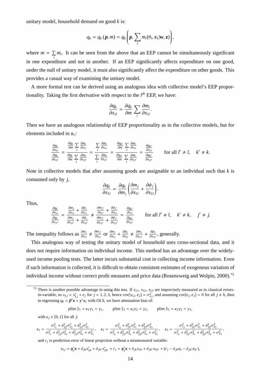
T 5: S F G V, C F ESURE SURE SURE SURE SURE QML QML QML QML QML

(1) (2) (3) (4) (5) (6) (7) (8) (9) (10)

hd age 1.720 0.822 2.164 2.886 4.061 0.020 0.019 0.026∗∗ 0.029∗∗∗ 0.036∗∗∗(2.467) (2.601) (2.564) (2.866) (4.183) (0.012) (0.013) (0.010) (0.011) (0.013)

hd yrs 0.987 1.278 4.129 3.307 2.307 −0.018 −0.016 −0.003 −0.010 −0.009(3.896) (4.191) (4.329) (4.574) (6.737) (0.022) (0.023) (0.022) (0.024) (0.029)

sp age −0.335 −0.526 −0.432 −0.914 −1.223 −0.016 −0.015 −0.017 −0.018∗ −0.028∗∗(2.028) (2.175) (2.018) (2.084) (2.989) (0.011) (0.012) (0.010) (0.010) (0.013)

sp yrs −11.277∗ −11.796∗ −9.755∗ −9.185 −9.795 −0.072∗ −0.072∗ −0.042 −0.037 −0.009(5.940) (6.737) (5.610) (5.839) (9.105) (0.038) (0.041) (0.035) (0.039) (0.059)

hd sex 27.599 26.690 44.903 50.898 84.708 0.742∗∗ 0.658∗ 0.666∗∗ 0.640∗ 0.603(40.071) (48.568) (48.171) (63.287) (92.609) (0.341) (0.344) (0.306) (0.348) (0.476)

total 14.954 13.313 18.746∗ 17.343∗ 18.862∗ −0.059 −0.034 −0.035 −0.051 −0.046(11.205) (10.842) (9.827) (9.787) (10.982) (0.044) (0.039) (0.037) (0.036) (0.038)

amales −8.332 −1.954 −2.414 −4.699 −0.116 −0.087 −0.086 −0.206∗(14.852) (15.870) (16.395) (24.798) (0.084) (0.086) (0.086) (0.118)

afemales 21.469 9.950 10.047 0.379 −0.034 −0.063 −0.096 −0.098(18.964) (18.557) (18.575) (30.283) (0.097) (0.085) (0.086) (0.104)

b lop −1.881 10.841 14.859 44.136∗∗ 0.036 0.135 0.174∗∗ 0.304∗∗∗(15.433) (16.050) (16.885) (22.222) (0.096) (0.085) (0.084) (0.080)

b upp −3.394 14.752 10.763 −9.603 −0.045 0.108 0.056 −0.074(20.397) (20.384) (21.277) (30.338) (0.122) (0.097) (0.097) (0.113)

b sec −6.712 −8.046 −9.356 −29.692 −0.042 −0.064 −0.075 −0.161(21.125) (21.475) (22.215) (30.373) (0.106) (0.095) (0.094) (0.107)

g lop 1.192 −8.918 −9.357 −12.481 −0.060 −0.085 −0.110 −0.108(13.367) (16.606) (17.464) (24.695) (0.087) (0.085) (0.087) (0.122)

g upp −7.080 −8.541 −3.872 −12.858 −0.115 −0.124 −0.114 −0.140(18.839) (18.899) (18.243) (24.864) (0.104) (0.086) (0.084) (0.103)

g sec −3.524 −15.785 −20.815 −47.192 −0.049 −0.087 −0.117 −0.223∗(23.382) (27.594) (29.381) (38.942) (0.120) (0.113) (0.114) (0.120)

imales 15.754 27.805 26.009 11.468 0.053 0.204 0.233 0.145(28.499) (31.285) (32.001) (38.712) (0.178) (0.164) (0.152) (0.163)

ifemales 6.732 −1.655 2.984 8.452 0.036 −0.049 −0.008 0.007(15.394) (17.488) (18.232) (27.912) (0.087) (0.086) (0.095) (0.106)

emales 58.239 8.390 2.440 43.281 0.218 −0.008 −0.031 0.052(51.297) (84.731) (87.485) (121.713) (0.221) (0.262) (0.252) (0.281)

efemales 0.135 −5.437 −8.939 7.836 −0.098 0.061 0.020 0.334∗(21.007) (29.968) (30.630) (45.215) (0.138) (0.152) (0.150) (0.179)

hdf alive −51.456 −32.472 −184.049 −0.487 −0.334 −1.115∗(44.175) (49.858) (114.771) (0.309) (0.367) (0.627)

hdm alive −51.558 −49.881 −49.206 −0.457∗ −0.511∗∗ −0.690∗∗(33.757) (35.080) (53.097) (0.237) (0.242) (0.330)

spf alive 53.610 47.720 80.366 0.282∗ 0.221 0.275∗(37.661) (36.189) (50.378) (0.157) (0.148) (0.161)

spm alive 40.583 43.789 66.030∗ 0.334∗∗ 0.378∗∗∗ 0.393∗∗(28.154) (28.471) (39.910) (0.150) (0.147) (0.154)

hdf vill −24.859 −34.738 143.341 −0.131 −0.267 0.815(56.802) (61.213) (127.376) (0.388) (0.454) (0.717)

hdm vill 48.522 30.677 23.876 0.194 0.033 0.001(41.373) (43.576) (55.741) (0.267) (0.272) (0.314)

spf vill −42.947 −33.060 −16.094 −0.217 −0.133 0.164(45.797) (46.623) (59.080) (0.285) (0.296) (0.308)

spm vill −33.119 −39.580 −80.027 −0.416 −0.492∗ −0.738∗∗(39.677) (42.327) (54.911) (0.262) (0.264) (0.304)

hdf cores 197.506 191.031 451.384∗∗ 0.942∗∗ 0.906∗∗ 2.057∗∗∗(136.130) (141.769) (224.622) (0.418) (0.451) (0.677)

hdm cores 65.433∗ 61.879 68.275 0.205 0.226 0.208(39.625) (40.416) (54.716) (0.249) (0.242) (0.270)

spf cores −198.632∗∗ −199.258∗∗ −183.041 −0.375 −0.430 0.070(83.879) (79.588) (117.148) (0.490) (0.436) (0.498)

spm cores 145.939∗∗ 135.927∗ 126.432 0.402 0.253 0.206(73.632) (73.119) (79.982) (0.310) (0.319) (0.337)

hdf lit 59.391 58.248 101.768∗∗ 0.568∗∗∗ 0.544∗∗∗ 0.791∗∗∗(36.705) (36.327) (51.775) (0.143) (0.142) (0.157)

spf lit −89.236∗∗∗ −92.922∗∗∗ −124.326∗∗∗ −0.608∗∗∗ −0.647∗∗∗ −0.864∗∗∗(29.640) (30.534) (38.728) (0.156) (0.155) (0.199)

hd bro −8.779 −17.466 −0.014 −0.062(8.520) (12.056) (0.036) (0.047)

hd sis 10.367 14.318 0.087∗∗ 0.105∗∗(8.187) (11.025) (0.040) (0.048)

sp bro 8.313 13.924 0.100∗∗∗ 0.147∗∗∗(6.104) (8.993) (0.035) (0.043)

sp sis −2.423 −7.811 −0.028 −0.050(7.559) (10.155) (0.043) (0.060)

hdf irr −6.547∗∗ −0.040∗∗∗(2.810) (0.013)

hdf dry 0.278 0.004(1.148) (0.004)

spf irr −9.674 −0.026(7.504) (0.025)

spf dry 0.097 0.000(1.297) (0.006)

hdp adiff −6.653 −0.036∗(4.174) (0.019)

spp adiff 1.599 −0.013(4.614) (0.021)

18

T 6: S M G V, C F ESURE SURE SURE SURE SURE QML QML QML QML QML

(1) (2) (3) (4) (5) (6) (7) (8) (9) (10)

hd age 0.068 −0.470 −0.394 −0.274 0.032 −0.010 −0.014 −0.013 −0.008 −0.011(0.538) (0.503) (0.525) (0.507) (0.670) (0.008) (0.008) (0.009) (0.008) (0.010)

hd yrs 1.770∗ 1.685∗ 1.563∗ 1.718∗ 2.120∗ 0.035∗∗ 0.033∗∗ 0.025∗ 0.029∗∗ 0.022(0.956) (0.953) (0.879) (0.893) (1.118) (0.016) (0.016) (0.014) (0.014) (0.016)

sp age 0.672 0.542 0.746 0.679 0.766 0.009 0.007 0.009 0.007 0.017(0.528) (0.554) (0.588) (0.569) (0.677) (0.008) (0.009) (0.010) (0.009) (0.010)

sp yrs 3.443∗ 2.118 1.761 1.816 4.045∗∗ 0.029 0.014 0.003 0.000 0.038(1.814) (1.713) (1.586) (1.603) (1.986) (0.024) (0.023) (0.022) (0.021) (0.024)

hd sex −30.637∗ −28.711∗ −21.547 −18.659 −13.500 0.053 0.036 0.087 0.116 0.441(17.479) (15.944) (14.616) (13.606) (17.757) (0.563) (0.518) (0.502) (0.458) (0.425)

total 4.053 1.865 1.862 1.447 0.313 −0.176∗∗∗ −0.267∗∗∗ −0.298∗∗∗ −0.314∗∗∗ −0.325∗∗∗(2.605) (1.563) (1.322) (1.290) (1.394) (0.039) (0.049) (0.049) (0.050) (0.050)

amales 2.767 5.594∗ 6.190∗ 11.794∗∗∗ 0.033 0.068 0.078 0.178∗∗∗(2.927) (3.312) (3.424) (3.776) (0.050) (0.052) (0.052) (0.064)

afemales 21.599∗∗∗ 20.464∗∗∗ 20.813∗∗∗ 13.884∗∗ 0.274∗∗∗ 0.267∗∗∗ 0.285∗∗∗ 0.168∗∗∗(4.012) (4.014) (3.984) (5.649) (0.058) (0.059) (0.055) (0.064)

b lop 0.728 1.097 1.379 −2.068 0.008 0.017 0.036 −0.038(2.385) (2.411) (2.472) (3.521) (0.045) (0.047) (0.044) (0.048)

b upp 0.508 2.532 3.101 7.261∗ −0.010 0.022 0.039 0.163∗∗(3.401) (3.568) (3.518) (4.412) (0.062) (0.063) (0.062) (0.065)

b sec −0.434 1.139 0.967 0.273 −0.019 0.009 0.001 0.024(3.222) (3.160) (3.202) (4.268) (0.059) (0.056) (0.053) (0.063)

g lop 0.730 1.044 2.011 0.361 −0.061 −0.053 −0.043 −0.077(2.800) (2.991) (3.048) (3.276) (0.052) (0.050) (0.049) (0.056)

g upp 7.268∗∗ 9.374∗∗∗ 10.261∗∗∗ 14.912∗∗∗ 0.092 0.130∗∗ 0.155∗∗∗ 0.253∗∗∗(3.467) (3.376) (3.371) (4.261) (0.058) (0.059) (0.057) (0.071)

g sec −2.358 −2.379 −3.266 −4.385 −0.144∗∗ −0.153∗∗ −0.178∗∗ −0.166∗∗(3.712) (3.783) (3.889) (4.036) (0.072) (0.070) (0.070) (0.074)

imales −4.154 −1.724 −3.025 1.037 −0.127∗ −0.059 −0.101 −0.071(4.144) (4.577) (4.735) (5.546) (0.065) (0.069) (0.069) (0.078)

ifemales −5.081∗ −6.761∗∗ −6.812∗∗ −2.174 −0.097∗ −0.106∗∗ −0.106∗∗ −0.015(3.036) (3.329) (3.372) (4.340) (0.055) (0.052) (0.051) (0.064)

emales −3.941 3.834 5.309 5.232 −0.006 0.108 0.076 0.274(7.902) (9.563) (9.679) (14.242) (0.127) (0.157) (0.158) (0.198)

efemales 9.956∗ 12.275∗ 10.290 4.760 0.117 0.199∗ 0.167 −0.007(5.232) (7.096) (7.319) (7.442) (0.083) (0.108) (0.109) (0.123)

hdf alive −15.935 −14.453 2.625 −0.292 −0.264 0.027(12.027) (12.270) (23.990) (0.201) (0.200) (0.261)

hdm alive 9.181 11.310 23.694∗ 0.140 0.182 0.380∗∗(11.600) (11.423) (13.262) (0.169) (0.161) (0.165)

spf alive 8.233 7.955 19.070∗∗ 0.154∗ 0.147∗ 0.267∗∗(5.904) (5.863) (7.566) (0.088) (0.084) (0.110)

spm alive 11.415∗∗ 12.926∗∗ 7.731 0.157∗ 0.193∗∗ 0.186∗(5.509) (5.553) (8.266) (0.092) (0.091) (0.112)

hdf vill 14.226 13.013 −3.224 0.304 0.337 0.060(16.122) (16.314) (28.515) (0.245) (0.247) (0.325)

hdm vill −3.070 −4.479 −9.692 −0.131 −0.144 −0.308(13.681) (13.325) (14.616) (0.193) (0.182) (0.198)

spf vill 0.613 2.311 −13.329 0.011 0.067 −0.275(10.393) (10.500) (11.481) (0.212) (0.198) (0.227)

spm vill −4.799 −6.686 1.111 −0.147 −0.176 0.045(9.413) (9.717) (9.355) (0.172) (0.159) (0.151)

hdf cores 6.075 0.770 −25.148 0.137 0.081 −0.472(14.968) (15.198) (27.041) (0.276) (0.273) (0.344)

hdm cores −5.675 −5.224 −6.032 −0.192 −0.190 −0.156(11.061) (11.074) (11.622) (0.155) (0.150) (0.154)

spf cores −11.628 −10.184 −2.614 −0.012 0.037 0.341(13.624) (14.651) (14.438) (0.226) (0.247) (0.243)

spm cores 13.181 13.076 20.363∗ 0.059 0.084 0.104(8.747) (8.820) (11.858) (0.142) (0.136) (0.173)

hdf lit 2.901 3.492 −3.141 0.022 0.049 −0.058(5.149) (4.882) (6.615) (0.089) (0.085) (0.107)

spf lit 11.863∗ 8.954 7.391 0.232∗∗ 0.187∗ 0.204(7.087) (7.370) (9.303) (0.105) (0.106) (0.127)

hd bro −2.041 −1.456 −0.072∗∗∗ −0.074∗∗(1.348) (1.886) (0.022) (0.034)

hd sis 1.831 −1.369 0.034 −0.019(1.511) (1.546) (0.021) (0.024)

sp bro 0.017 0.180 −0.022 −0.013(1.449) (1.546) (0.024) (0.023)

sp sis 0.490 1.467 0.007 0.045(1.654) (1.976) (0.025) (0.028)

hdf irr −0.838∗∗ −0.013∗(0.406) (0.007)

hdf dry 0.165 0.001(0.192) (0.003)

spf irr 0.431 0.008(1.048) (0.015)

spf dry 0.061 −0.003(0.326) (0.004)

hdp adiff −0.537 −0.012(0.776) (0.012)

spp adiff 1.549∗ 0.022(0.867) (0.013)

19

T 7: S C G V, C F ESURE SURE SURE SURE SURE QML QML QML QML QML

(1) (2) (3) (4) (5) (6) (7) (8) (9) (10)

hd age −0.519 −0.872 −0.630 −0.667 0.544 −0.029∗ −0.037∗∗ −0.032∗ −0.030 −0.033(0.664) (0.657) (0.671) (0.759) (1.007) (0.017) (0.016) (0.018) (0.019) (0.033)

hd yrs 3.390∗∗ 2.864∗∗ 2.017 1.966 −1.312 0.092∗∗∗ 0.072∗∗∗ 0.049∗ 0.042 −0.054(1.536) (1.445) (1.580) (1.572) (2.919) (0.028) (0.026) (0.028) (0.028) (0.043)

sp age 1.085 0.756 0.984 1.018 −0.338 0.021 0.008 0.013 0.012 0.040(0.702) (0.678) (0.728) (0.815) (1.244) (0.020) (0.017) (0.019) (0.021) (0.040)

sp yrs 4.077 3.815 3.898 3.989 7.859∗ −0.008 −0.001 0.026 0.028 0.089(3.475) (3.783) (3.769) (3.766) (4.400) (0.041) (0.046) (0.046) (0.045) (0.068)

hd sex −13.914 −20.667 −17.132 −7.350 41.137 0.026 −0.025 0.087 0.305 0.987(23.944) (26.207) (27.084) (29.080) (34.912) (0.896) (0.962) (0.936) (0.930) (0.790)

total 6.779 4.736 4.744 4.951 0.321 0.029 −0.026 −0.033 −0.027 −0.198∗∗(4.149) (3.576) (3.376) (3.510) (2.676) (0.043) (0.056) (0.080) (0.079) (0.085)

amales 0.659 −1.469 −2.038 7.437 0.152 0.113 0.092 0.440∗∗∗(5.219) (5.767) (5.940) (8.047) (0.104) (0.113) (0.116) (0.152)

afemales 13.433 13.632 14.464 0.471 0.237 0.234 0.257∗ 0.052(9.112) (10.118) (10.128) (11.313) (0.147) (0.154) (0.149) (0.196)

b lop −8.980∗ −8.860∗ −10.924∗ −17.875∗∗ −0.236 −0.214 −0.243∗ −0.091(5.114) (5.375) (6.056) (7.556) (0.144) (0.135) (0.145) (0.159)

b upp 8.274 8.403 7.457 14.561 0.171 0.180 0.131 0.467∗∗∗(6.439) (6.674) (6.835) (9.676) (0.129) (0.136) (0.138) (0.172)

b sec 10.763 12.348 10.884 6.797 0.271∗∗ 0.270∗∗ 0.252∗∗ −0.142(9.380) (9.907) (9.860) (10.592) (0.125) (0.125) (0.127) (0.143)

g lop −7.334∗ −7.143 −7.265 −3.795 −0.282∗∗ −0.288∗∗ −0.292∗∗ −0.204(3.969) (4.487) (4.754) (6.818) (0.118) (0.121) (0.125) (0.190)

g upp 19.965∗∗∗ 21.886∗∗∗ 21.752∗∗ 37.069∗∗∗ 0.484∗∗∗ 0.490∗∗∗ 0.469∗∗∗ 0.785∗∗∗(6.857) (8.001) (8.552) (11.792) (0.136) (0.146) (0.148) (0.154)

g sec 7.576 9.676 11.360 16.092∗ 0.166 0.202 0.224∗ 0.252∗(6.866) (7.243) (7.509) (9.076) (0.146) (0.138) (0.136) (0.147)

imales 1.674 3.025 3.813 1.178 −0.154 −0.185 −0.196 −0.521∗∗(5.198) (6.292) (6.996) (8.850) (0.190) (0.191) (0.197) (0.256)

ifemales −3.645 −2.376 −3.484 −0.492 −0.084 −0.013 −0.024 −0.160(4.429) (5.135) (5.067) (7.419) (0.153) (0.168) (0.168) (0.208)

emales −5.985 −10.359 −6.921 2.884 0.242 0.088 0.067 0.132(12.769) (14.853) (14.618) (17.868) (0.353) (0.352) (0.359) (0.510)

efemales 9.283 4.018 3.714 7.540 −0.061 −0.043 −0.027 −0.130(9.041) (10.243) (10.422) (12.338) (0.206) (0.225) (0.244) (0.362)

hdf alive −3.652 −10.065 17.594 0.555 0.489 1.066(23.486) (26.543) (51.687) (0.413) (0.425) (0.672)

hdm alive 11.312 8.915 42.406∗∗ 0.026 −0.019 0.830∗(14.060) (14.136) (20.667) (0.355) (0.350) (0.475)

spf alive −11.869 −9.582 13.811 −0.383∗ −0.359∗ 0.361(11.991) (11.421) (14.510) (0.205) (0.196) (0.328)

spm alive 2.730 0.428 −15.641 −0.109 −0.162 −0.613∗∗(12.321) (12.179) (13.484) (0.218) (0.223) (0.289)

hdf vill 3.156 9.299 −17.519 −0.219 −0.121 −0.976(24.962) (25.727) (55.071) (0.503) (0.490) (0.723)

hdm vill −8.237 −4.768 −33.514 −0.089 −0.042 −0.557(14.422) (14.728) (21.165) (0.438) (0.439) (0.544)

spf vill 40.758∗∗ 36.151∗∗ 13.557 1.435∗∗∗ 1.348∗∗∗ 1.065∗(18.998) (17.081) (24.295) (0.482) (0.463) (0.587)

spm vill −7.451 −3.466 7.354 −0.729∗ −0.634 −0.053(15.477) (14.280) (21.622) (0.434) (0.441) (0.497)

hdf cores 9.099 13.022 −40.002 −0.038 0.019 −0.896(27.648) (31.347) (54.058) (0.525) (0.548) (0.730)

hdm cores 4.980 10.913 −11.299 0.071 0.163 −0.217(17.097) (17.363) (21.640) (0.389) (0.370) (0.415)

spf cores 10.113 10.573 20.048 −0.591 −0.749 −2.107∗∗(37.980) (36.664) (41.279) (0.657) (0.655) (0.892)

spm cores −5.001 1.026 19.583 −0.745 −0.752 −0.665(17.838) (19.465) (24.021) (0.610) (0.698) (1.234)

hdf lit 12.020 12.313 −4.205 0.062 0.075 −0.216(9.011) (9.314) (16.339) (0.183) (0.186) (0.255)

spf lit 11.395 10.462 −21.823 0.211 0.250 −0.147(12.018) (13.883) (19.293) (0.242) (0.273) (0.261)

hd bro 1.963 −5.269 0.031 −0.075(2.866) (3.817) (0.061) (0.083)

hd sis −5.078∗∗ −5.000 −0.087 −0.127∗(2.548) (3.810) (0.069) (0.076)

sp bro 0.550 1.808 0.008 −0.006(2.741) (2.949) (0.056) (0.073)

sp sis 4.540 7.250 0.050 0.097(4.683) (4.955) (0.065) (0.081)

hdf irr −1.217 0.005(0.855) (0.021)

hdf dry 2.366∗∗ 0.031∗∗∗(1.131) (0.006)

spf irr 1.189 −0.009(2.149) (0.050)

spf dry 0.715 0.007(0.906) (0.008)

hdp adiff 1.741 −0.005(2.173) (0.030)

spp adiff −1.324 0.042(1.677) (0.027)

20

T 8: F G F E S Ishare of nonfood father goods share of father goods

(1) (2) (3) (4) (1) (2) (3) (4)hd age −0.022∗∗∗ −0.020∗∗ −0.016∗ −0.022∗∗∗ 0.025∗∗ 0.027∗∗ 0.035∗∗∗ 0.022∗∗

(0.008) (0.008) (0.010) (0.008) (0.010) (0.011) (0.013) (0.010)hd yrs −0.009 −0.009 0.000 −0.005 −0.004 −0.010 −0.005 0.000

(0.013) (0.014) (0.017) (0.014) (0.021) (0.023) (0.029) (0.022)sp age 0.022∗∗ 0.021∗∗ 0.010 0.014∗ −0.017 −0.018∗ −0.026∗ −0.016

(0.009) (0.009) (0.008) (0.007) (0.010) (0.010) (0.013) (0.010)sp yrs −0.005 −0.002 0.068∗∗ 0.006 −0.042 −0.036 0.004 −0.053

(0.027) (0.027) (0.033) (0.025) (0.035) (0.038) (0.058) (0.035)hd sex −1.011∗∗ −1.018∗∗ −1.199∗ −0.833∗∗ 0.711∗∗ 0.677∗ 0.606 0.645∗∗

(0.444) (0.441) (0.692) (0.425) (0.311) (0.354) (0.487) (0.305)total −0.192∗∗∗ −0.200∗∗∗ −0.250∗∗∗ −0.201∗∗∗ −0.038 −0.054 −0.057 −0.027

(0.041) (0.042) (0.045) (0.039) (0.037) (0.036) (0.039) (0.038)amales 0.290∗∗∗ 0.270∗∗∗ 0.223∗∗∗ 0.498∗∗∗ −0.083 −0.082 −0.210∗ 0.055

(0.069) (0.071) (0.058) (0.119) (0.086) (0.086) (0.120) (0.116)afemales 0.120∗∗ 0.121∗∗ 0.013 0.269∗∗∗ −0.072 −0.110 −0.111 0.063

(0.061) (0.060) (0.070) (0.095) (0.084) (0.085) (0.107) (0.120)b lop −0.022 −0.002 −0.006 0.234∗∗ 0.140 0.185∗∗ 0.331∗∗∗ 0.292∗∗

(0.044) (0.042) (0.047) (0.104) (0.086) (0.085) (0.081) (0.146)b upp 0.018 0.027 0.099 0.257∗∗ 0.102 0.046 −0.065 0.298∗∗

(0.062) (0.064) (0.067) (0.114) (0.097) (0.096) (0.108) (0.144)b sec 0.007 0.010 0.075 0.269∗∗ −0.058 −0.066 −0.169 0.112

(0.059) (0.060) (0.067) (0.116) (0.094) (0.093) (0.111) (0.161)g lop 0.011 0.010 0.063 0.237∗∗ −0.071 −0.099 −0.100 0.070

(0.049) (0.050) (0.058) (0.102) (0.086) (0.087) (0.118) (0.136)g upp −0.066 −0.050 0.058 0.195∗ −0.124 −0.121 −0.164 0.061

(0.063) (0.064) (0.070) (0.114) (0.085) (0.084) (0.109) (0.147)g sec −0.053 −0.054 −0.002 0.154 −0.081 −0.115 −0.220∗ 0.116

(0.065) (0.067) (0.074) (0.122) (0.113) (0.113) (0.122) (0.168)imales −0.121 −0.088 0.050 0.061 0.201 0.239 0.205 0.442∗∗

(0.077) (0.075) (0.076) (0.108) (0.166) (0.154) (0.173) (0.189)ifemales −0.143∗∗ −0.151∗∗∗ −0.111 0.049 −0.055 −0.013 0.004 0.094

(0.056) (0.054) (0.069) (0.097) (0.088) (0.097) (0.107) (0.122)emales 0.442∗∗ 0.424∗∗ 0.900∗∗∗ 0.678∗∗∗ 0.029 0.009 0.055 0.331

(0.183) (0.183) (0.200) (0.204) (0.261) (0.250) (0.263) (0.297)efemales −0.142 −0.115 −0.188 0.071 0.063 0.032 0.351∗ 0.228

(0.106) (0.107) (0.118) (0.125) (0.150) (0.147) (0.183) (0.189)hdf alive −0.382∗ −0.353∗ 0.101 −0.208 −0.413 −0.199 −0.815 −0.473

(0.202) (0.190) (0.278) (0.207) (0.337) (0.388) (0.600) (0.311)hdm alive 0.038 0.027 0.133 0.106 −0.463∗∗ −0.516∗∗ −0.611∗ −0.510∗∗

(0.138) (0.137) (0.162) (0.140) (0.232) (0.235) (0.319) (0.241)spf alive 0.225∗∗ 0.236∗∗ 0.092 0.097 0.312∗ 0.228 0.119 0.253∗

(0.113) (0.111) (0.125) (0.091) (0.175) (0.169) (0.196) (0.152)spm alive 0.105 0.134 −0.003 0.145 0.331∗∗ 0.382∗∗∗ 0.470∗∗∗ 0.372∗∗

(0.124) (0.126) (0.103) (0.121) (0.153) (0.149) (0.166) (0.151)hdf vill 0.181 0.173 −0.014 0.202 −0.091 −0.237 0.782 −0.136

(0.223) (0.218) (0.312) (0.239) (0.381) (0.440) (0.670) (0.388)hdm vill 0.026 0.008 −0.157 −0.084 0.217 0.041 −0.141 0.209

(0.143) (0.148) (0.156) (0.148) (0.264) (0.269) (0.332) (0.266)spf vill −0.332∗ −0.328∗ −0.519∗∗∗ −0.297∗ −0.182 −0.103 0.090 −0.218

(0.172) (0.172) (0.173) (0.167) (0.287) (0.297) (0.319) (0.274)spm vill 0.187 0.156 0.124 0.137 −0.421 −0.512∗ −0.843∗∗ −0.448∗

(0.133) (0.136) (0.149) (0.124) (0.269) (0.269) (0.342) (0.262)hdf cores 0.083 0.065 −0.825∗∗ 0.072 0.900∗∗ 0.851∗ 1.919∗∗∗ 0.934∗∗

(0.263) (0.261) (0.360) (0.280) (0.423) (0.453) (0.635) (0.415)hdm cores −0.030 −0.024 0.015 −0.118 0.222 0.227 0.132 0.259

(0.138) (0.141) (0.160) (0.140) (0.248) (0.241) (0.273) (0.246)spf cores −0.153 −0.124 0.122 −0.124 −0.380 −0.451 0.119 −0.314

(0.348) (0.341) (0.314) (0.325) (0.501) (0.439) (0.480) (0.475)spm cores 0.186 0.122 −0.103 0.080 0.437 0.284 0.174 0.347

(0.204) (0.194) (0.184) (0.203) (0.309) (0.318) (0.322) (0.342)hdf lit −0.134 −0.100 −0.086 0.000 0.602∗∗∗ 0.613∗∗∗ 0.974∗∗∗ 0.547∗∗∗

(0.119) (0.119) (0.132) (0.098) (0.159) (0.155) (0.200) (0.138)spf lit 0.173 0.220∗ 0.135 0.042 −0.491∗∗ −0.555∗∗∗ −0.937∗∗∗ −0.547∗∗∗

(0.118) (0.127) (0.158) (0.099) (0.205) (0.197) (0.274) (0.156)hdf alit 0.413∗∗ 0.349∗ 0.250 −0.215 −0.339 −0.536

(0.201) (0.196) (0.238) (0.326) (0.328) (0.334)spf alit −0.348∗∗ −0.321∗ −0.208 −0.307 −0.205 0.147

(0.167) (0.170) (0.207) (0.294) (0.292) (0.348)hd bro −0.020 −0.080∗∗∗ −0.008 −0.056

(0.024) (0.030) (0.037) (0.046)hd sis −0.012 −0.065∗∗ 0.087∗∗ 0.098∗

(0.022) (0.027) (0.040) (0.051)sp bro 0.020 0.039 0.101∗∗∗ 0.139∗∗∗

(0.027) (0.028) (0.035) (0.044)sp sis −0.022 −0.012 −0.030 −0.048

(0.023) (0.029) (0.043) (0.058)hdf irr −0.001 −0.041∗

(0.016) (0.023)hdf dry 0.004 0.005

(0.003) (0.005)spf irr 0.035∗∗ −0.025

(0.016) (0.026)spf dry −0.003 −0.007

(0.004) (0.006)hdp adiff −0.022∗∗ −0.035∗

(0.011) (0.018)spp adiff 0.004 −0.014

(0.011) (0.021)hdf airr −0.022 −0.021

(0.019) (0.028)hdf adry 0.010 0.004

(0.007) (0.012)spf adry 0.017∗∗ 0.018

(0.008) (0.011)blood1 −0.021 0.078

(0.032) (0.053)blood2 0.174∗∗ −0.267∗

(0.072) (0.140)blood3 −0.389∗∗∗ 0.014

(0.128) (0.185)

21

T 9: M C G F E S Ishare of mother goods share of child goods

(1) (2) (3) (4) (1) (2) (3) (4)hd age −0.012 −0.007 −0.014 −0.010 −0.033∗ −0.031 −0.039 −0.028

(0.009) (0.008) (0.010) (0.009) (0.017) (0.019) (0.033) (0.019)hd yrs 0.025∗ 0.030∗∗ 0.027∗ 0.024∗ 0.048∗ 0.041 −0.055 0.045∗

(0.014) (0.014) (0.016) (0.013) (0.028) (0.029) (0.042) (0.027)sp age 0.009 0.007 0.016 0.009 0.012 0.012 0.041 0.018

(0.010) (0.009) (0.010) (0.009) (0.019) (0.021) (0.039) (0.021)sp yrs 0.001 −0.004 0.045∗ 0.007 0.022 0.025 0.126∗ 0.021

(0.022) (0.021) (0.026) (0.022) (0.048) (0.047) (0.069) (0.051)hd sex 0.061 0.078 0.348 0.119 0.013 0.232 1.100 0.123

(0.499) (0.451) (0.375) (0.504) (0.962) (0.954) (0.808) (0.864)total −0.295∗∗∗ −0.311∗∗∗ −0.331∗∗∗ −0.305∗∗∗ −0.029 −0.023 −0.212∗∗∗ −0.019

(0.049) (0.049) (0.049) (0.051) (0.083) (0.081) (0.082) (0.083)amales 0.065 0.074 0.187∗∗∗ 0.067 0.113 0.095 0.438∗∗∗ −0.211

(0.052) (0.051) (0.061) (0.081) (0.113) (0.115) (0.152) (0.292)afemales 0.275∗∗∗ 0.301∗∗∗ 0.177∗∗∗ 0.232∗∗∗ 0.246 0.267∗ 0.067 0.095

(0.060) (0.056) (0.064) (0.073) (0.164) (0.158) (0.195) (0.229)b lop 0.013 0.028 −0.046 0.015 −0.229 −0.255 −0.104 −0.512

(0.048) (0.045) (0.049) (0.082) (0.146) (0.156) (0.159) (0.372)b upp 0.023 0.043 0.179∗∗∗ 0.039 0.194 0.147 0.455∗∗∗ −0.208

(0.062) (0.061) (0.063) (0.100) (0.138) (0.138) (0.173) (0.326)b sec 0.007 −0.006 0.024 0.015 0.268∗∗ 0.252∗∗ −0.098 −0.087

(0.056) (0.053) (0.060) (0.084) (0.126) (0.128) (0.140) (0.323)g lop −0.061 −0.053 −0.075 −0.030 −0.297∗∗ −0.295∗∗ −0.250 −0.620∗

(0.051) (0.050) (0.059) (0.083) (0.127) (0.128) (0.188) (0.345)g upp 0.131∗∗ 0.158∗∗∗ 0.216∗∗∗ 0.143 0.504∗∗∗ 0.483∗∗∗ 0.858∗∗∗ 0.132

(0.060) (0.058) (0.065) (0.097) (0.138) (0.140) (0.155) (0.366)g sec −0.153∗∗ −0.177∗∗ −0.146∗∗ −0.133 0.217 0.240∗ 0.273∗ −0.185

(0.070) (0.069) (0.070) (0.099) (0.139) (0.136) (0.145) (0.297)imales −0.057 −0.104 −0.042 −0.062 −0.165 −0.183 −0.607∗∗ −0.564∗

(0.069) (0.069) (0.077) (0.108) (0.189) (0.194) (0.256) (0.308)ifemales −0.103∗∗ −0.104∗∗ −0.008 −0.087 −0.011 −0.025 −0.083 −0.312

(0.051) (0.051) (0.060) (0.081) (0.164) (0.165) (0.225) (0.284)emales 0.096 0.052 0.336∗ −0.018 0.057 0.044 0.178 −0.243

(0.160) (0.162) (0.190) (0.179) (0.371) (0.373) (0.520) (0.473)efemales 0.200∗ 0.166 0.036 0.152 −0.030 −0.022 −0.109 −0.301

(0.109) (0.109) (0.125) (0.124) (0.232) (0.246) (0.357) (0.331)hdf alive −0.318 −0.334 −0.019 −0.303 0.354 0.293 1.269∗ 0.594

(0.209) (0.210) (0.245) (0.195) (0.520) (0.510) (0.720) (0.398)hdm alive 0.140 0.186 0.431∗∗∗ 0.146 0.029 −0.007 0.769 0.039

(0.169) (0.159) (0.161) (0.173) (0.355) (0.348) (0.480) (0.365)spf alive 0.126 0.122 0.110 0.151∗ −0.368 −0.327 0.450 −0.337∗

(0.096) (0.090) (0.127) (0.089) (0.247) (0.235) (0.422) (0.195)spm alive 0.158∗ 0.193∗∗ 0.207∗ 0.149 −0.120 −0.173 −0.676∗∗ −0.117

(0.095) (0.092) (0.118) (0.093) (0.224) (0.229) (0.290) (0.225)hdf vill 0.300 0.335 0.144 0.321 −0.216 −0.116 −0.906 −0.197

(0.247) (0.251) (0.307) (0.240) (0.509) (0.493) (0.726) (0.487)hdm vill −0.149 −0.158 −0.388∗∗ −0.105 −0.074 −0.021 −0.350 −0.077

(0.188) (0.178) (0.183) (0.202) (0.439) (0.443) (0.518) (0.440)spf vill −0.006 0.053 −0.415 0.012 1.457∗∗∗ 1.374∗∗∗ 1.030∗ 1.477∗∗∗

(0.219) (0.205) (0.257) (0.211) (0.503) (0.482) (0.611) (0.443)spm vill −0.146 −0.167 0.028 −0.127 −0.720 −0.623 0.116 −0.726∗

(0.175) (0.159) (0.180) (0.173) (0.451) (0.459) (0.511) (0.420)hdf cores 0.148 0.104 −0.388 0.171 0.024 0.067 −0.917 −0.057

(0.279) (0.277) (0.323) (0.268) (0.547) (0.557) (0.730) (0.497)hdm cores −0.197 −0.195 −0.240 −0.194 0.068 0.161 −0.243 0.114

(0.156) (0.150) (0.162) (0.158) (0.391) (0.372) (0.429) (0.392)spf cores −0.018 0.032 0.657∗∗ −0.023 −0.701 −0.829 −1.117 −0.582

(0.230) (0.249) (0.266) (0.235) (0.636) (0.646) (1.174) (0.678)spm cores 0.044 0.071 0.065 0.071 −0.769 −0.754 −0.603 −0.657

(0.145) (0.139) (0.173) (0.139) (0.635) (0.709) (1.228) (0.612)hdf lit 0.008 0.008 −0.018 0.056 −0.046 −0.026 −0.193 0.088

(0.099) (0.096) (0.125) (0.090) (0.205) (0.209) (0.269) (0.176)spf lit 0.182 0.128 0.289∗∗ 0.215∗∗ 0.233 0.284 −0.195 0.205

(0.117) (0.122) (0.126) (0.106) (0.281) (0.317) (0.374) (0.230)hdf alit 0.076 0.184 −0.042 0.368 0.365 0.082

(0.170) (0.178) (0.217) (0.471) (0.466) (0.512)spf alit 0.125 0.134 −0.266 −0.010 −0.075 0.189

(0.201) (0.182) (0.207) (0.412) (0.415) (0.475)hd bro −0.076∗∗∗ −0.069∗∗ 0.025 −0.083

(0.023) (0.033) (0.058) (0.086)hd sis 0.032∗ −0.030 −0.086 −0.120

(0.020) (0.026) (0.069) (0.078)sp bro −0.026 −0.027 −0.001 0.044

(0.024) (0.023) (0.058) (0.090)sp sis 0.008 0.055∗∗ 0.049 0.100

(0.026) (0.025) (0.065) (0.079)hdf irr −0.036∗∗∗ 0.001

(0.011) (0.044)hdf dry 0.002 0.030∗∗∗

(0.003) (0.006)spf irr 0.011 −0.011

(0.017) (0.048)spf dry −0.011∗∗∗ 0.014

(0.004) (0.010)hdp adiff −0.008 −0.001

(0.011) (0.029)spp adiff 0.016 0.031

(0.012) (0.029)hdf airr 0.024 0.044

(0.016) (0.050)hdf adry −0.004 −0.024

(0.007) (0.015)spf adry 0.030∗∗∗ −0.023

(0.007) (0.018)blood1 −0.078∗∗ 0.101

(0.033) (0.099)blood2 0.028 0.209

(0.066) (0.182)blood3 0.022 0.098

(0.092) (0.383)

22

T 4, 5, 6, and7 show the results of system regressions. Same column numbers in these tables

indicate that they are estimated under the same system of equations. The estimated results inT

4 show SURE estimation with Huber-White standard errors of levels and QML fractional logit esti-

mation with Huber-White standard errors of shares. The two estimation methods give qualitatively

similar results. In the level estimation, parameter estimates on total expenditure is weakly positive,

while they are significantly negative in the share estimation. This indicates that, with household

characteristics controlled, nonfood father goods increase to some extent with total expenditure, thus

they are weakly normal goods, but not at the rate total expenditure grows. Besides from total expen-

diture and number of adult and elderly males in households, smaller number of adult females and

residence of spouse’s father in the same village reduce nonfood father good spending share. The

presence of grandfather is considered to bolster female bargaining power, so the finding indicates

that collective models may be true in the study area. However, if adult female members act collec-

tively, this smaller number of adult females should increase the father good spending, thus there is a

mixed evidence for collective models.

T 5 provides estimated results for expenditure on father goods including alcohol and cigarettes.

Level estimates show that they are weakly normal goods, and share estimates show they increase at

a rate smaller than that of total expenditure, although the latter is mostly insignificant. Spousal age

and schooling years significantly reduce the shares in two specifications of (6) and (7), and so do in

the levels insignificantly, although the sizes of these effects are not large. Literacy of the spouse’s

father significantly reduces spending on father goods, both in levels and in shares. The size of these

effects are large, and they more than cancel the positive impact of the surviving spouse’s mother.

This is an interesting result because, whether or not the spouse’s father is surviving, the effects of

his education outlast and affect spending for the son-in-law. It is also notable that effects of total

expenditure in the levels estimation are much weaker than when vices are not included. Together

with the significant impact of father-in-law’s literacy, this indicates that vices can be cut back, prob-

ably through negotiations between members. A natural interpretation of the positive correlation with

coresiding head’s father is joint consumption of vices. Such effects are even stronger if the head’s

father is literate. The positive impacts of the surviving spousal mother may be puzzling. If an el-

der mother-in-law requires assistance from her son-in-law, that may adversely affect the bargaining

position of the spouses. Thus the findings inT 5 are generally consistent with collective models.

The estimated results inT 6 give the level estimates on total expenditure are positive (although

insignificant), and share estimates are negative. This pattern is similar to nonfood father goods.

However, the significance of level estimates is greater for nonfood father goods. The magnitude of

the effect in share estimation is also greater than nonfood father goods. This indicates that mothers

are more likely to give up their own growth dividends. Holding household characteristics fixed, both

fathers and mothers abstain from increasing their own nonfood expenditure and maintain a certain

fixed level, however, mothers do this more aggressively. The other parameter estimates show the

positive impact of the surviving and literate spousal father. This is also true for the surviving spousal

mother, and again, this is consistent with the collective models. An interpretation of these effects

23

needs some caution, however. Given that mother goods are non-inferior or weakly normal, these

results are not inconsistent with surviving and literate spousal father serveing as a source of wealth.

Positive parameter estimates simply pick up his wealth effects. While this is possible, the unitary

model is silent with regard to why such wealth effects are observed only in mother goods, as well

as why the head’s father variables are not significant in mother goods. Therefore, it indicates weak

support of collective model. The negative coefficients for girls of secondary school age and female

infants may reflect the mother’s altruistic decision to substitute their consumption with her own.

The estimated results inT 7 show that the residency of the spouse’s father in the same village

significantly increases both spending levels and share of child goods. The estimates on lower and

upper primary girls are somewhat puzzling. Spending increases if there are more upper primary

girls in the household. This does not conform with the intuition of gender discrimination against

them. It suggests that sampled households choose to spend on girls’ school-related costs up to the

upper primary level but not beyond. If we compare the girls with the boys, it shows that spending

share on child goods decreases for girls as their age increases, while the opposite occurs for boys.

This reflects the fact that girls stop schooling before boys, and this is a well documented form of

gender discrimination against girls. The positive signs on the head’s schooling years show that more

educated fathers choose to spend more on child goods. The positive impact of the literacy of spouse’s

father is again consistent with collective models.

In T 8 and in 9, we include in the share regressions the interaction terms of the surviving

grandparents indicator. As in previous results, same column numbers show the results from the same

system of equations. EEP’s are interacted with grandfather’s literacy and grandfather’s land hold-

ing. Except for nonfood father goods, most estimates are insignificant. The surviving and literate

head’s father is positively correlated with the nonfood father good expenditure share; the surviving

and literate spouse’s father has a negative correlation. The surviving spouse’s father’s rainfed land

holding increases the nonfood father and mother goods share. These may capture a positive corre-

lation between the spouse’s parents’ wealth and dowries paid. A spouse who brings more dowries

may increase the expenditure shares of parents. However, the size of an increase of the mother good

share is greater by a factor of three quarters. The overall impact of literacy of the surviving grandfa-

thers are examined withχ2 tests, and thep values are 0.2589, 0.2822, 0.5924 for each specification.

Nonrejection ofβ21 = 0 is probably due to imprecise estimates of regressions other than nonfood

father goods, and the aforementioned measurement errors in grandparental land holding variables

h which attenuateβ21 estimates. Nevertheless, considering significant and different-by-gender es-

timates of rainfed land holdings by the spouse’s father, one cannot confidently reject the null of

collective models.

Parameters on head’s blood relatives show that nonfood father goods increase if the head’s parents

and siblings are coresiding (blood2) but decreases if other extended family (blood3) live with them.

This is another evidence of bargaining may be taking place in a household where extended family

members feel less altruistic toward the head. This explains the puzzling positive estimates onafe-

males andefemales in T 4 in the father goods share regressions. The positive impacts of female

24

T 10: p V χ2 T H M

variables tested for proportionality SURE Fractional Logit

(1) (2) (3) (4) (5) (6) (7) (8) (9) (10)

education years, age 0.84 0.86 0.80 0.79 0.82 0.41 0.98 0.96 0.96 0.71

grandfather literacy 0.38 0.45 0.87 0.27 0.39 0.19

grandfather alive, grandmother alive 0.71 0.65 0.4 0.56 0.34 0.24

number of brothers and sisters 0.91 0.75 0.71 0.57

grandfather’s rainfed and irrigated land holdings 0.68 0.79

Note: The column numbers indicate the specification of estimated equations in Tables 2-4. The row entries arepvalues of null being examined, using the indicated EEP’s.

members are canceled if they are in the extended portion of the household. The parameter on own

children (blood1) in the mother goods regression shows a negative correlation. This is consistent

with mothers who cut back on their consumption in order to secure consumption for their children.

This further confirms the finding of mother goods consumption inT 6. The overall significance

test of blood relatives gives thep value of 0.0008, and the null of no blood relative effects is strongly

rejected.

While parameter estimates seem to favor collective rather than unitary models, one must formally

test each models.T 10 shows thep values of various tests run inT 4, 5, and6. The column

numbers show corresponding specification in these tables. A smallp value indicates the rejection

of the null. The first row tests proportionality ofs1, or the unitary model: age and schooling years

of head and spouse. Results suggest that the unitary model cannot be rejected. However, some

coefficients on EEP’s were statistically significant, and this is contrart to the unitary model. Thus,

results are mixed.

The second through fifth rows in each block are tests of collective models. Elements ofs that are

not considered to be included ins1 are: literacy of each grandfather, presence of surviving grandpar-

ents, number of brothers and sisters of the head and spouse, and land holdings of each grandfather.

We do not test the collective model in child goods equation because children are assumed to make

no decisions. The results indicate that theχ2 tests of proportionality generally do not reject the

collective models.*9

Empirical analysis shows the persistent effects of the spouse’s father. Through his literacy or

presence in the same village, father goods consumption is reduced while mother and child goods

consumption is increased.

It is also found that mothers tend to have lower assignable good consumption if there are more

daughters. This holds after we control the total expenditure. This is further confirmed in estimation

using blood relative indicators. It is the presence of her own daughters that reduces the mother goods

*9 Shall we consider these as an evidence for the last remaining category of the household model, i.e., noncooperativemodels? This is not necessarily so, given the size of standard errors of the estimates. Obviously, with large standarderrors, any tests examining equality of parameters do not reject the null irrespective of the true parameter values. Giventhat we test a nonlinear relationship between parameters, the power of tests can be reduced even further. In addition,the power of unitary and collective model tests may not be large because we use a ratio of parameters. If the elementin s in the denominator is irrelevant in spending, the parameter asymptotically approaches to the true value of zero andthe test statistic does not have a well defined probability limit.

25

consumption, but not that of other female members of the extended household. This is in accord with

Kurosaki et al. (2006)who find that mothers tend not to discriminate by gender while fathers do,

using the same data set as ours.

The coefficient on the surviving spouse’s father’s rainfed land holdings shows a positive impact

on both mother and father goods. This implies a wealth effect. However, the size of this effect is

much larger for mother goods, which further supports collective models. The last piece of evidence

is stronger than the mere significant estimates of other EEP’s. It is difficult to teel if significant

estimates of EEP’s is capturing preference heterogeneity or the parameters in sharing rule function.

On the other hand, it is not plausible that alive or deceased statuses of grandparents may affect the

preference of a unitary household. A collective model has a more natural interpretation of changes

in bargaining powers.

With the results generally supporting collective models and persistent effects of spousal fathers,

it is tempting to consider that there are greater impacts on child and female welfare if intervention

is targeted to both female spouses and their birth parents. However, caution should be exercised.

The strong effects of the spouse’s father, who is literate and lives close by, may be due to spurious

correlations through a third factor, such as the ability of spousal fathers. If parents try to find grooms

in remote area to diversify income risks (Rosenzweig and Stark, 1989), it is plausible that fathers

may live afar from their daughters who are married-off. It is also plausible that fathers with higher

abilities may rely less on marriage in risk diversification. This should lead them to live closer to

married-off daughters, or a selection in residential proximity. Such a possibility may mean that

providing supports to spouse’s father may not result in anticipated effects, because it is not by getting

more resources that fathers exert influences, but by their innate higher ability. Spousal fathers who

live close by can be individuals with exceptionally high abilities.

A simple check of correlations between proximate residence and ability indicators such as literacy

and land holding can give insights into the plausibility of spurious correlations. Such a check reveals

near zero correlations: 0.06 for literacy and 0.02 for total land holding.*10 This indicates that the

ability of spousal fathers does not systematically change by distance. Another check can be done

by computing the correlation between the riskiness in income and proximity. A proxy measure of

riskiness is the ratio of dry land holdings. The correlation with proximity has a negative but very

weak value of -0.02. This suggests that providing support to both spouses and their parents who live

close by, can help mothers invest more on girls.

VII Summary and Conclusions

We have conducted analysis based on the household demand for ‘adult goods’ to see how the

households discriminate allocation based on the gender of children. Results suggest a general bias

favoring boys over girls in the intrahousehold allocation of consumption goods among infants. This

bias is not as great for older children. Similar to those in existing literature, however, these findings

are not statistically significant.

*10 Irrigated acreage is multiplied by 2 to adjust for productivity differences.

26

To understand if such discrimination is unanimously supported by adult household members, we

tested for alternative models of households. The novelty in our test are: (1) use of grandparent vari-

ables as EEP’s in expenditure estimation, (2) derivation of a test of a unitary model without income

data, and (3) semi-formal use of the survival status of grandparents in testing unitary models. Find-

ings indicate that the spouse’s father characteristics are importantly correlated with greater mother

and child goods expenditure shares, and smaller father good shares. Their survival status makes a

difference, which is a stronger evidence against unitary models.

Evidence in this study leads to the conclusion that collective models are not falsified in the sur-

veyed area. Thus, those who implement policies must be careful about who they support. With a

high incidence of child labor in poverty stricken area, a careful consideration of repercussions within

the household is necessary.

Results generally support collective models and persistent effects of spousal fathers. It is thus

tempting to consider that there may be greater impacts on child and female welfare if intervention

is targeted to both female spouses and their birth parents. However, such effects can be a product of

spurious correlations through a third factor, namely the ability of spousal fathers. If this is the case,

providing support to spousal parents may not result in less discrimination in households. We run a

simple check on the possibility of proximity selection of spousal fathers, and find no evidence of

selection: very low correlation between proximity and ability as well as proximity and riskiness of

income. Thus we conclude that providing support to both spouses and their parents who live close

by can help spouses to provide a household environment with less gender discrimination.

REFERENCES

Ahmad, A. and Jonathan Morduch (1993), “Identifying Sex Bias in the Allocation of Household Resources: evidencefrom linked household surveys from Bangladesh,” Harvard Institute of Economic Research Discussion Paper no.1636.

Alderman, Harold, Pierre-Andr e Chiappori, Lawrence Haddad, John Hoddinott and Ravi Kanbur 1995, “Unitaryversus Collective Models of the Household: Is it Time to Shift the Burden of Proof?”World Bank ResearchObserver, 10. No. 1. pp. 1-19.

Beaton, G. H. and H. Ghassemi (1979), “Supplementary Feeding Programmes for Developing Countries,” a reportprepared for UNICEF and ACC Sub-committee on Nutrition of the United Nations.

Case, A., and A. Deaton (2002), “Consumption, Health, Gender and Poverty,” Mimeo.

Chiappori, Pierre-Andr e (1988), “Rational Household Labor Supply,”Econometrica, Vol. 56, No. 1 (January), pp.63-89.

(1992), “Collective Labor Supply and Welfare,”Journal of Political Economy, Vol. 100, No. 3 (June), pp.437-467.

Chen, Zhiqi and Frances Woolley (2001), “A Cournot-Nash Model of Family Decision Making,”Economic Journal,111, No. (October), pp.722-748.

Deaton, Angus (1989), “Looking for Boy-Girl Discrimination in Household Expenditure Data,”World Bank EconomicReview3, No. 1. pp. 1-15.

and Margaret Grosh (2000), “The Consumption Module in the Living Standards Measurement Study,” inDe-signing Household Survey Questionnaires for Developing Countries: Lessons from Ten Years of LSMS Experience,(eds.) Margaret Grosh and Paul Glewwe. Oxford University Press.

Deaton, Angus and John Muellbauer (1980), Economics and Consumer Behaviour, Cambridge University Press.

Deaton, Angus, J. Ruiz-Castillo and D. Thomas (1989), “The Influence of Household Composition on HouseholdExpenditure Patterns: Theory and Spanish Evidence.”Journal of Political Economy, 97:1, 179-200.

Duflo, Esther, and Christopher Udry (2004), “Intrahousehold Resource Allocation in Cote d’Ivoire: Social Norms,

27

Separate Accounts and Consumption Choices,”NBER Working Paper, No. 10498, May.

Fuwa, Nobuhiko (2005), “ Intrahousehold Analysis using Household Consumption Data: Would the Potential Benefitof Collecting Individual-Level Consumption Data Justify Its Cost?”, Ito (ed.),Agricultural Production, HouseholdBehavior, and Child Labor in Andhra Pradesh, Institute of Developing Economies, Joint Research Program SeriesNo. 135.

, Seiro Ito, Kensuke Kubo, Takashi Kurosaki, and Yasuyuki Sawada (2006), “An Introduction to A Study ofIntrahousehold Resource Allocation and Gender Discrimination in Rural Andhra Pradesh, India,” this volume.

Grouieroux, C., A. Monfort and A. Trognon (1984), “Pseudo Maximum Likelihood Methods: Theory,”Econometrica,Vol. 52, No.3 (May), pp. 681-700.

Haddad, Lawrence, and Ravi kanbur (1990), “How Serious is the Neglect of Intra-Household Inequality?”EconomicJournal, 100, No. (September), pp. 866-881.

Kurosaki, Takashi, Seiro Ito, Nobuhiko Fuwa, Kensuke Kubo, and Yasuyuki Sawada (2006), “Whose EducationMatters for Child Labor and School Enrollment? A Case of Rural Andhra Pradesh, India”, this volume.

Lundberg, Shelly and Robert A. Pollak (1993), “Separate Spheres Bargaining and the Marriage Market,”Journal ofPolitical Economy, Vol. 101, No. 6 (), pp.988-1010.

Papke, Leslie E. and Jeffrey M. Wooldridge (1996), “Econometric Methods for Fractional Response Variables with anApplication to 401(K) Pension Participation Rates,”Journal of Applied Econometrics, Vol. 11, No. 6 (November-December), pp. 619-632.

Pitt, Mark, Mark R. Rosenzweig and Md. Nazmul Hassan (1990), “Productivity, Health and Inequality in the Intra-household Distribution of Food in Low-Income Countries,”American Economic Review, 80, No.5 pp.1139-1156.

Rao, Vijayendra (1993), “The Rising Prices of Husbands: A Hedonic Analysis of Dowry Increases in Rural India,”Journal of Political Economy, 101, No. 4. (August), pp. 666-677.

Rosenzweig, Mark and T. Paul Schultz (1982), “Market Opportunities, Genetic Endowments, and Intrafamily ResourceDistribution: Child Survival in Rural India,”American Economic Review, 72, No. 4. (September), pp. 803-815.

Rosenzweig, Mark and Oded Stark (1989), “Consumption Smoothing, Migration, and Marriage: Evidence from RuralIndia,” Journal of Political Economy, 97, No. 4. (August), pp. 803-815.

Rosenzweig, Mark R. and Kenneth I. Wolpin (2000), “Natural ‘Natural Experiments’ in Economics,”Journal of Eco-nomic Literature, Vol. 38, No. 4 (December), pp.827-874.

Sen, Amartya (1990), “More Than 100 Million Women are Missing,”New York Times Review of Books, 37, No. 20(December), pp. 61-66.

Singh, Inderjit, Lyn Squire and John Strauss (1986), Agricultural Household Models: Extensions, Applications andPolicy, Baltimore: Johns Hopkins University Press.

Strauss, J., and K. Beegle (1996), “Intrahousehold Allocations: a review of theories, empirical evidence and policyissues,” MSU International Development Working Papers No. 62.

Subramanian, S. and A. Deaton (1990), “Gender Effects in Indian Consumption Patterns.” Research Program in Devel-opment Studies Discussion Paper No. 147. Princeton University.

Thomas, Duncan (1990), “Intra-household Resource Allocation: An Inferential Approach,”Journal of Human Resources,Vol. 25, No. 4 (Autumn) pp.634-665.

(1993), “The Distribution of Income and Expenditure within the Household,”Annales de Economie et de Statis-tique, 29, pp.109-136.

and Chien-Liang Chen (1994), “Income Shares and Shares of Income: Empirical Tests of Models of HouseholdResource Allocations,” RAND Labor and Population Program Working Paper Series 94-08.

Udy, Christopher (1996), “Gender, Agricultural Production, and the Theory of the Household,”Journal of PoliticalEconomy, Vol. 104, No. 5 (October) pp.1010-1046.

Wooldridge, Jeffrey M. (2002), Econometric Analysis of Cross Section and Panel Data, MIT Press.

Yen, Steven T., Biing-Hwan Lin, and David M. Smallwood (2003), “Quasi- and Simulated-Likelihood Approaches toCensored Demand Systems: Food Consumption by Food Stamp Recipients in the United States”,American Journalof Agricultural Economics, Vol. 85, Issue 2 (May), pp.458-478

28