General Relativity and Gravitation

1 23

General Relativity and Gravitation ISSN 0001-7701 Gen Relativ GravitDOI 10.1007/s10714-012-1372-1

A connection between fermionic stringsand quantum gravity states: a loop spaceapproach

Luiz C. L. Botelho

1 23

Your article is protected by copyright and

all rights are held exclusively by Springer

Science+Business Media, LLC. This e-offprint

is for personal use only and shall not be self-

archived in electronic repositories. If you

wish to self-archive your work, please use the

accepted author’s version for posting to your

own website or your institution’s repository.

You may further deposit the accepted author’s

version on a funder’s repository at a funder’s

request, provided it is not made publicly

available until 12 months after publication.

Gen Relativ GravitDOI 10.1007/s10714-012-1372-1

RESEARCH ARTICLE

A connection between fermionic strings and quantumgravity states: a loop space approach

Luiz C. L. Botelho

Received: 22 February 2012 / Accepted: 20 April 2012© Springer Science+Business Media, LLC 2012

Abstract We present physical arguments-based on loop space representations forDirac/Klein Gordon determinants—that some suitable Fermionic String Ising Modelsat the critical point and defined on the space-time base manifold M ⊂ R3 are formalquantum states of the gravitational field when quantized in the Ashtekar-Sen connec-tion canonical formalism. These results complements the author previous string-loopspace studies on the subject.

Keywords Loop quantum gravity · Supersymmetric loops · String representationfor quantum gravity

1 Introduction

The dynamical formulation of Einstein General Relativity in terms of a new set ofcomplex SU (2) coordinates has opened new perspectives in the general problem ofquantization of the gravitation field by non-perturbative means. The new set of dynami-cal variables proposed by Ashtekar are the projection of the tetrads (the so called triads)on the three-dimensional base manifold M of our cylindrical space-time M × R addedwith the four-dimensional spin connection for the left-handed spinor again restrictedto the embedded space-time base manifold M (the Ashtekar-Sen SU (2) connections)[1,2] and paralleling successful procedure used to quantize canonically pure three-dimensional gravity [3,4].

The fundamental result obtained with this approach is related to the fact that it ispossible to canonically quantizes the Einstein classical action in the same way one

L. C. L. Botelho (B)Departamento de Métodos Matemáticos-GMA, Universidade Federal FluminenseRua Mario Santos Braga, Niterói 24020-140, RJ, Brazile-mail: [email protected]

123

Author's personal copy

L. C. L. Botelho

canonically quantizes others quantum fields [5]. As a consequence, the governingSchrödinger–Wheeler–De witt dynamical equations which emerges in such gravitygauge field parametrization supports exactly highly non-trivial prospective explicitly(regularized) functional solutions [6–8].

In this paper we intend to present in Sect. 2 a loop space-path integral supportingthe fact that the formal continuum limit of a 3D Ising model, a Quantum FermionicString on the space-time base manifold M , is a (formal operatorial) solution of theWheeler–De Witt equation in the above mentioned Ashtekar-Sen parametrization ofthe Gravitation Einstein field. We present too a propose of ours on a Loop geometro-dynamical representation for a kind of λϕ4 third-quantized geometrodynamical fieldtheory of Einstein Gravitation in terms of Ashtekar-Sen gauge fields.

2 The loop space approach for quantum gravity

Let us start our analysis by writing the governing wave equations in the followingoperatorial ordered form [9].

C[A]ψ[A] = εi jk δ2

δAiμ(x)δA j

ν(x)

{[Fkμν(A(x))ψ[A]

]}= 0; (1)

Cμ[A]ψ[A] = δ

δAkν(x)

{Fkμν(A(x))ψ[A]

}= 0 ; (2)

Qμ = Di

{δ

δAiμ(x)

ψ[A]}

= 0; (3)

where we have considered in the usual operatorial-functional derivative form theHamiltonian, diffeomorphism and Gauss law constraints respectively implemented in afunctional space of quantum gravitational states formed by wave functionsψ[A] [1,2].

At this point we come to the usefulness of possessing linear-functional field equa-tions by considering explicitly functional solutions for the set Eqs. (1)–(3).

Let us therefore, consider the space of bosonic loops with a marked point x ∈ Mand the associated Gauge invariant Wilson Loop defined by a given Ashtekar gaugefield configuration Ai

μ(x).

W [Cxx ] = T r

⎛⎜⎝PSU (2)

⎧⎪⎨⎪⎩

exp i∮

Cxx

Aμ(X (σ )d Xμ(σ )

⎫⎪⎬⎪⎭

⎞⎟⎠ ; (4)

here the bosonic loop Cxx is explicitly parameterized by a continuous (in generaleverywhere non-differentiable) periodic function Xμ(σ ) = Xμ(σ + T ) and such thatXμ(T ) = Xμ(0) = xμ (see Refs. [10,11]).

Following Refs. [6–8], one shows that Eq. (4) satisfies the diffeomorphism con-straint, namely

123


A connection between fermionic strings and quantum gravity states

(δ

δAiν(x)

[∂μAi

ν − ∂ν Aiμ + εirs Ar

μAsν

](x)

)W [Cxx ]

+ Fiμν(A(x))

(δ

δAiν(x)

W [Cxx ])

= 2 ×[(∂ xμ + εirsδsi Ar

μ(x))

W [Cxx ]+(

P{

Fiμν(A(X (0)) · X ′ν(0)W [Cx(0)x(0)]

}]

= 2 ×(∂ xμ + δ

δXμ(0)

)W [Cxx ] = 0 ; (5)

where we have the Migdal usual derivative relation for the marked Wilson Loop—note that the loop orientability is responsible for the minus signal on the Wilson Loopmarked point derivative [10].

− ∂xμW [Cxx ] = lim

σ→0

{δ

δXμ(σ )W [Cxx ]

}; (6)

If one had used the usual Smolin factor ordering as given below instead of thatof Gambini–Pullin Eqs. (1)–(3), one could not satisfy in a straightforward way thediffeomorphism constraint

Fiμν(A(x))

δ

δAiν(x)

W [Cxx ]= P

{Fμν(A(X (0))X

ν(0)W [Cxx ]}

= P{

Xμ(0)W [Cxx ]} �= 0 ; (7)

Note that we have assumed the validity of the Lorentz dynamical equation for theloops Xμ(σ )(0 ≤ σ ≤ T ) on the last line of Eq. (7).

Also, the Schörindger-=Wheeler–De Witt equation is solved by the marked pointWilson Loop within the same functional derivative procedure. Firstly, we note that theSmolin and Gambini–Pullin operator ordering coincides in the realm of the Wheeler–De Witt equation. Namely:

εi jk δ2

δAiμ(x)δA j

ν(x)

{Fkμν(A(x))W [Cxx ]

}

=(εi jk δ2

δAiμ(x)δA j

ν(x)Fkμν(A(x))

)W [Cxx ]

+ εi jk

(δ

δAiμ(x)

Fkμν(A(x))

)(δW [Cxx ]δA j

ν(x)

)

+ εi jk

(δ

δA jν(x)

Fkμν(A(x))

)(δW [Cxx ]δAi

μ(x)

)

123


L. C. L. Botelho

+ εi jk Fkμν(A(x))

(δ2

δAiμ(x)δA j

ν(x)W [Cxx ]

)

= 0 + 0 + 0 + εi jk Fkμν(A(x))

δ2W [Cxx ]δAi

μ(x)δA jν(x)

; (8)

An important step should be implemented at this point of our analysis and related toa loop regularization process. We propose to consider a weak form of the Wheeler–DeWitt operatorial equation as expressed below

C(ε)[A] =∫

M

dxdyδ(ε)(x − y)εi jk Fkμν(A(x))

(δ2

δAiμ(x)δA j

ν(y)

); (9)

here δ(ε)(x − y) is a C∞(M) regularization of the delta function on the space-timebase manifold M . Rigorously, one should consider Eq. (9) in each local chart of Mwith the usual induced volume associated to the flat metric of R4. Note that the valid-ity of Eq. (9) (at least locally) comes from the supposed cylindrical topology of our(Euclidean) space-time.

Proceeding as usual one gets the following result

C(ε)[A]W [Cxx ]

=∫

M

dx∫

M

dyδ(ε)(x − y)

⎧⎪⎨⎪⎩

∮

Cxx

δ(x − X (σ ))d Xμ(σ )∮

Cxx

δ(y − X (σ ′))d Xν(σ ′)

×TrSU (2)P{

Fkμν(A(X (σ )))ε

i jk W [CX (0)X (σ ′)]

λ j W [CX (σ ′)X (σ )]λi W [CX (σ )X (T )]}⎫⎪⎬⎪⎭

=∮

Cxx

∮

Cxx

δ(ε)(X (σ )− X (σ ′))d Xμ(σ )d Xν(σ ′)

×TrSU (2)P{

Fkμν(A(X (σ )))ε

i jk W [CX (0)X (σ ′)]λ j W [CX (σ ′)X (σ )]λi W [CX (σ )X (T )]

}= 0; (10)

As a consequence, one should expect that the cut-off removing ε → 0 will be avery difficult technical problem in the ase of everywhere self-intersecting Brownianloops Cxx [11]. Note that in the case of trivial self-intersections σ = σ ′, the validityof Eq. (10) comes directly from the fact that d Xμ(σ )d Xν(σ ) is a symmetric tensor onthe spatial indexes (μ, ν) and Fμν(A(X (σ )) is an antisymmetric tensor with respect tothese same indexes. In the general case of smooth paths with non-trivial self-intersec-tion [1,2], one should makes the loop restrictive hypothesis of the (μ, ν) symmetry ofthe complete bosonic loop space object δ(ε)(X (σ )− X (σ ′))d Xμ(σ )d Xν(σ ′) [12–20],

123



otherwise we can not obviously satisfy the Wheeler–De Witt equation—a non-trivialfact in the Literature of Wilson Loop as formal quantum states defined by smoothC∞—differentiable paths, and not always called the attention for [15–20].

At this point we remark that all the governing equations of the theory Eqs. (1)–(3)are linear. As a consequence one can formally sum up over all closed Brownian loopsCxx (with a fixed back-ground metric) in the following way (see second ref. on [10]).

[Aiμ] = −

∫

M

d3xμ

∞∫

0

dT

T

∫

Xμ(0)=Xμ(T )=xμ

DF [Xμ(σ )]e− 12

∫ T0 (Xμ(σ))

2dσW [Cxx ]

= lg det[∇A∇∗A] ; (11a)

where one can see naturally the appearance of the functional determinant of Gauged-Klein-Gordon operator as a result of this formal loop sum.

At this point we introduce Fermionic Loops—an alternative procedure, which donot have non-trivial spatial self-intersections on R3—and representing now closedpath—trajectories of SU (2) Fermionic particles on the Wilson Loop Eq. (4) [12–14].Certainly an interesting loop solution for the problem of ultra-violet bosonic loopself-intersections above pointed out.

Here the Fermionic closed loop C Fxx is described by a fermionic (Grassmanian)

vector position X (F)μ (σ, θ) = Xμ(σ ) + iθψμ(σ), with Xμ(σ ) the ordinary periodic(bosonic) position coordinate and ψμ(σ) Grassman variables associated to intrinsicspin loop coordinates. The Fermionic Gauge-Invariant Wilson Loop is given as

W [X (F)μ (σ, θ)] = TrSU (2)

⎧⎨⎩P

⎡⎣exp

⎛⎝

T∫

0

dσ∫

dθ Aμ(X(F)μ (σ, θ))

(∂

∂σ+ iθ

∂

∂σ

)

X Fμ (σ, θ)

)⎤⎦⎫⎬⎭ ; (11b)

we get as a result the following expression:1

C(ε)[A]W [C Fxx ]

=∮

C Fxx

dσdθ∮

C Fxx

dσ ′dθ ′ DXμ(F)(σ′, θ ′)DXν(F)(σ, θ)(ε

i jk)δ(3)

empty set(∗)︷︸︸︷(Xμ(F)(σ, θ)− Xμ(F)(σ

′, θ ′)) δ(σ − σ ′)

1 (∗) Fermionic loops do not possesses self-intersections due to the Pauli exclusion principle [15–20], as aconsequence δ(3)(XμF (σ, θ)− XμF (σ

′, θ ′)) ≡ 0.

123


L. C. L. Botelho

×TrSU (2)P{

Fkμν

(A(X (F)(σ, θ))

)W

[C F

X (0)X (σ ′)

]λ j W

[C F

X (σ ′)X (σ )

]λi

W[C F

X (σ )X (T )

]}= 0 (11c)

By proceeding analogously as in the bosonic loop case Eq. (11a), we obtain as a(formal) operatorial quantum state of Gravity, the functional determinant of the DiracOperator on M (with a fixed back-ground metric associated to the embedding of Mon R4! which is not relevant in our study!) as another formal Einstein gravitationquantum state to be used in the analysis which follows [21–26], an important resultby itself.

[Aiμ(x)] = lg det[� D(A) � D∗(A)] ; (12)

We note that the others constraints Eqs. (2)–(3) are satisfied in a straightforwardmanner in the same way one verifies them for the Bosonic Loop case (Eqs. (5)–(6)and note the explicitly gauge invariance of the Fermionic Wilson Loop [12–14]).

Let us present our proposed loop space argument that one can obtain the contin-uum version of Ising models on M from the quantum gravity state 3D fermionicdeterminant Eq. (12).

In order to see this formal connection let us consider an ensemble of continuoussurfaces � on M and the restriction of the Ashtekar-Sen SU (2) connection to eachsurface �. Since the Ashtekar-Sen connection is the M-restriction of the four-dimen-sional left-handed spin connection, one one could expect that the�-restricted quantumgravity state can be re-written as a fermionic path-integral of covariant two-dimen-sional fermions now defined on the surface �, namely

(Z (n)[Ai

μ])

= exp(�[Ai

μ(x)])

=∫

d(cov)[�μ(ξ, σ )]dcov[ψ(n)(ξ, σ )]

× exp

(− 1

2πα′

∫dξdσ

(√ggab∂a�

μ∂b�μ)(ξ, σ )

))

× exp

(−1

2

∫dξdσ

(√gψ(n)μ (γ ∇a)ψ

(n)μ

)(ξ, σ )

); (13)

The main point of our argument on the connection of the string theory Eq. (13) andthe Ising model on M is basically related to the fact that the two-dimensional spin con-nection on the 2D-fermionic action Eq. (13) is exactly given by the restriction of thefour-dimensional spin connection to the surface� or—in an equivalently geometricalway—the restriction of the three-dimensional Ashtekar-Sen connection to the surface�!.

Let us now give a loop space argument that the string theory Eq. (13) representsa 3D Ising model at a formal replica limit on the geometrical fermionic degrees

123



{ψ(n)μ , ψ(n)μ }1≤n≤N . This can easily be seen by integrating out these geometrical fer-

mion fields, writing the resulting surface two-dimensional determinant in terms ofclosed loops {CL(t), L = 1, 2; CL(t) ∈ �} on the string world-sheet � by usingthe replica limit together with a surface proper-time representation for 2D fermiondeterminant [15–20]

limN→0

(Z (N )[Ai

μ] − 1

N

)= lg det[∇a]

=∑

{CL (t)}

⎡⎢⎣TrSU (2) exp

⎛⎜⎝i

∫

CL

ωL(CL)dC L

⎞⎟⎠

⎤⎥⎦ ; (14)

At this point one verifies that the Wilson Loop on the string surface as given byEq. (14) and defined by the two-dimensional spin connection ωL coincides with theIsing model sign factor of Sedrakyan and Kavalov [15–20] which is expected to under-lying the continuum string representation of the partition functional of the three-dimen-sional Ising model on a regular lattice in R3 at the critical point, namely

Z ising[β → βcrit] =

limβ→βcrit

⎧⎨⎩(cosh β)N

∑

{�}C Z3

{exp

[−A(�) ln

(1

tanh β

)]}�[C(�)]

⎫⎬⎭ ; (15)

where the sum in the above written equation is defined over the set of all closed two-dimensional lattice surfaces �C Z3 with a weight given by the (lattice) area of �; N isthe number of the plaquettes, β = J/kT denotes the ratio of the Ising hope parameterand the temperature. The presence of the Ising weight �[C(�)] inside the partitionfunctional expression Eq. (15) is the well-known sign factor defined on the manifoldof the lines of self-intersection C(�) appearing on the surface � with the explicitlyPolyakov–Sedrakyan–Kavalov expression �[C(�)] = exp{iπ length[C(�)]}.

As a consequence of the above made remarks, one can see that at the replica limitof N → 0 Eq. (14) should be expected to coincide at the critical point of the partitionfunctional Eq. (15), since the phase factor inside Eq. (14) is the continuum version ofthe Ising model factor �[C(�)] [15–20].

This completes the exposition of our loop space argument that critical Ising mod-els on M may be relevant quantum states to understand the new physics of quantumgravity when parameterized by the Gauge field-like connections of Ashtekar-Sen.

All the above made analysis would be a mathematical rigorous proof if one had amathematical result that Fermionic Loops (Grassmanian Wiener Trajectories) do nothave non-trivial space-time self-intersections on Eq. (11c) (see references on Refs.[21–26].

On the other hand this formal mathematical fact about the nonexistence of non-trivial self-intersection fermionic paths that leads naturally to the triviality of theThirring model (a “λϕ4”—Fermion Field Theory!) in space-times with dimension

123


L. C. L. Botelho

greater than 2. Finally, let us comment that it is expected that the Ashtekar-Sen con-nections defining the above studied quantum gravity states are distributional objectswith a functional measure given by a σ -model like path integral with a scalar intrin-sic field E(x, t) on M × R, the geometrodynamical analogous of the σ -dimensionalmanifold particle covariant Brink–Howe–Polyakov path integral, namely

dμ[Aiβ ] =

∏x∈M

t∈[0,∞]

3∏i=1

[d(Ai

β(x, t)d(E(x, t))]

× exp

⎧⎨⎩− 1

16πG

∞∫

0

dt∫

M

d3x(E(x, t))−1

×[(

∂

dtAi,μMμi,ν j [A] ∂

∂tA j,ν

)(x, t)

]⎫⎬⎭

× exp

⎧⎨⎩−μ

∞∫

0

dt∫

M

d3x E(x, t)

⎫⎬⎭ ; (16)

where the invariant metric on the Wheeler–De Witt super space of Ashtekar-Sen con-nections is given explicitly by ([27,28]).

Mμi,ν j [A] = (b(A))−1 (Jμi J ν j − Jμj J νi )(A) ; (17)

with

Jμa(A) = 1

2εμαρFa

αρ(A) ; (18)

and

b(A) = det(J (A)μa); (19)

Work on the averaged, Wilson Loop Eq. (4) with the functional path space measureEq. (16)—expected to be relevant to analyze the matter interaction with QuantumGravity is presented in next section.

3 The Wheeler–De witt geometrodynamical propagator

The starting point in Wheeler–De Witt Geometrodynamics is the Probability Ampli-tude for metrics propagation in a cylindrical Space Time R3 × [0, T ], the so calledWheeler Universe

123



G[3gI N ;3 gOU T ] =3gOU T∫

3gI N

dμ[hμν] exp[−S(hμν)] (20)

where the integration over the four metrics Functional Space on the cylinder R3×[0, T ]is implemented with the Boundary conditions that the metric field hμν(x, t) induceson the Cylinder Boundaries the Classically Observed metrics 3gI N (x) and 3gOU T (x)respectively. The Covariant Functional measure averaged with the Einstein S(hμν) =∫

R3×[0,T ] d3xdt (√

gR(g)) is given explicitly in ref. 4.Unfortunately the use of Eq. (20) in terms of metrics variables is difficulted by

the “Conformal Factor Problem” in the Euclidean Framework. In order to overcomesuch difficulty we follow Sect. 2 by using from the beginning, the Astekar Variablesto describe the Gometrodynamical Propagation.

Let we thus, consider Einstein Gravitation Theory Parameterized by the SU (2)Three-Dimensional Astekar-Sen connection Aa

μ(x, t) associated to the Projected SpinConnection on the Space—Time Three-Dimensional Boundaries.

Aa,I Nμ (x) = −iω0a

μ (x, 0)+ 1

2εa

biωbiμ (x, 0) (21)

Aa,OU Tμ (x) = −iω0a

μ (x, T )+ 1

2εa

biωbiμ (x, T ) (22)

An appropriate action on the Functional Space of Astekar-Sen connections is pro-posed by ourselves to be given explicitly by a covariant σ -model like Path Integralwith a scalar intrinsic field E(x, t) on R3 × [0, T ]. Here μ2 denotes a scalar “mass”parameter which my be vanishing (massless Wheeler-Universes).

Sμ2 [Aaμ(x, t), E(x, t)] = 1

16πG

T∫

0

dt∫

R3

d3x(E(x, t))−1

[(∂

∂tAa,μ

)Gμa,νb[A]

(∂

∂t

)Ab,ν

]+ μ2

T∫

0

dt∫

R3

d3x E(x, t), (23)

where the invariant metric on the Wheeler–De Witt superspace of Astekar connectionsis given by

Gμa,νb[A] = (b(A))−1(Jμa J νb − Jμb J νa)(A), (24)

with

Jμa(A) = 1

2∈μαρ Fa

αρ(A) (25)

123


L. C. L. Botelho

and

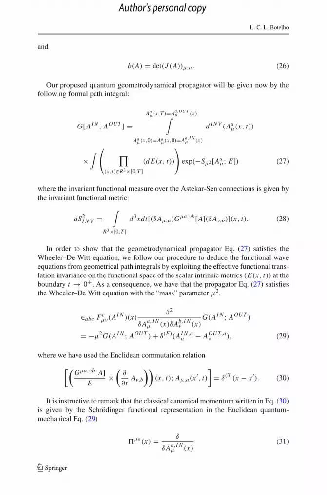
b(A) = det(J (A))μ;a . (26)

Our proposed quantum geometrodynamical propagator will be given now by thefollowing formal path integral:

G[AI N , AOU T ] =Aaμ(x,T )=Aa,OU T

μ (x)∫

Aaμ(x,0)=Aa

μ(x,0)=Aa,I Nμ (x)

d I N V (Aaμ(x, t))

×∫ ⎛

⎝ ∏

(x,t)∈R3×[0,T ](d E(x, t))

⎞⎠ exp(−Sμ2 [Aa

μ; E]) (27)

where the invariant functional measure over the Astekar-Sen connections is given bythe invariant functional metric

d S2I N V =

∫

R3×[0,T ]d3xdt[(δAμ,a)G

μa,νb[A](δAν,b)](x, t). (28)

In order to show that the geometrodynamical propagator Eq. (27) satisfies theWheeler–De Witt equation, we follow our procedure to deduce the functional waveequations from geometrical path integrals by exploiting the effective functional trans-lation invariance on the functional space of the scalar intrinsic metrics (E(x, t)) at theboundary t → 0+. As a consequence, we have that the propagator Eq. (27) satisfiesthe Wheeler–De Witt equation with the “mass” parameter μ2.

∈abc Fcμν(A

I N )(x)δ2

δAa,I Nμ (x)δAb,I N

ν (x)G(AI N ; AOU T )

= −μ2G(AI N ; AOU T )+ δ(F)(AI N ,aμ − AOU T,a

ν ), (29)

where we have used the Enclidean commutation relation

[(Gμa,νb[A]

E×(∂

∂tAν,b

))(x, t); Aμ,a(x

′, t)

]= δ(3)(x − x ′). (30)

It is instructive to remark that the classical canonical momentum written in Eq. (30)is given by the Schrödinger functional representation in the Euclidean quantum-mechanical Eq. (29)

�μa(x) = δ

δAa,I Nμ (x)

(31)

123



It is worth pointing out that the usual covariant Polyakov path integral for Klein-Gordon particles may be considered as the 0-dimensional reduction of the geometro-dynamical propagator Eq. (27).

At this point we remark that by fixing the gauge E(x, t) = Eμ2 , with μ2 the “mass”

parameter, we arrive at the analogous proper-time Schwinger representation for thisgeometrodynamical quantum gravity propagator

G E [AI N , AOU T ] =∞∫

0

dte−(E t) ×∫

d I N V (Aaμ) exp(−S[Aa

μ(x, t)]). (32)

where E = (E, μ2)× vol(R3) is the renormalized mass parameter in the SchwingerProper-Time representation with a finite volume base manifold M .

In the next we will use the proper-time-dependent propagator given below as usu-ally is done in the Symanzik’s loop space approach for quantum field theories towrite a third-quantized theory for gravitation Einstein theory in terms of Astekar-Senvariables.

G[AI N , AOU T ; T ] =Aaμ(x,T )=Aa,OU T

μ∫

Aaμ(x,0)=Aa,I N

μ (x)

d I N V (Aaμ)

× exp

⎧⎪⎨⎪⎩

− 1

16πG

T∫

0

dt∫

R3

[(∂

∂tAa,μ

)× Gμa,νb[A] ×

(∂

∂tAν,b

)](x, t)

⎫⎪⎬⎪⎭.

(33)

Unfortunately exactly solutions for Eq. (29) with μ2 �= 0 or Eq. (14) were notfound yet. However its σ -like structure and (SU (2) Gauge Invariance may afford totruncated approximate solutions as usually done for the Wheeler–De Witt equationsby means of the Mini-Super Space Ansatz. Finally let us comment on the introductionof a Quantized Matter Field represented by a massless field φ(x, t) on the Space Time.

By considering the effect of the introduction of this quantized field as a fluctua-tion on the geometrodynamical propagator Eq. (27) one should consider the follow-ing functional representing the interaction of this massless quantized matter and theAstekar-Sen connection as one can easily see by making E(x, t) variations

SI N T [Aaμ; E, ϕ] =

T∫

0

dt∫

R3

d3x

{[ϕ

(− ∂

∂t

(E∂

∂t

))ϕ

](x, t)

+(ϕ

[∂μ

(1

EGa,μ,bρ[A] ∂

∂tAb,ρ × Gμσ,aν[A] · ∂

∂tAσμ

)∂ν

]ϕ

)(x, t)

}(34)

123


L. C. L. Botelho

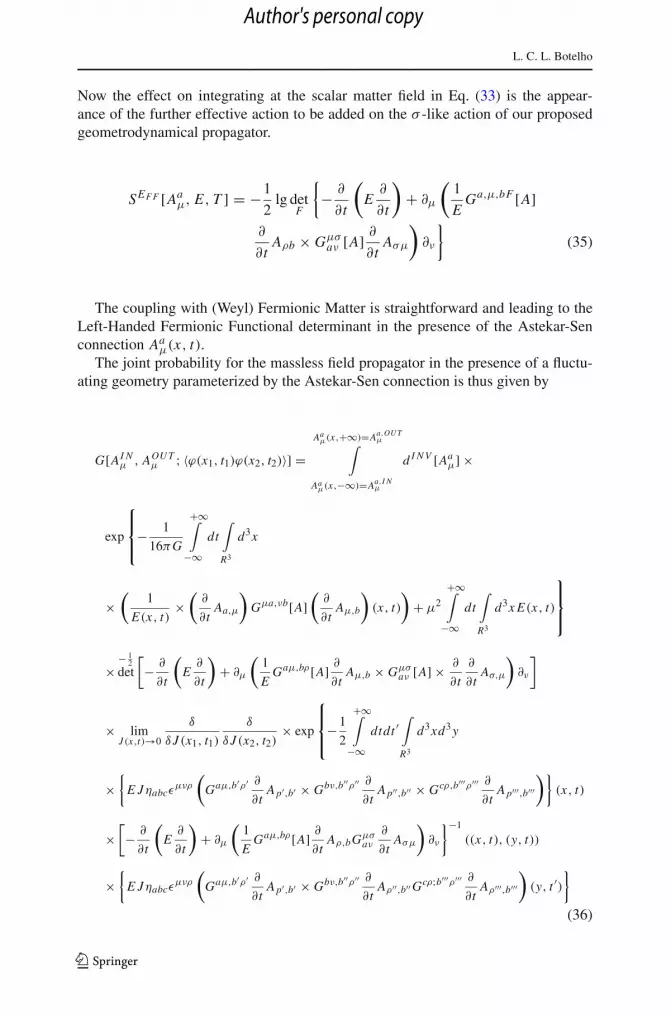
Now the effect on integrating at the scalar matter field in Eq. (33) is the appear-ance of the further effective action to be added on the σ -like action of our proposedgeometrodynamical propagator.

SEF F [Aaμ, E, T ] = −1

2lg det

F

{− ∂

∂t

(E∂

∂t

)+ ∂μ

(1

EGa,μ,bF [A]

∂

∂tAρb × Gμσ

aν [A] ∂∂t

Aσμ

)∂ν

}(35)

The coupling with (Weyl) Fermionic Matter is straightforward and leading to theLeft-Handed Fermionic Functional determinant in the presence of the Astekar-Senconnection Aa

μ(x, t).The joint probability for the massless field propagator in the presence of a fluctu-

ating geometry parameterized by the Astekar-Sen connection is thus given by

G[AI Nμ , AOU T

μ ; 〈ϕ(x1, t1)ϕ(x2, t2)〉] =Aaμ(x,+∞)=Aa,OU T

μ∫

Aaμ(x,−∞)=Aa,I N

μ

d I N V [Aaμ] ×

exp

⎧⎪⎨⎪⎩

− 1

16πG

+∞∫

−∞dt

∫

R3

d3x

×(

1

E(x, t)×(∂

∂tAa,μ

)Gμa,νb[A]

(∂

∂tAμ,b

)(x, t)

)+ μ2

+∞∫

−∞dt

∫

R3

d3x E(x, t)

⎫⎪⎬⎪⎭

×− 1

2det

[− ∂

∂t

(E∂

∂t

)+ ∂μ

(1

EGaμ,bρ [A] ∂

∂tAμ,b × Gμσ

aν [A] × ∂

∂t

∂

∂tAσ,μ

)∂ν

]

× limJ (x,t)→0

δ

δ J (x1, t1)

δ

δ J (x2, t2)× exp

⎧⎪⎨⎪⎩

−1

2

+∞∫

−∞dtdt ′

∫

R3

d3xd3 y

×{

E Jηabcεμνρ

(Gaμ,b′ρ′ ∂

∂tAp′,b′ × Gbν,b′′ρ′′ ∂

∂tAp′′,b′′ × Gcρ,b′′′ρ′′′ ∂

∂tAp′′′,b′′′

)}(x, t)

×[− ∂

∂t

(E∂

∂t

)+ ∂μ

(1

EGaμ,bρ [A] ∂

∂tAρ,bGμσ

aν∂

∂tAσμ

)∂ν

}−1

((x, t), (y, t))

×{

E Jηabcεμνρ

(Gaμ,b′ρ′ ∂

∂tAp′,b′ × Gbν,b′′ρ′′ ∂

∂tAρ′′,b′′ Gcρ;b′′′ρ′′′ ∂

∂tAρ′′′,b′′′

)(y, t ′)

}

(36)

123



4 A λφ4 geometrodynamical field theory for quantum gravity

Let us start the analysis by considering the generating functional of the following geo-metrodynamical field path integral as the simplest generalization for quantum gravityof a similar well-defined quantum field theory path integral of strings and particles [10]

Z [J (Z)] =∫

DF (φ[A])

× exp

[−∫

dν(A)φ[A] ×(∫

d3x

(∈abc Fc

μν(A)δ2

δAaμδAb

ν

)(x)

)φ[A]

}

× exp

{−λ

∫d3xd3 y

∫dν(A)dν( A)(φ2[A(x)](φ2[ A(y)])×δ(3)(Aμ(x)− Aμ(y)

}

× exp

{−∫

dν(A)J (A)φ[A]}. (37)

The notation is as follows: (i) The quantum gravity third-quantized field is givenby a functional φ[A] defined over the space of all Astekar-Sen connections configu-rations M = {Aa

μ(x); x ∈ R3}. The sum over the functional space M is defined bythe gauge and diffeomorphism invariant and topological non-trivial path integral of aChern-Simons field theory on the Astekar-Sen connections

dν(A) =∫ ⎛

⎝ ∏

x∈R3

d Aaμ(x)

⎞⎠ × exp

{−∫

d3x(A ∧ d A + 2

3A ∧ A∧)(x)

}.

(38)

(ii) The third quantized functional measure in Eq. (37) is given formally by the usualFeynman product measure

DF (φ[A]) =∏A∈M

dφ[A]. (39)

(iii) The λφ4-like interaction vertex is given by a self-avoiding geometrodynamicalinteraction among the Astekar-Sen field configurations in the extrinsic space R3

λ

3∑a=1

δ(3)(Aaμ(x)− Aa

μ(y)). (40)

The proposed interaction vertex was defined in such a way that it allows the replace-ment of the Four Universe interaction in Eq. (37) by an independent interaction of eachAstekar-Sen connection with an extrinsic triplet of Gaussian stochastic field W a(x)followed by an average over W a . A similar procedure is well known in the many-bodyand many-random surface path integral quantum field theory. So, we can write Eq. (37)in the following form

123


L. C. L. Botelho

Z [J (A)] =⟨∫

DF (φ[A])× exp

{−∫

dν(A)

[φ[A]

(L(A)

− iλ∫

d3x

(3∑

a=1

W a(Aaμ)

))φ[A] + J (A)φ[A]

]]⟩

W. (41)

Here, W a(Aa) means the external a-component of the triplet of the external sto-chastic field {W a} projected on the Astekar-Sen connection {Aa

μ}, namely

W a(Aa) = W a(Aa1(x), Aa

2(x), Aa3(x)), (42)

and has the white-noise stochastic correlation function

⟨W a(xμ)W b(yν)

⟩ = δ(3)(xμ − yμ)δab. (43)

The L(A) operator on the functional space of the universe field is the Wheeler–DeWitt operator defining the quadratic action in Eq. (41).

In the free case λ = 0. The third-quantized gravitation path integral Eq. (37) isexactly soluble with the following generating functional:

Z [J (A)]Z [0] = exp

{+ 1

2

∫dν(A)dν( A)J (A)

×(∫

d3x ∈abc Fcμν(A)

δ2

δAaμδAb

ν

)−1

(A, A)J ( A)

⎫⎬⎭ . (44)

Here the functional inverse of the Wheeler–De Witt operator is given explicitly bythe geometrodynamical propagator Eq. (32) with E = 0

(∫d3x ∈abc Fc

μν(A)δ2

δAaμδAb

ν

)−1

(A, A) =∞∫

0

dT G[A, A, T ]. (45)

In order to reformulate the third-quantized gravitation field theory as a dynamicsof self-avoiding geometrodynamical propagators, we evaluate formally the Gaussianφ[A] functional path integral in Eq. (37) with the following result

123



Z [J (A)] =⟨− 1

2det

⎡⎢⎣∫

R3


δ2

δAaμδAb

ν

+ iλ

(3∑

a=1

W a(Aa(x))

)⎤⎥⎦

× exp

⎧⎪⎨⎪⎩

+1

2

∫dν(A)dν( A)× J (A)

⎡⎢⎣∫

R3


δ2

δAaμδAb

ν

+ i λ

⎛⎜⎝

3∑a=1

W a(Aaμ(x))

)⎤⎥⎦

−1

(A, A)× J ( A)

⎫⎪⎬⎪⎭

⟩(46)

Let us follow our previous studies implemented for particles and strings in previouschapters by defining the functional determinant of the Wheeler–De Witt operator bythe proper-time technique

−1

2log det

⎡⎢⎣L(A)+ iλ

∫

R3

d3x

(3∑

a=1

W a(Aaμ(x))

)⎤⎥⎦

=+∞∫

0

dT

T

{∫dν(A)dν( A)δ(F)(A − A)

×⟨

A| exp

[−T

(L(A)+ iλ

∫d3x

(3∑

a=1

W a(Aaμ(x))

))]| A⟩}. (47)

with the geometrodynamical propagator (see Eq. 33) in the presence of the extrinsicpotential {W a

μ(x)} which is given explicitly by the path integral below

⟨A| exp

⎡⎢⎣−T (L(A))+ iλ

∫

R3

d3x

(3∑

a=1

W a(Aaμ(x))

)⎤⎥⎦ | A

⟩

=∫

d I N V [Baμ(x, t)] exp

⎧⎪⎨⎪⎩

− 1

16πG

T∫

0

dt∫

R3

d3x

[(∂

∂tBa,μ

)× Gμa,νb[B]

(∂

∂tBb,ν

)](x, t)

⎫⎬⎭

× exp

⎡⎢⎣−iλ

T∫

0

dt∫

R3

d3x

(3∑

a=1

W a(Baμ(x, t))

)⎤⎥⎦

⎤⎥⎦ . (48)

123


L. C. L. Botelho

By substituting Eqs. (48) and (47) into Eq. (46) and making a loop expansion of thefunctional determinant, we obtain Eq. (37) as a theory of an ensemble of geometrody-namical propagators interacting with the extrinsic Gaussian stochastic field {W a(x)}.The Gaussian average

⟨⟩w

may be straightforwardly evaluated at each loop expansionproducing the self-avoiding interaction among the geometrodynamical propagators(The Wheeler quantum universes) and leading to the picture of joining and splittingof these Wheeler Universes as necessary for the description of the Universe in itsSpace-Time Third Quantized form picture of Wheeler. For instance, by neglecting thefunctional determinant in Eq. (46) we have the following expression for the geomet-rodynamical third quantized propagator:

⟨�[Aa,I N

μ ]�[Aa,OU Tμ ]

⟩(0)

∞∫

0

dT ×∫

Baμ(x,0)=A;Ba

μ(x,T )= A

d I N V [Baμ(x, t)]

× exp

⎧⎪⎨⎪⎩

− 1

16πG

T∫

0

dt∫

R3

d3x

[(∂

∂tBa,μ

)Gμa,νb[B]

(∂

∂tBν,b

)](x, t)

⎫⎪⎬⎪⎭

× exp

⎧⎪⎨⎪⎩

−λ2

2

T∫

0

dt

T∫

0

dt ′∫

R3

d3xd3 y

(3∑

a=1

δ((Baμ(x, t)− (Ba

μ(y, t ′))))⎫⎪⎬⎪⎭.

(49)

Next corrections will involve self-avoiding interactions among differents WheelerUniverses associated to different Astekar-Sen connections associated to different geo-metrodynamical propagators appearing from the functional determinant loop expan-sion Eq. (47).

Finally, we comment that calculations will be done successfully only if one is ableto handle correctly the geometrodynamical propagator Eq. (33) on Eq. (36) and, thus,proceed to generalized for this Quantum gravity case the analogous framework usedin the Theory of Random Lines and Surfaces. And as a general conclusion of ournote we point out the usefulness of loops already possessing Grassmanian-Fermionicstructure D-dimensional supergravity as a solution for the problem of ultra-violetself-avoidance of the Former Cumbersome Bosonic loops. Certainly by adopting suchGrassmanian loop space approached, the whole present Framework for Loop quantumgravity must be changed.

Appendix A

In this short appendix we call the reader attention that there are (formal) states satis-fying the Wheeler–De Witt Eq. (1), the diffeomorphism constraint Eq. (2), but not thegauge-invariant Gauss law Eq. (3).

123



For instance, the non-gauge invariant “mass term” wave functional below

M[A] = exp

⎧⎨⎩−1

2

∫

M

d3x Aiμ(δ

i1δ j1δμν)A jν

⎫⎬⎭ ; (A1)

satisfies the Wheeler–De Witt equation, since

(εi jk Fk

μν(A)(x)δ2

δAiμ(x)δA j

ν(y)M[A]

)∼ ε11k(· · · ) = 0; (A2)

and the diffeomorphism constraint

δ

δAiν(x)

(Fiμν(A)M[A]

)= ∂x

μM[A]

+Fiμν[A]M[A]

(−1

2A1μ(x)

)δi1δνμ

= 0 − 1

2A1μ(x) · Fμμ(A) = 0; (A3)

At this point and closely related to the above made remark it is worth call the readerattention that the 3D-fermionic functional determinant with a mass term still satis-fies the Wheeler–De Witt and the diffeomorphism constraint. However, at the limitof large mass m → ∞, one can see the appearance of a complete cut-off dependentmass term like Eq. (A1), added with Chern-Simon terms and higher order terms ofthe strengh field Fαβ(A(x)) in the full quantum state [29]. As a result one can arguethat this “fermion classical limit” of large mass may be equivalent to the appearanceof a dynamical cosmological constant, if one neglects the gauge-violating quantuminduced mass term [1,2].

References

1. Ashtekar, A.: Knots and quantum gravity. In: Baez, H. (ed.) Oxford Lecture Series in Mathematicsand its applications, Vol. 1. Oxford Press, Oxford (1994)

2. Ashtekar, A.: Non-perturbative Canonical Quantum Gravity. World Scientific, Singapore (1991)3. Witten, E.: Nucl. Phys. B 311, 45 (1988)4. Botelho, L.C.L.: Phys. Rev. 38D, 2464 (1988)5. Bjorken, J.D., Drell, S.D.: Relativistic Quantum Fields. McGraw Hill, New York (1965)6. Jacobson, T., Smolin, L.: Nucl. Phys. B 299, 292 (1988)7. Kodma, H.: Phys. Rev. D 42, 2548 (1990)8. Botelho, L.C.L.: Phys. Rev. D 52, 6941 (1995)9. Brügmann, B., Gambini, R., Pullin, J.: Gen. Relativ. Gravit. 25, 1 (1992)

10. Botelho, L.C.L.: J. Math. Phys. 39, 2150 (1989)11. Symanzik, K.: A method for Euclidean Quantum Field theory. In: Jost, R. (ed.) Local Quantum Theory,

Academic, London (1969)12. Botelho, L.C.L.: Phys. Rev. D 52, 6941 (1995)13. Botelho, L.C.L.: Phys. Lett. 152B, 358 (1985)14. DiGiacomo, A., Dosch, H.G., Shevchenko, V.I., Simonov, Y. A.: Phys. Rep. 372, 319 (2002)

123


L. C. L. Botelho

15. Botelho, L.C.L.: Phys. Lett. 415B, 231 (1997)16. Botelho, L.C.L.: Phys. Rev. 56D, 1338 (1986)17. Botelho, L.C.L.: CBPF Report NF-044, Unpublished (1986)18. Polyakov, A.M.: Gauge Field and Strings. Harwood academic, Chur (1987)19. Botelho, L.C.L.: Il. Nuovo Cim. 112A, 1615 (1999)20. Botelho, L.C.L.: Il. Nuovo Cim. 116B, 859 (2001)21. Botelho, L.C.L.: Int. J. Mod. Phys. A 15(5), 755 (2000)22. Botelho, L.C.L.: J. Phys. A-Math. Gen. 23, 1661 (1990)23. Botelho, L.C.L.: J. Phys. A-Math. Gen. 22(11), 1945 (1989)24. Broda, B.: Phys. Rev. Lett. 63(25), 2709 (1989)25. Fröhlich, J.: Nucl. Phys. B 200(FS4), 281 (1982)26. Aizenman, M.: Commun. Math. Phys. 86, 1 (1982)27. Coppovilla, R., Jacobso, T., Dell, J.: Phys. Rev. Lett. 53, 2325 (1989)28. Soo, C., Smolin, L.: Nucl. Phys. B 449, 289 (1995)29. Botelho, L.C.L.: Int. J. Mod. Phys. A 15(5), 755 (2000)

123


Documents

General Relativity and Gravitation