Embed Size (px)
Citation preview
Geometrisation of 3-manifolds
Laurent Bessieres, Gerard Besson, Michel Boileau, Sylvain Maillot, Joan Porti
June 23, 2009
2
The authors wish to thank the Agence Nationale de la Recherche for itssupport under the program F.O.G., ANR-07-BLAN-0251-01 and the Feder/Micinn grant MTM2006-04546. We have also been supported by the ClayMathematics Institute, the Fondation des Sciences Mathematiques de Paris,the Centre Emile Borel, and the Centre de Recerca Matematica. The thirdauthor thanks the Institut Universitaire de France for his support. The lastauthor received the prize “ICREA Academia”, funded by the Generalitat deCatalunya.
We warmly thank B. Kleiner, J. Lott, J. Morgan and G. Tian for numer-ous fruitful exchanges. Part of this work originated in workshops organizedat Barcelona, Grenoble and Munchen. We thank all the participants of theseactivities, in particular J. Dinkelbach, V. Bayle, Y. Colin de Verdiere, S.Gallot, B. Leeb, L. Rozoy, T. Schick and H. Weiss. The trimestre on theRicci curvature organized at I.H.P. in the spring 2008 has played an essentialrole and we thank the participants and particularly E. Aubry, R. Bamler, R.Conlon, Z. Djadli and D. Semmes.
Finally, the authors wish to thank O. Biquard, T. Delzant, L. Guillou, P.Pansu and M. Paun for discussions and insights.
Contents
0 Geometrisation conjecture 90.1 Introduction . . . . . . . . . . . . . . . . . . . . . . . . . . . . 90.2 Ricci flow and elliptisation . . . . . . . . . . . . . . . . . . . . 13
0.2.1 Ricci flow . . . . . . . . . . . . . . . . . . . . . . . . . 130.2.2 Ricci flow with bubbling-off . . . . . . . . . . . . . . . 140.2.3 Application to elliptisation . . . . . . . . . . . . . . . . 17
0.3 3-manifolds with infinite fundamental group . . . . . . . . . . 190.3.1 Long time behaviour of the Ricci flow with bubbling-off 190.3.2 Hyperbolisation . . . . . . . . . . . . . . . . . . . . . . 20
0.4 Consequences . . . . . . . . . . . . . . . . . . . . . . . . . . . 220.4.1 Collapsing . . . . . . . . . . . . . . . . . . . . . . . . . 230.4.2 The refined invariant V ′
0 . . . . . . . . . . . . . . . . . 230.4.3 Other approaches . . . . . . . . . . . . . . . . . . . . . 24
I Ricci flow with bubbling-off: definitions and state-ments 25
0.5 Introduction . . . . . . . . . . . . . . . . . . . . . . . . . . . . 270.6 Basic definitions and notation . . . . . . . . . . . . . . . . . . 28
0.6.1 Riemannian geometry . . . . . . . . . . . . . . . . . . 280.6.2 Evolving metrics and Ricci flow with bubbling-off . . . 29
1 Piecing together necks and caps 331.1 Definitions . . . . . . . . . . . . . . . . . . . . . . . . . . . . . 33
1.1.1 Necks . . . . . . . . . . . . . . . . . . . . . . . . . . . 331.1.2 Caps and tubes . . . . . . . . . . . . . . . . . . . . . . 33
1.2 Gluing results . . . . . . . . . . . . . . . . . . . . . . . . . . . 341.3 More results on ε-necks . . . . . . . . . . . . . . . . . . . . . . 37
2 Key Notions 392.1 κ-noncollapsing . . . . . . . . . . . . . . . . . . . . . . . . . . 39
3
4 CONTENTS
2.2 κ-solutions . . . . . . . . . . . . . . . . . . . . . . . . . . . . . 402.2.1 Definition and main results . . . . . . . . . . . . . . . 402.2.2 Canonical neighbourhoods . . . . . . . . . . . . . . . . 41
2.3 The standard solution I . . . . . . . . . . . . . . . . . . . . . . 432.3.1 Definition and main results . . . . . . . . . . . . . . . 432.3.2 Neck Strengthening . . . . . . . . . . . . . . . . . . . . 44
2.4 Curvature pinched toward positive . . . . . . . . . . . . . . . 45
3 Ricci flow with (r, δ, κ)-bubbling-off 493.1 Let the constants be fixed . . . . . . . . . . . . . . . . . . . . 493.2 Metric Surgery and Cutoff Parameters . . . . . . . . . . . . . 503.3 Finite Time Existence Theorem . . . . . . . . . . . . . . . . . 533.4 Long time existence . . . . . . . . . . . . . . . . . . . . . . . . 57
II Ricci flow with bubbling-off: existence 61
4 Choosing cutoff parameters 654.1 Piecing together necks in noncompact manifolds . . . . . . . . 654.2 Bounded curvature at bounded distance . . . . . . . . . . . . 66
4.2.1 Preliminaries . . . . . . . . . . . . . . . . . . . . . . . 674.2.2 Proof of Theorem 4.2.1 . . . . . . . . . . . . . . . . . . 69
4.3 Existence of cutoff parameters . . . . . . . . . . . . . . . . . . 76
5 Proposition A 835.1 The standard solution II . . . . . . . . . . . . . . . . . . . . . 835.2 Proof of the Metric Surgery Theorem . . . . . . . . . . . . . . 875.3 Proof of Proposition A . . . . . . . . . . . . . . . . . . . . . . 94
6 Persistence 976.1 Introduction . . . . . . . . . . . . . . . . . . . . . . . . . . . . 976.2 Persistence of a model . . . . . . . . . . . . . . . . . . . . . . 986.3 Persistence of almost standard caps . . . . . . . . . . . . . . . 104
7 Proposition B 1077.1 Warming up . . . . . . . . . . . . . . . . . . . . . . . . . . . . 1077.2 The proof . . . . . . . . . . . . . . . . . . . . . . . . . . . . . 108
8 Proposition C 1198.1 Preliminaries . . . . . . . . . . . . . . . . . . . . . . . . . . . 1198.2 Proof of Theorem 8.0.4 . . . . . . . . . . . . . . . . . . . . . . 1228.3 Proof of Proposition C . . . . . . . . . . . . . . . . . . . . . . 126
CONTENTS 5
8.3.1 The case ρ0 < r . . . . . . . . . . . . . . . . . . . . . . 1278.3.2 The case ρ0 > r . . . . . . . . . . . . . . . . . . . . . 128
8.4 More on κ-noncollapsing . . . . . . . . . . . . . . . . . . . . . 1358.4.1 A formal computation . . . . . . . . . . . . . . . . . . 1378.4.2 Justification of the formal computations . . . . . . . . 138
III Long time behaviour of Ricci flow with bubbling-off 141
9 Thin-thick decomposition 145
10 Geometry of the thick part 14910.1 Consequences of the maximum principle . . . . . . . . . . . . 14910.2 Proof of the existence of limits . . . . . . . . . . . . . . . . . . 15310.3 Proof of the controlled curvature . . . . . . . . . . . . . . . . 158
11 Proofs of the technical theorems 16111.1 Proof of Theorem 9.0.4 . . . . . . . . . . . . . . . . . . . . . . 16111.2 Proof of Theorem 9.0.5 . . . . . . . . . . . . . . . . . . . . . . 170
IV Hyperbolisation 193
12 Simplicial volume and collapsing 19712.1 Simplicial volume . . . . . . . . . . . . . . . . . . . . . . . . . 19912.2 Sketch of proof of Theorem 12.0.12 . . . . . . . . . . . . . . . 200
13 Weak collapsing 20313.1 Structure of the thick part . . . . . . . . . . . . . . . . . . . . 203
13.1.1 Covering the thick part . . . . . . . . . . . . . . . . . . 20313.1.2 Submanifolds with compressible boundary . . . . . . . 20513.1.3 Proof of Propositions 13.1.2 and 13.1.3 . . . . . . . . . 207
13.2 Local structure of the thin part . . . . . . . . . . . . . . . . . 20713.3 Constructions of coverings . . . . . . . . . . . . . . . . . . . . 213
13.3.1 Embedding thick pieces in solid tori . . . . . . . . . . . 21313.3.2 Existence of a homotopically nontrivial open set . . . . 21413.3.3 End of the proof of Theorem 0.4.1 . . . . . . . . . . . . 221
13.4 Applications . . . . . . . . . . . . . . . . . . . . . . . . . . . . 22613.4.1 A sufficient condition for hyperbolicity . . . . . . . . . 22713.4.2 Proof of Theorem 0.3.5 . . . . . . . . . . . . . . . . . . 22913.4.3 Proof of Theorem 0.4.3 . . . . . . . . . . . . . . . . . . 230
6 CONTENTS
A Riemannian Geometry 231
B Ricci flow 233B.1 Existence and basic properties . . . . . . . . . . . . . . . . . . 233B.2 Consequences of the maximum principle . . . . . . . . . . . . 233B.3 Compactness . . . . . . . . . . . . . . . . . . . . . . . . . . . 234
C L-length 237
D Alexandrov spaces 239
Preface
The aim of this book is to give a proof of Thurston’s geometrisation conjec-ture, solved by G. Perelman in 2003. Perelman presented his ideas in threevery concise manuscripts [59, 61, 60]. Important work has since been doneto fill in the details. The first set of notes was posted on the web in June2003 by B. Kleiner and J. Lott. These notes have progressively grown to thepoint where they cover the two papers [59, 61]. The final version has beenpublished as [45]. A proof of the Poincare conjecture, following G. Perelman[59, 61, 60], is given in the book [51] by J. Morgan and G. Tian. Anothertext covering the geometrization conjecture following Perelman’s ideas is thearticle [12] by H.-D. Cao and X.-P. Zhu. Alternative approaches to some ofPerelman’s arguments were given by T. Colding and W. Minicozzi [21], T.Shioya and T. Yamaguchi [68], the authors of the present book [6] and J.Morgan and G. Tian [52].
One goal of this book is to present a proof more attractive to topologists.For this purpose, we have endeavoured to reduce its analytical aspects toblackboxes and refer to well-written sources [51],[19]. At various points, wehave favoured topological and geometric arguments over analytic ones.
We provide some technical simplifications of Perelman’s Ricci flow withsurgery. We replace it with a variant which we call Ricci flow with bubbling-off. This is a kind of piecewise smooth Ricci flow on a fixed manifold.Our proof of the geometrisation conjecture differs from Perelman’s proofby the use of Ricci flow with bubbling-off and topological arguments usingThurston’s hyperbolisation for Haken manifolds.
We have tried to make the various parts of the proof as independent aspossible, in order to clarify its overall structure. The book has four parts.The first two are devoted to the construction of Ricci flow with bubbling-off. These two parts, combined with [21] or [60], are sufficient to prove thePoincare conjecture. Part III is concerned with the long time behaviourof Ricci flow with bubbling-off. Part IV, which is based on the article [6],completes the proof of the geometrisation conjecture and can be read in-dependently from the rest. The material found here is of topological and
7
8 CONTENTS
geometric nature.The idea of writing this book originated from a discussion during the
party that followed the conference held in honour of Larry Siebenmann inDecember 2005. It came after several workshops held in Barcelona, Munchenand Grenoble devoted to the reading of Perelman’s papers and the Kleiner-Lott notes. A first version of this book was handed out as lecture notesduring the trimestre on the Ricci curvature held in I.H.P. (Paris) in May2008.
Chapter 0
Geometrisation conjecture
0.1 Introduction
In the international conference of mathematics devoted to Some Questionsof Geometry and Topology, organized in 1935 by the University of Geneva,W. Threlfall started his lecture by the following words:
“Nous savons tous que le probleme d’homeomorphie des varietes a n di-mensions, pose par Poincare, est un des plus interessants et des plus impor-tants de la Geometrie. Il est interessant en soi car il a donne naissance a laTopologie combinatoire ou algebrique, theorie comparable par son importancea la Theorie des fonctions classique. Il est important par ses applicationsa la Cosmologie, ou il s’agit de determiner l’aspect de l’espace de notre in-tuition et de la physique. Des l’instant ou le physicien a envisage la possi-bilite de considerer l’espace de notre intuition, espace ou nous vivons, commeclos, la tche du mathematicien est de lui proposer un choix d’espaces clos,et meme de les enumrer tous, comme il le ferait pour les polyedres reguliers.. . .Malheureusement le probleme n’est completement resolu que pour deuxdimensions.”
During the last 70 years this problem was central in 3-dimensional topol-ogy. It came down to Thurston’s Geometrisation Conjecture at the beginningof the 70’s. Finally this conjecture has been solved in 2003 by G. Perelman.
A major result of the beginning of last century is the proof that ev-ery compact surface admits a Riemannian metric with constant curvature.This result leads to the topological classification of surfaces mentioned byThrelfall. Moreover, some important properties of surfaces, e.g. linearity ofthe fundamental group, can be deduced from this fact. Geometric structureson surfaces are also central in studying their mapping class groups.
9
10 CHAPTER 0. GEOMETRISATION CONJECTURE
Recall that a Riemannian manifold X is called homogeneous if its isome-try group Isom(X) acts transitively on X. We call X unimodular if it has aquotient of finite volume. A geometry is a homogeneous, simply-connected,unimodular Riemannian manifold. A manifold M is geometric if M is diffeo-morphic to the quotient of a geometry X by a discrete subgroup of Isom(X)acting freely onX. We also say thatM admits a geometric structure modelledon X.
In dimension 2 the situation is rather special, since a geometry is alwaysof constant curvature. This is no longer true in dimension 3. Thurston ob-served that there are, up to a suitable equivalence relation, eight maximal1
3-dimensional geometries: those of constant curvature S3, E3, and H3; theproduct geometries S2×E1 and H2×E1; the twisted product geometries Nil
and ˜SL(2,R), and finally Sol, which is the only simply-connected, unimod-ular 3-dimensional Lie group which is solvable but not nilpotent.
A 3-manifold is spherical (resp. hyperbolic) if it admits a geometric struc-ture modelled on S3 (resp. H3.) The classification of spherical 3-manifoldswas completed by H. Seifert and W. Threlfall in 1932 [72, 73]. A key observa-tion for the classification is that every finite subgroup of SO(4) acting freelyand orthogonally on S3 commutes with the action of some SO(2)-subgroupof SO(4). This SO(2)-action induces a circle foliation on the manifold whereeach circle has a saturated tubular neighbourhood. This phenomenon ledSeifert [66] to classify all 3-manifolds carrying such a foliation by circles,nowadays called Seifert fibred manifolds.
A compact 3-manifold is Seifert fibred if and only if it admits a geomet-ric structure modelled on one of the six following geometries: S3,E3,S2 ×E1, Nil,H2×E1, ˜SL(2,R). Moreover, each compact Seifert fibred 3-manifoldadmits a finite regular cover which is a true circle bundle.
Besides, a theorem of Poincare gives a general method to build any hy-perbolic 3-manifold by identifying the faces of a convex polyhedron of H3.However, this construction does not provide a criterion to decide whether acompact 3-manifold admits a hyperbolic structure. It is only in 1977 thatsuch a criterion was conjectured by W. Thurston, and proved for a largeclass of compact 3-manifolds, the so-called Haken 3-manifolds. The fact thatthis criterion holds true is part of a wider conjecture proposed by Thurston,the Geometrisation Conjecture, which gives a general picture of all compact3-manifolds. The content of the Geometrisation Conjecture is that everycompact three-manifold splits along a finite collection of embedded surfaces
1In this context, maximal means that there is no Isom(X)-invariant Riemannian metricon X whose isometry group is strictly larger than Isom(X).
0.1. INTRODUCTION 11
into canonical geometric pieces. More precisely [75]:
Conjecture 0.1.1 (Thurston’s Geometrisation Conjecture). The interior ofany compact orientable 3-manifold can be split along a finite collection ofessential disjoint embedded spheres and tori into a canonical collection ofgeometric 3-manifolds after capping off all boundary spheres by balls.
A closed connected surface in a compact orientable 3-manifold M is es-sential if it is π1-injective and if it does not bound a 3-ball nor cobounds aproduct with a connected component of ∂M .
A special case of the Geometrisation Conjecture is the so-called Ellipti-sation Conjecture, which asserts that every 3-manifold of finite fundamentalgroup is spherical. The famous Poincare Conjecture is itself a special case ofthe Elliptisation Conjecture.
The Geometrisation Conjecture has far-reaching consequences for 3-mani-fold topology. For instance, it implies that every closed, orientable, aspherical3-manifold is determined, up to homeomorphism, by its fundamental group.This is a special case of the so-called Borel conjecture. A manifold is aspher-ical if all its higher homotopy groups vanish.
The topological decomposition required for Thurston’s geometrisationconjecture is a central result in 3-manifold topology. An orientable 3-manifoldM is irreducible if any embedding of the 2-sphere into M extends to anembedding of the 3-ball into M . The connected sum of two orientable 3-manifolds is the orientable 3-manifold obtained by pulling out the interior ofa 3-ball in each manifold and gluing the remaining parts together along theboundary spheres.
The first stage of the decomposition is due to H. Kneser for the existence[46], and to J. Milnor for the uniqueness [50]:
Theorem 0.1.2 (Kneser’s decomposition). Every compact, orientable 3-manifold M is a connected sum of 3-manifolds that are either homeomorphicto S1 × S2 or irreducible. Moreover, the connected summands are unique upto ordering and orientation-preserving homeomorphism.
The second stage of the decomposition is more subtle. An orientable sur-face of genus at least 1 embedded in a 3-manifold is called incompressible ifit is π1-injective. An embedded torus in a compact, orientable, irreducible3-manifold M is canonical if it is essential and can be isotoped off any in-compressible embedded torus (see [54]).
A compact orientable 3-manifold M is atoroidal if it contains no essentialembedded torus and is not homeomorphic to a product T 2×[0, 1] or a twistedproduct K2×[0, 1].
12 CHAPTER 0. GEOMETRISATION CONJECTURE
Theorem 0.1.3 (JSJ-splitting). A maximal (possibly empty) collection ofdisjoint, non-parallel, canonical tori is finite and unique up to isotopy. Itcuts M into 3-submanifolds that are atoroidal or Seifert fibred.
This splitting is called the JSJ-splitting because it has been constructedby W. Jaco and P. Shalen [40], and by K. Johannson [41].
A compact, orientable, irreducible 3-manifold is Haken if its boundary isnot empty, or if it contains a closed essential surface. In the mid 70’s W.Thurston proved the Geometrisation Conjecture for Haken 3-manifolds (seeOtal [57, 56]):
Theorem 0.1.4 (Thurston’s Hyperbolisation Theorem). The Geometrisa-tion Conjecture is true for Haken 3-manifolds.
In particular, any atoroidal Haken 3-manifold M is hyperbolic or Seifertfibred. Moreover, M is hyperbolic if and only if each subgroup isomorphicto Z⊕ Z in π1(M) is induced, up to conjugacy, by a boundary component.
The main goal of this book is to explain the proof of the remaining andmost difficult case, dealing with closed atoroidal manifolds:
Theorem 0.1.5 (G. Perelman). Let M be a closed, orientable, irreducible,atoroidal 3-manifold. Then:
i. If π1M is finite, then M is spherical.
ii. If π1M is infinite, then M is hyperbolic or Seifert fibred.
Note that Part (i) of Theorem 0.1.5 is the Elliptisation Conjecture. Moregenerally, Theorems 0.1.4 and 0.1.5 together imply:
Corollary 0.1.6 (Geometrisation Theorem). The Geometrisation Conjec-ture is true for all compact 3-manifolds.
Another important corollary is the following:
Corollary 0.1.7 (Hyperbolisation Theorem). A closed, orientable, irre-ducible 3-manifold is hyperbolic if and only if π1M is infinite and does notcontain a subgroup isomorphic to Z2.
In fact, Perelman’s proof deals with all cases and allow to recover thegeometric splitting of the manifold along spheres and tori. However, in thisbook we focus on Theorem 0.1.5, i.e. the irreducible, atoroidal case.
The main ingredient of the proof is the famous Ricci flow, which is anevolution equation introduced by R. Hamilton. In Section 0.2, we review
0.2. RICCI FLOW AND ELLIPTISATION 13
general facts about this equation, and define an object called Ricci flow withbubbling-off, which is a variation on Perelman’s Ricci flow with surgery (cf.also [33].) We then state an existence result and deduce the ElliptisationConjecture from this.
In Section 0.3 we tackle the long time behaviour of Ricci flow withbubbling-off and the case where π1M is infinite.
0.2 Ricci flow and elliptisation
0.2.1 Ricci flow
Notation. If g is a riemannian metric, we denote by Rmin(g) the minimum ofits scalar curvature, by Ricg its Ricci tensor, and by vol(g) its volume.
Let M be a closed, irreducible 3-manifold. In the Ricci flow approach togeometrisation, one studies solutions of the evolution equation
dg
dt= −2 Ricg(t), (1)
called the Ricci flow equation, which was introduced by R. Hamilton. A so-lution is an evolving metric g(t)t∈I , i.e. a 1-parameter family of riemannianmetrics on M defined on an interval I ⊂ R. In [30], Hamilton proved that forany metric g0 on M , there exists ε > 0 such that Equation (1) has a uniquesolution defined on [0, ε) with initial condition g(0) = g0. Thus there existsT ∈ (0,+∞] such that [0, T ) is the maximal interval where the solution to (1)with initial condition g0 is defined. When T is finite, one says that Ricci flowhas a singularity at time T . Ideally, one would like to see the geometry of Mappear by looking at the metric g(t) when t tends to T (whether T be finiteor infinite.) To understand how this works, we first consider some (very)simple examples, where the initial metric is locally homogeneous.
Example 1. If g0 has constant sectional curvature K, then the solution isgiven by g(t) = (1 − 4Kt)g0. Thus in the spherical case, where K > 0,we have T < ∞, and as t goes to T , the manifold shrinks to a point whileremaining of constant positive curvature.
By contrast, in the hyperbolic case, where K < 0, we have T = ∞ andg(t) expands indefinitely, while remaining of constant negative curvature. Inthis case, the rescaled solution g(t) := (4t)−1g(t) converges to the metric ofconstant sectional curvature −1.
Example 2. If M is the product of a circle with a surface of genus at least 2,and g0 is a product metric whose second factor has constant curvature, then
14 CHAPTER 0. GEOMETRISATION CONJECTURE
T = ∞; moreover, the metric is constant on the first factor, and expandingon the second factor.
In this case, g(t) does not have any convergent rescaling. However,one can observe that the rescaled solution g(t) defined above collapses withbounded curvature, i.e. has bounded curvature and injectivity radius going to0 everywhere as t goes to +∞.
Several important results were obtained by Hamilton [30, 31, 34]. Wheng0 has positive Ricci curvature, then T <∞, and the volume-rescaled Ricciflow vol(g(t))−2/3g(t) converges to a round metric as t → T . If T = ∞and g(t) has uniformly bounded sectional curvature, then it converges orcollapses, or M contains an incompressible torus.
The general case, however, is more difficult, because it sometimes happensthat T < ∞ while the behavior of g(t) as t tends to T does not allow todetermine the topology of M . One possibility is the so-called neck pinch,where part of M looks like a thinner and thinner cylindrical neck as oneapproaches the singularity. This can happen even if M is irreducible (see [2]for an example where M = S3); thus neck pinches may not give any usefulinformation on the topology of M .
0.2.2 Ricci flow with bubbling-off
Throughout the book, we suppose that M is closed, orientable and irreduci-ble. We also assume that M is RP 2-free, i.e. does not contain any submani-fold diffeomorphic to RP 2. This is not much of a restriction because the onlyclosed, irreducible 3-manifold that does contain an embedded copy of RP 2
is RP 3, which is a spherical manifold.
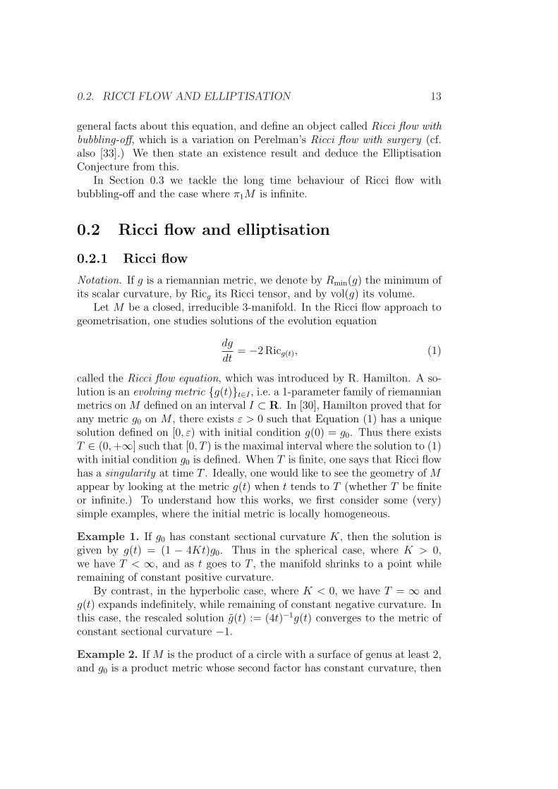
As we already explained, one of the main difficulties in the Ricci flowapproach to geometrisation is that singularities unrelated to the topologyof M may appear. Using maximum principle arguments, one shows thatsingularities in a 3-dimensional Ricci flow can only occur when the scalarcurvature tends to +∞ somewhere. One of Perelman’s major breakthroughswas to give a precise local description of the geometry at points of large scalarcurvature: every such point has a so-called canonical neighbourhood U .Forinstance U may be an ε-neck (i.e. almost homothetic to the product of theround 2-sphere of unit radius with an interval of length 2ε−1)
0.2. RICCI FLOW AND ELLIPTISATION 15
S2
2ε−1
ε-neck
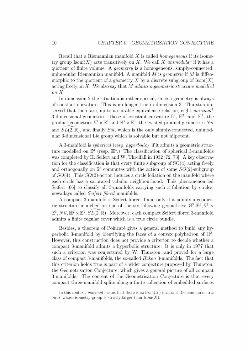
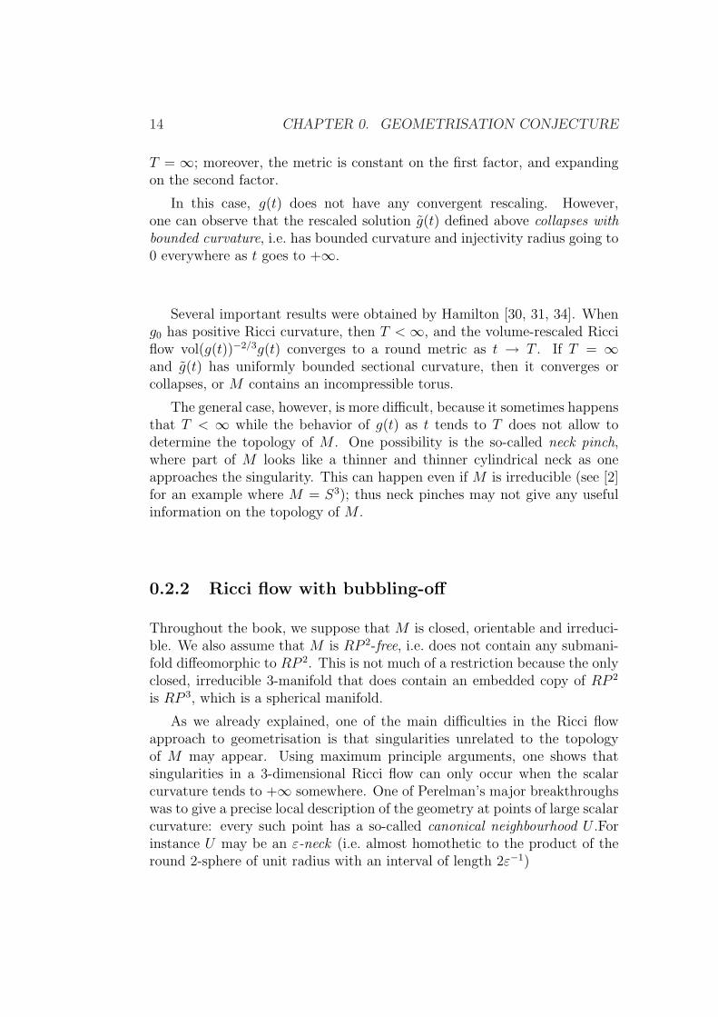
or an ε-cap (i.e. a 3-ball such that a collar neighbourhood of ∂U is anε-neck.)
S2
2ε−1
ε-neck
ε-cap
See Chapter 1 for the precise definitions and Chapter 2 for more infor-mation.
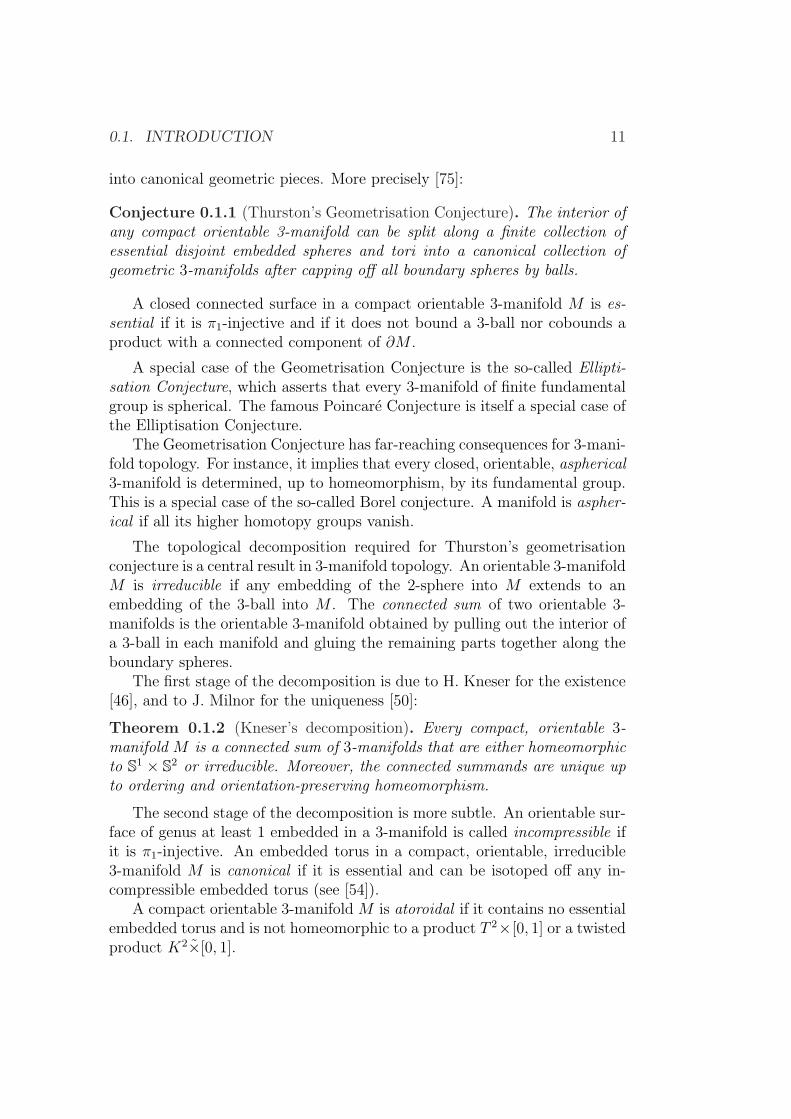
To avoid singularities, we fix a large number Θ, which plays the role of acurvature threshold. As long as the maximum of the scalar curvature is lessthan Θ, Ricci flow is defined. If it reaches Θ at some time t0, then there aretwo possibilities: if the minimum of the scalar curvature of the time-t0 metricis large enough, then every point has a canonical neighbourhood. We shallsee that this is enough to determine the topology of M (cf. Corollary 1.2.4.)Thus we can stop in this case.
Otherwise, we modify g0 so that the maximum of the scalar curvatureof the new metric, denoted by g+(t0), is at most Θ/2. This modification iscalled metric surgery.

16 CHAPTER 0. GEOMETRISATION CONJECTURE
δ-neck
Before surgery...
B3
B3
(M, g(t0))
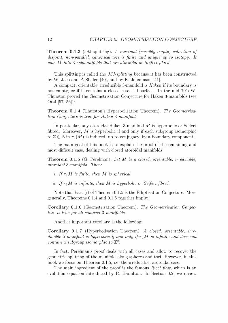
It consists in replacing the metric in some balls containing regions of highcurvature by a special type of ε-caps called almost standard caps.
almost standard caps
....after surgery
(M, g+(t0))
Then we start the Ricci flow again, using g+(t0) as new initial metric.This procedure is repeated as many times as necessary. The main difficultyis to choose Θ and do metric surgery in such a way that the constructioncan indeed by iterated. In practise, we will fix two parameters r, δ > 0,where r is the canonical neighbourhoods’ scale, i.e. is such that all pointsof scalar curvature at least r−2 have canonical neighbourhoods, and δ is asmall number describing the precision of surgery. The threshold Θ is thendetermined by the numbers r, δ (cf. Theorem 3.2.2 and the definition following
0.2. RICCI FLOW AND ELLIPTISATION 17
the statement of that theorem.)In this way, we construct an evolving metric g(t)t which is piecewise
C1-smooth with respect to t, and for each singular time t0 (i.e. value of tsuch that g(·) is not C1 in a neighbourhood of t0) the map t 7→ g(t) is left-continuous and has a right-limit g+(t0).
The result of this construction is called Ricci flow with (r, δ)-bubbling-off.Since its precise definition is quite intricate, we begin by the simpler, moregeneral definition of a Ricci flow with bubbling-off, which retains the essentialfeatures which are needed in order to deduce the elliptisation conjecture.
We say that an evolving metric g(t)t as above is a Ricci flow withbubbling-off if Equation (1) is satisfied at all nonsingular times, and for everysingular time t0 one has
i. Rmin(g+(t0)) > Rmin(g(t0)), and
ii. g+(t0) 6 g(t0).
The following result is one of the main issues of this monograph; its proofoccupies Parts I-II:
Theorem 0.2.1 (Finite time existence of Ricci flow with bubbling-off). LetM be a closed, orientable, irreducible 3-manifold. Then M is spherical, or forevery T > 0 and every riemannian metric g0 on M , there exists a Ricci flowwith bubbling-off g(·) on M , defined on [0, T ], with initial condition g(0) = g0.
By iteration, one obtains immediatly existence on [0,+∞) of Ricci flowwith bubbling-off on closed, orientable, irreducible 3-manifold which are notspherical. However, a lot of work remains to be done in order to obtainthe necessary estimates for hyperbolisation (see Section 0.3); this occupiesPart III. Let us begin with the application of Ricci flow with bubbling-off toelliptisation.
0.2.3 Application to elliptisation
To deduce from Theorem 0.2.1 the first part of Theorem 0.1.5, all we need isthe following result (cf. [60, 20]:)
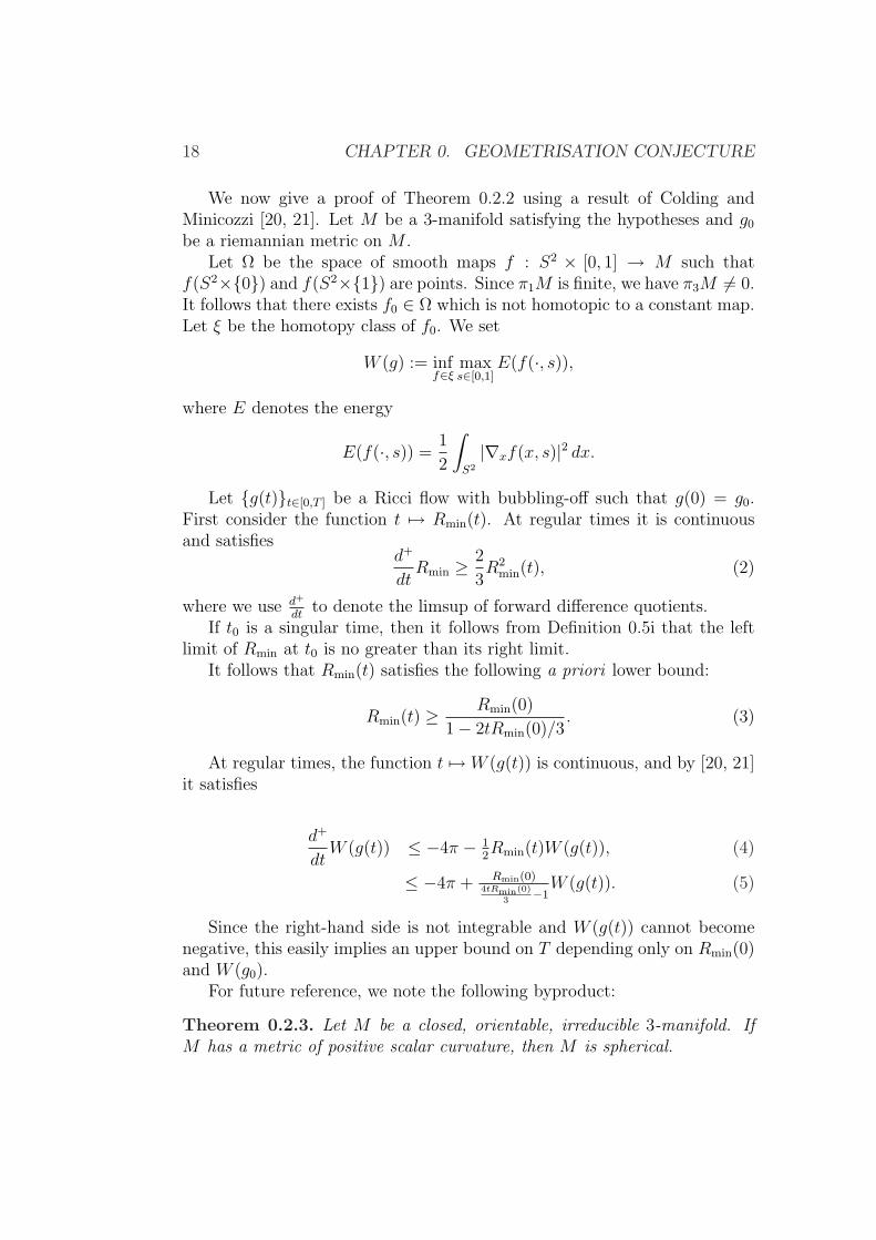
Theorem 0.2.2. Let M be a closed, orientable, irreducible 3-manifold withfinite fundamental group. For each riemannian metric g0 on M there is anumber T (g0) > 0 such that if g(t) on M is a Ricci flow with bubbling-offdefined on some interval [0, T ] and with initial condition g(0) = g0, thenT < T (g0).
18 CHAPTER 0. GEOMETRISATION CONJECTURE
We now give a proof of Theorem 0.2.2 using a result of Colding andMinicozzi [20, 21]. Let M be a 3-manifold satisfying the hypotheses and g0
be a riemannian metric on M .Let Ω be the space of smooth maps f : S2 × [0, 1] → M such that
f(S2×0) and f(S2×1) are points. Since π1M is finite, we have π3M 6= 0.It follows that there exists f0 ∈ Ω which is not homotopic to a constant map.Let ξ be the homotopy class of f0. We set
W (g) := inff∈ξ
maxs∈[0,1]
E(f(·, s)),
where E denotes the energy
E(f(·, s)) =1
2
∫
S2
|∇xf(x, s)|2 dx.
Let g(t)t∈[0,T ] be a Ricci flow with bubbling-off such that g(0) = g0.First consider the function t 7→ Rmin(t). At regular times it is continuousand satisfies
d+
dtRmin ≥ 2
3R2
min(t), (2)
where we use d+
dtto denote the limsup of forward difference quotients.
If t0 is a singular time, then it follows from Definition 0.5i that the leftlimit of Rmin at t0 is no greater than its right limit.
It follows that Rmin(t) satisfies the following a priori lower bound:
Rmin(t) ≥ Rmin(0)
1− 2tRmin(0)/3. (3)
At regular times, the function t 7→ W (g(t)) is continuous, and by [20, 21]it satisfies
d+
dtW (g(t)) ≤ −4π − 1
2Rmin(t)W (g(t)), (4)
≤ −4π + Rmin(0)4tRmin(0)
3−1W (g(t)). (5)
Since the right-hand side is not integrable and W (g(t)) cannot becomenegative, this easily implies an upper bound on T depending only on Rmin(0)and W (g0).
For future reference, we note the following byproduct:
Theorem 0.2.3. Let M be a closed, orientable, irreducible 3-manifold. IfM has a metric of positive scalar curvature, then M is spherical.
0.3. 3-MANIFOLDS WITH INFINITE FUNDAMENTAL GROUP 19
0.3 3-manifolds with infinite fundamental group
In Part III of this book, we shall refine Theorem 0.2.1 and construct for everynon-spherical 3-manifold M and initial condition g0 a special Ricci flow withbubbling-off defined on [0,+∞) and satisfying additional properties. Westate this result in Section 0.3 as Theorem 0.3.2 ( thin-thick decomposition).An intermediate result is obtained is Section 3.4 as Theorem 3.4.1 (long timeexistence).
In subsection 0.3.2 we deduce from the thin-thick decomposition theoremthe proof of the second half of Theorem 0.1.5.
We adopt the convention that throughout the book, all hyperbolic 3-manifoldsare complete and of finite volume.
0.3.1 Long time behaviour of the Ricci flow with bubbling-off
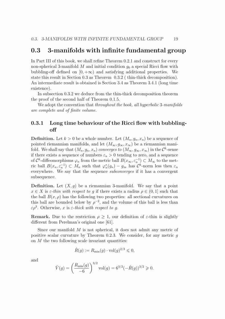
Definition. Let k > 0 be a whole number. Let (Mn, gn, xn) be a sequence ofpointed riemannian manifolds, and let (M∞, g∞, x∞) be a riemannian mani-fold. We shall say that (Mn, gn, xn) converges to (M∞, g∞, x∞) in the Ck-senseif there exists a sequence of numbers εn > 0 tending to zero, and a sequenceof Ck-diffeomorphisms ϕn from the metric ball B(x∞, ε−1
n ) ⊂M∞ to the met-ric ball B(xn, ε
−1n ) ⊂ Mn such that ϕ∗n(gn) − g∞ has Ck-norm less then εn
everywhere. We say that the sequence subconverges if it has a convergentsubsequence.
Definition. Let (X, g) be a riemannian 3-manifold. We say that a pointx ∈ X is ε-thin with respect to g if there exists a radius ρ ∈ (0, 1] such thatthe ball B(x, ρ) has the following two properties: all sectional curvatures onthis ball are bounded below by ρ−2, and the volume of this ball is less thanερ3. Otherwise, x is ε-thick with respect to g.
Remark. Due to the restriction ρ ≥ 1, our definition of ε-thin is slightlydifferent from Perelman’s original one [61].
Since our manifold M is not spherical, it does not admit any metric ofpositive scalar curvature by Theorem 0.2.3. We consider, for any metric gon M the two following scale invariant quantities:
R(g) := Rmin(g) · vol(g)2/3 6 0,
and
V (g) =
(Rmin(g)
−6
)3/2
vol(g) = 63/2(−R(g))3/2 > 0.
20 CHAPTER 0. GEOMETRISATION CONJECTURE
In particular, when H is a hyperbolic manifold, we let V (H) = volH de-note V (ghyp), and R(H) denote R(ghyp), where ghyp is the hyperbolic metric.
On the other hand, note that V (g) = 0 if Rmin(g) = 0.Those quantities are monotonic along the Ricci flow on a closed manifold,
as long as Rmin remain nonpositive (see Corollary B.2.2). This is also truein presence of bubbling-off by conditions (i) and (ii) of Definition 0.5. As aconsequence, we have:
Proposition 0.3.1. Let g(t) be a Ricci flow with bubbling-off on M . Thent 7→ R(g(t)) is nondecreasing, t 7→ V (g(t)) is nonincreasing.
We are now in position to state the main result of this subsection (cf. [61,Sections 6 and 7]).
Recall that we denote by g(t) the rescaled evolving metric (4t)−1g(t), therescaling being motivated by the example of hyperbolic manifolds.
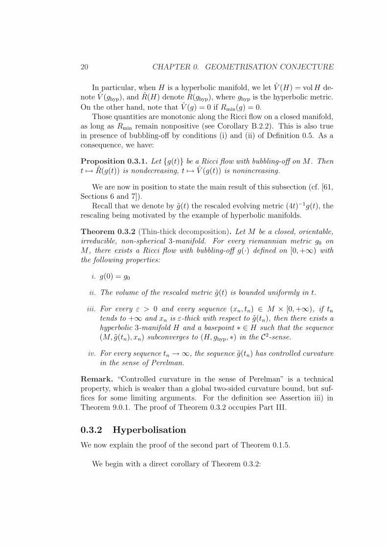
Theorem 0.3.2 (Thin-thick decomposition). Let M be a closed, orientable,irreducible, non-spherical 3-manifold. For every riemannian metric g0 onM , there exists a Ricci flow with bubbling-off g(·) defined on [0,+∞) withthe following properties:
i. g(0) = g0
ii. The volume of the rescaled metric g(t) is bounded uniformly in t.
iii. For every ε > 0 and every sequence (xn, tn) ∈ M × [0,+∞), if tntends to +∞ and xn is ε-thick with respect to g(tn), then there exists ahyperbolic 3-manifold H and a basepoint ∗ ∈ H such that the sequence(M, g(tn), xn) subconverges to (H, ghyp, ∗) in the C2-sense.
iv. For every sequence tn →∞, the sequence g(tn) has controlled curvaturein the sense of Perelman.
Remark. “Controlled curvature in the sense of Perelman” is a technicalproperty, which is weaker than a global two-sided curvature bound, but suf-fices for some limiting arguments. For the definition see Assertion iii) inTheorem 9.0.1. The proof of Theorem 0.3.2 occupies Part III.
0.3.2 Hyperbolisation
We now explain the proof of the second part of Theorem 0.1.5.
We begin with a direct corollary of Theorem 0.3.2:

0.3. 3-MANIFOLDS WITH INFINITE FUNDAMENTAL GROUP 21
Corollary 0.3.3. Let M be a closed, irreducible, non-spherical 3-manifold.For every riemannian metric g0 on M , there exists an infinite sequence ofriemannian metrics g1, . . . , gn, . . . with the following properties:
i) The sequence (vol(gn))n≥0 is bounded.
ii) For every ε > 0 and every sequence xn ∈ M , if xn is ε-thick withrespect to gn, then the sequence (M, gn, xn) subconverges in the pointedC2 topology to a pointed hyperbolic 3-manifold (H, ghyp, ∗), where volH =
V (H) 6 V (g0).
iii) The sequence gn has controlled curvature in the sense of Perelman.
Proof. Applying Theorem 0.3.2, we obtain a Ricci flow with bubbling-offg(t)t∈[0,∞) with initial condition g0. Pick any sequence tn → +∞ and setgn := g(tn) for n ≥ 1. Assertions (i),(iii) and the first part of (ii) followdirectly from the conclusions of Theorem 0.3.2. To see that V (H) 6 V (g0),remark that (V (gn))n≥0 is nonincreasing. Indeed, it follows from Proposi-
tion 0.3.1 and the scale invariance of V , that
V (g0) > V (g1) > · · · > V (gn) > · · · .
On the other hand, Rmin(ghyp) > lim inf Rmin(gn) and vol(H) 6 lim inf vol(gn),
hence V (H) 6 lim inf V (gn) 6 V (g0).
Next we define a topological invariant V0(M). Let M be a closed 3-manifold. For us, a link in M is a (possibly empty, possibly disconnected)closed 1-submanifold of M . A link is hyperbolic if its complement is a hy-perbolic 3-manifold. The invariant V0(M) is defined as the infimum of thevolumes of all hyperbolic links in M . This quantity is finite because anyclosed 3-manifold contains a hyperbolic link [53]. Since the set of volumesof hyperbolic 3-manifolds is well-ordered, this infimum is always realised bysome hyperbolic 3-manifold H0; in particular, it is positive. We note that Mis hyperbolic if and only if H0 = M (see e.g. [5].)
In Part IV, we shall prove the following theorem, which is independentof the results of Parts I–III:
Theorem 0.3.4. Let M be a non-simply connected, closed, orientable, irre-ducible 3-manifold. Suppose that there exists a sequence gn of Riemannianmetrics on M satisfying:
(1) The sequence vol(gn) is bounded.
22 CHAPTER 0. GEOMETRISATION CONJECTURE
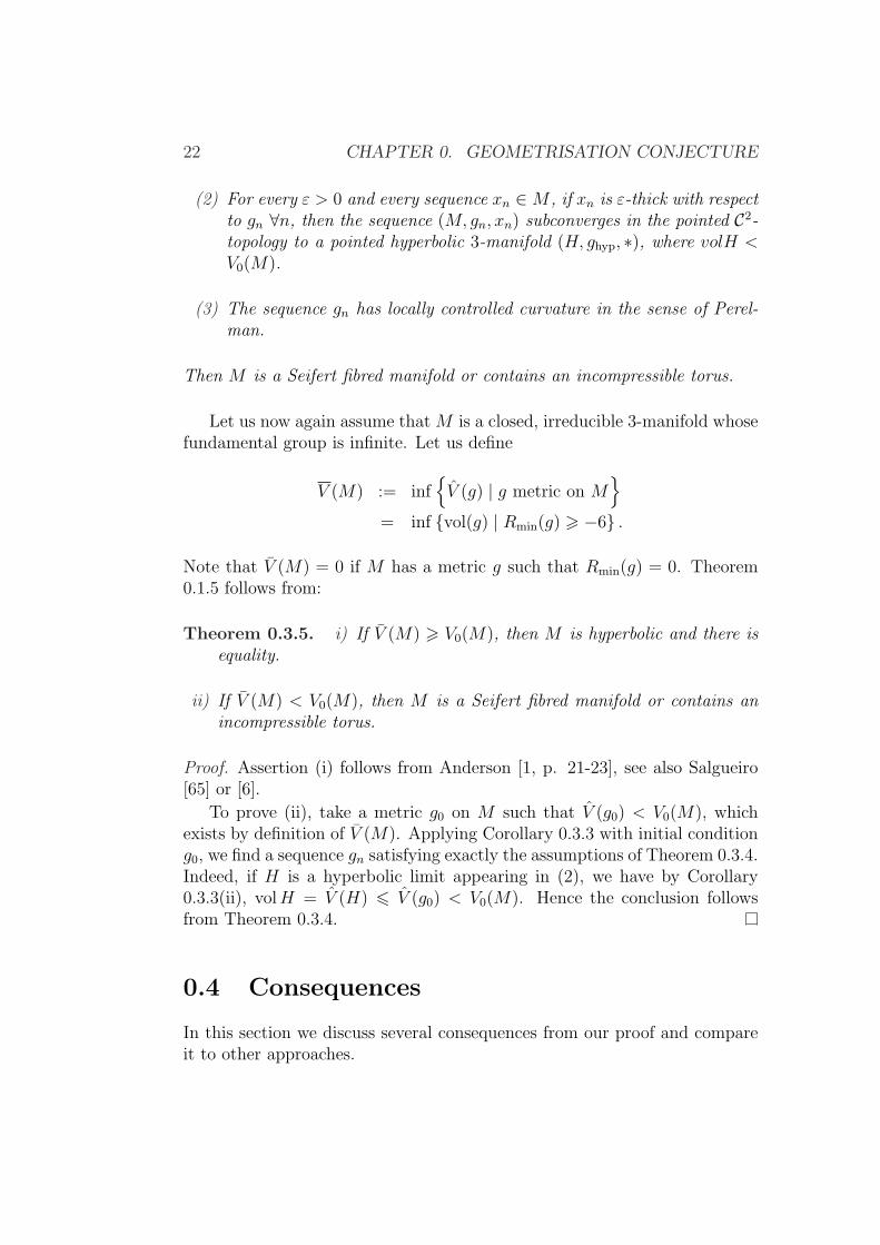
(2) For every ε > 0 and every sequence xn ∈M , if xn is ε-thick with respectto gn ∀n, then the sequence (M, gn, xn) subconverges in the pointed C2-topology to a pointed hyperbolic 3-manifold (H, ghyp, ∗), where volH <V0(M).
(3) The sequence gn has locally controlled curvature in the sense of Perel-man.
Then M is a Seifert fibred manifold or contains an incompressible torus.
Let us now again assume that M is a closed, irreducible 3-manifold whosefundamental group is infinite. Let us define
V (M) := infV (g) | g metric on M
= inf vol(g) | Rmin(g) > −6 .
Note that V (M) = 0 if M has a metric g such that Rmin(g) = 0. Theorem0.1.5 follows from:
Theorem 0.3.5. i) If V (M) > V0(M), then M is hyperbolic and there isequality.
ii) If V (M) < V0(M), then M is a Seifert fibred manifold or contains anincompressible torus.
Proof. Assertion (i) follows from Anderson [1, p. 21-23], see also Salgueiro[65] or [6].
To prove (ii), take a metric g0 on M such that V (g0) < V0(M), whichexists by definition of V (M). Applying Corollary 0.3.3 with initial conditiong0, we find a sequence gn satisfying exactly the assumptions of Theorem 0.3.4.Indeed, if H is a hyperbolic limit appearing in (2), we have by Corollary0.3.3(ii), volH = V (H) 6 V (g0) < V0(M). Hence the conclusion followsfrom Theorem 0.3.4.
0.4 Consequences
In this section we discuss several consequences from our proof and compareit to other approaches.
0.4. CONSEQUENCES 23
0.4.1 Collapsing
A sequence of Riemannian metrics gn on M is said to collapse if there existsa sequence εn → 0 such that, for every n, every point in (M, gn) is εn-thin.
When gn collapses, the proof of Theorem 0.3.4 does not use Hypothe-sis (1), and leads to the conclusion that M is a graph manifold. Hence wealso obtain the following version of Perelman’s collapsing theorem:
Theorem 0.4.1. Let M be a closed, orientable, irreducible, non-simply con-nected 3-manifold. If M admits a sequence of Riemannian metrics that col-lapses and has controlled curvature in the sense of Perelman, then M is agraph manifold.
This is is a version of Theorem 7.4 from [61] (see the discussion in Subsec-tion 0.4.3 below). Theorem 0.3.4 can be viewed as a weak collapsing result inthe sense that we allow the thick part to be nonempty, but require a controlon its volume.
0.4.2 The refined invariant V ′0
A consequence of Theorem 0.3.5 is the following:
Corollary 0.4.2. Let M be a colosed, orientable, irreducible 3-manifold.Then
V (M) 6 V0(M)
and we have equality if and only if M is hyperbolic.
The invariant V0 can be refined as follows. For a closed 3-manifold M , letV ′
0(M) denote the minimum of the volumes of all hyperbolic submanifoldsH ⊂M having the property that either H is the complement of a link in Mor ∂H has at least one component incompressible in M . By definition:
V ′0(M) ≤ V0(M).
Theorem 0.4.3. Let M be a closed, orientable, irreducible 3-manifold. ThenV (M) < V ′
0(M) if and only if M is a graph manifold.
This theorem is proved in Section 13.4.3.Summarizing, we get:
Corollary 0.4.4. Let M be a closed, orientable, irreducible 3-manifold.Then, one of the following occurs:
(i) 0 < V (M) = V ′0(M) = V0(M) if M is hyperbolic.
24 CHAPTER 0. GEOMETRISATION CONJECTURE
(ii) 0 < V ′0(M) ≤ V (M) < V0(M) if M is toroidal and has some hyperbolic
pieces in the JSJ decomposition.
(iii) 0 = V (M) < V ′0(M) ≤ V0(M) if M is graph.
This is a consequence of Theorems 0.3.5 and 0.4.3, except for the factthat V (M) = 0 for a graph manifold. This is a consequence of Cheeger-Gromov [15], who provides metrics with pinched curvature and arbitrarilysmall volume in graph manifolds.
0.4.3 Other approaches
EXPLAIN MORE??Alternatively, to prove hyperbolisation, one can show analytically that
the tori that appear as the boundary of the thick part in Ricci flow withbubbling-off are incompressible by adapting an argument of Hamilton [34](see [44, Section 91],[12]).
The last step of Perelman’s proof in the non-simply connected case relieson a “collapsing theorem” which is independent of the Ricci flow part. Thisresult is stated without proof as Theorem 7.4 in [61]. A version of thistheorem for closed 3-manifolds is given in the appendix of the paper by Shioyaand Yamaguchi [68] using deep results of Alexandrov space theory, includingPerelman’s stability theorem [58] (see also the paper by V. Kapovitch [42])and a fibration theorem for Alexandrov spaces, proved by Yamaguchi [77]. Adifferent approach has been proposed by Morgan and Tian [52]. Yet anotherproof has been announced by Kleiner and Lott [43].
Theorem 12.0.12 implies Theorem 7.4 of [61] for closed, irreducible 3-manifolds which are not simply connected, and it is sufficient to apply theRicci flow with bubbling-off (cf. Theorem 13.4.1). The proof of Theorem 12.0.12combines arguments from Riemannian geometry, algebraic topology, and 3-manifold theory. It uses Thurston’s hyperbolisation theorem for Haken man-ifolds [76, 49, 56, 57], but avoids the stability and fibration theorems forAlexandrov spaces (none of them used in the simply connected case).
Part I
Ricci flow with bubbling-off:definitions and statements
25

0.5. INTRODUCTION 27
0.5 Introduction
In Part I, we develop some notions that lead to the statement of an existenceresult for Ricci flow with bubbling-off (Theorem 3.3.1.) We reduce this the-orem to three technical propositions, called Propositions A, B, C, which areto be proved in Part II.
Let M be a n-manifold. An evolving metric on M defined on an interval[a, b] is a map t 7→ g(t) from [a, b] to the space of C∞ riemannian metricson M . In the sequel, this space is endowed with the C2 topology. We saythat an evolving metric g(·) is piecewise C1 if there is a finite subdivisiona = t0 < t1 < · · · < tp = b of the interval of definition with the followingproperty: for each i ∈ 0, . . . , p− 1, there exists a metric g+(ti) on M suchthat the map defined on [ti, ti+1] by sending ti to g+(ti) and every t ∈ (ti, ti+1]to g(t) is C1-smooth.
For t ∈ [a, b], we say that t is regular if g(·) is C1-smooth in a neighbour-hood of t. Otherwise t is called singular. By definition, the set of singulartimes is finite. If t ∈ (a, b) is a singular time, then it follows from the defini-tion that the map g(·) is continuous from the left at t, and has a limit fromthe right, denoted by g+(t).
There are similar definitions where the domain of definition [a, b] is re-placed by an open or a half-open interval I. When I has infinite length, theset of singular times may be infinite, but must be discrete as a subset of R.
Let Rmin(g) denote the minimum of the scalar curvature of a given metricg.
Definition. Let I ⊂ R be an interval. A piecewise C1 evolving metrict 7→ g(t) on M defined on I is said to be a Ricci flow with bubbling-off if
i) The Ricci flow equation ∂g∂t
= −2 Ric is satisfied at all regular times.
ii) For every singular time t ∈ I one has
a) Rmin(g+(t)) > Rmin(g(t)), and
b) g+(t) 6 g(t).
The basic existence theorem for Ricci flow with bubbling-off (stated inthe introduction as Theorem 0.2.1) asserts that if M is a closed, orientable,irreducible 3-manifold, then M is spherical, or for every T > 0 and everyriemannian metric g0 on M , there exists a Ricci flow with bubbling-off de-fined on [0, T ] with initial condition g0. This theorem is a consequence of amore precise result, Theorem 3.3.1, whose statement is much more involved.
28
Before even giving this statement, we need to introduce several importanttechnical notions, such as κ-noncollapsing, canonical neighbourhoods, andthe standard solution.
0.6 Basic definitions and notation
0.6.1 Riemannian geometry
Let n > 2 be an integer, M be a n-manifold and U ⊂M an open subset.
Notation Let g be a Riemannian metric on M . Then
Riem(X, Y, Z, T ) = g(DYDXZ −DXDYZ +D[X,Y ]Z, T )
is the Riemann curvature operator and for any x ∈M , we denote by Rm(x) :Λ2TxM → Λ2TxM the curvature operator defined by
〈Rm(X ∧ Y ), Z ∧ T 〉 = Riem(X, Y, Z, T ),
where ∧ and 〈·, ·〉 are normalised so that ei ∧ ej | i < j is an orthonormalbasis if ei is. 2
We denote by |Rm(x)| the operator norm of Rm, which is also the max-imum of the absolute values of the sectional curvatures at x. We let R(x)denote the scalar curvature of x. The infimum (resp. supremum) of the scalarcurvature of g on M is denoted by Rmin(g) (resp. Rmax(g)).
We write d : M ×M → [0,∞) for the distance function associated to g.For r > 0 we denote by B(x, r) the open ball of radius r around x.
Finally, if x, y are points of M , we denote by [xy] a geodesic segment,that is a minimizing curve, connecting x to y. This is a (common) abuse ofnotation, since such a segment is not unique in general.
Closeness of metrics
Definition. Let T be a tensor on U , and N a nonnegative integer. Onedenotes
‖T‖2N,U,g := sup
x∈U
N∑
k=0
| ∇kgT (x) |2g .
2This convention is the same as Morgan-Tian’s, but different from that used by Hamil-ton and many others.
0.6. BASIC DEFINITIONS AND NOTATION 29
Let ε be a positive number and g0 be a Riemannian metric on U . One saysthat g is ε-close to g0 on U if
‖g − g0‖[ε−1]+1,U,g0 < ε.
One says that g is ε-homothetic to g0 on U if there exists λ > 0 such that λgis ε-close to g0 on U . The map ψ is called a ε-isometry or a ε-homothety.
A pointed riemannian manifold (U, g, x) is called ε-close to a model(U0, g0, ∗) if there exists a C[ε−1]+1-diffeomorphism ψ from U0 to U sending∗ to x and such that the pull-back metric ψ∗(g) is ε-close to g0 on U0. Wesay that (U, g, x) is ε-homothetic to (U0, g0, ∗) if there is a positive number λsuch that (U, λg, x) is ε-close to (U0, g0, ∗).
A riemannian manifold (U, g) is ε-close (resp. ε-homothetic) to (U0, g0) ifthere exist points x ∈ U and ∗ ∈ U0 such that the pointed manifold (U, g, x)is ε-close (resp. ε-homothetic) to (U0, g0, ∗). If there is no ambiguity on therelevant metrics, we may simply say that U is ε-close (resp. ε-homothetic) toU0.
0.6.2 Evolving metrics and Ricci flow with bubbling-off
We often view an evolving metric g(·) on a manifold M as a 1-parameterfamily of metrics indexed by the interval I; thus we use the notation g(t)t∈I .For each pair (x, t) ∈ M × I, we have an inner product on TxM ; whenevernecessary, we use the notation g(x, t) for this inner product.
Let g(t)t∈I be a Ricci flow with bubbling-off on M . For t ∈ I, thetime-t singular locus of this solution, denoted by Σt, is the closure of the setx ∈ M |g(x, t) 6= g+(x, t). Note that Σt 6= ∅ if and only if t is a singulartime. We say that a pair (x, t) ∈ M × I is singular if x ∈ Σt; otherwise wecall (x, t) regular.
Definition. A product subset X × [a, b] ⊂ M × I is scathed if X × [a, b)contains a singular point. Otherwise, we say that X is unscathed.
Note that a subset X × [a, b] may be unscathed even if there is a singularpoint in X ×b. This definition is consistent with our choice of making themap t 7→ g(t) continuous from the left.
A Ricci flow with bubbling-off without singular point is of course a truesolution of the Ricci flow equation. For brevity, we sometimes call such asolution a Ricci flow.
It will be also useful to consider space-times X × (a, b] where a Ricci flowt 7→ g(t) is not defined on all of X × (a, b]. More precisely, we will consider
30
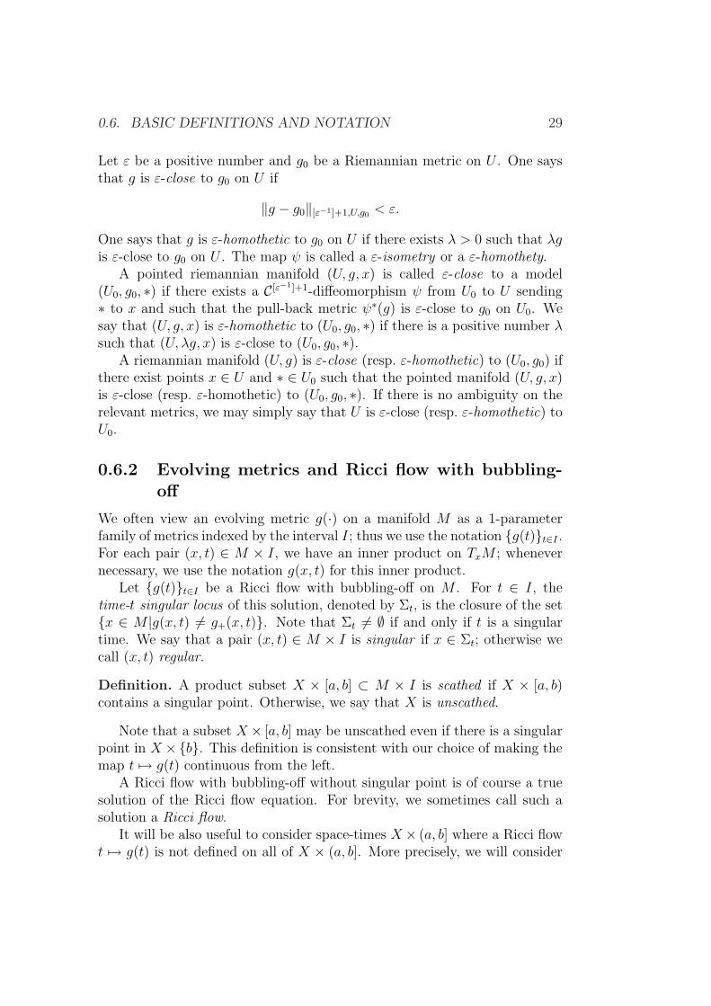
solutions such that the domain of definition of t 7→ g(x, t) may depend ofx ∈ X.
Definition. Let (a, b] a time interval. A partial Ricci flow on U × (a, b] isa pair (P , g(·, ·)), where P ⊂ U × (a, b] is an open subset which containsU × b and (x, t) 7→ g(x, t) is a smooth map defined on P such that therestriction of g to any subset V × I ⊂ P is a Ricci flow on V × I.
VU
t→ g(t)
Notation If g(t)t∈I is an evolving metric on M , and (x, t) ∈M×I, thenwe use the notation Rm(x, t), R(x, t) to denote the curvature operator andthe scalar curvature respectively. For brevity we set Rmin(t) := Rmin(g(t))and Rmax(t) := Rmax(g(t)).
We use dt(·, ·) for the distance function associated to g(t). The ball ofradius r around x for g(t) is denoted by B(x, t, r).
Closeness of evolving metrics Given two evolving metrics g0(·), g(·) onU , defined on [a, b], one says that g(·) is ε-close (resp. ε-homothetic) to g0(·)on U × [a, b], if
supt∈[a,b]
‖g(t)− g0(t)‖[ε−1]+1,U,g0(t) < ε,
(resp. there exists λ > 0 such that λg(·) is ε-close to g0(·) on U × [a, b]).Given two pointed evolving Riemannian manifolds (U0, g0(·), ∗) and (U, g(·), x),
where g0(·) and g(·) are defined on [a, b], one says that (U, g(·), x) is ε-close(resp. ε-homothetic) to (U0, g0(·), ∗) if there exists a C[ε−1]+1-diffeomorphismψ from U0 to U sending ∗ to x, and such that ψ∗g(·) is ε-close (resp. ε-homothetic) to g0(·) on U0 × [a, b]). We say that (U, g(·)) is ε-close to(U0, g0(·)) if there exist points x ∈ U and x0 ∈ U0 such that this propertyholds.
Definition. Let (g(t)t∈I) be an evolving metric on M , t0 ∈ I and Q > 0.The parabolic rescaling with factor Q at time t0 is the evolving metric
t 7→ Qg(t0 +t
Q).
0.6. BASIC DEFINITIONS AND NOTATION 31
Remark. Any parabolic rescaling of a Ricci flow is a Ricci flow.
Lemma 0.6.1 (Multiplicative distance-distortion). Let g(t) be a Ricci flowon U , defined for t ∈ [t1, t2]. Suppose that | Rm |6 Λ on U × [t1, t2]. Then
e−2(n−1)Λ(t2−t1) 6 g(t2)
g(t1)6 e2(n−1)Λ(t2−t1) .
Proof. If | Rm |6 Λ then | Ric |6 (n − 1)Λ. Let x ∈ U and u ∈ TxU be anonzero vector. Then
| ddtg(x,t)(u, u) |=| 2 Ric(x,t)(u, u) |6 2(n− 1)Λg(x,t)(u, u)
hence | ddt
ln g(x,t)(u, u) |6 2(n− 1)Λ. Integrating between t1 and t2 gives theresult.
Remark. In particular, if t2 − t1 6 (2Λ(n− 1))−1, we have
4−1 6 g(t2)
g(t1)6 4,
andB(x, t2,
r
2) ⊂ B(x, t1, r) ⊂ B(x, t2, 2r)
if B(x, t2, 2r) is compactly contained in U . This will be used repeatedly.
Lemma 0.6.2 (Additive distance-distortion). Let g(t) be a Ricci flow onM . Suppose dt(x0, x1) > 2r0 and Ric 6 (n − 1)K for all x ∈ Bt0(x0, r0) ∪Bt0(x1, r0). Then
d
dtdt(x0, x1) > −2(n− 1)
(2
3Kr0 + r−1
0
)(6)
at time t = t0.
Proof. See [44, Lemma 27.8].
Notes The word unscathed was introduced by Kleiner and Lott in [44].Our definition is slightly different from theirs.
The definition of Ricci flow with bubbling-off is new. There are twomain differences with Perelman’s Ricci flow with surgery: first, the manifolddoes not change with time; second, surgery is done before curvature blow-up(compare with [33]). This spares us the need to analyse the structure of themanifold at blow-up time as in [61, §3]. However, the proof of existence usescontradiction arguments which are quite close to Perelman’s (cf. [61, §4,5].)

32
Chapter 1
Piecing together necks and caps
1.1 Definitions
1.1.1 Necks
The standard ε-neck is the riemannian product Nε = S2×(−ε−1, ε−1), wherethe S2 factor is round of scalar curvature 1. Its metric is denoted by gcyl. Wefix a basepoint ∗ in S2 × 0.
Definition. Let (M, g) be a riemannian 3-manifold and x be a point of M .
A neighbourhood N ⊂M of x is called an ε-neck centred at x if (N, g, x)is ε-homothetic to (Nε, gcyl, ∗).
If N is an ε-neck and ψ : Nε → N is a parametrisation, i.e. a diffeo-morphism such that some rescaling of ψ∗(g) is close to gcyl, then the sphereS = ψ(S2 × 0) is called the middle sphere of N . This is slightly abusive,since the parametrisation is not unique.
1.1.2 Caps and tubes
Definition. Let (M, g) be a riemannian 3-manifold and x be a point of M .We say that U is an ε-cap centred at x if U is the union of two sets V,Wsuch that x ∈ IntV , V is a closed topological 3-ball, W ∩ V = ∂V , and W isan ε-neck. A subset V as above is called a core of U .
Definition. An ε-tube is an open subset U ⊂ M which is equal to a finiteunion of ε-necks, and whose closure in M is diffeomorphic to S2 × I.
33
34 CHAPTER 1. PIECING TOGETHER NECKS AND CAPS
1.2 Gluing results
There is a function ε 7→ f3(ε) tending to zero as ε tends to zero, such that ifN is an ε-neck with scaling factor λ and x, y ∈ N , then we have:
|λR(x)− 1| 6 f3(ε) ,
∣∣∣∣R(x)
R(y)− 1
∣∣∣∣ 6 f3(ε).
Fix ε0 ∈ (0, 10−3) sufficiently small so that f3(ε), f3(10ε) 6 10−2 if ε ∈(0, 2ε0].
Lemma 1.2.1. Let ε ∈ (0, 2ε0]. Let (M, g) be a riemannian 3-manifold.Let y1, y2 be points of M . Let U1 ⊂ M be an ε-neck centred at y1 withparametrisation ψ1 : S2 × (−ε−1, ε−1) → U1 and middle sphere S1. LetU2 ⊂ M be a 10ε-neck centred at y2 with middle sphere S2. Call π : U1 →(−ε−1, ε−1) the composition of ψ−1
1 with the projection of S2 × (−ε−1, ε−1)onto its first factor.
Assume that y2 ∈ U1 and |π(y2)| ≤ (2ε)−1. Then the following conclusionshold:
i) U2 is contained in U1;
ii) The boundary components of ∂U2 can be denoted by S+, S− in such away that
π(S−) ⊂ [π(y2)− (10ε)−1 − 10, π(y2)− (10ε)−1 + 10] ,
andπ(S+) ⊂ [π(y2) + (10ε)−1 − 10, π(y2) + (10ε)−1 + 10] ;
iii) The spheres S1, S2 are isotopic in U1.
Proof. Let ψ2 : S2×(−(10ε)−1, (10ε)−1) → U2 be a parametrisation, and callλi the scaling factor of ψi for i = 1, 2. By choice of ε, the quotient λ2/λ1 isclose to 1, so the map ψ−1
1 ψ2 is almost an isometry. Then (i) and (ii) followfrom straightforward distance computations.
To show (iii), recall that by Alexander’s theorem, it suffices to provethat S2 is not null-homologous in U1. Assume that on the contrary, S2 isnull-homologous in U1. Topologically, U2 is a tubular neighbourhood of S2,so the inclusion S2 → U2 is a homotopy equivalence. Hence the inducedhomomorphism H2U2 → H2U1 has zero image.
Set S := ψ1(S2 × π(y2)). By (ii), the diameter of S is less than the
distance between y2 and ∂U2. It follows that S ⊂ U2. Now the inclusion S →U1 is a homotopy equivalence, so the induced homomorphism H2S → H2U1
is an isomorphism. This is impossible.
1.2. GLUING RESULTS 35
Proposition 1.2.2. Let ε ∈ (0, 2ε0]. Let (M, g) be a closed, orientableriemannian 3-manifold. Let X be a compact, connected, nonempty subset ofM such that every point of X is the centre of an ε-neck or an ε-cap. Thenthere exists an open subset U ⊂M containing X such that either
a) U is equal to M and diffeomorphic to S3 or S2 × S1, or
b) U is a 10ε-cap, or
c) U is a 10ε-tube.
In addition, if M is irreducible and every point of X is the centre of anε-neck, then Case (c) holds.
Proof. First we deal with the case where X is covered by ε-necks.
Lemma 1.2.3. If every point of X is centre of an ε-neck, then there existsan open set U containing X such that U = M ∼= S2×S1, or U is a 10ε-tube.
Proof. Let x0 be a point of X and N0 be a 10ε-neck centred at x, containedin an ε-neck U0, also centred at x. If X ⊂ N0 we are done. Otherwise, sinceX is connected, we can pick a point x1 ∈ X ∩N0 and a 10ε-neck N1 centredat x1, with x1 arbitrarily near the boundary of N0. By Lemma 1.2.1, anappropriate choice of x1 ensures that N1 ⊂ U0 and the middle spheres of N0
and N1 are isotopic. In particular, the closure of N0 ∪N1 is diffeomorphic toS2 × I, so N0 ∪N1 is a 10ε-tube.
If X ⊂ N0 ∪ N1, then we can stop. Otherwise, we go on, producing asequence x0, x1, x2, . . . of points of X together with a sequence N0, N1, N2 . . .of 10ε-necks centred at those points, such that N0 ∪ · · · ∪ Nk is a 10ε-tube.Since X is compact, the scalar curvature on X is bounded. Hence definitevolume is added at each step. This implies that the construction must stop.Then either we have found a 10ε-tube containing X, or N0 ∩ Nk 6= ∅. Inthe latter case, we can adjust the choice of xk and Nk so that the necks Ni
cover M , and can be cyclically ordered in such a way that two consecutivenecks form a tube. Since M is orientable, it follows that M is diffeomorphicto S2 × S1.
To complete the proof of Proposition 1.2.2, we need to deal with thecase where there is a point x0 ∈ X which is the centre of an ε-cap C0. Bydefinition of a cap, a collar neighbourhood of the boundary of C0 is an ε-neckU0. If X 6⊂ C0, pick a point x1 close to the boundary of C0. If x1 is centre ofa 10ε-neck N1, then we apply Lemma 1.2.1 again to find that C1 := C0 ∪N1
is an ε-cap. If x1 is centre of an ε-cap C1, then by an appropriate choice
36 CHAPTER 1. PIECING TOGETHER NECKS AND CAPS
of x1 we can make sure that ∂C0 ∩ ∂C1 is empty. Thus either C0 ⊂ C1, orM = C0 ∪ C1.
Again we iterate the construction, producing an increasing sequence of10ε-caps C0 ⊂ C1 ⊂ · · · . For the same reason as before, the process stops,either when X ⊂ Cn, or when we have expressed M as the union of twocaps. In the latter case, it follows from Alexander’s theorem that M isdiffeomorphic to S3.
Finally, the addendum follows from Lemma 1.2.3, since S2 × S1 is re-ducible.
Putting X = M , we obtain the following corollary:
Corollary 1.2.4. Let ε ∈ (0, 2ε0]. Let (M, g) be a closed, orientable rieman-nian 3-manifold. If every point of M is the centre of an ε-neck or an ε-cap,then M is diffeomorphic to S3 or S2×S1. In particular, if M is irreducible,then M is diffeomorphic to S3.
Here is another consequence of Proposition 1.2.2:
Corollary 1.2.5. Let ε ∈ (0, 2ε0]. Let (M, g) be a closed, orientable rie-mannian 3-manifold. Let X be a compact submanifold of M such that everypoint of X is the centre of an ε-neck or an ε-cap. Then one of the followingconclusions holds:
a) M is diffeomorphic to S3 or S2 × S1, or
b) There exists a finite collection N1, . . . , Np of 10ε-caps and 10ε-tubes withdisjoint closures such that X ⊂ ⋃
iNi.
Proof. First apply Proposition 1.2.2 to each component of X. If Case a) doesnot occur, then we have found a finite collection N ′
1, . . . , N′q of 10ε-caps and
10ε-tubes which cover X. If the closures of those caps and tubes are disjoint,then we get Conclusion b).
Otherwise, we pick two members N ′i , N
′j is the collection whose closures
are not disjoint. By adding one or two necks if necessary, we can merge theminto a larger subset U ⊃ N ′
i ∪N ′j. Observe that:
• Merging two tubes produces a tube or shows that M ∼= S2 × S1;
• Merging two caps shows that M ∼= S3;
• Merging a cap with a tube yields a cap.
Hence after finitely many merging operations, we are done.
1.3. MORE RESULTS ON ε-NECKS 37
1.3 More results on ε-necks
Definition. Let (M, g) be a riemannian 3-manifold and N be a neck in M .Let [xy] be a geodesic segment such that x, y /∈ N . We say that [xy] traversesN if the intersection number of [xy] and the middle sphere of N is odd.
Lemma 1.3.1. Let ε ∈ (0, 10−1]. Let (M, g) be a riemannian 3-manifold,N ⊂M be an ε-neck, and S be a middle sphere of N . Let [xy] be a geodesicsegment such that x, y ∈ M \ N and [xy] ∩ S 6= ∅. Then [xy] traverses N .In particular, if S is separating in M , then x, y lie in different componentsof M \ S.
Proof. Let [x′y′] be a subsegment of [xy] such that x′, y′ ∈ ∂N and [x′y′]∩S 6=∅. Since [x′y′] is minimising, we have d(x′, y′) ≥ 2d(S, ∂N). By choice of ε,this is greater than the diameter of each component of ∂N . Hence x′, y′ mustbelong to two distinct such components.
This proves that there is exactly one subsegment [x′y′] such that x′, y′ ∈∂N , [x′y′] ∩ S 6= ∅ and (x′y′) ⊂ N . After perturbation, this segment mustintersect S transversally in an odd number of points.
Corollary 1.3.2. Let ε ∈ (0, 10−1]. Let (M, g) be a riemannian 3-manifold,U ⊂ M be an ε-cap and V be a core of U . Let x, y be points of M \ U and[xy] a geodesic segment connecting x to y. Then [xy] ∩ V = ∅.Proof. By definition, U = N ∪ V where N is a ε-neck of M . Let S be themiddle sphere of N . It is isotopic to ∂V , and separates M in two connectedcomponents, one of them containing x, y, the other V . If [xy] ∩ V 6= ∅ then[xy] intersects S. The last assertion of Lemma 1.3.1 gives the contradiction.
Notes Results similar to those in this chapter can be found in Chapter 19of [51]. The proofs there are somewhat different from ours, relying more ondifferential geometry and less on topology. See also [22].

38 CHAPTER 1. PIECING TOGETHER NECKS AND CAPS
Chapter 2
Key Notions
2.1 κ-noncollapsing
Let M be an n-manifold. Let g(t)t∈I be an evolving metric on M . A(backward) parabolic neighbourhood of a point (x, t) ∈ M × I is a set of theform
P (x, t, r,−∆t) = (x′, t′) ∈M × I | x′ ∈ B(x, t, r), t′ ∈ [t−∆t, t].
In particular, the set P (x, t, r,−r2) is called a parabolic ball of radius r.Notice that after parabolic rescaling with factor r−2 at time t, it becomes aparabolic ball P (x, 0, 1,−1) of radius 1.
Definition. Fix κ, r > 0. We say that g(·) is κ-collapsed at (x, t) on thescale r if for all (x′, t′) ∈ P (x, t, r,−r2) one has |Rm(x′, t′)| 6 r−2, and
volB(x, t, r) < κrn.
Otherwise, g(·) is κ-noncollapsed at (x, t) on the scale r.We say that the evolving metric g(·) is κ-noncollapsed on the scale r if it
is κ-noncollapsed on this scale at every point of M × I.
Remark. g(·) is κ-noncollapsed at (x, t) on the scale r if
|Rm | 6 r−2 on P (x, t, r,−r2) ⇒ volB(x, t, r) > κr3.
Lemma 2.1.1. Let g(·) be a Ricci flow with bubbling-off defined on an in-terval (a, b], x ∈ M and r, κ > 0. If for all t < b, g(·) is κ-noncollapsed at(x, t) on all scales less than or equal to r, then it is κ-noncollapsed at (x, b)on the scale r.
39
40 CHAPTER 2. KEY NOTIONS
Proof. Assume that |Rm | 6 r−2 on P (x, b, r,−r2). Fix s < r. There existsts < b such that for all t ∈ [ts, b) we have P (x, t, s,−s2) ⊂ P (x, b, r,−r2).Without loss of generality, we assume that there is no singular time in [ts, b).Now on P (x, t, s,−s2) we have |Rm | 6 r−2 6 s−2. Applying the noncollaps-ing hypothesis at (x, t) on the scale s, we deduce that volB(x, t, s) > κsn.The result follows by letting first t tend to b, then s tend to r.
2.2 κ-solutions
2.2.1 Definition and main results
Definition. Let κ > 0. A Ricci flow (M, g(·)) is called a κ-solution if
i) It is ancient, i.e. defined on (−∞, 0];
ii) For each t ∈ (−∞, 0], the metric g(t) is complete, and Rm(·, t) is non-negative and bounded;
iii) There exists (x, t) ∈M × (−∞, 0] such that Rm(x, t) 6= 0;
iv) For every r > 0, the evolving metric g(·) is κ-noncollapsed on the scaler.
A κ-solution is round if for each t, the metric g(t) has constant positivesectional curvature.
The asymptotic volume of a complete Riemannian manifold (Mn, g) ofnonnegative curvature is defined by
V(g) = limr→∞
volB(x, r)
rn.
One easily see using Bishop-Gromov that the limit is well defined and doesnot depend on x ∈M . We state here fundamental results on κ-solutions.
Theorem 2.2.1 (Vanishing asymptotic volume). For any κ-solution (M, g(·)),one has V(g(t)) = 0 for all t.
Proof. [59, Section 11.4],[44, Proposition 41.13].
Theorem 2.2.2 (Compactness theorem). For all κ > 0, the space of pointed3-dimensional κ-solutions (M, g(·), (x, 0)) such that R(x, 0) = 1 is compact.
Proof. [59, Section 11.7],[44, Theorem 46.1].
Theorem 2.2.3. Every 2-dimensional κ-solution is round.
2.2. κ-SOLUTIONS 41
Proof. [59, Corollary 11.3], [44, Corollary 40.1 and Section 43].
Theorem 2.2.4 (Universal κ). There exists a universal constant κsol > 0such that any 3-dimensional κ-solution is round or a κsol-solution.
Proof. [61, Section 1.5], [44, Proposition 50.1].
2.2.2 Canonical neighbourhoods
The cylindrical flow is S2 × R together with the product flow on (−∞, 0],where the first factor is round, normalised so that the scalar curvature attime 0 is identically 1. We denote this evolving metric by gcyl(t).
Definition. Let ε > 0. Let M be a 3-manifold, g(t)t∈I be an evolvingmetric on M , and (x0, t0) ∈ M × I. An open subset N ⊂ M is calleda strong ε-neck centred at (x0, t0) if there is a number Q > 0 such that(N, g(t)t∈[t0−Q−1,t0], x0) is unscathed, and after parabolic rescaling with fac-tor Q at time t0, ε-close to (S2 × (−ε−1, ε−1), gcyl(t)t∈[−1,0], ∗).
Remarks. i) Fix Q > 0, and consider the flow (S2 × R, Qgcyl(tQ−1))
restricted to (−Q, 0]. Then for every x ∈ S2 × R, the point (x, 0) iscentre of a strong ε-neck for all ε > 0.
ii) If (x0, t0) is centre of a strong ε-neck, then there is a neighbourhood Ωof x0 such that for all x ∈ Ω, (x, t0) is centre of a strong ε-neck: onecan use the same set N and factor Q, but change the parametrisation sothat the basepoint ∗ is sent to x rather than x0. Choosing Ω smaller, wehave also that (x, t0) is centre of a strong ε0-neck for all evolving metricg(·) sufficiently close to g(·) is the C[ε−1]+1 topology.
iii) By abuse of language, we shall sometimes call strong ε-neck the parabolicset N × [t0 −Q−1, t0] ⊂M × I, rather that the set N ⊂M .
Definition. Let ε, C > 0 and g(t)t∈I be an evolving metric on M . We saythat an open subset U ⊂ M is an (ε, C)-canonical neighbourhood centred at(x0, t0) if U is an ε-cap or a strong ε-neck centred at (x0, t0) which satisfiesfurthermore the following estimates for the metric g(t0) : R(x0) > 0 and
there exists r ∈ (C−1R(x0)− 1
2 , CR(x0)− 1
2 ) such that:
i) B(x0, r) ⊂ U ⊂ B(x0, 2r);
ii) The scalar curvature function restricted to U has values in a compactsubinterval of (C−1R(x0), CR(x0));
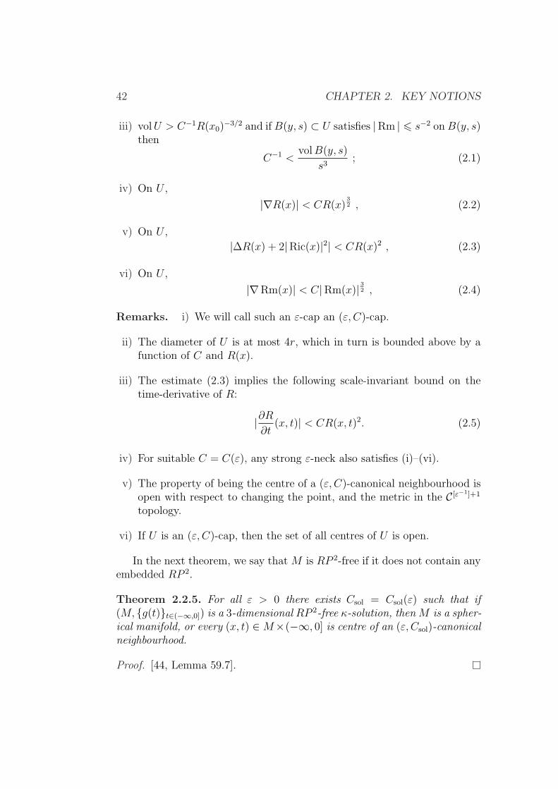
42 CHAPTER 2. KEY NOTIONS
iii) volU > C−1R(x0)−3/2 and ifB(y, s) ⊂ U satisfies |Rm | 6 s−2 onB(y, s)
then
C−1 <volB(y, s)
s3; (2.1)
iv) On U ,
|∇R(x)| < CR(x)32 , (2.2)
v) On U ,
|∆R(x) + 2|Ric(x)|2| < CR(x)2 , (2.3)
vi) On U ,
|∇Rm(x)| < C|Rm(x)| 32 , (2.4)
Remarks. i) We will call such an ε-cap an (ε, C)-cap.
ii) The diameter of U is at most 4r, which in turn is bounded above by afunction of C and R(x).
iii) The estimate (2.3) implies the following scale-invariant bound on thetime-derivative of R:
|∂R∂t
(x, t)| < CR(x, t)2. (2.5)
iv) For suitable C = C(ε), any strong ε-neck also satisfies (i)–(vi).
v) The property of being the centre of a (ε, C)-canonical neighbourhood isopen with respect to changing the point, and the metric in the C[ε−1]+1
topology.
vi) If U is an (ε, C)-cap, then the set of all centres of U is open.
In the next theorem, we say that M is RP 2-free if it does not contain anyembedded RP 2.
Theorem 2.2.5. For all ε > 0 there exists Csol = Csol(ε) such that if(M, g(t)t∈(−∞,0]) is a 3-dimensional RP 2-free κ-solution, then M is a spher-ical manifold, or every (x, t) ∈M×(−∞, 0] is centre of an (ε, Csol)-canonicalneighbourhood.
Proof. [44, Lemma 59.7].
2.3. THE STANDARD SOLUTION I 43
2.3 The standard solution I
2.3.1 Definition and main results
We fix a riemannian manifold S0 satisfying a number of properties, such as:
• S0 is diffeomorphic to R3;
• it is complete;
• the sectional curvature is nonnegative and bounded;
• it is rotationally symmetric;
• a neighbourhood of infinity is isometric to the product S2 × [0,+∞).
The centre of symmetry is denoted by p0.
For technical reasons, one needs to be more precise in the choice of S0,so the definition is given in Chapter 5. For now, we record some properties.
Theorem 2.3.1. The Ricci flow with initial condition S0 has a maximalsolution defined on [0, 1), which is unique among complete flows of boundedsectional curvature.
Proof. [61, Section 2], [44, Section 61-64], and [17],[48] for the uniqueness.
Definition. This solution is called the standard solution.
Proposition 2.3.2. There exist κst > 0 that the standard solution is κst-noncollapsed on all scales.
Proof. [44, Lemma 60.3]
Proposition 2.3.3. For every ε > 0 there exists Cst(ε) > 0 such that for all(x, t) ∈ S0× [0, 1), if t > 3/4 or x ∈ B(p0, 0, ε
−1), then (x, t) has an (ε, Cst)-canonical neighbourhood. In the other case, there is an ε-neck B(x, t, ε−1rsuch that P (x, t, ε−1r,−t) is ε-close to the corresponding subset of the cylin-drical flow.
Moreover, we have an estimate Rmin(t) > const(1− t)−1.
Proof. [44, Lemma 63.1]
44 CHAPTER 2. KEY NOTIONS
2.3.2 Neck Strengthening
Let Kst be the supremum of the sectional curvatures of the standard solutionon [0, 4/5].
Lemma 2.3.4 (Neck Strengthening). indexTheorem!Neck Strenghtening Forall ε ∈ (0, 10−4) there exists β = β(ε) ∈ (0, 10−3) such that the followingholds. Let a, b be real numbers satisfying a < b < 0 and |b| 6 3/4, let(M, g(·)) be a 3-dimensional Ricci flow with bubbling-off defined on (a, 0],and x ∈M be a point such that:
i) R(x, b) = 1;
ii) (x, b) is centre of a strong βε-neck;
iii) P (x, b, (βε)−1, |b|) is unscathed and satisfies |Rm | 6 2Kst.
Then (x, 0) is centre of a strong ε-neck.
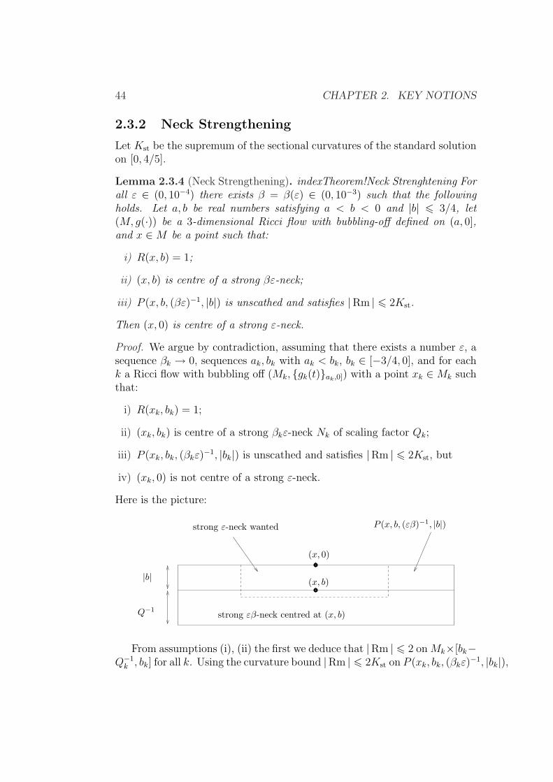
Proof. We argue by contradiction, assuming that there exists a number ε, asequence βk → 0, sequences ak, bk with ak < bk, bk ∈ [−3/4, 0], and for eachk a Ricci flow with bubbling off (Mk, gk(t)ak,0]) with a point xk ∈Mk suchthat:
i) R(xk, bk) = 1;
ii) (xk, bk) is centre of a strong βkε-neck Nk of scaling factor Qk;
iii) P (xk, bk, (βkε)−1, |bk|) is unscathed and satisfies |Rm | 6 2Kst, but
iv) (xk, 0) is not centre of a strong ε-neck.
Here is the picture:
(x, 0)
Q−1
|b|
strong εβ-neck centred at (x, b)
P (x, b, (εβ)−1, |b|)
(x, b)
strong ε-neck wanted
From assumptions (i), (ii) the first we deduce that |Rm | 6 2 onMk×[bk−Q−1k , bk] for all k. Using the curvature bound |Rm | 6 2Kst on P (xk, bk, (βkε)
−1, |bk|),
2.4. CURVATURE PINCHED TOWARD POSITIVE 45
the distance-distortion Lemma 0.6.1 gives a constant c such thatB(xk, 0, c(βkε)−1) ⊂
B(xk, bk, (βkε)−1). Hence we have |Rm | 6 max2Kst, 2 on P (xk, 0, c(βkε)
−1), Q−1k −
bk).
Using Cheeger’s injectivity radius estimate [13] (cf A.0.7), one deducesfrom the proximity with the cylinder at (xk, bk) and from the bounded cur-vature a positive lower bound on the injectivity radius at (xk, 0).
Note that the normalisation R(xk, bk) = 1 implies that Qk → 1. The com-pactness theorem B.3.1 gives a subsequence of (Mk, gkt∈[bk−Q−1
k ,0], (xk, 0))
which converges to a complete pointed Ricci flow (M∞, g∞(·), (x∞, 0)) ofbounded curvature, defined on (b − 1, 0], where b := lim bk ∈ [−3/4, 0].In particular, the sequence of pointed riemannian manifolds (Mk, gk(bk −(2Qk)
−1), xk) converges smoothly to (M∞, g∞(b− 1/2), x∞).
From the hypothesis that Nk is a strong βkε-neck of scaling factor Qk
centred at (xk, bk), we deduce that (Mk, Qkgk(bk − (2Qk)−1, xk) converges
to (S2 ×R, gcyl(−1/2), ∗). Hence (M∞, g∞(b− 1/2), x∞) is isometric to thiscylinder. By the Chen-Zhu uniqueness theorem [18], we deduce that the limitflow (M∞, g∞(t)t∈[b−1/2,0]) is the cylindrical flow up to parabolic scaling.The same conclusion holds on (b−1, 0] since Nk is a strong βkε-neck for eachk.
We have R(x∞, b) = 1, hence R(x∞, 0) = (1 + b)−1 > 1. By the remarkafter the definition of a strong ε-neck, we are done.
2.4 Curvature pinched toward positive
Let (M, g) be a 3-manifold and x ∈ M be a point. We denote by λ(x) >µ(x) > ν(x) the eigenvalues of the curvature operator Rm(x). By our defini-tion, all sectional curvatures lie in the interval [ν(x), λ(x)]. Moreover, λ(x)(resp. ν(x)) is the maximal (resp. minimal) sectional curvature at x. If C is areal number, we sometimes write Rm(x) > C instead of ν(x) > C. Likewise,Rm(x) 6 C means λ(x) 6 C.
It follows that the eigenvalues of the Ricci tensor are equal to λ + µ,λ + ν, and µ + ν; as a consequence, the scalar curvature R(x) is equal to2(λ(x) + µ(x) + ν(x)).
For evolving metrics, we use the notation λ(x, t), µ(x, t), and ν(x, t), andcorrespondingly write Rm(x, t) > C for ν(x, t) > C, and Rm(x, t) 6 C forλ(x, t) 6 C.
Definition. Let φ be a nonnegative function. A metric g on M has φ-almostnonnegative curvature if Rm > −φ(R).
46 CHAPTER 2. KEY NOTIONS
Remark. In this case, one has also a bound above of the curvature operatorby a function of the scalar curvature, namely
R
2− 2φ(R) > R
2− µ− ν = λ > Rm > ν > −φ(R).
Now we consider a familly of positive functions (φt)t>0 defined as follows.
Let st = e2
1+tand define
φt : [−2st,+∞) −→ [st,+∞)
as the reciprocal of the increasing function
s 7→ 2s(ln(s) + ln(1 + t)− 3).
As in [51], we use the following definition.
Definition. Let I ⊂ [0,∞) be an interval and g(t)t∈I be an evolving metricon M . We say that g(·) has curvature pinched toward positive at time t iffor all x ∈M we have
R(x, t) > − 6
4t+ 1, (2.6)
Rm(x, t) > −φt(R(x, t)). (2.7)
We say that g(·) has curvature pinched toward positive if it has curvaturepinched toward positive at each t ∈ I.Remark. If one set X = max0, |ν(x, t)|, Equation (2.7) is equivalent to 1
R(x, t) > 2X (lnX − ln(1 + t)− 3) , (2.8)
We have the following important property due to Hamilton and Ivey:
Proposition 2.4.1 ([34], [39] ). Let a, b be two real numbers such that 0 ≤a < b. Let g(t)t∈[a,b] be a Ricci flow solution on M such that g(·) hascurvature pinched toward positive at time a. Then g(·) has curvature pinchedtoward positive.
The following lemmas will be useful.
Lemma 2.4.2. i) φt(s) = φ0((1+t)s)1+t
.
1The factor 2 comes from our choices or normalisation of the curvature operator Rm.Compare to [34]
2.4. CURVATURE PINCHED TOWARD POSITIVE 47
ii) φt(s)s
decreases to 0 as s tends to +∞.
iii) φ0(s)s
= 14
if s = 4e5.
Proof. (i) is left to the reader. For (ii), Compute the reciprocal function ψ.One has
0 <φ0(s)
s= u⇔ φ0(s) = su⇔ s = 2(su)[ln(su)−3] ⇔ ψ(u) = s =
1
ue3+ 1
2u .
Now, since ψ′(u) < 0 ψ and s→ φ(s)/s are decreasing. Finally ψ(1/4) = 4e5
proves (iii).
Property ii) will ensure that limits of suitably rescaled evolving metricswith pinched toward positive curvature will have nonnegative curvature op-erator (see Proposition 4.2.5). Denote s = 4e5.
Lemma 2.4.3 (Pinching Lemma). Assume g(·) has curvature pinched to-ward positive and let t > 0, r > 0 be such that (1+t)r−2 > s. If R(x, t) 6 r−2
then |Rm(x, t)| 6 r−2 .
Proof. Assume that r ≤ r√t and R(x, t) < r−2. Note that tr−2 > r−2 > s.
By assumption, we have at (x, t),
Rm > −φt(R)
= −φ0((1 + t)R)
1 + t
> −φ0((1 + t)r−2)
1 + t
= −φ0((1 + t)r−2)
(1 + t)r−2r−2
> −1
4r−2
by Lemma 2.4.2. On the other hand
Rm 6 λ =R
2− ν − µ ≤ r−2
2+ 2(
r−2
4) = r−2.
Remarks. This lemma will be used in two kinds of settings:
i) r−2 > s. For example, if R(x, t) 6 Q = r−2 where, say, Q > 106,then |Rm | 6 Q. Hence if the scalar curvature is large, it bounds thecurvature operator.
48 CHAPTER 2. KEY NOTIONS
ii) tr−2 > s, which is equivalent to r ∈ (0, r√t] if one sets r = s−1/2. This
will be used in the study of the long time behaviour of the Ricci flowwith bubbling-off.
Notes Most of the material of this chapter is standard, with definitionsvarying slightly from author to author. Lemma 2.3.4 is inspired by [51,Proposition 15.2].
Chapter 3
Ricci flow with(r, δ, κ)-bubbling-off
From now on, we fix a closed, orientable, irreducible 3-manifold M . We alsoassume that M is not spherical.
In particular, M is RP 2-free, and not diffeomorphic to S3 or S2 × S1.Moreover, any manifold obtained from a sequence of riemannian metrics onM by taking a pointed limit automatically has the same properties (exceptcompactness, of course.)
3.1 Let the constants be fixed
Recall that ε0 has been fixed in Chapter 1. Let β0 := β(ε0) be the parametergiven by Lemma 2.3.4. Finally, define
C0 := max100ε0−1, 2Csol(ε0/2), 2Cst(β0ε0/2),
where Csol is defined by Theorem 2.2.5, and Cst by Proposition 2.3.3.
Definition. Let r > 0. An evolving metric g(t)t∈I on M has property(CN)r if for all (x, t) ∈ M × I, if R(x, t) > r−2, then (x, t) admits an(ε0, C0)-canonical neighbourhood.
Definition. Let κ > 0. An evolving metric g(t)t∈I on M has property(NC)κ if g(t) is κ-noncollapsed on all scales less than 1.
Remark. If (NC)κ is satisfied on some time interval (a, b), it is also satisfiedon (a, b]. This follows immediately from Lemma 2.1.1.
Definition. A metric g on M is normalised if |Rm | 6 1 and each ball ofradius one has volume at least half of the volume of the unit ball in Euclidean3-space.
49
50 CHAPTER 3. RICCI FLOW WITH (r, δ, κ)-BUBBLING-OFF
Since M is closed, any metric on M can be normalised by scaling.
Proposition 3.1.1. There exists a constant κnorm > 0 such that if g0 isa normalised metric on M , then the maximal Ricci flow solution g(·) withinitial condition g0 is defined at least on [0, 1/16], and on this interval itsatisfies:
i) |Rm| ≤ 2;
ii) (NC)κnorm, and
iii) g(·) has curvature pinched toward positive.
Remark. Conclusion (i) implies R 6 12, hence (CN)r is vacuously true forr < (2
√3)−1.
We define κ0 := min(κnorm, κsol/2, κst/2).
3.2 Metric Surgery and Cutoff Parameters
Recall that S0 is the initial condition of the standard solution and p0 itscentre of symmetry (see Section 2.3, and Section 5.1 for precise defintions).
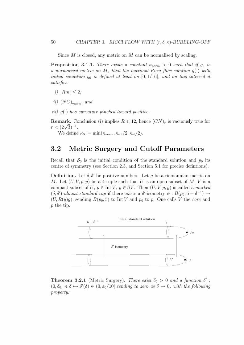
Definition. Let δ, δ′ be positive numbers. Let g be a riemannian metric onM . Let (U, V, p, y) be a 4-tuple such that U is an open subset of M , V is acompact subset of U , p ∈ IntV , y ∈ ∂V . Then (U, V, p, y) is called a marked(δ, δ′)-almost standard cap if there exists a δ′-isometry ψ : B(p0, 5 + δ−1) →(U,R(y)g), sending B(p0, 5) to IntV and p0 to p. One calls V the core andp the tip.
55 + δ−1
p
p0
V
initial standard solution
δ′-isometry
Theorem 3.2.1 (Metric Surgery). There exist δ0 > 0 and a function δ′ :(0, δ0] 3 δ 7→ δ′(δ) ∈ (0, ε0/10] tending to zero as δ → 0, with the followingproperty:
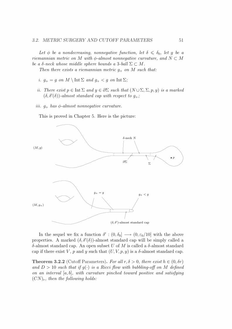
3.2. METRIC SURGERY AND CUTOFF PARAMETERS 51
Let φ be a nondecreasing, nonnegative function, let δ 6 δ0, let g be ariemannian metric on M with φ-almost nonnegative curvature, and N ⊂Mbe a δ-neck whose middle sphere bounds a 3-ball Σ ⊂M .
Then there exists a riemannian metric g+ on M such that:
i. g+ = g on M \ Int Σ and g+ < g on Int Σ;
ii. There exist p ∈ Int Σ and y ∈ ∂Σ such that (N ∪Σ,Σ, p, y) is a marked(δ, δ′(δ))-almost standard cap with respect to g+;
iii. g+ has φ-almost nonnegative curvature.
This is proved in Chapter 5. Here is the picture:
p
g+ = gg+ < g
(M, g)
(M, g+)
(δ, δ′)-almost standard cap
δ-neck N
Σ∂Σ
In the sequel we fix a function δ′ : (0, δ0] −→ (0, ε0/10] with the aboveproperties. A marked (δ, δ′(δ))-almost standard cap will be simply called aδ-almost standard cap. An open subset U of M is called a δ-almost standardcap if there exist V , p and y such that (U, V, p, y) is a δ-almost standard cap.
Theorem 3.2.2 (Cutoff Parameters). For all r, δ > 0, there exist h ∈ (0, δr)and D > 10 such that if g(·) is a Ricci flow with bubbling-off on M definedon an interval [a, b], with curvature pinched toward positive and satisfying(CN)r, then the following holds:
52 CHAPTER 3. RICCI FLOW WITH (r, δ, κ)-BUBBLING-OFF
Suppose that x, y, z ∈ M and t ∈ [a, b] are such that R(x, t) 6 2r−2,R(y, t) = h−2, R(z, t) ≥ Dh−2, and y lies on a g(t)-geodesic segment con-necting x to z. Then (y, t) is the centre of a strong δ-neck.
This will be proved in Chapter 4. In the sequel we fix functions (r, δ) 7→h(r, δ) and (r, δ) 7→ D(r, δ) with the above property. We set Θ(r, δ) :=2D(r, δ)h(r, δ)−2. This number will be used as a curvature threshold for thesurgery process.
Definition. We say that two real numbers r, δ are surgery parameters if0 < r < 10−3 and 0 < δ < min(ε0, δ0). The associated cutoff parameters areh := h(r, δ) and Θ := 2Dh−2.
Remark. The convention r < 10−3 implies that g(·) satisfies (CN)r vac-uously on [1, 1/16] if g(0) is normalised. See the remark after Proposition3.1.1.
Definition. Fix surgery parameters r, δ and let h,Θ be the associated cutoffparameters. Let g(t)t∈I be an evolving metric on M . Let g+ be a rie-mannian metric on M and t0 ∈ I. We say that g+ is obtained from g(·) by(r, δ)-surgery at time t0 if the following conditions are satisfied:
i) For all x ∈ M , if g+(x) 6= g(x, t0), then there exist a δ-almost standardcap (U, V, p, y) w.r.t. g+, such that
(a) x ∈ IntV ;
(b) R(y, t0) = h−2;
(c) (y, t0) is the centre of a strong δ-neck;
(d) g+ < g(t0) on IntV .
ii) Rmax(g(t0)) = Θ and Rmax(g+) 6 Θ/2.
Remark. It may seem at first sight more natural to define a purely rieman-nian notion, of a metric obtained by (r, δ)-surgery from another. However,this is made impractical by the requirement that (y, t0) be centre of a strongneck in Condition i(c), which is important for technical reasons. The require-ment that g+ < g(t0) on IntV is a simplification.
Definition. Fix surgery parameters r, δ and let h,D,Θ be the associatedcutoff parameters. Let I ⊂ [0,∞) be an interval and g(t)t∈I be a Ricciflow with bubbling-off on M . We say that g(t)t∈I is an Ricci flow with(r, δ)-bubbling-off if it has the following properties:
3.3. FINITE TIME EXISTENCE THEOREM 53
i) g(·) has curvature pinched toward positive and satisfies R(x, t) 6 Θ forall (x, t) ∈M × I;
ii) For every singular time t0 ∈ I, the metric g+(t0) is obtained from g(·)by (r, δ)-surgery at time t0;
iii) Condition (CN)r holds.
Let κ > 0. An Ricci flow with (r, δ)-bubbling-off which in addition sat-isfies Condition (NC)κ will be called an Ricci flow with (r, δ, κ)-bubbling-off.
The following lemma is easy, but extremely important, since it allows torule out accumulation of surgeries.
Lemma 3.2.3. Let r, δ be surgery parameters. Let g(t)t∈I be an Ricciflow with (r, δ)-bubbling-off on M . Let t1 < t2 be two singular times. Thent2 − t1 > (C0Θ)−1.
Proof. One can suppose that g(·) is smooth on (t1, t2]. Let x ∈M such thatR(x, t2) = Rmax(t2) = Θ. As Rmax(g+(t1)) 6 Θ/2, there exists t+ ∈ [t1, t2]maximal such that limt→t+,t>t+ R(x, t) = Θ/2. In particular, (x, t) is centre ofan (ε0, C0)-canonical neighbourhood for all t ∈ (t+, t2]. Integrating inequality(2.5) on (t+, t2] gives
1
R(x, t2)− lim
t→t+,t>t+
1
R(x, t)6 C0(t2 − t+) 6 C0(t2 − t1).
Hence t2 − t1 > 1C0
(− 1Θ
+ 2Θ
)= (C0Θ)−1.
3.3 Finite time existence theorem for Ricci
flow with (r, δ, κ)-bubbling-off
Recall that we are assuming that M is a closed, orientable, irreducible 3-manifold, and that M is not spherical.
In this case, Theorem 0.2.1 asserts that for any T > 0 and any metricg0 on M , there exists a Ricci flow with bubbling-off g(·) on M , defined on[0, T ], with initial condition g(0) = g0. This follows immediately from thefollowing technical result:
Theorem 3.3.1. For every T > 0, there exist r, δ, κ > 0 such that for anynormalised metric g0 on M , there exists a Ricci flow with (r, δ, κ)-bubbling-offdefined on [0, T ] with initial condition g0.
54 CHAPTER 3. RICCI FLOW WITH (r, δ, κ)-BUBBLING-OFF
Since any metric on M can be normalised by scaling, Theorem 3.3.1 impliesTheorem 0.2.1.
Our next aim is to reduce Theorem 3.3.1 to three results, called Proposi-tions A, B, C, which are independent of one another.
Proposition A. There exists a universal constant δA ∈ (0, δ0) having thefollowing property: let r, δ be surgery parameters, a, b be positive numberswith a < b, and g(t)t∈(a,b] be an Ricci flow with (r, δ)-bubbling-off on M .Suppose that δ 6 δA, and Rmax(b) = Θ.
Then M admits a metric g+ which is obtained from g(·) by (r, δ)-surgeryat time b, and in addition satisfies:
i. g+ has φb-almost nonnegative curvature;
ii. Rmin(g+) > Rmin(g(b)).
Proposition B. For all κ > 0 there exist r(κ) ∈ (0, 10−3) and δB = δB(κ) ∈(0, δ0) with the following property: let δ 6 δB, b > 0 and g(t) be a Ricci flowwith bubbling-off defined on [0, b] with normalised initial condition. Assumethat the restriction of g(·) to the half-open interval [0, b) is a Ricci flow with(r, δ, κ)-bubbling-off. Then it satisfies (CN)r on all of [0, b].
Proposition C. For all T > 0 there exists κ = κ(T ) ∈ (0, κ0) such thatfor all r ∈ (0, 10−3) there exists δC = δC(T, r) ∈ (0, δ0) with the followingproperty.
For all 0 < δ 6 δC and 0 < b 6 T , every Ricci flow with (r, δ)-bubbling-offdefined on [0, b) and having normalised initial condition satisfies (NC)κ.
Let us assume Propositions A, B, C, and prove Theorem 3.3.1.Let T > 0. Proposition C gives a constant κ = κ(T ). Proposition B gives
constants r, δB depending on κ. Then apply Proposition C again to get aconstant δC . Set δ = min(δA, δB, δC , C
−3/20 /10).
From r, δ we get the cutoff parameters h,D,Θ.Let g0 be a normalised metric on M . Let X be the set of ordered
pairs (T ′, g(t)t∈[0,T ′)) consisting of a number T ′ ∈ (0, T ] and a Ricci flowwith (r, δ, κ)-bubbling-off (g(t)t∈[0,T ′) such that g(0) = g0. By Proposi-tion 3.1.1, X is nonempty. It has a partial ordering, defined by (T ′1, g1(t)) 6(T ′2, g2(t)) if T ′1 6 T ′2 and g2(·) is an extension of g1(·).
We want to use Zorn’s lemma to prove existence of a maximal elementin X . In order to do this, we consider an infinite chain, that is an infinitesequence of numbers 0 < T1 < T2 < · · ·Tn < · · · < T and of Ricci flow with(r, δ, κ)-bubbling-off defined on the intervals [0, Tn), and which extend one an-other. In this way we get an evolving metric g(t) defined on [0, T∞), where
3.3. FINITE TIME EXISTENCE THEOREM 55
T∞ is the supremum of the Tn’s. By Lemma 3.2.3, the set of singular timesis a discrete subset of R, so g(t) is an Ricci flow with (r, δ, κ)-bubbling-off.
Hence we can apply Zorn’s lemma. Let (T ′, g(t)) ∈ X be a maximalelement. Its scalar curvature lies between −6 and Θ, so it is bounded.Its curvature is pinched toward positive so the sectional curvature is alsobounded. Hence by Proposition B.1.2 we can extend g(t) to a Ricci flowwith bubbling-off on [0, T ′], with Rmax(T
′) 6 Θ. By Proposition B, Prop-erty (CN)r is satisfied on [0, T ′]. By Lemma 2.1.1 the same holds true for(NC)κ (compare with the remark after the definition of Condition (NC)κ.)Hence we have obtained an Ricci flow with (r, δ, κ)-bubbling-off on the closedinterval [0, T ′].
To conclude, we prove by contradiction that T ′ = T . Assume that T ′ < Tand consider the following two cases:
Case 1 Rmax(T′) < Θ.
Applying the short time existence theorem for Ricci flow with initial met-ric g(T ′), we can extend g(·) to a Ricci flow with bubbling-off defined on aninterval [0, T ′ + α) for some α > 0. We choose α sufficiently small so thatwe still have Rmax(t) < Θ on [0, T ′ + α). There are no singular times in[T ′, T ′ + α), and by Proposition 2.4.1 the extension has curvature pinchedtoward positive.
Lemma 3.3.2. There exists α′ ∈ (0, α] such that Condition (CN)r holds forg(t)t∈[0,T ′+α′).
Proof. Arguing by contradiction, we assume that there exist sequences xk ∈M and tk → T ′ such that R(xk, tk) > r−2, but (xk, tk) does not have an(ε0, C0)-canonical neighbourhood. Since M is compact, we may assume thatthe sequence xk converges and call x its limit.
We have R(x, T ′) > r−2, so (x, T ′) has an (ε0, C0)-canonical neighbour-hood. First consider the case where (x, T ′) is centre of an (ε0, C0)-cap U .We use the remarks made after the definition of an (ε0, C)-cap. Since being
the centre of a (ε0, C0)-cap is an open property in the C[ε−10 ]+1-topology, U is
still an (ε0, C0)-cap with respect to g(tk), wit centre xk, for sufficiently largek. This is a contradiction.
Suppose now that (x, T ′) is centre of a strong ε0-neck N . Let ψ be aparametrisation of N . By definition, there exists a parabolic rescaling g of gwith factor Q at time T ′ such that
supt∈[−1,0]
‖ψ∗(g(t))− gcyl(t)‖C[ε−10 ]+1 < ε0.
56 CHAPTER 3. RICCI FLOW WITH (r, δ, κ)-BUBBLING-OFF
Note that the inequality is strict. Let gk(·) be the parabolic rescaling of gwith factor Q at time tk. Since tk → T ′, the same inequality holds with g(·)replaced by gk(·), for sufficiently large k. Hence (x, tk) is centre of a strongε0-neck. We conclude using the already remarked fact that being the centreof strong ε0-neck is an open property.
It follows that g(t)t∈[0,T ′+α′) is an Ricci flow with (r, δ)-bubbling-off. ByProposition C, it is an Ricci flow with (r, δ, κ)-bubbling-off. This contradictsmaximality of T ′.
Case 2 Rmax(T′) = Θ.
Proposition A yields a metric g+, which has curvature pinched towardpositive at time T ′. Applying the short time existence theorem for Ricciflow with initial metric g+, we obtain a positive number α and an evolvingmetric g(t)t∈(T ′,T ′+α) whose limit from the right as t tends to T ′ is equalto g+. We also may assume that Rmax remains bounded above by Θ. ByProposition 2.4.1 it has curvature pinched toward positive. Hence the re-sulting evolving metric g(t)t∈[0,T ′+α) satisfies the first two properties of thedefinition of Ricci flow with (r, δ)-bubbling-off.
Lemma 3.3.3. There exists α′ ∈ (0, α] such that Condition (CN)r holds forg(t)t∈[0,T ′+α′).
Proof. Arguing as above, consider sequences xk → x ∈M and tk → T ′ suchthat for each k, R(xk, tk) > r−2 but (xk, tk) does not have a canonical neigh-bourhood. Set g := h−2g+(T ′). We will distinguish several cases accordingto the proximity of x to the set
ΣT ′ := x ∈M | g+(x, T ′) 6= g(x, T ′).
By definition of the (r, δ)-surgery, this set is a union of 3-balls which are coreof δ-almost standard caps of g+(T ′).
Case a) dg(x,ΣT ′) > (2C0)3/2.
Claim 1. The point (x, T ′) has an (ε0, C0)-canonical neighbourhood U ′ suchthat U ′ ∩ ΣT ′ = ∅.
Once the claim is proved, Case a) follows by the arguments used to proveLemma 3.3.2.
Let us prove the claim: since t 7→ g(t) is smooth on [T ′, T ′ + α) in aneighbourhood of x we have R(x, T ′) = limR(xk, tk) > r−2. Hence (x, T ′)has an (ε0, C0)-canonical neighbourhood U ′. Suppose that U ′∩ΣT ′ 6= ∅. Pick
3.4. LONG TIME EXISTENCE 57
a point z′ ∈ U ′∩ΣT ′ 6= ∅. Since g+(T ′) is obtained from g(·) by (r, δ)-surgery,there is a δ-almost standard cap U whose core V contains z′.
Let z be a point of U ′ ∩ ∂V . We have (see Section 1.2)
1− f3(δ′) 6 h−2
R(z, T ′)6 1 + f3(δ
′).
Besides, we have R(z, T ′) < C0R(x, T ′), thus
R(x, T ′)−12 < R(z, T ′)−
12 · (2C0)
12 .
It follows that
dg(T ′)(x, z) 6 2C0R(x, T ′)−12 6 (2C0)
32h.
We conclude that dg(x,ΣT ′) 6 (2C0)32 , contradicting our hypothesis.
Case b) dg(x,ΣT ′) 6 (2C0)3/2.
In this case, there exists a δ-almost standard cap U with core V and tipp such that dg(x, V ) 6 (2C0)
3/2. In particular, Bg(x, 2ε−10 ) ⊂ U by choice of
δ. If Bg(x, 2ε−10 ) ∩ V = ∅, then (x, T ′) is centre of a strong ε0-neck disjoint
from ΣT ′ , and we can apply the argument used in the proof of Lemma 3.3.2.Hence we assume that Bg(x, 2ε
−10 ) ∩ V 6= ∅. Choose an ε0-neck N in U
at distance, say 5ε0−1 to p. Then U ′ = Bg(p, 6ε0) ∪ N is a (ε0, C0)-cap in
(M, g+(T ′)), with core U ′\N and centre x. As g(·) is smooth of (T ′, T ′ + α)and g+(T ′) = limt→T ′,t>T ′ g(t), we can conclude as in Lemma 3.3.2.
Hence g(t)t∈[0,T ′+α′) is an Ricci flow with (r, δ)-bubbling-off. By Propo-sition C, it is an Ricci flow with (r, δ, κ)-bubbling-off. Again this contradictsthe assumption that T ′ should be maximal.
3.4 Long time existence of Ricci flow with
bubbling-off
By iteration, Theorem 0.2.1 immediately extends to an existence theorem forRicci flow with bubbling-off defined on [0,+∞) on our nonspherical manifoldM . However, we need to extend the particular construction of Ricci flow with(r, δ)-bubbling-off. More precisely, we need this:
Theorem 3.4.1 (Long time existence). There exist decreasing sequences ofpositive numbers ri, κi and, for every continuous positive function t 7→ δ(t),
58 CHAPTER 3. RICCI FLOW WITH (r, δ, κ)-BUBBLING-OFF
a sequence of positive numbers δi with δi < miniε<t≤(i+1)ε δ(t) such that thefollowing holds: for every normalised metric g0 sur M , there exists a Ricciflow with bubbling-off g(·) defined on [0,+∞) such that g(0) = g0 and for alli, g(·) is a Ricci flow with (ri, δi, κi)-bubbling-off on (iε, (i+ 1)ε].
Remark. The presence of the function δ(·) allows to choose δ small comparedto r. The usefulness of this to prove Theorem 0.3.2 will be clear in Part III.
Theorem 3.4.1 will follow from a version of Theorem 3.3.1 suited foriteration. Before giving the statement, we need a definition.
Definition. Let Q > 0. One says that a Riemannian manifold (M, g) isQ-normalised if
i. |Rm | 6 Q on M .
ii. volB(x, 1) > Q−1
2υ0(1) for all x ∈M .
By compactness, any metric g is Q-normalised for some constant Q > 0.We can have some control with:
Assertion 3.4.2. Let g(·) be a Ricci flow with (r, δ, κ)-bubbling-off on someinterval [a, b]. Then g(·) is Q-normalised on [a, b] for some constant Q =Q(r, δ, κ).
Proof. Recall that R 6 Θ = 2Dh−2 where D and h are functions of (r, δ),hence |Rm | 6 Θ by the Pinching Lemma 2.4.3. Hence setting s = Θ−1/2,one has |Rm | 6 s−2 on P (x, t, s,−s2) for all (x, t) ∈ M × [a, b]. As g(·) isκ-noncollapsed at scales < 1, we deduce that
volB(x, t, 1) > volB(x, t, s) > κs3 =2κΘ−3/2
υ0(1)
υ0(1)
2.
Thus
Q = max
Θ,
υ0(1)
2κΘ−3/2
fit.
We leave to the reader to check that the proof of Theorem 3.3.1 goesthrough to show the following. An alternative proof, based on a dilationargument, is sketched below.
Theorem 3.4.3. For all Q > 0, 0 6 TA < TΩ, there exists κ > 0, such thatfor all r ∈ (0, 10−3), there exists r ∈ (0, r), such that for all δ, there existsδ ∈ (0, δ) and Q′ > 0 with the following property. Let g be a Riemannian
3.4. LONG TIME EXISTENCE 59
metric on M such that (M, g) is Q-normalised and has curvature pinchedtoward positive at time TA. Then there exists a Ricci flow with (r, δ, κ)-bubbling-off g(·) defined on [TA, TΩ], such that g(TA) = g, and such that g(·)is Q′-normalised.
Applying inductively this result proves Theorem 3.4.1.
Terminology In order to simplify the notation, given decreasing sequencesri and δi we introduce step functions t 7→ r(t), t 7→ δ(t), whose values arerespectively ri and δi on (iε, (i + 1)ε]. We will say that a Ricci flow withbubbling-off defined on some interval I ⊂ R is a Ricci flow with r(·), δ(·)-bubbling-off if, in restriction to I ∩ (iε, (i+1)ε] it is a Ricci flow with (ri, δi)-bubbling-off. This will appear in some technical results of Chapter 6 and 8,useful to Part III. This part is all concerned with Ricci flow with r(·), δ(·)-bubbling-off, and precisely to refine the choice of the function δ(·). Forsimplicity we shall denote h(t) := h(r(t), δ(t)), D(t) = D(r(t)), δ(t) andΘ(t) = D(t)h−2(t) the associated cutoff parameters.
Alternative proof of Theorem 3.4.3 Here we outline an alternativeproof of Theorem 3.4.3, based on the following variant of Theorem 3.3.1:
Theorem 3.4.4. For every T > 0, there exists κ > 0, such that for allr ∈ (0, 10−3), there exists r ∈ (0, r), such that for all δ > 0, there existsδ ∈ (0, δ) such that for any normalised metric g0 on M , there exists a Ricciflow with (r, δ, κ)-bubbling-off defined on [0, T ] with initial condition g0.
One can prove Theorem 3.4.3 directly from Theorem 3.3.1 by a dilationargument. To do this, one needs:
i) To compute some λ = λ(Q) such that if g is Q-normalised, then λg is 1-normalised. This can be done using the local version A.0.7 of Cheeger’sinjectivity radius estimate and Gunther comparison theorem [24, Theo-rem 3.101].
ii) To refine the Cutoff Parameters Theorem 3.2.2 so that h(·, δ) is linearwith respect to r. Indeed, if g(·) is the parabolic rescaling with factorλ of a Ricci flow with (r, δ)-bubbling-off g(·), it satisfies (V C)√λr and
his scale of surgery must be, by dilation,√λh(r, δ) = h(
√λr, δ). This
property is easily obtained by a dilation argument, replacing also thepinched toward positive curvature assumption by a φ0-pinched assump-tion (behaves better under rescaling).
60 CHAPTER 3. RICCI FLOW WITH (r, δ, κ)-BUBBLING-OFF
With this in hands, you can apply Theorem 3.4.4 on [0, λ(TΩ − TA)] withinitial metric λg to obtain a Ricci with (r, δ, κ)-bubbling-off, and then do theparabolic rescaling back to obtain a Ricci flow with (λ−1/2, δ, λ−3/2)-bubbling-off on [TA, TΩ].
Notes Theorem 3.2.1 is similar to [44, Lemma 72.20].The statement of Theorem 3.2.2 is new. Its proof is almost the same as
[61, Lemma 4.3].Propositions A, B, C correspond roughly to Section 4, Section 5.4 and
Lemma 5.2 of [61], respectively.The argument in the proof of Lemma 3.2.3 is new. It is not expected to
hold in Perelman’s construction.Theorem 3.4.1 is similar to [61, Proposition 5.1].
Part II
Ricci flow with bubbling-off:existence
61

63
In this part we prove the three main propositions A, B and C. Let us bemore precise. Chapter 4 is devoted to present some technical material. Weindeed prove the curvature-distance theorem which asserts that the curvatureon a given ball is compared to the curvature at the centre provided that wehave the canonical neighbourhood property and that the curvature at thecentre is large enough. From this we deduce the Cut-off Parameters Theorem(3.2.2).
In chapter 5 we state a precise definition for the standard solution anddescribe our version of the metric surgery, proving Theorem 3.2.1. Fromthat we prove proposition A which shows that we can perform the (r, δ)-surgery when the threshold for the scalar curvature is attained. It is shownto preserve the curvature pinched toward positive assumption.
Chapter 6 is a technical chapter. The main result is the so-called per-sistence theorem. It shows that near the added almost standard cap theevolving metric looks like the standard solution for an amount of time closeto one, after rescaling. This is used to show that the canonical neighbourhoodproperty persists after surgery.
In chapter 7 we prove proposition B. It shows that the canonical neigh-bourhood property is a closed condition in time; that is, if it is satisfied onan interval open in the future, it is also true on the closure, again if theparameters are well chosen.
Finally chapter 8 is devoted to the proof of proposition C. We proveseveral versions of the κ-non collapsing result. We give a n-dimensionalversion for smooth Ricci flow. We also prove a version on a given intervalfor the Ricci flow with bubbling off in dimension 3. Finally we give a usefulversion adapted to the long time study of the flow which is used in Part III.It applies in particular in the description of the thick part.

64
Chapter 4
Choosing cutoff parameters
The main goal of this chapter is to prove Theorem 3.2.2 which allows to geth,D, and therefore Θ, from r, δ.
Along the way we prove another result, Theorem 4.2.1 which allows todeduce relative curvature bounds on Ricci flow with bubbling-off that sat-isfy the Canonical Neighbourhoods and Curvature Pinched Toward Positiveassumptions. This will be again useful later on.
The first section contains some preliminary results on the structure ofsets obtained by gluing together ε-necks. These results will be used in theproofs of Theorems 3.2.2 and 4.2.1.
4.1 Piecing together necks in noncompact man-
ifolds
Definition. Let (X, g) be a (not necessarily complete) riemannian 3-manifoldand ε be a positive number. An ε-horn is an open subset U ⊂ X which hasthe following properties:
i. U is a union of ε-necks;
ii. U is diffeomorphic to S2 ×R;
iii. the scalar curvature is bounded on one end of U and tends to +∞ onthe other end.
Lemma 4.1.1. Let ε ∈ (0, 2ε0], (X, g) be a riemannian 3-manifold, andγ : [0, 1) → X be a continuous map such that every point of the image of γis centre of an ε-neck, and R(γ(s)) → +∞ as s → 1. Then there exists a10ε-horn U ⊂ X containing the image of γ.
65
66 CHAPTER 4. CHOOSING CUTOFF PARAMETERS
Proof. Set x0 := γ(0). Using the construction described in the proof ofLemma 1.2.3, we produce an infinite sequence of points x0, x1, x2, . . . in theimage of γ, and a sequence of necks N0, N1, N2, . . . centred at those points,such that for every k, N0 ∪ · · · ∪Nk is a tube.
Then the union U of all the Nk’s is a 10ε-horn. To see that is contains thewhole image of γ, suppose it does not. Choose s ∈ [0, 1) such that γ(s) 6∈ U .Then all the xk’s are images of numbers in the compact interval [0, s]. Hencewe have an upper bound for their scalar curvatures, which gives a lowerbound for the distance d(xk, xk+1). This in turn implies that d(x0, xk) goesto infinity, which is a contradiction.
Proposition 4.1.2. Let (M, g) be an open riemannian 3-manifold. If everypoint of M is the centre of a 2ε0-neck, then M is diffeomorphic to S2 ×R.
Proof. The proof is similar to that of Lemma 4.1.1, except that after thechoice of x0 and N0, we pick two points x−1, x1, one near each boundary com-ponent ofN0. In this way we construct biinfinite sequences . . . , x−2, x−1, x0, x1, x2, . . .and . . . , N−2, N−1, N0, N1, N2, . . . such that for each k, Nk is a neck centredat xk, and each finite union N−k . . . , Nk is a tube.
To see that the union of those tubes is the whole of M , we argue as in theproof of Lemma 4.1.1: if some point y ∈ M is not in the union of the Nk’s,then we connect it to x0 by a continuous path and use the compactness ofthis path to obtain a contradiction.
Therefore, M has an exhaustion by tubes. This implies that it is diffeo-morphic to S2 ×R.
4.2 Bounded curvature at bounded distance
The goal of this section is to prove the following theorem:
Theorem 4.2.1 (Curvature-Distance). For all A,C1 > 0 and all ε1 ∈(0, 2ε0], there exists Q = Q(A, ε1, C1) > 0 and Λ = Λ(A, ε1, C1) > 0 withthe following property. Let I ⊂ [0,+∞) be an interval and g(t)t∈I bea Ricci flow with bubbling-off with curvature pinched toward positive. Let(x0, t0) ∈M × I be such that:
i) (1 + t0)R(x0, t0) > Q;
ii) For each point y ∈ B(x0, t0, AR(x0, t0)−1/2), if R(y, t0) ≥ 2R(x0, t0),
then (y, t0) has an (ε1, C1)-canonical neighbourhood.
4.2. BOUNDED CURVATURE AT BOUNDED DISTANCE 67
Then for all y ∈ B(x0, t0, AR(x0, t0)−1/2), we have
R(y, t0)
R(x0, t0)6 Λ.
4.2.1 Preliminaries
Lemma 4.2.2 (Local curvature-distance lemma). Let (U, g) be a Rieman-nian manifold. Let Q > 1, C > 0, x ∈ U and set Qx =| R(x) | +Q. Assumethat [xy] is a geodesic segment of length 6 (2C
√Qx)
−1, on which
| ∇R |< CR3/2 (4.1)
holds any point of scalar curvature > Q. Then R(y) < 2Qx.
Proof. Let [x′y′] ⊂ [xy] be a maixmal segment such that R > Q on [x′y′]. Inparticular R(x′) > Qx. Integrating inequality (4.1) on [x′y′], one finds
| R−1/2(x′)−R−1/2(y′) |< C
2d(x′, y′) 6 (4
√Qx)
−1
hence
R−1/2(y′) > R−1/2(x′)− (4√Qx)
−1 > Qx−1/2 − (4
√Qx)
−1 =3
4
√Qx
−1
thus R(y′) < 169Qx < 2Qx and y′ = y.
Lemma 4.2.3 (Local curvature-time lemma). Let (U, g(·)) be a Ricci flowdefined on [t1, t2]. Let Q > 1, C > 0, x ∈ U and set Qx =| R(x, t2) | +Q.Assume that on [t2 − (2CQx)
−1, t2], the inequality
| dRdt
|< CR2 (4.2)
holds at (x, t) if R(x, t) > Q. Then R(x, t) < 2Qx on this interval.
Proof. Consider a maximal interval [t−, t+] ⊂ [t, t2] such that R(x, ·) > Q onit. Note that R(x, t+) 6 Qx. Integrating (4.2) on x × [t−, t+] gives
| R(x, t+)−1 −R(x, t−)−1 |< C(t+ − t−) 6 (2Qx)−1, .
hence R(x, t−)−1 > R(x, t+)−1 − (2Qx)−1 = Qx
−1 − (2Qx)−1 = (2Qx)
−1. Weconclude that R(x, t−) < 2Qx and t− = t.
68 CHAPTER 4. CHOOSING CUTOFF PARAMETERS
Lemma 4.2.4 (Local curvature-control lemma). Let Q > 0, C > 0, ε ∈(0, 2ε0], and g(t)t∈I be a Ricci flow with bubbling-off on M . Let (x0, t0) ∈M×I and set Q0 = |R(x0, t0)|+Q. Suppose that P = P (x0, t0,
12C√Q0,− 1
8CQ0)
is unscathed and that each (x, t) ∈ P with R(x, t) > Q has an (ε, C)-canonicalneighbourhood. Then for all (x, t) ∈ P ,
R(x, t) 6 4Q0 .
Proof. First we note that R(x, t0) ≤ 2Q0. It follows from the curvature-distance Lemma, as any point of B(x0, t0,
12C√Q0
) of scalar curvature larger
than Q is centre of a (ε, C)-canonical neighbourhood, and in particular sat-isfies (4.1). Let us show that R(x, t) ≤ 4Q0: if R(x, t) ≤ Q we are done.Otherwise, let t1 be the maximal time such that R(x, s) ≥ Q for all s ∈ [t, t1].Observe that R(x, t1) = Q ≤ 2Q0 or t1 = t0 and R(x, t0) ≤ 2Q0. Integrating|∂R/∂t| ≤ C1R
2 on [t, t1], we obtain
R(x, t) ≤ (R(x, t1)−1−C1(t1− t))−1 ≤ ((2Q0)
−1− (8Q0)−1)−1 ≤ 8
3Q0 ≤ 4Q0 .
Remark. In particular, this lemma applies to any Ricci flow with bubbling-off satisfying (CN)r, setting Q = r−2.
We shall use repeatedly the following property:
Proposition 4.2.5. Let (Uk, gk(·), ∗k) be a sequence of pointed evolving met-rics defined on intervals Ik ⊂ R+, and having curvature pinched toward pos-itive. Let (xk, tk) ∈ Uk × Ik be a sequence such that (1 + tk)R(xk, tk) goes to+∞. Then the sequence gk(·) := R(xk, tk)g(tk + ·
R(xk,tk)) has the following
properties:
i) The sequence Rmin(gk(·)) tends to 0.
ii) If (Uk, gk(·), ∗k) converges in the pointed C2 sense, then the limit hasnonnegative curvature operator.
Proof. Fix t ∈ R such that gk(t) is defined for all k, and denote Qk :=R(xk, tk) and t′k = tk + tQk
−1. Then we have
Rmin(gk(t)) = Qk−1Rmin(gk(t
′k))
> −6
(4t′k + 1)Qk
=−6
4tkQk + 4t+Qk
> −6
(1 + tk)Qk + 4t→ 0

4.2. BOUNDED CURVATURE AT BOUNDED DISTANCE 69
To prove the second assertion, call (U∞, g∞(·), ∗∞) the limit. Let (y∞, t) ∈U∞ × R be the limit of (yk, t) ∈ Uk × t. Since the convergence is C2, wehave Now
Rm(y∞, t)) = limk→∞
Rm(yk, t)
= limk→∞
Qk−1 Rm(yk, t
′k)
> −φt′k(R(yk, t
′k))
Qk
= −φ0((1 + t′k)R(yk, t′k))
(1 + t′k)Qk
.
Note that (1 + t′k)Qk = (1 + tk)Qk + t → +∞. Hence if, up to extracting asubsequence, (1 + t′k)R(yk, t
′k) < C for some constant C for all k, the above
expression is bounded below by − φ0(C)(1+t′k)Qk
→ 0 as k tends to +∞. Now if we
assume that (1 + t′k)R(yk, t′k) → ∞ the expression above is bounded below
by
−φ0((1 + t′k)R(yk, t′k))
(1 + t′k)R(yk, t′k)R(yk, t
′k)
Qk
,
which tends to 0 by Lemma 2.4.2ii), since the right term converges toR(y∞, t) ∈R by assumption.
Finally, we shall need the following lemma (cf [44, Theorem 41.2] ):
Lemma 4.2.6. Let (C, g0, p) be a Riemannian cone with base point p, suchthat the curvature operator of g0 is nonnegative and nonzero. Let U ⊂ C \ pbe an open subset and g(·) be a Ricci flow on U × [−τ, 0], for some τ > 0,with final time slice g(0) equal to g0. Then g(·) cannot have nonnegativecurvature operator.
4.2.2 Proof of Theorem 4.2.1
The proof is by contradiction. Assume that there exist constants A, ε1, C1,sequences Qk → +∞, Λk → +∞, and a sequence (gk(·), (xk, tk)) of pointedRicci flow with bubbling-off with curvature pinched toward positive, suchthat:
i) (1 + tk)R(xk, tk) ≥ Qk;
ii) for all y ∈ B(x0, t0, AR(xk, tk)−1/2), if R(y, tk) ≥ 2R(xk, tk), then y has
an (ε1, C1)-canonical neighbourhood;
70 CHAPTER 4. CHOOSING CUTOFF PARAMETERS
iii) for each k there exists a point yk such that
R(yk, tk)
R(xk, tk)> Λk and dtk(xk, yk) 6 AR(xk, tk)
−1/2.
For every k we let
gk(·) := R(xk, tk)gk(tk +·
R(xk, tk))
be the evolving metric resulting from gk(·) by parabolic rescaling at time tkwith factor R(xk, tk).
We shall use the following notation: if x is a point of M , then x denotesthe same point, but geometric quantities are computed using the rescaledevolving metrics. Thus we have R(xk, 0) = 1, R(yk, 0) > Λk and d0(xk, yk) 6A. Observe that all points of scalar curvature greater than or equal to 2 have(ε1, C1)-canonical neighbourhoods.
Step 1. There exists ρ > 0 such that the sequence (B(xk, 0, ρ), gk(0), xk)subconverges in the C1,α sense to (M∞, g∞, x∞) where M∞ is a smooth 3-manifold and g∞ is an incomplete C1,α-smooth riemannian metric.
Proof. Define
ρ := sups > 0 | ∃C(s) s.t. R(·, 0) 6 C(s) on B(xk, 0, s), ∀k > 0.First note that ρ is well defined. Indeed, the curvature-distance Lemma4.2.2, applied with Q = 2 and C = C1, gives R 6 6 on B(xk, 0, (2
√3C1)
−1)for all k, thus ρ > (2
√3C1)
−1. On the other hand, ρ 6 A by assumption.Since gk(·) has curvature pinched toward positive, Pinching Lemma 2.4.3(applied to gk(tk)) implies that |Rm(gk(0))| 6 C(s) on B(xk, 0, s) for all kand for each s < ρ. Indeed, we can assume (1 + tk)R(xk, tk)C(s) > s henceR 6 R(xk, tk)C(s) implies |Rm | 6 R(xk, tk)C(s).
Now we prove that the injectivity radius at (xk, 0) is positively boundeedbelow independently of k.
First note that, up to extracting a subsequence, there is a sequence y′k ∈B(xk, 0, ρ) such that
R(y′k, 0) −→k→+∞
+∞ and d0(y′k, xk) −→
k→+∞ρ .
Indeed, if the scalar curvature stays below C on B(xk, 0, ρ) , then it isbounded above by 2(C + 2) on B(xk, 0, ρ+ (2C1
√C + 2)−1 by Lemma 4.2.2
applied to the rescaled metric in a neighbourhood of the boundary of thisball. This contradicts the definition of ρ.
4.2. BOUNDED CURVATURE AT BOUNDED DISTANCE 71
Fix k and consider a ball B(xk, 0, s) of maximal radius such that R(·, 0) 62. Note that R 6 8 on B(xk, 0, s + (4C1)
−1). On the other hand, there isx ∈ ∂B(xk, 0, s) where R(x, 0) = 2, hence centre of a (ε1, C1)-canonicalneighbourhood U . This neighbourhood has scalar curvature, hence |Rm |,bounded by 2C1. Then the ball B(x, 0, (4C1)
−1) ⊂ U satisfies inequality(2.1). We deduce a positive bound below for the volume of B(xk, 0, s +(4C1)
−1) independant of k. Using |Rm | 6 8 on this ball, the local version ofthe Cheeger’s theorem A.0.7 gives a a positive bound below for the injectivityradius at (xk, 0).
This allows us to apply the Gromov’s compactness theorem [28, 62].
There is a convergent subsequence in the pointed C1,α topology to anincomplete manifold (M∞, g∞(0), x∞).
In order to simplify notation, set yk := y′k. We still have R(yk, 0) → +∞.Up to extracting, we may assume that the sequence [xkyk] converges to somegeodesic γ∞ : [0, ρ) →M∞ such that γ∞(0) = x∞.
Now we show that the metric is smooth near the end of γ, and is the finaltime slice of a partial Ricci flow there (see 0.6.2 for the definition).
Step 2. There exists s ∈ [0, ρ) and an open set U∞ ⊂M containing γ([s, ρ))such that U∞×[−1, 0] has a partial Ricci flow, whose final time slice U∞×0is a union of strong 2ε1-necks with nonnegative curvature operator.
Proof. This will follow from the local compactness theorem for flows B.3.2applied to a suitable covering of a subset of [xkyk] by strong necks.
First we pick points x′k, y′k such thatR(x′k, 0) = 2C1, R(y′k, 0 = R(yk, 0)/2C1,
and [x′ky′k] ⊂ [xkyk] is a maximal subsegment on which
2C1 6 R(·, 0) 6 R(yk, 0)
2C1
,
with x′k closest to xk (see next figure). It is possible to do this as soonas R(yk, 0) ≥ 4C2
1 , which holds if k is large enough. Remark also that
R(y′k, 0) = R(yk,0)2C1
goes to +∞, so d(x′k, y′k) → ρ as k → ∞. Since R ≥ 2 on
[x′ky′k], each point of this segment has an (ε1, C1)-canonical neighbourhood.
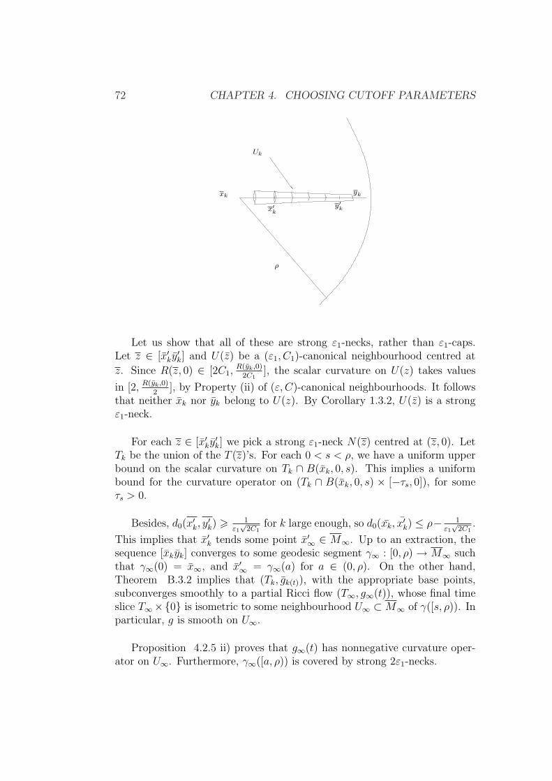
72 CHAPTER 4. CHOOSING CUTOFF PARAMETERS
xk
Uk
ρ
yk
y′kx′k
Let us show that all of these are strong ε1-necks, rather than ε1-caps.Let z ∈ [x′ky
′k] and U(z) be a (ε1, C1)-canonical neighbourhood centred at
z. Since R(z, 0) ∈ [2C1,R(yk,0)
2C1], the scalar curvature on U(z) takes values
in [2, R(yk,0)2
], by Property (ii) of (ε, C)-canonical neighbourhoods. It followsthat neither xk nor yk belong to U(z). By Corollary 1.3.2, U(z) is a strongε1-neck.
For each z ∈ [x′ky′k] we pick a strong ε1-neck N(z) centred at (z, 0). Let
Tk be the union of the T (z)’s. For each 0 < s < ρ, we have a uniform upperbound on the scalar curvature on Tk ∩ B(xk, 0, s). This implies a uniformbound for the curvature operator on (Tk ∩ B(xk, 0, s) × [−τs, 0]), for someτs > 0.
Besides, d0(x′k, y′k) > 1
ε1√
2C1for k large enough, so d0(xk, x′k) ≤ ρ− 1
ε1√
2C1.
This implies that x′k tends some point x′∞ ∈ M∞. Up to an extraction, thesequence [xkyk] converges to some geodesic segment γ∞ : [0, ρ) → M∞ suchthat γ∞(0) = x∞, and x′∞ = γ∞(a) for a ∈ (0, ρ). On the other hand,Theorem B.3.2 implies that (Tk, gk(t)), with the appropriate base points,subconverges smoothly to a partial Ricci flow (T∞, g∞(t)), whose final timeslice T∞×0 is isometric to some neighbourhood U∞ ⊂M∞ of γ([s, ρ)). Inparticular, g is smooth on U∞.
Proposition 4.2.5 ii) proves that g∞(t) has nonnegative curvature oper-ator on U∞. Furthermore, γ∞([a, ρ)) is covered by strong 2ε1-necks.
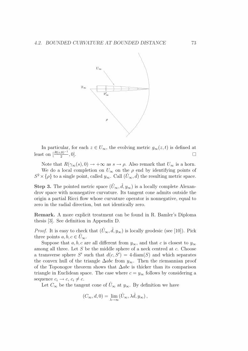
4.2. BOUNDED CURVATURE AT BOUNDED DISTANCE 73
x∞
ρ
U∞
x′∞
In particular, for each z ∈ U∞, the evolving metric g∞(z, t) is defined at
least on [R(z,0)−1
2, 0].
Note that R(γ∞(s), 0) → +∞ as s→ ρ. Also remark that U∞ is a horn.We do a local completion on U∞ on the ρ end by identifying points of
S2×ρ to a single point, called y∞. Call (U∞, d) the resulting metric space.
Step 3. The pointed metric space (U∞, d, y∞) is a locally complete Alexan-drov space with nonnegative curvature. Its tangent cone admits outside theorigin a partial Ricci flow whose curvature operator is nonnegative, equal tozero in the radial direction, but not identically zero.
Remark. A more explicit treatment can be found in R. Bamler’s Diplomathesis [3]. See definition in Appendix D.
Proof. It is easy to check that (U∞, d, y∞) is locally geodesic (see [10]). Pickthree points a, b, c ∈ U∞.
Suppose that a, b, c are all different from y∞, and that c is closest to y∞among all three. Let S be the middle sphere of a neck centred at c. Choosea transverse sphere S ′ such that d(c, S ′) = 4 diam(S) and which separatesthe convex hull of the triangle ∆abc from y∞. Then the riemannian proofof the Toponogov theorem shows that ∆abc is thicker than its comparisontriangle in Euclidean space. The case where c = y∞ follows by considering asequence ci → c, ci 6= c.
Let C∞ be the tangent cone of U∞ at y∞. By definition we have
(C∞, d, 0) = limλ→∞
(U∞, λd, y∞) ,
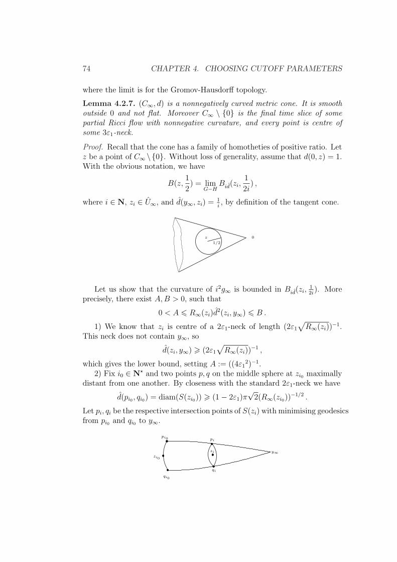
74 CHAPTER 4. CHOOSING CUTOFF PARAMETERS
where the limit is for the Gromov-Hausdorff topology.
Lemma 4.2.7. (C∞, d) is a nonnegatively curved metric cone. It is smoothoutside 0 and not flat. Moreover C∞ \ 0 is the final time slice of somepartial Ricci flow with nonnegative curvature, and every point is centre ofsome 3ε1-neck.
Proof. Recall that the cone has a family of homotheties of positive ratio. Letz be a point of C∞ \0. Without loss of generality, assume that d(0, z) = 1.With the obvious notation, we have
B(z,1
2) = lim
G−HBid(zi,
1
2i) ,
where i ∈ N, zi ∈ U∞, and d(y∞, zi) = 1i, by definition of the tangent cone.
z
1/2
0
Let us show that the curvature of i2g∞ is bounded in Bid(zi,12i
). Moreprecisely, there exist A,B > 0, such that
0 < A 6 R∞(zi)d2(zi, y∞) 6 B .
1) We know that zi is centre of a 2ε1-neck of length (2ε1
√R∞(zi))
−1.This neck does not contain y∞, so
d(zi, y∞) > (2ε1
√R∞(zi))
−1 ,
which gives the lower bound, setting A := ((4ε12)−1.
2) Fix i0 ∈ N? and two points p, q on the middle sphere at zi0 maximallydistant from one another. By closeness with the standard 2ε1-neck we have
d(pi0 , qi0) = diam(S(zi0)) > (1− 2ε1)π√
2(R∞(zi0))−1/2 .
Let pi, qi be the respective intersection points of S(zi) with minimising geodesicsfrom pi0 and qi0 to y∞.
zi
pi0
qi0
zi0
pi
qi
y∞
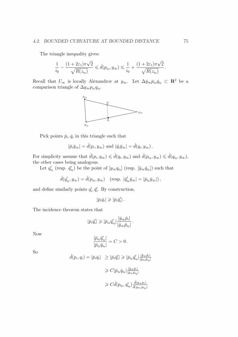
4.2. BOUNDED CURVATURE AT BOUNDED DISTANCE 75
The triangle inequality gives:
1
i0− (1 + 2ε1)π
√2√
R(zi0)6 d(pi0 , y∞) 6 1
i0+
(1 + 2ε1)π√
2√R(zi0)
.
Recall that U∞ is locally Alexandrov at y∞. Let ∆y∞pi0 qi0 ⊂ R2 be acomparison triangle of ∆y∞pi0qi0 .
y∞
pi0
qi0
pi
qi
Pick points pi, qi in this triangle such that
|piy∞| = d(pi, y∞) and |qiy∞| = d(qi, y∞) .
For simplicity assume that d(pi, y∞) 6 d(qi, y∞) and d(pi0 , y∞) 6 d(qi0 , y∞),the other cases being analogous.
Let q′i0 (resp. q′i0) be the point of [y∞qi0 ] (resp. [y∞qi0 ]) such that
d(q′i0 , y∞) = d(pi0 , y∞) (resp. |q′i0 y∞| = |pi0 y∞|) ,
and define similarly points q′i, q′i. By construction,
|piqi| > |piq′i| .
The incidence theorem states that
|piq′i| > |pi0 q′i0||y∞pi||y∞pi0|
.
Now |pi0 q′i0||pi0 qi0|
= C > 0 .
Sod(pi, qi) = |piqi| ≥ |piq′i| > |pi0 q′i0| |y∞pi|
|y∞pi0|
> C|pi0 qi0| |y∞pi||y∞pi0
|
> Cd(pi0 , q′i0) d(y∞pi)
d(y∞,pi0)
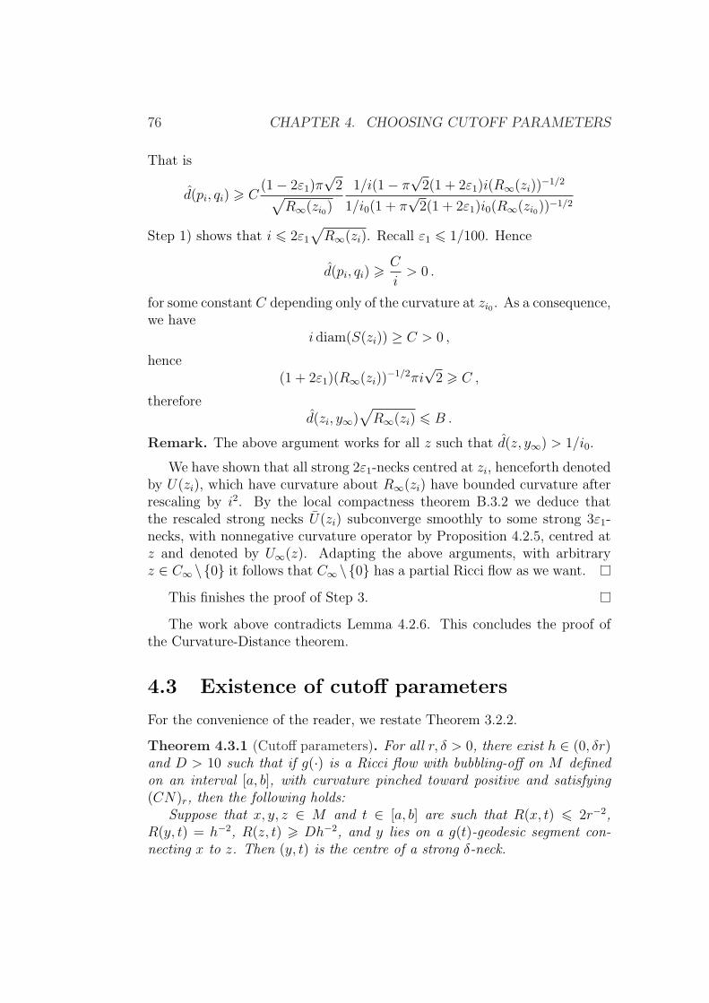
76 CHAPTER 4. CHOOSING CUTOFF PARAMETERS
That is
d(pi, qi) > C(1− 2ε1)π
√2√
R∞(zi0)
1/i(1− π√
2(1 + 2ε1)i(R∞(zi))−1/2
1/i0(1 + π√
2(1 + 2ε1)i0(R∞(zi0))−1/2
Step 1) shows that i 6 2ε1
√R∞(zi). Recall ε1 6 1/100. Hence
d(pi, qi) > C
i> 0 .
for some constant C depending only of the curvature at zi0 . As a consequence,we have
i diam(S(zi)) ≥ C > 0 ,
hence(1 + 2ε1)(R∞(zi))
−1/2πi√
2 > C ,
therefored(zi, y∞)
√R∞(zi) 6 B .
Remark. The above argument works for all z such that d(z, y∞) > 1/i0.
We have shown that all strong 2ε1-necks centred at zi, henceforth denotedby U(zi), which have curvature about R∞(zi) have bounded curvature afterrescaling by i2. By the local compactness theorem B.3.2 we deduce thatthe rescaled strong necks U(zi) subconverge smoothly to some strong 3ε1-necks, with nonnegative curvature operator by Proposition 4.2.5, centred atz and denoted by U∞(z). Adapting the above arguments, with arbitraryz ∈ C∞ \0 it follows that C∞ \0 has a partial Ricci flow as we want.
This finishes the proof of Step 3.
The work above contradicts Lemma 4.2.6. This concludes the proof ofthe Curvature-Distance theorem.
4.3 Existence of cutoff parameters
For the convenience of the reader, we restate Theorem 3.2.2.
Theorem 4.3.1 (Cutoff parameters). For all r, δ > 0, there exist h ∈ (0, δr)and D > 10 such that if g(·) is a Ricci flow with bubbling-off on M definedon an interval [a, b], with curvature pinched toward positive and satisfying(CN)r, then the following holds:
Suppose that x, y, z ∈ M and t ∈ [a, b] are such that R(x, t) 6 2r−2,R(y, t) = h−2, R(z, t) > Dh−2, and y lies on a g(t)-geodesic segment con-necting x to z. Then (y, t) is the centre of a strong δ-neck.
4.3. EXISTENCE OF CUTOFF PARAMETERS 77
Proof. Quite unsurprisingly, we argue by contradiction. Fix two constantsr > 0, δ > 0, sequences hk → 0, Dk → +∞, a sequence gk(·) of weak solutionssatisfying the above hypotheses, and sequences xk, yk, zk ∈ M , tk > 0, γk,where γk is a gk(tk)-geodesic segment connecting xk to zk, containing yk andsuch that R(xk, tk) 6 2r−2, R(zk, tk) > Dkh
−2k , and R(yk, tk) = h−2
k but(yk, tk) is not centre of any strong δ-neck.
Consider the sequence gk(·) on M defined by the following parabolicrescaling
gk(t) = h−2k gk(tk + th2
k) .
Let us recall that we shall put a bar on the points when they are involvedin geometric quantities computed with respect of the metric gk. Note thatR(yk, 0) = 1. The contradiction will come from extracting a convergingsubsequence of the pointed sequence (M, gk(·), yk, 0) and showing that thelimit is the standard flow on S2 ×R, which implies that for k large enough,yk is centre of some strong δ-neck, contrary to the hypothesis.
Step 1. (M, gk(0), yk) subconverges in the pointed C∞ sense to (S2×R, g∞)where g∞ is a product metric of nonnegative curvature operator and scalarcurvature at most 2.
Remark. It is not asserted at this stage that the metric on the S2 factor isround.
Proof. First we control the curvature on balls around yk. Since R(yk, tk) goesto +∞, Theorem 4.2.1 implies that for all ρ > 0, there exists Λ(ρ) > 0 andk0(ρ) > 0 such that gk(0) has scalar curvature bounded above by Λ(ρ) onB(yk, ρ) for k > k0(ρ). Since (yk, tk) has an (ε0, C0)-canonical neighbour-hood, gk(·) is κ0-noncollapsed at yk, which is enough to extract a convergingsubsequence with regularity C1,α.
For all sufficiently large k, the ballB(yk, ρ) is covered by (ε0, C0)-canonicalneighbourhoods. Indeed, gk(tk) satisfies
|∇R| < C0R3/2
at points of scalar curvature > r−2. Choose a point y such that R(y, tk) 63r−2 and integrate the previous inequality on the portion of [yky] whereR ≥ 3r−2. An easy computation yields
d(y, yk) ≥ 1
hk
1
2C0
(r√3− hk) , (4.3)
which implies d(y, yk) → +∞. As a consequence, for all ρ > 0 there existsk1(ρ) ≥ k0(ρ) such that for every integer k ≥ k1(ρ), the scalar curvature
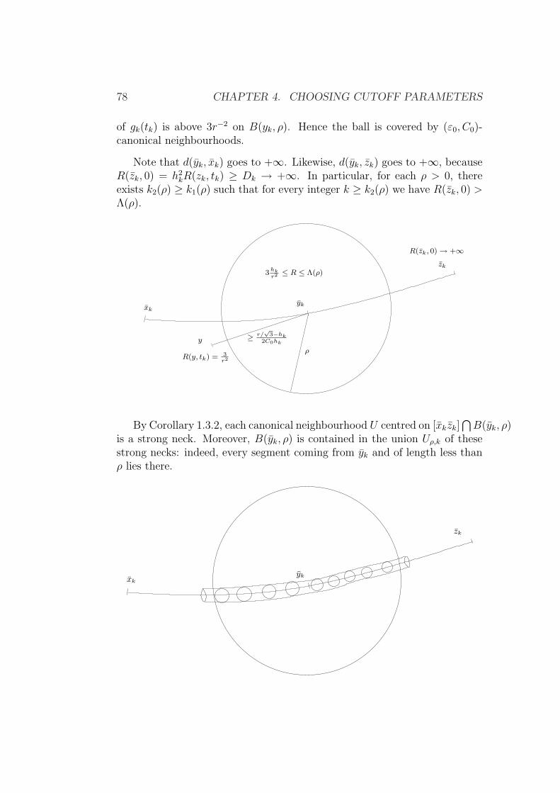
78 CHAPTER 4. CHOOSING CUTOFF PARAMETERS
of gk(tk) is above 3r−2 on B(yk, ρ). Hence the ball is covered by (ε0, C0)-canonical neighbourhoods.
Note that d(yk, xk) goes to +∞. Likewise, d(yk, zk) goes to +∞, becauseR(zk, 0) = h2
kR(zk, tk) ≥ Dk → +∞. In particular, for each ρ > 0, thereexists k2(ρ) ≥ k1(ρ) such that for every integer k ≥ k2(ρ) we have R(zk, 0) >Λ(ρ).
ρ
ykxk
R(y, tk) = 3r2
zk
R(zk, 0) → +∞
≥ r/√
3−hk2C0hk
3hkr2 ≤ R ≤ Λ(ρ)
y
By Corollary 1.3.2, each canonical neighbourhood U centred on [xkzk]⋂B(yk, ρ)
is a strong neck. Moreover, B(yk, ρ) is contained in the union Uρ,k of thesestrong necks: indeed, every segment coming from yk and of length less thanρ lies there.
ykxk
zk
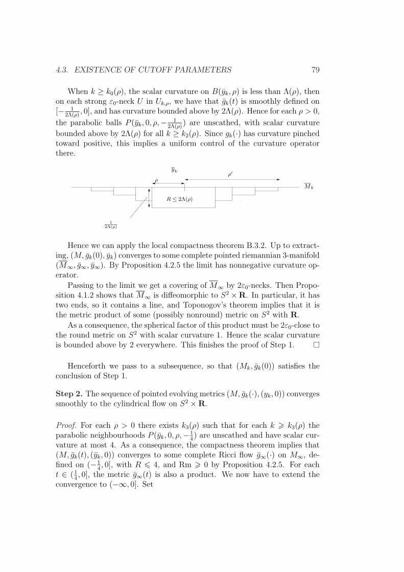
4.3. EXISTENCE OF CUTOFF PARAMETERS 79
When k ≥ k0(ρ), the scalar curvature on B(yk, ρ) is less than Λ(ρ), thenon each strong ε0-neck U in Uk,ρ, we have that gk(t) is smoothly defined on[− 1
2Λ(ρ), 0], and has curvature bounded above by 2Λ(ρ). Hence for each ρ > 0,
the parabolic balls P (yk, 0, ρ,− 12Λ(ρ)
) are unscathed, with scalar curvature
bounded above by 2Λ(ρ) for all k ≥ k2(ρ). Since gk(·) has curvature pinchedtoward positive, this implies a uniform control of the curvature operatorthere.
R ≤ 2Λ(ρ)
ykρ′
ρMk
12Λ(ρ)
Hence we can apply the local compactness theorem B.3.2. Up to extract-ing, (M, gk(0), yk) converges to some complete pointed riemannian 3-manifold(M∞, g∞, y∞). By Proposition 4.2.5 the limit has nonnegative curvature op-erator.
Passing to the limit we get a covering of M∞ by 2ε0-necks. Then Propo-sition 4.1.2 shows that M∞ is diffeomorphic to S2 ×R. In particular, it hastwo ends, so it contains a line, and Toponogov’s theorem implies that it isthe metric product of some (possibly nonround) metric on S2 with R.
As a consequence, the spherical factor of this product must be 2ε0-close tothe round metric on S2 with scalar curvature 1. Hence the scalar curvatureis bounded above by 2 everywhere. This finishes the proof of Step 1.
Henceforth we pass to a subsequence, so that (Mk, gk(0)) satisfies theconclusion of Step 1.
Step 2. The sequence of pointed evolving metrics (M, gk(·), (yk, 0)) convergessmoothly to the cylindrical flow on S2 ×R.
Proof. For each ρ > 0 there exists k3(ρ) such that for each k > k3(ρ) theparabolic neighbourhoods P (yk, 0, ρ,−1
4) are unscathed and have scalar cur-
vature at most 4. As a consequence, the compactness theorem implies that(M, gk(t), (yk, 0)) converges to some complete Ricci flow g∞(·) on M∞, de-fined on (−1
4, 0], with R 6 4, and Rm > 0 by Proposition 4.2.5. For each
t ∈ (14, 0], the metric g∞(t) is also a product. We now have to extend the
convergence to (−∞, 0]. Set
80 CHAPTER 4. CHOOSING CUTOFF PARAMETERS
τ0 := supτ > 0 | ∀ρ > 0 , ∃C(ρ, τ), ∃k(ρ) , ∀k ≥ k(ρ) , P (yk, 0, ρ,−τ) is unscathed,
and R ≤ C(ρ, τ) there .
Convergence extends and gives a flow g∞(t) defined on (−τ0, 0], with eachtime-slice a split nonnegatively curved metric. Let (p, s) ∈ M∞ × (−τ0, 0].We shall prove that ∂R∞
∂t(p, s) > 0. Here R∞ denotes the scalar curvature of
g∞.
With this goal in mind, pick a sequence (pk, sk) ∈ M × (−τ0, 0] whoselimit is (p, s). Set uk := tk+skh
2k. Then R(pk, uk) is comparable to h−2
k , hencegoes to +∞. Let us recall that here pk is the point pk but considered on themanifold M endowed with the unscaled metric gk; similarly, uk corresponds,after rescaling, to the time sk. Hence (pk, sk) has a canonical neighbourhood,which can only be a strong neck because (pk, sk) tends to (p, s). Denote
by gk(·) the parabolic rescaling of gk(·) around (pk, uk) and R its scalarcurvature. Then
∂R
∂t(pk, 0) ∼ 1 ,
which is the time zero value on the cylindrical flow. An easy computationshows that
∂R∞∂t
(p, s) = R∞(p, s)2 limk→∞
∂R
∂t(pk, 0) > 0 .
Therefore, the scalar curvature of g∞ is bounded above by 2 on M∞ ×(−τ0, 0]. It follows that for every ρ > 0 and every τ < τ0, there existsk(ρ, τ) > 0 such that for all k ≥ k(ρ, τ), scalar curvature stays below 3 onP (yk, 0, ρ,−τ).
Hence every point (p, t) ∈ P (yk, 0, ρ,−τ) is centre of some strong ε0-neck,whose time interval contains [t − 1/6, t] and whose scalar curvature is notgreater than 4. If τ0 < +∞, we can set τ = τ0−1/12. Then for all ρ > 0, fork ≥ k(ρ, τ) the scalar curvature on P (yk, 0, ρ,−τ0 − 1/6) is bounded aboveby 4. This contradicts the definition of τ0.
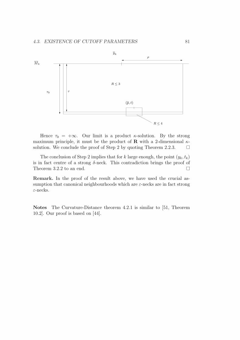
4.3. EXISTENCE OF CUTOFF PARAMETERS 81
yk
ρ
τ0 τ
R ≤ 4
(p, t)
Mk
R ≤ 3
Hence τ0 = +∞. Our limit is a product κ-solution. By the strongmaximum principle, it must be the product of R with a 2-dimensional κ-solution. We conclude the proof of Step 2 by quoting Theorem 2.2.3.
The conclusion of Step 2 implies that for k large enough, the point (yk, tk)is in fact centre of a strong δ-neck. This contradiction brings the proof ofTheorem 3.2.2 to an end.
Remark. In the proof of the result above, we have used the crucial as-sumption that canonical neighbourhoods which are ε-necks are in fact strongε-necks.
Notes The Curvature-Distance theorem 4.2.1 is similar to [51, Theorem10.2]. Our proof is based on [44].

82 CHAPTER 4. CHOOSING CUTOFF PARAMETERS
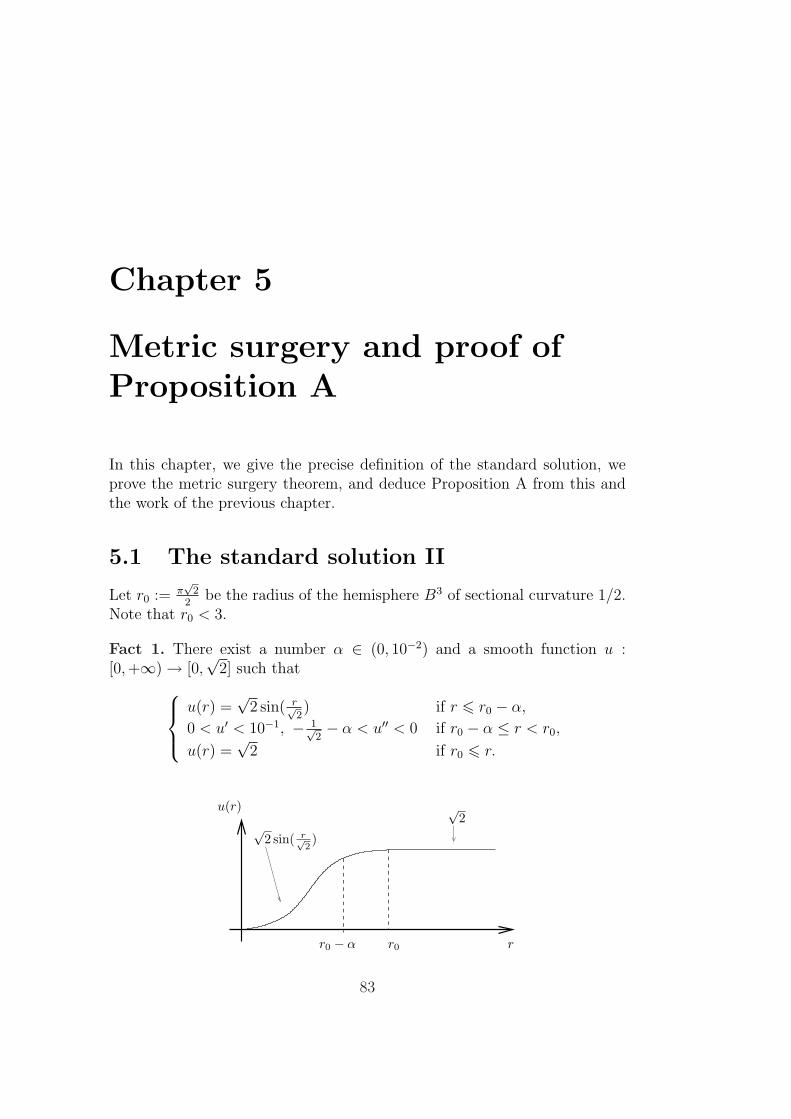
Chapter 5
Metric surgery and proof ofProposition A
In this chapter, we give the precise definition of the standard solution, weprove the metric surgery theorem, and deduce Proposition A from this andthe work of the previous chapter.
5.1 The standard solution II
Let r0 := π√
22
be the radius of the hemisphere B3 of sectional curvature 1/2.Note that r0 < 3.
Fact 1. There exist a number α ∈ (0, 10−2) and a smooth function u :[0,+∞) → [0,
√2] such that
u(r) =√
2 sin( r√2) if r 6 r0 − α,
0 < u′ < 10−1, − 1√2− α < u′′ < 0 if r0 − α ≤ r < r0,
u(r) =√
2 if r0 6 r.
r
√2√
2 sin( r√2)
u(r)
r0 − α r0
83
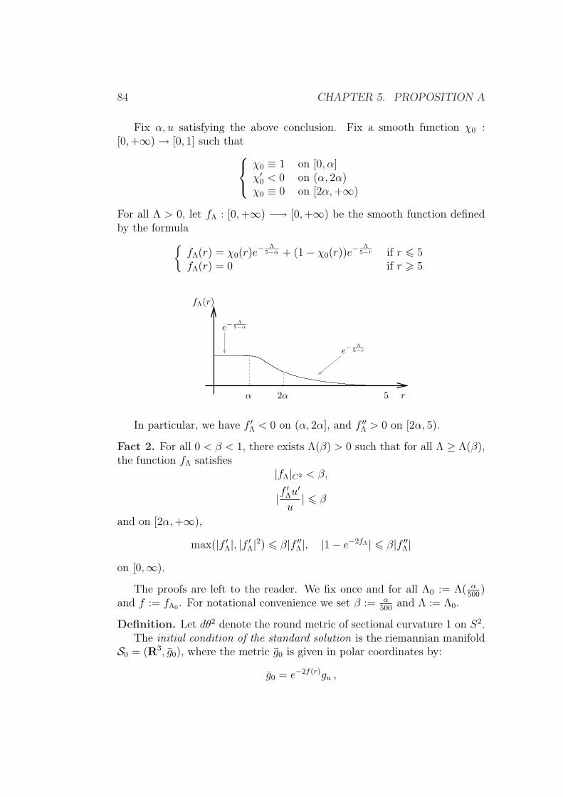
84 CHAPTER 5. PROPOSITION A
Fix α, u satisfying the above conclusion. Fix a smooth function χ0 :[0,+∞) → [0, 1] such that
χ0 ≡ 1 on [0, α]χ′0 < 0 on (α, 2α)χ0 ≡ 0 on [2α,+∞)
For all Λ > 0, let fΛ : [0,+∞) −→ [0,+∞) be the smooth function definedby the formula
fΛ(r) = χ0(r)e
− Λ5−α + (1− χ0(r))e
− Λ5−r if r 6 5
fΛ(r) = 0 if r > 5
α 2α 5
e−Λ
5−α
e−Λ
5−r
fΛ(r)
r
In particular, we have f ′Λ < 0 on (α, 2α], and f ′′Λ > 0 on [2α, 5).
Fact 2. For all 0 < β < 1, there exists Λ(β) > 0 such that for all Λ ≥ Λ(β),the function fΛ satisfies
|fΛ|C2 < β,
|f′Λu
′
u| 6 β
and on [2α,+∞),
max(|f ′Λ|, |f ′Λ|2) 6 β|f ′′Λ|, |1− e−2fΛ| 6 β|f ′′Λ|on [0,∞).
The proofs are left to the reader. We fix once and for all Λ0 := Λ( α500
)and f := fΛ0 . For notational convenience we set β := α
500and Λ := Λ0.
Definition. Let dθ2 denote the round metric of sectional curvature 1 on S2.The initial condition of the standard solution is the riemannian manifold
S0 = (R3, g0), where the metric g0 is given in polar coordinates by:
g0 = e−2f(r)gu ,
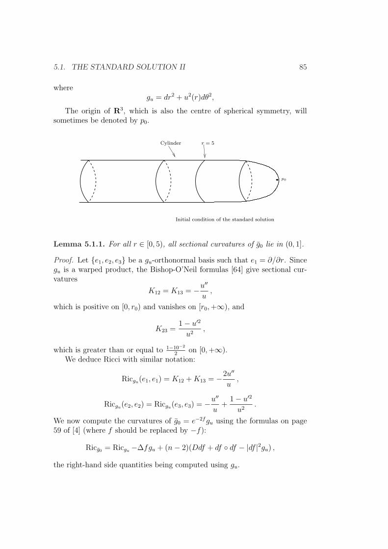
5.1. THE STANDARD SOLUTION II 85
wheregu = dr2 + u2(r)dθ2,
The origin of R3, which is also the centre of spherical symmetry, willsometimes be denoted by p0.
r = 5Cylinder
Initial condition of the standard solution
p0
Lemma 5.1.1. For all r ∈ [0, 5), all sectional curvatures of g0 lie in (0, 1].
Proof. Let e1, e2, e3 be a gu-orthonormal basis such that e1 = ∂/∂r. Sincegu is a warped product, the Bishop-O’Neil formulas [64] give sectional cur-vatures
K12 = K13 = −u′′
u,
which is positive on [0, r0) and vanishes on [r0,+∞), and
K23 =1− u′2
u2,
which is greater than or equal to 1−10−2
2on [0,+∞).
We deduce Ricci with similar notation:
Ricgu(e1, e1) = K12 +K13 = −2u′′
u,
Ricgu(e2, e2) = Ricgu(e3, e3) = −u′′
u+
1− u′2
u2.
We now compute the curvatures of g0 = e−2fgu using the formulas on page59 of [4] (where f should be replaced by −f):
Ricg0 = Ricgu −∆fgu + (n− 2)(Ddf + df df − |df |2gu) ,
the right-hand side quantities being computed using gu.
86 CHAPTER 5. PROPOSITION A
To fix convention, recall that ∆ = −traceDd. It is easily checked that
Ddf(∂
∂r,∂
∂r) = f ′′(r)
and
Ddf(X,X) =f ′u′
ugu(X,X)
if X ⊥ ∂/∂r. It follows that
Ricg0(e1, e1) = Ricgu(e1, e1) + f ′′ + 2f ′u′
u+ f ′′
and
Ricg0(e1, e1) = e2f
(Ricgu(e1, e1) + 2f ′′ + 2
f ′u′
u
)
where e1 = efe1. For i = 2, 3, we get, with similar notation:
Ricg0(ei, ei) = e2f
(Ricgu(ei, ei) + f ′′ + 3
f ′u′
u− f ′2
).
We deduce the values of the sectional curvatures of g0, with the obviousnotation:
K12 = K13 = e2f(K12 + f ′′ + 2
f ′u′
u
)
By choice of f and u, we have for all r ∈ [0, r0 − α]:
K12 = K13 > e2f
(1
2− 3α
)> 0.
Let r ∈ [r0 − α, 5). Since 2α 6 r0 − α, f ′′ > 0, we get
K12 = K13 > e2f (K12 + (1− α)f ′′) > e2fK12 > 0 .
Similarly, it is easily checked that
K23 = e2f
(K23 +
1
2(4f ′u′
u− 2f ′2)
)= e2f
(K23 + 2
f ′u′
u− f ′2
)
that is
K23 > e2f
(0.99
2− 3α
)> 0.
Observe that there is a constant K0 > 0 such that for all r ∈ [3, 4] andall i 6= j,
Kij > K0 > 0. (5.1)
To conclude, notice that the maximum of the sectional curvature is close to1/2, hence less than 1 by choice of the constants.
5.2. PROOF OF THE METRIC SURGERY THEOREM 87
5.2 Proof of the Metric Surgery Theorem
Recall that a riemannian manifold (N, g) is said to have φ-almost nonnegativecurvature, where φ is a nonnegative function, if it satisfies Rm > −φ(R).This is trivially true at points where ν > 0, i.e. all sectional curvatures arenonnegative. For convenience we restate the Metric Surgery Theorem
Theorem 5.2.1. There exists δ0 > 0 and a function δ′ : (0, δ0] 3 δ 7→ δ′(δ) ∈(0, ε0/10] tending to zero as δ → 0, with the following property:
Let φ be a nondecreasing, nonnegative function, let δ ≤ δ0, let (M, g) bea riemannian 3-manifold with φ-almost nonnegative curvature, and U ⊂ Mbe a δ-neck whose middle sphere bounds a 3-ball Σ ⊂M .
Then there exists a riemannian metric g+ on M such that:
i. g+ = g on M \ Int Σ and g+ < g on Int Σ;
ii. U ∪ Σ is a (δ, δ′(δ))-almost standard cap with respect to g+ and Σ is acore thereof;
iii. g+ has φ-almost nonnegative curvature.
Proof. We start by fixing some notation. For 0 6 r1 6 r2, we let C[r1, r2]denote the annular region of R3 defined by the inequations r1 ≤ r ≤ r2 inpolar coordinates. Define Su = (R3, gu). Observe that for all 3 ≤ r1 < r2,the restriction of gu) to C[r1, r2] is isometric to the cylinder S2× [r1, r2] withscalar curvature 1.
We first give a summary of the proof. Let φ be a nondecreasing nonnneg-ative function, δ be a positive number, U ⊂ M be a δ-neck whose middlesphere S bounds a 3-ball Σ ⊂ M (see picture page 89). Let y be a point ofS. Our first task is to construct a (1 + δ)-Lipschitz diffeomorphism
ψ : (Σ, R(y)g) −→ B(0, 5) ⊂ Suwhich is almost an isometry near C[3, 5]. Then we shall push g = R(y)g for-ward to obtain a metric on B(0, 5) ⊂ R3, and interpolate between e−2f g ande−2fgu = g0 on C(3, 4) to get a metric g+ on B(0, 5). The conformal factorwill guarantee that the resulting metric has φ-almost nonnegative curvature;we will then explain how to choose δ small enough so that g+ < g on B(0, 5),and finally pull back R(y)−1g+ to Int Σ using ψ. To do the interpolation we’lluse the following.
Fix a smooth function χ : [0, 5] → [0, 1] such that
χ ≡ 1 on [0, 3]χ′ < 0 on (3, 4)χ ≡ 0 on [4, 5]
88 CHAPTER 5. PROPOSITION A
Proposition 5.2.2. There exists δ1 > 0 and a function δ′ : (0, δ1] −→ (0, ε010
]with limit zero at zero, having the following property: let φ be a nondecreasingpositive function, 0 < δ ≤ δ1 and g be a metric on B(0, 5) ⊂ R3, with φ-almost nonnegative curvature, such that ||g−gu||C[δ−1]+1 < δ on C(3, 5). Thenthe metric
g+ = e−2f (χgu + (1− χ)g)
has φ-almost nonnegative curvature, and is δ′(δ)-close to g0 on B(0, 5).
Assuming this proposition, we prove Theorem 5.2.1. Let
δ2 := e2e−Λ − 1, and δ0 := min(δ1, δ2).
We begin by the construction of the diffeomorphism.
Lemma 5.2.3. There is a diffeomorphism
ψ : Σ ⊂M −→ B(0, 5) ⊂ R3
such that g := R(y)ψ?g satisfies
gu 6 (1 + δ)g on B(0, 5), and ||g − gu||C[δ−1]+1 6 δ on C[3, 5].
Proof. By definition of a δ-neck there exists a diffeomorphism
ψU : U −→ S2 × (−δ−1, δ−1)
such that ψU(S) = S2 × 0 and
||R(y)ψU ∗g − gcyl||C[δ−1]+1 6 δ.
The coordinate in the interval (−δ−1, δ−1) is here called z. We may assumethat U
⋂Σ is sent to S2 × [0, δ−1). Denote by U[0,5] the subset of U which is
sent to S2 × [0, 5] and ψ[0,5] the restriction of ψU to U[0,5]. Let s be the map
s : S2 × [0, 5] −→ S2 × [3, 8](θ, z) −→ (θ, 8− z = r)
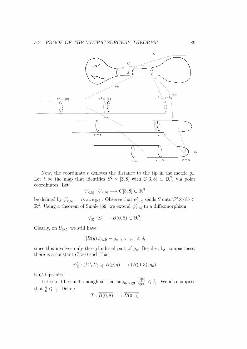
5.2. PROOF OF THE METRIC SURGERY THEOREM 89
S
r = 8
i s
ψ′Σ
r = ηr = 5
S2 × δ−1
U
Σ
S2 × 0 S2 × 5
r = 3
r = 3
Su
ψU
Now, the coordinate r denotes the distance to the tip in the metric gu.Let i be the map that identifies S2 × [3, 8] with C[3, 8] ⊂ R3, via polarcoordinates. Let
ψ′[0,5] : U[0,5] −→ C[3, 8] ⊂ R3
be defined by ψ′[0,5] := isψ[0,5]. Observe that ψ′[0,5] sends S onto S2×8 ⊂R3. Using a theorem of Smale [69] we extend ψ′[0,5] to a diffeomorphism
ψ′Σ : Σ −→ B(0, 8) ⊂ R3.
Clearly, on U[0,5] we still have:
||R(y)ψ′Σ∗g − gu||C[δ−1]+1 6 δ,
since this involves only the cylindrical part of gu. Besides, by compactness,there is a constant C > 0 such that
ψ′Σ : (Σ \ U[0,5], R(y)g) −→ (B(0, 3), gu)
is C-Lipschitz.
Let η > 0 be small enough so that sup0<r63u( ηr
6)
u(r)6 1
C. We also suppose
that η6
6 1C. Define
T : B(0, 8) −→ B(0, 5)
90 CHAPTER 5. PROPOSITION A
in polar coordinates by T (θ, r) = (θ, t(r)), where t : [0, 8] −→ [0, 5] is asmooth function satisfying:
t(r) = η6r on [0, 3]
0 < t′ < 1 on [3, 3 + η]t(r) = r − 3 on [3 + η, 8]
In particular, T is 1C-Lipschitz on (B(0, 3), gu). Indeed, the dilatation in
the radial direction is η6
while in the orthoradial directions it is u(ηr6)/u(r).
On (C[3, 6], gu), T is 1-Lipschitz since u is nondecreasing. Lastly, T restrictsto an isometry from C[6, 8] onto C[3, 5] endowed with gu.
Define a map ψ := T ψ′Σ from Σ onto B(0, 5). For the metric g =R(y)ψ∗g, we have by composition gu ≤ (1 + δ)g on C(0, 3). On C[3, 5] wehave ||g − gu||C[δ−1]+1 6 δ, and the proof of Lemma 5.2.3 is complete.
Proof of 5.2.1 i)On M \Int Σ, set g+ := g. Then apply Proposition 5.2.2 to the metric g =
R(y)ψ∗g on B(0, 5) and set g+ := R(y)−1ψ∗g+ on Int Σ. The property g+ < gon this set is a consequence of the following lemma and of the inequalityδ 6 δ0 ≤ δ2, since we have chosen δ2 = e2e−Λ − 1.
Lemma 5.2.4. Let g be a metric on B(0, 5) ⊂ R3 such that gu ≤ (1 + δ2)g.Then the metric g+ := e−2f (χgu + (1− χ)g) satisfies g+ < g on B(0, 5).
Proof. On C[4, 5) we have g+ = e−2f g < g. On [0, 4), we argue as follows:
g+ = e−2f (χgu + (1− χ)g) 6 e−2f (χ(1 + δ2)g + (1− χ)g) 6 e−2f (1 + δ2)g
Now on C[0, 4), we have f > e−Λ; hence e−2f < e−2e−Λ. The conclusion
follows by choice of δ2.
Proof of 5.2.1 ii) and iii).Assertion iii) follows from Proposition 5.2.2 applied to g = R(y)ψ∗g. To
prove Assertion ii), it suffices to combine the δ′(δ)-proximity of (B(0, 5), g+)with (B(0, 5), g0) and that of the half δ-neck (U \ Int Σ, R(y)g+ = R(y)g)with S2 × [5, 1
δ+ 5).
There remains to prove Proposition 5.2.2.
Proof of Proposition 5.2.2. The delicate part is φ-almost nonnegativity. Setg = e−2f g. Let a > b > c be the eigenvalues of Ricg and e1, e2, e3 be ag-orthonormal basis consisting of eigenvectors of Ricg. Remark that a is closeto 0, whereas b, c are close to 1/2 on C(3, 5). Let Di denote the covariantderivative along ei with respect to g.
5.2. PROOF OF THE METRIC SURGERY THEOREM 91
Assertion 5.2.5. There exists δ′1 > 0 such that for all 0 < δ < δ1 and onC(3, 5),
|D1r − 1| 6 β ,|Dir| 6 β for i = 2, 3 ,|DiDjr| 6 β for i, j = 1, 2, 3 .
Follows immediately from the fact that g is δ-close to the cylindricalmetric, for which the corresponding quantities are D1r = 1, D2r = D3r = 0.
Assertion 5.2.6. For all 0 < δ < δ′1 we have
|Dif | 6 2βf ′′ ,|DiDjf | 6 3βf ′′ si i, j 6= 1 ,|D1D1f − f ′′| 6 5βf ′′ .
Proof. We have Dif = ∂f∂rDir = f ′Dir, so
|Dif | 6 βf ′′|Dir| 6 βf ′′(1 + β) 6 2βf ′′ .
The first inequality comes from the properties of f and the second one fromAssertion 5.2.5. Furthermore,
DiDjf = f ′′DirDjr + f ′DiDjr .
For i, j 6= 1, we derive
|DiDjf | 6 f ′′β(1 + β) + βf ′′β 6 3βf ′′ 6 3βf ′′ .
Besides,
D1D1f = D1(f′D1r) = f ′′(D1r)
2 + f ′D1D1r .
Therefore,
|D1D1f − f ′′| 6 f ′′|(D1r)2 − 1|+ f ′|D1D1r|
6 f ′′|D1r − 1||D1r + 1|+ f ′|D1D1r|6 f ′′β(2 + β) + βf ′′(1 + β)6 5βf ′′ .
which proves the claim.
For simplicity we denote by Ric the Ricci tensor of g = e−2f g, and a >b > c its eigenvalues.
92 CHAPTER 5. PROPOSITION A
Assertion 5.2.7. For all 0 < δ < δ′1, we have
|a− e2f (a+ 2D1D1f)| 6 αD1D1f ,
|b− e2f (b+D1D1f)| 6 αD1D1f ,|c− e2f (c+D1D1f)| 6 αD1D1f .
Proof. Set β′ := 5β and ei := efei. The basis e1, e2, e3 is g-orthonormal.
Let A be the matrix of Ric in this basis. First we show that the eigenvaluesof Ric are close to the diagonal terms Aii of the matrix A. By [4, p. 59], wehave
Ric = Ric−∆fg −+(n− 2)(Ddf + df df − |df |2g) .where the right-hand side operators are those of g. Evaluating this formulaon a pair (ei, ej) for i 6= j, we get
Aij = e2f (DiDjf +DifDjf) ,
so
|Aij| 6 2(β′f ′′ + β′2f ′′2) 6 4β′f ′′ 6 4β′1
1− 5β′D1D1f 6 8β′D1D1f .
Using the following elementary lemma, whose proof is left to the reader, weget an upper bound on the distance between the Aii’s and the eigenvalues ofA by 24β′D1D1f ≤ α
2D1D1f .
Lemma 5.2.8. Let A,B be symmetric n × n matrices, of eigenvalues a1 6a2 6 · · · 6 an and b1 6 b2 6 · · · 6 bn respectively. Define ||M || = supi,j |mij|.Then for all i = 1, . . . , n, we have
|ai − bi| 6 n||B − A|| ,There remains to show that for i = 1, 2, 3, we have
|A11 − e2f (a+ 2D1D1f)| 6 α2D1D1f ,
|A22 − e2f (b+D1D1f)| 6 α2D1D1f ,
|A33 − e2f (c+D1D1f)| 6 α2D1D1f .
We deduce
A11 = Ric(e1, e1) = e2f (a−∆f +D1D1f +D1fD1f − |df |2)= e2f (a+ 2D1D1f +D2D2f +D3D3f + (D1f)2 − |df |2) ,
hence
|A11 − e2f (a+ 2D1D1f)| 6 e2f (β′f ′ + β′f ′′ + 2(βf ′′)2)6 2(4β′f ′′) 6 16β′D1D1f 6 α
2D1D1f .
5.2. PROOF OF THE METRIC SURGERY THEOREM 93
Now
A22 = e2f (b−∆f +D2D2f +D2fD2f − |Df |2)= e2f (b+D1D1f + 2D2D2f +D3D3f − (D1f)2 − (D3f)2) ,
thus
|A22 − e2f (b+D1D1f)| 6 e2f (3β′f ′′ + 2(β′f ′′)2)6 10β′f ′′ ≤ 20β′D1D1f 6 α
2D1D1f .
The proof of the third term is similar.
Assertion 5.2.9. For all 0 < δ ≤ δ′1, on C(4, 5) we have
i) a > a, b > b, c > c and R > R, where R (resp. R) is the scalarcurvature of g (resp. g).
ii) g+ = g has φ-almost positive curvature.
Proof. By Assertion 5.2.7,
a > e2f (a+D1D1f)− αD1D1f> a+ (1− α)D1D1f> a+ (1− α)2 f ′′,
Now on [4, 5], f is convex, so a > a. We can argue similarly for b and c. Theresult on the scalar curvature then follows from the formula R = a+ b+ c.
Let λ > µ > ν be the eigenvalues of the curvature operator of g andλ > µ > ν those of the curvature operator of g. Recall that
ν =a+ b− c
2, µ =
a+ c− b
2, λ =
b+ c− a
2
and similarly for g. By 5.2.7,
|ν − e2f (ν +D1D1f)| 6 3α
2D1D1f 6 1
2D1D1f .
In particular,
ν > e2f (ν +D1D1f)− 12D1D1f
> ν + 12D1D1f ≥ ν + 1
2(1− α)f ′′ > ν .
which proves (i). Since the metric g has φ-almost nonnegative curvature, andφ is nondecreasing, we deduce:
ν > ν > −φ(R)
> −φ(R) .
Hence in this interval, g+, which coincides with g, has φ-almost nonnegativecurvature.
94 CHAPTER 5. PROPOSITION A
Recall that on C(3, 4), the metric g+ is obtained by blending g0 = e−2fguand g = e−2f g. We show that if δ is sufficiently small, this metric has positive(hence a fortiori φ-almost nonnegative) curvature.
Assertion 5.2.10. There exists δ′′1 > 0 such that for δ 6 δ′′1 , the metric g+
has positive curvature on C(3, 4).
Proof. Recall that
g+ = χg0 + (1− χ)g .
By hypothesis g is δ-close to gu on C(3, 5). The metric g+ = e−2f (χgu +(1−χ)g) is therefore δ′(δ)-close to g0 on C(3, 5) for some δ′(δ) depending onf and on χ, and tending to 0 when δ does.
Since on C(3, 4), the metric g0 has sectional curvatures bounded belowby K0 > 0 (see inequality (5.1) page 86). We can choose δ′′1 sufficiently smallso that g+ has positive curvature on C(3, 4) provided δ 6 δ′′1 .
On B(0, 3) we have g+ = g0, which also has positive curvature. Moreover,g+ is δ′(δ)-close to g0 on B(0, 5). Proposition 5.2.2 is proven by settingδ1 := min(δ′1, δ
′′1).
This completes the proof of Theorem 5.2.1.
5.3 Proof of Proposition A
Let us first recall the statement of this proposition.
Proposition A. There exists a universal constant δA > 0 having the fol-lowing property: let r, δ be surgery parameters, a, b be positive numbers witha < b, and g(t)t∈(a,b] be an Ricci flow with (r, δ)-bubbling-off on M . Supposethat δ ≤ δA, and Rmax(b) = Θ.
Then M admits a metric g+ which is obtained from g(·) by (r, δ)-surgeryat time b, and in addition satisfies:
i) g+ has φb-almost nonnegative curvature;
ii) Rmin(g+) > Rmin(g(b)).
Throughout this section we shall work in the riemannian manifold (M, g(b)).In particular all curvatures and distances are taken with respect to this met-ric.
Let G (resp. O, resp. R) be the set of points of M of scalar curvature lessthan 2r−2, (resp. ∈ [2r−2,Θ/2), resp. > Θ/2.)
5.3. PROOF OF PROPOSITION A 95
Step 1. There exists a compact submanifold Y ⊂ G such that every com-ponent of ∂Y is a 2-sphere that bounds a 3-ball disjoint from the interior ofY .
Proof. LetX ⊂M be a compact submanifold containingO∪R and such thatevery point of X has scalar curvature at least, say 3
2r−2. Then every point of
X is the centre of an ε0-neck or an ε0-cap, so we can apply Corollary 1.2.5.Since M is irreducible and not spherical, we get a finite collection N1, . . . , Np
of 10ε0-caps and 10ε0-tubes which covers X and have disjoint closures.
Then N :=⋃iNi is a compact submanifold of M whose complement is
contained in G. Since each component of ∂N is a sphere and M is irreducibleand not S3, it follows that there is exactly one component Y of M \ IntNhaving the required property.
Note that M is the union of Y and the 3-balls bounded by its boundarycomponents. In particular, the ‘bad’ set R is contained in a union of 3-balls.Our next goal is to find δ-necks separating R from Y .
For technical convenience, we first choose a compact submanifold R ⊂Mcontaining R, and such that every point of R has curvature at least, say12Dh−2. In particular, R has finitely many connected components, which we
denote by R1, . . . , Rp. We also assume that each component of R contains apoint of R.
Step 2. For every i, there exists a point yi ∈ O of scalar curvature h−2, anda strong δ-neck Ui centred at yi whose middle sphere Si separates Ri fromY .
Proof. Let xi be a point of the component of ∂Y closest to Ri. Let zi ∈ Ri∩Rbe an arbitrary point. Choose a geodesic segment [xizi] and a point yi ∈ [xizi]of curvature h−2. By hypothesis R(xi) 6 2r−2 and R(zi) > Dh−2. ApplyingTheorem 3.2.2, we obtain a strong δ-neck Ui centred at yi. Call Si its middlesphere. Since M is irreducible, Si is separating in M . Together with the factthat Ui is traversed by a geodesic from xi to zi, Lemma 1.3.1 implies that Siseparates xi from zi, and therefore Y from Ri.
For each i, the sphere Si is contained in a unique component B′i of M \
IntY . Since B′i is a 3-ball, by Alexander’s theorem, Si bounds a 3-ball
Bi ⊂ B′i. The fact that Si separates Ri from Y implies that Ri ⊂ Bi.
Step 3. There exists a set of indices 1 6 i1, . . . , iq 6 p such that the 3-ballsBi1 , . . . , Biq are disjoint and their union contains R.
96 CHAPTER 5. PROPOSITION A
Proof. First remove among the Bi’s those which are not maximal for inclu-sion. The only problem left is that some of the Si’s intersect each other. Nowif there exist i 6= j such that Si ∩ Sj 6= ∅, then Sj is contained in Ui andisotopic to Si there. Hence Rj is also separated from Y by Si, and we maysafely remove Bj. After finitely many of these operations, we are left with afinite subcollection Bi1 , . . . , Biq which has the desired properties.
To conclude, it suffices to apply Theorem 3.2.1 finitely many times, re-placing at each step the cap Bik by a δ-almost standard cap. Call g+ theresult metric. Since all points in a δ-almost standard cap have scalar cur-vature comparable to h−2, we have Rmax(g+) ≤ Dh−2 = Θ/2. Hence g+ isobtained from g(·) by (r, δ)-surgery, and satisfies the pinching assumption.Moreover, note that Rmin(g+) is attained in M\⋃
Bi = Y ′, where g+ = g(b).Indeed, Y ′ ⊃ G where R 6 2r−2, and on
⋃Bi, R is comparable to h−2.
HenceRmin(g+) = Rmin|Y ′(g+) = Rmin|Y ′(g(b)) > Rmin(g(b)).
Hence the proof of Proposition A is complete.
Notes Our treament of metric surgery is based on notes of a workshop heldin Munchen in March 2005.
Chapter 6
Persistence
6.1 Introduction
In this chapter, we show that the behaviour of almost standard caps whichhave been added by surgery is modelled on the standard solution for sometime after surgery. This we call ‘persistence’ (of the closeness to some modelsolution), not to be confused with persistence of hyperbolic limits for largetime as in Hamilton’s article [34].
Notation If g(·) is a piecewise C1 evolving metric on some interval I ⊂ Rand [a, b] ⊂ I, one calls restriction of g to [a, b] the map
t 7→g+(a) if t = ag(t) if t ∈ (a, b]
We shall still denote by g(·) the restriction.If (U, g(t)t∈I) is a Ricci flow, then for all (x, t) ∈ U × I, r > 0 and
∆t > 0 we define the forward parabolic neighbourhood P (x, t, r,∆t) as theset B(x, t, r)× [t, t+ ∆t] ⊂ U × I. When we consider a restriction of g(·) tosome [a, b] ⊂ I, the parabolic neighbourhood P (x, a, r,∆t) will be B(x, a, r)×[a, a+ ∆t] where B(x, a, r) is the ball of radius r with respect to the metricg+(a).Given two Ricci flow with bubbling-off (U, g(·)) and (U0, g0(·)), we say thata parabolic neighbourhood P (x, t, r,∆t) of (U, g(·)) is ε-close to a parabolicneighbourhood P (x0, t, r0,∆t) of (U0, g0(·)) if (B(x, t, r), g(·)) is ε-close to(B(x0, t, r0), g0(·)) on [t, t + ∆t] . We say that P (x, t, r,∆t) is ε-homotheticto P (x0, t0, r0, λ∆t)) if it is ε-close after a parabolic rescaling by λ.
The goal of this chapter is to prove the following technical theorem:
97
98 CHAPTER 6. PERSISTENCE
Theorem 6.1.1 (Persistence of almost standard caps). For all A > 0, θ ∈[0, 1) and r > 0, there exists δ = δper(A, θ, r) with the following property. Letg(·) be a Ricci flow with bubbling-off on M defined on some interval [a, b],which is a Ricci flow with r(·), δ(·)-bubbling-off on [a, b), where r(·) > r andδ(·) 6 δ. Let t0 ∈ [a, b) be a singular time and consider the restriction g(·)to [t0, b]. Let p ∈ (M, g(t0)) be the tip of some δ-almost standard cap of scaleh. Let t1 ≤ minb, t0 + θh2 be maximal such that P (p, t0, Ah, t1 − t0) isunscathed. Then the following holds:
i. The parabolic neighbourhood P (p, t0, Ah, t1 − t0) is A−1-homothetic toP (p0, 0, A, (t1 − t0)h
−2);
ii. If t1 < minb, t0 + θh2, then B(p, t0, Ah) ⊂ Σt1.
Remark. The definition of Ricci flow with r(·), δ(·)-bubbling-off is given isSection 3.4. The hypothesis that g(·) is a Ricci flow with r(·), δ(·)-bubbling-off on [a, b) only, is made to facilitate the application of the theorem in thenext chapter, where essentially one wants to extend such a solution to [a, b].The persistence theorem is also used in Part III.
The proof of this theorem will follow from more general persistence re-sults, which are given in the next section.
6.2 Persistence of a model
We begin with local (in spacetime) persistence result.
Lemma 6.2.1 (Local persistence). For all α > 0, K > 0, there exist Tloc =Tloc(α,K) > 0 and δloc = δloc(α,K) > 0 with the following property. Let U bean n-manifold, and T ∈ (0, Tloc). Let g0(t) and g1(t) be two Ricci flowsdefined on U × [0, T ]. Suppose that
a) ‖Rm(gi(·))‖[α−1+1],U×[0,T ],gi(·) ≤ K for i = 0, 1;
b) g1(0) is δ-close to g0(0) on U .
Then g1(·) is α-close to g0(·) on U × [0, T ].
The norm here is the one defined page 28.
Proof. First we replace time-dependent norms by one involving g0(0), covari-ant derivatives being still taken with respect to g0(t). For i = 1, 2 the bounda) for p = 0 implies:
e−2Ktgi(0) 6 gi(t) ≤ e2Ktgi(0) , (6.1)
6.2. PERSISTENCE OF A MODEL 99
for all x ∈ B0(ρ). In the sequel we omit reference to x. Hence we have, atorder 0:
|g1(t)− g0(t)|g0(t) 6 e2Kt|g1(t)− g0(t)|g0(0) ,
and likewise|∇p
g0(t)g1(t)|g0(t) 6 e(p+22
)Kt|∇pg0(t)g1(t)|g0(0) .
To estimate |∇pg0(t)g1(t)|g0(0) we shall show the existence of Λp > 0, for all
p 6 [α−1] + 1, such that
d
dt|∇p
g0(t)g1(t)|g0(0) 6 Λp .
Indeed, it suffices to integrate and use proximity of the metrics at time 0 toobtain proximity at time t > 0. We have for p > 0:
d
dt|g1(t)− g0(t)|g0(0) 6 | d
dt(g1(t)− g0(t))|g0(0) ,
andd
dt|∇p
g0(t)g1(t)|g0(0) 6 | ddt∇pg0(t)g1(t)|g0(0) .
To simplify the exposition, we only do the cases p = 0 and 1 and leave thegeneral case to the reader. Note that
| ddt
(g1(t)−g0(t))|g0(0) = 2|Ric(g1(t))−Ric(g0(t))|g0(0) 6 2|Ric(g1(t))|g0(0)+2|Ric(g0(t))|g0(0) .
Proximity of g0(0) and g1(0), the estimate (6.1) and Hypothesis a) togetherimply that:
|Ric(gi(t))|g0(0) 6 (1+δ)|Ric(gi(t))|gi(0) 6 (1+δ)e2Kt|Ric(gi(t))|gi(t) 6 K(1+δ)e2Kt .
We deduce:
| ddt
(g1(t)− g0(t))|g0(0) 6 4K(1 + δ)e2Kt ,
and by integration,
|g1(t)− g0(t)|g0(0) 6 |g1(0)− g0(0)|g0(0) + 4K(1 + δ)eKtt 6 δ+ 4K(1 + δ)eKtt .
for p = 1,
d
dt∇g0(t)g1(t) =
d
dt
[(∇g0(t) −∇g1(t))g1(t)
]
= (∇g0(t) − ∇g1(t))g1(t)− 2(∇g0(t) −∇g1(t)) Ric(g1(t))(6.2)
100 CHAPTER 6. PERSISTENCE
where ∇g0(t) (resp. ∇g1(t)) denotes the time-derivative of the Levi-Civitaconnection of g0(t) (resp. g1(t)). Recall that if T is a 2-tensor and X1, X2, X3
are vector fields, then
∇X1T (X2, X3) = X1 · T (X2, X3)− T (∇X1X2, X3)− T (X2,∇X1X3) .
The difference of two connections is a 1-form with values in the Lie algebraof GL(n,R); in particular ∇g0 − ∇g1 , when applied to a tensor, does notdifferentiate it. The same holds for ∇g0(t) − ∇g1(t). The formula 6.2 showsthat it is enough to control the norms of the 1-forms ∇g0(t) − ∇g1(t) and
∇g0(t) − ∇g1(t). Now
|∇g0(t) − ∇g1(t)|g0(0) 6 Λ0|∇g0(t)|g0(t) + Λ1|∇g1(t)|g1(t) ,
where as before, Λ0,Λ1 depend on K, δ, t; Formula (18.3) from [44] gives
2 < ∇X1X2, X3 >= −2(∇X1 Ric)(X2, X3)−2(∇X2 Ric)(X1, X3)+2(∇X3 Ric)(X1, X2).
Hence we can estimate |∇gi(t)|gi(t) from above by |∇gi(t) Ricgi(t) |gi(t) (upto a constant). In the sequel, we denote by Λ a generic constat which maychange from line to line. We conclude that
|∇g0(t) − ∇g1(t)|g0(0) 6 Λ(δ,K, t) ,
and, integrating with respect to t:
|∇g0(t) −∇g1(t)|g0(0) 6 |∇g0(0) −∇g1(0)|g0(0) + Λ(δ,K, t) .
Proximity of the metrics at time 0 yields:
|∇g0(t) −∇g1(t)|g0(0) 6 Λ(δ,K, t) ,
and, using 6.2,d
dt|∇g0(t)g1(t)|g0(0) 6 Λ(δ,K, t) .
Generalising to arbitrary p > 1, one can show that there exist 0 < Λp =Λp(δ,K, T ) such that, for all t 6 T ,
d
dt|∇p
g0(t)g1(t)|g0(0) 6 Λp .
By integration and proximity at time 0, we get:
|∇pg0(t)g1(t)|g0(0) 6 δ + Λpt ,
6.2. PERSISTENCE OF A MODEL 101
and|∇p
g0(t)g1(t)|g0(t) 6 e(p+22
)Kt(δ + Λpt) .
Regrouping all terms, we conclude that ,
supx∈B0(ρ)
[α−1]+1∑p=1
|∇pg0g1|2g0(x) + |g1 − g0|2g0(x) < α2 .
if δ, t are small enough.
We now give a general persistence result. Let M0 = (X0, g0(.), p0) (themodel) be a complete n-dimensional Ricci flow defined on [0, T0] (T0 > 0)such that the quantity
ΛN := ‖Rm(g0(·))‖N,X0×[0,T0],g0(·)
is finite for all N ∈ N.
Proposition 6.2.2 (Persistence under bounded curvature). For all A,Λ > 0,there exists ρ = ρ(M0, A,Λ) > A with the following property. Let U bean open subset of X0 and T ∈ (0, T0]. Let g(·) be a Ricci flow defined onU × [0, T ], such that the ball B(p0, 0, ρ) is relatively compact. We assumethat
i) ‖Rmg(·) ‖0,U×[0,T ],g(·) 6 Λ;
ii) g(0) is ρ−1-close to g0(0) on B(p0, 0, ρ).
Then g(·) is A−1-close to g0(·) on B(p0, 0, A)× [0, T ].
From this proposition we deduce the two following corollaries which arevariations of the above proposition, one in dimension n and the second onespecific to dimension 3.
Corollary 6.2.3 (Persistence of n-dimensional models). Let A > 0 andC > 0, there exists ρ = ρ(M0, A, C) > A with the following property. Let Xbe an n-manifold, U be an open subset of X, p ∈ U and T ∈ (0, T0]. Let g(·)be a Ricci flow defined on U × [0, T ], such that the ball B(p, 0, ρ) is relativelycompact. We assume that
i’) |∂ Rmg(t)
∂t| 6 C|Rmg(t) |2g(t) when |Rm |g(t) > C,
ii) B(p, 0, ρ) is ρ−1-close to B(p0, 0, ρ).
Then P (p, 0, A, t) is A−1-close to P (p0, 0, A, t).
102 CHAPTER 6. PERSISTENCE
For the next corollary we suppose that the model X0 is 3-dimensional.We assume as usual that M is a closed, irreducible, nonspherical 3-manifold.For applications to sub-intervals of a given Ricci flow with bubbling-off, weintroduce a slightly more general definition than (CN)r.
Corollary 6.2.4 (Persistence of the model in dimension 3). Let A > 0, thereexists ρ = ρ(M0, A) > A with the following property. Let g(t)t∈[0,T ] be aRicci flow with bubbling-off on M with T 6 T0. Suppose that
a) g(·) has curvature pinched toward positive.
b) |∂R∂t| 6 C0R
2 at any (x, t) with R(x, t) > 1.
Let (p, t) ∈M × (0, T ] such that
c) B(p, 0, ρ) is ρ−1-close to B(p0, 0, ρ) ⊂M0,
d) P (p, 0, ρ, t) is unscathed.
Then P (p, 0, A, t) is A−1-close to P (p0, 0, A, t).
Proof of Proposition 6.2.2. We argue by contradiction. Let us fix A > 0 andΛ > 0 and assume that there exist a sequence of Ricci flow with bubbling-offgk(·) defined on [0, Tk] (Tk ≤ T0), a sequence ρk −→ +∞ when k →∞, suchthat Bk(p0, 0, ρk) ⊂ Uk,
i) |Rmgk(t) |gk(t) 6 Λ on Uk × [0, Tk]
ii) gk(0) is ρ−1k -close to g0(0) on B(p0, 0, ρk),
and tk ∈ [0, Tk] such that gk(tk) is not A−1-close to g0(tk), tk minimal for thisproperty.
By closeness at time 0, the quantities |∇p Rmgk(0) | for p = 0, . . . , [A] + 1are bounded independently of k, say by 2Λ[A]+1, on B(pk, 0, ρk). By the localShi estimates, there exists TShi > 0 and ΛShi > 0 such if ρk > A + 1 theinequality |∇p Rmgk(0) | 6 ΛShi holds on B(pk, 0, ρk − 1)× [0,mintk, TShi].
Indeed, let us consider a ball B(x, 0, 1) ⊂ B(pk, 0, ρk) and denote K =maxΛ, 2Λ[A]+1. By Theorem 3.28 of [51] applied with TShi = K−1 andc′p = c′p(K, 1, 1, n) for p = 1, . . . , [A] + 1, one has for all y ∈ B(x, 0, 1/2) andt ∈ [0,minTShi, Tk],
|∇p Rmgk(t)(y, t)|gk(t) 6 c′p .
This proves the above fact with ΛShi = supK, c′p | 0 6 p 6 [A] + 1. Nowthe local persistence lemma, applied with α = A−1 and ΛShi, gives numbers
6.2. PERSISTENCE OF A MODEL 103
Tloc(A−1,ΛShi) and δloc(A
−1,ΛShi) such thatB(pk, 0, ρ−1k )×[0,minTk, TShi, Tloc]
is A−1-close to B(p0, 0, ρ−1k ) × [0,minTk, TShi, Tloc], for all k large enough
such that ρ−1k < δloc. In particular tk > minTShi, Tloc for k large enough.
Let (after passing to a subsequence) t∞ = limk→∞ tk > minTShi, Tloc >0. By closeness at time 0 to g0(0), the metrics gk(0) have a uniform positivebound below for inj(X0, gk(0), pk). Applying Hamilton’s compactness theo-rem with extra curvature bounds ([32, Theorem 2.3], see [35, Theorem 13]for the local version) and arguing as in [32, Section 2], one obtains that
(B(p0, 0, ρk), gk(·), p0)× [0, t∞) −→ (X∞, g∞(·), p∞)× [0, t∞)
where the right-hand side is a complete Ricci flow with bounded curvature.As ‖gk(0)−g0(0)‖ is going to zero, it is clear from the proof of the compactnesstheorem that the diffeomorphism involved in the convergence above can betaken as the identity map, that is X∞ = X0 and g∞(0) = g0(0). By theChen-Zhu uniqueness theorem [18], we get that
(X∞, g∞(.), p∞) = (X0, g0(.), p0) .
Let σ to be chosen later, for k big enough tk > t∞−σ and P (pk, 0, A+1, t∞−σ)converges towards P (p0, 0, A + 1, t∞ − σ); in particular, |∇p Rm | 6 2Λ[A]+1
for p = 1, . . . , [A] + 1 on B(pk, 0, A+ 1) at time t∞ − σ. Now on [t∞ − σ, tk],|Rm | 6 Λ by hypothesis. Then, by Shi’s theorem there exists T ′Shi > 0 andΛ′Shi > 0 such that
|∇p Rm | 6 Λ′Shi on P (pk, 0, A,mintk, t∞ − σ + T ′Shi)),if 2σ < T ′Shi, tk 6 t∞−σ+T ′Shi. Indeed, for k big enough tk− (t∞−σ) 6 2σ.
Now, we can apply the local persistence lemma on B(pk, 0, A) betweent∞− σ and min(tk, t∞− σ+ T ′loc) where T ′loc = Tloc(A
−1,Λ′Shi). If σ ≤ T ′loc/2,this gives a contradiction.
Proof of Corollary 6.2.3. Define, for some A1 > 0 to be precised later, Λ =Λ[A1]+1 and ρ = ρ(M0, A1, 4Λ) given by Proposition 6.2.2. Pull back g(·) ing1(·) = ψ∗g(·), where ψ : B(p0, 0, ρ) → B(p, 0, ρ) is a diffeomorphism given bythe assumption that g(0) is ρ−1-close to g0(0). By closeness, |∇p Rmg1(0) | 62Λ on B(p0, 0, ρ). Let Integrating the inequality i′) gives that |Rm | 6 4Λon B(p0, 0, ρ)× [0, T×2], where T×2 = (4ΛC)−1 (we may assume Λ > C). Ap-plying the proposition gives that g1(·) is ρ−1
1 -close to g0(·) on B(p0, 0, A1)×[0, T×2] and, in particular, |Rm | 6 2Λ on this set (if ρ1 is big enough). Wecan now do the same argument with A1 = ρ(M0, A2, 4Λ), with A2 to be cho-sen later. Then g1(·) is A−1
2 -close to g0(·) on B(p, 0, A2)× [0, 2T×2]. After anumber of steps l ≤ T/T×2 ≤ T0/T×2 we reach the conclusion if Al is chosen
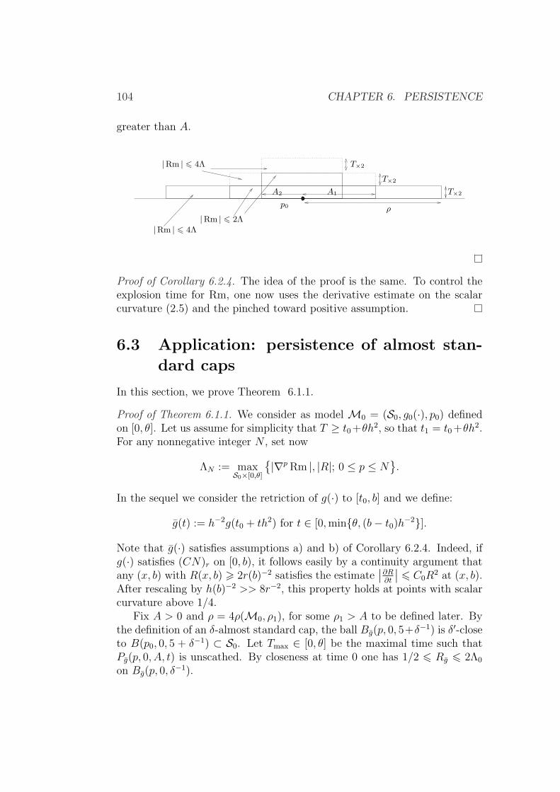
104 CHAPTER 6. PERSISTENCE
greater than A.
ρ
T×2A1
|Rm | 6 4Λ
|Rm | 6 2Λ
T×2
T×2
p0
A2
|Rm | 6 4Λ
Proof of Corollary 6.2.4. The idea of the proof is the same. To control theexplosion time for Rm, one now uses the derivative estimate on the scalarcurvature (2.5) and the pinched toward positive assumption.
6.3 Application: persistence of almost stan-
dard caps
In this section, we prove Theorem 6.1.1.
Proof of Theorem 6.1.1. We consider as model M0 = (S0, g0(·), p0) definedon [0, θ]. Let us assume for simplicity that T ≥ t0 +θh2, so that t1 = t0 +θh2.For any nonnegative integer N , set now
ΛN := maxS0×[0,θ]
|∇p Rm |, |R|; 0 ≤ p ≤ N.
In the sequel we consider the retriction of g(·) to [t0, b] and we define:
g(t) := h−2g(t0 + th2) for t ∈ [0,minθ, (b− t0)h−2].
Note that g(·) satisfies assumptions a) and b) of Corollary 6.2.4. Indeed, ifg(·) satisfies (CN)r on [0, b), it follows easily by a continuity argument thatany (x, b) with R(x, b) > 2r(b)−2 satisfies the estimate
∣∣∂R∂t
∣∣ 6 C0R2 at (x, b).
After rescaling by h(b)−2 >> 8r−2, this property holds at points with scalarcurvature above 1/4.
Fix A > 0 and ρ = 4ρ(M0, ρ1), for some ρ1 > A to be defined later. Bythe definition of an δ-almost standard cap, the ball Bg(p, 0, 5+δ−1) is δ′-closeto B(p0, 0, 5 + δ−1) ⊂ S0. Let Tmax ∈ [0, θ] be the maximal time such thatPg(p, 0, A, t) is unscathed. By closeness at time 0 one has 1/2 6 Rg 6 2Λ0
on Bg(p, 0, δ−1).
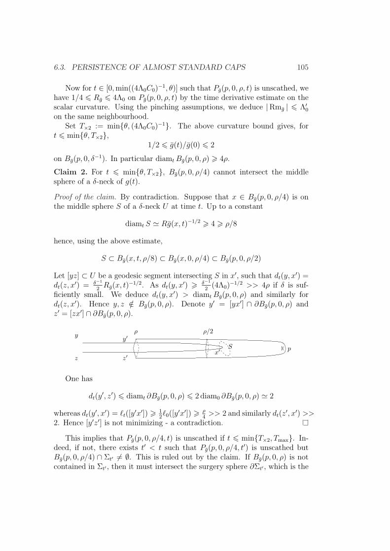
6.3. PERSISTENCE OF ALMOST STANDARD CAPS 105
Now for t ∈ [0,min((4Λ0C0)−1, θ)] such that Pg(p, 0, ρ, t) is unscathed, we
have 1/4 6 Rg 6 4Λ0 on Pg(p, 0, ρ, t) by the time derivative estimate on thescalar curvature. Using the pinching assumptions, we deduce |Rmg | 6 Λ′0on the same neighbourhood.
Set T×2 := minθ, (4Λ0C0)−1. The above curvature bound gives, for
t 6 minθ, T×2,1/2 6 g(t)/g(0) 6 2
on Bg(p, 0, δ−1). In particular diamtBg(p, 0, ρ) > 4ρ.
Claim 2. For t 6 minθ, T×2, Bg(p, 0, ρ/4) cannot intersect the middlesphere of a δ-neck of g(t).
Proof of the claim. By contradiction. Suppose that x ∈ Bg(p, 0, ρ/4) is onthe middle sphere S of a δ-neck U at time t. Up to a constant
diamt S ' Rg(x, t)−1/2 > 4 > ρ/8
hence, using the above estimate,
S ⊂ Bg(x, t, ρ/8) ⊂ Bg(x, 0, ρ/4) ⊂ Bg(p, 0, ρ/2)
Let [yz] ⊂ U be a geodesic segment intersecting S in x′, such that dt(y, x′) =
dt(z, x′) = δ−1
2Rg(x, t)
−1/2. As dt(y, x′) > δ−1
2(4Λ0)
−1/2 >> 4ρ if δ is suf-ficiently small. We deduce dt(y, x
′) > diamtBg(p, 0, ρ) and similarly fordt(z, x
′). Hence y, z /∈ Bg(p, 0, ρ). Denote y′ = [yx′] ∩ ∂Bg(p, 0, ρ) andz′ = [zx′] ∩ ∂Bg(p, 0, ρ).
S
y
z
y′
z′x′ p
ρ ρ/2
One has
dt(y′, z′) 6 diamt ∂Bg(p, 0, ρ) 6 2 diam0 ∂Bg(p, 0, ρ) ' 2
whereas dt(y′, x′) = `t([y
′x′]) > 12`0([y
′x′]) > ρ4>> 2 and similarly dt(z
′, x′) >>2. Hence [y′z′] is not minimizing - a contradiction.
This implies that Pg(p, 0, ρ/4, t) is unscathed if t 6 minT×2, Tmax. In-deed, if not, there exists t′ < t such that Pg(p, 0, ρ/4, t
′) is unscathed butBg(p, 0, ρ/4) ∩ Σt′ 6= ∅. This is ruled out by the claim. If Bg(p, 0, ρ) is notcontained in Σt′ , then it must intersect the surgery sphere ∂Σt′ , which is the
106 CHAPTER 6. PERSISTENCE
middle sphere of a δ-neck centred at (x, t′). The above estimate rules outthis possibility. Hence Bg(p, 0, A) ⊂ Bg(p, 0, ρ) ⊂ Σt′ for t′ < Tmax. This isimpossible by assumption.
We can now apply Corollary 6.2.4. We get that Pg(p, 0, ρ1, t) is ρ−11 -close
to P (p0, 0, ρ1, t) for all t 6 minT×2, Tmax. If T×2 > Tmax we are done.Otherwise by closeness we have that |Rmg | and |Rg| are not greater than2Λ0 on Pg(p, 0, ρ1, T×2), and Rg > 1/2. Then as before 1/4 6 Rg 6 4Λ0
on Pg(p, 0, ρ1,min(2T×2, Tmax)) where ρ1 = ρ(M0, ρ2) and ρ2 > 0. We theniterate the above argument, which terminates in finitely many steps, as donein Corollary 6.2.3. This finishes the proof of Theorem 6.1.1.
Notes Theorem 6.1.1 is similar to [61, Lemma 4.5].Lemma 6.2.1 and Proposition 6.2.2 are new.
Chapter 7
Canonical neighbourhoods andproof of Proposition B
Recall the statement of Proposition B:
Proposition B. For all κ > 0 there exist r = r(κ) ∈ (0, 10−3) and δB =δB(κ) ∈ (0, δ0) with the following property: let 0 < δ ≤ δB, b > 0 and g(·) be aRicci flow with bubbling-off defined on [0, b] with normalised initial condition.Assume that the restriction of g(·) to the half-open interval [0, b) is a Ricciflow with (r, δ, κ)-bubbling-off. Then it satisfies (CN)r on all of [0, b].
7.1 Warming up
Lemma 7.1.1. Let ε ∈ (0, ε0). Let g(·) be a Ricci flow with bubbling-offand (x, 0) be such that R(x, 0) > 0, and there exists a sequence of negativenumbers ti tending to 0 such that for every i, (x, ti) is centre of a strongε-neck. Then (x, 0) is centre of a strong 2ε-neck.
Proof. For each i, we fix a strong α-neck Ni centred at (x, ti), a parametri-sation ψi : S2 × (−ε−1, ε−1) → Ni and a scaling factor Qi. We set gi(t) :=Qig(ti + tQ−1
i ). By definition, we have
‖ψ∗i gi(t)− gcyl(t)‖C[ε−1]+1,gcyl< ε (7.1)
for all t ∈ [−1, 0].By choice of ε0, we have |QiR(x, ti) − 1| 6 10−1. Now the sequence
R(x, ti) converges to the positive number R(x, 0). Hence up to extracting asubsequence, we can assume that Qi converges to some positive number Q.Set g(t) := Qg(t/Q). This is defined for at least t/Q > ti − Q−1
i , hence fort > −1 since tiQi −Q/Qi > −Q/Qi → −1. Hence g is defined on (−1, 0].
107
108 CHAPTER 7. PROPOSITION B
For all t ∈ (−1, 0] we have g(t) = lim gi(t) in the C[ε−1]+1 topology. Hencewe have a uniform upper bound for the C[ε−1]+1-norm of ψi computed withrespect to the fixed metrics gcyl, g(0).
After passing to a subsequence, we get a map ψ : S2 × (−ε−1, ε−1) →Msuch that ψi → ψ in the C[ε−1] sense.
For all x, y ∈ S2 × (−2ε−1/3, 2ε−1/3) we have
(1− ε)dgcyl(x, y) ≤ dgi(0)(ψi(x), ψi(y)) ≤ (1 + ε)dgcyl
(x, y). (7.2)
Passing to the limit, we obtain:
(1− ε)dgcyl(x, y) ≤ dg(0)(ψ(x), ψ(y)) ≤ (1 + ε)dgcyl
(x, y). (7.3)
Hence the restriction of ψ to S2 × (−2ε−1/3, 2ε−1/3) is injective. Frominequality (7.1) we derive
‖ψ∗g(t)− gcyl(t)‖C[ε−1]+1,gcyl6 ε
for all t ∈ (−1, 0]. Hence the restriction of ψ to S2 × (−2ε−1/3, 2ε−1/3) is aC[ε−1]-diffeomorphism onto its image.
Pick λ > 1 close enough to 1 such that the metric g(t) := λg(t/λ) satisfies
‖ψ∗g(t)− gcyl(t)‖C[ε−1]+1,gcyl< 2ε
on (−λ, 0] ⊃ [−1, 0]. Then ψ(S2× (−(2ε)−1, (2ε)−1)) is a strong 2ε-neck.
7.2 The proof
We argue by contradiction. Suppose that some fixed number κ > 0 has theproperty that for all r ∈ (0, r0) and δB > 0 there exists counterexamples.Then we can consider sequences rk → 0, δk → 0, bk > 0, and a sequence ofRicci flow with (rk, δk, κ)-bubbling-off gk(·) on [0, bk) which admit extensionsas Ricci flow with bubbling-off on [0, bk] but such that (CN)rk fails at bk.This last assertion means that there exists xk ∈Mk such that
R(xk, bk) > r−2k ,
and yet xk does not have a (ε0, C0)-canonical neighbourhood.Without loss of generality, we assume that
δk 6 δper(k, 1− 1
k, rk)
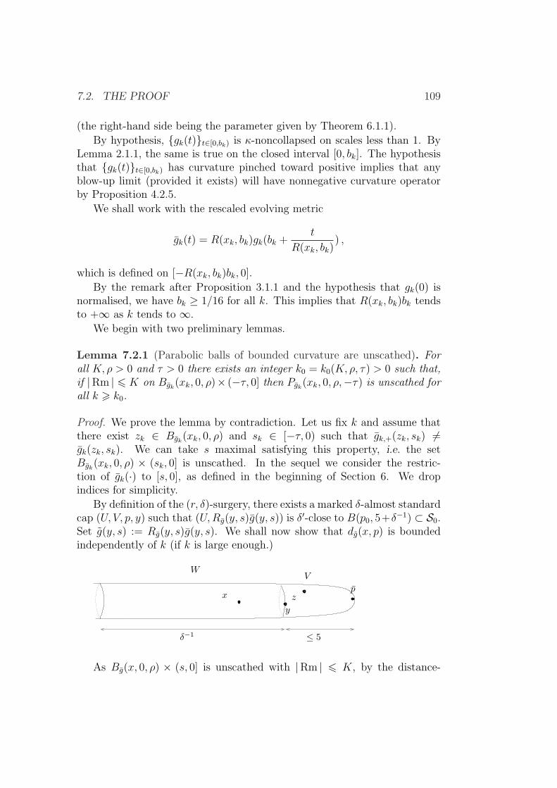
7.2. THE PROOF 109
(the right-hand side being the parameter given by Theorem 6.1.1).
By hypothesis, gk(t)t∈[0,bk) is κ-noncollapsed on scales less than 1. ByLemma 2.1.1, the same is true on the closed interval [0, bk]. The hypothesisthat gk(t)t∈[0,bk) has curvature pinched toward positive implies that anyblow-up limit (provided it exists) will have nonnegative curvature operatorby Proposition 4.2.5.
We shall work with the rescaled evolving metric
gk(t) = R(xk, bk)gk(bk +t
R(xk, bk)) ,
which is defined on [−R(xk, bk)bk, 0].
By the remark after Proposition 3.1.1 and the hypothesis that gk(0) isnormalised, we have bk ≥ 1/16 for all k. This implies that R(xk, bk)bk tendsto +∞ as k tends to ∞.
We begin with two preliminary lemmas.
Lemma 7.2.1 (Parabolic balls of bounded curvature are unscathed). Forall K, ρ > 0 and τ > 0 there exists an integer k0 = k0(K, ρ, τ) > 0 such that,if |Rm | 6 K on Bgk
(xk, 0, ρ)× (−τ, 0] then Pgk(xk, 0, ρ,−τ) is unscathed for
all k > k0.
Proof. We prove the lemma by contradiction. Let us fix k and assume thatthere exist zk ∈ Bgk
(xk, 0, ρ) and sk ∈ [−τ, 0) such that gk,+(zk, sk) 6=gk(zk, sk). We can take s maximal satisfying this property, i.e. the setBgk
(xk, 0, ρ) × (sk, 0] is unscathed. In the sequel we consider the restric-tion of gk(·) to [s, 0], as defined in the beginning of Section 6. We dropindices for simplicity.
By definition of the (r, δ)-surgery, there exists a marked δ-almost standardcap (U, V, p, y) such that (U,Rg(y, s)g(y, s)) is δ′-close to B(p0, 5+δ−1) ⊂ S0.Set g(y, s) := Rg(y, s)g(y, s). We shall now show that dg(x, p) is boundedindependently of k (if k is large enough.)
VW
≤ 5δ−1
x
y
zp
As Bg(x, 0, ρ) × (s, 0] is unscathed with |Rm | 6 K, by the distance-
110 CHAPTER 7. PROPOSITION B
distortion lemma 0.6.1 we have on Bbarg(x, 0, ρ),
e−4Kτ 6 g(0)
g(s)6 e4Kτ ,
which implies dg(s)(x, z) ≤ e2Kτρ. Hence,
dg(x, p) ≤ e2Kτ + 5 = ρ′(K, ρ, τ) =: ρ′ .
Let A > 2(ρ′ + 5) and θ < 1. The Persistence of the Almost Standard CapTheorem implies that the set Pg(p, s, ARg(y, s)
−1/2,minθRg(y, s)−1, |s|) is,
after parabolic rescaling at time s, A−1-close to P (p0, 0, A,minθ, |s|Rk(y, s)) .Indeed, the second alternative of the persistence theorem does not occur sincein this case, x ∈ Bg(p,A) ⊂ Σt+ for some t+ ∈ (−s, 0], i.e. (x, t+) is in thesingular set for t+ > s.
We now choose A = k and θ = 1− 1/k.
Claim 3. We have s+ θRg(y, s)−1 > 0 for large k.
Proof. If Rg(y, s) < (2τ)−1, then
s+ θRg(y, s)−1 > −τ + 1/2Rg(y, s)
−1 > 0 ,
since θ > 1/2.Suppose that Rg(y, s) > (2τ)−1. Seeking a contradiction, assume that
s1 := s+ θRg(y, s)−1 6 0 and apply the persistence theorem up to this time.
By Proposition 2.3.3 Rmin(t) > const(1−t)−1 on the standard solution, hencewe have by closeness
Rg(x, s1) > 1
2Rg(y, s)const(1− θ)−1 > const(4τ(1− θ))−1 =
k.const
4τ.
On the other hand, Rg(x, s1) 6 6K thus this is a contradiction for sufficientlylarge k. This proves the claim.
Denote g(·) the parabolic rescaling of g by Rg(y, s) at time s:
g(t) = Rg(y, s)g(s+ tRg(y, s)
−1).
By the conclusion of the Persistence Theorem 6.1.1, there exists a diffeo-morphism ψ : B(p0, 0, A) −→ Bg(p, 0, A) such that ψ∗g(·) is A−1-close tog0(·) on B(p0, 0, A) × [0,minθ, |s|Rg(y, s)]. By the above claim, the min-imum is |s|Rg(y, s) := s′. Let x′ = ψ−1(x), the point (x, 0) corresponds to(x′, s′) by the diffeomorphism. Recall that by Proposition 2.3.3, for all ε > 0,there exists Cst(ε) such that any point (x′, t) of the standard solution has an(ε, Cst(ε))-canonical neighbourhood or t < 3/4 and x′ /∈ B(p0, 0, ε
−1). Let uschoose ε = ε0β0/2 << ε, where β0 is the parameter fixed in Section 3.1, andCst = Cst(ε). There are again two possibilities.
7.2. THE PROOF 111
Case 1 The point (x′, s′) has an (ε, Cst)-canonical neighbourhood,
U ′ ⊂ B(x′, s′, 2CstR(x′, s′)−1/2) .
Here R(x′, s′) is the scalar curvature of the standard solution at (x′, s′). TheA−1-proximity between g0(s
′) and ψ∗g(s′) gives
R(x′, s′) ' Rg(x, s′) = Rg(y, s)
−1Rg(x, 0) = Rg(y, s)−1 .
On the other hand,
U ′ ⊂ B(x′, s′,ρ
2Rg(y, s)
1/2) ⊂ ψ−1(Bg(x, 0, ρ))
sinceρ
2Rg(y, s)
1/2 ' ρ
2R(x′, s′)−1/2 > 2CstR(x′, s′)−1/2 .
Hence ψ(U ′) is a canonical neighbourhood at (x, 0) of parameters (2ε, 2Cst),hence a (ε0, C0)-canonical neighbourhood by the choices made in Section 3.1.
Case 2 The point (x′, s′) has no (ε, Cst)-canonical neighbourhood. Thens′ 6 3/4 and x′ /∈ B(p0, 0, ε
−1). Hence we have
dg(s′)(x, p) > 9/10ε−1 > 3/2(ε0β0)−1 > (ε0β0)
−1 + 5.
We infer that (x,−s′) is centre of an (ε0β0)-neck, coming from the strong δ-neck that was there at the singular time. We now apply the Neck Strengthen-ing Lemma 2.3.4 which asserts that (x, 0) has an strong ε0-neck. Indeed theproximity with the standard solution ensures that Pg(x,−s′, (ε0β0)
−1, s′) ⊂Pg(x,−s′, A, s′) is unscathed and has |Rm | 6 2Kst. This proves Lemma 7.2.1.
Lemma 7.2.2. Each point (x, bk) of scalar curvature at least 2r−2k for gk(bk)
has a (2ε0, 2C0)-canonical neighbourhood.
Proof. For each t < bk close to bk, R(x, t) > r−2k hence (x, t) has a (ε0, C0)-
canonical neighbourhood. If there is a sequence of strong ε0-necks at timesti → bk, the conclusion follows from Lemma 7.1.1. The other case gives easilya (2ε0, 2C0)-cap at (x, bk).
Now we continue the proof of Proposition B.
Step 1. The sequence (Mk, gk(0), xk) subconverges to some complete pointedriemannian manifold (M∞, g∞, x∞) of nonnegative curvature operator.
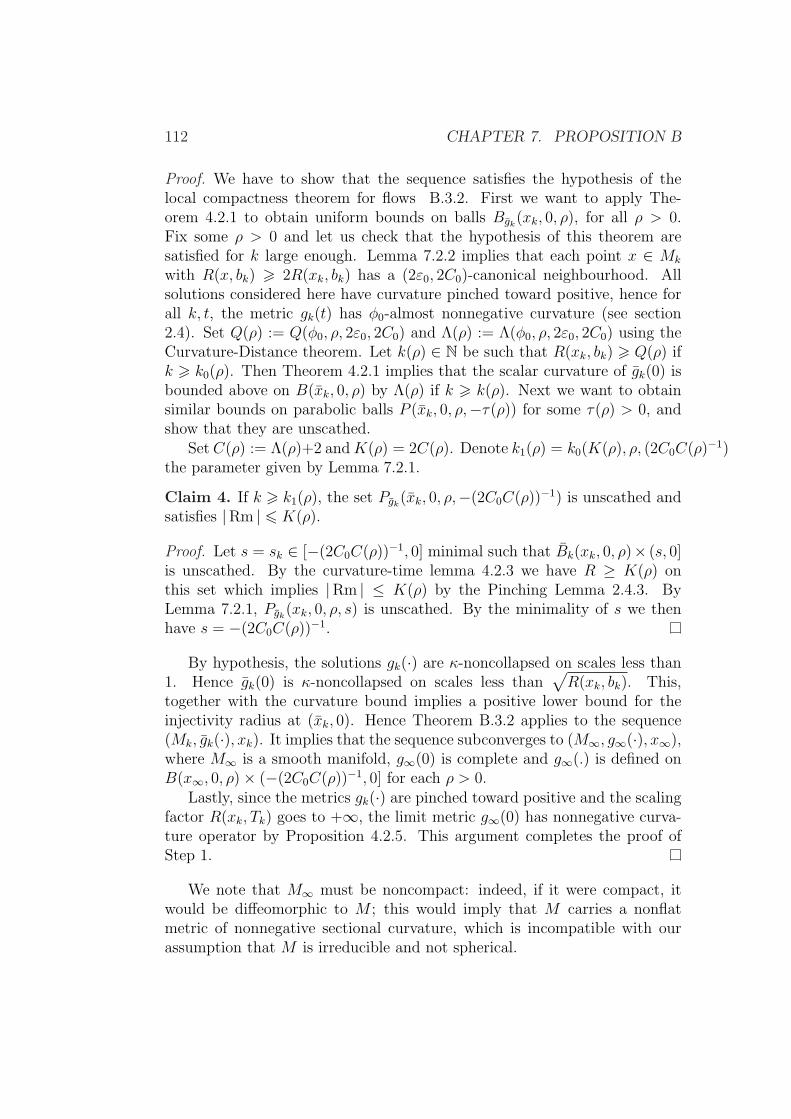
112 CHAPTER 7. PROPOSITION B
Proof. We have to show that the sequence satisfies the hypothesis of thelocal compactness theorem for flows B.3.2. First we want to apply The-orem 4.2.1 to obtain uniform bounds on balls Bgk
(xk, 0, ρ), for all ρ > 0.Fix some ρ > 0 and let us check that the hypothesis of this theorem aresatisfied for k large enough. Lemma 7.2.2 implies that each point x ∈ Mk
with R(x, bk) > 2R(xk, bk) has a (2ε0, 2C0)-canonical neighbourhood. Allsolutions considered here have curvature pinched toward positive, hence forall k, t, the metric gk(t) has φ0-almost nonnegative curvature (see section2.4). Set Q(ρ) := Q(φ0, ρ, 2ε0, 2C0) and Λ(ρ) := Λ(φ0, ρ, 2ε0, 2C0) using theCurvature-Distance theorem. Let k(ρ) ∈ N be such that R(xk, bk) > Q(ρ) ifk > k0(ρ). Then Theorem 4.2.1 implies that the scalar curvature of gk(0) isbounded above on B(xk, 0, ρ) by Λ(ρ) if k > k(ρ). Next we want to obtainsimilar bounds on parabolic balls P (xk, 0, ρ,−τ(ρ)) for some τ(ρ) > 0, andshow that they are unscathed.
Set C(ρ) := Λ(ρ)+2 andK(ρ) = 2C(ρ). Denote k1(ρ) = k0(K(ρ), ρ, (2C0C(ρ)−1)the parameter given by Lemma 7.2.1.
Claim 4. If k > k1(ρ), the set Pgk(xk, 0, ρ,−(2C0C(ρ))−1) is unscathed and
satisfies |Rm | 6 K(ρ).
Proof. Let s = sk ∈ [−(2C0C(ρ))−1, 0] minimal such that Bk(xk, 0, ρ)× (s, 0]is unscathed. By the curvature-time lemma 4.2.3 we have R ≥ K(ρ) onthis set which implies |Rm | ≤ K(ρ) by the Pinching Lemma 2.4.3. ByLemma 7.2.1, Pgk
(xk, 0, ρ, s) is unscathed. By the minimality of s we thenhave s = −(2C0C(ρ))−1.
By hypothesis, the solutions gk(·) are κ-noncollapsed on scales less than1. Hence gk(0) is κ-noncollapsed on scales less than
√R(xk, bk). This,
together with the curvature bound implies a positive lower bound for theinjectivity radius at (xk, 0). Hence Theorem B.3.2 applies to the sequence(Mk, gk(·), xk). It implies that the sequence subconverges to (M∞, g∞(·), x∞),where M∞ is a smooth manifold, g∞(0) is complete and g∞(.) is defined onB(x∞, 0, ρ)× (−(2C0C(ρ))−1, 0] for each ρ > 0.
Lastly, since the metrics gk(·) are pinched toward positive and the scalingfactor R(xk, Tk) goes to +∞, the limit metric g∞(0) has nonnegative curva-ture operator by Proposition 4.2.5. This argument completes the proof ofStep 1.
We note that M∞ must be noncompact: indeed, if it were compact, itwould be diffeomorphic to M ; this would imply that M carries a nonflatmetric of nonnegative sectional curvature, which is incompatible with ourassumption that M is irreducible and not spherical.
7.2. THE PROOF 113
By the Soul Theorem [14], M is diffeomorphic to R3, S1 × R2, or aline bundle over a closed surface. In particular, every smoothly embedded2-sphere in M is separating.
Step 2. The riemannian manifold (M∞, g∞(0)) has bounded curvature.
Proof. By passing to the limit, we see that every point p0 ∈ M∞ of scalarcurvature at least 3 is centre of a (3ε0, 3C0)-cap or a (not necessarily strong)3ε0-neck. In the sequel, we refer to this fact by saying that the limitingpartial flow g∞(·) satisfies the weak canonical neighbourhood property.
Let (pk) be a sequence of points of M∞ such that R∞(pk, 0) −→ +∞;in particular, d∞(pk, x∞) −→ +∞ as k → +∞. Consider segments [x∞pk]which, after passing to a subsequence, converge to a geodesic ray c startingat x∞.
On [x∞pk] we pick a point qk such that
R∞(qk) =R∞(pk)
4C0
.
For sufficiently large k, the point (qk, 0) is centre of a weak (3ε0, 3C0)-canonical neighbourhood Uk. Now the curvatures on Uk belong to the closedinterval
[(3C0)−1R∞(qk, 0), 3C0R∞(qk, 0)]
As a consequence, for large k, x∞ and pk do not belong to Uk. By Corol-lary 1.3.2 this neighbourhood is a 3ε0-neck.
p1 p2
pk
c
q2
Uk
qk
(M∞, g∞(0))
x∞
Lemma 7.2.3. For k large enough, c traverses Uk.
Proof. Assume it does not. Recall that g∞(0) is nonnegatively curved. Con-sider a geodesic triangle x∞qkc(t) for t ≥ 10C0. Choose k large enough sothat ](pkx∞c(t)) ≤ π/100. Let S− (resp. S+ ) be the component of ∂Uk
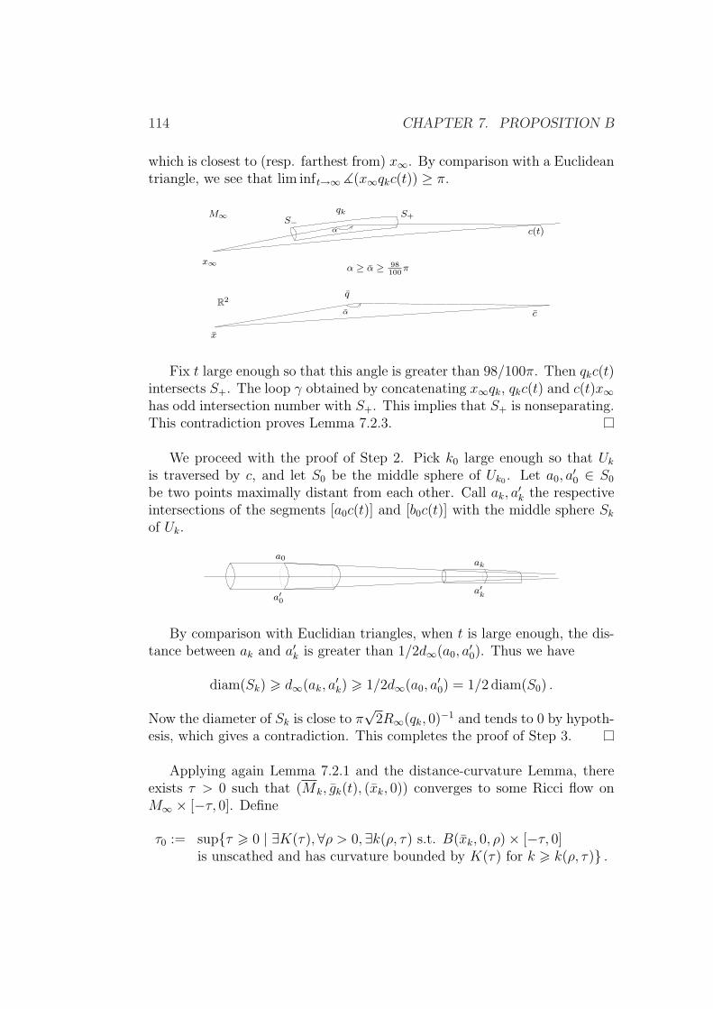
114 CHAPTER 7. PROPOSITION B
which is closest to (resp. farthest from) x∞. By comparison with a Euclideantriangle, we see that lim inft→∞ ](x∞qkc(t)) ≥ π.
x∞
qk
c(t)
M∞
R2
x
q
c
α
α
α ≥ α ≥ 98100
π
S−S+
Fix t large enough so that this angle is greater than 98/100π. Then qkc(t)intersects S+. The loop γ obtained by concatenating x∞qk, qkc(t) and c(t)x∞has odd intersection number with S+. This implies that S+ is nonseparating.This contradiction proves Lemma 7.2.3.
We proceed with the proof of Step 2. Pick k0 large enough so that Ukis traversed by c, and let S0 be the middle sphere of Uk0 . Let a0, a
′0 ∈ S0
be two points maximally distant from each other. Call ak, a′k the respective
intersections of the segments [a0c(t)] and [b0c(t)] with the middle sphere Skof Uk.
a0
a′0
ak
a′k
By comparison with Euclidian triangles, when t is large enough, the dis-tance between ak and a′k is greater than 1/2d∞(a0, a
′0). Thus we have
diam(Sk) > d∞(ak, a′k) > 1/2d∞(a0, a
′0) = 1/2 diam(S0) .
Now the diameter of Sk is close to π√
2R∞(qk, 0)−1 and tends to 0 by hypoth-esis, which gives a contradiction. This completes the proof of Step 3.
Applying again Lemma 7.2.1 and the distance-curvature Lemma, thereexists τ > 0 such that (Mk, gk(t), (xk, 0)) converges to some Ricci flow onM∞ × [−τ, 0]. Define
τ0 := supτ > 0 | ∃K(τ),∀ρ > 0,∃k(ρ, τ) s.t. B(xk, 0, ρ)× [−τ, 0]is unscathed and has curvature bounded by K(τ) for k > k(ρ, τ) .
7.2. THE PROOF 115
We already know that τ0 > 0 and the compactness theorem B.3.1 enables usto construct a flow g∞(t) on M∞ × (−τ0, 0], which is a limit of (Mk, gk(t))for the pointed convergence of flows. Moreover, the scalar curvature of g∞ isbounded by K(τ) on (−τ, 0] by passing to the limit, for all τ ∈ [0, τ0).
Step 3. There exists Q > 0 such that the curvature of g∞(t) is boundedabove by Q for all t ∈ (−τ0, 0].
Proof. We know that g∞(t) is nonnegatively curved and has the above-mentioned weak canonical neighbourhood property. We show that the con-clusion of the Curvature-Distance theorem holds on M∞, at points of scalarcurvature > 1. For this, we let p ∈ M∞ and t ∈ (−τ0, 0] be such thatR∞(p, t) > 1. Then there exists a sequence (pk, tk), where pk ∈Mk, converg-ing to (p, t) and such that R(pk, tk) > 1 for k large enough. As a consequence,they satisfy the hypotheses of the Curvature-Distance theorem as explainedin the proof of Step 1. Passing to the limit, we deduce that for every A > 0,there exists Λ(A) > 0 such that for all q ∈M∞,
R∞(q, t)
R∞(p, t)6 Λ
(d∞(p, q, t)R∞(p, t)−1
). (7.4)
Let us estimate the variation of curvatures and distances onM∞×(−τ0, 0].We recall the Harnack inequality for the scalar curvature
∂R∞∂t
+R∞t+ τ0
> 0 ,
which implies
R∞(., t) 6 K(0)τ0
t+ τ0.
Ricci curvature, which is positive, satisfies a similar estimate, which im-plies
const(τ0
t+ τ0)g∞ 6 ∂g∞
∂t≤ 0 ,
thus
const
√τ0
t+ τ06 ∂d∞
∂t(x, y, t) 6 0 .
By integration we obtain
|d∞(x, y, t)− d∞(x, y, 0)| 6 C .
Since M∞ is noncompact and nonnegatively curved, there exists D > 0such that for all y ∈ M∞, if d∞(x∞, y, 0) > D, then there exists z ∈ M∞such that
d∞(y, z, 0) = d∞(x∞, y, 0) and d∞(x∞, z, 0) > 1.99d∞(x, y, 0) (7.5)
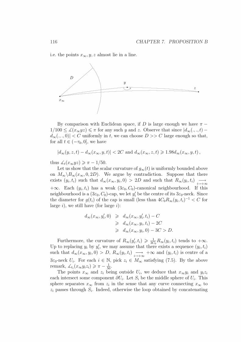
116 CHAPTER 7. PROPOSITION B
i.e. the points x∞, y, z almost lie in a line.
D
x∞
y
z
By comparison with Euclidean space, if D is large enough we have π −1/100 ≤ ](x∞yz) 6 π for any such y and z. Observe that since |d∞(., ., t)−d∞(., ., 0)| < C uniformly in t, we can choose D >> C large enough so that,for all t ∈ (−τ0, 0], we have
|d∞(y, z, t)− d∞(x∞, y, t)| < 2C and d∞(x∞, z, t) > 1.98d∞(x∞, y, t) ,
thus ]t(x∞yz) > π − 1/50.Let us show that the scalar curvature of g∞(t) is uniformly bounded above
on M∞\B∞(x∞, 0, 2D). We argue by contradiction. Suppose that thereexists (yi, ti) such that d∞(x∞, yi, 0) > 2D and such that R∞(yi, ti) −→
i→+∞+∞. Each (yi, ti) has a weak (3ε0, C0)-canonical neighbourhood. If thisneighbourhood is a (3ε0, C0)-cap, we let y′i be the centre of its 3ε0-neck. Sincethe diameter for g(ti) of the cap is small (less than 4C0R∞(yi, ti)
−1 < C forlarge i), we still have (for large i):
d∞(x∞, y′i, 0) > d∞(x∞, y′i, ti)− C
> d∞(x∞, yi, ti)− 2C
> d∞(x∞, yi, 0)− 3C > D.
Furthermore, the curvature of R∞(y′i, ti) > 13C0
R∞(yi, ti) tends to +∞.Up to replacing yi by y′i, we may assume that there exists a sequence (yi, ti)such that d∞(x∞, yi, 0) > D, R∞(yi, ti) −→
i→+∞+∞ and (yi, ti) is centre of a
3ε0-neck Ui. For each i ∈ N, pick zi ∈ M∞ satisfying (7.5). By the aboveremark, ]ti(x∞yizi) > π − 1
50.
The points x∞ and zi being outside Ui, we deduce that x∞yi and yizieach intersect some component ∂Ui. Let Si be the middle sphere of Ui. Thissphere separates x∞ from zi in the sense that any curve connecting x∞ tozi passes through Si. Indeed, otherwise the loop obtained by concatenating
7.2. THE PROOF 117
[x∞yi], [yizi] and [zix∞] would have odd intersection number with Si. Asbefore this leads to a contradiction.
Now diam(Si, ti) −→ 0 since R∞(yi, ti) −→ +∞ as i→ +∞. Since g∞(t)is nonnegatively curved, distances are nonincreasing in t. As a consequence,
diam(Si, 0) −→ 0i→+∞
.
At time 0 the curvature bounds and the hypothesis of κ-noncollapsing im-plies a uniform lower bound on the injectivity radius. Then for large i, thediameter of Si is less than the injectivity radius of g∞(0). This implies thatSi bounds a 3-ball which contains neither x∞ nor zi. Hence we can connectx∞ to zi by an arc which avoids Si.
This implies that the curvature is bounded outside the g∞(0)-ball of radius2D around x∞. We deduce a uniform curvature bound on (−τ0, 0] in the ballusing Equation (7.4).
Step 4. τ0 = +∞Proof. Consider a subsequence (Mk×(−τ0, 0], gk(t), (xk, 0)) that converges to(M∞× (−τ0, 0], g∞(t), (x∞, 0)). Since the limit has scalar curvature boundedabove by Q we deduce that (up to replacing Q par Q + 1), for all 0 < τ <τ0, for all ρ > 0, there exists k′(τ, ρ) ∈ N such that for all k > k′(τ, ρ),the parabolic neighbourhood Pgk
(xk, 0, ρ,−τ) is unscathed and has scalarcurvature ≤ Q.
Suppose that τ0 < +∞ and let 0 < σ < (4C0(Q + 2))−1. Then up toextracting a subsequence, for every K > 0, there exists ρ = ρ(σ,K) such thatPk := Pgk
(xk, 0, ρ,−(τ0 + σ)) is scathed or does not have curvature boundedabove by K.
SetK := 2(Q+2) and ρ := ρ(σ,K). If k > k′(τ0−σ, ρ), then Pk is scathed.Indeed, if k > k′(τ0 − σ, ρ), we have R 6 Q on Pgk
(xk, 0, ρ,−τ0 + σ)). If Pkis unscathed, the curvature-time lemma (4.2.3) applied between −τ0 +σ and−τ0−σ (since 2σ 6 (2C0(Q+2))−1) implies that R 6 2(Q+2) on Pk, whichexcludes the second alternative.
Thus there exists x′k ∈ Bk(xk, 0, ρ), and tk ∈ [−τ0 − σ,−τ0 + σ], assumedto be maximal, such that gk(tk) 6= gk+(tk) at x′k. Since B(xk, 0, ρ) × (tk, 0]is unscathed, the above argument shows that R 6 2(Q + 2) on this set,for all sufficiently large k. This implies an upper bound on the Riemanntensor on this set and hence by Lemma 7.2.1 the parabolic neighbourhoodPgk
(xk, 0, ρ, tk) is unscathed. This contradicts the definition of tk.
We can now finish the proof of Proposition B: since τ0 = +∞, the Ricciflow (M∞, g∞(·)) is defined on (−∞, 0], and has bounded, nonnegative curva-ture operator. Moreover, the rescaled evolving metric gk(·) is κ-noncollapsed
118 CHAPTER 7. PROPOSITION B
on scales less than√R(xk, bk), so passing to the limit we see that g∞(·) is
κ-noncollapsed on all scales. The metric g∞(·) is not flat since it has scalarcurvature 1 at the point (x∞, 0).
This shows that (M∞, g∞(·)) is a κ-solution. By Theorem 2.2.5 and thechoice of constants in Section 3.1, every point of M∞ has a ( ε0
2, C0
2)-canonical
neighbourhood. Hence for sufficiently large k, (xk, 0) has an (ε0, C0)-canonicalneighbourhood. This is the final contradiction.
Notes Our proof of Proposition B is inspired by [61, Section 5.4],[44, Sec-tion 80]. It uses also arguments from [59, Theorem 12.1],[44, Section 52].
Chapter 8
κ-noncollapsing and proof ofProposition C
The goal of this chapter is to prove Proposition C. We recall its statement:
Proposition C. For all T > 0 there exists κ = κ(T ) such that for allr ∈ (0, 10−3) there exists δC = δC(T, r) ∈ (0, δ0) such that the followingholds.
For all δ 6 δC, any Ricci flow with (r, δ)-bubbling-off defined on an in-terval of the form [0, b] with b ≤ T and having normalised initial conditionsatisfies (NC)κ.
We first prove a simpler theorem about κ-noncollapsing for Ricci flows.Since it is not harder in higher dimensions, we give the proof in all dimensions.Of course the definition needs to be adapted: an n-dimensional Ricci flow(U, g(t))t∈I is κ-noncollapsed on the scale ρ > 0 if for all (x, t) ∈ U × I, if|Rm | 6 ρ−2 on P = P (x, t, ρ,−ρ2), then volB(x, t, ρ) > κρn.
Theorem 8.0.4 (κ-noncollapsing). For each T > 0 there exists κ = κ(T ) >0 such that if (U, g(t)06t6T ) is a closed Ricci flow with normalised initialcondition, then it is κ-noncollapsed on all scales less than 1.
We first prove Theorem 8.0.4 as a warm-up, then explain how to adaptits proof to obtain a proof of Proposition C.
8.1 Preliminaries
Let υk(ρ) denote the volume of a ball of radius ρ in the model space ofcurvature k and dimension n.
119
120 CHAPTER 8. PROPOSITION C
Definition. Let κ > 0. One says that a Riemannian n-ball B(x, ρ) is κ-noncollapsed if |Rm | 6 ρ−2 on B(x, ρ) and if volB(x, ρ) > κρn. Simi-larly, a parabolic n-ball P (x, t, ρ,−ρ−2) is κ-noncollapsed if |Rm | 6 ρ−2 onP (x, t, ρ,−ρ−2) and if volB(x, t, ρ) > κρn.
Lemma 8.1.1. i. If B(x, ρ) is κ-noncollapsed, then for all ρ′ ∈ (0, ρ),B(x, ρ′) is Cκ-noncollapsed, where
C :=v0(1)
v−1(1).
The same property holds for P (x, t, ρ′,−ρ′2) ⊂ P (x, t, ρ,−ρ2).
ii. Let r, δ be surgery parameters and g(·) be a Ricci flow with (r, δ)-bubbling-off. Assume that P0 = P (x0, t0, ρ0,−ρ2
0) is a scathed parabolicneighbourhood such that |Rm | 6 ρ−2
0 on P0. Then P0 is e−12κst/2-noncollapsed.
Remark. κst is the constant defined in Proposition 2.3.2.
Proof. Let us prove Assertion (i): since ρ−2 6 ρ′−2, we have |Rm | 6 ρ′−2 onB(x, ρ′) ⊂ B(x, ρ). Hence we must check that volB(x, ρ′) > Cκρ′n.
Recall that the function υ−k2 satisfies υ−k2(ρ) = k−nυ−1(kρ) for k > 0.Since the sectional curvature is greater than or equal to −ρ−2 on B(x, ρ),Bishop-Gromov gives:
volB(x, ρ′)volB(x, ρ)
> υ−ρ−2(ρ′)υ−ρ−2(ρ)
=υ−1(ρ
′/ρ)υ−1(1)
> υ0(ρ′/ρ)
υ−1(1)=
υ0(1)
υ−1(1)
(ρ′
ρ
)n
.
Using the fact that B(x, ρ) is κ-noncollapsed, we get
volB(x, ρ′) > υ0(1)
υ−1(1)κρ′n .
This proves Assertion (i).
We turn to the proof of Assertion (ii). Let (y, t) be a point of P0 whereg+ 6= g. Assume that t is maximal such that there exists y with this property.The scalar curvature at (y, t) is comparable to the cutoff parameter h−2.
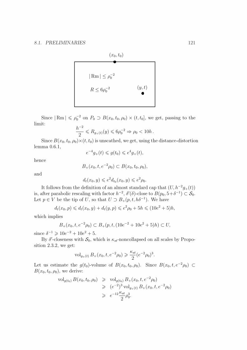
8.1. PRELIMINARIES 121
(x0, t0)
|Rm | ≤ ρ−20
R ≤ 6ρ−20
(y, t)
Since |Rm | 6 ρ−20 on P0 ⊃ B(x0, t0, ρ0) × (t, t0], we get, passing to the
limit:h−2
26 Rg+(t)(y) 6 6ρ−2
0 ⇒ ρ0 < 10h .
SinceB(x0, t0, ρ0)×(t, t0) is unscathed, we get, using the distance-distortionlemma 0.6.1,
e−4g+(t) 6 g(t0) 6 e4g+(t),
henceB+(x0, t, e
−2ρ0) ⊂ B(x0, t0, ρ0),
anddt(x0, y) 6 e2dt0(x0, y) 6 e2ρ0.
It follows from the definition of an almost standard cap that (U, h−2g+(t))is, after parabolic rescaling with factor h−2, δ′(δ)-close to B(p0, 5+δ−1) ⊂ S0.Let p ∈ V be the tip of U , so that U ⊃ B+(p, t, hδ−1). We have
dt(x0, p) 6 dt(x0, y) + dt(y, p) 6 e2ρ0 + 5h 6 (10e2 + 5)h,
which implies
B+(x0, t, e−2ρ0) ⊂ B+(p, t, (10e−2 + 10e2 + 5)h) ⊂ U,
since δ−1 > 10e−2 + 10e2 + 5.By δ′-closeness with S0, which is κst-noncollapsed on all scales by Propo-
sition 2.3.2, we get:
volg+(t)B+(x0, t, e−2ρ0) > κst
2(e−2ρ0)
3.
Let us estimate the g(t0)-volume of B(x0, t0, ρ0). Since B(x0, t, e−2ρ0) ⊂
B(x0, t0, ρ0), we derive:
volg(t0)B(x0, t0, ρ0) > volg(t0)B+(x0, t, e−2ρ0)
> (e−2)3 volg+(t)B+(x0, t, e−2ρ0)
> e−12κst2ρ3
0.
122 CHAPTER 8. PROPOSITION C
This completes the proof of Assertion (ii).
Remarks. i) From i), we deduce that in order to establish noncollapsingat some point (x, t) on all scales 6 1, it suffices to do it on the maximalscale ρ 6 1 such that |Rm | 6 ρ−2 on P (x, t, ρ, ρ−2). This observationwill be useful later.
ii) Assertion ii) will enable us to consider only unscathed parabolic neigh-bourhoods. This will be used the proof of Proposition C (see Section8.3).
iii) If some ball B(y, ρ) is contained in some (ε0, C0)-canonical neighbour-hood and satisfies |Rm | 6 ρ−2, then B(y, ρ) is C−1
0 -noncollapsed on thescale ρ by (2.1).
8.2 Proof of Theorem 8.0.4
Proof. Fix T > 0 and g(·) a Ricci flow on M × [0, T ] such that g(0) isnormalised. Let ρ0 ∈ (0, 1] and consider a parabolic neighbourhood P0 =P (x0, t0, ρ0,−ρ2
0) such that
|Rm | 6 ρ0−2
on P0. Set B0 := B(x0, t0, ρ0) and
κ :=volB(x0, t0, ρ0)
ρ0n
=volg(t0)B0
ρ0n
.
Our task is to bound κ below independently of g(·). By Proposition 3.1.1one can assume t0 > 1/16. The main tool is the reduced volume, whosedefinition and main properties are given in Appendix C.
Set τ0 := κ1/nρ02 6 κ1/n and assume that
κ <
(1
16
)n
,
which yields
t0 − τ0 > 0.
Controlling V (τ0) We use the Lτ0-exponential map to write the aboveintegral as an integral on Tx0M endowed with the metric g(x0, t0). We thencut Tx0M in two.
8.2. PROOF OF THEOREM 8.0.4 123
First step: cutting Tx0M First we show that the vectors v ∈ Tx0Mof norm less than (10κ1/2n)−1 generate L-geodesics which stay in B0 if κ issmall. More precisely, 26.6 page 48 of [44] gives:
∣∣∣ d
d(τ/r20)
√τ |X|
∣∣∣ 6 C(√τ |X|+ (τ/r2
0)1/2) ,
thus X = dγdτ
for γ a L-geodesic satisfying limτ→0
√τX(τ) = v. Henceforth
C is a generic constant depending only on n. We can rewrite this inequalityas ∣∣∣ d
d(τ/τ0)
(κ1/2n
√τ |X|)
∣∣∣ 6 Cκ1/n(κ1/2n√τ |X|+ (τ/τ0)
1/2) .
We limit ourselves to 0 ≤ τ/τ0 ≤ 1 and limτ→0 κ1/2n
√τ |X(τ)| = κ1/2n|v| ≤
1/10. We then set f(τ/τ0) = κ1/2n√τ |X(τ)|, the function f defined on [0, 1]
satisfies the differential inequality
|f ′(x)| 6 Cκ1/n(f(x) +√x) 6 Cκ1/n(f(x) + 1) .
By Gronwall’s Lemma, there exists κ(n) such that if κ ≤ κ(n), then
κ1/2n√τ |X(τ)| 6 1
9,
for all τ ∈ [0, τ0]. Thus∫ τ0
0
|X(τ)|g(t0−τ)dτ = κ−1/2n
∫ τ0
0
κ1/2n√τ |X(τ)| dτ√
τ≤ 2
9ρ0 .
On P (x0, t0, ρ0,−κ1/nρ02) the curvature bound implies
∣∣∣∣∂g
∂t
∣∣∣∣ 6 Cρ0−2 ,
so for all t1, t2 ∈ [t0 − κ1/nρ02, t0] = [t0 − τ0, t0], the metrics g(t1), g(t2) are
eCρ0−2κ1/nρ02
= eCκ1/n
-bilipchitz in that neighbourhood.As long as γ stays in this neighbourhood, its g(t0)-length is less than
eCκ1/n 2
9ρ0 ≤ 1
3ρ0 if κ is small enough. In conclusion, the image by the Lτ0-
exponential map of v ∈ Tx0M ; |v|g(t0) ≤ 110κ−1/2n is contained in B0 for
κ ≤ κ(n).
Step 2: computing the reduced volume on Tx0M From the previousparagraph we deduce:
I :=
∫
|v|g(t0)60,1κ−1/2n
τ−n/20 e−`(v,τ0)J(v, τ0)dv 6
∫
B0
τ−n/20 e−`(q,τ0)dq .
124 CHAPTER 8. PROPOSITION C
Now we bound `(q, τ0) from below for q ∈ B0. Let γ : [0, τ0] → M be aLτ0-geodesic such that γ(0) = x0 and γ(τ0) = q and which stays in B0. Thenwe have
Lτ0(γ) >∫ τ0
0
√τR(γ(τ))dτ > −n(n−1)ρ0
−2
∫ τ0
0
√τdτ = −2
3n(n−1)ρ0
−2τ3/20 ,
and
Lτ0(γ) =Lτ0(γ)2√τ0
> −n(n− 1)
3τ0ρ0
−2 = −n(n− 1)
3κ1/n ,
if γ is minimising. Thus,
I 6 en(n−1)
3κ1/n
τ−n/20
∫|v|g(t0)6 1
10κ−1/2n
J(v, τ0)dv
6 en(n−1)
3κ1/n
τ−n/20 volg(t0−τ0)B0 ,
andI 6 e
n(n−1)3
κ1/n
τ−n/20 eCκ
1/n
volg(t0)(B0) 6 eCκ1/n√
κ .
Define
I ′ :=∫
|v|g(t0)> 110κ−1/2n
τ−n/20 e−`(v,τ0)J(v, τ0)dv .
The integrand is nondecreasing in τ (see [59], section 7). In particular it issmaller than its limit at τ = 0. Now
limτ→0
τ−n/2 exp(−`(v, τ))J(v, τ) = 2ne−|v|2
g(t0) ,
(see [44] section 16). Therefore,
I ′ 6 2n∫
|v|g(t0)> 110κ−1/2n
e−|v|2g(t)dv 6 e−
110κ−1/2n
if κ ≤ κ(n).In conclusion,
V (τ0) 6 eCκ1/n
κ1/2 + e−110κ−1/2n
6 Cκ1/2, (8.1)
for some universal κ 6 κ(n).
Monotonicity of V implies that
V (t0) 6 V (τ0) .
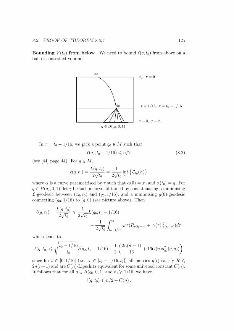
8.2. PROOF OF THEOREM 8.0.4 125
Bounding V (t0) from below We need to bound `(q, t0) from above on aball of controlled volume.
t = 1/16, τ = t0 − 1/16q0
q ∈ B(q0, 0, 1)
t0, τ = 0x0
t = 0, τ = t0
In τ = t0 − 1/16, we pick a point q0 ∈M such that
`(q0, t0 − 1/16) 6 n/2 (8.2)
(see [44] page 44). For q ∈M ,
`(q, t0) =L(q, t0)
2√t0
=1
2√t0
infα
Lt0(α)
where α is a curve parametrised by τ such that α(0) = x0 and α(t0) = q. Forq ∈ B(q0, 0, 1), let γ be such a curve, obtained by concatenating a minimisingL-geodesic between (x0, t0) and (q0, 1/16), and a minimising g(0)-geodesicconnecting (q0, 1/16) to (q, 0) (see picture above). Then
`(q, t0) =L(q, t0)
2√t0
6 1
2√t0L(q0, t0 − 1/16)
+1
2√t0
∫ t0
t0−1/16
√τ(Rg(t0−τ) + |γ(τ)|2g(t0−τ))dτ
which leads to
`(q, t0) 6
√t0 − 1/16
t0`(q0, t0 − 1/16) +
1
2
(2n(n− 1)
16+ 16C(n)d2
g0(q, q0)
)
since for t ∈ [0, 1/16] (i.e. τ ∈ [t0 − 1/16, t0]) all metrics g(t) satisfy R 62n(n−1) and are C(n)-Lipschitz equivalent for some universal constant C(n).It follows that for all q ∈ B(q0, 0, 1) and t0 > 1/16, we have
`(q, t0) 6 n/2 + C(n) .
126 CHAPTER 8. PROPOSITION C
By integration we get∫
M
τ−n/2e−`(q,t0)dq >∫
B(q0,0,1)
t−n/20 e−`(q,t0)dq > t
−n/20 C vol(B(q0, 0, 1))
where dq is the Lebesgue measure of g(0). Recall that infx∈M volB(x, 0, 1) >12v0(1). Then
V (t0) =
∫
M
t0−n/2e−`(q,t0)dq > C
2t0n/2
v0(1) ,
and from (8.1) we deduce
κ > C
t0n,
if κ 6 κ(n).
8.3 κ-noncollapsing of Ricci flow with bubbling-
off: proof of Proposition C
We turn to the proof of Proposition C, which deals with κ-noncollapsingproperties for Ricci flow with (r, δ)-bubbling-off. In fact, we shall prove astronger result, which applies to Ricci flow with r(·), δ(·)-bubbling-off. In-deed, in Part III we will need another κ-noncollapsing result, where κ is in-dependent of time (see Theorem 9.0.4a)). The proof of this theorem, whichis given is Section 8.4 below, uses the same arguments as for Proposition C,with some modifications due to the variation of the parameters. To avoidredondance, we prove directly Proposition C in the context of Ricci flow withr(·), δ(·)-bubbling-off. More precisely, we have the
Proposition C’. For any T > 0 there exists κ = κ(T ), such that for anyr ∈ (0, 10−3), there exists δC′ = δC′(T, r) ∈ (0, δ0) with the following property.Let g(·) be a Ricci flow with r(·), δ(·)-bubbling-off, with normalised initialcondition, defined on some intervall [0, b). Assume that r 6 r(·) 6 10−3,0 < δ(·) 6 δC′ and b 6 T . Then g(·) satisfies (NC)κ.
Remark. Letting r(·) = r and δ(·) = δ gives Proposition C.
Proof of Proposition C’. Thus fix T > 0, r ∈ (0, 10−3), g(·) a Ricci flow withr(·), δ(·)-bubbling-off on [0, b] where b 6 T , r 6 r(·) < 10−3 and δ(·) 6 δ, δto be defined.
Set Mreg := (x, t) ; x 6∈ Σt. This is an open, arcwise connected subsetof M × [0, b]. Likewise we define Msing := M \Mreg =
⋃t(Σt, t).
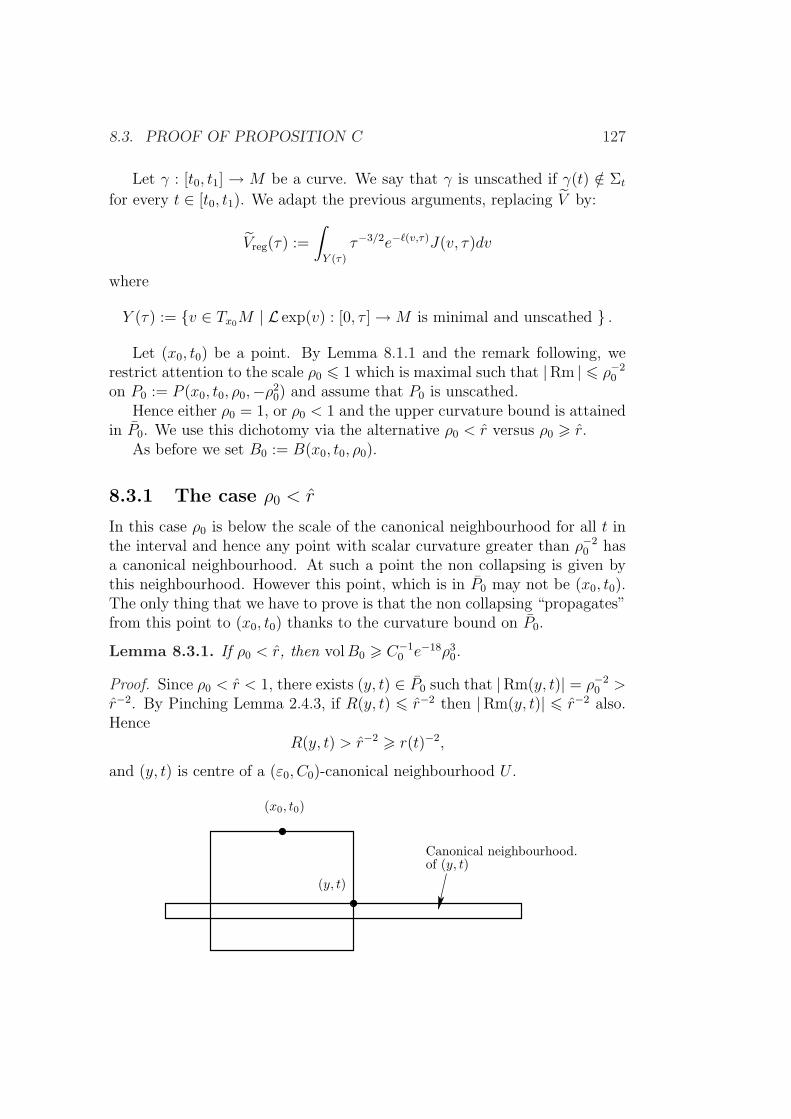
8.3. PROOF OF PROPOSITION C 127
Let γ : [t0, t1] → M be a curve. We say that γ is unscathed if γ(t) /∈ Σt
for every t ∈ [t0, t1). We adapt the previous arguments, replacing V by:
Vreg(τ) :=
∫
Y (τ)
τ−3/2e−`(v,τ)J(v, τ)dv
where
Y (τ) := v ∈ Tx0M | L exp(v) : [0, τ ] →M is minimal and unscathed .
Let (x0, t0) be a point. By Lemma 8.1.1 and the remark following, werestrict attention to the scale ρ0 6 1 which is maximal such that |Rm | 6 ρ−2
0
on P0 := P (x0, t0, ρ0,−ρ20) and assume that P0 is unscathed.
Hence either ρ0 = 1, or ρ0 < 1 and the upper curvature bound is attainedin P0. We use this dichotomy via the alternative ρ0 < r versus ρ0 > r.
As before we set B0 := B(x0, t0, ρ0).
8.3.1 The case ρ0 < r
In this case ρ0 is below the scale of the canonical neighbourhood for all t inthe interval and hence any point with scalar curvature greater than ρ−2
0 hasa canonical neighbourhood. At such a point the non collapsing is given bythis neighbourhood. However this point, which is in P0 may not be (x0, t0).The only thing that we have to prove is that the non collapsing “propagates”from this point to (x0, t0) thanks to the curvature bound on P0.
Lemma 8.3.1. If ρ0 < r, then volB0 > C−10 e−18ρ3
0.
Proof. Since ρ0 < r < 1, there exists (y, t) ∈ P0 such that |Rm(y, t)| = ρ−20 >
r−2. By Pinching Lemma 2.4.3, if R(y, t) 6 r−2 then |Rm(y, t)| 6 r−2 also.Hence
R(y, t) > r−2 > r(t)−2,
and (y, t) is centre of a (ε0, C0)-canonical neighbourhood U .
(x0, t0)
(y, t)of (y, t)Canonical neighbourhood.
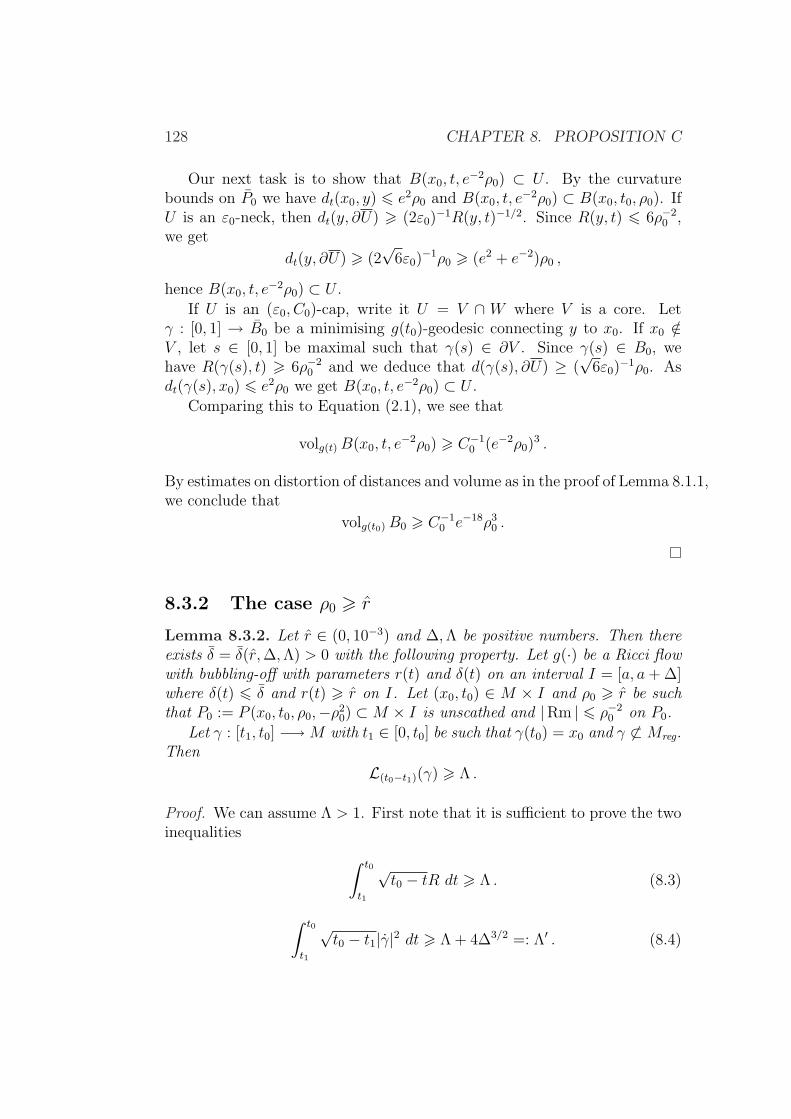
128 CHAPTER 8. PROPOSITION C
Our next task is to show that B(x0, t, e−2ρ0) ⊂ U . By the curvature
bounds on P0 we have dt(x0, y) 6 e2ρ0 and B(x0, t, e−2ρ0) ⊂ B(x0, t0, ρ0). If
U is an ε0-neck, then dt(y, ∂U) > (2ε0)−1R(y, t)−1/2. Since R(y, t) 6 6ρ−2
0 ,we get
dt(y, ∂U) > (2√
6ε0)−1ρ0 > (e2 + e−2)ρ0 ,
hence B(x0, t, e−2ρ0) ⊂ U .
If U is an (ε0, C0)-cap, write it U = V ∩ W where V is a core. Letγ : [0, 1] → B0 be a minimising g(t0)-geodesic connecting y to x0. If x0 /∈V , let s ∈ [0, 1] be maximal such that γ(s) ∈ ∂V . Since γ(s) ∈ B0, wehave R(γ(s), t) > 6ρ−2
0 and we deduce that d(γ(s), ∂U) ≥ (√
6ε0)−1ρ0. As
dt(γ(s), x0) 6 e2ρ0 we get B(x0, t, e−2ρ0) ⊂ U .
Comparing this to Equation (2.1), we see that
volg(t)B(x0, t, e−2ρ0) > C−1
0 (e−2ρ0)3 .
By estimates on distortion of distances and volume as in the proof of Lemma 8.1.1,we conclude that
volg(t0)B0 > C−10 e−18ρ3
0 .
8.3.2 The case ρ0 > r
Lemma 8.3.2. Let r ∈ (0, 10−3) and ∆,Λ be positive numbers. Then thereexists δ = δ(r,∆,Λ) > 0 with the following property. Let g(·) be a Ricci flowwith bubbling-off with parameters r(t) and δ(t) on an interval I = [a, a+ ∆]where δ(t) 6 δ and r(t) > r on I. Let (x0, t0) ∈ M × I and ρ0 > r be suchthat P0 := P (x0, t0, ρ0,−ρ2
0) ⊂M × I is unscathed and |Rm | 6 ρ−20 on P0.
Let γ : [t1, t0] −→M with t1 ∈ [0, t0] be such that γ(t0) = x0 and γ 6⊂Mreg.Then
L(t0−t1)(γ) > Λ .
Proof. We can assume Λ > 1. First note that it is sufficient to prove the twoinequalities
∫ t0
t1
√t0 − tR dt > Λ . (8.3)
∫ t0
t1
√t0 − t1|γ|2 dt > Λ + 4∆3/2 =: Λ′ . (8.4)
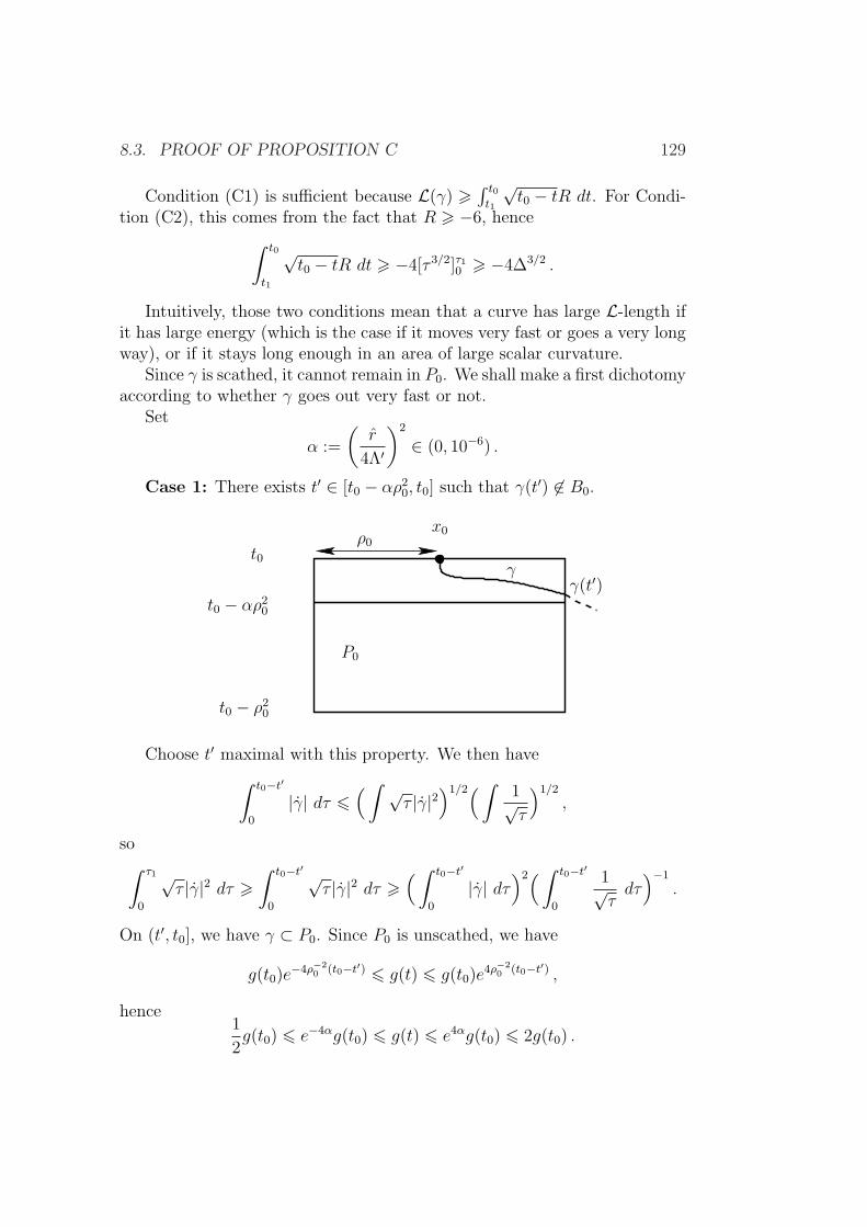
8.3. PROOF OF PROPOSITION C 129
Condition (C1) is sufficient because L(γ) >∫ t0t1
√t0 − tR dt. For Condi-
tion (C2), this comes from the fact that R > −6, hence
∫ t0
t1
√t0 − tR dt > −4[τ 3/2]τ10 > −4∆3/2 .
Intuitively, those two conditions mean that a curve has large L-length ifit has large energy (which is the case if it moves very fast or goes a very longway), or if it stays long enough in an area of large scalar curvature.
Since γ is scathed, it cannot remain in P0. We shall make a first dichotomyaccording to whether γ goes out very fast or not.
Set
α :=
(r
4Λ′
)2
∈ (0, 10−6) .
Case 1: There exists t′ ∈ [t0 − αρ20, t0] such that γ(t′) 6∈ B0.
x0
t0
t0 − αρ20
t0 − ρ20
γ
ρ0
P0
γ(t′)
Choose t′ maximal with this property. We then have
∫ t0−t′
0
|γ| dτ 6( ∫ √
τ |γ|2)1/2( ∫
1√τ
)1/2
,
so∫ τ1
0
√τ |γ|2 dτ >
∫ t0−t′
0
√τ |γ|2 dτ >
( ∫ t0−t′
0
|γ| dτ)2( ∫ t0−t′
0
1√τdτ
)−1
.
On (t′, t0], we have γ ⊂ P0. Since P0 is unscathed, we have
g(t0)e−4ρ−2
0 (t0−t′) 6 g(t) 6 g(t0)e4ρ−2
0 (t0−t′) ,
hence1
2g(t0) 6 e−4αg(t0) 6 g(t) 6 e4αg(t0) 6 2g(t0) .
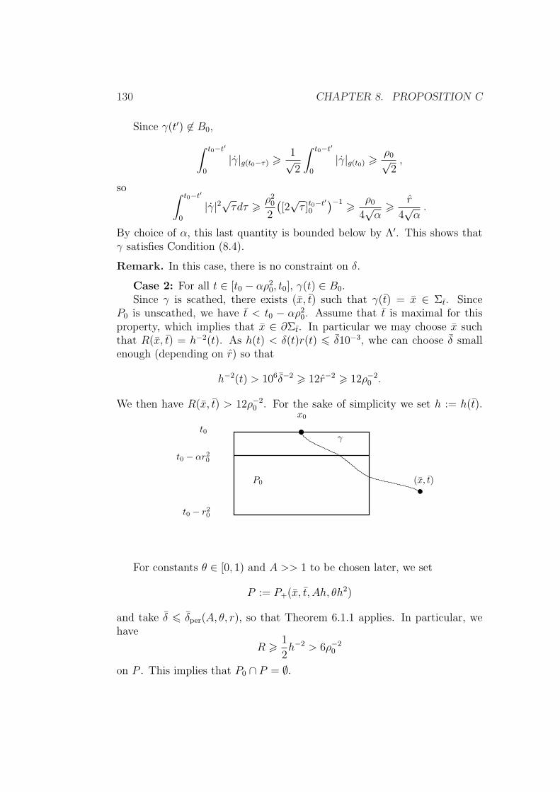
130 CHAPTER 8. PROPOSITION C
Since γ(t′) 6∈ B0,
∫ t0−t′
0
|γ|g(t0−τ) > 1√2
∫ t0−t′
0
|γ|g(t0) > ρ0√2,
so ∫ t0−t′
0
|γ|2√τdτ > ρ20
2
([2√τ ]t0−t
′0
)−1 > ρ0
4√α
> r
4√α.
By choice of α, this last quantity is bounded below by Λ′. This shows thatγ satisfies Condition (8.4).
Remark. In this case, there is no constraint on δ.
Case 2: For all t ∈ [t0 − αρ20, t0], γ(t) ∈ B0.
Since γ is scathed, there exists (x, t) such that γ(t) = x ∈ Σt. SinceP0 is unscathed, we have t < t0 − αρ2
0. Assume that t is maximal for thisproperty, which implies that x ∈ ∂Σt. In particular we may choose x suchthat R(x, t) = h−2(t). As h(t) < δ(t)r(t) 6 δ10−3, whe can choose δ smallenough (depending on r) so that
h−2(t) > 106δ−2 > 12r−2 > 12ρ−20 .
We then have R(x, t) > 12ρ−20 . For the sake of simplicity we set h := h(t).
P0
x0
t0
t0 − αr20
t0 − r20
γ
(x, t)
For constants θ ∈ [0, 1) and A >> 1 to be chosen later, we set
P := P+(x, t, Ah, θh2)
and take δ 6 δper(A, θ, r), so that Theorem 6.1.1 applies. In particular, wehave
R > 1
2h−2 > 6ρ−2
0
on P . This implies that P0 ∩ P = ∅.
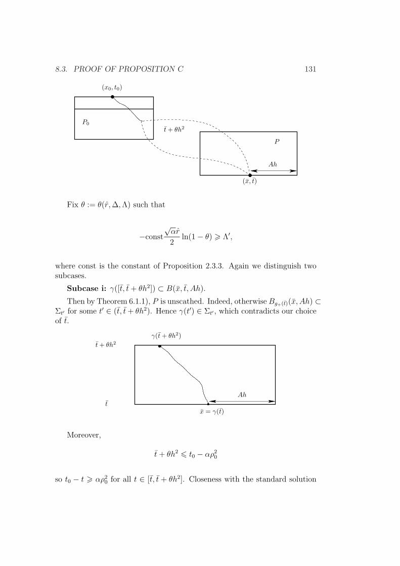
8.3. PROOF OF PROPOSITION C 131
Ah
(x0, t0)
P0
P
(x, t)
t + θh2
Fix θ := θ(r,∆,Λ) such that
−const
√αr
2ln(1− θ) > Λ′,
where const is the constant of Proposition 2.3.3. Again we distinguish twosubcases.
Subcase i: γ([t, t+ θh2]) ⊂ B(x, t, Ah).
Then by Theorem 6.1.1), P is unscathed. Indeed, otherwiseBg+(t)(x, Ah) ⊂Σt′ for some t′ ∈ (t, t+ θh2). Hence γ(t′) ∈ Σt′ , which contradicts our choiceof t.
t
Ah
γ(t + θh2)
x = γ(t)
t + θh2
Moreover,
t+ θh2 6 t0 − αρ20
so t0 − t > αρ20 for all t ∈ [t, t + θh2]. Closeness with the standard solution
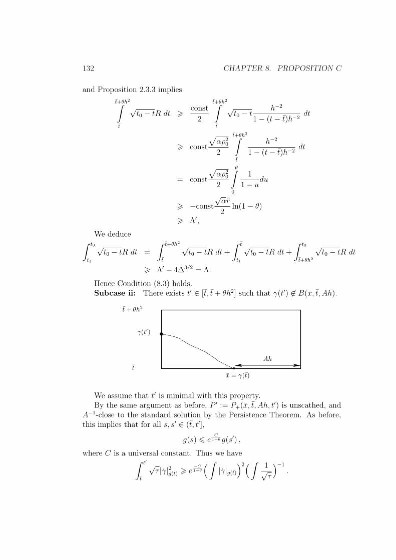
132 CHAPTER 8. PROPOSITION C
and Proposition 2.3.3 implies
t+θh2∫
t
√t0 − tR dt > const
2
t+θh2∫
t
√t0 − t
h−2
1− (t− t)h−2dt
> const
√αρ2
0
2
t+θh2∫
t
h−2
1− (t− t)h−2dt
= const
√αρ2
0
2
θ∫
0
1
1− udu
> −const
√αr
2ln(1− θ)
> Λ′,
We deduce∫ t0
t1
√t0 − tR dt =
∫ t+θh2
t
√t0 − tR dt+
∫ t
t1
√t0 − tR dt+
∫ t0
t+θh2
√t0 − tR dt
> Λ′ − 4∆3/2 = Λ.
Hence Condition (8.3) holds.Subcase ii: There exists t′ ∈ [t, t+ θh2] such that γ(t′) 6∈ B(x, t, Ah).
γ(t′)
Ah
x = γ(t)
t + θh2
t
We assume that t′ is minimal with this property.By the same argument as before, P ′ := P+(x, t, Ah, t′) is unscathed, and
A−1-close to the standard solution by the Persistence Theorem. As before,this implies that for all s, s′ ∈ (t, t′],
g(s) 6 eC
1−θ g(s′) ,
where C is a universal constant. Thus we have∫ t′
t
√τ |γ|2g(t) > e
−C1−θ
( ∫|γ|g(t)
)2( ∫1√τ
)−1
.
8.3. PROOF OF PROPOSITION C 133
Since t′ 6 t0 − αρ20 we bound τ from below by αρ2
0 on [t, t′], so
∫ t′
t
√τ |γ|2 > e
−C1−θ (Ah)2
√αρ2
0(t′−t)−1 > e
−C1−θ (Ah)2 r
10
√α
1
θh2= e
−C1−θ√αrA2
10θ.
Fixing A large enough, Condition (8.4) holds.
A consequence of the previous lemma is the following result (see [44]lemma 78.3 and 78.6 for more details). We shall not give the proof of thisstatement since in the next section a local version, in the spirit of 8.2 of [59],will be sketched.
Lemma 8.3.3. Let r ∈ (0, 10−3,∆,Λ be positive numbers. There existsδ := δ(r,∆,Λ) with the following property. Let g(·) be a Ricci flow withr(·), δ(·)-bubbling-off defined on [a, a + ∆] such that r 6 r(·) < 10−3 andδ(·) 6 δ. Let (x0, t0) and ρ0 > r be such that P0 := P (x0, t0, ρ0,−ρ2
0) isunscathed and |Rm | 6 ρ−2
0 on P0. Then
i) For all (q, t) ∈ M × [a, a + ∆], if `(q, t0 − t) < Λ, then there is anunscathed minimising L-geodesic γ connecting x0 to q.
ii) For all τ > 0, minq `(q, τ) 6 3/2 and is attained.
We come back to the proof of Proposition 8.3. Recall that P0 is un-scathed, and satisfies |Rm | 6 ρ−2
0 . The arguments of [59, Chapter 7] applyto unscathed minimising L-geodesics. In particular, if γ(τ) = Lτ exp(x0,t0)(v)is minimising and unscathed on [0, τ0], then
τ−3/2e−`(v,τ)J(v, τ)
is nonincreasing on [0, τ0].Set
Y (τ) := v ∈ Tx0M ; L exp(v) : [0, τ ] −→M is minimising and unscathed .It is easy to check that τ 6 τ ′ ⇒ Y (τ) ⊃ Y (τ ′). Then we set
Vreg(τ) :=
∫
Y (τ)
τ−3/2e−`(v,τ)J(v, τ)dv .
Thus this function is nondecreasing on [0, t0]. We shall adapt the proof of
κ-noncollapsing in the smooth case, replacing V by Vreg. Set
κ :=volg(t0)B0
ρ30
, τ0 = κ1/3ρ20 .
134 CHAPTER 8. PROPOSITION C
Upper bound on Vreg(τ0): As in the smooth case, we get
Lτ exp
(v ∈ Y (τ) ; |v| 6 1
10κ−1/6
)⊂ B0
thus
I :=
∫
v∈Y (τ) ; |v|6 110κ−1/6
τ−3/2e−`(v,τ)J(v, τ)dv 6 eCκ1/6√
κ
andI ′ :=
∫v∈Y (τ) ; |v|> 1
10κ−1/6
τ−3/2e−`(v,τ)J(v, τ)dv
≤ ∫v∈Y (τ) ; |v|> 1
10κ−1/6
limτ→0(τ−3/2e−`(v,τ)J(v, τ))dv
6 e−110κ−1/6
.
In conclusion,
I + I ′ 6 eCκ1/3√
κ+ e−110κ−1/6
6 C√κ
for κ 6 κ(3) and some universal C.
Lower bound for Vreg(t0) Monotonicity of Vreg(τ0) implies
Vreg(τ0) > Vreg(t0) .
We are going to bound Vreg(t0) from below as a function of volB(q0, 0, 1),where q0 ∈M .
Set Λ = 21 and apply Lemma 8.3.3 with parameter δ(r, T,Λ). Thereexists q0 ∈ M such that `(q0, t0 − 1
16) 6 3
2and the first part of Lemma 8.3.3
gives us a minimising curve γ connecting x0 to q0 realising the minimum`(q0, t0 − 1/16). Let q ∈ B(q0, 0, 1). Consider a curve γ obtained by con-catenating some g(0)-geodesic from (q, 0) to (q0, 1/16) with some minimisingL-geodesic between (q0, 1/16) and (x0, t0). We have
`(q, t0) =L(q, t0)
2√t0
6
1
2√t0L(q0, t0 − 1/16) +
1
2√t0
∫ t0
t0−1/16
√τ(Rg(t0−τ) + |γ(τ)|2g(t0−τ))dτ , (8.5)
8.4. MORE ON κ-NONCOLLAPSING 135
which leads to
`(q, t0) 6 3
2+
1
2
∫ t0
t0−1/16
(12 + e1/2|γ(τ)|2g(0))dτ .
since for s ∈ [0, 1/16] (i.e. τ ∈ [t0−1/16, t0]) the metrics g(s) satisfy Rm 6 2,hence R 6 12, and are 1/2-Lipschitz equivalent. We obtain
`(q, t0) 6 3
2+
1
2
(1
1612 + 16e1/2d2
g(0)(q, q0)
)6 20 .
Hence `(q, t0) < Λ, and Lemma 8.3.3 i) re-gives an unscathed minimisingL-geodesic γ connecting x0 to q. Hence q = γ(t0) = Lt0 exp(v) for v ∈ Y (t0).This shows that Lt0 exp(Y (t0)) ⊃ B(q, 0, 1).
Moreover, we have v ∈ Y (t0) ; Lt0 exp(v) ∈ B(q, 0, 1), ` 6 10, whichimplies
Vreg(t0) =∫Y (t0)
t−3/20 e−`(v,t0)J(v, t0)dv >
∫B(q0,0,1)
t−3/20 e−20dvg(0)
> T−3/2e−20 volg(0)B(q0, 0, 1) .
This completes the proof of Proposition C’.
8.4 κ-noncollapsing at bounded distance of
the thick part
In the previous section we proved a κ-noncollapsing result, for Ricci flow withr(·), δ(·)-bubbling-off defined on [0, T ] and with normalised initial condition.The key point to mention here is that κ = κ(T ). To study the behaviour at+∞ of Ricci flow with bubbling-off defined on [0,+∞), especially if one hasto take limits of such solutions based at (xi, ti) where ti → +∞, one thereforeneed another kind of result, where κ is independant of time but depend onthe distance to the base points, where we assume some volume control. Inthis section we prove such a result (see Theorem 9.0.4a and the statementbelow). In what follows the canonical neighbourhood scale r(t) is assumedto be non increasing.
Theorem 8.4.1. For all A > 0, there exists κ = κ(A) > 0 such that for anyt0 > 0, there exists δ := δ(t0) > 0 decreasing in t0, with the following property.Let g(·) be a Ricci flow with r(·), δ(·)-bubbling-off defined on [0,+∞) such thatδ(t) 6 δ for t ∈ [t0/2, t0]; if the parabolic neighbourhood P (x0, t0, ρ0,−ρ2
0),
136 CHAPTER 8. PROPOSITION C
where 2ρ20 < t0 is unscathed and the solution satisfies |Rm | 6 ρ−2
0 there, andif
volB(x0, t0, ρ0) > A−1ρ30 ,
then the solution is κ-noncollapsed on the scales less than ρ0 in the ballB(x0, t0, Aρ0).
Proof. We can assume that ρ0 > r(t0). Indeed, for ρ0 < r(t0) we can useLemma 8.3.1, with r = r(t0), which provides a universal value of κ. Here weuse that r(t) is chosen to be non increasing.
Since the noncollapsing property is unsensitive to homothety we canparabolically rescale the metric so that ρ0 = 1 and t0 = 1. More precisely weshall work with the flow,
g(t) =1
ρ20
g(t0 − ρ20 + tρ2
0) .
From now on, unless otherwise stated, we work with the flow g. For thesake of simplicity we shall not overline the geometric quantities related tothis metric unless it is necessary.
Let x ∈ B(x0, 1, A) and ρ 6 1 such that |Rm | 6 ρ−2 on P (x, 1, ρ,−ρ−2);let us define, as before,
κ =volB(x, 1, ρ)
ρ3,
and assume that κ 6 κ(3). We aim at showing that there exists C = C(A) >0 such that κ > C(A) > 0. We follow the line of the proof in the previoussection. We look at space-time curves starting from x. As before we consider,
Vreg(τ) :=
∫
Y (τ)
τ−3/2e−`(v,τ)J(v, τ)dv ,
for τ = 1− t ∈ [0, 1] and where,
Y (τ) := v ∈ Tx0M ; L exp(v) : [0, τ ] −→M is minimising and unscathed .
The function Vreg is non increasing in τ . The same computation as beforeyields the upper bound,
Vreg(κ1/3ρ2) 6 C
√κ
for a universal C > 0. Now the monotony of Vreg gives
Vreg(1) 6 Vreg(κ1/3ρ2) 6 C
√κ .
We thus have to estimate from below Vreg(1).
8.4. MORE ON κ-NONCOLLAPSING 137
8.4.1 A formal computation
By the pinched toward positive curvature assumption we have, before rescal-ing,
R > − 6
4t+ 1> − 3
2t,
hence, after rescaling
R > −3
2
ρ20
t0 − ρ20 + tρ2
0
> −3
2
ρ20
t0 − ρ20 + 1
2ρ2
0
for t ∈ [1/2, 1]. Let us recall that t0 > 2ρ20, then
R > −3
2
ρ20
2ρ20 − 1
2ρ2
0
= −1 .
Hence, using that τ = 1− t,
L(y, τ) = 2√τL(y, τ) > −2
√τ
∫ τ
0
√s ds = −4
3τ 2
(here we have neglected the energy of the curve in the definition of L). Wenow define L(y, τ) = L(y, τ) + 2
√τ . Then, for τ ∈ (0, 1/2],
L(y, τ) > −4
3τ 2 + 2
√τ > (−4
3+ 2)
√τ > 0 .
Define h(y, τ) = ψ(dt(x0, y))L(y, τ), where dt(x0, y) = dt(x0, y)− A(2t− 1).Here ψ is a cut-off function equal to 1 on (−∞, 1/20], to +∞ on [1/10,+∞),
non decreasing and smooth where defined. We now follow the computationin [59], 8.2 (page 21) and use the operator
2 :=∂
∂t−∆g(t) ;
it yields
2h > −(L+ 2√τ)C(A)ψ − 6ψ − 1√
τψ
= −C(A)h− (6 +1√τ)ψ dt (8.6)
Where C(A) is a constant depending on A only. At the spatial minimumpoint, with τ fixed, ∆h > 0. Let us define h0(τ) = minh(·, τ). We then have
d
dτ
(log(
h0(τ)√τ
)
)= h−1
0
dh0
dτ− 1
2τ6 C(A) +
6√τ + 1√
τL+ 2τ− 1
2τ.
138 CHAPTER 8. PROPOSITION C
As L > −4/3τ 2
d
dτ
(log(
h0(τ)√τ
)
)6 C(A) +
50√τ.
By integration we get,
log
(h0(τ)√
τ
)− lim
s→0log
(h0(s)√
s
)> C(A)τ + 100
√τ .
Now for s small,
L = L+ 2√s = 2
√sL+ 2
√s > 0 and h = ψL > 2 ,
2 <h0(s)√
s= minψ(2L+ 2) 6 2L(x, s) + 2
since ψ ≡ 1 near x when s is small. Indeed, dt(x0, x) < A and ψ ≡ 1 onB(x0, 0, 1/10 + A).
Now, using a curve which is constant equal to x, we have that,
L(x, s) 6∫ s
0
√sRds −→
s→00
and henceh0(s)√
s−→ 2s→0
which gives,
h0(τ) 6 2√τ exp(C(A)τ + 100
√τ) .
8.4.2 Justification of the formal computations
We now apply Lemma 8.3.2 with the unscaled metric g(t) and with theconstant
Λ = 3 exp(C(A) + 100)
√t02
and r 6 r(t0), ∆ = t0/2. This gives a δ = δ(A, t0) such that every curve γ(τ)starting at x and γ /∈Mreg (in particular γ exits P (x, t0, ρ,−ρ2)) satisfies theunnormalised inequality
Lg(γ) > Λ .
This implies that
Lg(γ) > Λ′ = Λ/√t0/2.
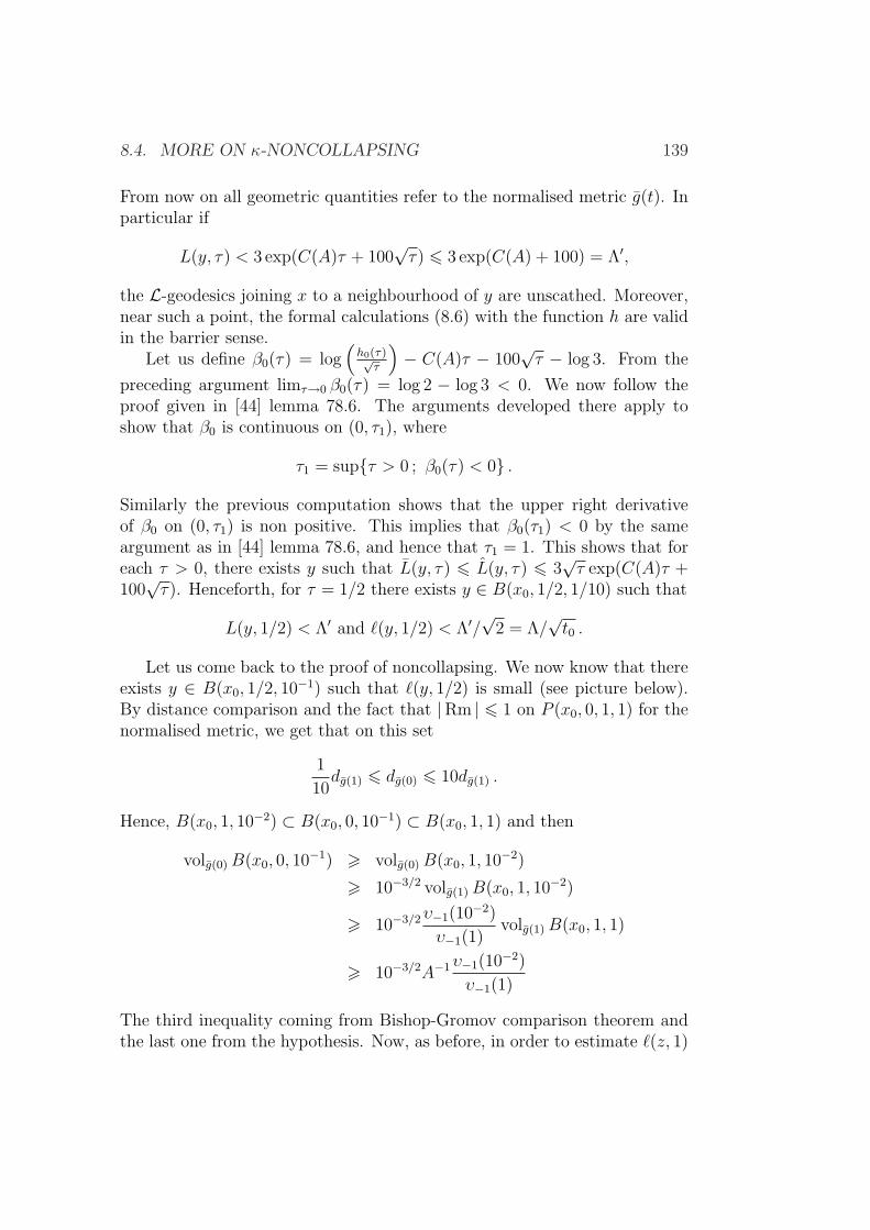
8.4. MORE ON κ-NONCOLLAPSING 139
From now on all geometric quantities refer to the normalised metric g(t). Inparticular if
L(y, τ) < 3 exp(C(A)τ + 100√τ) 6 3 exp(C(A) + 100) = Λ′,
the L-geodesics joining x to a neighbourhood of y are unscathed. Moreover,near such a point, the formal calculations (8.6) with the function h are validin the barrier sense.
Let us define β0(τ) = log(h0(τ)√
τ
)− C(A)τ − 100
√τ − log 3. From the
preceding argument limτ→0 β0(τ) = log 2 − log 3 < 0. We now follow theproof given in [44] lemma 78.6. The arguments developed there apply toshow that β0 is continuous on (0, τ1), where
τ1 = supτ > 0 ; β0(τ) < 0 .
Similarly the previous computation shows that the upper right derivativeof β0 on (0, τ1) is non positive. This implies that β0(τ1) < 0 by the sameargument as in [44] lemma 78.6, and hence that τ1 = 1. This shows that foreach τ > 0, there exists y such that L(y, τ) 6 L(y, τ) 6 3
√τ exp(C(A)τ +
100√τ). Henceforth, for τ = 1/2 there exists y ∈ B(x0, 1/2, 1/10) such that
L(y, 1/2) < Λ′ and `(y, 1/2) < Λ′/√
2 = Λ/√t0 .
Let us come back to the proof of noncollapsing. We now know that thereexists y ∈ B(x0, 1/2, 10−1) such that `(y, 1/2) is small (see picture below).By distance comparison and the fact that |Rm | 6 1 on P (x0, 0, 1, 1) for thenormalised metric, we get that on this set
1
10dg(1) 6 dg(0) 6 10dg(1) .
Hence, B(x0, 1, 10−2) ⊂ B(x0, 0, 10−1) ⊂ B(x0, 1, 1) and then
volg(0)B(x0, 0, 10−1) > volg(0)B(x0, 1, 10−2)
> 10−3/2 volg(1)B(x0, 1, 10−2)
> 10−3/2υ−1(10−2)
υ−1(1)volg(1)B(x0, 1, 1)
> 10−3/2A−1υ−1(10−2)
υ−1(1)
The third inequality coming from Bishop-Gromov comparison theorem andthe last one from the hypothesis. Now, as before, in order to estimate `(z, 1)
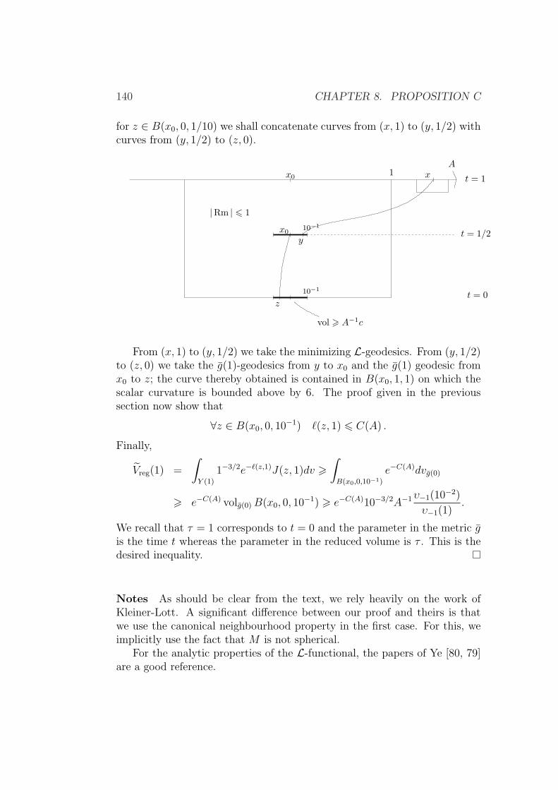
140 CHAPTER 8. PROPOSITION C
for z ∈ B(x0, 0, 1/10) we shall concatenate curves from (x, 1) to (y, 1/2) withcurves from (y, 1/2) to (z, 0).
t = 1/2
|Rm | 6 1
vol > A−1c
x0 x
x0
t = 1
t = 0z
y
A
10−1
10−1
1
From (x, 1) to (y, 1/2) we take the minimizing L-geodesics. From (y, 1/2)to (z, 0) we take the g(1)-geodesics from y to x0 and the g(1) geodesic fromx0 to z; the curve thereby obtained is contained in B(x0, 1, 1) on which thescalar curvature is bounded above by 6. The proof given in the previoussection now show that
∀z ∈ B(x0, 0, 10−1) `(z, 1) 6 C(A) .
Finally,
Vreg(1) =
∫
Y (1)
1−3/2e−`(z,1)J(z, 1)dv >∫
B(x0,0,10−1)
e−C(A)dvg(0)
> e−C(A) volg(0)B(x0, 0, 10−1) > e−C(A)10−3/2A−1υ−1(10−2)
υ−1(1).
We recall that τ = 1 corresponds to t = 0 and the parameter in the metric gis the time t whereas the parameter in the reduced volume is τ . This is thedesired inequality.
Notes As should be clear from the text, we rely heavily on the work ofKleiner-Lott. A significant difference between our proof and theirs is thatwe use the canonical neighbourhood property in the first case. For this, weimplicitly use the fact that M is not spherical.
For the analytic properties of the L-functional, the papers of Ye [80, 79]are a good reference.
Part III
Long time behaviour of Ricciflow with bubbling-off
141

143
The goal of this part is to prove the thick-thin decomposition Theorem0.3.2. To do this, we use the Ricci flow with bubbling-off provided by longtime existence Theorem 3.4.1. We shall need to choose the parameter func-tions r(·) and δ(·) carefully in order to have the necessary estimates.
In chapter 9 we state the corresponding refined results on the long timebehaviour of Ricci flow with bubbling-off, which are the most technical the-orems of this book (and of Perelman’s work). This corresponds to section 6of [61].
In chapter 10 we prove the thick-thin decomposition Theorem assumingthe technical results.
Finally, we prove the technical theorems in chapter 11. One of them givesversions of the κ-non collapsing, curvature-distance estimates and the canon-ical neighbourhood property at space-time points where the time multipliedby the curvature is large. The second one essentially shows that certainparabolic neighbourhoods in the thick part are unscathed and with boundedgeometry. This is used to show that on the thick part the rescaled metricconverges towards the hyperbolic metric.

144
Chapter 9
Thin-thick decomposition
First we recall the definitions of thick and thin parts that we are using.1
Let (X, g) be a Riemannian manifold and ε > 0. We call ε-thin part ofX the subset X−(ε) of points x ∈ X for which there exists 0 < ρ ≤ 1 suchthat the ball B(x, ρ) has sectional curvature > −ρ−2 and volume < ερ3. Itscomplementary is called the ε-thick part and denoted by X+(ε).
The goal is now to prove the following theorem announced in the intro-duction of this book.
Theorem 9.0.1 (Thin-Thick decomposition, Theorem 0.3.2). Let M be aclosed, irreducible, non-spherical 3-manifold and g0 a normalised metric onM . There exists a Ricci flow with bubbling-off g(·) on [0,+∞) with g0 asinitial condition, and such that:
i. There exists C > 0 such that vol(g(t)) 6 Ct3/2.
ii. Let w > 0, xn ∈ M and tn → +∞. If xn is in the w-thick partof (M, 1
tng(tn)) for every n, then the sequence of pointed manifolds
(M, 1tng(tn), xn) converges in C∞ topology towards a pointed, complete
and finite volume manifold, with sectional curvature equal to −1/4.
iii. For all w′ > 0 there exists r > 0, K0, K1 > 0 and t0 < ∞ such thatfor all t > t0, for all x ∈ M , for all r ∈ (0, r), if the ball centredat x and of radius r in (M, 1
tg(t)) has volume at least w′r3 and if the
sectional curvatures on it are bounded below by −r−2, then the sectionalcurvature at x is bounded above by K0r
−2 and its covariant derivativeby K1r
−3.
1As already remarked, our definitions differ slightly from those of [61].
145
146 CHAPTER 9. THIN-THICK DECOMPOSITION
Since we assume M to be non-spherical, Theorem 3.4.1 yields for ev-ery normalised initial condition a Ricci flow with r(·), δ(·)-bubbling-off on[0,+∞). The given function r(t) is now fixed forever. Note that it is non-increasing. Having the freedom of choosing δ(t) going to zero when t goesto infinity as steeply as we need, Theorem 9.0.1 is then an immediate conse-quence of Theorem 3.4.1 and of the following result:
Theorem 9.0.2. Let M be a closed, irreducible and non-spherical 3-manifold.There exists a function t 7→ δ(t) such that if r(·), δ(·) are step functions suchthat δ(t) 6 δ(t) for all t, and g(·) is a Ricci flow with r(·), δ(·)-bubbling-offon M defined on [0,∞) with normalised initial condition, then g(·) satisfiesassertions (i)–(iii) of theorem 9.0.1.
The proof of this theorem is given in Chapter 10. We shall need thefollowing technical results, whose proof is involved and which correspond toSection 6 of [61].
We begin with a lemma which has nothing to do with Ricci flow, but withAlexandrov spaces.
Lemma 9.0.3 (Sub-ball Lemma). For all w > 0, there exists θ0 = θ0(w) >0, such that if B(x, 1) is a ball with volume at least w, which is relativelycompact in a manifold without boundary whose sectional curvature is boundedbelow by −1, then, there exists a B(y, θ0) ⊂ B(x, 1), such that every sub-ballB(z, r) ⊂ B(y, θ0) of any radius r > 0 has volume bounded below by (1− ε0)times the volume of a Euclidean ball of the same radius.
We will say that B(z, r) has (1− ε0)-almost Euclidean volume.The next result contains versions of the no-local-collapsing theorem, of
the canonical neighbourhood theorem, and of the curvature distance theorem,for points of possibly “low” curvature but with large time.
Theorem 9.0.4 (Proposition 6.3 in [61]). For all A <∞ there exist positivenumbers κ, K, K ′, r and a nonincreasing function t 7→ δA(t) with the follow-ing property. Let (M, g(·)) be a Ricci flow with r(·), δ(·)-bubbling-off withnormalised initial condition, and let (x, t, ρ) with the following properties.Assume that 0 < ρ <
√t/2, that δ(·) < δA(t) on [t/2, t], and that
i) P (x, t, ρ,−ρ2) is unscathed,
ii) |Rm | 6 ρ−2 there,
iii) vol(B(x, t, ρ)) > A−1ρ3.
Then:
147
a) The solution is κ-non-collapsed at scales 6 ρ in B(x, t, Aρ) ;
b) every point of B(x, t, Aρ) whose scalar curvature is bounded below byKρ−2 admits a canonical neighbourhood ;
c) if ρ 6 r√t, then R 6 K ′ρ−2 in B(x, t, Aρ).
From now on, we set
δ(t) := min
δ2t(2t), η(t)
r(4t)
r(t)
, (9.1)
where η : [0,∞) −→ (0, 1] is some fixed decreasing function such that η(t) →0 as t→ +∞.
Remark. The first condition ensures that a Ricci flow with r(·), δ(·)-bubbling-off with δ(·) 6 δ(·) satisfies Theorem 9.0.4 at time t for A 6 t.
Theorem 9.0.5 (Curvature control in thick part, cf. Corollary 6.8 of [61]).For all w > 0, there exist positive numbers τ , θ, K, r, T with the followingproperty. Assume that g(t) is a Ricci flow with r(·), δ(·)-bubbling-off on[0,∞), with normalised initial condition and δ(·) ≤ δ(·). Let x ∈ M , t > T ,r > 0 such that
i) θ−1h 6 r 6 r√t, where h is the maximal surgery radius on [t/2, t],
ii) Rm > −r−2 on B(x, t, r),
iii) volB(x, t, r) > wr3.
Then P (x, t, r,−τ r2) is unscathed and |Rm | < Kr−2 there.
Remark. The radius of the parabolic neighbourhood is r/4 in Corollary 6.8of [61]. In fact, one can put Ar for any A > 0 if one allows the parametersto depend on A. For convenience, the control on the curvature is extendedto |Rm |.
Those technical results are proved in Chapter 11.

148 CHAPTER 9. THIN-THICK DECOMPOSITION
Chapter 10
Geometry of the thick part
In this chapter we assume the Sub-ball Lemma 9.0.3 and Theorems 9.0.4and 9.0.5, and we shall prove Theorem 9.0.2. Recall that the function δ(·) hasbeen fixed by equation (9.1) in the previous chapter. We also fix a closed, irre-ducible, non-spherical 3-manifold M and a Ricci flow with r(·), δ(·)-bubbling-off g(·) on M defined on [0,∞) with normalised initial condition. We assumethat δ(t) 6 δ(t) for all t.
For convenience, we restate Theorem 9.0.2:
Theorem 10.0.1. Let M and g(t)t∈[0,+∞) be as above. Then
i. There exists C > 0 such that vol(g(t)) 6 Ct3/2.
ii. Let w > 0, xn ∈ M and tn → +∞. If xn is in the w-thick partof (M, 1
tng(tn)) for every n, then the sequence of pointed manifolds
(M, 1tng(tn), xn) converges in C∞ topology towards a pointed, complete
and finite volume manifold, with sectional curvature equal to −1/4.
iii. For all w′ > 0 there exists r > 0, K0, K1 > 0 and t0 < ∞ such thatfor all t > t0, for all x ∈ M , for all r ∈ (0, r), if the ball centredat x and of radius r in (M, 1
tg(t)) has volume at least w′r3 and if the
sectional curvatures on it are bounded below by −r−2, then the sectionalcurvature at x is bounded above by K0r
−2 and its covariant derivativeby K1r
−3.
10.1 Consequences of the maximum principle
In this section we prove some preliminary results, following Section II.7.1 of[61] and [44], and obtain that g(·) satisfies Conclusion i) of Theorem 10.0.1.
149
150 CHAPTER 10. GEOMETRY OF THE THICK PART
Recall that R = RminV2/3. Note that at a singular time, Rmin and V may
be discontinous, but Rmin (resp. V ) can only go up (resp. down) by definitionof a Ricci flow with bubbling-off.
Below we gather some easy results that use only the fact that g(·) is aRicci flow with bubbling-off having normalised initial condition.
Proposition 10.1.1. i. Rmin(t) is bounded below by −64t+1
.
ii. R(t) is nondecreasing.
iii. V (t)(t+ 14)−
32 is nonincreasing.
Proof. (i) Follows from integrating the first equation of Corollary B.2.2 be-tween singular times and the fact that at a singular time, the left limit ofRmin is always less than or equal to its right limit.
Next note that If Rmin(t) became positive for some t, then by the samereasoning, we would obtain an a priori lower bound for Rmin(t) which goesto infinity in finite time. Since we are assuming that g(·) is defined on thewhole of [0,+∞), this implies that Rmin(t) stays nonnegative.
Thus (ii) follows from (B.3) of Corollary B.2.2 and the remark aboveabout the semicontinuity of Rmin at singular times.
From (B.1) of the same corollary and i), we get that if t is a regular time,then
V ′
V6 −Rmin 6 6
4t+ 1,
hence(V (t)(4t+ 1)−
32
)′= V ′(4t+ 1)−
32 − V 6(4t+ 1)−
52
= (4t+ 1)−32
(V ′ − 6V
4t+ 1
)6 0.
This proves (iii).
Thanks to Proposition 10.1.1(iii), we know that the function V (t)(t+ 14)−
32
is bounded. Hence V (t)t−32 is also bounded. Thus we have already proved
the first assertion of Theorem 10.0.1.Next we will show that whenever local limits exist (as t → +∞), they
are hyperbolic. Along the way, we prove a few other useful facts.Set R = lim R(t) and V = limV (t)(t + 1
4)−
32 where the limits are taken
when t→∞.
Lemma 10.1.2. If V > 0 then RV − 23 = −3
2and Rmin(t) ∼ − 3
2t.
10.1. CONSEQUENCES OF THE MAXIMUM PRINCIPLE 151
Proof. One has
RV − 23 = lim
t→∞Rmin(t)V (t)
23
(V (t)(t+
1
4)−
32
)− 23
= limt→∞
Rmin(t)(t+1
4)
> −3
2,
by Corollary B.2.2. Assume that RV − 23 = c > −3
2. Then Rmin(t)(t + 1
4) >
−32
+ µ for some µ > 0 and t > t0. From V ′V −1 6 −Rmin, one has
V ′
V6
(3
2− µ
)(t+
1
4)−1,
hence
V (t) 6 V (t0)(t+1
4)
32−µ.
But then
V (t)(t+1
4)−
32 6 V (t0)(t+
1
4)−µ → 0,
contradicting the assumption V > 0.
Proposition 10.1.3. Let 0 < r < 1 and P (xk, tk, r√tk,−r2tk) be a sequence
of parabolic neighbourhoods such that, when rescaled by 1/tk, it converges inC2-topology to a solution P (x∞, 1, r,−r2). Then all sectional curvatures ofthe limit equal to −1/4t, for all t ∈ [1− r2, 1].
Proof. Let us prove first that under the previous assumptions, V > 0. Denoteby gk the rescaled metric 1
tkg(tk). Then
V (tk)(tk +1
4)−
32 ∼ vol(gk) > volBgk
(xk, 1, r) → volB(x∞, 1, r) > 0.
Lemma 10.1.4. R is spatially constant on P (x∞, 1, r,−r2).
Proof. Suppose not. Then there exist s0 ∈ [1− r2, 1], c < 0 and µ > 0 suchthat
∀s ∈ [s0 − µ, s0 + µ],
∫
B(x∞,s,r)Rmin
∗(s)−R(x, s) dvg∞ < c,
152 CHAPTER 10. GEOMETRY OF THE THICK PART
where Rmin∗(s) = minR(x, s) | x ∈ B(x∞, s, r). Hence for large k,∫
B(xk,s tk,r√tk)
Rmin∗(s tk)−R(x, s tk) dvg(s tk) <
c
2
√tk,
where now Rmin∗(stk) = minR(x, s tk) | x ∈ B(xk, s tk, r
√tk) > Rmin(s tk)
Thus, ∫
B(xk,stk,r√tk)
Rmin(s tk)−R(x, s tk) dvg(s tk) <c
2
√tk, (10.1)
After passing to a subsequence, we can suppose
tk+1
tk>s0 + µ
s0 − µ,
that is tk+1(s0 − µ) > tk(s0 + µ). Then
R− R(0) =
∫ ∞
0
dR
dtdt
>∞∑
k=0
∫ tk(s0+µ)
tk(s0−µ)
dR
dtdt
=∞∑
k=0
∫ tk(s0+µ)
tk(s0−µ)
2
3R(t)V −1(t)
∫
M
(Rmin(t)−R(x, t)) dv dt
=∞∑
k=0
∫ s0+µ
s0−µ
2
3R(s tk)V
−1(s tk)
∫
M
(Rmin(s tk)−R(x, s tk)) dv tk ds
>∞∑
k=0
tk
∫ s0+µ
s0−µ
2
3R(s tk)V
−1(s tk)
∫
B(xk,s tk,r√tk)
(Rmin(s tk)−R(x, stk)) dv ds
> 2
3
∞∑
k=0
tk
∫ s0+µ
s0−µR(s tk)V
−1(s tk)c
2
√tk ds
=c
3
∞∑
k=0
∫ s0+µ
s0−µR(s tk)V
−1(s tk)t32k ds
UsingR(s tk) −→
k→∞R,
andV −1(s tk)t
32k = V −1(s tk)(s tk)
32 s−
23 −→k→∞
V −1s−23
and c R(s tk) > 0, we find that for some large k0 ∈ N,
R− R(0) > c R V −1
4
∞∑
k=k0
∫ s0+µ
s0−µs−
23 ds = +∞,
10.2. PROOF OF THE EXISTENCE OF LIMITS 153
which gives the contradiction.
As Rmin(t) ∼ − 32t
in (M, g(t)) by Lemma 10.1.2 , it follows that R(t) >− 3
2ton P (x∞, 1, r,−r2). Indeed,
Rmingk(t) = tkRming(tkt) ∼
k→∞tk−3
2tkt= − 3
2t.
If there exists s0 ∈ [1 − r2, 1] such that R(s0) >3
2s0, we can argue as
above from (10.1), replacing Rmin∗ by − 3
2s, to get a contradiction.
Hence R(t) = − 32t
on P (x∞, 1, r,−r2). Putting this in Equation (ii) ofProposition B.2.1, we get
3
2t2= 2|Ric0 |2 +
2
3(− 3
2t)2
and then |Ric0 |2 = 0 on P (x∞, 1, r,−r2). It follows that Ric = R3g = − 1
2tg,
finishing the proof of Proposition 10.1.3.
10.2 Proof of the existence of limits
In this section we continue the proof of Theorem 10.0.1, showing that g(t)satisfies Conclusion (ii).
Definition. If ξ > 0, we say that g(·) is ξ-almost hyperbolic at (x, t) if|2tRic(x) + g(t)(x)|g(t) < ξ.
Remark.
|2tRic(x) + g(t)(x)|g(t) = 2‖Ric(x) +g(t)
2t(x)‖t−1g(t) < ξ,
which means that the sectional curvatures of g(t)t
are close to −1/4t up toξ/2.
Proposition 10.2.1. For all w, r, ξ, A there exists positive numbers Λ, τ andT with the following property. Let x ∈M and t > T be such that
i) volB(x, t, r√t) > w(r
√t)3,
ii) Rm > −(r√t)−2 on B(x, t, r
√t).
Then
154 CHAPTER 10. GEOMETRY OF THE THICK PART
a) P (x, t, Ar√t,−τ(r√t)2) is unscathed and |Rm | < Λ(r
√t)−2 there,
b) g(·) is ξ-almost hyperbolic at every point of B(x, t, Ar√t).
Proof. We start by proving a local version of the proposition. In order tosimplify the statement, if w′ > 0 we denote
K ′ = K(w′), τ ′ = τ(w′), r′ = r(w′),
the parameters given by Theorem 9.0.5.
Lemma 10.2.2. For all w′ > 0, 0 < r < r′ and ξ > 0, there exists T ′ =T ′(w′, r, ξ) with the following property. Let x ∈M and t > T such that
i) volB(x, t, r√t) > w(r
√t)3,
ii) Rm > −(r√t)−2 on B(x, t, r
√t).
Then
a) P (x, t, r√t,−τ ′(r√t)2) is unscathed and |Rm | < K ′(r
√t)−2 there,
b) g(·) is ξ-almost hyperbolic at (x, t).
Proof of Lemma 10.2.2. Part a) follows from Theorem 9.0.5 if one has, forθ′ = θ(w),
θ′−1h 6 r√t 6 r′
√t.
where h = max[t/2,t]
h(s) = h(t/2). As h(t/2) 6 δ(t/2)r(t/2) 6 δ(t/2) −→ 0 as
t→∞, it clearly holds true for t larger than some T (w′, r) > 0.Now assume part b) of the lemma is false. Then there exist sequences of
times tk → +∞ and balls B(xk, tk, r√tk) satisfying i) and ii) but such that
(M, gk(tk)) is not ξ-almost hyperbolic at (xk, tk). By part a), the neighbour-hoods P (xk, tk, r
√tk,−τ ′(r
√tk)
2) are unscathed and |Rm | 6 K ′(r√tk)
−2
there for large k. It follows that, after normalising g(·) by tk to get gk(·) =tk−1g(tk·), the sequence of parabolic neighbourhoods P (xk, 1, r,−τ ′r2) satis-
fies the assumptions of the local compactness theorem B.3.2. Hence it sub-converges towards a Ricci flow g∞(·) defined on a neighbourhoodP (x∞, 1,−r,−τ ′r2). Then Proposition 10.1.3 applies to a smaller neighbour-hood P (xk, 1, r
′,−r′2) ⊂ P (x∞, 1,−r,−τ ′r2) converging to P (x∞, 1, r′,−r′2)and show that g∞(t) has constant sectional curvature equals to − 1
4tthere.
Thus we get a contradiction at (xk, tk) for k large enough.
10.2. PROOF OF THE EXISTENCE OF LIMITS 155
Let us come back to the proof of Proposition 10.2.1. We need to extendthe conclusion of the lemma to any radius r (allowing r > r′) and to anypoint of B(x, t, Ar
√t). Concerning the first question, let us recall that by
Bishop-Gromov inequality (cf. Lemma 8.1.1), for any B(x, r) ⊂ (Xn, g), ifRm > −r−2 on a ball B(x, r) and if volB(x, r) > w rn, then for all r′ ∈ (0, r),volB(x, r′) > cnw r
′n, where cn ∈ (0, 1] is a universal constant. Then givenw > 0, r > 0, if one sets
w′ = c3w and r′ = minr, r′,for any ξ > 0, Lemma 10.2.2 applies to B(x, t, r′
√t) if t > T ′(w′, r′, ξ) = T1.
It gives that P (x, t, r′√t,−τ ′(r′√t)2) is unscathed and |Rm | 6 K ′(r′
√t)−2
there, and that g(·) is ξ-almost hyperbolic at (x, t).Fix A > 0. We need to enlarge the ball where we have the conclusion
to B(x, t, Ar√t). Unfortunately we cannot use part c) of Theorem 9.0.4, as
we’ll explain below. Instead we use part b). The idea is then to apply Lemma10.2.2 again on the B(x, t, A′ρ/3), once the curvature is suitably controlled.Let us choose a radius which satisfies assumptions of Theorem 9.0.4. Define
B = minK ′− 12 , τ ′
12,
ρ = B r′√t, .
so that P (x, t, ρ,−ρ2) is unscathed and |Rm | 6 ρ−2 there. Clearly ρ <√t/2.
DefineA′ = max3AB−1rr′−1, w′−1,
which gives
A′ρ > 3Ar√t and volB(x, t, ρ) > A′−1ρ3.
Finally, recall that by our definition of δ(·) in (9.1), Theorem 9.0.4 applieswith data A′ if t > A′. Define T2 = maxA′, T1 and assume t > T2. Here wecan remark that we cannot apply part c) as it is required that ρ 6 r(A′)
√t,
or equivalently Br′ 6 r(A′), and we want A′Br′ > 3Ar. But we do not knowanything about the quantity A′r(A′). Anyway, letting K = maxK(A′), 10,we obtain by part b) that any point (y, t) ∈ B(x, t, A′ρ) where R(y, t) >Kρ−2 = Q is centre of a (ε0, C0)-canonical neighbourhood. Define
B′ = C0− 1
2 K− 12 ,
r′′ = minB′Br′, r(C0−1),
T3 = maxT ′(C0−1, r′′, 10−1), T2.
Claim 5. R < Q on B(x, t, A′ρ) if t > T3.
156 CHAPTER 10. GEOMETRY OF THE THICK PART
Proof. By contradiction. As R(x, t) 6 6ρ−2 < Q, we can pick (y, t) ∈B(x, t, A′ρ) such that R(y, t) = Q. Then (y, t) is the centre of a (ε0, C0)-canonical neighbourhood U ⊃ B(y, t, C−1
0 Q−1/2), and R(·, t) ∈ [C−10 Q,C0Q]
on U . From the Pinching Lemma 2.4.3, |Rm | 6 C0Q on U . Define
ρ′ = r′′√t 6 B′ρ,
and note that Rm > −C0Q > −ρ′−2 on B(y, t, ρ′). Moreover, by propertiesof the canonical neighbourhoods, volB(y, t, ρ′) > C0
−1ρ′3. As t > T3, Lemma10.2.2 applies on B(y, t, ρ′) and says that g(·) is 10−1-almost hyperbolic at(y, t). But this is not possible in a canonical neighbourhood.
Hence we have R < Q on B(x, t, A′ρ) if t > T3. By the Pinching Lemma,
Rm > −Q = −Kρ−2 on this ball. Now let σ = K− 12ρ, so Rm > −σ−2, and
let y ∈ B(x, t, A′ρ3
). By Bishop-Gromov’s Theorem one has,
volB(y, t, σ)
volB(y, t, 2A′ρ3
)> v−σ−2(σ)
v−σ−2(2A′ρ3
)
=v−1(1)
v−1(2A′ρ
3σ−1)
> v−1(1)
v−1(2A3K1/2)
= D.
Since B(y, t, 2A′ρ3
) ⊃ B(x, t, A′ρ3
) ⊃ B(x, t, ρ), we deduce
volB(y, t,2A′ρ
3) > volB(x, t, ρ) > w′ρ3,
hencevolB(y, t, σ) > Dw′ρ3 = Dw′k
32σ3.
It follows that for any σ′ ∈ (0, σ), we have
volB(y, t, σ′) > c3Dw′k
32σ′3 = w′′σ′3.
Define
r′′ = r(w′′),
r′′ = minK− 12Br, r′′,
T4 = maxT ′(w′′, r′′, ξ), T3,K ′′ = K(w′′),
τ ′′ = τ(w′′).
10.2. PROOF OF THE EXISTENCE OF LIMITS 157
As σ′ = r′′√t 6 σ, Lemma 10.2.2 applies on B(y, t, r′′
√t) and gives that
P (y, t, r′′√t,−τ ′′(r′′√t)2) is unscathed and |Rm | 6 K ′′(r′′
√t)−2 there, and
that g(·) is ξ-almost hyperbolic at (y, t). Thus, if one sets
τ = τ ′′(r′′
r
)2
, Λ = K ′′(r′′
r
)−2
, and T = T4,
and one recalls that (y, t) is an arbitrary point of B(x, t, A′ρ3
) ⊃ B(x, t, Ar√t),
it is clear now that the conclusion of Proposition 10.2.1 holds onP (x, t, Ar
√t,−τ(r√t)2).
Recall that x ∈ X is in the w-thick part of (X, g) if for all ρ ∈ (0, 1) suchthat Rm > −ρ−2 on B(x, ρ), one has volB(x, ρ) > wρ3. We also recall thatw′ = c3w.
Lemma 10.2.3. For all w > 0 there exist ρ > 0 and T < ∞ such that forall t > T , if x is in the w-thick part of (M, 1
tg(t)), then the ball B(x, t, ρ
√t)
has its volume bounded below by w′(ρ√t)3 and sectional curvatures bounded
below by −(ρ√t)−2.
Proof. We observe that the assertion on the volume follows from the assertionon the sectional curvatures. Indeed, by definition if x is in the w-thick partof (M, 1
tg(t)), for all ρ ∈ (0, 1) one has volB(x, t, ρ
√t) > w(ρ
√t)3 if Rm >
−(ρ√t)−2 on this ball. This is in particular true for ρ = ρ.
In order to obtain the lower bound on the sectional curvatures we argue bycontradiction. Let us assume that the assertion fails. We choose a sequenceρk of real numbers in (0, 1) going to 0, times tk > 0 going to +∞ such thattkρ
−2k → +∞ and points xk in the w-thick part of (M, 1
tkg(tk)) such that for
each integer k, the sectional curvatures are not bounded below by −(ρk√tk)
2
on the ball B(xk, tk, ρk√tk). Let ρ′k ∈ (0, ρk) such that infRm(y, tk) | y ∈
B(xk, tk, ρ′k
√tk) = −(ρ′k
√tk)
2. Let rk = ρ′k√tk such that the infimum of
the sectional curvatures of Rm(·, tk) on B(xk, tk, rk) is equal to −rk−2. Weremark that tkrk
−2 = ρ′k−2 → ∞. Let yk ∈ B(xk, tk, rk) be a point where
the minimum is achieved. We shall apply theorem 9.0.5, showing first thatrk > θ−1(w)hk, where hk is the maximum of the surgery radii on [tk/2, tk].
Assertion 10.2.4. rk > θ−1(w)hk.
Proof. We assume that rk < θ−1(w)hk. In particular rk−2 > θ2hk
−2 > r(tk)−2
is the canonical neighbourhood radius for all large enough k. as curvature ispinched towards positive, Equation (2.8) implies that
R(yk, tk)
rk−2> 1
2
(log((1 + tk)rk
−2)− 3) → +∞ (10.2)
158 CHAPTER 10. GEOMETRY OF THE THICK PART
Let us show that infB(xk,tk,rk)R(·, tk) rk2 also goes to +∞. If this is not true,then let c ∈ (1,+∞) and x′k ∈ B(xk, tk, rk) be such that R(x′k, tk) < crk
−2.We consider a point zk on the segment [yk, x
′k] such that R(zk, tk) = crk
−2.We apply the curvature-distance theorem to (zk, tk) with A = 2c1/2. Sinceevery point where the scalar curvature is greater than R(zk, tk) has a (ε0, C0)-canonical neighbourhood, when (1 + tk)R(zk, tk) > Q(A, ε0, C0), we get theupper bound R 6 Λ(A, ε0, C0)R(zk, tk) on the ball B(zk, tk, AR(zk, tk)
−1/2) =B(zk, tk, 2rk). In particular R(yk, tk) 6 Λcrk
−2 which is a contradiction.Hence infB(xk,tk,rk)R(·, tk) rk2 →∞.
From that we deduce that for k large enough, the scalar curvature onB(xk, tk, rk) is much greater than rk
−2. This implies that each point ofthe ball is the centre of a (ε0, C0)-canonical neighbourhood, of size muchsmaller than rk. We now recall that xk is in the w-thick part of (M, 1
tkg(tk))
and hence that volB(xk, tk, rk) > wrk3 by the very definition of rk. Sub-
ball Lemma 9.0.3 applied to the ball of half radius normalised by rk/2yields a ball B(yk, tk, θ0(w)rk/2) ⊂ B(xk, tk, rk) whose all sub-ball B(z, r) ⊂B(yk, tk, θ0(w)rk/2) have (1 − ε0)-almost Euclidean volume. But if we con-sider a sub-ball B(z, r) in a ε0-neck included in B(yk, tk, θ0(w)rk/2) withr = ε0
−1R(z, tk) being the radius of the ε0-neck, we obtain that volB(z, r) ≈ε0−12r is much less than r3. This contradicts the hypothesis rk < θ−1(w)hk.
Since ρ′k → 0, one has θ−1(w)hk 6 rk = ρ′k√tk 6 r(w′)
√tk. From
Theorem 9.0.5, the scalar curvature is 6 Krk−2 on P (xk, tk, rk,−τ rk2). From
that we deduce, as in the proof of proposition 10.2.1, that |Rm | 6 r′k−2 sur
P (xk, tk, r′k,−r′k2), where r′k ∈ (0, rk) is bounded below in terms of rk, K and
τ . Theorem 9.0.4 c) applied with a constant A > 2rkr′k
with k large enough in
order to have r′k>r(A)√tk implies that R < K ′r′k
2 on B(xk, tk, Ar′k). We thus
have R < crk−2 on B(xk, tk, rk), and in particular at yk. This contradicts
(10.2) and finishes the proof of Lemma 10.2.3,
In order to prove that g(t) satisfies Conclusion ii) of Theorem 10.0.1, itsuffices to apply Proposition 10.2.1 with r = ρ and Hamilton’s compactnesstheorem B.3.1.
10.3 Proof of the controlled curvature in the
sense of Perelman
To finish the proof of Theorem 10.0.1, we need to check Conclusion iii), i.e. forevery w′ > 0 there exist r > 0, K0, K1 > 0 and t0 < ∞ such that for all
10.3. PROOF OF THE CONTROLLED CURVATURE 159
t > t0, for all x ∈ M , for all r ∈ (0, r], if the ball of radius r centred at x in(M, 1
tg(t)) has volume at least w′r3 and if the sectional curvatures there are
bounded below by −r−2, then the sectional curvature at x is bounded aboveby K0r
−2 and its covariant derivative by K1r−3.
Recall that we assume that δ(·) 6 δ(·) where δ(·) has been defined at theend of Section 9. We set r = r(w′) given by theorem 9.0.5. Let t > T (w′),r ∈ (0, r
√t] and B(x, r) a ball in (M, g(t)) with volume bounded below
by w′r3 and sectional curvature bounded below by −r−2. We denote h themaximum of the function h(·) on[t/2, t]. If r > θ−1h, Theorem 9.0.5 assertsthat the neighbourhood P (x, t, r,−τ r2) is unscathed and |Rm | < Kr−2. Thebound on the covariant derivative follows then from Shi’s estimate (see [51,Theorem 3.29]). In the sequel we argue by contradiction, assuming r 6 θ−1h.Let (xk, tk), tk → +∞, rk ∈ (0, r
√tk] such that rk 6 θ−1hk, be a sequence of
counter-examples. Up to taking a subsequence there are two cases.
Case 1 rk 6 θ−1hk and R(xk, tk) > r(tk)−2.
We then have that (xk, tk) is the centre of a canonical neighbourhood. Theproperty (2.4) leads to |∇Rm | < C0|Rm |3/2 on this neighbourhood, and inparticular at (xk, tk). Thus it suffices to estimate from above |Rm(xk, tk)|by constrk
−2, and for this to show that R(xk, tk) is bounded above by crk−2,
where c depends on w′ only. We argue by contradiction and assume thatR(xk, tk)rk
−2 → +∞ (possibly after taking a sub-sequence). Then we canrepeat the proof of Lemma 10.2.3, starting at equation (10.2). Indeed,the distance-curvature theorem implies that the infimum of R(·, tk)rk2 onB(xk, tk, rk) goes tot +∞. As rk
−2 > θ2hk−2 >> r(tk)
−2 for all k largeenough, the ball B(xk, tk, rk) is totally covered by canonical neighbourhoodsof size very small compared to rk. We then get a contradiction by consideringa ball B(yk, tk, θ0(w
′′)) ⊂ B(xk, tk, rk) given by Sub-ball Lemma 9.0.3, all ofwhose sub-balls have (1 − ε0)-almost Euclidean volume, and a ε0-neck in-cluded in one of these sub-balls, whose volume is not almost Euclidean. Nowonce we got that R(xk, tk) 6 crk
−2, we conclude, using Pinching Lemma2.4.3, that |Rm | < K0rk
−2.
Case 2 rk 6 θ−1hk and R(xk, tk) < r(tk)−2.
We note that Qk = |R(xk, tk)|+ r(tk)−2 < 2r(tk)
−2 << θ2hk−2 6 rk
−2. IfP (xk, tk, (2C0
√Qk)
−1,−(8C0Qk)−1) is unscathed, then the curvature-distance
lemma 4.2.2 shows that R 6 4Qk 6 8rk−2 on this neighbourhood. The
Pinching Lemma implies that |Rm | 6 8rk−2 on the same neighbourhood.
160 CHAPTER 10. GEOMETRY OF THE THICK PART
The lifetime of the flow being greater than (16C0)−1rk
2, we obtain from Shi’sestimate [51, Theorem 3.29] the upper bound |∇Rm | 6 crk
−3 in (xk, tk),where c is independent of k, reaching a contradiction when the neighbour-hoods are unscathed.
Hence the neighbourhoods are not unscathed. Let sk ∈ [tk−(8C0Qk)−1, tk]
be a singular time, Uk a δk-almost standard cap for g+(sk), pk its tip andVk its centre, and zk ∈ B(xk, tk, (2C0
√Qk)
−1) ∩ Vk. We assume sk maximalso that the restriction of g(·) to [sk, tk] is smooth on B(xk, tk, (2C0
√Qk)
−1).The curvature-distance lemma implies that R ≤ 4Qk on this set, and wededuce that |Rm | 6 4Qk. Then
dg(sk)(xk, pk) 6 dg(sk)(xk, zk) + dg(sk)(zk, pk)
6 e2cQk(8C0Qk)−1
dg(tk)(xk, zk) + 5h(sk)
6 const.rk + 5h(sk) 6 const.h(sk)
For A < ∞ large enough, we then have xk ∈ B(pk, sk, Ah(sk)) for allk. We now apply the Persistence Theorem 6.1.1. Since δ(tk) → 0, forall θ ∈ [0, 1), for all k large enough P (pk, sk, Ah(sk),min(sk + θh2, tk)) is,after parabolic rescaling by h(sk)
−2, A−1-close to P (p0, 0, A,min(θ, (tk −sk)h(sk)
−2). We remark that on this neighbourhood, the standard solutionsatisfies |Rm | 6 Kst|Rm |3/2 at each point (x′, t′). Indeed, by Proposition2.3.3, for ε > 0,there exists C ′ = C(ε) such that (x′, t′) admits a (ε, C ′)-canonical neighbourhood or t′ 6 3/4 and x /∈ B(p0, 0, ε
−1). In this last case,P (x, t, ε−1R(x, t)−1/2,−t) is ε-close of the standard cylindrical flow. In or-der to control the curvatures at (xk, tk) using the closeness to the standardsolution, it suffices to find θ such that sk + θh(sk)
2 > tk for k large enough.Let us fix θ ∈ (0, 1) such that constst(1 − θ)−1θ > 4C0, where constst is theconstant given by Proposition 2.3.3. We choose k large enough so that thepersistence theorem applies. Let us assume that s′k = sk + θh(sk)
2 < tk.Then θh(sk)
2 < tk − sk 6 (8C0Qk)−1. The point (xk, s
′k) has, by proximity
with the standard solution and Proposition 2.3.3, a scalar curvature whichsatisfies
R(xk, s′k) > 1
2constst(1− θ)−1h(sk)
−2
> constst(1− θ)−1θ4C0Qk
> 4Q
This contradicts the inequality R 6 4Qk valid on B(xk, tk, (2C0
√Qk)
−1) ×[sk, tk], and we are done.
Notes Arguments of this chapter are taken from [61, 44].
Chapter 11
Proofs of the technicaltheorems
The proof of Theorem 9.0.4 is given is Section 11.1, and the proof of Theorem9.0.5 is given in Section 11.2.
We begin with the proof of the Sub-ball Lemma 9.0.3
Proof of Sub-ball Lemma. See [44, Lemma 83.1]
11.1 Proof of Theorem 9.0.4
In this section we prove Theorem 9.0.4. Let us recall the statement:
Theorem 11.1.1. For all A < ∞ there exist positive numbers κ, K, K ′, rand a nonincreasing function t 7→ δA(t) with the following property. Let(M, g(·)) be a Ricci flow with r(·), δ(·)-bubbling-off with normalised initialcondition, and let (x, t, ρ) with the following properties. Assume that 0 <ρ <
√t/2, that δ(·) < δA(t) on [t/2, t], and that
i) P (x, t, ρ,−ρ2) is unscathed,
ii) |Rm | 6 ρ−2 there,
iii) volB(x, t, ρ) > A−1ρ3.
Then:
a) The solution is κ-non-collapsed at scales 6 ρ in B(x, t, Aρ) ;
b) every point of B(x, t, Aρ) whose scalar curvature is bounded below byKρ−2 admits a canonical neighbourhood ;
161
162 CHAPTER 11. PROOFS OF THE TECHNICAL THEOREMS
c) if ρ 6 r√t, then R 6 K ′ρ−2 in B(x, t, Aρ).
Remarks. i. Conclusion a) of the theorem gives local non-collapsing withκ = κ(A) independent of t. This is crucial to have sequences of metricssub-converging after parabolic dilations based at (xi, ti) where ti →+∞.
ii. Conclusion b) gives canonical neighbourhoods for “small” curvature.
iii. Conclusion c) is a curvature-distance result in “small” curvature.
Proof. The proof of a) has been done in Chapter 8.
Proof of b) As usual it is done by contradiction. We fix A > 0, Kα → +∞and δα(·) a sequence of nonincreasing functions going to zero. In particularone can assume that δα(·) 6 δA′(·) where
A′ = max
v−1(1)
v−1(10−2)10−3A, 20A
,
and δA′(·) satisfies part a) of theorem. We also assume that
δα(t) 6 δper
(t, 1− 1
t, r(t)
),
which is the parameter appearing in Persistence Theorem 6.1.1.Let tα ∈ [0,+∞) and gα(·) be a Ricci flow with r(·), δα(·)-bubbling-off,
such that δα(t) 6 δα(tα) for t ∈ [tα/2, tα]. We assume that there exist
- ρα ∈ (0,√tα/2] and xα ∈ M such that P (xα, tα, ρα,−(ρα)2) is un-
scathed and has curvature |Rm | 6 (ρα)−2, and volB(xα, tα, ρα) >A−1(ρα)3.
- yα ∈ B(xα, tα, Aρα) such that R(yα, tα) > Kα(ρα)−2 and that (yα, tα)is not centre of a (ε0, C0)-canonical neighbourhood.
We observe that R(yα, tα) < r(tα)−2, and hence that Kα(ρα)−2 < r(tα)−2. Itfollows that 2Kα < tαr(tα)−2. Since t r(t)−2 is bounded on finite intervals,one has tα → +∞. In the sequel, for the sake of simplicity, we shall suppressthe indices α.
Lemma 11.1.2. For all α large enough, there exist t ∈ [t − ρ/2, t] andx ∈ B(x, t, 2Aρ) such that Q := R(x, t) > Kρ−2, (x, t) is not the centre of a(ε0, C0)-canonical neighbourhood but every (x′, t′) such that
t− 1
4KQ−1 6 t′ 6 t, dt′(x
′, x) < dt(x, x) + K1/2Q−1/2,
and R(x′, t′) > 4Q, is the centre of a (ε, C0)-canonical neighbourhood.
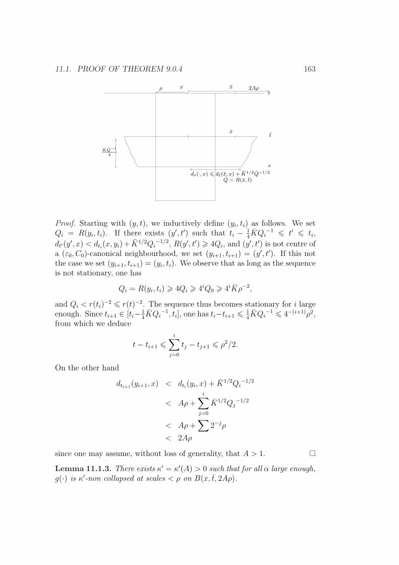
11.1. PROOF OF THEOREM 9.0.4 163
tx x
tx
KQ−1
4
s
ds(·, x) 6 dt(x, x) + K1/2Q−1/2
Q = R(x, t)
2Aρρ
Proof. Starting with (y, t), we inductively define (yi, ti) as follows. We setQi = R(yi, ti). If there exists (y′, t′) such that ti − 1
4KQi
−1 6 t′ 6 ti,
dt′(y′, x) < dti(x, yi)+ K1/2Qi
−1/2, R(y′, t′) > 4Qi, and (y′, t′) is not centre ofa (ε0, C0)-canonical neighbourhood, we set (yi+1, ti+1) = (y′, t′). If this notthe case we set (yi+1, ti+1) = (yi, ti). We observe that as long as the sequenceis not stationary, one has
Qi = R(yi, ti) > 4Qi > 4iQ0 > 4iKρ−2,
and Qi < r(ti)−2 6 r(t)−2. The sequence thus becomes stationary for i large
enough. Since ti+1 ∈ [ti− 14KQi
−1, ti], one has ti−ti+1 6 14KQi
−1 6 4−(i+1)ρ2,from which we deduce
t− ti+1 6i∑
j=0
tj − tj+1 6 ρ2/2.
On the other hand
dti+1(yi+1, x) < dti(yi, x) + K1/2Qi
−1/2
< Aρ+i∑
j=0
K1/2Qj−1/2
< Aρ+∑
2−jρ
< 2Aρ
since one may assume, without loss of generality, that A > 1.
Lemma 11.1.3. There exists κ′ = κ′(A) > 0 such that for all α large enough,g(·) is κ′-non collapsed at scales < ρ on B(x, t, 2Aρ).
164 CHAPTER 11. PROOFS OF THE TECHNICAL THEOREMS
Proof. It consists in applying claim a) of the theorem on the ballB(x, t, 10−1ρ)with the constant A′. Indeed, A′10−1ρ > 2Aρ. Let us remark that 10−1ρ 6√t/2 as t > t− ρ2/2 > t/2 > ρ2.Since |Rm | 6 ρ−2 on P (x, t, ρ,−ρ2) and t > t− ρ2/2, it follows from the
distance-distortion lemma 0.6.1 that,
10−1 6 g(t)
g(t)6 e4ρ−2(ρ2/2) = e2 6 10,
andB(x, t, 10−2ρ) ⊂ B(x, t, 10−1ρ) ⊂ B(x, t, ρ).
The neighbourhood P (x, t, 10−1ρ,−10−2ρ2) is thus unscathed and satisfiesthe required bound. Moreover, using Bishop-Gromov’s comparison theorem:
volB(x, t, 10−1ρ) > volB(x, t, 10−2ρ)
> v−ρ−2(10−2ρ)
v−ρ−2(ρ)
volB(x, t, ρ)
> v−1(10−2)
v−1(1)A−1ρ3
> A′−1(10−1ρ)3.
Let us recall that for α large enough, δα(·) < δA′(·). Claim a) of thetheorem yields a constant κ′ = κ(A′) such that g(·) is κ′-non collapsed onB(x, t, A′10−1ρ) at scales less 10−1ρ. We then deduce that g(·) is 10−3κ′-noncollapsed at scales ρ.
We now consider the parabolic rescalings
g(·) = R(x, t)g
(t+
·R(x, t)
),
and we argue as in the proof of proposition B in order to extract a sub-sequence converging towards a κ-solution. Unless otherwise stated we workwith these rescaled metrics. We note that (x, 0) is not the centre of a (ε0, C0)-canonical neighbourhood, but that the points (x′, t′)such that t′ ∈ [−K/4, 0],dt′(x
′, x) < d0(x, x) + K1/2 and R(x′, t′) > 4 are. In the sequel let P denotethe set
P = (x′, t′) | t′ ∈ [−K/4, 0], dt′(x′, x) < d0(x, x) + K1/2.
We remark that it is not a parabolic neighbourhood and that yields furthercomplications in the proof.
Since δα goes to 0, the preliminary lemma 7.2.1 is still valid. We state itagain here:
11.1. PROOF OF THEOREM 9.0.4 165
Lemma 11.1.4. For all K, A, τ > 0, there exists an integer α0 = α0(K, A, τ)such that for all integer α > α0, if |Rm | 6 K on B(x, 0, A) × (−τ, 0], thenP (x, 0, A,−τ) is unscathed.
Step 1. The sequence (M, g(·), x)αsub-converges towards a partial Ricci flow(M∞, g∞(·), x∞), where g∞(0) is complete and g∞(t) has nonnegative curva-ture operator.
Proof. From the curvature-distance theorem 4.2.1, for all A > 0, there existQ = Q(A) > 0 and Λ = Λ(A) > 0 such that if
i) (1 + t′)R(x′, t′) > Q,
ii) every y ∈ B(x′, t′, AR(x′, t′)−1/2) such that R(y, t′) > 4R(x′, t′) is thecentre of a (ε0, C0)-canonical neighbourhood,
then R(z, t′) 6 ΛR(x′, t′) for all z ∈ B(x′, t′, AR(x′, t′)−1/2).
The second condition is satisfied at (x, t) by definition, as soon as K1/2 >A since then B(x′, t′, AR(x′, t′)−1/2) ⊂ P . The first condition is also verifiedfor α large enough, for
(1 + t)R(x, t) > tKρ−2 > 2K.
We then conclude that the metrics g(·) satisfy R(·, 0)6Λ(A) on B(x, 0, A)for all α large enough. In order to be able to use the local compactnesstheorem for flows B.3.2, let us show that there exists τ(A) > 0 such thatP (x, 0, A,−τ(A)) is unscathed and has bounded curvature, for all α largeenough. We set K = K(A) = 2(Λ(A) + 4). We may assume this number tobe large enough so that, by Pinching Lemma 2.4.3, if R 6 K then |Rm | 6 K.We define α1(A) > α0(K, A, (C0K))−1) such that for α > α1, K
1/2 < 2(A+1).
Lemma 11.1.5. For all α > α1, P (x, 0, A,−(C0K)−1) ⊂ P , is unscathedand satisfies |Rm | 6 K(A).
Proof. Let us consider s ∈ [−(C0K)−1), 0] minimal (for α fixed) such thatB(x, 0, A)× (s, 0] ⊂ P and is unscathed.
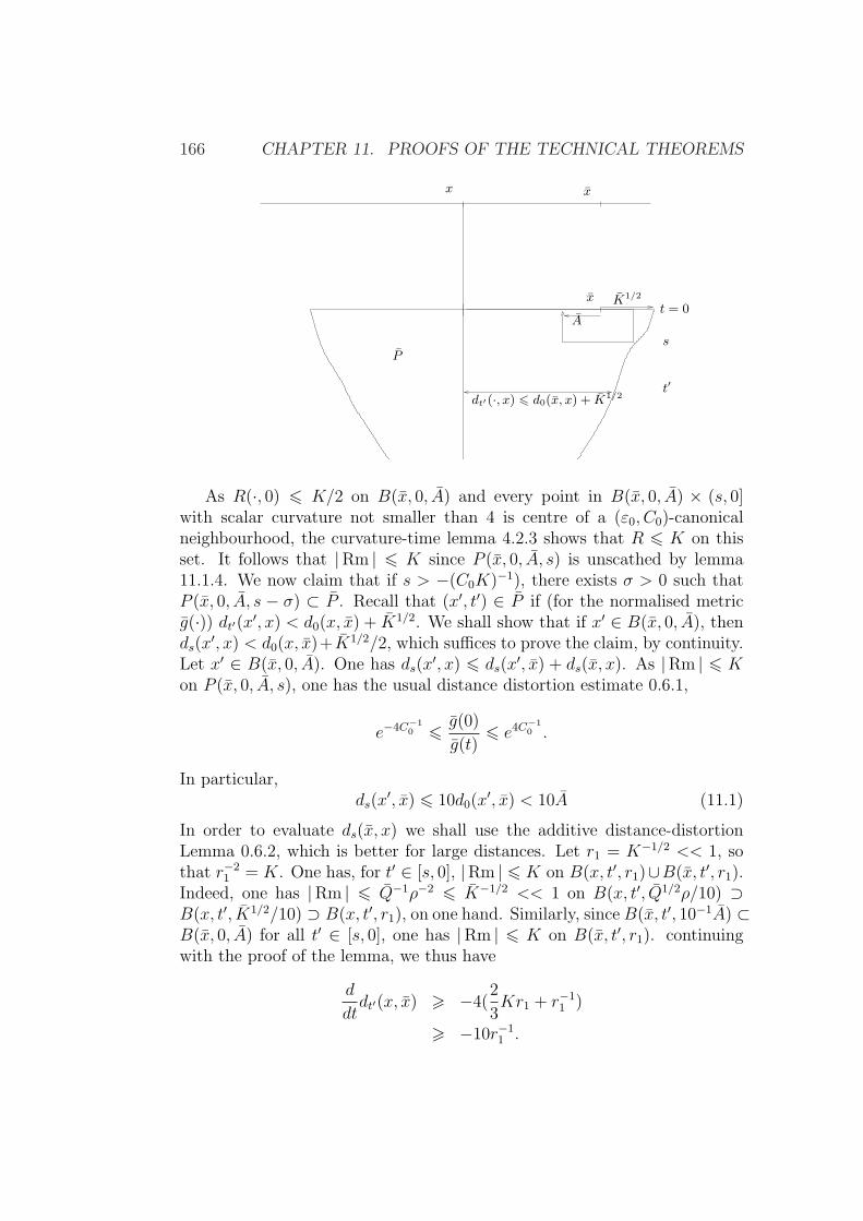
166 CHAPTER 11. PROOFS OF THE TECHNICAL THEOREMS
dt′(·, x) 6 d0(x, x) + K1/2
x
x
P
K1/2
A
x
t = 0
s
t′
As R(·, 0) 6 K/2 on B(x, 0, A) and every point in B(x, 0, A) × (s, 0]with scalar curvature not smaller than 4 is centre of a (ε0, C0)-canonicalneighbourhood, the curvature-time lemma 4.2.3 shows that R 6 K on thisset. It follows that |Rm | 6 K since P (x, 0, A, s) is unscathed by lemma11.1.4. We now claim that if s > −(C0K)−1), there exists σ > 0 such thatP (x, 0, A, s − σ) ⊂ P . Recall that (x′, t′) ∈ P if (for the normalised metricg(·)) dt′(x′, x) < d0(x, x) + K1/2. We shall show that if x′ ∈ B(x, 0, A), thends(x
′, x) < d0(x, x)+K1/2/2, which suffices to prove the claim, by continuity.Let x′ ∈ B(x, 0, A). One has ds(x
′, x) 6 ds(x′, x) + ds(x, x). As |Rm | 6 K
on P (x, 0, A, s), one has the usual distance distortion estimate 0.6.1,
e−4C−10 6 g(0)
g(t)6 e4C
−10 .
In particular,ds(x
′, x) 6 10d0(x′, x) < 10A (11.1)
In order to evaluate ds(x, x) we shall use the additive distance-distortionLemma 0.6.2, which is better for large distances. Let r1 = K−1/2 << 1, sothat r−2
1 = K. One has, for t′ ∈ [s, 0], |Rm | 6 K on B(x, t′, r1)∪B(x, t′, r1).Indeed, one has |Rm | 6 Q−1ρ−2 6 K−1/2 << 1 on B(x, t′, Q1/2ρ/10) ⊃B(x, t′, K1/2/10) ⊃ B(x, t′, r1), on one hand. Similarly, sinceB(x, t′, 10−1A) ⊂B(x, 0, A) for all t′ ∈ [s, 0], one has |Rm | 6 K on B(x, t′, r1). continuingwith the proof of the lemma, we thus have
d
dtdt′(x, x) > −4(
2
3Kr1 + r−1
1 )
> −10r−11 .
11.1. PROOF OF THEOREM 9.0.4 167
Integrating between s > −(C0K)−1 and t = 0 we obtain
d0(x, x)− ds(x, x) > −10C−10 r1 > −1,
Thus
ds(x, x) 6 d0(x, x) + 1.
Combining this with (11.1) and the definition of α1, we obtain
ds(x′, x) 6 10A+ d0(x, x) + 1 < d0(x, x) + K1/2/2.
This finishes the proof of lemma 11.1.5
From lemma 11.1.3, g(·) is κ′-non collapsed at (x, 0) at scales less thanQ1/2ρ, hence at scales less than K1/2. Combined with the curvature boundgiven by lemma 11.1.5, this shows that the injectivity radius of the met-rics g(0) is bounded below by c > 0 independent of α. From theoremB.3.2, the sequence (M, g(·), x)α sub-converges towards a partial Ricci flow(M∞, g∞(·), x∞) where g∞(0) is complete. Moreover, the curvature operatorof g∞(t) is non negative from proposition 4.2.5. This finishes the proof ofstep 1.
Step 2. The manifold (M∞, g∞(0)) has bounded curvature.
The proof is identical to the one given for proposition B: since the points inP (x, 0, A,−τ(A)) with scalar curvature larger than 4 are centres of (ε0, C0)-canonical neighbourhoods for all α large enough,we get by taking limits thateach point of (M∞, g∞(0)) with scalar curvature larger than 5 is centre ofa (2ε0, 2C0)-weak canonical neighbourhood. We conclude in the same waythat the scalar curvature of g∞(0) is bounded above by some constant Q0.
From that we deduce that the constant K(A) used in lemma 11.1.5 canbe chosen independently of A. We can define
τ0 := supτ > 0,∃K(τ) > 0,∀A > 0,∃α(A, τ),∀α > α(A, τ),P (x, 0, A,−τ) ⊂ P is unscathed and |Rm | 6 K(τ) there > 0.
Step 3. There exists Q > 0 such that the scalar curvature of g∞(t) isbounded above by Q, for all t ∈ (−τ0, 0].
The proof is identical to the one done for proposition B, using the nonnegativeness of the curvature and the canonical neighbourhoods property.
Step 4. τ0 = +∞.
168 CHAPTER 11. PROOFS OF THE TECHNICAL THEOREMS
We argue as in the proof of B. We deduce from step 3 that for all τ < τ0,for all A > 0, for all α large enough P (x, 0, A,−τ) ⊂ P , is unscathed and withsectional curvatures bounded above by a constant K independent of A and ofα. Let us assume that τ0 < +∞. We now need to extend the above propertybeyond −τ0. Let us consider τ close enough to τ0 so that τ−τ0 < 2(4C0(K+4))−1. Let s ∈ [−τ0 − (4C0(K + 4))−1,−τ ] minimal (depending on α) suchthat B(x, 0, A)×(s, 0] is contained in P and is unscathed. We can also use thecurvature-time lemma 4.2.3 in order to show that B(x, 0, A)×(s, 0] has scalarcurvature (hence sectional curvatures) bounded by 2(K + 4). Lemma 11.1.4then shows that P (x, 0, A, s) is unscathed for α large enough depending onlyon A and on K. Let us show that P (x, 0, A, s − σ) ⊂ P for σ > 0. We dothe same computations as in step 1.
Let x′ ∈ B(x, 0, A). We set K ′ = 2(K + 4).The distance-distortion esti-mate yields on B(x, 0, A).
e−4K′|s| 6 g(0)
g(s)6 e4K
′|s| 6 c21 := c21(τ0),
whereds(x
′, x) 6 c1A.
Let us set r1 = K ′−1/2. Integrating inequality (6) given by Lemma 0.6.2between s and 0 we find
d0(x, x)− ds(x, x) > −10r−11 s > c2(τ0),
whereds(x
′, x) 6 d0(x, x) + c1A+ c2 < d0(x, x) + K1/2/2,
for α large enough only depending on A and on τ0. By continuity ds−σ(x′, x) 6d0(x, x) + K1/2 for all x′ ∈ B(x, 0, A), pour σ > 0 small enough. It followsthat P (x, 0, A,−τ0− (4C0(K + 4))−1) ⊂ P , is unscathed and with curvaturebounded by K ′ for α large enough depending on A and on τ0. This contradictthe definition of τ0 and finishes the proof of b).
Proof of c) We fix A > 0. Let us denote κ(2A), K = K(2A) >> 1 andδ(t) = δ2A(t) the parameters satisfying part a) and b) of the theorem withthe constant 2A. Define, using the curvature-distance with parameters Λand Q (Theorem 4.2.1),
A′ = AK1/2,
Q = Q(A′, ε0, C0),
Λ = Λ(A′, ε0, C0),
K ′ = KΛ,
r = K12Q−
12 ,
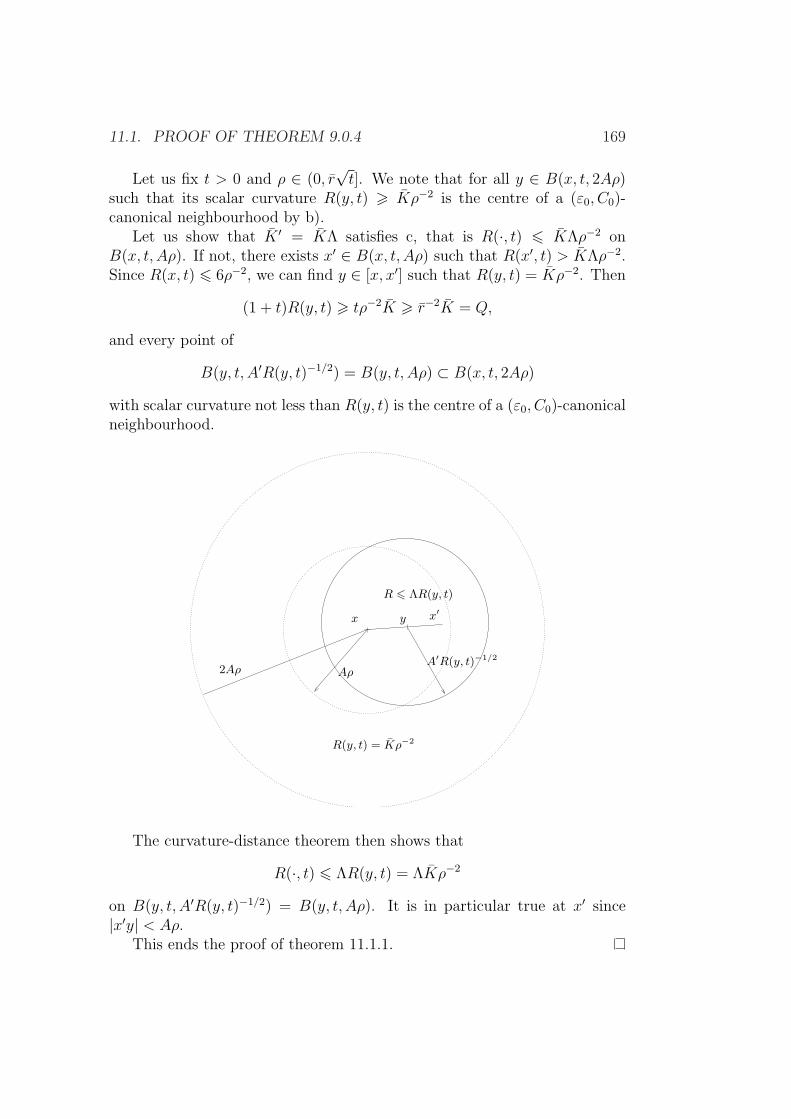
11.1. PROOF OF THEOREM 9.0.4 169
Let us fix t > 0 and ρ ∈ (0, r√t]. We note that for all y ∈ B(x, t, 2Aρ)
such that its scalar curvature R(y, t) > Kρ−2 is the centre of a (ε0, C0)-canonical neighbourhood by b).
Let us show that K ′ = KΛ satisfies c, that is R(·, t) 6 KΛρ−2 onB(x, t, Aρ). If not, there exists x′ ∈ B(x, t, Aρ) such that R(x′, t) > KΛρ−2.Since R(x, t) 6 6ρ−2, we can find y ∈ [x, x′] such that R(y, t) = Kρ−2. Then
(1 + t)R(y, t) > tρ−2K > r−2K = Q,
and every point of
B(y, t, A′R(y, t)−1/2) = B(y, t, Aρ) ⊂ B(x, t, 2Aρ)
with scalar curvature not less than R(y, t) is the centre of a (ε0, C0)-canonicalneighbourhood.
x
2Aρ Aρ
y x′
A′R(y, t)−1/2
R 6 ΛR(y, t)
R(y, t) = Kρ−2
The curvature-distance theorem then shows that
R(·, t) 6 ΛR(y, t) = ΛKρ−2
on B(y, t, A′R(y, t)−1/2) = B(y, t, Aρ). It is in particular true at x′ since|x′y| < Aρ.
This ends the proof of theorem 11.1.1.
170 CHAPTER 11. PROOFS OF THE TECHNICAL THEOREMS
11.2 Proof of Theorem 9.0.5
In this section we shall give the proof of Theorem 9.0.5, which is our versionof Corollary 6.8 of [61]. This is a key result for understanding the long-termbehaviour of a Ricci flow with bubbling-off on the thick part. It is stated inSection 9 and again below.
The following theorem shows that on the thick part of the evolving metric1tg(t) the scalar curvature is bounded above on suitable unscathed parabolic
neighbourhood. This has been used to show that on this thick part the metricconverges, after rescaling, to a complete hyperbolic metric.
Theorem 11.2.1 (cf. Corollary 6.8 in [61]). For all w > 0, there exist pos-itive numbers τ , θ, K, r, T with the following property. Assume that g(t)is a Ricci flow with r(·), δ(·)-bubbling-off on [0,∞[, with normalised initialcondition and δ(·) ≤ δ(·). Let x ∈M , t > T , r > 0 such that
i) θ−1h 6 r 6 r√t, where h is the maximal surgery radius on [t/2, t],
ii) Rm > −r−2 on B(x, t, r),
iii) volB(x, t, r) > wr3.
Then P (x, t, r,−τ r2) is unscathed and |Rm | < Kr−2 there.
We first give a corollary to Theorem 9.0.4, which will be useful to proveTheorem 11.2.1.
Corollary 11.2.2. For all A,w > 0 there exist positive numbers r1 610−3, θ1, K1, τ1 and T1 with the following property. Let g(t) be a Ricciflow with r(·), δ(·)-bubbling-off on [0,∞[, with normalised initial conditionand δ(·) 6 δ(·). Let x ∈M , t > T1, r > 0 such that
i) θ1−1h 6 r 6 r1
√t,
ii) P (x, t, r,−r2) is unscathed,
iii) |Rm | 6 r−2 there,
iv) volB(x, t, r) > wr3.
Then P (x, t, Ar,−τ1r2) is unscathed and |Rm | < K1r−2 there.
11.2. PROOF OF THEOREM 9.0.5 171
Proof of the corollary. Define
A′ = max
4A,
e3/2
8
υ−1(1)
υ−1(1/4)w
,
T1 = 2A′
r1 = r(A′),
K1 = 4K ′(A′),
θ1 = (2K1)−1/2
τ1 = (4K1)−1
Let (x, t, r) be a triple that satisfies the assumptions. Set r′ = r2. By
assumptions ii) and iii) and the multiplicative distortion, Lemma 0.6.1,
4−1 6 e−1 6 g(t)
g(s)6 e 6 4, (11.2)
for every s ∈ [t− r′2, t] = [t− r2
4, t], hence B(x, s, r′) ⊂ B(x, t, r) for such s.
In particular P (x, s, r′,−r′2) ⊂ P (x, t, r,−r2). It follows that P (x, s, r′,−r′2)is unscathed and |Rm | 6 r−2 6 r′−2, satisfying assumptions i) and ii) ofTheorem 9.0.4. Moreover, by (11.2) B(x, s, r′) ⊃ B(x, t, r
′2) thus
volg(s)B(x, s, r′) > volg(s)B(x, t,r′
2)
> e−3/2 volg(t)B(x, t,r
4)
> e−3/2υ−1(1/4)
υ−1(1)volg(t)B(x, t, r)
> e−3/2υ−1(1/4)
υ−1(1)wr3
= 8e−3/2υ−1(1/4)
υ−1(1)wr′3
> A′−1r′3.
Hence assumption iii) of Theorem 9.0.4 is satisfied at (x, s, r′) for all s ∈[t − r′2, t]. As r′ < r < r1
√t 6 10−3
√t, one has r′2 6 10−6t hence s >
t− r′2 > (1− 10−6)t > t/4, so r′ 6 10−3√t 6 10−32
√s 6
√s/2. In addition,
r′ =r
26 r1
√t
26 r1
√s,
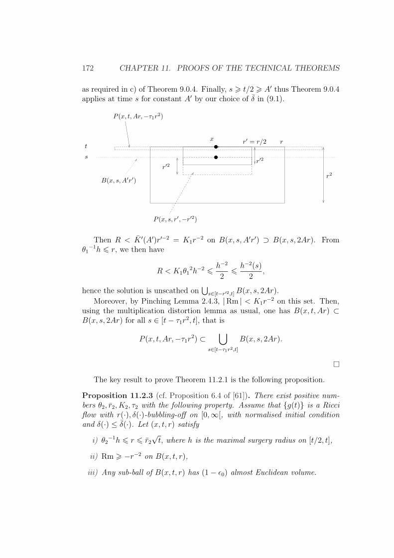
172 CHAPTER 11. PROOFS OF THE TECHNICAL THEOREMS
as required in c) of Theorem 9.0.4. Finally, s > t/2 > A′ thus Theorem 9.0.4applies at time s for constant A′ by our choice of δ in (9.1).
x
r′2
P (x, s, r′,−r′2)
B(x, s, A′r′)
P (x, t, Ar,−τ1r2)
t
s
r′ = r/2 r
r′2
r2
Then R < K ′(A′)r′−2 = K1r−2 on B(x, s, A′r′) ⊃ B(x, s, 2Ar). From
θ1−1h 6 r, we then have
R < K1θ12h−2 6 h−2
26 h−2(s)
2,
hence the solution is unscathed on⋃s∈[t−r′2,t]B(x, s, 2Ar).
Moreover, by Pinching Lemma 2.4.3, |Rm | < K1r−2 on this set. Then,
using the multiplication distortion lemma as usual, one has B(x, t, Ar) ⊂B(x, s, 2Ar) for all s ∈ [t− τ1r
2, t], that is
P (x, t, Ar,−τ1r2) ⊂⋃
s∈[t−τ1r2,t]B(x, s, 2Ar).
The key result to prove Theorem 11.2.1 is the following proposition.
Proposition 11.2.3 (cf. Proposition 6.4 of [61]). There exist positive num-bers θ2, r2, K2, τ2 with the following property. Assume that g(t) is a Ricciflow with r(·), δ(·)-bubbling-off on [0,∞[, with normalised initial conditionand δ(·) ≤ δ(·). Let (x, t, r) satisfy
i) θ2−1h 6 r 6 r2
√t, where h is the maximal surgery radius on [t/2, t],
ii) Rm > −r−2 on B(x, t, r),
iii) Any sub-ball of B(x, t, r) has (1− ε0) almost Euclidean volume.
11.2. PROOF OF THEOREM 9.0.5 173
Then P (x, t, r,−τ2r2) is unscathed and |Rm | < K2r−2 there.
We now prove 11.2.1 postponing the proof of this proposition.
Proof of Theorem 11.2.1 assuming 11.2.3. The idea is the following: Lemma9.0.3 provides a sub-ball of B(x, t, r) with (1− ε0)-amost Euclidean volume,on which we apply Proposition 11.2.3. Then we obtain curvature bounds onthe larger parabolic ball by Corollary 11.2.2. Let’s go into details.
Fix w > 0 and let θ0 = θ0(w) be the parameter given by the bub-balllemma, Lemma 9.0.3. Define
B = minK2
− 12 , τ2
12
θ0,
A = 2B−1,
Let r1, θ1, τ1, T1, K1 be the parameters given by Corollary 11.2.2, whichdepend on A and (1− ε0)υ0(1). Then define
r = min r1, r2 ,θ = min Bθ1, θ0θ2 ,τ = τ1B
2,
K = K1B−2,
T = max T1, T2 .Let (x, t, r) satisfying the assumptions:
θ−1h 6 r 6 r√t, t > T ,
Rm > −r−2 on B(x, t, r) and volB(x, t, r) > wr3.
Let r′ = θ0r. By the Sub-ball Lemma 9.0.3 there exists B(x′, t, r′) ⊂B(x, t, r) such that every sub-ball has (1 − ε0)-amost Euclidean volume.Clearly Rm > −r′−2on B(x′, t, r′). Moreover, t > T2 and
θ2h 6 θ−1θ0h 6 θ0r = r′ 6 r 6 r√t 6 r2
√t,
hence Proposition 11.2.3 applies to (x′, t, r′). Then P (x′, t, r′,−τ2r′2) is un-scathed and satisfies, using Pinching Lemma 2.4.3, |Rm | < K2r
′−2. Let
r′′ = Br = minK2
− 12 , τ2
12
r′.
This is precisely the choice such that K2r′−2 6 r′′−2 and τ2r
′2 > r′′2. ThenP (x′, t, r′′,−r′′2) is unscathed and |Rm | 6 r′′−2 there.
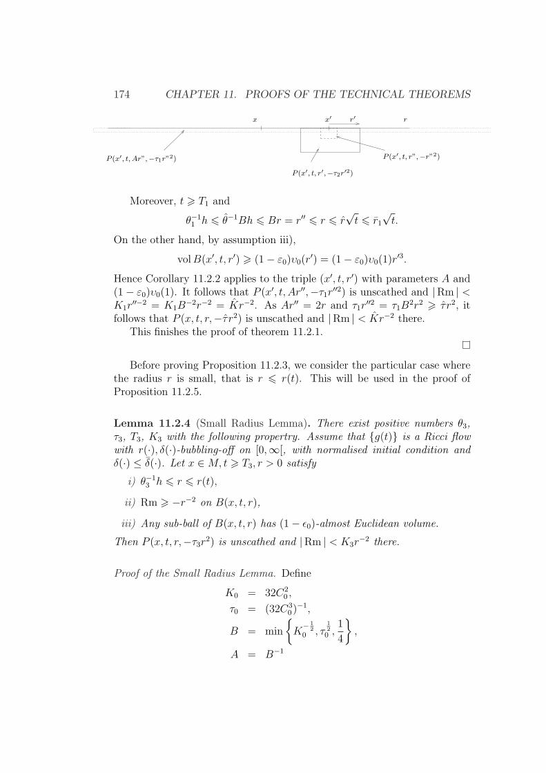
174 CHAPTER 11. PROOFS OF THE TECHNICAL THEOREMS
x x′ r
P (x′, t, r′,−τ2r′2)
P (x′, t, Ar”,−τ1r”2)
r′
P (x′, t, r”,−r”2)
Moreover, t > T1 and
θ−11 h 6 θ−1Bh 6 Br = r′′ 6 r 6 r
√t 6 r1
√t.
On the other hand, by assumption iii),
volB(x′, t, r′) > (1− ε0)υ0(r′) = (1− ε0)υ0(1)r′3.
Hence Corollary 11.2.2 applies to the triple (x′, t, r′) with parameters A and(1− ε0)υ0(1). It follows that P (x′, t, Ar′′,−τ1r′′2) is unscathed and |Rm | <K1r
′′−2 = K1B−2r−2 = Kr−2. As Ar′′ = 2r and τ1r
′′2 = τ1B2r2 > τ r2, it
follows that P (x, t, r,−τ r2) is unscathed and |Rm | < Kr−2 there.This finishes the proof of theorem 11.2.1.
Before proving Proposition 11.2.3, we consider the particular case wherethe radius r is small, that is r 6 r(t). This will be used in the proof ofProposition 11.2.5.
Lemma 11.2.4 (Small Radius Lemma). There exist positive numbers θ3,τ3, T3, K3 with the following propertry. Assume that g(t) is a Ricci flowwith r(·), δ(·)-bubbling-off on [0,∞[, with normalised initial condition andδ(·) ≤ δ(·). Let x ∈M, t > T3, r > 0 satisfy
i) θ−13 h 6 r 6 r(t),
ii) Rm > −r−2 on B(x, t, r),
iii) Any sub-ball of B(x, t, r) has (1− ε0)-almost Euclidean volume.
Then P (x, t, r,−τ3r2) is unscathed and |Rm | < K3r−2 there.
Proof of the Small Radius Lemma. Define
K0 = 32C20 ,
τ0 = (32C30)−1,
B = min
K− 1
20 , τ
120 ,
1
4
,
A = B−1
11.2. PROOF OF THEOREM 9.0.5 175
Let r1, θ1, τ1, T1, K1 be the parameters given by Corollary 11.2.2 dependingon A and (1− ε0)υ0(1). Then define
θ3 = minBθ1, (8C0)
−1,
τ3 = τ1B2,
K3 = K1B−2,
T3 > T1 such that r(t) 6 r1√t if t > T3.
Let (x, t, r) satisfying the assumptions of the small radius lemma. Inparticular 8C0h 6 r 6 r(t).
Claim 6. P (x, t, r/4,−τ0r2) is unscathed and R < K0r−2 there.
Proof of the claim. Let us prove first that R < 16C20r−2 on B(x, t, r/4). As-
sume it is not true and let x′ ∈ B(x, t, r/4) such that
R(x′, t) > 16C20r−2 > 16C2
0r(t)−2 > r(t)−2.
Then (x′, t) is centre of (ε0, C0)-canonical neighbourhood U , and B(x′, t, r′) ⊂U ⊂ B(x, t0, 2r
′), where r′ ∈ (C−10 R(x′, t)−1/2, C0R(x′, t)−1/2). In particular,
r′ ≤ C0R(x′, t)−1/2 ≤ r/4 ⇐⇒ 2r′ ≤ r/2 .
Hence U ⊂ B(x′, t, r/2) ⊂ B(x, t, r). This contradicts the assumptionof almost Euclidean volume for sub-balls. Indeed, there exists y ∈ U ands ≈ R(y, t)−1/2ε−1
0 ≤ r such that B(y, t, s) is close to an ε0-neck included inU , hence has volume
≈ R(y, t)−3/2 2
ε0vol(S2) ≈ (sε0)
3 2
ε0vol(S2) = 2ε20 vol(S2)s3,
which is much less than (1− ε0)υ0(1)s3. Hence R < 16C20r−2 on B(x, t, r/4).
Now consider s ∈ [t − τ0r2, t] minimal such that B(x, t, r/4) × (s, t] is
unscathed. By the same argument as in the curvature-time lemma 4.2.3,R < 32C2
0r−2 = K0r
−2 on this set. On the other hand 8C0h 6 r hence
R < 32C20(64)−1C−2
0 h−2 =h−2
26 h−2
s.
It follows that P (x, t, r/4, s − t) is unscathed and s = t − τ0r2, proving the
claim.
176 CHAPTER 11. PROOFS OF THE TECHNICAL THEOREMS
By Claim 6, P (x, t, r/4,−τ0r2) is unscathed and R < K0r−2 there. Set
r′ = Br. We have r′ 6 r/4 and r′2 = B2r2 6 τ0r2, hence P (x, t, r′,−r′2) ⊂
P (x, t, r/4,−τ0r2). Moreover, we have
θ−11 h 6 Bθ−1
3 h 6 Br = r′ 6 r 6 r(t) 6 r1√t.
In particular, Pinching Lemma 2.4.3 applies, giving |Rm | < K0r−2 6 r′−2
on P (x, t, r′,−r′2). Remenber that t > T1 and volB(x, t, r′) > (1− ε0)υ0(r′).
Hence assumptions of Corollary 11.2.2 are satisfied for parameters A and(1− ε0)υ0(1). We get that P (x, t, Ar′,−τ1r′2) is unscathed and
|Rm | < K1r′−2 = K1B
−2r−2 = K3r−2
there. As P (x, t, r,−τ3r2) ⊂ P (x, t, Ar′,−τ1r′2), the lemma is proved.
To prove Proposition 11.2.3, we use a weaker statement and again thecorollary. The weaker proposition involve union of balls rather than parabolicballs.
Proposition 11.2.5. There exists positive numbers θ′2, r′2, τ
′2, K
′2 and T ′2 with
the following property. Assume that g(t) is a Ricci flow with r(·), δ(·)-bubbling-off on [0,∞[, with normalised initial condition and δ(·) ≤ δ(·). Letx ∈M , t > T ′2, and r > 0 satisfy
i) θ′2−1h 6 r 6 r′2
√t, where h is the maximal surgery radius on [t/2, t],
ii) Rm > −r−2 on B(x, t, r),
iii) Any sub-ball of B(x, t, r) has (1− ε0) almost Euclidean volume.
Then⋃
[t−τ ′2r2,t]B(x, s, r/2) is unscathed and |Rm | < K ′
2r−2 there.
We explain first how Proposition 11.2.5 and Corollary 11.2.2 imply themain Proposition 11.2.3, and then prove Proposition 11.2.5.
Proof of Proposition 11.2.3 assuming 11.2.5. Let
τ = min
(4K ′2)− 1
2 , τ ′212
B = min
τ−
12 , K ′
2− 1
2 ,1
8
A = B−1
11.2. PROOF OF THEOREM 9.0.5 177
Let r1, θ1, τ1, T1, K1 be the parameters given by Corollary 11.2.2 dependingon A and (1− ε0)υ0(1). Then define
θ2 = min Bθ1, θ′2 ,
r2 = min r1, r′2 ,τ2 = τ1B
2,
K2 = K1B−2,
T2 = max T1, T′2 .
Let (x, t, r) satisfy the assumptions of Proposition 11.2.3. Then t > T2 > T ′2and
θ′2−1h 6 θ−1
2 h 6 h 6 r2√t 6 r′2
√t,
satisfying assumption i) of Proposition 11.2.5. Assumptions ii) iii) are also
satisfied, thus⋃
[t−τ ′2r2,t]B(x, s, r/2) is unscathed and |Rm | < K ′
2r−2 there. By
the multiplicative distance-distortion Lemma 0.6.1,
4−1 6 g(t)
g(s)6 4,
onB(x, t, r/4) if s ∈ [t−τr2, t]. Hence P (x, t, r/4,−τr2) ⊂⋃
[t−τ ′2r2,t]B(x, s, r/2)
is unscathed and |Rm | < K ′2r−2 there. Let r′ = Br, then P (x, t, r′,−r′2) ⊂
P (x, t, r/4,−τr2) and |Rm | 6 r′−2. On the other hand, t > T1 and
θ1−1h 6 Bθ−1
2 h 6 Br = r′ 6 r2√t 6 r1
√t.
Morover volB(x, t, r′) > (1−ε0)υ0(r′) by the assumption iii). Hence assump-
tions of Corollary 11.2.2 are satisfied for parameters A and (A − ε0)υ0(1).Then
P (x, t, Ar′,−τ1r′2) ⊃ P (x, t, r,−τ2r2)
is unscathed and |Rm | < K1r′−2 = K2r
−2 there.
After all those disgressions, now begin the tough part. The proof ofProposition 11.2.5 will be by contradiction. At the core of the argument,we’ll use the following lemma, whose proof is postponed again.
Lemma 11.2.6 (Compare to Lemma 6.5 in [61]). There exist positive num-bers K∗, τ∗ such that for any Ricci flow g(·) on M (not necessarily complete),τ ∈ [0, τ∗], and x ∈M the following hold. Assume that
i) For all t ∈ [−τ, 0], B(x, t, 1) ⊂M ,
178 CHAPTER 11. PROOFS OF THE TECHNICAL THEOREMS
ii) g(·) is smooth on⋃
[−τ,0]
B(x, t, 1) and Rm > −1 on this set.
iii ) vol(B(x, 0, 1)) ≥ (1− ε0)υ0(1).
Then
a) R ≤ K∗τ−1 on⋃
[−τ/2,0]
B(x, t, 1/2),
b) vol(B(x,−τ, 1/4)) > 110υ0(1/4).
Proof of Proposition 11.2.5 assuming Lemma 11.2.6. Define
θ′2 = θ3
K ′2 = max
K∗τ∗, K3
,
τ ′2 = minτ∗
4, (4K3)
−1, τ3
,
B =1
4θ0
(υ(1)
10
),
B′ = min
τ ′2− 1
2
√2,
(K∗τ ′2
)− 12
,1
40
,
A = 4(BB′)−1.
Here θ0(·) is the parameter given by Sub-ball Lemma 9.0.3. Let r1, θ1, τ1,T1, K1 be the parameters given by Corollary 11.2.2 depending on A and(1− ε0)υ0(1). Then define
K = K1(BB′)−2,
σ = min(4K)−1, τ1B
2B′2 .Let us make a preliminary observation. For any triple (x, t, r) satisfying
the assumptions, and moreover
θ′2−1 6 r 6 r(t),
the conclusion of the proposition is true. Indeed, in this case the smallradius lemma (Lemma 11.2.4) applies, so P (x, t, r,−τ3r2) is unscathed and|Rm | < K3r
−2 there. By the multiplicative distance-distortion Lemma 0.6.1,we get
B(x, s,r
2) ⊂ B(x, t, r),
11.2. PROOF OF THEOREM 9.0.5 179
for all s ∈ [t −min(4K3)−1, τ3r2, t]. The conclusion follows from the defi-
nition of τ ′2, K′2.
Thus, arguing by contradiction, we can suppose that counter-examplessatisfy r > r(t). Hence, we assume there exist a sequence rα → 0, Ricci flowwith r(·), δα(·)-bubbling-off gα(t) on Mα, defined on [0,+∞), with nor-malised initial parameters and δα(·) 6 δ(·), and counter-examples (xα, tα, rα),which satisfy tα > T ′2 and
i) θ′2−1hα 6 rα 6 rα
√tα, where hα is the maximal surgery radius on
[tα/2, tα],
i’) rα > r(tα),
ii) Rm > −(rα)−2 on B(xα, tα, rα),
iii) Any sub-ball of B(xα, tα, rα) has (1− ε0) almost Euclidean volume,
but⋃
[tα−τ ′2(rα)2,tα]
B(xα, t, rα/2) is scathed or |Rm | < K ′2(r
α)−2 is not true
there.
For each α, define
rα0 = infr > 0 | a counterexample (x, t, r) exist with t 6 tα, r 6 rα
√tα
.
Note that r > r(t) > r(tα) by the preliminary observation and the fact thatr(·) is nonincreasing. Hence rα0 > r(tα) > 0. Maybe the infimum is notachieved, but clearly we can redefine (xα, tα, rα) in such a way that
rα
rα0−→
α−→+∞1 .
In particular no counter-example exist with r 6 rα/2 and t 6 tα. Let usremark that tα → +∞. Indeed, from r(tα) 6 rα 6 rα
√tα, we get
tαr(tα)−2 > (rα)−2 → +∞,
and the remark follows from the fact that t r(t)−2 is bounded on any finiteinterval [0, T ].Define
τα = sup
τ > 0 |
⋃
[tα−τ(rα)2,tα]
B(xα, t, rα) is unscathed and Rm > −(rα)−2 there
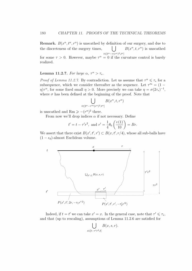
180 CHAPTER 11. PROOFS OF THE TECHNICAL THEOREMS
Remark. B(xα, tα, rα) is unscathed by definition of our surgery, and due to
the discreteness of the surgery times,⋃
t∈[tα−τ(rα)2,tα]
B(xα, t, rα) is unscathed
for some τ > 0. However, maybe τα = 0 if the curvature control is barelyrealized.
Lemma 11.2.7. For large α, τα > τ∗.
Proof of Lemma 11.2.7. By contradiction. Let us assume that τα 6 τ∗ for asubsequence, which we consider thereafter as the sequence. Let τ ′α = (1 −η)τα, for some fixed small η > 0. More precisely we can take η = σ(2τ∗)−1,where σ has been defined at the beginning of the proof. Note that⋃
t∈[tα−τ ′α(rα)2,tα]
B(xα, t, rα)
is unscathed and Rm > −(rα)2 there.From now we’ll drop indices α if not necessary. Define
t′ = t− τ ′r2, and r′ =1
4θ0
(υ(1)
10
)= Br.
We assert that there exist B(x′, t′, r′) ⊂ B(x, t′, r/4), whose all sub-balls have(1− ε0)-almost Euclidean volume.
x
x′
S[t′,t]B(x, s, r)
r
r′
τ ′r2
τr2
P (x′, t′, r′,−τ ′2r′2)P (x′, t′, 2r,−τ1r”2)
t
t′
Indeed, if t = t′ we can take x′ = x. In the general case, note that τ ′ 6 τ∗,and that (up to rescaling), assumptions of Lemma 11.2.6 are satisfied for
⋃
s∈[t−τ ′r2,t]B(x, s, r).
11.2. PROOF OF THEOREM 9.0.5 181
Then by Lemma 11.2.6 b), one has
volB(x, t′,r
4) > 1
10υ0
(r4
)=
1
10υ0(1)
(r4
)3
.
Now we can apply the Sub-ball Lemma 9.0.3 to B(x, t′, r/4) (after rescaling
by(r4
)−2) to get a ball
B(x′, t′, θ0
(υ0(1)
10
)r
4) ⊂ B(x, t′,
r
4),
satisfying the required assertion. Let us check now that the triple (x′, t′, r′)satisfies the assumptions of the proposition. In particular we must have
θ′2−1h′ 6 r′ 6 rα
√t′,
where now, h′ = max[t′/2,t′]
hα(·).Recall that h(·) is nonincreasing and h(·) 6 δ(·)r(·). Clearly, [t′/2, t′] ⊂
[t/4, t], as
t′ = t− τ ′r2
> t− τ ′r2t
> (1− 10−6)t.
On one hand, using the fact that η(tα) → 0 in definition (9.1) of δ, for largeα we have
r′ = Br > Br(t) > θ′2−1r(t
4)δ(
t
4)
> θ′2−1r(t
4)δ(
t
4)
> θ′2−1h(t
4)
> θ′2−1h(t′
2)
> θ′2−1h′.
On the other hand,
R′ = Br 6 Br√t 6 r
√t′B
√t
t′6 r
√t′.
182 CHAPTER 11. PROOFS OF THE TECHNICAL THEOREMS
Finally recall that tα → ∞ hence t′ > t/2 > T ′2 for large α. Assumption ii)of Proposition 11.2.5 is clearly true as r′ < r and iii) holds by definition ofB(x′, t′, r′). Finally, as r′α < rα
2and t′α 6 tα, recall that the conclusion of
the proposition is true by definition of rα and r0α. Then
⋃
[t′−τ ′2r′2,t′]B(x′, s, r′/2)
is unscathed and |Rm | < K ′2r′−2 there. We want extend the curvature con-
trol to B(x, s, r) by using Corollary 11.2.2, but before doing this we needbetter curvature control. Note that on the set above, by the amost nonneg-ative curvature property, one has (see Section 2.4)
Rm > −φs(R) > −φs(K ′2r′−2)
= −φ0 ((1 + s)K ′2r′−2)
(1 + s)K ′2r′−2
K ′2.r
′−2
> −r′−2
for large α. Indeed,
(1 + s)K ′2r′−2 > sr′−2 > B−2tα(rα)−2
4> B−2(rα)−2
4→∞,
as α go to +∞. Doing the parabolic rescaling by 4r′−2 at (x′, t′), one findsthat ⋃
[−4τ ′2,0]
B(x′, s, 1)
is unscathed and Rm > −1 there. Applying Lemma 11.2.6 a) (note that4τ ′2 6 τ∗), we obtain R < K∗
4τ ′2on
⋃
[−2τ ′2,0]
B(x′, s, 1/2),
hence, scaling back and using Pinching Lemma 2.4.3, |Rm | < K∗τ ′2r′−2 on
⋃
[t′− τ ′22r′2,t′]
B(x′, s, r′/2).
Set r′′ = B′r′ where B′ has been defined at the beginning. Then |Rm | < r′′−2
on the set above. Using the multiplicative distance-distortion lemma,
B(x′, t′, r′′) ⊂ B(x′, s, 10r′′) ⊂ B(x′, s,r′
4),
11.2. PROOF OF THEOREM 9.0.5 183
for s ∈ [t′ − r′′2, t′]. Then
P (x′, t′, r′′,−r′′2) ⊂⋃
[t′− τ ′22r′2,t′]
B(x′, s,r′
4)
and it is unscathed. Let us check that assumptions of Corollary 11.2.2 holdtrue at (x′, t′, r′′) for d parameters A = 4(BB′)−1 and (1−ε0)υ0(1). For largeα as before we have
r′′ = BB′r > BB′r(t) > θ1−1r(
t
4)δ(
t
4)
> θ1−1h(
t
4)
> θ1−1h′.
On the other hand, as t′ > (1− 10−6)t, we have
r′′ = BB′r 6 rα√tBB′ 6 r1
√t′.
Finally, t′ > (1 − 10−6)tα > T1 for large α. Then by Corollary 11.2.2,P (x′, t′, r′′,−τ1r′′2) is unscathed and |Rm | < K1r
′′−2 = K1(BB′)r−2 = Kr−2
there. As Ar′′ = 4r, we have also |Rm | < Kr−2 on P (x, t′, 2r,−τ1(BB′)2r2)(recall that dt′(x, x
′) < r/4). Using the distance-distortion lemma, we deducethat ⋃
[t′−σr2,t′]B(x, s, r) ⊂ P (x, t′, 2r,−τ1(BB′)2r2),
where σ has been defined at the beginning of the proof. By the same pinchingargument as before, we deduce that Rm > −r−2 on this set. Thus we haveobtained that, for large α,
⋃
[t−(τ ′+σ)r2,t]
B(x, s, r)
is unscathed and Rm > −r−2 there. But
τ ′ + σ = (1− η)τα + 2ητ∗> τα − ητ∗ + 2ητ∗> τα + ητ∗
contradicting the definition of τα and proving Lemma 11.2.7.
184 CHAPTER 11. PROOFS OF THE TECHNICAL THEOREMS
We conclude now the proof of Proposition 11.2.5. Having obtained thatτα > τ∗ for large α, we get that
⋃
[t−τ∗r2,t]B(x, s, r)
is unscathed and Rm > −r−2 there. Recall that sub-balls of B(x, t, r) have(1 − ε0)-almost Euclidean volume, and in particular B(x, t, r) itself. Hencewe can apply (after rescaling) Lemma 11.2.6 a) at (x, t, r) to get that R <K∗τ∗r−2 6 K ′
2r−2 on
⋃
[t− τ∗2r2,t]
B(x, s,r
2) ⊃
⋃
[t−τ ′2r2,t]B(x, s,
r
2).
This proves Proposition 11.2.5.
The remains to prove Lemma 11.2.6.
Proof of Lemma 11.2.6. It relies on several lemmas and claim that are de-tailed below
Lemma 11.2.8. There exists L > 0, τ∗ > 0 such that for a Ricci flow onM and τ ∈ [0, τ∗], x ∈ M , satisfying the assumption of 11.2.6, the followingholds. The scalar curvature satisfies R < L(t + τ)−1 on
⋃[−τ,0]B(x, t, 1/2)
for t ∈ [τ, 0].
Proof of Lemma 11.2.8. We proceed by contradiction. If the lemma is nottrue there exist τk → 0, Lk → +∞ when k goes to infinity, gk(.) Ricciflows with bubbling-off on Mk, smooth on Bk =
⋃[−τk,0]B(xk, t, 1/2) where
xk ∈ Mk. The sectional curvature is bounded below by −1 on Bk andvol(B(xk, 0, 1)) ≥ (1 − ε)υ0(1). Finally there exist points (x′′k, t
′′k) such that
x′′k ∈⋃
[−τk,0]B(xk, t, 1/2) and t′′k ∈ [−τk, 0], contradicting the conclusion,that is such that
R(x′′k, t′′k) ≥ Lk(t
′′k + τk)
−1 .
Define
C =υ−1(1/4)
4υ−1(1),
and
tk = inf t ∈ [−τk, 0] | ∀t′ ∈ [t, 0] vol(B(xk, t′, 1) ≥ C(1− ε)υ0(1) .
By continuity tk < 0. We can assume −1 6 −τk 6 tk.The next lemma shows that this time tk is such that a (scalar) curvature
bounds exist on the balls centred at xk and of radius 1/2. We then wouldhave to show that tk = −τk thus yielding a contradiction.
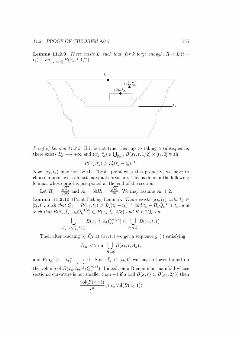
11.2. PROOF OF THEOREM 9.0.5 185
Lemma 11.2.9. There exists L′ such that, for k large enough, R < L′(t −tk)
−1 on⋃
[tk,0]B(xk, t, 1/2).
tk
0
(x′k, t′k)
(xk, tk)
Proof of Lemma 11.2.9. If it is not true, then up to taking a subsequence,there exists L′k −→ +∞ and (x′k, t
′k) ∈
⋃[tk,0]B(xk, t, 1/2)× [tk, 0] with
R(x′k, t′k) > L′k(t
′k − tk)
−1 .
Now (x′k, t′k) may not be the “best” point with this property; we have to
choose a point with almost maximal curvature. This is done in the followinglemma, whose proof is postponed at the end of the section.
Let Hk =
√L′k
2500and Ak = 50Hk =
√L′k
50. We may assume Ak > 2.
Lemma 11.2.10 (Point-Picking Lemma). There exists (xk, tk) with tk ∈[tk, 0], such that Qk = R(xk, tk) > L′k(tk − tk)
−1 and tk − HkQ−1k > tk, and
such that B(xk, tk, AkQ−1/2k ) ⊂ B(xk, tk, 2/3) and R < 2Qk on
⋃
[tk−HkQ−1k ,tk]
B(xk, t, AkQ−1/2k ) ⊂
⋃
[−τk,0]
B(xk, t, 1)
Then after rescaing by Qk at (xk, tk) we get a sequence gk(.) satisfying
Rgk< 2 on
⋃
[Hk,0]
B(xk, t, Ak) ,
and Rmgk> −Q−1
k −→k→∞
0. Since tk ∈ (tk, 0] we have a lower bound on
the volume of B(xk, tk, AkQ−1/2k ). Indeed, on a Riemannian manifold whose
sectional curvature is not smaller than −1 if a ball B(x, r) ⊂ B(x0, 2/3) then
vol(B(x, r))
rn> cn vol(B(x0, 1))
186 CHAPTER 11. PROOFS OF THE TECHNICAL THEOREMS
for a universal constant cn. This is an easy application of Bishop-Gromov’scomparison inequality. Applying this here, we get
vol(B(xk, tk, AkQ−1/2k )) > c3 vol(B(xk, tk, 1))(AkQ
−1/2k )3
> Cc3(AkQ−1/2k )3(1− ε0)υ0(1) ,
and, after rescaling
vol(B(xk, 0, Ak)) > Cc3(1− ε0)υ0(1)A3k .
Since Ak −→k→∞
∞ and R(x, t) ≤ 2 on this last ball, we have a lower bound
on the injectivity radius of gk(0) at xk. This allows to apply the local versionof Hamilton’s compactness theorem to get a limit flow g∞(.) defined on acomplete manifold M∞×(−∞, 0] which has non negative curvature operator,bounded sectional curvature and is ancient (recall that Hk −→
k→∞∞).
Let us denote V(t) the asymptotic volume of g∞(t). Since Ak −→k→∞
∞,
the above volume estimate shows that V(0) > 0. By Theorem 2.2.1, g∞(·)cannot be a κ-solution.
This means that for each κ there exist xκ, tκ and rκ such that Rm∞ >r−2κ on B(xκ, tκ, rκ) and volB(xκ, tκ, rκ) < κr3
κ. Now by Bishop-Gromov’scomparison theorem V(tκ) < κ. On the other hand, since the curvature isnon negative V is nonincreasing in t. Indeed, for U ⊂M∞
d vol
dt(U) = −
∫
U
Rdvg∞ 6 0 .
Moreover, the additive distance-distortion lemma shows that
dt ≤ d0 + c|t| for t < 0 ,
where c denotes a generic constant. This implies thatB(xκ, 0, r) ⊂ B(xκ, tκ, r+c|tκ|). Consequently
volB(xκ, 0, r)
r36 volg∞(0)B(xκ, tκ, r + c|tκ|)
(r + c|tκ|)3
(r + C|tκ|r
)3
≤ volg∞(tκ)B(xκ, tκ, r + c|tκ|)(r + c|tκ|)3
(r + c|tκ|r
)3
,
which gives, by letting r go to infinity, V(0) 6 V(tκ) < κ. Hence V(0) = 0, acontradiction.
To conclude the proof of Lemma 11.2.8, we need a last lemma.

11.2. PROOF OF THEOREM 9.0.5 187
Lemma 11.2.11. For any L > 1, a ∈ (0, 1/2), there exist τ(L, a) > 0 withthe following property. Assume that for some τ ∈ [0, τ(L, a)], Rm > −1 andR < L(t+ τ)−1 on
⋃[−τ,0]B(x, 0, 1/2). Then
dt(x, ·) 6 d0(x, ·) + 20L|t| 12 ,on B(x, 0, a)× [−τ, 0].
Proof. Denote
η =1/2− a
2> 0,
τ(L, a) =( η
40L
)2
Assume τ ∈ [0, τ(L, a)]. Let t′ ∈ [−τ, 0] minimal such that B(x, 0, a) ⊂B(x, t, 1
2− η) for all t ∈ [t′, 0]. Consider t ∈ [t′, 0] and x′ ∈ B(x, 0, a). Then
B(x′, t, η) ⊂ B(x, t, 1/2). Indeed, if y ∈ B(x′, t, η) then dt(x, t) 6 dt(x, x′) +
dt(x′, y) < 1/2− η+ η = 1/2. Now, set r = (t− τ)1/2 6 τ(L, a)1/2 < η. Then
B(x, t, r) ∪B(x′, t, r) ⊂ B(x, t,1
2).
It follows that one can apply the additive-distorsion lemma 0.6.2 on thoseballs. Indeed, as Rm > −1 one has also, denoting ν 6 µ 6 λ its eigenvalues,
Rm 6 λ =R
2− µ− ν 6 L(t+ τ)−1
2+ 2 6 L(t+ τ)−1.
Applying Lemma 0.6.2 at time t with constant K = L(t + τ)−1 and radiusr, we get
d
dtdt(x, x
′) > −4
(2
3L(t− τ)−1(t− τ)1/2 + (t− τ)−
12
),
> −10L(t− τ)12 .
Integrating beetwen t and 0, one finds
d0(x, x′)− dt(x, x
′) > −20L(τ
12 − (t− τ)
12
),
> −20L|t| 12 .In particular,
dt′(x, x′) 6 d0(x, x
′) + 20L|t′| 126 a+
η
2<
1
2− η,
hence t′ = −τ .
188 CHAPTER 11. PROOFS OF THE TECHNICAL THEOREMS
An immediate consequence of this lemma is that B(x, 0, a) ⊂ B(x, t, a+
20L|t| 12 ). Having show that R < L′(t − tk)−1 on
⋃
[tk,0]
B(xk, t, 1/2), we apply
Lemma 11.2.11 for all k sufficiently large such that tk ∈ [−τ(L′, 14), 0]. In
particular, B(xk, 0,14) ⊂ B(xk, tk, 1) for all large k. Then
voltk B(xk, tk, 1) > voltk B
(xk, 0,
1
4
)
> e3tk vol0B
(xk, 0,
1
4
)
> e3tkυ−1(
14)
υ−1(1)vol0B(xk, 0, 1) (by Bishop-Gromov)
> e3tkυ−1(
14)
υ−1(1)(1− ε0)υ0(1)
> 2C(1− ε0)υ0(1).
for k large enough. Here we used that Rm ≥ −1 hence Ric ≥ −2 whichimplies g(tk)/g(0) ≥ e2tk . If tk > −τk the previous estimate contradicts thedefinition of tk. Indeed by continuity voltk B(xk, t, 1) > C(1 − ε0)υ0(1) on[tk − σ, 0] for some σ > 0. Hence we have proved that tk = −τk. But thenLemma 11.2.9 contradicts the assumption made at the beginning of the proofof 11.2.8 that we have no such scalar curvature bound on Bk. This finishesthe proof of Lemma 11.2.8.
Now Proposition 11.2.6 a) follows by taking τ 6 τ(L, 14) and t ∈ [− τ
2, 0]
which gives that R 6 2L/τ on⋃
[τ/2,0]
B(x0, t, 1/2). We set K∗ = 2L.
Define
τ∗ = min
τ
(L,
1
4
),
(10−3
20L
)2
and let us check 11.2.6 b). By Lemma 11.2.8 and Lemma 11.2.11, if τ ∈ [0, τ∗],
B(x, 0, 1/4− 20Lτ12 ) ⊂ B(x,−τ, 1/4).
Let us denote η = 20Lτ12 6 20Lτ∗
12 6 10−3. Then the computation is
similar to the one done above, using that on the neighbourhood considered
11.2. PROOF OF THEOREM 9.0.5 189
Rm > −1. More precisely,
vol−τ B(x,−τ, 1/4) > vol−τ B(x, 0, (
1
4− η)
)
> (e−2τ )3/2 vol0B
(x, 0, (
1
4− η)
)
> (e−2τ∗)3/2υ−1(14− η)
υ−1(1)vol0B(x, 0, 1)
> e−3τ∗ υ−1(14− η)
υ−1(1)(1− ε0)υ0(1)
> e−3τ∗ υ−1(14− η)
υ−1(1)43(1− ε0)υ0(
1
4)
> 1
10υ0(
1
4)
as υ−1(1/5)υ−1(1)
43 > 0, 42.
We finish by proving Point-Picking Lemma 11.2.10.
Proof of Lemma 11.2.10. Since we are working with a fixed Riemannian man-ifold we may drop the index k. We prove first that there exist (x, t) suchthat
i. R(y, t) < 2Q = R(x, t) for all (y, t) such that t ∈ [t − HQ−1, t],dt(y, x) < dt(x, x) + AQ−1/2,
ii. B(x, t, AQ−1/2) ⊂ B(x, t, 2/3).
Let us start with a space-time point (x1, t1) such that x1 ∈ B(x, t1, 1/2),t1 ∈ [t, 0] and Q1 = R(x1, t1) ≥ L′(t1 − t)−1. The point (x1, t1) may satisfythe curvature requirement and we take (x, t) = (x1, t1). In that case HQ−1
1 ≤HL′−1(t1 − t) ≤ 1/4(t1 − t) (we may choose L′ ≥ 1). If this is not the case,there exists (x2, t2) with t2 ∈ [t1 −HQ−1
1 , t1] ⊂ [t1 − 1/4(t1 − t), t1] ⊂ [t, 0],
dt2(x2, x) < dt1(x1, x) + AQ−1/21 <
1
2+ AQ
−1/21 ,
and Q2 = R(x2, t2) ≥ 2R(x1, t1) = 2Q1. Let us notice that with our choices
t2 −HQ−12 > t2 − H
2Q−1
1 > t2 − 1
8(t1 − t) > t1 − 1
4(t1 − t)− 1
8(t1 − t) .
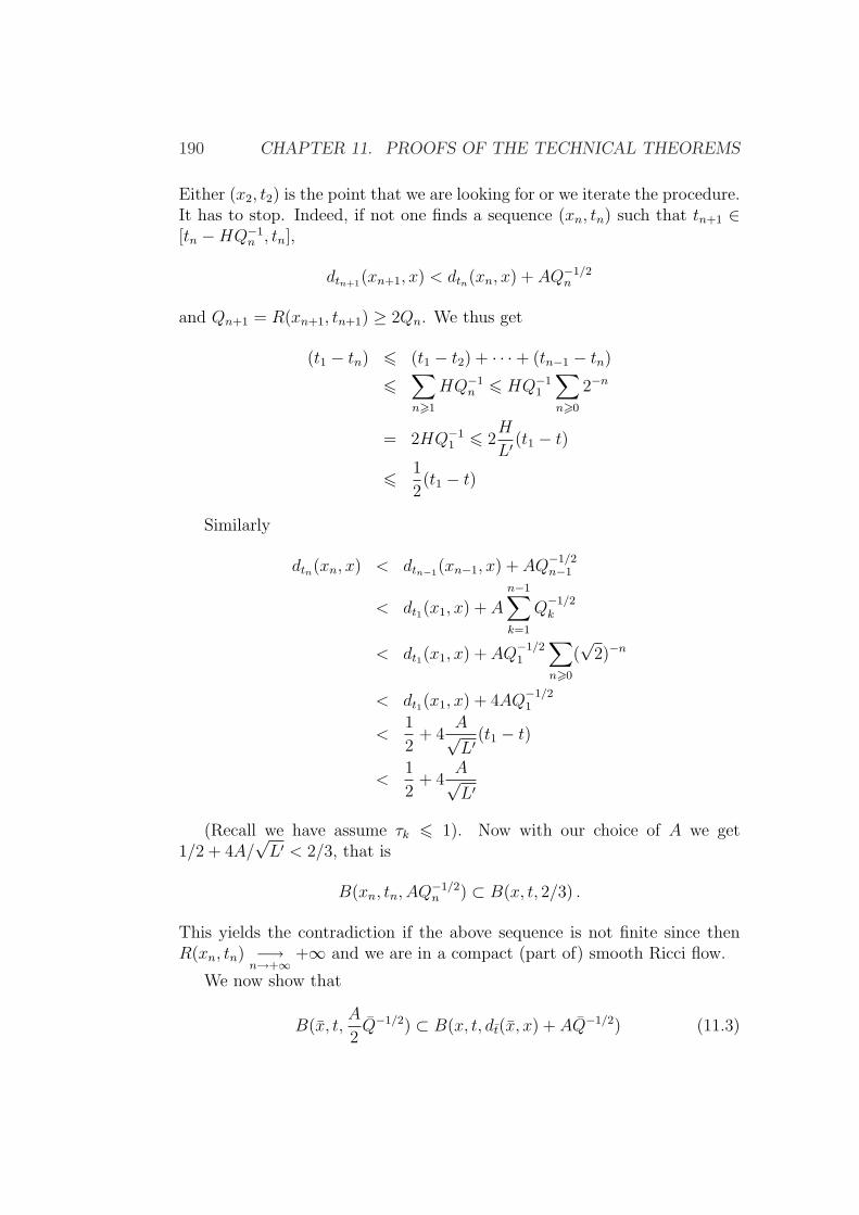
190 CHAPTER 11. PROOFS OF THE TECHNICAL THEOREMS
Either (x2, t2) is the point that we are looking for or we iterate the procedure.It has to stop. Indeed, if not one finds a sequence (xn, tn) such that tn+1 ∈[tn −HQ−1
n , tn],
dtn+1(xn+1, x) < dtn(xn, x) + AQ−1/2n
and Qn+1 = R(xn+1, tn+1) ≥ 2Qn. We thus get
(t1 − tn) 6 (t1 − t2) + · · ·+ (tn−1 − tn)
6∑n>1
HQ−1n 6 HQ−1
1
∑n>0
2−n
= 2HQ−11 6 2
H
L′(t1 − t)
6 1
2(t1 − t)
Similarly
dtn(xn, x) < dtn−1(xn−1, x) + AQ−1/2n−1
< dt1(x1, x) + A
n−1∑
k=1
Q−1/2k
< dt1(x1, x) + AQ−1/21
∑n>0
(√
2)−n
< dt1(x1, x) + 4AQ−1/21
<1
2+ 4
A√L′
(t1 − t)
<1
2+ 4
A√L′
(Recall we have assume τk 6 1). Now with our choice of A we get1/2 + 4A/
√L′ < 2/3, that is
B(xn, tn, AQ−1/2n ) ⊂ B(x, t, 2/3) .
This yields the contradiction if the above sequence is not finite since thenR(xn, tn) −→
n→+∞+∞ and we are in a compact (part of) smooth Ricci flow.
We now show that
B(x, t,A
2Q−1/2) ⊂ B(x, t, dt(x, x) + AQ−1/2) (11.3)
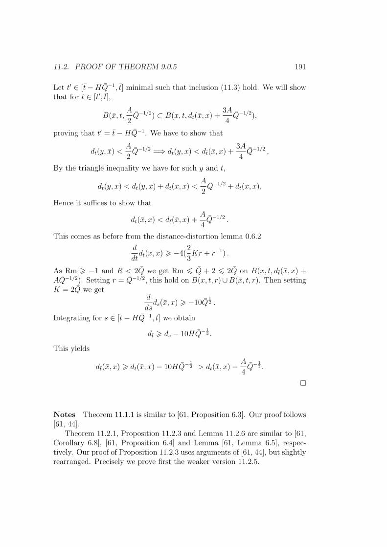
11.2. PROOF OF THEOREM 9.0.5 191
Let t′ ∈ [t−HQ−1, t] minimal such that inclusion (11.3) hold. We will showthat for t ∈ [t′, t],
B(x, t,A
2Q−1/2) ⊂ B(x, t, dt(x, x) +
3A
4Q−1/2),
proving that t′ = t−HQ−1. We have to show that
dt(y, x) <A
2Q−1/2 =⇒ dt(y, x) < dt(x, x) +
3A
4Q−1/2 ,
By the triangle inequality we have for such y and t,
dt(y, x) < dt(y, x) + dt(x, x) <A
2Q−1/2 + dt(x, x),
Hence it suffices to show that
dt(x, x) < dt(x, x) +A
4Q−1/2 .
This comes as before from the distance-distortion lemma 0.6.2
d
dtdt(x, x) > −4(
2
3Kr + r−1) .
As Rm > −1 and R < 2Q we get Rm 6 Q + 2 6 2Q on B(x, t, dt(x, x) +AQ−1/2). Setting r = Q−1/2, this hold on B(x, t, r)∪B(x, t, r). Then settingK = 2Q we get
d
dsds(x, x) > −10Q
12 .
Integrating for s ∈ [t−HQ−1, t] we obtain
dt > ds − 10HQ−12 .
This yields
dt(x, x) > dt(x, x)− 10HQ−12 > dt(x, x)− A
4Q−
12 .
Notes Theorem 11.1.1 is similar to [61, Proposition 6.3]. Our proof follows[61, 44].
Theorem 11.2.1, Proposition 11.2.3 and Lemma 11.2.6 are similar to [61,Corollary 6.8], [61, Proposition 6.4] and Lemma [61, Lemma 6.5], respec-tively. Our proof of Proposition 11.2.3 uses arguments of [61, 44], but slightlyrearranged. Precisely we prove first the weaker version 11.2.5.

192 CHAPTER 11. PROOFS OF THE TECHNICAL THEOREMS
Part IV
Hyperbolisation
193

195
In this part we prove Theorem 0.3.4, that we restate later as Theo-rem 12.0.12. In particular, throughout the whole Part IV we shall be con-cerned with the case where π1M is nontrivial.

196
Chapter 12
Simplicial volume andcollapsing
Let M is a 3-manifold. Recall the following definition
Definition. Let g be a Riemannian metric on M and ε > 0 be a real number.A point x ∈M is ε-thin with respect to g if there exists 0 < ρ ≤ 1 such thaton the ball B(x, ρ), the sectional curvature is greater than or equal to −ρ−2
and the volume of this ball is less than ε ρ3.
The following is a technical condition which guarantees the regularity ofcertain limits of Riemannian manifolds. The Riemann tensor is denoted byRm.
Definition. Let gn be a sequence of Riemannian metrics on M . We saythat gn has locally controlled curvature in the sense of Perelman if it has thefollowing property: for all ε > 0 there exist r(ε) > 0, K0(ε) > 0, K1(ε) >0, such that for n large enough, if 0 < r ≤ r(ε), x ∈ (M, gn) satisfiesvol(B(x, r))/r3 ≥ ε, and if the sectional curvature on B(x, r) is greater thanor equal to −r−2, then |Rm(x)| < K0r
−2 and |∇Rm(x)| < K1r−3.
Next we recall the definition of a topological invariant V0(M) which isessential to this chapter. As M is closed, for us, a link in M is a (possiblyempty, possibly disconnected) closed 1-submanifold ofM . A link is hyperbolicif its complement is a hyperbolic 3-manifold (recall that by convention, allhyperbolic manifolds are assumed to have finite volume ??). The invariantV0(M) is defined as the infimum of the volumes of all hyperbolic links inM . When M is closed, this quantity is finite because any closed 3-manifoldcontains a hyperbolic link [53]. Since the set of volumes of hyperbolic 3-manifolds is well-ordered, this infimum is always realised by some hyperbolic
197
198 CHAPTER 12. SIMPLICIAL VOLUME AND COLLAPSING
3-manifold H0; in particular, it is positive. We note that M is hyperbolic ifand only if H0 = M ; indeed, every hyperbolic Dehn filling on a hyperbolicmanifold strictly decreases the volume [5, 29, 74].
We now state the main result of this chapter (Theorem 0.3.4):
Theorem 12.0.12. Let M be a non-simply connected, closed, orientable,irreducible 3-manifold. Suppose that there exists a sequence gn of Riemannianmetrics on M satisfying:
(1) The sequence vol(gn) is bounded.
(2) For all ε > 0 and for every sequence xn ∈ M so that xn is ε-thickwith respect to gn ∀n, the sequence of pointed manifolds (M, gn, xn) hasa subsequence that converges in the C2-topology towards a hyperbolicpointed manifold with volume strictly less than V0(M).
(3) The sequence gn has locally controlled curvature in the sense of Perel-man.
Then M is a graph manifold or contains an incompressible torus.
Notice the following dichotomy: up to subsequence either there exists ε >0 such that (M, gn) has nonempty ε-thick part for every n, or the sequencecollapses.: the whole manifold (M, gn) is εn-thin for some sequence εn 0.Thus Theorem 12.0.12 can be viewed as a weak collapsing result in the sensethat we allow the thick part to be nonempty, but require a control on itsvolume.
A key notion used in the proof is the simplicial volume, sometimes calledGromov’s norm, introduced by M. Gromov in [29]. Our proof relies on an ad-ditivity result for the simplicial volume under gluing along incompressible tori(see [29, 47, 70]) which implies that the simplicial volume of a 3-manifold ad-mitting a geometric decomposition is proportional to the sum of the volumesof the hyperbolic pieces. In particular, such a manifold has zero simplicialvolume if and only if it is a graph manifold.
We also use in an essential way Gromov’s vanishing theorem [29, 38]:if a n-dimensional closed manifold M can be covered by open sets Ui suchthat the covering has dimension less than n and the image of the canonicalhomomorphism π1Ui → π1M is amenable for all i, then the simplicial volumeof M vanishes. (Recall that the dimension of a finite covering Ui is thedimension of its nerve, i.e. the minimal d such that every point in M belongsto at most d+ 1 open subsets of the covering.)
The definition and main properties of simplicial volume are recalled inSection 12.1. The proof of 12.0.12 is outlined in Section 12.2.
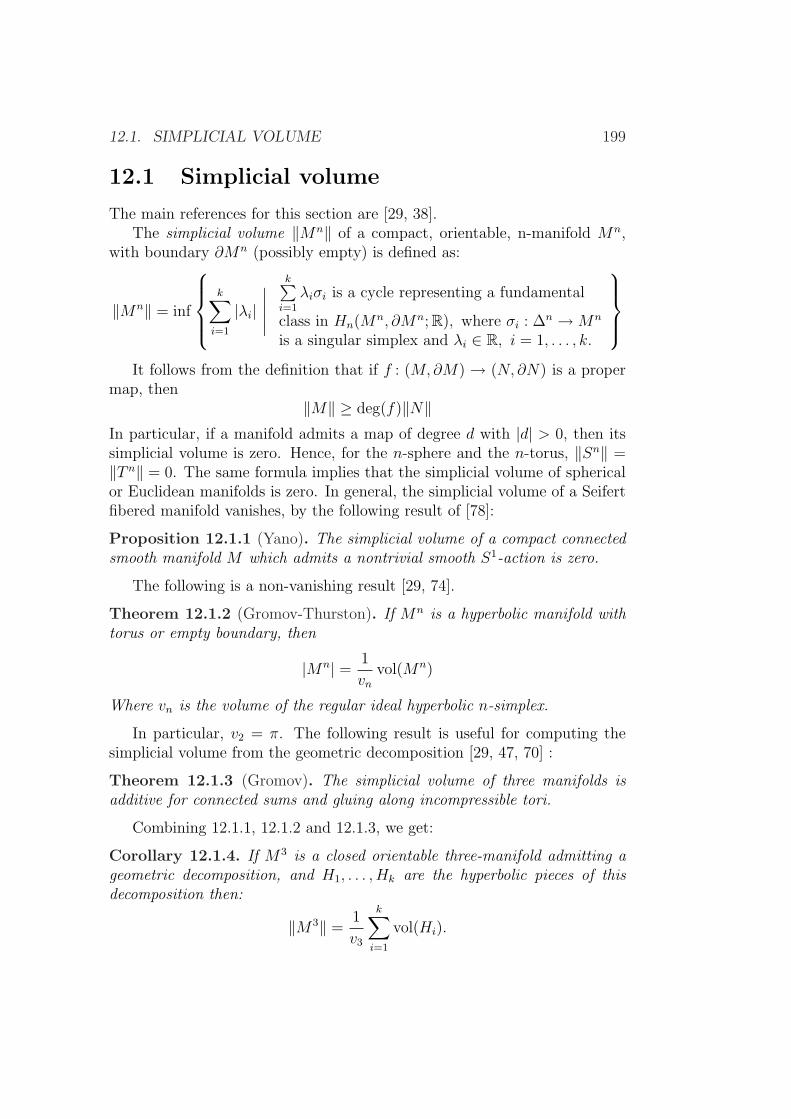
12.1. SIMPLICIAL VOLUME 199
12.1 Simplicial volume
The main references for this section are [29, 38].The simplicial volume ‖Mn‖ of a compact, orientable, n-manifold Mn,
with boundary ∂Mn (possibly empty) is defined as:
‖Mn‖ = inf
k∑i=1
|λi|∣∣∣∣∣
k∑i=1
λiσi is a cycle representing a fundamental
class in Hn(Mn, ∂Mn;R), where σi : ∆n →Mn
is a singular simplex and λi ∈ R, i = 1, . . . , k.
It follows from the definition that if f : (M,∂M) → (N, ∂N) is a propermap, then
‖M‖ ≥ deg(f)‖N‖In particular, if a manifold admits a map of degree d with |d| > 0, then itssimplicial volume is zero. Hence, for the n-sphere and the n-torus, ‖Sn‖ =‖T n‖ = 0. The same formula implies that the simplicial volume of sphericalor Euclidean manifolds is zero. In general, the simplicial volume of a Seifertfibered manifold vanishes, by the following result of [78]:
Proposition 12.1.1 (Yano). The simplicial volume of a compact connectedsmooth manifold M which admits a nontrivial smooth S1-action is zero.
The following is a non-vanishing result [29, 74].
Theorem 12.1.2 (Gromov-Thurston). If Mn is a hyperbolic manifold withtorus or empty boundary, then
|Mn| = 1
vnvol(Mn)
Where vn is the volume of the regular ideal hyperbolic n-simplex.
In particular, v2 = π. The following result is useful for computing thesimplicial volume from the geometric decomposition [29, 47, 70] :
Theorem 12.1.3 (Gromov). The simplicial volume of three manifolds isadditive for connected sums and gluing along incompressible tori.
Combining 12.1.1, 12.1.2 and 12.1.3, we get:
Corollary 12.1.4. If M3 is a closed orientable three-manifold admitting ageometric decomposition, and H1, . . . , Hk are the hyperbolic pieces of thisdecomposition then:
‖M3‖ =1
v3
k∑i=1
vol(Hi).
200 CHAPTER 12. SIMPLICIAL VOLUME AND COLLAPSING
Remark. By applying this corollary, once we know that M3 has a geometricdecomposition, then M3 is a graph manifold (non necesarily irreducible) iff‖M3‖ = 0.
We will also require a vanishing theorem of Gromov. We say that acovering UiiI by open sets of a topological space X has dimension at mostk if every point of X belongs to at most k+1 open sets of the covering. Thedimension of the covering is defined by taking a minimum of such k, and itequals the dimension of the nerve of the covering.
A connected subset U ⊂ M is said to be amenable if the image of itsfundamental group π1(U) → π1(M) is amenable. this definition extendsto non connected subsets, by requiring that all connected components areamenable.
Theorem 12.1.5 (Gromov). If Mn admits a covering of dimension at mostn− 1 by amenable open sets, then ‖Mn‖ = 0.
This theorem is proved in [29, 38] by using bounded cohomology, dual tosimplicial volume.
12.2 Sketch of proof of Theorem 12.0.12
Before discussing the proof proper, we give an example of a covering argumentwhich can be used to deduce topological information on M (namely that Mhas zero simplicial volume) from the collapsing hypothesis.
For n large enough, thanks to the local control on the curvature, eachpoint has a neighbourhood in (M, gn) which is close to a metric ball in somemanifold of nonnegative sectional curvature (Proposition 13.2.1), and whosevolume is small compared to the cube of the radius (by the collapsing hypoth-esis). These neighbourhoods will be called local models throughout the paper.From the classification of manifolds with nonnegative sectional curvature, wededuce that these local models have virtually abelian, hence amenable fun-damental groups. A technique introduced by Gromov [29] yields a coveringof M , whose dimension is at most 2, by open sets contained in these neigh-bourhoods. As a consequence, Gromov’s vanishing theorem implies that thesimplicial volume of M vanishes.
The previous scheme, together with the additivity of the simplicial volumeunder gluing along incompressible tori, shows that a manifold which admitsa geometric decomposition and a sequence of collapsing metrics is a graphmanifold. This is however insufficient to prove Theorem 0.4.1 since we do notassume that M admits a geometric decomposition! Hence we need a tricksimilar to those of [9] and [7], which we now explain.
12.2. SKETCH OF PROOF OF THEOREM 12.0.12 201
In the first step, in Proposition 13.3.1, we find a local model U such thatall connected components ofMrU are Haken. This requirement is equivalentto irreducibility of each component ofMrU , because each component ofMrU has nonempty boundary. Since M is irreducible, it suffices to show that Uis not contained in a 3-ball. This is in particular the case if U is homotopicallynontrivial, i.e. the homomorphism π1(U) → π1(M) has nontrivial image.
The proof of the existence of a homotopically nontrivial local model Uis done by contradiction: assuming that all local models are homotopicallytrivial, we construct a covering of M of dimension less than or equal to 2 byhomotopically trivial open sets (Assertion 13.3.5). By a result of J.C. Gomez-Larranaga and F. Gonzalez-Acuna [25], corresponding to Corollary 13.3.3here, a closed irreducible 3-manifold admitting such a covering must havetrivial fundamental group. This is where we use the hypothesis that M isnot simply connected.
The second step (Subsection 13.3.3) is again a covering argument but donerelatively to some fixed homotopically nontrivial local model U . It showsthat any manifold obtained by Dehn filling on Y := M rU has a covering ofdimension less than or equal to 2 by virtually abelian open sets, and thereforehas vanishing simplicial volume. We conclude using Proposition 13.3.15,which states that if Y is a Haken manifold with boundary a collection of toriand such that the simplicial volume of every Dehn filling on Y vanishes, thenY is a graph manifold.1 This finishes the sketch of proof of Theorem 0.4.1.
In this text, we shall not separate the case when gn collapses, but weshall treat directly the general case. This implies that we first need to coverthe thick part by submanifolds H i
n approximating compact cores of limitinghyperbolic manifolds (Section 13.1). We then cover the thin part by localmodels (Section 13.2). The bulk of the proof is in Section 13.3: assumingthat M contains no incompressible tori, we consider the covering of M byapproximately hyperbolic submanifolds and local models of the thin partand perform two covering arguments: the first one (Assertion 13.3.5) opensubsets is homotopically nontrivial in M ; the second one (Assertion 13.3.17)is done relatively to this homotopically nontrivial subset and proves that Mis a graph manifold.
1As already mentioned in [9, 7], Proposition 13.3.15 is a consequence of the geome-trisation of Haken manifolds, additivity of the simplicial volume mentioned above, andThurston’s hyperbolic Dehn filling theorem.

202 CHAPTER 12. SIMPLICIAL VOLUME AND COLLAPSING
Chapter 13
Weak collapsing
In this section we prove Theorem 12.0.12. Firstly, in section 13.1 we provethe structure of the thick part: either it contributs with essential torus or itis contained in solid torus. Then it Section 13.2 we give the local propertiesof the thin part, that are used in Section 13.3 to work with coverings and toconclude the proof of the theorem. In Section 13.4 we prove Theorems 0.3.5and 0.4.3.
13.1 Structure of the thick part
Until the end of Section 13.3, we consider a 3-manifold M and a sequenceof Riemannian metrics gn satisfying the hypotheses of Theorem 12.0.12. Forthe sake of simplicity, in the sequel we use the notation Mn := (M, gn). Thegoal of this section is to describe the thick part of the manifolds Mn and tomake the link between the topology of the thick part and the topology of M .We denote by M−
n (ε) the ε-thin part of Mn, and by M+n (ε) its ε-thick part.
13.1.1 Covering the thick part
Proposition 13.1.1. Up to taking a subsequence of Mn, there exists a fi-nite (possibly empty) collection of pointed hyperbolic manifolds (H1, ∗1), . . . ,(Hm, ∗m) and for every 1 ≤ i ≤ m a sequence xin ∈Mn satisfying:
(i) limn→∞
(Mn, xin) = (H i, ∗i) in the C2 topology.
(ii) For all sufficiently small ε > 0, there exist n0(ε) and C(ε) such thatfor all n ≥ n0(ε) one has M+
n (ε) ⊂ ⋃iB(xin, C(ε)).
203
204 CHAPTER 13. WEAK COLLAPSING
Proof. By assumption, the sequence vol(Mn) is bounded above. Let µ0 > 0be a universal number such that any hyperbolic manifold has volume at leastµ0.
If for all ε > 0 we have M+n (ε) = ∅ for n large enough, then Proposi-
tion 13.1.1 is vacuously true, with m = 0. Otherwise, we use Hypothesis (2)of Theorem 12.0.12: up to taking a subsequence of Mn, there exists ε1 > 0and a sequence of points x1
n ∈ M+n (ε1) such that (Mn, x
1n) converges to a
pointed hyperbolic manifold (H1, ∗1).If for all ε > 0 there exists C(ε) such that, for n large enough, M+
n (ε) isincluded in B(x1
n, C(ε)), then we are done. Otherwise there exists ε2 > 0 anda sequence x2
n ∈ M+n (ε2) such that d(x1
n, x2n) → ∞. Again Hypothesis (2)
of Theorem 12.0.12 ensures that, after taking a subsequence, the sequence(Mn, x
2n) converges to a pointed hyperbolic manifold (H2, ∗2). We iterate
this construction.Note that for each i, and for n sufficiently large, Mn contains a sub-
manifold C2-close to some compact core of Hi and whose volume is greaterthan or equal to µ0/2. Moreover, for n fixed and large, these submanifoldsare pairwise disjoint. Since the volume of the manifolds Mn is uniformlybounded above this construction has to stop. Condition (ii) of the conclu-sion of Proposition 13.1.1 is then satisfied for 0 < ε < εk.
Remark. By Proposition 13.1.1, up to subsequence one can choose sequencesεn → 0 and rn → ∞ such that the ball B(xin, rn) is arbitrarily close toa metric ball B(∗i, rn) ⊂ H i, for i = 1, . . . ,m, and every point of Mn \⋃iB(xin, rn) is εn-thin.
Let us fix a sequence of positive real numbers εn → 0. Let H1, . . . , Hm behyperbolic limits given by Proposition 13.1.1. For each i we choose a compactcore H i for H i and for each n a submanifold H i
n and an approximationφin : H i
n → H i. Up to renumbering, one can assume that for all n we haveMn \
⋃H in ⊂M−
n (εn), and that the H in’s are disjoint.
The hypothesis in Theorem 12.0.12 that the volume of each hyperboliclimit H i is less than V0 implies that for n sufficiently large no component H i
n
is homeomorphic to the exterior of a link in M .The logic of the proof of Theorem 12.0.12 is the following: each boundary
component of H in is a torus. If one of those tori is incompressible, then the
conclusion of Theorem 12.0.12 is true. The interesting case is when all thetori that appear in the boundary of the thick part are compressible, thiswill be considered in Proposition 13.1.3 and Sections 13.2 and 13.1. Theremainder of this section is devoted to the two following results:
Proposition 13.1.2. Under the assumptions of Theorem 12.0.12, up to tak-ing a subsequence, one of the following properties is satisfied:
13.1. STRUCTURE OF THE THICK PART 205
(i) There exists an integer i0 ∈ 1, . . . ,m such that ∂H i0n contains an
incompressible torus for all n, or
(ii) for all i ∈ 1, . . . ,m, H in is embedded in a solid torus or in a 3-ball
contained in Mn for all n.
Proposition 13.1.3. Under the assumptions of Theorem 12.0.12, if Con-clusion (ii) of Proposition 13.1.2 is satisfied, then either M is a lens spaceor there exists for each n a submanifold Wn ⊂Mn such that:
(i)⋃H in ⊂ Wn.
(ii) Each connected component of Wn is a solid torus, or contained in a3-ball embedded in Mn and homeomorphic to the exterior of a knot inS3.
(iii) The boundary of each component of Wn is a connected component of⋃i ∂H
in.
Subsection 13.1.2 is devoted to general topological results concerning com-pressible tori in 3-manifolds and abelian submanifolds. Propositions 13.1.2and 13.1.3 will be proved in Subsection 13.1.3.
13.1.2 Submanifolds with compressible boundary
Let X be an orientable, irreducible 3-manifold and T be a compressible torusembedded in X. The Loop Theorem shows the existence of a compressiondisc D for T , that is, a disc D embedded in M such that D ∩ T = ∂D andthe curve ∂D is not null homotopic in T . By cutting open T along an opensmall regular neighbourhood of D and gluing two parallel copies of D alongthe boundary curves, one constructs an embedded 2-sphere S in X. We saythat S is obtained by compressing T along D.
Since X is assumed to be irreducible, S bounds a 3-ball B. There are twopossible situations depending on whether B contains T or not. The followinglemma collects some standard results that we shall need.
Lemma 13.1.4. Let X be an orientable, irreducible 3-manifold and T be acompressible torus embedded in X. Let D be a compression disc for T , Sbe a sphere obtained by compressing T along D, and B a ball bounded by S.Then:
i) X \ T has two connected components U, V , and D is contained in theclosure of one of them, say U .
206 CHAPTER 13. WEAK COLLAPSING
ii) If B does not contain T , then B is contained in U , and U is a solidtorus.
iii) If B contains T , then B contains V , and V is homeomorphic to theexterior of a knot in S3. In this case, there exists a homeomorphism ffrom the boundary of S1 × D2 into T such that the manifold obtainedby gluing S1 ×D2 to U along f is homeomorphic to X.
Remark. If T is a component of ∂X and T is a compressible torus, the sameargument shows that X is a solid torus.
To understand the situation in Lemma 13.1.4 (iii), one has to think of theconnected sum of any manifold with a solid torus S1×D2, which is glued toany knot exterior in S3.
Lemma 13.1.5. Let X be a closed, orientable, irreducible 3-manifold. LetH ⊂ X be a connected, compact, orientable, irreducible submanifold of Xwhose boundary is a collection of compressible tori. If H is not homeomorphicto the exterior of a (possibly empty) link in X, then H is included in aconnected submanifold Y whose boundary is one of the tori of ∂H and whichsatisfies one of the following properties:
(i) Y is a solid torus, or
(ii) Y is homeomorphic to the exterior of a knot in S3 and contained in aball B ⊂ X.
Proof. By hypothesis the boundary of H is not empty. We denote by T1, . . . ,Tm the components of ∂H. If one of them bounds a solid torus containingH, then we can choose this solid torus as Y . Henceforth we assume that thisis not the case.
Each Tj being compressible, it separates and thus bounds a submanifoldVj not containing H. Up to renumbering the boundary components of H, wemay assume that V1, . . . , Vk are disjoint solid tori, but Vk+1, . . . , Vm are notsolid tori. At least one of the Vj’s is not a solid torus, otherwise H would behomeomorphic to the exterior of a link in X.
For the same reason, at least one Vj, for some j > k, is not contained inthe 3-ball bounded by the sphere obtained after compressing Tj. Otherwiseeach of the Vk+1, . . . , Vm is homeomorphic to the exterior of a knot in S3,by Lemma 13.1.4, and one could then replace each Vj ,k + 1 ≤ j ≤ m by asolid torus without changing the topological type of X. Hence H would behomeomorphic to the exterior of a link in X.
Pick a Vj, for j > k, which is not contained in a ball. Then compressingsurgery on the torus Tj = ∂Vj yields a sphere S bounding a ball B in X,
13.2. LOCAL STRUCTURE OF THE THIN PART 207
which contains H by the choice of Vj. This shows that conclusion (ii) issatisfied with Y = X \ intVj.
13.1.3 Proof of Propositions 13.1.2 and 13.1.3
Proof of 13.1.2. If Assertion (i) of Proposition 13.1.2 is not satisfied, then,up to a subsequence, one may assume that for all i ∈ 1, . . . ,m and forall n, each component of ∂H i
n is compressible in M . We fix an integeri ∈ 1, . . . ,m. From the hypotheses of Theorem 12.0.12, we get the in-equality vol(H i) < V0(M), which implies that H i is not homeomorphic tothe complement of a link in M . In particular since H i
n is homeomorphic tothe compact core of H i, it is not homeomorphic to the exterior of a link inM . Lemma 13.1.5 applied to (Hn,Mn) = (H,X) allows to conclude thatAssertion (ii) of Proposition 13.1.2 holds true.
Proof of 13.1.3. For each n and each i ∈ 1, . . . ,m, we choose a submanifoldY in containing H i
n, given by Lemma 13.1.5. We take Wn to be the union ofthe Y i
n. Then Assertion (i) of Proposition 13.1.3 is straightforward.Assume that M is not a lens space. Then Mn cannot be the union of two
submanifolds Y in and Y j
n , otherwise Mn can be covered either by two solidtori, or by a solid torus and a ball or by two balls. In the first case Mn wouldbe homeomorphic to a lens space by [27], while in the other two cases Mn
would be covered by three balls and thus homeomorphic to the 3-sphere S3
by [36], see also [26]. Thus for all i1, i2, the submanifolds Y i1n and Y i2
n aredisjoint or one contains the other, because they have disjoint boundaries. Inthis case each component of Wn is homeomorphic to one of the Y i
n. Thisyields Assertions (ii) and (iii) of Proposition 13.1.3.
13.2 Local structure of the thin part
In this section, it is implicit that any quantity depending on a point x ∈Mn
is computed with respect to the metric gn on Mn and thus depends also onn.
Let us choose a sequence εn → 0 (see the remark after Proposition 13.1.1).For all x ∈ M−
n (εn), we choose a radius 0 < ρ(x) ≤ 1, such that on theball B(x, ρ(x)) the curvature is ≥ −ρ−2(x) and the volume of this ball is< εnρ
3(x).Recall that a map f : X → Y is (1 + δ)-bi-Lipschitz if it is a diffeomor-
phism such that f and f−1 are (1 + δ)-lipschitz. Two Riemannian manifoldsX and Y are said to be δ-close if there exists a (1 + δ)-bi-Lipschitz mapbetween them.
208 CHAPTER 13. WEAK COLLAPSING
In the following proposition we use Cheeger-Gromoll’s soul theorem [14].
Proposition 13.2.1. For all D > 1 there exists n0(D) such that if n >n0(D), then we have the following alternative:
(a) Either Mn is 1D
-close to some closed nonnegatively curved 3-manifold,or
(b) for all x ∈ M−n (εn) there exists a radius ν(x) ∈ (0, ρ(x)) and a com-
plete noncompact Riemannian 3-manifold Xx, with nonnegative sec-tional curvature and soul Sx, such that the following properties aresatisfied:
(1) B(x, ν(x)) is 1D
-close to a metric ball in Xx.
(2) There exists a map fx : B(x, ν(x)) → Xx which is (1 + 1D
)-bi-Lipschitz with its image and such that
maxd(f(x), Sx), diamSx ≤ ν(x)D.
(3) vol(B(x, ν(x))) ≤ 1Dν3(x).
Remark. Since ν(x) < ρ(x), the sectional curvature on B(x, ν(x)) is greaterthan or equal to − 1
ρ2(x), which is in turn bounded below by − 1
ν2(x).
Remark. The only closed, orientable and irreducible 3-manifold containing aprojective plane is RP 3, which is a graph manifold. Therefore if the manifoldM is not homeomorphic to RP 3, then the soul Sx can be homeomorphic toa point, a circle, a 2-sphere, a 2-torus or a Klein bottle. In this case, theball B(x, ν(x)) is homeomorphic to R3, S1 ×R2, S2 ×R, T 2 ×R or to thetwisted R-bundle on the Klein bottle respectively.
Before starting the proof of this proposition, we prove the following lemmaand its consequence:
Lemma 13.2.2. There exists a small universal constant C > 0 such that forall ε > 0, for all x ∈ Mn, and for all r > 0, if the ball B(x, r) has volume≥ ε r3 and curvature ≥ −r−2, then for all y ∈ B(x, 1
3r) and all 0 < r′ < 2
3r,
the ball B(y, r′) has volume ≥ C · ε(r′)3 and curvature ≥ −(r′)−2.
We use the function v−κ2(r) to denote the volume of the ball of radiusr in the 3-dimensional hyperbolic space with curvature −κ2. Notice thatv−κ2(r) = κ−3v−1(κ r).
13.2. LOCAL STRUCTURE OF THE THIN PART 209
Proof. The lower bound on the curvature is a consequence of the monotonic-ity of the function −r−2 with respect to r. In order to estimate from belowthe normalised volume we apply Bishop-Gromov’s inequality twice (cf. [63,Lemma 9.1.6]). First to the ball around y, increasing the radius r′ to 2
3r:
vol(B(y, r′)) ≥ vol(B(y, 23r))
v−r−2(r′)v−r−2(2
3r).
Using that v−r−2(r′) = r3v−1(r′r) ≥ r3
(r′r
)3C1 for C1 > 0 uniform, v−r−2(2
3r) =
r3v−1(23), and that the ball B(y, 2
3r) contains B(x, 1
3r), we have
vol(B(y, r′)) ≥ vol(B(x, 13r))
(r′r
)3C2.
Applying again the Bishop-Gromov inequality:
vol(B(x, 13r)) ≥ vol(B(x, r))
v−r−2(13r)
v−r−2(r)≥ r3ε
v−1(13)
v−1(1)= r3εC3.
Hence vol(B(y, r′)) ≥ (r′)3 εC4.
We next deduce an “improvement” of the controlled curvature in the senseof Perelman, in which the conclusion is valid at each point of some metricball, not only the centre. The only price to pay is that the constants can beslightly different.
Corollary 13.2.3. For all ε > 0 there exist r′(ε) > 0, K ′0(ε), K
′1(ε) such
that for n large enough, if 0 < r ≤ r′(ε), x ∈ Mn and the ball B(x, r) hasvolume ≥ ε r3 and sectional curvatures ≥ −r−2 then, for all y ∈ B(x, 1
3r),
|Rm(y)| < K ′0 r
−2 and |∇Rm(y)| < K ′1 r
−3.
Proof. It suffices to apply Lemma 13.2.2, setting r′(ε) = r(Cε), K ′0(ε) =
K0(Cε) and K ′1(ε) = K1(Cε), so that we can apply the controlled curvature
condition on y ∈ B(x, 13x).
Proof of Proposition 13.2.1. Let us assume that there exists D0 > 1 and,after re-indexing, a sequence xn ∈ Mn such that neither of the conclusionsof Proposition 13.2.1 holds with D = D0.
Set ε0 := v−1(1)v0(1)
1D0
. We shall rescale the metrics using the following radii:
Definition. For x ∈Mn, define
rad(x) = infr > 0 | vol(B(x, r))/r3 ≤ ε0.
210 CHAPTER 13. WEAK COLLAPSING
Notice that rad(x) <∞ because Mn has finite volume, and that rad(x) >0, because vol(B(x, δ))/δ3 → 4
3π when δ → 0. We gather in the following
lemma some properties which will be useful for the proof:
Lemma 13.2.4. (i) For n large enough and x ∈Mn, one has 0 < rad(x) <ρ(x).
(ii) For x ∈M−n (εn), one has
vol(B(x, rad(x)))
rad(x)3= ε0.
(iii) For L > 1, there exists n0(L) such that for n > n0(L) and for x ∈M−
n (εn) we have
L rad(x) ≤ ρ(x).
In particular limn→∞
rad(xn) = limn→∞
rad(xn)ρ(xn)
= 0.
Proof of Lemma 13.2.4. Property (i) holds as long as εn < ε0, since rad isdefined as an infimum.
Assertion (ii) is proved by continuity.We prove (iii). For L > 1, we choose n0(L) so that εn <
ε0L3 for n > n0(L).
Then, for x ∈Mn and n ≥ n0(L),
vol(B(x, ρ(x)L
)
(ρ(x)L
)3≤ L3 vol(B(x, ρ(x))
ρ(x)3≤ L3εn ≤ ε0.
Hence ρ(x)/L ≥ rad(x).
Remark. For n large enough, from Lemma 13.2.4 (iii), we have rad(xn) <r′(ε0), where r′(ε0) is the parameter from Corollary 13.2.3.
Corollary 13.2.5. There exists a constant C > 0 such that any sequence ofxn ∈M−
n (εn) satisfiesinj(xn)
rad(xn)≥ C
for n large enough.
Proof. Let us first remark that, since rad(xn) < ρ(xn), the sectional curva-tures on B(xn, rad(xn)) are ≥ − 1
ρ(xn)2> − 1
rad(xn)2. Moreover, as rad(xn) <
13.2. LOCAL STRUCTURE OF THE THIN PART 211
r′(ε0), Corollary 13.2.3 shows that the curvature on the ball B(xn,rad(xn)
3) is
bounded above by K ′0(ε0)/ rad(xn)
2. This rescaled ball
1
rad(xn)B(xn,
13rad(xn))
has radius ≤ 1, volume ≥ ε0C0 (where C0 is a universal constant comingfrom Bishop-Gromov) and curvatures with absolute value ≤ K ′
0(ε0). UsingCheeger’s propeller lemma [16, Thm. 4.3], the injectivity radius at the centreof the rescaled ball is bounded below by some constant C > 0. This provesCorollary 13.2.5.
Having proved Lemma 13.2.4 and its corollary, we continue the proof ofProposition 13.2.1. Let us consider the rescaled manifold Mn = 1
rad(xn)Mn.
We look for a limit of the sequence (Mn, xn), where xn is the image of xn.
The ball B(xn,ρ(xn)
rad(xn)) ⊂ Mn has sectional curvature bounded below by
−(
rad(xn)ρ(xn)
)2
, which goes to 0 when n→∞, as follows from Assertion (iii) of
Lemma 13.2.4.Given L > 1, the ballB(xn, 3L) is obtained by rescaling the ballB(xn, 3L rad(xn)).
Since 3L rad(xn) < ρ(xn), the sectional curvature on B(xn, 3L rad(xn)) is≥ − 1
ρ(xn)2≥ − 1
(3L rad(xn))2. Moreover, by Lemma 13.2.4 (ii), we have
vol(B(xn, 3L rad(xn))
(3L rad(xn))3≥ vol(B(xn, rad(xn))
rad(xn)3
1
(3L)3≥ ε0
(3L)3.
By applying Corollary 13.2.3 for n sufficiently large so that we have3L rad(xn) ≤ r′( ε0
(3L)3), one gets that the curvature is locally controlled in
the sense of Perelman at each point of the ball B(xn, L rad(xn)). There-fore the curvature and its first derivative can be bounded above on any ballB(xn, L) ⊂Mn with a given radius L > 1.
Since the injectivity radius of the basepoint xn is bounded below alongthe sequence, this upper bound on the curvature allows to use Gromov’scompactness theorem, cf. [28, Chap. 8, Thm. 8.28], [62], [32, Thm. 2.3]or [23, Thm. 4.1 and 5.10]. It follows that the pointed sequence (Mn, xn)subconverges in the C2-topology towards a 3-dimensional smooth manifold(X∞, x∞), with a complete Riemannian metric of class C2 with nonnegativesectional curvature. This limit manifold cannot be closed, because that wouldcontradict the assumption that the conclusion of Proposition 13.2.1 does nothold.
Hence X∞ is not compact. By pointed convergence, Assertion (b) (1) ofProposition 13.2.1 holds true. Let S be the soul of X∞. Let us choose
ν(xn) = L rad(xn) where L ≥ 2 diam(S ∪ x∞)D0.
212 CHAPTER 13. WEAK COLLAPSING
For n large (to be specified later) we set
Xxn = rad(xn)X∞, and Sxn = rad(xn)S.
We then have
diam(Sxn) = rad(xn) diam(S) < ν(xn)/D0.
Let fn : B(xn, L) → (X∞, x∞) be a map which is (1 + δn)-bi-Lipschitzwith its image and such that d(fn(xn), x∞) < δn, where δn is a sequence goingto 0. After rescaling fn : B(xn, L rad(xn)) → Xxn is also (1+ δn)-bi-Lipschitzwith its image. We get:
d(fn(xn), Sxn) = rad(xn) d(fn(xn), S)
≤ rad(xn)(d(fn(xn), x∞) + d(x∞, S)
)
≤ rad(xn)δn +ν(xn)
2D0
≤ ν(xn)
D0
.
This proves assertion (b) (2) of Proposition 13.2.1.
Using the facts that ν(xn) = L rad(xn) < ρ(xn), the curvature onB(xn, ν(xn))is ≥ −1/ν(xn)
2, L > 1 and the Bishop-Gromov inequality, we get:
vol(B(xn, ν(xn)))
v− 1ν2(xn)
(ν(xn))≤ vol(B(xn, rad(xn)))
v− 1ν2(xn)
(rad(xn))= ε0
rad(xn)3
v− 1ν2(xn)
(rad(xn))=
ε0
(rad(xn)
ν(xn)
)31
v−1(rad(xn)ν(xn)
)= ε0
1
L3
1
v−1(1L).
Since v−1(1L) ≥ v0(
1L) = v0(1) 1
L3 , we find that:
vol(B(xn, ν(xn))) ≤ ε01
L3
v−1(1)
v−1(1L)ν3(xn) ≤
ε0v−1(1)
v0(1)ν3(xn) =
1
D0
ν3(xn),
where the last equality comes from the definition of ε0.
Hence we get the contradiction required to conclude the proof of Propo-sition 13.2.1.
13.3. CONSTRUCTIONS OF COVERINGS 213
13.3 Constructions of coverings
13.3.1 Embedding thick pieces in solid tori
We begin by making some reductions for the proof of Theorem 0.4.1.If case (a) of Proposition 13.2.1 occurs for arbitrarily large D, then M is a
closed, orientable, irreducible 3-manifold admitting a metric of nonnegativesectional curvature. By [30, 31], M is spherical or Euclidean, hence a graphmanifold. Therefore we may assume that all local models Xx produced byProposition 13.2.1 are noncompact.
For the same reasons, since lens spaces are graph manifolds, we can alsoassume that M is not homeomorphic to a lens space, and in particular doesnot contain a projective plane.
If there exists an integer i0 ∈ 1, . . . ,m such that, up to a subsequence,∂H i
n contains an incompressible torus for all n, then Theorem 12.0.12 isproved. We thus assume that for all i ∈ 1, . . . ,m and for all n, each com-ponent of ∂H i
n is compressible in Mn and thus Propositions 13.1.2 and 13.1.3apply and give for each n a submanifold Wn.
Assume that there exists a component X of Wn which is not a solid torus.From Proposition 13.1.3(ii), X is a knot exterior and contained in a 3-ballB ⊂ Mn. By Lemma 13.1.4, it is possible to replace X by a solid torus Ywithout changing the global topology. Let us denote by M ′
n the manifoldthus obtained. We can endow M ′
n with a Riemannian metric g′n, equal togn away from Y and such that an arbitrarily large collar neighbourhood of∂Y in Y is isometric to a collar neighbourhood ∂X in X, because the endof the interior of X is close to a hyperbolic cusp. When n is large, thisneighbourhood is thus almost isometric to a long piece of a hyperbolic cusp,and this geometric property will be sufficient for our covering arguments.
Repeating this construction for each component of Wn which is not asolid torus, we obtain a Riemannian manifold (M ′′
n , g′′n) together with a sub-
manifold W ′′n satisfying the following properties:
(i) M ′′n is homeomorphic to Mn.
(ii) M ′′n \W ′′
n is equal to Mn \Wn and the metrics gn and g′′n coincide onthis set.
(iii) M ′′n \W ′′
n = Mn \Wn is εn-thin.
(iv) When n goes to infinity, there exists a collar neighbourhood of ∂W ′′n in
W ′′n of arbitrarily large diameter isometric to the corresponding neigh-
bourhood in Wn.
214 CHAPTER 13. WEAK COLLAPSING
(v) Each component of W ′′n is a solid torus.
For simplicity, we use the notation Mn, gn, Wn instead of M ′′n , g′′n, W
′′n .
This amounts to assuming in the conclusion of Proposition 13.1.3 that allcomponents of Wn are solid tori.
13.3.2 Existence of a homotopically nontrivial open set
We say that a path–connected set U ⊂ M is homotopically trivial (in M)if the image of the homomorphism π1(U) → π1(M) is trivial. More gener-ally, we say that the subset U ⊂ M is homotopically trivial if all its path-connected components have this property.
We recall that the dimension of a finite covering Uii of M is the dimen-sion of its nerve, hence the dimension plus one equals the maximal numberof Ui’s containing a given point.
Proposition 13.3.1. There exists D0 > 1 such that for all D > D0, forevery n ≥ n0(D) (where n0(D) is given by Proposition 13.2.1), one of thefollowing assertions is true:
(a) some connected component of Wn is not homotopically trivial, or
(b) there exists x ∈Mn such that the image of π1(B(x, ν(x))) → π1(Mn) isnot homotopically trivial, where ν(x) is also given by Proposition 13.2.1.
In [25] J.C. Gomez-Larranaga and F. Gonzalez-Acuna have computed the1-dimensional Lusternik-Schnirelmann category of a closed 3-manifold. Onestep of their proof gives the following proposition (cf. [25, Proof of Prop.2.1]:)
Proposition 13.3.2. Let X be a closed, connected 3-manifold. If X has acovering of dimension 2 by open subsets which are homotopically trivial inX, then there is a connected 2-dimensional complex K and a continuous mapf : X → K such that the induced homomorphism f? : π1(X) → π1(K) is anisomorphism.
Standard homological arguments show the following, cf. [25, §3]:
Corollary 13.3.3. Let X be a closed, connected, orientable, irreducible 3-manifold. If X has a covering of dimension 2 by open subsets which arehomotopically trivial in X, then X is simply connected.
13.3. CONSTRUCTIONS OF COVERINGS 215
Proof. Following Proposition 13.3.2, let f : X → K be a continuous mapfrom X to a connected 2-dimensional complex K, such that the induced ho-momorphism f? : π1(X) → π1(K) is an isomorphism. Let Z be a K(π1(X), 1)space. Let φ : X → Z be a map from X to Z realising the identity homo-morphism on π1(X) and let ψ : K → Z be the map from K to Z realisingthe isomorphism f−1
? : π1(K) → π1(X). Then φ is homotopic to ψ fand the induced homomorphism φ∗ : H3(X;Z) → H3(Z;Z) factors throughψ∗ : H3(K;Z) → H3(Z;Z). Since H3(K;Z) = 0, the homomorphism φ∗must be trivial.
Xφ−→ Z
f ↓ ψ
K
If π1(X) is infinite, then X is aspherical and φ∗ is an isomorphism. There-fore π1(X) is finite.
If π1(X) is finite of order d > 1, then let X be the universal covering
of X. The covering map p : X → X induces an isomorphism betweenthe homotopy groups πk(X) and πk(X) for k ≥ 2. Since π2(X) = 0,π2(X) = 0, and by the Hurewicz theorem, the canonical homomorphism
π3(X) → H3(X;Z) = Z is an isomorphism. It follows that the canonical mapπ3(X) = Z→ H3(X;Z) = Z is the multiplication by the degree d > 1 of the
covering p : X → X. It is well known that one can construct a K(π1(X), 1)space Z by adding a 4-cell to kill the generator of π3(X) = Z, and addingfurther cells of dimension ≥ 5 to kill the higher homotopy groups. Thenthe inclusion φ : X → Z induces the identity on π1(X) and a surjectionφ∗ : H3(X;Z) = Z → H3(Z;Z) = Z/dZ. Therefore X must be simplyconnected.
In the proof of Proposition 13.3.1 we argue by contradiction using Corol-lary 13.3.3 and the fact that π1(M) is not trivial.
With the notation of Proposition 13.2.1, we may assume that for arbitrar-ily large D there exists n ≥ n0(D) such that the image of π1(B(x, ν(x))) →π1(Mn) is trivial for all x ∈ Mn \ int(Wn) as well as for each component ofWn.
Then for all x ∈Mn \ int(Wn) we set:
triv(x) = sup
r
∣∣∣∣∣∣
π1(B(x, r)) → π1(Mn) is trivial andB(x, r) is contained in B(x′, r′) withcurvature ≥ − 1
(r′)2
Assertion 13.3.4. The ball B(x, triv(x)) is contained in another ball B(x′, r′)with curvature ≥ − 1
(r′)2 and satisfying r′ ≥ 12triv(x)
216 CHAPTER 13. WEAK COLLAPSING
Proof. By definition, there exists a sequence of radii rk triv(x) satisfy-ing that π1(B(x, rk)) → π1(Mn) is trivial and that B(x, rk) is containedin some B(x′k, r
′k) with curvature ≥ − 1
(r′k)2. Since π1(Mn) is non trivial,
Mn 6⊂ B(x, rk), therefore there is a point yk ∈ Mn such that d(x, yk) = rk.By applying the triangle inequality to x, yk and x′k, we get rk ≤ 2r′k. Thenthe assertion follows by taking a partial subsequence so that both x′k and r′kconverge, since we are working in a fixed Mn, that has bounded diameter.
Notice that triv(x) ≥ ν(x), by Proposition 13.2.1.The proof of Proposition 13.3.1 follows by contradiction with the following
assertion.
Assertion 13.3.5. There exists a covering of Mn by open sets U1, . . . , Upsuch that:
• Each Ui is either contained in some B(xi, triv(xi)) or in a subset thatdeformation retracts to a component of int(Wn). In particular, Ui ishomotopically trivial in M .
• The dimension of this covering is at most 2.
Since M is irreducible and non-simply connected, this contradicts Corol-lary 13.3.3.
To prove Assertion 13.3.5, we define
r(x) = min 1
11triv(x), 1.
Remark. (1) ν(x)11
≤ r(x), where ν(x) < ρ(x) ≤ 1 is given by Proposi-tion 13.2.1.
(2) B(x, r(x)) is contained in some ball B(x′, r′(x)) with curvature ≥ − 1(r′)2
and satisfying r(x) ≤ 111
triv(x) ≤ 211r′(x), by Assertion 13.3.4.
Lemma 13.3.6. Let x, y ∈ Mn \ int(Wn). If B(x, r(x)) ∩ B(y, r(y)) 6= ∅,then
(a) 3/4 ≤ r(x)/r(y) ≤ 4/3;
(b) B(x, r(x)) ⊂ B(y, 4r(y)).
Proof. To prove (a), we may assume that r(x) ≤ r(y) and that r(x) =111
triv(x) < 1. Since B(x, triv(y)− r(x)− r(y)) ⊂ B(y, triv(y)), we get:
triv(x) ≥ triv(y)− r(x)− r(y),
13.3. CONSTRUCTIONS OF COVERINGS 217
hence11 r(x) = triv(x) ≥ 11r(y)− r(x)− r(y) ≥ 9r(y).
Consequently, we have 1 ≥ r(x)/r(y) ≥ 9/11 ≥ 3/4, which shows (a).Now (b) follows because 2 r(x) + r(y) ≤ (8
3+ 1)r(y) < 4r(y).
If n is sufficiently large, we can choose points x1, . . . , xq ∈ ∂Wn in sucha way that a tubular neighbourhood of each component of the boundary ofWn contains precisely one of the xj’s and that the balls B(xj, 1) are disjoint,have volume ≤ 1
Dand sectional curvature close to −1. Furthermore, we may
assume that B(xj, 1) is included in a submanifold W ′n which contains Wn and
can be retracted by deformation onto it. In particular W ′n and B(xj, 1) are
homotopically trivial, since we have assumed that Wn is. This implies thattriv(xj) is close to 1.
Moreover, for n large enough, we may assume that B(xj,23r(xj)) contains
an almost horospherical torus corresponding to a boundary component ofWn.We can even arrange for both components of B(xj, r(xj))rB(xj,
23r(xj)) to
also contain a parallel almost horospherical torus, which allows to retract Wn
on the complement of B(xj,23r(xj)).
We choose a sequence of points x1, x2, . . . in Mn such that the ballsB(x1,
14r(x1)), B(x2,
14r(x2)), . . . are pairwise disjoint. Such a sequence is
necessarily finite, since Mn is compact, and Lemma 13.3.6 implies a positivelocal lower bound for the function x 7→ r(x). Let us choose a maximal finitesequence x1, . . . , xp with this property.
Lemma 13.3.7. The balls B(x1,23r(x1)), . . . , B(xp,
23r(xp)) cover
Mn \ int(Wn).
Proof. Let x ∈Mn \ int(Wn) be an arbitrary point. By maximality, there ex-ists a point xj such that B(x, 1
4r(x))∩B(xj,
14r(xj)) 6= ∅. From Lemma 13.3.6,
we have r(x) ≤ 43r(xj) and d(x, xj) ≤ 1
4(r(x) + r(xj)) ≤ 7
12r(xj), hence
x ∈ B(xj,23r(xj)).
Let us define ri := r(xi). If Wn,1, . . . ,Wn,q are the components of Wn, sothat the almost horospherical torus ∂Wn,i ⊂ B(xi,
23ri), for i = 1, . . . , p, we
set:
• Vi := B(xi, ri) ∪Wn,i, for i = 1, . . . , q.
• Vi := B(xi, ri), for i = q + 1, . . . , p.
Furthermore, each component of Wn,i can be retracted in order not to inter-sect Vj when j 6= i.
Since ri ≤ 111
triv(xi), the Vi are homotopically trivial. The constructionof the open sets Vi and Lemma 13.3.7 imply the following:
218 CHAPTER 13. WEAK COLLAPSING
Lemma 13.3.8. The open sets V1, . . . , Vp cover Mn.
Let K be the nerve of the covering Vi. To shrink this covering, we shallstart with a map f : Mn → K by means of a partition of unity, shrink itto the 2-skeleton K(2) and take the pullback of open star of vertices in K(2).This is a technique from Gromov [29, §3.4].
The following lemma shows that the dimension of K is bounded aboveby a uniform constant.
Lemma 13.3.9. There exists a universal upper bound N on the number ofopen sets Vi which intersect a given Vk.
Proof. If Vi∩Vk 6= ∅, thenB(xi, ri)∩B(xk, rk) 6= ∅ andB(xi, ri) ⊂ B(xk, 2ri + rk) ⊆B(xk, 4rk). On the other hand, for all i1 6= i2 such that Vi1 and Vi2 intersectVk one has d(xi1 , xi2) ≥ 1
4(ri1+ri2) ≥ 3
8rk. Thus B(xi1 ,
316rk)∩B(xi2 ,
316rk) = ∅
and B(xi,316rk) ⊂ B(xk, 4rk). This motivates the following inequalities:
vol(B(xk, 4rk))
vol(B(xi,316rk))
≤ vol(B(xi, 8rk))
vol(B(xi,316rk))
≤ vol(B(xi, 11ri))
vol(B(xi,ri8))
.
As B(xi, 11ri) is included in a ball B(x′, r′) with curvature ≥ − 1(r′)2 , by the
Bishop–Gromov inequality this quotient is bounded above by:
v− 1(r′)2
(11ri)
v− 1(r′)2
( ri8)
=v−1(
11rir′ )
v−1(ri8r′ )
≤ N.
The existence of a uniform N uses r′ > 112ri. This N bounds the number of
Vi that intersect a given Vk.
Let ∆p−1 ⊂ Rp denote the standard unit simplex of dimension p− 1. Byusing test functions φi supported on the Vi, that are Lipschitz with gradient≤ 4
ri, we construct a map:
f =1∑i φi
(φ1, . . . , φp) : Mn → ∆p−1 ⊂ Rp.
In particular, the coordinate functions of f are a partition of unity subordi-nated to (Vi).
We view K as a subcomplex of ∆p−1, so that the range of f is containedin K, whose dimension is at most N . We first estimate the Lipschitz constantof the map f : Mn → K, by choosing the φi’s.
Lemma 13.3.10. There exists a uniform L > 0 such that the partition ofunity can be chosen so that the restriction f |Vk
is Lrk
-Lipschitz.
13.3. CONSTRUCTIONS OF COVERINGS 219
Proof. Let τ : [0, 1] → [0, 1] be an auxiliary function with Lipschitz constantbounded by 4, which vanishes in a neighbourhood of 0 and satisfies τ |[ 1
3,1] ≡ 1.
Let us define φk := τ( 1rkd(∂Vk, ·)) on Vk and let us extend it trivially on Mn.
Then φk is 4rk
-Lipschitz.
Let x ∈ Vk. The functions φi have Lipschitz constant ≤ 43· 4rk
on Vk, andall φi vanish at x except at most N + 1 of them. Since the functions
(y0, . . . , yN) 7→ yk∑Ni=0 yi
are Lipschitz on
y ∈ RN+1 | y0 ≥ 0, . . . , yN ≥ 0 andN∑i=0
yi ≥ 1,
and each x ∈ Mn belongs to some Vk with d(x, ∂Vk) ≥ rk3
by Lemma 13.3.7,the conclusion follows.
We shall now inductively deform f by homotopy into the 3-skeleton K(3),while keeping the local Lipschitz constant under control.
We recall that the open star of a vertex of K is the union of the interiorsof all simplices whose closure contains the given vertex.
Lemma 13.3.11. For all d ≥ 4 and L > 0 there exists L′ = L′(d, L) > 0such that the following assertion holds true:
Let g :Mn → K(d) be a map that is Lrk
-Lipschitz on Vk and such that the
pull-back of the open star of the vertex vVk∈ K(0) is contained in Vk. Then g
is homotopic rel K(d−1) to a map g : Mn → K(d−1) which is L′rk
-Lipschitz onVk and so that the pull-back of the open star of vVk
is still contained in Vk.
Proof. It suffices to find a constant θ = θ(d, L) > 0 such that each d-simplexσ ⊂ K contains a point z whose distance to ∂σ and to the image of g is≥ θ. In order to push g into the (d − 1)-skeleton, we compose it on σ withthe radial projection from z. This increases the Lipschitz constant by amultiplicative factor bounded above by a function of θ(d, L), and decreasesthe inverse image of the open stars of the vertices.
If θ does not satisfy the required property for some d-simplex σ, thenone can tile an open subset of σ r (θ − neighbourhood of ∂σ) with at leastC ′(d) · 1
θd cubes of length 2θ, and each cube contains a point of image(g)in its interior. By choosing one point of image(g) inside each cube whosetiling coordinates are even, we find a subset of cardinality at least C(d) · 1
θd ofpoints in image(g) ∩ int(σ) whose pairwise distances are ≥ θ. Let A ⊂ Mn
220 CHAPTER 13. WEAK COLLAPSING
be a set containing exactly one point of the inverse image of each of thesepoints. By hypothesis, A ⊂ Vk = B(xk, rk) for some k corresponding to avertex of σ. As g is L
rk-Lipschitz on Vk, the distance between any two distinct
points in A is bounded below by 1Lrkθ . Hence to bound the cardinality of
A, we use the following inequality for y ∈ A:
vol(B(xk, rk)
vol(B(y, rkθ2L
))≤ vol(B(y, 2 rk)
vol(B(y, rkθ2L
))≤v− 1
(r′)2(2 rk)
v− 1(r′)2
( rkθ2L
)=
v−1(2rkr′ )
v−1(θ
2Lrkr′ )
≤ C
(L
θ
)3
.
Since rk ≤ 211r′, such a uniform C exists. Thus the cardinality of A is at
most C(L/θ)3. In order to apply Bishop-Gromov, we used the fact thatB(xk, 11rk) is included in a ball of radius r′ with curvature ≥ −1/(r′)2. Theinequality C(d) · 1
θd ≤ C · (Lθ)3 gives a positive lower bound θ0(d, L) for θ.
Consequently, any θ < θ0 has the desired property.
Lemma 13.3.12. There exists a universal constant C such that the followingholds. Let D > 1 and n > n0(D) as in Proposition 13.2.1. Then
vol(B(xi, ri)) ≤ C1
Dr3i for all i.
Proof. We know that, by Proposition 13.2.1, vol(B(xi, ν(xi))) ≤ 1Dν(xi)
3.
Furthermore, ri ≥ ν(xi)11
and B(xi, ri) is included in a ball B(x′, r′) withcurvature ≥ − 1
r′2 . As r′ ≥ 112ri > ri, the curvature on B(xi, ri) is ≥ − 1
r2i.
The Bishop-Gromov inequality gives:
vol(B(xi,ν(xi)11
))
v− 1
r2i
(ν(xi)11
)≥ vol(B(xi, ri))
v− 1
r2i
(ri).
Equivalently,
vol(B(xi,ν(xi)
11)) ≥ vol(B(xi, ri))
v−1(1)v−1(
ν(xi)
11 ri) ≥ vol(B(xi, ri))
1
C
(ν(xi)
ri
)3
,
for some uniform C > 0. Hence, using Proposition 13.2.1 (b) (3),
vol(B(xi, ri)) ≤ C
(ri
ν(xi)
)3
vol(B(xi,ν(xi)
11)) ≤ Cr3
i
1
D.
13.3. CONSTRUCTIONS OF COVERINGS 221
Finally we push f into the 2-skeleton.
Lemma 13.3.13. For a suitable choice of D > 1, there exists a map f (2) :Mn → K(2) such that:
i. f (2) is homotopic to f rel K(2).
ii. The inverse image of the open star of each vertex vVk∈ K(0) is con-
tained in Vk.
Proof. The inverse image by f of the open star of the vertex vVk∈ K(0)
is contained in Vk. Using Lemma 13.3.11 several times, we find a mapf (3) : Mn → K(3) homotopic to f and a universal constant L such that
(f (3))−1(star(vVk)) ⊂ Vk and f
(3)|Vk
is Lrk
-Lipschitz.It now suffices to show that no 3-simplex σ ⊂ K can lie entirely in the
image of f (3). Indeed, once we know this, we can push f (3) into the 2-skeleton of K using a central projection in each simplex, with centre in thecomplement of this image. Note that here no metric estimate is required inthe conclusion.
Let us thus assume that there exists a 3-simplex σ contained in the imageof f (3). The inverse image of int(σ) by f (3) is a subset of the intersectionof those Vj’s such that vVj
is a vertex of σ. Let Vk be one of them. As
vol(f (3)(Vk)) ≤ vol(f (3)(B(xk, rk))), Lemma 13.3.12 yields:
vol(image(f (3)) ∩ σ) ≤ vol(f (3)(Vk)) ≤ (L
rk)3 vol(B(xk, rk)) ≤ CL3 1
D
with uniform constants C and L. Hence, if D is sufficiently large, then onehas vol(image(f (3)) ∩ σ) < vol(σ).
The inverse images of the open stars of the vertices vk satisfy (f (2))−1(star(vVk)) ⊂
Vk, thus (f (2))−1(star(vVk)) is homotopically trivial in M . This proves As-
sertion 13.3.5 and ends the proof by contradiction of Proposition 13.3.1.
13.3.3 End of the proof of Theorem 0.4.1
The following is a consequence of Proposition 13.3.1, where the constants D0
and n0(D) are provided by Propositions 13.3.1 and 13.2.1 respectively.
Corollary 13.3.14. There exists D0 > 0 such that if D > D0 and n ≥n0(D), then there exists a compact submanifold V0 ⊂ Mn with the followingproperties:
222 CHAPTER 13. WEAK COLLAPSING
(i) V0 is either a connected component of Wn or 1D
-close to a tubular neigh-bourhood of the soul of the local model of some point x0 ∈Mn.
(ii) V0 is a solid torus, a thickened torus or the twisted I-bundle on theKlein bottle.
(iii) V0 is homotopically non-trivial in Mn.
Proof. We recall that each component of Wn is a solid torus. If one ofthem is homotopically non-trivial, then we choose it. Otherwise, by Propo-sition 13.3.1, there exists a point x0 ∈ Mn such that B(x0, ν(x0)) is homo-topically non-trivial; one of the remarks following Proposition 13.2.1 showsthat B(x0, ν(x0)) is necessarily a solid torus, a thickened torus or a twistedI-bundle over the Klein bottle. Indeed, S0 can be neither a point nor a2-sphere, otherwise B(x0, ν(x0)) would be homeomorphic to B3 or S2 × I,which have trivial fundamental group.
As V0 is not contained in any 3-ball, each component Y of its comple-ment is irreducible, hence a Haken manifold whose boundary is a union oftori (possibly compressible). In particular, Y admits a geometric decomposi-tion. Here is an important consequence of Thurston’s hyperbolic Dehn fillingtheorem (cf. [7, Prop. 10.17], [8, Prop. 9.36]):
Proposition 13.3.15. Let Y be a Haken 3-manifold whose boundary is aunion of tori. Assume that any manifold obtained from Y by Dehn fillinghas vanishing simplicial volume. Then Y is a graph manifold.
In order to prove that Mn is a graph manifold, it is sufficient to show thateach component of Mn r V0 is a graph manifold. To conclude the proof ofTheorem 0.4.1, it suffices to show the following proposition:
Proposition 13.3.16. For n large enough, one can find a submanifold V0
as above such that every Dehn filling on each component Y of Mn r int(V0)has vanishing simplicial volume.
We choose the set V0 as follows:
• If some component of Wn is homotopically non-trivial, then we chooseit as V0.
• If all components of Wn are homotopically trivial, then there exists apoint x ∈ Mn such that B(x, ν(x)) is homotopically non-trivial. Wechoose x0 ∈Mn such that
ν0 = ν(x0) ≥ 1
2supx∈Mn
ν(x) | π1(B(x, ν(x))) → π1(Mn) is non-trivial.
13.3. CONSTRUCTIONS OF COVERINGS 223
Let S0 be the soul of the local model X0 of B(x0, ν0), provided byProposition 13.2.1. If fx0 : B(x0, ν0) → X0 is (1 + 1
D)-bi-Lipschitz with
its image, we chooseV0 = f−1
x0(Nδ(S0))
where Nδ(S0) denotes the metric open δ-neighbourhood of S0, with0 < δ < ν0
D, where D > D0 is given by Corollary 13.3.14.
After possibly shrinking Wn, one has V0 ∩Wn = ∅, as ν0 ≤ 1.
We say that a subset U ⊂ Mn is virtually abelian relatively to V0 if theimage in π1(MnrV0) of the fundamental group of each connected componentof U ∩ (Mn r V0) is virtually abelian.
We set:
ab(x) = sup
r
∣∣∣∣∣∣
B(x, r) is virtually abelian relatively to V0
and B(x, r) is contained in a ball B(x′, r′)with curvature ≥ − 1
(r′)2
and
r(x) = min 1
11ab(x), 1.
Since we may assume that Mn is not virtually abelian relatively to V0, forevery y ∈ Mn, Mn 6⊂ B(x, ab(x)). Therefore r(x) < 2
11r′, where B(x′, r′)
contains B(x, ab(x)) and has curvature ≥ − 1(r′)2 .
We are now led to prove the following assertion:
Assertion 13.3.17. With this choice of V0, for n large enough, Mn can becovered by a finite collection of open sets Ui such that:
• Each Ui is either contained in a component of Wn or a metric ballB(xi, r(xi)) for some xi ∈M−
n (εn). In particular, Ui is virtually abelianrelatively to V0.
• The dimension of this covering is not greater than 2, and it is zero onV0.
Let us first show why this assertion implies Proposition 13.3.16.
Proof. The covering described in the assertion induces naturally a coveringon every closed and orientable manifold Y , obtained by gluing solid torito ∂Y . By the second point of the Assertion 13.3.17, it is a 2-dimensionalcovering of Y by open sets which are virtually abelian and thus amenable inY . Gromov’s vanishing theorem [29, §3.1], see also [38], then implies thatthe simplicial volume of Y vanishes, which proves Proposition 13.3.16.
224 CHAPTER 13. WEAK COLLAPSING
We now prove Assertion 13.3.17. The argument for the construction of a2-dimensional covering by abelian open sets is similar to the one used in theproof of Assertion 13.3.5, replacing everywhere the triviality radius triv bythe abelianity radius ab. The direct analogues of Lemmas 13.3.6 to 13.3.13apply here, with two small fixes: the use of 13.3.7 for the proof of 13.3.10,and the constant in 13.3.12. We now precise the details.
If V0 is a connected component of Wn, then for n large enough we choosepoints x0, x1, . . . , xq ∈ ∂Wn, with x0 ∈ ∂V0 in such a way that
• Every boundary component of Wn contains exactly one of the xj’s.
• The balls B(xj, 1) are pairwise disjoint.
• Every B(xj, 1) has normalised volume ≤ 1D
and sectional curvatureclose to −1.
• Every B(xj, 1) is contained in a thickened torus (which implies thatthis ball is abelian).
Furthermore, going sufficiently far in the cusp and taking n large enough, onecan assume that B(xj,
19r(xj)) contains an almost horospherical torus corre-
sponding to a boundary component of Wn. In this case the proof previouslydone applies without any change, since the dimension of the original coveringand all those obtained by shrinking is zero on Wn (or on a set obtained byshrinking Wn).
From now on we shall assume that all connected components of Wn arehomotopically trivial. We then choose x0 ∈ V0 ⊂Mn \ int(Wn) as above andpoints x1, . . . , xq ∈ ∂Wn as before.
We complete the sequence x0, x1, . . . , xq to a maximal finite sequence
x0, x1, x2, . . . , xp
such that the balls B(xi,14r(xi)) are disjoint.
We set ri = r(xi), and, if Wn,1, . . .Wn,q are the connected components ofWn, then we set
• V0 := B(x0, r0).
• Vi := B(xi, ri) ∪Wn,i, for i = 1, . . . , q.
• Vi := B(xi, ri) \ V0 for i = q + 1, . . . , p.
After possibly shrinking Wn, we have V0∩B(xi, ri) = ∅ for i = 1, . . . , q, sinceri ≤ 1 and V0 ∩Wn = ∅. It follows that V0 ∩ Vi = ∅ for i 6= 0.
13.3. CONSTRUCTIONS OF COVERINGS 225
Lemma 13.3.18. Each x ∈ Mn belongs to some Vk such that d(x, ∂Vk) ≥13rk.
This is a version of Lemma 13.3.7 in the context of the new boundarycreated by V0 and it is used in the control of the Lipschitz constant of thecharacteristic map, Lemma 13.3.10. In order to prove it, we begin with thefollowing remark:
Remark. If n is large enough, we have
V0 ⊂ B(x0,4ν(x0)
D) ⊂ B(x0,
r09
) ⊂ V0.
The first inclusion uses the properties of Proposition 13.2.1: diam(S0) <ν0D
,d(fx0(x0), S0) <
ν0D
, the construction V0 = f−1x0
(Nδ(S0)) with δ < ν0D
and thefact that fx0 is (1 + 1
D)-bi-Lipschitz with its image.
Proof of Lemma 13.3.18. If x ∈ B(x0,23r0) we may choose k = 0. Let us
then assume that x 6∈ B(x0,23r0). There exists k such that x ∈ B(xk,
23rk),
by the analogue of Lemma 13.3.7. If Vk and V0 are disjoint, then Vk ∩V0 = ∅and we are done. Hence we assume that Vk∩V0 6= ∅. By the previous remarkand the analogue of Lemma 13.3.6, one has:
d(x,V0) ≥ d(x, x0)− 1
9r0 ≥ 2
3r0 − 1
9r0 ≥ 3
4· 5
9rk >
1
3rk.
This implies that d(x, ∂Vk) ≥ 13rk.
The second difference is that the triviality radius satisfies triv(xi) ≥ ν(xi)by construction. Here we shall prove that ab(xi) ≥ c ν(xi) for a uniformc > 0. This is used in the proof of Lemma 13.3.12, where the inequalityvol(Bi) ≤ C 1
Dr3i will still be true, but with a different constant C.
Lemma 13.3.19. There exists a universal c > 0 such that, if n is sufficientlylarge, then ri ≥ c ν(xi) for all i.
Proof. One has r0 ≥ 111ν(x0) by construction. For all i > 0, if B(xi,
ν(xi)11
) ∩V0 = ∅, then ri ≥ 1
11ν(xi). Hence we assume B(xi,
ν(xi)11
) ∩ V0 6= ∅, and weclaim that d(xi,V0) > c′ ν(xi) for a uniform c′ > 0. Since V0 ⊂ B(x0,
19r0):
ri ≥ d(xi,V0) ≥ d(xi, x0)− 1
9r0 ≥ 1
4r0 − 1
9r0 >
1
8r0 ≥ 1
100ν(x0). (13.1)
We distinguish two cases, according to whether V0 is contained in B(xi, ν(xi))or not.
226 CHAPTER 13. WEAK COLLAPSING
If V0 ⊂ B(xi, ν(xi)), the image of π1(B(xi, ν(xi))) → π1(Mn) cannot betrivial, since the image of π1(V0) → π1(Mn) is not. In addition,
ν(xi) ≤ 2 ν(x0), (13.2)
by the choice of x0 and ν(x0). Equations (13.1) and (13.2) give ri ≥ d(xi,V0) >ν(xi)/200.
If V0 6⊂ B(xi, ν(xi)), then since V0 ∩B(xi,ν(xi)11
) 6= ∅, we have
diam(V0) +ν(xi)
11≥ ν(xi).
Consequently, diam(V0)/ν(xi) ≥ 10/11. As diam(V0) ≤ 8ν(x0)/D (by theremark after Lemma 13.3.18), we deduce that
ν(x0)
ν(xi)≥ 10
88D.
Combining with (13.1), we get ri ≥ d(xi,V0) ≥ D880ν(xi).
13.4 Applications
In order to apply Theorem 12.0.12, we shall need the following straightfor-ward consequence of Ricci flow with bubbling-off. Namely,the following is arestatment from Theorem 0.3.2 and Propostion 0.3.1:
Theorem 13.4.1. Let M be a closed, orientable, irreducible 3-manifold.
(1) If π1M is finite, then M is spherical.
(2) If π1M is infinite, then for every riemannian metric g0 on M , thereexists an infinite sequence of riemannian metrics g1, . . . , gn, . . . with thefollowing properties:
(i) The sequence (R(gn))n≥0 is nondecreasing. In particular, it has a
limit, which is greater than or equal to R(g0).
(ii) The sequence (vol(gn))n≥0 is bounded.
(iii) Let ε > 0 be a real number and xn ∈ M be a sequence such thatfor all n, xn is ε-thick with respect to gn. Then the sequence(M, gn, xn) subconverges in the C2 topology towards some hyper-bolic pointed manifold.
(iv) The sequence gn has controlled curvature in the sense of Perelman.
13.4. APPLICATIONS 227
13.4.1 A sufficient condition for hyperbolicity
The following proposition is Assertion (1) of Theorem 0.3.5:
Proposition 13.4.2. Let M be a closed, orientable and irreducible 3-manifold.Suppose that the inequality R(M) ≤ −6V0(M)2/3 holds. Then, equality holds,M is hyperbolic and the hyperbolic metric realises R(M).
Proof. Let H0 be a hyperbolic manifold homeomorphic to the complement ofa link L0 inM and whose volume realises V0(M). To prove Proposition 13.4.2,it is sufficient to show that L0 is empty. Let us assume that it is not true andprove that M carries a metric gε such that vol(gε) < V0(M) and Rmin(gε) ≥−6. This can be done by a direct construction as in [1]. We give here adifferent argument relying on Thurston’s hyperbolic Dehn filling theorem.
If L0 6= ∅, then we consider the orbifold O with underlying space M ,singular locus L0 local group Z/nZ with n > 1 sufficiently large so thatthe orbifold carries a hyperbolic structure, by the hyperbolic Dehn fillingtheorem [74] (cf. [9, Appendix B]). We then desingularise the conical metricon M corresponding to the orbifold structure, in a tubular neighbourhood ofL0:
Lemma 13.4.3 (Salgueiro [65]). For each ε > 0 there exists a Riemannianmetric gε on M with sectional curvature bounded below by −1 and such thatvol(M, gε) < (1 + ε) vol(O).
For completeness we give the proof of this lemma, following [65, Chap.3].
Proof. Let g be the hyperbolic cone metric on M induced by the hyperbolicorbifold O. Let N ⊂ O be a tubular neighbourhood of radius r0 > 0 aroundthe singular locus L0. In N the local expression of the singular metric g incylindrical coordinates (r, θ, h) is:
ds2 = dr2 +
(1
nsinh(r)
)2
dθ2 + cosh2(r)dh2,
where r ∈ (0, r0) is the distance to L0, h is the the linear coordinate of theprojection to L0, and θ ∈ (0, 2π) is the rescaled angle parameter.
The deformation depends only on the parameter r and consists in replac-ing N with the metric g by a smaller cylinder N ′ with smooth metric g′ ofthe form
ds2 = dr2 + φ2(r)dθ2 + ψ2(r)dh2,
where for some δ = δ(ε) > 0 sufficiently small the functions
φ, ψ : [0, r0 − δ] → [0,+∞)
228 CHAPTER 13. WEAK COLLAPSING
are smooth and satisfy the following properties:
(1) In a neighbourhood of 0, φ(r) = r and ψ(r) is constant.
(2) In a neighbourhood of r0− δ, φ(r) = 1nsinh(r + δ) and ψ(r) = cosh(r+
δ).
(3) ∀r ∈ (0, r0 − δ), φ′′(r)φ(r)
≤ 1 + ε, ψ′′(r)ψ(r)
≤ 1 + ε and φ′(r)ψ′(r)φ(r)ψ(r)
≤ 1 + ε.
The new metric is Euclidean near L0 (hence non-singular) by (1), it matchesthe previous one away from N by (2) and has sectional curvature ≥ −1− εby (3).
We first deal with the construction of ψ, satisfying:
• On [0, η], ψ is constant, where η2 = δ.
• On [η, r0−δ], ψ ≥ cosh(r+δ), ψ′ ≤ sinh(r+δ), ψ′′ ≤ cosh(r+δ)(1+ε).
We start with a function fδ = ψ′ which vanishes in [0, η], fδ = sinh(r+δ) on aneighborhood of r0−δ, and satisfies fδ ≤ sinh(r+ δ), f ′δ ≤ cosh(r+δ)(1+ε).This fδ can be achieved by a suitable deformation of f0(r) = sinh(r), becausef ′0(r) < cosh(r)(1+ε). Then ψ is just the primitive of f that equals cosh(r+δ)at r = r0 − δ.
Next we deal with the construction of φ. Let r1 = r1(δ) > 0 be thesmallest positive real number satisfying r1 = 1
nsinh(r1 + δ). Consider the
piecewise smooth function:
r 7→r on [0, r1]1n
sinh(r + δ) on [r1, r0 − δ]
Then, since r1 ∼ 1n−1
δ ¿ η, φ can be choosen as a smooth modification ofthis function satisfying:
• On [0, r1], φ ≥ r/(1 + ε), φ′′ ≤ 0.
• On [r1, η], φ ≥ 1n
sinh(r + δ) 11+ε
, φ′′ ≤ 1n
sinh(r + δ).
• On [η, r0 − δ], φ = 1n
sinh(r + δ).
As δ → 0, vol(M, g′) → vol(O), since φ → 1nsinh(r) and ψ → cosh2(r).
So given ε > 0, for a choice of δ sufficiently small, one obtains a smoothRiemannian metric g′ on M with sectional curvature ≥ −1 − ε and volumevol(M, g′) ≤ (1 + ε) vol(O). Then the rescaled metric gε =
√1 + ε g′ on M
has sectional curvature ≥ −1 and volume vol(M, gε) ≤ (1 + ε)52 vol(O).
13.4. APPLICATIONS 229
As vol(O) < vol(H0) [74, 37, 55], for ε > 0 sufficiently small we obtain aRiemannian metric on M such that vol(M, gε) < vol(H0) and Rmin(gε) ≥ −6.In particular
R(gε) > −6 vol(H0)2/3 = −6V0(M)2/3
which contradicts the hypothesis. The link L0 is thus empty and we haveM = H0.
13.4.2 Proof of Theorem 0.3.5
Thanks to the previous section, there just remains to show Assertion (2). Ifπ1(M) is finite, then by Theorem 13.4.1(1), M is spherical, hence a graphmanifold. From now on we assume that π1M is infinite. In particular, M isnot simply connected.
By assumption, there exists a riemannian metric g0 on M such that−6V0(M)2/3 < R(g0). Applying Theorem 13.4.1(2), we get a sequence ofmetrics gn satisfying properties (i)–(iv) of the conclusion of this theorem.Note that properties (ii) and (iv) are respectively Hypotheses (1) and (3) ofTheorem 12.0.12. Next we check Hypothesis (2), which is the content of thefollowing lemma:
Lemma 13.4.4. In the situation of Theorem 13.4.1, if H is any hyperbolic 3-manifold which appears as a pointed C2-limit of some subsequence of (M, gn),then vol(H) < V0(M).
Proof. Looking for a contradiction, we assume vol(H) ≥ V0(M).By monotonicity of R(gn) and choice of g0, we have
lim R(gn) ≥ R(g0) > −6V0(M)2/3.
Let ξ > 0. We choose a compact core H(ξ) of H such that vol(H(ξ)) ≥(1 − ξ) vol(H). Since the convergence is C2, there exists, for n sufficientlylarge, a submanifold Hn(ξ) ⊂ Mn with volume at least (1 − ξ)2 vol(H) andwhose scalar curvature is less than or equal to −6(1− ξ). Thus, for n large,Rmin(gn) ≤ −6(1− ξ) and vol(Mn) ≥ vol(Hn(ξ)) ≥ (1− ξ)2 vol(H). Lettingξ → 0 we get
lim R(gn) ≤ −6 vol(H)2/3 ≤ −6V0(M)2/3,
which gives the desired contradiction.
Hence we can apply Theorem 12.0.12. It follows that M contains anincompressible torus or is a graph manifold. In the latter case, M containsan incompressible torus or is Seifert fibred.
230 CHAPTER 13. WEAK COLLAPSING
13.4.3 Proof of Theorem 0.4.3
Let us recall that V ′0(M) denotes the infimum of the volumes of hyperbolic
manifolds which can be embedded in M with an incompressible cusp in Mor as complement of a (possibly empty) link in M . Since hyperbolic volumesform a well-ordered set, this infimum is in fact a minimum, hence V ′
0(M) > 0.Let M be a graph manifold. After Cheeger-Gromov [15], one can con-
struct Riemannian metrics on M with sectional curvature pinched between−1 and 1 whose volume is arbitrarily small. Thus V (M) = 0. SinceV ′
0(M) > 0, this proves the ‘only if’ part of the equivalence.The ‘if’ part follows immediately from Theorem 13.4.1 and the following
variant of Theorem 12.0.12, which consist of replacing V0 by V ′0 :
Theorem 13.4.5. Let M be a closed, orientable, non-simply connected, ir-reducible 3-manifold. Let gn be a sequence of Riemannian metrics satisfying:
(1) The sequence vol(gn) is bounded.
(2) For all ε > 0, if xn ∈ M is a sequence such that for all n, xn is in theε-thick part of (M, gn), then (M, gn, xn) subconverges in the C2 topologyto a pointed hyperbolic manifold with volume strictly less than V ′
0(M).
(3) The sequence (M, gn) has locally controlled curvature in the sense ofPerelman.
Then M is a graph manifold.
Proof. Notice V ′0 ≤ V0 Let H1, . . . , Hm be hyperbolic limits given by Propo-
sition 13.1.1 and let εn → 0 be a sequence chosen as in the remark afterProposition 13.1.1, or in the beginning of Section 13.2 to describe the localstructure of the thin part. As in the proof of Theorem 13.4.5, for each iwe fix a compact core H i of H i and for each n a submanifold H i
n and anapproximation φin : H i
n → H i. The fact that the volume of each hyperbolicmanifold H i is less than V ′
0(M) implies the following result:
Lemma 13.4.6. Up to taking a subsequence of Mn, for all i ∈ 1, . . . ,m eachcomponent of ∂H i
n is compressible in M for all n.
Proof. Indeed if the conclusion of Lemma 13.4.6 does not hold, then upto extracting a subsequence, we may assume that there exists an integeri0 ∈ 1, · · · ,m such that ∂H i0
n contains an incompressible torus for all n.From the definition of V ′
0(M) this would contradict the inequality vol(H i0) <V ′
0(M).
From this lemma on, the proof of Theorem 13.4.5 is identical to the proofof Theorem 12.0.12, with the difference that now all tori are compressible.
Appendix A
Riemannian Geometry
From [16, Theorem 4.3], one has the following local version of Cheeger’sinjectivity radius estimate [13]:
Theorem A.0.7. For any K, v,D > 0 and any integer n > 2, there existsC = C(K, v,D, n) > 0 with the following property. Suppose that (M, g) isa riemannian n-manifold, and let B(x,D) ⊂ M be a geodesic ball of radiusD compactly embedded in M . Suppose also that |Rm | 6 K on B(x,D) andthat volB(x,D) > v. Then the injectivity radius at x of (M, g) satisfiesinj(M, g, x) > C.
231
232 APPENDIX A. RIEMANNIAN GEOMETRY
Appendix B
Ricci flow
B.1 Existence and basic properties
Theorem B.1.1 ([30, 67, 19, 18]). Let (M, g0) be a complete riemannianmanifold such that |Rm | 6 Λ for some Λ < +∞. Then there exists a uniquecomplete Ricci flow g(·) of bounded curvature defined on M × [0, (16Λ)−1],such that g(0) = g0. Moreover, we have |Rm | 6 2Λ everywhere.
Proposition B.1.2. Let (M, g(t)t∈[0,b)) be an n-dimensional Ricci flow. Ifthe interval of definition [0, b) is maximal, then sup(x,t) |Rm(x, t)| = +∞.
B.2 Consequences of the maximum principle
Proposition B.2.1. For a Ricci flow, the quantities R(x, t) and V (t) sat-isfy :
i.dV
dt= −
∫
M
RdV
ii.dR
dt= ∆R + 2|Ric0 |2 +
2
3R2
Corollary B.2.2.
dV
dt6 −RminV, (B.1)
dRmin
dt> 2
3R2min, (B.2)
dR
dt> 2
3RV −1
∫
M
(Rmin −R) dV. (B.3)
233
234 APPENDIX B. RICCI FLOW
Proof.
d
dtV (t) =
d
dt
∫
M
dvg(t)
=
∫1
2trg(
dg
dt) dvg(t)
=
∫−R dv
6 −RminV (t)
Equation (B.2) follows from Proposition B.2.1 ii) and the maximum principle.
d
dtR = R′minV
23 +
2
3Rmin
∫−R dvV − 1
3
> 2
3R2
minV23 +
2
3Rmin
∫−R dvV − 1
3
=2
3RminV
23
(RminV
−1
∫
M
dv +
∫−R dvV −1
)
=2
3RminV
23V −1
(∫
M
(Rmin −R) dvV −1
)
B.3 Compactness
A pointed evolving metric is a triple (M, g(t)t∈I , (x0, t0)) where M is amanifold, g(·) is an evolving metric on M , and (x0, t0) belongs to M × I.We say that a sequence of pointed evolving metrics (Mk, gk(t)t∈I , (xk, t0))converges smoothly to a pointed evolving metric (M∞, g∞(t)t∈I , (x∞, t0))if there exists an exhaustion of M by open sets Uk, such that x ∈ Uk forall k, and smooth maps ψk : Uk → Mk, diffeomorphic onto their images,sending x to xk, such that ψ∗kgk(·) − g(·) and all its derivatives converge tozero uniformly on compact subsets of M × I.
Theorem B.3.1 (Hamilton’s compactness). Let (Mk, gk(t)t∈(a,b], (xk, t0))be a sequence of complete pointed Ricci flows of the same dimension. Assume:
i. For all ρ > 0 ,supk∈N
supB(xk,t0,ρ)×(a,b]
|Rm | < +∞
B.3. COMPACTNESS 235
ii.infk∈N
inj(Mk, gk(t0), xk) > 0.
Then (Mk, gk(t)t∈(a,b], (xk, t0)) converges smoothly to a complete Ricci flowof the same dimension, defined on (a, b].
Remark. If g(t) is defined on [a, b], one can take t0 = a if one has alsouniform bounds on the derivatives of the curvature operator at time t0, thatis : for any ρ > 0, for any integer p, supk∈N supB(xk,t0,ρ)×t0 |∇p Rm | < +∞.
An inspection of the proof of Theorem B.3.1 shows that the followingnatural extension holds. The definition of a partial Ricci flow is given insection 0.6.2.
Theorem B.3.2 (Local compactness for flows). Let (Uk, gk(t)t∈(a,0], (xk, 0))be a sequence of pointed Ricci flows of the same dimension. Suppose that forsome ρ0 ∈ (0,+∞], all the balls B(xk, 0, ρ) of radius ρ < ρ0 are relativelycompact in Uk and that the following holds :
i. For any ρ ∈ (0, ρ0), there exists Λ(ρ) < +∞ and τ(ρ) > 0 such that|Rm | < Λ(ρ) on all P (xk, 0, ρ,−τ(ρ)).
ii.infk∈N
inj(Uk, gk(0), xk) > 0.
Then there is a riemannian ball B(x∞, ρ0) of the same dimension such thatthe pointed sequence (B(xk, 0, ρ0), gk(·), xk) subconverges smoothly to a partialRicci flow g∞(·) defined on
⋃ρ<ρ0
(B(x∞, ρ)× (−τ(ρ), 0]). Moreover, if ρ0 =+∞ then for any t ∈ [supρ−τ(ρ), 0], g∞(t) is complete.

236 APPENDIX B. RICCI FLOW
Appendix C
L-length
Let us recall the construction described in [59], Chapter 7. The reader mayalso look at Chapters 7 and 8 in the book [71], where most of the details aretreated. Let g(·) be a smooth evolving metric on a manifold M .
Definition ([59]). Let γ : [0, τ ] −→ M be a piecewise smooth curve; wedefine the Lτ -length of γ as follows
Lτ (γ) =
∫ τ
0
√τ(R(γ(τ)) + |γ(τ)|2)dτ .
The scalar curvature as well as the norm are computed with the evolvingmetric g(τ).
We now consider a Ricci flow (M, g(t)) pour t ∈ [0, T ] and define τ(t) =T − t, so that g(τ) = g(T − t). Let us fix p ∈ M , and τ > 0. We denote byL(q, τ) the minimum of the Lτ -length of curves γ going from (p, 0) to (q, τ),that is such that
γ(0) = p and γ(τ) = q .
We also set
`(q, τ) =1
2√τL(q, τ) .
Definition ([59]). We call reduced volume the quantity
V (τ) =
∫
M
τ−n/2 exp(− `(q, τ)
)dvg(τ)(q).
We can do the variational theory of this Lτ -length which provides min-imizing Lτ -geodesics and hence we can define a Lτ -exponential map. Moreprecisely, for v ∈ TpM ,
L − expτ (v) = γ(τ) ,
237
238 APPENDIX C. L-LENGTH
where γ is a Lτ -geodesic starting at (p, 0) such that
√sγ(s) −→
s→0v .
We then call J(τ) the Jacobian of the map v → L expτ (v). It is shown tosatisfy a differential inequality which implies the following.
Theorem C.0.3. For any L-geodesic the map
τ −→ τ−n/2 exp(−`(γ(τ), τ))J(τ)
is non-increasing.
Corollary C.0.4. The reduced volume is a non-increasing function of τ .
Appendix D
Alexandrov spaces
We recall a few facts about Alexandrov spaces that are used in this book.General references are [10, 11].
Definition ([11] 2.3, [10] 10.1.1). A locally complete length space M is calledan Alexandrov space of nonnegative curvature if in some neighbourhood Upof any point p ∈M the following condition is satisfied :
For any four (distinct) points (a, b, c, d) in Up we have the inequality
](bac) + ](bad) + ](cad) 6 2π .
Remarks. 1) Here ] denotes the comparison angle in R2. For a precisedefinition see the cited references.
2) For spaces in which locally, any two points are joined by a geodesic,the condition can be replaced by: For any triangle ∆(pqr) with vertices inUp and any s ∈ [qr], one has |ps| ≥ |ps|, where s is a point on [qr], side ofthe comparison triangle ∆(pqr) such that |qs| = |qs| and |rs| = |rs|. Thisdefinition applies in Section 4.2.2.
We recall that given a metric space (X, d) and x ∈ X, one calls tangentcone ofX at x, a pointed Gromov-Hausdorff limit, if it exists, of of (X,λid, x),where λi is a sequence of real numbers going to +∞.
In Section 4.2.2 we consider finite-dimensional Alexandrov spaces of non-negative curvature, for which we have:
Theorem D.0.5 ([10] page 391). Let X be a finite-dimensional Alexandrovspace of nonnegative curvature and x ∈ X. Then the tangent cone of X at xexists and is isometric to the cone on the space of directions at x.
Remark. In fact, Theorem D.0.5 is stated in [10] for complete spaces, but atobserved in the beginning of [10, Chapter 10], local results holds for locallycomplete spaces. Hence this theorem applies in our situation.
239

240 APPENDIX D. ALEXANDROV SPACES
Bibliography
[1] M. T. Anderson. Scalar curvature and the existence of geometric struc-tures on 3-manifolds. I. J. Reine Angew. Math., 553, 2002.
[2] S. Angenent and D. Knopf. An example of neckpinching for Ricci flowon Sn+1. Math. Res. Lett., 11(4):493–518, 2004.
[3] R. Bamler. Ricci flow with surgery. Diploma thesis, Munchen, 2007.
[4] A. L. Besse. Einstein manifolds, volume 10 of Ergebnisse der Mathematikund ihrer Grenzgebiete. Springer-Verlag, Berlin, 1987.
[5] L. Bessieres. Sur le volume minimal des varietes ouvertes. Ann. Inst.Fourier (Grenoble), 50(3):965–980, 2000.
[6] L. Bessieres, G. Besson, M. Boileau, S. Maillot, and J. Porti. Weak col-lapsing and geometrisation of aspherical 3-manifolds. ArXiv : 0706.2065,Jun 2007. Submitted.
[7] M. Boileau, B. Leeb, and J. Porti. Geometrization of 3-dimensionalorbifolds. Ann. of Math. (2), 162(1):195–290, 2005.
[8] M. Boileau, S. Maillot, and J. Porti. Three-dimensional orbifolds andtheir geometric structures, volume 15 of Panoramas et Syntheses. SocieteMathematique de France, Paris, 2003.
[9] M. Boileau and J. Porti. Geometrization of 3-orbifolds of cyclic type.Asterisque, 272:208, 2001. Appendix A by Michael Heusener and Porti.
[10] D. Burago, Y. Burago, and S. Ivanov. A course in metric geometry,volume 33 of Graduate Studies in Mathematics. Amer. Math. Soc. Prov-idence R.I., 2001.
[11] Y. Burago, M. Gromov, and G. Perel′man. A. D. Aleksandrov spaceswith curvatures bounded below. Uspekhi Mat. Nauk, 47(2(284)):3–51,222, 1992.
241
242 BIBLIOGRAPHY
[12] H.-D. Cao and X.-P. Zhu. A complete proof of the Poincare and ge-ometrization conjectures—application of the Hamilton-Perelman theoryof the Ricci flow. Asian J. Math., 10:165–492, 2006.
[13] J. Cheeger. Finiteness theorems for Riemannian manifolds. Amer. J.Math., 92:61–74, 1970.
[14] J. Cheeger and D. Gromoll. On the structure of complete manifolds ofnonnegative curvature. Ann. of Math. (2), 96:413–443, 1972.
[15] J. Cheeger and M. Gromov. Collapsing riemannian manifolds whilekeeping their curvature bounded I. J. Differential Geometry, 23:309–346, 1986.
[16] J. Cheeger, M. Gromov, and M. Taylor. Finite propagation speed, kernelestimates for functions of the Laplace operator, and the geometry ofcomplete Riemannian manifolds. J. Differential Geom., 17(1):15–53,1982.
[17] B.-L. Chen and X.-P. Zhu. Ricci flow with surgery on four-manifoldswith positive isotropic curvature. J. Differential Geom., 74(2):177–264,2006.
[18] B.-L. Chen and X.-P. Zhu. Uniqueness of the Ricci flow on completenoncompact manifolds. J. Differential Geom., 74(1):119–154, 2006.
[19] B. Chow and D. Knopf. The Ricci flow: an introduction, volume 110 ofMathematical Surveys and Monographs. American Mathematical Soci-ety, Providence, RI, 2004.
[20] T. H. Colding and W. P. Minicozzi, II. Estimates for the extinction timefor the Ricci flow on certain 3-manifolds and a question of Perelman. J.Amer. Math. Soc., 18(3):561–569 (electronic), 2005.
[21] T. H. Colding and W. P. Minicozzi, II. Width and finite extinction timeof ricci flow. ArXiv:0707.0108, Jul 2007.
[22] J. Dinkelbach and B. Leeb. Equivariant Ricci flow with surgery andapplications to finite group actions on geometric 3-manifolds. Geom.Topol., 13:11291173, 2009.
[23] K. Fukaya. Hausdorff convergence of Riemannian manifolds and itsapplications. In Recent topics in differential and analytic geometry,volume 18 of Adv. Stud. Pure Math., pages 143–238. Academic Press,Boston, MA, 1990.
BIBLIOGRAPHY 243
[24] S. Gallot, D. Hulin, and J. Lafontaine. Riemannian geometry. Univer-sitext. Springer-Verlag, Berlin, second edition, 1990.
[25] J. C. Gomez-Larranaga and F. Gonzalez-Acuna. Lusternik-Schnirel′mann category of 3-manifolds. Topology, 31(4):791–800, 1992.
[26] J. C. Gomez-Larranaga, F. Gonzalez-Acuna, and W. Heil. Anote on Hempel-McMillan coverings of 3-manifolds. Topology Appl.,154(7):1363–1367, 2007.
[27] J. C. Gomez-Larranaga, W. Heil, and F. Gonzalez-Acuna. 3-manifoldsthat are covered by two open bundles. Bol. Soc. Mat. Mexicana (3),10(Special Issue):171–179, 2004.
[28] M. Gromov. Structures metriques pour les varietes riemanniennes, vol-ume 1 of Textes Mathematiques [Mathematical Texts]. CEDIC, Paris,1981. Edited by J. Lafontaine and P. Pansu.
[29] M. Gromov. Volume and bounded cohomology. Inst. Hautes Etudes Sci.Publ. Math., 56:5–99 (1983), 1982.
[30] R. S. Hamilton. Three-manifolds with positive Ricci curvature. J. Dif-ferential Geom., 17(2):255–306, 1982.
[31] R. S. Hamilton. Four-manifolds with positive curvature operator. J.Differential Geom., 24(2):153–179, 1986.
[32] R. S. Hamilton. A compactness property for solutions of the Ricci flow.Amer. J. Math., 117(3):545–572, 1995.
[33] R. S. Hamilton. Four-manifolds with positive isotropic curvature.Comm. Anal.Geom., 1:1–92, 1997.
[34] R. S. Hamilton. Non-singular solutions of the Ricci flow on three-manifolds. Comm. Anal. Geom., 7(4):695–729, 1999.
[35] E. Hebey and M. Herzlich. Harmonic coordinates, harmonic radius andconvergence of Riemannian manifolds. Rend. Mat. Appl. (7), 17(4):569–605 (1998), 1997.
[36] J. P. Hempel and D. R. McMillan, Jr. Covering three-manifolds withopen cells. Fund. Math., 64:99–104, 1969.
[37] C. Hodgson. Degeneration and regeneration of hyperbolic structures onthree-manifolds. Ph.D. Thesis, Princeton University, 1986.
244 BIBLIOGRAPHY
[38] N. V. Ivanov. Foundations of the theory of bounded cohomology. Zap.Nauchn. Sem. Leningrad. Otdel. Mat. Inst. Steklov. (LOMI), 143:69–109, 177–178, 1985. Studies in topology, V.
[39] T. Ivey. Ricci solitons on compact three-manifolds. Diff. Geom. Appl.,pages 301–307, 1993.
[40] W. H. Jaco and P. B. Shalen. Seifert fibered spaces in 3-manifolds. Num-ber 220 in Memoirs of the American Mathematical Society. AmericanMathematical Society, Providence, Rhode Island, USA, Sept. 1979.
[41] K. Johannson. Homotopy equivalences of 3-manifolds with boundary,volume 761 of Lecture Notes in Mathematics. Springer, Berlin, 1979.
[42] V. Kapovitch. Perelman’s stability theorem. ArXiv : math.DG/0703002,13 mars 2007.
[43] B. Kleiner and J. Lott. In preparation.
[44] B. Kleiner and J. Lott. Notes on Perelman’s papers. ArXiv:math.DG/0605667, 25 mai 2006.
[45] B. Kleiner and J. Lott. Notes on Perelman’s papers. Geom. Topol.,12(5):2587–2855, 2008.
[46] H. Kneser. Geschlossene Flachen in dreidimensionalen Mannig-faltigkeiten. Jahresbericht D. M. V., 38:248–260, 1929.
[47] T. Kuessner. Efficient fundamental cycles of cusped hyperbolic mani-folds. Pacific J. Math., 211(2):283–313, 2003.
[48] P. Lu and G. Tian. Uniqueness of thestandard solution in the work of Perelman.http://www.math.lsa.umich.edu/ lott/ricciflow/StanUniqWork2.pdf,2005.
[49] C. McMullen. Iteration on Teichmuller space. Invent. Math., 99(2):425–454, 1990.
[50] J. Milnor. A unique decomposition theorem for 3-manifolds. Amer. J.Math., 84:1–7, 1962.
[51] J. Morgan and G. Tian. Ricci Flow and the Poincare Conjecture, vol-ume 3 of Clay mathematics monographs. American Mathematical Soci-ety, 2007.
BIBLIOGRAPHY 245
[52] J. Morgan and G. Tian. Completion of the proof of the geometrizationconjecture. http://arxiv.org/abs/0809.4040v1, september 2008.
[53] R. Myers. Simple knots in compact, orientable 3-manifolds. Trans.Amer. Math. Soc., 273(1):75–91, 1982.
[54] W. D. Neumann and G. A. Swarup. Canonical decompositions of 3-manifolds. Geom. Topol., 1:21–40 (electronic), 1997.
[55] W. D. Neumann and D. Zagier. Volumes of hyperbolic three-manifolds.Topology, 24(3):307–332, 1985.
[56] J.-P. Otal. Thurston’s hyperbolization of Haken manifolds. In Surveysin differential geometry, Vol. III (Cambridge, MA, 1996), pages 77–194.Int. Press, Boston, MA, 1998.
[57] J.-P. Otal. The hyperbolization theorem for fibered 3-manifolds, volume 7of SMF/AMS Texts and Monographs. American Mathematical Society,Providence, RI, 2001. Translated from the 1996 French original by LeslieD. Kay.
[58] G. Perelman. Alexandrov spaces with curvatures bounded from belowII. Preprint, http://www.math.psu.edu/petrunin/ papers/papers.html,1991.
[59] G. Perelman. The entropy formula for the Ricci flow and its geometricapplications. ArXiv : math.DG/0211159, november 2002.
[60] G. Perelman. Finite extinction time for the solutions to the Ricci flowon certain three-manifolds. ArXiv : math.DG/0307245, july 2003.
[61] G. Perelman. Ricci flow with surgery on three-manifolds. ArXiv :math.DG/0303109, march 2003.
[62] S. Peters. Convergence of Riemannian manifolds. Compositio Math.,62(1):3–16, 1987.
[63] P. Petersen. Riemannian geometry, volume 171 of Graduate Texts inMathematics. Springer-Verlag, New York, 1998.
[64] T. Sakai. Riemannian geometry, volume 149 of Translations of Mathe-matical Monographs. American Mathematical Society, Providence, RI,1996.
246 BIBLIOGRAPHY
[65] A. Salgueiro. Unicite de l’action d’un revetement cyclique ramifie.These, Universite de Toulouse III, 2004.
[66] H. Seifert. Topologie Dreidimensionaler Gefaserter Raume. Acta Math.,60(1):147–238, 1933.
[67] W.-X. Shi. Ricci deformation of the metric on complete noncompactRiemannian manifolds. J. Differential Geom., 30(2):303–394, 1989.
[68] T. Shioya and T. Yamaguchi. Volume collapsed three-manifolds with alower curvature bound. Math. Ann., 333(1):131–155, 2005.
[69] S. Smale. Diffeomorphisms of the 2-sphere. Proc. Amer. Math. Soc.,10:621–626, 1959.
[70] T. Soma. The Gromov invariant of links. Invent. Math., 64(3):445–454,1981.
[71] B. Chow, S.-C. Chu, D. Glickenstein, C. Guenther, J. Isenberg,T. Ivey, D. Knopf, P. Lu, F. Luo, and L. Ni. The Ricci flow: tech-niques and applications. Part II, volume 144 of Mathematical Surveysand Monographs. American Mathematical Society, Providence, RI, 2008.Analytic aspects.
[72] W. Threlfall and H. Seifert. Topologische Untersuchung der Diskon-tinuitatsbereiche endlicher Bewegungsgruppen des dreidimensionalenspharischen Raumes. Math. Ann., 104(1):1–70, 1931.
[73] W. Threlfall and H. Seifert. Topologische Untersuchung der Diskon-tinuitatsbereiche endlicher Bewegungsgruppen des dreidimensionalenspharischen Raumes (Schluß). Math. Ann., 107(1):543–586, 1933.
[74] W. P. Thurston. The Geometry and Topology of Three-Manifolds.
[75] W. P. Thurston. Three-dimensional manifolds, Kleinian groups andhyperbolic geometry. Bulletin of the Amer. Math. Soc., 6(3):357–381,1982.
[76] W. P. Thurston. Hyperbolic structures on 3-manifolds. I. Deformationof acylindrical manifolds. Ann. of Math. (2), 124(2):203–246, 1986.
[77] T. Yamaguchi. A convergence theorem in the geometry of Alexandrovspaces. In Actes de la Table Ronde de Geometrie Differentielle (Luminy,1992), volume 1 of Semin. Congr., pages 601–642. Soc. Math. France,Paris, 1996.
BIBLIOGRAPHY 247
[78] K. Yano. Gromov invariant and S1-actions. J. Fac. Sci. Univ. TokyoSect. IA Math., 29(3):493–501, 1982.
[79] R. Ye. On the l-function and the reduced volume of Perelman. I. Trans.Amer. Math. Soc., 360(1):507–531 (electronic), 2008.
[80] R. Ye. On the l-function and the reduced volume of Perelman. II. Trans.Amer. Math. Soc., 360(1):533–544 (electronic), 2008.
Index
(CN)r, 49(NC)κ, 49(r, δ)
-surgery, 52Csol(ε), 42Cst(ε), 43C0, 49D(r, δ), 51Rm, 28Rmin, 27Θ(r, δ), 52R, 150V , 150δ(t), 147δper(A, θ, r), 98g0, 85s, 47δA(t), 146β(ε), 44β0, 49S0, 43χ0, 84δ-almost standard cap, 51δ′(δ), 50ε
-cap, 33-close, 29-homothetic, 29-homothety, 29-isometry, 29-neck, 33-tube, 33
ε0, 34
R, 150κ
-collapsed, 39-noncollapsed, 39-solution, 40
κ0, 50κnorm, 50κsol, 41κst, 43φ-amost nonnegative curvature, 45φt, 46θ0(w), 146υk(ρ), 119ξ-almost hyperbolic, 153f3(ε), 34g+(t), 27gu, 85h(r, δ), 51h(t), 59r0, 83
Alexandrov space, 73, 235aspherical, 11atoroidal, 11
canonical neighbourhood, 14, 41(ε, C)-canonical neighbourhood, 41
cap(ε, C)-cap, 42δ-almost standard cap, 51ε-cap, 33
core, 33curvature pinched toward positive, 46cutoff parameters, 52
248
INDEX 249
cylindrical flow, 41
essential, 11evolving metric, 27
Geometrisation Conjecture, 11geometry, 10
Haken, 12homogeneous, 10hyperbolic, 10
irreducible, 11
middle sphere, 33
neckε-neck, 33standard ε-neck, 33strong ε-neck, 41
normalised, 49Q-normalised, 58
parabolicball, 39rescaling, 30
partial Ricci flow, 30persistence, 97
of a model, 98of almost standard caps, 104
regular time, 27restriction of a Ricci flow, 97Ricci flow, 13
with (r, δ)-bubbling-off, 52with (r, δ, κ)-bubbling-off, 53with r(·), δ(·)-bubbling-off, 59, 98with bubbling-off, 17, 27
scathed, 29seifert, 10simplicial volume, 199singular time, 27spherical, 10
standard solution, 43, 85strong ε-neck, 41surgery parameters, 52
TheoremCurvature-Distance, 66Cutoff Parameters, 51, 76Distance-distortion Lemma, 31Local persistence, 98Metric Surgery, 50, 87Persistence of almost standard caps,
97Persistence under bounded curva-
ture, 101Pinching Lemma, 47Point-Picking Lemma, 185Proposition A, 54, 94Proposition B, 54, 107Proposition C, 54, 119Sub-ball Lemma, 146
tubeε-tube, 33
unimodular, 10unscathed, 29


