Embed Size (px)
Citation preview
GEOTHERMAL RESOURCE ASSESSMENT OF
THE BASIN AND RANGE PROVINCE
IN WESTERN UTAH
by
Mason Cole Edwards
A thesis submitted to the faculty of The University of Utah
in partial fulfillment of the requirements for the degree of
Master of Science
in
Geophysics
Department o f Geology and Geophysics
The University o f Utah
December 2013
brought to you by COREView metadata, citation and similar papers at core.ac.uk
provided by The University of Utah: J. Willard Marriott Digital Library

Copyright © Mason Cole Edwards 2013
All Rights Reserved
The U n i v e r s i t y o f Ut a h G r a d u a t e S c h o o l
STATEMENT OF THESIS APPROVAL
The thesis of M ason Cole Edw ards
has been approved by the following supervisory committee members:
David S. Chapm an Co-Chair 6/11/2013Date Approved
Lisa E. Stright Co-Chair 6/11/2013Date Approved
C ari L. Johnson Member 6/11/2013Date Approved
and by D. Kip Solomon
the Department of Geology and Geophysics
Chair of
and by David B. Kieda, Dean of The Graduate School.
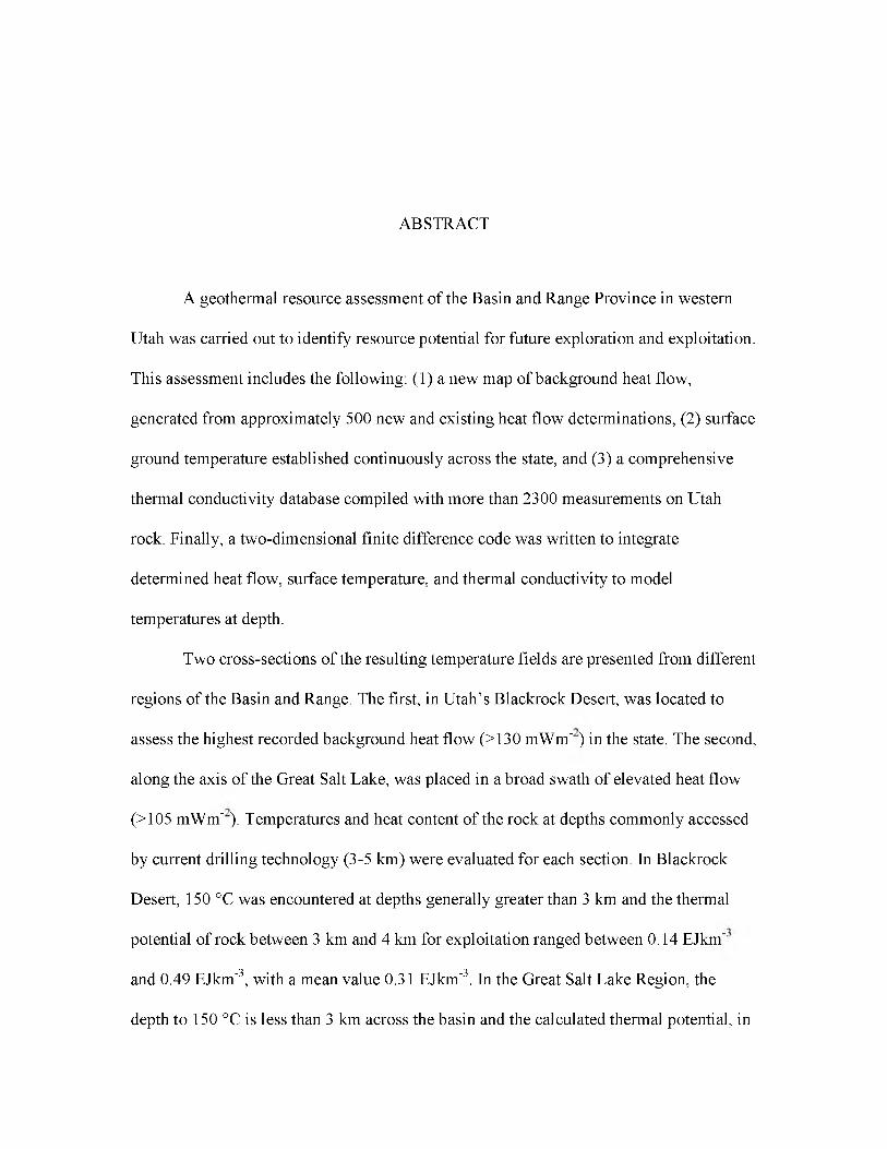
ABSTRACT
A geothermal resource assessment of the Basin and Range Province in western
Utah was carried out to identify resource potential for future exploration and exploitation.
This assessment includes the following: (1) a new map of background heat flow,
generated from approximately 500 new and existing heat flow determinations, (2) surface
ground temperature established continuously across the state, and (3) a comprehensive
thermal conductivity database compiled with more than 2300 measurements on Utah
rock. Finally, a two-dimensional finite difference code was written to integrate
determined heat flow, surface temperature, and thermal conductivity to model
temperatures at depth.
Two cross-sections of the resulting temperature fields are presented from different
regions of the Basin and Range. The first, in Utah’s Blackrock Desert, was located to
assess the highest recorded background heat flow (>130 mWm- ) in the state. The second,
along the axis of the Great Salt Lake, was placed in a broad swath of elevated heat flow
(>105 mWm- ). Temperatures and heat content of the rock at depths commonly accessed
by current drilling technology (3-5 km) were evaluated for each section. In Blackrock
Desert, 150 °C was encountered at depths generally greater than 3 km and the thermal
potential of rock between 3 km and 4 km for exploitation ranged between 0.14 EJkm-
3 3and 0.49 EJkm- , with a mean value 0.31 EJkm- . In the Great Salt Lake Region, the
depth to 150 °C is less than 3 km across the basin and the calculated thermal potential, in
3 3the 3 km to 4 km depth interval, is between 0.33 EJkm" and 0.40 EJkm" with a mean
0.37 EJkm-3.
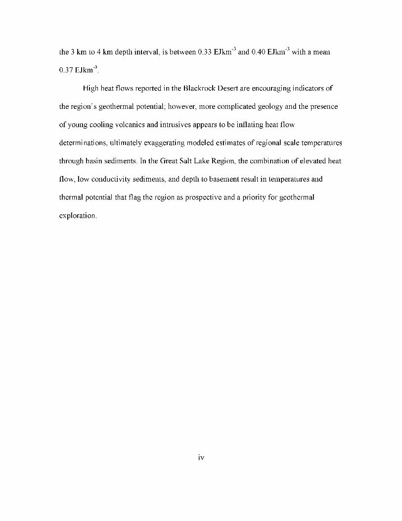
High heat flows reported in the Blackrock Desert are encouraging indicators of
the region’s geothermal potential; however, more complicated geology and the presence
of young cooling volcanics and intrusives appears to be inflating heat flow
determinations, ultimately exaggerating modeled estimates of regional scale temperatures
through basin sediments. In the Great Salt Lake Region, the combination of elevated heat
flow, low conductivity sediments, and depth to basement result in temperatures and
thermal potential that flag the region as prospective and a priority for geothermal
exploration.
iv
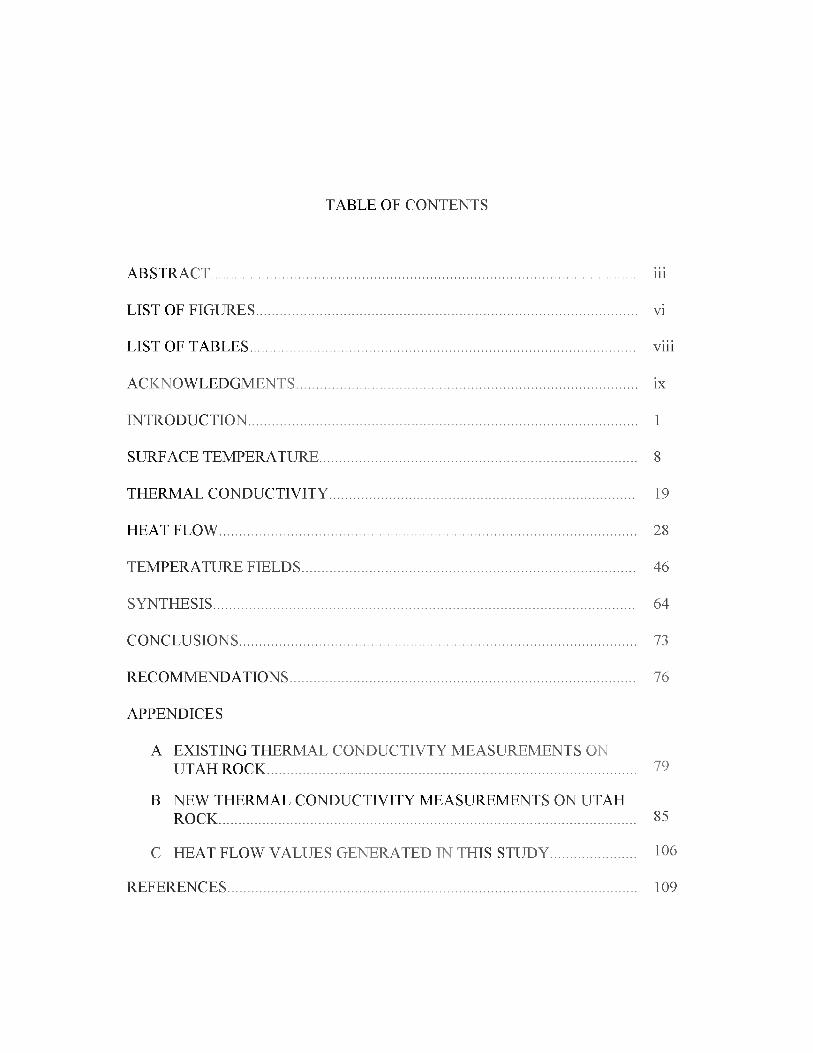
TABLE OF CONTENTS
ABSTRACT................................................................................................................... ...iii
LIST OF FIGURES..........................................................................................................vi
LIST OF TABLES............................................................................................................viii
ACKNOWLEDGMENTS............................................................................................... ix
INTRODUCTION............................................................................................................1
SURFACE TEMPERATURE...................................................................................... ...8
THERMAL CONDUCTIVITY......................................................................................19
HEAT FLOW................................................................................................................. ...28
TEMPERATURE FIELDS.......................................................................................... ...46
SYNTHESIS.................................................................................................................. ...64
CONCLUSIONS...............................................................................................................73
RECOMMENDATIONS.................................................................................................76
APPENDICES
A EXISTING THERMAL CONDUCTIVTY MEASUREMENTS ONUTAH ROCK.................................................................................................... ...79
B NEW THERMAL CONDUCTIVITY MEASUREMENTS ON UTAHROCK................................................................................................................. ...85
C HEAT FLOW VALUES GENERATED IN THIS STUDY..........................106
REFERENCES............................................................................................................... ...109
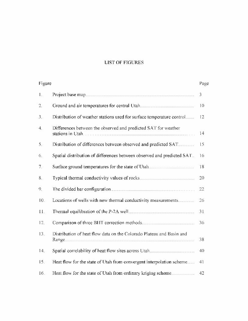
LIST OF FIGURES
Figure Page
1. Project base map ... 3
2. Ground and air temperatures for central Utah ....10
3. Distribution of weather stations used for surface temperature control ...12
4. Differences between the observed and predicted SAT for weatherstations in Utah................................................................................................... ..14
5. Distribution of differences between observed and predicted SAT ... 15
6. Spatial distribution of differences between observed and predicted SAT.. 16
7. Surface ground temperatures for the state of Utah ....18
8. Typical thermal conductivity values of rocks ...20
9. The divided bar configuration ...22
10. Locations of wells with new thermal conductivity measurements ...26
11. Thermal equilibration of the P-2A well ...31
12. Comparison of three BHT correction methods ...36
13. Distribution of heat flow data on the Colorado Plateau and Basin and Range.................................................................................................................. ... 38
14. Spatial correlability of heat flow sites across Utah ...40
15. Heat flow for the state of Utah from convergent interpolation scheme ...41
16. Heat flow for the state of Utah from ordinary kriging scheme ...42
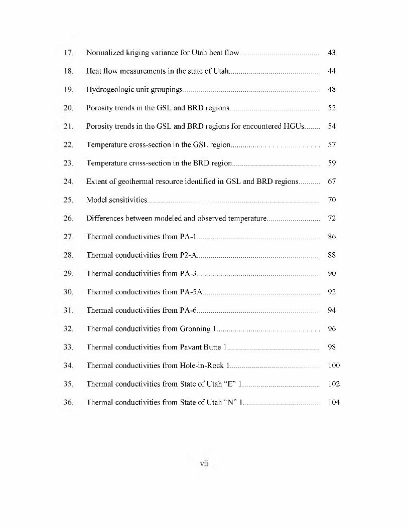
43
44
48
52
54
57
59
67
70
72
86
88
90
92
94
96
98
100
102
104
Normalized kriging variance for Utah heat flow...................................
Heat flow measurements in the state of Utah........................................
Hydrogeologic unit groupings.................................................................
Porosity trends in the GSL and BRD regions........................................
Porosity trends in the GSL and BRD regions for encountered HGUs
Temperature cross-section in the GSL region.......................................
Temperature cross-section in the BRD region.......................................
Extent of geothermal resource identified in GSL and BRD regions...
Model sensitivities.....................................................................................
Differences between modeled and observed temperature...................
Thermal conductivities from PA-1..........................................................
Thermal conductivities from P2-A..........................................................
Thermal conductivities from PA-3..........................................................
Thermal conductivities from PA-5A......................................................
Thermal conductivities from PA-6..........................................................
Thermal conductivities from Gronning 1...............................................
Thermal conductivities from Pavant Butte 1.........................................
Thermal conductivities from Hole-in-Rock 1........................................
Thermal conductivities from State of Utah “E” 1.................................
Thermal conductivities from State of Utah “N” 1.................................
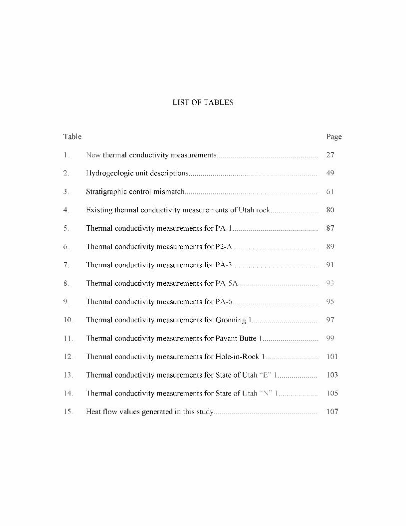
LIST OF TABLES
Table Page
1. New thermal conductivity measurements...................................................... ...27
2. Hydrogeologic unit descriptions......................................................................... 49
3. Stratigraphic control mismatch........................................................................... 61
4. Existing thermal conductivity measurements of Utah rock......................... ... 80
5. Thermal conductivity measurements for PA-1.................................................87
6. Thermal conductivity measurements for P2-A.................................................89
7. Thermal conductivity measurements for PA-3.................................................91
8. Thermal conductivity measurements for PA-5A.......................................... ... 93
9. Thermal conductivity measurements for PA-6.................................................95
10. Thermal conductivity measurements for Gronning 1...................................... 97
11. Thermal conductivity measurements for Pavant Butte 1............................. ...99
12. Thermal conductivity measurements for Hole-in-Rock 1............................ ...101
13. Thermal conductivity measurements for State of Utah “E” 1.........................103
14. Thermal conductivity measurements for State of Utah “N” 1........................ 105
15. Heat flow values generated in this study............................................................107
ACKNOWLEDGMENTS
The following work is a reflection of the large and small inputs (though mostly large) of
numerous contributors. For their guidance through the research process, I would like to share
my gratitude for my advisory committee members Dave Chapman, Lisa Stright, and Cari
Johnson. In particular, Dave’s effort to foster my growth from a passive student to an active
producer of knowledge has shaped much of my approach to this work. Additionally, the time
Lisa invested to help me develop many of the tools required to complete this work was
crucial. I would like to thank my labmates— Christian Hardwick, Mike Davis, Imam Raharjo,
Melissa Masbruch, and Paul Gettings—for their technical and frequent philosophical
suggestions. Thanks to members of the Utah Geological Survey: Mark Gwynn for his
collaboration developing the thermal database and Rick Allis for funding and making this
project possible. Thomas Etzle, Fahran Tunku, and Will Hurlbut were critical to processing
and measuring the sheer volume of the thermal conductivity data presented. Also, I would
like to thank my family for their support over the last two years. Finally, thanks to Alexa
Lewis for the abundance of encouragement, understanding, and aid she gave which
motivated this work to timely completion. I give my sincerest thanks to all of you.
INTRODUCTION
Increased interest in the development of sustainable energy sources to augment or
replace current US energy supply has led to renewed investment in geothermal
investigations. A 2005 international panel and associated 2006 report [Tester et al., 2006]
estimates that recoverable geothermal resource throughout the United States is between
1.2 TW and 12 TW, assuming 2% and 20% recovery efficiencies, respectively. The
majority of this resource located at commercially drillable depths (3 km to 5 km) is found
in the Basin and Range Province of the western US between the Southern Rocky
Mountains and the Sierra Nevadas and has no visible surface expression. Favorable
conditions exist where an area is tectonically active supplying a high basal heat flow, and
where young sedimentary basins are filled with low conductivity sediments [Tester et al.,
2006].
Utah’s Great Basin is noted for its high surface heat flow coupled with low
thermal-conductivity sedimentary basins. Because of these conditions, it is possible that
geothermal grade temperatures exist at commercially drillable depths. Identifying these
blind systems could provide great benefit to the State of Utah where currently most
resources being exploited are surface expressed. Notable examples are Blundell
Geothermal Plant near Milford, Utah, which generates 26 MWe [Chiasson, 2004], and the
Milgro greenhouses, which directly utilize blind geothermal resource to heat and cool 26
acres of productive greenhouses near Newcastle, in Utah’s Escalante Desert [Allred,
2004].
Blind geothermal systems are those without surface expression. They exist where
subsurface temperature is sufficiently high for commercial development at economic
depth. Estimating subsurface temperature, to identify these systems, in turn requires
knowledge of surface temperature, surface heat flow, and the thermal-conductivity of the
geologic section. Surface temperature can be estimated from elevation and latitude.
Thermal conductivity can be measured directly by sampling the stratigraphic section or
estimated based on common values for dominant lithology in the stratigraphic column.
Conductive heat flow in the Basin and Range varies locally between 60 mW/m and 150
2 2 2 mW/m , with a mean value of 90 mW/m and standard deviation of 10 mW/m [Chapman
et al., 1979]. While not yet widely exploited, blind resources have been described. For
example, Clement [1981] delineates a 13 MW system confined to 10 km .
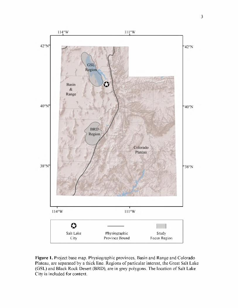
The study area encompasses the Great Basin Province in western Utah. Specific
examples of temperature at depth are presented for the Black Rock Desert, in Millard
County— approximately 200 km south-southwest of Salt Lake City— as well as the Great
Salt Lake region, which trends northwest-southeast primarily through Box Elder and
Davis Counties and is immediately adjacent to Salt Lake City (Figure 1).
Previous heat flow research includes a number of localized studies and one
regional assessment. Heat flow measurements in Utah were first carried out by Costain
[1973]. Near surface thermal gradients were calculated from shallow wellbores and then
combined with measured thermal-conductivities of the encountered formations.
Subsequent studies of surface heat flow for select regions in western Utah’s Great Basin
2
3
114°W nrw
oSalt Lake
CityPhysiographic
Province BoundStudy
Focus Region
Figure 1. Project base map. Physiographic provinces, Basin and Range and Colorado Plateau, are separated by a thick line. Regions of particular interest, the Great Salt Lake (GSL) and Black Rock Desert (BRD), are in grey polygons. The location of Salt Lake City is included for context.
have either utilized this “classic” method, being highly constrained but with limited
vertical extents, or have made very broad regional characterizations. Other classic heat
flow assessments throughout the state [Carrier, 1979; Mase, 1979; Wilson, 1980; Bodell,
1981; Bodell and Chapman, 1982; Carrier and Chapman, 1981; Chapman et al., 1981;
Clement, 1981; Bauer, 1985; Bauer and Chapman, 1986; Powell et al., 1988; Moran,
1991; Powell, 1997] retain similar methodology. This classic heat flow approach well
establishes thermal regimes for the near surface, but maintains inherent complications:
First, classically derived heat flow generally evaluates only the upper 500 meters, a depth
region susceptible to thermal disturbance from topography and groundwater flow.
Second, while heat flow may be mapped locally and in considerable detail, the data are
not laterally extensive. Choosing an appropriate interpolation method between these data
rich, yet isolated regions is challenging.
In 2001, an extensive regional scale study of heat flow of the Colorado Plateau as
well as the eastern Basin and Range in Utah was completed [Henrickson et al., 2001]. He
supplemented classic heat flow work by determining surface heat flow from bottom-hole
temperature (BHT) data in oil and gas wells. This work utilized the thermal resistance
method first described by Bullard [1939] but later employed in Utah by Keho [1987].
Thermal gradients are estimated by correcting well log transient BHTs and thermal-
conductivity is assigned where known or estimated from end member lithology of the
stratigraphic section. Heat flow data based in this method are affected by BHT
measurement or recording error. Heat flow determinations by this technique have the
advantage that many of these wells are drilled deep into sedimentary basins, thus
4
minimizing shallow groundwater effects and all seasonal or climatic temperature
signatures from the thermal gradient.
The major drawback to using BHT records is that temperature is not usually
priority data collected during the drilling and well logging operations that provide this
information. Extensive circulation of drilling muds in the wellbore annulus can
significantly cool the formation. Due to safety concerns and the expense associated with
maintaining an uncased or open hole, it is uncommon for re-equilibrated boreholes and
hence undisturbed formation temperatures to be logged and measured. Previous studies
exist that estimate undisturbed formation temperature [Lachenbruch and Brewer, 1959;
Cao et al., 1988; Deming and Chapman, 1988] and generally require a minimum of two
transient BHTs and the time since circulation ceased. Because log header data can be
questionable, significant care must be taken when selecting BHT data to generate thermal
gradients from these methods.
This study’s primary objective is to produce subsurface temperature maps on a
regional scale with the motivation of guiding future resource assessment in Utah’s
sedimentary basins. In analog to the oil and gas industry, where a resource
characterization would not be performed in the absence of a petroleum system, this study
deems the temperature field to be the most significant factor in a geothermal resource
assessment. While other parameters commonly characterized for basin reservoir
studies—porosity, permeability, and fluid content— are necessary to make up a
productive reservoir, they are subordinate to resource in place. To arrive at subsurface
temperature, the study builds on previous works, including compiling all preceding
investigations, and then augments the resulting dataset with more recent gradient holes
5
and additional BHT records. A more robust database of thermal conductivities specific to
the Basin and Range has been generated, again compiling all previous measurements and
including some 468 new values. In a broad sense, the main pursuit is to synthesize
previous works, with generally limited extents, into a single cohesive dataset. From this
dataset, a platform can be constructed to model a background conductive thermal regime
aiding in the assessment of Utah’s geothermal potential in this and future studies.
For a conductive regime, heat transfer is governed by Fourier’s Law. In order to
solve this numerically, boundary conditions—heat flow and surface temperature—must
be determined and the thermal resistance through the domain must be provided. The
greater study is broken into four tasks, three required to calculate the temperature field,
and the calculation itself. The first is a determination of ground surface temperature
which can be done analytically—provided the coefficients of the analytic expression,
latitude and elevation, are calibrated to the study area. Inversion techniques are utilized
on a dataset of 149 mean annual temperatures throughout the state of Utah and an
expression for surface temperature is achieved. The second task is to establish the thermal
resistance of units in the stratigraphic section. Previous work [Carrier, 1979; Mase, 1979;
Wilson, 1980; Bodell, 1981; Bodell and Chapman, 1982; Carrier and Chapman, 1981;
Chapman et al., 1981; Clement, 1981; Bauer, 1985; Bauer and Chapman, 1986; Powell et
al., 1988; Moran, 1991; Powell, 1997] provides some of the thermal conductivity data
required; however, additional sampling is carried out on cuttings and core from key wells
to help characterize the Great Salt Lake and Blackrock Desert regions. The third task is
constructing a surface heat flow map which integrates well-resolved, yet spatially isolated
work from previous studies. Geostatistical techniques are employed to interpolate
6

between heat flow measurements as well as quantify the uncertainty associated with
interpolation in areas with little or no data for constraint. Finally, the temperature field is
calculated analytically for a one-dimensional case by rearranging Fourier’s Law and
incrementally calculating to depth through intervals with unique thermal resistances. This
one-dimensional case is then supplied as a seed for a two-dimensional relaxation model,
as described in Beardsmore [2001], and visualized in cross-section.
7
SURFACE TEMPERATURE
Our task is to map the mean annual ground temperature over the study area as the
upper boundary condition for the subsurface temperature calculation. A robust dataset of
surface air temperature (SAT) records exists from a variety of reliable sources that date
back more than a century. Weather stations at municipal buildings, schools, and airports
provide much of the data available for use in this study. However plentiful, this dataset is
predominately measured at these discrete sites along major infrastructure. As a result,
when surface temperature is required at remote locations or over a continuous domain, it
is necessary either to extrapolate temperature from the nearest site or to estimate it based
on physical and geographic controls.
Mean annual SAT within Utah is primarily dependent on two key factors: (1)
solar radiation received annually, which is a function of latitude and (2) elevation through
the adiabatic lapse. A lapse model, which considers temperature as a function of
elevation and is well known from meteorology, was developed and described for central
Utah in Powell et al. [1988] as well as in Moran [1991]. The lapse model demonstrated in
Powell et al. relates temperature to elevation where temperature decreases with elevation
at approximately 7 °C/km. The Moran work employs this model to relate surface
temperatures in a localized region with a high degree of topographic relief, demonstrating
its reliability with respect to changes in elevation. The lateral extent of these studies is
relatively small, less than 90 km and 2 km, as described in Powell and Moran,
respectively. Because of their limited extents, neither study explored temperature change
due to the effect of decreasing solar radiation with increasing latitude.
Additionally, two observations come out of the Powell and Moran work that
allow us to make the transformation from SAT to surface ground temperature (SGT). The
first is a systematic shift of approximately 3 °C between air and ground temperature.
Ground temperatures are generally warmer than air temperatures for two reasons: (1) the
ground can be thermally insulated by snow cover during the winter, holding the soil at a
constant 0 °C while air temperatures fall below zero; (2) ground is heated directly by
absorbing solar radiation, whereas the air is free to convect and mix, maintaining a lower
temperature. Bartlett et al. [2004, 2005] and Masbruch [2012] demonstrate this
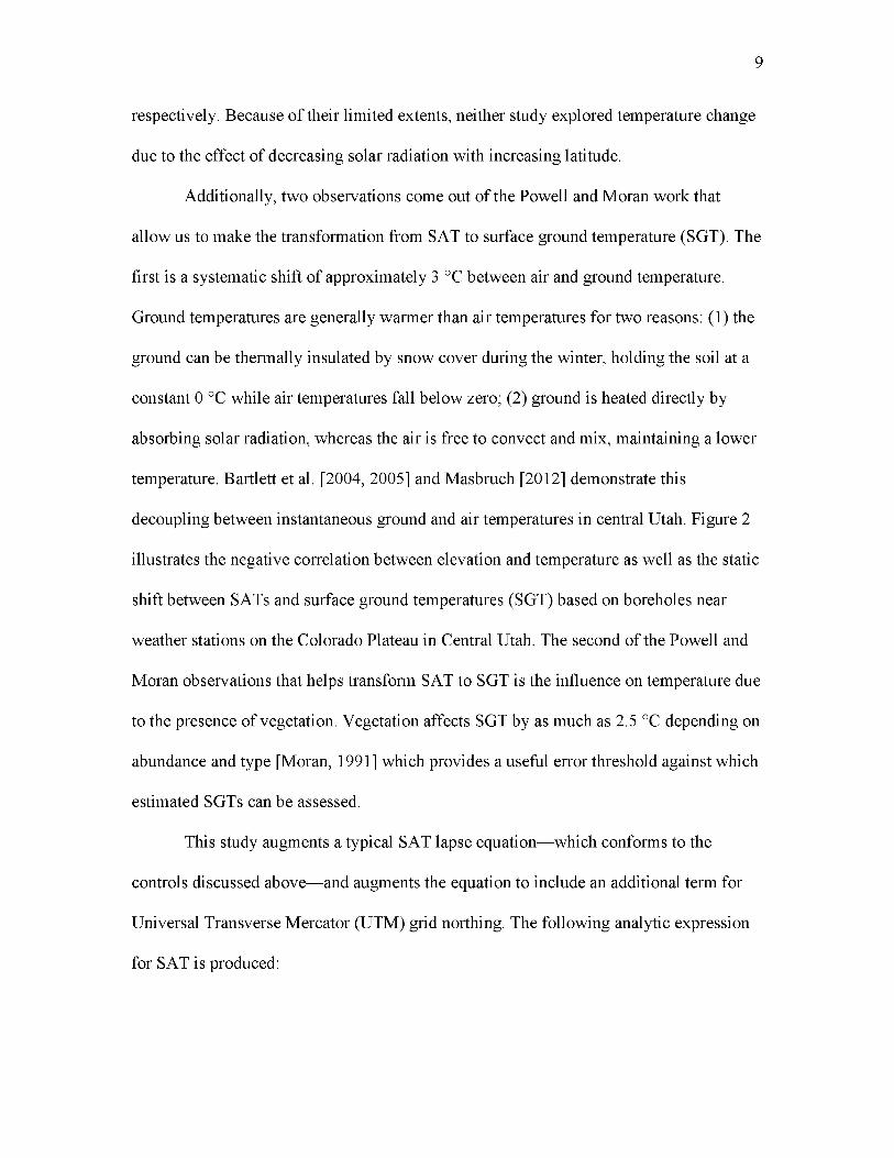
decoupling between instantaneous ground and air temperatures in central Utah. Figure 2
illustrates the negative correlation between elevation and temperature as well as the static
shift between SATs and surface ground temperatures (SGT) based on boreholes near
weather stations on the Colorado Plateau in Central Utah. The second of the Powell and
Moran observations that helps transform SAT to SGT is the influence on temperature due
to the presence of vegetation. Vegetation affects SGT by as much as 2.5 °C depending on
abundance and type [Moran, 1991] which provides a useful error threshold against which
estimated SGTs can be assessed.
This study augments a typical SAT lapse equation—which conforms to the
controls discussed above— and augments the equation to include an additional term for
Universal Transverse Mercator (UTM) grid northing. The following analytic expression
for SAT is produced:
9
10
20
15uo<L>!—D2<L>Cl
£uH 10C3C2<cco<L>
S 5
• GroundO Air
■ • •
V o • \8 x s • \
0
N,
"V V, V V V X
1000 1500 2000Elevation (m)
2500 3000
Figure 2. Ground and air temperatures for central Utah. Cross plotting mean annual ground temperatures from borehole temperature extrapolations (closed circles) and mean annual air temperatures from weather stations (open circles) against elevation reveals inversely correlated parallel trends between elevation and temperature with a 3 °C static offset between mean annual ground and mean annual air temperatures. Figure modified from Powell et al. [1988].
11
SA T(h , n ) = C]_/i + C2 n + C3, (1)
where h is the elevation in km, n is the UTM northing in km, and Cx, C2, and C3 are the
calibrated coefficients. A shift of 3 °C to account for the difference between SAT and
SGT can be applied after the coefficients are determined and residuals are assessed. Also,
because there is no convenient method to predict the presence and type of vegetation, an
error threshold of 2.5 °C is considered satisfactory for any results. Calibration of these
model coefficients to the study area was achieved performing a linear least squares
inversion on the forward problem of the generic form:
where is the coefficients , , and , is the operator of the analytic expression,
and d is the temperature associated with each elevation-northing pair.
The linear least squares method attempts to minimize the misfit between predicted
data and observed data given a set of model parameters using variational calculus, which
obeys the conditions of functionals in misfit space. A thorough derivation of the linear
least squares method is provided in Zhdanov [2002], but the final solution to the linear
least squares method takes the form:
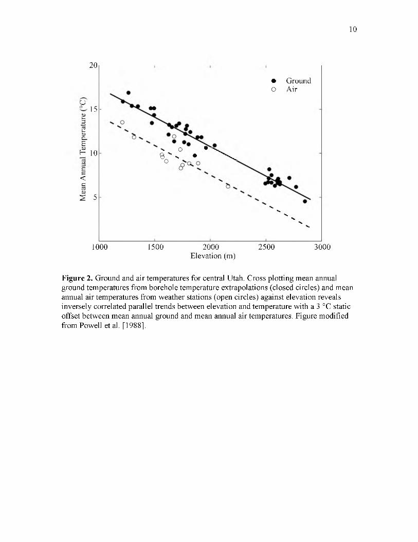
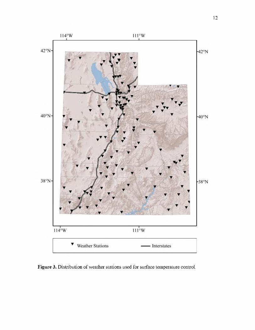
The inversion was supplied with temperature, elevation, and northing data from
149 weather stations throughout the state of Utah from the Western Regional Climate
Center database (http://www.wrcc.dri.edu). Station locations are mapped in Figure 3.
Mean annual temperatures were averaged for each site’s history, including only data that
A(m) = d , (2)
m = ( A t A ) ~ 1 At d. (3)
12
Figure 3. Distribution of weather stations used for surface temperature control.
were recorded during the previous two decades and contained at least ten years of
records. Older sites with sporadic or incomplete records were removed. Coverage is well
distributed with slightly higher density around population centers.
The inversion results produced values of -6.42 °C/km for the change with
elevation (Cx), -.0084 °C/km for the change with latitude (C2), and 56 °C for the free
parameter (C3) that serves as a baseline from which variations are added or subtracted.
The elevation lapse rate is close to the value reported in Powell et al. [1988] of -6.7
°C/km. The temperature change with northing corresponds to a total difference of about 4
°C between the north and south of Utah.
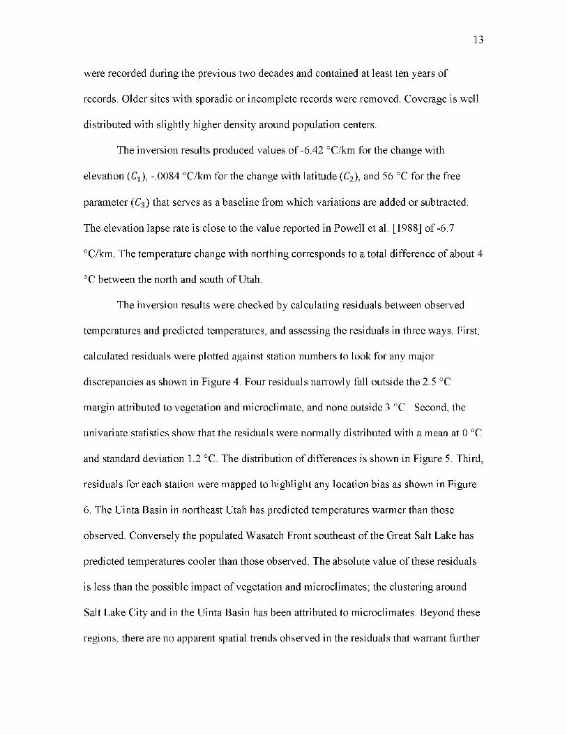
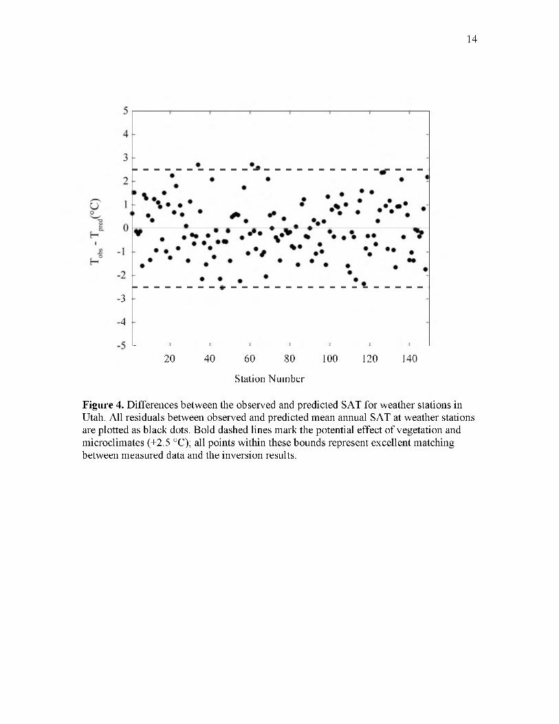
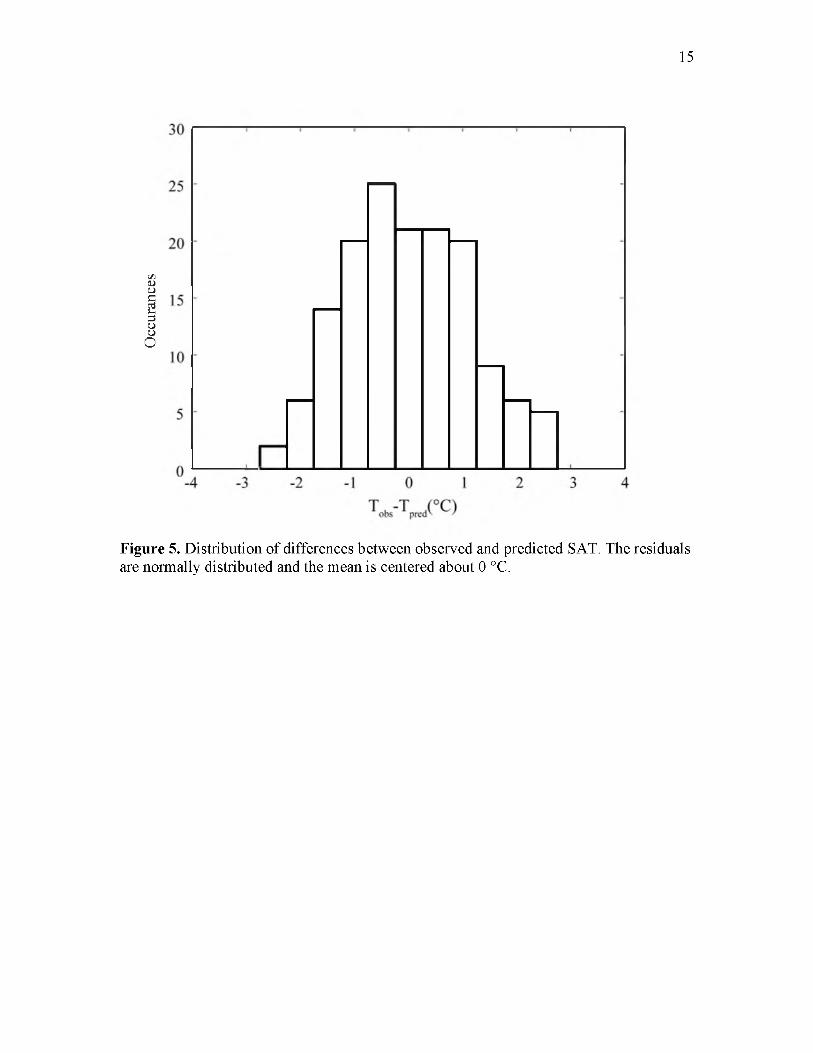
The inversion results were checked by calculating residuals between observed
temperatures and predicted temperatures, and assessing the residuals in three ways. First,
calculated residuals were plotted against station numbers to look for any major
discrepancies as shown in Figure 4. Four residuals narrowly fall outside the 2.5 °C
margin attributed to vegetation and microclimate, and none outside 3 °C. Second, the
univariate statistics show that the residuals were normally distributed with a mean at 0 °C
and standard deviation 1.2 °C. The distribution of differences is shown in Figure 5. Third,
residuals for each station were mapped to highlight any location bias as shown in Figure
6. The Uinta Basin in northeast Utah has predicted temperatures warmer than those
observed. Conversely the populated Wasatch Front southeast of the Great Salt Lake has
predicted temperatures cooler than those observed. The absolute value of these residuals
is less than the possible impact of vegetation and microclimates; the clustering around
Salt Lake City and in the Uinta Basin has been attributed to microclimates. Beyond these
regions, there are no apparent spatial trends observed in the residuals that warrant further
13
14
■3
■4
20 40 60 80 100 120 140
Station Number
Figure 4. Differences between the observed and predicted SAT for weather stations in Utah. All residuals between observed and predicted mean annual SAT at weather stations are plotted as black dots. Bold dashed lines mark the potential effect of vegetation and microclimates (±2.5 °C); all points within these bounds represent excellent matching between measured data and the inversion results.
Occ
uran
ces
15
Figure 5. Distribution of differences between observed and predicted SAT. The residuals are normally distributed and the mean is centered about 0 °C.
16
Figure 6. Spatial distribution of differences between observed and predicted SAT. Mean annual temperature residuals at weather stations throughout the state of Utah. Point size corresponds to absolute residual value with warmer colors being positive and cooler colors negative.
investigation, and even these regions fall within the expected scatter for residual
temperatures.
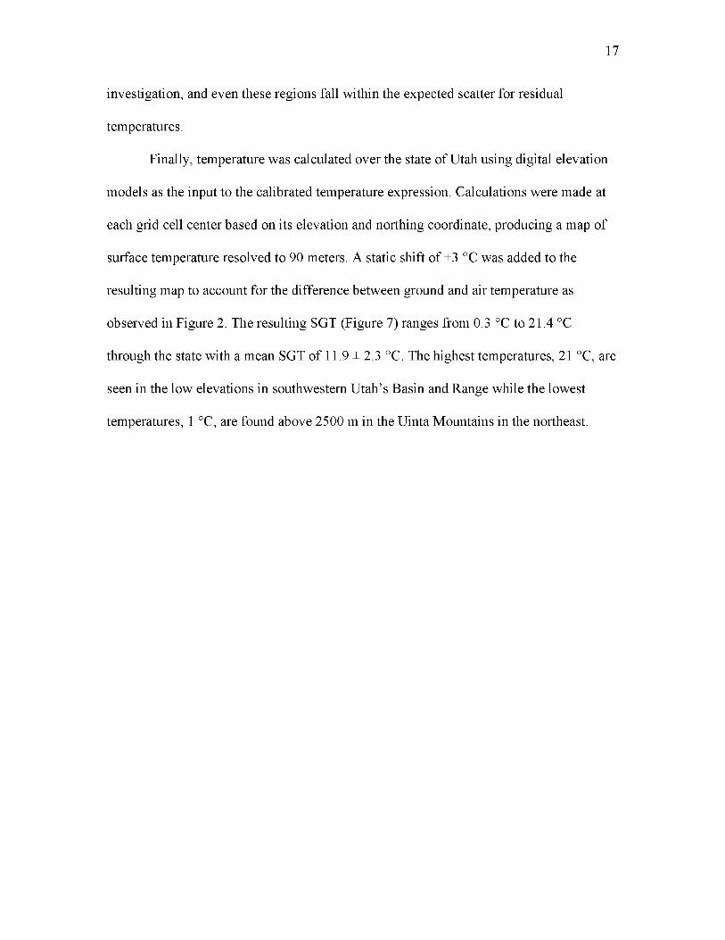
Finally, temperature was calculated over the state of Utah using digital elevation
models as the input to the calibrated temperature expression. Calculations were made at
each grid cell center based on its elevation and northing coordinate, producing a map of
surface temperature resolved to 90 meters. A static shift of +3 °C was added to the
resulting map to account for the difference between ground and air temperature as
observed in Figure 2. The resulting SGT (Figure 7) ranges from 0.3 °C to 21.4 °C
through the state with a mean SGT of 11.9 ± 2.3 °C. The highest temperatures, 21 °C, are
seen in the low elevations in southwestern Utah’s Basin and Range while the lowest
temperatures, 1 °C, are found above 2500 m in the Uinta Mountains in the northeast.
17
18
Figure 7. Surface ground temperatures for the state of Utah.
THERMAL CONDUCTIVITY
The calculation of temperature at depth requires an understanding of thermal
resistance, the quotient of thickness and thermal conductivity, through the stratigraphic
section. Fundamental to constructing a thermal resistance profile of the subsurface is the
ability to define the conductivity of a given formation. Thermal conductivity can be
deduced by measuring rocks of the formations directly or by estimating a value based on
a formation’s dominant lithology.
Thermal conductivity’s primary control is bulk composition consisting of both the
matrix mineralogy and pore space. The range of matrix conductivity for common rocks
and minerals is well established and observed variations range by more than a factor of
eight [Touloukin et al., 1970; Raznjevic, 1976; Majorowiscz and Jessop, 1981; Roy et al.,
1981; Reiter and Tovar, 1982; Reiter and Jessop, 1985; Drury, 1986; Taylor et al., 1986;
Beach et al., 1987; Barker, 1996; Beardsmore, 1996]. A single rock type, particularly
sedimentary rocks, can vary by as much as a factor of three, though such large variations
are not generally observed within a single formation. Figure 8 shows a compilation of
thermal conductivity ranges for common rocks determined from the above sources. Due
to the extent to which conductivity values can vary, more precise calculations of
temperature at depth can be made by measuring the conductivity specific to the
stratigraphic column. This study compiles all available conductivity measurements
specific to Utah geology and supplements this thermal conductivity database with new
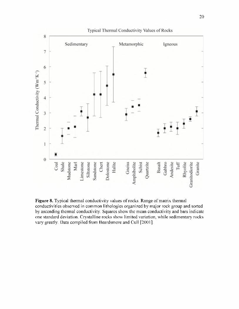
20
Figure 8. Typical thermal conductivity values of rocks. Range of matrix thermal conductivities observed in common lithologies organized by major rock group and sorted by ascending thermal conductivity. Squares show the mean conductivity and bars indicate one standard deviation. Crystalline rocks show limited variation, while sedimentary rocks vary greatly. Data compiled from Beardsmore and Cull [2001].
measurements of Basin and Range rocks. Previous studies on rocks found in Utah have
collected over 1900 samples and measured thermal conductivity in approximately 60
formations in the Basin and Range and Colorado Plateau [Bodell and Chapman, 1982;
Chapman et al., 1984; Deming and Chapman, 1988; Moran, 1991; Powell, 1997;
Henrickson, 2000]. A complete tabular summary presenting statistics for existing
measurements is given in Appendix A.
Thermal conductivity can be measured by either transient or steady state methods.
The line-source method is the most common transient technique and involves putting a
sample in contact with a heating element. Temperature is measured while constant heat is
supplied and a plot of temperature increase against the log of time is generated. The slope
of the best fit line is then the thermal conductivity of the sample. This technique is
employed in full-space as well as half space methods and is most appropriate when
measuring large samples. A common steady state technique is the divided bar method
[Sass et al., 1971]. The majority of previous measurements on Utah rock as well as those
measured for this study were made by the divided bar technique and a discussion of the
method follows.
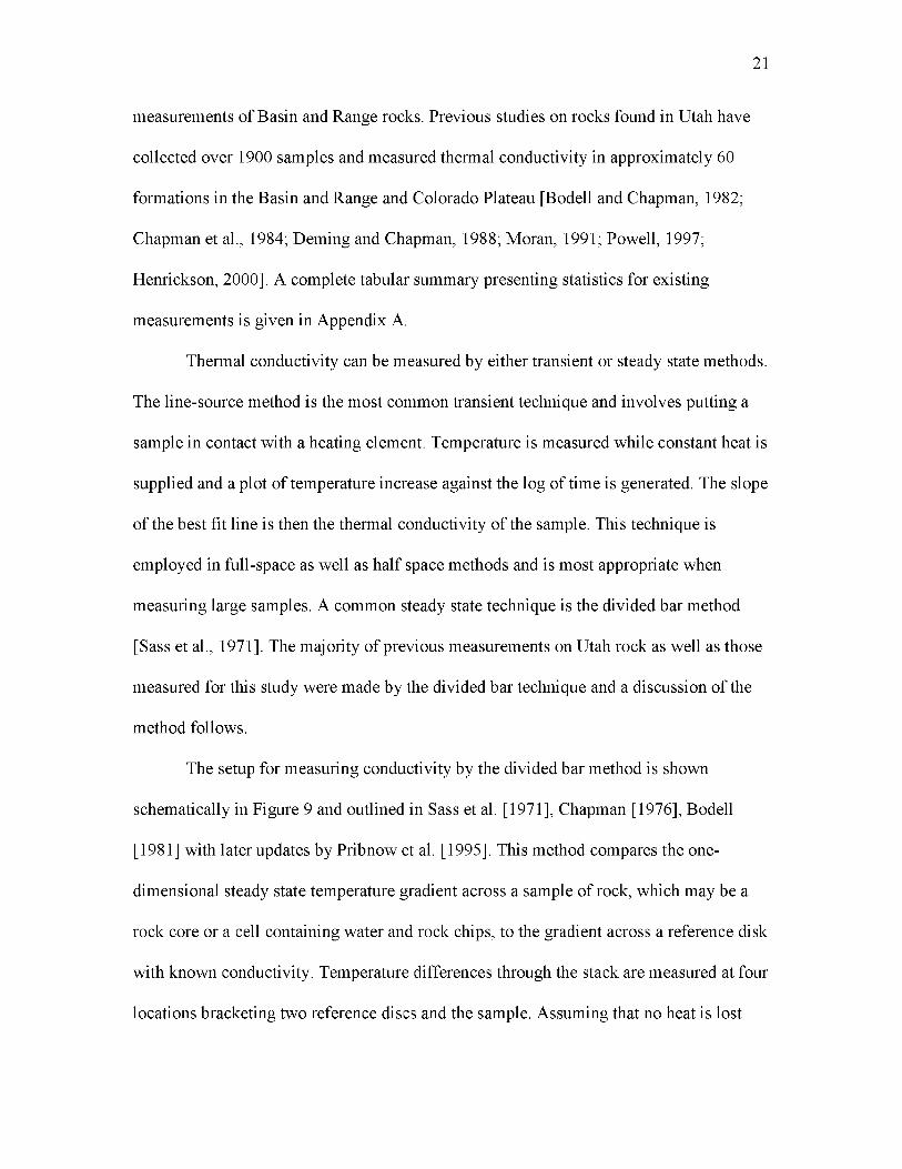
The setup for measuring conductivity by the divided bar method is shown
schematically in Figure 9 and outlined in Sass et al. [1971], Chapman [1976], Bodell
[1981] with later updates by Pribnow et al. [1995]. This method compares the one
dimensional steady state temperature gradient across a sample of rock, which may be a
rock core or a cell containing water and rock chips, to the gradient across a reference disk
with known conductivity. Temperature differences through the stack are measured at four
locations bracketing two reference discs and the sample. Assuming that no heat is lost
21
22
Figure 9. The divided bar configuration. Temperature at the top and base of the divided bar are maintained at fixed temperatures by flowing water from controlled temperature baths. Thermocouples placed in conductive material measure the thermal emf across the reference discs as well as the sample. A piston applies downward pressure holding all surfaces in contact, reducing the thermal contact resistance.
23
from the system laterally, the heat flow through the sample and reference can be equated:
(4)
(5)
(6)
where k ref is the conductivity of the reference, and VTref and VTs ampie are the gradients
across the reference and sample, respectively. The gradients and conductivity of the
references are known, thus the conductivity of the sample can be calculated. The surface
area of the sample may not be the same as the surface area of the divided bar where the
two are in contact. A correction for the difference in dimensions must be made:
For core samples, k di am is the final diameter corrected whole rock thermal conductivity.
Generally, the availability of drill cuttings is much greater than that of whole rock
cores. Because drill cuttings must be contained to measure on the divided bar, they are
packed as rock chips into water saturated cells. When measuring cells containing rock
chips and water, k di am includes the bulk contents of the cell as well as the cell itself.
Additional corrections are required, beyond those applied to core samples, which account
for the conductivity of the cell walls:
outer
(7)
2 2where d bar and d outer are the diameters of the divided bar and sample, respectively.
24
lr _ lr 1outer dinner lrK-bulk — ^diam “ 2 * ^wall
dinner
which yields the bulk conductivity of the rock chip and water mixture in terms of
d-outer and d inner, the diameters of the outer and inner cell walls and k waU, the
conductivity of the wall material. Finally, the rock chip conductivity can be determined
from a volumetric mixing expression with two constituents, rock chips ( k m atrix), water
( k w ate r), and the cell’s total pore space (O):
b — k . (1-0) * h- ® (9)n-bulk ~ /vmatrix n-water , v '
which rearranges to:
~i"Y — kujnter *k h,.lb \ 1 - ® (10)I ^bulk y
'k.u,nt-p'r/'■matrix ~ n-water _ _' xw a te rJ
The conductivity of water, k w a te r , is known to be 0.6 Wm-1K-1 at standard conditions,
and so equation (10) provides the thermal conductivity of the rock matrix.
New divided bar conductivity measurements were made on 468 cutting samples
from five shallow gradient wells and five deep oil and gas exploration wells. The five
gradient holes (PA-1, P-2A, PA-3, PA-5A, and PA-6) are part of a Utah Geological
Survey drilling program and are all located in the Black Rock Desert (BRD) in Millard
County, Utah. These wells were selected to characterize the thermal conductivity of
shallow lakebed sediments found widely throughout the Basin and Range. Five
exploration wells were selected to sample the deeper stratigraphic section of the BRD and
Great Salt Lake (GSL) regions. Three wells— Gronning 1 (API: 02710423), Pavant Butte
1 (API: 02730027), and Hole-in-Rock 1 (API: 02730019)— are located in BRD and two
wells— State of Utah “E” 1 (API: 01130002) and State of Utah “N” 1 (API: 04530010)—
are in the GSL region. Figure 10 illustrates the locations of the ten wells.
The shallow gradient holes encountered hydrated clays and basalt. Approximate
whole rock conductivities measured on 197 clay samples varied from 1.01 Wm-1K-1 to
1.67 Wm-1K-1 with a mean of 1.30 Wm-1K-1 and standard deviation 0.15 Wm-1K-1.
Basalts varied between 1.94 Wm-1K-1 and 2.89 Wm-1K-1 with a mean 2.26 Wm-1K-1 and
standard deviation 0.29 Wm-1K-1 for the 9 samples measured.
Conductivity measured in the deep wells varies between 1.8 Wm-1K-1 and 8.7
Wm-1K-1. The large range observed reflects the variable composition of the stratigraphic
section of interest and demonstrates the significance of characterizing its conductivity.
The two wells in GSL encountered Quaternary and Tertiary basin sediments, upper
Paleozoic carbonates, and Paleozoic metamorphosed basement, most likely the Tintic
Quartzite. Measured values of conductivity are 3.32 ± 0.62 Wm-1K-1, 3.39 ± 0.50 Wm-1K-
1, 3.37 ± 0.36 Wm-1K-1, and 6.36 ± 1.54 Wm-1K-1 for each, respectively. The three wells
in BRD logged mostly Tertiary basin sediment (mudstones, salt, and sandstone) and
basalts which unconformably overlay Paleozoic carbonates and metamorphosed
Paleozoic basement, most likely Prospect Mountain Quartzite, as observed by
penetrations at Hole-in-the-Rock 1 and Pavant Butte 1. Conductivities measured through
the stratigraphic section are 3.42 ± 0.87 Wm-1K-1 for the Quaternary section, 2.98 ± 0.58
Wm-1K-1 for the Tertiary basin fill, 4.84 ± 1.43 Wm-1K-1 in the Paleozoic carbonates, and
4.82 ± 0.73 Wm-1K-1 in the Prospect Mountain Quartzite. Table 1 summarizes the
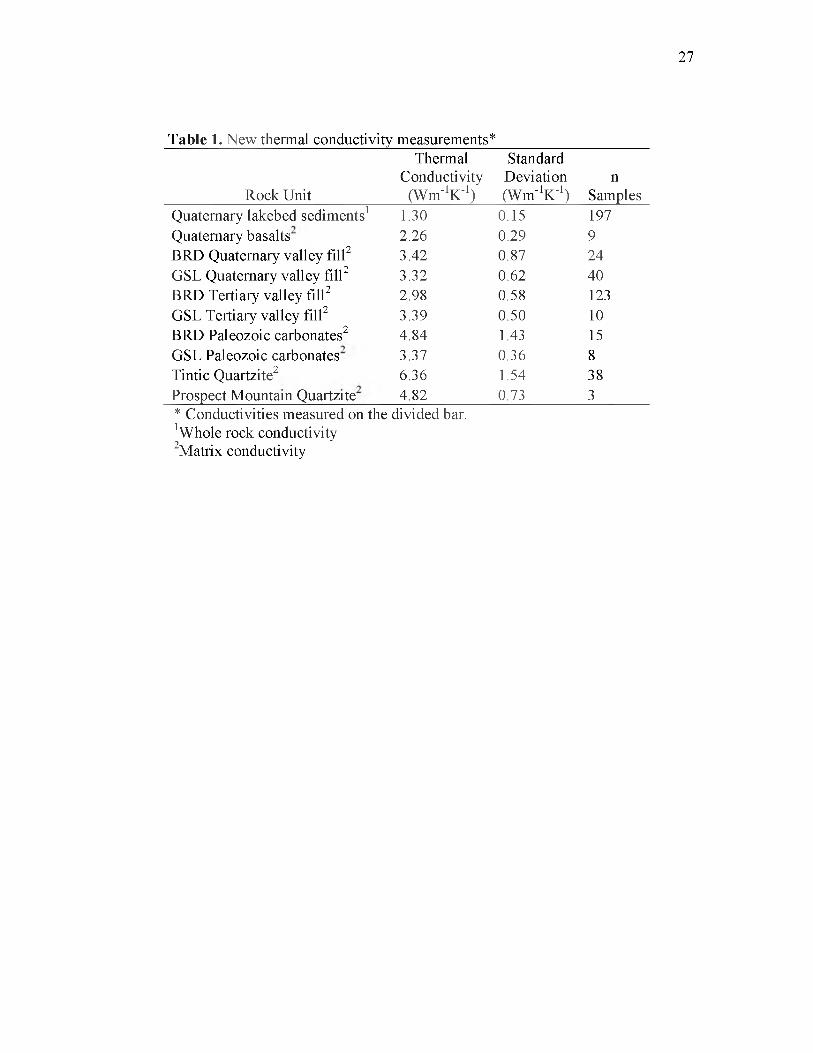
measured values by rock unit.
25
26
114°W 111°W
^ Gradient Hole V Oil & Gas Well
— Intcrstatcs
Figure 10. Locations of wells with new thermal conductivity measurements. White triangles indicate samples were taken from exploration wells and black triangles indicate samples were from shallow gradient holes.
27
Table 1. New thermal conductivity measurements*
Rock Unit
ThermalConductivity
(Wm-1K-1)
StandardDeviation(Wm-1K-1)
nSamples
Quaternary lakebed sediments1 1.30 0.15 197Quaternary basalts 2.26 0.29 9BRD Quaternary valley fill2 3.42 0.87 24GSL Quaternary valley fill2 3.32 0.62 40BRD Tertiary valley fill2 2.98 0.58 123GSL Tertiary valley fill2 3.39 0.50 10BRD Paleozoic carbonates2 4.84 1.43 15GSL Paleozoic carbonates 3.37 0.36 8Tintic Quartzite2 6.36 1.54 38Prospect Mountain Quartzite 4.82 0.73 3* Conductivities measured on the divided bar. 1Whole rock conductivity 2Matrix conductivity
HEAT FLOW
Surface heat flow provides another boundary condition required in the
temperature at depth calculation. As a boundary condition, heat flow is challenging to
determine for two reasons: it is susceptible to hydrologic disturbance and its sampling
distribution is sparse. This work seeks to address these issues by including only
measurements without obvious perturbations from groundwater and by producing a
continuous map of heat flow over the entire state of Utah. This task is accomplished by
compiling all available heat flow determinations for the state, augmenting the dataset
with new measurements in areas with limited coverage, and ultimately using
geostatistical methods to interpolate between measurements.
More than 450 measurements are available from previous academic works
[Carrier, 1979; Mase, 1979; Wilson, 1980; Bodell, 1981; Carrier and Chapman, 1981;
Chapman et al., 1981; Clement, 1981; Bodell and Chapman, 1982; Bauer, 1985; Bauer
and Chapman, 1986; Powell et al., 1988; Moran, 1991; Powell, 1997] along with industry
data in known geothermal resource areas (KGRAs) [Amax, 98] that assess heat flow
using a classic technique. Much of the work using shallow boreholes offers dense
coverage but exhibits sampling bias. For instance, many of the previous studies [Mase,
1979; Wilson, 1980; Clement, 1981] carry out work with a specific goal to define or
delineate geothermal resources and so have sampled regions with anticipated high heat
flow. Particular scrutiny needs to be given to shallow borehole sites before inclusion in a
picture of regional background heat flow. Also, hydrologic disturbance to shallow
gradient holes is common where advective transport via ground water flow flushes or
concentrates heat. These disturbances perturb heat flow locally and obscure the
conductive background temperature field. It is not appropriate to use hydrologically
disturbed boreholes in the calculation of temperature at depth. Additionally, the very near
surface is affected by seasonal and climatic shifts in temperature; therefore, wellbores
shallower than 60 m are usually not considered. Studies utilizing heat flows determined
from oil and gas wells [Keho, 1987; Funnell et al., 1996; Henrickson et al., 2001] attempt
to reduce these hydrologic and climatic effects by acquiring information on temperature
at depths below the influence of surface water flow or transitory temperature trends.
Measurements of terrestrial heat flow are made at discrete sites. Previous attempts
to map heat flow, interpolating heat flow between measurement sites, include work by
Blackwell and Steele [1989] and Blackwell and Richards [2004]. Standard practice for
these methods is to apply a common inverse distance weighting interpolation algorithm,
such as minimum curvature, and then manually adjust the result to fit the originator’s
sense for reasonable values and rates of change. These works provide useful estimates of
terrestrial heat flow, yet rely heavily on the empiricism of the interpreter and do not
provide quantifiable estimates of uncertainty.
Terrestrial heat flow is calculated by combining an estimate of the thermal
gradient with thermal conductivity information. The type of temperature data used leads
to two broad classifications of heat flow determinations: classic heat flow using a high-
resolution temperature log in a borehole at thermal equilibrium, and BHT heat flow using
29
one or two temperatures in oil and gas wells that may be out of thermal equilibrium. Each
class of heat flow determination has its strengths.
The first method makes heat flow determinations in shallow gradient holes, taking
advantage of a stable temperature regime after disturbances caused by the drilling process
have dissipated. Circulation of drilling mud alters the natural temperature down hole.
This disturbance is dependent upon how long circulation occurs and the amount of fluid
being flushed from the borehole to the formation. Because these holes are shallow and
sometimes drilled for observation rather than production, they can be cased and shut in
for a sufficient duration that allows a return to in-situ conditions. A demonstration of this
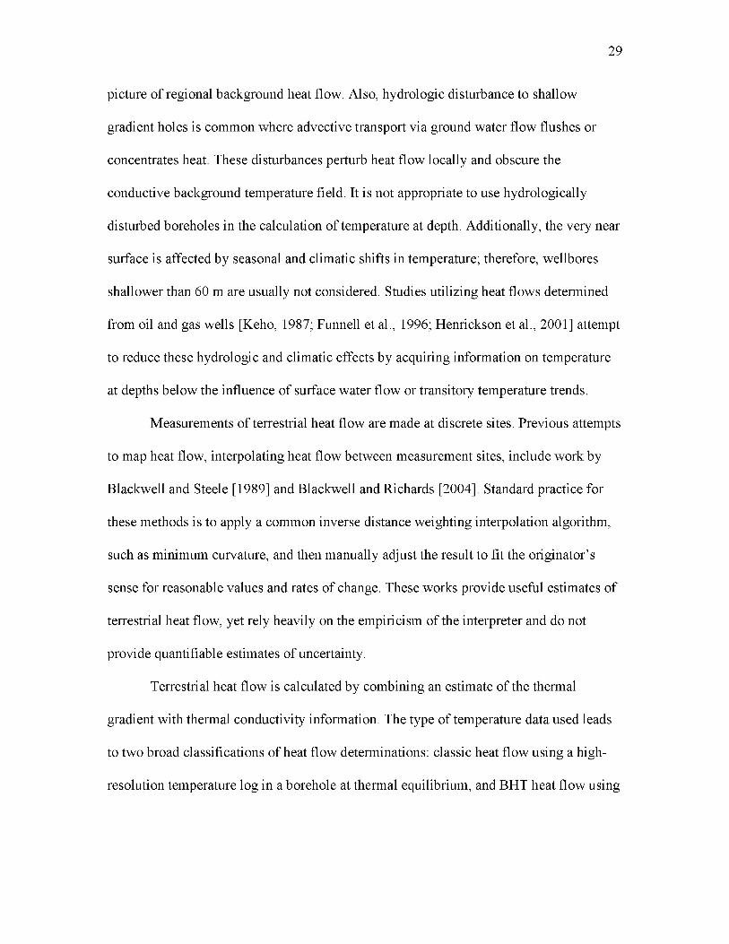
gradual return to natural conditions is demonstrated in the P-2A well, (Figure 11) where
temperature logs were acquired periodically over 18 months subsequent to drilling.
Measurements at different stages of re-equilibration illustrate the magnitude of
disturbances caused to the temperature field near the borehole. Comparing three logs
acquired immediately after drilling, to those acquired at 1 and 18 months following
drilling, shows the field is depressed by 1 °C at total depth and elevated by more than 5
°C in the shallow section. A gradient determined from the un-equilibrated data would
underestimate the true gradient by 14 °C/km.
Once equilibrated, some interpretation of the temperature log is required to select
an appropriate interval from which to extract the gradient. A linearly increasing
temperature with depth is characteristic of a conductive heat transfer regime, through
material with a constant conductivity, and is the sought after trend. These trends can be
obscured by a number of down hole conditions: changes in thermal conductivity cause
changes in thermal gradient; convecting hydrothermal systems can cause temperature-
30
Dept
h (m
)
31
50
100
150
200
25(j
-------- *------ 1---------------- [----------------\* *
K1 ^ • K*,.,.,.. .
26 i i i
V *, X25.5
\ a*V • < x\ *. X
u^ 25S <3■ \ A -
\ X1 24.5Ch
V EH 24
X 4/25/2011 \ a 4/26/2011 x \• 4/27/2011 * \
- • 6/1/2011 x \— 10/10/2012 *A.i
23.5
15 20Temperature (°C)
25 0.05 0.1 0.15T = ln[ts/(t+ tc)]
0.2
Figure 11. Thermal equilibration of the P-2A well. a) Temperature logs for the P-2A well. b) Horner correction to transient BHTs in the P-2A well performed on measurements taken during the 72 hours subsequent to drilling. Data from Gwynn et al. [2013].

32
depth profiles to be isothermal; variations in SGT attributed to seasonal or climate change
produce transient variations very near the surface. Only sites where a conductive gradient
is inferred were included for heat flow calculations in this study. For sites that meet this
qualification, the product of their gradient and the thermal conductivity gives heat flow:
The second method uses BHT data from oil and gas wells and the thermal
resistance of the penetrated stratigraphic section to determine surface heat flow. A
vertical section of thermal resistance is constructed based on the thickness of interpreted
formations and measured or estimated conductivity. If there is minimal heat production
through this horizontally stratified section of n layers, temperature at depth is given by:
where T0 is surface temperature, Azj is layer thickness, and k t is the layer conductivity.
Heat flow is determined by minimizing the difference between the observed BHT and
calculated temperature at depth. A drawback to this method is the uncertainty in BHT
records. Unlike gradient holes, temperature records in oil and gas wells are made
immediately after drilling when the wellbore is still disturbed, requiring correction from
transient to steady state.
A number of methods exist to correct disturbed BHTs, see for example Goutorbe
[2007]. The most common correction is the general Horner plot method. This technique
(11)
(12)
33
plots multiple uncorrected BHTs at a given depth against a unitless parameter t as shown
in Figure 11, where:
given t s, the shut in time, and tc, the duration of circulation at the depth of interest. A
Horner plot groups measured temperature versus t . The temperature intercept of the
linear regression provides undisturbed in-situ temperature, Tm, at t s ^ or t = 0.
Horner corrections have been successfully used to estimate in-situ temperatures in Utah’s
Uinta Basin [Keho, 1987; Willett and Chapman, 1988] and Sevier Fold and Thrust Belt
[Deming and Chapman, 1987]. This solution for undisturbed temperature requires at least
a pair of BHTs with shut in times and provides a more confident estimate if there are
multiple BHT-time pairs; that, however, is the exception more often than the rule. A
further complication arises because temperature, which is not generally a principle
objective for logging engineers and wellsite geologists, is frequently not recorded,
misrecorded, or only recorded once despite multiple logging runs.
Because single BHTs at a given depth are most common, several approaches have
been suggested to estimate equilibrium temperature from transient BHTs. Polynomial
corrections with depth for single transient BHTs have been most widely used since the
work of Kehle et al. [1970] and Harrison et al. [1983]. Harrison’s work proposed that a
static correction be calculated and applied to recorded BHTs:
(13)
Tc f ( z ) = -1 6 .5 + ,018z - 2.3 * 10-6z 2, (14)
34
where TCf is the temperature correction factor (°C) and z is the depth (m) of the recorded
Later work by Blackwell and Richards [2004] observed bias in the Harrison
correction that related to differences in thermal regimes and proposed a variation, which
is referred to as the SMU Correction. This correction applies an additional static shift to
the Harrison corrected data as a function of regional gradients:
where VT is the regionally observed thermal gradient (°C/km).
Work by Funnell et al. [1996], and later Henrickson [2000], moves away from
static corrections. These studies note that the slope of the Horner thermal recovery plot is
related to depth and wellbore diameter. Wells are grouped by borehole diameter and
Horner slopes from wells with multiple BHT records are plotted against depth. A linear
regression places a best fit line through the points of each diameter grouping and
coefficients are determined which allows an estimation of the Horner slope. With the
regressed thermal recovery slope, m , a single BHT-time pair can be corrected to pre
drilling temperature (Tm ):
Because of this method’s use in association with the University of Utah, it is termed the
Utah Method.
The Harrison, SMU, and Utah methods were evaluated against Horner corrected
BHTs. As the Horner method is the most robust and widely used estimate of equilibrated
BHT.
Tcf2 (V7) = -0.84V T + 23.98, (15)
down hole temperatures [Goutorbe, 2007], corrections from Horner plots were selected as
the true temperature against which the other methods would be assessed. Eighty-nine
wells throughout the Basin and Range had two or more recorded transient BHTs and
were used for the comparison. Corrected BHTs were calculated using each method for all
transient BHTs. Differences between corrected temperatures (Tcaic) and true temperatures
(T tru e ) were computed and statistics of these residuals for each method were assessed.
The Harrison correction generally over-predicts formation temperature with a mean
residual 4 °C above true and a standard deviation of 10 °C. Corrections using the SMU
method were much closer to the true formation temperature, under-predicting the true
formation temperature on average by 2 °C with a standard deviation of 10 °C. This
method shows large sensitivity to the selected regional gradient, shifting the static
correction by approximately 80 percent of the difference between inferred regional
gradient 34 °Ckm-1 and 26 °Ckm-1. The Utah correction produced steady state BHTs that
were closest to the true temperature, over-predicting by 1 °C, but with a slightly larger
standard deviation of 11 °C. A comparison of the three corrections is shown graphically
in Figure 12. While variation on the order of 10 °C is common [Goutorbe, 2007],
inaccuracies in any given single point BHT correction could be as large as 22 °C. For this
study, a sufficient spatial coverage of reliable heat flow data was available, and so the
more variable single point corrected BHTs were not included for the final heat flow map.
This study builds on the previous 410 heat flow measurements determined to be
representative of background, adding 5 sites from the recently drilled Utah Geological
Survey drilling program as well as calculating heat flow in 44 oil and gas wells. Shallow
gradient wells drilled in BRD ranged from 81 mWm-2 in PA-3 to 89 mWm-2 in P2-A with
35
Occ
uran
ces
36
Harrison Correction
H = 4 °C a = 10 °C
20 L
J-50 0 50
SMU Correction Utah Correction
i0 -50I T ( o C )
ca lc tru e v 7
Figure 12. Comparison of three BHT correction methods. Differences calculated between each of the three techniques and Horner corrected temperatures.
a mean heat flow 84 mWm . In addition to the shallow gradient holes, new heat flows
were calculated in 44 oil and gas wells throughout the state, 19 of which are in the Basin
and Range. Calculated heat flows of the Basin and Range measurements vary between 41
2 2 2 mWm and 145 mWm and have a mean value 89 mWm which compares favorably
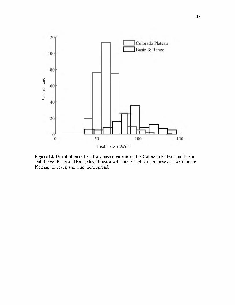
with the 90 m W m value from Chapman et al. [1979]. A histogram of heat flows for both
the Colorado Plateau and Basin and Range provinces can be seen in Figure 13. All heat
flow values determined for the study are summarized in Appendix C.
Compiling a heat flow database of discretely sampled heat flows is a step toward
the ultimate goal of calculated temperature at depth over a continuous region. The
aggregate of previously existing works and new measurements provides adequate spatial
coverage for a statewide interpolation; however, realizing a satisfactorily gridded
representation of continuous heat flow requires the selection of an appropriate
interpolation scheme. As with other geologic interpolation problems, choosing a method
that adheres to realistic behavior of the property of interest through space is crucial to
producing a credible result.
Two interpolation methods were tested before arriving at a final heat flow map.
The first was ordinary kriging and the second was a convergent interpolation algorithm.
Generally, interpolation techniques follow variations of the weighted difference scheme.
Weighted difference gridding algorithms can be considered in two broad classes: integral
and statistical. As described in Smith and Wessel [1990], integral methods attempt to
minimize the overall misfit between data and the gridding function. These methods return
results over the entire domain; however, they do not give a quantitative sense for how
well constrained the result is. Geostatistical methods, on the other hand, assess and
37
Occ
uran
ces
38
Heat Flow mWm'2
Figure 13. Distribution of heat flow measurements on the Colorado Plateau and Basin and Range. Basin and Range heat flows are distinctly higher than those of the Colorado Plateau, however, showing more spread.
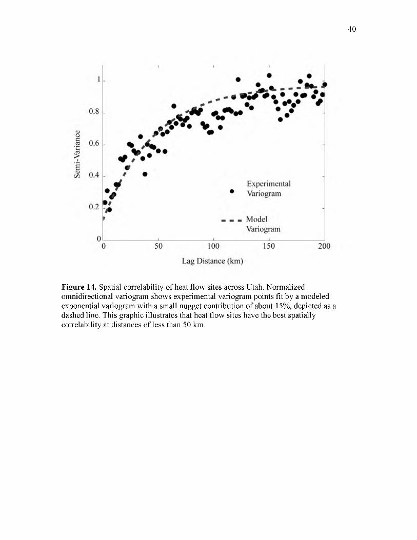
leverage the spatial correlability of control data (Figure 14) and minimize the error
variance at each point of estimation, while honoring all input data. Through this
minimization, a quantitative estimate of how well constrained the interpolation is in
reference to the variance of the dataset can be made. Geostatistical methods are limited in
regions of sparse data, falling back to the local mean of the data. The results of both
techniques are shown in Figures 15-16 with the estimate of the kriging variance shown in
Figure 17.
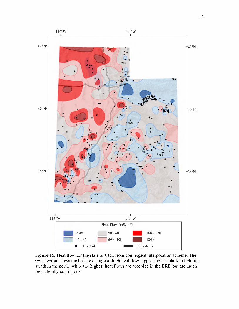
The mapped grids show generally lower heat flow on the Colorado Plateau and
higher heat flow in the Basin and Range. Distributions of the gridded results were
bimodally distributed with peaks corresponding to the two distinct heat flow provinces,
Basin and Range and Colorado Plateau. The modes of both grids compared favorably
-2 -2with those of the input data with peaks at 92 m W m and 62 m W m for the convergent
-2 -2 -2 interpolation and 89 m W m and 61 m W m for the krig, compared to 89 m W m and 63
-2m W m of the input data. The total extents of the convergent interpolation were, however,
-2 -2greater than those of the input data ranging from 24 m W m and 150 m W m , as opposed
-2 -2to the input and kriging range from 34 m W m to 145 m W m .
To preserve the remaining heat flow information from sites not included in the
gridding, all data were plotted as discrete values over the continuous background heat
flow surface Figure 18. Ultimately, the convergent interpolation appears to be less stable
than the ordinary kriging interpolation results and provided no estimate of the
interpolation uncertainty; therefore, the kriging algorithm was selected to best represent
background heat flow and the boundary condition for the calculation of temperature at
depth.
39
40
Figure 14. Spatial correlability of heat flow sites across Utah. Normalized omnidirectional variogram shows experimental variogram points fit by a modeled exponential variogram with a small nugget contribution of about 15%, depicted as a dashed line. This graphic illustrates that heat flow sites have the best spatially correlability at distances of less than 50 km.
41
42°N-
40°N-
38°N-
114°W 1II°W_L
i ^ :
2 Z , . • .
114°WT
nrw
-40°N
•42°N
-38°N
Heat Flow (mWnr2)
< 4 0 6 0 - 8 0 1 0 0 -1 2 0
□ 4 0 - 6 0 8 0 -1 0 0 120 <
• Control Interstates
Figure 15. Heat flow for the state of Utah from convergent interpolation scheme. The GSL region shows the broadest range of high heat flow (appearing as a dark to light red swath in the north) while the highest heat flows are recorded in the BRD but are much less laterally continuous.
42
Figure 16. Heat flow for the state of Utah from ordinary kriging scheme. Result of gridding data from Basin and Range and Colorado Plateau that considers spatial correlability of the data. The GSL region shows the broadest range of high heat flow— as in the convergent interpolation.
43
114°W l l l ° W
Normalized Variance
| | < 0.2 | 10.2 - 0.4 | 10.4 - 0.6 | 10.6 - 0.8 | 10.8 <
• H«-'al Flow Control -------- Interstates
Figure 17. Normalized kriging variance for Utah heat flow. As the kriging algorithm searches beyond the variogram range for control data, the kriging estimate becomes the local mean. Red and orange indicate the highest variance near or beyond the variogram range (150 km). Three regions along the edges of the state appear to be poorly constrained: northwestern Utah, northeastern Utah, and in southeastern Utah.
44
114°W ll l° W__I_____________________________ I__
—I------------------------------------------------ 1---114°W 111°W
1 1 < 4 0 1
Hcat Flow (mWrrr2)
___160 - 80 100 - 120
| | 4 0 - 6 0 1 18 0 - 100 120 <
• < 2 0 5 0 - 70 110 - 130 • 200 - 500
• 2 0 - 3 0 7 0 - 90 • 130 -150 • 500 <
• 3 0 - 5 0 9 0 - 110 • 150 -200 “ Interstates
Figure 18. Heat flow measurements in the state of Utah. All of approximately 800 heat flow sites measured throughout the state are displayed, as colored points, over the kriging results for comparison. High density clusters of heat flow in excess of 0.5 Wm-2 surround known geothermal resource areas with active direct use or energy production.
Elevated trends are observed in both grids through the GSL region where heat
2 2flow ranges from 105 mWm to 115 mWm and in the southern Basin and Range which
reaches heat flows as high as 145 m W m . The trend in the GSL region is both well
constrained and laterally extensive while the trend in the southern Basin and Range varies
laterally.
45
TEMPERATURE FIELDS
The culmination of this work is mapping temperature at depth in the Basin and
Range of Utah. Temperature can be conveniently portrayed on 2D cross-sections,
illustrated as contoured depth to isotherms, or temperatures at selected depths. As
examples of the first of these mapping styles, two cross-sections were constructed along
basin axes in regions with elevated mapped heat flow and located to intersect wells with
temperature control for model validation. The first was located in the GSL region, where
mapped heat flow was consistently greater than 100 mWm-2 through broad basins. The
second was located in the BRD, where recorded heat flows were highest but more rapid
lateral changes were observed.
The temperature fields in each cross-section were modeled numerically by a finite
difference scheme, developed in Matlab, using relevant boundary conditions and interior
properties. Finite difference schemes have been used previously to solve for temperature
fields in both 2D and 3D domains [Beardsmore and Cull, 2001]. The model coded for
this study uses a surface boundary held at a specified temperature distribution, a base
condition of specified heat flow, lateral boundaries with zero flow, and an interior
populated with in-situ thermal conductivity for a number of geologic units.
Regional control on geology was taken from nine surfaces mapped and described
as part of a United States Geological Survey (USGS) project to understand regional scale
hydrologic flow in the Basin and Range [Heilweil and Brooks, 2011]. The following nine
units, from oldest to youngest, were mapped and are described in Figure 19 and Table 2:
Noncarbonate Unit (NC), Lower Carbonate (LC) Unit, Upper Siliciclastic Unit (US),
Upper Carbonate Unit (UC), Thrusted Noncarbonate Unit (TNC), Thrusted Lower
Carbonate Unit (TLC), Volcanics Unit (VU), Lower Basin-Fill Unit (LBF), and Upper
Basin-Fill Unit (UBF).
The nine hydrogeologic units mapped represent distinct physical characteristics
that impact fluid flow, namely lithologic and hydraulic properties. Because thermal
conductivity is dominantly controlled by the rock matrix composition and pore space
volume, these units of hydrostratigraphic significance are particularly applicable to the
thermal modeling problem. These hydrogeologic unit (HGU) surfaces were used to
construct the majority of the model framework.
One additional unit, near surface lake bed clays, which was sampled and well
characterized by the five UGS gradient wells, was also included in the model framework.
A surface that represents this unit was generated and constrained by surface geological
maps and well penetrations.
A grid was constructed in Schlumberger’s Petrel 2011.2 as a 16 million cell
model with uniform rectangular dimensions (1000x1000x100 meters). Individual cells
were assigned index values corresponding to the HGU at each cell center. Storing only
indices allows properties associated with a given unit to be assigned during the
temperature field calculation, limiting the amount of storage and computational expense
required when manipulating the grid.
47
48
HydrogeologicUnit
StratigraphicUnit
Q
T
Mz
P
IP
M
D
S
0
PC
UBFAUBasin-fill deposits Basalt
LBFAUGarrett Ranch Group
North Horn Fm
VU Volcanic rock
TLCAU Thrusted rocks of the Sevierilold'and
TNCCU
UCAU Oquirrh Group
USCU Manning Canyon Sh.
Great Blue Fm
Humbug Fm
Gardison Limestone
LCAU Water Canyon Fm
Laketown Dolomite
Garden City Lime
Teutonic Limestone
NCCUPioche Formation
Tintic Quartzite
Figure 19. Hydrogeologic unit groupings. Modified from Heilweil and Brooks [2011].
49
Table 2. Hydrogeologic unit descriptions*HGU Abreviation Age Description
Upper Basin-Fill Unit UBF Quaternary Mostly unconsolidated basin-fill occurring syndepositionally with Basin and Range extension
Lower Basin-Fill Unit LBF Tertiary to Quaternary
Deepest basin fill
Volcanics Unit VU Tertiary Volcanic intrusions and accumulations
Thrusted Noncarbonate & Lower Carbonate Units
TNC & TLC
- Repeat of the two deepest units
Upper Carbonate Unit UC Pennsylvanian through Permian
Shallow marine carbonates
Upper Siliciclastic Unit US Devonian to Mississippian
Siliclastic sediments shed from Antler Orogeny
Lower Carbonate Unit LC CambrianthroughDevonian
Carbonates
Noncarbonate Unit NC Early Paleozoic and older
Metamorphosedbasement
*Hydrogeologic units as described in Heilweil and Brooks, 2011.
50
Populating the grid interior required determining in-situ thermal conductivity. Lab
measurements of thermal conductivity provide the conductivity of rock matrix. A volume
of rock in place, however, is composed of both rock matrix and fluid filled pore space. A
two-component volumetric mixing expression provides a reasonable estimate of thermal
conductivity in the subsurface:
k- ■ — k ■ (1-o) * k o (17)n-insitu ~ /vmatrix n-water , v '
where k matrix is the thermal conductivity of the rock matrix, k water is the thermal
conductivity of pore fluid which is assumed to be water, and O is the total porosity.
Matrix thermal conductivities and their statistics are known where the HGUs intersected
each well with measured conductivity. The thermal conductivity of water is known to be
0.6 Wm-1K-1, and porosity requires further estimation.
Porosity in the geologic section can be highly variable for a number of reasons
including sedimentation rate, depositional environment, and chemical cementation;
however, it has been observed that despite these processes, decreasing porosity with
depth can be approximated to a first order by an exponential function [Bahr et al., 2001].
Porosity in the subsurface is characterized by establishing unique compaction trends for
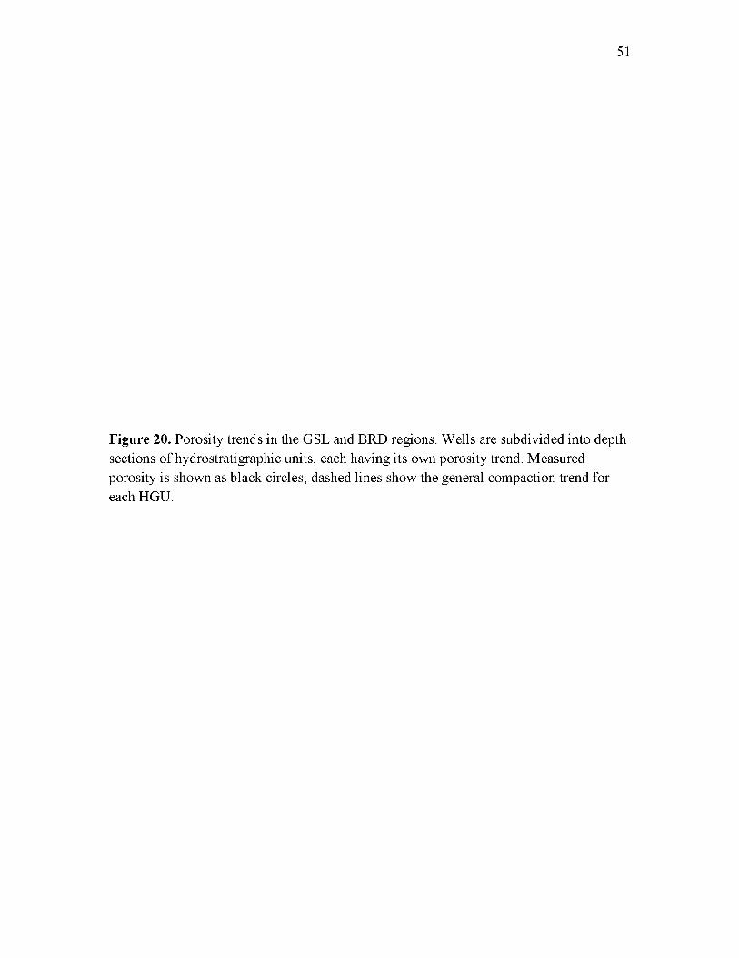
each HGU. Neutron-density cross-plot data were sampled at 30 meter intervals from logs
for ten key wells in the GSL and BRD regions. Hydrogeologic unit intersections with
each well were plotted (Figure 20) and porosity-depth relationships were grouped by unit.
Exponential decay trends were fit through the porosity-depth pairs for each HGU (Figure
21) and assessed for goodness of fit. With matrix conductivity and porosity constrained,
in-situ thermal conductivity is calculated and populated for each cell in the model.
51
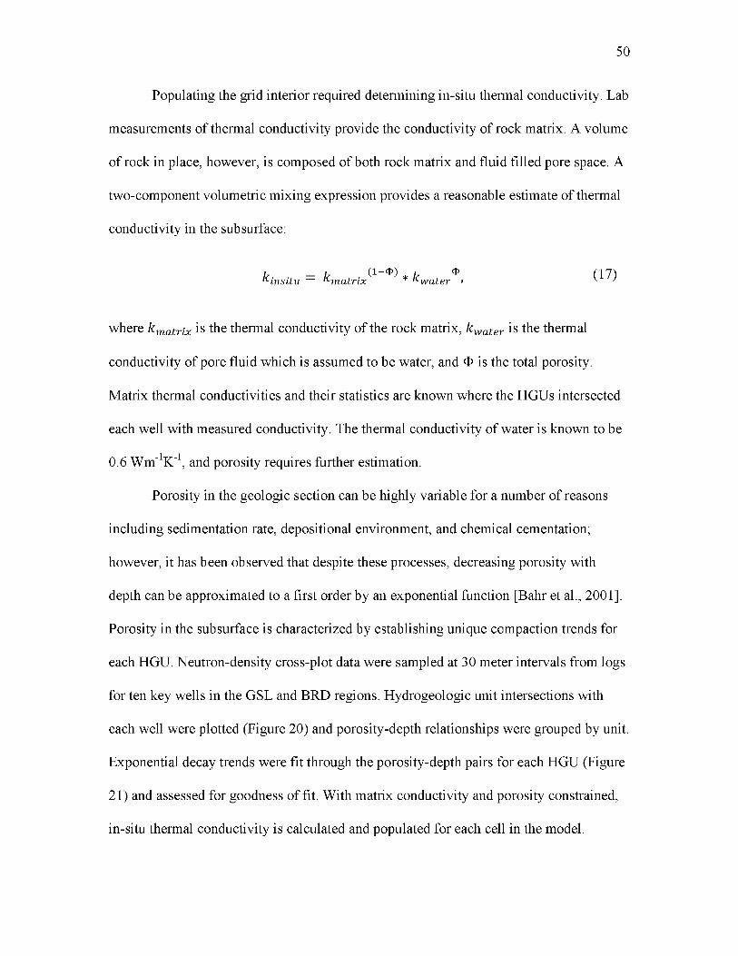
Figure 20. Porosity trends in the GSL and BRD regions. Wells are subdivided into depth sections of hydrostratigraphic units, each having its own porosity trend. Measured porosity is shown as black circles; dashed lines show the general compaction trend for each HGU.
Dep
th
(km
)
Beaver River 2
Pavant Butte 1
Saltair 1 St of UT“E” 1
UBF
0 0.35 0.7 Porosity
St of UT “H” 1
St of UT “L” 1
St of UT “P” 1
UBF
LBF
NC
0.35 0.7 0 0.35 0.7 0 0.35 0.7
53
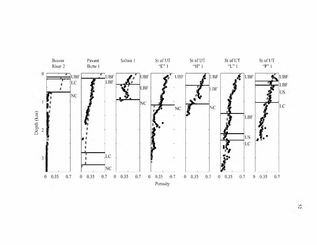
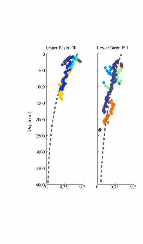
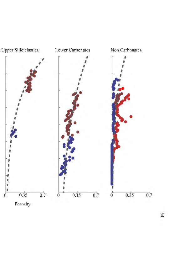
Figure 21. Porosity trends in the GSL and BRD regions for encountered HGUs. Measured porosity is shown in circles and the generalized compaction trend for each HGU is dashed in grey. Colors indicate individual wells tabulated for porosity measurements.
Dept
h (m
)
Upper Basin Fill
0
500
1000
1500
2000
2500
3000
3500
4000,
*I
IIII*II■
0.35 0.7
L ow er Basin Fill
a
0 >. I
I
0 0.35 0.7
Upper S ilic ic lastics L ow er Carbonates N on Carbonates
*II*
0 0.35 0.7
Porosity
0.35 0.7
With boundary conditions and internal parameters established, the finite
difference model is run to convergence. In a finite difference, or relaxation, model each
cell is checked for thermal equilibrium with adjacent cells until its change is less than a
specified convergence tolerance. For iterations prior to reaching the convergence
criterion, the cells are assigned new values based on the difference between each cell’s
neighbors and then checked again for convergence to thermal equilibrium. For
sufficiently small thermal equilibrium tolerances, many tens of thousands of iterations
can be required. To reduce the computational expense, the model is originally seeded
with an analytic solution for 1D temperature along each vertical column of the cross
section before proceeding with 2D relaxation. Providing a 1D approximation of the
temperature field reduces the required iterations from tens of thousands to hundreds and
drops the overall run time from minutes, for a single cross-section, to seconds.
The resulting temperature fields are presented in Figures 22-23. The GSL region
cross-section (Figure 22) was located to pass through two oil and gas exploration wells
with temperature control— State of Utah “L” 1 (API: 00330010) and Indian Cove State 1
(API: 00330002)—in the center of the basin. Good agreement was found between the
modeled temperature field and temperature observations at the wells. Temperatures
greater than 150 °C are observed at less than 3 km depth and 200 °C is observed between
3.5 km and 5 km. Absolute percent errors were calculated between the temperature data
and the modeled temperature field at coincident locations. The mean of absolute percent
errors was 3% indicating that the modeled field overpredicts temperature by a small
amount.
55
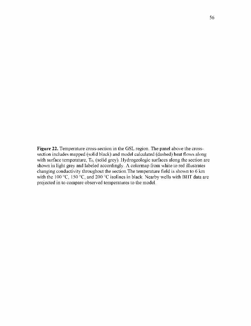
56
Figure 22. Temperature cross-section in the GSL region. The panel above the crosssection includes mapped (solid black) and model calculated (dashed) heat flows along with surface temperature, T0, (solid grey). Hydrogeologic surfaces along the section are shown in light grey and labeled accordingly. A colormap from white to red illustrates changing conductivity throughout the section.The temperature field is shown to 6 km with the 100 °C, 150 °C, and 200 °C isolines in black. Nearby wells with BHT data are projected in to compare observed temperatures to the model.
Hea
t Fl
owDe
pth
(km
) (m
Wnr
2)
130
10
1 1
r T
- - - - - Ji i
15
12.5
4580UTM (km)
Thermal Conductivity (Wm 'K 1) <1
Tem
pera
ture

58
Figure 23. Temperature section in the BRD region. The section is presented as Figure 21 with the addition of the volcanic HGU which was not present in the GSL region.
Hea
t Fl
ow
(mW
nr2)
Meadow Federal Unit 0
SA
Cl.UQ
4300 4310
Pavant Butte
4320 4330UTM (km)
__L
3 4Thermal Conductivity (W m'K.1)
4350
VO
Tem
pera
ture
The BRD region cross-section (Figure 23) was also placed to intersect two key
wells—Pavant Butte 1 (API: 02730027) and Meadow Federal 1 (API: 02730028). The
BRD region appears to be cooler than GSL above 4 km, generally reaching 150 °C at
depths between 3 km and 4.5 km and 200 °C at depths beyond 5 km. An exception occurs
in a 5 km radius around Pavant Butte 1 where temperatures reach 150 °C at 2 km and 200
°C at 3 km depth. Temperature control and the modeled temperature field show
reasonable agreement, with a 10% mean of absolute percent errors and a maximum
mismatch of 31% at the shallow record in Meadow Federal 1. Two explanations exist for
the larger observed discrepancy at BRD compared to GSL. The first considers a
mismatch between well intersections with the HGUs and the actual depth to formations
penetrated during drilling. The second considers geologic factors not accounted for in the
model and their impact on the resulting temperature field.
As the HGUs approximately correspond to a specific portion of the stratigraphic
section, their accuracy can be assessed at the wells where subsurface control is best. For
the two wells on the BRD cross-section, tops are compared to the HGU intersections and
the offsets are presented in Table 3. Depth to hydrogeologic units at Pavant Butte 1 are
significantly deeper than the observed geology and at Meadow Federal 1, the HGUs
replace 1900 meters of Tertiary sediments with volcanics to surface. The study evaluates
the impact of these observed offsets in one-dimensional temperature profiles calculated at
each well. The 1D profiles used the same boundary conditions as the two-dimensional
case. A 1D basecase was established for each well by calculating the temperature field
using the HGU intersections. For the Meadow Federal 1, the largest misfit was a 25% or
14 °C overprediction at 1900 meters, the smallest misfit was a 1% or 0.5 °C
60
Table 3. Stratigraphic control mismatch*
Well Top Name
TopDepth
(m)HGUName
HGUDepth
(m)Difference
(m)Pavant Butte 1 Quaternary 0 U. Basin Fill 0 0
Miocene 640 L. Basin Fill 2800 -2160Volcanics Volcanics 3800Chisholm 2987 L. Carbonates 3900 -913Prospect Mountain Quartzite 3234 Noncarbonates 4100 -866
Meadow Fed. 1 Quaternary 0 U. Basin FillTertiary 5 L. Basin FillVolcanics Volcanics 0Cambrian Carbonates 1780 L. Carbonates 1900 -120Prospect Mountain Quartzite 3960 Noncarbonates 3600 360
*Well stratigraphy compared to regionally mapped hydrogeologic unit equivalent.
overprediction at 4700 meters, and the average misfit was 14%. Correcting the
stratigraphic section to that observed at the well and recalculating reduced the
overprediction to 20% or 12 °C at 1900 meters, 8% or 10 °C at 4700 meters, and the
overall misfit to a 5% overprediction. At Pavant Butte 1, the same approach was taken for
the original case. The largest misfit was a 14% or 22 °C overprediciton at 2400 meters,
while the smallest was an 8% or 19 °C underprediction at 3300 meters, and the overall
underprediction was 3%. Changing the stratigraphic column to better reflect the rocks
encountered during drilling and recalculating the temperature field improves the
underprediciton nominally to 6% or 16 °C at 2400 meters, but slightly raises the error at
3300 meters to 17% or 28 °C, and the overall error to 4%.
The conductive heat flow model for temperature in the subsurface is relatively
simple, making the assumption that a single basal heat source is the only heat input. With
this assumption, the model may fail to characterize the temperature field accurately in the
presence of young volcanics and cooling intrusions which provide heat input to the model
interior. The eastern BRD is known for active volcanism throughout the Cenozoic
particularly in the last million years [Hintze and Davis, 2003]. Basalts, as young as
10,000 years, are found immediately adjacent to the Pavant Butte 1 in the Pavant Butte
volcanic field. Basaltic cinders and tuffs have also been described within 10 km of the
Pavant Butte 1 [Hintze and Davis, 2003]. Temperatures and heat flow in the Pavant Butte
1 are the highest recorded for any oil and gas well in the state of Utah. In the context of
the abundant volcanic activity in close proximity, the Pavant Butte 1 may not be
representative of a regional heat flow regime with only basal input. Instead, the elevated
temperature records and calculated heat flow are likely due to the cooling of nearby
62

volcanics. Based on these observations, the thermal regime at Pavant Butte 1 should be
treated as anomalous in the regional context.
63
SYNTHESIS
The primary objective of this study was to identify high temperatures at accessible
depths for potential future geothermal development in the sedimentary basins of Utah’s
Great Basin Province. The regional resource assessment required the development of new
digital infrastructure composed of an integrated thermal database and temperature
modeling code. A thermal database was constructed with over 1300 sites containing a
variety of thermal data that included the following: 323 wells with corrected BHTs where
44 are newly determined, more than 850 tabulated temperature logs, and 2300 thermal
conductivities of which more than 460 were new measurements. A finite difference code
was written in Matlab, a broadly accessible and inexpensive platform, designed to model
steady state temperature fields through stratified basins using boundary conditions and
rock properties derived in previous chapters.
The final temperature sections focus most closely on two areas: the Great Salt
Lake region—marked by a broad swath of high heat flow, elevated above the typical
Basin and Range values, and close proximity to a population center—and the Black Rock
Desert—because it contained the highest recorded heat flows. Temperatures determined
in the BRD generally did not exceed 150 °C above depths of 3000 m and misfit between
the well control and the calculated temperature field was less than 15% across this region.
The observed misfit and rapid lateral changes in heat flow is attributed to the presence of
unaccounted for intrusives and volcanics. In the Great Salt Lake region, temperatures
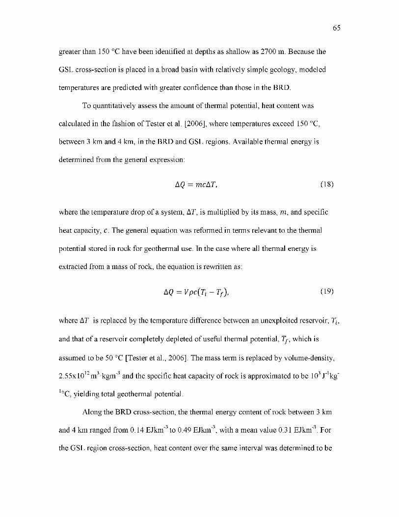
greater than 150 °C have been identified at depths as shallow as 2700 m. Because the
GSL cross-section is placed in a broad basin with relatively simple geology, modeled
temperatures are predicted with greater confidence than those in the BRD.
To quantitatively assess the amount of thermal potential, heat content was
calculated in the fashion of Tester et al. [2006], where temperatures exceed 150 °C,
between 3 km and 4 km, in the BRD and GSL regions. Available thermal energy is
determined from the general expression:
AQ = me AT, (18)
where the temperature drop of a system, AT, is multiplied by its mass, m, and specific
heat capacity, c. The general equation was reformed in terms relevant to the thermal
potential stored in rock for geothermal use. In the case where all thermal energy is
extracted from a mass of rock, the equation is rewritten as:
AQ = Vpc{Ti — Tf), ( 19)
where AT is replaced by the temperature difference between an unexploited reservoir, Tt,
and that of a reservoir completely depleted of useful thermal potential, 7y, which is
assumed to be 50 °C [Tester et al., 2006]. The mass term is replaced by volume-density,
12 3 3 3 12.55x10 m kgm and the specific heat capacity of rock is approximated to be 10 J' kg'
1°C, yielding total geothermal potential.
Along the BRD cross-section, the thermal energy content of rock between 3 km
3 3 3and 4 km ranged from 0.14 EJkm" to 0.49 EJkm" , with a mean value 0.31 EJkm" . For
the GSL region cross-section, heat content over the same interval was determined to be
65
between 0.33 EJkm-3 and 0.39 EJkm-3 with a mean 0.37 EJkm-3. The depth to 150 °C in
the GSL region is generally less than 3 km across the basin and the thermal gradient is
relatively constant between 3 km and 4 km. The narrow range of heat content is a
reflection of this.
In order for a region to be considered geothermally prospective in this study,
temperatures greater than 150 °C must be identified above 4 km depth. The extent of
temperatures exceeding 150 °C at or above 4 km was mapped (Figure 24) from cross
sections to delineate the lateral extent of geothermal resource in the BRD and GSL
regions. The total area in BRD where this criterion was met was approximately 560 km .
Temperatures greater than 150 °C at the target depths were generally not found beyond
12 km of the Pavant Butte 1 well and did not occur at all outside of a 20 km radius. The
total area in GSL containing 150 °C resource covered approximately 4100 km that
approximately coincide with the bounds of the Great Salt Lake.
Uncertainties in the temperature field were captured quantitatively by evaluating
parameter sensitivity on the modeled temperature fields using a Monte Carlo analysis.
Five parameters— surface temperature, surface heat flow, thermal conductivity, porosity,
and constraining unit thickness—were tested individually to evaluate their impact on the
calculated temperature field at nine locations in the project area. The nine locations were
selected in basins throughout the state of Utah to compare the uncertainties spatially as
well.
One-dimensional temperature fields were calculated using the thermal resistance
method, as in equation (12), and holding all but a single parameter constant. Four
parameters— surface temperature, surface heat flow, thermal conductivity, and porosity—
66
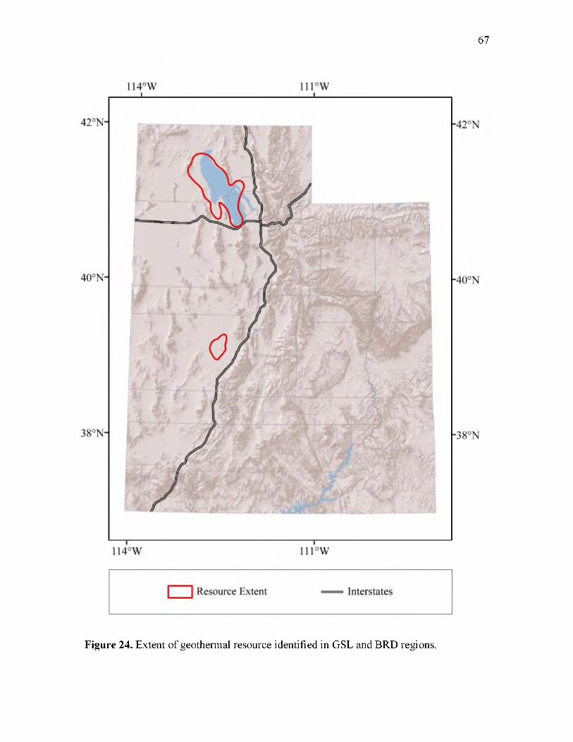
67
Figure 24. Extent of geothermal resource identified in GSL and BRD regions.
were tested through two standard deviations of their mean. For the fifth parameter, unit
thickness, there was not a good quantitative estimate of the potential error, so thickness
was varied by ± 20% at each location. Each parameter was randomly tested, sampled
through 20,000 iterations, and temperatures were recorded at 1 km, 3 km, and 5 km
depth.
For interpretation, results of the analysis were displayed graphically in a
modification to the tornado plot [Project Management Institute, 2013]. Tornado plots
have classically been used to test parameter sensitivities in a deterministic model. The
plot highlights minimum and maximum possible deviation from the model baseline, due
to perturbations on a single parameter. While identifying the limit of a parameter’s
possible effect is useful, the traditional tornado plot fails to represent all aspects of
parameter sensitivity. For instance, tornado plots do not indicate how perturbations to a
parameter affect the shape of the resulting model’s probability density function or even
where the median outcome occurs relative to the baseline. To remedy the graphical
deficiency of a traditional tornado plot, the stacked bars were replaced by normalized
probability density functions for each parameter, giving the appearance of a third
graphical dimension and providing the ability to represent distributions of modeled
outcomes. Additionally, overlaying tornado plots of each parameter at multiple depths for
a given location provides a view into how errors propagate to depth.
The error analysis, and resulting tornado plots, provided interesting insights into
the impact of the model parameters. These insights were considered and are offered as
recommendations to focusing the efforts of future thermal modeling in sedimentary
basins. Two parameters were not particularly influential on temperature at depth—
68
surface temperature and stratigraphic unit thickness. The minimal sensitivity of in-situ
temperature to that of the surface is expected since the model treats surface temperature
as a static shift and surface temperature is already well constrained. Also, the analysis
illustrated that stratigraphic unit thickness did not contribute an appreciable amount of
error to the modeled temperature. This is a surprising result as both porosity and thermal
conductivity differ throughout the stratigraphic section and each can vary by a large
amount. Because no robust estimate of the possible spread of stratigraphic unit thickness
was established, it is possible that the sensitivity analysis did not test a broad enough
range of thicknesses. Additionally, considering that the shallowest units, UBF and LBF,
were commonly deeper than 3 km, temperature records taken at 1 km and 3 km would be
unaffected by a change in thickness that only shifted deeper constraining surfaces. Given
a more detailed geologic model, the influence of variations in stratigraphic thickness
would be much greater. The model was consistently most sensitive to three parameters:
thermal conductivity, porosity, and heat flow. The model became more sensitive to all
three parameters at greater depths. This highlights the significance of constraining
porosity and thermal conductivity in the shallow stratigraphic section, which is most
important to predicting accurately the thermal regime at greater depths of interest.
Scrutiny of the distributions of the more sensitive parameters yields useful information as
well. Heat flow remains distributed symmetrically about the baseline, whereas porosity
and thermal conductivity do not. This asymmetry reveals that overpredicting porosity or
underprediciting conductivity will skew the model away from the baseline toward
overpredictions. An example of the study’s modified tornado plot is shown in Figure 25.
In addition to the sensitivity evaluation, the misfit between the modeled temperature field
69
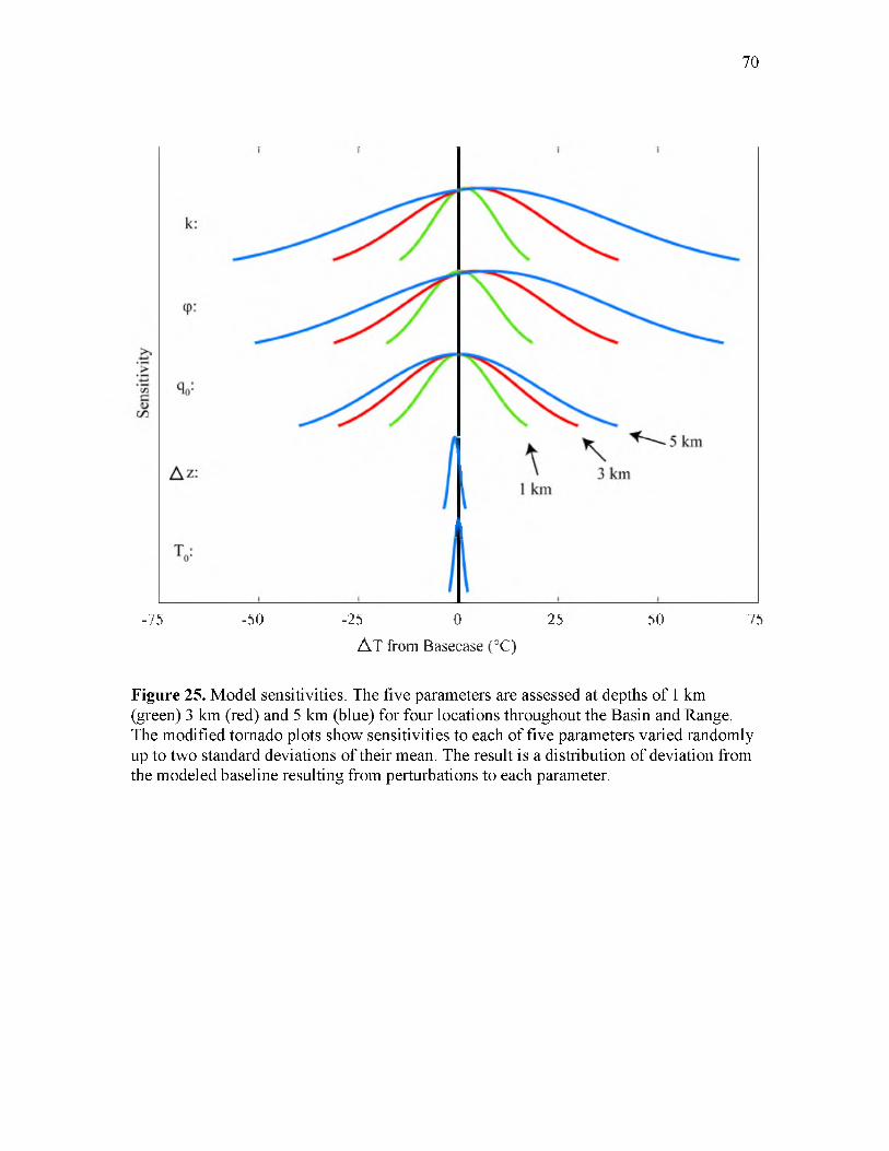
70
-75 -50 -25 0 25 50 75A T from Basecase (°C)
Figure 25. Model sensitivities. The five parameters are assessed at depths of 1 km (green) 3 km (red) and 5 km (blue) for four locations throughout the Basin and Range. The modified tornado plots show sensitivities to each of five parameters varied randomly up to two standard deviations of their mean. The result is a distribution of deviation from the modeled baseline resulting from perturbations to each parameter.
and BHTs was assessed. One-dimensional temperature fields were calculated at 78 wells
in the Basin and Range and compared to their Horner corrected BHTs. Residuals between
the calculated field and corrected BHTs revealed that the model overpredicts BHTs by 10
°C and the maximum residual was determined to be 87 °C. The differences are quite
large, which likely reflects the noise inherent to the BHT dataset being compounded with
model uncertainties. A distribution of all residuals is shown in Figure 26.
The uncertainty analysis provides two takeaway points: first, the most important
factors in the calculation of temperature at depth for a conductive regime are thermal
conductivity, porosity, and heat flow; second, errors associated with these parameters
increase with depth.
71
72
-TBUT model
50 0 50 % Difference
Figure 26. Differences between modeled and observed temperature. The differences were calculated for all wells with corrected BHTs in the Basin and Range. a) Absolute residuals are mean centered about 10 °C skewed toward underpredctions by the model. b) Absolute percent errors between the model and BHTs present a more representative depiction of misfit across all depths.
CONCLUSIONS
A geothermal resource assessment of the Basin and Range Province in western
Utah was carried out to identify resource potential for future exploration and exploitation.
The assessment involved several sequential tasks that provide for the following summary
observations and conclusions.
1. A rigorous, methodological architecture was developed for calculating regional
and local subsurface temperature fields and identifying areas with temperatures above
150 °C at depths shallower than 4 km. The architecture involves assigning surface
ground temperature, thermal conductivity, and heat flow throughout the state of Utah and
using these data as the basis for calculating temperatures.
2. A surface ground temperature function was developed based on the decrease of
temperature with elevation (known as the adiabatic lapse rate), the decrease of
temperature with an increase of latitude that results from lessening exposure to solar
energy input, and a constant offset between air and ground temperature. Use of weather
station data and extrapolation of borehole temperatures yielded the following coefficients
for the surface ground temperature function: -6.42 °Ckm-1 for an elevation lapse rate, -
0.0084 °Ckm-1 for the latitudinal cooling, and 3 °C to accommodate ground temperatures
being warmer than air temperatures.
3. All published thermal conductivity measurements for Utah rock samples were
combined with 468 new measurements to create a comprehensive compilation of more
than 2300 thermal conductivity measurements that were applied to characteristic Utah
geologic stratigraphic sections. Because thermal conductivity of porous rocks involves
thermal conductivity of both matrix and fluid that are combined using an appropriate
mixing model and porosity, porosity-depth trends for dominant formations also were
determined.
4. A new heat flow map for Utah was created based on approximately 150
classic heat-flow determinations in shallow boreholes with high-precision temperature
logs, and 300 oil and gas exploration wells with less precise bottom hole temperatures,
but taken at much greater depths. Heat flow for the Basin and Range is 89 mWm , 40%
higher than the 63 m W m value for the Colorado Plateau. A geostatistical kriging
algorithm was judged to be best for interpolating the irregularly positioned heat-flow
determinations.
5. Calculating temperature with depth, the ultimate goal of this study, required a
three-dimensional configuration for thermal conductivity over all regions of interest. We
were able to use a recent USGS result giving spatial variation and thicknesses of nine
hydrostratigraphic units throughout the study area. When combined with porosity
information, the HGU thermal conductivity structure, with surface temperature and heat
flow maps, afforded the first opportunity to calculate temperature-depth profiles for any
Utah Basin and Range site of interest.
6. Two cross-sections of the resulting temperature fields were chosen to illustrate
geothermal potential. The first, in Utah’s Black Rock Desert, examined what appeared to
be the highest background heat flow (>130 mWm ) in the state. In Black Rock Desert,
150 °C was encountered at depths generally greater than 3 km and the thermal potential
74
of rock between 3 km and 4 km for exploitation ranged between 0.14 EJkm and 0.49
3 3EJkm , with a mean value 0.34 EJkm . Total heat contained in the rock between 3 and 4
km depth in the Black Rock Desert thermal anomaly is 190 EJ; if this heat were used for
geothermal energy production at a heat sweep efficiency of 10 % and developed over 30
years, the geothermal power potential would be 1,900 MW. For the second thermal
anomaly examined, along the axis of the Great Salt Lake, heat flow is generally greater
than 105 m W m , the depth to 150 °C is less than 3 km across the basin, and the
calculated thermal potential in the 3 km to 4 km depth interval is between 0.33 EJkm
3 3and 0.40 E Jkm with a mean 0.37 EJkm . Because of the larger area of the Great Salt
Lake thermal anomaly compared to the Black Rock Desert, the total heat energy in rocks
between 3 and 4 km depth is 1517 EJ and the corresponding geothermal power potential
is 16,000 MW. Proximity to population centers and power transmission and
transportation corridors also favor the exploitation of these potential resources.
75
3
RECOMMENDATIONS
1. High heat flows reported in the Black Rock Desert are encouraging indicators
of the region’s geothermal potential; however, more complicated geology and the
presence of young cooling volcanics and intrusives appears to be inflating heat flow
determinations, ultimately exaggerating modeled estimates of regional scale temperatures
through basin sediments. In the Great Salt Lake Region, the combination of elevated heat
flow, low conductivity sediments, and depth to basement result in temperatures and
thermal potential that flag the region as a priority for geothermal exploration.
2. The most sensitive model parameters should be better constrained. Total rock
pore space and thermal conductivity of the rock matrix have been measured extensively
in the Quaternary and Tertiary sections; however, the broadly inclusive stratigraphic
groupings of the hydrogeologic units do not allow enough vertical stratification to take
full advantage of these detailed thermal conductivity measurements. For regional work,
mean values of the HGU thermal conductivity and generalized porosity compaction
trends are sufficient to identify the presence of geothermal resource at a basin scale; they
are not sufficient, however, to delineate resource to the field scale. A better resolved
stratigraphic model should be constructed to provide a more detailed framework for
property modeling. Conductivity and porosity were identified to be key parameters for a
temperature model in a conductive thermal regime and both could be better constrained
given a more detailed framework.
3. Rock properties necessary to identify productive reservoirs should be modeled.
When exploring for the presence of geothermal resource, this study gave no consideration
to the complications associated with exploiting reservoir fluids, namely flow properties of
the rock. Modeled total porosity indicates that significant pore space is present and
potentially occupied by high temperature fluids; nevertheless, the question remains, can
fluids be moved and can flow be predicted reliably? Again, a more resolved geological
model is necessary to evaluate the ability of GSL region basin sediments to host
productive reservoirs. This model should assess petrophysical parameters such as
effective porosity and permeability.
4. Advective heat transport should be incorporated into the thermal model. For
the sake of simplicity, the thermal model used in this study actively avoided thermal data
influenced by fluid flow; however, advective heat transport plays a large role in the
thermal state of sedimentary basins. A more inclusive model would incorporate the
coupled effect of heat and fluid flow at both the basin and reservoir scales.
5. Elements significant to petroleum systems— such as containers and seals—
need to be considered in the context of sedimentary basin geothermal exploitation. The
engineering challenge of producing and injecting to petroleum reservoirs in sedimentary
basins requires an understanding of reservoir geometries and extent. Presumably, to
sustainably produce geothermal reservoirs contained in sedimentary basins, the quality
and extent of their containment needs to be determined.
6. The thermal regime of two basins in Utah’s Basin and Range has been
considered using new digital infrastructure, a synthesis of new as well as pre-existing
thermal data, and a new paradigm for geothermal exploration. Temperatures between 150
77
°C and 200 °C, and thermal energy density between 0.33 EJkm-3 and 0.39 EJkm-3, at
depths of 2.5 km to 4.5 km were identified over broad areas in the Great Salt Lake region.
These results provide the impetus for an interdisciplinary project near Utah’s Great Salt
Lake with the goal to delineate the resource at a field scale, establish the engineering
challenges to producing that resource, and assess the potential economic benefit of
developing a geothermal exploitation program.
78
APPENDIX A
EXISTING THERMAL CONDUCTIVTY MEASUREMENTS
ON UTAH ROCK
Table 4. Existing Thermal Conductivity Measurements of Utah Rock*________________________________________Thermal
Conductivity1 n2 2_____ Formation_________(Wm~ K~ )_____ o Samples____________Lithology_____________________ Reference
Ankareh 3.23 0.25 15 Sandstone Deming and Chapman 1988
Aspen 2.56 0.06 17 Shale Deming and Chapman 1988
Bear River 2.98 0.09 20 Deming and Chapman 1988
Carmel 2.83 0.71 8 Mudstone, Sandstone Powell 19972
Carmel 2.88 0.58 17 Gypsum-Limestone Bodell and Chapman 19823
Carmel 2.6 0.38 6 Mudstone Bodell and Chapman 19823
Carmel 3.37 0.5 7 Siltstone-Sandstone Bodell and Chapman 19823
Carmel 1.38 1 Gypsum Bodell and Chapman 19823
Carmel 3.03 0.09 3 Limestone Bodell and Chapman 19823
Chinle 4.71 1.3 8 Siltstone-Conglomerate Bodell and Chapman 19823
Chinle 3.44 0.21 2 Siltstone Bodell and Chapman 19823
Chinle 4.96 0.51 3 Sandstone Bodell and Chapman 19823
Chinle 7.14 0.41 2 Very Coarse Sandstone Bodell and Chapman 19823
Chinle 2.47 1 Conglomerate Bodell and Chapman 19823
Chinle, Shinarump 7.26 0.97 4 Coarse Sandstone Powell 19972
Claron 3.68 0.2 29 Limestone Powell 19972
Claron 3.9 0.22 10 Silty Limestone Powell 19972
Coconino 4.82 1 Sandstone Powell 19972
Coconino 7.55 0.36 5 Sandstone Bodell and Chapman 19823
Table 4: Continued
Formation
ThermalConductivity1
(Wm'2K'2) G
nSamples Lithology Reference
Curtis 4.08 0.51 4 Conglomerate Bodell and Chapman 19823
Cutler-Rico 3.36 0.5 15 Sandstone-Limestone Bodell and Chapman 19823
Cutler-Rico 4.02 0.41 6 Silty Sandstone Bodell and Chapman 19823
Cutler-Rico 3.03 0.41 7 Arkose Sandstone Bodell and Chapman 19823
Cutler-Rico 3.1 0.22 2 Limestone Bodell and Chapman 19823
Dakota 6.38 1 Sandstone Bodell and Chapman 19823
Duchesne 4.80 1.3 51 Sandstone Chapman et al. 19842
Echo Canyon 6.43 0.65 21 Sandstone-Conglomerate Deming and Chapman 1988
Elephant Canyon 5.27 0.63 7 Dolomite-Sandstone Bodell and Chapman 19823
Elephant Canyon 5.39 0.42 4 Dolomite Bodell and Chapman 19823
Elephant Canyon 5.06 0.81 3 Siltstone-Sandstone Bodell and Chapman 19823
Entrada 4.77 0.74 2 Sandstone Powell 19972
Entrada 3.86 0.67 19 Siltstone-Sandstone Bodell and Chapman 19823
Entrada 3.17 0.43 10 Siltstone Bodell and Chapman 19823
Entrada 4.58 0.61 9 Sandstone Bodell and Chapman 19823
Ferron 4.22 1 Sandstone Bodell and Chapman 19823
Frontier 2.47 0.67 42 Sandstone-Shale Deming and Chapman 1988
Gannett 3.47 0.19 45 Limestone-Conglomerate Deming and Chapman 1988
Green River 3.05 0.85 352 Shale Chapman et al. 19842
Table 4: Continued
Formation
ThermalConductivity1
( W m V ) G
nSamples Lithology Reference
Guilmette 2.73 0.35 9 Limestone Henrickson 20004
Hermit 2.66 0.13 2 Siltstone Powell 19972
Hermosa 1.63 0.14 9 Shale Henrickson 20004
Hermosa 4.78 0.08 5 Sandstone Henrickson 20004
Honaker trail 3.25 0.64 10 Mudstone-Sandstone, Limestone Bodell and Chapman 19823
Honaker trail 2.46 0.32 2 Mudstone Bodell and Chapman 19823
Honaker trail 3.99 0.2 4 Sandstone Bodell and Chapman 19823
Honaker trail 2.91 0.09 4 Limestone Bodell and Chapman 19823
Jordanelle Stock 2.10 Moran 19915
Kaibab 3.3 0.31 2 Limestone Powell 19972
Kayenta 5.55 0.54 14 Silty Sandstone-Sandstone Bodell and Chapman 19823
Kayenta 4.68 0.3 5 Silty Sandstone Bodell and Chapman 19823
Kayenta 6 0.29 9 Sandstone Bodell and Chapman 19823
Kelvin 3.61 0.70 128 Shaley Sandstone Deming and Chapman 1988
Madison 4.3 0.28 20 Limestone Deming and Chapman 1988
Mancos 2.48 0.24 24 Shale Henrickson 20004
Mesaverde 2.80 0.5 79 Shaley Sandstone Chapman et al. 19842
Moenkopi 2.65 0.24 21 Mudstone Powell 19972
Morrison 2.74 1 Limestone Bodell and Chapman 19823
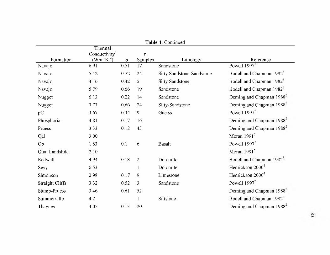
Table 4: Continued
Formation
ThermalConductivity1
(Wm'2K'2) G
nSamples Lithology Reference
Navajo 6.91 0.51 17 Sandstone Powell 19972
Navajo 5.42 0.72 24 Silty Sandstone-Sandstone Bodell and Chapman 19823
Navajo 4.16 0.42 5 Silty Sandstone Bodell and Chapman 19823
Navajo 5.79 0.66 19 Sandstone Bodell and Chapman 19823
Nugget 6.13 0.22 14 Sandstone Deming and Chapman 1988
Nugget 3.73 0.66 24 Silty-Sandstone Deming and Chapman 1988
pC 3.67 0.34 9 Gneiss Powell 19972
Phosphoria 4.81 0.17 16 Deming and Chapman 1988
Pruess 3.33 0.12 43 Deming and Chapman 1988
Qal 3.00 Moran 19915
Qb 1.63 0.1 6 Basalt Powell 19972
Quat Landslide 2.10 Moran 19915
Redwall 4.94 0.18 2 Dolomite Bodell and Chapman 19823
Sevy 6.53 1 Dolomite Henrickson 20004
Simonson 2.98 0.17 9 Limestone Henrickson 20004
Straight Cliffs 3.32 0.52 3 Sandstone Powell 19972
Stump-Pruess 3.46 0.61 52 Deming and Chapman 1988
Summerville 4.2 1 Siltstone Bodell and Chapman 19823
Thaynes 4.05 0.13 20 Deming and Chapman 1988
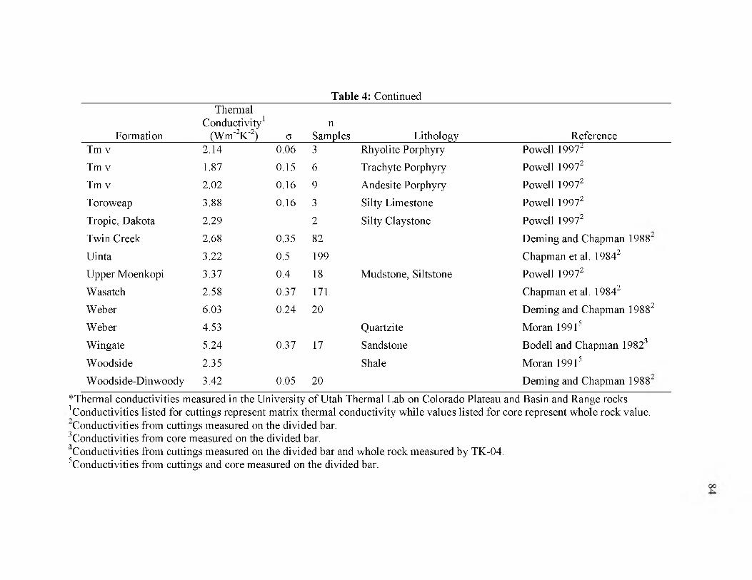
Table 4: Continued
Formation
ThermalConductivity1
( W m V ) G
nSamples Lithology Reference
Tm v 2.14 0.06 3 Rhyolite Porphyry Powell 19972
Tm v 1.87 0.15 6 Trachyte Porphyry Powell 19972
Tm v 2.02 0.16 9 Andesite Porphyry Powell 19972
Toroweap 3.88 0.16 3 Silty Limestone Powell 19972
Tropic, Dakota 2.29 2 Silty Claystone Powell 19972
Twin Creek 2.68 0.35 82 Deming and Chapman 1988
Uinta 3.22 0.5 199 Chapman et al. 19842
Upper Moenkopi 3.37 0.4 18 Mudstone, Siltstone Powell 19972
Wasatch 2.58 0.37 171 Chapman et al. 19842
Weber 6.03 0.24 20 Deming and Chapman 19882
Weber 4.53 Quartzite Moran 19915
Wingate 5.24 0.37 17 Sandstone Bodell and Chapman 19823
Woodside 2.35 Shale Moran 19915
Woodside-Dinwoody 3.42 0.05 20 Deming and Chapman 1988
*Thermal conductivities measured in the University of Utah Thermal Lab on Colorado Plateau and Basin and Range rocks. Conductivities listed for cuttings represent matrix thermal conductivity while values listed for core represent whole rock value. Conductivities from cuttings measured on the divided bar.
Conductivities from core measured on the divided bar.Conductivities from cuttings measured on the divided bar and whole rock measured by TK-04.Conductivities from cuttings and core measured on the divided bar.
APPENDIX B
NEW THERMAL CONDUCTIVITY MEASUREMENTS
ON UTAH ROCK
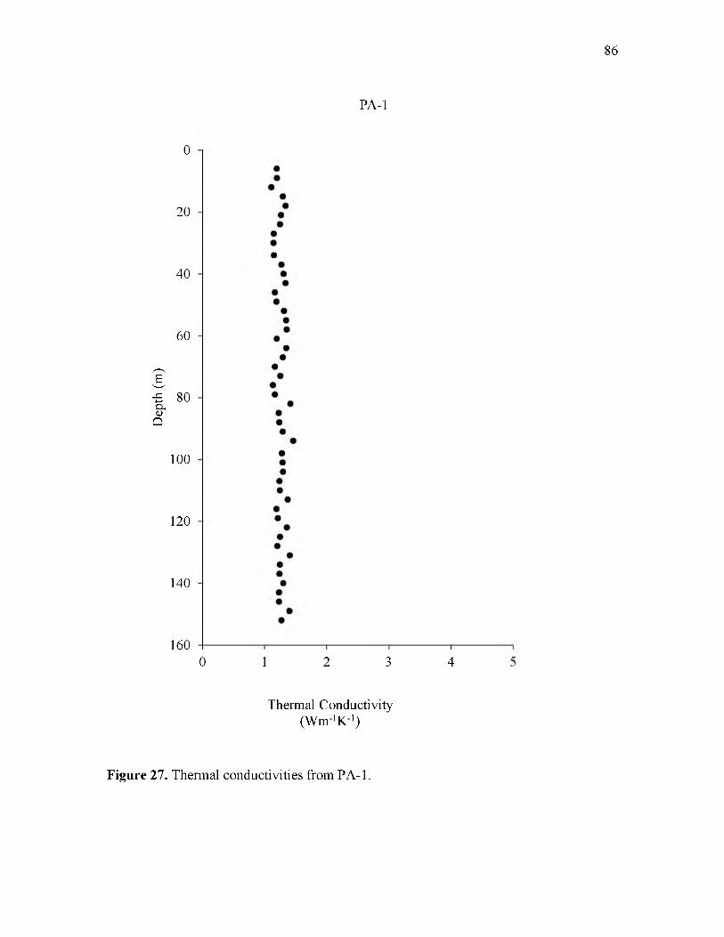
Dept
h (m
)
86
PA-1
20
40
60
80
100
120
140
160
4
I2
I4
0
0 1 3
Thermal Conductivity (Wm-1K"1)
Figure 27. Thermal conductivities from PA-1.

87
Table 5. Thermal conductivity measurements for PA-1*Depth
(m)Thermal
Conductivityw(Wm-1K-1)
Depth(m)
ThermalConductivityw
(Wm-1K-1)6.1 1.20 112.8 1.379.1 1.20 115.8 1.1912.2 1.11 118.9 1.2115.2 1.29 121.9 1.3618.3 1.34 125 1.2521.3 1.27 128 1.2124.4 1.25 131.1 1.4127.4 1.15 134.1 1.2530.5 1.14 137.2 1.2433.5 1.15 140.2 1.3036.6 1.27 143.3 1.2339.6 1.31 146.3 1.2342.7 1.34 149.4 1.4045.7 1.17 152.4 1.2748.8 1.1951.8 1.3154.9 1.3557.9 1.3661 1.2064 1.3567.1 1.3070.1 1.1773.2 1.2576.2 1.1379.2 1.1782.3 1.4285.3 1.2388.4 1.2491.4 1.2994.5 1.4697.5 1.28100.6 1.29103.6 1.30106.7 1.24109.7 1.25
*Thermal conductivity measured on divided bar. wApproximate whole rock conductivity.
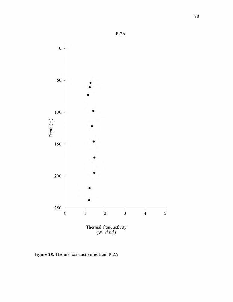
Dept
h (m
)
88
P-2A
0
50
100
150
200
250 “ I-------------------------------1-------------------------------1-------------------------------1-------------------------------1
1 2 3 4 5
Thermal Conductivity (Wm-1K-1)
0
Figure 28. Thermal conductivities from P-2A.
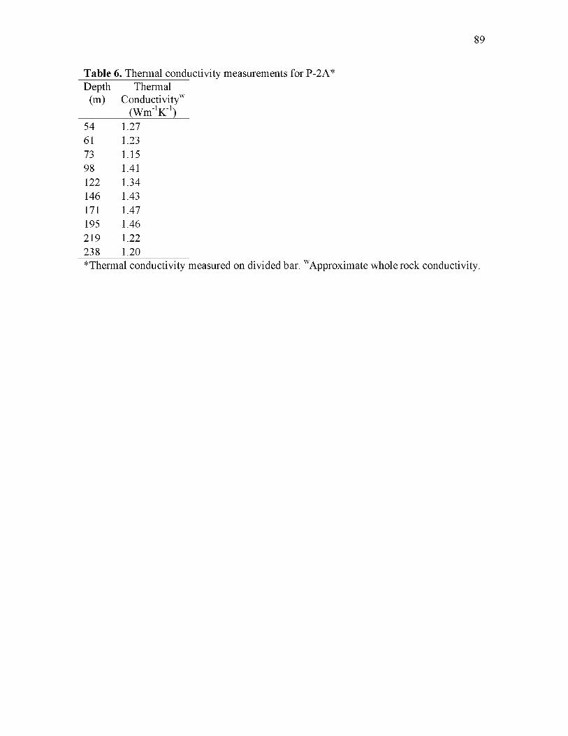
89
Table 6. Thermal conductivity measurements for P-2A*Depth
(m)Thermal
Conductivityw(Wm-1K-1)
54 1.2761 1.2373 1.1598 1.41122 1.34146 1.43171 1.47195 1.46219 1.22238 1.20*Thermal conductivity measured on divided bar. wApproximate whole rock conductivity.
Dept
h (m
)
90
PA-3
20
40
60
80
100
120
140
160 i2
i4
0
0 1 3
Thermal Conductivity (Wm-1K-1)
Figure 29. Thermal conductivities from PA-3.

91
Table 7. Thermal conductivity measurements for PA-3*Depth
(m)Thermal
Conductivityw(Wm-1K-1)
Depth(m)
ThermalConductivityw
(Wm-1K-1)6.1 1.10 112.8 1.309.1 1.12 115.8 1.3612.2 1.11 118.9 1.5315.2 1.26 121.9 1.3718.3 1.15 125 1.1821.3 1.15 128 1.3524.4 1.34 131.1 1.3127.4 1.06 134.1 1.3730.5 1.23 137.2 1.3033.5 1.46 140.2 1.2036.6 1.37 143.3 1.5339.6 1.25 146.3 1.3142.7 1.18 149.4 1.2645.7 1.40 152.4 1.4048.8 1.3551.8 1.2554.9 1.4057.9 1.4761 1.2364 1.4567.1 1.4070.1 1.2773.2 1.4276.2 1.3579.2 1.3382.3 1.5685.3 1.4088.4 1.1091.4 1.1994.5 1.2897.5 1.40100.6 1.47103.6 1.15106.7 1.30109.7 1.36
*Thermal conductivity measured on divided bar. wApproximate whole rock conductivity.
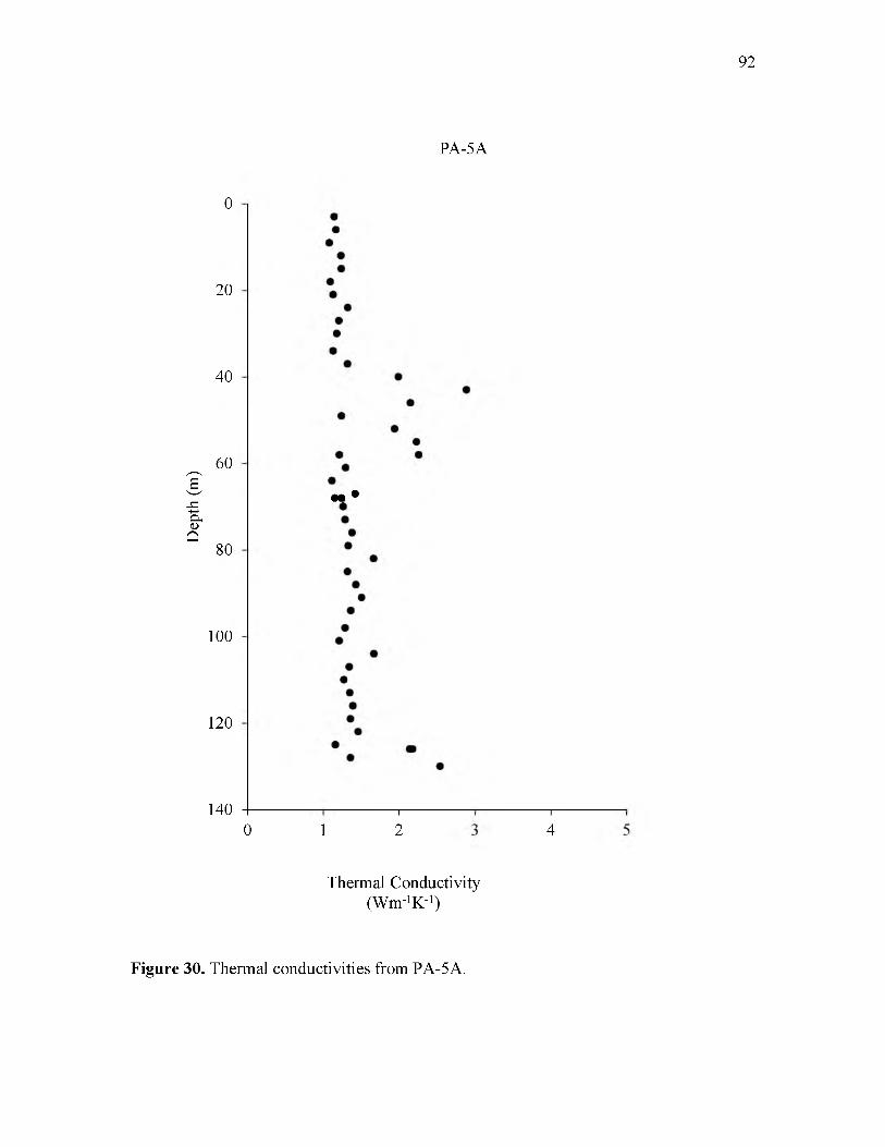
Dept
h (m
)
92
PA-5A
20
40
60
80
100
120
140
M *
I2
I4
0
0 1
Thermal Conductivity (Wm-1K-1)
Figure 30. Thermal conductivities from PA-5A.
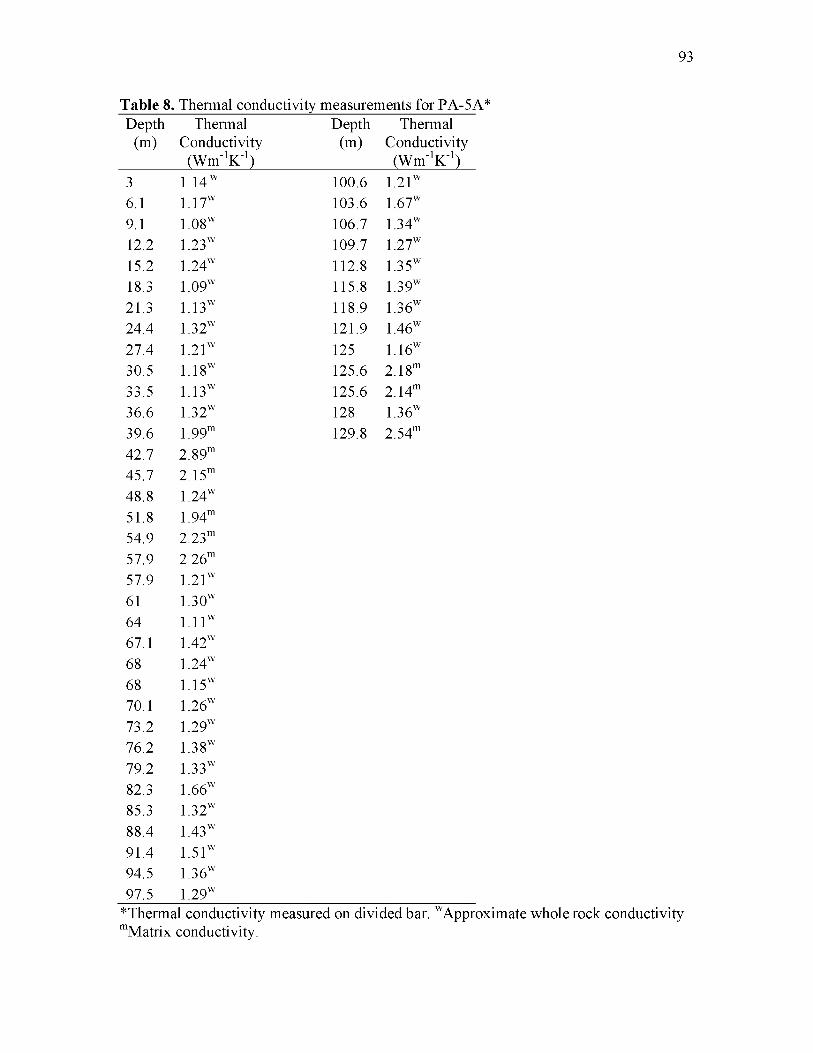
93
Table 8. Thermal conductivity measurements for PA-5A*Depth
(m)Thermal
Conductivity(Wm-1K-1)
Depth(m)
ThermalConductivity
(Wm-1K-1)3 1.14 w 100.6 1.21w6.1 1.17w 103.6 1.67w9.1 1.08w 106.7 1.34w12.2 1.23w 109.7 1.27w15.2 1.24w 112.8 1.35w18.3 1.09w 115.8 1.39w21.3 1.13w 118.9 1.36w24.4 1.32w 121.9 1.46w27.4 1.21w 125 1.16w30.5 1.18w 125.6 2.18m33.5 1.13w 125.6 2.14m36.6 1.32w 128 1.36w39.6 1.99m 129.8 2.54m42.7 2.89m45.7 2.15m48.8 1.24w51.8 1.94m54.9 2.23m57.9 2.26m57.9 1.21w61 1.30w64 1.11w67.1 1.42w68 1.24w68 1.15w70.1 1.26w73.2 1.29w76.2 1.38w79.2 1.33w82.3 1.66w85.3 1.32w88.4 1.43w91.4 1.51w94.5 1.36w97.5 1.29w
*Thermal conductivity measured on divided bar. wApproximate whole rock conductivity. mMatrix conductivity.
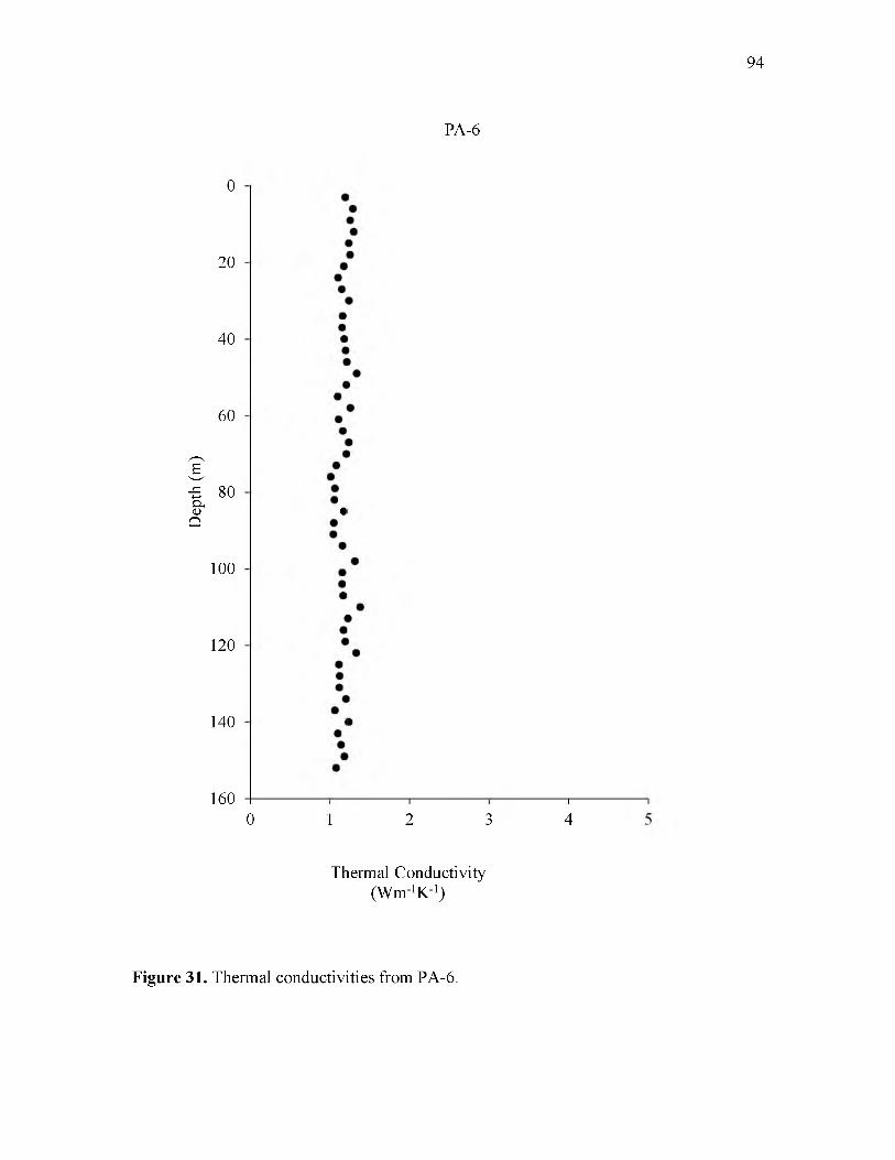
Dept
h (m
)
94
PA-6
20
40
60
80
100
120
140
160
a
i
i2
i4
0
0 1 3
Thermal Conductivity (Wm-1K-1)
Figure 31. Thermal conductivities from PA-6.
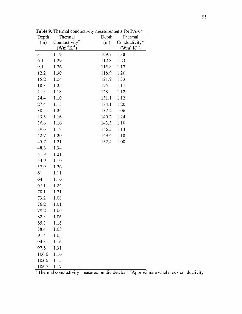
95
Table 9. Thermal conductivity measurements for PA-6*Depth
(m)Thermal
Conductivityw(Wm-1K-1)
Depth(m)
ThermalConductivityw
(Wm-1K-1)3 1.19 109.7 1.386.1 1.29 112.8 1.239.1 1.26 115.8 1.1712.2 1.30 118.9 1.2015.2 1.24 121.9 1.3318.3 1.25 125 1.1121.3 1.18 128 1.1224.4 1.10 131.1 1.1227.4 1.15 134.1 1.2030.5 1.24 137.2 1.0633.5 1.16 140.2 1.2436.6 1.16 143.3 1.1039.6 1.18 146.3 1.1442.7 1.20 149.4 1.1845.7 1.21 152.4 1.0848.8 1.3451.8 1.2154.9 1.1057.9 1.2661 1.1164 1.1667.1 1.2470.1 1.2173.2 1.0876.2 1.0179.2 1.0682.3 1.0685.3 1.1888.4 1.0591.4 1.0594.5 1.1697.5 1.31100.6 1.16103.6 1.15106.7 1.17
*Thermal conductivity measured on divided bar. wApproximate whole rock conductivity.
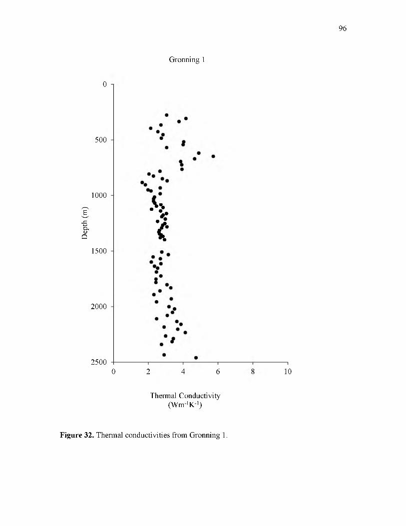
Dept
h (m
)
96
Gronning 1
500
1000
1500
2000
2500
1
i2
i4
i6
— i
10
Thermal Conductivity (Wm-1K-1)
0
0
Figure 32. Thermal conductivities from Gronning 1.
97
Table 10. Thermal conductivity measurements for Gronning 1*Depth
(m)Thermal
Conductivitym(Wm-1K-1)
Depth(m)
ThermalConductivitym
(Wm-1K-1)
Depth(m)
ThermalConductivitym
(Wm-1K-1)277 3.05 1125 2.19 1958 2.47308 4.16 1140 2.70 2001 3.18335 3.76 1164 3.04 2022 3.51366 2.73 1177 2.85 2053 3.39396 2.14 1192 2.77 2080 3.09427 2.55 1213 2.98 2110 2.48454 2.84 1234 2.53 2135 3.64485 2.75 1253 2.95 2160 3.87518 4.03 1268 2.83 2185 2.91543 4.00 1283 3.07 2204 3.69570 3.05 1292 2.77 2234 4.12619 4.90 1314 2.64 2265 2.99649 5.73 1329 2.60 2289 3.44671 4.66 1347 2.65 2316 3.37695 3.86 1356 2.74 2341 2.76725 3.92 1369 2.84 2435 2.90765 3.93 1381 2.69 2461 4.73783 2.67 1399 2.93808 2.04 1509 2.77826 2.29 1533 3.15850 2.81 1554 2.28869 3.08 1570 2.69884 1.65 1600 2.17905 1.83 1615 2.73933 2.68 1637 2.35951 1.98 1655 2.54960 2.15 1689 2.47985 2.68 1725 2.721015 2.35 1753 2.441030 2.30 1783 2.441052 2.30 1804 3.071070 2.37 1832 3.291082 2.72 1859 2.671097 2.47 1893 2.321109 2.85 1931 3.32
*Thermal conductivity measured on divided bar. mMatrix conductivity.
Dept
h (m
)
98
Pavant Butte 1
500
1000
1500
2000
2500
3000
35002 4 6
“ I--------------------------------------- 1
8 10
Thermal Conductivity (Wm-1K-1)
0
0
Figure 33. Thermal conductivities from Pavant Butte 1.

99
Table 11. Thermal conductivity measurements for Pavant Butte 1*Depth
(m)Thermal
Conductivitym(Wm-1K-1)
Depth(m)
ThermalConductivitym
(Wm-1K-1)274 3.03 3063 4.59375 3.41 3121 3.78494 3.10 3188 4.27594 2.89 3246 3.77686 2.95 3316 4.24777 2.76 3365 4.58878 2.59 3392 5.631079 2.911189 2.631262 3.231329 3.301393 3.171460 3.271530 3.271625 2.871689 2.941786 2.571875 1.841942 3.021984 2.982124 3.982182 4.072259 4.842338 3.212396 2.932457 3.322521 3.432573 2.812649 4.322694 3.582765 2.882822 4.572880 4.002944 3.623008 3.7
*Thermal conductivity measured on divided bar. mMatrix conductivity.
Dept
h (m
)
100
Hole-in-Rock 1
500
1000
1500
2000
2500
3000
3500
• •
“ i--------------------- r ~
2 4 6— i
10
Thermal Conductivity (Wm-1K-1)
0
0
Figure 34. Thermal conductivities from Hole-in-Rock 1.
101
Table 12. Thermal conductivity measurements for Hole-in-Rock 1 *Depth
(m)Thermal
Conductivity™(Wm-1K-1)
198 2.57472 3.08646 2.79719 3.09835 2.70835 3.18933 3.491070 2.931234 4.441350 3.311469 2.911533 3.731646 2.991807 3.341951 3.642131 3.392179 3.732240 3.162304 3.362365 3.222426 2.312487 2.792542 2.342609 2.812670 2.992731 3.052791 2.902847 5.602914 5.842975 6.153036 7.083088 6.443159 7.043222 4.903280 3.743344 2.80
*Thermal conductivity measured on divided bar. “ Matrix conductivity.
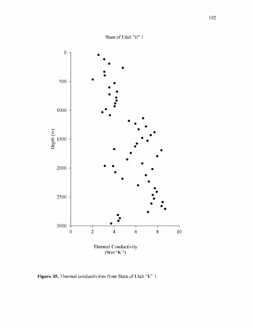
Dept
h (m
)
102
State of Utah "E" 1
500
1000
1500
2000
2500
3000
• •
2“ i-------------------1-------------------r ~
4 6 8 10
0
0
Thermal Conductivity (Wm-1K-1)
Figure 35. Thermal conductivities from State of Utah “E” 1.
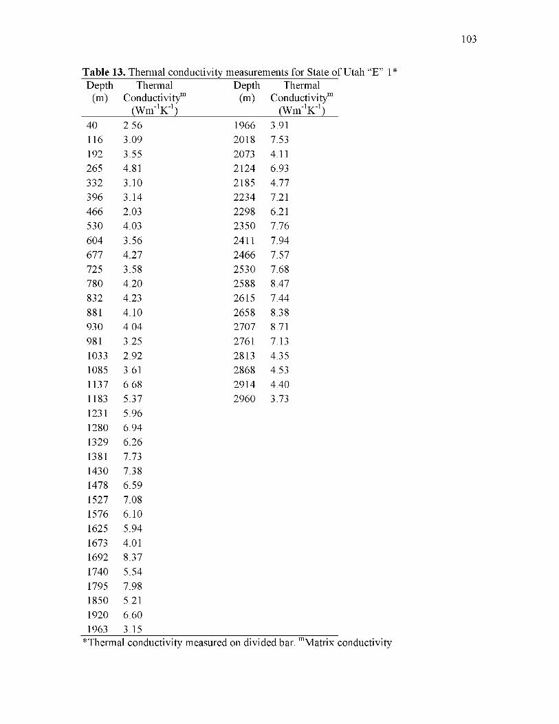
103
Table 13. Thermal conductivity measurements for State of Utah “E” 1*Depth
(m)Thermal
Conductivitym(Wm-1K-1)
Depth(m)
ThermalConductivitym
(Wm-1K-1)40 2.56 1966 3.91116 3.09 2018 7.53192 3.55 2073 4.11265 4.81 2124 6.93332 3.10 2185 4.77396 3.14 2234 7.21466 2.03 2298 6.21530 4.03 2350 7.76604 3.56 2411 7.94677 4.27 2466 7.57725 3.58 2530 7.68780 4.20 2588 8.47832 4.23 2615 7.44881 4.10 2658 8.38930 4.04 2707 8.71981 3.25 2761 7.131033 2.92 2813 4.351085 3.61 2868 4.531137 6.68 2914 4.401183 5.37 2960 3.731231 5.961280 6.941329 6.261381 7.731430 7.381478 6.591527 7.081576 6.101625 5.941673 4.011692 8.371740 5.541795 7.981850 5.211920 6.601963 3.15
*Thermal conductivity measured on divided bar. mMatrix conductivity.
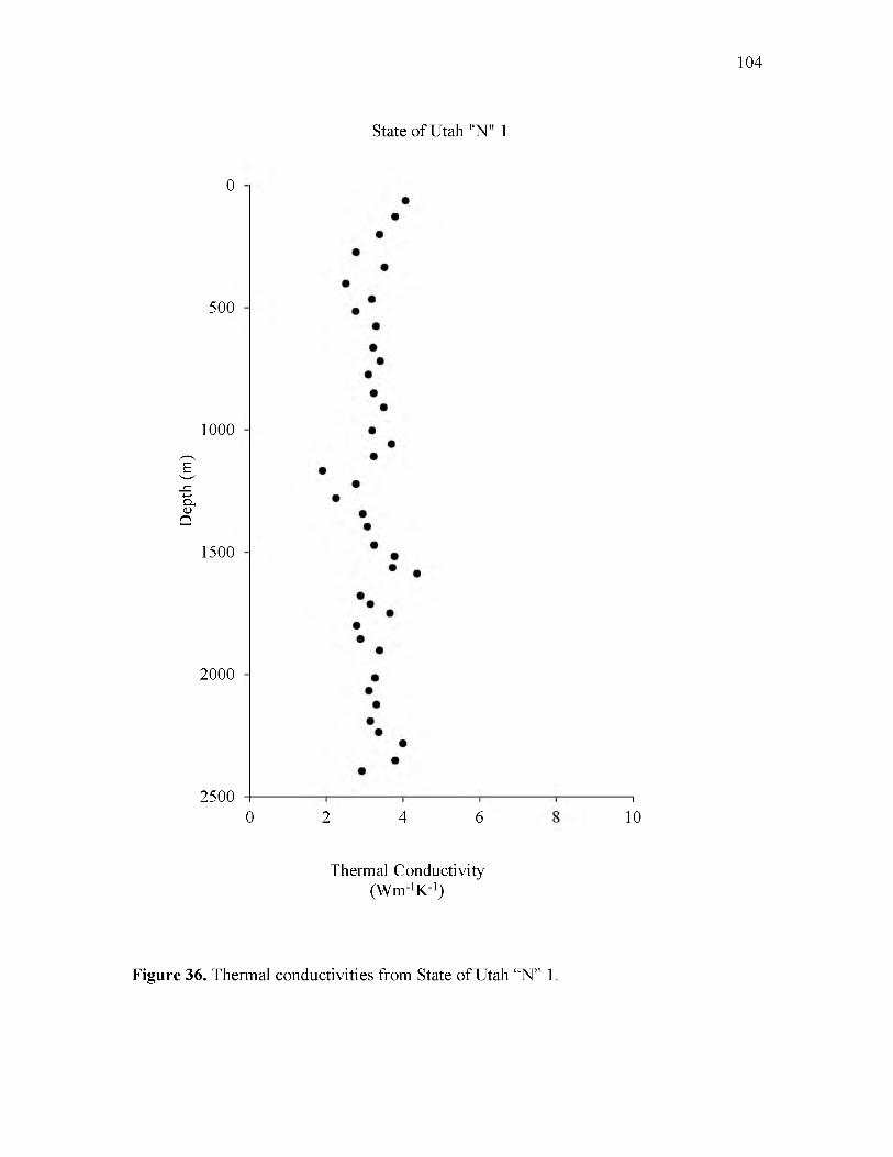
Dept
h (m
)
104
State of Utah "N" 1
500
1000
1500
2000
25002 4 6
— I
10
0
0
Thermal Conductivity (Wm-1K-1)
Figure 36. Thermal conductivities from State of Utah “N ” 1.
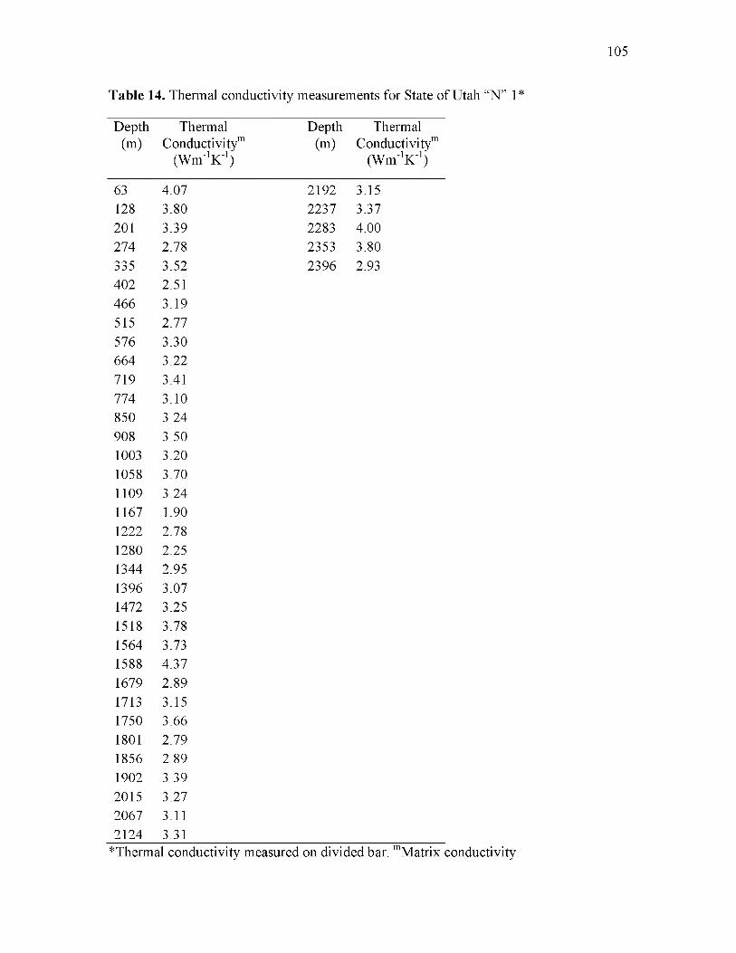
105
Table 14. Thermal conductivity measurements for State of Utah “N ” 1*
Depth(m)
ThermalConductivitym
(Wm-1K-1)
Depth(m)
ThermalConductivitym
(Wm-1K-1)
63 4.07 2192 3.15128 3.80 2237 3.37201 3.39 2283 4.00274 2.78 2353 3.80335 3.52 2396 2.93402 2.51466 3.19515 2.77576 3.30664 3.22719 3.41774 3.10850 3.24908 3.501003 3.201058 3.701109 3.241167 1.901222 2.781280 2.251344 2.951396 3.071472 3.251518 3.781564 3.731588 4.371679 2.891713 3.151750 3.661801 2.791856 2.891902 3.392015 3.272067 3.112124 3.31
*Thermal conductivity measured on divided bar. mMatrix conductivity.

APPENDIX C
HEAT FLOW VALUES GENERATED
IN THIS STUDY
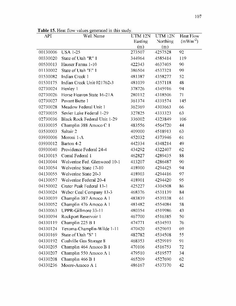
107
Table 15. Heat flow values generated in this study._______________________________API Well Name UTM 12N UTM 12N Heat Flow
Easting Northing (mWm-2) _______________________________________________ (m) (m)______________00130006 USA 1-25 273507 4257528 9200330020 State of Utah "R" 1 344964 4585414 11900530013 Hauser Farms 1-10 422343 4637405 9001130002 State of Utah "E" 1 386504 4537321 9901530082 Indian Creek 1 481387 4358277 5201530175 Indian Creek Unit 021762-3 481039 4357118 4802730024 Henley 1 378726 4345916 9402730026 Horse Heaven State 16-21A 280112 4318506 7102730027 Pavant Butte 1 361374 4331574 14502730028 Meadow Federal Unit 1 362369 4303663 6602730035 Sevier Lake Federal 1-29 327825 4333323 6302730036 Black Rock Federal Unit 1-29 336002 4323849 10603330035 Champlin 388 Amoco C 1 483556 4564720 4403530003 Saltair 2 409000 4518913 6303930006 Moroni 1-A 452032 4373946 6103930012 Barton 4-2 442334 4348214 4903930040 Providence Federal 24-4 434292 4322407 6204130015 Corral Federal 1 462827 4289435 8804130044 Wolverine Fed. Glenwood 10-1 413207 4286487 9004130054 Wolverine State 17-10 418900 4294425 9404130055 Wolverine State 20-3 418903 4294416 9704130057 Wolverine Federal 20-4 418901 4294420 9504150002 Crater Peak Federal 13-1 425227 4304508 8604330024 Weber Coal Company 13-3 468376 4531139 8404330039 Champlin 387 Amoco A 1 483839 4539338 6104330052 Champlin 476 Amoco A 1 481482 4554084 5804330063 UPPR-Gillmore 33-11 480354 4519986 4304330094 Rockport Reservoir 1 467700 4516385 5004330119 Champlin 225 B 1 474771 4534593 7604330124 Texoma-Champlin-Wilde 1-11 470420 4529693 6904330169 State of Utah "S" 1 482782 4534508 5504330192 Coalville Gas Storage 8 468353 4529919 9104330205 Champlin 464 Amoco B 1 470106 4516753 7204330207 Champlin 550 Amoco A 1 479510 4519577 3404330208 Champlin 466 B 1 465209 4527690 6204330236 Moore-Amoco A 1 486167 4537370 42
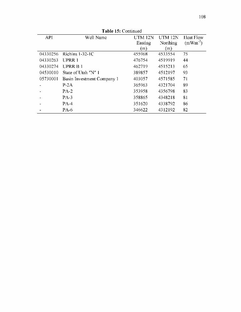
108
Table 15: ContinuedAPI Well Name UTM 12N
Easting (m)
UTM 12N Northing
(m)
Heat Flow (mWm-2)
04330256 Richins 1-32-1C 455968 4533554 7504330263 UPRR 1 476754 4519919 4404330274 UPRR B 1 462719 4515213 6504530010 State of Utah "N" 1 389857 4512197 9305730001 Basin Investment Company 1 403057 4571585 71- P-2A 365963 4321704 89- PA-2 353958 4356798 83- PA-3 358865 4348218 81- PA-4 351620 4338792 86- PA-6 346622 4312192 82
REFERENCES
Allred, J. (2004), Milgro Greenhouses Newcastle, Utah, GHCBulletin, 25(4), 34-39.
AMAX Exploration Inc. (1998), Temperature-gradient data for southwestern Utah obtained by Amax during the late 1970s and early 1980s, Energy and Geoscience Institute unpublished data.
Bahr, D. B., E. W. H. Hutton, J. P. M. Syvitski, and L. F. Pratson (2001), Exponential approximations to compacted sediment porosity profiles, Computers & Geosciences, 27(6), 691-700, doi:10.1016/S0098-3004(00)00140-0.
Barker, C. (1996), Thermal modeling o f petroleum generation: theory and applications, Elsevier.
Bartlett, M. G., D. S. Chapman, and R. N. Harris (2004), Snow and the groundtemperature record of climate change, Journal o f Geophysical Research, 109(F4), F04008, doi:10.1029/2004JF000224.
Bartlett, M. G., D. S. Chapman, and R. N. Harris (2005), Snow effect on North American ground temperatures, 1950-2002, Journal o f Geophysical Research, 110(F3), F03008, doi:10.1029/2005JF000293.
Bauer, M. S. (1985), Heat Flow at the Upper Stillwater Dam Site, Uinta Mountains, Utah, 94 pp., University of Utah.
Bauer, M. S., and D. S. Chapman (1986), Thermal regime at the Upper Stillwater dam site, Uinta mountains, Utah: Implications for terrain, microclimate and structural corrections in heat flow studies, Tectonophysics, 128(1-2), 1-20, doi:10.1016/0040- 1951(86)90305-7.
Beach, R. D. W., F. W. Jones, and J. A. Majorowicz (1987), Heat flow and heatgeneration estimates for the Churchill Basement of the western Canadian Basin in Alberta, Canada, Geothermics, 16(1), 1-16, doi:10.1016/0375-6505(87)90075-7.
Beardsmore, G. R. (1996), The Thermal History o f the Browse Basin and Its Implications for Petroleum Exploration, Monash University.
110
Beardsmore, G. R., and J. P. Cull (2001), CrustalHeat Flow: A Guide to Measurement and Modeling, Cambridge University Press, Cambridge.
Blackett, R. E. (2007), Temperature-Depth Monitoring in the Newcastle Geothermal System: Utah Geological Survey Report o f Investigation 258, Salt Lake City.
Blackwell, D. D., and M. Richards (2004), Geothermal Map of North America,
Blackwell, D. D., and J. L. Steele (1989), Thermal History o f Sedimentary Basins, edited by N. D. Naeser and T. H. McCulloh, Springer New York, New York, NY.
Bodell, J. M. (1981), Heat Flow in the North-Central Colorado Plateau, 134 pp., University of Utah.
Bodell, J. M., and D. S. Chapman (1982), Heat flow in the north-central Colorado Plateau, Journal o f Geophysical Research, 87(B4), 2869, doi:10.1029/JB087iB04p02869.
Bullard, E. C. (1947), The Time Necessary for a Bore Hole to Attain Temperature Equilibrium, Geophysical Journal International, 5, 127-130, doi: 10.1111/j .1365- 246X.1947.tb00348.x.
Cao, S., and C. Hermanrudl (1988), Formation temperature estimation by inversion of borehole measurements, Geophysics, 53(7), 979-988.
Carrier, D. L. (1979), Gravity and Heat Flow Studies at Twin Peaks: An Era of Late Tertiary Silicic Volcanism in Millard County, Utah, 120 pp., University of Utah.
Carrier, D. L., and D. S. Chapman (1981), Gravity and thermal models for the TwinPeaks Silicic Volcanic Center, southwestern Utah, Journal o f Geophysical Research, 86(B11), 10287, doi :10.1029/JB086iB 11p10287.
Chapman, D. S. (1976), Heat flow and heat production in Zambia, 94 pp., University of Michigan.
Chapman, D. S. (1979), Regional Heat Flow and Geochemical Studies in Southwest Utah: Final Report, Salt Lake City.
Chapman, D. S., M. D. Clement, and C. W. Mase (1981), Thermal regime of the Escalante Desert, Utah, with an analysis of the Newcastle Geothermal System, Journal o f Geophysical Research, 86(B12), 11735, doi:10.1029/JB086iB12p11735.
Chapman, D. S., T. H. Keho, M. S. Bauer, and M. D. Picard (1984), Heat flow in the Uinta Basin determined from bottom hole temperature (BHT) data, Geophysics, 49(4), 453-466, doi:10.1190/1.1441680.
111
Chiasson, A. (2004), Electric Power Generation in the Roosevelt Hot Springs Area - The Blundell Geothermal Power Plant, GHC Bulletin, 5(4), 16-20.
Chisholm, T. J. (1990), Climate Change Inferred from Borehole Temperatures: An Example from Western Utah, 94 pp., University of Utah.
Clement, M. D. (1981), Heat Flow and Geothermal Assessment of the Escalante Desert, Part of the Oligocene to Miocene Volcanic Belt in Southwestern Utah, 118 pp., University of Utah.
Clement, M. D., and D. S. Chapman (1981), Heat Flow and Geothermal Assessment o f the Escalante Desert, Southwestern Utah, With Emphasis on the Newcastle KGRA.
Deming, D., and D. S. Chapman (1988), Inversion of bottom-hole temperature data: The Pineview field, Utah-Wyoming thrust belt, Geophysics, 53(5), 707, doi: 10.1190/1.1442504.
Drury, M. J. (1986), Thermal conductivity, thermal diffusivity, density and porosity o f crystalline rocks, Ottawa.
Funnell, R., D. Chapman, R. Allis, and P. Armstrong (1996), Thermal state of theTaranaki Basin, New Zealand, Journal o f Geophysical Research, 101(B11), 2519725215, doi:10.1029/96JB01341.
Goutorbe, B., F. Lucazeau, and A. Bonneville (2007), Comparison of several BHT correction methods: a case study on an Australian data set, Geophysical Journal International, 170(2), 913-922, doi:10.1111/j.1365-246X.2007.03403.x.
Gwynn, M., B. Blackett, R. Allis, and C. Hardwick (2013), New Geothermal Resource Delineated Beneath Black Rock Desert, Utah, in Thirty-Eighth Workshop on Geothermal Reservoir Engineering, pp. 1511-1519, Stanford, California.
Harrison, W. E., and K. V. Luza (1983), Geothermal Resource Assessment of Oaklahoma, Norman, Oklahoma.
Heilweil, V., and L. Brooks (2011), Conceptual model of the Great Basin carbonate and alluvial aquifer system, U.S. Geological Survey Scientific Investigations Report 2010-5193, 191.
Henrickson, A. (2000), New Heat Flow Determinations from Oil and Gas wells in the Colorado Plateau and Basin and Range of Utah, 70 pp., University of Utah.
Hintze, L., and F. Davis (2003), Geology o f Millard County, Utah, Utah Geological Survey.
112
Issler, D. R., and C. Beaumont (1986), Estimates of terrestrial heat flow in offshore eastern Canada: Discussion, Canadian Journal o f Earth Sciences, 23(12), 20832085, doi:10.1139/e86-195.
Kehle, R. O., R. J. Schoeppel, and R. K. Deford (1970), The AAPG geothermal survey of North America, Geothermics, 2, 358-367, doi:10.1016/0375-6505(70)90034-9.
Keho, T. H. (1987), Heat Flow in the Uinta Basin Determined from Bottom Hole Temperature (BHT) Data, 99 pp., University of Utah.
Majorowicz, J. A., and A. M. Jessop (1981), Regional heat flow patterns in the Western Canadian Sedimentary Basin, Tectonophysics, 74(3-4), 209-238, doi:10.1016/0040- 1951(81)90191-8.
Masbruch, M. D., D. S. Chapman, and D. K. Solomon (2012), Air, ground, andgroundwater recharge temperatures in an alpine setting, Brighton Basin, Utah, Water Resources Research, 45(10), W10530, doi:10.1029/2012WR012100.
Mase, C. W. (1979), Geophysical study of the Monroe-Red Hill geothermal system, 108 pp., University of Utah.
Moran, K. J. (1991), Shallow Thermal Regime at the Jordanelle Dam Site, Central Rocky Mountains, Utah, 141 pp., University of Utah.
Powell, W. G. (1997), Thermal State of the Lithosphere in the Colorado Plateau-Basin and Range Transition Zone, Utah, 232 pp., University of Utah.
Powell, W. G., D. S. Chapman, N. Balling, and A. Beck (1988), Continental Heat-Flow Density, in Handbook o f Terrestrial Heat-Flow Density Determination, edited by R. Haenel, L. Rybach, and L. Stegena, p. 504, Kluwer Academic Publishers, Norwell, Ma.
Pribnow, D. F. C., and J. H. Sass (1995), Determination of thermal conductivity for deep boreholes, Journal o f Geophysical Research, 100(B6), 9981, doi:10.1029/95JB00960.
Project Management Institute (2013), A Guide to the Project Management Body o f Knowledge: PMBOK(R) Guide, 5th ed., Project Management Institute.
Raznjevic, K. (1995), Handbook o f Thermodynamic Tables, Begell House. [online]
Reiter, M., and A. M. Jessop (1985), Estimates of terrestrial heat flow in offshore eastern Canada, Canadian Journal o f Earth Sciences, 22(10), 1503-1517, doi:10.1139/e85- 156.
113
Reiter, M., and R. J. C. Tovar (1982), Estimates of terrestrial heat flow in northern Chihuahua, Mexico, based upon petroleum bottom-hole temperatures, Geological Society o f America Bulletin, 93(7), 613, doi:10.1130/0016- 7606(1982)93<613:EOTHFI>2.0.CO;2.
Roy, R. F., A. E. Beck, and Y. S. Touloukian (1981), Thermophysical properties ofrocks, in Physical Properties o f Rocks and Minerals, edited by Y. S. Touloukian, W. R. Judd, and R. F. Roy, pp. 409-502, McGraw-Hill, New York.
Sass, J. H., A. H. Lachenbruch, R. J. Munroe, G. W. Greene, and T. H. Moses (1971), Heat flow in the western United States, Journal o f Geophysical Research, 76(26), 6376-6413, doi:10.1029/JB076i026p06376.
Smith, W. H. F., and P. Wessel (1990), Griding with continuous curvature splines in tension, Geophysics, 55(3), 293-305, doi:10.1190/1.1442837.
Taylor, A., A. Judge, and V. Allen (1986), Terrestrial heat flow from project CESAR, Alpha Ridge, Arctic Ocean, Journal o f Geodynamics, 6(1-4), 137-176, doi:10.1016/0264-3707(86)90037-2.
Tester, W. J. et al. (2006), The Future o f Geothermal Energy The Future o f Geothermal Energy - Impact o f Enhanced Geothermal Systems (EGS) on the United States in the 21st Century.
Touloukian, Y. S., R. W. Powell, and C. Y. Ho (1970), Thermophysical Properties o f Matter, vol. 2, Thermal Conductivity, Non-Metallic Solids, IFI/Plenum, Washington and New York.
Western Regional Climate Center, [online] Available from: http://www.wrcc.dri.edu (Accessed 1 December 2011)
Willett, S. D. (1988), Spatial Variation of Temperature and Thermal History of the Uinta Basin, 121 pp., University of Utah.
Wilson, W. R. (1980), Thermal Studies in a Geothermal Area, 145 pp., University of Utah.
Zhdanov, M. S. (2002), Geophysical Inverse Theory and Regularization Problems, 1st ed., Elsevier.


