arX

iv:0

908.

0056

v2 [

hep-

th]

5 N

ov 2

009

Preprint typeset in JHEP style - HYPER VERSION SISSA/45/2009/EP

ULB-TH/09-25

hep-th/0908.0056

Ghost story. III. Back to ghost number zero

L.Bonora

International School for Advanced Studies (SISSA/ISAS)

Via Beirut 2–4, 34014 Trieste, Italy, and INFN, Sezione di Trieste

E-mail: bonora@sissa.it,

C.Maccaferri

International Solvay Institutes and Physique Theorique et Mathematique,

ULB C.P. 231, Universite Libre de Bruxelles, B-1050, Bruxelles, Belgium

E-mail: cmaccafe@ulb.ac.be,

D.D.Tolla

Department of Physics and University College, Sungkyunkwan University, Suwon

440-746, South Korea

E-mail: ddtolla@skku.edu

Abstract: After having defined a 3–strings midpoint–inserted vertex for the bc system, we

analyze the relation between gh=0 states (wedge states) and gh=3 midpoint duals. We find

explicit and regular relations connecting the two objects. In the case of wedge states this

allows us to write down a spectral decomposition for the gh=0 Neumann matrices, despite

the fact that they are not commuting with the matrix representation of K1. We thus trace

back the origin of this noncommutativity to be a consequence of the imaginary poles of

the wedge eigenvalues in the complex κ–plane. With explicit reconstruction formulas at

hand for both gh=0 and gh=3, we can finally show how the midpoint vertex avoids this

intrinsic noncommutativity at gh=0, making everything as simple as the zero momentum

matter sector.

Keywords: String Field Theory, Ghost Wedge States.

Contents

1. Introduction 1

2. Overview 4

2.1 Wedge States 4

2.2 Y (±i)–inserted wedge states 5

2.2.1 Principal gh=3 wedges 7

3. Reconstruction formulas for gh=3 wedges 8

3.1 Principal gh=3 wedges 8

3.2 Y (±i)–inserted gh=3 wedges 9

4. The relation between gh=3 and gh=0 10

4.1 The midpoint reflector 11

4.2 Midpoint Identities 13

4.2.1 Midpoint identities for ‘principal’ states 14

4.2.2 Midpoint identities for Y (i)–inserted wedges 15

4.2.3 Midpoint identities for the vertex 16

4.3 gh=0 from gh=3: zero modes coefficients 17

4.3.1 A check: gh = 0 zero mode coefficients of surface states 19

4.4 gh=0 from gh=3: bulk reconstruction 20

4.5 Normalization 24

5. Midpoint multiplication of gh=0 squeezed states 25

6. Conclusions and discussion 28

A. BRST invariant squeezed states 30

A.1 BRST invariant gh=0/3 wedges 32

B. Irrelevance of secondary poles 34

1. Introduction

This is the third and conclusive paper of a series including [1], referred to as I, and [2],

referred to as II; see also [3]. The whole story started up with a very simple question.

In Open String Field Theory, [4], wedge states are surface states |N〉 labeled by a real

(possibly integer) number N , obeying the star algebra relation

|N〉 ∗ |M〉 = |N +M − 1〉.

– 1 –

Wedge states, originally defined and studied in [5, 6, 7], have been a fundamental ingredient

for constructing and analyzing, following the breakthrough by Schnabl [8], analytic solu-

tions for the tachyon vacuum [9, 10, 11, 12, 13, 14, 15, 16], solutions describing marginal

deformations [17, 18, 19, 20, 21, 22, 23, 24, 25, 26] and related topics [27, 28, 29, 30, 31, 32].

See [33] for a recent review and a guide through other references.

While this simple commutative ∗–subalgebra has a very intuitive realization in terms of

gluing vertical strips in the arctan–sliver frame (or, equivalently, of gluing sectors of cones),

the oscillator realization of this multiplication rule has only been understood in detail in

the (non–universal) matter sector, [34, 35] (corresponding to D–free bosons) and in the

(universal) bosonized ghost system, [36]. Strangely enough, the original (universal) bc sys-

tem which naturally emerges from the Polyakov path integral, while quite similar to the

matter sector in the conventional normal ordering on c1|0〉, [37, 38, 39, 40, 41], turns out

to give a quite complicated oscillator formalism, when one normal–orders with respect to

the SL(2, R)–vacuum. This is due to several conspiring accidents but the very reason is

the presence of the three zero modes of the c ghost. Indeed, a closely related system, the

h = (1, 0) bc system, having just one c zero mode, turns out to be almost identical to the

zero momentum matter sector, [42, 43].

In this paper we deal with the co–existence of the gh=0 and the gh=3 sectors. These

two sectors are naturally conjugate to each other by the bpz inner product. Still, while

the gh=0 sector is a ∗–subalgebra, the gh=3 is not because the ghost number is additive

under the ∗–product. A related issue is that, in general, there is no unique prescription to

pair gh=0 and gh=3 states in a one–to–one way. Any insertion of 3 c’s operators could in

principle do the job. There are however better choices than others. In particular one would

like to pair gh = 0 and gh = 3 states in such a way that they retain the same conformal

properties. This implies the use of a gh=3 insertion with zero conformal weight. In the

ghost sector, there is just one such field, given by

Y (z) =1

2∂2c∂cc(z).

This composite field, also considered in [44] in the context of VSFT [45], has a number of

nice properties

• It is a weight zero primary

T (z)Y (w) =∂Y (w)

z − w + ... .

• It is BRST invariant

{QB , Y (z)} =

∮

z

dw

2πijB(w)Y (z) = 0.

• Its derivative is QB–exact

∂Y (z) = [QB , ∂2c∂c(z)].

– 2 –

This implies that, given two BRST invariant gh=0 states (for example surface states)

we have

∂z〈ψ1|Y (z)|ψ2〉 = 0,

So, for BRST–closed states, correlators are independent of the location of Y .

However OSFT deals with off shell states which need not be BRST–invariant. Moreover

the ∗–product breaks conformal invariance down to the subgroup of midpoint preserving

reparametrizations. This implies that, out of the infinite places where one could insert Y,

the only one which is not going to interfere is the midpoint. In general, when dealing with

conformal maps such as the ones which define the ∗–product, having midpoint insertions

is forbidden because such maps are singular precisely at the midpoint. The only exception

is when we are dealing with weight zero primaries, which will not pick up any singular

Jacobian from the conformal transformation. Once again, at gh=3, this uniquely selects

the operator Y . Concretely, the midpoint insertion of Y commutes with the generators of

midpoint preserving reparametrizations

[Kn, Y (±i)] = 0.

Here we will be mostly interested in K1–invariance, since this symmetry allowed, in all

previously known cases, [46, 36, 47] to diagonalize the Neumann matrices of the 3–string

vertex.

Given the above reasons, for any state at gh=0, ψ, we define its midpoint dual(s) to be

ψ(±i) ≡ Y (±i)ψ.

This relation is not a one to one map in general because of the non trivial kernel of Y (i)

but it is effectively so for gh=0 states which do not have c insertions at the midpoint. All

gh = 0 squeezed states (and in particular surface states) are in this class.

In this paper we deal with gh=0 and gh=3 squeezed states, where the latter are intended

to be obtained from the former by the insertion of Y at one of the two midpoints z = ±i.By using the method of images (doubling trick) one can associate two gh=3 states to each

gh=0 state

ψ ≡ Y(π

2

)

ψ =1

2(Y (i) + Y (−i))ψ =

1

2(ψ(i) ⊕ ψ(−i)) ≃ (ψ(i), ψ(−i)).

The reason for the above notation is that, under the ∗–product, squeezed states are a ring

rather than an algebra. This just means that we will separately consider states with a

holomorphic and an anti–holomorphic midpoint insertion, because their half sum is not a

squeezed state anymore.

One of the main problems we address in this paper is how to get back, in the case of

squeezed states (and, in particular, of surface states), the gh=0 states by knowing their

– 3 –

gh=3 cousins. To be more specific the Y midpoint insertion will be implemented via a

2–strings vertex (midpoint reflector) which is a squeezed state of total ghost number 6.

The ordinary 2–strings vertex (implementing the bpz conjugation) would have total ghost

number 3. So the two differ by 3 units of ghost number, which are provided by the Y

insertion.

We will see that gh=3 squeezed states which are obtained by applying Y (±i) to gh=0

squeezed states, are characterized by having a Neumann matrix whose zero mode part is

uniquely determined by the non zero mode part. We call this property midpoint identity.

The explicit knowledge of both Y (±i)–inserted gh=3 squeezed states, will allow us to

reconstruct the original gh=0 squeezed state. We will provide evidence that this is possible

at least for all (non–projectors) surface states.

After analyzing in detail the gh=0/gh=3 relations in the case of wedge states (which are

the only K1 invariant surface states), we will finally ∗–multiply them via the midpoint

3-string vertex defined in paper II. Here we will see how the midpoint identities of the

vertex, together with the structure of the gh=0 Neumann matrices (which represent the

states to be multiplied) conspire to effectively transform these gh=0 matrices into gh=3

ones. Differently from gh=0 case, K1–invariance at gh=3 does imply commuting matrices,

so the star product will be as easy as the zero momentum matter product. In particular

all the matrices in the game will commute, so, trading them with their eigenvalues, they

will reconstruct the star product of the two wedges with an overall Y (±i) insertion. This

insertion can then be undone by using once again the gh=0/gh=3 relation and to finally

get the gh=0 state which is just the star product of the 2 gh=0 states. This completes the

program started with I.

2. Overview

The aim of this section is to give an overview of the objects that will feature in this paper.

We will deal with gh=0 states, the wedge states, and gh=3 states, wedge states with a

midpoint Y insertion. Both of them can be uniquely defined as squeezed states on the vacua

|0〉 and |0〉 ≡ c−1c0c1|0〉, via a gh=0 Neumann function and a gh=3 one, respectively. The

two different Neumann functions are known once the conformal map is given. In the case

of wedges, we fix SL(2, C) invariance by choosing the conformal maps to be

fN (z) =

(

1 + iz

1− iz

) 2N

(2.1)

2.1 Wedge States

Wedge states are squeezed states on the gh=0 vacuum |0〉

|N〉 = ec†P

SPq b†q |0〉, (2.2)

– 4 –

with the (long-short) defining matrix given by

S(N)Mn =

∮

0

dz

2πi

∮

0

dw

2πi

1

zM−1

1

wn+2[

f ′N (z)2

f ′N (w)

1

fN(z)− fN (w)

(

fN (w) − fN (0)

fN (z)− fN (0)

)3

− w3

z3(z − w)

]

. (2.3)

(M = −1, 0, 1, . . ., n = 2, 3, . . ., see II for notation; moreover we will drop the label N in

S(N) whenever this is not strictly necessary). This matrix has the general bulk/zero mode

block decomposition

S =

(

0 s

0 S

)

,

where the upper left 0 represents a vanishing 3× 3 matrix, the lower left 0 represents three

infinite short columns, s represents three infinite short rows, while S is the bulk. Wedge

states are annihilated by K1 = L1 + L−1. This can be checked explicitly by writing K1 as

K1 = c†N GNM bM + b†nHnm cm − 3c2 b−1 (2.4)

We get K1|N〉 = 0 iff

(GS + SHT )Nm + 3SN2S−1m = 0 (2.5)

This relation can be explicitly checked by picking up residues in eq.(2.3).

Note that, despite the fact that K1|N〉 = 0, the Neumann coefficients do not anti–commute

with G and H. Moreover the violation of anti–commutativity depends explicitly on the

zero mode contribution of the gh=0 Neumann function. This is one of the main reasons

why it will be necessary to insert the operator Y at the midpoint and to consider gh=3

squeezed states, whose Neumann matrices will commute with G. We will see later on that

the knowledge of gh=3 midpoint inserted squeezed states will imply the knowledge of the

gh=0 ones, whose Y (±i) inserted versions give the former.

2.2 Y (±i)–inserted wedge states

We can define wedge states (and surface states in general) with local operator insertions.

In particular we are interested in the midpoint insertion of the BRST invariant, primary

scalar Y (z) = 12∂

2c∂cc(z).

Let us begin by observing that a surface state (which is identified via an analytic map,

f(z), from the unit semidisk of the UHP, to a Riemann surface Σ with the disk topology)

with an insertion of Y at a point ξ on the Riemann surface can be written as a squeezed

state on the gh=3 vacuum 〈0| = 〈0|c−1c0c1 as 1

〈Sξ| = 〈0| e−cn S(ξ)nM

bM (2.6)

1Note that there is no normalization arising from the transformation of the insertion, this is unambiguous

because Y is a zero–weight primary.

– 5 –

where the (short–long) Neumann coefficients are given by

S(ξ)nM =

∮

0

dz

2πi

∮

0

dw

2πi

1

zn−1

1

wM+2

[

f ′(z)2

f ′(w)

1

f(z)− f(w)

(

f(w)− ξf(z)− ξ

)3

− 1

z − w

]

(2.7)

A midpoint insertion (which is only acceptable for zero–weight primaries) is given by

ξ = f(±i).

Let us concentrate on wedge states |N〉 whose analytic map (up to SL(2, C)) is given

by fN(z) =(

1+iz1−iz

) 2N

. We have respectively

〈N |Y (i) ≡ 〈N(i)| = 〈0| e−cn S(fN (i))

nMbM (2.8)

〈N |Y (−i) ≡ 〈N(−i)| = 〈0| e−cn S(fN (−i))nM

bM , (2.9)

In order to lighten a bit the notation we will rename

S(±i) ≡ S(fN (±i)), (2.10)

and write the Neumann coefficients as (fN (i) = 0, fN (−i) =∞)

S(i)nM =

∮

0

dz

2πi

∮

0

dw

2πi

1

zn−1

1

wM+2

[

f ′N (z)2

f ′N (w)

1

fN (z)− fN (w)

(

fN(w)

fN(z)

)3

− 1

z − w

]

(2.11)

S(−i)nM =

∮

0

dz

2πi

∮

0

dw

2πi

1

zn−1

1

wM+2

[

f ′N (z)2

f ′N (w)

1

fN (z)− fN (w)− 1

z − w

]

(2.12)

It is easy to prove the twist property

S(i)nM =(

S(−i)nM

)∗= (−1)m+N S(−i)nM . (2.13)

From the fact that

[K1, Y (±i)] = 0

it follows that Y (±i)–inserted wedge states are also annihilated by K1 = L1 + L−1. This

can be checked explicitly by writing K1 as

K1 = c†nHTnm bm + b†N GT

NM cM + 3c†2 b†1. (2.14)

We get 〈N(±i)|K1 = 0 iff

(HT S(±i) + S(±i)G)nM + 3δn2δ−1M = 0, (2.15)

and it is easy to check this directly (see II).

We see that the Neumann coefficients still do not (anti–)commute with G and H. The

violation is however very mild and, contrary to the gh=0 case, it is universal (it doesn’t

depend on the particular wedge state).

– 6 –

As argued in II, these gh=3 matrices can be ‘augmented’ to auxiliary big matrices by

adding the ‘radial ordering’ matrix

zij = δi+j , i, j = −1, 0, 1 ,

to the 3x3 zero mode block, in the following way

S(±i) =

(

z 0

s(±i) S(±i)

)

. (2.16)

This extra term will not contribute to the state, because of normal ordering, and it is thus

a freedom we can take. It is then immediate to check that

GS(±i) + S(±i)G = 0 (2.17)

2.2.1 Principal gh=3 wedges

In order to understand the spectral decomposition of the above defined Neumann matrices

(both at gh=0 and at gh=3), it will be useful to define auxiliary twist invariant gh=3

squeezed states, which we dubbed in II ‘principal’ gh=3 wedges. Principal wedge states

are twist invariant squeezed states on the gh=3 vacuum 〈0| ≡ 〈0|c−1c0c1

〈N | = 〈0| e−cn SnM bM , (2.18)

with the (short-long) defining matrix given by2

SpQ =

∮

0

dz

2πi

∮

0

dw

2πi

1

zp−1

1

wQ+2

(

2i

N

1 +w2

(1 + z2)2fN (z) + fN(w)

fN (z)− fN(w)− 1

z − w

)

(2.19)

(2.20)

This matrix has the general form

S =

(

0 0

s S

)

.

We will see in the next section that these states differ from wedges with Y (±i) inser-

tion by a rank 2 matrix. It follows that they are not surface states with insertions and,

consequently, they are not BRST invariant (see appendix A for a discussion concerning

BRST invariance and the overlap between gh=0 and gh=3 squeezed states).

Their Neumann matrix is nonetheless the ‘principal’ part of all the gh=0 and gh=3 BRST

invariant Neumann matrices. All other matrices will differ from the former by a rank 2

correction. Principal gh=3 wedge states are also annihilated by K1 = L1 + L−1 and, as

we saw in paper II, their bulk is completely reconstructed from the continuous spectrum,

with the standard choice of contour given by the real axis of the complex κ–plane.

2This expression is not SL(2, C) invariant. This is the first indication that these states are not surface

states with insertions.

– 7 –

3. Reconstruction formulas for gh=3 wedges

Since the gh=3 Neumann matrices (anti)–commute with G, the standard continuous plus

discrete basis will reconstruct them starting from their eigenvalues. For the sake of clarity,

here we briefly review some of the results derived in paper II.

3.1 Principal gh=3 wedges

These are the simplest states, as their bulk is just given by the real continuous spectrum,

(and it is the ‘principal part’ for all the gh=3/0 states we will consider)

Spq =

∫

dκ1

2sinhπκ2

sinhπκ(2−N)4

sinhπκN4

V (2)p (−κ)V (−1)

q (κ), p, q ≥ 2. (3.1)

The complete reconstruction, including the zero modes 3–column and the radial ordering

block zij = δi+j , is given by the continuous + discrete spectrum

SPQ =

∫

dκ1

2sinhπκ2

sinhπκ(2−N)4

sinhπκN4

V (2)p (−κ)V (−1)

Q (κ)

+∑

ξ=±2i,0

(−1)ξ

2i v(2)P (−ξ)V (−1)

Q (ξ)

=

(

zij 0

spi Spq

)

. (3.2)

We recall, from paper II, that the v(2)(ξ) discrete eigenvectors are given by

v(2)(0) =1√2

1

0

1

0

−3

0

:

, v(2)(±2i) =1

2

1

∓i−1

±i1

∓i:

, (3.3)

while the V(−1)Q (ξ) are just the h = −1 continuous eigenvectors, evaluated at ξ = 0,±2i,

with the same normalization as the v(2)(ξ)’s.

V (−1)(0) =1√2V (−1)(0) =

1√2

(1, 0, 1; 0, 0, 0, ...) (3.4)

V (−1)(±2i) =1

2V (−1)(±2i) =

1

2(1,±2i,−1; 0, 0, 0, ...). (3.5)

These vectors just contain zero mode contributions. Moreover the continuous spectral

measure for the identity operator, 12sinhπκ

2, has simple poles precisely at (κ = 0,±2i). This

can be viewed as the origin of the discrete spectrum (for a thorough discussion see II).

– 8 –

3.2 Y (±i)–inserted gh=3 wedges

The Neumann functions of the gh=3 wedges 〈N(±i)| ≡ 〈N |Y (±i), and the one of the

‘principal’ wedges 〈N |, are very simply related. It is a matter of trivial algebra to check

that for 〈N(i)| we have

S(i)(z,w) =f ′N (z)2

f ′N (w)

1

fN (z)− fN (w)

(

fN (w)

fN(z)

)3

=2i

N

1 + w2

(1 + z2)2fN(z) + fN (w)

fN(z)− fN (w)− 4i

N

1 + w2

(1 + z2)2

(

fN(w)

fN(z)+

1

2

)

, (3.6)

while for 〈N(−i)|

S(−i)(z,w) =f ′N (z)2

f ′N (w)

1

fN(z)− fN (w)

=2i

N

1 +w2

(1 + z2)2fN (z) + fN (w)

fN (z)− fN (w)+

4i

N

1 + w2

(1 + z2)2

(

fN(z)

fN (w)+

1

2

)

. (3.7)

This readily gives the following reconstruction formulas

S(i)(z,w) = S(z,w) − 4i

N

(

f(2)

κ=− 4iN

(z)f(−1)

κ= 4iN

(w) +1

2f

(2)κ=0(z)f

(−1)κ=0 (w)

)

(3.8)

S(−i)(z,w) = S(z,w) +4i

N

(

f(2)

κ= 4iN

(z)f(−1)

κ=− 4iN

(w) +1

2f

(2)κ=0(z)f

(−1)κ=0 (w)

)

, (3.9)

where S(z,w) is the Neumann function for the ‘principal’ gh=3 wedges (whose bulk is just

given by the continuous spectrum) and

f (2)κ (z) =

1

(1 + z2)2eκ tan−1 z =

∞∑

n=2

V (2)n (κ) z−n+1

f (−1)κ (z) = (1 + z2) eκ tan−1 z =

∞∑

M=−1

V(−1)M (κ) z−M−2.

It is easy to see that the above reconstruction formulas can (almost) be obtained by inte-

grating (we focus on S(i)(z,w)) on a path along the band 4N< ℑ(κ) < 2. This gives (in

addition to the contribution along the real axis) the residue around κ = 4iN

and half the

residue at κ = 0 (this pole counts 12 because it sits on the real axis). Concretely

∫

4N

<ℑ(κ)<2dκ

1

2sinhπκ2

sinhπκ(2−N)4

sinhπκN4

f(2)−κ(z)f (−1)

κ (w) =

∫

R

dκ (...) −∮

4iN

dκ(...) − 1

2

∮

0dκ(...)

= S(z,w)|cont −4i

Nf

(2)

κ=− 4iN

(z)f(−1)

κ= 4iN

(w) − i(2−N)

Nf

(2)κ=0(z)f

(−1)κ=0 (w)

= S(i)(z,w)|cont + if(2)κ=0(z)f

(−1)κ=0 (w), (3.10)

where by the subscript (·)|cont, we indicate the contribution from just the continuous spec-

trum.

– 9 –

One should notice that a small mismatch is present: the half residue around κ = 0 gives

an extra if(2)κ=0(z)f

(−1)κ=0 (w). It should be stressed however that this extra contribution is

universal , i.e. it does not depend on the N of the wedge state under consideration, more-

over it only affects the 3–column of the Neumann matrix. We will see in a while that this

extra universal contribution is not an unwelcome accident but a manifestation of a very

important relation: the midpoint identity.

In conclusion, modulo universal stuff, Y (i)–inserted gh=3 wedges are precisely recon-

structed by shifting the path of the κ integration.

To this one should add the contribution from the discrete spectrum, which is the same as

for ‘principal’ states. In total we thus have (ξN = + 4iN

)

S(i)MQ =

∫

ℑ(κ)>ℑ(ξN )dκ

1

2sinhπκ2

sinhπκ(2−N)4

sinhπκN4

V (2)m (−κ)V (−1)

Q (κ)

+∑

ξ=±2i,0

(−1)ξ

2i v(2)M (−ξ)V (−1)

Q (ξ)

− iPmQ

=

(

zij 0

s(i)pj S(i)mq

)

, (3.11)

where, following II3, we have indicated

PmQ = V (2)m (0)V

(−1)Q (0). (3.12)

As anticipated above, the spurious −iPmQ contribution will find its rationale in the imple-

mentation of the midpoint identity, as we will see in the next section.

The same reconstruction obviously apply to S(−i)(z,w), by just integrating along the

band −2 < ℑ(κ) < − 4N

. Explicitly

S(−i)MQ =

∫

ℑ(κ)<−ℑ(ξN )dκ

1

2sinhπκ2

sinhπκ(2−N)4

sinhπκN4

V (2)m (−κ)V (−1)

Q (κ)

+∑

ξ=±2i,0

(−1)ξ

2i v(2)M (−ξ)V (−1)

Q (ξ)

+ iPmQ

=

(

zij 0

s(−i)pj S(−i)mq

)

. (3.13)

4. The relation between gh=3 and gh=0

In the last section we gave the reconstruction formulas for gh=3 wedge states. We saw at the

beginning that it is not going to be straightforward to write down a corresponding formula3In II the states augmented with z were denoted by a prime, S′. Now we think we can drop the prime

without harm.

– 10 –

for gh=0 states, the reason being that gh=0 Neumann matrices do not (anti)–commute

with G, so the relevant reconstruction formula cannot involve simply the continuous and

discrete eigenvectors of G (no matter whether κ is complex, as for all values of κ we for-

mally have eigenvectors of G).

4.1 The midpoint reflector

The strategy we are going to follow is thus a bottom up one and it is based on the midpoint

2–string vertex (reflector). This vertex is the oscillator incarnation of the insertion of Y at

the midpoint. Since we have ‘two’ midpoints (the holomorphic and the anti–holomorphic

one), the midpoint insertion will be given by the following reflector(s)

〈V (2)|(Y (i) , Y (−i)) =(

〈V (2)(+i)| , 〈V (2)

(−i)|)

(4.1)

where 〈V (2)| is just the usual 2–string vertex which implements bpz conjugation.

The midpoint reflector is meant to send a gh=0 right state (wedge state) to a gh=3 left

state (Y (i)–inserted wedge) as follows

(

〈V (2)(+i)| , 〈V

(2)(−i)|

)

|N〉 =(

〈N(+i)| , 〈N(−i)|)

(4.2)

Each of the two entries is a squeezed state given by

〈V (2)(±i)| = 〈V (2)|Y (±i)

= 12〈0| exp

−∑

n,M

crn Rrs(±i)nM bsM

, n ≥ 2,M ≥ −1, r, s = 1, 2 (4.3)

We concentrate from now on on the Y (+i) insertion, as all the results for the Y (−i)insertion can be obtained by simple complex conjugation. The Neumann coefficients are

given by (fr(i) = fs(i))

Rrs(i)nM =

∮

0

dz

2πi

∮

0

dw

2πi

1

zm−1

1

wN+2Rrs

(i)(z,w) (4.4)

Rrs(i)(z,w) = 〈Y (fr,s(i))fr ◦ b(z)fs ◦ c(w)〉 − δrs

z − w

=f ′r(z)

2

f ′s(w)

1

fr(z)− fs(w)

(

fr(w)

fs(z)

)3

− δrs

z − w, (4.5)

where the SL(2, C) gluing functions are

fr(z) = (−1)r1 + iz

1− iz . (4.6)

The ‘principal’/‘residual’ decomposition is given by

Rrs(i)(z,w) = Rrs(z,w) − 4i

2

(

(−1)r−sf(2)

− 4i2

(z)f(−1)4i2

(w) +1

2f

(2)κ=0(z)f

(−1)κ=0 (w)

)

, (4.7)

– 11 –

and the ‘principal’ part is

Rrs(z,w) =

(

2i

2

1 + w2

(1 + z2)2fr(z) + fs(w)

fr(z)− fs(w)− δrs

z − w

)

. (4.8)

As usual, in addition to the ‘principal’ part we have ‘residual’ contributions from κ = ±4i2 =

±2i and κ = 0. By explicitly computing the Neumann coefficients we get the following

matrices

R11(i) = R22

(i) ≡ R(i) =

(

0 0

rni 0

)

=

(

0 0

r 0

)

(4.9)

R12(i) = R21

(i) ≡ R′(i) =

(

0 0

(−1)n+1r∗n,−i (−1)nδnm

)

=

(

0 0

−Cr∗z C

)

(4.10)

The 3–column r is just the Neumann matrix of the N = 2 wedge (vacuum) with the Y (+i)

insertion, this matrix has no bulk but just three columns. Explicitly

r(z,w) =∑

n≥2

∑

|i|≤1

rniz−n+1w−i−2 =

1

z − w

(

w − iz − i

)3

− 1

z − w (4.11)

= t(z,w) − 2i

(

f(2)−2i(z)f

(−1)2i (w) +

1

2f

(2)κ=0(z)f

(−1)κ=0 (w)

)

,

Here t(z,w) is the Neumann function of the ‘principal’ N = 2 gh=3 wedge.

We now consider the most general gh=0 squeezed state

|S〉 = ec†N

SNm b†m |0〉,

the matrix S has the structure

S =

(

0 s

0 S

)

. (4.12)

Now we reflect it by adapting the general method of [53]

〈S(i)| ≡ 〈V (2)(i) | |S〉 = det(1− SR(i)) 〈0| exp

(

−cn[

R(i) + R′(i)

1

1− SR(i)

SR′(i)

]

nM

bM

)

Using the block decomposition, we have

1

1− SR(i)

=

11−sr

| 0

−−−−−−− | − −−−Sr 1

1−sr| 1

, (4.13)

and

det(1− SR(i)) = det3×3

(1− sr) (4.14)

– 12 –

In total, after some trivial algebra, we get

R(i) + R′(i)

1

1− SR(i)

SR′(i) =

(

0 0

r − S(i)r∗z S(i)

)

(4.15)

S(i) = C(

S + (Sr − r∗z) 1

1 − sr s)

C (4.16)

A clarification is in order. We are comparing the Neumann matrix of a ket state, S, with the

one of a bra, S(i). As we are going to check these relations explicitly for wedge states, this

does not cause any problem, because at gh=0 we have CSC = S. However, in view of other

possible applications, we should write the above gh=0/gh=3 relation in an unambiguous

way, even for (gh = 0) states that are not twist invariant. In doing this we have to declare if

the squeezed state matrices are the one relative to the bra or the ket representation. Since

surface states are usually defined as a bra, we reserve the notation S for the Neumann

matrices of bra–states. So, with these conventions, the most general ket–squeezed state is

given by

|S〉 = ec†N

[CSC]Nm b†m |0〉,

With this convention, using CrC = r∗, the equation (4.16) becomes

S(i) =

(

S + (Sr∗ − rz) 1

1− sr∗ s)

. (4.17)

All the matrices entering this equation are the ones which define bra states, both at gh = 0

and at gh = 3.

The Y (−i)–inserted gh=3 Neumann matrix (which is obtained from the reflector 〈V (2)(−i)|)

will be thus

S(−i) =

(

S + (Sr − r∗z) 1

1− sr s)

. (4.18)

4.2 Midpoint Identities

The first thing to notice is that when we reflect a gh=0 state, the resulting gh=3 state will

have the leftmost 3–column that is determined by the gh=3 bulk S(i), that is all the gh=3

squeezed states that we get by reflecting gh=0 squeezed states will have a defining matrix

of the form(

0 0

s(i) S(i)

)

,

where the 3–column is given by

s(i) = r − S(i)r∗z (4.19)

– 13 –

Following the terminology of [50] (where a similar relation for the gh=1/gh=2 doublet was

discussed, see also [51, 52]) we call this property midpoint identity.

Since we expect to get the Y –inserted gh=3 wedges by reflecting the gh=0 ones, the first

consistency check is to see if the gh=3 Neumann functions obey the midpoint identity.

The proof of gh=3 midpoint identities is a perfect playground to see the power of recon-

struction formulas at work.

It is indeed sufficient to use the previously stated reconstructions, plus the orthogonality

relation of the (-1,2) basis

∑

n≥2

V (−1)n (x)V (2)

n (y) = 2sinhπx

2δ(x− y). (4.20)

This orthogonality condition is valid for general complex (x, y), but when x coincides with

a pole in the measure 12sinhπx

2, great care must be exercised.

4.2.1 Midpoint identities for ‘principal’ states

We will first prove a related midpoint identity which links the 3–column and the bulk of the

principal gh=3 wedges. This will involve the use of the discrete and continuous spectrum,

as reviewed above from II. The complex midpoint identity we want to prove will be easily

obtained by just parallel–shifting the path of the κ integration at ℑ(κ) > 2. The ‘principal’

midpoint identity is

(Stz)pj = (t− s)pj (zij = δi+j), −1 ≤ i, j ≤ 1 (4.21)

The short–short matrix S is the bulk of the ‘principal’ gh=3 wedge

Spq =

∫ ∞

−∞dκ

1

2sinhπκ2

sinhπκ(2−N)4

sinhπκN4

V (2)p (−κ)V (−1)

q (κ) (4.22)

The 3–column spj is the zero mode part of the ‘principal’ gh=3 wedge (whose reconstruction

is given by both the continuous and the discrete spectrum)

spj =

∫ ∞

−∞dκ

1

2sinhπκ2

sinhπκ(2−N)4

sinhπκN4

V (2)p (−κ)V (−1)

j (κ)

+∑

ξ=±2i,0

(−1)ξ

2i v(2)p (−ξ) V (−1)

j (ξ) (4.23)

The 3–column tpj is the Neumann matrix of the N = 2 ‘principal’ gh=3 wedge. In turn

the same quantity arises in the ‘lame’ completeness relation of the continuous and discrete

spectrum in the zero mode sector. In particular

tnj = −∫ ∞

−∞dκ

1

2sinhπκ2

V (2)n (κ)V

(−1)−j (κ) =

∑

ξ=±2i,0

v(2)n (ξ)V

(−1)−j (ξ). (4.24)

– 14 –

We remark that in II this quantity was denoted in a different way,

tnj = −b−jn.

A consequence of the above relations is the fact that the zero modes of the h = −1 basis

are expressible as a linear combination of the non–zero modes

V(−1)i (κ) = −V (−1)

n (κ) tn,−i , κ ∈ R. (4.25)

Using the above equations it is then immediate to prove (4.21) in the form

sni = (t− Stz)ni

4.2.2 Midpoint identities for Y (i)–inserted wedges

Given the previous result for ‘principal’ gh=3 wedges, we can now easily prove the midpoint

identity for the Y (i) insertion

s(i) = r − S(i)r∗z.

To this end it is important to notice that the 3–column r∗ni has the same integral represen-

tation as tni but with a shifted path in the complex κ plane with ℑ(κ) > 2 4

r∗ni = −∫

ℑ(κ)>2dκ

1

2sinhπκ2

V (2)n (κ)V

(−1)−i (κ) (4.26)

This implies that we have

V(−1)i (κ) = −V (−1)

n (κ) r∗n,−i , 2 < ℑ(κ) < 4 (4.27)

We can now easily compute Sir∗z by using (4.20) and we get

[S(i)r∗z]nj =

∫

ℑ(κ)> 4N

dκtN (κ)

2sinhπκ2

V (2)n (−κ)V (−1)

m (κ)

×(

−∫

ℑ(κ′)>2dκ′

1

2sinhπκ′

2

V (2)m (κ′)V

(−1)j (κ′)

)

= −∫

ℑ(κ′)>2dκ′

tN (κ′)

2sinhπκ′

2

V (2)m (−κ′)V (−1)

j (κ′) (4.28)

It is important to notice that, to get the last line of the above equation, we have disregarded

the secondary poles of

tN (κ) =sinhπκ(2−N)

4

sinhπκN4

,

at κ = nξN for n > 1. Starting from the wedge N = 5 these poles would begin to give

contribution when the path is shifted from κ > ξN to κ > 2i. The reason why they must

be neglected is explained in appendix B, where the relevant part of this computation is

4The same is true for rni where the path is shifted at ℑ(κ) < −2.

– 15 –

performed in a regularized way on the original z–plane.

In order to use the result we got for the ‘principal’ part (‘principal’ states) we deform the

path back to the real line and we pick up the residues (from just the principal poles) along

the way

∫

ℑ(κ′)>2=

∫

R

−∮

2i

−∮

4iN

−1

2

∮

0, (4.29)

which gives (using the midpoint identity for the ‘principal’ states)

[S(i)r∗z]nj = tnj − snj − 2iV (2)

m (−2i)V(−1)j (2i) + ξNV

(2)m (−ξN )V

(−1)j (ξN )

+

(

ξN2− i)

V (2)m (0)V

(−1)j (0).

Remembering now

s(i)nj = snj − ξN(

V (2)n (−ξN )V

(−1)j (ξN ) +

1

2V (2)

n (0)V(−1)j (0)

)

(4.30)

rnj = [s(i)|N=2]nj = tnj − 2i

(

V (2)n (−2i)V

(−1)j (2i) +

1

2V (2)

n (0)V(−1)j (0)

)

, (4.31)

we get finally

[S(i)r∗z]nj = [r − si]nj (4.32)

Notice that the universal contribution at κ = 0,

−iPmj = −iV (2)m (0)V

(−1)j (0),

which comes from the wedge eigenvalue at κ = 0, is there precisely to implement the

midpoint identity.

4.2.3 Midpoint identities for the vertex

For the 3–strings vertex defined in paper II (Y (+i)–insertion), the midpoint identities easily

generalizes to

vab(i) = δabr − V ab

(i) r∗z, (4.33)

To see this we have to compute, using the same strategy as before,

[V ab(i) r

∗z]ni = −∫

ℑ(κ)>2dκ

vab(κ)

2sinhπκ2

V (2)n (−κ)V (−1)

i (κ).

It is important to notice that (see paper II)

vab(κ = ±2i) = δab, vab(κ = 0) =2

3− δab

– 16 –

Taking back the path to the real axis∫

ℑ(κ)>2=

∫

R

−∮

2i

−∮

4i3

−1

2

∮

0,

and using

2πiResκ= 4i3

vab(κ)

2sinhπκ2

=4i

3αa−b, α = e

2πi3 ,

we get

[V ab(i) r

∗z]nj = δabtnj − vabnj − 2iδabV (2)

n (−2i)V(−1)j (2i) + ξ3α

a−bV (2)n (−ξ3)V (−1)

j (ξ3)

+

(

ξ32− iδab

)

V (2)n (0)V

(−1)j (0)

= [δabr − vab(i)]nj . (4.34)

We can repeat the same procedure for the Y (−i)–insertion and prove that

vab(−i) = δabr∗ − V ab

(−i)rz (4.35)

These identities will be useful in order to simplify the midpoint product of two gh=0 states,

as we will see later.

4.3 gh=0 from gh=3: zero modes coefficients

The operator Y (z) has a non trivial kernel so it would seem that, by reflecting a state, some

gh=0 information will get necessarily lost. This would be the case indeed if we used only

one insertion (say Y (+i)). In order to appreciate this let us concentrate for a moment on

the subalgebra of surface states. Let |f〉 be the surface state associated (modulo SL(2, C))

to a function f , holomorphic on the unit semidisk of the UHP . Let then |f(i)〉 = Y (i)|f〉be the gh=3 ’dual’ of |f〉. Observing that

b−1b0b1Y (i)|0〉 = |0〉,

it follows that

f−1 ◦ b−1 f−1 ◦ b0 f−1 ◦ b1|f(i)〉 = |f〉.

Now, for i = −1, 0, 1, we have

f−1 ◦ bi|f〉 = (bi − Fimb†m)|f〉 = 0,

where Fim are the zero modes of the Neumann matrix of |f〉. So we get

∏

i=−1,0,1

(bi − Fimb†m)|f(i)〉 = |f〉.

Calling F and F the Neumann matrices of |f(i)〉 and |f〉 respectively we then get the

relation

Fnm = Fnm + Fn,−jFjm, n,m ≥ 2, j = −1, 0, 1 (4.36)

– 17 –

which is the same relation we get using the midpoint reflector, see below. Notice that,

without knowing in advance the zero mode components Fin, we cannot go back at gh=0.

This is a consequence of the fact that Y has a non trivial kernel.5

That’s the basic reason why the insertions we use are actually two (the holomorphic and

the anti–holomorphic midpoint). The simultaneous knowledge of these two gh=3 states

will be enough to reconstruct the corresponding gh=0 squeezed state. We would like now

to show how the gh=0 zero modes are related to the gh=3 Neumann matrices. To this

end we notice that, by using the midpoint identity (4.19), the gh=0/gh=3 relations for the

Y (+i) insertion, (4.16), can be written as 6

S − S(i) = s(i)zs, (4.37)

while doing the same for the Y (−i) insertion we get7

S − S(−i) = s(−i)zs. (4.38)

Taking the difference of the two we end up with

S(i) − S(−i) = (s(−i) − s(i))zs. (4.39)

Our task is to solve this equation for s (gh=0 zero mode contribution). A quick inspection,

(4.16), on the involved degrees of freedom shows that this equation is indeed consistent

since it is an equality between two (at most) rank 3 matrices. But we can be more explicit.

In case of wedge states (where exact reconstruction formulas are available at gh=3) it is

easy to solve this equation for s. For using the known reconstruction formulas, we have

(κ = 0 does not affect the bulk)

(S(i) − S(−i))nm = −ξN(

V (2)n (−ξN )V (−1)

m (ξN ) + V (2)n (ξN )V (−1)

m (−ξN ))

(s(−i) − s(i))nj = ξN

(

V (2)n (−ξN )V

(−1)j (ξN ) + V (2)

n (0)V(−1)j (0) + V (2)

n (ξN )V(−1)j (−ξN )

)

,

where, as usual, ξN = 4iN

. First, we notice that in order to be able to reproduce (4.39) we

take

V(−1)i (0) zij sim = V

(−1)−i (0) sim = 0, (4.40)

5It is clear that, if we limit ourselves to surface states, this treatment is kind of overshooting since, for

such states, starting from the gh=3 Neumann function (2.7), one can adapt the methods of [56] to directly

derive the surface–state function f(z). Knowing this function, one can then write down the Neumann

coefficients at gh=0. However our intent here is to establish a general algebraic procedure to go back at

gh=0, which can possibly be extended to more general squeezed states.6We are now comparing two bra’s so we get rid of the twist matrices in (4.16)7If the gh=0 state |S〉 is twist invariant, then the result from the Y (−i) insertion is obtained by simple

twist conjugation of the Y (i) insertion. However, in general, the star product of two twist invariant states

ψ and φ is not twist invariant so the two holomorphic/anti–holomorphic insertions are still needed to get

back the star–product ψ ∗ φ from Y (±i)(ψ ∗ φ).

– 18 –

that is

s−1,n = −s1,n. (4.41)

In this way we recover the fact that gh=0 wedge states are annihilated by b1 + b−1.

Now it is easy to see that the only form sin can take, in order to satisfy (4.39), is

sin = v(2)i (−ξN )V (−1)

m (ξN ) + v(2)i (ξN )V (−1)

m (−ξN ), (4.42)

where v(2)i (±ξN ) are 3–dimensional vectors to be determined by inserting this expression

in (4.39). This gives the following orthogonality constraints (which also yield, consistently

with our previous assumption, (b1 + b−1)|N〉 = 0)

V(−1)−i (±ξN ) v

(2)i (∓ξN ) = −1 (4.43)

V(−1)−i (±ξN ) v

(2)i (±ξN ) = 0 (4.44)

V(−1)−i (0) v

(2)i (±ξN ) = 0. (4.45)

These orthogonality relations completely constrain the v(2)’s to be

v(2)j (±ξN ) =

1

4

(

N2

4, ∓ iN

2, −N

2

4

)

, j = −1, 0, 1 (4.46)

One can easily check that, by plugging this in the ansatz (4.42), we exactly reproduce the

sin as defined by the gh = 0 Neumann function, (2.3). We stress again that this has been

possible because of the two complementary insertions of Y in ±i.

4.3.1 A check: gh = 0 zero mode coefficients of surface states

Since the possibility of getting back the gh=0 zero modes starting from gh=3 data is a

key–point of our strategy, we would like to elaborate a little bit on the actual solvability

of the equation

S(i) − S(−i) = (s(−i) − s(i))zs.By construction this equation can be solved for all gh=3 matrices coming from reflecting

gh=0 ones. This is however an empty statement unless we have a general independent

principle to identify a gh=3 matrix which is the result of a midpoint reflection. In order

to appreciate the problem, let us define

Γnm ≡ [S(i) − S(−i)]nm (4.47)

γnj ≡ [s(i) − s(−i)]nj (4.48)

We are supposed to know these quantities and we have to solve for sin the equation

Γnm = −γn,−j sjm = −(γn,−1s1,m + γn,0s0,m + γn,1s−1,m) (4.49)

This is an∞×∞ set of equations for the 3×∞ unknowns sin so, for a general Γ, the system

is over–constrained and thus without solution. This is obvious: not all gh=3 matrices we

– 19 –

could think of come from gh=0 by midpoint reflection. We can try to solve this system

by picking three different n’s and calling them ni with i = −1, 0, 1. This choice is not

completely free, but it should be done in such a way that

detijγni,j 6= 0. (4.50)

Then, for any m = 2, ...,∞, we can solve the 3× 3 system

Γni,m = −γni,js−jm (4.51)

for sjm and get a definite answer. But, in general, the result will depend on the particular

choice of the three ni’s. Without extra inputs we don’t know under which conditions the

whole ∞×∞ system (4.49) will not be overdetermined.

We can check that the above system is not overdetermined if we restrict to the subalge-

bra of surface states because in this case we have directly and independently the Neumann

functions at gh=3. Here too, however, there is a subtlety in the case of projectors because

the two midpoints collapse to the same point on the boundary thus giving S(i) = S(−i).

That’s not a surprise: projectors are kind of singular objects which should correctly be

interpreted as a limit of a sequence of well behaved surface states. For wedge states and

the sliver this just means that the N →∞ limit should be taken at the very end.

Modulo this subtlety, (4.49) can be explicitly solved for any surface state. In this case

we have an explicit expression for γnij and Γnm from the Neumann function which is just the

bc propagator on the surface state geometry in the presence of the midpoint Y –insertion.

We tried with many different surface states given by almost random holomorphic functions

on the disk and (excluding the case of projectors like the sliver, the butterflies, etc...) we

always found that, when detij γnij 6= 0, the solution of (4.51) for sjm is independent of

the random choice of the ni’s (and actually coincides with the gh=0 Neumann function).

Having found the sjm’s one can then plug them into (4.51) when detij γnij = 0 and verify

consistency.

The strongly constrained linear system we have found above is reminiscent of the

fact that surface states are known to satisfy the Hirota equations for the KP hierarchy

[54, 55](or the corresponding hierarchy for the ghost sector, [56]), which implies that the

whole Neumann matrix is known once a single row/column is. This leaves us with the

possibility that, perhaps, it is only for surface states that the whole picture is consistent.

We think that this point deserves further investigation, which, however, would go beyond

the scope of this paper; so we leave it as an interesting open problem.

4.4 gh=0 from gh=3: bulk reconstruction

Our strategy is to use the midpoint reflector to relate gh=0 Neumann matrices to gh=3

ones and hence to infer a spectral decomposition of the former by knowing the one of the

– 20 –

latter. The reflector gives the gh=3 Neumann matrices in terms of the gh=0 ones, see

(4.17)

S(i) = S + (Sr∗ − rz) 1

1− sr∗s. (4.52)

Because of the denominator (which arises from a geometric resummation) this relation is

very complicated; also, our logic is to derive the gh=0 Neumann matrices by knowing the

gh=3 ones (whose reconstruction is transparent), so we solve it for S (gh=0 bulk) and get

S = S(i) − (S(i)r∗ − rz)s (4.53)

This equation is now easy to check analytically using the known reconstruction formulas.

In particular for wedge states we can use the relations (zs = Cs) and (CrC = r∗) and

rewrite (4.53) as

S = S(i) − (S(i) − C)r∗s. (4.54)

The reconstruction formulae for all the terms on the right hand side are known and are

given by

S(i)nl =

∫

κ>ξN

dκtN (κ)

2sinhπκ2

V (2)n (−κ)V (−1)

l (κ) =

(∫

R

−∮

ξN

−1

2

∮

0

)

(...),

(Si − C)nm =

∫

κ>ξN

dκtN (κ) − 1

2sinhπκ2

V (2)n (−κ)V (−1)

m (κ)

(r∗s)ml = −∫

κ′>2i

dκ′V

(2)m (κ′)

2sinhπκ′

2

N2

32

(

κ′(κ′ + ξN )V(−1)l (ξN ) + κ′(κ′ − ξN )V

(−1)l (−ξN )

)

,

where R represents the real axis.

We recall that

tN (κ) =sinhπκ(2−N)

4

sinhπκN4

,

and we have also used

1∑

i=−1

V(−1)−i (κ)v

(2)i (±ξN ) =

N2

32κ(κ∓ ξN ).

To see the cancelation of some of the terms we would like to write S(i)nl more explicitly as

S(i)nl =

∫

R

dκtN (κ)

2sinhπκ2

V (2)n (−κ)V (−1)

l (κ)− ξNV (2)n (−ξN )V

(−1)l (ξN )− 1

2

∮

0(...). (4.55)

Now, to evaluate the product

(Si − C)nm(r∗s)ml,

– 21 –

we deform the κ′ > 2i contour to κ′ > ξN and we pick the residue at κ′ = 2i on the way.

Since tN (2i) = 1, this residue is actually vanishing.

Then we can write

(

(Si − C)r∗s)

nl= −

∫

κ>ξN

dκ(tN (κ)− 1)V

(2)n (κ′)

2sinhπκ′

2

(4.56)

× N2

32

(

κ(κ+ ξN )V(−1)l (ξN ) + κ(κ− ξN )V

(−1)l (−ξN )

)

.

Now we close the contour at infinity, above the line κ = ξN , so that the value of this

integral will be given by the sum of all the residues at κ = 2im, m = 1, 2... and at

κ = mξN , m = 2, 3, ..., where we assumed N > 2. For a reason which will become clear

soon we start the summation over the residues at κ = mξN from m = 1 and then subtract

the m = 1 contribution. Then we obtain

(

S(i) − C)r∗s)

nl=

∮

dz

2πi

1

zn−12ξ2N

{(

− 2

z3+

2

z− ξNz2

)

V(−1)l (ξN )

+(

− 2

z3+

2

z+ξNz2

)

V(−1)l (−ξN )

}

+

∮

dz

2πi

ξN (1 + z2)−2

zn−1

{ e2ξN tan−1 z

(−1 + eξN tan−1 z)3V

(−1)l (ξN )

+eξN tan−1 z

(−1 + eξN tan−1 z)3V

(−1)l (−ξN )

}

−ξNV (2)n (−ξN )V

(−1)l (ξN ), (4.57)

where the last term is the contribution from m = 1. We also recall that the 12

∮

0(...) of

(4.55) does not affect the bulk. Therefore, the right hand side of (4.53) is given by

(

Si − (Si − C)r∗s)

nl= −

∮

dz

2πi

1

zn−12ξ2N

{(

− 2

z3+

2

z− ξNz2

)

V(−1)l (ξN )

+(

− 2

z3+

2

z+ξNz2

)

V(−1)l (−ξN )

}

−∮

dz

2πi

ξN (1 + z2)−2

zn−1

{ e2ξN tan−1 z

(−1 + eξN tan−1 z)3V

(−1)l (ξN )

+eξN tan−1 z

(−1 + eξN tan−1 z)3V

(−1)l (−ξN )

}

+

∫

R

dκtN (κ)

2sinhπκ2

V (2)n (−κ)V (−1)

l (κ). (4.58)

The first term vanishes except for the first three rows. In this case the contribution from

this term is exactly canceled by the contribution from the second term. Therefore, in the

– 22 –

bulk calculation we can drop the first term and we obtain

(

Si − (Si − C)r∗s)

nl= −

∮

dz

2πi

ξN (1 + z2)−2

zn−1

{ e2ξN tan−1 z

(−1 + eξN tan−1 z)3V

(−1)l (ξN )

+eξN tan−1 z

(−1 + eξN tan−1 z)3V

(−1)l (−ξN )

}

+

∫

R

dκtN (κ)

2sinhπκ2

V (2)n (−κ)V (−1)

l (κ). (4.59)

This formula is meant to calculate only the bulk of the gh = 0 wedge state. However, it

also gives the correct value of the first three rows, in which case the second term is not

contributing and the first term is exactly the sin we have already obtained.

In total, the reconstruction of gh=0 wedge states is given by

SMn =

∫

R

dκtN (κ)

2sinhπκ2

V (2)m (−κ)V (−1)

n (κ)−∑

ξN=± 4iN

ξN V(2)M (−ξN )V (−1)

n (ξN ) (4.60)

The ‘exotic’ h=2 vector V(2)M is explicitly given by (its explicit form can be read from (4.59))

V(2)M (ξN ) =

∮

0

dz

2πi

1

zM−1F

(2)ξN

(z) (4.61)

F(2)ξN

(z) =1

(1 + z2)2

(

1

1− fN(z)

)3

fN (z) (4.62)

where fN (z) is the wedge mapping function

fN (z) = exp(ξN tan−1 z) =

(

1 + iz

1− iz

) 2N

(4.63)

It should be noted that V(2)M , when evaluated at ξN = ±2i, coincides, up to a normalization,

with the discrete v(2)(±2i) eigenvectors of G, (3.3).

One can explicitly check that the above reconstruction formula exactly reproduces the

Neumann coefficients of gh=0 wedges, (2.3).

As an example we show that a sample of the entries for N = 5 coincide with the residues

– 23 –

of (2.3)

S(N=5)−1,3 = −

∑

ξ5=± 4i5

4i

5V

(2)−1(−ξ5)V

(−1)3 (ξ5) = − 7

25

S(N=5)0,2 = −

∑

ξ5=± 4i5

4i

5V

(2)0 (−ξ5)V (−1)

2 (ξ5) = −14

25

S(N=5)1,3 = −

∑

ξ5=± 4i5

4i

5V

(2)1 (−ξ5)V (−1)

3 (ξ5) = +7

25

S(N=5)2,2 =

∫ ∞

−∞dκ

t(5)(κ)

2sinh(πκ2 )V

(2)2 (−κ)V (−1)

2 (κ)

−∑

ξ5=± 4i5

ξ5 V(2)2 (−ξ5)V (−1)

2 (ξ5) = − 651

3125+

448

625=

1589

3125.

Even more amazingly, this reconstruction formula also works for the identity string field

N = 1 (for which we have ℑ(ξ1) = 4 > ℑ(2i)), where the same few entries still agrees with

(2.3)

S(N=1)−1,3 = −

∑

ξ1=± 4i1

4i

1V

(2)−1(−ξ1)V

(−1)3 (ξ1) = 1

S(N=1)0,2 = −

∑

ξ1=± 4i1

4i

1V

(2)0 (−ξ1)V (−1)

2 (ξ1) = 2

S(N=1)1,3 = −

∑

ξ1=± 4i1

4i

1V

(2)1 (−ξ1)V (−1)

3 (ξ1) = −1

S(N=1)2,2 =

∫ ∞

−∞dκ

t(1)(κ)

2sinh(πκ2 )V

(2)2 (−κ)V (−1)

2 (κ)

−∑

ξ1=± 4i1

ξ1 V(2)2 (−ξ1)V (−1)

2 (ξ1) = 1 + 0 = 1.

This formula (as all the reconstruction formulas in general) is non vanishing also for the

(ij) block and the (ni) 3–column, these parts are however eliminated by the normal order-

ing on |0〉.

Perhaps with a slight abuse of language we call (4.60) the spectral representation of the

gh=0 wedges. With its help it is possible to verify directly the nature of the difficulties

met in App.C of II when trying to compute their eigenvalues.

4.5 Normalization

In the introduction we defined gh=0 and gh=3 wedges with no normalization in front

(because the normalization would be the one point function of Y on the surface–state

geometry). However we have seen that (see section (4.1)) when a gh=0 squeezed state

– 24 –

is reflected to a gh=3 one, a normalization is also produced. Since, for squeezed states,

BRST invariance implies that the overlap (see appendix A)

< gh = 3|gh = 0 >= 1,

the appearance of this normalization would seem to ruin everything. But looking closer at

this normalization

N = det(1− SR) = det3×3

(1− sr) (4.64)

it is easy to recognize that this expression is just the overlap of the dual gh=3 vacuum

〈0|Y (i)(whose Neumann matrix is bulkless, just the 3–column r) with the wedge state |n〉(the matter part does not contribute in this case, it is purely ghost business). Now, we

check in appendix A that, when universal regularization is used, [57], we have

N = 〈0|Y (i)|n〉 = 〈2i||n〉 = 1 (4.65)

So we see that, in total, the reflector does not produce any normalization when it acts on

a BRST gh=0 squeezed state.

This will be valid in general (see [58, 59, 36, 57] for previous, related works on this): The

total matter+ghost normalization which is produced by the midpoint star product is globally

1.

In particular we could generalize our construction to N–strings midpoint–vertices, [60],

with the expectation that

〈V(i)N ||I〉 = 〈V(i)N−1|will hold with no normalizations in front.

5. Midpoint multiplication of gh=0 squeezed states

In paper II we saw that if we were allowed to star multiply gh=3 matrices (which, upon

twisting with the C–matrix are reconstructed by the same upper path as the twisted ma-

trices defined by the vertex), all the matrices in the game would commute and the wedge

recursion relations would arise automatically, exactly as for the matter sector. Here we

are going to show that, as far as the product matrix is concerned, there is no difference in

using gh=3 matrices or gh=0 ones. This will be a consequence of the midpoint identities

and the gh=0/gh=3 relations which we just derived.

In order to avoid heavy computations, we will limit ourselves to8

〈V(i)3||N〉|0〉 = 〈N + 1(i)| (5.1)

Note that we intentionally avoided writing any normalization constant: we are thus as-

suming that a non–universal matter sector (for example 26 free real bosons) is coupled to

8The case with two general squeezed states works in exactly the same way.

– 25 –

make ctot = 0, ghosts alone cannot be consistent after all. In the absence of normalizations

this means

Y (i)(|N〉 ∗ |0〉) = Y (i)|N + 1〉 (5.2)

The explicit expressions for the midpoint–vertex are (see II)

〈V(i)| = 〈V3|Y (i) = 〈0| e−crn V(i)

rsnM bs

M (5.3)

V rs(i) (z,w) =

[

∂f r3 (z)2

∂f s3 (w)

1

f r3 (z)− f s

3 (w)

(

f s3 (w)

f r3 (z)

)3

− δrs

z − w

]

= V rs(z,w) − 4i

3

(

e2πi3

(r−s) f(2)

− 4i3

(z)f(−1)4i3

(w) +1

2f

(2)κ=0(z)f

(−1)κ=0 (w)

)

=

∫

κ>ξ3

vrs3 (κ)

2sinhπκ2

f(2)−κ(z)f (−1)

κ (w), only in the bulk. (5.4)

In passing from the 3rd to the 4th row we took the κ path above ℑ(κ) = ξ3 and we re-

stricted ourselves just to the bulk, so that we can ignore the discrete spectrum and the

κ = 0 contribution.

This, together with the previous properties extracted from the 2–vertex (and from the

known properties of the vertex) is all we need. In particular we recall the midpoint identities

vab(i) = δabr − V ab

(i) r∗z. (5.5)

By explicit use of the squeezed states formula, we get (we use a boldface notation to

represent (ls) and (sl) matrices and a plain one for their (ss) bulk)

〈V3(i)||N〉|0〉 = N e−cnˆ[S∗0](i)nM bM , (5.6)

with

N = det(1− V11(i)S). (5.7)

First, since

V11(i) = S(i)|N=3,

this is just the ghost part of the overlap 〈3(i)||N〉 which equals unity, when the matter sec-

tor is added and universal regularization is used, see appendix A. As claimed, the vertex

does not produce normalizations on BRST invariant states.

Let us now turn to the matrix defining the product, which is given by

ˆ[S ∗ 0](i) = V11(i) + V12

(i)S1

1− V11(i)S

V21(i). (5.8)

– 26 –

As we did for the reflector, we block decompose the above expression and use the identities

(5.5) to get

ˆ[S ∗ 0](i) =

(

0 0

r − ˆ(S ∗ 0)(i)r∗z ˆ(S ∗ 0)(i)

)

. (5.9)

Notice that the vertex automatically implements the midpoint identity for the product

state. The product–bulk is given by

ˆ(S ∗ 0)(i) = V 11(i) + (V 12

(i) S + v12(i)s)

1

1− V 11(i)S − v11

(i)sV 21

(i) . (5.10)

Here we see very clearly that, even if gh = 3 matrices commute among themselves, when

also gh = 0 matrices enter the game, commutativity seems to be lost because, in the

product–bulk, we get contributions from the zero modes of the states we multiply. In the

absence of a clear relation between gh = 0 matrices and gh = 3 ones, we would not be able

to proceed further.

But now we can use the results of section 4, in particular the midpoint identities (5.5)

and the gh=3/gh=0 relation

S = S(−i) − (S(−i)r − r∗z)s, (5.11)

which allow us to write

V 12(i)S + v12

(i)s = V 12(i) S(−i) (1− rs), (5.12)

and

1

1− V 11(i)S − v11

(i)s=

1

1− rs1

1− V 11(i) S(−i)

. (5.13)

Notice that the order of matrices matters in this case as gh = 0 and gh = 3 matrices

generically do not commute. All in all the product Neumann matrix will just contain

gh = 3 ingredients.

ˆ(S ∗ 0)(i) = V 11(i) + V 12

(i) S(−i)1

1− V 11(i) S(−i)

V 21(i) . (5.14)

By twisting the matrices and using CS(−i)C = S(i), we finally get

C ˆ(S ∗ 0)(i) = X11(i) + X12

(i)T(i)1

1− X11(i)T(i)

X21(i). (5.15)

This is quite nontrivial: when two gh=0 matrices are midpoint multiplied, they are effec-

tively represented in the star product by gh=3 ones.

So, as far as the Neumann matrix is concerned, there is no difference in multiplying gh=0

states or ‘pure bulk’ gh=0 states whose Neumann matrix is given by the gh=3 one (with

– 27 –

the opposite Y –chirality, since it is a ket).

All we have said till now about the product matrix is formally valid for any squeezed

state. But going back to our main interest on wedge states, we see that, if we write the

above expression in terms of twisted matrices, only matrices reconstructed by the upper κ–

path will enter the game, so their product will be regular and hence they will all commute

(because they are all reconstructed on the same basis and all the paths are homotopic,

in the sense that they can be deformed into one another without crossing singularities).

This means that we can substitute matrices with eigenvalues, multiply the eigenvalues and

then reconstruct the product matrix with the upper path common to all. Then, from the

knowledge of both ˆ(S ∗ 0)(i) and ˆ(S ∗ 0)(−i), we can use the results of section 4 to go back

to gh = 0 and thus finally show that

|n〉 ∗ |m〉 = |n +m− 1〉. (5.16)

We have thus completed our long journey. In particular we have showed that, at the

end of the day, everything works as easily as for the zero momentum matter sector where

K1–invariance directly implies commuting Neumann matrices.

6. Conclusions and discussion

Our initial task was to star–multiply two gh=0 wedge states in the oscillator formalism.

Finally we can claim that we succeeded. To start with we found an explicit regular oscillator

definition of the operation

Y (±i)(

|n〉 ∗ |m〉)

= Y (±i)|n +m− 1〉 (6.1)

which in oscillator language (taking the bpz to send ket’s into bra’s) reads

〈V (3)(±i)||n〉|m〉 = 〈 n+m− 1(±i)| (6.2)

That’s the only expression we can write in which

• All objects are BRST invariant

• All objects are squeezed states

• The vertex is cyclic in the strings indices

• All objects are annihilated by K1

The first property is the most important one as it implies that, if we regulate everything

with universal regularization, then the expression (6.2) is true without any normalization

in front, so there is no conflict with the CFT method (in which normalizations never enter).

The vertex matrices are not twist invariant but obey a complex twist symmetry whose

geometrical meaning is to exchange Y (i)↔ Y (−i). We saw that this apparent pathology is

– 28 –

not a problem at all, since the vertex matrices (in the bulk) are still completely commuting

as their reconstruction involves paths in the complex κ–plane which are all homotopic.

Hence dangerous divergences from the poles in the imaginary axis are avoided because

they are never crossed (the path is in the ”κ–UHP” for all matrices and it is in the same

place for the product). So the complex Neumann coefficients (and hence the lack of twist

invariance) are just the result of shifting the path from the real line (‘principal’ part) to

ℑ(κ) > ℑ(ξN ) (‘principal’ plus ‘residual’ part).

While there is no problem of convergence when the paths are homotopic, non–homotopic

paths will give rise to divergences, encoded in the explicit appearance of complex delta

functions (or, equivalently, in fN (−i) or f ′N (±i) if we use the generating function method

on the z–plane). The generating function method is actually more trustable because, on

the z–plane, universal regularization is just our usual branch–point displacement. In all

analyzed examples the generating function method shows very clearly that the divergences

arise from just the principal poles at (κ = −ξN , 0, ξN ) and not from secondary poles at

κ = ±nξN . Still it would be desirable to understand this directly on the κ–plane.

More concretely, we related gh=3 and gh=0 Neumann matrices by means of the mid-

point 2–string vertex which allowed us to uncover many interesting properties.

• All gh=3 reflected states obey a midpoint identity which relates the 3–column of

their Neumann matrix to the bulk.

• It is very important to have two complementary reflectors (corresponding to the

insertion of Y (±i)) since this allows us to derive the gh=0 zero mode reconstruction

by using the known reconstructions at gh=3. The elusive zero mode contribution of

the gh=0 Neumann matrices can be indeed derived by the combined use of the Y

insertion at the two midpoints ζ = ±i. We checked this property for random surface

states which are not projectors, finding perfect agreement.

• Once the gh = 0 zero modes are derived from the gh = 3 matrices, the bulk part can

also be easily reconstructed. This clarifies why we have simple commutation relations

at work at gh = 3, while this is not true at gh = 0.

• All the potential divergences arising from imaginary poles in the complex κ plane are

avoided because all the paths in the reconstruction formulas can be deformed into

one another without crossing (principal) poles, secondary poles should be ignored and

this is independently checked by computing the matrix products on the z-plane with

universal regularization. Secondary poles are nonetheless needed to go back to gh=0

where the ‘residual’ contributions (which include the complete zero mode sector) are

given by summing all of their residues on the imaginary axis.

• The reflector produces a normalization, but this normalization is 1 in universal regu-

larization (since it is just the overlap of the dual vacuum with the wedge state). So, in

– 29 –

total, the reflector takes a gh=0 BRST closed squeezed state with no normalization

and gives back a gh=3 BRST closed squeezed state with no normalization.

After exploration of the gh = 0/gh = 3 relation, we finally came to the conclusive

point of this paper: in the midpoint product the violation of commutativity at gh = 0 is

elegantly avoided and, in order to do the star product, one can use commuting gh = 3

matrices instead of gh = 0 ones. Thus everything works as in the matter sector. After all

the initial intuition of I was correct.

Acknowledgments

C.M. would like to thank Ted Erler for interesting discussions. L.B. would like to thank

the GGI Institute in Florence, where part of this research was carried out, for hospitality

and financial support. C.M. and D.D.T. would like to thank SISSA for the kind hospi-

tality during part of this research. The work of D.D.T. was supported by the Korean

Research Foundation Grant funded by the Korean Government with grant number KRF

2009-0077423. R.J.S.S is supported by CNPq-MCT-Brasil.

Appendix

A. BRST invariant squeezed states

It is assumed, [48, 49], that all surface states are BRST invariant when the total central

charge vanishes. We will also assume that all surface states with insertions are also BRST

invariant, if the insertions are given by BRST invariant primary operators. Example of

these operators are Y (z), c∂c(z) (which are gh=3/gh=2 and purely ghost) or c(z)V (m)(z)

(with V (m)(z) a weight 1 primary matter field).

We concentrate from now on on gh=0 and gh=3 squeezed states, and in particular we

zoom on the family of wedge states. This enhances BRST invariance with an extra sym-

metry, which is K1 = L1 +L−1. Wedge states are indeed the only surface states which are

annihilated by K1. There can be other gh=0/gh=3 squeezed states which are annihilated

by K1 but which are not BRST invariant. These states should be considered pathological;

examples of these states are gh=0/3 ‘principal’ wedges (whose bulk Neumann matrices are

just given by the continuous spectrum integrated along the real axis). Such states can be

used in intermediate computations because of their very simple structure, but at the end

one should add the ‘residual’ contribution from the ξN poles in order to restore BRST

invariance.

How can we check BRST invariance? The most direct way is to do it by brute force. As

a first step one can also check Kn = Ln + L−n invariance, which is in general anomalous

for even n and non–vanishing total central charge. These tests are of course possible, but

quite cumbersome. However, while it is difficult to directly check BRST invariance, it is

quite easy to disprove it, at least in the gh=0/3 sector. Indeed the cohomology at gh=0/3

is one–dimensional, i.e. there is just one state, [61]. The cohomology representative at

– 30 –

gh=0 can be chosen to be the unit operator 1. The representative at gh=3 can be chosen

to be Y (z). In terms of states, the gh=0 representative is just the SL(2,R) vacuum

|0〉 = 1(0)|0〉,

while at gh=3 it is

|0〉 = Y (0)|0〉 = c−1c0c1|0〉.

Since we are focusing on the sector, it is convenient to normalize the space-time volume

to (2π)D so that we have

〈0|Y (0)|0〉 = 〈0|c−1c0c1|0〉 =V

(2π)D= 1.

Now consider a pair of gh=0/gh=3 squeezed states in the total matter–ghost CFT

|f〉 = exp

(

1

2a† · F (m) · a†

)

exp

∑

N,m

c†N FNm b†m

|0〉 = |0〉+ (...)

〈g| = 〈0| exp

(

1

2a ·G(m) · a

)

exp

−∑

n,M

cnGnM bM

= 〈0|+ (...) (A.1)

If these two squeezed states are BRST invariant, it means that the (...) are Q–exact

(precisely because the two vacua exhaust the gh=0/3 cohomology). Then we are lead to

conclude that (ctot = 0, otherwise the notion of cohomology is not even defined)

〈g||f〉 = 〈0|c−1c0c1|0〉 = 1 (A.2)

That is: BRST invariance implies unit scalar product for any pair of BRST invariant

gh=0/3 squeezed states.

Reversing this property: If |f〉 and 〈g| are two gh=0/3 squeezed states and 〈g||f〉 6= 1,

then at least one of the two states is not BRST invariant.

We can thus use this property to show that some of the squeezed states which can be

built using the K1 basis are not Q–closed. In fact, in the oscillator language the quantity

〈g||f〉 is given by (bosons at the denominator, fermions at the numerator)

〈g||f〉 = det(1−GslFls)

det(1−G(m) · F (m))D2

=det(1− FlsGsl)

det(1−G(m) · F (m))D2

(A.3)

If this quantity can be computed and turns out not to be 1, it means that (at least) one of

the states is not BRST invariant. In practice this ratio is very delicate, and when it is not

1 it is vanishing or diverging (for Neumann matrices of infinite rank). One thus needs a

trustable regularization procedure to control this norm. This very non trivial regularization

was put on a firm ground by Fuchs and Kroyter, under the name of universal regularization,

[57]. The idea is very simple: shrink the string field a little bit with the operator esL0 with

s→ 1− in order to detach it from the midpoint while computing the overlaps. We actually

– 31 –

used this regularization when computing the product of infinite matrices on the z–plane in

II.

In this particular case this regularization consists in regulating the (matter and ghost)

matrices in the following universal (the same for matter and ghosts) way

F (m)nm → sn+m F (m)

nm (A.4)

G(m)nm → sn+mG(m)

nm (A.5)

FNm → sN+mFNm (A.6)

GnM → sn+MGnM , (A.7)

where s→ 1−.

For large (nm) this regularization has the effect of truncating with an exponential cutoff,

which is stronger than any other power–law divergence which one can encounter. So, as

far as s < 1, the Neumann matrices will be effectively truncated to a finite level. Let

us give the relation between the s regulator and level truncation. Using wedge states we

empirically found

1− s ∼ 2

L. (A.8)

This relation should be understood in the following way:

• Pick an s < 1 and compute numerically (A.3) by using the regularized matrices.

The numerical computation can only be done with finite size matrices, so one has to

truncate all the matrices to a level L (the same for matter and ghost). The result

will be finite.

• One increases the level by keeping the same s, the exp-cutoff given by s will assure

convergence to a finite value as L → ∞. The limiting value will be almost given by

a finite level L ∼ 21−s

, after this level corrections will become very small.

• Pick another s which is closer to 1 than the previous one. Repeat the above procedure.

• The closer is s to 1, the higher should be the level in order to see a convergence

pattern.

It is clear that one would like to be able to compute (A.3) analytically in the parameter

s: this is certainly doable by generalizing the techniques of [57] (which deal with bosonic

ghosts) to our case. In any case, even within a numerical approach, this procedure gives

very unambiguous results which mark a sharp distinction between BRST invariant squeezed

states and the others.

A.1 BRST invariant gh=0/3 wedges

Wedge states are given by (gh=0, matter plus ghosts)

|n〉 = e12a†p·M

(n)pq ·a†

q ec†N

S(n)Nm

b†m |0〉 (A.9)

– 32 –

with the defining matrices given by

M (n)pq =

1√p q

∮

0

dz

2πi

∮

0

dw

2πi

1

zp

1

wq

[

f ′n(z)f ′n(w)

fn(z)− fn(w)− 1

(z − w)2

]

(A.10)

S(n)Nm =

∮

0

dz

2πi

∮

0

dw

2πi

1

zN−1

1

wm+2

[

f ′n(z)2

f ′n(w)

1

fn(z)− fn(w)

(

fn(w) − fn(0)

fn(z)− fn(0)

)3

− w3

z3(z − w)

]

We now want to consider gh=3 wedges. There is an infinite family of them, as they

differ in the location where one inserts the operator Y (z). Out of the infinite places where

one can insert Y , it is only the midpoint which is consistent with K1 invariance. If we want

to have a single squeezed state we have two choices, z = ±i

〈n(+i)| = 〈n|Y (+i) = 〈0|e 12ap·M

(n)pq ·aq e

−cm S(n)(i) mN bN (A.11)

〈n(−i)| = 〈n|Y (−i) = 〈0|e 12ap·M

(n)pq ·aq e

−cm S(n)(−i)mN bN (A.12)

The only change wrt gh = 0 is in the ghost Neumann matrices, (2.11, 2.12).

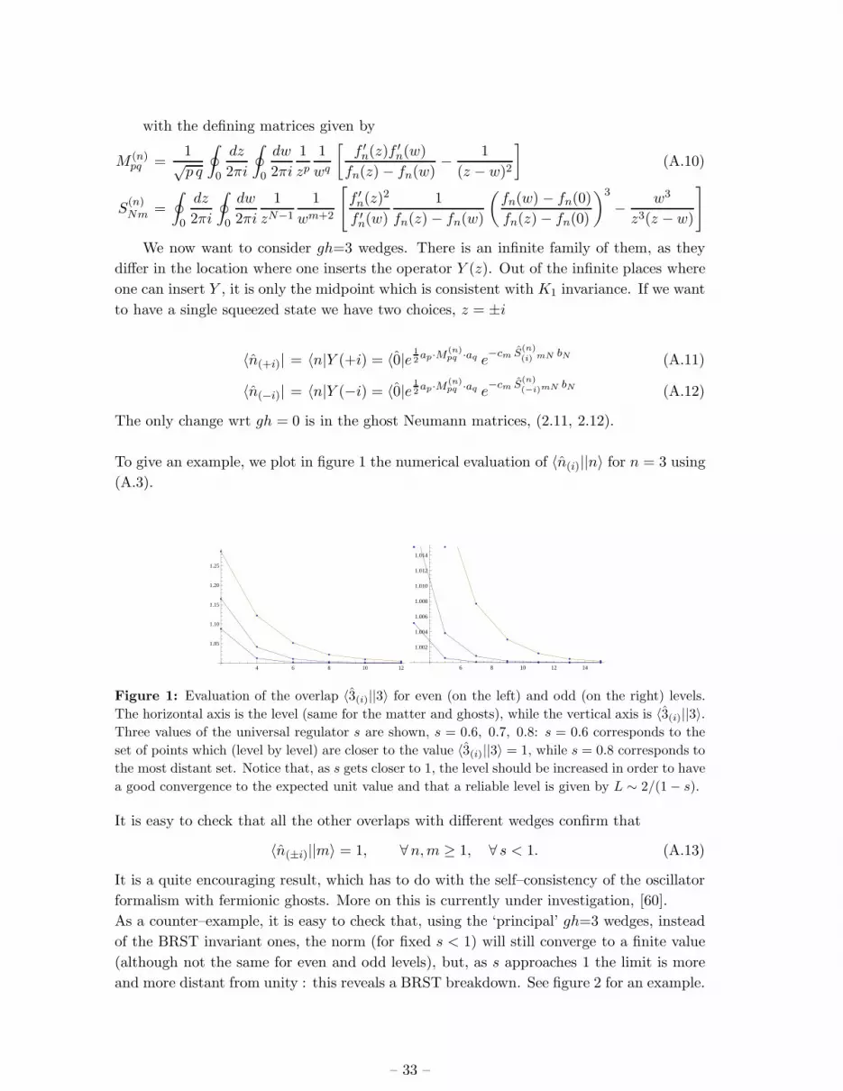
To give an example, we plot in figure 1 the numerical evaluation of 〈n(i)||n〉 for n = 3 using

(A.3).

4 6 8 10 12

1.05

1.10

1.15

1.20

1.25

6 8 10 12 14

1.002

1.004

1.006

1.008

1.010

1.012

1.014

Figure 1: Evaluation of the overlap 〈3(i)||3〉 for even (on the left) and odd (on the right) levels.

The horizontal axis is the level (same for the matter and ghosts), while the vertical axis is 〈3(i)||3〉.Three values of the universal regulator s are shown, s = 0.6, 0.7, 0.8: s = 0.6 corresponds to the

set of points which (level by level) are closer to the value 〈3(i)||3〉 = 1, while s = 0.8 corresponds to

the most distant set. Notice that, as s gets closer to 1, the level should be increased in order to have

a good convergence to the expected unit value and that a reliable level is given by L ∼ 2/(1− s).

It is easy to check that all the other overlaps with different wedges confirm that

〈n(±i)||m〉 = 1, ∀n,m ≥ 1, ∀ s < 1. (A.13)

It is a quite encouraging result, which has to do with the self–consistency of the oscillator

formalism with fermionic ghosts. More on this is currently under investigation, [60].

As a counter–example, it is easy to check that, using the ‘principal’ gh=3 wedges, instead

of the BRST invariant ones, the norm (for fixed s < 1) will still converge to a finite value

(although not the same for even and odd levels), but, as s approaches 1 the limit is more

and more distant from unity : this reveals a BRST breakdown. See figure 2 for an example.

– 33 –

4 6 8 10 12

0.85

0.90

0.95

1.00

6 8 10 12 14

0.86

0.88

0.90

0.92

0.94

0.96

Figure 2: Evaluation of the overlap 〈3||3〉 for even (on the left) and odd (on the right) levels, using

principal wedges instead of Y (±i)–inserted one as gh=3 duals. The three different sets of points

are given by s = 0.6, 0.7, 0.8: s = 0.6 corresponds to the highest set of points in the plot, while

s = 0.8 corresponds to the lowest set. Notice that there is a convergence pattern for any value of

s < 1, but the limit gets far from unity as s approaches 1.

B. Irrelevance of secondary poles

In this appendix we would like to show that secondary poles should not be considered when

the product of two gh = 3 matrices is performed. The way we are going to show this is via

an independent computation. We take as an example the proof of the midpoint identity

S(i)r∗z = r − s(i),

similar computations can be performed for all other products of gh = 3 matrices which are

considered in the main text.

First of all, let us trace the point where secondary poles would give a contribution in the

derivation of the above equation using the reconstruction formulas. We have

[S(i)r∗z]nj = −

∫

ℑ(κ′)>2dκ′∫

ℑ(κ)>ξN

dκtN (κ)

2sinhπκ′

2

V (2)n (−κ)V (−1)

j (κ′)δ(κ − κ′) (B.1)

In the main text we just assumed that, given ξN < 2i, we could always take the κ–path

to κ > 2i, because there is no pole at κ = 2i. However, in the κ–UHP, the wedge eigenvalue

tN (κ) have poles at κ = nξN for all positive integers n’s. We call the n = 1 pole a principal

pole, while we call the others secondary poles. The apparent problem here is that, starting

from N > 4, some secondary poles will be below ℑ(κ) = 2. So they should be picked up

when we shift the κ path from κ > ξN to κ > 2i.

Taking into account the contribution from secondary poles we would have ended with

[S(i)r∗z]nj = [r − s(i)]nj − 4iξN

n∗∑

k=2

sinhπkξN

2δ(kξN − 2i)V (2)

n (−kξN )V(−1)j (2i), (B.2)

where n∗ is the maximal integer for which 4Nn∗ < 2. Notice the naked complex delta con-

tribution which denounces an anomalous divergent part. In the main text we have assumed

that one need not consider this contribution.

– 34 –

We want to show here that what we did is correct and it is what is implied by universal

regularization. The way we are going to show it is via an independent computation which,

instead of using the power of reconstruction formulas, explicitly performs the matrix prod-

uct via generating functions defined on the ”Fourier transform” of the κ plane, the original

z–plane (that is by the method extensively used in II). In doing this we explicitly consider

the ‘principal’ + ‘residual’ decomposition

S(i)nm =

∮

0

dz

2πi

∮

0

dw

2πi

1

zn−1

1

wm+2

(

S(z,w) − ξNf (2)−ξN

(z) f(−1)ξN

(w))

= Snm − ξNV (2)n (−ξN )V (−1)

m (ξN ), (B.3)

and

r∗mj =

∮

0

dz

2πi

∮

0

dw

2πi

1

zm−1

1

wj+2

(

t(z,w) + 2if(2)2i (z) f

(−1)−2i (w) + if

(2)0 (z) f

(−1)0 (w)

)

= tmj + 2iV (2)m (2i)V

(−1)j (−2i) + iV (2)

m (0)V(−1)j (0). (B.4)

The terms which are going to contribute to our problem are∑

m≥2

(

− ξNV (2)n (−ξN )V (−1)

m (ξN ))(

2iV (2)m (2i)V

(−1)j (−2i)

)

and∑

m≥2

Snm

(

2iV (2)m (2i)V

(−1)j (−2i)

)

Let us begin by computing the inner product

V (−1)m (ξN )V (2)

m (2i).

Using the continuous basis we get the formal expression

V (−1)m (ξN )V (2)

m (2i) = 2sinhπξN2

δ(ξN − 2i). (B.5)

Since ξN 6= 2i, one would be tempted to take δ(ξN − 2i) = 0, this is however not consistent

with the explicit result we get by computing the same quantity on the z plane9

V (−1)m (ξN )V (2)

m (2i) =

∮

0

dz

2πi

∮

0

dw

2πi

1

zm+2

1

wm−1

1 + z2

(1 + w2)2fN (z)

(

1 + iw

1− iw

)

, (B.6)

where

fN (z) =

(

1 + iz

1− iz

) 2N

.

As we saw in II, in order to sum up the geometric series, we have to regulate the wedge–

function(

1+iz1−iz

)2N

by pushing the branch points away from z = ±i. As usual we do this

by

fN (z)→ f(K)N (z) ≡ fN(z/K).

9Also, from general properties of analytic continuation, δ(ix) is a formal divergent quantity, for x ∈ R.

– 35 –

Then, as argued in II (there are no poles at z = w), in the integration, we can choose the

ordering1

K<

1

z< w < 1 <

1

w< z < K,

and, by performing the integral around w, we end up with

V (−1)m (ξN )V (2)

m (2i) =

∮

i

dz

2πi

1

(z − i)2 f(K)N (z) =

d

dzf

(K)N (z)

∣

∣

∣

z=i, (B.7)

which is divergent. So, calling this divergence γ we can make the association,

γ ≡ d

dzf

(K)N (z)

∣

∣

∣

z=i←→ 2 sinh

πξN2

δ(ξN − 2i).

Finally we have

−ξNV (2)n (−ξN )V (−1)

m (ξN )2iV (2)m (2i)V

(−1)j (−2i) = −2iξN γ V (2)

n (−ξN )V(−1)j (−2i). (B.8)

This anomalous contribution needs to be compensated (and will) by the other term we

consider,∑

m≥2

Snm

(

2iV (2)m (2i)V

(−1)j (−2i)

)

.

Here we need to compute

SnmV(2)m (2i).

Again, we will first compute this quantity on the un–regularized κ–plane (that is with the

techniques of reconstruction formulas). This gives

SnmV(2)m (2i) = tN (2i)V (2)

n (−2i) + 2ξN sinhπξN2

V (2)n (−ξN ) δ(ξN − 2i)

+ 2ξN

n∗∑

k=2

sinhπkξN

2V (2)

n (−kξN ) δ(kξN − 2i)

this expression is what one gets by taking the κ path of Snm from the real axis to ℑ(κ) = 2,

and accordingly picking up the residues along the way. Notice the contribution from the

principal pole at κ = ξN (principal divergence), as well as from the secondary ones at

κ = kξN (secondary divergences). The divergence given by the principal pole exactly can-

cels with the previous term, but secondary poles cannot be canceled against anything else.

We now show that, doing the same computation on the regularized z–plane (that is point–

splitting plus contour integral techniques of section 2 of II), there will be no contribution

at all from secondary poles. Explicitly (we do not write down the radial ordering term 1z−w

in Snm, because we are just interested in extracting midpoint singularities)

SnmV(2)m (2i)

∣

∣

∣

sing=

∮

0

dz

2πi

∮

0

dw

2πi

∮

0

dx

2πi

1

zn−1

1

wm+2

1

xm−1

ξN2

1 + w2

(1 + z2)2fN(z) + fN (w)

fN(z) − fN (w)

1

(1 + x2)2

(

1 + ix

1− ix

)

. (B.9)

– 36 –

Again, in order to perform the sum over m, we regulate the wedge function

fN(w)→ f(K)N (w) ≡ fN (w/K)

and take1

K<

1

w< x < 1 <

1

x< w < K.

We can now safely integrate over x and get

=ξN2

∮

0

dz

2πi

1

zn−1

1

(1 + z2)2

∮

dw

2πi

1

(w − i)2fN (z) + f

(K)N (w)

fN (z)− f (K)N (w)

=ξN2

∮

0

dz

2πi

1

zn−1

1

(1 + z2)2d

dw

(

fN (z) + f(K)N (w)

fN (z)− f (K)N (w)

)

w=i

=ξN2

∮

0

dz

2πi

1

zn−1

1

(1 + z2)22

fN (z)

d

dwf

(K)N (w)

∣

∣

∣

w=i

= ξN γ V (2)n (−ξN ) = 2ξN sinh

πξN2

V (2)n (ξN ) δ(ξN − 2i) = SnmV

(2)m (2i)

∣

∣

∣

sing. (B.10)

In integrating over w we just considered the pole at w = i, because it is the only one which

is within the integration contour.

As claimed, the regularized computation on the z–plane (which is of course more

trustable than the un–regularized computation on the κ plane) clearly shows that sec-

ondary poles should not be considered. A clear κ–plane argument for disregarding them

should emerge by the use of universal regularization, [57], (whose basic effect, on the z–

plane, is just our branch–points displacement). We leave this quite technical point for

future investigations.

Similar checks can be done in all the other computations in the core of the paper: when

two gh = 3 (wedge) matrices are multiplied, only the poles at κ = −ξN , 0, ξN have to be

considered and the homotopy class of the paths in the game will be always understood to be

the one implied by these principal poles.

References

[1] L. Bonora, C. Maccaferri, R. J. Scherer Santos and D. D. Tolla, Ghost story. I. Wedge states

in the oscillator formalism, arXiv:0706.1025 [hep-th].

[2] L. Bonora, C. Maccaferri, R. J. Scherer Santos and D. D. Tolla, Ghost story. II. The

midpoint ghost vertex, arXiv:0908.0055 [hep-th].

[3] L. Bonora, R. J. Scherer Santos and D. D. Tolla, Spectral properties of ghost Neumann

matrices, Phys. Rev. D 77 (2008) 106001 [arXiv:0801.2099 [hep-th]].

[4] E. Witten, “Noncommutative Geometry And String Field Theory,” Nucl. Phys. B 268 (1986)

253.

[5] L. Rastelli and B. Zwiebach, “Tachyon potentials, star products and universality,” JHEP

0109 (2001) 038 [arXiv:hep-th/0006240].

– 37 –

[6] L. Rastelli, A. Sen and B. Zwiebach, “Boundary CFT construction of D-branes in vacuum

string field theory,” JHEP 0111 (2001) 045 [arXiv:hep-th/0105168].

[7] M. Schnabl, “Wedge states in string field theory,” JHEP 0301 (2003) 004

[arXiv:hep-th/0201095].

[8] M. Schnabl, Analytic solution for tachyon condensation in open string field theory, Adv.

Theor. Math. Phys. 10 (2006) 433 [arXiv:hep-th/0511286].

[9] Y. Okawa, Comments on Schnabl’s analytic solution for tachyon condensation in Witten’s

open string field theory, JHEP 0604 (2006) 055 [arXiv:hep-th/0603159].

[10] E. Fuchs and M. Kroyter, On the validity of the solution of string field theory, JHEP 0605

(2006) 006 [arXiv:hep-th/0603195].

[11] I. Ellwood and M. Schnabl, Proof of vanishing cohomology at the tachyon vacuum, JHEP

0702 (2007) 096 [arXiv:hep-th/0606142].

[12] L. Rastelli and B. Zwiebach, Solving open string field theory with special projectors,

arXiv:hep-th/0606131.

[13] Y. Okawa, L. Rastelli and B. Zwiebach, Analytic solutions for tachyon condensation with

general projectors, arXiv:hep-th/0611110.

[14] T. Erler and M. Schnabl, “A Simple Analytic Solution for Tachyon Condensation,”

arXiv:0906.0979 [hep-th].

[15] T. Erler, “Tachyon Vacuum in Cubic Superstring Field Theory,” JHEP 0801 (2008) 013

[arXiv:0707.4591 [hep-th]].

[16] I. Y. Aref’eva, R. V. Gorbachev and P. B. Medvedev, “Tachyon Solution in Cubic

Neveu-Schwarz String Field Theory,” Theor. Math. Phys. 158 (2009) 320 [arXiv:0804.2017

[hep-th]].

[17] Y. Okawa, Analytic solutions for marginal deformations in open superstring field theory,

arXiv:0704.0936 [hep-th].

[18] Y. Okawa, Real analytic solutions for marginal deformations in open superstring field theory,

arXiv:0704.3612 [hep-th].

[19] M. Schnabl, Comments on marginal deformations in open string field theory,

arXiv:hep-th/0701248.

[20] M. Kiermaier, Y. Okawa, L. Rastelli and B. Zwiebach, Analytic solutions for marginal

deformations in open string field theory, arXiv:hep-th/0701249.

[21] E. Fuchs, M. Kroyter and R. Potting, Marginal deformations in string field theory,

arXiv:0704.2222 [hep-th].

[22] B. H. Lee, C. Park and D. D. Tolla, “Marginal Deformations as Lower Dimensional D-brane

Solutions in Open String Field theory,” arXiv:0710.1342 [hep-th].

[23] O. K. Kwon, “Marginally Deformed Rolling Tachyon around the Tachyon Vacuum in Open

String Field Theory,” Nucl. Phys. B 804 (2008) 1 [arXiv:0801.0573 [hep-th]].

[24] M. Kiermaier and Y. Okawa, “General marginal deformations in open superstring field

theory,” arXiv:0708.3394 [hep-th].

– 38 –

[25] M. Kiermaier and Y. Okawa, “Exact marginality in open string field theory: a general

framework,” arXiv:0707.4472 [hep-th].

[26] T. Erler, “Marginal Solutions for the Superstring,” JHEP 0707 (2007) 050 [arXiv:0704.0930

[hep-th]].

[27] E. Fuchs and M. Kroyter, Schnabl’s L(0) operator in the continuous basis, JHEP 0610

(2006) 067 [arXiv:hep-th/0605254].

[28] M. Kroyter, “On string fields and superstring field theories,” arXiv:0905.1170 [hep-th].

[29] M. Kroyter, “Comments on superstring field theory and its vacuum solution,”

arXiv:0905.3501 [hep-th].

[30] I. Ellwood, “Singular gauge transformations in string field theory,” arXiv:0903.0390 [hep-th].

[31] M. Kiermaier, Y. Okawa and B. Zwiebach, “The boundary state from open string fields,”

arXiv:0810.1737 [hep-th].

[32] I. Ellwood, “The closed string tadpole in open string field theory,” JHEP 0808 (2008) 063

[arXiv:0804.1131 [hep-th]].

[33] E. Fuchs and M. Kroyter, Analytical Solutions of Open String Field Theory, arXiv:0807.4722

[hep-th].

[34] K. Furuuchi and K. Okuyama, “Comma vertex and string field algebra,” JHEP 0109 (2001)

035 [arXiv:hep-th/0107101].

[35] I. Kishimoto, Some properties of string field algebra, JHEP 0112 (2001) 007

[arXiv:hep-th/0110124].

[36] D. M. Belov, Witten’s ghost vertex made simple (bc and bosonized ghosts), Phys. Rev. D 69

(2004) 126001 [arXiv:hep-th/0308147].

[37] D.J.Gross and A.Jevicki, Operator Formulation of Interacting String Field Theory,

Nucl.Phys. B283 (1987) 1.

[38] D.J.Gross and A.Jevicki, Operator Formulation of Interacting String Field Theory, 2,

Nucl.Phys. B287 (1987) 225.

[39] E.Cremmer,A.Schwimmer, C.Thorn, ”The vertex function in Witten’s formulation of string

field theory, Phys.Lett. 179B (1986) 57.

[40] N. Ohta, “Covariant Interacting String Field Theory In The Fock Space Representation,”

Phys. Rev. D 34 (1986) 3785 [Erratum-ibid. D 35 (1987) 2627].

[41] S. Samuel, The Ghost Vertex In E. Witten’s String Field Theory, Phys. Lett. B 181 (1986)

255.

[42] C. Maccaferri and D. Mamone, Star democracy in open string field theory, JHEP 0309

(2003) 049 [arXiv:hep-th/0306252].

[43] A. Kling and S. Uhlmann, “String field theory vertices for fermions of integral weight,” JHEP

0307 (2003) 061 [arXiv:hep-th/0306254].

[44] D.Gaiotto, L.Rastelli, A.Sen and B.Zwiebach, Ghost Structure and Closed Strings in Vacuum

String Field Theory, [hep-th/0111129].

[45] L.Rastelli, A.Sen and B.Zwiebach, Classical solutions in string field theory around the

tachyon vacuum, Adv. Theor. Math. Phys. 5 (2002) 393 [arXiv:hep-th/0102112].

– 39 –

[46] L.Rastelli, A.Sen and B.Zwiebach, Star Algebra Spectroscopy, JHEP 0203 (2002) 029

[hep-th/0111281].

[47] D. M. Belov and C. Lovelace, Star products made easy, Phys. Rev. D 68 (2003) 066003

[arXiv:hep-th/0304158].

[48] A.Leclair, M.E.Peskin, C.R.Preitschopf, String Field Theory on the Conformal Plane. (I)

Kinematical Principles, Nucl.Phys. B317 (1989) 411.

[49] A. LeClair, M. E. Peskin and C. R. Preitschopf, “String Field Theory on the Conformal

Plane. 2. Generalized Gluing,” Nucl. Phys. B 317 (1989) 464.

[50] T. Erler and D. J. Gross, “Locality, causality, and an initial value formulation for open string

field theory,” arXiv:hep-th/0406199.

[51] K.Okuyama, Ghost Kinetic Operator of Vacuum String Field Theory, JHEP 0201 (2002) 027

[hep-th/0201015].

[52] L. Bonora, C. Maccaferri, D. Mamone and M. Salizzoni, “Topics in string field theory,”

arXiv:hep-th/0304270.

[53] V.A.Kostelecky and R.Potting, Analytical construction of a nonperturbative vacuum for the

open bosonic string, Phys. Rev. D 63 (2001) 046007 [hep-th/0008252].

[54] L. Bonora and A. S. Sorin, “Integrable structures in string field theory,” Phys. Lett. B 553

(2003) 317 [arXiv:hep-th/0211283].

[55] A. Boyarsky and O. Ruchayskiy, “Integrability in SFT and new representation of KP

tau-function,” JHEP 0303 (2003) 027 [arXiv:hep-th/0211010].

[56] E. Fuchs and M. Kroyter, “On surface states and star-subalgebras in string field theory,”

JHEP 0410 (2004) 004 [arXiv:hep-th/0409020].

[57] E. Fuchs and M. Kroyter, “Universal regularization for string field theory,” JHEP 0702

(2007) 038 [arXiv:hep-th/0610298].

[58] I. Y. Aref’eva, R. Gorbachev, P. B. Medvedev and D. V. Rychkov, “Descent relations and

oscillator level truncation method,” Theor. Math. Phys. 150 (2007) 2 [arXiv:hep-th/0606070].

[59] E. Fuchs and M. Kroyter, “Normalization anomalies in level truncation calculations,” JHEP

0512 (2005) 031 [arXiv:hep-th/0508010].

[60] C. Maccaferri, Work in progress

[61] see for example: I. B. Frenkel, H. Garland and G. J. Zuckerman, “Semiinfinite Cohomology

And String Theory,” Proc. Nat. Acad. Sci. 83 (1986) 8442.

– 40 –