GNSS/INS Aided Precise Re-photographing Erica Nocerino, Fabio Menna, Fabio Remondino

3D Optical Metrology Unit Bruno Kessler Foundation (FBK)

Trento, Italy E-mail: {nocerino, fmenna, remondino}@fbk.eu

Abstract—Re-photographing is a well-established method of acquiring new images in the same location where old photos were taken, in order to visualize changes and evolutions of the analyzed scene. According to the goal of the re-photographing procedure, different techniques can be employed, mainly based on visual methods, image cues or positioning sensors. The paper, after a review of the re-photographing procedures and techniques, presents a GNSS/INS aided method to achieve precise re-photographing results. Architectural and natural scenarios are used to test the developed method.

Keywords—re-photographing; photogrammetry; GNSS; INS; bundle block adjustment

I. INTRODUCTION Repeat photographing or re-photographing is the procedure

of finding the viewpoint of an old picture and taking a new photo showing the actual situation from the same viewpoint. Usually, the term re-photographing refers to terrestrial acquisitions of landscape, cities, social events, etc. even if examples of repeated aerial photos also exist [1-2]. The possibility of comparing photos acquired from the same viewpoint but in different moments provides a visual and qualitative interpretation of the progress of time, transformations occurred, etc. But applying appropriate metrological techniques, quantitative information for an objective and independent analysis can also be delivered. The value of re-photographing technique to document changes and evolution of landscape or urban areas has attracted scientists of different disciplines. Indeed this technique can offer impartial data for evaluating the rate of changes over both small and long-term periods by looking backward in time but also defining a frame of reference for assessing future developments.

Among the broad range of disciplines where re-photographing is applied, this paper mainly focuses on urban/architectural and natural science purposes. Applications in these fields are quite demanding as satisfactory results and accurate analyses require a certain degree of precision in taking the new image. The aim of the presented work is thus to provide a methodology that meets these requirements. The approach here proposed consists of an integrated use of photogrammetric, navigation and positioning techniques for retrieving the original position of a reference (old) photo and the geometrical characteristics of the employed camera. A new photo is then shooted re-positioning the camera with the aid of GNSS (Global Navigation Satellite System) / INS (Inertial Navigation System) sensors. The paper covers all the technical aspects of the developed sensor-based re-photographing

approach and presents results from urban and landscape scenarios.

A. History and applications of re-photographing The first steps in using re-photographing as scientific tool

were taken by Finsterwalder in 1888 when he began to conduct photogrammetric surveys of mountain glaciers in the Tyrolean Alps [3]. He returned to the same camera stations in different moments, obtaining multi-temporal images of the same area. Comparing the images and using photogrammetry, the scientist was able to evaluate glacier’s changes over time. Following Finsterwalder’s work, re-photographing has been widely used for applications in natural sciences, ranging from glaciology studies [4-5], coastal processes [2], landscape changes induced by land use [3], geological analyses related to weathering and bedrock erosion, ecology studies focused on plant population and vegetation [6], etc. Some of these studies were collected in photographic documentaries, such as for example the “Rephotographic Survey project” [7-8] which concerned 120 sites, firstly recorded in the 1870s and then re-photographed in 1977 and 2000’s. In [9] a wide bibliography of studies related to landscape changes and based on re-photographing is provided. An extensive review of past and current methods and applications of re-photographing across diverse disciplines related to the natural sciences is also presented in [3]. Urban re-photographing has been also proved to be a valid tool for recording changes in urban areas (abandonment and adaptive reuse of housing sites, changes in use of building [10-12], urbanization and deforestation [6]. Re-photography is also recognized as a useful visual method for researchers in sociology and communication to understand social change [13] and anthropology studies [14]. Re-photographing has also been used for social protest in Argentina where family pictures were taken before and after disappearance of relatives [15].

II. REVIEW OF RE-PHOTOGRAPHING TECHNIQUES In order to have a compelling and accurate “then and now”

of the area of interest based on photos taken in different moments, the pose (both position and orientation) of the reference (old) photo must be precisely recovered. Obviously, the results of the successive analyses mainly depend on the quality of re-photographing. Usually, retrieving the camera pose of the reference photo is a challenging task, in particular for historic images, since both camera information and shooting location could be inaccurate or totally unknown. Several methods have been proposed in literature to retrieve the

978-1-4673-2565-3/12/$31.00 ©2012 IEEE 235

position and orientation of the reference photo. These methods are afterwards described in ascending order of accuracy degree.

The simplest and less accurate method consists in a “trial and error” approach [16]: the camera is manually moved around until the view in the viewfinder matches the scene represented in the reference image. This “vintage” method has been the most popular, mainly because of its simplicity, but has several weak points: (i) it can take a lot of time for recovering camera position that matches the reference image reasonably; (ii) the quality of re-photographing cannot be univocally ascertained; (iii) the overall results in terms of both speed and accuracy in re-positioning are strictly related to the photographer skills. This approach can be feasible in urban environments where recognizable elements characterize the recorded scene, but it is impracticable for landscape re-photography unless an approximate knowledge of the camera position is known.

If the approximate shooting position is not known at all, the “Virtual repeat photography” (VRP) technique can be employed [1, 17]. The VRP finds camera stations for uncertain locations of a mile or less using a Digital Elevation Model (DEM) and aerial images. The geo-referencing is manually performed, shifting the view angle and distance until the reference photo (position and bearing) is lined up with the digital model. Once the photo-point has been found, a synthetic photograph of the digital landscape can be produced. The same method has been applied for locating and re-taking aerial photos: the digital model and orthophotos allow designing and planning flight routes fitting the identified positions of the reference aerial images. The accuracy of this method depends on the resolution of the used Digital Elevation Model (DEM). Nevertheless this approach can be useful for finding an approximate position and narrowing the search for specific sites where a more accurate re-photographing could be started [1]. For terrestrial re-photographing applications, a further step for improving precision is to measure parallaxes between objects visible in both the reference image and the current view: differences in the measurements indicate different orientation of the cameras. This method can be applied as iterative process for gradually reducing the misalignment between the photos (see [18] for more details and references).

For architectural studies requiring high accuracy and repeatability (e.g., reconstruction of portions of buildings or objects that have been destroyed or modified), the photogrammetric system of reverse perspective analysis can be used [19-20]. This method consists in finding the missed camera station identifying three vanishing points on the image plane and approximately scaling with the actual size of recognizable objects in the scene. An improvement to this method has been proposed in [21] where a real-time estimation and visualization technique based on image cues and computer vision algorithms is used. The method requires the camera being connected to a laptop. The relative viewpoint difference between the reference image and current scene is computed in real-time and an interactive tool guides the user to move the camera for matching the original pose. This method can yield visual accurate results for images that contain a reasonable number of image cues with good texture. It needs also sufficient parallax between the images and enough 3D structure

in the scene to make the viewpoint estimation well-posed. The intrinsic characteristics of this method make it appropriate for urban re-photographing but not suitable for re-photographing application in natural scenes.

In [18] a standard photogrammetric approach together with topographic measurements (total station and Global Positioning System-GPS receiver) is applied for retrieving the interior and exterior parameters of historical photos. Several points recognizable in the reference image are then used to solve via a spatial resection for the orientation parameters to be used for acquiring the new image. The method provides accurate results but the use of a total station for measuring control points is not a feasible solution in many situations.

III. GNSS POSITIONING TECHNIQUES Since its advent, the Global Navigation Satellite Systems

have transformed the way of navigating and travelling across the world. Due to several systematic errors or biases and random noise, accurate positioning of objects with GNSS satellites is not straightforward. In the past, several methods (Differential GPS-DGPS, Real Time Kinematic-RTK) were developed for improving the system’s accuracy and assuring satisfactory levels required for demanding applications (e.g., surveying, geodesy, geodynamics). Usually, these methods required (i) the use of two receivers (a reference or master and a moving rover) at least, (ii) time-consuming measurement sessions especially with code and single-frequency receivers that hardly allowed accurate real-time kinematic positioning, (iii) radio link for real-time measurements. High-quality receivers (double-frequency) and antennas were employed to solve the phase ambiguities faster and more reliably, eliminate the ionosphere error, reduce multipath effects and phase center variations. Double-frequency receivers made it possible to realize RTK that allows the user to obtain cm-level accuracy of the position in real time by processing carrier-phase measurements of GNSS signals. Unfortunately, the “geodetic-grade” equipment has always been really expensive; in [22] costs of 10-30k€ are reported, costs that significantly influenced and reduced the mass market of accurate point positioning. In the last years, many researches have been conducted with the aim to economize financial and physical resources required for getting accurate positioning with GNSS. Navigation-grade (code, phase-smoothed code, single-frequency) receivers and antennas less expensive than “standard” geodetic equipment are available on the market (5-300€). Low-cost equipment has been proved to work very reliably if the distance between reference and rover station (i.e., the baseline length) is below 10-15 km, but it has been considered not suitable for RTK due to its poor performance. In the last years, first RTK applications based on single-frequency receiver have been published. Pioneers in this research field were Takasu and Yasuda with the Open Source software package RTKLIB [23]. The software consists of several modules that can either process and store raw GPS data in real-time (RTKNavi) or elaborate them in post-processing (RTKPost). Differential GNSS (DGNSS) with low-cost GNSS receivers is always more diffusing, also thanks to the development and strengthening of Continuously Operating Reference Station (CORS) Networks. CORS systems enable positioning accuracies that approach a centimeter or better

236

relative to a worldwide network [22] and permit to save the cost of a master or reference station. Alternatively to DGNSS or RTK, Precise Point Positioning (PPP) can be used. Improvement in standalone or autonomous point positioning is attained through the use of precise satellite ephemeris and clock corrections produced by many organizations (e.g., International GPS service-IGS, Jet Propulsion Laboratory-JPL), and provided in both post-mission and real-time modes. Once orbit and clock errors are removed from GPS observations, much higher positioning accuracy can be expected even when a single GPS receiver is used. One advantage of PPP is that, since no base station is necessary, there is no need for simultaneous observations and no tight limit in range thanks to globally and regionally valid correction data [24]. Dual-frequency PPP has been extensively researched, whereas the possibility of using single frequency PPP to achieve high accuracy point positioning is a relatively new research area [25]. Nevertheless, some manufactures are delivering on the market low-cost navigation receivers equipped with factory PPP software (e.g., u-blox NEO-6P) for surveying, mapping, marine, and slow-moving recreational applications. For satisfying high accuracy level, but reducing the cost-effectiveness, the quality of the performance of navigation type receivers can be improved by using precise geodetic antennas [22, 26].

IV. INERTIAL NAVIGATION SYSTEMS Inertial Navigation technique uses motion sensors

(accelerometers) and rotation sensors (gyroscopes) to continuously calculate via dead reckoning the position, orientation and velocity of a moving object relative to a known starting point. Dead reckoning means that the object’s current position is calculated starting from a previously determined position or fix. Once it has been initialized, INS provides navigation information independent of external reference but does not provide absolute positioning information. Typically, Inertial Measurement Units (IMUs) are composed of a cluster of three orthogonal rate-gyroscopes and three orthogonal accelerometers. Low-cost IMUs are based on MEMS (Microelectromechanical systems or micromachines) technology that has reduced considerably dimension and weight of the devices. MEMS IMUs have lower performance with respect to more expensive, high-accuracy sensors which use, for example, fiber-optic or spinning mass technologies. MEMS sensors have significant bias instability and noise level; the short-term bias instability (drift) of gyros is the main limiting factor in the attainable accuracy [27-28]. At the end of 2007 the best published accuracy for a MEMS gyroscope was about one degree drift per hour, while combining three gyros into a single virtual sensor the bias drift can be reduced to 0.53 degrees per hour [29]. Errors in the computed orientation result in a rapidly accumulating error in position when the signals are subsequently integrated. In order to correct or reduce the sensor’s drift and improve MEMS IMUs accuracy, two methods are usually employed: (i) sensor fusion and (ii) domain specific assumption. Sensor fusion combines data from different types of sensors to update or maintain the state of the system (orientation, velocity and displacement). In literature it has been extensively shown that combining MEMS IMUs with GNSS receivers, magnetometers, barometers, and optical

sensors leads to more accurate results [28-32]. Kalman filters are very commonly used data fusion algorithms. Domain specific assumptions are software based techniques that compute corrections used to minimize drift making assumptions about the movement of the body to which the IMU is attached.

V. RE-PHOTOGRAPHING IN A NUTSHELL The first question that has to be addressed in realizing the

re-photographing is “where was my reference (old) picture taken from?” and “if a positioning error is committed, how this error affects the results of the re-photographing?”

The mathematical model that describes the imaging process is the well-known collinearity condition. The image coordinates are a function of the Exterior Orientation (EO, 6 Degree of Freedom-DOF of the photo) and Interior Orientation parameters (IO, geometrical characteristics of the camera). If the EO and IO parameters are known, the image coordinates (x,y) of 3D points (X,Y,Z) in the object space are univocally determined. Changing IO or EO parameters causes the object to be imaged in different position on the photograph. A precise re-photographing can thus be defined as “the procedure that minimizes the differences between the old reference and new picture image coordinates”. Assuming the characteristics (IO) of the reference camera known, the re-photographing problem reduces to retrieve EO parameters and come back to the reference photo position re-creating the 6DOF of such photo.

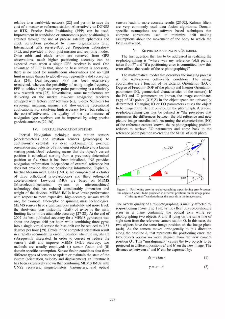
Figure 1. Positioning error in re-photographing: a positioning error b causes the objects A and B to be projected in different positions on the image plane

(“misalignment”) and produces the error ds in the image space.

The overall quality of a re-photographing is mainly affected by re-positioning errors. Fig. 1 shows the effect of a re-positioning error in a plane containing the optical axis while re-photographing two objects A and B lying on the same line of sight seen from the reference camera station O. In this case, the two objects have the same image position on the image plane (a�b). As the camera moves orthogonally to this direction along the baseline b, that represents the positioning error, the two objects appear no more aligned from the new camera position O’. This “misalignment” causes the two objects to be projected in different positions a’ and b’ on the new image. The distance ds between a’ and b’ can be expressed by:

�� � � ��� (1)

� � � (2)

237

� ��� ��

��� � � ��� �

�

�� (3)

Rearranging (1) with (2) and (3), the error ds can be obtained as a function of linear quantities:

�� � �� � ��� � ���

�� � �� � ������� (4)

���� ���

�� !"#�

�

�� !"#

� � ��� � ���

�� � �� � �����$�%&� (5)

where c is the principal distance of the camera, b the positioning error, dA, dB the distances between the original camera position O and points A and B respectively. It is noteworthy that ds is the maximum error in the image space given a position error b. This is because (4) has been determined considering the worst situation where the positioning error b is perpendicular to the line of sight between camera station and points A and B. In the neighborhood of the exact position, a positioning error in any direction can be decomposed in horizontal and vertical components, which can be evaluated with (4) or (5), relationships that hold in any plane containing the optical axis. Knowing the camera, that is c and pxsize, and established dA and dB, the relationship provides the “misalignment” in pixel dspx as function of the positioning error b. The error b represents the accuracy in determining the position of the reference image and in re-locating the camera for taking the new picture.

The precision required in retrieving and coming back to the exact reference camera position mainly depends on two factors: (i) the aim of the re-photographing (recreational, for studying landscape or glacial evolution, for analyzing modifications of old buildings, etc.); (ii) the relative position between the shooting point and the objects in the captured scene (re-photographing of wide and wild landscape or ancient urban centers), as shown in (4). For example, if the aim is to re-photograph an ancient church in the city center for architectural analysis, high precision (in the order of decimeters or even better) in re-positioning is required otherwise the new photo will not fit the reference image. On the contrary, a greater margin of error (in the order of one-hundred meter) can be allowed in re-photographing a mountainous landscape hundreds of meters away.

Among the 6DOF that univocally position a camera in the space, the projection center coordinates are the discriminant factor for obtaining a correct re-photographing, since a small error in orientation does not produce significant errors in matching the old and new photographs. Indeed, images taken by rotating the same camera around the center of projection can be stitched together as the images are simply related by a homography. That is also valid when the camera position deviates slightly from the original projection center if the captured scene is relatively distant (i.e., all points are very far from the camera). This principle is widely used in Computer Vision algorithms for making panoramic image stitching.

VI. THE PROPOSED RE-PHOTOGRAPHING METHOD Our method works through the following steps: (i) the

digital camera that will be used for acquiring the new photo is coupled with a GNSS receiver; (ii) a close-range photogrammetric survey is conducted to reconstruct a 3D sparse model of the area of interest; (iii) knowing the absolute coordinates of the camera stations from the GNSS receiver, the photogrammetric model can be scaled and geo-referenced: the GNSS coordinates of the projective centers can be either introduced as observations in the bundle block adjustment process (e.g., with APERO [33]) either used a-posteriori to perform a classical Helmert transformation for scaling and geo-referencing (e.g., Agisoft Photoscan [34]); (iv) approximate camera parameters can be estimated, e.g., through bibliography research and verified performing a standard DLT using Ground Control Points (GCPs) from the photogrammetric 3D model; (v) the same GCPs can be used to retrieve also the exterior parameters of the reference image (via spatial resection); (vi) the GNSS receiver and INS device are used to re-position the camera and acquire the new photo with the computed equivalent focal length; (vii) the new photo is merged and overlapped with the reference (old) photo by applying a projective transformation (homography).

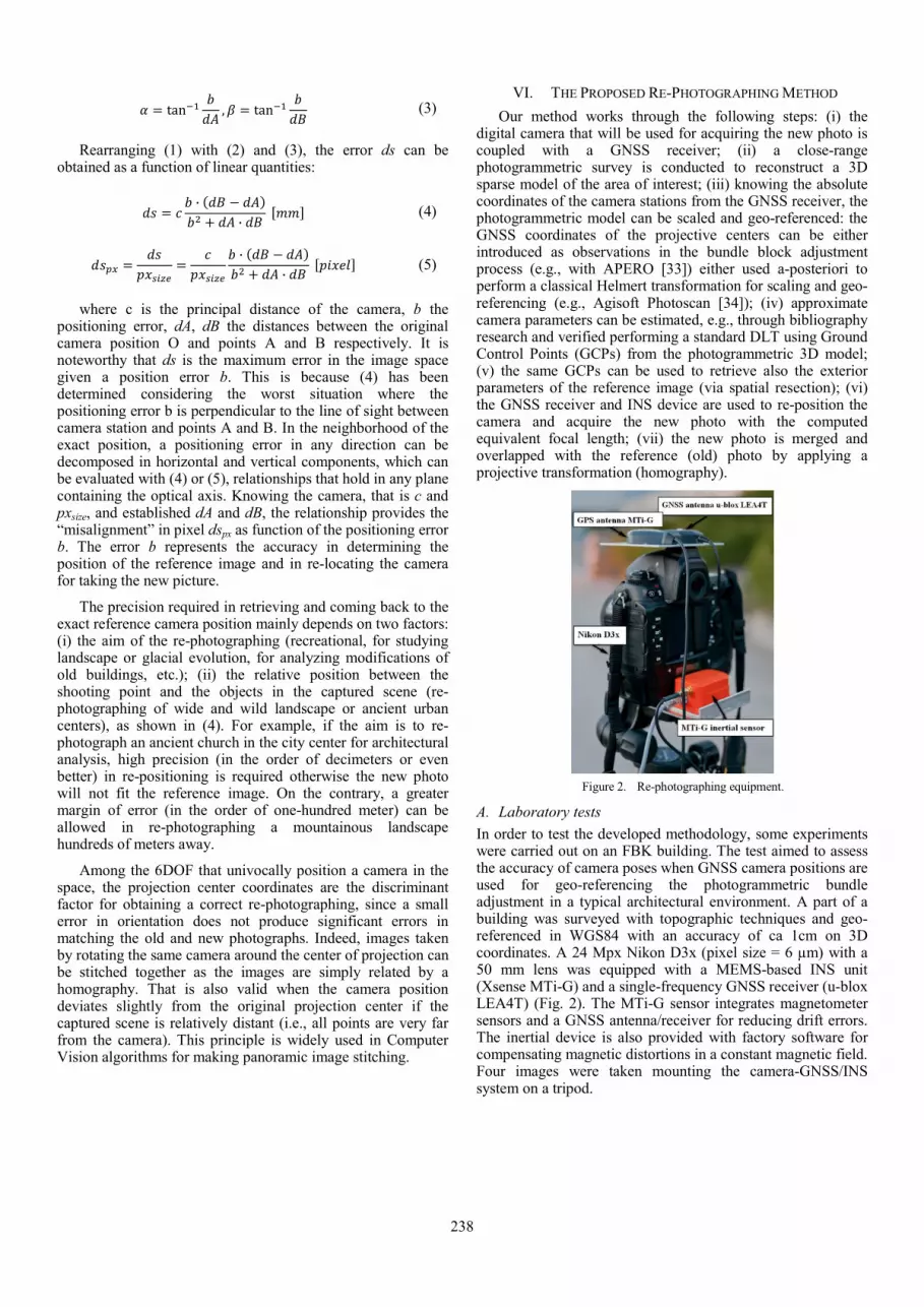
Figure 2. Re-photographing equipment.

A. Laboratory tests In order to test the developed methodology, some experiments were carried out on an FBK building. The test aimed to assess the accuracy of camera poses when GNSS camera positions are used for geo-referencing the photogrammetric bundle adjustment in a typical architectural environment. A part of a building was surveyed with topographic techniques and geo-referenced in WGS84 with an accuracy of ca 1cm on 3D coordinates. A 24 Mpx Nikon D3x (pixel size = 6 μm) with a 50 mm lens was equipped with a MEMS-based INS unit (Xsense MTi-G) and a single-frequency GNSS receiver (u-blox LEA4T) (Fig. 2). The MTi-G sensor integrates magnetometer sensors and a GNSS antenna/receiver for reducing drift errors. The inertial device is also provided with factory software for compensating magnetic distortions in a constant magnetic field. Four images were taken mounting the camera-GNSS/INS system on a tripod.

238

REFERENCE IMAGE RE-PHOTOGRAPHING RESULT

Figure 3. Re-photographing results of laboratory test.

The u-blox GNSS receiver was left for ca 20 minutes in a static mode to acquire raw observations for each image. The processing was made in RTKLIB for static single frequency relative positioning within the Autonomous Province of Trento CORS (nearest reference station at 3 Km). The INS system was used to compute the components of the eccentricity vector from u-blox antenna to camera perspective center. The four images were then processed in two different ways:

1) exterior orientation computation with some GCPs measured with topographic techniques and imported as observations in the bundle adjustment. The camera positions determined with the bundle adjustment were compared to those obtained from GNSS/INS system. The average difference was less than 5 cm. Thus the test showed that using standard photogrammetric procedure with accurate GCPs, the bundle block adjustment provides accurate camera position and orientation for precise re-photographing.

2) exterior orientation using the GNSS coordinates of the projective centers as observations in the bundle block adjustment process (i.e. direct geo-referencing). The RMSE in the GCPs was less than 10 cm. These results show that the use of GNSS camera positions avoids the need of measuring in a global reference system GCPs coordinates on site for re-photographing purposes.

The successive test was done using the same camera equipped with the GNSS/INS system to re-photograph the scene imaged in the previous test, this time assuming one of the previous images as reference. In the reference image the main body of the building is visible in the background while in the foreground a rail and a fire hydrant are present (only 6 m far from the camera). Applying Eq. (5) for the building with dA=30 m and dB=40 m, b=1m, the error ds is ca 70 pixels, barely visible in a 10x15cm print. If (5) is applied also considering the objects in the foreground (dA=6 m dB=40 m), the error ds grows up to 1200 pixels and it cannot be ignored. For re-photographing with one meter accuracy in positioning the camera, the procedure consisted in using the u-blox receiver in single point positioning mode with Wide Area Augmentation System (WAAS) corrections enabled. Compatibly with the satellite configuration, the elevation mask was set to 30 degrees to reduce multipath and ionospheric delays. The dynamic of receiver was also set to static. Under good circumstances for satellite configuration (Geometric Dilution of Precision-GDOP) and limited

multipath effects the accuracy reached with this procedure in repositioning is in the order of a meter in plan. For best results especially in critical environments, the GDOP should be taken in account by planning the survey with suitable software [35]. If a better accuracy in re-positioning is necessary, as in the case of re-photographing architectural structures, a relative positioning GNSS technique has to be considered. Unfortunately in our case the high sensitivity antenna of the u-blox did not allow real time kinematic processing due to continuous loss of the fix ambiguity solution. In [26], using a different antenna, centimeter accuracy has been declared. An alternative solution, especially valid in critical urban environment could be to: (i) reach an approximate position using single point positioning in real time; (ii) leave the receiver acquiring in rapid static mode for the necessary time; (iii) process the baseline using reference station raw data downloaded from internet on site (latency time 15 minutes) (iv) calculate the offset to the correct position. With this method, a re-positioning accuracy in the order of 10 cm can be reached. The last step in the re-photographing procedure consisted in using the MTi-G sensor for precisely orienting the camera as the reference image.

Fig. 3 shows the re-photographing of the building used for the test with the accurate method. With this procedure, an error of ca. 25 cm was committed in repositioning. This error affected the re-photo of the hydrant with an error ds on the image of 260 pixels (Fig. 3). On the building the maximum error was less than 20 pixels.

B. Re-photographing examples The discussed methodology was applied in the real

environment through two illustrative case studies, respectively for urban/architectural applications and landscape analysis.

1) “Case study 1 The urban test was conducted in the city center of Trento (Italy), close to “Torre Vanga”. Two pictures (named “Torre Vanga 1” and “Torre Vanga 2”) dating back to the Second World War (WWII) were used as reference images (Fig. 4a). The original films belong to a historical imagery repository taken by Fratelli Pedrotti photographers [36] and show the bombing attack over the train station of Trento in September 1943 from two different points of view. The IO of the two reference images were estimated through the following assumptions: (i) the images have the original dimensions (not

239

cropped); (ii) the original pictures were taken with 120 format film that allows several frame sizes; (iii) the aspect ratio, computed as ratio between the image dimensions in pixel, is ca. 1.50:1 (corresponding to 6x9 cm frame size) for both images; (iv) the focal length is 105 mm, a normal lens for 120 format film; (v) lens distortions is neglectable. The same equipment described for the laboratory test (Fig. 2) was used to acquire seven images using a tripod. The GNSS receiver was maintained still for ca 15 minutes and the acquired raw data were post-processed off-line with RTKLIB. The automatic image triangulation procedure described in section VI was used to obtain a sparse 3D point cloud of the scene of interest, geo-referenced in WGS84. GCPs were identified on features visible on the historical images and still observable in the current images: points were manually marked e.g. on “Torre Vanga”, the steeple of the church, town bell tower, etc. The GCPs were used to perform a standard resection and retrieve the IO and EO parameters. Equation (5) was then applied to both reference images considering a positioning error b of 50cm and 2m respectively (Table 1). In order to obtain the best accuracy in re-positioning in situ, the u-blox receiver in single point positioning mode (with WAAS corrections enabled) allowed to determine an approximate position. Finally, the cameras in the two (reference) positions were oriented with the aid of the MTi-G sensor according to the computed orientation angle of the historical photos. The obtained images were then overlapped over the reference pictures by means of a projective transformation (Fig. 4).

TABLE I. Estimated theoretical maximum errors in image space as function of positioning errors for the urban case study.

dA [m] dB [m] b [m] ds[pixel]

Torre_Vanga_1 44 407 0.5 88 44 407 2.0 351

Torre_Vanga_2 64 427 0.5 57 64 427 2.0 228

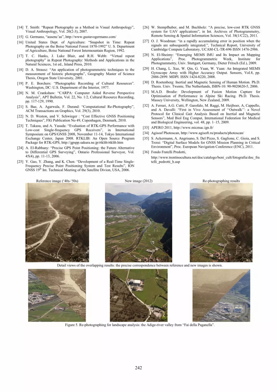
2) “Case study 2 The proposed methodology was also used for a landscape

re-photographing example (Adige-river valley seen from “Fai della Paganella” – Fig. 5). The reference image belongs to the Pedrotti’s repository too, but the date is uncertain. Also in this case, the original photo format was supposed to be a 120 format film. Assuming that the image was not cropped, the computed aspect ratio was ca. 1.35:1, characteristic of a 6x4.5 cm frame size. Finally a normal lens type was considered, i.e. a 75mm focal length. In order to retrieve the position of the reference photo, GCPs visible on the reference image were identified by an iterative procedure: first of all, the approximate DSM available on Google Earth was used and then the more detailed orthophotos and DSM delivered by the Autonomous Province of Trento were used to improve the GCPs positioning precision. The identified GCPs were used to perform a standard photogrammetric resection. A “lighter” version of the re-photographing equipment (Fig. 2) was employed in situ. The GNSS receiver was used for coming back to the computed reference position and, considering the not demanding accuracy, the use of the inertial sensor was avoided. The images were acquired without the tripod leading to the re-photographing results shown in Fig. 5. This example witnesses the importance of re-photographing to document landscape changes: by comparing the new and reference

images the urban expansion is immediately evident and could also be quantified.

VII. CONCLUSIONS The work presented a re-photographing methodology

based on the integration of GNSS and INS technologies with photogrammetry. A GNSS receiver is used to recover the position of the reference (old) photo and re-position the camera for taking the new image. The integration with an IMU sensor is also proposed and tested in order to place correctly the camera in the computed orientation. The use of INS can be very useful for “unmanned” re-photographing, as in the case of flights with UAVs for aerial landscape surveys. The choice of the GNSS receiver and INS device are strictly related to the precision required in the re-photographing procedure. As explained in section III, the use of geodetic double-frequency receiver can deliver millimeter accuracy, but is a high-cost solution. Multi-path effects are a challenging matter for urban applications but can be faced selecting a proper mask angle, excluding bad satellites and using geodetic antennas, less sensitive to multi-path problems. The best compromise between costs, time and precision can be achieved employing new-generation low-cost navigation receiver and applying DGNSS (within CORS network) or PPP techniques. Significant improvements can be achieved by planning the survey sessions and assuring strong satellite configuration. Analogously, a low-cost IMU, opportunely integrated with other sensors for reducing drift errors, can be used. The achieved results are quite satisfactory from a simple visual but also a geometrical point of view. These results can now be used for landscape or city center studies or as multimedia contents for museal exhibitions and are for sure promising considering the latest developments of mobile imaging and positioning sensors.

ACKNOWLEDGMENT The authors thank Prof. Salvatore Troisi (“Parthenope” University of Naples, Italy) for his precious contribution in GNSS planning, measurements and processing.

REFERENCES [1] R. Carstensen, K. Hocker: “Documenting Vegetational Change Through

Repeat Photography in Southeast Alaska 2004-2005”, Report, USDA Forest Service and Wilderness Exploration and Discovery, 2005.

[2] D. M. Bush, and R. Young: “Coastal features and processes”, in Young, R., and Norby, L., Geological Monitoring: Boulder, Colorado, Geological Society of America, pp. 47–67, 2009.

[3] R. H. Webb, D. E. Boyer, R. M. Turner: “Repeat Photography: Methods and Applications in the Natural Sciences, 1st ed., Island Press, 2010.

[4] NSIDC/WDC National Snow and Ice Data Center/World Data Center for Glaciology, Boulder: “Glacier Photograph Collection”, Boulder (CO) USA, 2009 http”//nsidc.org/data/docs/noaa/g00472_glacier_photos/

[5] H. J. Basagic, A. G. Fountain: “Quantifying 20th Century Glacier Change in the Sierra Nevada, California”, Arctic, Antarctic, and Alpine Research, Vol. 43(3), pp. 317-330, 2011.

[6] H. Chen, K. Yin, H. Wang, S. Zhong, N. Wu, F. Shi, D. Zhu, Q. Zhu, W. Wang, Z. Ma, X. Fang, W. Li, P. Zhao, C. Peng: “Detecting One-Hundred-Year Environmental Changes in Western China Using Seven-Year Repeat Photography”, PLoS ONE, Vol. 6(9), 2011.

[7] M. Klett, E. Manchester, J. Verburg, G. Bushaw, R. Dingus: Second View: The Rephotographic Survey Project, Univ. of New Mexico Press, pp. 211, 1984.

240

TORRE VANGA 1 TORRE VANGA 2 a) Reference images (1943)

b) New images (2012)

c) Re-photographing results after applying homography transformation

d) Detail views obtained “cutting” the re-photographing results after homography: the precise correspondence between reference and new images is shown.

Figure 4. Re-photographing for urban/architectural applications: the “Torre Vanga” example.

[8] M. Klett , K. Bajakian, W. L. Fox, M. Marshall, T. Ueshina, B. G. Wolfe: Third Views, Second Sights: A Rephotographic Survey of the American West, Museum of New Mexico Press, pp. 238, 2004.

[9] G. F. Rogers, H. E. Malde, R. M. Turner: “Bibliography of Repeat Photography for Evaluating Landscape Change”, Univ.Utah Press, 1984.

[10] C. J. Vergara, http://invinciblecities.camden.rutgers.edu/intro.html

[11] D. Levere, B. Yochelson, P. Goldberger: “New York Changing: Revisiting Berenice Abbott's New York”, pp. 192, 170 Duotones, 2004.

[12] P. B. Hales: Silver Cities: Photographing American Urbanization, 1839-1939, University of New Mexico Press, pp. 506, 2005.

[13] J. H. Rieger: “Photographing social change”, J Vis Soc., Vol. 11(1), 1996.

241

[14] T. Smith: “Repeat Photography as a Method in Visual Anthropology”, Visual Anthropology, Vol. 20(2-3), 2007.

[15] G. Germano, “ausenc’as”, http://www.gustavogermano.com/ [16] United States Dept. of Agriculture: “Snapshot in Time: Repeat

Photography on the Boise National Forest 1870-1992” U. S. Department of Agriculture, Boise National Forest Intermountain Region, 1992.

[17] T. C. Hanks, J. Luke Blair, and R.H. Webb: “Virtual repeat photography” in Repeat Photography: Methods and Applications in the Natural Sciences, 1st ed., Island Press, 2010.

[18] D. A. Strausz: “An application of photogrammetric techniques to the measurement of historic photographs”, Geography Master of Science Thesis, Oregon State University, 2001.

[19] P. E. Borchers: “Photographic Recording of Cultural Resources”. Washington, DC: U.S. Department of the Interior, 1977.

[20] N. M. Crankshaw: “CARPA: Computer Aided Reverse Perspective Analysis”, APT Bulletin, Vol. 22, No. 1/2, Cultural Resource Recording, pp. 117-129, 1990.

[21] S. Bae, A. Agarwala, F. Durand: “Computational Re-Photography”, ACM Transactions on Graphics, Vol. 29(3), 2010.

[22] N. D. Weston, and V. Schwieger : “Cost Effective GNSS Positioning Techniques”, FIG Publication No 49, Copenhagen, Denmark, 2010.

[23] T. Takasu, and A. Yasuda: “Evaluation of RTK-GPS Performance with Low-cost Single-frequency GPS Receivers”, in International Symposium on GPS/GNSS 2008, November 11-14, Tokyo International Exchange Center, Japan 2008. RTKLIB: An Open Source Program Package for RTK-GPS, http://gpspp.sakura.ne.jp/rtklib/rtklib.htm

[24] A. El-Rabbany: “Precise GPS Point Positioning: the Future Alternative to Differential GPS Surveying”, Ontario Professional Surveyor, Vol. 45(4), pp. 11-13, 2006.

[25] Y. Gao, Y. Zhang, and K. Chen: “Development of a Real-Time Single-Frequency Precise Point Positioning System and Test Results”, ION GNSS 19th Int. Technical Meeting of the Satellite Divion, USA, 2006.

[26] W. Stempfhuber, and M. Buchholz: “A precise, low-cost RTK GNSS system for UAV applications”, in Int. Archives of Photogrammetry, Remote Sensing & Spatial Information Sciences, Vol. 38(1/C22), 2011.

[27] O. J. Woodman: “in a rapidly accumulating error in position when the signals are subsequently integrated.”, Technical Report, University of Cambridge Compute Laboratory, UCAM-CL-TR-696 ISSN 1476-2986.

[28] N. El-Sheimy: “Emerging MEMS IMU and Its Impact on Mapping Applications”, Proc. Photogrammetric Week, Institute for Photogrammetry, Univ. Stuttgart, Germany, Dieter Fritsch (Ed.), 2009.

[29] H. Chang, L. Xue, W. Qin, G. Yuan, W. Yuan: An Integrated MEMS Gyroscope Array with Higher Accuracy Output. Sensors, Vol.8, pp. 2886-2899. MDPI. ISSN 1424-8220, 2008.

[30] D. Roetenberg: Inertial and Magnetic Sensing of Human Motion. Ph.D. Thesis. Univ. Twente, The Netherlands, ISBN-10: 90-9020620-5, 2006.

[31] M.A.D. Brodie: Development of Fusion Motion Capture for Optimisation of Performance in Alpine Ski Racing. Ph.D. Thesis. Massey University, Wellington, New Zealand, 2009.

[32] A. Ferrari, A.G. Cutti, P. Garofalo, M. Raggi, M. Heijboer, A, Cappello, and A. Davalli: “First in Vivo Assessment of ‘‘Outwalk’’: a Novel Protocol for Clinical Gait Analysis Based on Inertial and Magnetic Sensors”, Med Biol Eng Comput, International Federation for Medical and Biological Engineering, vol. 48, pp. 1–15, 2009.

[33] APERO 2011, http://www.micmac.ign.fr/ [34] Agisosf Photoscan, http://www.agisoft.ru/products/photoscan/ [35] S. Ackermann, A. Angrisano, S. Del Pizzo, S. Gaglione, C. Gioia, and S.

Troisi: “Digital Surface Models for GNSS Mission Planning in Critical Environment”, Proc. European Navigation Conference (ENC), 2011.

[36] Fondo Fratelli Predotti, http://www.trentinocultura.net/doc/catalogo/beni_cult/fotografia/doc_fratelli_pedrotti_h.asp

Reference image (‘40s-‘50s) New image (2012) Re-photographing results

Detail views of the overlapping results: the precise correspondence between reference and new images is shown.

Figure 5. Re-photographing for landscape analysis: the Adige-river valley from “Fai della Paganella”.

242