Graphics, Vision and Image Processing Journal, Volume (9), Issue (3), ICGST, Delaware, USA, June 2009

The International Congress for global

Science and Technology

ICGST International Journal on Graphics,

Vision and Image Processing (GVIP)

Volume (9), Issue (III) June, 2009

www.icgst.com

www.icgst-amc.com www.icgst-ees.com

© ICGST LLC, Delaware, USA, 2009

GVIP Journal ISSN Print 1687-398X

ISSN Online 1687-3998 ISSN CD-ROM 1687-4005

© ICGST LLC, Delaware, USA, 2009

Table of Contents Papers Pages P1150847487 B. Nagarajan and P. Balasubramanie

Hybrid Feature based Object Classification with Cluttered Background Combining Statistical and Central Moment

Textures

1--7

P1150906627

Rajeev Ratan and Sanjay Sharma and S. K. Sharma Brain Tumor Detection based on Multi-parameter MRI Image

Analysis

9--17

P1150847509 G. Khaissidi and H. Tairi and A. Aarab

A fast medical image registration using feature points

19--24

P1150804003 K. Thangavel and R. Manavalan and I. Laurence Aroquiaraj

Removal of Speckle Noise from Ultrasound Medical Image based on Special Filters: Comparative Study

25--32

P1150846481 C.Lakshmi Deepika and A.Kandaswamy

An Algorithm for Improved Accuracy in Unimodal Biometric Systems through Fusion of Multiple Feature Sets

33--40

P1150905607

Jun Zhang and Jinglu Hu Automatic Segmentation Technique for Color Images

41--49

ICGST International Journal on Graphics, Vision and Image

Processing - (GVIP)

A publication of the International Congress for global Science and Technology - (ICGST)

ICGST Editor in Chief: Dr. Ashraf Aboshosha

www.icgst.com, www.icgst-amc.com, www.icgst-ees.com

[email protected]

Hybrid Feature based Object Classification with Cluttered Background

Combining Statistical and Central Moment Textures

1B. Nagarajan, 2P. Balasubramanie 1Department of Computer Applications, Bannari Amman Institute of Technology, Sathyamangalam, Tamil Nadu, India.

2Department of Computer Science and Engineering, Kongu Engineering College, Perundurai, Tamil Nadu, India. E-mail: [email protected], [email protected]

Abstract Object classification in static images is a difficult task since motion information in no longer usable. The challenging task in object classification problem is the removal of cluttered background containing trees, road views, buildings and occlusions. The goal of this paper is to build a system that detects and classifies the car objects amidst background clutter and mild occlusion. This paper addresses the issues to classify objects of real-world images containing side views of cars with cluttered background with that of non-car images with natural scenes taken from University of Illinois at Urbana-Champaign (UIUC) standard database. The threshold technique with background subtraction is used to segment the background region to extract the object of interest. The background segmented image with region of interest is divided into equal sized blocks of sub-images. The statistical central moment features and statistical texture features are combined to form hybrid features. The hybrid features are extracted from each sub-block. The features of the objects are fed to the back-propagation neural classifier. Thus the performance of the neural classifier is compared with various categories of block size. Quantitative evaluation shows improved results of 94.7%. A critical evaluation of this approach under the proposed standards is presented. Keywords: Back Propagation, Background Segmentation, Cluttered Background, Hybrid Feature, Object Classifier. 1. Introduction Object detection and classification are necessary components in an artificially intelligent autonomous system. Especially, object classification plays a major role in applications such as security systems, traffic surveillance system, target identification, etc. It is expected that these artificially intelligent autonomous system venture onto the street of the world, thus requiring detection and classification of car objects commonly found on the street. In reality, these classification systems face two types of problem. (i)

Objects of same category with large variation in appearance. (ii) The objects with different viewing conditions like occlusion, complex background containing buildings, people, trees, road views, etc. This paper tries to bring out the importance of the background elimination with hybrid features by combining the statistical central moment features and statistical texture features of varying sub-block size for object classification. Since dynamic motion information is no longer usable for static images, background elimination becomes a more difficult task. Thus background removed and hybrid features of squared sub-blocks of the images are fed to the neural classifier. The objects of interest being a car and non-car images are classified. Image understanding is a major area where researchers design computational systems that can identify and classify objects automatically. Identification and classification of vehicles has been a focus of investigation over last decades [1-3]. Agarwal et al. 2004 proposed a new approach to object detection that makes use of a sparse, part-based representation model [4]. This study gives very promising results in the detection of vehicles from a group of non-vehicle category of natural scenes. Nagarajan and Balasubramanie 2007 have proposed their work based on wavelet features towards object classification with cluttered background [5]. Nagarajan and Balasubramanie 2008 have presented their work based on moment invariant features and statistical features to classify the objects with mild occlusion and complex background [6] [7]. Papageorgiou and Poggio 2000 utilized appropriate global statistical features for classification to detect the car objects [8]. The advantage of such approach is that it has some self-learning ability. Zhang and Marszalek 2006 demonstrate that image representation based on distributions of local features are effective for classification of texture and object images with challenging real-world conditions and background clutter [9]. Arivazhagan et al., [10][11] worked on classification of mosaic images using statistical features from Ridgelet

Graphics, Vision and Image Processing Journal, ISSN 1687-398X, Volume (9), Issue (III), ICGST, Delaware, USA, June 2009

1

and Curvelet Transformed Images. Devendran et al., 2008 discusses texture based scene classification problem using Neural Networks and Support Vector Machines [12]. In this paper background plays a major role in identification of scenes. The organization of the paper is as follows: Section 2 focuses on Background Removal and Mapping Function, Section 3 emphasizes on Hybrid Moment Features, Section 4 deals with Building a Neural Classifier, Section 5 explains the Proposed Work, Section 6 describes the Implementation, Section 7 deals with Discussion and Section 8 concludes with Conclusion. 2. Background Removal & Mapping Function The overall complexity increases for the natural images as the object of interest is lying on the background region. Qian Huang et. al. 1995 have addressed the issue of segmenting color images into foreground and background region using minimum description length principle [13]. This work limits to image regions that have relatively smooth background with gradually varying color or slightly texture. Qian Huang and Nimrod Megiddo 1996 have also worked on segmenting color images into foreground and background region with color background reconstruction [14]. Their Work limits to smooth background region without cluttered background. Pradeep K. Atrey et. al. 2006 proposed an improved foreground/background segmentation method which uses experiential sampling technique to restrict the computational efforts in the region of interest [15]. Ryan Crabb et. al. 2008 presented their work on foreground/background segmentation of a color video sequence based primarily on range data of a time-of-flight sensor [16]. Literature shows that most often foreground/background segmentation is done neither on smooth background nor on video images where by extraction of objects is easier. Segmenting cluttered and mild occluded objects in static images still remains a difficult task since motion information in no longer usable. In object classification problem, it is essential to distinguish the object of interest and the background. Segmentation of object is done through background subtraction technique. This method is more suitable when the intensity levels of the objects fall outside the range of levels in the background [17] [18]. Stage 1: Original image denoted as A in grayscale is shown in Figure. 1. If the input is a colored image, then it has to be converted to gray scale format for processing.

Figure. 1. Grayscale Image (A)

Stage 2: Convolve the image with a region filling technique using the morphological operation (1) and the resultant image is shown in Figure. 2.

,....3,2,1;)( 01 ==∩⊕= − kandpXABXX ckk (1)

Where, { }φ≠∩=⊕ XBzBX z)ˆ(|)( Fills a region in A, given a point p in the region. B denotes the structuring element with two-dimensional four-connected neighborhood connectivity. The four-connected structuring element is kept constant for all the images chosen from the database [22].

Figure. 2. Background Fill Operation (X)

Stage 3: Compute the absolute difference of images using (2) from Stage 1 and Stage 2, which is shown in Figure. 3.

{ }XAXAD ∉∈=−= ωωω ,| (2)

cXA∩=

Figure. 3. Image Subtraction (D)

Stage 4 : Mapping function (3) is used to restore the object of interest from that of the subtracted image. The blurred region is remapped to original intensity. The resultant image is shown in Figure. 4.

{ }0),(,0),,(

== yxDifOtherwiseyxAO(x,y) (3)

Where, O(x,y) is the transformed image, D(x,y) is image difference after fill operation and A(x,y) is the original image.

Figure. 4. Object of Interest (O)

Thus the object of interest (car side view) is segmented from the cluttered background with mild occlusions. This is depicted from stage 1 to stage 4. Noise present in the image does not affect much compared with cluttered background during feature extraction process. Few more samples with side view of car images taken from the UIUC standard database [22] with preprocessing stages are presented in Figure. 5.


2

a) b)

c) d)

Figure 5. a) A sample image with cluttered natural background denoted as I(x, y). b) The small regions are removed by filling the holes. c) Image difference obtained by subtraction (a) by (b) denoted as d(x, y). d) Image obtained by mapping function f(x, y).

3. Hybrid Moment Features Statistical functions such as mean, median, standard deviation and moments are most common to characterize data set, which have been used as pattern features in many applications [7][12][19]. One of the principal approaches for describing the shape of a histogram is via its central moments. Higher moments can be used to classify the actual shape of the distribution function Let iZ be a discrete random variable that denotes intensity levels in an image, and let

,1,......,2,1,0),( −= Lizp i be the corresponding normalized histogram, where L is the number of possible intensity values. A histogram component ),( jzp is an estimate of the probability of occurrence of intensity value ,jz and the histogram may be viewed as an approximation of the intensity probability density function. Thus the central moments is defined in (4).

∑−

=

−=1

0)()(

L

ii

nin zpmzμ (4)

Features extraction is done by computing the common descriptors based on statistical moments and also on uniformity and entropy. Thus the central moments and statistical texture moments are combined to form hybrid moments. The hybrid moments features are described as follows: Feature (1): Mean (m) – A measure of average intensity

)(1

0∑−

=

=L

iii zpzm (5)

Feature (2): Standard Deviation )(σ – A measure of average contrast.

22 )( σμσ == z (6)

Feature (3): Smoothness (R) – Measures the relative smoothness of the intensity in a region. R is 0 for a region of constant intensity and approaches 1 for regions with large excursions in the value of its intensity levels. )1(/11 2σ+−=R (7) Feature (4): Skewness – Measures the third moment, is a measure of asymmetry of distribution. This measure is 0 for symmetric histograms, positive by histograms skewed to the right (about the mean) and negative for histograms skewed to the left.

∑−

=

−=1

0

33 )()(

L

iii zpmzμ (8)

Feature (5): Measures the fourth central moment.

∑−

=

−=1

0

44 )()(

L

iii zpmzμ (9)

Feature (6): Measures the fifth central moment

∑−

=

−=1

0

55 )()(

L

iii zpmzμ (10)

Feature (7): Uniformity (U) – This measure is maximum when all gray levels are equal (maximally uniform) and decreases from there.

∑−

=

=1

0

2 )(L

iizpU (11)

Feature (8): Entropy (e) – A measure of randomness.

∑−

=

−=1

02 )(log)(

L

iii zpzpe (12)

Thus eight hybrid features (5-12) are calculated for every sub-block of an image. The feature vector is populated with multiples of eight with that of number of sub-blocks in an image. Feature extracted values are normalized (14) to the range [0, 1]. 4. Building a Neural Classifier A binary Artificial Neural Network (ANN) classifier is built with back-propagation algorithm [21] that learns to classify an image as a member or nonmember of a class. The number of input layer nodes is equal to the dimension of the feature space obtained from the hybrid features. The number of output nodes is usually determined by the application [20][21] which is 1 (either “Yes/No”) where, a threshold value nearer to 1 represents “Yes” and a value nearer to 0 represents “No”. The neural classifier is trained with different choices for the number of hidden layer. The final architecture is chosen with single hidden layer shown in Figure 6 that results with better performance.

Figure 6. The Three layer neural architecture

The connections carry the outputs of a layer (O) to the input of the next layer have a weight (W) associated with them. The node outputs are multiplied by these weights before reaching the inputs of the next layer. The output neuron (13) will be representing the existence of a particular class of object.

( ) ⎟⎟

⎠

⎞

⎜⎜

⎝

⎛= ∑

−

=

−

1

0

1

lN

m

lm

ljm

lj OwfkO (13)


3

5. Proposed Work This paper addresses the issues to classify objects of real-world images containing side views of cars amidst background clutter and mild occlusion. The objects of interest to be classified are car (positive) and non-car (negative) images taken from University of Illinois at Urbana-Champaign (UIUC) standard database. The image data set consists of 1000 real images for training and testing having 500 in each class. The sizes of the images are uniform with the dimension 100X40 pixels. The proposed framework consists of three methods followed by background removal as given in section II. Method-I: 10 Blocks of size 20x20 each, Method-II: 40 Blocks of size 10x10 each and Method-III: 160 Blocks of size 5x5 each. Eight hybrid features are formed by combining statistical central moment features and statistical texture features as mentioned in section-III. These hybrid features are calculated from each single block of the sub-image. Data normalization is applied for the hybrid features. Data normalization returns the deviation of each column of D from its mean normalized by its standard deviation. This is known as the Zscore of D. For a column vector V, Z score is calculated from equation (14). This process improves the performance of the neural classifier. The overall flow of the framework is shown in Figure 7. Z = (V - mean(V) ) / std(V) (14) 6. Implementation We trained our methods with different kinds of cars against a variety of background, partially occluded cars of positive class. The negative training examples include images of natural scenes, buildings, and road views. The training is done with 400 images (200 positive and 200 negative) against all the methods. The testing of images are done with 1000 images (500 positive and 500 negative) taken from the UIUC image database [22]. The feed-forward network for learning is done for 10 blocks of size 20x20 namely method-I, 40 blocks of size 10x10 namely method-II and 160 blocks of size 5x5 namely method-III respectively. The input nodes for method-I is 80 (10 blocks x 8 features), method-II is 320 (40 blocks x 8 features) and method-III is 1280 (160 blocks x 8 features) respectively. Optimal structure validation is done and the structure given below performs well and leads to better results. Thus the optimal structure (Figure 6) of the neural classifier for method-I is 80-20-1, method-II is 320-15-1 and method-III is 1280-9-1 respectively. The various parameters for the neural classifier training for all the methods are given in Table I. The Performance graph of the neural classifier for method-I, method-II and method-III are shown in Figure 8, Figure 9 and Figure 10 respectively.

Figure 7. The description of the proposed work.

Table I: Parameters for Training of the Neural Classifier

7. Discussion In object classification problem, the four quantities of results category are given below. (i) True Positive (TP): Classify a car image into class of cars. (ii) True Negative (TN): Misclassify a car image into class of Non-cars. (iii) False Positive (FP): Classify a non-car image into class of non-cars. (iv) False Negative (FN): Misclassify a non-car image into class of cars. The objective of any classification is to maximize the number of correct classification denoted by True Positive Rate (TPR) and False Positive Rate (FPR) where by minimizing the wrong classification denoted by True Negative Rate (TNR) and False Negative Rate (FNR).

Parameters Method-I

Method- II

Method-III

Learning Rate 0.5 0.5 0.5 Performance Goal 0.01 0.01 0.01 No. of Epochs taken to meet the performance goal. 9450 583 2250 Time taken to learn 125.15

Secs 13.23 Secs

103.93 Secs

Result analysis

Image block size

10 block of size 20x20

Background cluttered Car image of size 40x100

Data normalization

Built ANN classifier

Hybrid feature extraction in blocks



Background Removal


4

( )( )nPsetdatainpositiveofnumberTotal

TPpositivetrueofNumberTPR =

( )( )nNsetdatainnegativeofnumberTotal

TNnegativetrueofNumberTNR =

( )( )nPsetdatainpositiveofnumberTotal

FPpositivefalseofNumberFPR =

( )( )nFsetdatainnegativeofnumberTotal

FNnegativefalseofNumberFNR =

The values of nP and nN used as testing samples are 500 and 500 respectively. Most classification algorithm includes a threshold parameter for classification accuracy which can be varied to lie at different trade-off points between correct and false classification. The comparison of results of the proposed methods is shown in Table II which is obtained with an activation threshold value of 0.7. Classified images of category car and non-car as resultant sample images are shown below in the Figure 11 and Figure 12 respectively.

Figure 8. The performance graph of neural network training for Method-I: 10 Blocks of size 20x20.

Figure 9. The performance graph of neural network training for

Method-II: 40 Blocks of size 10x10.

Figure 10. The performance graph of neural network training for Method-III: 160 Blocks of size 5x5.

Figure 11. Sample results of the neural classifier of the category car images with cluttered background and mild occlusion.

Figure 12. Sample results of the neural classifier of the category non-car images containing trees, road view, bike, wall, buildings and persons.

Table II: Comparison of Experimental Methods

Threshold for classifica -

tion : 0.7

Classifying Positive Images

(Car Images)

Classifying Negative Images

(Non-Car Images)

TPR TNR FPR FNR

Method-I 10 Blocks of size 20x20

86.4 % 13.6 % 89.8 % 10.2 %

Method-I Overall Classification Accuracy

(TPR+FPR)/2 is 88.1 %

Method-II 40 Blocks of size 10x10

92.6 % 7.4 % 96.8 % 3.2 %

Method-II Overall Classification Accuracy

(TPR+FPR)/2 is 94.7 %

Method-III 160 Blocks of

size 5x5

93.6 % 6.4 % 95.8 % 4.2 %

Method-III Overall Classification Accuracy

(TPR+FPR)/2 is 94.7 %


5

79.0

83.8 84.9

94.7

70.0

75.0

80.0

85.0

90.0

95.0

100.0

Wav

elet

Met

hod

[5]

Stat

istic

al T

extu

reM

etho

d [7

]

Inva

riant

Mom

ent

Met

hod

[6]

Hyb

rid M

etho

d

(Pro

pose

d M

etho

d)Methods

Clas

sific

atio

n A

ccur

acy

(%)

Figure 13. Classification accuracy of various methods Table III: Parameters for Training of the Neural Classifier for Various Methods

Computational Complexity of Methods

20.5324.2

53.31

13.23

0

10

20

30

40

50

60

Wav

elet

Met

hod

[5]

Stat

istic

al T

extu

reM

etho

d [7

]

Inva

riant

Mom

ent

Met

hod

[6]

Hyb

rid M

etho

d(P

ropo

sed

Met

hod)

Methods

Lear

ning

Tim

e of

Neu

ral C

lass

ifier

(S

econ

ds)

Figure 14. Computational complexity of various methods

It is evident from Table-II that both the classifier with 40 blocks of size 10x10 (Method-II) and 160 blocks of size 5x5 (Method-III) are showing improved overall results of 94.7% of classification accuracy comparatively with that of 10 blocks of size 20x20 (Method-I). It is found that method-II produces better result (94.7%) based on the

time taken for training (Table I) with an optimal structure (320-15-1). The classification accuracy of the proposed hybrid feature based method gives a satisfactory classification rate of 94.7%. The classification accuracy is significantly improved by 9.8%, 10.9% and 15.7% compared with the invariant moment method [6], statistical texture method [7] and wavelet method [5] respectively as shown in Figure 13.

The computation complexity of the neural classifier is directly proportional to the learning time of the network. The parameters for training of the neural classifier for various methods are shown in Table III. The graph shown in Figure.14 presents the computational complexity of various methods. The learning time is very less (13.23 seconds) in the case of proposed hybrid method compared to the other methods. This is due to the fact that the proposed hybrid method has lesser computational complexity than other methods in the literature.

To summarize the result, it is clear from the Figure 13 and Figure 14 that the proposed hybrid feature based object classification is successful in terms of both classification accuracy and computational complexity. 8. Conclusion Thus an attempt is made to build a system that classifies the objects amidst background clutter and mild occlusion is achieved to certain extent. Thus the goal to classify objects of real-world images containing side views of cars with cluttered background with that of non-car images with natural scenes is presented. The limitation of this method is the object with a high degree of occlusion for classification. Further work extension can be made to improve the performance of the classifier system with various feature extraction methods. 9. Acknowledgement The authors would like to thank the software MATLAB from Mathworks. They would also like to thank their management for the constant support towards R&D activities. 10. References [1] Hsieh J.W. et al., “Automatic Traffic Surveillance

System for Vehicle Tracking and Classification,” IEEE Trans. Intell. Transport Sys., 7(2), pp. 175-187, 2006

[2] Shan Y. et al., “Vehicle Identification between Non-Overlapping Cameras without Direct Feature Matching,” Proc. of the Tenth IEEE Int. Conf. on Comp. Vision (ICCV’05), 2005.

[3] Sun Z. et al., “Monocular Precrash Vehicle Detection : Features and Classifiers,” IEEE Trans. Image Proc., Vol. 15, pp. 2019-2034, 2006

[4] Agarwal S., A. Awan and D. Roth, “Learning to Detect Objects in Images via a Sparse, Part-Based Representation,” IEEE Trans. on Pattern Anal. and Machine Intell., 26 (11), pp. 1475-1490, 2004

Parameters

Wav

elet

M

etho

d

Stat

. Tex

ture

M

etho

d

Inva

riant

M

omen

t M

etho

d

Prop

osed

H

ybrid

M

etho

d

Learning Rate 0.4 0.5 0.5 0.5

Performance Goal 0.01 0.01 0.01 0.01

No. of Epochs taken to meet the performance goal.

968 368 3041 583

Time taken to learn 20.53 Secs

24.20 Secs

53.31 Secs

13.23 Secs


6

[5] Nagarajan B. and P. Balasubramanie, “Wavelet feature based Neural Classifier system for Object classification with Complex Background,” Proc. Int. Conf. on Computational Intell. and Multimedia Applications (ICCIMA’07), IEEE CS Press, Vol. 1, pp. 302-307, 2007

[6] Nagarajan B. and P. Balasubramanie, “Neural Classifier System for Object Classification with Cluttered Background Using Invariant Moment Features,” Int. Journal of Soft Comp., 3(4), pp. 302-307, 2008

[7] Nagarajan B. and P. Balasubramanie, “Object Classification in Static Images with Cluttered Background Using Statistical Feature Based Neural Classifier,” Asian Journal of Info. Tech., 7(4), pp. 162-167, 2008

[8] Papageorgiou C. P. and T. Poggio, “A Trainable System for Object Detection,” Int. Journal of Comp.Vision, 38(1), pp. 15-33, 2000.

[9] Zhang J. and M. Marszalek, “Local Features and Kernels for Classification of Texture and Object Categories: A Comprehensive Study,” Int. Journal of Comp. Vision, Springer Science + Business Media, 10, pp. 1-26, 2006.

[10] Arivazhagan S et al., “Texture Classification using Ridgelet Transform,” Proc. of Sixth Intl. Conf. on Comp. Intell. and Multimedia Applications, 2005.

[11] Arivazhagan S et al., “Texture Classification using Curvelet Statistical and Co-occurrence Features,” Proc. of 18th Intl. Conf. on Pattern Recognition, 2006.

[12] Devendran V et. al., “Texture based Scene Categorization using Artificial Neural Networks and Support Vector Machines: A Comparative Study,” ICGST-GVIP, Vol. 8, Issue IV, pp. 45-52, December 2008.

[13] Qian Huang et. al., “Foreground/background segmentation of color images by integration of multiple cues,” IEEE Int. Conf. on Image Proc., Vol. 1, pp. 246-249, Oct. 1995.

[14] Qian Huang et al., “Color Image Background Segmentation and Representation,” Int. Conf. on Image Proc., Vol. 3, pp. 1027-1030, Sep. 1996.

[15] Atrey et. al., “Experiential Sampling based Foreground/Background Segmentation for Video Surveillance,” Int. Conf. on Multimedia and Expo., pp. 1809-1812, July 2006.

[16] Crabb et. al., “Real-time Foreground Segmentation via Range and Color Imaging,” IEEE Computer Vision and Pattern Recog. , pp. 1-5, June 2008.

[17] Richord J. R. et al., “Image Change Detection Algorithms :A Systematic Survey,” IEEE Trans. Image Proc., 14(3), pp. 294–306, 2005.

[18] Li L. et al., “Statistical modeling of complex backgrounds for foreground object detection,” IEEE Trans. Image Proc., 13(11), pp. 1459–1472, 2004.

[19] Said E. E. et al., “Neural Network Face Recognition Using Statistical Feature Extraction,” 17th National

Radio Science Conference. Minufiya University, Egypt, C31, pp. 1-8, 2000.

[20] Khotanzand A. and C. Chung, “Application of Multi-Layer Perceptron Neural Networks to Vision Problem,” Neural Computing & Applications, Springer-Verlag London Limited, 1998, pp: 249-259, 1998.

[21] B.Yegnanarayana, “Artificial Neural Networks”, Prentice-Hall of India, New Delhi, 1999.

[22] UIUC car dataset (Agarwal and Roth, 2002), http://L2r.cs.uiuc.edu/`cogcomp/Data/Car Bibliography

B. Nagarajan received MCA degree from Madras University, India in 1997, and M.Phil. degree in Computer Science from Manonmaniam Sundaranar University, India in 2002. Currently he is pursuing the Ph.D. His area of interest

in research includes Image Processing and Neural Networks. He has published eleven papers in National/International Conferences of repute and five papers in International Journals. He has worked as a Co-Investigator in a research project funded by DRDO, Newdelhi, India during 2003 and 2005. He is a Life member of Indian Society of Technical Education (ISTE) and Association of Computer Electronics and Electrical Engineers (ACEEE). Presently he is working as Assistant Professor in Department of Computer Applications, Bannari Amman Institute of Technology, Tamil Nadu, India.

P. Balasubramanie post graduated from Bharathiar University, India in 1990. He obtained his M.Phil. Degree in Mathematics and Ph.D. Degree in Discrete Mathematics from Anna University in 1992 and 1996

respectively. He was awarded Research fellowship by Council of Scientific and Industrial Research (CSIR) in 1990. He has published more than 25 papers in National and International Journals. He is the author of three books, One on Operational Research and other two are on Theory of Computation. His area of interest includes Discrete Mathematics, Theoretical Computer Science and Image Processing. Presently he is working as Professor of Computer Science and Engineering, Kongu Engineering College, Tamil Nadu, India.


7


8

Brain Tumor Detection based on Multi-parameter MRI Image Analysis

Rajeev Ratan A, Sanjay Sharma B, S. K. SharmaC

A Lecturer, Department of E & IE, Apeejay College of Engineering, Sohna, Gurgaon, Haryana, India B Assistant Professor, Department of ECE, Thapar University, Patiala, Punjab.

C Professor, Department of ECE, Apeejay College of Engineering, Sohna, Gurgaon, Haryana, India. Email: [email protected]

URL: http://www.thapar.edu Abstract Segmentation of anatomical regions of the brain is the fundamental problem in medical image analysis. While surveying the literature, it has been found out that no work has been done in segmentation of brain tumor by using watershed in MATLAB Environment. In this paper, a brain tumor segmentation method has been developed and validated segmentation on 2D & 3D MRI Data. This method can segment a tumor provided that the desired parameters are set properly. This method does not require any initialization while the others require an initialization inside the tumor. The visualization and quantitative evaluations of the segmentation results demonstrate the effectiveness of this approach. In this study, after a manual segmentation procedure the tumor identification, the investigations has been made for the potential use of MRI data for improving brain tumor shape approximation and 2D & 3D visualization for surgical planning and assessing tumor. Surgical planning now uses both 2D & 3D models that integrate data from multiple imaging modalities, each highlighting one or more aspects of morphology or functions. Firstly, the work was carried over to calculate the area of the tumor of single slice of MRI data set and then it was extended to calculate the volume of the tumor from multiple image MRI data set. Keywords: Brain tumor, Magnetic resonance Imaging (MRI), Image segmentation, watershed segmentation, MATLAB. 1. Introduction The body is made up of many types of cells. Each type of cell has special functions. Most cells in the body grow and then divide in an orderly way to form new cells as they are needed to keep the body healthy and working properly. When cells lose the ability to control their growth, they divide too often and

without any order. The extra cells form a mass of tissue called a tumor. Tumors are benign or malignant. There are three methods of segmentation. These are Snakes (Gradient Vector Flow), Level Set Segmentation and Watershed Segmentation [1]. The aim of this work is to design an automated tool for brain tumor quantification using MRI image data sets. This work is a small and modest part of a quite complex system. The whole system will when completed visualize the inside of the human body, and make surgeons able to perform operations inside a patient without open surgery. More specifically the aim for this work is to segment a tumor in a brain. This will make the surgeon able to see the tumor and then ease the treatment. The instruments needed for this could be ultrasound, Computer Tomography (CT Scan) and Magnetic Resonance Imaging (MRI). In this Paper, the technique used is Magnetic Resonance Imaging (MRI). Watershed segmentation uses the intensity as a parameter to segment the whole image data set. Moreover, the additional complexity of estimation imposed to such algorithms causes a tendency towards density dependent approaches.[2]. Three dimensional segmentation is a reliable approach to achieve a proper estimation of tumor volume. Among all possible methods for this purpose, watershed can be used as a powerful tool which implicitly extracts the tumor surface. Watershed segmentation based algorithm has been used for detection of tumor in 2D and in 3D. For detection of tumor in 2D the software used is MATLAB. But for detection of tumor in 3D, the software used were MATLAB and 3D Slicer. 3D Slicer was used to create the 3D image using axial, saggital and coronal images. This 3D image was then used by MATLAB to detect the tumor in 3D. Also, a Graphical User Interface (GUI) has been designed, which is user friendly environment to understand and run the work done by the one click of


9

a mouse. This user friendly graphical user interface (GUI) was developed with the help of MATLAB. The rest of the paper is organized as follows. Section-2 presents the methodology of the problem, section 3 & 4 gives materials and implementation of the problem and section 5 gives the result and section 6 discusses the conclusion. 2. Methodology 2.1 Methodology (Theoretical) A conceptually simple supervised block-based and image-based (shape, texture, and content) technique has been used to analyze MRI brain images with relatively lower computational requirements. The process flow of our proposed methodology may be shown as figure 1.

Figure 1. Methodology

The first section discusses how images are divided into regions using a block-based method. The second section shows how each classified block is studied individually by calculating its multiple parameter values. In this instance, the multiparameter features refer to the following three specific features: the edges (E), gray values (G), and local contrast (H) of the pixels in the block being analyzed [7]. Input Image The images we got from MRI are of three types: axial Images, saggital Images, coronal Images. The numbers of images depend on the resolution of the movement of the MRI magnets. 2.1.1. Preprocessing The Preprocessing is used for loading the Input MRI images to the MATLAB Environment and also it removes any kind of noise present in the input images. In preprocessing the first step is to load the MRI image data set on to the MATLAB workspace and after loading they will be processed in such a way that instead of processing 128 images in one

direction a whole clip of 128 images is processed by one command, otherwise it would have been very hectic situation for processing each and every image independently. Thus after this processing there are only three clips instead of 384 separate images, i.e. one clip for axial images, one clip for saggital images and one clip for coronal images. After that all the clips are combined to get the single clip for further processing. Then the noises are filtered out from MRI images using the Weiner filter which is a type of linear filter. The MRI image after removal of noise is further used for parameter calculation. [3], [4]. 2.1.2. Multiparameter Calculations Recent advances in medical image analysis often include processes for an image to be segmented in terms of a few parameters and into smaller sizes or regions, to address the different aspects of analyzing images into anatomically and pathologically meaningful regions. Classifying regions using their multiparameter values makes the study of the regions of physiological and pathological interest easier and more definable. Here, multiparameter features refer to the following three specific values for the edges (E), gray values (G), and local contrast (H) of the pixels[18],[19],[20]. 2.1.2.1. Edge (E) Parameter Edge information is often used to determine the boundaries of an object. This is mainly used for analysis to derive similarity criterion for a pre-determined object. The incidences of cerebral compression reduce the edge. Given this understanding, we use the Sobel edge detection method to detect image edges (IE) is obtained by filtering an input image with two convolution kernels concomitantly, one to detect changes in vertical contrast (hx) and the other to detect horizontal contrast (hy ), shown in equation (1). Image output (IE ) is obtained by calculating the gradient magnitude of each pixel, as shown in equation (2). Subsequently, the edge parameter (E) is calculated, whereby E (r, c) is increased by one each time when IE (x, y) = ‘1’ in a supervised block, as shown in equation (3)

Hx =⎥⎥⎥

⎦

⎤

⎢⎢⎢

⎣

⎡

−−−

101202101

,Hy = ⎥⎥⎥

⎦

⎤

⎢⎢⎢

⎣

⎡ −−−

121000121

(1)

),(),(),( 22 yxIyxIyxI yxE += (2)

∑∈

===Byx

Ecr PIE),(

),( )1( (3)


10

2.1.2.2. Gray (G) Parameter Gray parameter avoids the need to scale the data-to-color mapping, which would be required if we used a color map of a different size. The gray parameter (G) for each block of the brain is accumulated, and controlled by a binary image (IT ) using the GD value as a threshold, as shown in equation (6). GD value is calculated using the average pixel value (Iavs) of each image slice (S) for total image slices (T) of an image dataset, shown in equation (4) and (5).

∑= ),(65536

1 yxIIav ps (4)

T

IavG

T

Ss

D

∑== 0 (5)

∑∈

=∀=Byx

Tpcr yxIyxIG),(

),( 1),(),,( (6)

The pixels intensity for each slice was calculated to establish the threshold values and thus provide the basis for analysis of clinical MR images from patients with brain tumors[10],[11]. 2.1.2.3. Contrast (H) Parameter An intensity image is a data matrix, I, whose values represent intensities within some range. MATLAB stores an intensity image as a single matrix, with each element of the matrix corresponding to one image pixel. The matrix can be of class double, uint8, or uint16. While intensity images are rarely saved with a color map, MATLAB uses a color map to display them. In essence, MATLAB handles intensity images as indexed images. Contrast (H) is often used to characterize the extent of variation in pixel intensity. In the present technique, the computational program analyses the differences, especially in instances of strong dissimilarity, between entities or objects in an image I(x,y). We adopt the minimum/maximum stretch algorithm for the 8-neighborhood connectivity, where min H and max H represent the minimum and maximum intensity values of the neighborhood pixel C8(IH), as shown in equation (7). In the previous studies, tumor cells are often associated with higher value of contrast (H) parameter [9]. Hd is obtained by totaling the contrast of a supervised block, as shown in equation (8).

)(|maxminmaxmin),(),( 8 HH ICHH

HHHyxIyxI ∈×⎟⎠⎞

⎜⎝⎛

−−

= (7)

∑∈

=ByxHcrd yxIH

),(),( ),( (8)

2.1.2.4. Watershed Segmentation By interpreting the gradient map of an intensity image as height values, we get lines which appear to be ridges. If the contours were a terrain, falling rain would find the way from the dividing lines towards the connected catchments basin. These dividing lines are called watersheds. As illustrated in Fig. 5.1 steep edges cause high gradients which are watersheds [12]-[16]. Image segmentation by mathematical morphology is a methodology based upon the notations of modification. The watershed transformation can be built up by flooding process on a gray tone image and may be shown as shown in figure 2.

Figure 2. Watershed segmentation simplified to 2

Dimensions 2.1.2.5. Watershed Segmentation (Pros & Cons) It has been found that among the segmentation methods investigated in this work, the watershed segmentation, a classic in image segmentation, marked out as the most automatic method of the three. As watershed segmentation technique segregates any image as different intensity portions and also the tumerous cells have high proteinaceous fluid which has very high density and hence very high intensity, therefore watershed segmentation is the best tool to classify tumors and high intensity tissues of brain. Watershed segmentation can classify the intensities with very small difference also, which is not possible with snake and level set method. It has been found that the snake and the level set method were best initialized from the inside of the tumor. The program needs to be extending to handle segmentation with a probe through the tumor. This can be done by segmenting the probe or in combination with tracking information which provides the position of the probe. Improved robustness can be gained by segmenting the blood vessels inside the brain during preoperative image analysis. With the use of image registration the vessels can be found in the operative images and eliminate them from the feature map used in tumor segmentation. Such an extension also contributes to added complexity and there is no


11

guarantee the added feature will increase the robustness of the complete system. The watershed method did not require an initialization while the others require an initialization inside the tumor. The limitation of watershed segmentation is that its algorithms produce a region for each local minimum. This will normally lead to over segmentation. We can say the algorithm has solved the problem but detrains the result as a puzzle. Obviously there is a need for post processing these numerous regions. One way to face this problem is to recognize the regions in a hierarchy. 2.2. Methodology (Practically) The computational analysis is implemented on a IBM Think Centre Pentium IV 2.80GHz computer with 512 MB RAM. The support analysis software used is MATLAB and 3D Slicer. In order to evaluate the performance of our algorithms and methodology, the experiments were conducted on MRI data set. 2.2.1 Preprocessing Load and View Axial Images in MATLAB Environment as shown in figure 3(a).

Figure 3(a). Axial Slices

Load and View Saggital Images in MATLAB Environment as shown in figure 3(b).

Figure 3(b). Saggital Slices

Load and View Coronal Images in MATLAB Environment as shown in figure 3(c)

Now all the clips were combined together to produce a single clip and then any noise present in the MRI images had been removed by using the algorithm which is based on Weiner filter. 2.2.2. Multiparameter Calculations Recent advances in medical image analysis often include processes for an image to be segmented in terms of a few parameters and into smaller sizes or regions, to address the different aspects of analyzing images into anatomically and pathologically meaningful regions. Classifying regions using their multiparameter values makes the study of the regions of physiological and pathological interest easier and more definable. Here, multiparameter features refer to the following three specific values for the edges (E), gray values (G), and local contrast (H) of the pixels.

Figure 3(c). Coronal Slices

Extract Axial, saggital and coronal slices & create Movie clip as shown in figure 3(d).

Figure 3(d). Movie clips of axial, saggital and coronal

slices

Figure 4. Edge Image of MRI Data Set


12

2.2.2.1. Edge Parameter Calculation (E) We will be using Sobel edge detection for detecting edges as explained in the theoretical section. This can be achieved by executing the algorithms and the result obtained may be shown as figure 4. 2.2.2.2. Gray Parameter (G) Calculation The gray parameter (G) for each block of the brain is accumulated, and controlled by a binary image using the value as a threshold. Pixels intensity for each slice was calculated to establish the threshold values and thus provide the basis for analysis of clinical MR images from patients with brain tumors. This can be achieved by executing the algorithm and the result obtained may be shown as figure 5.

Figure 5. Binary Image of MRI Data Set

2.2.2.3. Contrast Parameter (H) Calculation using morphological watersheds Contrast (H) is often used to characterize the extent of variation in pixel intensity. A computational program analyses the differences, especially in instances of strong dissimilarity, between entities or objects in an image using Watershed Segmentation. As we know that malignant tumor cells contain highly proteinaceous fluid, which is represented as high signal intensity on MRI images of the brain [12],[13]. Usually the watershed transformation is applied to a boundary map, which is a gray scale function, derived from the input image, that has low values within the regions and high values along region boundaries. The gradient magnitude of an intensity based image is oftenly used as the boundary map, as well as higher order features such as curvature [18]. Watershed segmentation can be used for segregating the different intensity portions and this can be achieved by executing the algorithm in MATLAB and the result obtained may be shown as figure 6. 2.2.3. Tumor Block Detection & Visualization 2.2.3.1. Segmentation of brain tumor using Region of Interest (ROI) Command As it has been seen from the above result that high density images have been separated from the MRI images using Watershed Segmentation. Here main aim is to segment the tumor from the MRI images.

This can be done by using the ROI command in MATLAB. After the application of the ROI command, the tumor may be segmented. This can be achieved by executing the algorithm in MATLAB and the result obtained may be shown as figure 7.

Figure 6. Intensity Image of MRI Data Set

using Watershed Segmentation

Figure 7. Constructed Image after Application of ROI

Command on MRI intensity image The image after the application of the ROI command may be shown as figure 8: 2.2.3.2 Formation of 3D image of MRI Data Set using 3D Slicer As the MRI Image date set is collection of 2D images. The tumor can not be segmented in 3D unless and until we have 3D MRI image data set. Therefore, a software 3D SLICER has been used to get a 3D image from a collection of 2D MRI data set of axial, saggital & coronal images. Then, applying watershed segmentation (3D) in MATLAB to this 3D image, the segmented tumor in 3D with all its dimensions can be obtained using 3D Slicer.


13

Figure 8. Enhanced image of the area after

application of the ROI command 3D image of MRI data set using 3D SLICER may be shown as figure 9.

Figure 9. Viewer of 3D Slicer

2.2.3.4. Segmentation & Visualization of Brain tumor in 3D Now applying watershed segmentation (3D) by executing algorithm to the above MRI 3D image, we will get the image of tumor as Tumor image in 3D may be shown in figure 10.

Figure 10. Segmented Tumor Image-3D

2.2.4. Designing of Graphical User Interface (GUI): The MATLAB Graphical User Interface development environment, provides a set of tools for creating

graphical user interfaces (GUIs). These tools greatly simplify the process of designing and building GUIs. Designing of GUI for Tumor Detection & Visualization Using the above technique a GUI has been designed which is a user friendly approach to understand this project and to make calculations without any hectic practice while diagnosing a tumor. This GUI may be shown as figure 11.

Figure 11. Tumor Detection & Visualization GUI

By clicking on the push buttons we can check the results sequentially without any knowledge of MATLAB. Thus a user friendly environment has been designed which is helpful in understanding the work. 3. Results 3.1. Dimensions of Segmented Tumor The figure gives the result of 3D in the form of pixels in X, Y and Z directions respectively. As display settings are 1028 X 768 pixels on the monitor of the computer being used for the work and the dimensions of the monitor are 280mm X 210mm, thus the dimensions of the one pixel comes out to be 0.2734mm X 0.2734mm. By viewing the tumor from different angles, we may give the dimensions of tumor as under. The tumor shown may be considered to be made up of seven different layers. As viewed from upside the tumor’s layer may be given the names as: 1st upper layer, 2nd upper layer, 3rd upper layer, middle layer, the layer below middle layer, the second last layer, the last layer. The dimensions of the different layers of detected tumor of Data Set 1 may be tabulated as under. Thus we see that the total approximate volume of tumor of data set 1 comes out to be 4075.65 mm3

(4.07565 cm3)

The dimensions of the different layers of detected tumor of Data Set 2 may be tabulated, see table 2.


14

S.N. Name of Layer

Dimensions (Max) (pixels)

Dimensions (Max)

(mm*mm*mm)

App. Volume (mm3)

1 1st Upper Layer

33*23*7 9.02*6.29*1.91 108.37

2 2nd Upper Layer

54*38*11 14.76*10.39*3.01 461.60

3 3rd Upper Layer

63*48*14 17.22*13.12*3.83 865.29

4 Middle Layer

87*68*12 23.79*18.59*3.28 1450.60

5 The Layer Below Middle Layer

62*46*13 16.95*12.58*3.55 756.97

6 The Second Last Layer

52*34*10 14.22*9.29*2.73 360.64

7 The Last Layer

31*19*6 8.48*5.19*1.64 72.18

Total 4075.65

Table 1 The dimensions of the different layers of detected tumor

S.N. Name of

Layer Dimensions

(Max) (pixels)

Dimensions (Max)

(mm*mm*mm)

App. Volume (mm3)

1 1st Upper Layer

26*18*5 7.10*4.92*1.37 47.86

2 2nd Upper Layer

32*26*6 8.75*7.10*1.64 101.89

3 3rd Upper Layer

41*31*9 11.20*8.48*2.46 233.64

4 Middle Layer

54*46*7 14.76*12.58*1.91 354.65

5 The Layer Below Middle Layer

41*32*6 11.20*8.75*1.64 160.72

6 The Second Last Layer

30*24*8 8.20*6.56*2.19 117.80

7 The Last Layer

28*14*7 7.66*3.83*1.91 56.04

Tota3.83l 1072.60

Table 2. The dimensions of the different layers of detected tumor

Thus we see that the total approximate volume of tumor of data set 2 comes out to be 1072.60 mm3

(1.0726 cm3). As it is clear from the above two results that tumor can be segmented out from the MRI image data set very efficiently and effectively and 3D image can be visualized in MATLAB environment. After visualizing it becomes very easy to calculate the tumor dimensions. 4. Conclusion The results show that Watershed Segmentation can successfully segment a tumor provided the parameters are set properly in MATLAB environment. Watershed Segmentation algorithm performance is better for the cases where the intensity level difference between the tumor and non tumor regions is higher. It can also segment non homogenous tumors providing the non homogeneity is within the tumor region. This paper proves that

methods aimed at general purpose segmentation tools in medical imaging can be used for automatic segmentation of brain tumors. The quality of the segmentation was similar to manual segmentation and will speed up segmentation in operative imaging. Among the segmentation methods investigated, the watershed segmentation is marked out best out of all others. The user interface in the main application must be extended to allow activation of the segmentation and to collect initialization points from a pointing device and transfer them to the segmentation module. Finally the main program must receive the segmented image and present the image as an opaque volume. It has only one limitation that the method is semi-automatic. Further work can be carried out to make this method automatic so that it can calculate the dimensions of the segmented tumor automatically. 5. Acknowledgements We would like to acknowledge the technical support by Electronics & Instrumentation Engineering faculty and staff of Apeejay College of Engineering, Sohna and also I would like to thank Apeejay Education Society for providing me infrastructure for this work. 6. References [1] Abbasi,S and Mokhtarian, F. Affine-similar

Shape Retrieval: Applicationto Multiview 3-D object Recognition. 131-139. IEEE Trans, Image processing vol.10, no. 1, -2001.

[2] Abdel-Halim Elamy, Maidong Hu. Mining Brain Tumors & Their Growth rates. 872-875. IEEE Image Processing Society, 2007.

[3] Bailet, JW, Abemayor, E, Jabour, BA, Hawkins, RA, Hoh, CK, Ward, PH. Positron emission tomogarphy: A new precise modality for detection of primary head and neck tumor and assessment of cervical adenopathy. 281-288.Laryngosope, vol.102, 1992.

[4] Black PM, Moriarty T, Alexander E. Development and implementation of intraoperative magnetic resonance imaging and its neurosurgical applications. 831-845Neurosurgery 1997.

[5] Chun Yi Lin, Jun Xun Yin. An intelligent Model based on Fuzzy Bayesian networks to predict Astrocytoma Malignant degree. IEEE Image Processing Society, 2006.

[6] Deng. Y, Manjunath, BS, Kenney, C, Moore, MS, Shin, H. An efficient Color Representation for Image Retrieval. 140-147 IEEE Trans, Image processing vol.10,no. 1, 2001.

[7] Dewalle Vignion A.S., Betrouni N, Makni N. A new method based on both fuzzy set and possibility theories for tumor volume segmentation on PET images. 3122-3125. 30th


15

annual International IEEE EMBS Conference, August 20-24, 2008.

[8] Epifano, I, and Ayala, G. A Random Set View of Texture Classification. 859-867 IEEE Trans, Image processing vol.11, no.8, 2002.

[9] Fadi Abu Amara, Abdel Qadar. Detection of Breast Cancer using Independent component analysis. IEEE EIT Proceedings, 2007.

[10] G.G. Senaratne, Richard B. Keam, Winston L. Sweatman, Greame C. Wake. Solution to the 2 Dimensional Boundary value problem for Microwave Breast Tumor detection. IEEE Microwave & Wireless Component Letters, Vol. 16, No. 10, October 2006.

[11] Gering, D, Eric, W, Grimson, L, Kikinis, R. Recognizing Deviations from Normalcy for Brain Tumor Segmentation. 388-395. Medical Image Computing and Computer-Assisted Intervention (MICCAI), Tokyo Japan, Sept.2002.

[12] Gupta, R, and Undril, P. The use of texture analysis to delineate suspicious masses in mammography. 835-855. Physics in Medicine and Biology, vol.40, 1995.

[13] Haney, SM, Thompson, PM, Cloughesy, TF, Alger, JR, and Toga AW. Tracking Tumor Growth Rates in Patients with Malignant Gliomas: A Test of Two Algorithms. 73-82. AJNR Am J Neuroradiology, vol. 22, , January 2001.

[14] Hinz M, Pohle, R, Shin,H, Tonnies, KD. Region-based interactive 3D image analysis of structures in medical data by hybrid rendering. 388-395. Proc. SPIE in visualization, Image-Guided Procedures, and Display, vol.4681, 2002.

[15] Jason J. Corso, Eitan Sharon, Shishir Dube. Efficient Multilevel Brain Tumor Segmentation with Integrated Bayesian Model Classification. IEEE Transaction on Medical Imaging, Vol. 27 No. 5 May 2008.

[16] Jolesz FA. Image-guided procedures and the operating room of the future. 601-612. Radiology 1997.

[17] Krishnan K, and Atkins MS. Segmentation of multiple sclerosis lesions in MRI – an image analysis approach. 1106-1116. Proc of the SPIE Medical Imaging 1998, vol. 3338, February 1998.

[18] Lihua Li, Weidong Xu, Zuobao Wu, Angela Salem, Claudia Berman. A new computerized method for missed cancer detection in screening mammography. 21-25. Proceeding of IEEE National Conference on Integration Technology, March 20-24, 2007.

[19] Nacim Betrouni, Phillipe Puech, Anne Sophie Dewalle. 3 D automatic segmentation and reconstruction of prostate on MRI images. 5259-5262. Proceeding of the 29th Annual

International Conference of the IEEE EMBS, August 23-26, 2007.

[20] Nakajima S, Atsumi H, Bhalerao AH. Computer-assisted surgical planning for cerebrovascular neurosurgery. 403-409. Neurosurgery 1997.

[21] P. Bountris, E. Farantatos, N. Apostolou. Advanced image analysis tool development for the early stage bronchial cancer detection. 151-156. PWASET Volume 9 November 2005.

[22] Radu Calinescu, Steve Harris. Model Driven Architecture for cancer research. 59-68. IEEE International Conference on Software Engineering and Formal Methods, 2007.

[23] Vailaya, S, Figureueriodo, MAT, Jain, AK, and Zhang H-J. Image classification for content-Based Indexing. 117-130. IEEE Trans, Image processing vol.10,no. 1, -2001.

[24] Varsha H. Patil, S. Bormane, Vaishali S. Pawar. An automated computer aided breast cancer detection system. 69-72. ICGST International Journal on Graphics, Vision and Image Processing. Volume 6, Issue 1. July 2006.

[25] V. Rajamani, S. Murugavalli. A high speed parallel Fuzzy C-means algorithm for brain tumor segmentation. 29-34. ICGST International Journal on BIME.Volume 6, Issue 1. December 2006.

[26] Yao Yao. Segmentation of breast cancer mass in mammograms and detection using Magnetic Resonance Imaging. IEEE Image Processing Society, 2004.


16

Biographies

Mr. Rajeev Ratan is postgraduate in Instrumentation & Control Engineering. He is presently working as lecturer in Electronics & Instrumentation Engineering Department of Apeejay College of Engineering, Sohna. His areas of

interest are Biomedical Instrumentation and Wireless Sensor Networks.

Dr. Sanjay Sharma is Ph.D. in Electronics & Communication Engineering. He is presently working as Assistant Professor in ECE department of Thapar University. His areas of interest are VLSI, Signal

Processing and FPGA hardware.

Dr. S. K. Sharma is Ph. D. in Solid State Devices. He is presently working as Professor & Head in Electronics & Communication Engineering Department of Apeejay College of Engineering, Sohna. His

areas of interest are image processing and solid state devices.


17


18

A fast medical image registration using feature points

G. Khaissidi, H. Tairi* and A. Aarab LESSI, Department of physics

* LIIAN Department of mathematics and computer Faculty of Sciences Dhar El mahraz, BP 1796 FES Morocco

[email protected]

AbstractIn feature-based registration approach, the feature matching step and transform model estimation step are associated and usually conducted in a sequential way. In this paper, we propose a fully non supervised methodology dedicated to the fast registration of medical images. We adopt a method that integrates the both steps into one. First, the points of interest are automatically extracted from both images. Then, an algorithm based on Hough transform gives directly a rigid transformation, which allows information transfer between both modalities. Validation study is conducted under a series of controlled experiments and test on IRM images and a comparison study where the matching of the extracted points is established with a correlation technique combined to a relaxation technique. The LMS method is then used to estimate the registration parameters. Keywords: registration, medical imagery, interest points, matching, ZNCC, LMS. 1. Introduction The image registration aims to find a transformation that aligns images (two or more) of the same scene taken at different times, from different viewpoints, and/or by different sensors. It has been studied in various contexts due to its significance in a wide range of areas, including medical image fusion, remote sensing, recognition, tracking, computer vision etc. In medical image analysis, the main objective is to integrate the information obtained from different source streams to expand more complex and detailed scene representation [1]. Indeed, within the current clinical setting, medical imaging is a vital component of a large number of applications which occur throughout the clinical track of events or evaluation of surgical and radio therapeutically procedures. Since information gained from two images is usually of a complementary nature, proper integration of useful data obtained from the separate images is often desired. Among the difficulties inherent to

registration problem, we can notice that the images acquired from different modalities may differ significantly in overall appearance and resolution; and each imaging modality introduces its own unique challenges. This study is focused on rigid registration [2] that consists in determining parameters due to rotation, translation and scaling. A state of the art on rigid registration was published by Van Den Elsen [3] and by Lavallée [4]. Registration techniques applied in medical imaging are largely discussed in [ 5, 6,7]. In paper [8] we find an excellent review of recent as well as classic image registration methods. Principally the image registration methods are classified into two mains categories: feature-based methods and intensity-based methods. Hybrid methods that integrate the merits of both feature-based and intensity-based methods are proposed [ 9, 10,11]. Intensity-based registration methods [12, 13] operate directly with image intensity values, without prior feature extraction. These can be used for multimodality image matching by using an appropriate similarity measures. However, they tend to have high computational cost. Feature-based approaches extract a small number of corresponding features between the pair of images to be registered. The correspondence between the detected features is established using descriptors and similarity measures. And the parameters of registration are estimated with various techniques. Feature-based approaches have the advantage of greatly reducing computational complexity. Independent of the choice of a feature- or intensity-based technique, a model describing the geometric transform is required. A common and easy choice is a model that embodies a single global transformation. The problem of estimating a global transformation parameter has been largely studied and several closed-form solutions include methods based on singular value decomposition (SVD), least mean square (LMS), eigenvalue-eigenvector decomposition and unit quaternions has been proposed. Among the


19

registration steps, the feature matching and transform model estimation are associated and may be usually conducted in a sequential way. In this paper we propose an approach which does not requires a preliminary step of the features correspondence between the images. To show the efficiency and accuracy of the proposed method, we give a comparison with another approach registration that pass by matching step which is established with the correlation technique ZNCC (Zero mean Normalized Cross Correlation) combined with relaxation technique. The remainder of the paper is organized as follow. In section (2), we describe the salient point feature detector and our registration approach. In section (3), we present the experimental results on medical images that consist of controlled experiments, real images and comparative study. 2. The proposed approach 2.1. Features detection A feature is a significant part of information extracted from an image which provides more detailed understanding of the image. Common features include corresponding points, edges, contours or surfaces [14, 15]. The extraction of features constitutes a preliminary stage in many processes in computer vision. The used methods could be either worked interactively with an expert or automatically. The choice of a suitable detector method is closely linked to the situation. The detection methods should have good localization accuracy and should not be sensitive to the assumed image degradation. For region features we proceed usually to segmentation step. Line features are usually detected by means of an edge detector like the Canny detector.

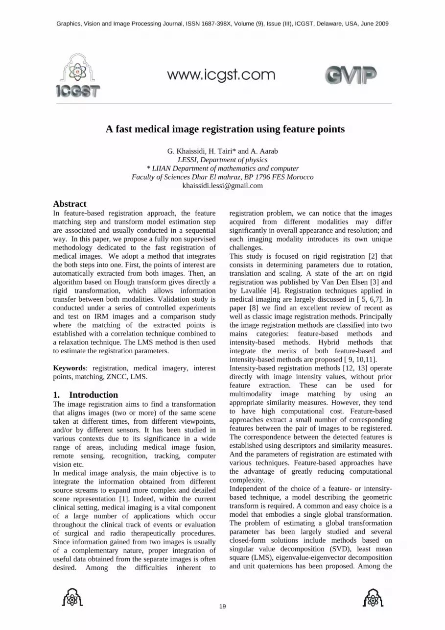
Figure (1): interest points detected, in source image (left) and in

destination image (Right).

Interest point is the most well-known and widely used method for analysis image thanks to the corresponding information which is more reliable than contours and no chaining operation is request. They are also robust to occlusion and other content changes. Their extraction is principally performed with the Harris detector. Indeed, the evaluation of interest point detectors presented in [16, 17] prove its excellent performance compared to other existing

approaches. In spite of its high computational cost, it is robust with respect to the geometrical transformations (rotation, translation), illumination variation and image noise [18, 19]. The Harris detector is based on the auto-correlation matrix which is often used for feature detection or for local image structures description and on the parameter adjustment that permit to choose the number of interest points so as to find a compromise between a good image representation and the time computing not penalizing. In figure (1) we give an illustration of interest points detection for the both images to be aligned. 2.2. Model estimation As we assume that the type of transformation is rigid and not deformable, the model that describes the geometric transformation has the following expression:

TpRP sd += * Where,

sp ),( yx is a source point

dp )','( yx its transformed corresponding point

11 12

21 22

R RR

R R⎛ ⎞

= ⎜ ⎟⎝ ⎠

is a rotation matrix

⎟⎟⎠

⎞⎜⎜⎝

⎛=

y

x

TT

T is a translation vector.

2.3. The Hough transform-based approach A feature matching between images constitutes a fundamental step in many computer vision applications such as the recovery of 3D scene structures, the detection of moving objects, or the synthesis image, registration image [20]. The matching is usually a critical and time consuming step. To overcome this problem, we apply the Hough transform-based approach. This approach is inspired by the works from the fingerprint recognition literature where a Hough transform technique has been used to align minutia in both images that have complex intensity distributions [21]. From their works, we learned an important aspect that would be beneficial when used in image registration. This approach converts point matching to the problem of detecting peaks in Hough space of transformation parameters. It performs under a discretization of the parameter space and an accumulation of evidence in the discretized space. Transformation parameters that relate two set of points feature is then derived. The alignment of the two images requires displacement in x and y and rotation θ to be recovered. Likely the scale transformation S must to be considered when the resolution of two images may vary due to the sensing system operating at different resolution. The estimation of registration parameters is performed with the following procedure:


20

1-We define a four array M whose components are the discretized parameters ),,,( STyTx θ

[ ] [ ][ ] [ ]dc

ba

SSS

TyTyTyTxTxTx

,..., , ,...,

,,..., , ,...,

11

11

∈∈

∈∈

θθθ

And we set the lists: { }snss ppL ...1= , { }dmdd ppL ...1=

where m and n are the number of interest points in source image S and destination image D respectively. 2- For each [ ] ,..., 1 cθθθ ∈ , for each

[ ]dSSS ,..., 1∈ While the lists Ls and Ld are not empty, we compute the displacement Tx and Ty from the equation:

⎥⎦

⎤⎢⎣

⎡⎟⎟⎠

⎞⎜⎜⎝

⎛ −−⎥

⎦

⎤⎢⎣

⎡=⎥

⎦

⎤⎢⎣

⎡

si

si

dj

dj

yx

Syx

TyTx

θθθθ

cossinsincos

''

ji TyTx , = the nearest values of TyTx,

belong to the array M [ ] [ ] 1,,,,,, += STyTxMSTyTxM θθ

3- At the end of accumulation process, the best alignment transformation ),,,( **** STyTx Δθ is obtained as

[ ]STyTxMSTyTx Δ=Δ ,,,maxarg),,,( **** θθ This procedure is schematically shown in figure (2)

Figure (2): The procedure of Hough transform

3. Experiments In this section first we present result related a series of controlled experiments and a test of IRM real images. Then we present a study comparison with a usual registration method. 3.1. Controlled experiments First of all, an analysis of several controlled simulations, embodying mixtures of registration transformation parameters and perturbation of images with noise, was carried out to determine the robustness, accuracy, and efficiency of the proposed registration algorithm. The simulation considers a pair of brain images one which is used as the fixed image and the second image permit to obtain a simulated destination image from a known transform with controlled parameters. The two images are originally registered, and the size of the images is 512x512. First, we study the invariance properties of our method to translation, scaling, and rotation. For that we vary only the value of one parameter at once. In each simulation, we generate randomly 50 simulated moving images. Then we apply registration algorithm to align the fixed image with each simulated destination image respectively. Since we know the ground truth transformation that was used to simulate each moving image, we can compare these ground truth with the recovered transformation parameters by our method. Working on the basis the average value of data deriving from simulation over the controlled experiments two statistical performance measures are useful: The Percentage of correctness (C): We consider the recovered transformation correct if its difference from the ground truth is less than a pre-defined error threshold. Here, the adopted threshold according to the registration parameters is: (the scaling errors es < 0.05, rotation angle errors eθ < 5 degrees, translation errors etx <M/50, and translation errors ety <N/50, where [M,N] is the image size). The average execution time (t): For one trial of registering a pair of fixed and moving images. Our method is implemented in Matlab using a computer (Pentium IV, 2.00GHZ, 256Mo). The results are listed in Table 1. It shows that the variation of registration error remains slight for different controlled values. It reflects the accuracy and convergence property of our registration method.

Controlled parameters Performance measures

T S R C t(s) Δx=15 Δy=15

[0.5, 1.5]. θ=0 98% 0,813

Δx=15 Δy=15

s = 1 [− π/ 2,π /2] 100% 0,863

[−50,50] s = 1 θ=0 100% 0,786 [−50,50] [0.5, 1.5] [− π/ 2,π /2] 94% 0,978

Table 1: Quantitative validation of the invariance properties of the method.


21

In the other hand, we study the robustness of the method to image noise. Then we generate test moving images by adding different levels of Gaussian noise to the original image, and transforming the noise corrupted images according to random transformations. The adopted Gaussian noise has zero mean with standard deviation λ. In Table 2, we show the summarized results for the performance measures described previously. The transformation parameters vary in the same ranges as in the first controlled experiment. From the results, one can see that, the method is quite robust to high levels of noise. This is partly due to the stability of the Harris detector.

parameters Performance measures Translation Δx=15,Δy=5

Error [θ,S, Δx, Δy]

Time Rotation θ=25 Scaling S=1 range of λ 0.01 [0, 0, 0, 0 ] 4.299013 s 0.02 [0, 0, 0, 0 ] 4.460801 s 0.03 [0, 0, 0, 0 ] 5.704416 s 0.04 [3, 0, 5, 0] 5.912439 s Table 2: Quantitative simulation study of the performance of the

method when images are corrupted by different levels of Gaussian noise.

3.2. Comparative study The proposed method has been compared to a usual geometrical method of registration that passes by a preliminary matching stage as we have proposed in [22]. The procedure consists of the matching of the extracted point features and the estimation registration parameters. First we search to establish correspondences between two sets of features under the optimization of a criterion measuring the similarity between two images. The choice of the similarity measure is determinant for both the accuracy and the robustness of the algorithm. As the considered features are the points, the matching procedure is established with the correlation criterion ZNCC (Zero mean Normalized Cross Correlation). It begin by taking out a candidate in the list of extracted point related to source image and determining its corresponding in the destination image dI which minimise the (ZNCC). The algorithm terminates with a completed matching once the list is empty. The matching procedure is improved with the relaxation technique [23]. After the matching step, the least mean square technique is used to determine the transformation that aligns the matched feature points. This method is described in [24], [25] and improved in [26].

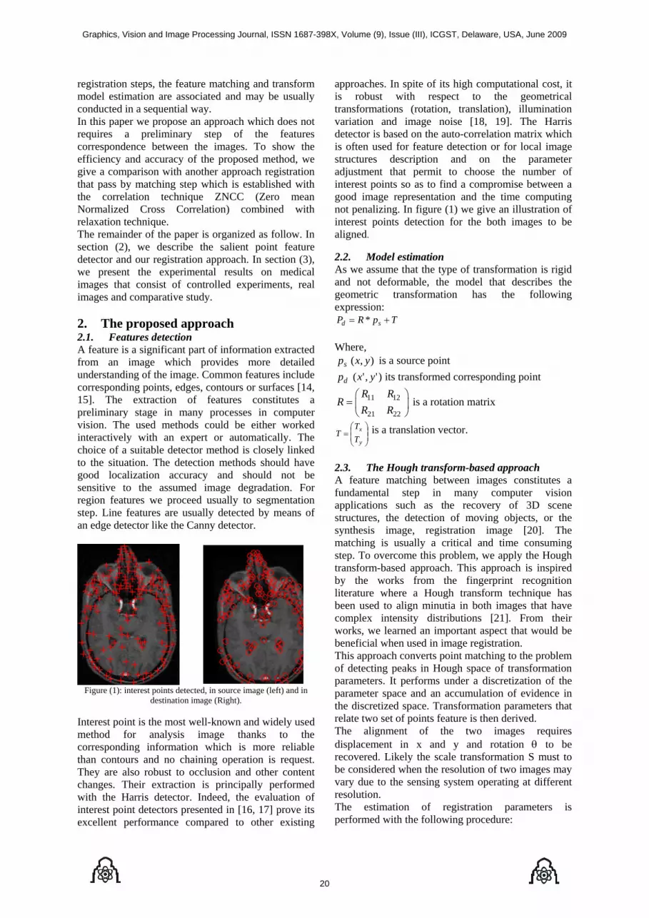
Figure 3: the matching algorithm. Top left: interest points detected in source image. Top right: interest points detected in destination

image. Bottom left: the corresponding features pairs by the technique of correlation ZNCC. Bottom right: the corresponding

features after application of rectification

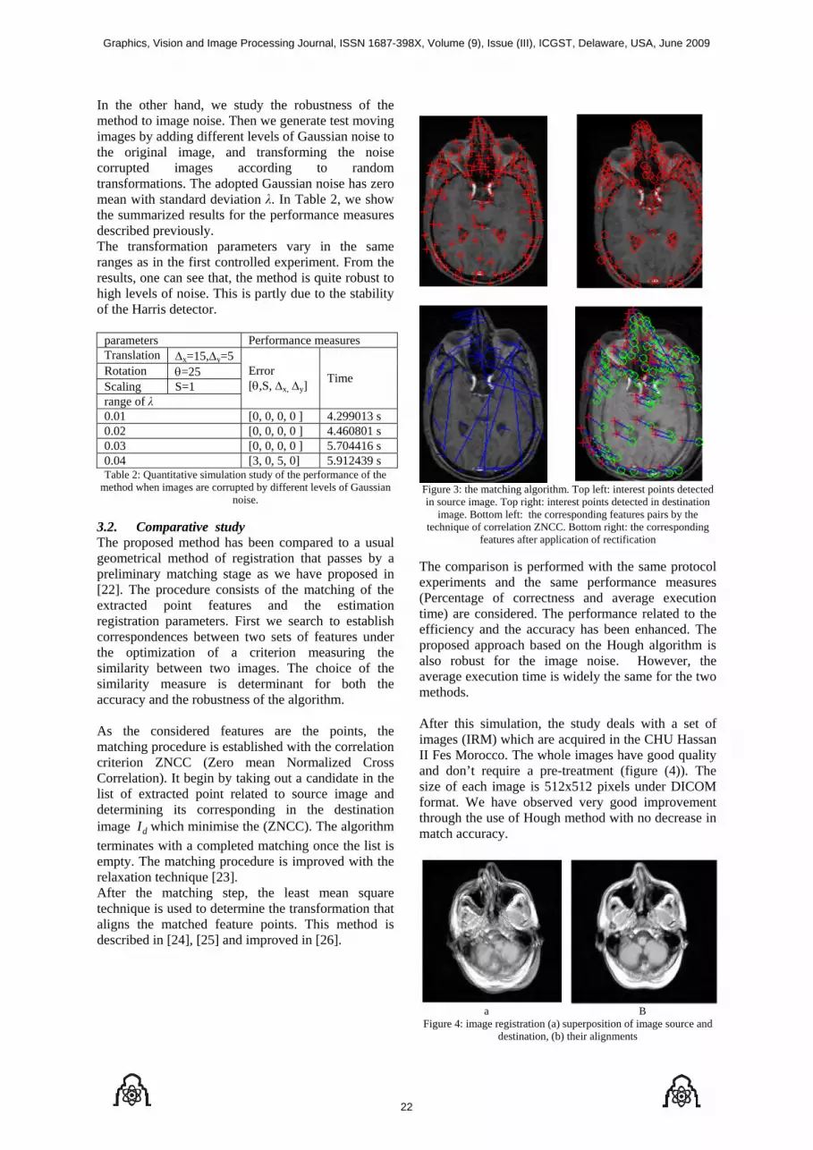
The comparison is performed with the same protocol experiments and the same performance measures (Percentage of correctness and average execution time) are considered. The performance related to the efficiency and the accuracy has been enhanced. The proposed approach based on the Hough algorithm is also robust for the image noise. However, the average execution time is widely the same for the two methods. After this simulation, the study deals with a set of images (IRM) which are acquired in the CHU Hassan II Fes Morocco. The whole images have good quality and don’t require a pre-treatment (figure (4)). The size of each image is 512x512 pixels under DICOM format. We have observed very good improvement through the use of Hough method with no decrease in match accuracy.

a B Figure 4: image registration (a) superposition of image source and

destination, (b) their alignments


22

4. Conclusion A new technique for a registration medical image based Hough algorithm has been presented. The technique decomposes the estimation parameters only in two steps: a detection of point feature and a voting process. It performs medical image without a matching features step. The preliminary results, in particular, showed that the proposed method has excellent robustness to image noise. It is also efficient because it exploits strict global geometric constraints. Other classical registration methods usually search the best matched points for the both images and past it into the estimation parameters algorithms. When the best matching field cannot satisfy the medical image requirement, those methods cannot provide the best efficiency. Compared with a method that belongs to this category approach which requires in addition a optimisation step, our approach does not only maintain the same efficiency, but also leads to the best cost calculation. References [1]. N. Y. El-Zehiry and R. Fahmi ‘Level Set Method

In Medical Imaging: An overview’ ICGST International Journal on Graphics, Vision and Image Processing, GVIP 06(Special Issue on Medical Image Processing): pp 15-29, December 2005.

[2]. G. L. Brown ‘A survey of image registration technique’, ACM Computing Surveys, pp 325-376, 1992.

[3]. P. A. Van Den Elsen, E. J. D. Pol, and M. A. Viergever ‘Medical image matching - a review with classification’, IEEE Engineering in Medicine and Biology, 12(4): pp 26-39, March 1993.

[4]. S. Lavallée ‘Registration for computer integrated surgery: methodology, state of the art’, In R. Taylor, S. Lavallée, G. Burdea, and R. Moesges, editors, Computer Integrated Surgery, MIT Press, pp 77-97, 1995.

[5]. D.L.G. Hill, P.G. Batchelor, M. Holden, D.J. Hawkes, Medical image registration, Physics in Medicine and Biology 46, R1–R45, 2001.

[6]. H. Lester, S.R. Arridge, A survey of hierarchical non-linear medical image registration, Pattern Recognition 32, pp 129–149, 1999.

[7]. J.B.A. Maintz, M.A. Viergever, A survey of medical image registration, Medical Image Analysis 2 (1998) 1–36

[8]. B. Zitovà, J. Flusser ‘Image registration methods: a survey’, Image and Vision Computing 21 pp 977–1000, 2003

[9]. D. Shen and C. Davatzikos ‘HAMMER: Hierarchical attribute matching mechanism for elastic registration’, IEEE Transactions on Medical Imaging, 21(11): pp 1421–1439, 2002.

[10]. T. Hartkens, D. L. Hill, A. D. Castellano-Smith, D. J. Hawkes, C. R. Maurer, A. J. Martin, W. A. Hall, H. Liu, and C. L. Truwit ‘Using points and

surfaces to improve voxel-based non rigid registration’, In Proc. of International Conf. on Medical Imaging Computing and Computer-Assisted Intervention, pp 565–572, 2002.

[11]. Y. Keller and A. Averbuch. ‘Implicit similarity: A new approach to multi-sensor image registration’, In Proc. of IEEE Conf. on Computer Vision and Pattern Recognition, pp 543–548, 2003.

[12]. P. Viola and W. Wells ‘Alignment by Maximization of Mutual Information’, In Proc. of IEEE International Conf. On Computer Vision, pp 16–23, 1995.

[13]. A. Collignon, F. Maes, D. Vandermeulen, P. Suetens, and G. Marchal. ‘Automated multimodality image registration using information theory’, In Proc. of Information Processing in Medical Imaging, pp 263–274, 1995.

[14]. A. Can, C. V. Stewart, B. Roysam, and H. L. Tanenbaum ‘A feature-based, robust, hierarchical algorithm for registering pairs of images of the curved human retina’, IEEE Transactions on Pattern Analysis and Machine Intelligence, 24(3): pp 347–364, 2002.

[15]. C. R. Maurer, R. J. Maciunas, and J. M. Fitzpatrick ‘Registration of head CT images to physical space using a weighted combination of points and surfaces’, IEEE Transactions on Medical Imaging, 17(5): pp 753–761, 1998.

[16]. C. Schmid, R. Mohr, and Bauckhage, ‘Comparing and evaluating interest points’, In IEEE Int. conf. on Computer Vision, pp 230-235, 1998.

[17]. K. Mikolajczyk and C. Schmid ‘Scale & Affine Invariant Interest Point Detectors’, International Journal of Computer Vision, 60(1): pp 63–86, 2004.

[18]. C. Harris and M. Stephens ‘A combined corner and edge detector’, In Proceedings of the 4th Alvey Vision Conf. , pp 147-151, 1988.

[19]. C. Schmid, R. Mohr, and C. Bauckhage ‘Evaluation of interest point detectors’, International Journal of Computer Vision, 37(2): pp 151–172, June 2000.

[20]. P. van den Elsen, A. J. B. Maintz, E. J. D. Pol, and M. A. Viergever ‘Automatic Registration of CT and MR Brain Images using Correlation of Geometrical Features’, IEEE Trans. on Medical Imaging, 14(2): pp 384-396, June 1995.

[21]. Ratha N.K., Karu K., Chen S and Jain A.K. ‘A real time matching system for large fingerprint databases’ IEE Transaction on Pattern Analysis and Machine Intelligence, Vol 18, pp. 799-813, 1996.

[22]. G. Khaissidi, M. Karoud, H. Tairi and A. Aarab ‘Medical Image Registration using Regions Matching with Invariant Geometrical Moments’ ICGST International Journal on Graphics, Vision


23

and Image Processing, GVIP, 08(2): pp 15-20, 2008.

[23]. A. Saaidi, H. Tairi and K. Satori ‘Fast Stereo Matching Using Rectification and Correlation technique’, Proceedings ISCCSP, Marrakech, Morocco, pp 13-15 March 2006.

[24]. K. S. Arun, T. S. Huang et S. D. Blostein. Least-Squares Fitting of Two 3-D Point Sets. IEEE Trans. Patt. Anal. Mach. Intell., vol. 9, no. 5, pp. 698-700, 1987.

[25]. R. M. Haralick, H. Joo, C. Lee, X. Zhuang, V. G. Vaidya et M. B. Kim. Pose Estimation from Corresponding Point Data. IEEE Trans. Syst. Man. Cybern., vol. 19, no. 6, pp. 1426-1446, 1989.

[26]. S. Umeyama. Least-Squares Estimation of Transformation Parameters Between Two Point Patterns. IEEE Trans. Patt. Anal. Mach. Intell., vol. 13, no. 4, pp. 376-380, 1991.

Biographies Ghizlane Khaissidi received his Master’s degree in 2004 from faculty of sciences and techniques (FST) Fes MORROCO. She is pursuing his Ph.D. degree. His doctoral study focused on registration and fusion in medical imagery. Hamid Tairi received the PhD degree from USMBA-Fez University in 2001. He is currently a professor of computer science at USMBA-Fez University. His is also a member of the LIIAN Laboratory. His research interests include image processing, biomedical, Image-based rendering, visual tracking for robotic control

and 3D reconstruction.

Abdellah Aarab is Professor at the Faculty of Sciences, Fes Morocco. He received his "Doctorat de 3ième cycle" degree from the University of Pau, France in 1982 and "Thèse d'Etat" degree in 1999 from university Sidi Mohamed Ben Abdellah Fes Morocco.

His research areas include, image processing, information retrieval and industrial applications.


24

Removal of Speckle Noise from Ultrasound Medical Image based on Special

Filters: Comparative Study

K. Thangavel *1, R. Manavalan**, I. Laurence Aroquiaraj*2 *. Department of Computer Science, Periyar University, Salem – 636 011, Tamil Nadu, India.

Email: 1 [email protected], 2 [email protected] ** Department of Computer Science and Application. K.S.R. College of Arts and Science,

Tiruchengode – 637 209, Tamil Nadu, India. Email: [email protected]

Abstract Removing noise from the original image is still a challenging research in image processing. Generally there is no common enhancement approach for noise reduction. Several approaches have been introduced and each has its own assumption, advantages and disadvantages. The speckle noise is commonly found in the ultrasound medical images. This paper proposes different filtering techniques based on statistical methods for the removal of speckle noise. A number of success full experiments validate the proposed filtering model. The quality of the enhanced images is measured by the statistical quantity measures: Signal-to-Noise Ratio (SNR), Peak Signal-to-Noise Ratio (PSNR), and Root Mean Square Error (RMSE). Keywords: Ultrasound Image, Prostate, Speckle Noise, SNR, PSNR, RMSE 1. Introduction Digital image plays a vital role in the early detection of cancers, such as prostate cancer, breast cancer, lungs cancer, cervical cancer and blood cancer. Prostate cancer is now most frequently diagnosed male malignancy with one in every 11 men. It is the second position in cancer–related cause of death only for male population. Ultrasound imaging method is suitable to diagnose and progenies [1]. The accurate detection of region of interest in ultrasound image is crucial. Since the result of reflection, refraction and deflection of ultrasound waves from different types of tissues with different acoustic impedance. Usually, the contrast in ultrasound image is very low and boundary between region of interest and background are fuzzy [2]. And also speckle noise and weak edges make the image difficult to identify the prostate region in the ultrasound image. So the analysis of ultrasound image is more challenging one. Noise is considered to be any measurement that is not part of the phenomena of interest. Images are prone to different types of noises. Departure of ideal signal is generally referred to as noise. Noise arises as a result

of unmodelled or unmodellable [3]. Processes going on in the production and capture of real signal. It is not part of the ideal signal and may be caused by a wide range of sources, for instance, variation in the detector sensitivity, environmental variations, the discrete nature of radiation, transmission or quantization errors, etc. It is also possible to treat irrelevant scene details as if they are image noises, for example, surface reflectance textures. Ultrasound medical imaging is commonly used to diagnosis the prostate cancer. Generally there are two common use of ultrasound medical imaging: first one is to guide the doctor in the biopsy procedure and second is in the establishing the volume of the prostate. It has been used in diagnosing for more than 50 years. The ultrasound imaging technique is nowadays outstands position among modern imaging techniques. The operating principle of ultrasound imaging is provided [4]. This paper is organized as follows: Section 2 describes problem description of denoising in ultrasound image. Section 3 discusses the various spatial filtering techniques for denoising the speckle noise in the ultrasound medical image. Section 4 proposes filtering techniques for speckle noise removal. Section 5 discusses experimental analysis and discussion. Section 6 concludes this paper and provides direction for further research. 2. Problem Description An image may be defined as a two dimensional function f(x, y), where x and y are spatial (plane) coordinates, and the amplitude of f at any pair of co-ordinates (x, y) is called the intensity or grey level of the image at that point [5]. Data sets collected by image sensor are generally contaminated by noise. The region of interest in the image can be degraded by the impact of imperfect instrument, the problem with data acquisition process and interfering natural phenomena. Therefore the original image may not be suitable for applying image processing techniques and analysis. Thus image enhancement technique is often necessary and should be taken as the first and foremost step before image is


25

processed and analyzed. An efficient filtering method is necessary for removing noise in the images. The noise removal in the image is still a challenging problem for researcher because noise removal introduces artifacts and causes blurring of the image. Noise modeling in images is affected by capturing instrument, data transmission media, image quantization and discrete source of radiation. There is no unique technique for image enhancement. Different algorithms are used depending on the noise model. Gaussian noise (Random additive) is observed in natural images, speckle noise [6] is observed in ultrasound images where as rician noise [7] affects Magnetic Resonance Image (MRI). The characteristics of noise depend on its source, as does the operator which reduces its effects. Many image processing packages contains operators to artificially add noise to an image. Deliberately corrupting an image with noise allows us to test the resistance of an image processing operator to noise and assess the performance of various noise filters. Noise is generally grouped into two categories viz., image independent noise and image data dependent noise. These noises are discussed in the following sequel. 2.1 Image Data Independent Noise It is described by an additive noise model, where the recorded image, i(m, n) is the sum of the true image t(m, n) and the noise n(m, n)[5, 8, 9] i(m,n)=t(m,n)+n(m,n) The noise n(m, n) is often zero-mean and described by its variance σn

2 . In fact, the impact of the noise on the image is often described by the SNR [6], which is given by

2

2 1i

n

SNR σσ

= − (1)

Where, σt

2 and σn2 are the variances of the true image and

the recorded image respectively. In many cases, additive noise is evenly distributed over the frequency domain (white noise), whereas an image contains mostly low frequency information. Therefore, such a noise is dominant for high frequencies and is generally referred as Gaussian noise and it is observed in natural images [10, 11]. 2.2 Image Data Dependent Noise Data-dependent noise (e.g. arising when monochromatic radiation is scattered from a surface whose roughness is of the order of a wavelength, causing wave interference which results in image speckle), it is possible to model noise with a multiplicative, or non-linear, model. These models are mathematically more complicated; hence, if possible, the noise is assumed to be data independent. 2.2.1 Detector Noise This is other kind of Gaussian noise, which occurs in all recorded images to a certain extent, detector noise and it is due to the discrete nature of radiation that is the fact that each imaging system is recording an image by counting photons. Allowing some assumptions (which are valid for many applications) this noise can be modeled with an independent, additive model, where the

noise has a zero-mean Gaussian distribution described by its standard deviation (σ) or variance [12]. This means that each pixel in the noisy image is the sum of the true pixel value and a random, Gaussian distributed noise value. 2.2.2 Speckle Noise Another common form of noise is data dropout noise generally referred to as speckle noise. This noise is, in fact, caused by errors in data transmission [13, 14]. The corrupted pixels are either set to the maximum value, which is something like a snow in image or have single bits flipped over. This kind of noise affects the ultrasound images [14]. Speckle noise has the characteristic of multiplicative noise [15]. Speckle noise follows a gamma distribution and is given as

1

( )( 1)!

ga

gF ga e

∝−−

∝

⎡ ⎤= ⎢ ⎥∝ −⎣ ⎦

(2)

Where, variance is a2 α and g is the gray level. 2.2.3 Salt and Pepper Noise This type of noise is also caused by errors in data transmission and is a special case of data dropout noise when in some cases single, single pixels are set alternatively to zero or to the maximum value, giving the image a salt and pepper like appearance [16]. Unaffected pixels always remain unchanged. The noise is usually quantified by the percentage of pixels which are corrupted. It is found in mammogram images [17]. It probability distribution of function is in [8]. 2.2.4 Poisson Noise This type of noise is caused by the nonlinear response of the image detectors and recorders. Here the image data dependent (signal dependent) term arises because detection and recording processes involve random electron emission having a Poisson distribution with a mean response value [18]. Since the mean and variance of a Poisson distribution are equal, the signal dependent term has a standard deviation if it is assumed that the noise has a unity variance. This noise causes the natural images [10, 11]. The number of observed occurrences fluctuates about its mean μ with a standard deviation σ. These fluctuations are denoted as Poisson noise or as shot noise. Poisson noise follows a Poisson distribution [8]. 3. Spatial Filter The primary objective of the image enhancement is to adjust the digital image so that the resultant image is more suitable than the original image for a specific application [5, 8, and 9]. There are many image enhancement techniques. They can be categorized into two general categories. The first category is based on the direct manipulation of pixels in an image, for instance: image negative, low pass filter (smoothing), and high pass filter (sharpening). Second category is based on the position manipulation of pixels of an image, for instance image scaling.


26

In the first category, the image processing function in a spatial domain can be expressed as

( , y) T (f(x, y))g x = (3) Where, T is the transformation function, f (x, y) is the pixel value of input image, and g(x, y) is the pixel value of the processed image [5, 8, 9]. The median, mean, high pass, low pass filtering techniques have been applied for denoising the different images [5, 9]. 4. Proposed Filtering Techniques 4.1. Max Filter The max filter plays a key role in low level image processing and vision. It is identical to the mathematical morphological operation: dilation [19]. The brightest pixel gray level values are identified by this filter. It has been applied by many researchers to remove pepper noise. Though it removes the pepper noise it also removes the block pixel in the border [5]. This filter has not yet applied to remove the speckle in the ultrasound medical image. Hence it is proposed for speckle noise removal from the ultrasound medical image. it is expressed as:

{ }( , )

( , ) max ( , )xys t S

f x y g s t∈

= (4)

It reduces the intensity variation between adjacent pixels. Implementation of this method for smoothing images is easy and also reducing the amount of intensity variation between one pixel and the next. The result of this filter is the max selection processing in the sub image area SXY. 4.2. Min Filter The min filter plays a significant role in image processing and vision. It is equivalent to mathematical morphological operation: erosion [19]. It recognizes the darkest pixels gray value and retains it by performing min operation. This filter was proposed for removing the salt noise from the image by researchers. Salt noise has very high values in images. The operation of this filter can be expressed as:

{ }( , )

( , ) min ( , )xys t S

f x y g s t∈

= (5)

It removes noise better than max filter but it removed some white points around the border of the region of the interest [5]. In this filter each output pixel value can be calculated by selecting minimum gray level value of the chosen classical window SXY. 4.3. Harmonic Mean Filter The harmonic mean filter is a nonlinear filtering technique for image enhancement. The harmonic mean filter is member of a set of nonlinear mean filters, which are better at removing Gaussian type noise and preserving edge features than the arithmetic mean filter. The harmonic mean filter is very good at removing positive outliers. The definition of harmonic mean filter is provided as:

( , )

( , ) 1( , )xys t S

mnf x y

g s t∈

=∑

(6)

The Harmonic mean filter is more suitable for salt noise removal but it fails to remove the pepper noise. It also removes other types of noise like Gaussian noise [5]. Each output pixel value is computed by dividing the size of the image with the sum of reciprocal of each pixel in the classical window Sxy. 4.4. Contra harmonic Mean Filter The contra-harmonic mean filter is nonlinear filtering method. The contra-harmonic mean filter is member of a set of nonlinear mean filters, which are better at removing Gaussian type noise and preserving edge features than the arithmetic mean filter. The contra-harmonic filter is very good at removing positive outliers for negative values of Q and negative outliers for positive values of Q. The contra harmonic mean [5] filter operation is given by the expression

1

( , )

( , )

( , )( , )

( , )xy

xy

Q

s t S

Q

s t S

g s tf x y

g s t

+

∈

∈

=∑

∑ (7)

Where, Q is called the order of the filter. This filter is well suited for reducing or virtually eliminating the effects of salt-and-pepper noise. It is well suitable for impulse noise [20] removal but it has disadvantage if the noise is dark or light in order to select the proper value for Q. 4.5. Geometric Mean Filter For the gray level of pixel (x, y) in g, the Geometric filter replaces the gray level f(x, y) by taking into account the surrounding detail and attenuating the noise by lowering the variance. This filter is known as smoothing spatial filters, with the median and geometric mean filters outperforming the arithmetic mean filter in reducing noise while preserving edge details. Increasing neighborhood size, n, results in higher noise attenuation, but also loss of edge detail. For further details on spatial filters and in-depth explanations see [5]. The geometric mean filter is member of a set of nonlinear mean filters, which are better at removing Gaussian type noise and preserving edge features than the arithmetic mean filter. The geometric mean filter is very susceptible to negative outliers. The geometric mean filter is defined as:

1

( , )

( , ) ( , )mn

xys t S

f x y g s t∈

⎡ ⎤= ⎢ ⎥⎢ ⎥⎣ ⎦∏ (8)

It is not suitable for removing impulse noise in the image [5]. Each output pixel is given by the product of the pixels in the subimage window and raised to the power 1/mn. Where m is number of rows in the image and n is number of columns in the image. It is better than mean filter in smoothing but it tends to lose less image detail in


27

the process [5]. Geometric mean filter did not blur the image as much as mean filter. It is suitable for Gaussian noise. The output of each pixel is calculated by the power of reciprocal of the image size of the product of all pixels values in the classical window SXY.

4.6. Midpoint Filter The midpoint filter [5] simply computes the midpoint between the maximum and minimum values in the area encompassed by the filter:

{ } { }( , )( , )

1( , ) max ( , ) min ( , )2 xyxy s t Ss t S

f x y g s t g s t∈∈

⎡ ⎤= +⎢ ⎥⎣ ⎦ (9)

This filter works best for randomly distributed noise, like Gaussian or uniform noise. It combines order statistics and averaging [5]. The Midpoint filter blurs the image by replacing each pixel with the average of the highest pixel and the lowest pixel (with respect to intensity) within the specified window size. Midpoint filter, however, is not robust against impulse noise. And it fails to retain the image boundaries.

Midpoint smoother is a nonlinear point estimator based on order-statistics [21]. Indeed, it has been proven to be the optimal L-filter for smoothing the images contaminated with noise having uniform probability density function [22]. Midpoint filter, however, is not robust against impulse noise and fails to retain the image boundaries [23]. The filtering scheme that removes uniform noise with edge preservation properties.

4.7. High Boots Filter High boost filter highlights the high frequency content of the image along with low frequency information [5]. High boost = ( A - 1) original image + high pass It amplified version of the original image with the removal of low frequency content of the image given. It restores the original background detail and enhances the sharpness of the image. The high boost filter operation is given by the expression

( , ) ( , ) ( , ) ( , )( 1) ( , ) ( , )

hb S

S

f x y A f x y f x y f x yA f x y f x y

= ∗ − −= − ∗ −

(10)

Where, A is high boost coefficient. It increases average gray level of the image. Thus it helps to improve the brightness of the image. This filter becomes standard high pass when A is one. If A is greater than one, the high boost image will become approximately equal to the original image multiplied by a constant. 4.8. Trace median Filter Trace median of an n x n subimage is defined to be the sort of the pixel gray values on the main diagonal of the subimage and pick up middle term. The trace median filter has not yet introduced by researchers for speckle noise removal from the ultrasound medical images. Trace median filter reduces the dimensionality of the problem for N*N Pixels in each sub image into N where N is number of elements in diagonal. It is expressed as

{ }( , )

( , ) ( , )xys t S

f x y Tracmedian g s t∈

= (11)

This filter covers all the rows and columns of the image and reduces the dimensionality. And it does not involves more computation when compare with other. It calculates the trace median for each subimage and assigns this value into center pixel in the output image. 4.9. Trace means Filter Trace mean of an n x n subimage is defined to be the sum of the pixel gray values on the main diagonal of the subimage and divided it by total number of diagonal pixels in the subimage. Still trace mean filter not yet introduced by researchers for speckle noise removal from the ultrasound medical images. Trace mean filter reduces the dimensionality of the problem for N*N Pixels in each sub image into N where N is number of elements in diagonal [23]. It is defined as

{ }( , )

( , ) ace ( , )xys t S

f x y Tr mean g s t∈

= (12)

This filter covers all the rows and columns of the image and reduces the dimensionality. And it does not involves more computation when compare with other [24]. It calculates the trace mean for each subimage and assigns this value into center pixel in the output image. 4.10. Standard Deviation Filter Normally the interpretations of the images are quite difficult, since the backscatter causes the unwanted noise. The standard deviation was proposed to remove the noise in radar satellite images [2]. This filter has not proposed to remove the speckle noise from the ultrasound medical images to the best of our knowledge. The standard deviation filter [5] calculates the standard deviation for each group of pixels in the subimage, and assigns this value to the center pixel in the output image. By using a standard deviation filter, we are able to recognize some patterns. It is expressed as

22

1 1

1 ( )n n

w rcr c

S x xn = =

= −∑∑ (13)

Where, n x n is the total number of pixels in a subimage, w denotes the indices of the subimage, xrc is the value of the pixel at row r and column c in the subimage and x is the mean of pixel values in the window. It measures of heterogeneity in the subimage at centered over each pixel. Standard deviation filter is applied to detect the changes in subimages [5]. A small mask was used for the filter in order to obtain sharp edges. A size of 3x3 pixels was supposed to be sufficient. The filter generates a new image based on the value of the standard deviation. 4.11. Variance Filter The variance filter has been applied to highlight the edges in the X-ray and CT images of normal brain. For clarity some regions are made transparent while the significant details can be easily seen [25].The variance


28

filter makes areas of changing reflectance appear brighter than relatively uniform areas which appear darker the more uniform they are. It provides a measure of local homogeneity of the intensities in an image, can also be regarded as a non-linear non-directional edge detector [21, 26]. The variance filter involves replacing a central pixel value with the variance of a specified set of pixel values surrounding it in a window on the image, which does not need to be square. This filter is defined as

2

21 1

1 ( )n n

w rcr c

v x xn

−

= =

= −∑∑ (14)

Where, 21 1

1 n n

rcr c

x xn = =

= ∑∑ (15)

and n x n is the total number of pixels in the subimage, w is the indices of the subimages, xrc is the value of the pixel at row r and column c in the subimages and x is the mean of pixel values in the window. 4.12. Correlation Filter Consider 3 x 3 window as correlation kernel h. The kernel h is used as mask. And also consider image kernel S of order 3 x 3. The correlation of each pixel is computed as the sum of the product of corresponding pixel values in the mask h and image kernel S. 4.13. M3- Filter The M3-Filter is proposed with hybridization of mean and median filter. This replaces the central pixel by the maximum value of mean and median for each subimages SXY. It is expressed as M3-Filter, the intensity values are reduced in the adjacent pixel and it preserves the high frequency components in image. Therefore it may be suitable for denoising the speckle noise in the ultrasound medical image. It is a simple, intuitive and easy to implement method of smoothing images.

{ } { }( , ) ( , )

( , ) max( ( , ) , ( , ) )xy xys t S s t S

f x y median g s t mean g s t∈ ∈

= (16)

5. Experimental Analysis and Discussion The proposed algorithms have been implemented using MATLAB. The performance of various spatial enhancement approaches are analyzed and discussed. The measurement of image enhancement is difficult to measure. There is no common algorithm for the enhancement of the image. The statistical measurement could be used to measure enhancement of the image. The Root Mean Square Error (RMSE), Signal-to-Noise Ratio (SNR), and Peak Signal-to-Noise Ratio (PSNR) are used to evaluate the enhancement performance [13]. The noise level is measured by the standard deviation of the image:

21 ( ) ,ib bN

σ = −∑ (17)

Where, i=1,2,3,…,N , b is the mean gray level value of the original image and bi is the gray level value of the surrounding region and N is the total number of pixel in

the image. The RMSE, SNR, and PSNR are provided in the table 1.

Table 1: Statistical Measurement Statistical

Measurement Formula

MSE

RMSE

SNR

PSNR

Here, f (i, j) is original image, F (i, j) is enhanced image, σ2 is variance of original image and σe

2 is variance of enhanced image. The original ultrasound image and filtered images of the prostate obtained by various filtering techniques are shown in figure 4.1. If the value of RMSE is low and the values of SNR and PSNR are larger then the enhancement approach is better. The table 2 shows the performance analysis of the proposed approaches and existing approaches with the regard to ultrasound medical images for prostate. It was observed from the figure 4.2 that the proposed M3-Filter removes the speckle noise better than other enhancement approaches.

0

20

40

60

80

100

120

140

160

1 2 3 4 5 6 7 8 9 10 11 12 13 14 15 16

FILTERING METHODS

RM

SE S

NR

PSN

R

RMSE

SNR

PSNR

Figure 4.2: Performance Analysis Chart 6. Conclusion The performance of noise removing algorithms is measured using quantitative performance measures such as PSNR, SNR, and RMSE as well as in term of visual quality of the images. Many of the methods fail to remove speckle noise present in the ultrasound medical image, since the information about the variance of the noise may not be identified by the methods. Performance of all algorithms is tested with ultrasound image regard to prostate. The computational result showed one of the proposed algorithms M3-Filter performed better than others.

MNjiFjif∑ − 2)),(),((

MNjiFjif∑ − 2)),(),((

2

2

10log10eσ

σ

RMSE255log20 10


29

ORIGINAL ULTRASOUND IMAGE OF PROSTATE

TRACE MEDIAN FILTER

MEDIAN FILTER

MEAN FILTER

MIN FILTER

MIN FILTER

M3-FILTER

STANDARD DEVIATION FILTER

VARIANCE FILTER

CORRELATION FILTER

LOW PASS FILTER

HIGH PASS FILTER

HIGH BOOST FILTER

HARMONIC MEAN FILTER

CONTRAHARMONIC MEAN FILTER

GEOMETRIC FILTER

TRACE MEAN FILTER

Figure 4.1: Output Images of the Filters


30

TABLE 2: Computational Results

S.NO FILTERING METHOD RMSE SNR PSNR

1 M3-Filter 27.04 1.24 19.49

2 Median Filter

27.11 1.03 19.47

3

Mean Filtering

27.69 1.82 19.29

4 Max filter

76.82 2.32 10.42

5 Min filter

69.64 6.73 11.27

6 Standard Deviation Filtering

89.40 25.75 9.10

7

Variance Filtering

141.23 10.47 5.13

8

Correlation Filter

143.19 11.59 5.01

9

Low pass Filter

128.44 9.02 5.96

10

High pass Filter

109.44 18.90 7.35

11

High Boots Filter

103.95 24.51 7.79

12

Harmonic Mean Filtering

114.86 96.92 6.93

13

Contra harmonic Mean Filtering

114.86 92.64 6.93

14

Geometric Filter

114.87 96.67 6.93

15 Trace mean Filter 114.91 148.31 6.92

16 Trace median filter 114.86 96.54 6.93

References [1] Yanong Zhu, Stuart Williams, Reyer Zwiggelaar,

Computer Technology in Detection and Staging of Prostate Carcinoma: A review, Medical image Analysis 10(2006),pp 178-199.

[2] J. G. Abbott and F. L. Thurstone, "Acoustic speckle: Theory and experimental analysis," Ultrason. Imag., vol. 1, pp. 303-324, 1979.

[3] Raman Maini, J.S.Sohal, Performance Evaluation of Prewitt Edge Detector for Noisy Images, GVIP Journal, Volume 6, Issue 3, December, 2006,pp 39-46.

[4] D Hykes, W.Hedrick and D.Starchman, Ultrasound Physics and Instrumentation, Churchill New York: Livingstone Inc., 1985

[5] R.C. Gonzalez and R.E. Woods: 'Digital Image Processing', Addison-Wesley Publishing company, 1992.

[6] Image Processing Fundamentals – Statistics, “Signal to Noise Ratio”, 2001.

[7] Robert D Nowak, “Wavelet based Rician noise Removal”, IEEE Transaction on image processing, Vol. 8, no. 10, PP 1480, October 1999.

[8] R.C. Gonzalez and R.E. Woods: 'Digital Image Processing', Addison-Wesley Publishing company, 1992.

[9] A.K. Jain, fundamental of digital image processing. Englewood cliffs, NJ Prentice-Hall, 1989.

[10] B. Zhang, J. M. Fadili, and J.-L. Starck “Wavelets, Ridgelets and Curvelets for Poisson Noise Removal” IEEE Transactions on Image Processing, 2007.

[11] Yunyi Yan and Baolong Guo. Application of Wavelet Neural Network (WNN) and Gradient Descent Method (GDM) in Natural Image Denoising. Journal of Computational Information Systems, 2(2):625–631, 2006.

[12] S.G. Chang, Y. Bin and M. Vetterli: 'Adaptive wavelet thresholding for image denoising and compression', IEEE Trans. On Image Processing, vol. 9, no.9, pp. 1532-1546, Sep 2006.

[13] L. Gagnon and F.D. Smaili: 'Speckle Noise Reduction of Airborne SAR Images with Symmetric Daubechies Wavelets', SPIE Proc. #2759, pp. 1424,1996.

[14] H. GUO, J E Odegard, M.Lang, R.A.Gopinath, I.W.Selesnick, and C.S. Burrus, “Wavelet based Speckle reduction with application to SAR based ATD/R”, First Int’I Conf. on image processing , vol. 1, pp. 75-79,Nov 1994.

[15] Langis Ganon “ Wavelet Filtering of Speckle Noise-Some Numerical Result,” Proceeding of the Conference Vision Interface 1999 , Trois-Riveres.

[16] Z. Wang and D. Hang, “Progressive Switching Median Filter for the Removal of Impulse Noise from Highly Corrupted Images," IEEE Trans. on Circuits and Systems-II: Analog and Digital Signal processing, vol. 46, no. 1, pp. 78-80 Jan. 1999.

[17] Scott E Umbaugh, Computer Vision and Image Processing, Prentice Hall PTR, New Jersey, 1998.


31

[18] K. Timmermann and R. Novak: 'Multiscale modeling and estimation of poisson processeswith applications to photon-limited imaging'. 1999.

[19] P. Soille, Mathematical image analysis: principles and applications, Springer- Verlag, 1999.

[20] G.A ASTIN, Adaptive filters for digital image noise smoothing, an evaluation, Comput. Vis. Graphics Image Process. 1985, 31, pp. 103-121.

[21] G.R.Arce and S.A.Fontana, "On the Midrange Estimator," IEEE Trans. Acoust., Speech and Signal Processing, vol.ASSP-36, no.6, pp.920-922, June 1988.

[22] A.C.Bovik, T.S.Huang and D.C.Munson, "A Generalisation of Median Filtering Using Linear Combinations of Order-Statistics," IEEE Trans. Acoust., Speech and Signal Processing, vol.ASSP-31, no.6, pp.1342-1349, Dec.1983.

[23] I.Pitas and A.N. Venetsanopoulos, Nonlinear Digital Filters: Principles and Applications. Boston, MA: Kluwer Academic, 1990.

[24] Y P Gowramma, Dr C N Ravikumar , Development of novel fast block based trace mean correspondence algorithm for face tracking , International Conference Advanced computing and communications ,2006 Proceedings, IEEE pp 263-266.

[25] E.D SELEPCHI , O.G DULIU “Image processing and data analysis in computed tomography” PP 665-675, Received September 12, 2006.

[26] Peter Lohmann Andreas KOCH, Michael SCHAEFFER “APPROACHES TO FILTERING OF LASER CANNER DATA” IAPRS, Vol. XXXIII, Amsterdam, 2000.

Dr. THANGAVEL KUTTIANNAN received the Master of Science from Department of Mathematics, Bharathidasan University in 1986, and Master of Computer Applications Degree from Madurai Kamaraj University,

India in 2001. He obtained his Ph. D. Degree from the Department of Mathematics, Gandhigram Rural University in 1999. He worked as Reader in the Department of Mathematics, Gandhigram Rural University, upto 2006. Currently he is working as Professor and Head, Department of Computer Science, Periyar University, Salem, Tamilnadu, India. His areas of interest include medical image processing, artificial intelligence, neural network, fuzzy logic, data mining, pattern recognition and mobile computing.

Mr. R. MANAVALAN Obtained M.Sc.,Computer Science from St.Joseph’s College of Bharathidasan University, Trichirappalli, Tamilnadu, India, in the year 1999, and M.Phil., in Computer Science from Manonmaniam Sundaranar University, Thirunelveli,

Tamilnadu, India in the year 2002. He works as Sr. Lecturer, in the Department of Computer Science and Applications, KSR College of Arts and Science, Thiruchengode, Nammakal, Tamilnadu, India. He pursues Ph.D in Medical Image Processing. His areas of interest are Medical image processing and analysis, soft computing, pattern recognition and Theory of Computation.

Mr. I. Laurence Aroquiaraj received the M.Sc.,Computer Science from Pondicherry University, Ponidicherry, India in 2002, M.Phil., degree from Manonmaniam University, India in 2003. He is working as Lecturer in Computer Science,

Periyar University, Salem, Tamilnadu, India. He is pursuing his Ph.D in Image Processing. His research interests includes image processing, biometrics and pattern recognition


32

An Algorithm for Improved Accuracy in Unimodal Biometric Systems through

Fusion of Multiple Feature Sets

C.Lakshmi Deepika1, A.Kandaswamy2

Department of Biomedical Engineering, PSG College of Technology, Coimbatore, TamilNadu, India [email protected], [email protected]

Abstract The major concern in a Biometric Identification System is its accuracy. In spite of the improvements in image acquisition and image processing techniques, the amount of research still being carried out in person verification and identification show that a recognition system which gives 0% FAR (False Acceptance Rate) and FRR (False Rejection Rate) is still not a reality. Multibiometric systems which combine two different biometric modalities or two different representations of the same biometric, to verify a person’s identity are a means of improving the accuracy of a biometric system. The former case however requires the user to produce his biometric identity two times to two different sensors. The image processing and pattern matching activities also increase nearly twofold compared to unimodal systems. In this paper we propose a fusion of two different feature sets, one extracted from the morphological features and the other from statistical features, of the same biometric template, namely the hand vein biometric. The proposed system gives the accuracy of a multimodal system at the speed and cost of a unimodal system.

Keywords: Biometrics, Vein, Minutia, Feature Vector, Fusion, FRR, FAR, Unimodal, Multimodal, Neural Network 1. Introduction Traditional methods of identity verification such as username and password, PIN numbers, are slowly being replaced by biometric verification methods. Face, Fingerprint, Hand Veins, Hand Geometry and Iris are popular physiological biometric modalities. Non-universality, Noise in Sensor Data, Reliability of sensor used, Limited discriminability, Upper bound in performance, Lack of Permanence and Spoofing are the limitations of a unimodal system which bring down its accuracy [1]. Face Recognition System is sensitive to Illumination, Pose, and Facial Accessories and can also be easily spoofed by a static photo / moving video. Fingerprint Recognition System suffers due to lack of information in the form of poor ridge details and is also

easily spoofed by imitations.[1] Damage of fingerprint is common for people who do lot of manual work. Hand Geometry is not very distinctive and cannot be used to identify an individual from a large population. [2]. The accuracy and speed of iris recognition systems are quite high; however the user participation and cost are also high. In spite of certain striking disadvantages, fingerprint is still widely used all over the world. Hence we developed an authentication system using fingerprint biometric. We created a database consisting of 740 images collected from 74 persons belonging to various age groups and both the gender, at 10 different instances. The fingerprint images were processed and minutia points (termination and bifurcation points on the ridges and furrows of the fingerprint) were extracted. 10 Feature vectors consisting of minutia points were created for each person and stored. To verify the performance of the fingerprint biometric for authentication, we used the neural network classifier. The network was trained with five vectors called the training vectors and later tested with the other five vectors called the test vectors. The FAR we obtained was 1.808 and the FRR was 1.35. To further improve the accuracy of the authentication system, we propose a System that uses the vascular network in the human body. Vein patterns are universally present for all, collected easily using a near IR camera and is a permanent trait, which will not be damaged or obscured by cuts, wounds, dirt or diseases. It is a randotypic trait, which is formed during the early phases of embryonic development and hence unique to everyone. Vein structure is present beneath the skin and hence cannot be imitated like fingerprints. The advantage of the Face Recognition System, namely Biometric Acquisition without User cooperation, is also possible in the Vein Verification System, especially in applications like Indoor Security Systems. The IR camera is mounted at a vantageous position in the door well hidden from the sight of the intruder opening the door. When the intruder opens the door by pressing down the handle, so that his fist is clenched, the vein structure at the back of the hand is captured by the camera and transmitted to the


33

identification system, where, the intruder’s vein pattern is compared with the templates in the database to identify him. Even though the Vein Verification System has numerous advantages over the other conventional biometric systems, in this paper we try to further increase its accuracy by using our proposed algorithm. Multi biometrics is used in recent times as a method of increasing the accuracy of biometric systems. Two different modalities such as the Face and Fingerprint [3] of the same person, Lip movements and Voice [4], Hand geometry and palm print [5] are fused. The fusion is done either at the sensor level [6], feature level or score level [7]. In general, fusion of two feature sets yields more accuracy only when the two feature sets are independent of each other [8]. In this paper we propose a multibiometric system in which two different feature sets of the same modality, rather than two different modalities, are fused. Fusion of information in a biometric system at an earlier stage provides, better results, since the amount of information available is richer than the information available at the later stages such as decision level or score level. Feature level fusion is a relatively unexplored area since multiple feature sets may be incompatible and hence cannot be fused, or fusion of the vectors may lead to the problem of ‘curse of dimensionality’. In our system we propose to increase the accuracy by merging statistical data with morphological data namely the minutiae points that have been extracted from the hand vein image based on the vein bifurcations and terminations. Feature extraction is commonly done for biometric template creation as done by Ahmad Poursaberi et al who use morphological features for iris edge detection [ ] and Helen Sulochana et al [ ] who use the directionality of the iris structure to extract features using a filter bank. We found that the morphological data and statistical data sets do not have any compatibility problems. In our proposed system seven moments are calculated for the hand vein image and a feature vector is formed. This feature vector based on statistical data alleviates the effects of rotation and scaling in the acquired vein image. The feature vector formed from the minutia points is concatenated with the feature vector formed from the moments. The fused vectors are stored in a database. The hand vein image of the person, who is to be identified, is acquired using a near IR camera, the image is preprocessed and feature points are extracted. The fused feature vector is compared with the database. A trained Neural Network based Classifier is used at the decision making stage for classification of the user to be genuine or an imposter. To validate the accuracy and reliability of hand veins as a biometric, a database of seven hundred and forty images was created from seventy-four individuals belonging to both the gender and various age groups.

Figure 1 Hand Vein System

The hand vein system is implemented as shown in Figure 1. Vein images were collected from each person at ten different instances. The images were filtered to remove noise and other unwanted structures in the hand. Processing was done in four steps: Noise and other high frequency components were removed by smoothing, the region of interest was extracted; the vein pattern was segmented and finally skeletonized. Minutia points namely the corners and vertices in the image and seven moments of each image were extracted. The morphological data namely the minutia points and the statistical data namely the moments extracted from the images were fused to create a single feature vector. The process is repeated for all the seven hundred and forty images in the database. Whenever a user is to be authenticated, he produces his hand, the vein image is captured, processed, feature vector created and compared with the templates stored in the database. Hence to assess the performance of the system, pattern matching is done among the vectors in the database and two parameters namely the False Acceptance Rate (FAR) and False Rejection Rate (FRR) are calculated. We have used the Neural Network classifier for pattern matching. The remainder of the paper is organized as follows: Section (2) focuses on Image Acquisition and Processing, Section (3) emphasizes on Feature Extraction and Fusion, Section(4) focuses on Pattern Matching and Verification and Section(5) gives the Conclusion and the References are given in Section(6)

2. Image Acquisition and Processing 2.1 Image Acquisition Vein Pattern Recognition is relatively an unexplored area in Biometrics and hence no public database is available. To validate our proposed fusion method, we have created a database of vein images of 74 individuals. Blood vessels are present beneath the skin and hence are not visible to the human eyes or the conventional cameras, which are sensitive to light only in the wavelengths 400 –700nm. The imaging techniques used to capture vascular images are X-rays, Ultrasonic Imaging and Infrared Imaging. Infrared Imaging is a non-invasive contact less technique and hence is preferred over the others. There are two IR imaging technologies, the Near IR and Far IR Imaging. The Far-IR imaging technique captures the thermal patterns emitted by the human body. This thermal profile is unique even to identical twins. Near IR cameras on the other hand capture radiation in the range 800 – 1100 nm of the electromagnetic spectrum. The experiments conducted by Wang Lingu and Graham Leedam [9] show that Near IR imaging is comparatively less expensive and also gives good quality vein images. They have also found that Near IR imaging is more tolerant to environmental and body conditions and provides a stable image. Zhong Bo Zhang et al. [10], Junichi Hashimoto et al. [11] use Finger Vein Patterns. However since the hand veins are bigger, we use the veins at the back of the hand. Lin and Fan [12] use the palm veins, captured by an Infracam, a high cost IR

Biometric Image Acquisition

Vein Image Processing

Feature Extraction

Pattern Matching


34

camera. We propose a relatively low cost imaging setup using a WAT 902H near IR camera. With our setup, we found that when the fist is clenched, the veins appear more prominent in the captured image rather than the veins in the palm. Hence we have captured the vein pattern at the back of the hand. According to Medical Physics, the hemoglobin in blood is sensitive to light in the wavelength range of 800 – 1100 nm and absorbs the same. Hence the blood vessels in the superficial layer of the body appear dark compared to the other parts of the hand. The WAT 902H is a monochrome CCD camera. To increase the sensitivity of the capturing setup, an IR filter of 880 nm wavelength is mounted in front of the camera lens. An unexposed Ektachrome color film served effectively as an IR filter. An IR source consisting of IR LEDs was used to illuminate the back of the hand.[13-18]. The output of the camera which is an analog signal is transferred to the computer using a PIXCI frame grabber. Ten images were obtained from each of the 74 individuals. A database of 740 images was thus created. The acquisition was done in a normal office environment at room temperature. The skin colors of the subjects varied from fair to dark. The distribution of the age of the subjects varied from 21 years to 55 years. The images were obtained for both the gender. It was observed that age, gender and skin colors do not play any role in the clarity of the vein image obtained. The failure to enroll rate which measures the proportion of individuals for whom the system is unable to generate templates was found to be 0.1%. Figure 3 shows the Image Acquisition setup we have used to capture Vein Images. The user has to place his hand in the ‘hand placement area’ with the fist clenched.

Figure 2: Complete Diagram of Proposed Technique

Figure 3 Outline of the Image Acquisition Setup

We observed that acquired vein images are independent of skin color, as seen in Figure 4(a)

Figure 4(a) Fair skin Medium Skin Dark Skin

Figure 4(b) Vein pattern clear in Left and vague in Right hand

For certain persons, the vein pattern was not clear in one hand, but was quite clear in the other hand as seen in Figure 4(b). Rarely, (for about 0.1% of people) the vein patterns were not visible in both the hands as shown in Figure 4(c):

Figure 4( c ) Vein pattern vague in both left and right hands

The Acquisition setup used in our system is a low cost setup. The WAT 902H camera is a low cost camera compared to cameras like the Thermal Tracer, Infracam, etc. Also, we have fabricated our own LED power source whose radiation is also well within the acceptable limits, namely 5,100 Watts/sq.m..The IR filter we have used is also easily and cheaply available than the conventional IR filters such as th Hoya filters.

2.2 Vein Image Processing The captured raw vein image has lot of unwanted details such as hair, skin, flesh and bone structures. The image is also contaminated with noise due to extraneous lighting effects and sensor noise. Hence pre-processing is done as shown in Figure 5.

Figure 5 Vein Image Processing

1. Smoothing: Noise introduces high frequency components in the image. Median filter is popularly used to remove noise [14,17-18]. We propose an anisotropic

Smoothing ROI Extraction

Segmentation Thinning


35

diffusion process similar to the physical diffusion process where the concentration balance between the molecules depends on the density gradient. In anisotropic diffusion, for the given image u(x,y,t), the diffusivity ‘g’ depends on the gradient as shown in (1)

01

0

→∇→

∞→∇→

uforg

uforg (1)

We have calculated the gray value of each pixel iteratively depending on the gray value gradient in a 4-pixel neighborhood surrounding the pixel. The

Figure 6 Noisy and Noiseless Images

gradient is calculated using the non-linear diffusion function ‘g’ so that the smoothing is more over the homogenous regions rather than the edges, so that the edges remain sharp. 2. ROI Selection: We propose an iterative method to extract the ROI. The hand image is binarised to extract its outline. Horizontal and Vertical scans are done to assess the size of the image as the size differs from person to person. A rectangle is generated and centered on a window. The size of the rectangle, which depends on its length and breadth, is altered in accordance with the size of the hand by altering an amplification factor. The portion of the hand inside the rectangle is extracted as the region of interest.

Figure 7 Binarised hand image ROI Selection

3. Segmentation: Ling u Wang et al and Kejun Wang et al [20] use a local dynamic threshold based segmentation process where the threshold is determined for each pixel by examining an r x r neighborhood of each pixel. In order to reduce the complexity by reducing the number of times the threshold is calculated, we propose a histo-threshold based segmentation to extract the vein structure from the background of the flesh and skin. It is seen that the gray level intensity values of the vein image vary at different locations of the image. Hence different threshold values are chosen for different gray levels in

the image. The gray levels available in the image are extracted from the histogram of the image. The thresholds chosen are 0, 255 and all minima extracted from the histogram. This method reduces the number of thresholds determined and hence the complexity of the segmentation process.

Figure 8 ROI Segmented Image Thinned Image

4. Thinning: The segmented vein image is skeletonised by a morphological operation called thinning.

Figure 9 : Snapshot of MATLAB software

Figure 9 shows a snapshot of the software “MATLAB (Ver. 7.0)” used to process the vein images. The operation “thin” is used to remove the pixels so that the veins shrink to a minimally connected stroke. Then the operator “spur” is used to remove the end points of lines without allowing objects to break apart. 3. Feature Extraction and Fusion Feature sets are extracted from the hand vein images by using two feature extraction modules. The first module namely morphological feature extractor extracts the minutiae points. The second module, namely the statistical feature extractor extracts seven moments from the hand vein images. The different forms of fusion include Multi-sensorial, Multi-modal, Multi-impression, Multi-instance and Multi-algorithmic fusions. In this paper we have used a multi-algorithmic fusion, where two different feature extraction algorithms or modules are used to extract features from the same data, which are then fused to form a single feature vector. 3.1Feature Extraction from Hand Vein geometry: Kejun Wang et al [20] have extracted the endpoints and cross points from vein images similar to the extraction of minutiae points in a fingerprint image. In our paper we


36

propose to extract the corners in the vein image using a slightly different approach as suggested by Sojka [21]. He defines a corner as an intersection of two straight non-collinear gray value edges. Let ‘Q’ be an image point and let Ω be its certain neighborhood. We define certain isolines of brightness in the neighborhood. Let ‘X’ be a point of approximation in an isoline, which has the same brightness as ‘Q’. Here ‘X’ is assumed to approximate ‘Q’. The probability ‘P’ of ‘Q’ lying on the same curve as ‘X’ is calculated. Let g(X) be the size of the brightness gradient and ϕ(X) represent the direction of the brightness gradient at ‘X’. Let w(r(X)) be a weight function that represents the distance between ‘Q’ and ‘X’. Let W = ∑ Ω∈iX ii XrwXP ))(()( (2)

∑Ω

=ε

ϕ ϕμX

iii XXrwXPW

)()(()(1

∑Ω

−=ε

ϕϕ μϕσiX

iii XXrwXPW

22 ])())[(()(1

The image points for which the size of the gradient of brightness is greater than a predefined threshold (we have fixed it to be 30) are considered to be the candidates for the corners. Of the candidates, those points for which Corr (Q) exhibits its local maximum and at which the values of ϕσ (Q) and Appar (Q) are greater than the

chosen thresholds are corners.

Figure 10 Minutia points of Veins

∑Ω

−=

=

εϕ

ϕ

μϕ

σ

jXiii XXgXPQAppar

QQgQCorr

)()()()(

)()()( 2

(3)

The thresholds chosen for ϕσ (Q) is 0.75 and 90 for

Appar (Q). Figure 9 shows the corners or rather the minutia points marked on the skeletonised vein structure. The minutiae points have a structure as shown in Table 2 Table 2 Numerical Representation of Minutia points 6.9114 47.698 56.7958 80.1303 94.471 15 49.1955 58.0473 82.2046 98.8777 27.6809 51.7903 65.9943 83.7327 100 28.1091 51.9766 67.0773 84.4435 100.811 39.432 52.1809 69.6938 86.6478 103.837 40.1236 52.3859 70.6423 90.5409 104.102 43.5988 53.1179 79.2831 91.7869 104.361 45.7478 55.9142 79.6952 94.1736 108.742

The graph in Figure 11 shows the distribution of minutia points for 5 persons. It can be seen that they are well apart and unique to each person.

Figure 11 Endpoint and cross point distances for 5 persons

3.2 Feature Extraction using Moment Calculation: Each feature vector can be considered as a random variable and the distribution of the feature vectors taken at ten different instances with the same subject, as a random process. Moments are calculated for all the seventy-four random processes. In our paper we have used seven invariable moments as proposed by Hu, to describe each random variable, namely the feature vector. For a discrete image f (i,j), of size M x N, its geometry moment in p+q ranks, where p,q are constants can be defined as

2)2(,

,

),(1 1

++==

∈∈

= ∑∑= =

qprMM

Set

NjMi

jifjiM

rpq

pq

M

i

N

j

qppq

μ

(4)

The 7 absolute moments which are rotation scaling and translation invariant are taken as given by (5)

])()(3)[)(3(

])(3))[()(3(

)()(4

])())[((

)()(3)[()(3(

])(3))[)(3(

)()(

)3()3(

4)(

20321

2123003211230

20321

2)1230123003127

03212

123011

03212

123002206

20321

2123003210321

20321

21230123012305

20321

212304

20321

212303

1122

02202

02201

μμμμμμμμ

μμμμμμμμ

μμμμμ

μμμμμμ

μμμμμμμμ

μμμμμμμμ

μμμμ

μμμμ

μμμ

μμ

+−++−+

+−++−=

++

++−+−=

+−++−+

+−++−=

+++=

−+−=

+−=

+=

M

M

M

M

M

M

M

(5) The moments take on values for one instance of a person as follows for example: 19.61538, 381.7633, 383.7633, 769.5266, 592171.2, 296085.6, -592171. The distribution of moments for 5 different instances of the same person are shown in Figure 12


37

Figure 12 Moments M1, M2, M3, M4 and M5, M6, M7

It can be seen the moments calculated are indeed rotation scaling and time invariant. 3.3 Fusion of Feature Vectors: The feature vectors created using the two different feature extraction algorithms are fused to form a single feature vector. Figures 10 and 11 show that the minutia points and moments are entirely two different entities with different nature and different distributions in space. Being totally independent modalities, these two data sets, when fused give a feature vector whose randomness is further increased, which in turn enhances the accuracy of the system. We have estimated the randomness among the feature vectors created from minutia points by performing cross correlation and observing the plots. The cross correlation between the feature vectors of subjects 1 and 2, subjects 1 and 3, subjects 1 and 4,

Figure 13(a) Cross Correlation between minutia point

vectors is shown in Figure 13(a). Similarly the cross correlations are estimated for the feature vectors created from the moments. Figure13 (b) shows the cross correlations between subjects 1, 2; subjects 1, 3; subjects 1, 4. Cross correlation is also estimated among the feature vectors created by fusing minutia points and moments. Figure 13(c) shows the correlation among subjects 1 and 2, subjects 2 and 3, subjects 1 and 4.

Figure 13(b) Cross Correlation between moment vectors

Figure 13(c) Cross Correlation between fused vectors

It can be seen from Figure 13(a),(b),(c), that the variation between different subjects is more, or the correlation is less when the pattern classification is done using the fused vectors. Hence we consider only the feature vectors created by concatenating the morphological data and statistical data, for identification. 4. Pattern Matching and Verification During the verification process the user’s vein image is acquired, processed and compared with the templates stored in the database. The user is accepted to be genuine or rejected to be an imposter by means of pattern matching. Mohammed Shannin et al [18] use Correlation Ratios between the skeletonised vein images and classify them based on a decision threshold. Kejun Wang et al [20] have performed feature extraction and use multi-classifiers for feature vector classification and fuse the decisions of all the classifiers. In this paper we have extracted feature vectors and attempted to classify them using the neural network classifier. Neural Network Classifier: The feature vectors at different instances of the same person have similar values, while those of others differ significantly. Out of the ten images captured for each person, five are used as the training set for the neural network and five are used as the testing set. After training the network for all the user templates in the database, one person’s testing set is matched against all the other members’ training set and the occurrence of false matches are noted. A 2 layer supervised feed forward back propagation (bpnn) neural network with sigmoid

Figure 14 Training of the Neural Network

Neurons in the hidden layer and linear neurons in the output layer are used. Fig shows the topology of the proposed neural network. Figure 14 shows the output when one person’s testing set is matched against the


38

training sets of all persons. Figure 15 shows the output we obtained while matching the testing set and training set of the same person. In each pair in the entries in set of value in Figures 14 and 15, the entry on the left denotes the test vector and the entry on the right denotes the training vector. On the right hand side, the ‘1’ signifies that the neuron with the particular inputs on the left hand side is the winning neuron. It has the greatest output, namely ‘1’, and hence inhibits the outputs of the other neurons strongly so that their outputs are negligible. It can be seen from Figure 14 that there are two instances of false acceptance.

Figure 15 Output for matching Testing Set of one person against

Training Sets of all persons. that is, an imposter being recognized as a true user. The False Acceptance Rate was calculated by finding the ratio of the number of false instances to the total number of instances.

( )No. of fraud attempts against a person n

No. of all fraud attempts against a person n

FA R n =

∑=

=N

n

nFARN

FAR1

)(1 (6)

In Figure 15, there is one instance of false rejection that

Figure 15 Output for matching the testing and training set of the same person

is a true user being considered as an imposter. This process is repeated for all the persons in the database and the FAR is calculated. The False Rejection Rate was calculated by finding the ratio of the number of instances of false rejection to the total number of instances.

( )No. rejected attempts for qualified person n

No. all attempts for qualified person n

FRR n =

∑=

=N

nnFRR

NFRR

1)(1

(7)

The False Acceptance Rate (FRR) was found to be 0.54% and the False Rejection rate (FAR) was calculated to be 0.3%.

Table 2 Performance Parameters Performance Parameter of Biometric System

Values obtained using Proposed Algorithm

FAR 0.3% FRR 0.54%

Using our proposed algorithm, we are able to attain accuracies comparable to and even better than multimodal systems, at the cost of a unimodal system. For instance, Lin Hong and Anil Jain have integrated two modalities namely Face and Fingerprint at the Feature level and have obtained an FAR of 1% and FRR of 1.8%. S.Y.Kung, Man-Wai-Mak have implemented score level fusion of audio and visual modalities. They have obtained an FAR of 2.5% and FRR of 4%. 5. Conclusion In this paper we have thus successfully implemented a Vein verification System. We have chosen a volunteer crew with varied age groups, gender and skin color. We found that age, gender and skin color do not have any significant roles to play in the quality of the vein images obtained. We also have made a detailed analysis of the available biometric traits and concluded that the Vein Verification System has lot of potential to become the most secure means of authentication. In this paper we have proposed and implemented our algorithm for improved accuracy in unimodal biometric systems. Two independent feature sets of the same biometric modality, namely the morphological and statistical features have been combined to form the feature vector of each person and an FAR of 0.3% and FRR of 0.54% have been obtained. Thus we are able to improve the accuracy of unimodal biometric systems, without compromising much on cost. 6. Acknowledgements We would like to acknowledge the support provided by our institution PSG College of Technology, Coimbatore for successfully carrying out this work. We thank the institution for all the facilities and infrastructure they provided us.

7. References [1] http://www.cesg.gov.uk/site/ast/biometrics/media/B

iometric/Security Concerns.pdf [2] Anil K. Jain, Arun Ross, Sharath Pankanti,”

Biometrics: A Tool for Information Security” IEEE Transactionss on IInformation Forensics and Scurity, Vol. 1, No. 2, June 2006


39

[3] Souheil Ben-Yacoub, Yousri Abdeljaoued, and Eddy Mayoraz, “Fusion of Face and Speech Data for Person Identity Verification”, IEEE Transactions on Neural Networks, Vol 10, September 1999

[4] Masatsugu Ichino_, Hitoshi Sakano__ and Naohisa Komatsu, “Multimodal Biometrics of Lip Movements and Voice using Kernel Fisher Discriminant Analysis” ICARCV 2006, IEEE [5]Miguel A. Ferrer, Carlos M. Travieso, Jesus B. Alonso, “Multimodal Biometric System based on Hand Geometry and Palm Print Texture”,2006 IEEE

[5] Lisa Osadciw, Pramod Varshney, and Kalyan Veeramachaneni, “Improving Personal Identification Accuracy Using Multisensor Fusion for Building Access Control Applications”, ISIF 2002

[6] Teddy Ko, “Multimodal Biometric Identification for Large User Population Using Fingerprint, Face and Iris Recognition” Proceedings of the 34th Applied Imagery and Pattern Recognition Workshop (AIPR05), IEEE Computer Society

[7] Karthik Nandakumar, “Multibiometric Systems: Fusion Strategies and Template Security:, Dissertation submitted to Michigan State University in partial fulfillment of Doctor of Philosophy, 2008

[8] Wang LingYu, Graham Leedham, “Near and Far Infrared Imaging for Vein Pattern Biometrics”, Proceedings of the IEEE International Conference on Video and Signal Based Surveillance (AVSS'06), IEEE Computer Society

[9] Zhongbo Zhang, Siliang Ma ,Xiao Han, Institute of Mathematics, Jilin University, Changchun 130012, China, “Multiscale Feature Extraction of Finger-Vein Patterns Based on Curvelets and Local Interconnection Structure Neural Network *

[10] Junichi Hashimoto Information & Telecommunication Systems Group, Hitachi, Ltd.,” Finger Vein Authentication Technology and its Future”, 2006 Symposium on VLSI Circuits Digest of Technical Papers

[11] N. Miura, A. Nagasaka, and T. Miyatake, “Feature Extraction of Finger-Vein Patterns Based on Repeated Line Tracking and its Application to Personal Identification”, Machine Vision and Applications, vol. 15, pp. 194-203, 2004.

[12] C. Lin and K. Fan, “Biometric Verification Using Thermal Imagesof Palm Dorsa Vein Patterns”, IEEE Transactions on Circuits and systems for Video Technology vol. 14, No. 2, February 2004.

[13] J. M. Cross and C. L. Smith, “Thermographic Imaging of the Subcutaneous Vascular Network of the Back of the Hand for Biometric Identification”, Proceedings of 29th International Carnahan Conference on Security Technology, Institute of Electrical and Electronics Engineers, pp. 20–35, 1995.

[14] S. Im, H. Park, Y. Kim, S. Han, S. Kim, C. Kang, and C. Chung, “A Biometric Identification System by Extracting Hand Vein Patterns”, Journal of the Korean Physical Society, vol. 38-3, pp. 268-272, March 2001.

[15] T. Tanaka and N. Kubo, “Biometric Authentication by Hand Vein Patterns” SICE, Annual Conference in Sapporo, pp. 249-253, Aug. 2004.

[16] S. K. Im, H. M. Park, Y.W. Kim, S. C. Han, S.W. Kim, and C. H. Hang, “An biometric identification system by extracting hand vein patterns,” J. Korean Phys. Soc., vol. 38, pp. 268–272, Mar. 2001.J. U. Duncombe, “Infrared navigation—Part I: An assessment of feasibility (Periodical style),” IEEE Trans. Electron Devices, vol. ED-11, pp. 34–39, Jan. 1959.

[17] Mohamed Shahin, Ahmed Badawi, and Mohamed Kamel, “Biometric Authentication using Fast Correlation of Near Infrared hand vein patterns” International Journal of Biomedical sciences Volume 2 number 3 2007 ISSN 1306-1216

[18] Teddy Ko “Multimodal Biometric Identification for Large User Population using Fingerprint, Face and Iris Recognition”, Proceedings of the 34th Applied Imagery and Pattern Recognition Workshop (AIPR05) 0- 7695-2479-6/05 © 2005 IEEE

[19] Kejun Wang, Yan Zhang, Zhi Yuan and Dayan Zhuang, “Hand Vein Recognition based on Multi supplemental features of multi-classifier fusion decision”, Proceedings of the 2006 IEEE International Conference on Mechatronics and Automation, June 2006.

[20] Eduard Sojka: “A New and Efficient Algorithm for Detecting the Corners in Digital Images”. Pattern Recognition, Luc Van Gool (Editor), LNCS 2449, pp. 125-132, Springer Verlag, 2002.

[21] Jain, R. Bolle, and S. Pankanti. Biometrics: PersonalIdentification In Networked Society. Kluwer Academic Publishers, Dordrecht, 1999.

Biographies:

C.Lakshmi Deepika received her M.E degree in Communication Systems from PSG College of Technology, Coimbatore, India, in June 2006. She is pursuing her Ph.D degree from Anna University, Chennai, India. She has been working with PSG College of Technology as teaching faculty

since December 1998. Her research interests include Image Processing, VLSI Design and Embedded Systems.

Dr.A.Kandaswamy Arumugam is Professor and Head , Department of Biomedical Engineering, PSG College of Technology, Coimbatore, India. He has 38 years of teaching experience. He has published more than 80 papers in national and international journals and conference proceedings. His

fields of interest are Image Processing Applications in Medicine and wireless communication systems.


40

��

�� †,†† �� ††��

††��

��

�� !"#$ �� %%$ � �� "�� & �� !"#%% � �� '�� & �� (�� )�� !"# %% ��'�� "�� '�� '�� )� �� !"# %% !�� & �� & ��&�� )�� & �&�� )�� *�� (��&��

�� !��"�� #�� $�!�#%�&�� &��'$&&%� �� (

� ��

+�� & �� &��(� �� & �� (�� &�� (� �� &�� ,� � �� -�� (� �� &�� (�� )�� &�� ./ �� 224$ �-�� 01 �� 234 �� )�� (��& �� & ��

�� "�� -��

��(� �� *�� ,�� &�� 5�� (�� )�� 5��& �� 5�� & �� "��&+�� 6.� 07 �� 8�� 697 )�� 5�� & �� -��(� �� &�� 5��& �� (��

�� (��'�� (� �� 61� :� /� ;� <� =7 8��(�� 617 ��&�� *�� >�� 6:7 ��(�� *�� +�� 6=7 �� (�� ,�� & �� (�� & �� (& ��

%��&� �� %%$ �� (�� 6.?� ..� .0� .97 @�� %%� A�� AA#$ �� AA#� �� 6.?7 )�� & �� !"#$ +�� 6..7�� -�� B� �� '�� 6.07 C�� (�� 5�� & �� & �� &�� )�� (�� (�� '�� (� ��

�� & �� (� �� (�& �� '��


41

no split

layer 0

layer 1

layer 2

layer 3 63333213 34 53

42322212

2111

0

"�� .D 4��& )�� +��

� �� !"# %% )�� &�� '�� 5�� )�� (�� )�� -��(�� ,� ��

)�� 0 �� #��(�� !"# %% � �� ,�� !"# �� 9 �*�� *�� "��& �� 1 ��

� ��

, �� *�� *� � � �� )�� & �� (�� & �&�� , �� 9E (�� *� (i, j) �� (c1(i, j), c2(i, j), c3(i, j)) F�� & �� (�� *�� (�� "�� *�� 234 �� '�� (�� (�� (0, 0, 0) �� (255, 255, 255) � �� (� ��& J �� '�� *�� (��

)� ��(� �� (� �� &� �� & �� &�� "� . ,�� 5�� &��&��&�� *�� '�� )�� *�� '�� & ��

�� 5�� )�� '�� '�� C�� '�� '�� & �� *�� (�� &��

)�� '�� !"# %%�� & �� (�� )�� !"# 6.1� .:� ./7� ��(�& �� 8��B�� ,�� !"# ��'�� %�*�� *� � ��'�� &� �� (�� (� �� *��

��

�� !"# %%� �� (�� G��&��G (�� G��G ��*�� !"# %% ��& �� )�� (�� (� �� *�� @�� %%� �� *� � ��'�� J �� (�� '�� & ��

��

)�� !"# %% �� "� 0 �� M �� N �� .E �� )�� (�� (c1(i, j), c2(i, j), c3(i, j))� �� M = 3 F�� &�� )��


42

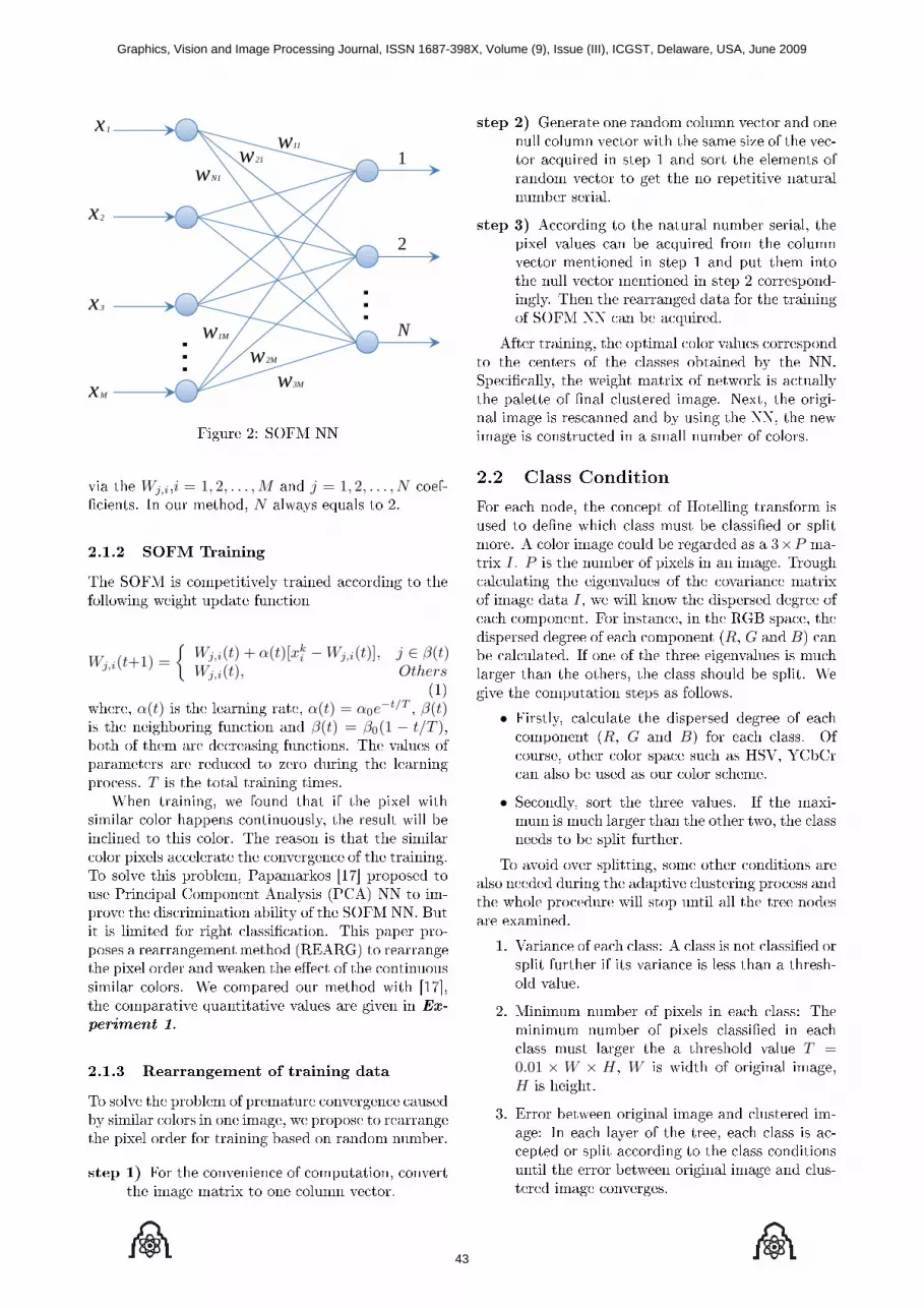
1

2

N

x1

x2

x3

xM

…

…

w11w21

wN1

w1M

w2M

w3M

"�� 0D !"# %%

(� �� Wj,i�i = 1, 2, . . . , M �� j = 1, 2, . . . , N ��'�� N ��&� �5�� 0

��

)�� !"# � ��(�& ��

Wj,i(t+1) ={

Wj,i(t) + α(t)[xki − Wj,i(t)], j ∈ β(t)

Wj,i(t), Others�.$

�� α(t) � �� α(t) = α0e−t/T � β(t)

� �� β(t) = β0(1 − t/T )�� )�� (�� T � ��

C�� *� �� &� �� )�� *�� (�� )� ��(� �� >�� 6.;7 �� >�� +�� ,��&�� >+,$ %% �� (� �� & �� !"# %% 4�� '�� )�� 2F,23$ �� *� �� -�� C� �� 6.;7�� (� 5��(� (�� (��

��

��

)� ��(� �� (�� & �� *� ��

�� "�� (�� (�� * �� (��

�� 3�� (�� (�� (�� 5�� . �� (�� (� ��

�� ,�� *� (�� 5�� (�� . �� (�� 0 ��& )�� !"# %% �� 5��

,�� (�� & �� %% ��'��&� �� * �� &�� '�� %�*�� & �� %%� ��

��

"�� '�� '�� , �� 3×P ��* I P � �� *�� )�� (�� (�� *�� I� �� "�� 234 �� R� G �� B$ �� (�� C��(� ��

• "��&� �� R� G �� B$ �� !�� H� I+�+��

• ��&� �� (�� *��

)� �(�� (�� (� �� *��

. H�� D , �� '�� (�� (��

0 #�� *�� D )�� *�� '�� (�� T =0.01 × W × H � W � �� H � ��

9 F�� D �� &�� (��


43

End

No

YesYes

Original image

Class 1 Class 2

No

Classification

by SOFM NN

Judgment Judgment

Clustered image

Create palette

"�� 9D +�� >��

��

,�� (� ��&�� (� ��5�� "� 9

�� E�'��

�� +�� !"# %%

�� %% �� %%��

�� ,� �� '��

� ��

�� (� �� *�� , �� +>@ �� . <93�� #,)A,4; ? �� !"# %% �� & 234 (�� *�� !� �� (�� H� I@H etc �� '��& "��&� �� (�� ,+ $

� �� D)� ��(� �� & ��

!"# %%� �� %% C� �� 2F,23 "� 1 �(�� -�� & ��

!"#� �� 6.;7 �� 2F,23 )�� . �(�� (� �� "� 1 )�� '�� )*� &*+� )+�� &� �� &�� (�� "�� 6.;7

� �� D�� *��

�� & �� "��&� �� -��(��

2F,23 �� "� : �� & �� !"# �� (�� !"# �& 2F,23 "� :��$ � �� 4�� (�� & �� *�� *�� & �� "� :��$ "� :��$ �� '�� & �� !"# %% �� & �� "� :��$ )�� & ��'�� (�� )�� (�� )�� 0 �� (�� "� :��$ �� "� :��$��& +0 � �� & �� C� �� +0 � "� :��$ � �� "� :��$�� &��

��&� �� & �� 5�� )�� "� / � �� & �� ,�� (� (�� '(� �� & �� "+#$ ��5�� )�� 9 �� '�� I(i, j, k)� i = 1, . . . , W �� j = 1, . . . , H �� O(i, j, k) �� '��

�( )�� *�� $)*%,

AE =1

W · HW∑i=1

H∑j=1

√√√√ 3∑k=1

(I(i, j, k) − O(i, j, k))2

�0$

-( &��"�� *�� +�� $&*+%,

NED =1

W · H

√√√√ W∑i=1

H∑j=1

[3∑

k=1

(I(i, j, k) − O(i, j, k))2]

�9$

( )�� +�� $)+�%,

ADC =1

Nc

Nc∑i=1

‖Ci − q(Ci)‖ �1$


44

��

"�� 1D 2�� & !"#� �� 6.;7 �� 2F,23

)�� .D )�� +��(� 2��

#�� )* &*+ )+� �&� ��&�

!"# .? 1;9 ? .=. . ??? 0/ :?= 9? 1/=�� 6.;7 .? 1/. ? .=? . ??? 0/ :.; 9? 1;<2F,23 : 9<. ? .;/ ? =/; 0; 0.< 9. .;<

��

"�� :D F-�� 2��

)�� 0D )�� 2��

)�� +�� 2 3 4 %�� >�� +0

"� :��$+. .1: .0? =/ :;0=.

0: 1J+0 ..; </ /= .=:?=+. .:9 .0; =/ 910.=

:: 1J"� :��$+0 .0= .?? ;1 10:<.

SNR = 10 log10

⎛⎜⎜⎜⎜⎜⎝

W∑i=1

H∑j=1

[3∑

k=1

I2(i, j, k)

]

W∑i=1

H∑j=1

[3∑

k=1

(I(i, j, k) − O(i, j, k))2]

⎞⎟⎟⎟⎟⎟⎠

�:$

PSNR = 10 log10

⎛⎜⎜⎜⎜⎜⎝

2552

13 · W · H

W∑i=1

H∑j=1

[3∑

k=1

(I(i, j, k) − O(i, j, k)2)

]

⎞⎟⎟⎟⎟⎟⎠

�/$


45

)�� 9D )�� +��(� H�� 4�� "+# �� >�� #��

�� #�� )* &*+ )+� �&� ��&�

�� . ,+ 1 /;. ? ?9< 0 0?: 9? =0? 9< 1.:�/: ��$ "+# 1 :?: ? ?1? 0 09; 9? /9. 9< .9?�� 0 ,+ 1 /.. ? ?9; 0 .=/ 9. .;0 9< /?<

�;= ��$ "+# 1 :/. ? ?1. 0 00< 9? 9:; 9; ;=;�� 9 ,+ 1 <<: ? ?1? 0 0=< 90 </= 9< ?01

�;/ ��$ "+# 1 ;:; ? ?19 0 9/? 90 0/1 9; 10.�� 1 ,+ 1 ;19 ? ?9= 0 .;= 99 .:? 9< ./1

�;< ��$ "+# 1 ;=9 ? ?11 0 .=< 90 ?<; 9; .?<

��.

!�� +�� 4��& �� )�� *��

��0

��9

��1

"�� /D +�� +�� F*�� 2��

)�� 1D )�� +��(� H��

�� #�� )* &*+ )+� �&� ��&�

�� .,+ ; ;99 ? ?;= 9 ;:= 0/ ;/? 90 ;:9"+# < .</ ? .?9 9 =<: 01 1<; 9? 1<9

�� 0,+ / 01: ? ?/0 9 ?<? 0= /;0 91 =9."+# / 111 ? ?;< 9 .1= 0; /?< 90 <;=

�� 9,+ : ?0= ? ?1; 0 99; 90 ?:9 9; 090"+# 1 =.0 ? ?1= 0 9<? 9. <90 9; ?.0

�� 1,+ < <;= ? ?<. 1 :=. 0; ?== 90 :<;"+# = ??; ? ?=? 1 9/< 0/ 00; 9. /=;


46

!��

�� . �� 0 �� 9 �� 1

>��,+

"+#��

"�� ;D ,+ �� "+# �� E-�� )��

�� C � �� 5�� NC

�� 5�� q(x) �� x

�( �� &�� $�&�%,F5�� :

�( ��' �� &�� $��&�%,F5�� / "��&� �*�� $ ��

�� 4��'� �� & �� (� �� *�� & �� (�� (��)�. $ � ��

ACV = (r g b) �;$

��

r =W∑i=1

H∑j=1

O(i, j, 1)

g =W∑i=1

H∑j=1

O(i, j, 2)

b =W∑i=1

H∑j=1

O(i, j, 3)

)�� g(i, j) �� 5�� &�� 5��

g(i, j) ={

1, if r(i, j), g(i, j), b(i, j) > r, g, b0, Other

�<$)�� "� / � �� 5�� < )�� *�� & �� (� ��

� �� DC� ��

�-�� "� ; �� *�� & ,+ �� "+# ��& )�� 1 �� (� (�� (�� "+#

� �� D�� *�� ,+ � �� -��

�� I+�+�� H� �� A,4 �� 234 "� < �� C� �� (� �� 5��(�� )�� : "�� 234�� '�� *�� 234 ��


47

��

�� ! �"� #��

"�� <D E-�� 2�� E-�� +��

)�� :D )�� F�� E-�� +��

+�� )* &*+ )+� �&� ��&�

234 / =?1 ? ?9/ ? 1./ 0: 0== 99 /<.I+�+� ; :99 ? ?9= ? :;/ 01 1;: 90 <:;� H .. /=1 ? ?/1 . ?.0 0? 01= 0< /9.� � .. /:. ? ?/9 ? ==1 0? 9/; 0< ;1=A�� ; /=0 ? ?1. ? /1< 01 .1: 90 :0;

��

)�� !"# %% �� ,��(� �� &�� )�� & �� '�� '�� )�� (� �� '�� ,�� &�� (� �� )�� & 234 �� &�� (�& �� '�� (�� 5�� & �� )�� (��

�� (��& �� &��

�� (�� D

• C� ��& �� (� �� & �� !"# %% ��(�� (�� *�� 5�(�� -��

• "�� *�� (� �� & ��

��

6.7 I C A� �� @ A�� !� �� & �� 5�� (� 09�=$D=9:K=:0� .==?


48

607 , �� ) 8�� /�� /� �� F��&�� ,��'�� + �� E F�� F�� %��I��DC�&� .=<;

697 ! H��(�� 0� �� 1 �� 2��"�� # � ��@�( ,�� F�� ,4� +�� .==:

617 % 8��(�� %�� #�� , C�� +�� ( �***� </D.10L.1;� .==<

6:7 E 8 >�� 3 ��& #��( �� '�� (�� *�� *** 0��( ��)��( #�� (� .;D=9=L=:1� .==:

6/7 A A�� 8 #�� ,� �� (�� )�� @�( +�� 4�� .===

6;7 # +�� , �� 5�� ( �� .��( ��(� :0D.1:L.;?� .==?

6<7 , C�� 3 �� +�� ( ��* ��( *��( ��(� �� )� .==;

6=7 4 +�� # 3�� ,�� +�� ( �� ( �*** +�� (� �� <:;L</?� .==;

6.?7 F A�� 2�� ,��(� �� *** 0��( &�� &��'��<D.;:L.<:� .==;

6..7 > +�� E #�� 2 �� +�� '�� .��( ��(� .:D./.L.//� .==;

6.07 + A �� >�� '�� '�� ( 3��(�.9D91:L9:9� .==9

6.97 , H�� 8 #��5(�� A 4�� +�� & �� ( 3��(� .<D.;9L.<:� .==;

6.17 ��&�� %�� D , ��(� �� )�� %�� I��D#��#�� .==1

6.:7 ) 8�� )�� %��I��D ��H�� .==;

6./7 % A �� I " A "�� (�� *** 0��(�� #�� -�� 99�9$� 0??9

6.;7 % >�� F ,�� > �� ,��(� �� *** 0��( �� #�� -�� 90�.$� 0??0

!��

�� (�� 4 F �� ,�� # F �� >��2�� &�� MB�� @�(��&�� )��&� +�� 0??.�� 0??: ��(�& "��0??. �� 0??0� �� MB�� %�� +� ��

"�� 0??: �� 0??;� �� MB�� >�� )�� E�� +��)��& �� 0??;� �� E�� 3�� >�� &�� C�� @�(��&� �� &�� +�� F�� FFF��F�+F� ��FF� �� ,#�)

�� (�� # �� F�� F�� @��(��&� +�� .=</� �� >� E �� +�� F�� 8&�� )��&�� .==; "�� .=</ ��.==9� �� @�(��&� �� 2��

�� ,�� A�� "�� .==; ��#�� 0??9� �� 2�� ,�� 3�� F�� F�� 8&�� @�(��&� �� "�� ,�� 0??9 ��#�� 0??<� �� ,�� >�� 3�� >�� &��C�� @�(��& �� ,�� 0??<� �� >�� 3�� >�� &�� C�� @�(��& �� FFF� �+F� �FF� �� F�+F


49


50

Documents

Graphics, Vision and Image Processing Journal, Volume (9), Issue (3), ICGST, Delaware, USA, June 2009