arX

iv:1

005.

1420

v5 [

gr-q

c] 1

2 M

ar 2

011

Gravitomagnetic Jets

C. Chicone

Department of Mathematics and Department of Physics and Astronomy,

University of Missouri, Columbia, Missouri 65211, USA

B. Mashhoon

Department of Physics and Astronomy,

University of Missouri, Columbia, Missouri 65211, USA

We present a family of dynamic rotating cylindrically symmetric Ricci-flat grav-

itational fields whose geodesic motions have the structure of gravitomagnetic jets.

These correspond to helical motions of free test particles up and down parallel to the

axis of cylindrical symmetry and are reminiscent of the motion of test charges in a

magnetic field. The speed of a test particle in a gravitomagnetic jet asymptotically

approaches the speed of light. Moreover, numerical evidence suggests that jets are

attractors. The possible implications of our results for the role of gravitomagnetism

in the formation of astrophysical jets are briefly discussed.

PACS numbers: 04.20.Cv

I. INTRODUCTION

A constant uniform magnetic field configuration in an inertial frame of reference has

cylindrical symmetry; therefore, the motion of a test charge in this field is such that the

particle’s momentum and angular momentum in the direction of the field are constants of

the motion. The particle in general moves with constant speed on a helix whose axis is along

the field direction; moreover, the radius and step of the helical path are constants as well.

The sense of helical motion about the direction of the magnetic field is positive (negative)

for a test particle of negative (positive) electric charge. If the initial velocity of the particle

is normal to the direction of the magnetic field, then the particle simply moves along a circle

in the plane perpendicular to the field.

The purpose of this paper is to study the analogous situation for the motion of free test

2

particles in a gravitomagnetic field. The nonlinearity of this field implies that only a rough

similarity may be anticipated. We investigate geodesic motion in a rotating dynamic space-

time region that is a Ricci-flat solution of Einstein’s equations with cylindrical symmetry [1].

Though this time-dependent gravitational case is considerably more complicated than the

magnetic case, we find qualitatively similar phenomena. In fact, the helical motions up and

down parallel to the axis of symmetry are reminiscent of the double-jet structure of certain

high-energy astrophysical sources.

Quasars and active galactic nuclei generally exhibit distinct relativistic outflows. These

jets are conjectured to originate from massive rotating black holes surrounded by accretion

disks; the outflows are focused beams of relativistic particles that proceed up and down

along the rotation axis of the black hole (see, for instance, [2]). Similar phenomena have

been observed in other high-energy astrophysical sources such as the Galactic X-ray binary

systems. While our results suggest a mechanism for astrophysical jet formation, the more

complicated physical process involves general relativistic MHD [3, 4]. The present work—

together with previous efforts [5–10]—contributes to the purely gravitational aspects of this

fundamental problem in astrophysics.

For a subclass of the Ricci-flat solutions under consideration, we show that the geodesic

equations have families of special exact solutions that we call gravitomagnetic jets. More

precisely, a gravitomagnetic jet is a set of special geodesics. These generally exhibit helical

motions about the axis of cylindrical symmetry and their union is a non-compact connected

invariant manifold that attracts all nearby geodesics. While we highlight features of these

jets in the source-free cylindrical spacetime region of interest and provide strong (numerical)

evidence that these families are attractors, the interesting question of the nature of the

external matter currents that could generate such a gravitational field remains beyond the

scope of our present investigation.

According to general relativity, a rotating mass generates a relativistic, and hence non-

Newtonian, gravitomagnetic field that is due to mass current. The exterior gravitomagnetic

field of the Earth has recently been directly measured via Gravity Probe B (GP-B) [11].

On the theoretical side, solutions of Einstein’s equations in the case of axial symmetry have

received attention for a long time (see Ch. VIII of [12] and references cited therein). In

particular, rotating solutions with cylindrical symmetry have been investigated by a number

of authors (see [13–15] and references therein).

3

Previous interesting work on exact cylindrically symmetric gravitational fields in con-

nection with the origin and structure of astrophysical jets has mainly involved the study of

geodesics in the interior of time-independent rigidly rotating dust cylinders [16]. The behav-

ior of free test particles in this case is directly influenced by the gravitational attraction of

the rotating dust particles; to avoid this circumstance, we concentrate here on certain source-

free gravitational fields that happen to depend exponentially upon time. These Ricci-flat

fields are perhaps more representative of the strongly time-dependent near-zone exteriors

of accreting and growing gravitationally collapsed configurations where astrophysical jets

are expected to originate. The temporal variation of the gravitational fields considered in

our work leads to a significant and surprising feature of the special exact solutions of the

geodesic equations. The speeds of test particles in gravitomagnetic jets start from values

that are always above a certain minimum speed, rapidly increase along their paths and

asymptotically approach the speed of light. The minimum speed represents the speed of

circular motion perpendicular to the axis of rotation. The range of this minimum speed

turns out to be from zero up to about 0.63 c.

Is the main general relativistic problem of high-energy astrophysical jets solved in our

paper? Our gravitational model is certainly too elementary to be an adequate representation

of the complex physical situation. Nevertheless, in our simple model free test particles appear

to be exponentially accelerated to almost the speed of light resulting in ultrarelativistic jet

streams parallel and antiparallel to the axis of rotation.

The plan of the paper is as follows. The class of spacetime metrics that we study in

this paper is described in section II. Each metric in this class involves a function X(r)

that is a solution of an ordinary differential equation and must be so chosen as to render

our system of cylindrical coordinates admissible in the spacetime region of interest. The

procedure for the determination of an appropriate X(r) is described in section III. The

rotational aspects of the resulting gravitational field are discussed in section IV. Section V

treats the motion of free test particles and null rays in the spacetime region of interest. This

section also contains a discussion of the special analytic solutions of the geodesic equations

that form gravitomagnetic jets. Numerical evidence that gravitomagnetic jets are indeed

attractors is presented in section VI. Section VII contains a discussion of our results. For

clarity of presentation, some of the detailed calculations and mathematical arguments are

relegated to the appendices. Specifically, Appendix A contains useful formulas related to

4

the principal dynamic spacetime metric under consideration in this paper. The proofs of

the main mathematical results regarding the solutions of a certain highly nonlinear ordinary

differential equation are given in Appendix B, where, due to the nature of the subject matter,

some of the notation employed is independent of the rest of the paper. Appendix C treats

the geodesics of the time-reversed metric.

II. SPACETIME METRIC

In a study devoted to gravitational radiation [1], a solution of the source-free gravi-

tational field equations was described and partially interpreted using rotating cylindrical

gravitational waves. The present paper is about the physical interpretation of a variant of

this solution in a different physical domain.

Consider the spacetime metric given in Eq. (35) of [1]

− ds2 = e−tXr

X(−X2dt2 +

1

r3dr2) +

e−t

ℓ2r(ℓXdt+ dΦ)2 + etdZ2 (1)

in (t, r,Φ, Z) coordinates. Here we employ the notation and conventions of Ref. [1], so that

the speed of light in vacuum is unity (c = 1) and the metric signature is +2. Moreover,

Xr = dX/dr, ℓ is a constant and (r,Φ, Z) are standard circular cylindrical coordinates. The

function X is a solution of the differential equation (cf. Eq. (31) of [1])

r2X2d2X

dr2+

dX

dr= 0, (2)

which is a special case of the generalized Emden-Fowler equation of the type y′′ = αq(x)yny′m

with y′ = dy/dx, m = 1, n = −2, α = −1 and q(x) = x−2 (see [17]). We transform it to the

Lotka-Volterra system (B27) in Appendix B. We do not know an explicit general solution

of Eq. (2). For the only explicit solutions known to exist, we note that X = constant is

unacceptable as the 4D metric (1) would then degenerate into a 3D spacetime, and the

solutions

X = ±(3

2r)−1/2

(3)

correspond to the special free rotating gravitational waves investigated in detail in [1] and

the references cited therein.

About fifteen years ago, searching for a general description of rotating cylindrical grav-

itational waves, one of us (BM) found the Ricci-flat metric (1), where X is a solution of

5

Eq. (2) once Rµν = 0. Among the solutions of Eq. (2), there is a class for which X2 is a

monotonically decreasing function of r as well as a class where X2 is monotonically increas-

ing. The former class of solutions, which includes Eq. (3) as a special case, was investigated

in Ref. [1] and related to rotating gravitational waves. The physical interpretation of the

latter class of solutions is taken up in the present work.

Let us note that if X is a solution of Eq. (2), then so is −X ; therefore, it is possible

to assume ℓ > 0 in Eq. (1) with no loss of generality. We define a lengthscale λ such that

ℓ := λ−1/2. Only positive square roots are considered throughout. Let us now introduce the

dimensionless quantities r, X and z such that

r = λr, X = λ−1/2X, z = λ−1Z. (4)

Moreover, t in Eq. (1) is dimensionless as well; therefore, we assume that the physical time

coordinate is given by λ′t, where λ′ is in general a different arbitrary constant lengthscale.

Under the scale transformation (r,X) 7→ (r, X), Eq. (2) remains invariant. Furthermore,

with s = λ−1s the spacetime interval (1) essentially remains invariant as well; that is,

dropping all the tildes and working only with dimensionless quantities, the spacetime metric

takes the form

− ds2 = e−tXr

X(−X2dt2 +

1

r3dr2) +

e−t

r(Xdt+ dφ)2 + etdz2, (5)

where t = t and Φ = φ. Starting from dimensionless (t, r, φ, z) coordinates, we can always

return to regular coordinates by choosing arbitrary lengthscales λ and λ′; then, the physical

coordinates are (λ′t, λ−1r, φ, λz) and the other physical quantities in the metric are λ1/2X

and λs.

For the physical interpretation proposed in this work, the spacetime metric is obtained

from Eq. (5) by t 7→ −t. Henceforth, we will deal with dimensionless quantities and the

spacetime metric

− ds2 = etXr

X(−X2dt2 +

1

r3dr2) +

et

r(−Xdt+ dφ)2 + e−tdz2, (6)

where X is a solution of Eq. (2) specified in the next section, and we will show that under

certain conditions geodesics of metric (6) allow gravitomagnetic jets. Thus the main focus

of the following sections and Appendices A and B is on metric (6); we return to the time-

reversed case—namely, metric (5)—in Appendix C.

6

As shown in [1], Eq. (6) represents an algebraically general Ricci-flat solution of type I

in the Petrov classification. It admits two commuting spacelike Killing vector fields ∂z and

∂φ associated with the cylindrical symmetry of the gravitational field. The corresponding

two-parameter isometry group is not orthogonally transitive. The invariant magnitude of

the hypersurface-orthogonal ∂z is given by exp(−12t), while for ∂φ, which is not hypersurface-

orthogonal, the invariant magnitude is r−1/2 exp(12t). Thus t and r can be invariantly defined

in this way. The t = constant hypersurfaces are always spacelike. We interpret t as the time

coordinate in this paper; therefore, at a given time t, ρ = r−1/2 is, up to a constant factor,

an appropriate radial coordinate. Using this quantity, metric (6) takes the form

− ds2 = −1

2etρ3

Xρ

X(−X2dt2 + 4dρ2) + etρ2(−Xdt + dφ)2 + e−tdz2, (7)

so that the circumference of a circle orthogonal to the axis of cylindrical symmetry is 2πρ∗,

where ρ∗ = ρ exp(12t). The symmetry axis is thus defined by ρ = 0 (or r = ∞). Despite its

shortcoming as a proper radial coordinate, we nevertheless use r extensively in this paper

to simplify formulas.

We define the proper radial distance R∗ = exp(t/2)R via Eq. (7) such that for the proper

radial distance from the axis to a point with ρ = ρ0, R = R0 is given by

R0 =

∫ ρ0

0

(

− 2ρ3Xρ

X

)1/2dρ =

∫ ∞

r0

( Xr

r3X

)1/2dr, (8)

where r0 = 1/ρ20.

The coordinates xµ = (t, r, φ, z) are assumed to be admissible in the spacetime domain

under consideration here. Thus, the gravitational potentials must be sufficiently smooth

functions of these coordinates; moreover, the Lichnerowicz admissibility conditions [18] re-

quire that the principal minors of the metric tensor and its inverse be negative for our choice

of metric signature. For a symmetric n× n matrix M , the principal minors are given by

det

M11 · · · M1k

......

Mk1 · · · Mkk

(9)

for k = 1, . . . , n. These admissibility conditions are essentially equivalent to the inequalities

X(rXr −X) > 0, XXr > 0, (10)

7

for all values of r in the domain of the solution X . This fact follows from a detailed exam-

ination of the spacetime metric tensor gµν , with −ds2 = gµνdxµdxν defined in display (6),

and its inverse given in Appendix A; we note, in particular, that for an admissible solution

− gtt =e−t

XXr> 0, (−g)−1/2 =

r2e−t

|Xr|> 0. (11)

There are four algebraically independent scalar polynomial curvature invariants in a Ricci-

flat spacetime that can be represented as (see Ch. 9 of [13])

I1 = RµνρσRµνρσ − iRµνρσR

∗µνρσ, (12)

I2 = RµνρσRρσαβR µν

αβ + iRµνρσRρσαβR∗ µν

αβ . (13)

For metric (6), I1 and I2 are both real and are given by

I1 = −e−2t

rX4X2r

(1− 3rX2 − 2r2XXr − r3X3Xr + r4X2X2r ), (14)

I2 = −3e−3t

4rX5X3r

(1− 2rX2 − 2r2XXr + 2r3X3Xr + r4X2X2r ). (15)

These invariants vanish in the case of special solution (3), but are in general nonzero. For

any finite value of the coordinate time t, I1 and I2 depend on the particular branch of the

function X . This will be discussed in detail in section III.

III. CHOICE OF X

The mathematical investigation needed to identify admissible solutions X(r) of Eq. (2)

that would allow the existence of jets is given in Appendix B; here, we present the main

conclusions of this analysis.

The character of metric tensor (6) depends on the choice of a solution of the differential

Eq. (2). We will consider admissible solutions in (t, r, φ, z) coordinates that correspond to

solutions X of the differential Eq. (2) such that X2 is monotonically increasing with r and

Q(r) := rXr −X (16)

is such that XQ > 0.

Throughout this paper, we take advantage of the scale transformation already mentioned

in the previous section: The differential Eq. (2) remains invariant under the scaling (r,X) 7→

8

0 2 4 6 8-15

-10

-5

0

5

10

15

r

X

F H X

W

0 2 4 6 8 10-1

0

1

2

3

4

5

r

F

H

X

W

0 1 2 3 4

0.0

0.5

1.0

1.5

r

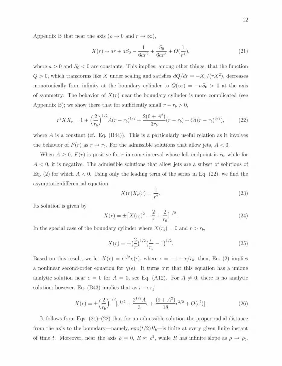
FIG. 1: The top panel shows computer-generated plots of admissible solutions ±X versus r for the

differential Eq. (2). The thick curve is for the initial data X(1) = 1 and Xr(1) = 2; the thin curve

is for the data X(1) = 1 and Xr(1) = 3. The middle (bottom) panel depicts computer generated

graphs of F , H, W and X for the “thick” (“thin”) solution. The graphs of F , H and X vanish

at the left end-point rb of the domain of definition of X, which is rb ≈ 0.720 for the thick solution

that allows jets and rb ≈ 0.787 for the thin solution that does not allow jets.

9

(r, X), where for σ > 0, r = σr and X(r) = σ−1/2X(r). Using scale-invariant variables, it is

then possible to reduce the second-order Eq. (2) to equations of first order—see Appendix B.

Indeed, consideration of scale-invariant quantities leads to substantial simplifications in our

work. The admissible class that we seek is a scale-invariant subclass of solutions of Eq. (2)

that are all of the form depicted for two cases in the top panel of Figure 1. In fact, in

Appendix B we prove that there is an open set of initial conditions that corresponds to

admissible solutions each of which exists on an interval (rb,∞), where rb > 0, with limiting

values X(rb) = 0 and Xr(rb) = ∞ such that XXr = 1/r2b at rb, the function X2 is increasing,

X2r is decreasing and X2 approaches infinity as r approaches infinity. In addition, we show

that there is an open set of initial conditions for solutions defined on (rb,∞) with the same

end-point asymptotics such that the scale-invariant function F defined by

F (r) = r2X(r)Xr(r)− 1 (17)

has a zero rJ in the interior of the interval of existence (rb,∞). The physical significance of

this property is that it is the necessary and sufficient condition for the existence of jets; that

is, if F has such a zero, then the (timelike and null) geodesic equations admit special helical

solutions propagating upward and downward on an interior cylinder of radius rJ . These

special solutions form gravitomagnetic jets. We also show that there is an open set of initial

data corresponding to solutions that satisfy both conditions.

To clarify the connection of the present work with the solutions treated in Ref. [1], let us

consider, as in [1], the scale-invariant quantities

δ =2

3rX2, α = −

4Xr

3X3(18)

and note that these quantities are related by the autonomous differential equation

dα

dδ=

3α(α− δ2)

2δ(α− δ). (19)

By introducing a temporal parameter θ, we will also consider the corresponding first-order

system

dδ

dθ= 2δ(α− δ),

dα

dθ= 3α(α− δ2),

(20)

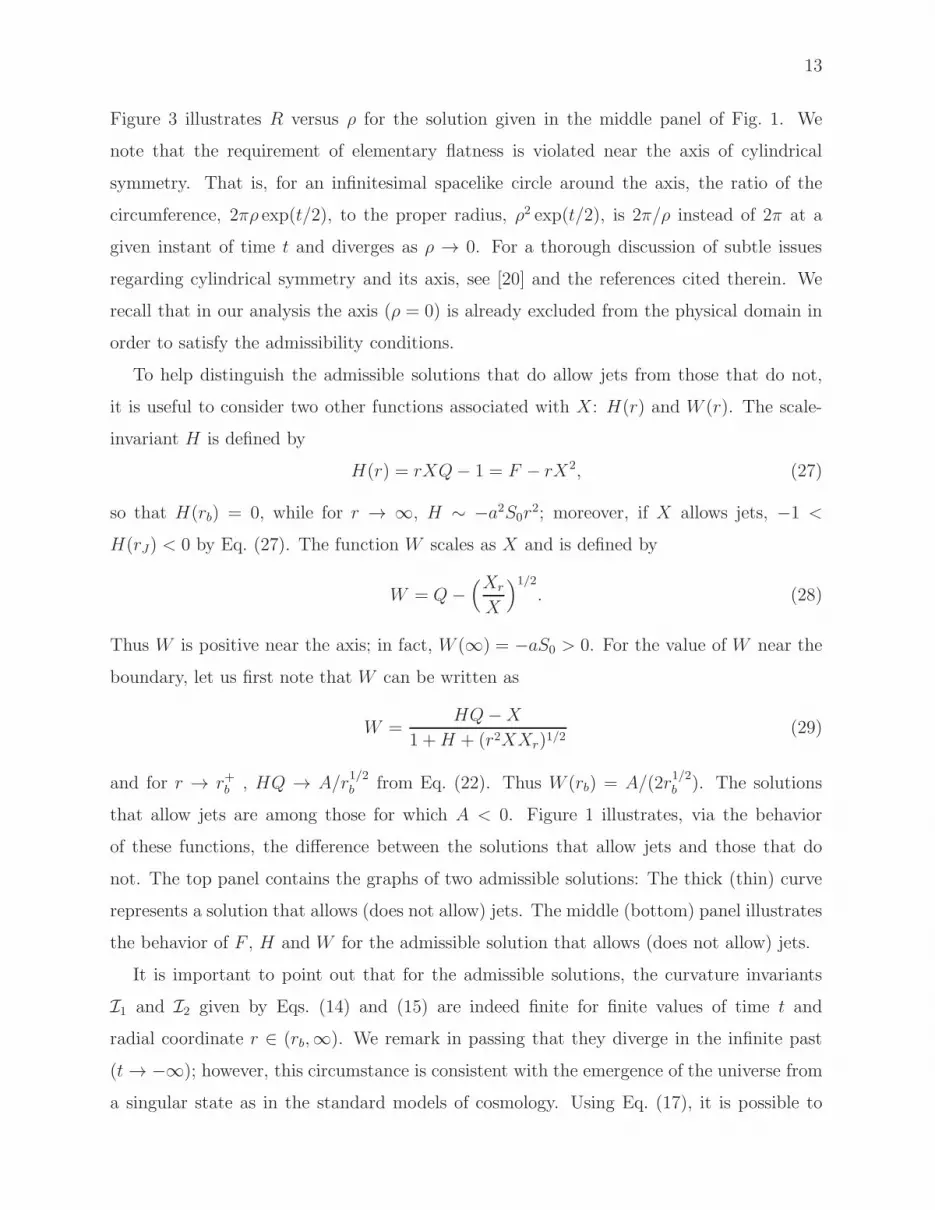
whose phase portrait is depicted in Fig. 2. With the choice of r as a positive radial coordinate

in metric (6), δ ≥ 0 and hence the first and fourth quadrants of Fig. 2 are physically relevant.

10

-3 -2 -1 0 1 2 3-3

-2

-1

0

1

2

3

∆

Α

FIG. 2: Computer generated phase portrait for system (20). The rest point at (δ, α) = (0, 0) is a

degenerate singularity of system (20), while the other rest point at (1, 1) is a simple singularity.

This latter isolated singularity is a spiral point that corresponds to the special solution (3).

The solutions in the first quadrant have α > 0 or XXr < 0, so that X2 monotonically

decreases with r. These solutions, which were discussed in [1], tend to the special rest point

(δ, α) = (1, 1) that corresponds to exact solution (3). The present paper is therefore devoted

to the study of solutions in the fourth quadrant for which α < 0 and hence XXr > 0. Since

system (20) is autonomous and the coordinate axes are invariant, it follows immediately

that the fourth quadrant is invariant; that is, solutions that start in the fourth quadrant

stay there [19]. In particular, X(r)Xr(r) > 0 as long as such a solution exists. If X(r) > 0,

then Xr(r) > 0, X increases as r increases, and Xrr(r) is negative. Thus, if X(r) > 0

for some r > 0, this function increases as r increases and is concave down. Using our

symmetry, if X(r) < 0 for some r > 0, then X decreases with r and is concave up (see

Fig. 1). Each member of this class of solutions of Eq. (2) is asymptotic to the degenerate

rest point (δ, α) = (0, 0) that corresponds to the axis of cylindrical symmetry, where r = ∞

and X2 = ∞. In fact, it can be shown that, with our choice of temporal variable θ, each

solution is asymptotic to (0, 0) (corresponding to axis of cylindrical symmetry) in positive

time and approaches a point at infinity (δ, α) = (∞,−∞) in negative time (corresponding

11

to the cylindrical boundary r = rb > 0 and XXr = r−2b ).

0.0 0.5 1.0 1.5 2.0 2.50.0

0.5

1.0

1.5

2.0

2.5

Ρ

R

FIG. 3: Plot of R versus ρ corresponding to the spacetime defined by X with X(1) = 1 and

Xr(1) = 2, as in the middle panel of Fig. 1.

Consider a hypersurface such that at every instant of time t, the hypersurface is char-

acterized by the cylindrical surface r = constant for rb < r < ∞. The gravitomagnetic

jets lie on such a hypersurface with r = rJ . The normal to such a hypersurface is given by

nµ = (0, 1, 0, 0); hence, nµnµ = grr = exp(−t)r3X/Xr > 0 using Eq. (A2) of Appendix A.

That is, the hypersurface is always timelike, but as r → r+b , nµnµ → 0, so that the boundary

hypersurface is null.

The admissibility conditions require that we explicitly leave the inner and outer bound-

aries out of the domain of the solution X . That is, the axis of cylindrical symmetry (r = ∞)

and the boundary cylinder (r = rb) are excluded from the spacetime region of physical

interest, since gtt vanishes at the axis and (−g)−1/2 vanishes at the boundary (see Eq. (11)).

It is interesting to describe further some of the significant properties of the admissible

solutions. Let us first note that the invariance of Eq. (2) under X 7→ −X is a scale-

invariant property; henceforth, we will work exclusively with the X > 0 branch. We show in

12

Appendix B that near the axis (ρ → 0 and r → ∞),

X(r) ∼ ar + aS0 −1

6ar2+

S0

6ar3+O(

1

r4), (21)

where a > 0 and S0 < 0 are constants. This implies, among other things, that the function

Q > 0, which transforms like X under scaling and satisfies dQ/dr = −Xr/(rX2), decreases

monotonically from infinity at the boundary cylinder to Q(∞) = −aS0 > 0 at the axis

of symmetry. The behavior of X(r) near the boundary cylinder is more complicated (see

Appendix B); we show there that for sufficiently small r − rb > 0,

r2XXr = 1 +( 2

rb

)1/2

A(r − rb)1/2 +

2(6 + A2)

3rb(r − rb) +O((r − rb)

3/2), (22)

where A is a constant (cf. Eq. (B44)). This is a particularly useful relation as it involves

the behavior of F (r) as r → rb. For the admissible solutions that allow jets, A < 0.

When A ≥ 0, F (r) is positive for r in some interval whose left endpoint is rb, while for

A < 0, it is negative. The admissible solutions that allow jets are a subset of solutions of

Eq. (2) for which A < 0. Using only the leading term of the series in Eq. (22), we find the

asymptotic differential equation

X(r)Xr(r) =1

r2. (23)

Its solution is given by

X(r) = ±[

X(r0)2 −

2

r+

2

r0

]1/2. (24)

In the special case of the boundary cylinder where X(rb) = 0 and r > rb,

X(r) = ±(2

r

)1/2( r

rb− 1

)1/2. (25)

Based on this result, we let X(r) = ǫ1/2χ(ǫ), where ǫ = −1 + r/rb; then, Eq. (2) implies

a nonlinear second-order equation for χ(ǫ). It turns out that this equation has a unique

analytic solution near ǫ = 0 for A = 0, see Eq. (A12). For A 6= 0, there is no analytic

solution; however, Eq. (B43) implies that as r → r+b

X(r) = ±( 2

rb

)1/2

[ǫ1/2 +21/2A

3ǫ+

(9 + A2)

18ǫ3/2 +O(ǫ2)]. (26)

It follows from Eqs. (21)–(22) that for an admissible solution the proper radial distance

from the axis to the boundary—namely, exp(t/2)Rb—is finite at every given finite instant

of time t. Moreover, near the axis ρ = 0, R ≈ ρ2, while R has infinite slope as ρ → ρb.

13

Figure 3 illustrates R versus ρ for the solution given in the middle panel of Fig. 1. We

note that the requirement of elementary flatness is violated near the axis of cylindrical

symmetry. That is, for an infinitesimal spacelike circle around the axis, the ratio of the

circumference, 2πρ exp(t/2), to the proper radius, ρ2 exp(t/2), is 2π/ρ instead of 2π at a

given instant of time t and diverges as ρ → 0. For a thorough discussion of subtle issues

regarding cylindrical symmetry and its axis, see [20] and the references cited therein. We

recall that in our analysis the axis (ρ = 0) is already excluded from the physical domain in

order to satisfy the admissibility conditions.

To help distinguish the admissible solutions that do allow jets from those that do not,

it is useful to consider two other functions associated with X : H(r) and W (r). The scale-

invariant H is defined by

H(r) = rXQ− 1 = F − rX2, (27)

so that H(rb) = 0, while for r → ∞, H ∼ −a2S0r2; moreover, if X allows jets, −1 <

H(rJ) < 0 by Eq. (27). The function W scales as X and is defined by

W = Q−(Xr

X

)1/2

. (28)

Thus W is positive near the axis; in fact, W (∞) = −aS0 > 0. For the value of W near the

boundary, let us first note that W can be written as

W =HQ−X

1 +H + (r2XXr)1/2(29)

and for r → r+b , HQ → A/r1/2b from Eq. (22). Thus W (rb) = A/(2r

1/2b ). The solutions

that allow jets are among those for which A < 0. Figure 1 illustrates, via the behavior

of these functions, the difference between the solutions that allow jets and those that do

not. The top panel contains the graphs of two admissible solutions: The thick (thin) curve

represents a solution that allows (does not allow) jets. The middle (bottom) panel illustrates

the behavior of F , H and W for the admissible solution that allows (does not allow) jets.

It is important to point out that for the admissible solutions, the curvature invariants

I1 and I2 given by Eqs. (14) and (15) are indeed finite for finite values of time t and

radial coordinate r ∈ (rb,∞). We remark in passing that they diverge in the infinite past

(t → −∞); however, this circumstance is consistent with the emergence of the universe from

a singular state as in the standard models of cosmology. Using Eq. (17), it is possible to

14

express these scalars as

I1 = −e−2t

rX4X2r

[F 2 − rX2(F + 4)],

I2 = −3e−3t

4rX5X3r

F (F + 2rX2).

(30)

Thus I1(rJ) = 4r4J exp(−2t) and I2(rJ) = 0 for any solution that allows jets. Specifically, for

the case that allows jets depicted in the middle panel of Fig. 1, I1 has one zero and I2 has

two zeros in the interval (rb,∞), while for the case that does not allow jets depicted in the

bottom panel of Fig. 1, I1 has one zero and I2 has no zeros in the interval (rb,∞). Moreover,

it is straightforward to show that as the boundary cylinder is approached (r → rb),

I1 → (4−A2)e−2tr4b , I2 → −3A2

4e−3tr6b , (31)

while as the axis of cylindrical symmetry is approached (r → ∞),

I1 → e−2tS0a−2, I2 → −

9

4e−3ta−4. (32)

Once X has been properly chosen, we can turn to the treatment of gravitational physics

in the corresponding singularity-free spacetime region. This is an open hollow cylindrical

domain that expands; it has an inner boundary around the symmetry axis (r = ∞) and an

outer boundary (r = rb). We therefore consider test particles and gyroscopes in the radial

interval (rb,∞) in the rest of this paper.

The rotational aspects of the spacetimes under consideration here provide the basis for

the interesting features that free test particle motion can exhibit in these gravitational fields;

therefore, we now turn to the gravitomagnetic properties of admissible solutions.

IV. GRAVITOMAGNETIC FIELD

The gravitational Larmor theorem implies a local equivalence, in the linear approxima-

tion, between gravitomagnetism and rotation [21, 22]. This correspondence may be employed

in order to provide a definite measure of the gravitomagnetic field. It is therefore useful to

study the precession of ideal test gyroscopes that are held at rest in the spacetime region of

interest; the precession frequency may then be identified with the gravitomagnetic field for

the class of observers that carry the gyros along their world lines.

15

To simplify matters, we consider the class of fundamental observers that are spatially at

rest by definition; that is, xi is constant for each i = 1, 2, 3 for a fundamental observer in the

physical spacetime region of interest. Therefore, the four-velocity field of the fundamental

observers is given in (t, r, φ, z) coordinates by

λµ(t) = ((−gtt)

−1/2, 0, 0, 0). (33)

These observers’ natural orthonormal tetrad frame is given by λµ(α), where

λµ(r) = (0, (grr)

−1/2, 0, 0), (34)

λµ(φ) = (st, 0, sφ, 0), (35)

λµ(z) = (0, 0, 0, et/2) (36)

are the corresponding spatial unit directions. Here, st and sφ are given by

st = −e−t/2(XrQ)−1/2, sφ = e−t/2( Q

Xr

)1/2. (37)

The fundamental observers are accelerated; their acceleration tensor ω(α)(β) is defined via

Dλµ(α)

dT= ω

(β)(α) λµ

(β), (38)

where T is the proper time along the world line xµ(T ) of a fundamental observer such that

dxµ/dT = λµ(t). In analogy with electrodynamics, the antisymmetric acceleration tensor

consists of an “electric” part ω(t)(i) = A(i) and a “magnetic” part ω(i)(j) = ǫ(i)(j)(k)Ω(k). The

corresponding spacelike vectors are then Aµ = A(i)λ(i)

µ and Ωµ = Ω(k)λµ(k). It follows from

a detailed calculation that in the present case

A(r) = −1

2e−t/2

(rXr

X

)1/2 Xr −XQ2

XXrQ, (39)

A(φ) = −1

2e−t/2(XrQ)−1/2 (40)

are the nonzero tetrad components of the translational acceleration Aµ of the fundamental

observers. These are finite in the physical region (rb,∞); moreover, as the symmetry axis is

approached

A(r) → −1

2e−t/2S0 > 0, A(φ) → −

1

2e−t/2a(−S0)

−1/2 < 0, (41)

while near the boundary r → r+b one can show, using the expressions given in the previous

section, that

A(r) →1

2e−t/2Arb, A(φ) → 0. (42)

16

0.0 0.2 0.4 0.6 0.8 1.0 1.2 1.40.0

0.1

0.2

0.3

0.4

0.5

Ρ

H2XQL-1

FIG. 4: Plots of (2XQ)−1 versus ρ = r−1/2 for the two cases of X given in the top panel of

Fig. 1. The upper curve here corresponds to initial data X(1) = 1 and Xr(1) = 2; the lower curve

corresponds to X(1) = 1 and Xr(1) = 3. In general, the maximum of (2XQ)−1 occurs where

H(r) = rXQ− 1 vanishes; this happens at r = 1 for the upper curve.

Furthermore, Ωµ can be obtained from

Ω(z) = −1

2e−t/2(XQ)−1, (43)

which is the rotation frequency about the z axis of the local spatial frame of the fundamen-

tal observers with respect to the local nonrotating—that is, Fermi-Walker transported—

frame. All of the other nonzero components of the acceleration tensor can be obtained from

Eqs. (39)–(40) and (43).

These considerations imply that ideal test gyroscopes carried along the world lines of the

fundamental observers precess, with frequency −Ω(z) about the z axis, with respect to the

natural spatial frame of the fundamental observers. Thus

− Ωµ = (0, 0, 0,1

2XQ) (44)

characterizes the gravitomagnetic field in this case. It is variable in magnitude but constant

in direction (parallel to the z axis). We note that (2XQ)−1 ≥ 0 vanishes along the axis

of cylindrical symmetry and tends to rb/2 with infinite slope at the outer boundary of the

region under consideration here (see Fig. 4). The situation is more complicated, however,

when we consider the gravitomagnetic components of the curvature tensor as measured by

the fundamental observers. In particular, as demonstrated in Appendix A, these do not all

vanish along the symmetry axis.

To illustrate these results further, let us consider a unit spacelike vector field V µ that is

17

carried by the fundamental observers and is orthogonal to the z axis; that is,

V µ = cosϕλµ(r) + sinϕλµ

(φ). (45)

If this is a gyro axis, then it is Fermi-Walker transported along xµ(T ), namely,

DV µ

dT= (AνV

ν)λµ(t). (46)

It follows from a detailed calculation that Eq. (46) is equivalent to the condition that

dϕ/dT = −Ω(z). Thus the gyro rotates with proper frequency dϕ/dT about the z axis

with respect to the spatial frame of the fundamental observers.

The electric and magnetic components of the Riemann curvature tensor, projected on

the tetrad frame of the fundamental observers, are given in Appendix A.

V. GEODESICS

Spacetime geodesics are generally obtained from the condition that the spacetime interval

along the geodesic path be an extremal, namely, δ∫

ds = 0, where ds2 is given by Eq. (6).

The geodesic equation then takes the form

d2xµ

ds2+ Γµ

αβ

dxα

ds

dxβ

ds= 0. (47)

In this section we treat timelike and null geodesics in turn.

A. Timelike Geodesics

The geodesics of the dimensionless spacetime metric (6) depend on the choice of solution

X of the differential Eq. (2) or the equivalent first-order system

dX

dr= Y,

dY

dr= −

Y

r2X2. (48)

For an admissible X , we choose its positive branch X(r) > 0; moreover, to obtain the

corresponding geodesic equations with respect to proper time τ , we define U := dr/dτ and

note the reparameterization of system (48):

dr

dτ= U,

dX

dτ= UY,

dY

dτ= −

UY

r2X2. (49)

18

The components of the four-velocity vector of the free test particle along Killing vector

fields are constants of geodesic motion. Therefore, due to cylindrical symmetry, there are

two constants of the motion Cz = gzαdxα/dτ , the specific momentum in the z direction, and

Cφ = gφαdxα/dτ , the specific angular momentum about the z axis; that is,

dz

dτ= Cze

t,dφ

dτ−X

dt

dτ= Cφre

−t. (50)

By inserting these relations into the metric and simplifying, we find that

X2( dt

dτ

)2

=1

r3

(dr

dτ

)2

+X

Xr(e−t + C2

z + C2φre

−2t), (51)

ordt

dτ=

1

XV, (52)

where

V :=[ 1

r3U2 +

X

Xr(e−t + C2

z + C2φre

−2t)]1/2

. (53)

Our choice of positive sign in Eq. (52) is in conformity with the notion that the temporal co-

ordinate should monotonically increase with proper time along the world line of an observer.

The Christoffel symbols Γrµν that are needed for the radial geodesic equation—namely, the

component of Eq. (47) for the variation of the radial coordinate along the geodesic path—are

given by

Γrtt =

1

2r(−1 +Q2X

Y),

Γrtr = Γr

rt =1

2,

Γrtφ = Γr

φt =rXQ

2Y,

Γrrr = −

1 + 3rX2 + r2XY

2r2X2,

Γrφφ =

rX

2Y.

(54)

19

Thus a full set of differential equations for the timelike geodesics can be expressed as

dt

dτ=

1

XV,

dr

dτ= U,

dφ

dτ= V + Cφre

−t,

dz

dτ= Cze

t,

dU

dτ= −Γr

tt

V 2

X2−

V U

X− 2Γr

tφ

V

X(V + Cφre

−t)− ΓrrrU

2 − Γrφφ(V + Cφre

−t)2,

dX

dτ= UY,

dY

dτ= −

UY

r2X2.

(55)

In a constant magnetic field configuration, the motion of a test charge is a combination

of uniform rectilinear motion along the field direction together with uniform circular motion

around this direction. The analogous situation in the gravitational field under consideration

is, however, much more complex. In particular, the free motion of a test particle purely

parallel to the rotation axis is impossible in the physical region (rb,∞), since system (55)

does not have a solution for constant r and φ coordinates. However, for a subset of admissible

field configurations, special circular and helical motions are possible.

In analogy with the magnetic case, let us look for geodesic motion that is confined to a

cylinder of fixed radius r > 0; that is, we let U = 0 and dU/dτ = 0 in system (55). The

latter equation, after division by (dφ/dτ)2 > 0, can be written as

Γrtt

( dt

dφ

)2+ 2Γr

tφ

( dt

dφ

)

+ Γrφφ = 0, (56)

which is reminiscent of the quadratic equation usually encountered in discussions of the

gravitomagnetic clock effect [23]. It is simple to show from Eqs. (54) that

(Γrtφ)

2 − ΓrttΓ

rφφ =

r2X

4Y(57)

and

Γrtt =

rX

2Y

[

Q−(Y

X

)1/2][Q+

(Y

X

)1/2]. (58)

It follows from Eqs. (56)–(58) that

dt

dφ= −

1

Q± (Y/X)1/2. (59)

20

For an admissible solution X of Eq. (2), X(r) > 0, Y (r) > 0 and Q(r) > 0; hence, the upper

sign in Eq. (59) would always lead to helical motion in the negative sense about the z axis,

while for the lower sign the sense of the motion depends on the sign of

W (r) := Q−(Y

X

)1/2

. (60)

This function has been discussed in Sec. III; it is given by A/(2r1/2b ) at r = rb and asymptot-

ically approaches −aS0 > 0 as r → ∞. In the class of admissible solutions, either W (r) > 0

or W has a zero rw in the physical interval (rb,∞). This situation is illustrated in Fig. 1.

In the former case, the sense of helical motion would always be negative, while in the latter

case we find from Eq. (56)( dt

dφ

)

r=rw= −

1

2Q. (61)

For r ∈ (rb, rw), however, there could be helical motion in the positive sense. This is crucial

since we find from the relations for dt/dτ and dφ/dτ in system (55) that

dt

dφ=

V

X(V + Cφre−t). (62)

In this relation we must have Cφ = 0, since it follows from Eq. (59) that dt/dφ must be

constant for fixed r. Thus, dt/dφ = X−1 > 0 and from Eq. (59) we find that

−1

Q− (Y/X)1/2=

1

X(63)

holds for rY = (Y/X)1/2, or

r2XY = 1. (64)

If this condition is satisfied for some rJ ∈ (rb, rw), then there is in general helical geodesic

motion in the positive sense about the z axis regardless of the value of Cz 6= 0. From the

definition of F (r) in Eq. (17), we see that if F (r) = 0 has a solution rJ in the interior of the

physical interval (rb,∞), then special helical solutions of the geodesic equation (47) exist;

these special solutions reside in the gravitomagnetic jet.

For Cz = Cφ = 0, there is a special family of timelike circular geodesic orbits at z = z0

with radius rJ given by Eq. (64),

φ = φ0 +X(rJ)(t− t0) (65)

and

et/2 = et0/2 +1

2rJ(τ − τ0), (66)

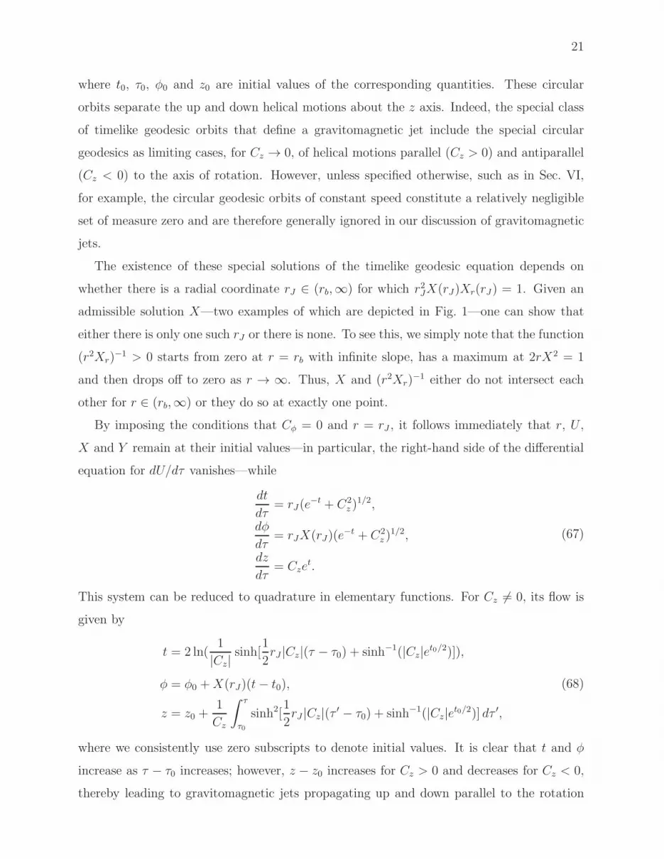
21

where t0, τ0, φ0 and z0 are initial values of the corresponding quantities. These circular

orbits separate the up and down helical motions about the z axis. Indeed, the special class

of timelike geodesic orbits that define a gravitomagnetic jet include the special circular

geodesics as limiting cases, for Cz → 0, of helical motions parallel (Cz > 0) and antiparallel

(Cz < 0) to the axis of rotation. However, unless specified otherwise, such as in Sec. VI,

for example, the circular geodesic orbits of constant speed constitute a relatively negligible

set of measure zero and are therefore generally ignored in our discussion of gravitomagnetic

jets.

The existence of these special solutions of the timelike geodesic equation depends on

whether there is a radial coordinate rJ ∈ (rb,∞) for which r2JX(rJ)Xr(rJ) = 1. Given an

admissible solution X—two examples of which are depicted in Fig. 1—one can show that

either there is only one such rJ or there is none. To see this, we simply note that the function

(r2Xr)−1 > 0 starts from zero at r = rb with infinite slope, has a maximum at 2rX2 = 1

and then drops off to zero as r → ∞. Thus, X and (r2Xr)−1 either do not intersect each

other for r ∈ (rb,∞) or they do so at exactly one point.

By imposing the conditions that Cφ = 0 and r = rJ , it follows immediately that r, U ,

X and Y remain at their initial values—in particular, the right-hand side of the differential

equation for dU/dτ vanishes—while

dt

dτ= rJ(e

−t + C2z )

1/2,

dφ

dτ= rJX(rJ)(e

−t + C2z )

1/2,

dz

dτ= Cze

t.

(67)

This system can be reduced to quadrature in elementary functions. For Cz 6= 0, its flow is

given by

t = 2 ln(1

|Cz|sinh[

1

2rJ |Cz|(τ − τ0) + sinh−1(|Cz|e

t0/2)]),

φ = φ0 +X(rJ)(t− t0),

z = z0 +1

Cz

∫ τ

τ0

sinh2[1

2rJ |Cz|(τ

′ − τ0) + sinh−1(|Cz|et0/2)] dτ ′,

(68)

where we consistently use zero subscripts to denote initial values. It is clear that t and φ

increase as τ − τ0 increases; however, z − z0 increases for Cz > 0 and decreases for Cz < 0,

thereby leading to gravitomagnetic jets propagating up and down parallel to the rotation

22

axis. The function z(t) may be expressed as

z(t) = z0 +K+(t)−K+(t0), (69)

where

K+ =Cz

rJ |Cz|3κ+(1 + κ+2

)1/2 − ln[κ+ + (1 + κ+2)1/2],

κ+ = |Cz|et/2.

(70)

B. Null Geodesics

Let ζ be an affine parameter along the world line of a null geodesic. It follows from the

existence of the spacelike Killing vectors ∂z and ∂φ that

dz

dζ= Cze

t,dφ

dζ−X

dt

dζ= Cφre

−t, (71)

where Cz and Cφ are constants of the motion. The spacetime path is null ( ds2 = 0); hence,

X2( dt

dζ

)2=

1

r3(dr

dζ

)2+

X

Xr

(C2z + C2

φre−2t). (72)

Let us define U and V such that U = dr/dζ and

V :=[ 1

r3U2 +

X

Xr(C2

z + C2φre

−2t)]1/2

. (73)

Then, the geodesic equations for a null path are

dt

dζ=

V

X,

dr

dζ= U ,

dφ

dζ= V + Cφre

−t,

dz

dζ= Cze

t,

dU

dζ= − Γr

tt

V 2

X2−

U V

X− 2Γr

tφ

V

X(V + Cφre

−t)

− ΓrrrU

2 − Γrφφ(V + Cφre

−t)2,

dX

dζ= UY,

dY

dζ= −

UY

r2X2.

(74)

23

As before, with Cφ = 0, it is possible to find an exact class of solutions of these equations

once r2XXr = 1 for some rJ ∈ (rb,∞). Each null geodesic in this special class follows a

helical trajectory in the positive sense on the cylindrical surface r = rJ with Cz 6= 0 and

t− t0 = rJ |Cz|(ζ − ζ0),

φ− φ0 = rJX(rJ)|Cz|(ζ − ζ0),

z − z0 =1

rJ

Cz

|Cz|(et − et0).

(75)

For the example of X depicted in the middle panel of Fig. 1, rJ ≈ 0.7739, X(rJ) ≈ 0.4288

and Xr(rJ) ≈ 3.8941. Let us observe that z(t) for the special null geodesics coincides with

the late-time behavior of special timelike geodesics with Cz 6= 0, since K+ is given, as t → ∞,

by

K+ ∼Cz

rJ |Cz|et. (76)

We remark that the special case of null circular geodesics is excluded here; that is,

Cz = Cφ = 0 is not possible, since dt/dζ would then vanish and this is forbidden.

A characteristic feature of the special (timelike and null) solutions of the geodesic equa-

tions is that the sense of helical motion is always positive. This is due to our choice of the

positive branch of solutions of Eq. (2), namely, X > 0. In fact, metric (6) remains invariant

under X 7→ −X and φ 7→ −φ. Thus if we work exclusively with the negative branch X < 0

instead, the sense of helical motion will be negative. Hence the significant feature of gravit-

omagnetic jets that must be emphasized here is simply that in the double-jet configuration,

both jets have the same helical sense. Moreover, it follows from the solutions of the equa-

tions of jet motion that there is a characteristic exponential dependence of |z − z0| upon

the azimuthal angle φ − φ0 in gravitomagnetic jets. It is important to emphasize that the

radius of the helical path of a gravitomagnetic jet is constant only in terms of r; in fact, the

helix expands as its proper radius is given by exp(t/2)RJ . We note that helical motions in

astrophysical jets have been the subject of recent investigations—see, for instance, [24, 25]

and references therein.

C. Jets

It is important to note that for t → ∞, the special helical timelike geodesics approach

the special null geodesics asymptotically; in fact, this can be simply seen from the formal

24

correspondence between the respective geodesic equations. That is, systems (55) and (74)

become formally equivalent once V and V in Eqs. (53) and (73), respectively, take the same

form; this actually happens when exp(−t) → 0 in Eq. (53). To gain physical perspective,

however, let uµ = dxµ/dτ be the four-velocity vector of a free test particle following a special

timelike geodesic. With regard to the fundamental observers along the path of the particle,

uµ = u(α)λµ(α), (77)

where u(α) = γ(1,v), v is the local velocity of the particle as measured by the fundamental

observers and γ is the corresponding Lorentz factor. Thus γ = −uµλµ(t), which can be

calculated using Eq. (33) and the result is

γ =( 1 + C2

zet

1 +H(rJ)

)1/2

, (78)

where H is given by Eq. (27).

For a jet, Cz 6= 0 and hence the Lorentz factor for a jet is always larger than γmin, which

is defined by Eq. (78) with Cz = 0. Thus according to the fundamental observers, γmin is

the Lorentz factor for a free test particle on a circular orbit of radius rJ about the axis of

cylindrical symmetry. Let us recall that for admissible solutions of Eq. (2), rXQ > 0 and

hence 1 + H(r) > 0 for all r ∈ (rb,∞). When jets are allowed in an admissible solution,

there exists a unique rJ ∈ (rb,∞) for which F (rJ) = 0. From H = F − rX2, we find that

−1 < H(rJ) = −rJX2(rJ), so that γmin corresponds to a scale-invariant minimum speed

βmin given by

β2min

= rJX2(rJ). (79)

Thus the jet speed is always greater than βmin. For the solution displayed in the middle

panel of Figure 1, βmin ≈ 0.3772. In general, the local velocity of the particle as determined

by the fundamental observers can be written as v = (vr, vφ, vz), where vr = 0, vφ = βmin and

γvz = Cz exp(t/2). It is clear from Eq. (78) that for Cz 6= 0, γ diverges as t → ∞, so that the

local jet speed asymptotically approaches the speed of light according to the fundamental

observers. This circumstance comes about due to the specific exponential dependence of

metric (6) upon time t. This fascinating dynamical feature of the gravitational field is

presumably caused by an exterior configuration whose characterization would necessitate a

separate investigation. As a free test particle in a jet follows a helical path either up or down

on a cylinder of radius rJ , the gravitational potentials along its world line vary in time in just

25

such a way that the particle is apparently accelerated with its speed approaching the light

speed for t → ∞. For such extremely energetic test particles, however, our approximation

scheme may break down at some point; that is, the gravitational influence of the test particle

on the background spacetime may no longer be negligible.

The preceding considerations may be employed to illustrate certain asymptotic charac-

teristics of the gravitomagnetic jets using Eq. (75). Let z∗ be the proper distance parallel

to the axis of cylindrical symmetry; then, dz∗ = exp(−t/2) dz from Eq. (6). Moreover, an

appropriate radial coordinate is ρ∗ = ρ exp(t/2). Therefore, along the special null geodesics

we havedz∗

dt=

Cz

rJ |Cz|et/2, ρ∗ = r

−1/2J et/2. (80)

It follows that∣

∣

∣

ρ∗ − ρ∗0z∗ − z∗0

∣

∣

∣=

1

2r1/2J . (81)

How can one numerically find admissible solutions of Eq. (2) that allow jets? For every

solution with or without a jet, scaling provides a one-parameter family of solutions of the

same kind. That is, every jet solution belongs to a one-parameter family of solutions due

to the scaling property of Eq. (2); indeed, this differential equation remains invariant under

the transformation r 7→ σr and X(r) 7→ σ−1/2X(r) for σ ∈ (0,∞). The scaled solution

is defined over the interval (σrb,∞); moreover, Q 7→ Q/σ1/2, W 7→ W/σ1/2, H 7→ H and

F 7→ F . In particular, if a jet exists in the original solution at rJ , the new scaled solution has

a jet at σrJ . This property may thus be employed to set rJ = 1 for every jet solution. One

can then numerically integrate Eq. (2) with initial conditions such that rJ = 1, X(1) = 1/ϑ

and Xr(1) = ϑ, where ϑ ≥ ϑmin. Here ϑ−1min

is the maximum allowed value of βmin, which

according to Fig. 7 of Appendix B is about 0.63; hence, ϑmin ≈ 1.6. All such solutions are

admissible according to the arguments presented in Appendix B. Moreover, rb ≈ 1− ϑ−2/2

for ϑ ≫ 1 in accordance with Eq. (25). As ϑ → ∞, all (azimuthal) helical motions disappear

and the special timelike and null geodesics become vertical.

Finally, along the special timelike geodesic path with uµ = dxµ/dτ given by Eq. (67),

consider an observer that carries an orthonormal parallel-propagated tetrad frame Λµ(α) with

Λµ(0) = uµ and a spatial frame given by a set of unit gyro axes that can be expressed in

26

(t, r, φ, z) coordinates as

Λµ(1) =(0, r

5/2J X(rJ)e

−t/2 cost

2, r

1/2J e−t/2 sin

t

2, 0), (82)

Λµ(2) =(0, r

5/2J X(rJ)e

−t/2 sint

2, −r

1/2J e−t/2 cos

t

2, 0), (83)

Λµ(3) =(rJCz, 0, rJX(rJ)Cz, e

t(e−t + C2z )

1/2). (84)

A free pointlike test gyroscope with spin Sµ carried by the observer along the path is then

given by Sµ = S(i)Λµ(i), where S(i), i = 1, 2, 3, are constants. It is straightforward to verify

that the requirements of orthogonality (uµSµ = 0) and parallel transport (DSµ/dτ = 0)

are satisfied; moreover, SµSµ = S(i)S

(i) is a constant of the motion. The spin vector in

general undergoes damped precessional motion of frequency 12with respect to time t; by

contrast, the orbital frequency of geodesic motion is X(rJ). The precessional motion decays

exponentially; in fact, as t → ∞ the special timelike geodesic with Cz 6= 0 approaches a null

geodesic and Sµ ∼ (S(3)Cz/|Cz|)uµ, as expected [26]. This follows from the fact that for

t → ∞, Λµ(1) and Λµ

(2) asymptotically tend to zero and Λµ(3) ∼ (Cz/|Cz|)u

µ. The projection

of the curvature tensor on Λµ(α) turns out to involve somewhat complicated functions of time

t. In principle, the curvature components as measured by the observer may be used to study

the generalized Jacobi equation [6] along the special geodesic world line, but that is beyond

the scope of this paper.

VI. NUMERICAL RESULTS: JETS ARE ATTRACTORS

The special exact solutions of the geodesic equations that correspond to jets have vanish-

ing (canonical) angular momentum Cφ = 0 and are confined to cylindrical surfaces of fixed

r = rJ ; otherwise, they have arbitrary Cz, t0, φ0 and z0 for an admissible solution X that

allows jets; for example, the one with X(1) = 1 and Xr(1) = 2 given in the middle panel

of Fig. 1. For this X , we have numerically integrated system (55) with Cz = ±1 and initial

data t0 = 0, r0 = 1, U0 = 0, φ0 = 0 and z0 = 0 at τ0 = 0; we find that from Cφ = 0 to

Cφ = 0.9, solutions are attracted to the jet while for Cφ ≥ 1, solutions are not attracted to

the jet. The numerical results are presented in Figs. 5 and 6.

More generally, our numerical experiments suggest that the codimension-two submanifold

(t, r, φ, z, U): r = rJ and U = 0 (85)

27

0.7 0.8 0.9 1.0 1.1 1.20.0

0.2

0.4

0.6

0.8

1.0

1.2

1.4

r

X

0.7 0.8 0.9 1.0 1.1 1.20.0

0.2

0.4

0.6

0.8

1.0

1.2

1.4

r

X

FIG. 5: Schematic diagram illustrating the results of our numerical work. Right panel: For a range

of parameters close to the jet parameters, the radial coordinate as a function of the particle’s

proper time starts from its initial value r0 and reaches rJ . It is then fixed at rJ while the test

particle executes helical motion up or down parallel to the rotation axis as in jets (see Fig. 6). Left

panel: Beyond a certain range in the canonical angular momentum Cφ, the test particle cannot be

confined; that is, rJ is bypassed and the particle soon reaches the boundary cylinder, thus leaving

the spacetime region of interest. In constructing this figure, we have used the solution X given in

the middle panel of Fig. 1; therefore, rb ≈ 0.720, rJ ≈ 0.774 and r0 = 1.

is a gravitomagnetic jet. The flow on the invariant manifold (85) has a simple geometric

interpretation in physical space: each geodesic remains at a fixed radius rJ from the axis

of cylindrical symmetry. Solutions with Cz 6= 0 spiral around the z axis on a helix that

becomes unbounded as proper time approaches infinity. The measure-zero set of solutions

with Cz = 0 remains bounded in circular motion about the z axis. While we have not

explored the entire parameter and state spaces, our numerical experiments confirm that

the manifold (85) attracts all nearby geodesics. Thus, our experiments suggest that after

transient motions nearby geodesics spiral about the z axis with radii approaching rJ and,

except for the negligible set with Cz = 0, become unbounded as proper time approaches

infinity.

More precisely, in our four-dimensional spacetime the geodesic flow takes place in an

eight-dimensional state space (the tangent bundle of the spacetime). By the introduction of

proper time, we consider only unit-speed geodesics. This reduces the state space to seven

dimensions. Cylindrical symmetry implies that there are two integrals of the motion Cφ

and Cz; the state space is thereby reduced to five dimensions (t, r, φ, z, U). Since the jet is

confined to the cylinder r = rJ , it is a three-dimensional manifold parameterized by (t, φ, z).

28

-1

0

1

x

-1

0

1y

0

2

4

6

z`

-1

0

1

x

-1

0

1y

-6

-4

-2

0

z`

FIG. 6: The result of integration of system (55) for timelike geodesics attracted to jets. The initial

data at τ0 = 0 are t0 = 0, r0 = 1, U0 = 0, φ0 = 0, z0 = 0, X0 = 1 and Y0 = 2. The parameters

are Cφ = 0.9 and Cz = ±1. The left-hand plot (jet going up) is for Cz = 1 and the right-hand

plot (jet going down) is for Cz = −1. The coordinates are (x, y, z), where x = ρ cosφ, y = ρ sinφ

and ρ = r−1/2; moreover, z = ln | ln z| for the left-hand plot and z = − ln | ln |z|| for the right-hand

plot. We use z instead of z for the sake of clarity.

We also note that the third and fourth differential equations for φ and z in the geodesic

equations (55) may be decoupled from this system. Thus, the attraction properties of the

manifold of special solutions correspond to the behavior of r and U . A geodesic is attracted

to the manifold (85) if r approaches rJ and U approaches zero as τ → ∞.

29

VII. DISCUSSION

The cylindrical symmetry employed throughout this work has been a useful simplifying

assumption. However, axial symmetry is expected to be a better approximation for the

treatment of high-energy astrophysical jets that appear in circumstances involving a rotating

collapsed configuration surrounded by a rotating accretion disk. On the other hand, in this

case an analytical treatment appears to be prohibitively complicated.

How could one generate the gravitational fields discussed in this paper? In electrody-

namics, the magnetic field B inside an infinite circular cylinder is uniform and parallel to

the axis of symmetry, provided the cylinder is surrounded by a uniform current sheet. The

connection between the source and the interior field is given by B = 4πi/c, where i is the

amount of electric current per unit length of the cylinder. This is a good approximation

around the axis near the center of a long solenoid. In our gravitational case, we would expect

that the source-free dynamic interior solution could be joined—perhaps along the inner and

outer boundaries—to an exterior solution that could serve as the source of the interior field.

However, finding such a source requires a separate investigation that is beyond the scope of

this paper. In fact, it may be advantageous to look for gravitomagnetic jets in more realistic

axisymmetric systems in general relativity.

Despite these drawbacks, it is remarkable that general relativity permits the existence

of Ricci-flat rotating cylindrical gravitational fields that admit gravitomagnetic jets, which

are formed from solutions of the geodesic equation corresponding to generally helical mo-

tions of free test particles up and down parallel to the axis of symmetry with speeds that

asymptotically approach the speed of light. Particle acceleration mechanisms are important

in astrophysics [27]. We have shown that general relativity can in principle provide a purely

gravitational mechanism for the directional acceleration of test particles to ultrarelativistic

speeds.

30

Appendix A: Curvature Tensor

For the Ricci-flat spacetime metric represented by Eq. (6) and xµ = (t, r, φ, z), the metric

tensor and its inverse are given by

(gµν) =

−etXQr

0 −etXr

0

0 etXr

r3X0 0

−etXr

0 et

r0

0 0 0 e−t

, (A1)

(gµν) =

− e−t

XXr0 −e−t

Xr0

0 e−tr3XXr

0 0

−e−t

Xr0 e−tQ

Xr0

0 0 0 et

. (A2)

The nonzero components of the connection, modulo its symmetry (Γαµν = Γα

νµ), can be

expressed as

Γttt =

1

2(1 +

X

rXr), Γt

tr =H

2r2X2, (A3)

−Γttφ = XΓt

φφ =X

XrΓtrφ = −

1

XQΓφtt =

1

QΓφtφ = Γφ

φφ =1

2rXr, (A4)

XΓtrr = −

1

rΓφtr = Γφ

rr =1

2r3X, (A5)

XΓtzz = Γφ

zz = −e−2t

2Xr

, Γztz = −

1

2, (A6)

together with the Γrµν components given in Eq. (54) of Sec. V. We note that Q and H have

been defined in Eq. (16) and Eq. (27), respectively.

The components of the curvature tensor projected on the tetrad frame of fundamental

observers,

R(α)(β)(γ)(δ) = Rµνρσλµ(α)λ

ν(β)λ

ρ(γ)λ

σ(δ), (A7)

can be represented as a 6× 6 matrix in the standard manner,

R =

E H

H −E

, (A8)

where E andH are symmetric and traceless 3×3 matrices in a Ricci-flat spacetime. We iden-

tify E and H respectively with the electric and magnetic components of spacetime curvature

31

according to the fundamental observers. The tidal matrix E is given by

E =e−t

4QXXr

Q+ 3X −P 0

−P Q 0

0 0 −2Q− 3X

, (A9)

where P = (Q/(rX))1/2.

The magnetic part of the curvature is given by

H =e−t

4Q

( r

XXr

)1/2

0 0 3

0 0 P

3 P 0

, (A10)

where P can be expressed, using H = rXQ− 1, as P = HP/X .

Near the symmetry axis, r → ∞, we have X ∼ ar, Xr ∼ a and Q ∼ −aS0, so that etE

and etH are in general nonzero constant matrices. Similarly, etE and etH are in general

nonzero constant matrices at the boundary cylinder as well. That is, near the boundary

r → rb, X → 0, Xr → ∞ and F → 0. Moreover, H = F − rX2 and using Eq. (22), we find

that(P

Q

)

r=rb= Ar

1/2b . (A11)

We recall that A < 0 when jets are present and A ≥ 0 in the absence of jets. In the special

case of A = 0, etH vanishes at the boundary; moreover, it is possible to show that for r → rb,

X = ±(2ǫ

rb

)1/2(1 +

1

2ǫ−

5

72ǫ2 +O(ǫ3)), (A12)

where r = rb(1 + ǫ). This result corrects an error in Eq. (34) of [1], where 3/76 occurs in

place of 5/72.

Appendix B: Properties of solutions of r2X2Xrr +Xr = 0

To avoid confusion, we emphasize that some of the notation employed in this appendix

is specific to the mathematical arguments at hand and is independent of the rest of the

appendixes or this paper.

We begin with two obvious facts about the solutions of the differential Eq. (2): If X is a

solution, then −X is a solution. Also, we have that

d

dr(X2

r ) = −2(Xr

rX

)2

. (B1)

32

Given r0 > 0 and initial data X(r0) > 0 and Xr(r0) > 0, there is, by the usual existence

theory, a unique solution of the differential Eq. (2) defined on some maximal interval (rb, rB)

with rb < r0 < rB. In fact, rB = ∞. To prove this, we may use the extension theorem

for ordinary differential equations (see, for example, [19]). In effect, a solution continues

to exist until it reaches the domain of definition of the differential equation or it blows up

to infinity. By Eq. (B1) and for our choice of (positive) initial data, Xr is a monotonically

decreasing function of r as long as X(r) and Xr(r) are both positive. If either of these

functions vanishes for some r > r0, then there must be a point where Xr vanishes. Let rω

be the infimum of all such points and note that by continuity Xr(rω) = 0. The function

X(r) ≡ X(rω) is clearly a solution of the differential equation that has the same (initial)

data at rω. By uniqueness the two solutions must be the same. But, this is a contradiction:

the original solution is not constant. This proves that Xr is a monotonically decreasing

function of r on the entire interval of existence. In particular, we have that

Xr(r) < Xr(r0)

on this interval; therefore,

X(r) < X(r0) +Xr(r0)(r − r0)

for all r > r0. That is, X does not blow up at some finite r. Since X and Xr do not blow

up for finite r, the solution may be extended to the interval (rb,∞).

We claim that rb ≥ 0 and as r → r+b the function X approaches zero and Xr approaches

infinity. Under our assumption that X and Xr are positive at the initial point r0, X is

decreasing andXr is increasing as r decreases toward the left-hand endpoint rb of its maximal

interval of existence. Suppose there is some point p in the interior of this interval such that

X(p) = 0. The function X is then defined in an open interval containing p; therefore, Xrr(p)

is finite. By inspection of the differential equation we must have Xr(p) = 0. But, this is

impossible because Xr increases from its positive initial value. Thus, we may assume that

X > 0 on its maximal interval of existence. If rb < 0, then r = 0 is an interior point of the

interval of existence and again Xr(0) = 0, in contradiction. Therefore, rb ≥ 0 and X > 0

on its maximal interval of existence. Suppose that X is bounded above zero on this interval

and rb > 0. Then, in view of equation (B1), for rb < r < r0 and

b := infrb<r<r0

1

2r2X2(r),

33

we have the inequality

−d

dr(X2

r (r)) <1

bX2

r (r) (B2)

ord

drln(X2

r (r)) > −1

b. (B3)

By integrating both sides of this inequality on the interval (r, r0) and rearranging, we find

that

X2r (r) < e−(r−r0)/bX2

r (r0). (B4)

In particular, Xr is bounded on the interval (rb, r0). But, since the interval of existence

was chosen to be maximal, this is impossible by the standard extension theorem for ordi-

nary differential equations: solutions continue to exist until they reach the boundary of the

domain of definition of the differential equation or they become unbounded. In effect, the

solution under consideration here must continue to exist unless X reaches zero, which we

have excluded, or Xr grows to infinity. But, using our assumption that X is bounded above

zero, we have proved that Xr is bounded; thus, we have reached a contradiction. It follows

that X approaches zero as r approaches rb.

We will show that Xr blows up to infinity as r approaches rb. By writing the differential

equation in the formXrr

Xr= −

1

r2X2, (B5)

integrating both sides from r to r0 and rearranging, we find that

Xr(r) = Xr(r0) exp(

∫ r0

r

1

s2X2(s)ds)

. (B6)

Because Xrr < 0, the graph of X is concave down; therefore, this graph lies below each of its

tangent lines. We know that Xr is increasing as r → r+b . If Xr is unbounded on the interval

(rb, r0), we have limr→r+b

Xr(r) = ∞, as desired. On the other hand, if Xr is bounded then

limr→r+b

Xr(r) = K := suprb<r<r0 Xr(r) < ∞. It follows that X(r) < K(r − rb), where

r 7→ K(r − rb) is the function giving the limit tangent line to X at rb. By inserting the

inequality1

X2(r)>

1

K2(r − rb)2(B7)

in Eq. (B6), it is easy to see that

Xr(r) > Xr(r0) exp( 1

K2r20

∫ r0

r

1

(s− rb)2ds)

(B8)

34

for rb < r < r0. But, the last inequality implies that Xr(r) → ∞ as r → r+b , in contradiction

to the assumption that Xr is bounded on (rb, r0).

To determine the admissible solutions that allow jets, we consider the new scale-invariant

functions

x = r3/2Xr(r), y = r1/2X(r) (B9)

(first found by Weishi Liu [28]) and note that

dx

dr=

x

r(3

2−

1

y2),

dy

dr=

1

r(x+

1

2y). (B10)

Thus, we have determined a first-order system equivalent to the second-order differential

Eq. (2). By the change of independent variable r = es, this system is made autonomous. In

fact, with

ξ(s) = x(es), η(s) = y(es), (B11)

system (B10) is transformed to the autonomous system

ξ =ξ

η2(3

2η2 − 1), η = ξ +

1

2η, (B12)

where the overdot denotes differentiation with respect to the new independent variable s.

Recall that solutions are admissible if XXr > 0 and X(rXr −X) > 0. We will consider

only solutions with X > 0 for simplicity. Solutions with X < 0 have similar properties by

symmetry. The first condition is satisfied if both ξ and η are positive; that is, solutions that

start in the (open) first quadrant of the (ξ, η) space remain there. Because,

X(rXr −X) =y

r(x− y), (B13)

a positive solution of the differential Eq. (2) is admissible exactly when it is confined to the

sector Σ in the open first quadrant where ξ > η.

The positive ξ axis is part of the boundary of the domain of definition of system (B12).

In particular, solutions of this system starting in Σ do not exit along this ray. An easy

calculation using system (B12) yields the inequality

(ξ − η)∣

∣

ξ=η= −

1

ξ. (B14)

It follows that Σ is not positively invariant because solutions that meet the upper boundary

of Σ leave this sector.

35

An admissible solution (that is, one that stays in Σ) allows jets exactly when F (r) =

r2X(r)Xr(r)− 1 vanishes at some r > rb. In the new coordinates,

r2XXr − 1 = xy − 1. (B15)

From Eq. (B12), we have that

d

ds(ξη − 1)

∣

∣

∣

ξη=1= 2 > 0. (B16)

Therefore, solutions of system (B12) starting in the sector Σ cross the hyperbola ξη = 1 at

most once.

It is convenient to consider the change of coordinates

u =1

ξ, v =

η

ξ, (B17)

where the line u = 0 may be viewed as the line at infinity (see [29]). Using the new

coordinates, system (B12) is transformed to

u = −u

v2(3

2v2 − u2), v =

1

v(v − v2 + u2). (B18)

It has the same phase portrait in the first quadrant as the system

u = u(u2 −3

2v2), v = v(v − v2 + u2). (B19)

The upper boundary of Σ corresponds to the line v = 1 in the new coordinates, and the

curve xy = 1 (representing F (r) = 0) corresponds to v = u2.

We note that system (B19) has two rest points on the line at infinity: (u, v) = (0, 0)

corresponding to the boundary cylinder at r = rb and (u, v) = (0, 1) corresponding to the

axis of symmetry at r = ∞. The second rest point is a hyperbolic sink, and the system

matrix of its linearization is diagonal. The eigenvalue of the system matrix corresponding to

the vertical direction is −3/2 and the eigenvalue corresponding to the horizontal direction

is −1. It follows from basic invariant manifold theory that there is an analytic solution Z

which approaches the rest point (0, 1) tangent to the line v = 1 and has the Taylor series

expansion

v = 1−1

2u2 −

3

10u4 +O(u6).

Therefore, Z approaches the rest point (0, 1) from below the line v = 1. Numerical experi-

ments suggest that Z also approaches the origin (in the backward direction of the indepen-

dent variable) and it crosses the curve v = u2 (see Fig. 7).

36

0.0 0.2 0.4 0.6 0.8 1.00.0

0.2

0.4

0.6

0.8

1.0

1.2

u

v

FIG. 7: A portion of the (u, v) state space for system (B19) is shown here. We have plotted the

line v = 1, the parabola v = u2, the line v = (2/3)1/2u (which is the vertical isocline) and the thick

curve Z that is an approximation of the solution that approaches the rest point at (0, 1) tangent

to v = 1. This solution Z connects the two rest points and crosses the parabola.

Our numerical evidence suggests that all solutions of system (B19) starting in the first

quadrant to the left of the curve Z correspond to admissible solutions that allow jets. It is

clear that every solution starting to the left of Z remains to the left; therefore, such a solution

does not cross the line v = 1. This means that corresponding solutions remain in Σ for all

time. As previously mentioned, this fact implies that the quantity X(r)(rXr(r) − X(r))

is positive for all r so that these solutions are admissible. Figure 7 strongly suggests that

an open segment of the parabola v = u2 lies to the left of Z. It follows that all solutions

starting on this portion of the parabola correspond to spacetimes that allow jets.

We note that Fig. 7 indicates the range of βmin defined in Eq. (79). Indeed, using the

coordinates defined in this appendix,

βmin = y = η =v

u(B20)

37

at points in (u, v) space on the curve v = u2, which corresponds to evaluation at r = rJ .

Thus, we have that

βmin = u (B21)

for those values of u such that (u, u2) is in the region of admissible solutions to the left of

the curve Z depicted in Fig. 7. The corresponding range of u is approximately the interval

(0, 0.63).

The nonlinear system (B19) will behave asymptotically the same as its linearization near

the hyperbolic rest point (0, 1), which is given in the fourth quadrant by

U = −3

2U, V = −V.

Its solutions lie on curves of the form

V = −a2U2/3;

hence, the corresponding solutions of the nonlinear system lie on curves with asymptotic

expansions of the form

v = 1− a2u2/3 + bu2 +O(u5/2).

Also, since the solution Z is analytic and tangent to the horizontal axis, a computation with

power series can be used to show that it lies on an analytic curve of the form

v = 1−1

2u2 +O(u3)

near this rest point. Thus, all the admissible solutions have expansions of the form

v = 1− a2u2/3 −1

2u2 +O(u5/2).

For v = 1, which corresponds to the leading-order behavior of an admissible solution as

r → ∞, we have that y = x and X(r) = rXr(r). The solutions of this differential equation

have the form X(r) = ar, for some constant a > 0. This suggests the asymptotic behavior

of the differential Eq. (2) as r → ∞ might be obtained by studying solutions of the form

X(r) = arS(1/r) for some function S such that S(0) = 1. By inserting this relation into

the original differential Eq. (2) and using η = 1/r, we find that if S0 is a constant and S

satisfies the initial value problem

a2S2S ′′ − η2S ′ + ηS = 0, S(0) = 1, S ′(0) = S0, (B22)

38

then X(r) = arS(1/r) is a solution of (2). We note that the differential equation is not

singular at S = 1. Therefore the initial value problem has an analytic solution, which may

be obtained by inserting a formal series representation for S in powers of η and equating

coefficients. The solution has the form

S(η) = 1−η3

6a2+O(η4) + S0η(1 +

η3

6a2+O(η4)).

It corresponds to

X(r) = ar(1 +S0

r−

1

6a2r3+

S0

6a2r4+O(

1

r5)). (B23)

We have that limr→∞ rXr(r) − X(r) = −aS0. But for admissible solutions, the quantity

rXr(r)−X(r) has the same sign as X(r); thus, we see that −aS0 must be chosen to have

the sign of X(r). That is, under our assumption that X(r) is positive, we take S0 < 0.

While the numerical evidence is compelling, we will prove that there is an open set of

admissible spacetimes that allow jets. Our argument uses new coordinates. We note first

that for the basic differential Eq. (2), we have X(rb) = 0 and Xr(rb) = ∞. To avoid

the infinite derivative, we consider instead the inverse function Y , which is defined by the

relations Y (X(r)) = r and X(Y (s)) = s, and note that it satisfies the initial value problem

s2Y 2Yss = Y 2s , Y (0) = rb, Ys(0) = 0. (B24)

We define the scale-invariant quantities

x(s) = s3Ys(s), y(s) = s2Y (s)

and

ξ(t) = x(e−t), η(t) = y(e−t)

to obtain the corresponding first-order system

ξ = −ξ

η2(3η2 + ξ), η = −(ξ + 2η). (B25)

It is convenient to make the change of coordinates

ξ =p2

q, η =

p

q(B26)

that transforms system (B25) to

p = p(p− q − 1), q = q(1 + 2p− q). (B27)

39

We note that system (B27) is a Lotka-Volterra system, a family of differential equations

that arises in many applications such as, for instance, chemical kinetics and ecology [30].

Recall that the admissibility conditions are XXr > 0 and X(rXr − X) > 0. The first

condition is effectively redundant. Indeed the second condition is equivalent to

rXr(r)

X(r)− 1 > 0,

which can only be satisfied for XXr > 0. Note that

rXr(r)

X(r)=

Y (s)

sYs(s)=

y(s)

x(s)=

η(t)

ξ(t)=

1

p(t),

hence

p(t) =X

rXr

, q(t) =1

r2XXr

, (B28)

where t = − lnX . Thus, a solution is admissible when 0 < p(t) < 1 for all t. Similarly,

an admissible solution allows jets when r2X(r)Xr(r) − 1 vanishes for some r > rb. This

condition is satisfied for those solutions such that q(t) = 1 for some finite t, where t = −∞

at the symmetry axis and t = ∞ at the boundary.

To show that there are admissible solutions that allow jets, we analyze the phase portrait

of system (B27)—see Fig. 8. There are several important properties: (i) There is a hyperbolic

saddle point at the origin whose stable manifold is the p axis and whose unstable manifold

is the q axis. In particular, the axes are invariant sets. (ii) There is a hyperbolic source at

(p, q) = (1, 0), which corresponds to the axis of symmetry (r = ∞), and a smooth solution

that approaches this rest point in negative time tangent to the line q = −2p + 2 with

both p and q components positive. (iii) There is a hyperbolic sink at (p, q) = (0, 1), which

corresponds to the boundary (r = rb), and a smooth solution that approaches this rest point

in positive time tangent to the line q = −2p + 1 with both p and q components positive.

Moreover, this solution approaches the sink faster than the solutions along the q axis. (iv)

Solutions cross the segment of the line p+ q = 1 between this source and sink from below to

above. More precisely, they cross in the positive direction of the normal to the line, which

has components (1, 1). (v) Solutions cross the line p = 1 from right to left. (vi) Solutions

cross the line q = 1 from below to above. Facts (i), (ii) and (iii) are proved by linearization

and stable manifold theory. Facts (iv), (v) and (vi) are proved by checking the direction of

the vector field associated with system (B27) on the lines.

40

0.0 0.2 0.4 0.6 0.8 1.00.0

0.2

0.4

0.6

0.8

1.0

1.2

1.4

p

q

FIG. 8: A portion of the phase portrait of system (B27) is shown. The shaded region is bounded

by the trajectory J that leaves the source at (p, q) = (1, 0) tangent to the line q = −2p+2 (which is

also depicted) and the trajectory that approaches the sink at (0, 1) tangent to the line q = −2p+1

(which is also depicted). Solutions that correspond to trajectories that lie in the shaded region are

admissible (because their p components remain in the interval 0 < p < 1) and allow jets (because

they cross the line q = 1).

Given the properties just enumerated, consider a solution J leaving the source tangent

to the line q = −2p + 2 and note that J starts above the line p + q = 1. Hence, by (iv)

it stays above the line. Also by (v) and (vi), J is confined to the triangle with corners

(1, 0), (1, 1) and (0, 1) unless it crosses the line q = 1. It is easy to see—by inspection or

one may use the Poincare-Bendixson theorem—that J cannot remain in the triangle for all

time unless it approaches the sink. In fact, it does approach this rest point but not until

after it crosses the line q = 1. To prove this fact requires a further analysis of the local

behavior at the sink. The important point is that J approaches the sink above the line

41

q = −2p + 1. A solution of the system approaching this hyperbolic rest point tangent to

this line—according to (iii)—approaches faster than the solutions approaching along the

q axis. It follows that all solutions except those on the trajectory approaching tangent to

q = −2p+1 must approach the sink tangent to the q axis. Hence, the solutions approaching

above this tangent must cross the line q = 1, as required.

It is interesting to note here the connection between these results and Eq. (22), which

implicitly expresses the wayX(r) approaches zero as r → rb relative to the parameter A. The

trajectory that approaches the sink at the boundary (p, q) = (0, 1) tangent to q = −2p + 1

uniquely corresponds to A = 0, see Eq. (A12). All other trajectories must approach this sink

tangent to the q axis and have A 6= 0; while those with A > 0 stay below q = 1 and have no

jets, the admissible solutions that allow jets all have A < 0. As shown in Fig. 8, there is a

negative critical value of A (corresponding to trajectory J ) below which the corresponding

solutions are not admissible.

If J crosses the line q = 1 at a point with coordinates (j, 1), then all solutions crossing

the line q = 1 with p coordinate in the interval (0, j) are admissible and allow jets. It follows

that j is the same as the maximum possible β2min

, which is approximately 0.4 according to

Figs. 7 and 8.

Let us return to the behavior of the solutions of Eq. (2) as r → r+b to prove Eq. (22).

This series representation may be found formally in several ways. To prove that it is correct

seems to require several steps that are outlined here.

In the coordinates of system (B27), which are related to solutions of Eq. (2) in dis-

play (B28), the corresponding problem is the asymptotic behavior near the rest point at

(p, q) = (0, 1). For computational convenience—that is, the ability to compute at the origin

with a system whose linear part is diagonal—we change coordinates via

P = p, Q = q − 1 + 2p

to obtain the equivalent system

P = −2P + 3P 2 − PQ, Q = −Q− 2P 2 + 4PQ−Q2. (B29)

Since the eigenvalue −2 of the coefficient matrix of the linear part of this system is twice

the other eigenvalue −1, normal form theory (see [31]) implies that there is a near-identity

analytic transformation defined in a neighborhood of the origin that transforms system (B29)

42

to

x1 = −2x1 + γx22, x2 = −x2 (B30)

for some constant γ. By performing the reduction to normal form to second order, we find

that γ = 0 for system (B29). More precisely, the near-identity change of coordinates

x1 = P −3

2P 2 + PQ, x2 = Q+

2

3P 2 − 2PQ+Q2

transforms system (B29) to a system with the same linear part and a nonlinear part without

quadratic terms. Stated differently, our system is linearizable in a neighborhood of the origin;

that is, there exists a near-identity analytic change of coordinates defined in a neighborhood

of the origin that transforms system (B29) to (B30) with γ = 0. This fact implies that

system (B29) has an analytic first integral defined in a neighborhood of the origin. More

precisely, if x1 = P+G(P,Q) and x2 = Q+H(P,Q) is the near-identity change of coordinates

(where G and H contain no linear terms), we may simply transform the analytic integral

x22 − kx1 = 0 for system (B30) with γ = 0 to

(Q +H(P,Q))2 = k(P +G(P,Q))

to obtain the desired analytic first integral of system (B29). Since the physical domain

corresponds to P > 0, the corresponding constant k is positive. We may therefore define

k = A2, where A can be positive or negative. Using this fact together with the implicit

function theorem, it follows that the differential equation

dQ

dP=

−Q− 2P 2 + 4PQ−Q2

−2P + 3P 2 − PQ

has an analytic family of solutions passing through the singularity at the origin. In fact,

these solutions have the form

P =1

A2(Q2 −Q3 +

2A2 + 5

2A2Q4 +O(Q5)). (B31)

We will determine the behavior of X as r → rb. To this end, we assume that A 6= 0,

view the integral (B31) in the abstract form P = f(Q,A2) and change coordinates back to

(p, q)-coordinates with ζ := q − 1 to obtain the relation

p− f(ζ + 2p, A2) = 0. (B32)

43

Let F(p, ζ, A) = p − f(ζ + 2p, A2). We have F(0, 0, A) = 0 and Fp(0, 0, A) = 1; hence,

by the implicit function theorem, we may solve for p as an analytic function of ζ and A at

(p, ζ, A) = (0, 0, A). Let us write the result as

p = g(ζ, A2). (B33)

This relation must hold for solutions of system (B27) near the rest point at (p, q) = (0, 1).

Using the second differential equation in system (B27), we have that

ζ = (ζ + 1)(2g(ζ, A2)− ζ) = −ζ +O(ζ2). (B34)

The right-hand side of this differential equation is an analytic function of ζ defined in a

neighborhood of ζ = 0. Of course, we may recover solutions of system (B27) simply as

p(t) = g(ζ(t), A2), q(t) = 1 + ζ(t).

Using the coordinates defined in displays (B24) and (B28) and noting that s = e−t, we

have

X(r) = e−t, rX2(r) =p(t)

q(t)=

g(ζ(t), A2)

1 + ζ(t). (B35)

The linearization of the scalar differential Eq. (B34) has eigenvalue −1; therefore, this

differential equation is linearizable. More precisely, there is a near-identity analytic change

of coordinates

ζ = φ+H(φ) (B36)

(defined near ζ = 0) that transforms Eq. (B34) to φ = −φ, which has the general solution

φ(t) = φ0 exp(−t), where φ0 = φ(0) is an integration constant. Thus, Eq. (B34) has the

corresponding solution

ζ(t) = φ0e−t +H(φ0e

−t).

In view of Eq. (B35), we have

rX2(r) =g(φ0X(r) +H(φ0X(r)), A2)

1 + φ0X(r) +H(φ0X(r)). (B37)

We will show that it is possible to solve for X(r) in this equation. To this end, we first

determine the series representation of H at the origin. Using Eq. (B36), we have the relation

ζ = (1 +Hφ(φ,A2))φ = −φ(1 +Hφ(φ,A

2)).

44

After substitution for ζ (again using Eq. (B34)), we may determine the coefficients of the

power series representation of H . Using the power series in Eq. (B37), we find the relation

rX2(r) =φ20X

2(r)

A2+

φ40X

4(r)

2A4+

φ50X

5(r)

3A4+O(X6(r)),

which may be simplified to

X2( φ4

0

2A4+

φ50

3A4X)

+O(X4) = r −φ20

A2. (B38)

Since X(rb) = 0, it follows that φ20 = A2rb. Thus, φ0 = ±Ar

1/2b ; however, for the sake of

consistency with Eq. (22), we choose φ0 = −Ar1/2b . Thus, Eq. (B38) becomes

X2(r2b2

−Ar

5/2b

3X)

+O(X4) = r − rb. (B39)

To solve for X(r) in Eq. (B39), define

G(X, r) = r − rb −X2(r2b2−

Ar5/2b

3X)

+O(X4)

and note that

G(0, rb) = 0,∂G

∂X(0, rb) = 0,

∂2G

∂X2(0, rb) = −r2b .

Under the assumption that rb 6= 0, a condition that holds for admissible solutions that allow

jets, the Weierstrass preparation theorem (see, for example, [19]) implies that

G(X, r) = (a(r) + b(r)X +X2)U(X, r), (B40)

where the functions a, b and U are analytic in a neighborhood of X = 0 and r = rb and

U(0, rb) 6= 0. It follows that the left-hand side of Eq. (B40) is zero for (X, r) near (0, rb)

exactly when a+ bX +X2 = 0 or

X =1

2(−b(r)± (b2(r)− 4a(r))1/2). (B41)

We return to Eq. (B40), expand both sides in power series of both variables about the

point X = 0 and r = rb and equate coefficients to get

a(r) = −2

r2b(r − rb)−

2(9− A2)

9r3b(r − rb)

2 +O((r − rb)3),

b(r) = −4A

3r3/2b

(r − rb)−4A(9− A2)

135r5/2(r − rb)

2 +O((r − rb)3).

(B42)

45

Substitution of these results in Eq. (B41) results in

X(r) =21/2

rb(r − rb)

1/2 +2

3

A

r3/2b

(r − rb) +1

9

(9 + A2)

21/2r2b(r − rb)

3/2

+2

135

A(9− A2)

r5/2b

(r − rb)2 +O((r− rb)

5/2).

(B43)

This expansion is valid for fixed A 6= 0 in case |r − rb| is sufficiently small. Moreover,

X(r) is an analytic function of (r − rb)1/2 near r = rb. Using this fact, the form of the

representation (B43) may be recovered in the usual manner by substitution of an appropriate

series with undetermined coefficients in differential Eq. (2).

Using the expansion (B43), we have

F = r2X(r)Xr(r)− 1 =( 2

rb

)1/2

A(r − rb)1/2 +

2(6 + A2)

3rb(r − rb) +

1

9

A(57 + A2)

21/2r3/2b

(r − rb)3/2

+3105 + 954A2 − 11A4

540r2b(r − rb)

2 +O((r − rb)5/2).

(B44)

Appendix C: Time Reversal

This paper has mainly treated geodesic motion in the gravitational field given by met-

ric (6), which was obtained from metric (5) by time reversal. The purpose of this appendix

is to study the geodesics of metric (5) with X(r) given by Eq. (2). As Eq. (2) is invariant

under X 7→ −X , we can, with no loss in generality, replace X by −X in metric (5); that is,

− ds2 = e−tXr

X(−X2dt2 +

1

r3dr2) +

e−t

r(−Xdt + dφ)2 + etdz2. (C1)

We are interested in the geodesics of Eq. (C1). If in metric (6) we change exp(t) to exp(−t)

and vice versa, we get metric (C1). The same transformation turns out to be valid for

the main equations of this paper that we need for this appendix. That is, in the analysis

of metric (C1), we find it convenient to deal exclusively with the X > 0 branch of the

admissible solutions of Eq. (2); then, the same equations essentially follow—such as the

expressions for the invariants I1 and I2 and the equations of motion for the special timelike

and null geodesics—except that exp(±t) must be everywhere replaced by exp(∓t). Consider,

46

for instance, the special timelike geodesics given by

dt

dτ= rJ(e

t + C2z )

1/2,

dφ

dτ= rJX(rJ)(e

t + C2z )

1/2,

dz

dτ= Cze

−t.

(C2)

The solutions are

κ−(t) = sinh[−1

2|Cz|rJ (τ − τ0) + sinh−1(κ−

0 )],

φ = φ0 +X(rJ)(t− t0),

z(t) = z0 +K−(t0)−K−(t).

(C3)

Here,

κ−(t) = |Cz|e−t/2,

K−(t) =Cz

rJ |Cz|3κ−(1 + κ−2

)1/2 − ln[κ− + (1 + κ−2)1/2],

(C4)

and κ−(t0) = κ−0 . We note that as t → ∞, κ− → 0, τ → τend and z → zend, where

τend =2

rJ |Cz|sinh−1(κ−

0 ),

zend = z0 +K−(t0).

(C5)

It follows that the special timelike geodesics are incomplete in this case [32]. On the other

hand, for metric (C1),

I1(rJ) = 4e2tr4J , I2(rJ) = 0, (C6)

so that as t → ∞, I1 → ∞. More generally, I1 and I2 are proportional to exp(2t) and

exp(3t), respectively, in the case of metric (C1). This is consistent with the incompleteness

of the special timelike geodesics for t → ∞, since the whole spacetime region becomes

singular in this limit. Let us note, however, that the special null geodesics are complete,

since

t− t0 = rJ |Cz|(ζ − ζ0),

φ− φ0 = rJX(rJ)|Cz|(ζ − ζ0),

z − z0 =1

rJ

Cz

|Cz|(e−t0 − e−t),

(C7)

so that z(t = ∞) = z0 + Cz exp(−t0)/(rJ |Cz|).

We conclude that the special (timelike and null) geodesics in this case simply wrap in-

finitely around the axis of symmetry, while z remains forever finite.

47

Acknowledgments

CC was supported in part by the NSF grant DMS 0604331.

[1] B. Mashhoon, J. C. McClune and H. Quevedo, Class. Quantum Grav. 17, 533 (2000) [arXiv:

gr-qc/9609017].

[2] <http://apod.gsfc.nasa.gov/apod/ap100314.html>.

[3] F. de Felice and O. Zanotti, Gen. Rel. Grav. 32, 1449 (2000).

[4] B. Punsly, Black Hole Gravitohydromagnetics, 2nd. ed. (Springer-Verlag, Berlin, 2008).

[5] B. Mashhoon and J. C. McClune, Mon. Not. R. Astron. Soc. 262, 881 (1993).

[6] C. Chicone and B. Mashhoon, Class. Quantum Grav. 19, 4231 (2002).

[7] C. Chicone, B. Mashhoon and B. Punsly, Int. J. Mod. Phys. D 13, 945 (2004); Phys. Lett. A

343, 1 (2005).

[8] C. Chicone and B. Mashhoon, Class. Quantum Grav. 21, L139 (2004); Class. Quantum Grav.

22, 195 (2005); Ann. Phys. (Berlin) 14, 290 (2005); Astron. & Astrophys. 437, L39 (2005);

Ann. Phys. (Berlin) 14, 751 (2005); Class. Quantum Grav. 23, 4021 (2006).

[9] Y. Kojima and K. Takami, Class. Quantum Grav. 23, 609 (2006) [arXiv: gr-qc/0509084].

[10] C. Chicone and B. Mashhoon, Phys. Rev. D 74, 064019 (2006).

[11] C.W.F. Everitt et al., Space Sci. Rev. 148, 53 (2009).

[12] J.L. Synge, Relativity: The General Theory (North-Holland, Amsterdam, 1960).

[13] H. Stephani, D. Kramer, M. MacCallum, C. Hoenselaers and E. Herlt, Exact Solutions of

Einstein’s Field Equations, 2nd ed. (Cambridge University Press, Cambridge, 2003), ch. 22.

[14] W.B. Bonnor, J.B. Griffiths and M.A.H. MacCallum, Gen. Rel. Grav. 26, 687 (1994).

[15] L. Wylleman and N. Van den Bergh, Phys. Rev. D 74, 084001 (2006).

[16] R. Opher, N.O. Santos and A. Wang, J. Math. Phys. 37, 1982 (1996).

[17] L.M. Berkovich, Symmetry in Nonlinear Math. Phys. 1, 155 (1997); H. Goenner and P. Havas,

J. Math. Phys. 41, 7029 (2000).

[18] A. Lichnerowicz, Theories Relativistes de la Gravitation et de l’Electromagnetisme (Masson,

Paris, 1955).

[19] C. Chicone, Ordinary Differential Equations with Applications, 2nd ed. (Springer-Verlag, New

48

York, 2006).

[20] M.A.H. MacCallum, Gen. Rel. Grav. 30, 131 (1998); J. Carot, J.M.M. Senovilla and R. Vera,

Class. Quantum Grav. 16, 3025 (1999).

[21] B. Mashhoon, “On the gravitational analogue of Larmor’s theorem”, Phys. Lett. A 173, 347

(1993).

[22] B. Mashhoon,“Gravitoelectromagnetism: A Brief Review”, in The Measurement of Gravito-

magnetism: A Challenging Enterprise, edited by L. Iorio (NOVA Science, Hauppauge, New

York, 2007), pp. 29–39 [arXiv: gr-qc/0311030].

[23] B. Mashhoon and N.O. Santos, Ann. Phys. (Berlin) 9, 49 (2000) [arXiv: gr-gc/9807063];

B. Mashhoon, F. Gronwald and H.I.M. Lichtenegger, Lect. Notes Phys. 562, 83

(2001)[arXiv:gr-qc/9912027].

[24] A. E. Broderick and A. Loeb, Astrophys. J. 703, L104 (2009) [arXiv:0908.2999].

[25] F.M. Rieger, Chin. J. Astron. Astrophys. 5S, 305 (2005); X.Y. Hong et al., New Astron. Rev.

43, 699 (1999).

[26] B. Mashhoon, Ann. Phys. (N.Y.) 89, 254 (1975).

[27] V. Petrosian and A.M. Bykov, Space Sci. Rev. 134, 207 (2008) [ arXiv:0801.0923].

[28] W. Liu, Private Communication.

[29] F. Dumortier, J. Llibre and J.C. Artes, Qualitative Theory of Planar Differential Systems

(Springer, Berlin, 2006).

[30] J.D. Murray, Mathematical Biology, 3rd ed. (Springer, Berlin, 2002).

[31] V.I. Arnold, Geometrical Methods in the Theory of Ordinary Differential Equations (Springer,

Berlin, 1983).

[32] S.W. Hawking and G.F.R. Ellis, The Large Scale Structure of Space-Time (Cambridge Uni-

versity Press, Cambridge, 1973).