"Waveguidability" of idealized jets

JOURNAL OF GEOPHYSICAL RESEARCH: ATMOSPHERES, VOL. 118, 10,432–10,440, doi:10.1002/jgrd.50758, 2013

“Waveguidability” of idealized jetsIris Manola,1 Frank Selten,1 Hylke de Vries,1 and Wilco Hazeleger1

Received 5 April 2013; revised 9 August 2013; accepted 13 August 2013; published 20 September 2013.

[1] It is known that strong zonal jets can act as waveguides for Rossby waves. In thisstudy we use the European Center for Medium-Range Weather Forecasts (ECMWF)reanalysis data to analyze the connection between jets and zonal waves at timescalesbeyond 10 days. Moreover, a barotropic model is used to systematically study the abilityof idealized jets to trap Rossby wave energy (“waveguidability”) as a function of jetstrength, jet width, and jet location. In general, strongest waveguidability is found fornarrow, fast jets. In addition, when the stationary wave number is integer, a resonantresponse is found through constructive interference. In Austral summer, the SouthernHemispheric jet is closest to the idealized jets considered and it is for this season thatsimilar jet-zonal wave relationships are identified in the ECMWF reanalysis data.Citation: Manola, I., F. Selten, H. de Vries, and W. Hazeleger (2013), “Waveguidability” of idealized jets, J. Geophys. Res.Atmos., 118, 10,432–10,440, doi:10.1002/jgrd.50758.

1. Introduction[2] It has been long known that strong zonal jets can

act as waveguides for Rossby waves [Hoskins and Karoly,1981; Branstator, 1983; Hoskins and Ambrizzi, 1993]. Cir-cumglobal quasi-stationary zonal waves with wave numberbetween 3 and 6 are often observed along Northern andSouthern Hemisphere jet streams and have an equivalentbarotropic structure [Salby, 1982; Branstator, 2002]. Theexistence of these zonal Rossby waves leads to covariabil-ity of atmospheric variations between remote locations, andthey play a role in the response of the atmosphere to trop-ical sea surface temperature variations [Trenberth et al.,1998; Haarsma and Hazeleger, 2007] and increasing lev-els of greenhouse gasses [Selten et al., 2004; Brandefelt andKörnich, 2008; Branstator and Selten, 2009]. Recent stud-ies focusing on the Northern Hemisphere summer seasonhighlight the connection between such recurrent zonal waveanomalies along the jet and large regional temperature andprecipitation anomalies, including the U.S. 1988 drought(during June) and the 1993 U.S. Midwest flooding (duringJuly) [Lau and Weng, 2002; Wang et al., 2010; Ding et al.,2011; Schubert et al., 2011].

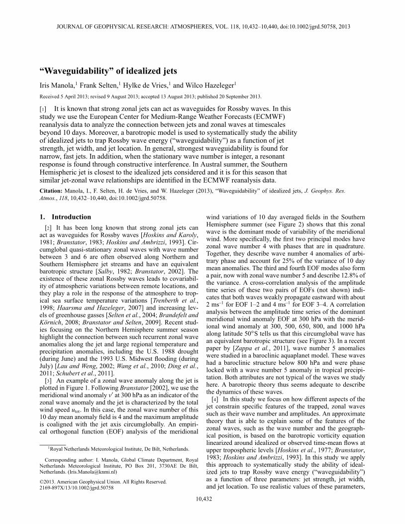
[3] An example of a zonal wave anomaly along the jet isplotted in Figure 1. Following Branstator [2002], we use themeridional wind anomaly v0 at 300 hPa as an indicator of thezonal wave anomaly and the jet is characterized by the totalwind speed utot. In this case, the zonal wave number of this10 day mean anomaly field is 4 and the maximum amplitudeis coaligned with the jet axis circumglobally. An empiri-cal orthogonal function (EOF) analysis of the meridional

1Royal Netherlands Meteorological Institute, De Bilt, Netherlands.

Corresponding author: I. Manola, Global Climate Department, RoyalNetherlands Meteorological Institute, PO Box 201, 3730AE De Bilt,Netherlands. ([email protected])

©2013. American Geophysical Union. All Rights Reserved.2169-897X/13/10.1002/jgrd.50758

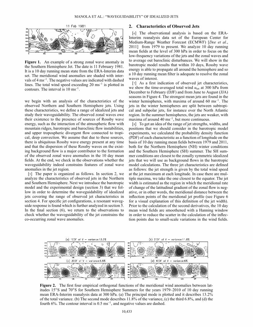
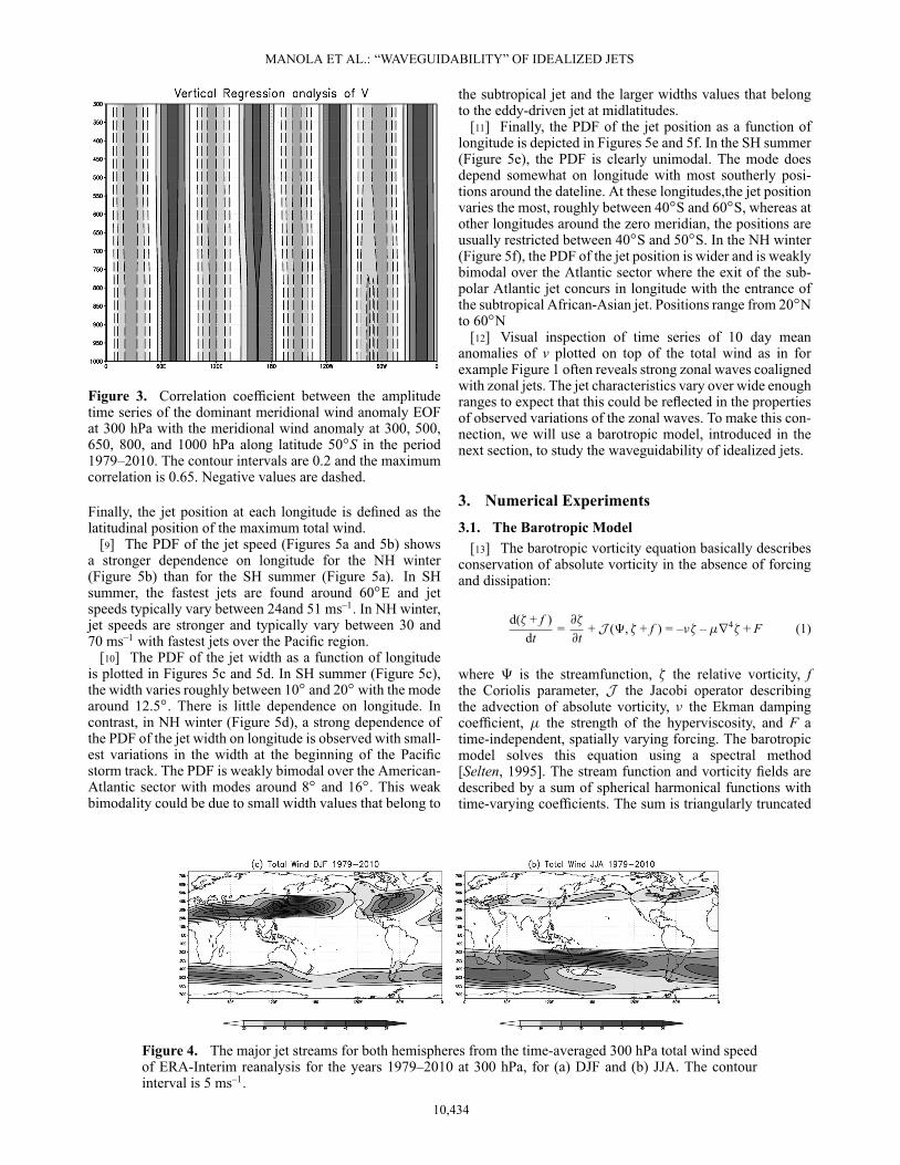
wind variations of 10 day averaged fields in the SouthernHemisphere summer (see Figure 2) shows that this zonalwave is the dominant mode of variability of the meridionalwind. More specifically, the first two principal modes havezonal wave number 4 with phases that are in quadrature.Together, they describe wave number 4 anomalies of arbi-trary phase and account for 25% of the variance of 10 daymean anomalies. The third and fourth EOF modes also forma pair, now with zonal wave number 5 and describe 12.8% ofthe variance. A cross-correlation analysis of the amplitudetime series of these two pairs of EOFs (not shown) indi-cates that both waves weakly propagate eastward with about2 ms–1 for EOF 1–2 and 4 ms–1 for EOF 3–4. A correlationanalysis between the amplitude time series of the dominantmeridional wind anomaly EOF at 300 hPa with the merid-ional wind anomaly at 300, 500, 650, 800, and 1000 hPaalong latitude 50ıS tells us that this circumglobal wave hasan equivalent barotropic structure (see Figure 3). In a recentpaper by [Zappa et al., 2011], wave number 5 anomalieswere studied in a baroclinic aquaplanet model. These waveshad a baroclinic structure below 800 hPa and were phaselocked with a wave number 5 anomaly in tropical precipi-tation. Both attributes are not typical of the waves we studyhere. A barotropic theory thus seems adequate to describethe dynamics of these waves.

[4] In this study we focus on how different aspects of thejet constrain specific features of the trapped, zonal wavessuch as their wave number and amplitudes. An approximatetheory that is able to explain some of the features of thezonal waves, such as the wave number and the geograph-ical position, is based on the barotropic vorticity equationlinearized around idealized or observed time-mean flows atupper tropospheric levels [Hoskins et al., 1977; Branstator,1983; Hoskins and Ambrizzi, 1993]. In this study we applythis approach to systematically study the ability of ideal-ized jets to trap Rossby wave energy (“waveguidability”)as a function of three parameters: jet strength, jet width,and jet location. To use realistic values of these parameters,

10,432

MANOLA ET AL.: “WAVEGUIDABILITY” OF IDEALIZED JETS

Figure 1. An example of a strong zonal wave anomaly inthe Southern Hemisphere Jet. The date is 11 February 1981.It is a 10 day running mean state from the ERA-Interim dataset. The meridional wind anomalies are shaded with inter-vals of 4 ms–1. The negative values are indicated with dashedlines. The total wind speed exceeding 20 ms–1 is plotted incontours. The interval is 10 ms–1.

we begin with an analysis of the characteristics of theobserved Northern and Southern Hemisphere jets. Usingthese characteristics, we define a range of idealized jets andstudy their waveguidability. The observed zonal waves owetheir existence to the presence of sources of Rossby waveenergy, such as the interaction of the atmospheric flow withmountain ridges, barotropic and baroclinic flow instabilities,and upper tropospheric divergent flow connected to tropi-cal, deep convection. We assume that due to these sources,there is ubiquitous Rossby wave energy present at any timeand that the dispersion of these Rossby waves on the exist-ing background flow is a major contributor to the formationof the observed zonal wave anomalies in the 10 day meanfields. At the end, we check in the observations whether thewaveguidability indeed constrains features of zonal waveanomalies in the jet region.

[5] The paper is organized as follows. In section 2, weanalyze the characteristics of observed jets in the Northernand Southern Hemisphere. Next we introduce the barotropicmodel and the experimental design (section 3) that we fol-low in order to determine the waveguidability of idealizedjets covering the range of observed jet characteristics insection 4. For specific jet configurations, a resonant waveg-uide response is found which is further analyzed in section 5.In the final section (6), we return to the observations tocheck whether the waveguidability of the jet constrains theco-occurring zonal wave anomalies.

2. Characteristics of Observed Jets[6] The observational analysis is based on the ERA-

Interim reanalysis data set of the European Center forMedium-Range Weather Forecast (ECMWF) [Dee et al.,2011] from 1979 to present. We analyze 10 day runningmean fields at the level of 300 hPa in order to focus on thelow-frequency variations of the jets and the zonal waves andto average out baroclinic disturbances. We will show in thebarotropic model results that within 10 days, Rossby waveenergy is able to propagate all around the hemisphere and soa 10 day running mean filter is adequate to resolve the zonalwaves of interest.

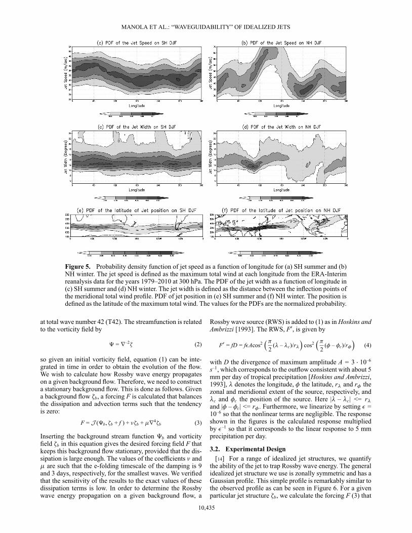
[7] As a first indication of observed jet characteristics,we show the time-averaged total wind utot at 300 hPa fromDecember to February (DJF) and from June to August (JJA)seasons in Figure 4. The strongest mean jets are found in thewinter hemispheres, with maxima of around 60 ms–1. Thejets in the winter hemispheres are split between subtropi-cal and subpolar jets, for instance over the North Atlanticregion. In the summer hemispheres, the jets are weaker, withmaxima of around 40 ms–1, but more continuous.

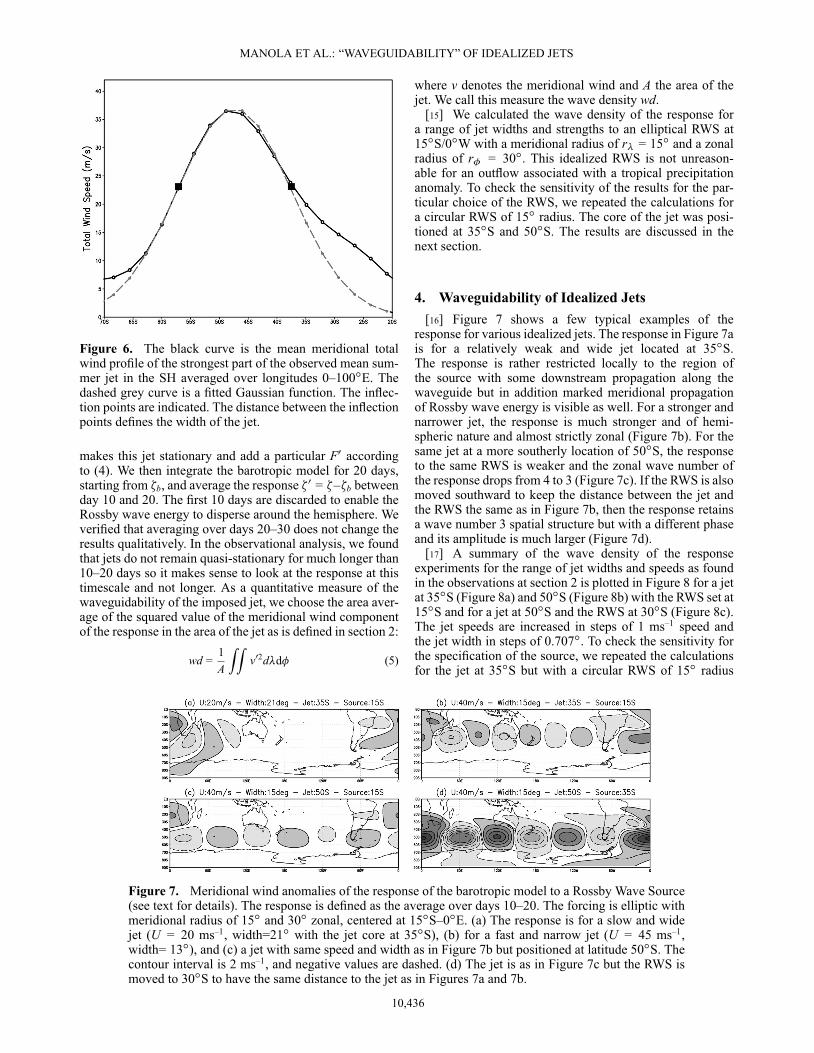
[8] To get an idea of the range of jet strengths, widths, andpositions that we should consider in the barotropic modelexperiments, we calculated the probability density function(PDF) of each characteristic as a function of longitude on thebasis of 10 day running mean fields between 1979 and 2011,both for the Northern Hemisphere (NH) winter conditionsand the Southern Hemisphere (SH) summer. The SH sum-mer conditions are closest to the zonally symmetric idealizedjets that we will use as background flows in the barotropicmodel calculations. The three jet characteristics are definedas follows: the jet strength is given by the total wind speedat the jet maximum at each longitude. In case there are mul-tiple maxima, we take the one closest to the equator. The jetwidth is estimated as the region in which the meridional rateof change of the latitudinal gradient of the zonal flow is neg-ative, or in other words, the meridional distance between theinflection points of the meridional jet profile (see Figure 6for a visual explanation of this definition of the jet width).Prior to the calculation of the second derivatives, the 10 daymean wind fields are smoothened with a Hanning windowin order to reduce the scatter in the calculation of the inflec-tion points due to small-scale variations in the wind fields.

Figure 2. The first four empirical orthogonal functions of the meridional wind anomalies between lat-itudes 15ıS and 70ıS for Southern Hemisphere Summers for the years 1979–2010 of 10 day runningmean ERA-Interim reanalysis data at 300 hPa. (a) The principal mode is plotted and it describes 13.2%of the total variance. (b) The second mode describes 11.8% of the variance, (c) the third 6.8%, and (d) thefourth 6%. The contour interval is 0.5 ms–1, and negative values are dashed.

10,433


Figure 3. Correlation coefficient between the amplitudetime series of the dominant meridional wind anomaly EOFat 300 hPa with the meridional wind anomaly at 300, 500,650, 800, and 1000 hPa along latitude 50ıS in the period1979–2010. The contour intervals are 0.2 and the maximumcorrelation is 0.65. Negative values are dashed.

Finally, the jet position at each longitude is defined as thelatitudinal position of the maximum total wind.

[9] The PDF of the jet speed (Figures 5a and 5b) showsa stronger dependence on longitude for the NH winter(Figure 5b) than for the SH summer (Figure 5a). In SHsummer, the fastest jets are found around 60ıE and jetspeeds typically vary between 24and 51 ms–1. In NH winter,jet speeds are stronger and typically vary between 30 and70 ms–1 with fastest jets over the Pacific region.

[10] The PDF of the jet width as a function of longitudeis plotted in Figures 5c and 5d. In SH summer (Figure 5c),the width varies roughly between 10ı and 20ı with the modearound 12.5ı. There is little dependence on longitude. Incontrast, in NH winter (Figure 5d), a strong dependence ofthe PDF of the jet width on longitude is observed with small-est variations in the width at the beginning of the Pacificstorm track. The PDF is weakly bimodal over the American-Atlantic sector with modes around 8ı and 16ı. This weakbimodality could be due to small width values that belong to

the subtropical jet and the larger widths values that belongto the eddy-driven jet at midlatitudes.

[11] Finally, the PDF of the jet position as a function oflongitude is depicted in Figures 5e and 5f. In the SH summer(Figure 5e), the PDF is clearly unimodal. The mode doesdepend somewhat on longitude with most southerly posi-tions around the dateline. At these longitudes,the jet positionvaries the most, roughly between 40ıS and 60ıS, whereas atother longitudes around the zero meridian, the positions areusually restricted between 40ıS and 50ıS. In the NH winter(Figure 5f), the PDF of the jet position is wider and is weaklybimodal over the Atlantic sector where the exit of the sub-polar Atlantic jet concurs in longitude with the entrance ofthe subtropical African-Asian jet. Positions range from 20ıNto 60ıN

[12] Visual inspection of time series of 10 day meananomalies of v plotted on top of the total wind as in forexample Figure 1 often reveals strong zonal waves coalignedwith zonal jets. The jet characteristics vary over wide enoughranges to expect that this could be reflected in the propertiesof observed variations of the zonal waves. To make this con-nection, we will use a barotropic model, introduced in thenext section, to study the waveguidability of idealized jets.

3. Numerical Experiments3.1. The Barotropic Model

[13] The barotropic vorticity equation basically describesconservation of absolute vorticity in the absence of forcingand dissipation:

d(� + f )dt

=@�

@t+ J (‰, � + f ) = –�� – �r4� + F (1)

where ‰ is the streamfunction, � the relative vorticity, fthe Coriolis parameter, J the Jacobi operator describingthe advection of absolute vorticity, � the Ekman dampingcoefficient, � the strength of the hyperviscosity, and F atime-independent, spatially varying forcing. The barotropicmodel solves this equation using a spectral method[Selten, 1995]. The stream function and vorticity fields aredescribed by a sum of spherical harmonical functions withtime-varying coefficients. The sum is triangularly truncated

Figure 4. The major jet streams for both hemispheres from the time-averaged 300 hPa total wind speedof ERA-Interim reanalysis for the years 1979–2010 at 300 hPa, for (a) DJF and (b) JJA. The contourinterval is 5 ms–1.

10,434


Figure 5. Probability density function of jet speed as a function of longitude for (a) SH summer and (b)NH winter. The jet speed is defined as the maximum total wind at each longitude from the ERA-Interimreanalysis data for the years 1979–2010 at 300 hPa. The PDF of the jet width as a function of longitude in(c) SH summer and (d) NH winter. The jet width is defined as the distance between the inflection points ofthe meridional total wind profile. PDF of jet position in (e) SH summer and (f) NH winter. The position isdefined as the latitude of the maximum total wind. The values for the PDFs are the normalized probability.

at total wave number 42 (T42). The streamfunction is relatedto the vorticity field by

‰ = r–2� (2)

so given an initial vorticity field, equation (1) can be inte-grated in time in order to obtain the evolution of the flow.We wish to calculate how Rossby wave energy propagateson a given background flow. Therefore, we need to constructa stationary background flow. This is done as follows. Givena background flow �b, a forcing F is calculated that balancesthe dissipation and advection terms such that the tendencyis zero:

F = J (‰b, �b + f ) + ��b + �r4�b (3)

Inserting the background stream function ‰b and vorticityfield �b in this equation gives the desired forcing field F thatkeeps this background flow stationary, provided that the dis-sipation is large enough. The values of the coefficients � and� are such that the e-folding timescale of the damping is 9and 3 days, respectively, for the smallest waves. We verifiedthat the sensitivity of the results to the exact values of thesedissipation terms is low. In order to determine the Rossbywave energy propagation on a given background flow, a

Rossby wave source (RWS) is added to (1) as in Hoskins andAmbrizzi [1993]. The RWS, F0, is given by

F0 = fD = f�Acos2��

2(� – �c)/r�

�cos2

��2

(� – �c)/r��

(4)

with D the divergence of maximum amplitude A = 3 � 10–6

s–1, which corresponds to the outflow consistent with about 5mm per day of tropical precipitation [Hoskins and Ambrizzi,1993], � denotes the longitude, � the latitude, r� and r� thezonal and meridional extent of the source, respectively, and�c and �c the position of the source. Here |� – �c| <= r�and |� – �c| <= r� . Furthermore, we linearize by setting � =10–6 so that the nonlinear terms are negligible. The responseshown in the figures is the calculated response multipliedby �–1 so that it corresponds to the linear response to 5 mmprecipitation per day.

3.2. Experimental Design[14] For a range of idealized jet structures, we quantify

the ability of the jet to trap Rossby wave energy. The generalidealized jet structure we use is zonally symmetric and has aGaussian profile. This simple profile is remarkably similar tothe observed profile as can be seen in Figure 6. For a givenparticular jet structure �b, we calculate the forcing F (3) that

10,435


Figure 6. The black curve is the mean meridional totalwind profile of the strongest part of the observed mean sum-mer jet in the SH averaged over longitudes 0–100ıE. Thedashed grey curve is a fitted Gaussian function. The inflec-tion points are indicated. The distance between the inflectionpoints defines the width of the jet.

makes this jet stationary and add a particular F0 accordingto (4). We then integrate the barotropic model for 20 days,starting from �b, and average the response �0 = �–�b betweenday 10 and 20. The first 10 days are discarded to enable theRossby wave energy to disperse around the hemisphere. Weverified that averaging over days 20–30 does not change theresults qualitatively. In the observational analysis, we foundthat jets do not remain quasi-stationary for much longer than10–20 days so it makes sense to look at the response at thistimescale and not longer. As a quantitative measure of thewaveguidability of the imposed jet, we choose the area aver-age of the squared value of the meridional wind componentof the response in the area of the jet as is defined in section 2:

wd =1A

ZZv02d�d� (5)

where v denotes the meridional wind and A the area of thejet. We call this measure the wave density wd.

[15] We calculated the wave density of the response fora range of jet widths and strengths to an elliptical RWS at15ıS/0ıW with a meridional radius of r� = 15ı and a zonalradius of r� = 30ı. This idealized RWS is not unreason-able for an outflow associated with a tropical precipitationanomaly. To check the sensitivity of the results for the par-ticular choice of the RWS, we repeated the calculations fora circular RWS of 15ı radius. The core of the jet was posi-tioned at 35ıS and 50ıS. The results are discussed in thenext section.

4. Waveguidability of Idealized Jets[16] Figure 7 shows a few typical examples of the

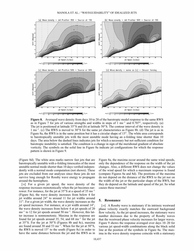
response for various idealized jets. The response in Figure 7ais for a relatively weak and wide jet located at 35ıS.The response is rather restricted locally to the region ofthe source with some downstream propagation along thewaveguide but in addition marked meridional propagationof Rossby wave energy is visible as well. For a stronger andnarrower jet, the response is much stronger and of hemi-spheric nature and almost strictly zonal (Figure 7b). For thesame jet at a more southerly location of 50ıS, the responseto the same RWS is weaker and the zonal wave number ofthe response drops from 4 to 3 (Figure 7c). If the RWS is alsomoved southward to keep the distance between the jet andthe RWS the same as in Figure 7b, then the response retainsa wave number 3 spatial structure but with a different phaseand its amplitude is much larger (Figure 7d).

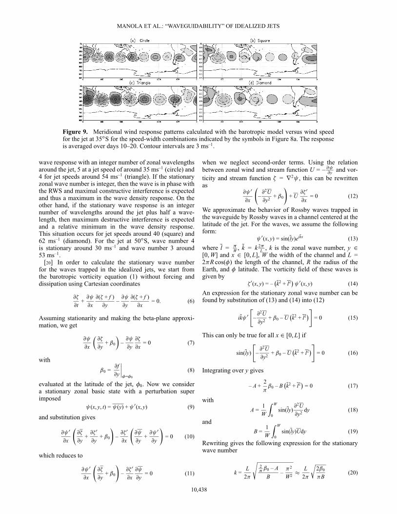
[17] A summary of the wave density of the responseexperiments for the range of jet widths and speeds as foundin the observations at section 2 is plotted in Figure 8 for a jetat 35ıS (Figure 8a) and 50ıS (Figure 8b) with the RWS set at15ıS and for a jet at 50ıS and the RWS at 30ıS (Figure 8c).The jet speeds are increased in steps of 1 ms–1 speed andthe jet width in steps of 0.707ı. To check the sensitivity forthe specification of the source, we repeated the calculationsfor the jet at 35ıS but with a circular RWS of 15ı radius

Figure 7. Meridional wind anomalies of the response of the barotropic model to a Rossby Wave Source(see text for details). The response is defined as the average over days 10–20. The forcing is elliptic withmeridional radius of 15ı and 30ı zonal, centered at 15ıS–0ıE. (a) The response is for a slow and widejet (U = 20 ms–1, width=21ı with the jet core at 35ıS), (b) for a fast and narrow jet (U = 45 ms–1,width= 13ı), and (c) a jet with same speed and width as in Figure 7b but positioned at latitude 50ıS. Thecontour interval is 2 ms–1, and negative values are dashed. (d) The jet is as in Figure 7c but the RWS ismoved to 30ıS to have the same distance to the jet as in Figures 7a and 7b.

10,436


Figure 8. Averaged wave density from days 10 to 20 of the barotropic model response to the same RWSas in Figure 7 for jets of various strengths and widths in steps of 1 ms–1 and 0.707ı, respectively. (a)The jet is positioned at latitude 35ıS and (b) at latitude 50ıS. The contour interval of the wave density is1 ms–1. (c) The RWS is moved to 30ıS for the same jet characteristics as Figure 8b. (d) The jet is as inFigure 8a, the RWS is in the same position but it has a circular shape of 15ı. The white area correspondsto barotropically unstable jets with the most unstable mode having an e-folding time shorter than 10days. The area below the dashed lines indicates jets for which a necessary but not sufficient condition forbarotropic instability is satisfied. The condition is a change in sign of the meridional gradient of absolutevorticity. The symbols on the solid line in Figure 8a indicate jet configurations for which the responsepattern is shown in Figure 9.

(Figure 8d). The white area marks narrow fast jets that arebarotropically unstable with e-folding timescales of the mostunstable normal mode shorter than 10 days verified indepen-dently with a normal mode computation (not shown). Thesejets are excluded from our analyses since these jets do notsurvive long enough for Rossby wave energy to propagatearound the hemisphere.

[18] For a given jet speed, the wave density of theresponse increases monotonically when the jet becomes nar-rower. For instance, for the jet at 35ıS at a speed of 35 ms–1

(Figure 8a), the wave density increases from below 4 forjet widths around 24ı to around 11 for jet widths around11ı. For a given jet width, the wave density increases as thejet speed increases. For instance, at a jet width around 14ı,the wave density increases from below 4 at jet speeds of 20ms–1 to 12 for jet speeds around 50 ms–1. However, this lat-ter increase is nonmonotonic. Maxima in the response arefound for jet speeds around 35, 54, and 68 ms–1 for the jetat 35ıS. For the jet at 50ıS (Figures 8b and 8c), maximaare found around 30 and 53 ms–1. When for the jet at 50ıS,the RWS is moved 15ı to the south (Figure 8c) in order tohave the same distance between the jet and the RWS as in

Figure 8a, the maxima occur around the same wind speeds,only the dependence of the response on the width of the jetchanges. Also, a different RWS does not change the valuesof the wind speed for which a maximum response is found(compare Figures 8a and 8d). The positions of the maximado not depend on the distance of the RWS to the jet nor onthe width of the jet or the particular shape of the RWS, butthey do depend on the latitude and speed of the jet. So whatcauses these maxima?

5. Resonance[19] A Rossby wave is stationary if its intrinsic westward

phase velocity exactly matches the eastward backgroundflow velocity. As the jet speed increases, the stationary wavenumber decreases due to the property of Rossby wavesthat the westward phase velocity increases for larger waves.Figure 9 shows the response averaged over days 10–20 forvarious jet speed-width combinations along the black solidline at the position of the symbols in Figure 8a. The max-ima in the wave density response coincide with a stationary

10,437


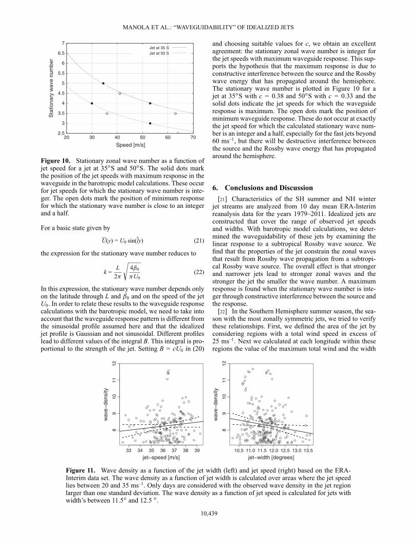
Figure 9. Meridional wind response patterns calculated with the barotropic model versus wind speedfor the jet at 35ıS for the speed-width combinations indicated by the symbols in Figure 8a. The responseis averaged over days 10–20. Contour intervals are 3 ms–1.

wave response with an integer number of zonal wavelengthsaround the jet, 5 at a jet speed of around 35 ms–1 (circle) and4 for jet speeds around 54 ms–1 (triangle). If the stationaryzonal wave number is integer, then the wave is in phase withthe RWS and maximal constructive interference is expectedand thus a maximum in the wave density response. On theother hand, if the stationary wave response is an integernumber of wavelengths around the jet plus half a wave-length, then maximum destructive interference is expectedand a relative minimum in the wave density response.This situation occurs for jet speeds around 40 (square) and62 ms–1 (diamond). For the jet at 50ıS, wave number 4is stationary around 30 ms–1 and wave number 3 around53 ms–1.

[20] In order to calculate the stationary wave numberfor the waves trapped in the idealized jets, we start fromthe barotropic vorticity equation (1) without forcing anddissipation using Cartesian coordinates

@�

@t+@

@x@(� + f )@y

–@

@y@(� + f )@x

= 0. (6)

Assuming stationarity and making the beta-plane approxi-mation, we get

@

@x

�@�

@y+ ˇ0

�–@

@y@�

@x= 0 (7)

withˇ0 =

@f@y

ˇ̌̌ˇ�=�0

(8)

evaluated at the latitude of the jet, �0. Now we considera stationary zonal basic state with a perturbation superimposed

(x, y, t) = (y) + 0(x, y) (9)

and substitution gives

@ 0

@x

@�

@y+@�0

@y+ ˇ0

!–@�0

@x

@

@y+@ 0

@y

!= 0 (10)

which reduces to

@ 0

@x

@�

@y+ ˇ0

!–@�0

@x@

@y= 0 (11)

when we neglect second-order terms. Using the relationbetween zonal wind and stream function U = –@

@y and vor-ticity and stream function � = r2 , this can be rewrittenas

@ 0

@x

–@2U@y2 + ˇ0

!+ U

@�0

@x= 0 (12)

We approximate the behavior of Rossby waves trapped inthe waveguide by Rossby waves in a channel centered at thelatitude of the jet. For the waves, we assume the followingform:

0(x, y) = sin(Qly)eiQkx (13)where Ql = �

W , Qk = k 2�L , k is the zonal wave number, y 2

[0, W] and x 2 [0, L], W the width of the channel and L =2�R cos(�) the length of the channel, R the radius of theEarth, and � latitude. The vorticity field of these waves isgiven by

�0(x, y) = –�Qk2 + Ql2

� 0(x, y) (14)

An expression for the stationary zonal wave number can befound by substitution of (13) and (14) into (12)

iQk 0"

–@2U@y2 + ˇ0 – U

�Qk2 + Ql2

�#= 0 (15)

This can only be true for all x 2 [0, L] if

sin(Qly)

"–@2U@y2 + ˇ0 – U

�Qk2 + Ql2

�#= 0 (16)

Integrating over y gives

– A +2�ˇ0 – B

�Qk2 + Ql2

�= 0 (17)

withA =

1W

Z W

0sin(Qly)

@2U@y2 dy (18)

andB =

1W

Z W

0sin(Qly)Udy (19)

Rewriting gives the following expression for the stationarywave number

k =L

2�

s2�ˇ0 – A

B–�2

W2 �L

2�

r2ˇ0

�B(20)

10,438


2.5

3

3.5

4

4.5

5

5.5

6

6.5

7

20 30 40 50 60 70

Sta

tiona

ry w

ave

num

ber

Speed [m/s]

Jet at 35 SJet at 50 S

Figure 10. Stationary zonal wave number as a function ofjet speed for a jet at 35ıS and 50ıS. The solid dots markthe position of the jet speeds with maximum response in thewaveguide in the barotropic model calculations. These occurfor jet speeds for which the stationary wave number is inte-ger. The open dots mark the position of minimum responsefor which the stationary wave number is close to an integerand a half.

For a basic state given by

U(y) = U0 sin(Qly) (21)

the expression for the stationary wave number reduces to

k =L

2�

s4ˇ0

�U0(22)

In this expression, the stationary wave number depends onlyon the latitude through L and ˇ0 and on the speed of the jetU0. In order to relate these results to the waveguide responsecalculations with the barotropic model, we need to take intoaccount that the waveguide response pattern is different fromthe sinusoidal profile assumed here and that the idealizedjet profile is Gaussian and not sinusoidal. Different profileslead to different values of the integral B. This integral is pro-portional to the strength of the jet. Setting B = cU0 in (20)

and choosing suitable values for c, we obtain an excellentagreement: the stationary zonal wave number is integer forthe jet speeds with maximum waveguide response. This sup-ports the hypothesis that the maximum response is due toconstructive interference between the source and the Rossbywave energy that has propagated around the hemisphere.The stationary wave number is plotted in Figure 10 for ajet at 35ıS with c = 0.38 and 50ıS with c = 0.33 and thesolid dots indicate the jet speeds for which the waveguideresponse is maximum. The open dots mark the position ofminimum waveguide response. These do not occur at exactlythe jet speed for which the calculated stationary wave num-ber is an integer and a half, especially for the fast jets beyond60 ms–1, but there will be destructive interference betweenthe source and the Rossby wave energy that has propagatedaround the hemisphere.

6. Conclusions and Discussion[21] Characteristics of the SH summer and NH winter

jet streams are analyzed from 10 day mean ERA-Interimreanalysis data for the years 1979–2011. Idealized jets areconstructed that cover the range of observed jet speedsand widths. With barotropic model calculations, we deter-mined the waveguidability of these jets by examining thelinear response to a subtropical Rossby wave source. Wefind that the properties of the jet constrain the zonal wavesthat result from Rossby wave propagation from a subtropi-cal Rossby wave source. The overall effect is that strongerand narrower jets lead to stronger zonal waves and thestronger the jet the smaller the wave number. A maximumresponse is found when the stationary wave number is inte-ger through constructive interference between the source andthe response.

[22] In the Southern Hemisphere summer season, the sea-son with the most zonally symmetric jets, we tried to verifythese relationships. First, we defined the area of the jet byconsidering regions with a total wind speed in excess of25 ms–1. Next we calculated at each longitude within theseregions the value of the maximum total wind and the width

jet−speed [m/s]

wav

e−de

nsity

33 34 35 36 37 38 39

89

1011

12

10.5 11.0 11.5 12.0 12.5 13.0 13.5

89

1011

12

jet−width [degrees]

wav

e−de

nsity

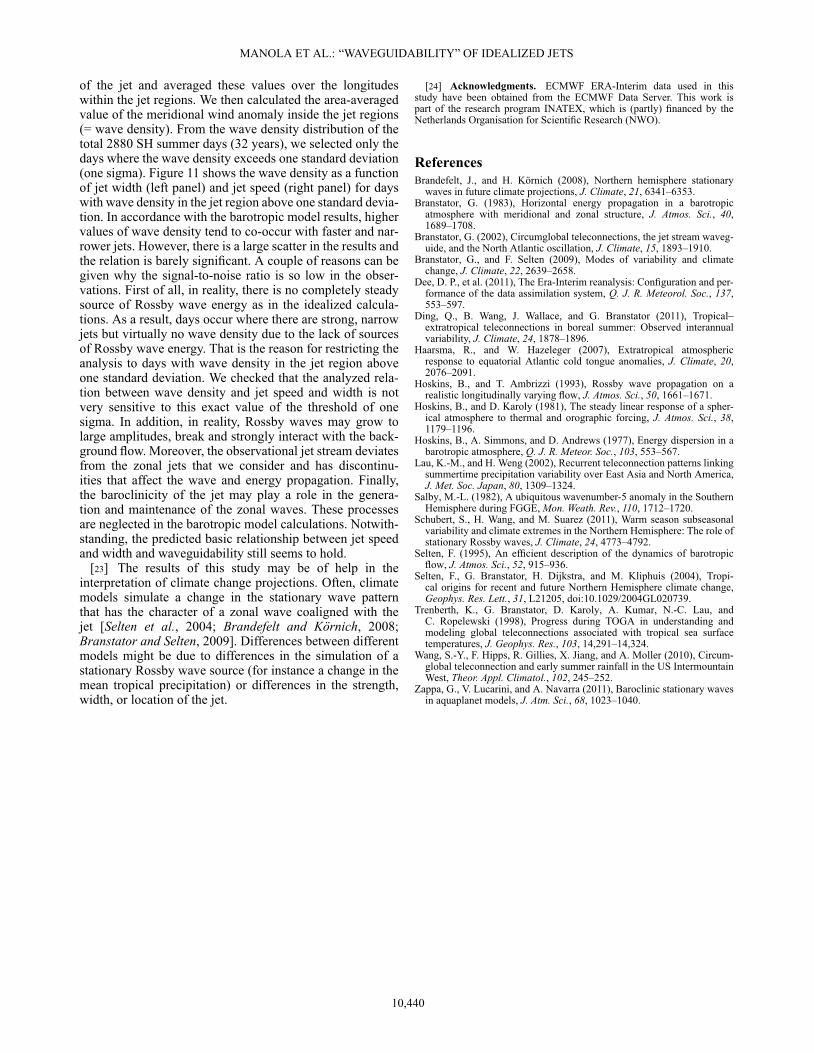
Figure 11. Wave density as a function of the jet width (left) and jet speed (right) based on the ERA-Interim data set. The wave density as a function of jet width is calculated over areas where the jet speedlies between 20 and 35 ms–1. Only days are considered with the observed wave density in the jet regionlarger than one standard deviation. The wave density as a function of jet speed is calculated for jets withwidth’s between 11.5ı and 12.5 ı.

10,439


of the jet and averaged these values over the longitudeswithin the jet regions. We then calculated the area-averagedvalue of the meridional wind anomaly inside the jet regions(= wave density). From the wave density distribution of thetotal 2880 SH summer days (32 years), we selected only thedays where the wave density exceeds one standard deviation(one sigma). Figure 11 shows the wave density as a functionof jet width (left panel) and jet speed (right panel) for dayswith wave density in the jet region above one standard devia-tion. In accordance with the barotropic model results, highervalues of wave density tend to co-occur with faster and nar-rower jets. However, there is a large scatter in the results andthe relation is barely significant. A couple of reasons can begiven why the signal-to-noise ratio is so low in the obser-vations. First of all, in reality, there is no completely steadysource of Rossby wave energy as in the idealized calcula-tions. As a result, days occur where there are strong, narrowjets but virtually no wave density due to the lack of sourcesof Rossby wave energy. That is the reason for restricting theanalysis to days with wave density in the jet region aboveone standard deviation. We checked that the analyzed rela-tion between wave density and jet speed and width is notvery sensitive to this exact value of the threshold of onesigma. In addition, in reality, Rossby waves may grow tolarge amplitudes, break and strongly interact with the back-ground flow. Moreover, the observational jet stream deviatesfrom the zonal jets that we consider and has discontinu-ities that affect the wave and energy propagation. Finally,the baroclinicity of the jet may play a role in the genera-tion and maintenance of the zonal waves. These processesare neglected in the barotropic model calculations. Notwith-standing, the predicted basic relationship between jet speedand width and waveguidability still seems to hold.

[23] The results of this study may be of help in theinterpretation of climate change projections. Often, climatemodels simulate a change in the stationary wave patternthat has the character of a zonal wave coaligned with thejet [Selten et al., 2004; Brandefelt and Körnich, 2008;Branstator and Selten, 2009]. Differences between differentmodels might be due to differences in the simulation of astationary Rossby wave source (for instance a change in themean tropical precipitation) or differences in the strength,width, or location of the jet.

[24] Acknowledgments. ECMWF ERA-Interim data used in thisstudy have been obtained from the ECMWF Data Server. This work ispart of the research program INATEX, which is (partly) financed by theNetherlands Organisation for Scientific Research (NWO).

ReferencesBrandefelt, J., and H. Körnich (2008), Northern hemisphere stationary

waves in future climate projections, J. Climate, 21, 6341–6353.Branstator, G. (1983), Horizontal energy propagation in a barotropic

atmosphere with meridional and zonal structure, J. Atmos. Sci., 40,1689–1708.

Branstator, G. (2002), Circumglobal teleconnections, the jet stream waveg-uide, and the North Atlantic oscillation, J. Climate, 15, 1893–1910.

Branstator, G., and F. Selten (2009), Modes of variability and climatechange, J. Climate, 22, 2639–2658.

Dee, D. P., et al. (2011), The Era-Interim reanalysis: Configuration and per-formance of the data assimilation system, Q. J. R. Meteorol. Soc., 137,553–597.

Ding, Q., B. Wang, J. Wallace, and G. Branstator (2011), Tropical–extratropical teleconnections in boreal summer: Observed interannualvariability, J. Climate, 24, 1878–1896.

Haarsma, R., and W. Hazeleger (2007), Extratropical atmosphericresponse to equatorial Atlantic cold tongue anomalies, J. Climate, 20,2076–2091.

Hoskins, B., and T. Ambrizzi (1993), Rossby wave propagation on arealistic longitudinally varying flow, J. Atmos. Sci., 50, 1661–1671.

Hoskins, B., and D. Karoly (1981), The steady linear response of a spher-ical atmosphere to thermal and orographic forcing, J. Atmos. Sci., 38,1179–1196.

Hoskins, B., A. Simmons, and D. Andrews (1977), Energy dispersion in abarotropic atmosphere, Q. J. R. Meteor. Soc., 103, 553–567.

Lau, K.-M., and H. Weng (2002), Recurrent teleconnection patterns linkingsummertime precipitation variability over East Asia and North America,J. Met. Soc. Japan, 80, 1309–1324.

Salby, M.-L. (1982), A ubiquitous wavenumber-5 anomaly in the SouthernHemisphere during FGGE, Mon. Weath. Rev., 110, 1712–1720.

Schubert, S., H. Wang, and M. Suarez (2011), Warm season subseasonalvariability and climate extremes in the Northern Hemisphere: The role ofstationary Rossby waves, J. Climate, 24, 4773–4792.

Selten, F. (1995), An efficient description of the dynamics of barotropicflow, J. Atmos. Sci., 52, 915–936.

Selten, F., G. Branstator, H. Dijkstra, and M. Kliphuis (2004), Tropi-cal origins for recent and future Northern Hemisphere climate change,Geophys. Res. Lett., 31, L21205, doi:10.1029/2004GL020739.

Trenberth, K., G. Branstator, D. Karoly, A. Kumar, N.-C. Lau, andC. Ropelewski (1998), Progress during TOGA in understanding andmodeling global teleconnections associated with tropical sea surfacetemperatures, J. Geophys. Res., 103, 14,291–14,324.

Wang, S.-Y., F. Hipps, R. Gillies, X. Jiang, and A. Moller (2010), Circum-global teleconnection and early summer rainfall in the US IntermountainWest, Theor. Appl. Climatol., 102, 245–252.

Zappa, G., V. Lucarini, and A. Navarra (2011), Baroclinic stationary wavesin aquaplanet models, J. Atm. Sci., 68, 1023–1040.

10,440

Documents

"Waveguidability" of idealized jets