Embed Size (px)
Citation preview

University of New Hampshire University of New Hampshire
University of New Hampshire Scholars' University of New Hampshire Scholars'
Repository Repository
PREP Reports & Publications Institute for the Study of Earth, Oceans, and Space (EOS)
3-2018
Great Bay Estuary Water Quality Monitoring Program: Quality Great Bay Estuary Water Quality Monitoring Program: Quality
Assurance Project Plan, 2018 Assurance Project Plan, 2018
Thomas K. Gregory University of New Hampshire, Durham
Kalle Matso University of New Hampshire, Durham
Follow this and additional works at: https://scholars.unh.edu/prep
Recommended Citation Recommended Citation Gregory, Thomas K. and Matso, Kalle, "Great Bay Estuary Water Quality Monitoring Program: Quality Assurance Project Plan, 2018" (2018). PREP Reports & Publications. 405. https://scholars.unh.edu/prep/405
This Report is brought to you for free and open access by the Institute for the Study of Earth, Oceans, and Space (EOS) at University of New Hampshire Scholars' Repository. It has been accepted for inclusion in PREP Reports & Publications by an authorized administrator of University of New Hampshire Scholars' Repository. For more information, please contact [email protected].


2018 UNH Estuarine Water Quality Monitoring Program QAPP March 2018
Page 2
Table of Contents
List of Appendices Page 3 List of Tables Page 4 List of Figures Page 4 Section A3 Distribution List Page 5 Section A4 Project/Task Organization Page 6 Section A5 Problem Definition/Background Page 8 Section A6 Project/Task Description Page 9 Section A7 Quality Objectives and Criteria Page 10 Section A8 Special Training/Certification Page 15 Section A9 Documents and Records Page 15 Section B1 Sampling Process Design Page 16 Section B2 Sampling Methods Page 22 Section B3 Sample Handling and Custody Page 23 Section B4 Analytical Methods Page 23 Section B5 Quality Control Page 25 Section B6 Instrument/Equipment Testing, Inspection, Maintenance Page 25 Section B7 Instrument/Equipment Calibration and Frequency Page 26 Section B8 Inspection/Acceptance Requirements for Supplies and Consumables Page 26 Section B9 Non-Direct Measurements Page 26 Section B10 Data Management Page 26 Section C1 Assessments and Response Actions Page 27 Section C2 Reports to Management Page 27 Section D1 Data Review, Verification and Validation Page 27 Section D2 Verification and Validation Procedures Page 27 Section D3 Reconciliation with User Requirements Page 28 References Page 28

2018 UNH Estuarine Water Quality Monitoring Program QAPP March 2018
Page 3
List of Appendices Appendix A QAPP for Water Quality Analysis Lab at UNH Page 29 Appendix B SOPs for Nutrient Analyses Page 45 Appendix C SOPs for Dissolved Organic Carbon and Total Dissolved Nitrogen Page 63 Appendix D SOPs for Total Solids, Total Suspended Solids, and Total Dissolved Solids Page 68 Appendix E SOPs for Particulate Carbon and Nitrogen Page 75 Appendix F Quality Assurance Plan: Microbiology Laboratory at UNH-Jackson Estuarine Laboratory Page 82 Appendix G SOPs for Detection of Total Coliforms, Fecal Coliforms, Escherichia coli and Enterococci from Environmental Samples Page 88 Appendix H SOPs for LI-1400 DataLogger PAR Measurements Page 102 Appendix I Ocean Optics Protocols Page 105 Appendix J SOPs for NERRS SWMP EXO Sondes Page 149 Appendix K Field Data Sheet Page 182

2018 UNH Estuarine Water Quality Monitoring Program QAPP March 2018
Page 4
List of Tables Table 1: QAPP Distribution List Page 5 Table 2: Project Schedule Timeline Page 9 Table 3: Measurement Performance Criteria for Nutrient Samples Page 10 Table 4: Surface Water Target Analytes and Reference Limits Page 11 Table 5: Measurement performance criteria for bacterial indicators Page 12 Table 6: Data Reliability for Bacterial Indicators Page 12 Table 7: Data quality objectives for in-situ PAR measurements Page 14 Table 8: Special personnel training requirements Page 15 Table 9: Sampling specifications by station Page 17 Table 10: Sampling Station Locations Page 19 Table 11: Sampling Design Page 19 Table 12: Sample requirements Page 22 Table 13: Analytes and Analytical Methods Page 24 Table 14: Water bacterial indicators and reference limits. Page 25 Table 15: Laboratory Instruments Page 26 Table 16: Project Assessment Table Page 27 List of Figures Figure 1 Organizational Chart Page 7 Figure 2 Water Quality Monitoring Stations Map Page 21

2018 UNH Estuarine Water Quality Monitoring Program QAPP March 2018
Page 5
A3 – Distribution List
Table 1 presents a list of people who will receive the approved QAPP, the QAPP revisions, and any amendments.
Table 1. QAPP Distribution List QAPP Recipient
Name Project Role Organization Telephone number
and Email address Rachel Rouillard PREP Director UNH/PREP 603-862-3948
[email protected] Kalle Matso Project Manager UNH/PREP 603-781-6591
[email protected] Lara Martin Project QA Officer UNH 415-680-4944
[email protected] Tom Gregory Field Operations Manager UNH School of Marine
Science and Ocean Engineering
603-862-5136 [email protected]
Stephen Jones Microbiological Laboratory Manager
UNH Jackson Estuarine Laboratory
603-862-5124 [email protected]
Jody Potter Laboratory Manager UNH, Water Quality Analysis Lab, Department of Natural Resources
603-862-2341 [email protected]
Jean Brochi USEPA Project Officer USEPA 603-918-1536 [email protected]
Nora Conlon USEPA Quality Assurance Officer
USEPA New England (617) 918-8335; [email protected]
Ted Diers Data Repository/Access NH DES 603-271-3289; [email protected]
Based on EPA-NE Worksheet #3

2018 UNH Estuarine Water Quality Monitoring Program QAPP March 2018
Page 6
A4 – Project/Task Organization
The Piscataqua Region Estuaries Partnership (PREP) is part of the U.S. Environmental Protection Agency’s National Estuary Program, which is a joint local/state/federal program established under the Clean Water Act with the goal of protecting and enhancing nationally significant estuarine resources. PREP receives its funding from the EPA and is administered by the University of New Hampshire (UNH). The project will be conducted and managed by PREP. The Project Manager (Kalle Matso) will be responsible for coordinating all program activities, including administration. The Project QA Officer (Lara Martin) will focus on reviewing data and ensuring that quality objectives are met.
The Field Operations Manager (Tom Gregory) will manage all field staff, be responsible for “stop/go” decisions for daily sampling runs during extreme events and will notify the Laboratory Manager when samples will be delivered. The Field Operations Manager will be responsible for resolving any logistical problems and communicating the results to the field staff.
The work described here is partially funded by and follows protocols from the National Estuarine Research Reserve (NERR) System, following the System-Wide Monitoring Program (SWMP).
Samples will be analyzed by the Water Quality Analysis Laboratory (WQAL) at the University of New Hampshire (UNH) except for chlorophyll-a and total suspended solids samples, which are analyzed by UNH School of Marine Science and Ocean Engineering staff at the Jackson Estuarine Laboratory, and fecal-borne indicator bacteria, which are analyzed at the Jackson Estuarine Laboratory microbiology lab, overseen by Stephen Jones. Laboratory operations will be managed by the Laboratory Managers (Jody Potter and Stephen Jones). The Laboratory Managers will be responsible for conducting analyses according to the procedures in this QA Project Plan; the QA Project Officer will identify any non-conformities or analytical problems and reporting any problems to the Project Manager. The Laboratory Managers will be responsible for resolving any problems and communicating the results to the laboratory staff.
At the end of the project, the Project QA Officer will review the results of QA/QC checks and verify that the procedures of the Plan were completed. The Project QA Officer will be responsible for a memorandum to the project manager summarizing any deviations from the procedures in the QA Project Plan, the results of the QA/QC tests, and whether the reported data meets the data quality objectives of the project. All data and QA/QC reports will be shared with the New Hampshire State Department of Environmental Services (NH DES), which provides data to the public via the Environmental Monitoring Database.
PREP is considered part of the U.S. Environmental Protection Agency. Therefore, the Project Manager will be accountable to the EPA QA Officer (Nora Conlon) and the EPA Project Officer (Jean Brochi), who will be responsible for approving the Quality Assurance Project Plan.
The principal user of the data from this project will be PREP for State of Our Estuaries Reports. The Project Manager will prepare a report for PREP at the end of the project with all the data and the QA Officer’s summary report. Figure 1 shows an organizational chart for this project.

2018 UNH Estuarine Water Quality Monitoring Program QAPP March 2018
Page 7
Figure 1. Project organizational chart
Kalle Matso PREP
Project Manager
Jody Potter UNH WQAL Laboratory Manager
Nora Conlon USEPA
QA Officer
Tom Gregory; UNH Field Operations Manager
Stephen Jones; UNH
Microbiological Laboratory Manager
Jean Brochi USEPA
Project Officer
Lara Martin UNH
Project QA Officer

2018 UNH Estuarine Water Quality Monitoring Program QAPP March 2018
Page 8
A5 – Problem Definition/Background
PREP helps coordinate the water quality monitoring in NH’s estuarine waters. Historically, water quality stations in the estuaries have been monitored for nutrients, fecal-borne bacteria, and a suite of physicochemical parameters. This effort involves datasondes as well as grab samples. Directly below, datasonde parameters are described, and this is followed by a description of the grab sample parameters.
Datasonde instruments used will be Yellow Springs International (YSI) EXO2 or 6600 Multiparameter Sondes. Parameters monitored by this effort include: temperature, conductivity (salinity), dissolved oxygen, turbidity, depth, and pH. The following parameters will be included at some stations: chlorophyll-a and fDOM. (Note: the chlorophyll-a probes actually measure chlorophyll-a and additional pigments, either phycocyanin or phycoerythrin, depending on the probe.)
With regard to monthly grab samples, the specific parameters monitored by this program are:
Dissolved Nutrients Bacteria Eutrophication Physicochemical Nitrate+nitrite Ammonium Orthophosphate Dissolved Organic Carbon Total Dissolved Nitrogen Silica* Dissolved Inorganic Nitrogen Dissolved Organic Nitrogen
Fecal coliform** E. coli** Enterococci
Dissolved oxygen Chlorophyll-a Pheophytin-a Total suspended solids Particulate Organic Carbon Particulate Organic Nitrogen
Water Temperature Salinity Light attenuation (Kd)
* Only at following stations: Adam’s Point, Hampton River
** Due to shortage of funds, fecal coliform and E. coli may not be sampled at all sites.
The purpose of this effort is to track long-term changes in water quality parameters that have been shown to impact critical biological resources such as salt marshes and eelgrass. Also, some of these parameters are important for assessing human health concerns related to swimming and the consumption of shellfish.
The study design will follow the National Estuarine Research Reserves System Wide Monitoring Program (SWMP) sampling design. The sampling design is described in Section B of this QAPP. Grab samples will be collected from ten monitoring locations throughout the estuary. Samples will be collected monthly from April to December at each location. At seven of the sampling locations grab samples will be collected at low tide, with one station receiving sampling every other hour for 24 hours. Replication for QA purposes will be performed on greater than 10% of samples. The samples will be analyzed by laboratories at Jackson Estuarine Laboratory and the Water Quality Analysis Laboratory at the University of New Hampshire. In addition to the grab samples, datasondes will be deployed at eight of the monitoring locations and at two sites that do not receive grab sampling (see Table 9). Most sondes are deployed approximately 0.5 m off the bottom per SWMP protocol.
A final component of this effort involves grab sampling at the Lamprey River Station using an auto-sampler to capture water samples through an entire diurnal cycle. The purpose of this component of the effort is to balance the snapshot and low-tide samples with a description of one entire tidal cycle. This is part of the NERRS SWMP Protocol. Parameters measured as part of this component represent a subset of the monthly grab sample parameters and include: all of the dissolved nutrients with the exception of silica; chlorophyll-a, TSS and PC/PN.
2018 UNH Estuarine Water Quality Monitoring Program QAPP March 2018
Page 9
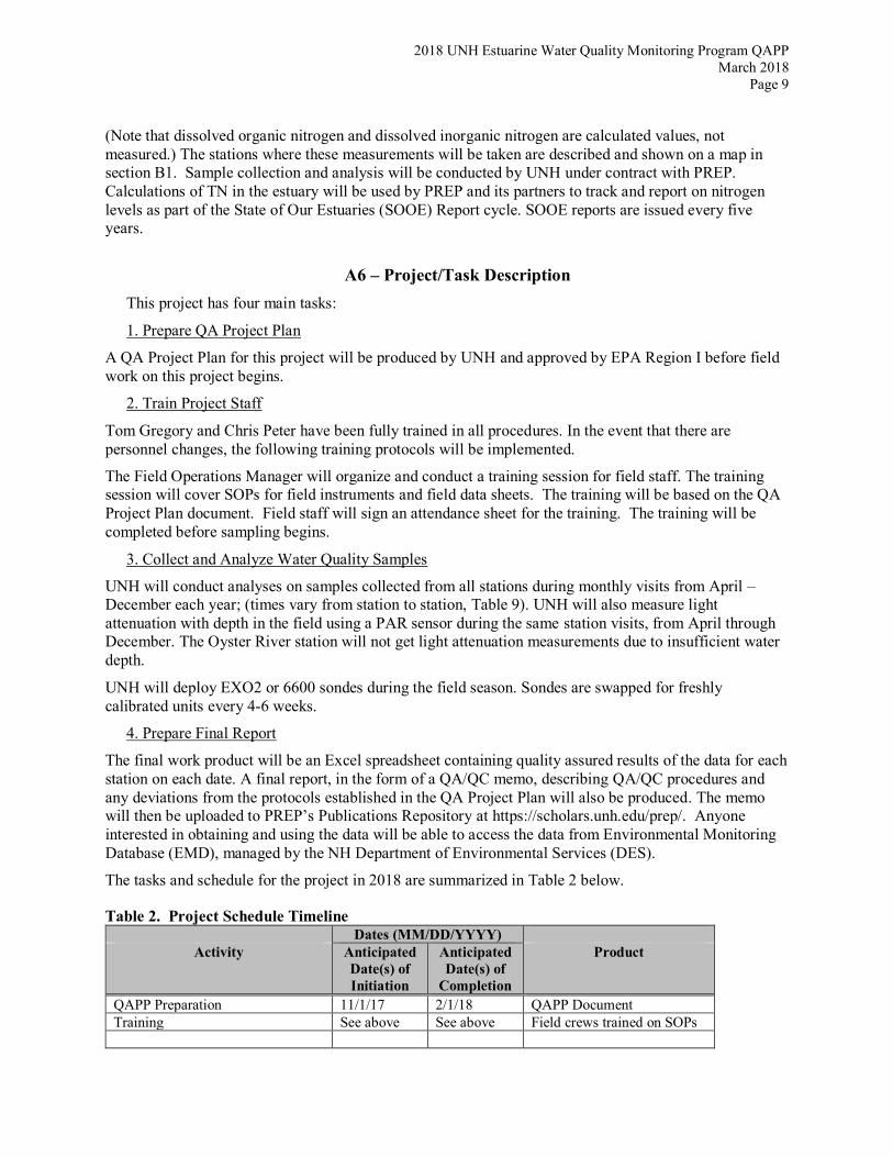
(Note that dissolved organic nitrogen and dissolved inorganic nitrogen are calculated values, not measured.) The stations where these measurements will be taken are described and shown on a map in section B1. Sample collection and analysis will be conducted by UNH under contract with PREP. Calculations of TN in the estuary will be used by PREP and its partners to track and report on nitrogen levels as part of the State of Our Estuaries (SOOE) Report cycle. SOOE reports are issued every five years.
A6 – Project/Task Description This project has four main tasks:
1. Prepare QA Project Plan
A QA Project Plan for this project will be produced by UNH and approved by EPA Region I before field work on this project begins.
2. Train Project Staff
Tom Gregory and Chris Peter have been fully trained in all procedures. In the event that there are personnel changes, the following training protocols will be implemented.
The Field Operations Manager will organize and conduct a training session for field staff. The training session will cover SOPs for field instruments and field data sheets. The training will be based on the QA Project Plan document. Field staff will sign an attendance sheet for the training. The training will be completed before sampling begins.
3. Collect and Analyze Water Quality Samples
UNH will conduct analyses on samples collected from all stations during monthly visits from April – December each year; (times vary from station to station, Table 9). UNH will also measure light attenuation with depth in the field using a PAR sensor during the same station visits, from April through December. The Oyster River station will not get light attenuation measurements due to insufficient water depth.
UNH will deploy EXO2 or 6600 sondes during the field season. Sondes are swapped for freshly calibrated units every 4-6 weeks.
4. Prepare Final Report
The final work product will be an Excel spreadsheet containing quality assured results of the data for each station on each date. A final report, in the form of a QA/QC memo, describing QA/QC procedures and any deviations from the protocols established in the QA Project Plan will also be produced. The memo will then be uploaded to PREP’s Publications Repository at https://scholars.unh.edu/prep/. Anyone interested in obtaining and using the data will be able to access the data from Environmental Monitoring Database (EMD), managed by the NH Department of Environmental Services (DES).
The tasks and schedule for the project in 2018 are summarized in Table 2 below.
Table 2. Project Schedule Timeline Dates (MM/DD/YYYY)
Activity Anticipated Date(s) of Initiation
Anticipated Date(s) of
Completion
Product
QAPP Preparation 11/1/17 2/1/18 QAPP Document Training See above See above Field crews trained on SOPs

2018 UNH Estuarine Water Quality Monitoring Program QAPP March 2018
Page 10
Sample collection April of each year
December of each year
Nutrient and bacteria samples collected, delivered to laboratory, and stored
Sample analysis Ongoing February after year completed
Laboratory analyses for nutrient and bacteria samples completed
Analytical Results Delivery Ongoing, monthly
results provided in the March after year collected
Report from Laboratory Manager with final, quality-assured results for estuarine samples and QC samples
Data Quality Audit January after field season, annually
End of April, annually
Memo from Project QA Officer summarizing results of QC samples and QAPP discrepancies
QA/QC Memo January, annually
End of May, annually
Final report (memo) describing deviations from QA/QC objectives, hosted at: https://scholars.unh.edu/prep/
Based on EPA-NE Worksheet 10. A7 – Quality Objectives and Criteria
Table 3 summarizes the performance criteria for the nitrate+nitrite, ammonium, orthophosphate, organic carbon, total dissolved nitrogen, silica and particulate organic matter samples that will be collected for this project. More details on each data quality objective are provided in the paragraphs below the table. The data quality objectives for the PAR measurements are discussed at the end of this section.
Table 3. Measurement Performance Criteria for Nutrient Samples
Data Quality Indicators Measurement Performance Criteria
QC Sample and/or Activity Used to Assess
Measurement Performance
Precision-Overall RSD < 20% Field triplicates
Precision-Lab RSD < 15%
Certified Reference Material, Laboratory Fortified Matrix
Samples
Accuracy/Bias RPD < 15%
>85% and <115% recovery Same as above
Comparability Measurements should follow standard
methods that are repeatable NA
Sensitivity Not expected to be an issue for this
project (see discussion below) NA
Data Completeness 80% of samples meet quality objectives Data Completeness Check Based on EPA-NE QAPP Workbook for 3/19/02 DES QAPP writing class. Precision: Relative standard deviation (RSD) of triplicate samples is used as one index of precision for nutrient analyses. This is defined as the standard deviation of the replicates divided by the mean of the replicates. For laboratory replicates, a difference greater than 10% requires further investigation of the sample run. A difference greater than 15% is failure (unless the average of the two samples is less than

2018 UNH Estuarine Water Quality Monitoring Program QAPP March 2018
Page 11
10X the MDL), and results in reanalysis of the entire sample queue, unless there is a reasonable and supported explanation for the inconsistency. For field triplicates, taken at a minimum of 10% of all station visits, a difference > 20% will be flagged.
Accuracy/Bias. For nutrient analyses, certified reference materials are analyzed periodically (approximately every 20 samples) in each sample queue to assure accuracy. Generally, a recovery <90% or >110% requires further investigation of the sample run. A recovery greater than or less than <85% or >115% is failure (unless the sample is less than 10X the MDL), and results in reanalysis of the entire sample queue, unless there is a reasonable and supported explanation for the inconsistency. Percent recovery (R) for certified reference materials will be calculated using the following equation:
%1002
21
x
xxRPD
where x1 is the measured concentration x2 is the known concentration for the certified reference material
Laboratory Fortified Matrix samples are also used to assess accuracy of nutrient analyses. The difference of the spiked sample concentration (SA) minus the unspiked sample concentration (SU) divided by the known concentration added (A) (expressed as percent) gives percent recovery (R):
%100)(
ASUSAR
Generally, a recovery <90% or >110% requires further investigation. A recovery greater than or less than <85% or >115% is failure (unless the sample is less than 10X the Method Detection Limit, MDL), and results in reanalysis of the entire sample queue, unless there is a reasonable and supported explanation for the inconsistency.
Representativeness: The samples should be taken at the same locations and times as water quality samples for the existing water quality monitoring programs in order to ensure that the data are representative of the same water mass as was monitored for the other parameters.
Comparability: Standardized field and analytical methods should be used. These methods should follow the current industry standard for the types of measurements being taken. Written SOPs should be followed for field and analytical measurements. Standardized field data sheets should be used.
Sensitivity. In northern macrotidal estuaries, studies have shown the total nitrogen concentration to be twice the dissolved inorganic nitrogen concentration (EPA, 2001). In NH’s estuaries, the DIN concentration in the middle of the bay is approximately 15 uM (0.2 mg/l), with concentrations increasing in the tidal tributaries. Therefore, the expectation is that DON and PON, which make up the majority of the difference between total nitrogen and DIN, will be at least 0.2 mg/l. Assuming equal apportioning between DON and PON, the methods for each parameter should be able to detect 0.1 mg/l. The analytical method, analytical/achievable MDL, and the analytical/achievable laboratory quantitation limits for this project are shown below in Table 4.
Table 4: Surface Water Target Analytes and Reference Limits
Analyte Analytical method
Project
Action Level Analytical/Achievable
Method Detection Limit
Project Quantitation
Limit DON Appendix C NA 0.1 mg/L 0.1 mg/L PON Appendix D NA 0.1 mg/L 0.1 mg/L
Based on EPA-NE Worksheet #9b and 9c.

2018 UNH Estuarine Water Quality Monitoring Program QAPP March 2018
Page 12
Completeness: This study will be deemed successful if data meeting the data quality objectives is obtained for 80% of the water quality samples (not including field/laboratory duplicates). In the event that this objective is not reached, the Program Manager will note this in the final report. In the event that samples are contaminated, preserved samples will be used for the analysis.
Data Quality Objectives for Bacteriological Analyses
Table 5 lists the performance criteria for field collection and enumeration analysis of bacterial indicators in water samples collected for GBE monitoring projects. Table 6 summarizes the performance criteria for enumeration analyses.
Table 5. Measurement performance criteria for bacterial indicators.
Data Quality Indicators Measurement Performance Criteria QC Sample and/or Activity
Used to Assess Measurement Performance
Precision-Field RPD≤ 50% Field duplicates
Precision-Lab R< precision criterion (see text below) Lab duplicates
Representativeness Project Specific See Appendix G
Detection limits 1 cfu/100 ml Sterility tests
Accuracy/Bias Positive results with positive controls
Negative results with negative controls Positive and negative
controls
Comparability Deviation from SOPs should not influence
more than 5% of the data Data comparability check
Sensitivity Not expected to be an issue
for these projects N/A
Data Completeness 75% samples collected
(on a project basis) Data completeness check
Table 6: Data reliability for bacterial indicators. Parameter Meas. Range Precision Accuracy Reporting Limit
Bacterial Indicators >= 1cfu/100mls 1 cfu/100mls 1 cfu 1 cfu
Precision & Accuracy/Bias The method detection limits, precisions and accuracy for collected data are given in tables 2, 3, and 4.

2018 UNH Estuarine Water Quality Monitoring Program QAPP March 2018
Page 13
Field precisions yield RPDs ≤ 50%. If the RPD routinely exceeds 50%, acceptable level may need to be adjusted. This is noted in each final report. Relative percent difference (RPD) is calculated:
Laboratory precision for bacterial indicator measurements is typically determined according to Standard Methods 9020 B-8. (APHA, 1998). The range I for duplicate samples is calculated and compared to predetermined precision criteria. The precision criterion is calculated from the range of log-transformed results for 15 duplicates according to the following formula:
3.27 × (mean of log ranges for 15 duplicates) = precision criterion
The precision criterion is updated periodically using the first 15 duplicate samples analyzed in a month by the same analyst. If the range of ensuing pairs of duplicate samples is greater than the precision criterion, then the increase in imprecision is evaluated to determine if it is acceptable. If not, analytical results obtained since the previous precision check is evaluated and potentially discarded. The cause of the imprecision is identified and resolved.
Comparability
The results for every year of monitoring will be compared to results from previous monitoring year results. In particular, the degree to which bacterial indicator concentrations vary identified under a given set of conditions is a useful comparability guide.
Comparability between samples is achieved through maintaining consistency with SOPs, sampling locations, sampling holding times, and sampling methods.
Completeness
Sampling event completeness is largely determined by weather conditions that affect access to particular sites. Staff is not permitted to collect samples when it is unsafe to do so, for example during periods of high winds or lightning. For years including E. coli sampling, the laboratory will accept an E. coli confirmation level of >75%. (In 2018, E. coli will not be sampled.)
Sensitivity For indicator organisms, we are interested in whatever range we can detect. However, at the low end, concentrations that are below the detection limit of 1 cfu/100 ml are not of interest because of the low level of loading to estuarine waters that such numbers represent. To increase the sensitivity of bacterial analysis, filtration of larger volumes is required. However, volumes >100 ml typically cause clogging problems with membrane filters and is avoided if at all possible.
Data Quality Objectives for PAR Measurements Quantitation Limits: Table 7 summarizes the data quality objectives for the in-situ PAR measurements. More details on each data quality objective are provided in the paragraphs below the table.
100
221
21 ´+-=XXXXRPD

2018 UNH Estuarine Water Quality Monitoring Program QAPP March 2018
Page 14
Data Quality Objectives for PAR measurements
Table 7: Data Quality Objectives for in-situ PAR measurements
Data Quality Indicators Measurement Performance Criteria
QC Sample and/or Activity Used to Assess
Measurement Performance
Precision-Overall SE < 10% Field Replicates
Precision-Lab Not applicable
Accuracy/Bias R2 of correlation >0.95
Goal: 6 measurements per profile
Regression of ln(PAR) vs. depth. Number of
measurements per profile.
Comparability Measurements should follow standard
methods that are repeatable NA
Sensitivity Not expected to be an issue for this
project (see discussion below) NA
Data Completeness 80% of samples meeting data quality
objectives Data Completeness Check Based on EPA-NE QAPP Workbook for 3/19/02 DES QAPP writing class. Precision: Fifteen measurements of PAR (>10% of total) will be replicated three times. The standard error (SE) of the mean light attenuation coefficient value from the three casts will be used to assess the precision of the result. SE values <10% will be acceptable. Casts with SE values >10% will be rejected.
Accuracy/Bias. For PAR measurements, absolute accuracy measurements are not necessary. The light attenuation coefficient is calculated based on the relative change in light with depth. Therefore, the quality of the regressions with depth, not the absolute light intensity, is the measurement of concern. The quality of the regressions will be considered sufficient when the r2 values are greater than 0.95.
Representativeness: The samples should be taken at the same locations and times as water quality samples for the existing water quality monitoring programs to ensure that the data are representative of the same water mass as was monitored for the other parameters.
Comparability: Standardized field and analytical methods should be used. These methods should follow the current industry standard for the types of measurements being taken. Written SOPs should be followed for field and analytical measurements. Standardized field data sheets should be used.
Sensitivity. In general, diffuse light attenuation coefficients for Great Bay should be between 0.02 and 12. Results outside of this range will be flagged for investigation.
Completeness: This study will be deemed successful if data meeting the data quality objectives is obtained for 80 water quality samples (not including field/laboratory duplicates).
Tide Stage Validation: Station visits are reported as being associated with a certain tide (low or high). The tides at each station were predicted from Portland tide predictions and established tide lags for each station. A sample is considered to be a “high tide” or “low tide” sample if it was collected no more than 3 hours before and no more than 1 hour after the time of high tide or low tide.

2018 UNH Estuarine Water Quality Monitoring Program QAPP March 2018
Page 15
A8 – Special Training/Certification
Tom Gregory and Chris Peter have been fully trained in all procedures. In the event that there are personnel changes, the following training protocols will be implemented.
The Field Operations Manager will organize and conduct a training session for field staff. The training session will cover SOPs for field instruments and field data sheets (Table 8). The training will be based on the QA Project Plan document. Field staff will sign an attendance sheet for the training. The training will be completed before sampling begins.
Table 8. Special Personnel Training Requirements Project function
Description of Training Training Provided by
Training Provided to
Location of Training Records
Water quality sampling and field measurements
Field method SOPs and field data sheets. This training will be conducted once at the beginning of the field season.
Field Operations Manager
All field team staff
With Project Manager and included in final report to PREP.
Based on EPA-NE Worksheet #7.
A9 – Documents and Records
QA Project Plan
The Project Manager will be responsible for maintaining the approved QA Project Plan and for distributing the latest version to all parties on the distribution list in section A3. A copy of the approved plan will be on file with the Project Manager at the PREP offices, as well as at scholars.unh.edu/prep/
Field Data Sheets
The field data sheet template for this project is attached as App. K. Field crews fill in this form during the day and return the form to the Field Operations Manager upon completion. The information will be transferred to an Excel Spreadsheet. The original forms will be retained by the Field Operations Manager, and sheets will be scanned and included as an appendix in the Project QA Officer’s memo to the Project Manager.
Laboratory Data Sheets
Data packages from the Laboratory Manager to the Project Manager will be electronic laboratory data sheets containing the results of analyses plus the results of QC tests performed by the Laboratory Manager. See Appendix A, Section II and VI for details of laboratory electronic and paper records.
Reports to Management
The Project Manager will develop a final memo on an annual basis. The final work product will be an Excel spreadsheet containing quality assured results of the analyses for each station on each date and a final memo (from the Project QA Officer) describing any deviations from the protocols established in the QA Project Plan. The final report is due on June 30 following each field season. The annual report will be posted to the PREP publications website (scholars.unh.edu/prep/).
Archiving
The QA Project Plan and final report will be kept on file with the Project Manager at PREP in Durham for a minimum of 5 years after the publication date of the final report. The original field data sheets, or

2018 UNH Estuarine Water Quality Monitoring Program QAPP March 2018
Page 16
scanned copies of the original field data sheets will be retained by the Field Operations Manager and laboratory data sheets will be retained by the Laboratory Manager for a minimum of 5 years.
B1 – Sampling Process Design
This QAPP will cover the samples collected and analyzed starting in April 2018 (the anticipated date of QAPP approval is 2/16/18). The number of samples listed in Tables 9 through 11 reflects the total number of samples that UNH will collect for the project in order to be consistent with the contract agreements.
UNH will collect water samples for sample analyses, measure Kd (light attenuation) in the field and on monthly visits during April – December in each year. The sample breakdown will be:
• Monthly (Apr-Dec) samples at low tide at 11 estuarine stations (GRBGB, GRBGBE, GRBUPR, HHHR, GRBOR, GRBAP, GRBCL, GRBLR, GRBCR, GRBBR, and GRBSQ.)
• Approximately every two hours over one lunar day (Once per month, at GRBLR). • At least 15 field triplicate samples over the year (every 10th sample). • An attempt will be made to collect all monthly samples in the first half of each month. • See Table 9 for details on which stations will be sampled for bacteria.
Datasondes will collect data every 15 minutes, April through December at ten stations (GRBGB, GRBOR, GRBLR, GRBSQ, GRBUPR, GRBGBE, GRBLB, GRBCR, GRBBR and HHHR). The SWMP standard for sondes distance from the bottom is 0.5 m. This is easily achieved for stations that are piling-mounted; anchor/tube stations are closer to .25 m. For grab samples, the hand-held YSI Pro 2030 instrument (YSI 2010) is used to measure dissolved oxygen, conductivity and temperature in the water.
Tables 9, 10 and 11 summarize the sampling program. Figure 2 (on page 21) illustrates the locations of the stations.

2018 UNH Estuarine Water Quality Monitoring Program QAPP March 2018
Page 17
Table 9: Sampling Specifications by Station.
Station ID
GRBSQ GRBGB
GRBGBE
HHHR
GRBUPR GRBOR GRBLR GRBBR GRBCR
GRBSF (In 2018,
deployment not occurring.)
GRBLPR (In 2018,
deployment not occurring.) GRBLB
GRBCML (In 2018,
deployment not
occurring.) GRBAP GRBCL
Datasondes
Collection Depth Bottom Bottom Bottom Bottom Bottom Mid
N/A N/A
Sampling Duration April - December April - December July - September April - December April - December April -
December
Sampling Frequency
Continuous (15 min) Continuous (15 min) Continuous (15 min) Continuous (15
min) Continuous (15
min) Continuous (15
min)
Sonde Parameters
Water Temperature Water Temperature Water Temperature Water
Temperature Water
Temperature Water
Temperature Specific
Conductance Specific
Conductance Specific Conductance Specific Conductance
Specific Conductance
Specific Conductance
Salinity Salinity Salinity Salinity Salinity Salinity
DO Saturation DO Saturation DO Saturation DO Saturation DO Saturation DO Saturation
DO Concentration DO Concentration DO Concentration DO Concentration
DO Concentration
DO Concentration
Depth Depth Depth Depth Depth Depth
pH pH pH pH pH pH
-- fDOM -- -- fDOM --
-- Chl-a -- -- Chl-a --
Turbidity Turbidity Turbidity Turbidity Turbidity Turbidity
Grab Samples
Collection Depth Surface Surface
N/A N/A
Surface Surface
Sampling Duration April - December April - December April -
December April -
December
Sampling Frequency
Monthly (H & L Tide)*
Monthly (H & L Tide)* N/A N/A Monthly
(H & L Tide) Monthly
Parameters DOC DOC DOC DOC

2018 UNH Estuarine Water Quality Monitoring Program QAPP March 2018
Page 18
TDN TDN TDN TDN
NO3+NO2 NO3+NO2 NO3+NO2 NO3+NO2
NH4 NH4 NH4 NH4
PO4 PO4 PO4 PO4
DON DON DON DON
DIN DIN DIN DIN
POC POC POC POC
PON PON PON PON
Chlorophyll A Chlorophyll A
Chlorophyll A Chlorophyll A
Pheophytin-A Pheophytin-A Pheophytin-A Pheophytin-A Water
Temperature Water Temperature Water Temperature
Water Temperature
Salinity Salinity Salinity Salinity
DO Saturation DO Saturation DO Saturation DO Saturation
DO Concentration DO Concentration DO Concentration
DO Concentration
Kd** Kd Kd Kd
TSS TSS TSS TSS
Fecal Coliform Fecal Coliform Fecal Coliform Fecal Coliform
Escherichia coli Escherichia coli Escherichia coli
Escherichia coli
Enterococci*** Enterococci Enterococci Enterococci
Silica Silica
Parameters shaded in gray (e.g., see Fecal Coliform and Escherichia coli) may not be sampled every year, due to funding limitations.
Parameters in italics (e.g., Enterococci) may not be sampled at all stations, due to funding limitations.
* In 2018, stations GRBSQ, GRBGB, GRBLR, GRBOR, GRBCL, GRBGBE, HHHR and GRBUPR will not be sampled at high tide. ** Kd is not ascertained at Oyster River due to insufficient water depth. *** In 2018, GRBGBE will not receive bacteria sampling.

2018 UNH Estuarine Water Quality Monitoring Program QAPP March 2018
Page 19
Table 10: Sampling station locations Station ID
(Description). Latitude Longitude Comments
GRBAP (Adams Point) 43.092078 -70.864279 Sampling only
GRBGB (Great Bay) 43.072200 -70.869400 SWMP station, low tide only GRBLR (Lamprey
River) 43.080000 -70.934400 SWMP station
GRBCL (Squamscott River at Chapmans
Landing) 43.039400 -70.928300 Sampling only
GRBSQ (Squamscott River at RR Bridge) 43.052900 -70.911400 SWMP station, low tide only
GRBOR (Oyster River) 43.134000 -70.911000 SWMP station
GRBCML (Coastal Marine Laboratory) 43.072361 -70.710303 Not a SWMP station
*Not sampled in 2018 GRBUPR (Upper Piscataqua River) 43.155500 -70.832000 Datasonde, low tide only
GBRGBE (Great Bay East) 43.063967* -70.853350* Not a SWMP station
GBRLPR (Lower Piscataqua River) 43.10628 -70.79264 Datasonde only
*Not sampled in 2018 GRBLB (Little Bay) 43.12623 -70.86580 Datasonde only
HHHR (Hampton Harbor Estuary – Hampton River)
42.923934 -70.837130 Not a SWMP station
GRBBR (Bellamy River) 43.15994 -70.85350 Not a SWMP station
GRBCR (Cocheco River)
43.183891
-70.837240
Not a SWMP station
* Lat/Lon data are approximate only.
Table 11: Sampling design.
Parameter No. of
sampling locations
Samples per event per
site
Number of samples/year
Number of field duplicates
Number of bottle blanks
Total number to
lab To be analyzed at the UNH lab
DOC 11 1 sample/ site/event 243 samples/yr >10% 0 267
TDN 11 1 sample/ site/event 243 samples/yr >10% 0 267
NO3+NO2 11 1 sample/ site/event
243 samples/yr >10% 0 267
NH4 11 1 sample/ site/event
243 samples/yr >10% 0 267

2018 UNH Estuarine Water Quality Monitoring Program QAPP March 2018
Page 20
Parameter No. of
sampling locations
Samples per event per
site
Number of samples/year
Number of field duplicates
Number of bottle blanks
Total number to
lab
PO4 11 1 sample/ site/event
243 samples/yr >10% 0 267
Si 2 1 sample/ site/event 27 samples/yr >10% 0 30
POC 11 1 sample/ site/event 126 samples/yr >10% 0 138
PON 11 1 sample/ site/event 126 samples/yr >10% 0 138
Chl-a 12 1 sample/ site/event 243 samples/yr >10% 0 267
TSS 11 1 sample/ site/event 243 samples/yr >10% 0 267
Fecal Coliform* 8 1 sample/
site/event 60 samples/yr >10% 0 66
Escherichia coli* 8 1 sample/
site/event 60 samples/yr >10% 0 66
Enterococci 3 1 sample/ site/event 18 samples/yr >10% 0 20
Measured in the field
PAR 10 1sample/ site/event 126 samples/yr >10% Not
applicable measured in
situ Water Temperature 11 1 sample/
site/event n/a n/a Not applicable
measured in situ
Specific Conductance 11 1 sample/
site/event n/a n/a Not applicable
measured in situ
Salinity 11 1 sample/ site/event n/a n/a Not
applicable measured in
situ Dissolved Oxygen 11 1 sample/
site/event n/a n/a Not applicable
measured in situ
Oxygen Saturation 11 1 sample/
site/event n/a n/a Not applicable
measured in situ
Based on EPA-NE Worksheet #9c. * not sampled in 2018 due to limited funding.

2018 UNH Estuarine Water Quality Monitoring Program QAPP March 2018
Page 21
Figure 2: Water Quality Monitoring Stations Map

2018 UNH Estuarine Water Quality Monitoring Program QAPP March 2018
Page 22
B2 – Sampling Methods
Field samples are collected by boat at all the stations except the Coastal Marine Laboratory, Lamprey River, Hampton Harbor and Oyster River, which are sampled from floating docks. The sample bottle preparation/decontamination and field sampling procedures used for the sample collection are listed below. (Note: bacteria sampling requires an additional sterilized one-liter Nalgene bottle. All other water quality parameters are achieved with the single bottle.)
Sample Bottle Preparation: One-liter Nalgene bottles are prepared before sampling by acid-washing in a 10% HCl solution. Bottles and caps are then rinsed with deionized water three times then dried thoroughly before being stored. Before field sampling day, bottles are labeled with appropriate site and placed in a cooler for transfer and storage. Water Sampling Field Procedures: At each site, one sample bottle is immersed by hand approximately 0.5 m below the surface and filled facing the direction of the current (if any current pattern is detected). The bottle is opened individually and rinsed three times with estuarine water before collecting the sample. Filtration: Particulate material is separated from dissolved constituents via filtration in the laboratory immediately upon delivery to the laboratory (normally within 5 hours of collection). For dissolved nitrogen species (NO3+NO2, TDN, and ammonium), a portion of the original sample is filtered through 25 mm membranes with pore size 0.45 µm, collected in a pre-washed HDPE bottle, and then immediately frozen. For particulate nitrogen and carbon species, a portion of the original sample is processed using the filtration procedures in Appendix E.
The SOP for PAR measurements in situ is in App. F. No special decontamination procedures are needed for the PAR measurements. Field teams are responsible for reporting sampling method problems to the Field Operations Manager who is responsible for taking corrective action.
The datasonde program will follow methods adopted by SWMP. These are detailed in the NERRS SWMP EXO SOP V1.1, Appendix J.
Table 12. Sample Requirements Analytical parameter
Collection method
Sampling SOP Sample
volume
Container size and type
Preservation requirements
Max. holding time
(preparation and analysis)
Nitrate+nitrite (NO3+NO2)
Grab Section B2 40 mL
1 liter bottle (for field); 60 mL HDPE bottle ( filtered sample in lab
Filter and freeze within 8 hours of sample collection
Indefinite once frozen
TDN Grab Section B2 40 mL
See above Filter and freeze within 8 hours of sample collection
Indefinite once frozen
Ammonium Grab Section B2 40 mL
See above Filter and freeze within 8 hours of sample collection
Indefinite once frozen
Particulates for PON
Grab Section B2 280 mL
Filter for particulates
Filter and dry overnight then store in desiccator
Indefinite once dried
PAR measured in-situ
Appendix H NA NA NA NA

2018 UNH Estuarine Water Quality Monitoring Program QAPP March 2018
Page 23
DOC Grab Section B2 40 mL
60 mL HDPE bottle
Filter and freeze within 8 hours of sample collection
Indefinite once frozen
PO4 Grab Section B2 40 mL
60 mL HDPE bottle
Filter and freeze within 8 hours of sample collection
Indefinite once frozen
POC Grab Section B2 280 mL
Filter for particulates
Filter and dry overnight then store in desiccator
Indefinite once dried
Chlorophyll A Grab Section B2 62 mL
Filter for particulates
Filter then store in liquid nitrogen
Pheophytin Grab Section B2 62 mL
Filter for particulates
Filter then store in liquid nitrogen
TSS Grab Section B2 280
mL Filter for particulates
Filter and dry overnight then store in desiccator
Indefinite once dried
Fecal coliform Grab Appendix G 5-100
ml 1000 ml HPDE bottle
Immediate refrigeration
Within 8 h after sampling
Escherichia coli
Grab Appendix G 5-100 ml
1000 ml HPDE bottle
Immediate refrigeration
Within 8 h after sampling
Enterococci Grab Appendix G 5-100
ml 1000 ml HPDE bottle
Immediate refrigeration
Within 8 h after sampling
B3 – Sample Handling and Custody
Sample handling and custody procedures for nutrient samples are described in Appendix A. The Field Operations Manager will be responsible for having the samples delivered to the laboratory within 8 hours of collection so that they can be frozen.
B4 – Analytical Methods
See Table 13 for list of analytes and methods. Appendix A is the QA Plan for the UNH Water Quality Analysis Laboratory. Analytical methods for this study are described in detail in Appendices B, C, D, and E. Appendix B contains the SOPs for determining nitrate+nitrite concentrations and ammonia concentrations. Appendix C contains the SOP for total dissolved nitrogen concentrations. Dissolved organic nitrogen (DON) concentrations will be calculated by subtracting nitrate/nitrite and ammonia from total dissolved nitrogen. Dissolved inorganic nitrogen (DIN) will be calculated by adding nitrate/nitrite and ammonia.
Appendix D contains the protocol for filtering samples to capture particulates. Appendix E contains the protocol for the CHN analysis of the filters (mass of carbon and nitrogen by elemental analysis) to determine the mass of nitrogen that was retained on the filter. PON will be calculated from these two measurements as follows:
PON = Mass N on filter (mg) / Volume of water filtered (l)

2018 UNH Estuarine Water Quality Monitoring Program QAPP March 2018
Page 24
The Laboratory Manager is responsible for corrective actions if any problems with the analytical methods arise. All data for the project must be delivered from the laboratory to the Project Manager by March 31, 2019.
The bacterial analyses are conducted at UNH/JEL—see Appendix F, JEL Microbiology Lab QAPP—and are in accordance with standard membrane filtration methods. The SOPs for the bacterial indicators are included in Appendix G. The reference limits for each bacterial indicator are listed in Table 14. The microbiological laboratory manager will be responsible for all corrective actions and will also be responsible for all non-standard method validation.
Appendix H contains the protocols for calculating light attenuation coefficients from the field measurements of PAR. The field teams are responsible for notifying the Project Manager of any problems with the PAR measurement. The Project Manager is responsible for taking corrective actions to resolve these problems. PAR measurements are made in situ so turn-around times for data are not relevant.
Table 13: Analytes and Analytical Methods
Analyte
Analytical method (See Appendices for SOP
details)
Project Action Level
Analytical/Achievable Method Detection
Limit
Project Reporting Limits
NO2/NO3 USEPA 353.2 Revision 2.0, August, 1993 (App. B2)
NA-data will be used for
trend analysis 0.005 mg/L 0.005 mg/L
NH4 USEPA method 350.1, 1971, modified March 1983 (App. B1)
NA-data will be used for
trend analysis 0.005 mg/L 0.005 mg/L
TDN High temperature catalytic oxidation (App. C)
NA-data will be used for
trend analysis 0.1 mg/L 0.1 mg/L
TSS APHA Method 2540-D (App. D)
NA-data will be used for
trend analysis 1 mg/L 1 mg/L
Chlorophyll a
Ocean Optics Protocols for Satellite Ocean Color Sensor Validation, Revision 5, Volume V: Biogeochemical and Bio-Optical Measurements and Data Analysis Protocols (Appendix I)
NA-data will be used for
trend analysis
0.12 ug/L 0.12 ug/L
Pheophytin-A
Ocean Optics Protocols for Satellite Ocean Color Sensor Validation, Revision 5, Volume V: Biogeochemical and Bio-Optical Measurements and Data Analysis Protocols (Appendix I)
NA-data will be used for
trend analysis
0.12 ug/L 0.12 ug/L
DOC USEPA 415.3, Revision 1.1, February 2005 (App. C)
NA-data will be used for
trend analysis
0.05 mg/L 0.05 mg/L

2018 UNH Estuarine Water Quality Monitoring Program QAPP March 2018
Page 25
Analyte
Analytical method (See Appendices for SOP
details)
Project Action Level
Analytical/Achievable Method Detection
Limit
Project Reporting Limits
PO4 USEPA 365.3, 1978 (App. B3)
NA-data will be used for
trend analysis
0.001 mg P/L 0.001 mg P/L
POC USEPA 440.0, Revision 1.4, September 1997 (App. E)
NA-data will be used for
trend analysis
4 ug C* 4 ug C*
PON USEPA 440.0, Revision 1.4, September 1997 (App. E)
NA-data will be used for
trend analysis
3 ug N* 3 ug N*
Table 14: Water bacterial indicator reference limits.
Indicator
Analytical method SOP Reference
Project Action Level
Analytical/Achievable Method Detection
Limit
Project Quantitation
Limit
Escherichia coli Membrane Filter Procedure, EPA Method 1103.1 (EPA 2002)
406 cfu/100ml 0+ cts/100 mL
(depends on dilution and sample volume)
0+ cts/100 mL (depends on
dilution and sample volume)
Enterococci Membrane Filter Procedure, EPA Method 1600 (EPA, 2006)
104 cfu/100 ml
Same as above Same as above
Fecal coliforms Rippey, et al. (1987) 14 cfu/100 ml Same as above Same as above
B5 – Quality Control
Section VII of Appendix A describes the quality control measures that will be used for nutrient analyses by the UNH Water Quality Analysis Laboratory. For the PAR monitoring, the field duplicate measurements (every 10th measurement) will serve as the quality control. Section A7 describes how the data quality objectives will be evaluated.
The Project Manager will verify that the field crews are following the protocols correctly during the field sampling audit (see Section C1).
Databases of results will be checked for transcription errors and bad data using two methods. First, the entire data set will be checked against the entries in each field or laboratory data sheet by the Field Operations Manager. Second, the Field Operations Manager will construct scatter plots to determine if there are outliers in the data set. The Field Operations Manager, working with the Project QA Officer, will report any outliers to the Project Manager, who will determine whether these data should be flagged as invalid.
B6 – Instrument/Equipment Testing, Inspection, Maintenance
Equipment inspections and maintenance schedules for the laboratory are described in Section IX of Appendix A. PAR measurements will be made using a Li-Cor 1400 datalogger and spherical (2-pi) quantum sensors. The instrument will be inspected before each use following the SOP in Appendix H.

2018 UNH Estuarine Water Quality Monitoring Program QAPP March 2018
Page 26
B7 – Instrument/Equipment Calibration and Frequency
Equipment calibration procedures for the laboratory are listed in Section V of Appendix A. Calibration runs are stored in the laboratory database along with the run sheets for environmental samples. The PAR sensor calibrations are not critical because only the relative light intensities (not their absolute values) are used to determine the light attenuation within the water. Calibration records will be retained by the Project Manager for a minimum of 5 years.
Laboratory instruments and equipment are inspected, maintained and calibrated by the laboratory. Refer to the UNH JEL Microbiology Laboratory Quality Assurance Plan (Appendix F) for additional information on laboratory instruments and equipment. All documents are on file at the laboratory in Durham. Table 15 summarizes inspection, maintenance and calibration requirements.
Table 15: Laboratory instruments.
Equipment name Activity Frequency of activity
Acceptance criteria Corrective action Person
responsible
VWR Model 1510 E incubator
(41°C)
Check temperature
Daily before use and at end
of day
Meets analytical
requirements
Adjust temperature control and confirm
stability of acceptable temperature
JEL-Micro
Fisher Isolatemp Incubator (44.5°C)
Check temperature
Daily before use and at end
of day
Meets analytical
requirements
Adjust temperature control and confirm
stability of acceptable temperature
JEL-Micro
B8 – Inspection/Acceptance Requirements for Supplies and Consumables
Inspection schedules for consumables are listed in Section V of Appendix A. The PAR sensor does not require supplies or consumables.
B9 – Non-direct Measurements
Not applicable. No non-direct measurements will be used for this project.
B10 – Data Management
Field data will be recorded on standard field data sheets (see Appendix K) and transferred to Excel data files. Laboratory data will be transferred from laboratory data sheets to Excel spreadsheets. All data will be stored electronically in Excel spreadsheets which will be transferred to the Project Manager as part of the final report. The Project Manager will be responsible for uploading the data to the DES’ Environmental Monitoring Database (which is compatible with EPA’s Water Quality Exchange). The Project IDs for the data will include “NERRSND” (GBNERR Datasonde Program), “NERRDIEL” (GBNERR Diel Water Quality Monitoring Program), “NERRTWQ” (GBNERR Tidal Water Quality Monitoring Program), “JELSND” (UNH Datasonde Program), and “JELTWQ” (UNH Tidal Water Quality Monitoring Program). Management of hardcopy data and documents is described in Section A9.

2018 UNH Estuarine Water Quality Monitoring Program QAPP March 2018
Page 27
C1 – Assessments and Response Actions
In order to confirm that field sampling, field analysis and laboratory activities are occurring as planned, the Project Manager, field staff, and laboratory personnel shall meet, after the first sampling event, to discuss the methods being employed and to review the quality assurance samples. At this time, all concerns regarding the sampling protocols and analysis techniques shall be addressed and any changes deemed necessary shall be made to ensure consistency and quality of subsequent sampling. The Project Manager will have the authority to resolve any problems encountered. Assessment frequencies and responsible personnel are shown in the following table.
Table 16. Project Assessment Table
Assessment Type
Frequency
Person responsible for performing
assessment
Person responsible for responding to
assessment findings
Person responsible
for monitoring effectiveness of
corrective actions Field sampling audit
Once after first sampling day
Field Operations Manager Project Manager Project Manager
Field analytical audit
Once after first sampling day
Field Operations Manager Project Manager Project Manager
UNH laboratory audit Quarterly (see Section VIII of Appendix A)
Laboratory Manager Project Manager Project Manager
Data Quality Audit Annually Project QA Officer Project Manager Project Manager Based on EPA-NE Worksheet #27b.
C2 – Reports to Management
The Project QA Officer will produce an annual report. The final work product will be a table containing quality assured laboratory and field results for each station on each date and an annual report describing any deviations from the protocols established in the QA Project Plan. Data from the annual reports will be published in PREP’s State of Our Estuaries Reports and will also be sent to the distribution list and added to the PREP Publications website at: scholars.unh.edu
D1 – Data Review, Verification and Validation
The Project QA Officer will be responsible for a memo to the Project Manager summarizing any deviations from the procedures in the QA Project Plan. The Project QA Officer will review all field data sheets and final computer data files for completeness and quality based on the criteria described in Section A7. The Project QA Officer will also affirmatively verify that the methods used for the study followed the procedures outlined in this QA Project Plan. If questionable entries or data are encountered during the review process (see methods in Section B5), the Project QA Officer will contact the appropriate personnel to determine their validity.
D2 – Verification and Validation Procedures
The Project Manager will review the memorandum from the Project QA Officer to see if there have been deviations from the QA Project Plan. Any decisions made regarding the usability of

2018 UNH Estuarine Water Quality Monitoring Program QAPP March 2018
Page 28
the data will be left to the Project Manager, however the Project Manager may consult with project personnel, PREP’s director, or with personnel from EPA, if necessary.
D3 – Reconciliation with User Requirements
The Project Manager will be responsible for reconciling the results from this study with the ultimate use of the data. Results that are qualified by the Project QA Officer may still be used if the limitations of the data are clearly reported to decision-makers. Data for this project are being collected as part of a long-term monitoring program. It is not possible to repeat sampling events without disrupting the time series. Therefore, the Project Manager will:
1. Review data with respect to sampling design.
2. Review the Data Verification and Validation reports from the Project QA Officer.
3. If the data quality objectives from Section A7 are met, the user requirements have been met. If the data quality objectives have not been met, corrective action as discussed in D2 will be established by the Project Manager.
4. Submit data to NH DES for upload to the Environmental Monitoring Database.
5. Publish final report (QA/QC Memo) summarizing data, deviations from QA/QC objectives, and drawing conclusions from the data, as appropriate.
References
Rippey, S.R., W.N. Adams and W.D. Watkins (1987) Enumeration of fecal coliforms and E. coli in marine and estuarine waters: an alternative to the APHA-MPN approach. J. Wat. Pollut. Cont. Fed. 59: 795-798.
EPA (2001) Nutrient Criteria Technical Guidance Manual: Estuarine and Coastal Marine Waters.
EPA-822-B-01-003. U.S. Environmental Protection Agency, Office of Water, Washington DC. October 2001.
EPA (2002) Method 1103.1: Escherichia coli (E. coli) in Water by Membrane Filtration Using
membrane-Thermotolerant Escherichia coli Agar (mTEC). EPA 821-R-02-020. EPA, Washington, DC.
EPA (2006) Method 1600: Enterococci in Water by Membrane Filtration Using membrane-
Enterococcus Indoxyl-B-D-Glucoside Agar (mEI). EPA-821-R-06-009. EPA, Washington, DC.
YSI (2010). User Manual: YSI Pro 2030.
https://www.ysi.com/File%20Library/Documents/Manuals/605056-YSI-Pro2030-User-Manual-RevC.pdf

2018 UNH Estuarine Water Quality Monitoring Program QAPP March 2018
Page 29
Appendix A
QAPP for the Water Quality Analysis Lab at the University of New Hampshire, Department of Natural Resources, Durham,
NH
Prepared by: Jeff Merriam Date of Last Revision: 8/3/2017 Revised by: Jody Potter I. Laboratory Organization and Responsibility
Dr. William H. McDowell - Director
Jody Potter – Lab Manager/QA manager. Mr. Potter supervises all activities in
the lab. His responsibilities include data processing and review (QA review), database
management, protocol development and upkeep, training of new users, instrument
maintenance and repair, and sample analysis.
Katie Swan & Lisle Snyder – Lab Technicians. Ms. Swan and Mr. Snyder’s
responsibilities, with the help of undergraduate employees, include sample analysis,
logging of incoming samples, sample preparation (filtering when appropriate), daily
instrument inspection and minor maintenance.
All analyses are completed by Katie Swan, Lisle Snyder, or Jody Potter, and all
data from each sample analysis batch (generally 40-55 samples) is reviewed by Jody
Potter for QC compliance. All users are trained by the lab manager and must
demonstrate (through close supervision and inspection) proficiency with the analytical
instrumentation used and required laboratory procedures.

2018 UNH Estuarine Water Quality Monitoring Program QAPP March 2018
Page 30
II. Standard Operating Procedures
Standard Operating Procedures for all instruments and methods are kept in a 3-
ring binder in the laboratory, and are stored electronically on the Lab manager’s
computer. The electronic versions are password protected. SOPs are reviewed annually,
or as changes are required due to new instrumentation or method development.
III. Field Sampling Protocols
Sample collection procedures are generally left up to the sample originators,
however we recommend the guidelines described below, and provide our field filtering
protocol on request.
All samples are filtered in the field through 0.7 um precombusted (5+ hours at
450 C) glass fiber filters (e.g. Whatman GF/F). Samples are collected in acid-washed 60-
mL HDPE bottles. We prefer plastic to glass as our preservative technique is to freeze.
Sample containers are rinsed 3 times with filtered sample, and the bottle is filled with
filtered sample. Samples are stored in the dark and as cool as possible until they can be
frozen. Samples must be frozen or refrigerated (SiO2) within 8 hours of sample
collection. Once frozen, samples can be stored indefinitely (Avanzino and Kennedy,
1993), although they are typically analyzed within a few months.
After collection and freezing, samples are either hand delivered to the lab, or are
shipped via an over-night carrier. Samples arriving in the lab are inspected for frozen
contents, broken caps, cracked bottles, illegible labels, etc. Any pertinent information is
entered into a password protected database (MS Access).

2018 UNH Estuarine Water Quality Monitoring Program QAPP March 2018
Page 31
We provide an electronic sample submission form that also serves as a chain of
custody form. Submitters should indicate all analyses required for the samples,
preservation (if any), and sample information (name, date, etc …). They should also
indicate project name and a description of the project.
IV. Laboratory Sample Handling Procedures
Samples are given a unique 5-digit code. This code and sample information
including name, collection date, time (if applicable), project name, collector, logger, the
date received at the WQAL, sample type (e.g. groundwater, surface water, soil solution)
and any other miscellaneous information, are entered into a password protected database.
From this point through the completion of all analyses, we use the log number to track
samples. Log numbers are used on sample run queues, spreadsheets, and when importing
concentrations and run information into the database
After samples are logged into the WQAL, they are stored frozen in dedicated
sample walk-in freezer or refrigerator located next to the lab. These units log temperature
and alarms indicate when they are out of range. The paper print-outs are replaced
quarterly and kept on file. Samples from different projects are kept separated in
cardboard box-tops, or in plastic bags. Samples that may pose a contamination threat
(based on the source or presumed concentration range) are further isolated by multiple
plastic bags, or isolation in separate freezer space. This is typically not an issue as we
primarily deal with uncontaminated samples.
We do not pay special attention to holding time of samples, as frozen samples are
stable indefinitely (Avanzino and Kennedy, 1993). However, we do keep track of the

2018 UNH Estuarine Water Quality Monitoring Program QAPP March 2018
Page 32
date samples arrive at the WQAL, and can report holding times if necessary. After
samples are analyzed they are returned to the project’s manager for safe keeping or they
are held for a period of time at the WQAL to allow necessary review and analysis of the
data by the interested parties (not from a laboratory QC sense, but from a project specific
viewpoint). Once the data is analyzed by the project’s manager(s), the samples are
returned or disposed of, based on the preference of the project’s manager.
Samples that arrive unfrozen, with cracked bottles/caps, or with loose caps, are
noted in the database and are not analyzed. These samples are disposed of to prevent
accidental analysis. The sample originator is notified (generally via e-mail) of which
samples were removed from the sample analysis stream. Similarly, if while in the
possession of the WQAL, a sample bottle is broken or improperly stored (e.g. not frozen),
the sample is removed and the sample originator is notified.
V. Calibration procedures for chemistry
Calibration curves are generally linear, and are made up of 4-7 points. A full
calibration is performed at the beginning of each run (a run is generally 40-60 samples)
with a reduced calibration (3-5 points) performed at the end of the run. Occasionally
calibration data is best fit with a quadratic equation, and this is used if it best describes
the data within a specific run.
Standards are made from reagent grade chemicals (typically Fisher Scientific or
ACROS) that have been dried and are stored in a desiccator when required. Working
stock solutions are labeled with the content description, concentration, initials of the
maker, and the date the stock solution was made. Generally stock solutions are kept less
2018 UNH Estuarine Water Quality Monitoring Program QAPP March 2018
Page 33
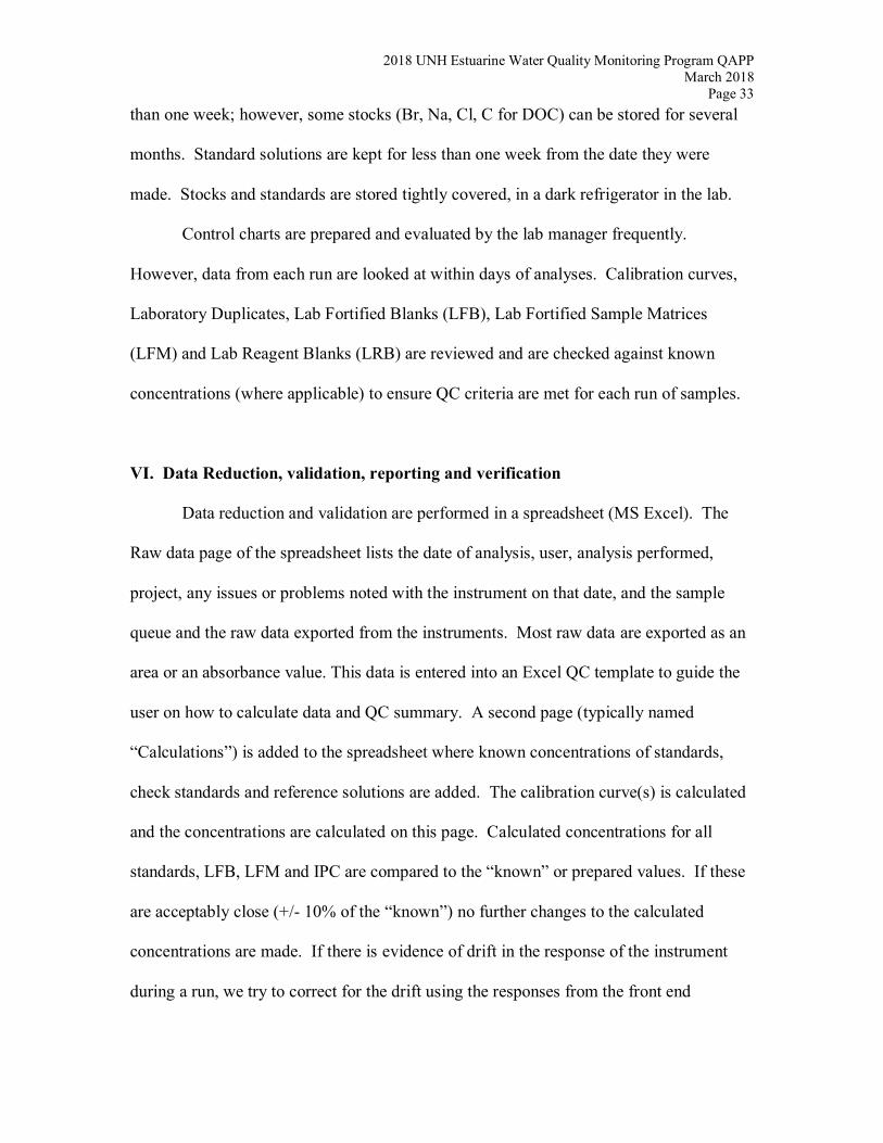
than one week; however, some stocks (Br, Na, Cl, C for DOC) can be stored for several
months. Standard solutions are kept for less than one week from the date they were
made. Stocks and standards are stored tightly covered, in a dark refrigerator in the lab.
Control charts are prepared and evaluated by the lab manager frequently.
However, data from each run are looked at within days of analyses. Calibration curves,
Laboratory Duplicates, Lab Fortified Blanks (LFB), Lab Fortified Sample Matrices
(LFM) and Lab Reagent Blanks (LRB) are reviewed and are checked against known
concentrations (where applicable) to ensure QC criteria are met for each run of samples.
VI. Data Reduction, validation, reporting and verification
Data reduction and validation are performed in a spreadsheet (MS Excel). The
Raw data page of the spreadsheet lists the date of analysis, user, analysis performed,
project, any issues or problems noted with the instrument on that date, and the sample
queue and the raw data exported from the instruments. Most raw data are exported as an
area or an absorbance value. This data is entered into an Excel QC template to guide the
user on how to calculate data and QC summary. A second page (typically named
“Calculations”) is added to the spreadsheet where known concentrations of standards,
check standards and reference solutions are added. The calibration curve(s) is calculated
and the concentrations are calculated on this page. Calculated concentrations for all
standards, LFB, LFM and IPC are compared to the “known” or prepared values. If these
are acceptably close (+/- 10% of the “known”) no further changes to the calculated
concentrations are made. If there is evidence of drift in the response of the instrument
during a run, we try to correct for the drift using the responses from the front end

2018 UNH Estuarine Water Quality Monitoring Program QAPP March 2018
Page 34
calibration curve and the set of standards analyzed at the end of the run. All reference
solutions and replicates must meet certain QC criteria (described below) for a run to be
accepted.
Data are then exported to the WQAL database. Exported information includes the
unique 5-digit code, calculated concentration, the analysis date, the user, the filename the
raw data and calculations are saved in, and any notes from the run regarding the specific
sample. Data are sent to sample originators upon completion of all requested sample
analyses and following review by the WQAL lab manager. Generally the data include
the 5-digit code, the sample name, collection date, and concentrations, in row-column
format. Any information entered into the database can be included upon request. Data
transfer is typically via e-mail or electronic medium (CD or floppy disk).
All data corrections are handled by the lab manager. Corrections to data already
entered into the database are very infrequent. Typically they involve reanalysis of a
sample. In this case, the old data is deleted from the database, and the new value is
imported, along with a note indicating that it was re-analyzed, the dates of initial and
secondary analysis and the reason for the correction.
Hand written or computer printed run sheets are saved for each run and filed,
based on the project and the analysis. Spreadsheet files with raw data and calculations
are stored electronically by analysis and date. Information in the database allows easy
cross-reference and access from individual samples to the raw data and the runsheets.
This provides a complete data trail from sample log-in to completion of analysis.

2018 UNH Estuarine Water Quality Monitoring Program QAPP March 2018
Page 35
VII. Quality Control
All analyses conducted at the WQAL follow approved or widely accepted
methods (Table 1).
Quality Control Samples (QCS) (from Ultra Scientific or SPEC Certiprep) are
analyzed periodically (approximately every 10-15 samples) in each sample analysis batch
to assure accuracy. The response/unit concentration is also used to monitor day-to-day
variation in instrument performance. A difference from the certified concentration of
more than 10% requires further investigation of that run. A difference greater than 15%
is failure (unless the average of the two samples is less than 10X the MDL), and results in
re-analysis of the entire sample queue, unless there is a very reasonable and supported
explanation for the inconsistency. Table 2 lists historical average % recoveries. At least
2 QCS are analyzed on each run.
Standards and reagents are prepared from reagent grade chemicals (typically JT
Baker) or from pre-made stock solutions. All glassware is acid washed (10% HCl) and
rinsed 6 times with ultra-pure-low DOC water (18.2 mega-ohm). All analyses (except
CHN) use multi-point calibration curves (4-7) points, which are analyzed at the
beginning and the end of each run. A Laboratory Reagent Blank (LRB), Laboratory
Fortified Blank (LFB) (a standard run as a sample) and Laboratory Duplicate are
analyzed every 10 to 15 samples during each run. At least one Laboratory Fortified
Sample Matrix (LFM) is analyzed during each run to ensure that sample matrices do not
affect method analysis efficiency. Field Duplicates are not required by our lab, and are
the responsibility of the specific project’s manager.

2018 UNH Estuarine Water Quality Monitoring Program QAPP March 2018
Page 36
Laboratory Duplicates must fall within 10% relative percent difference (RPD =
abs(dup1-dup2)/average of dup1 and dup 2). A difference greater than 5% requires
further investigation of the sample run. A difference greater than 10% is failure (unless
the average of the two samples is less than 10X the MDL), and results in re-analysis of
the entire sample queue, unless there is a very reasonable and supported explanation for
the inconsistency. Long-term averages for relative % difference are included in Table 2.
LFM must show 85% to 115% recovery. A recovery <90% or > 110% requires
further investigation of the sample run. A recovery <85% or >115% is failure (unless the
sample is less than 10X the MDL), and results in re-analysis of the entire sample queue,
unless there is a very reasonable and supported explanation for the inconsistency. Long-
term averages for % recovery are included in Table 2.
All QC information from each run is stored in a separate Access database. This
includes calibration r2, error, slope and intercept. The prepared concentration and
measured concentration of LFM and calibration standards analyzed throughout the run
are also entered. Finally, the lab duplicate measured concentrations are included. All this
information can be queried for the project manager. Control charts (PDF) are generated
from this database in R and reviewed weekly by the lab manager.
Method Detection Limits are calculated regularly, and whenever major changes to
instrumentation or methods occur. Table 2 lists most recently measured MDL values.

2018 UNH Estuarine Water Quality Monitoring Program QAPP March 2018
Page 37
VIII. Schedule of Internal/External Audits
Internal audits are not routinely performed, however, QC for each run is
thoroughly reviewed by the lab manager before entering data into the database and a
review of QC charts, and tables is done at least annually by the lab manager.
External audit samples are analyzed routinely throughout the year. The WQAL
takes part in the USGS Round Robin inter-laboratory comparison study twice per year
and the Environment Canada Proficiency Testing Program three times per year. The
USGS and Environment Canada provide Standard Reference Samples and provide
compliance results after analytical testing at the WQAL. Environment Canada is
accredited by the American Association for Laboratory Accreditation. These audits are
designed to quantify and improve the lab’s performance. Poor results are identified and
backtracked through the lab to the sources of the issue.
IX. Preventive maintenance procedures and schedules
The laboratory manager, Jody Potter, has 12 years of experience and is highly
experienced with all laboratory equipment used within the WQAL. The laboratory
manager conducts all maintenance and inspection of equipment based on manufacturer
requirements and specifications.
Each day an instrument is used, it receives a general inspection for obvious
problems (e.g. worn tubing, syringe plunger tips, leaks). The instruments are used
frequently and data is inspected within a few days of sample analysis. This allows
instrument (or user) malfunctions to be caught quickly, and corrected as needed.

2018 UNH Estuarine Water Quality Monitoring Program QAPP March 2018
Page 38
Each day’s run is recorded in the instrument’s run log, with the date, the user, the
number of injections (standards, samples, and QC samples), the project, and other notes
of interests. Maintenance, routine or otherwise, is recorded in the instrument run log, and
includes the date, the person doing the maintenance, what was fixed, and any other notes
of interest.
X. Corrective Action Contingencies
Jody Potter is responsible for all QC checks and performs or supervises all
maintenance and troubleshooting. When unacceptable results are obtained (based on
within sample analysis batch QC checks) the data from the run are NOT imported into
the database. The cause of the problem is determined and corrected, and the samples are
re-analyzed. Problems are recorded in the sample queue’s data spreadsheet, or on the
handwritten runsheet associated with the run. Corrective actions (instrument
maintenance and troubleshooting) are documented in each instrument’s run log.
XI. Record Keeping Procedures
Protocols, Instrument Logs, QC charts, databases and all raw data files are kept on
the lab manager’s computer. These are backed up continuously, with the back up stored
off site. The computer is password protected, and is only used by the lab manager.
Protocols and the sample database are also password protected. Handwritten run sheets
are stored in a filing cabinet in the lab. Instrument run and maintenance logs are
combined with the QC data in an access database where instrument performance can

2018 UNH Estuarine Water Quality Monitoring Program QAPP March 2018
Page 39
easily be compared to instrument repair and the number of analyses, etc. This file is also
stored on the lab manager’s computer and is password protected.
All information pertinent to a sample is stored in the sample database. From this
database we can easily determine the date of analysis and the location of the raw data file
if further review is necessary. The amount of information provided to sample originators
is dependent on what is required by the project or funding agencies.
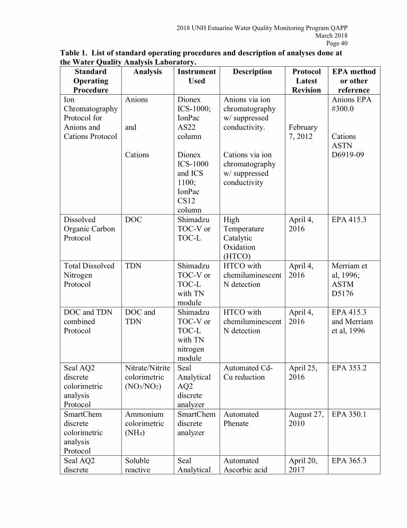
2018 UNH Estuarine Water Quality Monitoring Program QAPP March 2018
Page 40
Table 1. List of standard operating procedures and description of analyses done at the Water Quality Analysis Laboratory.
Standard Operating Procedure
Analysis
Instrument Used
Description Protocol Latest
Revision
EPA method or other
reference Ion Chromatography Protocol for Anions and Cations Protocol
Anions and Cations
Dionex ICS-1000; IonPac AS22 column Dionex ICS-1000 and ICS 1100; IonPac CS12 column
Anions via ion chromatography w/ suppressed conductivity. Cations via ion chromatography w/ suppressed conductivity
February 7, 2012
Anions EPA #300.0 Cations ASTN D6919-09
Dissolved Organic Carbon Protocol
DOC Shimadzu TOC-V or TOC-L
High Temperature Catalytic Oxidation (HTCO)
April 4, 2016
EPA 415.3
Total Dissolved Nitrogen Protocol
TDN Shimadzu TOC-V or TOC-L with TN module
HTCO with chemiluminescent N detection
April 4, 2016
Merriam et al, 1996; ASTM D5176
DOC and TDN combined Protocol
DOC and TDN
Shimadzu TOC-V or TOC-L with TN nitrogen module
HTCO with chemiluminescent N detection
April 4, 2016
EPA 415.3 and Merriam et al, 1996
Seal AQ2 discrete colorimetric analysis Protocol
Nitrate/Nitrite colorimetric (NO3/NO2)
Seal Analytical AQ2 discrete analyzer
Automated Cd-Cu reduction
April 25, 2016
EPA 353.2
SmartChem discrete colorimetric analysis Protocol
Ammonium colorimetric (NH4)
SmartChem discrete analyzer
Automated Phenate
August 27, 2010
EPA 350.1
Seal AQ2 discrete
Soluble reactive
Seal Analytical
Automated Ascorbic acid
April 20, 2017
EPA 365.3

2018 UNH Estuarine Water Quality Monitoring Program QAPP March 2018
Page 41
colorimetric analysis Protocol
Phosphorous colorimetric (SRP or PO4)
AQ2 discrete analyzer
SmartChem discrete colorimetric analysis Protocol
Silica (SiO2) SmartChem discrete analyzer
November, 10, 2005
EPA 370.1
Seal AQ2 discrete colorimetric analysis Protocol
Total Dissolved Phosphorus (TDP) (Filtered sample)
Seal Analytical AQ2 discrete analyzer
Persulfate Oxidation of filtered sample, followed by colorimetric SRP analysis.
April 25, 2016
USGS Test Method 1-4560-03
Seal AQ2 discrete colorimetric analysis Protocol
Total Phosphorus (TP) and Total Nitrogen (TN) (Unfiltered sample)
Seal Analytical AQ2 discrete analyzer
Persulfate Oxidation of unfiltered sample, followed by colorimetric SRP analysis.
April 25, 2016
Resources Investigations Report 03-4174
CHN Protocol Particulate Carbon (PC) and Nitrogen (PN)
Perkin Elmer 2400 Series II CHN
Filtration of sample followed by Elemental Analysis of the filter and particulates
February 14, 2013
EPA 440.0
Particulate Carbon and Nitrogen filtration
Laboratory Sample Filtration
Filtration of samples for water chemical analysis and particulate analysis
February 14, 2013
EPA 440.0
Acid Washing Protocol
Glass and plastic-ware cleaning
10% HCl rinse and 6 rinses with DDW
July 19, 2012
Field Filtering Protocol
Sample prep 3-times rinse with filtered sample
July 13, 2015
Fluorescence EEMs Horiba Jobin Yvon Fluoromax 3
Scanning Fluorescence Excitation & Emission on whole water
June 26, 2013
Absorbance Abs 254 & SUVA
Shimadzu TOC-V & Shimadzu
Scanning absorbance
June 26, 2013
EPA 415.3

2018 UNH Estuarine Water Quality Monitoring Program QAPP March 2018
Page 42
PDA SPD-M20A
spectra on whole water
pH, Closed cell pH, Closed cell
Electrode & Thermo Orion 525A
pH in a closed environment under atmospheric CO2 conditions
August 27, 2015
EPA 150.1
pH, aerated pH, aerated Electrode and Radiometer ION450
pH equilibrated with atmosphere
January 4, 2013
EPA 150.1
Specific conductance
Specific conductance
Electrode Specific conductance
May 15, 2017
EPA 120.1
ANC protocol ANC Electrode & Radiometer ION450
Gran titration May 15, 2017
EPA 310.1
Greenhouse Gases
Greenhouse Gases extracted from water
Shimadzu GC-2014
CH4, N2O, & CO2 on GC with FID, ECD, & TCD
December 6, 2012
Alkalinity protocol
Alkalinity Electrode & Radiometer ION450
Inflection Point EPA 310.1

2018 UNH Estuarine Water Quality Monitoring Program QAPP March 2018
Page 43
Table 2. Detection limits, acceptable ranges, and recent historical averages for QC samples at the Water Quality Analysis Lab. 1 Detection limit based on user experience and previous analysis (not statistically calculated). 2 Method Detection Limit (MDL) is the minimum concentration of a substance that can be measured and reported with 99% confidence that the analyte concentration is greater than zero.
Ana
lyte
Uni
ts
Typi
cal
Ran
ge
Reg
ress
ion
Type
# of
Cal
. Po
ints
MD
L 2
Lab
Dup
licat
e%
Rel
ativ
e D
iffer
ence
Lim
it
LFM
%
reco
very
Lim
it
+/-
IPC
%
reco
very
Lim
it
+/-
SiO2 mg SiO2/
L
0 – 40 Linear 4-7 .01 3.5 15.0 92.8 15.0
PO4 g P/L
0 – 200 Linear 4-7 5 7.8 15.0 95.5 15.0 93.7 15.0
NH4 g N/L
0 – 200 Linear 4-7 5 7.1 15.0 103.9 15.0 95.0 15.0
NO3 FIA
mg N/L
0 – 10 Linear 4-7 0.005 4.6 15.0 100.9 15.0 102.6 15.0
Na+ mg Na/L
0 – 15 Quadratic
4-7 0.02 0.9 15.0 112.7
K+ mg K/L
0 – 7 Quadratic
4-7 0.02 10.4 15.0 97.8
Mg2+ mg Mg/L
0 – 7 Quadratic
4-7 0.02 4.5 15.0 89.7
Ca2+ mg Ca/L
0 – 10 Quadratic
4-7 0.1 4.0 15.0 98.2
Cl- mg Cl/L
0 – 15 Quadratic
4-7 0.02 1.6 15.0 92.7
NO3- mg
N/L 0 – 3 Quadr
atic 4-7 0.004 0.3 15.0 96.3
SO42- mg
S/L 0 – 8 Quadr
atic 4-7 0.04 2.2 15.0 86.5
TDN mg N/L
0 – 10 Linear 4-7 0.035 7.8 15.0 100.3 15.0 102.1 15.0
DOC mg C/L
0 – 20 Linear 4-7 0.05 4.9 15.0 100.5 15.0 97.0 15.0

2018 UNH Estuarine Water Quality Monitoring Program QAPP March 2018
Page 44
References Avanzino R.J. and V.C. Kennedy, 1993. Long-term frozen storage of stream water samples for dissolved orthophosphate, nitrate plus nitrite, and ammonia analysis. Water Resources Research, 29(10) 3357-3362. Merriam, J.L, W.H. McDowell, W.S. Currie, 1996. A high-temperature catalytic oxidation technique for determining total dissolved nitrogen. Soil Science Society of America Journal, 60(4) 1050-1055.

2018 UNH Estuarine Water Quality Monitoring Program QAPP March 2018
Page 45
Appendix B (Including B1 through B4) Standard Operating Procedures for Nutrient Analyses
B1: NH4 Standard Operating Procedure using Smartchem Discrete Analyzer
Water Quality Analysis Laboratory at the University of New Hampshire
Prepared by: Jody Potter Date of Last Revision: 8/27/10 Method is based on: USEPA Method 350.1, 1971, modified March 1983. Determination of Ammonia Nitrogen by
Semi-Automated Colorimetry.
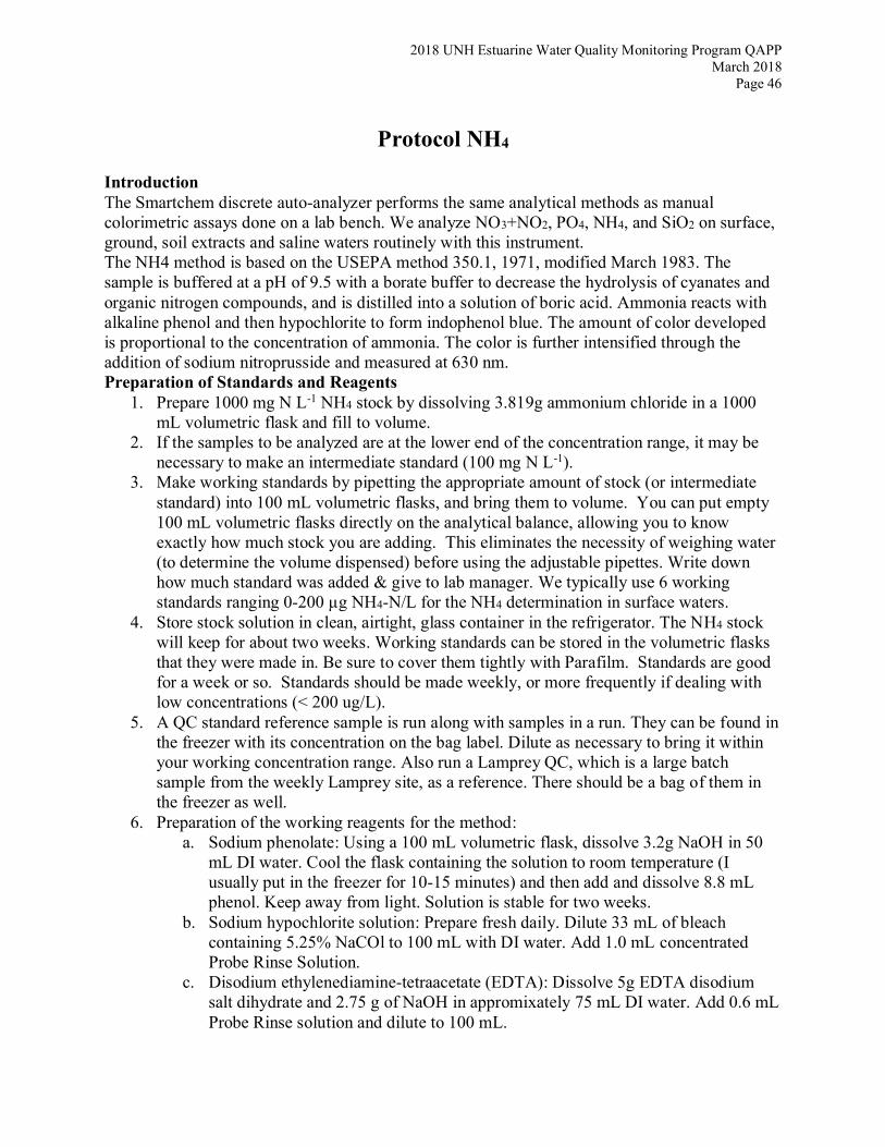
2018 UNH Estuarine Water Quality Monitoring Program QAPP March 2018
Page 46
Protocol NH4 Introduction The Smartchem discrete auto-analyzer performs the same analytical methods as manual colorimetric assays done on a lab bench. We analyze NO3+NO2, PO4, NH4, and SiO2 on surface, ground, soil extracts and saline waters routinely with this instrument. The NH4 method is based on the USEPA method 350.1, 1971, modified March 1983. The sample is buffered at a pH of 9.5 with a borate buffer to decrease the hydrolysis of cyanates and organic nitrogen compounds, and is distilled into a solution of boric acid. Ammonia reacts with alkaline phenol and then hypochlorite to form indophenol blue. The amount of color developed is proportional to the concentration of ammonia. The color is further intensified through the addition of sodium nitroprusside and measured at 630 nm. Preparation of Standards and Reagents
1. Prepare 1000 mg N L-1 NH4 stock by dissolving 3.819g ammonium chloride in a 1000 mL volumetric flask and fill to volume.
2. If the samples to be analyzed are at the lower end of the concentration range, it may be necessary to make an intermediate standard (100 mg N L-1).
3. Make working standards by pipetting the appropriate amount of stock (or intermediate standard) into 100 mL volumetric flasks, and bring them to volume. You can put empty 100 mL volumetric flasks directly on the analytical balance, allowing you to know exactly how much stock you are adding. This eliminates the necessity of weighing water (to determine the volume dispensed) before using the adjustable pipettes. Write down how much standard was added & give to lab manager. We typically use 6 working standards ranging 0-200 µg NH4-N/L for the NH4 determination in surface waters.
4. Store stock solution in clean, airtight, glass container in the refrigerator. The NH4 stock will keep for about two weeks. Working standards can be stored in the volumetric flasks that they were made in. Be sure to cover them tightly with Parafilm. Standards are good for a week or so. Standards should be made weekly, or more frequently if dealing with low concentrations (< 200 ug/L).
5. A QC standard reference sample is run along with samples in a run. They can be found in the freezer with its concentration on the bag label. Dilute as necessary to bring it within your working concentration range. Also run a Lamprey QC, which is a large batch sample from the weekly Lamprey site, as a reference. There should be a bag of them in the freezer as well.
6. Preparation of the working reagents for the method: a. Sodium phenolate: Using a 100 mL volumetric flask, dissolve 3.2g NaOH in 50
mL DI water. Cool the flask containing the solution to room temperature (I usually put in the freezer for 10-15 minutes) and then add and dissolve 8.8 mL phenol. Keep away from light. Solution is stable for two weeks.
b. Sodium hypochlorite solution: Prepare fresh daily. Dilute 33 mL of bleach containing 5.25% NaCOl to 100 mL with DI water. Add 1.0 mL concentrated Probe Rinse Solution.
c. Disodium ethylenediamine-tetraacetate (EDTA): Dissolve 5g EDTA disodium salt dihydrate and 2.75 g of NaOH in appromixately 75 mL DI water. Add 0.6 mL Probe Rinse solution and dilute to 100 mL.

2018 UNH Estuarine Water Quality Monitoring Program QAPP March 2018
Page 47
d. Sodium nitroprusside: Dissolve 0.3g sodium nitroprusside dihydrate (sodium nitroferricyanide dihydrate) in 100 mL of DI water. Add 0.5 mL Probe Rinse. Store solution in glass. Solution should be prepared fresh weekly.
Sample Preparation
1. Frozen samples should be completely thawed the day of analysis. Preparation for Analysis
1. New reagents should be put into the reagent cups each day. If there is old reagent in the cups, dump them into the appropriate waste container and rinse the reagent cups several times with DI water and then add the refrigerated reagent.
2. The diluent cup should be dumped and replaced with fresh DI water (or extract) each day. 3. The reservoirs on the side of the machine should be full at the start of each day and may
need to be refilled if more than one run is done in a day. To refill, rinse the reservoirs several times with DI water. The DI water reservoir needs DI water only. Fill the Probe Rinse reservoir with DI water to the top and then 1 mL of Smartchem Probe Rinse is added. Fill the Cleaning Solution reservoir to 1 L and then add 50 mL Smartchem Cleaning Solution.
4. The Smartchem may need to be turned on & will need to be reset (shut instrument off and restart software) if it is on. The power switch is on the back left side of the instrument. Start up the Smartchem software that is labeled “SmartchemNew”. To log in the username is “Westco” and password is “joe”.
5. When the software says “Standby” at the bottom of the window, click the “Diagnostic” button on the lower right. Click on the “Miscellaneous” tab and click on “Reset” in the “General” area of the window. After system is finished resetting, click on “Diagnostic” tab again to close. Allow system to go to “Standby” again before proceeding.
6. Wash cuvetts prior to every run and wait 15 minutes for cuvetts to dry before starting the run. This can be done while you are entering samples and preparing the sample racks.
7. If this is the first run with new working standards, then the calculated standard concentrations need to be entered into the Method. Click on “Method” and enter the standards into the appropriate spaces to the right of the window.
8. Click on “Sample Entry” and then start up the appropriate method by double clicking on it at the bottom of the window. In the upper left of the window enter the number of samples and standards that you are going to run and click on the check mark to accept. The method is set up to automatically enter blanks, QC standards, duplicates, and spikes every 12 samples, so this does not to be included in the amount that you enter. On the right side of the window enter the UNH ID # and standards for your run.
9. In addition to the standards automatically entered, two standards should be run every 12 samples and the full range of working standards should be run at the end of the run. Standards are typically run after the Blanks and QC sample so that duplicates are performed on samples not standards. Names cannot be duplicated, so change names of standards slightly each time you enter them. When finished entering, click the “save” icon at the top right of the window.
10. Name the file as you wish to differentiate between runs. Click “Yes” to print and then click on the printer icon. This will print your run sheet. Attach the run sheet header

2018 UNH Estuarine Water Quality Monitoring Program QAPP March 2018
Page 48
provided and write in the information that it asks for. Staple the header to the top of the run sheets.
11. Rinse each vial once with sample or standard and then fill between the top two lines of the Smartchem vial.
12. Samples should be placed in the appropriate Smartchem rack and location number, which is indicated on the run sheet. Racks should be placed in the proper position & are keyed to ensure that they are.
13. START the run by clicking on the Play icon in the upper left of the window. Uncheck “RBL” and then check “WBL” to initiate Water Baseline at the beginning of the run. This measures the absorbance of water in the cuvette to account for changes in the cuvette over time and check the condition of the filters and lamp. WBL only needs to be run once a day.
14. After the run has started & the calibration curve window appears, check the “results” page to make sure the calibration curve is acceptable and that the first set of NH4 and QC standards are recovered appropriately.
15. When run is complete click on “Export” to the left of the window and export to an Excel file.
Quality Assurance and Control
1. Prior to running the Smartchem you must log-in on the Log-In Excel sheet on the Smartchem computer. Please fill-in all designated information. This information will aid in maintenance of the instrument and will be used in conjunction with the Quality Control data.
2. Following completion of your analysis you are responsible for checking the data. The data is to be copied and pasted into the appropriate lab Excel Report Template on the Smartchem computer and the file should be named by date of analysis (described in worksheet). This template will guide you to report the QC results for the run. This includes % recovery of QC standards (CRM), run time check standards, and lab duplicates. Lab % recovery of sample duplicates, run time check standards, and QC standards should be between 85 and 115 % (see WQAL QAPP for more information).
3. When completed copy the Excel file into the lab manager’s directory on the main lab computer. This information, along with the data, will be entered into the WQAL database by the lab manager to create control charts.

2018 UNH Estuarine Water Quality Monitoring Program QAPP March 2018
Page 49
B2: NO3-NO2 Standard Operating Procedure using SEAL Analytical Discrete Multi-Chemistry Analyzer (AQ2)
Water Quality Analysis Laboratory at the University of New Hampshire
Prepared by: Katie Swan Date of Last Revision: 4/25/16 Method is based on: USEPA 353.2 Revision 2.0, August, 1993. Determination of Nitrate-Nitrite Nitrogen by
Automated Colorimetry.

2018 UNH Estuarine Water Quality Monitoring Program QAPP March 2018
Page 50
Protocol NO3+NO2 Introduction The SEAL analytical discrete multi-chemistry auto-analyzer performs the same analytical methods as manual colorimetric assays done on a lab bench. We analyze NO3+NO2, PO4, and TN/TP on surface, ground, soil extracts, and saline waters routinely with this instrument. The NO3+NO2 method is based on USEPA 353.2 Revision 2.0, August, 1993. This method determines the combined nitrate (NO3) + nitrite (NO2) present in the sample. Nitrate is reduced to nitrite by passage of a filtered sample through an open tubular copperized cadmium redactor (OTCR). The nitrate reduced to nitrite plus any nitrite originally present in the sample is then determined as nitrite by diazotizing with sulfanilamide followed by coupling with N-(naphthyl)-ethylenediamine dihydrochloride to form a highly colored azo dye, which is measured colorimetrically at 550 nm. Preparation of Standards and Reagents
1. Prepare 1000 mg N L-1 NO3 stock by dissolving 6.0667 g sodium nitrate a 1000 mL volumetric flask and fill to volume. Also, prepare 1000 mg N L-1 NO2 stock by dissolving 4.926g sodium nitrite in a 1000 mL volumetric flask and fill to volume.
2. If the samples to be analyzed are at the lower end of the concentration range, it may be necessary to make an intermediate standard (100 mg N L-1).
3. Make working standards for by pipetting the appropriate amount of stock (or intermediate standard) into 100 mL volumetric flasks, and bring them to volume. You can put empty 100 mL volumetric flasks directly on the analytical balance, allowing you to know exactly how much stock you are adding. This eliminates the necessity of weighing water (to determine the volume dispensed) before using the adjustable pipettes. Record weighed values in the TN/TP_NO3 Stds electronic file under McDowell Shared in drobox.
4. We typically use 6 working standards ranging 0 to 1.0 mg NO3-N/L for the NO3 determination in surface waters. One working NO2 standard are also needed as a check to ensure that the cadmium coil is reducing NO3 fully to NO2. Make the NO2 standards within the working NO3 range. This is NO2 QC in the NO2 stds working file.
5. Store stock solution in volumetric flask that it was made in and covered securely with Parafilm in the refrigerator. The NO3 stock will keep for about one (1) month. Working standards can be stored in the volumetric flasks that they were made in. Be sure to cover them tightly with Parafilm. Standards are good for a week or so. Standards should be made weekly, or more frequently if dealing with low concentrations (< 0.3 mg/L).
6. A QC standard reference sample is run along with samples in a run. The QC is made using pre-made SPEX standards that is pipetted for specified amount and weighed out on the analytical balance and diluted to final desired volume. Refer to TN/TP_NO3 electronic file under McDowell Shared file in drobox. Also run a Lamprey CCV, which is a large batch sample from the weekly Lamprey site, as a reference. There should be a bag of them in the freezer as well.
7. Preparation of the working reagents for the method: a. Ammonium Chloride Buffer solution: In a hood, to the dedicated 1L plastic bottle
add and dissolve 500 mL DI water, 180 g Ammonium chloride, and 2.0 g

2018 UNH Estuarine Water Quality Monitoring Program QAPP March 2018
Page 51
disodium EDTA. Adjust the pH to 8.55 with Ammonium hydroxide. Dilute to 1 L and mix.
b. Working Buffer solution: To approximately 75 mL of DI water in a 200 volumetric flask add 200 ml of the Ammonium Chloride Buffer solution and 1.0 mL of Triton X-100 solution and dilute to 200 mL with DI water. Transfer the solution to a dark 250 mL plastic bottle. Solution is stable for two weeks.
c. Sulfanilamide-NEDD solution: To approximately 250 mL of DI water in a 500 mL volumetric flask dissolve 1.0 g of sodium hydroxide pellets, slowly add 20 mL of phosphoric acid, add 7.5 g of sulfanilamide and 0.375 g of N-(1-napthyl) ethylene diamine dihydrochloride and stir to dissolve. Dilute to 500 mL with DI water. Solution is stable for six weeks.
Sample Preparation
1. Frozen samples should be completely thawed the day of analysis. Preparation for Analysis
1. Reagents are poured into the Seal wedges and the reagent name and its position in the wedge tray should be marked. If there are reagents in the wedges and they were kept cold (i.e. in the fridge or in the Seal with it left on in the refrigerated compartment), then they can be reused if it is valid for the reagent to do so. Some reagents might need to be made daily, so please check the method. If they were not refrigerated and left in the wedges, then please dump them into the appropriate waste container and rinse the wedges several times with DI water and replace the reagent.
2. The DI water reagent wedge should be dumped and replaced with fresh DI water (or extract) about once per week.
3. The DI water reservoir on the side of the SEAL should be full at the start of each day and may need to be refilled if more than one run is done in a day. To refill, rinse the reservoir several times with DI water. The DI water reservoir needs DI water only.
4. Change out the appropriate reaction segments (1-10) that need to be changed (i.e. have been used). This can be checked in the “Maintenance” of the Seal software, which will be described below.
5. The SEAL may need to be turned on. The power switch is on the back right side of the instrument. Start up the SEAL software that is labeled “SEAL AQ2”. To log in the username is “wrrc lab” and password is “waterlab”.
6. When the software opens on the “run screen”, select the “Maintenance and Daily Start Up” tab on the top right of the screen. a. Click on the “Maintenance” tab and the “main maintenance and setup” window will
come up. Want to zero reaction segments each run, select “Zero Segments” and select yes. To select desired maintenance function is on the left side of the window.
b. Select the “Diluter” tab. The diluter needs to be primed each day to ensure that there are no air bubbles present. To prime the diluter, select the “diluter” tab and select total number of primes (10x) and start prime.
c. When finished priming the diluter, then select the “Cuvette functions” tab. The aspiration wash bath needs to be auto washed at the start of the day. Select the total

2018 UNH Estuarine Water Quality Monitoring Program QAPP March 2018
Page 52
number of washes (2x) and click on the “auto wash” button. Make sure that the aspiration bath is filling up and draining.
d. When finished with the auto wash, select the “test aspiration tab”. Take off the cover in the left corner in SEAL and will see an inlet and outlet tubing from the cuvette. The value that is used (e.g. 200) is to ensure that the headspace in the outlet and inlet tubing is about 1 inch from the cuvette. Click on “test aspiration” tab and watch where the headspace is when the test finishes. If need to make adjustments to increase or decrease the headspace in the tubing, increase or decrease the initial value and run the aspiration test again.
e. When finished with the test aspiration, select the “extra wash” tab. Make sure to have the cuvette cleaning solution wedge in the first position in the reagent tray on the right side of the seal. Run the extra wash and watch to see if the syringe is pulling up the solution properly (no dripping or beading at the tip). Make sure that the syringe is landing in the right well in the reaction segments.
f. When finished with the extra wash, take the cuvette cleaning solution wedge out. Exit the main maintenance and setup screen and select “daily start up.” Hit continue. The daily startup will measure and absorbance and a list eight absorbance readings will be reported on the far right side of the main screen. Record the absorbance values each week and make sure the absorbance values do not drift too much each day. This measures the absorbance of water in the cuvette to account for changes in the cuvette over time and check the condition of the filters and lamp.
7. To prime the cadmium coil (refer to the NO3+NO2 method in the SEAL manual). 8. If this is the first run with new working standards, then the calculated standard
concentrations need to be entered into the Tests. Click on “Tests” under the maintenance and daily startup tab, select the appropriate method, select calibration, and enter the standards into the appropriate spaces under the manual standards (S1-S7; S1 is a blank).
9. In “Maintenance” make sure that the appropriate tray is selected for the tray that you are going to use.
10. Click on “Scheduling”, select tray number and select reagent set #2, and type in the run file (i.e. 160304NO301). In the upper left of the window select the sample type (standards and unknowns), select standards 1-7 (S1-S7). Then enter the UNH ID # in sample ID, which automatically will be entered as type “unknown”, and enter a rep after every 12 samples and Enter a subset or all of the standards at the end of your run setup without using type “standards”, so that they will be entered as unknowns. The method is set up to automatically enter blanks, QCs, and duplicates every 12 samples, so this does not to be included in the amount that you enter. On the right hand side in the “Requested Tests” column highlight all the cells that contain samples in that column and then select “NOx” at the top. When finished entering, click the “save” icon at the top left of the window.
11. Select “run” when run is set up and saved. Select the run file for the run and continue. 12. Rinse each vial once with sample or standard and then fill ¾ full with the SEAL sample
cups (1.2 mL or 2mL sample cups). 13. Samples should be placed in the appropriate SEAL sample tray (57 samples or 100
samples trays). Sample trays should be placed in the proper position and screwed in tightly to ensure the tray is not moving around during the run.

2018 UNH Estuarine Water Quality Monitoring Program QAPP March 2018
Page 53
14. START the run by clicking on the “Run” tab and select to continue. 15. After the run has started, check the “calibration” tab to make sure the calibration curve is
analyzed and check that it is acceptable after it has run the calibration standards at the beginning. Select the “Data Review” tab and that the first set of NO2, NO3 and QC standards are recovered appropriately. If NO2 recovery is high, may need to re-prime the cadmium coil.
16. When the run is complete, click on “Data Review” to the left of the window, select “Accept All” on the top tabs and export to a document file and save under export file.
Data Export
1. Following completion of your analysis you are responsible for checking the data. The data is to be copied and pasted into the appropriate lab Excel Report Template on the SEAL computer and the file should be named by date of analysis (described in worksheet). This template will guide you to report the QC results for the run. This includes % recovery of QC standards (CRM), run time check standards, and lab duplicates. Lab % recovery of sample duplicates, run time check standards, and QC standards should be between 85 and 115 % (see WQAL QAPP for more information).
2. When completed copy the Excel file into the lab manager’s directory on the main lab computer. This information, along with the data, will be entered into the WQAL database by the lab manager to create control charts.
Shut Down Instrument 1. When finished exporting data, need to shut down the instrument. a. Go to the main screen, click on the seal icon on the upper left corner and choose to exit
the software. A window will come up and select both boxes “shutting down instrument overnight? and close program?”
2. Put the reagent tray back in the fridge with the reagents in the wedges. 3. Turn off the lamp on the instrument, leave the reagent cooling tray on. 4. Empty the sample tray (sample in the sink and sample vials in the trash). 5. Empty out the DI water reservoir.

2018 UNH Estuarine Water Quality Monitoring Program QAPP March 2018
Page 54
B3: Ortho-phosphate (PO4) Standard Operating Procedure SEAL Analytical Discrete Multi-Chemistry Analyzer (AQ2)
Water Quality Analysis Laboratory at the University of New Hampshire
Prepared by: Katie Swan Date of Last Revision: 4/25/16 Method is based on: USEPA method 365.2, 1971, modified March 1983. . Determination of Ortho-phosphate by
Semi-Automated Colorimetry.

2018 UNH Estuarine Water Quality Monitoring Program QAPP March 2018
Page 55
Protocol PO4 Introduction The SEAL analytical discrete multi-chemistry auto-analyzer performs the same analytical methods as manual colorimetric assays done on a lab bench. We analyze NO3+NO2, PO4, and TN/TP on surface, ground, soil extracts, and saline waters routinely with this instrument. The PO4 method is based on the USEPA method 365.2, 1971, modified March 1983. Ammonium molybdate and antimony potassium tartrate react in an acid medium with dilute solutions of phosphorous to form an antimony-phospho-moybdate complex. This complex is reduced to an intensely blue-colored complex by ascorbic acid. The color measured at 880nm is proportional to the phosphorous concentration. Preparation of Standards and Reagents
1. Prepare 1000 mg N L-1 PO4 stock by dissolving 4.3937 g potassium phosphate in a 1000 mL volumetric flask and fill to volume.
2. If the samples to be analyzed are at the lower end of the concentration range, it may be necessary to make an intermediate standard (100 mg P L-1).
3. Make working standards for by pipetting the appropriate amount of stock (or intermediate standard) into 100 mL volumetric flasks, and bring them to volume. You can put empty 100 mL volumetric flasks directly on the analytical balance, allowing you to know exactly how much stock you are adding. This eliminates the necessity of weighing water (to determine the volume dispensed) before using the adjustable pipettes. Write down how much standard was added & give to lab manager. We typically use 6 working standards ranging 0 to 200 µg PO4-P/L for the PO4 determination in surface waters.
4. Store stock solution in clean, airtight, glass container in the refrigerator. The PO4 stock will keep for about one month. Working standards can be stored in the volumetric flasks that they were made in. Be sure to cover them tightly with Parafilm. Standards are good for a week or so. Standards should be made weekly, or more frequently if dealing with low concentrations (< 200 ug/L).
5. A QC standard reference sample is run along with samples in a run. The QC is made using pre-made SPEX standards that is pipetted for specified amount and weighed out on the analytical balance and diluted to final desired volume. Refer to PO4 electronic file under McDowell Shared file in drobox. Also run a Lamprey QC, which is a large batch sample from the weekly Lamprey site, as a reference. There should be a bag of them in the freezer as well.
6. Preparation of the working reagents for the method: a. Sulfuric acid solution, 5N: Slowly add 70 mL of concentrated H2SO4 to 400 mL DI
water. Cool to room temperature and dilute to 500 mL. b. Antimony potassium tartrate solution (0.3%): Weight 0.30 g Antimony potassium tartrate
in 75 mL of DI water, dilute to 100 mL in dedicated plastic bottle. Prepare fresh monthly. c. Ammonium moybdate solution (4%): Dissolve 4 g Ammonium moybdate tetrahydrate in
75 mL DI water, dilute to 100 mL in dedicated plastic bottle. Discard reagent if becomes turbid or discolored.
d. Working Ascorbic Acid: Dissolve 1.5 g Ascorbic acid in 80 mL of DI water. Add 2 mL of 15% SDS solution, dilute to 100 mL of DI water. Prepare this solution fresh daily.

2018 UNH Estuarine Water Quality Monitoring Program QAPP March 2018
Page 56
e. Color Reagent: To a clean 125 mL plastic bottle add 75 mL of prepared 5N sulfuric acid and then add 18.0 mL Ammonium molybdate solution and mix. Add 7.5 mL Antimony potassium tartrate solution and mix. Add 4 mL 15% SDS and dilute to 100 mL with DI water. Mix. This solution should be prepared every 3 weeks.
Sample Preparation
1. Frozen samples should be completely thawed the day of analysis. Preparation for Analysis
1. Reagents are poured into the Seal wedges and the reagent name and its position in the wedge tray should be marked. If there are reagents in the wedges and they were kept cold (i.e. in the fridge or in the Seal with it left on in the refrigerated compartment), then they can be reused if it is valid for the reagent to do so. Some reagents might need to be made daily, so please check the method. If they were not refrigerated and left in the wedges, then please dump them into the appropriate waste container and rinse the wedges several times with DI water and replace the reagent.
2. The DI water reagent wedge should be dumped and replaced with fresh DI water (or extract) each day.
3. The DI water reservoir on the side of the SEAL should be full at the start of each day and may need to be refilled if more than one run is done in a day. To refill, rinse the reservoir several times with DI water. The DI water reservoir needs DI water only.
4. Change out the appropriate reaction segments (1-10) that need to be changed (i.e. have been used). This can be checked in the “Maintenance” of the Seal software, which will be described below.
5. The SEAL may need to be turned on. The power switch is on the back right side of the instrument. Start up the SEAL software that is labeled “SEAL AQ2”. To log in the username is “wrrc lab” and password is “waterlab”.
6. When the software opens on the “run screen”, select the “Maintenance and Daily Start Up” tab on the top right of the screen. a. Click on the “Maintenance” tab and the “main maintenance and setup” window will
come up. Want to zero reaction segments each run, select “Zero Segments” and select yes. To select desired maintenance function is on the left side of the window.
b. Select the “Diluter” tab. The diluter needs to be primed each day to ensure that there are no air bubbles present. To prime the diluter, select the “diluter” tab and select total number of primes (10x) and start prime.
c. When finished priming the diluter, then select the “Cuvette functions” tab. The aspiration wash bath needs to be auto washed at the start of the day. Select the total number of washes (2x) and click on the “auto wash” button. Make sure that the aspiration bath is filling up and draining.
d. When finished with the auto wash, select the “test aspiration tab”. Take off the cover in the left corner in SEAL and will see an inlet and outlet tubing from the cuvette. The value that is used (e.g. 200) is to ensure that the headspace in the outlet and inlet tubing is about 1 inch from the cuvette. Click on “test aspiration” tab and watch where the headspace is when the test finishes. If need to make adjustments to increase

2018 UNH Estuarine Water Quality Monitoring Program QAPP March 2018
Page 57
or decrease the headspace in the tubing, increase or decrease the initial value and run the aspiration test again.
e. When finished with the test aspiration, select the “extra wash” tab. Make sure to have the cuvette cleaning solution wedge in the first position in the reagent tray on the right side of the seal. Run the extra wash and watch to see if the syringe is pulling up the solution properly (no dripping or beading at the tip). Make sure that the syringe is landing in the right well in the reaction segments.
f. When finished with the extra wash, take the cuvette cleaning solution wedge out. Exit the main maintenance and setup screen and select “daily start up.” Hit continue. The daily startup will measure and absorbance and a list eight absorbance readings will be reported on the far right side of the main screen. Record the absorbance values each week and make sure the absorbance values do not drift too much each day. This measures the absorbance of water in the cuvette to account for changes in the cuvette over time and check the condition of the filters and lamp.
7. If this is the first run with new working standards, then the calculated standard concentrations need to be entered into the Tests. Click on “Tests” under the maintenance and daily startup tab, select the appropriate method, select calibration, and enter the standards into the appropriate spaces under the manual standards (S1-S7; S1 is a blank).
8. In “Maintenance” make sure that the appropriate tray is selected for the tray that you are going to use.
9. Click on “Scheduling”, select tray number and select reagent set #1, and type in the run file (i.e. 160304NO301). In the upper left of the window select the sample type (standards and unknowns), select standards 1-7 (S1-S7). Then enter the UNH ID # in sample ID, which automatically will be entered as type “unknown”, and enter a rep after every 12 samples and Enter a subset or all of the standards at the end of your run setup without using type “standards”, so that they will be entered as unknowns. The method is set up to automatically enter blanks, QCs, and duplicates every 12 samples, so this does not to be included in the amount that you enter. On the right hand side in the “Requested Tests” column highlight all the cells that contain samples in that column and then select “op1” at the top. When finished entering, click the “save” icon at the top left of the window.
10. Double click“run” when run is set up and saved. Select the run file for the run and continue.
11. Rinse each vial once with sample or standard and then fill ¾ full with the SEAL sample cups (1.2 mL or 2mL sample cups).
12. Samples should be placed in the appropriate SEAL sample tray (57 samples or 100 samples trays). Sample trays should be placed in the proper position and screwed in tightly to ensure the tray is not moving around during the run.
13. START the run by clicking on the “Run” tab and select to continue. 14. After the run has started, check the “calibration” tab to make sure the calibration curve is
analyzed and check that it is acceptable after it has run the calibration standards at the beginning. Select the “Data Review” tab and that the first set of QC standards are recovered appropriately.
15. When the run is complete, click on “Data Review” to the left of the window, select “Accept All” on the top tabs and export to a document file and save under export file.

2018 UNH Estuarine Water Quality Monitoring Program QAPP March 2018
Page 58
Data Export
1. Following completion of your analysis you are responsible for checking the data. The data is to be copied and pasted into the appropriate lab Excel Report Template on the SEAL computer and the file should be named by date of analysis (described in worksheet). This template will guide you to report the QC results for the run. This includes % recovery of QC standards (CRM), run time check standards, and lab duplicates. Lab % recovery of sample duplicates, run time check standards, and QC standards should be between 85 and 115 % (see WQAL QAPP for more information).
2. When completed copy the Excel file into the lab manager’s directory on the main lab computer. This information, along with the data, will be entered into the WQAL database by the lab manager to create control charts.
Shut Down Instrument 6. When finished exporting data, need to shut down the instrument. b. Go to the main screen, click on the seal icon on the upper left corner and choose to exit
the software. A window will come up and select both boxes “shutting down instrument overnight? and close program?”
7. Put the reagent tray back in the fridge with the reagents in the wedges. 8. Turn off the lamp on the instrument, leave the reagent cooling tray on. 9. Empty the sample tray (sample in the sink and sample vials in the trash). 10. Empty out the DI water reservoir.

2018 UNH Estuarine Water Quality Monitoring Program QAPP March 2018
Page 59
B4: Total Nitrogen (TN) and Total Phosphorous (TP) Standard Operating Procedure using SEAL Analytical Discrete Multi-
Chemistry Analyzer (AQ2)
Water Quality Analysis Laboratory at the University of New Hampshire
Prepared by: Katie Swan Date of Last Revision: 4/25/16 Method is based on: USGS Water-Resources Investigations Report 03-4174, “Methods of Analysis by the US Geological Survey National Water Quality Laboratory-Evaluation of Alkaline Persulfate Digestion as an Alternative to Kjeldahl Digestion for Determination of Total and Dissolved Nitrogen and Phosphorous in Water.”

2018 UNH Estuarine Water Quality Monitoring Program QAPP March 2018
Page 60
Total P (TP), Total Dissolved P (TDP), Total N (TN) and Total Dissolved N (TDN) using Alkaline Persulfate Digestion.
Introduction This digest is applied to water samples to convert all species of P into PO4 and all species of N to NO3. The resulting digestion can be measured by automated colorimetry on the SEAL AQ2 for PO4 and NO3 to give Total P and N, respectively. Dissolved vs Total is operationally defined as digesting a filtered sample (GF/F) or an unfiltered sample. The method is based on USGS Water-Resources Investigations Report 03-4174, “Methods of Analysis by the US Geological Survey National Water Quality Laboratory-Evaluation of Alkaline Persulfate Digestion as an Alternative to Kjeldahl Digestion for Determination of Total and Dissolved Nitrogen and Phosphorous in Water.” Method Detection Limits (MDL) have been calculated to be 6 ug P/L and 10 ug N/L. Reporting Detection Levels (RDL) are approximately 15 ug P/L and 50 ug N/L. Precision for TP and TDP is approximately +/- 5 ug P/L or 10%, whichever is greater. Precision for TN and TDN is approximately +/- 10 ug N/L or 10%, whichever is larger. Reagent Preparation 1.5 M Sodium Hydroxide Dissolve 60 g Sodium Hydroxide (NaOH) in about 800 mL of DI water in a 1 L volumetric flask. Let cool and fill to volume with DI water. This should be stable for months. (12 g NaOH in 200mL DI water). 2x Recrystallized Potassium Persulfate (K2SO8)
Even the cleanest reagent grade Potassium Persulfate appears to be loaded with Nitrogen, so it’s critical that it be purified by recrystallizing twice it prior to use.
Potassium persulfate recrystallization
1. Dissolve 100 g of potassium persulfate in approximately 600 ml of Milli-Q previously heated to 60˚ C. Use a medium sized stir bar and a 1000 mL flask.
2. Filter the solution rapidly through a sintered glass funnel.
3. Rinse the 1000 mL flask
4. Pour filtrate back into the flask used to heat the potassium persulfate solution.
5. Cool solution to about 4˚ C by placing the flask in ice water or freezer. Whirl the flask continuously to prevent the solution from freezing. (~1.5 hours in freezer)
6. Filter the 4˚ C solution and wash with 1 or 2 squeezes of ice cold Milli-Q, save the white solid.
7. Discard the filtrate from the sidearm flask.

2018 UNH Estuarine Water Quality Monitoring Program QAPP March 2018
Page 61
8. Rinse the flask used to cool the solution with Milli-Q
9. Fill the flask with 450ml of Milli-Q and heat to 60˚ C.
10. Add the crystals from step 5 and mix into solution.
11. Repeat steps 4 and 5. The white granules on top of the filter are crystals!
12. Dry crystals in a vacuum desiccators. Rapid drying in a good vacuum and thus at a low temperature is essential as this will minimize the sulfuric acid formation on the crystals. Drying will be complete in several days.
Working digest solution
Add 18 grams of 2x recryrstallized Potassium Persulfate and 45 mL of the 1.5 M Sodium Hydroxide solution to about 350 mL of DI. Swirl to dissolve. Once dissolved, fill to 450 mL. Prepare this daily. Fill to ____ with DI 150mL 300mL 450mL 2x recrystallized Potassium Persulfate
6g 12g 18g
1.5 M Sodium Hydroxide 15mL 30mL 45mL
Standards, blanks and QC sample preparation Blanks, standards and QC samples should all be digested using the same method as the samples. Blanks are DI water. Standards should be made from PO4 and NO3 stock solutions. QC samples should be one of the several Ultra Scientific QC reference samples we have in the freezer. Pick one that will be appropriate to the range of standard concentrations (typically 6-200 ug P/L or 6-500 ug N/L). Also, prepare another QC check from a Disodium EDTA stock solution (for N) and a sodium pyrophosphate stock solution (for P). Prepare extra blank digestions, as you’ll need the blank as the diluent for both the PO4 and NO3 analyses on the Smartchem. PREPARE… FOR EVERY… 1 Blank (DI) ~10 samples 1 Standard (#1-6) ~25 samples 1 QC (TN/TP) ~16 samples 1 CCV (UNFULTERED) ~16 samples 1 NO2 QC ~32 samples 1 SAMPLE REP ~12 samples
Digestion
1. Use acidwashed 20 mL PP widemouth bottles for sample digestion. 2. Shake sample thoroughly, then pipette 10 mL of sample into the digestion bottle.

2018 UNH Estuarine Water Quality Monitoring Program QAPP March 2018
Page 62
3. Add 5 mL of digestion solution. 4. A replicate digest should be done every 10-12 samples. 5. Cap loosely (threads hardly engaged) and put in autoclave for 1 hour. Autoclave
Cycle #11 Liquids. Sterilize Temp = 121°C, Pressure = 117.2 kPa 6. Let samples cool after digestion. 7. Cap tightly until analysis.
Samples are ready for analysis. They can be placed in the refrigerator until time for analysis on the SEAL AQ2 using the appropriate protocols. PO4 based on EPA 365.1 (molybdate blue method), and NO3 based on EPA 353.2 (Cd-Cu reduction). Note: For TN method, use the Smartchem working buffer reagent. Working Buffer (TN analysis) - Ammonium Chloride Buffer, pH 8.5 Concentrated hydrochloric acid (HCl) 105 mL Ammonium hydroxide (NH4OH) 95 mL Ethylenediaminetetraccetic acid disodium salt dehydrate (Disodium EDTA) 1.0 g DI water Dilute to 1 L Adjust pH to 8.5 with HCL or 5 N NaOH In a 1 L volumetric flask, add 500 mL of DI water, dissolve 1.0 g of disodium EDTA, 105 mL of concentrated hydrochloric acid, and 95 mL of ammonium hydroxide. Fill to mark with DI water and mix well. Adjust the pH to 8.5 using 5 N sodium hydroxide or HCL. CAUTION- Fumes will be produced when add ammonium hydroxide to the mixed solution with HCL and disodium EDTA.

2018 UNH Estuarine Water Quality Monitoring Program QAPP March 2018
Page 63
Appendix C
Dissolved Organic Carbon (DOC) and Total Dissolved Nitrogen (TDN) Standard Operating Procedure Shimadzu TOCL and TOCV
CPH
Water Quality Analysis Laboratory at the University of New Hampshire
Prepared by: Jody Potter Date of Last Revision: 4/12/2016 Method is based on: EPA Method 415.1 Organic Carbon, Total (Combustion or Oxidation). And TDN Method: Method Reference: Shimadzu Scientific Instruments Inc., TOC-V with TNM-1 Nitrogen Module. High Temperature Catalytic Oxidation with chemiluminescent detection. Merriam, J.L., W.H. McDowell, W.S. Currie, 1996. A high-temperature catalytic oxidation technique for determining total dissolved nitrogen. Soil Science Society of America Journal, 60(4) 1050-1055.

2018 UNH Estuarine Water Quality Monitoring Program QAPP March 2018
Page 64
Protocol for TOC-V CPH and TOC-L CPH
There are one of each of these machines. Both the TOC-L CSH and TOC-V CSH can analyze NPOC and TDN in the same run. These protocols include both, but TDN is all that is required by the project. NPOC Method: Official Name: EPA Method 415.1 Organic Carbon, Total (Combustion or Oxidation). Organic carbon in a sample is converted to carbon dioxide by catalytic combustion or wet chemical oxidations. The carbon dioxide formed can be measured directly by an infrared detector or converted to methane and measured by a flame ionization detector. The amount of carbon dioxide or methane is directly proportional to the concentration of carbonaceous material in the sample. TDN Method: Method Reference: Shimadzu Scientific Instruments Inc., TOC-V with TNM-1 Nitrogen Module. High Temperature Catalytic Oxidation with chemiluminescent detection. Merriam, J.L., W.H. McDowell, W.S. Currie, 1996. A high-temperature catalytic oxidation technique for determining total dissolved nitrogen. Soil Science Society of America Journal, 60(4) 1050-1055. A precisely measured aliquot of filtered sample is injected and combusted on a catalyst at 720 C. All fixed N is converted to Nitric Oxide (NO) and then coupled with ozone (O3) producing Nitrogen Dioxide* (NO2
*) which is measured chemiluminescently.
1. Preparation of Standard Solutions A. NPOC. Weigh out 2.125 g dried potassium acid phthalate (KHP). Dissolve it in 500 mL
of Milli-Q water (DDW) in a 1 L volumetric flask. Bring the solution to volume. This makes a 1000 mg C L-1 TC stock (1000 ppm). TDN. Weigh out 0.60677 g dried sodium nitrate. Dissolve it in a 100 mL volumetric flask and fill to volume. This makes a 1000 mg N L-1 NO3 stock solution.
B. If the samples to be analyzed are at the lower end of the concentration range, it may be necessary to make an intermediate standard (100 mg L-1).
C. When doing more than one analysis, NPOC and TDN standards should be combined in the same volumetric flask to reduce the amount of standard vials taking up space on a run. The lowest NPOC standard should be combined with the lowest TDN standard and so on.
D. Make working standards by pipetting the appropriate amount of stock (or intermediate standard) into 250 mL volumetric flasks, and bring them to volume. You can put the 250 mL volumetric flasks directly on the analytical balance, allowing you to know exactly how much stock you are adding. This eliminates the necessity of weighing water (to determine the volume dispensed) before using the adjustable pipettes.

2018 UNH Estuarine Water Quality Monitoring Program QAPP March 2018
Page 65
E. Store stock solution in clean, airtight, glass container in the refrigerator. TOC stock will keep for two (2) months. The NO3 and IC stock will keep for about one (1) month. Working standards can be stored in the volumetric flasks that they were made in. Be sure to cover them tightly with Parafilm. An airtight seal is especially important for the IC stock and standards due to absorption of CO2 from the atmosphere. TOC and TDN standards are good for a week or so. IC standards should be remade every 2 or 3 days. Standards should be made weekly, or more frequently if dealing with low concentrations (< 0.3 mg/L). Refer to Acid Washing protocol for details.
2. Sample Preparation A. Sample vials (9 mL or 22 mL) are prepared by rinsing them at least 2 times with DDW
and then combusting them in the muffle furnace at 450 - 500C for 6 hours. It takes the muffle furnace one hour to get up to temperature.
B. Fill each vial about ½ full for 22 mL vials. Fill the 9 mL vials completely full. C. Cover the 22 mL vials with the caps that are provided. The septa should be removed
and new ones should be put in the caps every 3-4 runs. You should be able to tell how many times the caps have been pierced. The dark side of the septa should face up.
D. Put the vials in the sample tray. The sample tray can be removed from the autosampler by lifting the hood and releasing the magnet that holds the tray down. You can then simply lift the sample tray off the autosampler.
E. Please refer to the Quality Assurance and Control Section for information on replicates, certified reference standards and check standards. A copy of the NPOC/TDN/POC runsheet is attached.
3. System Inspection A. Confirm gas pressure on the TOC gas generator. Carrier Flow meter (on TOC-V CSH)
should read about 150 mL min-1. B. Inspect the dehumidifier drain vessel water level. The water in the drain vessel should
reach the outflow port on the drain vessel sidewall. Add DDW to get it to that level, if necessary. Make sure there is no bubbling in the drain vessel. If there is, inspect the halogen scrubber and membrane filter for plug.
C. Inspect humidifier water level. Confirm that the water level is between the two line markings. Add DDW through the supply port if necessary.
D. Inspect the IC reagent reservoir on outside of instrument. This reservoir should have some solution. If it is empty, you must fill it with H3PO4 according to recipe.
E. Inspect needle rinse bottle to the left of the autosampler. It should be filled with DDW. F. Inspect the HCl bottle on the outside of the instrument. It should be filled with 2N HCl
for NPOC and POC analysis. G. Inspect the dilution water bottle to the left of the instrument and make sure it is filled
with DDW (only necessary if going to do auto dilution with the instrument). H. Perform a leak check. The IC vessel inside the instrument should be bubbling.

2018 UNH Estuarine Water Quality Monitoring Program QAPP March 2018
Page 66
4. Preparation for Analysis A. Check to see that waste vessel for the TOC-V (TOC-L drains to sink) is relatively
empty, and that the waste tube is in the waste vessel and has no kinks. B. The TOCs are normally left on. If it is off, then turn it on and allow the furnace to heat
up. C. The system setup for the instrument is usually set to be done from the computer. Ask
the lab manager for help if the instrument screen is on. Start up the software, which is labeled TOC Control L or V. Then click on the Sample Table Editor icon. It will ask you for user and password, but just click ok with nothing filled in.
D. Open a new sample table by selecting New from the File menu. Click on the sample run icon and then click OK.
E. To establish communication between the software and the instrument, select the connect icon on the toolbar. The Parameter Configuration dialog box is displayed. Click the Use Settings on PC button for TOC-V.
F. Insert the samples by first placing the cursor in the first line of the sample table. From the insert menu, select sample. The Insert multiple samples for TOC-L and Auto Generate for TOC-V option may also be selected if you have several values of the same type (i.e. standards or samples) in a row (manual section 4.4.5.1 “Auto Generate). For single samples (sample): 1. Click on the Method radio button. Select one of the previously created method files
depending on which method you need (i.e. NPOC-TN method) to perform the type of analysis you are doing. Then click next.
2. Type in the name of the sample in sample name and sample ID. Change the number of determinations if you want it to be sampled more than once.
3. Click on next until you click on finish. 4. Continue as needed. For several samples in a row (Auto Generate): 1. Click on the method radio button. Select one of the previously created method files
depending on which method you need (i.e. NPOC-TN method) to perform the type of analysis you are doing. Then click next.
2. Type in the number of vials, the start vial, and the name of the samples. If entering ID numbers, select Index Start instead of entering the name of the samples. Type in the ID number of the beginning vial for the string of samples.
3. Click next until reach finish and then click finish.
G. Save the Sample Table by selecting Save from the File menu. H. Check the status of the instrument detectors before starting analysis. From the
Instrument menu, select Background Monitor. On the TOC tab, the status of the baseline should be OK for each parameter (position, fluctuation, and noise). Do the same for the TN tab. Then close the window.
I. Place the cursor in the first row of the Sample Table. From the Instrument menu, select Start, or click on the Start button on the toolbar. The Standby window is displayed.
J. Press standby. The Sparging/Acid Addition window is displayed. K. Verify the vial positions, and then click OK. L. The Start ASI measurement window is displayed. Click on Start.

2018 UNH Estuarine Water Quality Monitoring Program QAPP March 2018
Page 67
5. Data Export A. Click on File and select ASCII Export options. B. Click on the data tab and select sample ID, dilution (if needed), inj no, analysis (inj.),
and mean area. Click OK. C. Click on File and select ASCII Export. Choose a file name and save it under the data
directory for the TOCs. The data file is now ready to be used in Excel.
6. Quality Assurance and Control A. Blank Stabilization. At least three blanks should be run at the start of your run to allow
for blank stabilization. B. Standard Replicates, Sample Replicates, Certified Reference Standards
1. A blank, two standard replicates, a known stream sample (CCV) and two certified reference standards (“QC”; one for NPOC/POC and one for TDN) will be run about every 12 samples as identified on the run sheets. The date for the QC standards and CCVs should be written down on the run sheet. This will allow you to track the run to run variability of your analysis, as well as to confirm the accuracy of your standards.
2. At the end of your run, a standard curve consisting of four standards and a blank will be run. This will help to detect and account for any drift in the calibration during the run.
D. Quality Control Table. 1. The data is to be copied and pasted into the appropriate lab Excel Report
Template on the TOC-V computer and the file should be named by date of analysis (described in worksheet). This template will guide you to report the QC results for the run. This includes % recovery of QC standards (CRM), run time check standards, and lab duplicates. Lab % recovery of sample duplicates, run time check standards, and QC standards should be between 85 and 115 % (see WQAL QAPP for more information).
2. When completed copy the Excel file into the lab manager’s directory on the main lab computer. This information, along with the data, will be entered into the WQAL database by the lab manager to create control charts.

2018 UNH Estuarine Water Quality Monitoring Program QAPP March 2018
Page 68
Appendix D
STANDARD OPERATING PROCEDURE
for determination of
Total Solids, Total Suspended Solids
and Total Dissolved Solids
in Aquatic Systems
Water Quality Analysis Laboratory at the University of New Hampshire
Prepared by: Jody Potter Date of Last Revision: 3/30/17

2018 UNH Estuarine Water Quality Monitoring Program QAPP March 2018
Page 69
1.0 SCOPE AND PURPOSE Natural waters contain varying amounts of solid materials in a wide range of sizes. "Dissolved" substances include individual molecules, ions, atoms and colloids (the smallest clay particles). "Particulates" or "suspended solids" are larger particles of mineral or organic material from large clays up to sand. Total Suspended Solids (TSS) is the mass per unit volume of solids that are retained by a 1.5 m filter (ProWeigh cat# F93447MM). 2.0 MATERIALS AND EQUIPMENT Equipment Drying oven that can be set to 80, 95 and 105C Analytical balance (measures down to 0.0001g = 0.1 mg) Vacuum Pump Materials 1L graduated cylinder pre-weighed and pre-ashed glass fiber filters; 25mm desiccator with desiccant forceps membrane filter funnels 1L sidearm flasks 1L polyethylene sampling bottles, labeled.

2018 UNH Estuarine Water Quality Monitoring Program QAPP March 2018
Page 70
3.0 SAMPLING PROCEDURE • Sample bottles should be made of an inert material like high-density polyethylene (HDPE),
low-density polyethylene (LDPE) or polypropylene (PP). Wide-mouth bottles are essential for collecting samples for sediment analysis. All sample bottles should be 10% HCl for at least 10 minutes and rinsed four times with ultra-pure (DDIW) water. Under low flow, low suspended sediment conditions, 2L or more of sample should be collected for best accuracy.
• A duplicate sample should be analyzed with each batch of samples. Collect at least 2L of sample for this purpose (see section 7).
• The amount of sediment being measured can be minute, therefore any contamination of the interior of the bottles or caps by soil, fingerprints, or even dust can alter the test results. Keep bottles capped until you are ready to collect the sample. Replace the cap immediately after filling the sample bottle.
• Before collecting the sample, fill out the label on the bottle. Each bottle label should contain the date, sampling location, and collector’s initials. In a field notebook or field data sheet, record the date, sampling location, time (24 hr), any relevant field notes (flow conditions, visible sediment etc) and collector’s name.
• When collecting the water sample, try to sample as close to the middle of the stream as possible. A simple sampling pole can be constructed from a broom stick or a closet rod and an adjustable duct clamp.
• Remove the cap, submerge the bottle in the water with the bottle opening facing upstream. Make sure any part of you that is in the water is downstream from the bottle. Collect water from the upper 10 cm of the stream. If the stream is shallow, do your best to avoid stirring up sediment. Try not to get bugs, leaves, sticks, etc. in the bottle.
• Store samples in a cooler with ice until return to the laboratory. Refrigerate the samples as soon as possible to slow down decomposition of organic matter. Analyze samples within 48 hours.

2018 UNH Estuarine Water Quality Monitoring Program QAPP March 2018
Page 71
4.0 SAMPLE PREPARATION Use the pre-weighed 25mm filters. Place an ID# and weight on the aluminum holding tin. It is very important that the filter be kept in its respective pan to assure correct identification. 5.0 ANALYSIS 5.1. Filtration ▪ Assemble filter apparatus (vacuum pump, side arm flask and funnel base). ▪ Select a pre-weighed filter and tin. Record the sample id (and collection date if necessary),
filter id and filter weight on the TSS data sheet. ▪ Using forceps, place the filter on the base of the filter tower. ▪ Wet the filter using a few drops of DDW to seat the filter. ▪ Gently place the top of the filter tower on the base, and secure as necessary. ▪ Shake sample bottle vigorously to suspend any sediment that has settled on the bottom and
produce a homogenous solution.
▪ Pour sample into a large graduated cylinder (1 L) and record volume of sample on the TSS
data sheet. Pour sample into filtration apparatus in small quantities (approximately 100 mL), making sure not to overflow over the top. Add sample until filtration becomes very slow. Allow last of sample to be pulled through and for the filter to dry.
▪ If the filtration slows down before the entire graduated cylinder has been filtered, record the
actual volume filtered (volume poured into graduated cylinder minus volume remaining) and discard the remaining sample. It is important to always filter the entire sample poured into the filtration apparatus and it may be necessary to use less than 1 L of sample under elevated suspended sediment conditions (e.g. during high flow). Under low flow, low suspended sediment conditions, 2L or more of sample may be filtered to capture a significant amount of sediment on the filter. Just be certain to record actual volume filtered and to not overflow side-arm flask into vacuum pump
▪ Using forceps transfer the filter paper to the original pre-labeled aluminum weighing dish. ▪ Discard filtrate
▪ Rinse filter apparatus and graduated cylinder with DI.
5.2. Measuring Dry Mass ▪ Place aluminum dishes with filters in 105C oven for at least 24 hours. ▪ Remove from oven and turn off oven ▪ Place in desiccator to cool before weighing. Try to limit the time the filters are out of the
desiccator prior to weighing as they will absorb moisture from the air.
2018 UNH Estuarine Water Quality Monitoring Program QAPP March 2018
Page 72
▪ Calibrate the balance (See below) and zero the balance. Be sure the balance is level by verifying that the bubble is in the center of the circle and is isolated from wind and vibrations (don’t lean on the bench when while weighing). Be certain that the balance is free of any debris on or near the balance pan.
▪ Using forceps, place the filter on the balance. Weigh only the filter as the weight on the tin is for the filter only!
▪ Allow the balance to stabilize and record the mass as "Filter post-weight" in TSS lab datasheets .
▪ Record any notes, problems, or observations on the TSS data sheet. ▪ Put the weighed filter back into its respective pan, and put the pan/filter back into a
desiccator until the data can be calculated and checked or save/prepare the filter for particulate analysis. Discard filters and tin once TSS data has been checked by lab manager.
Calibrating the balance
▪ Calibrate the balance daily, ▪ Zero the balance. ▪ Place the smaller of two calibration weights on the balance (use 2 weights that are
appropriate for the masses you’ll be measuring). ▪ Record the mass on the log sheet, including your initials, and the date. ▪ Remove the weight from the balance. ▪ Zero the balance. ▪ Place the larger of the two calibration weights on the balance. ▪ Record the mass on the log sheet, including you initials, and the date.
6.0 Calculations, Units and Data Recording Total Suspended Solids TSS (mg L-1) = (Filter Post-Weight (mg) - Filter Pre-Weight (mg))*1000 Sample Volume (mL)

2018 UNH Estuarine Water Quality Monitoring Program QAPP March 2018
Page 73
7.0 QUALITY ASSURANCE/QUALITY CONTROL 7.1. Precision Check (Replicates) Samples
For every 10 samples analyzed, include a Precision Check sample:
a. After analyzing 10 samples, process a replicate sample. A replicate is a second subsample removed from a sample bottle and carried through the entire analysis. Record the result in the QC section of the Laboratory Bench Sheet.
7.2. Method Blanks
For every 10 samples include a DDIW blank sample. Filter it just as you would a normal sample. Subtract the blank value from all sample values.
7.3. Field Blanks
Twice a year, include a field blank. Add DDIW to a clean sampling bottle and carry it into the field during sampling. Then analyze it as if it were a sample. Record the results in the QC section of the Laboratory Notebook.
7.4. MDLs
The Method Detection Limit (MDL) is determined once per year by processing several low concentration samples through the complete analytical method (including filtering, storage, digestion, dilution, addition of preservatives or reagents, etc.).
a. Collect 7 liters of river or stream water. Take seven 1000-mL subsamples from
this sample and process each through the entire analysis. Calculate the standard deviation (s) of the 7 values. Estimate the MDL in the following manner:
MDL for TSS (mg L-1) = t * s
where t is the t-value from a one-sided t distribution at the 99% level and 6 degrees of freedom (t = 3.143). Include these results in the Laboratory Notebook and report the MDL in all laboratory reports.

2018 UNH Estuarine Water Quality Monitoring Program QAPP March 2018
Page 74
8.0 References American Public Health Association. 1995. Solids:2540 In (A.D. Eaton, L.S. Clesceri and A.E.
Greenberg, eds.) Standard Methods for the Examination of Water and Wastewater. 19th ed. APHA, Washington, DC. section 2, p. 53.
U.S. Environmental Protection Agency. 1983. Methods for Chemical Analysis of Water and
Wastes. Environmental Monitoring and Support Laboratory, Cincinnatti, OH. EPA-600/4-79-020.

2018 UNH Estuarine Water Quality Monitoring Program QAPP March 2018
Page 75
Appendix E
Particulate Carbon and Nitrogen Standard Operating Procedure using Perkin Elmer 2400
Water Quality Analysis Laboratory at the University of New Hampshire
Prepared by: Jody Potter Date of Last Revision: 8/26/10

2018 UNH Estuarine Water Quality Monitoring Program QAPP March 2018
Page 76
CHN Analysis Protocol An accurately measured amount of particulate matter is combusted at 975C using an elemental analyzer. The combustion products are passed over a copper reduction tube. Carbon dioxide, water vapor, and nitrogen are homogeneously mixed at a known volume, temperature and pressure. The mixture is released to a series of thermal conductivity detectors/traps, measuring in turn by difference, hydrogen (as water vapor), C (as CO2) and N (as N2). This assumes you have a homogenous sample that has been ground or sieved. Always have the pan arrests in the raised position when placing or removing items from the weighing tray. Always close the balance door when not placing or removing items. Be very careful. Cases of the “shakes” are not allowed.
Calibrating the Micro-Balance
1. Remove all samples and weights from the sample and reference trays. 2. Be sure that the trays are free of debris (there are small brushes in the drawer beneath
the balance). 3. Lower the pan arrests. 4. Press the AUTOTARE button and wait until integration (“Int”) is complete. 5. Press the RANGE button until “200 mg” appears on the left display. 6. Raise the pan arrests and place a 100 mg calibration weight on the sample pan (the
pan on the right). The calibration weight is in a box labeled “AD6 Kit”, located in the drawer to the left of the balance. DO NOT touch the weight with your fingers. Use the forceps.
7. Lower the pan arrests, and enter 100 on the numeric key pad. 8. Press the CALIB button. Calibration is complete.
Sample Preparation
Filters Filters for Particulate C and N analysis are prepared by folding them in flat tin disks and compressing them into compact packets using the pellet press. Generally ½ the filter is used for 47 mm filters, and the entire filter is used for 25 mm filters. The weight and volume of water fitlered have previously been recorded during the TSS analysis.

2018 UNH Estuarine Water Quality Monitoring Program QAPP March 2018
Page 77
Homogenous ground soil or plant material. These samples must be weighed prior to loading into tin capsules and analyzed.
Using the Micro-Balance
1. Press the RANGE button until it reads 20 mg. This is normally the most appropriate range, although for ultra-low, super-critical weighing, you can use the 2 mg range, though generally not recommended.
2. Place the tare weight on the LEFT tray. This is a small piece of copper wire that weighs approximately as much as a sample tin and tin holder
3. Place a sample tin into a black tin holder (found in the drawer below the micro-balance) and carefully place the combination on the right tray.
4. Lower the pan arrests. 5. Press the AUTOTARE button and wait until integration (“Int” is complete). 6. Raise the pan arrests and remove the tared sample tin and holder. 7. Add 2 mg (+/- 0.5 mg) of you sample to the tin. Be careful not to get any sample
material on the outside of the tin. NOTE: For mineral soils, you may add 10 to 20 mg of sample to the tin in order for there to be enough C and N to measure accurately.
8. Place the sample, sample tin and holder on the right weighing tray. 9. Lower the pan arrests and wait for the weight to stabilize. 10. Record weight. 11. Raise pan arrests and remove sample from Micro-Balance. 12. On a clean surface. Fold the top of the tin over to seal it and flatten the bottom of the
tin with the butt end of the forceps. Then fold again so it is in thirds. 13. Place the tin so that the area where most of the sample is it facing up. Fold into thirds
again so the sample is surrounded by an equal amount of tin. Page 4-61 in the CHN manual shows a modified version of this procedure.
14. Record your sample name and weight on the forms provide and store in a labeled sample tray.
RUNNING THE INSTRUMENT Gas Flow Stable and precise gas flow to the CHN analyzer is critical for successful analysis. Prior to starting the CHN analysis, check that all three gas tanks have an internal pressure of at least 500 psi (typically the dial on the left). Please inform the lab manager if any of the tanks are below 500 psi, or are close that limit. Check the regulators (dial on the right) to see that each is set to deliver the appropriate pressure to the instrument. Helium (He) – The “carrier”, 20 psi. Air – Runs the pneumatics in the instrument (valves, etc), 60 psi. Oxygen (O2) – Allows for oxidation of the sample, 16 psi.

2018 UNH Estuarine Water Quality Monitoring Program QAPP March 2018
Page 78
Check the Run Counters 1. Press the PARAMETERS button. 2. Press 4 and ENTER.
i. You should see RUN COUNTERS REDUCTION ###
ii. If this number is less than the number of samples you’re planning to analyze, and is less than 30, you need to fill and install a new reduction tube (see maintenance section). If the number is more than 30, you should run up to that many samples, and plan on changing the reduction tube after that.
3. Press the ENTER key.
i. You should see RUN COUNTERS COMBUSTION ###
ii. If this number is less than the number of samples you’re planning to analyze, and is less than 30, you need to fill and install a new combustion tube (see maintenance section). If the number is more than 30, you should run up to that many samples, and plan on changing the combustion tube after that.
4. Press the ENTER key.
i. You should see RUN COUNTERS VRCPT ###
ii. If this number is less than the number of samples you’re planning to analyze, and is less than 30, you need to replace the vial receptacle (see maintenance section). If the number is more than 30, you should run up to that many samples, and plan on replacing the vial receptacle after that.
5. Press the ENTER key again, and you should be back to the PARAMETERS prompt. 6. Press PARAMETERS button and you should return to STANDBY.
System Purge
1. Press the PURGE GAS button. 2. You should see PURGE GAS
HELIUM Y/N 3. Press the YES button. 4. You should see PURGE GAS
ENTER TIME 5. Enter the time you want to purge in seconds. Typically 180 is sufficient for Helium. 6. Press ENTER. 7. You should see PURGE GAS
OXYGEN Y/N 8. Press the YES button. 9. You should see PURGE GAS

2018 UNH Estuarine Water Quality Monitoring Program QAPP March 2018
Page 79
ENTER TIME 10. Enter the time you want to purge in seconds. Typically 120 is sufficient for Oxygen 11. After the gasses have finished purging, you should be back in STANDBY.
Tray Set Up
Your first sample on you tray should be a series of Blanks, Conditioners, and K-factors, in the following order;
1. Blank 2. Blank 3. Blank 4. Conditioner 5. Blank 6. Conditioner 7. Blank 8. K-Factor 9. K-Factor 10. K-Factor
Blanks are sample tins with nothing in them. Conditioners have some type of sample in
them, usually standard material. K-Factors have a precisely measured amount of standard material in them. The standard is usually Acetanalide, although there are other standard materials in the dessicator in room 228.
These initial samples only need to be run at the beginning of a tray, and will allow you to assess how the machine is running. For the blanks and the K-factors, consistency is as important as the actual value. Blanks will likely start off higher and decrease slightly. They should be consistent by the last blank. If not, run additional blanks. K-factors should also be consistent. Typical values are:
Blank C = 20 H = 120 N = 30 K-Factor C = 12.700 H = 32.5 N = 4.485
Your samples follow these initial samples. Please run a Blank, K-factor, and replicate of one of your samples and a standard reference sample every 12-15 samples. There are several reference samples near the instrument in the dessicator (2 mineral soils, ground Ivy, or you can also run some standard material and call it a sample). Setting up a New Run Sequence
1. Press the AUTORUN key 2. You should see
AUTO RUN NO. XX

2018 UNH Estuarine Water Quality Monitoring Program QAPP March 2018
Page 80
1B 2K 3S 4RP 3. If the number is not 1, press 4 to reset the starting number. 4. You should see
1 RESET 2 PRINT INFO 3 PRINT RESULTS
5. Press 1. 6. You should see
RESET ALL? Y/N 7. Press YES. 8. You should then see
AUTO RUN NO. 1 1B 2K 3S 4RP
9. Enter the appropriate number that describes the sample for the specified position on the sample tray; 1 for Blank, 2 for K-factor, 3 for Sample, or 4 to reset or print.
10. If you enter 1 (blank), you will immediately go to the next sample. 11. If you enter 2 (K-factor), you will see
THEORY STANDARDS S1 S2 S3 S4
i. Enter 1 (S1 = Acetanalide), and then the weight of the standard, and press ENTER
12. If you enter 3 (Sample), you will see ID _
13. You must put some number or letter combination here. It does not need to be unique, or
relevant to your sample, but the machine requires a value. 14. The instrument will automatically prompt you for information about the next sample. 15. When you are done entering information for all your samples, press AUTORUN, which
will put you back at STANDBY. 16. With the sample carousel removed from the instrument, turn it so position 60 is over the
hole in the bottom of the carousel. 17. Fill your tray with your blanks, standards and samples up to position 59 (leave 60 empty
for now). 18. Put the sample carousel on the instrument so that position 60 is lined up with the arrow
on the front of the machine, and tighten the knurled nut. 19. Turn the carousel on click clockwise (to the left) so that position 1 is lined up with the
arrow. 20. Put sample 60 in position 60. 21. Press the START button.
Adding to a Run Sequence See manual, page 5-117, and is also attached to the protocol in the lab Protocol binder. Modifying Run Parameters See manual, page 5-119, and is also attached to the protocol in the lab Protocol binder.

2018 UNH Estuarine Water Quality Monitoring Program QAPP March 2018
Page 81
Data Retrieval and Processing Data from each of your runs is printed out at the completion of each sample. You will need to manually enter this information into an Excel spreadsheet. Your spreadsheet should have at least the following columns and the appropriate information for each sample in your run. Occasionally, the raw signals are useful to correct for a bad blank, or other problem with the run. Don’t throw your print out away until you’re sure your run is perfect, or you’ve entered all of the data (including the raw signal values), as there is no other way to retrieve your data once the paper copy is gone. Tray position
Sample Weight (mg) C (mass, blank count, or K-factor)
H (mass, blank count, or K-factor)
N (mass, blank count, or K-factor)
Once you have the mass for C, H, and N, you can easily calculate %C, %N, C:N, mg C or N/L for sediment samples etc. for your sample. You must also calculate the % recovery of the reference material analyzed in the analysis. The data file should be saved into the lab manager’s directory on the main lab computer. This information, along with the data, will be entered into the WQAL database by the lab manager to create control charts.

2018 UNH Estuarine Water Quality Monitoring Program QAPP March 2018
Page 82
Appendix F
Quality Assurance Plan: Microbiology Laboratory at the UNH-Jackson Estuarine Laboratory
September 2002
Latest Revision January 24, 2018
As part of the UNH Estuarine Water Quality Monitoring Program QAPP
Dr. Stephen H. Jones Jackson Estuarine Laboratory University of New Hampshire
85 Adams Point Rd. Durham, NH 03824
November 26, 2002 version reviewed and approved by Arthur Clark, EPA, on 12/2/2002.

2018 UNH Estuarine Water Quality Monitoring Program QAPP March 2018
Page 83
Microbiology Laboratory Quality Assurance Plan Jackson Estuarine Laboratory
The Jackson Estuarine Laboratory’s Microbiology Laboratory is a research laboratory that supports a variety of different projects on an ongoing basis. The lab also does some analysis for contracts, but this is not the major activity of the lab. As part of these projects, the lab routinely analyzes environmental samples for a variety of different fecal indicator bacteria, including total and fecal coliforms, enterococci and Escherichia coli. The procedures for these analyses are described in an SOP recently updated in September, 2002 (see below: Jones and Bryant, 2002). Various types of environmental samples are processed for analysis, including sediments; soils, feces, wastewater and water, but the vast majority of samples processed are surface water. Other bacteria have also been of interest for some past projects, including various pathogenic vibrio species, Clostridium perfringens, and a variety of environmentally relevant pure and mixed cultures. 1. Laboratory organization and responsibility
Table 1. Personnel Responsibilities and Qualifications Relative to Microbiology Laboratory Name and Title Responsibilities Immediate Supervisor
Steve Jones, Ph.D. Principal Investigator on all lab projects
Administration and oversight on all projects, personnel training, QA Manager on many projects
NA
Randi Foxall, Laboratory Manager
Collection of water samples for microbial analysis and data compilation
Steve Jones
Audrey Gilbert, Laboratory technician
Collection of water samples for microbial analysis and data compilation
Steve Jones
Dr. Jones is the QA manager for most projects and is responsible for ensuring the production of valid measurements and the routine assessment of measurement systems for precision and accuracy (e.g., internal audits and reviews of the implementation of the QA plan and its requirements). All job descriptions and employee qualifications are on file in Dr. Jones’ office. All personnel are trained by those identified above for different projects to keep personnel updated on regulations and methodology. Dr. Jones keeps records on all the training that personnel receive outside of the laboratory. List of SOPs with the dates of the most recent revisions
Stephen H. Jones & Tamara Bryant. Standard Procedure for Detection of Total Coliforms, Fecal
coliforms, Escherichia coli and Enterococci from Environmental Samples. Revised: September, 2002. (based on: APHA, 1998; US EPA, 1986; 1996).
Copies of the SOP are on file in Dr. Jones’ office and in the main laboratory. All listed SOPs are all reviewed annually and/or revised as changes are made.
3. Field sampling procedures
Microbiological sampling from the field requires sterile containers, either autoclaved plastic bottles with caps or WhirlPak bags. The plastic bottles can be reused, so cleaning involves re-autoclaving for

2018 UNH Estuarine Water Quality Monitoring Program QAPP March 2018
Page 84
disinfection, thorough cleaning with soap and hot water then rinsing in tap water and deionized water. Surface sediment samples are collected using sterile scoops to remove surface sediment samples that are transferred to WhirlPak bags. In general, the time interval between water sample collection and analysis is minimized to optimize the reliability of the analytical results. All samples are temporarily stored on ice in coolers in the field to reduce biological activity and changes in the microflora. Water samples can only be held for a total of 8 hours prior to analysis, or, 6 h maximum for transport to the laboratory and 2 h maximum time between arrival of sample at lab and analysis (APHA, 1998). For some projects where screening of samples is done to see generally what levels of bacteria exist, samples may be held for somewhat longer time intervals. All samples are stored in a refrigerator for at until the next day following the initial analysis to allow for re-analysis if the initial analysis was not acceptable for any reason. Data from reanalyzed sample results are flagged and only used for informational purposes. The only time custody forms are required is for projects other than internal projects, where another collaborative entity may require such forms. All sample containers are checked just prior to analysis to ensure proper labeling, proper containment and that no cross contamination has occurred. 4. Laboratory sample handling procedures Bound laboratory notebooks are used for entering sample information into the laboratory records. Information is filled out in ink, dated and the person entering the information includes their name on the page(s). These notebooks are stored in the analytical laboratory and records throughout the holding time of the samples are maintained in them. After each batch of samples has been analyzed, the results are recorded into spreadsheet databases on a computer in a room adjacent to the analytical laboratory. All unprocessed and processed samples are stored in designated areas within a walk-in cooler located adjacent to the analytical area of the laboratory. The temperature of the walk-in cooler is thermostatically controlled to be 4°C but actually ranges between 3-8°C; a chart recorder maintains a record of actual temperatures. UNH facilities personnel periodically check the cooler and maintain it. Unprocessed and processed samples are stored separately in the cooler, with unprocessed samples remaining in field coolers on the floor and processed samples stored on shelves. All sampling occurs according to predetermined schedules to ensure that holding times will not be exceeded and that incubations and final analyses will occur according to SOP requirements. Chain-of-Custody procedures are not normally imposed because samples likely to be the basis for an enforcement action are not analyzed in this laboratory. However, occasional samples are received for analysis from other entities that may require Chain of Custody procedures for their own purposes. Samples collected by other entities and delivered to the JEL Microbiology lab may be rejected if it is determined that they do not meet shipping, holding time and/or preservation requirements. This is determined by review of the datasheet provided to them by our laboratory to see when samples were collected and how they were shipped. Sample originators are immediately notified either by telling the delivery person or emailing/telephoning and providing them with the reasons for the rejection. 5. Calibration procedures for chemistry
There are no chemical analyses performed by the Microbiology Laboratory. 6. Data reduction, validation, reporting and verification Data in laboratory notebooks are reviewed to ensure completeness of data entry and accuracy of labeling as soon as final analytical results are made. Within a few days, the raw data in the laboratory

2018 UNH Estuarine Water Quality Monitoring Program QAPP March 2018
Page 85
notebook are initially subject to calculation of average values from laboratory duplicate and any field duplicate analytical results. Two technicians working together conduct this calculation process. The sample average is recorded directly into the laboratory notebook. Sample averages are entered into spreadsheet databases for each project by two technicians: one reads the values from the lab notebook and relates the values to the other who enters the data into the computer. The project database(s) is organized by bacterial indicator, date and sample site, along with any other pertinent sampling date and site-specific data, measured or observed.
Dr. Jones is responsible for evaluating all data. This process includes assessment of database completeness, transcription errors and compliance with procedures. When possible, the data are also evaluated for consistency with previous correlated databases to determine if data are within expected ranges for sites and time of year. Omissions of data in spreadsheets will trigger a search of raw datasheets for missing data or possibly reanalysis of the questionable sample, if possible. If reanalysis is not possible or if data remain missing, invalid or otherwise affected entries will not be incorporated into the useable data set. When results appear to be abnormal, all appropriate project participants will review the available data and discuss the problem in periodic meetings to attempt to identify potential problems in sampling or analyses.
The reporting of analytical results is project dependent. For internal research projects, the data are fully analyzed by the PI and appropriate project technicians or graduate students, and eventually published in reports provided to the funding agency. For contract analysis results, the data are provided to funding agencies in Excel spreadsheets in formats pre-determined by the agency or project participants.
Each quantification procedure for the different bacterial indicators has specific verification procedures that are followed, and the procedures used at JEL are exactly as described in APHA (1998) . Counts are then adjusted based on the percent verification of these results.
Membrane filtration: In general, membrane filtration method verification procedures all require monthly verification of the identity of 10 colonies from one positive sample, as well as representative colonies of non-positive reactions or morphologies. All positive and negative total coliform, fecal coliform and E. coli colonies are verified by inoculation of LT and EC-MUG broths to check for lactose fermentation at 35°C, lactose fermentation at 44.5°C and b-glucuronidase activity. For enterococci verification, the colonies are streaked to BHI agar, growth is transferred to BHI broth. The24 h suspension is tested for catalase activity using H2O2 and checked microscopically for cocci and gram stain. Catalse negative, gram positive cocci cultures are then transferred to bile esculin agar (35°C), BHI broth (44.5°C) and BHI broth + 6.5% NaCl (35°C) to verify cultures as fecal streptococci and enterococci.
Multiple tube fermentation: In general, all MTF procedures are verified by using 10% of positive samples. TC, FC and Ec tests are verified using brilliant green and EC-MUG broths as described in SM 9221 B.3. C. perfringens tests are verified by streaking positive tubes to mCP agar and confirming C. perfringens by observing characteristic colonies after 24 h of anaerobic incubation at 44.5°C.
7. Quality control a. Within Sample Batches
Positive and negative samples are to be run with each sample set. These include positive samples of enterococci, total coliforms, fecal coliform and E. coli, either Enterococcus faecalis or E. coli.

2018 UNH Estuarine Water Quality Monitoring Program QAPP March 2018
Page 86
Negative sample cultures for the fecal indicator bacteria or other target bacteria (vibrio species, Clostridium perfringens, etc.) are selected from a variety of different non-fecal and non-target bacterial species that are maintained in the laboratory. In each sample set, duplicate analyses of a positive sample are run by the analyst. Colony counts are expected to agree within 5%. Monthly positive samples are also run in duplicate by the different analysts, and colony counts between analysts are expected to agree within 10%. b. Precision
Precision for bacterial indicator measurements is typically determined according to Standard Methods 9020 B-8. (APHA, 1998). The range (R) for duplicate samples is calculated and compared to predetermined precision criteria. The precision criterion is calculated from the range of log-transformed results for 15 duplicate according to the following formula:
3.27 × (mean of log ranges for 15 duplicates) = precision criterion
The precision criterion is updated periodically using the first 15 duplicate samples analyzed in a month by the same analyst. If the range of ensuing pairs of duplicate samples is greater than the precision criterion, then the increase in imprecision will be evaluated to determine if it is acceptable. If not, analytical results obtained since the previous precision check will be evaluated and potentially discarded. The cause of the imprecision will be identified and resolved.
c. Media Preparation and Equipment
Various types of sterility controls are included in the different procedures used to detect and enumerate microorganisms. Sterile water is filtered through membrane filters in filter towers prior to use of the filter tower for sample filtration for the first and last samples of a sample batch. The membrane filter is then incubated on the target test media to see if any bacteria are present. Uninoculated dilution tubes and agar media are incubated along with inoculated media to check for contamination for each batch of samples. If the results of the positive or negative controls indicate either contamination or culture problems, all sample results will be discarded and samples will be reanalyzed, if holding time requirements are not exceeded. Other QC procedures for lab supplies generally follow SM 9020 B.4 for pH and inhibitory substances on glassware, laboratory reagent water quality, quality of media and reagents and membrane filter integrity. Procedures for preparing, sterilizing, handling and storing media and other equipment are as described in SM 9020 B.4i.1-5. 8. Schedule of internal audits
Dr. Jones conducts periodic (minimum frequency: annually for projects >1 year in duration) internal audits of all aspects of project QA/QC and personnel performance. The timing of performance audits is project specific, and typically occurs in the very beginning of a project, within one month of project analysis initiation, and later in the project after the technicians have established procedural prowess. Any problems are noted, corrective actions are recommended and follow-up audits are conducted to verify compliance with correct procedures. Written records in the form of checklists with details of problems and follow-up audit results are kept in Dr. Jones’ office. 9. Preventive maintenance procedures and schedules The technicians responsible for project or laboratory QC conduct all maintenance and inspection of equipment based on manufacture requirements and specifications. Every day a piece of equipment is

2018 UNH Estuarine Water Quality Monitoring Program QAPP March 2018
Page 87
used it receives a general inspection for obvious problems. The most common assessment requiring corrective action is maintenance of correct temperatures for incubators. Results of inspections are recorded on datasheets that include date, time, and inspector initials, and completed sheets are on file in Dr. Jones’ office. Much of the other equipment used in the Microbiology Lab is not under the direct control of Dr. Jones and is maintained by regular UNH inspections (Autoclave, walk-in coolers, scales, etc.). Lab technicians always check chart recorders and digital read outs on the autoclave and the coolers with each use to confirm correct settings and conditions. Any problems are reported to the JEL Lab Manager who contact UNH Maintenance for any necessary repairs beyond his expertise. Scales are checked annually by UNH-hired experts and the date, time, results and inspector’s initials are recorded on the scale. In addition, microbiological data are inspected within a few days of sample analysis to allow instrument (or user) malfunctions to be caught quickly and corrected as needed. 10. Corrective action contingencies and record keeping procedures Unacceptable lab QC checks triggers immediate review of analytical procedures, sample processing and equipment with the technicians involved. Data results from the time period between the previous acceptable lab QC checks are reviewed to determine if there is evidence for accepting the data, otherwise, it is considered invalid. All project-specific personnel are responsible for participating in corrective actions like re-training or learning modified QC procedures to ensure future acceptability. A database of corrective actions is maintained on a computer in the PI’s office. The office is either occupied by the PI or is locked and no one else is admitted in. REFERENCES American Public Health Association. (APHA). 1998. Standard Methods for the Examination of Water and Wastewater. 20th Edition. American Public Health Association, Washington, DC. U.S. Environmental Protection Agency (USEPA). 1996. ICR Microbial Laboratory Manual. Sections X (E. coli) and XI (C. perfringens). EPA 600/R-95/178. Environmental Protection Agency, Office of Research and Development, Washington, DC. U.S. Environmental Protection Agency (USEPA). 1986. Test methods for Escherichia coli and enterococci by the membrane filtration procedure. EPA 600/4-85/076. Environmental Protection Agency, Environmental Monitoring and Support Laboratory, Cincinnati, OH.

2018 UNH Estuarine Water Quality Monitoring Program QAPP March 2018
Page 88
Appendix G
Standard Procedure for Detection of Total Coliforms, Fecal Coliforms, Escherichia coli and Enterococci from Environmental Samples
September, 2002
Latest Revision
January 24, 2018
As part of the UNH Estuarine Water Quality Monitoring Program QAPP.
Prepared by:
Stephen H. Jones & Tamara Bryant Jackson Estuarine Laboratory University of New Hampshire
Durham, NH 03824

2018 UNH Estuarine Water Quality Monitoring Program QAPP March 2018
Page 89
INTRODUCTION Various bacterial species and groups of bacteria have been used as indicators of fecal contamination in surface water, groundwater and food. In New Hampshire, state laws dictate the use of 4 different bacterial indicators for use for classifying different types of water. Total coliforms are used for groundwater and some waste water treatment facility (WWTF) permitted discharges, fecal coliforms are used by the NH Shellfish Program for classifying shellfish harvesting areas, enterococci are used for classifying recreational marine and estuarine waters and Escherichia coli is used for freshwater recreational waters. The microbiology lab at the Jackson Estuarine Laboratory has conducted projects and has otherwise worked closely with various state agencies concerned with surface water quality in the Seacoast region of NH. Protocols have been used and modified over the past 15 years for the detection and enumeration of different bacterial indicators of fecal contamination. The most recent protocols are presented in the following sections. This Standard Operating Procedure also includes descriptions of sampling and media preparation. The basic approach is to collect water samples in sterile containers from the field and transport them on ice to the lab as soon as possible. The water samples are filtered through membrane filters and the organisms caught on the filters are grown to colonies on indicator specific media and conditions. The colonies showing the indicator-specific reaction on the agar media are enumerated following appropriate incubation times. I. Space Requirements 1.1 Specimen Collection. Not applicable. 1.2 Specimen Intake, Processing and Detection. This area should include 2 meters of counter space with shelves for storage, and equipped with a water source and a refrigerator. A small area must be designated “clean” for paper work for the prevention of contamination to yourself and others. 1.3 Biochemical Preparation. This area should include approximately 3.5 meters of counter space with shelves, a readily available de-ionized water supply, an autoclave, storage for biohazard waste, and a large sink. II. Equipment Requirements 2.1 Specimen Collection.

2018 UNH Estuarine Water Quality Monitoring Program QAPP March 2018
Page 90
Laboratory van and/or boat for access to sites, devices for reaching and sampling from surface water. 2.2 Specimen Intake, Processing and Detection. Autoclave, balance, vacuum pump, filter towers, vortex, Stomacher, computer system for database management, printer, 44.5•C incubator, 35•C incubator, 41•C incubator, thermometers, 4•C refrigerator, ice chest, alcohol burners, loops, scissors, forceps, pipette pump. 2.3 Biochemical Preparation. Autoclave, test tube washer, hot plate stirrers, alcohol burners, 4•C refrigerator, -22•C freezer, Parafilm®, balance, vacuum pump, filter towers, filter membranes, vortex, pH meter. III. Chemicals and Supply Requirements 3.1 Specimen Collection. 1000 ml sterile Whirlpac® bags, or autoclavable plastic bottles, waterproof gloves, sterile gloves, permanent marker, cooler and ice, datasheets. 3.2 Specimen Intake, Processing and Detection. Filter membranes, cellulose pads, Buffered peptone water, de-ionized water (DI) DEPC treated DI, goggles, sterile gloves, pipettes of various volumes, graduated cylinders, sterile cellulose pads, Petri dishes containing agar media, 3.3 Biochemical Preparation. Autoclavable flasks (25 ml- 4000 ml), beakers (10 ml- 500 ml), test tube racks, 50 ml test tube with caps, 13 ml test tubes with caps, stir bars, 15 mm Petri dishes, 3 mm Petri dishes, weigh boats, 0-10 µl pipette,10-100 µl pipette, 100-1000 µl pipette, 1 ml-10 ml pipette, pipette tips for each size pipette, autoclave tape, aluminum foil, indole, mTEC, Mac Conkey, Oxidase, Tryptic Soy agar, Tryptic Soy Broth, Simmon’s Citrate, Urea Agar, Urease, Methyl Red, Voges-Proskaur, DEPC treated de-ionized water. IV. Biochemical Media, Solutions, Preparation and Storage 4.1 Media All media is to be prepared in a sterile fashion under a hood, lightly covered with tin foil or foam stoppers, wearing gloves, lab coat, autoclave mitts, goggles and tie backs for those with long

2018 UNH Estuarine Water Quality Monitoring Program QAPP March 2018
Page 91
hair. Store the media agar side up to prevent condensation and at 4•C in plastic sleeves (Atlas and Parks, 1993). 4.1.1 Mac Conkey Agar (Mac) 50 g of Mac Conkey 1000 ml DEPC DI Mix and boil to dissolve Autoclave Dispense to small plates flaming the lip of the flask between plates. 4.1.2 mTec Agar 45.3 g mTec agar 1000 ml DI Mix and boil to dissolve Autoclave Dispense to small plates flaming the lip of flask between plates. 4.1.3 Simmon’s Citrate (SimCit) 24.2 g of Simmons Citrate 1000 ml DEPC DI Mix and boil to dissolve Autoclave Dispense to small plates flaming the lip of the flask between plates. 4.1.4 Tryptic Soy Agar (TSA) 40 g Granulated TSA Agar 1000 ml DI Mix and boil to dissolve Autoclave Pour to large plates flaming the lip of the flask between plates. 4.1.5 Urea Agar 29 g Urea Agar Base (in 5ºC) 100 ml DEPC DI Filter sterilize/DO NOT HEAT In separate flask suspend: 15 g Granulated Agar 900 ml DI Autoclave/Cool to 55ºC Add Filtered Urea Agar Base Mix well and pour into small plates flaming the lip of the flask between plates. 4.2 Solutions

2018 UNH Estuarine Water Quality Monitoring Program QAPP March 2018
Page 92
All solutions are to be prepared in a sterile fashion under the a hood, wearing gloves, lab coat, goggles, autoclave mitts and tie backs for those with long hair (Atlas and Parks, 1993). 4.2.1 Buffered Peptone Water (BPW) 2.8 g Na2HPO4 (Sodium Phosphate Dibasic) 1.2 g KH2PO4 (Potassium phosphate Monobasic) 4.0 g NaCl 8.0 g Bacto peptone 800 ml DEPC DI Adjust pH to 7.2 with HCl Dispense 9.6 ml into large tubes and cap Autoclave Store at 4•C 4.2.2 Brain Heart Infusion Broth
37 g Dehydrated Brain Heart Infusion Powder 1000 ml DI Adjust pH to 7.4±.02 Dispense 10 ml into 20 ml tubes Cap and Autoclave Remove and cool to room temperature then store at 4ºC 4.2.3 EC MUG 29.68 g Dehydrated EC medium with MUG 800 ml DI Adjust pH to 6.9± .2 Carefully dispense 10 ml in to 20 ml tubes containing inverted Durham tubes Remove and cool to room temperature then store at 4ºC 4.2.4 Indole Reagent 75 ml Iso-Amyl Alcohol 25 ml conc. HCl pH to <6.0 then add: 5 g p-dimethylaminobenzadehyde Store at 4ºC 4.2.5 LT Broth 28.48 g Dehydrated lauryl tryptose broth 800 ml DI Warm to dissolve Adjust pH to 6.8 ± .0 Dispense 10 ml into 20 ml tubes containing inverted Durham tubes Autoclave
2018 UNH Estuarine Water Quality Monitoring Program QAPP March 2018
Page 93
Store at 4ºC 4.2.6 MRVP Broth (Methyl-Red, Voges-Proskauer) 5.0 g Glucose 5.0 g K2HPO4 3.5 g Pancreatic digest of casein 3.5 g Peptic digest of animal tissue Add all components to 900 ml of DI. Mix to dissolve Bring to 1000 ml pH to 6.9 at 25ºC Distribute 10 mls into 50 ml tubes and cap Autoclave Store at 4ºC 4.2.7 MRVP Indicator Solution 0.1 g Methyl red 300 ml 95 % Ethyl alcohol Bring to 500 ml with DI Filter sterilize Store at 4ºC 4.2.8 Oxidase Reagent 1% 1 g Tetramethyl-p-phenylenediamine dihydrochloride 100 ml DI Filter sterilize Store in dark area at 4ºC 4.2.9 Tryptic Broth for Indole 80 g Tryptic Soy Broth 1000 ml DI Warm to dissolve Dispense 5 mls to small tubes and cap Autoclave Store at 4ºC 4.2.10 Urea substrate (for use with mTEC) 4 g Urea pellets 200 ml DI 0.02 g Phenol Red Indicator Mix to dissolve Adjust pH to 5.0 with dilute HCl (10%) Filter sterilize DO NOT AUTOCLAVE Store at 4ºC
2018 UNH Estuarine Water Quality Monitoring Program QAPP March 2018
Page 94
4.2.11 Voges-Proskauer Indicators Difco VP-A # 261192 Difco VP-B # 261193 Use per manufacturers instructions 4.2.12 Cryoprotectant Solution 1: 8.5 g NaCl 0.65 g potassium phosphate dibasic 0.35 g potassium phosphate monobasic 1000 ml DI Autoclave and cool to room temperature Solution 2: 50 ml autoclaved glycerol, cooled to room temperature 50 ml DMSO Aseptically mix 800 ml of Solution 1 to all of Solution 2 Store at 4ºC *Hints* When boiling any agar media it is wise to keep an eye on the foam that forms on the surface of the media. As the temperature increases in the flask the foam rises (Atlas and Parks, 1993). When the foam is one inch thick quickly remove the flask from the stir plate. This will prevent the media from boiling over. Put the media in the autoclave as soon as possible to prevent premature setting. V. Specimen Collection 5.1 Water Samples With a gloved hand, submerge 100 ml Whirlpac® bag 10-30 cm below the water surface in a direction facing the current and open. For plastic bottles, submerge the bottle with gloved hand in a direction facing the current and remove cap. In a boat, sample from the upstream side. Care must be taken to avoid disturbance of the surrounding waters prior to or during the sample retrieval. Fill the bag or bottle to capacity and twist the bag closed or re-cap the bottle before surfacing. The data sheet should be made of Write-In-the Rain® paper, filled out completely with a Write-In-the Rain® marker and those spaces not applicable crossed off. Record the time, date, conditions, and collector’s initials. Put sample on ice and transport. 5.2 Finding and Identifying Scat There are general approaches to locating scat, and the details of the method used are presented in the NHDES SOP for identification and collection of scat samples (Appendix 2). Knowing the type of habitat that a certain animal resides is critical. A large broad sweep of a field and the

2018 UNH Estuarine Water Quality Monitoring Program QAPP March 2018
Page 95
surrounding transitional zone is an excellent place to start. Riparian zones often provide a wide variety of scat. Try to identify paths to water and food sources. Temporal bodies of water offer seasonal scat collection. One must also remember that some animals mark territory by defecating or urinating on conspecific scat. A witnessed event is the best identification, but in the wild very rare. Identification of scat can be assisted with the aid of guide books. 5.3 Fecal Samples Fecal samples should be collected fresh, this reduces the chance of contamination, resource competition, and transformation. Samples that are very dry, found after a rain event, or that show signs of deterioration should not be collected. Invert Whirlpac® bag over gloved hand and pick up quantity of fresh fecal specimen. Make sure the sample is as debris free as possible. Revert bag over hand and feces, twist shut. The data sheet should be made of Write-In-the Rain® paper, filled out completely with a permanent marker and those spaces not applicable crossed off. Record date, time, sex (if possible), location, species/breed (using a species code list, appendix 2) and the collectors’ initials. Put sample on ice for transport and processing. 5.4 Preparation for incoming fecal and water samples. Prior to receiving the samples the area should be disinfected. The log book with date and time of sample arrival should be ready for entries. Check the samples against the original collection sheets making sure that all samples have the correct information on their respective containers. Record the samples and their conditions into the log book and have the person delivering the specimens sign the book. VI. Specimen Intake 6.1 Acceptable Samples Samples of water should be in water tight containers preferably in a secondary sealed plastic bag. Containers should be labeled with time and date of sample collection, site number and sample collector’s name. The water samples have to be analyzed within 2 hours of receipt in the lab. If this holding time is exceeded, then any data for analysis of such samples need to be “flagged”, or labeled in a way to reflect this violation of sample integrity. Fecal samples should be fresh in nature with minimal debris attached. If it appears that a sample has been compromised or has compromised others during transport it/they should be discarded. It is important to note that the integrity and homogeneity of the samples should be without question. A customized Laboratory Management System (see 6.2) should be in place to track samples and analytical data. These data may include: Sample number that is unique to that site, date received, sample descriptions, additional comments, notations about special handling, and name of person delivering samples.

2018 UNH Estuarine Water Quality Monitoring Program QAPP March 2018
Page 96
6.2 Specimen Sample Log Sheet A log book of collection sites, dates the site was sampled, the type of specimen collected, and the date and time of receipt of the sample in the lab should be maintained. Two copies for each sample is recommended. A log book of samples received into the lab and the condition of the samples should also be maintained. A spreadsheet database should be utilized for tracking the specimen and its isolates through the laboratory procedures. Occasionally, sample analysis requires use of chain of custody sheets for some clients. The procedure is to sign the sheets as required and to take a copy for our laboratory records. 6.2.1 Sample Log Sheet
COLLECTION DATA LOG SHEET Site Name: Type of Sample Site Description: Fecal Water Animal Species: Location: Water Temp: % DO Saturation: DO: pH: Conductivity: Location: In stream Seep Swale Storm Drain Other: Street: Town: Watershed: Date: Time: Sampled by: Parameters Weather: Air Temp:

2018 UNH Estuarine Water Quality Monitoring Program QAPP March 2018
Page 97
Flow Rate: Comments and Sketch/Description Delivered to lab by: Date: Time: Received by: VII. Detection and Biochemical Confirmation Methods 7.1 Water Samples Use flame sterilize forceps dipped into alcohol to aseptically place a sterile gridded 0.45 µm membrane filter on the filter base of a sterile 250 ml filter and attach magnetic filter tower. Vigorously shake the sample bottle or bag at least 30 x and measure out volume to be filtered either in a sterile graduated cylinder or by using a sterile pipette. If the sample is turbid or is suspected of having a high colony count, dilutions of a water sample may be necessary. Add one ml sample to 9 ml sterile BPW and decimally dilute from 10-1 to 10-7. Pour up to 100 ml of a sample into the filter tower and conduct routine filtration at 25 millibar until all water has passed through the filter. Turn the vacuum pump off and aseptically remove the filter using sterile forceps. Positive and negative samples are to be run with each sample set. These include positive samples of enterococci, total coliforms, fecal coliform and E. coli, and negative samples for total and fecal coliforms and enterococci. If the results of the positive or negative controls indicate either contamination or culture problems, all sample results will be discarded and samples will be reanalyzed, if holding time requirements are not exceeded. Field duplicates are routinely collected as part of projects. Colony counts of positive field samples, as well as laboratory duplicate analyses, are expected to agree within 5%. Each quantification procedure for the different bacterial indicators has specific verification procedures that are followed, and the procedures used at JEL are exactly as described in Standard Methods (APHA 1998). Counts are then adjusted based on the percent verification of these results. Membrane filtration methods require monthly verification of the identity of 10 colonies from one positive sample, as well as representative colonies of non-positive colonies. All positive and negative total coliforms, fecal coliforms and E. coli colonies are verified by inoculation of LT and EC-MUG broths to check for lactose fermentation at 35°C, lactose fermentation at 45°C and ß-glucuronidase activity. For enterococci verification, the colonies are streaked to BHI agar, growth is transferred to BHI broth. The 24 h suspension is tested for catalase activity using H2O2 and checked microscopically for cocci and gram stain. Catalase

2018 UNH Estuarine Water Quality Monitoring Program QAPP March 2018
Page 98
negative, gram positive cocci cultures are then transferred to bile esculin agar (35°C), BHI broth (44.5°C) and BHI broth + 6.5%NaCl (35°C) to verify cultures as fecal streptococci and enterococci. 7.1.1 Detection of Total Coliforms Place the filter onto an M-Endo medium plate, grid side up, by rolling the paper onto the agar surface to minimize air bubbles under the filter. Incubate all plates inverted in incubators at 35±0.5 °C for 22-24 hours (APHA, 1998). Count the colonies that are pink to dark-red and have a metallic surface sheen for each sample/site at best (or all) dilutions (10-30 readable colonies) and record as total coliforms. Pick an isolated colony from a plate from each sample batch and inoculate Mac Conkey agar, Trypticase Broth for indole, Urea agar, MRVP Broth and Simmons Citrate agar, incubate at 35±0.5 º C overnight. Conduct Oxidase test (looking for no color change) on isolates that are Citrate negative (no growth, no color change), Urea negative (no color change), and Indole positive (pink to violet color), MRVP (red color change), Mac Conkey positive (pink colonies). These are confirmed E. coli colonies, the target species for total coliform analyses. 7.1.2 Detection of Fecal Coliforms and E. coli Place the filter onto an mTEC medium plate, grid side up, by rolling the paper onto the agar surface to minimize air bubbles under the filter. Incubate all plates inverted in incubators at 35±0.5 °C for 2 h and at 44.5±0.2 °C for 22 hours (USEPA, 1986). Count the yellow colonies for each sample/site at best (or all) dilutions (10-30 readable colonies) and record as fecal coliforms (Rippey et al., 1986). Remove top of Petri dish and invert onto counter. Place cellulose pad in lid and pipette 2.0 ml of Urea substrate solution onto pad. Roll filter onto pad to discourage air bubbles, cover and incubate for 10-20 minutes at room temperature. Count the yellow/yellow brown colonies using a magnifying lens and record as E. coli. Pick an isolated colony from a plate from each sample batch and inoculate Mac Conkey agar, Trypticase Broth for indole, Urea agar, MRVP Broth and Simmons Citrate agar, incubate at 35±0.5 º C overnight. Conduct Oxidase test (looking for no color change) on isolates that are Citrate negative (no growth, no color change), Urea negative (no color change), and Indole positive (pink to violet color), MRVP (red color change), Mac Conkey positive (pink colonies). These are confirmed E. coli colonies. For ribotyping projects, pick up to ten isolated, removable, presumptive E. coli colonies (yellow colonies after Urease test) per plate and four quadrant streak to Tryptic Soy Agar. Incubate at 35±0.5 °C for 24 hours. Repeat the biochemical tests for confirmation of E. coli colonies. Those that meet the above criteria can be re-streaked to TSA and incubated at room temperature overnight. Keep presumptive E. coli isolates frozen in a Saline Phosphate Buffer and Cryoprotectant media at -80°C.

2018 UNH Estuarine Water Quality Monitoring Program QAPP March 2018
Page 99
7.1.3 Detection of Enterococci Place the filter onto an mEi medium plate, grid side up, by rolling the paper onto the agar surface to minimize air bubbles under the filter. Incubate all plates inverted in an incubator at 41±0.5 °C for 24 h (USEPA, 2006). Count blue colonies using a magnifying lens and record as enterococci. Pick an isolated colony from a plate from each sample batch and inoculate Brain Heart Infusion (BHI) agar, incubate at 35±0.5 º C overnight. Conduct a catalase and a gram stain test on an isolated colony. For catalase negative/gram positive cultures, transfer a colony to BHI broth and incubate for 24 h at 35±0.5 °C. Inoculate BHI broth (incubate at 45±0.5 °C for 48 h), BHI broth with 6.5% NaCl (incubate at 35±0.5 °C for 48 h) and streak a plate of bile esculin agar incubate at 35±0.5 °C for 48 h). Growth on both media indicates that the colony belonged to the enterococcus group of the fecal streptococci. 7.2 Detection of E. coli in Fecal Samples For fecal samples, add 1 g of feces to 9 ml of BPW in a sterile Whirlpac® and place in stomacher on medium for 30 sec. Using 2.5 mls of digest, serial dilute in BPW to 10-7. Make sure that each tube is labeled as to the dilution, this reduces error. Filter 10 mls of all dilutions (except first) of every sample and place on mTEC agar that has been labeled with the appropriate dilution. Incubate at 44.5°C for 24 hours. Count and record yellow colonies for each sample/site at best dilutions (10-30 readable colonies). Remove top of Petri dish and invert onto counter. Place cellulose pad in lid and pipette 2.0 ml of Urea substrate solution onto pad. Place filter colony side up onto pad, cover and incubate for 10 minutes at room temperature. Count and record yellow colonies. Pick up to ten isolated, removable, presumptive E. coli colonies (yellow colonies after Urease test) per plate and 4 quadrant streak each onto separate Tryptic Soy Agar plates. Incubate at 35-37°C for 24 hours. Pick one isolated colony from each plate and inoculate Mac Conkey agar, Trypticase Broth for Indole, Urea agar, MRVP Broth and Simmons Citrate agar, incubate at 35-37º C overnight. Conduct Oxidase test (looking for no color change) on isolates that are Citrate negative (no growth, no color change), Urea negative (no color change), and Indole positive (violet color), MRVP positive, Mac Conkey positive (pink colonies). Those that meet the above criteria can be re-streaked to TSA and incubated at room temperature overnight.

2018 UNH Estuarine Water Quality Monitoring Program QAPP March 2018
Page 100
Keep presumptive E. coli isolates frozen in a Saline Phosphate Buffer and Cryoprotectant media at -80°C. 7.3 Storage of all bacteria From TSA plate pick one colony and place in to vial. Add 1.0 ml of buffer/ protectant mixture. Vortex until colony is dispersed completely in buffer. Label cap with specimen number and original collection date. Record the tray and shelf number into the log book then enter it to the database. Place in labeled cryo-rack and put in -80º C freezer. VIII. Notes on Quality Control The JEL Microbiology Laboratory QA Plan provides details of QA procedures required to detection of bacterial indicators. The notes below are additional details specific to these procedures. 8.1 General Laboratory Practices The first concern of any lab is the safety of its personnel. Each person working in the laboratory is trained in lab safety and will be well informed of any hazardous material they might encounter. A chemical roster is stored in the laboratory and Material Safety Data Sheet (MSDS) folders are stored in the JEL Lab Technician’s office and kept up to date. Gloves, goggles, gowns or lab coats are advised. No open toed shoes or shorts are allowed. Personnel that have long hair need to tie it back to prevent injury. All instrumentation, cold units, pipettes, incubators, etc. are routinely calibrated by a qualified instrumentation technician. 8.2 Specimen Collection All collection devises and receptacles must be sterile. Gloves should be rinsed (water) or changed (feces samples) between each sample collected. If a spatula or other collection devise is used it must be sterile. Feces may be double bagged to insure no contact. Water sample lids should be tightened and each bag/ bottle stored and transported upright. Leaking specimens and others in the same transport container may be cross contaminated and should not be accepted. Care should be taken that no specimen comes in direct contact with any other. If at any time a question of contamination arises, discard the sample. 8.3 Specimen Intake and Processing The laboratory bench surfaces and instruments are to be decontaminated and or autoclaved prior to introduction of specimens. A daily log of instrument cleaning, and temperature control should be checked off, initialed and displayed in a prominent place. If a specimen has been spilled use the lab approved spill kit and all precautions to prevent contamination. Change pipette tips, forceps, and filter towers after each specimen serial dilution.

2018 UNH Estuarine Water Quality Monitoring Program QAPP March 2018
Page 101
8.4 Biochemical Preparation and Detection Biochemicals are the foundation of accurate indicator identification. If the methods or materials are compromised the results would be in question. Gloves and goggles need to be worn for safety and the reduction of contamination. Those that have long hair should tie it away from the face. Compounds, chemicals and other disposables that are received at the lab should have the receive date and the date opened recorded on the receptacle. It is recommended that media and solutions be made in autoclaved containers, under the hood and autoclaved unless otherwise stated. All disposables should be aliquoted to the appropriate containers. Storage of the disposables described in the media section should be strictly followed. The date and the initials of the person that made the disposable should be clearly written on the container. A weekly check of the plated media and a day-of-analysis aseptic check of the pH of solutions is required. As always use the oldest acceptable media first. Tubes and other glass and plastic ware (pipette tips, graduated cylinders) should be capped, autoclaved and stored in the autoclave bags. References American Public Health Association. (APHA). 1998. Standard Methods for the Examination of Water and Wastewater. 20th Edition. American Public Health Association, Washington, DC. Atlas, R., L.C. Parks, Eds. 1993. Handbook of Microbiological Media. CRC Press. Boca Raton, FL. Rippey, S.R., W.N. Adams and W.D. Watkins. 1987. Enumeration of fecal coliforms and E. coli in marine and estuarine waters: an alternative to the APHA-MPN approach. J. Wat. Pollut. Cont. Fed. 59: 795-798. U.S. Environmental Protection Agency (USEPA). 2006. Method 1600: Enterococci in Water by Membrane Filtration Using membrane-Enterococcus Indoxyl-B-D-Glucoside Agar (mEI). EPA-821-R-06-009. EPA, Washington, DC.

2018 UNH Estuarine Water Quality Monitoring Program QAPP March 2018
Page 102
Appendix H
LI-1400 DataLogger PAR Measurements Standard Operating Procedures
Overview The LI-1400 DataLogger and calibrated quantum sensors provide the capability to quantify Photosynthetically Active Radiation (PAR) both above and below the water surface. The ‘air’ sensor remains above the water and quantifies downwelling radiance from the sun each time a discrete measurement is taken; this is most often used to normalize readings taken over several minutes to a constant downwelling value. The ‘underwater’ sensor is deployed on a frame that is lowered into the water. This sensor is generally used to measure a profile of in-water irradiance versus depth so as to estimate the diffuse attenuation coefficient (Kd), a measure of the rate at which photosynthetically active radiation is attenuated as it passes down through the water-column. In general, the attenuation of light is exponential versus depth. To obtain Kd from a series of light readings with depth, a series of measurements at at least 8 depths is desired (in shallow waters this may not be possible). One obtains Kd by making a linear regression of sample depth versus ln (PAR) and calculating 1/(slope of the regression). Additional information of interest includes the percent of surface radiation reaching the bottom. Estimates of Kd are considered robust if the r2 of the regression is >0.95 (generally >0.98). The precision of the method is estimated by taking 3 complete profiles sequentially and calculating the standard error (SE) of the measurement. The SE should be less than 10%. Before First Sampling of the Day
1. Insure that the sensors are securely attached to their frames and confirm that the calibrations factors stored in the DataLogger are correct for the sensors in use.
2. Hook up the Underwater BNC connector to Channel I1 labeled “underwater”. 3. Hook up the Air BNC connector to Channel I2 labeled “air”. 4. Turn the DataLogger ‘ON’. 5. Under View, press ‘ENTER’ to view new data. 6. The first view should say “I1I” which corresponds to the underwater connector. “I2I”
corresponds to the air connector. 7. Switch to view I2I, take the cap off of the air sensor, check the reading then cover the
sensor with your hand to confirm the reading changes (the reading should decrease with a decrease in light).

2018 UNH Estuarine Water Quality Monitoring Program QAPP March 2018
Page 103
8. Switch to view I1I, take the protective covering off of the underwater sensor, check the reading and then cover the sensor with your hand to confirm the reading changes (again the reading should decrease).
At Each Station
1. Turn on the DataLogger. 2. Take out the respective data sheet for the site. Record the time when the underwater
sensor is put in the water. 3. Lower the sensor to 10cm. Allow the reading to stabilize (1-2 seconds) and then press
‘ENTER’. This logs the data into the DataLogger. Cross off 10cm (and each subsequent depth for which you log data into the DataLogger) on the data sheet.
4. Lower the sensor to the next depth. In shallow areas, record measurements every 25cm as marked on the cable. In deep and/or clearer water areas the sensor can be lowered every 50cm. At least 6-8 depths should be recorded in the DataLogger for each station.
5. When (If) the sensor reaches bottom, write the bottom depth (approximate using the depth markers) on the datasheet and press ‘ENTER’ to log data into the DataLogger. You do not need to go to the bottom if you have >10 good readings; if the DataLogger is showing light readings less than 0.5 or if the sensor begins to stream out in strong currents.
6. Raise the underwater sensor out of the water and put the protective cover on. Put the cap on the air sensor also. Turn the DataLogger ‘OFF’ until reaching the next station.
At End of Sampling
1. Unplug the BNC connectors from the LI-1400. 2. Rinse underwater sensor, frame and cable with freshwater and let dry before storage.
Download Data to Excel in the Laboratory
1. After returning to the lab the data should be retrieved from the DataLogger. 2. Attach the DataLogger to the computer using the serial cable. 3. Open the LI-1400 program and then turn the DataLogger on. 4. Under the remote menu click on ‘CONNECT’. Under the connect window, type ‘2’ next
to com port number and click ‘CONNECT’. 5. Under the remote menu click ‘RECEIVE DATA’. Save the data on the computer. 6. Open Microsoft Excel and then open the file you just saved. The file is a delimited file
and click ‘FINISH’. 7. Download LiCor Data into a new Excel file and Save As GBSWMP Raw Light Profile
(MMDDYY) where the MMDDYY represents the sampling date. 8. Once you are certain that you have successfully downloaded and saved the data the data
in the DataLogger should be cleared from memory. This can be done 2 ways:

2018 UNH Estuarine Water Quality Monitoring Program QAPP March 2018
Page 104
a. On the DataLogger, press the ‘FCT’ key. Arrow to the right twice till clear memory is in the window. Arrow down to clear all, down to date, down to time, and down to clear memory yes/no. Confirm that “clear memory yes” is in the window and then press ‘ENTER’. (This may not clear the memory).
b. In the LI-1400 program, under the remote menu click ‘CLEAR DATABASE’. In the clear database window confirm that all is chosen then click ‘OK’.
9. Under the remote menu click ‘DISCONNECT’. Unplug the DataLogger from the computer, turn it off, make sure that there is no dirt or salt on it and put it away.

2018 UNH Estuarine Water Quality Monitoring Program QAPP January 2018
Page 29
Appendix A
QAPP for the Water Quality Analysis Lab at the University of New Hampshire, Department of Natural Resources, Durham,
NH
Prepared by: Jeff Merriam Date of Last Revision: 8/3/2017 Revised by: Jody Potter I. Laboratory Organization and Responsibility
Dr. William H. McDowell - Director
Jody Potter – Lab Manager/QA manager. Mr. Potter supervises all activities in
the lab. His responsibilities include data processing and review (QA review), database
management, protocol development and upkeep, training of new users, instrument
maintenance and repair, and sample analysis.
Katie Swan & Lisle Snyder – Lab Technicians. Ms. Swan and Mr. Snyder’s
responsibilities, with the help of undergraduate employees, include sample analysis,
logging of incoming samples, sample preparation (filtering when appropriate), daily
instrument inspection and minor maintenance.
All analyses are completed by Katie Swan, Lisle Snyder, or Jody Potter, and all
data from each sample analysis batch (generally 40-55 samples) is reviewed by Jody
Potter for QC compliance. All users are trained by the lab manager and must
demonstrate (through close supervision and inspection) proficiency with the analytical
instrumentation used and required laboratory procedures.

2018 UNH Estuarine Water Quality Monitoring Program QAPP January 2018
Page 30
II. Standard Operating Procedures
Standard Operating Procedures for all instruments and methods are kept in a 3-
ring binder in the laboratory, and are stored electronically on the Lab manager’s
computer. The electronic versions are password protected. SOPs are reviewed annually,
or as changes are required due to new instrumentation or method development.
III. Field Sampling Protocols
Sample collection procedures are generally left up to the sample originators,
however we recommend the guidelines described below, and provide our field filtering
protocol on request.
All samples are filtered in the field through 0.7 um precombusted (5+ hours at
450 C) glass fiber filters (e.g. Whatman GF/F). Samples are collected in acid-washed 60-
mL HDPE bottles. We prefer plastic to glass as our preservative technique is to freeze.
Sample containers are rinsed 3 times with filtered sample, and the bottle is filled with
filtered sample. Samples are stored in the dark and as cool as possible until they can be
frozen. Samples must be frozen or refrigerated (SiO2) within 8 hours of sample
collection. Once frozen, samples can be stored indefinitely (Avanzino and Kennedy,
1993), although they are typically analyzed within a few months.
After collection and freezing, samples are either hand delivered to the lab, or are
shipped via an over-night carrier. Samples arriving in the lab are inspected for frozen
contents, broken caps, cracked bottles, illegible labels, etc. Any pertinent information is
entered into a password protected database (MS Access).

2018 UNH Estuarine Water Quality Monitoring Program QAPP January 2018
Page 31
We provide an electronic sample submission form that also serves as a chain of
custody form. Submitters should indicate all analyses required for the samples,
preservation (if any), and sample information (name, date, etc …). They should also
indicate project name and a description of the project.
IV. Laboratory Sample Handling Procedures
Samples are given a unique 5-digit code. This code and sample information
including name, collection date, time (if applicable), project name, collector, logger, the
date received at the WQAL, sample type (e.g. groundwater, surface water, soil solution)
and any other miscellaneous information, are entered into a password protected database.
From this point through the completion of all analyses, we use the log number to track
samples. Log numbers are used on sample run queues, spreadsheets, and when importing
concentrations and run information into the database
After samples are logged into the WQAL, they are stored frozen in dedicated
sample walk-in freezer or refrigerator located next to the lab. These units log temperature
and alarms indicate when they are out of range. The paper print-outs are replaced
quarterly and kept on file. Samples from different projects are kept separated in
cardboard box-tops, or in plastic bags. Samples that may pose a contamination threat
(based on the source or presumed concentration range) are further isolated by multiple
plastic bags, or isolation in separate freezer space. This is typically not an issue as we
primarily deal with uncontaminated samples.
We do not pay special attention to holding time of samples, as frozen samples are
stable indefinitely (Avanzino and Kennedy, 1993). However, we do keep track of the

2018 UNH Estuarine Water Quality Monitoring Program QAPP January 2018
Page 32
date samples arrive at the WQAL, and can report holding times if necessary. After
samples are analyzed they are returned to the project’s manager for safe keeping or they
are held for a period of time at the WQAL to allow necessary review and analysis of the
data by the interested parties (not from a laboratory QC sense, but from a project specific
viewpoint). Once the data is analyzed by the project’s manager(s), the samples are
returned or disposed of, based on the preference of the project’s manager.
Samples that arrive unfrozen, with cracked bottles/caps, or with loose caps, are
noted in the database and are not analyzed. These samples are disposed of to prevent
accidental analysis. The sample originator is notified (generally via e-mail) of which
samples were removed from the sample analysis stream. Similarly, if while in the
possession of the WQAL, a sample bottle is broken or improperly stored (e.g. not frozen),
the sample is removed and the sample originator is notified.
V. Calibration procedures for chemistry
Calibration curves are generally linear, and are made up of 4-7 points. A full
calibration is performed at the beginning of each run (a run is generally 40-60 samples)
with a reduced calibration (3-5 points) performed at the end of the run. Occasionally
calibration data is best fit with a quadratic equation, and this is used if it best describes
the data within a specific run.
Standards are made from reagent grade chemicals (typically Fisher Scientific or
ACROS) that have been dried and are stored in a desiccator when required. Working
stock solutions are labeled with the content description, concentration, initials of the
maker, and the date the stock solution was made. Generally stock solutions are kept less

2018 UNH Estuarine Water Quality Monitoring Program QAPP January 2018
Page 33
than one week; however, some stocks (Br, Na, Cl, C for DOC) can be stored for several
months. Standard solutions are kept for less than one week from the date they were
made. Stocks and standards are stored tightly covered, in a dark refrigerator in the lab.
Control charts are prepared and evaluated by the lab manager frequently.
However, data from each run are looked at within days of analyses. Calibration curves,
Laboratory Duplicates, Lab Fortified Blanks (LFB), Lab Fortified Sample Matrices
(LFM) and Lab Reagent Blanks (LRB) are reviewed and are checked against known
concentrations (where applicable) to ensure QC criteria are met for each run of samples.
VI. Data Reduction, validation, reporting and verification
Data reduction and validation are performed in a spreadsheet (MS Excel). The
Raw data page of the spreadsheet lists the date of analysis, user, analysis performed,
project, any issues or problems noted with the instrument on that date, and the sample
queue and the raw data exported from the instruments. Most raw data are exported as an
area or an absorbance value. This data is entered into an Excel QC template to guide the
user on how to calculate data and QC summary. A second page (typically named
“Calculations”) is added to the spreadsheet where known concentrations of standards,
check standards and reference solutions are added. The calibration curve(s) is calculated
and the concentrations are calculated on this page. Calculated concentrations for all
standards, LFB, LFM and IPC are compared to the “known” or prepared values. If these
are acceptably close (+/- 10% of the “known”) no further changes to the calculated
concentrations are made. If there is evidence of drift in the response of the instrument
during a run, we try to correct for the drift using the responses from the front end

2018 UNH Estuarine Water Quality Monitoring Program QAPP January 2018
Page 34
calibration curve and the set of standards analyzed at the end of the run. All reference
solutions and replicates must meet certain QC criteria (described below) for a run to be
accepted.
Data are then exported to the WQAL database. Exported information includes the
unique 5-digit code, calculated concentration, the analysis date, the user, the filename the
raw data and calculations are saved in, and any notes from the run regarding the specific
sample. Data are sent to sample originators upon completion of all requested sample
analyses and following review by the WQAL lab manager. Generally the data include
the 5-digit code, the sample name, collection date, and concentrations, in row-column
format. Any information entered into the database can be included upon request. Data
transfer is typically via e-mail or electronic medium (CD or floppy disk).
All data corrections are handled by the lab manager. Corrections to data already
entered into the database are very infrequent. Typically they involve reanalysis of a
sample. In this case, the old data is deleted from the database, and the new value is
imported, along with a note indicating that it was re-analyzed, the dates of initial and
secondary analysis and the reason for the correction.
Hand written or computer printed run sheets are saved for each run and filed,
based on the project and the analysis. Spreadsheet files with raw data and calculations
are stored electronically by analysis and date. Information in the database allows easy
cross-reference and access from individual samples to the raw data and the runsheets.
This provides a complete data trail from sample log-in to completion of analysis.
2018 UNH Estuarine Water Quality Monitoring Program QAPP January 2018
Page 35
VII. Quality Control
All analyses conducted at the WQAL follow approved or widely accepted
methods (Table 1).
Quality Control Samples (QCS) (from Ultra Scientific or SPEC Certiprep) are
analyzed periodically (approximately every 10-15 samples) in each sample analysis batch
to assure accuracy. The response/unit concentration is also used to monitor day-to-day
variation in instrument performance. A difference from the certified concentration of
more than 10% requires further investigation of that run. A difference greater than 15%
is failure (unless the average of the two samples is less than 10X the MDL), and results in
re-analysis of the entire sample queue, unless there is a very reasonable and supported
explanation for the inconsistency. Table 2 lists historical average % recoveries. At least
2 QCS are analyzed on each run.
Standards and reagents are prepared from reagent grade chemicals (typically JT
Baker) or from pre-made stock solutions. All glassware is acid washed (10% HCl) and
rinsed 6 times with ultra-pure-low DOC water (18.2 mega-ohm). All analyses (except
CHN) use multi-point calibration curves (4-7) points, which are analyzed at the
beginning and the end of each run. A Laboratory Reagent Blank (LRB), Laboratory
Fortified Blank (LFB) (a standard run as a sample) and Laboratory Duplicate are
analyzed every 10 to 15 samples during each run. At least one Laboratory Fortified
Sample Matrix (LFM) is analyzed during each run to ensure that sample matrices do not
affect method analysis efficiency. Field Duplicates are not required by our lab, and are
the responsibility of the specific project’s manager.

2018 UNH Estuarine Water Quality Monitoring Program QAPP January 2018
Page 36
Laboratory Duplicates must fall within 10% relative percent difference (RPD =
abs(dup1-dup2)/average of dup1 and dup 2). A difference greater than 5% requires
further investigation of the sample run. A difference greater than 10% is failure (unless
the average of the two samples is less than 10X the MDL), and results in re-analysis of
the entire sample queue, unless there is a very reasonable and supported explanation for
the inconsistency. Long-term averages for relative % difference are included in Table 2.
LFM must show 85% to 115% recovery. A recovery <90% or > 110% requires
further investigation of the sample run. A recovery <85% or >115% is failure (unless the
sample is less than 10X the MDL), and results in re-analysis of the entire sample queue,
unless there is a very reasonable and supported explanation for the inconsistency. Long-
term averages for % recovery are included in Table 2.
All QC information from each run is stored in a separate Access database. This
includes calibration r2, error, slope and intercept. The prepared concentration and
measured concentration of LFM and calibration standards analyzed throughout the run
are also entered. Finally, the lab duplicate measured concentrations are included. All this
information can be queried for the project manager. Control charts (PDF) are generated
from this database in R and reviewed weekly by the lab manager.
Method Detection Limits are calculated regularly, and whenever major changes to
instrumentation or methods occur. Table 2 lists most recently measured MDL values.

2018 UNH Estuarine Water Quality Monitoring Program QAPP January 2018
Page 37
VIII. Schedule of Internal/External Audits
Internal audits are not routinely performed, however, QC for each run is
thoroughly reviewed by the lab manager before entering data into the database and a
review of QC charts, and tables is done at least annually by the lab manager.
External audit samples are analyzed routinely throughout the year. The WQAL
takes part in the USGS Round Robin inter-laboratory comparison study twice per year
and the Environment Canada Proficiency Testing Program three times per year. The
USGS and Environment Canada provide Standard Reference Samples and provide
compliance results after analytical testing at the WQAL. Environment Canada is
accredited by the American Association for Laboratory Accreditation. These audits are
designed to quantify and improve the lab’s performance. Poor results are identified and
backtracked through the lab to the sources of the issue.
IX. Preventive maintenance procedures and schedules
The laboratory manager, Jody Potter, has 12 years of experience and is highly
experienced with all laboratory equipment used within the WQAL. The laboratory
manager conducts all maintenance and inspection of equipment based on manufacturer
requirements and specifications.
Each day an instrument is used, it receives a general inspection for obvious
problems (e.g. worn tubing, syringe plunger tips, leaks). The instruments are used
frequently and data is inspected within a few days of sample analysis. This allows
instrument (or user) malfunctions to be caught quickly, and corrected as needed.

2018 UNH Estuarine Water Quality Monitoring Program QAPP January 2018
Page 38
Each day’s run is recorded in the instrument’s run log, with the date, the user, the
number of injections (standards, samples, and QC samples), the project, and other notes
of interests. Maintenance, routine or otherwise, is recorded in the instrument run log, and
includes the date, the person doing the maintenance, what was fixed, and any other notes
of interest.
X. Corrective Action Contingencies
Jody Potter is responsible for all QC checks and performs or supervises all
maintenance and troubleshooting. When unacceptable results are obtained (based on
within sample analysis batch QC checks) the data from the run are NOT imported into
the database. The cause of the problem is determined and corrected, and the samples are
re-analyzed. Problems are recorded in the sample queue’s data spreadsheet, or on the
handwritten runsheet associated with the run. Corrective actions (instrument
maintenance and troubleshooting) are documented in each instrument’s run log.
XI. Record Keeping Procedures
Protocols, Instrument Logs, QC charts, databases and all raw data files are kept on
the lab manager’s computer. These are backed up continuously, with the back up stored
off site. The computer is password protected, and is only used by the lab manager.
Protocols and the sample database are also password protected. Handwritten run sheets
are stored in a filing cabinet in the lab. Instrument run and maintenance logs are
combined with the QC data in an access database where instrument performance can

2018 UNH Estuarine Water Quality Monitoring Program QAPP January 2018
Page 39
easily be compared to instrument repair and the number of analyses, etc. This file is also
stored on the lab manager’s computer and is password protected.
All information pertinent to a sample is stored in the sample database. From this
database we can easily determine the date of analysis and the location of the raw data file
if further review is necessary. The amount of information provided to sample originators
is dependent on what is required by the project or funding agencies.

2018 UNH Estuarine Water Quality Monitoring Program QAPP January 2018
Page 40
Table 1. List of standard operating procedures and description of analyses done at the Water Quality Analysis Laboratory.
Standard Operating Procedure
Analysis
Instrument Used
Description Protocol Latest
Revision
EPA method or other
reference Ion Chromatography Protocol for Anions and Cations Protocol
Anions and Cations
Dionex ICS-1000; IonPac AS22 column Dionex ICS-1000 and ICS 1100; IonPac CS12 column
Anions via ion chromatography w/ suppressed conductivity. Cations via ion chromatography w/ suppressed conductivity
February 7, 2012
Anions EPA #300.0 Cations ASTN D6919-09
Dissolved Organic Carbon Protocol
DOC Shimadzu TOC-V or TOC-L
High Temperature Catalytic Oxidation (HTCO)
April 4, 2016
EPA 415.3
Total Dissolved Nitrogen Protocol
TDN Shimadzu TOC-V or TOC-L with TN module
HTCO with chemiluminescent N detection
April 4, 2016
Merriam et al, 1996; ASTM D5176
DOC and TDN combined Protocol
DOC and TDN
Shimadzu TOC-V or TOC-L with TN nitrogen module
HTCO with chemiluminescent N detection
April 4, 2016
EPA 415.3 and Merriam et al, 1996
Seal AQ2 discrete colorimetric analysis Protocol
Nitrate/Nitrite colorimetric (NO3/NO2)
Seal Analytical AQ2 discrete analyzer
Automated Cd-Cu reduction
April 25, 2016
EPA 353.2
SmartChem discrete colorimetric analysis Protocol
Ammonium colorimetric (NH4)
SmartChem discrete analyzer
Automated Phenate
August 27, 2010
EPA 350.1
Seal AQ2 discrete
Soluble reactive
Seal Analytical
Automated Ascorbic acid
April 20, 2017
EPA 365.3

2018 UNH Estuarine Water Quality Monitoring Program QAPP January 2018
Page 41
colorimetric analysis Protocol
Phosphorous colorimetric (SRP or PO4)
AQ2 discrete analyzer
SmartChem discrete colorimetric analysis Protocol
Silica (SiO2) SmartChem discrete analyzer
November, 10, 2005
EPA 370.1
Seal AQ2 discrete colorimetric analysis Protocol
Total Dissolved Phosphorus (TDP) (Filtered sample)
Seal Analytical AQ2 discrete analyzer
Persulfate Oxidation of filtered sample, followed by colorimetric SRP analysis.
April 25, 2016
USGS Test Method 1-4560-03
Seal AQ2 discrete colorimetric analysis Protocol
Total Phosphorus (TP) and Total Nitrogen (TN) (Unfiltered sample)
Seal Analytical AQ2 discrete analyzer
Persulfate Oxidation of unfiltered sample, followed by colorimetric SRP analysis.
April 25, 2016
Resources Investigations Report 03-4174
CHN Protocol Particulate Carbon (PC) and Nitrogen (PN)
Perkin Elmer 2400 Series II CHN
Filtration of sample followed by Elemental Analysis of the filter and particulates
February 14, 2013
EPA 440.0
Particulate Carbon and Nitrogen filtration
Laboratory Sample Filtration
Filtration of samples for water chemical analysis and particulate analysis
February 14, 2013
EPA 440.0
Acid Washing Protocol
Glass and plastic-ware cleaning
10% HCl rinse and 6 rinses with DDW
July 19, 2012
Field Filtering Protocol
Sample prep 3-times rinse with filtered sample
July 13, 2015
Fluorescence EEMs Horiba Jobin Yvon Fluoromax 3
Scanning Fluorescence Excitation & Emission on whole water
June 26, 2013
Absorbance Abs 254 & SUVA
Shimadzu TOC-V & Shimadzu
Scanning absorbance
June 26, 2013
EPA 415.3

2018 UNH Estuarine Water Quality Monitoring Program QAPP January 2018
Page 42
PDA SPD-M20A
spectra on whole water
pH, Closed cell pH, Closed cell
Electrode & Thermo Orion 525A
pH in a closed environment under atmospheric CO2 conditions
August 27, 2015
EPA 150.1
pH, aerated pH, aerated Electrode and Radiometer ION450
pH equilibrated with atmosphere
January 4, 2013
EPA 150.1
Specific conductance
Specific conductance
Electrode Specific conductance
May 15, 2017
EPA 120.1
ANC protocol ANC Electrode & Radiometer ION450
Gran titration May 15, 2017
EPA 310.1
Greenhouse Gases
Greenhouse Gases extracted from water
Shimadzu GC-2014
CH4, N2O, & CO2 on GC with FID, ECD, & TCD
December 6, 2012
Alkalinity protocol
Alkalinity Electrode & Radiometer ION450
Inflection Point EPA 310.1

2018 UNH Estuarine Water Quality Monitoring Program QAPP January 2018
Page 43
Table 2. Detection limits, acceptable ranges, and recent historical averages for QC samples at the Water Quality Analysis Lab. 1 Detection limit based on user experience and previous analysis (not statistically calculated). 2 Method Detection Limit (MDL) is the minimum concentration of a substance that can be measured and reported with 99% confidence that the analyte concentration is greater than zero.
Ana
lyte
Uni
ts
Typi
cal
Ran
ge
Reg
ress
ion
Type
# of
Cal
. Po
ints
MD
L 2
Lab
Dup
licat
e%
Rel
ativ
e D
iffer
ence
Lim
it
LFM
%
reco
very
Lim
it
+/-
IPC
%
reco
very
Lim
it
+/-
SiO2 mg SiO2/
L
0 – 40 Linear 4-7 .01 3.5 15.0 92.8 15.0
PO4 g P/L
0 – 200 Linear 4-7 5 7.8 15.0 95.5 15.0 93.7 15.0
NH4 g N/L
0 – 200 Linear 4-7 5 7.1 15.0 103.9 15.0 95.0 15.0
NO3 FIA
mg N/L
0 – 10 Linear 4-7 0.005 4.6 15.0 100.9 15.0 102.6 15.0
Na+ mg Na/L
0 – 15 Quadratic
4-7 0.02 0.9 15.0 112.7
K+ mg K/L
0 – 7 Quadratic
4-7 0.02 10.4 15.0 97.8
Mg2+ mg Mg/L
0 – 7 Quadratic
4-7 0.02 4.5 15.0 89.7
Ca2+ mg Ca/L
0 – 10 Quadratic
4-7 0.1 4.0 15.0 98.2
Cl- mg Cl/L
0 – 15 Quadratic
4-7 0.02 1.6 15.0 92.7
NO3- mg
N/L 0 – 3 Quadr
atic 4-7 0.004 0.3 15.0 96.3
SO42- mg
S/L 0 – 8 Quadr
atic 4-7 0.04 2.2 15.0 86.5
TDN mg N/L
0 – 10 Linear 4-7 0.035 7.8 15.0 100.3 15.0 102.1 15.0
DOC mg C/L
0 – 20 Linear 4-7 0.05 4.9 15.0 100.5 15.0 97.0 15.0
2018 UNH Estuarine Water Quality Monitoring Program QAPP January 2018
Page 44
References Avanzino R.J. and V.C. Kennedy, 1993. Long-term frozen storage of stream water samples for dissolved orthophosphate, nitrate plus nitrite, and ammonia analysis. Water Resources Research, 29(10) 3357-3362. Merriam, J.L, W.H. McDowell, W.S. Currie, 1996. A high-temperature catalytic oxidation technique for determining total dissolved nitrogen. Soil Science Society of America Journal, 60(4) 1050-1055.
2018 UNH Estuarine Water Quality Monitoring Program QAPP January 2018
Page 45
Appendix B (Including B1 through B4) Standard Operating Procedures for Nutrient Analyses
B1: NH4 Standard Operating Procedure using Smartchem Discrete Analyzer
Water Quality Analysis Laboratory at the University of New Hampshire
Prepared by: Jody Potter Date of Last Revision: 8/27/10 Method is based on: USEPA Method 350.1, 1971, modified March 1983. Determination of Ammonia Nitrogen by
Semi-Automated Colorimetry.

2018 UNH Estuarine Water Quality Monitoring Program QAPP January 2018
Page 46
Protocol NH4 Introduction The Smartchem discrete auto-analyzer performs the same analytical methods as manual colorimetric assays done on a lab bench. We analyze NO3+NO2, PO4, NH4, and SiO2 on surface, ground, soil extracts and saline waters routinely with this instrument. The NH4 method is based on the USEPA method 350.1, 1971, modified March 1983. The sample is buffered at a pH of 9.5 with a borate buffer to decrease the hydrolysis of cyanates and organic nitrogen compounds, and is distilled into a solution of boric acid. Ammonia reacts with alkaline phenol and then hypochlorite to form indophenol blue. The amount of color developed is proportional to the concentration of ammonia. The color is further intensified through the addition of sodium nitroprusside and measured at 630 nm. Preparation of Standards and Reagents
1. Prepare 1000 mg N L-1 NH4 stock by dissolving 3.819g ammonium chloride in a 1000 mL volumetric flask and fill to volume.
2. If the samples to be analyzed are at the lower end of the concentration range, it may be necessary to make an intermediate standard (100 mg N L-1).
3. Make working standards by pipetting the appropriate amount of stock (or intermediate standard) into 100 mL volumetric flasks, and bring them to volume. You can put empty 100 mL volumetric flasks directly on the analytical balance, allowing you to know exactly how much stock you are adding. This eliminates the necessity of weighing water (to determine the volume dispensed) before using the adjustable pipettes. Write down how much standard was added & give to lab manager. We typically use 6 working standards ranging 0-200 µg NH4-N/L for the NH4 determination in surface waters.
4. Store stock solution in clean, airtight, glass container in the refrigerator. The NH4 stock will keep for about two weeks. Working standards can be stored in the volumetric flasks that they were made in. Be sure to cover them tightly with Parafilm. Standards are good for a week or so. Standards should be made weekly, or more frequently if dealing with low concentrations (< 200 ug/L).
5. A QC standard reference sample is run along with samples in a run. They can be found in the freezer with its concentration on the bag label. Dilute as necessary to bring it within your working concentration range. Also run a Lamprey QC, which is a large batch sample from the weekly Lamprey site, as a reference. There should be a bag of them in the freezer as well.
6. Preparation of the working reagents for the method: a. Sodium phenolate: Using a 100 mL volumetric flask, dissolve 3.2g NaOH in 50
mL DI water. Cool the flask containing the solution to room temperature (I usually put in the freezer for 10-15 minutes) and then add and dissolve 8.8 mL phenol. Keep away from light. Solution is stable for two weeks.
b. Sodium hypochlorite solution: Prepare fresh daily. Dilute 33 mL of bleach containing 5.25% NaCOl to 100 mL with DI water. Add 1.0 mL concentrated Probe Rinse Solution.
c. Disodium ethylenediamine-tetraacetate (EDTA): Dissolve 5g EDTA disodium salt dihydrate and 2.75 g of NaOH in appromixately 75 mL DI water. Add 0.6 mL Probe Rinse solution and dilute to 100 mL.
2018 UNH Estuarine Water Quality Monitoring Program QAPP January 2018
Page 47
d. Sodium nitroprusside: Dissolve 0.3g sodium nitroprusside dihydrate (sodium nitroferricyanide dihydrate) in 100 mL of DI water. Add 0.5 mL Probe Rinse. Store solution in glass. Solution should be prepared fresh weekly.
Sample Preparation
1. Frozen samples should be completely thawed the day of analysis. Preparation for Analysis
1. New reagents should be put into the reagent cups each day. If there is old reagent in the cups, dump them into the appropriate waste container and rinse the reagent cups several times with DI water and then add the refrigerated reagent.
2. The diluent cup should be dumped and replaced with fresh DI water (or extract) each day. 3. The reservoirs on the side of the machine should be full at the start of each day and may
need to be refilled if more than one run is done in a day. To refill, rinse the reservoirs several times with DI water. The DI water reservoir needs DI water only. Fill the Probe Rinse reservoir with DI water to the top and then 1 mL of Smartchem Probe Rinse is added. Fill the Cleaning Solution reservoir to 1 L and then add 50 mL Smartchem Cleaning Solution.
4. The Smartchem may need to be turned on & will need to be reset (shut instrument off and restart software) if it is on. The power switch is on the back left side of the instrument. Start up the Smartchem software that is labeled “SmartchemNew”. To log in the username is “Westco” and password is “joe”.
5. When the software says “Standby” at the bottom of the window, click the “Diagnostic” button on the lower right. Click on the “Miscellaneous” tab and click on “Reset” in the “General” area of the window. After system is finished resetting, click on “Diagnostic” tab again to close. Allow system to go to “Standby” again before proceeding.
6. Wash cuvetts prior to every run and wait 15 minutes for cuvetts to dry before starting the run. This can be done while you are entering samples and preparing the sample racks.
7. If this is the first run with new working standards, then the calculated standard concentrations need to be entered into the Method. Click on “Method” and enter the standards into the appropriate spaces to the right of the window.
8. Click on “Sample Entry” and then start up the appropriate method by double clicking on it at the bottom of the window. In the upper left of the window enter the number of samples and standards that you are going to run and click on the check mark to accept. The method is set up to automatically enter blanks, QC standards, duplicates, and spikes every 12 samples, so this does not to be included in the amount that you enter. On the right side of the window enter the UNH ID # and standards for your run.
9. In addition to the standards automatically entered, two standards should be run every 12 samples and the full range of working standards should be run at the end of the run. Standards are typically run after the Blanks and QC sample so that duplicates are performed on samples not standards. Names cannot be duplicated, so change names of standards slightly each time you enter them. When finished entering, click the “save” icon at the top right of the window.
10. Name the file as you wish to differentiate between runs. Click “Yes” to print and then click on the printer icon. This will print your run sheet. Attach the run sheet header

2018 UNH Estuarine Water Quality Monitoring Program QAPP January 2018
Page 48
provided and write in the information that it asks for. Staple the header to the top of the run sheets.
11. Rinse each vial once with sample or standard and then fill between the top two lines of the Smartchem vial.
12. Samples should be placed in the appropriate Smartchem rack and location number, which is indicated on the run sheet. Racks should be placed in the proper position & are keyed to ensure that they are.
13. START the run by clicking on the Play icon in the upper left of the window. Uncheck “RBL” and then check “WBL” to initiate Water Baseline at the beginning of the run. This measures the absorbance of water in the cuvette to account for changes in the cuvette over time and check the condition of the filters and lamp. WBL only needs to be run once a day.
14. After the run has started & the calibration curve window appears, check the “results” page to make sure the calibration curve is acceptable and that the first set of NH4 and QC standards are recovered appropriately.
15. When run is complete click on “Export” to the left of the window and export to an Excel file.
Quality Assurance and Control
1. Prior to running the Smartchem you must log-in on the Log-In Excel sheet on the Smartchem computer. Please fill-in all designated information. This information will aid in maintenance of the instrument and will be used in conjunction with the Quality Control data.
2. Following completion of your analysis you are responsible for checking the data. The data is to be copied and pasted into the appropriate lab Excel Report Template on the Smartchem computer and the file should be named by date of analysis (described in worksheet). This template will guide you to report the QC results for the run. This includes % recovery of QC standards (CRM), run time check standards, and lab duplicates. Lab % recovery of sample duplicates, run time check standards, and QC standards should be between 85 and 115 % (see WQAL QAPP for more information).
3. When completed copy the Excel file into the lab manager’s directory on the main lab computer. This information, along with the data, will be entered into the WQAL database by the lab manager to create control charts.

2018 UNH Estuarine Water Quality Monitoring Program QAPP January 2018
Page 49
B2: NO3-NO2 Standard Operating Procedure using SEAL Analytical Discrete Multi-Chemistry Analyzer (AQ2)
Water Quality Analysis Laboratory at the University of New Hampshire
Prepared by: Katie Swan Date of Last Revision: 4/25/16 Method is based on: USEPA 353.2 Revision 2.0, August, 1993. Determination of Nitrate-Nitrite Nitrogen by
Automated Colorimetry.

2018 UNH Estuarine Water Quality Monitoring Program QAPP January 2018
Page 50
Protocol NO3+NO2 Introduction The SEAL analytical discrete multi-chemistry auto-analyzer performs the same analytical methods as manual colorimetric assays done on a lab bench. We analyze NO3+NO2, PO4, and TN/TP on surface, ground, soil extracts, and saline waters routinely with this instrument. The NO3+NO2 method is based on USEPA 353.2 Revision 2.0, August, 1993. This method determines the combined nitrate (NO3) + nitrite (NO2) present in the sample. Nitrate is reduced to nitrite by passage of a filtered sample through an open tubular copperized cadmium redactor (OTCR). The nitrate reduced to nitrite plus any nitrite originally present in the sample is then determined as nitrite by diazotizing with sulfanilamide followed by coupling with N-(naphthyl)-ethylenediamine dihydrochloride to form a highly colored azo dye, which is measured colorimetrically at 550 nm. Preparation of Standards and Reagents
1. Prepare 1000 mg N L-1 NO3 stock by dissolving 6.0667 g sodium nitrate a 1000 mL volumetric flask and fill to volume. Also, prepare 1000 mg N L-1 NO2 stock by dissolving 4.926g sodium nitrite in a 1000 mL volumetric flask and fill to volume.
2. If the samples to be analyzed are at the lower end of the concentration range, it may be necessary to make an intermediate standard (100 mg N L-1).
3. Make working standards for by pipetting the appropriate amount of stock (or intermediate standard) into 100 mL volumetric flasks, and bring them to volume. You can put empty 100 mL volumetric flasks directly on the analytical balance, allowing you to know exactly how much stock you are adding. This eliminates the necessity of weighing water (to determine the volume dispensed) before using the adjustable pipettes. Record weighed values in the TN/TP_NO3 Stds electronic file under McDowell Shared in drobox.
4. We typically use 6 working standards ranging 0 to 1.0 mg NO3-N/L for the NO3 determination in surface waters. One working NO2 standard are also needed as a check to ensure that the cadmium coil is reducing NO3 fully to NO2. Make the NO2 standards within the working NO3 range. This is NO2 QC in the NO2 stds working file.
5. Store stock solution in volumetric flask that it was made in and covered securely with Parafilm in the refrigerator. The NO3 stock will keep for about one (1) month. Working standards can be stored in the volumetric flasks that they were made in. Be sure to cover them tightly with Parafilm. Standards are good for a week or so. Standards should be made weekly, or more frequently if dealing with low concentrations (< 0.3 mg/L).
6. A QC standard reference sample is run along with samples in a run. The QC is made using pre-made SPEX standards that is pipetted for specified amount and weighed out on the analytical balance and diluted to final desired volume. Refer to TN/TP_NO3 electronic file under McDowell Shared file in drobox. Also run a Lamprey CCV, which is a large batch sample from the weekly Lamprey site, as a reference. There should be a bag of them in the freezer as well.
7. Preparation of the working reagents for the method: a. Ammonium Chloride Buffer solution: In a hood, to the dedicated 1L plastic bottle
add and dissolve 500 mL DI water, 180 g Ammonium chloride, and 2.0 g

2018 UNH Estuarine Water Quality Monitoring Program QAPP January 2018
Page 51
disodium EDTA. Adjust the pH to 8.55 with Ammonium hydroxide. Dilute to 1 L and mix.
b. Working Buffer solution: To approximately 75 mL of DI water in a 200 volumetric flask add 200 ml of the Ammonium Chloride Buffer solution and 1.0 mL of Triton X-100 solution and dilute to 200 mL with DI water. Transfer the solution to a dark 250 mL plastic bottle. Solution is stable for two weeks.
c. Sulfanilamide-NEDD solution: To approximately 250 mL of DI water in a 500 mL volumetric flask dissolve 1.0 g of sodium hydroxide pellets, slowly add 20 mL of phosphoric acid, add 7.5 g of sulfanilamide and 0.375 g of N-(1-napthyl) ethylene diamine dihydrochloride and stir to dissolve. Dilute to 500 mL with DI water. Solution is stable for six weeks.
Sample Preparation
1. Frozen samples should be completely thawed the day of analysis. Preparation for Analysis
1. Reagents are poured into the Seal wedges and the reagent name and its position in the wedge tray should be marked. If there are reagents in the wedges and they were kept cold (i.e. in the fridge or in the Seal with it left on in the refrigerated compartment), then they can be reused if it is valid for the reagent to do so. Some reagents might need to be made daily, so please check the method. If they were not refrigerated and left in the wedges, then please dump them into the appropriate waste container and rinse the wedges several times with DI water and replace the reagent.
2. The DI water reagent wedge should be dumped and replaced with fresh DI water (or extract) about once per week.
3. The DI water reservoir on the side of the SEAL should be full at the start of each day and may need to be refilled if more than one run is done in a day. To refill, rinse the reservoir several times with DI water. The DI water reservoir needs DI water only.
4. Change out the appropriate reaction segments (1-10) that need to be changed (i.e. have been used). This can be checked in the “Maintenance” of the Seal software, which will be described below.
5. The SEAL may need to be turned on. The power switch is on the back right side of the instrument. Start up the SEAL software that is labeled “SEAL AQ2”. To log in the username is “wrrc lab” and password is “waterlab”.
6. When the software opens on the “run screen”, select the “Maintenance and Daily Start Up” tab on the top right of the screen. a. Click on the “Maintenance” tab and the “main maintenance and setup” window will
come up. Want to zero reaction segments each run, select “Zero Segments” and select yes. To select desired maintenance function is on the left side of the window.
b. Select the “Diluter” tab. The diluter needs to be primed each day to ensure that there are no air bubbles present. To prime the diluter, select the “diluter” tab and select total number of primes (10x) and start prime.
c. When finished priming the diluter, then select the “Cuvette functions” tab. The aspiration wash bath needs to be auto washed at the start of the day. Select the total

2018 UNH Estuarine Water Quality Monitoring Program QAPP January 2018
Page 52
number of washes (2x) and click on the “auto wash” button. Make sure that the aspiration bath is filling up and draining.
d. When finished with the auto wash, select the “test aspiration tab”. Take off the cover in the left corner in SEAL and will see an inlet and outlet tubing from the cuvette. The value that is used (e.g. 200) is to ensure that the headspace in the outlet and inlet tubing is about 1 inch from the cuvette. Click on “test aspiration” tab and watch where the headspace is when the test finishes. If need to make adjustments to increase or decrease the headspace in the tubing, increase or decrease the initial value and run the aspiration test again.
e. When finished with the test aspiration, select the “extra wash” tab. Make sure to have the cuvette cleaning solution wedge in the first position in the reagent tray on the right side of the seal. Run the extra wash and watch to see if the syringe is pulling up the solution properly (no dripping or beading at the tip). Make sure that the syringe is landing in the right well in the reaction segments.
f. When finished with the extra wash, take the cuvette cleaning solution wedge out. Exit the main maintenance and setup screen and select “daily start up.” Hit continue. The daily startup will measure and absorbance and a list eight absorbance readings will be reported on the far right side of the main screen. Record the absorbance values each week and make sure the absorbance values do not drift too much each day. This measures the absorbance of water in the cuvette to account for changes in the cuvette over time and check the condition of the filters and lamp.
7. To prime the cadmium coil (refer to the NO3+NO2 method in the SEAL manual). 8. If this is the first run with new working standards, then the calculated standard
concentrations need to be entered into the Tests. Click on “Tests” under the maintenance and daily startup tab, select the appropriate method, select calibration, and enter the standards into the appropriate spaces under the manual standards (S1-S7; S1 is a blank).
9. In “Maintenance” make sure that the appropriate tray is selected for the tray that you are going to use.
10. Click on “Scheduling”, select tray number and select reagent set #2, and type in the run file (i.e. 160304NO301). In the upper left of the window select the sample type (standards and unknowns), select standards 1-7 (S1-S7). Then enter the UNH ID # in sample ID, which automatically will be entered as type “unknown”, and enter a rep after every 12 samples and Enter a subset or all of the standards at the end of your run setup without using type “standards”, so that they will be entered as unknowns. The method is set up to automatically enter blanks, QCs, and duplicates every 12 samples, so this does not to be included in the amount that you enter. On the right hand side in the “Requested Tests” column highlight all the cells that contain samples in that column and then select “NOx” at the top. When finished entering, click the “save” icon at the top left of the window.
11. Select “run” when run is set up and saved. Select the run file for the run and continue. 12. Rinse each vial once with sample or standard and then fill ¾ full with the SEAL sample
cups (1.2 mL or 2mL sample cups). 13. Samples should be placed in the appropriate SEAL sample tray (57 samples or 100
samples trays). Sample trays should be placed in the proper position and screwed in tightly to ensure the tray is not moving around during the run.

2018 UNH Estuarine Water Quality Monitoring Program QAPP January 2018
Page 53
14. START the run by clicking on the “Run” tab and select to continue. 15. After the run has started, check the “calibration” tab to make sure the calibration curve is
analyzed and check that it is acceptable after it has run the calibration standards at the beginning. Select the “Data Review” tab and that the first set of NO2, NO3 and QC standards are recovered appropriately. If NO2 recovery is high, may need to re-prime the cadmium coil.
16. When the run is complete, click on “Data Review” to the left of the window, select “Accept All” on the top tabs and export to a document file and save under export file.
Data Export
1. Following completion of your analysis you are responsible for checking the data. The data is to be copied and pasted into the appropriate lab Excel Report Template on the SEAL computer and the file should be named by date of analysis (described in worksheet). This template will guide you to report the QC results for the run. This includes % recovery of QC standards (CRM), run time check standards, and lab duplicates. Lab % recovery of sample duplicates, run time check standards, and QC standards should be between 85 and 115 % (see WQAL QAPP for more information).
2. When completed copy the Excel file into the lab manager’s directory on the main lab computer. This information, along with the data, will be entered into the WQAL database by the lab manager to create control charts.
Shut Down Instrument 1. When finished exporting data, need to shut down the instrument. a. Go to the main screen, click on the seal icon on the upper left corner and choose to exit
the software. A window will come up and select both boxes “shutting down instrument overnight? and close program?”
2. Put the reagent tray back in the fridge with the reagents in the wedges. 3. Turn off the lamp on the instrument, leave the reagent cooling tray on. 4. Empty the sample tray (sample in the sink and sample vials in the trash). 5. Empty out the DI water reservoir.

2018 UNH Estuarine Water Quality Monitoring Program QAPP January 2018
Page 54
B3: Ortho-phosphate (PO4) Standard Operating Procedure SEAL Analytical Discrete Multi-Chemistry Analyzer (AQ2)
Water Quality Analysis Laboratory at the University of New Hampshire
Prepared by: Katie Swan Date of Last Revision: 4/25/16 Method is based on: USEPA method 365.2, 1971, modified March 1983. . Determination of Ortho-phosphate by
Semi-Automated Colorimetry.

2018 UNH Estuarine Water Quality Monitoring Program QAPP January 2018
Page 55
Protocol PO4 Introduction The SEAL analytical discrete multi-chemistry auto-analyzer performs the same analytical methods as manual colorimetric assays done on a lab bench. We analyze NO3+NO2, PO4, and TN/TP on surface, ground, soil extracts, and saline waters routinely with this instrument. The PO4 method is based on the USEPA method 365.2, 1971, modified March 1983. Ammonium molybdate and antimony potassium tartrate react in an acid medium with dilute solutions of phosphorous to form an antimony-phospho-moybdate complex. This complex is reduced to an intensely blue-colored complex by ascorbic acid. The color measured at 880nm is proportional to the phosphorous concentration. Preparation of Standards and Reagents
1. Prepare 1000 mg N L-1 PO4 stock by dissolving 4.3937 g potassium phosphate in a 1000 mL volumetric flask and fill to volume.
2. If the samples to be analyzed are at the lower end of the concentration range, it may be necessary to make an intermediate standard (100 mg P L-1).
3. Make working standards for by pipetting the appropriate amount of stock (or intermediate standard) into 100 mL volumetric flasks, and bring them to volume. You can put empty 100 mL volumetric flasks directly on the analytical balance, allowing you to know exactly how much stock you are adding. This eliminates the necessity of weighing water (to determine the volume dispensed) before using the adjustable pipettes. Write down how much standard was added & give to lab manager. We typically use 6 working standards ranging 0 to 200 µg PO4-P/L for the PO4 determination in surface waters.
4. Store stock solution in clean, airtight, glass container in the refrigerator. The PO4 stock will keep for about one month. Working standards can be stored in the volumetric flasks that they were made in. Be sure to cover them tightly with Parafilm. Standards are good for a week or so. Standards should be made weekly, or more frequently if dealing with low concentrations (< 200 ug/L).
5. A QC standard reference sample is run along with samples in a run. The QC is made using pre-made SPEX standards that is pipetted for specified amount and weighed out on the analytical balance and diluted to final desired volume. Refer to PO4 electronic file under McDowell Shared file in drobox. Also run a Lamprey QC, which is a large batch sample from the weekly Lamprey site, as a reference. There should be a bag of them in the freezer as well.
6. Preparation of the working reagents for the method: a. Sulfuric acid solution, 5N: Slowly add 70 mL of concentrated H2SO4 to 400 mL DI
water. Cool to room temperature and dilute to 500 mL. b. Antimony potassium tartrate solution (0.3%): Weight 0.30 g Antimony potassium tartrate
in 75 mL of DI water, dilute to 100 mL in dedicated plastic bottle. Prepare fresh monthly. c. Ammonium moybdate solution (4%): Dissolve 4 g Ammonium moybdate tetrahydrate in
75 mL DI water, dilute to 100 mL in dedicated plastic bottle. Discard reagent if becomes turbid or discolored.
d. Working Ascorbic Acid: Dissolve 1.5 g Ascorbic acid in 80 mL of DI water. Add 2 mL of 15% SDS solution, dilute to 100 mL of DI water. Prepare this solution fresh daily.

2018 UNH Estuarine Water Quality Monitoring Program QAPP January 2018
Page 56
e. Color Reagent: To a clean 125 mL plastic bottle add 75 mL of prepared 5N sulfuric acid and then add 18.0 mL Ammonium molybdate solution and mix. Add 7.5 mL Antimony potassium tartrate solution and mix. Add 4 mL 15% SDS and dilute to 100 mL with DI water. Mix. This solution should be prepared every 3 weeks.
Sample Preparation
1. Frozen samples should be completely thawed the day of analysis. Preparation for Analysis
1. Reagents are poured into the Seal wedges and the reagent name and its position in the wedge tray should be marked. If there are reagents in the wedges and they were kept cold (i.e. in the fridge or in the Seal with it left on in the refrigerated compartment), then they can be reused if it is valid for the reagent to do so. Some reagents might need to be made daily, so please check the method. If they were not refrigerated and left in the wedges, then please dump them into the appropriate waste container and rinse the wedges several times with DI water and replace the reagent.
2. The DI water reagent wedge should be dumped and replaced with fresh DI water (or extract) each day.
3. The DI water reservoir on the side of the SEAL should be full at the start of each day and may need to be refilled if more than one run is done in a day. To refill, rinse the reservoir several times with DI water. The DI water reservoir needs DI water only.
4. Change out the appropriate reaction segments (1-10) that need to be changed (i.e. have been used). This can be checked in the “Maintenance” of the Seal software, which will be described below.
5. The SEAL may need to be turned on. The power switch is on the back right side of the instrument. Start up the SEAL software that is labeled “SEAL AQ2”. To log in the username is “wrrc lab” and password is “waterlab”.
6. When the software opens on the “run screen”, select the “Maintenance and Daily Start Up” tab on the top right of the screen. a. Click on the “Maintenance” tab and the “main maintenance and setup” window will
come up. Want to zero reaction segments each run, select “Zero Segments” and select yes. To select desired maintenance function is on the left side of the window.
b. Select the “Diluter” tab. The diluter needs to be primed each day to ensure that there are no air bubbles present. To prime the diluter, select the “diluter” tab and select total number of primes (10x) and start prime.
c. When finished priming the diluter, then select the “Cuvette functions” tab. The aspiration wash bath needs to be auto washed at the start of the day. Select the total number of washes (2x) and click on the “auto wash” button. Make sure that the aspiration bath is filling up and draining.
d. When finished with the auto wash, select the “test aspiration tab”. Take off the cover in the left corner in SEAL and will see an inlet and outlet tubing from the cuvette. The value that is used (e.g. 200) is to ensure that the headspace in the outlet and inlet tubing is about 1 inch from the cuvette. Click on “test aspiration” tab and watch where the headspace is when the test finishes. If need to make adjustments to increase

2018 UNH Estuarine Water Quality Monitoring Program QAPP January 2018
Page 57
or decrease the headspace in the tubing, increase or decrease the initial value and run the aspiration test again.
e. When finished with the test aspiration, select the “extra wash” tab. Make sure to have the cuvette cleaning solution wedge in the first position in the reagent tray on the right side of the seal. Run the extra wash and watch to see if the syringe is pulling up the solution properly (no dripping or beading at the tip). Make sure that the syringe is landing in the right well in the reaction segments.
f. When finished with the extra wash, take the cuvette cleaning solution wedge out. Exit the main maintenance and setup screen and select “daily start up.” Hit continue. The daily startup will measure and absorbance and a list eight absorbance readings will be reported on the far right side of the main screen. Record the absorbance values each week and make sure the absorbance values do not drift too much each day. This measures the absorbance of water in the cuvette to account for changes in the cuvette over time and check the condition of the filters and lamp.
7. If this is the first run with new working standards, then the calculated standard concentrations need to be entered into the Tests. Click on “Tests” under the maintenance and daily startup tab, select the appropriate method, select calibration, and enter the standards into the appropriate spaces under the manual standards (S1-S7; S1 is a blank).
8. In “Maintenance” make sure that the appropriate tray is selected for the tray that you are going to use.
9. Click on “Scheduling”, select tray number and select reagent set #1, and type in the run file (i.e. 160304NO301). In the upper left of the window select the sample type (standards and unknowns), select standards 1-7 (S1-S7). Then enter the UNH ID # in sample ID, which automatically will be entered as type “unknown”, and enter a rep after every 12 samples and Enter a subset or all of the standards at the end of your run setup without using type “standards”, so that they will be entered as unknowns. The method is set up to automatically enter blanks, QCs, and duplicates every 12 samples, so this does not to be included in the amount that you enter. On the right hand side in the “Requested Tests” column highlight all the cells that contain samples in that column and then select “op1” at the top. When finished entering, click the “save” icon at the top left of the window.
10. Double click“run” when run is set up and saved. Select the run file for the run and continue.
11. Rinse each vial once with sample or standard and then fill ¾ full with the SEAL sample cups (1.2 mL or 2mL sample cups).
12. Samples should be placed in the appropriate SEAL sample tray (57 samples or 100 samples trays). Sample trays should be placed in the proper position and screwed in tightly to ensure the tray is not moving around during the run.
13. START the run by clicking on the “Run” tab and select to continue. 14. After the run has started, check the “calibration” tab to make sure the calibration curve is
analyzed and check that it is acceptable after it has run the calibration standards at the beginning. Select the “Data Review” tab and that the first set of QC standards are recovered appropriately.
15. When the run is complete, click on “Data Review” to the left of the window, select “Accept All” on the top tabs and export to a document file and save under export file.

2018 UNH Estuarine Water Quality Monitoring Program QAPP January 2018
Page 58
Data Export
1. Following completion of your analysis you are responsible for checking the data. The data is to be copied and pasted into the appropriate lab Excel Report Template on the SEAL computer and the file should be named by date of analysis (described in worksheet). This template will guide you to report the QC results for the run. This includes % recovery of QC standards (CRM), run time check standards, and lab duplicates. Lab % recovery of sample duplicates, run time check standards, and QC standards should be between 85 and 115 % (see WQAL QAPP for more information).
2. When completed copy the Excel file into the lab manager’s directory on the main lab computer. This information, along with the data, will be entered into the WQAL database by the lab manager to create control charts.
Shut Down Instrument 6. When finished exporting data, need to shut down the instrument. b. Go to the main screen, click on the seal icon on the upper left corner and choose to exit
the software. A window will come up and select both boxes “shutting down instrument overnight? and close program?”
7. Put the reagent tray back in the fridge with the reagents in the wedges. 8. Turn off the lamp on the instrument, leave the reagent cooling tray on. 9. Empty the sample tray (sample in the sink and sample vials in the trash). 10. Empty out the DI water reservoir.

2018 UNH Estuarine Water Quality Monitoring Program QAPP January 2018
Page 59
B4: Total Nitrogen (TN) and Total Phosphorous (TP) Standard Operating Procedure using SEAL Analytical Discrete Multi-
Chemistry Analyzer (AQ2)
Water Quality Analysis Laboratory at the University of New Hampshire
Prepared by: Katie Swan Date of Last Revision: 4/25/16 Method is based on: USGS Water-Resources Investigations Report 03-4174, “Methods of Analysis by the US Geological Survey National Water Quality Laboratory-Evaluation of Alkaline Persulfate Digestion as an Alternative to Kjeldahl Digestion for Determination of Total and Dissolved Nitrogen and Phosphorous in Water.”

2018 UNH Estuarine Water Quality Monitoring Program QAPP January 2018
Page 60
Total P (TP), Total Dissolved P (TDP), Total N (TN) and Total Dissolved N (TDN) using Alkaline Persulfate Digestion.
Introduction This digest is applied to water samples to convert all species of P into PO4 and all species of N to NO3. The resulting digestion can be measured by automated colorimetry on the SEAL AQ2 for PO4 and NO3 to give Total P and N, respectively. Dissolved vs Total is operationally defined as digesting a filtered sample (GF/F) or an unfiltered sample. The method is based on USGS Water-Resources Investigations Report 03-4174, “Methods of Analysis by the US Geological Survey National Water Quality Laboratory-Evaluation of Alkaline Persulfate Digestion as an Alternative to Kjeldahl Digestion for Determination of Total and Dissolved Nitrogen and Phosphorous in Water.” Method Detection Limits (MDL) have been calculated to be 6 ug P/L and 10 ug N/L. Reporting Detection Levels (RDL) are approximately 15 ug P/L and 50 ug N/L. Precision for TP and TDP is approximately +/- 5 ug P/L or 10%, whichever is greater. Precision for TN and TDN is approximately +/- 10 ug N/L or 10%, whichever is larger. Reagent Preparation 1.5 M Sodium Hydroxide Dissolve 60 g Sodium Hydroxide (NaOH) in about 800 mL of DI water in a 1 L volumetric flask. Let cool and fill to volume with DI water. This should be stable for months. (12 g NaOH in 200mL DI water). 2x Recrystallized Potassium Persulfate (K2SO8)
Even the cleanest reagent grade Potassium Persulfate appears to be loaded with Nitrogen, so it’s critical that it be purified by recrystallizing twice it prior to use.
Potassium persulfate recrystallization
1. Dissolve 100 g of potassium persulfate in approximately 600 ml of Milli-Q previously heated to 60˚ C. Use a medium sized stir bar and a 1000 mL flask.
2. Filter the solution rapidly through a sintered glass funnel.
3. Rinse the 1000 mL flask
4. Pour filtrate back into the flask used to heat the potassium persulfate solution.
5. Cool solution to about 4˚ C by placing the flask in ice water or freezer. Whirl the flask continuously to prevent the solution from freezing. (~1.5 hours in freezer)
6. Filter the 4˚ C solution and wash with 1 or 2 squeezes of ice cold Milli-Q, save the white solid.
7. Discard the filtrate from the sidearm flask.

2018 UNH Estuarine Water Quality Monitoring Program QAPP January 2018
Page 61
8. Rinse the flask used to cool the solution with Milli-Q
9. Fill the flask with 450ml of Milli-Q and heat to 60˚ C.
10. Add the crystals from step 5 and mix into solution.
11. Repeat steps 4 and 5. The white granules on top of the filter are crystals!
12. Dry crystals in a vacuum desiccators. Rapid drying in a good vacuum and thus at a low temperature is essential as this will minimize the sulfuric acid formation on the crystals. Drying will be complete in several days.
Working digest solution
Add 18 grams of 2x recryrstallized Potassium Persulfate and 45 mL of the 1.5 M Sodium Hydroxide solution to about 350 mL of DI. Swirl to dissolve. Once dissolved, fill to 450 mL. Prepare this daily. Fill to ____ with DI 150mL 300mL 450mL 2x recrystallized Potassium Persulfate
6g 12g 18g
1.5 M Sodium Hydroxide 15mL 30mL 45mL
Standards, blanks and QC sample preparation Blanks, standards and QC samples should all be digested using the same method as the samples. Blanks are DI water. Standards should be made from PO4 and NO3 stock solutions. QC samples should be one of the several Ultra Scientific QC reference samples we have in the freezer. Pick one that will be appropriate to the range of standard concentrations (typically 6-200 ug P/L or 6-500 ug N/L). Also, prepare another QC check from a Disodium EDTA stock solution (for N) and a sodium pyrophosphate stock solution (for P). Prepare extra blank digestions, as you’ll need the blank as the diluent for both the PO4 and NO3 analyses on the Smartchem. PREPARE… FOR EVERY… 1 Blank (DI) ~10 samples 1 Standard (#1-6) ~25 samples 1 QC (TN/TP) ~16 samples 1 CCV (UNFULTERED) ~16 samples 1 NO2 QC ~32 samples 1 SAMPLE REP ~12 samples
Digestion
1. Use acidwashed 20 mL PP widemouth bottles for sample digestion. 2. Shake sample thoroughly, then pipette 10 mL of sample into the digestion bottle.

2018 UNH Estuarine Water Quality Monitoring Program QAPP January 2018
Page 62
3. Add 5 mL of digestion solution. 4. A replicate digest should be done every 10-12 samples. 5. Cap loosely (threads hardly engaged) and put in autoclave for 1 hour. Autoclave
Cycle #11 Liquids. Sterilize Temp = 121°C, Pressure = 117.2 kPa 6. Let samples cool after digestion. 7. Cap tightly until analysis.
Samples are ready for analysis. They can be placed in the refrigerator until time for analysis on the SEAL AQ2 using the appropriate protocols. PO4 based on EPA 365.1 (molybdate blue method), and NO3 based on EPA 353.2 (Cd-Cu reduction). Note: For TN method, use the Smartchem working buffer reagent. Working Buffer (TN analysis) - Ammonium Chloride Buffer, pH 8.5 Concentrated hydrochloric acid (HCl) 105 mL Ammonium hydroxide (NH4OH) 95 mL Ethylenediaminetetraccetic acid disodium salt dehydrate (Disodium EDTA) 1.0 g DI water Dilute to 1 L Adjust pH to 8.5 with HCL or 5 N NaOH In a 1 L volumetric flask, add 500 mL of DI water, dissolve 1.0 g of disodium EDTA, 105 mL of concentrated hydrochloric acid, and 95 mL of ammonium hydroxide. Fill to mark with DI water and mix well. Adjust the pH to 8.5 using 5 N sodium hydroxide or HCL. CAUTION- Fumes will be produced when add ammonium hydroxide to the mixed solution with HCL and disodium EDTA.

2018 UNH Estuarine Water Quality Monitoring Program QAPP January 2018
Page 63
Appendix C
Dissolved Organic Carbon (DOC) and Total Dissolved Nitrogen (TDN) Standard Operating Procedure Shimadzu TOCL and TOCV
CPH
Water Quality Analysis Laboratory at the University of New Hampshire
Prepared by: Jody Potter Date of Last Revision: 4/12/2016 Method is based on: EPA Method 415.1 Organic Carbon, Total (Combustion or Oxidation). And TDN Method: Method Reference: Shimadzu Scientific Instruments Inc., TOC-V with TNM-1 Nitrogen Module. High Temperature Catalytic Oxidation with chemiluminescent detection. Merriam, J.L., W.H. McDowell, W.S. Currie, 1996. A high-temperature catalytic oxidation technique for determining total dissolved nitrogen. Soil Science Society of America Journal, 60(4) 1050-1055.

2018 UNH Estuarine Water Quality Monitoring Program QAPP January 2018
Page 64
Protocol for TOC-V CPH and TOC-L CPH
There are one of each of these machines. Both the TOC-L CSH and TOC-V CSH can analyze NPOC and TDN in the same run. These protocols include both, but TDN is all that is required by the project. NPOC Method: Official Name: EPA Method 415.1 Organic Carbon, Total (Combustion or Oxidation). Organic carbon in a sample is converted to carbon dioxide by catalytic combustion or wet chemical oxidations. The carbon dioxide formed can be measured directly by an infrared detector or converted to methane and measured by a flame ionization detector. The amount of carbon dioxide or methane is directly proportional to the concentration of carbonaceous material in the sample. TDN Method: Method Reference: Shimadzu Scientific Instruments Inc., TOC-V with TNM-1 Nitrogen Module. High Temperature Catalytic Oxidation with chemiluminescent detection. Merriam, J.L., W.H. McDowell, W.S. Currie, 1996. A high-temperature catalytic oxidation technique for determining total dissolved nitrogen. Soil Science Society of America Journal, 60(4) 1050-1055. A precisely measured aliquot of filtered sample is injected and combusted on a catalyst at 720 C. All fixed N is converted to Nitric Oxide (NO) and then coupled with ozone (O3) producing Nitrogen Dioxide* (NO2
*) which is measured chemiluminescently.
1. Preparation of Standard Solutions A. NPOC. Weigh out 2.125 g dried potassium acid phthalate (KHP). Dissolve it in 500 mL
of Milli-Q water (DDW) in a 1 L volumetric flask. Bring the solution to volume. This makes a 1000 mg C L-1 TC stock (1000 ppm). TDN. Weigh out 0.60677 g dried sodium nitrate. Dissolve it in a 100 mL volumetric flask and fill to volume. This makes a 1000 mg N L-1 NO3 stock solution.
B. If the samples to be analyzed are at the lower end of the concentration range, it may be necessary to make an intermediate standard (100 mg L-1).
C. When doing more than one analysis, NPOC and TDN standards should be combined in the same volumetric flask to reduce the amount of standard vials taking up space on a run. The lowest NPOC standard should be combined with the lowest TDN standard and so on.
D. Make working standards by pipetting the appropriate amount of stock (or intermediate standard) into 250 mL volumetric flasks, and bring them to volume. You can put the 250 mL volumetric flasks directly on the analytical balance, allowing you to know exactly how much stock you are adding. This eliminates the necessity of weighing water (to determine the volume dispensed) before using the adjustable pipettes.

2018 UNH Estuarine Water Quality Monitoring Program QAPP January 2018
Page 65
E. Store stock solution in clean, airtight, glass container in the refrigerator. TOC stock will keep for two (2) months. The NO3 and IC stock will keep for about one (1) month. Working standards can be stored in the volumetric flasks that they were made in. Be sure to cover them tightly with Parafilm. An airtight seal is especially important for the IC stock and standards due to absorption of CO2 from the atmosphere. TOC and TDN standards are good for a week or so. IC standards should be remade every 2 or 3 days. Standards should be made weekly, or more frequently if dealing with low concentrations (< 0.3 mg/L). Refer to Acid Washing protocol for details.
2. Sample Preparation A. Sample vials (9 mL or 22 mL) are prepared by rinsing them at least 2 times with DDW
and then combusting them in the muffle furnace at 450 - 500C for 6 hours. It takes the muffle furnace one hour to get up to temperature.
B. Fill each vial about ½ full for 22 mL vials. Fill the 9 mL vials completely full. C. Cover the 22 mL vials with the caps that are provided. The septa should be removed
and new ones should be put in the caps every 3-4 runs. You should be able to tell how many times the caps have been pierced. The dark side of the septa should face up.
D. Put the vials in the sample tray. The sample tray can be removed from the autosampler by lifting the hood and releasing the magnet that holds the tray down. You can then simply lift the sample tray off the autosampler.
E. Please refer to the Quality Assurance and Control Section for information on replicates, certified reference standards and check standards. A copy of the NPOC/TDN/POC runsheet is attached.
3. System Inspection A. Confirm gas pressure on the TOC gas generator. Carrier Flow meter (on TOC-V CSH)
should read about 150 mL min-1. B. Inspect the dehumidifier drain vessel water level. The water in the drain vessel should
reach the outflow port on the drain vessel sidewall. Add DDW to get it to that level, if necessary. Make sure there is no bubbling in the drain vessel. If there is, inspect the halogen scrubber and membrane filter for plug.
C. Inspect humidifier water level. Confirm that the water level is between the two line markings. Add DDW through the supply port if necessary.
D. Inspect the IC reagent reservoir on outside of instrument. This reservoir should have some solution. If it is empty, you must fill it with H3PO4 according to recipe.
E. Inspect needle rinse bottle to the left of the autosampler. It should be filled with DDW. F. Inspect the HCl bottle on the outside of the instrument. It should be filled with 2N HCl
for NPOC and POC analysis. G. Inspect the dilution water bottle to the left of the instrument and make sure it is filled
with DDW (only necessary if going to do auto dilution with the instrument). H. Perform a leak check. The IC vessel inside the instrument should be bubbling.

2018 UNH Estuarine Water Quality Monitoring Program QAPP January 2018
Page 66
4. Preparation for Analysis A. Check to see that waste vessel for the TOC-V (TOC-L drains to sink) is relatively
empty, and that the waste tube is in the waste vessel and has no kinks. B. The TOCs are normally left on. If it is off, then turn it on and allow the furnace to heat
up. C. The system setup for the instrument is usually set to be done from the computer. Ask
the lab manager for help if the instrument screen is on. Start up the software, which is labeled TOC Control L or V. Then click on the Sample Table Editor icon. It will ask you for user and password, but just click ok with nothing filled in.
D. Open a new sample table by selecting New from the File menu. Click on the sample run icon and then click OK.
E. To establish communication between the software and the instrument, select the connect icon on the toolbar. The Parameter Configuration dialog box is displayed. Click the Use Settings on PC button for TOC-V.
F. Insert the samples by first placing the cursor in the first line of the sample table. From the insert menu, select sample. The Insert multiple samples for TOC-L and Auto Generate for TOC-V option may also be selected if you have several values of the same type (i.e. standards or samples) in a row (manual section 4.4.5.1 “Auto Generate). For single samples (sample): 1. Click on the Method radio button. Select one of the previously created method files
depending on which method you need (i.e. NPOC-TN method) to perform the type of analysis you are doing. Then click next.
2. Type in the name of the sample in sample name and sample ID. Change the number of determinations if you want it to be sampled more than once.
3. Click on next until you click on finish. 4. Continue as needed. For several samples in a row (Auto Generate): 1. Click on the method radio button. Select one of the previously created method files
depending on which method you need (i.e. NPOC-TN method) to perform the type of analysis you are doing. Then click next.
2. Type in the number of vials, the start vial, and the name of the samples. If entering ID numbers, select Index Start instead of entering the name of the samples. Type in the ID number of the beginning vial for the string of samples.
3. Click next until reach finish and then click finish.
G. Save the Sample Table by selecting Save from the File menu. H. Check the status of the instrument detectors before starting analysis. From the
Instrument menu, select Background Monitor. On the TOC tab, the status of the baseline should be OK for each parameter (position, fluctuation, and noise). Do the same for the TN tab. Then close the window.
I. Place the cursor in the first row of the Sample Table. From the Instrument menu, select Start, or click on the Start button on the toolbar. The Standby window is displayed.
J. Press standby. The Sparging/Acid Addition window is displayed. K. Verify the vial positions, and then click OK. L. The Start ASI measurement window is displayed. Click on Start.

2018 UNH Estuarine Water Quality Monitoring Program QAPP January 2018
Page 67
5. Data Export A. Click on File and select ASCII Export options. B. Click on the data tab and select sample ID, dilution (if needed), inj no, analysis (inj.),
and mean area. Click OK. C. Click on File and select ASCII Export. Choose a file name and save it under the data
directory for the TOCs. The data file is now ready to be used in Excel.
6. Quality Assurance and Control A. Blank Stabilization. At least three blanks should be run at the start of your run to allow
for blank stabilization. B. Standard Replicates, Sample Replicates, Certified Reference Standards
1. A blank, two standard replicates, a known stream sample (CCV) and two certified reference standards (“QC”; one for NPOC/POC and one for TDN) will be run about every 12 samples as identified on the run sheets. The date for the QC standards and CCVs should be written down on the run sheet. This will allow you to track the run to run variability of your analysis, as well as to confirm the accuracy of your standards.
2. At the end of your run, a standard curve consisting of four standards and a blank will be run. This will help to detect and account for any drift in the calibration during the run.
D. Quality Control Table. 1. The data is to be copied and pasted into the appropriate lab Excel Report
Template on the TOC-V computer and the file should be named by date of analysis (described in worksheet). This template will guide you to report the QC results for the run. This includes % recovery of QC standards (CRM), run time check standards, and lab duplicates. Lab % recovery of sample duplicates, run time check standards, and QC standards should be between 85 and 115 % (see WQAL QAPP for more information).
2. When completed copy the Excel file into the lab manager’s directory on the main lab computer. This information, along with the data, will be entered into the WQAL database by the lab manager to create control charts.

2018 UNH Estuarine Water Quality Monitoring Program QAPP January 2018
Page 68
Appendix D
STANDARD OPERATING PROCEDURE
for determination of
Total Solids, Total Suspended Solids
and Total Dissolved Solids
in Aquatic Systems
Water Quality Analysis Laboratory at the University of New Hampshire
Prepared by: Jody Potter Date of Last Revision: 3/30/17

2018 UNH Estuarine Water Quality Monitoring Program QAPP January 2018
Page 69
1.0 SCOPE AND PURPOSE Natural waters contain varying amounts of solid materials in a wide range of sizes. "Dissolved" substances include individual molecules, ions, atoms and colloids (the smallest clay particles). "Particulates" or "suspended solids" are larger particles of mineral or organic material from large clays up to sand. Total Suspended Solids (TSS) is the mass per unit volume of solids that are retained by a 1.5 m filter (ProWeigh cat# F93447MM). 2.0 MATERIALS AND EQUIPMENT Equipment Drying oven that can be set to 80, 95 and 105C Analytical balance (measures down to 0.0001g = 0.1 mg) Vacuum Pump Materials 1L graduated cylinder pre-weighed and pre-ashed glass fiber filters; 25mm desiccator with desiccant forceps membrane filter funnels 1L sidearm flasks 1L polyethylene sampling bottles, labeled.
2018 UNH Estuarine Water Quality Monitoring Program QAPP January 2018
Page 70
3.0 SAMPLING PROCEDURE • Sample bottles should be made of an inert material like high-density polyethylene (HDPE),
low-density polyethylene (LDPE) or polypropylene (PP). Wide-mouth bottles are essential for collecting samples for sediment analysis. All sample bottles should be 10% HCl for at least 10 minutes and rinsed four times with ultra-pure (DDIW) water. Under low flow, low suspended sediment conditions, 2L or more of sample should be collected for best accuracy.
• A duplicate sample should be analyzed with each batch of samples. Collect at least 2L of sample for this purpose (see section 7).
• The amount of sediment being measured can be minute, therefore any contamination of the interior of the bottles or caps by soil, fingerprints, or even dust can alter the test results. Keep bottles capped until you are ready to collect the sample. Replace the cap immediately after filling the sample bottle.
• Before collecting the sample, fill out the label on the bottle. Each bottle label should contain the date, sampling location, and collector’s initials. In a field notebook or field data sheet, record the date, sampling location, time (24 hr), any relevant field notes (flow conditions, visible sediment etc) and collector’s name.
• When collecting the water sample, try to sample as close to the middle of the stream as possible. A simple sampling pole can be constructed from a broom stick or a closet rod and an adjustable duct clamp.
• Remove the cap, submerge the bottle in the water with the bottle opening facing upstream. Make sure any part of you that is in the water is downstream from the bottle. Collect water from the upper 10 cm of the stream. If the stream is shallow, do your best to avoid stirring up sediment. Try not to get bugs, leaves, sticks, etc. in the bottle.
• Store samples in a cooler with ice until return to the laboratory. Refrigerate the samples as soon as possible to slow down decomposition of organic matter. Analyze samples within 48 hours.

2018 UNH Estuarine Water Quality Monitoring Program QAPP January 2018
Page 71
4.0 SAMPLE PREPARATION Use the pre-weighed 25mm filters. Place an ID# and weight on the aluminum holding tin. It is very important that the filter be kept in its respective pan to assure correct identification. 5.0 ANALYSIS 5.1. Filtration ▪ Assemble filter apparatus (vacuum pump, side arm flask and funnel base). ▪ Select a pre-weighed filter and tin. Record the sample id (and collection date if necessary),
filter id and filter weight on the TSS data sheet. ▪ Using forceps, place the filter on the base of the filter tower. ▪ Wet the filter using a few drops of DDW to seat the filter. ▪ Gently place the top of the filter tower on the base, and secure as necessary. ▪ Shake sample bottle vigorously to suspend any sediment that has settled on the bottom and
produce a homogenous solution.
▪ Pour sample into a large graduated cylinder (1 L) and record volume of sample on the TSS
data sheet. Pour sample into filtration apparatus in small quantities (approximately 100 mL), making sure not to overflow over the top. Add sample until filtration becomes very slow. Allow last of sample to be pulled through and for the filter to dry.
▪ If the filtration slows down before the entire graduated cylinder has been filtered, record the
actual volume filtered (volume poured into graduated cylinder minus volume remaining) and discard the remaining sample. It is important to always filter the entire sample poured into the filtration apparatus and it may be necessary to use less than 1 L of sample under elevated suspended sediment conditions (e.g. during high flow). Under low flow, low suspended sediment conditions, 2L or more of sample may be filtered to capture a significant amount of sediment on the filter. Just be certain to record actual volume filtered and to not overflow side-arm flask into vacuum pump
▪ Using forceps transfer the filter paper to the original pre-labeled aluminum weighing dish. ▪ Discard filtrate
▪ Rinse filter apparatus and graduated cylinder with DI.
5.2. Measuring Dry Mass ▪ Place aluminum dishes with filters in 105C oven for at least 24 hours. ▪ Remove from oven and turn off oven ▪ Place in desiccator to cool before weighing. Try to limit the time the filters are out of the
desiccator prior to weighing as they will absorb moisture from the air.

2018 UNH Estuarine Water Quality Monitoring Program QAPP January 2018
Page 72
▪ Calibrate the balance (See below) and zero the balance. Be sure the balance is level by verifying that the bubble is in the center of the circle and is isolated from wind and vibrations (don’t lean on the bench when while weighing). Be certain that the balance is free of any debris on or near the balance pan.
▪ Using forceps, place the filter on the balance. Weigh only the filter as the weight on the tin is for the filter only!
▪ Allow the balance to stabilize and record the mass as "Filter post-weight" in TSS lab datasheets .
▪ Record any notes, problems, or observations on the TSS data sheet. ▪ Put the weighed filter back into its respective pan, and put the pan/filter back into a
desiccator until the data can be calculated and checked or save/prepare the filter for particulate analysis. Discard filters and tin once TSS data has been checked by lab manager.
Calibrating the balance
▪ Calibrate the balance daily, ▪ Zero the balance. ▪ Place the smaller of two calibration weights on the balance (use 2 weights that are
appropriate for the masses you’ll be measuring). ▪ Record the mass on the log sheet, including your initials, and the date. ▪ Remove the weight from the balance. ▪ Zero the balance. ▪ Place the larger of the two calibration weights on the balance. ▪ Record the mass on the log sheet, including you initials, and the date.
6.0 Calculations, Units and Data Recording Total Suspended Solids TSS (mg L-1) = (Filter Post-Weight (mg) - Filter Pre-Weight (mg))*1000 Sample Volume (mL)

2018 UNH Estuarine Water Quality Monitoring Program QAPP January 2018
Page 73
7.0 QUALITY ASSURANCE/QUALITY CONTROL 7.1. Precision Check (Replicates) Samples
For every 10 samples analyzed, include a Precision Check sample:
a. After analyzing 10 samples, process a replicate sample. A replicate is a second subsample removed from a sample bottle and carried through the entire analysis. Record the result in the QC section of the Laboratory Bench Sheet.
7.2. Method Blanks
For every 10 samples include a DDIW blank sample. Filter it just as you would a normal sample. Subtract the blank value from all sample values.
7.3. Field Blanks
Twice a year, include a field blank. Add DDIW to a clean sampling bottle and carry it into the field during sampling. Then analyze it as if it were a sample. Record the results in the QC section of the Laboratory Notebook.
7.4. MDLs
The Method Detection Limit (MDL) is determined once per year by processing several low concentration samples through the complete analytical method (including filtering, storage, digestion, dilution, addition of preservatives or reagents, etc.).
a. Collect 7 liters of river or stream water. Take seven 1000-mL subsamples from
this sample and process each through the entire analysis. Calculate the standard deviation (s) of the 7 values. Estimate the MDL in the following manner:
MDL for TSS (mg L-1) = t * s
where t is the t-value from a one-sided t distribution at the 99% level and 6 degrees of freedom (t = 3.143). Include these results in the Laboratory Notebook and report the MDL in all laboratory reports.

2018 UNH Estuarine Water Quality Monitoring Program QAPP January 2018
Page 74
8.0 References American Public Health Association. 1995. Solids:2540 In (A.D. Eaton, L.S. Clesceri and A.E.
Greenberg, eds.) Standard Methods for the Examination of Water and Wastewater. 19th ed. APHA, Washington, DC. section 2, p. 53.
U.S. Environmental Protection Agency. 1983. Methods for Chemical Analysis of Water and
Wastes. Environmental Monitoring and Support Laboratory, Cincinnatti, OH. EPA-600/4-79-020.

2018 UNH Estuarine Water Quality Monitoring Program QAPP January 2018
Page 75
Appendix E
Particulate Carbon and Nitrogen Standard Operating Procedure using Perkin Elmer 2400
Water Quality Analysis Laboratory at the University of New Hampshire
Prepared by: Jody Potter Date of Last Revision: 8/26/10

2018 UNH Estuarine Water Quality Monitoring Program QAPP January 2018
Page 76
CHN Analysis Protocol An accurately measured amount of particulate matter is combusted at 975C using an elemental analyzer. The combustion products are passed over a copper reduction tube. Carbon dioxide, water vapor, and nitrogen are homogeneously mixed at a known volume, temperature and pressure. The mixture is released to a series of thermal conductivity detectors/traps, measuring in turn by difference, hydrogen (as water vapor), C (as CO2) and N (as N2). This assumes you have a homogenous sample that has been ground or sieved. Always have the pan arrests in the raised position when placing or removing items from the weighing tray. Always close the balance door when not placing or removing items. Be very careful. Cases of the “shakes” are not allowed.
Calibrating the Micro-Balance
1. Remove all samples and weights from the sample and reference trays. 2. Be sure that the trays are free of debris (there are small brushes in the drawer beneath
the balance). 3. Lower the pan arrests. 4. Press the AUTOTARE button and wait until integration (“Int”) is complete. 5. Press the RANGE button until “200 mg” appears on the left display. 6. Raise the pan arrests and place a 100 mg calibration weight on the sample pan (the
pan on the right). The calibration weight is in a box labeled “AD6 Kit”, located in the drawer to the left of the balance. DO NOT touch the weight with your fingers. Use the forceps.
7. Lower the pan arrests, and enter 100 on the numeric key pad. 8. Press the CALIB button. Calibration is complete.
Sample Preparation
Filters Filters for Particulate C and N analysis are prepared by folding them in flat tin disks and compressing them into compact packets using the pellet press. Generally ½ the filter is used for 47 mm filters, and the entire filter is used for 25 mm filters. The weight and volume of water fitlered have previously been recorded during the TSS analysis.

2018 UNH Estuarine Water Quality Monitoring Program QAPP January 2018
Page 77
Homogenous ground soil or plant material. These samples must be weighed prior to loading into tin capsules and analyzed.
Using the Micro-Balance
1. Press the RANGE button until it reads 20 mg. This is normally the most appropriate range, although for ultra-low, super-critical weighing, you can use the 2 mg range, though generally not recommended.
2. Place the tare weight on the LEFT tray. This is a small piece of copper wire that weighs approximately as much as a sample tin and tin holder
3. Place a sample tin into a black tin holder (found in the drawer below the micro-balance) and carefully place the combination on the right tray.
4. Lower the pan arrests. 5. Press the AUTOTARE button and wait until integration (“Int” is complete). 6. Raise the pan arrests and remove the tared sample tin and holder. 7. Add 2 mg (+/- 0.5 mg) of you sample to the tin. Be careful not to get any sample
material on the outside of the tin. NOTE: For mineral soils, you may add 10 to 20 mg of sample to the tin in order for there to be enough C and N to measure accurately.
8. Place the sample, sample tin and holder on the right weighing tray. 9. Lower the pan arrests and wait for the weight to stabilize. 10. Record weight. 11. Raise pan arrests and remove sample from Micro-Balance. 12. On a clean surface. Fold the top of the tin over to seal it and flatten the bottom of the
tin with the butt end of the forceps. Then fold again so it is in thirds. 13. Place the tin so that the area where most of the sample is it facing up. Fold into thirds
again so the sample is surrounded by an equal amount of tin. Page 4-61 in the CHN manual shows a modified version of this procedure.
14. Record your sample name and weight on the forms provide and store in a labeled sample tray.
RUNNING THE INSTRUMENT Gas Flow Stable and precise gas flow to the CHN analyzer is critical for successful analysis. Prior to starting the CHN analysis, check that all three gas tanks have an internal pressure of at least 500 psi (typically the dial on the left). Please inform the lab manager if any of the tanks are below 500 psi, or are close that limit. Check the regulators (dial on the right) to see that each is set to deliver the appropriate pressure to the instrument. Helium (He) – The “carrier”, 20 psi. Air – Runs the pneumatics in the instrument (valves, etc), 60 psi. Oxygen (O2) – Allows for oxidation of the sample, 16 psi.
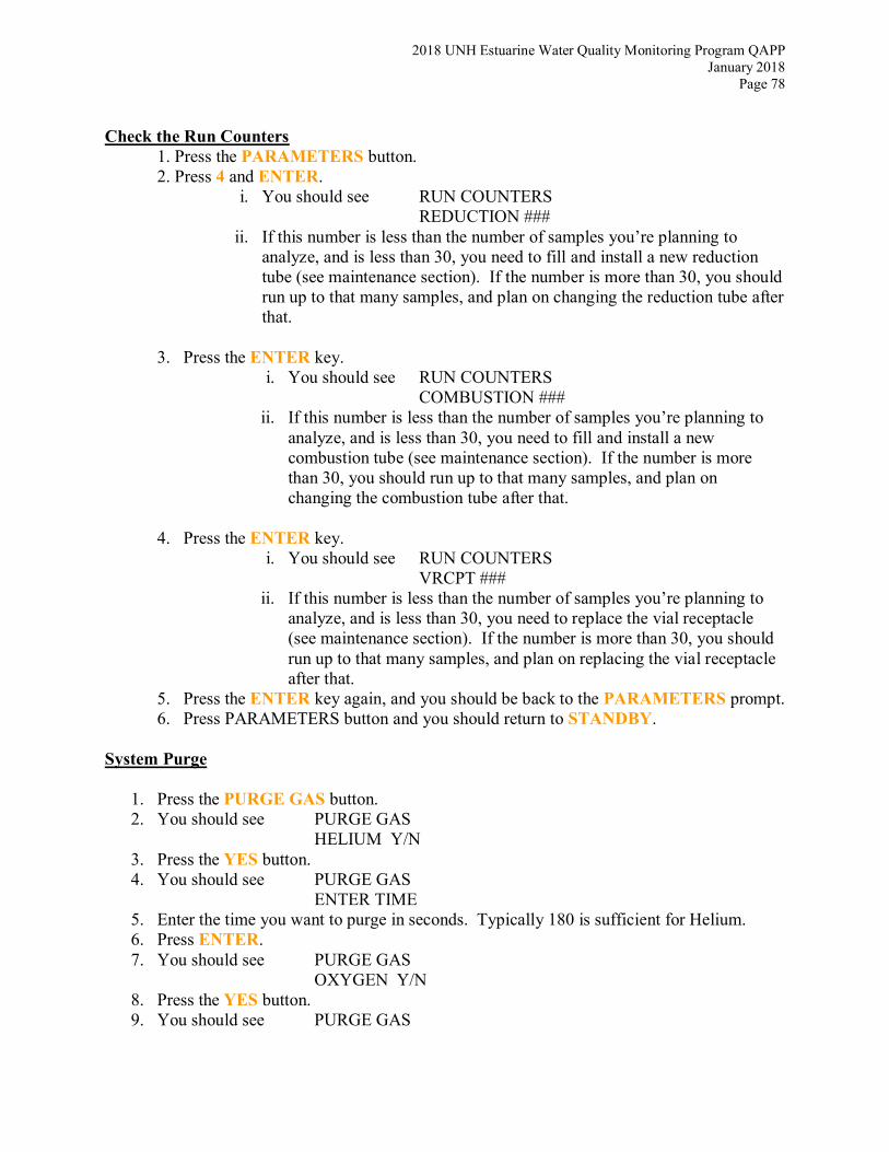
2018 UNH Estuarine Water Quality Monitoring Program QAPP January 2018
Page 78
Check the Run Counters 1. Press the PARAMETERS button. 2. Press 4 and ENTER.
i. You should see RUN COUNTERS REDUCTION ###
ii. If this number is less than the number of samples you’re planning to analyze, and is less than 30, you need to fill and install a new reduction tube (see maintenance section). If the number is more than 30, you should run up to that many samples, and plan on changing the reduction tube after that.
3. Press the ENTER key.
i. You should see RUN COUNTERS COMBUSTION ###
ii. If this number is less than the number of samples you’re planning to analyze, and is less than 30, you need to fill and install a new combustion tube (see maintenance section). If the number is more than 30, you should run up to that many samples, and plan on changing the combustion tube after that.
4. Press the ENTER key.
i. You should see RUN COUNTERS VRCPT ###
ii. If this number is less than the number of samples you’re planning to analyze, and is less than 30, you need to replace the vial receptacle (see maintenance section). If the number is more than 30, you should run up to that many samples, and plan on replacing the vial receptacle after that.
5. Press the ENTER key again, and you should be back to the PARAMETERS prompt. 6. Press PARAMETERS button and you should return to STANDBY.
System Purge
1. Press the PURGE GAS button. 2. You should see PURGE GAS
HELIUM Y/N 3. Press the YES button. 4. You should see PURGE GAS
ENTER TIME 5. Enter the time you want to purge in seconds. Typically 180 is sufficient for Helium. 6. Press ENTER. 7. You should see PURGE GAS
OXYGEN Y/N 8. Press the YES button. 9. You should see PURGE GAS

2018 UNH Estuarine Water Quality Monitoring Program QAPP January 2018
Page 79
ENTER TIME 10. Enter the time you want to purge in seconds. Typically 120 is sufficient for Oxygen 11. After the gasses have finished purging, you should be back in STANDBY.
Tray Set Up
Your first sample on you tray should be a series of Blanks, Conditioners, and K-factors, in the following order;
1. Blank 2. Blank 3. Blank 4. Conditioner 5. Blank 6. Conditioner 7. Blank 8. K-Factor 9. K-Factor 10. K-Factor
Blanks are sample tins with nothing in them. Conditioners have some type of sample in
them, usually standard material. K-Factors have a precisely measured amount of standard material in them. The standard is usually Acetanalide, although there are other standard materials in the dessicator in room 228.
These initial samples only need to be run at the beginning of a tray, and will allow you to assess how the machine is running. For the blanks and the K-factors, consistency is as important as the actual value. Blanks will likely start off higher and decrease slightly. They should be consistent by the last blank. If not, run additional blanks. K-factors should also be consistent. Typical values are:
Blank C = 20 H = 120 N = 30 K-Factor C = 12.700 H = 32.5 N = 4.485
Your samples follow these initial samples. Please run a Blank, K-factor, and replicate of one of your samples and a standard reference sample every 12-15 samples. There are several reference samples near the instrument in the dessicator (2 mineral soils, ground Ivy, or you can also run some standard material and call it a sample). Setting up a New Run Sequence
1. Press the AUTORUN key 2. You should see
AUTO RUN NO. XX

2018 UNH Estuarine Water Quality Monitoring Program QAPP January 2018
Page 80
1B 2K 3S 4RP 3. If the number is not 1, press 4 to reset the starting number. 4. You should see
1 RESET 2 PRINT INFO 3 PRINT RESULTS
5. Press 1. 6. You should see
RESET ALL? Y/N 7. Press YES. 8. You should then see
AUTO RUN NO. 1 1B 2K 3S 4RP
9. Enter the appropriate number that describes the sample for the specified position on the sample tray; 1 for Blank, 2 for K-factor, 3 for Sample, or 4 to reset or print.
10. If you enter 1 (blank), you will immediately go to the next sample. 11. If you enter 2 (K-factor), you will see
THEORY STANDARDS S1 S2 S3 S4
i. Enter 1 (S1 = Acetanalide), and then the weight of the standard, and press ENTER
12. If you enter 3 (Sample), you will see ID _
13. You must put some number or letter combination here. It does not need to be unique, or
relevant to your sample, but the machine requires a value. 14. The instrument will automatically prompt you for information about the next sample. 15. When you are done entering information for all your samples, press AUTORUN, which
will put you back at STANDBY. 16. With the sample carousel removed from the instrument, turn it so position 60 is over the
hole in the bottom of the carousel. 17. Fill your tray with your blanks, standards and samples up to position 59 (leave 60 empty
for now). 18. Put the sample carousel on the instrument so that position 60 is lined up with the arrow
on the front of the machine, and tighten the knurled nut. 19. Turn the carousel on click clockwise (to the left) so that position 1 is lined up with the
arrow. 20. Put sample 60 in position 60. 21. Press the START button.
Adding to a Run Sequence See manual, page 5-117, and is also attached to the protocol in the lab Protocol binder. Modifying Run Parameters See manual, page 5-119, and is also attached to the protocol in the lab Protocol binder.

2018 UNH Estuarine Water Quality Monitoring Program QAPP January 2018
Page 81
Data Retrieval and Processing Data from each of your runs is printed out at the completion of each sample. You will need to manually enter this information into an Excel spreadsheet. Your spreadsheet should have at least the following columns and the appropriate information for each sample in your run. Occasionally, the raw signals are useful to correct for a bad blank, or other problem with the run. Don’t throw your print out away until you’re sure your run is perfect, or you’ve entered all of the data (including the raw signal values), as there is no other way to retrieve your data once the paper copy is gone. Tray position
Sample Weight (mg) C (mass, blank count, or K-factor)
H (mass, blank count, or K-factor)
N (mass, blank count, or K-factor)
Once you have the mass for C, H, and N, you can easily calculate %C, %N, C:N, mg C or N/L for sediment samples etc. for your sample. You must also calculate the % recovery of the reference material analyzed in the analysis. The data file should be saved into the lab manager’s directory on the main lab computer. This information, along with the data, will be entered into the WQAL database by the lab manager to create control charts.

2018 UNH Estuarine Water Quality Monitoring Program QAPP January 2018
Page 82
Appendix F
Quality Assurance Plan: Microbiology Laboratory at the UNH-Jackson Estuarine Laboratory
September 2002
Latest Revision January 24, 2018
As part of the UNH Estuarine Water Quality Monitoring Program QAPP
Dr. Stephen H. Jones Jackson Estuarine Laboratory University of New Hampshire
85 Adams Point Rd. Durham, NH 03824
November 26, 2002 version reviewed and approved by Arthur Clark, EPA, on 12/2/2002.

2018 UNH Estuarine Water Quality Monitoring Program QAPP January 2018
Page 83
Microbiology Laboratory Quality Assurance Plan Jackson Estuarine Laboratory
The Jackson Estuarine Laboratory’s Microbiology Laboratory is a research laboratory that supports a variety of different projects on an ongoing basis. The lab also does some analysis for contracts, but this is not the major activity of the lab. As part of these projects, the lab routinely analyzes environmental samples for a variety of different fecal indicator bacteria, including total and fecal coliforms, enterococci and Escherichia coli. The procedures for these analyses are described in an SOP recently updated in September, 2002 (see below: Jones and Bryant, 2002). Various types of environmental samples are processed for analysis, including sediments; soils, feces, wastewater and water, but the vast majority of samples processed are surface water. Other bacteria have also been of interest for some past projects, including various pathogenic vibrio species, Clostridium perfringens, and a variety of environmentally relevant pure and mixed cultures. 1. Laboratory organization and responsibility
Table 1. Personnel Responsibilities and Qualifications Relative to Microbiology Laboratory Name and Title Responsibilities Immediate Supervisor
Steve Jones, Ph.D. Principal Investigator on all lab projects
Administration and oversight on all projects, personnel training, QA Manager on many projects
NA
Randi Foxall, Laboratory Manager
Collection of water samples for microbial analysis and data compilation
Steve Jones
Audrey Gilbert, Laboratory technician
Collection of water samples for microbial analysis and data compilation
Steve Jones
Dr. Jones is the QA manager for most projects and is responsible for ensuring the production of valid measurements and the routine assessment of measurement systems for precision and accuracy (e.g., internal audits and reviews of the implementation of the QA plan and its requirements). All job descriptions and employee qualifications are on file in Dr. Jones’ office. All personnel are trained by those identified above for different projects to keep personnel updated on regulations and methodology. Dr. Jones keeps records on all the training that personnel receive outside of the laboratory. List of SOPs with the dates of the most recent revisions
Stephen H. Jones & Tamara Bryant. Standard Procedure for Detection of Total Coliforms, Fecal
coliforms, Escherichia coli and Enterococci from Environmental Samples. Revised: September, 2002. (based on: APHA, 1998; US EPA, 1986; 1996).
Copies of the SOP are on file in Dr. Jones’ office and in the main laboratory. All listed SOPs are all reviewed annually and/or revised as changes are made.
3. Field sampling procedures
Microbiological sampling from the field requires sterile containers, either autoclaved plastic bottles with caps or WhirlPak bags. The plastic bottles can be reused, so cleaning involves re-autoclaving for

2018 UNH Estuarine Water Quality Monitoring Program QAPP January 2018
Page 84
disinfection, thorough cleaning with soap and hot water then rinsing in tap water and deionized water. Surface sediment samples are collected using sterile scoops to remove surface sediment samples that are transferred to WhirlPak bags. In general, the time interval between water sample collection and analysis is minimized to optimize the reliability of the analytical results. All samples are temporarily stored on ice in coolers in the field to reduce biological activity and changes in the microflora. Water samples can only be held for a total of 8 hours prior to analysis, or, 6 h maximum for transport to the laboratory and 2 h maximum time between arrival of sample at lab and analysis (APHA, 1998). For some projects where screening of samples is done to see generally what levels of bacteria exist, samples may be held for somewhat longer time intervals. All samples are stored in a refrigerator for at until the next day following the initial analysis to allow for re-analysis if the initial analysis was not acceptable for any reason. Data from reanalyzed sample results are flagged and only used for informational purposes. The only time custody forms are required is for projects other than internal projects, where another collaborative entity may require such forms. All sample containers are checked just prior to analysis to ensure proper labeling, proper containment and that no cross contamination has occurred. 4. Laboratory sample handling procedures Bound laboratory notebooks are used for entering sample information into the laboratory records. Information is filled out in ink, dated and the person entering the information includes their name on the page(s). These notebooks are stored in the analytical laboratory and records throughout the holding time of the samples are maintained in them. After each batch of samples has been analyzed, the results are recorded into spreadsheet databases on a computer in a room adjacent to the analytical laboratory. All unprocessed and processed samples are stored in designated areas within a walk-in cooler located adjacent to the analytical area of the laboratory. The temperature of the walk-in cooler is thermostatically controlled to be 4°C but actually ranges between 3-8°C; a chart recorder maintains a record of actual temperatures. UNH facilities personnel periodically check the cooler and maintain it. Unprocessed and processed samples are stored separately in the cooler, with unprocessed samples remaining in field coolers on the floor and processed samples stored on shelves. All sampling occurs according to predetermined schedules to ensure that holding times will not be exceeded and that incubations and final analyses will occur according to SOP requirements. Chain-of-Custody procedures are not normally imposed because samples likely to be the basis for an enforcement action are not analyzed in this laboratory. However, occasional samples are received for analysis from other entities that may require Chain of Custody procedures for their own purposes. Samples collected by other entities and delivered to the JEL Microbiology lab may be rejected if it is determined that they do not meet shipping, holding time and/or preservation requirements. This is determined by review of the datasheet provided to them by our laboratory to see when samples were collected and how they were shipped. Sample originators are immediately notified either by telling the delivery person or emailing/telephoning and providing them with the reasons for the rejection. 5. Calibration procedures for chemistry
There are no chemical analyses performed by the Microbiology Laboratory. 6. Data reduction, validation, reporting and verification Data in laboratory notebooks are reviewed to ensure completeness of data entry and accuracy of labeling as soon as final analytical results are made. Within a few days, the raw data in the laboratory

2018 UNH Estuarine Water Quality Monitoring Program QAPP January 2018
Page 85
notebook are initially subject to calculation of average values from laboratory duplicate and any field duplicate analytical results. Two technicians working together conduct this calculation process. The sample average is recorded directly into the laboratory notebook. Sample averages are entered into spreadsheet databases for each project by two technicians: one reads the values from the lab notebook and relates the values to the other who enters the data into the computer. The project database(s) is organized by bacterial indicator, date and sample site, along with any other pertinent sampling date and site-specific data, measured or observed.
Dr. Jones is responsible for evaluating all data. This process includes assessment of database completeness, transcription errors and compliance with procedures. When possible, the data are also evaluated for consistency with previous correlated databases to determine if data are within expected ranges for sites and time of year. Omissions of data in spreadsheets will trigger a search of raw datasheets for missing data or possibly reanalysis of the questionable sample, if possible. If reanalysis is not possible or if data remain missing, invalid or otherwise affected entries will not be incorporated into the useable data set. When results appear to be abnormal, all appropriate project participants will review the available data and discuss the problem in periodic meetings to attempt to identify potential problems in sampling or analyses.
The reporting of analytical results is project dependent. For internal research projects, the data are fully analyzed by the PI and appropriate project technicians or graduate students, and eventually published in reports provided to the funding agency. For contract analysis results, the data are provided to funding agencies in Excel spreadsheets in formats pre-determined by the agency or project participants.
Each quantification procedure for the different bacterial indicators has specific verification procedures that are followed, and the procedures used at JEL are exactly as described in APHA (1998) . Counts are then adjusted based on the percent verification of these results.
Membrane filtration: In general, membrane filtration method verification procedures all require monthly verification of the identity of 10 colonies from one positive sample, as well as representative colonies of non-positive reactions or morphologies. All positive and negative total coliform, fecal coliform and E. coli colonies are verified by inoculation of LT and EC-MUG broths to check for lactose fermentation at 35°C, lactose fermentation at 44.5°C and b-glucuronidase activity. For enterococci verification, the colonies are streaked to BHI agar, growth is transferred to BHI broth. The24 h suspension is tested for catalase activity using H2O2 and checked microscopically for cocci and gram stain. Catalse negative, gram positive cocci cultures are then transferred to bile esculin agar (35°C), BHI broth (44.5°C) and BHI broth + 6.5% NaCl (35°C) to verify cultures as fecal streptococci and enterococci.
Multiple tube fermentation: In general, all MTF procedures are verified by using 10% of positive samples. TC, FC and Ec tests are verified using brilliant green and EC-MUG broths as described in SM 9221 B.3. C. perfringens tests are verified by streaking positive tubes to mCP agar and confirming C. perfringens by observing characteristic colonies after 24 h of anaerobic incubation at 44.5°C.
7. Quality control a. Within Sample Batches
Positive and negative samples are to be run with each sample set. These include positive samples of enterococci, total coliforms, fecal coliform and E. coli, either Enterococcus faecalis or E. coli.

2018 UNH Estuarine Water Quality Monitoring Program QAPP January 2018
Page 86
Negative sample cultures for the fecal indicator bacteria or other target bacteria (vibrio species, Clostridium perfringens, etc.) are selected from a variety of different non-fecal and non-target bacterial species that are maintained in the laboratory. In each sample set, duplicate analyses of a positive sample are run by the analyst. Colony counts are expected to agree within 5%. Monthly positive samples are also run in duplicate by the different analysts, and colony counts between analysts are expected to agree within 10%. b. Precision
Precision for bacterial indicator measurements is typically determined according to Standard Methods 9020 B-8. (APHA, 1998). The range (R) for duplicate samples is calculated and compared to predetermined precision criteria. The precision criterion is calculated from the range of log-transformed results for 15 duplicate according to the following formula:
3.27 × (mean of log ranges for 15 duplicates) = precision criterion
The precision criterion is updated periodically using the first 15 duplicate samples analyzed in a month by the same analyst. If the range of ensuing pairs of duplicate samples is greater than the precision criterion, then the increase in imprecision will be evaluated to determine if it is acceptable. If not, analytical results obtained since the previous precision check will be evaluated and potentially discarded. The cause of the imprecision will be identified and resolved.
c. Media Preparation and Equipment
Various types of sterility controls are included in the different procedures used to detect and enumerate microorganisms. Sterile water is filtered through membrane filters in filter towers prior to use of the filter tower for sample filtration for the first and last samples of a sample batch. The membrane filter is then incubated on the target test media to see if any bacteria are present. Uninoculated dilution tubes and agar media are incubated along with inoculated media to check for contamination for each batch of samples. If the results of the positive or negative controls indicate either contamination or culture problems, all sample results will be discarded and samples will be reanalyzed, if holding time requirements are not exceeded. Other QC procedures for lab supplies generally follow SM 9020 B.4 for pH and inhibitory substances on glassware, laboratory reagent water quality, quality of media and reagents and membrane filter integrity. Procedures for preparing, sterilizing, handling and storing media and other equipment are as described in SM 9020 B.4i.1-5. 8. Schedule of internal audits
Dr. Jones conducts periodic (minimum frequency: annually for projects >1 year in duration) internal audits of all aspects of project QA/QC and personnel performance. The timing of performance audits is project specific, and typically occurs in the very beginning of a project, within one month of project analysis initiation, and later in the project after the technicians have established procedural prowess. Any problems are noted, corrective actions are recommended and follow-up audits are conducted to verify compliance with correct procedures. Written records in the form of checklists with details of problems and follow-up audit results are kept in Dr. Jones’ office. 9. Preventive maintenance procedures and schedules The technicians responsible for project or laboratory QC conduct all maintenance and inspection of equipment based on manufacture requirements and specifications. Every day a piece of equipment is

2018 UNH Estuarine Water Quality Monitoring Program QAPP January 2018
Page 87
used it receives a general inspection for obvious problems. The most common assessment requiring corrective action is maintenance of correct temperatures for incubators. Results of inspections are recorded on datasheets that include date, time, and inspector initials, and completed sheets are on file in Dr. Jones’ office. Much of the other equipment used in the Microbiology Lab is not under the direct control of Dr. Jones and is maintained by regular UNH inspections (Autoclave, walk-in coolers, scales, etc.). Lab technicians always check chart recorders and digital read outs on the autoclave and the coolers with each use to confirm correct settings and conditions. Any problems are reported to the JEL Lab Manager who contact UNH Maintenance for any necessary repairs beyond his expertise. Scales are checked annually by UNH-hired experts and the date, time, results and inspector’s initials are recorded on the scale. In addition, microbiological data are inspected within a few days of sample analysis to allow instrument (or user) malfunctions to be caught quickly and corrected as needed. 10. Corrective action contingencies and record keeping procedures Unacceptable lab QC checks triggers immediate review of analytical procedures, sample processing and equipment with the technicians involved. Data results from the time period between the previous acceptable lab QC checks are reviewed to determine if there is evidence for accepting the data, otherwise, it is considered invalid. All project-specific personnel are responsible for participating in corrective actions like re-training or learning modified QC procedures to ensure future acceptability. A database of corrective actions is maintained on a computer in the PI’s office. The office is either occupied by the PI or is locked and no one else is admitted in. REFERENCES American Public Health Association. (APHA). 1998. Standard Methods for the Examination of Water and Wastewater. 20th Edition. American Public Health Association, Washington, DC. U.S. Environmental Protection Agency (USEPA). 1996. ICR Microbial Laboratory Manual. Sections X (E. coli) and XI (C. perfringens). EPA 600/R-95/178. Environmental Protection Agency, Office of Research and Development, Washington, DC. U.S. Environmental Protection Agency (USEPA). 1986. Test methods for Escherichia coli and enterococci by the membrane filtration procedure. EPA 600/4-85/076. Environmental Protection Agency, Environmental Monitoring and Support Laboratory, Cincinnati, OH.

2018 UNH Estuarine Water Quality Monitoring Program QAPP January 2018
Page 88
Appendix G
Standard Procedure for Detection of Total Coliforms, Fecal Coliforms, Escherichia coli and Enterococci from Environmental Samples
September, 2002
Latest Revision
January 24, 2018
As part of the UNH Estuarine Water Quality Monitoring Program QAPP.
Prepared by:
Stephen H. Jones & Tamara Bryant Jackson Estuarine Laboratory University of New Hampshire
Durham, NH 03824

2018 UNH Estuarine Water Quality Monitoring Program QAPP January 2018
Page 89
INTRODUCTION Various bacterial species and groups of bacteria have been used as indicators of fecal contamination in surface water, groundwater and food. In New Hampshire, state laws dictate the use of 4 different bacterial indicators for use for classifying different types of water. Total coliforms are used for groundwater and some waste water treatment facility (WWTF) permitted discharges, fecal coliforms are used by the NH Shellfish Program for classifying shellfish harvesting areas, enterococci are used for classifying recreational marine and estuarine waters and Escherichia coli is used for freshwater recreational waters. The microbiology lab at the Jackson Estuarine Laboratory has conducted projects and has otherwise worked closely with various state agencies concerned with surface water quality in the Seacoast region of NH. Protocols have been used and modified over the past 15 years for the detection and enumeration of different bacterial indicators of fecal contamination. The most recent protocols are presented in the following sections. This Standard Operating Procedure also includes descriptions of sampling and media preparation. The basic approach is to collect water samples in sterile containers from the field and transport them on ice to the lab as soon as possible. The water samples are filtered through membrane filters and the organisms caught on the filters are grown to colonies on indicator specific media and conditions. The colonies showing the indicator-specific reaction on the agar media are enumerated following appropriate incubation times. I. Space Requirements 1.1 Specimen Collection. Not applicable. 1.2 Specimen Intake, Processing and Detection. This area should include 2 meters of counter space with shelves for storage, and equipped with a water source and a refrigerator. A small area must be designated “clean” for paper work for the prevention of contamination to yourself and others. 1.3 Biochemical Preparation. This area should include approximately 3.5 meters of counter space with shelves, a readily available de-ionized water supply, an autoclave, storage for biohazard waste, and a large sink. II. Equipment Requirements 2.1 Specimen Collection.
2018 UNH Estuarine Water Quality Monitoring Program QAPP January 2018
Page 90
Laboratory van and/or boat for access to sites, devices for reaching and sampling from surface water. 2.2 Specimen Intake, Processing and Detection. Autoclave, balance, vacuum pump, filter towers, vortex, Stomacher, computer system for database management, printer, 44.5•C incubator, 35•C incubator, 41•C incubator, thermometers, 4•C refrigerator, ice chest, alcohol burners, loops, scissors, forceps, pipette pump. 2.3 Biochemical Preparation. Autoclave, test tube washer, hot plate stirrers, alcohol burners, 4•C refrigerator, -22•C freezer, Parafilm®, balance, vacuum pump, filter towers, filter membranes, vortex, pH meter. III. Chemicals and Supply Requirements 3.1 Specimen Collection. 1000 ml sterile Whirlpac® bags, or autoclavable plastic bottles, waterproof gloves, sterile gloves, permanent marker, cooler and ice, datasheets. 3.2 Specimen Intake, Processing and Detection. Filter membranes, cellulose pads, Buffered peptone water, de-ionized water (DI) DEPC treated DI, goggles, sterile gloves, pipettes of various volumes, graduated cylinders, sterile cellulose pads, Petri dishes containing agar media, 3.3 Biochemical Preparation. Autoclavable flasks (25 ml- 4000 ml), beakers (10 ml- 500 ml), test tube racks, 50 ml test tube with caps, 13 ml test tubes with caps, stir bars, 15 mm Petri dishes, 3 mm Petri dishes, weigh boats, 0-10 µl pipette,10-100 µl pipette, 100-1000 µl pipette, 1 ml-10 ml pipette, pipette tips for each size pipette, autoclave tape, aluminum foil, indole, mTEC, Mac Conkey, Oxidase, Tryptic Soy agar, Tryptic Soy Broth, Simmon’s Citrate, Urea Agar, Urease, Methyl Red, Voges-Proskaur, DEPC treated de-ionized water. IV. Biochemical Media, Solutions, Preparation and Storage 4.1 Media All media is to be prepared in a sterile fashion under a hood, lightly covered with tin foil or foam stoppers, wearing gloves, lab coat, autoclave mitts, goggles and tie backs for those with long

2018 UNH Estuarine Water Quality Monitoring Program QAPP January 2018
Page 91
hair. Store the media agar side up to prevent condensation and at 4•C in plastic sleeves (Atlas and Parks, 1993). 4.1.1 Mac Conkey Agar (Mac) 50 g of Mac Conkey 1000 ml DEPC DI Mix and boil to dissolve Autoclave Dispense to small plates flaming the lip of the flask between plates. 4.1.2 mTec Agar 45.3 g mTec agar 1000 ml DI Mix and boil to dissolve Autoclave Dispense to small plates flaming the lip of flask between plates. 4.1.3 Simmon’s Citrate (SimCit) 24.2 g of Simmons Citrate 1000 ml DEPC DI Mix and boil to dissolve Autoclave Dispense to small plates flaming the lip of the flask between plates. 4.1.4 Tryptic Soy Agar (TSA) 40 g Granulated TSA Agar 1000 ml DI Mix and boil to dissolve Autoclave Pour to large plates flaming the lip of the flask between plates. 4.1.5 Urea Agar 29 g Urea Agar Base (in 5ºC) 100 ml DEPC DI Filter sterilize/DO NOT HEAT In separate flask suspend: 15 g Granulated Agar 900 ml DI Autoclave/Cool to 55ºC Add Filtered Urea Agar Base Mix well and pour into small plates flaming the lip of the flask between plates. 4.2 Solutions

2018 UNH Estuarine Water Quality Monitoring Program QAPP January 2018
Page 92
All solutions are to be prepared in a sterile fashion under the a hood, wearing gloves, lab coat, goggles, autoclave mitts and tie backs for those with long hair (Atlas and Parks, 1993). 4.2.1 Buffered Peptone Water (BPW) 2.8 g Na2HPO4 (Sodium Phosphate Dibasic) 1.2 g KH2PO4 (Potassium phosphate Monobasic) 4.0 g NaCl 8.0 g Bacto peptone 800 ml DEPC DI Adjust pH to 7.2 with HCl Dispense 9.6 ml into large tubes and cap Autoclave Store at 4•C 4.2.2 Brain Heart Infusion Broth
37 g Dehydrated Brain Heart Infusion Powder 1000 ml DI Adjust pH to 7.4±.02 Dispense 10 ml into 20 ml tubes Cap and Autoclave Remove and cool to room temperature then store at 4ºC 4.2.3 EC MUG 29.68 g Dehydrated EC medium with MUG 800 ml DI Adjust pH to 6.9± .2 Carefully dispense 10 ml in to 20 ml tubes containing inverted Durham tubes Remove and cool to room temperature then store at 4ºC 4.2.4 Indole Reagent 75 ml Iso-Amyl Alcohol 25 ml conc. HCl pH to <6.0 then add: 5 g p-dimethylaminobenzadehyde Store at 4ºC 4.2.5 LT Broth 28.48 g Dehydrated lauryl tryptose broth 800 ml DI Warm to dissolve Adjust pH to 6.8 ± .0 Dispense 10 ml into 20 ml tubes containing inverted Durham tubes Autoclave

2018 UNH Estuarine Water Quality Monitoring Program QAPP January 2018
Page 93
Store at 4ºC 4.2.6 MRVP Broth (Methyl-Red, Voges-Proskauer) 5.0 g Glucose 5.0 g K2HPO4 3.5 g Pancreatic digest of casein 3.5 g Peptic digest of animal tissue Add all components to 900 ml of DI. Mix to dissolve Bring to 1000 ml pH to 6.9 at 25ºC Distribute 10 mls into 50 ml tubes and cap Autoclave Store at 4ºC 4.2.7 MRVP Indicator Solution 0.1 g Methyl red 300 ml 95 % Ethyl alcohol Bring to 500 ml with DI Filter sterilize Store at 4ºC 4.2.8 Oxidase Reagent 1% 1 g Tetramethyl-p-phenylenediamine dihydrochloride 100 ml DI Filter sterilize Store in dark area at 4ºC 4.2.9 Tryptic Broth for Indole 80 g Tryptic Soy Broth 1000 ml DI Warm to dissolve Dispense 5 mls to small tubes and cap Autoclave Store at 4ºC 4.2.10 Urea substrate (for use with mTEC) 4 g Urea pellets 200 ml DI 0.02 g Phenol Red Indicator Mix to dissolve Adjust pH to 5.0 with dilute HCl (10%) Filter sterilize DO NOT AUTOCLAVE Store at 4ºC

2018 UNH Estuarine Water Quality Monitoring Program QAPP January 2018
Page 94
4.2.11 Voges-Proskauer Indicators Difco VP-A # 261192 Difco VP-B # 261193 Use per manufacturers instructions 4.2.12 Cryoprotectant Solution 1: 8.5 g NaCl 0.65 g potassium phosphate dibasic 0.35 g potassium phosphate monobasic 1000 ml DI Autoclave and cool to room temperature Solution 2: 50 ml autoclaved glycerol, cooled to room temperature 50 ml DMSO Aseptically mix 800 ml of Solution 1 to all of Solution 2 Store at 4ºC *Hints* When boiling any agar media it is wise to keep an eye on the foam that forms on the surface of the media. As the temperature increases in the flask the foam rises (Atlas and Parks, 1993). When the foam is one inch thick quickly remove the flask from the stir plate. This will prevent the media from boiling over. Put the media in the autoclave as soon as possible to prevent premature setting. V. Specimen Collection 5.1 Water Samples With a gloved hand, submerge 100 ml Whirlpac® bag 10-30 cm below the water surface in a direction facing the current and open. For plastic bottles, submerge the bottle with gloved hand in a direction facing the current and remove cap. In a boat, sample from the upstream side. Care must be taken to avoid disturbance of the surrounding waters prior to or during the sample retrieval. Fill the bag or bottle to capacity and twist the bag closed or re-cap the bottle before surfacing. The data sheet should be made of Write-In-the Rain® paper, filled out completely with a Write-In-the Rain® marker and those spaces not applicable crossed off. Record the time, date, conditions, and collector’s initials. Put sample on ice and transport. 5.2 Finding and Identifying Scat There are general approaches to locating scat, and the details of the method used are presented in the NHDES SOP for identification and collection of scat samples (Appendix 2). Knowing the type of habitat that a certain animal resides is critical. A large broad sweep of a field and the

2018 UNH Estuarine Water Quality Monitoring Program QAPP January 2018
Page 95
surrounding transitional zone is an excellent place to start. Riparian zones often provide a wide variety of scat. Try to identify paths to water and food sources. Temporal bodies of water offer seasonal scat collection. One must also remember that some animals mark territory by defecating or urinating on conspecific scat. A witnessed event is the best identification, but in the wild very rare. Identification of scat can be assisted with the aid of guide books. 5.3 Fecal Samples Fecal samples should be collected fresh, this reduces the chance of contamination, resource competition, and transformation. Samples that are very dry, found after a rain event, or that show signs of deterioration should not be collected. Invert Whirlpac® bag over gloved hand and pick up quantity of fresh fecal specimen. Make sure the sample is as debris free as possible. Revert bag over hand and feces, twist shut. The data sheet should be made of Write-In-the Rain® paper, filled out completely with a permanent marker and those spaces not applicable crossed off. Record date, time, sex (if possible), location, species/breed (using a species code list, appendix 2) and the collectors’ initials. Put sample on ice for transport and processing. 5.4 Preparation for incoming fecal and water samples. Prior to receiving the samples the area should be disinfected. The log book with date and time of sample arrival should be ready for entries. Check the samples against the original collection sheets making sure that all samples have the correct information on their respective containers. Record the samples and their conditions into the log book and have the person delivering the specimens sign the book. VI. Specimen Intake 6.1 Acceptable Samples Samples of water should be in water tight containers preferably in a secondary sealed plastic bag. Containers should be labeled with time and date of sample collection, site number and sample collector’s name. The water samples have to be analyzed within 2 hours of receipt in the lab. If this holding time is exceeded, then any data for analysis of such samples need to be “flagged”, or labeled in a way to reflect this violation of sample integrity. Fecal samples should be fresh in nature with minimal debris attached. If it appears that a sample has been compromised or has compromised others during transport it/they should be discarded. It is important to note that the integrity and homogeneity of the samples should be without question. A customized Laboratory Management System (see 6.2) should be in place to track samples and analytical data. These data may include: Sample number that is unique to that site, date received, sample descriptions, additional comments, notations about special handling, and name of person delivering samples.

2018 UNH Estuarine Water Quality Monitoring Program QAPP January 2018
Page 96
6.2 Specimen Sample Log Sheet A log book of collection sites, dates the site was sampled, the type of specimen collected, and the date and time of receipt of the sample in the lab should be maintained. Two copies for each sample is recommended. A log book of samples received into the lab and the condition of the samples should also be maintained. A spreadsheet database should be utilized for tracking the specimen and its isolates through the laboratory procedures. Occasionally, sample analysis requires use of chain of custody sheets for some clients. The procedure is to sign the sheets as required and to take a copy for our laboratory records. 6.2.1 Sample Log Sheet
COLLECTION DATA LOG SHEET Site Name: Type of Sample Site Description: Fecal Water Animal Species: Location: Water Temp: % DO Saturation: DO: pH: Conductivity: Location: In stream Seep Swale Storm Drain Other: Street: Town: Watershed: Date: Time: Sampled by: Parameters Weather: Air Temp:

2018 UNH Estuarine Water Quality Monitoring Program QAPP January 2018
Page 97
Flow Rate: Comments and Sketch/Description Delivered to lab by: Date: Time: Received by: VII. Detection and Biochemical Confirmation Methods 7.1 Water Samples Use flame sterilize forceps dipped into alcohol to aseptically place a sterile gridded 0.45 µm membrane filter on the filter base of a sterile 250 ml filter and attach magnetic filter tower. Vigorously shake the sample bottle or bag at least 30 x and measure out volume to be filtered either in a sterile graduated cylinder or by using a sterile pipette. If the sample is turbid or is suspected of having a high colony count, dilutions of a water sample may be necessary. Add one ml sample to 9 ml sterile BPW and decimally dilute from 10-1 to 10-7. Pour up to 100 ml of a sample into the filter tower and conduct routine filtration at 25 millibar until all water has passed through the filter. Turn the vacuum pump off and aseptically remove the filter using sterile forceps. Positive and negative samples are to be run with each sample set. These include positive samples of enterococci, total coliforms, fecal coliform and E. coli, and negative samples for total and fecal coliforms and enterococci. If the results of the positive or negative controls indicate either contamination or culture problems, all sample results will be discarded and samples will be reanalyzed, if holding time requirements are not exceeded. Field duplicates are routinely collected as part of projects. Colony counts of positive field samples, as well as laboratory duplicate analyses, are expected to agree within 5%. Each quantification procedure for the different bacterial indicators has specific verification procedures that are followed, and the procedures used at JEL are exactly as described in Standard Methods (APHA 1998). Counts are then adjusted based on the percent verification of these results. Membrane filtration methods require monthly verification of the identity of 10 colonies from one positive sample, as well as representative colonies of non-positive colonies. All positive and negative total coliforms, fecal coliforms and E. coli colonies are verified by inoculation of LT and EC-MUG broths to check for lactose fermentation at 35°C, lactose fermentation at 45°C and ß-glucuronidase activity. For enterococci verification, the colonies are streaked to BHI agar, growth is transferred to BHI broth. The 24 h suspension is tested for catalase activity using H2O2 and checked microscopically for cocci and gram stain. Catalase

2018 UNH Estuarine Water Quality Monitoring Program QAPP January 2018
Page 98
negative, gram positive cocci cultures are then transferred to bile esculin agar (35°C), BHI broth (44.5°C) and BHI broth + 6.5%NaCl (35°C) to verify cultures as fecal streptococci and enterococci. 7.1.1 Detection of Total Coliforms Place the filter onto an M-Endo medium plate, grid side up, by rolling the paper onto the agar surface to minimize air bubbles under the filter. Incubate all plates inverted in incubators at 35±0.5 °C for 22-24 hours (APHA, 1998). Count the colonies that are pink to dark-red and have a metallic surface sheen for each sample/site at best (or all) dilutions (10-30 readable colonies) and record as total coliforms. Pick an isolated colony from a plate from each sample batch and inoculate Mac Conkey agar, Trypticase Broth for indole, Urea agar, MRVP Broth and Simmons Citrate agar, incubate at 35±0.5 º C overnight. Conduct Oxidase test (looking for no color change) on isolates that are Citrate negative (no growth, no color change), Urea negative (no color change), and Indole positive (pink to violet color), MRVP (red color change), Mac Conkey positive (pink colonies). These are confirmed E. coli colonies, the target species for total coliform analyses. 7.1.2 Detection of Fecal Coliforms and E. coli Place the filter onto an mTEC medium plate, grid side up, by rolling the paper onto the agar surface to minimize air bubbles under the filter. Incubate all plates inverted in incubators at 35±0.5 °C for 2 h and at 44.5±0.2 °C for 22 hours (USEPA, 1986). Count the yellow colonies for each sample/site at best (or all) dilutions (10-30 readable colonies) and record as fecal coliforms (Rippey et al., 1986). Remove top of Petri dish and invert onto counter. Place cellulose pad in lid and pipette 2.0 ml of Urea substrate solution onto pad. Roll filter onto pad to discourage air bubbles, cover and incubate for 10-20 minutes at room temperature. Count the yellow/yellow brown colonies using a magnifying lens and record as E. coli. Pick an isolated colony from a plate from each sample batch and inoculate Mac Conkey agar, Trypticase Broth for indole, Urea agar, MRVP Broth and Simmons Citrate agar, incubate at 35±0.5 º C overnight. Conduct Oxidase test (looking for no color change) on isolates that are Citrate negative (no growth, no color change), Urea negative (no color change), and Indole positive (pink to violet color), MRVP (red color change), Mac Conkey positive (pink colonies). These are confirmed E. coli colonies. For ribotyping projects, pick up to ten isolated, removable, presumptive E. coli colonies (yellow colonies after Urease test) per plate and four quadrant streak to Tryptic Soy Agar. Incubate at 35±0.5 °C for 24 hours. Repeat the biochemical tests for confirmation of E. coli colonies. Those that meet the above criteria can be re-streaked to TSA and incubated at room temperature overnight. Keep presumptive E. coli isolates frozen in a Saline Phosphate Buffer and Cryoprotectant media at -80°C.

2018 UNH Estuarine Water Quality Monitoring Program QAPP January 2018
Page 99
7.1.3 Detection of Enterococci Place the filter onto an mEi medium plate, grid side up, by rolling the paper onto the agar surface to minimize air bubbles under the filter. Incubate all plates inverted in an incubator at 41±0.5 °C for 24 h (USEPA, 2006). Count blue colonies using a magnifying lens and record as enterococci. Pick an isolated colony from a plate from each sample batch and inoculate Brain Heart Infusion (BHI) agar, incubate at 35±0.5 º C overnight. Conduct a catalase and a gram stain test on an isolated colony. For catalase negative/gram positive cultures, transfer a colony to BHI broth and incubate for 24 h at 35±0.5 °C. Inoculate BHI broth (incubate at 45±0.5 °C for 48 h), BHI broth with 6.5% NaCl (incubate at 35±0.5 °C for 48 h) and streak a plate of bile esculin agar incubate at 35±0.5 °C for 48 h). Growth on both media indicates that the colony belonged to the enterococcus group of the fecal streptococci. 7.2 Detection of E. coli in Fecal Samples For fecal samples, add 1 g of feces to 9 ml of BPW in a sterile Whirlpac® and place in stomacher on medium for 30 sec. Using 2.5 mls of digest, serial dilute in BPW to 10-7. Make sure that each tube is labeled as to the dilution, this reduces error. Filter 10 mls of all dilutions (except first) of every sample and place on mTEC agar that has been labeled with the appropriate dilution. Incubate at 44.5°C for 24 hours. Count and record yellow colonies for each sample/site at best dilutions (10-30 readable colonies). Remove top of Petri dish and invert onto counter. Place cellulose pad in lid and pipette 2.0 ml of Urea substrate solution onto pad. Place filter colony side up onto pad, cover and incubate for 10 minutes at room temperature. Count and record yellow colonies. Pick up to ten isolated, removable, presumptive E. coli colonies (yellow colonies after Urease test) per plate and 4 quadrant streak each onto separate Tryptic Soy Agar plates. Incubate at 35-37°C for 24 hours. Pick one isolated colony from each plate and inoculate Mac Conkey agar, Trypticase Broth for Indole, Urea agar, MRVP Broth and Simmons Citrate agar, incubate at 35-37º C overnight. Conduct Oxidase test (looking for no color change) on isolates that are Citrate negative (no growth, no color change), Urea negative (no color change), and Indole positive (violet color), MRVP positive, Mac Conkey positive (pink colonies). Those that meet the above criteria can be re-streaked to TSA and incubated at room temperature overnight.

2018 UNH Estuarine Water Quality Monitoring Program QAPP January 2018
Page 100
Keep presumptive E. coli isolates frozen in a Saline Phosphate Buffer and Cryoprotectant media at -80°C. 7.3 Storage of all bacteria From TSA plate pick one colony and place in to vial. Add 1.0 ml of buffer/ protectant mixture. Vortex until colony is dispersed completely in buffer. Label cap with specimen number and original collection date. Record the tray and shelf number into the log book then enter it to the database. Place in labeled cryo-rack and put in -80º C freezer. VIII. Notes on Quality Control The JEL Microbiology Laboratory QA Plan provides details of QA procedures required to detection of bacterial indicators. The notes below are additional details specific to these procedures. 8.1 General Laboratory Practices The first concern of any lab is the safety of its personnel. Each person working in the laboratory is trained in lab safety and will be well informed of any hazardous material they might encounter. A chemical roster is stored in the laboratory and Material Safety Data Sheet (MSDS) folders are stored in the JEL Lab Technician’s office and kept up to date. Gloves, goggles, gowns or lab coats are advised. No open toed shoes or shorts are allowed. Personnel that have long hair need to tie it back to prevent injury. All instrumentation, cold units, pipettes, incubators, etc. are routinely calibrated by a qualified instrumentation technician. 8.2 Specimen Collection All collection devises and receptacles must be sterile. Gloves should be rinsed (water) or changed (feces samples) between each sample collected. If a spatula or other collection devise is used it must be sterile. Feces may be double bagged to insure no contact. Water sample lids should be tightened and each bag/ bottle stored and transported upright. Leaking specimens and others in the same transport container may be cross contaminated and should not be accepted. Care should be taken that no specimen comes in direct contact with any other. If at any time a question of contamination arises, discard the sample. 8.3 Specimen Intake and Processing The laboratory bench surfaces and instruments are to be decontaminated and or autoclaved prior to introduction of specimens. A daily log of instrument cleaning, and temperature control should be checked off, initialed and displayed in a prominent place. If a specimen has been spilled use the lab approved spill kit and all precautions to prevent contamination. Change pipette tips, forceps, and filter towers after each specimen serial dilution.

2018 UNH Estuarine Water Quality Monitoring Program QAPP January 2018
Page 101
8.4 Biochemical Preparation and Detection Biochemicals are the foundation of accurate indicator identification. If the methods or materials are compromised the results would be in question. Gloves and goggles need to be worn for safety and the reduction of contamination. Those that have long hair should tie it away from the face. Compounds, chemicals and other disposables that are received at the lab should have the receive date and the date opened recorded on the receptacle. It is recommended that media and solutions be made in autoclaved containers, under the hood and autoclaved unless otherwise stated. All disposables should be aliquoted to the appropriate containers. Storage of the disposables described in the media section should be strictly followed. The date and the initials of the person that made the disposable should be clearly written on the container. A weekly check of the plated media and a day-of-analysis aseptic check of the pH of solutions is required. As always use the oldest acceptable media first. Tubes and other glass and plastic ware (pipette tips, graduated cylinders) should be capped, autoclaved and stored in the autoclave bags. References American Public Health Association. (APHA). 1998. Standard Methods for the Examination of Water and Wastewater. 20th Edition. American Public Health Association, Washington, DC. Atlas, R., L.C. Parks, Eds. 1993. Handbook of Microbiological Media. CRC Press. Boca Raton, FL. Rippey, S.R., W.N. Adams and W.D. Watkins. 1987. Enumeration of fecal coliforms and E. coli in marine and estuarine waters: an alternative to the APHA-MPN approach. J. Wat. Pollut. Cont. Fed. 59: 795-798. U.S. Environmental Protection Agency (USEPA). 2006. Method 1600: Enterococci in Water by Membrane Filtration Using membrane-Enterococcus Indoxyl-B-D-Glucoside Agar (mEI). EPA-821-R-06-009. EPA, Washington, DC.

2018 UNH Estuarine Water Quality Monitoring Program QAPP January 2018
Page 102
Appendix H
LI-1400 DataLogger PAR Measurements Standard Operating Procedures
Overview The LI-1400 DataLogger and calibrated quantum sensors provide the capability to quantify Photosynthetically Active Radiation (PAR) both above and below the water surface. The ‘air’ sensor remains above the water and quantifies downwelling radiance from the sun each time a discrete measurement is taken; this is most often used to normalize readings taken over several minutes to a constant downwelling value. The ‘underwater’ sensor is deployed on a frame that is lowered into the water. This sensor is generally used to measure a profile of in-water irradiance versus depth so as to estimate the diffuse attenuation coefficient (Kd), a measure of the rate at which photosynthetically active radiation is attenuated as it passes down through the water-column. In general, the attenuation of light is exponential versus depth. To obtain Kd from a series of light readings with depth, a series of measurements at at least 8 depths is desired (in shallow waters this may not be possible). One obtains Kd by making a linear regression of sample depth versus ln (PAR) and calculating 1/(slope of the regression). Additional information of interest includes the percent of surface radiation reaching the bottom. Estimates of Kd are considered robust if the r2 of the regression is >0.95 (generally >0.98). The precision of the method is estimated by taking 3 complete profiles sequentially and calculating the standard error (SE) of the measurement. The SE should be less than 10%. Before First Sampling of the Day
1. Insure that the sensors are securely attached to their frames and confirm that the calibrations factors stored in the DataLogger are correct for the sensors in use.
2. Hook up the Underwater BNC connector to Channel I1 labeled “underwater”. 3. Hook up the Air BNC connector to Channel I2 labeled “air”. 4. Turn the DataLogger ‘ON’. 5. Under View, press ‘ENTER’ to view new data. 6. The first view should say “I1I” which corresponds to the underwater connector. “I2I”
corresponds to the air connector. 7. Switch to view I2I, take the cap off of the air sensor, check the reading then cover the
sensor with your hand to confirm the reading changes (the reading should decrease with a decrease in light).

2018 UNH Estuarine Water Quality Monitoring Program QAPP January 2018
Page 103
8. Switch to view I1I, take the protective covering off of the underwater sensor, check the reading and then cover the sensor with your hand to confirm the reading changes (again the reading should decrease).
At Each Station
1. Turn on the DataLogger. 2. Take out the respective data sheet for the site. Record the time when the underwater
sensor is put in the water. 3. Lower the sensor to 10cm. Allow the reading to stabilize (1-2 seconds) and then press
‘ENTER’. This logs the data into the DataLogger. Cross off 10cm (and each subsequent depth for which you log data into the DataLogger) on the data sheet.
4. Lower the sensor to the next depth. In shallow areas, record measurements every 25cm as marked on the cable. In deep and/or clearer water areas the sensor can be lowered every 50cm. At least 6-8 depths should be recorded in the DataLogger for each station.
5. When (If) the sensor reaches bottom, write the bottom depth (approximate using the depth markers) on the datasheet and press ‘ENTER’ to log data into the DataLogger. You do not need to go to the bottom if you have >10 good readings; if the DataLogger is showing light readings less than 0.5 or if the sensor begins to stream out in strong currents.
6. Raise the underwater sensor out of the water and put the protective cover on. Put the cap on the air sensor also. Turn the DataLogger ‘OFF’ until reaching the next station.
At End of Sampling
1. Unplug the BNC connectors from the LI-1400. 2. Rinse underwater sensor, frame and cable with freshwater and let dry before storage.
Download Data to Excel in the Laboratory
1. After returning to the lab the data should be retrieved from the DataLogger. 2. Attach the DataLogger to the computer using the serial cable. 3. Open the LI-1400 program and then turn the DataLogger on. 4. Under the remote menu click on ‘CONNECT’. Under the connect window, type ‘2’ next
to com port number and click ‘CONNECT’. 5. Under the remote menu click ‘RECEIVE DATA’. Save the data on the computer. 6. Open Microsoft Excel and then open the file you just saved. The file is a delimited file
and click ‘FINISH’. 7. Download LiCor Data into a new Excel file and Save As GBSWMP Raw Light Profile
(MMDDYY) where the MMDDYY represents the sampling date. 8. Once you are certain that you have successfully downloaded and saved the data the data
in the DataLogger should be cleared from memory. This can be done 2 ways:

2018 UNH Estuarine Water Quality Monitoring Program QAPP January 2018
Page 104
a. On the DataLogger, press the ‘FCT’ key. Arrow to the right twice till clear memory is in the window. Arrow down to clear all, down to date, down to time, and down to clear memory yes/no. Confirm that “clear memory yes” is in the window and then press ‘ENTER’. (This may not clear the memory).
b. In the LI-1400 program, under the remote menu click ‘CLEAR DATABASE’. In the clear database window confirm that all is chosen then click ‘OK’.
9. Under the remote menu click ‘DISCONNECT’. Unplug the DataLogger from the computer, turn it off, make sure that there is no dirt or salt on it and put it away.

NASA/TM-2003-
Ocean Optics Protocols For Satellite Ocean Color Sensor
Validation, Revision 5, Volume V: Biogeochemical and Bio-Optical Measurements and Data Analysis
Protocols James L. Mueller, Giulietta S. Fargion and Charles R. McClain, Editors J. L. Mueller, R. R. Bidigare, C. Trees, W. M. Balch, J. Dore, D.T. Drapeau, D. Karl, L. Van Heukelem, and J. Perl Authors. National Aeronautical and Space administration Goddard Space Flight Space Center Greenbelt, Maryland 20771 December 2003
Appendix I

NASA/TM-2003- Ocean Optics Protocols For Satellite Ocean Color Sensor Validation, Revision 5, Volume V:
Biogeochemical and Bio-Optical Measurements and Data Analysis Protocols
James L. Mueller, CHORS, San Diego State University, San Diego, California Giulietta S. Fargion, Science Applications International Corporation, Beltsville, Maryland Charles R. McClain, Goddard Space Flight Center, Greenbelt, Maryland C. C. Trees and J. Perl, CHORS, San Diego State University, San Diego, California R. R. Bidigare, D. M. Karl and J. Dore, Dept. of Oceanography, University of Hawaii, Hawaii W. M. Balch and D. T. Drapeau, Bigelow Laboratory for Ocean Sciences, E. Boothbay Harbor, Maine L. Van Heukelem, University of Maryland Center for Environmental Science, Maryland National Aeronautical and Space administration Goddard Space Flight Space Center Greenbelt, Maryland 20771 December 2003

Ocean Optics Protocols For Satellite Ocean Color Sensor Validation, Revision 5,Volume 5
Preface To Revision 5
This document stipulates protocols for measuring bio-optical and radiometric data for the Sensor Intercomparison and Merger for Biological and Interdisciplinary Oceanic Studies (SIMBIOS) Project activities and algorithm development. The document is organized into 6 separate volumes, and in Revision 5, Volume VI is divided into 2 parts. Revision 5 consists of a new version of Volume V (Biogeochemical and Bio-Optical Properties) that supercedes and replaces Volume V (Revision 4), and new additions to Volume VI (Special Topics) are issued as Part 2 of that volume. The currently effective ocean optics protocol volumes, as of Revision 5, are:
Ocean Optics Protocols for Satellite Ocean Color Sensor Validation Volume I: Introduction, Background and Conventions (Rev. 4) Volume II: Instrument Specifications, Characterization and Calibration (Rev. 4) Volume III: Radiometric Measurements and Data Analysis Methods (Rev. 4) Volume IV: Inherent Optical Properties: Instruments, Characterization, Field Measurements and Data
Analysis Protocols (Rev. 4 and Erratum 1 dated 28 Aug. 2003) Volume V: Biogeochemical and Bio-Optical Measurements and Data Analysis Methods (Rev. 5) Volume VI: Special Topics in Ocean Optics Protocols and Appendices (Rev. 4) Volume VI, Part 2: Special Topics in Ocean Optics Protocols, Part 2 (Rev. 5)
Volume V (Revision 5): This volume is issued as a complete replacement for Volume V (Revision 4). The overview chapter (Chapter 1) briefly reviews biogeochemical and bio-optical measurements, and points to literature covering methods for measuring these variables. Detailed protocols for HPLC measurement of phytoplankton pigment concentrations are given in Chapter 2, and the Revision 5 version incorporates the Erratum issued in June 2003 to modify the HPLC protocols related to water retention by GF/F filters. Chapter 3 gives protocols for Fluorometric measurement of chlorophyll a concentration, and is carried over unchanged from Revision 4. Chapter 4 is a new addition which describes protocols for determining backscattering by Coccolithophorids and detached Coccoliths.
Volume VI, Part 2 (Revision 5): This volume supplements the 5 chapters of Volume VI (Rev. 4), adding two new “Special Topics” chapters:
• Chapter 6 briefly reviews recent progress in protocols for instrument self shading corrections to in-water upwelled radiance measurements;
• Chapter 7 reviews recent advances in radiometric characterization and measurement methods that are directly relevant to ocean color remote sensing and validation of satellite ocean color sensors.
This technical report is not meant as a substitute for scientific literature. Instead, it will provide a ready and responsive vehicle for the multitude of technical reports issued by an operational Project. The contributions are published as submitted, after only minor editing to correct obvious grammatical or clerical errors.
i

Ocean Optics Protocols For Satellite Ocean Color Sensor Validation, Revision 5,Volume 5
Preface To Revision 4
This document stipulates protocols for measuring bio-optical and radiometric data for the Sensor Intercomparison and Merger for Biological and Interdisciplinary Oceanic Studies (SIMBIOS) Project activities and algorithm development. The document is organized into 6 separate volumes as:
Ocean Optics Protocols for Satellite Ocean Color Sensor Validation, Revision 4 Volume I: Introduction, Background and Conventions Volume II: Instrument Specifications, Characterization and Calibration Volume III: Radiometric Measurements and Data Analysis Methods Volume IV: Inherent Optical Properties: Instruments, Characterization, Field Measurements and Data
Analysis Protocols Volume V: Biogeochemical and Bio-Optical Measurements and Data Analysis Methods Volume VI: Special Topics in Ocean Optics Protocols and Appendices
The earlier version of Ocean Optics Protocols for Satellite Ocean Color Sensor Validation, Revision 3 (Mueller and Fargion 2002, Volumes 1 and 2) is entirely superseded by the seven Volumes of Revision 4 listed above.
The new multi-volume format for publishing the ocean optics protocols is intended to allow timely future revisions to be made reflecting important evolution of instruments and methods in some areas, without reissuing the entire document. Over the years, as existing protocols were revised, or expanded for clarification, and new protocol topics were added, the ocean optics protocol document has grown from 45pp (Mueller and Austin 1992) to 308pp in Revision 3 (Mueller and Fargion 2002). This rate of growth continues in Revision 4. The writing and editorial tasks needed to publish each revised version of the protocol manual as a single document has become progressively more difficult as its size increases. Chapters that change but little, must nevertheless be rewritten for each revision to reflect relatively minor changes in, e.g., cross-referencing and to maintain self-contained consistency in the protocol manual. More critically, as it grows bigger, the book becomes more difficult to use by its intended audience. A massive new protocol manual is difficult for a reader to peruse thoroughly enough to stay current with and apply important new material and revisions it may contain. Many people simply find it too time consuming to keep up with changing protocols presented in this format - which may explain why some relatively recent technical reports and journal articles cite Mueller and Austin (1995), rather than the then current, more correct protocol document. It is hoped that the new format will improve community access to current protocols by stabilizing those volumes and chapters that do not change significantly over periods of several years, and introducing most new major revisions as new chapters to be added to an existing volume without revision of its previous contents.
The relationships between the Revision 4 chapters of each protocol volume and those of Revision 3 (Mueller and Fargion 2002), and the topics new chapters, are briefly summarized below:
Volume I: This volume covers perspectives on ocean color research and validation (Chapter 1), fundamental definitions, terminology, relationships and conventions used throughout the protocol document (Chapter 2), requirements for specific in situ observations (Chapter 3), and general protocols for field measurements, metadata, logbooks, sampling strategies, and data archival (Chapter 4). Chapters 1, 2 and 3 of Volume I correspond directly to Chapters 1, 2 and 3 of Revision 3 with no substantive changes. Two new variables, Particulate Organic Carbon (POC) and Particle Size Distribution (PSD) have been added to Tables 3.1 and 3.2 and the related discussion in Section 3.4; protocols covering these measurements will be added in a subsequent revision to Volume V (see below). Chapter 4 of Volume I combines material from Chapter 9 of Revision 3 with a brief summary of SeaBASS policy and archival requirements (detailed SeaBASS information in Chapter 18 and Appendix B of Revision 3 has been separated from the optics protocols).
Volume II: The chapters of this volume review instrument performance characteristics required for in situ observations to support validation (Chapter 1), detailed instrument specifications and underlying rationale (Chapter 2) and protocols for instrument calibration and characterization standards and methods (Chapters 3 through 5). Chapters 1 through 5 of Volume II correspond directly to Revision 3 chapters 4 through 8, respectively, with only minor modifications.
Volume III: The chapters of this volume briefly review methods used in the field to make the in situ radiometric measurements for ocean color validation, together with methods of analyzing the data (Chapter 1), detailed measurement and data analysis protocols for in-water radiometric profiles (Chapter 2), above water measurements of remote sensing reflectance (Chapter III-3), determinations of exact normalized water-leaving
ii

Ocean Optics Protocols For Satellite Ocean Color Sensor Validation, Revision 5,Volume 5
radiance (Chapter 4), and atmospheric radiometric measurements to determine aerosol optical thickness and sky radiance distributions (Chapter 5). Chapter 1 is adapted from relevant portions of Chapter 9 in Revision 3. Chapter 2 of Volume III corresponds to Chapter 10 of Revision 3, and Chapters 3 through 5 to Revision 3 Chapters 12 through 14, respectively. Aside from reorganization, there are no changes in the protocols presented in this volume.
Volume IV: This volume includes a chapter reviewing the scope of inherent optical properties (IOP) measurements (Chapter 1), followed by 4 chapters giving detailed calibration, measurement and analysis protocols for the beam attenuation coefficient (Chapter 2), the volume absorption coefficient measured in situ (Chapter 3), laboratory measurements of the volume absorption coefficients from discrete filtered seawater samples (Chapter 4), and in situ measurements of the volume scattering function, including determinations of the backscattering coefficient (Chapter 5). Chapter 4 of Volume IV is a slightly revised version of Chapter 15 in Revision 3, while the remaining chapters of this volume are entirely new contributions to the ocean optics protocols. These new chapters may be significantly revised in the future, given the rapidly developing state-of-the-art in IOP measurement instruments and methods.
Volume V: The overview chapter (Chapter 1) briefly reviews biogeochemical and bio-optical measurements, and points to literature covering methods for measuring these variables; some of the material in this overview is drawn from Chapter 9 of Revision 3. Detailed protocols for HPLC measurement of phytoplankton pigment concentrations are given in Chapter 2, which differs from Chapter 16 of Revision 3 only by its specification of a new solvent program. Chapter 3 gives protocols for Fluorometric measurement of chlorophyll a concentration, and is not significantly changed from Chapter 17of Revision 3. New chapters covering protocols for measuring, Phycoerythrin concentrations, Particle Size Distribution (PSD) and Particulate Organic Carbon (POC) concentrations are likely future additions to this volume.
Volume VI: This volume gathers chapters covering more specialized topics in the ocean optics protocols. Chapter 1 introduces these special topics in the context of the overall protocols. Chapter 2 is a reformatted, but otherwise unchanged, version of Chapter 11 in Revision 3 describing specialized protocols used for radiometric measurements associated with the Marine Optical Buoy (MOBY) ocean color vicarious calibration observatory. The remaining chapters are new in Revision 4 and cover protocols for radiometric and bio-optical measurements from moored and drifting buoys (Chapter 3), ocean color measurements from aircraft (Chapter 4), and methods and results using LASER sources for stray-light characterization and correction of the MOBY spectrographs (Chapter 5). In the next few years, it is likely that most new additions to the protocols will appear as chapters added to this volume. This volume also collects appendices of useful information. Appendix A is an updated version of Appendix A in Revision 3 summarizing characteristics of past, present and future satellite ocean color missions. Appendix B is the List of Acronyms used in the report and is an updated version of Appenix C in Revision 3. Similarly, Appendix C, the list of Frequently Used Symbols, is an updated version of Appendix D from Rev. 3. The SeaBASS file format information given in Appendix B of Revision 3 has been removed from the protocols and is promulgated separately by the SIMBIOS Project.
In the Revision 4 multi-volume format of the ocean optics protocols, Volumes I, II and III are unlikely to require significant changes for several years. The chapters of Volume IV may require near term revisions to reflect the rapidly evolving state-of-the-art in measurements of inherent optical properties, particularly concerning instruments and methods for measuring the Volume Scattering Function of seawater. It is anticipated that new chapters will be also be added to Volumes V and VI in Revision 5 (2003).
This technical report is not meant as a substitute for scientific literature. Instead, it will provide a ready and responsive vehicle for the multitude of technical reports issued by an operational Project. The contributions are published as submitted, after only minor editing to correct obvious grammatical or clerical errors.
iii

Ocean Optics Protocols For Satellite Ocean Color Sensor Validation, Revision 5,Volume 5
Table of Contents CHAPTER 1................................................................................................................................................. 1
OVERVIEW OF BIOGEOCHEMICAL MEASUREMENTS AND DATA ANALYSIS IN OCEAN COLOR RESEARCH
1.1 INTRODUCTION ........................................................................................................................... 1 1.2 PHYTOPLANKTON PIGMENT CONCENTRATIONS............................................................... 1
High Performance Liquid Chromatography (HPLC) Measurements and Analysis ........................ 1 Fluorometric Measurement of Chlorophyll a Concentration.......................................................... 1 Phycoerythrin and other Phycobiliproteins .................................................................................... 2
1.3 IN SITU CHLOROPHYLL A FLUORESCENCE ......................................................................... 2 1.4 SUSPENDED PARTICLES............................................................................................................ 3
Suspended Particulate Matter ......................................................................................................... 3 Particulate Organic Carbon and Particulate Organic Nitrogen .................................................... 3 Particle Size Distributions............................................................................................................... 3 Coccolith Concentrations................................................................................................................ 3
1.5 FUTURE DIRECTIONS ................................................................................................................. 3 REFERENCES ....................................................................................................................................... 4
CHAPTER 2................................................................................................................................................. 5
HPLC PHYTOPLANKTON PIGMENTS: SAMPLING, LABORATORY METHODS, AND QUALITY ASSURANCE PROCEDURES
2.1 INTRODUCTION ........................................................................................................................... 5 2.2 SAMPLING PROTOCOLS FOR PHYTOPLANKTON PIGMENTS ........................................... 6
Water Samples................................................................................................................................. 6 Filtration ......................................................................................................................................... 6 Sample Handling and Storage......................................................................................................... 7 Recordkeeping................................................................................................................................. 8
2.3 LABORATORY METHODS FOR HPLC PHYTOPLANKTON PIGMENT ANALYSIS ........... 8 Internal Standard and Solvent Preparation .................................................................................... 8 Extraction........................................................................................................................................ 8 Apparatus ........................................................................................................................................ 9 HPLC Eluants and Gradient Programs .......................................................................................... 9 Determination of Algal Chlorophyll and Carotenoid Pigments by HPLC (Wright et al. 1991): .... 9
2.4 QUALITY ASSURANCE PROCEDURES ................................................................................. 11 2.5 PROTOCOL STATUS AND FUTURE DIRECTIONS FOR RESEARCH ................................ 12 REFERENCES ..................................................................................................................................... 12
CHAPTER 3............................................................................................................................................... 15
FLUOROMETRIC CHLOROPHYLL A: SAMPLING, LABORATORY METHODS, AND DATA ANALYSIS PROTOCOLS
3.1 INTRODUCTION ........................................................................................................................ 15 3.2 SAMPLE ACQUISITION AND STORAGE............................................................................... 16
Filtration ....................................................................................................................................... 16 Sample Handling, and Storage...................................................................................................... 17 Recordkeeping............................................................................................................................... 17
3.3 LABORATORY METHODS FOR FLUOROMETRIC DETERMINATION OF CHL. A AND PHEOPIGMENT CONCENTRATIONS ............................................................................................ 17
Fluorometer Calibrations.............................................................................................................. 18 Solvent Preparation....................................................................................................................... 19 Extraction...................................................................................................................................... 19 Measurement ................................................................................................................................. 19
3.4 IN SITU CHLOROPHYLL A FLUORESCENCE PROFILES ................................................... 20 3.5 PROTOCOL STATUS AND FUTURE DIRECTIONS FOR RESEARCH ................................ 20 REFERENCES ..................................................................................................................................... 24
iv

Ocean Optics Protocols For Satellite Ocean Color Sensor Validation, Revision 5,Volume 5
CHAPTER 4............................................................................................................................................... 27
BACKSCATTERING BY COCCOLITHOPHORIDS AND COCCOLITHS: SAMPLE PREPARATION, MEASUREMENT AND ANALYSIS PROTOCOLS
4.1 INTRODUCTION ........................................................................................................................ 27 4.2 VOLUME SCATTERING FUNCTION INSTRUMENTS AND CALIBRATION .................... 28 4.3 DISCRETE WATER SAMPLES: SAMPLE ACQUISITION, TREATMENT, AND VSF MEASUREMENTS............................................................................................................................. 31
Sample Acquisition........................................................................................................................ 31 VSF Measurements of Untreated Seawater Samples..................................................................... 31 Sample Acidification to Dissolve Particulate CaCO3 ................................................................... 31 VSF Measurements of Acidified Samples ...................................................................................... 32 Quality Control and Uncertainty................................................................................................... 32
4.4 CONTINUOUS FLOW-THROUGH MEASUREMENTS ALONG SHIP TRACKS: SAMPLE ACQUISITION, TREATMENT, AND VSF MEASUREMENTS ..................................................... 32
Flow-Through Sampling Apparatus and Debubbler ..................................................................... 32 In Line Acidification and Flushing Method................................................................................... 32 Measurement Cycles: Untreated Sample VSF – Acidified Sample VSF – System Flushing.......... 32 Quality Control ............................................................................................................................. 33
4.5 ANCILLARY MEASUREMENTS.............................................................................................. 33 Coccolith and Coccolithophore Enumeration............................................................................... 33 Particulate Inorganic Carbon ....................................................................................................... 33
4.6 DATA ANALYSIS METHODS ................................................................................................... 34 4.7 DISCUSSION: PROTOCOL STATUS AND FUTURE DIRECTIONS ...................................... 34 ACKNOWLEDGEMENTS.................................................................................................................. 35 REFERENCES ..................................................................................................................................... 35
v

Ocean Optics Protocols For Satellite Ocean Color Sensor Validation, Revision 5,Volume 5
Chapter 1
Overview of Biogeochemical Measurements and Data Analysis in Ocean Color Research
James L. Mueller Center for Hydro-Optics and Remote Sensing, San Diego State University, California
1.1 INTRODUCTION A total of 9 biogeochemical and bio-optical observations are listed in Tables 3.1 and 3.2 (Vol. I).
Phytoplankton pigment concentrations determined by the HPLC method, and fluorometric chlorophyll a and pheopigment concentrations are required measurements for which detailed protocols are described in Vol. I, Chapters 2 and 3, respectively. Observation of chlorophyll a fluorescence intensity in situ is listed as highly desired, and protocols for its measurement and data analysis are also included in Chapter 3. Six additional biogeochemical observations are listed as specialized measurements. These include concentrations of Phycobiliprotein (Phycoerythrin), and suspended particulate measurements including Coccolith concentrations, total Suspended Particulate Matter (SPM), Particulate Organic Carbon (POC), Particulate Organic Nitrogen (PON, and Particle Size Distribution (PSD). Methods for measurement and data analysis for backscattering by Coccolithophorids and detached Coccoliths are described in Chapter 4, a new addition in Revision 5. Methods of measurement and data analysis for these specialized observations, most of which are related to applications of ocean color image data to ocean process studies, are reviewed briefly in the present chapter.
1.2 PHYTOPLANKTON PIGMENT CONCENTRATIONS
High Performance Liquid Chromatography (HPLC) Measurements and Analysis (Chapter 2) Mueller and Austin (1995) simply adopted the JGOFS HPLC protocols for measuring phytoplankton pigment
concentrations by reference (UNESCO 1994), and supplemented them with some brief instructions on sampling and sample handling procedures. Although this approach embraced protocol documentation describing a complete methodology, and represented a community consensus, the lack of a comprehensive end-to-end protocol statement has proved to be a source of confusion and debate within the ocean color community. Furthermore, the JGOFS protocols (UNESCO 1994) specified that pigment concentrations should be reported in units of pigment mass per mass of seawater (ng Kg-1), rather than in units of pigment mass per volume of seawater (either µg L-1, or mg m-3). The use of volumetric concentrations is critical because radiative transfer in the ocean, and absorption by pigments, are volumetric processes. One could use the mass concentration values preferred by JGOFS, but it would be essential to supplement them with densities computed from CTD data, and make the conversion to volumetric concentrations. Therefore, a complete set of protocols for HPLC measurement of phytoplankton pigment concentrations was added as Chapter 13 of Revision 2.0 to the Ocean Optics Protocols (Fargion and Mueller 2000), updated as Chapter 16 of Revision 3 (Mueller and Fargion 2002), and updated here again as Chapter 2 of the present volume. Chapter 2 provides complete protocols for obtaining water samples, filtering them, freezing the filtered samples in liquid nitrogen, sample handling and storage, extraction, HPLC calibrations and measurements, data analysis and quality control. A new HPLC solvent program in Chapter 2 replaces that specified in the previous version of the protocols (Bidegare et al. 2002).
Fluorometric Measurement of Chlorophyll a Concentration (Chapter 3) For reasons similar to those described above for HPLC pigment measurements, it was decided that the protocols
for fluorometric measurement of the concentrations of chlorophyll a and phaeopigments were too briefly abstracted in Mueller and Austin (1995). Therefore, new detailed protocols for this measurement were added as Chapter 14 to Revision 2 (Fargion and Mueller 2000), updated as Chapter 17 of Revision 3 (Mueller and Fargion 2002), and reproduced here without significant change as Chapter 3. Chapter 3 provides complete protocols for obtaining water
1

Ocean Optics Protocols For Satellite Ocean Color Sensor Validation, Revision 5,Volume 5
samples, filtering them, freezing the filtered samples in liquid nitrogen, sample handling and storage, extraction, fluorometer calibrations and measurements, data analysis and quality control.
In addition, Chapter 3 discusses geographic and temporal variability in the relationship between fluorometric chlorophyll concentrations and combined concentrations of total chlorophyll pigments determined by the HPLC methods (Chapter 2). It is both easier and less expensive to measure chlorophyll a and pheopigment concentrations using the fluorometric method, which has the added advantage of allowing shipboard analyses at sea during lengthy cruises. When these data are used for remote sensing algorithm development or validation, however, regional and temporal (i.e. cruise-to-cruise) dispersions and/or biases may be introduced unless the fluorometric data are first statistically adjusted (on a local basis) to agree with HPLC determinations of the concentration of total chlorophylls. A cost-effective strategy is to acquire, on each cruise, a majority of filtered pigment samples for fluorometric chlorophyll a and pheopigment analysis, supplemented by a smaller number of replicate samples for HPLC pigment analysis. The HPLC replicates should provide a representative distribution over geographic location, depth and time during a cruise, and will be used to determine a local regression relationship between the two measurements. This approach is now required for pigment data submitted for SeaBASS archival and SIMBIOS validation analysis.
Phycoerythrin and other Phycobiliproteins RRS(λ) may be enhanced by fluorescence by phycoerythrin (PE) in a band near 565 nm (e.g. Hoge et al. 1998;
Wood et al. 1999). The detection from aircraft of laser-induced phycoerythrin fluorescence is already well established (Hoge et al. 1998). It is more difficult to detect and quantify solar induced phycoerythrin fluorescence, but some work has been done in that area as well (Morel et al. 1993; Morel 1997; Hoge et al. 1999; Subramaniam et al. 1999).
Various phycoerythrins differ from one another in chromophore composition. All phycoerythrins contain phycoerythrobilin chromophores [PEB; maximum a(λ) near λ ~ 550 nm]; many others also contain phycourobilin chromophores [PUB; maximum a(λ) near λ ~ 500 nm], which extends the range of wavelengths absorbed by the pigment molecule into the blue regions of the spectrum. The ratio of PUB:PEB chromophores in the PE pigments synthesized by different Synechococcus strains greatly affects the absorption spectrum of the whole cells (Wood et al. 1985). Clearly, the dependence of a(λ) on the PUB:PEB ratio of phycoerythrin will affect also RRS(λ) in water masses dominated by cyanobacteria. The PUB:PEB ratio for the PE in a given water mass may be characterized using scanning fluorescence spectroscopy (Wood et al., 1999; Wyman, 1992).
The measurement of phycoerythrin is not yet as routine, nor as accurate, as the measurements of chlorophylls and carotenoids. The techniques introduced by Stewart and Farmer (1984) work well for measuring biliproteins in freshwater and estuarine species, but are less successful for natural populations of marine species. Wyman (1992) reported a linear relationship between the in vivo fluorescence emission intensity of PE measured in the presence of glycerol and the PE content of Synechococcus strain WH7803. Scanning spectral fluorescence measurements have been used to estimate PE concentration of extracted bulk samples (Vernet et al., 1990). Nevertheless, there are few direct measurements of separated PE proteins from natural samples. High Performance Capillary Electrophoresis (HPCE) is a powerful analytical tool currently used in clinical, biochemical, pharmaceutical, forensic, and environmental research. In HPCE, high voltages (typically 10-30 KV) are used to separate molecules rapidly in narrow-bore (25-100 µm), fused-silica capillaries based on differences in the charge-to-mass ratio of the analytes. HPCE is an automated analytical separation system with reduced analysis times and on-line quantification of compounds, ideally suited to the separation and quantification of water-soluble proteins (like phycobilins) from seawater. HPCE methods for separation analyses of phycoerythrin from cyanobacterial cultures and natural samples are currently under development and may be included in a future revision to the ocean optics protocols (C. Kinkade, Pers. Comm.).
1.3 IN SITU CHLOROPHYLL a FLUORESCENCE Protocols for measuring and analyzing profiles of in situ fluorescence by chlorophyll a, F(z) (Table 3.1 in
Chapter 3, Volume I) are described in Chapter 3. When measured together with c(z,660) profiles (Chapter 2, Volume IV), the structure of F(z) provides valuable guidance for selecting depths of water samples, analyses of structure in K(z,λ) derived from radiometric profiles, and various aspects of quality control analysis. It is often useful to digitally record one-minute averages of F(z, lat, lon) in water pumped from a near-surface depth (z ~ 3 m) to measure horizontal variability while underway steaming between stations, especially in water masses where
2

Ocean Optics Protocols For Satellite Ocean Color Sensor Validation, Revision 5,Volume 5
mesoscale and sub-mesoscale variability is strong (Section 4.2, Chapter 4, Vol. I). If supplemented by frequent fluorometric chlorophyll a samples filtered from the flow-through system, the alongtrack profile of F(z, lat, lon) can be “calibrated” in units of chlorophyll a concentration (mg m-3).
1.4 SUSPENDED PARTICLES
Suspended Particulate Matter All total suspended particulate material (SPM) dry weight (mg L-1) will be determined gravimetrically as
outlined in Strickland and Parsons (1972)1. In general, samples are filtered through preweighed 0.4 µm polycarbonate filters. The filters are washed with three 2.5 mL - 5.0 mL aliquots of DIW and immediately dried, either in an oven at 75o C, or in a dessicator. The filters are then reweighed in a laboratory, back on shore, using an electrobalance with at least seven digits of precision.
Particulate Organic Carbon and Particulate Organic Nitrogen Protocols for measuring concentrations in seawater of Particulate Organic Carbon (POC) and Particulate
Organic Nitrogen (PON), as specified for JGOFS (UNESCO 1994, Chapter 15), are also adopted here. The units of POC and PON are and , respectively. Therefore, it is mandatory that each of thes measurements be accompanied by Conductivity, Temperature and Pressure measurements so that the density of seawater may be calculated.
-1µg C Kg -1µg N Kg
-3Kg m
Particle Size Distributions Particle size distributions can potentially provide important information about the shape of the volume
scattering function, which strongly influences the bidirectional aspects of remote-sensing reflectance (Chapter 4 of Volume III and, e.g., Morel and Gentili 1996). Particle size distributions have been measured for many years using Coulter Counters and related to IOP, including c(λ) (e.g. Kitchen et al. 1982). More recently, several investigators have used the Spectrix Particle Size Analyzer to measure particle size distributions (see, e.g., Chapter 2, Vol. VI). Protocols for measurements and analyses of particle size distributions are not included in this version of the ocean optics protocols, but should be written and added to a future revision of this protocol volume.
Coccolith Concentrations (Chapter 4) Concentrations of coccoliths, calcium carbonate (CaCO3) platelets detached from coccolithophorids (sp.), are
measured as cell counts [number density per unit volume] using a microscope with polarization optics (Balch et al. 1991). An epifluorescence microscope is used to count plated and naked intact cells, before and after the coccoliths are dissolved by acidification. Also measured, before and after acidification, are the Volume Scattering Function (VSF) values at many angles, from which the volume specific backscattering coefficient for coccoliths is determined by subtraction (Voss et al. 1998). These methods are described in Chapter 4, which is a new addition to the protocols in Revision 5.
1.5 FUTURE DIRECTIONS Future additions to this volume may include chapters providing detailed prototols for Phycoerythrin
measurement and data analysis, and methods for measurement and analyses of SPM, PSD, and the organic suspended particulate fractions POC and PON.
1 In some previous versions of the Ocean Optics Protocols (Mueller and Austin 1992, 1995; Fargion and Mueller 2000), it was incorrectly stated that suitable protocols were part of the JGOFS core measurements protocols (UNESCO 1994). The JGOFS protocols do not include SPM measurements of the type specified here.
3

Ocean Optics Protocols For Satellite Ocean Color Sensor Validation, Revision 5,Volume 5
REFERENCES Balch, W.M., P.M. Holligan, S.G. Ackleson, and K.J. Voss, 1991: Biological and optical properties of mesoscale
coccolithophore blooms in the Gulf of Maine. Limnol. Oceanogr., 36: 629-643.
Bidegare, R.R., L. Van Heukelem, and C.C. Trees, 2002: HPLC phytoplankton pigments: sampling, laboratory methods, and quality assurance procedures. Chapter 17 in Ocean Optics Protocols for Satellite Ocean Color Sensor Validation, Revision 3, Mueller J.L. and G.S. Fargion [Eds.], NASA TM 2002-210004, NASA Goddard Space Flight Center, Greenbelt, Maryland, pp258-268.
Fargion, G.S. and J.L. Mueller, 2000: Ocean Optics Protocols for Satellite Ocean Color Sensor Validation, Revision 2, NASA TM 2001-209955, NASA Goddard Space Flight Center, Greenbelt, Maryland, 184 pp.
Hoge, F. E., C. W. Wright, P. E. Lyon, R. N. Swift, and J. Yungel, 1999: Satellite retrival of the absorption coefficient of phytoplankton phycoerythrin pigment: Theory and feasibility status. MODIS ATBD doc. 27.
Kitchen, J.C., J.R.V. Zaneveld and H. Pak, 1982: Effect of particle size distribution and chloropyll content on beam attenuation spectra. Appl. Opt., 21: 3913-3918.
Morel, A. 1997: Consequences of a Synechococcus bloom upon the optical properties of oceanic (case 1) waters. Limnol. Oceanogr., 42: 1746-1754.
Morel, A., Y.H. Ahn, F. Partensky, D. Vaulot, and H. Claustre. 1993: Prochlorococcus and Synechococcus: A comparative study of their optical properties in relation to their size and pigmentation. J. Mar. Res., 51: 617-647.
Mueller, J.L., and R.W. Austin, 1995: Ocean Optics Protocols for SeaWiFS Validation, Revision 1. NASA Tech. Memo. 104566, Vol. 25, S.B. Hooker, E.R. Firestone and J.G. Acker, Eds., NASA Goddard Space Flight Center, Greenbelt, Maryland, 67 pp.
Mueller, J.L. and G.S. Fargion, 2002: Ocean Optics Protocols for Satellite Ocean Color Sensor Validation, Revision 3, NASA TM 2002-210004, NASA Goddard Space Flight Center, Greenbelt, Maryland, 184 pp.
Stewart, D.E. and F.H. Farmer. 1984: Extraction, identification, and quantification of phycobiliprotein pigments from phototrophic plankton. Limnol. Oceanogr., 29: 392-397.
Strickland, J.D.H., and T.R. Parsons, 1972: A Practical Handbook of Sea Water Analysis, Fisheries Research Board of Canada, 310 pp.
Subramaniam, A., E. J. Carpenter, and P. G. Falkowski, 1999: Bio-optical properties of the marine diazotrophic cyanobacteria Trichodesmium spp. II. A reflectance model for remote sensing. Limnol. Oceanogr., 44: 618-627.
UNESCO, 1994: Protocols for the Joint Global Ocean Flux Study (JGOFS) Core Measurements, Manuals and Guides 29: 170pp
Vernet, M., B.G. Mitchell, and O. Holm-Hansen: 1990: Adaptation of Synechococcus in situ determined by variability in intracellular phycoerythrin-543 at a coastal station off the Southern California coast, USA. Mar. Ecol. Prog. Ser., 63: 9-16.
Voss, K.J., W.M. Balch and K.A. Kilpatrick, 1998,. Scattering and attenuation properties of Emiliania huxleyi cells and their detached coccoliths. . Limnol. Oceangr., 43(5): 870-876.
Wood, A.M., P.K. Horan, K. Muirhead, D. Phinney, C.M. Yentsch, and J.M. Waterbury, 1985: Discrimination between types of pigments in marine Synechococcus by scanning spectroscopy, epifluorescence microscopy, and flow cytometry. Limnol. and Oceanogr., 30: 1303-1315.
Wood, A.M., M. Lipsen and P. Coble, 1999: Fluorescence based characterization of phycoerythrin-containing cyanobacterial communities in the Arabian Sea during the Notheast and early Southwest Monsoon (1994-1995). Deep-Sea Res. II, 46: 1769-1790.
Wyman, M. 1992: An in vivo method for the estimation of phycoerythrin concentrations in marine cyanobacteria (Synechococcus spp.). Limnol. Oceangr., 37: 1300-1306.
4

Ocean Optics Protocols For Satellite Ocean Color Sensor Validation, Revision 5,Volume 5
Chapter 2
HPLC Phytoplankton Pigments: Sampling, Laboratory Methods, and Quality Assurance Procedures
Robert R. Bidigare1, Laurie Van Heukelem2 Charles C. Trees3 and Jason Perl3 1 Department of Oceanography, University of Hawaii, Hawaii
2Horn Point Environmental Laboratory, University of Maryland, Maryland 3Center for Hydro-Optics and Remote Sensing, San Diego State University, California
2.1 INTRODUCTION Marine phytoplankton utilize chlorophyll a as their major light harvesting pigment for photosynthesis. Other
accessory pigment compounds, such as chlorophylls b and c, carotenoids and phycobiliproteins, also play a significant role in photosynthesis by extending the organism's optical collection window, thereby improving absorption efficiencies and adaptation capabilities. The important chlorophyll degradation products found in the aquatic environment are the chlorophyllides, phaeophorbides, and phaeophytins. The presence, or absence, of the various photosynthetic pigments is used to separate the major algal groups, and to map the chemotaxonomic composition of phytoplankton in the oceans.
The unique optical properties of chlorophyll a have been used to develop spectrophotometric (Jeffrey and Humphrey 1975) and fluorometric (Holm-Hansen et al. 1965) measurement techniques. With the commercial availability of fluorometers for routine measurements of chlorophyll a, this pigment became a universal parameter in biological oceanography for estimating phytoplankton biomass and productivity. These optical methods can significantly under- or overestimate chlorophyll a concentrations, because of the overlap of the absorption and fluorescence bands of co-occurring chlorophylls b and c, chlorophyll degradation products, and accessory pigments (Trees et al. 1985; Smith et al. 1987; Hoepffner and Sathyendranath 1992; Bianchi et al. 1995; Tester et al. 1995).
The application of HPLC to phytoplankton pigment analysis has lowered the uncertainty for measuring chlorophyll a and pheopigments, as well as the accessory pigments, since compounds are physically separated and individually quantified. HPLC has provided oceanographers with a powerful tool for studying the processes affecting the phytoplankton pigment pool. Pigment distribution is useful for quantitative assessment of phytoplankton community composition, phytoplankton growth rate and zooplankton grazing activity.
For low uncertainty determinations of chlorophylls a, b, and c, chlorophyll degradation products, and carotenoid pigments, HPLC techniques are recommended. It should be noted, however, that the reverse-phase C18 HPLC method recommended by the Scientific Committee on Oceanographic Research (SCOR) (Wright et al. 1991) is not capable of separating monovinyl chlorophyll a from divinyl chlorophyll a, nor monovinyl chlorophyll b from divinyl chlorophyll b. This method, therefore, only provides concentration estimates for these co-eluting pigment pairs; methods for optically resolving monovinyl chlorophyll a and divinyl chlorophyll a are given below.
Divinyl chlorophyll a, the major photosynthetic pigment found in Prochlorococcus, accounts for 10 % to 60 % of the total chlorophyll a in subtropical and tropical oceanic waters (Goericke and Repeta 1993; Letelier et al. 1993; Andersen et al. 1996; Bidigare and Ondrusek 1996; Gibb et al. 2000). Divinyl chlorophyll a is spectrally different from normal (monovinyl) chlorophyll a and its presence results in a significant overestimation of total chlorophyll a concentration as determined by the conventional HPLC methods (Goericke and Repeta 1993; Letelier et al. 1993; Latasa et al. 1996). To avoid these errors, it is recommended that monovinyl and divinyl chlorophyll a be spectrally resolved, or chromatographically separated, to obtain an unbiased determination of total chlorophyll a for ground-truthing satellite ocean color algorithms and imagery. Total chlorophyll a, TChl a, is the sum of divinyl chlorophyll a, monovinyl chlorophyll a, chlorophyllide a, and chlorophyll a epimers and allomers. These co-eluting chlorophyll species can be resolved spectrally following C18 HPLC chromatography (Wright et al. 1991) and quantified using dichromatic equations at 436 nm and 450 nm (Latasa et al. 1996). Alternatively, these two chlorophyll species can be separated chromatographically and individually quantified using C8 HPLC techniques (see below).
5
Ocean Optics Protocols For Satellite Ocean Color Sensor Validation, Revision 5,Volume 5
The protocols specified below for HPLC pigment analyses follow closely those prescribed in the JGOFS Core Measurement Protocols (UNESCO 1994). Both sets of protocols include:
1. Use of Whatman GF/F glass fiber filters, approximately 0.7 µm pore size;
2. Extraction in aqueous acetone; and
3. Calibration with standards.
The present protocols differ from the JGOFS protocols in one critical respect. Absorption of light in seawater, or any other medium, is a volumetric process, even though the volume absorption coefficient may vary with the density of the medium. For ocean color and optical analyses, therefore, the concentrations in seawater of all phytoplankton pigments shall be expressed in units of mass per unit volume of seawater (µg L–1 or mg m–3). This differs from the JGOFS protocols, which specify that concentrations in seawater of all phytoplankton pigments should be expressed in ng Kg–1.
In addition to HPLC analyses, it is recommended that the standard fluorometric methodology used for measuring chlorophylls and pheopigments (Holm-Hansen et al. 1965, Strickland and Parson 1972) also be applied to the same extracted pigment samples used for HPLC analysis. Protocols for fluorometric measurements of chlorophyll a and pheopigments are given here in Chapter 3 of the present volume. For a more in depth review of guidelines for measuring phytoplankton pigments in oceanography see Jeffrey et al. (1997)
2.2 SAMPLING PROTOCOLS FOR PHYTOPLANKTON PIGMENTS
Water Samples Water samples should be taken using, e.g., Niskin bottles at the site of, and simultaneously with, the surface in-
water upwelled radiance and reflectance measurements, and at depth increments sufficient to resolve variability within at least the top optical depth. The K(z,λ), profiles over this layer will be used to compute optically weighted, near-surface pigment concentration for bio-optical algorithm development (Gordon and Clark 1980).
When possible, samples should be acquired at several depths distributed throughout the upper 200 m of the water column [or in turbid water, up to seven diffuse attenuation depths, i.e. ln(E(z,λ)/E(z,λ))=7, to provide a basis for relating fluorescence signals to pigment mass concentrations.
Samples should be filtered as soon as possible after collection. If processing must be delayed for more than an hour, hold the samples on ice, or in a freezer at 4oC, and protect them from exposure to light. For delays longer than several hours, the samples should be stored in liquid nitrogen. Use opaque sample bottles, because even brief exposure to light during sampling and/or storage might alter pigment values.
Filtration Whatman GF/F glass fiber filters, with approximately 0.7 µm pore size, are preferred for removing
phytoplankton from water. The glass fibers assist in breaking the cells during grinding, accommodate larger sample volumes, and do not form precipitates after acidification. Twenty-five mm diameter GF/F glass fiber filters should be used with vacuum (7-8 inches of mercury) or positive pressure (1-2 psi). Positive pressure filtration is recommended, because it filters larger volumes of water at reduced filtration times. The only problem with vacuum filtration is that unobservable air leaks may occur around the filtration holder, and as a result the pressure gradient across the filter is much less than what is indicated on the vacuum gauge. When positive filtration is used, any leakage around the filter holder results in observable dripping water.
Inert membrane filters, such as polyester filters, may be used when size fraction filtration is required. When this is done, it is recommended to also filter a replicate sample through a GF/F to determine the total concentration. Summing the various size-fractionated concentrations may not produce an accurate estimate of the total, because of the potential for cell disruption during filtration.
There has been an ongoing discussion of filter types and retention efficiencies for natural samples. Phinney and Yentsch (1985) showed the inadequacy of GF/F filters for retaining chlorophyll a in oligotrophic waters, as did Dickson and Wheeler (1993) for samples from the North Pacific. In response to Dickson and Wheeler (1993),
6

Ocean Optics Protocols For Satellite Ocean Color Sensor Validation, Revision 5,Volume 5
Chavez et al. (1995) compared samples collected in the Pacific Ocean using GF/F and 0.2 µm membrane filters with small filtered volumes (100 mL to 540 mL). Their results showed a very close agreement between the two filter types, with GF/F filters having only a slightly positive 5 % bias.
Filtration volume can directly affect the retention efficiency for GF/F filters. Particles can be retained by filters through a variety of ways, such as filter sieving, filter adsorption, electrostatic and van der Waals attractions (Brock, 1983). When water flows through the pores of a Nuclepore filter, streamlines are formed that can align small particles longitudinally, with the result that cell diameter becomes important with these filters. It is known, on the other hand, that Whatman GF/F filters can retain particles much smaller than their rated pore size. Generally, at small volumes (100 mL to 300 mL) filter adsorption, and electrostatic and van der Waals attractions are important, whereas at larger volumes (>2,000 mL) sieving dominates. This has been tested in oligotrophic waters off Hawaii in which small (<500 mL) and large volumes (> 2 L to 4 L) retained similar amounts of chlorophyll a on the two types of filters, whereas for intermediate sample volumes the GF/F filters showed lower concentrations. During several cruises off the Hawaiian Islands, differences in retention efficiencies were found for GF/F filters to be a function of sample volume; large sample volumes (2 L and 4 L) retained about 18 % more chlorophyll a than replicate 1 L samples.
Filtration volumes are usually limited by the concentration of particles present in each sample. For HPLC analysis it is important to filter as large a volume as possible, so as to accurately measure most of the major pigments. A qualitative check to determine whether a large enough volume has been filtered is to count the number of accessory pigments (chlorophylls b, c1, c2, c3, and carotenoids) quantified, excluding chlorophyll degradation products (Trees et al. 2000). Most algal groups (excluding phycobiliprotein-containing groups) contain at least four HPLC-measurable accessory pigments (see Jeffrey et al. 1997). Therefore, pigment samples that do not meet this minimum accessory pigment criterion may have detection limit problems related to low signal-to-noise ratios for the HPLC detectors and/or inadequate concentration techniques (e.g. low filtration volumes). It is generally recommended that the following volumes be filtered for HPLC pigment analyses: 3 L to 4 L for oligotrophic waters, 1 L to 2 L for mesotrophic waters, and 0.5 L to 1 L for eutrophic waters.
It is recommended to not pre-filter seawater samples to remove large zooplankton and particles, because this practice may exclude pigment-containing colonial and chain-forming phytoplankton, such as diatoms and Trichodesmium sp. Forceps may be used to remove large zooplankton from the GF/Fs following filtration.
Sample Handling and Storage Samples should be filtered as quickly as possible after collection and stored immediately in liquid nitrogen.
Liquid nitrogen is the best method for storing samples with minimum degradation for short, as well as, longer storage times (e.g. 1 year). Placing samples in liquid nitrogen also assists in pigment extraction by weakening the cell wall and membrane during this rapid temperature change. Ultra-cold freezers (-90 oC) can be used for storage, although they have not been tested for longer than 60 days (Jeffrey et al. 1997). Conventional deep freezers should not be used for storing samples more than 20 hours before transferring them to an ultra-cold freezer, or liquid nitrogen. Again, storage of samples in liquid nitrogen immediately after filtration is the preferred method.
Samples should be folded in half with the filtered halves facing in. This eliminates problems of rubbing particles off the filter during placement in sample containers and storage.
It is strongly recommended to use aluminum foil wrappings for sample containers. This simple, but effective, container is both inexpensive and easy to use. Cut small pieces of heavy-duty aluminum foil into approximately 4 cm squares. Fold each piece in half, and using a fine-point permanent marker, write a short sample identifier (e.g. first letter of the cruise and a sequential sample number) on the foil. Writing on the folded foil, prior to placement of the filter, both avoids puncturing the foil with the marking pen, and improves the legibility of the sample identifier. Place the folded filter in the aluminum foil. Fold the three open sides to form an envelope that is only slightly larger than the folded filter (~3 cm x 1.5 cm).
The use of foil containers minimizes the size requirement of the storage container. It is also acceptable to use either cryogenic tubes, or HistoPrep tissue capsules, but they occupy more storage volume per sample, and they are more expensive than aluminum foil. If fluorometric analysis is to be done soon after collection, it is still recommended to place the samples in liquid nitrogen to assist in pigment extraction, and on removal from the liquid nitrogen to place them immediately in chilled 90 % acetone.
7

Ocean Optics Protocols For Satellite Ocean Color Sensor Validation, Revision 5,Volume 5
Recordkeeping Information regarding sample identification should be logged in a laboratory notebook with the analyst’s
initials. For each filter sample record the sample identifier (as written on the sample container), station number for the cruise, water volume filtered (VFILT) in mL, and depth of the water sample, together with the date, time, latitude, and longitude of the bottle cast during which the sample was acquired.
2.3 LABORATORY METHODS FOR HPLC PHYTOPLANKTON PIGMENT ANALYSIS
Internal Standard and Solvent Preparation In addition to daily calibration of the HPLC system with external standards, an internal standard (e.g.
canthaxanthin) should be used to determine the extraction volume. It is important to verify that the internal standard employed is not a naturally occurring analyte in the field samples to be analyzed by HPLC. Canthaxanthin is recommended as an internal standard because it has a restricted distribution in ocean waters, and it is readily available in high purity from commercial sources. For additional background on the use of internal standards see Snyder and Kirkland (1979). The internal standard should be added to the sample prior to extraction and used to correct for the addition of GF/F filter-retained seawater and sample volume changes during extraction. When new external and internal standards are prepared they should be verified against previous standards and a standard reference solution if available. An internal standard with an HPLC peak removed from those of all the pigments, canthaxanthin, is added at a fixed concentration to the HPLC-grade acetone solvent used to extract the pigments from the filtered samples. A sample of canthaxanthin spiked acetone solvent is injected into the HPLC system and its peak area is recorded to provide a baseline internal standard for monitoring the solvent concentration in each extracted sample.
CanthaSTDA
Extraction Filters are removed from the liquid nitrogen, briefly thawed (~1 min), and placed in glass centrifuge tubes for
extraction in acetone. Three mL HPLC-grade acetone is added to each tube, followed by the addition of a fixed volume of internal standard (typically 50 µL canthaxanthin in acetone). Alternatively, canthaxanthin spiked HPLC-grade acetone solvent may be prepared in advance, in a batch large enough for all samples, and 3.00 mL is added to each tube in a single step. Since GF/F filters retain a significant amount of seawater following filtration (ca. 0.22 mL per 25 mm filter), the final acetone concentration in the pigment extracts is ~ 94 % (acetone:water, by volume); by measuring the canthaxanthin peak area for each sample, the ratio Cantha
STDA Cantha CanthaSTD SampleA A
extracted
may be used to adjust for sample to sample variations in the extraction volume. If a canthaxanthin internal standard is used to correct for volume differences caused by dilution, or evaporation, the volume extracted, V , is recorded as the unadjusted volume of solvent added during extraction. If an internal standard is not used, then V must be corrected for the water retained by the filter. The correction for seawater retention by a GF/F filter is approximately 0.22 mL, a value determined originally by Trees (1978) and recently confirmed in a laboratory experiment at CHORS by J. Perl.
extracted
Samples are disrupted by sonication, placed in a freezer, and allowed to extract at 0oC for 24 h. Alternatively, the cells can be mechanically disrupted using a glass/Teflon tissue grinder and allowed to extract at 0oC for 24 h. If after disrupting the cells, it is necessary to rinse the tissue grinder, or mortar and pestle, then a known volume of 90 % acetone, measured using a Class A volumetric pipette, should be used. The ease with which the pigments are removed from the cells varies considerably with different phytoplankton. In all cases, freezing the sample filters in liquid nitrogen improves extraction efficiency.
Prior to analysis, pigment extracts are vortexed and centrifuged to minimize cellular debris. To remove fine glass fiber and cellular debris from the extract, as well as enhance the life expectancy of the HPLC column, filter the extract through 13 mm PTFE (polytetrafluoroethylene) membrane syringe filters (0.2 µm pore size). The use of Nylon filters is not recommended as they may bind certain hydrophobic pigments.
8

Ocean Optics Protocols For Satellite Ocean Color Sensor Validation, Revision 5,Volume 5
Apparatus The HPLC system consists of solvent pumps, sample injector, guard and analytical columns, absorption (and
fluorescence) detector, and a computer. A temperature-controlled autosampler is optional, but highly recommended, to chill the samples chilled prior to injection and to reduce uncertainties during sample preparation and injection. A variety of companies manufacture HPLC systems (e.g. Agilent Technologies, Beckman, ThermoQuest, Waters Associates). For a review of hardware and software requirements for measuring chlorophylls and their degradation products, as well as carotenoids, see Jeffrey et al. (1997).
HPLC Eluants and Gradient Programs There are several currently recognized HPLC methods for separating chlorophylls, chlorophyll derivatives and
taxonomically important carotenoids. The C18 method of Wright et al. (1991) is recommended by SCOR and separates more than 50 chlorophylls, carotenoids, and their derivatives using a ternary gradient system. This HPLC method is described in detail below. The separation of the various pigments requires about 30 minutes. Prior to injection, 1000 µL of the aqueous acetone pigment extract is diluted with 300 µL HPLC-grade water to increase the affinity of pigments for the column during the loading step. This procedure results in sharper peaks, allowing greater loading than can be obtained with undiluted samples.
This method does not separate monovinyl and divinyl chlorophylls a and b. The presence of divinyl chlorophylls a and b, can cause errors if they are not separated either physically on the column, or by a channels ratio method from the monovinyl forms. Latasa et al. (1996) showed that the use of a single response factor (only for monovinyl chlorophyll a) could result in a 15 % to 25 % overestimation of total chlorophyll a concentration if divinyl chlorophyll a was present in significant concentrations. Although monovinyl and divinyl chlorophyll a co-elute, each compound absorbs differently at 436 nm and 450 nm and it is therefore possible to deconvolve the absorption signals due to these pigments (Latasa et al. 1996).
Alternatively, these two chlorophyll species can be separated chromatographically and individually quantified using the C8 HPLC techniques described by Goericke and Repeta (1993) and Van Heukelem and Thomas (2001). The latter technique uses a two solvent system and elevated column temperature to achieve desired separations.
Regardless of the method or column-packing material used (C18 or C8), it is important that HPLC performance be validated before and during use. This would include validation that resolution between peaks is acceptable, or when peaks are not chromatographically resolved, that equations based on spectral deconvolution are possible in order to quantify relative proportions of each pigment in a co-eluting pair.
Determination of Algal Chlorophyll and Carotenoid Pigments by HPLC (Wright et al. 1991): a. Equipment and reagents:
1. Reagents: HPLC grade acetone (for pigment extraction); HPLC-grade water, methanol, acetonitrile and ethyl acetate; 0.5 M ammonium acetate aq. (pH = 7.2); and BHT (2,6-di-tert-butyl-p-cresol, Sigma Chemical Co.).
2. High-pressure injector valve equipped with a 200µL sample loop.
3. Guard-column (50 mm x 4.6 mm, ODS-2 Spherisorb C18 packing material, 5 µm particle size) for extending the life of the primary column.
4. Reverse-phase HPLC column with end capping (250 mm x 4.6 mm, 5 µm particle size, ODS-2 Spherisorb C18 column).
5. Variable wavelength or filter absorbance detector with low volume flow through cell. Detection wavelengths are 436 nm and 450 nm.
6. Data recording device: a strip chart recorder, or preferably, an electronic integrator and computer equipped with hardware and software for chromatographic data analysis.
7. Glass syringe (500 µL) or HPLC autosampler.
9

Ocean Optics Protocols For Satellite Ocean Color Sensor Validation, Revision 5,Volume 5
8. HPLC Solvents: solvent A (80:20, by volume; methanol:0.5 M ammonium acetate aq., pH=7.2; 0.01 % BHT, w:v), solvent B (87.5:12.5, by volume; acetonitrile:water; 0.01 % BHT, w:v) and solvent C (ethyl acetate). Solvents A and B contain BHT to prevent the formation of chlorophyll a allomers. Use HPLC-grade solvents. Measure volumes before mixing. Filter solvents through a solvent resistant 0.4 µm filter before use, and degas with helium, or an in-line vacuum degassing system, during analysis.
9. Calibration standards: Chlorophylls a and b and β, and β-carotene can be purchased from Sigma Chemical Co. (St. Louis, MO 63178, USA). Other pigment standards can be purchased from the International Agency for 14C Determination, VKI Water Quality Institute, Agern Allé 11, DK-2970 HØrsholm, Denmark. The concentrations of all standards in the appropriate solvents should be determined, using a monochromator-based spectrophotometer, prior to calibration of the HPLC system (Latasa et al. 1999). Spectrophotometric readings should be made at a bandwidth < 2 nm and the optical density (OD) of the pigment standards should range between 0.2 to 0.8 OD units at λmax (Marker et al. 1980). The recommended extinction coefficients for the various phytoplankton pigments can be found in Appendix E of Jeffrey et al. (1997). Absorbance is measured in a 1 cm cuvette at the peak wavelength λmax, and at 750 nm to correct for light scattering.
10. Concentrations of the standards are calculated as
6
maxSTD
1cm
10 [ ( ) (750)],
i i ii
i
A AC
bEλ −
= (2.1)
where is the concentration (µg LSTDiC -1) of the standard for pigment i, and
are absorbances at and 750 nm, respectively, b is the pathlength of the cuvette (cm), and
is the weight-specific absorption coefficient (L g
( maxi iA λ ) (750)iA
maxiλ
maxiλ
1cmiE
1cmiE
-1 cm-1) of pigment i. Values for and
are given in Appendix E of Jeffrey et al. (1997). Standards stored under nitrogen in the dark at -20oC do not change appreciably over a one-month period, provided that they are stored in containers proven to prevent evaporation (e.g. glass or Teflon bottles/vials).
b. Procedure:
1. Set up and equilibrate the HPLC system with eluant A at a flow rate of 1 mL min-1.
2. Calibrate the HPLC system using working standards prepared, on the day of use, by diluting the primary standard with the appropriate solvent (Jeffrey et al. 1997, Appendix E). When preparing calibration standards, one should only use dilution devices for which the precision and uncertainty have been validated with the solvent to be measured. Prepare at least 5 concentrations (µg L–1) of working standards for each pigment spanning the concentration range appropriate for the samples to be analyzed.
3. For each working standard, mix 1000 µL with 300 µL of distilled water, shake, and equilibrate for 5 min prior to injection (diluting the standards and sample extracts with water increases the affinity of pigments for the column in the loading step, resulting in an improved separation of the more polar pigments). Rinse the sample syringe twice with 300 µL of the diluted working standard and draw 500 µL of the working standard into the syringe for injection. Place the syringe in the injector valve, overfilling the 200 µL sample loop 2.5-fold. To check for possible interferences in the extraction solvent and/or filter, prepare a blank by extracting a glass fiber filter in 90 % acetone, mixing 1000 µL of the 90 % acetone filter extract and 300 µL distilled water, and injecting the mixture onto the HPLC system. For each pigment i, plot absorbance peak areas (arbitrary system units) against working standard pigment masses (concentrations multiplied by injection volume). The HPLC system response factor Fi (area µg-1) for pigment i is calculated as the slope of the regression of the peak areas of the parent pigment (plus areas of peaks for structurally-related isomers if present) against the pigment masses of the injected working standards (µg). Structurally related isomers (e.g. chlorophyll a allomer) contribute to the absorption signal of the standards and disregarding them will result in the over-estimation of analytes in sample extracts (Bidigare 1991).
10

Ocean Optics Protocols For Satellite Ocean Color Sensor Validation, Revision 5,Volume 5
4. Prepare pigment samples for injection by mixing a 1000 µL portion of the aqueous acetone pigment extract and 300 µL distilled water, shake, and equilibrate for 5 min prior to injection. Inject the sample onto the HPLC column. Samples that are pre-mixed with distilled water (or other injection buffer) should not be allowed to reside in autosampler compartments for extended durations, because hydrophobic pigments will precipitate out of solution (Mantoura et al. 1997). For additional information regarding HPLC method implementation and injection conditions see Wright and Mantoura (1997).
5. Following injection of the sample onto the HPLC system, use the following solvent system program to separate the chlorophyll and carotenoid pigments: 0.0’ (90%A, 10%B), 1.0’ (100%B), 11.0’ (78%B, 22%C), 27.5’ (10%B, 90%C), 29.0’ (100%B), and 30.0’ (100%B). Degas solvents with helium or an in-line vacuum degassing system during analysis. It should be noted that method performance varies significantly between HPLC systems because of differences in dwell volume, equilibration time, and injection conditions. It is, therefore, recommended that analysts validate that desired peak separations are attained for pigment pairs of interest by calculating the peak resolution indices Rs as
( )R2 R1
sB1 B2
2,
t tR
w w−
=+
(2.2)
where and are the retention times (min) of peaks 1 and 2, and and are the widths (min) of peaks 1 and 2 at their respective bases (Wright 1997). Peak separation values R
R1t R2t B1w B2w
s < 1.0 are insufficient for accurate quantification of peak areas (Wright 1997).
6. Peak identities are routinely determined by comparing the retention times of sample peaks with those of pure standards. Peak identities can be confirmed spectrophotometrically by collecting eluting peaks from the column outlet (or directly with an on-line diode array spectrophotometer). Absorption maxima for the various phytoplankton pigments can be found in Part IV of Jeffrey et al. (1997).
7. Calculate individual pigment concentrations as
Cantha
Sample Extracted STDSample Cantha
Injected Sample Sample
,i
ii
A V AC
F V V A= (2.3)
where is the individual pigment concentration (µg LSampleiC -1), is the area of individual
pigment peak for a sample injection, V is the volume extracted (mL, to nearest 0.01 mL)SampleiA
Extracted2,
is the volume injected (mL, measured to the nearest 0.001 mL), V is the sample volume filtered (L, measured to the nearest 0.001 L), and the other coefficients are defined above.
InjectedV Sample
8. This method is designed for the separation of chlorophyll and carotenoid pigments, but it is also capable of separating the major chlorophyll breakdown products.
9. The uncertainty of the HPLC method was assessed by performing triplicate injections of a mixture of phytoplankton and plant extracts; coefficients of variation (standard deviation/mean x 100 %) ranged from 0.6 % to 6.0 %. The use of an appropriate internal standard, such as canthaxanthin, will decrease the uncertainty.
2.4 QUALITY ASSURANCE PROCEDURES Quality assurance procedures outlined here should be routinely employed to insure accurate, precise and
representative results.
2 If an internal standard, such as canthaxanthin, is not used in the HPLC analysis, then 0.22 mL (Trees 1978; or a value determined independently by the analyst) should be added to V to account for water retention by the GF/F filter (Section 2.3 above).
Extracted
11

Ocean Optics Protocols For Satellite Ocean Color Sensor Validation, Revision 5,Volume 5
As a means of monitoring an instrument's performance, individual pigment response factors (Fi) should be charted as functions of time (Clesceri et al. 1998). These quality control graphs should be retained with the data analysis logbooks to document the quality of each data set.
A selected number of samples should be analyzed in duplicate (or triplicate) to assess representativeness and uncertainty in the method and instrumentation. In multi-ship/investigator studies, replicate samples should be collected and archived for future intercalibration checks.
Fortified samples should be analyzed as part of the quality assurance effort. Fortified samples are prepared in duplicate by spiking a sample with known quantities of the analytes of interest at concentrations within the range expected in the samples. Fortified samples are used to assess the method's uncertainty in the presence of a typical sample matrix.
The method detection limit (MDL) for the analytes of interest can be determined by measuring seven replicate standard injections (Glaser et al 1981). The standard deviation of the seven replicate measurements is calculated, and the MDL is computed as
cS
( ) c= 6,0.99 .MDL t S (2.4)
where is the Student's t value for a one-tailed test at the 99 % confidence level, with (N-1)=6 degrees of
freedom. For this particular sample size (N=7) and the 99% confidence level, (6,0.99t )
( )6,0.99 3.707=t (Abramowitz and Segun 1968, Table 26.10).
System and spiked blanks should be routinely analyzed. A system blank consists of a filter, reagents, and the glassware and hardware utilized in the analytical scheme. The system blank is quantified under identical instrumental conditions as the samples and is analyzed by appropriate quantitative methods. The system blank may not contain any of the analytes of interest above the MDL or corrective action must be taken. A spiked blank is defined as a system blank plus an authentic external standard containing the analytes of interest. Each set of samples should be accompanied by a spiked blank and is quantified under the same instrumental conditions as the samples.
2.5 PROTOCOL STATUS AND FUTURE DIRECTIONS FOR RESEARCH Recent studies have identified the presence of novel bacterial phototrophs in coastal and oceanic waters. These
include proteorhodopsin-containing Bacteria (Béjà et al. 2000, 2001) and aerobic anoxygenic phototrophic Bacteria (Kolber et al. 2000, 2001). Sequence analysis of BAC clone libraries prepared from Monterey Bay, Station ALOHA and the Southern Ocean revealed that numerous uncultivated members of the γ-Proteobacteria contain genes that code for proteorhodopsin. This membrane-bound pigment contains trans-retinal, absorbs at blue-green to green wavelengths, and functions as a light-driven proton pump. In an unrelated study, Kolber et al. (2000) used an infrared fast repetition rate (IRFRR) fluorometer to document the widespread occurrence of aerobic anoxygenic phototrophs (AAPs) in the world oceans. These microbes possess low amounts of bacteriochlorophyll a (λmax = 358 nm, 581 nm and 771 nm) and unusually high levels of bacteriocarotenoids (λmax = 454 nm, 465 nm, 482 nm and 514 nm). They require molecular oxygen for growth. One of us (RRB) has initiated HPLC pigment analysis of these latter clones and retinal-related compounds to determine if the Wright et al. (1991) method can be used for their separation and quantification.
REFERENCES Abramowitz, A. and I.A. Segun, 1968: Handbook of Mathematical Functions, Dover, New York (5th Printing),
1046pp.
Andersen, R.A., R.R. Bidigare, M.D. Keller, and M. Latasa, 1996: A comparison of HPLC pigment signatures and electron microscopic observations for oligotrophic waters of the North Atlantic and Pacific Oceans. Deep-Sea Res. II, 43, 517-537.
Béjà O, L. Aravind, E. V. Koonin, M. T. Suzuki, A. Hadd, L. P. Nguyen, S. B. Jovanovich, C. M. Gates, R. A. Feldman, J. L. Spudich, E. N. Spudich, and E. F. DeLong, 2000: Bacterial rhodopsin: Evidence for a new type of phototrophy in the sea. Science, 289, 1902-1906.
12
Ocean Optics Protocols For Satellite Ocean Color Sensor Validation, Revision 5,Volume 5
Béjà, O., E. N. Spudich, J. L. Spudich, M. LeClerc, and E. F. DeLong, 2001: Proteorhodopsin phototrophy in the ocean. Nature, 411, 786-789.
Bianchi, T. S., C. Lambert, and D. C. Biggs. 1995: Distribution of chlorophyll a and pheopigments in the northwestern Gulf of Mexico: a comparison between fluorometric and high-performance liquid chromatography measurements. Bull. Mar. Science 56 ,25-32.
Bidigare, R.R., 1991: Analysis of algal chlorophylls and carotenoids. In: Marine Particles: Analysis and Characterization, D.C. Hurd and D.W. Spencer, Eds., Am. Geophys. Union, Washington, DC, 119-123.
Bidigare, R.R., and M.E. Ondrusek, 1996: Spatial and temporal variability of phytoplankton pigment distributions in the central equatorial Pacific Ocean. Deep-Sea Res. II, 43, 809-833.
Brock, T.D., 1983: Membrane filtration: a user's guide and reference manual. Science Tech., Madison, WI, 381 pp.
Chavez, F., K.R. Buck, R.R. Bidigare, D.M. Karl, D. Hebel, M. Latasa, L. Campbell, and J. Newton, 1995: On the chlorophyll a retention properties of glass-fiber GF/F filters. Limnol. Oceanogr., 40, 428-433.
Clesceri, L.S., A.E. Greenberg, and A.D. Eaton (editors), 1998: Part 10000, Biological Examination, Section 1020 B. in Standard Methods for the Examination of Water and Wastewater. 20th ed. Balitmore (MD): American Public Health Association, American Water Works Association, Water Environment Federation.
Dickson, M.-L., and P.A. Wheller, 1993: Chlorophyll a concentrations in the North Pacific: Does a latitudinal gradient exist? Limnol. Oceanogr., 38, 1813-1818.
Gibb, S.W, R.G. Barlow, D.G. Cummings, N.W. Rees, C.C. Trees, P. Holligan and D. Suggett, 2000: Surface phytoplankton pigment distribution in the Atlantic: an assessment of basin scale variability between 50oN and 50oS. Progress in Oceanography, 45 (3-4), 329-368.
Glaser, J.A., D.L. Foerst, G.D. McKee, S.A. Quave, and W.L. Budde, 1981: Trace analyses for wastewaters. Environ. Sci. Technol., 15, 1426-1435.
Goericke, R., and D.J. Repeta, 1993: Chlorophylls a and b and divinyl chlorophylls a and b in the open subtropical North Atlantic Ocean. Mar. Ecol. Prog. Ser., 101, 307-313.
Gordon, H.R., and D.K. Clark, 1980: Remote sensing optical properties of a stratified ocean: an improved interpretation. Appl. Optics, 19, 3,428-3,430.
Hoepffner, N., and S. Sathyendranath, 1992: Bio-optical characteristics of coastal waters: absorption spectra of phytoplankton and pigment distribution in the western North Atlantic. Limnol. Oceanogr. 37,1660-1679.
Holm-Hansen, O., C.J. Lorenzen, R.W. Holmes, and J.D.H. Strickland, 1965: Fluorometric determination of chlorophyll. J. du Cons. Intl. Pour l'Expl. de la Mer.,30, 3-15.
Jeffrey, S.W., and G.F. Humphrey, 1975: New spectrophotometric equations for determining chlorophylls a, b, c1 and c2 in higher plants, algae and natural phytoplankton. Biochem. Physiol. Pflanzen, 167, 191-194.
Jeffrey, S.W., R.F.C. Mantoura, and S.W. Wright (eds.), 1997: Phytoplankton Pigments in Oceanography, Monographs on Oceanographic Methodology, UNESCO, 661 pp.
Kolber, Z. S., C. L. Van Dover, R. A. Niederman, and P. G. Falkowski, 2000: Bacterial photosynthesis in surface waters of the open ocean. Nature, 407, 177-179.
Kolber, Z. S., F. G. Plumley, A. S. Lang, J. T. Beatty, R. E. Blankenship, C. L. VanDover, C. Vetriani, M. Koblizek, C. Rathgeber, and P. G. Falkowski, 2001: Contribution of aerobic photoheterotrophic bacteria to the carbon cycle in the ocean. Science, 292, 2492-2495.
Latasa, M., R. R. Bidigare, M. E. Ondrusek, and M. C. Kennicutt II, 1996: HPLC analysis of algal pigments: A comparison exercise among laboratories and recommendations for improved analytical performance. Mar. Chem., 51, 315-324.
Latasa, M., R. R. Bidigare, M. E. Ondrusek, and M. C. Kennicutt II, 1999: On the measurement of pigment concentrations by monochromator and diode-array spectrophotometers. Mar. Chem., 66, 253-254.
13

Ocean Optics Protocols For Satellite Ocean Color Sensor Validation, Revision 5,Volume 5
Letelier, R.M., R.R. Bidigare, D.V. Hebel, M.E. Ondrusek, C.D. Winn, and D.M. Karl, 1993: Temporal variability of phytoplankton community structure at the U.S.-JGOFS time-series Station ALOHA (22045'N, 1580W) based on HPLC pigment analysis. Limnol. Oceanogr., 38, 1,420-1,437.
Mantoura, R.F.C., R.G. Barlow and E.J.H. Head, 1997: Simple isocratic HPLC methods for chlorophylls and their degradation products. Ch. 11 in Jeffrey, S.W., R.F.C. Mantoura, and S.W. Wright (editors), Phytoplankton pigment in oceanography: guidelines to modern methods. Vol. 10, Monographs on oceanographic methodology. UNESCO Publishing, 661 pp.
Marker, A.F.H., E.A. Nusch, H. Rai and B. Riemann, 1980: The measurement of photosynthetic pigments in freshwaters and standardization of methods: conclusion and recommendations. Arch. Hydrobiol. Beih. Ergebn. Limnol. 14: 91-106.
Phinney, D.A., C.S. Yentsch, 1985: A novel phytoplankton chlorophyll technique: Toward automated analysis. J. Plankton Res., 7, 633-642.
Smith, R. C., R. R. Bidigare, B. B. Prezelin, K. S. Baker, and J. M. Brooks, 1987: Optical characterization of primary productivity across a coastal front. Mar. Biol. 96, 575-591.
Snyder, L.R. and Kirkland, J.J, 1979: Quantitative and trace analysis. In: Introduction to modern liquid chromatography, John Wiley and Sons, New York, 541-574.
Strickland, J.D.H., and T.R. Parsons, 1972: A Practical Handbook of Sea Water Analysis, Fisheries Research Board of Canada, 310 pp.
Tester, P. A., M. E. Geesey, C. Guo, H. W. Paerl, and D. F. Millie, 1995: Evaluating phytoplankton dynamics in the Newport River estuary (North Caroline, USA) by HPLC-derived pigment profiles. Mar. Ecol. Prog. Ser. 124, 237-245.
Trees, C.C., 1978: Analytical analysis of the effect of dissolved solids on suspended solids determination. J. Water Pollution Control Federation, Oct 1978. pp 2370-2373.
Trees, C.C., M.C. Kennicutt II, and J.M. Brooks, 1985: Errors associated with the standard fluorometric determination of chlorophylls and pheopigments. Mar. Chem., 17, 1-12.
Trees, C.C., D.C. Clark, R.R. Bidigare, M.E. Ondrusek and J.L. Mueller, 2000. Accessory pigments versus chlorophyll a concentrations within the euphotic zone: a ubiquitous relationship. Limnol. Oceanogr., 45(5): 1130-1143.
UNESCO, 1994: Protocols for the Joint Global Ocean Flux Study (JGOFS) Core Measurements, Manual and Guides 29, 170pp.
Van Heukelem, L. and C.S. Thomas, 2001: Computer-assisted high-performance liquid chromatography method development with applications to the isolation and analysis of phytoplankton pigments. J. Crom. A. 910:31-49.
Wright, S.W., S.W. Jeffrey, R.F.C. Mantoura, C.A. Llewellyn, T. Bjornland, D. Repeta, and N. Welschmeyer, 1991: Improved HPLC method for the analysis of chlorophylls and carotenoids from marine phytoplankton. Mar. Ecol. Prog. Ser., 77, 183-196.
Wright, S.W., 1997: Summary of terms and equations used to evaluate HPLC chromatograms. Appendix H in Jeffrey, S.W., R.F.C. Mantoura, and S.W. Wright (editors), Phytoplankton pigment in oceanography: guidelines to modern methods. Vol. 10, Monographs on oceanographic methodology. UNESCO Publishing, 661 pp.
Wright, S.W., and R.F.C. Mantoura, 1997: Guidelines for selecting and setting up an HPLC system and laboratory. Ch. 15 in Jeffrey, S.W., R.F.C. Mantoura, and S.W. Wright (editors), Phytoplankton pigment in oceanography: guidelines to modern methods. Vol. 10, Monographs on oceanographic methodology. UNESCO Publishing, 661 pp.
14

Ocean Optics Protocols For Satellite Ocean Color Sensor Validation, Revision 5,Volume 5
Chapter 3
Fluorometric Chlorophyll a: Sampling, Laboratory Methods, and Data Analysis Protocols
Charles C. Trees1, Robert R. Bidigare2, David M. Karl2 Laurie Van Heukelem3
and John Dore2 1Center for Hydro-Optics & Remote Sensing, San Diego State University, California
2 Department of Oceanography, University of Hawaii, Hawaii
3Horn Point Laboratory, University of Maryland Center for Environmental Science, Horn Point, Maryland
3.1 INTRODUCTION In addition to HPLC analyses, it is recommended that the standard fluorometric methodology used for
measuring chlorophylls and pheopigments also be applied to (i) the same extracted pigment samples used for HPLC analysis, and (ii) additional independent samples. Analysis of fluorometric chlorophyll a concentration is a far simpler procedure than HPLC analysis, especially at sea. On a given research cruise, therefore, it is economically feasible to acquire and process many more fluorometric than HPLC samples and to statistically relate fluorometric and HPLC chlorophyll a concentrations using linear regression analysis. This additional analysis will also enable a direct link to the historical bio-optical algorithms and database development during the CZCS validation experiments.
Protocols for fluorometric determination of the concentrations of chlorophyll and pheopigments were developed initially by Yentsch and Menzel (1963) and Holm-Hansen et al. (1965), and are described in detail by Strickland and Parsons (1972). Holm-Hansen et al. (1965) and Strickland and Parsons (1972) used first principles of fluorescence spectroscopy to derive these fluorometric equations. The equation proposed by Yentsch and Menzel (1963) is only indirectly linked to first principles, through debatable assumptions, and its use is not recommended. Although these measurements have been shown to contain errors as compared to HPLC determinations (Trees et al. 1985; Smith et al. 1987; Hoepffner and Sathyendranath 1992; Bianchi et al. 1995; Tester et al. 1995), the CZCS phytoplankton pigment concentration algorithms were based on them entirely. The SeaWiFS protocols for this analysis will be those given in Strickland and Parsons (1972) as updated by this chapter.
Pigment databases generally show a log-normal distribution, which is consistent with that proposed by Campbell (1995) for bio-optical properties. Therefore, it is appropriate to perform log-linear regressions on HPLC determined total chlorophyll a (chlorophyllide a, chlorophyll a epimer, chlorophyll a allomer, monovinyl chlorophyll a and divinyl chlorophyll a) and fluorometrically determined chlorophyll a, using model I regressions. Standard Model I regressions were selected because HPLC determined total chlorophyll a concentrations are to be predicted from fluorometrically determined chlorophyll [Model I regressions are appropriate for both predictions and determining functional relationships, whereas Model II regressions should not be used to predict values of y given x (page 543, Sokal and Rohlf 1995)].
Examples of regression models predicting log HPLC total chlorophyll a (following Chapter 2 HPLC protocols) from log fluorometric chlorophyll a are shown in Figures 3.1, 3.2, and 3.3 for three cruises in different geographic areas. In each example, the regression slopes are significantly different from a one-to-one relationship, although for the Gulf of California (GoCAL November 1996, Figure 3.3) the slope is close to unity. One-to-one ratios have also been found for other geographic areas, but not necessarily during all seasons. Therefore, the relationship (slope and offset) between HPLC total chlorophyll a and fluorometric chlorophyll a must be determined for a selected number of samples for each cruise, so that a cruise-specific scaling factor can be applied to other fluorometric samples.
The protocols specified below for fluorometric chlorophyll a analyses follow closely those prescribed in the JGOFS Core Measurement Protocols (UNESCO 1994), but they differ in one important respect. Absorption of light in seawater, or any other medium, is a volumetric process, even though the volume absorption coefficient may
15

Ocean Optics Protocols For Satellite Ocean Color Sensor Validation, Revision 5,Volume 5
vary with the density of the medium. For ocean color and optical analyses, therefore, the concentration of chlorophyll a shall be expressed in units of mass per unit volume of seawater, either in µg L-1, or mg m-3. This differs from the JGOFS protocols, which specify that concentrations in seawater of chlorophyll a and pheopigments should be expressed in µg kg-1.
3.2 SAMPLE ACQUISITION AND STORAGE Water samples should be taken using, e.g., Niskin bottles at the site of, and simultaneously with, the surface in-
water upwelled radiance and reflectance measurements, and at depth increments sufficient to resolve variability within at least the top optical depth.
The K(z), profiles over this layer will be used to compute optically weighted, near-surface pigment concentration for bio-optical algorithm development (Gordon and Clark 1980). When possible, samples should also be acquired at several depths distributed throughout the upper 200 m of the water column [or in turbid water, up to seven diffuse attenuation depths, i.e. ln(E(0)/E(z))=7, to provide a basis for relating fluorescence signals to pigment mass concentration.
Samples should be filtered as soon as possible after collection. If processing must be delayed for more than an hour, hold the samples on ice, or in a freezer at 4oC, and protect them from exposure to light. For delays longer than several hours, the samples should be stored in liquid nitrogen. Use opaque sample bottles, because even brief exposure to light during sampling and/or storage might alter pigment values.
Filtration Whatman GF/F glass fiber filters, with approximately 0.7 µm pore size, are preferred for removing
phytoplankton from water. The glass fibers assist in breaking the cells during grinding and no precipitate forms after acidification. Twenty-five mm diameter GF/F glass fiber filters should be used with a vacuum or positive pressure with a pressure differential equivalent to 180-200 mm of mercury. Large filtration volumes are not required, because of the increased sensitivity of the fluorescence measurement.
Inert membrane filters, such as polyester filters, may be used when size fraction filtration is required. When this is done, it is recommended to also filter a replicate sample through a GF/F to determine the total concentration. Summing the various size-fractionated concentrations may not produce an accurate estimate of the total, because of the potential for cell disruption during filtration.
There has been an ongoing discussion on filter types and retention efficiencies for natural samples. Phinney & Yentsch (1985) showed the inadequacy of GF/F filters for retaining chlorophyll a in oligotrophic waters, as did Dickson and Wheeler (1993) for samples from the North Pacific. In response to Dickson and Wheeler (1993), Chavez et al. (1995) compared samples collected in the Pacific Ocean using GF/F and 0.2 µm membrane filters with small filtered volumes (100-540 mL). Their results for small volumes showed a very close agreement between the two filter types with GF/F filters having only a slightly positive 5% bias.
Filtration volume can directly affect the retention efficiency for GF/F filters. Particles can be retained by filters through a variety of ways, such as filter sieving, filter adsorption, electrostatic and van der Waals attractions (Brock, 1983). When water flows through the pores of a Nuclepore filter, streamlines are formed that can align small particles longitudinally, with the result that cell diameter becomes important with these filters. It is known, on the other hand, that Whatman GF/F filters can retain particles much smaller than their rated pore size. Generally, at small volumes (100-300 mL) filter adsorption, and electrostatic and van der Waals attractions are important, whereas at larger volumes (> 2,000 mL) sieving dominates. This has been tested in oligotrophic waters off Hawaii in which small (< 500 mL) and large volumes (> 2-4 liters) retained similar amounts of chlorophyll a on the two types of filters, whereas for intermediate sample volumes the GF/F filters showed lower concentrations. As a general rule, it is recommended that the following volumes be filtered for these water types: 0.5-1.0 liter for oligotrophic, 0.2-0.5 liter for mesotrophic, and 0.1 liter and less for eutrophic water.
It is recommended to not pre-filter seawater samples to remove large zooplankton and particles, because this practice may exclude pigment-containing colonial and chain-forming phytoplankton, such as diatoms and Trichodesmium sp. Forceps should be used to remove large zooplankton from the GF/Fs following filtration.
16

Ocean Optics Protocols For Satellite Ocean Color Sensor Validation, Revision 5,Volume 5
Sample Handling, and Storage Samples should be filtered as quickly as possible after collection, and the filters stored immediately in liquid
nitrogen. Liquid nitrogen is the best method for storing filter samples with minimum degradation for short, as well as, longer storage times (e.g. 1 year). Placing samples in liquid nitrogen also assists in pigment extraction by weakening the cell wall and membrane during this rapid temperature change. Ultra-cold freezers (-90oC) can be used for storage, although they have not been tested for longer than 60 days (Jeffrey et al. 1997). Conventional deep freezers should not be used for storing samples more than 20 hours before transferring them to an ultra-cold freezer, or liquid nitrogen.
Again, storage of samples in liquid nitrogen immediately after filtration is the preferred method. The addition of MgCO3 at the end of the filtration process to stabilize chlorophyll has not been used for many years as a routine oceanographic method, because of the uncertainty in pigment absorption by MgCO3.
If samples are to be stored for any length of time prior to fluorometric analysis, they should be folded in half with the filtered halves facing in. This eliminates problems of rubbing particles off the filter during placement in sample containers and storage.
It is strongly recommended to use aluminum foil wrappings for sample containers. This simple, but effective, container is both inexpensive and easy to use. Cut small pieces of heavy-duty aluminum foil into approximately 4 cm squares. Fold each piece in half, and using a fine-point permanent marker, write a short sample identifier (e.g. first letter of the cruise and a sequential sample number) on the foil. Writing on the folded foil, prior to placement of the filter, both avoids puncturing the foil with the marking pen, and improves the legibility of the sample identifier. Place the folded filter in the aluminum foil. Fold the three open sides to form an envelope that is only slightly larger than the folded filter (~3cm x 1.5cm).
The use of foil containers minimizes the size requirement of the storage container. It is also acceptable to use either cryogenic tubes, or HistoPrep tissue capsules, but they occupy more storage volume per sample, and they are more expensive than aluminum foil. If fluorometric analysis is to be done soon after collection, it is still recommended to place the samples in liquid nitrogen to assist in pigment extraction, and on removal from the liquid nitrogen toplace them immediately in chilled 90% acetone.
Recordkeeping Information regarding sample identification should be logged in a laboratory notebook with the analyst’s
initials. For each filter sample record the sample identifier (as written on the sample container), station number for the cruise, water volume filtered (VFILT) in mL, and depth of the water sample, together with the date, time, latitude, and longitude of the bottle cast during which the sample was acquired.
3.3 LABORATORY METHODS FOR FLUOROMETRIC DETERMINATION OF CHL. a AND PHEOPIGMENT CONCENTRATIONS
Chlorophyll and pheopigments can be determined using either a Turner Designs (or Sequoia) fluorometers equipped with the standard light sources and Corning excitation and emission filters, following the manufacture's recommendation for measuring extracted chlorophyll. The fluorometric instrument should be warmed-up for at least 30 to 45 minutes prior to making measurements.
Because of the acidification requirement for the standard fluorometric method (Holm-Hansen et al. 1965), differences in excitation and emission wavelength bands between fluorometers can produce uncertainties (Trees et al. 1985). The sensitivity with which a particular instrument is able to differentiate between chlorophyll and pheopigment is a function of the excitation wavelength. This effect is measured during calibration of the fluorometer and is called the tau factor (τ). Saijo and Nishizawa (1969) have shown that τ can vary from 1 to 11.5, depending upon the excitation wavelength (in the range between 410 nm and 440 nm). For example, a comparison between a Turner Designs (Model 10-005R) analog fluorometer and a Turner Designs (Model 10-AU-005) digital fluorometer showed statistically significant differences for 42 oceanic samples (slope = 1.06), even though both were calibrated with exactly the same standards (Figure 3.4). The departure from a unit slope is attributable to differences in the excitation bands for the two fluorometers.
17

Ocean Optics Protocols For Satellite Ocean Color Sensor Validation, Revision 5,Volume 5
Fluorometer Calibrations Bench fluorometers used to measure concentrations of extracted chlorophyll and pheopigments should be
calibrated using authentic chlorophyll a standards, as prescribed also in the HPLC Protocols (Chapter 2). Chlorophyll a standards can be purchased from Sigma Chemical Co. (St. Louis, MO 63178, USA).
If a fluorometer has been shipped for a cruise, or if it has been unused for several weeks, it is strongly recommended that it be recalibrated with an authentic chlorophyll a standard. The use of solid standards, like those provided by Turner Designs and other manufacturers, can only provide a check for instrumental drift. They cannot be used as primary pigment standards. However, the solid standard should be used at frequent intervals during each day's analyses to monitor instrument drift.
The concentration of the chlorophyll a standard, in the appropriate solvent, must be determined using a monochromator-based spectrophotometer prior to calibrating the fluorometer. The recommended extinction coefficients for chlorophyll a in several solvents can be found in Appendix E of Jeffrey et al. (1997). Absorbance is measured in a 1 cm cuvette at the peak wavelength λmax, and at 750 nm to correct for light scattering. The bandwidth of the spectrophotometer should be between 0.5 and 2 µm, with the standard concentration being such that the absorbance falls between 0.1 and 1.0 optical density units (Clesceri et al., 1998a). The concentration of the standard is calculated as
6
maxSTD
1cm
10 [ ( ) (750)],
A AC
bEλ −
= (3.1)
where is the concentration (µg LSTDC -1) of the chlorophyll a standard, max(A )λ and are absorbances at (750)A
maxλ and 750 nm, b is the pathlength of cuvette (cm), and is the specific absorption coefficient (L g1cmE –1 cm–1) of chlorophyll a in 90% acetone. For 90% acetone =87.67 L g1cmE –1 cm–1, and for 100% acetone =88.15 L g1cmE –
1 cm–1, when applied to the absorption measured at the peak wavelength maxλ (Jeffrey et al. 1997, Appendix E). The peak wavelength maxλ must be determined by inspection of the measured spectrum, because its location may shift due to interactions between the particular solvent and mixture of pigment compounds in each sample. Standards stored under nitrogen in the dark at -20oC do not change appreciably over a one-month period, provided that they are stored in containers proven to prevent evaporation (e.g. glass or Teflon bottles/vials).
The stock chlorophyll a standard, with its concentration measured on a spectrophotometer as described above, should be diluted using calibrated gas-tight syringes, and Class A volumetric pipettes and flasks. The minimum number of dilutions of the stock standard for calibrating a fluorometer depends on whether it is a digital model (Turner Designs 10-AU-005), or it is an analog model with a mechanical mode for changing sensitivity (e.g. Turner Designs 10-005). A minimum of 5 dilutions is required for calibrating a digital fluorometer. Analog fluorometers with a variety of door settings, such as the Turner Designs Model 10-005, must be calibrated for each door setting using at least three standard concentrations per door. The diluted standard pigment concentrations used in calibrating the fluorometer must bracket the range of concentrations found in the samples being analyzed.
Each diluted chlorophyll a standard is placed in the fluorometer and the signal (Fb) is recorded, after waiting a short period of time (60 seconds) for it to stabilize. The standard is removed and diluted HCL acid (2 drops of 5 %, or 1 drop of 10 %, both concentrations by volume) is added and mixed within the test tube. The tube is then placed back into the fluorometer, and after stabilization, the acidified fluorescence signal (Fa) is recorded. Following acidification of the chlorophyll a standard, the fluorescence signal stabilizes relatively quickly. This is not the case for natural samples that contain a mixture of pigment compounds, however, and stabilization time may vary from sample to sample. Stabilization time has to be the same for both pigment standards and for natural samples. To minimize this source of uncertainty, and to standardize this measurement technique, it is recommended that both acidified natural sample and acidified pigment standards be allowed to react with the acid for one minute prior to recording the acidified fluorescence signal (Fa). Two drops of 5 % (by volume) hydrochloric acid is added to each of the pigment standards and natural samples. Once the acid is added, the sample in the test tube should be mixed by inverting the tube several times, using parafilm as a stopper. All fluorometric measurements for both pigment standards and natural samples should be carried out at room temperature. A 90 % (by volume) acetone blank (Blkb) and an acidified acetone blank (Blka) should also be measured, even though the acidified blank (Blka) is frequently found to be equal to the non-acidified blank (Blkb). The fluorometer’s sensitivity to pheopigments, τ, is calculated as
18

Ocean Optics Protocols For Satellite Ocean Color Sensor Validation, Revision 5,Volume 5
b b
a a
,F BlkF Blk
−=
−τ ( 3.2)
and is averaged over all concentrations of the chlorophyll a standard. For the mechanical door model fluorometers, data from the higher gain door settings will often become noisy and computed τ values will begin to decrease. These data should be excluded from the average. The fluorometer’s response factor, FR (µg L-1 per fluorescence signal), is determined as the slope of the simple linear regression equation
( )STD R b b ,C F F Blk= − ( 3.3) calculated for the sample of diluted concentrations of the pigment standard, and forcing a zero intercept. With a digital fluorometer, the regression analysis is applied to the data from the entire 5, or more, concentrations and a single FR factor is determined for the instrument. With a mechanical fluorometer, the regression is applied to the data from the 3, or more, concentrations of the standard, and a separate FR factor is determined, for each door setting. As a means of monitoring an instrument's performance, FR factors from successive calibrations should be charted as functions of time (Clesceri et al., 1998b). These quality control graphs should be retained with the data analysis logbooks to document the quality of each data set for which that fluorometer is used.
Solvent Preparation. It is recommended that 90 % acetone (by volume) be used to extract pigments for the fluorometric analysis.
Richard and Thompson (1952) were the first to propose 90 % acetone as a solvent to extract pigments from marine phytoplankton. Their results indicated improved extraction efficiencies, and also showed that the procedure minimized the activity of the naturally occurring chlorophyllase enzyme, which degrades the pigment. With a graduated cylinder, make up 90 % acetone by first pouring in distilled water, followed by 100 % acetone. Using volumetric pipettes, or auto-pipettes, accurately measure 8 mL to 10 mL of 90 % acetone and place it in a centrifuge tube. Record this volume as VEXT. A number of such tubes containing acetone are then stored in a freezer and individually removed as filter samples are collected. Pre-chilling the solvent in this way reduces the possibility of temperature induced pigment degradation.
Extraction Filters are removed from liquid nitrogen and placed in the chilled centrifuge tubes for extraction in VEXT mL of
90% acetone. Samples are disrupted by sonication, placed in a freezer, and allowed to extract at 0oC for 24 h. Alternatively, the cells can be mechanically disrupted using a glass/Teflon tissue grinder and allowed to extract at 0oC for 24 h. If after disrupting the cells, it is necessary to rinse the tissue grinder, or mortar and pestle, then a known volume of 90% acetone, measured using a Class A volumetric pipette, should be used. The ease at which the pigments are removed from the cells varies considerably with different phytoplankton. In all cases, freezing the sample filters in liquid nitrogen improves extraction efficiency. Prior to analysis, pigment extracts are swirled into a vortex to remove particles from the sides of the tube, and then centrifuged to minimize cellular debris.
Measurement Following the same measurement procedure described above under Fluorometer Calibration, each extracted
sample is placed in the fluorometer and its non-acidified and acidified responses, Fb and Fa, are measured and recorded. The concentration of chlorophyll [Chl] (µg L–1) in the sample is calculated as
[ ] ( ) EXTb a b a R
FILT
,1
VChl F F Blk Blk FV
= − − +−τ
τ ( 3.4)
and pheopigments concentration [Pheo] (µg L-1) as
[ ] ( ) ( ){ } EXTa a b b R
FILT
,1
VPheo F Blk F Blk FV
= − − −−ττ
τ ( 3.5)
where volumes extracted VEXT and filtered VFILT are in mL. Pheopigment concentrations determined using the standard fluorometric method of Holm-Hansen et al. (1965) have not been reported in published articles for many years. This is based on the fact that (i) there is always a residual amount of pheopigments in all natural samples (Smith and Baker, 1978; 25% of the summed chlorophyll plus pheopigment), (ii) pheopigment concentrations are
19

Ocean Optics Protocols For Satellite Ocean Color Sensor Validation, Revision 5,Volume 5
overestimated in the presence of chlorophyll b (Lorenzen and Jeffrey, 1980; Vernet and Lorenzen, 1987), and (iii) HPLC measured pheopigments, generally contribute very little to the chlorophyll a pigment pool (e.g., Hallegraeff, 1981; Everitt et al., 1990; and Bricaud et al., 1995). Trees et al. (2000a) assembled an extensive HPLC pigment database (5,617 samples) extending over a decade of sampling and analysis, and including a variety of environments ranging from freshwater to marine, oligotrophic to eutrophic, and tropical to polar, and found that the average pheopigment to chlorophyll a ratio was only 0.037. This global scale result emphasizes the problems associated with estimating pheopigments using the standard fluorometric method.
3.4 In Situ CHLOROPHYLL a FLUORESCENCE PROFILES An in situ fluorometer should be employed to measure a continuous profile of chlorophyll fluorescence. The
fluorometer should be mounted on the same underwater package as the water sampler, ideally together with a CTD, transmissometer and other inherent optical properties (IOP) sensors. In some cases it may be desirable to also include a radiometer on this package, if shading effects associated with the package and/or ship are not significant.
In situ fluorometers produce nearly continuous profiles of artificially stimulated fluorescence. Fluorometer data (in volts) should be corrected by subtracting an offset, determined by shading the instrument on deck. These unscaled fluorescence responses are adequate to provide guidance in K-profile analysis and interpretation.
To produce vertical continuous profiles of pigment concentration, HPLC-derived pigment concentrations from water samples taken at discrete depths may be interpolated, with the aid of in situ fluorescence profiles. These fluorescence interpolated profiles should then be used with Kd(z,λ) profiles to compute the optically weighted average pigment concentration over the top attenuation length (Gordon and Clark 1980).
The A/D channel used to acquire and record signal voltages from the in situ fluorometer must be calibrated, and its temperature-dependent response to known voltage inputs characterized. The range dependent A/D bias coefficients should be determined at approximately 50 C intervals over the range from 0-250 C to characterize the temperature sensitivity of the data acquisition system.
Zero fluorescence offsets should be measured on deck before and after each cast; the optical windows should be shaded to avoid contamination of the zero offset value by ambient light. Before each cast, the fluorometer windows should be cleaned following the manufacturer's instructions.
3.5 PROTOCOL STATUS AND FUTURE DIRECTIONS FOR RESEARCH In order to minimize interferences caused by the overlapping excitation and emission wavebands of
chlorophylls a, b, c and pheopigments, Turner Designs (Sunnyvale, CA) manufactures the multi-spectral fluorometer TD-700. This instrument was recently tested using samples collected at the US JGOFS Hawaii Ocean Time-series Station ALOHA (22.750N, 1580W). A set of replicate monthly (May - Dec 2000) pigment samples collected between the surface and 175 m were analyzed by HPLC using the protocols described in Chapter 2. Duplicate samples were subsequently analyzed in 100% acetone with the TD-700 using the manufacturer’s calibration. The results of these comparisons are illustrated in Figures 3.5, 3.6 and 3.7 for chlorophylls a, b, and c, respectively. The Model I regression equations predicting each HPLC pigment (in mg m-3) from the equivalent TD700 estimate are:
• HPLC Chl a = 0.729[TD-700 Chl a] + 0.0144; (r2 = 0.894). • HPLC Chl b = 0.607[TD-700 Chl b] – 0.0163; (r2 = 0.816). • HPLC Chl c = 1.083[TD-700 Chl c] – 0.00249; (r2 = 0.906). These equations differ significantly from a one-to-one relationship. The present comparisons differ also from
those published in Trees et al. (2000a), although care must be used in this comparison since the concentrations were expressed there in ng L-1 (which accounts for the factor of 10-3 differences in the respective offset coefficients). These results call into question the stability of the fluorometer. It is also evident that the equations provided by the manufacturer must be verified with HPLC data, and that these calibration relationships should be reviewed frequently.
It is interesting and noteworthy that the TD-700 fluorometer did not detect pheopigments in any of the samples analyzed.
20

Ocean Optics Protocols For Satellite Ocean Color Sensor Validation, Revision 5,Volume 5
Figure 3.1: Comparisons between fluorometrically determined chlorophyll and HPLC determined total chlorophyll a (chlorophyllide a, chlorophyll a epimer, chlorophyll a allomer, monovinyl chlorophyll a, and divinyl chlorophyll a) from samples collected during Atlantic Meridional Transect 3 cruise (30oN to 30oS, October 1996).
Figure 3.2: Same as Figure 3.1 for data collected during the Marine Optical Characterization Experiment (MOCE) 4 cruise.
21

Ocean Optics Protocols For Satellite Ocean Color Sensor Validation, Revision 5,Volume 5
Figure 3.3 Same as Figure 3.1 for data collected during the Gulf of California cruise (Gulf of California, November 1996).
Figure 3.4. Comparison of fluorometrically determined chlorophyll a using the VisLab Turner Fluorometer (10-005R) and the Moss Landing Marine Laboratory Turner Fluorometer (10-AU-005). Samples were analyzed from a MOBY Nov 96 cruise and a Gulf of California cruise (Mueller, Nov 96).
22

Ocean Optics Protocols For Satellite Ocean Color Sensor Validation, Revision 5,Volume 5
Figure 3.5. Comparison between chlorophyll a determined by the TD700 equation supplied by the manufacturer and that measured by HPLC methods.
Figure 3.6. Same as Figure 3.5 for chlorophyll b.
23

Ocean Optics Protocols For Satellite Ocean Color Sensor Validation, Revision 5,Volume 5
Figure 3.7. Same as Figure 3.5 for chlorophyll c.
REFERENCES Bianchi, T. S., C. Lambert, and D. C. Biggs. 1995: Distribution of chlorophyll a and pheopigments in the
northwestern Gulf of Mexico: a comparison between fluorometric and high-performance liquid chromatography measurements. Bull. Mar. Science, 56, 25-32.
Brock, T.D., 1983: Membrane filtration: a user's guide and reference manual. Science Tech., Madison, WI, 381 pp.
Campbell, J.W. 1995: The lognormal distribution as a model for bio-optical variability in the sea. J. Geophys Res., 100, 13237-13254.
Chavez, F., K.R. Buck, R.R. Bidigare, D.M. Karl, D. Hebel, M. Latasa, L. Campbell, and J. Newton, 1995: On the chlorophyll a retention properties of glass-fiber GF/F filters. Limnol. Oceanogr., 40, 428-433.
Clesceri, L.S., A.E. Greenberg and A.D. Eaton (eds), 1998a: Part 10000, Biological Examination, Section 10200 H. in Standard Methods for the Examination of Water and Wastewater. 20th ed. Baltimore (MD): American Public Health Association, American Water Works Association, Water Environment Federation.
Clesceri, L.S., A.E. Greenberg and A.D. Eaton (eds), 1998b: Part 10000, Biological Examination, Section 10200 B. in Standard Methods for the Examination of Water and Wastewater. 20th ed. Baltimore (MD): American Public Health Association, American Water Works Association, Water Environment Federation.
Dickson, M.-L., and P.A. Weeller, 1993: Chlorophyll a concentrations in the North Pacific: Does a latitudinal gradient exist? Limnol. Oceanogr., 38, 1813-1818.
Gordon, H.R., and D.K. Clark, 1980: Remote sensing optical properties of a stratified ocean: an improved interpretation. Appl. Optics, 19, 3,428--3,430.
Hoepffner, N., and S. Sathyendranath. 1992: Bio-optical characteristics of coastal waters: absorption spectra of phytoplankton and pigment distribution in the western North Atlantic. Limnol. Oceanogr. 37: 1660-1679.
Holm-Hansen, O., C.J. Lorenzen, R.W. Holmes, and J.D.H. Strickland, 1965: Fluorometric determination of chlorophyll. J. du Cons. Intl. Pour l'Expl. de la Mer.,30, 3-15.
24

Ocean Optics Protocols For Satellite Ocean Color Sensor Validation, Revision 5,Volume 5
Jeffrey, S.W., R.F.C. Mantoura, and S.W. Wright (eds.), 1997: Phytoplankton Pigments in Oceanography, Monographs on Oceanographic Methodology, UNESCO, 661 pp.
Lorenzen, C.J. and S.W. Jeffrey. 1980: Determination of Chlorophyll in Seawater. UNESCO Technical Papers in Marine Science, Vol. 35, UNESCO, 20 pp.
Phinney, D.A. and C.S. Yentsch, 1985: A novel phytoplankton chlorophyll technique: Toward automated analysis. J. Plankton Res., 7, 633-642.
Richards, F.A. and T.G. Thompson. 1952: The estimation and characterization of plankton populations by pigment analysis. II. A spectrophotometric method for the estimation of plankton pigments. J. Mar. Res., 11, 156-172.
Saijo, Y. and S. Nishizawa. 1969: Excitation spectra in the fluorometric determination of chlorophyll a and phaeophytin a. Mar Biol,. 2, 135-136.
Smith, R. C., and K. S. Baker. 1978: The bio-optical state of ocean waters and remote sensing. Limnol. Oceanogr., 23, 247-259.
Smith, R. C., R. R. Bidigare, B. B. Prezelin, K. S. Baker, and J. M. Brooks. 1987: Optical characterization of primary productivity across a coastal front. Mar. Biol. 96: 575-591.
Strickland, J.D.H., and T.R. Parsons, 1972: A Practical Handbook of Sea Water Analysis, Fisheries Research Board of Canada, 310 pp.
Tester, P. A., M. E. Geesey, C. Guo, H. W. Paerl, and D. F. Millie, 1995: Evaluating phytoplankton dynamics in the Newport River estuary (North Caroline, USA) by HPLC-derived pigment profiles. Mar. Ecol. Prog. Ser. 124, 237-245.
Trees, C.C., R.R. Bidigare, D.M. Karl and L. Van Heukelem, 2000a: Fluorometric chlorophyll a: sampling, laboratory methods, and data analysis protocols, Chapter 14 in: Fargion, G.S. and J.L. Mueller (Eds.) Ocean Optics Protocols for Satellite Ocean Color Sensor Validation. NASA/TM-2000-209966, NASA Goddard Space Flight Center, Greenbelt, MD. pp 162-169.
Trees, C.C., D.K. Clark, R.R. Bidigare, M.E. Ondrusek, and J.L. Mueller. 2000: Accessory pigments versus chlorophyll a concentrations within the euphotic zone: a ubiquitous relationship. Limnol. Oceanogr., 45(5): 1130-1143.
Trees, C.C., M.C. Kennicutt II, and J.M. Brooks, 1985: Errors associated with the standard fluorometric determination of chlorophylls and pheopigments. Mar. Chem., 17, 1-12.
UNESCO, 1994: Protocols for the Joint Global Ocean Flux Study (JGOFS) Core Measurements, Manual and Guides 29, 170pp.
Vernet, M., and C. J. Lorenzen. 1987: The presence of chlorophyll b and the estimation of pheopigments in marine phytoplankton. J. Plankton Res., 9, 255-265.
Yentsch, C.S., and D.W. Menzel, 1963: A method for the determination of phytoplankton, chlorophyll, and phaeophytin by fluorescence. Deep-Sea Res., 10, 221-231.
25

Ocean Optics Protocols For Satellite Ocean Color Sensor Validation, Revision 5,Volume 5
26

Ocean Optics Protocols For Satellite Ocean Color Sensor Validation, Revision 5,Volume 5
Chapter 4
Backscattering by Coccolithophorids and Coccoliths: Sample Preparation, Measurement and Analysis Protocols
William M. Balch and David T. Drapeau Bigelow Laboratory for Ocean Sciences, E. Boothbay Harbor, Maine
4.1 INTRODUCTION Estimates of backscattering are of direct relevance to understanding reflectance properties of marine
phytoplankton. This is particularly true for certain phytoplankton species that are highly optically-scattering, such as coccolithophores that produce calcium carbonate scales (“coccoliths”) and shed them into seawater. Due to the high rates of coccolith production by coccolithophorids, the small size of the coccoliths (2 µm to 5µm) and low sinking rate (0.1 m d-1), suspended coccoliths are ubiquitous in the world ocean, and their residence time can be considerable. They typically are responsible for 10-20% of the total backscattering in the sea, and they thus contribute a significant part of the ocean’s radiative budget. Their presence also can cause errors in the remote sensing of chlorophyll (Balch et al. 1989). Coccolithophores produce mesoscale blooms spanning hundreds of thousands of square kilometers, and the large bloom size makes remote sensing one of the few ways to study their spatial extent. Therefore, knowledge of coccolithophore and coccolith backscattering properties is critical for understanding their overall contributions to remote sensing reflectance, as well as for development of algorithms for detecting their abundance.
Commercially available instruments3 for measuring backscattering rely on measurement of volume scattering at a single angle (141o for the HOBILABS Hydroscat; 117o for the WET Labs ECO meter) or three angles (100o, 125o, and 150o; WET Labs EcoVSF3). While one to three angles can do a reasonable job of characterizing the backward part of the volume scattering function (VSF), measurements of the VSF at more angles improves the definition of its shape, and subsequent integration over the backward directions provides a more accurate estimate of the backscattering coefficient. One limitation of in situ instruments is that they do not allow easy sample manipulation; a benchtop instrument allows measurements under much more controlled conditions than can be found in the field and it also allows the manipulation of samples prior to sampling (such as the experimental removal of coccoliths from the suspension). Because of the importance of calcium carbonate coccoliths to light scattering in the sea, two other ancillary measurements are important for algorithm development: microscopic counts of coccolith concentration and measurements of particulate inorganic carbon (calcium carbonate) using atomic absorption, or inductively-coupled plasma atomic absorption. What follows is a description of the methods for determining volume scattering, and ultimately backscattering, using a bench-top instrument, the Wyatt Technologies LASER light-scattering photometer. The methods are designed to estimate volume scattering of total particulate matter as well as particulate inorganic carbon (CaCO3 which involves measuring the VSF of seawater samples before and after sample acidification). These VSF measurements can be made in discrete water samples (Sect. 4.3), and along ship tracklines in a flow-through setup (Sect. 4.4).
3 Certain commercial equipment, instrument, or materials are identified in this document to foster understanding. Such identification does not imply recommendation or endorsement by the National Aeronautics and Space Administration, nor does it imply that the materials or equipment identified are necessarily the best available for the purpose.
27

Ocean Optics Protocols For Satellite Ocean Color Sensor Validation, Revision 5,Volume 5
4.2 VOLUME SCATTERING FUNCTION INSTRUMENTS AND CALIBRATION
A Wyatt Technologies Dawn-F LASER Light-Scattering Photometer is used for measurement of the volume scattering function at 15 angles. It has a vertically polarized LASER source, and the particular instrument used for the work reported here has been fitted, at different times, with a Helium-Neon LASER (632.8 nm) and an Argon Ion LASER (514.0 nm). We have also used the newer Wyatt instrument, the EOS LASER light scattering photometer, equipped with a frequency-doubled Neodinium Yttrium Vanadate LASER (532 nm). The EOS instrument has a similar optical lay-out to the Dawn-F, and here we describe only the Dawn F instrument.
Figure 4.1 (Wyatt 1992) shows the physical layout of the LASER light source and detectors. The vertically-polarized LASER beam travels through a “doughnut” shaped, anodized aluminum block, with radial holes bored to the center “well”, which holds the glass cuvette. The instrument is equipped with two photodiodes for LASER power monitoring (one prior to passage through the viewing cuvette, and one post-passage). The detector ports are at the outside of the “doughnut”, and volume scattering is measured in a plane containing the LASER axis. For discrete measurements, the cuvette is cylindrical, and is inserted into the center of the well. For discrete aqueous measurements, the instrument viewing angles are 26.56 o, 29.05 o, 32.00 o, 35.54 o, 39.80 o, 45.00 o, 51.34 o, 59.04 o, 68.20 o, 78.69 o, 90.00 o, 101.31 o, 111.80 o, 120.46 o, 128.66 o, 135.00 o, 140.19 o, and 144.46 o. These angles are chosen to provide relatively small scattering angles for various liquid solvents, and to space the cotangents of the measurement angles at equal intervals. The first three detectors are useable for some solvents, but owing to the viewing geometries, and refraction by water and glass acting together with cell geometry, they cannot be used for measurements of aqueous samples. Complete scans of the VSF at the above angles are measured at 200 Hz, and averaged over 10 s. Examples of batch-mode data measured with this instrument can be found in Balch et al. (2001).
Figure. 4.1: Top view of the read head of the Dawn-F LASER light scattering photometer, showing the LASER and multiple detectors arranged radially around the central viewing volume. [Figure taken from the instrument manual (Wyatt 1992)].
The LASER beam in the Dawn-F has a e-2 Gaussian beam profile radius of 0.39 mm, which makes the effective viewing volume of the light-scattering photometer ~0.25 mL, although this varies for each detector since the scattering volume is the intersection of the beam cross section and each detector’s field of view. The LASER beam divergence is 2.04 mrad, its polarization ratio is >500:1 and optical noise is <1 %. Power stability of the Dawn is +/- 5%. In terms of static alignment, the concentricity is < 0.05 mm and parallelism is < 0.6 mrad. For making discrete scattering measurements, a glass cuvette is placed in the center well of the instrument (Fig. 4.2). Glass scintillation vials are of the correct size to fit within the instrument, but extra care must be taken if they are used due to irregularities in the thickness of the glass walls. In a batch of 100 vials, for example, only 2 or 3 may have walls with minimal irregularities and thickness variations that are optically suitable for their use in these measurements.
28

Ocean Optics Protocols For Satellite Ocean Color Sensor Validation, Revision 5,Volume 5
Even when such vials are carefully selected for optical quality, they should be rotated slightly between replicate measurements to average the effects of surface irregularities. The best solution is to custom fabricate cuvettes from optical-grade glass, for use in this instrument.
Figure 4.2: Side view of Dawn-F light scattering photometer read head, configured with a glass vial to make measurements of volume scattering in discrete water samples. [Figure taken from the instrument manual (Wyatt 1992)].
The Wyatt Technologies Dawn F Laser Light-Scattering Photometer can also be used for flow-through measurements. Most specifications are the same as given above for batch mode, except for the cuvette, which is adapted from one used for high-performance liquid chromatography applications. The flow-through cuvette is shown schematically in Figure 4.3. In this case, water flows through a polished glass cuvette, along the axis of the LASER beam, away from the LASER. In this manner, the cuvette walls are not near to the detected volume, which minimizes interaction of the LASER beam with cuvette walls. The “cuvette” is actually a cylindrical cavity in a glass disk, flattened at each end of the flow tube, that fills the read head enclosure so that the detectors view its glass-air interface at normal incidence; this geometry eliminates a second refractive direction change of the measured radiant intensities. Flow enters and exits the sensing volume through fittings outside the plane of VSF measurements. By virtue that the refractive index of the water is less than the cuvette glass, it is possible to measure the VSF at relatively small angles with low background noise. For flow-through measurements, the angles are slightly different than they are in batch mode, due to the composition and geometry of the cuvette. The 15 VSF angles (ψ) are: 21.7o, 28.7o, 36.1o, 44.5o, 54.0o, 64.9o 77.1o, 90.0o, 102.9o, 115.1o, 126.0o, 135.5o, 143.9o, 151.3o, and 158.3o.
The angular dependence of scattered light intensity measured using the Dawn-F instrument is expressed in terms of the Rayleigh ratio, defined as:
( ) ( )( )
2
0I r
RI V
ψψ = , (4.1)
where is the scattered radiant intensity, ( )I ψ ( )0I is the radiant intensity of the incident beam, V is the volume of the intersection of the LASER beam and detector field-of-view, and r is the distance from the scattering volume to the detector. To determine the combined Rayleigh ratio for suspended particles Rp(ψ) and dissolved materials Rd(ψ) in water (or another liquid), the baseline scattered radiant intensity, e.g. ( )WI ψ due to pure water, may be subtracted to yield
29
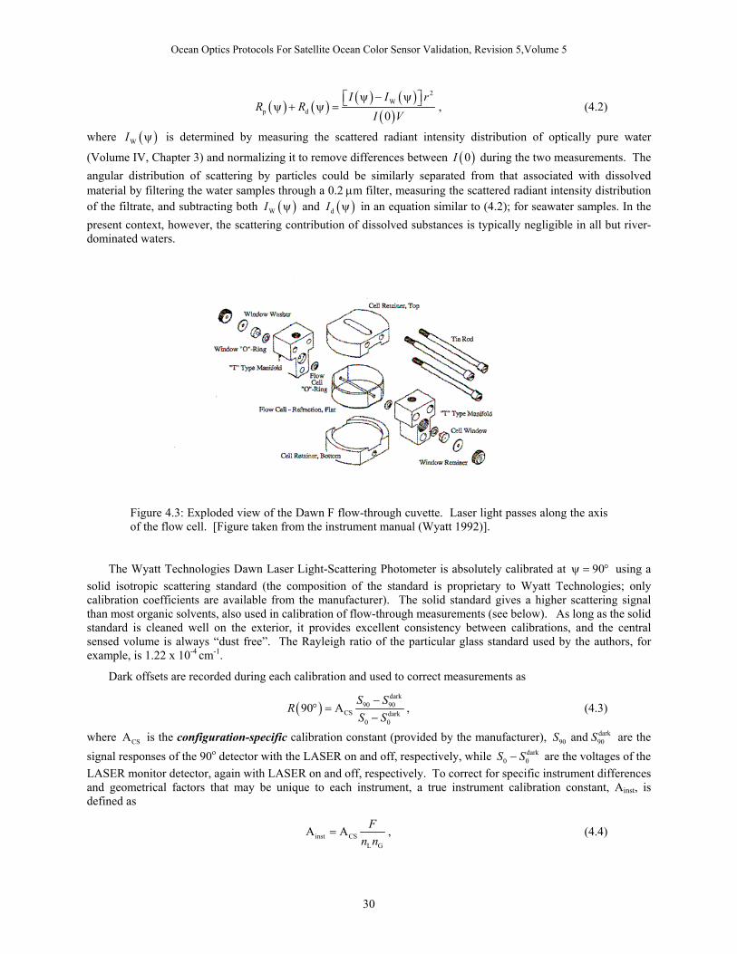
Ocean Optics Protocols For Satellite Ocean Color Sensor Validation, Revision 5,Volume 5
( ) ( )( ) ( )
( )
2W
p d 0I I r
R RI V
ψ − ψψ + ψ = , (4.2)
where is determined by measuring the scattered radiant intensity distribution of optically pure water
(Volume IV, Chapter 3) and normalizing it to remove differences between ( )WI ψ
( )0I during the two measurements. The angular distribution of scattering by particles could be similarly separated from that associated with dissolved material by filtering the water samples through a 0.2 µm filter, measuring the scattered radiant intensity distribution of the filtrate, and subtracting both and ( )WI ψ ( )dI ψ in an equation similar to (4.2); for seawater samples. In the present context, however, the scattering contribution of dissolved substances is typically negligible in all but river-dominated waters.
Figure 4.3: Exploded view of the Dawn F flow-through cuvette. Laser light passes along the axis of the flow cell. [Figure taken from the instrument manual (Wyatt 1992)].
The Wyatt Technologies Dawn Laser Light-Scattering Photometer is absolutely calibrated at using a solid isotropic scattering standard (the composition of the standard is proprietary to Wyatt Technologies; only calibration coefficients are available from the manufacturer). The solid standard gives a higher scattering signal than most organic solvents, also used in calibration of flow-through measurements (see below). As long as the solid standard is cleaned well on the exterior, it provides excellent consistency between calibrations, and the central sensed volume is always “dust free”. The Rayleigh ratio of the particular glass standard used by the authors, for example, is 1.22 x 10
90ψ = °
-4 cm-1.
Dark offsets are recorded during each calibration and used to correct measurements as
( )dark
90 90CS dark
0 0
90 AS S
RS S
−° =
−, (4.3)
where is the configuration-specific calibration constant (provided by the manufacturer), are the signal responses of the 90
CSA dark90 90 and S S
o detector with the LASER on and off, respectively, while are the voltages of the LASER monitor detector, again with LASER on and off, respectively. To correct for specific instrument differences and geometrical factors that may be unique to each instrument, a true instrument calibration constant, A
dark0 0S S−
inst, is defined as
inst CSL G
A A Fn n
= , (4.4)
30

Ocean Optics Protocols For Satellite Ocean Color Sensor Validation, Revision 5,Volume 5
where and are the liquid and cuvette refractive indices, respectively, and F represesnts Fresnel reflection losses at the various interfaces in the cell as
Ln Gn
22 2
G L G
G L G
11 1
1n n n
Fn n n
− −= − −
+ +. (4.5)
With the two calibration constants, Ainst and ACS, the Dawn F can be calibrated with one solvent, and the results of that calibration may be applied to measurements made with another solvent.
Detector signals are normalized to the calibrated Rayleigh ratio at 90o using the above-mentioned isotropic glass scattering standard, to correct for the fact that each detector views a different scattering volume and subtends a different solid angle with respect to the scattering volume.
Characterization of the Wyatt in flow-through mode is identical to batch mode, except for the cuvette (see above). In flow-through mode, normalization of the detectors is achieved by running a solution of Dextran (Mol. Wt 39,200; Sigma 9004-54-0) through the flow-through cuvette. This solution scatters isotropically (Wyatt 1992). Absolute calibration of the instrument is achieved by pumping 0.02µm filtered, analytical grade methanol, toluene, or optically pure water through the optical cell. The software can accommodate particle-free methanol or toluene as a calibration standard. Toluene has the highest Rayleigh ratio (1.406 x 10⁻⁵ cm-1 at 632.8nm) of any of the commonly-available solvents, and is therefore useful for calibration. The Rayleigh ratios for various solvents and wavelengths are embedded in the instrument software.
Quality control of the Wyatt Technologies measurements is checked by viewing 0.02µm-filtered, Milli-Q water and comparing the VSF at 90o and derived bb to published values for pure water (Vol. I, Ch. 2 and Vol. IV, Ch. 1). For ultra filtered, HPLC-grade distilled water measurements, our software fits a standard Rayleigh function to the volume scattering data instead of the Beardsley-Zaneveld (1969) polynomial function (which is fitted to volume scattering measurements of suspended particles). Accurate calibration is evident immediately when viewing the fitted volume scattering function along with actual data.
4.3 DISCRETE WATER SAMPLES: SAMPLE ACQUISITION, TREATMENT, AND VSF MEASUREMENTS
Sample Acquisition Discrete seawater samples for VSF measurements can be drawn from a bucket, or from Niskin bottles, provided
that samples are well-mixed, with particles suspended. It should be noted that if Niskin bottles are left on deck without stirring, large, negatively buoyant, mineral particles can settle below the sampling valve. The approximate volume needed for discrete measurements with the Dawn F is 10 mL to 15 mL. Prior to running discrete seawater samples, vials are checked for any irregularities in wall thickness, and blanks are run using 0.02 µm-filtered, HPLC-grade distilled water. In the event that particles do not remain in suspension over the period of a measurement, samples can be regularly swirled, or a small magnetic stirring motor can be installed below the sample well and a thoroughly-cleaned magnetic stir bar (“flea”) placed within the sample vial. Care should be taken to slightly rotate the sample cuvette between sample replicates to average the effects of any irregularities in the walls of the cuvette.
VSF Measurements of Untreated Seawater Samples Volume scattering measurements of discrete, or “batch”, samples are performed using 3 to 5 replicates of 10 s
measurements sampled at 200 Hz; this yields to 6000-10000 VSF measurements, which are averaged. The replicated measurement sets are combined to determine the average total backscattering coefficient ( )b λb (Sect. 4.6 below) for the sample.
Sample Acidification to Dissolve Particulate CaCO3 To acidify discrete samples and dissolve CaCO3 coccoliths, seawater aliquots can be either bubbled with CO2
for 30 s, or 0.02 µm-filtered acetic acid maybe be added (0.05 % final concentration) to give a final pH < 5.8. Acid addition is preferred over CO2 bubbling, because the bubbling process can induce formation of more particles.
31
Ocean Optics Protocols For Satellite Ocean Color Sensor Validation, Revision 5,Volume 5
VSF Measurements of Acidified Samples Following acidification to dissolve particulate CaCO3, 3 to 5 additional replicate 10 s VSF measurements are
recorded at 200 Hz. The overall set of VSF measurements is then combined to determine the average “acidified” backscattering coefficient of the seawater sample. ( )acid
bb λ
Quality Control and Uncertainty Quality control is assured by frequent checks of the volume scattering of 0.02µm filtered, Milli-Q water. Based
on more than 5 years of measurements of “particle-free” water with the Wyatt instrument, the Type A uncertainty of the VSF determinations at 632.8 nm is approximately 1.5 x 10⁻⁴ m-1 sr-1.
4.4 CONTINUOUS FLOW-THROUGH MEASUREMENTS ALONG SHIP TRACKS: SAMPLE ACQUISITION, TREATMENT, AND VSF MEASUREMENTS
Flow-Through Sampling Apparatus and Debubbler Water flow in the continuous underway system is first run through three de-bubblers, arranged in series, to
remove small bubbles (and their associated light scattering). A metering pump then delivers the water to the Wyatt Technologies Dawn F light scattering photometer at an approximate flow rate of 11 mL min-1. It is easy to detect bubble contamination either by visual inspection of the cuvette during measurements, or retrospectively, by screening the data for evidence of the high scattering levels that occur when bubbles are present in the LASER beam.
In Line Acidification and Flushing Method To estimate the backscattering of particulate CaCO3 in raw seawater measurements, a peristaltic pump is
activated, following VSF measurements of raw seawater, to inject 0.05 % (final concentration) glacial acetic acid into the flow stream. Flow through a mixing coil insures adequate mixing of the acid and seawater. A micro-pH probe downstream of the optical cuvette monitors the pH. The conventional solubility product for calcite in seawater at 25o C and 35 PSU is calc 7
spK 4.467 10−= × (UNESCO 1987). This value assumes that the activity of the pure solid phase is unity, and that the calcite is in its chemically pure form (Stumm and Morgan 1981); these are both reasonable assumptions. When the pH of the sea water flow is < 5.8 (since calc
sppK 6.3= 5
))
)t
, a pH less than this value assures dissolution of CaCO3), the VSF of the acidified seawater flow is ready to be measured, without scattering contributions from particulate CaCO3.
Measurement Cycles: Untreated Sample VSF – Acidified Sample VSF – System Flushing In flow mode, the Wyatt Technologies Model Dawn LASER light scattering photometer has seawater flowing
at an approximate rate of 11 mL min-1. As with the batch measurements, all detectors can be scanned at rates up to 400 Hz, but for most flow-through applications we slow the scanning rate to 200 Hz in order not to sample the same seawater volume twice.
Labview software is used to control all aspects of sampling. The VSF, at all angles specied above (Sect. 4.2) for the flow-through configuration, are measured at 200 Hz, and averaged over 1 s intervals for calculation of the backscattering coefficient. The 1 s averages are recorded for 50 s, and combined to determine the average total backscattering coefficient (Sect. 4.6 below). This measurement cycle is first performed to determine the
VSF, and for raw seawater. Following acidification to dissolve particulate CaCO(b ,b tλ
(b ,b tλ 3, data from the Wyatt
Dawn light scattering photometer are recorded and averaged for 50 s to determine . Finally, the acid pump is stopped, and the flow-through system is flushed until the pH returns to the alkaline values of raw seawater. The entire measurement cycle is then repeated.
(acidb ,b λ
32
Ocean Optics Protocols For Satellite Ocean Color Sensor Validation, Revision 5,Volume 5
The time for a complete acidification cycle can be adjusted, but we have preferred to collect average VSF measurements such that one complete raw/acidification cycle takes 4 min. At a typical ship speed of 10 knots (5 m s-1), a 4 min measurement cycle represents an alongtrack distance of 1200 m, which is comparable to the resolution of satellite ocean color measurements using, e.g., SeaWiFS and MODIS.
Quality Control Quality control is assured by frequent checks of the measured VSF of 0.02 µm filtered, Milli-Q water. The
flow-through cuvette can be observed through a viewing port on top of the cuvette to check for bubbles or bio-fouling. Essentially, the sides of the flow tube become visible if any biofouling occurs. If this happens, then the cuvette should be rinsed, and if necessary, disassembled and cleaned.
Routinely, at intervals of 24 hours, the flow is stopped and the flow cell is cleaned to remove bio-fouling. Storage of the cell with ultra clean solvent, or detergent, solves most problems associated with wall coatings by organisms. Sonication of the cuvette also helps maintain cleanliness. Complete cleaning requires removal of the end windows, and cleaning of the internal bore with solvent soaked lens paper. To correct for any bio-fouling, or instrument drift, 0.02 µm filtered Milli-Q distilled water is pushed through the flow cell to adjust the calibration at frequent intervals throughout the duration of a measurement sequence. After the cruise, all data are corrected using the distilled water calibration results, by comparison to the known backscattering of pure water.
LASER alignment, which is a critical characteristic for good instrument performance, and has proven to be extremely stable with the Dawn F.
As with the discrete measurements above, based on water measurements of “particle-free” water, measurements of the VSF with the Wyatt Dawn in flow mode have a Type A uncertainty of 1.5 x 10⁻⁴ m-1 sr-1. This combined standard uncertainty includes uncertainties associated with instrument calibration and bio-fouling of the flow-through cuvette during continuous use.
4.5 ANCILLARY MEASUREMENTS
Coccolith and Coccolithophore Enumeration Microscope enumeration of coccolithophores and coccoliths is done by filtering a 50 mL water sample through
a Millipore HA filter. The filter is then rinsed with borate buffer and frozen in a Petri dish until the time that the cells and coccoliths will be counted (Haidar et al. 2000; Haidar and Thierstein 2001). To prepare the sample for counting, the filter is placed on a glass microscope slide, and 60oC Canada Balsam is placed on top of the filter, followed by a cover slip. The clarified filter is examined with an Olympus BH2 microscope equipped with polarization optics. Coccoliths and plated coccolithophores can then be counted based on their unique birefringence patterns. For an example of these patterns, see Moshkovitz (1989). For statistical reasons, 200 coccoliths or cells are counted from each sample, when that number or more are present on the filter.
Particulate Inorganic Carbon Particulate inorganic carbon (PIC) is estimated from measurements of particulate calcium. Samples of 100 mL
to 300 mL are filtered through 0.4 µm poresize polycarbonate filters. The filters are then rinsed with filtered seawater and borate buffer (pH = 8) to remove CaCl2 (Fernández et al. 1993), and are placed in centrifuge tubes with 5 mL of 0.5 % Optima grade HNO3. Particulate Ca is measured according to Balch, Drapeau, and Fritz (2000), except that an inductively-coupled plasma atomic absorption spectrometer is now used to measure calcium, instead of a graphite furnace atomic absorption spectrometer. The sensitivity of the technique, after correction for the volume of seawater filtered, is about 2 ng Ca L-1. The coefficient of variation for the measurements is ~± 3 % at a PIC concentration of ~1 µgC L-1. By using polycarbonate filters, any Ca contamination from residual, interstitial water in the filter is minimized. This helps lower blank values.
33

Ocean Optics Protocols For Satellite Ocean Color Sensor Validation, Revision 5,Volume 5
4.6 DATA ANALYSIS METHODS Backscattering is calculated by integrating the VSF measurements from 90o to 144.5o using standard trapezoidal
integration. Integration of backscattering from 144.5o to 180o is accomplished by fitting a polynomial function (Beardsley and Zaneveld 1969) to VSF measurements at 45o, 90o, and 135o. The polynomial function is then integrated, and the two integrals (90o to 144.5o and 144.5o to 180o) are summed to estimate backscattering coefficients ( )b λb and ( )acid
b λb from the raw and acidified seawater samples, respectively. The difference between integration using the above method, versus simply integrating the fitted poynomial between 90o and 180o, shows differences < 5%, in accordance with the observations of Gordon (1976; his Table 1). Finally, the backscattering coefficient for particulate CaCO3 (calcite) is calculated as
( ) ( ) ( )calc acid -1b b b m .b b bλ = λ − λ (4.6)
The values of calcite backscattering can be used to estimate the quantity of suspended calcium carbonate, provided one has an estimate of the backscattering cross-section of coccoliths (Balch et al. 1999). Discrete estimates of particulate inorganic carbon can be used to calibrate the optically-derived estimates.
4.7 DISCUSSION: PROTOCOL STATUS AND FUTURE DIRECTIONS The first results of this instrument were published in 1999 (Balch et al. 1999), in which a flow cytometer was
used to sort individual calcium carbonate particles into the cuvette. Continuous, surface bb observations from the Arabian Sea have also been described (Balch et al. 2001).
The Wyatt Technology Dawn photometer and HOBILABS Hydroscat 2 scattering photometer are plumbed in series for our NASA Gulf of Maine ferry program (Fargion and McClain 2001). Both instruments are used to continuously log backscattering along a 325 Km track between Yarmouth, Nova Scotia and Portland, ME. This has provided a large data set from which to compare the two instruments. Particulate backscattering measured with the Hydroscat-2, has been compared to particulate backscattering measured with the Wyatt Technology instrument. To do these comparisons our Hydroscat-2 was directed into a 21 L volume of water and bb estimates were based on a VSF measurement at one angle and two wavelengths (assuming one shape for the VSF). The Wyatt instrument estimated average bb pg in 9 mL to 12.5 mL of seawater by measuring the VSF at 15 angles and one wavelength at 200Hz (such bb calculations allowed the shape of the VSF to vary). Data from our 1999 and 2000 field seasons were used for this comparison. The Hydroscat 2 data at 476 nm and 676 nm were interpolated to estimate the 514 nm value. The interpolation assumed that backscattering increases as the wavelength raised to a power (Mobley 1994). The results (Fig. 4.4) produced a cloud of data approximately centered about the 1:1 line, but with significant variability. Generally, the two instruments tracked each other quite well, with divergences occurring primarily in very turbid water. The best-fit relationship between the two instruments was: bbp514 Hobi = 0.19 (bbp514
Wyatt0.715) [r2 = 0.423; n = 3029; P < 0.001]. Some of the differences can be ascribed to the shape of the VSF
implicitly assumed in the HOBILABS instrument. Detailed comparisons between VSF at the same angles, as measured by the HOBILABS and Wyatt Technology instruments, has been published elsewhere (Vaillancourt et al. 2003).
34

Ocean Optics Protocols For Satellite Ocean Color Sensor Validation, Revision 5,Volume 5
Fig. 4.4: Comparison between particulate backscattering estimates by the Wyatt Dawn F LASER light scattering photometer and the HOBILABS Hydroscat-2 (see text). Data from 1999 (+ symbols) and 2000 (triangles), continuous underway sampling in the Gulf of Maine were used in this comparison.
ACKNOWLEDGEMENTS Special thanks go to Bruce Bowler (Bigelow Laboratory for Ocean Sciences) and Charlie Byrne (Univ. Miami),
who wrote our software for collecting data from the Wyatt Dawn F and EOS light scattering photometers while at sea. Thanks also go to Katherine Kilpatrick (Univ. Miami) for her earlier help in setting up the Dawn F scattering photometer for shipboard use. Dr. Jennifer Fritz (Univ. Miami), Amanda Ashe (Oregon State University) and Emily Booth (Bigelow Laboratory for Ocean Sciences) helped collect shipboard data sets on volume scattering. Dr. Ken Voss (Univ. Miami) helped us perform an intercalibration of various light scattering photometers, including the Wyatt instruments described here. Lastly, we'd like to thank the many individuals at Wyatt Technology Corporation (Santa Barbara, CA, U.S.A.) for their helpful advice on using their scattering photometers for oceanographic applications. Methods development, instrumentation, and observations described herein were generously supported by various grants to W.M.B. over the years: National Aeronautics and Space Administration (NAGW2426; NAS5-97268; NAS5-31363; NAG5-10622; NASA EPSCOR EP-02-14); Office of Naval Research (ONR N00014-91-J-1048, N00014-97-1-0034; N00014-98-1-0882; N00014-99-1-0645; N00014-01-1-0042), National Science Foundation (OCE-9022227; OCE-9596167), and NOAA (NA56RM0258; 40-AA-NE-005996).
REFERENCES Balch W.M., D. Drapeau, and J. Fritz, 2000: Monsoonal forcing of calcification in the Arabian Sea. Deep-Sea
Research II, 47: 1301-1337
Balch W.M., Drapeau D., J Fritz, B. Bowler, and J. Nolan, 2001: Optical backscattering in the Arabian Sea-continuous underway measurements of particulate inorganic and organic carbon. Deep Sea Research I, 48: 2423-2452
35

Ocean Optics Protocols For Satellite Ocean Color Sensor Validation, Revision 5,Volume 5
36
Balch W.M., D.T. Drapeau, T.L. Cucci, R.D. Vaillancourt, K.A. Kilpatrick, and J. Fritz, 1999: Optical backscattering by calcifying algae--Separating the contribution by particulate inorganic and organic carbon fractions. J. Geophys. Res. 104: 1541-1558
Balch W.M., R.W. Eppley, M.R. Abbott, and F.M.H. Reid, 1989: Bias in satellite-derived pigment measurements due to coccolithophores and dinoflagellates. J. Plankton Res., 11: 575-581
Beardsley, G.F. and J.R.V. Zaneveld (1969) Theoretical dependence of the near-asymptotic apparent optical properties on the inherent optical properties of sea water. J. Opt. Soc. Am., 59: 373-377
Fargion, G.S. and C.R. McClain, 2001: SIMBIOS project 2000 annual report. National Aeronautics and Space Administration, Goddard Space Flight Center, Greenbelt, MD
Fernández, E., P. Boyd, P.M. Holligan and D.S. Harbour, 1993: Production of organic and inorganic carbon within a large scale coccolithophore bloom in the northeast Atlantic Ocean., Mar. Ecol. Prog. Ser., 97: 271-285
Gordon, H.R., 1976: Radiative transfer in the ocean: A method for determination of absorption and scattering properties., Appl. Opt., 15: 2611-2613
Haidar, A.T. and H.R. Thierstein, 2001: Coccolithophore dynamics off Bermuda (N. Atlantic). Deep Sea Research, 48: 1925-1956
Haidar, A.T., H.R. Thierstein and W.G. Deuser, 2000: Calcareous phytoplankton standing stocks, fluxes and accumulation in Holocene sediments off Bermuda (N. Atlantic). Deep Sea Research, 47: 1907-1938
Mobley, C.D. 1994: Light and water: Radiative transfer in natural waters. Academic Press, New York
Moshkovitz, S.and K. Osmond, 1989: The optical properties and microcrystallography of Arkhangelskiellaceae and some other calcareous nannofossils in the Late Cretaceous. In: Crux, J.A. and S.E.van Heck (eds) Nannofossils and their applications. Ellis Horwood, Chichester, pp 76-97
Stumm, W., J.J. Morgan, 1981: Aquatic Chemistry. John Wiley & Sons, Inc., New York
UNESCO (1987) Thermodynamics of the carbon dioxide system in seawater. Report by the carbon dioxide sub-panel of the joint panel on oceanographic tables and standards. United Nations Educational, Scientific and Cultural Organization, 51, Paris
Vaillancourt, R.D., C.W. Brown, R.R.L. Guillard and W.M. Balch, 2003: Light backscattering by phytoplankton algae and a heterotrophic bacterium measured with a multi-wavelength, fixed-angle backscattering meter. Journal of Plankton Research (in press)
Wyatt, P., 1992: Instruction manual for the DAWN Model F., Wyatt Technology Corporation, Santa Barbara, CA

National Estuarine Research Reserve (NERRS) System-Wide Monitoring Program (SWMP)
YSI/Xylem EXO Multi-Parameter Water Quality Monitoring Standard Operating Procedure
Version 1.1
March 2017
Written by: Mike Mensinger, Delaware National Estuarine Research Reserve
Edited by: Mike Lizotte, YSI/Xylem Curtis Butler, YSI/Xylem
Melissa Ide, NERRS Centralized Data Management Office
NOAA National Estuarine Research Reserve System Centralized Data Management Office
c/o Belle W. Baruch Institute for Marine and Coastal Sciences University of South Carolina
22 Hobcaw Road Georgetown, SC 29440
© Copyright March 2017 CDMO
Appendix J
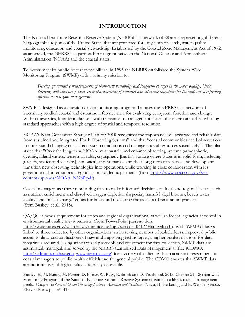
INTRODUCTION The National Estuarine Research Reserve System (NERRS) is a network of 28 areas representing different biogeographic regions of the United States that are protected for long-term research, water-quality monitoring, education and coastal stewardship. Established by the Coastal Zone Management Act of 1972, as amended, the NERRS is a partnership program between the National Oceanic and Atmospheric Administration (NOAA) and the coastal states. To better meet its public trust responsibilities, in 1995 the NERRS established the System-Wide Monitoring Program (SWMP) with a primary mission to:
Develop quantitative measurements of short-term variability and long-term changes in the water quality, biotic diversity, and land-use / land -cover characteristics of estuaries and estuarine ecosystems for the purposes of informing effective coastal zone management.
SWMP is designed as a question driven monitoring program that uses the NERRS as a network of intensively studied coastal and estuarine reference sites for evaluating ecosystem function and change. Within these sites, long-term datasets with relevance to management issues of concern are collected using standard approaches with a high degree of spatial and temporal resolution. NOAA's Next Generation Strategic Plan for 2010 recognizes the importance of “accurate and reliable data from sustained and integrated Earth Observing Systems” and that “coastal communities need observations to understand changing coastal ecosystem conditions and manage coastal resources sustainably”. The plan states that "Over the long-term, NOAA must sustain and enhance observing systems (atmospheric, oceanic, inland waters, terrestrial, solar, cryospheric [Earth’s surface where water is in solid form, including glaciers, sea ice and ice caps], biological, and human) – and their long-term data sets – and develop and transition new observing technologies into operations, while working in close collaboration with it’s governmental, international, regional, and academic partners” (from http://www.ppi.noaa.gov/wp-content/uploads/NOAA_NGSP.pdf). Coastal managers use these monitoring data to make informed decisions on local and regional issues, such as nutrient enrichment and dissolved oxygen depletion (hypoxia), harmful algal blooms, beach water quality, and “no-discharge” zones for boats and measuring the success of restoration projects (from Buskey, et al., 2015). QA/QC is now a requirement for states and regional organizations, as well as federal agencies, involved in environmental quality measurements. (from PowerPoint presentation: http://water.usgs.gov/wicp/acwi/monitoring/ppt/sanjose_0412/Hameedi.pdf). With SWMP datasets linked to those collected by other organizations, an increasing number of stakeholders, improved public access to data, and applications of new and improving technologies, a higher burden of proof for data integrity is required. Using standardized protocols and equipment for data collection, SWMP data are assimilated, managed, and served by the NERRS Centralized Data Management Office (CDMO; http://cdmo.baruch.sc.edu; www.nerrsdata.org) for a variety of audiences from academic researchers to coastal managers to public health officials and the general public. The CDMO ensures that SWMP data are authoritative, of high quality, and easily accessible. Buskey, E., M. Bundy, M. Ferner, D. Porter, W. Reay, E. Smith and D. Trueblood. 2015. Chapter 21 - System-wide Monitoring Program of the National Estuarine Research Reserve System: research to address coastal management needs. Chapter in Coastal Ocean Observing Systems: Advances and Syntheses. Y. Liu, H. Kerkering and R. Weisberg (eds.). Elsevier Press. pp. 391-415.

This document outlines the standard operating procedures (SOP) for the collection of data using YSI/Xylem EXO Multi-Parameter Water Quality Sondes for the National Estuarine Research Reserve's (NERR) System-Wide Monitoring Program (SWMP). This SOP does not replace the YSI/Xylem EXO User Manual or the CDMO Data Management Manual. Users must become familiar with procedures in these manuals as well. The purpose of the SWMP SOP is to standardize instrument handling, maintenance, calibration, deployment, and post-deployment procedures for the NERR SWMP. The procedures in this SOP are the MINIMUM requirements for operating the EXO sondes; therefore all NERR sites must follow these procedures. Participating NERR sites may undertake additional procedures to ensure quality data collection, but following the procedures in this SOP will ensure consistency across the NERRS, minimize the collection of inaccurate data, and support effective data QAQC after collection. For questions or concerns about this document, please contact: [email protected]. This document is separated into nine sections: I. EXO Communication & KORS Software II. Calibration III. EXO Programming & Deployment Preparation IV. EXO Deployment V. EXO Retrieval VI. EXO Data Download & Post Deployment Readings VII. SWMP Water Quality Monitoring Calibration Log sheet VIII. Probe care and storage IX. Appendices for troubleshooting and other detailed documents.

I. EXO COMMUNICATION & KORS SOFTWARE A copy of KORS software, stored on a USB thumb drive, is included with purchase of each EXO sonde. This software is used for EXO communication, calibration, post-deployment readings, data file download, sonde/probe firmware updates, and any other necessary interaction with the sonde via a PC. This section briefly covers communication options using KORS. It also covers the various functions of the software and the icon-based locations of said functions. Sonde Connectivity – EXO sondes are accessed via one of two potential options:
1) USB/SOA (Signal Output Adapter) Cabled Connection
a. Open KORS Software
b. Connect the USB cable to the PC and the blue SOA adapter to the sonde connector located on the top of the sonde. The connector on the right side of the sonde (when looking at the sonde from a view where the yellow plastic component faces the user) is used for wired connection.
c. Click the “Circular Blue/Green Arrows” icon (7th icon from the left in KORS)
d. Click Rescan
e. Click the COMM port that has the EXO USB adapter and EXO sonde ID shown
f. Click “Connect”
g. If the USB adapter or sonde do not show up at first, unplug the USB cable from the computer, plug it in again, and repeat steps 3 through 6. If this fails to show the sonde, unplug the adapter from the sonde, re-connect the adapter, and repeat steps 3 through 6.
2) Wireless Bluetooth Connection
a. Open KORS Software
b. Place the magnetized section of the black probe removal tool over the magnet icon located on the sonde (about halfway down the sonde within the black stickered area that says EXO2) to activate the sonde
c. Click the “Circular Blue/Green Arrows” icon (7th icon from the left in KORS)
d. Click Rescan
e. Click the EXO sonde ID shown
f. Click “Connect”
g. Note: make sure to connect to the appropriate EXO sonde as the Bluetooth may pick up other active EXO sondes nearby.
NOTE: Additional information about bluetooth connection and troubleshooting is available in the EXO manual
KORS Software Icons – the KORS software features eight major icons located within the software that serve various purposes. Each icon and its functions are explained below in detail

1) Green Running Man (1st icon to the right of the KORS software logo) – once connected to the
EXO sonde, clicking this icon places the sonde into discrete mode; a mode used for making real-time measurements
2) Calibration Target (2nd icon to the right of the KORS software logo) – clicking this icon brings up sub-menus showing each port and the port’s installed probe. Each probe/parameter’s rectangular icon is vertically stacked to the left of the screen. Clicking a particular parameter brings up the calibration screen for that probe. Detailed calibration steps for each parameter are discussed in the calibration section of this document.
3) Large Green Arrow (3rd icon to the right of the KORS software logo) – clicking this icon
brings up two sub menus used in preparing the sonde for unattended sampling prior to deployment;
a. Read Current Sonde Settings – accesses the current template file present within the EXO sonde
b. Open Template – allows the user to choose a particular template file for the sonde
4) Map with Blue Inverted Tear Drop (4th icon to the right of the KORS software logo) – clicking this icon brings up a place where individual monitoring site names are added or removed
5) Data Folder (5th icon to the right of the KORS software logo) – clicking this icon reveals 4
submenus icons involved in the following
a. Transfer – used to transfer .BIN data files from the sonde to the PC
b. View Export – used to select .BIN files and export them into .CSV or other file formats
c. Settings – used to designate a location on the PC where files are downloaded/exported. It is recommended to leave the default pathway in place and simply copy and paste files to other locations after download and export.
d. View Calibration Worksheets – used to access copies of calibration information sheets for each calibrated probe type. Calibration sheets can be located, accessed, sorted, and displayed within this submenu.
6) Gears (6th icon to the right of the KORS software logo) – clicking this icon reveals seven submenu icons:
a. Smart QC – provides a list of the sonde ports and associated probes installed within each port along with a QC score (green check mark for good)
b. Sonde – provides an input space for the sonde ID, allows the user to update the sonde time (internal clock), select battery type, and alter the averaging mode (for SWMP this should be left at default)
c. User – allows the user to change the language, timespan in which the sonde will drop communication (go into idle mode), select the local time zone, time format preference (should be set to 24 hr for SWMP), UTC (GMT) or time zone adjusted (should select time zone adjusted for SWMP), and a time zone check option
d. Units – this submenu provides a stacked icon list of each parameter. Clicking on an

individual parameter allows the user to change to unit of measure for said parameter by clicking to place a checkmark in next to the chosen unit of measure. For SWMP, parameters should be set to the following units: Note: These configurations are computer settings and not changes that are sent to the sonde.
i. Temperature (Temp): Temp C ii. Conductivity (Cond): SpCond mS/cm & Sal psu iii. Dissolved Oxygen (ODO): ODO % iv. pH: pH & pH mV v. Depth: Depth m vi. Barometric Pressure (Baro): Baro mmHg vii. Turbidity (Turb): Turbidity FNU viii. Sonde: Battery V ix. External Battery Voltage x. Wiper Position xi. Once selected, click “apply”. This only needs to be done once when initially
setting up the software
e. Firmware – this submenu shows each probe, the port in which it is installed, the probe serial number, address, and firmware version. Both the sonde and all probe firmware can be updated from this screen
f. Calibration – this submenu provides a stacked icon list of each parameter. Clicking a parameter provides a series of unit options. When clicked, the unit of measure screen opens allowing the user to input specific calibration points and information about the calibration standard used for calibration that probe type (type, manufacturer, and lot number). These only need to be set once unless the user is changing calibration standard lots numbers. Everything set in these menus will show up as part of the calibration screens (see Section II Calibration).
g. Sync With Handheld – allows the user to access files on an EXO handheld device, update handheld firmware, etc.
7) Circular Blue & Green Arrows (7th icon to the right of the KORS software logo)- clicking this icon reveals four submenu options
a. Rescan (see KORS software section 1)
b. Map – shows all ports, probes installed, and probe serial numbers
c. Settings – Bluetooth and USB adapter settings
d. Advanced – allows comm port selection for cabled communication
8) Question Mark (8th icon to the right of the KORS software logo) – self-explanatory help menu

II. CALIBRATION General Calibration Considerations:
1) Good laboratory practices should always be followed when handling calibration standards. Please refer to MSDS sheets for any standard when necessary.
2) A NERRS SWMP Water Quality Calibration Log and Field Log (combined, a deployment
log) must be completed for each instrument’s calibration, deployment and retrieval, and post-calibration (see section VII). These deployment logs must be submitted to the CDMO via the online Deployment Log Interface. Reserves are encouraged to use hardcopy sheets to record data in the field and customized logs may be used internally in order to support additional parameters or partner program requirements, but the approved online deployment logs will be the only versions accepted by CDMO.
3) The sonde should be visually inspected for any abnormalities, such as a broken probe or
damaged bulkhead 4) Remove the Wiper Brush from the sonde! The brush can trap residual standard and affect the
calibration accuracy, The EXO2 sensors easily dislodge air bubbles so it is not needed during calibration. If you elect to leave it on the bristles will have to be cleaned and thoroughly rinsed between standards / buffers
5) Calibrations are best performed using a guard and calibration cup that are dedicated to
calibration only and never taken in the field. This insures a high level of cleanliness and non-contamination during the calibration process.
6) During the calibration of the probes NEVER accept any calibrations that display an error
message. Troubleshoot the cause of the problem, correct it, and recalibrate or replace the probe before deploying the instrument.
7) Standards must be active (check expiration date) and fresh for all calibrations. Previously used,
clean standards may be used to rinse probes but must not be used to calibrate probes. Discard and replace all expired standards.
8) All diagnostic parameters (pH millivolts, DO gain, and conductivity cell constant) for EXO
sondes are presented after calibration of the respective parameter on the KORS generated calibration sheet and should be recorded on the NERRS data sheet once calibration of those probes is complete.
9) Recommended probe calibration order: Temperature (not a true calibration, but a check
against NIST source), Specific Conductivity, pH, Depth, Turbidity, Dissolved Oxygen. 10) Prior to calibration it is a good idea to record serial number for the sonde and probe on in the
Calibration Log’s “Datasonde & Probe Identification Numbers” section. To quickly access all serial numbers, perform the following:
a. Click the Gear Icon

b. Click Firmware c. Record all serial numbers on the data sheet (the user can double check accuracy of the
serial number during calibration of each parameter. Serial #’s may also be written during calibration, but the user loses the opportunity to quickly double check them with that method.
11) Batch calibrations (sometimes referred to as gang calibrations) are permissible for SWMP, but
this is an advanced form of calibration that is not recommended when learning to calibrate EXO sondes. During gang calibrations, multiple versions of the same probe type are installed into an EXO sonde and calibrated one after the other. Once calibrated in this fashion, the probes are then installed into their respective EXO sondes.
Calibration Procedures - The following sections provide step-by-step SWMP approved methods for the calibration of each probe type.
1) Temperature Sensor and SC Functional Check – while it is not possible to calibrate the temperature probe, this does not exclude you from performing a temperature test to verify that the temperature probe is working properly. A traceable NIST thermometer will be required for this test. The Specific Conductivity check will verify that cleaned and dry electrodes read < 2 us/cm with the probe dry and in air. Note: At least once a year the temperature sensor should be checked at 3 points, ice water, room temperature, and warm water ~ 35 C.
a. Temperature Test
a. Allow the sonde to sit in a bucket of room temperature tap water for at least 5 minutes to reach temperature equilibrations,
b. Connect to the sonde (see I. KORS Software section 2)
c. Click Green Running Man icon to place sonde into discrete mode
d. Verify temperature readings have stabilized and record the sonde’s temperature value in the Pre-Deployment section of the data sheet in the “Before Cal” field for Temp
e. Record the temperature reading from the NIST thermometer in the data sheet’s Pre-Deployment “Standards” column.
f. Note: that the accuracy of the NIST device must be included in your temperature accuracy determination.
g. Remove the sonde from the water bucket
b. Conductivity Test
a. Rinse the SC probe with DI water after the temperature verification test
b. Using a compressed air source (Dust Off) blow the conductivity cells dry on the CT2 sensor, on the Wiped CT probe you can use the air or dry the open channels with a KimWipe.
c. The SC reading in air for both sensors must be < 2 us/cm, if greater that 2 us/cm contact Xylem/YSI for assistance

2) Conductivity Probe (Specific Conductivity & Salinity) – 1 Point Calibration
a. Fill EXO calibration cup with a small amount of rinse conductivity calibration standard (rinse standard is the term for calibration standard used during the previous calibration and its use reduces cost and standard consumption)
b. Place the sonde with guard installed into the EXO calibration cup and shake to rinse the guard and probes
c. Empty out the rinse standard
d. Repeat the above process 1-2 more times (YSI recommends rinsing a total of three times)
e. Fill calibration cup to the second line with new/unused conductivity calibration standard
f. Screw the guard back on and place the EXO sonde into the calibration cup
g. Click the calibration icon
h. Click “Conductivity”
i. Click “SpCond” (Specific Conductivity)
j. Choose 1 point calibration and make sure the calibration standard value shows up properly (this may be entered manually each time or can be set to show up automatically by clicking the Gears icon, Calibration submenu icon, , Cond icon, SpCond icon, and then entering the standard value for Cal Point 1, followed by clicking apply)
k. Type in the standard type, manufacturer, and lot # of the standard (standard type and manufacturer can be entered manually each time or auto-set using the procedure described in Step J.)
l. Click “Start Cal”
m. Once the temperature value has stabilized and “unstable data” in red font changes to “stable data” in green font, click “apply”.
n. Verify the “Pending (Post) value is correct and click “Complete”
o. The calibration worksheet for the probe will pop up and the user should record the following three values:
a. Pre Calibration Value: record this value in the data sheet’s “Before Cal” column
b. Post Calibration Value: record this value in the data sheet’s “Calibrated” column
c. Cell Constant: record in the data sheet’s “Sensor Diagnostics/Pre-Deployment” cell constant field
p. Review the cell constant value to make sure it is within the proper range of 5.05 – 5.95 for the CT2 sensor and 0.5 +/- 0.1 for the Wiped CT
q. Close the calibration worksheet
r. Pour the used standard into a container labelled “rinse” as this standard can be used as a rinse later
s. YSI Tips:
a. Never calibrate with a standard less than 1.0 mS/cm as they are easily contaminated by residual DI water and electrical noise

b. Typical calibration errors are attributed to incorrect standard value input, inadequate calibration standard volume in the EXO calibration cup, or air bubbles in the conductivity cell
3) pH Probe – 2 Point Calibration (pH7 and pH10) (please note if you are one of the two or three
Reserves that perform 3 point pH calibrations, you will simply have another round of standard (pH 4) added to the following procedure) Note: All pH sensors require periodic reconditioning and cleaning, the pH reconditioning procedure should be performed quarterly and at the beginning of a new season. Remove the Wiper Brush from the sonde prior to calibration, it can trap residual buffer and affect the calibration accuracy
a. Rinse the EXO calibration cup, guard, and probes with DI water to remove standard from the previous calibration
b. Fill EXO calibration cup with a small amount of rinse pH7 calibration standard (Rinse standard is the term for calibration standard used during the previous calibration and its use reduces cost and standard consumption)
c. Place the sonde with guard installed into the EXO calibration cup and shake to rinse the guard and probes
d. Empty out the rinse standard
e. Repeat the above process 1-2 more times (YSI recommends rinsing a total of three times)
f. Place the sonde on the work bench with the guard removed
g. Click the Green Running Man icon to run the sonde in discrete mode to get an air temperature reading. Once the temperature has stabilized, use that value to determine the exact values to input for your calibration standards. The standards will have pH values at various temperatures or ranges listed on the container.
h. Write the temperature compensated pH values in the data sheet’s Pre-Deployment “Standards” column for the two or three standards to be used
i. Fill calibration cup to the first line with the first pH calibration standard (ph7)
j. Click the calibration icon
k. Click “pH”
l. Choose 2 or 3 point calibration and enter the pH7 and pH10 standard values determined in Step G. (these values can initially be set by clicking the Gears icon, clicking the Calibration icon, clicking the pH icon, and entering the standard values for each pH cal point) It is critical to note that unlike all other parameters, the exact pH value used for calibration may change slightly based on the air temperature at which you are calibrating. If the standard values shown in the calibration page have been auto-set and do not match the values you want, simply input the correct values and proceed to the next step.
m. Enter the standard type, manufacturer, and lot # for each calibration point (standard type and manufacturer can be entered manually each time or auto-set using the procedure described in Step L.)
n. Click “Start Cal”
o. Once the temperature value has stabilized and “unstable data” in red font changes to “stable data” in green font, click “apply”.
p. Verify the “Pending (Post) value is correct and click “Proceed”

q. Rinse the EXO calibration cup, guard, and probes with DI water to remove pH7 standard from the first part of the calibration
r. Fill the EXO calibration cup with a small amount of rinse pH10 calibration standard
s. Place the EXO sonde with guard installed into the EXO calibration cup and shake to rinse the guard and probes
t. Empty out the rinse standard
u. Repeat the above process 1-2 more times (YSI recommends rinsing a total of three times)
v. Fill the calibration cup with the next pH calibration standard (pH10 in this case)
w. Click “OK” when the small window pops up saying “Proceed to Standard (10.00 pH)
x. Once the temperature value has stabilized and “unstable data” in red font changes to “stable data” in green font, click “apply”.
y. Verify the “Pending (Post) value is correct and click “Complete”
z. The calibration worksheet for the probe will pop up and the user should record the following values:
a. Pre Calibration Value for Cal Point 1: record this value in the data sheet’s “Before Cal” column
b. Post Calibration Value for Cal Point 1: record this value in the data sheet’s “Calibrated” column
c. Raw Value pH mV): record in the data sheet’s “Sensor Diagnostics/Pre-Deployment” phX millivolts field
d. Record the values (Pre Calibration Value, Post Calibration Value, and Raw Value) on the data sheet for the 2nd calibration point
e. Also record the pH probe slope in the data sheet’s “Sensor Diagnostics/Pre-Deployment” next to the text “calculated pH slope”
f. Verify that the pH slope is within the ideal range of 160 – 180. pH data collected with a probe slope of less than 155 requires mandatory coding as suspect data, so it is not recommended to deploy a sonde displaying a pH slope at or below 155. A brand new pH probe will display a slope at or near 180. A probe displaying a slope of 160-165 indicates the probe tip is nearing the end of its lifespan and will require replacement in the near future.
aa. Close the calibration worksheet
bb. Pour the used standard into a container labelled “rinse” as this standard can be used as a rinse later
cc. YSI Tips:
a. pH probe tips typically last 1 – 1.5 years on average
b. The entire probe does not need to be replaced when its lifespan has ended; only the probe tip (Part #599795-02).

4) Depth/Water Level – 1 Point Calibration – the directions presented here are applicable to users collecting depth with the EXO sonde. Alternative calibration procedures for water level are detailed in Appendix C
a. Fill EXO calibration cup with a small amount of water (the volume should not reach anywhere near the probes) to create a water-saturated air environment
b. Screw the guard onto the sonde and place it into the calibration cup
c. Allow the sonde to remain in a vertical position on the work bench
d. Click the calibration icon
e. Click “Depth”
f. Click “Depth m”
g. Determine the most current local barometric pressure value in mmHG (preferably from your SWMP weather station) and record it in the “Pre-Deployment” “Before Cal” column inside the field next to “Baro Pres. (Depth Calib). To convert other units to mm Hg, multiply inches of Hg by 25.4 or millibars by 0.75.
NOTE: Reserves located at a ‘significant’ elevation, MUST use the barometric pressure reading from their corresponding MET station for this calculation to ensure the most accurate depth correction possible. While this is recommended for everyone, it specifically applies to those that use an offset in their Campbell program (following NWS protocols) to adjust barometric pressure readings from their MET station to sea level. Currently those two Reserves are OWC and LKS.
h. Input the mm Hg in the online Deployment Log or Depth/Offset Calculator to determine the correct barometric pressure offset to use for calibration (the charts in Appendix B may also be used to determine correct offset).
i. Write this value on the data sheet by putting a line through 0.0 and writing the barometric pressure offset above the word offset in the “Pre-Deployment” “Standards” section. The 0.0 listed on the data sheet is an artifact of the equation present within the online Log Sheets. In the Online Log Sheets, entry of the barometric pressure automatically changes the 0.0 to the relevant barometric pressure offset.
j. Click Advanced
k. Click Edit
l. Enter the barometric pressure offset into the “Offset” field
m. Click Apply
n. Click OK
o. Click Back
p. Click “Start Cal”
q. Once the depth value has stabilized and “unstable data” in red font changes to “stable data” in green font, click “apply”.
r. Click “Complete”
s. The calibration worksheet for the probe will pop up and the user should record the following values:

a. Pre Calibration Value: record this value in the data sheet’s “Before Cal” column for depth
b. Post Calibration Value: record this value in the data sheet’s “Calibrated” column for depth
NOTE: The station offset and level fields on the data sheet should be left blank when performing depth calibrations. The fields are only applicable to calibration for water level (see Appendix C for details)
t. Close the calibration worksheet
u. YSI Tips
a. Make sure the correct latitude has been entered into the EXO sonde (may be checked and changed during Step L. from the above instructions
5) Turbidity probe – 2-point calibrations are required at least monthly and when sensor drift is evident. As such, the following step-by-step methods detail a 2 point calibration procedure using DI water and 126 NTU standard (other DMC SWMP-approved standards include: Hach StablCal, diluted Hach 4000 NTU formazin, or standards that have been approved according to the instructions in Standard Methods, 20th ed. (Section 2130 B)).
Turbidity Probe calibration considerations:
a. NTU (nephelometric turbidity units) and FNU (formazin nephelometric unuts) are considered synonymous for the purposes of this document
b. The 6-Series 126 NTU standard is now relabeled and has two numbers on the bottle the value for 6-Series probe is 126 and for the EXO it is 124. Always use the 124 entry when calibrating EXO turbidity sensors!
c. Do not calibrate turbidity in the field as clean surfaces and solutions are essential for a good turbidity calibration.
d. Use the EXO calibration cup for turbidity probe calibration; do not use any other calibration vessel.
e. Bubbles over the optics will interfere with calibration therefore it is recommended to carefully pour standards into the calibration cup with the cup held at an angle to avoid aeration and to visually confirm all air bubbles are clear from the probe face before calibration.
f. Turbidity Zero Calibration Note: Recent studies have concluded that in many applications it is almost impossible to clean a used sonde and its calibration cup to a level that will eliminate contamination of the zero standard. In controlled laboratory conditions with new equipment contamination levels of 0.1 ntu’s were observed even when extreme precautions were used. Used equipment even when properly cleaned can contaminate the zero standard to levels between 0.2 and 0.6 ntu’s.
Calibrating the sonde to a zero standard that is actually a positive number will result in negative field reading if the in-situ environment is cleaner. If you routinely see negative turbidity data (<1 ntu) from your deployments this could be the cause.
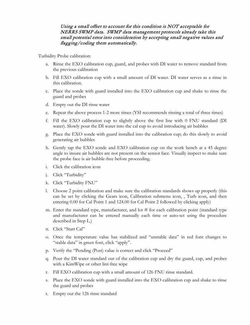
Using a small offset to account for this condition is NOT acceptable for NERRS SWMP data. SWMP data management protocols already take this small potential error into consideration by accepting small negative values and flagging/coding them automatically.
Turbidity Probe calibration:
a. Rinse the EXO calibration cup, guard, and probes with DI water to remove standard from the previous calibration
b. Fill EXO calibration cup with a small amount of DI water. DI water serves as a rinse in this calibration.
c. Place the sonde with guard installed into the EXO calibration cup and shake to rinse the guard and probes
d. Empty out the DI rinse water
e. Repeat the above process 1-2 more times (YSI recommends rinsing a total of three times)
f. Fill the EXO calibration cup to slightly above the first line with 0 FNU standard (DI water). Slowly pour the DI water into the cal cup to avoid introducing air bubbles
g. Place the EXO sonde with guard installed into the calibration cup; do this slowly to avoid generating air bubbles
h. Gently tap the EXO sonde and EXO calibration cup on the work bench at a 45 degree angle to insure air bubbles are not present on the sensor face. Visually inspect to make sure the probe face is air bubble-free before proceeding.
i. Click the calibration icon
j. Click “Turbidity”
k. Click “Turbidity FNU”
l. Choose 2 point calibration and make sure the calibration standards shows up properly (this can be set by clicking the Gears icon, Calibration submenu icon, , Turb icon, and then entering 0.00 for Cal Point 1 and 124.00 for Cal Point 2 followed by clicking apply)
m. Enter the standard type, manufacturer, and lot # for each calibration point (standard type and manufacturer can be entered manually each time or auto-set using the procedure described in Step L.)
n. Click “Start Cal”
o. Once the temperature value has stabilized and “unstable data” in red font changes to “stable data” in green font, click “apply”.
p. Verify the “Pending (Post) value is correct and click “Proceed”
q. Pour the DI water standard out of the calibration cup and dry the guard, cup, and probes with a KimWipe or other lint-free wipe
r. Fill EXO calibration cup with a small amount of 126 FNU rinse standard.
s. Place the EXO sonde with guard installed into the EXO calibration cup and shake to rinse the guard and probes
t. Empty out the 126 rinse standard

u. Repeat the above process 1-2 more times (YSI recommends rinsing a total of three times)
v. Fill the EXO calibration cup to slightly above the first line with new/unused 124 FNU calibration standard by holding the calibration cup at an angle and slowly pouring the standard into the cal cup to avoid introducing air bubbles
w. Place the EXO sonde with guard installed into the calibration cup; do this slowly to avoid generating air bubbles
x. Gently tap the EXO sonde and calibration cup on the work bench at a 45 degree angle to insure air bubbles are not present on the sensor face. Visually inspect to make sure the probe face is air bubble-free before proceeding.
y. Click “OK” when the small window pops up saying “Proceed to Standard (124 FNU)”
z. Once the temperature value has stabilized and “unstable data” in red font changes to “stable data” in green font, click “apply”.
aa. Verify the “Pending (Post) value is correct and click “Complete”
bb. The calibration worksheet for the probe will pop up and the user should record the following two values:
a. Pre Calibration Value: record this value in the data sheet’s “Before Cal” column
b. Post Calibration Value: record this value in the data sheet’s “Calibrated” column
cc. Close the calibration worksheet
dd. Pour the used standard into a container labelled “rinse” as this standard can be used as a rinse later
ee. YSI Tips
a. Holding a finger of the face of the turbidity probe (optics) should give a full response by the probe in discrete mode
b. YSI 126 NTU turbidity standard shelf life is 1 year
6) Dissolved Oxygen Probe – 1 point calibration
a. Aerate a 5 gallon bucket filled ¾ full with tap water for at least an hour prior to calibrating a dissolved oxygen probe. This creates an air-saturated environment referred to as a 100% air-saturated water bath.
b. Place the EXO sonde into the bucket for 15-20 minutes before calibrating the DO probe in order to achieve temperature probe stabilization. Do not allow air bubbles to flow directly towards the DO probe’s face.
c. Click the calibration icon
d. Click “ODO”
e. Click “ODO % sat”
f. Review the temperature value on the screen and make sure it is stable
g. Enter the current barometric pressure value in mmHG
h. Choose 1 point calibration and make sure the calibration standard shows up properly as air saturated (this can be set by clicking the Gears icon, Calibration submenu icon, , ODO icon, ODO % sat icon, and then selecting “air saturated” followed by clicking apply)

i. Click “Start Cal”
j. Once the temperature value has stabilized and “unstable data” in red font changes to “stable data” in green font, click “apply”.
k. Verify the “Pending (Post) value is correct and click “Complete”
l. The calibration worksheet for the probe will pop up and the user should record the following three values:
a. Pre Calibration Value: record this value in the data sheet’s “Before Cal” column
b. Post Calibration Value: record this value in the data sheet’s “Calibrated” column
c. DO Gain: record in the data sheet’s “Sensor Diagnostics/Pre-Deployment” optical DO gain field
m. Review the DO Gain to make sure it is within the recommended 0.87 – 1.25 range
n. Close the calibration worksheet
o. YSI Tips:
a. DO probe sensor caps should last 1 – 2 years (possibly longer), but do require replacement once its lifespan has ended
b. Note: For optimum performance Optical DO sensor membranes must be kept fully hydrated in water. If your DO probe has been dry stored it will need to hydrate in saturated tap water over night. If the probe was stored in saturated air the sensor should be placed in saturated water for a few hours to ensure full hydration. Always make sure that the DO membrane is clean and free of any slime or mold.
7) Total Algae/chlorophyll: Chlorophyll fluorescence is an optional SWMP parameter and
calibration for this parameter is not as straight forward as other parameters. Calibration instructions are included in Appendix D.
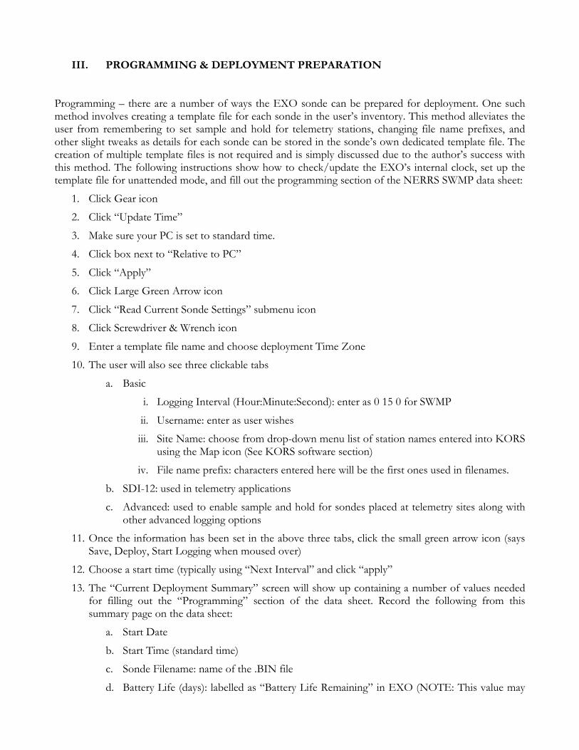
III. PROGRAMMING & DEPLOYMENT PREPARATION Programming – there are a number of ways the EXO sonde can be prepared for deployment. One such method involves creating a template file for each sonde in the user’s inventory. This method alleviates the user from remembering to set sample and hold for telemetry stations, changing file name prefixes, and other slight tweaks as details for each sonde can be stored in the sonde’s own dedicated template file. The creation of multiple template files is not required and is simply discussed due to the author’s success with this method. The following instructions show how to check/update the EXO’s internal clock, set up the template file for unattended mode, and fill out the programming section of the NERRS SWMP data sheet:
1. Click Gear icon
2. Click “Update Time”
3. Make sure your PC is set to standard time.
4. Click box next to “Relative to PC”
5. Click “Apply”
6. Click Large Green Arrow icon
7. Click “Read Current Sonde Settings” submenu icon
8. Click Screwdriver & Wrench icon
9. Enter a template file name and choose deployment Time Zone
10. The user will also see three clickable tabs
a. Basic
i. Logging Interval (Hour:Minute:Second): enter as 0 15 0 for SWMP
ii. Username: enter as user wishes
iii. Site Name: choose from drop-down menu list of station names entered into KORS using the Map icon (See KORS software section)
iv. File name prefix: characters entered here will be the first ones used in filenames.
b. SDI-12: used in telemetry applications
c. Advanced: used to enable sample and hold for sondes placed at telemetry sites along with other advanced logging options
11. Once the information has been set in the above three tabs, click the small green arrow icon (says Save, Deploy, Start Logging when moused over)
12. Choose a start time (typically using “Next Interval” and click “apply”
13. The “Current Deployment Summary” screen will show up containing a number of values needed for filling out the “Programming” section of the data sheet. Record the following from this summary page on the data sheet:
a. Start Date
b. Start Time (standard time)
c. Sonde Filename: name of the .BIN file
d. Battery Life (days): labelled as “Battery Life Remaining” in EXO (NOTE: This value may

be inaccurate during cabled communication as the PC is providing power to the EXO. Checking battery life via a Bluetooth connection yields a more accurate number of days)
e. Free Memory (days): labelled as “Logging Space Duration
f. Free Memory Status (bytes or %): labelled as Log Space Available in % in EXO
14. The sonde is now ready for deployment! Place the sonde back into the air-saturated water bath and allow it to take readings there until deployment time arrives. These bucket readings, or “data tails” as they are often referred to as, provide valuable data on how the sonde was functioning prior to deployment.
IV. EXO DEPLOYMENT
1. The NERRS Data Management Committee strongly recommends using the same sonde type at each location. If you have 2 EXO sondes, they should be rotated at the same station. If you do not have enough sondes to dedicate a specific type to each station, you may alternate but must document the sonde type used for each deployment in your metadata. Telemetered stations MUST be designated as either EXO or 6600 stations with the CDMO and should not be rotated.
2. When transporting the sondes, a tap-water-soaked white towel must be wrapped around each sonde. This is to be done during both deployment and upon retrieval. The wet towels reduce shock and vibration damage and ensure a saturated environment for the oxygen probe during transport. This task is MANDATORY to improve the oxygen data we are collecting. If there are extenuating circumstances DMC may approve another method for transport.
3. Sondes should be transported in a cooler of sufficient size to allow them to lie horizontal across the bottom. Suggested size is 28” x 15” x 14” for up to 4 sondes.
4. All sondes are to be deployed so that the probes stay submerged at low tides and are at a fixed distance off the bottom to allow for tidal and flow amplitude measurements. Suggested methods include a perforated PVC (or other plastic) tube attached to a pile of bridge abutment or a steel cage resting on the bottom (be sure probes are 0.25 to 0.5 meter off bottom). If you use a perforated tube, this tube must be periodically inspected for fouling and cleaned. YSI recommendations for tube construction are available at the following link: https://www.ysi.com/File%20Library/Documents/Guides/Long-Term-Deployment-Tube-Guide.pdf
5. The length of time the instrument is deployed is dependent on the rate of fouling at your site. This will range from less than a week to up to a maximum of four weeks. At the time of writing, the NERRS Data Management Committee is currently evaluating whether an increase in the maximum deployment time of EXO sondes is feasible.
6. Independent, paired field data readings are required at all sonde retrievals/deployments. Ideally, use a hand-held meter, Winkler titration, or other properly calibrated instrument to collect this data alongside the deployed sonde for its last reading and the newly deployed sonde for its first reading. At a minimum, you must take an independent paired reading with the freshly calibrated sonde against the deployed sonde before replacing. Record the data from the independent instrument in

the NERRS SWMP Water Quality Field Log with one log following each sonde through its deployment.
7. ABS or PVC deployment tubes:
a. Service the tubes annually
b. To check on the integrity of the installation tube, deploy a second sonde outside the tube and at the same depth. Compare the data from the two sondes. If the tube is fouled, the sonde inside will only be recording the microcosm of the pipe, not the water itself.
V. EXO RETRIEVAL
1. Retrieve the sonde from the water and visually examine it and the probes for fouling and/or damage. Note any fouling type and amount in the “Fouling Presence” section of the NERRS SWMP Water Quality Field Log, however DO NOT remove fouling, so that true post-deployment readings may be obtained. NERRS Data Management Committee strongly recommends using the same sonde type at each location.
2. Record field data for the following mandatory parameters on the data sheets: water temperature, specific conductivity, salinity, DO percent saturation, and DO concentration. Additional optional parameters may be recorded in the “Other” field of the data sheet.
3. Wrap the EXO sonde in a tap-water saturated white towel and placed in a secure container, or other DMC approved transport method, in order to prevent severe vibrations to the EXO sonde during transportation.
VI. EXO DATA DOWNLOAD & POST-DEPLOYMENT READINGS
1. Post Deployment Calibration Checks – These checks note any changes or drift of the probe during deployment combined with effects of biofouling. This process is critical not only for data QAQC, but also for data users to know if the data were affected by biofouling, wear and tear, or other issues. Ideally these checks will take place within 24 hours of EXO sonde retrieval. If not, it is critical to make a visual inspection of the conductivity cells and note, either photographically or via notes, any visible fouling to document related drift. Bubbles and saturated water bath currents may dislodge material and significantly impact drift. Gang calibration is NOT permitted during post-deployment readings since it is important to take these readings with the sonde remaining in a condition similar to what it was while deployed in the field.
2. Data Download
a. Place the EXO sonde into a bucket of clean water that has been aerated for at least 60 minutes to create a 100% air saturated water bath. Allow the sonde ample time to reach temperature equilibration prior to beginning the download and post-deployment readings procedures.
b. Connect to the EXO sonde via the USB/SOA adapter or wirelessly via Bluetooth

c. Click Large Green Arrow icon
d. Click Stop Logging
e. Click Data Folder icon
f. Click “Transfer”
g. Click to highlight the file of interest
h. Click “Selected”
i. Click “View/Export”
j. If a PC folder window comes up, click the file of interest in that window and click “okay”. If it does not pop up, click the small blue folder icon that says “select file” when you mouse over it (NOT the Main Data folder icon), select the file and click “okay”.
k. Click the icon next to the small blue folder icon (two white pages stacked on each other) that says “export data” when moused over
l. Two files should now be visible in the “Data Files” folder within the KORS folder on the PC hard drive; a .BIN file and an Excel file, the latter of which often opens automatically
m. Do NOT remove the sonde from the aerated water bath yet
3. Post-Deployment Readings – these readings are taken in discrete mode via the Green Running Man icon and exhibit many procedural similarities to the calibration procedure. While not specifically listed by step for brevity purposes, Reserves should follow the same rinsing procedures between readings for each probe as detailed in the Calibration Section. Values recorded during Post-Deployment checks are written in the “Post-Deployment” or “Sensor Diagnostics” sections of the NERRS WQ Data Sheet.
a. Reconnect to the sonde if necessary
b. Click the Green Running Man icon
c. Record the temperature reading given by the EXO sonde near the bottom of the data sheet in the “Comments- Post” section (no field is currently available in the data sheet’s post-deployment section where all other readings go)
d. Also record the water temperature using the same NIST traceable external thermometer that was used during calibration and record that value in the same section as in line c)
e. Open the Excel file that was previously downloaded
f. Record the last two DO % saturation readings taken in the air saturated water bath in the post-deployment section of the data sheet along with the barometric pressure reading that lines up closest to the time of the second DO% reading
g. Remove the EXO from the saturated water bath
h. Remove the guard and using an Allen wrench, remove the wiper from the wiper probe. Clean all debris from the brush immediately, so the brush bristles do not dry out with gaps.
i. Place the freshly cleaned wiper to the side to dry as it is no longer needed for this section
j. Place it in a water-saturated air environment (loosely fitted calibration cup with a tiny amount of water in it or EXO wrapped in a wet towel)
k. Record the water depth/level value given by the EXO sonde and closest barometric

pressure reading to the measurement while the EXO sonde is taking discrete measurements
l. Record post-deployment conductivity reading
m. Record post-deployment pH readings and diagnostic millivolt readings on the data sheet by running the EXO sonde in discrete mode in each of the 2 pH standards (or 3 pH standards if using 3 point calibrations)
n. Disconnect the sonde from KORS (remove the adapter for cabled communication or put the EXO sonde to sleep with the magnet tool for blue tooth connection)
o. Clean the EXO sonde thoroughly. All fouling should be removed at this point to avoid contamination of the turbidity standards.
p. Reconnect the sonde to KORS
q. Take discrete readings in both 0 and 126 NTU standards (remember that the EXO interprets the 126 NTU YSI standard as 124 NTU) and record those values in the Post-Deployment section of the data sheet
VII. SWMP WATER QUALITY MONITORING CALIBRATION & FIELD LOGS NERRS SWMP Calibration and Field Logs must be filled out with every instrument deployment. They are now combined into one deployment log, which should contain all the calibration and field information for a particular sonde through its deployment in the field. Deployment logs are now completed, archived, and submitted through the Deployment Log Interface located on the CDMO’s data upload page. They may be filled out live while calibrating instruments or printed out as hardcopies to be handwritten and input later. Filling the logs out thoroughly and including any additional notes on equipment or field conditions is critical. These logs will aid in data QAQC procedures, identification of anomalous data, and help to identify faulty equipment. Once completed and reviewed, SWMP Calibration and Field Logs are to be electronically submitted to the CDMO through the Deployment Log Interface by the designated annual water quality submission due date.
VIII. PROBE CARE & STORAGE Most of the probes, except Conductivity, have a limited shelf life so do not purchase replacements too far in advance. The procedure for storage of probes is different for short-term (1 month or less) and long-term (greater than 1 month).
Short-term Storage
For short term storage, it is important to keep the probes moist but not immersed in water. Keep probes attached to the EXO sonde and place the sonde in approx. 0.5 in of tap water (not distilled) in the sealed EXO calibration cup.
Long-term Storage
1. Clean conductivity sensors and store them either dry or wet. If they are in contact with solution, it

should not be corrosive.
2. The pH probe should be removed from the EXO sonde if storage will exceed 30 days and stored in the pH storage cup (the one it was shipped in) containing 1 molar KCL or pH 4 buffer.
3. No special precautions are necessary for the Depth sensor.
4. Store the turbidity probe dry in air and cover the optical surface with a cap to prevent scratching or
in air saturated water (installed in the sonde with a small amount of water in the calibration cup).
5. Dissolved Oxygen probes should be stored in a water-saturated air environment (attached to the sonde with a small amount of water in the calibration cup to maintain humidity) to avoid the need for a 12 hour membrane rehydration at a later date. The probe can be stored dry, but if done so it must be re-hydrated in saturated water for a 12 hour period.
6. Remove the brush from the wiper probe and store dry (make sure it is clean and dries in original
shape – no gaps or forks in the bristles). The wiper itself can be stored in a humid environment or dry environment.
7. Remover copper tape applied directly to the sensors prior to long-term storage to prevent the glue
from hardening and becoming difficult to remove. Copper tape can remain in place if a protective barrier is applied underneath like packing tape or YSI clear anti-fouling sleeves
8 For EXO sondes:
a. Remove batteries prior to storage greater than 30 days. b. The battery compartment and compartment cap should be cleaned thoroughly and re-greased
prior to storage. c. Clean and re-grease the two sonde connectors (located at the top of the sonde) and place
connector caps on both. d. Plug ports of any missing sensors.
IX. APPENDICES FOR TROUBLESHOOTING & OTHER DOCUMENTS
Appendix A: Antifouling Measures Antifouling measures have come a long way throughout the history of SWMP. YSI and NERRS personnel continue to make advancements in bio-fouling reduction. This section contains a list of recommended anti-fouling measures for sondes and probes along with guidance on their usage. Sonde Antifouling Measures:
1. Copper Sensor Guard – a copper alloy sensor guard offers biofouling properties and replaces the normal black plastic sensor guard
2. Duct tape – may be applied to the sonde body to both reduce biofouling and aid in ease of its removal

3. Shrink-wrap Sleeves – specially crafted plastic sleeves designed to fit the sonde body and sold by YSI. The sleeve is applied to the sonde and hit with hot air via a blow-dryer o heat-gun to “shrink” it into a form fitting protective layer
4. C-Spray: while it does not prevent fouling, this spray material can be applied to the sonde connector region, sensors, and internal sensor guard faces to make biofouling removal easier
Probe Antifouling Measures:
1. Copper Tape – this adhesive-backed tape, sold by YSI and other vendors, reduces biofouling when applied to the body of each probe. Sensor faces should not be covered with copper tape and care must be taken to cut holes that correspond to the openings in the side of the temperature/conductivity probe
2. Temperature Conductivity Probe Screens – copper alloy screen sold by YSI that prevents critters from entering the conductivity cell region when applied to the outside of the probe
3. C-Spray - while it does not prevent fouling, this spray material can be applied to the sonde connector region, sensors, and internal sensor guard faces to make biofouling removal easier
4. Mesh screens – 0.25” mesh screens can be applied to the outer surface of the sensor guard to prevent critters from gaining access to the probes and inner sensor guard are. The mesh should be wrapped around the guard 1.25 times and secured with a zip tie to secure it
Appendix B: Depth Offsets

Pressure Offset Pressure Offset Pressure Offset mb meter mb meter mb meter 930 -0.849 980 -0.340 1030 0.170 931 -0.839 981 -0.329 1031 0.180 932 -0.829 982 -0.319 1032 0.191 933 -0.819 983 -0.309 1033 0.201 934 -0.809 984 -0.299 1034 0.211 935 -0.798 985 -0.289 1035 0.221 936 -0.788 986 -0.278 1036 0.231 937 -0.778 987 -0.268 1037 0.242 938 -0.768 988 -0.258 1038 0.252 939 -0.758 989 -0.248 1039 0.262 940 -0.747 990 -0.238 1040 0.272 941 -0.737 991 -0.227 1041 0.282 942 -0.727 992 -0.217 1042 0.293 943 -0.717 993 -0.207 1043 0.303 944 -0.707 994 -0.197 1044 0.313 945 -0.696 995 -0.187 1045 0.323 946 -0.686 996 -0.176 1046 0.333 947 -0.676 997 -0.166 1047 0.344 948 -0.666 998 -0.156 1048 0.354 949 -0.656 999 -0.146 1049 0.364 950 -0.645 1000 -0.136 1050 0.374 951 -0.635 1001 -0.125 1051 0.384 952 -0.625 1002 -0.115 1052 0.395 953 -0.615 1003 -0.105 1053 0.405 954 -0.605 1004 -0.095 1054 0.415 955 -0.594 1005 -0.085 1055 0.425 956 -0.584 1006 -0.074 1056 0.435 957 -0.574 1007 -0.064 1057 0.446 958 -0.564 1008 -0.054 1058 0.456 959 -0.554 1009 -0.044 1059 0.466 960 -0.544 1010 -0.034 1060 0.476 961 -0.533 1011 -0.023 1061 0.486 962 -0.523 1012 -0.013 1062 0.497 963 -0.513 1013 -0.003 1063 0.507 964 -0.503 1014 0.007 1064 0.517 965 -0.493 1015 0.017 1065 0.527 966 -0.482 1016 0.028 1066 0.537 967 -0.472 1017 0.038 1067 0.548 968 -0.462 1018 0.048 1068 0.558 969 -0.452 1019 0.058 1069 0.568 970 -0.442 1020 0.068 1070 0.578 971 -0.431 1021 0.079 1071 0.588 972 -0.421 1022 0.089 1072 0.599 973 -0.411 1023 0.099 1073 0.609 974 -0.401 1024 0.109 1074 0.619 975 -0.391 1025 0.119 1075 0.629 976 -0.380 1026 0.130 1076 0.639 977 -0.370 1027 0.140 1077 0.650 978 -0.360 1028 0.150 1078 0.660 979 -0.350 1029 0.160 1079 0.670

Pressure Offset Pressure Offset Pressure Offset in Hg meter in Hg meter in Hg meter 27.40 -0.870 28.90 -0.352 30.40 0.166 27.43 -0.860 28.93 -0.342 30.43 0.176 27.46 -0.849 28.96 -0.332 30.46 0.186 27.49 -0.839 28.99 -0.321 30.49 0.197 27.52 -0.829 29.02 -0.311 30.52 0.207 27.55 -0.818 29.05 -0.300 30.55 0.218 27.58 -0.808 29.08 -0.290 30.58 0.228 27.61 -0.798 29.11 -0.280 30.61 0.238 27.64 -0.787 29.14 -0.269 30.64 0.249 27.67 -0.777 29.17 -0.259 30.67 0.259 27.70 -0.767 29.20 -0.249 30.70 0.269 27.73 -0.756 29.23 -0.238 30.73 0.280 27.76 -0.746 29.26 -0.228 30.76 0.290 27.79 -0.736 29.29 -0.218 30.79 0.300 27.82 -0.725 29.32 -0.207 30.82 0.311 27.85 -0.715 29.35 -0.197 30.85 0.321 27.88 -0.704 29.38 -0.186 30.88 0.332 27.91 -0.694 29.41 -0.176 30.91 0.342 27.94 -0.684 29.44 -0.166 30.94 0.352 27.97 -0.673 29.47 -0.155 30.97 0.363 28.00 -0.663 29.50 -0.145 31.00 0.373 28.03 -0.653 29.53 -0.135 31.03 0.383 28.06 -0.642 29.56 -0.124 31.06 0.394 28.09 -0.632 29.59 -0.114 31.09 0.404 28.12 -0.622 29.62 -0.104 31.12 0.414 28.15 -0.611 29.65 -0.093 31.15 0.425 28.18 -0.601 29.68 -0.083 31.18 0.435 28.21 -0.591 29.71 -0.073 31.21 0.445 28.24 -0.580 29.74 -0.062 31.24 0.456 28.27 -0.570 29.77 -0.052 31.27 0.466 28.30 -0.559 29.80 -0.041 31.30 0.477 28.33 -0.549 29.83 -0.031 31.33 0.487 28.36 -0.539 29.86 -0.021 31.36 0.497 28.39 -0.528 29.89 -0.010 31.39 0.508 28.42 -0.518 29.92 0.000 31.42 0.518 28.45 -0.508 29.95 0.010 31.45 0.528 28.48 -0.497 29.98 0.021 31.48 0.539 28.51 -0.487 30.01 0.031 31.51 0.549 28.54 -0.477 30.04 0.041 31.54 0.559 28.57 -0.466 30.07 0.052 31.57 0.570 28.60 -0.456 30.10 0.062 31.60 0.580 28.63 -0.445 30.13 0.073 31.63 0.591 28.66 -0.435 30.16 0.083 31.66 0.601 28.69 -0.425 30.19 0.093 31.69 0.611 28.72 -0.414 30.22 0.104 31.72 0.622 28.75 -0.404 30.25 0.114 31.75 0.632 28.78 -0.394 30.28 0.124 31.78 0.642 28.81 -0.383 30.31 0.135 31.81 0.653 28.84 -0.373 30.34 0.145 31.84 0.663 28.87 -0.363 30.37 0.155 31.87 0.673

Pressure Offset Pressure Offset Pressure Offset mm Hg meter mm Hg meter mm Hg meter
680 -1.088 730 -0.408 780 0.272 681 -1.074 731 -0.394 781 0.285 682 -1.060 732 -0.381 782 0.299 683 -1.047 733 -0.367 783 0.313 684 -1.033 734 -0.353 784 0.326 685 -1.020 735 -0.340 785 0.340 686 -1.006 736 -0.326 786 0.353 687 -0.992 737 -0.313 787 0.367 688 -0.979 738 -0.299 788 0.381 689 -0.965 739 -0.285 789 0.394 690 -0.952 740 -0.272 790 0.408 691 -0.938 741 -0.258 791 0.421 692 -0.924 742 -0.245 792 0.435 693 -0.911 743 -0.231 793 0.449 694 -0.897 744 -0.218 794 0.462 695 -0.884 745 -0.204 795 0.476 696 -0.870 746 -0.190 796 0.489 697 -0.856 747 -0.177 797 0.503 698 -0.843 748 -0.163 798 0.517 699 -0.829 749 -0.150 799 0.530 700 -0.816 750 -0.136 800 0.544 701 -0.802 751 -0.122 801 0.557 702 -0.789 752 -0.109 802 0.571 703 -0.775 753 -0.095 803 0.585 704 -0.761 754 -0.082 804 0.598 705 -0.748 755 -0.068 805 0.612 706 -0.734 756 -0.054 806 0.625 707 -0.721 757 -0.041 807 0.639 708 -0.707 758 -0.027 808 0.653 709 -0.693 759 -0.014 809 0.666 710 -0.680 760 0.000 810 0.680 711 -0.666 761 0.014 811 0.693 712 -0.653 762 0.027 812 0.707 713 -0.639 763 0.041 813 0.721 714 -0.625 764 0.054 814 0.734 715 -0.612 765 0.068 815 0.748 716 -0.598 766 0.082 816 0.761 717 -0.585 767 0.095 817 0.775 718 -0.571 768 0.109 818 0.789 719 -0.557 769 0.122 819 0.802 720 -0.544 770 0.136 820 0.816 721 -0.530 771 0.150 821 0.829 722 -0.517 772 0.163 822 0.843 723 -0.503 773 0.177 823 0.856 724 -0.489 774 0.190 824 0.870 725 -0.476 775 0.204 825 0.884 726 -0.462 776 0.218 826 0.897 727 -0.449 777 0.231 827 0.911 728 -0.435 778 0.245 828 0.924 729 -0.421 779 0.258 829 0.938

Appendix C: Calibration Procedures for Water Level
1. Fill EXO calibration cup with a small amount of water (the volume should not reach anywhere near the probes) to create a water-saturated air environment
2. Screw the guard onto the sonde and place it into the calibration cup
3. Allow the sonde to remain in a vertical position on the work bench
4. Click the calibration icon
5. Click “Depth”
6. Click “Depth m”
7. Determine the most current local barometric pressure value in mmHG (preferably from your SWMP weather station) and record this value in the “Pre-Deployment” “Before Cal” column inside the field next to “Baro Pres. (Depth Calib). To convert other units to mm Hg, multiply inches of Hg by 25.4 or millibars by 0.75.
NOTE: Reserves located at a ‘significant’ elevation, MUST use the barometric pressure reading from their corresponding MET station for this calculation to ensure the most accurate depth correction possible. While this is recommended for everyone, it specifically applies to those that use an offset in their Campbell program (following NWS protocols) to adjust barometric pressure readings from their MET station to sea level. Currently those two Reserves are OWC and LKS.
8. Input the barometric pressure value (mm Hg) in the online Deployment Log or Depth/Offset Calculator to determine the correct barometric pressure offset to use for calibration (the charts in Appendix B may also be used to determine correct offset).
9. Write this value on the data sheet by putting a line through 0.0 and writing the barometric pressure offset above the word “offset” for Level in the “Pre-Deployment” “Standards” section. The 0.0 listed on the data sheet is an artifact of the equation present within the online Calibration Log. In the Online Log Sheets, entry of the barometric pressure automatically changes the 0.0 to the relevant barometric pressure offset.
10. Write the station offset (the station offset is the elevation of the pressure transducer at the site you
are calibrating for) in the “Before Cal” field on the data sheet
11. Add the BP offset and Station Offset to get the value needed for calibration or simply use the Depth/Offset Calculator to generate the value
12. Click Advanced
13. Click Edit 14. Enter the value calculated in step K. into the “Offset” field

15. Click Apply
16. Click OK
17. Click Back
18. Click “Start Cal”
19. Once the depth value has stabilized and “unstable data” in red font changes to “stable data” in
green font, click “apply”.
20. Click “Complete”
21. The calibration worksheet for the probe will pop up and the user should record the following values:
a. Pre Calibration Value: record this value in the data sheet’s “Before Cal” column for level
b. Post Calibration Value: record this value in the data sheet’s “Calibrated” column for level
NOTE: The depth field on the data sheet should be left blank when performing water level calibration. That field is only applicable to calibration for water depth.
22. Close the calibration worksheet

Appendix D: Calibration Procedures for Total Algae (Chl and BGA) sensor Tracy Buck, North Inlet Winyah Bay National Estuarine Research Reserve
Chlorophyll fluorescence is an optional SWMP-supported parameter that may be collected and submitted to the CDMO, but is not a required parameter. Notes:
1. The EXO total algae sensor can be used to not only measure chlorophyll-a, but also phycocyanin or phycoerythrin to give a more accurate estimate of total autotrophic planktonic biomass. Depending on your interest in measuring freshwater plankton (phycocyanin) or marine plankton (phycoerythrin) pigments, you would need to order the appropriate sensor for your application. See the YSI EXO Manual for part numbers. As chlorophyll-a (reported as chlorophyll fluorescence) is the only optional SWMP-supported parameter, its calibration procedures are the only ones that will be addressed here.
2. For chlorophyll-a measurement, the Total Algae sensor allows calibration for two units of measure: RFU and µg/L. RFU (Relative Fluorescence Units) is used to calibrate output relative to a standard such as Rhodamine WT dye, thereby standardizing all sensors relative to each other and allowing for post-calibration at that same standard calibration value. µg/L (micrograms per liter) is used to estimate chlorophyll-a pigment concentration. A semi-quantitative estimate of chlorophyll-a µg/L can be done by calibrating the sensor using sample water of known chlorophyll concentration determined through extraction, or using a dye such as Rhodamine WT for which a correlation between its fluorescence value and chlorophyll-a concentration has been developed.
3. The CDMO requires chlorophyll data submitted in µg/L, so for the purpose of these Standard
Operating Procedures a two-point calibration for µg/L will be the only method discussed. As chlorophyll-a extraction methods can vary, calibration in Rhodamine WT dye will be discussed here.
4. As with all optical probes, makes sure the optics are clean before calibration.
5. Since rhodamine is a strong dye, if possible, have a dedicated calibration cup for rhodamine use-only to avoid potential contamination of your zero (deionized water) standard.
6. To avoid aeration of the standard and interference from bubbles during calibration, it is
recommended to pour standards slowly down the side of the calibration cup as it’s held at an angle. Once immersed in standard, visually inspect the optics for bubbles and holding sonde at an angle, gently tap the bottom of the calibration cup against your worktop to dislodge any bubbles from the sensor optics. Alternatively you can give the sonde and cal-cup a gentle swirl to remove any bubbles that may be present on the surface of the optics.
7. The Rhodamine WT dye solution should be approximately 2.5% Rhodamine WT. The YSI-recommended supplier is:
Kingscote Chemicals 3334 South Tech Blvd., Miamisburg, OH 45342 1-800-394-0678; http://www.brightdyes.com/ item# 106023 Water Tracer Dye: Fluorescent FWT Red 25 – Liquid
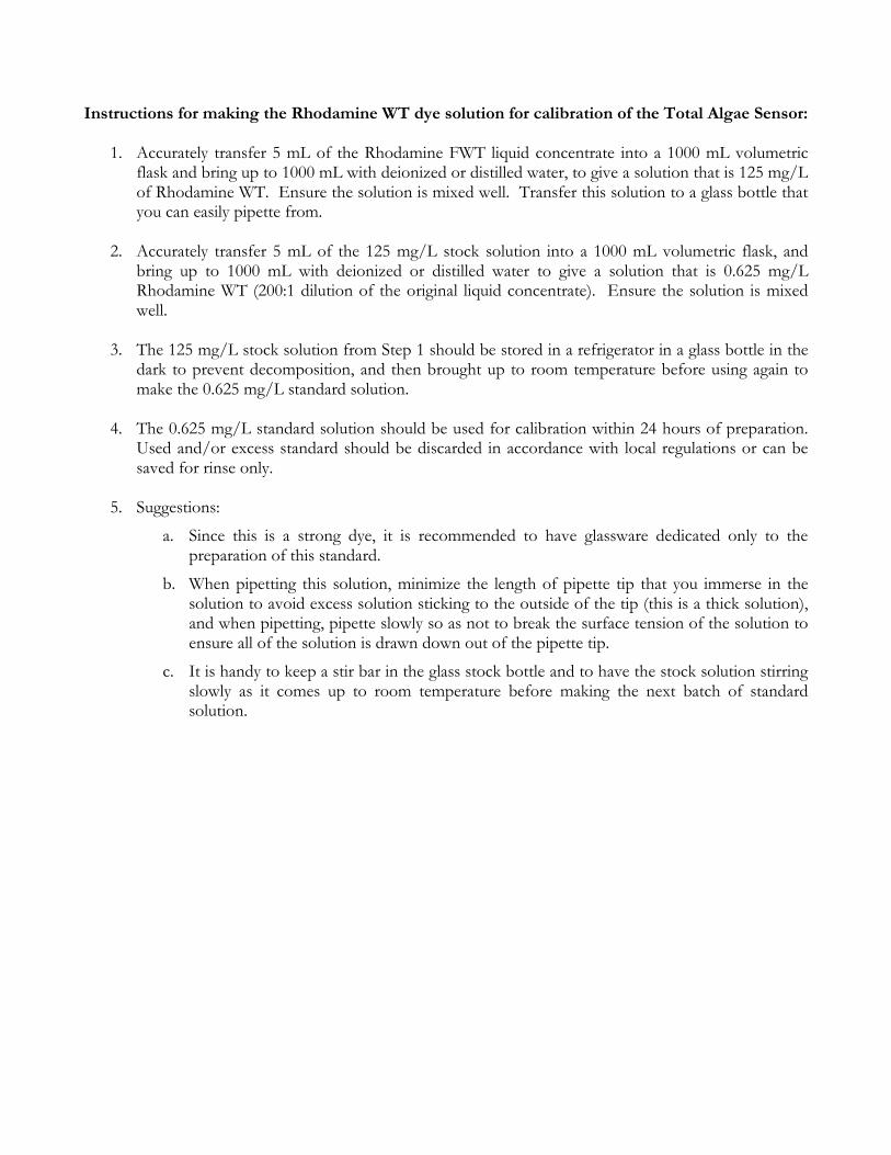
Instructions for making the Rhodamine WT dye solution for calibration of the Total Algae Sensor:
1. Accurately transfer 5 mL of the Rhodamine FWT liquid concentrate into a 1000 mL volumetric flask and bring up to 1000 mL with deionized or distilled water, to give a solution that is 125 mg/L of Rhodamine WT. Ensure the solution is mixed well. Transfer this solution to a glass bottle that you can easily pipette from.
2. Accurately transfer 5 mL of the 125 mg/L stock solution into a 1000 mL volumetric flask, and bring up to 1000 mL with deionized or distilled water to give a solution that is 0.625 mg/L Rhodamine WT (200:1 dilution of the original liquid concentrate). Ensure the solution is mixed well.
3. The 125 mg/L stock solution from Step 1 should be stored in a refrigerator in a glass bottle in the
dark to prevent decomposition, and then brought up to room temperature before using again to make the 0.625 mg/L standard solution.
4. The 0.625 mg/L standard solution should be used for calibration within 24 hours of preparation.
Used and/or excess standard should be discarded in accordance with local regulations or can be saved for rinse only.
5. Suggestions:
a. Since this is a strong dye, it is recommended to have glassware dedicated only to the preparation of this standard.
b. When pipetting this solution, minimize the length of pipette tip that you immerse in the solution to avoid excess solution sticking to the outside of the tip (this is a thick solution), and when pipetting, pipette slowly so as not to break the surface tension of the solution to ensure all of the solution is drawn down out of the pipette tip.
c. It is handy to keep a stir bar in the glass stock bottle and to have the stock solution stirring slowly as it comes up to room temperature before making the next batch of standard solution.

Effect of temperature on fluorescence The effect of temperature on the fluorescence of Rhodamine WT dye must be accounted for when calibrating the EXO Total-Algae sensor. The table below gives the µg/L value that corresponds to the temperature of the calibration standard.
Temp (oC) µg/L Chl RFU Chl
30 56.5 14.0
28 58.7 14.6
26 61.3 15.2
24 63.5 15.8
22 66.0 16.4
20 68.4 17.0
18 70.8 17.6
16 73.5 18.3
14 76.0 18.9
12 78.6 19.5
10 81.2 20.2
8 83.8 20.8 Two point calibration for chlorophyll-a µg/L - This calibration procedure zeroes the fluorescence sensor and uses the default sensitivity of the sensor to only semi-quantitatively calculate chlorophyll concentration in µg/L.
1. Using a NIST traceable thermometer, measure the temperature of your Rhodamine WT standard solution and using the included table, cross reference that temperature to the appropriate µg/L Chl value for Rhodamine WT.
2. In KOR, select CALIBRATE.
3. Choose BGA-PC/Chlor (or -PE depending on which sensor you have).
4. Choose Chlorophyll µg/L. If you have both units of measure, RFU and µg/L selected for the display of chlorophyll values, you must calibrate chlorophyll twice for EACH unit, RFU and µg/L to completely calibrate this parameter. Units of measure can be turned on/off under OPTIONS -> UNITS -> CHL.
5. Choose a 2-point calibration and enter the values of your standards in the appropriate boxes.
Standard value 1 would be 0 (deionized water) and standard value 2 would be the chl concentration from the reference table acquired in Step 1. For additional tips on this process, see below.

6. Fill a clean EXO calibration cup with the appropriate amount of deionized water, pouring along the side to minimize bubbles.
7. Rinse all of the sensors well with deionized water and install a clean (preferably calibration
dedicated) black plastic EXO guard with the bottom installed.
8. Slowly lower the guard and sensors into the calibration cup until seated and tighten the seal on the calibration cup. Lift the sonde, and at an angle, gently tap the bottom of the calibration cup against your worktop to dislodge any bubbles from the sensor optics. Visually inspect the optics to ensure there are no bubbles attached that might affect the calibration.
9. Press START CAL.
10. Once the temperature has stabilized and the readings have stabilized, the data should change from
red UNSTABLE DATA to green STABLE DATA. At this point, press APPLY. A popup window with PROCEED to next standard will appear.
11. Remove the sonde from the calibration cup.
12. Pour a small amount of Rhodamine standard into a clean (preferably dedicated) calibration cup
(enough to coat sensors well), and place sonde in to the calibration cup and tighten the collar gasket.
13. Gently invert the sonde several times to coat all of the sensors, bulkhead and connectors with the
standard. Repeat this step twice more with fresh standard rinse.
14. Fill the calibration cup with fresh Rhodamine WT standard to the appropriate volume and, same as in Step 8 above, gently lower the guard and sensors in to the calibration cup, then tap the sonde against your work surface to dislodge any bubbles that may be on the surface of the optics.
15. Press PROCEED and wait for the readings to change from UNSTABLE DATA to STABLE
DATA.
16. Press APPLY.
17. Press COMPLETE.
18. A successful calibration will be indicated by a green check on the calibration summary screen. If a calibration error occurred, indicated by a yellow exclamation point, you will need to redo the calibration. An error could be caused by the sonde reading too high or low compared to the standard value, and could be caused by improperly made standard, contaminated standard or bubbles on the optics.
19. If your calibration is successful, be sure to record your pre-calibration and post-calibration values
for entry into your CDMO digital calibration logs.
20. Save the used and any unused Rhodamine WT standard for RINSE standard for the next set of calibrations. Remember that the Rhodamine WT must be used within 24 hours of preparation, but can be saved as RINSE ONLY beyond that time.

21. If calibrating RFU, repeat steps 1-17 above using the RFU values from the table above. See calibration tip below for minimizing the amount of standard that you need to prepare and use.
22. Rinse the probes, bulkhead and connectors well with deionized water before calibrating the next
probe or storing the instrument. CALIBRATION TIP: If calibrating both µg/L and RFU, you may conserve standard by doing a reverse calibration on your second unit. For example, you would do a 2-point calibration, deionized water (pt 1) and Rhodamine WT (pt 2) for RFU. Then, leaving the instrument in the Rhodamine WT, you can do a 2 point-calibration for µg/L using the Rhodamine WT as your 1st point and deionized water (zero) as your 2nd point. This is especially helpful if you have multiple chlorophyll probes to calibrate and are doing a batch calibration on one instrument.

Appendix K


