water

Article

Groundwater Level Prediction Using a Multiple ObjectiveGenetic Algorithm-Grey Relational Analysis Based WeightedEnsemble of ANFIS Models

Dilip Kumar Roy 1,*, Sujit Kumar Biswas 1, Mohamed A. Mattar 2,3,4 , Ahmed A. El-Shafei 2,4,5 ,Khandakar Faisal Ibn Murad 1 , Kowshik Kumar Saha 6,7 , Bithin Datta 8 and Ahmed Z. Dewidar 4,*

�����������������

Citation: Roy, D.K.; Biswas, S.K.;

Mattar, M.A.; El-Shafei, A.A.; Murad,

K.F.I.; Saha, K.K.; Datta, B.; Dewidar,

A.Z. Groundwater Level Prediction

Using a Multiple Objective Genetic

Algorithm-Grey Relational Analysis

Based Weighted Ensemble of ANFIS

Models. Water 2021, 13, 3130.

https://doi.org/10.3390/w13213130

Academic Editors: Hakan Basagaoglu,

Debaditya Chakraborty and Marcio

Giacomoni

Received: 15 September 2021

Accepted: 2 November 2021

Published: 6 November 2021

Publisher’s Note: MDPI stays neutral

with regard to jurisdictional claims in

published maps and institutional affil-

iations.

Copyright: © 2021 by the authors.

Licensee MDPI, Basel, Switzerland.

This article is an open access article

distributed under the terms and

conditions of the Creative Commons

Attribution (CC BY) license (https://

creativecommons.org/licenses/by/

4.0/).

1 Irrigation and Water Management Division, Bangladesh Agricultural Research Institute,Gazipur 1701, Bangladesh; sujitbari@yahoo.com (S.K.B.); faisal.ae.bau@gmail.com (K.F.I.M.)

2 Department of Agricultural Engineering, College of Food and Agriculture Sciences, King Saud University,Riyadh 11451, Saudi Arabia; mmattar@ksu.edu.sa (M.A.M.); aelshafei1bn.c@ksu.edu.sa (A.A.E.-S.)

3 Agricultural Research Centre, Agricultural Engineering Research Institute (AEnRI), Giza 12618, Egypt4 Prince Sultan Institute for Environmental, Water and Desert Research, King Saud University, P.O. Box 2454,

Riyadh 11451, Saudi Arabia5 Department of Agricultural Engineering, Faculty of Agriculture (El-Shatby), Alexandria University,

Alexandria 21545, Egypt6 Faculty V, Technische Universität Berlin, Straße des 17. Juni 135, 10623 Berlin, Germany;

kksaha.bari@gmail.com7 ASICT Division, Bangladesh Agricultural Research Institute, Gazipur 1701, Bangladesh8 Discipline of Civil Engineering, College of Science and Engineering, James Cook University,

Townsville, QLD 4811, Australia; bithin.datta@jcu.edu.au* Correspondence: dilip.roy@my.jcu.edu.au (D.K.R.); adewidar@ksu.edu.sa (A.Z.D.)

Abstract: Predicting groundwater levels is critical for ensuring sustainable use of an aquifer’s limitedgroundwater reserves and developing a useful groundwater abstraction management strategy. Thepurpose of this study was to assess the predictive accuracy and estimation capability of variousmodels based on the Adaptive Neuro Fuzzy Inference System (ANFIS). These models includedDifferential Evolution-ANFIS (DE-ANFIS), Particle Swarm Optimization-ANFIS (PSO-ANFIS), andtraditional Hybrid Algorithm tuned ANFIS (HA-ANFIS) for the one- and multi-week forwardforecast of groundwater levels at three observation wells. Model-independent partial autocorrelationfunctions followed by frequentist lasso regression-based feature selection approaches were used torecognize appropriate input variables for the prediction models. The performances of the ANFISmodels were evaluated using various statistical performance evaluation indexes. The results revealedthat the optimized ANFIS models performed equally well in predicting one-week-ahead groundwaterlevels at the observation wells when a set of various performance evaluation indexes were used.For improving prediction accuracy, a weighted-average ensemble of ANFIS models was proposed,in which weights for the individual ANFIS models were calculated using a Multiple ObjectiveGenetic Algorithm (MOGA). The MOGA accounts for a set of benefits (higher values indicate bettermodel performance) and cost (smaller values indicate better model performance) performanceindexes calculated on the test dataset. Grey relational analysis was used to select the best solutionfrom a set of feasible solutions produced by a MOGA. A MOGA-based individual model rankingrevealed the superiority of DE-ANFIS (weight = 0.827), HA-ANFIS (weight = 0.524), and HA-ANFIS (weight = 0.697) at observation wells GT8194046, GT8194048, and GT8194049, respectively.Shannon’s entropy-based decision theory was utilized to rank the ensemble and individual ANFISmodels using a set of performance indexes. The ranking result indicated that the ensemble modeloutperformed all individual models at all observation wells (ranking value = 0.987, 0.985, and 0.995at observation wells GT8194046, GT8194048, and GT8194049, respectively). The worst performerswere PSO-ANFIS (ranking value = 0.845), PSO-ANFIS (ranking value = 0.819), and DE-ANFIS(ranking value = 0.900) at observation wells GT8194046, GT8194048, and GT8194049, respectively.The generalization capability of the proposed ensemble modelling approach was evaluated forforecasting 2-, 4-, 6-, and 8-weeks ahead groundwater levels using data from GT8194046. Theevaluation results confirmed the useability of the ensemble modelling for forecasting groundwater

Water 2021, 13, 3130. https://doi.org/10.3390/w13213130 https://www.mdpi.com/journal/water

Water 2021, 13, 3130 2 of 35

levels at higher forecasting horizons. The study demonstrated that the ensemble approach maybe successfully used to predict multi-week-ahead groundwater levels, utilizing previous laggedgroundwater levels as inputs.

Keywords: groundwater level predictions; multiple objective genetic algorithm; evolutionaryalgorithm optimized ANFIS; ensemble prediction; entropy

1. Introduction

Groundwater aquifers are considered as vital sources of the world’s potable water sup-plies and take part in an essential role in the sustainability of irrigated agriculture; domesticand industrial water supplies in areas where good quality surface water is inadequate.Human pressure due to population growth, increasing water demand to different sectors,and a changing climate have created an enhanced pressure on groundwater resources. As aconsequence, groundwater systems are experiencing rapid degradation. Although humanintervention, such as over-pumping, is considered as the prime indicator of groundwaterlevel declination, climate change, as evidenced by recent projections, has indicated that thesituation will become even worse earlier than was anticipated [1]. Excessive abstraction ofgroundwater resources leads to continuous depletion and variable fluctuations of ground-water level, causing a variety of problems such as lowering of the suction heads of pumps,reduction of crop yields due to inadequate irrigation water supplies, decrease in potablewater supplies for domestic and industrial purposes, and degradation of water quality,among others. As with many areas in the world, groundwater is the most importantusable form of water reserves in Bangladesh, where approximately 80% of the total popula-tion depends primarily on the groundwater reserves for their water needs [2]. Therefore,proper management and sustainable utilization of the scanty groundwater reserves in theaquifer in an efficient manner are imperative to secure continuous supplies of groundwaterfor future generations. Accurate prediction and forecasting of future groundwater levelfluctuations may aid in developing such a meaningful groundwater management strategy.

Numerical simulation models of groundwater flow processes have traditionally beenapplied in groundwater hydrology to better understand the underlying system processeswhile predicting the future scenarios of groundwater levels [3–5]. However, predictinggroundwater levels using these physically-based models require a detailed understandingof the aquifer properties, as well as expertise and in-depth knowledge of the modelerabout the aquifer geometry and modelling techniques. It is often difficult to obtain relevantand good quality data on aquifer properties and other appropriate prerequisites, i.e.,model “initial and boundary conditions” required to develop physically-based models.Sometimes, unavailable data are substituted by assumptions made on the data based onthe prior knowledge of the modeler regarding the model domain. These assumptions andestimations may lead to difficulties in the calibration and validation processes, which arevery important in employing the developed model for prediction purposes. To overcomethese unavoidable complexities associated with physically-based numerical modellingapproaches, data-driven prediction modelling approaches relying on machine-learning andartificial intelligence have been introduced and applied in hydrology [6–12]. Data-drivenmodelling does not require an explicit definition of the parameters of the physical systemsbeing modelled. In data-driven modelling approaches, a direct mapping or correlationbetween the predictors (inputs) and responses (outputs) of a model is established by wayof an iterative learning method of a machine-learning algorithm [13]. Artificial NeuralNetworks (ANN)-based data-driven prediction models have been found to perform as goodas or even better than the physically-based simulation models in the field of predictionof nonlinear time series data, e.g., groundwater table data [14,15]. As such, there hasbeen a growing appreciation that data-driven approaches can be utilized as an alternative

Water 2021, 13, 3130 3 of 35

modelling approach for capturing nonlinear dynamics of the aquifer responses quiteaccurately [16–19].

Groundwater level prediction comes into play when it is an essential task to evaluatethe dynamics of the groundwater system, i.e., how much groundwater is being abstractedfrom the aquifer system and how much is permitted to be abstracted. Adequately preciseshort- to medium-term groundwater level prediction aids in developing a sustainable andflexible management strategy in areas where climate change-induced droughts or human-induced over-pumping is a major driving force [20–22]. Thus, groundwater level predictionhas been an interesting topic in the hydrological research area. Numerous data-driven mod-elling methods are being increasingly used since they require less data and are easier to ap-ply than conventional hydrogeological modelling methodologies [23]. Several approacheshave recently been utilized in the research domain of groundwater level predictions. Theseinclude machine learning-based prediction modelling [21,22,24], ANNs [25–27], hybridizedwavelet transform—machine learning methods [16,28–30], hybridized ensemble empiricalmode decomposition and machine learning-based models [31], nonlinear autoregressivewith exogenous inputs (NARX) neural networks [21], ARIMA-particle swarm optimiza-tion [32], ANN—whale algorithm [33], integrated linear polynomial and nonlinear systemidentification models [34], ANFIS [30,35–38], wavelet—ANFIS [39], Support Vector Ma-chine (SVM) [35,40], hybrid SVM-PSO [41], Gaussian Process Regression [30], GeneticProgramming [42], Facebook’s prophet approach of groundwater level forecasting [43],physics-inspired coupled space-time artificial neural networks [44]. A detailed review ofartificial intelligence-based approaches to groundwater level modelling is given in [45]. Itis obvious that a variety of modelling methodologies have been used to anticipate ground-water level fluctuations with differing degrees of prediction accuracies. It is also clearthat recommending a specific prediction model for a specific problem, such as predictinggroundwater level fluctuations, is difficult, if not impossible. Therefore, more advancedapproaches to groundwater level prediction are necessary for increasing the predictionaccuracy of groundwater level fluctuations.

A hybrid/coupled model or an ensemble of models is likely to perform better than anindividual prediction model [45]. Different types of prediction models may be developedfor groundwater level forecasting and the best-performing models may be selected tocombine them into an ensemble to have an optimum model performance. However, it isoften very difficult, if not impossible, to identify the best machine-learning algorithm-basedprediction models. In such cases, one of the most effective strategies for providing suffi-ciently accurate predictions has been to integrate the predictions of known best predictionmodels. Such integration of prediction models is generally referred to as an ensemble [46].Ensemble predictions are believed to be more robust than a standalone prediction modelwith respect to grabbing hold of the true relationships between the inputs and outputs ofa given prediction problem through incorporating the best features of the participatingprediction models. Ensemble approaches include boosting, bagging, ranking, voting, andstacking [47]. In groundwater level forecasting, [28] utilized a least-square boosting algo-rithm to integrate different wavelet-neural network models. The present study seeks toemploy a Multiple Objective Genetic Algorithm (MOGA) for integrating the predictionpower of the evolutionary algorithm tuned ANFIS models in the framework of an ensembleprediction to predict one- and multi-week ahead groundwater levels.

An ensemble of data-driven prediction models can be created utilizing a simpleaveraging approach [48,49], in which the prediction of the selected individual models iscombined by simply averaging the individual outputs. On the other hand, an ensembleof individual models can be formed by assigning weights to individual models withreference to their prediction precision [46,50]. Among them, the weighted average ensembleapproach has gained popularity as it assigns weights to single prediction models regardingtheir prediction precision. Specific weights to single prediction models may be assignedthrough the utilization of the concepts of entropy [51], set pair analysis [52], or Dempster–Shafer evidence theory [53,54]. Another approach of assigning weights to individual

Water 2021, 13, 3130 4 of 35

models is the utilization of a population-based optimization algorithm such as GeneticAlgorithm (GA) [55], which is employed to find out the optimum weights with respectto either minimizing a cost index (the lower, the better) or maximizing a benefit index(the higher, the better). GA has previously been applied to allocate specific weights tostandalone models based on a single performance index, e.g., MAE or RMSE [56]. However,the utilization of a single performance index in determining the weights is often not asuitable choice due to the conflicting nature of performance indexes. For instance, amodel will possibly be regarded as the top performer among other models when a specificperformance evaluation index is considered. In contrast, a different model may wellbe found as the worthiest model when another performance index is considered. Thisconflicting characteristic demands the incorporation of a set of performance indexes indetermining the weights assigned to different individual prediction models for developingan integrated prediction model. Previous studies have successfully utilized the concepts ofentropy weight [57] and Dempster–Shafer’s theory of evidence [58,59] for incorporatingdifferent performance indexes of many prediction models to compute individual modelweights. In this study, a Multiple Objective GA (MOGA) [60] is utilized to develop a trade-off between the benefits (the larger the values, the better will be the model predictions)and the cost indexes (the smaller the values, the better will be the model predictions). Theconflicting objective functions considered are to maximize the sum of benefit indexes andto minimize the sum of cost indexes. The variables are the associated weights of individualmodels. The MOGA provides numerous alternate feasible solutions rather than a singlesolution. The best solution from the set of feasible solutions is selected by applying theconcept of Grey Relational Analysis. To the best of the author’s understanding, this methodof weight assignment in the weighted average ensemble technique has not been appliedpreviously in predicting groundwater levels.

Although long-term groundwater level prediction is desirable in many applications,including the development of groundwater management plans, short-term predictionsoften provide valuable insights into groundwater level fluctuations to better understand theunderlying physical phenomena of an aquifer [15,25,61,62]. However, since the one-step-ahead prediction is strongly conditioned by exogeneous variables containing the stochasticcomponent, the generalization capability of the proposed model needs to be investigatedfor multi-step ahead prediction horizons. Because groundwater flow and levels typicallydo not vary significantly over a short period [63], the present study aims at proposingboth short-term (one-week ahead) and medium-term (2–8-weeks ahead) groundwater levelforecasts using novel approaches.

The key motivation and focus of this study are to (1) delve into the potential ofoptimized ANFIS models in predicting one- and multi-step ahead groundwater level in theselected observation wells; (2) develop an ensemble of evolutionary algorithm optimizedANFIS models through weights assigned by a MOGA by incorporating a set of differentperformance indexes; and (3) provide a ranking of the ensemble and the individual ANFISmodels through Shannon’s entropy. To the best of the authors’ understanding, this isthe first time an ensemble of optimized ANFIS models (weighted average ensemble forwhich a MOGA determines the associated weights) has been employed to forecast one-step(one-week) and multi-step (multiple weeks) forward groundwater level fluctuations.

2. Methodology2.1. Study Area and the Data

The study area, located between 24.46–24.73◦ N latitudes and between 88.40–88.65◦

E longitudes, is under the Tanore Upazila of Rajshahi district in the division of Rajshahi,Bangladesh. It has an aerial extent of 295.40 km2. A river named Shiba flows across thestudy area, which provides an inadequate amount of irrigation water for irrigating themajor crops. Barind Tract constitutes a major portion (81.8%) of the geologic formation. Incomparison, Old Gangetic Floodplain (3%) and Tista Floodplain (4.8%) cover only a smallportion of the geology. The remaining 10.4% of the entire area is occupied by homestead

Water 2021, 13, 3130 5 of 35

areas, ponds, wetlands, and rivers [64]. The land formation of Tanore Upazila is composedmainly of clay loam (46%), loam (35%), and clay (8%) [65]. Pumped groundwater appears tobe the prime water resource for household usage and crop irrigation. Excessive abstractionof groundwater from the aquifer has been increasing every year, resulting in the gradualdeclination of groundwater levels. As the study area is categorized as a flood-free zone inBangladesh due to its high elevation with respect to the mean sea level, monsoon rainfall isthe only source of water that can be percolated to the water-bearing strata to recharge thegroundwater. However, the study area’s thick and sticky clay surface is not favourable forthe natural recharge of groundwater into the aquifer. The combined interaction of the lowrecharge potential of the land formation, inadequate rainfall, and increased groundwaterabstraction result in a decline in groundwater level in the Tanore Upazila of Rajshahidistrict (the study area).

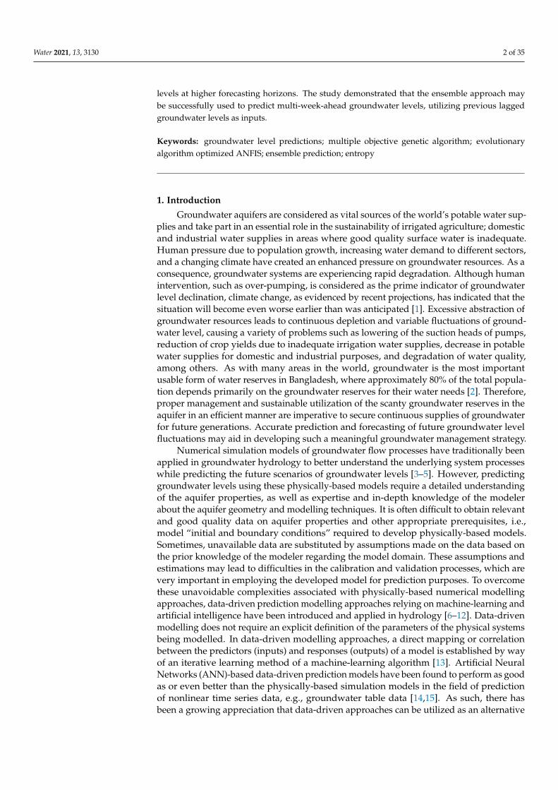
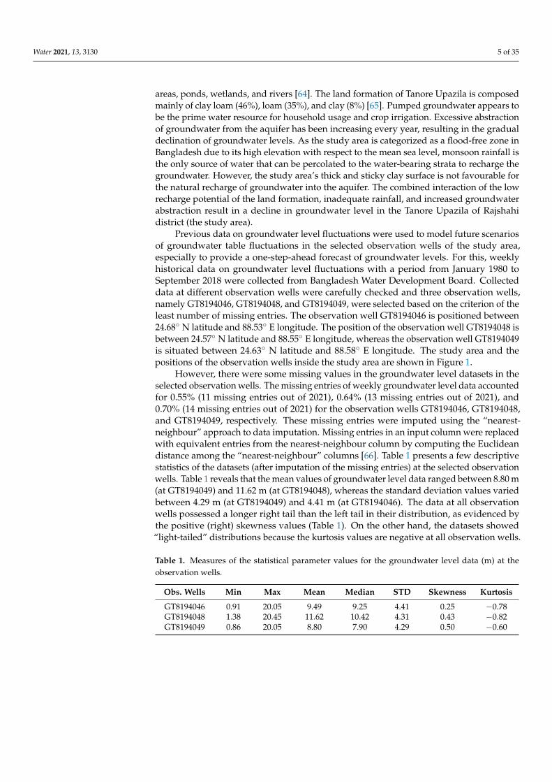
Previous data on groundwater level fluctuations were used to model future scenariosof groundwater table fluctuations in the selected observation wells of the study area,especially to provide a one-step-ahead forecast of groundwater levels. For this, weeklyhistorical data on groundwater level fluctuations with a period from January 1980 toSeptember 2018 were collected from Bangladesh Water Development Board. Collecteddata at different observation wells were carefully checked and three observation wells,namely GT8194046, GT8194048, and GT8194049, were selected based on the criterion of theleast number of missing entries. The observation well GT8194046 is positioned between24.68◦ N latitude and 88.53◦ E longitude. The position of the observation well GT8194048 isbetween 24.57◦ N latitude and 88.55◦ E longitude, whereas the observation well GT8194049is situated between 24.63◦ N latitude and 88.58◦ E longitude. The study area and thepositions of the observation wells inside the study area are shown in Figure 1.

However, there were some missing values in the groundwater level datasets in theselected observation wells. The missing entries of weekly groundwater level data accountedfor 0.55% (11 missing entries out of 2021), 0.64% (13 missing entries out of 2021), and0.70% (14 missing entries out of 2021) for the observation wells GT8194046, GT8194048,and GT8194049, respectively. These missing entries were imputed using the “nearest-neighbour” approach to data imputation. Missing entries in an input column were replacedwith equivalent entries from the nearest-neighbour column by computing the Euclideandistance among the “nearest-neighbour” columns [66]. Table 1 presents a few descriptivestatistics of the datasets (after imputation of the missing entries) at the selected observationwells. Table 1 reveals that the mean values of groundwater level data ranged between 8.80 m(at GT8194049) and 11.62 m (at GT8194048), whereas the standard deviation values variedbetween 4.29 m (at GT8194049) and 4.41 m (at GT8194046). The data at all observationwells possessed a longer right tail than the left tail in their distribution, as evidenced bythe positive (right) skewness values (Table 1). On the other hand, the datasets showed“light-tailed” distributions because the kurtosis values are negative at all observation wells.

Table 1. Measures of the statistical parameter values for the groundwater level data (m) at theobservation wells.

Obs. Wells Min Max Mean Median STD Skewness Kurtosis

GT8194046 0.91 20.05 9.49 9.25 4.41 0.25 −0.78GT8194048 1.38 20.45 11.62 10.42 4.31 0.43 −0.82GT8194049 0.86 20.05 8.80 7.90 4.29 0.50 −0.60

Water 2021, 13, 3130 6 of 35Water 2021, 13, 3130 6 of 36

Figure 1. Schematic representation of the study area.

However, there were some missing values in the groundwater level datasets in the

selected observation wells. The missing entries of weekly groundwater level data ac-

counted for 0.55% (11 missing entries out of 2021), 0.64% (13 missing entries out of 2021),

and 0.70% (14 missing entries out of 2021) for the observation wells GT8194046,

GT8194048, and GT8194049, respectively. These missing entries were imputed using the

“nearest-neighbour” approach to data imputation. Missing entries in an input column

were replaced with equivalent entries from the nearest-neighbour column by computing

the Euclidean distance among the “nearest-neighbour” columns. [66]. Table 1 presents a

few descriptive statistics of the datasets (after imputation of the missing entries) at the

selected observation wells. Table 1 reveals that the mean values of groundwater level data

ranged between 8.80 m (at GT8194049) and 11.62 m (at GT8194048), whereas the standard

deviation values varied between 4.29 m (at GT8194049) and 4.41 m (at GT8194046). The

data at all observation wells possessed a longer right tail than the left tail in their distri-

bution, as evidenced by the positive (right) skewness values (Table 1). On the other hand,

the datasets showed “light-tailed” distributions because the kurtosis values are negative

at all observation wells.

Figure 1. Schematic representation of the study area.

2.1.1. Missing Value Imputation

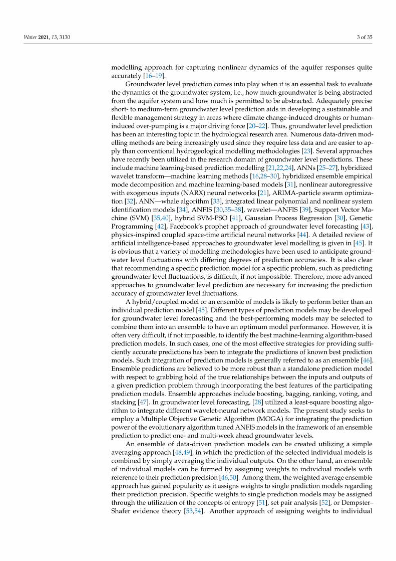
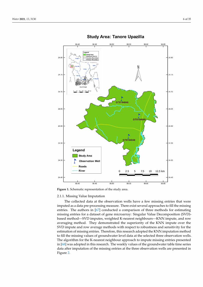
The collected data at the observation wells have a few missing entries that wereimputed as a data pre-processing measure. There exist several approaches to fill the missingentries. The authors in [67] conducted a comparison of three methods for estimatingmissing entries for a dataset of gene microarray: Singular Value Decomposition (SVD)-based method—SVD imputes, weighted K-nearest neighbours—KNN impute, and rowaveraging method. They demonstrated the superiority of the KNN impute over theSVD impute and row average methods with respect to robustness and sensitivity for theestimation of missing entries. Therefore, this research adopted the KNN imputation methodto fill the missing values of groundwater level data at the selected three observation wells.The algorithm for the K-nearest neighbour approach to impute missing entries presentedin [68] was adopted in this research. The weekly values of the groundwater table time seriesdata after imputation of the missing entries at the three observation wells are presented inFigure 2.

Water 2021, 13, 3130 7 of 35

Water 2021, 13, 3130 7 of 36

Table 1. Measures of the statistical parameter values for the groundwater level data (m) at the ob-

servation wells.

Obs. Wells Min Max Mean Median STD Skewness Kurtosis

GT8194046 0.91 20.05 9.49 9.25 4.41 0.25 −0.78

GT8194048 1.38 20.45 11.62 10.42 4.31 0.43 −0.82

GT8194049 0.86 20.05 8.80 7.90 4.29 0.50 −0.60

2.1.1. Missing Value Imputation

The collected data at the observation wells have a few missing entries that were im-

puted as a data pre-processing measure. There exist several approaches to fill the missing

entries. The authors in [67] conducted a comparison of three methods for estimating miss-

ing entries for a dataset of gene microarray: Singular Value Decomposition (SVD)-based

method—SVD imputes, weighted K-nearest neighbours—KNN impute, and row averag-

ing method. They demonstrated the superiority of the KNN impute over the SVD impute

and row average methods with respect to robustness and sensitivity for the estimation of

missing entries. Therefore, this research adopted the KNN imputation method to fill the

missing values of groundwater level data at the selected three observation wells. The al-

gorithm for the K-nearest neighbour approach to impute missing entries presented in [68]

was adopted in this research. The weekly values of the groundwater table time series data

after imputation of the missing entries at the three observation wells are presented in Fig-

ure 2.

Figure 2. Time series of the groundwater level data.

It is observed from Figure 2 that the groundwater level data at all three observation

wells have some noisy data, especially at the later part of the time series. This noise in the

input data was intentionally kept to evaluate the prediction power of the suggested ma-

chine-learning algorithms on the noisy input data. As such, no data smoothing operation

was performed on the input time series (weekly values) of the groundwater level data.

2.1.2. Selection of Input Variables

The most significant and pertinent aspect in creating machine-learning-based predic-

tion models should be the choice of suitable input variables from a list of candidate input

variables that may enhance the prediction capability of models. As there exists no explicit

approach to determining model inputs for data-driven modelling applications [69], sev-

eral methods were adopted and applied by various researchers. It is also noted that useful

Figure 2. Time series of the groundwater level data.

It is observed from Figure 2 that the groundwater level data at all three observationwells have some noisy data, especially at the later part of the time series. This noise inthe input data was intentionally kept to evaluate the prediction power of the suggestedmachine-learning algorithms on the noisy input data. As such, no data smoothing operationwas performed on the input time series (weekly values) of the groundwater level data.

2.1.2. Selection of Input Variables

The most significant and pertinent aspect in creating machine-learning-based predic-tion models should be the choice of suitable input variables from a list of candidate inputvariables that may enhance the prediction capability of models. As there exists no explicitapproach to determining model inputs for data-driven modelling applications [69], severalmethods were adopted and applied by various researchers. It is also noted that usefulinput variable selection approaches are non-unique and different techniques may resultin different combinations of important input variables [44]. A two-step approach can beadopted in selecting the most useful input variables [70]: utilization of Autocorrelation andPartial Autocorrelation Functions (PACF) (to obtain time-lagged information), followedby a “trial and error” approach, wherein several possible combinations of preselectedlags can be used as model inputs. However, evaluating each of the combinations usingseveral data-driven models to select the significant input variables is undoubtedly a time-consuming and laborious task. As an improvement to this laborious and computationallyintensive input variable selection method, the present study adopts Frequentist LassoRegression (FLR) [71] performed on the preselected lags (using PACF) for determiningthe most significant input variables. The proposed approach, utilizing the combination ofPACF and the FLR, is outlined below:

1. Partial autocorrelations (PACF)

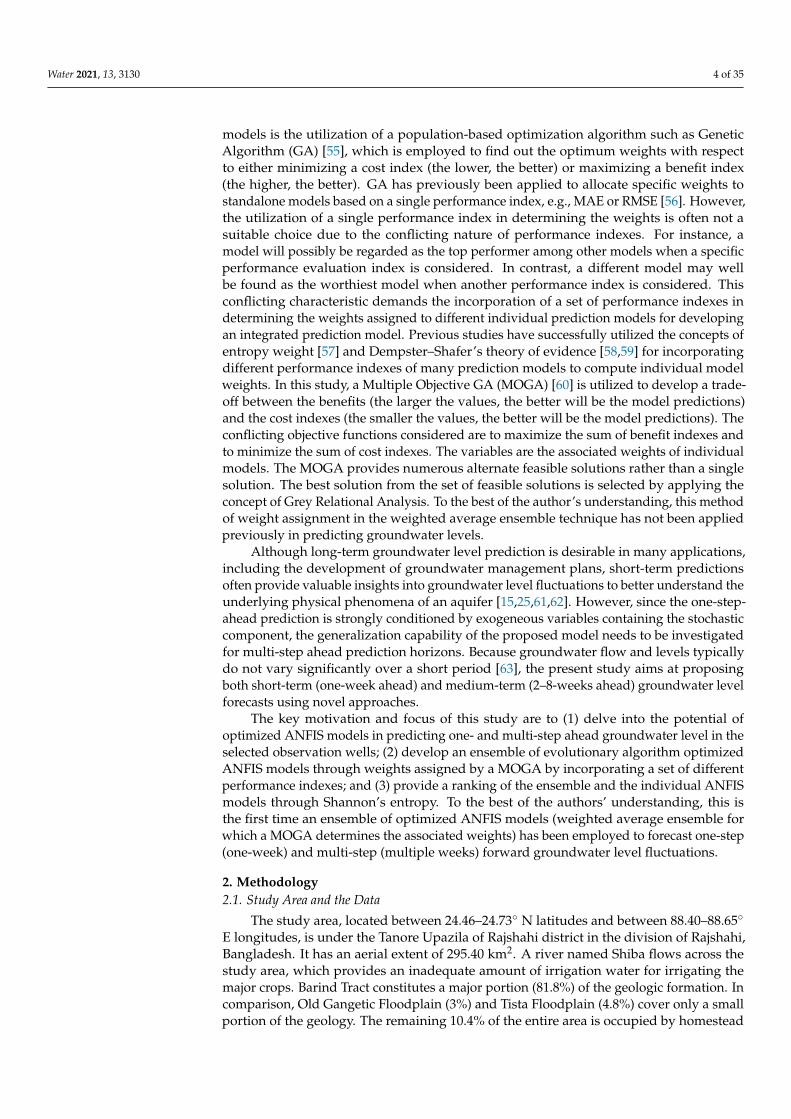
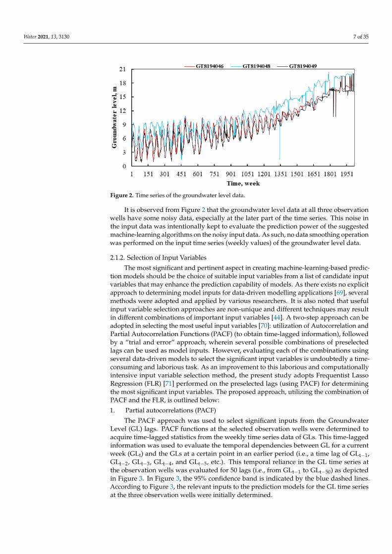
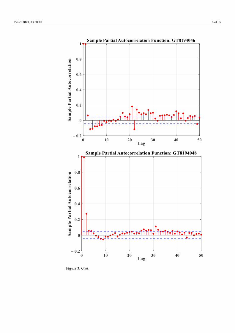
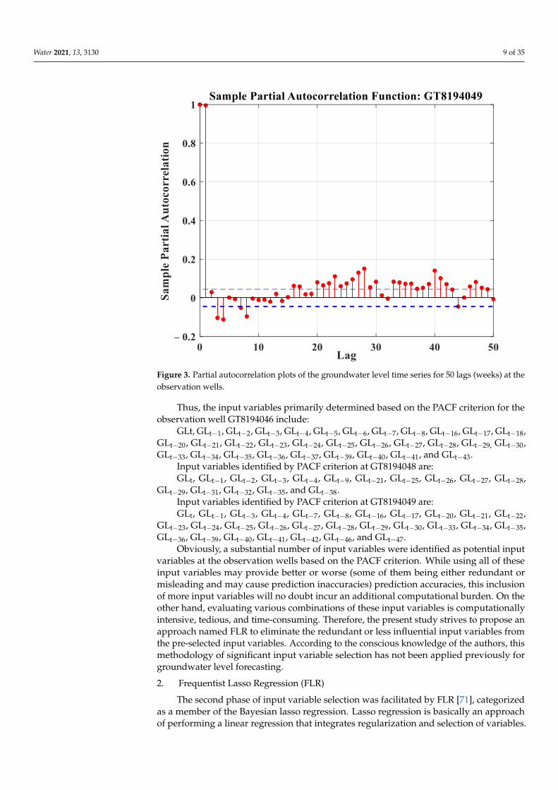
The PACF approach was used to select significant inputs from the GroundwaterLevel (GL) lags. PACF functions at the selected observation wells were determined toacquire time-lagged statistics from the weekly time series data of GLs. This time-laggedinformation was used to evaluate the temporal dependencies between GL for a currentweek (GLt) and the GLs at a certain point in an earlier period (i.e., a time lag of GLt−1,GLt−2, GLt−3, GLt−4, and GLt−5, etc.). This temporal reliance in the GL time series atthe observation wells was evaluated for 50 lags (i.e., from GLt−1 to GLt−50) as depictedin Figure 3. In Figure 3, the 95% confidence band is indicated by the blue dashed lines.According to Figure 3, the relevant inputs to the prediction models for the GL time seriesat the three observation wells were initially determined.

Water 2021, 13, 3130 8 of 35Water 2021, 13, 3130 9 of 36

Figure 3. Cont.

Water 2021, 13, 3130 9 of 35Water 2021, 13, 3130 10 of 36

Figure 3. Partial autocorrelation plots of the groundwater level time series for 50 lags (weeks) at the observation wells.

Thus, the input variables primarily determined based on the PACF criterion for the

observation well GT8194046 include:

GLt, GLt − 1, GLt − 2, GLt − 3, GLt − 4, GLt − 5, GLt − 6, GLt − 7, GLt − 8, GLt − 16, GLt − 17, GLt − 18, GLt − 20,

GLt − 21, GLt − 22, GLt − 23, GLt − 24, GLt − 25, GLt − 26, GLt − 27, GLt − 28, GLt − 29, GLt − 30, GLt − 33, GLt − 34,

GLt − 35, GLt − 36, GLt − 37, GLt − 39, GLt − 40, GLt − 41, and GLt − 43.

Input variables identified by PACF criterion at GT8194048 are:

GLt, GLt − 1, GLt − 2, GLt − 3, GLt − 4, GLt − 9, GLt − 21, GLt − 25, GLt − 26, GLt − 27, GLt − 28, GLt − 29, GLt − 31,

GLt − 32, GLt − 35, and GLt − 38.

Input variables identified by PACF criterion at GT8194049 are:

GLt, GLt − 1, GLt − 3, GLt − 4, GLt − 7, GLt − 8, GLt − 16, GLt − 17, GLt − 20, GLt − 21, GLt − 22, GLt − 23, GLt − 24,

GLt − 25, GLt − 26, GLt − 27, GLt − 28, GLt − 29, GLt − 30, GLt − 33, GLt − 34, GLt − 35, GLt − 36, GLt − 39, GLt − 40,

GLt − 41, GLt − 42, GLt − 46, and GLt − 47.

Obviously, a substantial number of input variables were identified as potential input

variables at the observation wells based on the PACF criterion. While using all of these

input variables may provide better or worse (some of them being either redundant or

misleading and may cause prediction inaccuracies) prediction accuracies, this inclusion of

more input variables will no doubt incur an additional computational burden. On the

other hand, evaluating various combinations of these input variables is computationally

intensive, tedious, and time-consuming. Therefore, the present study strives to propose

an approach named FLR to eliminate the redundant or less influential input variables

from the pre-selected input variables. According to the conscious knowledge of the au-

thors, this methodology of significant input variable selection has not been applied previ-

ously for groundwater level forecasting.

2. Frequentist Lasso Regression (FLR)

Figure 3. Partial autocorrelation plots of the groundwater level time series for 50 lags (weeks) at theobservation wells.

Thus, the input variables primarily determined based on the PACF criterion for theobservation well GT8194046 include:

GLt, GLt−1, GLt−2, GLt−3, GLt−4, GLt−5, GLt−6, GLt−7, GLt−8, GLt−16, GLt−17, GLt−18,GLt−20, GLt−21, GLt−22, GLt−23, GLt−24, GLt−25, GLt−26, GLt−27, GLt−28, GLt−29, GLt−30,GLt−33, GLt−34, GLt−35, GLt−36, GLt−37, GLt−39, GLt−40, GLt−41, and GLt−43.

Input variables identified by PACF criterion at GT8194048 are:GLt, GLt−1, GLt−2, GLt−3, GLt−4, GLt−9, GLt−21, GLt−25, GLt−26, GLt−27, GLt−28,

GLt−29, GLt−31, GLt−32, GLt−35, and GLt−38.Input variables identified by PACF criterion at GT8194049 are:GLt, GLt−1, GLt−3, GLt−4, GLt−7, GLt−8, GLt−16, GLt−17, GLt−20, GLt−21, GLt−22,

GLt−23, GLt−24, GLt−25, GLt−26, GLt−27, GLt−28, GLt−29, GLt−30, GLt−33, GLt−34, GLt−35,GLt−36, GLt−39, GLt−40, GLt−41, GLt−42, GLt−46, and GLt−47.

Obviously, a substantial number of input variables were identified as potential inputvariables at the observation wells based on the PACF criterion. While using all of theseinput variables may provide better or worse (some of them being either redundant ormisleading and may cause prediction inaccuracies) prediction accuracies, this inclusionof more input variables will no doubt incur an additional computational burden. On theother hand, evaluating various combinations of these input variables is computationallyintensive, tedious, and time-consuming. Therefore, the present study strives to propose anapproach named FLR to eliminate the redundant or less influential input variables fromthe pre-selected input variables. According to the conscious knowledge of the authors, thismethodology of significant input variable selection has not been applied previously forgroundwater level forecasting.

2. Frequentist Lasso Regression (FLR)

The second phase of input variable selection was facilitated by FLR [71], categorizedas a member of the Bayesian lasso regression. Lasso regression is basically an approachof performing a linear regression that integrates regularization and selection of variables.

Water 2021, 13, 3130 10 of 35

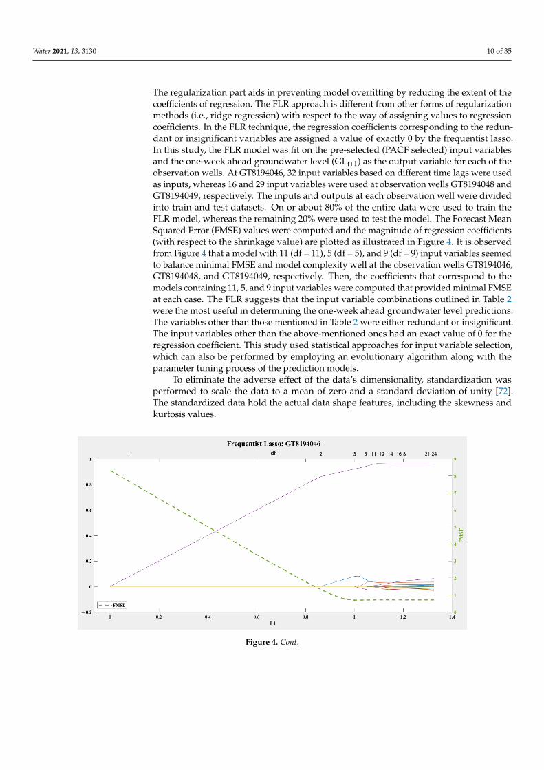
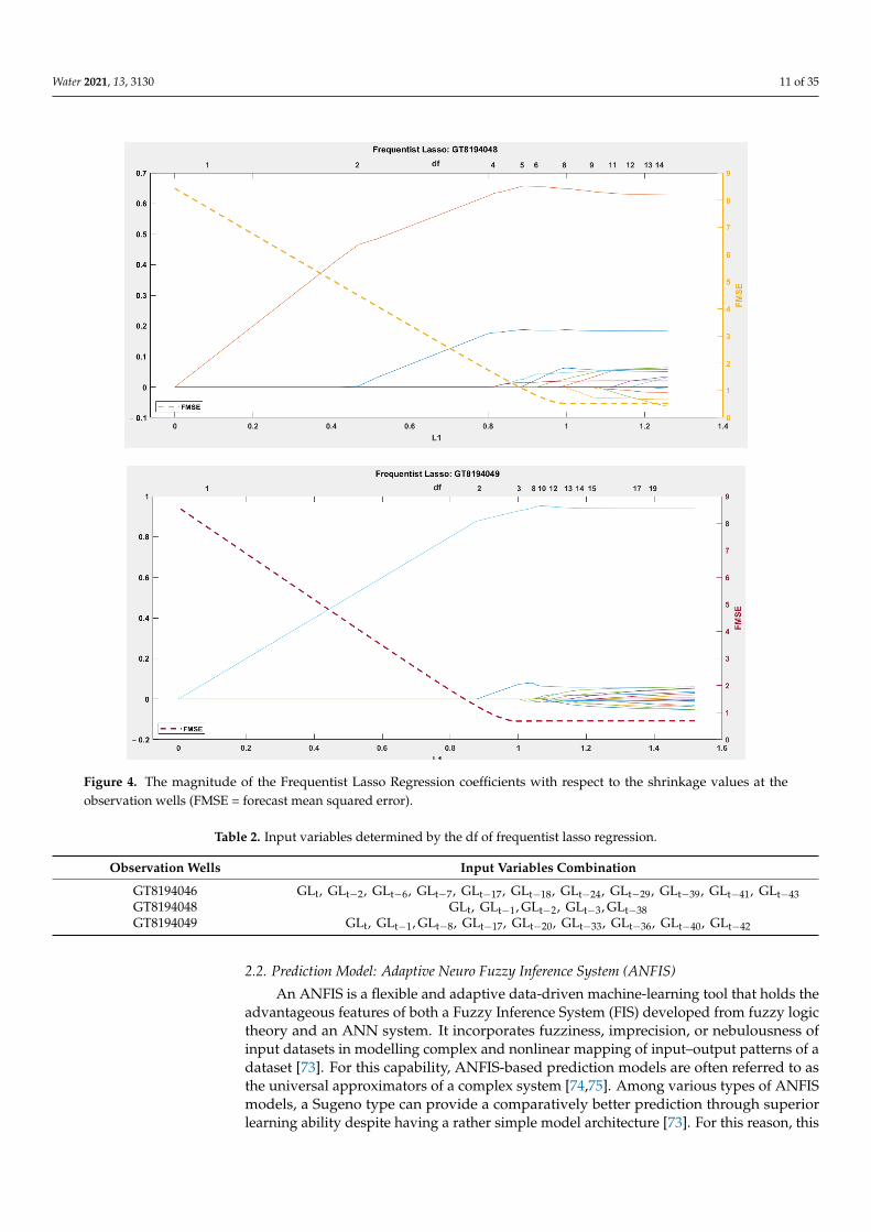
The regularization part aids in preventing model overfitting by reducing the extent of thecoefficients of regression. The FLR approach is different from other forms of regularizationmethods (i.e., ridge regression) with respect to the way of assigning values to regressioncoefficients. In the FLR technique, the regression coefficients corresponding to the redun-dant or insignificant variables are assigned a value of exactly 0 by the frequentist lasso.In this study, the FLR model was fit on the pre-selected (PACF selected) input variablesand the one-week ahead groundwater level (GLt+1) as the output variable for each of theobservation wells. At GT8194046, 32 input variables based on different time lags were usedas inputs, whereas 16 and 29 input variables were used at observation wells GT8194048 andGT8194049, respectively. The inputs and outputs at each observation well were dividedinto train and test datasets. On or about 80% of the entire data were used to train theFLR model, whereas the remaining 20% were used to test the model. The Forecast MeanSquared Error (FMSE) values were computed and the magnitude of regression coefficients(with respect to the shrinkage value) are plotted as illustrated in Figure 4. It is observedfrom Figure 4 that a model with 11 (df = 11), 5 (df = 5), and 9 (df = 9) input variables seemedto balance minimal FMSE and model complexity well at the observation wells GT8194046,GT8194048, and GT8194049, respectively. Then, the coefficients that correspond to themodels containing 11, 5, and 9 input variables were computed that provided minimal FMSEat each case. The FLR suggests that the input variable combinations outlined in Table 2were the most useful in determining the one-week ahead groundwater level predictions.The variables other than those mentioned in Table 2 were either redundant or insignificant.The input variables other than the above-mentioned ones had an exact value of 0 for theregression coefficient. This study used statistical approaches for input variable selection,which can also be performed by employing an evolutionary algorithm along with theparameter tuning process of the prediction models.

To eliminate the adverse effect of the data’s dimensionality, standardization wasperformed to scale the data to a mean of zero and a standard deviation of unity [72].The standardized data hold the actual data shape features, including the skewness andkurtosis values.

Water 2021, 13, 3130 11 of 36

The second phase of input variable selection was facilitated by FLR [71], categorized

as a member of the Bayesian lasso regression. Lasso regression is basically an approach of

performing a linear regression that integrates regularization and selection of variables.

The regularization part aids in preventing model overfitting by reducing the extent of the

coefficients of regression. The FLR approach is different from other forms of regulariza-

tion methods (i.e., ridge regression) with respect to the way of assigning values to regres-

sion coefficients. In the FLR technique, the regression coefficients corresponding to the

redundant or insignificant variables are assigned a value of exactly 0 by the frequentist

lasso. In this study, the FLR model was fit on the pre-selected (PACF selected) input var-

iables and the one-week ahead groundwater level (GLt + 1) as the output variable for each

of the observation wells. At GT8194046, 32 input variables based on different time lags

were used as inputs, whereas 16 and 29 input variables were used at observation wells

GT8194048 and GT8194049, respectively. The inputs and outputs at each observation well

were divided into train and test datasets. On or about 80% of the entire data were used to

train the FLR model, whereas the remaining 20% were used to test the model. The Forecast

Mean Squared Error (FMSE) values were computed and the magnitude of regression co-

efficients (with respect to the shrinkage value) are plotted as illustrated in Figure 4. It is

observed from Figure 4 that a model with 11 (df = 11), 5 (df = 5), and 9 (df = 9) input

variables seemed to balance minimal FMSE and model complexity well at the observation

wells GT8194046, GT8194048, and GT8194049, respectively. Then, the coefficients that cor-

respond to the models containing 11, 5, and 9 input variables were computed that pro-

vided minimal FMSE at each case. The FLR suggests that the input variable combinations

outlined in Table 2 were the most useful in determining the one-week ahead groundwater

level predictions. The variables other than those mentioned in Table 2 were either redun-

dant or insignificant. The input variables other than the above-mentioned ones had an

exact value of 0 for the regression coefficient. This study used statistical approaches for

input variable selection, which can also be performed by employing an evolutionary al-

gorithm along with the parameter tuning process of the prediction models.

To eliminate the adverse effect of the data’s dimensionality, standardization was per-

formed to scale the data to a mean of zero and a standard deviation of unity [72]. The

standardized data hold the actual data shape features, including the skewness and kurto-

sis values.

Figure 4. Cont.

Water 2021, 13, 3130 11 of 35Water 2021, 13, 3130 12 of 36

Figure 4. The magnitude of the Frequentist Lasso Regression coefficients with respect to the shrinkage values at the ob-

servation wells (FMSE = forecast mean squared error).

Table 2. Input variables determined by the df of frequentist lasso regression.

Observation Wells Input Variables Combination

GT8194046 GLt, GLt − 2, GLt − 6, GLt − 7, GLt − 17, GLt − 18, GLt − 24, GLt − 29, GLt − 39, GLt − 41, GLt − 43

GT8194048 GLt, GLt − 1, GLt − 2, GLt − 3, GLt − 38

GT8194049 GLt, GLt − 1, GLt − 8, GLt − 17, GLt − 20, GLt − 33, GLt − 36, GLt − 40, GLt − 42

2.2. Prediction Model: Adaptive Neuro Fuzzy Inference System (ANFIS)

An ANFIS is a flexible and adaptive data-driven machine-learning tool that holds the

advantageous features of both a Fuzzy Inference System (FIS) developed from fuzzy logic

theory and an ANN system. It incorporates fuzziness, imprecision, or nebulousness of

input datasets in modelling complex and nonlinear mapping of input–output patterns of

a dataset [73]. For this capability, ANFIS-based prediction models are often referred to as

the universal approximators of a complex system [74,75]. Among various types of ANFIS

models, a Sugeno type can provide a comparatively better prediction through superior

learning ability despite having a rather simple model architecture [73]. For this reason,

this research adopted a Sugeno-type ANFIS model. Sugeno-type ANFIS models are de-

veloped from an initial FIS structure, the parameters of which needed to be tuned using a

Figure 4. The magnitude of the Frequentist Lasso Regression coefficients with respect to the shrinkage values at theobservation wells (FMSE = forecast mean squared error).

Table 2. Input variables determined by the df of frequentist lasso regression.

Observation Wells Input Variables Combination

GT8194046 GLt, GLt−2, GLt−6, GLt−7, GLt−17, GLt−18, GLt−24, GLt−29, GLt−39, GLt−41, GLt−43GT8194048 GLt, GLt−1, GLt−2, GLt−3, GLt−38GT8194049 GLt, GLt−1, GLt−8, GLt−17, GLt−20, GLt−33, GLt−36, GLt−40, GLt−42

2.2. Prediction Model: Adaptive Neuro Fuzzy Inference System (ANFIS)

An ANFIS is a flexible and adaptive data-driven machine-learning tool that holds theadvantageous features of both a Fuzzy Inference System (FIS) developed from fuzzy logictheory and an ANN system. It incorporates fuzziness, imprecision, or nebulousness ofinput datasets in modelling complex and nonlinear mapping of input–output patterns of adataset [73]. For this capability, ANFIS-based prediction models are often referred to asthe universal approximators of a complex system [74,75]. Among various types of ANFISmodels, a Sugeno type can provide a comparatively better prediction through superiorlearning ability despite having a rather simple model architecture [73]. For this reason, this

Water 2021, 13, 3130 12 of 35

research adopted a Sugeno-type ANFIS model. Sugeno-type ANFIS models are developedfrom an initial FIS structure, the parameters of which needed to be tuned using a preferableoptimization algorithm. The number of tuneable or modifiable parameters (both linearand nonlinear) depends on the number of input variables for a specific problem. Thehigher the number of modifiable parameters, the more complex the ANFIS model will be,and consequently, the higher the computational requirements. Therefore, an additionalstep of reducing the dimensionality of the input space is generally adopted to developan ANFIS model. The present study employed a Fuzzy C-Mean Clustering (FCM) [76]algorithm to reduce the training dataset’s dimensionality. This FCM approach significantlyreduces the computational requirements by minimizing the number of linear and nonlinearmodifiable parameters of an ANFIS model architecture. The modelling was performedby utilizing input and output Membership Functions (MFs), which were Gaussian andlinear, respectively. The input Gaussian MF is expressed by two parameters (c, σ) and canbe denoted by [73]:

gaussian (x, c, σ) = e−12 (

x−cσ )

2(1)

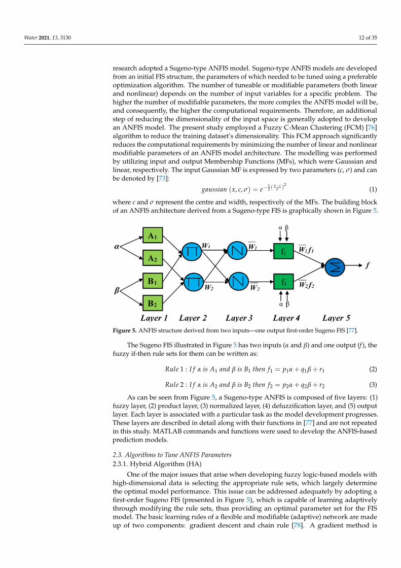
where c and σ represent the centre and width, respectively of the MFs. The building blockof an ANFIS architecture derived from a Sugeno-type FIS is graphically shown in Figure 5.

Water 2021, 13, 3130 13 of 36

preferable optimization algorithm. The number of tuneable or modifiable parameters

(both linear and nonlinear) depends on the number of input variables for a specific prob-

lem. The higher the number of modifiable parameters, the more complex the ANFIS

model will be, and consequently, the higher the computational requirements. Therefore,

an additional step of reducing the dimensionality of the input space is generally adopted

to develop an ANFIS model. The present study employed a Fuzzy C-Mean Clustering

(FCM) [76] algorithm to reduce the training dataset’s dimensionality. This FCM approach

significantly reduces the computational requirements by minimizing the number of linear

and nonlinear modifiable parameters of an ANFIS model architecture. The modelling was

performed by utilizing input and output Membership Functions (MFs), which were

Gaussian and linear, respectively. The input Gaussian MF is expressed by two parameters

(c, σ) and can be denoted by [73]:

𝑔𝑎𝑢𝑠𝑠𝑖𝑎𝑛 (𝑥, 𝑐, 𝜎) = 𝑒−12(𝑥 − 𝑐𝜎 )

2 (1)

where c and σ represent the centre and width, respectively of the MFs. The building block

of an ANFIS architecture derived from a Sugeno-type FIS is graphically shown in Figure

5.

Figure 5. ANFIS structure derived from two inputs—one output first-order Sugeno FIS [77].

The Sugeno FIS illustrated in Figure 5 has two inputs (α and β) and one output (f),

the fuzzy if-then rule sets for them can be written as:

𝑅𝑢𝑙𝑒 1: 𝐼𝑓 𝛼 𝑖𝑠 𝐴1 𝑎𝑛𝑑 𝛽 𝑖𝑠 𝐵1 𝑡ℎ𝑒𝑛 𝑓1 = 𝑝1𝛼 + 𝑞1𝛽 + 𝑟1 (2)

𝑅𝑢𝑙𝑒 2: 𝐼𝑓 𝛼 𝑖𝑠 𝐴2 𝑎𝑛𝑑 𝛽 𝑖𝑠 𝐵2 𝑡ℎ𝑒𝑛 𝑓2 = 𝑝2𝛼 + 𝑞2𝛽 + 𝑟2 (3)

As can be seen from Figure 5, a Sugeno-type ANFIS is composed of five layers: (1)

fuzzy layer, (2) product layer, (3) normalized layer, (4) defuzzification layer, and (5) out-

put layer. Each layer is associated with a particular task as the model development pro-

gresses. These layers are described in detail along with their functions in [77] and are not

repeated in this study. MATLAB commands and functions were used to develop the AN-

FIS-based prediction models.

2.3. Algorithms to Tune ANFIS Parameters

2.3.1. Hybrid Algorithm (HA)

One of the major issues that arise when developing fuzzy logic-based models with

high-dimensional data is selecting the appropriate rule sets, which largely determine the

optimal model performance. This issue can be addressed adequately by adopting a first-

order Sugeno FIS (presented in Figure 5), which is capable of learning adaptively through

modifying the rule sets, thus providing an optimal parameter set for the FIS model. The

basic learning rules of a flexible and modifiable (adaptive) network are made up of two

components: gradient descent and chain rule [78]. A gradient method is usually exploited

to tune parameters of the antecedent and consequent components of the rule base. This

gradient approach results in slow convergence of the tuning process and is prone to

Figure 5. ANFIS structure derived from two inputs—one output first-order Sugeno FIS [77].

The Sugeno FIS illustrated in Figure 5 has two inputs (α and β) and one output (f ), thefuzzy if-then rule sets for them can be written as:

Rule 1 : I f α is A1 and β is B1 then f1 = p1α + q1β + r1 (2)

Rule 2 : I f α is A2 and β is B2 then f2 = p2α + q2β + r2 (3)

As can be seen from Figure 5, a Sugeno-type ANFIS is composed of five layers: (1)fuzzy layer, (2) product layer, (3) normalized layer, (4) defuzzification layer, and (5) outputlayer. Each layer is associated with a particular task as the model development progresses.These layers are described in detail along with their functions in [77] and are not repeatedin this study. MATLAB commands and functions were used to develop the ANFIS-basedprediction models.

2.3. Algorithms to Tune ANFIS Parameters2.3.1. Hybrid Algorithm (HA)

One of the major issues that arise when developing fuzzy logic-based models withhigh-dimensional data is selecting the appropriate rule sets, which largely determinethe optimal model performance. This issue can be addressed adequately by adopting afirst-order Sugeno FIS (presented in Figure 5), which is capable of learning adaptivelythrough modifying the rule sets, thus providing an optimal parameter set for the FISmodel. The basic learning rules of a flexible and modifiable (adaptive) network are madeup of two components: gradient descent and chain rule [78]. A gradient method is

Water 2021, 13, 3130 13 of 35

usually exploited to tune parameters of the antecedent and consequent components ofthe rule base. This gradient approach results in slow convergence of the tuning processand is prone to become trapped in local optima instead of global optima. To overcomethese issues of slow convergence and infeasible solutions, a “hybrid learning rule” thatintegrates Gradient Descent (GD) and Least Squares Estimates (LSE) is proposed to searchfor optimal FIS parameters [77]. In a FIS rule base, the antecedent parameters are regardedas nonlinear in nature, whereas the consequent parameters are linear. In the hybridalgorithm proposed by [77], the antecedent parameters are computed by means of the GDvia error backpropagation, while the recursive LSE determines the consequent parameters.This integration of GD and LSE in parameter tuning of ANFIS models is referred to as aHybrid Algorithm (HA), which employs a frontward and a rearward pass to perform thehybrid learning method. In this study, the HA was employed to tune the parameters of atraditional ANFIS model.

Various hybridized ANFIS models have been widely applied to various researchdomains for improving the performance of the traditional ANFIS models. However, the useof evolutionary algorithm tuned ANFIS models has not been observed in recent literatureto predict groundwater level fluctuations (daily or multiple steps ahead prediction). As apioneering effort, this research proposes the hybridized learning of ANFIS models usingDifferential Evolution (DE) and Particle Swarm Optimization (PSO) to forecast one- andmulti-week-ahead groundwater levels at the selected observation wells. A brief descriptionof DE and PSO is provided in the following sub-sections.

2.3.2. Differential Evolution (DE)

The DE algorithm [79,80] is a stochastic and population-inspired optimization al-gorithm that is ideally suited for providing solutions to numerous nonlinear optimiza-tion formulations. The concept of DE is simple, with a fundamental configuration ofDE/rand/1/bin [81,82]. In DE, a preliminary set of the population is arbitrarily createdfollowing a uniform distribution with the specified lower and higher bounds of xL

j and

xUj , respectively. This randomly created initial population contains NP vectors such that

Xi, ∀i = 1, 2, 3, . . . , NP. Following this initialization, the created individuals are evolvedby mutation and crossover operators, resulting in the production of a trial vector. Theresulting trial vector is compared to the associated parent to determine which vector shouldbe passed on to the subsequent cohort of the population [83]. The basic steps of the DEalgorithm consist of initialization, mutation, crossover, and selection. The details of thesesteps can be found in [83] and are not repeated here.

2.3.3. Particle Swarm Optimization (PSO)

The PSO [84], a population-inspired stochastic algorithm for solving optimizationproblems, is stimulated by social and psychological principles. The PSO is derived fromswarm intelligence principles, which simulate the societal characteristics of bird flocking orfish schooling predation. The algorithm has acquired popularity as a result of its numerousadvantageous properties, including its simple structure, robust manoeuvrability, and easeof implementation [85], which makes it ideal for training various intelligent models. PSOconsiders each particle as a possible solution inside the search domain of an optimizationproblem. On the other hand, the flight behaviour of the particles is recognized as anindividual’s exploration phenomenon. In PSO, the dynamic update of a particle’s velocityis determined by the particle’s previous optimal location and the swarm population.

PSO considers the values of the particle’s objective function to be the correspondingfitness values. These fitness values are used to calculate the particles’ optimal position. Thefitness values are also utilized to update the particles’ past most advantageous location andthe swarm population’s optimum location. Thus, the PSO algorithm’s control parametersdetermine the convergence of particles trajectories [85]. The PSO algorithm converges bykeeping records of each particle’s best fitness values, finding the global best particle, andupdating the locations and velocities of each particle. In the event that the convergence is

Water 2021, 13, 3130 14 of 35

not achieved, the iterative process continues until the optimization problem converges toits optimal solution, or until the user-defined maximum number of iterations is satisfied.

2.4. Developed ANFIS Models

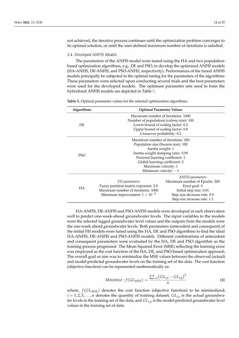
The parameters of the ANFIS model were tuned using the HA and two population-based optimization algorithms, e.g., DE and PSO, to develop the optimized ANFIS models(HA-ANFIS, DE-ANFIS, and PSO-ANFIS, respectively). Performances of the tuned ANFISmodels principally be subjected to the optimal tuning for the parameters of the algorithms.These parameters were selected upon conducting several trials and the best parameterswere used for the developed models. The optimum parameter sets used to train thehybridized ANFIS models are depicted in Table 3.

Table 3. Optimal parameter values for the selected optimization algorithms.

Algorithms Optimal Parameter Values

DE

Maximum number of iterations: 1000Number of populations (colony size): 100

Lower bound of scaling factor: 0.2Upper bound of scaling factor: 0.8

Crossover probability: 0.2

PSO

Maximum number of iterations: 200Population size (Swarm size): 100

Inertia weight: 1Inertia weight damping ratio: 0.99

Personal learning coefficient: 1Global learning coefficient: 2

Maximum velocity: 1Minimum velocity: −1

HA

FIS parametersFuzzy partition matrix exponent: 2.0Maximum number of iterations: 1000

Minimum improvement: 1 × 10−5

ANFIS parametersMaximum number of Epochs: 200

Error goal: 0Initial step size: 0.01

Step size decrease rate: 0.9Step size increase rate: 1.1

HA-ANFIS, DE-ANFIS and PSO-ANFIS models were developed at each observationwell to predict one-week-ahead groundwater levels. The input variables to the modelswere the selected lagged groundwater level values and the outputs from the models werethe one-week ahead groundwater levels. Both parameters (antecedent and consequent) ofthe initial FIS models were tuned using the HA, DE and PSO algorithms to find the idealHA-ANFIS, DE-ANFIS and PSO-ANFIS models. Different combinations of antecedentand consequent parameters were evaluated by the HA, DE and PSO algorithm as thetraining process progressed. The Mean Squared Error (MSE) reflecting the learning errorwas employed as the cost function of the HA, DE, and PSO-based optimization approach.The overall goal or aim was to minimalize the MSE values between the observed (actual)and model-predicted groundwater levels on the training set of the data. The cost function(objective function) can be represented mathematically as:

Minimize : f (GLMSE) =∑n

i=1(GLi,a − GLi,p

)2

n(4)

where, f (GLMSE) denotes the cost function (objective function) to be minimalized;i = 1, 2, 3, . . . , n denotes the quantity of training dataset; GLi,a is the actual groundwa-ter levels in the training set of the data; and GLi,p is the model-predicted groundwater levelvalues in the training set of data.

Water 2021, 13, 3130 15 of 35

The properly trained optimized models were then presented with the test dataset andthe testing errors were computed. The performances of the DE-ANFIS and PSO-ANFISwere weighed against those of the traditional ANFIS model (HA-ANFIS).

2.5. Training of Optimized ANFIS Models

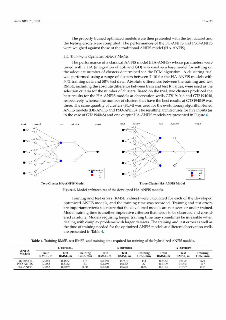
The performance of a classical ANFIS model (HA-ANFIS) whose parameters weretuned with a HA (integration of LSE and GD) was used as a base model for settling onthe adequate number of clusters determined via the FCM algorithm. A clustering trialwas performed using a range of clusters between 2–10 for the HA-ANFIS models with50% training data and 50% test data. Absolute differences between the training and testRMSE, including the absolute difference between train and test R values, were used as theselection criteria for the number of clusters. Based on the trial, two clusters produced thebest results for the HA-ANFIS models at observation wells GT8194046 and GT8194048,respectively, whereas the number of clusters that have the best results at GT8194049 wasthree. The same quantity of clusters (FCM) was used for the evolutionary algorithm-tunedANFIS models (DE-ANFIS and PSO-ANFIS). The resulting architectures for five inputs (asin the case of GT8194048) and one output HA-ANFIS models are presented in Figure 6.

Water 2021, 13, 3130 16 of 36

where, 𝑓(𝐺𝐿𝑀𝑆𝐸) denotes the cost function (objective function) to be minimalized; 𝑖 =

1,2,3, … , 𝑛 denotes the quantity of training dataset; 𝐺𝐿𝑖,𝑎 is the actual groundwater levels

in the training set of the data; and 𝐺𝐿𝑖,𝑝 is the model-predicted groundwater level values

in the training set of data.

The properly trained optimized models were then presented with the test dataset and

the testing errors were computed. The performances of the DE-ANFIS and PSO-ANFIS

were weighed against those of the traditional ANFIS model (HA-ANFIS).

2.5. Training of Optimized ANFIS Models

The performance of a classical ANFIS model (HA-ANFIS) whose parameters were

tuned with a HA (integration of LSE and GD) was used as a base model for settling on the

adequate number of clusters determined via the FCM algorithm. A clustering trial was

performed using a range of clusters between 2–10 for the HA-ANFIS models with 50%

training data and 50% test data. Absolute differences between the training and test RMSE,

including the absolute difference between train and test R values, were used as the selec-

tion criteria for the number of clusters. Based on the trial, two clusters produced the best

results for the HA-ANFIS models at observation wells GT8194046 and GT8194048, respec-

tively, whereas the number of clusters that have the best results at GT8194049 was three.

The same quantity of clusters (FCM) was used for the evolutionary algorithm-tuned AN-

FIS models (DE-ANFIS and PSO-ANFIS). The resulting architectures for five inputs (as in

the case of GT8194048) and one output HA-ANFIS models are presented in Figure 6.

Two-Cluster HA-ANFIS Model Three-Cluster HA-ANFIS Model

Figure 6. Model architectures of the developed HA-ANFIS models.

Training and test errors (RMSE values) were calculated for each of the developed

optimized ANFIS models, and the training time was recorded. Training and test errors

are important criteria to ensure that the developed models are not over- or under-trained.

Model training time is another imperative criterion that needs to be observed and consid-

ered carefully. Models requiring longer training time may sometimes be infeasible when

dealing with complex problems with larger datasets. The training and test errors as well

as the time of training needed for the optimized ANFIS models at different observation

wells are presented in Table 4.

Table 4. Training RMSE, test RMSE, and training time required for training of the hybridized ANFIS models.

ANFIS Mod-

els

GT8194046 GT8194048 GT8194049

Train

RMSE, m

Test

RMSE, m

Training

Time, min

Train

RMSE, m

Test

RMSE, m

Training

Time, min

Train

RMSE, m

Test

RMSE, m

Training

Time, min

DE-ANFIS 0.3565 0.4877 413 0.4485 0.7610 144 0.3453 0.5026 622

PSO-ANFIS 0.3382 0.5332 83 0.4389 0.8965 27 0.3109 0.4846 117

Figure 6. Model architectures of the developed HA-ANFIS models.

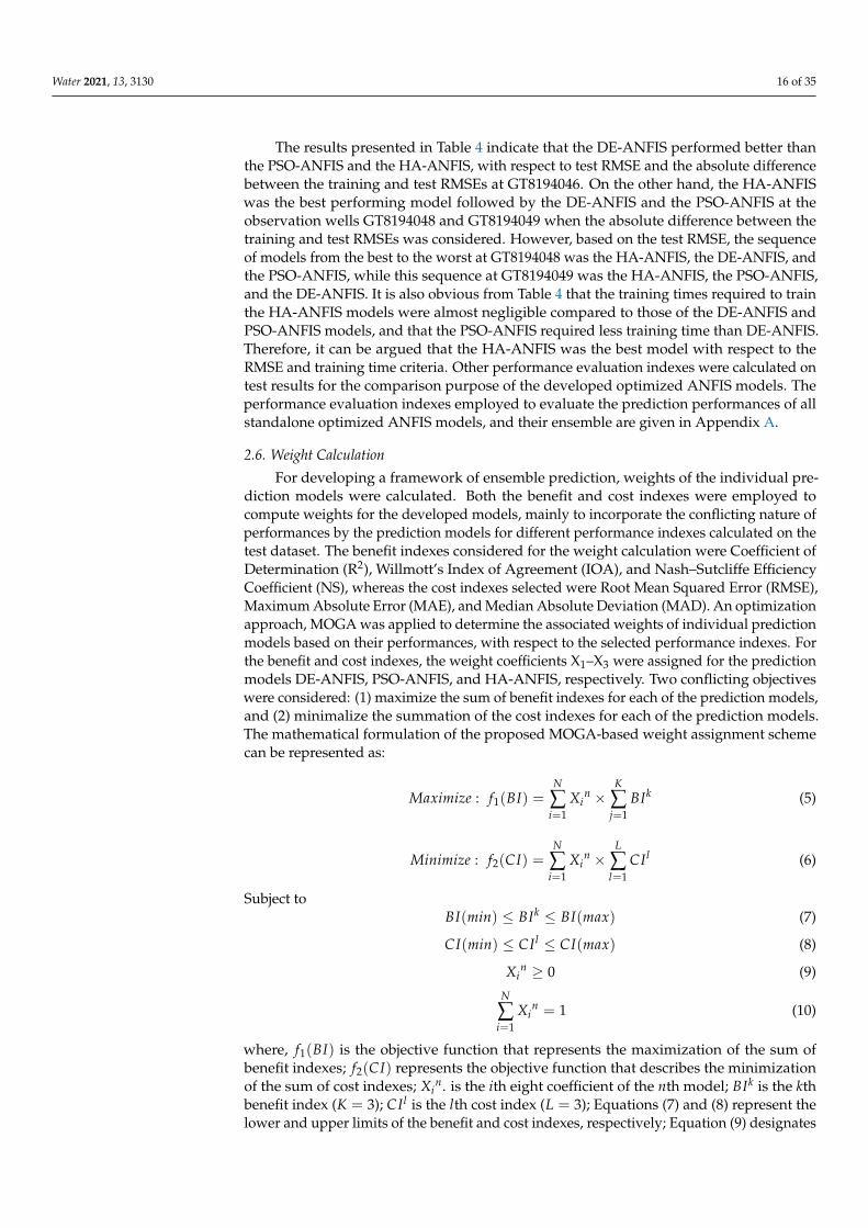
Training and test errors (RMSE values) were calculated for each of the developedoptimized ANFIS models, and the training time was recorded. Training and test errorsare important criteria to ensure that the developed models are not over- or under-trained.Model training time is another imperative criterion that needs to be observed and consid-ered carefully. Models requiring longer training time may sometimes be infeasible whendealing with complex problems with larger datasets. The training and test errors as well asthe time of training needed for the optimized ANFIS models at different observation wellsare presented in Table 4.

Table 4. Training RMSE, test RMSE, and training time required for training of the hybridized ANFIS models.

ANFISModels

GT8194046 GT8194048 GT8194049

TrainRMSE, m

TestRMSE, m

TrainingTime, min

TrainRMSE, m

TestRMSE, m

TrainingTime, min

TrainRMSE, m

TestRMSE, m

TrainingTime, min

DE-ANFIS 0.3565 0.4877 413 0.4485 0.7610 144 0.3453 0.5026 622PSO-ANFIS 0.3382 0.5332 83 0.4389 0.8965 27 0.3109 0.4846 117HA-ANFIS 0.3382 0.5089 0.60 0.4270 0.6761 0.36 0.3123 0.4578 0.45

Water 2021, 13, 3130 16 of 35

The results presented in Table 4 indicate that the DE-ANFIS performed better thanthe PSO-ANFIS and the HA-ANFIS, with respect to test RMSE and the absolute differencebetween the training and test RMSEs at GT8194046. On the other hand, the HA-ANFISwas the best performing model followed by the DE-ANFIS and the PSO-ANFIS at theobservation wells GT8194048 and GT8194049 when the absolute difference between thetraining and test RMSEs was considered. However, based on the test RMSE, the sequenceof models from the best to the worst at GT8194048 was the HA-ANFIS, the DE-ANFIS, andthe PSO-ANFIS, while this sequence at GT8194049 was the HA-ANFIS, the PSO-ANFIS,and the DE-ANFIS. It is also obvious from Table 4 that the training times required to trainthe HA-ANFIS models were almost negligible compared to those of the DE-ANFIS andPSO-ANFIS models, and that the PSO-ANFIS required less training time than DE-ANFIS.Therefore, it can be argued that the HA-ANFIS was the best model with respect to theRMSE and training time criteria. Other performance evaluation indexes were calculated ontest results for the comparison purpose of the developed optimized ANFIS models. Theperformance evaluation indexes employed to evaluate the prediction performances of allstandalone optimized ANFIS models, and their ensemble are given in Appendix A.

2.6. Weight Calculation

For developing a framework of ensemble prediction, weights of the individual pre-diction models were calculated. Both the benefit and cost indexes were employed tocompute weights for the developed models, mainly to incorporate the conflicting nature ofperformances by the prediction models for different performance indexes calculated on thetest dataset. The benefit indexes considered for the weight calculation were Coefficient ofDetermination (R2), Willmott’s Index of Agreement (IOA), and Nash–Sutcliffe EfficiencyCoefficient (NS), whereas the cost indexes selected were Root Mean Squared Error (RMSE),Maximum Absolute Error (MAE), and Median Absolute Deviation (MAD). An optimizationapproach, MOGA was applied to determine the associated weights of individual predictionmodels based on their performances, with respect to the selected performance indexes. Forthe benefit and cost indexes, the weight coefficients X1–X3 were assigned for the predictionmodels DE-ANFIS, PSO-ANFIS, and HA-ANFIS, respectively. Two conflicting objectiveswere considered: (1) maximize the sum of benefit indexes for each of the prediction models,and (2) minimalize the summation of the cost indexes for each of the prediction models.The mathematical formulation of the proposed MOGA-based weight assignment schemecan be represented as:

Maximize : f1(BI) =N

∑i=1

Xin ×

K

∑j=1

BIk (5)

Minimize : f2(CI) =N

∑i=1

Xin ×

L

∑l=1

CIl (6)

Subject toBI(min) ≤ BIk ≤ BI(max) (7)

CI(min) ≤ CIl ≤ CI(max) (8)

Xin ≥ 0 (9)

N

∑i=1

Xin = 1 (10)

where, f1(BI) is the objective function that represents the maximization of the sum ofbenefit indexes; f2(CI) represents the objective function that describes the minimizationof the sum of cost indexes; Xi

n. is the ith eight coefficient of the nth model; BIk is the kthbenefit index (K = 3); CIl is the lth cost index (L = 3); Equations (7) and (8) represent thelower and upper limits of the benefit and cost indexes, respectively; Equation (9) designates

Water 2021, 13, 3130 17 of 35

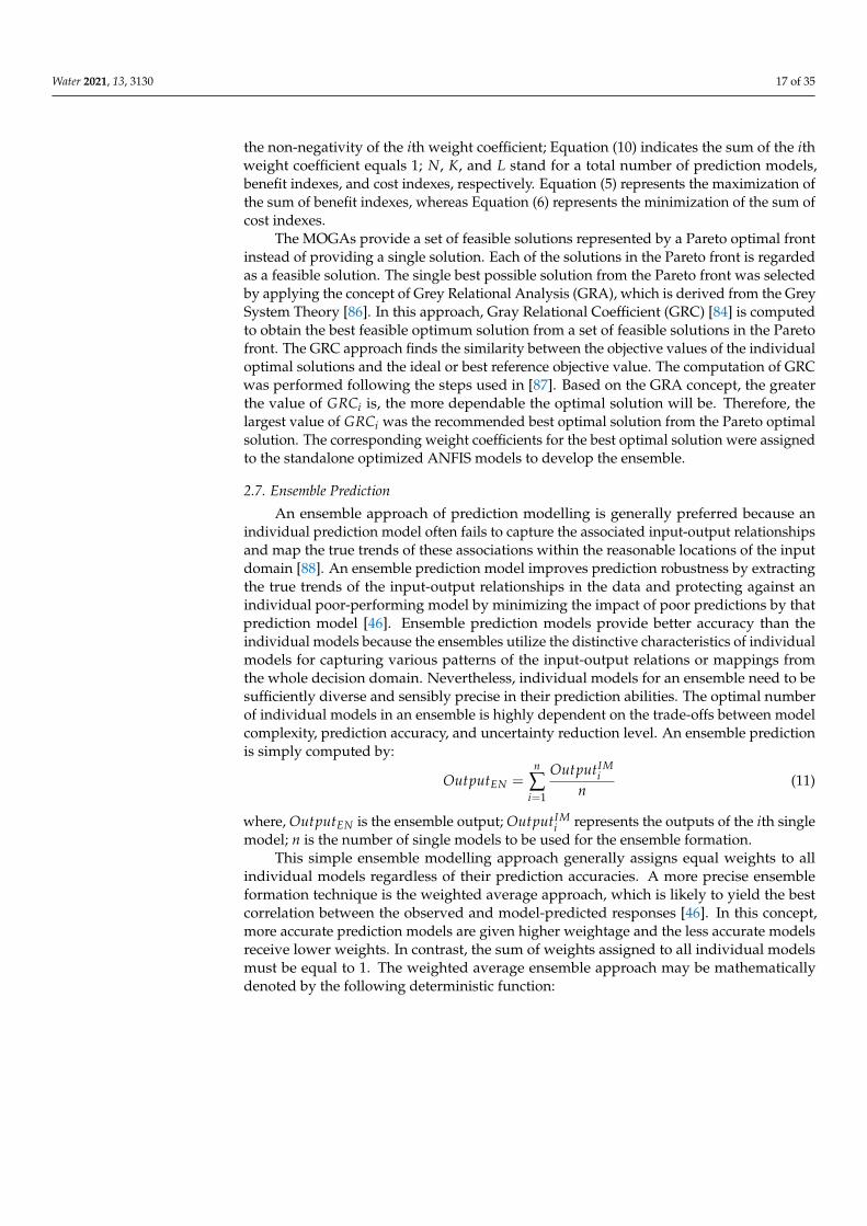
the non-negativity of the ith weight coefficient; Equation (10) indicates the sum of the ithweight coefficient equals 1; N, K, and L stand for a total number of prediction models,benefit indexes, and cost indexes, respectively. Equation (5) represents the maximization ofthe sum of benefit indexes, whereas Equation (6) represents the minimization of the sum ofcost indexes.

The MOGAs provide a set of feasible solutions represented by a Pareto optimal frontinstead of providing a single solution. Each of the solutions in the Pareto front is regardedas a feasible solution. The single best possible solution from the Pareto front was selectedby applying the concept of Grey Relational Analysis (GRA), which is derived from the GreySystem Theory [86]. In this approach, Gray Relational Coefficient (GRC) [84] is computedto obtain the best feasible optimum solution from a set of feasible solutions in the Paretofront. The GRC approach finds the similarity between the objective values of the individualoptimal solutions and the ideal or best reference objective value. The computation of GRCwas performed following the steps used in [87]. Based on the GRA concept, the greaterthe value of GRCi is, the more dependable the optimal solution will be. Therefore, thelargest value of GRCi was the recommended best optimal solution from the Pareto optimalsolution. The corresponding weight coefficients for the best optimal solution were assignedto the standalone optimized ANFIS models to develop the ensemble.

2.7. Ensemble Prediction

An ensemble approach of prediction modelling is generally preferred because anindividual prediction model often fails to capture the associated input-output relationshipsand map the true trends of these associations within the reasonable locations of the inputdomain [88]. An ensemble prediction model improves prediction robustness by extractingthe true trends of the input-output relationships in the data and protecting against anindividual poor-performing model by minimizing the impact of poor predictions by thatprediction model [46]. Ensemble prediction models provide better accuracy than theindividual models because the ensembles utilize the distinctive characteristics of individualmodels for capturing various patterns of the input-output relations or mappings fromthe whole decision domain. Nevertheless, individual models for an ensemble need to besufficiently diverse and sensibly precise in their prediction abilities. The optimal numberof individual models in an ensemble is highly dependent on the trade-offs between modelcomplexity, prediction accuracy, and uncertainty reduction level. An ensemble predictionis simply computed by:

OutputEN =n

∑i=1

OutputIMi

n(11)

where, OutputEN is the ensemble output; OutputIMi represents the outputs of the ith single

model; n is the number of single models to be used for the ensemble formation.This simple ensemble modelling approach generally assigns equal weights to all

individual models regardless of their prediction accuracies. A more precise ensembleformation technique is the weighted average approach, which is likely to yield the bestcorrelation between the observed and model-predicted responses [46]. In this concept,more accurate prediction models are given higher weightage and the less accurate modelsreceive lower weights. In contrast, the sum of weights assigned to all individual modelsmust be equal to 1. The weighted average ensemble approach may be mathematicallydenoted by the following deterministic function:

Water 2021, 13, 3130 18 of 35

YWA(x) =n

∑i=1

ωi(x)×YIMi (x) (12)

where, x represents the input space; YWA is the prediction of the weighted average ensemblewith respect to x; ωi is the numeric value of weight allotted to ith individual model; YIMi isthe prediction of the ith single model; n is the number of single models to be used for theensemble formation. The ensemble thus obtained is adaptive in nature because the weightsare a function of x [50]. This adaptive weighted average ensemble approach was adoptedin this research wherein the assigned weights were calculated using a MOGA.

Once the ensemble prediction was obtained, the corresponding performance indexeswere calculated for the ensemble model for comparison purposes with the individualmodels. Then, a decision theory was applied by incorporating the same benefit and costindexes as in the case of the MOGA-based weight assignment scheme. In this case, theensemble model’s performance indexes were also considered to provide a ranking of allindividual models and the ensemble. The decision theory employed in this study was theShannon’s entropy [51]. The phases or steps adopted in [89,90] were used to calculate theentropy-based weights. The calculation steps are provided in Appendix A.

3. Results and Discussion

The study aims at providing a comparison of the three machine-learning algorithms,DE-ANFIS, PSO-ANFIS, and HA-ANFIS for predicting one- and multi-week ahead ground-water levels using the previous lags as the input variables. A weighted-average ensemble ofthese prediction models is also developed, and precision in the prediction of the ensemblemodel is weighed against the prediction accuracy of the individual prediction models.

3.1. Prediction of Individual Models

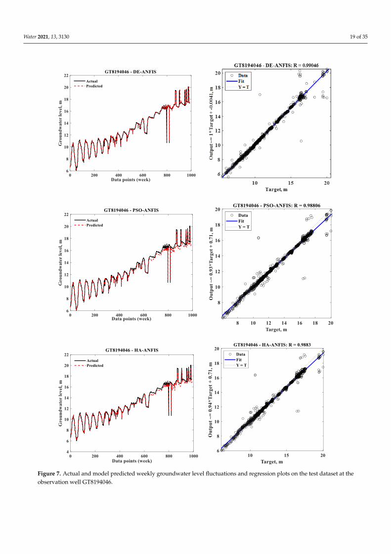
After satisfactory training of the proposed prediction models, results are evaluatedwith respect to various performance evaluation indexes computed on the actual andpredicted test datasets. The model predictions at different observation wells are presentedin Figures 7–9 in the form of hydrographs and scatterplots.

It is observed from the hydrographs and scatterplots presented in Figure 7 that atGT8194046, the DE-ANFIS predictions have better agreement with the actual groundwaterlevel values when compared to other models. The other models face difficulties capturingthe true trends in the groundwater level fluctuations, especially at the later parts of the timeseries (higher values of groundwater level fluctuations), which are underestimated by thePSO-ANFIS and HA-ANFIS models. The PSO-ANFIS appears to be the worst performingmodel at this observation well.

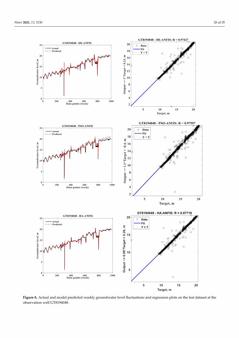
The hydrograph of the HA-ANFIS (Figure 8) indicates the best matching betweenthe actual and predicted groundwater levels at GT8194048. The prediction results ofDE-ANFIS, for this instance, are the second-best, followed by the prediction outcomes ofthe PSO-ANFIS. PSO-ANFIS overestimates the actual groundwater level fluctuations thatbegin at the middle of the time series and continue until the end. In contrast, the DE-ANFISslightly overestimates the actual values.

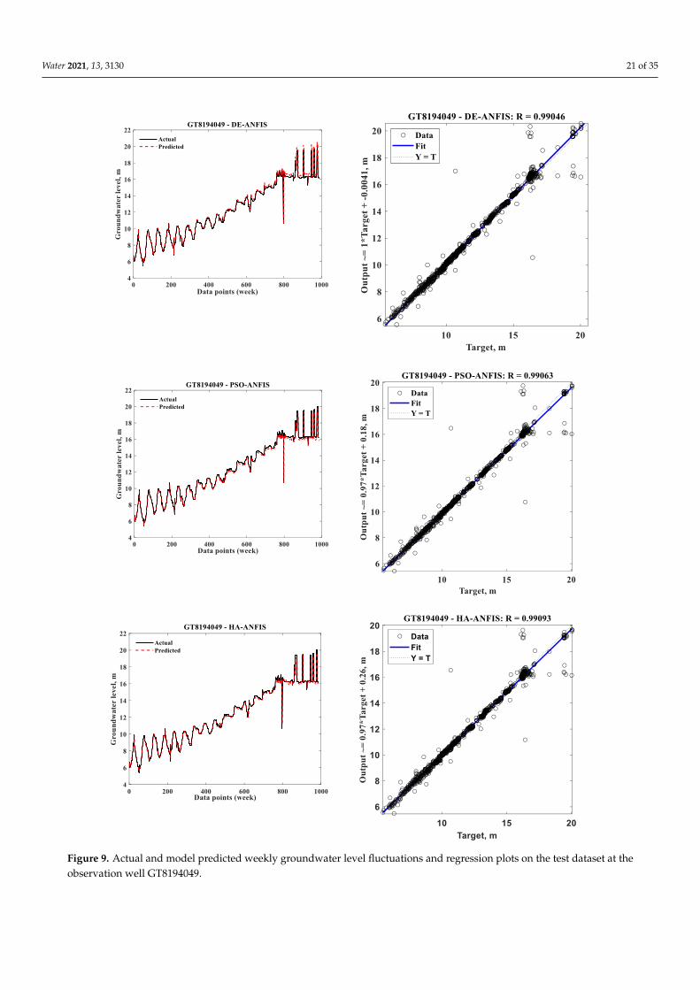
At GT8194049 (Figure 9), the hydrographs indicate the similar prediction accuraciesof the DE-ANFIS, PSO-ANFIS, and HA-ANFIS with the slightly better accomplishment ofthe HA-ANFIS model. The performance results for the one-week-ahead groundwater levelpredictions on the test dataset are provided in Table 5.

Water 2021, 13, 3130 19 of 35Water 2021, 13, 3130 20 of 36

Figure 7. Actual and model predicted weekly groundwater level fluctuations and regression plots

on the test dataset at the observation well GT8194046.

The hydrograph of the HA-ANFIS (Figure 8) indicates the best matching between the

actual and predicted groundwater levels at GT8194048. The prediction results of DE-AN-

FIS, for this instance, are the second-best, followed by the prediction outcomes of the PSO-

ANFIS. PSO-ANFIS overestimates the actual groundwater level fluctuations that begin at

the middle of the time series and continue until the end. In contrast, the DE-ANFIS slightly

overestimates the actual values.

Figure 7. Actual and model predicted weekly groundwater level fluctuations and regression plots on the test dataset at theobservation well GT8194046.

Water 2021, 13, 3130 20 of 35Water 2021, 13, 3130 21 of 36

Figure 8. Actual and model predicted weekly groundwater level fluctuations and regression plots

on the test dataset at the observation well GT8194048.

At GT8194049 (Figure 9), the hydrographs indicate the similar prediction accuracies

of the DE-ANFIS, PSO-ANFIS, and HA-ANFIS with the slightly better accomplishment of

the HA-ANFIS model. The performance results for the one-week-ahead groundwater

level predictions on the test dataset are provided in Table 5.

Figure 8. Actual and model predicted weekly groundwater level fluctuations and regression plots on the test dataset at theobservation well GT8194048.

Water 2021, 13, 3130 21 of 35Water 2021, 13, 3130 22 of 36

Figure 9. Actual and model predicted weekly groundwater level fluctuations and regression plots

on the test dataset at the observation well GT8194049.

Table 5. Performance evaluation indexes of the proposed prediction models on test data at the ob-

servation wells.

PEI GT8194046 GT8194048 GT8194049

M1 M2 M3 M1 M2 M3 M1 M2 M3

RMSE 0.488 0.533 0.509 0.761 0.897 0.676 0.503 0.485 0.458

Figure 9. Actual and model predicted weekly groundwater level fluctuations and regression plots on the test dataset at theobservation well GT8194049.

Water 2021, 13, 3130 22 of 35

Table 5. Performance evaluation indexes of the proposed prediction models on test data at theobservation wells.

PEIGT8194046 GT8194048 GT8194049

M1 M2 M3 M1 M2 M3 M1 M2 M3

RMSE 0.488 0.533 0.509 0.761 0.897 0.676 0.503 0.485 0.458rRMSE 0.038 0.041 0.039 0.050 0.059 0.045 0.041 0.039 0.038

R2 0.976 0.976 0.977 0.950 0.953 0.955 0.981 0.981 0.982MAE 6.148 5.675 5.736 12072 12.178 11.966 6.323 5.794 5.861MAD 0.045 0.130 0.112 0.105 0.275 0.155 0.081 0.066 0.062IOA 0.994 0.992 0.993 0.985 0.981 0.988 0.995 0.995 0.995NS 0.976 0.971 0.973 0.940 0.917 0.953 0.978 0.979 0.981

a-10 index 0.980 0.985 0.984 0.978 0.973 0.979 0.981 0.981 0.981PEI = Performance evaluation index, M1 = DE-ANFIS, M2 = PSO-ANFIS, M3 = HA-ANFIS.

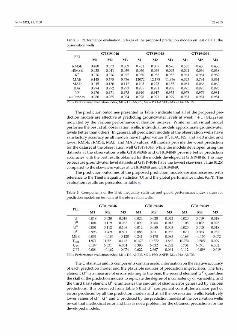
The prediction outcomes presented in Table 5 indicate that all of the proposed pre-diction models are effective at predicting groundwater levels at week t + 1 (GLt+1) asindicated by the various performance evaluation indexes. While no individual modelperforms the best at all observation wells, individual models approximate groundwaterlevels better than others. In general, all prediction models at the observation wells havesatisfactory accuracy as all models have higher values R2, IOA, NS, and a-10 index andlower RMSE, rRMSE, MAE, and MAD values. All models provide the worst predictionfor the dataset at the observation well GT8194048, while the models developed using thedatasets at the observation wells GT8194046 and GT8194049 provide better predictionaccuracies with the best results obtained for the models developed at GT8194046. This maybe because groundwater level datasets at GT8194046 have the lowest skewness value (0.25)compared to the skewness values at GT8194048 and GT8194049.

The prediction outcomes of the proposed prediction models are also assessed withreference to the Theil inequality statistics (U) and the global performance index (GPI). Theevaluation results are presented in Table 6.

Table 6. Components of the Theil inequality statistics and global performance index values forprediction models on test data at the observation wells.

PEIGT8194046 GT8194048 GT8194049

M1 M2 M3 M1 M2 M3 M1 M2 M3

U 0.018 0.020 0.019 0.024 0.028 0.022 0.020 0.019 0.018UB 0.004 0.119 0.063 0.099 0.284 0.015 0.105 0.102 0.025UV 0.001 0.112 0.106 0.012 0.085 0.003 0.025 0.015 0.018UC 0.995 0.769 0.831 0.888 0.631 0.982 0.870 0.883 0.957

MBE 0.031 −0.184 −0.128 0.241 0.478 0.083 0.163 −0.155 −0.072Tstat 1.971 11.521 8.143 10.473 19.772 3.862 10.754 10.585 5.029U95 6.197 6.031 6.034 6.380 6.632 6.292 6.731 6.591 6.582GPI 0.004 −0.162 −0.074 0.622 2.667 0.061 0.112 −0.098 −0.019

PEI = Performance evaluation index, M1 = DE-ANFIS, M2 = PSO-ANFIS, M3 = HA-ANFIS.

The U statistics and its components contain useful information on the relative accuracyof each prediction model and the plausible sources of prediction imprecision. The firstelement UB is a measure of errors relating to the bias, the second element UV quantifiesthe skill of the prediction models to replicate the degree of inconsistency or variability, andthe third (last) element UC enumerates the amount of chaotic error generated by variouspredictions. It is observed from Table 6 that UC component constitutes a major part oferrors produced by all the prediction models and at all the observation wells. Relativelylower values of UB, UV and U produced by the prediction models at the observation wellsreveal that methodical error and bias is not a problem for the obtained predictions for thedeveloped models.

Water 2021, 13, 3130 23 of 35

To further appraise the performances of the developed models, the GPI criterion isemployed, which evaluates the model performance skill by combining the impacts of MBE,RMSE, U95, t-stat, and R2 values in the prediction accuracy. The MBE index indicateswhether the developed prediction model over- or under-estimates the groundwater levelpredictions at the observation wells. Positive values of MBE mean that the prediction modelunder-estimates the observed groundwater level data, while the negative value indicatesan over-estimation of the observed groundwater level data. The t-stat [91] criterion and theRMSE and MBE criteria measure the closeness of the actual and predicted groundwaterlevel values, thus offering a relatively more complicated evaluation of model performance.The U95 criterion measures a models’ predictive deviations within the 95% confidenceband [92,93]. The U95 values produced by the prediction models are within acceptablelimits, varying only slightly at all the observation wells. The t-stat values differ substantiallyamong the prediction models and at the observation wells: at GT8194046, DE-ANFIS hasthe lowest value of t-stat; at GT8194048, the HA-ANFIS has the lowest value of t-stat; andat GT8194049, the HA-ANFIS has the lowest value of t-stat. The MBE, RMSE, U95, t-stat,and R2 values are used to compute the values of the GPI index. The reliability of a model isreversely proportionate to the absolute values of GPI (negative values of GPI originate fromthe negative MBE values), i.e., the lower the numeric value of the GPI index, the higher theaccuracy of the prediction model and the other way around. Based on the GPI index, theDE-ANFIS is the best performer among others at GT8194046, while the HA-ANFIS is thebest prediction model at both the observation wells GT8194048 and GT8194049.

It is perceived from Tables 5 and 6 that models show varying accuracies depending onthe performance evaluation matrix computed on the actual and predicted groundwaterlevel values. This means a contradiction in the prediction performance when differentperformance evaluation indexes are used. For instance, at GT8194046, one can selectDE-ANFIS as the best model when RMSE, MAD, IOA, and NS are considered (Table 5).However, the HA-ANFIS and the PSO-ANFIS perform better with respect to R2 and MAEcriteria, respectively. At GT8194048, the HA-ANFIS has the better performance based onthe RMSE, R2, MAE, IOA, and NS criteria, whereas the DE-ANFIS models’ performance isthe best when the MAD criterion is considered. The HA-ANFIS is the best model amongothers at GT8194049 with reference to the RMSE, R2, and NS criteria, while the PSO-ANFIScan be treated as the top-performing model in terms of the MAE and IOA criteria. On theother hand, the DE-ANFIS is deemed to be superior when the MAD criterion is considered.It is noted that the differences in numeric values among various performance evaluationindexes are often very small. Nevertheless, decision making in this situation is very difficultif not impossible. Decision-making can be facilitated either by selecting a prediction modelto be the best one when most of the performance evaluation indexes are better for thatparticular model or by incorporating different performance evaluation indexes. The laterapproach is promising because it incorporates various performance indexes to decide onthe best performing model. This is often performed by assigning weights to individualmodels and ranking them according to the numeric values of the weights. The presentstudy employs a MOGA for this purpose by utilizing R2, IOA, and NS as the benefit indexesand RMSE, MAE, and MAD as the cost indexes. The outcomes are shown in Table 7. Theweights presented in Table 7 are assigned to the respective prediction models to developthe ensemble model.

Table 7. Weights of the individual prediction models calculated using a Multiple Objective GeneticAlgorithm at the observation wells.

ModelsWeights

GT8194046 GT8194048 GT8194049

DE-ANFIS 0.827 0.345 0.191PSO-ANFIS 0.157 0.133 0.112HA-ANFIS 0.017 0.524 0.697

Sum of weights 1 1 1

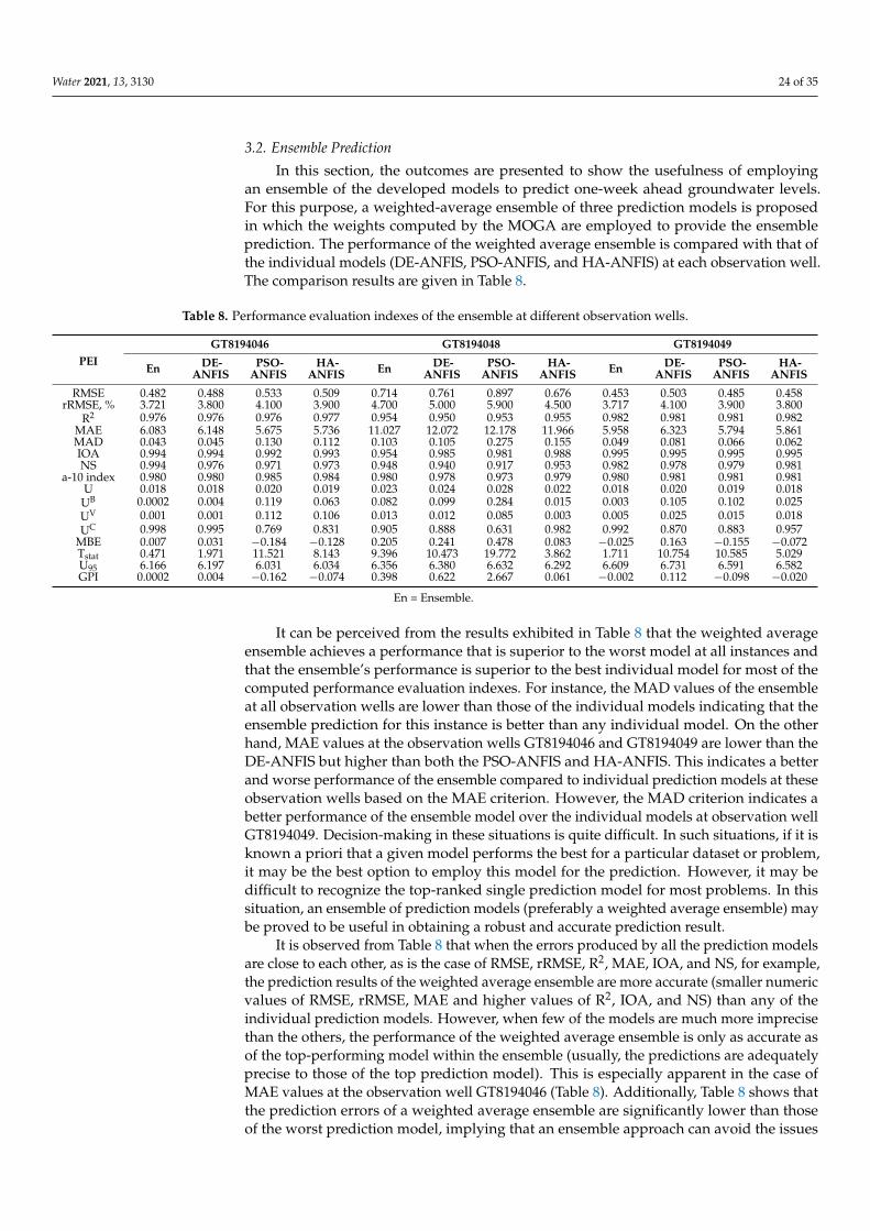
Water 2021, 13, 3130 24 of 35

3.2. Ensemble Prediction

In this section, the outcomes are presented to show the usefulness of employingan ensemble of the developed models to predict one-week ahead groundwater levels.For this purpose, a weighted-average ensemble of three prediction models is proposedin which the weights computed by the MOGA are employed to provide the ensembleprediction. The performance of the weighted average ensemble is compared with that ofthe individual models (DE-ANFIS, PSO-ANFIS, and HA-ANFIS) at each observation well.The comparison results are given in Table 8.

Table 8. Performance evaluation indexes of the ensemble at different observation wells.

PEIGT8194046 GT8194048 GT8194049

En DE-ANFIS

PSO-ANFIS

HA-ANFIS En DE-

ANFISPSO-

ANFISHA-

ANFIS En DE-ANFIS

PSO-ANFIS

HA-ANFIS

RMSE 0.482 0.488 0.533 0.509 0.714 0.761 0.897 0.676 0.453 0.503 0.485 0.458rRMSE, % 3.721 3.800 4.100 3.900 4.700 5.000 5.900 4.500 3.717 4.100 3.900 3.800

R2 0.976 0.976 0.976 0.977 0.954 0.950 0.953 0.955 0.982 0.981 0.981 0.982MAE 6.083 6.148 5.675 5.736 11.027 12.072 12.178 11.966 5.958 6.323 5.794 5.861MAD 0.043 0.045 0.130 0.112 0.103 0.105 0.275 0.155 0.049 0.081 0.066 0.062IOA 0.994 0.994 0.992 0.993 0.954 0.985 0.981 0.988 0.995 0.995 0.995 0.995NS 0.994 0.976 0.971 0.973 0.948 0.940 0.917 0.953 0.982 0.978 0.979 0.981

a-10 index 0.980 0.980 0.985 0.984 0.980 0.978 0.973 0.979 0.980 0.981 0.981 0.981U 0.018 0.018 0.020 0.019 0.023 0.024 0.028 0.022 0.018 0.020 0.019 0.018

UB 0.0002 0.004 0.119 0.063 0.082 0.099 0.284 0.015 0.003 0.105 0.102 0.025UV 0.001 0.001 0.112 0.106 0.013 0.012 0.085 0.003 0.005 0.025 0.015 0.018UC 0.998 0.995 0.769 0.831 0.905 0.888 0.631 0.982 0.992 0.870 0.883 0.957

MBE 0.007 0.031 −0.184 −0.128 0.205 0.241 0.478 0.083 −0.025 0.163 −0.155 −0.072Tstat 0.471 1.971 11.521 8.143 9.396 10.473 19.772 3.862 1.711 10.754 10.585 5.029U95 6.166 6.197 6.031 6.034 6.356 6.380 6.632 6.292 6.609 6.731 6.591 6.582GPI 0.0002 0.004 −0.162 −0.074 0.398 0.622 2.667 0.061 −0.002 0.112 −0.098 −0.020

En = Ensemble.

It can be perceived from the results exhibited in Table 8 that the weighted averageensemble achieves a performance that is superior to the worst model at all instances andthat the ensemble’s performance is superior to the best individual model for most of thecomputed performance evaluation indexes. For instance, the MAD values of the ensembleat all observation wells are lower than those of the individual models indicating that theensemble prediction for this instance is better than any individual model. On the otherhand, MAE values at the observation wells GT8194046 and GT8194049 are lower than theDE-ANFIS but higher than both the PSO-ANFIS and HA-ANFIS. This indicates a betterand worse performance of the ensemble compared to individual prediction models at theseobservation wells based on the MAE criterion. However, the MAD criterion indicates abetter performance of the ensemble model over the individual models at observation wellGT8194049. Decision-making in these situations is quite difficult. In such situations, if it isknown a priori that a given model performs the best for a particular dataset or problem,it may be the best option to employ this model for the prediction. However, it may bedifficult to recognize the top-ranked single prediction model for most problems. In thissituation, an ensemble of prediction models (preferably a weighted average ensemble) maybe proved to be useful in obtaining a robust and accurate prediction result.

It is observed from Table 8 that when the errors produced by all the prediction modelsare close to each other, as is the case of RMSE, rRMSE, R2, MAE, IOA, and NS, for example,the prediction results of the weighted average ensemble are more accurate (smaller numericvalues of RMSE, rRMSE, MAE and higher values of R2, IOA, and NS) than any of theindividual prediction models. However, when few of the models are much more imprecisethan the others, the performance of the weighted average ensemble is only as accurate asof the top-performing model within the ensemble (usually, the predictions are adequatelyprecise to those of the top prediction model). This is especially apparent in the case ofMAE values at the observation well GT8194046 (Table 8). Additionally, Table 8 shows thatthe prediction errors of a weighted average ensemble are significantly lower than thoseof the worst prediction model, implying that an ensemble approach can avoid the issues

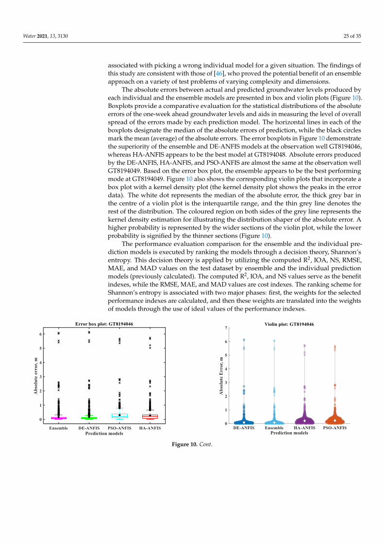
Water 2021, 13, 3130 25 of 35

associated with picking a wrong individual model for a given situation. The findings ofthis study are consistent with those of [46], who proved the potential benefit of an ensembleapproach on a variety of test problems of varying complexity and dimensions.

The absolute errors between actual and predicted groundwater levels produced byeach individual and the ensemble models are presented in box and violin plots (Figure 10).Boxplots provide a comparative evaluation for the statistical distributions of the absoluteerrors of the one-week ahead groundwater levels and aids in measuring the level of overallspread of the errors made by each prediction model. The horizontal lines in each of theboxplots designate the median of the absolute errors of prediction, while the black circlesmark the mean (average) of the absolute errors. The error boxplots in Figure 10 demonstratethe superiority of the ensemble and DE-ANFIS models at the observation well GT8194046,whereas HA-ANFIS appears to be the best model at GT8194048. Absolute errors producedby the DE-ANFIS, HA-ANFIS, and PSO-ANFIS are almost the same at the observation wellGT8194049. Based on the error box plot, the ensemble appears to be the best performingmode at GT8194049. Figure 10 also shows the corresponding violin plots that incorporate abox plot with a kernel density plot (the kernel density plot shows the peaks in the errordata). The white dot represents the median of the absolute error, the thick grey bar inthe centre of a violin plot is the interquartile range, and the thin grey line denotes therest of the distribution. The coloured region on both sides of the grey line represents thekernel density estimation for illustrating the distribution shaper of the absolute error. Ahigher probability is represented by the wider sections of the violin plot, while the lowerprobability is signified by the thinner sections (Figure 10).

The performance evaluation comparison for the ensemble and the individual pre-diction models is executed by ranking the models through a decision theory, Shannon’sentropy. This decision theory is applied by utilizing the computed R2, IOA, NS, RMSE,MAE, and MAD values on the test dataset by ensemble and the individual predictionmodels (previously calculated). The computed R2, IOA, and NS values serve as the benefitindexes, while the RMSE, MAE, and MAD values are cost indexes. The ranking scheme forShannon’s entropy is associated with two major phases: first, the weights for the selectedperformance indexes are calculated, and then these weights are translated into the weightsof models through the use of ideal values of the performance indexes.

Water 2021, 13, 3130 26 of 36

example, the prediction results of the weighted average ensemble are more accurate

(smaller numeric values of RMSE, rRMSE, MAE and higher values of R2, IOA, and NS)

than any of the individual prediction models. However, when few of the models are much

more imprecise than the others, the performance of the weighted average ensemble is only

as accurate as of the top-performing model within the ensemble (usually, the predictions

are adequately precise to those of the top prediction model). This is especially apparent in

the case of MAE values at the observation well GT8194046 (Table 8). Additionally, Table

8 shows that the prediction errors of a weighted average ensemble are significantly lower

than those of the worst prediction model, implying that an ensemble approach can avoid

the issues associated with picking a wrong individual model for a given situation. The

findings of this study are consistent with those of [46], who proved the potential benefit

of an ensemble approach on a variety of test problems of varying complexity and dimen-

sions.

The absolute errors between actual and predicted groundwater levels produced by

each individual and the ensemble models are presented in box and violin plots (Figure

10). Boxplots provide a comparative evaluation for the statistical distributions of the ab-

solute errors of the one-week ahead groundwater levels and aids in measuring the level

of overall spread of the errors made by each prediction model. The horizontal lines in each

of the boxplots designate the median of the absolute errors of prediction, while the black

circles mark the mean (average) of the absolute errors. The error boxplots in Figure 10

demonstrate the superiority of the ensemble and DE-ANFIS models at the observation

well GT8194046, whereas HA-ANFIS appears to be the best model at GT8194048. Absolute

errors produced by the DE-ANFIS, HA-ANFIS, and PSO-ANFIS are almost the same at

the observation well GT8194049. Based on the error box plot, the ensemble appears to be

the best performing mode at GT8194049. Figure 10 also shows the corresponding violin

plots that incorporate a box plot with a kernel density plot (the kernel density plot shows

the peaks in the error data). The white dot represents the median of the absolute error, the

thick grey bar in the centre of a violin plot is the interquartile range, and the thin grey line

denotes the rest of the distribution. The coloured region on both sides of the grey line

represents the kernel density estimation for illustrating the distribution shaper of the ab-

solute error. A higher probability is represented by the wider sections of the violin plot,

while the lower probability is signified by the thinner sections (Figure 10).

Figure 10. Cont.

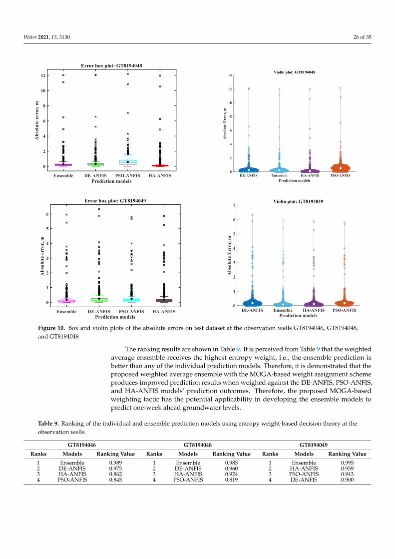
Water 2021, 13, 3130 26 of 35

Water 2021, 13, 3130 27 of 36

Figure 10. Box and violin plots of the absolute errors on test dataset at the observation wells GT8194046, GT8194048, and

GT8194049.

The performance evaluation comparison for the ensemble and the individual predic-

tion models is executed by ranking the models through a decision theory, Shannon’s en-

tropy. This decision theory is applied by utilizing the computed R2, IOA, NS, RMSE, MAE,

and MAD values on the test dataset by ensemble and the individual prediction models

(previously calculated). The computed R2, IOA, and NS values serve as the benefit in-

dexes, while the RMSE, MAE, and MAD values are cost indexes. The ranking scheme for

Shannon’s entropy is associated with two major phases: first, the weights for the selected

performance indexes are calculated, and then these weights are translated into the weights

of models through the use of ideal values of the performance indexes.

The ranking results are shown in Table 9. It is perceived from Table 9 that the

weighted average ensemble receives the highest entropy weight, i.e., the ensemble pre-

diction is better than any of the individual prediction models. Therefore, it is demon-

strated that the proposed weighted average ensemble with the MOGA-based weight as-

signment scheme produces improved prediction results when weighed against the DE-

ANFIS, PSO-ANFIS, and HA-ANFIS models’ prediction outcomes. Therefore, the pro-

posed MOGA-based weighting tactic has the potential applicability in developing the en-

semble models to predict one-week ahead groundwater levels.

Table 9. Ranking of the individual and ensemble prediction models using entropy weight-based

decision theory at the observation wells.

GT8194046 GT8194048 GT8194049

Figure 10. Box and violin plots of the absolute errors on test dataset at the observation wells GT8194046, GT8194048,and GT8194049.

The ranking results are shown in Table 9. It is perceived from Table 9 that the weightedaverage ensemble receives the highest entropy weight, i.e., the ensemble prediction isbetter than any of the individual prediction models. Therefore, it is demonstrated that theproposed weighted average ensemble with the MOGA-based weight assignment schemeproduces improved prediction results when weighed against the DE-ANFIS, PSO-ANFIS,and HA-ANFIS models’ prediction outcomes. Therefore, the proposed MOGA-basedweighting tactic has the potential applicability in developing the ensemble models topredict one-week ahead groundwater levels.

Table 9. Ranking of the individual and ensemble prediction models using entropy weight-based decision theory at theobservation wells.

GT8194046 GT8194048 GT8194049

Ranks Models Ranking Value Ranks Models Ranking Value Ranks Models Ranking Value

1 Ensemble 0.989 1 Ensemble 0.985 1 Ensemble 0.9952 DE-ANFIS 0.975 2 DE-ANFIS 0.960 2 HA-ANFIS 0.9593 HA-ANFIS 0.862 3 HA-ANFIS 0.924 3 PSO-ANFIS 0.9434 PSO-ANFIS 0.845 4 PSO-ANFIS 0.819 4 DE-ANFIS 0.900

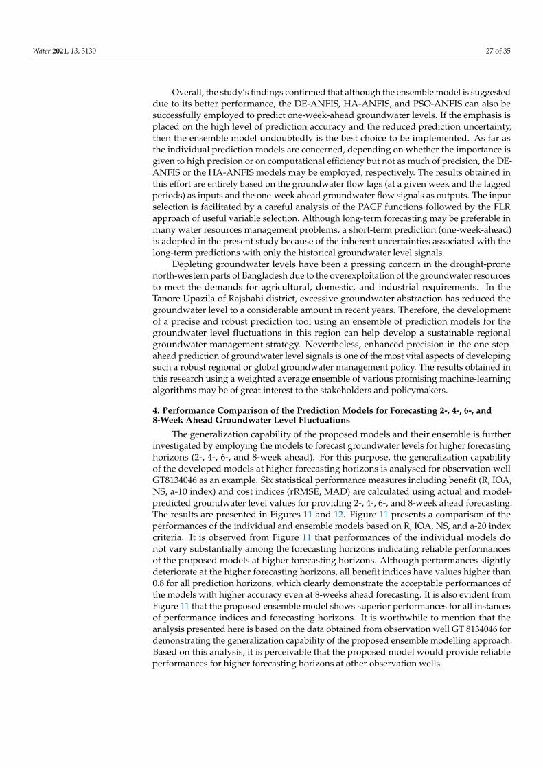
Water 2021, 13, 3130 27 of 35

Overall, the study’s findings confirmed that although the ensemble model is suggesteddue to its better performance, the DE-ANFIS, HA-ANFIS, and PSO-ANFIS can also besuccessfully employed to predict one-week-ahead groundwater levels. If the emphasis isplaced on the high level of prediction accuracy and the reduced prediction uncertainty,then the ensemble model undoubtedly is the best choice to be implemented. As far asthe individual prediction models are concerned, depending on whether the importance isgiven to high precision or on computational efficiency but not as much of precision, the DE-ANFIS or the HA-ANFIS models may be employed, respectively. The results obtained inthis effort are entirely based on the groundwater flow lags (at a given week and the laggedperiods) as inputs and the one-week ahead groundwater flow signals as outputs. The inputselection is facilitated by a careful analysis of the PACF functions followed by the FLRapproach of useful variable selection. Although long-term forecasting may be preferable inmany water resources management problems, a short-term prediction (one-week-ahead)is adopted in the present study because of the inherent uncertainties associated with thelong-term predictions with only the historical groundwater level signals.

Depleting groundwater levels have been a pressing concern in the drought-pronenorth-western parts of Bangladesh due to the overexploitation of the groundwater resourcesto meet the demands for agricultural, domestic, and industrial requirements. In theTanore Upazila of Rajshahi district, excessive groundwater abstraction has reduced thegroundwater level to a considerable amount in recent years. Therefore, the developmentof a precise and robust prediction tool using an ensemble of prediction models for thegroundwater level fluctuations in this region can help develop a sustainable regionalgroundwater management strategy. Nevertheless, enhanced precision in the one-step-ahead prediction of groundwater level signals is one of the most vital aspects of developingsuch a robust regional or global groundwater management policy. The results obtained inthis research using a weighted average ensemble of various promising machine-learningalgorithms may be of great interest to the stakeholders and policymakers.

4. Performance Comparison of the Prediction Models for Forecasting 2-, 4-, 6-, and8-Week Ahead Groundwater Level Fluctuations

The generalization capability of the proposed models and their ensemble is furtherinvestigated by employing the models to forecast groundwater levels for higher forecastinghorizons (2-, 4-, 6-, and 8-week ahead). For this purpose, the generalization capabilityof the developed models at higher forecasting horizons is analysed for observation wellGT8134046 as an example. Six statistical performance measures including benefit (R, IOA,NS, a-10 index) and cost indices (rRMSE, MAD) are calculated using actual and model-predicted groundwater level values for providing 2-, 4-, 6-, and 8-week ahead forecasting.The results are presented in Figures 11 and 12. Figure 11 presents a comparison of theperformances of the individual and ensemble models based on R, IOA, NS, and a-20 indexcriteria. It is observed from Figure 11 that performances of the individual models donot vary substantially among the forecasting horizons indicating reliable performancesof the proposed models at higher forecasting horizons. Although performances slightlydeteriorate at the higher forecasting horizons, all benefit indices have values higher than0.8 for all prediction horizons, which clearly demonstrate the acceptable performances ofthe models with higher accuracy even at 8-weeks ahead forecasting. It is also evident fromFigure 11 that the proposed ensemble model shows superior performances for all instancesof performance indices and forecasting horizons. It is worthwhile to mention that theanalysis presented here is based on the data obtained from observation well GT 8134046 fordemonstrating the generalization capability of the proposed ensemble modelling approach.Based on this analysis, it is perceivable that the proposed model would provide reliableperformances for higher forecasting horizons at other observation wells.

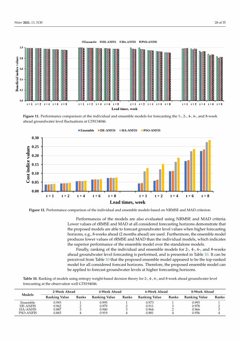
Water 2021, 13, 3130 28 of 35

Water 2021, 13, 3130 29 of 36

instances of performance indices and forecasting horizons. It is worthwhile to mention

that the analysis presented here is based on the data obtained from observation well GT

8134046 for demonstrating the generalization capability of the proposed ensemble mod-

elling approach. Based on this analysis, it is perceivable that the proposed model would

provide reliable performances for higher forecasting horizons at other observation wells.

Figure 11. Performance comparison of the individual and ensemble models for forecasting the 1-, 2-, 4-, 6-, and 8-week

ahead groundwater level fluctuations at GT8134046.

Performances of the models are also evaluated using NRMSE and MAD criteria.

Lower values of rRMSE and MAD at all considered forecasting horizons demonstrate that

the proposed models are able to forecast groundwater level values when higher forecast-

ing horizons, e.g., 8-weeks ahead (2 months ahead) are used. Furthermore, the ensemble

model produces lower values of rRMSE and MAD than the individual models, which in-

dicates the superior performance of the ensemble model over the standalone models.

Figure 12. Performance comparison of the individual and ensemble models based on NRMSE and MAD criterion.

Finally, ranking of the individual and ensemble models for 2-, 4-, 6-, and 8-weeks

ahead groundwater level forecasting is performed, and is presented in Table 10. It can be

perceived from Table 10 that the proposed ensemble model appeared to be the top-ranked

model for all considered forecast horizons. Therefore, the proposed ensemble model can

be applied to forecast groundwater levels at higher forecasting horizons.

0.00

0.05

0.10

0.15

0.20

0.25

0.30

t + 1 t + 2 t + 4 t + 6 t + 8 t + 1 t + 2 t + 4 t + 6 t + 8

Cost

in

dic

e valu

es

Lead times, week

Ensemble DE-ANFIS HA-ANFIS PSO-ANFIS

Figure 11. Performance comparison of the individual and ensemble models for forecasting the 1-, 2-, 4-, 6-, and 8-weekahead groundwater level fluctuations at GT8134046.

Water 2021, 13, 3130 29 of 36

instances of performance indices and forecasting horizons. It is worthwhile to mention

that the analysis presented here is based on the data obtained from observation well GT

8134046 for demonstrating the generalization capability of the proposed ensemble mod-

elling approach. Based on this analysis, it is perceivable that the proposed model would

provide reliable performances for higher forecasting horizons at other observation wells.

Figure 11. Performance comparison of the individual and ensemble models for forecasting the 1-, 2-, 4-, 6-, and 8-week

ahead groundwater level fluctuations at GT8134046.

Performances of the models are also evaluated using NRMSE and MAD criteria.

Lower values of rRMSE and MAD at all considered forecasting horizons demonstrate that

the proposed models are able to forecast groundwater level values when higher forecast-

ing horizons, e.g., 8-weeks ahead (2 months ahead) are used. Furthermore, the ensemble

model produces lower values of rRMSE and MAD than the individual models, which in-

dicates the superior performance of the ensemble model over the standalone models.

Figure 12. Performance comparison of the individual and ensemble models based on NRMSE and MAD criterion.

Finally, ranking of the individual and ensemble models for 2-, 4-, 6-, and 8-weeks

ahead groundwater level forecasting is performed, and is presented in Table 10. It can be

perceived from Table 10 that the proposed ensemble model appeared to be the top-ranked

model for all considered forecast horizons. Therefore, the proposed ensemble model can

be applied to forecast groundwater levels at higher forecasting horizons.

0.00

0.05

0.10

0.15

0.20

0.25

0.30

t + 1 t + 2 t + 4 t + 6 t + 8 t + 1 t + 2 t + 4 t + 6 t + 8

Cost

in

dic

e valu

es

Lead times, week

Ensemble DE-ANFIS HA-ANFIS PSO-ANFIS

Figure 12. Performance comparison of the individual and ensemble models based on NRMSE and MAD criterion.

Performances of the models are also evaluated using NRMSE and MAD criteria.Lower values of rRMSE and MAD at all considered forecasting horizons demonstrate thatthe proposed models are able to forecast groundwater level values when higher forecastinghorizons, e.g., 8-weeks ahead (2 months ahead) are used. Furthermore, the ensemble modelproduces lower values of rRMSE and MAD than the individual models, which indicatesthe superior performance of the ensemble model over the standalone models.

Finally, ranking of the individual and ensemble models for 2-, 4-, 6-, and 8-weeksahead groundwater level forecasting is performed, and is presented in Table 10. It can beperceived from Table 10 that the proposed ensemble model appeared to be the top-rankedmodel for all considered forecast horizons. Therefore, the proposed ensemble model canbe applied to forecast groundwater levels at higher forecasting horizons.

Table 10. Ranking of models using entropy weight-based decision theory for 2-, 4-, 6-, and 8-week ahead groundwater levelforecasting at the observation well GT8194046.

Models2-Week Ahead 4-Week Ahead 6-Week Ahead 8-Week Ahead

Ranking Value Ranks Ranking Value Ranks Ranking Value Ranks Ranking Value Ranks

Ensemble 0.993 1 0.995 1 0.973 1 0.995 1DE-ANFIS 0.962 2 0.979 2 0.911 3 0.978 2HA-ANFIS 0.887 3 0.940 3 0.964 2 0.966 3PSO-ANFIS 0.865 4 0.919 4 0.881 4 0.956 4

Water 2021, 13, 3130 29 of 35

5. Conclusions

Precise and robust prediction of groundwater levels can be effectively employed inproviding a short- and medium-term prediction modelling approach for groundwater levelfluctuations. This study provides a robust prediction tool for one- and multi-week aheadgroundwater level fluctuations through a weighted average ensemble of three optimizationalgorithm tuned ANFIS models (DE-ANFIS, PSO-ANFIS, and HA-ANFIS). The suitableweekly lag times of groundwater levels are used as inputs to the prediction models, whilethe output from the models is the one- and multi-week ahead groundwater levels. Theoptimal combination of inputs for the models is executed by carefully examining the PACFfunctions followed by performing the FLR approach. The performance comparison of theproposed models is performed by adopting a set of performance evaluation indexes. Resultsdemonstrate that the optimized ANFIS models have sufficiently accurate predictions asindicated by the higher values of R2, IOA, and NS as well as lower values of RMSE, MAE,and MAD. A weighted average ensemble of the optimized ANFIS models is proposed toachieve more reliable and accurate predictions. The weights of the individual predictionmodels computed by a Multiple Objective Genetic Algorithm (MOGA) are used to constructthe ensemble of the optimized ANFIS models. The performance evaluation indexes for theensemble prediction are computed and compared with those of the individual models. Theperformance comparison is performed using a ranking scheme of a well-known decisiontheory, Shannon’s entropy. The results of this ranking scheme reveal the superiority of theensemble models over all the individual models.

The most important finding of this study is that employing a weighted-average ensem-ble of data-driven prediction models can improve predictions’ robustness by minimizingthe influence of a worse-performing prediction model. This is especially important becauseit is difficult, if not impossible, to select the best prediction model for a particular problemdue to a vast number of alternatives and that the best prediction model can be changedwith the changes in the dataset. Therefore, it can be concluded that the proposed weightedaverage ensemble approach can be considered as a robust approximation method for pre-dicting one-week-ahead groundwater level fluctuations for the selected observation wells.Furthermore, groundwater level forecasts conducted for 2-, 4-, 6-, and 8-weeks in advanceusing data from the observation well GT8194046 reveal the potential applicability of theensemble approach proposed in this effort. Future research may be directed towards apply-ing the proposed approach in predicting multi-step-ahead groundwater level fluctuationsat other locations.

Author Contributions: Conceptualization, supervision, methodology, formal analysis, writing—original draft preparation, writing—review and editing, D.K.R., S.K.B.; data curation, project ad-ministration, investigation, K.F.I.M., K.K.S., B.D.; writing—review and editing, funding acquisi-tion, M.A.M., A.A.E.-S., A.Z.D. All authors have read and agreed to the published version ofthe manuscript.

Funding: This research was financially supported by the Vice Deanship of Research Chairs at KingSaud University.

Institutional Review Board Statement: Not applicable.

Informed Consent Statement: Not applicable.

Data Availability Statement: Not applicable.

Acknowledgments: This work was financially supported by the Vice Deanship of Research Chairsat King Saud University.

Conflicts of Interest: The authors declare no conflict of interest.

Water 2021, 13, 3130 30 of 35

Appendix A

Appendix A.1. Performance Evaluation Indexes

The performance evaluation indexes employed to evaluate the performance of allstandalone optimized ANFIS models, as well as their ensemble, are given below.

Correlation Coefficient, R

R =∑n

i=1(GLi,a − GLa

)(GLi,a − GLp

)√∑n

i=1(GLi,a − GLa

)2√

∑ni=1(GLi,p − GLp

)2(A1)

Relative RMSE, rRMSE

rRMSE =RMSEGLa

=

√1n ∑n

i=1(GLi,a − GLi,p

)2

GLa(A2)

The rRMSE is often referred to as the Scatter Index (SI), which provides a qualitativecomparison of model performances (excellent, good, fair, and poor). The SI index classifiesa model as acceptable or unacceptable according to the following criteria

SI < 0.1 Excellent0.1 < SI < 0.2 Good0.2 < SI < 0.3 Fair

SI > 0.3 Poor

(A3)

Maximum Absolute Error, MAE

MAE = max[∣∣GLi,a − GLi,p

∣∣] (A4)

Median Absolute Deviation, MAD

MAD(GLa, GLp

)= median

(∣∣GL1,a − GL1,p∣∣, ∣∣GL2,a − GL2,p

∣∣, . . . ,∣∣GLn,a − GLn,p

∣∣)f or i = 1, 2, . . . , n

(A5)

Mean Bias Error, MBE

MBE =1n

n

∑i=1

(GLi,a − GLi,p

)(A6)

T-statistic test, Tstat [91]

Tstat =

√(n− 1) ∗MBE2

RMSE2 −MBE2(A7)

Uncertainty with 95% confidence level, U95

U95 = 1.96×√

Standard deviation2 − RMSE2 (A8)

Global Performance Index, GPI

GPI = MBE ∗ RMSE ∗U95 ∗ Tstat ∗(

1− R2)

(A9)

Nash–Sutcliffe Efficiency Coefficient, NS

NS = 1−∑n

i=1(GLi,a − GLi,p

)2

∑ni=1(GLi,a − GLa

)2 (A10)

Water 2021, 13, 3130 31 of 35

Theil inequality statistics, U

U =

√1n ∑(GLi,p − GLi,a

)2√1n ∑(GLi,p

)2+√

1n ∑(GLi,a)

2(A11)

Bias proportion of Theil inequality statistics, UB

UB =

(GLp − GLa

)2

(1/T)∑(GLi,p − GLi,a

)2 (A12)

Variance proportion of Theil inequality statistics, UV

UV =

(σp − σa

)2

(1/T)∑(GLi,p − GLi,a

)2 (A13)

Covariance proportion of Theil inequality statistics, UC

UC =2(1− R)σpσa

(1/T)∑(GLi,p − GLi,a

)2 (A14)

where GLi,a and GLi,p represent actual (obtained) and model predicted GL values at theith step, respectively; GLa is the mean value of the actual GL values; σa indicates standarddeviation value of the actual GL, σp denotes standard deviation of the predicted GL values,n represents the numeral of data points, ED is the Euclidian distance of any data pointsfrom their ideal values, ∝ is relative variability in the predicted and actual GL values, andβ is the ratio between the mean (average) predicted and mean (average) actual GL datademonstrating the bias.

In addition, according to a recently proposed engineering index, a20 − index, wecalculated an a10 − index to assess the reliability of the developed prediction models.

a10 − index =m10

M(A15)

where, M denotes the quantity of test datasets and m10 is the numeral of test samplesthat have a Actual value/Predicted value ranging between 0.90–1.10. For an impeccabledata-driven prediction modelling approach, the numeric value of a10 − index is anticipatedto have a value of unity (i.e., 1). The values of a10 − index has physical engineeringsignificance: it states that the number of samples that comply with forecasted values withina range of variation of ± 10% weighed against the actual values.

Appendix A.2. Ranking of the Prediction Models Using Shannon’s Entropy

The following steps are used to calculate Shannon’s entropy:Step 1: Formation of a decision matrix of prediction models (individual models and the

ensemble) and performance evaluation indexes. It is assumed that there be m predictionmodels and n performance evaluation indexes. Then, the resulting decision matrix isgiven by:

GLij =

GL11GL12

...GL1n

GL21GL22

...GL2n

· · ·· · ·

...· · ·

GLm1GLm2

...GLmn

(A16)

Water 2021, 13, 3130 32 of 35

Step 2: Standardization of the decision matrix for minimizing the impacts of indexdimensionality. The performance index values are standardized between 0–1 (Sij ∈ [0, 1],i = 1, 2, . . . , m; j = 1, 2, . . . , n). The values of Sij are computed as:

Sij =

GLij

max(GLi1,GLi2,...,GLin), f or bene f it indexes

GLijmin(GLi1,GLi2,...,GLin)

, f or cost indexes(A17)

Step 3: Computation of each index’s entropy via utilizing the concepts of Shannon’sentropy. The entropy value of the jth index was calculated as:

Entropyj = −km

∑i=1

fijln fij (A18)

where,fij = Sij/ ∑m

i=1 Sij (A19)

k = 1/lnm (A20)

Step 4: Calculation of each index’s entropy weight value. The jth index’s entropy weightwas calculated as:

w(entropy)j =1− Entropyj

n−∑nj=1 Entropyj

(A21)

This entropy-based weight designates the prominence of any particular performanceindex in the phases of the entire decision-making. The larger the numeric value of theentropy weight, the greater information the specific index conveys, and the more significantthis performance index will become in the decision-making process.

Step 5: Calculation of each model’s rank weight is carried out by summing up themultiplication of every index’s entropy weight and the normalized value of that particularindex. This step is mathematically represented by:

w(entropy)i =n

∑j=1

Sij × w(entropy)j (A22)

Step 6: Determination of model ranking

max [w(entropy)i], . . . ., min[w(entropy)i]; f or i = 1, 2, . . . , m (A23)

References1. Wada, Y.; Bierkens, M.F.P. Sustainability of global water use: Past reconstruction and future projections. Environ. Res. Lett. 2014,

9, 104003. [CrossRef]2. Hoque, M.A.; Adhikary, S.K. Prediction of groundwater level using artificial neural network and multivariate time series models.

In Proceedings of the 5th International Conference on Civil Engineering and Sustainable Development (ICCESD 2020), Khulna,Bangladesh, 7–9 February 2020; pp. 1–8.

3. Doble, R.C.; Pickett, T.; Crosbie, R.S.; Morgan, L.K.; Turnadge, C.; Davies, P.J. Emulation of recharge and evapotranspirationprocesses in shallow groundwater systems. J. Hydrol. 2017, 555, 894–908. [CrossRef]

4. Masterson, J.P.; Garabedian, S.P. Effects of sea-level rise on ground water flow in a coastal aquifer system. Groundwater 2007, 45,209–217. [CrossRef] [PubMed]

5. Park, E.; Parker, J.C. A simple model for water table fluctuations in response to precipitation. J. Hydrol. 2008, 356, 344–349.[CrossRef]

6. Fahimi, F.; Yaseen, Z.M.; El-shafie, A. Application of soft computing based hybrid models in hydrological variables modeling: Acomprehensive review. Theor. Appl. Climatol. 2017, 128, 875–903. [CrossRef]

7. Govindaraju, R.S. Artificial neural networks in hydrology. I: Preliminary concepts. J. Hydrol. Eng. 2000, 5, 115–123. [CrossRef]8. Govindaraju, R.S. Artificial neural networks in hydrology. II: Hydrologic applications. J. Hydrol. Eng. 2000, 5, 124–137.9. Maier, H.R.; Jain, A.; Dandy, G.C.; Sudheer, K.P. Methods used for the development of neural networks for the prediction of water

resource variables in river systems: Current status and future directions. Environ. Model. Softw. 2010, 25, 891–909. [CrossRef]

Water 2021, 13, 3130 33 of 35

10. Sadler, J.M.; Goodall, J.L.; Morsy, M.M.; Spencer, K. Modeling urban coastal flood severity from crowd-sourced flood reportsusing Poisson regression and Random Forest. J. Hydrol. 2018, 559, 43–55. [CrossRef]

11. Yang, T.; Asanjan, A.A.; Welles, E.; Gao, X.; Sorooshian, S.; Liu, X. Developing reservoir monthly inflow forecasts using artificialintelligence and climate phenomenon information. Water Resour. Res. 2017, 53, 2786–2812. [CrossRef]

12. Yaseen, Z.M.; El-shafie, A.; Jaafar, O.; Afan, H.A.; Sayl, K.N. Artificial intelligence based models for stream-flow forecasting:2000–2015. J. Hydrol. 2015, 530, 829–844. [CrossRef]

13. Solomatine, D.P.; Ostfeld, A. Data-driven modelling: Some past experiences and new approaches. J. Hydroinform. 2008, 10, 3–22.[CrossRef]

14. Karandish, F.; Šimunek, J. A comparison of numerical and machine-learning modeling of soil water content with limited inputdata. J. Hydrol. 2016, 543, 892–909. [CrossRef]

15. Mohanty, S.; Jha, M.K.; Kumar, A.; Panda, D.K. Comparative evaluation of numerical model and artificial neural network forsimulating groundwater flow in Kathajodi–Surua Inter-basin of Odisha, India. J. Hydrol. 2013, 495, 38–51. [CrossRef]

16. Adamowski, J.; Chan, H.F. A wavelet neural network conjunction model for groundwater level forecasting. J. Hydrol. 2011, 407,28–40. [CrossRef]

17. Daliakopoulos, I.N.; Coulibaly, P.; Tsanis, I.K. Groundwater level forecasting using artificial neural networks. J. Hydrol. 2005, 309,229–240. [CrossRef]

18. Obergfell, C.; Bakker, M.; Maas, K. Identification and explanation of a change in the groundwater regime using time seriesanalysis. Groundwater 2019, 57, 886–894. [CrossRef]

19. Roshni, T.; Jha, M.K.; Deo, R.C.; Vandana, A. Development and evaluation of hybrid artificial neural network architectures formodeling spatio-temporal groundwater fluctuations in a complex aquifer system. Water Resour. Manag. 2019, 33, 2381–2397.[CrossRef]

20. Feng, S.; Kang, S.; Huo, Z.; Chen, S.; Mao, X. Neural networks to simulate regional ground water levels affected by humanactivities. Groundwater 2008, 46, 80–90. [CrossRef]

21. Guzman, S.M.; Paz, J.O.; Tagert, M.L.M. The use of NARX neural networks to forecast daily groundwater levels. Water Resour.Manag. 2017, 31, 1591–1603. [CrossRef]

22. Sahoo, S.; Russo, T.A.; Elliott, J.; Foster, I. Machine learning algorithms for modeling groundwater level changes in agriculturalregions of the U.S. Water Resour. Res. 2017, 53, 3878–3895. [CrossRef]

23. Zhang, Z.; Zhang, Q.; Singh, V.P. Univariate streamflow forecasting using commonly used data-driven models: Literature reviewand case study. Hydrol. Sci. J. 2018, 63, 1091–1111. [CrossRef]

24. Dong, L.; Guangxuan, L.; Qiang, F.; Mo, L.; Chunlei, L.; Abrar, F.M.; Imran, K.M.; Tianxiao, L.; Song, C. Application of particleswarm optimization and extreme learning machine forecasting models for regional groundwater depth using nonlinear predictionmodels as preprocessor. J. Hydrol. Eng. 2018, 23, 4018052.

25. Mohanty, S.; Jha, M.K.; Raul, S.K.; Panda, R.K.; Sudheer, K.P. Using artificial neural network approach for simultaneous forecastingof weekly groundwater levels at multiple sites. Water Resour. Manag. 2015, 29, 5521–5532. [CrossRef]

26. Ghorbani, M.A.; Deo, R.C.; Karimi, V.; Yaseen, Z.M.; Terzi, O. Implementation of a hybrid MLP-FFA model for water levelprediction of Lake Egirdir, Turkey. Stoch. Environ. Res. Risk Assess. 2018, 32, 1683–1697. [CrossRef]

27. Lee, S.; Lee, K.-K.; Yoon, H. Using artificial neural network models for groundwater level forecasting and assessment of therelative impacts of influencing factors. Hydrogeol. J. 2019, 27, 567–579. [CrossRef]

28. Barzegar, R.; Fijani, E.; Asghari Moghaddam, A.; Tziritis, E. Forecasting of groundwater level fluctuations using ensemble hybridmulti-wavelet neural network-based models. Sci. Total Environ. 2017, 599–600, 20–31. [CrossRef]

29. Peng, T.; Zhou, J.; Zhang, C.; Fu, W. Streamflow forecasting using empirical wavelet transform and artificial neural networks.Water 2017, 9, 406. [CrossRef]

30. Raghavendra, S.N.; Deka, P.C. Forecasting monthly groundwater level fluctuations in coastal aquifers using hybrid Waveletpacket–Support vector regression. Cogent Eng. 2015, 2, 999414. [CrossRef]

31. Gong, Y.; Wang, Z.; Xu, G.; Zhang, Z. A comparative study of groundwater level forecasting using data-driven models based onensemble empirical mode decomposition. Water 2018, 10, 730. [CrossRef]

32. Boubaker, S. Identification of monthly municipal water demand system based on autoregressive integrated moving averagemodel tuned by particle swarm optimization. J. Hydroinform. 2017, 19, 261–281. [CrossRef]

33. Banadkooki, F.B.; Ehteram, M.; Ahmed, A.N.; Teo, F.Y.; Fai, C.M.; Afan, H.A.; Sapitang, M.; El-Shafie, A. Enhancement ofgroundwater-level prediction using an integrated machine learning model optimized by whale algorithm. Nat. Resour. Res. 2020,29, 3233–3252. [CrossRef]

34. Makungo, R.; Odiyo, J.O. Estimating groundwater levels using system identification models in Nzhelele and Luvuvhu areas,Limpopo Province, South Africa. Phys. Chem. Earth 2017, 100, 44–50. [CrossRef]

35. Nadiri, A.A.; Naderi, K.; Khatibi, R.; Gharekhani, M. Modelling groundwater level variations by learning from multiple modelsusing fuzzy logic. Hydrol. Sci. J. 2019, 64, 210–226. [CrossRef]

36. Nourani, V.; Mousavi, S. Spatiotemporal groundwater level modeling using hybrid artificial intelligence-meshless method. J.Hydrol. 2016, 536, 10–25. [CrossRef]

37. Wen, X.; Feng, Q.; Yu, H.; Wu, J.; Si, J.; Chang, Z.; Xi, H. Wavelet and adaptive neuro-fuzzy inference system conjunction modelfor groundwater level predicting in a coastal aquifer. Neural Comput. Appl. 2015, 26, 1203–1215. [CrossRef]

Water 2021, 13, 3130 34 of 35

38. Zare, M.; Koch, M. Groundwater level fluctuations simulation and prediction by ANFIS- and hybrid Wavelet-ANFIS/FuzzyC-Means (FCM) clustering models: Application to the Miandarband plain. J. Hydro-Environ. Res. 2018, 18, 63–76. [CrossRef]

39. Moosavi, V.; Vafakhah, M.; Shirmohammadi, B.; Behnia, N. A wavelet-ANFIS hybrid model for groundwater level forecasting fordifferent prediction periods. Water Resour. Manag. 2013, 27, 1301–1321. [CrossRef]

40. Tang, Y.; Zang, C.; Wei, Y.; Jiang, M. Data-driven modeling of groundwater level with least-square support vector machine andspatial–temporal analysis. Geotech. Geol. Eng. 2019, 37, 1661–1670. [CrossRef]

41. Wei, Z.-L.; Wang, D.-F.; Sun, H.-Y.; Yan, X. Comparison of a physical model and phenomenological model to forecast groundwaterlevels in a rainfall-induced deep-seated landslide. J. Hydrol. 2020, 586, 124894. [CrossRef]

42. Fallah-Mehdipour, E.; Bozorg Haddad, O.; Mariño, M.A. Prediction and simulation of monthly groundwater levels by geneticprogramming. J. Hydro-Environ. Res. 2013, 7, 253–260. [CrossRef]

43. Aguilera, H.; Guardiola-Albert, C.; Naranjo-Fernández, N.; Kohfahl, C. Towards flexible groundwater-level prediction foradaptive water management: Using Facebook’s Prophet forecasting approach. Hydrol. Sci. J. 2019, 64, 1504–1518. [CrossRef]

44. Ghaseminejad, A.; Uddameri, V. Physics-inspired integrated space-time artificial neural networks for regional groundwater flowmodeling. Hydrol. Earth Syst. Sci. 2020, 24, 5759–5779. [CrossRef]

45. Rajaee, T.; Ebrahimi, H.; Nourani, V. A review of the artificial intelligence methods in groundwater level modeling. J. Hydrol.2019, 572, 336–351. [CrossRef]

46. Goel, T.; Haftka, R.T.; Shyy, W.; Queipo, N.V. Ensemble of surrogates, Struct. Multidiscip. Optim. 2007, 33, 199–216. [CrossRef]47. Jafari, S.A.; Mashohor, S.; Varnamkhasti, M.J. Committee neural networks with fuzzy genetic algorithm. J. Pet. Sci. Eng. 2011, 76,

217–223. [CrossRef]48. Roy, D.K.; Datta, B. Multivariate adaptive regression spline ensembles for management of multilayered coastal aquifers. J. Hydrol.

Eng. 2017, 22, 4017031. [CrossRef]49. Sreekanth, J.; Datta, B. Coupled simulation-optimization model for coastal aquifer management using genetic programming-based

ensemble surrogate models and multiple-realization optimization. Water Resour. Res. 2011, 47. [CrossRef]50. Zerpa, L.E.; Queipo, N.V.; Pintos, S.; Salager, J.-L. An optimization methodology of alkaline–surfactant–polymer flooding

processes using field scale numerical simulation and multiple surrogates. J. Pet. Sci. Eng. 2005, 47, 197–208. [CrossRef]51. Shannon, C.E. A mathematical theory of communication. Bell Syst. Tech. J. 1948, 27, 379–423. [CrossRef]52. Zhao, K.Q.; Xuan, A.L. Set pair theory-a new theory method of non-define and its applications. Syst. Eng. 1996, 14, 18–23.53. Dempster, A.P. Upper and Lower Probabilities Induced by a Multivalued Mapping BT-Classic Works of the Dempster-Shafer Theory of

Belief Functions; Yager, R.R., Liu, L., Eds.; Springer: Berlin/Heidelberg, Germany, 2008; pp. 57–72.54. Shafer, G. A mathematical theory of evidence turns 40. Int. J. Approx. Reason. 2016, 79, 7–25. [CrossRef]55. Goldberg, D.E.; Holland, J.H. Genetic algorithms and machine learning. Mach. Learn. 1988, 3, 95–99. [CrossRef]56. Shen, Z.-Q.; Kong, F.-S. Optimizing Weights by Genetic Algorithm for Neural Network Ensemble BT-Advances in Neural Networks–ISNN

2004; Yin, F.-L., Wang, J., Guo, C., Eds.; Springer: Berlin/Heidelberg, Germany, 2004; pp. 323–331.57. Roy, D.K.; Datta, B. Selection of meta-models to predict saltwater intrusion in coastal aquifers using entropy weight based

decision theory. In Proceedings of the 2018 IEEE Conference on Technologies for Sustainability (SusTech), Long Beach, CA, USA,11–13 November 2018; pp. 1–6.

58. Roy, D.K.; Datta, B. An ensemble meta-modelling approach using the Dempster-Shafer theory of evidence for developingsaltwater intrusion management strategies in coastal aquifers. Water Resour. Manag. 2019, 33, 775–795. [CrossRef]

59. Roy, D.K.; Datta, B. Saltwater intrusion prediction in coastal aquifers utilizing a weighted-average heterogeneous ensemble ofprediction models based on Dempster-Shafer theory of evidence. Hydrol. Sci. J. 2020, 65, 1555–1567. [CrossRef]

60. Deb, K.; Pratap, A.; Agarwal, S.; Meyarivan, T. A fast and elitist multiobjective genetic algorithm: NSGA-II. IEEE Trans. Evol.Comput. 2002, 6, 182–197. [CrossRef]

61. Mohanty, S.; Jha, M.K.; Kumar, A.; Sudheer, K.P. Artificial neural network modeling for groundwater level forecasting in a riverisland of eastern India. Water Resour. Manag. 2010, 24, 1845–1865. [CrossRef]

62. Wang, X.; Liu, T.; Zheng, X.; Peng, H.; Xin, J.; Zhang, B. Short-term prediction of groundwater level using improved randomforest regression with a combination of random features. Appl. Water Sci. 2018, 8, 1–12. [CrossRef]

63. Huang, F.; Huang, J.; Jiang, S.H.; Zhou, C. Prediction of groundwater levels using evidence of chaos and support vector machine.J. Hydroinform. 2017, 19, 586–606. [CrossRef]

64. SRDI. Upazila Land and Soil Resource Utilization Guide: Tanore, Rajshahi; SRDI: Dhaka, Bangladesh, 2000.65. SRDI. Land and Soil Statistical Appraisal Book of Bangladesh; SRDI (Soil Resource Development Institute): Dhaka, Bangladesh, 2010.66. Mathworks, Technical Documentation, Impute Missing Data Using Nearest-Neighbor Method. 2020. Available online: https:

//au.mathworks.com/help/bioinfo/ref/knnimpute.html (accessed on 23 April 2020).67. Troyanskaya, O.; Cantor, M.; Sherlock, G.; Brown, P.; Hastie, T.; Tibshirani, R.; Botstein, D.; Altman, R.B. Missing value estimation

methods for DNA microarrays. Bioinformatics 2001, 17, 520–525. [CrossRef]68. Hastie, T.; Tibshirani, R.; Sherlock, G.; Eisen, M.; Brown, P.; Botstein, D. Imputing Missing Data for Gene Expression Arrays; Technical

Report; Division of Biostatistics, Stanford University: Stanford, CA, USA, 1999.69. Deo, R.C.; Tiwari, M.K.; Adamowski, J.F.; Quilty, J.M. Forecasting effective drought index using a wavelet extreme learning

machine (W-ELM) model. Stoch. Environ. Res. Risk Assess. 2017, 31, 1211–1240. [CrossRef]

Water 2021, 13, 3130 35 of 35

70. Mouatadid, S.; Adamowski, J.; Tiwari, M.K.; Quilty, J.M. Coupling the maximum overlap discrete wavelet transform and longshort-term memory networks for irrigation flow forecasting. Agric. Water Manag. 2019, 219, 72–85. [CrossRef]

71. Tibshirani, R. Regression Shrinkage and Selection via the Lasso. J. R. Stat. Soc. Ser. B 1996, 58, 267–288. [CrossRef]72. Mathworks, Technical Documentation: Zscore, Stand. z-Scores. 2020. Available online: https://au.mathworks.com/help/stats/

zscore.html (accessed on 2 May 2020).73. Jang, J.-S.R.; Sun, C.T.; Mizutani, E. Neuro-Fuzzy and Soft Computing: A Computational Approach to Learning and Machine Intelligence;

Prentice Hall: Upper Saddle River, NJ, USA, 1997.74. Sugeno, M.; Yasukawa, T. A fuzzy-logic-based approach to qualitative modeling. IEEE Trans. Fuzzy Syst. 1993, 1, 7. [CrossRef]75. Takagi, T.; Sugeno, M. Fuzzy identification of systems and its applications to modeling and control. IEEE Trans. Syst. Man. Cybern.

1985, SMC-15, 116–132. [CrossRef]76. Bezdek, J.C.; Ehrlich, R.; Full, W. FCM: The fuzzy c-means clustering algorithm. Comput. Geosci. 1984, 10, 191–203. [CrossRef]77. Jang, J.-S.R. ANFIS: Adaptive-network-based fuzzy inference system. IEEE Trans. Syst. Man. Cybern. 1993, 23, 665–685. [CrossRef]78. Werbos, P.J. Beyond Regression: New Tools for Prediction and Analysis in the Behavioral Sciences. Ph.D. Dissertation, Harvard

University, Cambridge, MA, USA, 1974.79. Price, K.V. An Introduction to Differential Evolution; Corne, D., Dorigo, M., Glover, F., Eds.; New Ideas Optim., McGraw-Hill Ltd.:

London, UK, 1999; pp. 79–108.80. Storn, R. Designing Digital Filters with Differential Evolution; Corne, D., Dorigo, M., Glover, F., Eds.; New Ideas Optim., McGraw-Hill

Ltd.: London, UK, 1999; pp. 109–126.81. Storn, R.; Price, K. Differential evolution—A simple and efficient heuristic for global optimization over continuous spaces. J. Glob.

Optim. 1997, 11, 341–359. [CrossRef]82. Fan, H.-Y.; Lampinen, J. A trigonometric mutation operation to differential evolution. J. Glob. Optim. 2003, 27, 105–129. [CrossRef]83. Das, S.; Suganthan, P.N. Differential evolution: A survey of the state-of-the-art. IEEE Trans. Evol. Comput. 2011, 15, 4–31.

[CrossRef]84. Kennedy, J.; Eberhart, R. Particle swarm optimization. In Proceedings of the ICNN’95—International Conference on Neural

Networks, Perth, WA, USA, 27 November–1 December 1995; Volume 4, pp. 1942–1948.85. Sun, L.; Song, X.; Chen, T. An improved convergence particle swarm optimization algorithm with random sampling of control

parameters. J. Control Sci. Eng. 2019, 7478498.86. Deng, J.-L. Control problems of grey systems. Syst. Control Lett. 1982, 1, 288–294.87. Wang, Z.; Rangaiah, G.P. Application and analysis of methods for selecting an optimal solution from the Pareto-optimal front

obtained by multiobjective optimization. Ind. Eng. Chem. Res. 2017, 56, 560–574. [CrossRef]88. Roy, D.K.; Datta, B. A review of surrogate models and their ensembles to develop saltwater intrusion management strategies in

coastal aquifers. Earth Syst. Environ. 2018, 2, 193–211. [CrossRef]89. Wu, J.; Sun, J.; Liang, L.; Zha, Y. Determination of weights for ultimate cross efficiency using Shannon entropy. Expert Syst. Appl.

2011, 38, 5162–5165. [CrossRef]90. Li, X.; Wang, K.; Liu, L.; Xin, J.; Yang, H.; Gao, C. Application of the entropy weight and TOPSIS method in safety evaluation of

coal mines. Procedia Eng. 2011, 26, 2085–2091. [CrossRef]91. Stone, R.J. Improved statistical procedure for the evaluation of solar radiation estimation models. Sol. Energy 1993, 51, 289–291.

[CrossRef]92. Behar, O.; Khellaf, A.; Mohammedi, K. Comparison of solar radiation models and their validation under Algerian climate–The

case of direct irradiance. Energy Convers. Manag. 2015, 98, 236–251. [CrossRef]93. Gueymard, C.A. A review of validation methodologies and statistical performance indicators for modeled solar radiation data:

Towards a better bankability of solar projects. Renew. Sustain. Energy Rev. 2014, 39, 1024–1034. [CrossRef]