Embed Size (px)
Citation preview
GROUNDWATER RECHARGE ASSESSMENT OF THE BASEMENT
AQUIFERS OF CENTRAL NAMAQUALAND
Report to the Water Research Commission
by
Shafick Adams Rian Titus
Yongxin Xu
Groundwater Group University of the Western Cape
Private Bag X17 Bellville
7535 WRC Report No. 1093/1/04 August 2004 ISBN: 1-77005-214-3

Disclaimer This report emanates from a project financed by the Water Research Commission (WRC) and is approved for publication. Approval does not signify that the contents necessarily reflect the views and policies of the WRC or the members of the project steering committee, nor does mention of trade names or commercial products constitute endorsement or recommendation for use.
Obtainable from: Water Research Commission Private Bag X03 GEZINA 0031
Executive summary
Introduction Understanding groundwater recharge is a prerequisite for effective groundwater
management. Recharge is defined as the portion of rainfall that reaches the saturated zone,
either by direct contact in the riparian zone or by downward percolation through the
unsaturated zone. To provide the necessary understanding, this study has investigated the
recharge processes and rates of the Central Namaqualand area of the Northern Cape, South
Africa. The area is characterised by a semi-arid to arid climate with groundwater occurring
in the crystalline basement and alluvial aquifers. Recharge in arid to semi-arid crystalline
basement aquifers are neither straightforward nor simple and needs both a qualitative and a
quantitative approach. This was achieved by using a variety of methods, including the
chloride mass balance (CMB) method, methods involving correlating storativity, rainfall
and water level fluctuations (i.e. saturated volume fluctuations and cumulative rainfall
departures), 18O and 2H stable isotope analyses, radiogenic isotope (14C) interpretation, R-
and Q mode factor analyses and a GIS approach.
The processes involved in recharge and the rate of recharge are influenced by several
factors, which may include the geology, climate, geomorphology and soils. There exists no
set procedure to estimate recharge in fractured rock dominated terrain. Assessing recharge
depends on the application of a suite of methods.
Objective, scope and approach
The primary objective of the research is to quantify and characterise recharge to the
crystalline basement and alluvial aquifers of Central Namaqualand for sustainable
groundwater development and management.
The scope of the study includes:
(1) Identifying methods suitable for recharge studies in the Central Namaqualand region.
(2) Delineating recharge areas.
(3) Applying and comparing of a number of independent approaches for recharge characterisation/estimation as well as selecting the best method(s) for recharge estimation.
(4) Developing a conceptual model for the groundwater recharge.
The development of the conceptual model of the area is based on previous studies and
hydrologic data (chemical and isotopic data, water-level measurements, borehole logs,
geophysical measurements, climatological data, and hydraulic properties determined from
aquifer tests, as well as information based on field observations). Areas for recharge
studies will be identified based on the amount of data available (water levels, abstraction
rates, climatic data, borehole distribution). A strong bias will be introduced towards areas
where abstraction zones supply water to the rural communities. Methods, which are
suitable for recharge estimation for the area, will be applied at selected sites.
Identifying methods suitable for recharge studies in the Central Namaqualand region
Five methods have been identified that can be applied in the study area, and they are:
� Chloride mass balance (CMB) method;
� Cumulative rainfall departures (CRD) method;
� Saturated volume fluctuation (SVF) method;
� Statistical approach; and
� GIS approach.
The methods were selected based on the availability of data and data that can be obtained
easily and cost-effectively. A spreadsheet program was developed to assist in selecting
different methods, based on data availability and requirements.
Delineating recharge areas
Recharge areas were delineated on regional and local scales. Regionally, recharge areas
correspond with the higher lying areas that receive most of the annual rainfall. Recharge
areas were identified using factor analysis, employing the interrelationship between
groundwater chemistry, isotopes and altitude to define recharge and discharge areas as well
as intermediate areas. The results of the factor analysis also indicated recharge of polluted
water into the aquifer. The GIS approach correlated various thematic layers to recharge
probability. The layers were then integrated to generate a recharge potential map. Applying
the rainfall distribution map over the area effectively shows the areas most likely to receive
recharge. Although the approach gives a map that is conceptually correct, it can be further
refined.
Localised recharge areas are related to the type of aquifer. It was found that the alluvial
aquifers are easily recharged due to their hydraulic characteristics and their position within
the landscape. The structural control on the ephemeral drainage systems is evident in their
alignment along fracture systems that are associated with the underlying bedrock. The
alluvial systems are major pathways for groundwater recharge to the weathered and
bedrock zone aquifers.
Application and comparison of a number of independent approaches for recharge
characterisation/estimation and selection of the best method(s) for recharge estimation
Assessing recharge to any aquifer depends on the type of area under investigation, the
availability of data, the distribution of available data and the ability to obtain meaningful
data. Groundwater resources assessment is inherently complex in semi-arid to arid
crystalline terrain. Groundwater recharge rates over large areas are difficult to estimate due
to problems associated with upscaling and data distribution. Two approaches have been
followed in this study whereby recharge was qualitatively and quantitatively assessed. The
qualitative assessment involved using existing data from the area and applying statistical
and spatial techniques to assess recharge processes and patterns. Applying the CMB
method and water level to rainfall relationships gave quantitative estimates of recharge.
The qualitative assessments of recharge, using statistical analysis (R and Q mode factor
analysis) and the GIS assessment techniques, identify areas that are receiving recharge as
well as being favourable for potential recharge. The statistical analysis is useful in that it
also indicates areas of localised artificial recharge through agricultural and domestic
activities. The isotope approach also provided some useful information in terms of
recharge processes and the time since recharge. It was found that most of the recharged
water was evaporated at the surface, as evidenced in the stable isotope data. Recharge is
thus mainly indirect except for the higher-lying mountainous areas where recharge is
mainly direct. The isotope samples of the higher-lying areas plot in a distinct pattern on the
�2H- �18O plot. The radiogenic isotopes indicated the existence of very old water to
recently recharged water.
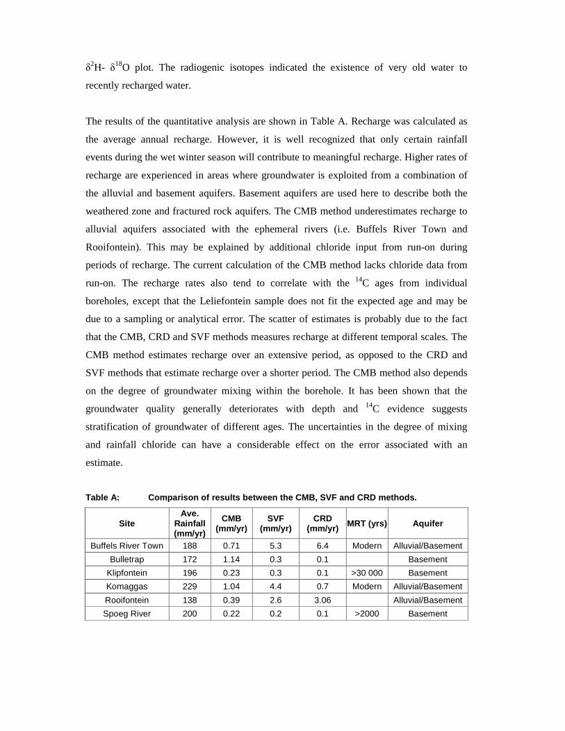
The results of the quantitative analysis are shown in Table A. Recharge was calculated as
the average annual recharge. However, it is well recognized that only certain rainfall
events during the wet winter season will contribute to meaningful recharge. Higher rates of
recharge are experienced in areas where groundwater is exploited from a combination of
the alluvial and basement aquifers. Basement aquifers are used here to describe both the
weathered zone and fractured rock aquifers. The CMB method underestimates recharge to
alluvial aquifers associated with the ephemeral rivers (i.e. Buffels River Town and
Rooifontein). This may be explained by additional chloride input from run-on during
periods of recharge. The current calculation of the CMB method lacks chloride data from
run-on. The recharge rates also tend to correlate with the 14C ages from individual
boreholes, except that the Leliefontein sample does not fit the expected age and may be
due to a sampling or analytical error. The scatter of estimates is probably due to the fact
that the CMB, CRD and SVF methods measures recharge at different temporal scales. The
CMB method estimates recharge over an extensive period, as opposed to the CRD and
SVF methods that estimate recharge over a shorter period. The CMB method also depends
on the degree of groundwater mixing within the borehole. It has been shown that the
groundwater quality generally deteriorates with depth and 14C evidence suggests
stratification of groundwater of different ages. The uncertainties in the degree of mixing
and rainfall chloride can have a considerable effect on the error associated with an
estimate.
Table A: Comparison of results between the CMB, SVF and CRD methods.
Site Ave.
Rainfall (mm/yr)
CMB (mm/yr)
SVF (mm/yr)
CRD (mm/yr) MRT (yrs) Aquifer
Buffels River Town 188 0.71 5.3 6.4 Modern Alluvial/Basement
Bulletrap 172 1.14 0.3 0.1 Basement
Klipfontein 196 0.23 0.3 0.1 >30 000 Basement
Komaggas 229 1.04 4.4 0.7 Modern Alluvial/Basement
Rooifontein 138 0.39 2.6 3.06 Alluvial/Basement
Spoeg River 200 0.22 0.2 0.1 >2000 Basement
Conclusions
This is the first systematic recharge study carried out in the central Namaqualand region.
The results indicate that recharge is higher in the alluvial aquifers than in the hard rock
basement aquifers. The results also indicate that recharge decreases from the escarpment
zone to the coastal zone. Even under favourable rainfall conditions the areas around
Klipfontein and Spoeg River receives minimal recharge. This phenomenon is probably
related to the surface features in the areas. The chloride mass balance, saturated volume
fluctuation (SVF) and the cumulative rainfall departures (CRD) methods were used to
quantify recharge rates. Recharge was calculated as the average annual recharge. The
CMB, SVF and CRD methods gave different recharge rates, mainly because of the fact that
recharge are calculated over different temporal and spatial scales. The SVF and CRD
methods generally gave results that are in close agreement. The stable isotopes, 18O and 2H, and the radiogenic isotope 14C were used to assess groundwater recharge processes and
mean residence times of the groundwater, respectively. The stable isotopes indicate that
recharge is mainly indirect with direct recharge dominating in the mountainous areas. The
mean residence times of the groundwater range from very old (>30 000 years) to recently
recharged groundwater. A statistical and GIS approach were used to delineate recharge
areas and discharge areas or where recharge is negligible. Recharge is higher in the
mountainous areas than in the lower lying areas, with minimal recharge along the coastal
lowland. It was also established that recharge mainly occurs through the alluvial aquifers
associated with ephemeral rivers with significant soil cover. Some salient points are
highlighted below:
� Groundwater recharge rates to the basement and alluvial aquifers are estimated to
be within 0.1 and 10 mm/yr, with the higher values being mainly to the alluvial
aquifers and high altitude sites, and the lower limits to the fractured rock aquifers.
� Groundwater level fluctuations and rainfall (CRD and SVF) was successfully used
to estimate groundwater recharge. Water level data is usually available in most
areas due to community water supply schemes. Uncertainties with regard to the
determination of storage coefficients and contributing areas to recharge in fractured
hard rock terrain are still of concern for most hydrogeologists. The estimates used
in the calculations are ‘best estimates’.
� The CMB method is still a useful method for recharge estimations in most
hydrogeological provinces as a first estimate of recharge. However, the method, if
applied on its own, may not give an accurate account of recharge rates. The
uncertainties and assumptions of the method need to be considered when
interpreting the results. The recharge rates estimated for the alluvial aquifers are
lower than expected. This is a result of the unaccounted chloride in the surface
runoff flux.
� Isotope data indicate water ranging from very young to very old (<50 years - >30
000 years). Intermediate ages indicate active mixing of younger and old water.
� Recharge is related to the amount of rainfall and the position of the aquifers within
the landscape, which is, in turn, related to altitude and topography. Recharge
mainly occurs when rainfall is above normal. Above-normal rainfall produces more
intense runoff that can travel further down the hydrological profile, recharging
more of the alluvial aquifers.
� Recharge occurs as primary recharge in the mountainous areas where direct
infiltration is more likely. Indirect recharge involves the infiltration of surface
runoff and discharges from springs and adjacent aquifers, dominating in most of the
areas.
� Flood events will produce significant recharge, mainly to the alluvial aquifers.
� Recharge estimates that may seem to be within acceptable limits of error when
interpreted, may be significantly high when applied to determine aquifer
sustainability. Rainfall in semi-arid regions is episodic in nature, where most of the
annual rainfall can occur within a very short period of time with a concomitant
increase in recharge if favourable conditions exist, as opposed to distributing the
rainfall over an entire year. The use of mean annual recharge rates can be
misleading, as the simulated period only includes years of above-average rainfall
and not the long-term cyclicity of rainfall.
� Recharge in arid to semi-arid crystalline basement aquifers is neither
straightforward nor simple and needs both a qualitative (e.g. field observations and
local knowledge) and a quantitative approach.
� The approach can be adopted for similar hydrogeological regions or regions where
there are limited data.

Recommendations for future research
Topics or issues that must be considered for future research include:
� Results and techniques provided by this baseline study should be used to acquire
additional data to optimise the recharge rates estimated.
� The utilisation of complementary water sources needs to be highlighted, such as
rainwater harvesting, fog water collection, and artificial recharge using runoff from
the bornhardts. Some of these schemes are operated on a limited scale in the area
and can be expanded to other areas.
� Measurement campaigns for chloride deposition.
� Application of the recharge estimates to management scenarios.
� Quantification of episodic recharge at various temporal scales.
� Scenario-based studies on the impact of climatic change on future groundwater
resources.
� Expanding the GIS approach to distribute point estimates from a particular area to
similar areas elsewhere. The spatial heterogeneity of recharge introduces
difficulties in upscaling, and needs additional research aimed at improving the
application of point data to larger areas.
� Hill slope processes and their impact on groundwater flow and recharge.

Acknowledgements
The WRC is thanked for funding this research.
The following institutions and individuals are acknowledged for their support:
� The Steering Committee members for this project
- The late Dr Oliver Sililo formerly CSIR
- Dr Dave Bredenkamp Water Resources Evaluation and Management CC
- Dr Hans Beekman formerly CSIR
- Prof Yongxin Xu UWC
- Dr Rian Titus UWC and Council for Geoscience
- Mr Gawie van Dyk DWAF
- Mr Eddy van Wyk DWAF
- Mr HD Roberts Northern Cape Government
- Dr Kevin Pietersen WRC
- Dr George Green WRC
� Toens and Partners now with SRK for providing some of the monitoring data and
consultancy reports.
� Rian Titus and Kevin Pietersen are thanked for initiating the project.
� Professor Yongxin Xu for his support and encouragement as well as the three
external examiners of the PhD thesis from which this report was derived from.
� The postgraduate students who assisted with the collection of some of the data,
especially Lindie Hassan and Lloyd Flanagan.
� The isotope laboratories of the University of the Witwatersrand (Schonland
Research Institute) and the University of Cape Town for conducting the isotope
analysis. Prof. Balt Verhagen’s input during the carbon-14 sampling is
acknowledged.
� The chemistry laboratories of Bemlab, CSIR and Eskom (TSI) are acknowledged
for the groundwater and rainwater chemistry analysis.
� Julian Conrad for creating the GIS database and aiding in formulating the GIS
approach.
� Bryan Lawrence for all the logistical support.
Abbreviations and symbols
14C - Carbon-14 18O - Oxygen-18 2H/D - Deuterium
CMB - Chloride mass balance
CRD - Cumulative rainfall departures
DWAF - Department of Water Affairs and Forestry
FC - Flow Characteristic
GMWL - Global meteoi water line
K - Hydraulic conductivity
LMWL - Local meteoric water line
MAE - Mean annual evapotranspiration
mamsl - Meters above mean sea level
MAP - Mean annual precipitation
MAR - Mean annual runoff
mbgl - Meters below ground level
NGDB - National Groundwater Database
pmC - Percent modern carbon
PMWIN - Processing Modflow for Windows
S-value - Storativity or specific yield
SVF - Saturated volume fluctuation
T - Transmissivity
WRC - Water Research Commission
Table of Contents
EXECUTIVE SUMMARY ............................................................................................... i ACKNOWLEDGEMENTS .............................................................................................xiii ABBREVIATIONS AND SYMBOLS ............................................................................ ix TABLE OF CONTENTS ................................................................................................x LIST OF FIGURES .........................................................................................................xiii LIST OF TABLES...........................................................................................................xvi LIST OF APPENDICES .................................................................................................xvii 1 INTRODUCTION ......................................................................................... 1 1.1 Introduction .....................................................................................................1 1.2 Background......................................................................................................2 1.3 Previous work ..................................................................................................3 1.4 Objective and scope .........................................................................................3 1.5 Approach .........................................................................................................4 1.6 Outline .............................................................................................................4 2 GROUNDWATER RECHARGE TO BASEMENT AQUIFERS.................... 6
2.1 Introduction .....................................................................................................6 2.2 Characteristics of arid and semi-arid zones.......................................................7
2.3 Characteristics of basement aquifers.................................................................8 Weathered zone................................................................................................11 Fractured bedrock............................................................................................12 2.4 Recharge, storage and groundwater flow ..........................................................13 Recharge.........................................................................................................13 Storage............................................................................................................14 Groundwater flow ...........................................................................................14
3 THEORETICAL ASPECTS OF RECHARGE ESTIMATION........................ 16 3.1 Introduction ......................................................................................................16 3.2 Recharge estimation methods............................................................................17 3.3 Groundwater recharge estimation methods applicable for Central Namaqualand........................................................................................17 3.4 Physical and chemical recharge estimation methods..........................................21
3.4.1 Chemical and isotope tracer methods........................................................21 Chloride mass balance (CMB)..................................................................21 Stable and radiogenic isotopes .................................................................27 3.4.2 Physical methods......................................................................................31 Saturated volume fluctuation (SVF) ..........................................................31
Cumulative rainfall departures (CRD)......................................................33

3.5 Statistical approach using factor analysis .......................................................... 35 3.6 Geographical Information Systems (GIS) ......................................................... 36 4 MEASUREMENT AND EXPERIMENTAL TECHNIQUES ...........................49 4.1 Introduction..................................................................................................... 49 4.2 Precipitation monitoring and sampling............................................................. 49
4.2.1 Bulk Rainfall Samples ............................................................................ 50 4.2.2 Event samples ......................................................................................... 57
4.3 Groundwater.................................................................................................... 58 4.3.1 Chemistry and isotopes .......................................................................... 58 4.3.2 Data quality ........................................................................................... 59
5 DESCRIPTION OF THE CENTRAL NAMAQUALAND AREA ....................61
5.1 Introduction..................................................................................................... 61 5.2 Climate............................................................................................................ 61 Precipitation.................................................................................................... 61 Temperature .................................................................................................... 66 Evapotranspiration .......................................................................................... 66
5.3 Topography ..................................................................................................... 67 5.4 Geomorphology............................................................................................... 69 5.5 Vegetation ....................................................................................................... 72 5.6 Geology........................................................................................................... 73 5.7 Surface water drainage .................................................................................... 77 5.8 Hydrogeology.................................................................................................. 80
5.8.1 Aquifer types and conditions................................................................... 80 Fractured and weathered zone aquifers .................................................. 80 Alluvial aquifers...................................................................................... 80 5.8.2 Piezometry and groundwater flow........................................................... 81 5.8.3 Hydrogeochemistry................................................................................. 87 5.8.4 Aquifer characteristics ............................................................................ 89 Intrinsic properties of the basement rocks ............................................... 89 Transmissivity and storativity................................................................... 92 Comparison of results between FC and AQUATEST ................................... 94
6 GROUNDWATER RECHARGE ASSESSMENT ........................................96 6.1 Introduction..................................................................................................... 96 6.2 Chemical and isotope tracer methods............................................................... 96
6.2.1 Chloride mass balance ............................................................................ 96 Precipitation composition ....................................................................... 97 Groundwater composition....................................................................... 103 Recharge estimation................................................................................ 105
6.2.2 Stable isotopes (deuterium and oxygen-18) ............................................. 108 Precipitation composition ....................................................................... 108 Groundwater composition....................................................................... 111
6.2.3 Radiogenic isotope (carbon-14) ...............................................................113 Mean residence times of the groundwater ................................................113 6.2.4 Summary.................................................................................................116
6.3 Physical Methods .............................................................................................117 Aquifer response.......................................................................................118 Water level approach ...............................................................................122 Site descriptions ......................................................................................123 6.3.1 Saturated Volume Fluctuation .................................................................124 6.3.2 Cumulative Rainfall Departure ................................................................126 6.3.4 Summary.................................................................................................130
6.4 Statistical techniques........................................................................................132 6.4.1 R-and Q-mode factor analysis..................................................................133 6.4.2 Summary.................................................................................................138 6.5 GIS based recharge assessment ........................................................................139 6.5.1 Recharge map..........................................................................................144 6.5.2 Summary.................................................................................................148 7 SYNTHESIS ................................................................................................ 149 7.1 Evaluation of recharge assessment in Namaqualand ........................................149 7.1.1 Identifying methods suitable for recharge studies in Central Namaqualand region...............................................................................149 7.1.2 Delineating recharge areas......................................................................149 7.1.3 Application and comparison of a number of independent approaches for recharge characterisation/estimation and selection of the best method(s) for recharge estimation..........................................150 7.1.4 A conceptual model for groundwater recharge........................................153 7.2 Regional perspective .......................................................................................158 7.3 Final remarks ..................................................................................................161 7.4 Future research................................................................................................162 REFERENCES....................................................................................................... 163 APPENDICES ........................................................................................................ A-180
List of Figures
Figure 2.1: Classification of the different climate zones. Figure 2.2: Recharge mechanisms in different climate zones. Figure 2.3: Bornhardts of the Central Namaqualand area. Figure 2.4: Development of landforms in basement rock areas. Figure 2.5: Weathered profiles for basement aquifers. Figure 3.1: Example of the Excel programme for selecting suitable methods. Figure 3.2: Conceptual depth profiles for the chloride tracer.
A. Piston flow with abstraction of water by roots. B. Abstraction of water by roots, but with either preferred flow of water to beneath
the root zone, or diffuse loss of chloride to the water table. C. Profile that may reflect the recharge history of a site.
Figure 3.3: Range of fluxes that can be estimated in the unsaturated zone. Figure 3.4: Range of fluxes that can be estimated in the saturated zone. Figure 3.5: 3D view of the nine different hillslopes. Figure 3.6a: Normalised subsurface flow rates at different locations along the nine hillslopes
(dotted line: x = 25m; dash-dotted line: x = 50m; dashed line: x= 75m; solid line: at outlet, x = 100m).
Figure 3.6b: Relative soil moisture storage for characteristic time steps (dotted line: initial time, t = 0; dash-dotted line: t = 5 days; dashed line: t = 10 days; solid line: t = 15 days).
Figure 3.7a: Normalised subsurface flow rates at different locations along the nine hillslopes during a constant recharge event of 10mm.day (dotted line: x = 25m; dash-dotted line: x = 25m; dashed line: x= 50m; solid line: at outlet, x = 100m).
Figure 3.7b: Relative soil moisture storage for characteristic time steps during a constant recharge event of 10mm/day (dotted line: t = 5; dash-dotted line: t = 10 days; dashed line: t = 15 days; solid line: steady state). Arrows indicate saturated area of the respective slopes.
Figure 3.8: Relations between lithological properties of bedrock, soil structure and dimensions of soil slips for granite and gneiss slopes.
Figure 3.9: Processes involved in upscaling and downscaling. Figure 4.1a-b: The standard bulk rainfall and UWC bulk rainfall sampler designs. Figure 4.2: Comparison between temperature changes inside the two rainfall samplers and the
temperature of the environment (without water). Figure 4.3: Comparison between temperature changes inside the two rainfall samplers and the
temperature of the environment (with water). Figure 4.4. Chloride content of different samples collected in HDPE and PVC samples. Figure 5.1: The study area. Figure 5.2: Average monthly rainfall for six rainfall stations. Figure 5.3: Altitude versus average annual rainfall. Figure 5.4: Average annual rainfall versus distance from the sea. Figure 5.5: Rainfall deviations from the mean over a 120-year period, for the Springbok area. Figure 5.6: Average monthly evaporation for the Okiep area and the relationship that exists
with temperature and rainfall. Figure 5.7a: Surface elevations and topography of the study area. Figure 5.7b: Topographical profiles of the study area. Figure 5.8: Different geomorphic zones across the W-E profiles of the area. Figure 5.9: Distribution of erosion surface of the southern African subcontinent. Figure 5.10: Log [Ca2+]/ [H+] versus SiO2 diagram for groundwater of the Namaqualand region. Figure 5.11: Geological map of the area. Figure 5.12: Ternary diagram of the soil classes found in Namaqualand. Figure 5.13: Distribution of the rivers in the study area.
Figure 5.14: Profile across the Buffels River near the town Kamassies. Figure 5.15: Dry and wet season profiles of the Buffels River near the town of Buffels River. A: Dry season: 930 Hz GEM-300 data, north is down
B: Dry season: 330 Hz GEM-300 data, north is down C: Wet season: 930 Hz GEM-300 data, north is to the left D: Wet season: 330 Hz GEM-300 data, north is to the left
Figure 5.16: Frequency diagram for water levels of the central Namaqualand area (source NGDB).
Figure 5.17: Regional distribution of groundwater levels. Figure 5.18: Borehole depth versus yield for boreholes contained in the NGDB. Figure 5.19: Comparison between lineament frequency densities and borehole yield density
contour map of Namaqualand. Figure 5.20: Electrical conductivity logs for borehole G45772 in the vicinity of Garies. Figure 5.21: Conceptual model of the flow processes in the three aquifer types found in the
study area. Figure 5.22: Piper diagram of the groundwater sampled in the study area. Figure 5.23: Porosity versus depth below ground level. Figure 5.24: Hydraulic conductivity versus depth below ground level. Figure 5.25: Range of measured or inferred permeability of basement and metamorphic rocks as
a function of the characteristic length scale the broken line indicate ranges of intact and weathered values for the Namaqualand region.
Figure 6.1: Map showing localities described in this chapter. Figure 6.2: Chloride versus rainfall amount relationship for individual samples. Figure 6.3: Chloride versus rainfall amount relationship for the coastal areas of South Africa. Figure 6.4: Chloride versus elevation relationship for the coastal areas of South Africa. Figure 6.5: Chloride versus distance from the sea relationship for the coastal areas of South
Africa. Figure 6.6: Chloride concentration in the soils of three geomorphic areas. Figure 6.7: Homogenous rainfall regions of South Africa and the regions overlapping with the
study area. Figure 6.8: Chloride distribution in the aquifers of the three catchments. Figure 6.9: Recharge as %MAP for the central Namaqualand area using NGDB data. Figure 6.10: Recharge as %MAP for the central Namaqualand area using hydrocensus data. Figure 6.10: Sampling localities for stable isotopes. Figure 6.11: Plot of rainfall δ18O and δD versus longitude. Figure 6.12: Plot of rainfall δD versus δ18O data. Figure 6.13: δD versus δ18O diagram for the groundwater of the study area. Figure 6.14: Plot of chloride versus 14C for selected localities. Figure 6.15: Water level data for the study area (hydrocensus database). Figure 6.16: Type 1 hydrograph. Figure 6.17: Type 2 hydrograph. Figure 6.18: Type 3 hydrograph. Figure 6.19: Type 4 hydrograph. Figure 6.20: Bank storage response to periods of high recharge from a stream. Figure 6.21: Observed and simulated water levels for the Buffels River town area. Figure 6.22: Observed and simulated water levels for the Bulletrap area. Figure 6.23: Observed and simulated water levels for the Klipfontein area. Figure 6.24: Observed and simulated water levels for the Komaggas area. Figure 6.25: Observed and simulated water levels for the Rooifontein area. Figure 6.26: Observed and simulated water levels for the Spoeg River area. Figure 6.27: Distribution of factor scores for factor 1. Figure 6.28: Distribution of factor scores for factor 2. Figure 6.29: Distribution of factor scores for factor 3. Figure 6.30: Distribution of factor scores for factor 4. Figure 6.31: Recharge potential map for the Central Namaqualand region.

Figure 6.32: Recharge rate potential map with the average CRD recharge estimate for the Central Namaqualand region.
Figure 6.33: Recharge rate potential map with the average CMB recharge estimate for the Central Namaqualand region.
Figure 7.1: Distribution of recharge according to the national map of Vegter (1995). Figure 7.2: Presence of groundwater at the foot of a granite dome. Figure 7.3: Runoff after a rainfall event. Figure 7.4: Conceptual model for recharge pathways and flow. Figure 7.5: Average annual rainfall versus average annual maximum temperature for the
Springbok area (1960-2002). Figure 7.6: Periodicity of recharge in the Namaqualand region. Figure 7.7: Recharge per capita for the Southern African region. Figure 7.8: Recharge estimates for Southern Africa integrating the Namaqualand estimates
from the CRD method.
List of Tables
Table 2.1: Changes in regolith from the conditions of formation. Table 2.2: Recharge estimates for basement aquifers around the world. Table 2.3: Recharge probability to different basement aquifer settings. Table 2.4: Storativities of crystalline aquifers in different parts of the world. Table 3.1: Comparison of methods for estimation of recharge. Table 3.2: A listing of the data sets that is often available Table 3.3: Typical values of porosity. Table 4.1: Chloride concentrations (mg/l) of precipitation collected from bulk rainfall
samplers. Table 4.2: Physical and chemical determinants. Table 5.1: Climatological data for the various catchments that comprise the study area. Table 5.2: Temperature variations over the three topographic regions. Table 5.3: Three evaporation stations with S-pan and A-pan MAE (mm) data. Table 5.4: Classification of major geological provinces. Table 5.5: Namaqua Metamorphic Province. Table 5.6: Stratigraphy of the western coastline of southern Africa. Table 5.7: Yield data obtained from the NGDB. Table 5.8: Permeability and porosity values for the different rock types. Table 5.9: T and S values extracted from reports. Table 5.10: T and S values calculated using AQUATEST. Table 5.11: FC and AQUATEST derived T & S values for Paulshoek.. Table 6.1: Chloride and bromide concentrations of event based sampled rainwater. Table 6.2: Summary statistics of the chloride concentrations of the event samples. Table 6.3: Summary statistics of the chloride concentrations found in the groundwater
samples of the NGDB and hydrocensus database. Table 6.4: Assumptions when using the CMB method and the situation in Namaqualand. Table 6.5: Recharge estimation using the CMB method. Table 6.6: Stable isotope data collected in bulk rainfall samplers. Table 6.7: Environmental isotope and chemistry data for the ten selected sites. Table 6.8: Unadjusted and adjusted mean residence times of the groundwater in the study
area. Table 6.9: S-values calculated for the study area compared to the pumping test results. Table 6.10: Recharge estimations using the two CRD methods and different S-values. Table 6.11: Recharge values for different time steps for two sites. Table 6.12: Namaqualand Hydrocensus chemistry database. Table 6.13: Factor loadings for the 12 variables selected. Table 6.14: A listing of the data sets used in the GIS approach. Table 6.15: Lithology and recharge potential found within the study area. Table 6.16: The classification system used for lineaments. Table 6.17: Lineament intersection values. Table 6.18: Land cover types occurring within the study area and assigned recharge potential. Table 6.19: The relationship used between surface topography, slope and percentage recharge
potential. Table 6.20: The relationship used between depth to water level and recharge probability. Table 6.21: A listing of the data sets used with assigned weights. Table 7.1: Comparison of results between the CMB, SVF and CRD methods. Table 7.2: Advantages and disadvantages of the methods used. Table 7.3: Geomorphic features that influences recharge and discharge.

List of Appendices
Appendix A1 Rainfall chloride chemistry data. Appendix A2 Soil chemistry data. Appendix A3 Groundwater chemistry data. Appendix A4 Groundwater isotope data. Appendix A5 Borehole monitoring data.
Groundwater Recharge Assessment of the Basement Aquifers of Central Namaqualand
1
CHAPTER 1
Introduction
1.1 Introduction
The quantification of the rate of groundwater recharge is vital for efficient groundwater
resource management or sustainable management of groundwater sources (Simmers, 1996,
Bredenkamp et al., 1995). The prediction of sustainable yields of aquifers is dependent on
the amount of water recharging the aquifers. Recharge is important in basement aquifers
due to their small storage; it becomes even more important if the basement aquifers occur
in arid regions. As a result, the need exists to assess recharge in these regions with suitable
methods. The definition of recharge used in this report is: the portion of rainfall that
reaches the saturated zone, either by direct contact in the riparian zone or by downward
percolation through the unsaturated zone (Rushton and Ward, 1979).
Recharge estimation techniques are numerous and no two methods, if applied to the same
area, will give similar recharge rates. These methods are often limited to particular
environments (i.e. humid or arid), and the availability of data (especially long-term
monitoring data). Techniques are not too often replicable from one environment to another.
Recharge estimation is probably the most difficult hydrogeological variable to determine.
Recharge is estimated by using known variables that are directly measurable, to some
degree of accuracy. Recharge can be estimated by determining the fluxes in the unsaturated
zone or by estimating the net contribution to the saturated zone. Methods that are
applicable in the different zones can be classified as chemical and isotopic methods,
physical methods, and combination methods that can be integrated into mathematical and
GIS models. Crucial to the estimation of groundwater recharge is a proper understanding
of the aquifer system being investigated.
Estimating recharge in the Namaqualand area is difficult, due to the paucity of data. This
study provides a base for future groundwater resource assessments. The approach of this
Groundwater Recharge Assessment of the Basement Aquifers of Central Namaqualand
2
study is to use existing data and data that can be easily obtained, to systematically estimate
and characterise recharge in the area.
1.2 Background
The South African climate is generally divided into a wet east coast and a drier west coast.
The study area, Central Namaqualand, is situated on the west coast of the subcontinent and
experiences an arid to semi-arid climatic regime, brought about mainly by the topography
of the area, as well as the climatic systems operating on the subcontinent. No perennial
river systems occur in the study area. The Orange River, to the north of the study area, is
the only perennial river in the primary catchment area. Most rural communities rely on
groundwater for their existence. The Orange River is a major source of piped water supply
for the larger towns (Springbok, O’kiep and Steinkopf) and for the large-scale diamond
and base-metal mining activities.
Groundwater development has been dominated by the rural community water supply
subsidised by the government, the private water supply for domestic and agricultural
activities and the exploitation of groundwater for mining activities. The development of the
groundwater resource is a complex task, due to the complexity of the aquifer systems.
Crystalline rocks are inherently poor aquifers due to their low storage capacity and water-
quality problems. The basement aquifers are broadly divided into weathered zone aquifers
and fractured rock aquifers.
Groundwater hydrology in South Africa mainly concerned itself with the supplying of
water to areas where surface water was not sufficient or too expensive to meet demands.
Vegter (2001) gives a detailed account of the various stages through which groundwater
hydrology went in South Africa. The current trend is in the fields of integrated
management of water resources; this is mainly as a result of the National Water Act
promulgated in 1998.
The poor understanding of the aquifer systems and rates of aquifer recharge in
Namaqualand led to poor management practices. The assessment of the groundwater
systems and the socio-economic dynamics of the area have been the focus of research by
the Department of Earth Sciences at the University of the Western Cape. One of the main
Groundwater Recharge Assessment of the Basement Aquifers of Central Namaqualand
3
constraints identified was that the processes and rates of aquifer replenishment/recharge
were not fully understood. This study was initiated to specifically investigate the recharge
characteristics of meteoric water to the aquifers of Central Namaqualand.
1.3 Previous work
The Department of Water Affairs and Forestry (DWAF) and Toens and Partners did most
of the community water supply projects for the area, which led to numerous consultancy
reports and monitoring data. The Atomic Energy Corporation (AEC) did hydro-geological
work in and around the Vaalputs area (a radioactive waste repository) to the east of the
study area. As of 1996, the Earth Sciences Department (University of the Western Cape)
presented reports on the groundwater characteristics of the area. A detailed description of
the groundwater resources and hydrogeology of the study area can be found in Titus et al.
(2002). The recharge manual by Bredenkamp et al. (1995) gives an overview of recharge
in South Africa, except for the crystalline basement aquifers. No detailed recharge studies,
either published or unpublished, exist for the specific area. Toens and Partners (2001)
estimated recharge in the Bitterfontein and Rietfontein areas to be between 0.9% (1.03
mm/yr) and 2.2% (3.62 mm/yr). Vegter (1995) cited recharge rates for the towns of
Springbok and Garies of 7.3 mm/yr and 2.9 mm/yr respectively, based on Vegter’s
regional De Aar model. Recharge in the Komaggas area was estimated at 9.6 mm/yr
(DWAF, 1990). Verhagen and Levin (1986), using environmental isotopes in the Vaalputs
area, noted that recharge is “minimal”, occurring only periodically during periods of
above-normal rainfall.
1.4 Objective and scope
The primary objective of the research is to quantify and characterise recharge to the
crystalline basement and alluvial aquifers of Central Namaqualand for sustainable
groundwater development and management.
The scope of the study includes:
(1) Identifying methods suitable for recharge studies in the Central Namaqualand
region.
Groundwater Recharge Assessment of the Basement Aquifers of Central Namaqualand
4
(2) Delineating recharge areas.
(3) Applying and comparing of a number of independent approaches for recharge
characterisation/estimation as well as selecting the best method(s) for recharge
estimation.
(4) Developing a conceptual model for the groundwater recharge.
1.5 Approach
The development of the conceptual model of the area is based on previous studies and
hydrologic data (chemical and isotopic data, water-level measurements, borehole logs,
geophysical measurements, climatological data, and hydraulic properties determined from
aquifer tests, as well as information based on field observations). Areas for recharge
studies will be identified based on the amount of data available (water levels, abstraction
rates, climatic data, borehole distribution). A strong bias will be introduced towards areas
where abstraction zones supply water to the rural communities. Methods, which are
suitable for recharge estimation for the area, will be applied at selected sites.
1.6 Outline
This report is divided into 7 chapters:
Chapter 1 outlines the objectives and scope of the thesis. The thesis outline and
approach are also discussed in this chapter. An overview of previous
hydrogeological investigations is outlined.
Chapter 2 gives an account of groundwater recharge to basement aquifers and the
importance of these aquifers.
Chapter 3 deals with selecting appropriate methods for recharge estimation in arid
basement areas. A theoretical overview of the methods used in the
assessment of groundwater recharge to the arid basement aquifers is
discussed here.
Chapter 4 describes the measurement and experimental techniques performed. The
sampling and analysis of rainfall, and groundwater chemistry are discussed.
Groundwater Recharge Assessment of the Basement Aquifers of Central Namaqualand
5
The collection of rainfall samples for chemical analysis is discussed. A new
bulk rainfall sampler was developed for the sampling of rainwater for
chemical analysis.
Chapter 5 gives an overview of the physiography of the study area in terms of the
climate, topography, geomorphology, geology, hydrology and hydrogeology
of the three catchments that constitutes the study area.
Chapter 6 focuses on the application of the different recharge estimation and
characterisation methods suitable for assessment of recharge in the study
area. The methods applied are the chemical and tracer approaches using the
chloride mass balance (CMB) method and the stable and radiogenic isotopes 18O, 2H and 14C. Methods involving the use of water levels and aquifer
properties to estimate storativity and recharge (i.e. SVF and CRD) are used
to estimate recharge. Complementary methods applied are statistical and GIS
approaches, mainly to delineate recharge areas.
Chapter 7 summarises the main findings in terms of the research objectives and gives a
regional perspective of the estimates of this study. Recommendations for
further research are also made.
Groundwater Recharge Assessment of the Basement Aquifers of Central Namaqualand
6
CHAPTER 2
Groundwater recharge to basement aquifers
2.1 Introduction
Literature on the characteristics of crystalline basement aquifers has increased considerably
over the last few decades (e.g UNESCO, 1984; Wright and Burgess, 1992; Lloyd, 1999;
Banks and Robins, 2002). These aquifer systems are mostly described for humid areas (e.g.
Acworth, 1987; Chilton and Foster, 1995; Taylor and Howard, 1999). However, literature
on systematic groundwater recharge studies in crystalline basement aquifers is still limited.
Banks and Robins (2002) noted that “...we have a very poor understanding of exactly what
proportion of rainfall ends up entering a crystalline rock aquifer”. Groundwater recharge is
probably the most difficult parameter of the hydrological budget to estimate (Stephens,
1993), even more so in crystalline basement aquifers.
Groundwater resources in crystalline basement aquifers in semi-arid areas are dependent
on factors such as the presence of brittle structures and weathered zones. Infiltrating water
and topography mainly drive the weathering of the bedrock at the surface and the
subsurface. In humid regions the weathered zones are often thicker than in the arid zones.
The term crystalline basement refers to igneous and/or metamorphic rocks, such as
granites, gneisses, meta-quartzites, and basalts with negligible primary porosity.
Crystalline basement aquifers are generally classified as two-layer systems comprised of
fractured bedrock overlain by a weathered/regolith zone (Chilton and Foster, 1995).
Regolith is defined as the solid product of intense in situ weathering (Howard and
Karundu, 1992). Groundwater is primarily explored in the weathered and alluvial zones.
Alluvial zones play a crucial role in the formation of basement aquifer systems. The
alluvial aquifers are often the main source of water supply in arid and semi-arid areas
underlain by basement aquifers.
Groundwater Recharge Assessment of the Basement Aquifers of Central Namaqualand
7
2.2 Characteristics of arid and semi-arid zones
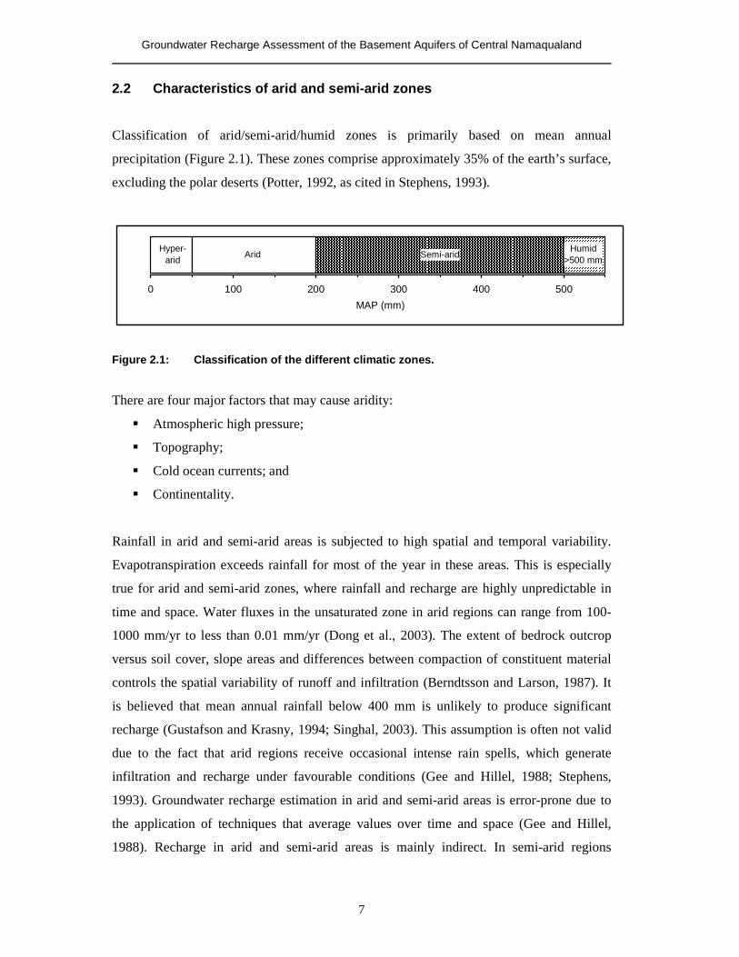
Classification of arid/semi-arid/humid zones is primarily based on mean annual
precipitation (Figure 2.1). These zones comprise approximately 35% of the earth’s surface,
excluding the polar deserts (Potter, 1992, as cited in Stephens, 1993).
Hyper-arid
Arid Semi-aridHumid
>500 mm
0 100 200 300 400 500
MAP (mm)
Figure 2.1: Classification of the different climatic zones.
There are four major factors that may cause aridity:
� Atmospheric high pressure;
� Topography;
� Cold ocean currents; and
� Continentality.
Rainfall in arid and semi-arid areas is subjected to high spatial and temporal variability.
Evapotranspiration exceeds rainfall for most of the year in these areas. This is especially
true for arid and semi-arid zones, where rainfall and recharge are highly unpredictable in
time and space. Water fluxes in the unsaturated zone in arid regions can range from 100-
1000 mm/yr to less than 0.01 mm/yr (Dong et al., 2003). The extent of bedrock outcrop
versus soil cover, slope areas and differences between compaction of constituent material
controls the spatial variability of runoff and infiltration (Berndtsson and Larson, 1987). It
is believed that mean annual rainfall below 400 mm is unlikely to produce significant
recharge (Gustafson and Krasny, 1994; Singhal, 2003). This assumption is often not valid
due to the fact that arid regions receive occasional intense rain spells, which generate
infiltration and recharge under favourable conditions (Gee and Hillel, 1988; Stephens,
1993). Groundwater recharge estimation in arid and semi-arid areas is error-prone due to
the application of techniques that average values over time and space (Gee and Hillel,
1988). Recharge in arid and semi-arid areas is mainly indirect. In semi-arid regions
Groundwater Recharge Assessment of the Basement Aquifers of Central Namaqualand
8
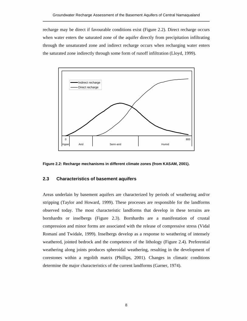
recharge may be direct if favourable conditions exist (Figure 2.2). Direct recharge occurs
when water enters the saturated zone of the aquifer directly from precipitation infiltrating
through the unsaturated zone and indirect recharge occurs when recharging water enters
the saturated zone indirectly through some form of runoff infiltration (Lloyd, 1999).
0 800
Hyper Arid Semi-arid Humid
Indirect recharge
Direct recharge
Figure 2.2: Recharge mechanisms in different climate zones (from KASAM, 2001).
2.3 Characteristics of basement aquifers
Areas underlain by basement aquifers are characterized by periods of weathering and/or
stripping (Taylor and Howard, 1999). These processes are responsible for the landforms
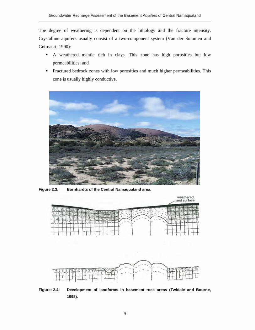
observed today. The most characteristic landforms that develop in these terrains are
bornhardts or inselbergs (Figure 2.3). Bornhardts are a manifestation of crustal
compression and minor forms are associated with the release of compressive stress (Vidal
Romaní and Twidale, 1999). Inselbergs develop as a response to weathering of intensely
weathered, jointed bedrock and the competence of the lithology (Figure 2.4). Preferential
weathering along joints produces spheroidal weathering, resulting in the development of
corestones within a regolith matrix (Phillips, 2001). Changes in climatic conditions
determine the major characteristics of the current landforms (Garner, 1974).
Groundwater Recharge Assessment of the Basement Aquifers of Central Namaqualand
9
The degree of weathering is dependent on the lithology and the fracture intensity.
Crystalline aquifers usually consist of a two-component system (Van der Sommen and
Geirnaert, 1990):
� A weathered mantle rich in clays. This zone has high porosities but low
permeabilities; and
� Fractured bedrock zones with low porosities and much higher permeabilities. This
zone is usually highly conductive.
Figure 2.3: Bornhardts of the Central Namaqualand area.
Figure: 2.4: Development of landforms in basement rock areas (Twidale and Bourne,
1998).
Groundwater Recharge Assessment of the Basement Aquifers of Central Namaqualand
10
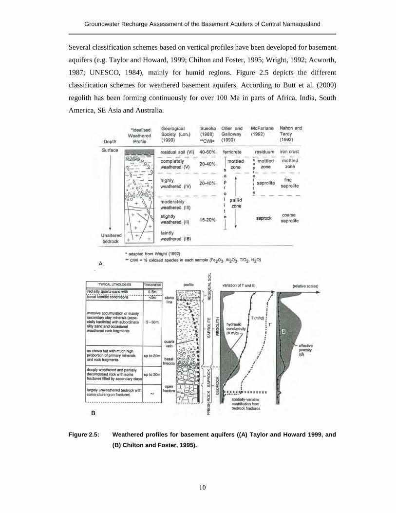
Several classification schemes based on vertical profiles have been developed for basement
aquifers (e.g. Taylor and Howard, 1999; Chilton and Foster, 1995; Wright, 1992; Acworth,
1987; UNESCO, 1984), mainly for humid regions. Figure 2.5 depicts the different
classification schemes for weathered basement aquifers. According to Butt et al. (2000)
regolith has been forming continuously for over 100 Ma in parts of Africa, India, South
America, SE Asia and Australia.
Figure 2.5: Weathered profiles for basement aquifers ((A) Taylor and Howard 1999, and
(B) Chilton and Foster, 1995).
B
A
B
Groundwater Recharge Assessment of the Basement Aquifers of Central Namaqualand
11
Weathered zone
The extent and depth of the weathered zone is determined by weathering susceptibility and
moisture availability. The weathered zone in arid terrain is generally shallower than in
more humid terrain. However, thick weathered zones occur in semi-arid areas and are a
result of a more humid period during the Pleistocene Age (UNESCO, 1984). The higher
the weathering susceptibility and moisture availability, the more the weathering rates
dominate; greater permeability is created which leads to more moisture; and a faster
weathering rate leads to more intense weathering (Phillips, 2001). The deeper the
weathering, the higher the degree of fragmentation (Lan et al., 2003; Wright, 2002) :
intact rock � big block-like � fragment-like � gravel-like � sand-like � clay-like.
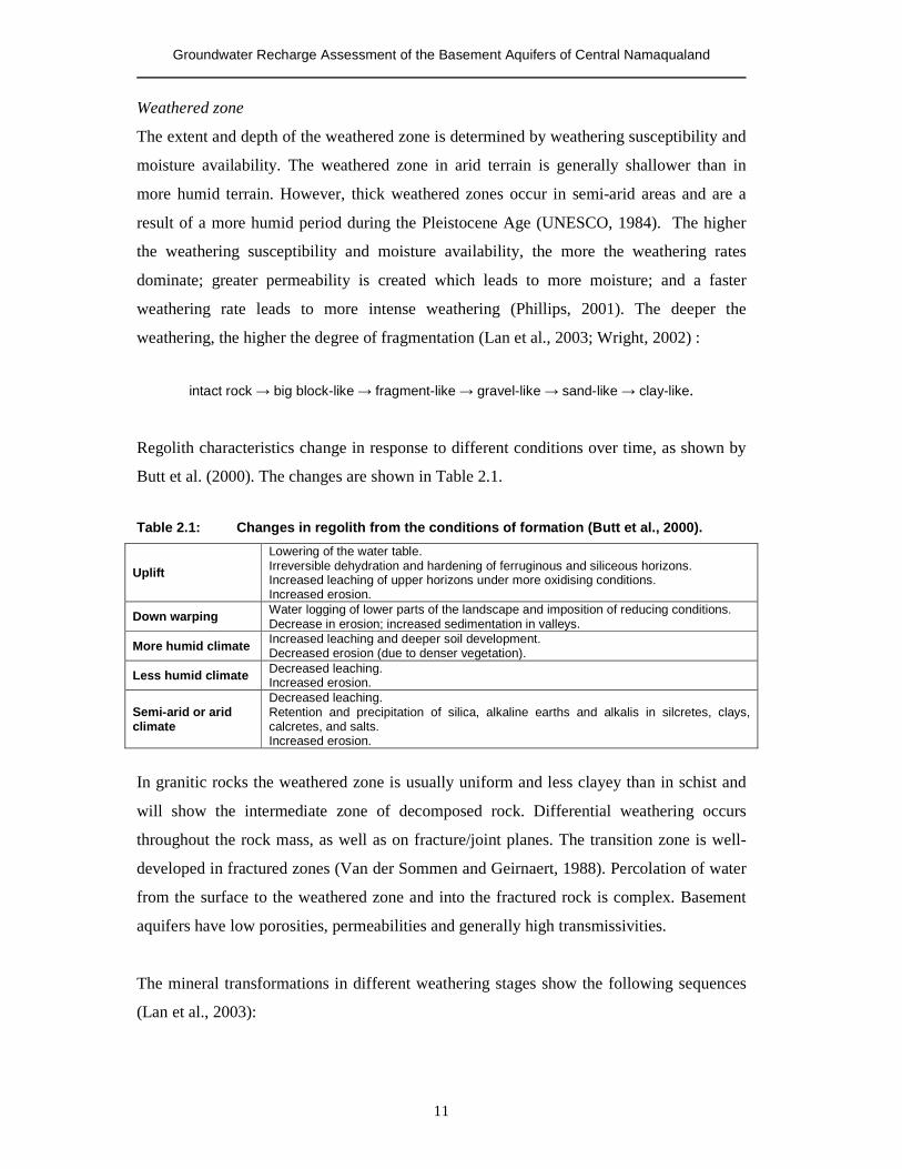
Regolith characteristics change in response to different conditions over time, as shown by
Butt et al. (2000). The changes are shown in Table 2.1.
Table 2.1: Changes in regolith from the conditions of formation (Butt et al., 2000).
Uplift
Lowering of the water table. Irreversible dehydration and hardening of ferruginous and siliceous horizons. Increased leaching of upper horizons under more oxidising conditions. Increased erosion.
Down warping Water logging of lower parts of the landscape and imposition of reducing conditions. Decrease in erosion; increased sedimentation in valleys.
More humid climate Increased leaching and deeper soil development. Decreased erosion (due to denser vegetation).
Less humid climate Decreased leaching. Increased erosion.
Semi-arid or arid climate
Decreased leaching. Retention and precipitation of silica, alkaline earths and alkalis in silcretes, clays, calcretes, and salts. Increased erosion.
In granitic rocks the weathered zone is usually uniform and less clayey than in schist and
will show the intermediate zone of decomposed rock. Differential weathering occurs
throughout the rock mass, as well as on fracture/joint planes. The transition zone is well-
developed in fractured zones (Van der Sommen and Geirnaert, 1988). Percolation of water
from the surface to the weathered zone and into the fractured rock is complex. Basement
aquifers have low porosities, permeabilities and generally high transmissivities.
The mineral transformations in different weathering stages show the following sequences
(Lan et al., 2003):
Groundwater Recharge Assessment of the Basement Aquifers of Central Namaqualand
12
1. feldspar � sericite � hydromica � kaolinite;
2. pyroxene and hornblende � chlorite � montmorillonite � halloysite � kaolonite;
3. biotite � vermiculite � montmorillonite � kaolonite
4. quartz � silica � chalcedony � secondary quartz.
Fractured bedrock
Exposed fractured bedrock is mainly associated with higher-lying areas and the
bornhardts/inselbergs that characterise the area. The porosity and permeability of hard
rocks are mainly determined by the intensity, orientation, connectivity, aperture and infill
of fracture systems (Skjernaa and Jørgensen, 1994). Black (1994) identifies three main
fracture configurations in non-layered fractured rocks. These are: 1. random fracture
locations (Poisson), 2. structured fracture locations (fractal) and 3. clustered fracture
locations. Fracture zones may be infilled by secondary minerals due to the different modes
of genesis, deformation and reactivation (Banks et al., 1994; Srinivas et al., 1999). Sheet
structures are widely developed on bornhardts. Sheet fractures are arcuate fractures that
trend parallel to the land surface (Vidal Romaní and Twidale, 1999). These fractures are
convex-upward in many residual hills and concave-upward in the valley floors (Vidal
Romaní and Twidale, 1999). The favoured explanation for these sheet fractures is that they
are the result of expansion and tangential fracturing, consequent on erosional offloading
(Vidal Romaní and Twidale, 1999). The frequency of the sheet fractures and the fracture
openings decrease rapidly with depth. Fractures range from microns to hundreds of
kilometers. The inherent complexity of obtaining accurate data on fractured formations,
both structural and hydraulic, is a major obstacle in developing accurate fractured medium
models (Berkowitz, 2002).
According to Gustafson and Krásný (1994), the hydraulic conductivity determined by field
methods can vary by several orders of magnitude within the same rock unit, and usually
over very short distances. Daniel (1996) states that, as a general rule, the abundance of
fractures and size of fracture openings, decreases with depth as a result of lithostatic
pressures. In central Spain Gonzales-Yelamos et al. (1993) showed, with permeability
tests, that permeability generally declines with depth. Fracture apertures in granite, gneiss
and metavolcanics, ranging from 75-100 µ in the upper 10 m of bedrock and decreasing to
50-100 µm at 15-60 m depth, have been reported by Snow (1968), using packer tests.
Fracture zones usually occur along lineaments and often correspond to the surface drainage
Groundwater Recharge Assessment of the Basement Aquifers of Central Namaqualand
13
patterns. An aquifer in regolith is between one and two orders of magnitude more
transmissive than the underlying bedrock aquifer (Tindimugaya, 1995).
2.4 Recharge, Storage and Groundwater flow
Recharge
Recharge to crystalline rocks is a function of the mode of chemical weathering of its
surface, and the rate of fracturing (Lerner et al., 1990). Recharging or infiltrating water is
responsible for the development of the weathered zone aquifers. Deep weathering in a
stable tectonic environment is dominated by high infiltration rates, and land denudation is
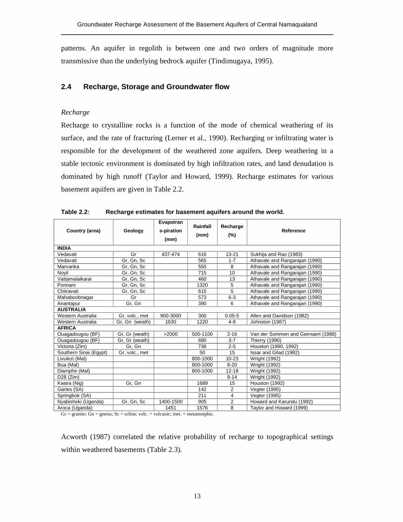
dominated by high runoff (Taylor and Howard, 1999). Recharge estimates for various
basement aquifers are given in Table 2.2.
Table 2.2: Recharge estimates for basement aquifers around the world.
Country (area) Geology
Evapotran
s-piration
(mm)
Rainfall
(mm)
Recharge
(%) Reference
INDIA Vedavati Gr 437-474 616 13-21 Sukhija and Rao (1983) Vedavati Gr, Gn, Sc 565 1-7 Athavale and Rangarajan (1990) Marvanka Gr, Gn, Sc 550 8 Athavale and Rangarajan (1990) Noyil Gr, Gn, Sc 715 10 Athavale and Rangarajan (1990) Vattamalaikarai Gr, Gn, Sc 460 13 Athavale and Rangarajan (1990) Ponnani Gr, Gn, Sc 1320 5 Athavale and Rangarajan (1990) Chitravati Gr, Gn, Sc 615 5 Athavale and Rangarajan (1990) Mahaboobnagar Gr 573 6-3 Athavale and Rangarajan (1990) Anantapur Gr, Gn 390 6 Athavale and Rangarajan (1990) AUSTRALIA Western Australia Gr, volc., met 900-3000 300 0.05-5 Allen and Davidson (1982) Western Australia Gr, Gn (weath) 1630 1220 4-8 Johnston (1987) AFRICA Ouagadougou (BF) Gr, Gr (weath) >2000 500-1100 2-16 Van der Sommen and Geirnaert (1988) Ouagadougou (BF) Gr, Gr (weath) 690 3-7 Thierry (1990) Victoria (Zim) Gr, Gn 736 2-5 Houston (1990, 1992) Southern Sinai (Egypt) Gr, volc., met 50 15 Issar and Gilad (1982) Livulezi (Mal) 800-1000 10-23 Wright (1992) Bua (Mal) 800-1000 8-20 Wright (1992) Diamphe (Mal) 800-1000 12-18 Wright (1992) D28 (Zim) 9-14 Wright (1992) Kwara (Nig) Gr, Gn 1689 15 Houston (1992) Garies (SA) 142 2 Vegter (1995) Springbok (SA) 211 4 Vegter (1995) Nyabisheki (Uganda) Gr, Gn, Sc 1400-1500 905 2 Howard and Karundu (1992) Aroca (Uganda) 1451 1576 8 Taylor and Howard (1999)
Gr = granite; Gn = gneiss; Sc = schist; volc. = volcanic; met. = metamorphic.
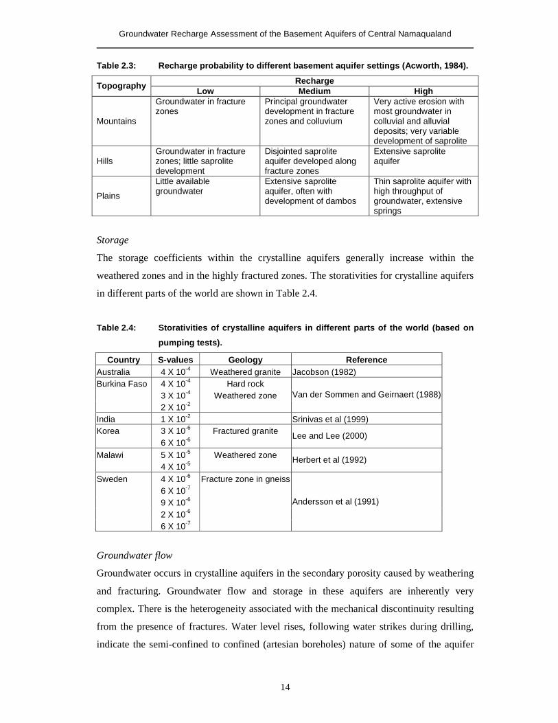
Acworth (1987) correlated the relative probability of recharge to topographical settings
within weathered basements (Table 2.3).
Groundwater Recharge Assessment of the Basement Aquifers of Central Namaqualand
14
Table 2.3: Recharge probability to different basement aquifer settings (Acworth, 1984).
Recharge Topography Low Medium High
Mountains
Groundwater in fracture zones
Principal groundwater development in fracture zones and colluvium
Very active erosion with most groundwater in colluvial and alluvial deposits; very variable development of saprolite
Hills Groundwater in fracture zones; little saprolite development
Disjointed saprolite aquifer developed along fracture zones
Extensive saprolite aquifer
Plains
Little available groundwater
Extensive saprolite aquifer, often with development of dambos
Thin saprolite aquifer with high throughput of groundwater, extensive springs
Storage
The storage coefficients within the crystalline aquifers generally increase within the
weathered zones and in the highly fractured zones. The storativities for crystalline aquifers
in different parts of the world are shown in Table 2.4.
Table 2.4: Storativities of crystalline aquifers in different parts of the world (based on
pumping tests).
Country S-values Geology Reference Australia 4 X 10⁻⁴ Weathered granite Jacobson (1982) Burkina Faso 4 X 10⁻⁴ Hard rock 3 X 10⁻⁴ Weathered zone 2 X 10⁻²
Van der Sommen and Geirnaert (1988)
India 1 X 10⁻² Srinivas et al (1999) Korea 3 X 10⁻⁶ Fractured granite 6 X 10⁻⁶
Lee and Lee (2000)
Malawi 5 X 10⁻⁵ Weathered zone 4 X 10⁻⁵
Herbert et al (1992)
Sweden 4 X 10⁻⁶ Fracture zone in gneiss 6 X 10⁻⁷ 9 X 10⁻⁶ 2 X 10⁻⁶ 6 X 10⁻⁷
Andersson et al (1991)
Groundwater flow
Groundwater occurs in crystalline aquifers in the secondary porosity caused by weathering
and fracturing. Groundwater flow and storage in these aquifers are inherently very
complex. There is the heterogeneity associated with the mechanical discontinuity resulting
from the presence of fractures. Water level rises, following water strikes during drilling,
indicate the semi-confined to confined (artesian boreholes) nature of some of the aquifer

Groundwater Recharge Assessment of the Basement Aquifers of Central Namaqualand
15
systems. Weathering and fracturing decreases with depth in hard rock terrain, at which the
cost of drilling deeper outweighs the chance of significantly increasing the yield of the
borehole. This may be due to increasing lithostatic pressure, which tends to close fractures,
which increases resistance to groundwater flow. It is not the rocks themselves that transmit
the groundwater but the fractures and fissures that form the conductive openings through
the impervious rock matrix (Gustafson and Krásný, 1993). Regional flow occurs within the
major interconnected fracture systems. The main groundwater flow systems are relatively
localised between recharge on watersheds to discharge by runoff or evaporation in valley
bottomlands in crystalline terrains (Wright, 1992). Groundwater flow in topographic highs
occurs along major fractures as a function of the naturally high hydraulic gradients in these
regions.
Due to its larger porosity the weathered/regolith zone acts as a reservoir that slowly feeds
water downward into fractures in the bedrock (Daniel, 1996). Fractures exposed at the
surface act as preferential flow paths. Stephens (1993) defined preferential flow paths as
open conduits or macropores that can short circuit the path to the water table. Infiltration
at a point between soil and rock are dependent on the hydraulic conditions at that zone
(Olofsson, 1994). If water enters a fracture above a point of saturation, the movement of
the water will be predominantly in the direction of the dip of such fractures. Water will
only enter a fracture after the fluid pressure exceeds the water-entering pressure of the
fracture (Stephens, 1993). Below the saturated zone, movement can be both vertical and
horizontal. The lateral motion along the strike of the fracture would predominate (Ellis,
1909). Any connected series of joints will have a complex circulation. Nevertheless, the
main circulation will be towards and along the fractures having the largest openings and
the nearest discharge points, and in these fractures the general movement will be in the
direction of a land slope. Percolation of the groundwater from the surface to the weathered
zone and into the fractured rock is complex. Flow paths in fractured rocks are very
complex and heterogeneous, due to its complex geometry (Karasaki et al., 2000).
Groundwater Recharge Assessment of the Basement Aquifers of Central Namaqualand
16
CHAPTER 3
Theoretical aspects of recharge estimation
3.1 Introduction
Aquifer recharge is dependent on factors such as: climate, geology (lithology and
structures), geomorphology, vegetation, soil conditions and antecedent soil moisture.
Recharge can either be diffuse and/or through preferential pathways. Lerner et al., (1990)
defined three principle mechanisms for aquifer recharge:
� Direct recharge – the addition of water to the aquifer in excess of soil moisture
deficits and evapotranspiration by vertical percolation through the unsaturated
zone;
� Indirect recharge – the percolation of water through the beds of surface water
bodies or ephemeral streambeds; and
� Localised recharge – this entails recharge from localised water ponding directly
overlying the aquifer and percolating through the unsaturated zone.
Several methods have been developed over the last few decades to determine recharge
originating from the above mechanisms. Publications that deals exclusively with recharge
and the different methods include, among others, Lerner et al. (1990); Bredenkamp et al.
(1995); Simmers et al. (1997); Kinzelbach et al. (2002); Scanlon and Cook (2002) and Xu
and Beekman (2003). Estimation techniques are divided into physical techniques, tracer
techniques and numerical models. Different techniques estimate recharge over different
spatial and temporal scales (e.g. Scanlon et al., 2002; Beekman and Xu, 2003).
Bredenkamp et al. (1995) and Beekman and Xu (2003) give an account of the recharge
estimation methods applied in semi-arid southern Africa and identified the following
methods as the most promising for application in semi-arid to arid conditions:
� Chloride mass balance (CMB);
� Cumulative rainfall departures (CRD);
� EARTH model;
� Water table fluctuations;
Groundwater Recharge Assessment of the Basement Aquifers of Central Namaqualand
17
� Groundwater models (GM); and
� Saturated volume fluctuations (SVF).
3.2 Recharge estimation methods
The applicability of any recharge estimate depends on the availability of data and the
potential to obtain data, the characteristics of the area and importantly the cost of obtaining
data. Recharge estimation methods and case studies are well documented. It is beyond the
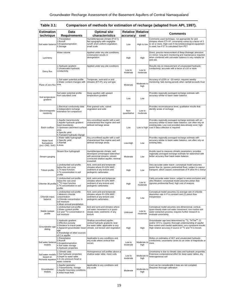
scope of this document to describe all the techniques. A brief summary of the methods is
listed in Table 3.1. Bredenkamp et al. (1995) and Beekman and Xu (2003) also give a
comparison of methods used in estimating recharge. Only the methods identified in the
next section will be described in this chapter. It should be noted that the accuracy and cost
of a particular method are relative and depends on factors such as:
� The proximity of the study area to the research institution/headquarter;
� The availability of laboratories (in-house versus commercial);
� The availability of specialised sampling equipment (in-house versus commercial or
acquisition);
� The availability of skilled human resources (in-house versus consultants); and
� Level of accuracy and quality assurance required.
3.3 Groundwater recharge estimation methods applicable for Central
Namaqualand
In order to find methods that may be applicable for estimating recharge to the aquifers of
Central Namaqualand an Excel spreadsheet was programmed to determine the suitability
of different methods, based on the availability of data and the potential to gather data. An
example of the elimination/validation process is shown in Figure 3.1. A suitability index
was also created for specific areas to determine the data availability and type of data
available, an example is also shown in Figure 3.1.
The suitability index is based on a simple approach whereby the amount of data available
is listed and scored. The scores are calculated based on the availability of the data and
whether the data is of a quantitative or qualitative nature. If the available information is
quantitative it scores higher than more qualitative data. Qualitative data is also important
Groundwater Recharge Assessment of the Basement Aquifers of Central Namaqualand
18
for the development of conceptual models but it cannot be used to estimate recharge. The
approach is subjective and requires that it be evaluated against the objectives of the study.
If insufficient data is available the recharge study will become more complex and
expensive, if the objective is to obtain reliable recharge estimates.
If sufficient quantitative and qualitative data are available, the user can proceed to the
methods sheet. Different methods are listed and each method is preprogrammed with the
minimum data requirements. The user can input the type of data available or data that can
be obtained within a specific project. The minimum requirements of each method are
assigned a value of 1, if the corresponding data is available or if it can be obtained. If all
the data for a specific method is available the column will be totaled and if the total equals
the preprogrammed value the applicable cell will return a yes. The sheet will essentially
determine which methods are applicable for any specific area based on the available data.
Five methods have been identified that can be applied in the study area these methods are
the CMB method, CRD method and the SVF method and a GIS approach using available
data. The following sections will outline the selected methods. The CMB method cannot
be applied in the unsaturated zone due to several conditions that cannot be met, as outlined
in the next section. The use of the stable and radiogenic isotopes; 18O, 2H and 14C, will be
discussed as it is used to develop and constrain the conceptual understanding of
groundwater recharge.
Groundwater Recharge Assessment of the Basement Aquifers of Central Namaqualand
19
Table 3.1: Comparison of methods for estimation of recharge (adapted from API, 1997).
Estimation technique
Data Requirements
Optimal site characteristics
Relative accuracy
Relative cost Comments
Soil water balance
1.Precipitation 2.Runoff 3.Evapotranspiration 4.Storage
Humid/temperate climate (P>ET); flat topography with negligible runoff; short uniform vegetation; small scale
Low High to low
Commonly used technique, not appropriate for arid climates where ET>>P; uncertainty varies by a factor of 3 to 10 or more. High cost if micrometeorological equipment is used; low if ET is calculated from PET
Lysimetry
Water volume Applied under any site conditions; construction results in devegetation High High
Direct, precise measurement of deep drainage; precision ±1 mm/yr; long term monitoring and maintenance required; when combined with soil-water balance is very reliable for arid site
Darcy flux
1.Hydraulic gradient 2.Unsaturated hydraulic conductivity
Applied under any site conditions
Low to moderate
Low to moderate
Results rely on measurement of unsaturated hydraulic conductivity; accurate with a factor of ±10 or more
Plane of zero flux
1.Soil water potential profile 2.Water content changes with time
Temperate, semi-arid or arid climates (ET>P); any soil type
Moderate Moderate to high
Accuracy of ±15% or ~20 mm/yr; requires weekly monitoring; fails during periods when rainfall exceeds Ksat
Soil temperature gradient
Soil water potential profile from saturated zone
Deep aquifers with upward temperature gradient
Low Low
Provides regionally averaged recharge estimate with accuracy similar to basin water balance
Electromagnetic resistivity
1.Electrical conductivity data 2.Independent recharge estimation for comparison
Fine grained soils; varied vegetation and soils
Non-quantitative
Low to moderate
Provides reconnaissance level, qualitative results that identify areas of recharge
Basin outflow
1.Aquifer transmissivity 2.Aquifer hydraulic gradient basin boundaries 3.Upstream catchment surface area 4.Specific yield 5.Transient hydraulic change
Any unconfined aquifer with a well characterised flow regime and well defined recharge areas
Low Low to high
Provides regionally averaged recharge estimate with an accuracy similar to basin water balance; can often rely on existing data. Low cost provided data already exist; high cost if data collection is required
Water level fluctuations
(incl. CRD, SVF)
1.Water table hydrograph 2.Specific yield 3.Rainfall 4.Area
Any unconfined aquifer with a well characterised flow regime and well defined recharge areas Low-High Low
Provides regionally averaged recharge estimate with accuracy similar to basin water balance; can often rely on existing data.
Stream gauging
Stream flow hydrograph Humid/temperate climate; well developed unmanaged watershed with perennial streams;-stream connected shallow aquifer; minimal snowmelt
Moderate Low
Avoids need to measure climatic parameters; provides regionally averaged recharge estimate for watershed with better accuracy than basin water balance
Tritium profile
1.Undisturbed soil profile below the root zone 2.3H input function 3.3H concentration in soil profile
Arid, semi-arid and temperate climates where R>10% MAP; sediment of any texture and pedogenic carbonates
High Low
Very accurate water tracer; conceptual model assumes piston flow (ie. Ignores preferential flow); subject to vapour transport, which causes overestimate of R wher R<1 mm/yr
Chlorine-36 profile
1.Undisturbed soil profile below the root zone 2.36Cl input function 3.3H concentration in soil profile
Arid, semi-arid and temperate climates where R>10% MAP; sediment of any texture and pedogenic carbonates
High Low to moderate
Fairly accurate water tracer, subject to anion exclusion and ultra filtration; conceptual model assumes piston flow (ignores preferential flow); high cost of analysis
Chloride mass balance
1.Undisturbed soil profile 2.Meteoric chloride concentration 3.Chloride concentration in soil moisture 4.Mean annual precipitation
Arid, semi-arid and temperate climates where R>10% MAP; sediment of any texture and pedogenic carbonates High Low
Conceptual model assumes (1) average rate of chloride deposition rate in P is constant and (2) piston flow. Inexpensive
Stable isotope profile
1.Undisturbed soil profile 2.Water content profile 3.D and 18O concentration in soil moisture
Arid and semi-arid climates where soil water movement is in quasi-steady state; sediments of any texture
Unknown Low to moderate
Conceptual model assumes one-dimensional, vertical, quasi-steady state soil water movement; non-routine soil water extraction process; requires further research to evaluate uncertainty
Groundwater age dating
1.Hydraulic gradient 2.Effective porosity 3.Distance to tracer peak 4.Apparent groundwater tracer age 5.Knowledge of other sources of C in aquifer
Shallow unconfined aquifer; vertical hydraulic gradients near the water table; applicable to any climate, soil texture and vegetation High High
Groundwater age best determined by 14C, 3H/3He36, Cl and/or CFC's; requires thorough understanding of aquifer flow system and careful application; very consistent results. High relative accuracy if source of 14C and 3H is known.
Soil water balance models
1.Precipitation 2.Runoff 3.Evapotranspiration 4.Soil water storage 5.Hydraulic properties
Applicable to any conditions and any scale where vertical flow occurs Low to
moderate Moderate to
high
Relies on estimates of AET and unsaturated hydraulic conductivity; uncertainty varies by an order of magnitude or more
Soil water models based on
Richards equation
1.Climatic data 2.Soil hydraulic properties 3.Depth to water table 4.In situ pressure head or water contents
Homogeneous soil profiles above a shallow water table; moist soils
Low to moderate
Moderate to high
Uncertainty is due to climatic data and hydraulic properties. Extensive computational effort for deep water tables, dry heterogeneous soil
Groundwater models
1.Aquifer geometry 2.Transmissivity, storage 3.Aquifer boundary conditions 4.Initial head field
Applicable to any conditions and any scale
Moderate Moderate to high
Cost can be considerable if data are not compiled. Requires thorough calibration
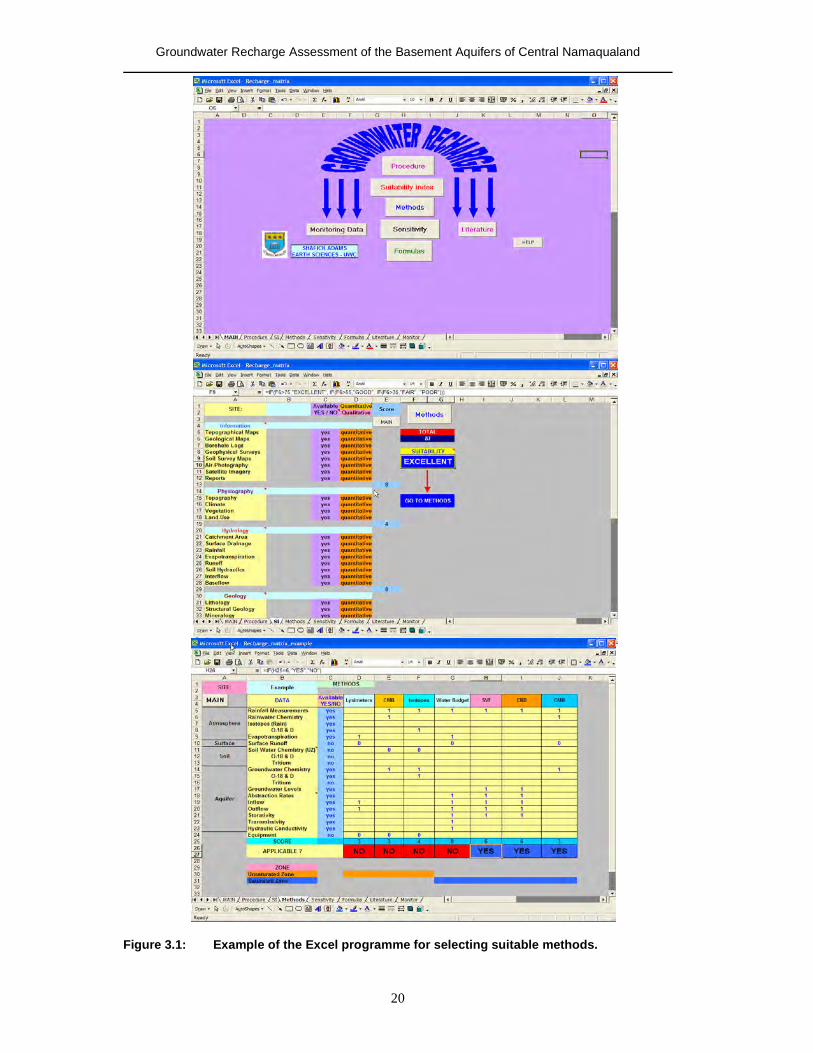
Groundwater Recharge Assessment of the Basement Aquifers of Central Namaqualand
20
Figure 3.1: Example of the Excel programme for selecting suitable methods.
Groundwater Recharge Assessment of the Basement Aquifers of Central Namaqualand
21
3.4 Physical and chemical recharge estimation methods
3.4.1 Chemical and isotope tracer methods
Chloride Mass Balance (CMB)
The method is often used as a first approximation of recharge due to its simplicity and
relatively low cost. The method was first applied in the saturated zone by Eriksson and
Khunakasem (1969) and has become one of the most widely used recharge estimation
methods
The chloride ion is highly soluble, non-absorbing, chemically conservative and easily
measurable. Chloride has the advantage over other tracers involving the water molecule
(18O, 2H, 3H) in that atmospheric inputs are conserved during the recharge process,
allowing a mass balance approach to be used (Edmunds and Gaye, 1994). Preferably,
results should be verified with other methods. There are three approaches to estimate
recharge using the CMB method:
� The first approach involves the chloride concentration of rain and soil moisture
(unsaturated zone) and gives an estimate of the moisture flux;
� The second approach involves the chloride concentrations of groundwater
(saturated zone), whereby the total recharge is estimated; and
� The third approach involves the comparison of the first two approaches to define
the recharge mechanism.
The use of the CMB method or methods that involve chemical tracers provide more
accurate estimates of groundwater recharge in arid to semi-arid regions (Bazuhair and
Wood, 1996). The method is applicable in areas of high evapotranspiration where the
infiltrating water becomes concentrated (Johansson, 1987). The following is required when
applying the method:
� Precipitation (mm);
� Precipitation chemistry (mg/l);
� Dry deposition (chloride) (mg/m2/yr);
� Soil moisture chloride concentration (mg/l); and
� Groundwater chloride concentration (mg/l).
Groundwater Recharge Assessment of the Basement Aquifers of Central Namaqualand
22
Unsaturated zone
The method is applied in the unsaturated zone between the deepest zero flux plane and the
water table. The method yields a recharge flux for a specific locality and should ideally be
integrated with area weights to estimate areal recharge. Most plant species do not take up
significant quantities of chloride from soil water, thus chloride is mainly concentrated by
evapotranspiration in the root zone (Allison et al., 1994). However, White and Broadley
(2001) have shown that chloride can be taken up and accumulated by plants. Edmunds and
Gaye (1994) correlated recharge with the chloride concentrations in soils. High chloride
concentrations are generally associated with lower rates of recharge and visa versa. If a
steady state is attained between the chloride flux at the surface and the chloride flux
beneath the evapotranspiration and mixing zone, the following mass balance can be
defined (Eriksson and Khunakasem, 1969):
(3.1)
where: Rsm = moisture flux (mm/yr) P = precipitation (mm/yr) Clp = chloride concentration in precipitation (mg/l) Clsm = chloride concentration in soil moisture (mg/l) D = dry chloride deposition (mg/m2/yr)
The sum of P*Clp and D is also referred to as the total atmospheric chloride deposition
(TD) and originates from both precipitation and dry fall out.
A better estimate of the moisture flux is obtained from a mass balance, which integrates
chloride and moisture contents cumulatively over a specific depth interval (Gieske, 1992):
(3.2)
where: TM = total moisture content (mm/m2) TC = total chloride content (mg/m2) Three potential problems have been identified with the above calculation methods (Wood,
1999):
� It is difficult to quantitatively evaluate the mass flux of chloride that has run onto,
or from, the topographic features present at the sampling sites;
Cl
TD
Cl
D+Cl*P=R
smsm
psm =
TC
TMTD=R csm
*)(
Groundwater Recharge Assessment of the Basement Aquifers of Central Namaqualand
23
� The system may not be at steady state with respect to the input mass flux; and
� This method cannot measure total recharge if any unmeasured recharge takes place
through macropores in the system.
To incorporate the additional mass resulting from run-on Wood and Sanford (1995)
suggests the following equation for a closed depression:
(3.3)
where: r = run-on flux from the catchment area (mm/yr) Ab = total area of the basin (m2) Clr = chloride concentration of the runoff water to the basin floor (mg/l) Af = area of basin floor (m2) The transient chloride flux can be evaluated by plotting chloride concentration from the
pore water as a function of depth. For steady state, a graphical plot of depth versus chloride
will show chloride increasing gradually from the surface to a maximum value at shallow
depth. The exact depth at which equilibrium is attained is a function of the climatic
condition, grain-size distribution of the material and other factors.
Below this depth, the chloride concentration in the pore water should remain constant until
it reaches the water table (where diffusion and water table fluctuation will distort the
profile). In Figure 3.2, conceptual chloride profiles are shown. Any significant deviation
from the equilibrium profile indicates a temporal variability in the chloride mass flux and
thus steady state assumption would become questionable.
If recharge takes place through macropores the equation above is inappropriate. Total
recharge is a combination of macropore and matrix recharge. If macropores exists in the
area under investigation, the unsaturated zone core profiling method will not yield reliable
results. The total recharge flux is thus the sum of the recharge attributed to diffuse flow
through the matrix and recharge attributed to macropore or recharge through preferential
flow paths.
��
�
�
��
�
�+���
����
�=
smf
rb
smsm ClA
ClAr
ClTD
R
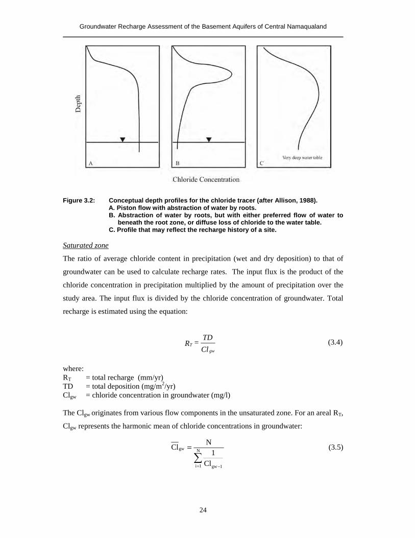
Groundwater Recharge Assessment of the Basement Aquifers of Central Namaqualand
24
Figure 3.2: Conceptual depth profiles for the chloride tracer (after Allison, 1988).
A. Piston flow with abstraction of water by roots. B. Abstraction of water by roots, but with either preferred flow of water to
beneath the root zone, or diffuse loss of chloride to the water table. C. Profile that may reflect the recharge history of a site.
Saturated zone
The ratio of average chloride content in precipitation (wet and dry deposition) to that of
groundwater can be used to calculate recharge rates. The input flux is the product of the
chloride concentration in precipitation multiplied by the amount of precipitation over the
study area. The input flux is divided by the chloride concentration of groundwater. Total
recharge is estimated using the equation:
(3.4)
where: RT = total recharge (mm/yr) TD = total deposition (mg/m2/yr) Clgw = chloride concentration in groundwater (mg/l) The Clgw originates from various flow components in the unsaturated zone. For an areal RT,
Clgw represents the harmonic mean of chloride concentrations in groundwater:
(3.5)
Cl
TD=R
gwT
�= −
= N
1i 1gw
gw
Cl1
NCl
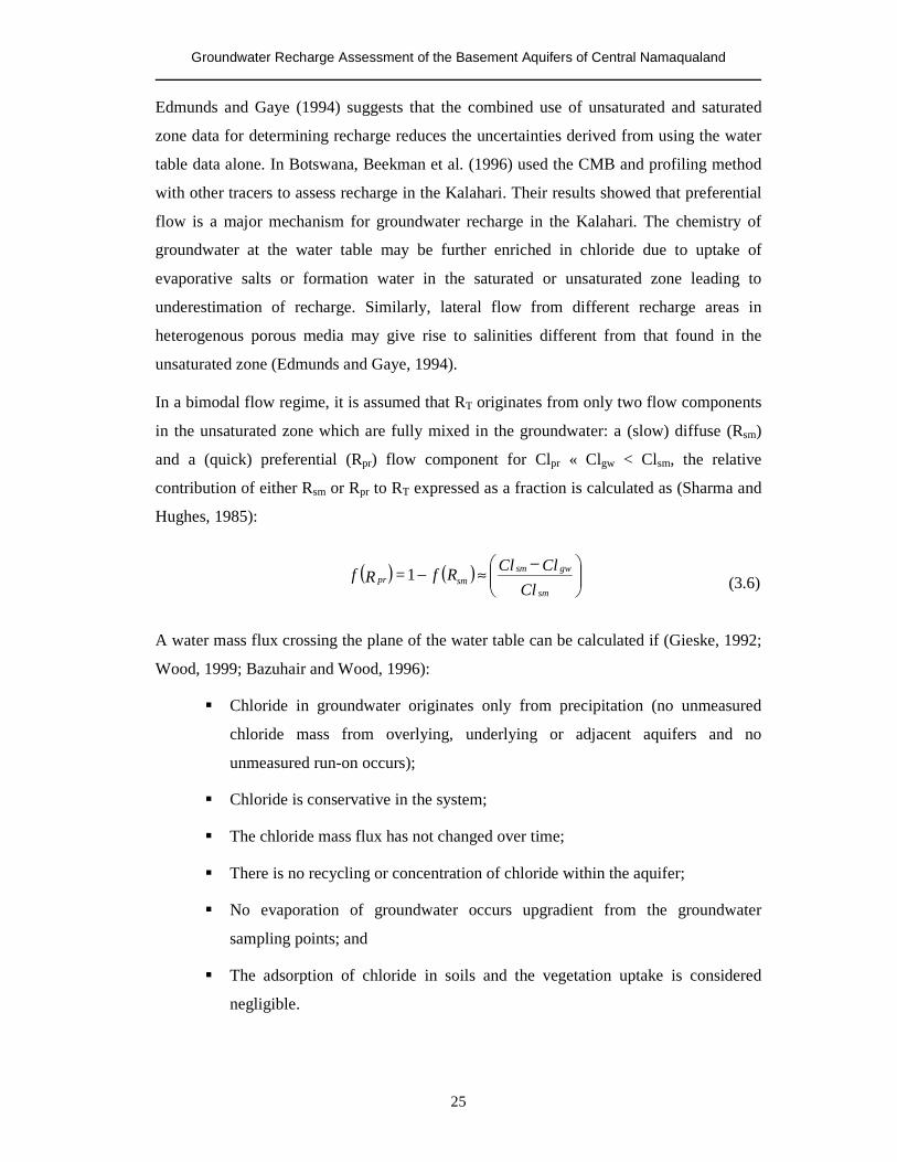
Groundwater Recharge Assessment of the Basement Aquifers of Central Namaqualand
25
Edmunds and Gaye (1994) suggests that the combined use of unsaturated and saturated
zone data for determining recharge reduces the uncertainties derived from using the water
table data alone. In Botswana, Beekman et al. (1996) used the CMB and profiling method
with other tracers to assess recharge in the Kalahari. Their results showed that preferential
flow is a major mechanism for groundwater recharge in the Kalahari. The chemistry of
groundwater at the water table may be further enriched in chloride due to uptake of
evaporative salts or formation water in the saturated or unsaturated zone leading to
underestimation of recharge. Similarly, lateral flow from different recharge areas in
heterogenous porous media may give rise to salinities different from that found in the
unsaturated zone (Edmunds and Gaye, 1994). In a bimodal flow regime, it is assumed that RT originates from only two flow components
in the unsaturated zone which are fully mixed in the groundwater: a (slow) diffuse (Rsm)
and a (quick) preferential (Rpr) flow component for Clpr « Clgw < Clsm, the relative
contribution of either Rsm or Rpr to RT expressed as a fraction is calculated as (Sharma and
Hughes, 1985):
(3.6)
A water mass flux crossing the plane of the water table can be calculated if (Gieske, 1992;
Wood, 1999; Bazuhair and Wood, 1996):
� Chloride in groundwater originates only from precipitation (no unmeasured
chloride mass from overlying, underlying or adjacent aquifers and no
unmeasured run-on occurs);
� Chloride is conservative in the system;
� The chloride mass flux has not changed over time;
� There is no recycling or concentration of chloride within the aquifer;
� No evaporation of groundwater occurs upgradient from the groundwater
sampling points; and
� The adsorption of chloride in soils and the vegetation uptake is considered
negligible.
( ) ( ) ���
����
� −≈−
Cl
Cl Cl Rf =Rfsm
gwsmsmpr 1
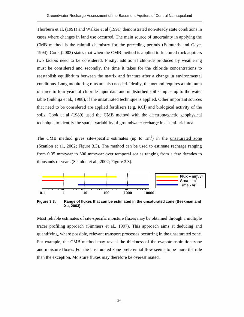
Groundwater Recharge Assessment of the Basement Aquifers of Central Namaqualand
26
Thorburn et al. (1991) and Walker et al (1991) demonstrated non-steady state conditions in
cases where changes in land use occurred. The main source of uncertainty in applying the
CMB method is the rainfall chemistry for the preceding periods (Edmunds and Gaye,
1994). Cook (2003) states that when the CMB method is applied to fractured rock aquifers
two factors need to be considered. Firstly, additional chloride produced by weathering
must be considered and secondly, the time it takes for the chloride concentrations to
reestablish equilibrium between the matrix and fracture after a change in environmental
conditions. Long monitoring runs are also needed. Ideally, the method requires a minimum
of three to four years of chloride input data and undisturbed soil samples up to the water
table (Sukhija et al., 1988), if the unsaturated technique is applied. Other important sources
that need to be considered are applied fertilisers (e.g. KCl) and biological activity of the
soils. Cook et al (1989) used the CMB method with the electromagnetic geophysical
technique to identify the spatial variability of groundwater recharge in a semi-arid area.
The CMB method gives site-specific estimates (up to 1m2) in the unsaturated zone
(Scanlon et al., 2002; Figure 3.3). The method can be used to estimate recharge ranging
from 0.05 mm/year to 300 mm/year over temporal scales ranging from a few decades to
thousands of years (Scanlon et al., 2002; Figure 3.3).
Figure 3.3: Range of fluxes that can be estimated in the unsaturated zone (Beekman and Xu, 2003).
Most reliable estimates of site-specific moisture fluxes may be obtained through a multiple
tracer profiling approach (Simmers et al., 1997). This approach aims at deducing and
quantifying, where possible, relevant transport processes occurring in the unsaturated zone.
For example, the CMB method may reveal the thickness of the evapotranspiration zone
and moisture fluxes. For the unsaturated zone preferential flow seems to be more the rule
than the exception. Moisture fluxes may therefore be overestimated.
0.1 1 10 100 1000 10000
Flux – mm/yr Area – m2 Time - yr
Groundwater Recharge Assessment of the Basement Aquifers of Central Namaqualand
27
The spatial scale of recharge increases significantly when the saturated zone is used to
estimate recharge and similar temporal scales and fluxes are observed as the unsaturated
zone profiling techniques (Figure 3.4).
Figure 3.4: Range of fluxes that can be estimated in the saturated zone (Beekman and
Xu, 2003).
The CMB method for the saturated zone may be especially useful in areas where
groundwater levels do not fluctuate or data on groundwater levels are lacking.
Wood and Sanford (1995) observed that obtaining recharge rates using the CMB method is
comparable to recharge rates obtained by physically based methods in semi-arid areas. The
method is independent of whether recharge is focused or diffused (Bazuhair and Wood,
1996). Uncertainties in the rainfall chloride concentrations, as a result of measurement
errors and other contributing sources, are the main factors that influence the accuracy of
the method.
Stable and radiogenic isotopes
Oxygen-18 and deuterium
Sampling for the stable isotopes 18O and D/2H has become routine, in most
hydrogeological studies, over the last few decades. The stable isotopes 18O and D/2H are
useful in recharge studies as they can provide constraints on the possible location and
altitude of recharge (Mazor, 1991). This approach is best suited when data from springs are
used (e.g. Mazor, 1991; Diamond and Harris, 2000). The differences in the isotopic
composition of groundwater may be due to several factors. Factors that may control the
isotopic variation in precipitation are (Mook, 1994):
� Temperature;
� Latitude;
� Altitude; and
� Seasonality.
0.1 1 10 100 1000 10000
Flux - mm/yr Area - m2 Time - yr
Groundwater Recharge Assessment of the Basement Aquifers of Central Namaqualand
28
10O*�8�D 18 +=
Oxygen-18 and deuterium are used to elucidate recharge by means of soil moisture
profiling in the unsaturated zone. The isotopic composition of the groundwater is used to
establish whether recharge was fast or delayed, if recharge took place immediately after a
rainfall event the water would have undergone minimal evaporation prior to infiltration and
visa versa. The isotopic composition of the groundwater is compared to the Global
Meteoric Water Line (GMWL) of Craig (1961) or a Local Meteoric Water Line (LMWL)
established for a specific area. The GMWL is represented by the equation:
(3.7)
In Australia, Allison et al. (1984) developed the �D displacement method for the
unsaturated zone. This method uses stable isotope soil moisture measurements and plotting
it on a �D – �18O diagram and the displacement from the GMWL or LMWL is used to
calculate recharge using:
(3.8)
where: �� = displacement of either D or 18O from the MWL C = slope of the line through the inverse of the square root of moisture fluxes
obtained from � displacements from the MWL for different sites. Allison et al. (1984) found that in Australia C equal 20.
Carbon-14
Groundwater ages or mean residence times can be used to elucidate recharge areas,
recharge rates, groundwater flow as well as to identify non-renewable water resources (e.g.
Mazor, 1991; Beekman and Selaolo, 1997; Plummer and Sprinkle, 2001; Verhagen, 2003).
It is important that radiocarbon analysis and dating of groundwater be incorporated with
other geochemical and isotopic data and interpretations to derive a meaningful
interpretation. It is important that the combined inorganic and isotopic geochemistry first
be used to develop a conceptual model of the groundwater system before interpreting the
radiocarbon results (Edmunds and Wright, 1979).
Prior to 1952/3 most of the 14C in the atmosphere was derived by the natural transmutation
of nitrogen as a result of the bombardment of cosmic rays (Freeze and Cherry, 1979). Post
1952/3, additional 14C was introduced by nuclear bomb testing. Carbon dioxide (CO2) from
the air is trapped in rain and snow and the water is tagged by atmospheric 14C. As this
Recharge
C�� =
Groundwater Recharge Assessment of the Basement Aquifers of Central Namaqualand
29
water infiltrates into the subsurface it becomes isolated from the atmosphere. When water
moves below the water table and becomes isolated from the earth’s CO2 reservoir
radioactive decay causes the 14C content in the dissolved inorganic carbon to gradually
decline (Freeze and Cherry, 1979). Carbon-14 ages refer to the period of time that has
elapsed since the water moved deep enough into the groundwater zone to be isolated from
the earth’s atmosphere (Freeze and Cherry, 1979).
Radioactive decay is expressed as:
(3.9)
where: A0 = the specific activity (disintegrations per unit time per unit mass of sample) of 14C A = the activity per unit mass of sample t = the decay age of the carbon isotope (years) T = half life of 14C (5730 years) 14C is reported as percent modern carbon (pmC) determined as the ratio of the sample
activity to that of the international standard expressed as a percentage.14C activities may
exceed 100 pmC in areas where groundwater contains tritium (Izbicki and Martin, 1997).
When equation 3.9 is rearranged and upon substitution of T = 5730 years the unadjusted
age of groundwater can be determined by:
(3.10)
Mook (1980), Reardon and Fritz (1978) and Wigley et al. (1978), as cited in Domenico and
Schwartz (1990), list the following processes that can alter the 14C activity of groundwater:
� The congruent dissolution of carbonate minerals, which add ‘dead carbon’ or
carbon without 14C activity to the groundwater. This process lowers the 14C
activity.
� The incongruent dissolution of carbonate or other Ca containing minerals
accompanied by the precipitation of calcite. This process will remove 14C as calcite
precipitates and if dolomite is the mineral dissolving add dead carbon through the
above process. This process could occur in the zone of saturation following the
rapid solution of calcite to equilibrium with subsequent precipitation as dolomite
slowly dissolves.
Tt
AA−
= 20
���
����
�−=
0
ln8270AA
t
Groundwater Recharge Assessment of the Basement Aquifers of Central Namaqualand
30
� The addition of dead carbon from other sources such as the oxidation of old organic
matter, sulphate reduction and methanogenesis can reduce the 14C activity.
� Isotopic exchange involving CO3 and carbonate minerals could lower the 14C
activity. This process is generally considered to have a negligible effect at normal
groundwater temperatures.
If the factors above are not considered radiocarbon dating can yield unrealistic old
radiocarbon ages, these ages can be corrected using geochemical models (Plummer and
Sprinkle, 2001). To better estimate the mean age of groundwater the following equation is
used (Hendry, 1988):
(3.11)
where: Q = the fraction of dissolved inorganic carbon derived from mineral dissolution or the
oxidation of organic carbon. A value of 0.85 is used as an estimate for Q in most natural groundwater systems due to
complexities in estimating Q (Hendry, 1988). The value of Q is not that important when
solving groundwater flow problems for very old groundwater because of its logarithmic
form (Hendry, 1988). At younger ages the value of Q becomes important. Vogel (1967)
reported that numerous measurements have shown that the initial concentration of 14C in
dissolved bicarbonate is about 85 ± 5% that of modern biogenic carbon.
Mazor (1991) states that a practical way to determine the initial 14C that groundwater
attains due to rapid water-rock interactions is to measure the 14C in recent local
groundwater and apply it to the age calculation of older water of aquifers with similar
rocks. Mazor (1991) further states that in the absence of recently recharged water, a drop
of 60% of the initial 14C may be attributed to water-rock interactions in carbonate aquifers
and 90% in silicate rocks (plutonic and volcanic rocks, sandstone, shale and quartzite).
Vogel (1967) states that in a confined aquifer with uniform permeability no age
stratification occurs in the aquifer and the groundwater age increases in the direction of
flow and in unconfined aquifers age stratification occurs due to recharge from
QAA
t ln8270ln82700
+���
����
�−=
Groundwater Recharge Assessment of the Basement Aquifers of Central Namaqualand
31
precipitation. Recharge rates can be calculated using 14C ages, aquifer depth and porosity
(Vogel, 1967):
(3.12)
where: n = porosity H = saturated aquifer thickness (m)
The parameters required for equation 3.12 is difficult to determine in basement aquifers
because groundwater occurs within the weathered zone and the fractured bedrock aquifers.
The sampled water would represent a mixture of different ages if the water is stratified or
the borehole intersects different flow lines arising from the presence of fracture, bedding
and joint planes. Verhagen (2003) noted that the use of the effective porosity in a dual
porous medium could be used. The assumption is that the isotope tracer would label all the
water in the aquifer by advection or diffusion.
3.4.2 Physical methods
Saturated Volume Fluctuation (SVF)
This method comprises an inventory of inputs in relation to outputs over a specific time
period of the water balance. It also comprises the change in the system caused by an
imbalance between components. This is important, as one has to relate the input to rainfall
that occurred over the same period. The responses (i.e. run-off, base flow or groundwater
level change) are assumed to occur within the selected time interval. However, this
response can be delayed and needs to be incorporated. Variable rainfall, delayed response
(e.g. due to catchment features) and drainage due to soil type, thickness and geology, often
makes it difficult to link hydrological output to specific rainfall events.
The SVF-method gives a combined picture of the water level response of an aquifer. This
method determines effective recharge and aquifer storativity and allows these to be
quantified reliably as lumped parameters. The methods presents one of the most valuable
contributions to water balance interpretations, in that it determines average annual rainfall
and annual variability of recharge. It also derives aquifer storativity from linear plots of
SVF versus Q graphs. It is suitable for most hydrological analysis and aquifer management
tnH
R =
Groundwater Recharge Assessment of the Basement Aquifers of Central Namaqualand
32
applications (Bredenkamp et al., 1995). It is based on the saturated water balance, with the
following formula:
(3.13)
where: S = storativity/specific yield �V = saturated volume of aquifer I = lateral inflow O = lateral outflow Re = recharge Q = net discharge. �t = time The status of the aquifer, based on the water level fluctuations of the monitoring boreholes,
is combined and its variation with time is analysed. The water levels from the different
observation boreholes are combined to produce the saturated volume status for the entire
aquifer. This can be achieved by means of a network of finite elements, which is
constructed using the monitoring boreholes or points of abstraction as nodal points for the
grid network (Van Tonder and Kirchner, 1990). A random value for the base thickness of
the aquifer is given, allowing the saturated volume values to be positive.
The SVF change can also be derived from contours of water levels in relation to an
uncertain base. The following simplifying assumptions apply:
� The base is impervious; no losses or inflow via the base is considered; and
� If evapotranspiration losses are included, they have to be added to the abstraction,
but if not, the estimated recharge will represent the effective percolation to
groundwater (i.e. the recharge after evapotranspiration losses have been included).
In the simplest form, this saturated water balance is represented by the general formula:
(3.14)
The balance between the inflow and outflow effects the change in volume of stored water
over a specific time interval. The inflow represents both recharge and lateral inflow. The
outflow represents abstraction, flow of springs, evapotranspiration and lateral outflow.
tV
SQOI∆∆=−+− Re
tV
SOI∆∆=−
Groundwater Recharge Assessment of the Basement Aquifers of Central Namaqualand
33
Hydrological processes react to rainfall almost immediately, but their combined
cumulative response, affecting groundwater levels, may not. Even on a daily basis, the
input-output balance could be unacceptable. This is because even though groundwater
levels often rise quickly in response to a rainfall event, the effect could remain for many
months.
S - values calculated during periods of no recharge, using the saturated volume fluctuation
method, are expressed as:
(3.15)
Cumulative Rainfall Departures (CRD)
Wentzel (1936) demonstrated that the cumulative rainfall departure (CRD) series
correspond to fluctuations of the ground water level. According to Bredenkamp et al.
(1995), “the CRD method conforms to the concept that equilibrium conditions develop in
an aquifer over time until the average rate of losses equal the average recharge of the
system”. The rationale behind the departure method is that in any area, despite large annual
variations in precipitation, equilibrium is established between the average annual
precipitation and the hydrological response (Bredenkamp et al., 1995). The CRD method is
represented by the following equation:
(3.16)
where: CRDi = accumulated rainfall departures from the mean at time i Ri = rainfall at time i k = 1 indicate natural conditions and k > 1 indicate that the aquifer system is being
exploited Rav = average rainfall.
This equation responds remarkably well with ground water level fluctuations. However, it
does not determine aquifer statistics and does not relate water level trends and the CRD.
The water balance equation can be used to calculate storativity of an aquifer.
(3.17)
( )
tV
QOIS
∆∆
−−=
111
−+−= iavaviiav CRDkRRCRD
QO)(IVS −+−=∆ Re.
Groundwater Recharge Assessment of the Basement Aquifers of Central Namaqualand
34
Re or S can be obtained by correlating V with CRD. The aquifer responds differently
during prolonged wet and dry rainfall cycles and the system adapts to the prevailing
conditions. A ‘long term – memory’ is introduced to the natural losses from an aquifer.
This is dependent of the status at the present time over n months. Most aquifers indicate a
delayed recharge response, which correspond to the antecedent rainfall. Recharge in a
specific month depends on the average of more than one month proceeding the current
month. Introducing the long and short antecedent conditions the CRD can be calculated
(Bredenkamp, 2000):
(3.18)
where: m = number of months denoting the short memory antecedent effective rainfall
n = period signifying the long term average condition of the system
k = exploitation factor which is dependent on abstraction /pumping:
= short term average rainfall (3.19)
= long term average rainfall (3.20)
Xu and Van Tonder (2001) derived a new formula for the CRD method. The k parameter
applied in the Bredenkamp et al. (1995) formula is important to mimic groundwater flow.
An appropriate value for k must be selected to adequately mimic the water level fluctuation
in boreholes. The physical value of k is still unclear (Xu and Van Tonder, 2001). If only a
short series of data is available, it often tends to be bias to a certain degree. Especially if
the rainfall varies over short time scales, the Xu and Van Tonder (2001) formula can be
applied:
(3.21)
Rt often ranges from 0 to Rav, where 0 = aquifer being closed and Rav = open aquifer
system. The cumulative rainfall average would conform to Rav if Ri does not show a trend
�� −−=
=
−−= − −+= i
nj j
ij
mij imnji
mn R
nk
CRDRm
CRD)1(1)1( 1
1
� −−=
i
mij jRm )1(
1
� −−=
i
nj jRnk
)1(1
�� �== =
���
����
�−−=
i
nt
i
n
i
nn
avnt RR
iRRCRDi
11 1
1 12
Groundwater Recharge Assessment of the Basement Aquifers of Central Namaqualand
35
(Rt = k Rav). It is assumed that the CRD is the driving force behind the monthly water level
changes if the other stress is relatively constant. The groundwater level will rise if the
cumulative departure is positive and will decline if it is negative.
Since CRD ∝ (∆h + (Qp + Qout)/(AS)), making rCRD = S(∆h + (Qp + Qout)/(AS)). After
rearrangement of the formulas the following formula is obtained:
(3.22)
where: �h = water level change Re = recharge Qpi and Qout = pumping and out flow rates A = recharge area The Xu and Van Tonder (2001) formula can account for changing pumping and outflow
rates (Qp + Qout). This is an important factor to estimate recharge rates to the basement
aquifers of Namaqualand as most of the data that is available for the area is from
community water supply boreholes. The method also incorporates a time lag function that
can be used if recharge is delayed. Time lags may be brief for macropore recharge and
longer for matrix recharge depending on the unsaturated zone characteristics and the depth
to water table.
3.5 Statistical approach using factor analysis
The statistical approach involves using groundwater chemistry to delineate areas of
recharge and discharge. Lawrence and Upchurch (1982) and Tarvainen and Paukola (1998)
used geochemical databases to delineate recharge areas and risk areas for contaminated
groundwater, respectively. This approach can also indicate regions were direct rainfall
recharge occurs to the hard rock aquifers. Due to climatic factors, topography and the
heterogeneity of the aquifers the crystalline basement aquifers are generally yielding poor
qualities and quantities of groundwater. Groundwater in the recharge areas is usually of a
better quality than that of discharge areas and areas intermediate between these two
regimes. The basic assumption is that in areas receiving direct recharge the water
chemistry would not show large deviations from the rainfall chemistry as opposed to water
( ) ( )AS
QQCRDi
Sh outipii
ti
+−�
�
���
�=∆ Re
Groundwater Recharge Assessment of the Basement Aquifers of Central Namaqualand
36
that have undergone significant chemical changes as a result of evapotranspiration, “old”
water and stagnant waters with no “refreshening” from recharging rainwater.
If the chemical character of the groundwater in recharge and discharge areas are known,
then the processes involved in producing the specific groundwater chemistry can be used
to delineate recharge areas using factor analysis. Factor analysis is a tool used to rearrange
data to present it in a manner that better explains the structure of the underlying system that
produced the data (Dawdy and Feth, 1967). Thus, a set of factors is created in a simple
structure to explain the interrelations of the chemical parameters. Two types of factor
analysis are used, R-mode analysis and the Q-mode of analysis. R-mode analysis describes
the similarities between different variables and Q-mode analysis show correlations
between sampling sites.
Factor analysis has proved useful as an aid in the interpretation of geohydrochemical data
(Lawrence and Upchurch, 1976; Ashley and Lloyd, 1978; Dalton and Upchurch, 1978;
Usunoff and Guzman-Guzman, 1989; Schot and Van der Wal, 1992; Adams et al., 2001).
The purpose of factor analysis is to find groups of variables with shared common variances
(Johnston, 1989). Factor analysis has several advantages over classical graphical
approaches. It can be used to interpret neutral chemical species and non-chemical data (e.g.
altitude, temperature, etc.) and secondly, variations in ions present in small concentrations
are not masked by chemically similar ions in greater concentrations (e.g. Cl) in the data
sets (Usunoff and Guzman-Guzman, 1989).
3.6 Geographical Information Systems (GIS)
In semi-arid rural areas, the paucity of data necessitates the use of techniques that can
present recharge spatially. Redistributing point estimates are still a complex subject due to
different, among others, climatologic, geologic, land cover and topographic conditions.
GIS techniques are powerful in that it can give a qualitative assessment of recharge, if
combined with other estimation methods a semi-quantitative estimation can be obtained
over a specific area. GIS aids in the integration of different thematic layers, manipulation
and visualisation of data that may aid in the conceptualisation of recharge processes and
rates.
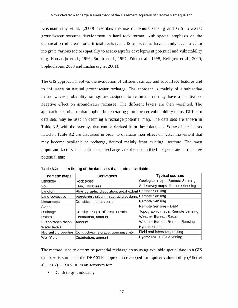
Groundwater Recharge Assessment of the Basement Aquifers of Central Namaqualand
37
Krishnamurthy et al. (2000) describes the use of remote sensing and GIS to assess
groundwater resource development in hard rock terrain, with special emphasis on the
demarcation of areas for artificial recharge. GIS approaches have mainly been used to
integrate various factors spatially to assess aquifer development potential and vulnerability
(e.g. Kamaraju et al., 1996; Smith et al., 1997; Edet et al., 1998; Kellgren et al., 2000;
Sophocleous, 2000 and Lachassagne, 2001).
The GIS approach involves the evaluation of different surface and subsurface features and
its influence on natural groundwater recharge. The approach is mainly of a subjective
nature where probability ratings are assigned to features that may have a positive or
negative effect on groundwater recharge. The different layers are then weighted. The
approach is similar to that applied in generating groundwater vulnerability maps. Different
data sets may be used in defining a recharge potential map. The data sets are shown in
Table 3.2, with the overlays that can be derived from these data sets. Some of the factors
listed in Table 3.2 are discussed in order to evaluate their effect on water movement that
may become available as recharge, derived mainly from existing literature. The most
important factors that influences recharge are then identified to generate a recharge
potential map.
Table 3.2: A listing of the data sets that is often available
Thematic maps Derivatives Typical sources Lithology Rock types Geological maps, Remote Sensing
Soil Clay, Thickness Soil survey maps, Remote Sensing
Landform Physiographic disposition, areal extent Remote Sensing Land cover/use Vegetation, urban infrastructure, dams Remote Sensing Lineaments Densities, intersections Remote Sensing Slope Remote Sensing – DEM Drainage Density, length, bifurcation ratio Topographic maps, Remote Sensing
Rainfall Distribution, amount Weather Bureau, Radar
Evapotranspiration Amount Weather Bureau, Remote Sensing Water levels Hydrocensus
Hydraulic properties Conductivity, storage, transmissivity Field and laboratory testing
Well Yield Distribution, amount Hydrocensus, Field testing
The method used to determine potential recharge areas using available spatial data in a GIS
database is similar to the DRASTIC approach developed for aquifer vulnerability (Aller et
al., 1987). DRASTIC is an acronym for:
� Depth to groundwater;
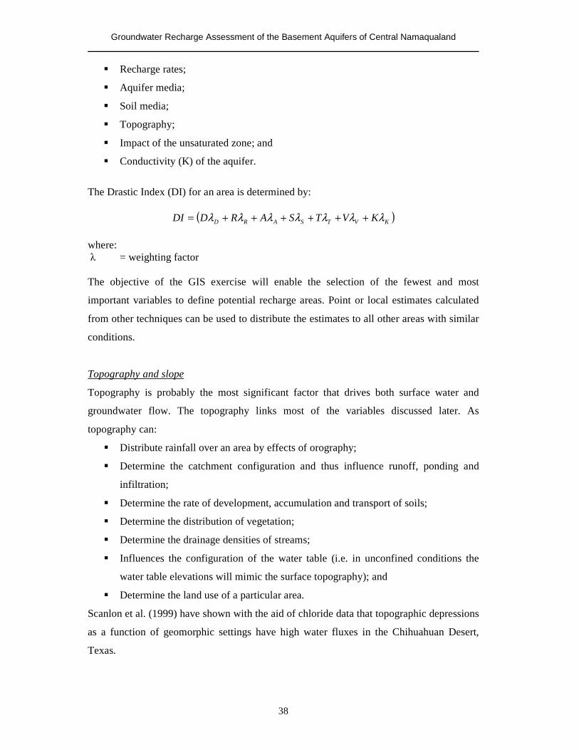
Groundwater Recharge Assessment of the Basement Aquifers of Central Namaqualand
38
� Recharge rates;
� Aquifer media;
� Soil media;
� Topography;
� Impact of the unsaturated zone; and
� Conductivity (K) of the aquifer.
The Drastic Index (DI) for an area is determined by:
( )KVTSARD KVTSARDDI λλλλλλλ ++++++=
where: � = weighting factor The objective of the GIS exercise will enable the selection of the fewest and most
important variables to define potential recharge areas. Point or local estimates calculated
from other techniques can be used to distribute the estimates to all other areas with similar
conditions.
Topography and slope
Topography is probably the most significant factor that drives both surface water and
groundwater flow. The topography links most of the variables discussed later. As
topography can:
� Distribute rainfall over an area by effects of orography;
� Determine the catchment configuration and thus influence runoff, ponding and
infiltration;
� Determine the rate of development, accumulation and transport of soils;
� Determine the distribution of vegetation;
� Determine the drainage densities of streams;
� Influences the configuration of the water table (i.e. in unconfined conditions the
water table elevations will mimic the surface topography); and
� Determine the land use of a particular area.
Scanlon et al. (1999) have shown with the aid of chloride data that topographic depressions
as a function of geomorphic settings have high water fluxes in the Chihuahuan Desert,
Texas.
Groundwater Recharge Assessment of the Basement Aquifers of Central Namaqualand
39
Interflow and overland flow reduces groundwater recharge and the main drivers of these
two processes are the physical configuration of the catchment. A catchment is made up of
interconnected slopes and the channel network draining these slopes. The slope angle
affects the moisture content of the unsaturated zone by governing the proportion of surface
runoff to infiltration. The strongest flow-inducing gradients are mainly vertical in the
unsaturated zone and lateral variations occur under saturated conditions. Troch et al.
(2002) characterized the drainage response functions of the basic nine-hillslope functions
derived from plan and profile curvatures (Figure 3.5). Plan and profile curvatures are the
most dominant topographic controls on flow along hillslopes. The main limitations of their
analyses are (Troch et al., 2002):
� The kinematic wave assumption of subsurface flow;
� The assumption of spatially homogenous hydraulic characteristics of the hillslopes;
� The assumption that capillarity effects of the unsaturated zone above the phreatic
layer can be neglected; and
� Recharge is spatially uniform.
Slopes in the Namaqualand areas have basically the shape of no. 9 and 8 in Figure 3.5.
Troch et al. (2002) modeled the subsurface flow rates and soil moisture storage for the nine
hillslopes during free drainage at a constant depth of 2m (Figure 3.6 a-b). Zones with a
concave topography will produce more subsurface flow (Dunne, 1983; Troch et al, 2002).
Troch et al. (2002) also evaluated the drainage response functions under a constant rainfall
recharge event; the results are shown in Figure 3.7a-b.
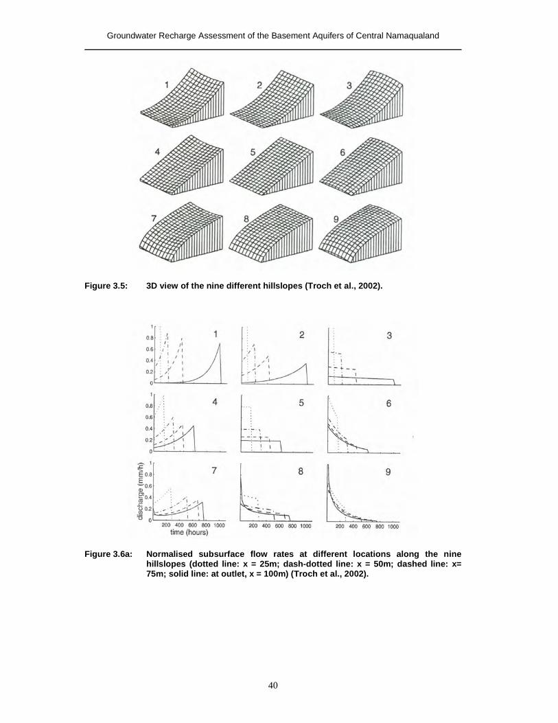
Groundwater Recharge Assessment of the Basement Aquifers of Central Namaqualand
40
Figure 3.5: 3D view of the nine different hillslopes (Troch et al., 2002).
Figure 3.6a: Normalised subsurface flow rates at different locations along the nine
hillslopes (dotted line: x = 25m; dash-dotted line: x = 50m; dashed line: x= 75m; solid line: at outlet, x = 100m) (Troch et al., 2002).
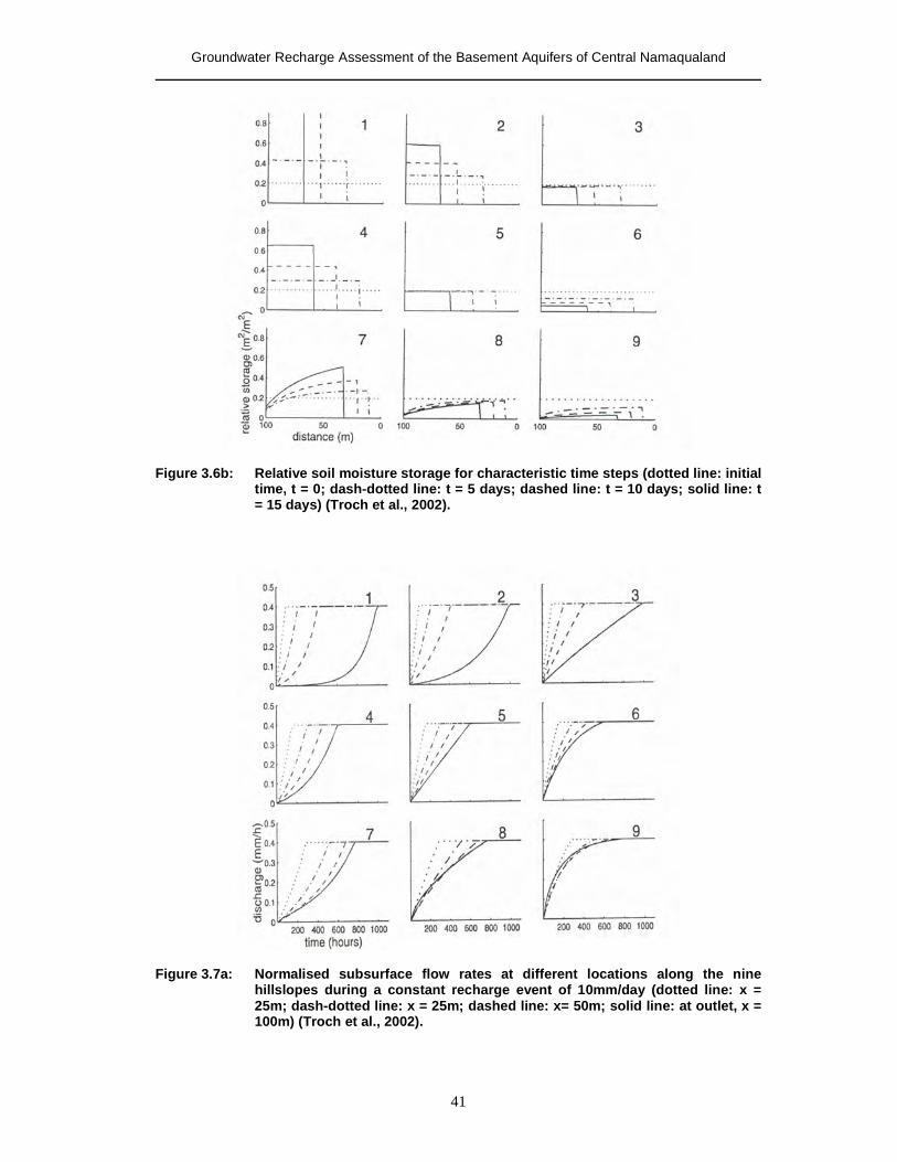
Groundwater Recharge Assessment of the Basement Aquifers of Central Namaqualand
41
Figure 3.6b: Relative soil moisture storage for characteristic time steps (dotted line: initial
time, t = 0; dash-dotted line: t = 5 days; dashed line: t = 10 days; solid line: t = 15 days) (Troch et al., 2002).
Figure 3.7a: Normalised subsurface flow rates at different locations along the nine
hillslopes during a constant recharge event of 10mm/day (dotted line: x = 25m; dash-dotted line: x = 25m; dashed line: x= 50m; solid line: at outlet, x = 100m) (Troch et al., 2002).
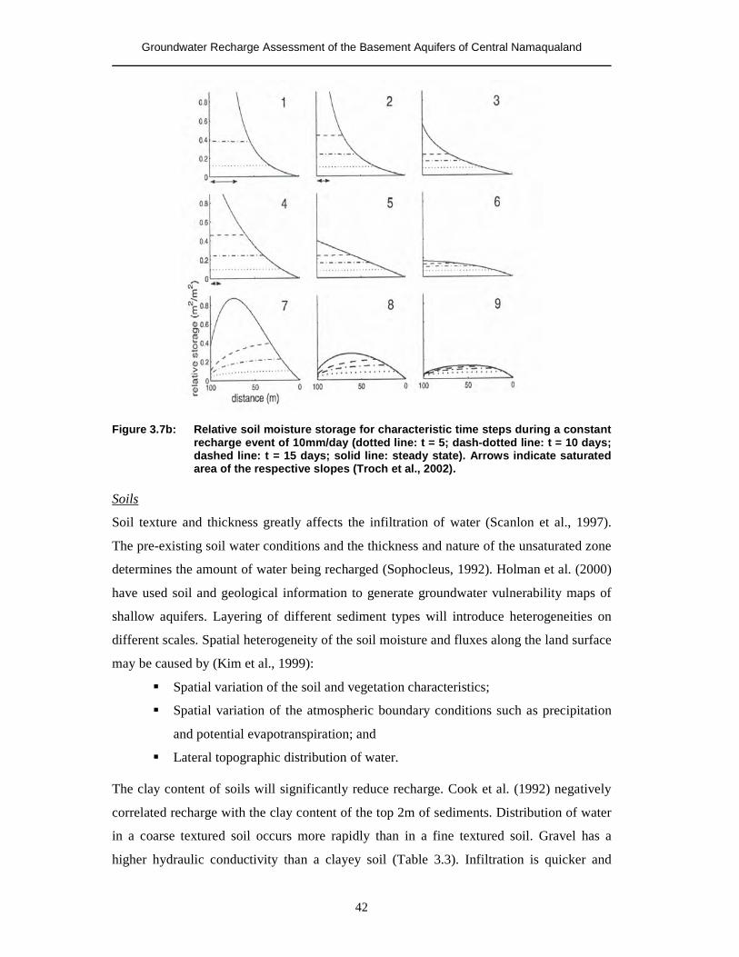
Groundwater Recharge Assessment of the Basement Aquifers of Central Namaqualand
42
Figure 3.7b: Relative soil moisture storage for characteristic time steps during a constant
recharge event of 10mm/day (dotted line: t = 5; dash-dotted line: t = 10 days; dashed line: t = 15 days; solid line: steady state). Arrows indicate saturated area of the respective slopes (Troch et al., 2002).
Soils
Soil texture and thickness greatly affects the infiltration of water (Scanlon et al., 1997).
The pre-existing soil water conditions and the thickness and nature of the unsaturated zone
determines the amount of water being recharged (Sophocleus, 1992). Holman et al. (2000)
have used soil and geological information to generate groundwater vulnerability maps of
shallow aquifers. Layering of different sediment types will introduce heterogeneities on
different scales. Spatial heterogeneity of the soil moisture and fluxes along the land surface
may be caused by (Kim et al., 1999):
� Spatial variation of the soil and vegetation characteristics;
� Spatial variation of the atmospheric boundary conditions such as precipitation
and potential evapotranspiration; and
� Lateral topographic distribution of water. The clay content of soils will significantly reduce recharge. Cook et al. (1992) negatively
correlated recharge with the clay content of the top 2m of sediments. Distribution of water
in a coarse textured soil occurs more rapidly than in a fine textured soil. Gravel has a
higher hydraulic conductivity than a clayey soil (Table 3.3). Infiltration is quicker and
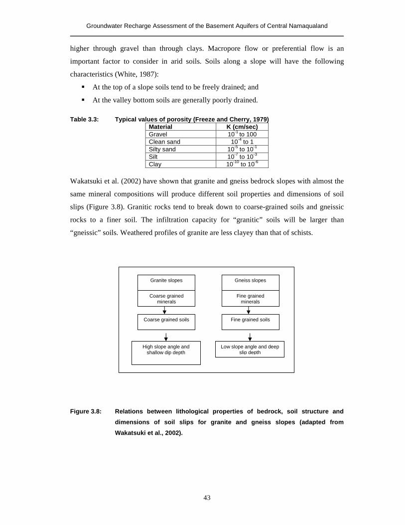
Groundwater Recharge Assessment of the Basement Aquifers of Central Namaqualand
43
higher through gravel than through clays. Macropore flow or preferential flow is an
important factor to consider in arid soils. Soils along a slope will have the following
characteristics (White, 1987):
� At the top of a slope soils tend to be freely drained; and
� At the valley bottom soils are generally poorly drained.
Table 3.3: Typical values of porosity (Freeze and Cherry, 1979)
Material K (cm/sec) Gravel 10-1 to 100 Clean sand 10-4 to 1 Silty sand 10-5 to 10-1
Silt 10-7 to 10-3
Clay 10-10 to 10-6
Wakatsuki et al. (2002) have shown that granite and gneiss bedrock slopes with almost the
same mineral compositions will produce different soil properties and dimensions of soil
slips (Figure 3.8). Granitic rocks tend to break down to coarse-grained soils and gneissic
rocks to a finer soil. The infiltration capacity for “granitic” soils will be larger than
“gneissic” soils. Weathered profiles of granite are less clayey than that of schists.
Figure 3.8: Relations between lithological properties of bedrock, soil structure and
dimensions of soil slips for granite and gneiss slopes (adapted from
Wakatsuki et al., 2002).
Granite slopes Gneiss slopes
Coarse grained minerals
Fine grained minerals
Coarse grained soils Fine grained soils
High slope angle and shallow dip depth
Low slope angle and deep slip depth
Groundwater Recharge Assessment of the Basement Aquifers of Central Namaqualand
44
Lineaments
Lineaments can be traced from remotely sensed data and aerial photographs. Lineaments
are easily identified in areas of thin overburden and outcrops. Fractures observed at
outcrop scale can be correlated to the lineaments by applying a buffer analysis. Degnan
and Clarke (2002) state that a lineament is fracture correlated, if fractures in bedrock
outcrops have strikes similar to the trend of the individual lineament within a specific
buffer zone. Fractures need to be interconnected in order for groundwater flow to occur.
Fracture connectivity increases with fracture densities and length (Cook, 2003). Koch and
Mather (1997) state that in order for the fractures to be hydrogeologically significant it
must be significantly extensive to provide hydraulic connectivity between adjacent
watersheds to increase the total recharge area. Minor fractures may provide only storage if
not hydraulically connected to the larger fracture network. Lineaments are described in
terms of its length density (Ld) and frequency (Lf), where (Greenbaum, 1985):
(3.23) where:
�=
=
ni
i
Li1
= total length of all lineaments
�=
=
ni
i
Ln1
= total number of lineaments
A = area
The following factors must exist to create favourable conditions for groundwater targets
(Walls and Kalinauskas, 2000):
� Brittle host rocks;
� Dilatant stresses to create open fractures;
� Conjugate fractures to enhance interconnections;
� Structural traps to retain water;
� Intersections with the surface to allow recharge; and
� Fracture and void enhancement by dissolution.
A
LnLf
A
LiLd
ni
i
ni
i
�
�
=
=
=
=
=
=
1
1
Groundwater Recharge Assessment of the Basement Aquifers of Central Namaqualand
45
Drainage
Scanlon et al. (1999) concluded that higher recharge rates in arid basins are associated with
drainage areas. High drainage densities are associated with areas covered by low
permeability bedrock with appreciable runoff. Low drainage densities are common in
regions with permeable soils and a low relief, resulting in increased infiltration capacities
(Smith et al., 1997). Drainage are described in terms of length-density (Dld) and frequency
(Df), where (Greenbaum, 1985):
(3.24)
where:
�=
=
ni
i
Si1
= cumulative length of all streams
�=
=
ni
i
Sn1
= total number of streams
A = area
Vegetation
Due to the limited rain supply, vegetation in arid and semi-arid regions are sparse and often
occur in geomorphic and surface drainage zones with a high moisture content. However,
plants are opportunistic and will populate an area where water is easily accessible.
Phreatophytes are the most reliable groundwater indicator.
Vegetative canopies exert a significant control on the rainfall reaching the ground surface
and contributing to evapotranspiration. Berndtsson and Larson (1987) states that vegetation
cover tends to increase infiltration as opposed to areas with bare soil in arid and semi-arid
areas. Vegetation increases infiltration by (Berndtsson and Larson, 1987, Dunne, 1983):
� Retarding surface water movement;
� Reducing raindrop compaction; and
� Increasing organic matter content, bulk density and surface horizon depth.
A
SnDf
A
SiDld
ni
i
ni
i
�
�
=
=
=
=
=
=
1
1
Groundwater Recharge Assessment of the Basement Aquifers of Central Namaqualand
46
Scanlon et al. (1997) states that vegetation is most probably the most important control on
unsaturated water movement. Areas of coarse and bare soil have higher rates of water
movement then vegetated areas. Vegetation tends to decrease the volumetric water content
for sand, loamy sand and silty loam in arid regions (Dong et al., 2003). On remotely sensed
data vegetation found in areas of excess moisture, with groundwater occurring close to the
surface or at discharging areas, the vegetation is characterised by low spectral brightness
coefficients in the red part of the spectrum and maximal values in the near infrared zone
(Ob’yedkov, 1992).
Rainfall
Rainfall in arid and semi-arid areas produces sporadic runoff that seldom reaches the
valley bottom. Rainfall in topographically distinct areas will be higher in areas of higher
altitude (orographic effect). Bare rock outcrops produces runoff under most rainfall
conditions and only infiltrates once it reaches alluvial or colluvial cover (Van Wesemale et
al., 1998).
Water table depth
Infiltration and evapotranspiration are related to water table depth. Recharge is related the
distribution of rainfall into infiltration, runoff and evapotranspiration (Kim et al., 1999).
Recharge will be less if the water table is deep and higher when water tables are shallow in
arid to semi-arid areas. Evapotranspiration will dominate under both cases but will be
significantly higher if the water table is close to the surface. When the water table is
shallow, infiltration reaches the saturated zone fairly fast, so that most of the individual
rainfall events correspond to isolated infiltration events with small time lags (Wu et al.,
1996). As the depth to groundwater increases the potential for rainfall to percolate to the
saturated zone decreases (Wu et al., 1996). Wu et al (1996) also state that for groundwater
at intermediate depth the recharge events produced by individual rainfall events merge into
one single annual process although a few peaks of recharge correspond to large rainfall
events or concentrated rainfall clusters. Sophocleus (1991) states that time lags may be
brief for macropore recharge and longer for matrix recharge depending on the unsaturated
zone characteristics, depth to water table and other factors.
Land use
Intensive land use in arid and semi-arid areas is focused near the channels of ephemeral
Groundwater Recharge Assessment of the Basement Aquifers of Central Namaqualand
47
rivers, valleys and areas adjacent to streambeds. Urban or peri-urban areas that have
impermeable surfaces will tend to reduce direct recharge but recharge rates may increase in
areas where infrastructure (e.g. leaking pipes, septic tanks, etc) creates pathways for
recharge (Lerner, 1990). This is mainly applicable to dense settlements and may not be a
significant in rural areas. The major land use activities that may impact on groundwater
recharge processes are tillage and irrigation of farmlands as well as overgrazing.
Problems of scale
Hierarchy theory suggests that at a regional scale only a limited number of variables should
be able to describe any relationships between recharge and rainfall over an area. At finer
scales more variables must be incorporated in the model. The methodology proposed for
the GIS approach involves knowledge acquisition and identification of variables
favourable for recharge and then using GIS and remote sensing techniques to integrate, rate
and weigh the variables to generate a recharge potential map. The recharge potential map
can be calibrated with point and area estimates. It is thus obvious that scaling up or down is
a major factor that needs to be evaluated.
The issue of temporal and spatial scales and its impact on hydrological studies has been
well documented (e.g. Blöschl and Sivapalan, 1995; Bergström and Graham, 1998;
Bergkamp, 1998; Western and Blöschl, 1999; Schulze, 2000; Brunsell and Gillies, 2003).
Bergström and Graham (1998) make the point that hydrological modelers have different
views on the scale problem depending on their perspectives and scientific viewpoint. As an
example, a small lysimeter study of 1km2 may be considered large and heterogeneous and
a forecaster may consider a basin of several thousand km2 as small and heterogeneous. A
water resource evaluation study often assumes uniform rates of water movement
throughout an area. According Scanlon et al. (1997), this assumption does not greatly
affect resource estimates. However, contaminant transport studies require more detailed
analysis of the spatial variability of water movement. Large spatial and temporal variations
of recharge to arid zones are the rule. Six causes of scale (temporal and spatial) problems
in hydrological responses have been identified (Schulze, 2000):
� Spatial heterogeneity in surface processes;
� Non-linearity in responses;
� Processes require threshold scales to occur;
� Dominant processes change with scale;
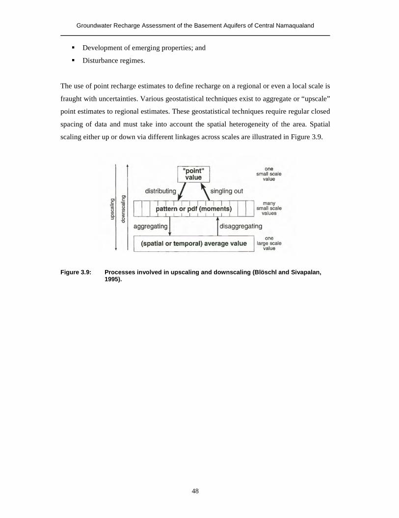
Groundwater Recharge Assessment of the Basement Aquifers of Central Namaqualand
48
� Development of emerging properties; and
� Disturbance regimes.
The use of point recharge estimates to define recharge on a regional or even a local scale is
fraught with uncertainties. Various geostatistical techniques exist to aggregate or “upscale”
point estimates to regional estimates. These geostatistical techniques require regular closed
spacing of data and must take into account the spatial heterogeneity of the area. Spatial
scaling either up or down via different linkages across scales are illustrated in Figure 3.9.
Figure 3.9: Processes involved in upscaling and downscaling (Blöschl and Sivapalan,
1995).
Groundwater Recharge Assessment of the Basement Aquifers of Central Namaqualand
49
CHAPTER 4
Measurement and experimental techniques
4.1. Introduction
To complement the existing data from the operational borehole monitoring programmes,
chemical and isotope data were collected from the rainfall and groundwater sampling
programme. A bulk rainfall-monitoring network and later an event based monitoring
programme was developed for the area for the application of the CMB method and the
isotope characterisation.
4.2 Precipitation monitoring and sampling
Precipitation is often measured for hydro(geo)logical and meteorological studies.
Specifically in recharge studies precipitation is important to determine the rate and mode
of groundwater recharge. The chloride and stable isotope chemistry of the precipitation are
compared with that of the groundwater and/or soil moisture. These methods are widely
applied and literature on the subject is extensive (e.g. Eriksson and Khunakasem, 1969;
Allison and Hughes, 1978; Sharma and Hughes, 1985; Bazuhair and Wood, 1996,
Edmunds and Gaye, 1994; Gaye and Edmunds, 1996). Currently, no national programme
exists in South Africa to sample rainfall chemistry. Bredenkamp (2000) also noted that
specific measurements of chloride in precipitation are lacking in South Africa and a
representative monitoring program needs to be initiated. The establishment of such a
program would have to rely heavily on the collection of chemical and isotopic
measurements that are representative of the atmospheric inputs. Rainfall sampling occurs
on a project basis and is usually abandoned after the completion of the project. In South
Africa, it is often not practical to empty rainfall collectors after each rainfall event, due to
great distances and the inaccessibility of certain areas. Automated systems are expensive
and require regular maintenance. A need exists in the southern African region to develop a
regional precipitation monitoring programme. Several methods exist for the collection of
rainfall for chemical analysis:
Groundwater Recharge Assessment of the Basement Aquifers of Central Namaqualand
50
� Manually collecting daily or event rainfall;
� Bulk rainfall collectors;
� Automatic continuous analysers; and
� Ion exchange resins.
The first two methods listed above are the most cost effective. The bulk rainfall samplers
(BRS) are often used in groundwater recharge studies to collect rainfall for chemistry and
stable isotope analyses over extended periods, usually six to twelve months. The most
important data derived from such sampling exercises are the concentration of chloride and
the ratios of the stable oxygen and hydrogen isotopes. The amount of rainfall is also
determined and compared with rainfall totals at the nearest weather observation station.
The amount of rainfall is also important for the weighting of the chemical parameters. The
chloride data obtained from such collectors need to be representative of the atmospheric
deposition as the methods used to calculate recharge are very sensitive to variations in
chloride concentrations in rainwater. An error in the concentration of chloride will yield
significant over- or underestimation of recharge. Bulk samplers are open continuously and
collect both wet and dry depositions. During periods of no rainfall aerosols deposit on the
funnel and are washed into the sampling vessel during the next rainfall event (Appelo and
Postma, 1993). The integrated O- and H isotope ratios are used to determine the local
meteoric water line (LMWL) and the ratios of the input water and the deviation of the
groundwater from this input water.
The current bulk rainfall samplers used in South Africa, sometimes called totalisers or
cumulative rainfall samplers, are evaluated and compared with a new bulk rainfall sampler
developed and tested during this research.
4.2.1 Bulk Rainfall Samplers Several totalisers were purchased from the Council for Scientific and Industrial Research
(CSIR) for rainfall monitoring in the Namaqualand region. The CSIR uses these rainfall
samplers or totalisers, called the standard bulk rainfall samplers (SBRS), at various sites as
part of their research activities (Weaver et al., 1999; Weaver and Talma, 2002). Gieske
(1992) also used totalisers in his recharge study in Botswana and came to the conclusion
that this method of sampling is worthwhile. The SBRS depicted in Figure 4.1a is typically
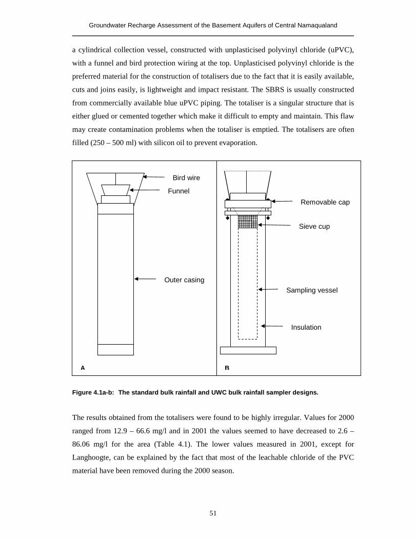
Groundwater Recharge Assessment of the Basement Aquifers of Central Namaqualand
51
a cylindrical collection vessel, constructed with unplasticised polyvinyl chloride (uPVC),
with a funnel and bird protection wiring at the top. Unplasticised polyvinyl chloride is the
preferred material for the construction of totalisers due to the fact that it is easily available,
cuts and joins easily, is lightweight and impact resistant. The SBRS is usually constructed
from commercially available blue uPVC piping. The totaliser is a singular structure that is
either glued or cemented together which make it difficult to empty and maintain. This flaw
may create contamination problems when the totaliser is emptied. The totalisers are often
filled (250 – 500 ml) with silicon oil to prevent evaporation.
Figure 4.1a-b: The standard bulk rainfall and UWC bulk rainfall sampler designs.
The results obtained from the totalisers were found to be highly irregular. Values for 2000
ranged from 12.9 – 66.6 mg/l and in 2001 the values seemed to have decreased to 2.6 –
86.06 mg/l for the area (Table 4.1). The lower values measured in 2001, except for
Langhoogte, can be explained by the fact that most of the leachable chloride of the PVC
material have been removed during the 2000 season.
Outer casing
Funnel
Bird wire
Removable cap
Sampling vessel
Insulation
Sieve cup
A B
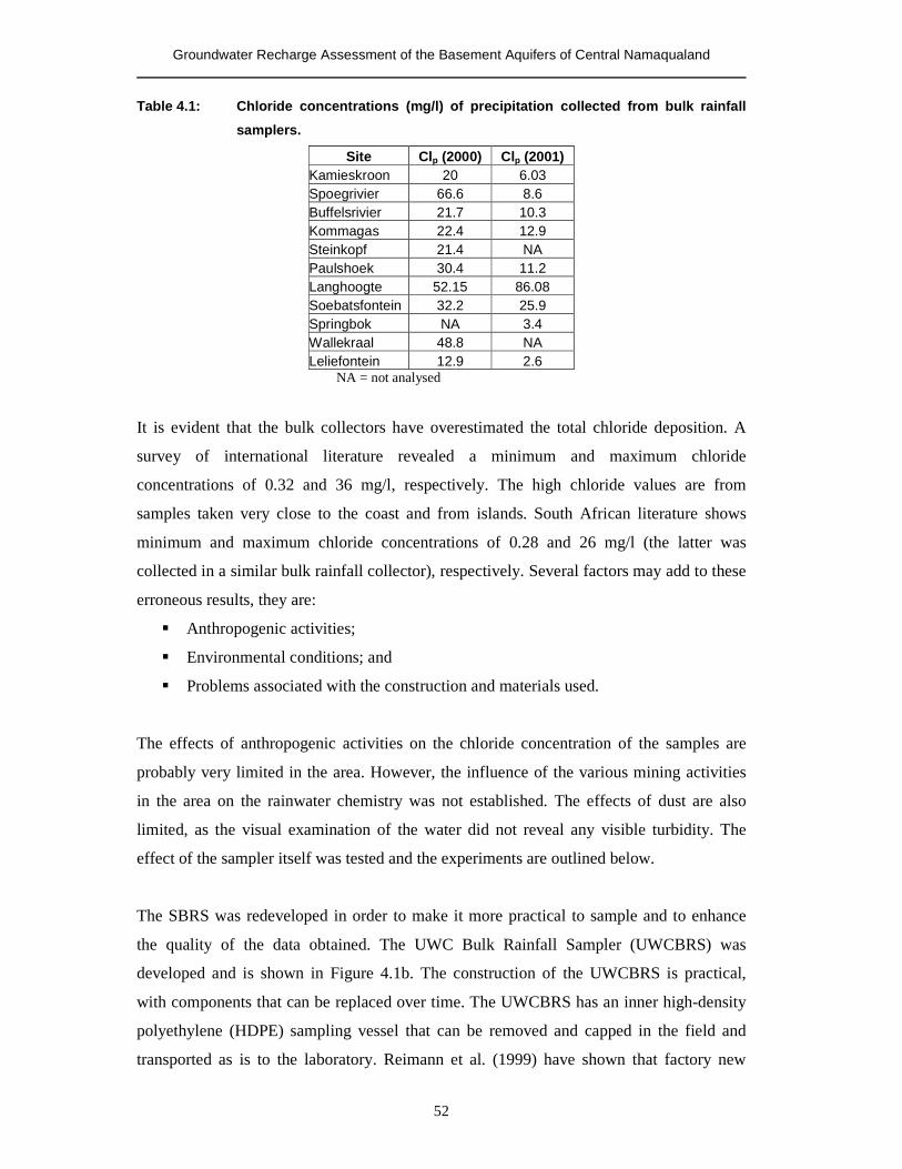
Groundwater Recharge Assessment of the Basement Aquifers of Central Namaqualand
52
Table 4.1: Chloride concentrations (mg/l) of precipitation collected from bulk rainfall
samplers.
Site Clp (2000) Clp (2001) Kamieskroon 20 6.03 Spoegrivier 66.6 8.6 Buffelsrivier 21.7 10.3 Kommagas 22.4 12.9 Steinkopf 21.4 NA Paulshoek 30.4 11.2 Langhoogte 52.15 86.08 Soebatsfontein 32.2 25.9 Springbok NA 3.4 Wallekraal 48.8 NA Leliefontein 12.9 2.6
NA = not analysed
It is evident that the bulk collectors have overestimated the total chloride deposition. A
survey of international literature revealed a minimum and maximum chloride
concentrations of 0.32 and 36 mg/l, respectively. The high chloride values are from
samples taken very close to the coast and from islands. South African literature shows
minimum and maximum chloride concentrations of 0.28 and 26 mg/l (the latter was
collected in a similar bulk rainfall collector), respectively. Several factors may add to these
erroneous results, they are:
� Anthropogenic activities;
� Environmental conditions; and
� Problems associated with the construction and materials used.
The effects of anthropogenic activities on the chloride concentration of the samples are
probably very limited in the area. However, the influence of the various mining activities
in the area on the rainwater chemistry was not established. The effects of dust are also
limited, as the visual examination of the water did not reveal any visible turbidity. The
effect of the sampler itself was tested and the experiments are outlined below.
The SBRS was redeveloped in order to make it more practical to sample and to enhance
the quality of the data obtained. The UWC Bulk Rainfall Sampler (UWCBRS) was
developed and is shown in Figure 4.1b. The construction of the UWCBRS is practical,
with components that can be replaced over time. The UWCBRS has an inner high-density
polyethylene (HDPE) sampling vessel that can be removed and capped in the field and
transported as is to the laboratory. Reimann et al. (1999) have shown that factory new
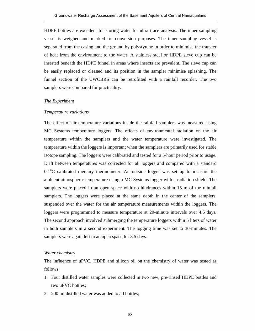
Groundwater Recharge Assessment of the Basement Aquifers of Central Namaqualand
53
HDPE bottles are excellent for storing water for ultra trace analysis. The inner sampling
vessel is weighed and marked for conversion purposes. The inner sampling vessel is
separated from the casing and the ground by polystyrene in order to minimise the transfer
of heat from the environment to the water. A stainless steel or HDPE sieve cup can be
inserted beneath the HDPE funnel in areas where insects are prevalent. The sieve cup can
be easily replaced or cleaned and its position in the sampler minimise splashing. The
funnel section of the UWCBRS can be retrofitted with a rainfall recorder. The two
samplers were compared for practicality.
The Experiment Temperature variations The effect of air temperature variations inside the rainfall samplers was measured using
MC Systems temperature loggers. The effects of environmental radiation on the air
temperature within the samplers and the water temperature were investigated. The
temperature within the loggers is important when the samplers are primarily used for stable
isotope sampling. The loggers were calibrated and tested for a 5-hour period prior to usage.
Drift between temperatures was corrected for all loggers and compared with a standard
0.1oC calibrated mercury thermometer. An outside logger was set up to measure the
ambient atmospheric temperature using a MC Systems logger with a radiation shield. The
samplers were placed in an open space with no hindrances within 15 m of the rainfall
samplers. The loggers were placed at the same depth in the center of the samplers,
suspended over the water for the air temperature measurements within the loggers. The
loggers were programmed to measure temperature at 20-minute intervals over 4.5 days.
The second approach involved submerging the temperature loggers within 5 liters of water
in both samplers in a second experiment. The logging time was set to 30-minutes. The
samplers were again left in an open space for 3.5 days.
Water chemistry
The influence of uPVC, HDPE and silicon oil on the chemistry of water was tested as
follows:
1. Four distilled water samples were collected in two new, pre-rinsed HDPE bottles and
two uPVC bottles;
2. 200 ml distilled water was added to all bottles;
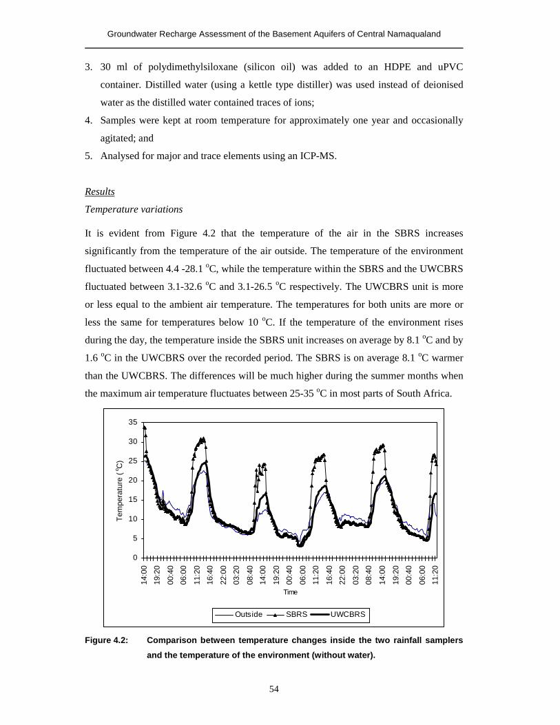
Groundwater Recharge Assessment of the Basement Aquifers of Central Namaqualand
54
3. 30 ml of polydimethylsiloxane (silicon oil) was added to an HDPE and uPVC
container. Distilled water (using a kettle type distiller) was used instead of deionised
water as the distilled water contained traces of ions;
4. Samples were kept at room temperature for approximately one year and occasionally
agitated; and
5. Analysed for major and trace elements using an ICP-MS.
Results
Temperature variations It is evident from Figure 4.2 that the temperature of the air in the SBRS increases
significantly from the temperature of the air outside. The temperature of the environment
fluctuated between 4.4 -28.1 oC, while the temperature within the SBRS and the UWCBRS
fluctuated between 3.1-32.6 oC and 3.1-26.5 oC respectively. The UWCBRS unit is more
or less equal to the ambient air temperature. The temperatures for both units are more or
less the same for temperatures below 10 oC. If the temperature of the environment rises
during the day, the temperature inside the SBRS unit increases on average by 8.1 oC and by
1.6 oC in the UWCBRS over the recorded period. The SBRS is on average 8.1 oC warmer
than the UWCBRS. The differences will be much higher during the summer months when
the maximum air temperature fluctuates between 25-35 oC in most parts of South Africa.
0
5
10
15
20
25
30
35
14:0
0
19:2
0
00:4
0
06:0
0
11:2
0
16:4
0
22:0
0
03:2
0
08:4
0
14:0
0
19:2
0
00:4
0
06:0
0
11:2
0
16:4
0
22:0
0
03:2
0
08:4
0
14:0
0
19:2
0
00:4
0
06:0
0
11:2
0
Time
Tem
pera
ture
(o C
)
Outside SBRS UWCBRS
Figure 4.2: Comparison between temperature changes inside the two rainfall samplers
and the temperature of the environment (without water).
Groundwater Recharge Assessment of the Basement Aquifers of Central Namaqualand
55
The temperature of the water inside the samplers reacts differently to that of the
environment as shown in Figure 4.3. The water temperature of the SBRS increased
significantly during the day and attains temperatures higher than that of the ambient air
temperature. The temperature of the air fluctuated between 9.5-32.2 oC, while the
temperature of the water in the SBRS and the UWCBRS fluctuated between 12.5-36.6 oC
and 14.9-22.7 oC respectively. On average the water in the SBRS is 4.4 oC warmer than the
environment and the UWCBRS is 9.5oC cooler than the environment. The water in the
UWCBRS retains most of its heat during night time. The water temperature in the SBRS is
on average 13.9oC warmer than the water temperature of the UWCBRS unit. The fact that
the inner sampling vessel is smaller in diameter than the SBRS prevents the formation of
elevated temperatures above the water. Al-Malack (2001) has shown that uPVC pipes
leach significant concentrations of calcium, barium and tin at temperatures above 35 oC.
0
5
10
15
20
25
30
35
40
12:3
0
18:3
0
00:3
0
06:3
0
12:3
0
18:3
0
00:3
0
06:3
0
12:3
0
18:3
0
00:3
0
06:3
0
12:3
0
Time
Tem
pera
ture
(o C
)
UWCBRS SBRS Outside
Figure 4.3: Comparison between temperature changes inside the two rainfall samplers
and the temperature of the environment (with water).
Water chemistry
The water samples were analysed for major and trace elements. The chloride content of the
water is shown in Figure 4.4. It is evident from the plot that the silicon oil and the PVC
material increased the chloride content of the control sample. The control sample in the
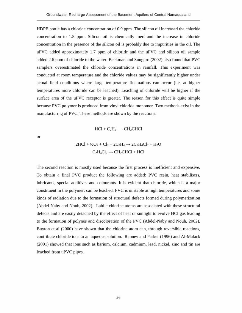
Groundwater Recharge Assessment of the Basement Aquifers of Central Namaqualand
56
HDPE bottle has a chloride concentration of 0.9 ppm. The silicon oil increased the chloride
concentration to 1.8 ppm. Silicon oil is chemically inert and the increase in chloride
concentration in the presence of the silicon oil is probably due to impurities in the oil. The
uPVC added approximately 1.7 ppm of chloride and the uPVC and silicon oil sample
added 2.6 ppm of chloride to the water. Beekman and Sunguro (2002) also found that PVC
samplers overestimated the chloride concentrations in rainfall. This experiment was
conducted at room temperature and the chloride values may be significantly higher under
actual field conditions where large temperature fluctuations can occur (i.e. at higher
temperatures more chloride can be leached). Leaching of chloride will be higher if the
surface area of the uPVC receptor is greater. The reason for this effect is quite simple
because PVC polymer is produced from vinyl chloride monomer. Two methods exist in the
manufacturing of PVC. These methods are shown by the reactions:
HCl + C2H2 � CH2CHCl
or
2HCl + ½O2 + Cl2 + 2C2H4 � 2C2H4Cl2 + H2O
C2H4Cl2 � CH2CHCl + HCl
The second reaction is mostly used because the first process is inefficient and expensive.
To obtain a final PVC product the following are added: PVC resin, heat stabilisers,
lubricants, special additives and colourants. It is evident that chloride, which is a major
constituent in the polymer, can be leached. PVC is unstable at high temperatures and some
kinds of radiation due to the formation of structural defects formed during polymerization
(Abdel-Naby and Nouh, 2002). Labile chlorine atoms are associated with these structural
defects and are easily detached by the effect of heat or sunlight to evolve HCl gas leading
to the formation of polynes and discoloration of the PVC (Abdel-Naby and Nouh, 2002).
Buxton et al (2000) have shown that the chlorine atom can, through reversible reactions,
contribute chloride ions to an aqueous solution. Ranney and Parker (1996) and Al-Malack
(2001) showed that ions such as barium, calcium, cadmium, lead, nickel, zinc and tin are
leached from uPVC pipes.
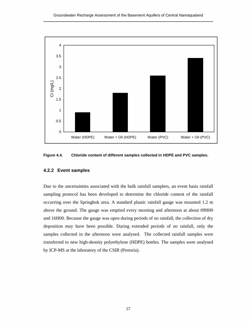
Groundwater Recharge Assessment of the Basement Aquifers of Central Namaqualand
57
0
0.5
1
1.5
2
2.5
3
3.5
4
Water (HDPE) Water + Oil (HDPE) Water (PVC) Water + Oil (PVC)
Cl (
mg/
L)
Figure 4.4. Chloride content of different samples collected in HDPE and PVC samples.
4.2.2 Event samples
Due to the uncertainties associated with the bulk rainfall samplers, an event basis rainfall
sampling protocol has been developed to determine the chloride content of the rainfall
occurring over the Springbok area. A standard plastic rainfall gauge was mounted 1.2 m
above the ground. The gauge was emptied every morning and afternoon at about 09H00
and 16H00. Because the gauge was open during periods of no rainfall, the collection of dry
deposition may have been possible. During extended periods of no rainfall, only the
samples collected in the afternoon were analysed. The collected rainfall samples were
transferred to new high-density polyethylene (HDPE) bottles. The samples were analysed
by ICP-MS at the laboratory of the CSIR (Pretoria).
Groundwater Recharge Assessment of the Basement Aquifers of Central Namaqualand
58
4.3 Groundwater
4.3.1 Chemistry and isotopes
Boreholes were sampled for chemical and isotopic analyses, each sample being analysed
for the parameters listed in Table 4.2. The datasets are presented in Appendix A3.
Parameters that were measured and recorded at the time of sampling were alkalinity,
electrical conductivity (EC), pH, temperature and redox potential (Eh). Alkalinity was
measured using a Hach® field titration kit. The EC, pH, temperature and Eh were measured
using portable Orion EC and pH meters. When possible, the water level and discharge of
the borehole were also recorded. Water was only taken from boreholes that were pumping
for a significant amount of time. Samples were filtered in the field with a hand-held
syringe using 0.45 µm membrane filters. Samples were collected in three new 250 ml
polyethylene bottles. All sampling bottles were washed with de-ionised water and again
with filtered sample water. Unfiltered samples were collected for isotope analyses. All
samples were kept cool prior to despatch to the laboratory. Groundwater chemistry
analyses were performed at the laboratories of Bemlab, CSIR and Infruitec.
Table 4.2: Physical and chemical determinants.
Group Determinants Physical determinants EC, pH, Temperature, Eh Major cations Na, Mg, Ca, K Major anions Cl, SO4, NOx - N, F, HCO3 Trace elements Al, Ba, Ni, P, Sr, B, U, Cu, Mn, Zn Isotopes 18O, D, 14C Aggregate determinants Alkalinity
The stable isotope analyses were performed at the Geochemistry Department of the
University of Cape Town and the 14C analysis at the Schonland Research Centre for
Nuclear Sciences at the University of the Witwatersrand.. Stable isotope data are presented
in “delta notation” where δ (‰) is defined as:
10001R
R
standard
sample ∗���
�
��
�
�−���
����
�=δ ‰ (4.1)
where:
R sample and R standard = 18O/16O or 2H/1H.
Groundwater Recharge Assessment of the Basement Aquifers of Central Namaqualand
59
For 14C sampling purged boreholes were sampled using the following procedures
(Verhagen, pers. comm.):
1. Rinse container with sample water. 2. Fill container (with hose or bucket) – preventing aeration. 3. Empty a sachet of BaCl2 into bucket and fill about ½ with sample water. Stir to
dissolve. 4. Fill container, then:
4.1 Pour a few ml of phenolphthalein suspension 4.2 Pour in a ¼ of clean NaOH solution. Sample container should now be bright
pink. 4.3 Pour in the BaCl2 solution (prepared in bucket). Sample should turn cloudy.
5. Fill container to near top. Ensure good mixture whilst filling and/or stirring. Screw on cap.
6. If pink colour disappears, more NaOH and BaCl2 dissolved in sample water is added. 7. The precipitate is allowed to settle leaving clear, still pink solution for typically 1hour. 8. The supernatant is drained. 9. When draining stops, tip container until liquid begins to entrain precipitate. 10. Replace cap and gently swirl container. 11. Pour precipitate in 2-3 containers and label. 12. The next day precipitate would have shrunk. Pour off supernatant and transfer to
smaller container (1-½ L) – top up with supernatant – seal and label. 13. When sample alkalinity is less than 1 meq/L or less – perform a second precipitation.
Based on the alkalinity of the water the amount of water needed for proper preciptation the
following formula was used:
of Ccipitationed for prewater needamount of CaCOLmgAlkalinity
=) /(
7500
3
(4.2)
With each 14C sample, a 1L sample of water was collected for chemical analysis. The usual
wellhead measurements were also made (i.e. pH, alkalinity, temperature and EC).
4.3.2 Data quality
To determine the accuracy of the laboratory analyses duplicate samples was sent to two
different laboratories using different analytical techniques. Duplicate samples were also
sent to the same laboratory. Intercomparison of the data was considered necessary in order
to ensure confidence in the results. Accuracy of the analyses of the ions can be interpreted
from the electro-neutrality condition since the sum of the positive and negative charges in
Groundwater Recharge Assessment of the Basement Aquifers of Central Namaqualand
60
the water must balance. Samples that had ionic balance errors (IBE) above 10% were
investigated. The ion balance error is expressed as (ions expressed in meq/L):
)()( 100*
� ���
+−
=anionscations
anionsscationIBE % (4.3)
The quality of the data in the database was checked by simple 2D scatter plots and by
sorting the data in Excel. By sorting the data (variables) either descending or ascending
typographical errors can be identified. Extreme outliers on 2D scatter plots were
investigated.
Groundwater Recharge Assessment of the Basement Aquifers of Central Namaqualand
61
CHAPTER 5
Description of the Central Namaqualand area
5.1 Introduction
The study area is located in the Northern Cape Province of South Africa and is situated in
an area called Namaqualand (Figure 5.1). The area is well known for its copper and
diamond mining activities as well as for its annual mass flowering after the first significant
rainfall. The place names given by the Nama Hottentots are often associated by the quality
and quantity of the water and land resources because of its importance to the communities
(Laidler, 1927). Most of the modern farm names are corruptions of the original Nama
names.
5.2 Climate
The study area falls in the tropical desert arid, hot climatic region of South Africa,
according to the Koeppen classification. The climate of the study area is controlled by
altitude, topography and distance from the sea. Climatological data for the study area (i.e.
precipitation, evaporation and temperature) were received from the South African Weather
Bureau, Computing Centre for Water Research and data from the WR90 publication of
Midgeley et al. (1994).
Precipitation
The region can be classified as arid to semi-arid. The mean annual precipitation (MAP)
varies from 44 mm in the coastal zone area to 480 mm in the Kamies Mountains, for the
period June 1999 to August 2001. Higher rainfall in the higher lying areas is a result of
orographic rainfall. Rainfall mostly occurs during the winter months. High incidences of
fog days on the West Coast of South Africa contribute significant moisture to the coastal
areas of Namaqualand (Olivier and van Heerden, 1999). Climatological data (Midgeley et
al, 1994) for the various subcatchments are shown in Table 5.1. Snow in the Kamies
Mountains is not uncommon during the winter months.
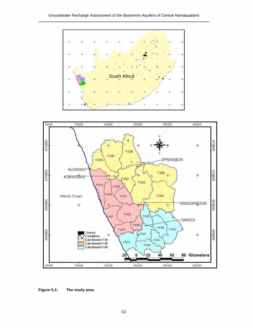
Groundwater Recharge Assessment of the Basement Aquifers of Central Namaqualand
62
Figure 5.1: The study area.
South Africa
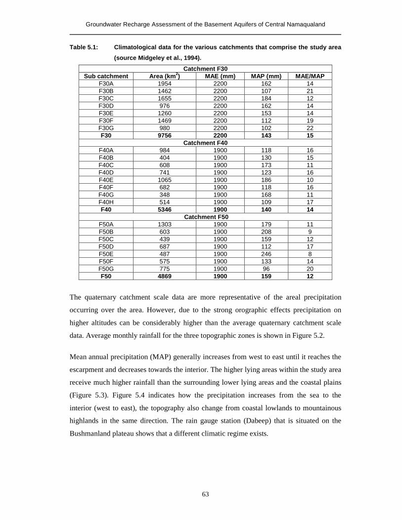
Groundwater Recharge Assessment of the Basement Aquifers of Central Namaqualand
63
Table 5.1: Climatological data for the various catchments that comprise the study area
(source Midgeley et al., 1994).
Catchment F30 Sub catchment Area (km2) MAE (mm) MAP (mm) MAE/MAP
F30A 1954 2200 162 14 F30B 1462 2200 107 21 F30C 1655 2200 184 12 F30D 976 2200 162 14 F30E 1260 2200 153 14 F30F 1469 2200 112 19 F30G 980 2200 102 22 F30 9756 2200 143 15
Catchment F40 F40A 984 1900 118 16 F40B 404 1900 130 15 F40C 608 1900 173 11 F40D 741 1900 123 16 F40E 1065 1900 186 10 F40F 682 1900 118 16 F40G 348 1900 168 11 F40H 514 1900 109 17 F40 5346 1900 140 14
Catchment F50 F50A 1303 1900 179 11 F50B 603 1900 208 9 F50C 439 1900 159 12 F50D 687 1900 112 17 F50E 487 1900 246 8 F50F 575 1900 133 14 F50G 775 1900 96 20 F50 4869 1900 159 12
The quaternary catchment scale data are more representative of the areal precipitation
occurring over the area. However, due to the strong orographic effects precipitation on
higher altitudes can be considerably higher than the average quaternary catchment scale
data. Average monthly rainfall for the three topographic zones is shown in Figure 5.2.
Mean annual precipitation (MAP) generally increases from west to east until it reaches the
escarpment and decreases towards the interior. The higher lying areas within the study area
receive much higher rainfall than the surrounding lower lying areas and the coastal plains
(Figure 5.3). Figure 5.4 indicates how the precipitation increases from the sea to the
interior (west to east), the topography also change from coastal lowlands to mountainous
highlands in the same direction. The rain gauge station (Dabeep) that is situated on the
Bushmanland plateau shows that a different climatic regime exists.
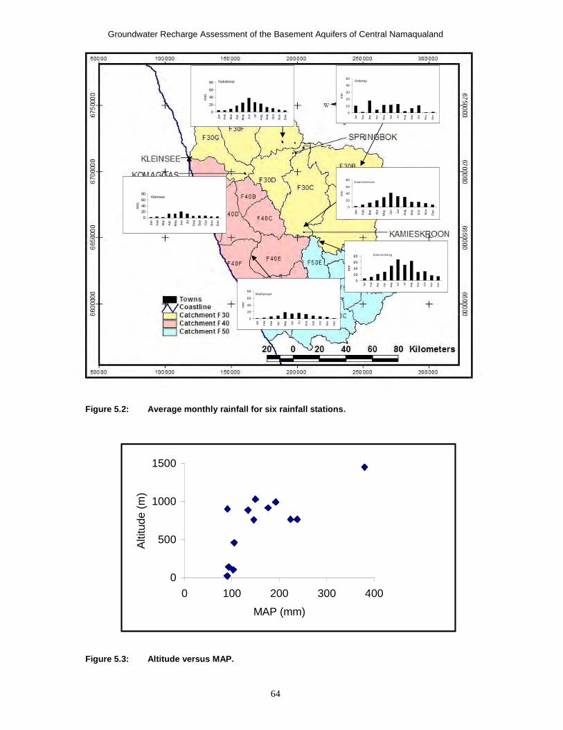
Groundwater Recharge Assessment of the Basement Aquifers of Central Namaqualand
64
Figure 5.2: Average monthly rainfall for six rainfall stations.
Figure 5.3: Altitude versus MAP.
0
500
1000
1500
0 100 200 300 400
MAP (mm)
Alti
tude
(m)
Kleinsee
0204060
80
Jan
Feb
Mar
Apr
May Jun
Jul
Aug Sep Oct
Nov
Dec
mm
Wallekraal
0
20
40
60
80
Jan
Feb
Mar
Apr
May Jun
Jul
Aug Sep Oct
Nov
Dec
mm
Kam ies kroon
0
20
40
60
80
Jan
Feb
Mar
Apr
May Ju
n
Jul
Aug
Sep Oct
Nov
Dec
mm
Nababeep
0
20
40
60
80
Jan
Feb
Mar
Apr
May Jun
Jul
Aug Sep Oct
Nov
Dec
mm
Kam ies berg
0
20
40
60
80
Jan
Feb
Mar
Apr
May Jun
Jul
Aug Sep Oct
Nov
Dec
mm
Dabeep
0
10
20
30
40
50
Jan
Feb
Mar
Apr
May Jun
Jul
Aug Sep Oct
Nov
Dec
mm
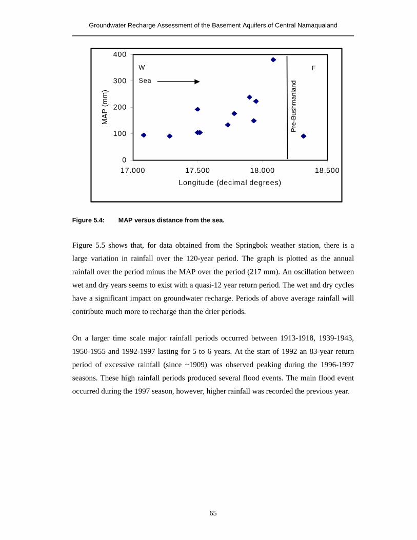
Groundwater Recharge Assessment of the Basement Aquifers of Central Namaqualand
65
Figure 5.4: MAP versus distance from the sea.
Figure 5.5 shows that, for data obtained from the Springbok weather station, there is a
large variation in rainfall over the 120-year period. The graph is plotted as the annual
rainfall over the period minus the MAP over the period (217 mm). An oscillation between
wet and dry years seems to exist with a quasi-12 year return period. The wet and dry cycles
have a significant impact on groundwater recharge. Periods of above average rainfall will
contribute much more to recharge than the drier periods.
On a larger time scale major rainfall periods occurred between 1913-1918, 1939-1943,
1950-1955 and 1992-1997 lasting for 5 to 6 years. At the start of 1992 an 83-year return
period of excessive rainfall (since ~1909) was observed peaking during the 1996-1997
seasons. These high rainfall periods produced several flood events. The main flood event
occurred during the 1997 season, however, higher rainfall was recorded the previous year.
0
100
200
300
400
17.000 17.500 18.000 18.500
Longitude (decimal degrees)
MA
P (m
m)
Sea
Pre
-Bus
hman
land
W E
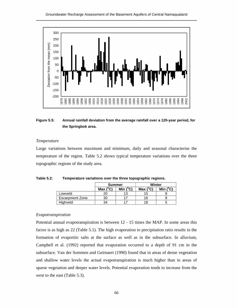
Groundwater Recharge Assessment of the Basement Aquifers of Central Namaqualand
66
-200
-150
-100
-50
0
50
100
150
200
250
300
1878
1882
1886
1890
1894
1898
1902
1906
1910
1914
1918
1922
1926
1930
1934
1938
1942
1946
1950
1954
1958
1962
1966
1970
1974
1978
1982
1986
1990
1994
1998
2002
Dev
iatio
n fro
m th
e m
ean
(mm
)
Figure 5.5: Annual rainfall deviation from the average rainfall over a 120-year period, for
the Springbok area.
Temperature
Large variations between maximum and minimum, daily and seasonal characterise the
temperature of the region. Table 5.2 shows typical temperature variations over the three
topographic regions of the study area.
Table 5.2: Temperature variations over the three topographic regions.
Summer Winter Max (oC) Min (oC) Max (oC) Min (oC) Lowveld 20 13 15 8 Escarpment Zone 30 17 16 8 Highveld 34 17 18 5
Evapotranspiration
Potential annual evapotranspiration is between 12 - 15 times the MAP. In some areas this
factor is as high as 22 (Table 5.1). The high evaporation to precipitation ratio results in the
formation of evaporitic salts at the surface as well as in the subsurface. In alluvium,
Campbell et al. (1992) reported that evaporation occurred to a depth of 91 cm in the
subsurface. Van der Sommen and Geirnaert (1990) found that in areas of dense vegetation
and shallow water levels the actual evapotranspiration is much higher than in areas of
sparse vegetation and deeper water levels. Potential evaporation tends to increase from the
west to the east (Table 5.3).
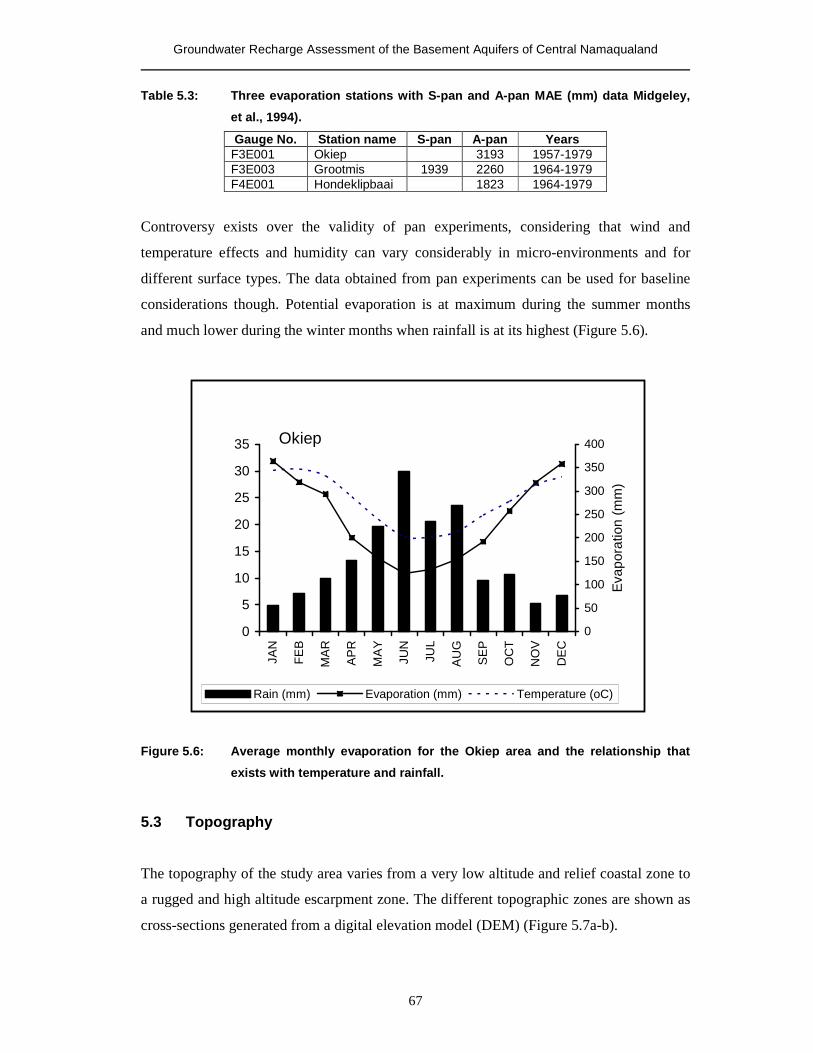
Groundwater Recharge Assessment of the Basement Aquifers of Central Namaqualand
67
Table 5.3: Three evaporation stations with S-pan and A-pan MAE (mm) data Midgeley,
et al., 1994).
Gauge No. Station name S-pan A-pan Years F3E001 Okiep 3193 1957-1979 F3E003 Grootmis 1939 2260 1964-1979 F4E001 Hondeklipbaai 1823 1964-1979
Controversy exists over the validity of pan experiments, considering that wind and
temperature effects and humidity can vary considerably in micro-environments and for
different surface types. The data obtained from pan experiments can be used for baseline
considerations though. Potential evaporation is at maximum during the summer months
and much lower during the winter months when rainfall is at its highest (Figure 5.6).
Figure 5.6: Average monthly evaporation for the Okiep area and the relationship that
exists with temperature and rainfall.
5.3 Topography
The topography of the study area varies from a very low altitude and relief coastal zone to
a rugged and high altitude escarpment zone. The different topographic zones are shown as
cross-sections generated from a digital elevation model (DEM) (Figure 5.7a-b).
Okiep
0
5
10
15
20
25
30
35
JAN
FEB
MA
R
AP
R
MA
Y
JUN
JUL
AU
G
SE
P
OC
T
NO
V
DE
C
0
50
100
150
200
250
300
350
400
Eva
pora
tion
(mm
)
Rain (mm) Evaporation (mm) Temperature (oC)
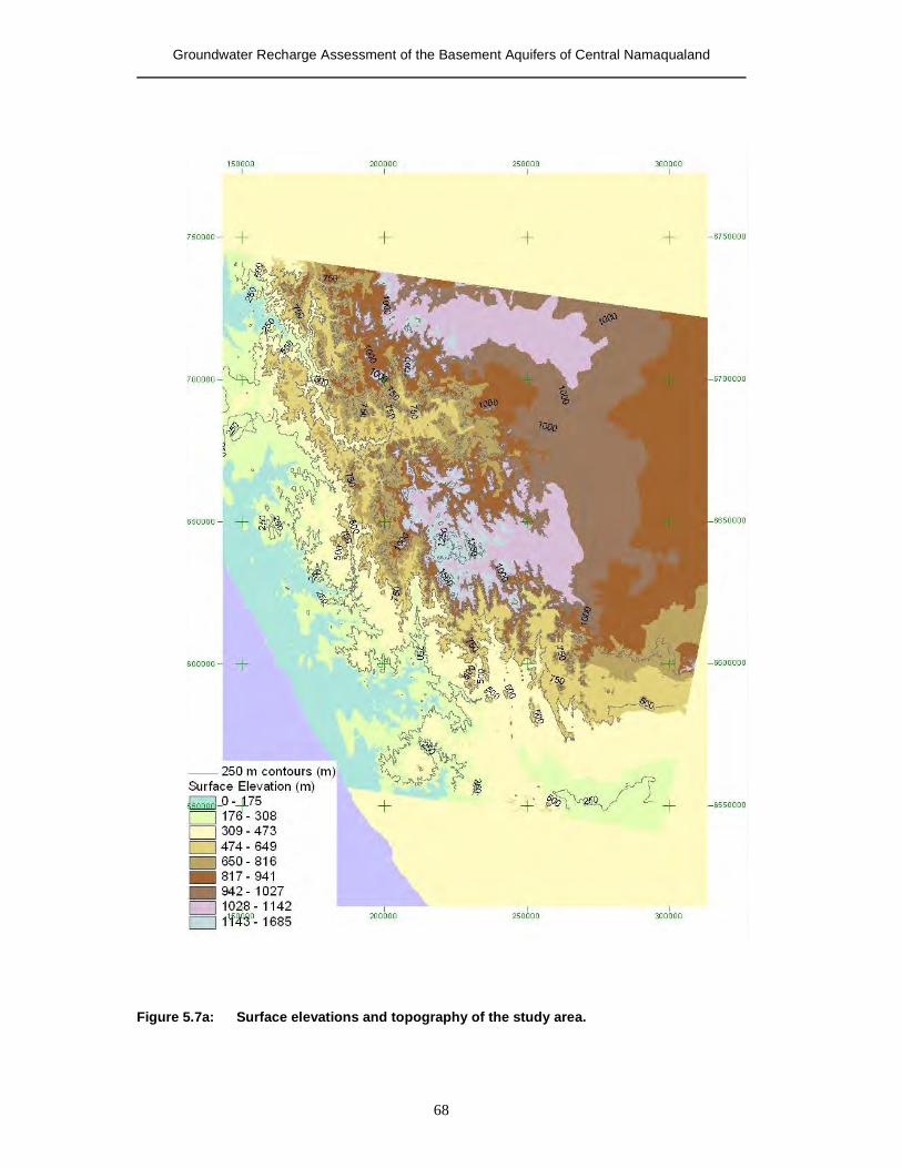
Groundwater Recharge Assessment of the Basement Aquifers of Central Namaqualand
68
Figure 5.7a: Surface elevations and topography of the study area.
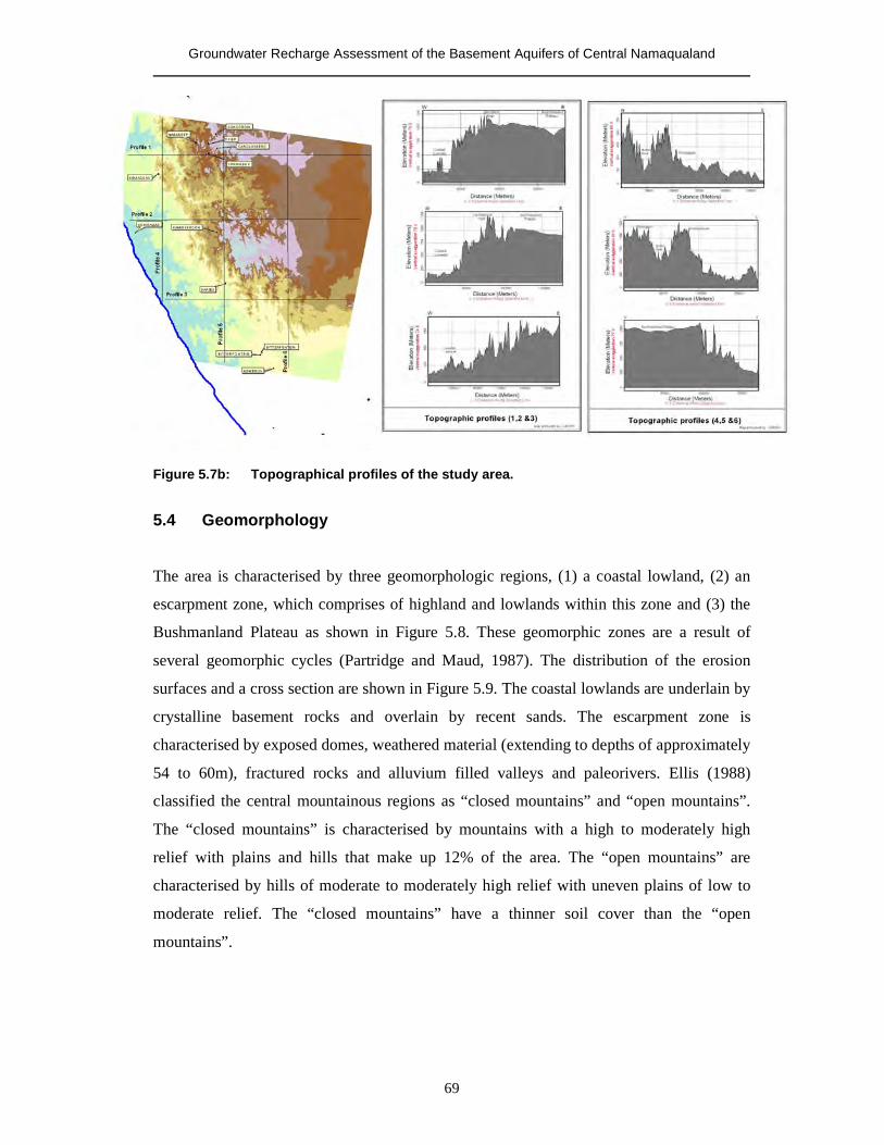
Groundwater Recharge Assessment of the Basement Aquifers of Central Namaqualand
69
Figure 5.7b: Topographical profiles of the study area.
5.4 Geomorphology
The area is characterised by three geomorphologic regions, (1) a coastal lowland, (2) an
escarpment zone, which comprises of highland and lowlands within this zone and (3) the
Bushmanland Plateau as shown in Figure 5.8. These geomorphic zones are a result of
several geomorphic cycles (Partridge and Maud, 1987). The distribution of the erosion
surfaces and a cross section are shown in Figure 5.9. The coastal lowlands are underlain by
crystalline basement rocks and overlain by recent sands. The escarpment zone is
characterised by exposed domes, weathered material (extending to depths of approximately
54 to 60m), fractured rocks and alluvium filled valleys and paleorivers. Ellis (1988)
classified the central mountainous regions as “closed mountains” and “open mountains”.
The “closed mountains” is characterised by mountains with a high to moderately high
relief with plains and hills that make up 12% of the area. The “open mountains” are
characterised by hills of moderate to moderately high relief with uneven plains of low to
moderate relief. The “closed mountains” have a thinner soil cover than the “open
mountains”.
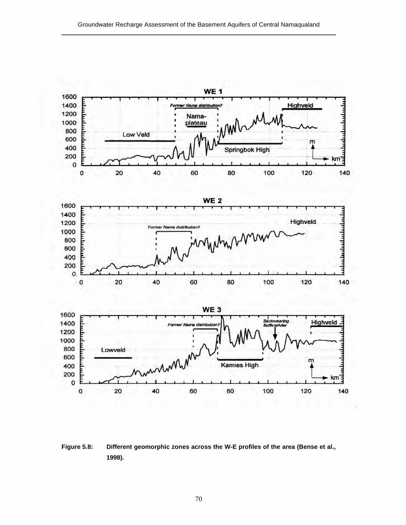
Groundwater Recharge Assessment of the Basement Aquifers of Central Namaqualand
70
Figure 5.8: Different geomorphic zones across the W-E profiles of the area (Bense et al.,
1998).
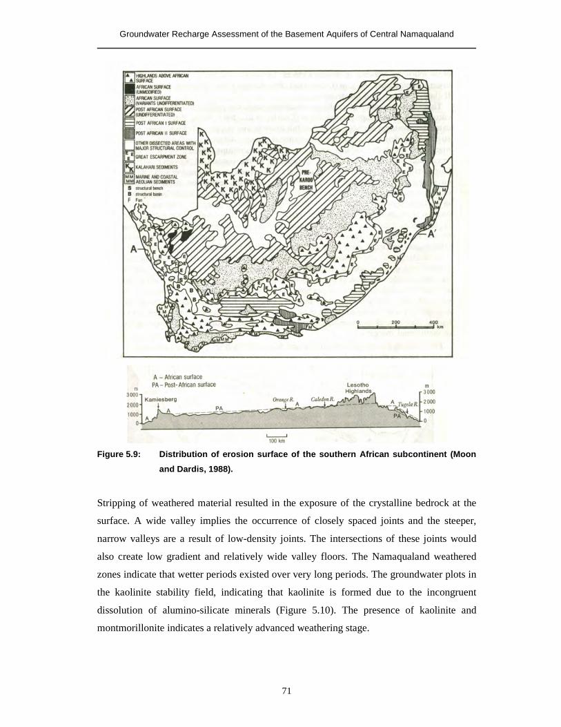
Groundwater Recharge Assessment of the Basement Aquifers of Central Namaqualand
71
Figure 5.9: Distribution of erosion surface of the southern African subcontinent (Moon
and Dardis, 1988).
Stripping of weathered material resulted in the exposure of the crystalline bedrock at the
surface. A wide valley implies the occurrence of closely spaced joints and the steeper,
narrow valleys are a result of low-density joints. The intersections of these joints would
also create low gradient and relatively wide valley floors. The Namaqualand weathered
zones indicate that wetter periods existed over very long periods. The groundwater plots in
the kaolinite stability field, indicating that kaolinite is formed due to the incongruent
dissolution of alumino-silicate minerals (Figure 5.10). The presence of kaolinite and
montmorillonite indicates a relatively advanced weathering stage.
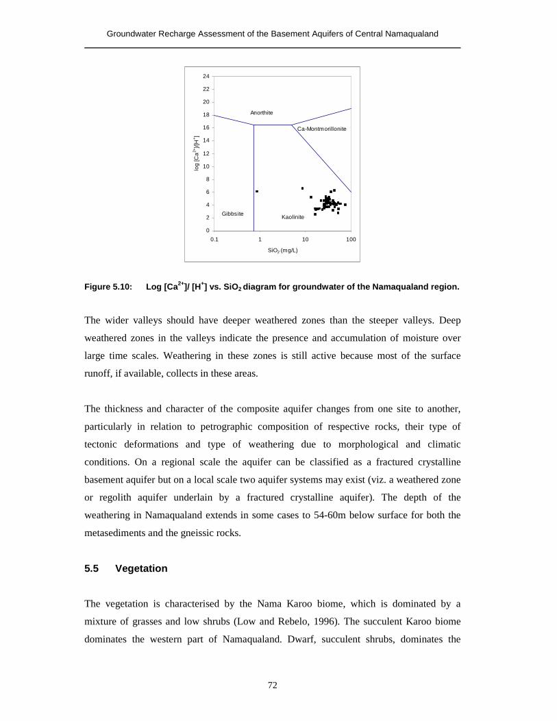
Groundwater Recharge Assessment of the Basement Aquifers of Central Namaqualand
72
Figure 5.10: Log [Ca2+]/ [H+] vs. SiO2 diagram for groundwater of the Namaqualand region.
The wider valleys should have deeper weathered zones than the steeper valleys. Deep
weathered zones in the valleys indicate the presence and accumulation of moisture over
large time scales. Weathering in these zones is still active because most of the surface
runoff, if available, collects in these areas.
The thickness and character of the composite aquifer changes from one site to another,
particularly in relation to petrographic composition of respective rocks, their type of
tectonic deformations and type of weathering due to morphological and climatic
conditions. On a regional scale the aquifer can be classified as a fractured crystalline
basement aquifer but on a local scale two aquifer systems may exist (viz. a weathered zone
or regolith aquifer underlain by a fractured crystalline aquifer). The depth of the
weathering in Namaqualand extends in some cases to 54-60m below surface for both the
metasediments and the gneissic rocks.
5.5 Vegetation
The vegetation is characterised by the Nama Karoo biome, which is dominated by a
mixture of grasses and low shrubs (Low and Rebelo, 1996). The succulent Karoo biome
dominates the western part of Namaqualand. Dwarf, succulent shrubs, dominates the
0
2
4
6
8
10
12
14
16
18
20
22
24
0.1 1 10 100
SiO2 (mg/L)
log
[Ca2+
]/[H
+]
Kaolinite
Ca-Montmorillonite
Anorthite
Gibbsite

Groundwater Recharge Assessment of the Basement Aquifers of Central Namaqualand
73
vegetation. Mass flowering of annuals occurs in spring when the rainfall is sufficient.
Most of the shrubs are classified as drought deciduous and tend to develop deep root
systems.
In the alluvial plains and riparian zones vegetation is dependent on groundwater
availability. Plant species such as Prospis (moderately drought tolerant, facultative
phreatophytes) form extensive thickets in these zones, which indicates available
groundwater (Low and Rebelo, 1996). Acacia karoo (riparian shrubs and trees) is found in
the alluvial aquifers of the Buffels River. Succulent Karoo vegetation dominates at the
coastal zones, ranging from subterranean, stemless dwarfs to 2.5 m high shrubs (Acocks,
1988).
Vegetation is an important component in any recharge study as vegetative cover intercepts
precipitation before it reaches the surface. The water losses as a result of transpiration are
also an important factor and are usually grouped with evaporation. Transpiration only takes
place if the vapour pressure in the air is less than that in the leaf cells. Where the
evaporating surface is the soil surface, the degree of shading of the crop canopy and the
amount of water available at the evaporating surface are other factors that affect the
evaporation process. Vegetation also influences the rate of runoff within a particular area.
5.6 Geology
Namaqualand can be subdivided into three major geological provinces (Tankard et al.,
1982). These are the basement rocks of the Namaqua Province, the volcano-sedimentary
rocks of the Gariep Complex (Visser, 1989) in the northwest and a Phanerozoic cratonic
cover (Table 5.4). The geology of the area has been discussed in detail by Titus et al.
(2002) and Titus (2003).
The Namaqua Province represents most of the crystalline basement in the northern Cape
and southern Namibia (Tankard et al., 1982). In Namaqualand, the margins of the
Namaqua Province are largely obscured by younger cover rocks of the Gariep, Nama and
Karoo sequences, as well as with Cenozoic surficial sediments to the east and west (Figure
5.11). In the west and extreme north, rocks of the Namaqua Province and its correlatives
are bordered by formations of the late Proterozoic Gariep Complex and in the east adjoin
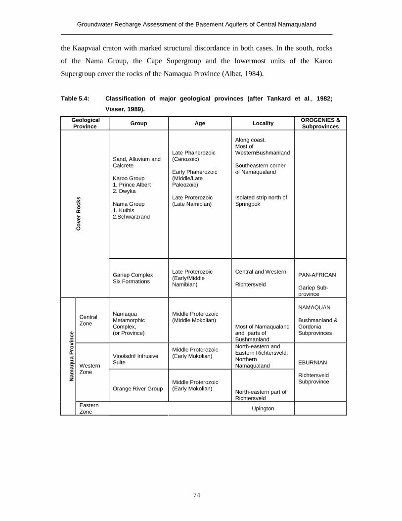
Groundwater Recharge Assessment of the Basement Aquifers of Central Namaqualand
74
the Kaapvaal craton with marked structural discordance in both cases. In the south, rocks
of the Nama Group, the Cape Supergroup and the lowermost units of the Karoo
Supergroup cover the rocks of the Namaqua Province (Albat, 1984).
Table 5.4: Classification of major geological provinces (after Tankard et al., 1982;
Visser, 1989).
Geological Province Group Age Locality OROGENIES &
Subprovinces
Sand, Alluvium and Calcrete Karoo Group 1. Prince Albert 2. Dwyka Nama Group 1. Kuibis 2.Schwarzrand
Late Phanerozoic (Cenozoic) Early Phanerozoic (Middle/Late Paleozoic) Late Proterozoic (Late Namibian)
Along coast. Most of WesternBushmanland Southeastern corner of Namaqualand Isolated strip north of Springbok
Cov
er R
ocks
Gariep Complex Six Formations
Late Proterozoic (Early/Middle Namibian)
Central and Western Richtersveld
PAN-AFRICAN Gariep Sub-province
Central Zone
Namaqua Metamorphic Complex, (or Province)
Middle Proterozoic (Middle Mokolian)
Most of Namaqualand and parts of Bushmanland
NAMAQUAN Bushmanland & Gordonia Subprovinces
Vioolsdrif Intrusive Suite
Middle Proterozoic (Early Mokolian)
North-eastern and Eastern Richtersveld. Northern Namaqualand
Western Zone
Orange River Group
Middle Proterozoic (Early Mokolian)
North-eastern part of Richtersveld
EBURNIAN Richtersveld Subprovince
N
amaq
ua
Pro
vinc
e
Eastern Zone
Upington
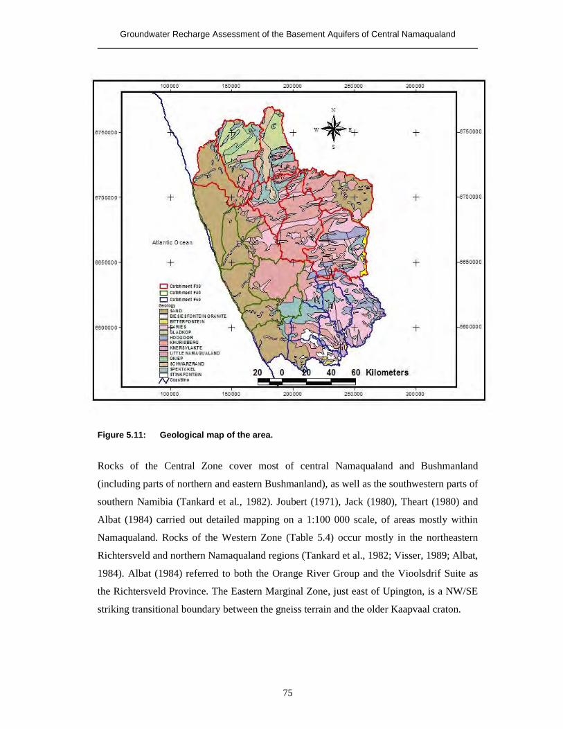
Groundwater Recharge Assessment of the Basement Aquifers of Central Namaqualand
75
Figure 5.11: Geological map of the area.
Rocks of the Central Zone cover most of central Namaqualand and Bushmanland
(including parts of northern and eastern Bushmanland), as well as the southwestern parts of
southern Namibia (Tankard et al., 1982). Joubert (1971), Jack (1980), Theart (1980) and
Albat (1984) carried out detailed mapping on a 1:100 000 scale, of areas mostly within
Namaqualand. Rocks of the Western Zone (Table 5.4) occur mostly in the northeastern
Richtersveld and northern Namaqualand regions (Tankard et al., 1982; Visser, 1989; Albat,
1984). Albat (1984) referred to both the Orange River Group and the Vioolsdrif Suite as
the Richtersveld Province. The Eastern Marginal Zone, just east of Upington, is a NW/SE
striking transitional boundary between the gneiss terrain and the older Kaapvaal craton.
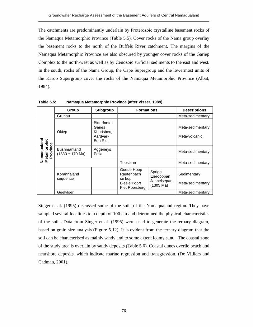
Groundwater Recharge Assessment of the Basement Aquifers of Central Namaqualand
76
The catchments are predominantly underlain by Proterozoic crystalline basement rocks of
the Namaqua Metamorphic Province (Table 5.5). Cover rocks of the Nama group overlay
the basement rocks to the north of the Buffels River catchment. The margins of the
Namaqua Metamorphic Province are also obscured by younger cover rocks of the Gariep
Complex to the north-west as well as by Cenozoic surficial sediments to the east and west.
In the south, rocks of the Nama Group, the Cape Supergroup and the lowermost units of
the Karoo Supergroup cover the rocks of the Namaqua Metamorphic Province (Albat,
1984).
Table 5.5: Namaqua Metamorphic Province (after Visser, 1989).
Group Subgroup Formations Descriptions Grunau Meta-sedimentary
Okiep
Bitterfontein Garies Khurisberg Aardvark Een Riet
Meta-sedimentary Meta-volcanic
Bushmanland (1330 ± 170 Ma)
Aggeneys Pella
Meta-sedimentary
Toeslaan Meta-sedimentary
Korannaland sequence
Goede Hoop Rautenbach se kop Biesje Poort Piet Rooisberg
Sprigg Eierdoppan Jannelsepan (1305 Ma)
Sedimentary Meta-sedimentary
Nam
aqua
land
M
etam
orph
ic
Pro
vinc
e
Geelvloer Meta-sedimentary
Singer et al. (1995) discussed some of the soils of the Namaqualand region. They have
sampled several localities to a depth of 100 cm and determined the physical characteristics
of the soils. Data from Singer et al. (1995) were used to generate the ternary diagram,
based on grain size analysis (Figure 5.12). It is evident from the ternary diagram that the
soil can be characterised as mainly sandy and to some extent loamy sand. The coastal zone
of the study area is overlain by sandy deposits (Table 5.6). Coastal dunes overlie beach and
nearshore deposits, which indicate marine regression and transgression. (De Villiers and
Cadman, 2001).
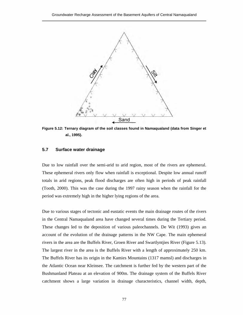
Groundwater Recharge Assessment of the Basement Aquifers of Central Namaqualand
77
Figure 5.12: Ternary diagram of the soil classes found in Namaqualand (data from Singer et
al., 1995).
5.7 Surface water drainage
Due to low rainfall over the semi-arid to arid region, most of the rivers are ephemeral.
These ephemeral rivers only flow when rainfall is exceptional. Despite low annual runoff
totals in arid regions, peak flood discharges are often high in periods of peak rainfall
(Tooth, 2000). This was the case during the 1997 rainy season when the rainfall for the
period was extremely high in the higher lying regions of the area.
Due to various stages of tectonic and eustatic events the main drainage routes of the rivers
in the Central Namaqualand area have changed several times during the Tertiary period.
These changes led to the deposition of various paleochannels. De Wit (1993) gives an
account of the evolution of the drainage patterns in the NW Cape. The main ephemeral
rivers in the area are the Buffels River, Groen River and Swartlyntjies River (Figure 5.13).
The largest river in the area is the Buffels River with a length of approximately 250 km.
The Buffels River has its origin in the Kamies Mountains (1317 mamsl) and discharges in
the Atlantic Ocean near Kleinsee. The catchment is further fed by the western part of the
Bushmanland Plateau at an elevation of 900m. The drainage system of the Buffels River
catchment shows a large variation in drainage characteristics, channel width, depth,
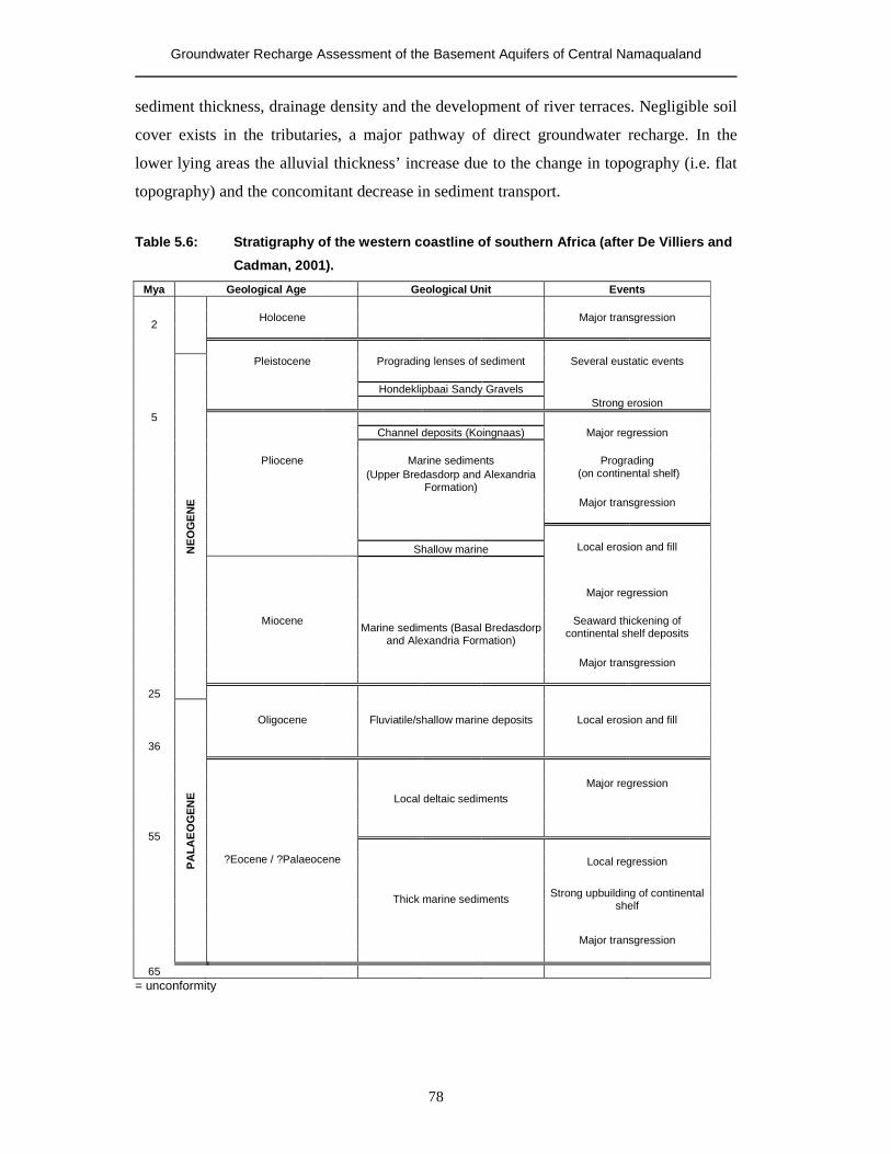
Groundwater Recharge Assessment of the Basement Aquifers of Central Namaqualand
78
sediment thickness, drainage density and the development of river terraces. Negligible soil
cover exists in the tributaries, a major pathway of direct groundwater recharge. In the
lower lying areas the alluvial thickness’ increase due to the change in topography (i.e. flat
topography) and the concomitant decrease in sediment transport.
Table 5.6: Stratigraphy of the western coastline of southern Africa (after De Villiers and
Cadman, 2001).
Mya Geological Age Geological Unit Events
Holocene Major transgression
2
Pleistocene Prograding lenses of sediment Several eustatic events Hondeklipbaai Sandy Gravels
Strong erosion 5
Channel deposits (Koingnaas) Major regression Pliocene Marine sediments
Prograding (on continental shelf)
(Upper Bredasdorp and Alexandria
Formation) Major transgression
Shallow marine
Local erosion and fill
Major regression Miocene
Seaward thickening of continental shelf deposits
Marine sediments (Basal Bredasdorp and Alexandria Formation)
Major transgression
NE
OG
EN
E
25
Oligocene Fluviatile/shallow marine deposits Local erosion and fill
36
Major regression Local deltaic sediments
55
Local regression
Thick marine sediments Strong upbuilding of continental shelf
Major transgression
PA
LAE
OG
EN
E
?Eocene / ?Palaeocene
65
= unconformity
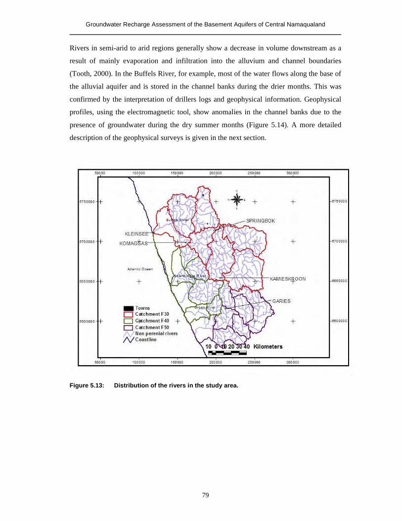
Groundwater Recharge Assessment of the Basement Aquifers of Central Namaqualand
79
Rivers in semi-arid to arid regions generally show a decrease in volume downstream as a
result of mainly evaporation and infiltration into the alluvium and channel boundaries
(Tooth, 2000). In the Buffels River, for example, most of the water flows along the base of
the alluvial aquifer and is stored in the channel banks during the drier months. This was
confirmed by the interpretation of drillers logs and geophysical information. Geophysical
profiles, using the electromagnetic tool, show anomalies in the channel banks due to the
presence of groundwater during the dry summer months (Figure 5.14). A more detailed
description of the geophysical surveys is given in the next section.
Figure 5.13: Distribution of the rivers in the study area.
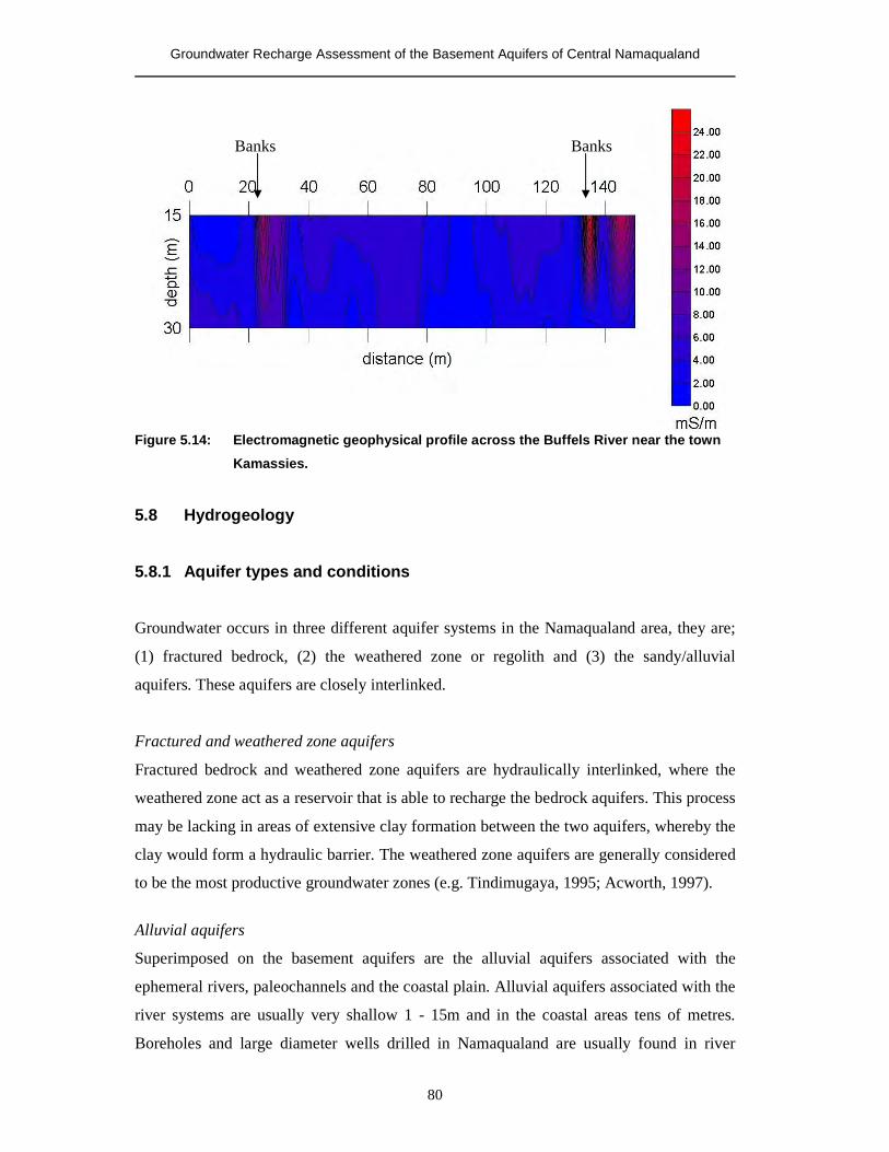
Groundwater Recharge Assessment of the Basement Aquifers of Central Namaqualand
80
Figure 5.14: Electromagnetic geophysical profile across the Buffels River near the town
Kamassies.
5.8 Hydrogeology
5.8.1 Aquifer types and conditions
Groundwater occurs in three different aquifer systems in the Namaqualand area, they are;
(1) fractured bedrock, (2) the weathered zone or regolith and (3) the sandy/alluvial
aquifers. These aquifers are closely interlinked.
Fractured and weathered zone aquifers
Fractured bedrock and weathered zone aquifers are hydraulically interlinked, where the
weathered zone act as a reservoir that is able to recharge the bedrock aquifers. This process
may be lacking in areas of extensive clay formation between the two aquifers, whereby the
clay would form a hydraulic barrier. The weathered zone aquifers are generally considered
to be the most productive groundwater zones (e.g. Tindimugaya, 1995; Acworth, 1997).
Alluvial aquifers
Superimposed on the basement aquifers are the alluvial aquifers associated with the
ephemeral rivers, paleochannels and the coastal plain. Alluvial aquifers associated with the
river systems are usually very shallow 1 - 15m and in the coastal areas tens of metres.
Boreholes and large diameter wells drilled in Namaqualand are usually found in river
Banks Banks
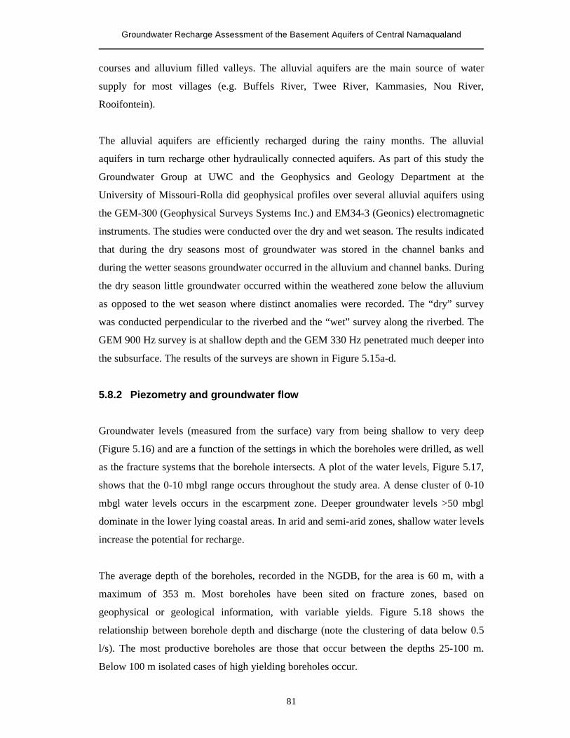
Groundwater Recharge Assessment of the Basement Aquifers of Central Namaqualand
81
courses and alluvium filled valleys. The alluvial aquifers are the main source of water
supply for most villages (e.g. Buffels River, Twee River, Kammasies, Nou River,
Rooifontein).
The alluvial aquifers are efficiently recharged during the rainy months. The alluvial
aquifers in turn recharge other hydraulically connected aquifers. As part of this study the
Groundwater Group at UWC and the Geophysics and Geology Department at the
University of Missouri-Rolla did geophysical profiles over several alluvial aquifers using
the GEM-300 (Geophysical Surveys Systems Inc.) and EM34-3 (Geonics) electromagnetic
instruments. The studies were conducted over the dry and wet season. The results indicated
that during the dry seasons most of groundwater was stored in the channel banks and
during the wetter seasons groundwater occurred in the alluvium and channel banks. During
the dry season little groundwater occurred within the weathered zone below the alluvium
as opposed to the wet season where distinct anomalies were recorded. The “dry” survey
was conducted perpendicular to the riverbed and the “wet” survey along the riverbed. The
GEM 900 Hz survey is at shallow depth and the GEM 330 Hz penetrated much deeper into
the subsurface. The results of the surveys are shown in Figure 5.15a-d.
5.8.2 Piezometry and groundwater flow
Groundwater levels (measured from the surface) vary from being shallow to very deep
(Figure 5.16) and are a function of the settings in which the boreholes were drilled, as well
as the fracture systems that the borehole intersects. A plot of the water levels, Figure 5.17,
shows that the 0-10 mbgl range occurs throughout the study area. A dense cluster of 0-10
mbgl water levels occurs in the escarpment zone. Deeper groundwater levels >50 mbgl
dominate in the lower lying coastal areas. In arid and semi-arid zones, shallow water levels
increase the potential for recharge.
The average depth of the boreholes, recorded in the NGDB, for the area is 60 m, with a
maximum of 353 m. Most boreholes have been sited on fracture zones, based on
geophysical or geological information, with variable yields. Figure 5.18 shows the
relationship between borehole depth and discharge (note the clustering of data below 0.5
l/s). The most productive boreholes are those that occur between the depths 25-100 m.
Below 100 m isolated cases of high yielding boreholes occur.
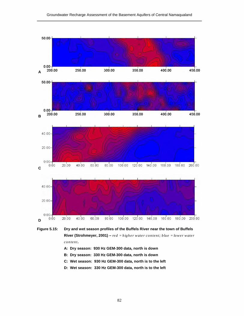
Groundwater Recharge Assessment of the Basement Aquifers of Central Namaqualand
82
A
B
CC
D
Figure 5.15: Dry and wet season profiles of the Buffels River near the town of Buffels
River (Strohmeyer, 2001) – red = higher water content; blue = lower water
content.
A: Dry season: 930 Hz GEM-300 data, north is down
B: Dry season: 330 Hz GEM-300 data, north is down
C: Wet season: 930 Hz GEM-300 data, north is to the left
D: Wet season: 330 Hz GEM-300 data, north is to the left
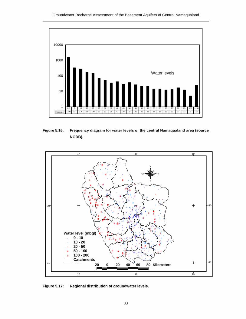
Groundwater Recharge Assessment of the Basement Aquifers of Central Namaqualand
83
Water levels
1
10
100
1000
10000
Frequency 1496 337 276 165 140 67 52 35 41 29 37 26 21 21 14 14 12 13 17 12 5 24
0.5 5 10 15 20 25 30 35 40 45 50 55 60 65 70 75 80 85 90 95 100 >100
Figure 5.16: Frequency diagram for water levels of the central Namaqualand area (source
NGDB).
### # ###
####
#### ####### ## # ###
###
# ################# #
### ##
################# # ## ####
### ###### ######### ######## ########### ######## ##
##
########
###
##
######
##
## ### #
#########################
########### ### #
# #### ###### ###
########## ## ####
## ####### ########## # ## #### ###### # ## ##### ### ######### #### ### ## ### ## ###
####### ## #### ### ############ #
#
####
####
#### ### ######
######
###
##### #
#### ########
########## ######
# ##### ### #
########
######## #### ## #### ######## # # ########## ### ### ###
########## ### ########### # ## ######## ########## ########## ## ###### ####### ########### ## ########### ### ## ###### ######## ########## ### ### # ### ##### ### ## ### ############# # ## ######################## ##### ### #### ### ## ######### ### ######### ########### ## ##### #### ## ###### # ###### ### ##### ### #### ######## ### ############ ####### ### ### ### ## ###### ######## ## ### ## ## ######### ######## ### ## #### ## ####
###### ## ########## #### ### ####### ### # #### # ####### ## #
###
##### # ##### ## ### ### # ## #### ####### ### ########### ################## #### ## # # #### ## ###
## #### ##### ######## ### #### ### ########## ####### #### ## ######## ## ## ######
############### ####### #### ############################# # #
# ### ###### #### #### ####
# ### ## ######## ### ## ######
# ############## ####
# ### ############# ## ## ### ## #### # #### #### ## ### ## ### ##### ############# # #### #### ## ## ###### ### # ########### ##### #### ###
######## ######## ## ## ##### ## ### #
## ##### ### ## ### ## ### ######## ### ### ## # ## ### # #
#### ###
#
########
#####
Catchments
Water level (mbgl)# 0 - 10# 10 - 20# 20 - 50# 50 - 100# 100 - 200
20 0 20 40 60 80 Kilometers
N
EW
S
17
17
18
18
19
19
-31 -31
-30 -30
Figure 5.17: Regional distribution of groundwater levels.
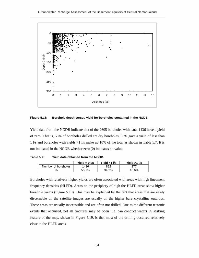
Groundwater Recharge Assessment of the Basement Aquifers of Central Namaqualand
84
0
50
100
150
200
250
3000 1 2 3 4 5 6 7 8 9 10 11 12 13
Discharge (l/s)
Dep
th (m
bgl)
Figure 5.18: Borehole depth versus yield for boreholes contained in the NGDB.
Yield data from the NGDB indicate that of the 2605 boreholes with data, 1436 have a yield
of zero. That is, 55% of boreholes drilled are dry boreholes, 33% gave a yield of less than
1 l/s and boreholes with yields >1 l/s make up 10% of the total as shown in Table 5.7. It is
not indicated in the NGDB whether zero (0) indicates no value.
Table 5.7: Yield data obtained from the NGDB.
Yield = 0 l/s Yield <1 l/s Yield >1 l/s Number of boreholes 1436 892 277
% 55.1% 34.2% 10.6%
Boreholes with relatively higher yields are often associated with areas with high lineament
frequency densities (HLFD). Areas on the periphery of high the HLFD areas show higher
borehole yields (Figure 5.19). This may be explained by the fact that areas that are easily
discernable on the satellite images are usually on the higher bare crystalline outcrops.
These areas are usually inaccessible and are often not drilled. Due to the different tectonic
events that occurred, not all fractures may be open (i.e. can conduct water). A striking
feature of the map, shown in Figure 5.19, is that most of the drilling occurred relatively
close to the HLFD areas.
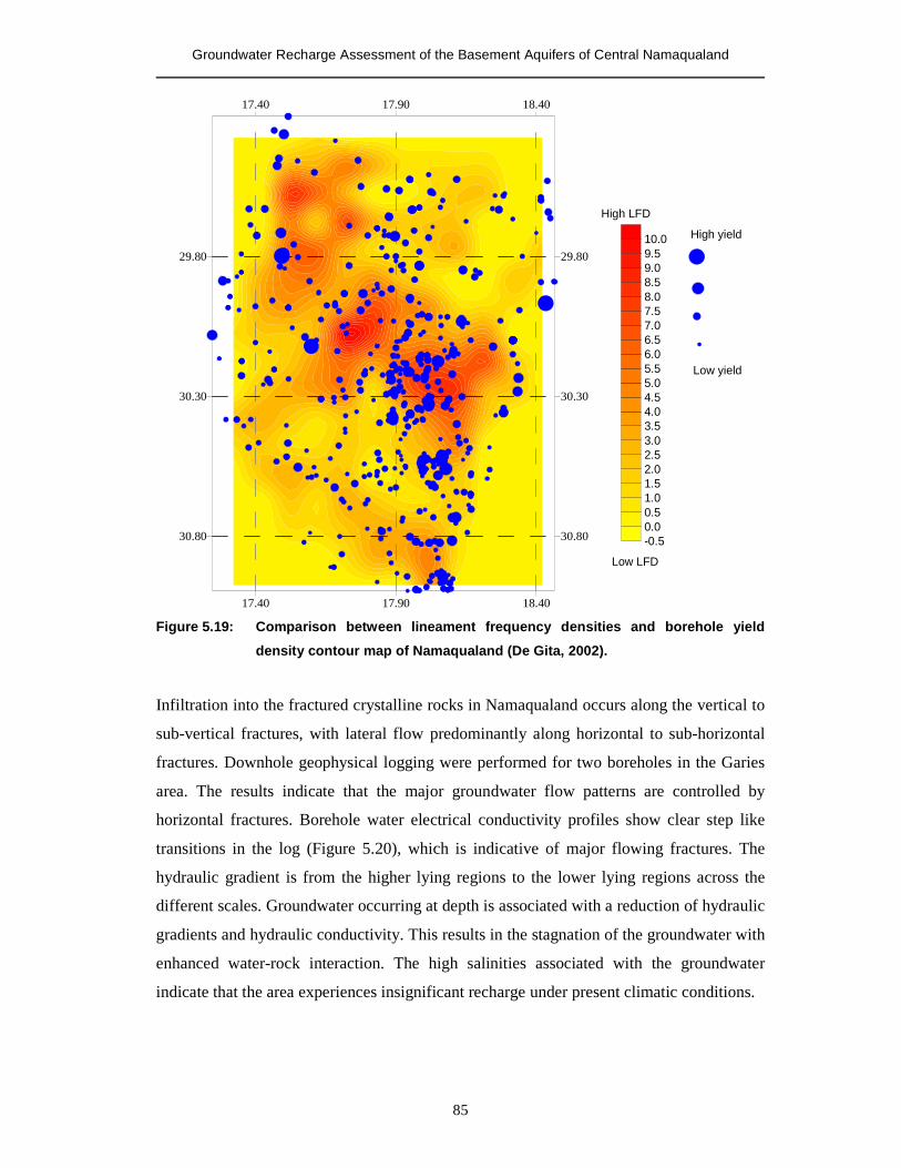
Groundwater Recharge Assessment of the Basement Aquifers of Central Namaqualand
85
17.40 17.90 18.40
17.40 17.90 18.40
30.80
30.30
29.80
30.80
30.30
29.80
-0.50.00.51.01.52.02.53.03.54.04.55.05.56.06.57.07.58.08.59.09.510.0
Low LFD
High LFD
High yield
Low yield
Figure 5.19: Comparison between lineament frequency densities and borehole yield
density contour map of Namaqualand (De Gita, 2002).
Infiltration into the fractured crystalline rocks in Namaqualand occurs along the vertical to
sub-vertical fractures, with lateral flow predominantly along horizontal to sub-horizontal
fractures. Downhole geophysical logging were performed for two boreholes in the Garies
area. The results indicate that the major groundwater flow patterns are controlled by
horizontal fractures. Borehole water electrical conductivity profiles show clear step like
transitions in the log (Figure 5.20), which is indicative of major flowing fractures. The
hydraulic gradient is from the higher lying regions to the lower lying regions across the
different scales. Groundwater occurring at depth is associated with a reduction of hydraulic
gradients and hydraulic conductivity. This results in the stagnation of the groundwater with
enhanced water-rock interaction. The high salinities associated with the groundwater
indicate that the area experiences insignificant recharge under present climatic conditions.
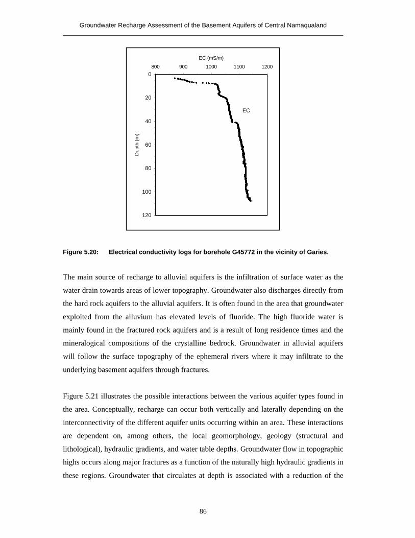
Groundwater Recharge Assessment of the Basement Aquifers of Central Namaqualand
86
0
20
40
60
80
100
120
800 900 1000 1100 1200
EC (mS/m)
Dep
th (m
)
EC
Figure 5.20: Electrical conductivity logs for borehole G45772 in the vicinity of Garies.
The main source of recharge to alluvial aquifers is the infiltration of surface water as the
water drain towards areas of lower topography. Groundwater also discharges directly from
the hard rock aquifers to the alluvial aquifers. It is often found in the area that groundwater
exploited from the alluvium has elevated levels of fluoride. The high fluoride water is
mainly found in the fractured rock aquifers and is a result of long residence times and the
mineralogical compositions of the crystalline bedrock. Groundwater in alluvial aquifers
will follow the surface topography of the ephemeral rivers where it may infiltrate to the
underlying basement aquifers through fractures.
Figure 5.21 illustrates the possible interactions between the various aquifer types found in
the area. Conceptually, recharge can occur both vertically and laterally depending on the
interconnectivity of the different aquifer units occurring within an area. These interactions
are dependent on, among others, the local geomorphology, geology (structural and
lithological), hydraulic gradients, and water table depths. Groundwater flow in topographic
highs occurs along major fractures as a function of the naturally high hydraulic gradients in
these regions. Groundwater that circulates at depth is associated with a reduction of the
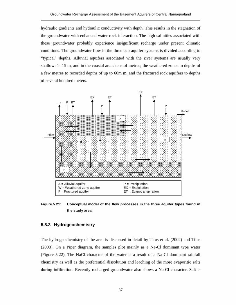
Groundwater Recharge Assessment of the Basement Aquifers of Central Namaqualand
87
hydraulic gradients and hydraulic conductivity with depth. This results in the stagnation of
the groundwater with enhanced water-rock interaction. The high salinities associated with
these groundwater probably experience insignificant recharge under present climatic
conditions. The groundwater flow in the three sub-aquifer systems is divided according to
“typical” depths. Alluvial aquifers associated with the river systems are usually very
shallow: 1- 15 m, and in the coastal areas tens of metres; the weathered zones to depths of
a few metres to recorded depths of up to 60m m, and the fractured rock aquifers to depths
of several hundred meters.
Figure 5.21: Conceptual model of the flow processes in the three aquifer types found in
the study area.
5.8.3 Hydrogeochemistry
The hydrogeochemistry of the area is discussed in detail by Titus et al. (2002) and Titus
(2003). On a Piper diagram, the samples plot mainly as a Na-Cl dominant type water
(Figure 5.22). The NaCl character of the water is a result of a Na-Cl dominant rainfall
chemistry as well as the preferential dissolution and leaching of the more evaporitic salts
during infiltration. Recently recharged groundwater also shows a Na-Cl character. Salt is
A = Alluvial aquifer P = Precipitation W = Weathered zone aquifer EX = Exploitation F = Fractured aquifer ET = Evapotranspiration
F
A
W
ET
ET
ET
P EX
EX
EX
Outflow
Runoff
P P
Inflow
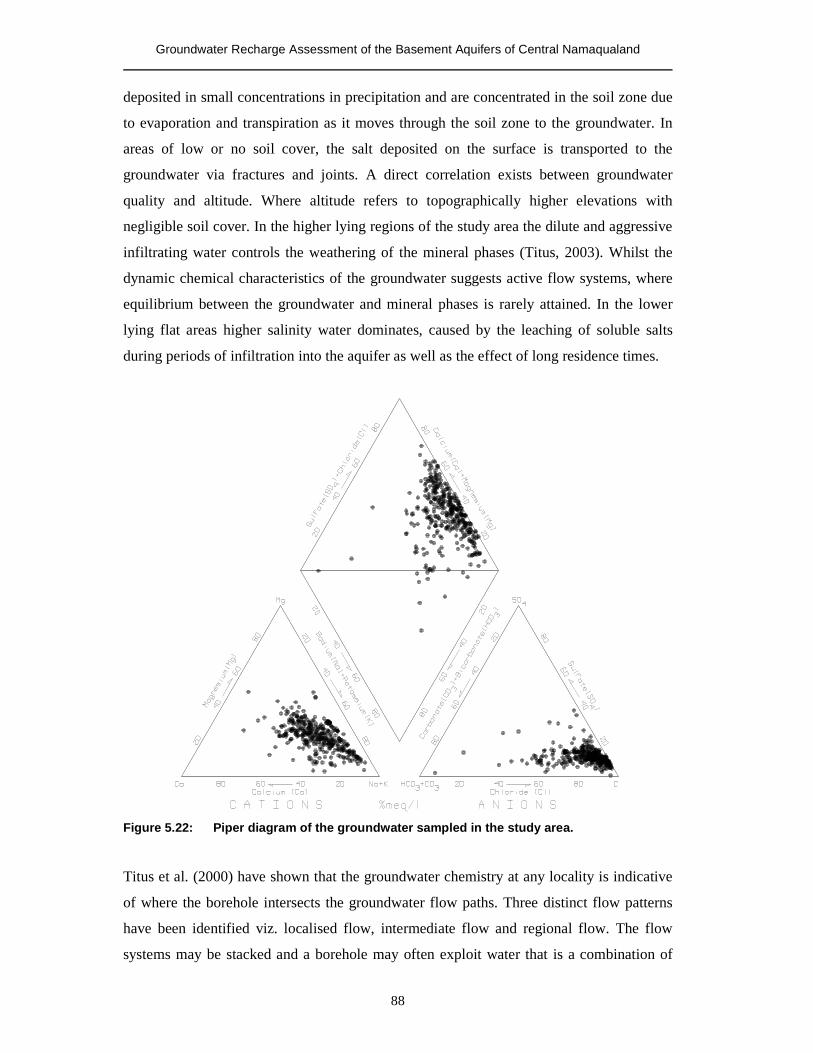
Groundwater Recharge Assessment of the Basement Aquifers of Central Namaqualand
88
deposited in small concentrations in precipitation and are concentrated in the soil zone due
to evaporation and transpiration as it moves through the soil zone to the groundwater. In
areas of low or no soil cover, the salt deposited on the surface is transported to the
groundwater via fractures and joints. A direct correlation exists between groundwater
quality and altitude. Where altitude refers to topographically higher elevations with
negligible soil cover. In the higher lying regions of the study area the dilute and aggressive
infiltrating water controls the weathering of the mineral phases (Titus, 2003). Whilst the
dynamic chemical characteristics of the groundwater suggests active flow systems, where
equilibrium between the groundwater and mineral phases is rarely attained. In the lower
lying flat areas higher salinity water dominates, caused by the leaching of soluble salts
during periods of infiltration into the aquifer as well as the effect of long residence times.
Figure 5.22: Piper diagram of the groundwater sampled in the study area.
Titus et al. (2000) have shown that the groundwater chemistry at any locality is indicative
of where the borehole intersects the groundwater flow paths. Three distinct flow patterns
have been identified viz. localised flow, intermediate flow and regional flow. The flow
systems may be stacked and a borehole may often exploit water that is a combination of
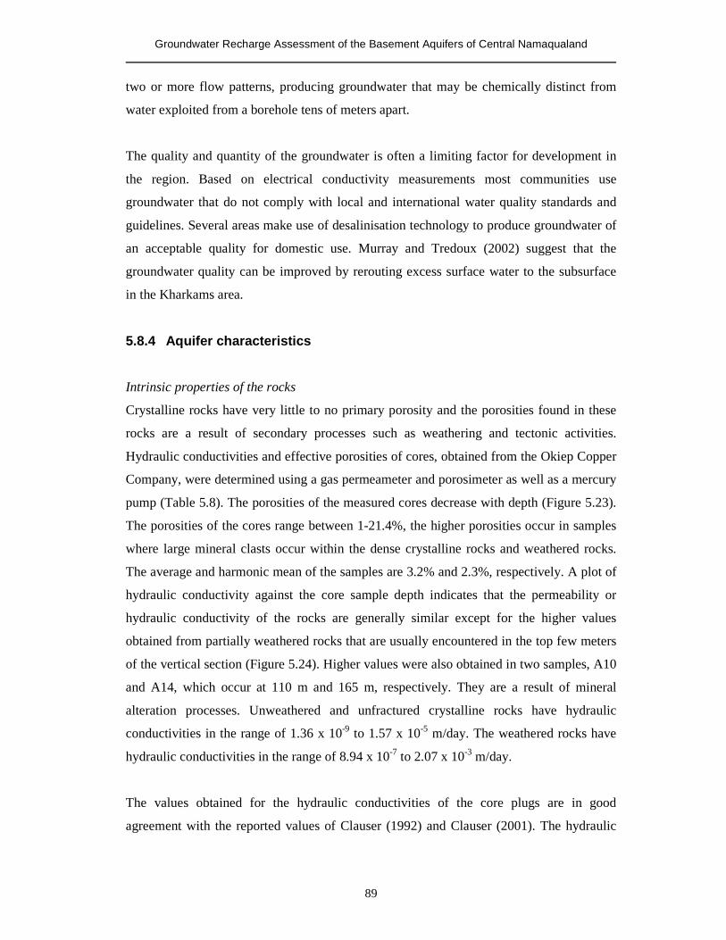
Groundwater Recharge Assessment of the Basement Aquifers of Central Namaqualand
89
two or more flow patterns, producing groundwater that may be chemically distinct from
water exploited from a borehole tens of meters apart.
The quality and quantity of the groundwater is often a limiting factor for development in
the region. Based on electrical conductivity measurements most communities use
groundwater that do not comply with local and international water quality standards and
guidelines. Several areas make use of desalinisation technology to produce groundwater of
an acceptable quality for domestic use. Murray and Tredoux (2002) suggest that the
groundwater quality can be improved by rerouting excess surface water to the subsurface
in the Kharkams area.
5.8.4 Aquifer characteristics
Intrinsic properties of the rocks
Crystalline rocks have very little to no primary porosity and the porosities found in these
rocks are a result of secondary processes such as weathering and tectonic activities.
Hydraulic conductivities and effective porosities of cores, obtained from the Okiep Copper
Company, were determined using a gas permeameter and porosimeter as well as a mercury
pump (Table 5.8). The porosities of the measured cores decrease with depth (Figure 5.23).
The porosities of the cores range between 1-21.4%, the higher porosities occur in samples
where large mineral clasts occur within the dense crystalline rocks and weathered rocks.
The average and harmonic mean of the samples are 3.2% and 2.3%, respectively. A plot of
hydraulic conductivity against the core sample depth indicates that the permeability or
hydraulic conductivity of the rocks are generally similar except for the higher values
obtained from partially weathered rocks that are usually encountered in the top few meters
of the vertical section (Figure 5.24). Higher values were also obtained in two samples, A10
and A14, which occur at 110 m and 165 m, respectively. They are a result of mineral
alteration processes. Unweathered and unfractured crystalline rocks have hydraulic
conductivities in the range of 1.36 x 10⁻⁹ to 1.57 x 10⁻⁵ m/day. The weathered rocks have
hydraulic conductivities in the range of 8.94 x 10⁻⁷ to 2.07 x 10⁻³ m/day.
The values obtained for the hydraulic conductivities of the core plugs are in good
agreement with the reported values of Clauser (1992) and Clauser (2001). The hydraulic
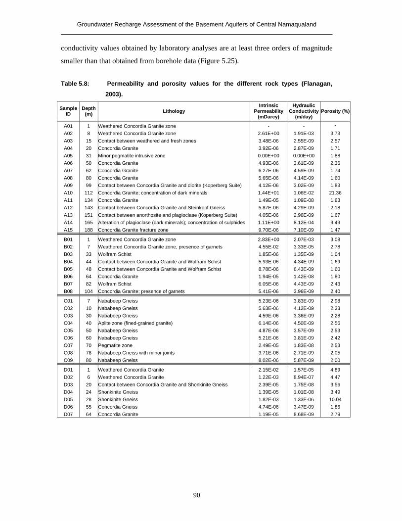
Groundwater Recharge Assessment of the Basement Aquifers of Central Namaqualand
90
conductivity values obtained by laboratory analyses are at least three orders of magnitude
smaller than that obtained from borehole data (Figure 5.25).
Table 5.8: Permeability and porosity values for the different rock types (Flanagan,
2003).
Sample ID
Depth (m) Lithology
Intrinsic Permeability
(mDarcy)
Hydraulic Conductivity
(m/day) Porosity (%)
A01 1 Weathered Concordia Granite zone - - -
A02 8 Weathered Concordia Granite zone 2.61E+00 1.91E-03 3.73 A03 15 Contact between weathered and fresh zones 3.48E-06 2.55E-09 2.57 A04 20 Concordia Granite 3.92E-06 2.87E-09 1.71 A05 31 Minor pegmatite intrusive zone 0.00E+00 0.00E+00 1.88 A06 50 Concordia Granite 4.93E-06 3.61E-09 2.36 A07 62 Concordia Granite 6.27E-06 4.59E-09 1.74 A08 80 Concordia Granite 5.65E-06 4.14E-09 1.60 A09 99 Contact between Concordia Granite and diorite (Koperberg Suite) 4.12E-06 3.02E-09 1.83 A10 112 Concordia Granite; concentration of dark minerals 1.44E+01 1.06E-02 21.36 A11 134 Concordia Granite 1.49E-05 1.09E-08 1.63 A12 143 Contact between Concordia Granite and Steinkopf Gneiss 5.87E-06 4.29E-09 2.18 A13 151 Contact between anorthosite and plagioclase (Koperberg Suite) 4.05E-06 2.96E-09 1.67 A14 165 Alteration of plagioclase (dark minerals); concentration of sulphides 1.11E+00 8.12E-04 9.49 A15 188 Concordia Granite fracture zone 9.70E-06 7.10E-09 1.47
B01 1 Weathered Concordia Granite zone 2.83E+00 2.07E-03 3.08 B02 7 Weathered Concordia Granite zone, presence of garnets 4.55E-02 3.33E-05 2.78 B03 33 Wolfram Schist 1.85E-06 1.35E-09 1.04 B04 44 Contact between Concordia Granite and Wolfram Schist 5.93E-06 4.34E-09 1.69 B05 48 Contact between Concordia Granite and Wolfram Schist 8.78E-06 6.43E-09 1.60 B06 64 Concordia Granite 1.94E-05 1.42E-08 1.80 B07 82 Wolfram Schist 6.05E-06 4.43E-09 2.43 B08 104 Concordia Granite; presence of garnets 5.41E-06 3.96E-09 2.40
C01 7 Nababeep Gneiss 5.23E-06 3.83E-09 2.98 C02 10 Nababeep Gneiss 5.63E-06 4.12E-09 2.33 C03 30 Nababeep Gneiss 4.59E-06 3.36E-09 2.28 C04 40 Aplite zone (fined-grained granite) 6.14E-06 4.50E-09 2.56 C05 50 Nababeep Gneiss 4.87E-06 3.57E-09 2.53 C06 60 Nababeep Gneiss 5.21E-06 3.81E-09 2.42 C07 70 Pegmatite zone 2.49E-05 1.83E-08 2.53 C08 78 Nababeep Gneiss with minor joints 3.71E-06 2.71E-09 2.05 C09 80 Nababeep Gneiss 8.02E-06 5.87E-09 2.00
D01 1 Weathered Concordia Granite 2.15E-02 1.57E-05 4.89 D02 6 Weathered Concordia Granite 1.22E-03 8.94E-07 4.47 D03 20 Contact between Concordia Granite and Shonkinite Gneiss 2.39E-05 1.75E-08 3.56 D04 24 Shonkinite Gneiss 1.39E-05 1.01E-08 3.49 D05 28 Shonkinite Gneiss 1.82E-03 1.33E-06 10.04 D06 55 Concordia Gneiss 4.74E-06 3.47E-09 1.86 D07 64 Concordia Granite 1.19E-05 8.68E-09 2.79
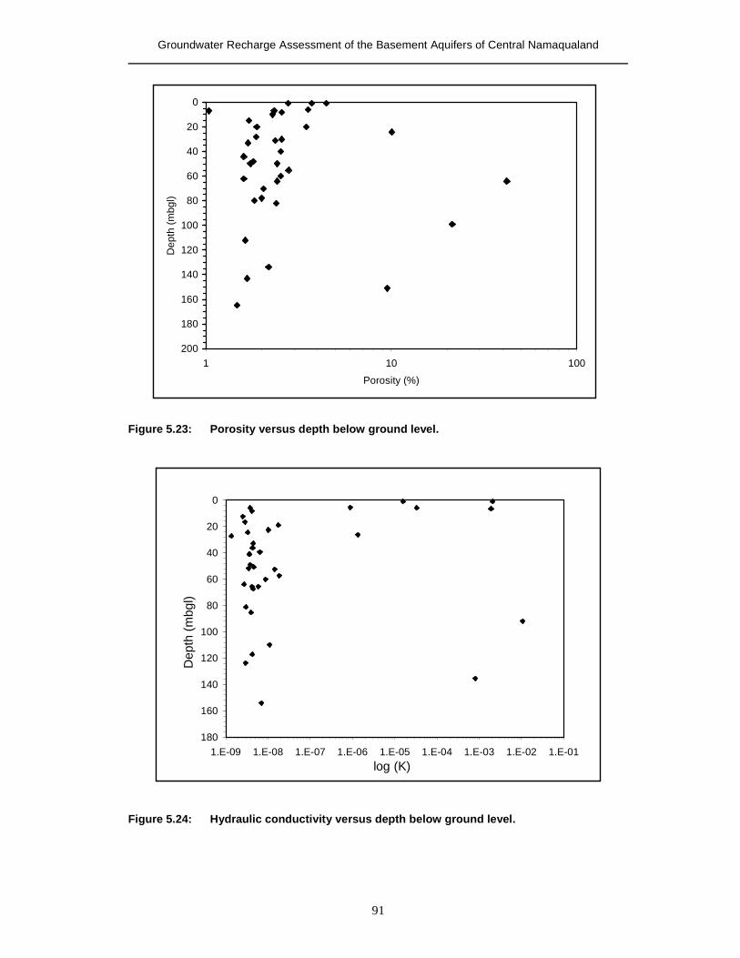
Groundwater Recharge Assessment of the Basement Aquifers of Central Namaqualand
91
Figure 5.23: Porosity versus depth below ground level.
0
20
40
60
80
100
120
140
160
1801.E-09 1.E-08 1.E-07 1.E-06 1.E-05 1.E-04 1.E-03 1.E-02 1.E-01
log (K)
Dep
th (m
bgl)
Figure 5.24: Hydraulic conductivity versus depth below ground level.
0
20
40
60
80
100
120
140
160
180
2001 10 100
Porosity (%)
Dep
th (m
bgl)
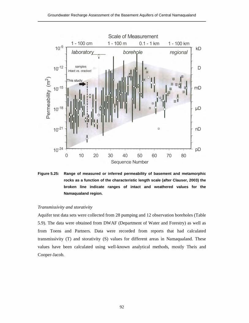
Groundwater Recharge Assessment of the Basement Aquifers of Central Namaqualand
92
Figure 5.25: Range of measured or inferred permeability of basement and metamorphic
rocks as a function of the characteristic length scale (after Clauser, 2003) the
broken line indicate ranges of intact and weathered values for the
Namaqualand region.
Transmissivity and storativity
Aquifer test data sets were collected from 28 pumping and 12 observation boreholes (Table
5.9). The data were obtained from DWAF (Department of Water and Forestry) as well as
from Toens and Partners. Data were recorded from reports that had calculated
transmissivity (T) and storativity (S) values for different areas in Namaqualand. These
values have been calculated using well-known analytical methods, mostly Theis and
Cooper-Jacob.
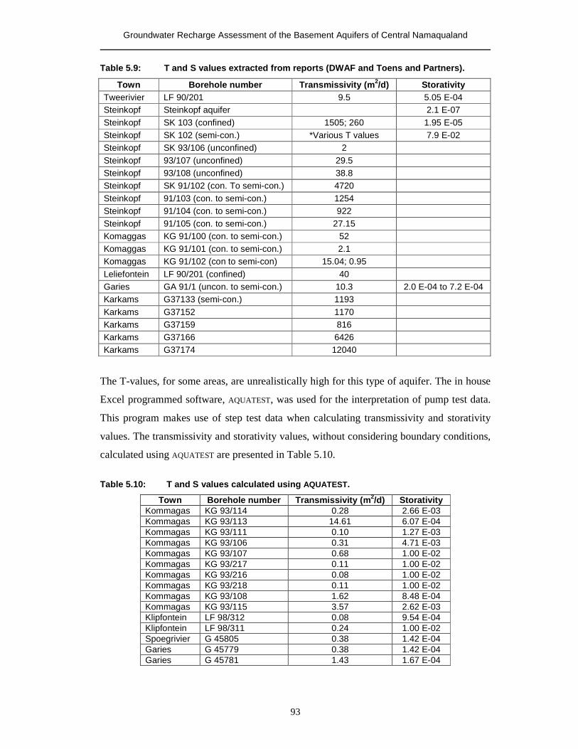
Groundwater Recharge Assessment of the Basement Aquifers of Central Namaqualand
93
Table 5.9: T and S values extracted from reports (DWAF and Toens and Partners).
Town Borehole number Transmissivity (m2/d) Storativity Tweerivier LF 90/201 9.5 5.05 E-04 Steinkopf Steinkopf aquifer 2.1 E-07
Steinkopf SK 103 (confined) 1505; 260 1.95 E-05 Steinkopf SK 102 (semi-con.) *Various T values 7.9 E-02 Steinkopf SK 93/106 (unconfined) 2 Steinkopf 93/107 (unconfined) 29.5 Steinkopf 93/108 (unconfined) 38.8 Steinkopf SK 91/102 (con. To semi-con.) 4720 Steinkopf 91/103 (con. to semi-con.) 1254 Steinkopf 91/104 (con. to semi-con.) 922 Steinkopf 91/105 (con. to semi-con.) 27.15 Komaggas KG 91/100 (con. to semi-con.) 52 Komaggas KG 91/101 (con. to semi-con.) 2.1 Komaggas KG 91/102 (con to semi-con) 15.04; 0.95 Leliefontein LF 90/201 (confined) 40 Garies GA 91/1 (uncon. to semi-con.) 10.3 2.0 E-04 to 7.2 E-04 Karkams G37133 (semi-con.) 1193 Karkams G37152 1170 Karkams G37159 816 Karkams G37166 6426 Karkams G37174 12040
The T-values, for some areas, are unrealistically high for this type of aquifer. The in house
Excel programmed software, AQUATEST, was used for the interpretation of pump test data.
This program makes use of step test data when calculating transmissivity and storativity
values. The transmissivity and storativity values, without considering boundary conditions,
calculated using AQUATEST are presented in Table 5.10.
Table 5.10: T and S values calculated using AQUATEST.
Town Borehole number Transmissivity (m2/d) Storativity Kommagas KG 93/114 0.28 2.66 E-03 Kommagas KG 93/113 14.61 6.07 E-04 Kommagas KG 93/111 0.10 1.27 E-03 Kommagas KG 93/106 0.31 4.71 E-03 Kommagas KG 93/107 0.68 1.00 E-02 Kommagas KG 93/217 0.11 1.00 E-02 Kommagas KG 93/216 0.08 1.00 E-02 Kommagas KG 93/218 0.11 1.00 E-02 Kommagas KG 93/108 1.62 8.48 E-04 Kommagas KG 93/115 3.57 2.62 E-03 Klipfontein LF 98/312 0.08 9.54 E-04 Klipfontein LF 98/311 0.24 1.00 E-02 Spoegrivier G 45805 0.38 1.42 E-04 Garies G 45779 0.38 1.42 E-04 Garies G 45781 1.43 1.67 E-04
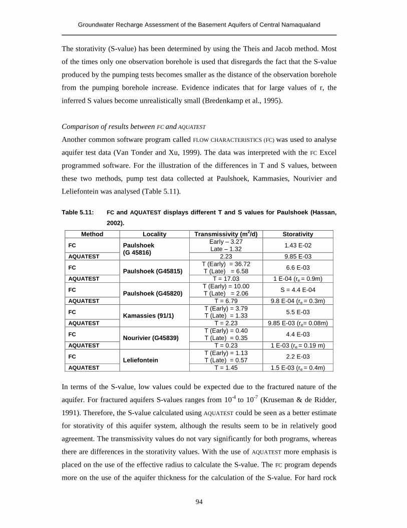
Groundwater Recharge Assessment of the Basement Aquifers of Central Namaqualand
94
The storativity (S-value) has been determined by using the Theis and Jacob method. Most
of the times only one observation borehole is used that disregards the fact that the S-value
produced by the pumping tests becomes smaller as the distance of the observation borehole
from the pumping borehole increase. Evidence indicates that for large values of r, the
inferred S values become unrealistically small (Bredenkamp et al., 1995).
Comparison of results between FC and AQUATEST
Another common software program called FLOW CHARACTERISTICS (FC) was used to analyse
aquifer test data (Van Tonder and Xu, 1999). The data was interpreted with the FC Excel
programmed software. For the illustration of the differences in T and S values, between
these two methods, pump test data collected at Paulshoek, Kammasies, Nourivier and
Leliefontein was analysed (Table 5.11).
Table 5.11: FC and AQUATEST displays different T and S values for Paulshoek (Hassan,
2002).
Method Locality Transmissivity (m2/d) Storativity
FC Early – 3.27 Late – 1.32 1.43 E-02
AQUATEST
Paulshoek (G 45816)
2.23 9.85 E-03
FC T (Early) = 36.72 T (Late) = 6.58 6.6 E-03
AQUATEST Paulshoek (G45815)
T = 17.03 1 E-04 (re = 0.9m)
FC T (Early) = 10.00 T (Late) = 2.06 S = 4.4 E-04
AQUATEST Paulshoek (G45820)
T = 6.79 9.8 E-04 (re = 0.3m)
FC T (Early) = 3.79 T (Late) = 1.33 5.5 E-03
AQUATEST Kamassies (91/1)
T = 2.23 9.85 E-03 (re= 0.08m)
FC T (Early) = 0.40 T (Late) = 0.35 4.4 E-03
AQUATEST Nourivier (G45839)
T = 0.23 1 E-03 (re = 0.19 m)
FC T (Early) = 1.13 T (Late) = 0.57 2.2 E-03
AQUATEST Leliefontein
T = 1.45 1.5 E-03 (re = 0.4m)
In terms of the S-value, low values could be expected due to the fractured nature of the
aquifer. For fractured aquifers S-values ranges from 10-4 to 10-7 (Kruseman & de Ridder,
1991). Therefore, the S-value calculated using AQUATEST could be seen as a better estimate
for storativity of this aquifer system, although the results seem to be in relatively good
agreement. The transmissivity values do not vary significantly for both programs, whereas
there are differences in the storativity values. With the use of AQUATEST more emphasis is
placed on the use of the effective radius to calculate the S-value. The FC program depends
more on the use of the aquifer thickness for the calculation of the S-value. For hard rock

Groundwater Recharge Assessment of the Basement Aquifers of Central Namaqualand
95
aquifers a value of < 40m is recommended by this program (Hassan, 2002). Storativity
values seem to be on the high end of the ranges for hard rock terrains. It is postulated that
the S values will be smaller if integrated over a larger area.
Groundwater Recharge Assessment of the Basement Aquifers of Central Namaqualand
96
CHAPTER 6
Groundwater recharge assessment
6.1 Introduction
Quantitative and qualitative information on aquifer recharge rates and storage are needed
to manage the groundwater resources of the Namaqualand region. General information on
recharge rates and aquifer storage are lacking for the area. This systematic approach to
assess groundwater recharge is the first for the area. The results contained in this chapter
are a foundation on which future work can be based. The assessment of recharge rates for
such a large area requires evaluation on a regional scale, often using local scale data.
The chloride mass balance (CMB) method is used to estimate recharge on a local and
regional scale using the saturated zone approach. The stable isotopes oxygen-18 and
deuterium as well as the radiogenic isotope 14C are used together with factor analysis and
the GIS assessment method to delineate and constrain recharge areas and processes. The
saturated volume fluctuation (SVF) method is used to estimate storage coefficients and
recharge. The cumulative rainfall departures (CRD) method is used to estimate the
recharge rates to the aquifers. A numerical model was developed, as a case study, of the
Buffels River alluvial aquifer. The sites described in this chapter are shown in Figure 6.1.
6.2 Chemical and isotope tracer methods
6.2.1 Chloride mass balance
The method is attractive to obtain a first estimate of total recharge. This section will
highlight the use of the CMB method to characterise and estimate groundwater recharge
both on a local and regional scale by using the chloride concentration in rainfall and
comparing it to that of the groundwater chloride concentrations.
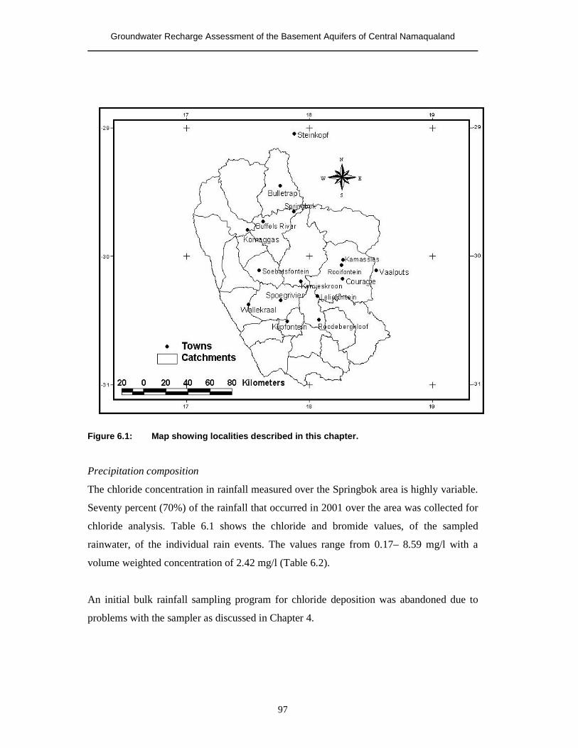
Groundwater Recharge Assessment of the Basement Aquifers of Central Namaqualand
97
Figure 6.1: Map showing localities described in this chapter.
Precipitation composition
The chloride concentration in rainfall measured over the Springbok area is highly variable.
Seventy percent (70%) of the rainfall that occurred in 2001 over the area was collected for
chloride analysis. Table 6.1 shows the chloride and bromide values, of the sampled
rainwater, of the individual rain events. The values range from 0.17– 8.59 mg/l with a
volume weighted concentration of 2.42 mg/l (Table 6.2).
An initial bulk rainfall sampling program for chloride deposition was abandoned due to
problems with the sampler as discussed in Chapter 4.
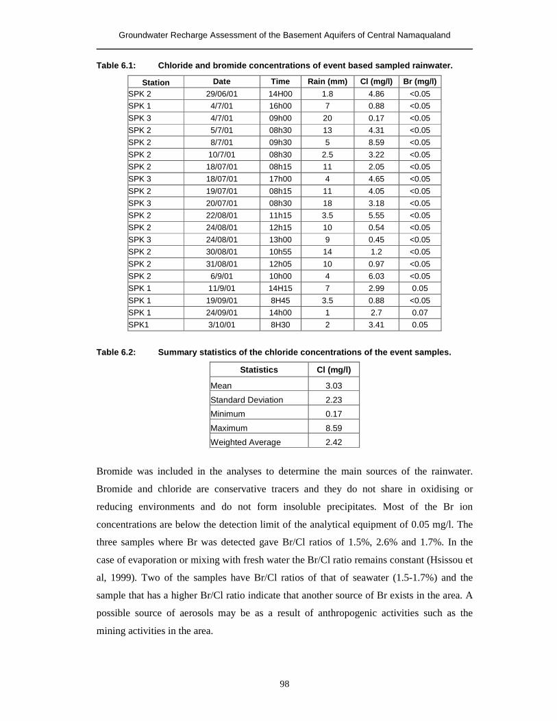
Groundwater Recharge Assessment of the Basement Aquifers of Central Namaqualand
98
Table 6.1: Chloride and bromide concentrations of event based sampled rainwater.
Station Date Time Rain (mm) Cl (mg/l) Br (mg/l) SPK 2 29/06/01 14H00 1.8 4.86 <0.05 SPK 1 4/7/01 16h00 7 0.88 <0.05 SPK 3 4/7/01 09h00 20 0.17 <0.05 SPK 2 5/7/01 08h30 13 4.31 <0.05 SPK 2 8/7/01 09h30 5 8.59 <0.05 SPK 2 10/7/01 08h30 2.5 3.22 <0.05 SPK 2 18/07/01 08h15 11 2.05 <0.05 SPK 3 18/07/01 17h00 4 4.65 <0.05 SPK 2 19/07/01 08h15 11 4.05 <0.05 SPK 3 20/07/01 08h30 18 3.18 <0.05 SPK 2 22/08/01 11h15 3.5 5.55 <0.05 SPK 2 24/08/01 12h15 10 0.54 <0.05 SPK 3 24/08/01 13h00 9 0.45 <0.05 SPK 2 30/08/01 10h55 14 1.2 <0.05 SPK 2 31/08/01 12h05 10 0.97 <0.05 SPK 2 6/9/01 10h00 4 6.03 <0.05 SPK 1 11/9/01 14H15 7 2.99 0.05 SPK 1 19/09/01 8H45 3.5 0.88 <0.05 SPK 1 24/09/01 14h00 1 2.7 0.07 SPK1 3/10/01 8H30 2 3.41 0.05
Table 6.2: Summary statistics of the chloride concentrations of the event samples.
Statistics Cl (mg/l)
Mean 3.03
Standard Deviation 2.23
Minimum 0.17
Maximum 8.59
Weighted Average 2.42
Bromide was included in the analyses to determine the main sources of the rainwater.
Bromide and chloride are conservative tracers and they do not share in oxidising or
reducing environments and do not form insoluble precipitates. Most of the Br ion
concentrations are below the detection limit of the analytical equipment of 0.05 mg/l. The
three samples where Br was detected gave Br/Cl ratios of 1.5%, 2.6% and 1.7%. In the
case of evaporation or mixing with fresh water the Br/Cl ratio remains constant (Hsissou et
al, 1999). Two of the samples have Br/Cl ratios of that of seawater (1.5-1.7%) and the
sample that has a higher Br/Cl ratio indicate that another source of Br exists in the area. A
possible source of aerosols may be as a result of anthropogenic activities such as the
mining activities in the area.
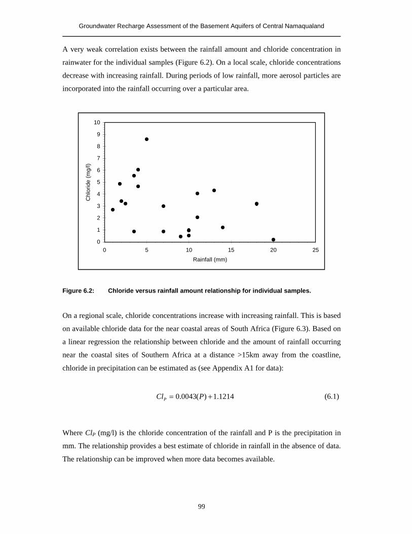
Groundwater Recharge Assessment of the Basement Aquifers of Central Namaqualand
99
A very weak correlation exists between the rainfall amount and chloride concentration in
rainwater for the individual samples (Figure 6.2). On a local scale, chloride concentrations
decrease with increasing rainfall. During periods of low rainfall, more aerosol particles are
incorporated into the rainfall occurring over a particular area.
0
1
2
3
4
5
6
7
8
9
10
0 5 10 15 20 25
Rainfall (mm)
Chl
orid
e (m
g/l)
Figure 6.2: Chloride versus rainfall amount relationship for individual samples.
On a regional scale, chloride concentrations increase with increasing rainfall. This is based
on available chloride data for the near coastal areas of South Africa (Figure 6.3). Based on
a linear regression the relationship between chloride and the amount of rainfall occurring
near the coastal sites of Southern Africa at a distance >15km away from the coastline,
chloride in precipitation can be estimated as (see Appendix A1 for data):
1214.1)(0043.0 += PClP (6.1)
Where ClP (mg/l) is the chloride concentration of the rainfall and P is the precipitation in
mm. The relationship provides a best estimate of chloride in rainfall in the absence of data.
The relationship can be improved when more data becomes available.
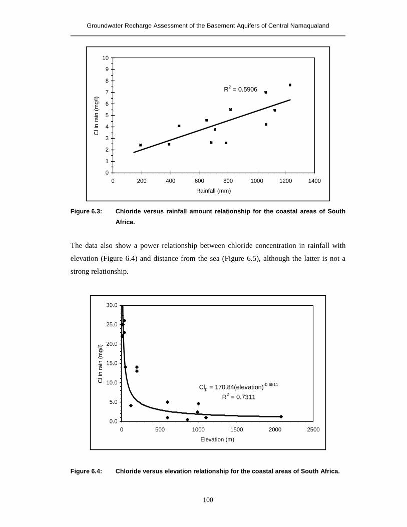
Groundwater Recharge Assessment of the Basement Aquifers of Central Namaqualand
100
R2 = 0.5906
0
1
2
3
4
5
6
7
8
9
10
0 200 400 600 800 1000 1200 1400
Rainfall (mm)
Cl i
n ra
in (m
g/l)
Figure 6.3: Chloride versus rainfall amount relationship for the coastal areas of South
Africa.
The data also show a power relationship between chloride concentration in rainfall with
elevation (Figure 6.4) and distance from the sea (Figure 6.5), although the latter is not a
strong relationship.
Clp = 170.84(elevation)-0.6511
R2 = 0.7311
0.0
5.0
10.0
15.0
20.0
25.0
30.0
0 500 1000 1500 2000 2500
Elevation (m)
Cl i
n ra
in (m
g/l)
Figure 6.4: Chloride versus elevation relationship for the coastal areas of South Africa.
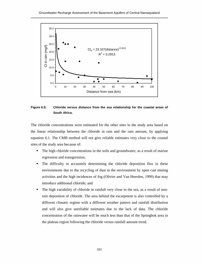
Groundwater Recharge Assessment of the Basement Aquifers of Central Namaqualand
101
Clp = 23.107(distance)-0.4615
R2 = 0.2913
0.0
5.0
10.0
15.0
20.0
25.0
30.0
35.0
0 10 20 30 40 50 60 70 80 90 100
Distance from sea (km)
Cl i
n ra
in (m
g/l)
Figure 6.5: Chloride versus distance from the sea relationship for the coastal areas of
South Africa.
The chloride concentrations were estimated for the other sites in the study area based on
the linear relationship between the chloride in rain and the rain amount, by applying
equation 6.1. The CMB method will not give reliable estimates very close to the coastal
sites of the study area because of:
� The high chloride concentrations in the soils and groundwater, as a result of marine
regression and transgression;
� The difficulty in accurately determining the chloride deposition flux in these
environments due to the recycling of dust in the environment by open cast mining
activities and the high incidences of fog (Olivier and Van Heerden, 1999) that may
introduce additional chloride; and
� The high variability of chloride in rainfall very close to the sea, as a result of non-
rain deposition of chloride. The area behind the escarpment is also controlled by a
different climatic regime with a different weather pattern and rainfall distribution
and will also give unreliable estimates due to the lack of data. The chloride
concentration of the rainwater will be much less than that of the Springbok area in
the plateau region following the chloride versus rainfall amount trend.
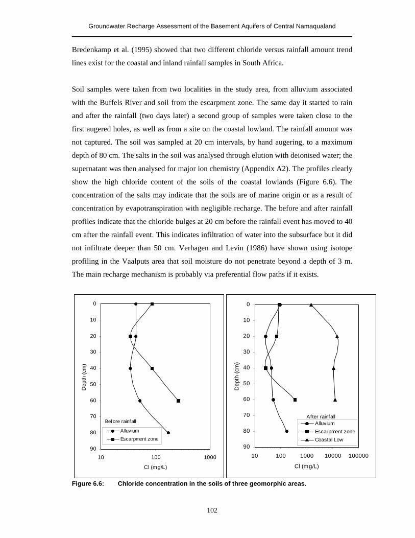
Groundwater Recharge Assessment of the Basement Aquifers of Central Namaqualand
102
Bredenkamp et al. (1995) showed that two different chloride versus rainfall amount trend
lines exist for the coastal and inland rainfall samples in South Africa.
Soil samples were taken from two localities in the study area, from alluvium associated
with the Buffels River and soil from the escarpment zone. The same day it started to rain
and after the rainfall (two days later) a second group of samples were taken close to the
first augered holes, as well as from a site on the coastal lowland. The rainfall amount was
not captured. The soil was sampled at 20 cm intervals, by hand augering, to a maximum
depth of 80 cm. The salts in the soil was analysed through elution with deionised water; the
supernatant was then analysed for major ion chemistry (Appendix A2). The profiles clearly
show the high chloride content of the soils of the coastal lowlands (Figure 6.6). The
concentration of the salts may indicate that the soils are of marine origin or as a result of
concentration by evapotranspiration with negligible recharge. The before and after rainfall
profiles indicate that the chloride bulges at 20 cm before the rainfall event has moved to 40
cm after the rainfall event. This indicates infiltration of water into the subsurface but it did
not infiltrate deeper than 50 cm. Verhagen and Levin (1986) have shown using isotope
profiling in the Vaalputs area that soil moisture do not penetrate beyond a depth of 3 m.
The main recharge mechanism is probably via preferential flow paths if it exists.
Figure 6.6: Chloride concentration in the soils of three geomorphic areas.
0
10
20
30
40
50
60
70
80
90
10 100 1000 10000 100000
Cl (mg/L)
Dep
th (c
m)
AlluviumEscarpment zoneCoastal Low
After rainfall
0
10
20
30
40
50
60
70
80
90
10 100 1000
Cl (mg/L)
Dep
th (c
m)
Alluvium
Escarpment zone
Before rainfall
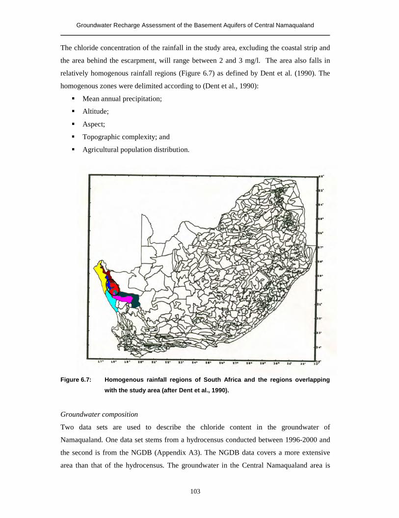
Groundwater Recharge Assessment of the Basement Aquifers of Central Namaqualand
103
The chloride concentration of the rainfall in the study area, excluding the coastal strip and
the area behind the escarpment, will range between 2 and 3 mg/l. The area also falls in
relatively homogenous rainfall regions (Figure 6.7) as defined by Dent et al. (1990). The
homogenous zones were delimited according to (Dent et al., 1990):
� Mean annual precipitation;
� Altitude;
� Aspect;
� Topographic complexity; and
� Agricultural population distribution.
Figure 6.7: Homogenous rainfall regions of South Africa and the regions overlapping
with the study area (after Dent et al., 1990).
Groundwater composition
Two data sets are used to describe the chloride content in the groundwater of
Namaqualand. One data set stems from a hydrocensus conducted between 1996-2000 and
the second is from the NGDB (Appendix A3). The NGDB data covers a more extensive
area than that of the hydrocensus. The groundwater in the Central Namaqualand area is
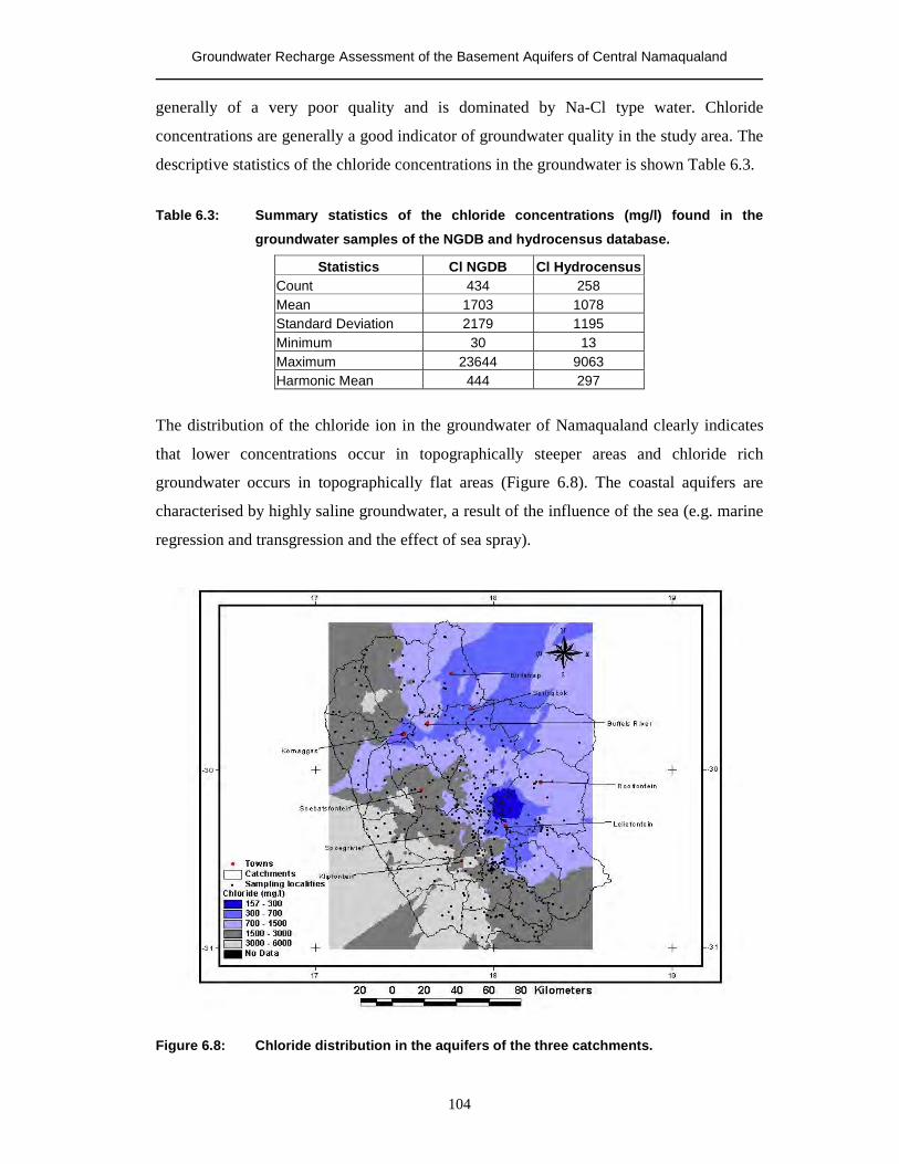
Groundwater Recharge Assessment of the Basement Aquifers of Central Namaqualand
104
generally of a very poor quality and is dominated by Na-Cl type water. Chloride
concentrations are generally a good indicator of groundwater quality in the study area. The
descriptive statistics of the chloride concentrations in the groundwater is shown Table 6.3.
Table 6.3: Summary statistics of the chloride concentrations (mg/l) found in the
groundwater samples of the NGDB and hydrocensus database.
Statistics Cl NGDB Cl Hydrocensus Count 434 258 Mean 1703 1078 Standard Deviation 2179 1195 Minimum 30 13 Maximum 23644 9063 Harmonic Mean 444 297
The distribution of the chloride ion in the groundwater of Namaqualand clearly indicates
that lower concentrations occur in topographically steeper areas and chloride rich
groundwater occurs in topographically flat areas (Figure 6.8). The coastal aquifers are
characterised by highly saline groundwater, a result of the influence of the sea (e.g. marine
regression and transgression and the effect of sea spray).
Figure 6.8: Chloride distribution in the aquifers of the three catchments.
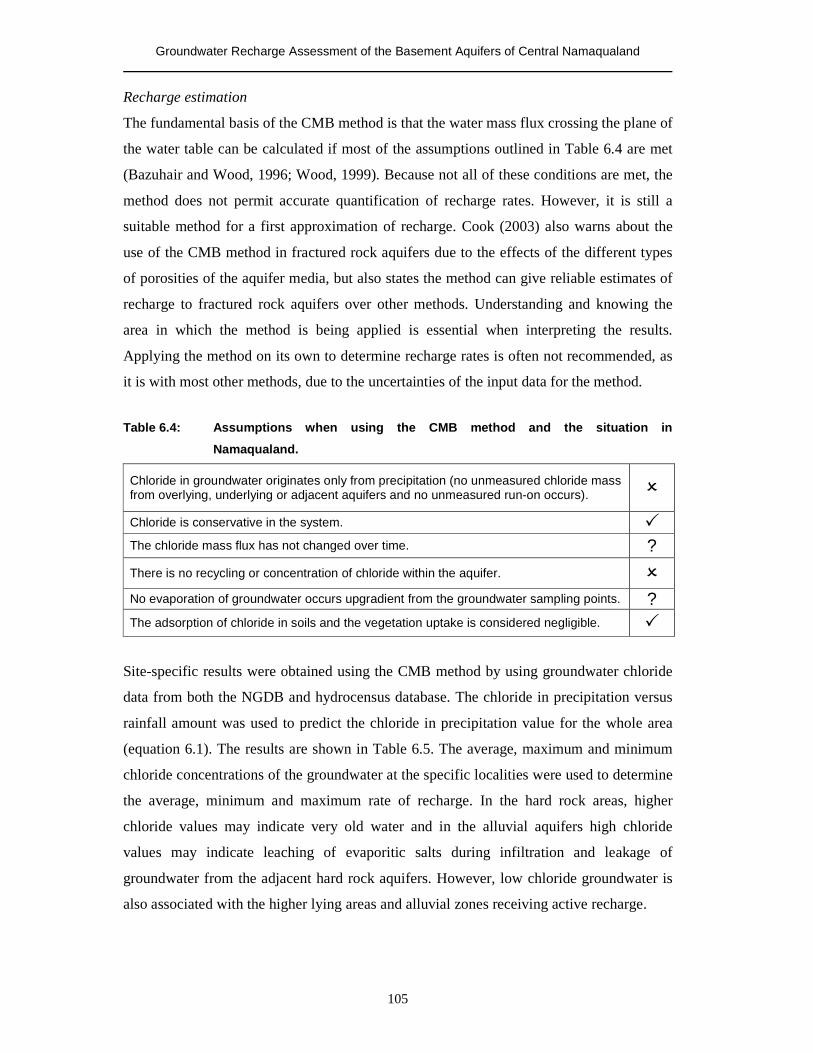
Groundwater Recharge Assessment of the Basement Aquifers of Central Namaqualand
105
Recharge estimation
The fundamental basis of the CMB method is that the water mass flux crossing the plane of
the water table can be calculated if most of the assumptions outlined in Table 6.4 are met
(Bazuhair and Wood, 1996; Wood, 1999). Because not all of these conditions are met, the
method does not permit accurate quantification of recharge rates. However, it is still a
suitable method for a first approximation of recharge. Cook (2003) also warns about the
use of the CMB method in fractured rock aquifers due to the effects of the different types
of porosities of the aquifer media, but also states the method can give reliable estimates of
recharge to fractured rock aquifers over other methods. Understanding and knowing the
area in which the method is being applied is essential when interpreting the results.
Applying the method on its own to determine recharge rates is often not recommended, as
it is with most other methods, due to the uncertainties of the input data for the method.
Table 6.4: Assumptions when using the CMB method and the situation in
Namaqualand.
Chloride in groundwater originates only from precipitation (no unmeasured chloride mass from overlying, underlying or adjacent aquifers and no unmeasured run-on occurs). �
Chloride is conservative in the system. � The chloride mass flux has not changed over time. ? There is no recycling or concentration of chloride within the aquifer. � No evaporation of groundwater occurs upgradient from the groundwater sampling points. ? The adsorption of chloride in soils and the vegetation uptake is considered negligible. �
Site-specific results were obtained using the CMB method by using groundwater chloride
data from both the NGDB and hydrocensus database. The chloride in precipitation versus
rainfall amount was used to predict the chloride in precipitation value for the whole area
(equation 6.1). The results are shown in Table 6.5. The average, maximum and minimum
chloride concentrations of the groundwater at the specific localities were used to determine
the average, minimum and maximum rate of recharge. In the hard rock areas, higher
chloride values may indicate very old water and in the alluvial aquifers high chloride
values may indicate leaching of evaporitic salts during infiltration and leakage of
groundwater from the adjacent hard rock aquifers. However, low chloride groundwater is
also associated with the higher lying areas and alluvial zones receiving active recharge.
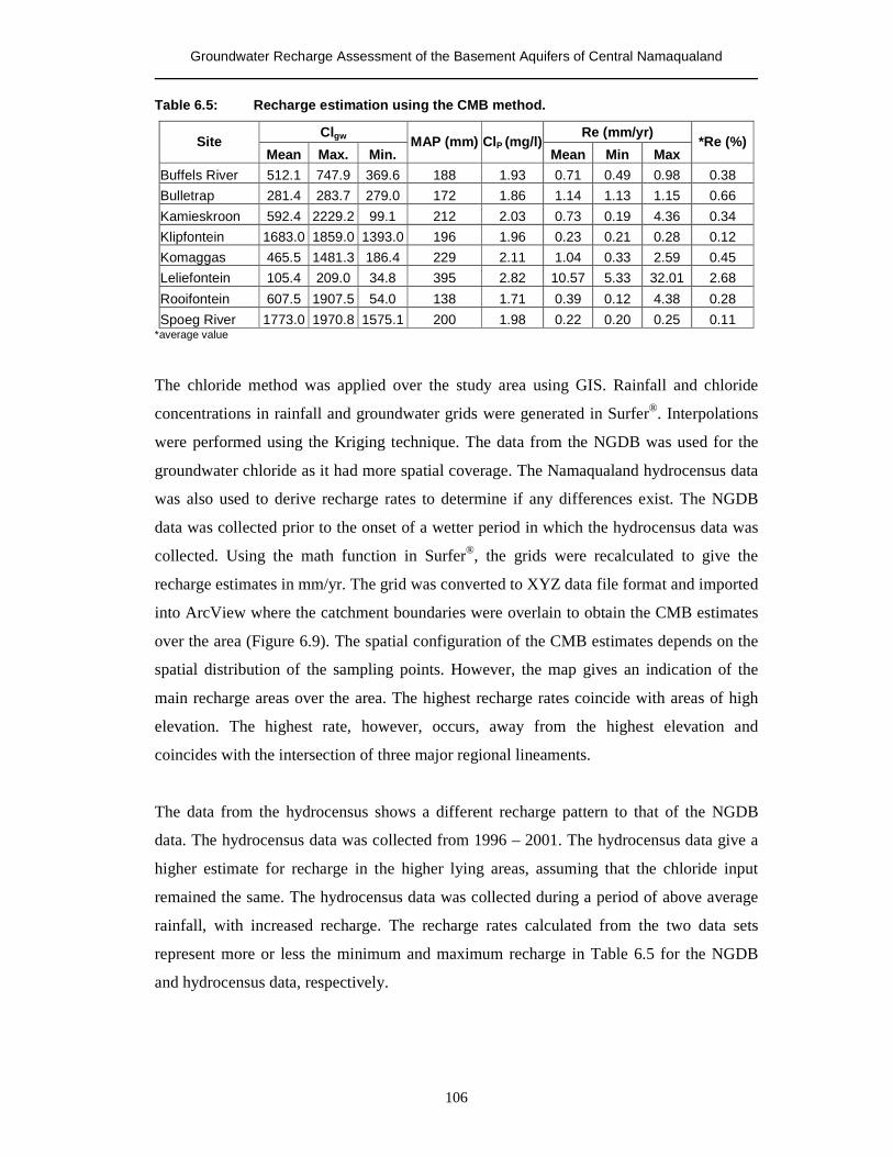
Groundwater Recharge Assessment of the Basement Aquifers of Central Namaqualand
106
Table 6.5: Recharge estimation using the CMB method.
Clgw Re (mm/yr) Site
Mean Max. Min. MAP (mm) ClP (mg/l)
Mean Min Max *Re (%)
Buffels River 512.1 747.9 369.6 188 1.93 0.71 0.49 0.98 0.38 Bulletrap 281.4 283.7 279.0 172 1.86 1.14 1.13 1.15 0.66 Kamieskroon 592.4 2229.2 99.1 212 2.03 0.73 0.19 4.36 0.34 Klipfontein 1683.0 1859.0 1393.0 196 1.96 0.23 0.21 0.28 0.12 Komaggas 465.5 1481.3 186.4 229 2.11 1.04 0.33 2.59 0.45 Leliefontein 105.4 209.0 34.8 395 2.82 10.57 5.33 32.01 2.68 Rooifontein 607.5 1907.5 54.0 138 1.71 0.39 0.12 4.38 0.28 Spoeg River 1773.0 1970.8 1575.1 200 1.98 0.22 0.20 0.25 0.11
*average value
The chloride method was applied over the study area using GIS. Rainfall and chloride
concentrations in rainfall and groundwater grids were generated in Surfer®. Interpolations
were performed using the Kriging technique. The data from the NGDB was used for the
groundwater chloride as it had more spatial coverage. The Namaqualand hydrocensus data
was also used to derive recharge rates to determine if any differences exist. The NGDB
data was collected prior to the onset of a wetter period in which the hydrocensus data was
collected. Using the math function in Surfer®, the grids were recalculated to give the
recharge estimates in mm/yr. The grid was converted to XYZ data file format and imported
into ArcView where the catchment boundaries were overlain to obtain the CMB estimates
over the area (Figure 6.9). The spatial configuration of the CMB estimates depends on the
spatial distribution of the sampling points. However, the map gives an indication of the
main recharge areas over the area. The highest recharge rates coincide with areas of high
elevation. The highest rate, however, occurs, away from the highest elevation and
coincides with the intersection of three major regional lineaments.
The data from the hydrocensus shows a different recharge pattern to that of the NGDB
data. The hydrocensus data was collected from 1996 – 2001. The hydrocensus data give a
higher estimate for recharge in the higher lying areas, assuming that the chloride input
remained the same. The hydrocensus data was collected during a period of above average
rainfall, with increased recharge. The recharge rates calculated from the two data sets
represent more or less the minimum and maximum recharge in Table 6.5 for the NGDB
and hydrocensus data, respectively.
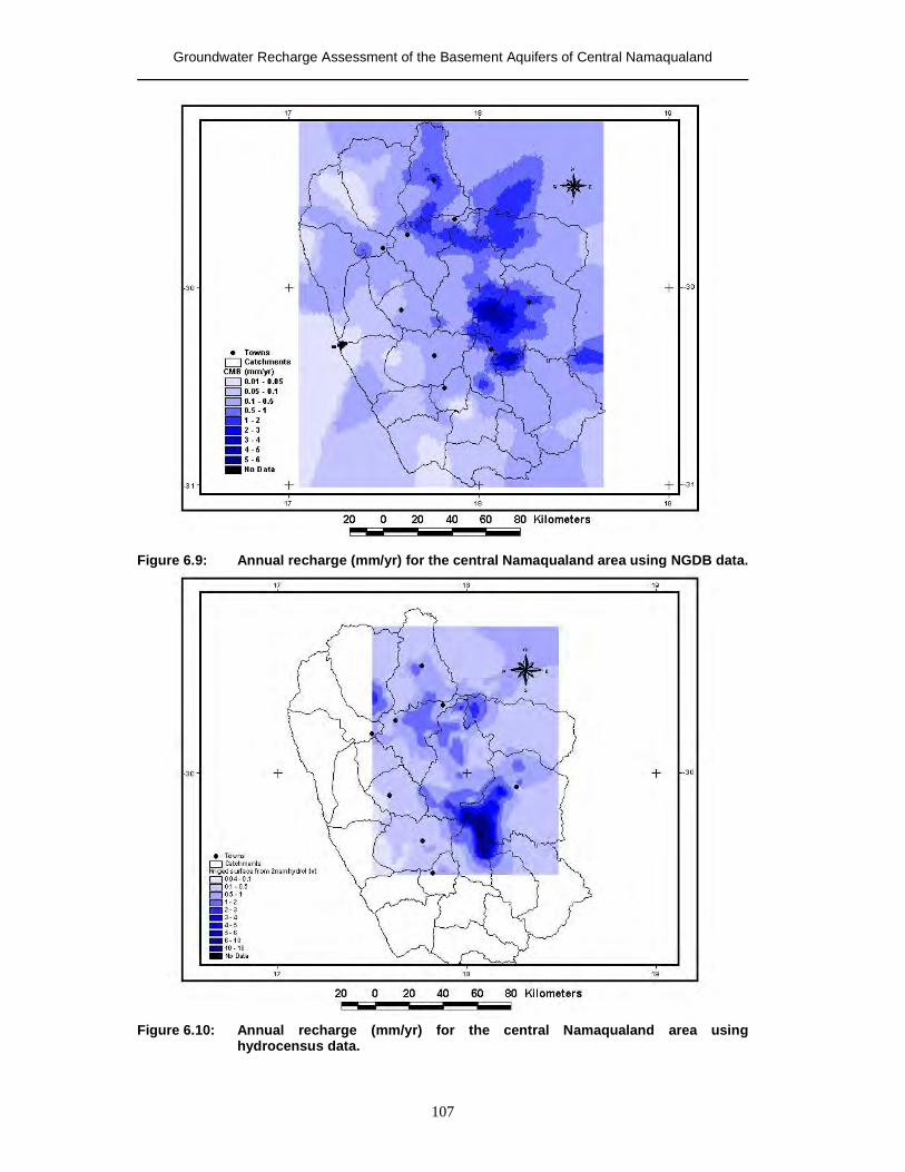
Groundwater Recharge Assessment of the Basement Aquifers of Central Namaqualand
107
Figure 6.9: Annual recharge (mm/yr) for the central Namaqualand area using NGDB data.
Figure 6.10: Annual recharge (mm/yr) for the central Namaqualand area using
hydrocensus data.
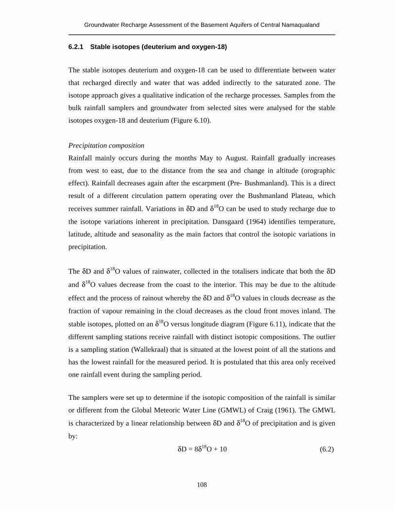
Groundwater Recharge Assessment of the Basement Aquifers of Central Namaqualand
108
6.2.1 Stable isotopes (deuterium and oxygen-18)
The stable isotopes deuterium and oxygen-18 can be used to differentiate between water
that recharged directly and water that was added indirectly to the saturated zone. The
isotope approach gives a qualitative indication of the recharge processes. Samples from the
bulk rainfall samplers and groundwater from selected sites were analysed for the stable
isotopes oxygen-18 and deuterium (Figure 6.10).
Precipitation composition
Rainfall mainly occurs during the months May to August. Rainfall gradually increases
from west to east, due to the distance from the sea and change in altitude (orographic
effect). Rainfall decreases again after the escarpment (Pre- Bushmanland). This is a direct
result of a different circulation pattern operating over the Bushmanland Plateau, which
receives summer rainfall. Variations in δD and δ18O can be used to study recharge due to
the isotope variations inherent in precipitation. Dansgaard (1964) identifies temperature,
latitude, altitude and seasonality as the main factors that control the isotopic variations in
precipitation.
The δD and δ18O values of rainwater, collected in the totalisers indicate that both the δD
and δ18O values decrease from the coast to the interior. This may be due to the altitude
effect and the process of rainout whereby the δD and δ18O values in clouds decrease as the
fraction of vapour remaining in the cloud decreases as the cloud front moves inland. The
stable isotopes, plotted on an δ18O versus longitude diagram (Figure 6.11), indicate that the
different sampling stations receive rainfall with distinct isotopic compositions. The outlier
is a sampling station (Wallekraal) that is situated at the lowest point of all the stations and
has the lowest rainfall for the measured period. It is postulated that this area only received
one rainfall event during the sampling period.
The samplers were set up to determine if the isotopic composition of the rainfall is similar
or different from the Global Meteoric Water Line (GMWL) of Craig (1961). The GMWL
is characterized by a linear relationship between δD and δ18O of precipitation and is given
by:
δD = 8δ18O + 10 (6.2)
Groundwater Recharge Assessment of the Basement Aquifers of Central Namaqualand
109
This relationship is based on precipitation data from different locations around the world.
Individual locations have lines of best fit with slightly different equations to the GMWL,
which are termed local meteoric water lines (LMWL). The Local Meteoric Water Line for
the study area was determined by using data from the bulk rainfall samplers (Figure 6.12).
The data is shown in Table 6.6. The LMWL is defined by the following equation:
δD = 7δ18O + 8 (6.3)
The bulk rainfall samplers collected rainfall over a one-year period, the rainfall represents
the weighted average of the annual rainfall. It is assumed that minimal evaporation from
the bulk rainfall samplers occur due to the silicon oil layer. However, the amount of
evaporation from the bulk rainfall samplers with the silicon oil layer is directly related to
the depth of the floating silicon oil layer (Weaver and Talma, 2002). Ideally, rainfall
amounts from the bulk rainfall samplers should be compared with rainfall amounts from
another rainfall gauge at the same site. The weighted average annual δD and δ18O values of
precipitation would be expected to remain constant from year to year (Kendall et al, 1995).
It may be lesser in an area of sporadic rainfall such as Namaqualand. The LMWL of
Namaqualand is similar to the Western Cape LMWL of Diamond and Harris (1997). The
precipitation of the Western Cape is defined by a meteoric water line with the approximate
equation δD = 6.1δ18O + 8.6 (Diamond and Harris, 1997). Rain, for both areas, is derived
from the same Atlantic Ocean frontal system.
Evaporated water generally forms an array on a δD versus δ18O diagram, which has a
shallower gradient than the LMWL. The slope of this line depends on the humidity at the
place of evaporation (Gat, 1980). The lower the humidity, the less steep the gradient of the
“evaporation line”. The samples taken from large diameter wells were removed from the
data set because of the isotopic enrichment of the water within the wells, due to the high
humidity above the water in the large diameter wells.
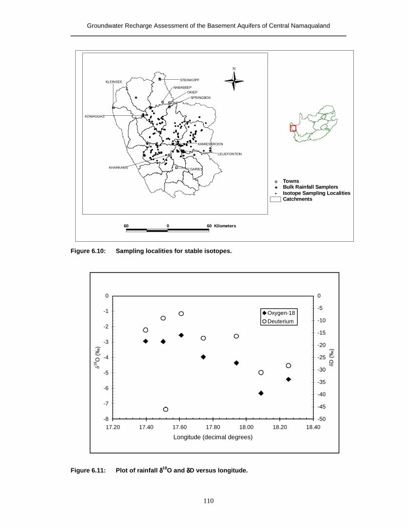
Groundwater Recharge Assessment of the Basement Aquifers of Central Namaqualand
110
Figure 6.10: Sampling localities for stable isotopes.
Figure 6.11: Plot of rainfall δδδδ18O and δδδδD versus longitude.
-8
-7
-6
-5
-4
-3
-2
-1
0
17.20 17.40 17.60 17.80 18.00 18.20 18.40
Longitude (decimal degrees)
�18
O (‰
)
-50
-45
-40
-35
-30
-25
-20
-15
-10
-5
0
�D
(‰)
Oxygen-18Deuterium
60 0 60 Kilometers
Catchments� Isotope Sampling Localities� Bulk Rainfall Samplers� Towns
N
�
�����
�
�
��
�
�
�
��
��
�
��
�
�
�
�
��
�
�
��
�
��
�
�
�
��
��
�
�
�
��
�
�
�
�
�
���
�
�
�
�
�
��
�
�
�
�
�
�
�
�
�
�
��
���
�
�
��
�
�
�
�
���
�
�
��
�
�
�
��
�
�
�
�
��
�
�
�
�
�
�
�
�
�
��
�
�
�
��
�
�
�
��
�
�
����
�
�
�
�
�
���
�
��
�
�
�
�
�
��
�
�
�
�
��
��
�
���
��
�����
��
���
�
�
�
���
�
�
�
�
�
�
�
�
�
��
�
�
�
�
�
�
�
�
�
�
$
NABABEEP
$
OKIEP
$
SPRINGBOK
$
KLEINSEE
$ GARIES
$ KAMIESKROON
# STEINKOPF
#KOMAGGAS
#
KHARKAMS
#
LELIEFONTEIN
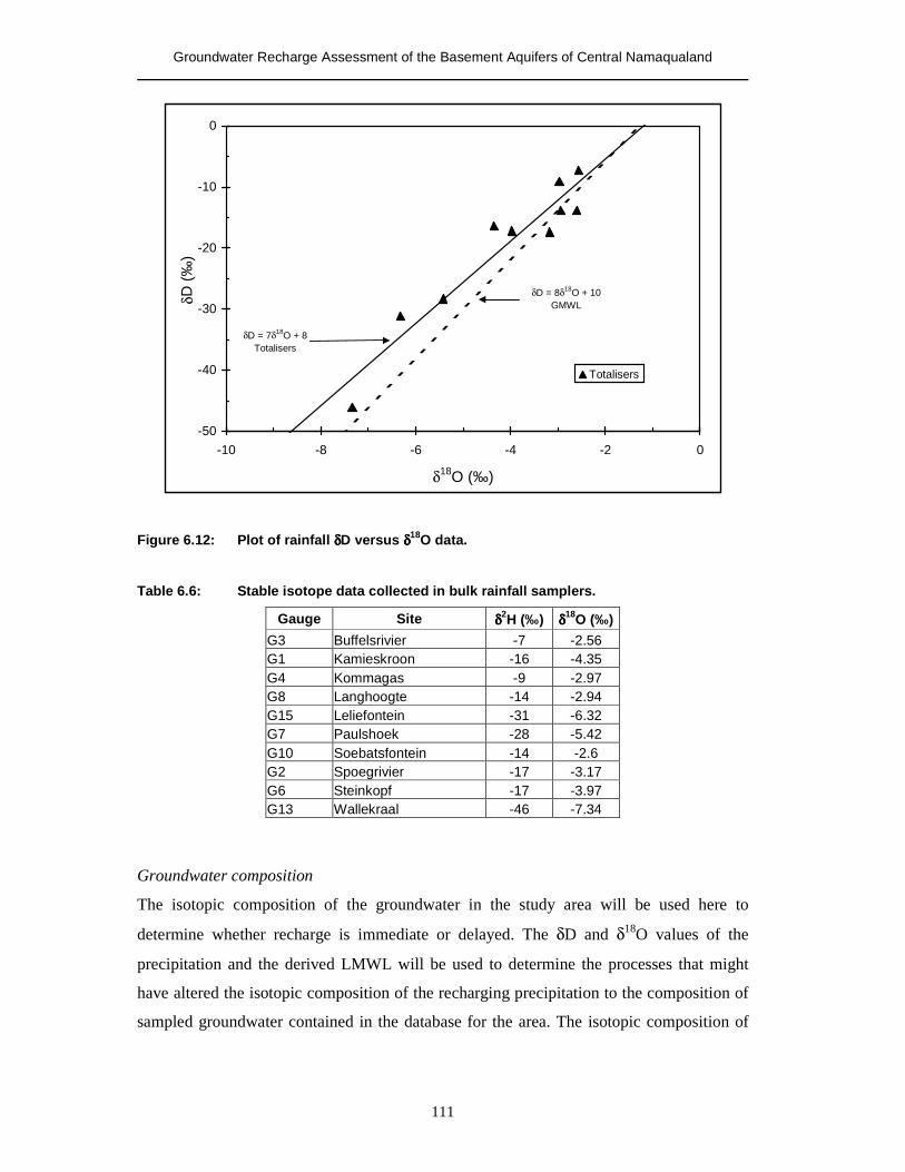
Groundwater Recharge Assessment of the Basement Aquifers of Central Namaqualand
111
δD = 8δ18O + 10GMWL
δD = 7δ18O + 8Totalisers
-50
-40
-30
-20
-10
0
-10 -8 -6 -4 -2 0
δ18O (‰)
δD (‰
)
Totalisers
Figure 6.12: Plot of rainfall δδδδD versus δδδδ18O data.
Table 6.6: Stable isotope data collected in bulk rainfall samplers.
Gauge Site δδδδ2H (‰) δδδδ18O (‰) G3 Buffelsrivier -7 -2.56 G1 Kamieskroon -16 -4.35 G4 Kommagas -9 -2.97 G8 Langhoogte -14 -2.94 G15 Leliefontein -31 -6.32 G7 Paulshoek -28 -5.42 G10 Soebatsfontein -14 -2.6 G2 Spoegrivier -17 -3.17 G6 Steinkopf -17 -3.97 G13 Wallekraal -46 -7.34
Groundwater composition
The isotopic composition of the groundwater in the study area will be used here to
determine whether recharge is immediate or delayed. The δD and δ18O values of the
precipitation and the derived LMWL will be used to determine the processes that might
have altered the isotopic composition of the recharging precipitation to the composition of
sampled groundwater contained in the database for the area. The isotopic composition of
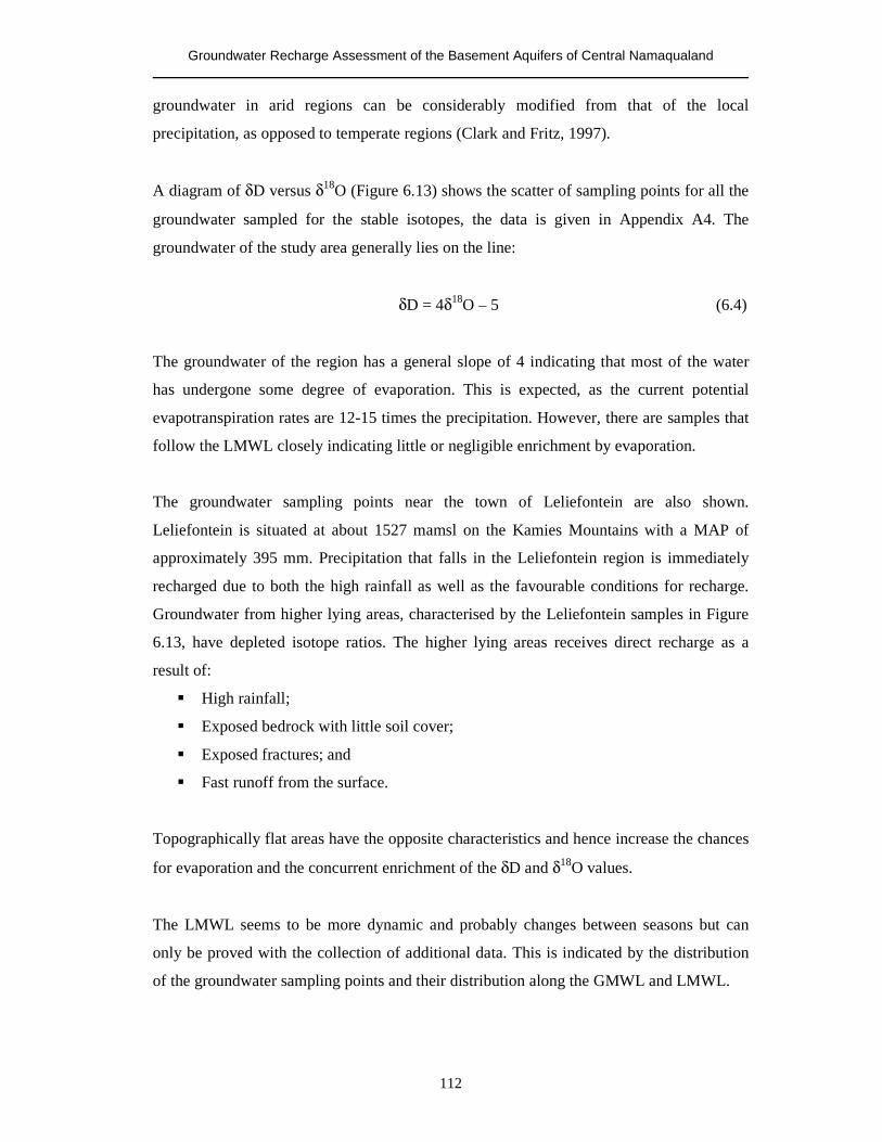
Groundwater Recharge Assessment of the Basement Aquifers of Central Namaqualand
112
groundwater in arid regions can be considerably modified from that of the local
precipitation, as opposed to temperate regions (Clark and Fritz, 1997).
A diagram of δD versus δ18O (Figure 6.13) shows the scatter of sampling points for all the
groundwater sampled for the stable isotopes, the data is given in Appendix A4. The
groundwater of the study area generally lies on the line:
δD = 4δ18O – 5 (6.4)
The groundwater of the region has a general slope of 4 indicating that most of the water
has undergone some degree of evaporation. This is expected, as the current potential
evapotranspiration rates are 12-15 times the precipitation. However, there are samples that
follow the LMWL closely indicating little or negligible enrichment by evaporation.
The groundwater sampling points near the town of Leliefontein are also shown.
Leliefontein is situated at about 1527 mamsl on the Kamies Mountains with a MAP of
approximately 395 mm. Precipitation that falls in the Leliefontein region is immediately
recharged due to both the high rainfall as well as the favourable conditions for recharge.
Groundwater from higher lying areas, characterised by the Leliefontein samples in Figure
6.13, have depleted isotope ratios. The higher lying areas receives direct recharge as a
result of:
� High rainfall;
� Exposed bedrock with little soil cover;
� Exposed fractures; and
� Fast runoff from the surface.
Topographically flat areas have the opposite characteristics and hence increase the chances
for evaporation and the concurrent enrichment of the δD and δ18O values.
The LMWL seems to be more dynamic and probably changes between seasons but can
only be proved with the collection of additional data. This is indicated by the distribution
of the groundwater sampling points and their distribution along the GMWL and LMWL.
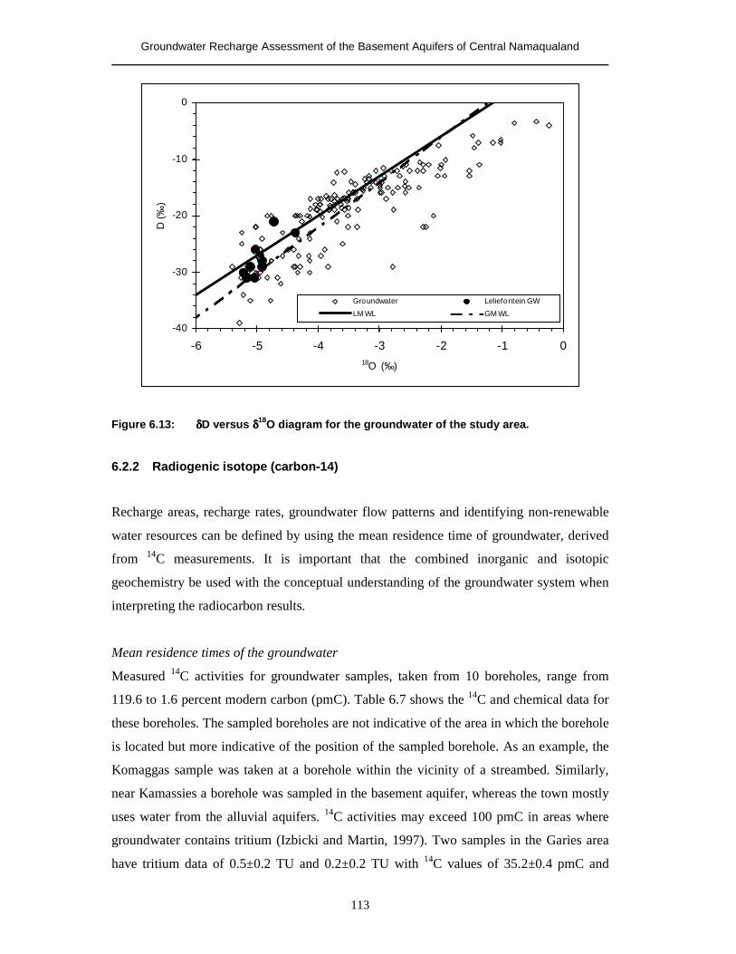
Groundwater Recharge Assessment of the Basement Aquifers of Central Namaqualand
113
-40
-30
-20
-10
0
-6 -5 -4 -3 -2 -1 018O (‰)
D (‰
)
Groundwater Leliefontein GW
LM WL GM WL
Figure 6.13: δδδδD versus δδδδ18O diagram for the groundwater of the study area.
6.2.2 Radiogenic isotope (carbon-14)
Recharge areas, recharge rates, groundwater flow patterns and identifying non-renewable
water resources can be defined by using the mean residence time of groundwater, derived
from 14C measurements. It is important that the combined inorganic and isotopic
geochemistry be used with the conceptual understanding of the groundwater system when
interpreting the radiocarbon results.
Mean residence times of the groundwater
Measured 14C activities for groundwater samples, taken from 10 boreholes, range from
119.6 to 1.6 percent modern carbon (pmC). Table 6.7 shows the 14C and chemical data for
these boreholes. The sampled boreholes are not indicative of the area in which the borehole
is located but more indicative of the position of the sampled borehole. As an example, the
Komaggas sample was taken at a borehole within the vicinity of a streambed. Similarly,
near Kamassies a borehole was sampled in the basement aquifer, whereas the town mostly
uses water from the alluvial aquifers. 14C activities may exceed 100 pmC in areas where
groundwater contains tritium (Izbicki and Martin, 1997). Two samples in the Garies area
have tritium data of 0.5±0.2 TU and 0.2±0.2 TU with 14C values of 35.2±0.4 pmC and
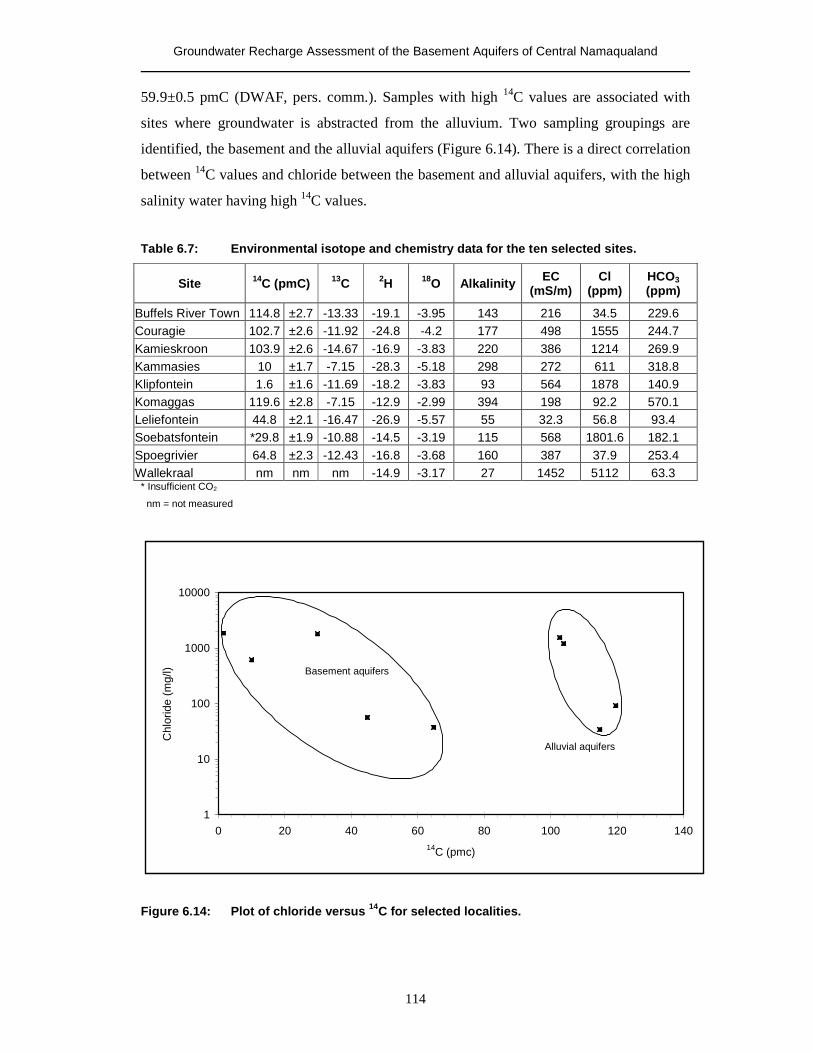
Groundwater Recharge Assessment of the Basement Aquifers of Central Namaqualand
114
59.9±0.5 pmC (DWAF, pers. comm.). Samples with high 14C values are associated with
sites where groundwater is abstracted from the alluvium. Two sampling groupings are
identified, the basement and the alluvial aquifers (Figure 6.14). There is a direct correlation
between 14C values and chloride between the basement and alluvial aquifers, with the high
salinity water having high 14C values.
Table 6.7: Environmental isotope and chemistry data for the ten selected sites.
Site 14C (pmC) 13C 2H 18O Alkalinity EC (mS/m)
Cl (ppm)
HCO3 (ppm)
Buffels River Town 114.8 ±2.7 -13.33 -19.1 -3.95 143 216 34.5 229.6 Couragie 102.7 ±2.6 -11.92 -24.8 -4.2 177 498 1555 244.7 Kamieskroon 103.9 ±2.6 -14.67 -16.9 -3.83 220 386 1214 269.9 Kammasies 10 ±1.7 -7.15 -28.3 -5.18 298 272 611 318.8 Klipfontein 1.6 ±1.6 -11.69 -18.2 -3.83 93 564 1878 140.9 Komaggas 119.6 ±2.8 -7.15 -12.9 -2.99 394 198 92.2 570.1 Leliefontein 44.8 ±2.1 -16.47 -26.9 -5.57 55 32.3 56.8 93.4 Soebatsfontein *29.8 ±1.9 -10.88 -14.5 -3.19 115 568 1801.6 182.1 Spoegrivier 64.8 ±2.3 -12.43 -16.8 -3.68 160 387 37.9 253.4 Wallekraal nm nm nm -14.9 -3.17 27 1452 5112 63.3
* Insufficient CO2
nm = not measured
Basement aquifers
1
10
100
1000
10000
0 20 40 60 80 100 120 14014C (pmc)
Chl
orid
e (m
g/l)
Alluvial aquifers
Figure 6.14: Plot of chloride versus 14C for selected localities.
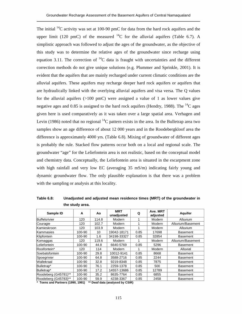
Groundwater Recharge Assessment of the Basement Aquifers of Central Namaqualand
115
The initial 14C activity was set at 100-90 pmC for data from the hard rock aquifers and the
upper limit (120 pmC) of the measured 14C for the alluvial aquifers (Table 6.7). A
simplistic approach was followed to adjust the ages of the groundwater, as the objective of
this study was to determine the relative ages of the groundwater since recharge using
equation 3.11. The correction of 14C data is fraught with uncertainties and the different
correction methods do not give unique solutions (e.g. Plummer and Sprinkle, 2001). It is
evident that the aquifers that are mainly recharged under current climatic conditions are the
alluvial aquifers. These aquifers may recharge deeper hard rock aquifers or aquifers that
are hydraulically linked with the overlying alluvial aquifers and visa versa. The Q values
for the alluvial aquifers (>100 pmC) were assigned a value of 1 as lower values give
negative ages and 0.85 is assigned to the hard rock aquifers (Hendry, 1988). The 14C ages
given here is used comparatively as it was taken over a large spatial area. Verhagen and
Levin (1986) noted that no regional 14C pattern exists in the area. In the Bulletrap area two
samples show an age difference of about 12 000 years and in the Roodebergkloof area the
difference is approximately 4000 yrs. (Table 6.8). Mixing of groundwater of different ages
is probably the rule. Stacked flow patterns occur both on a local and regional scale. The
groundwater “age” for the Leliefontein area is not realistic, based on the conceptual model
and chemistry data. Conceptually, the Leliefontein area is situated in the escarpment zone
with high rainfall and very low EC (averaging 35 mS/m) indicating fairly young and
dynamic groundwater flow. The only plausible explanation is that there was a problem
with the sampling or analysis at this locality.
Table 6.8: Unadjusted and adjusted mean residence times (MRT) of the groundwater in
the study area.
Sample ID A Ao MRT unadjusted Q Ave. MRT
adjusted Aquifer
Buffelsrivier 120 114.8 Modern 1 Modern Alluvium Couragie 120 102.7 Modern 1 Modern Alluvium/Basement Kamieskroon 120 103.9 Modern 1 Modern Alluvium Kammasies 100-90 10 19042-18171 0.85 17698 Basement Klipfontein 100-90 1.6 34198-33327 0.85 32854 Basement Komaggas 120 119.6 Modern 1 Modern Alluvium/Basement Leliefontein 100-90 44.8 6640-5769 0.85 5296 Basement Rooifontein* 120 114 Modern 1 Modern Alluvial Soebatsfontein 100-90 29.8 10012-9141 0.85 8668 Basement Spoegrivier 100-90 64.8 3588-2716 0.85 2244 Basement Wallekraal 100-90 32.8 9219-8348 0.85 7875 Basement Bulletrap* 100-90 76.1 2259-1378 0.85 500 Basement Bulletrap* 100-90 17.2 14557-13686 0.85 12789 Basement Roodeberg (G45781)** 100-90 35.2 8635-7764 0.85 6855 Basement Roodeberg (G45783)** 100-90 59.9 4238-3367 0.85 2458 Basement * Toens and Partners (1990, 1991) ** Dwaf data (analysed by CSIR)
Groundwater Recharge Assessment of the Basement Aquifers of Central Namaqualand
116
6.2.3 Summary
The chemical and isotopic data of the study area can be used to characterise and delineate
groundwater recharge. However, it is essential that the hydrogeology and aquifer
characteristics be well understood in order to make any meaningful interpretations.
The use of the CMB method in this study is used to essentially delineate areas where direct
recharge is occurring. Chloride concentrations in the saturated zone are a result of various
processes and a mixture of various groundwater flow lines. The CMB method overestimate
recharge due the fact that recharge in arid and semi-arid areas are event driven, with above
average rainfall only occurring episodically. The rainwater chloride will be lower than that
of the annual or wet season chloride input. Sami and Hughes (1996) came to the same
conclusion for rainfall occurring over the Karoo. In addition, if there is runoff contributing
to recharge over an area the CMB method will underestimate recharge. The CMB method
will always underestimate recharge in the alluvial aquifers; they are recharged during
events of significant runoff.
Rainfall over the study area varies in its isotopic composition. There is, as expected, a
decrease in δD and δ18O as the rain front moves from the sea towards the inland. The
escarpment acts as a barrier for rainfall with the amount of rain rapidly decreasing behind
the escarpment zone.
Groundwater level fluctuations show that recharge occurs mainly during the months of
peak rainfall (May to August), as shown in the next section. The amount of rain is in turn
related to the orographic effect (i.e. more rainfall in high lying areas). The higher lying
areas are the main recharge zones for the basement aquifers, if favourable conditions exist.
However, groundwater discharges directly from the aquifers as springs or seeps and can re-
enter the subsurface, under favourable conditions, lower down the topographic profile.
Often the water would evaporate prior to infiltration. Recharge is redistributed through the
different aquifer systems, both laterally and/or vertically. The stable isotope signatures of
the Leliefontein area are generally not the same as for the other higher lying areas (i.e.
Springbok area) due to the effects of latitude (atmospheric circulation) and longitude
(distance from the sea). Rainfall is further evaporated in areas where infiltration is delayed.
In areas with thick soil cover (alluvial zones) infiltration is slow and as the water moves to
Groundwater Recharge Assessment of the Basement Aquifers of Central Namaqualand
117
the water table, it is evaporated through the unsaturated zone. Fractures and joints will act
as conduits if they are open and well distributed. Recharge will be faster in unexposed
areas where jointing and fracturing is dominant. Where stable isotope ratios do not appear
to have been affected by evaporation, recharge must have infiltrated very fast due to the
fact the annual potential evaporation is approximately 12-15 times the amount of
precipitation.
The 14C data shows that the alluvial aquifers host the most recently recharged water. This
is a result of the local topography of the areas. The alluvial aquifers occur as narrow strips
in the incised valleys. Runoff is channelled in most cases to these areas and hence the
increased potential for recharge.
6.3 Physical Methods
Estimating recharge by correlating water levels, rainfall and aquifer storage was identified
as the most promising method for application in the study area. Bredenkamp et al. (1995)
and Bredenkamp (2000) have shown that the CRD and SVF methods are probably the most
successful in estimating recharge in South Africa. Bredenkamp (2000) also developed the
moving average (MA) method to estimate recharge using mainly rainfall and water level
data. The methods involving water levels require a good knowledge of the S-values of the
aquifers. Water level data are used to determine the spatial and temporal changes in water
levels and apply these changes, whether it is anthropogenic and/or naturally induced
changes, to estimate aquifer storativity and then recharge. Conversely, if recharge is known
the storativity of an aquifer can be determined. Water level monitoring is mainly restricted
to the boreholes incorporated into the rural water supply schemes of the study area. Water
levels in the study area, extracted from the Namaqualand hydrocensus database, reveal that
most of the water levels occur between 5-20 mbgl (Figure 6.15). Water levels can be
measured with ease in shallow groundwater systems and the errors associated with water
level measurements are considered minimal. Methods involving the use of water levels are
sensitive to the depth to water level. As the water level becomes deeper, the relationship
between rainfall and recharge becomes weaker. The area of influence is also an important
parameter to determine. The area of influence is generally considered to coincide with
areas that contribute to recharge.
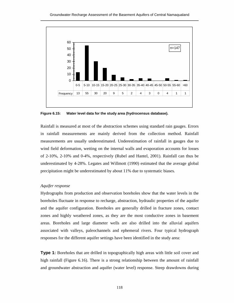
Groundwater Recharge Assessment of the Basement Aquifers of Central Namaqualand
118
n=147
0
10
20
30
40
50
60
Frequency 13 55 30 20 9 5 2 4 3 0 4 1 1
0-5 5-10 10-15 15-20 20-25 25-30 30-35 35-40 40-45 45-50 50-55 55-60 >60
Figure 6.15: Water level data for the study area (hydrocensus database).
Rainfall is measured at most of the abstraction schemes using standard rain gauges. Errors
in rainfall measurements are mainly derived from the collection method. Rainfall
measurements are usually underestimated. Underestimation of rainfall in gauges due to
wind field deformation, wetting on the internal walls and evaporation accounts for losses
of 2-10%, 2-10% and 0-4%, respectively (Rubel and Hantel, 2001). Rainfall can thus be
underestimated by 4-28%. Legates and Willmott (1990) estimated that the average global
precipitation might be underestimated by about 11% due to systematic biases.
Aquifer response
Hydrographs from production and observation boreholes show that the water levels in the
boreholes fluctuate in response to recharge, abstraction, hydraulic properties of the aquifer
and the aquifer configuration. Boreholes are generally drilled in fracture zones, contact
zones and highly weathered zones, as they are the most conductive zones in basement
areas. Boreholes and large diameter wells are also drilled into the alluvial aquifers
associated with valleys, paleochannels and ephemeral rivers. Four typical hydrograph
responses for the different aquifer settings have been identified in the study area:
Type 1: Boreholes that are drilled in topographically high areas with little soil cover and
high rainfall (Figure 6.16). There is a strong relationship between the amount of rainfall
and groundwater abstraction and aquifer (water level) response. Steep drawdowns during
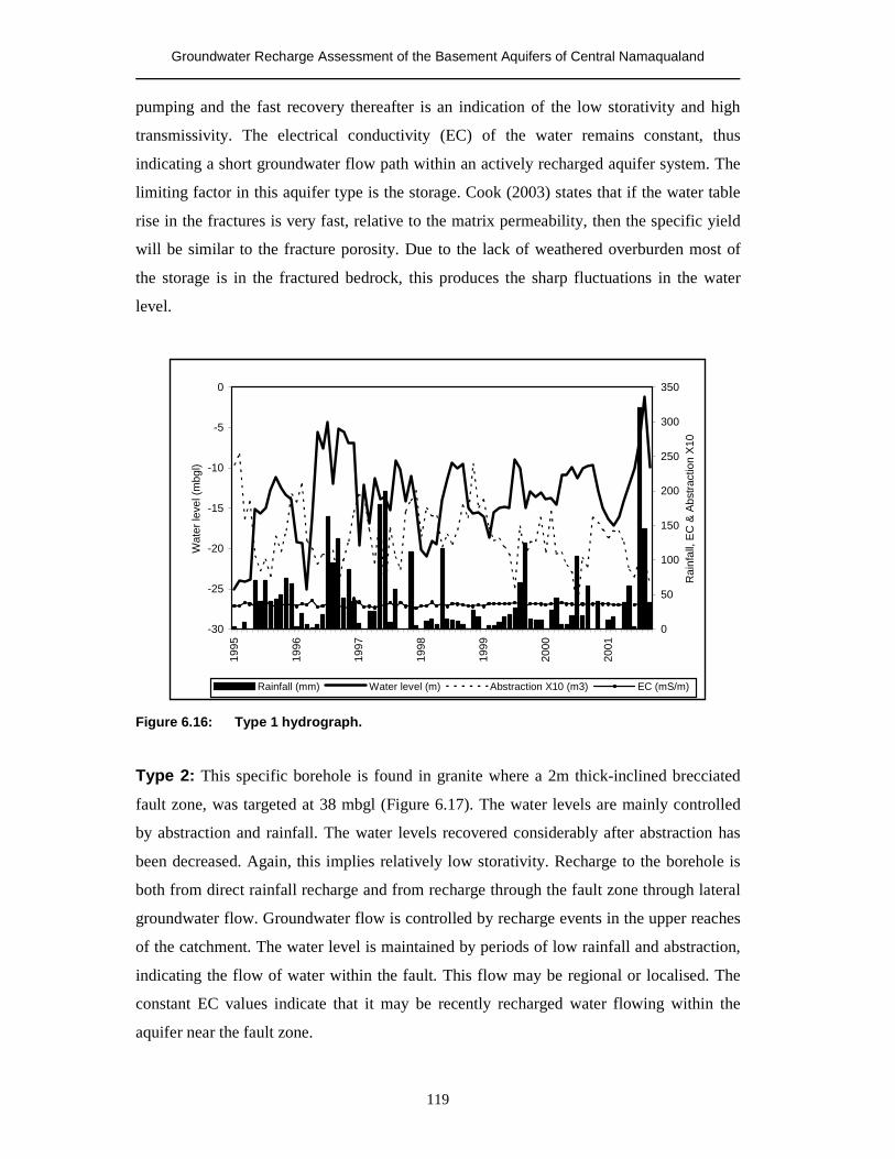
Groundwater Recharge Assessment of the Basement Aquifers of Central Namaqualand
119
pumping and the fast recovery thereafter is an indication of the low storativity and high
transmissivity. The electrical conductivity (EC) of the water remains constant, thus
indicating a short groundwater flow path within an actively recharged aquifer system. The
limiting factor in this aquifer type is the storage. Cook (2003) states that if the water table
rise in the fractures is very fast, relative to the matrix permeability, then the specific yield
will be similar to the fracture porosity. Due to the lack of weathered overburden most of
the storage is in the fractured bedrock, this produces the sharp fluctuations in the water
level.
-30
-25
-20
-15
-10
-5
0
1995
1996
1997
1998
1999
2000
2001
Wat
er le
vel (
mbg
l)
0
50
100
150
200
250
300
350
Rai
nfal
l, E
C &
Abs
tract
ion
X10
Rainfall (mm) Water level (m) Abstraction X10 (m3) EC (mS/m)
Figure 6.16: Type 1 hydrograph.
Type 2: This specific borehole is found in granite where a 2m thick-inclined brecciated
fault zone, was targeted at 38 mbgl (Figure 6.17). The water levels are mainly controlled
by abstraction and rainfall. The water levels recovered considerably after abstraction has
been decreased. Again, this implies relatively low storativity. Recharge to the borehole is
both from direct rainfall recharge and from recharge through the fault zone through lateral
groundwater flow. Groundwater flow is controlled by recharge events in the upper reaches
of the catchment. The water level is maintained by periods of low rainfall and abstraction,
indicating the flow of water within the fault. This flow may be regional or localised. The
constant EC values indicate that it may be recently recharged water flowing within the
aquifer near the fault zone.
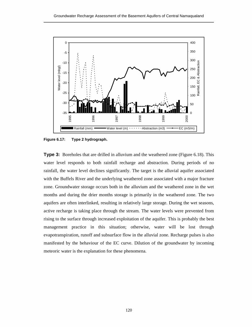
Groundwater Recharge Assessment of the Basement Aquifers of Central Namaqualand
120
-35
-30
-25
-20
-15
-10
-5
0
1995
1996
1997
1998
1999
2000
Wat
er le
vel (
mbg
l)
0
50
100
150
200
250
300
350
400
Rai
nfal
l, E
C &
Abs
tract
ion
Rainfall (mm) Water level (m) Abstraction (m3) EC (mS/m)
Figure 6.17: Type 2 hydrograph.
Type 3: Boreholes that are drilled in alluvium and the weathered zone (Figure 6.18). This
water level responds to both rainfall recharge and abstraction. During periods of no
rainfall, the water level declines significantly. The target is the alluvial aquifer associated
with the Buffels River and the underlying weathered zone associated with a major fracture
zone. Groundwater storage occurs both in the alluvium and the weathered zone in the wet
months and during the drier months storage is primarily in the weathered zone. The two
aquifers are often interlinked, resulting in relatively large storage. During the wet seasons,
active recharge is taking place through the stream. The water levels were prevented from
rising to the surface through increased exploitation of the aquifer. This is probably the best
management practice in this situation; otherwise, water will be lost through
evapotranspiration, runoff and subsurface flow in the alluvial zone. Recharge pulses is also
manifested by the behaviour of the EC curve. Dilution of the groundwater by incoming
meteoric water is the explanation for these phenomena.
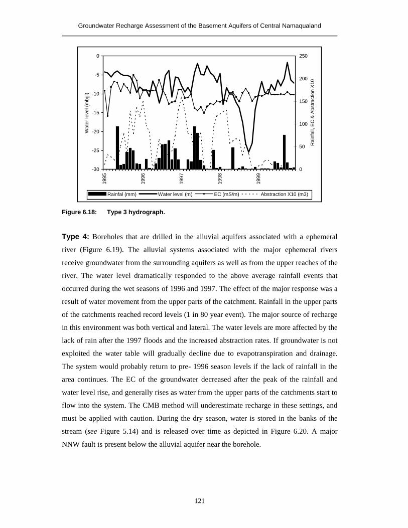
Groundwater Recharge Assessment of the Basement Aquifers of Central Namaqualand
121
-30
-25
-20
-15
-10
-5
0
1995
1996
1997
1998
1999
Wat
er le
vel (
mbg
l)
0
50
100
150
200
250
Rai
nfal
l, E
C &
Abs
tract
ion
X10
Rainfal (mm) Water level (m) EC (mS/m) Abstraction X10 (m3)
Figure 6.18: Type 3 hydrograph.
Type 4: Boreholes that are drilled in the alluvial aquifers associated with a ephemeral
river (Figure 6.19). The alluvial systems associated with the major ephemeral rivers
receive groundwater from the surrounding aquifers as well as from the upper reaches of the
river. The water level dramatically responded to the above average rainfall events that
occurred during the wet seasons of 1996 and 1997. The effect of the major response was a
result of water movement from the upper parts of the catchment. Rainfall in the upper parts
of the catchments reached record levels (1 in 80 year event). The major source of recharge
in this environment was both vertical and lateral. The water levels are more affected by the
lack of rain after the 1997 floods and the increased abstraction rates. If groundwater is not
exploited the water table will gradually decline due to evapotranspiration and drainage.
The system would probably return to pre- 1996 season levels if the lack of rainfall in the
area continues. The EC of the groundwater decreased after the peak of the rainfall and
water level rise, and generally rises as water from the upper parts of the catchments start to
flow into the system. The CMB method will underestimate recharge in these settings, and
must be applied with caution. During the dry season, water is stored in the banks of the
stream (see Figure 5.14) and is released over time as depicted in Figure 6.20. A major
NNW fault is present below the alluvial aquifer near the borehole.
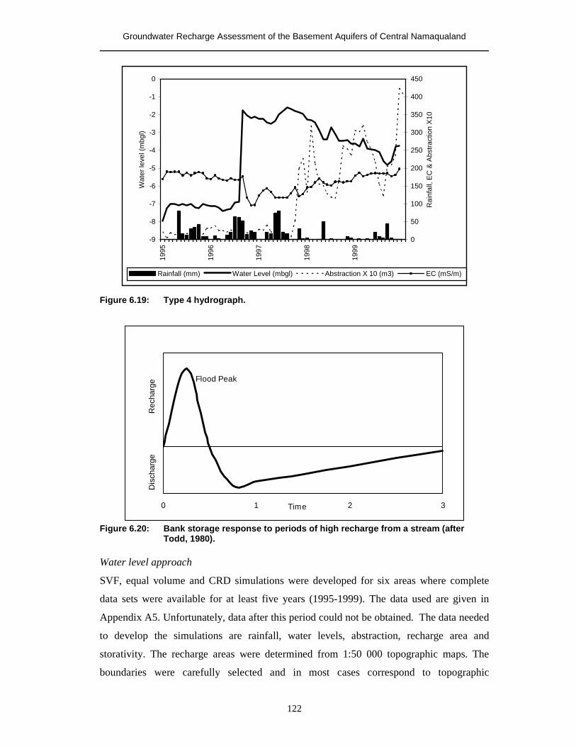
Groundwater Recharge Assessment of the Basement Aquifers of Central Namaqualand
122
-9
-8
-7
-6
-5
-4
-3
-2
-1
0
1995
1996
1997
1998
1999
Wat
er le
vel (
mbg
l)
0
50
100
150
200
250
300
350
400
450
Rai
nfal
l, E
C &
Abs
tract
ion
X10
Rainfall (mm) Water Level (mbgl) Abstraction X 10 (m3) EC (mS/m)
Figure 6.19: Type 4 hydrograph.
Flood Peak
0 1 2 3Time
Dis
char
ge
R
echa
rge
Figure 6.20: Bank storage response to periods of high recharge from a stream (after
Todd, 1980). Water level approach
SVF, equal volume and CRD simulations were developed for six areas where complete
data sets were available for at least five years (1995-1999). The data used are given in
Appendix A5. Unfortunately, data after this period could not be obtained. The data needed
to develop the simulations are rainfall, water levels, abstraction, recharge area and
storativity. The recharge areas were determined from 1:50 000 topographic maps. The
boundaries were carefully selected and in most cases correspond to topographic
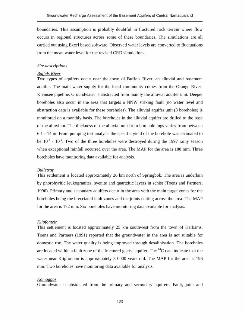
Groundwater Recharge Assessment of the Basement Aquifers of Central Namaqualand
123
boundaries. This assumption is probably doubtful in fractured rock terrain where flow
occurs in regional structures across some of these boundaries. The simulations are all
carried out using Excel based software. Observed water levels are converted to fluctuations
from the mean water level for the revised CRD simulations.
Site descriptions
Buffels River Two types of aquifers occur near the town of Buffels River, an alluvial and basement
aquifer. The main water supply for the local community comes from the Orange River-
Kleinsee pipeline. Groundwater is abstracted from mainly the alluvial aquifer unit. Deeper
boreholes also occur in the area that targets a NNW striking fault (no water level and
abstraction data is available for these boreholes). The alluvial aquifer unit (3 boreholes) is
monitored on a monthly basis. The boreholes in the alluvial aquifer are drilled to the base
of the alluvium. The thickness of the alluvial unit from borehole logs varies from between
6.1 - 14 m. From pumping test analysis the specific yield of the borehole was estimated to
be 10-3 - 10-2. Two of the three boreholes were destroyed during the 1997 rainy season
when exceptional rainfall occurred over the area. The MAP for the area is 188 mm. Three
boreholes have monitoring data available for analysis.
Bulletrap This settlement is located approximately 26 km north of Springbok. The area is underlain
by phorphyritic leukogranites, syenite and quartzitic layers in schist (Toens and Partners,
1996). Primary and secondary aquifers occur in the area with the main target zones for the
boreholes being the brecciated fault zones and the joints cutting across the area. The MAP
for the area is 172 mm. Six boreholes have monitoring data available for analysis.
Klipfontein This settlement is located approximately 25 km southwest from the town of Karkams.
Toens and Partners (1991) reported that the groundwater in the area is not suitable for
domestic use. The water quality is being improved through desalinisation. The boreholes
are located within a fault zone of the fractured gneiss aquifer. The 14C data indicate that the
water near Klipfontein is approximately 30 000 years old. The MAP for the area is 196
mm. Two boreholes have monitoring data available for analysis.
Komaggas Groundwater is abstracted from the primary and secondary aquifers. Fault, joint and
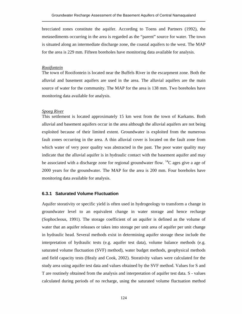
Groundwater Recharge Assessment of the Basement Aquifers of Central Namaqualand
124
brecciated zones constitute the aquifer. According to Toens and Partners (1992), the
metasediments occurring in the area is regarded as the “parent” source for water. The town
is situated along an intermediate discharge zone, the coastal aquifers to the west. The MAP
for the area is 229 mm. Fifteen boreholes have monitoring data available for analysis.
Rooifontein The town of Rooifontein is located near the Buffels River in the escarpment zone. Both the
alluvial and basement aquifers are used in the area. The alluvial aquifers are the main
source of water for the community. The MAP for the area is 138 mm. Two boreholes have
monitoring data available for analysis.
Spoeg River This settlement is located approximately 15 km west from the town of Karkams. Both
alluvial and basement aquifers occur in the area although the alluvial aquifers are not being
exploited because of their limited extent. Groundwater is exploited from the numerous
fault zones occurring in the area. A thin alluvial cover is located on the fault zone from
which water of very poor quality was abstracted in the past. The poor water quality may
indicate that the alluvial aquifer is in hydraulic contact with the basement aquifer and may
be associated with a discharge zone for regional groundwater flow. 14C ages give a age of
2000 years for the groundwater. The MAP for the area is 200 mm. Four boreholes have
monitoring data available for analysis.
6.3.1 Saturated Volume Fluctuation Aquifer storativity or specific yield is often used in hydrogeology to transform a change in
groundwater level to an equivalent change in water storage and hence recharge
(Sophocleous, 1991). The storage coefficient of an aquifer is defined as the volume of
water that an aquifer releases or takes into storage per unit area of aquifer per unit change
in hydraulic head. Several methods exist in determining aquifer storage these include the
interpretation of hydraulic tests (e.g. aquifer test data), volume balance methods (e.g.
saturated volume fluctuation (SVF) method), water budget methods, geophysical methods
and field capacity tests (Healy and Cook, 2002). Storativity values were calculated for the
study area using aquifer test data and values obtained by the SVF method. Values for S and
T are routinely obtained from the analysis and interpretation of aquifer test data. S - values
calculated during periods of no recharge, using the saturated volume fluctuation method
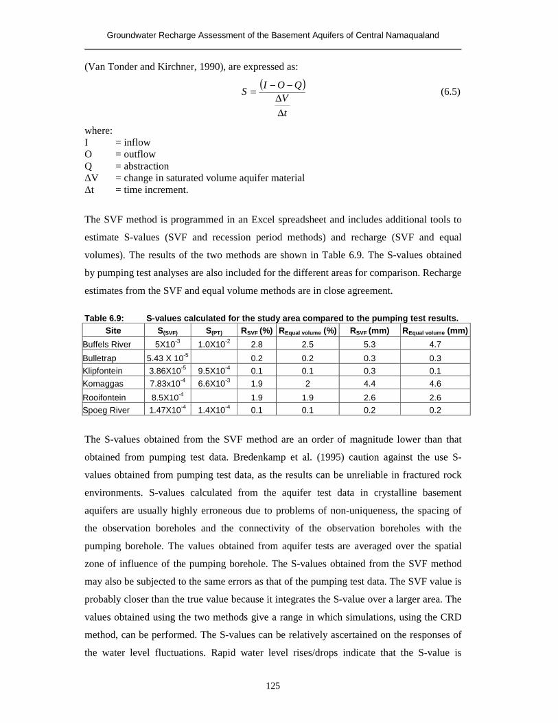
Groundwater Recharge Assessment of the Basement Aquifers of Central Namaqualand
125
(Van Tonder and Kirchner, 1990), are expressed as:
( )
tV
QOIS
∆∆
−−= (6.5)
where: I = inflow O = outflow Q = abstraction �V = change in saturated volume aquifer material �t = time increment.
The SVF method is programmed in an Excel spreadsheet and includes additional tools to
estimate S-values (SVF and recession period methods) and recharge (SVF and equal
volumes). The results of the two methods are shown in Table 6.9. The S-values obtained
by pumping test analyses are also included for the different areas for comparison. Recharge
estimates from the SVF and equal volume methods are in close agreement.
Table 6.9: S-values calculated for the study area compared to the pumping test results.
Site S(SVF) S(PT) RSVF (%) REqual volume (%) RSVF (mm) REqual volume (mm)
Buffels River 5X10⁻³ 1.0X10⁻² 2.8 2.5 5.3 4.7
Bulletrap 5.43 X 10⁻⁵ 0.2 0.2 0.3 0.3 Klipfontein 3.86X10⁻⁵ 9.5X10⁻⁴ 0.1 0.1 0.3 0.1 Komaggas 7.83x10⁻⁴ 6.6X10⁻³ 1.9 2 4.4 4.6
Rooifontein 8.5X10⁻⁴ 1.9 1.9 2.6 2.6 Spoeg River 1.47X10⁻⁴ 1.4X10⁻⁴ 0.1 0.1 0.2 0.2
The S-values obtained from the SVF method are an order of magnitude lower than that
obtained from pumping test data. Bredenkamp et al. (1995) caution against the use S-
values obtained from pumping test data, as the results can be unreliable in fractured rock
environments. S-values calculated from the aquifer test data in crystalline basement
aquifers are usually highly erroneous due to problems of non-uniqueness, the spacing of
the observation boreholes and the connectivity of the observation boreholes with the
pumping borehole. The values obtained from aquifer tests are averaged over the spatial
zone of influence of the pumping borehole. The S-values obtained from the SVF method
may also be subjected to the same errors as that of the pumping test data. The SVF value is
probably closer than the true value because it integrates the S-value over a larger area. The
values obtained using the two methods give a range in which simulations, using the CRD
method, can be performed. The S-values can be relatively ascertained on the responses of
the water level fluctuations. Rapid water level rises/drops indicate that the S-value is
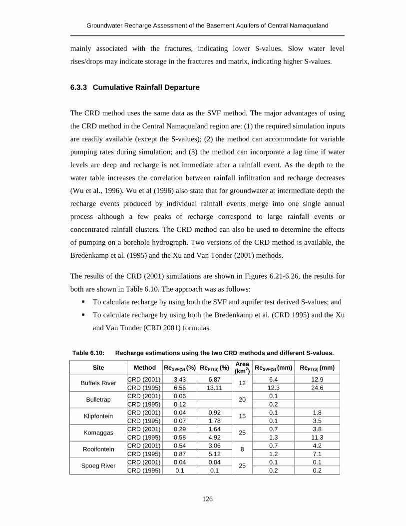
Groundwater Recharge Assessment of the Basement Aquifers of Central Namaqualand
126
mainly associated with the fractures, indicating lower S-values. Slow water level
rises/drops may indicate storage in the fractures and matrix, indicating higher S-values.
6.3.3 Cumulative Rainfall Departure
The CRD method uses the same data as the SVF method. The major advantages of using
the CRD method in the Central Namaqualand region are: (1) the required simulation inputs
are readily available (except the S-values); (2) the method can accommodate for variable
pumping rates during simulation; and (3) the method can incorporate a lag time if water
levels are deep and recharge is not immediate after a rainfall event. As the depth to the
water table increases the correlation between rainfall infiltration and recharge decreases
(Wu et al., 1996). Wu et al (1996) also state that for groundwater at intermediate depth the
recharge events produced by individual rainfall events merge into one single annual
process although a few peaks of recharge correspond to large rainfall events or
concentrated rainfall clusters. The CRD method can also be used to determine the effects
of pumping on a borehole hydrograph. Two versions of the CRD method is available, the
Bredenkamp et al. (1995) and the Xu and Van Tonder (2001) methods.
The results of the CRD (2001) simulations are shown in Figures 6.21-6.26, the results for
both are shown in Table 6.10. The approach was as follows:
� To calculate recharge by using both the SVF and aquifer test derived S-values; and
� To calculate recharge by using both the Bredenkamp et al. (CRD 1995) and the Xu
and Van Tonder (CRD 2001) formulas.
Table 6.10: Recharge estimations using the two CRD methods and different S-values.
Site Method ReSVF(S) (%) RePT(S) (%) Area (km2) ReSVF(S) (mm) RePT(S) (mm)
CRD (2001) 3.43 6.87 6.4 12.9 Buffels River CRD (1995) 6.56 13.11
12 12.3 24.6
CRD (2001) 0.06 0.1 Bulletrap CRD (1995) 0.12
20 0.2
CRD (2001) 0.04 0.92 0.1 1.8 Klipfontein CRD (1995) 0.07 1.78
15 0.1 3.5
CRD (2001) 0.29 1.64 0.7 3.8 Komaggas CRD (1995) 0.58 4.92
25 1.3 11.3
CRD (2001) 0.54 3.06 0.7 4.2 Rooifontein CRD (1995) 0.87 5.12
8 1.2 7.1
CRD (2001) 0.04 0.04 0.1 0.1 Spoeg River CRD (1995) 0.1 0.1
25 0.2 0.2
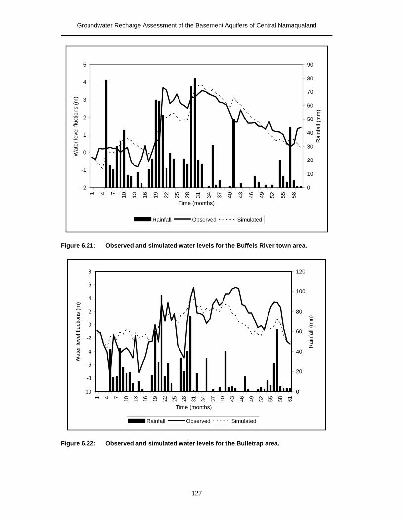
Groundwater Recharge Assessment of the Basement Aquifers of Central Namaqualand
127
-2
-1
0
1
2
3
4
5
1 4 7 10 13 16 19 22 25 28 31 34 37 40 43 46 49 52 55 58
Time (months)
Wat
er le
vel f
luct
ions
(m)
0
10
20
30
40
50
60
70
80
90
Rai
nfal
l (m
m)
Rainfall Observed Simulated
Figure 6.21: Observed and simulated water levels for the Buffels River town area.
-10
-8
-6
-4
-2
0
2
4
6
8
1 4 7 10 13 16 19 22 25 28 31 34 37 40 43 46 49 52 55 58 61
Time (months)
Wat
er le
vel f
luct
ions
(m)
0
20
40
60
80
100
120
Rai
nfal
l (m
m)
Rainfall Observed Simulated
Figure 6.22: Observed and simulated water levels for the Bulletrap area.
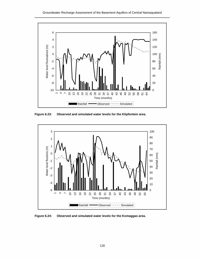
Groundwater Recharge Assessment of the Basement Aquifers of Central Namaqualand
128
-10
-8
-6
-4
-2
0
2
4
6
1 4 7 10 13 16 19 22 25 28 31 34 37 40 43 46 49 52 55 58 61 64
Time (months)
Wat
er le
vel f
luct
uatio
ns (m
)
0
20
40
60
80
100
120
140
160
Rai
nfal
l (m
m)
Rainfall Observed Simulated
Figure 6.23: Observed and simulated water levels for the Klipfontein area.
-5
-4
-3
-2
-1
0
1
2
3
1 4 7 10 13 16 19 22 25 28 31 34 37 40 43 46 49 52 55
Time (months)
Wat
er le
vel f
luct
ions
(m)
0
10
20
30
40
50
60
70
80
90
100
Rai
nfal
l (m
m)
Rainfall Observed Simulated
Figure 6.24: Observed and simulated water levels for the Komaggas area.
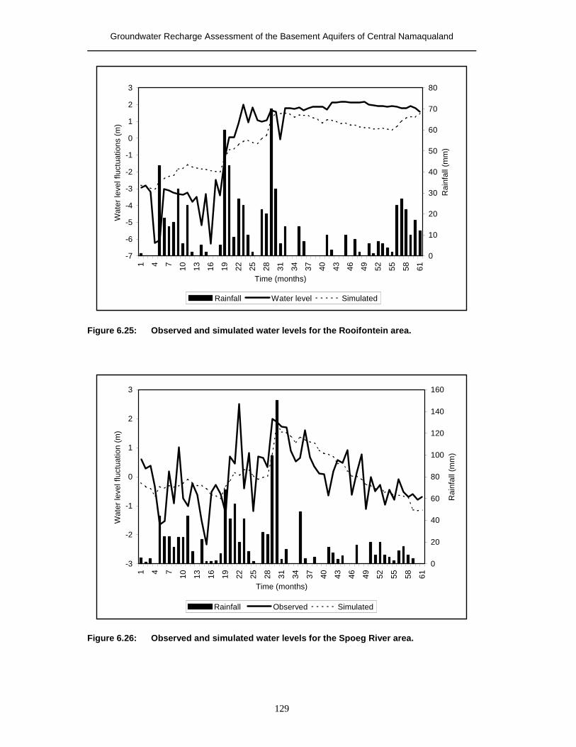
Groundwater Recharge Assessment of the Basement Aquifers of Central Namaqualand
129
-7
-6
-5
-4
-3
-2
-1
0
1
2
3
1 4 7 10 13 16 19 22 25 28 31 34 37 40 43 46 49 52 55 58 61
Time (months)
Wat
er le
vel f
luct
uatio
ns (m
)
0
10
20
30
40
50
60
70
80
Rai
nfal
l (m
m)
Rainfall Water level Simulated
Figure 6.25: Observed and simulated water levels for the Rooifontein area.
-3
-2
-1
0
1
2
3
1 4 7 10 13 16 19 22 25 28 31 34 37 40 43 46 49 52 55 58 61
Time (months)
Wat
er le
vel f
luct
uatio
n (m
)
0
20
40
60
80
100
120
140
160
Rai
nfal
l (m
m)
Rainfall Observed Simulated
Figure 6.26: Observed and simulated water levels for the Spoeg River area.
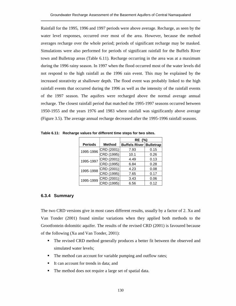
Groundwater Recharge Assessment of the Basement Aquifers of Central Namaqualand
130
Rainfall for the 1995, 1996 and 1997 periods were above average. Recharge, as seen by the
water level responses, occurred over most of the area. However, because the method
averages recharge over the whole period; periods of significant recharge may be masked.
Simulations were also performed for periods of significant rainfall for the Buffels River
town and Bulletrap areas (Table 6.11). Recharge occurring in the area was at a maximum
during the 1996 rainy season. In 1997 when the flood occurred most of the water levels did
not respond to the high rainfall as the 1996 rain event. This may be explained by the
increased storativity at shallower depth. The flood event was probably linked to the high
rainfall events that occurred during the 1996 as well as the intensity of the rainfall events
of the 1997 season. The aquifers were recharged above the normal average annual
recharge. The closest rainfall period that matched the 1995-1997 seasons occurred between
1950-1955 and the years 1976 and 1983 where rainfall was significantly above average
(Figure 3.5). The average annual recharge decreased after the 1995-1996 rainfall seasons.
Table 6.11: Recharge values for different time steps for two sites.
RE (%) Periods Method Buffels River Bulletrap
CRD (2001) 7.93 0.15 1995-1996 CRD (1995) 10.1 0.26 CRD (2001) 4.49 0.13 1995-1997 CRD (1995) 6.84 0.28 CRD (2001) 4.23 0.08 1995-1998 CRD (1995) 7.65 0.17 CRD (2001) 3.43 0.06 1995-1999 CRD (1995) 6.56 0.12
6.3.4 Summary
The two CRD versions give in most cases different results, usually by a factor of 2. Xu and
Van Tonder (2001) found similar variations when they applied both methods to the
Grootfontein dolomitic aquifer. The results of the revised CRD (2001) is favoured because
of the following (Xu and Van Tonder, 2001):
� The revised CRD method generally produces a better fit between the observed and
simulated water levels;
� The method can account for variable pumping and outflow rates;
� It can account for trends in data; and
� The method does not require a large set of spatial data.
Groundwater Recharge Assessment of the Basement Aquifers of Central Namaqualand
131
The disadvantages of the method are:
� The approach does not address parameter variations spatially; and
� Recharge is averaged over the simulated period and may be significantly higher
than the average during periods of peak rainfall. It is well recognised that in drier
climates that recharge events are associated with short periods of intense rainfall.
The simulations did not need time lag adjustments, as most of the responses were shorter
than one month. Indicating that recharge from the surface to the groundwater is relatively
fast if recharge occurs. The abstraction and the low S-values associated with the aquifers
weaken the correlation between water fluctuations and rainfall. The simulated water levels
deviate from the observed water levels due to the addition or removal of groundwater from
the aquifer due to inflow and outflow. When water is flowing out of the aquifer the
simulated fluctuation is higher than the observed fluctuation and if groundwater is being
added via lateral flow or surface runoff from outside the recharge area the simulated water
level will be lower than the observed water level. The spatial variability of recharge in the
basement aquifers complicates the estimation of recharge and the relationship between the
CRD and water levels due to the fact that spatial water levels are averaged. Bredenkamp
(2003) indicates that the method works best in dolomitic aquifers where the highly
permeable aquifers equalises the spatial differences in recharge. It has also been shown that
the alluvial aquifers are receiving most of the recharge as opposed to the basement
aquifers. Lumping the different water levels of basement and alluvial aquifers to estimate
recharge may introduce discrepancies in the recharge rates calculated for different areas.
The recharge values estimated for the six areas indicate that recharge is not uniform over
the study area. The variability of groundwater recharge is a function of the amount of
rainfall, aquifer properties, geomorphology of the area and the geometry of the aquifer.
Recharge, as a percentage of rainfall, is higher in areas where the main groundwater targets
are alluvial aquifers or a combination of alluvial and basement aquifers. The Buffels River,
Kamassies, Komaggas and Twee River communities are abstracting groundwater from the
alluvium, which are fed by the surrounding hard rock and weathered aquifers. Areas
underlain by fractured hard rock and weathered zone aquifers receive little recharge.
Recharge to the fractured hard rock aquifers in the Spoeg River and Klipfontein areas
receive very little recharge, manifested by the groundwater chemistry and 14C data. The
groundwater in these two towns are desalinised to make it fit for drinking. If groundwater
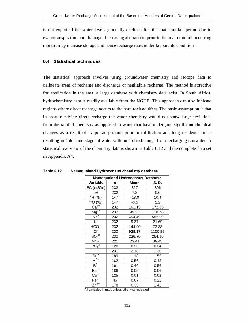
Groundwater Recharge Assessment of the Basement Aquifers of Central Namaqualand
132
is not exploited the water levels gradually decline after the main rainfall period due to
evapotranspiration and drainage. Increasing abstraction prior to the main rainfall occurring
months may increase storage and hence recharge rates under favourable conditions.
6.4 Statistical techniques
The statistical approach involves using groundwater chemistry and isotope data to
delineate areas of recharge and discharge or negligible recharge. The method is attractive
for application in the area, a large database with chemistry data exist. In South Africa,
hydrochemistry data is readily available from the NGDB. This approach can also indicate
regions where direct recharge occurs to the hard rock aquifers. The basic assumption is that
in areas receiving direct recharge the water chemistry would not show large deviations
from the rainfall chemistry as opposed to water that have undergone significant chemical
changes as a result of evapotranspiration prior to infiltration and long residence times
resulting in “old” and stagnant water with no “refreshening” from recharging rainwater. A
statistical overview of the chemistry data is shown in Table 6.12 and the complete data set
in Appendix A4.
Table 6.12: Namaqualand Hydrocensus chemistry database.
Namaqualand Hydrocensus Database Variable n Mean S. D.
EC (mS/m) 232 327 305 pH 232 7.2 0.6
2H (‰) 147 -18.8 10.4 18O (‰) 147 -3.5 2.2
Ca2+ 232 161.15 172.65 Mg2+ 232 99.26 118.76 Na+ 232 454.49 582.99 K+ 232 9.37 21.69
HCO3- 232 144.90 72.33
Cl- 232 938.17 1150.92 SO4
2- 232 236.70 264.16 NO3
- 221 23.41 39.45 PO4
3- 120 0.23 0.34 F- 231 2.18 1.30
Sr2+ 189 1.18 1.55 Al3+ 162 0.56 0.43 B3+ 161 0.46 0.56
Ba2+ 186 0.05 0.06 Cu2+ 125 0.01 0.02 Fe3+ 46 0.07 0.22 Zn2+ 178 0.35 1.42
All variables in mg/L unless otherwise indicated
Groundwater Recharge Assessment of the Basement Aquifers of Central Namaqualand
133
The Statistica computer program was used to perform the factor analysis. Data was
imported from the chemical database and missing data was casewise deleted. A correlation
matrix was calculated for the different variables. Several variables, mainly the trace
elements, were not included in the analysis due to missing data. The data was rotated
(varimax rotation) to reduce the factor loadings to a simple structure by placing the highest
possible loadings on the fewest number of variables, while preserving the independence of
each factor and reducing the complexity further by allowing the factors to become slightly
correlated (Levinson, 1980). In the data set, factor extraction was carried out by means of
principal components. Varimax rotations are orthogonal and results in factors that are
uncorrelated. During rotation, the Kaiser normalisation is applied, where only factors with
eigenvalues greater than one are retained.
Numerical values are assigned to each factor, which can range from +1.00 to -1.00. These
are commonly referred to as loadings, which are a measure of the extent to which each
factor is associated with a particular value. If two loadings of the same factor have the
same sign (either positive-positive or negative-negative) then they are positively
correlated. If they have opposite signs then they are negatively correlated. Factor loadings
and factor scores were extracted and interpreted. Only factor loadings greater than +3 and
smaller than –3 are used in interpreting the factor loadings. These new combinations are
then examined for significance in terms of process, types of samples, geological and
geochemical information (Rose et al., 1979). Factor scores (Q-mode) are extracted for each
sampling site for each factor. The factor scores for each sample were plotted and
interpolated using Kriging over the study area. This process gives insight into the areal
importance of the chemical processes represented by the different factors. The factor
scores are related to the intensity of the chemical process described by any particular factor
(Lawrence and Upchurch, 1982). Extreme negative values (< -1) indicates that an area is
unaffected by the chemical process and positive scores (> +1) reflect areas most affected,
whilst scores of zero (0) approximate areas affected to an average degree by the chemical
process (Lawrence and Upchurch, 1982).
6.4.1 R- and Q-mode factor analysis
Four factors account for 70.4 % of the variance in the data set (Table 6.13). Factor 1 has a
high loading of variables that contribute to the salinity of the groundwater in the area.
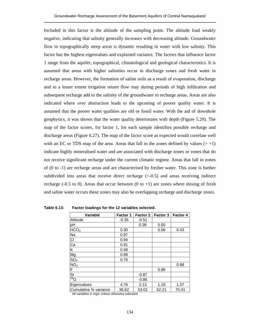
Groundwater Recharge Assessment of the Basement Aquifers of Central Namaqualand
134
Included in this factor is the altitude of the sampling point. The altitude load weakly
negative, indicating that salinity generally increases with decreasing altitude. Groundwater
flow in topographically steep areas is dynamic resulting in water with low salinity. This
factor has the highest eigenvalues and explained variance. The factors that influence factor
1 range from the aquifer, topographical, climatological and geological characteristics. It is
assumed that areas with higher salinities occur in discharge zones and fresh water in
recharge areas. However, the formation of saline soils as a result of evaporation, discharge
and to a lesser extent irrigation return flow may during periods of high infiltration and
subsequent recharge add to the salinity of the groundwater in recharge areas. Areas are also
indicated where over abstraction leads to the upconing of poorer quality water. It is
assumed that the poorer water qualities are old or fossil water. With the aid of downhole
geophysics, it was shown that the water quality deteriorates with depth (Figure 5.20). The
map of the factor scores, for factor 1, for each sample identifies possible recharge and
discharge areas (Figure 6.27). The map of the factor score as expected would correlate well
with an EC or TDS map of the area. Areas that fall in the zones defined by values (> +1)
indicate highly mineralised water and are associated with discharge zones or zones that do
not receive significant recharge under the current climatic regime. Areas that fall in zones
of (0 to -1) are recharge areas and are characterised by fresher water. This zone is further
subdivided into areas that receive direct recharge (<-0.5) and areas receiving indirect
recharge (-0.5 to 0). Areas that occur between (0 to +1) are zones where mixing of fresh
and saline water occurs these zones may also be overlapping recharge and discharge zones.
Table 6.13: Factor loadings for the 12 variables selected.
Variable Factor 1 Factor 2 Factor 3 Factor 4 Altitude -0.35 -0.51 pH 0.38 0.50 HCO3 0.30 0.56 0.43 Na 0.87 Cl 0.94 Ca 0.91 K 0.58 Mg 0.89 SO4 0.76 NO3 0.88 F 0.88 Sr -0.87 18O -0.86 Eigenvalues 4.76 2.13 1.19 1.07 Cumulative % variance 36.62 53.02 62.21 70.41
All variables in mg/L unless otherwise indicated
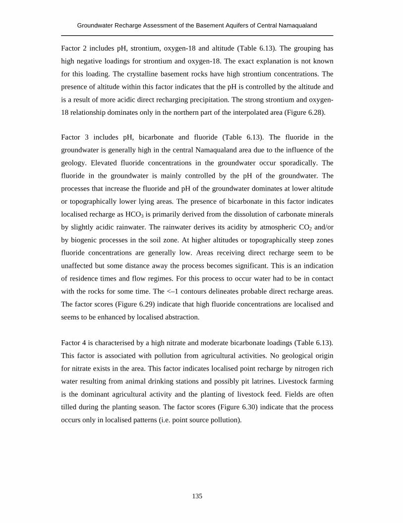
Groundwater Recharge Assessment of the Basement Aquifers of Central Namaqualand
135
Factor 2 includes pH, strontium, oxygen-18 and altitude (Table 6.13). The grouping has
high negative loadings for strontium and oxygen-18. The exact explanation is not known
for this loading. The crystalline basement rocks have high strontium concentrations. The
presence of altitude within this factor indicates that the pH is controlled by the altitude and
is a result of more acidic direct recharging precipitation. The strong strontium and oxygen-
18 relationship dominates only in the northern part of the interpolated area (Figure 6.28).
Factor 3 includes pH, bicarbonate and fluoride (Table 6.13). The fluoride in the
groundwater is generally high in the central Namaqualand area due to the influence of the
geology. Elevated fluoride concentrations in the groundwater occur sporadically. The
fluoride in the groundwater is mainly controlled by the pH of the groundwater. The
processes that increase the fluoride and pH of the groundwater dominates at lower altitude
or topographically lower lying areas. The presence of bicarbonate in this factor indicates
localised recharge as HCO3 is primarily derived from the dissolution of carbonate minerals
by slightly acidic rainwater. The rainwater derives its acidity by atmospheric CO2 and/or
by biogenic processes in the soil zone. At higher altitudes or topographically steep zones
fluoride concentrations are generally low. Areas receiving direct recharge seem to be
unaffected but some distance away the process becomes significant. This is an indication
of residence times and flow regimes. For this process to occur water had to be in contact
with the rocks for some time. The <–1 contours delineates probable direct recharge areas.
The factor scores (Figure 6.29) indicate that high fluoride concentrations are localised and
seems to be enhanced by localised abstraction.
Factor 4 is characterised by a high nitrate and moderate bicarbonate loadings (Table 6.13).
This factor is associated with pollution from agricultural activities. No geological origin
for nitrate exists in the area. This factor indicates localised point recharge by nitrogen rich
water resulting from animal drinking stations and possibly pit latrines. Livestock farming
is the dominant agricultural activity and the planting of livestock feed. Fields are often
tilled during the planting season. The factor scores (Figure 6.30) indicate that the process
occurs only in localised patterns (i.e. point source pollution).
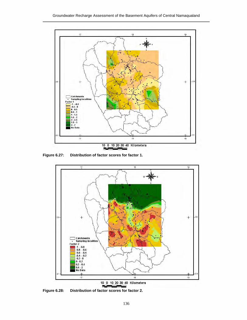
Groundwater Recharge Assessment of the Basement Aquifers of Central Namaqualand
136
Figure 6.27: Distribution of factor scores for factor 1.
Figure 6.28: Distribution of factor scores for factor 2.
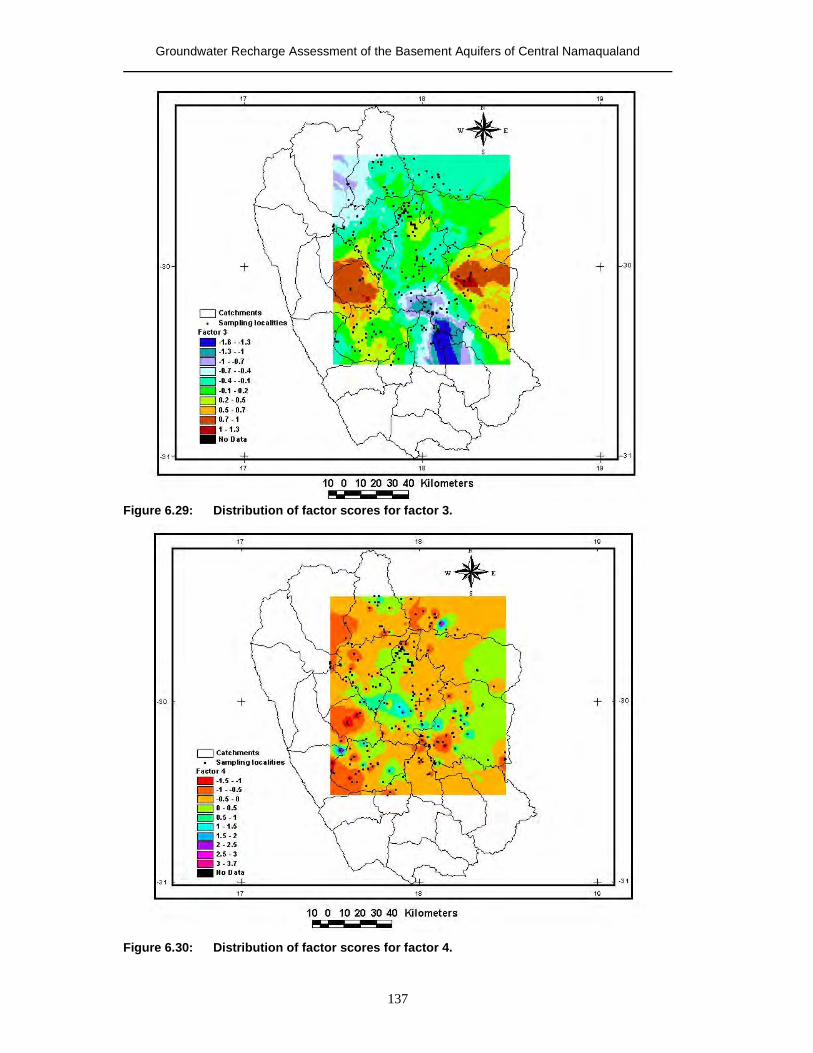
Groundwater Recharge Assessment of the Basement Aquifers of Central Namaqualand
137
Figure 6.29: Distribution of factor scores for factor 3.
Figure 6.30: Distribution of factor scores for factor 4.
Groundwater Recharge Assessment of the Basement Aquifers of Central Namaqualand
138
6.4.2 Summary
The statistical approach, using mainly the groundwater chemistry, indicates regions of
relatively fresh water and highly mineralised water. Factor analysis is useful in the study
area due to the fact that:
� Chemistry data are readily available;
� Factor analysis mainly describes the underlying processes and/or factors that
produced the data;
� Variabilities of ions in small concentrations are not dominated by major ions (eg.
chloride);
� Intermediate areas are delineated and not just the two extremities;
� Conventional methods, like the Piper diagram, would not indicate hydrochemical
trends because of a dominant Na-Cl type water in the recharge and discharge areas;
and
� Regional distribution and analysis of the different factors can be made.
The result of the statistical approach can aid in describing the regional groundwater and
recharge trends. Direct recharge in the Central Namaqualand region is dominant in the
higher lying regions. This is a direct result of the amount of rainfall over these areas due to
the orographic effect. The rainfall is also recharged rapidly due to the favourable surface
conditions. The hydraulic gradients in the higher lying areas are in the direction of
structurally controlled surface depressions (valleys, alluvial plains, etc.). The water, both
groundwater and surface water, collects in fracture controlled valleys, having a thick
weathered zone. Rapid infiltration in the higher lying areas result in groundwater with a
superior quality than groundwater occurring in topographically lower lying flat areas. The
absence of significant soil cover is also a dominant factor in topographically steep zones.
In the lower lying areas the soils generally have a high salt content due to the lower rainfall
and high evapotranspiration rates and the fact that they act as sinks where groundwater
accumulate. These areas may receive indirect recharge during periods of peak overland
flow. Discharge is dominant in the lower lying areas and occurs as natural springs,
evapotranspiration and aquifer exploitation. Overland flow occurs in the higher lying areas
when the rate of vertical movement is slow. Discharge in lower lying areas is dominant
along the horizontal to sub horizontal fracture and joint planes. Mixing zones, between
modern (recently recharged) and older water, exist between recharge and discharge zones.
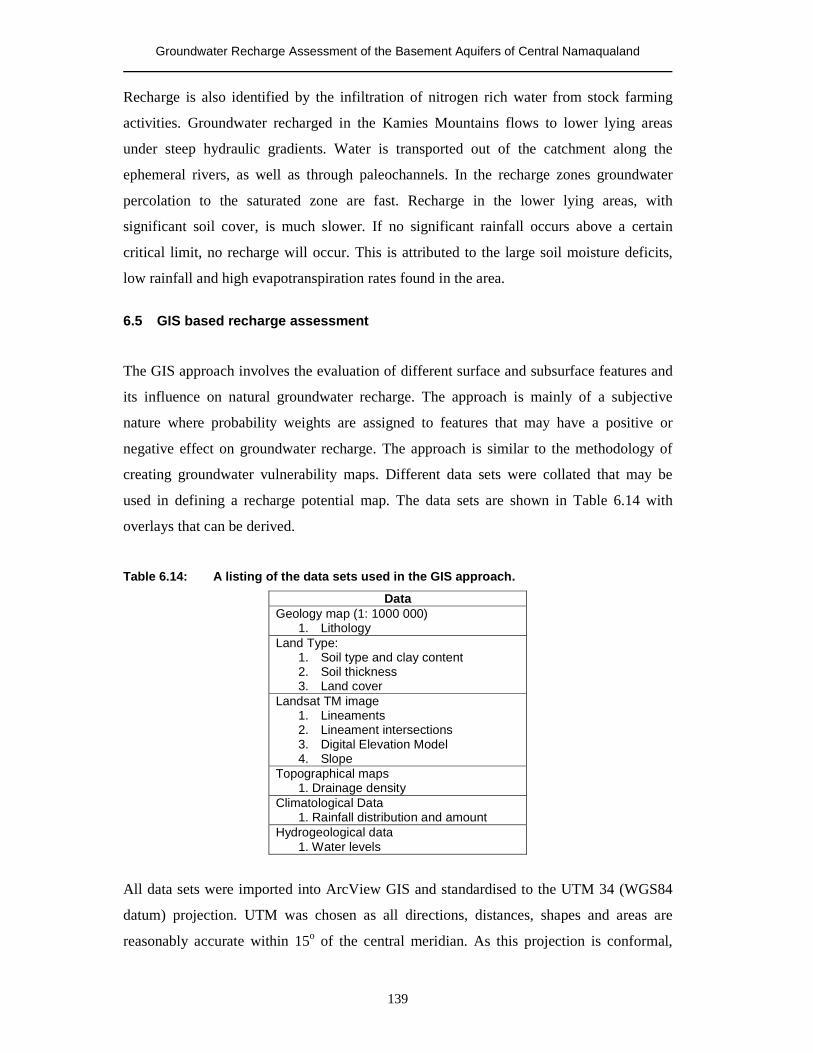
Groundwater Recharge Assessment of the Basement Aquifers of Central Namaqualand
139
Recharge is also identified by the infiltration of nitrogen rich water from stock farming
activities. Groundwater recharged in the Kamies Mountains flows to lower lying areas
under steep hydraulic gradients. Water is transported out of the catchment along the
ephemeral rivers, as well as through paleochannels. In the recharge zones groundwater
percolation to the saturated zone are fast. Recharge in the lower lying areas, with
significant soil cover, is much slower. If no significant rainfall occurs above a certain
critical limit, no recharge will occur. This is attributed to the large soil moisture deficits,
low rainfall and high evapotranspiration rates found in the area.
6.5 GIS based recharge assessment
The GIS approach involves the evaluation of different surface and subsurface features and
its influence on natural groundwater recharge. The approach is mainly of a subjective
nature where probability weights are assigned to features that may have a positive or
negative effect on groundwater recharge. The approach is similar to the methodology of
creating groundwater vulnerability maps. Different data sets were collated that may be
used in defining a recharge potential map. The data sets are shown in Table 6.14 with
overlays that can be derived.
Table 6.14: A listing of the data sets used in the GIS approach.
Data Geology map (1: 1000 000)
1. Lithology Land Type:
1. Soil type and clay content 2. Soil thickness 3. Land cover
Landsat TM image 1. Lineaments 2. Lineament intersections 3. Digital Elevation Model 4. Slope
Topographical maps 1. Drainage density
Climatological Data 1. Rainfall distribution and amount
Hydrogeological data 1. Water levels
All data sets were imported into ArcView GIS and standardised to the UTM 34 (WGS84
datum) projection. UTM was chosen as all directions, distances, shapes and areas are
reasonably accurate within 15o of the central meridian. As this projection is conformal,
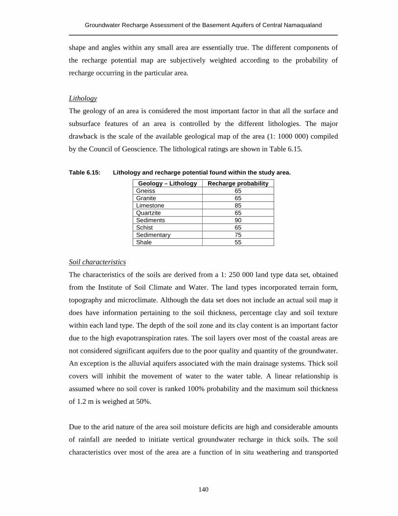
Groundwater Recharge Assessment of the Basement Aquifers of Central Namaqualand
140
shape and angles within any small area are essentially true. The different components of
the recharge potential map are subjectively weighted according to the probability of
recharge occurring in the particular area.
Lithology
The geology of an area is considered the most important factor in that all the surface and
subsurface features of an area is controlled by the different lithologies. The major
drawback is the scale of the available geological map of the area (1: 1000 000) compiled
by the Council of Geoscience. The lithological ratings are shown in Table 6.15.
Table 6.15: Lithology and recharge potential found within the study area.
Geology – Lithology Recharge probability Gneiss 65 Granite 65 Limestone 85 Quartzite 65 Sediments 90 Schist 65 Sedimentary 75 Shale 55
Soil characteristics
The characteristics of the soils are derived from a 1: 250 000 land type data set, obtained
from the Institute of Soil Climate and Water. The land types incorporated terrain form,
topography and microclimate. Although the data set does not include an actual soil map it
does have information pertaining to the soil thickness, percentage clay and soil texture
within each land type. The depth of the soil zone and its clay content is an important factor
due to the high evapotranspiration rates. The soil layers over most of the coastal areas are
not considered significant aquifers due to the poor quality and quantity of the groundwater.
An exception is the alluvial aquifers associated with the main drainage systems. Thick soil
covers will inhibit the movement of water to the water table. A linear relationship is
assumed where no soil cover is ranked 100% probability and the maximum soil thickness
of 1.2 m is weighed at 50%.
Due to the arid nature of the area soil moisture deficits are high and considerable amounts
of rainfall are needed to initiate vertical groundwater recharge in thick soils. The soil
characteristics over most of the area are a function of in situ weathering and transported
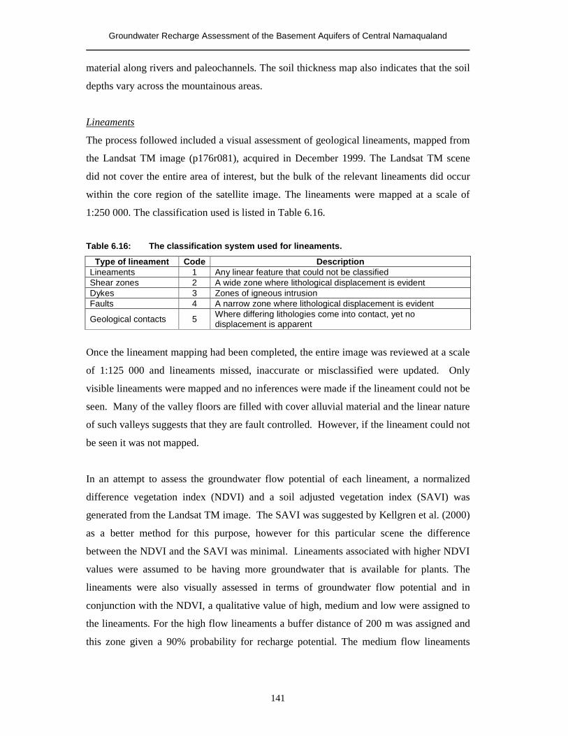
Groundwater Recharge Assessment of the Basement Aquifers of Central Namaqualand
141
material along rivers and paleochannels. The soil thickness map also indicates that the soil
depths vary across the mountainous areas.
Lineaments
The process followed included a visual assessment of geological lineaments, mapped from
the Landsat TM image (p176r081), acquired in December 1999. The Landsat TM scene
did not cover the entire area of interest, but the bulk of the relevant lineaments did occur
within the core region of the satellite image. The lineaments were mapped at a scale of
1:250 000. The classification used is listed in Table 6.16.
Table 6.16: The classification system used for lineaments.
Type of lineament Code Description Lineaments 1 Any linear feature that could not be classified Shear zones 2 A wide zone where lithological displacement is evident Dykes 3 Zones of igneous intrusion Faults 4 A narrow zone where lithological displacement is evident
Geological contacts 5 Where differing lithologies come into contact, yet no displacement is apparent
Once the lineament mapping had been completed, the entire image was reviewed at a scale
of 1:125 000 and lineaments missed, inaccurate or misclassified were updated. Only
visible lineaments were mapped and no inferences were made if the lineament could not be
seen. Many of the valley floors are filled with cover alluvial material and the linear nature
of such valleys suggests that they are fault controlled. However, if the lineament could not
be seen it was not mapped.
In an attempt to assess the groundwater flow potential of each lineament, a normalized
difference vegetation index (NDVI) and a soil adjusted vegetation index (SAVI) was
generated from the Landsat TM image. The SAVI was suggested by Kellgren et al. (2000)
as a better method for this purpose, however for this particular scene the difference
between the NDVI and the SAVI was minimal. Lineaments associated with higher NDVI
values were assumed to be having more groundwater that is available for plants. The
lineaments were also visually assessed in terms of groundwater flow potential and in
conjunction with the NDVI, a qualitative value of high, medium and low were assigned to
the lineaments. For the high flow lineaments a buffer distance of 200 m was assigned and
this zone given a 90% probability for recharge potential. The medium flow lineaments
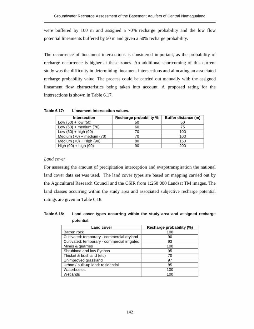
Groundwater Recharge Assessment of the Basement Aquifers of Central Namaqualand
142
were buffered by 100 m and assigned a 70% recharge probability and the low flow
potential lineaments buffered by 50 m and given a 50% recharge probability.
The occurrence of lineament intersections is considered important, as the probability of
recharge occurrence is higher at these zones. An additional shortcoming of this current
study was the difficulty in determining lineament intersections and allocating an associated
recharge probability value. The process could be carried out manually with the assigned
lineament flow characteristics being taken into account. A proposed rating for the
intersections is shown in Table 6.17.
Table 6.17: Lineament intersection values.
Intersection Recharge probability % Buffer distance (m) Low (50) + low (50) 50 50 Low (50) + medium (70) 60 75 Low (50) + high (90) 70 100 Medium (70) + medium (70) 70 100 Medium (70) + High (90) 80 150 High (90) + high (90) 90 200
Land cover
For assessing the amount of precipitation interception and evapotranspiration the national
land cover data set was used. The land cover types are based on mapping carried out by
the Agricultural Research Council and the CSIR from 1:250 000 Landsat TM images. The
land classes occurring within the study area and associated subjective recharge potential
ratings are given in Table 6.18.
Table 6.18: Land cover types occurring within the study area and assigned recharge
potential.
Land cover Recharge probability (%) Barren rock 100 Cultivated: temporary - commercial dryland 90 Cultivated: temporary - commercial irrigated 93 Mines & quarries 100 Shrubland and low Fynbos 95 Thicket & bushland (etc) 70 Unimproved grassland 97 Urban / built-up land: residential 85 Waterbodies 100 Wetlands 100
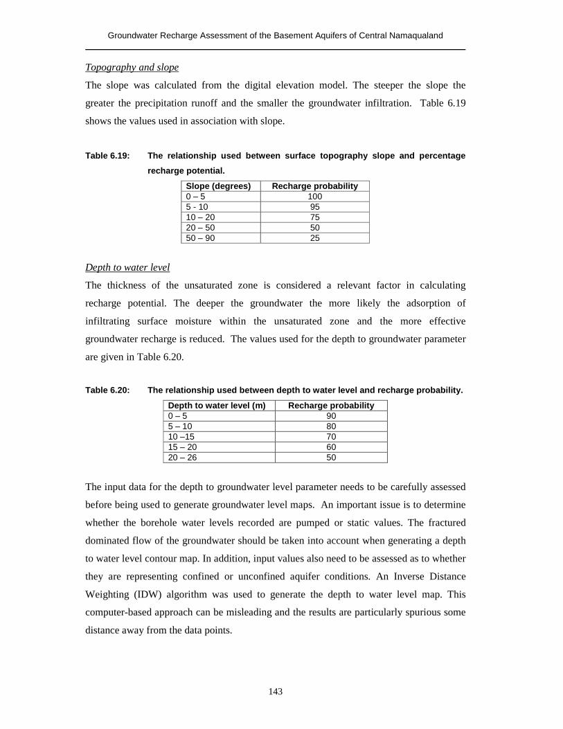
Groundwater Recharge Assessment of the Basement Aquifers of Central Namaqualand
143
Topography and slope
The slope was calculated from the digital elevation model. The steeper the slope the
greater the precipitation runoff and the smaller the groundwater infiltration. Table 6.19
shows the values used in association with slope.
Table 6.19: The relationship used between surface topography slope and percentage
recharge potential.
Slope (degrees) Recharge probability 0 – 5 100 5 - 10 95 10 – 20 75 20 – 50 50 50 – 90 25
Depth to water level
The thickness of the unsaturated zone is considered a relevant factor in calculating
recharge potential. The deeper the groundwater the more likely the adsorption of
infiltrating surface moisture within the unsaturated zone and the more effective
groundwater recharge is reduced. The values used for the depth to groundwater parameter
are given in Table 6.20.
Table 6.20: The relationship used between depth to water level and recharge probability.
Depth to water level (m) Recharge probability 0 – 5 90 5 – 10 80 10 –15 70 15 – 20 60 20 – 26 50
The input data for the depth to groundwater level parameter needs to be carefully assessed
before being used to generate groundwater level maps. An important issue is to determine
whether the borehole water levels recorded are pumped or static values. The fractured
dominated flow of the groundwater should be taken into account when generating a depth
to water level contour map. In addition, input values also need to be assessed as to whether
they are representing confined or unconfined aquifer conditions. An Inverse Distance
Weighting (IDW) algorithm was used to generate the depth to water level map. This
computer-based approach can be misleading and the results are particularly spurious some
distance away from the data points.
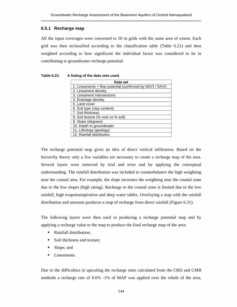
Groundwater Recharge Assessment of the Basement Aquifers of Central Namaqualand
144
6.5.1 Recharge map All the input coverages were converted to 50 m grids with the same area of extent. Each
grid was then reclassified according to the classification table (Table 6.21) and then
weighted according to how significant the individual factor was considered to be in
contributing to groundwater recharge potential.
Table 6.21: A listing of the data sets used.
Data set 1. Lineaments + flow potential (confirmed by NDVI / SAVI) 2. Lineament density 3. Lineament intersections 4. Drainage density 5. Land cover 6. Soil type (clay content) 7. Soil thickness 8. Soil texture (% rock vs % soil) 9. Slope (degrees) 10. Depth to groundwater 11. Lithology (geology) 12. Rainfall distribution
The recharge potential map gives an idea of direct vertical infiltration. Based on the
hierarchy theory only a few variables are necessary to create a recharge map of the area.
Several layers were removed by trial and error and by applying the conceptual
understanding. The rainfall distribution was included to counterbalance the high weighting
near the coastal area. For example, the slope increases the weighting near the coastal zone
due to the low slopes (high rating). Recharge to the coastal zone is limited due to the low
rainfall, high evapotranspiration and deep water tables. Overlaying a map with the rainfall
distribution and amounts produces a map of recharge from direct rainfall (Figure 6.31).
The following layers were then used in producing a recharge potential map and by
applying a recharge value to the map to produce the final recharge map of the area:
� Rainfall distribution;
� Soil thickness and texture;
� Slope; and
� Lineaments.
Due to the difficulties in upscaling the recharge rates calculated from the CRD and CMB
methods a recharge rate of 0.6% -1% of MAP was applied over the whole of the area,
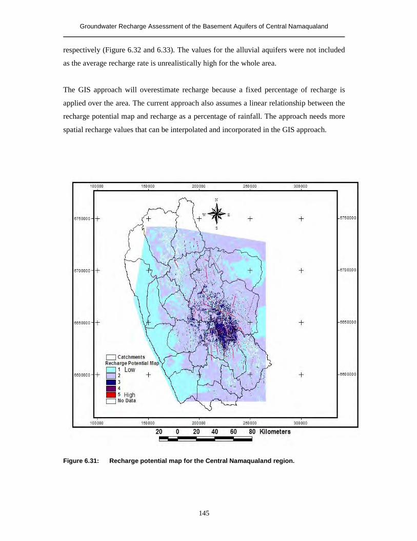
Groundwater Recharge Assessment of the Basement Aquifers of Central Namaqualand
145
respectively (Figure 6.32 and 6.33). The values for the alluvial aquifers were not included
as the average recharge rate is unrealistically high for the whole area.
The GIS approach will overestimate recharge because a fixed percentage of recharge is
applied over the area. The current approach also assumes a linear relationship between the
recharge potential map and recharge as a percentage of rainfall. The approach needs more
spatial recharge values that can be interpolated and incorporated in the GIS approach.
Figure 6.31: Recharge potential map for the Central Namaqualand region.
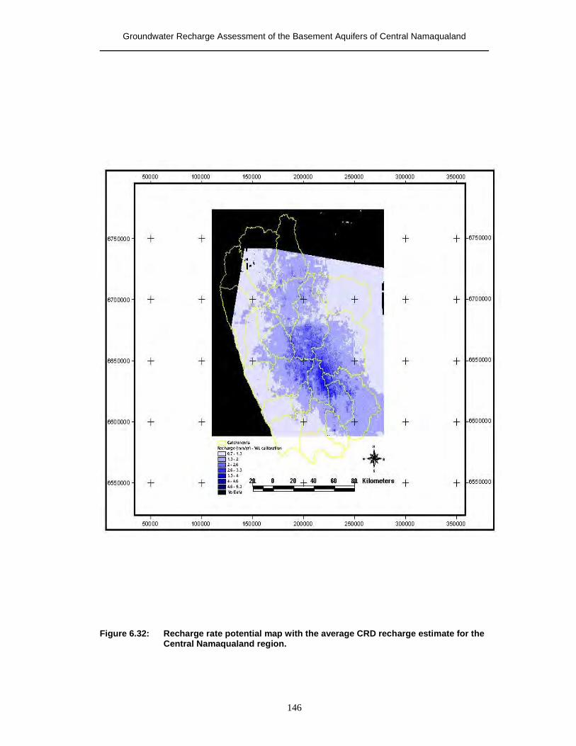
Groundwater Recharge Assessment of the Basement Aquifers of Central Namaqualand
146
Figure 6.32: Recharge rate potential map with the average CRD recharge estimate for the
Central Namaqualand region.

Groundwater Recharge Assessment of the Basement Aquifers of Central Namaqualand
147
Figure 6.33: Recharge rate potential map with the average CMB recharge estimate for the
Central Namaqualand region.
Groundwater Recharge Assessment of the Basement Aquifers of Central Namaqualand
148
6.5.2 Summary The GIS approach is an excellent tool for visualisation and spatial analysis. The method is
more descriptive, less quantitative and more subjective. The main shortcoming of the
approach is that it only assumes direct vertical infiltration. It has been demonstrated that
recharge is predominantly indirect, away from the higher lying areas. The recharge
potential map seems conceptually correct. The method is also combined with rainfall and
the spatial average of recharge from the CMB and water level fluctuation methods. A
constant value for recharge, expressed as a percentage of MAP, is applied over the entire
site. It has been shown that this is not the case for the Namaqualand region. It is now well
recognised that the rainfall to recharge relationships are not always linear in arid and semi-
arid regions, especially at finer scales.
In the mountainous regions, where rainfall is extremely high for the area, the model
assumes that most of the water is available for recharge; this may not be true. The rainfall
in the higher lying areas is available for recharge further down the topographic profile
where favourable conditions exist. The recharge for the downhill site is estimated using the
rainfall of the area, which may be lower, by a factor of two than the rainfall of the higher
lying areas. Recharge in the coastal areas is very low, but the model will assign high
recharge values to the favourable conditions specified in the weighting and overlaying
process. Data sets that may be collected that may refine the model are drainage density
maps and distribution of the alluvial aquifers associated with rivers and paleochannels.
Groundwater Recharge Assessment of the Basement Aquifers of Central Namaqualand
149
CHAPTER 7
Summary and Discussion
7.1 Evaluation of recharge assessment in Namaqualand
The main objective of this study was to estimate and characterise groundwater recharge to
the basement and alluvial aquifers of Namaqualand. The conclusions are discussed in
terms of the objectives as outlined in Chapter One.
7.1.1 Identifying methods suitable for recharge studies in the Central
Namaqualand region
Five methods have been identified that can be applied in the study area, and they are:
� Chloride mass balance (CMB) method;
� Cumulative rainfall departures (CRD) method;
� Saturated volume fluctuation (SVF) method;
� Statistical approach; and
� GIS approach.
The methods were selected based on the availability of data and data that can be obtained
easily and cost-effectively. An Excel spreadsheet program was developed to assist in
selecting different methods, based on data availability and requirements.
7.1.2 Delineating recharge areas
Recharge areas were delineated on regional and local scales. Regionally, recharge areas
correspond with the higher lying areas that receive most of the annual rainfall. Recharge
areas were identified using factor analysis, employing the interrelationship between
groundwater chemistry, isotopes and altitude to define recharge and discharge areas as well
as intermediate areas. The results of the factor analysis also indicated recharge of polluted
water into the aquifer. The GIS approach correlated various thematic layers to recharge
Groundwater Recharge Assessment of the Basement Aquifers of Central Namaqualand
150
probability. The layers were then integrated to generate a recharge potential map. Applying
the rainfall distribution map over the area effectively shows the areas most likely to receive
recharge. Although the approach gives a map that is conceptually correct, it can be further
refined.
Localised recharge areas are related to the type of aquifer. It was found that the alluvial
aquifers are easily recharged due to their hydraulic characteristics and their position within
the landscape. The structural control on the ephemeral drainage systems is evident in their
alignment along fracture systems that are associated with the underlying bedrock. The
alluvial systems are major pathways for groundwater recharge to the weathered and
bedrock zone aquifers.
7.1.3 Application and comparison of a number of independent approaches
for recharge characterisation/estimation and selection of the best
method(s) for recharge estimation
Assessing recharge to any aquifer depends on the type of area under investigation, the
availability of data, the distribution of available data and the ability to obtain meaningful
data. Groundwater resources assessment is inherently complex in semi-arid to arid
crystalline terrain. Groundwater recharge rates over large areas are difficult to estimate due
to problems associated with upscaling and data distribution. Two approaches have been
followed in this study whereby recharge was qualitatively and quantitatively assessed. The
qualitative assessment involved using existing data from the area and applying statistical
and spatial techniques to assess recharge processes and patterns. Applying the CMB
method and water level to rainfall relationships gave quantitative estimates of recharge.
The qualitative assessments of recharge, using statistical analysis (R and Q mode factor
analysis) and the GIS assessment techniques, identify areas that are receiving recharge as
well as being favourable for potential recharge. The statistical analysis is useful in that it
also indicates areas of localised artificial recharge through agricultural and domestic
activities. The isotope approach also provided some useful information in terms of
recharge processes and the time since recharge. It was found that most of the recharged
water was evaporated at the surface, as evidenced in the stable isotope data. Recharge is
thus mainly indirect except for the higher-lying mountainous areas where recharge is
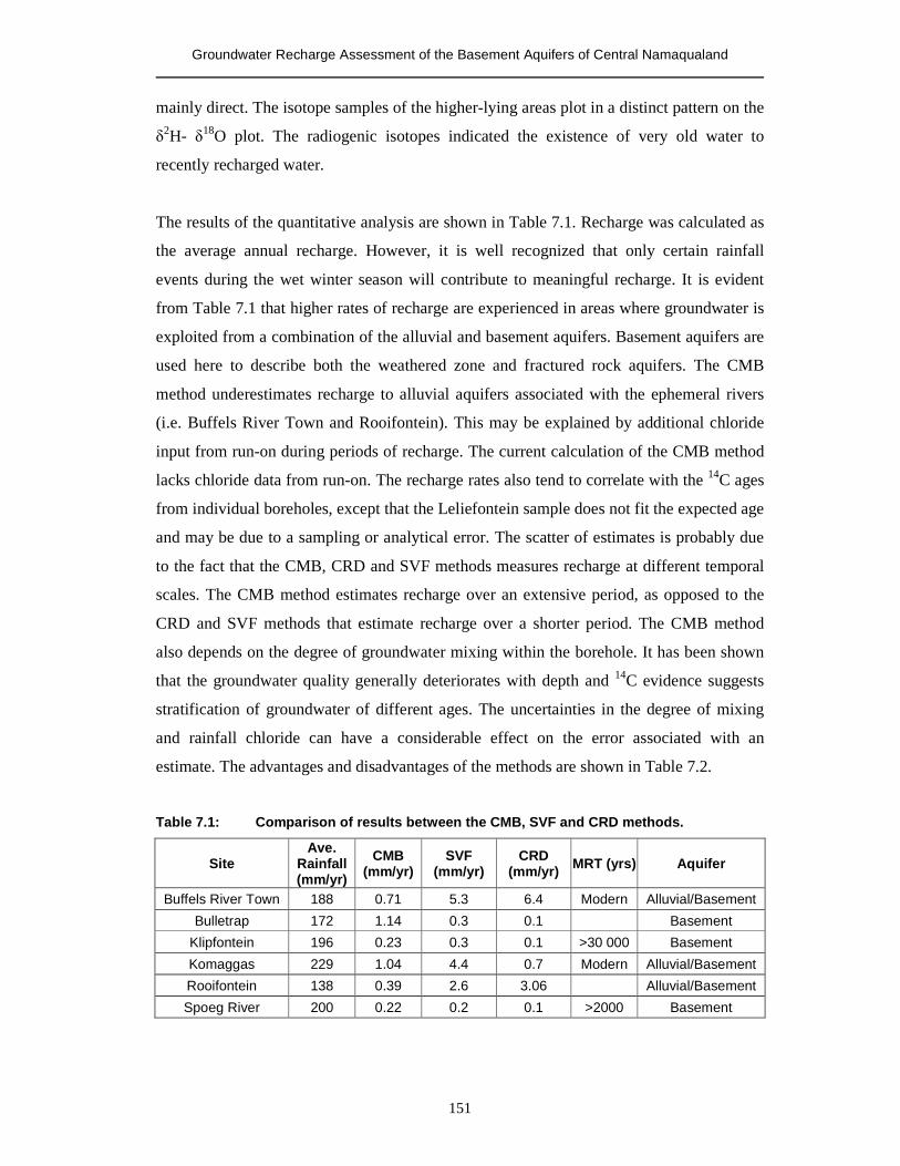
Groundwater Recharge Assessment of the Basement Aquifers of Central Namaqualand
151
mainly direct. The isotope samples of the higher-lying areas plot in a distinct pattern on the
�2H- �18O plot. The radiogenic isotopes indicated the existence of very old water to
recently recharged water.
The results of the quantitative analysis are shown in Table 7.1. Recharge was calculated as
the average annual recharge. However, it is well recognized that only certain rainfall
events during the wet winter season will contribute to meaningful recharge. It is evident
from Table 7.1 that higher rates of recharge are experienced in areas where groundwater is
exploited from a combination of the alluvial and basement aquifers. Basement aquifers are
used here to describe both the weathered zone and fractured rock aquifers. The CMB
method underestimates recharge to alluvial aquifers associated with the ephemeral rivers
(i.e. Buffels River Town and Rooifontein). This may be explained by additional chloride
input from run-on during periods of recharge. The current calculation of the CMB method
lacks chloride data from run-on. The recharge rates also tend to correlate with the 14C ages
from individual boreholes, except that the Leliefontein sample does not fit the expected age
and may be due to a sampling or analytical error. The scatter of estimates is probably due
to the fact that the CMB, CRD and SVF methods measures recharge at different temporal
scales. The CMB method estimates recharge over an extensive period, as opposed to the
CRD and SVF methods that estimate recharge over a shorter period. The CMB method
also depends on the degree of groundwater mixing within the borehole. It has been shown
that the groundwater quality generally deteriorates with depth and 14C evidence suggests
stratification of groundwater of different ages. The uncertainties in the degree of mixing
and rainfall chloride can have a considerable effect on the error associated with an
estimate. The advantages and disadvantages of the methods are shown in Table 7.2.
Table 7.1: Comparison of results between the CMB, SVF and CRD methods.
Site Ave.
Rainfall (mm/yr)
CMB (mm/yr)
SVF (mm/yr)
CRD (mm/yr) MRT (yrs) Aquifer
Buffels River Town 188 0.71 5.3 6.4 Modern Alluvial/Basement
Bulletrap 172 1.14 0.3 0.1 Basement
Klipfontein 196 0.23 0.3 0.1 >30 000 Basement
Komaggas 229 1.04 4.4 0.7 Modern Alluvial/Basement
Rooifontein 138 0.39 2.6 3.06 Alluvial/Basement
Spoeg River 200 0.22 0.2 0.1 >2000 Basement
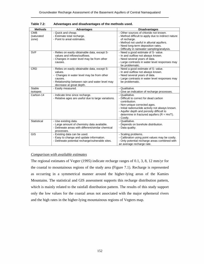
Groundwater Recharge Assessment of the Basement Aquifers of Central Namaqualand
152
Table 7.2: Advantages and disadvantages of the methods used.
Methods Advantages Disadvantages CMB (saturated zone)
- Quick and cheap. - Estimate total recharge. - Point to areal estimates.
- Other sources of chloride not known. - Method difficult to apply due to indirect nature
of recharge. - Method not useful in alluvial aquifers. - Need long-term deposition rates. - Difficulty in rainwater sampling/analysis.
SVF - Relies on easily obtainable data, except S- values and inflows/outflows.
- Changes in water level may be from other causes.
- Need a good estimate of S- value. - In and outflow not always known. - Need several years of data. - Large contrasts in water level responses may
be problematic. CRD - Relies on easily obtainable data, except S-
values. - Changes in water level may be from other
causes. - Relationship between rain and water level may
decrease at great depth.
- Need a good estimate of S- value. - In and outflow not always known. - Need several years of data. - Large contrasts in water level responses may
be problematic.
Stable isotopes
- Easily measured. - Qualitative. - Give an indication of recharge processes.
Carbon-14 - Indicate time since recharge. - Relative ages are useful due to large variations.
- Qualitative. - Difficult to correct for dead carbon
contribution. - Non-unique corrected ages. - Initial radionuclide activity not always known. - Aquifer depth and porosity difficult to
determine in fractured aquifers (R = Hn/T). - Costly.
Statistical - Use existing data. - Large amount of chemistry data available. - Delineate areas with different/similar chemical
processes.
- Qualitative. - Depends on borehole distribution. - Data quality.
GIS - Existing data can be used. - Easy to change and update information. - Delineate potential recharge/vulnerable sites.
- Scaling problems. - Calibration using point values may be costly. - Only potential recharge areas combined with an average recharge rate.
Comparison with available estimates
The regional estimates of Vegter (1995) indicate recharge ranges of 0.1, 3, 8, 12 mm/yr for
the coastal to mountainous regions of the study area (Figure 7.1). Recharge is represented
as occurring in a symmetrical manner around the higher-lying areas of the Kamies
Mountains. The statistical and GIS assessment supports this recharge distribution pattern,
which is mainly related to the rainfall distribution pattern. The results of this study support
only the low values for the coastal areas not associated with the major ephemeral rivers
and the high rates in the higher-lying mountainous regions of Vegters map.
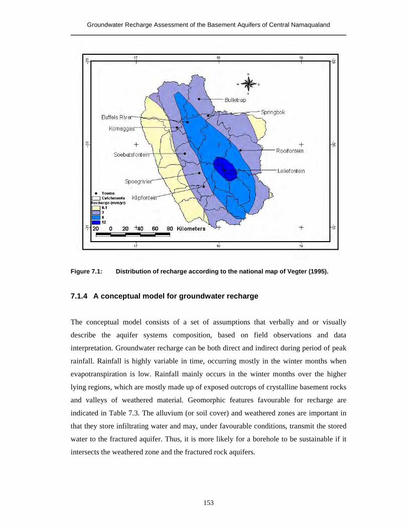
Groundwater Recharge Assessment of the Basement Aquifers of Central Namaqualand
153
Figure 7.1: Distribution of recharge according to the national map of Vegter (1995).
7.1.4 A conceptual model for groundwater recharge
The conceptual model consists of a set of assumptions that verbally and or visually
describe the aquifer systems composition, based on field observations and data
interpretation. Groundwater recharge can be both direct and indirect during period of peak
rainfall. Rainfall is highly variable in time, occurring mostly in the winter months when
evapotranspiration is low. Rainfall mainly occurs in the winter months over the higher
lying regions, which are mostly made up of exposed outcrops of crystalline basement rocks
and valleys of weathered material. Geomorphic features favourable for recharge are
indicated in Table 7.3. The alluvium (or soil cover) and weathered zones are important in
that they store infiltrating water and may, under favourable conditions, transmit the stored
water to the fractured aquifer. Thus, it is more likely for a borehole to be sustainable if it
intersects the weathered zone and the fractured rock aquifers.
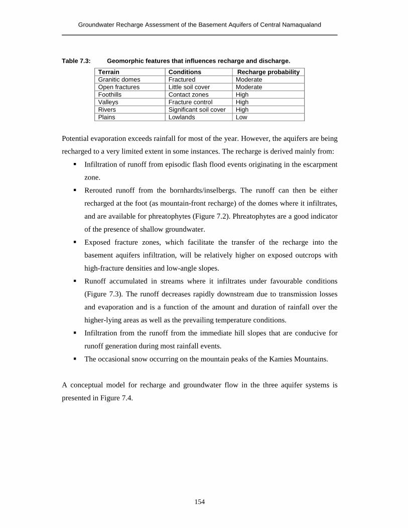
Groundwater Recharge Assessment of the Basement Aquifers of Central Namaqualand
154
Table 7.3: Geomorphic features that influences recharge and discharge.
Terrain Conditions Recharge probability Granitic domes Fractured Moderate Open fractures Little soil cover Moderate Foothills Contact zones High Valleys Fracture control High Rivers Significant soil cover High Plains Lowlands Low
Potential evaporation exceeds rainfall for most of the year. However, the aquifers are being
recharged to a very limited extent in some instances. The recharge is derived mainly from:
� Infiltration of runoff from episodic flash flood events originating in the escarpment
zone.
� Rerouted runoff from the bornhardts/inselbergs. The runoff can then be either
recharged at the foot (as mountain-front recharge) of the domes where it infiltrates,
and are available for phreatophytes (Figure 7.2). Phreatophytes are a good indicator
of the presence of shallow groundwater.
� Exposed fracture zones, which facilitate the transfer of the recharge into the
basement aquifers infiltration, will be relatively higher on exposed outcrops with
high-fracture densities and low-angle slopes.
� Runoff accumulated in streams where it infiltrates under favourable conditions
(Figure 7.3). The runoff decreases rapidly downstream due to transmission losses
and evaporation and is a function of the amount and duration of rainfall over the
higher-lying areas as well as the prevailing temperature conditions.
� Infiltration from the runoff from the immediate hill slopes that are conducive for
runoff generation during most rainfall events.
� The occasional snow occurring on the mountain peaks of the Kamies Mountains.
A conceptual model for recharge and groundwater flow in the three aquifer systems is
presented in Figure 7.4.
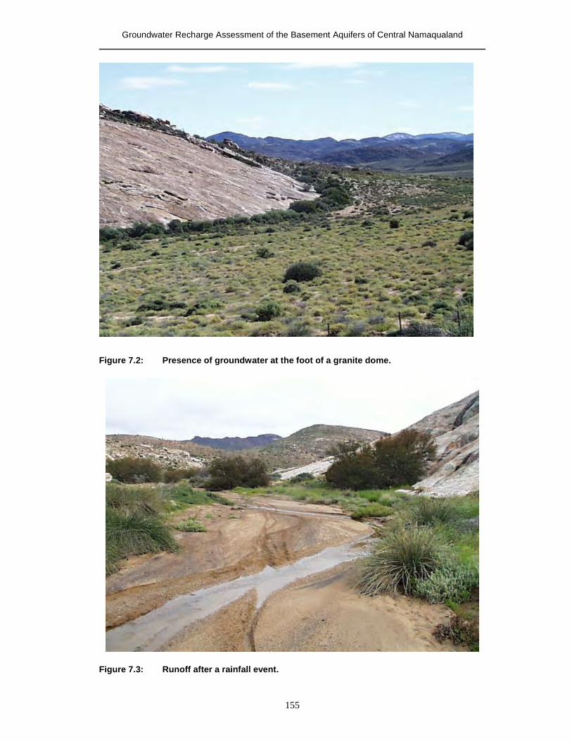
Groundwater Recharge Assessment of the Basement Aquifers of Central Namaqualand
155
Figure 7.2: Presence of groundwater at the foot of a granite dome.
Figure 7.3: Runoff after a rainfall event.
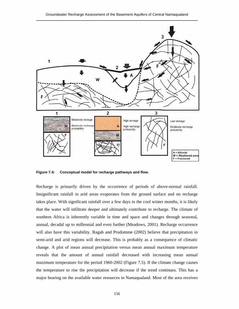
Groundwater Recharge Assessment of the Basement Aquifers of Central Namaqualand
156
Figure 7.4: Conceptual model for recharge pathways and flow.
Recharge is primarily driven by the occurrence of periods of above-normal rainfall.
Insignificant rainfall in arid areas evaporates from the ground surface and no recharge
takes place. With significant rainfall over a few days in the cool winter months, it is likely
that the water will infiltrate deeper and ultimately contribute to recharge. The climate of
southern Africa is inherently variable in time and space and changes through seasonal,
annual, decadal up to millennial and even further (Meadows, 2001). Recharge occurrence
will also have this variability. Ragab and Prudomme (2002) believe that precipitation in
semi-arid and arid regions will decrease. This is probably as a consequence of climatic
change. A plot of mean annual precipitation versus mean annual maximum temperature
reveals that the amount of annual rainfall decreased with increasing mean annual
maximum temperature for the period 1960-2002 (Figure 7.5). If the climate change causes
the temperature to rise the precipitation will decrease if the trend continues. This has a
major bearing on the available water resources in Namaqualand. Most of the area receives
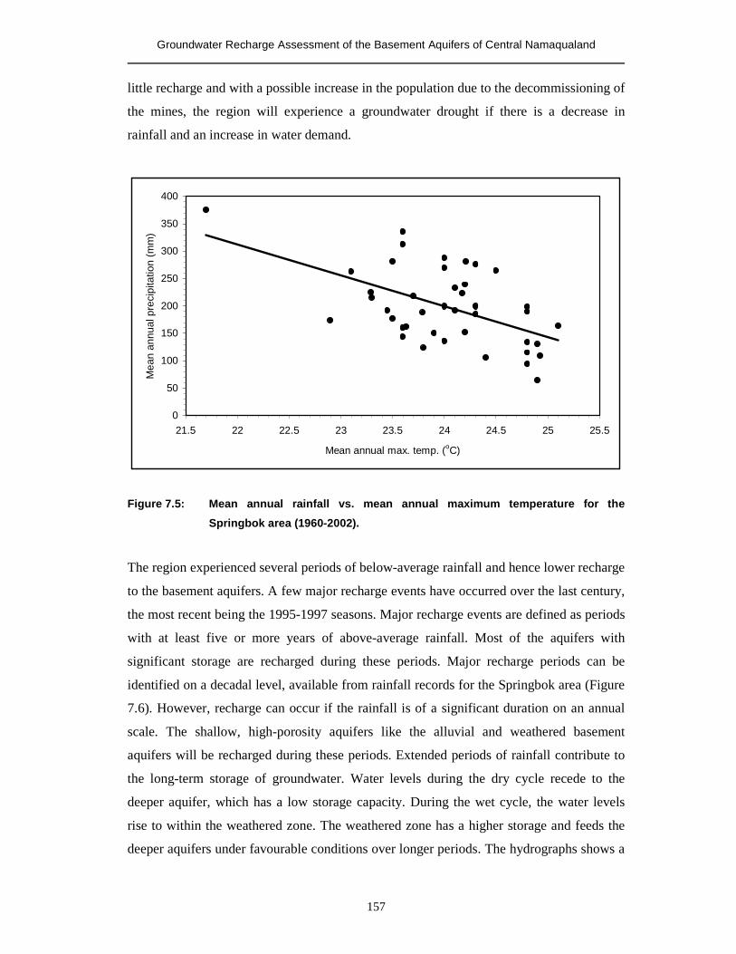
Groundwater Recharge Assessment of the Basement Aquifers of Central Namaqualand
157
little recharge and with a possible increase in the population due to the decommissioning of
the mines, the region will experience a groundwater drought if there is a decrease in
rainfall and an increase in water demand.
0
50
100
150
200
250
300
350
400
21.5 22 22.5 23 23.5 24 24.5 25 25.5
Mean annual max. temp. (oC)
Mea
n an
nual
pre
cipi
tatio
n (m
m)
Figure 7.5: Mean annual rainfall vs. mean annual maximum temperature for the
Springbok area (1960-2002).
The region experienced several periods of below-average rainfall and hence lower recharge
to the basement aquifers. A few major recharge events have occurred over the last century,
the most recent being the 1995-1997 seasons. Major recharge events are defined as periods
with at least five or more years of above-average rainfall. Most of the aquifers with
significant storage are recharged during these periods. Major recharge periods can be
identified on a decadal level, available from rainfall records for the Springbok area (Figure
7.6). However, recharge can occur if the rainfall is of a significant duration on an annual
scale. The shallow, high-porosity aquifers like the alluvial and weathered basement
aquifers will be recharged during these periods. Extended periods of rainfall contribute to
the long-term storage of groundwater. Water levels during the dry cycle recede to the
deeper aquifer, which has a low storage capacity. During the wet cycle, the water levels
rise to within the weathered zone. The weathered zone has a higher storage and feeds the
deeper aquifers under favourable conditions over longer periods. The hydrographs shows a
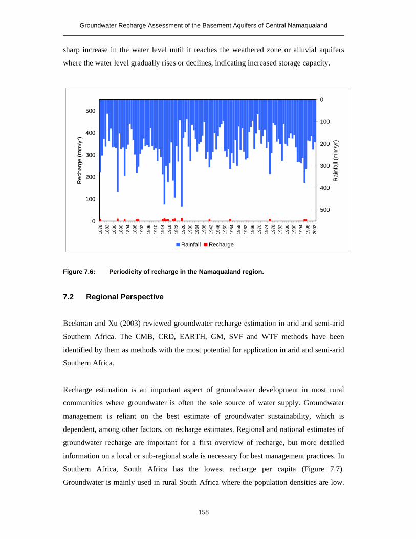
Groundwater Recharge Assessment of the Basement Aquifers of Central Namaqualand
158
sharp increase in the water level until it reaches the weathered zone or alluvial aquifers
where the water level gradually rises or declines, indicating increased storage capacity.
0
100
200
300
400
500
1878
1882
1886
1890
1894
1898
1902
1906
1910
1914
1918
1922
1926
1930
1934
1938
1942
1946
1950
1954
1958
1962
1966
1970
1974
1978
1982
1986
1990
1994
1998
2002
Rec
harg
e (m
m/y
r)
0
100
200
300
400
500
Rai
nfal
l (m
m/y
r)
Rainfall Recharge
Figure 7.6: Periodicity of recharge in the Namaqualand region.
7.2 Regional Perspective
Beekman and Xu (2003) reviewed groundwater recharge estimation in arid and semi-arid
Southern Africa. The CMB, CRD, EARTH, GM, SVF and WTF methods have been
identified by them as methods with the most potential for application in arid and semi-arid
Southern Africa.
Recharge estimation is an important aspect of groundwater development in most rural
communities where groundwater is often the sole source of water supply. Groundwater
management is reliant on the best estimate of groundwater sustainability, which is
dependent, among other factors, on recharge estimates. Regional and national estimates of
groundwater recharge are important for a first overview of recharge, but more detailed
information on a local or sub-regional scale is necessary for best management practices. In
Southern Africa, South Africa has the lowest recharge per capita (Figure 7.7).
Groundwater is mainly used in rural South Africa where the population densities are low.
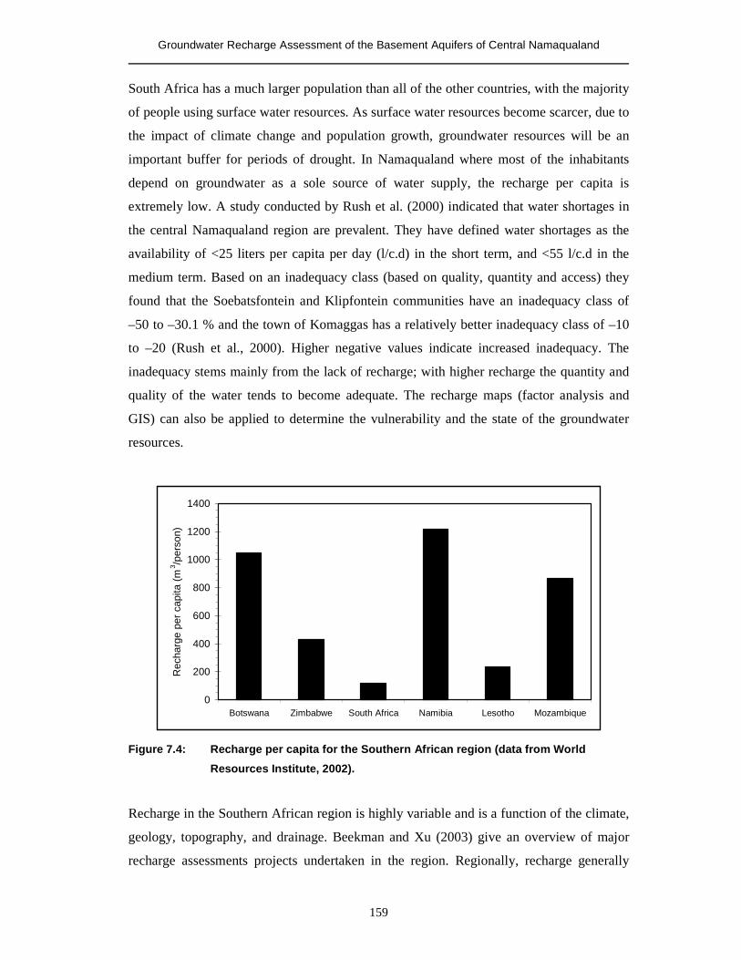
Groundwater Recharge Assessment of the Basement Aquifers of Central Namaqualand
159
South Africa has a much larger population than all of the other countries, with the majority
of people using surface water resources. As surface water resources become scarcer, due to
the impact of climate change and population growth, groundwater resources will be an
important buffer for periods of drought. In Namaqualand where most of the inhabitants
depend on groundwater as a sole source of water supply, the recharge per capita is
extremely low. A study conducted by Rush et al. (2000) indicated that water shortages in
the central Namaqualand region are prevalent. They have defined water shortages as the
availability of <25 liters per capita per day (l/c.d) in the short term, and <55 l/c.d in the
medium term. Based on an inadequacy class (based on quality, quantity and access) they
found that the Soebatsfontein and Klipfontein communities have an inadequacy class of
–50 to –30.1 % and the town of Komaggas has a relatively better inadequacy class of –10
to –20 (Rush et al., 2000). Higher negative values indicate increased inadequacy. The
inadequacy stems mainly from the lack of recharge; with higher recharge the quantity and
quality of the water tends to become adequate. The recharge maps (factor analysis and
GIS) can also be applied to determine the vulnerability and the state of the groundwater
resources.
0
200
400
600
800
1000
1200
1400
Botswana Zimbabwe South Africa Namibia Lesotho Mozambique
Rec
harg
e pe
r cap
ita (m
3 /per
son)
Figure 7.4: Recharge per capita for the Southern African region (data from World
Resources Institute, 2002).
Recharge in the Southern African region is highly variable and is a function of the climate,
geology, topography, and drainage. Beekman and Xu (2003) give an overview of major
recharge assessments projects undertaken in the region. Regionally, recharge generally
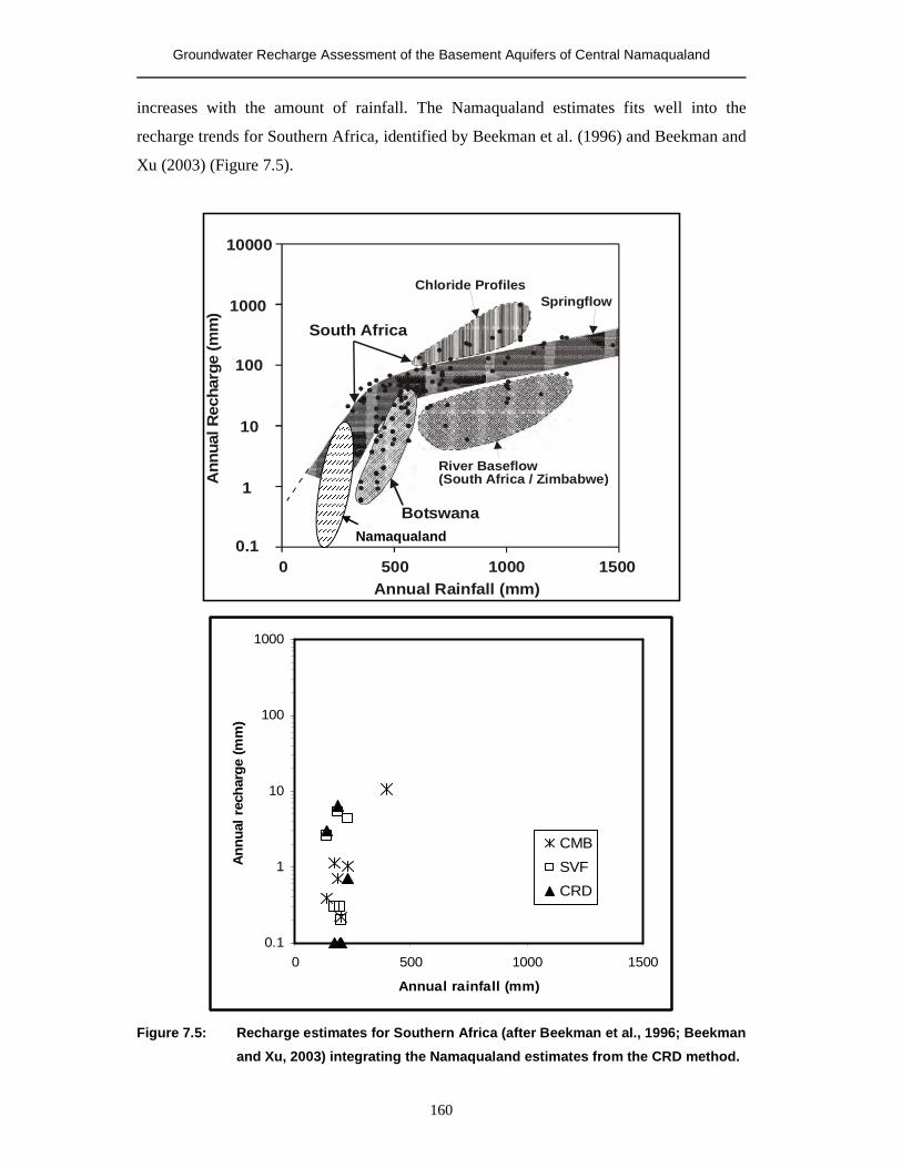
Groundwater Recharge Assessment of the Basement Aquifers of Central Namaqualand
160
increases with the amount of rainfall. The Namaqualand estimates fits well into the
recharge trends for Southern Africa, identified by Beekman et al. (1996) and Beekman and
Xu (2003) (Figure 7.5).
0.1
1
10
100
1000
0 500 1000 1500
Annual rainfall (mm)
Ann
ual r
echa
rge
(mm
)
CMB
SVF
CRD
Figure 7.5: Recharge estimates for Southern Africa (after Beekman et al., 1996; Beekman
and Xu, 2003) integrating the Namaqualand estimates from the CRD method.
Annual Rainfall (mm)
Botswana
Ann
ual R
echa
rge
(mm
)
10000
1000
100
10
1
0.10 500 1000 1500
River Baseflow(South Africa / Zimbabwe)
South Africa
Chloride ProfilesSpringflow
Namaqualand
Groundwater Recharge Assessment of the Basement Aquifers of Central Namaqualand
161
7.3 Final remarks
This is the first systematic recharge study carried out in the central Namaqualand region.
The results indicate that recharge is higher in the alluvial aquifers than in the hard rock
basement aquifers. The results also indicate that recharge decreases from the escarpment
zone to the coastal zone. Even under favourable rainfall conditions the areas around
Klipfontein and Spoeg River receives minimal recharge. This phenomenon is probably
related to the surface features in the areas.
� Groundwater recharge rates to the basement and alluvial aquifers are estimated to
be within 0.1 and 10 mm/yr, with the higher values being mainly to the alluvial
aquifers and high altitude sites, and the lower limits to the fractured rock aquifers.
� Groundwater level fluctuations and rainfall (CRD and SVF) was successfully used
to estimate groundwater recharge. Water level data is usually available in most
areas due to community water supply schemes. Uncertainties with regard to the
determination of storage coefficients and contributing areas to recharge in fractured
hard rock terrain are still of concern for most hydrogeologists. The estimates used
in the calculations are ‘best estimates’.
� The CMB method is still a useful method for recharge estimations in most
hydrogeological provinces as a first estimate of recharge. However, the method, if
applied on its own, may not give an accurate account of recharge rates. The
uncertainties and assumptions of the method need to be considered when
interpreting the results. The recharge rates estimated for the alluvial aquifers are
lower than expected. This is a result of the unaccounted chloride in the surface
runoff flux.
� Isotope data indicate water ranging from very young to very old (<50 years - >30
000 years). Intermediate ages indicate active mixing of younger and old water.
� Recharge is related to the amount of rainfall and the position of the aquifers within
the landscape, which is, in turn, related to altitude and topography. Recharge
mainly occurs when rainfall is above normal. Above-normal rainfall produces more
intense runoff that can travel further down the hydrological profile, recharging
more of the alluvial aquifers.
� Recharge occurs as primary recharge in the mountainous areas where direct
infiltration is more likely. Indirect recharge involves the infiltration of surface
Groundwater Recharge Assessment of the Basement Aquifers of Central Namaqualand
162
runoff and discharges from springs and adjacent aquifers, dominating in most of the
areas.
� Flood events will produce significant recharge, mainly to the alluvial aquifers.
� Recharge estimates that may seem to be within acceptable limits of error when
interpreted, may be significantly high when applied to determine aquifer
sustainability. Rainfall in semi-arid regions is episodic in nature, where most of the
annual rainfall can occur within a very short period of time with a concomitant
increase in recharge if favourable conditions exist, as opposed to distributing the
rainfall over an entire year. The use of mean annual recharge rates can be
misleading, as the simulated period only includes years of above-average rainfall
and not the long-term cyclicity of rainfall.
� Recharge in arid to semi-arid crystalline basement aquifers is neither
straightforward nor simple and needs both a qualitative (e.g. field observations and
local knowledge) and a quantitative approach.
7.4 Future research
Topics or issues that must be considered for future research include:
� Results and techniques provided by this baseline study should be used to acquire
additional data to optimise the estimated recharge rates.
� The utilisation of complementary water sources needs to be highlighted, such as
rainwater harvesting, fog water collection, and artificial recharge using runoff, for
example, from the bornhardts. Some of these schemes are operated on a limited
scale in the area and can be expanded to other areas.
� Measurement campaigns for chloride deposition in precipitation.
� Application of the recharge estimates to management scenarios.
� Quantification of episodic recharge at various temporal scales.
� Scenario-based studies on the impact of climatic change on future groundwater
resources.
� Expanding the GIS approach to distribute point estimates from a particular area to
similar areas elsewhere. The spatial heterogeneity of recharge introduces
difficulties in upscaling, and needs additional research aimed at improving the
application of point data to larger areas.
� Hill slope processes and their impact on groundwater flow and recharge.
Groundwater Recharge Assessment of the Basement Aquifers of Central Namaqualand
163
References
Abdel-Naby AS and Nouh SA (2002). Stabilization of poly(vinyl chloride) against laser
radiation with ethyl-N-phenylmaleimide-4-carboxylate. Polymer Degradation and
Stability, 76, 419-423.
Acocks, J.P.H. (1988). Veld types of South Africa. Third edition. Botanical Survey
Memoir 57.
Acworth RI (1987). The development of crystalline basement aquifers in atropical
environment. Quaterly Journal of Engineering Geology, 20, 265-272.
Adams S, Titus RA, Pietersen KC, Tredoux G and Harris C (2001). Hydrochemical
characteristics of aquifers near Sutherland in the Western Karoo, South Africa.
Journal of Hydrology, 241, 91-103.
Albat HM (1984). The Proterozoic granulite facies terrane around Kliprand, Namaqualand
Metamorphic Complex. Bulletin 33, Precambrian Research Unit. Dept. of
Geology, University of Cape Town.
Allen AD and Davidson WA (1982). Review of groundwater resources in fractured rocks
in western Australia. In: Papers of the groundwater in fractured rock conference,
Canberra, Aug. 31 – Sept 3. AWRC Conf. Ser. No. 5, 1-12.
Aller L, Bennet T, Lehr JH and Petty RJ (1987). DRASTIC – A standardised system for
evaluating groundwater pollution potential using hydrogeological setting. US EPA
Report EPA/600/2-87/035, United States Environmental Protection Agency.
Allison GB (1988). A review of the physical, chemical and isotopic techniques available
for estimating groundwater recharge. In: I. Simmers (ed), Estimation of natural
groundwater recharge. NATO ASI Series C222, Reidel, Dorderecht.
Allison GB and Hughes MW (1978). The use of environmental chloride and tritium to
estimate total recharge to an unconfined aquifer. Australian Journal of Soil
Research, 16, 181-195.
Allison GB, Barnes CJ, Hughes MW and Leaney FWJ (1984). Effect of climate and
vegetation on oxygen-18 and deuterium profiles in soils. Isotope Hydrology 1983.
Proc. Symp. Vienna, IAEA, 105-123.
Allison GB, Gee GW and Tyler SW (1994). Vadose-zone techniques for estimating
groundwater recharge in arid and semiarid regions. Soil Sci. Soc. Am. J., 58, 6.14.
Groundwater Recharge Assessment of the Basement Aquifers of Central Namaqualand
164
Al-Malack MH (2001). Migration of lead from unplasticized polyvinyl chloride pipes.
Journal of Hazardous Materials. B82, 263-274.
Andersson J-E, Ekman L, Nordqvist R and Winberg A (1991). Hydraulic testing and
modelling of a low angle fracture zone at Finnsjön, Sweden. Journal of Hydrology,
126, 1-2, 45-77.
API (American Petroleum Institute) (1997). Estimation of infiltration and recharge for
environmental site assessment. API Soil and Groundwater Research Bulletin, 2, 1-
4.
Appelo CAJ and Postma D (1994). Geochemistry groundwater and pollution. Balkema,
Rotterdam.
Ashley RP and Lloyd JW (1978). An example of the use of factor analysis and cluster
analysis in groundwater chemistry interpretation. Journal of Hydrology, 39, 355-
364.
Athavale RN and Rangarajan R (1990). Natural recharge measurements in the hard rock
regions of semi-arid India using tritium injection – a review. In Lerner et al. (eds).
Groundwater recharge: A guide to understanding and estimating natural recharge.
Volume 8, IAH, Heise, Hannover.
Banks D and Robins N (2002). An introduction to groundwater in crystalline bedrock.
Geological Survey of Norway.
Banks D, Rohr-Torp E and Skarphagen H (1994). Groundwater resources in hard rock:
experiences from the Hvaler study, southeastern Norway. Applied Hydrogeology,
2,2, 33-42.
Bazuhair AS and Wood WW (1996). Chloride mass-balance method for estimating ground
water recharge in arid areas: examples from western Saudi Arabia. Journal of
Hydrology. Elsevier.153-159.
Bear J (1972). Dynamics of fluids in porous media. Elsevier, New York
Bear J, Beljin MS and Ross RR (1992). Ground Water Issue: Fundamentals of Ground-
Water Modeling. EPA Report 540/S-92/005
Beekman HE and Selaolo ET (1997). Recharge in the Eastern Botswana Kalahari –
Hydrochemical isotope and noble gases tracer study in the Letlhakeng-
Botlhlapatlou area. GRES II project: Technical report, Department of Geological
Survey, Lobatse, University of Botswana and the Free University Amsterdam, The
Netherlands.
Groundwater Recharge Assessment of the Basement Aquifers of Central Namaqualand
165
Beekman HE and Xu Y (2003). Review of groundwater recharge estimation in arid and
semi-arid Southern Africa. In Xu Y and Beekman HE (eds). UNESCO IHP Series
64.
Beekman HE and Sunguro S (2002). Groundwater recharge estimation – suitability and
reliability of three types of rain gauges for monitoring chloride deposition.
Groundwater Division, Western Cape Conference: Tales of a hidden treasure.
Somerset West 16 September.
Beekman HE, Gieske A and Selaolo ET (1996). GRES: Groundwater Recharge Studies in
Botswana 1987-1996. Botswana Journal of Earth Sciences, 3, 1-17.
Bense V, Hooijboer A and Brokx W (1998). Morphotectonic and hydrogeomorphic control
on the hydrogeology of the Buffelsrivier catchment. Vrije Universiteit, Amsterdam.
Bergkamp G (1998). A hierarchical view of the interactions of runoff and infiltration with
vegetation and microtopography in semiarid shrublands. Catena, 33, 201-220.
Bergström S and Graham PL (1998). On the scale problem in hydrological modelling.
Journal of Hydrology, 253-265.
Berkowitz B (2002). Characterisisng flow and transport in fractured geological media: a
review. Advances in Water Resources, 25, 861-884.
Berndtsson R and Larson M (1987). Spatial variability of infiltration in a semi-arid
environment. Journal of Hydrology, 90, 117-133.
Black JH (1994). Hydrogeology of fractured rocks – a question of uncertainty about
geometry. Applied Hydrogeology, 3, 56-70.
Blöschl G and Sivapalan M (1995). Scale issues in hydrological modelling. Hydrological
Processes, 9, 251-290.
Bredenkamp DB (2000). Groundwater monitoring: a critical evaluation of groundwater
monitoring in water resources evaluation and management. WRC Report No.
838/1/00.
Bredenkamp DB, Botha LJ, Van Tonder GJ and Van Rensburg HJ (1995). Manual on
quantitative estimation of groundwater recharge and aquifer storativity. WRC
Report TT 73/95.
Brunsell N and Gillies RR (2003). Scale issues in land-atmosphere interactions:
implications for remote sensing of the surface energy balance. Agricultural and
Forest Meteorology, 117, 203-221.
Groundwater Recharge Assessment of the Basement Aquifers of Central Namaqualand
166
Butt CRM, Lintern MJ and Anand RR (2000). Evolution of regoliths and landscapes in
deeply weathered terrain – implications for geochemical exploration. Ore Geology
Reviews, 16, 167-183.
Buxton GV, Bydder M, Salmon GA and Williams JE (2000). The reactivity of chlorine
atoms in aqueous solution: Part III. The reactions of Cl. with solutes.
Campbell EE, Parker-Nance T and Bate GC (1992). A Compilation of the information on
the magnitude, nature and importance of coastal aquifers in Southern Africa. WRC
Report No 370/1/92.
Chiang W-H, Kinzelbach W (2001). 3D-Groundwater modelling with PMWIN. Springer.
Berlin, Heidelberg, New York.
Chilton PJ and Foster SSD (1995). Hydrogeological characteristics and water-supply
potential of basement aquifers in tropical Africa. Hydrogeology Journal, 3, 1, 36-
49.
Clark ID and Fritz P (1997). Environmental Isotopes in Hydrogeology. Lewis Publishers.
Clauser C (1992). Permeability of Crystalline rocks. EOS Trans. Am. Geophys. Union, 73,
21, 233-240.
Clauser C (2001). Update of the permeability of crystalline rocks. http://www.rwth-
aachen.de/geop/Forschung/Petrophysik/rocks/perm.htm. Accessed July 2003.
Cook PG (2003). A guide to regional groundwater flow in fractured rock aquifers. CSIRO
Land and Water, Glen Osmond, Australia.
Cook PG, Walker GR and Jolly ID (1989). Spatial variability of groundwater recharge in a
semiarid region. Journal of Hydrology, 111, 195.212.
Craig H (1961). Isotopic variations in meteoric waters. Science, 133: 1702-1703.
Dalton MG and Upchurch SB (1979). Interpretation of hydrochemical facies by factor
analysis. Ground Water, 16, 4, 228-233.
Daniel III CC (1996). Ground-water recharge to the regolith-fractured crystalline rock
aquifer system, Orange County, North Carolina. USGS Water Resources
Investigations Report 96-4220.
Dansgaard W (1964). Stable isotopes in precipitation. Tellus, 16 (4): 436-468.
Dawdy DR and Feth JH (1967). Applications of factor analysis in study of chemistry of
groundwater quality, Mojave River Valley, California. Water Resources Research,
3, 2, 505-510.
De Gita J (2002). PhD progress report. University of the Western Cape.
Groundwater Recharge Assessment of the Basement Aquifers of Central Namaqualand
167
De Villiers SE and Cadman A (2001). An analysis of the palynomorphs obtained from
Tertiary sediments at Koingnaas, Namaqualand, South Africa. Journal of African
Earth Sciences, 33, 1, 17-47.
De Wit MCJ (1993). Cainozoic evolution of drainage systems in the North-Western Cape.
Ph.D Thesis, University of Cape Town.
Degnan JR and Clark Jr SF (2002). Fracture-correlated lineaments at Great Bay,
Southeastern New Hampshire. USGS Open-File Report 02-13, New Hampshire.
Dent MC, Lynch SD and Tarboton H (1990). Detailed delimitation of rainfall regions in
southern Africa. Water SA, 16, 1, 1-4.
Diamond RE and Harris C (2000). Oxygen and hydrogen isotope geochemistry of thermal
springs of the Western Cape: Recharge at high altitude? Journal of African Earth
Sciences, 31, 467-481.
Diamond RE and Harris C (1997). Oxygen and hydrogen isotope composition of Western
Cape meteoric water. South African Journal of Science, 93, 371-374.
Domenico PA and Schwartz FW (1990). Physical and Chemical Hydrogeology. John
Wiley and Sons. New York.
Dong W, Yu Z and Weber D (2003). Simulations on soil water variation in arid regions.
Journal of Hydrology, 275, 162-181.
Dunne T (1983). Relation of field studies and modelling in the prediction of storm runoff.
Journal of Hydrology, 65, 25-48.
DWAF (1990). Grondwaterondersoek in die Komaggas-kleurling gebied, distrik
Namakwaland. Tegniese Verslg GH 3654. Department of Water Affairs and
Forestry.
DWAF (pers. comm.). Directorate Geohydrology, Kimberley office.
Edet AE, Okereke CS, Teme SC and Esu EO (1998). Application of remote-sensing data to
groundwater exploration: A case study of the Cross River State, southeastern
Nigeria. Hydrogeology Journal, 6, 394-404.
Edmunds WM and Gaye CB (1994). Estimating the spatial variability of groundwater
recharge in the Sahel using chloride. Journal of Hydrology, 156, 47-59.
Edmunds WM and Wright EP (1979). Groundwater recharge and paleoclimate in the Sirte
and Kufra basins, Libya. Journal of Hydrology, 40, 215-241.
Ellis F (1988). Die gronde van die Karoo. PhD thesis. University of Stellenbosch.
Groundwater Recharge Assessment of the Basement Aquifers of Central Namaqualand
168
Ellis EE (1909). Ground water in the crystalline rocks of Connecticut. In: Gregory, HE.
Underground water resources of Connecticut. United States Geological Survey
Water-Supply Paper 232, 54-103.
Eriksson E and Khunakasem V (1969). Chloride concentration in groundwater recharge
rate of deposition of chloride in the Israel coastal plain. Journal of Hydrology, 7,
178-197.
Flanagan LE (2003). Application of laboratory core analysis techniques to determine the
intrinsic primary hydraulic properties of basement rocks in the vicinity of
Nababeep, Northen Cape Province, South Africa. Unpublished MSc Thesis,
University of the Western Cape.
Franke OL, Reilly TE and Bennett GD (1987). Definition of boundary and initial
conditions in the analysis of saturated ground-water flow systems – An
introduction: Techniques of Water-Resource Investigations of the US Geological
Survey. Book 3: Applications of Hydraulics, Chapter B5. USGS.
Freeze R and Cherry JA (1979). Groundwater. Prentice-Hall Inc, New Jersey.
Galloway JN and Likens GE (1978). The collection of precipitation for chemical analysis.
Tellus, 30, 71-82.
Garner HF (1974). The origin of landscapes.: A synthesis of geomorphology. Oxford
University Press, New York.
Gat JR (1980). The isotopes pf hydrogen and oxygen in precipitation. In Handbook of
environmental isotope geochemistry, (eds) Fritz P and Ch. Fontes J, Elsevier,
Amsterdam.
Gaye CB and Edmunds WM (1996). Groundwater recharge estimation using chloride,
stable isotopes and tritium profiles in the sands of northwestern Senegal.
Environmental Geology, 27, 246-251.
Gee GW and Hillel D (1988). Groundwater recharge in arid regions: Review and critique
of estimation methods. Hydrological Processes, 2, 255-266.
Gieske A (1992). Dynamics of groundwater recharge: A case study in semi-arid Eastern
Botswana. PhD Thesis. Vrije Universiteit, Amsterdam.
Greenbaum D (1985). Review of remote sensing applications to groundwater exploration
in basement and regolith. British Geological Survey Report OD 85/8.
Gupta AS and Rao KS (1998). Index properties of weathered rocks: inter-relationships and
applicability. Bull. Eng. Geol. Env., 57, 161-172.
Groundwater Recharge Assessment of the Basement Aquifers of Central Namaqualand
169
Gustafson G and Krásný J (1994). Crystalline rock aquifers: their occurrence, use and
importance. Applied Hydrogeology, 2, 2, 64-75.
Hassan LR (2002). An approach to aquifer test pumping in fractured crystalline aquifers
with a case study in Namaqualand. Unpublished MSc Thesis, University of the
Western Cape.
Healy RW and Cook PG (2002). Using groundwater levels to estimate recharge.
Hydrogeology Journal, 10, 91-109.
Hendry MJ (1988). Do isotopes have a place in ground-water studies? Ground Water, 26,
4, 410-415.
Herbert R, Barker JA and Kitching R (1992). New approaches to pumping test
interpretation for dug wells constructed on hard rocks. Geol. In Wright EP and
Burgess WG (eds) Geological Society Special Publication, London. 66: 221-242.
Holman IP, Palmer RC and Leonavi�i�t� N (2000). Using soil and Quaternary geological
information to assess the intrinsic groundwater vulnerability of shallow aquifers: an
example from Lithuania. Hydrogeology Journal, 8, 636-645.
Houston J (1990). Rainfall-runoff-recharge relationships in the basement rocks of
Zimbabwe. In Lerner et al. (eds). Groundwater recharge: A guide to understanding
and estimating natural recharge. Volume 8, IAH, Heise, Hannover.
Howard KWF and Karundu J (1992). Constraints on the exploitation of basement aquifers
in the East Africa – water balance implications and the role of the regolith. Journal
of Hydrology, 139, 18-196.
Hsissou Y, Mudry J, Mania J Bouchaou and Chauve P (1999). Use of the Br/Cl ratio to
determine the origin of the salinity of groundwater: an example from the Souss
plain (Morocco). Earth And Planetary Sciences, 328, 381-386.
Issar A and Gilad D(1982). Groundwater flow systems in the arid crystalline province of
Southern Sinai. Hydrol. Sci. J., 27, 309-325.
Izbicki JA and Martin P (1997). Use of isotopic data to evaluate recharge and geologic
controls on the movement of ground water in Las Posas Valley, Ventura County,
California. USGS Water Resources Investigations Report 97-4035.
Jack AM (1980). The geology of western Namaqualand. Bulletin 29, Precambrian
Research Unit. Dept. of Geology, University of Cape Town.
Jacobsen G (1982). Groundwater in fractured rock aquifers of the Australian Capital
Territory – a valuable resource…or a major problem. AWRC Conference
Proceedings: Groundwater in fractured rock, Canberra.
Groundwater Recharge Assessment of the Basement Aquifers of Central Namaqualand
170
Johansson P (1987). Methods for estimation of direct natural groundwater recharge in
humid climates. Royal Institute of Technology. Dept. of Land Improvement and
Drainage, Stockholm.
Johnston CD (1987). Preferred water flow and localised recharge in a variable regolith.
Journal of Hydrology, 94, 129-142.
Johnston RJ (1989). Multivariate statistical analysis in geography. Longman Group Ltd.,
Harlow.
Joubert P (1971). Geological survey of Namaqualand and Bushmanaland. Annual Report,
Precambrian Research Unit. Dept. of Geology, University of Cape Town.
Kamaraju MVV, Bhattacharya A, Sreenivasa Reddy G, Chandrasekhar Rao G, Murthy GS
and Malleswara Rao T.Ch (1996). Ground-Water potential evaluation of West
Godavari District, Andhra Pradesh State, India – A GIS approach. Ground Water,
34, 2, 318-325.
Karasaki K, Freifeld B, Cohen A, Grossenbacher K, Cook P and Vasco D (2000). A
multidisciplinary fractured rock characterization study at Raymond field site,
Raymond, Ca. Journal of Hydrology, 236, 17-34.
Karlsson V, Laurén M and Peltoniemi S (2000). Stability of major ions and sampling
variability in daily bulk precipitation samples. Atmospheric Environment, 34,
4859-4865.
KASAM (2001). Nuclear waste: state-of-the-art reports 2001.Swedish Governmnet
Official reports SOU 2001:35. National Council for Nuclear Waste, Stockholm.
Kellgren N, Sander P, Blomquist-Lilja N, Groenewald J, Smit P and Smith L (2000).
Remote sensing data for effective borehole siting. Progress report No. 3.
Department of Geology, Chalmers University of Technology, Göteberg, Sweden.
Kendall C, Sklash MG and Bullen TD (1995) Isotope tracers of water and solute sources in
catchments. In Solute modeling in catchment systems (ed) Trudgill ST. John Wiley
and Sons.
Kinzelbach W, Aeschbach W, Alberich C, Goni LB, Beyerle U, Brunner P, Chiang W.-H,
Rueedi J and Zoellman K (2002). A Survey of Methods for Groundwater Recharge
in arid and Semi- arid regions. Early warning and assessment Report series,
UNEP/DEWA/R.S.02-2. United Nations Environment Programme, Nairobi, Kenya.
Kim CP, Salvucci GD and Entekhabi D (1999). Groundwater-surface water interaction and
the climatic spatial patterns of hillslope hydrological response. Hydrology and
Earth System Sciences, 3, 3, 375-384.
Groundwater Recharge Assessment of the Basement Aquifers of Central Namaqualand
171
Kirchner J and Van Tonder GJ (1995). Proposed guidelines for the execution, evaluation
and interpretation of pumping tests in fractured-rock formations. Water SA, 21, 3,
187-200.
Koch M and Mather PM (1997). Lineament mapping for groundwater resource assessment:
a comparison of digital Synthetic Aperture Radar (SAR) imagery and stereoscopic
Large Formal Camera (LFC) photographs in the Red Sea Hills, Sudan.
International Journal of Remote Sensing, 18, 7, 1465-1482.
Krishnamurthy J, Mani A, Jayaraman V and Manivel M (2000). Groundwater resources
development in hard rock terrain – an approach using remote sensing and GIS
techniques. JAG, 2, 3-4, 204-215.
Kruseman GP and de Ridder NA (1991). Analysis and Evolution of Pump Test Data.
International Institute for Land Reclamation and Improvement. Netherlands.
Lachassagne P, Wyns R, Bérard P, Bruel T, Chéry L, Coutland T, Desprats J and Le Strat
P (2001). Exploitation of high-yields in hard-rock aquifers: Downscaling
methodology combining GIS and multicriteria analysis to delineate field
prospecting zones. Ground Water, 9, 4, 568-581).
Laidler PW (1927). The place names of the Nama Hottentots, gathered in the Richtersveld
and Kamiesberg districts of Little Namaqualand. Man, 27, 147-150.
Lan HX, Hu RL, Yue ZQ, Lee CF and Wang SJ (2003). Engineering and geological
characteristics of granite weathering profiles in South China. Journal of Asian Earth
Sciences, 21, 353-364.
Lawrence FW and Upchurch SB (1982). Identification of recharge areas using
geochemical factor analysis. Ground Water, 20, 6, 680-687.
Lee J-Y and Lee K-K (2000). Use of hydrologic time series dat for identification of
recharge mechanism in a fractured bedrock aquifer system. Journal of Hydrology,
229, 190-201.
Legates DR and Willmott CJ (1990). Mean seasonal and spatial variability in gauge-
corrected, global precipitation. International Journal of Climatology, 10, 111-128.
Lerner DN (1990). Groundwater recharge in urban areas. Atmospheric Environment, 24B,
1, 29-33.
Lerner DN, Issar AS and Simmers I (1990). Groundwater recharge. IAH, International
contributions to Hydrogeology, 8. Verlag Heinz Heise, Hanover.
Levinson AA (1980). Introduction to exploration geochemistry. Second edition. Applied
Publishing Ltd., Calgary.
Groundwater Recharge Assessment of the Basement Aquifers of Central Namaqualand
172
Lloyd JW (1999). Water resources in hard rock aquifers in arid and semi-arid areas.
UNESCO Studies and Reports in Hydrogeology No. 58. UNESCO, Paris.
Low AB and Rebelo AG (1996). Vegetation of South Africa, Lesotho and Swaziland,
Department of Environmental Affairs and Tourism. Pretoria.
Mazor E (1991) Applied chemical and isotopic groundwater hydrology. Open University
Press, Buckingham.
McDonald MG and Harbaugh AW (1988). Modflow, A modular three-dimensional finite
difference ground-water flow model. USGS Open File Report 83-875, Chapter A1.
Meadows M (2001). The role of Quaternary environmental change in the evolution of
landscape: case studies from southern Africa. Catena, 42, 39-57.
Midgeley DC, Pitman WV and Middleton BJ (1994). Surface Water Resources of South
Africa. Water Research Commission Report No. 298/1/94.
Mook WG (1994). Principles of isotope hydrology: Introduction course on isotope
hydrology. Centre of Isotope Research, University of Groningen.
Moon BP and Dardis GF (1988). The geomeorphology of Southern Africa. Southern Book
Publishers, Halfway House.
Murray R and Tredoux G (2002). Pilot artificial recharge schemes: Testing sustainable
water resource development in fractured aquifers. WRC Report No. 967/1/02.
Ob’yedkov YL (1992). Remote sensing interpretation keys in the search for fresh
groundwater in arid regions. Mapping Sciences and Remote Sensing, 29, 1, 4-8.
Olivier J and Van Heerden J (1999). The South African fog water collection project. WRC
Report No. 671/1/99.
Olofsson B (1994). Flow of groundwater from soil to crystalline rock. Applied
Hydrogeology, 3, 71-83.
Partridge TC and Maud RR (1987). Geomorphic evolution of Southern Africa since the
Mesozoic. South African Journal of Geology, 90, 2, 179-208.
Phillips JD (2001). Inherited vs. acquired complexity in east Texas weathering profiles.
Geomorphology, 40, 1-14.
Plummer LN and Sprinkle CL (2001). Radiocarbon dating of dissolved inorganic carbon in
groundwater from confined parts of the Upper Floridan aquifer, Florida, USA.
Hydrogeology Journal, 9, 127-150.
Plummer, L.N., Prestemon, E.C. and Parkhurst, D.L. 1994. An interactive code
(NETPATH) for modelling net geochemical reactions along a flow path. Water-
Resources Investigations rteport 94-4169, USGS.
Groundwater Recharge Assessment of the Basement Aquifers of Central Namaqualand
173
Ragab R and Prudhomme C (2002). Climate change and water resources management in
arid and semi-arid regions: prospective and challenges for the 21st century.
Biosystems Engineering, 81, 1, 3034.
Ranney TA and Parker LV (1996). Sorption and leaching of trace-level metals by
polymeric well casings. USA Cold Regions Research and Engineering Laboratory,
Special Report 96-8.
Reardon EJ and Fritz P (1978). Computer modelling of groundwater 13C and 14C isotope
composition. Journal of Hydrology, 36, 210-224.
Reilly TE (2001). System and boundary conceptualization in ground-water flow
simulations. Techniques of Water-Resource Investigations of the US Geological
Survey. Book 3: Applications of Hydraulics, Chapter B8. USGS.
Reimann C, Siewers U, Skarphagen H and Banks D (1999). Does bottle type and acid
washing influence trace element analyses by ICP-MS on water samples? A test
covering 62 elements and four bottle types: high density polyethylene (HDPE),
polypropene (PP), fluorinated ethane propene copolymer (FEP) and
perfluoroalkoxy polymer (PFA). The Science of the Total Environment, 239, 111-
130.
Rubel F and Hantel M (2001). Baltex 1/6 degree daily precipitation climatology 1996-
1998. Meteorol. Atmos. Phys., 77, 155-166.
Rush K, Van Huyssteen MKR and Oliver J (2000). Patterns of domestic water inadequacy
on the South African West Coast. Water SA, 26, 4, 537-555.
Rushton KR and Ward C (1979). The estimation of groundwater recharge. Journal of
Hydrology, 41, 345-361.
Salbu B and Oughton DH (1995). Strategies of sampling, fractionation and analysis. In
Salbu B and Steinnes E (eds). Trace elements in natural waters. CRC press inc.,
Boca Raton.
Sami K and Hughes D (1996). A comparison of recharge estimates to a fractured
sedimentary aquifer in South Africa from a chloride mass balance and an integrated
surface-subsurface model. Journal of Hydrology, 179 (1-4), 111-136.
Sanford W (2002). Recharge and groundwater models: a review. Hydrogeology Journal,
10, 1, 110-120.
Scanlon BR and Cook PG (2002). Theme Issue: Groundwater Recharge. Hydrogeology
Journal, 10, 1.Scanlon BR, Healy RW and Cook PG (2002). Choosing appropriate
techniques for quantifying groundwater recharge. Hydrogeology Journal, 10, 1, 18-39.
Groundwater Recharge Assessment of the Basement Aquifers of Central Namaqualand
174
Scanlon BR, Langford RP and Goldsmith RS (1999). Relationship between geomorphic
settings and unsaturated flow. Water Resources Research, 35, 4, 983-999.
Scanlon BR, Tyler SW and Wierenga PJ (1997). Hydrologic issues in arid, unsaturated
systems and implications for contaminant transport. Reviews of Geophysics, 35, 4,
461-490.
Schulze R (2000). Transcending scales of space and time in impact studies of climate
change on agrohydrological responses. Agriculture, Ecosystems and Environment,
82, 185-212.
Sharma ML and Hughes MW (1985). Groundwater recharge estimation using chloride
deuterium and oxygen-18 profiles in the deep coastal sands of western Australia.
Journal of Hydrology. 81, 93-109.
Simmers I (1996). Challenges in estimating groundwater recharge. WRC: Groundwater –
Surface Water Issues in Arid and Semi-arid Areas. Pretoria.
Simmers I, Hendickx JMH, Kruseman GP and Rushton KR (1997). Recharge of phreatic
aquifers in (Semi.) Arid Areas. Balkema, Amsterdam.
Singer A, Kirsten W and Bühmann C (1995). Fibrous clay minerals in the soils of
Namaqualand, South Africa: characteristics and formation. Geoderma, 66, 43-70.
Singhal BBS (2003). Estimation of groundwater resources in hard-rock aquifers of India.
In Krasny et al. (eds).. International Conference on groundwater in fractured rocks,
Prague, Czech Republic. IHP-IV, Series on Groundwater No. 7.
Skjernaa L and Jørgensen NO (1994). Evaluation of local fracture systems by azimuthal
Resistivity surveys: examples from south Norway. Applied Hydrogeology, 2,2, 19-
25.
Smith SE, El-Shamy I and Abd-El Monsef H (1997). Locating regions of high probability
for groundwater in the Wadi El-Arish Basin, Sinai, Egypt. Journal of African Earth
Sciences, 28, 2, 253-262.
Sophocleous M (1991). Combining the soilwater balance and water-level fluctuation
methods to estimate natural groundwater recharge: Practical aspects. Journal of
Hydrology, 124, 229-241.
Sophocleous M (1992). Groundwater recharge estimation and regionalization: the Great
Bend Prairie of central Kansas and its recharge statistics. Journal of Hydrology,
137, 113-140.
Groundwater Recharge Assessment of the Basement Aquifers of Central Namaqualand
175
Sophocleous M (2000). Quantification and regionalization of groundwater recharge in
South-Central Kansas: Integrating field characterization, statistical analysis and
GIS. The Compass, Journal of Earth Sciences, 75,2 and 3, 101-115.
Srinivas A, Venkateswara Rao B, Gurunadha Rao VVS (1999). Recharge process and
aquifer models of a small watershed. Hydrological Sciences Journal, 44, 5, 681-
692.
Stephens DB (1994). A perspective on diffuse natural recharge mechanisms in areas of low
precipitation. Soil Science Society of America Journal, 58, 40-48.
Strohmeyer J (2001). A geophysical study of shallow subsurface groundwater in
Namaqualand, South Africa. Unpublished thesis, University of Missouri-Rolla.
Sukhija BS and Rao AA (1983). Environmental tritium and radiocarbon studies in the
Vedavati River basin, Karnataka and Andra Pradesh, Journal of Hydrology, 60,
185-196.
Sukhija BS, Reddy DV, Nagabhushanam P and Chand R (1988). Validity of the
environmental chloride method for recharge evaluation of coastal aquifers, India.
Journal of Hydrology, 99, 349.366.
Tankard AJ, Jackson MP, Eriksson KA, Hobday DK, Hunter DR and Minter WEL (1982).
Crustal evolution of South Africa: 3.8 Billion years of earth history. Springer-
Verlag, New York.
Tarvainen T and Paukola T (1998). Use of geochemical databases to delineate risk areas
for contaminated groundwater. Journal of Geochemical Exploration, 64, 177-184.
Taylor R and Howard K (1999).Lithological evidence for the evolution of weathered
mantles in Uganda by tectonically controlled cycles of deep weathering and
stripping. Catena, 35, 65-94.
Taylor R and Howard K (2000). A tectono-geomorphic model of the hydrogeology of
deeply weathered crystalline rock: Evidence from Uganda. Hydrogeology Journal,
8, 279-294.
Taylor RG and Howard KWF (1999). The influence of tectonic setting on the hydrological
characteristics of deeply weathered terrains: evidence from Uganda. Journal of
Hydrology, 218, 44-71.
Theart HFJ (1980). The geology of the Precambrian terrane in parts of western
Namaqualand. Bulletin 30, Precambrian Research Unit. Dept. of Geology,
University of Cape Town.
Groundwater Recharge Assessment of the Basement Aquifers of Central Namaqualand
176
Thiery D (1990). Analysis of long duration piezometric records from Burkina Faso to
determine aquifer recharge. In Lerner et al. (eds). Groundwater recharge: A guide
to understanding and estimating natural recharge. Volume 8, IAH, Heise,
Hannover.
Thorburn PJ, Cowie BA and Lawrence PA (1991). Effect of land development on
groundwater recharge determined from non-steady chloride profiles. Journal of
Hydrology, 124, 43.58.
Tindimugaya C (1995). Regolith importance in groundwater development. 21st WEDC
conference. Kampala, Uganda.
Titus R (2003). Hydrogeochemical characteristics of the basement aquifers in
Namaqualand. PhD Thesis, University of the Western Cape.
Titus RA, Adams S, Pietersen KC and Tredoux G (2000). Groundwater flow in fractured
rocks of central Namaqualand, Northern Cape, South Africa. In Sililo et al (eds).
Groundwater: Past achievements and future challenges. AA Balkema, Rotterdam.
Titus RA, Pietersen KC, Williams ML, Adams S, Xu Y, Colvin C and Saayman IC (2002).
Groundwater assessment and strategies for sustainable resource supply in arid
zones – The Namaqualand case study. WRC Report 721/1/02. Water Research
Commission, Pretoria.
Toens and Partners (1990). Report on the groundwater resources at the operation hunger
boreholes at Steinkopf, Bulletrap and Rooifontein. Progress Report No. 18. Toens
and Partners, Cape Town.
Toens and Partners (1991). Geohidrologiese ondersoek van die Leliefontein landelike
gebied uitgevoer gedurende November and Desember 1990. Verdoringsverslag No.
9 (b). Toens and Partners, Cape Town.
Toens and Partners (1992). Komaggas: Bespreking van die Buffelsrivier watersisteem.
Verslag nr. 47.
Toens and Partners (1995). Komaggas en Buffelsrivier: Verslag oor die 1993-1994
grondwaterondersoek vir watervoorsiening aan die gemeenskappe.
Vorderingsverslag nr. 86.
Toens and Partners (1996). Steinkopf landelike gebied: Bulletrap grondwaterondersoek en
boorprogram. Verslag Nr. 91.
Toens and Partners (2001). Regional geohydrological assessment of the Bitterfontein and
Rietpoort rural areas. Report No. 2001251.
Groundwater Recharge Assessment of the Basement Aquifers of Central Namaqualand
177
Tooth S (2000). Process, form and change in dryland rivers: a reviewof recent research.
Earth-Science Reviews, 51, 67-107.
Troch P, Van Loon E and Hilberts A (2002). Analytical solution to a hillslope-storage
kinematic wave equation for subsurface flow. Advances In Water Resources, 25,
637-649.
Twidale CR and Bourne JA (1998). Multistage landform development, with particular
reference to a cratonic bornhardt. Geografisika Annaler, 80A (1), 79-94.
UNESCO (1984). Ground water in hard rocks. Project 8.6 of the International
Hydrological Programme. UNESCO, Paris.
Usunoff EJ and Guzman-Guzman A (1989). Multivariate analysis in hydrochemistry: An
example of the use of factor and correspondence analyses. Ground Water, 27, 1,
27-34.
Van der Sommen JJ and Geirnaert W (1988). On the continuity of aquifer systems on the
crystalline basement of Burkina Faso. I. Simmers (ed): Estimation of Natural
Groundwater Recharge. 29-45. D. Reidel Publishing Company.
Van Tonder GJ and Kirchner J (1990). Estimation of natural groundwater recharge in the
Karoo aquifers of South Africa. Journal of Hydrology, 121, 395-419.
Van Tonder GJ and Xu Y (1999). A guide for the interpretation of pumping tests and
estimation of sustainable yields of boreholes in fractured rock aquifers. Technical
Report GH 3927. Department of Water Affairs and Forestry.
Van Wesemael B, Poesen J, Solé Benet A, Cara Barrionuesvo§ and Puigdefábregas J
(1998). Journal of Arid Environments, 40, 1-14.
Vegter JR (1995). Groundwater resources of South Africa. An explanation of a set of
National Groundwater maps. WRC Report No. TT 74/95. Water Research
Commission, Pretoria.
Vegter JR (1995). Groundwater resources of South Africa. An explanation of a set of
National Groundwater maps. WRC Report No. TT 74/95. Water Research
Commission, Pretoria.
Vegter JR (2001). Groundwater development in South Africa and an introduction to the
hydrogeology of groundwater regions. WRC Report No. TT 134/00. Water
Research Commission, Pretoria.
Verhagen B Th and Levin M (1986). Environmental isotopes assist in the site assessment
of Vaalputs radioactive waste disposal facility. In Ainslie LC (ed) Proceedings
Groundwater Recharge Assessment of the Basement Aquifers of Central Namaqualand
178
volume – Conference on the treatment and containment of radioactive waste, and
its disposal in arid environments. Atomic Energy Corporation of SA, Pretoria.
Verhagen B.Th (2003). Recharge quantified with radiocarbon in three studies of Karoo
aquifers in the Kalahari and independent corroboration. In Xu and Beekman (eds).
Groundwater recharge estimation in Southern Africa. UNESCO IHP Series No, 64.
Verhagen B.Th. Personal Communication. Schonland Research Institute, Wits University.
Vidal Romaní JR and Twidale CR (1999). Sheet fractures, other stress forms and some
engineering implications. Geomorphology, 31, 13-27.
Visser DJL ed. (1989). Explanation of the 1:1.000.000 geological map, fourth edition.
Department of Mineral and Energy Affairs. Government Printer. ISBN 0-621-
12516
Vogel JC (1967). Investigation of groundwater flow with radiocarbon. In Isotopes in
Hydrology, IAEA, Vienna, 355-368.
Wakatsuki T, Tanaka Y and Matsukuru Y (2002). The effects of bedrock lithology on soil
layer structure, slip depth and slope angle of shallow soil slips on granite and gneiss
slopes in Korea. Transactions, Japanese Geomorphology Union, 23-2, 223-236.
Walker GR, Jolly ID and Cook PG (1991). A new chloride leaching approach to the
estimation of diffuse recharge following a change in land use. Journal of
Hydrology, 128, 49.67.
Walls JR and Kalinauskas AR (2000). The delineation of groundwater resources in
bedrock aquifers using RADARSAT. Fourteenth International Conference on
Applied Geologic Remote Sensing, Las Vegas, Nevada, 6-8 November 2000.
Weaver JMC, Talma AS and Cavé LC (1999). Geochemistry and Isotopes for resource
evaluation in the Fractured rock aquifers of the Table Mountain Group. WRC
Report No 481/1/99.
Weaver JMC and Talma AS (2002). Cumulative rainfall collectors – A tool for assessing
groundwater recharge. Groundwater Division, Western Cape Conference: Tales of
a hidden treasure. Somerset West 16 September.
Wentzel LK (1936). Several methods of studying of groundwater levels. Trans. Amer.
Geophysical Union. Vol. 17.
Western AW and Blöschl G (1999). On the spatial scaling of soil moisture. Journal of
Hydrology, 217, 203-224.
White PJ and Broadley MR (2001). Chloride in soils and its uptake and movement within
the plant: a review. Annals of Botany, 88, 967-988.
Groundwater Recharge Assessment of the Basement Aquifers of Central Namaqualand
179
White RE (1987). Introduction to the principles and practices of soil science. Second
Edition. Blackwell Science, Cambridge.
Wigley TML, Plummer LN and Pearson FJ Jr. (1978). Mass transfer and carbon isotope
evolution in natural water systems. Geochimica et Cosmochimica Acta, 42, 1117-
1139.
Wood WW (1999). Use and misuse of the chloride-mass balance method in estimating
ground water recharge. Ground Water, 37, 1, 2-3 (Technical commentary).
Wood WW and Sanford WE (1995). Chemical and isotopic methods for quantifying
ground-water recharge in a regional semiarid environment. Ground Water, 33, 3,
458.468.
World Resources Institute (2002). Groundwater recharge per capita. UNEP/DEWA/GRID,
Geneva.
http://geocompendium.grid.unep.ch/data_sets/freshwater/data/sreg_groundwater_re
charge_capita.htm
Wright EP (1992). The hydrogeology of crystalline basement aquifers in Africa. Geol. In
Wright EP and Burgess WG (eds) Geological Society Special Publication, London.
66:1-28.
Wright JS (2002). Particle size characteristics and quartz microfracture patterns in I-type
and S-type granitoid weathering profiles: some preliminary observations from
eastern Australia. Transactions, Japanese Geomorphological Union, 23-2, 309-333.
Wu J, Zhang R and Yang Z (1996), Analysis of rainfall-recharge relationships. Journal of
Hydrology, 177, 143-160.
www.science.uwc.ac.za/earthscience.
Xu Y and Beekman HE (eds) (2003). Groundwater recharge estimation in Southern Africa.
UNESCO IHP Series No. 64. UNESCO, Paris.
Xu Y and Van Tonder (2000). Excel recharge program (REME).
Xu Y and Van Tonder (2001) Estimation of recharge using a revised CRD method. Water
SA, 27, 3, 341-343.

Groundwater Recharge Assessment of the Basement Aquifers of Central Namaqualand
A-180
Appendices
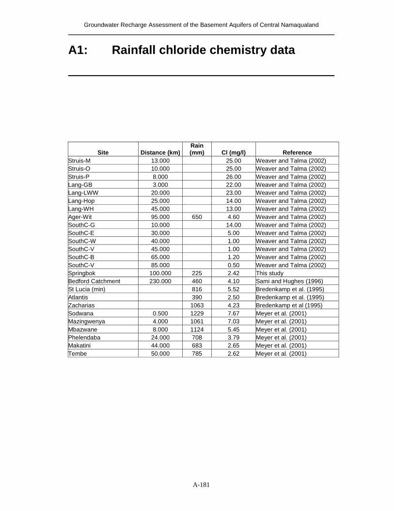
Groundwater Recharge Assessment of the Basement Aquifers of Central Namaqualand
A-181
A1: Rainfall chloride chemistry data
Site Distance (km) Rain (mm) Cl (mg/l) Reference
Struis-M 13.000 25.00 Weaver and Talma (2002) Struis-O 10.000 25.00 Weaver and Talma (2002) Struis-P 8.000 26.00 Weaver and Talma (2002) Lang-GB 3.000 22.00 Weaver and Talma (2002) Lang-LWW 20.000 23.00 Weaver and Talma (2002) Lang-Hop 25.000 14.00 Weaver and Talma (2002) Lang-WH 45.000 13.00 Weaver and Talma (2002) Ager-Wit 95.000 650 4.60 Weaver and Talma (2002) SouthC-G 10.000 14.00 Weaver and Talma (2002) SouthC-E 30.000 5.00 Weaver and Talma (2002) SouthC-W 40.000 1.00 Weaver and Talma (2002) SouthC-V 45.000 1.00 Weaver and Talma (2002) SouthC-B 65.000 1.20 Weaver and Talma (2002) SouthC-V 85.000 0.50 Weaver and Talma (2002) Springbok 100.000 225 2.42 This study Bedford Catchment 230.000 460 4.10 Sami and Hughes (1996) St Lucia (min) 816 5.52 Bredenkamp et al. (1995) Atlantis 390 2.50 Bredenkamp et al. (1995) Zacharias 1063 4.23 Bredenkamp et al (1995) Sodwana 0.500 1229 7.67 Meyer et al. (2001) Mazingwenya 4.000 1061 7.03 Meyer et al. (2001) Mbazwane 8.000 1124 5.45 Meyer et al. (2001) Phelendaba 24.000 708 3.79 Meyer et al. (2001) Makatini 44.000 683 2.65 Meyer et al. (2001) Tembe 50.000 785 2.62 Meyer et al. (2001)
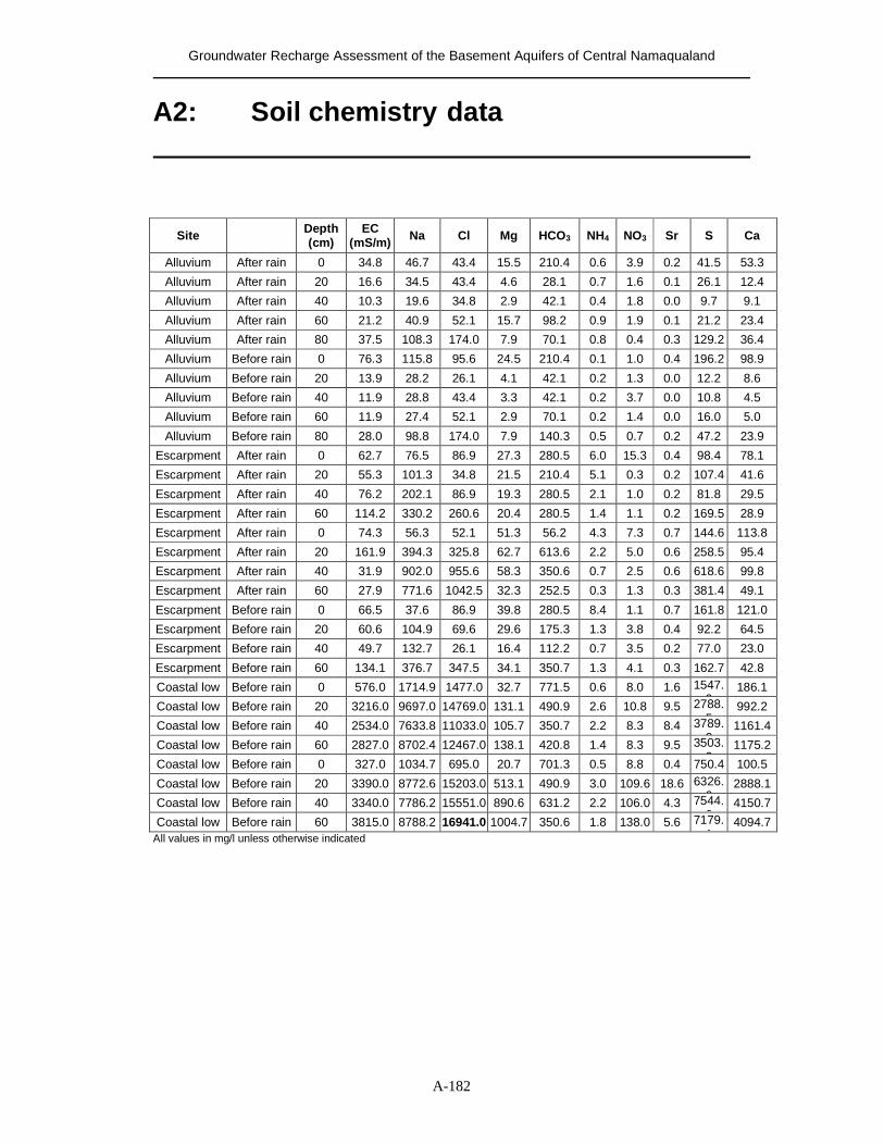
Groundwater Recharge Assessment of the Basement Aquifers of Central Namaqualand
A-182
A2: Soil chemistry data
Site Depth (cm)
EC (mS/m) Na Cl Mg HCO3 NH4 NO3 Sr S Ca
Alluvium After rain 0 34.8 46.7 43.4 15.5 210.4 0.6 3.9 0.2 41.5 53.3
Alluvium After rain 20 16.6 34.5 43.4 4.6 28.1 0.7 1.6 0.1 26.1 12.4
Alluvium After rain 40 10.3 19.6 34.8 2.9 42.1 0.4 1.8 0.0 9.7 9.1
Alluvium After rain 60 21.2 40.9 52.1 15.7 98.2 0.9 1.9 0.1 21.2 23.4
Alluvium After rain 80 37.5 108.3 174.0 7.9 70.1 0.8 0.4 0.3 129.2 36.4
Alluvium Before rain 0 76.3 115.8 95.6 24.5 210.4 0.1 1.0 0.4 196.2 98.9
Alluvium Before rain 20 13.9 28.2 26.1 4.1 42.1 0.2 1.3 0.0 12.2 8.6
Alluvium Before rain 40 11.9 28.8 43.4 3.3 42.1 0.2 3.7 0.0 10.8 4.5
Alluvium Before rain 60 11.9 27.4 52.1 2.9 70.1 0.2 1.4 0.0 16.0 5.0
Alluvium Before rain 80 28.0 98.8 174.0 7.9 140.3 0.5 0.7 0.2 47.2 23.9
Escarpment After rain 0 62.7 76.5 86.9 27.3 280.5 6.0 15.3 0.4 98.4 78.1
Escarpment After rain 20 55.3 101.3 34.8 21.5 210.4 5.1 0.3 0.2 107.4 41.6
Escarpment After rain 40 76.2 202.1 86.9 19.3 280.5 2.1 1.0 0.2 81.8 29.5
Escarpment After rain 60 114.2 330.2 260.6 20.4 280.5 1.4 1.1 0.2 169.5 28.9
Escarpment After rain 0 74.3 56.3 52.1 51.3 56.2 4.3 7.3 0.7 144.6 113.8
Escarpment After rain 20 161.9 394.3 325.8 62.7 613.6 2.2 5.0 0.6 258.5 95.4
Escarpment After rain 40 31.9 902.0 955.6 58.3 350.6 0.7 2.5 0.6 618.6 99.8
Escarpment After rain 60 27.9 771.6 1042.5 32.3 252.5 0.3 1.3 0.3 381.4 49.1
Escarpment Before rain 0 66.5 37.6 86.9 39.8 280.5 8.4 1.1 0.7 161.8 121.0
Escarpment Before rain 20 60.6 104.9 69.6 29.6 175.3 1.3 3.8 0.4 92.2 64.5
Escarpment Before rain 40 49.7 132.7 26.1 16.4 112.2 0.7 3.5 0.2 77.0 23.0
Escarpment Before rain 60 134.1 376.7 347.5 34.1 350.7 1.3 4.1 0.3 162.7 42.8
Coastal low Before rain 0 576.0 1714.9 1477.0 32.7 771.5 0.6 8.0 1.6 1547.9
186.1
Coastal low Before rain 20 3216.0 9697.0 14769.0 131.1 490.9 2.6 10.8 9.5 2788.5
992.2
Coastal low Before rain 40 2534.0 7633.8 11033.0 105.7 350.7 2.2 8.3 8.4 3789.3
1161.4
Coastal low Before rain 60 2827.0 8702.4 12467.0 138.1 420.8 1.4 8.3 9.5 3503.3
1175.2
Coastal low Before rain 0 327.0 1034.7 695.0 20.7 701.3 0.5 8.8 0.4 750.4 100.5
Coastal low Before rain 20 3390.0 8772.6 15203.0 513.1 490.9 3.0 109.6 18.6 6326.0
2888.1
Coastal low Before rain 40 3340.0 7786.2 15551.0 890.6 631.2 2.2 106.0 4.3 7544.2
4150.7
Coastal low Before rain 60 3815.0 8788.2 16941.0 1004.7 350.6 1.8 138.0 5.6 7179.1
4094.7 All values in mg/l unless otherwise indicated
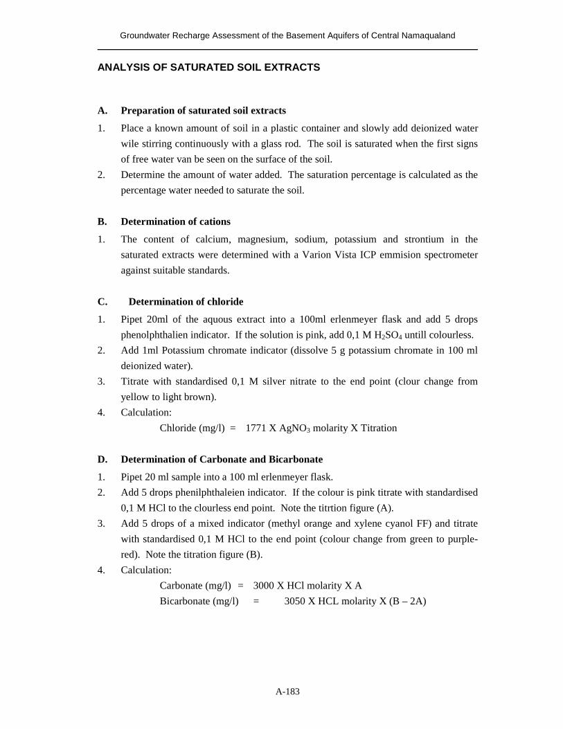
Groundwater Recharge Assessment of the Basement Aquifers of Central Namaqualand
A-183
ANALYSIS OF SATURATED SOIL EXTRACTS A. Preparation of saturated soil extracts
1. Place a known amount of soil in a plastic container and slowly add deionized water wile stirring continuously with a glass rod. The soil is saturated when the first signs of free water van be seen on the surface of the soil.
2. Determine the amount of water added. The saturation percentage is calculated as the percentage water needed to saturate the soil.
B. Determination of cations
1. The content of calcium, magnesium, sodium, potassium and strontium in the saturated extracts were determined with a Varion Vista ICP emmision spectrometer against suitable standards.
C. Determination of chloride
1. Pipet 20ml of the aquous extract into a 100ml erlenmeyer flask and add 5 drops phenolphthalien indicator. If the solution is pink, add 0,1 M H2SO4 untill colourless.
2. Add 1ml Potassium chromate indicator (dissolve 5 g potassium chromate in 100 ml deionized water).
3. Titrate with standardised 0,1 M silver nitrate to the end point (clour change from yellow to light brown).
4. Calculation: Chloride (mg/l) = 1771 X AgNO3 molarity X Titration
D. Determination of Carbonate and Bicarbonate
1. Pipet 20 ml sample into a 100 ml erlenmeyer flask. 2. Add 5 drops phenilphthaleien indicator. If the colour is pink titrate with standardised
0,1 M HCl to the clourless end point. Note the titrtion figure (A). 3. Add 5 drops of a mixed indicator (methyl orange and xylene cyanol FF) and titrate
with standardised 0,1 M HCl to the end point (colour change from green to purple-red). Note the titration figure (B).
4. Calculation: Carbonate (mg/l) = 3000 X HCl molarity X A Bicarbonate (mg/l) = 3050 X HCL molarity X (B – 2A)
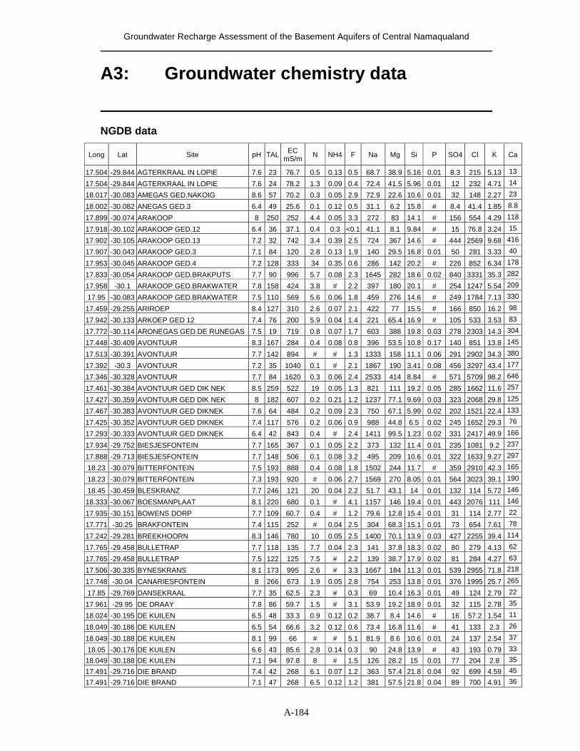
Groundwater Recharge Assessment of the Basement Aquifers of Central Namaqualand
A-184
A3: Groundwater chemistry data
NGDB data
Long Lat Site pH TAL EC mS/m N NH4 F Na Mg Si P SO4 Cl K Ca
17.504 -29.844 AGTERKRAAL IN LOPIE 7.6 23 76.7 0.5 0.13 0.5 68.7 38.9 5.16 0.01 8.3 215 5.13 13
17.504 -29.844 AGTERKRAAL IN LOPIE 7.6 24 78.2 1.3 0.09 0.4 72.4 41.5 5.96 0.01 12 232 4.71 14
18.017 -30.083 AMEGAS GED.NAKOIG 8.6 57 70.2 0.3 0.05 2.9 72.9 22.6 10.6 0.01 32 148 2.27 23
18.002 -30.082 ANEGAS GED.3 6.4 49 25.6 0.1 0.12 0.5 31.1 6.2 15.8 # 8.4 41.4 1.85 8.8
17.899 -30.074 ARAKOOP 8 250 252 4.4 0.05 3.3 272 83 14.1 # 156 554 4.29 118
17.918 -30.102 ARAKOOP GED.12 6.4 36 37.1 0.4 0.3 <0.1 41.1 8.1 9.84 # 15 76.8 3.24 15
17.902 -30.105 ARAKOOP GED.13 7.2 32 742 3.4 0.39 2.5 724 367 14.6 # 444 2569 9.68 416
17.907 -30.043 ARAKOOP GED.3 7.1 84 120 2.8 0.13 1.9 140 29.5 16.8 0.01 50 281 3.33 40
17.953 -30.045 ARAKOOP GED.4 7.2 128 333 34 0.35 0.6 286 142 20.2 # 226 852 6.34 178
17.833 -30.054 ARAKOOP GED.BRAKPUTS 7.7 90 996 5.7 0.08 2.3 1645 282 18.6 0.02 840 3331 35.3 282
17.958 -30.1 ARAKOOP GED.BRAKWATER 7.8 158 424 3.8 # 2.2 397 180 20.1 # 254 1247 5.54 209
17.95 -30.083 ARAKOOP GED.BRAKWATER 7.5 110 569 5.6 0.06 1.8 459 276 14.6 # 249 1784 7.13 330
17.459 -29.255 ARIROEP 8.4 127 310 2.6 0.07 2.1 422 77 15.5 # 166 850 16.2 98
17.942 -30.133 ARKOEP GED 12 7.4 76 200 5.9 0.04 1.4 221 65.4 16.9 # 105 533 3.53 83
17.772 -30.114 ARONEGAS GED.DE RUNEGAS 7.5 19 719 0.8 0.07 1.7 603 388 19.8 0.03 278 2303 14.3 304
17.448 -30.409 AVONTUUR 8.3 167 284 0.4 0.08 0.8 396 53.5 10.8 0.17 140 851 13.8 145
17.513 -30.391 AVONTUUR 7.7 142 894 # # 1.3 1333 158 11.1 0.06 291 2902 34.3 380
17.392 -30.3 AVONTUUR 7.2 35 1040 0.1 # 2.1 1867 190 3.41 0.08 456 3297 43.4 177
17.346 -30.328 AVONTUUR 7.7 84 1620 0.3 0.06 2.4 2533 414 8.84 # 571 5709 98.2 646
17.461 -30.384 AVONTUUR GED DIK NEK 8.5 259 522 19 0.05 1.3 821 111 19.2 0.05 285 1662 11.6 257
17.427 -30.359 AVONTUUR GED DIK NEK 8 182 607 0.2 0.21 1.2 1237 77.1 9.69 0.03 323 2068 29.8 125
17.467 -30.383 AVONTUUR GED DIKNEK 7.6 64 484 0.2 0.09 2.3 750 67.1 5.99 0.02 202 1521 22.4 133
17.425 -30.352 AVONTUUR GED DIKNEK 7.4 117 576 0.2 0.06 0.9 988 44.8 6.5 0.02 245 1652 29.3 76
17.293 -30.333 AVONTUUR GED DIKNEK 6.4 42 843 0.4 # 2.4 1411 99.5 1.23 0.02 331 2417 49.9 166
17.934 -29.752 BIESJESFONTEIN 7.7 165 367 0.1 0.05 2.2 373 132 11.4 0.01 235 1081 9.2 237
17.888 -29.713 BIESJESFONTEIN 7.7 148 506 0.1 0.08 3.2 495 209 10.6 0.01 322 1633 9.27 297
18.23 -30.079 BITTERFONTEIN 7.5 193 888 0.4 0.08 1.8 1502 244 11.7 # 359 2910 42.3 165
18.23 -30.079 BITTERFONTEIN 7.3 193 920 # 0.06 2.7 1569 270 8.05 0.01 564 3023 39.1 190
18.45 -30.459 BLESKRANZ 7.7 246 121 20 0.04 2.2 51.7 43.1 14 0.01 132 114 5.72 146
18.333 -30.067 BOESMANPLAAT 8.1 220 680 0.1 # 4.1 1157 146 19.4 0.01 443 2076 111 146
17.935 -30.151 BOWENS DORP 7.7 109 60.7 0.4 # 1.2 79.6 12.8 15.4 0.01 31 114 2.77 22
17.771 -30.25 BRAKFONTEIN 7.4 115 252 # 0.04 2.5 304 68.3 15.1 0.01 73 654 7.61 78
17.242 -29.281 BREEKHOORN 8.3 146 780 10 0.05 2.5 1400 70.1 13.9 0.03 427 2255 39.4 114
17.765 -29.458 BULLETRAP 7.7 118 135 7.7 0.04 2.3 141 37.8 18.3 0.02 80 279 4.13 62
17.765 -29.458 BULLETRAP 7.5 122 125 7.5 # 2.2 139 38.7 17.9 0.02 81 284 4.27 63
17.506 -30.335 BYNESKRANS 8.1 173 995 2.6 # 3.3 1667 184 11.3 0.01 539 2955 71.8 218
17.748 -30.04 CANARIESFONTEIN 8 266 673 1.9 0.05 2.8 754 253 13.8 0.01 376 1995 25.7 265
17.85 -29.769 DANSEKRAAL 7.7 35 62.5 2.3 # 0.3 69 10.4 16.3 0.01 49 124 2.79 22
17.961 -29.95 DE DRAAY 7.8 86 59.7 1.5 # 3.1 53.9 19.2 18.9 0.01 32 115 2.78 35
18.024 -30.195 DE KUILEN 6.5 48 33.3 0.9 0.12 0.2 38.7 8.4 14.6 # 16 57.2 1.54 11
18.049 -30.186 DE KUILEN 6.5 54 66.6 3.2 0.12 0.6 73.4 16.8 11.6 # 41 133 2.3 26
18.049 -30.188 DE KUILEN 8.1 99 66 # # 5.1 81.9 8.6 10.6 0.01 24 137 2.54 37
18.05 -30.176 DE KUILEN 6.6 43 85.6 2.8 0.14 0.3 90 24.8 13.9 # 43 193 0.79 33
18.049 -30.188 DE KUILEN 7.1 94 97.8 8 # 1.5 126 28.2 15 0.01 77 204 2.8 35
17.491 -29.716 DIE BRAND 7.4 42 268 6.1 0.07 1.2 363 57.4 21.8 0.04 92 699 4.59 45
17.491 -29.716 DIE BRAND 7.1 47 268 6.5 0.12 1.2 381 57.5 21.8 0.04 89 700 4.91 36
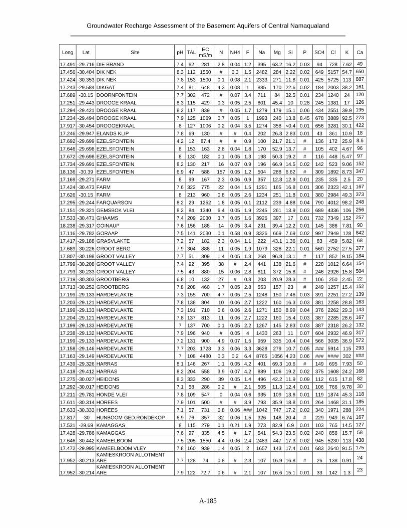
Groundwater Recharge Assessment of the Basement Aquifers of Central Namaqualand
A-185
Long Lat Site pH TAL EC mS/m N NH4 F Na Mg Si P SO4 Cl K Ca
17.491 -29.716 DIE BRAND 7.4 62 281 2.8 0.04 1.2 395 63.2 16.2 0.03 94 728 7.62 49
17.456 -30.404 DIK NEK 8.3 112 1550 # 0.3 1.5 2482 284 2.22 0.02 649 5157 54.7 650
17.424 -30.353 DIK NEK 7.8 153 1500 0.1 0.08 2.1 2333 271 11.8 0.01 425 5725 113 887
17.243 -29.584 DIKGAT 7.4 81 648 4.3 0.08 1 885 170 22.6 0.02 184 2003 38.2 161
17.689 -30.15 DOORNFONTEIN 7.7 302 472 # 0.07 3.4 711 84 32.5 0.01 234 1240 24 120
17.251 -29.443 DROOGE KRAAL 8.3 115 429 0.3 0.05 2.5 801 45.4 10 0.28 245 1381 17 126
17.294 -29.421 DROOGE KRAAL 8.2 117 839 # 0.05 1.7 1279 179 15.1 0.06 434 2551 39.9 195
17.234 -29.494 DROOGE KRAAL 7.9 125 1069 0.7 0.05 1 1993 240 13.8 8.45 678 3889 92.5 273
17.917 -30.454 DROOGEKRAAL 8 127 1006 0.2 0.04 3.5 1274 358 <0.4 0.01 656 3281 30.1 422
17.246 -29.947 ELANDS KLIP 7.8 69 130 # # 0.4 202 26.8 2.83 0.01 43 361 10.9 18
17.692 -29.699 EZELSFONTEIN 4.2 12 87.4 # # 0.9 100 21.7 21.1 # 136 172 25.9 8.6
17.646 -29.698 EZELSFONTEIN 8 153 163 2.8 0.04 1.8 170 52.9 13.7 # 105 402 4.67 96
17.672 -29.698 EZELSFONTEIN 8 130 182 0.1 0.05 1.3 198 50.3 19.2 # 116 448 5.47 97
17.734 -29.691 EZELSFONTEIN 8.2 130 217 16 0.07 0.9 196 66.9 14.5 0.02 142 523 9.06 152
18.136 -30.39 EZELSFONTEIN 6.9 47 588 157 0.05 1.2 504 288 6.62 # 309 1892 8.73 347
17.169 -29.271 FARM 8 99 167 2.3 0.06 0.9 357 12.8 12.9 0.01 235 335 2.5 20
17.424 -30.473 FARM 7.6 322 775 22 0.04 1.5 1291 165 16.8 0.01 306 2323 42.1 167
17.626 -30.15 FARM 8 213 960 0.8 0.05 2.6 1234 251 11.8 0.01 380 2984 49.3 373
17.295 -29.244 FARQUARSON 8.2 29 1252 1.8 0.05 0.1 2112 239 4.88 0.04 790 4012 98.2 248
17.151 -29.321 GEMSBOK VLEI 8.2 84 1340 6.4 0.05 1.9 2245 261 13.9 0.03 689 4336 106 256
17.533 -30.471 GHAAMS 7.4 209 2030 3.7 0.05 1.6 3926 397 17 0.01 732 7349 152 257
18.238 -29.317 GOINAUP 7.6 156 188 14 0.05 3.4 231 39.4 12.2 0.01 145 386 7.81 90
17.116 -29.782 GORAAP 7.5 141 2030 0.1 0.58 0.9 3326 669 7.69 0.02 997 7949 128 842
17.417 -29.188 GRASVLAKTE 7.2 57 182 2.3 0.04 1.1 222 43.1 1.36 0.01 83 459 5.82 68
17.689 -30.226 GROOT BERG 7.9 304 888 11 0.05 1.9 1079 326 22.1 0.01 560 2752 27.5 377
17.807 -30.198 GROOT VALLEY 7.7 51 309 1.4 0.05 1.3 268 96.8 13.1 # 117 852 9.15 184
17.799 -30.208 GROOT VALLEY 7.4 92 395 38 # 2.4 441 138 21.6 # 228 1012 6.64 154
17.793 -30.233 GROOT VALLEY 7.5 43 880 15 0.06 2.8 811 372 15.8 # 246 2926 15.8 504
17.719 -30.303 GROOTBERG 6.8 10 132 27 # 0.8 203 20.9 28.3 # 106 250 2.45 22
17.713 -30.252 GROOTBERG 7.8 208 460 1.7 0.05 2.8 553 157 23 # 249 1257 15.4 152
17.199 -29.133 HARDEVLAKTE 7.3 155 700 4.7 0.05 2.5 1248 150 7.46 0.03 391 2251 27.2 139
17.203 -29.121 HARDEVLAKTE 7.8 138 804 10 0.06 2.7 1222 160 16.3 0.03 381 2258 28.8 163
17.199 -29.133 HARDEVLAKTE 7.3 191 710 0.6 0.06 2.6 1271 150 8.99 0.04 376 2262 29.3 143
17.204 -29.121 HARDEVLAKTE 7.8 137 813 11 0.06 2.7 1222 160 15.4 0.03 387 2285 28.6 167
17.199 -29.133 HARDEVLAKTE 7 137 700 0.1 0.05 2.2 1267 145 2.83 0.03 387 2318 26.2 132
17.238 -29.132 HARDEVLAKTE 7.9 196 940 # 0.05 4 1430 263 11 0.07 604 2932 46.9 317
17.199 -29.133 HARDEVLAKTE 7.2 131 900 4.9 0.07 1.5 959 335 10.4 0.04 566 3035 36.9 572
17.158 -29.146 HARDEVLAKTE 7.7 203 1728 3.3 0.06 3.3 3628 279 10.7 0.05 ### 5914 115 293
17.163 -29.149 HARDEVLAKTE 7 108 4480 0.3 0.2 6.4 8765 1056 4.23 0.06 ### #### 302 ###
17.439 -29.326 HARRAS 8.1 146 267 1.1 0.05 4.2 401 69.3 10.6 # 149 695 7.93 50
17.418 -29.412 HARRAS 8.2 204 558 3.9 0.07 4.2 889 106 19.2 0.02 375 1608 24.2 168
17.275 -30.027 HEIDONS 8.3 333 290 39 0.05 1.4 496 42.2 11.9 0.09 112 615 17.8 82
17.292 -30.017 HEIDONS 7.1 58 286 0.2 # 2.1 505 11.3 12.4 0.01 106 766 9.78 30
17.211 -29.781 HONDE VLEI 7.8 109 547 0 0.04 0.6 935 109 13.6 0.01 119 1874 45.3 118
17.611 -30.314 HOREES 7.9 101 500 # # 3.9 793 35.9 18.8 0.01 264 1468 31.1 185
17.633 -30.333 HOREES 7.1 57 731 0.8 0.06 ### 1042 747 17.2 0.02 340 1971 288 224
17.817 -30 HUNBOOM GED.RONDEKOP 6.9 76 357 32 0.06 1.5 326 148 20.4 # 229 949 6.74 167
17.531 -29.69 KAMAGGAS 8 115 279 0.1 0.21 1.9 273 82.9 6.9 0.01 103 765 14.5 127
17.428 -29.786 KAMAGGAS 7.6 97 335 4.5 # 1.7 541 54.3 23.5 0.02 240 856 15.7 58
17.646 -30.442 KAMEELBOOM 7.5 205 1550 4.4 0.06 2.4 2483 447 17.3 0.02 945 5230 113 438
17.472 -29.995 KAMEELBOOM VLEY 7.8 160 939 1.4 0.05 2 1657 143 17.4 0.01 683 2640 91.5 175
17.952 -30.213 KAMIESKROON ALLOTMENT ARE 7.7 128 74 0.8 # 2.3 107 16.9 16.8 # 26 138 0.91 24
17.952 -30.214 KAMIESKROON ALLOTMENT ARE 7.9 122 72.7 0.6 # 2.1 107 16.6 15.1 0.01 33 142 1.3 23
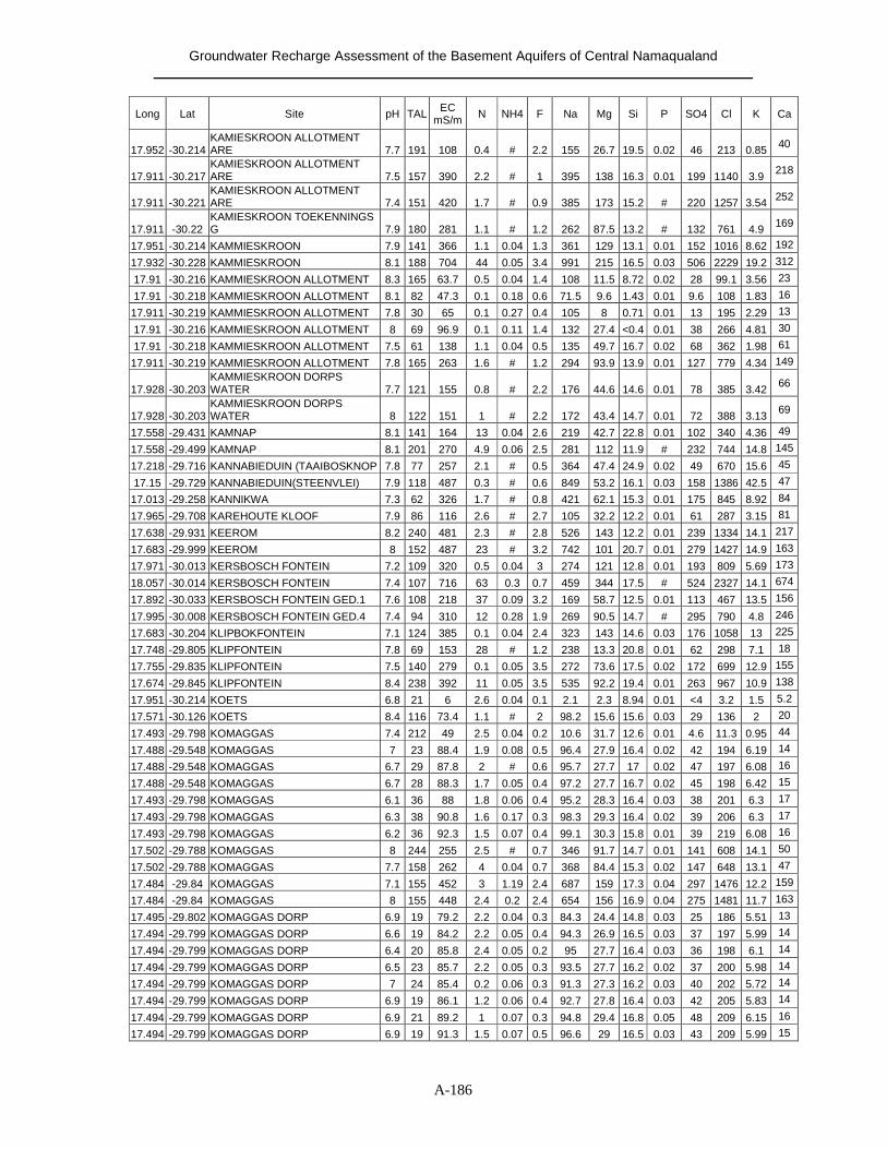
Groundwater Recharge Assessment of the Basement Aquifers of Central Namaqualand
A-186
Long Lat Site pH TAL EC mS/m N NH4 F Na Mg Si P SO4 Cl K Ca
17.952 -30.214 KAMIESKROON ALLOTMENT ARE 7.7 191 108 0.4 # 2.2 155 26.7 19.5 0.02 46 213 0.85 40
17.911 -30.217 KAMIESKROON ALLOTMENT ARE 7.5 157 390 2.2 # 1 395 138 16.3 0.01 199 1140 3.9 218
17.911 -30.221 KAMIESKROON ALLOTMENT ARE 7.4 151 420 1.7 # 0.9 385 173 15.2 # 220 1257 3.54 252
17.911 -30.22 KAMIESKROON TOEKENNINGS G 7.9 180 281 1.1 # 1.2 262 87.5 13.2 # 132 761 4.9 169
17.951 -30.214 KAMMIESKROON 7.9 141 366 1.1 0.04 1.3 361 129 13.1 0.01 152 1016 8.62 192
17.932 -30.228 KAMMIESKROON 8.1 188 704 44 0.05 3.4 991 215 16.5 0.03 506 2229 19.2 312
17.91 -30.216 KAMMIESKROON ALLOTMENT 8.3 165 63.7 0.5 0.04 1.4 108 11.5 8.72 0.02 28 99.1 3.56 23
17.91 -30.218 KAMMIESKROON ALLOTMENT 8.1 82 47.3 0.1 0.18 0.6 71.5 9.6 1.43 0.01 9.6 108 1.83 16
17.911 -30.219 KAMMIESKROON ALLOTMENT 7.8 30 65 0.1 0.27 0.4 105 8 0.71 0.01 13 195 2.29 13
17.91 -30.216 KAMMIESKROON ALLOTMENT 8 69 96.9 0.1 0.11 1.4 132 27.4 <0.4 0.01 38 266 4.81 30
17.91 -30.218 KAMMIESKROON ALLOTMENT 7.5 61 138 1.1 0.04 0.5 135 49.7 16.7 0.02 68 362 1.98 61
17.911 -30.219 KAMMIESKROON ALLOTMENT 7.8 165 263 1.6 # 1.2 294 93.9 13.9 0.01 127 779 4.34 149
17.928 -30.203 KAMMIESKROON DORPS WATER 7.7 121 155 0.8 # 2.2 176 44.6 14.6 0.01 78 385 3.42 66
17.928 -30.203 KAMMIESKROON DORPS WATER 8 122 151 1 # 2.2 172 43.4 14.7 0.01 72 388 3.13 69
17.558 -29.431 KAMNAP 8.1 141 164 13 0.04 2.6 219 42.7 22.8 0.01 102 340 4.36 49
17.558 -29.499 KAMNAP 8.1 201 270 4.9 0.06 2.5 281 112 11.9 # 232 744 14.8 145
17.218 -29.716 KANNABIEDUIN (TAAIBOSKNOP 7.8 77 257 2.1 # 0.5 364 47.4 24.9 0.02 49 670 15.6 45
17.15 -29.729 KANNABIEDUIN(STEENVLEI) 7.9 118 487 0.3 # 0.6 849 53.2 16.1 0.03 158 1386 42.5 47
17.013 -29.258 KANNIKWA 7.3 62 326 1.7 # 0.8 421 62.1 15.3 0.01 175 845 8.92 84
17.965 -29.708 KAREHOUTE KLOOF 7.9 86 116 2.6 # 2.7 105 32.2 12.2 0.01 61 287 3.15 81
17.638 -29.931 KEEROM 8.2 240 481 2.3 # 2.8 526 143 12.2 0.01 239 1334 14.1 217
17.683 -29.999 KEEROM 8 152 487 23 # 3.2 742 101 20.7 0.01 279 1427 14.9 163
17.971 -30.013 KERSBOSCH FONTEIN 7.2 109 320 0.5 0.04 3 274 121 12.8 0.01 193 809 5.69 173
18.057 -30.014 KERSBOSCH FONTEIN 7.4 107 716 63 0.3 0.7 459 344 17.5 # 524 2327 14.1 674
17.892 -30.033 KERSBOSCH FONTEIN GED.1 7.6 108 218 37 0.09 3.2 169 58.7 12.5 0.01 113 467 13.5 156
17.995 -30.008 KERSBOSCH FONTEIN GED.4 7.4 94 310 12 0.28 1.9 269 90.5 14.7 # 295 790 4.8 246
17.683 -30.204 KLIPBOKFONTEIN 7.1 124 385 0.1 0.04 2.4 323 143 14.6 0.03 176 1058 13 225
17.748 -29.805 KLIPFONTEIN 7.8 69 153 28 # 1.2 238 13.3 20.8 0.01 62 298 7.1 18
17.755 -29.835 KLIPFONTEIN 7.5 140 279 0.1 0.05 3.5 272 73.6 17.5 0.02 172 699 12.9 155
17.674 -29.845 KLIPFONTEIN 8.4 238 392 11 0.05 3.5 535 92.2 19.4 0.01 263 967 10.9 138
17.951 -30.214 KOETS 6.8 21 6 2.6 0.04 0.1 2.1 2.3 8.94 0.01 <4 3.2 1.5 5.2
17.571 -30.126 KOETS 8.4 116 73.4 1.1 # 2 98.2 15.6 15.6 0.03 29 136 2 20
17.493 -29.798 KOMAGGAS 7.4 212 49 2.5 0.04 0.2 10.6 31.7 12.6 0.01 4.6 11.3 0.95 44
17.488 -29.548 KOMAGGAS 7 23 88.4 1.9 0.08 0.5 96.4 27.9 16.4 0.02 42 194 6.19 14
17.488 -29.548 KOMAGGAS 6.7 29 87.8 2 # 0.6 95.7 27.7 17 0.02 47 197 6.08 16
17.488 -29.548 KOMAGGAS 6.7 28 88.3 1.7 0.05 0.4 97.2 27.7 16.7 0.02 45 198 6.42 15
17.493 -29.798 KOMAGGAS 6.1 36 88 1.8 0.06 0.4 95.2 28.3 16.4 0.03 38 201 6.3 17
17.493 -29.798 KOMAGGAS 6.3 38 90.8 1.6 0.17 0.3 98.3 29.3 16.4 0.02 39 206 6.3 17
17.493 -29.798 KOMAGGAS 6.2 36 92.3 1.5 0.07 0.4 99.1 30.3 15.8 0.01 39 219 6.08 16
17.502 -29.788 KOMAGGAS 8 244 255 2.5 # 0.7 346 91.7 14.7 0.01 141 608 14.1 50
17.502 -29.788 KOMAGGAS 7.7 158 262 4 0.04 0.7 368 84.4 15.3 0.02 147 648 13.1 47
17.484 -29.84 KOMAGGAS 7.1 155 452 3 1.19 2.4 687 159 17.3 0.04 297 1476 12.2 159
17.484 -29.84 KOMAGGAS 8 155 448 2.4 0.2 2.4 654 156 16.9 0.04 275 1481 11.7 163
17.495 -29.802 KOMAGGAS DORP 6.9 19 79.2 2.2 0.04 0.3 84.3 24.4 14.8 0.03 25 186 5.51 13
17.494 -29.799 KOMAGGAS DORP 6.6 19 84.2 2.2 0.05 0.4 94.3 26.9 16.5 0.03 37 197 5.99 14
17.494 -29.799 KOMAGGAS DORP 6.4 20 85.8 2.4 0.05 0.2 95 27.7 16.4 0.03 36 198 6.1 14
17.494 -29.799 KOMAGGAS DORP 6.5 23 85.7 2.2 0.05 0.3 93.5 27.7 16.2 0.02 37 200 5.98 14
17.494 -29.799 KOMAGGAS DORP 7 24 85.4 0.2 0.06 0.3 91.3 27.3 16.2 0.03 40 202 5.72 14
17.494 -29.799 KOMAGGAS DORP 6.9 19 86.1 1.2 0.06 0.4 92.7 27.8 16.4 0.03 42 205 5.83 14
17.494 -29.799 KOMAGGAS DORP 6.9 21 89.2 1 0.07 0.3 94.8 29.4 16.8 0.05 48 209 6.15 16
17.494 -29.799 KOMAGGAS DORP 6.9 19 91.3 1.5 0.07 0.5 96.6 29 16.5 0.03 43 209 5.99 15
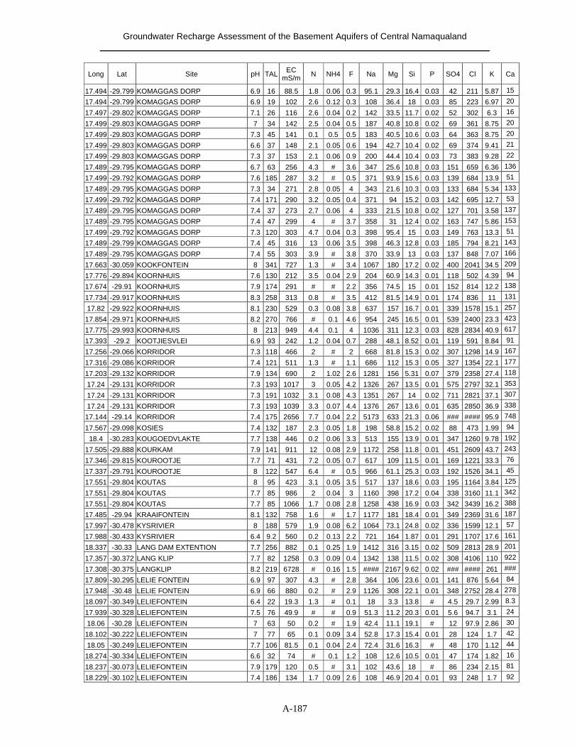
Groundwater Recharge Assessment of the Basement Aquifers of Central Namaqualand
A-187
Long Lat Site pH TAL EC mS/m N NH4 F Na Mg Si P SO4 Cl K Ca
17.494 -29.799 KOMAGGAS DORP 6.9 16 88.5 1.8 0.06 0.3 95.1 29.3 16.4 0.03 42 211 5.87 15
17.494 -29.799 KOMAGGAS DORP 6.9 19 102 2.6 0.12 0.3 108 36.4 18 0.03 85 223 6.97 20
17.497 -29.802 KOMAGGAS DORP 7.1 26 116 2.6 0.04 0.2 142 33.5 11.7 0.02 52 302 6.3 16
17.499 -29.803 KOMAGGAS DORP 7 34 142 2.5 0.04 0.5 187 40.8 10.8 0.02 69 361 8.75 20
17.499 -29.803 KOMAGGAS DORP 7.3 45 141 0.1 0.5 0.5 183 40.5 10.6 0.03 64 363 8.75 20
17.499 -29.803 KOMAGGAS DORP 6.6 37 148 2.1 0.05 0.6 194 42.7 10.4 0.02 69 374 9.41 21
17.499 -29.803 KOMAGGAS DORP 7.3 37 153 2.1 0.06 0.9 200 44.4 10.4 0.03 73 383 9.28 22
17.489 -29.795 KOMAGGAS DORP 6.7 63 256 4.3 # 3.6 347 25.6 10.8 0.03 151 659 6.36 136
17.499 -29.792 KOMAGGAS DORP 7.6 185 287 3.2 # 0.5 371 93.9 15.6 0.03 139 684 13.9 51
17.489 -29.795 KOMAGGAS DORP 7.3 34 271 2.8 0.05 4 343 21.6 10.3 0.03 133 684 5.34 133
17.499 -29.792 KOMAGGAS DORP 7.4 171 290 3.2 0.05 0.4 371 94 15.2 0.03 142 695 12.7 53
17.489 -29.795 KOMAGGAS DORP 7.4 37 273 2.7 0.06 4 333 21.5 10.8 0.02 127 701 3.58 137
17.489 -29.795 KOMAGGAS DORP 7.4 47 299 4 # 3.7 358 31 12.4 0.02 163 747 5.86 153
17.499 -29.792 KOMAGGAS DORP 7.3 120 303 4.7 0.04 0.3 398 95.4 15 0.03 149 763 13.3 51
17.489 -29.799 KOMAGGAS DORP 7.4 45 316 13 0.06 3.5 398 46.3 12.8 0.03 185 794 8.21 143
17.489 -29.795 KOMAGGAS DORP 7.4 55 303 3.9 # 3.8 370 33.9 13 0.03 137 848 7.07 166
17.663 -30.059 KOOKFONTEIN 8 341 727 1.3 # 3.4 1067 180 17.2 0.02 400 2041 34.5 209
17.776 -29.894 KOORNHUIS 7.6 130 212 3.5 0.04 2.9 204 60.9 14.3 0.01 118 502 4.39 94
17.674 -29.91 KOORNHUIS 7.9 174 291 # # 2.2 356 74.5 15 0.01 152 814 12.2 138
17.734 -29.917 KOORNHUIS 8.3 258 313 0.8 # 3.5 412 81.5 14.9 0.01 174 836 11 131
17.82 -29.922 KOORNHUIS 8.1 230 529 0.3 0.08 3.8 637 157 16.7 0.01 339 1578 15.1 257
17.854 -29.971 KOORNHUIS 8.2 270 766 # 0.1 4.6 954 245 16.5 0.01 539 2400 23.3 423
17.775 -29.993 KOORNHUIS 8 213 949 4.4 0.1 4 1036 311 12.3 0.03 828 2834 40.9 617
17.393 -29.2 KOOTJIESVLEI 6.9 93 242 1.2 0.04 0.7 288 48.1 8.52 0.01 119 591 8.84 91
17.256 -29.066 KORRIDOR 7.3 118 466 2 # 2 668 81.8 15.3 0.02 307 1298 14.9 167
17.316 -29.086 KORRIDOR 7.4 121 511 1.3 # 1.1 686 112 15.3 0.05 327 1354 22.1 177
17.203 -29.132 KORRIDOR 7.9 134 690 2 1.02 2.6 1281 156 5.31 0.07 379 2358 27.4 118
17.24 -29.131 KORRIDOR 7.3 193 1017 3 0.05 4.2 1326 267 13.5 0.01 575 2797 32.1 353
17.24 -29.131 KORRIDOR 7.3 191 1032 3.1 0.08 4.3 1351 267 14 0.02 711 2821 37.1 307
17.24 -29.131 KORRIDOR 7.3 193 1039 3.3 0.07 4.4 1376 267 13.6 0.01 635 2850 36.9 338
17.144 -29.14 KORRIDOR 7.4 175 2656 7.7 0.04 2.2 5173 633 21.3 0.06 ### #### 95.9 748
17.567 -29.098 KOSIES 7.4 132 187 2.3 0.05 1.8 198 58.8 15.2 0.02 88 473 1.99 94
18.4 -30.283 KOUGOEDVLAKTE 7.7 138 446 0.2 0.06 3.3 513 155 13.9 0.01 347 1260 9.78 192
17.505 -29.888 KOURKAM 7.9 141 911 12 0.08 2.9 1172 258 11.8 0.01 451 2609 43.7 243
17.346 -29.815 KOUROOTJE 7.7 71 431 7.2 0.05 0.7 617 109 11.5 0.01 169 1221 33.3 76
17.337 -29.791 KOUROOTJE 8 122 547 6.4 # 0.5 966 61.1 25.3 0.03 192 1526 34.1 45
17.551 -29.804 KOUTAS 8 95 423 3.1 0.05 3.5 517 137 18.6 0.03 195 1164 3.84 125
17.551 -29.804 KOUTAS 7.7 85 986 2 0.04 3 1160 398 17.2 0.04 338 3160 11.1 342
17.551 -29.804 KOUTAS 7.7 85 1066 1.7 0.08 2.8 1258 438 16.9 0.03 342 3439 16.2 388
17.485 -29.94 KRAAIFONTEIN 8.1 132 758 1.6 # 1.7 1177 181 18.4 0.01 349 2369 31.6 187
17.997 -30.478 KYSRIVIER 8 188 579 1.9 0.08 6.2 1064 73.1 24.8 0.02 336 1599 12.1 57
17.988 -30.433 KYSRIVIER 6.4 9.2 560 0.2 0.13 2.2 721 164 1.87 0.01 291 1707 17.6 161
18.337 -30.33 LANG DAM EXTENTION 7.7 256 882 0.1 0.25 1.9 1412 316 3.15 0.02 509 2813 28.9 201
17.357 -30.372 LANG KLIP 7.7 82 1258 0.3 0.09 0.4 1342 138 11.5 0.02 308 4106 110 922
17.308 -30.375 LANGKLIP 8.2 219 6728 # 0.16 1.5 #### 2167 9.62 0.02 ### #### 261 ###
17.809 -30.295 LELIE FONTEIN 6.9 97 307 4.3 # 2.8 364 106 23.6 0.01 141 876 5.64 84
17.948 -30.48 LELIE FONTEIN 6.9 66 880 0.2 # 2.9 1126 308 22.1 0.01 348 2752 28.4 278
18.097 -30.349 LELIEFONTEIN 6.4 22 19.3 1.3 # 0.1 18 3.3 13.8 # 4.5 29.7 2.99 8.3
17.939 -30.328 LELIEFONTEIN 7.5 76 49.9 # # 0.9 51.3 11.2 20.3 0.01 5.6 94.7 3.1 24
18.06 -30.28 LELIEFONTEIN 7 63 50 0.2 # 1.9 42.4 11.1 19.1 # 12 97.9 2.86 30
18.102 -30.222 LELIEFONTEIN 7 77 65 0.1 0.09 3.4 52.8 17.3 15.4 0.01 28 124 1.7 42
18.05 -30.249 LELIEFONTEIN 7.7 106 81.5 0.1 0.04 2.4 72.4 31.6 16.3 # 48 170 1.12 44
18.274 -30.334 LELIEFONTEIN 6.6 32 74 # 0.1 1.2 108 12.6 10.5 0.01 47 174 1.82 16
18.237 -30.073 LELIEFONTEIN 7.9 179 120 0.5 # 3.1 102 43.6 18 # 86 234 2.15 81
18.229 -30.102 LELIEFONTEIN 7.4 186 134 1.7 0.09 2.6 108 46.9 20.4 0.01 93 248 1.7 92
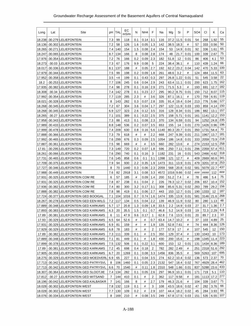
Groundwater Recharge Assessment of the Basement Aquifers of Central Namaqualand
A-188
Long Lat Site pH TAL EC mS/m N NH4 F Na Mg Si P SO4 Cl K Ca
18.238 -30.279 LELIEFONTEIN 7.3 99 118 0.1 0.14 3.1 116 37.2 11.5 0.01 54 268 1.92 55
18.136 -30.302 LELIEFONTEIN 7.2 58 126 1.6 0.05 1.3 142 38.5 18.3 # 57 333 0.56 50
18.265 -30.271 LELIEFONTEIN 7.4 140 154 1.5 0.08 2.4 154 53 14.9 0.01 92 336 1.61 65
18.247 -30.065 LELIEFONTEIN 8.7 134 166 8 0.08 2.8 174 48 21.7 0.01 100 339 2.67 75
17.976 -30.354 LELIEFONTEIN 7.2 76 166 0.2 0.09 2.3 182 51.8 12 0.01 86 406 4.1 53
18.273 -30.03 LELIEFONTEIN 7.3 67 176 9.9 0.08 5 224 38.4 36.1 # 110 439 1.24 66
18.017 -30.336 LELIEFONTEIN 8.1 137 188 # 0.05 2.7 192 62.2 23.2 0.04 142 470 5.33 100
17.979 -30.344 LELIEFONTEIN 7.5 99 198 0.2 0.09 1.8 261 48.6 3.2 # 124 484 11.5 63
17.952 -30.358 LELIEFONTEIN 3.5 <4 199 0.1 0.43 0.3 297 26.8 1.22 0.01 51 545 3.58 22
18.2 -30.253 LELIEFONTEIN 7.7 106 245 0.6 0.04 2.9 243 63.4 11.1 0.01 200 623 1.75 162
17.935 -30.382 LELIEFONTEIN 7.4 98 278 0.1 0.16 2.9 271 71.5 5.3 # 193 691 12.7 182
18.308 -30.34 LELIEFONTEIN 7.4 142 278 0.1 0.23 2.7 295 90.2 8.75 0.01 150 712 8.07 115
17.992 -30.354 LELIEFONTEIN 7.7 119 285 2.3 # 3.6 326 87.1 16.1 # 170 759 6.91 119
18.021 -30.328 LELIEFONTEIN 8 143 282 0.3 0.07 2.8 335 91.4 19.4 0.04 213 776 5.66 127
18.268 -30.345 LELIEFONTEIN 7.2 67 304 3.6 0.04 1.7 297 122 11.9 0.03 193 859 4.14 150
18.268 -30.345 LELIEFONTEIN 6.9 127 323 2.6 0.12 3.5 316 128 8.34 0.01 186 882 13.1 157
18.265 -30.27 LELIEFONTEIN 7.1 101 389 0.1 0.22 2.5 375 158 5.71 0.01 161 1141 12.2 153
17.958 -30.343 LELIEFONTEIN 7.3 88 413 0.1 0.08 2.3 370 134 6.59 0.01 94 1252 24.8 235
17.989 -30.433 LELIEFONTEIN 8.8 148 536 0.2 0.07 3.5 653 155 14 0.01 270 1426 0.96 196
17.999 -30.478 LELIEFONTEIN 7.4 209 630 0.8 0.16 5.6 1140 80.3 20.7 0.01 350 1731 54.4 70
17.888 -30.366 LELIEFONTEIN 7.3 79 618 # # 2.2 668 247 9.39 0.01 211 1967 13.7 181
17.992 -30.465 LELIEFONTEIN 7.6 299 676 0.3 0.09 2.5 1054 186 14.8 0.01 333 2059 73.9 218
17.887 -30.361 LELIEFONTEIN 7.5 98 669 # # 3.5 660 282 13.6 # 274 2153 12.5 258
17.81 -30.295 LELIEFONTEIN 7.3 149 720 0.2 0.07 1.8 596 250 7.11 0.01 296 2359 57.4 611
18.261 -30.066 LELIEFONTEIN 7.6 290 740 0.1 0.16 3 1182 231 16 0.01 543 2466 4.62 318
17.731 -30.465 LELIEFONTEIN 7.6 145 858 0.6 0.1 3.1 1398 121 12.7 # 409 2669 60.6 341
17.709 -30.375 LELIEFONTEIN 7.9 94 930 2.2 0.35 1.9 1473 311 13.9 0.01 479 3201 37.9 253
17.727 -30.346 LELIEFONTEIN 8 70 1440 0.3 0.06 2.3 2059 568 20.8 0.02 581 5079 22.7 437
17.988 -30.449 LELIEFONTEIN 7.6 82 2918 3.1 0.08 3.3 4572 1016 9.66 0.02 ### #### 112 ###
17.931 -30.325 LELIEFONTEIN COM RE 6 57 185 # 0.09 1.4 200 51.2 7.4 # 78 486 5.4 75
17.931 -30.325 LELIEFONTEIN COM RE 7.8 87 238 0.1 0.04 2 226 78.3 12.7 0.02 206 657 10.4 152
17.936 -30.382 LELIEFONTEIN COM RE 7.4 80 300 3.2 0.17 3.1 308 85.6 5.31 0.02 283 789 29.2 156
17.888 -30.382 LELIEFONTEIN COM RE 7.8 98 419 0.1 0.06 2.7 443 153 12.7 0.01 190 1333 12 187
17.724 -30.377 LELIEFONTEIN GED BOOIGAL 7.1 104 1016 0.7 0.74 1.6 1474 335 13.9 0.01 581 3146 21.6 268
18.267 -30.278 LELIEFONTEIN GED EEN-WILG 7.2 117 134 0.5 0.04 2.2 139 46.9 11.9 0.02 80 280 1.13 48
17.889 -30.348 LELIEFONTEIN GED KARKAMS 5.7 17 20.8 1.3 0.09 1.8 33.5 2.2 14.9 0.03 27 31.7 1.36 2.7
17.893 -30.383 LELIEFONTEIN GED KARKAMS 6.3 20 35.5 1.5 0.1 0.7 46.8 5.2 14.9 0.03 19 72.3 2.29 6.8
17.89 -30.381 LELIEFONTEIN GED KARKAMS 6 11 47.9 9.6 0.17 1 62.8 7.6 13.5 0.01 20 89.7 2.3 10
17.93 -30.329 LELIEFONTEIN GED KARKAMS 6.5 64 52.6 # # 0.7 63.4 14.7 10.2 # 37 103 4.89 25
17.931 -30.329 LELIEFONTEIN GED KARKAMS 6.9 81 159 # # 1.9 135 52.8 7.61 # 74 444 8.36 126
17.929 -30.329 LELIEFONTEIN GED KARKAMS 6.8 78 183 # # 2 177 57.9 17 # 107 545 12 150
17.89 -30.382 LELIEFONTEIN GED KARKAMS 7.3 111 339 0.1 # 2.5 350 129 37.4 # 130 1043 10 173
17.889 -30.348 LELIEFONTEIN GED KARKAMS 7.1 81 449 0.1 # 1.8 430 200 15.6 # 198 1345 11.4 223
17.899 -30.378 LELIEFONTEIN GED KARKAMS 7.5 132 506 0.1 0.22 3.1 600 153 12 0.01 131 1434 8.36 189
17.89 -30.381 LELIEFONTEIN GED KARKAMS 7.2 45 698 0.4 0.18 2 782 282 2.49 # 251 2318 51.6 292
17.905 -30.359 LELIEFONTEIN GED KARKAMS 6.7 20 1269 0.1 0.08 3.3 1456 836 35.5 # 569 5263 107 695
18.275 -30.329 LELIEFONTEIN GED MOEDVERL 6.9 65 227 0.1 0.04 3.5 274 62.2 10.4 0.02 136 573 2.37 70
17.713 -30.342 LELIEFONTEIN GED PATRYSVL 8 106 1460 0.1 0.05 2.3 2132 547 18.4 0.02 767 4929 28.4 462
17.713 -30.342 LELIEFONTEIN GED PATRYSVL 6.6 70 1540 # 0.11 1.8 2310 548 1.66 0.01 837 5288 23.6 433
18.307 -30.364 LELIEFONTEIN GED SLOOTJIE 7.4 134 282 0.1 0.05 2.6 297 96.9 10.1 0.01 171 719 5.1 110
17.812 -30.27 LELIEFONTEIN GED WITSAND 7 144 410 0.1 # 2 362 117 9.58 # 181 1113 17.2 277
18.196 -30.042 LELIEFONTEIN GED.KALBASKR 7 141 166 8 # 2.7 179 46.3 21.6 # 104 339 3.67 71
18.028 -30.302 LELIEFONTEIN WEST 7.8 132 119 0.1 # 3 108 43.5 18.6 0.02 47 282 3.76 66
18.028 -30.302 LELIEFONTEIN WEST 7.7 130 109 0.2 # 2.9 107 44.4 18.2 0.02 45 284 3.93 66
18.076 -30.334 LELIEFONTEIN WEST 8 169 210 # 0.08 3.5 249 67.8 17.5 0.03 151 535 6.55 107
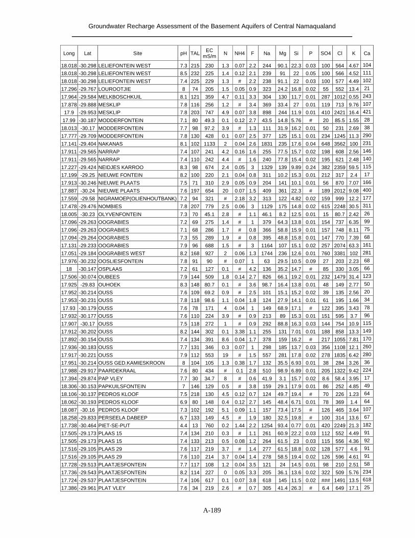
Groundwater Recharge Assessment of the Basement Aquifers of Central Namaqualand
A-189
Long Lat Site pH TAL EC mS/m N NH4 F Na Mg Si P SO4 Cl K Ca
18.018 -30.298 LELIEFONTEIN WEST 7.3 215 230 1.3 0.07 2.2 244 90.1 22.3 0.03 100 564 4.67 104
18.018 -30.298 LELIEFONTEIN WEST 8.5 232 225 1.4 0.12 2.1 239 91 22 0.05 100 566 4.52 111
18.018 -30.298 LELIEFONTEIN WEST 7.4 225 229 1.3 # 2.2 238 91.1 22 0.03 100 577 4.49 102
17.296 -29.767 LOUROOTJIE 8 74 205 1.5 0.05 0.9 323 24.2 16.8 0.02 55 552 13.4 21
17.964 -29.584 MELKBOSCHKUIL 8.1 121 359 4.7 0.11 3.3 304 130 11.7 0.01 287 1012 0.55 243
17.878 -29.888 MESKLIP 7.8 116 256 1.2 # 3.4 369 33.4 27 0.01 119 713 9.76 107
17.9 -29.953 MESKLIP 7.8 203 747 4.9 0.07 3.8 898 244 11.9 0.01 410 2421 16.4 421
17.99 -30.187 MODDERFONTEIN 7.1 80 49.3 0.1 0.12 2.7 43.5 14.8 5.76 # 20 85.5 1.55 28
18.013 -30.17 MODDERFONTEIN 7.7 98 97.2 3.9 # 1.3 111 31.9 16.2 0.01 50 231 2.69 38
17.777 -29.709 MODDERFONTEIN 7.8 130 428 0.1 0.07 2.5 377 125 15.1 0.01 234 1245 11.3 290
17.141 -29.404 NAKANAS 8.1 102 1133 2 0.04 2.6 1831 235 17.6 0.04 648 3562 100 231
17.911 -29.565 NARRAP 7.4 107 241 4.2 0.16 1.6 255 77.5 15.7 0.02 198 608 2.56 146
17.911 -29.565 NARRAP 7.4 110 242 4.4 # 1.6 240 77.8 15.4 0.02 195 621 2.48 140
17.227 -29.424 NEIDJES KARROO 8.3 98 674 2.4 0.05 3 1329 139 9.89 0.24 382 2359 59.5 115
17.199 -29.25 NIEUWE FONTEIN 8.2 100 220 2.1 0.04 0.8 311 10.2 15.3 0.01 212 317 2.4 17
17.913 -30.246 NIEUWE PLAATS 7.5 71 310 2.9 0.05 0.9 204 141 10.1 0.01 56 870 7.07 166
17.887 -30.24 NIEUWE PLAATS 7.6 197 654 20 0.07 1.5 409 361 22.3 # 189 2012 9.08 400
17.559 -29.58 NIGRAMOEP(OLIENHOUTBANK) 7.2 94 321 # 2.18 3.2 313 122 4.82 0.02 159 999 12.2 177
17.478 -29.476 NOMBIES 7.8 207 779 2.5 0.06 3 1129 175 14.8 0.02 615 2248 30.5 311
18.005 -30.23 OLYVENFONTEIN 7.3 70 45.1 2.8 # 1.1 46.1 8.2 12.5 0.01 15 80.7 2.42 26
17.096 -29.263 OOGRABIES 7.2 69 275 1.4 # 1 379 64.3 13.8 0.01 154 737 6.35 99
17.096 -29.263 OOGRABIES 7.1 68 286 1.7 # 0.8 366 58.8 15.9 0.01 157 748 8.11 75
17.094 -29.264 OOGRABIES 7.3 55 289 1.9 # 0.8 395 48.8 15.8 0.01 147 770 7.39 68
17.131 -29.233 OOGRABIES 7.9 96 688 1.5 # 3 1164 107 15.1 0.02 257 2074 63.3 161
17.051 -29.184 OOGRABIES WEST 8.2 168 927 2 0.06 1.3 1744 236 12.6 0.01 760 3381 102 281
17.976 -30.232 OOSLIESFONTEIN 7.8 91 90 # 0.07 1 63 29.5 10.5 0.09 27 203 2.23 68
18 -30.147 OSPLAAS 7.2 61 127 0.1 # 4.2 136 35.2 14.7 # 85 330 3.05 66
17.506 -30.074 OUBEES 7.9 144 509 1.8 0.14 2.7 826 66.1 19.2 0.01 232 1479 31.4 123
17.925 -29.83 OUHOEK 8.3 148 80.7 0.1 # 3.6 98.7 16.4 13.8 0.01 48 149 2.77 50
17.952 -30.214 OUSS 7.6 109 69.2 0.9 # 2.5 101 15.1 15.2 0.02 39 135 2.56 20
17.953 -30.231 OUSS 7.8 118 98.6 1.1 0.04 1.8 124 27.9 14.1 0.01 61 195 1.66 34
17.93 -30.179 OUSS 7.6 78 171 4 0.04 1 149 68.9 17.1 # 122 395 3.43 78
17.932 -30.177 OUSS 7.6 110 224 3.9 # 0.9 213 89 15.3 0.01 151 595 3.7 96
17.907 -30.17 OUSS 7.5 118 272 1 # 0.9 292 88.8 16.3 0.03 144 754 10.9 115
17.912 -30.202 OUSS 8.2 144 302 0.1 3.38 1.1 255 131 7.01 0.01 188 858 13.3 149
17.892 -30.154 OUSS 7.4 134 391 8.6 0.04 1.7 378 159 16.2 # 217 1055 7.81 170
17.936 -30.183 OUSS 7.7 131 346 0.3 0.07 1 298 185 13.7 0.03 356 1108 12.1 260
17.917 -30.221 OUSS 7.9 112 553 19 # 1.5 557 281 17.8 0.02 278 1835 6.42 280
17.951 -30.214 OUSS GED.KAMIESKROON 8 104 105 1.3 0.38 1.7 132 35.5 6.93 0.01 38 284 3.26 36
17.988 -29.917 PAARDEKRAAL 7.6 80 434 # 0.1 2.8 510 98.9 6.89 0.01 205 1322 9.42 224
17.394 -29.874 PAP VLEY 7.7 30 34.7 8 # 0.6 41.9 3.1 15.7 0.02 8.6 58.4 3.95 17
18.306 -30.153 PAPKUILSFONTEIN 7 146 129 0.5 # 3.8 159 29.1 17.9 0.01 86 252 4.85 49
18.106 -30.137 PEDROS KLOOF 7.5 218 130 4.5 0.12 0.7 124 49.7 19.4 # 70 226 1.23 64
18.062 -30.193 PEDROS KLOOF 6.9 80 148 0.4 0.12 2.7 145 48.4 6.71 0.01 78 369 1.4 64
18.087 -30.16 PEDROS KLOOF 7.3 102 192 5.1 0.09 1.1 157 73.4 17.5 # 126 465 3.64 107
18.258 -29.833 PERSEELA DABEEP 6.7 133 149 4.5 # 1.9 180 32.5 19.8 # 100 314 13.6 67
17.738 -30.464 PIET-SE-PUT 4.4 13 760 0.2 1.44 2.2 1254 93.4 0.77 0.01 420 2249 21.3 182
17.505 -29.173 PLAAS 15 7.4 134 210 0.3 # 1.1 261 60.9 22.2 0.03 112 552 4.49 91
17.505 -29.173 PLAAS 15 7.4 133 213 0.5 0.08 1.2 264 61.5 23 0.03 115 556 4.36 92
17.516 -29.105 PLAAS 29 7.6 117 219 3.7 # 1.4 277 61.5 18.8 0.02 128 577 4.6 91
17.516 -29.105 PLAAS 29 7.6 110 214 3.7 0.04 1.4 278 58.5 19.4 0.02 126 596 4.61 91
17.728 -29.513 PLAATJESFONTEIN 7.7 117 108 1.2 0.04 3.5 121 24 14.5 0.01 98 210 2.51 58
17.736 -29.543 PLAATJESFONTEIN 8.2 114 227 0 0.05 3.3 205 36.1 13.6 0.02 322 509 5.76 234
17.724 -29.537 PLAATJESFONTEIN 7.4 106 617 0.1 0.07 3.8 618 145 11.5 0.02 ### 1491 13.5 618
17.386 -29.961 PLAT VLEY 7.6 34 219 2.6 # 0.7 305 41.4 26.3 # 6.4 649 17.1 25
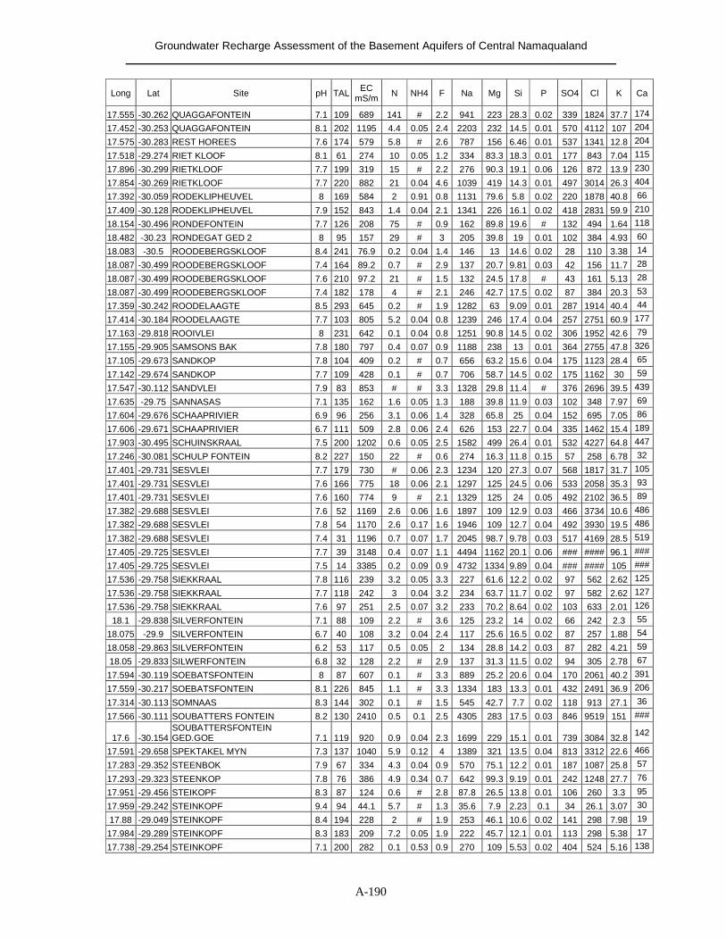
Groundwater Recharge Assessment of the Basement Aquifers of Central Namaqualand
A-190
Long Lat Site pH TAL EC mS/m N NH4 F Na Mg Si P SO4 Cl K Ca
17.555 -30.262 QUAGGAFONTEIN 7.1 109 689 141 # 2.2 941 223 28.3 0.02 339 1824 37.7 174
17.452 -30.253 QUAGGAFONTEIN 8.1 202 1195 4.4 0.05 2.4 2203 232 14.5 0.01 570 4112 107 204
17.575 -30.283 REST HOREES 7.6 174 579 5.8 # 2.6 787 156 6.46 0.01 537 1341 12.8 204
17.518 -29.274 RIET KLOOF 8.1 61 274 10 0.05 1.2 334 83.3 18.3 0.01 177 843 7.04 115
17.896 -30.299 RIETKLOOF 7.7 199 319 15 # 2.2 276 90.3 19.1 0.06 126 872 13.9 230
17.854 -30.269 RIETKLOOF 7.7 220 882 21 0.04 4.6 1039 419 14.3 0.01 497 3014 26.3 404
17.392 -30.059 RODEKLIPHEUVEL 8 169 584 2 0.91 0.8 1131 79.6 5.8 0.02 220 1878 40.8 66
17.409 -30.128 RODEKLIPHEUVEL 7.9 152 843 1.4 0.04 2.1 1341 226 16.1 0.02 418 2831 59.9 210
18.154 -30.496 RONDEFONTEIN 7.7 126 208 75 # 0.9 162 89.8 19.6 # 132 494 1.64 118
18.482 -30.23 RONDEGAT GED 2 8 95 157 29 # 3 205 39.8 19 0.01 102 384 4.93 60
18.083 -30.5 ROODEBERGSKLOOF 8.4 241 76.9 0.2 0.04 1.4 146 13 14.6 0.02 28 110 3.38 14
18.087 -30.499 ROODEBERGSKLOOF 7.4 164 89.2 0.7 # 2.9 137 20.7 9.81 0.03 42 156 11.7 28
18.087 -30.499 ROODEBERGSKLOOF 7.6 210 97.2 21 # 1.5 132 24.5 17.8 # 43 161 5.13 28
18.087 -30.499 ROODEBERGSKLOOF 7.4 182 178 4 # 2.1 246 42.7 17.5 0.02 87 384 20.3 53
17.359 -30.242 ROODELAAGTE 8.5 293 645 0.2 # 1.9 1282 63 9.09 0.01 287 1914 40.4 44
17.414 -30.184 ROODELAAGTE 7.7 103 805 5.2 0.04 0.8 1239 246 17.4 0.04 257 2751 60.9 177
17.163 -29.818 ROOIVLEI 8 231 642 0.1 0.04 0.8 1251 90.8 14.5 0.02 306 1952 42.6 79
17.155 -29.905 SAMSONS BAK 7.8 180 797 0.4 0.07 0.9 1188 238 13 0.01 364 2755 47.8 326
17.105 -29.673 SANDKOP 7.8 104 409 0.2 # 0.7 656 63.2 15.6 0.04 175 1123 28.4 65
17.142 -29.674 SANDKOP 7.7 109 428 0.1 # 0.7 706 58.7 14.5 0.02 175 1162 30 59
17.547 -30.112 SANDVLEI 7.9 83 853 # # 3.3 1328 29.8 11.4 # 376 2696 39.5 439
17.635 -29.75 SANNASAS 7.1 135 162 1.6 0.05 1.3 188 39.8 11.9 0.03 102 348 7.97 69
17.604 -29.676 SCHAAPRIVIER 6.9 96 256 3.1 0.06 1.4 328 65.8 25 0.04 152 695 7.05 86
17.606 -29.671 SCHAAPRIVIER 6.7 111 509 2.8 0.06 2.4 626 153 22.7 0.04 335 1462 15.4 189
17.903 -30.495 SCHUINSKRAAL 7.5 200 1202 0.6 0.05 2.5 1582 499 26.4 0.01 532 4227 64.8 447
17.246 -30.081 SCHULP FONTEIN 8.2 227 150 22 # 0.6 274 16.3 11.8 0.15 57 258 6.78 32
17.401 -29.731 SESVLEI 7.7 179 730 # 0.06 2.3 1234 120 27.3 0.07 568 1817 31.7 105
17.401 -29.731 SESVLEI 7.6 166 775 18 0.06 2.1 1297 125 24.5 0.06 533 2058 35.3 93
17.401 -29.731 SESVLEI 7.6 160 774 9 # 2.1 1329 125 24 0.05 492 2102 36.5 89
17.382 -29.688 SESVLEI 7.6 52 1169 2.6 0.06 1.6 1897 109 12.9 0.03 466 3734 10.6 486
17.382 -29.688 SESVLEI 7.8 54 1170 2.6 0.17 1.6 1946 109 12.7 0.04 492 3930 19.5 486
17.382 -29.688 SESVLEI 7.4 31 1196 0.7 0.07 1.7 2045 98.7 9.78 0.03 517 4169 28.5 519
17.405 -29.725 SESVLEI 7.7 39 3148 0.4 0.07 1.1 4494 1162 20.1 0.06 ### #### 96.1 ###
17.405 -29.725 SESVLEI 7.5 14 3385 0.2 0.09 0.9 4732 1334 9.89 0.04 ### #### 105 ###
17.536 -29.758 SIEKKRAAL 7.8 116 239 3.2 0.05 3.3 227 61.6 12.2 0.02 97 562 2.62 125
17.536 -29.758 SIEKKRAAL 7.7 118 242 3 0.04 3.2 234 63.7 11.7 0.02 97 582 2.62 127
17.536 -29.758 SIEKKRAAL 7.6 97 251 2.5 0.07 3.2 233 70.2 8.64 0.02 103 633 2.01 126
18.1 -29.838 SILVERFONTEIN 7.1 88 109 2.2 # 3.6 125 23.2 14 0.02 66 242 2.3 55
18.075 -29.9 SILVERFONTEIN 6.7 40 108 3.2 0.04 2.4 117 25.6 16.5 0.02 87 257 1.88 54
18.058 -29.863 SILVERFONTEIN 6.2 53 117 0.5 0.05 2 134 28.8 14.2 0.03 87 282 4.21 59
18.05 -29.833 SILWERFONTEIN 6.8 32 128 2.2 # 2.9 137 31.3 11.5 0.02 94 305 2.78 67
17.594 -30.119 SOEBATSFONTEIN 8 87 607 0.1 # 3.3 889 25.2 20.6 0.04 170 2061 40.2 391
17.559 -30.217 SOEBATSFONTEIN 8.1 226 845 1.1 # 3.3 1334 183 13.3 0.01 432 2491 36.9 206
17.314 -30.113 SOMNAAS 8.3 144 302 0.1 # 1.5 545 42.7 7.7 0.02 118 913 27.1 36
17.566 -30.111 SOUBATTERS FONTEIN 8.2 130 2410 0.5 0.1 2.5 4305 283 17.5 0.03 846 9519 151 ###
17.6 -30.154 SOUBATTERSFONTEIN GED.GOE 7.1 119 920 0.9 0.04 2.3 1699 229 15.1 0.01 739 3084 32.8 142
17.591 -29.658 SPEKTAKEL MYN 7.3 137 1040 5.9 0.12 4 1389 321 13.5 0.04 813 3312 22.6 466
17.283 -29.352 STEENBOK 7.9 67 334 4.3 0.04 0.9 570 75.1 12.2 0.01 187 1087 25.8 57
17.293 -29.323 STEENKOP 7.8 76 386 4.9 0.34 0.7 642 99.3 9.19 0.01 242 1248 27.7 76
17.951 -29.456 STEIKOPF 8.3 87 124 0.6 # 2.8 87.8 26.5 13.8 0.01 106 260 3.3 95
17.959 -29.242 STEINKOPF 9.4 94 44.1 5.7 # 1.3 35.6 7.9 2.23 0.1 34 26.1 3.07 30
17.88 -29.049 STEINKOPF 8.4 194 228 2 # 1.9 253 46.1 10.6 0.02 141 298 7.98 19
17.984 -29.289 STEINKOPF 8.3 183 209 7.2 0.05 1.9 222 45.7 12.1 0.01 113 298 5.38 17
17.738 -29.254 STEINKOPF 7.1 200 282 0.1 0.53 0.9 270 109 5.53 0.02 404 524 5.16 138
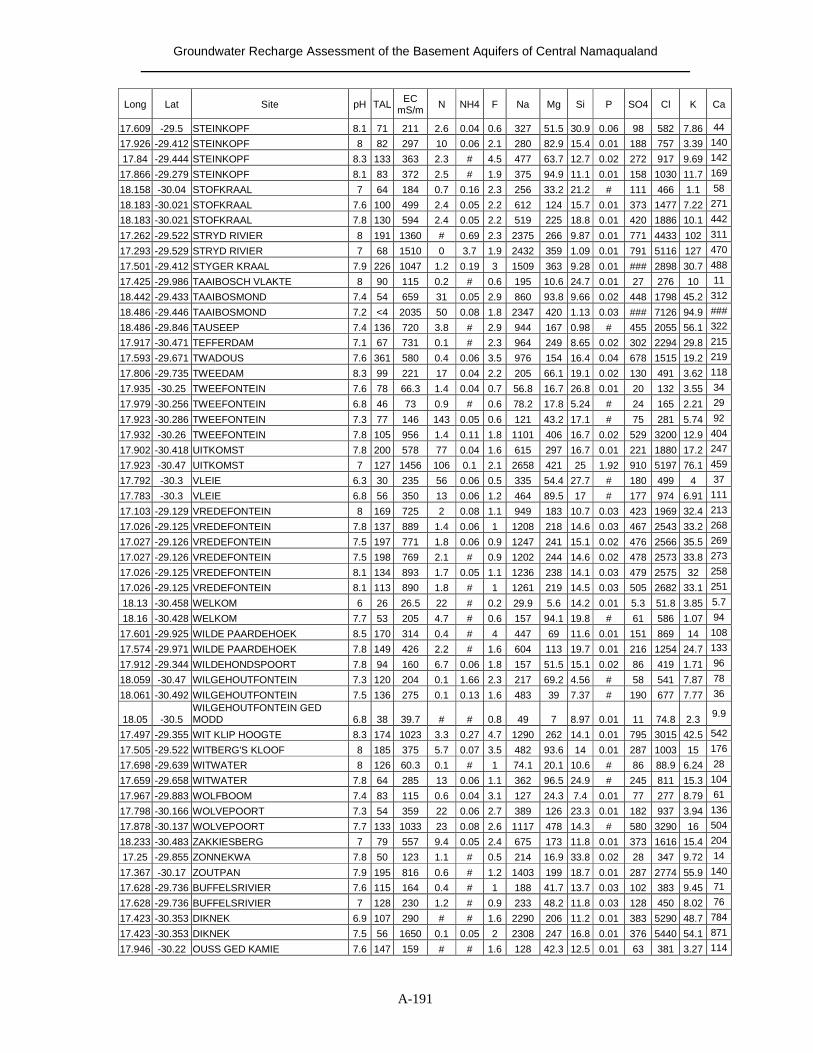
Groundwater Recharge Assessment of the Basement Aquifers of Central Namaqualand
A-191
Long Lat Site pH TAL EC mS/m N NH4 F Na Mg Si P SO4 Cl K Ca
17.609 -29.5 STEINKOPF 8.1 71 211 2.6 0.04 0.6 327 51.5 30.9 0.06 98 582 7.86 44
17.926 -29.412 STEINKOPF 8 82 297 10 0.06 2.1 280 82.9 15.4 0.01 188 757 3.39 140
17.84 -29.444 STEINKOPF 8.3 133 363 2.3 # 4.5 477 63.7 12.7 0.02 272 917 9.69 142
17.866 -29.279 STEINKOPF 8.1 83 372 2.5 # 1.9 375 94.9 11.1 0.01 158 1030 11.7 169
18.158 -30.04 STOFKRAAL 7 64 184 0.7 0.16 2.3 256 33.2 21.2 # 111 466 1.1 58
18.183 -30.021 STOFKRAAL 7.6 100 499 2.4 0.05 2.2 612 124 15.7 0.01 373 1477 7.22 271
18.183 -30.021 STOFKRAAL 7.8 130 594 2.4 0.05 2.2 519 225 18.8 0.01 420 1886 10.1 442
17.262 -29.522 STRYD RIVIER 8 191 1360 # 0.69 2.3 2375 266 9.87 0.01 771 4433 102 311
17.293 -29.529 STRYD RIVIER 7 68 1510 0 3.7 1.9 2432 359 1.09 0.01 791 5116 127 470
17.501 -29.412 STYGER KRAAL 7.9 226 1047 1.2 0.19 3 1509 363 9.28 0.01 ### 2898 30.7 488
17.425 -29.986 TAAIBOSCH VLAKTE 8 90 115 0.2 # 0.6 195 10.6 24.7 0.01 27 276 10 11
18.442 -29.433 TAAIBOSMOND 7.4 54 659 31 0.05 2.9 860 93.8 9.66 0.02 448 1798 45.2 312
18.486 -29.446 TAAIBOSMOND 7.2 <4 2035 50 0.08 1.8 2347 420 1.13 0.03 ### 7126 94.9 ###
18.486 -29.846 TAUSEEP 7.4 136 720 3.8 # 2.9 944 167 0.98 # 455 2055 56.1 322
17.917 -30.471 TEFFERDAM 7.1 67 731 0.1 # 2.3 964 249 8.65 0.02 302 2294 29.8 215
17.593 -29.671 TWADOUS 7.6 361 580 0.4 0.06 3.5 976 154 16.4 0.04 678 1515 19.2 219
17.806 -29.735 TWEEDAM 8.3 99 221 17 0.04 2.2 205 66.1 19.1 0.02 130 491 3.62 118
17.935 -30.25 TWEEFONTEIN 7.6 78 66.3 1.4 0.04 0.7 56.8 16.7 26.8 0.01 20 132 3.55 34
17.979 -30.256 TWEEFONTEIN 6.8 46 73 0.9 # 0.6 78.2 17.8 5.24 # 24 165 2.21 29
17.923 -30.286 TWEEFONTEIN 7.3 77 146 143 0.05 0.6 121 43.2 17.1 # 75 281 5.74 92
17.932 -30.26 TWEEFONTEIN 7.8 105 956 1.4 0.11 1.8 1101 406 16.7 0.02 529 3200 12.9 404
17.902 -30.418 UITKOMST 7.8 200 578 77 0.04 1.6 615 297 16.7 0.01 221 1880 17.2 247
17.923 -30.47 UITKOMST 7 127 1456 106 0.1 2.1 2658 421 25 1.92 910 5197 76.1 459
17.792 -30.3 VLEIE 6.3 30 235 56 0.06 0.5 335 54.4 27.7 # 180 499 4 37
17.783 -30.3 VLEIE 6.8 56 350 13 0.06 1.2 464 89.5 17 # 177 974 6.91 111
17.103 -29.129 VREDEFONTEIN 8 169 725 2 0.08 1.1 949 183 10.7 0.03 423 1969 32.4 213
17.026 -29.125 VREDEFONTEIN 7.8 137 889 1.4 0.06 1 1208 218 14.6 0.03 467 2543 33.2 268
17.027 -29.126 VREDEFONTEIN 7.5 197 771 1.8 0.06 0.9 1247 241 15.1 0.02 476 2566 35.5 269
17.027 -29.126 VREDEFONTEIN 7.5 198 769 2.1 # 0.9 1202 244 14.6 0.02 478 2573 33.8 273
17.026 -29.125 VREDEFONTEIN 8.1 134 893 1.7 0.05 1.1 1236 238 14.1 0.03 479 2575 32 258
17.026 -29.125 VREDEFONTEIN 8.1 113 890 1.8 # 1 1261 219 14.5 0.03 505 2682 33.1 251
18.13 -30.458 WELKOM 6 26 26.5 22 # 0.2 29.9 5.6 14.2 0.01 5.3 51.8 3.85 5.7
18.16 -30.428 WELKOM 7.7 53 205 4.7 # 0.6 157 94.1 19.8 # 61 586 1.07 94
17.601 -29.925 WILDE PAARDEHOEK 8.5 170 314 0.4 # 4 447 69 11.6 0.01 151 869 14 108
17.574 -29.971 WILDE PAARDEHOEK 7.8 149 426 2.2 # 1.6 604 113 19.7 0.01 216 1254 24.7 133
17.912 -29.344 WILDEHONDSPOORT 7.8 94 160 6.7 0.06 1.8 157 51.5 15.1 0.02 86 419 1.71 96
18.059 -30.47 WILGEHOUTFONTEIN 7.3 120 204 0.1 1.66 2.3 217 69.2 4.56 # 58 541 7.87 78
18.061 -30.492 WILGEHOUTFONTEIN 7.5 136 275 0.1 0.13 1.6 483 39 7.37 # 190 677 7.77 36
18.05 -30.5 WILGEHOUTFONTEIN GED MODD 6.8 38 39.7 # # 0.8 49 7 8.97 0.01 11 74.8 2.3 9.9
17.497 -29.355 WIT KLIP HOOGTE 8.3 174 1023 3.3 0.27 4.7 1290 262 14.1 0.01 795 3015 42.5 542
17.505 -29.522 WITBERG'S KLOOF 8 185 375 5.7 0.07 3.5 482 93.6 14 0.01 287 1003 15 176
17.698 -29.639 WITWATER 8 126 60.3 0.1 # 1 74.1 20.1 10.6 # 86 88.9 6.24 28
17.659 -29.658 WITWATER 7.8 64 285 13 0.06 1.1 362 96.5 24.9 # 245 811 15.3 104
17.967 -29.883 WOLFBOOM 7.4 83 115 0.6 0.04 3.1 127 24.3 7.4 0.01 77 277 8.79 61
17.798 -30.166 WOLVEPOORT 7.3 54 359 22 0.06 2.7 389 126 23.3 0.01 182 937 3.94 136
17.878 -30.137 WOLVEPOORT 7.7 133 1033 23 0.08 2.6 1117 478 14.3 # 580 3290 16 504
18.233 -30.483 ZAKKIESBERG 7 79 557 9.4 0.05 2.4 675 173 11.8 0.01 373 1616 15.4 204
17.25 -29.855 ZONNEKWA 7.8 50 123 1.1 # 0.5 214 16.9 33.8 0.02 28 347 9.72 14
17.367 -30.17 ZOUTPAN 7.9 195 816 0.6 # 1.2 1403 199 18.7 0.01 287 2774 55.9 140
17.628 -29.736 BUFFELSRIVIER 7.6 115 164 0.4 # 1 188 41.7 13.7 0.03 102 383 9.45 71
17.628 -29.736 BUFFELSRIVIER 7 128 230 1.2 # 0.9 233 48.2 11.8 0.03 128 450 8.02 76
17.423 -30.353 DIKNEK 6.9 107 290 # # 1.6 2290 206 11.2 0.01 383 5290 48.7 784
17.423 -30.353 DIKNEK 7.5 56 1650 0.1 0.05 2 2308 247 16.8 0.01 376 5440 54.1 871
17.946 -30.22 OUSS GED KAMIE 7.6 147 159 # # 1.6 128 42.3 12.5 0.01 63 381 3.27 114
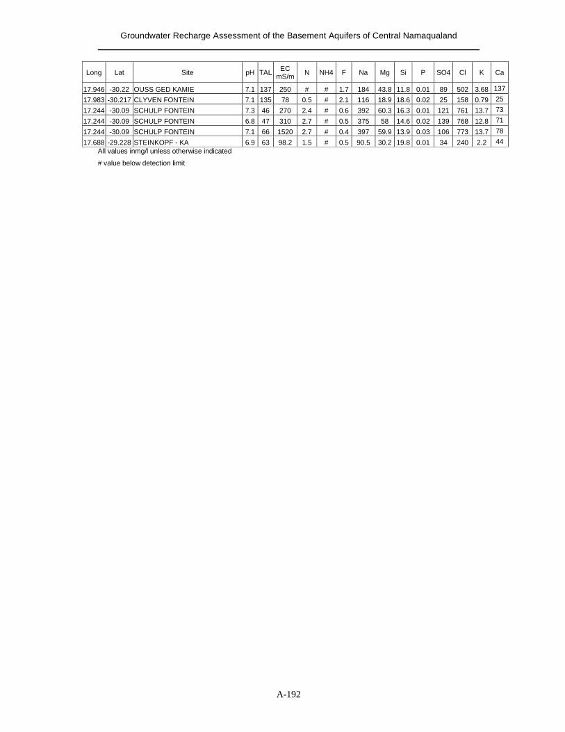
Groundwater Recharge Assessment of the Basement Aquifers of Central Namaqualand
A-192
Long Lat Site pH TAL EC mS/m N NH4 F Na Mg Si P SO4 Cl K Ca
17.946 -30.22 OUSS GED KAMIE 7.1 137 250 # # 1.7 184 43.8 11.8 0.01 89 502 3.68 137
17.983 -30.217 CLYVEN FONTEIN 7.1 135 78 0.5 # 2.1 116 18.9 18.6 0.02 25 158 0.79 25
17.244 -30.09 SCHULP FONTEIN 7.3 46 270 2.4 # 0.6 392 60.3 16.3 0.01 121 761 13.7 73
17.244 -30.09 SCHULP FONTEIN 6.8 47 310 2.7 # 0.5 375 58 14.6 0.02 139 768 12.8 71
17.244 -30.09 SCHULP FONTEIN 7.1 66 1520 2.7 # 0.4 397 59.9 13.9 0.03 106 773 13.7 78
17.688 -29.228 STEINKOPF - KA 6.9 63 98.2 1.5 # 0.5 90.5 30.2 19.8 0.01 34 240 2.2 44 All values inmg/l unless otherwise indicated
# value below detection limit
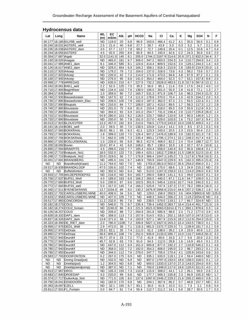
Groundwater Recharge Assessment of the Basement Aquifers of Central Namaqualand
A-193
Hydrocensus data Lat Long Name WL
(m) EC
mS/m Alk. pH HCO3 Na Cl Ca K Mg SO4 N F
-30.177 18.185 91LF88_well ND 119.0 20 6.8 96.9 163.6 466.4 41.2 4.1 35.5 56.5 0.1 0.9 -30.240 18.031 AGTER1_well 2.5 21.4 40 6.8 27.7 28.7 43.9 5.3 0.3 5.2 5.7 2.1 0.4 -30.235 18.038 AGTER2_dam 3.5 67.7 117 7.8 69.2 72.7 149.6 20.4 0.1 12.5 10.8 4.7 0.4 -30.244 18.055 AGTER3 4.5 92.5 250 8.9 85.9 84.3 193.5 42.6 0.2 24.3 35.6 0.6 2.0 -30.354 17.687 Aigab 32.0 1141.0 145 8.1 205.0 1744.2 3167.9 314.6 20.9 371.3 832.0 34.4 3.7 -30.130 18.020 Anagas ND 465.0 181 6.7 306.0 347.2 903.0 234.3 3.4 110.7 294.9 3.4 1.5 -30.041 17.985 ANE1_dam 8.1 346.0 585 8.1 124.6 414.4 809.5 152.6 3.0 129.1 244.3 1.4 4.0 -30.126 18.017 ANE2_dam ND 329.0 854 6.9 166.2 308.1 818.3 210.9 2.8 183.9 219.9 20.0 1.5 -30.110 17.920 Arkoep ND 179.2 79 7.2 104.0 137.0 318.0 73.6 4.3 58.2 73.6 0.7 2.0 -30.110 17.920 Arkoep ND 220.0 42 7.3 114.0 171.6 473.0 94.8 4.8 67.9 87.2 0.1 2.6 -30.140 17.940 Arkoep ND 276.0 95 6.8 141.0 354.2 464.0 52.3 0.7 53.1 157.8 8.8 2.0 -29.999 17.778 ARREGAS ND 635.0 210 6.7 227.5 732.2 2628.0 483.5 21.8 317.6 567.8 13.1 2.1 -30.242 18.061 BAK1_well 2.2 52.3 125 7.0 39.3 56.0 85.1 11.6 0.9 17.6 24.3 4.0 1.0 -29.710 17.900 BeginWeer ND 134.0 102 7.6 138.0 106.5 301.0 55.9 2.8 41.8 72.1 1.3 2.7 -30.384 17.836 Bethel 1.0 359.0 80 7.2 165.7 531.3 971.9 106.7 3.6 98.3 234.3 21.0 3.2 -29.740 17.930 Biesiesfontein ND 167.5 62 7.4 111.0 178.6 370.0 70.4 1.5 42.9 104.2 2.0 3.3 -29.730 17.880 Biesiesfontein_Elec ND 209.0 100 7.9 192.0 187.3 362.0 97.3 2.1 55.5 122.4 0.1 2.8 -29.720 17.890 Blouputs ND 210.0 84 7.7 108.0 187.1 413.0 89.5 1.7 58.3 117.3 1.2 2.8 -29.740 17.880 Bloustasie ND 201.0 75 6.8 81.0 153.4 318.0 89.3 0.9 55.9 112.8 9.3 1.2 -29.730 17.880 Bloustasie ND 394.0 93 6.9 101.0 254.7 731.0 196.4 2.8 110.7 235.8 26.0 1.4 -29.710 17.910 Bloustasie 54.9 280.0 101 8.2 118.0 223.7 568.0 110.9 3.9 90.3 146.9 1.2 2.5 -29.720 17.890 Bloustasie ND 250.0 50 7.8 151.0 217.0 429.0 103.5 1.6 73.2 167.3 9.4 2.5 -30.013 17.823 BLOUSYFER 13.3 457.0 192 8.9 210.6 758.5 1773.0 243.9 10.0 228.5 409.5 4.2 2.9 -30.191 18.154 BOB1_well 2.0 59.5 30 7.0 138.5 103.8 114.4 14.1 0.9 8.5 37.3 0.3 0.9 -29.802 17.560 BOKKRAAL 36.0 86.1 65 6.3 42.1 123.3 243.0 20.5 2.3 23.5 50.4 2.2 1.0 -29.793 17.563 BOKKRAAL 1.8 399.0 120 7.0 126.4 607.2 1476.0 189.9 3.9 182.5 321.3 7.8 3.5 -30.209 17.706 BOKSKRAAL 7.0 662.0 109 7.3 235.4 993.1 1795.1 274.1 10.1 248.2 417.4 4.8 3.1 -29.866 17.592 BOSLUISKRAAL 1.0 226.0 65 6.9 98.3 417.6 468.0 82.2 2.4 70.4 188.7 12.7 3.0 -30.200 18.050 Bovlei 10.0 87.4 42 6.8 108.0 85.7 138.0 32.9 1.8 32.7 67.4 10.8 1.1 -29.890 17.594 BRAKPITS 4.5 289.0 216 7.7 185.4 424.4 558.0 140.4 8.0 95.9 190.8 0.1 3.7 -30.246 17.710 Brakputs_No1 18.0 532.0 122 7.5 199.4 623.1 1812.7 238.8 11.5 198.9 312.5 10.4 2.9 -30.248 17.710 Brakputs_No2 20.0 319.5 56 7.7 176.9 366.4 1047.1 145.2 7.3 117.8 178.8 10.3 2.1 -30.001 17.691 BRANDBERG ND 495.0 101 6.7 148.9 793.9 1647.0 229.9 8.5 162.3 395.0 21.8 2.6
ND ND Brandhoek(kraan) 11.2 764.0 ND 7.0 ND 1753.0 3813.0 502.0 35.5 254.0 656.0 0.1 2.0 -29.517 19.939 BRANDKLOOF 47.0 105.6 102 7.4 ND 105.6 175.0 68.6 1.3 24.9 215.2 ND 2.5
ND ND Buffelsfontein ND 302.0 ND 6.4 ND 513.0 1167.0 159.0 13.1 114.0 206.0 6.9 0.8 -29.933 17.705 WILDEPERDEPAS ND 216.0 ND 8.0 165.7 290.0 638.9 141.1 6.3 49.0 153.6 0.1 3.4 -29.736 17.637 BUFS1_Well 4.0 189.0 163 6.8 166.2 260.5 440.0 87.1 11.6 54.7 109.0 0.1 0.9 -29.770 17.660 BUFS3_Well 5.0 230.0 67 6.6 102.5 301.9 545.6 110.6 10.7 74.6 240.3 0.1 0.5 -29.772 17.660 BUFS5_well 5.0 317.0 145 7.4 166.2 525.8 747.9 137.3 17.0 78.2 289.4 16.0 1.2 -30.340 17.511 BYENESKRANS 13.7 1034.0 69 8.0 130.2 1876.9 2956.6 215.0 44.6 207.2 538.2 1.8 3.0 -29.583 17.792 CAROLUSBERG MINE 40.0 408.0 34 5.5 ND 129.0 158.0 350.5 3.6 404.3 6903.0 ND 125.0 -29.633 17.958 CAROLUSBERG MINE ND 407.0 105 7.0 ND 448.3 544.0 356.2 3.5 119.2 3254.0 ND 2.6 -29.517 17.983 CONCORDIA 11.2 232.0 95 7.6 ND 238.5 579.0 119.1 1.7 66.7 324.9 ND 1.5 -30.181 18.273 COU1 ND 546.0 75 6.7 235.4 736.4 1452.0 363.7 16.4 214.4 451.7 21.0 1.9 -30.182 18.274 COU2_fontain ND 2240.0 86 8.3 221.5 4521.0 9063.0 1014.1 71.1 992.1 878.6 0.3 1.6 -30.126 18.257 COU3 ND 209.0 88 7.2 294.9 261.8 585.9 98.9 2.4 71.2 177.0 3.9 4.5 -29.828 18.332 DAP1_dam ND 358.0 113 7.3 157.9 514.5 915.1 202.1 18.0 107.0 247.8 13.0 1.9 -29.827 18.326 DAP2_dam 13.8 371.0 58 7.4 193.9 527.1 967.9 215.9 18.2 112.9 254.5 15.0 1.9 -30.323 18.390 DE_RIET_dam 2.0 780.0 1108 7.2 339.8 5827.1 1927.6 203.3 22.4 243.5 738.0 0.1 5.0 -29.959 17.975 DED1_Well 2.9 472.0 38 7.1 116.3 681.5 1372.7 220.3 7.1 139.9 181.7 0.1 0.9 -29.950 17.970 DeDraai 29.3 82.1 35 7.4 111.0 61.2 138.0 39.2 1.9 23.9 40.9 1.2 2.6 -29.960 17.970 DeDraai 36.6 805.0 108 7.6 252.0 935.8 2133.0 285.7 10.0 110.7 448.8 81.0 3.3 -29.770 17.940 Deurdrif 45.7 37.4 23 7.2 77.0 41.9 69.0 16.3 1.7 5.6 20.0 2.3 0.6 -29.770 17.940 Deurdrif 45.7 62.8 63 7.9 91.0 64.3 112.0 28.8 1.6 14.9 49.4 0.1 2.5 -29.780 17.960 Deurdrif ND 647.0 112 6.9 161.0 900.8 877.0 192.2 2.7 110.8 546.2 0.1 4.6 -29.780 17.940 Deurdrif ND 358.0 102 7.2 192.0 354.3 808.0 195.0 2.2 98.7 283.2 0.1 2.5 -29.780 17.950 Deurdrif ND 344.0 112 7.6 279.0 347.7 705.0 170.4 4.1 105.8 243.6 0.6 3.0 -29.583 17.793 DOOIFONTEIN 6.2 267.0 175 6.9 ND 335.1 633.0 118.1 2.4 59.4 448.0 ND 2.5
ND ND Doring Draai(put) ND 432.0 ND 6.8 ND 897.0 1797.0 193.0 18.6 158.0 318.0 0.1 1.0 ND ND Drieklip(put) 1.2 354.0 ND 6.8 ND 600.0 1333.0 137.0 27.3 143.0 254.0 9.9 0.6 ND ND Drieklip(windpomp) ND 387.0 ND 7.1 ND 760.0 1348.0 117.0 19.6 120.0 311.0 4.0 2.7
-29.913 17.967 DRO1 ND 105.3 155 7.3 110.8 115.9 308.0 44.1 1.2 26.1 59.0 2.6 2.1 -29.683 17.840 DROEDAP 4.0 220.0 99 6.8 ND 177.7 569.3 155.8 2.3 66.9 155.3 ND 1.7 -30.374 17.717 Duikerkop_font ND 771.5 105 8.0 137.6 1097.6 2446.2 229.2 21.6 265.2 469.0 0.8 1.5 -29.750 18.041 EENDOORN ND 182.9 170 6.8 ND 204.1 367.9 86.2 0.7 48.8 157.7 ND 3.3 -30.393 18.097 EZEL1 ND 32.1 155 6.7 83.1 35.0 61.6 10.3 0.1 7.3 2.1 0.8 0.4 -29.811 17.501 F1_Fontain 0.0 84.7 61 7.4 55.4 112.7 211.2 14.1 5.6 28.7 30.5 1.7 0.3
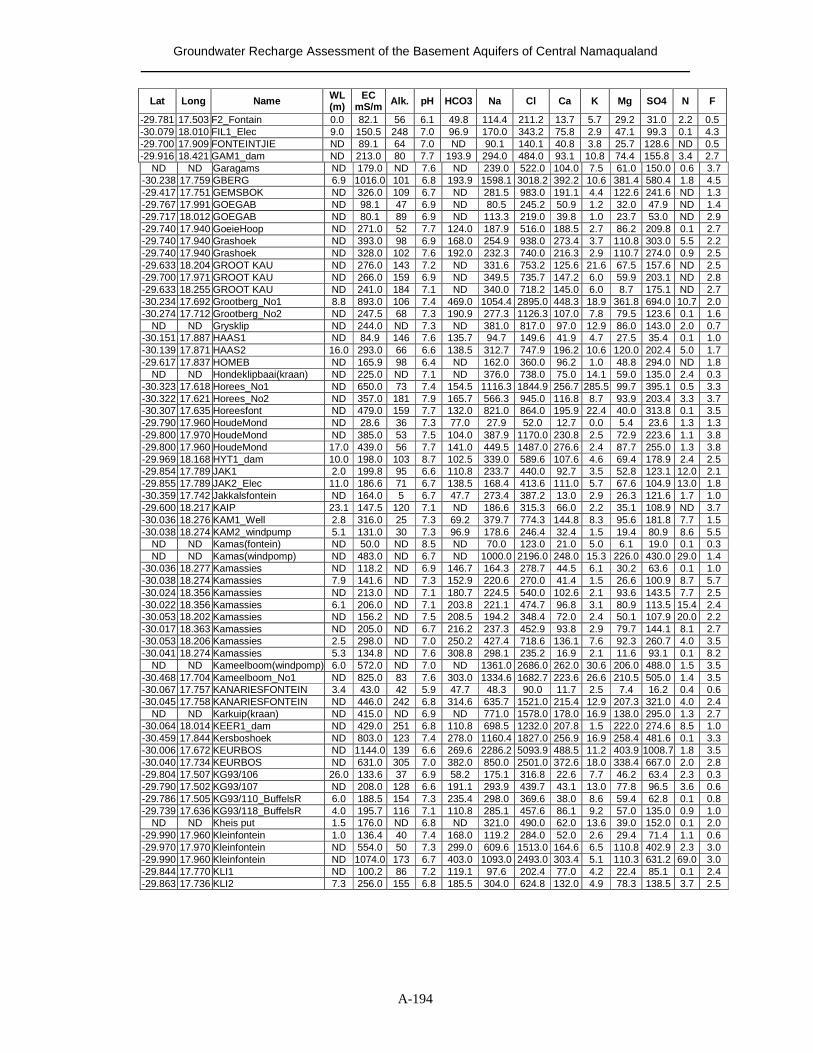
Groundwater Recharge Assessment of the Basement Aquifers of Central Namaqualand
A-194
Lat Long Name WL (m)
EC mS/m Alk. pH HCO3 Na Cl Ca K Mg SO4 N F
-29.781 17.503 F2_Fontain 0.0 82.1 56 6.1 49.8 114.4 211.2 13.7 5.7 29.2 31.0 2.2 0.5 -30.079 18.010 FIL1_Elec 9.0 150.5 248 7.0 96.9 170.0 343.2 75.8 2.9 47.1 99.3 0.1 4.3 -29.700 17.909 FONTEINTJIE ND 89.1 64 7.0 ND 90.1 140.1 40.8 3.8 25.7 128.6 ND 0.5 -29.916 18.421 GAM1_dam ND 213.0 80 7.7 193.9 294.0 484.0 93.1 10.8 74.4 155.8 3.4 2.7
ND ND Garagams ND 179.0 ND 7.6 ND 239.0 522.0 104.0 7.5 61.0 150.0 0.6 3.7 -30.238 17.759 GBERG 6.9 1016.0 101 6.8 193.9 1598.1 3018.2 392.2 10.6 381.4 580.4 1.8 4.5 -29.417 17.751 GEMSBOK ND 326.0 109 6.7 ND 281.5 983.0 191.1 4.4 122.6 241.6 ND 1.3 -29.767 17.991 GOEGAB ND 98.1 47 6.9 ND 80.5 245.2 50.9 1.2 32.0 47.9 ND 1.4 -29.717 18.012 GOEGAB ND 80.1 89 6.9 ND 113.3 219.0 39.8 1.0 23.7 53.0 ND 2.9 -29.740 17.940 GoeieHoop ND 271.0 52 7.7 124.0 187.9 516.0 188.5 2.7 86.2 209.8 0.1 2.7 -29.740 17.940 Grashoek ND 393.0 98 6.9 168.0 254.9 938.0 273.4 3.7 110.8 303.0 5.5 2.2 -29.740 17.940 Grashoek ND 328.0 102 7.6 192.0 232.3 740.0 216.3 2.9 110.7 274.0 0.9 2.5 -29.633 18.204 GROOT KAU ND 276.0 143 7.2 ND 331.6 753.2 125.6 21.6 67.5 157.6 ND 2.5 -29.700 17.971 GROOT KAU ND 266.0 159 6.9 ND 349.5 735.7 147.2 6.0 59.9 203.1 ND 2.8 -29.633 18.255 GROOT KAU ND 241.0 184 7.1 ND 340.0 718.2 145.0 6.0 8.7 175.1 ND 2.7 -30.234 17.692 Grootberg_No1 8.8 893.0 106 7.4 469.0 1054.4 2895.0 448.3 18.9 361.8 694.0 10.7 2.0 -30.274 17.712 Grootberg_No2 ND 247.5 68 7.3 190.9 277.3 1126.3 107.0 7.8 79.5 123.6 0.1 1.6
ND ND Grysklip ND 244.0 ND 7.3 ND 381.0 817.0 97.0 12.9 86.0 143.0 2.0 0.7 -30.151 17.887 HAAS1 ND 84.9 146 7.6 135.7 94.7 149.6 41.9 4.7 27.5 35.4 0.1 1.0 -30.139 17.871 HAAS2 16.0 293.0 66 6.6 138.5 312.7 747.9 196.2 10.6 120.0 202.4 5.0 1.7 -29.617 17.837 HOMEB ND 165.9 98 6.4 ND 162.0 360.0 96.2 1.0 48.8 294.0 ND 1.8
ND ND Hondeklipbaai(kraan) ND 225.0 ND 7.1 ND 376.0 738.0 75.0 14.1 59.0 135.0 2.4 0.3 -30.323 17.618 Horees_No1 ND 650.0 73 7.4 154.5 1116.3 1844.9 256.7 285.5 99.7 395.1 0.5 3.3 -30.322 17.621 Horees_No2 ND 357.0 181 7.9 165.7 566.3 945.0 116.8 8.7 93.9 203.4 3.3 3.7 -30.307 17.635 Horeesfont ND 479.0 159 7.7 132.0 821.0 864.0 195.9 22.4 40.0 313.8 0.1 3.5 -29.790 17.960 HoudeMond ND 28.6 36 7.3 77.0 27.9 52.0 12.7 0.0 5.4 23.6 1.3 1.3 -29.800 17.970 HoudeMond ND 385.0 53 7.5 104.0 387.9 1170.0 230.8 2.5 72.9 223.6 1.1 3.8 -29.800 17.960 HoudeMond 17.0 439.0 56 7.7 141.0 449.5 1487.0 276.6 2.4 87.7 255.0 1.3 3.8 -29.969 18.168 HYT1_dam 10.0 198.0 103 8.7 102.5 339.0 589.6 107.6 4.6 69.4 178.9 2.4 2.5 -29.854 17.789 JAK1 2.0 199.8 95 6.6 110.8 233.7 440.0 92.7 3.5 52.8 123.1 12.0 2.1 -29.855 17.789 JAK2_Elec 11.0 186.6 71 6.7 138.5 168.4 413.6 111.0 5.7 67.6 104.9 13.0 1.8 -30.359 17.742 Jakkalsfontein ND 164.0 5 6.7 47.7 273.4 387.2 13.0 2.9 26.3 121.6 1.7 1.0 -29.600 18.217 KAIP 23.1 147.5 120 7.1 ND 186.6 315.3 66.0 2.2 35.1 108.9 ND 3.7 -30.036 18.276 KAM1_Well 2.8 316.0 25 7.3 69.2 379.7 774.3 144.8 8.3 95.6 181.8 7.7 1.5 -30.038 18.274 KAM2_windpump 5.1 131.0 30 7.3 96.9 178.6 246.4 32.4 1.5 19.4 80.9 8.6 5.5
ND ND Kamas(fontein) ND 50.0 ND 8.5 ND 70.0 123.0 21.0 5.0 6.1 19.0 0.1 0.3 ND ND Kamas(windpomp) ND 483.0 ND 6.7 ND 1000.0 2196.0 248.0 15.3 226.0 430.0 29.0 1.4
-30.036 18.277 Kamassies ND 118.2 ND 6.9 146.7 164.3 278.7 44.5 6.1 30.2 63.6 0.1 1.0 -30.038 18.274 Kamassies 7.9 141.6 ND 7.3 152.9 220.6 270.0 41.4 1.5 26.6 100.9 8.7 5.7 -30.024 18.356 Kamassies ND 213.0 ND 7.1 180.7 224.5 540.0 102.6 2.1 93.6 143.5 7.7 2.5 -30.022 18.356 Kamassies 6.1 206.0 ND 7.1 203.8 221.1 474.7 96.8 3.1 80.9 113.5 15.4 2.4 -30.053 18.202 Kamassies ND 156.2 ND 7.5 208.5 194.2 348.4 72.0 2.4 50.1 107.9 20.0 2.2 -30.017 18.363 Kamassies ND 205.0 ND 6.7 216.2 237.3 452.9 93.8 2.9 79.7 144.1 8.1 2.7 -30.053 18.206 Kamassies 2.5 298.0 ND 7.0 250.2 427.4 718.6 136.1 7.6 92.3 260.7 4.0 3.5 -30.041 18.274 Kamassies 5.3 134.8 ND 7.6 308.8 298.1 235.2 16.9 2.1 11.6 93.1 0.1 8.2
ND ND Kameelboom(windpomp) 6.0 572.0 ND 7.0 ND 1361.0 2686.0 262.0 30.6 206.0 488.0 1.5 3.5 -30.468 17.704 Kameelboom_No1 ND 825.0 83 7.6 303.0 1334.6 1682.7 223.6 26.6 210.5 505.0 1.4 3.5 -30.067 17.757 KANARIESFONTEIN 3.4 43.0 42 5.9 47.7 48.3 90.0 11.7 2.5 7.4 16.2 0.4 0.6 -30.045 17.758 KANARIESFONTEIN ND 446.0 242 6.8 314.6 635.7 1521.0 215.4 12.9 207.3 321.0 4.0 2.4
ND ND Karkuip(kraan) ND 415.0 ND 6.9 ND 771.0 1578.0 178.0 16.9 138.0 295.0 1.3 2.7 -30.064 18.014 KEER1_dam ND 429.0 251 6.8 110.8 698.5 1232.0 207.8 1.5 222.0 274.6 8.5 1.0 -30.459 17.844 Kersboshoek ND 803.0 123 7.4 278.0 1160.4 1827.0 256.9 16.9 258.4 481.6 0.1 3.3 -30.006 17.672 KEURBOS ND 1144.0 139 6.6 269.6 2286.2 5093.9 488.5 11.2 403.9 1008.7 1.8 3.5 -30.040 17.734 KEURBOS ND 631.0 305 7.0 382.0 850.0 2501.0 372.6 18.0 338.4 667.0 2.0 2.8 -29.804 17.507 KG93/106 26.0 133.6 37 6.9 58.2 175.1 316.8 22.6 7.7 46.2 63.4 2.3 0.3 -29.790 17.502 KG93/107 ND 208.0 128 6.6 191.1 293.9 439.7 43.1 13.0 77.8 96.5 3.6 0.6 -29.786 17.505 KG93/110_BuffelsR 6.0 188.5 154 7.3 235.4 298.0 369.6 38.0 8.6 59.4 62.8 0.1 0.8 -29.739 17.636 KG93/118_BuffelsR 4.0 195.7 116 7.1 110.8 285.1 457.6 86.1 9.2 57.0 135.0 0.9 1.0
ND ND Kheis put 1.5 176.0 ND 6.8 ND 321.0 490.0 62.0 13.6 39.0 152.0 0.1 2.0 -29.990 17.960 Kleinfontein 1.0 136.4 40 7.4 168.0 119.2 284.0 52.0 2.6 29.4 71.4 1.1 0.6 -29.970 17.970 Kleinfontein ND 554.0 50 7.3 299.0 609.6 1513.0 164.6 6.5 110.8 402.9 2.3 3.0 -29.990 17.960 Kleinfontein ND 1074.0 173 6.7 403.0 1093.0 2493.0 303.4 5.1 110.3 631.2 69.0 3.0 -29.844 17.770 KLI1 ND 100.2 86 7.2 119.1 97.6 202.4 77.0 4.2 22.4 85.1 0.1 2.4 -29.863 17.736 KLI2 7.3 256.0 155 6.8 185.5 304.0 624.8 132.0 4.9 78.3 138.5 3.7 2.5
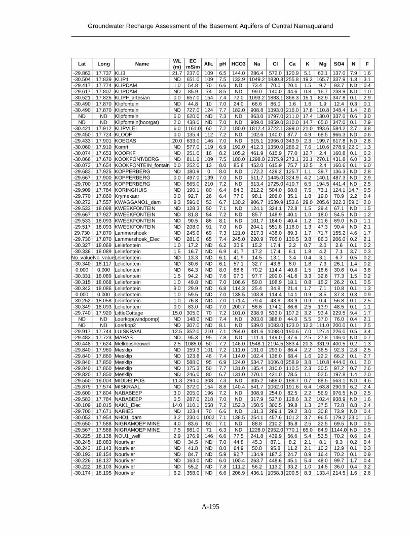
Groundwater Recharge Assessment of the Basement Aquifers of Central Namaqualand
A-195
Lat Long Name WL (m)
EC mS/m Alk. pH HCO3 Na Cl Ca K Mg SO4 N F
-29.863 17.737 KLI3 21.7 237.0 109 6.5 144.0 286.4 572.0 120.9 5.1 63.1 137.0 7.9 1.6 -30.504 17.839 KLIP1 ND 651.0 109 7.5 132.9 1049.2 1830.3 255.8 19.2 165.7 337.9 1.3 3.1 -29.417 17.774 KLIPDAM 1.0 54.8 70 6.6 ND 73.4 70.0 20.1 1.5 9.7 93.7 ND 0.4 -29.617 17.807 KLIPDAM ND 85.9 74 8.5 ND 99.0 140.0 44.6 0.8 16.7 238.9 ND 1.0 -30.521 17.826 KLIPF_artesian 0.0 657.0 154 7.4 72.0 1093.2 1883.1 366.3 15.1 82.9 347.8 0.1 2.9 -30.490 17.870 Klipfontein ND 44.8 10 7.0 24.0 66.6 86.0 1.6 1.6 1.9 12.4 0.3 0.1 -30.490 17.870 Klipfontein ND 727.0 124 7.7 182.0 908.8 1393.0 216.0 17.8 110.8 348.4 1.4 2.8
ND ND Klipfontein 6.0 620.0 ND 7.3 ND 863.0 1797.0 211.0 17.4 130.0 337.0 0.6 3.0 ND ND Klipfontein(boorgat) 2.0 438.0 ND 7.0 ND 909.0 1859.0 310.0 14.7 65.0 347.0 0.1 2.9
-30.421 17.912 KLIPVLEI 6.0 1161.0 60 7.2 180.0 1812.4 3722.1 399.0 21.0 493.6 584.2 2.7 3.8 -29.450 17.724 KLOOF 0.0 135.4 112 7.2 ND 102.6 140.0 87.7 4.9 68.5 966.3 ND 0.6 -29.433 17.901 KOEGAS 20.0 633.0 146 7.0 ND 615.1 1966.0 343.9 2.3 199.7 617.8 ND 2.8 -30.060 17.910 Komri ND 577.0 119 6.9 192.0 412.3 1350.0 286.2 7.6 110.6 278.9 22.0 1.3 -30.074 17.653 KOOFKF ND 251.0 16 8.2 105.2 461.9 615.9 77.0 12.7 2.4 160.8 0.1 6.2 -30.066 17.670 KOOKFONT/BERG ND 811.0 109 7.5 180.0 1298.0 2375.9 273.1 33.1 270.1 431.8 6.0 3.3 -30.073 17.654 KOOKFONTEIN_fontain 0.0 252.0 13 8.0 85.8 452.0 615.9 75.7 12.5 2.4 160.6 0.1 6.0 -29.683 17.925 KOPPERBERG ND 180.9 0 8.0 ND 172.2 429.2 125.7 1.1 39.7 136.3 ND 2.8 -29.667 17.900 KOPPERBERG 0.0 497.0 139 7.0 ND 511.7 1445.0 324.9 4.2 140.1 487.3 ND 2.9 -29.700 17.905 KOPPERBERG ND 565.0 210 7.2 ND 513.4 1725.0 410.7 6.5 194.5 441.4 ND 2.5 -29.909 17.784 KORINGHUIS ND 190.1 80 6.4 84.3 212.2 504.0 68.0 7.5 73.1 124.1 14.7 0.5 -29.770 17.860 Krymekaar 0.0 92.7 26 6.4 77.0 98.1 206.0 35.1 1.8 19.0 70.9 2.2 0.4 -30.272 17.557 KWAGGANO1_dam 9.3 596.0 53 6.7 130.2 906.7 1539.9 153.6 29.0 205.6 322.3 59.0 2.0 -29.533 18.098 KWEEKFONTEIN ND 128.3 50 7.1 ND 124.1 324.1 72.8 1.5 29.4 67.1 ND 1.5 -29.667 17.927 KWEEKFONTEIN ND 81.8 54 7.2 ND 85.7 148.9 40.1 1.0 18.0 54.5 ND 1.2 -29.533 18.093 KWEEKFONTEIN ND 90.5 86 8.1 ND 101.7 184.0 40.4 1.2 21.6 69.0 ND 1.1 -29.517 18.093 KWEEKFONTEIN ND 208.0 91 7.0 ND 204.1 551.8 116.0 1.3 47.3 90.4 ND 2.1 29.730 17.870 Lammershoek ND 245.0 69 7.3 121.0 217.3 438.0 89.3 1.7 71.7 155.2 4.6 1.7 -29.730 17.870 Lammershoek_Elec ND 281.0 65 7.4 245.0 220.9 705.0 130.5 3.8 86.3 206.0 0.2 2.1 -30.327 18.069 Leliefontein 1.0 17.2 ND 6.2 30.9 15.2 17.4 2.2 0.7 2.0 2.6 0.1 0.2 -30.336 18.089 Leliefontein 1.5 16.7 ND 6.9 41.7 17.2 17.4 6.1 1.8 4.2 7.1 3.7 0.3
No_valueNo_valueLeliefontein ND 13.3 ND 6.1 41.9 14.5 13.1 3.4 0.4 3.1 6.7 0.5 0.2 -30.340 18.117 Leliefontein ND 30.6 ND 6.1 57.1 32.7 43.6 8.0 1.8 7.3 26.1 1.4 0.2 0.000 0.000 Leliefontein ND 64.3 ND 8.0 88.6 70.2 114.4 40.8 1.5 18.6 30.6 0.4 3.8
-30.331 18.089 Leliefontein 1.5 94.2 ND 7.6 97.3 97.7 209.0 41.6 3.3 32.6 77.3 1.5 0.2 -30.315 18.068 Leliefontein 1.0 49.8 ND 7.0 106.6 59.0 108.9 18.1 0.8 15.2 26.2 0.1 0.5 -30.342 18.086 Leliefontein 9.0 29.9 ND 6.8 114.3 25.4 34.8 21.4 1.7 7.1 10.8 0.1 1.3 0.000 0.000 Leliefontein 1.0 59.5 ND 7.0 138.5 103.8 114.4 14.1 0.9 8.5 37.3 0.3 0.9
-30.252 18.058 Leliefontein 1.0 76.8 ND 7.0 171.4 79.4 43.6 33.9 0.9 0.4 56.8 0.1 2.5 -30.349 18.093 Leliefontein 0.0 83.0 ND 7.0 200.7 56.6 174.2 86.6 2.5 13.9 48.5 0.1 1.1 -29.740 17.920 LittleCottage 15.0 305.0 70 7.2 101.0 238.9 533.0 197.2 3.2 93.4 229.5 9.4 1.7
ND ND Loerkop(windpomp) ND 148.0 ND 7.4 ND 203.0 388.0 44.0 5.5 37.0 76.0 0.4 2.1 ND ND Loerkop2 ND 307.0 ND 8.1 ND 539.0 1083.0 123.0 12.3 111.0 200.0 0.1 2.5
-29.917 17.744 LUISKRAAL 12.5 352.0 210 7.1 264.0 481.6 1098.0 190.6 7.0 127.4 226.0 0.5 3.4 -29.483 17.723 MARAS ND 95.3 95 7.8 ND 111.4 149.0 37.6 2.5 27.8 146.0 ND 0.7 -30.448 17.624 Melkbosheuwel 2.5 1085.0 50 7.2 146.0 1548.1 2194.5 383.4 20.3 331.9 400.5 0.2 1.3 -29.840 17.960 Mesklip ND 159.3 101 7.2 111.0 131.0 293.0 86.4 2.2 36.5 92.3 2.8 2.5 -29.840 17.860 Mesklip ND 123.8 46 7.4 114.0 102.4 138.0 68.4 1.6 22.2 66.2 0.1 2.7 -29.840 17.850 Mesklip ND 588.0 95 6.9 124.0 534.7 1006.0 258.9 3.8 110.8 444.0 0.1 2.0 -29.840 17.860 Mesklip ND 175.3 50 7.7 131.0 135.4 310.0 110.5 2.3 30.5 97.2 0.7 2.6 -29.820 17.850 Mesklip ND 246.0 80 6.7 131.0 270.1 421.0 78.5 1.1 52.5 197.8 1.4 2.0 -29.550 19.004 MIDDELPOS 11.3 294.0 308 7.3 ND 305.2 588.0 188.7 0.7 88.5 563.1 ND 4.6 -29.879 17.574 MISKRAAL ND 372.0 154 8.8 140.4 541.7 1062.0 191.6 6.4 163.8 290.9 6.2 2.4 -29.600 17.804 NABABEEP 3.0 205.0 196 7.2 ND 308.9 254.0 82.5 2.2 56.9 976.5 ND 2.5 -29.583 17.784 NABABEEP 0.5 287.0 218 7.0 ND 317.9 527.0 128.6 3.2 102.4 938.9 ND 1.6 -30.109 18.015 NAK1_Elec 14.0 110.1 558 7.2 152.3 150.5 300.5 39.8 1.3 37.5 72.8 8.8 2.4 -29.700 17.671 NARIES ND 123.4 70 6.6 ND 131.3 289.1 59.2 3.0 30.8 73.9 ND 0.4 -30.053 17.954 NHO1_dam 3.2 230.0 1002 7.1 138.5 254.1 457.6 101.2 3.7 96.5 179.2 23.0 1.5 -29.650 17.588 NIGRAMOEP MINE 4.0 83.6 50 7.1 ND 88.8 210.2 35.8 2.5 22.5 69.5 ND 0.5 -29.567 17.588 NIGRAMOEP MINE 7.5 981.0 71 6.3 ND 1228.0 2952.0 770.1 65.0 84.9 1144.0 ND 0.5 -30.225 18.138 NOU1_well 2.9 176.9 146 6.6 77.5 241.8 439.9 56.6 5.4 53.5 70.2 0.6 0.4 -30.245 18.083 Nourivier ND 34.5 ND 7.0 44.8 45.3 87.1 8.2 2.1 8.1 9.3 0.2 0.4 -30.243 18.143 Nourivier ND 41.8 ND 8.0 64.9 50.8 95.8 11.2 2.1 10.2 12.9 0.1 0.3 -30.193 18.154 Nourivier ND 84.7 ND 5.9 92.7 134.9 187.3 24.7 0.9 16.4 70.2 0.1 0.9 -30.226 18.137 Nourivier ND 163.0 ND 6.0 100.4 263.7 448.6 45.1 5.4 48.0 99.7 1.7 0.4 -30.222 18.103 Nourivier ND 55.2 ND 7.8 111.2 56.2 113.2 33.2 1.0 14.5 36.0 0.4 3.2 -30.174 18.195 Nourivier 6.2 358.0 ND 6.6 206.9 436.1 1058.3 200.5 8.3 133.4 214.5 1.6 2.6
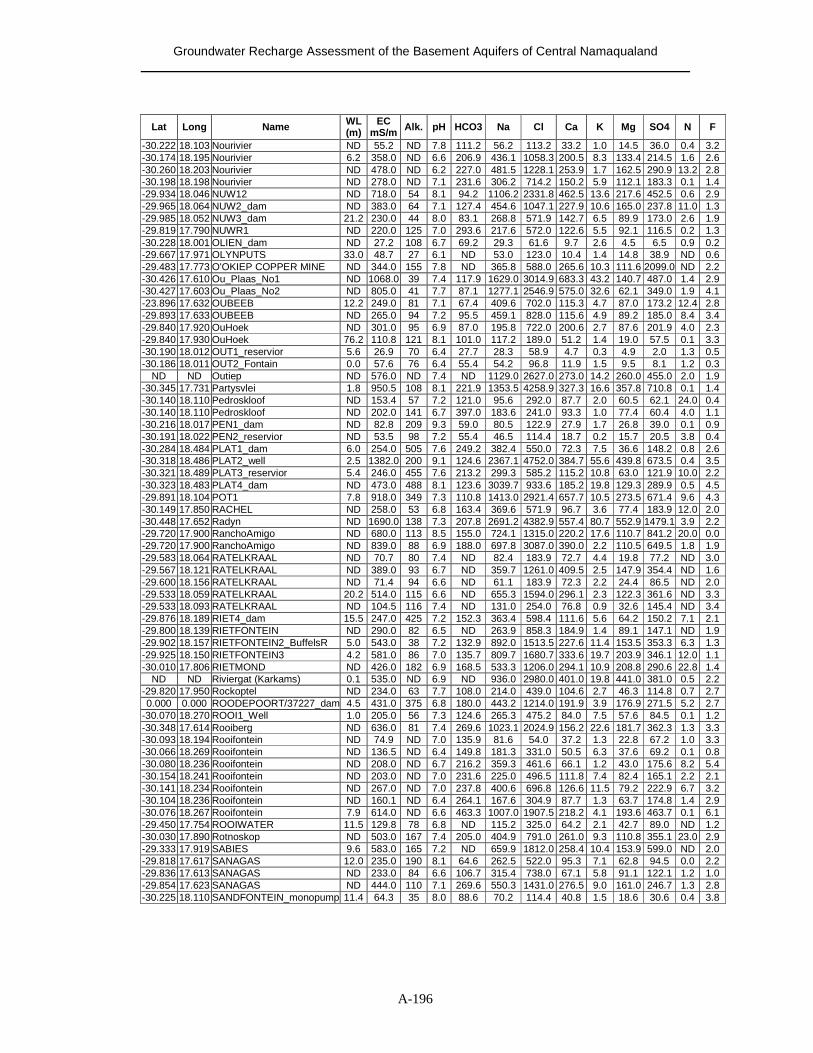
Groundwater Recharge Assessment of the Basement Aquifers of Central Namaqualand
A-196
Lat Long Name WL (m)
EC mS/m Alk. pH HCO3 Na Cl Ca K Mg SO4 N F
-30.222 18.103 Nourivier ND 55.2 ND 7.8 111.2 56.2 113.2 33.2 1.0 14.5 36.0 0.4 3.2 -30.174 18.195 Nourivier 6.2 358.0 ND 6.6 206.9 436.1 1058.3 200.5 8.3 133.4 214.5 1.6 2.6 -30.260 18.203 Nourivier ND 478.0 ND 6.2 227.0 481.5 1228.1 253.9 1.7 162.5 290.9 13.2 2.8 -30.198 18.198 Nourivier ND 278.0 ND 7.1 231.6 306.2 714.2 150.2 5.9 112.1 183.3 0.1 1.4 -29.934 18.046 NUW12 ND 718.0 54 8.1 94.2 1106.2 2331.8 462.5 13.6 217.6 452.5 0.6 2.9 -29.965 18.064 NUW2_dam ND 383.0 64 7.1 127.4 454.6 1047.1 227.9 10.6 165.0 237.8 11.0 1.3 -29.985 18.052 NUW3_dam 21.2 230.0 44 8.0 83.1 268.8 571.9 142.7 6.5 89.9 173.0 2.6 1.9 -29.819 17.790 NUWR1 ND 220.0 125 7.0 293.6 217.6 572.0 122.6 5.5 92.1 116.5 0.2 1.3 -30.228 18.001 OLIEN_dam ND 27.2 108 6.7 69.2 29.3 61.6 9.7 2.6 4.5 6.5 0.9 0.2 -29.667 17.971 OLYNPUTS 33.0 48.7 27 6.1 ND 53.0 123.0 10.4 1.4 14.8 38.9 ND 0.6 -29.483 17.773 O'OKIEP COPPER MINE ND 344.0 155 7.8 ND 365.8 588.0 265.6 10.3 111.6 2099.0 ND 2.2 -30.426 17.610 Ou_Plaas_No1 ND 1068.0 39 7.4 117.9 1629.0 3014.9 683.3 43.2 140.7 487.0 1.4 2.9 -30.427 17.603 Ou_Plaas_No2 ND 805.0 41 7.7 87.1 1277.1 2546.9 575.0 32.6 62.1 349.0 1.9 4.1 -23.896 17.632 OUBEEB 12.2 249.0 81 7.1 67.4 409.6 702.0 115.3 4.7 87.0 173.2 12.4 2.8 -29.893 17.633 OUBEEB ND 265.0 94 7.2 95.5 459.1 828.0 115.6 4.9 89.2 185.0 8.4 3.4 -29.840 17.920 OuHoek ND 301.0 95 6.9 87.0 195.8 722.0 200.6 2.7 87.6 201.9 4.0 2.3 -29.840 17.930 OuHoek 76.2 110.8 121 8.1 101.0 117.2 189.0 51.2 1.4 19.0 57.5 0.1 3.3 -30.190 18.012 OUT1_reservior 5.6 26.9 70 6.4 27.7 28.3 58.9 4.7 0.3 4.9 2.0 1.3 0.5 -30.186 18.011 OUT2_Fontain 0.0 57.6 76 6.4 55.4 54.2 96.8 11.9 1.5 9.5 8.1 1.2 0.3
ND ND Outiep ND 576.0 ND 7.4 ND 1129.0 2627.0 273.0 14.2 260.0 455.0 2.0 1.9 -30.345 17.731 Partysvlei 1.8 950.5 108 8.1 221.9 1353.5 4258.9 327.3 16.6 357.8 710.8 0.1 1.4 -30.140 18.110 Pedroskloof ND 153.4 57 7.2 121.0 95.6 292.0 87.7 2.0 60.5 62.1 24.0 0.4 -30.140 18.110 Pedroskloof ND 202.0 141 6.7 397.0 183.6 241.0 93.3 1.0 77.4 60.4 4.0 1.1 -30.216 18.017 PEN1_dam ND 82.8 209 9.3 59.0 80.5 122.9 27.9 1.7 26.8 39.0 0.1 0.9 -30.191 18.022 PEN2_reservior ND 53.5 98 7.2 55.4 46.5 114.4 18.7 0.2 15.7 20.5 3.8 0.4 -30.284 18.484 PLAT1_dam 6.0 254.0 505 7.6 249.2 382.4 550.0 72.3 7.5 36.6 148.2 0.8 2.6 -30.318 18.486 PLAT2_well 2.5 1382.0 200 9.1 124.6 2367.1 4752.0 384.7 55.6 439.8 673.5 0.4 3.5 -30.321 18.489 PLAT3_reservior 5.4 246.0 455 7.6 213.2 299.3 585.2 115.2 10.8 63.0 121.9 10.0 2.2 -30.323 18.483 PLAT4_dam ND 473.0 488 8.1 123.6 3039.7 933.6 185.2 19.8 129.3 289.9 0.5 4.5 -29.891 18.104 POT1 7.8 918.0 349 7.3 110.8 1413.0 2921.4 657.7 10.5 273.5 671.4 9.6 4.3 -30.149 17.850 RACHEL ND 258.0 53 6.8 163.4 369.6 571.9 96.7 3.6 77.4 183.9 12.0 2.0 -30.448 17.652 Radyn ND 1690.0 138 7.3 207.8 2691.2 4382.9 557.4 80.7 552.9 1479.1 3.9 2.2 -29.720 17.900 RanchoAmigo ND 680.0 113 8.5 155.0 724.1 1315.0 220.2 17.6 110.7 841.2 20.0 0.0 -29.720 17.900 RanchoAmigo ND 839.0 88 6.9 188.0 697.8 3087.0 390.0 2.2 110.5 649.5 1.8 1.9 -29.583 18.064 RATELKRAAL ND 70.7 80 7.4 ND 82.4 183.9 72.7 4.4 19.8 77.2 ND 3.0 -29.567 18.121 RATELKRAAL ND 389.0 93 6.7 ND 359.7 1261.0 409.5 2.5 147.9 354.4 ND 1.6 -29.600 18.156 RATELKRAAL ND 71.4 94 6.6 ND 61.1 183.9 72.3 2.2 24.4 86.5 ND 2.0 -29.533 18.059 RATELKRAAL 20.2 514.0 115 6.6 ND 655.3 1594.0 296.1 2.3 122.3 361.6 ND 3.3 -29.533 18.093 RATELKRAAL ND 104.5 116 7.4 ND 131.0 254.0 76.8 0.9 32.6 145.4 ND 3.4 -29.876 18.189 RIET4_dam 15.5 247.0 425 7.2 152.3 363.4 598.4 111.6 5.6 64.2 150.2 7.1 2.1 -29.800 18.139 RIETFONTEIN ND 290.0 82 6.5 ND 263.9 858.3 184.9 1.4 89.1 147.1 ND 1.9 -29.902 18.157 RIETFONTEIN2_BuffelsR 5.0 543.0 38 7.2 132.9 892.0 1513.5 227.6 11.4 153.5 353.3 6.3 1.3 -29.925 18.150 RIETFONTEIN3 4.2 581.0 86 7.0 135.7 809.7 1680.7 333.6 19.7 203.9 346.1 12.0 1.1 -30.010 17.806 RIETMOND ND 426.0 182 6.9 168.5 533.3 1206.0 294.1 10.9 208.8 290.6 22.8 1.4
ND ND Riviergat (Karkams) 0.1 535.0 ND 6.9 ND 936.0 2980.0 401.0 19.8 441.0 381.0 0.5 2.2 -29.820 17.950 Rockoptel ND 234.0 63 7.7 108.0 214.0 439.0 104.6 2.7 46.3 114.8 0.7 2.7 0.000 0.000 ROODEPOORT/37227_dam 4.5 431.0 375 6.8 180.0 443.2 1214.0 191.9 3.9 176.9 271.5 5.2 2.7
-30.070 18.270 ROOI1_Well 1.0 205.0 56 7.3 124.6 265.3 475.2 84.0 7.5 57.6 84.5 0.1 1.2 -30.348 17.614 Rooiberg ND 636.0 81 7.4 269.6 1023.1 2024.9 156.2 22.6 181.7 362.3 1.3 3.3 -30.093 18.194 Rooifontein ND 74.9 ND 7.0 135.9 81.6 54.0 37.2 1.3 22.8 67.2 1.0 3.3 -30.066 18.269 Rooifontein ND 136.5 ND 6.4 149.8 181.3 331.0 50.5 6.3 37.6 69.2 0.1 0.8 -30.080 18.236 Rooifontein ND 208.0 ND 6.7 216.2 359.3 461.6 66.1 1.2 43.0 175.6 8.2 5.4 -30.154 18.241 Rooifontein ND 203.0 ND 7.0 231.6 225.0 496.5 111.8 7.4 82.4 165.1 2.2 2.1 -30.141 18.234 Rooifontein ND 267.0 ND 7.0 237.8 400.6 696.8 126.6 11.5 79.2 222.9 6.7 3.2 -30.104 18.236 Rooifontein ND 160.1 ND 6.4 264.1 167.6 304.9 87.7 1.3 63.7 174.8 1.4 2.9 -30.076 18.267 Rooifontein 7.9 614.0 ND 6.6 463.3 1007.0 1907.5 218.2 4.1 193.6 463.7 0.1 6.1 -29.450 17.754 ROOIWATER 11.5 129.8 78 6.8 ND 115.2 325.0 64.2 2.1 42.7 89.0 ND 1.2 -30.030 17.890 Rotnoskop ND 503.0 167 7.4 205.0 404.9 791.0 261.0 9.3 110.8 355.1 23.0 2.9 -29.333 17.919 SABIES 9.6 583.0 165 7.2 ND 659.9 1812.0 258.4 10.4 153.9 599.0 ND 2.0 -29.818 17.617 SANAGAS 12.0 235.0 190 8.1 64.6 262.5 522.0 95.3 7.1 62.8 94.5 0.0 2.2 -29.836 17.613 SANAGAS ND 233.0 84 6.6 106.7 315.4 738.0 67.1 5.8 91.1 122.1 1.2 1.0 -29.854 17.623 SANAGAS ND 444.0 110 7.1 269.6 550.3 1431.0 276.5 9.0 161.0 246.7 1.3 2.8 -30.225 18.110 SANDFONTEIN_monopump 11.4 64.3 35 8.0 88.6 70.2 114.4 40.8 1.5 18.6 30.6 0.4 3.8
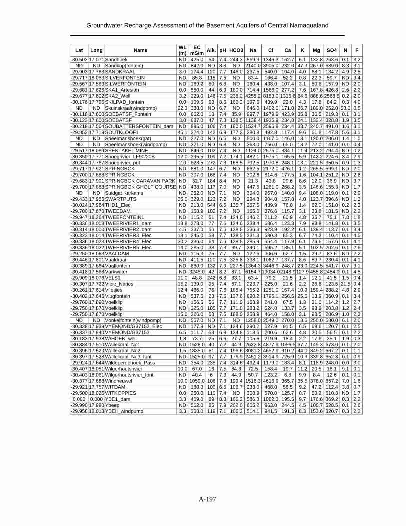
Groundwater Recharge Assessment of the Basement Aquifers of Central Namaqualand
A-197
Lat Long Name WL (m)
EC mS/m Alk. pH HCO3 Na Cl Ca K Mg SO4 N F
-30.502 17.071 Sandhoek ND 425.0 54 7.4 244.3 569.9 1346.3 162.7 6.1 132.8 263.6 0.1 3.2 ND ND Sandkop(fontein) ND 842.0 ND 8.8 ND 2140.0 3905.0 232.0 47.3 267.0 689.0 8.3 3.1
-29.903 17.783 SANDKRAAL 3.0 174.4 120 7.7 146.0 237.5 540.0 104.0 4.0 68.1 134.2 4.9 2.5 -29.717 18.053 SILVERFONTEIN ND 85.8 115 7.5 ND 83.4 166.4 52.2 0.8 22.3 59.7 ND 3.4 -29.567 17.583 SILWERFONTEIN ND 169.2 60 6.8 ND 160.4 438.0 107.4 3.1 50.6 157.9 ND 2.0 -29.681 17.626 SKA1_Artesian 0.0 550.0 44 6.9 180.0 714.4 1566.0 277.2 7.6 167.8 426.8 2.6 2.2 -29.677 17.602 SKA2_Well 3.2 229.0 146 7.5 238.2 4255.2 8183.0 1316.6 64.6 888.6 2568.5 0.2 2.0 -30.176 17.795 SKILPAD_fontain 0.0 109.6 63 8.6 166.2 197.6 439.9 22.0 4.3 17.8 84.2 0.3 4.0
ND ND Skuinskraal(windpomp) 22.3 388.0 ND 6.7 ND 646.0 1402.0 171.0 26.7 189.0 252.0 53.0 0.5 -30.118 17.600 SOEBATSF_Fontain 0.0 662.0 13 7.4 85.9 997.7 1979.9 423.9 35.8 36.5 219.3 0.1 3.1 -30.123 17.600 SOEBATSF 3.0 687.0 47 7.3 138.5 1138.4 1935.9 234.8 24.1 132.4 328.8 1.9 3.5 -30.218 17.564 SOUBATTERSFONTEIN_dam ND 895.0 106 7.4 180.0 1524.7 2595.8 234.4 33.7 240.7 491.0 1.6 3.1 -29.852 17.719 SOUTKLOOF1 45.1 224.0 142 6.9 177.2 280.8 492.8 117.4 9.6 61.8 147.8 5.6 3.1
ND ND Speelmanshoek(gat) ND 227.0 ND 6.5 ND 500.0 1167.0 146.0 13.1 120.0 206.0 1.4 1.0 ND ND Speelmanshoek(windpomp) ND 321.0 ND 6.8 ND 363.0 756.0 65.0 13.2 72.0 141.0 0.1 0.4
-29.517 18.089 SPEKTAKEL MINE ND 846.0 102 7.4 ND 1124.0 2575.0 384.1 11.4 213.2 794.4 ND 0.2 -30.350 17.771 Spoegrivier_LF90/20B 12.0 395.5 109 7.2 174.1 482.1 1575.1 165.5 5.9 142.2 224.6 3.4 2.9 -30.344 17.767 Spoegrivier_put 2.0 623.5 272 7.3 168.5 792.5 1970.8 248.1 13.1 221.5 350.5 0.9 1.3 -29.717 17.921 SPRINGBOK ND 681.0 147 6.7 ND 662.5 2172.0 426.1 1.2 265.5 599.1 ND 2.0 -29.700 17.888 SPRINGBOK ND 307.0 166 7.4 ND 302.6 814.6 177.5 1.6 104.1 251.2 ND 2.6 -29.683 17.901 SPRINGBOK CARAVAN PARK ND 32.7 184 8.4 ND 21.3 43.8 29.6 8.6 12.0 36.9 ND 3.7 -29.700 17.888 SPRINGBOK GHOLF COURSE ND 438.0 117 7.0 ND 447.5 1261.0 268.2 3.5 146.6 155.3 ND 1.7
ND ND Suidgat Karkams ND 252.0 ND 7.1 ND 394.0 967.0 140.0 9.4 108.0 119.0 0.1 2.9 -29.433 17.956 SWARTPUTS 35.0 329.0 123 7.2 ND 294.8 904.0 157.8 4.0 123.7 396.6 ND 1.3 -30.024 17.984 THD1_Elec ND 213.0 544 6.5 135.7 267.5 439.9 76.0 1.4 62.0 151.0 0.2 2.3 -29.700 17.670 TWEEDAM ND 158.9 102 7.2 ND 165.6 376.6 115.7 3.1 33.8 181.5 ND 2.2 -29.947 18.264 TWEEFONTEIN1 ND 115.2 51 7.4 124.6 146.2 211.2 60.9 4.8 35.7 75.1 7.8 1.8 -30.336 18.003 TWEERIVIER1_dam 18.8 278.0 77 7.6 124.6 333.4 686.4 123.3 7.9 93.8 141.8 0.1 3.5 -30.314 18.000 TWEERIVIER2_dam 4.5 337.0 56 7.5 138.5 336.3 923.9 192.2 6.1 139.4 113.7 0.1 3.4 -30.323 18.014 TWEERIVIER3_Elec 18.1 245.0 58 7.7 138.5 331.3 580.8 85.3 6.7 74.3 110.4 0.1 4.5 -30.336 18.023 TWEERIVIER4_Elec 30.2 236.0 64 7.5 138.5 285.9 554.4 117.9 6.1 76.6 157.6 0.1 4.1 -30.336 18.022 TWEERIVIER5_Elec 14.0 285.0 38 7.3 99.7 340.1 695.2 135.1 5.1 102.5 202.6 0.1 2.6 -29.250 18.063 VAALDAM ND 115.3 75 7.7 ND 122.6 306.6 62.7 1.5 29.7 83.6 ND 2.2 -30.446 17.801 Vaaldraai ND 411.5 120 7.5 325.8 338.1 1062.7 137.7 8.6 89.7 230.4 0.1 4.1 -30.389 17.664 Vaalfontein ND 860.0 132 7.9 227.5 1364.3 3446.9 248.7 23.0 224.5 541.7 0.7 3.1 -30.418 17.568 Varkwater ND 3245.0 42 8.2 87.1 6154.7 19034.02148.9 127.9 455.8 2454.9 0.1 4.5 -29.909 18.076 VELS1 11.0 48.8 242 6.8 83.1 63.4 79.2 21.5 1.4 12.1 41.5 1.5 0.4 -30.307 17.722 Vleie_Naries 15.2 139.0 95 7.4 67.1 223.7 225.0 21.6 2.2 26.8 123.5 21.5 0.4 -30.261 17.614 Vlietjies 12.4 486.0 76 7.6 185.4 755.2 1251.0 167.4 10.9 159.4 288.2 4.8 2.9 -30.402 17.646 Vlugfontein ND 537.5 23 7.6 137.6 890.2 1795.1 256.5 25.6 13.9 360.9 0.1 3.4 -29.760 17.890 Voelklip ND 156.5 56 7.7 111.0 163.9 241.0 67.5 1.3 31.0 114.2 1.2 2.7 -29.750 17.870 Voelklip ND 325.0 105 7.7 171.0 283.2 524.0 133.7 3.5 98.9 203.8 1.2 2.4 -29.750 17.870 Voelklip 15.0 326.0 58 7.5 188.0 258.9 464.0 158.0 3.1 98.5 206.9 1.0 2.3
ND ND Vonkelfontein(windpomp) ND 557.0 ND 7.1 ND 1258.0 2549.0 270.0 13.6 250.0 580.0 6.1 2.0 -30.338 17.939 VYEMOND/G37152_Elec ND 177.9 ND 7.1 124.6 290.2 527.9 91.5 6.5 69.6 120.7 0.1 2.5 -30.337 17.940 VYEMOND/G37153 6.5 111.7 53 6.9 134.8 118.6 200.6 62.6 4.8 30.5 56.5 0.1 2.2 -30.183 17.938 W/HOEK_well 1.8 73.7 25 6.6 27.7 105.6 219.9 18.4 2.2 17.6 35.1 1.9 0.3 -30.384 17.510 Wallekraal_No1 ND 1528.0 40 7.2 44.9 2622.8 4877.9 1056.5 37.7 149.3 673.0 0.1 2.0 -30.396 17.520 Wallekraal_No2 1.5 1835.0 61 7.4 196.6 3081.2 4652.9 910.2 44.0 349.2 667.2 0.1 1.1 -30.397 17.528 Wallekraal_No3_font ND 1525.0 97 7.7 176.9 2451.2 3914.9 725.9 10.3 339.8 652.3 0.1 0.9 -29.924 17.644 Wildeperdehoek_Pass ND 354.0 235 7.4 314.6 492.4 1179.0 183.4 8.1 118.9 248.0 0.0 3.0 -30.407 18.051 Wilgerhoutsrivier 10.0 67.0 16 7.5 84.3 72.5 158.4 19.7 11.2 20.5 18.1 9.1 0.1 -30.403 18.061 Wilgerhoutsrivier_font ND 40.4 6 7.3 44.9 50.7 123.2 6.8 9.9 8.4 12.6 0.1 0.1 -30.377 17.688 Windheuwel 10.0 1059.0 106 7.8 199.4 1516.3 4616.9 365.7 35.5 378.0 657.2 7.0 1.6 -29.921 17.757 WITDAM ND 180.3 100 6.5 106.7 233.0 468.0 58.5 9.2 47.2 112.4 3.8 0.7 -29.500 18.026 WITKOPPIES 0.0 250.0 110 7.4 ND 308.9 570.0 125.7 0.7 50.2 610.3 ND 1.7 0.000 0.000 YBE1_dam 3.3 409.0 89 8.3 166.2 586.8 1082.3 195.5 9.7 176.6 369.2 0.3 2.2
-29.990 17.990 Ybeep ND 562.0 85 7.9 202.0 605.2 963.0 244.5 4.5 100.7 528.5 0.1 2.6 -29.958 18.013 YBEII_windpump 3.3 368.0 119 7.1 166.2 514.1 941.5 191.3 8.3 153.6 320.7 0.3 2.2
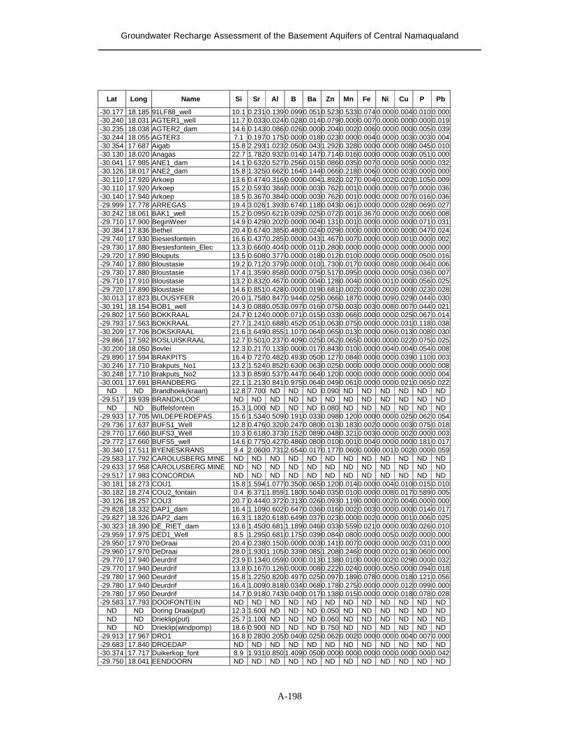
Groundwater Recharge Assessment of the Basement Aquifers of Central Namaqualand
A-198
Lat Long Name Si Sr Al B Ba Zn Mn Fe Ni Cu P Pb
-30.177 18.185 91LF88_well 10.1 0.231 0.139 0.099 0.051 0.523 0.533 0.074 0.000 0.004 0.010 0.000 -30.240 18.031 AGTER1_well 11.7 0.033 0.024 0.028 0.014 0.079 0.000 0.007 0.000 0.000 0.000 0.019 -30.235 18.038 AGTER2_dam 14.6 0.143 0.086 0.026 0.000 0.204 0.002 0.006 0.000 0.000 0.005 0.039 -30.244 18.055 AGTER3 7.1 0.197 0.175 0.000 0.018 0.023 0.000 0.004 0.000 0.003 0.003 0.004 -30.354 17.687 Aigab 15.8 2.293 1.023 2.050 0.043 1.292 0.328 0.000 0.000 0.008 0.045 0.010 -30.130 18.020 Anagas 22.7 1.782 0.932 0.014 0.147 0.714 0.016 0.000 0.000 0.003 0.051 0.000 -30.041 17.985 ANE1_dam 14.1 0.632 0.527 0.256 0.015 0.086 0.035 0.007 0.000 0.005 0.000 0.032 -30.126 18.017 ANE2_dam 15.8 1.325 0.662 0.164 0.144 0.066 0.218 0.006 0.000 0.003 0.000 0.000 -30.110 17.920 Arkoep 13.6 0.474 0.316 0.000 0.004 1.892 0.027 0.004 0.002 0.020 0.105 0.009 -30.110 17.920 Arkoep 15.2 0.593 0.384 0.000 0.003 0.762 0.001 0.000 0.000 0.007 0.000 0.036 -30.140 17.940 Arkoep 18.5 0.367 0.384 0.000 0.003 0.762 0.001 0.000 0.000 0.007 0.016 0.036 -29.999 17.778 ARREGAS 19.4 3.026 1.393 0.674 0.118 0.043 0.061 0.000 0.000 0.028 0.069 0.027 -30.242 18.061 BAK1_well 15.2 0.095 0.621 0.039 0.025 0.072 0.001 0.367 0.000 0.002 0.006 0.008 -29.710 17.900 BeginWeer 14.9 0.429 0.202 0.000 0.004 0.131 0.001 0.000 0.000 0.000 0.071 0.031 -30.384 17.836 Bethel 20.4 0.674 0.385 0.480 0.024 0.029 0.000 0.000 0.000 0.000 0.047 0.024 -29.740 17.930 Biesiesfontein 16.6 0.437 0.285 0.000 0.043 1.467 0.007 0.000 0.000 0.001 0.000 0.002 -29.730 17.880 Biesiesfontein_Elec 13.3 0.660 0.404 0.000 0.011 0.280 0.000 0.000 0.000 0.000 0.000 0.000 -29.720 17.890 Blouputs 13.5 0.608 0.377 0.000 0.018 0.012 0.010 0.000 0.000 0.000 0.050 0.016 -29.740 17.880 Bloustasie 19.2 0.712 0.379 0.000 0.010 1.730 0.017 0.000 0.008 0.000 0.064 0.006 -29.730 17.880 Bloustasie 17.4 1.359 0.858 0.000 0.075 0.517 0.095 0.000 0.000 0.005 0.036 0.007 -29.710 17.910 Bloustasie 13.2 0.832 0.467 0.000 0.004 0.128 0.004 0.000 0.001 0.000 0.056 0.025 -29.720 17.890 Bloustasie 14.6 0.851 0.428 0.000 0.019 0.681 0.002 0.000 0.000 0.000 0.023 0.028 -30.013 17.823 BLOUSYFER 20.0 1.758 0.847 0.944 0.025 0.066 0.187 0.000 0.009 0.029 0.044 0.030 -30.191 18.154 BOB1_well 14.3 0.088 0.053 0.097 0.016 0.075 0.003 0.003 0.008 0.007 0.044 0.021 -29.802 17.560 BOKKRAAL 24.7 0.124 0.000 0.071 0.015 0.033 0.066 0.000 0.000 0.025 0.067 0.014 -29.793 17.563 BOKKRAAL 27.7 1.241 0.688 0.452 0.051 0.063 0.075 0.000 0.000 0.031 0.118 0.038 -30.209 17.706 BOKSKRAAL 21.6 1.649 0.855 1.107 0.064 0.065 0.013 0.000 0.006 0.013 0.008 0.030 -29.866 17.592 BOSLUISKRAAL 12.7 0.501 0.237 0.409 0.025 0.062 0.065 0.000 0.000 0.022 0.075 0.025 -30.200 18.050 Bovlei 12.3 0.217 0.133 0.000 0.017 0.843 0.010 0.000 0.004 0.004 0.054 0.008 -29.890 17.594 BRAKPITS 16.4 0.727 0.482 0.493 0.050 0.127 0.084 0.000 0.000 0.039 0.110 0.003 -30.246 17.710 Brakputs_No1 13.2 1.524 0.852 0.630 0.063 0.025 0.000 0.000 0.000 0.000 0.000 0.008 -30.248 17.710 Brakputs_No2 13.3 0.859 0.537 0.447 0.064 0.120 0.000 0.000 0.000 0.000 0.000 0.004 -30.001 17.691 BRANDBERG 22.1 1.213 0.841 0.975 0.064 0.049 0.061 0.000 0.000 0.021 0.065 0.022
ND ND Brandhoek(kraan) 12.8 7.700 ND ND ND 0.090 ND ND ND ND ND ND -29.517 19.939 BRANDKLOOF ND ND ND ND ND ND ND ND ND ND ND ND
ND ND Buffelsfontein 15.3 1.000 ND ND ND 0.080 ND ND ND ND ND ND -29.933 17.705 WILDEPERDEPAS 15.6 1.534 0.509 0.191 0.033 0.098 0.120 0.000 0.000 0.025 0.062 0.054 -29.736 17.637 BUFS1_Well 12.8 0.476 0.320 0.247 0.080 0.013 0.183 0.002 0.000 0.003 0.075 0.018 -29.770 17.660 BUFS3_Well 10.3 0.618 0.373 0.152 0.089 0.048 0.321 0.003 0.000 0.002 0.000 0.003 -29.772 17.660 BUFS5_well 14.6 0.775 0.427 0.486 0.080 0.010 0.001 0.004 0.000 0.000 0.181 0.017 -30.340 17.511 BYENESKRANS 9.4 2.060 0.731 2.654 0.017 0.177 0.060 0.000 0.001 0.002 0.000 0.059 -29.583 17.792 CAROLUSBERG MINE ND ND ND ND ND ND ND ND ND ND ND ND -29.633 17.958 CAROLUSBERG MINE ND ND ND ND ND ND ND ND ND ND ND ND -29.517 17.983 CONCORDIA ND ND ND ND ND ND ND ND ND ND ND ND -30.181 18.273 COU1 15.8 1.594 1.077 0.350 0.065 0.120 0.014 0.000 0.004 0.010 0.015 0.010 -30.182 18.274 COU2_fontain 0.4 6.371 1.859 1.180 0.504 0.035 0.010 0.000 0.008 0.017 0.589 0.005 -30.126 18.257 COU3 20.7 0.444 0.372 0.313 0.026 0.093 0.119 0.000 0.002 0.004 0.000 0.000 -29.828 18.332 DAP1_dam 16.4 1.109 0.602 0.647 0.036 0.016 0.002 0.003 0.000 0.000 0.014 0.017 -29.827 18.326 DAP2_dam 16.3 1.182 0.618 0.649 0.037 0.023 0.000 0.002 0.000 0.001 0.006 0.025 -30.323 18.390 DE_RIET_dam 13.6 1.450 0.681 1.189 0.046 0.033 0.559 0.021 0.000 0.003 0.026 0.010 -29.959 17.975 DED1_Well 8.5 1.295 0.681 0.175 0.039 0.084 0.080 0.000 0.005 0.002 0.000 0.000 -29.950 17.970 DeDraai 20.4 0.238 0.150 0.000 0.003 0.141 0.007 0.000 0.000 0.002 0.031 0.000 -29.960 17.970 DeDraai 28.0 1.930 1.105 0.339 0.085 1.208 0.246 0.000 0.002 0.013 0.060 0.000 -29.770 17.940 Deurdrif 23.9 0.134 0.059 0.000 0.013 0.138 0.010 0.000 0.002 0.029 0.000 0.032 -29.770 17.940 Deurdrif 13.8 0.167 0.126 0.000 0.008 0.222 0.024 0.000 0.005 0.000 0.094 0.018 -29.780 17.960 Deurdrif 15.8 1.225 0.820 0.497 0.025 0.097 0.189 0.078 0.000 0.018 0.121 0.056 -29.780 17.940 Deurdrif 16.4 1.009 0.818 0.034 0.068 0.178 0.275 0.000 0.000 0.012 0.099 0.000 -29.780 17.950 Deurdrif 14.7 0.918 0.743 0.040 0.017 0.138 0.015 0.000 0.000 0.018 0.078 0.028 -29.583 17.793 DOOIFONTEIN ND ND ND ND ND ND ND ND ND ND ND ND
ND ND Doring Draai(put) 12.3 1.600 ND ND ND 0.050 ND ND ND ND ND ND ND ND Drieklip(put) 25.7 1.100 ND ND ND 0.060 ND ND ND ND ND ND ND ND Drieklip(windpomp) 18.6 0.900 ND ND ND 0.750 ND ND ND ND ND ND
-29.913 17.967 DRO1 16.8 0.280 0.205 0.040 0.025 0.062 0.002 0.000 0.000 0.004 0.007 0.000 -29.683 17.840 DROEDAP ND ND ND ND ND ND ND ND ND ND ND ND -30.374 17.717 Duikerkop_font 8.9 1.931 0.850 1.409 0.050 0.000 0.000 0.000 0.000 0.000 0.000 0.042 -29.750 18.041 EENDOORN ND ND ND ND ND ND ND ND ND ND ND ND
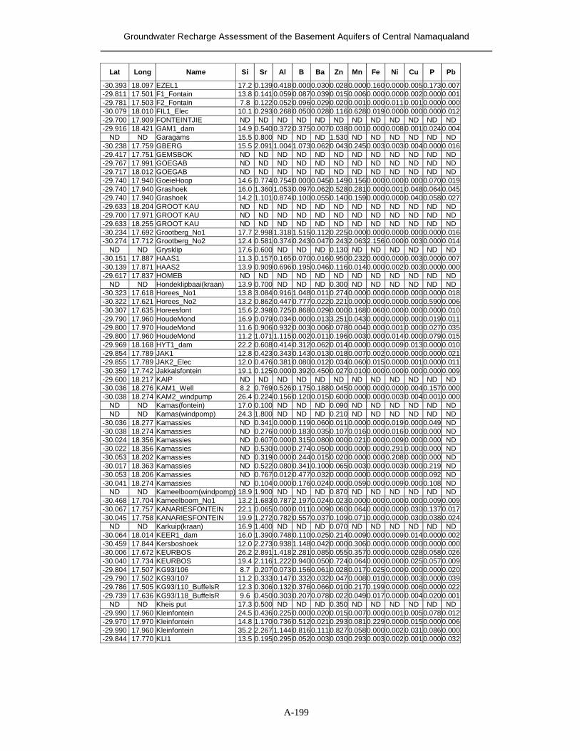
Groundwater Recharge Assessment of the Basement Aquifers of Central Namaqualand
A-199
Lat Long Name Si Sr Al B Ba Zn Mn Fe Ni Cu P Pb
-30.393 18.097 EZEL1 17.2 0.139 0.418 0.000 0.030 0.028 0.000 0.160 0.000 0.005 0.173 0.007 -29.811 17.501 F1_Fontain 13.8 0.141 0.059 0.087 0.039 0.015 0.006 0.000 0.000 0.002 0.000 0.001 -29.781 17.503 F2_Fontain 7.8 0.122 0.052 0.096 0.029 0.020 0.001 0.000 0.011 0.001 0.000 0.000 -30.079 18.010 FIL1_Elec 10.1 0.293 0.268 0.050 0.028 0.116 0.628 0.019 0.000 0.000 0.000 0.012 -29.700 17.909 FONTEINTJIE ND ND ND ND ND ND ND ND ND ND ND ND -29.916 18.421 GAM1_dam 14.9 0.540 0.372 0.375 0.007 0.038 0.001 0.000 0.008 0.001 0.024 0.004
ND ND Garagams 15.5 0.800 ND ND ND 1.530 ND ND ND ND ND ND -30.238 17.759 GBERG 15.5 2.091 1.004 1.073 0.062 0.043 0.245 0.003 0.003 0.004 0.000 0.016 -29.417 17.751 GEMSBOK ND ND ND ND ND ND ND ND ND ND ND ND -29.767 17.991 GOEGAB ND ND ND ND ND ND ND ND ND ND ND ND -29.717 18.012 GOEGAB ND ND ND ND ND ND ND ND ND ND ND ND -29.740 17.940 GoeieHoop 14.6 0.774 0.754 0.000 0.045 0.149 0.156 0.000 0.000 0.000 0.070 0.019 -29.740 17.940 Grashoek 16.0 1.360 1.053 0.097 0.062 0.528 0.281 0.000 0.001 0.048 0.064 0.045 -29.740 17.940 Grashoek 14.2 1.101 0.874 0.100 0.055 0.140 0.159 0.000 0.000 0.040 0.058 0.027 -29.633 18.204 GROOT KAU ND ND ND ND ND ND ND ND ND ND ND ND -29.700 17.971 GROOT KAU ND ND ND ND ND ND ND ND ND ND ND ND -29.633 18.255 GROOT KAU ND ND ND ND ND ND ND ND ND ND ND ND -30.234 17.692 Grootberg_No1 17.7 2.998 1.318 1.515 0.112 0.225 0.000 0.000 0.000 0.000 0.000 0.016 -30.274 17.712 Grootberg_No2 12.4 0.581 0.374 0.243 0.047 0.243 2.063 2.156 0.000 0.003 0.000 0.014
ND ND Grysklip 17.6 0.600 ND ND ND 0.130 ND ND ND ND ND ND -30.151 17.887 HAAS1 11.3 0.157 0.165 0.070 0.016 0.950 0.232 0.000 0.000 0.003 0.000 0.007 -30.139 17.871 HAAS2 13.9 0.909 0.696 0.195 0.046 0.116 0.014 0.000 0.002 0.003 0.000 0.000 -29.617 17.837 HOMEB ND ND ND ND ND ND ND ND ND ND ND ND
ND ND Hondeklipbaai(kraan) 13.9 0.700 ND ND ND 0.300 ND ND ND ND ND ND -30.323 17.618 Horees_No1 13.8 3.084 0.916 1.048 0.011 0.274 0.000 0.000 0.000 0.000 0.000 0.018 -30.322 17.621 Horees_No2 13.2 0.862 0.447 0.777 0.022 0.221 0.000 0.000 0.000 0.000 0.590 0.006 -30.307 17.635 Horeesfont 15.6 2.398 0.725 0.868 0.029 0.000 0.168 0.060 0.000 0.000 0.000 0.010 -29.790 17.960 HoudeMond 16.9 0.079 0.034 0.000 0.013 3.251 0.043 0.000 0.000 0.000 0.019 0.011 -29.800 17.970 HoudeMond 11.6 0.906 0.932 0.003 0.006 0.078 0.004 0.000 0.001 0.000 0.027 0.035 -29.800 17.960 HoudeMond 11.2 1.071 1.115 0.002 0.011 0.196 0.003 0.000 0.014 0.000 0.079 0.015 -29.969 18.168 HYT1_dam 22.2 0.608 0.414 0.312 0.062 0.014 0.000 0.000 0.009 0.013 0.000 0.010 -29.854 17.789 JAK1 12.8 0.423 0.343 0.143 0.013 0.018 0.007 0.002 0.000 0.000 0.000 0.021 -29.855 17.789 JAK2_Elec 12.0 0.476 0.381 0.080 0.012 0.034 0.060 0.015 0.000 0.001 0.000 0.011 -30.359 17.742 Jakkalsfontein 19.1 0.125 0.000 0.392 0.450 0.027 0.010 0.000 0.000 0.000 0.000 0.009 -29.600 18.217 KAIP ND ND ND ND ND ND ND ND ND ND ND ND -30.036 18.276 KAM1_Well 8.2 0.769 0.526 0.175 0.188 0.045 0.000 0.000 0.000 0.004 0.157 0.000 -30.038 18.274 KAM2_windpump 26.4 0.224 0.156 0.120 0.015 0.600 0.000 0.000 0.003 0.004 0.001 0.000
ND ND Kamas(fontein) 17.0 0.100 ND ND ND 0.090 ND ND ND ND ND ND ND ND Kamas(windpomp) 24.3 1.800 ND ND ND 0.210 ND ND ND ND ND ND
-30.036 18.277 Kamassies ND 0.341 0.000 0.119 0.060 0.011 0.000 0.000 0.019 0.000 0.049 ND -30.038 18.274 Kamassies ND 0.276 0.000 0.183 0.035 0.107 0.016 0.000 0.016 0.000 0.000 ND -30.024 18.356 Kamassies ND 0.607 0.000 0.315 0.080 0.000 0.021 0.000 0.009 0.000 0.000 ND -30.022 18.356 Kamassies ND 0.530 0.000 0.274 0.050 0.000 0.000 0.000 0.291 0.000 0.000 ND -30.053 18.202 Kamassies ND 0.319 0.000 0.244 0.015 0.020 0.000 0.000 0.208 0.000 0.000 ND -30.017 18.363 Kamassies ND 0.522 0.080 0.341 0.100 0.065 0.003 0.000 0.003 0.000 0.219 ND -30.053 18.206 Kamassies ND 0.767 0.012 0.477 0.032 0.000 0.000 0.000 0.000 0.000 0.092 ND -30.041 18.274 Kamassies ND 0.104 0.000 0.176 0.024 0.000 0.059 0.000 0.009 0.000 0.108 ND
ND ND Kameelboom(windpomp) 18.9 1.900 ND ND ND 0.870 ND ND ND ND ND ND -30.468 17.704 Kameelboom_No1 13.2 1.683 0.787 2.197 0.024 0.023 0.000 0.000 0.000 0.000 0.009 0.009 -30.067 17.757 KANARIESFONTEIN 22.1 0.065 0.000 0.011 0.009 0.060 0.064 0.000 0.000 0.030 0.137 0.017 -30.045 17.758 KANARIESFONTEIN 19.9 1.272 0.782 0.557 0.037 0.109 0.071 0.000 0.000 0.030 0.038 0.024
ND ND Karkuip(kraan) 16.9 1.400 ND ND ND 0.070 ND ND ND ND ND ND -30.064 18.014 KEER1_dam 16.0 1.390 0.748 0.110 0.025 0.214 0.009 0.000 0.009 0.014 0.000 0.002 -30.459 17.844 Kersboshoek 12.0 2.273 0.938 1.148 0.042 0.000 0.306 0.000 0.000 0.000 0.000 0.000 -30.006 17.672 KEURBOS 26.2 2.891 1.418 2.281 0.085 0.055 0.357 0.000 0.000 0.028 0.058 0.026 -30.040 17.734 KEURBOS 19.4 2.116 1.222 0.940 0.050 0.724 0.064 0.000 0.000 0.025 0.057 0.009 -29.804 17.507 KG93/106 8.7 0.207 0.073 0.156 0.061 0.028 0.017 0.025 0.000 0.000 0.000 0.020 -29.790 17.502 KG93/107 11.2 0.333 0.147 0.332 0.032 0.047 0.008 0.010 0.000 0.003 0.000 0.039 -29.786 17.505 KG93/110_BuffelsR 12.3 0.306 0.132 0.376 0.066 0.010 0.217 0.199 0.000 0.006 0.000 0.022 -29.739 17.636 KG93/118_BuffelsR 9.6 0.450 0.303 0.207 0.078 0.022 0.049 0.017 0.000 0.004 0.020 0.001
ND ND Kheis put 17.3 0.500 ND ND ND 0.350 ND ND ND ND ND ND -29.990 17.960 Kleinfontein 24.5 0.436 0.225 0.000 0.020 0.015 0.007 0.000 0.001 0.005 0.078 0.012 -29.970 17.970 Kleinfontein 14.8 1.170 0.736 0.512 0.021 0.293 0.081 0.229 0.000 0.015 0.000 0.006 -29.990 17.960 Kleinfontein 35.2 2.267 1.144 0.816 0.111 0.827 0.058 0.000 0.002 0.031 0.086 0.000 -29.844 17.770 KLI1 13.5 0.195 0.295 0.052 0.003 0.030 0.293 0.003 0.002 0.001 0.000 0.032
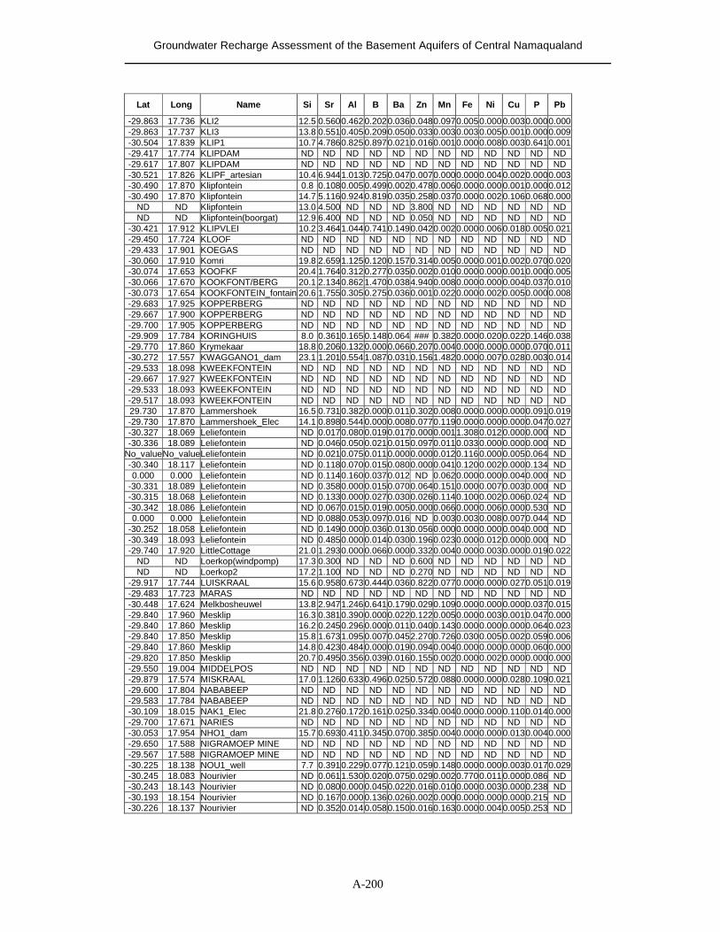
Groundwater Recharge Assessment of the Basement Aquifers of Central Namaqualand
A-200
Lat Long Name Si Sr Al B Ba Zn Mn Fe Ni Cu P Pb
-29.863 17.736 KLI2 12.5 0.5600.462 0.202 0.036 0.048 0.0970.005 0.000 0.003 0.0000.000 -29.863 17.737 KLI3 13.8 0.5510.405 0.209 0.050 0.033 0.0030.003 0.005 0.001 0.0000.009 -30.504 17.839 KLIP1 10.7 4.7860.825 0.897 0.021 0.016 0.0010.000 0.008 0.003 0.6410.001 -29.417 17.774 KLIPDAM ND ND ND ND ND ND ND ND ND ND ND ND -29.617 17.807 KLIPDAM ND ND ND ND ND ND ND ND ND ND ND ND -30.521 17.826 KLIPF_artesian 10.4 6.9441.013 0.725 0.047 0.007 0.0000.000 0.004 0.002 0.0000.003 -30.490 17.870 Klipfontein 0.8 0.1080.005 0.499 0.002 0.478 0.0060.000 0.000 0.001 0.0000.012 -30.490 17.870 Klipfontein 14.7 5.1160.924 0.819 0.035 0.258 0.0370.000 0.002 0.106 0.0680.000
ND ND Klipfontein 13.0 4.500 ND ND ND 3.800 ND ND ND ND ND ND ND ND Klipfontein(boorgat) 12.9 6.400 ND ND ND 0.050 ND ND ND ND ND ND
-30.421 17.912 KLIPVLEI 10.2 3.4641.044 0.741 0.149 0.042 0.0020.000 0.006 0.018 0.0050.021 -29.450 17.724 KLOOF ND ND ND ND ND ND ND ND ND ND ND ND -29.433 17.901 KOEGAS ND ND ND ND ND ND ND ND ND ND ND ND -30.060 17.910 Komri 19.8 2.6591.125 0.120 0.157 0.314 0.0050.000 0.001 0.002 0.0700.020 -30.074 17.653 KOOFKF 20.4 1.7640.312 0.277 0.035 0.002 0.0100.000 0.000 0.001 0.0000.005 -30.066 17.670 KOOKFONT/BERG 20.1 2.1340.862 1.470 0.038 4.940 0.0080.000 0.000 0.004 0.0370.010 -30.073 17.654 KOOKFONTEIN_fontain 20.6 1.7550.305 0.275 0.036 0.001 0.0220.000 0.002 0.005 0.0000.008 -29.683 17.925 KOPPERBERG ND ND ND ND ND ND ND ND ND ND ND ND -29.667 17.900 KOPPERBERG ND ND ND ND ND ND ND ND ND ND ND ND -29.700 17.905 KOPPERBERG ND ND ND ND ND ND ND ND ND ND ND ND -29.909 17.784 KORINGHUIS 8.0 0.3610.165 0.148 0.064 ### 0.3820.000 0.020 0.022 0.1460.038 -29.770 17.860 Krymekaar 18.8 0.2060.132 0.000 0.066 0.207 0.0040.000 0.000 0.000 0.0700.011 -30.272 17.557 KWAGGANO1_dam 23.1 1.2010.554 1.087 0.031 0.156 1.4820.000 0.007 0.028 0.0030.014 -29.533 18.098 KWEEKFONTEIN ND ND ND ND ND ND ND ND ND ND ND ND -29.667 17.927 KWEEKFONTEIN ND ND ND ND ND ND ND ND ND ND ND ND -29.533 18.093 KWEEKFONTEIN ND ND ND ND ND ND ND ND ND ND ND ND -29.517 18.093 KWEEKFONTEIN ND ND ND ND ND ND ND ND ND ND ND ND 29.730 17.870 Lammershoek 16.5 0.7310.382 0.000 0.011 0.302 0.0080.000 0.000 0.000 0.0910.019 -29.730 17.870 Lammershoek_Elec 14.1 0.8980.544 0.000 0.008 0.077 0.1190.000 0.000 0.000 0.0470.027 -30.327 18.069 Leliefontein ND 0.0170.080 0.019 0.017 0.000 0.0011.308 0.012 0.000 0.000 ND -30.336 18.089 Leliefontein ND 0.0460.050 0.021 0.015 0.097 0.0110.033 0.000 0.000 0.000 ND
No_value No_valueLeliefontein ND 0.0210.075 0.011 0.000 0.000 0.0120.116 0.000 0.005 0.064 ND -30.340 18.117 Leliefontein ND 0.1180.070 0.015 0.080 0.000 0.0410.120 0.002 0.000 0.134 ND 0.000 0.000 Leliefontein ND 0.1140.160 0.037 0.012 ND 0.0620.000 0.000 0.004 0.000 ND
-30.331 18.089 Leliefontein ND 0.3580.000 0.015 0.070 0.064 0.1510.000 0.007 0.003 0.000 ND -30.315 18.068 Leliefontein ND 0.1330.000 0.027 0.030 0.026 0.1140.100 0.002 0.006 0.024 ND -30.342 18.086 Leliefontein ND 0.0670.015 0.019 0.005 0.000 0.0660.000 0.006 0.000 0.530 ND 0.000 0.000 Leliefontein ND 0.0880.053 0.097 0.016 ND 0.0030.003 0.008 0.007 0.044 ND
-30.252 18.058 Leliefontein ND 0.1490.000 0.036 0.013 0.056 0.0000.000 0.000 0.004 0.000 ND -30.349 18.093 Leliefontein ND 0.4850.000 0.014 0.030 0.196 0.0230.000 0.012 0.000 0.000 ND -29.740 17.920 LittleCottage 21.0 1.2930.000 0.066 0.000 0.332 0.0040.000 0.003 0.000 0.0190.022
ND ND Loerkop(windpomp) 17.3 0.300 ND ND ND 0.600 ND ND ND ND ND ND ND ND Loerkop2 17.2 1.100 ND ND ND 0.270 ND ND ND ND ND ND
-29.917 17.744 LUISKRAAL 15.6 0.9580.673 0.444 0.036 0.822 0.0770.000 0.000 0.027 0.0510.019 -29.483 17.723 MARAS ND ND ND ND ND ND ND ND ND ND ND ND -30.448 17.624 Melkbosheuwel 13.8 2.9471.246 0.641 0.179 0.029 0.1090.000 0.000 0.000 0.0370.015 -29.840 17.960 Mesklip 16.3 0.3810.390 0.000 0.022 0.122 0.0050.000 0.003 0.001 0.0470.000 -29.840 17.860 Mesklip 16.2 0.2450.296 0.000 0.011 0.040 0.1430.000 0.000 0.000 0.0640.023 -29.840 17.850 Mesklip 15.8 1.6731.095 0.007 0.045 2.270 0.7260.030 0.005 0.002 0.0590.006 -29.840 17.860 Mesklip 14.8 0.4230.484 0.000 0.019 0.094 0.0040.000 0.000 0.000 0.0600.000 -29.820 17.850 Mesklip 20.7 0.4950.356 0.039 0.016 0.155 0.0020.000 0.002 0.000 0.0000.000 -29.550 19.004 MIDDELPOS ND ND ND ND ND ND ND ND ND ND ND ND -29.879 17.574 MISKRAAL 17.0 1.1260.633 0.496 0.025 0.572 0.0880.000 0.000 0.028 0.1090.021 -29.600 17.804 NABABEEP ND ND ND ND ND ND ND ND ND ND ND ND -29.583 17.784 NABABEEP ND ND ND ND ND ND ND ND ND ND ND ND -30.109 18.015 NAK1_Elec 21.8 0.2760.172 0.161 0.025 0.334 0.0040.000 0.000 0.110 0.0140.000 -29.700 17.671 NARIES ND ND ND ND ND ND ND ND ND ND ND ND -30.053 17.954 NHO1_dam 15.7 0.6930.411 0.345 0.070 0.385 0.0040.000 0.000 0.013 0.0040.000 -29.650 17.588 NIGRAMOEP MINE ND ND ND ND ND ND ND ND ND ND ND ND -29.567 17.588 NIGRAMOEP MINE ND ND ND ND ND ND ND ND ND ND ND ND -30.225 18.138 NOU1_well 7.7 0.3910.229 0.077 0.121 0.059 0.1480.000 0.000 0.003 0.0170.029 -30.245 18.083 Nourivier ND 0.0611.530 0.020 0.075 0.029 0.0020.770 0.011 0.000 0.086 ND -30.243 18.143 Nourivier ND 0.0800.000 0.045 0.022 0.016 0.0100.000 0.003 0.000 0.238 ND -30.193 18.154 Nourivier ND 0.1670.000 0.136 0.026 0.002 0.0000.000 0.000 0.000 0.215 ND -30.226 18.137 Nourivier ND 0.3520.014 0.058 0.150 0.016 0.1630.000 0.004 0.005 0.253 ND
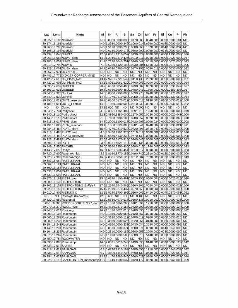
Groundwater Recharge Assessment of the Basement Aquifers of Central Namaqualand
A-201
Lat Long Name Si Sr Al B Ba Zn Mn Fe Ni Cu P Pb
-30.222 18.103 Nourivier ND 0.090 0.000 0.039 0.017 0.089 0.0340.000 0.009 0.0000.101 ND -30.174 18.195 Nourivier ND 1.235 0.000 0.342 0.100 0.014 3.6990.000 0.015 0.0000.000 ND -30.260 18.203 Nourivier ND 1.511 0.000 0.298 0.080 0.068 0.1320.000 0.014 0.0060.034 ND -30.198 18.198 Nourivier ND 0.613 0.000 0.173 0.080 0.000 0.0080.000 0.034 0.0000.000 ND -29.934 18.046 NUW12 12.6 2.838 1.191 0.652 0.013 0.029 0.0000.000 0.000 0.1100.0000.026 -29.965 18.064 NUW2_dam 14.9 1.294 0.737 0.435 0.081 0.311 0.0210.000 0.000 0.0020.0000.017 -29.985 18.052 NUW3_dam 11.7 0.712 0.504 0.251 0.024 0.042 0.0010.000 0.000 0.0070.0000.023 -29.819 17.790 NUWR1 7.8 0.628 0.412 0.102 0.053 0.084 1.6610.066 0.000 0.0070.0020.006 -30.228 18.001 OLIEN_dam 14.7 0.074 0.038 0.000 0.017 0.153 0.0080.011 0.000 0.0030.0000.022 -29.667 17.971 OLYNPUTS ND ND ND ND ND ND ND ND ND ND ND ND -29.483 17.773 O'OKIEP COPPER MINE ND ND ND ND ND ND ND ND ND ND ND ND -30.426 17.610 Ou_Plaas_No1 13.4 7.970 1.772 1.542 0.041 0.138 0.2920.000 0.005 0.0000.0000.031 -30.427 17.603 Ou_Plaas_No2 13.8 6.805 1.608 1.620 0.076 0.063 0.0000.000 0.000 0.0000.0000.014 -23.896 17.632 OUBEEB 20.2 0.637 0.385 0.405 0.073 0.807 0.0620.000 0.000 0.0230.0470.027 -29.893 17.633 OUBEEB 19.8 0.655 0.369 0.489 0.078 0.046 0.1300.000 0.000 0.0350.3060.017 -29.840 17.920 OuHoek 14.0 0.808 0.790 0.000 0.033 0.273 0.0240.000 0.007 0.0170.0000.017 -29.840 17.930 OuHoek 14.6 0.197 0.211 0.000 0.005 0.043 0.0020.000 0.009 0.0130.0590.014 -30.190 18.012 OUT1_reservior 10.7 0.036 0.017 0.012 0.000 0.017 0.0130.004 0.010 0.0030.0190.000 -30.186 18.011 OUT2_Fontain 14.2 0.108 0.038 0.000 0.031 0.039 0.0020.011 0.000 0.0030.0100.022
ND ND Outiep 13.3 2.000 ND ND ND 0.690 ND ND ND ND ND ND -30.345 17.731 Partysvlei 4.0 2.389 1.116 1.482 0.069 1.710 0.1250.000 0.000 0.0000.0020.019 -30.140 18.110 Pedroskloof 22.3 0.886 0.338 0.000 0.117 0.052 0.0030.000 0.000 0.0020.0430.000 -30.140 18.110 Pedroskloof 21.5 0.710 0.390 0.106 0.098 0.057 0.0020.000 0.007 0.0000.0680.018 -30.216 18.017 PEN1_dam 14.3 0.290 0.110 0.017 0.043 0.003 0.0000.024 0.000 0.0060.0090.008 -30.191 18.022 PEN2_reservior 19.4 0.165 0.072 0.000 0.020 1.641 0.0240.002 0.000 0.0030.0210.011 -30.284 18.484 PLAT1_dam 15.4 0.477 0.281 0.530 0.022 0.091 0.0310.047 0.008 0.0010.0000.005 -30.318 18.486 PLAT2_well 4.0 3.545 0.998 1.970 0.101 0.017 0.0000.002 0.000 0.0040.0150.016 -30.321 18.489 PLAT3_reservior 18.7 0.683 0.413 0.330 0.057 0.139 0.0000.002 0.000 0.0030.0000.000 -30.323 18.483 PLAT4_dam 12.6 1.417 0.617 0.915 0.024 0.045 0.0000.002 0.000 0.0040.0020.013 -29.891 18.104 POT1 23.5 3.921 1.452 1.110 0.090 1.135 0.0060.000 0.004 0.0040.0120.008 -30.149 17.850 RACHEL 20.0 0.516 0.335 0.400 0.059 0.016 0.1740.007 0.000 0.0000.0000.033 -30.448 17.652 Radyn 16.6 4.602 1.550 3.454 0.031 0.017 0.0000.000 0.000 0.0000.0090.023 -29.720 17.900 RanchoAmigo 2.3 1.816 0.877 0.156 0.049 0.740 0.2310.000 0.012 0.0190.0320.000 -29.720 17.900 RanchoAmigo 16.5 2.880 1.505 0.123 0.091 2.084 0.7390.000 0.002 0.0000.0350.043 -29.583 18.064 RATELKRAAL ND ND ND ND ND ND ND ND ND ND ND ND -29.567 18.121 RATELKRAAL ND ND ND ND ND ND ND ND ND ND ND ND -29.600 18.156 RATELKRAAL ND ND ND ND ND ND ND ND ND ND ND ND -29.533 18.059 RATELKRAAL ND ND ND ND ND ND ND ND ND ND ND ND -29.533 18.093 RATELKRAAL ND ND ND ND ND ND ND ND ND ND ND ND -29.876 18.189 RIET4_dam 15.4 0.639 0.410 0.491 0.042 0.150 0.0000.004 0.000 0.0020.0180.020 -29.800 18.139 RIETFONTEIN ND ND ND ND ND ND ND ND ND ND ND ND -29.902 18.157 RIETFONTEIN2_BuffelsR 17.6 1.259 0.654 0.568 0.086 0.361 0.0020.004 0.000 0.0000.0220.006 -29.925 18.150 RIETFONTEIN3 16.4 2.201 0.927 0.437 0.097 0.068 0.0000.004 0.000 0.0090.0050.008 -30.010 17.806 RIETMOND 12.8 1.514 0.970 0.399 0.086 0.066 0.8410.000 0.007 0.0270.0510.022
ND ND Riviergat (Karkams) 12.0 3.600 ND ND ND 0.180 ND ND ND ND ND ND -29.820 17.950 Rockoptel 12.6 0.568 0.407 0.017 0.010 0.138 0.0010.000 0.000 0.0000.0230.000 0.000 0.000 ROODEPOORT/37227_dam 12.2 1.107 0.686 0.260 0.018 1.094 0.1210.003 0.000 0.0000.0000.000
-30.070 18.270 ROOI1_Well 10.7 0.432 0.287 0.156 0.072 0.009 0.0000.004 0.000 0.0000.1240.009 -30.348 17.614 Rooiberg 16.9 1.132 0.602 1.618 0.020 0.036 0.1810.000 0.000 0.0000.0000.012 -30.093 18.194 Rooifontein ND 0.135 0.000 0.058 0.012 0.357 0.0210.000 0.009 0.0000.232 ND -30.066 18.269 Rooifontein ND 0.318 0.000 0.112 0.040 0.019 0.0200.000 0.020 0.0030.010 ND -30.080 18.236 Rooifontein ND 0.356 0.000 0.525 0.032 0.051 0.0130.000 0.008 0.0090.000 ND -30.154 18.241 Rooifontein ND 0.495 0.000 0.331 0.043 0.034 0.3680.000 0.000 0.0000.099 ND -30.141 18.234 Rooifontein ND 0.861 0.000 0.371 0.060 0.071 0.0390.000 0.014 0.0040.033 ND -30.104 18.236 Rooifontein ND 0.261 0.000 0.186 0.050 0.055 0.2200.000 0.024 0.0000.000 ND -30.076 18.267 Rooifontein ND 1.149 0.000 0.586 0.080 0.018 0.5440.000 0.002 0.0000.022 ND -29.450 17.754 ROOIWATER ND ND ND ND ND ND ND ND ND ND ND ND -30.030 17.890 Rotnoskop 14.5 2.003 1.001 0.248 0.043 0.035 0.0140.000 0.003 0.0000.1230.042 -29.333 17.919 SABIES ND ND ND ND ND ND ND ND ND ND ND ND -29.818 17.617 SANAGAS 6.3 0.672 0.291 0.192 0.038 0.050 0.1710.000 0.000 0.0240.0320.032 -29.836 17.613 SANAGAS 9.7 0.410 0.144 0.233 0.059 0.132 0.0630.000 0.000 0.0220.0520.041 -29.854 17.623 SANAGAS 13.3 1.147 0.928 0.546 0.056 0.028 0.0900.000 0.000 0.0270.0270.040 -30.225 18.110 SANDFONTEIN_monopump 11.7 0.114 0.160 0.037 0.012 0.172 0.0620.000 0.000 0.0040.0000.009
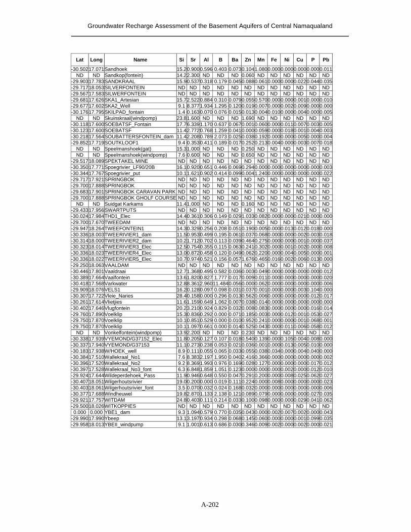
Groundwater Recharge Assessment of the Basement Aquifers of Central Namaqualand
A-202
Lat Long Name Si Sr Al B Ba Zn Mn Fe Ni Cu P Pb
-30.50217.071 Sandhoek 15.20.900 0.596 0.403 0.0730.104 1.0800.0000.0000.0000.0000.011ND ND Sandkop(fontein) 14.22.300 ND ND ND 0.060 ND ND ND ND ND ND
-29.90317.783 SANDKRAAL 15.90.537 0.318 0.179 0.0450.088 0.0610.0000.0000.0220.0440.035-29.71718.053 SILVERFONTEIN ND ND ND ND ND ND ND ND ND ND ND ND -29.56717.583 SILWERFONTEIN ND ND ND ND ND ND ND ND ND ND ND ND -29.68117.626 SKA1_Artesian 15.72.522 0.884 0.310 0.0790.055 0.5700.0000.0000.0010.0000.010-29.67717.602 SKA2_Well 9.1 8.377 1.934 1.295 0.1200.019 0.0070.0000.0020.0090.0000.000-30.17617.795 SKILPAD_fontain 1.4 0.163 0.070 0.076 0.0150.013 0.0040.0100.0000.0040.0000.005
ND ND Skuinskraal(windpomp) 23.81.600 ND ND ND 1.690 ND ND ND ND ND ND -30.11817.600 SOEBATSF_Fontain 17.76.339 1.170 0.637 0.0670.001 0.0600.0000.0110.0070.0030.005-30.12317.600 SOEBATSF 11.42.772 0.768 1.259 0.0410.000 0.0590.0000.0180.0010.0040.003-30.21817.564 SOUBATTERSFONTEIN_dam 11.42.208 0.789 2.073 0.0250.038 0.1920.0000.0000.0050.0000.004-29.85217.719 SOUTKLOOF1 9.4 0.353 0.411 0.189 0.0170.252 0.2130.0040.0000.0030.0070.018
ND ND Speelmanshoek(gat) 15.31.000 ND ND ND 0.250 ND ND ND ND ND ND ND ND Speelmanshoek(windpomp) 7.6 0.600 ND ND ND 0.650 ND ND ND ND ND ND
-29.51718.089 SPEKTAKEL MINE ND ND ND ND ND ND ND ND ND ND ND ND -30.35017.771 Spoegrivier_LF90/20B 16.10.920 0.651 0.446 0.0690.294 0.0000.0000.0000.0000.0000.003-30.34417.767 Spoegrivier_put 10.11.621 0.902 0.414 0.0990.004 1.2400.0000.0000.0000.0000.022-29.71717.921 SPRINGBOK ND ND ND ND ND ND ND ND ND ND ND ND -29.70017.888 SPRINGBOK ND ND ND ND ND ND ND ND ND ND ND ND -29.68317.901 SPRINGBOK CARAVAN PARK ND ND ND ND ND ND ND ND ND ND ND ND -29.70017.888 SPRINGBOK GHOLF COURSE ND ND ND ND ND ND ND ND ND ND ND ND
ND ND Suidgat Karkams 11.41.000 ND ND ND 0.160 ND ND ND ND ND ND -29.43317.956 SWARTPUTS ND ND ND ND ND ND ND ND ND ND ND ND -30.02417.984 THD1_Elec 14.40.361 0.306 0.149 0.0291.033 0.0820.0000.0000.0210.0000.000-29.70017.670 TWEEDAM ND ND ND ND ND ND ND ND ND ND ND ND -29.94718.264 TWEEFONTEIN1 14.30.329 0.256 0.208 0.0510.190 0.0050.0000.0130.0120.0180.000-30.33618.003 TWEERIVIER1_dam 11.50.953 0.499 0.195 0.0610.037 0.0680.0000.0000.0020.0030.018-30.31418.000 TWEERIVIER2_dam 10.21.712 0.702 0.113 0.0390.464 0.2750.0000.0000.0010.0000.037-30.32318.014 TWEERIVIER3_Elec 12.50.754 0.355 0.115 0.0630.241 0.3020.0000.0010.0020.0000.008-30.33618.023 TWEERIVIER4_Elec 13.00.872 0.458 0.120 0.0490.062 0.2200.0000.0040.0050.0000.001-30.33618.022 TWEERIVIER5_Elec 10.70.974 0.521 0.156 0.0571.676 0.4650.0160.0020.0060.0130.000-29.25018.063 VAALDAM ND ND ND ND ND ND ND ND ND ND ND ND -30.44617.801 Vaaldraai 12.71.368 0.495 0.582 0.0360.003 0.0490.0000.0000.0000.0000.012-30.38917.664 Vaalfontein 13.61.820 0.827 1.777 0.0170.009 0.0110.0000.0000.0000.0000.020-30.41817.568 Varkwater 12.88.361 2.96011.4840.0560.000 0.0620.0000.0000.0000.0000.006-29.90918.076 VELS1 16.20.128 0.097 0.098 0.0310.037 0.0010.0000.0000.0030.1040.000-30.30717.722 Vleie_Naries 28.40.158 0.000 0.296 0.0130.562 0.0060.0000.0000.0000.0120.017-30.26117.614 Vlietjies 11.61.159 0.649 1.062 0.0070.038 0.0140.0000.0000.0000.0000.000-30.40217.646 Vlugfontein 20.23.210 0.924 0.829 0.0320.008 0.0830.0000.0000.0000.0160.014-29.76017.890 Voelklip 15.30.836 0.292 0.000 0.0710.185 0.0030.0000.0120.0010.0530.027-29.75017.870 Voelklip 10.10.851 0.529 0.000 0.0100.952 0.2410.0000.0000.0010.0680.001-29.75017.870 Voelklip 10.11.097 0.661 0.000 0.0140.525 0.0430.0000.0110.0060.0580.012
ND ND Vonkelfontein(windpomp) 13.92.200 ND ND ND 0.230 ND ND ND ND ND ND -30.33817.939 VYEMOND/G37152_Elec 11.80.205 0.127 0.107 0.0180.540 0.1390.0000.1050.0040.0080.000-30.33717.940 VYEMOND/G37153 11.10.273 0.238 0.053 0.0210.036 0.0010.0000.0130.0050.0100.000-30.18317.938 W/HOEK_well 8.9 0.111 0.055 0.065 0.0330.055 0.0380.0340.0000.0040.0400.000-30.38417.510 Wallekraal_No1 7.6 8.383 2.197 1.950 0.0402.416 0.3660.0000.0000.0000.0000.002-30.39617.520 Wallekraal_No2 9.2 8.369 1.993 0.976 0.1690.028 0.1270.0000.0000.0000.0170.012-30.39717.528 Wallekraal_No3_font 6.3 6.848 1.859 1.051 0.1230.000 0.0000.0000.0020.0000.0120.010-29.92417.644 Wildeperdehoek_Pass 11.90.946 0.648 0.550 0.0470.291 0.2000.0000.0080.0250.0620.027-30.40718.051 Wilgerhoutsrivier 19.00.200 0.000 0.019 0.1110.224 0.0000.0080.0000.0000.0000.023-30.40318.061 Wilgerhoutsrivier_font 3.5 0.070 0.032 0.024 0.1680.032 0.0000.0000.0000.0000.0000.006-30.37717.688 Windheuwel 19.82.870 1.133 2.138 0.1210.089 0.0790.0000.0000.0000.0270.035-29.92117.757 WITDAM 24.80.403 0.111 0.214 0.0330.100 0.0980.0000.0000.0290.0410.062-29.50018.026 WITKOPPIES ND ND ND ND ND ND ND ND ND ND ND ND 0.000 0.000 YBE1_dam 9.3 1.094 0.579 0.770 0.0350.043 0.0000.0020.0070.0020.0000.043
-29.99017.990 Ybeep 13.13.197 0.934 0.298 0.0680.145 0.0600.0000.0000.0010.0990.035-29.95818.013 YBEII_windpump 9.1 1.001 0.613 0.686 0.0300.346 0.0090.0020.0000.0020.0000.021
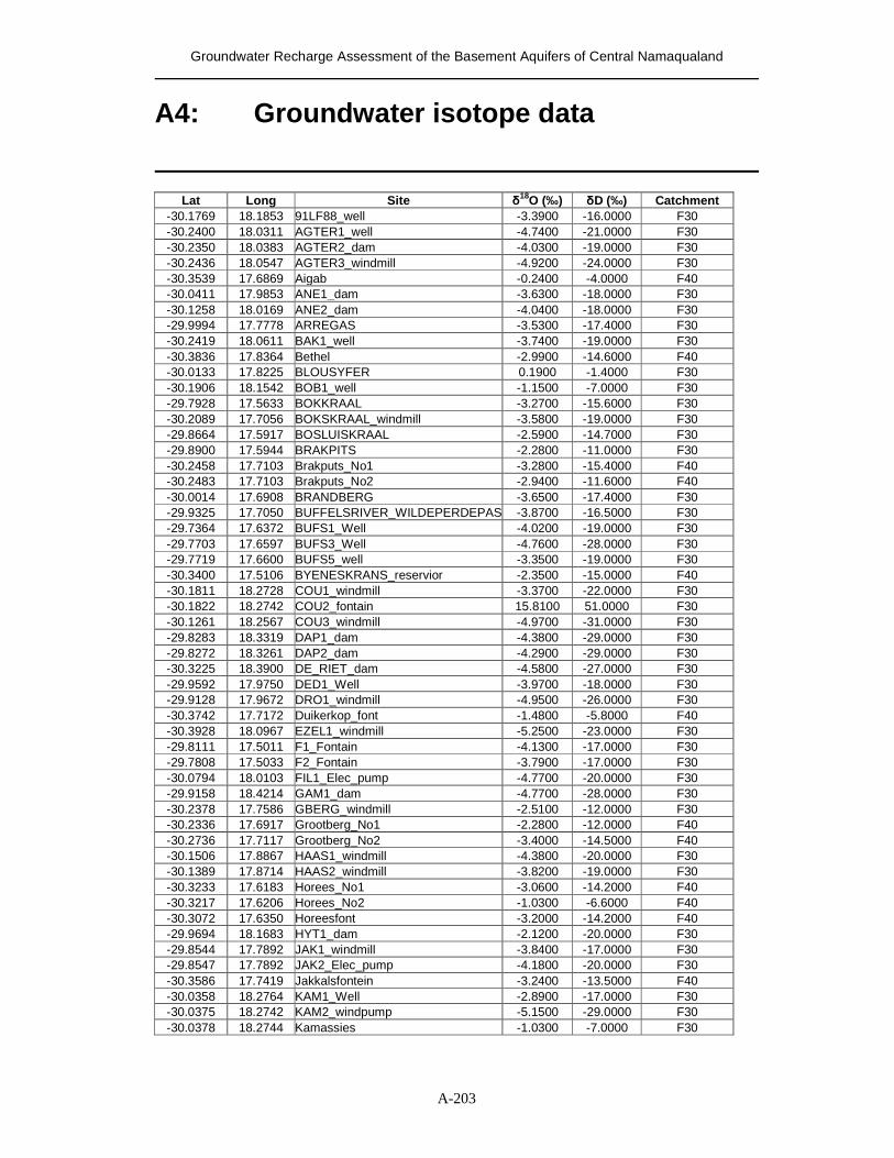
Groundwater Recharge Assessment of the Basement Aquifers of Central Namaqualand
A-203
A4: Groundwater isotope data
Lat Long Site �
18O (‰) �D (‰) Catchment -30.1769 18.1853 91LF88_well -3.3900 -16.0000 F30 -30.2400 18.0311 AGTER1_well -4.7400 -21.0000 F30 -30.2350 18.0383 AGTER2_dam -4.0300 -19.0000 F30 -30.2436 18.0547 AGTER3_windmill -4.9200 -24.0000 F30 -30.3539 17.6869 Aigab -0.2400 -4.0000 F40 -30.0411 17.9853 ANE1_dam -3.6300 -18.0000 F30 -30.1258 18.0169 ANE2_dam -4.0400 -18.0000 F30 -29.9994 17.7778 ARREGAS -3.5300 -17.4000 F30 -30.2419 18.0611 BAK1_well -3.7400 -19.0000 F30 -30.3836 17.8364 Bethel -2.9900 -14.6000 F40 -30.0133 17.8225 BLOUSYFER 0.1900 -1.4000 F30 -30.1906 18.1542 BOB1_well -1.1500 -7.0000 F30 -29.7928 17.5633 BOKKRAAL -3.2700 -15.6000 F30 -30.2089 17.7056 BOKSKRAAL_windmill -3.5800 -19.0000 F30 -29.8664 17.5917 BOSLUISKRAAL -2.5900 -14.7000 F30 -29.8900 17.5944 BRAKPITS -2.2800 -11.0000 F30 -30.2458 17.7103 Brakputs_No1 -3.2800 -15.4000 F40 -30.2483 17.7103 Brakputs_No2 -2.9400 -11.6000 F40 -30.0014 17.6908 BRANDBERG -3.6500 -17.4000 F30 -29.9325 17.7050 BUFFELSRIVER_WILDEPERDEPAS -3.8700 -16.5000 F30 -29.7364 17.6372 BUFS1_Well -4.0200 -19.0000 F30 -29.7703 17.6597 BUFS3_Well -4.7600 -28.0000 F30 -29.7719 17.6600 BUFS5_well -3.3500 -19.0000 F30 -30.3400 17.5106 BYENESKRANS_reservior -2.3500 -15.0000 F40 -30.1811 18.2728 COU1_windmill -3.3700 -22.0000 F30 -30.1822 18.2742 COU2_fontain 15.8100 51.0000 F30 -30.1261 18.2567 COU3_windmill -4.9700 -31.0000 F30 -29.8283 18.3319 DAP1_dam -4.3800 -29.0000 F30 -29.8272 18.3261 DAP2_dam -4.2900 -29.0000 F30 -30.3225 18.3900 DE_RIET_dam -4.5800 -27.0000 F30 -29.9592 17.9750 DED1_Well -3.9700 -18.0000 F30 -29.9128 17.9672 DRO1_windmill -4.9500 -26.0000 F30 -30.3742 17.7172 Duikerkop_font -1.4800 -5.8000 F40 -30.3928 18.0967 EZEL1_windmill -5.2500 -23.0000 F30 -29.8111 17.5011 F1_Fontain -4.1300 -17.0000 F30 -29.7808 17.5033 F2_Fontain -3.7900 -17.0000 F30 -30.0794 18.0103 FIL1_Elec_pump -4.7700 -20.0000 F30 -29.9158 18.4214 GAM1_dam -4.7700 -28.0000 F30 -30.2378 17.7586 GBERG_windmill -2.5100 -12.0000 F30 -30.2336 17.6917 Grootberg_No1 -2.2800 -12.0000 F40 -30.2736 17.7117 Grootberg_No2 -3.4000 -14.5000 F40 -30.1506 17.8867 HAAS1_windmill -4.3800 -20.0000 F30 -30.1389 17.8714 HAAS2_windmill -3.8200 -19.0000 F30 -30.3233 17.6183 Horees_No1 -3.0600 -14.2000 F40 -30.3217 17.6206 Horees_No2 -1.0300 -6.6000 F40 -30.3072 17.6350 Horeesfont -3.2000 -14.2000 F40 -29.9694 18.1683 HYT1_dam -2.1200 -20.0000 F30 -29.8544 17.7892 JAK1_windmill -3.8400 -17.0000 F30 -29.8547 17.7892 JAK2_Elec_pump -4.1800 -20.0000 F30 -30.3586 17.7419 Jakkalsfontein -3.2400 -13.5000 F40 -30.0358 18.2764 KAM1_Well -2.8900 -17.0000 F30 -30.0375 18.2742 KAM2_windpump -5.1500 -29.0000 F30 -30.0378 18.2744 Kamassies -1.0300 -7.0000 F30
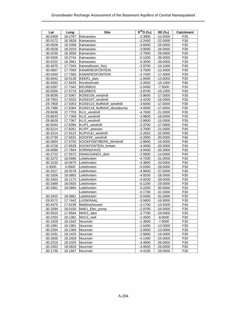
Groundwater Recharge Assessment of the Basement Aquifers of Central Namaqualand
A-204
Lat Long Site �
18O (‰) �D (‰) Catchment -30.0358 18.2767 Kamassies -2.3800 -12.0000 F30 -30.0172 18.3628 Kamassies -2.2400 -22.0000 F30 -30.0528 18.2058 Kamassies -3.6000 -25.0000 F30 -30.0528 18.2019 Kamassies -3.9000 -26.0000 F30 -30.0236 18.3556 Kamassies -2.7900 -29.0000 F30 -30.0406 18.2744 Kamassies -5.1200 -35.0000 F30 -30.0222 18.3561 Kamassies -5.3000 -39.0000 F30 -30.4675 17.7044 Kameelboom_No1 -2.9700 -14.1000 F40 -30.0667 17.7569 KANARIESFONTEIN -3.7000 -12.4000 F30 -30.0450 17.7583 KANARIESFONTEIN -3.7400 -17.4000 F30 -30.0642 18.0136 KEER1_dam -1.9400 -13.0000 F30 -30.4592 17.8439 Kersboshoek -3.2600 -15.1000 F40 -30.0397 17.7342 KEURBOS -2.0400 -7.5000 F30 -30.0056 17.6719 KEURBOS -2.8700 -15.1000 F30 -29.8039 17.5067 KG93/106_windmill -3.9600 -17.0000 F30 -29.7903 17.5022 KG93/107_windmill -3.4200 -16.0000 F30 -29.7858 17.5053 KG93/110_BuffelsR_windmill -3.6000 -17.0000 F30 -29.7386 17.6364 KG93/118_BuffelsR_dieselpump -4.0000 -17.0000 F30 -29.8436 17.7703 KLI1_windmill -4.7600 -21.0000 F30 -29.8633 17.7358 KLI2_windmill -3.9800 -18.0000 F30 -29.8628 17.7367 KLI3_windmill -2.9900 -15.0000 F30 -30.5044 17.8394 KLIP1_windmill -3.3700 -17.0000 F40 -30.5214 17.8261 KLIPF_artesian -3.7000 -21.0000 F40 -30.4214 17.9122 KLIPVLEI_windmill -2.2923 -22.0000 F30 -30.0739 17.6531 KOOFKF_windmill -4.2900 -20.0000 F40 -30.0664 17.6700 KOOKFONT/BERG_Windmill -2.9900 -16.0000 F40 -30.0728 17.6539 KOOKFONTEIN_fontain -4.3400 -20.0000 F40 -29.9086 17.7844 KORINGHUIS -3.9400 -20.3000 F30 -30.2722 17.5572 KWAGGANO1_dam -2.5800 -14.0000 F40 -30.3272 18.0686 Leliefontein -4.7200 -21.0000 F30 -30.3150 18.0675 Leliefontein -4.3800 -23.0000 F30 0.0000 0.0000 Leliefontein -5.0300 -26.0000 F30
-30.2517 18.0578 Leliefontein -4.9600 -27.0000 F30 -30.3306 18.0892 Leliefontein -4.9200 -28.0000 F30 -30.3403 18.1172 Leliefontein -4.9200 -29.0000 F30 -30.3489 18.0925 Leliefontein -5.1200 -29.0000 F30 -30.3361 18.0894 Leliefontein -5.2200 -30.0000 F30
Leliefontein -5.1700 -31.0000 F30 -30.3422 18.0861 Leliefontein -5.0400 -31.0000 F30 -29.9172 17.7442 LUISKRAAL -3.5800 -16.9000 F30 -30.4475 17.6239 Melkbosheuwel -3.1700 -13.5000 F40 -30.1094 18.0150 NAK1_Elec_pump -2.9700 -16.0000 F30 -30.0525 17.9544 NHO1_dam -2.7700 -19.0000 F30 -30.2253 18.1381 NOU1_well -1.4500 -8.0000 F30 -30.1928 18.1542 Nourivier -1.3900 -7.0000 F30 -30.1981 18.1981 Nourivier -1.5400 -12.0000 F30 -30.2264 18.1369 Nourivier -2.0500 -13.0000 F30 -30.2431 18.1425 Nourivier -2.5800 -16.0000 F30 -30.2600 18.2028 Nourivier -4.1400 -24.0000 F30 -30.2219 18.1025 Nourivier -4.4900 -26.0000 F30 -30.2453 18.0828 Nourivier -4.9500 -26.0000 F30 -30.1739 18.1947 Nourivier -4.4100 -29.0000 F30
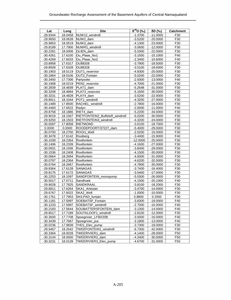
Groundwater Recharge Assessment of the Basement Aquifers of Central Namaqualand
A-205
Lat Long Site �
18O (‰) �D (‰) Catchment -29.9344 18.0458 NUW12_windmill -1.3700 -11.0000 F30 -29.9650 18.0639 NUW2_dam -3.5200 -20.0000 F30 -29.9853 18.0519 NUW3_dam -4.1300 -23.0000 F30 -29.8189 17.7900 NUWR1_windmill -3.0600 -12.0000 F30 -30.2281 18.0006 OLIEN_dam -5.0300 -22.0000 F30 -30.4261 17.6100 Ou_Plaas_No1 -3.1500 -15.1000 F40 -30.4269 17.6033 Ou_Plaas_No2 -2.3400 -10.6000 F40 -23.8958 17.6317 OUBEEB -3.7900 -18.5000 F30 -29.8928 17.6328 OUBEEB -3.5100 -18.6000 F30 -30.1903 18.0119 OUT1_reservior -4.8300 -20.0000 F30 -30.1864 18.0106 OUT2_Fontain -5.0200 -22.0000 F30 -30.3450 17.7306 Partysvlei -2.9300 -13.0000 F40 -30.1908 18.0219 PEN2_reservior -4.7000 -21.0000 F30 -30.2839 18.4839 PLAT1_dam -5.2648 -31.0000 F30 -30.3208 18.4894 PLAT3_reservior -5.1600 -30.0000 F30 -30.3231 18.4828 PLAT4_dam -3.5200 -22.0000 F30 -29.8911 18.1044 POT1_windmill -4.3200 -27.0000 F30 -30.1489 17.8500 RACHEL_windmill -2.7800 -16.0000 F30 -30.4483 17.6522 Radyn -2.0000 -11.0000 F40 -29.8758 18.1886 RIET4_dam -5.2200 -34.0000 F30 -29.9019 18.1567 RIETFONTEIN2_BuffelsR_windmill -5.0200 -30.0000 F30 -29.9250 18.1503 RIETFONTEIN3_windmill -4.3200 -24.0000 F30 -30.0097 17.8058 RIETMOND -3.6100 -18.7000 F30 0.0000 0.0000 ROODEPOORT/37227_dam -5.4000 -29.0000 F30
-30.0700 18.2700 ROOI1_Well -2.5200 -15.0000 F30 -30.3478 17.6142 Rooiberg -3.4400 -15.9000 F40 -30.1039 18.2364 Rooifontein -12.0000 -25.0000 F30 -30.1406 18.2339 Rooifontein -4.1600 -27.0000 F30 -30.0931 18.1936 Rooifontein -3.8400 -29.0000 F30 -30.1536 18.2408 Rooifontein -4.1500 -30.0000 F30 -30.0664 18.2694 Rooifontein -4.8300 -31.0000 F30 -30.0797 18.2364 Rooifontein -4.6200 -32.0000 F30 -30.0764 18.2667 Rooifontein -4.7800 -35.0000 F30 -29.8364 17.6128 SANAGAS -3.7400 -16.4000 F30 -29.8175 17.6172 SANAGAS -3.5400 -17.0000 F30 -30.2253 18.1097 SANDFONTEIN_monopump -5.0300 -26.0000 F30 -30.5017 17.0711 Sandhoek -4.1500 -20.1000 F40 -29.9028 17.7825 SANDKRAAL -3.8100 -18.2000 F30 -29.6811 17.6264 SKA1_Artesian -3.4700 -14.0000 F30 -29.6767 17.6022 SKA2_Well -1.9300 -10.0000 F30 -30.1761 17.7953 SKILPAD_fontain 0.8800 0.2000 F30 -30.1181 17.5997 SOEBATSF_Fontain -3.8300 -19.0000 F40 -30.1233 17.5997 SOEBATSF_windmill -2.7000 -15.0000 F40 -30.2183 17.5644 SOUBATTERSFONTEIN_dam -3.1300 -14.0000 F40 -29.8517 17.7189 SOUTKLOOF1_windmill -2.8100 -12.0000 F30 -30.3500 17.7708 Spoegrivier_LF90/20B -3.5000 -16.0000 F40 -30.3439 17.7667 Spoegrivier_put -3.1800 -13.0000 F40 -30.0236 17.9839 THD1_Elec_pump -3.7300 -18.0000 F30 -29.9467 18.2642 TWEEFONTEIN1_windmill -6.7300 -42.0000 F30 -30.3364 18.0028 TWEERIVIER1_dam -4.1400 -28.0000 F50 -30.3144 18.0000 TWEERIVIER2_dam -4.3400 -30.0000 F50 -30.3231 18.0139 TWEERIVIER3_Elec_pump -4.6700 -31.0000 F50
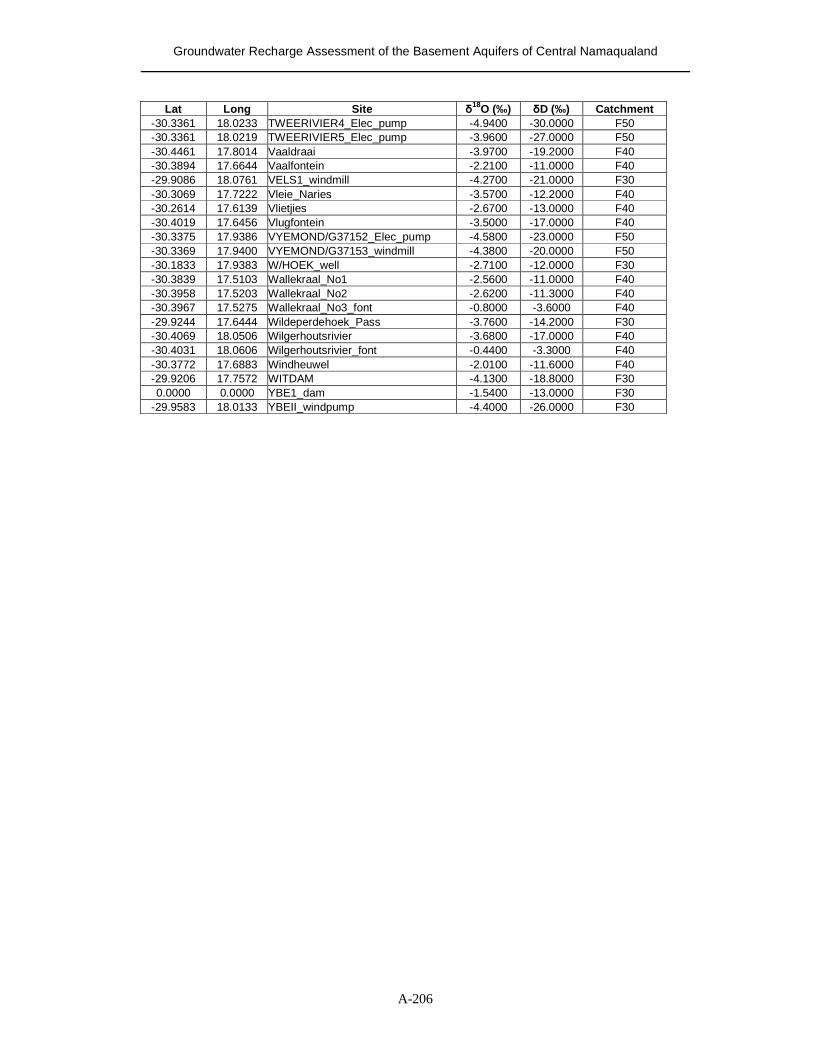
Groundwater Recharge Assessment of the Basement Aquifers of Central Namaqualand
A-206
Lat Long Site �
18O (‰) �D (‰) Catchment -30.3361 18.0233 TWEERIVIER4_Elec_pump -4.9400 -30.0000 F50 -30.3361 18.0219 TWEERIVIER5_Elec_pump -3.9600 -27.0000 F50 -30.4461 17.8014 Vaaldraai -3.9700 -19.2000 F40 -30.3894 17.6644 Vaalfontein -2.2100 -11.0000 F40 -29.9086 18.0761 VELS1_windmill -4.2700 -21.0000 F30 -30.3069 17.7222 Vleie_Naries -3.5700 -12.2000 F40 -30.2614 17.6139 Vlietjies -2.6700 -13.0000 F40 -30.4019 17.6456 Vlugfontein -3.5000 -17.0000 F40 -30.3375 17.9386 VYEMOND/G37152_Elec_pump -4.5800 -23.0000 F50 -30.3369 17.9400 VYEMOND/G37153_windmill -4.3800 -20.0000 F50 -30.1833 17.9383 W/HOEK_well -2.7100 -12.0000 F30 -30.3839 17.5103 Wallekraal_No1 -2.5600 -11.0000 F40 -30.3958 17.5203 Wallekraal_No2 -2.6200 -11.3000 F40 -30.3967 17.5275 Wallekraal_No3_font -0.8000 -3.6000 F40 -29.9244 17.6444 Wildeperdehoek_Pass -3.7600 -14.2000 F30 -30.4069 18.0506 Wilgerhoutsrivier -3.6800 -17.0000 F40 -30.4031 18.0606 Wilgerhoutsrivier_font -0.4400 -3.3000 F40 -30.3772 17.6883 Windheuwel -2.0100 -11.6000 F40 -29.9206 17.7572 WITDAM -4.1300 -18.8000 F30 0.0000 0.0000 YBE1_dam -1.5400 -13.0000 F30
-29.9583 18.0133 YBEII_windpump -4.4000 -26.0000 F30
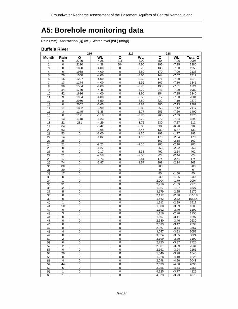
Groundwater Recharge Assessment of the Basement Aquifers of Central Namaqualand
A-207
A5: Borehole monitoring data
Rain (mm); Abstraction (Q) (m3); Water level (WL) (mbgl) Buffels River
216 217 218 Month Rain Q WL Q WL Q WL Total Q
1 0 2729 -4.28 216 -4.00 50 -7.96 2995 2 0 2180 -4.38 504 -4.90 196 -7.25 2880 3 0 1820 -4.00 0 -3.70 136 -7.00 1956 4 0 1968 -4.00 0 -3.80 170 -7.00 2138 5 79 1568 -4.00 0 -3.60 144 -7.07 1712 6 16 1207 -4.00 0 -3.55 171 -7.00 1378 7 13 1174 -4.00 0 -3.55 167 -7.10 1341 8 30 1534 -4.00 0 -3.70 190 -7.01 1724 9 34 1739 -4.45 0 -3.70 243 -7.20 1982
10 42 1686 -4.00 0 -3.60 154 -7.25 1840 11 9 1984 -4.00 0 -3.56 317 -7.00 2301 12 8 2050 -6.50 0 -3.50 322 -7.10 2372 13 0 2002 -6.65 0 -3.83 380 -7.13 2382 14 11 1862 -6.90 0 -3.85 255 -7.12 2117 15 3 1145 -5.38 0 -3.77 255 -7.20 1400 16 0 1171 -3.10 0 -3.70 205 -7.39 1376 17 13 1118 -6.23 0 -3.70 272 -7.34 1390 18 21 281 -4.29 0 -3.75 230 -7.27 511 19 64 0 -3.42 0 -3.30 98 -6.90 98 20 63 0 -3.68 0 -3.45 133 -6.87 133 21 53 0 -1.00 0 -1.20 193 -1.77 193 22 14 0 -1.02 0 -1.10 179 -2.04 179 23 25 0 0 167 -2.18 167 24 21 0 -2.23 0 -2.16 283 -2.10 283 25 0 0 -1.27 0 263 -2.22 263 26 0 0 -2.17 0 -2.38 402 -2.24 402 27 21 0 -2.50 0 -2.55 224 -2.44 224 28 17 0 -2.73 0 -2.81 174 -2.51 174 29 74 0 -1.97 0 -1.57 203 -2.34 203 30 80 0 0 200 200 31 20 0 0 0 0 32 17 0 0 85 -1.60 85 33 0 0 0 530 -1.66 530 34 1 0 0 2,004 -1.79 2004 35 31 0 0 2,270 -1.89 2270 36 2 0 0 1,327 -1.97 1327 37 5 0 0 3,179 -2.25 3179 38 0 0 0 2,117 -2.30 2116.8 39 0 0 0 1,562 -2.42 1562.4 40 1 0 0 1,512 -2.89 1512 41 50 0 0 1,300 -3.39 1300 42 0 0 0 1,192 -3.40 1192 43 3 0 0 1,156 -2.70 1156 44 0 0 0 1,697 -3.11 1697 45 0 0 0 2,630 -3.46 2630 46 0 0 0 2,533 -3.47 2533 47 8 0 0 2,367 -3.44 2367 48 4 0 0 3,057 -3.63 3057 49 0 0 0 3,024 -3.65 3024 50 2 0 0 3,199 -3.80 3199 51 0 0 0 2,725 -3.37 2725 52 2 0 0 2,531 -3.89 2531 53 0 0 0 2,161 -3.94 2161 54 20 0 0 1,540 -3.98 1540 55 8 0 0 1,228 -4.10 1228 56 4 0 0 2,048 -4.60 2048 57 44 0 0 2,093 -4.80 2093 58 5 0 0 2,356 -4.64 2356 59 1 0 0 4,225 -3.77 4225 60 1 0 0 4,073 -3.73 4073
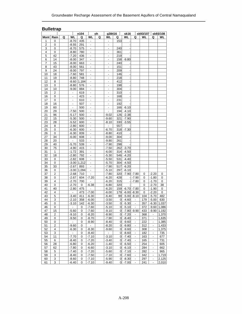
Groundwater Recharge Assessment of the Basement Aquifers of Central Namaqualand
A-208
Bulletrap n104 oh g38416 sk16 sk93/107 sk93/108 Mont Rain Q WL Q WL Q WL Q WL Q WL Q WL
1 0 -8.70 435 - - 153 - 2 0 -8.55 291 - - - 3 0 -8.70 575 - - 240 - 4 0 -8.80 780 - - 361 - 5 42 -7.20 436 - - 219 - 6 14 -8.00 347 - - 158 -9.80 7 15 -8.00 663 - - 240 - 8 43 -8.00 561 - - 151 - 9 24 -8.00 797 - - 209 -
10 18 -7.60 581 - - 146 - 11 19 -8.80 748 - - 218 - 12 8 -8.60 1,184 - - 412 - 13 0 -8.80 576 - - 198 - 14 10 -9.00 884 - - 304 - 15 2 - 619 - - 310 - 16 0 - 423 - - 168 - 17 0 - 610 - - 231 - 18 16 - 507 - - 192 - 19 60 - 500 - - 166 -6.10 20 29 -7.50 500 - - 194 -4.10 21 96 -5.17 500 - -9.02 126 -2.38 22 15 -5.30 500 - -9.60 321 -7.90 23 28 -5.52 600 - -8.10 330 -3.55 24 8 -2.80 600 - - 557 - 25 0 -6.30 600 - -6.70 318 -7.30 26 0 -6.30 839 - -8.80 410 - 27 34 -6.00 608 - -9.00 304 - 28 20 - 533 - -9.80 261 - 29 40 -5.70 539 - -7.90 298 - 30 75 -4.90 415 - -7.50 262 -3.70 31 1 -1.72 391 - -6.00 314 -4.50 32 18 -2.80 792 - -5.30 546 -4.20 33 0 -2.82 608 - -5.50 531 -4.40 34 0 -3.00 1,212 - -5.70 304 -4.50 35 33 -2.67 893 - -7.90 517 -6.20 36 0 -3.00 1,094 - -5.10 297 -6.10 37 2 -2.68 710 - -7.80 320 -7.90 -7.80 0 -2.20 0 38 0 -2.67 604 -7.20 -6.20 428 - -7.90 0 -1.80 0 39 4 -2.70 700 - -6.20 315 - -7.80 0 -1.70 0 40 0 -2.70 0 -6.38 -6.80 320 - 0 -2.70 38 41 40 -2.80 475 - -6.20 159 -6.70 -7.80 0 -1.90 0 42 4 - 473 -7.00 -6.00 179 -6.00 -8.30 0 -2.20 0 43 5 -3.40 411 -6.30 -6.40 99 -5.00 -8.10 104 -5.70 482 44 3 -2.10 358 -6.00 -3.50 0 -4.60 - 179 -5.00 630 45 0 -3.10 142 -6.30 -3.50 0 -5.30 - 357 -6.30 1,037 46 0 - 0 -7.60 -5.10 0 -5.10 - 372 -9.60 1,086 47 15 -5.60 0 -7.60 -9.10 0 -7.80 -9.90 433 -9.90 1,192 48 2 -9.10 0 -8.20 -8.90 0 -7.20 - 368 - 1,370 49 0 -9.50 0 -8.70 -7.90 0 -8.40 - 371 - 1,635 50 0 - 0 -8.90 -8.40 0 -9.60 - 222 - 1,385 51 2 -9.60 0 - -8.20 0 -9.80 - 312 - 1,433 52 4 -6.30 0 -8.30 -9.60 0 -9.60 - 308 - 1,375 53 3 - 0 -8.40 - 0 -8.60 - 182 - 735 54 11 -7.70 0 -7.10 -3.10 0 -7.40 - 163 - 677 55 6 -8.40 0 -7.20 -3.40 0 -7.40 - 165 - 731 56 28 -6.80 0 -6.20 -1.40 0 -6.50 - 254 - 605 57 62 -7.80 0 -6.60 -3.10 0 -6.10 - 284 - 662 58 5 -7.40 0 -7.20 -5.60 0 -7.10 - 282 - 965 59 3 -8.40 0 -7.50 -7.10 0 -7.60 - 342 - 1,719 60 3 -8.60 0 -7.10 -5.90 0 -8.30 - 297 - 2,125 61 3 -6.40 0 -7.10 -9.40 0 -7.00 - 241 - 2,010
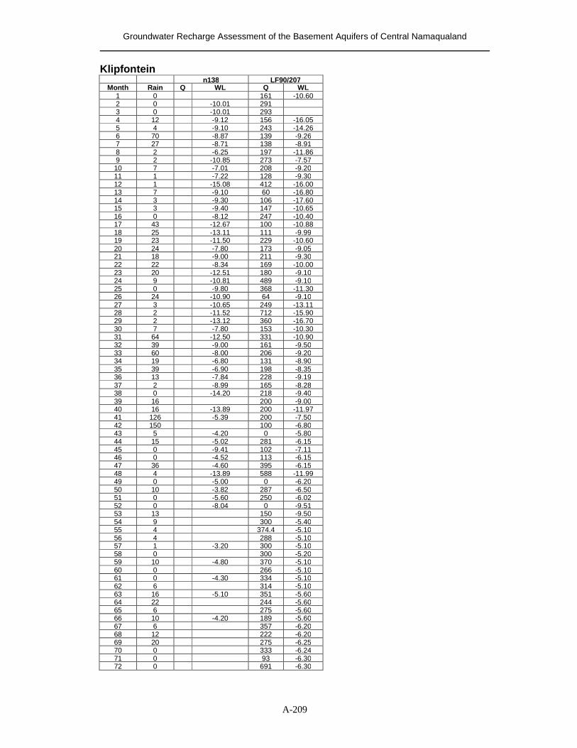
Groundwater Recharge Assessment of the Basement Aquifers of Central Namaqualand
A-209
Klipfontein n138 LF90/207
Month Rain Q WL Q WL 1 0 161 -10.60 2 0 -10.01 291 3 0 -10.01 293 4 12 -9.12 156 -16.05 5 4 -9.10 243 -14.26 6 70 -8.87 139 -9.26 7 27 -8.71 138 -8.91 8 2 -6.25 197 -11.86 9 2 -10.85 273 -7.57 10 7 -7.01 208 -9.20 11 1 -7.22 128 -9.30 12 1 -15.08 412 -16.00 13 7 -9.10 60 -16.80 14 3 -9.30 106 -17.60 15 3 -9.40 147 -10.65 16 0 -8.12 247 -10.40 17 43 -12.67 100 -10.88 18 25 -13.11 111 -9.99 19 23 -11.50 229 -10.60 20 24 -7.80 173 -9.05 21 18 -9.00 211 -9.30 22 22 -8.34 169 -10.00 23 20 -12.51 180 -9.10 24 9 -10.81 489 -9.10 25 0 -9.80 368 -11.30 26 24 -10.90 64 -9.10 27 3 -10.65 249 -13.11 28 2 -11.52 712 -15.90 29 2 -13.12 360 -16.70 30 7 -7.80 153 -10.30 31 64 -12.50 331 -10.90 32 39 -9.00 161 -9.50 33 60 -8.00 206 -9.20 34 19 -6.80 131 -8.90 35 39 -6.90 198 -8.35 36 13 -7.84 228 -9.19 37 2 -8.99 165 -8.28 38 0 -14.20 218 -9.40 39 16 200 -9.00 40 16 -13.89 200 -11.97 41 126 -5.39 200 -7.50 42 150 100 -6.80 43 5 -4.20 0 -5.80 44 15 -5.02 281 -6.15 45 0 -9.41 102 -7.11 46 0 -4.52 113 -6.15 47 36 -4.60 395 -6.15 48 4 -13.89 588 -11.99 49 0 -5.00 0 -6.20 50 10 -3.82 287 -6.50 51 0 -5.60 250 -6.02 52 0 -8.04 0 -9.51 53 13 150 -9.50 54 9 300 -5.40 55 4 374.4 -5.10 56 4 288 -5.10 57 1 -3.20 300 -5.10 58 0 300 -5.20 59 10 -4.80 370 -5.10 60 0 266 -5.10 61 0 -4.30 334 -5.10 62 6 314 -5.10 63 16 -5.10 351 -5.60 64 22 244 -5.60 65 6 275 -5.60 66 10 -4.20 189 -5.60 67 6 357 -6.20 68 12 222 -6.20 69 20 275 -6.25 70 0 333 -6.24 71 0 93 -6.30 72 0 691 -6.30
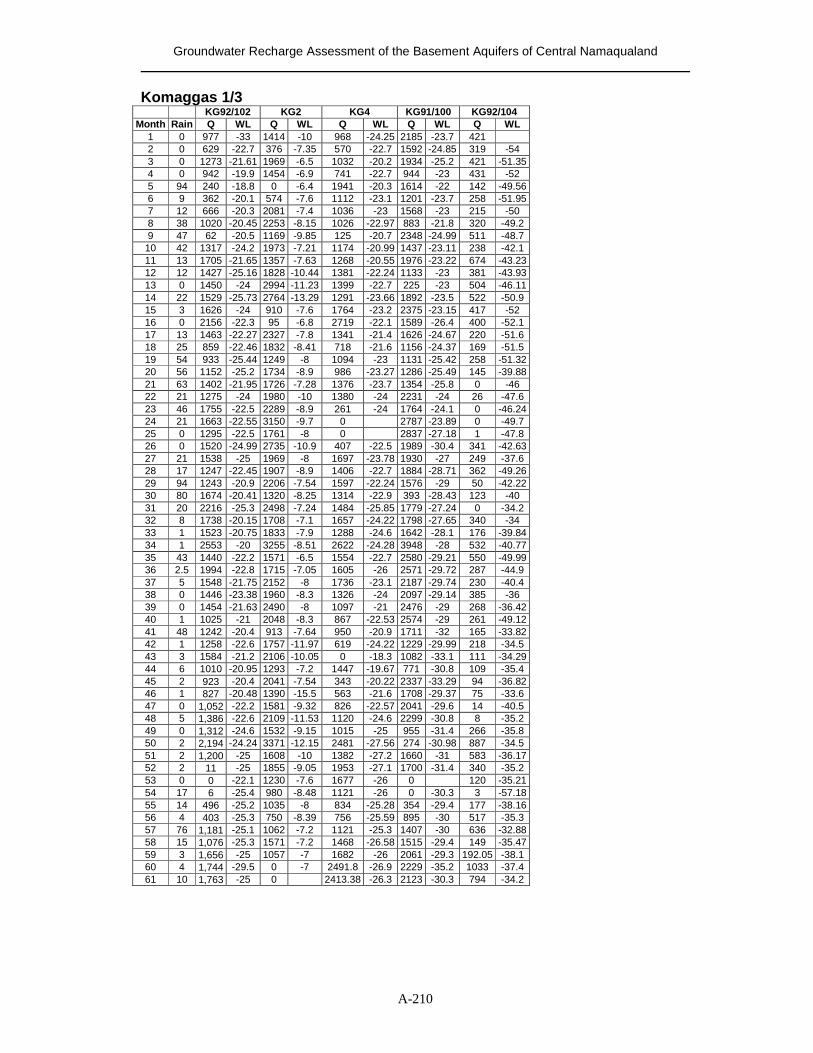
Groundwater Recharge Assessment of the Basement Aquifers of Central Namaqualand
A-210
Komaggas 1/3 KG92/102 KG2 KG4 KG91/100 KG92/104
Month Rain Q WL Q WL Q WL Q WL Q WL 1 0 977 -33 1414 -10 968 -24.25 2185 -23.7 421 2 0 629 -22.7 376 -7.35 570 -22.7 1592 -24.85 319 -54 3 0 1273 -21.61 1969 -6.5 1032 -20.2 1934 -25.2 421 -51.35 4 0 942 -19.9 1454 -6.9 741 -22.7 944 -23 431 -52 5 94 240 -18.8 0 -6.4 1941 -20.3 1614 -22 142 -49.56 6 9 362 -20.1 574 -7.6 1112 -23.1 1201 -23.7 258 -51.95 7 12 666 -20.3 2081 -7.4 1036 -23 1568 -23 215 -50 8 38 1020 -20.45 2253 -8.15 1026 -22.97 883 -21.8 320 -49.2 9 47 62 -20.5 1169 -9.85 125 -20.7 2348 -24.99 511 -48.7
10 42 1317 -24.2 1973 -7.21 1174 -20.99 1437 -23.11 238 -42.1 11 13 1705 -21.65 1357 -7.63 1268 -20.55 1976 -23.22 674 -43.23 12 12 1427 -25.16 1828 -10.44 1381 -22.24 1133 -23 381 -43.93 13 0 1450 -24 2994 -11.23 1399 -22.7 225 -23 504 -46.11 14 22 1529 -25.73 2764 -13.29 1291 -23.66 1892 -23.5 522 -50.9 15 3 1626 -24 910 -7.6 1764 -23.2 2375 -23.15 417 -52 16 0 2156 -22.3 95 -6.8 2719 -22.1 1589 -26.4 400 -52.1 17 13 1463 -22.27 2327 -7.8 1341 -21.4 1626 -24.67 220 -51.6 18 25 859 -22.46 1832 -8.41 718 -21.6 1156 -24.37 169 -51.5 19 54 933 -25.44 1249 -8 1094 -23 1131 -25.42 258 -51.32 20 56 1152 -25.2 1734 -8.9 986 -23.27 1286 -25.49 145 -39.88 21 63 1402 -21.95 1726 -7.28 1376 -23.7 1354 -25.8 0 -46 22 21 1275 -24 1980 -10 1380 -24 2231 -24 26 -47.6 23 46 1755 -22.5 2289 -8.9 261 -24 1764 -24.1 0 -46.24 24 21 1663 -22.55 3150 -9.7 0 2787 -23.89 0 -49.7 25 0 1295 -22.5 1761 -8 0 2837 -27.18 1 -47.8 26 0 1520 -24.99 2735 -10.9 407 -22.5 1989 -30.4 341 -42.63 27 21 1538 -25 1969 -8 1697 -23.78 1930 -27 249 -37.6 28 17 1247 -22.45 1907 -8.9 1406 -22.7 1884 -28.71 362 -49.26 29 94 1243 -20.9 2206 -7.54 1597 -22.24 1576 -29 50 -42.22 30 80 1674 -20.41 1320 -8.25 1314 -22.9 393 -28.43 123 -40 31 20 2216 -25.3 2498 -7.24 1484 -25.85 1779 -27.24 0 -34.2 32 8 1738 -20.15 1708 -7.1 1657 -24.22 1798 -27.65 340 -34 33 1 1523 -20.75 1833 -7.9 1288 -24.6 1642 -28.1 176 -39.84 34 1 2553 -20 3255 -8.51 2622 -24.28 3948 -28 532 -40.77 35 43 1440 -22.2 1571 -6.5 1554 -22.7 2580 -29.21 550 -49.99 36 2.5 1994 -22.8 1715 -7.05 1605 -26 2571 -29.72 287 -44.9 37 5 1548 -21.75 2152 -8 1736 -23.1 2187 -29.74 230 -40.4 38 0 1446 -23.38 1960 -8.3 1326 -24 2097 -29.14 385 -36 39 0 1454 -21.63 2490 -8 1097 -21 2476 -29 268 -36.42 40 1 1025 -21 2048 -8.3 867 -22.53 2574 -29 261 -49.12 41 48 1242 -20.4 913 -7.64 950 -20.9 1711 -32 165 -33.82 42 1 1258 -22.6 1757 -11.97 619 -24.22 1229 -29.99 218 -34.5 43 3 1584 -21.2 2106 -10.05 0 -18.3 1082 -33.1 111 -34.29 44 6 1010 -20.95 1293 -7.2 1447 -19.67 771 -30.8 109 -35.4 45 2 923 -20.4 2041 -7.54 343 -20.22 2337 -33.29 94 -36.82 46 1 827 -20.48 1390 -15.5 563 -21.6 1708 -29.37 75 -33.6 47 0 1,052 -22.2 1581 -9.32 826 -22.57 2041 -29.6 14 -40.5 48 5 1,386 -22.6 2109 -11.53 1120 -24.6 2299 -30.8 8 -35.2 49 0 1,312 -24.6 1532 -9.15 1015 -25 955 -31.4 266 -35.8 50 2 2,194 -24.24 3371 -12.15 2481 -27.56 274 -30.98 887 -34.5 51 2 1,200 -25 1608 -10 1382 -27.2 1660 -31 583 -36.17 52 2 11 -25 1855 -9.05 1953 -27.1 1700 -31.4 340 -35.2 53 0 0 -22.1 1230 -7.6 1677 -26 0 120 -35.21 54 17 6 -25.4 980 -8.48 1121 -26 0 -30.3 3 -57.18 55 14 496 -25.2 1035 -8 834 -25.28 354 -29.4 177 -38.16 56 4 403 -25.3 750 -8.39 756 -25.59 895 -30 517 -35.3 57 76 1,181 -25.1 1062 -7.2 1121 -25.3 1407 -30 636 -32.88 58 15 1,076 -25.3 1571 -7.2 1468 -26.58 1515 -29.4 149 -35.47 59 3 1,656 -25 1057 -7 1682 -26 2061 -29.3 192.05 -38.1 60 4 1,744 -29.5 0 -7 2491.8 -26.9 2229 -35.2 1033 -37.4 61 10 1,763 -25 0 2413.38 -26.3 2123 -30.3 794 -34.2
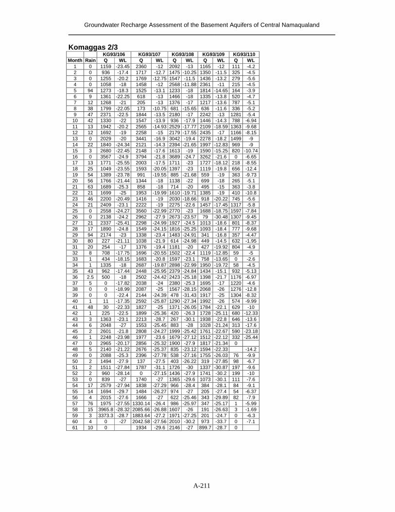
Groundwater Recharge Assessment of the Basement Aquifers of Central Namaqualand
A-211
Komaggas 2/3 KG93/106 KG93/107 KG93/108 KG93/109 KG93/110
Month Rain Q WL Q WL Q WL Q WL Q WL 1 0 1159 -23.45 2360 -12 2092 -13 1165 -12 111 -4.2 2 0 936 -17.4 1717 -12.7 1475 -10.25 1350 -11.5 325 -4.5 3 0 1255 -20.2 1769 -12.75 1547 -11.5 1436 -13.2 279 -5.6 4 0 1058 -18 1458 -12 2568 -11.88 2361 -11 215 -4.5 5 94 1273 -18.3 1525 -13.1 1233 -18 1814 -14.65 164 -3.9 6 9 1361 -22.25 618 -13 1466 -18 1335 -13.8 520 -4.7 7 12 1268 -21 205 -13 1376 -17 1217 -13.6 787 -5.1 8 38 1799 -22.05 173 -10.75 681 -15.65 636 -11.6 336 -5.2 9 47 2371 -22.5 1844 -13.5 2180 -17 2242 -13 1281 -5.4
10 42 1330 -22 1547 -13.9 936 -17.9 1446 -14.3 788 -6.94 11 13 1942 -20.2 2565 -14.93 2529 -17.77 2109 -18.59 1363 -9.68 12 12 1692 -19 2258 -15 2179 -17.55 2435 -17 1166 -8.15 13 0 2029 -20 3441 -16.9 3042 -19.4 2278 -18.2 1499 -9 14 22 1840 -24.34 2121 -14.3 2394 -21.65 1997 -12.83 969 -9 15 3 2680 -22.45 2148 -17.6 1613 -19 1590 -15.25 820 -10.74 16 0 3567 -24.9 3794 -21.8 3689 -24.7 3262 -21.6 0 -6.65 17 13 1771 -25.55 2003 -17.5 1711 -23 1727 -18.12 218 -8.55 18 25 1049 -23.55 1593 -20.05 1397 -23 1119 -19.8 656 -12.4 19 54 1389 -23.78 991 -19.55 885 -21.68 559 -19 363 -9.73 20 56 1766 -21.44 1344 -18 1138 -22 699 -18 265 -5.1 21 63 1689 -25.3 858 -18 714 -20 495 -15 363 -3.8 22 21 1699 -25 1953 -19.99 1610 -19.71 1385 -19 410 -10.8 23 46 2200 -20.49 1416 -19 2030 -18.66 918 -20.22 745 -5.6 24 21 2409 -23.1 2222 -19 2275 -22.6 1457 -17.45 1317 -5.8 25 0 2558 -24.27 3560 -22.99 2770 -23 1688 -18.75 1597 -7.84 26 0 2138 -24.2 2962 -27.9 2673 -23.57 79 -30.48 1307 -9.45 27 21 2337 -25.41 2298 -24.99 1927 -24.5 1013 -18.6 801 -8.37 28 17 1890 -24.8 1549 -24.15 1816 -25.25 1093 -18.4 777 -9.68 29 94 2174 -23 1338 -23.4 1483 -24.91 341 -16.8 357 -4.47 30 80 227 -21.11 1038 -21.9 614 -24.98 449 -14.5 632 -1.95 31 20 254 -17 1376 -19.4 1181 -20 427 -19.92 804 -4.9 32 8 708 -17.75 1696 -20.55 1502 -22.4 1119 -12.85 59 -5 33 1 434 -18.15 1683 -20.8 1597 -23.1 758 -13.65 0 -2.6 34 1 1335 -18 2687 -19.87 2898 -22.99 1950 -19.72 58 -4.5 35 43 962 -17.44 2448 -25.95 2379 -24.84 1434 -15.1 932 -5.13 36 2.5 500 -18 2502 -24.42 2423 -25.18 1398 -21.7 1176 -6.97 37 5 0 -17.82 2038 -24 2380 -25.3 1695 -17 1220 -4.6 38 0 0 -18.99 2087 -25 1567 -28.15 2068 -26 1276 -12.8 39 0 0 -22.4 2144 -24.39 478 -31.43 1917 -25 1304 -8.32 40 1 11 -17.35 2592 -25.87 1290 -27.34 1992 -26 574 -9.99 41 48 30 -22.33 1827 -25 1371 -26.05 1784 -22.1 629 -10 42 1 225 -22.5 1899 -25.36 420 -26.3 1728 -25.11 680 -12.33 43 3 1363 -23.1 2213 -28.7 267 -30.1 1938 -22.8 646 -13.6 44 6 2048 -27 1553 -25.45 883 -28 1028 -21.24 313 -17.6 45 2 2601 -21.8 2808 -24.27 1999 -25.42 1761 -22.67 590 -23.18 46 1 2248 -23.98 1977 -23.6 1679 -27.12 1512 -22.12 332 -25.44 47 0 2965 -20.17 2856 -25.32 1900 -27.9 1817 -21.34 0 48 5 2140 -21.22 2676 -25.37 835 -23.12 1594 -22.33 -14.2 49 0 2088 -25.3 2396 -27.78 538 -27.16 1755 -26.03 76 -9.9 50 2 1494 -27.9 137 -27.5 403 -26.22 319 -27.85 98 -6.7 51 2 1511 -27.84 1787 -31.1 1726 -30 1337 -30.87 197 -9.6 52 2 960 -28.14 0 -27.15 1436 -27.9 1741 -30.2 199 -10 53 0 839 -27 1740 -27 1365 -29.6 1073 -30.1 111 -7.6 54 17 2579 -27.94 1838 -27.29 966 -28.4 384 -28.1 84 -9.1 55 14 1694 -29.7 1484 -26.27 974 -27 205 -27.4 54 -6.37 56 4 2015 -27.6 1666 -27 622 -25.46 343 -29.89 82 -7.9 57 76 1975 -27.55 1330.14 -26.4 986 -25.97 347 -25.17 1 -5.99 58 15 3965.8 -28.32 2085.66 -26.88 1607 -26 191 -26.63 3 -1.69 59 3 3373.3 -28.7 1883.64 -27.2 1971 -27.25 201 -24.7 0 -6.3 60 4 0 -27 2042.58 -27.56 2010 -30.2 973 -33.7 0 -7.1 61 10 0 1934 -29.6 2146 -27 899.7 -28.7 0
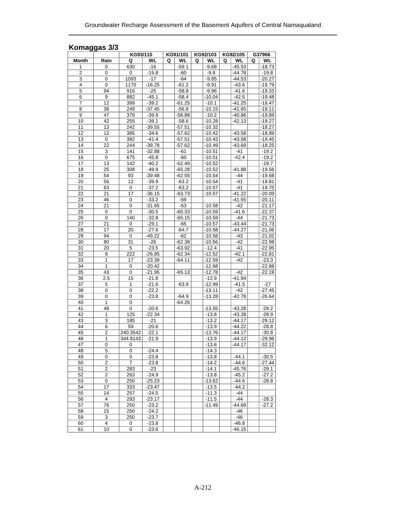
Groundwater Recharge Assessment of the Basement Aquifers of Central Namaqualand
A-212
Komaggas 3/3 KG93/115 KG91/101 KG92/103 KG92/105 G37966
Month Rain Q WL Q WL Q WL Q WL Q WL 1 0 630 -16 -59.1 -9.68 -45.53 -18.73 2 0 0 -15.8 -60 -9.8 -44.78 -19.8 3 0 1093 -17 -64 -9.85 -44.53 -20.27 4 0 1170 -16.25 -61.2 -9.91 -43.6 -19.79 5 94 916 -25 -58.8 -9.96 -41.6 -19.33 6 9 882 -45.1 -58.4 -10.04 -42.5 -19.48 7 12 399 -39.2 -61.25 -10.1 -41.25 -19.47 8 38 249 -37.45 -56.8 -10.15 -41.65 -19.11 9 47 379 -39.9 -58.88 -10.2 -40.86 -19.89 10 42 255 -39.1 -58.6 -10.28 -42.13 -19.27 11 13 242 -39.55 -57.51 -10.32 -18.27 12 12 385 -34.6 -57.62 -10.42 -43.58 -18.89 13 0 382 -41.4 -57.51 -10.43 -43.58 -19.45 14 22 244 -39.78 -57.62 -10.49 -43.69 -18.25 15 3 141 -32.88 -61 -10.51 -41 -19.2 16 0 675 -45.8 -60 -10.51 -42.4 -19.2 17 13 142 -40.2 -62.49 -10.52 -19.7 18 25 308 -49.9 -65.28 -10.52 -41.88 -19.56 19 54 93 -39.48 -62.55 -10.54 -44 -19.68 20 56 12 -39.9 -63.2 -10.54 -41 -19.81 21 63 0 -37.2 -63.2 -10.57 -41 -19.75 22 21 17 -36.15 -63.73 -10.57 -41.22 -20.09 23 46 0 -33.2 -59 -41.55 -20.11 24 21 0 -31.65 -63 -10.58 -42 -21.17 25 0 0 -30.5 -60.33 -10.59 -41.6 -22.37 26 0 140 -32.8 -65.15 -10.59 -44 -21.73 27 21 0 -29.1 -65 -10.57 -43.44 -21.73 28 17 20 -27.6 -64.7 -10.58 -44.27 -21.06 29 94 0 -49.22 -62 -10.58 -43 -21.02 30 80 31 -26 -62.38 -10.56 -42 -22.98 31 20 5 -23.5 -63.92 -12.4 -41 -22.95 32 8 222 -26.85 -62.34 -12.52 -42.1 -22.81 33 1 17 -23.39 -64.11 -12.59 -42 -23.3 34 1 0 -20.42 -12.68 -22.88 35 43 0 -21.95 -65.13 -12.78 -42 -22.19 36 2.5 15 -21.8 -12.9 -41.94 37 5 1 -21.6 -63.9 -12.99 -41.5 -27 38 0 0 -22.2 -13.11 -42 -27.45 39 0 0 -23.8 -64.9 -13.28 -42.78 -26.64 40 1 0 -64.26 41 48 0 -20.6 -13.55 -43.28 -29.2 42 1 125 -22.34 -13.8 -43.28 -28.9 43 3 185 -21 -13.2 -44.17 -29.12 44 6 59 -20.6 -13.9 -44.22 -28.8 45 2 240.3542 -22.1 -13.76 -44.17 -30.8 46 1 344.8143 -21.9 -13.9 -44.12 -29.96 47 0 0 -13.6 -44.17 -32.12 48 5 0 -24.4 -14.3 49 0 0 -23.8 -13.8 -44.1 -30.5 50 2 7 -23.8 -14.2 -44.6 -27.44 51 2 283 -23 -14.1 -45.76 -29.1 52 2 263 -24.9 -13.8 -45.2 -27.2 53 0 250 -25.23 -13.62 -44.6 -28.8 54 17 333 -23.47 -13.5 -44.2 55 14 257 -24.5 -11.3 -44 56 4 293 -23.17 -11.5 -44 -28.3 57 76 250 -23.2 -11.49 -44.69 -27.2 58 15 250 -24.2 -46 59 3 250 -23.7 -46 60 4 0 -23.8 -46.8 61 10 0 -23.6 -46.15
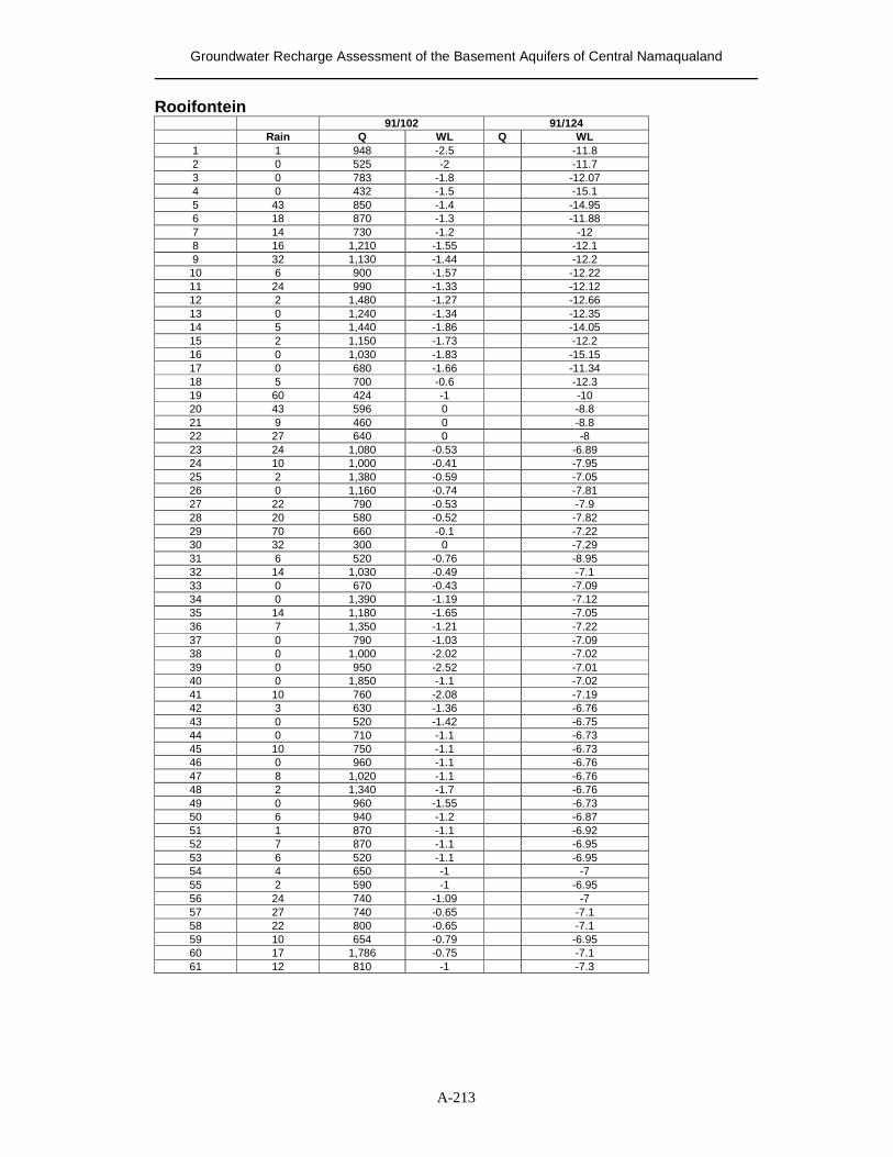
Groundwater Recharge Assessment of the Basement Aquifers of Central Namaqualand
A-213
Rooifontein 91/102 91/124 Rain Q WL Q WL 1 1 948 -2.5 -11.8 2 0 525 -2 -11.7 3 0 783 -1.8 -12.07 4 0 432 -1.5 -15.1 5 43 850 -1.4 -14.95 6 18 870 -1.3 -11.88 7 14 730 -1.2 -12 8 16 1,210 -1.55 -12.1 9 32 1,130 -1.44 -12.2 10 6 900 -1.57 -12.22 11 24 990 -1.33 -12.12 12 2 1,480 -1.27 -12.66 13 0 1,240 -1.34 -12.35 14 5 1,440 -1.86 -14.05 15 2 1,150 -1.73 -12.2 16 0 1,030 -1.83 -15.15 17 0 680 -1.66 -11.34 18 5 700 -0.6 -12.3 19 60 424 -1 -10 20 43 596 0 -8.8 21 9 460 0 -8.8 22 27 640 0 -8 23 24 1,080 -0.53 -6.89 24 10 1,000 -0.41 -7.95 25 2 1,380 -0.59 -7.05 26 0 1,160 -0.74 -7.81 27 22 790 -0.53 -7.9 28 20 580 -0.52 -7.82 29 70 660 -0.1 -7.22 30 32 300 0 -7.29 31 6 520 -0.76 -8.95 32 14 1,030 -0.49 -7.1 33 0 670 -0.43 -7.09 34 0 1,390 -1.19 -7.12 35 14 1,180 -1.65 -7.05 36 7 1,350 -1.21 -7.22 37 0 790 -1.03 -7.09 38 0 1,000 -2.02 -7.02 39 0 950 -2.52 -7.01 40 0 1,850 -1.1 -7.02 41 10 760 -2.08 -7.19 42 3 630 -1.36 -6.76 43 0 520 -1.42 -6.75 44 0 710 -1.1 -6.73 45 10 750 -1.1 -6.73 46 0 960 -1.1 -6.76 47 8 1,020 -1.1 -6.76 48 2 1,340 -1.7 -6.76 49 0 960 -1.55 -6.73 50 6 940 -1.2 -6.87 51 1 870 -1.1 -6.92 52 7 870 -1.1 -6.95 53 6 520 -1.1 -6.95 54 4 650 -1 -7 55 2 590 -1 -6.95 56 24 740 -1.09 -7 57 27 740 -0.65 -7.1 58 22 800 -0.65 -7.1 59 10 654 -0.79 -6.95 60 17 1,786 -0.75 -7.1 61 12 810 -1 -7.3
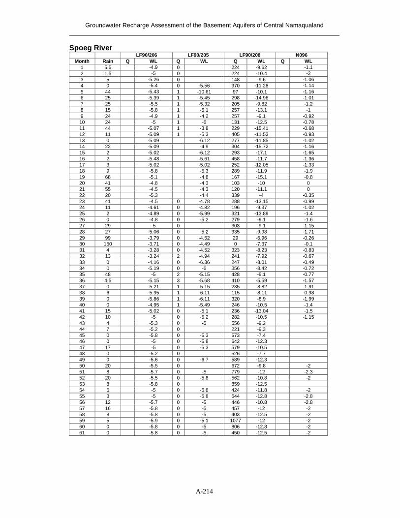
Groundwater Recharge Assessment of the Basement Aquifers of Central Namaqualand
A-214
Spoeg River LF90/206 LF90/205 LF90/208 N096
Month Rain Q WL Q WL Q WL Q WL 1 5.5 -4.9 0 224 -9.62 -1.1 2 1.5 -5 0 224 -10.4 -2 3 5 -5.26 0 148 -9.6 -1.06 4 0 -5.4 0 -5.56 370 -11.28 -1.14 5 44 -5.43 1 -10.61 97 -10.1 -1.16 6 25 -5.39 1 -5.45 298 -14.96 -1.01 7 25 -5.5 1 -5.32 205 -9.82 -1.2 8 15 -5.8 1 -5.1 257 -13.1 -1 9 24 -4.9 1 -4.2 257 -9.1 -0.92 10 24 -5 1 -6 131 -12.5 -0.78 11 44 -5.07 1 -3.8 229 -15.41 -0.68 12 11 -5.09 1 -5.3 405 -11.53 -0.93 13 0 -5.09 -6.12 277 -11.85 -1.02 14 22 -5.09 -4.9 304 -15.72 -1.16 15 2 -5.02 -6.12 293 -17.1 -1.65 16 2 -5.48 -5.61 458 -11.7 -1.36 17 3 -5.02 -5.02 252 -12.05 -1.33 18 9 -5.8 -5.3 289 -11.9 -1.9 19 68 -5.1 -4.8 167 -15.1 -0.8 20 41 -4.8 -4.3 103 -10 0 21 55 -4.5 -4.3 120 -11.1 0 22 20 -5.3 -4.4 339 -4 -0.35 23 41 -4.5 0 -4.78 288 -13.15 -0.99 24 11 -4.61 0 -4.82 196 -9.37 -1.02 25 2 -4.89 0 -5.99 321 -13.89 -1.4 26 0 -4.8 0 -5.2 279 -9.1 -1.6 27 29 -5 0 303 -9.1 -1.15 28 27 -5.06 0 -5.2 335 -9.98 -1.71 29 99 -3.79 0 -4.52 29 -6.96 -0.26 30 150 -3.71 0 -4.49 0 -7.37 -0.1 31 4 -3.28 0 -4.52 323 -8.23 -0.83 32 13 -3.24 2 -4.94 241 -7.92 -0.67 33 0 -4.16 0 -6.36 247 -8.01 -0.49 34 0 -5.19 0 -6 356 -8.42 -0.72 35 48 -5 2 -5.15 428 -9.1 -0.77 36 4.5 -5.15 3 -5.68 410 -5.59 -1.57 37 0 -5.21 1 -5.15 235 -8.82 -1.91 38 6 -5.95 1 -6.11 115 -8.11 -0.98 39 0 -5.86 1 -6.11 320 -8.9 -1.99 40 0 -4.95 1 -5.49 246 -10.5 -1.4 41 15 -5.02 0 -5.1 236 -13.04 -1.5 42 10 -5 0 -5.2 282 -10.5 -1.15 43 4 -5.3 0 -5 556 -9.2 44 7 -5.2 0 221 -9.3 45 0 -5.8 0 -5.3 573 -7.4 46 0 -5 0 -5.8 642 -12.3 47 17 -5 0 -5.3 579 -10.5 48 0 -5.2 0 526 -7.7 49 0 -5.6 0 -6.7 589 -12.3 50 20 -5.5 0 672 -9.8 -2 51 8 -5.7 0 -5 779 -12 -2.3 52 20 -5.5 0 -5.8 562 -10.8 -2 53 8 -5.8 0 859 -12.5 54 6 -5 0 -5.8 424 -11.8 -2 55 3 -5 0 -5.8 644 -12.8 -2.8 56 12 -5.7 0 -5 446 -10.8 -2.8 57 16 -5.8 0 -5 457 -12 -2 58 8 -5.8 0 -5 403 -12.5 -2 59 5 -5.9 0 -5.1 1077 -12 -2 60 0 -5.8 0 -5 806 -12.8 -2 61 0 -5.8 0 -5 450 -12.5 -2


