Heuristic Scheduling ofParallel Heterogeneous Queues with Set-UpsIzak Duenyas and Mark P. Van OyenTechnical Report 92-60Department of Industrial and Operations EngineeringThe University of MichiganAnn Arbor, MI 48109October 1992Revised June 1995

Heuristic Scheduling ofParallel Heterogeneous Queues with Set-UpsIzak DuenyasDepartment of Industrial and Operations EngineeringThe University of Michigan, Ann Arbor, Michigan 48109Mark P. Van OyenDepartment of Industrial Engineering and Management SciencesNorthwestern University, Evanston, Illinois 60208-3119AbstractWe consider the problem of allocating a single server to a system of queues with Poissonarrivals. Each queue represents a class of jobs and possesses a holding cost rate, general servicedistribution, and general set-up time distribution. The objective is to minimize the expectedholding cost due to the waiting of jobs. A set-up time is required to switch from one queueto another. We provide a limited characterization of the optimal policy and a simple heuristicscheduling policy for this problem. Simulation results demonstrate the e�ectiveness of ourheuristic over a wide range of problem instances.1. IntroductionIn many manufacturing environments, a facility processes several di�erent kinds of jobs. Inmany cases, a set-up time is required before the facility can switch from producing one type ofjob to another. If several di�erent types of jobs are waiting when a unit has been completed, thedecision maker is faced with the problem of deciding whether to produce one more unit of the sametype of job that the machine is currently set up to produce, or to set up the machine to process adi�erent kind of job.The control decisions of when to set up the system and which type of job to produce have im-portant e�ects on the performance of the system. First, for each unit of Work-In-Process Inventorythat is waiting at a machine to be processed, the �rm incurs signi�cant holding costs. Second,companies quote due dates to customers based on the work load they have in the system. To quotefeasible due dates, the facility manager must understand the job scheduling policy employed. Toquote competitive due dates, the manager must have an e�cient policy for scheduling service. It1

is essential to provide an e�cient rule for the sequencing of jobs in the facility to quote customersfeasible and competitive due dates.The optimal control of the Work- In-Process in manufacturing systems without set-up times aswell as the problem of quoting customer due dates have been extensively addressed in the literature.It is well known, for example, that for an M=G=1 queue with multiple job types, if jobs of type iare charged holding costs at rate ci and are processed at rate �i, the c� rule (Average WeightedProcessing Time rule) minimizes the average holding cost per unit time (see Baras et al. [3],Buyukkoc et al. [6], Cox and Smith [8], Gittins [13], Nain [25], Nain et al. [26], and Walrand [35]).Other stochastic scheduling problems in the literature for which there are no costs (or no time lost)for switching from one type of job to another may be found in Baras et al. [3], Dempster et al.[9], Gittins [13], Harrison[15],[16], Klimov [18], [19], Lai and Ying [21], Nain [25], Nain et al. [26],Varaiya et al. [34], and Walrand [35]. For systems with no switching times or costs, researcherssuch as Wein [36] and Wein and Chevalier [37] have developed due date setting rules.There are few known results for the optimal scheduling of systems with switching costs orswitching times. The reason for this is the di�culty of the problem. Most intuitive results developedfor systems without switching penalties no longer hold in this case. Gupta et al. [14] considered theproblem with switching costs and only two types of jobs with the same processing time distributions.Hofri and Ross [17] considered a similar problem with switching times, switching costs, and twohomogeneous classes of jobs. They conjectured that the optimal policy is of a threshold type.Recently, Rajan and Agrawal [27] and Liu et al. [24] have studied systems similar to the oneconsidered here and have partially characterized an optimal policy (in the sense of the stochasticdominance of the queue length process) for the case of homogeneous service processes. Browne andYechiali [5] considered cycle times in heterogeneous systems and completely characterized schedulingpolicies that optimize cycle times. Other work has concentrated on performance evaluation andstochastic comparisons of di�erent policies (see Baker and Rubin [2], Levy and Sidi [22], Levy etal. [23], Takagi [30] and Srinivasan [29]). Recently, Federgruen and Katalan [10] have analyzedthe performance of exhaustive and gated polling policies where the server is also allowed to idle.2

Their policies are applicable to the make-to-stock version of the problem considered here as well.Federgruen and Katalan [11] have also analyzed the impact of changes in setup times on theperformance of multi-class production systems.In this paper, we address the stochastic scheduling of a system with several di�erent types of jobsand switching times (equivalently set-up times) in a multiclass M=G=1 queue. Our purpose is todevelop a heuristic that is simple enough to be implemented in a manufacturing environment whileremaining highly e�ective. We contribute a perspective on this problem based on reward rates.The applicability of reward rate notions is demonstrated by their use in partially characterizingan optimal scheduling policy under a discounted cost criterion. We relate the discounted case tothe average cost problem. We then use this perspective to develop a heuristic for the stochasticscheduling problem with set-up times. The heuristic that we develop is extremely simple, since itis based only on statistical averages. Moreover, our simulation results indicate that our heuristicpolicy consistently outperforms other policies suggested in the literature.The rest of the paper is organized as follows. In Section 2, we formulate the problem. InSection 3, we partially characterize an optimal policy. In Section 4, we develop a heuristic policy,and indicate special cases under which the heuristic is optimal. In Section 5, we test this heuristicby comparing this heuristic to other heuristics in the literature. Our results indicate that for alarge variety of problems, our heuristic consistently outperforms other policies in the literature.The paper concludes in Section 6.2. Problem FormulationA single server is to be allocated to jobs in a system of parallel queues labeled 1; 2; : : : ; N andfed by Poisson arrivals. By parallel queues, we mean that a job served in any queue directly exitsthe system. Each queue (equivalently, node) n possesses a general, strictly positive service perioddistribution with mean ��1n (0 < ��1n < 1) and a �nite second moment. Successive servicesin node n are independent and identically distributed (i.i.d.) and independent of all else. Jobsarrive to queue n according to a Poisson process with strictly positive rate �n (independent of allother processes). As a necessary condition for stability, we assume that � = PNi=1 �i < 1; where3

�i = �i=�i.Holding cost is assessed at a rate of cn (cn � 0) cost units per job per unit time spent in queuen (including time in service). A switching or set-up time, Dn is incurred at each instant (includingtime 0) the server switches to queue n from a di�erent queue to process a job. The switching time,Dn, represents a period of time which is required to prepare the server for processing jobs in aqueue di�erent than the current one. We assume that successive set-ups for node n require strictlypositive periods which are i.i.d., possess a �nite mean and second moment, and are independent ofall else.A policy speci�es, at each decision epoch, that the server either remain working in the presentqueue, idle in the present queue, or set-up another queue for service. With IR+(ZZ+) denoting thenonnegative reals (integers), let fXgn(t) : t 2 IR+g be the right-continuous queue length process ofnode n under policy g (including any customer of node n in service). Denote the vector of initialqueue lengths by X(0�) 2 (ZZ+)N , where X(0�) is �xed. Without loss of generality, we assumethat node one has been set up prior to time t = 0 and that the server is initially placed in nodeone. The average cost per unit time of policy g, �J(g), can now be expressed as�J(g) = lim supT!1 1T E(Z T0 NXn=1 cnXgn(t)dt) : (2.1)The class of admissible strategies, G, is taken to be the set of non-preemptive and non-anticipative policies that are based on perfect observations of the queue length processes. Bynon-preemptive, we mean that neither the service of a job nor the execution of a set-up can beinterrupted (by job service, queue set-up, or idling) until its completion. Idling is allowed at any de-cision time. The set of decision epochs is assumed to be the set of all arrival epochs, service epochs,set-up completion epochs, and instances of idling. The objective of the optimization problem is todetermine a policy g� 2 G that minimizes �J(g).For many policies (2.1) may be in�nite. To cite a well-studied example, the limited-l cyclicservice policies become unstable for � < 1, as is demonstrated in Kuehn [20] and Georgiadis andSzpankowski [12]. For � < 1, it is well known that policies such as the exhaustive and gated cyclicpolling strategies yield a stable system (see Altman et al. [1]). Thus, �nite steady state average4

queue lengths exist under an optimal policy, and the objective is to minimize the weighted sum ofthe average queue lengths.Our analysis is framed within the class of policies, G, which contains (in general) nonstationaryand randomized policies. Nevertheless, it is helpful to explicitly describe the subclass GPM � Gconsisting of pure Markov (that is, stationary and non-randomized) policies. Under the restrictionto pure Markov policies (and a memoryless arrival process), it su�ces to regard the decision toidle as a commitment that the server idle for one (system) interarrival period. Thus, the state ofthe system is described by the vector X(t) = (X1(t); X2(t); : : : ; XN(t); n(t); �(t)) 2 S, where n(t)denotes that the server is located at node n(t) at time t, �(t) is zero if the set-up of node n(t) is notcomplete at time t and is one otherwise, and S denotes the state space (ZZ+)N�f1; 2; : : : ; Ng�f0; 1g.Let the action space be U = f0; 1; 2; : : : ; Ng � f0; 1; 2g. Suppose at a decision epoch, t, the stateis X(t) = (x1; x2; : : : ; xN ; n(t); �(t)) 2 S. Thus, �(t) = 1, since we require non-preemptive set-ups. Action U(t) = (n; 2) 2 U , where n 6= n(t), causes the server to set up node n. ActionU(t) = (n(t); 1) results in the service of a job in n(t). Action U(t) = (n(t); 0) selects the option toidle in the current queue until the next decision epoch, another system arrival. No other actionsare possible.3. On an Optimal PolicyIn this section, we provide a partial characterization of an optimal policy within the class ofpolicies G. The special case with all switching times equal to 0 has been well studied, with earlyresults found in Cox and Smith [8]. The non-preemptive c� rule is optimal: The index ci�i isattached to each job in the ith queue. At any decision epoch, serve the available job possessing thelargest index. Note that the index of any queue is independent of both the queue length (providedit is strictly positive) and the arrival rate of that queue. Another special case has been treatedin Liu et al. [24] and Rajan and Agrawal [27]. For problems that are completely homogeneouswith respect to cost and to the service process, they partially characterized optimal policies asexhaustive and as serving the longest queue upon switching.We begin our analysis with the following de�nitions:5

De�nition 1: A policy serves node i in a greedy manner if the server never idles in queue i whilejobs are still available in i and queue i has been set up for service.De�nition 2: A policy serves node i in an exhaustive manner if it never switches out of node iwhile jobs are still available in i.De�nition 3: A top-priority queue refers to any queue (there may be more than one) that isserved in a greedy and exhaustive manner.Although our focus for our heuristic is on the average cost per unit time criterion, we havefound it insightful to study the discounted cost criterion as well because it demonstrates the use ofreward rate expressions which prove to be pertinent to the heuristic we develop. We de�ne the totalexpected discounted cost criterion, which we note is �nite for any policy: For discount parameter� > 0, let J�(g) = EfZ 10 NXn=1 cnXgn(t)! e��tdtg : (3.1)As in Harrison [15] we transform the cost criterion of (3.1) to a reward criterion using thedevice of Bell [4]. Letting Y gn (t) denote the right-continuous cumulative departure process fromnode n under g through time t, we have Xgn(t) = Xn(0�) + An(t)� Y gn (t). One can show that theminimization of J�(g) is equivalent to the maximization of the following reward criterion:R�(g) = Ef NXn=1 cn��1 Z 10 e��tdY gn (t)g = Ef NXn=1 1Xk=1 e��T gn(k)cn��1g ; (3.2)where T gn(k) is the kth service completion epoch under g corresponding to a service in node n . Theterm cn��1 is interpreted as the reward received upon job completion, and it equals the discountedcost of holding that job forever.It is useful to consider the policy, call it g0, that at time t = 0 sets-up node n, serves adeterministic number u jobs, and then idles thereafter. We denote the expected discounted rewardearned from this action sequence by rn(u). Using (3.2), rn(u) = cn��1EfR10 e��tdY g0n (t)g. Letfn;k denote the sum of k service durations in queue n. Letting Sn �= Efe��fn;1g, we use the i.i.d.nature of successive services to get Efe��fn;kg = Skn. Thusrn(u) = cn��1Sn(1� Sn)�1(1� Sun)Efe��Dng : (3.3)6

We de�ne the reward rate associated with this sequence of actions to be the ratio of expecteddiscounted reward, rn(u), to the expected discounted length of time required by the action sequence:rn(u)EfRDn+fn;u0 e��tdtg = cn��1Sn(1� Sn)�1(1� Sun)Efe��Dng��1(1� SunEfe��Dng) < hn; (3.4)where hn is de�ned by hn �= cnSn=(1� Sn) : (3.5)Given a discount parameter � > 0, the reward rate earned by serving a single job in node i(without a set-up) is hn. To see this key fact, simply set Dn = 0 in (3.4). Theorem 1, which follows,states that a top-priority queue always exists under an optimal policy and can be determined asthe node maximizing hn over all n. Theorem 1 is similar to the results presented in Gupta et al[14], Hofri and Ross [17], Liu et al. [24] and Rajan and Agrawal [27]. The novelty of our result liesprimarily in our treatment of unequal or heterogeneous service distributions at each queue.Theorem 1: If hi � hj for all j = 1; 2; : : : ; N then there exists a policy for which queue i is a top-priority queue that is optimal within G under the discounted cost criterion. Similarly, if ci�i � cj�jfor all j = 1; 2; : : : ; N the same result holds under the average cost per unit time criterion.Proof : The proof is found in the Appendix.Since a top-priority policy is optimal for any discount factor � > 0, we note that the discountedand average cost per unit time cases can be linked as follows:lim�!0�hn = lim�!0�cnEfe��fn;1g=EfZ fn;10 e��tdtg = cn�n : (3.6)The quantity cn�n can be regarded as the (reward) rate at which holding costs are reduced byserving a job in node n. On the other hand, a reward rate of zero is earned during idle periodsand set-up periods. We use these concepts of reward rates in the next section to derive a heuristicpolicy for the problem.4. A Heuristic PolicyWe develop a greedy heuristic for the problem formulated in Section 2, where the queues areordered such that c1�1 � c2�2 � : : : � cN�N . We let xi denote the queue length at queue i. We�rst develop a heuristic for the problem with two queues and then extend it to N queues.7

4.1. Heuristic for Systems with Two QueuesConsistent with the result of Section 3 that top-priority service of queue 1 is optimal, we restrictattention to a policy that does not switch from queue 1 to queue 2 when queue 1 is not empty.De�ning a heuristic policy for two queues requires deciding when to switch from queue 2 to 1 whenqueue 2 is not empty, as well as the characterization of a rule for idling (i.e., should the server idleat queue i or switch to the other queue?). Our heuristic is based in part on reward rate indicescorresponding to action sequences. In computing indices for each queue, we assume that once theserver switches to a queue, the server will remain at that queue until the end of its busy period.We begin with the development of the rule for switching, then prescribe a rule for idling.Rule for SwitchingWe assume that nodes 1 and 2 are both nonempty (x1 > 0; x2 > 0) and focus on the questionof when to switch from node 2 to 1. We let 'i(xi; r) denote the reward rate (or expected rewardper expected unit of time) associated with remaining in queue i. If the server remains at queue iand xi > 0, it will continue earning rewards at a rate of ci�i until the end of queue i's busy period.Hence, we de�ne the index to remain in queue 2 if there is a job at queue 2 to be'2(x2; r) = c2�2 if x2 � 1: (4.1)On the other hand, if the server decides to switch to queue 1, it will �rst have to set-up queue1 and earn no rewards for the (random) duration of time D1. Then, by Theorem 1, it will servequeue 1 until the end of its busy period. Although the server could actually remain at node 1 fora longer amount of time by idling at node 1 for a certain duration of time, we disallow idling incalculating an index for switching to node 1. We also assume that at the end of the busy periodof node 1, the server switches back to node 2, and for a (random) duration of time D2 again earnsno rewards. Hence, by switching to node 1 to serve the jobs at node 1 and returning to 2 at theend of the busy period of node 1, the server will have spent an expected total amount of timeED1 + ED2 + x1+�1ED1�1��1 . On average, however, the server will have earned a reward only for theexpected duration of time equal to x1+�1ED1�1��1 . Hence, the index for switching to node 1 is given by8

the reward rate of this action sequence:'1(x1; s) = c1�1 x1+�1ED1�1��1ED1 + x1+�1ED1�1��1 +ED2 (4.2)= c1�1 x1 + �1ED1x1 + �1ED1 + (�1 � �1)ED2 : (4.3)Comparing the terms '1(x1; s) and '2(x2; r), it is easy to see that regardless of how large theexpected set-up times ED1 and ED2 are, '(x1; s) can be larger than '2(x2; r), even for x1 = 1,if c1 is su�ciently large. This means that for large values of c1, the index for remaining at queue2 would always be smaller than the index for switching to queue 1, even when queue 1 has only1 job. It is clear, however, that when set-up times are non-zero, switching to queue 1 as soonas queue 1 has one job is not necessarily optimal, even if c1 is large. To see this, note that oneway to interpret �, the utilization of the server, is that (for a stable system) the server is busyprocessing jobs � proportion of the time. The proportion of the time available to the server for forset-ups and idling is 1� �. However, if the server switches to queue 1 when queue 1 has only onejob and set-up times are high compared to processing times, the server may spend a much largerproportion of the time than (1� �) on switching. In such a case, the server spends less than therequired proportion of time (�2=�2) serving queue 2, which would result in instability at queue 2.Note by (4.2), however, that the condition '(x1; s) > �c1�1 implies that the server , on average,spends a proportion greater than � of the time actually processing jobs, during the time intervalconsisting of the set-up of queue 1, the service of queue 1, and the subsequent set-up of queue 2.Hence, we impose this constraint as a requirement to be satis�ed before the server is allowed toswitch to queue 1. In particular, we use the following heuristic condition for switching from queue2 to 1 when x2 � 1: '1(x1; s) > �c1�1 + (1� �)c2�2 = c2�2 + �(c1�1 � c2�2) (4.4)If (4.4) is satis�ed, then the constraint '1(x1; s) > �c1�1 is also satis�ed. Also, if c1�1 = c2�2,then (4.4) will never be satis�ed and by Theorem 1, both queues are top-priority queues and it isoptimal never to switch from queue 2 to 1 (or from queue 1 to 2) when x2 > 0 (when x1 > 0). Wenote that the condition in (4.4) has some other desirable characteristics. As ED1 or ED2 get large,9

x1 must be increasingly large to merit a switch from 2 to 1 when x2 > 0. Also, as � approaches 1,the number of jobs required at queue 1 before a switch is allowed increases, and the policy tendsto serve the queues exhaustively.Rule for IdlingTo complete the characterization of our heuristic policy, we specify a policy for idling whenthere are no jobs in the node the server is currently set up to serve. Equation (4.4) does not applyin this case, since the server receives no rewards by idling at the current node. In order to decidewhether to switch to the other node or to idle, we compare the reward rate at which the server willearn rewards by immediately switching to the other node with that of idling until one more arrivaloccurs at the other node. As in the derivation of (4.3), a switch from node 1 to 2 that proceedsto exhaust node 2 and returns to set up node one will earn a reward rate of '2(x2; s) for the nextED1 +ED2 + x2+�2ED2�2��2 units of time (on average), where'2(x2; s) = c2�2 x2 + �2ED2x2 + �2ED2 + (�2 � �2)ED1 : (4.5)Now, consider the policy that idles at node 1 until the next arrival at node 2 and then switchesto node 2. Of course, before the next arrival at node 2, arrivals could occur at node 1, and theserver would earn some reward by serving them. However, we assume (only for the purpose ofreward rate calculation) that no rewards are earned while idling, and compute the reward rateof the inadmissible policy that idles until the next arrival at node 2, then switches to node 2 toexhaust it, and returns to node one. This results in the following reward rate:'02(x2; s) = c2�2 x2+1+�2ED2�2��2x2+1+�2ED2�2��2 + 1�2 + ED1+ ED2 : (4.6)The condition for switching from 1 to 2 when there are no jobs at node 1 is then given by'02(x2; s) < '2(x2; s) ; (4.7)which implies that the server earns rewards at a higher rate by switching now than by waitingfor one more arrival at node 2. Simplifying (4.7) leads to a very simple formula for the number10

required at node 2 so that the server will switch to node 2 from node 1 without idling:x2 > �2ED1 : (4.8)Similarly, when the server is at node 2, and there are no more jobs to serve, it immediatelyswitches to node 1 if x1 > �1ED2. We also note that our simulation experience indicates thatrequiring the server to serve at least one job upon switching to a queue before it can switch toanother queue improves the performance of the heuristic. Hence, we also place this constraint onthe server. We now describe our heuristic control rule in full:Heuristic Policy for Systems with Two Queues1. If the server is currently at node 1 and x1 > 0, then serve one more job at node 1.2. If the server is currently at node 1 and x1 = 0, then switch to node 2 if x2 > �2ED1. Else,idle until the next arrival to the system.3. If the server is currently at node 2, x2 > 0, and '1(x1; s) � c1�1� + (1� �)c2�2 then serveone more job at node 2; otherwisea) If no jobs have been processed since the last set-up, process one more job at node 2.b) If at least one job has been processed since the last set-up, switch to node 1.4. If the server is currently at node 2 and x2 = 0, then switch to node 1 if x1 > �1ED2. Else,idle until the next arrival to the system.We note that regardless of the initial number of jobs in either queue 1 or queue 2, the condition(4.4) of our heuristic for two queues guarantees that eventually the length of queue 1 will be lessthan �1ED2 and the length of queue 2 will simultaneously be less than �2ED1, (i.e., that thequeues will be stable). To see this, �rst suppose that (4.4) can be satis�ed for a �nite queue lengthx�1. Note that x1 > x�1 is required for the server to switch from queue 2 to 1. Since we assume that�1 > �1 and the server serves queue 1 exhaustively, only the stability of queue 2 is in question.Without loss of generality, assume that at time t = 0 the server is set-up to serve queue 2 and that11

x2 > �2ED1. The server will serve queue 2 either until it is exhausted or until x1 > x�1 (in whichcase it switches to queue 1). The server will then alternate without idling between the exhaustiveservice of queue 1 and the (possibly non-exhaustive) service of queue 2. For the sake of argument,construe the set-ups of both queues as being associated with the service of queue 1. The epochsof switching to node one occur only at points under which (4.4) is satis�ed. Hence, during thetime interval consisting of setting up queue 1, processing jobs in queue 1, and setting-up queue2, the percentage of time that the server does useful work (i.e., the server is processing jobs andnot being set-up nor idling) is greater than 100� percent (compare (4.3) and (4.4)). Under ourconstruction, the server is 100% utilized during the remaining periods, which correspond to actualservice in queue 2. Thus, the server is utilized greater than 100� percent of the time prior to the�rst instance of idling, and thereby e�ciently works o� both queues. The �rst instance of idlingoccurs when one queue, i, is exhausted and the other, say j, is such that xj < �jEDi. Thus,stability is ensured when x�1 is �nite. We conclude with the case where no �nite x�1 exists to satisfy(4.4). In that case, provided x1 and x2 are both large at t = 0, our heuristic serves both queuesexhaustively and without idling until the point at which one queue, i, is exhausted and the other,say j, is such that xj < �jEDi. It is well known that exhaustive, nonidling service is stable for� < 1.4.2. Heuristic For Systems with N QueuesUsing the ideas developed previously for 2 queues, we can now extend our heuristic to the casewhere the system has any number of queues. To begin, assume that the server is currently servingqueue i and that xi > 0. Because a reward rate of ci�i can be achieved by serving a job in nodei and a reward rate of at most cj�j can be achieved by serving jobs in node j, it su�ces to onlyconsider switching from i to queue j 2 f1; 2; : : : ; i� 1g. Then to switch to any queue j, we requirethat 'j(xj ; s) � cj�j�+ ci�i(1� �) and j 2 f1; 2; : : : ; i� 1g ; (4.9)12

where 'j(xj ; s) = cj�j xj + �jEDjxj + �jEDj + (�j � �j)EDi : (4.10)Unlike the case of two queues, there may be more than one queue j that satis�es the constraint(4.9). Thus, we require that the server switch to the one with the highest reward rate, 'j(xj ; s).Similar to the case of two queues, we de�ne an idling policy to treat the case where the serveris in queue i with xi = 0. In this case, the server must decide not only whether to idle but also towhich queue to switch to. We place a constraint similar to (4.9) on switching from queue i whenxi = 0. To develop such a rule, we �rst note that the reward rate of (4.10), 'j(xj ; s), includesboth EDi and EDj. This is because by switching from queue i to queue j, the server is leavingbehind some un�nished jobs at queue i and must return to �nish them at a certain point. If xi = 0,however, there will be no jobs left behind and in this case, we de�ne the reward rate earned byswitching to queue i as �j(xj ; s) = cj�j xj + �jEDjxj + �jEDj : (4.11)We use the following idling procedure for choosing the queue to switch to when the server is inqueue i and xi = 0.1. Let � = ;.2. For all j 6= i, if �j(xj ; s) > cj�j�, then let � = � [ j.3. If � 6= ; then among all j 2 �, let k denote the queue such that k = argmaxj2� �j(xj ; s). Ifxk > �kEDi, then switch to queue k, else idle until the next arrival to the system.4. If � = ;, then let k denote the queue such that k = argmaxj 6=i �(xj ; s). If xk > �kEDi thenswitch to queue k, else idle until the next arrival to the system.The above procedure determines the set of queues such that if the server switched to a queuein this set, it would actually be processing jobs at least � fraction of the time until the end of thatqueue's busy period. From this set, it selects as a candidate the queue that has the highest rewardrate. On the other hand, if the set � is empty, another queue may yet be attractive enough to13

justify a switch, and the heuristic selects as a candidate the queue that has the highest reward rateamong all queues 1; :::; N . The procedure then uses the simple rule developed for the case of twoqueues to decide whether to idle or to switch to the candidate queue. Having explained the logicof our heuristic, we can now state it formally.Heuristic Policy for N QueuesAssume that c1�1 � c2�2 � : : : � cN�N , the server is set up to serve queue i, and queue icontains xi jobs.1. If xi = 0, use the idling policy developed above.2. If xi > 0 and no jobs have been served in queue i since the last set-up, serve a job in i;otherwise, employ the following switching rule: For all j < i, compute 'j(xj ; s) using (4.10).Let � = ;. For j = 1; : : : ; i � 1, if queue j satis�es constraint (4.9), then � = � [ j. If �is nonempty, then switch to the queue j 2 � that has the highest index 'j(xj ; s); otherwiseserve one more job of type i.The heuristic, which we described above, is known to have optimal characteristics in the fol-lowing limiting cases.1. Di = 0 for all i: In the case where all the set-up times are zero, our heuristic reduces to thec� rule which is known to be optimal. That is, at each instant serve the job that maximizesci�i.2. Symmetrical systems: Suppose that all the queues are identical with respect to holding costs,service distribution, arrival rate, and set-up distribution. In this case, the heuristic wouldserve each node exhaustively, and upon switching would always choose the queue that hasthe largest number of jobs. These policies have been shown to be optimal among the set ofnon-idling policies (Liu et al. [24], Rajan and Agrawal [27]). The optimal idling policy is notknown. 14

3. �i = 0 for all i = 1; : : : ; N : In the case of no arrivals, our heuristic serves all the queues inan exhaustive manner. Once a queue is exhausted, the server switches to the queue that hasthe highest index cj�j xj��1jxj��1j +Dj . Van Oyen et al. [32] proved this index policy to be optimalfor the system with an initial number of jobs in each queue and no arrivals.Having developed our heuristic, and speci�ed the cases where it has optimal characteristics, weundertake a simulation study in the next section to test its performance.5. A Simulation StudyThe real test of any heuristic is its performance with respect to the optimal solution. In theproblem considered here, however, an optimal solution is not known, except for a few special cases.Hence, we chose to compare our heuristic to other widely used policies in the literature. To test ourheuristic, we generated a large variety of problems. The cases that we tested included symmetricas well as asymmetric queues, high and moderate utilization, and both equal and di�erent holdingcosts for di�erent job classes. For each of the cases, we tested our heuristic by simulating 50000job completions from the system. We repeated the simulation 10 times and averaged the holdingcost per unit time that we obtained in each run.We �rst tested our heuristic on a variety of problems with 2 queues. The data for the 14 di�erentexamples with 2 queues are displayed in Table 1. In all of the test problems that we report here,the service times and the set-up times are exponential. However, we have also tested our heuristicwith other distributions, including the uniform, normal and deterministic cases, and have obtainedresults very similar to those reported here. Examples 1-8 have c1�1 = c2�2. For these cases, thebest policy that we know of is of an exhaustive, threshold type such that the server remains at eachqueue until it is exhausted and idles until the number of jobs at the other queue is beyond a certainthreshold. Thus, these 8 cases test the idling rule of our heuristic. They include cases with high aswell as moderate utilization and mean set-up times. If one test case pairs the queue with the higharrival rate with a high set-up time as well, the next case pairs that queue with a low set-up time.We compared our heuristic to �ve widely used and analyzed policies from the literature. The�rst of these (Exhaustive) serves each of the queues in an exhaustive and cyclic manner. That is,15

the server �nishes all of the jobs of type 1, then if there are any jobs of type 2, switches to queue 2and exhausts all the jobs of type 2, and so forth. (We found that not switching to any empty queueimproved performance, hence our exhaustive and gated policies do not switch into queues thatare empty). The second alternative, the gated heuristic, does not exhaust the jobs at each queue;rather, the server gates all the jobs present at the time its set-up is completed, and serves onlythose jobs. As a third alternative, we tested the (exhaustive, strict-priority) c� rule as a heuristic.We also tested heuristic policies requiring a search. We searched a class of exhaustive, thresholdpolicies by simulation to �nd the best policy of that class. Speci�cally, we denote by (EX-TR) theclass of exhaustive, threshold policies de�ned by the pair (y1; y2) which serve both nodes 1 and 2exhaustively and idle in queue j 6= i unless queue i exceeds a threshold yi, upon which event theserver immediately switches to i. For problems 1-8, the queues are symmetrical with respect toservice rate and holding cost, while in problems 9-14, the c� values are not equal. For cases 9-14,it may make sense to switch from queue 2 to queue 1 without exhausting it. For this reason, wesearched the class of nonexhaustive-threshold policies, which we denote by (NONEX-TR). A policyin this class is described by three variables (y1; y2; y21). For i 6= j, if the server is currently set-upto serve jobs of type i, and xi = 0, then the server switches to queue j if, and only if, xj > yj .Finally, if the server is set-up to process jobs of type 2 and x2 > 0, the server switches to queue 1if, and only if, x1 > y21. We note that this is a fairly general class of policies for the case of two jobclasses. In particular, our heuristic represents a special case within the class NONEX-TR. Hence,our heuristic can not do better than the best policy found by a very computationally expensivesearch over this class of policies. Thus, the di�erence in performance between our heuristic and thebest policy in NONEX-TR is one measure of the success of the heuristic.In Table 2, we tabulate the average holding costs per unit time (and 95% con�dence intervalsfor the simulation results) under our heuristic policy as well as the other policies. (In the case ofc1�1 = c2�2, we assumed queue 1 had priority over queue 2 for the c� rule.) The results in Table2 show that our heuristic performed well. The heuristic outperformed the exhaustive, gated andc� rule heuristics. For problems 1-8, the queues are symmetrical with respect to service rate and16

Example c1 c2 �1 �2 �1 �2 ED1 ED21 1.0 1.0 2.0 2.0 0.3 0.7 0.1 0.42 1.0 1.0 2.0 2.0 0.3 0.7 1.0 4.03 1.0 1.0 2.0 2.0 0.7 0.3 0.1 0.44 1.0 1.0 2.0 2.0 0.7 0.3 1.0 4.05 1.0 1.0 2.0 2.0 0.6 1.0 0.1 0.46 1.0 1.0 2.0 2.0 0.6 1.0 1.0 4.07 1.0 1.0 2.0 2.0 1.0 0.6 0.1 0.48 1.0 1.0 2.0 2.0 1.0 0.6 1.0 4.09 1.5 1.0 2.0 1.5 0.3 0.7 0.1 0.410 1.5 1.0 2.0 1.5 0.3 0.7 1.0 4.011 1.5 1.0 2.0 1.5 0.7 0.3 0.1 0.412 1.5 1.0 2.0 1.5 0.7 0.3 1.0 4.013 2.0 1.0 2.0 1.0 0.4 0.4 0.5 0.514 5.0 1.0 2.0 0.5 0.3 0.4 0.2 0.2Table 1: Input Data for Examples 1-14.Example Heuristic Exhaustive Gated c� EX-TR NONEX-TR1 1.26 � 0.01 1.28 � 0.01 1.41 � 0.03 1.47 � 0.04 1.21 � 0.01 1.21 � 0.012 5.42 � 0.07 5.65 � 0.08 8.63 � 0.12 1 5.20 � 0.06 5.20 � 0.063 1.27 � 0.01 1.29 � 0.01 1.41 � 0.02 1.44 � 0.02 1.27 � 0.01 1.27 � 0.014 5.58 � 0.08 5.65 � 0.09 8.50 � 0.15 1 5.36 � 0.06 5.36 � 0.065 5.20 � 0.08 5.21 � 0.07 6.81 � 0.10 18.46 � 0.75 5.13 � 0.08 5.13 � 0.086 17.73 � 0.42 18.36 � 0.55 35.41 � 1.42 1 17.46 � 0.45 17.46 � 0.457 5.12 � 0.07 5.28 � 0.07 6.51 � 0.12 15.88 � 0.83 5.10 � 0.06 5.10 � 0.068 17.73 � 0.27 18.01 � 0.25 34.62 � 1.55 1 17.66 � 0.35 17.66 � 0.359 2.29 � 0.04 2.37 � 0.04 2.51 � 0.06 2.49 � 0.07 2.36 � 0.03 2.19 � 0.0310 8.24 � 0.32 8.55 � 0.35 13.29 � 0.37 1 7.96 � 0.21 7.96 � 0.2111 1.96 � 0.02 2.06 � 0.03 2.34 � 0.05 2.12 � 0.02 2.04 � 0.02 1.96 � 0.0212 8.29 � 0.41 8.41 � 0.31 13.05 � 0.60 1 7.84 � 0.40 7.84 � 0.4013 3.25 � 0.08 3.62 � 0.09 3.88 � 0.10 3.68 � 0.08 3.58 � 0.08 3.15 � 0.0914 52.5 � 3.6 199.4 � 13.7 58.9 � 3.7 155.4 � 15.1 142.3 � 12.5 37.3 � 2.1Table 2: Results for Examples 1-1417

Example c1 c2 c3 �1 �2 �3 �1 �2 �3 ED1 ED2 ED315 5 1 0.5 1 1 1 0.2 0.1 0.6 0.1 0.1 0.116 1.0 1.0 1.017 0.1 1.0 2.018 1.0 0.1 2.019 1.0 2.0 0.120 0.1 0.1 2.021 2.0 0.1 0.122 0.1 2.0 0.123 5 1.5 0.5 1 1 1 0.25 0.25 0.25 0.1 0.1 0.124 1.0 1.0 1.025 0.1 1.0 2.026 1.0 0.1 2.027 1.0 2.0 0.128 0.1 0.1 2.029 0.1 2.0 0.130 5 1 0.5 1 1 1 0.6 0.15 0.15 0.1 0.1 0.131 1.0 1.0 1.032 0.1 1.0 2.033 1.0 0.1 2.034 1.0 2.0 0.135 0.1 0.1 1.036 0.1 1.0 0.137 1.0 0.1 0.138 1 5 2 4 0.2 0.25 0.8 0.04 0.1 0.1 0.1 0.139 1.0 1.0 1.040 3.0 0.1 0.141 0.1 3.0 0.142 0.1 0.1 3.043 3.0 3.0 0.144 0.1 3.0 3.0Table 3: Input Data for Examples 15-44.holding cost. Hofri and Ross [17] conjecture that an exhaustive, single-threshold policy is optimal.Indeed the best exhaustive, threshold policy (EX-TR) performed as well as any policy tested. Inexamples 9-14, our heuristic again performed very well and the di�erence between our heuristicand the best policy found in the class of non-exhaustive threshold policies was in general not large.Considering the fact that the search for the best threshold policy is a nontrivial computationalproblem, our heuristic, requiring no search, performed very well.We tested our heuristic on a large sample of problems with three di�erent types of jobs. In the�rst set of test problems (Examples 15-37), the mean processing times of the three di�erent jobswere the same but their holding costs were di�erent. On the other hand, in Examples 38-44, all18

jobs have di�erent holding costs and di�erent mean processing times. Examples 15-22 representsystems where the �rm gets a large number of jobs that are not very important (low holding costs),and a smaller number of urgent jobs. Examples 23-29 represent systems where the arrival ratesof jobs of di�ering importance are equal. Examples 30-37 represent systems where the jobs withhigher holding costs also have the higher arrival rates. For each of these sets of examples, we variedthe set-up times. For Examples 15-44, we again compared our heuristic to the exhaustive, gatedand c� rules.The results in Table 4 indicate that our heuristic easily outperforms all of these widely usedrules. In general, if the set-up times were high enough, the exhaustive regime performed well, andif the set-up times were close to 0, the c� rule performed well. However, our heuristic was the onlyrule that performed well for all of the problems.Whereas Examples 15-37 have jobs with the same processing times but di�erent holding costs,Examples 45-68 have jobs with di�erent mean processing times, but the same holding cost rates(see Table 5). Examples 45-52 represent cases where each of the three queues have the sameutilization. Examples 53-60 represent cases where the �rm has a large quantity of jobs that canbe processed very quickly, and a small number of jobs that require a large amount of processing.Finally, Examples 61-68 represent situations where the �rm spends most of its time processing jobsthat require much processing, but gets fewer quick jobs.We test six policies in Examples 45-68. These include the heuristic developed in this paper;the exhaustive, gated, and c� rules; as well as two scheduling policies due to Browne and Yechiali[5]. Browne and Yechiali point out that since the problem of minimizing the sum of (weighted)waiting times appears to be \computationally hard", another objective that can be considered is the(greedy) objective of minimizing or maximizing the cycle time where the cycle time is the amountof time it takes the server to visit each queue once. (Since Browne and Yechiali only consideredjobs having di�erent processing time distributions and not di�erent holding costs, we did not testtheir policies in Examples 15-44.) In particular, in a symmetric system, Browne and Yechiali's rulesfor maximizing the cycle time reduce to serving the longest queue (over one cycle). Since this is19

Example Heuristic Exhaustive Gated c�15 9.4 � 0.6 19.2 � 0.6 13.5 � 0.8 8.9 � 0.916 29.1 � 1.5 32.6 � 1.4 32.9 � 1.3 117 27.4 � 1.0 33.5 � 1.3 35.5 � 1.8 118 31.9 � 1.6 35.1 � 1.4 34.9 � 1.7 119 23.1 � 1.4 34.5 � 1.7 32.5 � 2.0 120 26.2 � 0.4 30.5 � 1.1 29.7 � 1.4 121 28.8 � 0.8 30.0 � 1.0 27.1 � 1.0 122 12.9 � 0.5 29.9 � 1.2 25.9 � 1.1 123 5.0 � 0.2 7.7 � 0.3 7.8 � 0.2 5.1 � 0.124 12.6 � 0.2 14.9 � 0.3 17.4 � 0.3 125 11.5 � 0.2 15.6 � 0.3 18.1 � 0.4 126 12.8 � 0.3 15.0 � 0.3 18.0 � 0.4 127 12.9 � 0.2 15.8 � 0.3 17.7 � 0.5 128 9.1 � 0.3 12.9 � 0.4 14.8 � 0.3 129 9.5 � 0.4 13.2 � 0.2 15.3 � 0.6 130 16.0 � 1.0 27.1 � 1.4 37.8 � 2.0 16.2 � 1.031 36.1 � 2.5 45.3 � 2.1 110. 7 � 4.3 132 29.9 � 1.9 47.6 � 3.8 102.3 � 8.2 133 32.0 � 2.1 48.2 � 2.5 97.4 � 8.4 134 34.3 � 2.5 46.1 � 2.8 104.9 � 9.1 135 20.3 � 1.0 33.1 � 1.8 57.8 � 5.2 136 21.7 � 1.7 32.0 � 2.4 58.8 � 5.4 137 24.8 � 2.0 38.4 � 2.9 63.5 � 4.0 138 11.4 � 0.7 21.0 � 1.2 17.7 � 0.6 11.4 � 0.939 19.6 � 0.7 26.0 � 1.4 26.1 � 1.3 140 23.0 � 1.0 27.0 � 1.5 28.5 � 1.4 141 16.5 � 1.4 26.6 � 2.0 25.8 � 1.6 142 20.0 � 0.7 27.5 � 1.4 29.2 � 1.7 143 29.7 � 1.6 33.9 � 1.2 37.6 � 2.0 144 25.9 � 1.4 35.9 � 1.8 38.4 � 1.7 1Table 4: Results for Examples 15-4420

Example c1 c2 c3 �1 �2 �3 �1 �2 �3 ED1 ED2 ED345 1 1 1 8 2 0.5 2 0.5 0.125 0.1 0.1 0.146 0.5 0.5 0.547 1.0 1.0 0.148 0.1 1.0 1.049 1.0 0.1 1.050 0.1 0.1 2.051 2.0 0.1 0.152 0.1 2.0 0.153 1 1 1 6 2 0.5 3.6 0.2 0.05 0.1 0.1 0.154 1.0 1.0 1.055 2.0 2.0 0.156 2.0 0.1 2.057 0.1 2.0 2.058 0.1 0.1 2.059 0.1 2.0 0.160 2.0 0.1 0.161 1 1 1 6 2 0.5 1.2 0.2 0.3 0.1 0.1 0.162 1.0 1.0 1.063 2.0 2.0 0.164 2.0 0.1 2.065 0.1 2.0 2.066 0.1 0.1 2.067 0.1 2.0 0.168 2.0 0.1 0.1Table 5: Input Data for Examples 45-68.21

similar to the optimal policy for symmetric systems, which serves queues exhaustively and switchesto the longest queue once a queue has been exhausted, we tested the performance of the Browneand Yechiali rules for maximizing the cycle times. In the exhaustive rule developed by Browneand Yechiali, (EXH-BY), at the beginning of each cycle, the server calculates the index xi��1i +EDi�ifor each queue i, where �i = �i=�i. The server �rst switches to the queue with the highest index.Once this queue is exhausted, the indices for the queues that have not been served in that cycleare recalculated, and the server switches to the one with the highest index among these remainingqueues in the cycle, and so on. Once all of the queues have been visited, the indices are calculatedagain. The gated regime developed by Browne and Yechiali (GATE-BY) is similar, except thatthe server ranks the di�erent queues in decreasing order of xi��1i +(1+�i)EDi�i . Browne and Yechialishowed that these rules maximize the cycle time, and it is easy to see that for the case wherethe queues are homogeneous, these rules reduce to serving the longest queue among all queues yetunserved in the cycle. As before, we found that not switching to an empty queue improved theperformance of the rules, and thus the rule we implemented prevented switching into empty queues.The results for Examples 45-68 are displayed in Table 6. Our heuristic consistently gave thebest results, sometimes resulting in an average holding cost of 50% of that of its nearest competitor.In general, we found that when a queue with the lower c� value had a high utilization, �i, thenthe gated rules did better than the exhaustive rule. On the other hand, if a high c� node alsohad a high utilization, then the exhaustive rules were better than the gated rules since the serverremained at the high reward node until it exhausted it. (It is interesting to note that whereas Levyet al. [23] have shown that the total workload in the system is less under the exhaustive rule thanunder the gated policy, this result does not extend to the average weighted waiting time criterion, asindicated by our simulation results in which the gated policy outperformed the exhaustive rule forsome examples and was outperformed by the exhaustive rule for others.) Our heuristic, however,consistently gave the best results.Finally, examples 69-75 demonstrate that the performance of our heuristic does not deteriorateas the number of queues increase. In these examples, the system has six queues, and the holding22

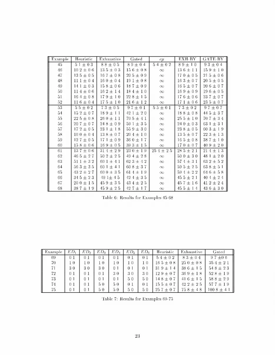
Example Heuristic Exhaustive Gated c� EXH-BY GATE-BY45 5.1 � 0.3 8.8 � 0.5 8.9 � 0.4 5.4 � 0.2 8.9 � 1.0 9.3 � 0.446 10.2 � 0.6 13.5 � 0.3 15.6 � 0.8 1 13.6 � 1.1 15.9 � 1.047 13.5 � 0.5 16.7 � 0.8 20.5 � 0.9 1 17.0 � 0.5 21.5 � 0.648 11.1 � 0.4 16.0 � 0.4 19.1 � 0.8 1 16.3 � 0.7 20.5 � 0.549 14.1 � 0.3 15.8 � 0.6 18.7 � 0.9 1 16.5 � 0.7 20.6 � 0.750 11.4 � 0.6 16.2 � 1.4 18.4 � 1.0 1 16.9 � 0.9 19.6 � 0.551 16.4 � 0.8 17.9 � 1.0 22.8 � 1.5 1 17.6 � 0.6 23.7 � 0.752 11.6 � 0.4 17.5 � 1.0 21.6 � 1.2 1 17.1 � 0.6 23.5 � 0.753 5.5 � 0.2 7.3 � 0.5 9.7 � 0.1 5.5 � 0.1 7.3 � 0.2 9.7 � 0.754 15.2 � 0.7 18.9 � 1.1 42.1 � 2.0 1 18.8 � 0.8 44.5 � 3.755 22.5 � 0.8 26.0 � 1.1 70.5 � 4.1 1 25.5 � 1.0 70.7 � 3.456 20.7 � 0.7 24.8 � 0.9 59.1 � 3.5 1 24.0 � 0.3 63.1 � 3.157 17.2 � 0.5 23.1 � 1.8 55.9 � 3.0 1 23.8 � 0.5 60.3 � 1.958 10.0 � 0.4 13.8 � 0.7 20.4 � 1.0 1 13.5 � 0.7 22.3 � 1.359 12.7 � 0.5 17.1 � 0.9 36.0 � 1.7 1 16.5 � 0.8 38.7 � 1.060 15.8 � 0.6 16.9 � 0.5 39.3 � 1.5 1 17.0 � 0.7 40.9 � 2.061 13.7 � 0.6 31.4 � 2.9 23.0 � 1.9 25.4 � 2.5 28.5 � 2.1 21.4 � 1.362 46.5 � 2.7 50.2 � 2.5 49.4 � 2.8 1 50.0 � 3.0 48.1 � 2.063 51.1 � 3.2 60.1 � 4.1 62.3 � 4.2 1 57.4 � 3.1 63.2 � 5.264 56.3 � 3.5 60.1 � 4.1 60.8 � 3.7 1 59.5 � 2.5 63.8 � 5.165 43.2 � 2.7 60.0 � 3.5 61.4 � 1.9 1 59.4 � 2.2 64.6 � 5.866 34.5 � 2.3 49.1� 4.5 42.4 � 3.5 1 45.5 � 2.1 40.4 � 2.467 20.0 � 1.5 45.9 � 3.5 43.4 � 2.5 1 45.7 � 1.6 41.2 � 2.468 38.7 � 1.9 45.9 � 2.5 42.7 � 1.7 1 45.5 � 1.4 43.6 � 3.0Table 6: Results for Examples 45-68Example ED1 ED2 ED3 ED4 ED5 ED6 Heuristic Exhaustive Gated69 0.1 0.1 0.1 0.1 0.1 0.1 5.4 � 0.2 8.3 � 0.4 9.7 �0.670 1.0 1.0 1.0 1.0 1.0 1.0 16.5 � 0.8 25.0 � 0.8 35.4 � 2.171 3.0 3.0 3.0 0.1 0.1 0.1 31.9 � 1.4 38.6 � 1.5 54.8 � 2.372 0.1 0.1 0.1 3.0 3.0 3.0 12.9 � 0.7 36.9 � 1.8 52.8 � 1.973 0.1 0.1 0.1 0.1 5.0 5.0 14.8 � 0.7 41.6 � 1.5 58.8 � 2.974 0.1 0.1 5.0 5.0 0.1 0.1 15.5 � 0.7 42.2 � 2.5 57.7 � 1.975 0.1 0.1 5.0 5.0 5.0 5.0 25.7 � 0.7 75.8 � 4.8 100.8 � 4.1Table 7: Results for Examples 69-7523

costs for the queues are respectively 5, 2, 0.5, 0.4, 0.3, 0.2. The processing rate is 1 for all thequeues, while the arrival rates equal 0.2 for queues 1 and 2 and 0.1 for all other queues. The meanset-up times for each queue as well as the average holding cost per unit time obtained under eachpolicy is displayed in Table 7. The results in Table 7 are representative of the performance of theheuristic as the number of queues increases. We found that as the number of queues increases, thedi�erence in the performance of our heuristic and the exhaustive and gated policies increased dueto the server's having more opportunities to switch to queues with higher reward rates.6. Conclusions and Further ResearchUsing notions of reward rate, we have partially characterized an optimal policy for the schedulingof parallel queues with set-up times. We used this insight to develop a heuristic policy. Oursimulation study indicates that, in the case of two queues, the heuristic performs nearly as wellas computationally expensive search-based rules. In the case of problems with more than twoqueues, our study suggests that the heuristic substantially outperforms other widely used policiesthat have been analyzed in the literature. Moreover, the simplicity of the algorithm enhances itsattractiveness.Further research is necessary to develop a more complete characterization of the optimal policy.This would aid in developing new and possibly more e�ective heuristics. This is doubtless a verychallenging problem, however, since even in the case of controlling two queues with set-up costs,the optimal policy has not yet been completely characterized. Further research should also addresssystems in which a job has to be processed by more than one server and follows a general routethrough the system. Such a system without set-up costs has recently been addressed by Wein andChevalier [37].Acknowledgments:The work of the �rst author was partially supported by NSF Grant No. DDM-9308290, andthat of the second author by Northwestern University Grant 510-24XJ. The authors would like tothank Professors Demosthenis Teneketzis, Rajeev Agrawal, and Awi Federgruen, as well as twoanonymous reviewers for many helpful comments that have improved the content and clarity of24

this paper.Appendix: Proof of Theorem 1:We �rst state a purely technical lemma which we will use in the proof of the theorem. Theproof of Lemma 1 is straightforward and we omit it.Lemma 1: Consider a single stage optimization problem with a �nite set of control actions, U.Action u 2 U results in an expected discounted reward �ru 2 IR and requires an expected discountedlength of time ��u 2 (0;1). Let pu 2 [0; 1] denote the probability that action u is taken wherePu pu = 1. Then, the single-stage reward rate is at most maxu2U �ru=��u; equivalently,(Xu2U pu�ru)=(Xu2U pu��u) � maxu2U �ru=��u: (A.1)Proof of Theorem 1 for the Discounted Cost Case: Without loss of generality, suppose h1maximizes hn over n. Suppose policy g is optimal but does not serve node one as a top prioritynode. We �rst prove that because jobs of type one o�er the greatest single stage reward rate, anoptimal policy must serve node one exhaustively. We then justify greedy service in node one. Forthe sake of presentation, we initially assume g to be non-randomized and stationary, and we removethis restriction later.Suppose that policy g does not exhaust node one. Thus, for some state (x1; : : : ; xN ; 1; 1) 2 Swith x1 � 1, policy g chooses to switch to node j. We assume, without loss of generality, that gchooses to switch to node j at t = 0; thus Ug(0) = (j; 2) for some j 6= 1. For l 2 IN, let t(l) denotethe time at which the lth control action is taken under policy g. Thus, t(1) = 0, and t(2) = Dj .With respect to policy g, let the random variable L 2 fIN [1g denote the stage, or index of thedecision epoch, at which g �rst chooses to serve a job of node one. Thus, Ug(t(L � 1)) = (1; 2),and Ug(t(L)) = (1; 1). If g never serves a job in node one with probability p0, then L takes onthe value 1 with probability p0. Let the random variable g(l) taking values in f1; 2; : : : ; N + 1gdenote the job, if any, served during stage l, where g(l) = N+1 with the probability that the server25

idled in or set up any queue during stage l. Thus, g(1) = N + 1 and g(2) = j. Let the randomvariable r(g(l)) denote the single stage reward associated with stage l and control selection g(l),where by (3.2), r(g(l)) = cg(l)��1e��fg(l);1 for g(l) � N and r(g(l)) = 0 for the aggregated stateg(l) = N + 1. De�ne �(g(l)) = t(l+ 1)� t(l). For g(l) � N; �(g(l)) = fg(l);1.In accordance with (3.2), we de�ne R�(gL�1) to be the total expected discounted reward earnedunder policy g from stages 1; 2; : : : ; L� 1 during [0; t(L)). Along each sample path of the system,we construct a policy ~g, which interchanges the service of the job in queue one (stage L under g)with the �rst L� 1 stages under g as follows. At time t = 0, ~g serves the job in node one that isserved under policy g at t(L), which possesses the processing time f1;1. During [f1;1; f1;1+ t(L)), ~gmimics the actions taken by g during [0; t(L)), the �rst L�1 stages. At time t(L+1) = t(L)+f1;1,both g and ~g reach the same state along any realization, and ~g mimics g from that point on. Notethat the construction of ~g is feasible, and that the average single-stage reward earned by serving asingle job of node one is given byEfe��f1;1gc1��1 = h1��1(1� S1) = h1EfZ f1;10 e��tdtg : (A.2)Thus, the di�erence in expected discounted reward of policy ~g with respect to g results from the�rst L stages and can be computed from (3.2) and (A.2) asR�(~g)� R�(g)= Efe��f1;1 [c1��1 + R�(gL�1)]g � [R�(gL�1) +Efe��t(L)c1��1e��f1;1g]= [h1��1(1� S1) + S1R�(gL�1)]� [R�(gL�1) +Efe��t(L)gh1��1(1� S1)]= ��1(1� S1)(1�Efe��t(L)g)[h1 �R�(gL�1)=(��1(1�Efe��t(L)g))] : (A.3)Let H(l) be de�ned as the information history vector that records current and past states anddecision epochs: fX(t(i)); t(i) : i = 0; 1; : : : ; lg. Since r(g(1)) = 0, we see thatR�(gL�1) = EfL�1Xl=2 e��t(l)r(g(l))g= 1Xl=2Ef11fL > lge��t(l)Efr(g(l)) j H(l); L > lg g : (A.4)26

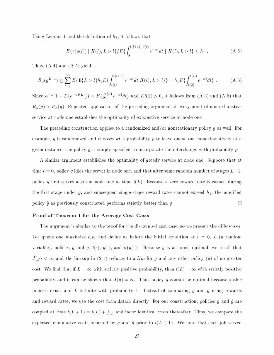
Using Lemma 1 and the de�nition of h1, it follows thatEfr(g(l)) j H(l); L > lg=EfZ t(l+1)�t(l)0 e��tdt j H(l); L > lg � h1 : (A.5)Thus, (A.4) and (A.5) yieldR�(gL�1) � 1Xl=2Ef11fL > lgh1EfZ t(l+1)t(l) e��tdtjH(l); L > lgg = h1EfZ t(L)t(2) e��tdtg : (A.6)Since ��1(1� Efe��t(L)g) = EfR t(L)0 e��tdtg and Et(2) > 0, it follows from (A.3) and (A.6) thatR�(~g) > R�(g). Repeated application of the preceding argument at every point of non-exhaustiveservice at node one establishes the optimality of exhaustive service at node one.The preceding construction applies to a randomized and/or nonstationary policy g as well. Forexample, g is randomized and chooses with probability p to leave queue one nonexhaustively at agiven instance, the policy ~g is simply speci�ed to incorporate the interchange with probability p.A similar argument establishes the optimality of greedy service at node one. Suppose that attime t = 0, policy g idles the server in node one, and that after some random number of stages L�1,policy g �rst serves a job in node one at time t(L). Because a zero reward rate is earned duringthe �rst stage under g, and subsequent single-stage reward rates cannot exceed h1, the modi�edpolicy ~g as previously constructed performs strictly better than g. 2Proof of Theorem 1 for the Average Cost Case:The argument is similar to the proof for the discounted cost case, so we present the di�erences.Let queue one maximize ci�i and de�ne as before the initial condition at t = 0, L (a randomvariable), policies g and ~g, t(�), g(�), and �(g(�)). Because g is assumed optimal, we recall that�J(g) < 1 and the lim sup in (2.1) reduces to a lim for g and any other policy (~g) of no greatercost. We �nd that if L =1 with strictly positive probability, then t(L) =1 with strictly positiveprobability and it can be shown that �J(g) = 1. Thus policy g cannot be optimal because stablepolicies exist, and L is �nite with probability 1. Instead of comparing g and ~g using rewardsand reward rates, we use the cost formulation directly. For our construction, policies g and ~g arecoupled at time t(L+ 1) = t(L) + f1;1 and incur identical costs thereafter. Thus, we compare theexpected cumulative costs incurred by g and ~g prior to t(L + 1). We note that each job served27

during (t(2); t(L)] under g is delayed by f1;1 time units under ~g, which represents an increased costfor ~g. On the other hand,the �rst job in queue 1 is completed at time f1;1 under ~g and at t(L)+f1;1under g, a cost savings of c1t(L) for ~g.To compare the di�erence between g and ~g, we de�ne the costs associated with the stages1; 2; : : : ; L prior to the coupling of g and ~g. Let the holding cost of the stage l action be denotedby C(g(l)), where C(g(l)) = cg(l) for g(l) � N and C(N + 1) = 0. Because C(N + 1) = 0, for ourpurposes, it su�ces to note that for the aggregated state N + 1; �(N + 1) has a �nite mean. Wenote that g(1) = N + 1. From time t(L+ 1) onwards, ~g has an expected cumulative (not averagecost per unit time) cost advantage over policy g, which we denote as Z(g; ~g). Thus,Z(g; ~g) = EfZ 10 NXn=1 cn �Xgn(t)�X~gn(t)�dtg (A.7)= Efc1t(L)� L�1Xl=1 C(g(l))f1;1g (A.8)= 1Xl=2Ef11fL > lg(c1�(g(l))� C(g(l))f1;1)g+ c1EfDjg (A.9)> 1Xl=2Ef11fL > lg(c1Ef�(g(l))jH(l); L > lg � EfC(g(l))jH(l); L > lgEff1;1g)g ; (A.10)where we have used the fact that f1;1 is independent of all else. To conclude that Z(g; ~g) 2 (0;1],it su�ces to show that for l 2 f2; 3; : : : ; L� 1g,EfC(g(l))jH(l); L > lg=Ef�(g(l))jH(l); L > lg � c1=Eff1;1g = c1�1 : (A.11)This follows from Lemma 1. There exists a perturbation of g that serves a single additional jobof queue one at the �rst instance of non-exhaustion and results in an expected cumulative costsavings in (0;1]. If, following the job of queue one inserted at time t(1) = 0, additional jobsremain in queue 1, apply the argument thus far iteratively until the resulting perturbation of g,say g0, exhaustively serves queue 1 during the visit at t(1). Thus, Z(g; g0) 2 (0;1].To conclude, we build on this result to show that a top-priority policy exists which performs atleast as well as g with respect to average cost per unit time. Consider a policy g00 with a countablenumber of stages. The nth stage removes the nth instance of non-exhaustion of queue 1. Thesequencing of jobs not in queue 1 is una�ected. Note that our construction implies Z(g; g00) 2 (0;1]28

and since �J(g) 2 (0;1), it follows that �J(g00) 2 (0;1). There exists a policy that always exhaustsqueue one and performs at least as well as any other policy in G.The proof of the greedy property follows using the argument made in the discounted case, nowextended as above to the average cost case. 2Bibliography[1] Altman, E., Konstantopoulos, P., and Liu, Z. (1992) Stability, monotonicity and invariant quantities ingeneral polling systems, Queueing Systems 11, 35{57.[2] Baker, J.E. and Rubin, I. (1987) Polling with a general-service order table, IEEE Trans. Comm.COM-35, 283{288.[3] Baras, J.S., Ma, D.J., and Makowski, A.M. (1985) K competing queues with geometric service require-ments and linear costs: the �c rule is always optimal, Systems Control Letters, 6, 173-180.[4] Bell, C. (1971) Characterization and computation of optimal policies for operating anM=G=1 queueingsystem with removable server, Operations Research 19, 208{218.[5] Browne, S. and Yechiali U. (1989) Dynamic priority rules for cyclic-type queues, Advances in AppliedProbability, 21, 432-450.[6] Buyukkoc, C., Varaiya, P., andWalrand J. (1985) The c�-rule revisited, Advances in Applied Probability,17, 237-238.[7] Conway, R.W.,Maxwell, W.L., and Miller, L.W. (1967)Theory of Scheduling, Addison-Wesley, Reading,MA.[8] Cox, D.R. and Smith, W.L. (1960) Queues, Methuen, London.[9] Dempster, M.A.H., Lenstra, J.K., and Rinnooy Kan A.M.G. (1982) Deterministic and StochasticScheduling, D. Reidel, Dordrecht.[10] Federgruen, A. and Z. Katalan (1993a) \The stochastic economic lot scheduling problem: Cyclical base-stock policies with idle times," Working paper, Graduate School of Business, Columbia University, NewYork, NY.[11] Federgruen, A. and Z. Katalan (1993b) \The impact of setup times on the performance of multi-classservice and production systems," Working paper, Graduate School of Business, Columbia University,New York, NY.[12] Georgiadis, L. and Szpankowski, W. (1992) Stability of Token Passing Rings, Queueing Systems, 11,7{34.[13] Gittins, J.C., (1989) Multi-armed Bandit Allocation Indices, Wiley, New York.[14] Gupta, D., Gerchak, Y., and Buzacott J.A. (1987) On optimal priority rules for queues with switchovercosts, Preprint, Department of Management Sciences, University of Waterloo.[15] Harrison, J.M. (1975a) A priority queue with discounted linear costs, Operations Research 23, 260{269.[16] Harrison, J.M. (1975b) Dynamic Scheduling of a Multiclass Queue: Discount Optimality, OperationsResearch 23, 270{282.[17] Hofri, M. and Ross, K.W. (1987) On the optimal control of two queues with server set-up times and itsanalysis, SIAM Journal of Computing, 16, 399-420.29

[18] Klimov, G.P. (1974) Time sharing service systems I, Theory of Probability and Its Applications, 19,532-551.[19] Klimov, G.P. (1978) Time sharing service systems II, Theory of Probability and Its Applications 23,314-321.[20] Kuehn,P.J. (1979) Multiqueue systems with nonexhaustive cyclic service, Bell Syst. Tech. J. 58, 671-698.[21] Lai, T.L., and Ying, Z. (1988) Open bandit processes and optimal scheduling of queueing networks,Advances in Applied Probability, 20, 447-472.[22] Levy, H. and Sidi, M. (1990) Polling systems: applications, modelling, and optimization, IEEETrans. Commun. 38, 1750{1760.[23] Levy, H., Sidi, M., and Boxma, O.J. (1990) Dominance relations in polling systems, Queueing Systems6, 155-172.[24] Liu, Z., Nain, P., and Towsley, D. (1992) On optimal polling policies, Queueing Systems (QUESTA)11, 59{84.[25] Nain, P. (1989) Interchange arguments for classical scheduling problems in queues, Systems ControlLetters, 12, 177-184.[26] Nain, P., Tsoucas, P., and Walrand, J. (1989) Interchange arguments in stochastic scheduling, Journalof Applied Probability 27, 815-826.[27] Rajan, R. and Agrawal, R. (1991) Optimal server allocation in homogeneous queueing systems withswitching costs, preprint, Electrical and Computer Engineering, Univ. of Wisconsin-Madison, Madison,WI 53706.[28] Santos, C. and Magazine, M. (1985) Batching in single operation manufacturing systems, OperationsRes. Letters 4, 99{103.[29] Srinivasan, M.M. (1991) Nondeterministic Polling Systems, Management Science 37 667.[30] Takagi, H. (1990) Priority queues with set-up times, Operations Research 38, 667{677.[31] Van Oyen, M.P. (1992) Optimal Stochastic Scheduling of Queueing Networks: Switching Costs andPartial Information, Ph.D. Thesis, University of Michigan.[32] Van Oyen, M.P., Pandelis, D.G., and Teneketzis, D. (1992) Optimality of index policies for stochasticscheduling with switching penalties, J. of Appl. Prob., 29, 957{966.[33] Van Oyen, M.P. and Teneketzis, D. (1994) Optimal Stochastic Scheduling of Forest Networks withSwitching Penalties, Adv. Appl. Prob., 26, 474-497.[34] Varaiya, P., Walrand, J., and Buyukkoc C. (1985) Extensions of the multi-armed bandit problem, IEEETransactions on Automatic Control, AC-30, 426-439.[35] Walrand, J. (1988) An Introduction to Queueing Networks, Prentice Hall, Englewood Cli�s.[36] Wein, L.M. (1991) Due date setting and priority sequencing in a multiclass M/G/1 queue, ManagementScience 37, 834-850.[37] Wein, L.M., and Chevalier P. (1992) A broader view of the job shop scheduling problem, ManagementScience 38, 1018-1033.30