387

Hierarchical Linear Modeling ofMultilevel Data

Samuel Y. ToddGeorgia Southern University

T. Russell CrookNorthern Arizona University

Anthony G. BarillaGeorgia Southern University

Most data involving organizations are hierarchical in nature and often contain variables measured at multiple levels of analysis. Hierarchical linear modeling (HLM) is a relatively new and innovative statistical method that organizational scientists have used to alleviate some common problems associated with multilevel data, thus advancing our understanding of organizations. This article presents a broad overview of HLM’s logic through an empirical analysis and outlines how its use can strengthen sport management research. For illustration purposes, we use both HLM and the traditional linear regression model to analyze how orga-nizational and individual factors in Major League Baseball impact individual players’ salaries. A key implication is that, depending on the method, parameter estimates differ because of the multilevel data structure and, thus, findings differ. We explain these differences and conclude by presenting theoretical discussions from strategic management and consumer behavior to provide a potential research agenda for sport management scholars.

Organizational science necessarily involves hierarchically ordered entities. In general, most organizations are composed of individuals who belong to a spe-cific work group or department in a particular division subsisting under the larger umbrella of the organization. Each of these entities, then, is “nested” within a group, and members of each group (e.g., marketing employees) share certain indubitable similarities that might not be shared among other groups (e.g., finance employees). Likewise, in the larger global economic environment, consumers are nested within specific firms, which are nested within industries. Based on this rubric, a sample of

Journal of Sport Management, 2005, 19, 387-403© Human Kinetics, Inc.

Todd is with Georgia Southern University, Department of Sport Management, P.O. Box 8077, Statesboro, GA. Crook is with Northern Arizona University, Department of Management, College of Business Administration, Flagstaff, AZ. Barilla is with Georgia Southern University, School of Economic Development, P.O. Box 8152, Statesboro, GA.

388 Todd, Crook, and Barilla Hierarchical Linear Modeling 389

consumers might share unique similarities depending on the group to which they belong. Wal-Mart and Target customers, for example, are likely more similar to each other than to customers who shop at Macy’s or Bloomingdale’s. Thus, cus-tomers in each group might share some unique similarities. In each of these cases, the data contain variables measured at different levels of analysis, which presents the analyst with a formidable methodological challenge.

Until recently, researchers lacked the requisite tools to analyze multilevel data properly. Instead, researchers relied on methodological tools such as traditional linear regression that are often incapable of capturing potentially meaningful relationships in multilevel data. In a study investigating the moderating effect of leadership climate between task significance and perceived hostility, for example, Bliese, Halverson, and Schriesheim (2002) reported that a single-level, cross-sectional analysis of 2,042 U.S. Army soldiers failed to uncover any meaningful relationships. When analyzed as individuals nested within units (e.g., groups), however, significant group-level moderating effects of leadership climate emerged. In other words, group-level variables such as unit leadership moderated the rela-tionship among individual-level outcomes, thus indicating a cross-level interaction. Because of the possibility that group effects such as these might be overlooked in a single-level linear model analysis, several prominent scholars have suggested that many research methods fail to detect some important relationships and noteworthy phenomena in the data (e.g., Bettis, 1991; Daft, 1985; Goldstein, 1995; Rouse & Daellenbach, 1999).

In the broader social and organizational sciences, critics have been wary of analyzing data containing multilevel data structures because of parameter mises-timation, data aggregation, and clustering problems that can arise using traditional linear regression methods, hereafter called regression (e.g., Hoffman, 1997; Klein, Dansereau, & Foti, 1994; Mossholder & Bedeian, 1983; Rousseau, 1985). First, parameter misestimation results from violations of the independence assumption, leading to inaccurate standard errors (Klein & Kozlowski, 2000; Raudenbush & Bryk, 2002). In short, observations within each group often possess similarities and, thus, are dependent, not independent, upon other group scores. When stan-dard error estimates are inaccurate, one runs a higher risk of committing a Type I error. Second, data aggregation occurs when data are combined from one level to represent higher-level variables (Rousseau, 1985). Aggregated lower-level vari-ables, however, might not be representative of group-level constructs, leading to misinterpretations (Goldstein, 1995). Third, when the data are inherently clustered in nature, the relationships between individual characteristics and outcomes might vary across organizations, and the causes of this variance might be of substantive interest (Goldstein; Raudenbush & Bryk, 2002).

Hierarchical linear modeling (HLM) is a multilevel data analysis method that can resolve these problems through the use of interdependent regression equations estimated simultaneously (Raudenbush & Bryk, 2002). With HLM, the ambiguity arising from hierarchical and some longitudinal effects, as well as the problems associated with multilevel data, dissipate.1 The use of HLM can help clarify the effects among variables measured at different levels, and relationships that might have previously gone undetected can be identified. Given that the purpose of this special issue is epistemological progress regarding methodological advances, that data are often hierarchically structured, and that the use of regression might fail

388 Todd, Crook, and Barilla Hierarchical Linear Modeling 389

to detect important relationships of interest, an overview of the HLM method and an illustration of its utility in sport management seem both timely and warranted. Thus, our paper’s overarching objective is to provide a broad overview of HLM and show how its use can more accurately uncover meaningful relationships in hierarchical, or multilevel, data.

Our article proceeds as follows. First, we investigate the impact of individual- and organizational-level variables on professional baseball players’ salaries, and in the process, we introduce the HLM method. Second, we compare the results of an HLM analysis with a regression analysis on the same data to demonstrate how HLM can more accurately illuminate multilevel effects in hierarchical data beyond regression. Finally, we conclude by suggesting several direct areas of application for the HLM method to sport management research.

Background to the StudyIn labor economics, pay is often characterized as either piece-wise compensa-

tion or time-duration compensation (Frank & Bernanke, 2004). Piece-wise com-pensation is determined by measurable output levels (e.g., $1 per widget) whereas time-durational compensation is payment by the hour, month, or year (Borjas, 1999). In either case, conventional wisdom holds that the more productive a worker is, the higher his or her compensation. Although Scully (1974) first examined how athletic performance in professional sports relates to player compensation, more recent research uses compensation as a dependent variable for a variety of research purposes. For example, some scholars use the pay–performance link to analyze discriminatory compensation practices across teams or leagues (e.g., Bodvarsson & Pettman, 2002; Scully, 2004), whereas others use salary data to detail the effect of player arbitration status on negotiated salary (e.g., Marburger, 2004; Marburger & Scoggins, 1996). Our study examines how individual performance, or piecework, and experience relate to player compensation and analyzes how the group-level variables of team, league, and talent impact these relationships in Major League Baseball (MLB).

As a result of the detailed statistics available, MLB provides a reliable con-text for our study. As noted earlier, performance is a key underlying determinant of compensation, but for professional baseball it is only one part of the equation. Paraphrasing George Steinbrenner, the owner of the New York Yankees, a player’s worth depends not only on his contribution to the team but also on his ability to attract fans to the ballpark (CBS Sportsline). Indeed, Hausman and Leonard (1997) discovered the presence of all-stars to be a significant determinant of television ratings in the National Basketball Association (NBA) after controlling for team quality. A player’s salary must therefore reflect his fan appeal and his performance; all-star appearances capture both of those attributes. We used a player’s total number of all-star appearances as a proxy to represent piece-wise, or performance, and the player’s number of years of experience as a proxy to represent the time duration element.

In addition, we intend here to highlight the added value of a multilevel analyti-cal procedure to the study of hierarchical data. Thus, we set out to investigate these relationships and demonstrate the utility of the HLM method. By incorporating both performance and time measures concurrently and analyzing multilevel effects, we

390 Todd, Crook, and Barilla Hierarchical Linear Modeling 391

examine research questions that formerly presented researchers with a methodological challenge. Because of advances in multilevel data analysis techniques, however, and in particular, the advent of HLM, we can now answer these questions. Therefore, we investigate (a) what types of team characteristics explain variance in average player salaries among teams and (b) what types of team characteristics explain variance in the effects that individual performance and time measures have on player salaries among teams (cross-level interactions or moderators of slopes). We propose the fol-lowing research questions and subsequently define each variable.

RQ1: Do teams vary in mean player salaries (SAL)? If so, by how much?

RQ2: (a) Is the strength of association between player experience (EXP) and SAL (i.e., the slope) similar across all teams? Or, is EXP a more important predictor of SAL in some teams than others?

(b) Is the strength of association between player performance (PERF) and SAL similar across all teams?

RQ3: Are there any team-level explanations for mean salary differences among teams?

RQ4: (a) Does talent moderate the relationship between EXP and SAL?

(b) Does the league to which a team belongs moderate the relationship between PERF and SAL?

METHODS

Sample

In order to demonstrate HLM’s logic, we collected data on 471 players nested within 30 MLB teams over the 2000 season using Thorn, Palmer, and Gershman’s (2001) Total Baseball and reports from Doug Pappas, Chairman of the Society for American Baseball Research Business of Baseball Committee (Pappas, 2000). Because major league pitchers use a different productivity measure, our sample is restricted to nonpitchers with at least 1 year of major-league experience.

Measures

Team-level variables included league and talent. MLB teams are divided into two leagues: the American League has 14 teams and the National League has 16. Mean team-total player ratings for each team were used as a proxy for talent. Player-level data included player performance, measured by total all-star appearances, and experience, a time variable estimated by years of experience. We used HLM 5 (Raudenbush, Bryk, Cheong, & Congdon, 2001) to estimate the model, although several statistical computing programs are available for multilevel research (e.g., MIXOR: Hedeker & Gibbons, 1996; ML3: Prosser, Rasbash, & Goldstein, 1991; SAS Proc Mixed: Littell, Milliken, Stroup, & Wolfinger, 1996; Splus: Everitt, 2005; VARCL: Longford, 1991).

390 Todd, Crook, and Barilla Hierarchical Linear Modeling 391

RESULTS

Analysis via Hierarchical Linear Models

One key advantage of HLM is that it allows researchers to separate variance into within- and between-level variance while assessing a unique moderating impact, such as cross-level interactions of variables, at different levels (Raudenbush & Bryk, 2002). Indeed, with HLM researchers can model the variance within a particular level and then use higher level constructs to model the variance among different groups or levels. In the present study, the outcome of interest is player salary and the Level-1 independent variables are the players’ experience and performance.

In a similar style to a typical regression equation, the initial model for this design is in the form of the general linear model:

SALij = β

0j + β

1jEXP

ij + β

2jPERF

ij + r

ij

where SALij is the outcome of interest (salary in this case) for player i on team j,

β0j is the intercept estimated for each team, β

1j is the expected changed in salary

with a one-unit increase in EXPij, years of experience; β2j is the expected change in

salary with a one-unit change in PERFij, player performance; and rij is the residual.

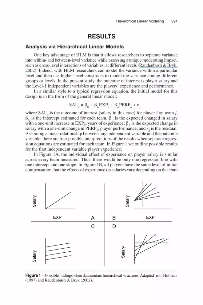
Assuming a linear relationship between any independent variable and the outcome variable, there are four possible interpretations of the results when separate regres-sion equations are estimated for each team. In Figure 1 we outline possible results for the first independent variable player experience.

In Figure 1A, the individual effect of experience on player salary is similar across every team measured. Thus, there would be only one regression line with one intercept and one slope. In Figure 1B, all players have the same level of initial compensation, but the effects of experience on salaries vary depending on the team

Salary

A B

D

EXP

EXP

EXP

EXP

Salary

Salary

Salary

C

Figure 1—Possible findings when data contain hierarchical structures. Adapted from Hofman(1997) and Raudenbush & Bryk (2002).

392 Todd, Crook, and Barilla Hierarchical Linear Modeling 393

(or group). In this case, the analyst might be interested in the team-level variables that cause the differential slopes. For instance, it could be that certain teams value experienced players more than others, and thus, the association between experience and pay is stronger in particular situations. In this case, team-level variables might explain variations in the slope between experience and salary. In Figure 1C, the effect of experience (slope) on salary is similar across all teams; average player salaries between teams, however, vary (intercepts). In this case, the intercepts appear to be a function of some team characteristic and the cause of the variance is of immedi-ate interest. Thus, the analyst might attempt to uncover the team characteristics that potentially explain these differences. In Figure 1D, both the intercepts and the slopes differ, suggesting that teams differ in both the average salary and the average effect of experience on salary.

In three of the four aforementioned cases, organizational-level characteristics might explain variance among teams. The second-level HLM equations are designed to shed light on such issues. A typical Level-2 model takes the following form:

β0j = γ

00 + γ

01W

j + u

0j

β1j = γ

10 + γ

11W

j + u

1j

β2j = γ

20 + γ

21W

j + u

2j

where each of the Level-1 point estimates is modeled in separate Level-2 equations by Level-2 independent variables. β

0j is the intercept from the Level-1 equation,

whereas β1j and β

2j are the slopes. W

j is the organizational variable (could be league

or talent) that potentially explains differences in each intercept and slope. The Level-2 intercepts are γ

00, γ

10, and γ

20,whereas the Level-2 slopes are γ

01, γ

11, and γ

21,

respectively. The u0j, u

1j, and u

2j are the level-two residuals, or unique effects of

each team upon the outcome of interest. Because β0j, β

1j, and β

2j are parameter

estimates, and not observed in the data, we substitute the Level-2 model into the Level-1 model, yielding the following mixed model:

Y = γ00

+ γ01

Wj + γ

10 (X

ij) + γ

11W

j(X

ij) + u

0j + u

1j(X

ij) +

γ20

(Xij) + γ

21W

j(X

ij) + u

1j + u

2j(X

ij) + r

ij

There are two key differences between the equations used in regression models and HLM. First, the error term in HLM is more complex and thus allows for a more accurate estimate of cross-level interactions. Under traditional linear regression assumptions, random error terms are normally and independently distributed and have constant variance (Cohen & Cohen, 1983). In contrast, the random error in the previous equation, u

0j + u

1j + u

1j(X

ij) + u

2j(X

ij) + r

ij, is more complex (Goldstein, 1995).

HLM error terms are not independent within each group because the terms u0j, u

1j, and

u

2j are shared by every individual within the group j. Furthermore, this complex error

term captures unique effects across both levels and can accurately estimate cross-level interactions, for example, γ

11W

j(X

ij). Second, the errors have unequal variances

because u0j + u

1j (X

ij) depend on u

0j and u

1j, which vary across groups (or teams), as

well as on the value of (Xij), which varies across individuals.

To demonstrate the effects of variables measured at different levels, we restricted our attention to three individual-level variables and two team-level variables.

392 Todd, Crook, and Barilla Hierarchical Linear Modeling 393

Individual-level variables include: (a) the outcome, Yij, which is a measure of player

salary (SAL); (b) the first predictor, (EXP)ij; and (c) the second predictor, (PERF)

ij.

Team-level outcomes assessed include (LEAGUE)j, which takes on a value of

zero for American League teams and one for National League teams, and (TALENT)j,

the accumulated talent on each team.When testing hierarchical relationships with HLM, there is a progression of

steps that must be followed.2 In the present study, our primary concern is: What types of individual and team characteristics explain variance in average player salaries (i.e., the intercepts and the slopes from Figure 1)? The next sections outline the typical sequence of steps that allow the testing of each research question.

Research Question 1

In the current study, we are ultimately interested in RQ3 and RQ4, or explain-ing variation in the intercepts and slopes of the Level-1 model. In order to test RQ3 and RQ4, however, we must first draw inferences from RQ1 and RQ2. In other words, to discover the extent to which certain team-level variables, such as league or talent, explain the variance in average player salaries, we must first determine whether significant differences exist in the intercepts and slopes for players’ salaries. Thus, the first step is to assess whether mean differences exist in player salaries among teams.

The one-way ANOVA model with random effects provides the necessary infor-mation regarding whether variation in player salaries exists among teams. The test of this model yields the average team mean of player salaries, as well as a variance component of the team-level random error term, u

0j. A preliminary analysis sug-

gested that salary was not normally distributed; therefore, we used a logarithmictransformation to create an acceptable alternative after the standard practice recom-mended in Hair, Anderson, Tatham, and Black (1998) and demonstrated in Combs and Ketchen (1999). The overall unconditional mean, γ

00, was estimated to be .038

(p > .05) and the variance component, or β00

, was .016 (p < .01). Thus, with respect to R

1, we conclude that there is significant variation among teams in average player

salaries. Additionally, the HLM procedure allows for computation of an intraclass correlation, which represents the proportion of variance in the outcome among teams, or second-level units (Raudenbush & Byrk, 2002). The intraclass correlation was .047, suggesting that 5% of the variation in mean player salaries was among teams. Next, we attempt to model this variation among teams.

Research Question 2

Next in the order of progressive steps toward the ultimate research questions (RQ3 and RQ4), we must determine whether significant variation exists among teams in the slopes of: (a) experience and salary, and (b) performance and salary. In order to determine explanations of potential variation, ostensibly the slopes must vary. The analyst uses the random coefficient model to make this assessment (Longford, 1993). First, the analyst might estimate the amount of explained vari-ance in the Level-1 outcome as a result of the additions of the Level-1 predictors as an auxiliary statistic. Because the first model estimated was the random effects ANOVA model, a comparison of the results between the ANOVA model and the

394 Todd, Crook, and Barilla Hierarchical Linear Modeling 395

random coefficient model yields the reduction in variance of the outcome. The results of this analysis suggested that 41% of the variance in player salaries across teams could be explained by the predictors of experience and performance.

Next, the analyst tests the variance in the random error terms of both slopes: Var(u

1j)

= τ

10;Var(u

2j) = τ

20). If the critical values of the chi-square statistic are

significant at the set alpha level, the analyst concludes that there is statistically significant variation among teams in the strength of association between: (a) experience and salary and (b) performance and salary. If differences among teams exist, variance must be decomposed to discover what team-level variables explain the variance. In other words, upon finding a statistically significant amount of variance in the outcome, the analyst would then attempt to explain this variance with additional predictors. In the current study, γ

10 is estimated to be .06 (p < .001)

and γ20

is estimated to be .11 (p < .001). The variance components of each of the three outcomes in the Level-2 model, β

0j, β

1j, and β

2j, were calculated to determine

whether significant variation in each existed. The variance of the experience slope was .00051 (p < .01) and the variance of the performance slope was .005 (p < .001). Thus, there is significant variation among teams in the experience and performance slopes. Given the variation among teams in both intercepts and slopes, we shall attempt to explain the differences with team-level variables.

Research Questions 3 & 4

The final model allows the researcher to address RQ3 and RQ4. Because there is significant variation among teams in both mean player salaries and the effects of both experience and performance on player salaries, these differences can now be modeled. The Level-1 model remains the same; the Level-2 model, however, is expanded to include team-level predictors of the intercept and slope differences.

Our final results are presented in Table 1. Talent was identified as an important predictor of the variance among teams in average player salaries (γ

01, β = .0006, t =

11.78, p < .001). Talent also appeared to be a good explanation of the differences among teams in the slopes of experience and salary (γ

11, β = –.00007, t = –9.74, p

< .001). Thus, talent is a cross-level moderator of the relationship between experi-

ence and salary. The league to which a team belongs was not a good explanation for the differences among teams in the effect of performance on salary. The final variance component of the intercept, Var(u

0j)

= τ

00 = .018, p < .05, indicated that

there is additional variance in the between-team differences in salaries to potentially explain with other team-level variables. Likewise, the results suggested additional variance was also present in both of the slopes (τ

10 = .0005, p < .01; τ

20 = .005, p

< .001).

Analysis via Regression

In the past, researchers who encountered multilevel data often used multiple regression. As noted earlier, the use of regression can create misestimation, aggre-gation, and clustering problems, which cumulatively cast doubt on the ability of the procedure to accurately analyze hierarchical data. Nevertheless, analysts have tried to alleviate these methodological shortcomings in two ways. The first option is to disaggregate the data so all variables are represented as lowest level variables

394 Todd, Crook, and Barilla Hierarchical Linear Modeling 395

(Hofmann, 1997). In the present study, all variables would be at the player level. Thus, the analyst would repeat each team-level variable score for every player on each team. For example, every player on team j would be assigned the value for talent, which is a team-level variable. This option, however, restricts variance at the player level of team talent and reinforces the tendencies pre-existent in the data, because every team-talent score is duplicated for each player on team j.

The second option is to aggregate the data to the team level (Hofmann, 1997). In this case, each player-level variable would be aggregated to a total team mean score and used as a predictor variable. This method could jeopar-dize the existing relationships in the data at the player level, which could be important to investigate. Beyond these problems, regression requires random errors be both normally and independently distributed with a mean of zero and a constant variance (Cohen & Cohen, 1983). In multilevel data, errors at higher levels are not independent, but rather, are common to every individual within every higher level unit. Thus, the random errors resulting from a model of players nested within teams would all necessarily be common to every player on the team, therefore violating the statistical assumption required to appropriately run the regression model. Further, misestimated standard errors could result from a violation of independence, which would increase the prob-ability of a Type I error.

To demonstrate the shortcomings of regression with multilevel data, we created two models and analyzed the data. In Model 1 we disaggregated thedata to the player level, and in model two we aggregated the data to the team level. The results presented in Table 2 reveal some of the inadequacies of

Table 1 Estimation of Final HLM Model

Fixed Effect Estimates SE t ratio

Model for team salary means, β0

Intercept, γ00

–.431 .047 –9.22***

TALENT,γ01

.0006 .0005 11.78***

Model for EXP/SAL slope, β1

Intercept,γ10

.058 .0069 8.44***

TALENT, γ11

–.00007 .0069 –9.74***

Model for PERF/SAL slope, β2

Intercept, γ20

.01113 .0243 4.56***

LEAGUE, γ21

–.0057 .031 –.181

Random Effects Variance df 2

Team salaries, u0j

.018 27 41.01*

EXP slope, u1j

.0005 27 48.35**

PERF slope, u2j

.0052 27 74.41***

Level 1, r .188Note. SAL = salary; PERF = performance; EXP = experience; df of all t ratios above is 27.*p < .05; **p < .01; ***p < .001.

396 Todd, Crook, and Barilla Hierarchical Linear Modeling 397

regression with reference to hierarchical data. In model one, the results failed to suggest that talent was related to player salaries, thus creating the possibility of a Type II error. Likewise, the results did not capture the cross-level interaction of talent on the relationship between experience and salary as suggested by theHLM model. In model two (aggregated data), we also found no moderating effect. Furthermore, if aggregated to the team level, the number of observations drops to 28, which adversely impacts the power of the analysis and further increases the likelihood of committing errors in estimation (Cohen & Cohen, 1983).

In summary, one of the inadequacies of a typical linear regression model with respect to multilevel data is evident when relationships between individual outcomes vary across groups, such as the relationships depicted in Figure 1b, 1c, and 1d, in which the intercepts and/or the slopes might be different for each team. In some cases the causes of these differences are of much importance. In the current study, the intercept and both of the slopes varied substantially across teams; thus, our study sought to uncover team-level explanations for those differences. When the data were pooled in the regression models, however, the variance among teams in the intercepts and slopes was not directly evident. In contrast, the HLM analysis allowed the separation of between-team variance from within-team variance in all outcomes, which permitted the modeling at the team level.

Table 2 Traditional Regression Outputs for Player Salaries

Model 1 Model 2

Estimates SE Estimates SE

Step 1Intercept –.256*** .049 5.41*** .181EXP .062*** .006 .152*** .032PERF .074*** .017 –.064 .089R2 .368 .432

F Value 136.13*** 9.87**

Step 2

TALENT .129 .109 .751 .396LEAGUE .004 .046 .061 .109ΔR2 .002 .164

F Value 68.29 8.85*

Step 3

TALENT × EXP .010 .013 -.081 .056LEAGUE × PERF -.018 .021 -.268* .105ΔR2 .002 .111

F Value 45.64 8.79*

Note. Model 1: regression model with disaggregated data at player level, N = 470; Model 2: regression model with aggregated data at team level, N = 28.∗p < .05; ∗∗p < .01; ∗∗∗p < .001.

396 Todd, Crook, and Barilla Hierarchical Linear Modeling 397

General DiscussionAs expected, the pooled talent variable explained variance in the mean salaries

among teams and the slope of experience versus salary. Perhaps the explanation of this finding can be traced to 1975, when MLB entered an era of free agency for the first time. Until that moment, owners of major league teams possessed monopsonis-tic power over the players, therefore suppressing player salaries as a result of the lack of player availability to a free trade market. Currently, players become eligible for free agency after 6 years of play (Gustafson & Hadley, 1995). Therefore, we would expect salaries to be contingent on player experience because players gain negotiating power to influence salaries when market forces apply.

The league effect did not predict the variation in the slope parameters for per-formance or salary. Although MLB is divided into two separate leagues, the teams operating in each league are bidding for the same players. In some cases, teams from different leagues are competing against each other in similar markets. A par-ticular team might have their own geographic market, but they must still compete with other teams for television and radio contracts and merchandise sales. Other ways MLB further closed the gap of league distinction includes the introduction of interleague play and the incorporation of one group of umpires working both leagues.3 In light of these explanations, it is not surprising that league effect did not explain variance.

Applications of HLM to Sport ManagementAs noted earlier, we have attempted to provide a parsimonious overview of

HLM as an appropriate analytical method for estimating effects in multilevel data. Our goal in the preceding sections was to show not only the proper application of HLM but also the additional knowledge that can be extracted from hierarchical data. It is clear that the HLM approach can shed light on relationships present in multilevel data structures that have previously presented a formidable methodologi-cal challenge. In light of this exposition, we next propose several potentially fruitful avenues of inquiry in sport management. More specifically, we use insights from strategic management and consumer behavior to suggest how scholars can use HLM to investigate relationships that have been elusive in past research efforts.

Strategic Management

Understanding performance is the central goal of strategic management research (Meyer, 1991; Rumelt, Schendel, & Teece, 1991). In contrast to focusing mainly on how the environment and industry positioning influence performance (e.g., Porter, 1979), resource-based theory (RBT) illuminates how a firm’s embedded resources contribute to firm performance (Barney, 1991, Wernerfelt, 1984). With its focus on internal firm attributes, RBT has surfaced as one of the most influential theoretical perspectives informing strategic management research (Barney, Wright, & Ketchen, 2001). A firm’s resources refer to tangible and intangible “assets, capabilities, organizational processes, information, and knowledge” (Barney, p. 101). The three main categories of resources include human, organizational, and physical capital (Barney). These resources are assumed to be heterogeneously distributed and not

398 Todd, Crook, and Barilla Hierarchical Linear Modeling 399

perfectly mobile among organizations, which allows organizations to craft and implement strategies aimed at improving their efficiency and effectiveness over both the short and long term. Recognizing that resources shape performance, sport man-agement scholars have recently drawn on RBT to explain differential performance outcomes in sport (e.g., Amis, Pant, & Slack, 1997; Smart & Wolfe, 2000).

RBT predictions are straightforward. Ceteris paribus, RBT predicts that enti-ties possessing valuable, rare, not substitutable, and hard-to-copy resources can outperform those lacking such resources (Barney, 1991). Value is derived from a resource’s ability to neutralize threats or exploit opportunities. Rarity simply means that a resource is not widely held. Nonsubstitutable resources can be similar or different; generally speaking, however, this refers to resources that do not have comparable alternatives. Hard-to-copy resources are not easily imitated. Taken together, resource value and rarity can improve performance, although, these resources must also be difficult to substitute and copy in order for firms to achieve a sustained competitive advantage.

Whereas resources are nested at the intraorganizational level (e.g., players or employees), outcomes are typically measured at the organizational level (Black & Boal, 1994). Rousseau (1985) persuasively argued that more multilevel research is necessary to understand how variables at one level of analysis shape outcomes at other levels. For instance, at lower levels of analysis, it has been shown that inimi-table human resources create both short- and long-term advantages (e.g., Bolino, Turnley, & Bloodgood, 2002; Nahapiet & Ghoshal, 1998). Indeed, committed and knowledgeable employees can be relatively valuable and rare and, thus, intangible strategic resources. Moreover, it has been suggested that commitment influences turnover, which impacts organizational success (Bedeian, Kemery, & Pizzolatto, 1991; Huselid, 1995). These findings illuminate the importance of organizational commitment as a vital strategic resource; there is, however, a paucity of research linking such findings to other levels of analysis using more sophisticated methods (Klein, Tosi, & Cannella, 1999). With HLM, researchers would be capable of examining how Level-1 human capital variables are connected to Level-2 organi-zational variables (e.g., classification, firm size, centralization, etc.) and how the combinations shape performance. This is merely one example in which employing HLM advances scholarship through multilevel research.

Sport management researchers could also examine how resources impact success in team settings. Berman, Down, and Hill (2002) found a curvilinear relationship between team experience and team performance in a study of NBA teams over 13 years. Specifically, they argued that shared team experience, cat-egorized as an intangible strategic resource, improves team performance up to a point; over time, however, the benefits dissipate as a result of competitive learning and “competency traps” (Levitt & March, 1988). Yet this finding was limited to the NBA, thereby restricting the study’s generalizability. Extending this study, researchers could use HLM to explore these issues in a more fine-grained manner and assess them across different leagues. Moreover, sport management scholars could examine how resources influence firm performance in different segments of sport manufacturing. For example: Do certain resources improve performance more in one segment of the industry than others (e.g., is the relationship between firm resources and firm performance moderated by a hierarchically ordered vari-able such as industry subgroup)? In sum, HLM would allow sport management

398 Todd, Crook, and Barilla Hierarchical Linear Modeling 399

researchers to advance their knowledge by linking strategic resources to outcomes and, therefore, open the “black box” of how resources influence outcomes at other levels of analysis (Godfrey & Hill, 1995).

Consumer Behavior in Sport

Scholars have long studied various issues related to sports fans and their consumption habits directed towards sport products and services. Central among these issues is the study of motivational factors determining spectator attendance (Baade & Tiehen, 1990; Funk, Mahony, & Ridinger, 2002; Trail, Anderson, & Fink, 2000). Although a variety of theoretical frameworks have been proposed to explain spectator motivations (e.g., Sloan, 1989; Trail et al.; Wann, 1995), social identity theory remains one of the more prominent perspectives. Social identity theory maintains that people have a tendency to classify themselves into social categories, such as age, gender, organizational affiliation, occupational affiliation, or religious membership, and rests on intergroup social comparisons that seek to confirm or establish in-group favoring and in-group/out-group distinctiveness (Tajfel & Turner, 1985).

At the root of social identity is the belief that individuals identify with some-thing, in part, to enhance their self-esteem (Hogg & Turner, 1985; Tajfel, 1981). It was this line of thinking that inspired the term, “Basking in Reflected Glory” (BIRG), first explained by Cialdini and colleagues (1976). This seminal work illus-trates the general desire people have to associate with success and to make others aware of particular accomplishments even if they are vicarious in nature. Indeed, much of fan behavior research is grounded in the BIRGing phenomenon because individuals differ in the degree to which they identify with various teams. Since identification can be one of the motivators of spectator attendance, scholars have investigated these effects in various settings (Funk et al., 2002; Kahle, Kambara, & Rose, 1996). Shoham and Kahle (1996), however, outlined how attendance motives might change depending on different sports, teams, and contexts, thus suggesting that the relationship between identification and attendance could be influenced by an organizational-level variable such as team type. In light of these discoveries, HLM can be used to elicit the true relationship between identification and attendance. With HLM, the Level-1 model would outline what individual characteristics (e.g., identification, camaraderie, etc.) predict one’s attendance at events, whereas the Level-2 units would include organizational variables (e.g., type of sport, winning percentage, historical success rate, etc.). Hence, the variance in both the average attendance (the intercept) and the relationship between identification and attendance (slope) could possibly be explained at Level 2 by organizational variables, thus providing a richer understanding of this particular fanship phenomenon.

ConclusionAs Parks (1992, p. 224) stated, sport management research should ask, “What

new knowledge is needed in sport management and how do we discover it?”The study of organizations is by nature hierarchical because it often involvesconsumers nested within firms and individuals nested within organizations, indus-tries, or even teams. Scholars have long been critical of the “level of analysis”

400 Todd, Crook, and Barilla Hierarchical Linear Modeling 401

problem that hierarchically ordered entities present in research (Klein, Tosi, & Cannella, 1999; Rousseau, 1985). Therefore, in light of this challenge, we argue that HLM is a significant methodological enhancement that can be used to discover new knowledge in multilevel data. To demonstrate this, we outlined problematic measurement issues associated with multilevel data analysis in a traditional regres-sion approach and showed how HLM resolved these problems when analyzing data from MLB. It is also apparent that, with the incorporation of the HLM procedure, variance can be decomposed into both between and within components while concurrently estimating the effects of cross-level interactions. Thus, the researcher is provided a means to more richly explore the complexities of organizations and entities in sport.

Acknowledgments

We would like to thank Dr. Bryan Griffin from Georgia Southern University and three anonymous reviewers for helpful comments on earlier drafts of this paper.

ReferencesAmis, J., Pant, N., & Slack, T. (1997). Achieving a sustainable competitive advantage: A

resource based view of sport sponsorship. Journal of Sport Management, 11, 80-96.Baade, R.A., & Tiehen, L.J. (1990). An analysis of major league baseball attendance, 1969-

1987. Journal of Sport Management, 14(1), 14-32.Barney, J. (1991). Firm resources and sustained competitive advantage. Journal of Manage-

ment, 17, 99-120.Barney, J., Wright, M., & Ketchen, D. (2001). The resource-based view of the firm: Ten

years after 1991. Journal of Management, 27(6), 625-641.Bedeian, A.G., Kemery, E.R., & Pizzolatto, A.B. (1991). Career commitment and expected

utility of present job as predictors of turnover intentions and turnover behavior. Journal of Vocational Behavior, 39, 331-334.

Berman, S., Down, J., & Hill, W. (2002). Tacit knowledge as a source of competitive advantage in the National Basketball Association. Academy of Management Journal, 45(1), 13-31.

Bettis, R.A. (1991). Strategic management and the straightjacket: An editorial essay. Orga-nization Science, 2, 315-319.

Black, J.A., & Boal, K.B. (1994). Strategic resources: Traits, configurations and paths to sustainable competitive advantage. Strategic Management Journal, 15, 131-148.

Bliese, P.D., Halverson, R.R., & Schriesheim, C.A. (2002). Benchmarking multilevel methods in leadership: The articles, the model, and the data set. The Leadership Quarterly, 13, 3-14.

Bodvarsson, O.B., & Pettman, S.P. (2002). Racial wage discrimination in major league baseball: Do free agency and league size matter? Applied Economics Letters, 9(12), 791-797.

Bolino, M.C., Turnley, W.H., & Bloodgood, J.M. (2002). Citizenship behavior and the creation of social capital in organizations. Academy of Management Review, 27(4), 505-522.

Borjas, G. (1999). Labor Economics. New York: McGraw Hill.CBS Sportsline, The Baseball Online Library. Retrieved June 2002 from http://cbs.sports.com/

u/ baseball/bol/index.htmlCialdini, R.B., Borden, R.J., Thorne, A., Walker, M.R., Freeman, S., & Sloan, L.R. (1976).

Basking in reflected glory: Three (football) field studies. Journal of Personality and Social Psychology, 34(3), 366-375.

400 Todd, Crook, and Barilla Hierarchical Linear Modeling 401

Cohen, J., & Cohen, P. (1983). Applied multiple regression/correlation analysis for the behavioral sciences. Hillsdale, NJ: Erlbaum.

Combs, J., & Ketchen, D. (1999). Can capital scarcity help agency theory explain franchis-ing?: Revisiting the capital scarcity hypothesis. Academy of Management Journal, 42(2), 196-207.

Daft, R.L. (1985). Why I recommended that your manuscript be rejected and what you can do about it. In L.L. Cummings & P. Frost (Eds.), Publishing in the Organizational Sciences (pp. 193-209). Thousand Oaks, CA: Sage.

Everitt, B.S. (2005). Statistics for social science, education, public policy, law: An R and S-Plus companion to multivariate analysis. New York, NY: Springer.

Frank, R.H., & Bernanke, B.S. (2004). Principles of economics. New York, NY: McGraw Hill.Funk, D.C., Mahony, D.F., & Ridinger, L.L. (2002). Characterizing consumer motivation as

individual difference factors: Augmenting the sport interest inventory (SII) to explain level of spectator support. Sport Marketing Quarterly, 11(1), 33-43.

Godfrey, P.C., & Hill, C.W. (1995). The problem of unobservables in strategic management research. Strategic Management Journal, 16(7), 519-533.

Goldstein, H. (1995). Multilevel statistical models. New York, NY: John Wiley & Sons.Gustafson, E., & Hadley, L. (1995). Arbitration and salary gaps in Major League Baseball.

Quarterly Journal of Business and Economics, 34(3), 32-46.Hair, J.F., Jr., Anderson, R.E., Tatham, R.L., & Black, W.C. (1998). Multivariate data analysis

(5th ed.). Upper Saddle River, NJ: Prentice Hall.Hausman, J.A., & Leonard, G.K. (1997). Superstars in the National Basketball Association:

Economic value and policy. Journal of Labor Economics, 15(4), 586-624.Hedeker, D., & Gibbons, R. (1996). MIXOR: A computer program for mixed-effects

ordinal probit and logistic regression analysis. Computer Methods and Programs in Biomedicine, 49, 157-176.

Hofmann, D.A. (1997). An overview of the logic and rationale of hierarchical linear models. Journal of Management, 23(6), 723-744.

Hogg, M.A., & Turner, J.C. (1985). Interpersonal attraction, social identification and psy-chological group formation. European Journal of Social Psychology, 12, 241-269.

Huselid, M.A. (1995). The impact of human resource management practices on turnover, productivity, and corporate financial performance. Academy of Management Journal, 33(3), 635-672.

Kahle, L.R., Kambara, K.M., & Rose, G.M. (1996). A functional model of fan attendance motivations for college football. Sport Marketing Quarterly, 5(4), 51-60.

Klein, K.J., Dansereau, F., & Foti, R J. (1994). Levels issues in theory development, data collection and analysis. Academy of Management Review, 19, 195-229.

Klein, K.J., & Kozlowski, S.W. (2000). Multilevel theory, research, and methods in organiza-tions. San Francisco, CA: Jossey-Bass.

Klein, K., Tosi, H., & Cannella, A. (1999). Multilevel theory building: Benefits, barriers, and new developments. Academy of Management Review, 24, 243-248.

Levitt, B., & March, J. (1988). Organizational learning. Annual Review of Sociology, 14, 319-340.Littell, R., Milliken, G., Stroup, W., & Wolfinger, R. (1996). SAS system for mixed models.

Cary, NC: SAS.Longford, N.T. (1991). VARCL—software for variance component analysis of date with

hierarchically nested random effects (maximum likelihood). Princeton, NJ: Educational Testing Service.

Longford, N.T. (1993). Random coefficient models. New York, NY: Oxford University Press.Marburger, D.R. (2004). Arbitrator compromise in final offer arbitration: Evidence from

major league baseball. Economic Inquiry, 42(1), 60-69.Marburger, D.R., & Scoggins, J.F. (1996). Risk and final offer arbitration usage rates: Evi-

dence from major league baseball. Journal of Labor Research, 17(4), 735-746.

402 Todd, Crook, and Barilla Hierarchical Linear Modeling 403

Meyer, A. (1991). What is strategy’s distinctive competence? Journal of Management, 17, 821-833.

Mossholder, K.W., & Bedeian, A.G. (1983). Cross-level inference for organizational research: Perspectives on interpretation and application. Academy of Management Review, 8, 547-558.

Nahapiet, J., & Ghoshal, S. (1998). Social capital, intellectual capital, and the organizational advantage. Academy of Management Review, 23, 242-266.

Pappas, D. (2000). Retrieved July 2002 from http://roadsidephotos.com/baseball/data.htmParks, J.B. (1992). Scholarship: The other “bottom line” in sport management. Journal of

Sport Management, 6(3), 220-229.Porter, M.E. (1979, March/April). How competitive forces shape strategy. Harvard Busi-

ness Review, 137-145.Prosser, R., Rasbash, J., & Goldstein, H. (1991). ML3 software for three-level analysis:

User’s guide for version 2. London, UK: Institute of Education.Raudenbush, S.W., & Bryk, A.S. (2002). Hierarchical linear models: Applications and data

analysis methods (2nd ed.). Thousand Oaks, CA: Sage.Raudenbush, S.W., Bryk, A.S., Cheong, Y.F., & Congdon, R.T. Jr. (2001). HLM 5: Hierarchical

linear and nonlinear modeling. Lincolnwood, IL: Scientific Software International.Rouse, M., & Daellenbach, U. (1999). Rethinking research methods for the resource-based

perspective: Isolating sources of competitive advantage. Strategic Management Jour-nal, 20, 487-494.

Rousseau, D.M. (1985). Issues of level in organizational research: Multi-level and cross-level perspectives. Research in Organizational Behavior, 7, 1-37.

Rumelt, R.P., Schendel, D., & Teece, D.J. (1991). Strategic management and economics. Strategic Management Journal, 12, 5-29.

Scully, G.W. (1974). Pay and performance in Major League Baseball. American Economic Review, 64(6), 915-930.

Scully, G.W. (2004). Player salary share and the distribution of player earnings. Managerial & Decision Economics, 25(2), 77-87.

Shoham, A., & Kahle, L.R. (1996). Spectators, viewers, readers: Communication and con-sumption communities in sport marketing. Sport Marketing Quarterly, 5(1), 11-20.

Sloan, L.R. (1989). The motives of sports fans. In J.H. Goldstein (Ed.), Sports, games, and play: Social and psychological viewpoints. (pp 175-240). Hillsdale NJ: Lawrence Erlbaum Associates.

Smart, D.L., & Wolfe, R.A. (2000). Examining sustainable competitive advantage in intercol-legiate athletics: A resource-based view. Journal of Sport Management, 14, 133-153.

Tajfel, H. (1981). Human groups and social categories: Studies in social psychology. Cam-bridge, UK: Cambridge University Press.

Tajfel, H., & Turner, J.C. (1985). The social identity theory of intergroup behavior. In S. Worchel & W.G. Austin (Eds.), Psychology of intergroup relations (2nd ed., pp. 7-24). Chicago: Nelson-Hall.

Thorn, J., Palmer, P., & Gershman, M. (2001). Total Baseball Volume 7. Kingston, NY: Viking Penguin.

Trail, G.T., Anderson, D.F., & Fink, J. (2000). A theoretical model of sport spectator con-sumption behavior. International Journal of Sport Management, 3, 154-180.

Verbeke, G., & Molenberghs, G. (2002). Linear mixed models for longitudinal data. New York: Springer-Verlag.

Wann, D.L. (1995). Preliminary validation of the sport fan motivation scale. Journal of Sport and Social Issues, 20, 377-396.

Wernerfelt, B. (1984). A resource-based view of the firm. Strategic Management Journal, 5, 171-180.

402 Todd, Crook, and Barilla Hierarchical Linear Modeling 403

Notes1We are grateful to an anonymous reviewer for this suggestion. In short, generalized mixed

models, including HLM, can also be used for longitudinal (repeated or time) data analysis to examine growth over time. HLM can be used to examine cross-level effects; it can also, however, handle various spatial correlation and covariance models and thus be used to test and model such variance components, including growth over time (Goldstein, 1995; Verbeke & Molenberghs, 2002).

2A complete HLM review is beyond the scope of this article. Interested readers who wish to gain a richer understanding of the method are directed to other excellent reviews (Hoffmann, 1997; Klein & Kozlowski, 2000; Longford, 1993; Raudenbush & Byrk, 2002).

3Previously, umpires were designated into two different groups and then worked only a particular league and only games in their league’s ballparks.