1

Ecological Zones on the George Washington National Forest First Approximation Mapping

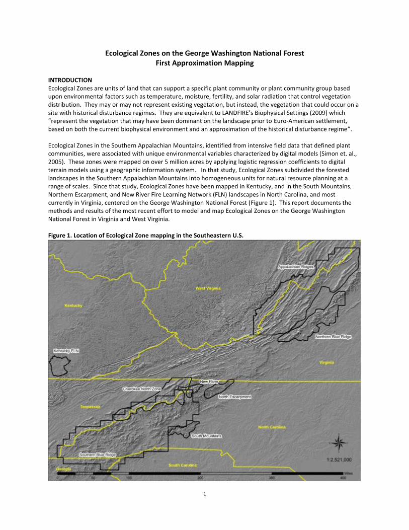
INTRODUCTION Ecological Zones are units of land that can support a specific plant community or plant community group based upon environmental factors such as temperature, moisture, fertility, and solar radiation that control vegetation distribution. They may or may not represent existing vegetation, but instead, the vegetation that could occur on a site with historical disturbance regimes. They are equivalent to LANDFIRE’s Biophysical Settings (2009) which “represent the vegetation that may have been dominant on the landscape prior to Euro-American settlement, based on both the current biophysical environment and an approximation of the historical disturbance regime”. Ecological Zones in the Southern Appalachian Mountains, identified from intensive field data that defined plant communities, were associated with unique environmental variables characterized by digital models (Simon et. al., 2005). These zones were mapped on over 5 million acres by applying logistic regression coefficients to digital terrain models using a geographic information system. In that study, Ecological Zones subdivided the forested landscapes in the Southern Appalachian Mountains into homogeneous units for natural resource planning at a range of scales. Since that study, Ecological Zones have been mapped in Kentucky, and in the South Mountains, Northern Escarpment, and New River Fire Learning Network (FLN) landscapes in North Carolina, and most currently in Virginia, centered on the George Washington National Forest (Figure 1). This report documents the methods and results of the most recent effort to model and map Ecological Zones on the George Washington National Forest in Virginia and West Virginia. Figure 1. Location of Ecological Zone mapping in the Southeastern U.S.

2

Ecological Zones - background and uses: This term, developed in 2001, was used to define units of land that can support a specific plant community or plant community group based upon environmental and physical factors that control vegetation distribution, i.e., the past and potential landscapes based upon measurable environmental factors, such as climate, topography, and geology. Prior to this, comparable environmental models used for ecological classification in the Southeastern U.S. were called “plant association predictive models”, “potential vegetation”, or “pre-settlement vegetation”. The Chattooga River Ecosystem Management Demonstration Project started in 1993 in South Carolina, Georgia, and North Carolina, was the first attempt at applying environmental models, like those used for developing Ecological Zones, to predict ‘potential’ plant community distribution across extensive landscapes in the Southeastern U.S. One of the primary goals of this project was to produce an ecological classification that would provide the information for implementing ecosystem management tied to the National Hierarchical Framework of Ecological Units, “a regionalization, classification and mapping system for stratifying the Earth into progressively smaller areas of increasingly uniform ecological potential for use in ecosystem management” (ECOMAP, 1993). What are now termed Ecological Zones were then called “plant association predictive models” or “Potential Vegetation”. In the Chattooga project, plant association predictive models were developed, under the guidance of Henry McNab - Southern Forest Service Experiment Station, based upon the relationships between field locations of example plant association types and digitally derived landform factors such as elevation, landform index, and relative slope position (McNab 1991). These models were used in combination with soil maps to develop ecological units at different resolutions, i.e., Landtype Associations, Landtypes, and Landtype Phases. In 1999, as part of the forest planning process on the Croatan National Forest, pre-settlement vegetation maps, equivalent to Ecological Zones (Frost 1996), were used to develop an Ecological Classification that included: Landtype Associations, Landtypes, and Landtype Phases, “A new tool that needed to be incorporated into the revised Plan” (USDA 2002). An ecological classification system was developed for the Croatan National Forest that provided a basis for ecologically based land management decisions. This classification organized the landscape into “units having similar topography, geology, soil, climate, and natural disturbance regimes” (USDA 2002) and was used to define management areas, management prescription boundaries, standards, and to set forest-wide objectives. Similarly, in 2001, the Forest Service in cooperation with the Department of Defense (DOD), Camp Lejeune Marine Corps. Base, developed an Ecological Classification System (ECS) to guide conservation management decisions for their Integrated Natural Resource Management Plan (INRMP). The ECS was based, in part, on a report titled “Presettlement Vegetation and Natural Fire Regimes of Camp Lejeune” by Cecil Frost, January 24, 2001, a map analogous to Ecological Zones. In DOD’s most current INRMP, Camp Lejeune continues to refer to the ECS for overall guidance on the desired future condition for specialized habitat areas, i.e., natural areas (DOD 2006). In 2001, the staff of the National Forests of North Carolina conducted a status review of management indicator species (MIS) habitats and population trends using Ecological Zone mapping to quantify the amount and distribution of plant community types on the Nantahala and Pisgah National Forests (USDA 2004). Ecological Zones were also used to identify sites capable of supporting eastern and Carolina hemlock plant communities as part of a conservation area design to prioritize areas for Hemlock Woolly Adelgid control. This conservation area is currently being used to maintain, on portions of the Forests, important hemlock ecosystem functions and to serve as a genetic reserve to maintain a diverse hemlock gene pool ‘in situ’ (USDA 2005). Ecological Zones were used in the Uwharrie National Forest plan revision process to develop a map of the potential extent of Nature Serve Ecological Systems. This mapping provided the basis for the Ecological Sustainability Analysis and was used to define management areas, restoration areas, and desired conditions, and to help set objectives and guidelines (USDA, 2009). Ecological Zones were used in a Plan amendment to evaluate the appropriateness of various management indicator species on the Nantahala and Pisgah National Forests (USDA, 2005), and were combined with satellite imagery to map existing vegetation on the Nantahala National Forest in a multi-year, USFS Southern Region pilot project to demonstrate a process for mid-level existing vegetation mapping suitable in the hardwood dominated forests of the Southern Region (USDA 2006).

3

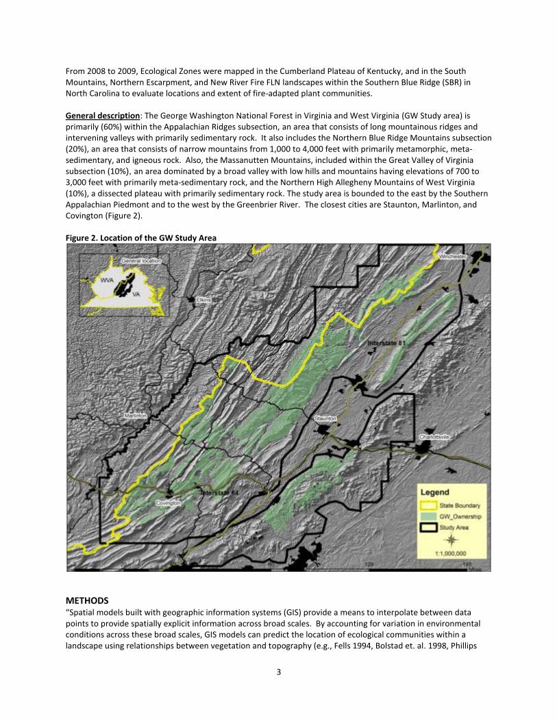
From 2008 to 2009, Ecological Zones were mapped in the Cumberland Plateau of Kentucky, and in the South Mountains, Northern Escarpment, and New River Fire FLN landscapes within the Southern Blue Ridge (SBR) in North Carolina to evaluate locations and extent of fire-adapted plant communities. General description: The George Washington National Forest in Virginia and West Virginia (GW Study area) is primarily (60%) within the Appalachian Ridges subsection, an area that consists of long mountainous ridges and intervening valleys with primarily sedimentary rock. It also includes the Northern Blue Ridge Mountains subsection (20%), an area that consists of narrow mountains from 1,000 to 4,000 feet with primarily metamorphic, meta-sedimentary, and igneous rock. Also, the Massanutten Mountains, included within the Great Valley of Virginia subsection (10%), an area dominated by a broad valley with low hills and mountains having elevations of 700 to 3,000 feet with primarily meta-sedimentary rock, and the Northern High Allegheny Mountains of West Virginia (10%), a dissected plateau with primarily sedimentary rock. The study area is bounded to the east by the Southern Appalachian Piedmont and to the west by the Greenbrier River. The closest cities are Staunton, Marlinton, and Covington (Figure 2). Figure 2. Location of the GW Study Area

METHODS “Spatial models built with geographic information systems (GIS) provide a means to interpolate between data points to provide spatially explicit information across broad scales. By accounting for variation in environmental conditions across these broad scales, GIS models can predict the location of ecological communities within a landscape using relationships between vegetation and topography (e.g., Fells 1994, Bolstad et. al. 1998, Phillips

4

2000) derived from field data” Pearson and Dextraze (2002). The process of interpolating between field data points involves applying coefficients from predictive equations, developed through statistical analyses, to geospatial data that characterize terrain and environmental variables for the target landscape. Care must be taken not to extrapolate to landscapes far away from data points or to landscapes having very different environmental characteristics. Most of the data was collected on the GW National Forest and therefore Ecological Zone predictions outside of this area are likely less accurate. A multi-stage process was used to model Ecological Zones in the project area that included: 1) data acquisition, i.e., identifying Ecological Zones at field locations, 2) creating a digital terrain GIS database and extracting environmental data, 3) statistical analysis, 4) spatial modeling, 5) post-processing of digital model outputs, and 6) evaluating the accuracy of Ecological Zone map units.

Data acquisition: Approximately 5 months during the 2009 and 2010 growing seasons were spent in the field documenting (through GIS, notes, and photos) the location of plant community types and Ecological Zones that occur across the project area. A laptop computer attached to a Global positioning system (GPS), to enable real-time locational tracking in the field, was used in conjunction with ArcGIS 9.3.1 to document on-site observations of ecological characteristics and to access resource data layers for each site. Sample sites predominantly in forested stands >60 years of age and not recently disturbed, were subjectively selected to represent uniform site conditions, i.e., similar aspect, landform, and species composition. Specifically, these reference sites for plant community types described in the literature for the Southeastern U.S. were targeted for sampling especially if they were in ‘good condition’ and therefore easily recognized. Of equal importance, was the evaluation of where these types occurred, i.e., their pattern on the landscape. Good condition plant community types found repeatedly within the same environments were therefore more heavily sampled. Quality control included a nightly review of individual plot photos, and Ecological Zone “calls”, and a weekly review of these relationships based upon Nature Serve Ecological Systems and Virginia Natural Heritage Program plant community descriptions. Ecological Zones were identified at over 3,700 sample areas by evaluating overstory and understory species composition, growth form, stand density, and site factors. A portion of the Pine-Oak Heath sample sites, (less than 10 plots and each well over 10 acres in size), were identified using a combination of 1-meter color Digital Ortho Photos, high powered binoculars, and topographic map data. Data from nearly 800 plots, collected within the project area during the past 15 years by the Virginia and West Virginia Natural Heritage programs (VA_WVA NHP 2009), were used in this sample. This generous contribution to the project included data for less common Ecological Systems such as Central and Southern Appalachian Spruce-Fir Forests, Southern Ridge & Valley / Cumberland Dry Calcareous Forests, and Appalachian Shale Barrens and provided the author a means of evaluating local ecological interpretations by visiting established plots within the area. Ecological Zone classification units are relatively coarse and fairly easy to recognize in the field. They do not include most rare types such as barrens (except Shale barrens), bogs, cliff-talus, fens, glades, seepage swamps, small wetlands, or white cedar because the digital data needed to model these unique environments, such as rock outcrops and wetlands, are incomplete or at too coarse a resolution. The 25 different Ecological Zones identified in the study area, arranged from wet to xeric moisture regimes, are cross-walked below with George Washington National Forest ESE Tool Systems, Nature Serve Ecological Systems (NatureServe 2010) and Virginia Natural Heritage Natural Communities (Fleming and Patterson 2010) to help in describing the composition of types observed in the field and mapped across the study area (Table 1). More detailed site and species composition descriptions for Ecological Zones, Nature Serve Ecological Systems, and Virginia Natural Heritage Community groups are in Appendix I. This cross-walk reflects the author’s ongoing adjustment of Ecological Zone concepts to fit local landscapes based upon work between 2008 and 2009 evaluating Biophysical Setting (BpS) map units (LANDFIRE 2009), in the Southern Blue Ridge Mountains in North Carolina, South Carolina, Tennessee, and Georgia, and modeling Ecological Zones in the Cumberland Plateau in Kentucky, in North Carolina’s South Mountains and Northern Blue Ridge Escarpment, and in the VA_WVA FLN.

5

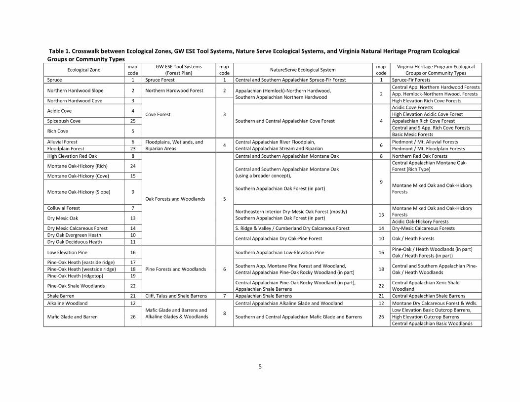
Table 1. Crosswalk between Ecological Zones, GW ESE Tool Systems, Nature Serve Ecological Systems, and Virginia Natural Heritage Program Ecological Groups or Community Types

Ecological Zone map code

GW ESE Tool Systems (Forest Plan)

map code

NatureServe Ecological System map code

Virginia Heritage Program Ecological Groups or Community Types

Spruce 1 Spruce Forest 1 Central and Southern Appalachian Spruce-Fir Forest 1 Spruce-Fir Forests

Northern Hardwood Slope 2 Northern Hardwood Forest 2 Appalachian (Hemlock)-Northern Hardwood, Southern Appalachian Northern Hardwood

2

Central App. Northern Hardwood Forests

App. Hemlock-Northern Hwood. Forests

Northern Hardwood Cove 3

Cove Forest

3

High Elevation Rich Cove Forests

Acidic Cove 4

Southern and Central Appalachian Cove Forest 4

Acidic Cove Forests

High Elevation Acidic Cove Forest

Spicebush Cove 25 Appalachian Rich Cove Forest

Rich Cove 5 Central and S.App. Rich Cove Forests

Basic Mesic Forests

Alluvial Forest 6 Floodplains, Wetlands, and Riparian Areas

4 Central Appalachian River Floodplain, Central Appalachian Stream and Riparian

6 Piedmont / Mt. Alluvial Forests

Floodplain Forest 23 Piedmont / Mt. Floodplain Forests

High Elevation Red Oak 8

Oak Forests and Woodlands 5

Central and Southern Appalachian Montane Oak 8 Northern Red Oak Forests

Montane Oak-Hickory (Rich) 24 Central and Southern Appalachian Montane Oak (using a broader concept), Southern Appalachian Oak Forest (in part)

9

Central Appalachian Montane Oak-Forest (Rich Type)

Montane Oak-Hickory (Cove) 15

Montane Mixed Oak and Oak-Hickory Forests Montane Oak-Hickory (Slope) 9

Colluvial Forest 7 Northeastern Interior Dry-Mesic Oak Forest (mostly) Southern Appalachian Oak Forest (in part)

13 Montane Mixed Oak and Oak-Hickory Forests

Dry Mesic Oak 13 Acidic Oak-Hickory Forests

Dry Mesic Calcareous Forest 14 S. Ridge & Valley / Cumberland Dry Calcareous Forest 14 Dry-Mesic Calcareous Forests

Dry Oak Evergreen Heath 10 Central Appalachian Dry Oak-Pine Forest 10 Oak / Heath Forests

Dry Oak Deciduous Heath 11

Low Elevation Pine 16

Pine Forests and Woodlands 6

Southern Appalachian Low-Elevation Pine 16 Pine-Oak / Heath Woodlands (in part) Oak / Heath Forests (in part)

Pine-Oak Heath (eastside ridge) 17 Southern App. Montane Pine Forest and Woodland, Central Appalachian Pine-Oak Rocky Woodland (in part)

18 Central and Southern Appalachian Pine-Oak / Heath Woodlands

Pine-Oak Heath (westside ridge) 18

Pine-Oak Heath (ridgetop) 19

Pine-Oak Shale Woodlands 22 Central Appalachian Pine-Oak Rocky Woodland (in part), Appalachian Shale Barrens

22 Central Appalachian Xeric Shale Woodland

Shale Barren 21 Cliff, Talus and Shale Barrens 7 Appalachian Shale Barrens 21 Central Appalachian Shale Barrens

Alkaline Woodland 12

Mafic Glade and Barrens and Alkaline Glades & Woodlands

8

Central Appalachian Alkaline Glade and Woodland 12 Montane Dry Calcareous Forest & Wdls.

Mafic Glade and Barren 26 Southern and Central Appalachian Mafic Glade and Barrens 26

Low Elevation Basic Outcrop Barrens,

High Elevation Outcrop Barrens

Central Appalachian Basic Woodlands

6

Creating a digital terrain database: Development of the individual Ecological Zone models began with the creation of a spatial database that described the study area environment using landform and environmental variables. Site conditions for each field plot were extracted these 32 landform / environmental models (DTMS) used to characterized these variables (Table 2) in a GIS. For statistical analyses, data were stored in a database that included plot number, Ecological Zone, and digital landform / environment values for each plot. The methods used for developing DTMs are described in detail in Appendix III.

Table 2. Environmental variables evaluated for Ecological Zone model inclusion

Aspect (slope direction in degrees) Aspect (slope direction in cosine of radian degrees) Curvature of land all directions Curvature of land in the direction of slope Curvature of land perpendicular to slope Distance to stream Distance to river Elevation Distance to carbonate-bearing rocks Distance to mafic-silicate rocks Distance to siliciclastic rocks Distance to carbonaceous-sulfidic rocks Distance to very acid carbonaceous-sulfidic rocks (Brallier Formation) Landform index (from McNab 1993) Average annual precipitation Local relief River influence Difference in elevation from nearest river Surface curvature roughness Relative slope position (from Wilds 1997) Slope length Slope steepness Distance to high snowfall zones Distance to the Great Lakes (influence of lake effect snow) Solar radiation (yearly) Solar radiation (growing season) Difference in elevation from nearest stream Terrain relative moisture index (from Iverson et.al. 1997) Terrain shape index (from McNab 1993) Valley position Distance to high snowfall zones Distance to river

3) Statistical analysis: The relationship between Ecological Zone and environments, characterized by DTMs, were analyzed and predictive equations developed at this stage of the process. Ecological Zone field locations were used to train habitat suitability models using MAXENT 3.2.1 (Phillips and Dudik 2004). MAXENT (maximum entropy) is a relatively new modeling approach (Phillips, et. al. 2004, 2006) that emphasizes the ecological characteristics of a location where a target species is observed (an Ecological Zone in our case) as the primary focus while presuming nothing about locations where these condition are not observed. MAXENT, unlike logistic regression, is therefore a “presence only” modeling approach; it used only Ecological Zone presence (the field data points) to estimate individual Ecological Zone models across the project area. MAXENT works by finding the largest spread (maximum entropy) in a geographic dataset of Ecological Zone presences in relation to a set of environmental predictors for these same locations and 100,000+ randomly selected points / pixels within the project area. The MAXENT logistic

7

outputs are continuous estimates of habitat suitability (probability) for each Ecological Zone ranging from zero to one for each pixel within the project area. This analysis process is described in Appendix IV. 4) Spatial modeling / creating final Ecological Zone maps: To produce a final Ecological Zone (Zone) map, all Zone models were merged and each pixel in the project area was first assigned to the Zone having the highest probability for that pixel. In the event of a “tie”, preference was given to the less extensive Zone(s) by using the ArcGrid 9.3.1 Merge command preference of order. Although MAXENT works well to predict the distribution of individual Zones, merging the models in this fashion did not always reflect the true field condition because of different model ‘strengths’. To better balance individual Zone model strengths, a ‘sensitivity analysis’ based upon accuracy evaluations (Appendix V), was used to adjust probability levels across the project area for some models. For example, the High Elevation Red Oak Ecological Zone had lower probability levels relative to all Zones found at similar elevations and slope positions, especially Montane Oak-Hickory (rich) and Pine-Oak Heath (ridgetop). By increasing High Elevation Red Oak probability levels by just .03 across the project area, the distribution of this Zone based upon field plots, local knowledge, and the overall accuracy of this type, was improved significantly. The Mafic Glades model was processed separately from the other types until the final mapping. A probability of .31 was chosen as the threshold value to define the type and was based an accuracy of 60% for the 23 plots documented in the project area (most of which were outside of the GW ownership).

5) Post-processing of digital model outputs: Post-processing was used to reduce “data noise” i.e., the number of isolated single 10x10 meter pixels (about 1/40

th of an acre in size) within the combined

Ecological Zone model area and to improve processing time for converting pixels to polygons. This post- processing included 1 ArcGrid Majority filter command which replaces cells in a raster based on the majority of their contiguous neighboring cells. An additional ArcGrid Majority filter was used to produce the Nature Serve Ecological Systems and GW ESE Tools System grids. If there is a desire to produce maps having a defined minimum map unit size, then further processing is recommended using the ESRI “eliminate” command, however this tends to overemphasize the size of major types at the expense of less common types. 6) Assessing the accuracy of Ecological Zone map units: Field plots were used as reference data to evaluate the accuracy of the final Ecological Zone maps. Although this is a biased measure of accuracy because these were the same data used to produce the predictive equations, MAXENT does not force a classification upon a sample plot based upon its location, rather, environmental data from that location is used to model the entire landscape with no bias to where a plot is located. Also, using field plots as reference data is a reasonable means of objectively comparing different analysis methods and does indicate how well map composition reflects the plot data composition in these landscapes in comparison to other areas where Ecological Zones have been identified. RESULTS and DISCUSSSION The location, extent, accuracy, and usefulness of Ecological Zones modeled in the project area were evaluated from the following: 1) Field observations 2) Relative importance of environmental factors in predicting Ecological Zones (Tables 3 to 6) 3) Accuracy of map units relative to field sample plot information (Table 7 and Appendix V) 4) Location and extent of Ecological Zones based on acreage of map units (Table 8), Nature Serve Ecological Systems (Table 9), GW ESE Tool Systems (Table 10), and displays relative to topography (Figures 3 to 7) and, 5) The extent of fire-adapted plant communities within Ecological Zones and their mapped accuracy (Tables 6-9, Appendix V). Two fire-adaptation classes, less-adapted and more-adapted, were evaluated using the same classes assessed in North Carolina and Kentucky for FLN Ecological Zone mapping projects (Simon 2008, 2010). These two classes are based on target communities identified by the SBR Fire Learning Network in 2008 for restoring fire regimes (http://www.tncfire.org/training_usfln SBRfln.htm).

8

They include pine-oak heath, shortleaf pine-oak, dry-mesic oak-hickory, and high-elevation red oak forests (and their equivalent Ecological Zones); the assumption was made that more mesic zones (alluvial forests and wetter) were less fire-adapted. A refinement of these groups is possible, and may follow methods described in “Rule-based Mapping of Fire-adapted Vegetation and Fire Regimes for the Monongahela National Forest”, (Tomas-Van Gundy et. al. 2007). 1) Field Observations: The most common Ecological Zones observed in the GW study area were those that support oak-dominated communities, especially Dry Oak and Dry-Mesic Oak. Dry Oak sites were dominated by chestnut oak and had three distinct stand and understory conditions; open woodlands on broader ridges especially on limestone, woodlands to forests with a dense mountain laurel understory most often associated with Pine-Oak heath at mid to higher elevations, and forests or woodlands with a dense to sparse huckleberry and blueberry understory and only occasional mountain laurel at mostly mid to lower elevations. Dry-Mesic oak sites were dominated by white oak with a sparse understory and were situated in concave portions of the landscape or associated with broader floodplains on colluvial surfaces; dry-mesic to sub-mesic oak sites in the later situation were labeled ‘Colluvial Forests’. Highly dissected slopes on the northwest-facing side of major ridges were dominated by Pine-oak heath on west-facing slopes, and Dry Oak or Dry-Mesic Oak on northwest to north facing slopes. Table mountain pine was the predominant species in this Pine-oak heath. This striking pattern of alternating Pine-Oak and Oak Ecological Zones repeated itself across these landscapes throughout the project area but were more subtle in the Blue Ridge. A much weaker but similar pattern was observed on the southeast-facing slopes of major ridges in the Appalachian Ridges portion of the study area. There, the Pine-Oak Heath occurred in much smaller patches confined to south-facing slopes and pitch pine was more common than table mountain pine. Pine-Oak heath was also observed on high ridges where it mixed with High Elevation Red Oak types. Patch sizes were typically small in these situations. Except for areas closest to the Allegheny Plateau, Northern Hardwood types were confined to more concave landscapes on the northwest-face of major ridges where they mixed with Montane Oak-Hickory and High Elevation Red Oak types. Differentiating between these latter two types was difficult because they formed a very broad transition zone along most high ridges and often included Dry Oak types intermixed on the most exposed sites. Along broader ridges and near saddles, Montane Oak-Hickory (rich) types occurred especially in the Blue Ridge associated with mafic rock. Spruce was observed only in the northwest portion of the study area and patterns in this area have been highly altered from farming and pasturing. Only along cold air drainages below higher ridges was a distinct Spruce Ecological Zone discernable. However, some of the highest ridges had remnant spruce stands or were planted extensively to Red spruce, presumably based on historical evidence / local knowledge that these areas once supported spruce. Rich Cove Forests were uncommon except in limestone lithology and most of these areas have likely had multiple timber harvests and were highly disturbed and therefore hard to interpret. Spicebush Coves were common in these same environments in the Blue Ridge but small and less extensive in the Appalachian Ridges. Very distinctive Virginia pine dominated woodlands were observed at low elevations on west-facing slopes mostly on loose, friable, shale. Trees on these steep sites were stunted and gnarled and the understory was very sparse and often lichen dominated. These types did not seem to fit the typical shale barren description where continual undercutting of weak shale strata by a river maintains a poorly vegetated hillside. Instead, they seem to fit the description for Mountain / Piedmont Acidic Woodlands (VA Natural Heritage program 2009) and were placed in the Pine-Oak Shale Woodlands Ecological Zone. Recognition of vegetation / landform patterns was most difficult in limestone areas and on lower elevation gently sloping broad ridges where apparently continual management has occurred on these productive sites. However, a distinct pattern was observed on some broad low ridges on sandstones and metasediments where occasional shortleaf pine was observed. These sites and species composition looked similar to extensive pine types observed in Kentucky, North Carolina, and Georgia, and to what has been described historically in lower elevation forests in Virginia. They therefore warranted recognition and fit well with the description for the Nature Serve Southern Appalachian Low Elevation Pine Ecological System. Photo examples for most of these types are included in Appendix II. 2) Relative importance of environmental factors: The relationship between plant community types and the environments in which they occur (the Ecological Zone) can be evaluated by examining the relative importance of environmental variables found by MAXENT to be the best predictors of Ecological Zone location (Tables 3-5). Some

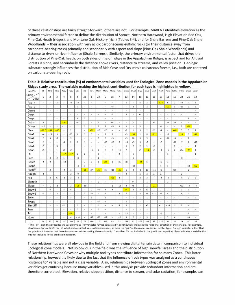
9

of these relationships are fairly straight-forward, others are not. For example, MAXENT identifies elevation as the primary environmental factor to define the distribution of Spruce, Northern Hardwood, High Elevation Red Oak, Pine-Oak Heath (ridges), and Montane Oak-Hickory (rich) (Tables 3-4), and for Shale Barrens and Pine-Oak Shale Woodlands – their association with very acidic carbonaceous-sulfidic rocks (or their distance away from carbonate-bearing rocks) primarily and secondarily with aspect and slope (Pine-Oak Shale Woodlands) and distance to rivers or river influence (Shale Barrens). Similarly, the primary environmental factor that drives the distribution of Pine-Oak heath, on both sides of major ridges in the Appalachian Ridges, is aspect and for Alluvial Forests is slope, and secondarily the distance above rivers, distance to streams, and valley position. Geologic substrate strongly influences the distribution of Rich Cove and Dry-mesic calcareous forests, i.e., both are centered on carbonate-bearing rock. Table 3: Relative contribution (%) of environmental variables used for Ecological Zone models in the Appalachian Ridges study area. The variable making the highest contribution for each type is highlighted in yellow. EZONE SF NhW NhC Acov Rcov Allu Fld Hero MonR MonS MonC Collu Dmok Dmcal DryE DryD LowP PohW PohE PohRd POshl ShaleB AlkW

Code DTM

1 2 3 4 5 6 23 8 24 9 15 7 13 14 10 11 16 17 18 19 22 21 12

Asp_r - - -15 - -4 -3 - - - - 1 - 6 2 - +23 6 2 +4 - 3

Asp_c - - - - - 3 - - - +5 - 2 - 2 7 -21 3 -11 2 2

Curve - - - - - - - - -

Curpl - 1 - - - - - - -5 2 - +4 2 - - - - -

Curpr - - 6 2 - - - - - - - 1 -

Dstrm 3 -16 1 -11 1 - 2 - +10 - - 2 - - +4 +4 +4 1 - -

Driver +10 - 2 +11 - 1 2 1 2 2 +5 2 2 1 3 1 1 +4 - - 2 -21

Elev +59 1/ +53 +47 - 2 - +29 +7 +7 - - -8 1 3 2 -12 -4 - +48 3 3 1

Geo1 +4 +19 3 - -15 6 3 1 - 2 1 +5 -38 1 8 -21 - +2 18 3 -32

Geo2 2 3 -7 - 9 - - 3 6 +5 +5 10 9 5 4 -10 +5 - 2

Geo3 2 - - -3 2 2 1 - - -10 -10 2 -10 +5 3 -7 - -7 -11 -7 1 +17

Geo4 - 2/ - 3 - - - - - - 1 2 2 1 +9 - 1 - - 1

Geo6 +5 1 1 +6 +5 - +6 2 5 6 -16 2 - +9 +14 +3 -3 -6 2 +14 -20 1

Lfi - - - +17 +17 2 2 1 - 2 - 1 - - 1 1

Prec 3 2 1 - +5 - 2 - - 1 - - - - -8 -

Relief 2 2 +10 - 7 3 1 20 2 +6 +8 +32 5 +9 4 - - -

Rivinfl - - - -4 1 - - - - - +12 - - - 1 1 - 18 +32

Rivdiff 3 - -4 1 -56 27 31 16 +18 -26 -7 2 -8 10 +11 +3 +16 - 2

Rough 2 - - 2 +4 - - - - - +4 3 - 1 2 2 2 - 2 -

Rsp 3 +7 -3 3 -4 - - -7 - +25 3 - - 3 3 - -2 -8 -6 2 2

Slength - - - - - 2 - - - +4 - 1 - - 1 - -

Slope -4 1 -8 - 2 -29 -10 - - - 1 -12 3 +5 - 1 -21 - +13 +8 +4

Snow1 -5 - 3 8 - - 2 +4 4 3 14 2 8 10 2 2 7 2 2 -

Snow2 -7 - 3 - - 1 3 +4 - 6 3 5 4 11 +11 +9 4 6 -

Solyr - - - 3 - 3 1 - - - - - - - - --

Solgw - - - - - +7 2 1 - - - - -

Stmdiff - - -13 3 - 1 1 - - 4 2 1 +5 1 +11 +16 1 2 -

Trmi - - - 3 - - 1 - - - - - - -

Tsi 1 - -18 - - - -11 - - - -2 - 2

Vpos - - 4 +16 4 -17 -25 -12 - -10 3 7 1 5 - - 7 6 +4 -

n 28 97 26 187 100 15 74 166 17 243 43 13 293 62 377 204 39 215 81 22 79 41 26 1/

The + or – sign that precedes the variable value (for variables having at least a 5% contribution) indicates the relational direction of the variable. For example, elevation in Spruce-fir (SF) is +59 which indicates that as elevation increases, so does the ‘gain’ in the model prediction for this type. No sign indicates either that the gain is not linear or that there is confusion in interpreting the relationship.

2/ less than 1% but included in the prediction equation, blank indicates a variable that

was not included in the prediction equation.

These relationships were all obvious in the field and from viewing digital terrain data in comparison to individual Ecological Zone models. Not so obvious in the field was the influence of high snowfall areas and the distribution of Northern Hardwood Coves or why multiple rock types contribute information for so many Zones. This latter relationship, however, is likely due to the fact that the influence of rock types was analyzed as a continuous “distance to” variable and not a class variable. Also, relationships between Ecological Zones and environmental variables get confusing because many variables used in this analysis provide redundant information and are therefore correlated. Elevation, relative slope position, distance to stream, and solar radiation, for example, can

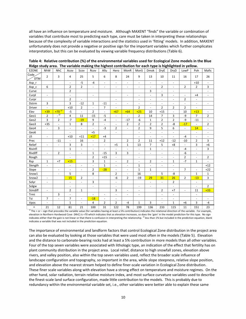
10

all have an influence on temperature and moisture. Although MAXENT “finds” the variable or combination of variables that contribute most to predicting each type, care must be taken in interpreting these relationships because of the complexity of variable interactions and the statistics used in ‘fitting’ models. In addition, MAXENT unfortunately does not provide a negative or positive sign for the important variables which further complicates interpretation, but this can be evaluated by viewing variable frequency distributions (Table 6). Table 4: Relative contribution (%) of the environmental variables used for Ecological Zone models in the Blue Ridge study area. The variable making the highest contribution for each type is highlighted in yellow. EZONE NhW NhC Acov Scov Rcov Allu Hero MonR MonS Dmok DryE DryD LowP Poh Mafic

Code DTM

2 3 4 25 5 6 8 24 9 13 10 11 16 17 26

Asp_r - -5 -4 - - - - - - - +10 -

Asp_c 6 2 2 - - - - - - 2 - 2 2 3

Curve 2 - 3 - - -

Curpl - - - - - - 3 - - +4 -

Curpr 2 - - - - - - 2 -

Dstrm 3 3 -12 1 -11 - - - - - - - - -

Driver - +10 2 - 7 - 2 - 2 2 2 -

Elev +39 +70 1/ -5 - 2 - +67 +64 +25 10 +15 - 10 +13 -

Geo1 2 - 2/ 4 11 -15 -5 - - 2 14 7 3 -9 7 2

Geo2 3 2 -7 -19 9 -4 - -17 -6 1 2 2 -9 -11 -

Geo3 +35 - 1 8 2 - - 2 2 2 2 -8 -17 - 2

Geo4 - 3 - - - -3 2 - 2 9 5 6 - 14 -

Geo6 - +5 - - - - - - -

Lfi - +10 +11 +17 +4 - - - - -4 - -

Prec -11 - 16 - 2 2 2 11 +12 -12 -10 2 3

Relief - - 3 3 - - +5 1 13 7 5 +8 - 3 +6

Rivinfl 1 - - - - - - 1 - - -4 - 3

Rivdiff - 2 - - 1 -15 3 3 - - - - -6 -

Rough - 2 +15 - - - - 2 - 2

Rsp 1 +7 +15 3 1 - 2 - 2 - 1 -7 1 -

Slength - - - - 1 - - 1 - - - +12

Slope - - - 2 -28 - - 1 1 - 7 - +22

Snow1 - 5 8 2 - 16 - 5 -8 1 1

Snow2 - 15 2 - -6 2 -19 29 31 26 2 -13 3

Solyr - - - 3 - - - 2 -

Solgw - - - - - - - 2

Stmdiff - 2 1 3 - - 2 +7 - 11 +33

Trmi 3 - - - - - - - - -

Tsi 7 - 7 - -18 - - - - - -

Vpos - 1 - 4 2 2 -4 1 3 - 1 +6 3 -4

n 21 12 81 21 100 31 122 78 199 136 233 115 11 151 23 1/ The + or – sign that precedes the variable value (for variables having at least a 5% contribution) indicates the relational direction of the variable. For example, elevation in Northern Hardwood Cove (NhC) is +70 which indicates that as elevation increases, so does the ‘gain’ in the model prediction for this type. No sign indicates either that the gain is not linear or that there is confusion in interpreting the relationship. 2/ less than 1% but included in the prediction equation, blank indicates a variable that was not included in the prediction equation.

The importance of environmental and landform factors that control Ecological Zone distribution in the project area can also be evaluated by looking at those variables that were used most often in the models (Table 5). Elevation and the distance to carbonate-bearing rocks had at least a 5% contribution in more models than all other variables. Four of the top seven variables were associated with lithologic type, an indication of the effect that fertility has on plant community distribution in the project area. Local relief, distance to high snowfall zones, elevation above rivers, and valley position, also within the top seven variables used, reflect the broader scale influence of landscape configuration and topography, so important in the area, while slope steepness, relative slope position, and elevation above the nearest stream helped to define finer-scale variation in Ecological Zone distribution. These finer scale variables along with elevation have a strong effect on temperature and moisture regimes. On the other hand, solar radiation, terrain relative moisture index, and most surface curvature variables used to describe the finest-scale land surface configuration, made little contribution to the models. This is probably due to redundancy within the environmental variable set, i.e., other variables were better able to explain these same

11

factors. For example, slope steepness, relative slope position, and terrain shape index individually were perhaps better able to explain moisture regime than terrain relative moisture index which combines these same variables into one value (Appendix III). Table 5: Environmental variables having at least a 5% contribution to the Ecological Zone models Environmental variable % of all

models % of models App. Ridges

% of models Blue Ridge

Elevation 50 39 67 Distance to carbonate-bearing rocks 45 44 47 Distance to mafic-silicate rocks 45 44 47 Local relief 37 35 40 Distance to high snowfall zones 37 30 47 Distance to very acidic shales 34 52 7 Difference in elevation from the nearest river 34 48 13 Distance to siliciclastic rocks 34 39 27 Slope steepness 29 35 20 Distance to the Great Lakes 29 26 33 Valley position 26 39 7 Average annual precipitation 21 9 40 Relative slope position 18 17 20 Difference in elevation from the nearest stream 18 17 20 Aspect in degrees 16 17 13 Distance to closest river 16 17 13 Aspect cosine 13 17 7 Distance to closest stream 13 13 13 Landform index 13 9 20 Terrain shape index 13 9 20 Distance to carbonaceous-sulfidic rocks 13 4 27 River influence 8 13 - Surface curvature perpendicular to slope direction 3 4 - Surface curvature in the direction of slope 3 4 - Solar radiation during the growing season 3 4 - Surface curvature roughness 3 - 7 Slope length 3 - 7 Surface curvature - - - Solar radiation during the entire year - - - Terrain relative moisture index - - -

12

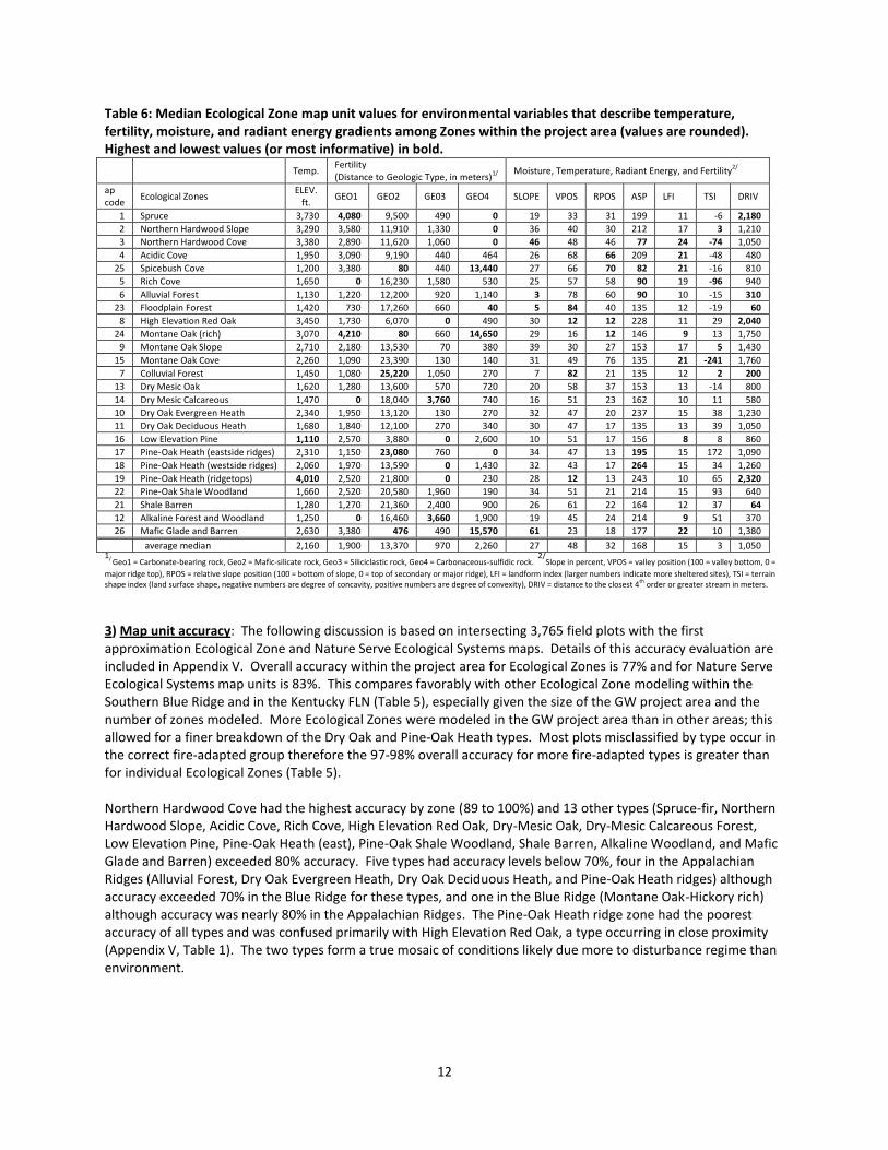
Table 6: Median Ecological Zone map unit values for environmental variables that describe temperature, fertility, moisture, and radiant energy gradients among Zones within the project area (values are rounded). Highest and lowest values (or most informative) in bold.

Temp. Fertility (Distance to Geologic Type, in meters)

1/ Moisture, Temperature, Radiant Energy, and Fertility2/

ap code

Ecological Zones ELEV.

ft. GEO1 GEO2 GE03 GEO4 SLOPE VPOS RPOS ASP LFI TSI DRIV

1 Spruce 3,730 4,080 9,500 490 0 19 33 31 199 11 -6 2,180

2 Northern Hardwood Slope 3,290 3,580 11,910 1,330 0 36 40 30 212 17 3 1,210

3 Northern Hardwood Cove 3,380 2,890 11,620 1,060 0 46 48 46 77 24 -74 1,050

4 Acidic Cove 1,950 3,090 9,190 440 464 26 68 66 209 21 -48 480

25 Spicebush Cove 1,200 3,380 80 440 13,440 27 66 70 82 21 -16 810

5 Rich Cove 1,650 0 16,230 1,580 530 25 57 58 90 19 -96 940

6 Alluvial Forest 1,130 1,220 12,200 920 1,140 3 78 60 90 10 -15 310

23 Floodplain Forest 1,420 730 17,260 660 40 5 84 40 135 12 -19 60

8 High Elevation Red Oak 3,450 1,730 6,070 0 490 30 12 12 228 11 29 2,040

24 Montane Oak (rich) 3,070 4,210 80 660 14,650 29 16 12 146 9 13 1,750

9 Montane Oak Slope 2,710 2,180 13,530 70 380 39 30 27 153 17 5 1,430

15 Montane Oak Cove 2,260 1,090 23,390 130 140 31 49 76 135 21 -241 1,760

7 Colluvial Forest 1,450 1,080 25,220 1,050 270 7 82 21 135 12 2 200

13 Dry Mesic Oak 1,620 1,280 13,600 570 720 20 58 37 153 13 -14 800

14 Dry Mesic Calcareous 1,470 0 18,040 3,760 740 16 51 23 162 10 11 580

10 Dry Oak Evergreen Heath 2,340 1,950 13,120 130 270 32 47 20 237 15 38 1,230

11 Dry Oak Deciduous Heath 1,680 1,840 12,100 270 340 30 47 17 135 13 39 1,050

16 Low Elevation Pine 1,110 2,570 3,880 0 2,600 10 51 17 156 8 8 860

17 Pine-Oak Heath (eastside ridges) 2,310 1,150 23,080 760 0 34 47 13 195 15 172 1,090

18 Pine-Oak Heath (westside ridges) 2,060 1,970 13,590 0 1,430 32 43 17 264 15 34 1,260

19 Pine-Oak Heath (ridgetops) 4,010 2,520 21,800 0 230 28 12 13 243 10 65 2,320

22 Pine-Oak Shale Woodland 1,660 2,520 20,580 1,960 190 34 51 21 214 15 93 640

21 Shale Barren 1,280 1,270 21,360 2,400 900 26 61 22 164 12 37 64

12 Alkaline Forest and Woodland 1,250 0 16,460 3,660 1,900 19 45 24 214 9 51 370

26 Mafic Glade and Barren 2,630 3,380 476 490 15,570 61 23 18 177 22 10 1,380

average median 2,160 1,900 13,370 970 2,260 27 48 32 168 15 3 1,050 1/ Geo1 = Carbonate-bearing rock, Geo2 = Mafic-silicate rock, Geo3 = Siliciclastic rock, Geo4 = Carbonaceous-sulfidic rock.

2/Slope in percent, VPOS = valley position (100 = valley bottom, 0 =

major ridge top), RPOS = relative slope position (100 = bottom of slope, 0 = top of secondary or major ridge), LFI = landform index (larger numbers indicate more sheltered sites), TSI = terrain shape index (land surface shape, negative numbers are degree of concavity, positive numbers are degree of convexity), DRIV = distance to the closest 4th order or greater stream in meters.

3) Map unit accuracy: The following discussion is based on intersecting 3,765 field plots with the first approximation Ecological Zone and Nature Serve Ecological Systems maps. Details of this accuracy evaluation are included in Appendix V. Overall accuracy within the project area for Ecological Zones is 77% and for Nature Serve Ecological Systems map units is 83%. This compares favorably with other Ecological Zone modeling within the Southern Blue Ridge and in the Kentucky FLN (Table 5), especially given the size of the GW project area and the number of zones modeled. More Ecological Zones were modeled in the GW project area than in other areas; this allowed for a finer breakdown of the Dry Oak and Pine-Oak Heath types. Most plots misclassified by type occur in the correct fire-adapted group therefore the 97-98% overall accuracy for more fire-adapted types is greater than for individual Ecological Zones (Table 5). Northern Hardwood Cove had the highest accuracy by zone (89 to 100%) and 13 other types (Spruce-fir, Northern Hardwood Slope, Acidic Cove, Rich Cove, High Elevation Red Oak, Dry-Mesic Oak, Dry-Mesic Calcareous Forest, Low Elevation Pine, Pine-Oak Heath (east), Pine-Oak Shale Woodland, Shale Barren, Alkaline Woodland, and Mafic Glade and Barren) exceeded 80% accuracy. Five types had accuracy levels below 70%, four in the Appalachian Ridges (Alluvial Forest, Dry Oak Evergreen Heath, Dry Oak Deciduous Heath, and Pine-Oak Heath ridges) although accuracy exceeded 70% in the Blue Ridge for these types, and one in the Blue Ridge (Montane Oak-Hickory rich) although accuracy was nearly 80% in the Appalachian Ridges. The Pine-Oak Heath ridge zone had the poorest accuracy of all types and was confused primarily with High Elevation Red Oak, a type occurring in close proximity (Appendix V, Table 1). The two types form a true mosaic of conditions likely due more to disturbance regime than environment.

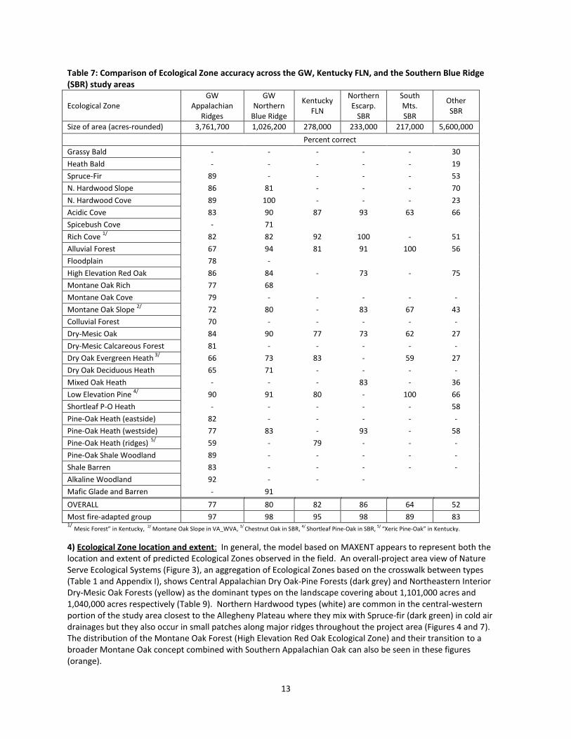
13

Table 7: Comparison of Ecological Zone accuracy across the GW, Kentucky FLN, and the Southern Blue Ridge (SBR) study areas

Ecological Zone GW

Appalachian Ridges

GW Northern

Blue Ridge

Kentucky FLN

Northern Escarp.

SBR

South Mts. SBR

Other SBR

Size of area (acres-rounded) 3,761,700 1,026,200 278,000 233,000 217,000 5,600,000

Percent correct

Grassy Bald - - - - - 30

Heath Bald - - - - - 19

Spruce-Fir 89 - - - - 53

N. Hardwood Slope 86 81 - - - 70

N. Hardwood Cove 89 100 - - - 23

Acidic Cove 83 90 87 93 63 66

Spicebush Cove - 71

Rich Cove 1/

82 82

92

100 - 51

Alluvial Forest 67 94 81 91 100 56

Floodplain 78 -

High Elevation Red Oak 86 84 - 73 - 75

Montane Oak Rich 77 68

Montane Oak Cove 79 - - - - -

Montane Oak Slope 2/

72 80 - 83 67 43

Colluvial Forest 70 - - - - -

Dry-Mesic Oak 84 90 77 73 62 27

Dry-Mesic Calcareous Forest 81 - - - - -

Dry Oak Evergreen Heath 3/

66 73 83 - 59 27

Dry Oak Deciduous Heath 65 71 - - - -

Mixed Oak Heath - - - 83 - 36

Low Elevation Pine 4/

90 91 80 - 100 66

Shortleaf P-O Heath - - - - - 58

Pine-Oak Heath (eastside) 82 - - - - -

Pine-Oak Heath (westside) 77 83 -

93 - 58

Pine-Oak Heath (ridges) 5/

59 - 79 - - -

Pine-Oak Shale Woodland 89 - - - - -

Shale Barren 83 - - - - -

Alkaline Woodland 92 - - -

Mafic Glade and Barren - 91

OVERALL 77 80 82 86 64 52

Most fire-adapted group 97 98 95 98 89 83 1/

Mesic Forest” in Kentucky, 2/ Montane Oak Slope in VA_WVA, 3/ Chestnut Oak in SBR, 4/ Shortleaf Pine-Oak in SBR, 5/ “Xeric Pine-Oak” in Kentucky.

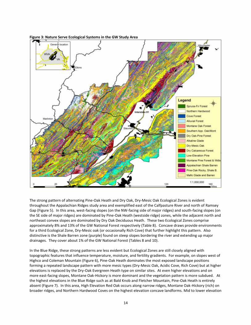
4) Ecological Zone location and extent: In general, the model based on MAXENT appears to represent both the location and extent of predicted Ecological Zones observed in the field. An overall-project area view of Nature Serve Ecological Systems (Figure 3), an aggregation of Ecological Zones based on the crosswalk between types (Table 1 and Appendix I), shows Central Appalachian Dry Oak-Pine Forests (dark grey) and Northeastern Interior Dry-Mesic Oak Forests (yellow) as the dominant types on the landscape covering about 1,101,000 acres and 1,040,000 acres respectively (Table 9). Northern Hardwood types (white) are common in the central-western portion of the study area closest to the Allegheny Plateau where they mix with Spruce-fir (dark green) in cold air drainages but they also occur in small patches along major ridges throughout the project area (Figures 4 and 7). The distribution of the Montane Oak Forest (High Elevation Red Oak Ecological Zone) and their transition to a broader Montane Oak concept combined with Southern Appalachian Oak can also be seen in these figures (orange).

14

Figure 3: Nature Serve Ecological Systems in the GW Study Area

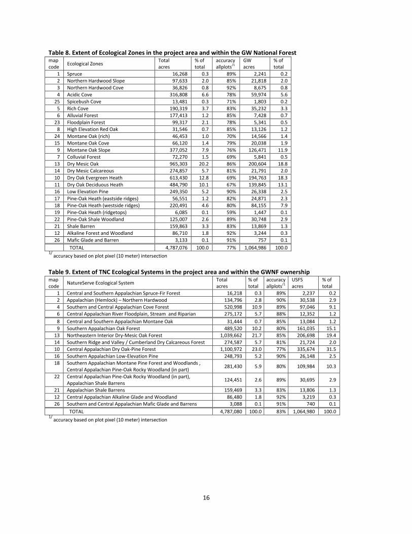
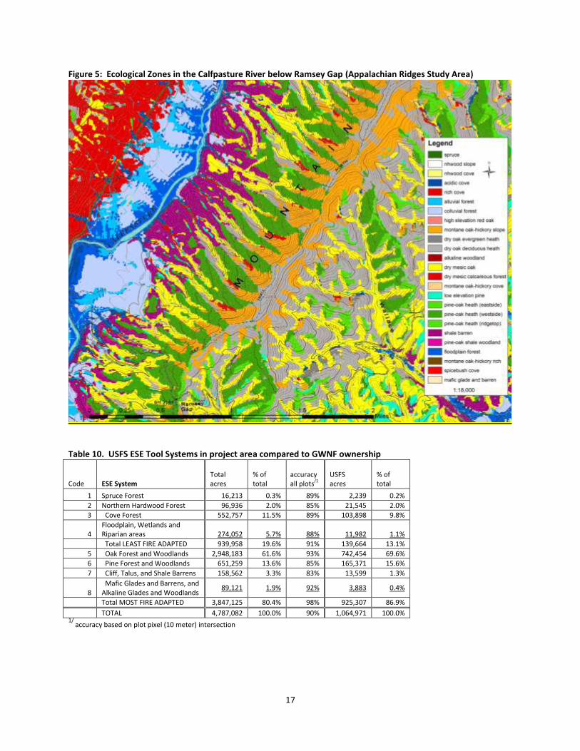
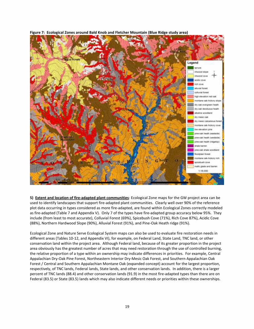
The strong pattern of alternating Pine-Oak Heath and Dry Oak, Dry-Mesic Oak Ecological Zones is evident throughout the Appalachian Ridges study area and exemplified east of the Calfpasture River and north of Ramsey Gap (Figure 5). In this area, west-facing slopes (on the NW-facing side of major ridges) and south-facing slopes (on the SE side of major ridges) are dominated by Pine-Oak Heath (westside ridge) zones, while the adjacent north and northeast convex slopes are dominated by Dry Oak Deciduous Heath. These two Ecological Zones comprise approximately 8% and 13% of the GW National Forest respectively (Table 8). Concave draws provide environments for a third Ecological Zone, Dry-Mesic oak (or occasionally Rich Cove) that further highlight this pattern. Also distinctive is the Shale Barren zone (purple) found on steep slopes bordering the river and extending up major drainages. They cover about 1% of the GW National Forest (Tables 8 and 10). In the Blue Ridge, these strong patterns are less evident but Ecological Zones are still closely aligned with topographic features that influence temperature, moisture, and fertility gradients. For example, on slopes west of Highco and Coleman Mountain (Figure 6), Pine-Oak Heath dominates the most exposed landscape positions forming a repeated landscape pattern with more mesic types (Dry-Mesic Oak, Acidic Cove, Rich Cove) but at higher elevations is replaced by the Dry-Oak Evergreen Heath type on similar sites. At even higher elevations and on more east-facing slopes, Montane Oak-Hickory is more dominant and the vegetation pattern is more subdued. At the highest elevations in the Blue Ridge such as at Bald Knob and Fletcher Mountain, Pine-Oak Heath is entirely absent (Figure 7). In this area, High Elevation Red Oak occurs along narrow ridges, Montane Oak-Hickory (rich) on broader ridges, and Northern Hardwood Coves on the highest elevation concave landforms. Mid to lower elevation

15

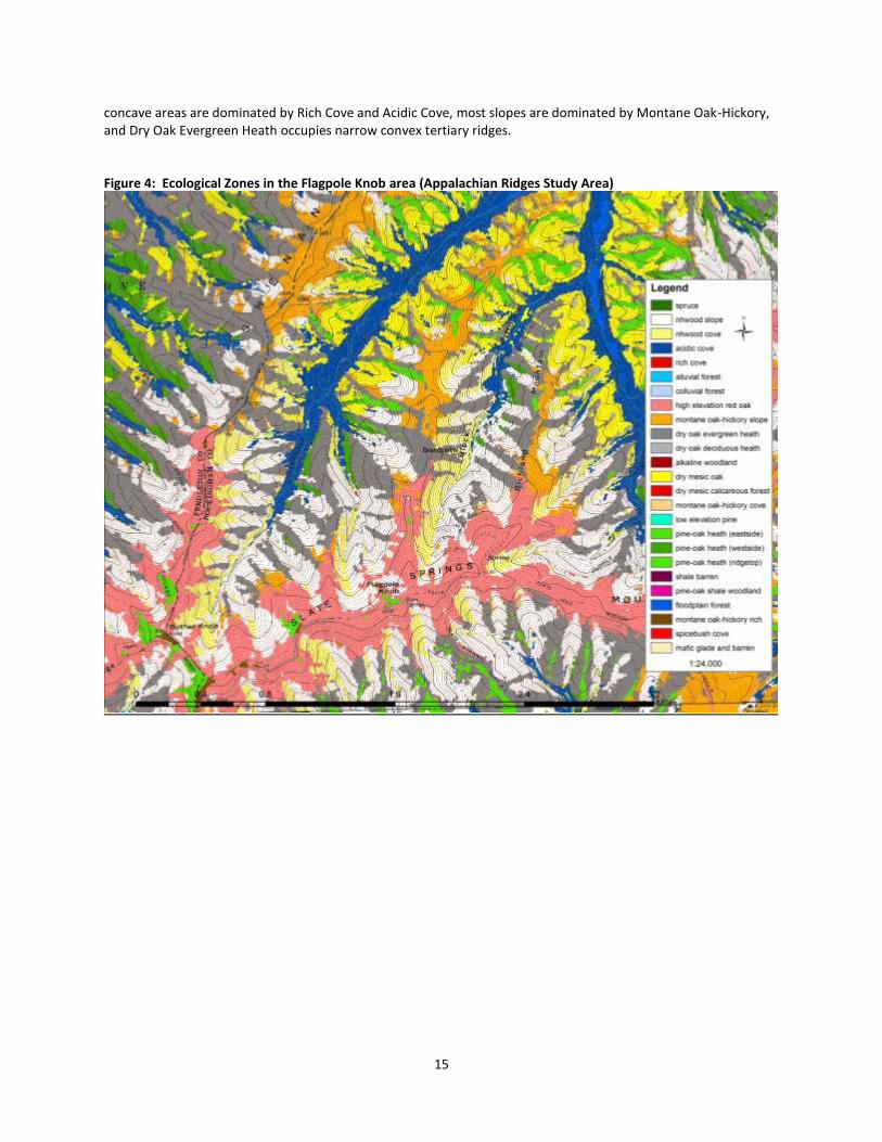
concave areas are dominated by Rich Cove and Acidic Cove, most slopes are dominated by Montane Oak-Hickory, and Dry Oak Evergreen Heath occupies narrow convex tertiary ridges. Figure 4: Ecological Zones in the Flagpole Knob area (Appalachian Ridges Study Area)

16

Table 8. Extent of Ecological Zones in the project area and within the GW National Forest map code

Ecological Zones Total acres

% of total

accuracy allplots/1

GW acres

% of total

1 Spruce 16,268 0.3 89% 2,241 0.2

2 Northern Hardwood Slope 97,633 2.0 85% 21,818 2.0

3 Northern Hardwood Cove 36,826 0.8 92% 8,675 0.8

4 Acidic Cove 316,808 6.6 78% 59,974 5.6

25 Spicebush Cove 13,481 0.3 71% 1,803 0.2

5 Rich Cove 190,319 3.7 83% 35,232 3.3

6 Alluvial Forest 177,413 1.2 85% 7,428 0.7

23 Floodplain Forest 99,317 2.1 78% 5,341 0.5

8 High Elevation Red Oak 31,546 0.7 85% 13,126 1.2

24 Montane Oak (rich) 46,453 1.0 70% 14,566 1.4

15 Montane Oak Cove 66,120 1.4 79% 20,038 1.9

9 Montane Oak Slope 377,052 7.9 76% 126,471 11.9

7 Colluvial Forest 72,270 1.5 69% 5,841 0.5

13 Dry Mesic Oak 965,303 20.2 86% 200,604 18.8

14 Dry Mesic Calcareous 274,857 5.7 81% 21,791 2.0

10 Dry Oak Evergreen Heath 613,430 12.8 69% 194,763 18.3

11 Dry Oak Deciduous Heath 484,790 10.1 67% 139,845 13.1

16 Low Elevation Pine 249,350 5.2 90% 26,338 2.5

17 Pine-Oak Heath (eastside ridges) 56,551 1.2 82% 24,871 2.3

18 Pine-Oak Heath (westside ridges) 220,491 4.6 80% 84,155 7.9

19 Pine-Oak Heath (ridgetops) 6,085 0.1 59% 1,447 0.1

22 Pine-Oak Shale Woodland 125,007 2.6 89% 30,748 2.9

21 Shale Barren 159,863 3.3 83% 13,869 1.3

12 Alkaline Forest and Woodland 86,710 1.8 92% 3,244 0.3

26 Mafic Glade and Barren 3,133 0.1 91% 757 0.1

TOTAL 4,787,076 100.0 77% 1,064,986 100.0 1/

accuracy based on plot pixel (10 meter) intersection

Table 9. Extent of TNC Ecological Systems in the project area and within the GWNF ownership map code

NatureServe Ecological System Total acres

% of total

accuracy allplots/1

USFS acres

% of total

1 Central and Southern Appalachian Spruce-Fir Forest 16,218 0.3 89% 2,237 0.2

2 Appalachian (Hemlock) – Northern Hardwood 134,796 2.8 90% 30,538 2.9

4 Southern and Central Appalachian Cove Forest 520,998 10.9 89% 97,046 9.1

6 Central Appalachian River Floodplain, Stream and Riparian 275,172 5.7 88% 12,352 1.2

8 Central and Southern Appalachian Montane Oak 31,444 0.7 85% 13,084 1.2

9 Southern Appalachian Oak Forest 489,520 10.2 80% 161,035 15.1

13 Northeastern Interior Dry-Mesic Oak Forest 1,039,662 21.7 85% 206,698 19.4

14 Southern Ridge and Valley / Cumberland Dry Calcareous Forest 274,587 5.7 81% 21,724 2.0

10 Central Appalachian Dry Oak-Pine Forest 1,100,972 23.0 77% 335,674 31.5

16 Southern Appalachian Low-Elevation Pine 248,793 5.2 90% 26,148 2.5

18 Southern Appalachian Montane Pine Forest and Woodlands , Central Appalachian Pine-Oak Rocky Woodland (in part)

281,430 5.9 80% 109,984 10.3

22 Central Appalachian Pine-Oak Rocky Woodland (in part), Appalachian Shale Barrens

124,451 2.6 89% 30,695 2.9

21 Appalachian Shale Barrens 159,469 3.3 83% 13,806 1.3

12 Central Appalachian Alkaline Glade and Woodland 86,480 1.8 92% 3,219 0.3

26 Southern and Central Appalachian Mafic Glade and Barrens 3,088 0.1 91% 740 0.1

TOTAL 4,787,080 100.0 83% 1,064,980 100.0 1/

accuracy based on plot pixel (10 meter) intersection

17

Figure 5: Ecological Zones in the Calfpasture River below Ramsey Gap (Appalachian Ridges Study Area)

Table 10. USFS ESE Tool Systems in project area compared to GWNF ownership

Code ESE System Total acres

% of total

accuracy all plots/1

USFS acres

% of total

1 Spruce Forest 16,213 0.3% 89% 2,239 0.2%

2 Northern Hardwood Forest 96,936 2.0% 85% 21,545 2.0%

3 Cove Forest 552,757 11.5% 89% 103,898 9.8%

4 Floodplain, Wetlands and Riparian areas 274,052 5.7% 88% 11,982 1.1%

Total LEAST FIRE ADAPTED 939,958 19.6% 91% 139,664 13.1%

5 Oak Forest and Woodlands 2,948,183 61.6% 93% 742,454 69.6%

6 Pine Forest and Woodlands 651,259 13.6% 85% 165,371 15.6%

7 Cliff, Talus, and Shale Barrens 158,562 3.3% 83% 13,599 1.3%

8 Mafic Glades and Barrens, and Alkaline Glades and Woodlands

89,121 1.9% 92% 3,883 0.4%

Total MOST FIRE ADAPTED 3,847,125 80.4% 98% 925,307 86.9%

TOTAL 4,787,082 100.0% 90% 1,064,971 100.0% 1/

accuracy based on plot pixel (10 meter) intersection

18

Figure 6: Ecological Zones around Coleman and Highco Mountain (Blue Ridge Study area)

19

Figure 7: Ecological Zones around Bald Knob and Fletcher Mountain (Blue Ridge study area)

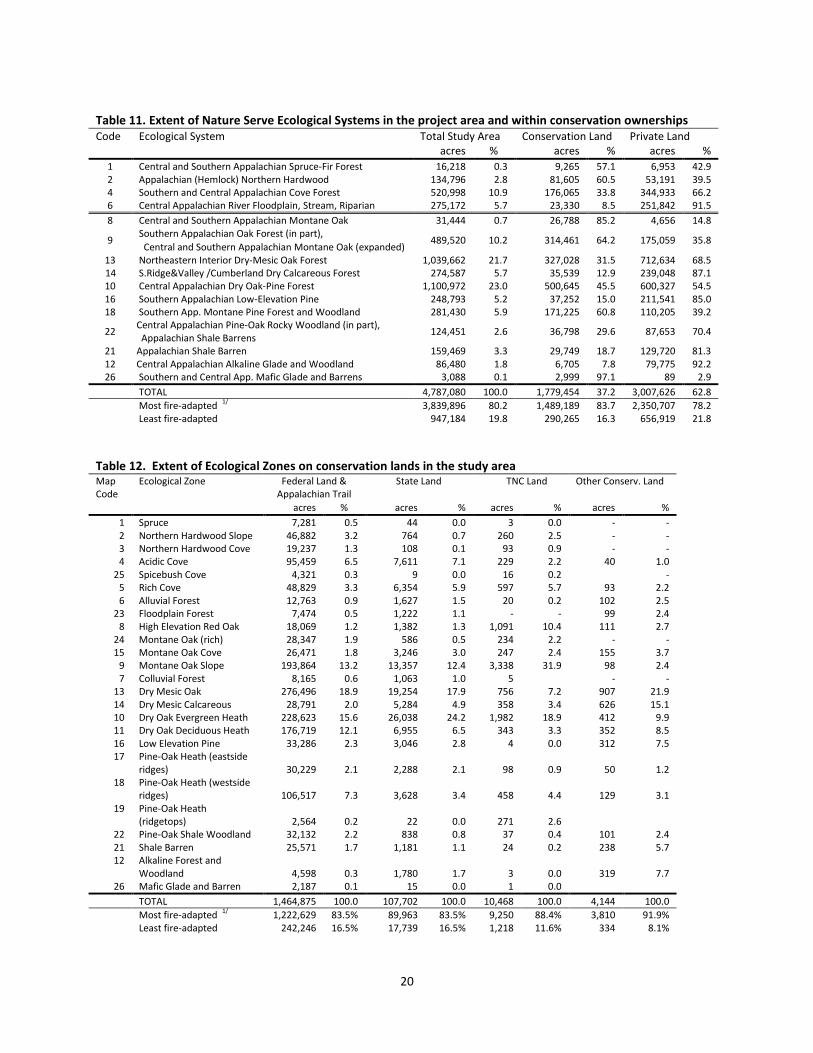
5) Extent and location of fire-adapted plant communities: Ecological Zone maps for the GW project area can be used to identify landscapes that support fire-adapted plant communities. Clearly well over 90% of the reference plot data occurring in types considered as more fire-adapted, are found within Ecological Zones correctly modeled as fire-adapted (Table 7 and Appendix V). Only 7 of the types have fire-adapted group accuracy below 95%. They include (from least to most accurate), Colluvial Forest (69%), Spicebush Cove (71%), Rich Cove 87%), Acidic Cove (88%), Northern Hardwood Slope (90%), Alluvial Forest (91%), and Pine-Oak Heath ridge (91%). Ecological Zone and Nature Serve Ecological System maps can also be used to evaluate fire restoration needs in different areas (Tables 10-12, and Appendix VI), for example, on Federal Land, State Land, TNC land, or other conservation land within the project area. Although Federal land, because of its greater proportion in the project area obviously has the greatest number of acres that may need restoration through the use of controlled burning, the relative proportion of a type within an ownership may indicate differences in priorities. For example, Central Appalachian Dry-Oak Pine Forest, Northeastern Interior Dry-Mesic Oak Forest, and Southern Appalachian Oak Forest / Central and Southern Appalachian Montane Oak (expanded concept) account for the largest proportion, respectively, of TNC lands, Federal lands, State lands, and other conservation lands. In addition, there is a larger percent of TNC lands (88.4) and other conservation lands (91.9) in the most fire-adapted types than there are on Federal (83.5) or State (83.5) lands which may also indicate different needs or priorities within these ownerships.

20

Table 11. Extent of Nature Serve Ecological Systems in the project area and within conservation ownerships Code Ecological System Total Study Area Conservation Land Private Land acres % acres % acres %

1 Central and Southern Appalachian Spruce-Fir Forest 16,218 0.3 9,265 57.1 6,953 42.9 2 Appalachian (Hemlock) Northern Hardwood 134,796 2.8 81,605 60.5 53,191 39.5 4 Southern and Central Appalachian Cove Forest 520,998 10.9 176,065 33.8 344,933 66.2 6 Central Appalachian River Floodplain, Stream, Riparian 275,172 5.7 23,330 8.5 251,842 91.5

8 Central and Southern Appalachian Montane Oak 31,444 0.7 26,788 85.2 4,656 14.8

9 Southern Appalachian Oak Forest (in part),

489,520 10.2 314,461 64.2 175,059 35.8 Central and Southern Appalachian Montane Oak (expanded)

13 Northeastern Interior Dry-Mesic Oak Forest 1,039,662 21.7 327,028 31.5 712,634 68.5 14 S.Ridge&Valley /Cumberland Dry Calcareous Forest 274,587 5.7 35,539 12.9 239,048 87.1 10 Central Appalachian Dry Oak-Pine Forest 1,100,972 23.0 500,645 45.5 600,327 54.5 16 Southern Appalachian Low-Elevation Pine 248,793 5.2 37,252 15.0 211,541 85.0 18 Southern App. Montane Pine Forest and Woodland 281,430 5.9 171,225 60.8 110,205 39.2

22 Central Appalachian Pine-Oak Rocky Woodland (in part), Appalachian Shale Barrens

124,451 2.6 36,798 29.6 87,653 70.4

21 Appalachian Shale Barren 159,469 3.3 29,749 18.7 129,720 81.3 12 Central Appalachian Alkaline Glade and Woodland 86,480 1.8 6,705 7.8 79,775 92.2 26 Southern and Central App. Mafic Glade and Barrens 3,088 0.1 2,999 97.1 89 2.9

TOTAL 4,787,080 100.0 1,779,454 37.2 3,007,626 62.8

Most fire-adapted 1/ 3,839,896 80.2 1,489,189 83.7 2,350,707 78.2 Least fire-adapted 947,184 19.8 290,265 16.3 656,919 21.8

Table 12. Extent of Ecological Zones on conservation lands in the study area Map Code

Ecological Zone Federal Land & Appalachian Trail

State Land TNC Land Other Conserv. Land

acres % acres % acres % acres %

1 Spruce 7,281 0.5 44 0.0 3 0.0 - - 2 Northern Hardwood Slope 46,882 3.2 764 0.7 260 2.5 - - 3 Northern Hardwood Cove 19,237 1.3 108 0.1 93 0.9 - - 4 Acidic Cove 95,459 6.5 7,611 7.1 229 2.2 40 1.0

25 Spicebush Cove 4,321 0.3 9 0.0 16 0.2 - 5 Rich Cove 48,829 3.3 6,354 5.9 597 5.7 93 2.2 6 Alluvial Forest 12,763 0.9 1,627 1.5 20 0.2 102 2.5

23 Floodplain Forest 7,474 0.5 1,222 1.1 - - 99 2.4 8 High Elevation Red Oak 18,069 1.2 1,382 1.3 1,091 10.4 111 2.7

24 Montane Oak (rich) 28,347 1.9 586 0.5 234 2.2 - - 15 Montane Oak Cove 26,471 1.8 3,246 3.0 247 2.4 155 3.7

9 Montane Oak Slope 193,864 13.2 13,357 12.4 3,338 31.9 98 2.4 7 Colluvial Forest 8,165 0.6 1,063 1.0 5 - -

13 Dry Mesic Oak 276,496 18.9 19,254 17.9 756 7.2 907 21.9 14 Dry Mesic Calcareous 28,791 2.0 5,284 4.9 358 3.4 626 15.1 10 Dry Oak Evergreen Heath 228,623 15.6 26,038 24.2 1,982 18.9 412 9.9 11 Dry Oak Deciduous Heath 176,719 12.1 6,955 6.5 343 3.3 352 8.5 16 Low Elevation Pine 33,286 2.3 3,046 2.8 4 0.0 312 7.5 17 Pine-Oak Heath (eastside

ridges) 30,229 2.1 2,288 2.1 98 0.9 50 1.2 18 Pine-Oak Heath (westside

ridges) 106,517 7.3 3,628 3.4 458 4.4 129 3.1 19 Pine-Oak Heath

(ridgetops) 2,564 0.2 22 0.0 271 2.6 22 Pine-Oak Shale Woodland 32,132 2.2 838 0.8 37 0.4 101 2.4 21 Shale Barren 25,571 1.7 1,181 1.1 24 0.2 238 5.7 12 Alkaline Forest and

Woodland 4,598 0.3 1,780 1.7 3 0.0 319 7.7 26 Mafic Glade and Barren 2,187 0.1 15 0.0 1 0.0

TOTAL 1,464,875 100.0 107,702 100.0 10,468 100.0 4,144 100.0

Most fire-adapted 1/ 1,222,629 83.5% 89,963 83.5% 9,250 88.4% 3,810 91.9% Least fire-adapted 242,246 16.5% 17,739 16.5% 1,218 11.6% 334 8.1%

21

Improving Map Unit Accuracy The accuracy of the 1

st approximation Ecological Zone map is good In comparison to other similar Ecological Zone

modeling efforts in the Southeastern U.S. (Table 7), but can be improved. Model accuracy can be affected by several major factors: 1) plot location accuracy, 2) Ecological Zone identification, 3) DTM accuracy, and 4) modeling methods. 1) Plot location accuracy: Incorrect plot locations from poor GPS readings or inaccurate topographic map interpretations can lead to erroneous data and therefore models that do not reflect reality. Furthermore ‘ecotone’ samples can and may have contributed to modeling errors in the project area. This reality was confirmed by results of the post-processing procedures used to reduce data noise and produce a cleaner product in 2009 within the VA-WVA FLN. Using just 3 majority filters of the ‘raw’ model, 52 of the 1,321 reference plots (about 4%), shifted into different Ecological Zone map units; 17 of these moved to incorrect classes and thus reduced the overall accuracy by about 2% points. The majority filter command merely replaces individual 1/40

th acre cells in a

grid based on the majority of their contiguous neighboring cells, a change that would only occur on the edges or interior of a type. These changes observed in plot accuracy indicate the close proximity of these ‘shifted’ plots to the narrow moisture-temperature-fertility gradients that occur between many Ecological Zones, i.e. the ecotone which is certainly largest around sample sites near ecotones. Although difficult to capture in GIS modeling, this variability in environmental conditions over short distances is common in the study area where numerous Ecological Zones may be encountered while traversing along only a 100 meter transect in highly dissected landscapes. 2) Ecological Zone field identification: The identification of reference condition (the Ecological Zone) at individual site locations is of equal or greater importance as plot location accuracy in developing a truer representation of landscapes that may have existed prior to Euro-American settlement. Ecological Zone models are evaluated from a sample of plot locations in a project area and from the interpretation of data collected from these areas that describe existing vegetation and often only remnant site indicator species. Incorrect identification of the Ecological Zone can therefore have a major impact on the outcome of map unit extent and accuracy especially for those zones that are hard to recognize because of past disturbance or because of lack of experience in the area by the observer. 3) DTM accuracy: The accuracy of DTMs used to reflect temperature, moisture, and fertility gradients, especially geologic / lithologic type in the project area, have a significant impact on Ecological Zone map unit accuracy. Lithology in the project area influences soil fertility, (also slope and aspect), thus having a major influence on the distribution of Ecological Zones across the complex background of temperature and moisture regimes described by other DTMs. Although lithologic map units were aggregated into just five distinct groups, there were still differences between these grouped map units across State lines; not only map line differences but also map unit labeling differences. An improvement in map unit accuracy could be possible by correlating lithologic map units between among the State-wide maps and those acquired from the GW-Jeff and Shenandoah Park. 4) Modeling methods. The 1

st approximation Ecological Zones are based on merging 25 individual Ecological Zone

models into one map based upon the zone having the highest probability of occurrence. Although this seems to be a reasonable approach, other techniques might be evaluated. For example, choosing a threshold probability value for each type that maximizes the correct plot inclusion and minimizes inclusion of plots representing other types could be used to map the location of individual zones having their greatest probability of occurrence. This coverage could then be merged with the 1

st approximation to fill areas where these conditions are not met.

22

Literature cited.

Bolstad, P. V., Swank, W. and Vose, J. 1998. Predicting Southern Appalachian overstory vegetation with digital terrain data. Landscape Ecology 13:271-283. ECOMAP. 1993. National hierarchical framework of ecological units. Washington, DC: U.S. Department of Agriculture, Forest Service. 20 pg.

DOD - Department of Defense, Camp Lejeune Marine Corp Base, 2006. Integrated Natural Resource Management Plan, Camp Lejeune, North Carolina. www.lejeune.usmc.mil/emd/INRMP/INRMP Fels, J. E. 1994. Modeling and mapping potential vegetation using digital terrain data. Ph.D. Dissertation, North Carolina State University; Raleigh, North Carolina. Fleming, Gary P. and Karen D. Patterson. 2010. Natural Communities of Virginia: Ecological Groups and Community Types. Natural Heritage Technical Report 10-11. Virginia Department of Conservation and Recreation, Division of Natural Heritage, Richmond, Virginia. 35 pages. Frost, C.C. 1996. Presettlement vegetation and natural fire regimes of the Croatan National Forest. North Carolina Department of Agriculture, Plant Conservation Program. 128 pp. Iverson, L. R., M. E. Dale, C. T. Scott, and A. Prasad. 1997. A GIS-derived integrated moisture index to predict forest composition and productivity of Ohio forests (U. S. A.). Landscape Ecology 12:331-348. LANDFIRE. URL: http://www.landfire.gov/NationalProductDescriptions20.php - 43KB - 29 Jan 2009 NatureServe. 2010. NatureServe Explorer online. http://www. natureserve.org NatureServe, 1101 Wilson Boulevard, 15

th Floor, Arlington, VA.

McNab, W. H. 1991. Predicting forest type in Bent Creek Experimental Forest from topographic variables. In: Coleman, Sandra S.; Neary, Daniel G., comps. Eds. Proceedings of the sixth biennial southern silvicultural research conference; 1990 October 30-Noverber 1: Memphis, TN. Gen. Tech. Rep. SE-70. Asheville, NC: U.S. Department of Agriculture, Forest Service, Southeastern Forest Experiment Station. 496-504. (2 vols.) McNab, W. H. 1993. A topographic index to quantify the effect of mesoscale landform on site productivity. Canadian Journal of Forest Research 23:1100-1107. McNab, W. Henry; Avers, Peter E., comps. 1994 Ecological subregions of the United States: Section descriptions. Administrative Publication WO-WSA-5. Washington, DC: U.S. Department of Agriculture, Forest Service. 267p. Pearson, Scott M, and Dawn M. Dextraze. 2002. Mapping Forest Communities of the Jacob Fork Watershed, South Mountains State Park. Mars Hill College Biology Department, Mars Hill, NC. Phillips, R. J. 2000. Classification and predictive modeling of plant communities in the Gorges State Park and Gamelands, North Carolina. M.S. thesis. North Carolina State University; Raleigh, North Carolina. Phillips, S.J., M. Dudik, and R.E. Shapire. 2004. A maximum entropy approach to species distribution modeling. Pages 655-662 in Proceedings 21st International Conference of Machine Learning, Banff, Canada. ACM Press, New York. Phillips, S.J., R.P. Anderson, and R.E. Shapire. 2006. Maximum entropy modeling of species geographic distribution. Ecol. Modeling 190:231-259. Phillips, S.J., R.P. Anderson, and R.E. Shapire. 2006.

23

Simon, Steven A.,; Collins, Thomas K.; Kauffman, Gary L.; McNab, W. Henry; Ulrey, Christopher J. 2005. Ecological Zones in the Southern Appalachians: first approximation. Res. Pap. SRS-41, Asheville, NC: U.S. Department of Agriculture, Forest Service, Southern Research Station. 41 p. Simon, Steven A. 2008. Second Approximation of Ecological Zones in the Southern Appalachian Mountains. The Nature Conservancy, Southern Region. Unpublished report. Simon, Steven A. 2010. Ecological Zones in the Kentucky Fire Learning Network Project Area. Nature Conservancy, Kentucky Field Office. Unpublished report. Story, M., and R. Congalton. 1986. Accuracy assessment: a user’s perspective. Photogrammetric Engineering and Remote Sensing, 52, pp. 397-399. Nature Serve (2010). Nature Serve Ecological Systems. USDA. Forest Service. 1995. Classification, Mapping, and Inventory of the Chattooga River Watershed. R8- Regional Office, Atlanta, GA., Unpublished report. USDA, Forest Service, 2002. Croatan National Forest Land and Resource Management Plan, Asheville, North Carolina. www.cs.unca.edu/nfsnc/nepa/croatan_plan/croatan_plan.pdf USDA, Forest Service, 2004. Management Indicator Species Habitat and Population Trends, Nantahala and Pisgah National Forests 8/30/2004, National Forests in North Carolina, Asheville, NC. Unpublished report, 815 pgs. USDA, Forest Service, 2005. The Suppression of Hemlock Woolly Adelgid Infestations On The Nantahala and Pisgah National Forests (USDA 2005), Atlanta, GA. http://www.cs.unca.edu/nfsnc/nepa/hwa_dn.pdf USDA, Forest Service, 2005. Amending the Nantahala and Pisgah Land and Resources Management Plan – Changing the List of Management Indicator Species, the Species Groups to be Monitored, and Associated Changes to Forest Plan Directions, Asheville, North Carolina. www.cs.unca.edu/nfsnc/ nepa/mis_decision.pdf USDA, Forest Service, 2006. Southern Region Existing Vegetation Mapping Pilot Test Report. Atlanta, Georgia, unpublished report. USDA, Forest Service, 2009. Uwharrie National Forest Land and Resource Management Plan Revision, Asheville, North Carolina. www.cs.unca.edu/nfsnc/uwharrie_plan/ Thomas-Van Gundy, Melissa A.; Nowacki, Gregory J.; Schuler, Thomas M. 2007. Rule-based mapping of fire-adapted vegetation and fire regimes for the Monongahela National Forest. Gen. Tech. Rep. NRS-12. Newtown Square, PA; U.S. Department of Agriculture, Forest Service, Northern Research Station. 24p. Virginia Natural Communities (2010): http://www.dcr.virginia.gov/naturalheritage/ncTIg.shtml. Wilds, S. P. 1997. Gradient analysis of the distribution of a fungal disease of Cornus florida in the Southern Appalachians, Tennessee. Journal of Vegetation Science 8:811-818.

24

Appendix I: Ecological Zone cross-walks

Ecological Zones were cross-walked with Nature Serve Ecological Systems and Virginia Natural Heritage Natural Community Groups by comparing field observations with descriptions of indicator species and species with high constancy or abundance identified in the “Ecological Zones in the Southern Appalachians: First Approximation” (1st approximation NC), from descriptions of dominant species and site relationships in Nature Serve Ecological Systems (2010), and Virginia Natural Heritage Program Natural Communities (2010). The following descriptions were excerpted from these sources. Additional Ecological Zone site or vegetation indicators not included in the NC 1st approximation but identified from local knowledge within the Appalachian Ridges and Blue Ridge study area are indicated by italics.

In general, it was not difficult to find agreement (to cross-walk) among these three ecological interpretations (Ecological Zones, Ecological Systems, and VA Heritage Natural Community Groups) that may break an environmental gradient at different points, except for the dry-mesic and mesic oak-dominated types. This should be considered normal, i.e., the hardest distinction in any ecological classification is between those types that are the most extensive and the most similar in species composition and landscape position such as the oak systems in the Appalachians. Although ‘fire adaptation’ was not considered in the Ecological Zone breaks, this disturbance component is nonetheless an important factor that could help to define the limits of “natural” plant community distribution. Additional information that was used to develop and evaluate the ‘cross-walk’ included the confusion, i.e., commission and omission errors among oak-dominated types indicated in the accuracy evaluation matrix (Appendix V), and the landscape distribution of Ecological Zones versus the distribution of LANDFIRE’s Biophysical Settings (BPS) in the project area.

Spruce-Fir Ecological Zone This zone includes spruce, fir, spruce-fir, and yellow birch-spruce forests and high elevation successional tree, shrub, and sedge communities. This type is the dominant zone at the highest elevations in the Southern Blue Ridge Mountains. Indicator species and species with high constancy or abundance include: Fraser fir, red spruce, mountain ash, yellow birch, mountain woodfern, Pennsylvania sedge, mountain woodsorrel, hobblebush, fire cherry, clubmoss, various bryophytes, and Catawba rhododendron.

Nature Serve -- Central and Southern Appalachian Spruce-Fir Forest: This system consists of forests in the highest elevation zone of the Blue Ridge and parts of the Central Appalachians generally dominated by red spruce, Fraser fir, or by a mixture of spruce and fir. Elevation and orographic effects make the climate cool and wet, with heavy moisture input from fog as well as high rainfall. Understory species are variable and include rhododendron, mountain woodsorrel, hobblebush, Pennsylvania sedge, mountain ash, and various mosses.

VA Heritage – Spruce and Fir Forests: Communities in this group are characterized by coniferous and mixed forests with overstory dominance by red spruce or Fraser fir. Habitats are characterized by extremely acidic, organic-rich soils; cold microclimates; high rainfall; frequent fogs; and lush bryophyte cover. Understory layers are sparse, while mountain wood-fern and mountain wood-sorrel dominate a relatively dense herb layer.

Northern Hardwood Ecological Zone (slopes and cove) This zone was split into two zones -- Northern Hardwood Slopes, and Northern Hardwood Coves in the second approximation (Simon 2008), (2

nd approximation NC), and in the VA_WVA FLN study area. The Northern

Hardwood Slopes include beech gaps, and Northern Hardwood plant communities occurring on upper slopes and ridges. Indicator species include: American beech, Pennsylvania sedge, northern red oak, eastern hemlock, striped maple, sweet birch, hay-scented fern, and Allegheny service berry. Northern Hardwood Coves include high elevation boulder fields, and Northern Hardwood plant communities that occur on toeslopes, and coves, i.e., broad to narrow concave drainages at higher elevations. In the Southern Appalachians, this type occurs as the highest elevation extension of Rich Coves. Indicator species and species with high constancy or abundance

25

include yellow birch, sugar maple, black cherry, northern red oak, mountain holly, Basswood, Canadian woodnettle, and ramps. --- Northern Hardwood Slopes:

Nature Serve – Appalachian (Hemlock)-Northern Hardwood: This system is one of the matrix forest types in the northern part of the Central Interior and Appalachian Division. Northern hardwoods such as sugar maple, yellow birch, and beech are characteristic, either forming a deciduous canopy or mixed with eastern hemlock. Other common and sometimes dominant trees include northern red oak, tulip poplar, black birch, and sweet birch. Understory species include striped maple, Christmas fern, evergreen woodfern, maple-leaf viburnum, jack-in-the-pulpit, and mountain holly.

VA Heritage – Central Appalachian Northern Hardwood Forests: These mixed hardwood forests are prevalent at high elevations but are more common northward in the high Allegheny Mountains to the unglaciated Allegheny Plateau of northern Pennsylvania and Southern New York. In Virginia, sugar maple, black cherry, northern red oak, red maple, and sweet birch are the most abundant overstory trees while American beech, yellow birch, and eastern hemlock are less frequent co-dominants. Striped maple and mountain holly are the chief understory species. The herb layers of many stands are characterized by patch-dominance of hay-scented fern.

VA Heritage – Appalachian Hemlock-Northern Hardwood Forests: This association includes hemlock - northern hardwood forests of the northeastern United States associated with cool, dry-mesic to mesic sites and acidic soils, often on rocky, north-facing slopes. While hemlock generally forms at least 50% of the canopy, in some cases it may be as low as 25% relative dominance. Hardwood codominants include yellow birch or sugar maple, with beech common but not usually abundant. The shrub layer may be dense to fairly open and often includes maple-leaved viburnum and striped maple. Herbs may be sparse but include evergreen woodfern, Indian cucumber-root, common wood sorrel, Canadian lily-of-the-valley, Christmas fern, hay-scented fern, and New York fern.

--- Northern Hardwood Cove:

Nature Serve – Appalachian (Hemlock)-Northern Hardwood: This system is one of the matrix forest types in the northern part of the Central Interior and Appalachian Division. Northern hardwoods such as sugar maple, yellow birch, and beech are characteristic, either forming a deciduous canopy or mixed with eastern hemlock. Other common and sometimes dominant trees include northern red oak, tulip poplar, black birch, and sweet birch. Understory species include striped maple, Christmas fern, evergreen woodfern, maple-leaf viburnum, jack-in-the-pulpit, and mountain holly.

VA Heritage – High-Elevation Cove Forests: Protected concave slope and ravines at elevation from 3,500’ to 4,800’ on the highest mountains of Virginia support the mixed mesophytic hardwood (rich) or coniferous-deciduous (acidic) forests of this group. Overstory dominants in richer high-elevation cove forests include sugar maple, yellow birch, basswoods, American beech, white ash, and yellow buckeye. Stands typically have lush herb layers with patch-dominance of mountain bugbane, ramps, blue cohosh, Goldie’s wood-fern, wood nettle, and many others. The acidic forests in this group were placed in the Acidic Cove Ecological Zone.

Acidic Cove Ecological Zone This zone includes hemlock and mixed hardwood-conifer forests typically dominated by an evergreen understory occurring in narrow coves (ravines) and often extending well up on adjacent protected, north-facing slopes. Indicator species and species with high constancy or abundance include great rhododendron, eastern hemlock, black birch, heartleaf species, partridgeberry, mountain doghobble, eastern white pine, yellow-poplar, common greenbrier, chestnut oak, and red maple.

26

Nature Serve – Southern and Central Appalachian Cove Forest: This system consists of mesophytic hardwood or hemlock-hardwood forests of sheltered topographic positions. Examples are generally found on concave slopes that promote moist conditions. The system includes a mosaic of acidic and “rich” coves that may be distinguished by individual plant communities based on perceived difference in soil fertility and species richness. Both acidic and rich coves may occur in the same site, with the acidic coves potentially creeping out of the draw-up to at least midslope on well-protected north-facing slopes. Characteristic species in the canopy include yellow buckeye, sugar maple, white ash, American basswood, tulip poplar, silverbell, eastern hemlock, American beech, and magnolias. Understories can include high diversity and density in the herbaceous layer or a sparse herbaceous layer over-topped by dense rhododendron and / or dog hobble. Obviously only the acidic cove sites in this type correspond to the Acidic Cove Ecological System.

VA Heritage – Acidic Cove Forests: This group contains mixed hardwood and hardwood-hemlock forests of infertile, mesic, mountain-slope habitats. In Virginia, these forests occupy moist lower slopes, ravines, and coves underlain by sandstone, quartzite, or other acidic bedrock. Typical overstory trees include tulip poplar, eastern hemlock, red maple, sweet and yellow birch, eastern white pine, cucumber magnolia, and Fraser magnolia in variable mixtures. American beech is an important overstory tree in northern Blue Ridge and Cumberland Mountain stands. Dense, evergreen shrub layers of great rhododendron are characteristic. Some Acidic Cove Forests have an “evergreen-lush” herb layer, with species such as galax and Christmas fern forming large colonies.

VA Heritage – Eastern Hemlock-Hardwood Forests: Forests of this group are characterized by the dominance or co-dominance by eastern hemlock in nearly every vertical stratum. In Virginia, stands occupy mesic, sheltered habitats throughout the mountains. A number of tree associates, especially sweet and yellow birch, northern red oak, chestnut oak and eastern white pine, usually contribute to mixed overstories, but the total cover of overstory and understory hemlock in these forests usually exceeds that of any other species. Eastern Hemlock-Hardwood Forests are closely related to Acidic Cove Forests but generally have a less diverse composition of woody species, a greater dominance of hemlock in all strata, and considerably lower species richness.

VA Heritage – High-Elevation Cove Forests: Protected concave slope and ravines at elevations from 3,500’ to 4,800’ on the highest mountains of Virginia support the mixed mesophytic hardwood (rich) or coniferous-deciduous (acidic) forests of this group. Overstory dominants in acidic cove forests typically have overstories of yellow birch, eastern hemlock, and sometimes red spruce, with a dense shrub layer of great rhododendron. The herb layer is sparse and contains a number of northern species that are restricted to the higher elevations in Virginia. The rich forests in this group were placed in the Northern Hardwood Cove Ecological Zone.

Spicebush Cove Ecological Zone This zone was not included in the 1

st approximation NC. It includes a variant of Rich Coves where spicebush is the

diagnostic shrub and often dense enough to limit the abundance of more typical ‘rich herb’ species such as black cohosh, blue cohosh, mandarin, northern maidenhair fern, wood nettle, rattlesnake fern, and mountain sweet-cicely found on these sites. Typically forests are dominated by tulip poplar with co-dominant white ash, American basswood, and cucumber magnolia. This zone was modeled only in the Blue Ridge although it was observed occasionally in the Appalachian Ridges study area but along narrow ephemeral streams. It was included with Rich Coves in the Appalachian Ridges.

Nature Serve – Southern and Central Appalachian Cove Forest: This system consists of mesophytic hardwood or hemlock-hardwood forests of sheltered topographic positions. Examples are generally found on concave slopes that promote moist conditions. The system includes a mosaic of acidic and “rich” coves that may be distinguished by individual plant communities based on perceived difference in soil fertility and species richness. Both acidic and rich coves may occur in the same site, with the acidic coves potentially creeping out of the draw-up to at least midslope on well-protected north-facing slopes. Characteristic species in the canopy include yellow buckeye, sugar maple, white ash, American basswood

27

VA Heritage – Appalachian Rich Cove Forest: This association represents deciduous forests of concave lower slopes and flats at middle elevations (2000-4500 feet) in the Southern Blue Ridge and at low to middle elevations (650-3000 feet) in the Northern Blue Ridge and adjacent Ridge and Valley. The canopy is dominated by some mixture of rich-site mesophytic species such as white ash, American basswood, yellow buckeye, and cucumber magnolia occurring with more widely tolerant tree species such as tulip poplar, red maple, eastern hemlock, and black birch. The most diagnostic species (relative to similar types) are spicebush, hogpeanut, tulip poplar, black cohosh, Christmas fern, and showy orchid. This association is also distinguished by the absence or scarcity of calciphilic species, such as glade fern, walking fern, Goldie’s fern, red columbine, zig-zag goldenrod, silvery glade fern, and lowland bladder fern.

Rich Cove Ecological Zone This zone includes mixed mesophytic forests typically dominated by a diverse herbaceous understory and occurs in broader coves and on adjacent protected slopes (mostly north to north-east facing). Indicator species and species with high constancy or abundance include black cohosh, American ginseng, blue cohosh, mandarin, bloodroot, northern maidenhair fern, Dutchman’s pipe, rattlesnake fern, mountain sweet-cicely, Appalachian basswood, yellow buckeye, white ash, yellow-poplar, wood nettle, cucumber magnolia, and northern red oak.

Nature Serve – Southern and Central Appalachian Cove Forest: This system consists of mesophytic hardwood or hemlock-hardwood forests of sheltered topographic positions. Examples are generally found on concave slopes that promote moist conditions. The system includes a mosaic of acidic and “rich” coves that may be distinguished by individual plant communities based on perceived difference in soil fertility and species richness. Both acidic and rich coves may occur in the same site, with the acidic coves potentially creeping out of the draw-up to at least midslope on well-protected north-facing slopes. Characteristic species in the canopy include yellow buckeye, sugar maple, white ash, American basswood, tulip poplar, silverbell, eastern hemlock, American beech, and magnolias. Understories can include high diversity and density in the herbaceous layer or a sparse herbaceous layer over-topped by dense rhododendron and / or dog hobble. Obviously only the “rich” cove sites correspond to the Rich Cove Ecological System.

VA Heritage – Central and Southern Appalachian Rich Cove and Slope Forests: Mixed hardwood forests of this group occupy fertile, mesic, mountain-slope habitats and are strongly associated with moist, sheltered landforms (i.e., coves, ravines, and concave lower slopes). Characteristic trees include sugar maple, basswoods, white ash, tulip poplar, and yellow buckeye. Herbaceous growth is lush with spring ephemerals and leafy, shade-tolerant forbs such as blue cohosh, yellow jewelweed, large-flowered trillium, wood nettle, black bugbane, sweet cicely, yellow mandarin, and many others.

VA Heritage – Basic Mesic Forests: This group is represented by forests occurring in fertile, mesic, low-elevation valleys of the Appalachian region. Typical sites are sheltered north- or east-facing slopes subtending large streams and rivers. Dominant trees include the species of Rich Cove and Slope Forests, as well as chinkapin oak, black maple, southern sugar maple, American beech, Bitternut hickory, and black walnut. Shrub and herb layers contain a number of species that are atypical of mountain slopes, such as paw-paw, painted buckeye, twinleaf, harbinger-of-spring, lowland brittle fern, and toadshade. This group, although sampled in the field especially on the lower slopes at Lake Moomaw, was lumped with the Rich Cove Ecological Zone because of its limited extent.

Alluvial and Floodplain Forest Ecological Zones These zones were not included in the 1st approximation NC but were added in the 2

nd approximation as an

aggregated type. Although modeling results for these zones were poor in the 2nd

approximation they were improved significantly in the South Mountains, Northern Escarpment, Kentucky, and the VA_WVA FLN project areas by adding additional DTMs that describe the elevation of this zone relative to stream and river elevations.

28

This zone characterizes small to large floodplains that support alluvial forests and imbedded riparian areas and overlap with smaller riparian areas associated with sites adjacent to streams that support Acidic Cove or Rich Cove Ecological Zones. Characteristic trees in the Alluvial Forest zone include sycamore, river birch, silver maple, tulip poplar, and box elder. The understory is highly variable, depending upon the time since the last ‘flooding’ event but common species may include paw-paw, spicebush, and switchgrass. Most all of the Floodplain Ecological Zone has been highly altered, not in USFS ownership or other conservation tracts, likely farmed by Native Americans, and therefore difficult to characterize. They are even more difficult to characterize if we consider Ecological Zones equivalent to BpS mapping units that include Native American influences, especially burning, as part of the ‘natural environment’ that shaped the composition and structure of vegetation that occurs within this zone. Therefore, the description of both the Alluvial and Floodplain Forest Ecological Zones is left unformulated at this point and, instead, relies heavily on TNC Ecological System and VA Heritage Ecological Group and Association descriptions.

Nature Serve – Central Appalachian River Floodplain: This system encompasses floodplains of medium to large rivers and can include a complex of wetland and upland vegetation on deep alluvial deposits and scoured vegetation on depositional bars and on bedrock where rivers cut through resistant geology. This complex includes floodplain forests in which silver maple, cottonwood, and sycamore are characteristic, as well as herbaceous sloughs, shrub wetlands, riverside prairies and woodlands. Most areas are underwater each spring; microtopography determines how long the various habitats are inundated. Depositional and erosional features may both be present depending on the particular floodplain.

Nature Serve – Central Appalachian Stream and Riparian: This riparian system occurs over a wide range of elevations and develops on floodplains and shores along river channels that lack a broad flat floodplain due to steeper sideslopes, higher gradient, or both. It may include communities influenced by flooding, erosion, or groundwater seepage. The vegetation if often a mosaic of forest, woodland, shrubland, and herbaceous communities. Common trees include river birch, sycamore, and box elder. Open, flood-scoured rivershore prairies feature switchgrass, big bluestem, and twisted sedge is typical of wetter areas near the channel.

VA Heritage – Piedmont / Mountain Floodplain Forests: These temporarily and intermittently flooded forests encompass most river floodplain habitats of the Piedmont and major mountain valleys. From the James River north, sandy river banks and first-bottom terraces that frequently (but shortly) flooded support forests dominated by silver maple and boxelder, with herb layers containing many broad-leaved forbs. Higher, better drained, sandy or silty river floodplains support mixed forest of sycamore, back walnut, hackberry, American elm, and boxelder, with understories of paw-paw and spicebush. Herb layers in the mixed floodplains are usually very lush with nutrient demanding, early-season species.

VA Heritage – Piedmont / Mountain Alluvial Forests: Forests in this group occupy temporarily flooded habitats along smaller-order streams, where distinct alluvial landforms (e.g., levees, terraces, and backswamps) occur at very small scales. These communities are found along many small rivers and streams throughout the Piedmont and mountain-region valleys. Habitats generally consist of narrow floodplains with fine to coarse alluvial soils; boulder or cobbly alluvium and rocky streambeds are typical in and at the foot of the mountains. Characteristic trees include sycamore, boxelder, American elm, green ash, river birch, red maple, sweetgum, yellow buckeye, black walnut, tulip poplar, and black willow.

VA Heritage- Mesic and Wet-Mesic Prairies: Vegetation in this group consists of tall grasslands occurring on moderately well drained to somewhat poorly drained floodplain terraces in mountain valleys of the Ridge and Valley region and in the southern Blue Ridge. The original, pre-colonial extent and the ecological dynamic which maintained them (e.g., fire, grazing) are now conjectural. The vegetation is dominated by the tall, warm-season grasses big bluestem and Indian grass.

High Elevation Red Oak Ecological Zone This zone includes forests dominated by northern red oak on exposed slopes and ridges at higher elevations. Site extremity and exposure results in stunted and often windswept tree form, however, there is a broad transition

29

between this extreme and the more common Montane Oak Ecological Zone; the break between these two types is complicated primarily by past management practices, especially timber harvest intensity and ground disturbance. Indicator species and species with high constancy or abundance include: northern red oak, American chestnut, flame azalea, whorled yellow loosestrife, Pennsylvania sedge, speckled wood-lily, highbush blueberry, mountain laurel, hayscented fern, witchhazel, striped maple, and New York fern.

Nature Serve -- Central and Southern Appalachian Montane Oak Forest: This generally oak-dominated system is found in the central and southern Appalachian Mountains. These high-elevation deciduous forests occur on exposed sites, including ridgecrests and south- to west-facing slopes. In most associations attributed to this system, the soils are thin, weathered, nutrient-poor, low in organic matter, and acidic. The forests are dominated by oaks, most commonly red oak and white oak with the individuals often stunted or wind-flagged. American chestnut sprouts are common. Characteristic shrubs include mountain holly and early azalea.

VA Heritage – Northern Red Oak Forests: Dominance by northern red oak characterizes these forests, which reach maximal importance at elevations above 3,000 ft. throughout western Virginia. Although composition varies with parent material and landscape position, prolonged weathering and limited accumulation of soil organic matter have generally resulted in moderately to strongly infertile soils and consequently moderate to low species richness. In addition to the prevalent red oaks, scattered associates of white oak, sweet birch, yellow birch, and black cherry are often present in the overstory. Typically small trees and shrubs include mountain holly, witch-hazel, striped maple, Minnie bush, early azalea, beaked hazelnut, and sprouts of American chestnut. Stands typically contain ground layers of hayscented fern, low ericaceous shrubs, or patches of graminoids such as Pennsylvania sedge and wavy hairgrass.

Montane Oak-Hickory (rich, slope, cove) Ecological Zones These zones includes mesic to submesic mixed-oak and oak-hickory forests that occur along broad mid- to higher elevation ridges and smooth to concave slopes below the highest and more narrow ridges where this zone forms a gradual transition to the High Elevation Red Oak and Northern Hardwood zones. It also includes drainage headlands at higher elevations that merge with Rich Coves and Northern Hardwood Cove Ecological Zones, mid to lower elevations in often narrow sub-mesic coves that merge with Dry-Mesic Ecological Zones, and more exposed slopes in very close proximity with High Elevation Red Oak Ecological Zones. Forests in this zone are often floristically diverse. Indicator species and species with high constancy or abundance include: northern red oak, white oak, flowering dogwood, tulip poplar, Canada richweed, mockernut hickory, New York fern, pignut hickory, white ash chestnut oak, magnolias, sweet birch, striped maple, and witchhazel --- Montane Oak-Hickory (Rich):

Nature Serve -- Central and Southern Appalachian Montane Oak Forest: This generally oak-dominated system is found in the central and southern Appalachian Mountains. These high-elevation deciduous forests occur on exposed sites, including ridgecrests and south- to west-facing slopes. In most associations attributed to this system, the soils are thin, weathered, nutrient-poor, low in organic matter, and acidic. The forests are dominated by oaks, most commonly red oak and white oak with the individuals often stunted or wind-flagged. American chestnut sprouts are common. Characteristic shrubs include mountain holly and early azalea. This Nature Serve Ecological System is an uncomfortable fit in the Montane Oak-Hickory (rich) Ecological Zone unless a broader Nature Serve concept is assumed that includes more sub-mesic forests.

VA Heritage – Central Appalachian Montane Oak Forest (Rich Type): Dominance by northern red oak characterizes these forests, This community is known from the southern part of the Central Appalachians, extending into the extreme northern portions of the Southern Blue Ridge, Southern Ridge and Valley, and Cumberland Mountains. It occurs throughout western Virginia and adjacent eastern West Virginia,

30

forming extensive patches on the Northern Blue Ridge and, somewhat more locally, on the higher ridges of the Ridge and Valley province. Favorable sites are upper slopes and ridge crests with deep, base-rich soils weathered from mafic and calcareous parent material, including metabasalt (greenstone), amphibolite, pyroxene-bearing granulite, charnockite, and actinolite schist. It also occurs on sites underlain by calcareous sandstone, siltstone, metasiltone, phyllite, and felsic granites with mafic clasts. Occurrences span a range of intermediate elevations, from 680-1265 m (2250-4150 feet), with a mean elevation of approximately 1000 m (3280 feet). Slopes are mostly gentle to moderate, averaging about 15 degrees. Aspect varies considerably, but a majority of stands are located on sites with southwestern to northwestern or flat exposures. Soils are mostly dark, friable loams and silt loams with variable chemistry, but typically high in calcium, magnesium, and/or manganese. The characteristic expression of this community is that of an oak or oak-hickory forest with an herb layer that resembles that of a rich cove forest. Quercus rubra is the most constant member of the overstory but usually shares dominance with Carya ovalis, Carya ovata, Fraxinus americana or, less frequently, other mesophytic hardwoods such as Tilia americana (both var. americana and var. heterophylla), Quercus alba, Carya cordiformis, Prunus serotina, and Betula lenta. Both Liriodendron tulipifera and Quercus prinus, which are ubiquitous in much of the Central Appalachians, are uncommon to rare in this community type. The subcanopy tends to be strongly dominated by Carya spp. and Fraxinus americana, with Acer saccharum, Acer rubrum, Acer pensylvanicum, and Ostrya virginiana also important in some stands. The shrub layer is typically sparse. Most stands have a lush and generally diverse herb layer, with total cover often exceeding 80% and strong patch-dominance by leafy, colonial forbs such as Actaea racemosa (= Cimicifuga racemosa), Ageratina altissima var. altissima, Hydrophyllum virginianum, Collinsonia canadensis, Caulophyllum thalictroides, Laportea canadensis, Impatiens pallida, Thalictrum coriaceum, and Asclepias exaltata. At higher elevations, where the type is transitional to northern red oak forests, Dennstaedtia punctilobula often dominates the herb layer in large clones.

--- Montane Oak-Hickory (Cove):

Nature Serve -- Northeastern Interior Dry-Mesic Oak Forest: These oak-dominated forests are one of the matrix forest systems in the northeastern and north-central U.S. Occurring in dry-mesic settings, they are typically closed-canopy forests, though there may be areas of patchy-canopy woodlands. They cover large expanses at low to mid elevations, where the topography is flat to gently rolling, occasionally steep. Soils are mostly acidic and relatively infertile but not strongly xeric. Local areas of calcareous bedrock, or colluvial pockets, may support forests typical of richer soils. Oak species characteristic of dry-mesic conditions (e.g., Northern red oak, white oak, black oak, and scarlet oak) and hickories are dominant in mature stands. Chestnut oak may be present but is generally less important than the other oak species. American chestnut was a prominent tree before chestnut blight eradicated it as a canopy constituent. Red maple, sweet birch, and yellow birch may be common associates; sugar maple is occasional. With a long history of human habitation, many of the forests are early- to mid-successional, where white pine, Virginia pine, or tulip poplar may be dominant or codominant. Within these forests, hillslope pockets with impeded drainage may support small isolated wetlands, including non-forested seeps or forested wetlands. This is an uncomfortable fit in the Northeastern Interior Dry-Mesic Oak Forest and represents the more colluvial and concave portions of the landscape that includes more mesic oak-dominated forests.

VA Heritage -- Montane Mixed Oak and Oak – Hickory Forests: This group contains relatively diverse, mixed oak and oak-hickory forests of submesic to subxeric mountain slopes and crests up to about 4,000’ elevation. Communities of this group are transitional to Northern Red Oak Forests at higher elevations. Overstory composition contains mixtures of chestnut oak, northern red oak, and white oak. Overstory associates vary with geography but often include sweet birch, magnolias, hickories, red maple, tulip poplar, and white pine. The understories usually contain some heaths, but also witch-hazel, striped maple, maple-leaved viburnum, flowering dogwood, mountain holly, and hazelnuts. More fertile sites often support a diverse herbaceous flora and may rival that of the Rich Cove and Slope Forests.

31

--- Montane Oak-Hickory (Slope):

Nature Serve -- Central and Southern Appalachian Montane Oak Forest: This generally oak-dominated system is found in the central and southern Appalachian Mountains. These high-elevation deciduous forests occur on exposed sites, including ridgecrests and south- to west-facing slopes. In most associations attributed to this system, the soils are thin, weathered, nutrient-poor, low in organic matter, and acidic. The forests are dominated by oaks, most commonly red oak and white oak with the individuals often stunted or wind-flagged. American chestnut sprouts are common. Characteristic shrubs include mountain holly and early azalea. Based on the Nature Serve description for this type, this is an uncomfortable fit in the Montane Oak-Hickory (Slope) Ecological Zone unless a broader Nature Serve concept is assumed that includes more sub-mesic forests. The majority of this Ecological Zone coincides with the LANDFIRE BpS - Montane Oak Ecological Systems map unit which may indicate that the LANDFIRE modelers were working with a broader concept (more similar to Ecological Zones) than what is being described in this Nature Serve type.

VA Heritage -- Montane Mixed Oak and Oak – Hickory Forests: This group contains relatively diverse, mixed oak and oak-hickory forests of submesic to subxeric mountain slopes and crests up to about 4,000’ elevation. Communities of this group are transitional to Northern Red Oak Forests at higher elevations. Overstory composition contains mixtures of chestnut oak, northern red oak, and white oak. Overstory associates vary with geography but often include sweet birch, magnolias, hickories, red maple, tulip poplar, and white pine. The understories usually contain some heaths, but also witch-hazel, striped maple, maple-leaved viburnum, flowering dogwood, mountain holly, and hazelnuts. More fertile sites often support a diverse herbaceous flora and may rival that of the Rich Cove and Slope Forests.

Colluvial Forest Ecological Zone This Ecological Zone was not in the 1

st or 2

nd approximations NC but was modeled in the VA-WVA FLN to

characterize the extensive, low elevation toe-slopes and ‘terraces’ above true alluvial floodplains found along most major 4

th order and larger streams. Based upon field observations of surface material, slope, and surface

configuration, substrates consist of cobble to boulder-sized rock of variable rock type. This zone is well above the floodplain (10 feet minimum) at its upper end (toward the confining mountain ridges) where it is moderate to moderately-steep sloping, but in broader valleys it is relatively flat and may be less than 10’ above the apparent floodplain. This zone is often dominated by white pine or more commonly by a mixture of white oak, white pine, red oak, black oak, hickories, and magnolias and is always in close proximity to Alluvial Forests. The moisture regime in these forests is dry-mesic to sub-mesic.

Nature Serve - Northeastern Interior Dry-Mesic Oak Forest: Oak-dominated matrix forest occurring in dry-mesic settings and covering large expanses at low to mid elevations. Characteristic species include red oak, white oak, black oak, scarlet oak, and hickories. Red maple, sweet birch, yellow birch may be common associates. With a long history of human habitation many of the forests are early to mid successional, where white pine, Virginia pine, or tulip poplar may be dominant or codominant.

VA Heritage -- Montane Mixed Oak and Oak – Hickory Forests: This group contains relatively diverse, mixed oak and oak-hickory forests of submesic to subxeric mountain slopes and crests up to about 4,000 ft elevation. Communities of this group are transitional to Northern Red Oak Forests at higher elevations. Overstory composition contains mixtures of chestnut oak, northern red oak, and white oak. Overstory associates vary with geography but often include sweet birch, magnolias, hickories, red maple, tulip poplar, and white pine. The understories usually contain some heaths, but also witch-hazel, striped maple, maple-leaved viburnum, flowering dogwood, mountain holly, and hazelnuts. More fertile sites often support a diverse herbaceous flora and rival that of the Rich Cove and Slope Forests.

VA Heritage -- Eastern White Pine-Hardwood Forests: This group is characterized by mixed forests having a co-dominance of eastern white pine and hardwoods. On submesic sites, codominant hardwoods include white oak, red oak, hickories, tulip poplar, and eastern hemlock while on subxeric sites; chestnut oak and scarlet oak are common co-dominants. The ecological dynamics of this group are poorly understood.

32

Dry-Mesic Oak Ecological Zone This zone was included in the Dry and Dry-Mesic Oak-Hickory type in the 1st approximation NC but separated into its components -- Dry Oak and Dry-Mesic Oak in the 2

nd approximation both in the KY FLN (Simon 2009) and in the

VA_WVA FLN study areas. This zone is very similar to the Montane Oak-Hickory zone but occurs at lower elevations. It includes dry-mesic, mixed-oak forests that occur along broad lower to mid elevation ridges and smooth to concave slopes and lower elevation drainage headlands, and often narrow, dry coves. Indicator species and species with high constancy or abundance include: white oak, black oak, scarlet oak, flowering dogwood, sourwood, low bush blueberry, and huckleberries.

Nature Serve - Northeastern Interior Dry-Mesic Oak Forest: Oak-dominated matrix forest occurring in dry-mesic settings and covering large expanses at low to mid elevations. Characteristic species include red oak, white oak, black oak, scarlet oak, and hickories. Red maple, sweet birch, yellow birch may be common associates. With a long history of human habitation many of the forests are early to mid successional, where white pine, Virginia pine, or tulip poplar may be dominant or codominant.

Nature Serve -- Southern Appalachian Oak Forest: This system consists of predominantly dry-mesic (to dry) forests occurring on open and exposed topography at lower to mid elevations. Characteristic species include chestnut oak, white oak, red oak, black oak, scarlet oak, with varying amounts of hickories, blackgum, and red maple. Some areas (usually on drier sites) now have dense evergreen ericaceous shrub layers. Northward this system grades into Northeastern Interior Dry-Mesic Oak Forest.

VA Heritage – Acidic Oak-Hickory Forests (in part): Forests in this group occupy submesic to subxeric upland sites over subacidic rocks. Dominant oaks include white oak, black oak, scarlet oak, southern red oak, and chestnut oak. Flowering dogwood is a characteristic, often dominant understory tree. Deciduous ericads, especially lowbush blueberry and deerberry, are usually present but patchy in the shrub layer. Herbaceous diversity is somewhat less than in Basic Oak-Hickory Forests but considerably greater than in Oak/Heath Forests.

Dry-Mesic Calcareous Forest Ecological Zone This Ecological Zone was not in the 1

st or 2

nd NC approximations and was modeled in the VA-WVA FLN study area

to characterize fairly common sites in this area that support Dry-Mesic forests on calcareous substrates. Characteristic trees include white oak, with sugar maple, black maple, northern red oak, chinkapin oak, and hickories. Characteristic understory species include redbud and black cohosh. In disturbed areas, autumn olive may be the dominant midcanopy shrub.

Nature Serve -- Southern Ridge and Valley / Cumberland Dry Calcareous Forest: This system includes dry to dry-mesic calcareous forests that occur in a variety of habitats and are the matrix vegetation type that covers most of these landscape under natural conditions. The range of this system is primarily composed of circumneutral substrates, which exert an expected influence on the composition of the vegetation. Characteristic species found in the plant associations in this type include white oak, northern red oak, chinkapin oak, sugar maple, juniper, and redbud.

VA Heritage – Dry-Mesic Calcareous Forests: This group of montane, mixed hardwood forest occupies submesic slopes and crests with southeast to southwest aspects and fertile soils weathered from underlying limestone, dolomite, calcareous sandstone, and calcareous siltstone. Habitats in western Virginia include valley sideslopes, lower mountain slopes, gentle crests, and ravines. Mixtures of sugar maple, black maple, white oak, northern red oak, black oak, and hickories are typical. Another variant lacks maples and features codominance by white oak, chinkapin oak, white ash and hickories. Understory and herbaceous vegetation varies from sparse to lush but is generally dominated by species characteristic of submesic soil moisture conditions, such as white snakeroot, hog-peanut, common eastern bromegrass, and black bugbane (cohosh).

33

Dry Oak Heath Ecological Zones (Mt. Laurel and Huckleberry-Vaccinium) This zone, called Chestnut Oak Heath in the 1st approximation NC, includes xeric to dry mixed-oak forests typically dominated by an ericaceous (evergreen or deciduous) understory and represents the driest zone where oaks are the dominant species. In general, on the George Washington NF, the Dry Oak/Huckleberry zone is more transitional to the Dry-Mesic Oak Ecological Zone and the Dry Oak/Mountain Laurel zone is more transitional to the Pine-Oak Heath Ecological Zone, however, this varies considerably according to slope position and the predominantly east or west-facing side of major ridges. Further work is needed to differentiate these two zones to separate what is truly an environmental influence and what may be an influence of current fire return interval. Indicator species and species with high constancy or abundance include: chestnut oak, scarlet oak, northern red oak, mountain laurel, black huckleberry, hillside blueberry, red maple, great rhododendron, and sourwood.

Nature Serve -- Central Appalachian Dry Oak-Pine Forest: These oak and oak-pine forests cover large areas at low- to mid-elevations. The forest is mostly closed-canopy but can include patches of more open woodlands. It is dominated by a variable mixture of dry-site oak and pine species, most typically chestnut oak, Virginia pine, and white pine, but sometimes white oak and/or scarlet oak. Heath species such as hillside blueberry, black huckleberry, and mountain laurel are common in the understory and often form a dense layer.

VA Heritage – Oak / Heath Forests: This group of oak-dominated forests is prominent on xeric infertile upland sites. Regionally varying mixtures of white oak, chestnut oak, scarlet oak, black oak, northern red oak, southern red oak, and post oak compose the overstories of these forests. Forests overwhelmingly dominated by chestnut oak are widespread on sandstone or quartzite ridges in the mountains. Ericaceous plants, including mountain-laurel, black huckleberry, wild azalea, and blueberries, form dense colonies in the shrub layer. Rhododendron and flame azalea are locally prevalent member of the ericaceous shrub complex in the mountains.

VA Heritage – Acidic Oak-Hickory Forests (in part): Forests in this group occupy submesic to subxeric upland sites over subacidic rocks. Dominant oaks include white oak, black oak, scarlet oak, southern red oak, and chestnut oak. Flowering dogwood is a characteristic, often dominant understory tree. Deciduous ericads, especially lowbush blueberry and deerberry, are usually present but patchy in the shrub layer. Herbaceous diversity is somewhat less than in Basic Oak-Hickory Forests but considerably greater than in Oak/Heath Forests.

Low Elevation Pine Ecological Zone / Shortleaf Pine-Oak Heath Ecological Zone This zone includes dry to dry-mesic pine-oak forests dominated by shortleaf pine or pitch pine that occur at lower elevations on exposed broad ridges and sideslopes. Indicator species and species with high constancy or abundance include: shortleaf pine, pitch pine, sourwood, sand hickory, scarlet oak, southern red oak, post oak, hillside blueberry, American holly, featherbells, black huckleberry, and spring iris.

Nature Serve -- Southern Appalachian Low-Elevation Pine: This system consists of shortleaf pine- and Virginia pine-dominated forests in the lower elevation Southern Appalachians and adjacent Piedmont and Cumberland Plateau. Examples can occur on a variety of topographic and landscape positions, including ridgetops, upper and midslopes, as well as low elevation mountain valleys in the Southern Appalachians. Under current conditions, stands are dominated by shortleaf pine and Virginia pine. Pitch pine may sometimes be present and hardwoods are sometimes abundant, especially dry-site oaks such as southern red oak, chestnut oak, scarlet oak, but also pignut hickory, red maple, and others. The shrub layer may be well-developed, with hillside blueberry, black huckleberry, or other acid-tolerant species most characteristic. Herbs are usually sparse but may include narrowleaf silkgrass and goat’s rue.

VA Heritage – VA Heritage – Oak / Heath Forests (in part): This group of oak-dominated forests is prominent on xeric infertile upland sites. Regionally varying mixtures of white oak, chestnut oak, scarlet oak, black oak, northern red oak, southern red oak, and post oak compose the overstories of these

34

forests. Forests overwhelmingly dominated by chestnut oak are widespread on sandstone or quartzite ridges in the mountains. Ericaceous plants, including mountain-laurel, black huckleberry, wild azalea, and blueberries, form dense colonies in the shrub layer. Rhododendron and flame azalea are locally prevalent member of the ericaceous shrub complex in the mountains.

VA Heritage – Pine – Oak / Heath Woodlands (in part): This group contains species-poor, mixed woodlands of xeric, exposed montane habitats. Short-statured Table Mountain pine and pitch pine are usually the dominants forming an open overstory, often with co-dominant chestnut oak. Bear oak is characteristically abundant in the shrub layer along with various ericaceous species.

Pine-Oak Heath Ecological Zone (Eastside, Westside, Ridges) This zone was included in the Xeric Pine-Oak Heath and Oak Heath type in the 1st approximation NC but separated into three pine-oak heath types in the VA_WVA FLN but as only one type, Pine-Oak Heath in the Blue Ridge. Indicator species and species with high constancy or abundance in all three types include: Table Mountain pine, scarlet oak, chestnut oak, pitch pine, black huckleberry, mountain laurel, hillside blueberry, bear oak, and wintergreen. Pine-Oak Heath (Eastside) includes landscapes located on the east side of major ridges where patch sizes are smaller, pitch pine is more common, and black huckleberry is normally more abundant than mountain laurel. Pine-Oak Heath (Westside) includes landscapes located on the west site of major ridges where patch sizes are larger, Table Mountain Pine is more common, and mountain laurel is normally more abundant than black huckleberry. Pine-Oak Heath (Ridgetop) includes exposed sites along mostly narrow ridges. Northern red oak and Catawba rhododendron are common associates in these areas and all trees are more stunted or wind-flagged than in other Pine-Oak Heath Ecological Zones.

Nature Serve – Southern Appalachian Montane Pine Forest: This system consists of predominantly evergreen woodland (or more rarely forests) occupying very exposed, convex, often rocky south- and west-facing slopes, ridge spurs, crests, and cliff-tops. Most examples are dominated by Table Mountain pine, often with Pitch pine and / or Virginia pine and occasionally Carolina hemlock. Based on the component Associations, understories commonly include mountain laurel, black huckleberry, and hillside blueberry.

VA Heritage – Pine – Oak / Heath Woodlands: This group contains species-poor, mixed woodlands of xeric, exposed montane habitats. Short-statured Table Mountain pine and pitch pine are usually the dominants forming an open overstory, often with co-dominant chestnut oak. Bear oak is characteristically abundant in the shrub layer along with various ericaceous species.

Pine-Oak Shale Woodlands Ecological Zone (Acidic Woodland in the VA-WVA FLN 2009 report) This Ecological Zone was not in the NC 1

st or 2

nd approximations and was modeled in the VA-WVA FLN to

characterize the very distinctive, pine-dominated, xeric sites found predominately on acidic shales at lower elevations on south to west facing slopes. Virginia pine is most often the dominant tree and is stunted in size and widely spaced. Other characteristic trees include: chestnut oak, pitch pine, bear oak, blackjack oak, eastern red cedar (occasionally), and post oak. The understory is normally very sparsely vegetated; lichens often provide the dominant ground cover. Other characteristic species in the understory include Pennsylvania sedge, poverty oat grass, and little bluestem.

Nature Serve – Central Appalachian Pine-Oak Rocky Woodland (in part): This system encompasses open or patchily wooded hilltops and outcrops or rocky slopes. It occurs mostly at lower elevations, but occasionally up to 1220 m (4000 feet) in West Virginia. The vegetation is patchy, with woodland as well as open portions. Pinus rigida (and within its range Pinus virginiana) is diagnostic and often mixed with xerophytic Quercus spp. and sprouts of Castanea dentata. Conditions are dry and for the most part nutrient-poor, and at many, if not most, sites, a history of fire is evident.

Nature Serve – Appalachian Shale Barrens (in part): This system encompasses the distinctive shale barrens of the central and southern Appalachians at low to mid elevations. The exposure and lack of soil create extreme conditions for plant growth. Vegetation is mostly classified as woodland, overall, but may

35

include large open areas of sparse vegetation. Dominant trees are primarily chestnut oak and Virginia pine. The substrate includes areas of solid rock as well as unstable areas of shale scree, usually steeply sloped. The fully exposed areas are extremely dry.

VA Heritage – Central Appalachian Xeric Shale Woodland (Mountain / Piedmont Acidic Woodlands in the VA-WVA FLN 2009 report) (in part, but, more acidic): Most commonly exhibiting a patchy woodland cover, often with herbaceous openings, these barrens occasionally range from a closed canopy to open shrublands; most sites have less than 50% canopy cover of stunted trees. Shrubs are often sparse and usually less than 30% cover. Herbaceous cover varies widely but is typically less than 50%. Pinus virginiana and Quercus prinus, in varying mixtures, are the dominant trees. Associates vary from site to site; the more frequent are Carya glabra, Quercus rubra, Fraxinus americana, Juniperus virginiana, Quercus alba, Pinus strobus, Quercus velutina, and Carya ovata. Amelanchier arborea is a common small tree. Shrubs include Quercus ilicifolia, Vaccinium stamineum, Vaccinium pallidum, Rosa carolina, and Rhus aromatica. The ground layer is dominated by the graminoids Carex pensylvanica, Danthonia spicata, and occasionally Schizachyrium scoparium.

Shale Barren Ecological Zone This Ecological Zone was not in the NC 1

st or 2

nd approximations but was modeled in the VA-WVA FLN to

characterize the very distinctive barrens found on acidic shales primarily at lower elevations and lower slopes above larger streams and rivers. Characteristic species include Virginia pine, eastern red cedar, chestnut oak, shagbark hickory, little bluestem, and Pennsylvania sedge.

Nature Serve – Appalachian Shale Barrens: This system encompasses the distinctive shale barrens of the central and southern Appalachians at low to mid elevations. The exposure and lack of soil create extreme conditions for plant growth. Vegetation is mostly classified as woodland, overall, but may include large open areas of sparse vegetation. Dominant trees are primarily chestnut oak and Virginia pine; although on higher-pH substrates the common trees include eastern red cedar and white ash. Shale barren endemics are diagnostic in the herb layer. The substrate includes areas of solid rock as well as unstable areas of shale scree, usually steeply sloped. The fully exposed areas are extremely dry.

VA Heritage – Central Appalachian Shale Barrens: This is variable group of sparse woodland, shrublands, and open herbaceous rock outcrops occurring on Ridge and Valley shales and Blue Ridge metashales of the central Appalachian Mountains. Habitats generally occur on steep slopes with south to west aspects. The steep xeric slopes and friable nature of the shale create poorly vegetated hillsides of bare bedrock and loose channery visible from afar. Continual undercutting of thick but relatively weak shale strata by streams maintain most shale barrens. Less common, densely graminoid dominated variants occurring on steep spur ridge crests and mountain summits are sometimes referred to as “shale ridge balds”. Although stunted trees of several species – e.g., chestnut oak and pignut hickory are common, shale barrens are strongly characterized by their open physiognomy and by a suite of uncommon and rare plants found almost exclusively in these habitats.

Alkaline Woodland / Dry Oak Woodland Ecological Zone This Ecological Zone was not in the 1

st or 2

nd NC approximations but was modeled in the VA-WVA FLN to

characterize fairly common sites in this area that support natural, open canopy forests, i.e., (< 60% canopy cover). It was not found or modeled in the Blue Ridge. This zone was restricted to models created by plots that occur only on limestone geology, and unlike the VA-WVA FLN work does not include non-calcareous lithologies. Chestnut oak, Chinkapin oak, white oak, hickories, and occasional sugar maple, black maple, and redbud were often present. Understories were characteristically shrub-free and dominated by graminoids and herbs, however, many areas have sparse huckleberry and/or blueberry cover.

36

Nature Serve -- Allegheny-Cumberland Dry Oak Forest and Woodland: This system encompasses dry hardwood forests on predominately acidic substrates. Forests in the system are dominated by white oak, southern red oak, chestnut oak, and scarlet oak. Based on the component Associations, understories are variable and may include ericaceous shrubs.

– Montane Dry Calcareous Forest and Woodlands: These deciduous or occasionally mixed forests and woodlands occur on subxeric, fertile habitats over carbonate formations. Tree canopies vary from nearly closed to sparse and woodland-like. Overstory mixtures of chinkapin oak, sugar maple, black maple, northern red oak, and white oak are typical. Considerable compositional variation is evident in these communities across western Virginia.

VA Heritage– Central Appalachian Basic Woodland: This association is a woodland dominated by Fraxinus americana and Carya glabra, occurring in dry, rocky, fertile soils derived from mafic igneous and metamorphic rocks and, less frequently, granitic rocks and calcareous sedimentary and metasedimentary formations. Stands are found from 60 to 1000 m (240-3300 feet) in elevation in the Blue Ridge and upper Piedmont of Virginia, Maryland, and West Virginia. Less constant and important canopy species include Carya ovalis, Quercus prinus, Quercus rubra var. rubra, Juniperus virginiana, and Pinus virginiana. Subcanopy species include Celtis tenuifolia, Celtis occidentalis, Cercis canadensis var. canadensis, Ostrya virginiana, and Ulmus rubra. The shrub stratum includes Rhus aromatica var. aromatica, Ptelea trifoliata, Viburnum rafinesquianum (= var. rafinesquianum), Rhus typhina, Toxicodendron radicans, and Vaccinium pallidum. Typical species of the herb stratum include Muhlenbergia sobolifera, Helianthus divaricatus, Pycnanthemum incanum, Elymus hystrix, Carex pensylvanica, Polygonum tenue, Woodsia ilvensis, Woodsia obtusa, Phacelia dubia, Symphyotrichum oblongifolium (= Aster oblongifolius), Solidago arguta var. harrisii (= Solidago harrisii), Selaginella rupestris, Cheilanthes lanosa, Danthonia spicata, Cardamine parviflora var. arenicola, Draba ramosissima, Sedum glaucophyllum, and others.

Mafic Glades and Barrens Ecological Zone This Ecological Zone was not in the 1

st or 2

nd NC approximations but was modeled in the Blue Ridge study area

from plots documented by the VA Natural Heritage Program in this area and classified in the following NVCS types: CEGL003683, CEGL6037, CEGL8508, CEGL8509, and CEGL8529.

Nature Serve – Southern and Central Appalachian Mafic Glade and Woodland: This southern and central Appalachian system consists of vegetation associated with shallow soils over predominantly mafic bedrock, usually with significant areas of rock outcrop. Bedrock includes a variety of igneous and metamorphic rock types such as greenstone and amphibolite. These areas support a patchy mosaic of open woodland and grassy herbaceous vegetation sometimes with a predominant woody short-shrub community present.

VA Heritage – Low Elevation Basic Outcrop Barrens (Central Appalachian Circumneutral Barrens): This barrens community occurs on steep slopes with exposed outcrops of calcareous sedimentary, metasedimentary, and metamorphic rocks of the Central Appalachians. Blue Ridge sites are underlain by Catoctin Formation metabasalt, amphibolite, and Harpers Formation metasiltstone and phyllite. Habitats are on steep, southeast - to southwest-facing slopes at elevations from 170 to 580 m (550-1900 feet). Mafic-rock sites typically have high cover (about 50%) of exposed bedrock outcrops with some areas of shallow soil development. Canopy closure is usually less than 30%, occasionally higher, and tends to be patchy, with herbaceous openings. Shrubs are sparse at most known locations. The herbaceous layer forms 25-90% ground cover. The canopy is codominated by Juniperus virginiana and Fraxinus americana, with other associates including Carya glabra, Quercus prinus, Quercus stellata, Celtis tenuifolia, Amelanchier arborea, Quercus rubra, and Pinus virginiana. Rhus aromatica is a characteristic shrub. The herbaceous layer is very diverse. Carex pensylvanica is constant and dominant. Danthonia spicata is frequent but sparse.

VA Heritage - High-Elevation Outcrop Barrens: This community type is known from scattered localities

along nearly the full length of the Blue Ridge in Virginia. This vegetation type is associated with medium-

to high-elevation exposed outcrops of igneous and metamorphic rocks, including metabasalt

37

(greenstone), porphyritic leucocharnockite, amphibolite, and rhyolite. Elevation ranges from about 880 to 1400 m (2900-4600 feet). Habitats are typically on strongly convex, upper slopes and rocky summits with west to northwest or flat aspects. The community is a patchwork of shrub thickets, small herbaceous mats, and exposed, lichen-covered rock surfaces. Photinia melanocarpa (= Aronia melanocarpa) is the dominant shrub, or is codominant with Gaylussacia baccata, Hamamelis virginiana, Smilax tamnoides,

and/or Kalmia latifolia. … and the Greenland Stitchwort Igneous / Metamorphic Type: This community is

known from only two sites in the Virginia Blue Ridge. The type occupies open, convex, rocky summits at elevations of about 1200 m (3950 feet) on Buffalo Mountain and 1170 m (3850 feet) on Spy Rock. The moisture regime of these sites is xeric, and soil development is limited to shallow accumulations of disintegrated rock and humus. The community is characterized by herbaceous vegetation with very low species richness. A few small (<0.5 m tall) individuals of Kalmia latifolia, Rhododendron catawbiense, and Vaccinium pallidum are present, contributing <1% cover. Total herbaceous cover varies from 5-40%, with plants rooting in crevices, moss, and thin soil deposits. Minuartia groenlandica and Paronychia

argyrocoma form locally abundant mats or cushions.

VA Heritage - Central Appalachian Basic Woodland: This association is a woodland dominated by Fraxinus

americana and Carya glabra, occurring in dry, rocky, fertile soils derived from mafic igneous and metamorphic rocks and, less frequently, granitic rocks and calcareous sedimentary and metasedimentary formations. Stands are found from 60 to 1000 m (240-3300 feet) in elevation in the Blue. Less constant and important canopy species include Carya ovalis, Quercus prinus, Quercus rubra var. rubra, Juniperus virginiana, and Pinus virginiana. Subcanopy species include Celtis tenuifolia, Celtis occidentalis, Cercis canadensis var. canadensis, Ostrya virginiana, and Ulmus rubra. The shrub stratum includes Rhus aromatica var. aromatica, Ptelea trifoliata, Viburnum rafinesquianum (= var. rafinesquianum), Rhus typhina, Toxicodendron radicans, and Vaccinium pallidum. Typical species of the herb stratum include Muhlenbergia sobolifera, Helianthus divaricatus, Pycnanthemum incanum, Elymus hystrix, Carex pensylvanica, Polygonum tenue, Woodsia ilvensis, Woodsia obtusa, Phacelia dubia, Symphyotrichum oblongifolium (= Aster oblongifolius), Solidago arguta var. harrisii (= Solidago harrisii), Selaginella rupestris, Cheilanthes lanosa, Danthonia spicata, Cardamine parviflora var. arenicola, Draba ramosissima, Sedum glaucophyllum, and others.

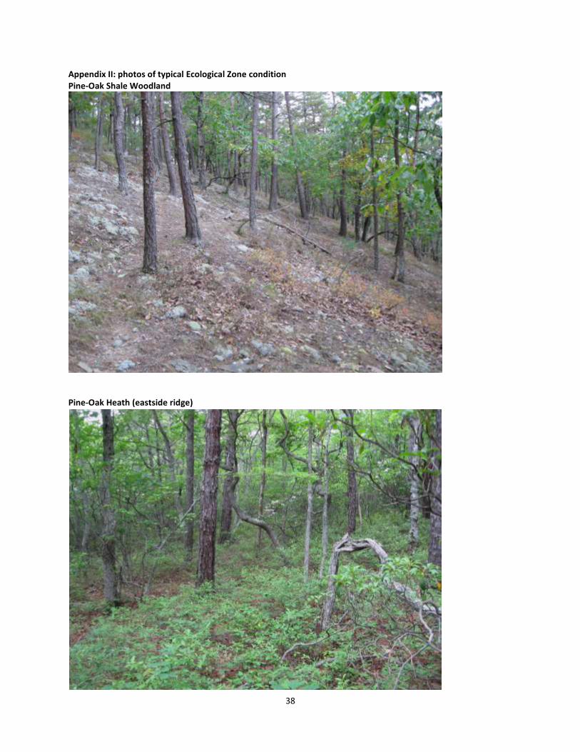
38

Appendix II: photos of typical Ecological Zone condition Pine-Oak Shale Woodland

Pine-Oak Heath (eastside ridge)

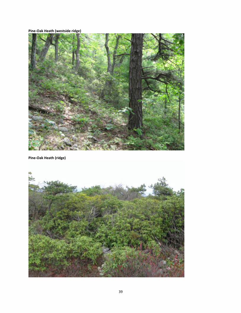
39

Pine-Oak Heath (westside ridge)

Pine-Oak Heath (ridge)

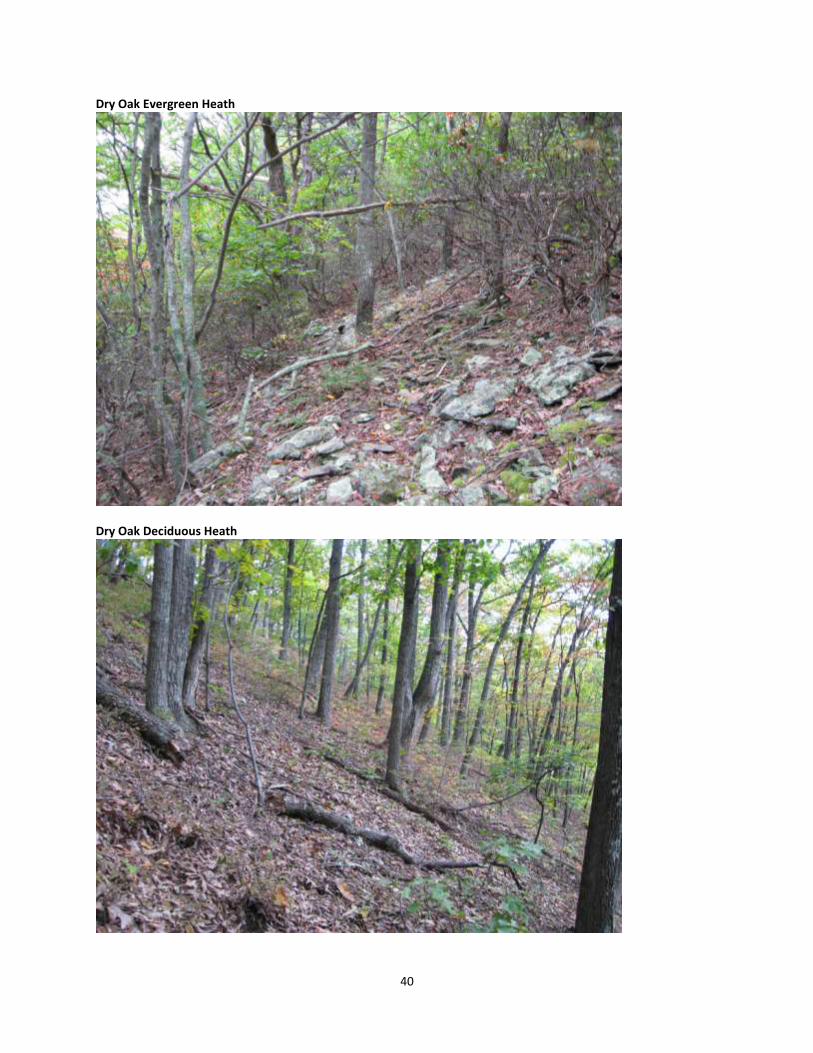
40

Dry Oak Evergreen Heath

Dry Oak Deciduous Heath

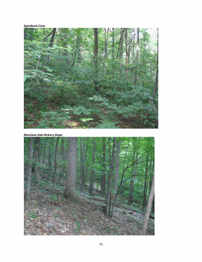
41

Spicebush Cove

Montane Oak-Hickory Slope

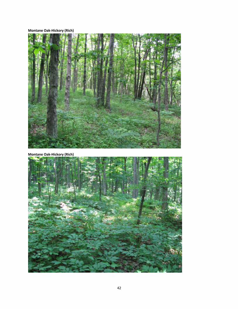
42

Montane Oak-Hickory (Rich)

Montane Oak-Hickory (Rich)

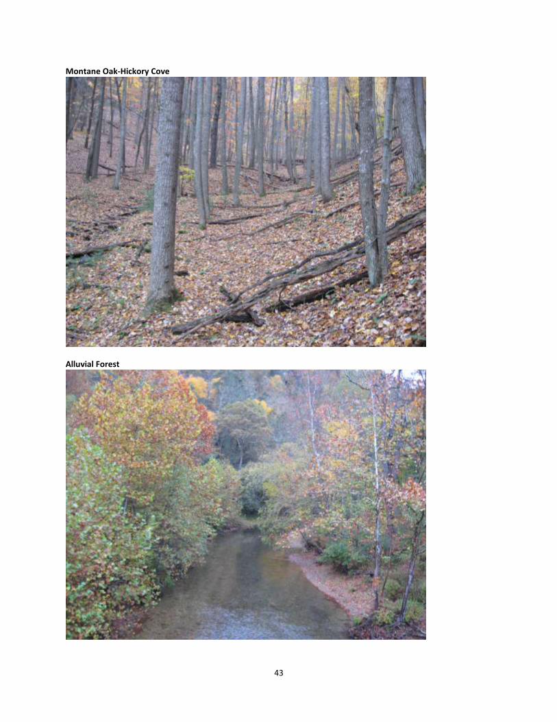
43

Montane Oak-Hickory Cove

Alluvial Forest

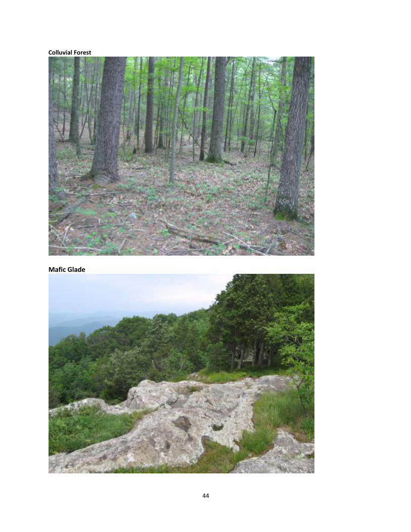
44

Colluvial Forest

Mafic Glade

45

Appendix III: Methods used in developing Digital Terrain Models (DTMS) The following DTMs were developed to characterize environmental factors that control temperature, moisture, fertility, and solar radiation input within the GW study areas. These environmental factors affect the distribution of Ecological Zones and their component plant communities in different landscapes. They were used to develop site specific probability values for each Ecological Zone based upon their correlation to representative or reference field sample locations for each type. All processing of 2

nd derivative grids (slope, aspect, etc.) used a 10 meter

DEM except Valley position and Relief which was evaluated with 30 meter DEMs. 1. elevation (meters and feet) Elevation extracted from the National Map Seamless Server: http://seamless.usgs.gov/index.php, 1/3 arc second DEMs, NAD83 Geographic projection, i.e., 10 meter resolution. The National Elevation Dataset (NED) 1/3 Arc Second is a raster product assembled by the U.S. Geological Survey. NED 1/3 Arc Second is designed to provide National elevation data in a seamless form with a consistent datum, elevation unit, and projection. Data corrections are made in the NED 1/3 Arc Second assembly process to minimize, but not eliminate, artifacts, perform edge matching, and fill sliver areas of missing data. The following process was used to build the elevation DTM for the project area. a) Select and download ‘workable’ sized portions of the study area (about 8 - 1:24,000 USGS quads). b) Project each downloaded area to NAD83 UTM zone 17, select 10x10 m cell size, cubic convolution before trying to mosaic them … the extracted raw DEMs from the site don’t always fit together perfectly. c) Mosaic all re-projected parts into one or a series of coverage. d) Fill “no data” values that may occur between individual downloaded area, for example: c:\gw_2010\dtms\temp1= con(isnull(c:\gw_2010\dtms\gw_dem_meters), focalmean(c:\gw_2010\dtms\gw_dem_meters, rectangle, 3,3), c:\gw_2010\dtms\gw_dem_meters) c:\gw_2010\dtms\temp2= con(isnull(c:\gw_2010\dtms\temp1), focalmean(c:\gw_2010\dtms\temp1, rectangle, 3,3), c:\gw_2010\dtms\temp1) … This was completed for 3 iterations. 2. aspect Aspect (transformed aspect and raw) is a measure of aspect at each cell location derived from the DEM. The following steps were performed to produce aspect:

a. GRID function ASPECT from the DEM filled for sinks (elev_fill). = aspectraw

b. Convert degrees to radians (1 degrees = 0.0174532925 radian), in raster calculator: (ASPECT *

0.017432925). This is done because cosine measurements for a continuous aspect variable are

derived from radians and not degrees.

c. Calculate cosine using ARC TOOLBOX Spatial Analyst Tools, Math, Trigometric, Cos. Value varies

from -1 to 1 = aspectrans

3. curve The curvature of a surface at each cell center in a 3x3 neighborhood derived from the DEM: used GRID curvature function. NOTE: if the DEM used has z units (height) in feet while the x,y units are in meters, then a z-factor of 0.3048 (1 ft = 0.3048 meters) must be used. This is part of the ESRI tools options to choose in calculation of curvature. If necessary, use one focalmean command to improve highly pixilated raw output. For the entire GW area, the meters DEM (x,y,z) was used so no z unit adjustment was necessary. 4. curveplan The curvature of a surface in a 3x3 neighborhood perpendicular to the slope direction derived from the DEM: GRID curvature function with {out_plan_curve} - an optional output grid referred to as the planiform curvature. If necessary, use focalmean commands to improve highly pixilated raw output.

46

5. curvepro The curvature of surface in a 3x3 neighborhood in the direction of slope derived from the DEM: GRID curvature function with {out_profile_curve} - an optional output grid showing the rate of change of slope for each cell. If necessary, use focalmean commands used to improve highly pixilated raw output. 6. slopep The rate of maximum change in z value (elevation_ft) from each cell derived from the DEM: GRID function slope with percentrise. 7. solaryr The yearly solar radiation per cell derived from the DEM. See “Area Solar Radiation” in ARC TOOLBOX, Spatial Analyst Tools, Radiation. If x,y units are meters and z units are feet, specify a z-value of 0.3048 to convert feet to meters. 8. solargw The growing season solar radiation per cell derived from the DEM. See “Area Solar Radiation” in ARC TOOLBOX, Spatial Analyst Tools, Radiation. Identified growing season as April 1 to Sept 30. 9. rsp RSP (relative slope position) is an estimate of the slope position at each cell location (Wilds 1996)… 100 is bottom and 0 is top. It is a measure of the cell position along a slope in relationship to the nearest ridge and drainage. Relative slope position uses (1) a threshold level of flow accumulation to represent slope bottom, (2) the difference between mean elevation and highest elevation in a moving window to represent ridges, and (3) flowlength to calculate distance. Steps to produce RSP performed with the raster calculator:

a) GRID commands: note* create flowdirection and flowaccumulation (floating point) coverages from the elevationgrid first

b) streams = con(flowacc < 300, 1) rsp1 in GW and VA_WVA uses 300, 10 meter cells = 7.4 acres for the threshold to start a stream rsp2 in GW and VA_WVA uses 807, 10 meter cells = 20 acres, for the threshold to start a stream

c) c:\gw_2010\dtms\slength_calc\streams_flip1 = con(isnull(c:\gw_2010\dtms\slength_calc\streams300), 1, 0)

d) c:\gw_2010\dtms\slength_calc\streams_thin1 = thin(c:\gw_2010\dtms\slength_calc\streams_flip1) e) c:\gw_2010\dtms\slength_calc\streams2 = setnull(c:\gw_2010\dtms\slength_calc\streams_thin1 > 0, 1) f) setmask streams2 (do in spatial analysis, options) g) c:\gw_2010\dtms\slength_calc\flow_dir2 = c:\gw_2010\dtms\slength_calc\flowdir h) setmask off (do spatial analysis, options) i) c:\gw_2010\dtms\slength_calc\flow_down = flowlength(c:\gw_2010\dtms\slength_calc\flow_dir2, #,

downstream) j) c:\gw_2010\dtms\slength_calc\mean = focalmean(c:\gw_2010\dtms\gw_dem_meters, rectangle, 10, 10) k) c:\gw_2010\dtms\slength_calc\differ = c:\gw_2010\dtms\slength_calc\mean -

c:\gw_2010\dtms\gw_dem_meters l) c:\gw_2010\dtms\slength_calc\ridges = con(c:\gw_2010\dtms\slength_calc\differ < -10, 1, 0) m) c:\gw_2010\dtms\slength_calc\thin_ridges = thin(c:\gw_2010\dtms\slength_calc\ridges, #, #, #, 15) n) c:\gw_2010\dtms\slength_calc\top = setnull(c:\gw_2010\dtms\slength_calc\thin_ridges > 0, 1) o) setmask top p) c:\gw_2010\dtms\slength_calc\flow_dir3 = c:\gw_2010\dtms\slength_calc\flowdir q) setmask off r) c:\gw_2010\dtms\slength_calc\flow_up = flowlength(c:\gw_2010\dtms\slength_calc\flow_dir3, #,

upstream) s) rsp_float = flow_up / (flow_up + flow_down) (this puts large number on btm)

47

t) rspa = int(rsp_float * 100) u) rspb = con(thin_ridges == 1, 0, rspa) v) rspc= con(streams_thin1 == 1, 100, rspb) w) rspfinal = focalmean (rspc, rectangle, 3, 3)

This was run with both 7.4 and 20 acre minimum flow accumulation; the 20 acre flow accumulation was used for analysis.

10. trmi TRMI (terrain relative moisture index) is an estimate of the moisture regime for each cell based upon 3 variables: aspect, slope position, and slope curvature using the weighted scalar developed by Parker (1982). TRMI combines aspect, slope, slope configuration (curvature) and relative slope position. The following GRID commands were used in the raster calculator. These commands require additional reclassification tables found in *.rmt files. The

directory location for the *.rmt files needs to be specified in the equations. Steps include:

a) config_a = reclass(curvepl, plan.rmt) b) config_b = reclass(curvepr, prof.rmt) c) config1 = con(config_a < 0 & config_b < 0, 10, 0) d) config2 = con(config_a == 0 & config_b < 0, 8, 0) e) config3 = con(config_a < 0 & config_b == 0, 7, 0) f) config4 = con(config_a == 0 & config_b == 0, 5, 0) g) config5 = con(config_a > 0 & config_b == 0, 3, 0) h) config6 = con(config_a == 0 & config_b > 0, 2, 0) i) config = config1 + config2 + config3 + config4 + config5 + config6 j) trmi_slope = reclass(slope, slope.rmt) *NOTE THAT SLOPE IS MEASURED IN DEGREES FOR THIS EQUATION *

k) trmi_asp = reclass(aspect, aspect.rmt) (USE aspect in degrees) l) trmi_rsp = reclass(rsp, rsp.rmt) (used rsp1 based on larger drainage area, i.e., 20ac vs 7 ac, see above m) trmi_final = trmi_asp + trmi_slope + trmi_rsp + config n) setnull all trmi values > 100 and fill these with focalmean 3x3 c:\fln_va\dtms\trmi_temp1=

con(isnull(c:\fln_va\dtms\trmi_final2), focalmean(c:\fln_va\dtms\trmi_final2, rectangle, 3,3), c:\fln_va\dtms\trmi_final2)

o) 2 majority filters done because coverage was highly pixilated 11. lfi LFI (landform index) is an index of landform shape (site protection) and macro-scale landform derived from the DEM. Larger number = more concave shape, more protected landform. From: McNab, W.H. 1996. Classification of local- and landscape-scale ecological types in the Southern Appalachian Mountains. Environmental Monitoring and Assessment 39:215-229. The software TopoMetrix is required to calculate LFI. The calculation of LFI is data intensive and requires very large RAM, and caching capability and therefore will not perform except on rather small DEMs. Processing lfi from topometrix requires the following steps: 1. clip DEM to reasonable-sized areas and convert the clipped elevation to .asc file 2. run lfi in topometrix and saving as .asc file 3. in ArcMap, convert .asc back to grid as floating point 4. set null for all grid values < -100 5. multiply this grid by 0.001 6. check all grids for projection, this process usually drops the projection and it needs to be redefined 7. mosaic these grids together – using BLEND (the output cell value of the overlapping areas will be a blend of

values that overlap; this blend value relies on an algorithm that is weight based and dependent on the distance from the pixel to the edge within the overlapping areas) if there is overlap – which there won’t be if

48

watershed boundaries are used. When watersheds are used as clip areas, the boundary areas, which will show as “nodata” need to be filled. Use the following:

8. outgrid = con(isnull(lfib), focalmean (lfia, rectangle, 10, 10), lfia) c:\gw_2010\lfimerge6 =

con(isnull(c:\gw_2010\lfimerge5), focalmean (c:\gw_2010\lfimerge5, rectangle, 3, 3), c:\gw_2010\lfimerge5)

9. to reduce pixelization (and differences that exist between the stitched elevations), do a focalmean 3x3 (this

was done only for the VA_WVA FLN area).

12. dstrm DSTRM (distance to stream- IN METERS) is a measure of each cell’s distance to the nearest stream, regardless of stream order. Streams are modeled from DEM using ESRI hydrology tools. The steps used to produce distance to streams: Make streams from 10m DEM. Set 13 acres to accumulate water (526 10x10 meter cells, 1633 – 20x20ft cells). In raster calculator = streamgrid = setnull(flowaccumulation < 526, 1). Calculate Euclidean distance to stream (GRID command, Dstrm = eucdistance stream). 13-16. Distance to geology type

Clip geology coverages from VA and WVA by a larger extent (18,394,240 acres - rounded). The VA and WVA geology coverages were derived by combining Virginia and West Virginia geologic map databases: (Nicholson, S.W., Dicken, C.L., Horton, J.D., Labay, K.A., Foose, M.P., and Mueller, J.A.L., 2005, Preliminary integrated geologic map databases for the United States: Kentucky,Ohio, Tennessee, and West Virginia: U.S. Geological Survey, Open-File Report OF-2005-1324, scale 1:250000, and, Dicken, C.L., Nicholson, S.W., Horton, J.D., Kinney, S.A., Gunther, Gregory, Foose, M.P., and Mueller, J.A.L., 2005, Preliminary integrated geologic map databases for the United States: Delaware, Maryland, New York, Pennsylvania, and Virginia: U.S. Geological Survey, Open-File Report OF-2005-1325, scale 1:250000. Although these are the most current GIS coverages of geology for the area, there still are some miss-matches of map units across State boundaries. This is most obvious in the Snowy Mountain, Moatstown, Monterey, Doe Hill, and Palo Alto USGS 1:24,000 quadrangles and is apparently due to higher resolution mapping in West Virginia. Delete all elements except Unit_type, rock_type1, rock_type2, modify the field extents so they match between coverages. The following steps were used to create the final DTMs.

1. Merge the following geology coverages, giving precedence to the most current or higher resolution

information:

the statewide VA and WVA merged coverage from above

the geologic coverage from the GW-JEFF (original mapping at higher resolution than above)

bedrock coverage from Shenandoah Park (most current)

2. Add item “group” and use Peper et.al (2001), Appendix 2: ‘Table of numerical lithogeochemical codes and original geologic map symbols’ to match geologic map symbols to their appropriate lithogeochemical code and populate the “group” item. The following group codes were used: 1 = CARBONATE-BEARING ROCKS 2 = MAFIC SILICATE ROCKS 3 = SILICICLASTIC ROCKS 4 = CARBONACEOUS-SULFIDIC ROCKS 5 = VERY ACID SHALE (Brallier Formation)

3. Create 5 separate grids for each of the lithogeochemical groups. 4. Calculate distance (Euclidean) to each of the grids to help ‘smooth’ the differences in scales and mapping

resolution.

17. Average Precipitation Average precipitation in inches. Based on a 30 year average, orographic effects in model. Coverage resampled to 10 meter cell size. Data available at: http://www.ocs.orst.edu/pub/maps/Precipitation/Total/States/

49

18. Difference in elevation relative to streams (uses elev in feet) Stream_diff (each cell’s difference in elevation relative to the closest stream, (can not exclude 1

st order streams in

the ridge and valley) is a measure of the difference in elevation of the individual cell and the closest river (above river = positive number, below river = negative number). Create a coverage describing river elevations using the raster calculator: river_elev = con(stream_order > 0, elevation from filled dem, 0), i.e., where a 1

st order (or higher

order) stream occurs, display its elevation. – OR extract by mask, streamgrid = mask, extract from elev_fill – OR c:\gw_2010\dtms\stream_elev = con(c:\gw_2010\dtms\stream13 > 0, c:\gw_2010\dtms\gw_fill_ft, 0) Fill in areas that are not streams through a series of focalmin commands: outgrid = con(isnull(stream_elev), focalmin (stream_elev, circle, 3), stream_elev). Use 3x3 for at least 10 iterations, then 10x10 for the remainder. c:\gw_2010\dtms\temp1 = con(isnull(c:\gw_2010\dtms\stream_elev), focalmin (c:\gw_2010\dtms\stream_elev, circle, 3), c:\gw_2010\dtms\stream_elev) c:\gw_2010\dtms\temp2 = con(isnull(c:\gw_2010\dtms\temp1), focalmin(c:\gw_2010\dtms\temp1, circle, 3), c:\gw_2010\dtms\temp1) This is an attempt to fill in the non-river landscape with the closest river elevation to allow easy subtraction with grid algebra. Repeat16 iterations (10 – 3x3, 6 – 10x10) Calculate difference in elevation between each cell and the closest river: river_diff = elevation - river_elevfill 19) Valley position: Valley position is a measure of the elevational position of a cell relative to the watershed divide and the valley floor. The old method of calculating this DTM used the original DEM (meters x, y, and z) to model streams with a 13 acre accumulation area (see above) and stream order, to identify valley floor and the same DEM to identify watershed divide. The new method determines valley floor from the minimum elevation within a 3000x3000 meter window. The watershed divide is defined as the maximum elevation within a 3000x3000 meter window, i.e., it is an estimate (model) of where major ridges occur and the elevation of grid cells at those locations. It uses a 30 meter DEM (resampled from the original 10 meter DEM) because: (a) this is a mesoscale indicator meant to evaluate environments at a broader scale than Relative Slope Position, and (b) this reduces computing time considerably (using a 10 meter DEM would take up to about 10x longer, virtually – days using a computer with 2.10 GHz duo processors and minimum 4.00 GB RAM).

GRID commands: The DEM was converted from 10m resolution to 30m resolution in improve analysis speed, but 10m resolution

for the GW NF. These coverages were merged.

C:\gw_2010\dtms\gw_maxelev1=focalmax(c:\gw_2010\dtms\dem_add_meter,circle,100) In the expansion of GW, 10m was used and combined with the 30m from the VA_WVA_FLN, used ‘blend’ in the mosaic process. = GW_maxelev2 (each area had to be clipped inward 3000’ to get correct values) used circle, 100, 100 then focalmean 3,3 rectangle (twice) Minelev = focalmin(dtm30meter, circle, 100) Relief = maxelev – minelev Down = Elevationgrid – minelev Vposfloat = 1 - (down/relief) Vpos = int (vposfloat * 100) Resampled back to 10 meter

50

20) Local Relief Local relief is a measure of the difference in elevation between the watershed divide and the valley floor relative to a cell’s location. Local Relief uses (1) 4

th order and greater streams to represent slope bottom, and (2) the

watershed divide defined from the maximum elevation within 3000 meters of the cell to represent ridges. See above procedure for valley position. Set all negative numbers to 0. 21) Profile Curvature Roughness Developed to characterize the variety of site conditions across the slope due to aspect that is so evident in field sampling and from aerial photography and topographic maps. This broad-scale surface curvature is controlled by bedrock strike and dip. It could be an important variable in modeling the repeated pattern of Pine-Oak Heath Ecological Zones and adjacent Dry Oak or Dry-Mesic Oak Ecological Zones on the ‘strike side’ of a mountain range, and conversely, the smooth surface on the ‘dip side’ of the mountain. Although various methods were evaluated, the following process creates a reasonable surface that reflects the diversity in profile curvature:

a) Calculate the standard deviation within a window oriented along the major NE trending major ridges within a neighborhood that includes at least 3 patterns of tertiary ridge and drainages on the typical ‘strike side’ of a mountain range, usually the NW-facing side), i.e., a slice approximately 1000’ in length. No tools were available to orient the neighborhood directionally except , the “WEDGE”.

b) Use a wedge start angle = 30, end angle = 70 for 100 cells NOTE: there are several areas that appear in error, especial a slice in the SW corner of the Waynesboro east quad. This area has the highest SDs and an abrupt boundary to adjacent areas – for no apparent reason except the proximity to a reservoir. However, this is on PVT land and the majority of the output looks very good.

22) Lake Effect Snowfall (snow1) This coverage attempts to explain climate patterns that may influence average annual snowfall amounts controlled by the North American jet-stream and ‘lake effects’ from the Great Lakes during a prolonged period (100s to 1000s of years). This climate pattern is likely a major environmental driver for where spruce and northern hardwood Ecological Zones may occur. Tropical storms from the southeastern seaboard may also influence snowfall events and interact with the seasonal jetstream, especially in the late winter / early spring and; these may be evaluated through another DTM). The following process was used to develop the distance to snowfall coverage:

a) Method for larger GW area: extract polygon of ‘waterbodies’ from ESRI’, that includes the Great Lakes shoreline; the width and height of this waterbody need to be the same as the GW study area, so a fake shoreline was created to the west but more distant than the true shoreline.

b) Used the draw tool to outline the poly and moved this ‘drawn’ outline 350 kilometers closer to the project area (this was done to reduce the analysis area – because it kept bombing out at the larger – true size),

c) Create a new poly and use to the “drawn” convert to grid, d) Calculate Euclidean distance to these waterbodies (use an analysis area that MUST include the x and y

dimension of the GW analysis area) e) Clip to the project boundary.

23) Local Snowfall influence (snow2) This coverage attempts to explain the combined influence of the jet-stream (DTM 22 above) and local topography and is based on average annual snowfall amounts (some over a 100 year period) from areas just west or just within the project area.

a) Create a polygon that connects high snowfall areas in West Virginia close to the project area, i.e., Elkins, Beckley, Seneca State Forest. Petersburg, Keyser; = 77.7”, 60.0”, 60.8”,69”, 64”; respectively. Data from the following sources: http://lwf.ncdc.noaa.gov/oa/climate/online/ccd/snowfall.html, http://www.city-data.com/cite/petersburg-west-virginia.html, http://www.city-data.com/city/keyser-west-virginia.htm

51

b) Convert polygon to grid, use Euclidean distance to create coverage c) IMPORTANT to: set extent of analysis area and mask to include the entire project area. Check especially

Tools, options, Environment Settings, General Settings, Extent … which needs to be set to top, left, right, bottom.

d) Clip to project area = distsnow2

24) Distance to rivers (Rivdist)

Same process as distance to streams but using 4th

order and greater streams only.

25) Distance above rivers (i.e., streams equal or greater than 4th

order) (Riveldiff)

The following process was used: a) create elevation coverage of 4

th order+ streams (rivers) at 10x10 meters = rivelev.

b) expand this elevation to the landscape; this process fills in the non-river landscape with the closest river elevation to allow easy subtraction with grid algebra using the following commands in the raster calculator:

C:\gw_2010\dtms\temp2 = con(isnull(c:\gw_2010\dtms\temp1),focalmin(c:\gw_2010\dtms\temp1, circle, 3), c:\gw_2010\dtms\temp1) C:\gw_2010\dtms\temp2 = con(isnull(c:\gw_2010\dtms\temp1), focalmin(c:\gw_2010\dtms\temp1, circle, 10), c:\gw_2010\dtms\temp1)

Use 10x10 circle for 57 iterations, use 30x30 circle for the final iteration (total = 58 iterations)

This coverage = gw_rivel_lnd

Elevation in meters – rivelev_land = rivelevdiff This creates some areas that are BELOW the river due to the constant filling in nodata with the focalmin of elevation .. some which is actually on the other side of the watershed divide. To partially fix this, these areas were assigned back to nodata and the filling in was done with con(isnull) as above. MAKE SURE A MASK AND EXTENT ARE SET TO INCLUDE JUST THE ANALYSIS AREA, otherwise all perimeter cells will expand outward. This still results in some sharp boundaries where there shouldn’t be. So, focal analysis showing the standard deviation between adjacent cells was used to identify these areas and they were set to null and again, as above, smoothed by using calculating the mean in these nodata areas. Con(standard deviation > 10 (from the std dev of rivelefdiff), setnull (rivelevdiff), rivelevdiff) = gw_rivel_diff. The ultimate fix might be to follow a procedure similar to RSP but to specify the bottom as 5

th order and greater streams and to specify the top as the 10

th order HUC boundaries. This

procedure was started without much success and includes inverting the elevation grid to show ridges as bottoms and to use hydrology tools to identify a ‘ridge network’. 26) River influence (Rivinf) This coverage attempts to explain the influence of large streams down-cutting shale hills as an important factor in predicting the location of Shale Barrens. b) calculate distance to 4

th order and greater streams = rivdist. Either set 0.00 to 0.1 in rivdist, or fill in

nodata values generated from the following calculation …. My choice for GW_2010) c) calculate this DTM as: Elev_meters – rivelev_land = (rivelevdiff) / distance to rivers (rivdist) RISE RUN

Label as rivinfl (filled nodata values with focalmean)

52

27) Terrain shape index This DTM estimates local convexity or concavity slightly broader than curvature and is calculated by subtracting elevation value of center cell from value of each of 8 neighbors.

a) C:\gw_2010\dtms\gw_tsi = c:\gw_2010\dtms\gw_dem_meters – focalmean(c:\gw_2010\dtms\gw_dem_meters, circle, 5) This looks much like curvature from ESRI only a bit smoother. From: McNab, H.W. 1993. A topographic index to quantify the effect of mesoscale landform on site productivity. Can. J. For. Res. 23: 1100-1107.

28. slopelength Slope length is an estimate of the cell position along a slope segment, from the ridges (major and tertiary) to the bottom of the slope. The ridges and slope bottom were estimated following similar procedures the RSP calculation (Wilds 1996) equals the sum of ‘flowup’ and ‘flowdown’ from rsp1 (uses 7.4 acres to accumulate enough to start stream). Steps to produce slopelength performed with the raster calculator:

a) GRID commands: note* create flowdirection and flowaccumulation (floating point) coverages from the elevationgrid first

b) C:\tn\dtms\streams = con(c:\tn\dtms\flowacc < 300, 1) rsp1 in GW and VA_WVA and TN uses 300, 10 meter cells = 7.4 acres for the threshold to start a stream

c) c:\tn\dtms\streams_flip1 = con(isnull(c:\tn\dtms\streams300), 1, 0) d) c:\tn\dtms\streams_thin1 = thin(c:\tn\dtms\streams_flip1) e) c:\tn\dtms\streams2 = setnull(c:\tn\dtms\streams_thin1 > 0, 1) f) setmask streams2 (do in spatial analysis, options) g) c:\tn\dtms\flow_dir2 = c:\tn\dtms\flowdir h) setmask off (do spatial analysis, options) i) c:\tn\dtms\flow_down = flowlength(c:\tn\dtms\flow_dir2, #, downstream) j) c:\tn\dtms\mean = focalmean(c:\tn\dtms\elev_projarea, rectangle, 10, 10) k) c:\tn\dtms\differ = c:\tn\dtms\mean - c:\tn\dtms\elev_projarea l) c:\tn\dtms\ridges = con(c:\tn\dtms\differ < -10, 1, 0) m) c:\tn\dtms\thin_ridges = thin(c:\tn\dtms\ridges, #, #, #, 15) n) c:\tn\dtms\top = setnull(c:\tn\dtms\thin_ridges > 0, 1) o) setmask top p) c:\tn\dtms\flow_dir3 = c:\tn\dtms\flowdir q) setmask off r) c:\tn\dtms\flow_up = flowlength(c:\tn\dtms\flow_dir3, #, upstream)

s) c:\tn\dtms\slopelength1 = c:\tn\dtms\flow_up + c:\tn\dtms\flow_down t) extract to study area = slopelength2 u) c:\tn\dtms\slopelength3 = con(isnull(c:\tn\dtms\slopelength2), focalmean(c:\tn\dtms\slopelength2,

rectangle, 3, 3), c:\tn\dtms\slopelength2) v) c:\tn\dtms\slolpelength4 = con(isnull(c:\tn\dtms\slopelength3), focalmean(c:\tn\dtms\slopelength3,

rectangle,3,3), c:\tn\dtms\slopelength3) w) c:\tn\dtms\slopelength5 = con(c:\tn\dtms\slolpelength4 > 3000, 3000, c:\tn\dtms\slolpelength4) x) c:\tn\dtms\slengtfin1 = focalmean(c:\tn\dtms\slopelength5, rectangle, 3, 3) y) c:\tn\dtms\slength2 = con(isnull(c:\tn\dtms\slength), focalmean(c:\tn\dtms\slength, rectangle,3,3),

c:\tn\dtms\slength)

z) This process results in single pixels at some stream locations that are very different their adjacent pixels; otherwise, the remainder of the coverage looks good.

53

APPENDIX IV: Analysis Process

Maximum Entrophy (MAXENT) Create DTMs with the same extent as project area boundary: Extract each DTM by Mask (Arc tools) to ensure that grids are the same extent. Covert all Grids to ASCII DO THESE as a BATCH process, i.e., right click the tool

Create CSV file with the following variables: TYPE, Xcoordinate, Ycoodinate, DTM values.

Use Hawth tools to attach X,Y to original plot coverage Use Hawth tools to attach DTM data to points: Hawth Analysis, point intersection. Export table and check that format, otherwise, strip all but TYPE, X, Y and DTM from file, save as CSV file. i.e., (open an .xl file and select ‘open as dbf’, edit if necessary and SAVE AS *MSDOS+ CSV file), i.e., (Comma delimited)

Run Maxent Follow wizard and locate plot data file with attributes Follow wizard and locate folder with environmental data, wizard inserts all .asc files. Identify location for results (make separate directory) Appalachian Ridges run takes approximately 20 hours. Export all the resulting .asc files with floating point to create a Grid for each Ecological Zone.

Maximum probability Grid

Uses multiple Ecological Zone models to determine the maximum value on a cell-by-cell basis within the Analysis window, for example: l:\blueridge\models\max20gd = max ~ (l:\blueridge\models\nhwood, l:\blueridge\models\nhcove2, ~ l:\blueridge\models\lowspice3, ~ l:\blueridge\models\montoakslope, l:\blueridge\models\montoak_rich2, l:\blueridge\models\dmoak, ~ l:\blueridge\models\acove2, l:\blueridge\models\rcove, l:\blueridge\models\hero2, l:\blueridge\models\poh, ~ l:\blueridge\models\dryoakDheath2,l:\blueridge\models\dryoakEheath, l:\blueridge\models\alluvial2, l:\blueridge\models\lowpine2)

Creating the Ecological Zone model Read each model Grid to compare to the maximum probability for that grid cell; if a match occurs, insert Ecological Zone model code. l:\blueridge\models\blue20gd = con(l:\blueridge\models\max20gd == l:\blueridge\models\nhwood, 2, ~ l:\blueridge\models\max20gd == l:\blueridge\models\nhcove2, 3, ~ l:\blueridge\models\max20gd == l:\blueridge\models\lowspice3, 25, ~ l:\blueridge\models\max20gd == l:\blueridge\models\montoak_rich2, 24, ~ l:\blueridge\models\max20gd == l:\blueridge\models\montoakslope, 9, ~ l:\blueridge\models\max20gd == l:\blueridge\models\alluvial2, 6, ~ l:\blueridge\models\max20gd == l:\blueridge\models\acove2, 4, ~ l:\blueridge\models\max20gd == l:\blueridge\models\rcove, 5, ~ l:\blueridge\models\max20gd == l:\blueridge\models\dmoak, 13, ~ l:\blueridge\models\max20gd == l:\blueridge\models\hero2, 8, ~ l:\blueridge\models\max20gd == l:\blueridge\models\poh, 18, ~ l:\blueridge\models\max20gd == l:\blueridge\models\dryoakEheath, 10, ~ l:\blueridge\models\max20gd == l:\blueridge\models\dryoakDheath2, 11, ~ l:\blueridge\models\max20gd == l:\blueridge\models\lowpine2, 16, 0)

54

Appendix V: Accuracy Evaluation Accuracy assessments are essential parts of all vegetation mapping projects but they are time-consuming and expensive especially in mixed ownerships. They provide the basis to compare different map production methods, information regarding the reliability and usefulness of the maps for particular applications, and the support for spatial data used in decision-making processes. It is useful to evaluate accuracy relative to the aerial extent of each class. For example, when a particularly common class (e.g., 10-15% of the map area) has either a very high or a very low accuracy it has a disproportionate effect on the utility of the map for general analysis applications without a corresponding effect on the overall accuracy assessment. Conversely, a relatively rare type (e.g., < 1% of the map area) regardless of its accuracy has relatively little effect on the utility of the map for general analysis applications but has the same effect on the accuracy assessment as the common type. A true accuracy assessment was not completed for this project, hence the title “Accuracy Evaluation”. However, the same procedure was followed, i.e., a comparison was made of reference data for a site to categorized (classified, modeled) data (map units) on the same site. A quantitative accuracy assessment depends on the collection of reference data. Reference data is known information of high accuracy (theoretically 100% accuracy) about a specific area on the ground (the accuracy assessment site). The assumed-true reference data can be obtained from ground visits, photo interpretation, video interpretations, or some combination of these methods. In a map unit accuracy assessment, sites are generally the same type of modeling unit used to create the map. In a true field accuracy assessment, the evaluation would be made around randomly generated points on the ground or more realistically within a ‘stand’ or other reasonable-size area. For this study, the sample plots were considered the reference data and were buffered by 10 meters (the base resolution of all DTMS) to create a ‘fuzzy’ boundary between Ecological Zones to better account for ecotones between types. These buffered reference sites were considered ‘correctly classified’ if they fell even partially within a map unit having the same classification. This assessment was done for Ecological Zones only. Accuracy of TNC Ecological Systems and USFS ESE Systems were computed by aggregating these values into their appropriate classes. Error Matrix The error matrix (Tables 1, 2) below are a square array in which accuracy assessment sites are tallied by both their classified category and their actual category according to the reference data. For this study, the columns in the matrix represent the classified Ecological Zone map units, while the rows represent the reference data (non-traditional approach). The major diagonal, highlighted in the following table, contains those sites where the classified data agree with the reference data. The nature of errors in the classified map can also be derived from the error matrix. In the matrix, errors (the off-diagonal elements) are shown to be either errors of inclusion (commission errors) or errors of exclusion (omission errors). Commission errors are shown in the off-diagonal matrix cells that form the horizontal row for a particular class. Omission error is represented in the off-diagonal vertical row cells. High errors of omission/commission between two or more classes indicate spectral confusion between these classes. The following measures of accuracy were derived from the Ecological Zone error matrix.

Overall Accuracy, a common measure of accuracy, is computed by dividing the total correct samples (the diagonal elements) by the total number of assessment sites found in the bottom right cell of the matrix. Producer's Accuracy, which is based on omission error, is the probability of a reference site being correctly classified. It is calculated by dividing the total number of correct accuracy sites for a class (diagonal elements) by the total number of reference sites for that class found in the right-hand cell of each row (Story and Congalton 1968). Producer’s accuracy indicates how many times an Ecological Zone on the ground was identified as that Ecological Zone on the map.

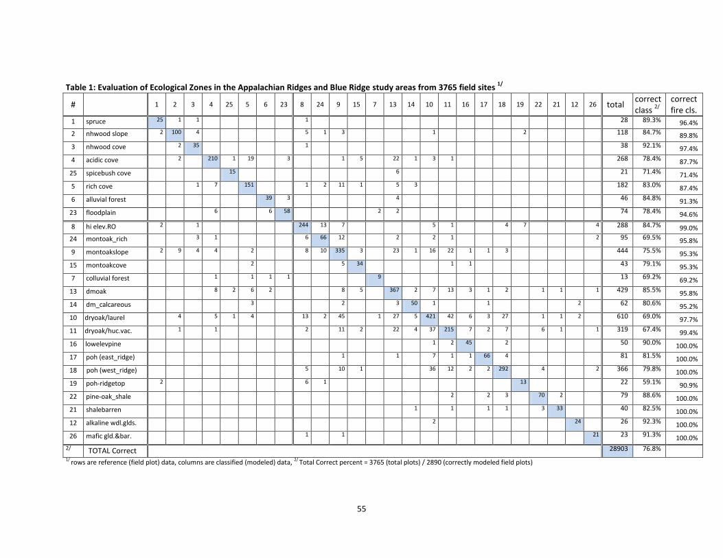
55

Table 1: Evaluation of Ecological Zones in the Appalachian Ridges and Blue Ridge study areas from 3765 field sites 1/

# 1 2 3 4 25 5 6 23 8 24 9 15 7 13 14 10 11 16 17 18 19 22 21 12 26 total correct class

2/ correct fire cls.

1 spruce 25 1 1 1 28 89.3% 96.4%

2 nhwood slope 2 100 4 5 1 3 1 2 118 84.7% 89.8%

3 nhwood cove 2 35 1 38 92.1% 97.4%

4 acidic cove 2 210 1 19 3 1 5 22 1 3 1 268 78.4% 87.7%

25 spicebush cove 15 6 21 71.4% 71.4%

5 rich cove 1 7 151 1 2 11 1 5 3 182 83.0% 87.4%

6 alluvial forest 39 3 4 46 84.8% 91.3%

23 floodplain 6 6 58 2 2 74 78.4% 94.6%

8 hi elev.RO 2 1 244 13 7 5 1 4 7 4 288 84.7% 99.0%

24 montoak_rich 3 1 6 66 12 2 2 1 2 95 69.5% 95.8%

9 montoakslope 2 9 4 4 2 8 10 335 3 23 1 16 22 1 1 3 444 75.5% 95.3%

15 montoakcove 2 5 34 1 1 43 79.1% 95.3%

7 colluvial forest 1 1 1 1 9 13 69.2% 69.2%

13 dmoak 8 2 6 2 8 5 367 2 7 13 3 1 2 1 1 1 429 85.5% 95.8%

14 dm_calcareous 3 2 3 50 1 1 2 62 80.6% 95.2%

10 dryoak/laurel 4 5 1 4 13 2 45 1 27 5 421 42 6 3 27 1 1 2 610 69.0% 97.7%

11 dryoak/huc.vac. 1 1 2 11 2 22 4 37 215 7 2 7 6 1 1 319 67.4% 99.4%

16 lowelevpine 1 2 45 2 50 90.0% 100.0%

17 poh (east_ridge) 1 1 7 1 1 66 4 81 81.5% 100.0%

18 poh (west_ridge) 5 10 1 36 12 2 2 292 4 2 366 79.8% 100.0%

19 poh-ridgetop 2 6 1 13 22 59.1% 90.9%

22 pine-oak_shale 2 2 3 70 2 79 88.6% 100.0%

21 shalebarren 1 1 1 1 3 33 40 82.5% 100.0%

12 alkaline wdl.glds. 2 24 26 92.3% 100.0%

26 mafic gld.&bar. 1 1 21 23 91.3% 100.0%

2/ TOTAL Correct 3/ 1/3

28903

/

76.8%

1/ rows are reference (field plot) data, columns are classified (modeled) data, 2/ Total Correct percent = 3765 (total plots) / 2890 (correctly modeled field plots)

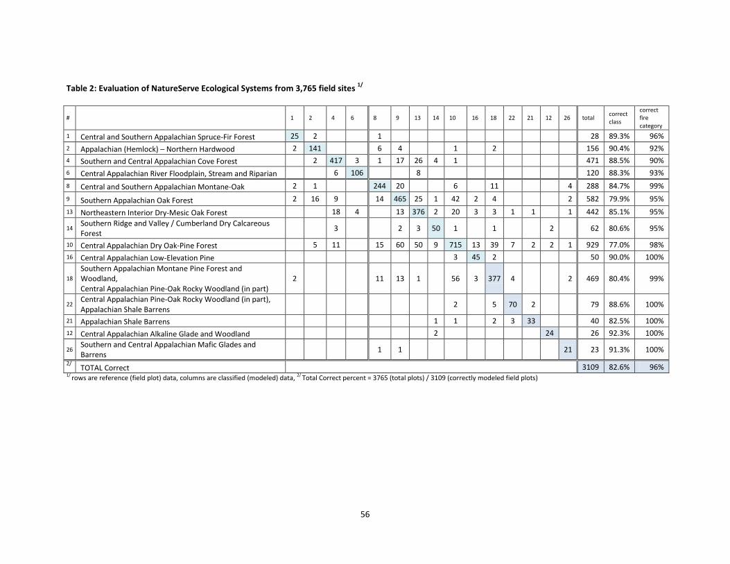
56

Table 2: Evaluation of NatureServe Ecological Systems from 3,765 field sites 1/

#

1 2 4 6 8 9 13 14 10 16 18 22 21 12 26 total correct class

correct fire category

1 Central and Southern Appalachian Spruce-Fir Forest 25 2 1 28 89.3% 96%

2 Appalachian (Hemlock) – Northern Hardwood 2 141 6 4 1 2 156 90.4% 92%

4 Southern and Central Appalachian Cove Forest 2 417 3 1 17 26 4 1 471 88.5% 90%

6 Central Appalachian River Floodplain, Stream and Riparian 6 106 8 120 88.3% 93%

8 Central and Southern Appalachian Montane-Oak 2 1 244 20 6 11 4 288 84.7% 99%

9 Southern Appalachian Oak Forest 2 16 9 14 465 25 1 42 2 4 2 582 79.9% 95%

13 Northeastern Interior Dry-Mesic Oak Forest 18 4 13 376 2 20 3 3 1 1 1 442 85.1% 95%

14 Southern Ridge and Valley / Cumberland Dry Calcareous Forest

3 2 3 50 1 1 2 62 80.6% 95%

10 Central Appalachian Dry Oak-Pine Forest 5 11 15 60 50 9 715 13 39 7 2 2 1 929 77.0% 98%

16 Central Appalachian Low-Elevation Pine 3 45 2 50 90.0% 100%

18

Southern Appalachian Montane Pine Forest and Woodland, Central Appalachian Pine-Oak Rocky Woodland (in part)

2 11 13 1 56 3 377 4 2 469 80.4% 99%

22 Central Appalachian Pine-Oak Rocky Woodland (in part), Appalachian Shale Barrens

2 5 70 2 79 88.6% 100%

21 Appalachian Shale Barrens 1 1 2 3 33 40 82.5% 100%

12 Central Appalachian Alkaline Glade and Woodland 2 24 26 92.3% 100%

26 Southern and Central Appalachian Mafic Glades and Barrens

1 1 21 23 91.3% 100%

2/ TOTAL Correct 3109 82.6% 96%

1/ rows are reference (field plot) data, columns are classified (modeled) data, 2/ Total Correct percent = 3765 (total plots) / 3109 (correctly modeled field plots)

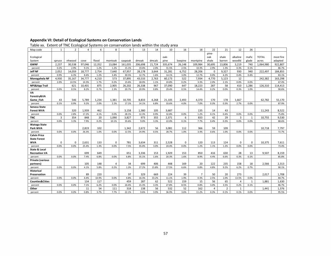
57

Appendix VI: Detail of Ecological Systems on Conservation Lands

Table xx. Extent of TNC Ecological Systems on conservation lands within the study area Map code 1 2 4 6 8 9 13 14 10 16 18 22 21 12 26

Ecological System spruce nhwood cove flood montoak saapoak dmoak dmcalc

oak-pine lowpine montpine

pine-oak shale

shale barren

alkaline woodld

mafic glade

TOTAL acres

most fire adapted

GWNF 2,237 30,538 97,046 12,352 13,084 161,035 206,698 21,724 335,674 26,148 109,984 30,695 13,806 3,219 740 1,064,980 922,807 percent 0.2% 2.9% 9.1% 1.2% 1.2% 15.1% 19.4% 2.0% 31.5% 2.5% 10.3% 2.9% 1.3% 0.3% 0.1% 86.7%

Jeff NF 2,052 14,059 18,777 2,754 7,640 67,957 28,178 3,644 31,281 6,752 28,206 0 9,327 930 940 222,497 184,855 percent 0.9% 6.3% 8.4% 1.2% 3.4% 30.5% 12.7% 1.6% 14.1% 3.0% 12.7% 0.0% 4.2% 0.4% 0.4% 83.1%

Monogahela NF 4,930 35,167 34,777 4,210 573 37,895 43,533 2,763 60,173 522 7,934 4,770 5,123 12 242,382 163,298 percent 2.0% 14.5% 14.3% 1.7% 0.2% 15.6% 18.0% 1.1% 24.8% 0.2% 3.3% 2.0% 2.1% 0.0% 0.0% 67.4%

NPS&App Trail 621 10,401 875 2,905 26,202 26,338 967 37,090 647 18,223 287 58 410 1,286 126,310 114,413 percent 0.0% 0.5% 8.2% 0.7% 2.3% 20.7% 20.9% 0.8% 29.4% 0.5% 14.4% 0.2% 0.0% 0.3% 1.0% 90.6%

VA Forestry&VA Game_Fish 43 546 5,789 1,234 1,381 10,705 8,833 4,268 21,105 2,493 4,370 170 178 1,667 62,782 55,170 percent 0.1% 0.9% 9.2% 2.0% 2.2% 17.1% 14.1% 6.8% 33.6% 4.0% 7.0% 0.3% 0.3% 2.7% 0.0% 87.9%

Seneca State Forest WVA 320 1,939 462 3,158 1,380 105 3,687 135 14 43 11,243 8,522 percent 0.0% 2.8% 17.2% 4.1% 0.0% 28.1% 12.3% 0.9% 32.8% 0.0% 1.2% 0.1% 0.4% 0.0% 0.0% 75.8%

TNC 3 354 848 20 1,090 3,827 973 355 2,371 6 833 42 29 3 1 10,755 9,530 percent 0.0% 3.3% 7.9% 0.2% 10.1% 35.6% 9.0% 3.3% 22.0% 0.1% 7.7% 0.4% 0.3% 0.0% 0.0% 88.6%

Watoga State Park WVA 2,819 102 1,342 2,672 56 3,081 112 366 59 109 10,718 7,797 percent 0.0% 0.0% 26.3% 1.0% 0.0% 12.5% 24.9% 0.5% 28.7% 1.0% 3.4% 0.6% 1.0% 0.0% 0.0% 72.7%

Calvin Price State Forest WVA 0 0 2,631 133 0 781 3,634 311 2,528 0 120 113 124 0 0 10,375 7,611 percent 0.0% 0.0% 25.4% 1.3% 0.0% 7.5% 35.0% 3.0% 24.4% 0.0% 1.2% 1.1% 1.2% 0.0% 0.0% 73.4%

State & Local Recreation VA 699 649 651 3,336 153 1,929 153 850 416 630 28 13 9,507 8,159 percent 0.0% 0.0% 7.4% 6.8% 0.0% 6.8% 35.1% 1.6% 20.3% 1.6% 8.9% 4.4% 6.6% 0.3% 0.1% 85.8%

Private (various partners) 105 148 4 34 699 406 448 169 20 122 235 158 18 2,566 2,313 percent 0.0% 0.0% 4.1% 5.8% 0.2% 1.3% 27.2% 15.8% 17.5% 6.6% 0.8% 4.8% 9.2% 6.2% 0.7% 90.1%

Historical Preservation 89 220 97 329 669 224 39 7 50 20 273 2,017 1,708 percent 0.0% 0.0% 4.4% 10.9% 0.0% 4.8% 16.3% 33.2% 11.1% 1.9% 0.3% 2.5% 1.0% 13.5% 0.0% 84.7%

Counties&Cities 134 117 459 287 62 522 159 15 56 65 4 1 1,881 1,630 percent 0.0% 0.0% 7.1% 6.2% 0.0% 24.4% 15.3% 3.3% 27.8% 8.5% 0.8% 3.0% 3.5% 0.2% 0.1% 86.7%

Other 11 54 111 318 138 56 532 52 162 4 2 1 1,441 1,376 percent 0.0% 0.0% 0.8% 3.7% 7.7% 22.1% 9.6% 3.9% 36.9% 3.6% 11.2% 0.3% 0.1% 0.1% 0.0% 95.5%

58

Appendix VII: products included on external drive 1) Analysis_coverages (used to create summary tables)

app_fsfs: Grid coverage of USFS Systems for USFS ownership in the Appalachian Ridges study area derived from ecozones (1 majority filter on ecozones)

app_fsfsf1: Grid coverage of USFS Systems for USFS ownership in the Appalachian Ridges study area derived from ecozones (1 majority filter on ecozones, 1 majority filter on USFS Systems)

app_fsfs1_poly: Polygon coverage of app_fsfsf1

app_fsfsf2: Grid coverage of USFS Systems for USFS ownership in the Appalachian Ridges study area derived from ecozones (1 majority filter on ecozones, 2 majority filters on USFS Systems)

app_fsfsf2_poly: Polygon coverage of app_fsfsf2

app_fstypesf1: Grid coverage of USFS Systems for the Appalachian Ridges study area derived from ecozones (1 majority filter on ecozones, 1 majority filter on USFS Systems)

app_fstypesf1_poly: Polygon coverage of app_fstypesf1

app_fstypes: USFS Systems for the Appalachian Ridges study area derived from ecozone (1 majority filter on ecozones, no majority filter on USFS Systems)

app_ridge3mf1: Grid coverage of ecozones within the Appalachian Ridges study area (1 majority filter)

app_ridge3mf1_poly: Polygon coverage of app_ridge3mf1

app_ridge3mf2: Grid coverage of ecozones within the Appalachian Ridges study area (2 majority filters)

app_tnctype: Grid coverage of TNC Ecological Systems within the Appalachian Ridges study area derived from Ecological Zone (1 majority filter on ecozones)

app_tnctypef1: Grid coverage of TNC Ecological Systems within the Appalachian Ridges study area derived from Ecological Zone (1 majority filter on ecozones, 1 majority filter on TNC Ecological Systems)

app_tnctypef1_poly: Polygon coverage of app_tnctypef1

bl_tnctype: Grid coverage of TNC Ecological Systems within the Blue Ridge study area derived from Ecological Zones (1 majority filter on ecozones)

bl_tnctypef1: Grid coverage of TNC Ecological Systems within the Blue Ridge study area derived from Ecological Zones (1 majority filter on ecozones, 1 majority filter on TNC Ecological Systems)

bl_tnctypef1_poly: Polygon coverage of bl_tnctypef1

blu_fstypef1: Grid coverage of USFS Systems within the Blue Ridge study area derived from ecozones (1 majority filter on ecozones, 1 majority filter on USFS Systems)

blu_fstypef1_poly: polygon coverage of blu_fstypef1

blu_fstypes: Grid coverage of USFS Systems within the Blue Ridge study area derived from ecozones (1 majority filter on ecozones, no majority filter on USFS Systems)

blue_fsfs: Grid coverage of USFS Systems for USFS ownership in the Blue Ridge study area derived from ecozones (1 majority filter on ecozones, no majority filter on USFS Systems)

blue_fsfsf1: Grid coverage of USFS Systems for USFS ownership in the Blue Ridge study area derived from ecozones (1 majority filter on ecozones, 1 majority filter on USFS Systems)

blue_fsfsf1_poly: Polygon coverage of blue_fsfsf1

blue_fsfsf2: Grid coverage of USFS Systems for USFS ownership in the Blue Ridge study area derived from ecozones (1 majority filter on ecozones, 2 majority filters on USFS Systems)

blue_fsfsf2_poly: Polygon coverage of blue_fsfsf2

blueggf1: Grid coverage of Ecological Zones in the Blue Ridge study area (1 majority filter)

blueggf1_poly: Polygon coverage of blueggf1

blueggf2: Grid coverage of Ecological Zones in the Blue Ridge study area (2 majority filters) 2) Background_coverages:

allplots2 = point coverage of 3,765 field plots

allplots2_buffer = 10 meter buffer around allplots2

app_ridges_studyarea = Polygon coverage of the extent of the Appalachian Ridges study area

blueridge_studyarea = Polygon coverage of the extent of the Blue Ridge study area

GW_Ownership = Polygon coverage of the George Washington NF ownership

States_utm = Polygon coverage of multistate area around study area

USGS24ktopo = Polygon coverage of all USFS24k DRGs in the study area

VA_conlands_tnctypes = Polygon coverage of the extent of TNC Ecological Systems on conservation lands in VA

59

WVA_conlands_tnctypes = Polygon coverage of the extent of TNC Ecological Systems on conservation lands in WVA

3) DRGs: all digital raster graphics for 1:24,000 USGS quads that cover the GW National Forest and the VA_WVA_FLN in .tiff format) downloaded from: http://geoserve.asp.radford.edu/Virginia.html#M, and, http://ftp//ftp.wvgis.wvu.edu/pub/Clearinghouse/imagerybasemaps/24kDRG_USGS/NAD27/collar/. This includes the following quads (144 total): alleghany, alvon, anthony, arnold_valley, augusta_springs, baker, bath_alum, bentonville, bergton, beuna_vista, big_island, big_levels, big meadows, brandywine, bridgewater, brierybranch, broadway, brownsburg, brownscove, buchanan, burnsville, callaghan, capon_springs, cass, chestergap, churchville, circleville, clifton_forge, clover_lick, collierstown, conicville, corwell, covington, cow_knob, craigsville, crimora, crozet, deerfield, denmar, doehill, droop, durbin, eaglerock, edinburg, elktoneast, elktonwest, elliot_knob, fallingspring, fletcher, forks_buff, fort_seybert, franklin, fulksrun, gap_mills, glace, glasgow, goshen, green_bank, greenfield, greenvalley, greenvillespr, grottoes, hamburg, healingsprings, hightown, horseshoemt, jerrys_run, jordan_mine, lake_sherwood, lewisburg, lexington, longdale_furnace, lost_city, luray, madison, marlinton, massiesmill, mcdowel, mcgayeysville, milam, millsboro, minnehaha_springs, moatstown, monterey, monterey_se, montibello, montvale, mtfalls, mtgrove, mustoe, naturalbridge, new_castle, newmarket, nimrodhall, olragmt, oriskany, orkney_springs, paddy_knob, paint_bank, palo_alto, parnassas, peaksotter, potts, reddishknob, rawleyspings, rileyville, ronceverte, rucker_gap, salisbury, sedalia, sherando, singersglen, snowden, snowy_mountain, spruce_knob, stanley, staunton, stokesville, strasburg, strom, stuartsdraft, sugar_grove, sugarloakmt, sunrise, swiftsrun, tenthlegion, thornton, thornwood, timberville, tomsbrook, townsend, vesuvius, villamont, waiteville, wardensville, warmsprings, waynesboroE, waynesboroW, west_augusta, white_sulphur_springs, williamsville, wolf_gap, woodstock. 4) DTMs: digital terrain models used with Ecological Zone field locations in Maxent analysis to create Ecological Zones

app_ridges_dtms (folder) includes: blueridge_dtms (folder) includes:

aspcos3 = cosine of aspect asp_cos = cosine of aspect

aspraw3 = aspect in degrees asp_raw = aspect in degrees

curpl3 = planiform curvature curpl = planiform curvature

curpr3 = profile curvature curpr = profile curvature

curve3 = curvature curve = curvature

driver2 = distance to rivers driver = distance to river

snow1 = distance to high snowfall zone dsnow1 = distance to high snowfall zone

snow2 = distance to Great Lakes dsnow2 = distance to Great Lakes

dstream = distance to streams dstream = distance to streams

elev_ft = elevation in feet elev_ft = elevation in feet

elev_m3 = elevation in meters elev_m = elevation in meters

geo1dis = distance to geology1 geo1 = distance to geology1

geo2dis = distance to geology2 geo2 = distance to geology2

geo3dis = distance to geology3 geo3 = distance to geology3

geo4dis = distance to geology4 geo4 = distance to geology4

geo6dis = distance to geology6 Geology1 = carbonate-bearing rocks, Geology2 = mafic-silicate rocks, Geology 3 = siliciclastic rocks, Geology4 = carbonaceous-sulfidic rocks, Geology6 = very acidic shales

lfi3 = landform index lfi = landform index

precip2 = average annual precipitation precip = average annual precipitation

relief2 = local relief relief = local relief

rivdif2 = difference in elevation from rivers rivdif = difference in elevation from rivers

rivinfl = river influence rivinfl = river influence

rough2 = surface curvature roughness rough = surface curvature roughness

rsp2 = relative slope position rsp = relative slope position

slength = slope segment length slength = slope segment length

slope3 = slope steepness slope = slope steepness

solgw2 = growing season solar radiation solgw = growing season solar radiation

solyr2 = yearly solar radiation solyr = yearly solary radiation

strmdif = difference in elevation from streams strmdif = difference in elevation from streams

trmi2 = terrain relative moisture index trmi = terrain relative moisture index

60

vpos2 = valley position vpos = valley position 5) Maxent_outputs: Original model outputs developed using MAXENT (maximum entropy) analysis for the 2 project areas (app_ridges_maxent, blueridge_maxent) and the one add-on Ecological Zone (maxout_mafic). 6) Models:

app_ridges and blueridge folders: These folders contain the individual models for each ecozone in the Appalachian Ridges and Blue Ridge study areas. A number following the type name (except for shale1 and shale2) indicates a zone that was modified following sensitivity analysis. Highest numbers indicate the last modification and therefore final model used to produce “maxprob3m” and “max20ge”, the coverages showing the maximum probability values (but not the type) for each grid cell.

app_ridge3m: grid coverage of the final ecozone model for the Appalachian Ridges study area

bluegg: grid coverage of the final ecozone model for the Blueridge study area with Mafic Glades

blue20ge: grid coverage of the final ecozone model for the Blueridge study area without Mafic Glades

eco_all_poly: polygon coverage of Ecological Zones within the project area created by appending app_ridge3mf1_poly and blueggf1 (1 majority filter on the app_ridge3m and bluegg grids)

eco_gw_poly: polygon coverage of Ecological Zones within GW ownership (clipped from eco_all_poly)

fstypes_all_poly: polygon coverage of the 8 - USFS ESE Tool Systems within the project area (1 majority filter on ecozones, 1 majority filter on USFS Systems)

fstypes_gw1_poly: polygon coverage of the 8- USFS ESE Tool Systems within GW ownership (1 majority filter on ecozones and 1 majority filter on USFS Systems)

fstypes_gw2_poly: polygon coverage of the 8 -USFS ESE Tool Systems within GW ownership (1 majority filter on ecozones and 2 majority filters on USFS Systems)

tnc_all_poly: polygon coverage of TNC Ecological Systems within the project area created by appending app_tnctypef1_poly and bl_tnctypef1_poly (1 majority filter on ecozone, 1 majority filter on TNC Ecological Systems)

tnc_gw_poly: polygon coverage of TNC Ecological Systems within GW ownership (clipped from tnc_all_poly) 7) Photos: Field plot photos from 5/30/2010 to 8/12/2001. 8) Reports:

Accuracy assessment excel spreadsheet for ESE Systems, Ecological Zones, and TNC Ecological Systems

Report titled “Ecological Zones on the George Washington National Forest First Approximation Mapping”, in GWNF Ecological Zones.doc

61

Appendix VIII: Codes for Ecological Zones and NatureServe Ecological Systems

Code Ecological Zone name

1 Spruce 2 Northern Hardwood Slope 3 Northern Hardwood Cove 4 Acidic Cove 5 Rich Cove 6 Alluvial Forest 7 Colluvial Forest 8 High Elevation Red Oak 9 Montane Oak Slope

10 Dry Oak Heath (Mt. Laurel) 11 Dry Oak Heath (Huckleberry-Vaccinium) 12 Alkaline Woodland 13 Dry Mesic Oak 14 Dry Mesic Calcareous Forest 15 Montane Oak Cove 16 Low Elevation Pine 17 Pine-Oak Heath (eastside major ridges) 18 Pine-Oak Heath (westside major ridges) 19 Pine-Oak Heath (ridgetop) 21 Shale Barren 22 Pine-Oak Shale Woodland 23 Floodplains 24 Montane Oak (rich type) 25 Spicebush Cove 26 Mafic glades and barrens

Code NatureServe Ecological System

1 Central and Southern Appalachian Spruce-Fir Forest 2 Appalachian (Hemlock)-Northern Hardwood 4 Southern and Central Appalachian Cove Forest 6 Central Appalachian River Floodplain, Stream and Riparian 8 Central and Southern Appalachian Montane Oak 9 Southern Appalachian Oak Forest

10 Central Appalachian Dry Oak-Pine Forest 12 Central Appalachian Alkaline Glade and Woodland 13 Northeastern Interior Dry-Mesic Oak Forest 14 Southern Ridge and Valley / Cumberland Dry Calcareous Forest 16 Southern Appalachian Low-Elevation Pine

18 Southern Appalachian Montane Pine Forest and Woodland Central Appalachian Pine-Oak Rocky Woodland (in part)

21 Appalachian Shale Barren

22 Central Appalachian Pine-Oak Rocky Woodland (in part) Appalachian Shale Barren

26 Southern and Central Appalachian Mafic Glade and Barrens