High order extensions of Roe schemes for two

dimensional nonconservative hyperbolic

systems

M. J. Castro a, E.D. Fernandez-Nieto b, A. M. Ferreiro c,

J. A. Garcıa-Rodrıguez c, C. Pares a

aDpto. de Analisis Matematico, Universidad de Malaga, Campus Teatinos s/n,29080 Malaga. Spain.

bDpto. de Matematica Aplicada I, Universidad de Sevilla, E.T.S. Arquitectura,41012 Sevilla. Spain.

cDpto. de Matematicas, Universidad de A Coruna, Campus de Elvina s/n, 15071A Coruna. Spain.

Abstract

This paper is concerned with the development of well-balanced high order Roemethods for two-dimensional nonconservative hyperbolic systems. In particular, weare interested in extending the methods introduced in [4] to the two-dimensionalcase. We also investigate the well-balance properties and the consistency of theresulting schemes. We focus in applications to one and two layer shallow watersystems.

Key words: Generalized Roe Schemes, 2d nonconservative hyperbolic systems,nonconservative products, finite volume schemes, conservation laws, source terms,Shallow Water systems, two-layer problems, geophysical flows.

Email addresses: castro@anamat.cie.uma.es (M. J. Castro), edofer@us.es(E.D. Fernandez-Nieto), aferreiro@udc.es (A. M. Ferreiro),jagrodriguez@udc.es (J. A. Garcıa-Rodrıguez), pares@anamat.cie.uma.es (C.Pares).

Preprint submitted to Elsevier Science 31 July 2008

1 Introduction

The motivating question in this paper is how to develop well-balanced highorder numerical schemes for PDE systems of the form

∂U

∂t+

∂F1

∂x1

(U) +∂F2

∂x2

(U) = B1(U)∂U

∂x1

+ B2(U)∂U

∂x2

+ S1(U)∂H

∂x1

+ S2(U)∂H

∂x2

,

(1)where the unknown U(x, t) is defined in D × (0, T ), D being a domain of R

2,and takes values on an open convex subset Ω of R

N ; Fi, i = 1, 2 are two regularfunctions from Ω to R

N ; Bi, i = 1, 2 are two regular matrix-valued functionfrom Ω to MN×N(R); Si, i = 1, 2 are two functions from Ω to R

N ; and finallyH(x) is a known function from D to R.

System (1) includes as particular cases: systems of conservation laws (Bi = 0,Si = 0, i = 1, 2); systems of conservation laws with source term or balancelaws (Bi = 0, i = 1, 2); and coupled systems of conservation laws.

In particular, the shallow water systems that govern the flow of one layeror two superposed layers of immiscible homogeneous fluids can be written inthe form (1). Systems with similar characteristics also appear in other fluidmodels as two-phase flows.

The purpose of this paper is to extend to the two-dimensional case the high-order numerical methods introduced in [4], based on a generalized first orderRoe scheme and a high order reconstruction operator. To do this, first thesystem is written in the form:

Wt + A1(W )Wx1+ A2(W )Wx2

= 0, x = (x1, x2) ∈ D, t ∈ (0, T ), (2)

being Ai, i = 1, 2 two regular matrix-valued functions from D × R toM(N+1)×(N+1)(R). In effect, adding to (1) the equation

∂H

∂t= 0,

the system can be rewritten in this form (see [18], [9], [10], [12], [13]).The nonconservative products involved in (2) do not make sense in general

within the framework of distributions. Here, we follow the theory developedby Dal Maso, Le Floch and Murat in [7] to give a sense to these products asBorel measures. This theory is based on the choice of a family of paths.

Once the system has been rewritten, the first goal is to obtain a generalexpression of a Roe scheme for (2). To do this, first we extend to the two-dimensional case the notion of Roe linearization introduced in [30], which isalso based on the choice of a family of paths. Next, a finite volume mesh ofΩ is constructed and piecewise constant approximations of the solution areconsidered. These approximations are updated by considering, at any timelevel, a family of projected Riemann Problem in the normal direction to eachedge of the mesh. These projected Riemann problems are then linearized by

2

using the Roe linearization. The approximated solutions of these 1d linearRiemann problems are finally averaged in the cells to obtain the new piecewiseconstant approximation of the solution.

High order extensions are next obtained by extending to the 2d case theprocedure developed in [4] for 1d problems: a reconstruction operator is con-sidered, i.e. an operator that, given a family of constant values at the cells ofthe mesh, provides two functions at the edges, in such a manner that if thevalues at the cell are the averages of a regular function, then the functions atthe edges provided by the operator are high order approximations of the valueof the traces of that regular function.

This paper is organized as follows: in the next section we discuss brieflythe definition of a weak solution of (2). In Section 3 we present the generalexpression of a Roe method for such a system and we give some general resultsconcerning its consistency and well-balance properties. Section 4 is devoted tothe high order extension of Roe methods based on a reconstruction operator.The well-balance properties of such a scheme are also discussed. The numericalschemes obtained in Sections 2 and 3 are specialized to systems (1) in Section5. The application to the particular cases of the one and two-layer shallowwater systems are discussed in Section 6 and 7, respectively. A number ofnumerical tests are presented in these Sections to verify the performance andwell-balanced properties of the schemes.

2 Weak solutions

We consider the problem:

Wt + A1(W )Wx1+ A2(W )Wx2

= 0, x = (x1, x2) ∈ D ⊂ R2, t ∈ (0, T ), (3)

where W (x, t) takes values on a convex domain Ω of RN and Ai, i = 1, 2 are

two smooth and locally bounded matrix-valued functions from Ω to MN×N(R).Given an unitary vector η = (η1, η2) ∈ R

2, we define the matrix

A(W, η) = A1(W )η1 + A2(W )η2.

We assume that (3) is strictly hyperbolic, i.e. for all W ∈ Ω and ∀ η ∈ R2,

the matrix A(W, η) has N real and distinct eigenvalues

λ1(W, η) < · · · < λN(W, η).

A(W, η) is thus diagonalizable:

A(W, η) = K(W, η)D(W, η)K−1(W, η),

being D(W, η) the diagonal matrix whose coefficients are the eigenvalues ofA(W, η) and K(W, η) is a matrix whose j-th column is an eigenvector Rj(W, η)associated to the eigenvalue λj(W, η), j = 1, . . . , N .

3

For discontinuous solutions W , the nonconservative products Ak(W )Wxk,

k = 1, 2 do not make sense as distributions. However, the theory developedby Dal Maso, LeFloch and Murat in [7] allows to give a rigorous definition ofnonconservative products, associated to the choice of a family of paths in Ω.Definition 1 A family of paths in Ω ⊂ R

N is a locally Lipschitz map

Φ: [0, 1] × Ω × Ω × S1 → Ω,

where S1 ⊂ R2 denotes the unit sphere, that satisfies the following properties:

(1) Φ(0; WL, WR, η) = WL and Φ(1; WL, WR, η) = WR, for any WL, WR ∈ Ω,η ∈ S1.

(2) Φ(s; WL, WR, η) = Φ(1−s; WR, WL,−η), for any WL, WR ∈ Ω, s ∈ [0, 1],η ∈ S1.

(3) Given an arbitrary bounded set B ⊂ Ω, there exists a constant k such that

∣∣∣∣∣∂Φ

∂s(s; WL, WR, η)

∣∣∣∣∣ ≤ k|WL − WR|,

for any WL, WR ∈ B, s ∈ [0, 1], η ∈ S1.(4) For every bounded set B ⊂ Ω, there exists a constant K such that

∣∣∣∣∣∂Φ

∂s(s; W 1

L, W 1R, η) − ∂Φ

∂s(s; W 2

L, W 2R, η)

∣∣∣∣∣ ≤ K(|W 1L − W 2

L| + |W 1R − W 2

R|),

for each W 1L, W 1

R, W 2L, W 2

R ∈ B, s ∈ [0, 1], η ∈ S1.

Remark 1 The dependency of the family of paths on η can be dropped forrotationally invariant systems. In fact , in [7] the families of path introducedto define the nonconservative products in the multidimensional case do notdepend on η.

Suppose that a family of paths Φ in Ω has been chosen. Then, the noncon-servative products in (3) can be interpreted as a Borel measure and a rigorousdefinition of weak solution can be given (see [7] for details). According to thisdefinition, a piecewise regular function W is a weak solution if and only if thetwo following conditions are satisfied:(i) W is a classical solution where it is smooth.(ii) At every point of a discontinuity W satisfies the jump condition

∫ 1

0

(σI − A(Φ(s; W−, W+, η), η)

)∂Φ

∂s(s; W−, W+, η) ds = 0, (4)

where I is the identity matrix; σ, the speed of propagation of the dis-continuity; η a unit vector normal to the discontinuity at the consideredpoint; and W−, W+, the lateral limits of the solution at the discontinuity.

Together with the definition of weak solutions, a notion of entropy has to bechosen. We will assume here that the system can be endowed with an entropypair (η,G), i.e. a pair of regular functions η : Ω → R and G = (G1, G2) : Ω →

4

R2 such that:

∇Gi(W ) = ∇η(W ) · Ai(W ), ∀ W ∈ Ω, i = 1, 2.

Definition 2 A weak solution is said to be an entropy solution if it satisfiesthe inequality

∂tη(W ) + ∂x1G1(W ) + ∂x2

G2(W ) ≤ 0,

in the distributions sense.The choice of the family of paths is important because it determines the

speed of propagation of discontinuities. The simplest choice is given by thefamily of segments:

Φ(s; WL, WR, η) = WL + s(WR − WL), (5)

that corresponds to the definition of nonconservative products proposed byVolpert (see [32]). In practical applications, it has to be based on the physicalbackground of the problem. In [18] a clear motivation for the selection ofthe family of paths is provided when a physical regularization by diffusion,dispersion, etc is available. Nevertheless, it is natural from the mathematicalpoint of view to require this family to satisfy some hypotheses concerningthe relation of the paths with the integral curves of the characteristic fields.Following [22], in this article we shall assume that the following hypothesesare fulfilled:

(H1) Given η ∈ S1 and two states WL and WR belonging to the same integralcurve γ of a linearly degenerate field of A(W, η), the path Φ(·; WL, WR, η)is a parameterization of the arc of γ linking WL and WR.

(H2) Given η ∈ S1 and two states WL and WR belonging to the same integralcurve γ of a genuinely nonlinear field and such that λi(WL, η) < λi(WR, η),the path Φ(·; WL, WR, η) is a parameterization of the arc of γ linking WL

and WR.(H3) Given η ∈ S1, let us denote by RPη ⊂ Ω × Ω the set of pairs (WL, WR)

such that the Riemann problem

Ut + A(U, η)Uξ = 0,

U(ξ, 0) =

WL if ξ < 0,

WR if ξ > 0,

(6)

has a unique self-similar weak solution composed by J + 1 states

U0 = WL, U1, . . . , UJ−1, UJ = WR,

with J ≤ N , linked by entropy shocks, contact discontinuities or rarefactionwaves. Then, given (WL, WR) ∈ RPη, the curve described by the pathΦ(·; WL, WR, η) in Ω is equal to the union of those corresponding to thepaths Φ(·; Uj−1, Uj , η), j = 1, . . . , J .

5

The reason to set these hypotheses is that they allow us to prove the threefollowing natural properties (see [22]):Proposition 3 Let us assume that the concept of weak solutions of (3) isdefined on the basis of a family of paths satisfying hypotheses (H1)-(H3). Then:

(i) Given two states WL and WR belonging to the same integral curve of alinearly degenerate field of A(W, η), the contact discontinuity given by

W (x, t) =

WL if x1η1 + x2η2 < σt,

WR if x1η1 + x2η2 > σt,

where σ is the (constant) value of the corresponding eigenvalue through theintegral curve, is an entropy weak solution of (3).

(ii) Let (WL, WR) be a pair belonging to RPη and let U be the solution of theRiemann problem (6). For every t > 0 the total mass in R of the Borelmeasure A(U(·, t), η)Uξ(·, t) (according to the definition related to the chosenfamily of paths) is equal to:

∫ 1

0A(Φ(s; WL, WR, η))

∂Φ

∂s(s; WL, WR, η) ds.

(iii) Let (WL, WR) be a pair belonging to RPη and Uj any of the intermediatestates involved by the solution of the Riemann problem (6). Then:

∫ 1

0A(Φ(s; WL, WR, η))

∂Φ

∂s(s; WL, WR, η) ds

=∫ 1

0A(Φ(s; WL, Uj, η))

∂Φ

∂s(s; WL, Uj, η) ds

+∫ 1

0A(Φ(s; Uj, WR, η))

∂Φ

∂s(s; Uj , WR, η) ds.

3 Roe methods for two-dimensional nonconservative systems

In order to construct a first order numerical scheme for (3), we first extendthe concept of Roe linearization introduced in [30] for 1d problems, which isalso based on the use of a family of paths:Definition 4 Given a family of paths Ψ, a function AΨ : Ω × Ω × S1 →MN×N(R) is called a Roe linearization of (3), if it verifies the following prop-erties:(1) For each WL, WR ∈ Ω and η ∈ S1, AΨ(WL, WR, η) has N distinct real

eigenvalues:

λ1(WL, WR, η) < λ2(WL, WR, η) < · · · < λN(WL, WR, η).

(2) AΨ(W, W, η) = A(W, η), for every W ∈ Ω, η ∈ S1.(3) For any WL, WR ∈ Ω, η ∈ S1:

6

AΨ(WL, WR, η)(WR − WL) =∫ 1

0A(Ψ(s; WL, WR, η), η)

∂Ψ

∂s(s; WL, WR, η)ds.

(7)Notice that if Ak(W ), k = 1, 2 are the Jacobian matrices of two smooth flux

functions Fk(W ), k = 1, 2, (7) is independent of the family of paths and itreduces to the usual Roe property:

AΨ(WL, WR, η) · (WR − WL) = Fη(WR) − Fη(WL), (8)

for any η = (η1, η2) ∈ S1, where

Fη(W ) = η1F1(W ) + η2F2(W ), (9)

represents the flux along the η direction.Once a Roe linearization AΨ has been chosen, in order to discretize the

system, the domain D is decomposed into subsets with an easy geometry,called cells or finite volumes, Vi ⊂ R

2. We assume here that the cells areclosed convex polygons whose intersections are either empty, a complete edgeor a vertex. We will denote by T the mesh, i.e. the set of cells, and by NVthe number of cells.

The following notation is considered: given a finite volume Vi, Ni ∈ R2

represents its center; Ni is the set of indexes j such that Vj is a neighbor of Vi;Eij is the common edge to two neighbor cells Vi and Vj , and |Eij | representsits length; ηij = (ηij,1, ηij,2) is the normal unit vector of the edge Eij pointingtowards the cell Vj (see Figure 1). Each cell can be decomposed in triangularsubcells Vijj∈Ni

: Vij is the triangle defined by the center of the cell Ni andthe edge Eij. |Vi| and |Vij| represent, respectively, the areas of Vi and Vij .∆x is the maximum of the diameters of the cells. Finally, W n

i will representthe constant approximation of the averaged solution in the cell Vi at time tn

provided by the numerical scheme:

W ni∼= 1

|Vi|∫

Vi

W (x, tn)dx.

Let us suppose that the approximations in the cells at time n, W ni , are

already known. To progress in time, we consider at each edge Eij the followingRiemann problem:

Wt + A1(W )Wx1+ A2(W )Wx2

= 0,

W (x1, x2, tn) =

W ni if ηij,1x1 + ηij,2x2 < kij,

W nj if ηij,1x1 + ηij,2x2 > kij,

(10)

being kij ∈ R such that Eij is contained in the straight line of equation:

ηij,1x1 + ηij,2x2 = kij. (11)

7

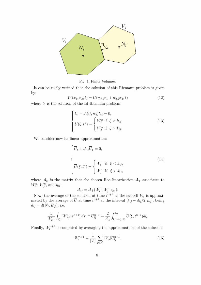
Fig. 1. Finite Volumes.

It can be easily verified that the solution of this Riemann problem is givenby:

W (x1, x2, t) = U(ηij,1x1 + ηij,2x2, t) (12)

where U is the solution of the 1d Riemann problem:

Ut + A(U, ηij)Uξ = 0,

U(ξ, tn) =

W ni if ξ < kij ,

W nj if ξ > kij ,

(13)

We consider now its linear approximation:

U t + AijU ξ = 0,

U(ξ, tn) =

W ni if ξ < kij,

W nj if ξ > kij,

(14)

where Aij is the matrix that the chosen Roe linearization AΨ associates toW n

i , W nj , and ηij :

Aij = AΨ(W ni , W n

j , ηij).

Now, the average of the solution at time tn+1 at the subcell Vij is approxi-mated by the average of U at time tn+1 at the interval [kij − dij/2, kij], beingdij = d(Ni, Eij), i.e.

1

|Vij|∫

Vij

W (x, tn+1) dx ∼= Un+1ij =

2

dij

∫ kij

kij−dij/2U(ξ, tn+1)dξ.

Finally, W n+1i is computed by averaging the approximations of the subcells:

W n+1i =

1

|Vi|∑

j∈Ni

|Vij|Un+1ij . (15)

8

Assuming the CFL condition

max|λij,k| : k = 1, . . . , N · ∆t ≤ dij

2, (16)

where λij,k represent the eigenvalues of Aij, some straightforward calcula-tions allow us to write the numerical scheme as follows:

W n+1i = W n

i − 1

|Vi|∑

j∈Ni

|Eij |A−ij(W

nj − W n

i ), (17)

whereA−

ij = KijD−ijK−1

ij ,

being D−ij the diagonal matrix whose coefficients are the negative parts of the

eigenvalues of Aij and Kij is a N × N matrix whose columns are associatedeigenvectors. (17) is the general expression of a Roe scheme for problem (3).

The best choice of the family of paths Ψ appearing in the definition of theRoe linearization seems to be the family Φ selected for the definition of weaksolutions. In effect, Roe methods based on the family of paths Φ approachescorrectly the admissible discontinuities in the following sense: let us supposethat the approximations at two neighbor cells, W n

i and W nj , can be linked by

an entropy discontinuity located at the straight line containing the edge Eij

and propagating at speed σ; then, from (7) and (4) we deduce:

Aij

(W n

j − W ni

)= σ

(W n

j − W ni

),

i.e. σ is an eigenvalue of the intermediate matrix and W nj −W n

i is an associatedeigenvector. As a consequence, the solution of the linear Riemann problem (14)corresponding to the intercell Eij coincides with the solution of the Riemannproblem (10). Nevertheless, the construction of a Roe scheme with Ψ = Φ canbe difficult or very costly in practice. In this case, a simpler family of paths Ψhas to be chosen, as the family of segments.Remark 2 Even if the Roe linearization is based on the family of paths Φused to define the weak solutions of the problem, the numerical solutions maynot converge to the right weak solutions: in general, the limits of the numericalsolutions solve a system involving a source term which is a convergence errorsource measure supported in the discontinuities: see [5]. This phenomenon, thatwas first studied for nonconservative methods applied to scalar conservationlaws in [16], affects not only Roe methods but any numerical method whichis consistent in a certain sense with the chosen family of paths (see [5] fordetails). Nevertheless, in general this convergence error is only noticeable forvery fine meshes, for discontinuities of great amplitude, and/or for large-timesimulations. The only methods which are known to avoid this difficulty areGlimm scheme or the front tracking methods: see [19]. Unfortunately, thesemethods may be time consuming and difficult to implement since they requirethe explicit knowledge of the solution of Riemann problems. This, togetherwith the fact that non-conservative models are usually derived from modeling

9

approximation assumptions, fully justifies the use of a numerical strategy basedon a direct discretization of the nonconservative hyperbolic model (3) by meansof robust and efficient high-order schemes.Remark 3 In certain special situations, the convergence error measure isfound to vanish identically. This is the case of systems of balance laws. In thiscase, two kind of discontinuities may appear in weak solutions: shocks evolv-ing in regions where the source term is continuous that satisfy the standardRankine-Hugoniot conditions and stationary contact discontinuities standingover the discontinuities of the source term. If the Roe linearization is based ona family of paths satisfying (H1) then all of the discontinuities are correctlyapproximated by the corresponding Roe method and the numerical solutionsdoes converge to the correct solutions. Nevertheless, systems of balance lawsmay also exhibit an additional difficulty (the resonance problem) if one of theeigenvalues of the Jacobian matrix vanishes. In this case, the weak solutionsmay not be uniquely determined by the initial data, and the limits of the nu-merical solutions may depend both on the family of paths and on the numericalscheme itself.Remark 4 Observe that in the deduction of the schemes a CFL-like require-ment (16) has been imposed. In practice, the following condition:

max

|λij,k|dij

: i = 1, . . . , NV, j ∈ Ni, k = 1, . . . , N

· ∆t ≤ γ, (18)

with 0 < γ ≤ 1, ensures the linear stability.Remark 5 As in the case of systems of conservation laws, when sonic rar-efaction waves appear it is necessary to modify the approximate Riemann prob-lem solver in order to obtain entropy-satisfying solutions. The Harten-HymanEntropy Fix technique (see [15]), for instance, can be easily adapted to thiscase.

3.1 Consistency

The following result of consistency for smooth solutions can be proved:Theorem 5 Let us suppose that A1(W ), A2(W ) are C1 matrices with boundedderivatives. Let us also suppose that the chosen Roe linearizations AΨ(·, ·; ηij)at each edge Eij as well as the functions |A(·, ηij)| are C1 with bounded deriva-tives. Let us assume that the finite volume mesh consists of regular polygonswith an even number of edges and with the same diameter ∆x. Then, thescheme (17) is consistent for smooth solutions.

Remark 6 The regularity assumption for |AΨ(·, ·; ηij)| is equivalent, in prac-tice, to assume that the eigenvalues of the intermediate matrices do not vanish,i.e. that the solutions to be approached do not have transitions. However, inpractice the entropy fix applied to the scheme prevents the eigenvalues fromvanishing and thus the hypothesis are satisfied even when transitions occur.Proof:

10

First, the following notation is introduced: Ni = (Ni,1, Ni,2) and Nij = (Nij,1, Nij,2)represent, respectively, the center of the cell Vi and the mid-point of the edgeEij , so that

dij = d(Ni, Nij).

Some simple applications of the divergence theorem allow us to prove theequalities:

∑

j∈Ni

|Eij |ηij = 0; (19)

∑

j∈Ni

dij |Eij|η2ij,1 = |Vi|; (20)

∑

j∈Ni

dij |Eij|η2ij,2 = |Vi|; (21)

∑

j∈Ni

dij |Eij|ηij,1ηij,2 = 0. (22)

More precisely, the divergence theorem has to be applied to the fields: (1, 0),(0, 1), (x1 − Ni,1, 0), (0, x2 − Ni,2), and (x2 − Ni,2, 0) in Vi.

Let us consider W a regular solution of (3) and W ni = W (Ni, t

n). We wantto prove that:

W n+1i − W n

i

∆t+

1

|Vi|∑

j∈Ni

|Eij |A−ij(W

nj − W n

i )

= (Wt + A1(W )Wx1+ A2(W )Wx2

) (Ni, tn) (23)

+ O(∆x, ∆t).

Clearly the first term is equal to Wt(Ni, tn) + O(∆t).

Let us analyze the second term. First, we use the equality

A−ij =

1

2(Aij − |Aij|), (24)

where|Aij| = Kij |Dij|K−1

ij ,

being |Dij| the diagonal matrix whose coefficients are the absolute value ofthe eigenvalues of Aij. We obtain:

1

|Vi|∑

j∈Ni

|Eij |A−ij(W

nj − W n

i ) =1

2|Vi|∑

j∈Ni

|Eij|Aij(Wnj − W n

i )

(25)

− 1

2|Vi|∑

j∈Ni

|Eij||Aij|(W nj − W n

i ).

For the first summand in the right-hand side of (25) we have the equalities:

11

1

2|Vi|∑

j∈Ni

|Eij|Aij(Wnj − W n

i )

=1

|Vi|∑

j∈Ni

|Eij |A(W ni , ηij)dij (ηij,1Wx1

(Ni, tn) + ηij,2Wx2

(Ni, tn)) + O(∆x)

= A1(Wni )Wx1

(Ni, tn) + A2(W

ni )Wx2

(Ni, tn) + O(∆x), (26)

where we have used the equalities

AΨ(W ni , W n

i , ηij) = A(W ni , ηij) =

2∑

k=1

ηij,kAk(Wni ),

the relations (19)-(22), and

1

2|Vi|∑

j∈Ni

|Eij |dij = 1,

∣∣∣∣∣∣1

|Vi|∑

j∈Ni

|Eij|d2ij

∣∣∣∣∣∣≤ ∆x.

Let us see finally that the second summand in the right-hand side of (25) isO(∆x). To do this, we first consider a partition Ji, Ki of the set of indexesNi such that:• card(Ji) = card(Ki);• given an index j ∈ Ji, there exists a unique index j∗ ∈ Ki such that

ηij∗ = −ηij .

Using this partition we have:

1

2|Vi|∑

j∈Ni

|Eij||Aij|(W nj − W n

i )

=1

2|Vi|∑

j∈Ji

|Eij||Aij|(W nj − W n

i )

+1

2|Vi|∑

j∈Ji

|Eij∗||Aij∗|(W nj∗ − W n

i )

=1

2|Vi|∑

j∈Ji

|Eij|(|A(W (Nij, t

n), ηij)|(W nj − W n

i )

+ |A(W (Nij∗, tn), ηij)|(W n

j∗ − W ni ))

+ O(∆x)

=1

2|Vi|∑

j∈Ji

|Eij|(|A(W (Nij, t

n), ηij)|Wηij(Nij , t

n)dij

− |A(W (Nij∗, tn), ηij)|Wηij

(Nij∗ , tn)dij

)+ O(∆x)

=1

2|Vi|∑

j∈Ni

|Eij |d2ij

∂

∂ηij

(|A(W, ηij)|Wηij

)(Ni, t

n) + O(∆x)

= O(∆x),

12

where Wη = ηij,1Wx1+ ηij,2Wx2

.2

Remark 7 The hypothesis on the finite volume mesh can be relaxed. Theprevious theorem still holds under the following hypothesis:

• the cells of T have an even number of edges;• for every cell Vi:

−−−→NiNij = dijηij + O(∆x), ∀j ∈ Ni,

being ∆x = maxdiam(Vi);• the edges of every cell Vi can be taken in pairs (Eij , Eij∗) verifying:

ηij∗ = −ηij + O(∆x),

|Eij∗| = |Eij| + O(∆x);

• given two neighbor cells Vi, Vj:

dij = dji + O(∆x).

• |A(·, ·)| is C1 with bounded derivatives.

For meshes consisting of polygons with an odd number of edges, the consis-tency may fail. Let us consider, for instance, the 1d linear transport equationinterpreted as a 2d problem:

ut + aux1= 0, x = (x1, x2) ∈ R

2, t ≥ 0, (27)

where a is, say, positive. This equation is a particular case of (3) with N = 1,W = u, A1(W ) = a; A2(W ) = 0.

We fix the time step ∆t and the space step ∆x and consider points:

xkj = (j∆x, k∆x), j, k ∈ Z.

We consider the mesh composed by the triangles whose vertices are the pointsof coordinates:

xkj ,x

kj+1,x

k+1j , (28)

and those whose vertices are:

xkj ,x

k+1j−1 ,x

k+1j . (29)

Let us consider the strip composed by the triangles of both families corre-sponding to a fixed value of k. Let Vi the triangle whose vertices are (28) withj = (i− 1)/2 if i is odd, and the triangle whose vertices are (29) with j = i/2if i is even. Some straightforward calculations allow us to rewrite the scheme

13

as follows:

un+1i = un

i − 2∆t

∆xa(un

i − uni−1).

Clearly, the local truncation error is not first order. Nevertheless, the errors atthe cells may compensate and the numerical scheme converge: notice that, evenin the 1d case, the classical requirement of consistency fails for conservativeschemes with consistent numerical fluxes when the grid is not uniform. Thefailure of consistency of Finite Volume schemes on triangular meshes has beennoted in [17]. See also [14].

3.2 Well-balancing

The well-balance properties of Roe schemes for 1d nonconservative systemshave been studied in [24]. In general, these properties are not inherited bytheir two dimensional extensions. Nevertheless some partial results can stillbe given.

Definition 6 Given an edge Eij, we will denote by Γij the set of integralcurves of linearly degenerated fields of A(W, ηij) such that the correspondingeigenvalue vanishes along the curve.

Theorem 7 Let W be a regular stationary solution of (3) satisfying the fo-llowing property: given two neighbor cells Vi, Vj the path

s ∈ [0, 1] → Ψ(s, W (Ni), W (Nj), ηij)

is a parametrization of an arc γγγ of Γij. Then the numerical scheme computesexactly the solution W .Proof:

Defining W 0i = W (Ni), for all i. We obtain the following equalities:

Aij(W0j − W 0

i ) =AΨ(W 0i , W 0

j , ηij)(W0j − W 0

i ) =

=∫ 1

0A(Ψ(s, W 0

i , W 0j , ηij), ηij

)· ∂Ψ

∂s(s, W 0

i , W 0j , ηij) ds = 0

where we have used the definition of Aij, the property (7) of the linearizationand the fact that Ψij(s, W

0i , W 0

j , ηij) is a parametrization of a curve of Γij .Then, 0 is an eigenvalue of Aij and W 0

j − W 0i an associated eigenvector. By

definition of A−ij we have:

A−ij(W

0j − W 0

i ) = 0, for all j ∈ Ni, (30)

and thus:W n

i = W 0i , ∀i, n.

2

14

Corollary 8 If Ψ is the family of segments (5), then the numerical schemesolves exactly any regular stationary solution W such that, for any pair ofneighbor cells, Vi, Vj the segment linking W (Ni) and W (Nj) belongs to acurve γγγ of Γij.Theorem 9 Let us assume that A1, A2 are of class C1 with bounded deriva-tives and that the finite volume mesh T satisfies the regularity conditions ofTheorem 5. Let W be a regular stationary solution of (3) with the followingproperty: given two neighbor cells Vi, Vj the states W (Ni), W (Nj) belong to asame curve γγγ of Γij, and it is possible to find a parametrization

U : [0, 1] −→ Ω,

of class Ck+1 of the arch of γγγ linking them, such that:

∫ 1

0|U ′(s) − ∂Ψ

∂s(s, W (Ni), W (Nj), ηij)| ds = O(d(Ni, Nj)

k+1). (31)

Then, the scheme approximates the solutions W with order k.

Proof:

We define again:W 0

i = W (Ni), for all i.

Following the proof of Theorem 2 in [24], we obtain from (31) the estimate:

A−ij(W

0j − W 0

i ) = O(d(Ni, Nj)k+1), for all j ∈ Ni.

As a result:

W 1i =W 0

i − 1

|Vi|∑

j∈Ni

|Eij |A−ij(W

0j − W 0

i )

=W 0i − 1

|Vi|∑

j∈Ni

2|Vij|dij

A−ij(W

0j − W 0

i )

=W 0i + O(∆xk).

2

Theorem 10 Under the same hypothesis of Theorem 9, let us suppose thatΨ is the family of segments (5). Let W be a C3 stationary solution of (3) suchthat, given two neighbor cells Vi, Vj, the function

s ∈ [0, 1] → W (Ni + s(Nj − Ni))

is a parametrization of an arc of some curve of Γij. Then, the scheme approx-imates the solution W with order 2.

Proof:

15

Defining:W 0

i = W (Ni), for all i,

and proceeding as in the proof of Theorem 3 in [24], the following estimatecan be obtained:

A−ij(W

0j − W 0

i ) = O(d(Ni, Nj)3), for all j ∈ Ni.

From this estimate, the proof is concluded as in Theorem 9.2

Remark 8 In the proofs of the two previous theorems it is possible to weakenthe hypothesis for the mesh: it is enough to assume that there exists C∗ > 0independent of ∆x such that

d(Ni, Nj)

2dij≤ C∗.

Notice that the hypotheses concerning the stationary solutions in the previ-ous theorems are much more restrictive than in the 1d case: while in 1d prob-lems the values taken by a stationary solution at the centers of two neighborcells always belong to the same integral curve of a linearly degenerate fieldwhose corresponding eigenvalue vanishes along the curve (see [24]), this is notthe case for general two dimensional stationary solutions. Nevertheless, thishappens when the stationary solution is essentially 1d and the mesh is rect-angular and properly oriented. More precisely, let η ∈ R

2 be a fixed unitaryvector and U(ξ) a regular stationary solution of the one dimensional problem:

Ut + A(U, η)Uξ = 0. (32)

Let W be the stationary solution of problem (3) given by:

W (x1, x2) = U(x1η1 + x2η2).

If we have a rectangular mesh such that for every edge Eij , the vector ηij

is either parallel or orthogonal to η, then it can be easily verified that therestriction of the solution to the segment linking the centers of two neighborcells is a solution of the projected problem:

Ut + A(U, ηij)Uξ = 0,

and, as a result, its values at those centers are connected by a curve of Γij.For this kind of solutions and meshes, the 2d schemes have the same well

balanced properties that the one dimensional schemes from which they havebeen derived.

Nevertheless, we will see that Corollary 8 is enough to ensure the C-Property(see [2] for details) of the schemes applied to shallow water systems of one or

16

two layers, i.e. the stationary solutions corresponding to water at rest situa-tions are preserved.

4 High order schemes based on reconstruction of states

In this section, we present a high order extension by state reconstructions ofthe previously proposed scheme.

Let us consider first the case of systems of conservation laws

Wt + F1(W )x1+ F2(W )x2

= 0. (33)

These systems can be considered as a particular case of (3) in which thematrices Ai(W ), i = 1, 2 are the Jacobians:

Ai(W ) =∂Fi

∂W, i = 1, 2.

High order methods based on the reconstruction of states can be built for(33) using the following procedure: given a first order conservative schemewith numerical flux function G(U, V ; η), a reconstruction operator of order pis considered, that is, an operator that associates to a given family WiNV

i=1

of values at the cells two families of functions defined at the edges:

γ ∈ Eij → W±ij (γ),

in such a way that, whenever

Wi =1

|Vi|∫

Vi

W (x) dx (34)

for some smooth function W , then

W±ij (γ) = W (γ) + O(∆xp), ∀γ ∈ Eij.

Once the first order method and the reconstruction operator have been cho-sen, the method of lines can be used to develop high order methods for (33):the idea is to discretize only in space, leaving the problem continuous in time.This procedure leads to a system of ordinary differential equations that hasto be numerically solved. The choice of the numerical method is important: alinearly stable time discretization which is non-TVD (Total Variation Dimin-

ishing) can generate spurious oscillations even for TVD spatial discretization.Therefore we will consider in the numerical tests the TVD Runge-Kutta meth-ods introduced in [27]. See also [11], [28].

Let W i(t) denotes the cell average of a regular solution W of (33) over thecell Vi at time t:

W i(t) =1

|Vi|∫

Vi

W (x, t) dx.

17

The following equation can be easily obtained for the cell averages:

W′

i(t) = − 1

|Vi|

∑

j∈Ni

∫

Eij

F (W (γ, t)) · ηij dγ

. (35)

The first order method and the reconstructions are now used to approach thevalues of the fluxes at the edges:

W′

i (t) = − 1

|Vi|

∑

j∈Ni

∫

Eij

G(W−ij (γ, t), W+

ij (γ, t), ηij) dγ

, (36)

being Wi(t) the approximation to W i(t) provided by the scheme and W±ij (γ, t)

the reconstruction at γ ∈ Eij corresponding to the family Wi(t)NVi=1 . It can

be shown that (36) is an approximation of order p of (35).In practice, the integral terms in (36) are approached by means of a numerical

quadrature of order r ≥ p at least:

∫ b

af(s)ds = (b − a)

n(r)∑

l=1

ωlf(xl)

+ O(∆xr), (37)

where n(r) denotes the number of points, ωl are the weights, and xl = a +sl(b − a) with sl ∈ [0, 1], represent the quadrature points. The expression ofthe corresponding semi-discrete numerical scheme is then as follows:

W′

i (t) = − 1

|Vi|∑

j∈Ni

|Eij |

n(r)∑

l=1

ωlG(W−

ij,l(t), W+ij,l(t), ηij

) . (38)

where

W±ij,l(t) = W±

ij (aij + sl(bij − aij), t) , (39)

aij and bij being the extremes of the edge Eij .We assume here that the first order scheme is a Roe method, i.e.:

G(U, V, η) =Fη(U) + Fη(V )

2− 1

2|A(U, V, η)| (V − U), (40)

where Fη is given by (9) and A(U, V, η) is the Roe matrix associated to thestates U , V , and to the unit vector η, i.e. an intermediate matrix that verifiesthe Roe property:

Fη(V ) − Fη(U) = A(U, V, η) · (V − U). (41)

Let us now generalize the semi-discrete methods (36) or (38) to the noncon-servative system (3). We will assume that the reconstructions are calculated asfollows: given the family WiNV

i=1 of values at the cells, first an approximation

18

function is constructed at every cell Vi, based on the values of Wi at some ofthe cells close to Vi (the stencil):

Pi(x) = Pi (x; Wjj∈Bi) ,

for some set of indexes Bi. If, for instance, the reconstruction only depends onthe neighbor cells of Vi, then Bi = Ni∪i. These approximations functions arecalculated usually by means of an interpolation or approximation procedure.Once these functions have been constructed, the reconstruction at γ ∈ Eij aredefined as follows:

W−ij (γ) = lim

x→γPi(x), W+

ij (γ) = limx→γ

Pj(x). (42)

Clearly, for any γ ∈ Eij the following equalities are satisfied:

W−ij (γ) = W+

ji (γ); W+ij (γ) = W−

ji (γ).

We suppose that the reconstruction operator satisfies the following proper-ties:

(HP1) It is conservative, i.e. the following equality holds for any cell Vi:

Wi =1

|Vi|∫

Vi

Pi(x)dx. (43)

(HP2) If the operator is applied to a sequence Wi satisfying (34) for somesmooth function W (x), then

W±ij (γ) = W (γ) + O(∆xp), ∀γ ∈ Eij,

andW+

ij (γ) − W−ij (γ) = O(∆xp+1), ∀γ ∈ Eij .

(HP3) It is of order q in the interior of the cells, i.e. if the operator is applied toa sequence Wi satisfying (34) for some smooth function W (x), then:

Pi(x) = W (x) + O(∆xq), ∀x ∈ int(Vi). (44)

(HP4) Under the assumption of the previous property, the gradient of Pi pro-vides an approximation of order m of the gradient of W :

∇Pi(x) = ∇W (x) + O(∆xm), ∀x ∈ int(Vi). (45)

Remark 9 Notice that, in general, m ≤ q ≤ p. If, for instance, the approxi-mation functions are polynomials of degree p obtained by interpolating the cellvalues on a fixed stencil, then m = p − 1 and q = p. In the case of WENO-like reconstructions (see [28]), the approximation functions are obtained as aweighted combination of interpolation polynomials whose accuracy is greateron the boundary than at the interior of the cell: in this case q < p.

19

Let us denote by P ti the approximation functions corresponding to the ap-

proximations of the cell averages Wi(t), i.e.

P ti (x) = Pi (x; Wj(t)j∈Bi

) .

W−ij (γ, t) (resp. W+

ij (γ, t)) is then defined by

W−ij (γ, t) = lim

x→γP t

i (x), W+ij (γ, t) = lim

x→γP t

j (x). (46)

Using (24) and (41), (36) can be rewritten as follows:

W ′i (t) = − 1

|Vi|∑

j∈Ni

∫

Eij

(A−

ij(γ, t)(W+ij (γ, t) − W−

ij (γ, t)))

dγ

− 1

|Vi|∑

j∈Ni

∫

Eij

(Fηij

(W−ij (γ, t))

)dγ

= − 1

|Vi|∑

j∈Ni

∫

Eij

(A−

ij(γ, t)(W+ij (γ, t) − W−

ij (γ, t)))

dγ

− 1

|Vi|∫

Vi

∇ · (F P ti )(x)) dx

= − 1

|Vi|∑

j∈Ni

∫

Eij

(A−

ij(γ, t)(W+ij (γ, t) − W−

ij (γ, t)))

dγ

− 1

|Vi|∫

Vi

(A1(P

ti (x))

∂P ti

∂x1

(x) + A2(Pti (x))

∂P ti

∂x2

(x)

)dx,

(47)

where the following notation has been used

Aij(γ, t) = A(W+

ij (γ, t), W−ij (γ, t), ηij

),

together with the definition of the reconstructions and the divergence theorem.Notice now that (36) can be easily generalized to obtain a numerical scheme

for solving (3):

W ′i (t) = − 1

|Vi|

∑

j∈Ni

∫

Eij

(A−

ij(γ, t)(W+ij (γ, t) − W−

ij (γ, t)))

dγ

+∫

Vi

(A1(P

ti (x))

∂P ti

∂x1(x) + A2(P

ti (x))

∂P ti

∂x2(x)

)dx

],

(48)

where now

Aij(γ, t) = AΨ

(W−

ij (γ, t), W+ij (γ, t), ηij

),

being AΨ the chosen Roe linearization.

20

4.1 Order of accuracy

The cell averages of a smooth solution of (3), W i(t), satisfy:

W′i(t) = − 1

|Vi|∫

Vi

(A1(W (x))Wx1(x) + A2(W (x))Wx2

(x)) dx. (49)

Thus, (48) is expected to be an accurate approximation of (49). This factis stated in the following result, whose proof is similar to the correspondingresult for 1d problems (see [4]):

Theorem 11 Let us assume that A1 and A2 are of class C2 with boundedderivatives and AΨ is bounded for all i, j. Let us also suppose that the re-construction operator satisfies the hypothesis (HP1)-(HP4). Then (48) is anapproximation of order at least α = min(p, q, m) to the system (49) in thefollowing sense:

1

|Vi|∑

j∈Ni

[∫

Eij

(A−

ij(γ, t)(W+ij (γ, t) − W−

ij (γ, t)))

dγ

+∫

Vi

(A1(P

ti (x))

∂P ti

∂x1(x) + A2(P

ti (x))

∂P ti

∂x2(x)

)dx

]

=1

|Vi|∑

j∈Ni

∫

Vi

(A1(W (x, t))Wx1(x, t) + A2(W (x, t))Wx2

(x, t)) dx + O(∆xα),

(50)for every solution W smooth enough, being W±

ij (γ, t) the associated reconstruc-tions and P t

i the approximation functions corresponding to the family

W i(t) =1

|Vi|∫

Vi

W (x, t) dx.

Remark 10 According to Remark 9 the expected order of the numerical schemeis m. Nevertheless, this theoretical result is rather pessimistic: in practice, asit will be seen in Section, the order q is often achieved.

4.2 Approximation of the integral terms

In practice, the integral terms in (48) are numerically approached. In thiscase, together with a 1d formula (37) for the integrals on the edges, it can bealso necessary to choose a quadrature formula of order s for the integrals inthe cells:

∫

Vi

f(x) dx = |Vi|n(s)∑

l=1

αilf(xi

l) + O(|Vi|s). (51)

In order to preserve the order of the numerical scheme, it is necessary to

21

have r ≥ α and s ≥ α. The numerical scheme writes then as follows:

W′

i (t) = − 1

|Vi|

∑

j∈Ni

|Eij|n(r)∑

l=1

wlA−ij,l(t)(W

+ij,l(t) − W−

ij,l(t))

+|Vi|n(s)∑

l=1

αil

(A1(P

ti (x

il))

∂P ti

∂x1(xi

l) + A2(Pti (x

il))

∂P ti

∂x2(xi

l)

) ,

(52)

whereW±

ij,l(t) = W±ij (aij + sl(bij − aij), t),

Aij,l(t) = AΨ(W−ij,l(t), W

+ij,l(t), ηij).

Remark 11 If a quadrature formula is used, the properties (HP2)-(HP4) haveto be satisfied only at the quadrature points to obtain the accuracy result givenby Theorem 11. In [23] an interesting technique has been introduced that couldavoid the explicit computation of ∇Pi(x) making thus the expected order of ac-curacy equal to α = min(p, q). The extension to 2d problems of this technique,which is based on the use of the trapezoidal rule and Romberg extrapolationfor the numerical integration, would be straightforward for structured meshes.For unstructured meshes a Romberg extrapolation formula on triangles couldbe used (see [33] ).

4.3 Well-balance properties.

In this section we study the well-balanced properties of the schemes (48) or(52).Definition 12 We consider a semi-discrete method to approximate (3):

W ′i (t) =

1

|Vi|H (Wj(t), j ∈ Bi) ,

W(0) = W0,

(53)

where W(t) = Wi(t)NVi=1 represents the vector of the approximations to the

averaged values of the exact solution; W0 = W 0i is the vector of the initial

conditions; and Bi are the stencils. Given a smooth stationary solution W ofthe system, the numerical scheme is said to be exactly well-balanced for W ifthe vector or its cell averages is a critical point of (53), i.e.

H(Wj , j ∈ Bi) = 0, (54)

ant it is said to be well-balanced with order p if

H(Wj , j ∈ Bi) = O(∆xp+2). (55)

Let us also introduce the concept of well-balance reconstruction operator:

22

Definition 13 Given a smooth stationary solution of (3), a reconstructionoperator is said to be well-balanced for W (x) if the approximation functionsPi(x) associated to the averaged values of W are also stationary solutions ofthe system, i.e.

A1(Pi(x))Pi(x)x1+ A2(Pi(x))Pi(x)x2

= 0, ∀x ∈ Vi, i = 1, . . . , NV.

The two following results can be easily proved:Theorem 14 Let W be a smooth stationary solution of (3). Let us supposethat both the first order Roe method and the reconstruction operator chosenare exactly well-balanced for W . Then the numerical schemes (48) and (52)are also exactly well-balanced for W .Theorem 15 Under the hypotheses of Theorem 11, the schemes (48) and(52) are well-balanced with order at least α = min(p, q, m).

5 Systems of conservation laws with non conservative products and

source terms

We consider in this section systems of the form:

Wt+F1(W )x1+F2(W )x2

= B1(W )Wx1+B2(W )Wx2

+S1(W )Hx1+S2(W )Hx2

,(56)

where W (x, t) : D × (0, T ) 7→ Ω ⊂ RN , D being a bounded domain of R

2; Ω,a convex subset of R

N ; Fi : Ω 7→ RN , Bi : Ω 7→ MN×N(R) and Si : Ω 7→ R

N ,i = 1, 2, are regular and locally bounded functions. Finally H : D ⊂ R

2 : 7→ R

is a known function.If the equation

Ht = 0,

is added to the system and H is considered like a new unknown of the problem(whose value is determined by the initial condition), (56) can be rewritten inthe form:

Wt + A1(W )Wx1+ A2(W )Wx2

= 0, (57)

where W is the augmented vector:

W =

W

H

,

and the block structure of the matrices Ak(W ) ∈ M(N+1)×(N+1)(R), k = 1, 2,are given by

Ak(W ) =

Ak(W ) −Sk(W )

0 0

, k = 1, 2. (58)

Here,Ak(W ) = Jk(W ) − Bk(W ), k = 1, 2,

23

being Jk, k = 1, 2 the Jacobian matrix of the flux functions Fk, k = 1, 2:

Jk(W ) =∂Fk

∂W, k = 1, 2.

The following notation will be used:

A(W, η)= η1A1(W ) + η2A2(W ),

J (W, η)= η1J1(W ) + η2J2(W ),

B(W, η)= η1B1(W ) + η2B2(W ),

S(W, η)= η1S1(W ) + η2S2(W ).

We assume that (56) is hyperbolic: for any η and W ∈ Ω, the matrix A(W, η)has N real distinct eigenvalues

λ1(W, η) < · · · < λN(W, η),

and associated eigenvectors Rj(W, η), j = 1, . . . , N . If these eigenvalues donot vanish, (57) is a strictly hyperbolic system: given a unit vector η and astate W , the eigenvalues of the matrix

A(W , η) = A1(W1)η1 + A2(W2)η2,

are:λ1(W, η), . . . , λN(W, η), 0

with associated eigenvectors:

R1(W , η), . . . , RN+1(W , η),

given by

Ri(W , η) =

Ri(W, η)

0

, i = 1, . . . , N ; RN+1(W , η) =

A(W, η)−1 · S(W, η)

1

.

In order to construct Roe matrices for (57), first of all a family of pathsΨ has to be chosen. The following notation will be used to describe, given avector η, the path linking two states W0, W1:

Ψ(s; W0, W1, η) =

Ψ(s; W0, W1, η)

ΨN+1(s; W0, W1, η)

=

Ψ1(s; W0, W1, η)

Ψ2(s; W0, W1, η)...

ΨN+1(s; W0, W1, η)

.

Let us suppose that, given any unit vector η and two states Wj = [Wj, Hj]T ,

j = 0, 1 it is possible to calculate:

24

• A matrix J (W0, W1, η) such that:

J (W0, W1, η)(W1 − W0) = Fη(W1) − Fη(W0),

i.e. a Roe matrix for the flux function Fη.• A matrix B

Ψ(W0, W1, η) satisfying:

BΨ(W0, W1, η)(W1−W0) =

∫ 1

0B(Ψ(s; W0, W1, η), η

) ∂Ψ

∂s

(s; W0, W1, η

)ds;

(59)• A vector S

Ψ(W0, W1, η) satisfying:

SΨ(W0, W1, η)(H1−H0) =

∫ 1

0S(Ψ(s; W0, W1, η), η

)·∂ΨN+1

∂s

(s; W0, W1, η

)ds,

(60)Then, it can be easily verified that the matrix:

AΨ(W0, W1, η) =

A

Ψ(W0, W1, η) −S

Ψ(W0, W1, η)

0 0

, (61)

withA

Ψ(W0, W1, η) = J (W0, W1, η) − B

Ψ(W0, W1, η),

is a Roe linearization provided that it has N + 1 real different eigenvalues.Let us suppose that the approximations at time tn

W ni =

W ni

Hi

,

have already been obtained. The following notation will be used:

Jij =J (W ni , W n

j , ηij),

Bij =BΨ(W n

i , W nj , ηij),

Sij =SΨ(W n

i , W nj , ηij),

Aij =Jij − Bij ,

Aij = AΨ(W n

i , W nj , ηij) =

Aij −Sij

0 0

.

The corresponding Roe scheme reads then as follows:

W n+1i = W n

i − ∆t

|Vi|∑

j∈Ni

|Eij |A−ij(W

nj − W n

i ). (62)

Dropping the (N +1)-th components (which are not relevant as H is a knownfunction), some straightforward calculations allow us to rewrite the scheme as

25

follows:

W n+1i = W n

i − ∆t

|Vi|∑

j∈Ni

|Eij|(Gij − Bij · (W n

j − W ni ) − P−

ij Sij(Hj − Hi))

(63)where

Gij =1

2

(Fηij

(W ni ) + Fηij

(W nj ))− 1

2|Aij| (W n

j − W ni )

is the usual Roe flux and

P−ij =

1

2

(I − |Aij| A−1

ij

).

This latter matrix can also be written in the form

P−ij =

1

2Kij

(I − sgn (Dij)

)K−1

ij ,

where sgn (Dij) is the diagonal matrix whose coefficients are the signs of theeigenvalues λij,1,. . . , λij,N of Aij and Kij is an N × N matrix whose columnsare associated eigenvectors.

Using the equality A−ij = P−

ijAij the numerical scheme can also be writtenin this way:

W n+1i = W n

i − ∆t

|Vi|∑

j∈Ni

|Eij |F−ij , (64)

where

F−ij = P−

ij (Aij(Wnj − W n

i ) − Sij(Hj − Hi)). (65)

In a similar way, the semi-discrete high order extension of the Roe scheme(63) based on a reconstruction operator (48) can be expressed as follows:

W ′i = − 1

|Vi|∑

j∈Ni

∫

Eij

(Gij(γ, t) − Bij(γ, t)(W+

ij (γ, t) − W−ij (γ, t))

−P−ij (γ, t)Sij(γ, t)(H+

ij (γ) − H−ij (γ))

)dγ

+1

|Vi|∫

Vi

(2∑

k=1

Bk(Pti (x))

∂P ti

∂xk(x) +

2∑

k=1

Sk(Pti (x))

∂P tN+1,i

∂xk(x)

)dx,

(66)where the following notation has been used:

x ∈ Vi → P ti (x) =

P ti (x)

P tN+1,i(x)

=

P t1,i(x)

P t2,i(x)...

P tN,i(x)

P tN+1,i(x)

,

26

represents the approximation function at the cell Vi at time t;

γ ∈ Eij → W±ij (γ, t) =

W±ij (γ, t)

H±ij (γ)

,

the reconstructions at the edge Γij at time t;

Jij(γ, t) =J (W−ij (γ, t), W+

ij (γ, t), ηij),

Bij(γ, t) =BΨ(W−

ij (γ, t), W+ij (γ, t), ηij),

Sij(γ, t) =SΨ(W−

ij (γ, t), W+ij (γ, t), ηij),

Aij(γ, t) =Jij(γ, t) − Bij(γ, t),

Gij(γ, t) =1

2

(Fηij

(W−ij (γ, t) + Fηij

(W+ij (γ, t))

)

−1

2|Aij(γ, t)| (W+

ij (γ, t) − W−ij (γ, t)),

P−ij (γ, t) =

1

2Kij(γ, t)

(I − sgn (Dij(γ, t)

)K−1

ij (γ, t),

where sgn (Dij(γ, t)) is the diagonal matrix whose coefficients are the signs ofthe eigenvalues λij,1(γ, t),. . . , λij,N(γ, t) of Aij(γ, t) and Kij(γ, t) is a N × Nmatrix whose columns are associated eigenvectors.

Finally, the numerical scheme (52) can be rewritten in this particular caseas follows:

W ′i = − 1

|Vi|∑

j∈Ni

|Eij|n(r)∑

l=1

wl

(Gij,l(t) − Bij,l(t)(W

+ij,l(t) − W−

ij,l(t))

−Pij,l(t)−Sij,l(t)(H

+ij,l(t) − H−

ij,l(t)))

+1

|Vi|n(s)∑

l=1

αil

(2∑

k=1

Bk(Pti (xl))

∂P ti

∂xk

(xl) +2∑

k=1

Sk(Pti (xl))

∂P tN+1,i

∂xk

(xl)

)

(67)using the obvious notation.

6 Applications to the shallow water system

6.1 Equations

Let us consider the one layer shallow water system without friction terms:

27

∂h

∂t+

∂q1

∂x1

+∂q2

∂x2

= 0,

∂q1

∂t+

∂

∂x1

(q21

h+

g

2h2

)+

∂

∂x2

(q1q2

h

)= gh

∂H

∂x1,

∂q2

∂t+

∂

∂x1

(q1q2

h

)+

∂

∂x2

(q22

h+

g

2h2

)= gh

∂H

∂x2

.

(68)

which are the equations governing the flow of a shallow layer of homogeneousinviscid fluid in a two dimensional domain D ⊂ R

2. In the equations, H(x)represents the depth function measured from a fixed level of reference; g isthe gravity; qj(x, t) represents the mass-flow in the direction j; and h(x, t),the thickness of the layer. These quantities are related to the vertical averagedvelocity (u1(x, t), u2(x, t)) by the relations:

qj(x, t) = uj(x, t)h(x, t), j = 1, 2.

Problem (68) can be written in the form (56) with:

W =

h

q1

q2

, (69)

F1(W ) =

q1

q21

h+

1

2gh2

q1q2

h

, F2(W ) =

q2

q1q2

h

q22

h+

1

2gh2

,

S1(W ) =

0

gh

0

, S2(W ) =

0

0

gh

,

and B1(W ) = B2(W ) = 0.

6.2 Numerical schemes

We consider here a Roe linearization based on the family of segments:

Ψ(s; WL, WR, η) = WL + s(WR − WL).

28

Following the procedure described in Section 5 we obtain the following nu-merical scheme:

W n+1i = W n

i − ∆t

|Vi|∑

j∈Ni

|Eij |(P−

ij (Aij(Wnj − W n

i ) − Sij(Hj − Hi))), (70)

where:

W ni =

hni

qn1,i

qn2,i

, unl,i =

qnl,i

hni

, l = 1, 2,

Aij =

0 ηij,1 ηij,2

(−u21,ij + c2

ij)ηij,1 − u1,iju2,ijηij,2 2u1,ijηij,1 + u2,ijηij,2 u1,ijηij,2

−u1,iju2,ijηij,1 + (−u22,ij + c2

ij)ηij,2 u2,ijηij,1 u1,ijηij,1 + 2u2,ijηij,2

,

(71)

Sij =

0

ghijηij,1

ghijηij,2

. (72)

The following notation has been used:

cij =√

ghij, ul,ij =

√hiul,i +

√hjul,j

√hi +

√hj

, l = 1, 2 y hij =hi + hj

2. (73)

As the family of paths doesn’t verify the hypotheses (H1)-(H3) required tothe family of paths related to the definition of weak solutions, the numericalscheme is not expected to correctly capture every discontinuity. As it is thecase for the corresponding 1d scheme, while shocks related to the genuinelynonlinear fields evolving in regions where H is continuous are expected to becorrectly approached, this is not the case for contact discontinuities related tobottom jumps, unless if the states linked for such a discontinuity correspondto water at rest solutions (see [24] for the discussion of these aspects in the1d case). Nevertheless, this is not a limiting factor when the function H iscontinuous, as stationary contact discontinuities cannot appear.

Concerning the well-balance properties of the schemes, the following resultscan be stated:

Proposition 16 The scheme (70) solves exactly the stationary solutions cor-responding to water at rest:

q1 = 0, q2 = 0, h − H = cst, (74)

29

or vacuum:

q1 = 0, q2 = 0, h = 0. (75)

.

Proof:

The expression of the matrix A(W , η) for (68) is:

A(W , η) =

0 η1 η2 0

(−u21 + c2)η1 − u1u2η2 2u1η1 + u2η2 u1η2 −ghη1

−u1u2η1 + (−u22 + c2)η2 u2η1 u1η1 + 2u2η2 −ghη2

0 0 0 0

,

where ul = ql/h, l = 1, 2, and c =√

gh. Some straightforward calculationsallow us to show that the straight lines of equations (74) and (75) are integralcurves of the linearly degenerate field of A(W , η).

Let us consider a stationary solution corresponding to water at rest:

W (x1, x2) =

C + H(x1, x2)

0

0

H(x1, x2)

, (76)

being C a positive constant. Given two neighbor cells Vi, Vj the segment linking

W (Ni) and W (Nj) is clearly contained in a straight line of the family (74).Applying Corollary 8, we deduce that the scheme solves exactly this solution.The proof is similar for the stationary solutions corresponding to vacuum.

2

Let us now turn to the semi-discrete high order extension of (70). FollowingSection 5 its general expression is as follows:

W ′i = − 1

|Vi|∑

j∈Ni

∫

Eij

(Fηij

(W−ij (γ, t))

+Pij(γ, t)−(Aij(γ, t)(W+

ij (γ, t) − W−ij (γ, t)) − Sij(γ, t)(H+

ij − H−ij )))

dγ

+1

|Vi|∫

Vi

0

gP th,i(x)

∂P tH,i

∂x1(x)

gP th,i(x)

∂P tH,i

∂x2

(x)

dx,

(77)

30

where the following notation has been used:

P ti (x) =

P th,i(x)

P tq1,i(x)

P tq2,i(x)

P tH,i(x)

represents the approximation function at time t at the i-th cell; W±ij (γ, t),

H±ij (γ, t) the reconstructed states at γ ∈ Eij at time t; and Aij(γ, t), Pij(γ, t)−,

the Roe and projection matrices associated to the reconstructed states W±ij (γ, t).

Concerning the well-balance properties of this high order extension, the fol-lowing result can be stated:Proposition 17 Let us suppose that the approximation functions are exactfor constant functions. Moreover, let us suppose that the reconstructions ofthe variables h and H satisfy the equality:

P tη,i = P t

h,i − P tH,i, ∀i, (78)

being η = h−H. Then, the reconstruction operator, and thus the semi-discretescheme (77), is well-balanced for the stationary solutions corresponding towater at rest and vacuum.

Proof:Let us consider again a stationary solution corresponding to water at rest

(76). We have:

η(x) = h(x) − H(x) = C, ∀x.

As a consequence:

Pη,i(x) = C, ∀x ∈ Vi, ∀i,

and thus:

P 0h,i(x) − P 0

H,i(x) = C, ∀x ∈ Vi, ∀i.

Using this last equality, it is trivial to verify that:

P 0i (x) =

P 0h,i(x)

0

0

P 0H,i(x)

is also a stationary solution corresponding to water at rest.2

31

6.3 Numerical experiments

Some numerical tests are presented here in order to validate the performancesof the Roe scheme and its high order extension. We have considered structuredmeshes. The high order extension is based on the third order bi-hyperbolicreconstruction introduced in [25] that generalizes the 1d reconstruction pre-sented in [21] (see also [26]). This reconstruction operator satisfies hypotheses(HP1)-(HP3) with p = q = 3, m = 2. The time-stepping used for the thirdorder scheme is based on an optimal TVD Runge-Kutta method (see [11], [27],[28]). In order to obtain the equality (78), the reconstruction procedure is ap-plied to η and the variable H , and then (78) is used to define the reconstruc-tion of the remaining variable. The integral terms have been approximated bymeans of a Gaussian quadrature of order three. In the sequel, this high orderextension of Roe scheme will be referred to as BHRoe.

0 0.1 0.2 0.3 0.4 0.5 0.6 0.7 0.8 0.9 1

−0.5

−0.4

−0.3

−0.2

−0.1

0

0.1

h−H−H

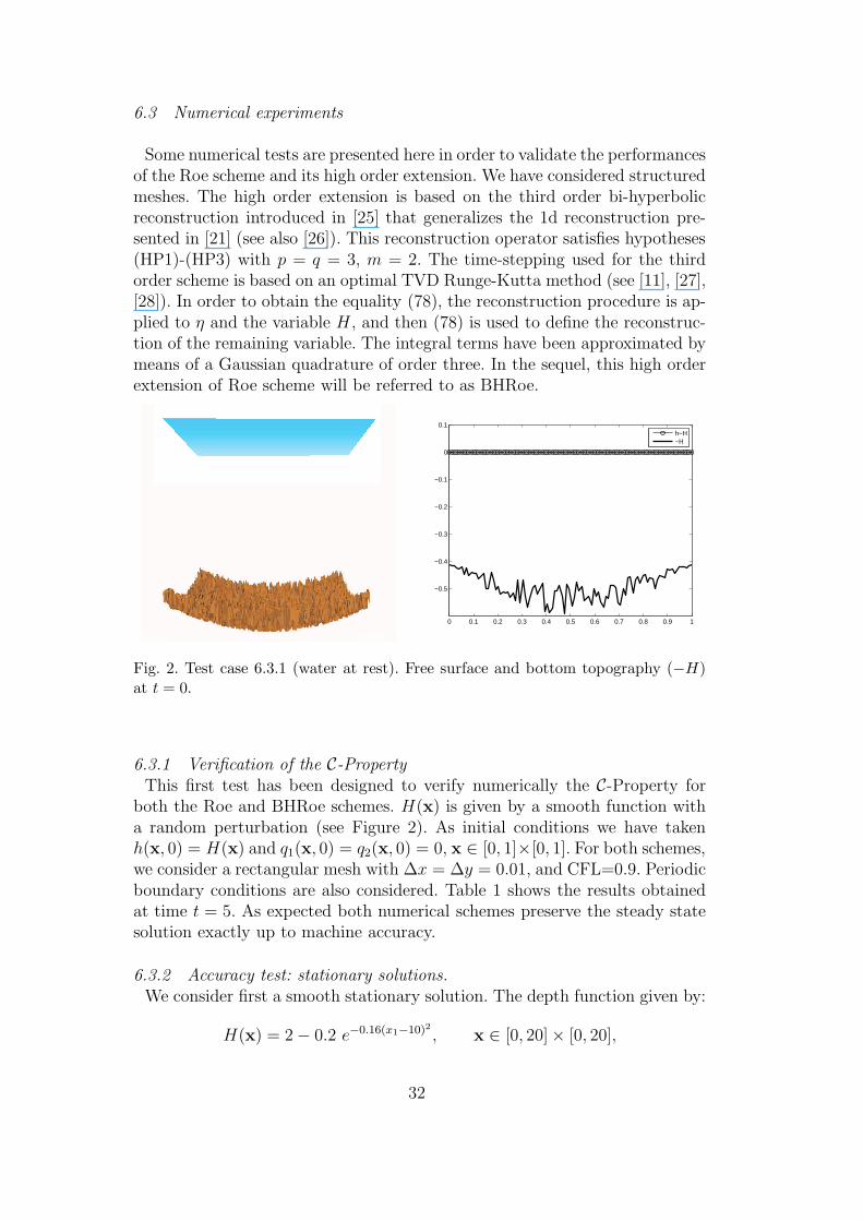
Fig. 2. Test case 6.3.1 (water at rest). Free surface and bottom topography (−H)at t = 0.

6.3.1 Verification of the C-PropertyThis first test has been designed to verify numerically the C-Property for

both the Roe and BHRoe schemes. H(x) is given by a smooth function witha random perturbation (see Figure 2). As initial conditions we have takenh(x, 0) = H(x) and q1(x, 0) = q2(x, 0) = 0, x ∈ [0, 1]×[0, 1]. For both schemes,we consider a rectangular mesh with ∆x = ∆y = 0.01, and CFL=0.9. Periodicboundary conditions are also considered. Table 1 shows the results obtainedat time t = 5. As expected both numerical schemes preserve the steady statesolution exactly up to machine accuracy.

6.3.2 Accuracy test: stationary solutions.We consider first a smooth stationary solution. The depth function given by:

H(x) = 2 − 0.2 e−0.16(x1−10)2 , x ∈ [0, 20] × [0, 20],

32

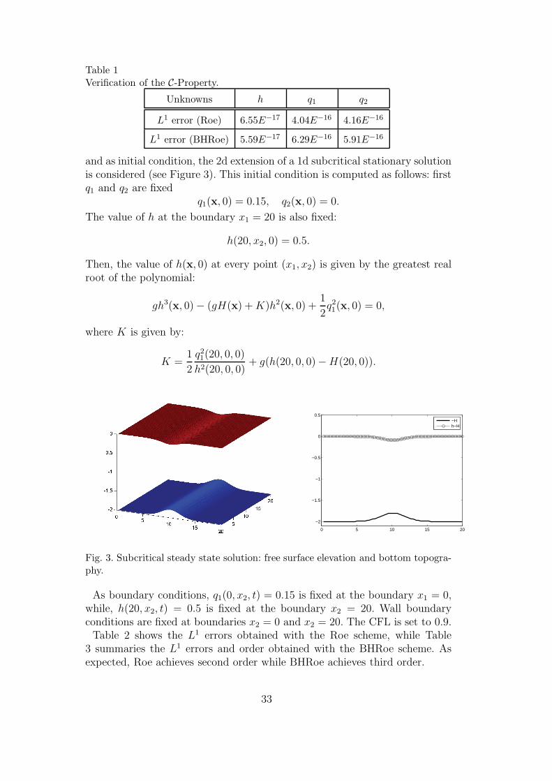
Table 1Verification of the C-Property.

Unknowns h q1 q2

L1 error (Roe) 6.55E−17 4.04E−16 4.16E−16

L1 error (BHRoe) 5.59E−17 6.29E−16 5.91E−16

and as initial condition, the 2d extension of a 1d subcritical stationary solutionis considered (see Figure 3). This initial condition is computed as follows: firstq1 and q2 are fixed

q1(x, 0) = 0.15, q2(x, 0) = 0.

The value of h at the boundary x1 = 20 is also fixed:

h(20, x2, 0) = 0.5.

Then, the value of h(x, 0) at every point (x1, x2) is given by the greatest realroot of the polynomial:

gh3(x, 0) − (gH(x) + K)h2(x, 0) +1

2q21(x, 0) = 0,

where K is given by:

K =1

2

q21(20, 0, 0)

h2(20, 0, 0)+ g(h(20, 0, 0)− H(20, 0)).

0 5 10 15 20

−2

−1.5

−1

−0.5

0

0.5

−Hh−H

Fig. 3. Subcritical steady state solution: free surface elevation and bottom topogra-phy.

As boundary conditions, q1(0, x2, t) = 0.15 is fixed at the boundary x1 = 0,while, h(20, x2, t) = 0.5 is fixed at the boundary x2 = 20. Wall boundaryconditions are fixed at boundaries x2 = 0 and x2 = 20. The CFL is set to 0.9.

Table 2 shows the L1 errors obtained with the Roe scheme, while Table3 summaries the L1 errors and order obtained with the BHRoe scheme. Asexpected, Roe achieves second order while BHRoe achieves third order.

33

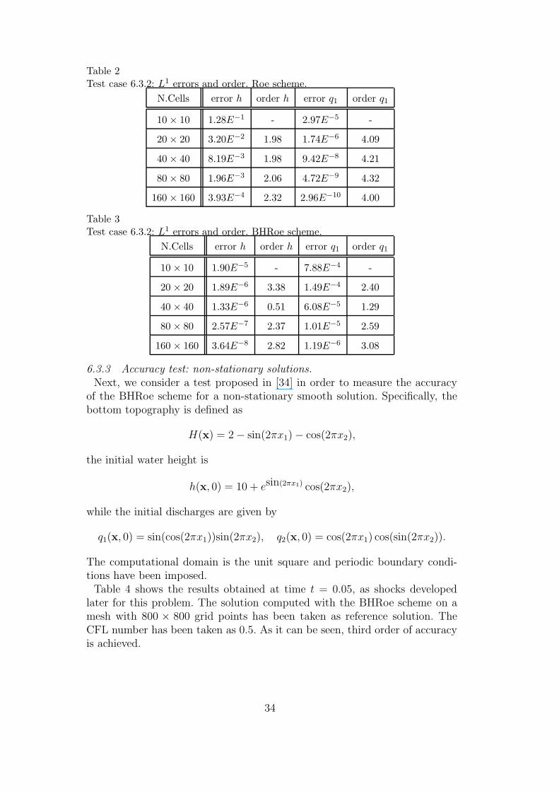
Table 2Test case 6.3.2: L1 errors and order. Roe scheme.

N.Cells error h order h error q1 order q1

10 × 10 1.28E−1 - 2.97E−5 -

20 × 20 3.20E−2 1.98 1.74E−6 4.09

40 × 40 8.19E−3 1.98 9.42E−8 4.21

80 × 80 1.96E−3 2.06 4.72E−9 4.32

160 × 160 3.93E−4 2.32 2.96E−10 4.00

Table 3Test case 6.3.2: L1 errors and order. BHRoe scheme.

N.Cells error h order h error q1 order q1

10 × 10 1.90E−5 - 7.88E−4 -

20 × 20 1.89E−6 3.38 1.49E−4 2.40

40 × 40 1.33E−6 0.51 6.08E−5 1.29

80 × 80 2.57E−7 2.37 1.01E−5 2.59

160 × 160 3.64E−8 2.82 1.19E−6 3.08

6.3.3 Accuracy test: non-stationary solutions.Next, we consider a test proposed in [34] in order to measure the accuracy

of the BHRoe scheme for a non-stationary smooth solution. Specifically, thebottom topography is defined as

H(x) = 2 − sin(2πx1) − cos(2πx2),

the initial water height is

h(x, 0) = 10 + esin(2πx1) cos(2πx2),

while the initial discharges are given by

q1(x, 0) = sin(cos(2πx1))sin(2πx2), q2(x, 0) = cos(2πx1) cos(sin(2πx2)).

The computational domain is the unit square and periodic boundary condi-tions have been imposed.

Table 4 shows the results obtained at time t = 0.05, as shocks developedlater for this problem. The solution computed with the BHRoe scheme on amesh with 800 × 800 grid points has been taken as reference solution. TheCFL number has been taken as 0.5. As it can be seen, third order of accuracyis achieved.

34

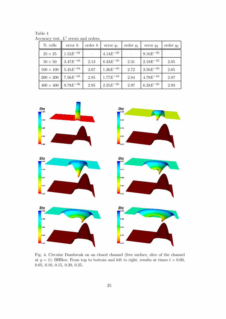
Table 4Accuracy test. L1 errors and orders.

N. cells error h order h error q1 order q1 error q2 order q2

25 × 25 1.52E−02 – 4.13E−02 – 9.10E−02 –

50 × 50 3.47E−03 2.13 8.33E−03 2.31 2.19E−02 2.05

100 × 100 5.45E−04 2.67 1.26E−03 2.72 3.50E−03 2.65

200 × 200 7.56E−05 2.85 1.77E−04 2.84 4.79E−04 2.87

400 × 400 9.79E−06 2.95 2.25E−05 2.97 6.28E−05 2.93

Fig. 4. Circular Dambreak on an closed channel (free surface, slice of the channelat y = 1): BHRoe. From top to bottom and left to right, results at times t = 0.00,0.05, 0.10, 0.15, 0.20, 0.25.

35

0.4 0.6 0.8 1 1.2 1.4 1.6 1.80.3

0.35

0.4

0.45

0.5

0.55

0.6

0.65

0.7

0.75

Bi Hyperbolic RecRoeEx. Sol

0.4 0.6 0.8 1 1.2 1.4 1.6 1.8−0.4

−0.3

−0.2

−0.1

0

0.1

0.2

Bi Hyperbolic RecRoeEx. Sol

0.4 0.6 0.8 1 1.2 1.4 1.6 1.80.3

0.35

0.4

0.45

0.5

0.55

0.6

0.65

0.7

0.75

Bi Hyperbolic RecRoeEx. Sol

0.4 0.6 0.8 1 1.2 1.4 1.6 1.8−0.4

−0.3

−0.2

−0.1

0

0.1

0.2

Bi Hyperbolic RecRoeEx. Sol

0.4 0.6 0.8 1 1.2 1.4 1.6 1.80.3

0.35

0.4

0.45

0.5

0.55

0.6

0.65

0.7

0.75

Bi Hyperbolic RecRoeEx. Sol

0.4 0.6 0.8 1 1.2 1.4 1.6 1.8−0.4

−0.3

−0.2

−0.1

0

0.1

0.2

Bi Hyperbolic RecRoeEx. Sol

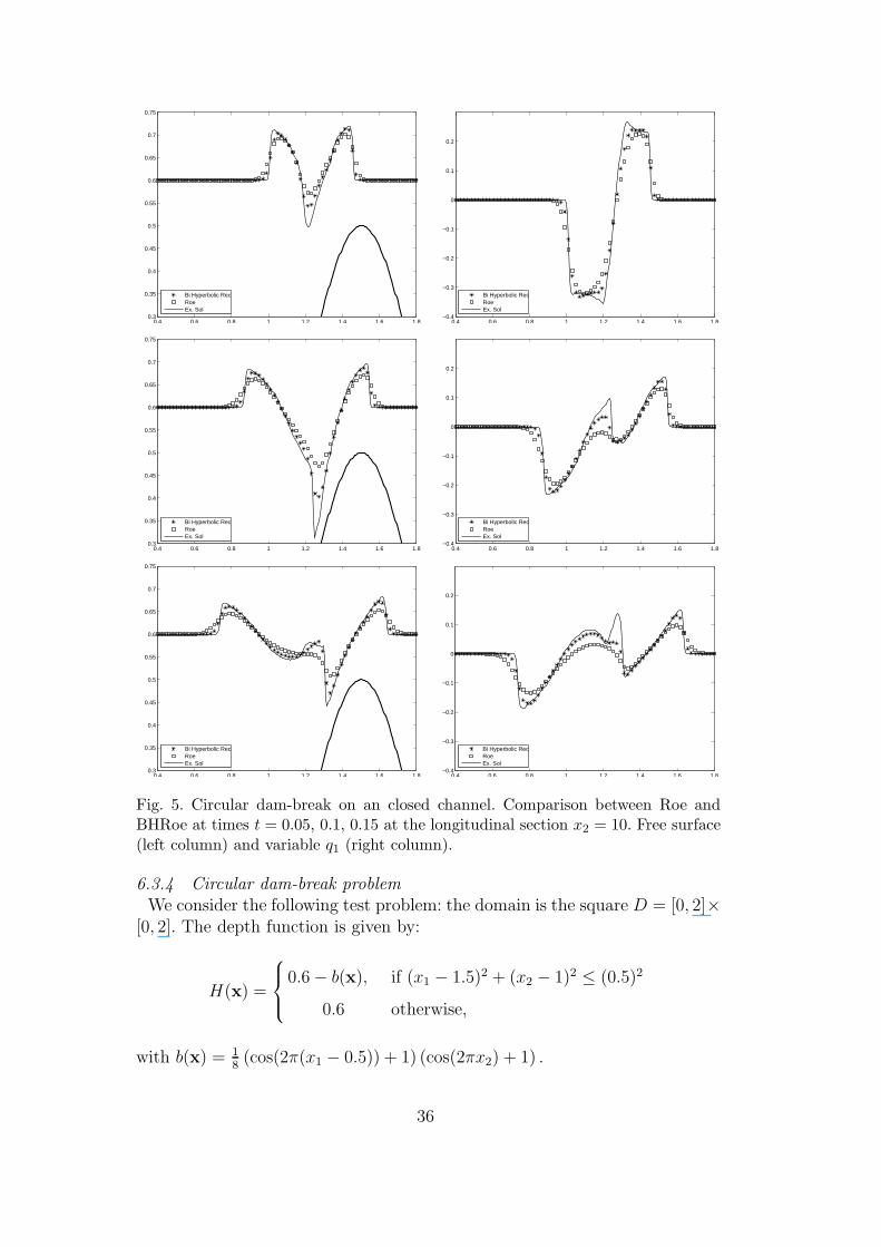
Fig. 5. Circular dam-break on an closed channel. Comparison between Roe andBHRoe at times t = 0.05, 0.1, 0.15 at the longitudinal section x2 = 10. Free surface(left column) and variable q1 (right column).

6.3.4 Circular dam-break problemWe consider the following test problem: the domain is the square D = [0, 2]×

[0, 2]. The depth function is given by:

H(x) =

0.6 − b(x), if (x1 − 1.5)2 + (x2 − 1)2 ≤ (0.5)2

0.6 otherwise,

with b(x) = 18(cos(2π(x1 − 0.5)) + 1) (cos(2πx2) + 1) .

36

The initial condition is:

h(x, 0) =

H(x) + 0.5 if (x1 − 1.25)2 + (x2 − 1)2 ≤ (0.1)2,

H(x) otherwise,

and q1(x, 0) = q2(x, 0) = 0 (see Figure 4).We consider wall boundary condi-tions at x2 = 0 and x2 = 2 and free boundary conditions at x1 = 0 and x1 = 2.The CFL is set to 0.9 and ∆x = ∆y = 0.02.

In Figure 4, the computed free surface and the bottom topography obtainedwith BHRoe at different times (t = 0, 0.05, 0.1, 0.15, 0.2, 0.25 s) are shown.

0.4 0.6 0.8 1 1.2 1.4 1.6 1.80.3

0.35

0.4

0.45

0.5

0.55

0.6

0.65

0.7

0.75

BHROEBHGFORCE

(a)

0.4 0.6 0.8 1 1.2 1.4 1.6 1.8−0.4

−0.3

−0.2

−0.1

0

0.1

0.2

BHROEBHGFORCE

(b)

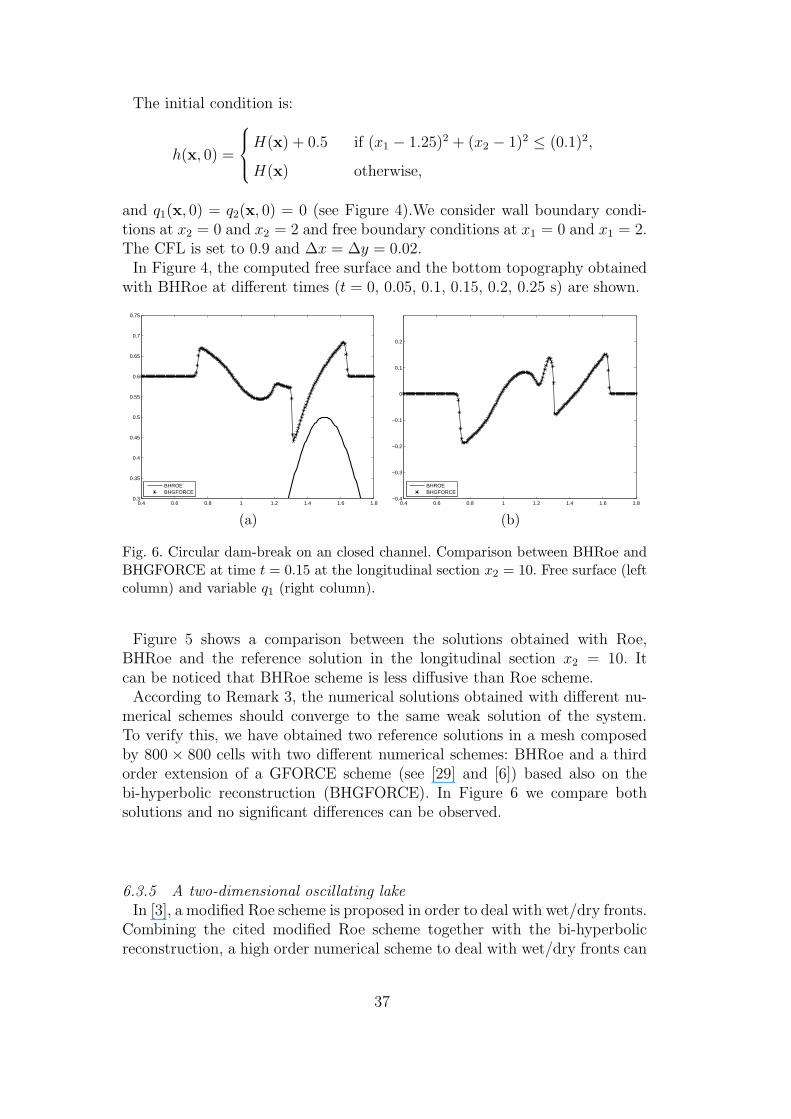
Fig. 6. Circular dam-break on an closed channel. Comparison between BHRoe andBHGFORCE at time t = 0.15 at the longitudinal section x2 = 10. Free surface (leftcolumn) and variable q1 (right column).

Figure 5 shows a comparison between the solutions obtained with Roe,BHRoe and the reference solution in the longitudinal section x2 = 10. Itcan be noticed that BHRoe scheme is less diffusive than Roe scheme.

According to Remark 3, the numerical solutions obtained with different nu-merical schemes should converge to the same weak solution of the system.To verify this, we have obtained two reference solutions in a mesh composedby 800 × 800 cells with two different numerical schemes: BHRoe and a thirdorder extension of a GFORCE scheme (see [29] and [6]) based also on thebi-hyperbolic reconstruction (BHGFORCE). In Figure 6 we compare bothsolutions and no significant differences can be observed.

6.3.5 A two-dimensional oscillating lakeIn [3], a modified Roe scheme is proposed in order to deal with wet/dry fronts.

Combining the cited modified Roe scheme together with the bi-hyperbolicreconstruction, a high order numerical scheme to deal with wet/dry fronts can

37

−2 −1.5 −1 −0.5 0 0.5 1 1.5 2

−0.1

−0.05

0

0.05

0.1

0.15

0.2

0.25

numerical

exact

bottom

(a) t = 2T .

−2 −1.5 −1 −0.5 0 0.5 1 1.5 2

−0.1

−0.05

0

0.05

0.1

0.15

0.2

0.25

numerical

exact

bottom

(b) t = 2T + T/6.

−2 −1.5 −1 −0.5 0 0.5 1 1.5 2

−0.1

−0.05

0

0.05

0.1

0.15

0.2

0.25

numerical

exact

bottom

(c) t = 2T + T/3.

−2 −1.5 −1 −0.5 0 0.5 1 1.5 2

−0.1

−0.05

0

0.05

0.1

0.15

0.2

0.25

numerical

exact

bottom

(d) t = 2T + T/2.

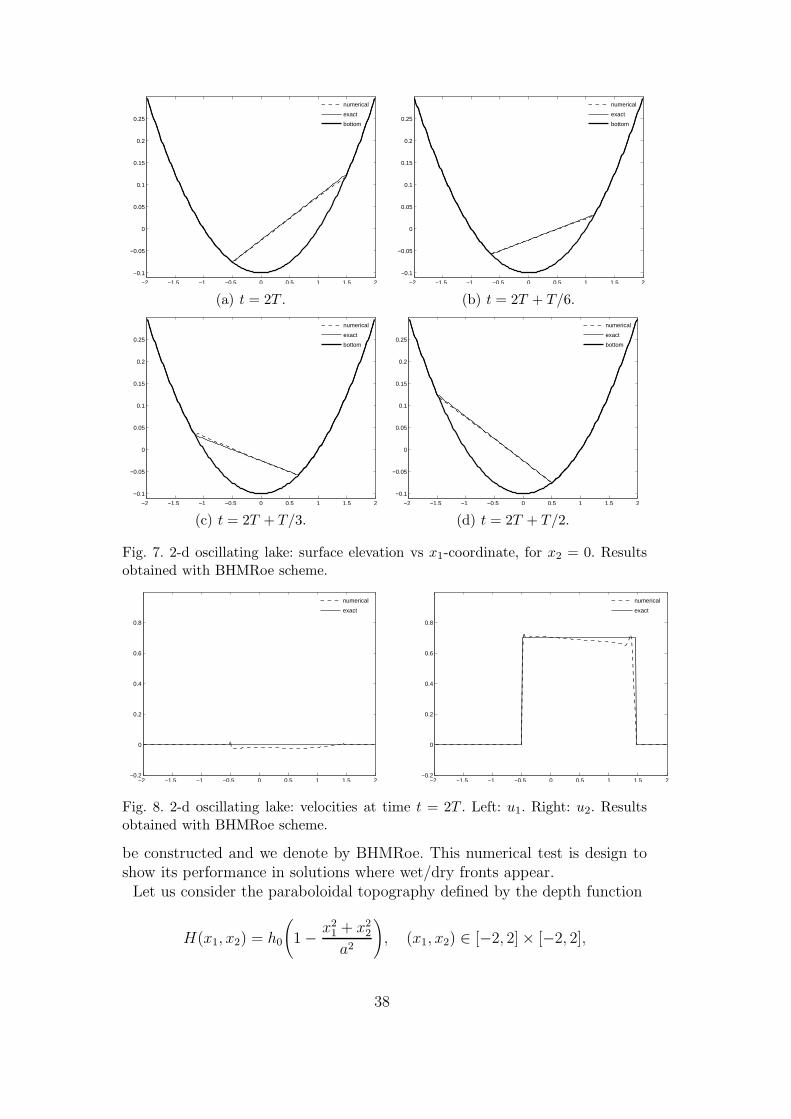
Fig. 7. 2-d oscillating lake: surface elevation vs x1-coordinate, for x2 = 0. Resultsobtained with BHMRoe scheme.

−2 −1.5 −1 −0.5 0 0.5 1 1.5 2−0.2

0

0.2

0.4

0.6

0.8

numerical

exact

−2 −1.5 −1 −0.5 0 0.5 1 1.5 2−0.2

0

0.2

0.4

0.6

0.8

numerical

exact

Fig. 8. 2-d oscillating lake: velocities at time t = 2T . Left: u1. Right: u2. Resultsobtained with BHMRoe scheme.

be constructed and we denote by BHMRoe. This numerical test is design toshow its performance in solutions where wet/dry fronts appear.

Let us consider the paraboloidal topography defined by the depth function

H(x1, x2) = h0

(1 − x2

1 + x22

a2

), (x1, x2) ∈ [−2, 2] × [−2, 2],

38

together with the periodic analytical solution of the two-dimensional shallowwater equations stated in [31]:

h(x1, x2, t) = max

(0,

σh0

a2

(2x1 cos(ωt) + x2sen (ωt) − σ

)+ H(x1, x2)

),

u1(x1, x2, t) = −σωsen (ωt), u2(x1, x2, t) = σω cos(ωt),

where u1 and u2 are the velocities in the x1 and x2 directions, and ω =√2gh0/a. The values a = 1, σ = 0.5 and h0 = 0.1 have been considered for

this test.The computations have been performed using a quadrilateral mesh with

∆x = ∆y = 0.02 and CFL number 0.7. Comparisons between the numeri-cal and the analytical free surfaces at different times are shown in Figure 7,where T represents the oscillation period. Althought a small distortion nearthe shorelines can be observed in some cases, they can be reduced using a finerspatial discretization. On the other hand, the planar form of the free surfaceis maintained throughout the computation.

To obtain accurate approximations of the velocity is a much more difficultissue. In Figure 8 are shown comparisons for both the u1 and u2 velocities attime t = 2T . As it can be observed, the position of the wet/dry fronts havebeen accurately captured, despite the small perturbations appearing in thewet zone.

7 Application to the two-layer shallow water system

7.1 Equations

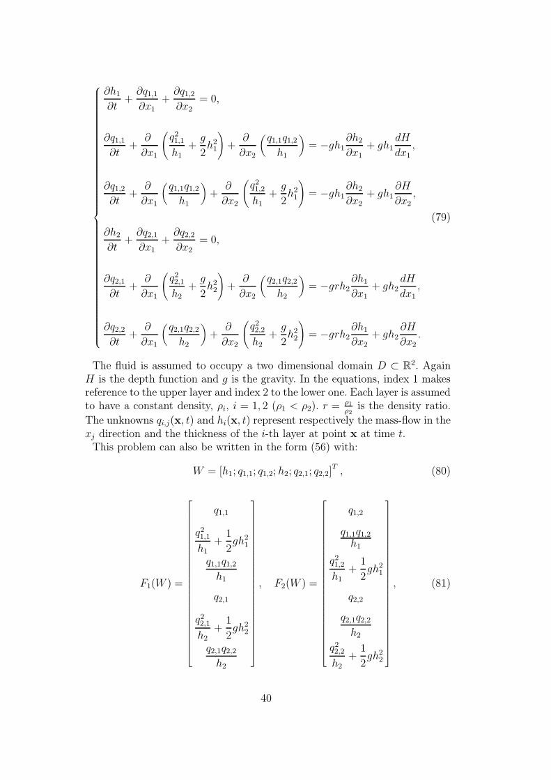
We consider the two-layer shallow water system without friction terms:

39

∂h1

∂t+

∂q1,1

∂x1+

∂q1,2

∂x2= 0,

∂q1,1

∂t+

∂

∂x1

(q21,1

h1+

g

2h2

1

)+

∂

∂x2

(q1,1q1,2

h1

)= −gh1

∂h2

∂x1+ gh1

dH

dx1,

∂q1,2

∂t+

∂

∂x1

(q1,1q1,2

h1

)+

∂

∂x2

(q21,2

h1+

g

2h2

1

)= −gh1

∂h2

∂x2+ gh1

∂H

∂x2,

∂h2

∂t+

∂q2,1

∂x1+

∂q2,2

∂x2= 0,

∂q2,1

∂t+

∂

∂x1

(q22,1

h2+

g

2h2

2

)+

∂

∂x2

(q2,1q2,2

h2

)= −grh2

∂h1

∂x1+ gh2

dH

dx1,

∂q2,2

∂t+

∂

∂x1

(q2,1q2,2

h2

)+

∂

∂x2

(q22,2

h2+

g

2h2

2

)= −grh2

∂h1

∂x2+ gh2

∂H

∂x2.

(79)

The fluid is assumed to occupy a two dimensional domain D ⊂ R2. Again

H is the depth function and g is the gravity. In the equations, index 1 makesreference to the upper layer and index 2 to the lower one. Each layer is assumedto have a constant density, ρi, i = 1, 2 (ρ1 < ρ2). r = ρ1

ρ2

is the density ratio.

The unknowns qi,j(x, t) and hi(x, t) represent respectively the mass-flow in thexj direction and the thickness of the i-th layer at point x at time t.

This problem can also be written in the form (56) with:

W = [h1; q1,1; q1,2; h2; q2,1; q2,2]T , (80)

F1(W ) =

q1,1

q21,1

h1

+1

2gh2

1

q1,1q1,2

h1

q2,1

q22,1

h2

+1

2gh2

2

q2,1q2,2

h2

, F2(W ) =

q1,2

q1,1q1,2

h1

q21,2

h1+

1

2gh2

1

q2,2

q2,1q2,2

h2

q22,2

h2+

1

2gh2

2

, (81)

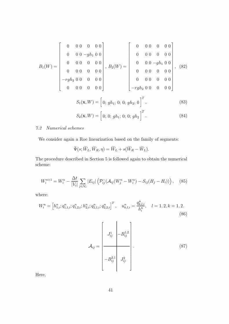
40

B1(W ) =

0 0 0 0 0 0

0 0 0 −gh1 0 0

0 0 0 0 0 0

0 0 0 0 0 0

−rgh2 0 0 0 0 0

0 0 0 0 0 0

, B2(W ) =

0 0 0 0 0 0

0 0 0 0 0 0

0 0 0 −gh1 0 0

0 0 0 0 0 0

0 0 0 0 0 0

−rgh2 0 0 0 0 0

, (82)

S1(x, W ) =[0; gh1; 0; 0; gh2; 0

]T, (83)

S2(x, W ) =[0; 0; gh1; 0; 0; gh2

]T. (84)

7.2 Numerical schemes

We consider again a Roe linearization based on the family of segments:

Ψ(s; WL, WR, η) = WL + s(WR − WL).

The procedure described in Section 5 is followed again to obtain the numericalscheme:

W n+1i = W n

i − ∆t

|Vi|∑

j∈Ni

|Eij |(P−

ij (Aij(Wnj − W n

i ) − Sij(Hj − Hi))), (85)

where:

W ni =

[hn

1,i; qn1,1,i; q

n1,2,i; h

n2,i; q

n2,1,i; q

n2,2,i

]T, un

k,l,i =qnk,l,i

hni

, l = 1, 2, k = 1, 2.

(86)

Aij =

J1ij −B1,2

ij

−B2,1ij J2

ij

. (87)

Here,

41

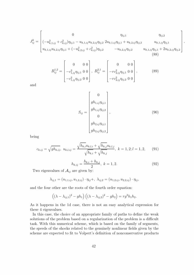
Jkij =

0 ηij,1 ηij,2

(−u2k,1,ij + c2

k,ij)ηij,1 − uk,1,ijuk,2,ijηij,2 2uk,1,ijηij,1 + uk,2,ijηij,2 uk,1,ijηij,1

uk,1,ijuk,2,ijηij,1 + (−u2k,2,ij + c2

k,ij)ηij,2 −uk,2,ijηij,2 uk,1,ijηij,1 + 2uk,2,ijηij,2

,

(88)

B1,2ij =

0 0 0

−c21,ijηij,1 0 0

−c21,ijηij,2 0 0

, B2,1ij =

0 0 0

−rc22,ijηij,1 0 0

−rc22,ijηij,2 0 0

, (89)

and

Sij =

0

gh1,ijηij,1

gh1,ijηij,2

0

gh2,ijηij,1

gh2,ijηij,2

, (90)

being

ck,ij =√

ghk,ij, uk,l,ij =

√hk,iuk,l,i +

√hk,juk,l,j

√hk,i +

√hk,j

, k = 1, 2; l = 1, 2, (91)

hk,ij =hk,i + hk,j

2, k = 1, 2. (92)

Two eigenvalues of Aij are given by:

λij,1 = (u1,1,ij, u1,2,ij) · ηij+, λij,2 = (u1,2,ij, u2,2,ij) · ηij ,

and the four other are the roots of the fourth order equation:((λ − λij,1)

2 − gh1

) ((λ − λij,2)

2 − gh2

)= rg2h1h2.

As it happens in the 1d case, there is not an easy analytical expression forthese 4 eigenvalues.

In this case, the choice of an appropriate family of paths to define the weaksolutions of the problem based on a regularization of the problem is a difficulttask. With this numerical scheme, which is based on the family of segments,the speeds of the shocks related to the genuinely nonlinear fields given by thescheme are expected to fit to Volpert’s definition of nonconservative products

42

(see [32]) which is equivalent to the definition corresponding to the family ofsegments, i.e. they are expected to fit to the Rankine-Hugoniot condition (4)corresponding to the family of segments.

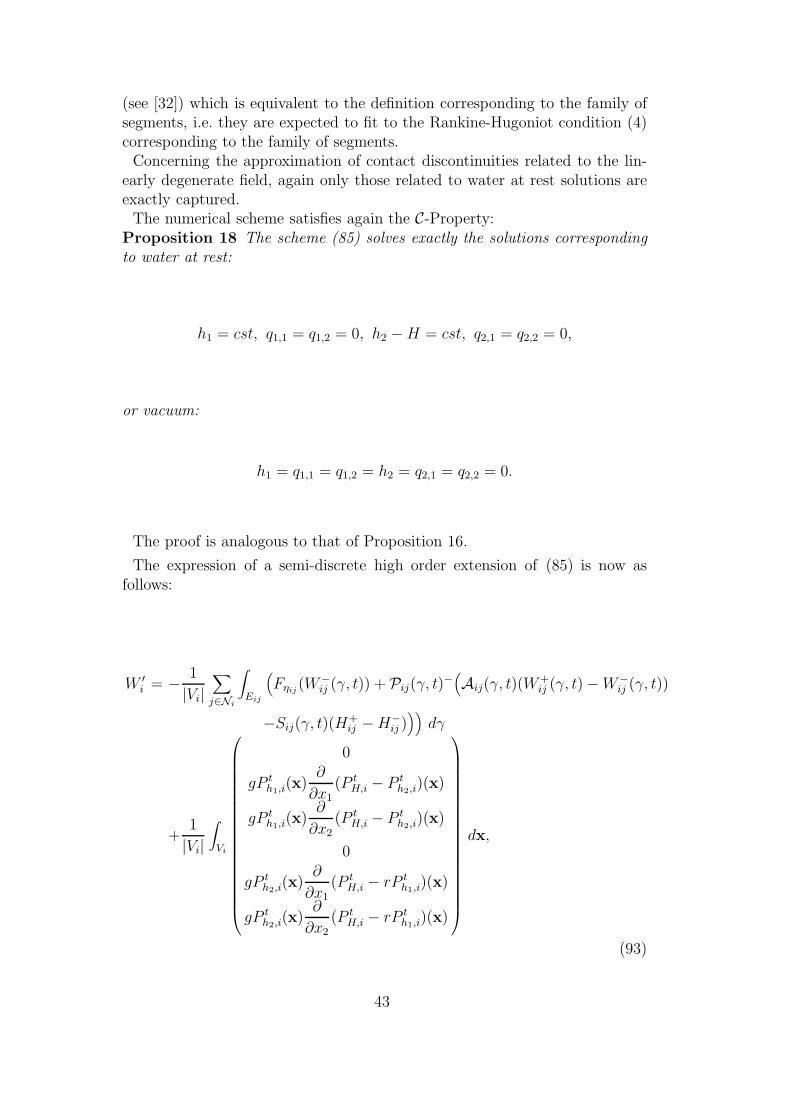
Concerning the approximation of contact discontinuities related to the lin-early degenerate field, again only those related to water at rest solutions areexactly captured.

The numerical scheme satisfies again the C-Property:Proposition 18 The scheme (85) solves exactly the solutions correspondingto water at rest:

h1 = cst, q1,1 = q1,2 = 0, h2 − H = cst, q2,1 = q2,2 = 0,

or vacuum:

h1 = q1,1 = q1,2 = h2 = q2,1 = q2,2 = 0.

The proof is analogous to that of Proposition 16.

The expression of a semi-discrete high order extension of (85) is now asfollows:

W ′i = − 1

|Vi|∑

j∈Ni

∫

Eij

(Fηij

(W−ij (γ, t)) + Pij(γ, t)−

(Aij(γ, t)(W+

ij (γ, t) − W−ij (γ, t))

−Sij(γ, t)(H+ij − H−

ij )))

dγ

+1

|Vi|∫

Vi

0

gP th1,i(x)

∂

∂x1(P t

H,i − P th2,i)(x)

gP th1,i(x)

∂

∂x2(P t

H,i − P th2,i)(x)

0

gP th2,i(x)

∂

∂x1

(P tH,i − rP t

h1,i)(x)

gP th2,i(x)

∂

∂x2(P t

H,i − rP th1,i)(x)

dx,

(93)

43

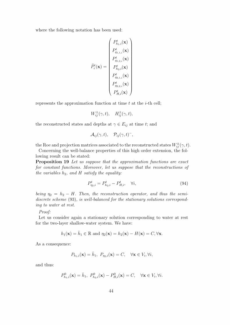
where the following notation has been used:

P ti (x) =

P th1,i(x)

P tq1,1,i

(x)

P tq1,2,i

(x)

P th2,i(x)

P tq2,1,i

(x)

P tq2,2,i

(x)

P tH,i(x)

represents the approximation function at time t at the i-th cell;

W±ij (γ, t), H±

ij (γ, t),

the reconstructed states and depths at γ ∈ Eij at time t; and

Aij(γ, t), Pij(γ, t)−,

the Roe and projection matrices associated to the reconstructed states W±ij (γ, t).

Concerning the well-balance properties of this high order extension, the fol-lowing result can be stated:Proposition 19 Let us suppose that the approximation functions are exactfor constant functions. Moreover, let us suppose that the reconstructions ofthe variables h2, and H satisfy the equality:

P tη2,i = P t

h2,i − P tH,i, ∀i, (94)

being η2 = h2 − H. Then, the reconstruction operator, and thus the semi-discrete scheme (93), is well-balanced for the stationary solutions correspond-ing to water at rest.

Proof:Let us consider again a stationary solution corresponding to water at rest

for the two-layer shallow-water system. We have:

h1(x) = h1 ∈ R and η2(x) = h2(x) − H(x) = C, ∀x.

As a consequence:

Ph1,i(x) = h1, Pη2,i(x) = C, ∀x ∈ Vi, ∀i,

and thus:

P 0h1,i(x) = h1, P 0

h2,i(x) − P 0H,i(x) = C, ∀x ∈ Vi, ∀i.

44

Using this last equality, it is trivial to verify that:

P 0i (x) =

P 0h1,i(x)

0

0

P 0h2,i(x)

0

0

P 0H,i(x)

is also a stationary solution corresponding to water at rest.2

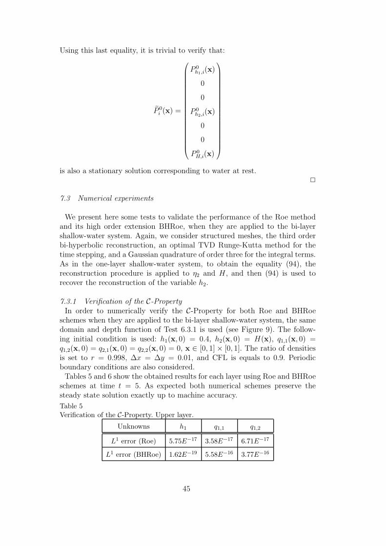
7.3 Numerical experiments

We present here some tests to validate the performance of the Roe methodand its high order extension BHRoe, when they are applied to the bi-layershallow-water system. Again, we consider structured meshes, the third orderbi-hyperbolic reconstruction, an optimal TVD Runge-Kutta method for thetime stepping, and a Gaussian quadrature of order three for the integral terms.As in the one-layer shallow-water system, to obtain the equality (94), thereconstruction procedure is applied to η2 and H , and then (94) is used torecover the reconstruction of the variable h2.

7.3.1 Verification of the C-PropertyIn order to numerically verify the C-Property for both Roe and BHRoe

schemes when they are applied to the bi-layer shallow-water system, the samedomain and depth function of Test 6.3.1 is used (see Figure 9). The follow-ing initial condition is used: h1(x, 0) = 0.4, h2(x, 0) = H(x), q1,1(x, 0) =q1,2(x, 0) = q2,1(x, 0) = q2,2(x, 0) = 0, x ∈ [0, 1] × [0, 1]. The ratio of densitiesis set to r = 0.998, ∆x = ∆y = 0.01, and CFL is equals to 0.9. Periodicboundary conditions are also considered.

Tables 5 and 6 show the obtained results for each layer using Roe and BHRoeschemes at time t = 5. As expected both numerical schemes preserve thesteady state solution exactly up to machine accuracy.

Table 5Verification of the C-Property. Upper layer.

Unknowns h1 q1,1 q1,2

L1 error (Roe) 5.75E−17 3.58E−17 6.71E−17

L1 error (BHRoe) 1.62E−19 5.58E−16 3.77E−16

45

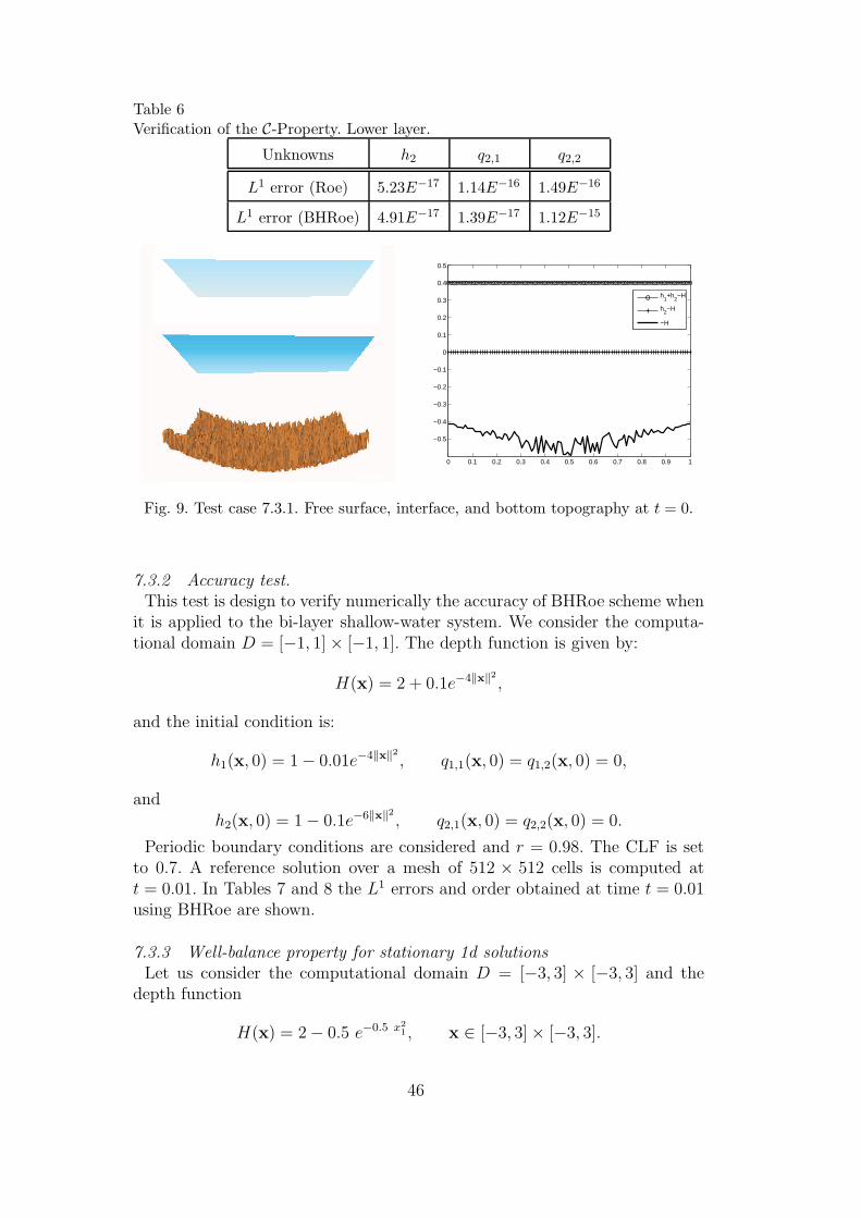
Table 6Verification of the C-Property. Lower layer.

Unknowns h2 q2,1 q2,2

L1 error (Roe) 5.23E−17 1.14E−16 1.49E−16

L1 error (BHRoe) 4.91E−17 1.39E−17 1.12E−15

0 0.1 0.2 0.3 0.4 0.5 0.6 0.7 0.8 0.9 1

−0.5

−0.4

−0.3

−0.2

−0.1

0

0.1

0.2

0.3

0.4

0.5

h1+h

2−H

h2−H

−H

Fig. 9. Test case 7.3.1. Free surface, interface, and bottom topography at t = 0.

7.3.2 Accuracy test.This test is design to verify numerically the accuracy of BHRoe scheme when

it is applied to the bi-layer shallow-water system. We consider the computa-tional domain D = [−1, 1] × [−1, 1]. The depth function is given by:

H(x) = 2 + 0.1e−4‖x‖2

,

and the initial condition is:

h1(x, 0) = 1 − 0.01e−4‖x‖2

, q1,1(x, 0) = q1,2(x, 0) = 0,

andh2(x, 0) = 1 − 0.1e−6‖x‖2

, q2,1(x, 0) = q2,2(x, 0) = 0.

Periodic boundary conditions are considered and r = 0.98. The CLF is setto 0.7. A reference solution over a mesh of 512 × 512 cells is computed att = 0.01. In Tables 7 and 8 the L1 errors and order obtained at time t = 0.01using BHRoe are shown.

7.3.3 Well-balance property for stationary 1d solutionsLet us consider the computational domain D = [−3, 3] × [−3, 3] and the

depth function

H(x) = 2 − 0.5 e−0.5 x2

1 , x ∈ [−3, 3] × [−3, 3].

46

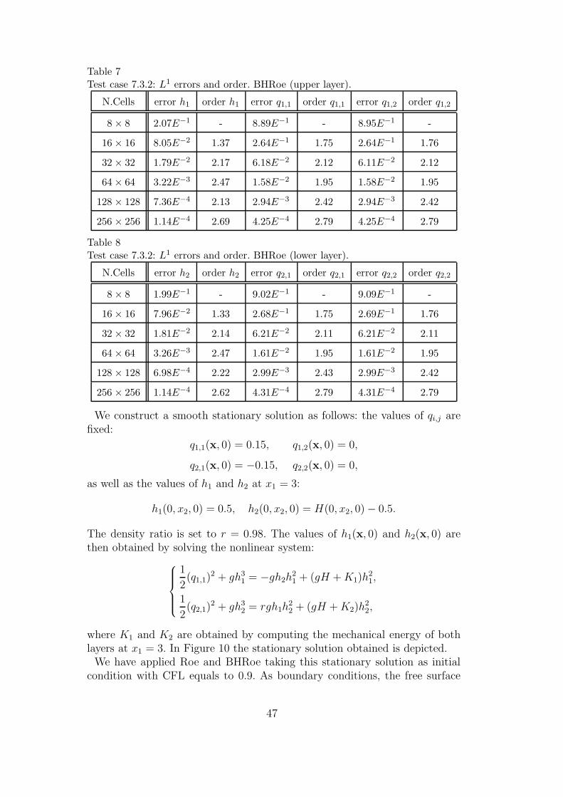
Table 7Test case 7.3.2: L1 errors and order. BHRoe (upper layer).

N.Cells error h1 order h1 error q1,1 order q1,1 error q1,2 order q1,2

8 × 8 2.07E−1 - 8.89E−1 - 8.95E−1 -

16 × 16 8.05E−2 1.37 2.64E−1 1.75 2.64E−1 1.76

32 × 32 1.79E−2 2.17 6.18E−2 2.12 6.11E−2 2.12

64 × 64 3.22E−3 2.47 1.58E−2 1.95 1.58E−2 1.95

128 × 128 7.36E−4 2.13 2.94E−3 2.42 2.94E−3 2.42

256 × 256 1.14E−4 2.69 4.25E−4 2.79 4.25E−4 2.79

Table 8Test case 7.3.2: L1 errors and order. BHRoe (lower layer).

N.Cells error h2 order h2 error q2,1 order q2,1 error q2,2 order q2,2

8 × 8 1.99E−1 - 9.02E−1 - 9.09E−1 -

16 × 16 7.96E−2 1.33 2.68E−1 1.75 2.69E−1 1.76

32 × 32 1.81E−2 2.14 6.21E−2 2.11 6.21E−2 2.11

64 × 64 3.26E−3 2.47 1.61E−2 1.95 1.61E−2 1.95

128 × 128 6.98E−4 2.22 2.99E−3 2.43 2.99E−3 2.42

256 × 256 1.14E−4 2.62 4.31E−4 2.79 4.31E−4 2.79

We construct a smooth stationary solution as follows: the values of qi,j arefixed:

q1,1(x, 0) = 0.15, q1,2(x, 0) = 0,

q2,1(x, 0) = −0.15, q2,2(x, 0) = 0,

as well as the values of h1 and h2 at x1 = 3:

h1(0, x2, 0) = 0.5, h2(0, x2, 0) = H(0, x2, 0) − 0.5.

The density ratio is set to r = 0.98. The values of h1(x, 0) and h2(x, 0) arethen obtained by solving the nonlinear system:

1

2(q1,1)

2 + gh31 = −gh2h

21 + (gH + K1)h

21,

1

2(q2,1)

2 + gh32 = rgh1h

22 + (gH + K2)h

22,

where K1 and K2 are obtained by computing the mechanical energy of bothlayers at x1 = 3. In Figure 10 the stationary solution obtained is depicted.

We have applied Roe and BHRoe taking this stationary solution as initialcondition with CFL equals to 0.9. As boundary conditions, the free surface

47

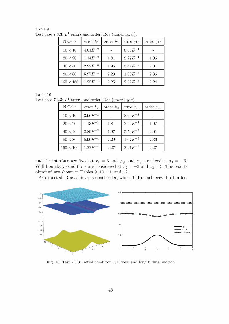
Table 9Test case 7.3.3: L1 errors and order. Roe (upper layer).

N.Cells error h1 order h1 error q1,1 order q1,1

10 × 10 4.01E−2 - 8.86E−4 -

20 × 20 1.14E−2 1.81 2.27E−4 1.96

40 × 40 2.92E−3 1.96 5.62E−5 2.01

80 × 80 5.97E−4 2.29 1.09E−5 2.36

160 × 160 1.25E−4 2.25 2.32E−6 2.24

Table 10Test case 7.3.3: L1 errors and order. Roe (lower layer).

N.Cells error h2 order h2 error q2,1 order q2,1

10 × 10 3.96E−2 - 8.69E−4 -

20 × 20 1.13E−2 1.81 2.22E−4 1.97

40 × 40 2.89E−3 1.97 5.50E−5 2.01

80 × 80 5.90E−4 2.29 1.07E−5 2.36

160 × 160 1.22E−4 2.27 2.21E−6 2.27

and the interface are fixed at x1 = 3 and q1,1 and q2,1 are fixed at x1 = −3.Wall boundary conditions are considered at x2 = −3 and x2 = 3. The resultsobtained are shown in Tables 9, 10, 11, and 12.

As expected, Roe achieves second order, while BHRoe achieves third order.

−3 −2 −1 0 1 2 3

−2

−1.5

−1

−0.5

0

0.5

−H

h2−H

h1+h2−H

Fig. 10. Test 7.3.3: initial condition. 3D view and longitudinal section.

48

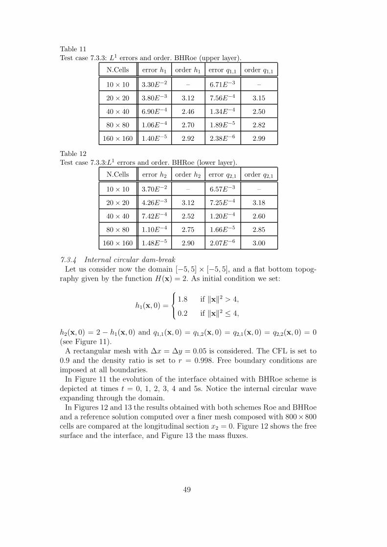
Table 11Test case 7.3.3: L1 errors and order. BHRoe (upper layer).

N.Cells error h1 order h1 error q1,1 order q1,1

10 × 10 3.30E−2 – 6.71E−3 –

20 × 20 3.80E−3 3.12 7.56E−4 3.15

40 × 40 6.90E−4 2.46 1.34E−4 2.50

80 × 80 1.06E−4 2.70 1.89E−5 2.82

160 × 160 1.40E−5 2.92 2.38E−6 2.99

Table 12Test case 7.3.3:L1 errors and order. BHRoe (lower layer).

N.Cells error h2 order h2 error q2,1 order q2,1

10 × 10 3.70E−2 – 6.57E−3 –

20 × 20 4.26E−3 3.12 7.25E−4 3.18

40 × 40 7.42E−4 2.52 1.20E−4 2.60

80 × 80 1.10E−4 2.75 1.66E−5 2.85

160 × 160 1.48E−5 2.90 2.07E−6 3.00

7.3.4 Internal circular dam-breakLet us consider now the domain [−5, 5] × [−5, 5], and a flat bottom topog-

raphy given by the function H(x) = 2. As initial condition we set:

h1(x, 0) =

1.8 if ‖x‖2 > 4,

0.2 if ‖x‖2 ≤ 4,

h2(x, 0) = 2 − h1(x, 0) and q1,1(x, 0) = q1,2(x, 0) = q2,1(x, 0) = q2,2(x, 0) = 0(see Figure 11).

A rectangular mesh with ∆x = ∆y = 0.05 is considered. The CFL is set to0.9 and the density ratio is set to r = 0.998. Free boundary conditions areimposed at all boundaries.

In Figure 11 the evolution of the interface obtained with BHRoe scheme isdepicted at times t = 0, 1, 2, 3, 4 and 5s. Notice the internal circular waveexpanding through the domain.

In Figures 12 and 13 the results obtained with both schemes Roe and BHRoeand a reference solution computed over a finer mesh composed with 800×800cells are compared at the longitudinal section x2 = 0. Figure 12 shows the freesurface and the interface, and Figure 13 the mass fluxes.

49

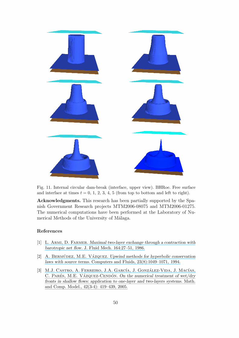
Fig. 11. Internal circular dam-break (interface, upper view). BHRoe. Free surfaceand interface at times t = 0, 1, 2, 3, 4, 5 (from top to bottom and left to right).

Acknowledgments. This research has been partially supported by the Spa-nish Government Research projects MTM2006-08075 and MTM2006-01275.The numerical computations have been performed at the Laboratory of Nu-merical Methods of the University of Malaga.

References

[1] L. Armi, D. Farmer. Maximal two-layer exchange through a contraction withbarotropic net flow. J. Fluid Mech. 164:27–51, 1986.

[2] A. Bermudez, M.E. Vazquez. Upwind methods for hyperbolic conservationlaws with source terms. Computers and Fluids, 23(8):1049–1071, 1994.

[3] M.J. Castro, A. Ferreiro, J.A. Garcıa, J. Gonzalez-Vida, J. Macıas,

C. Pares, M.E. Vazquez-Cendon. On the numerical treatment of wet/dryfronts in shallow flows: application to one-layer and two-layers systems. Math.and Comp. Model., 42(3-4): 419–439, 2005.

50

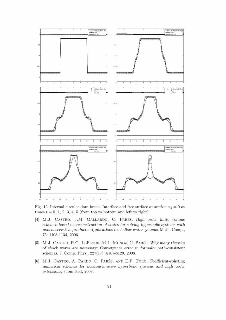
−5 −4 −3 −2 −1 0 1 2 3 4 5

−2

−1.5

−1

−0.5

0

Bi Hyperbolic RecRoeEx. Sol.

−5 −4 −3 −2 −1 0 1 2 3 4 5

−2

−1.5

−1

−0.5

0

Bi Hyperbolic RecRoeEx. Sol.

−5 −4 −3 −2 −1 0 1 2 3 4 5

−2

−1.5

−1

−0.5

0

Bi Hyperbolic RecRoeEx. Sol.

−5 −4 −3 −2 −1 0 1 2 3 4 5

−2

−1.5

−1

−0.5

0

Bi Hyperbolic RecRoeEx. Sol.

−5 −4 −3 −2 −1 0 1 2 3 4 5

−2

−1.5

−1

−0.5

0

Bi Hyperbolic RecRoeEx. Sol.

−5 −4 −3 −2 −1 0 1 2 3 4 5

−2

−1.5

−1

−0.5

0

Bi Hyperbolic RecRoeEx. Sol.

Fig. 12. Internal circular dam-break. Interface and free surface at section x2 = 0 attimes t = 0, 1, 2, 3, 4, 5 (from top to bottom and left to right).

[4] M.J. Castro, J.M. Gallardo, C. Pares. High order finite volumeschemes based on reconstruction of states for solving hyperbolic systems withnonconservative products. Applications to shallow water systems. Math. Comp.,75: 1103-1134, 2006.

[5] M.J. Castro, P.G. LeFloch, M.L. Munoz, C. Pares. Why many theoriesof shock waves are necessary: Convergence error in formally path-consistentschemes. J. Comp. Phys., 227(17): 8107-8129, 2008.

[6] M.J. Castro, A. Pardo, C. Pares, and E.F. Toro, Coefficient-splittingnumerical schemes for nonconservative hyperbolic systems and high orderextensions, submitted, 2008.

51

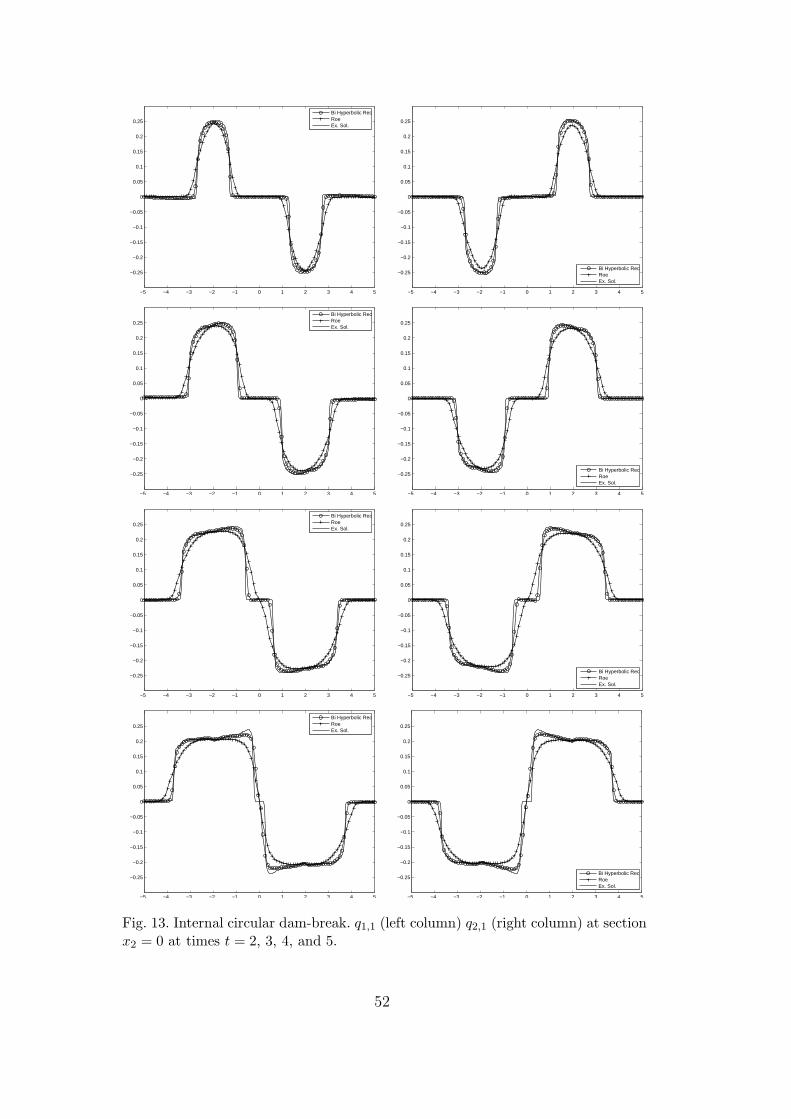
−5 −4 −3 −2 −1 0 1 2 3 4 5

−0.25

−0.2

−0.15

−0.1

−0.05

0

0.05

0.1

0.15

0.2

0.25

Bi Hyperbolic RecRoeEx. Sol.

−5 −4 −3 −2 −1 0 1 2 3 4 5

−0.25

−0.2

−0.15

−0.1

−0.05

0

0.05

0.1

0.15

0.2

0.25

Bi Hyperbolic RecRoeEx. Sol.

−5 −4 −3 −2 −1 0 1 2 3 4 5

−0.25

−0.2

−0.15

−0.1

−0.05

0

0.05

0.1

0.15

0.2

0.25

Bi Hyperbolic RecRoeEx. Sol.

−5 −4 −3 −2 −1 0 1 2 3 4 5

−0.25

−0.2

−0.15

−0.1

−0.05

0

0.05

0.1

0.15

0.2

0.25

Bi Hyperbolic RecRoeEx. Sol.

−5 −4 −3 −2 −1 0 1 2 3 4 5

−0.25

−0.2

−0.15

−0.1

−0.05

0

0.05

0.1

0.15

0.2

0.25

Bi Hyperbolic RecRoeEx. Sol.

−5 −4 −3 −2 −1 0 1 2 3 4 5

−0.25

−0.2

−0.15

−0.1

−0.05

0

0.05

0.1

0.15

0.2

0.25

Bi Hyperbolic RecRoeEx. Sol.

−5 −4 −3 −2 −1 0 1 2 3 4 5

−0.25

−0.2

−0.15

−0.1

−0.05

0

0.05

0.1

0.15

0.2

0.25

Bi Hyperbolic RecRoeEx. Sol.

−5 −4 −3 −2 −1 0 1 2 3 4 5

−0.25

−0.2

−0.15

−0.1

−0.05

0

0.05

0.1

0.15

0.2

0.25

Bi Hyperbolic RecRoeEx. Sol.

Fig. 13. Internal circular dam-break. q1,1 (left column) q2,1 (right column) at sectionx2 = 0 at times t = 2, 3, 4, and 5.

52

[7] G. Dal Maso, P.G. LeFloch and F. Murat. Definition and weak stabilityof nonconservative products. J. Math. Pures Appl. 74:483–548, 1995.

[8] D. Farmer, L. Armi. Maximal two-layer exchange over a sill and througha combination of a sill and contraction with barotropic flow. J. Fluid Mech.164:53–76, 1986.

[9] L. Gosse A well-balanced flux-vector splitting scheme designed for hyperbolicsystems of conservation laws with source terms. Comp. Math. with Applic.39:135–159, 2000.

[10] L. Gosse. A well-balanced scheme using non-conservative productsdesigned for hyperbolic system of conservation laws with source terms.Mat. Mod. Meth. Appl. Sc. 11: 339–365, 2001.

[11] S. Gottlieb and C. W. Shu. Total variation diminishing Runge-Kuttaschemes. Mat. Comp. 67: 73–85, 1998.

[12] J.M. Greenberg and A.Y. LeRoux. A well balanced scheme forthe numerical processing of source terms in hyperbolic equations. SIAMJ. Numer. Anal. 33: 1–16, 1996.

[13] J.M. Greenberg, A.Y. LeRoux, R. Baraille, A. Noussair. Analysis andapproximation of conservation laws with source terms. SIAM J. Numer. Anal.34: 1980–2007, 1997.

[14] E. Godlewski, P.A. Raviart.Numerical approximation of hyperbolicsystems of conservation laws. Applied Mathematical Sciences, 118. Springer-Verlag, New York, 1996.

[15] A. Harten, J.M. Hyman. Self-adjusting grid methods for one-dimensionalhyperbolic conservation laws. J. Comp. Phys. 50:235–269, 1983.

[16] T.Y. Hou and P.G. LeFloch. Why nonconservative schemes converge towrong solutions: error analysis. Math. Comp. 62: 497–530, 1994.

[17] D. Krner, M. Rokyta, M. Wierse.A Lax-Wendroff type theorem for upwindfinite volume schemes in 2-D. East-West J. Numer. Math. 4(4): 279–292, 1996.

[18] P.G. LeFloch. Shock waves for nonlinear hyperbolic systems innonconservative form, Institute for Math. and its Appl., Minneapolis, Preprint593, 1989.

[19] P.G. LeFloch and T.-P. Liu.Existence theory for nonlinear hyperbolicsystems in nonconservative form. Forum Math. 5: 261– 280, 1993.

[20] R. J. LeVeque. Balancing source terms and flux gradient in high-resolutionGodunov methods: the quasi-steady wave-propagation algorithm. J. Comput.Phys. 146: 346–365, 1998.

[21] A. Marquina. Local piecewise hyperbolic reconstruction of numerical fluxesfor non linear scalar conservation laws. SIAM, Journal Sci. Comput. 15(4),892–915, 1994.

53

[22] M.L. Munoz and C. Pares. Godunov’s method for nonconservativehyperbolic systems. ESAIM: M2AN 41(1): 169-185, 2007.

[23] S. Noelle, N. Pankratz, G. Puppo, J. Natvig. Well-balanced finite volumeschemes of arbitrary order of accuracy for shallow water flows. J. Comput. Phys.,213: 474–499, 2006.

[24] C. Pares, M.J. Castro. On the well-balance property of Roe’s method fornonconservative hyperbolic systems. Applications to shallow-water systems.ESAIM: M2AN, 38(5):821–852, 2004.

[25] H. J. Schroll and F. Svensson. A Bihyperbolic Fiinite Volume Method forQuadrilateral Meshes. SIAM: J. Sci. Comput., 26(2): 237–260, 2006.

[26] S. Serna. A class of extended limiters applied to piecewise hyperbolic methods.SIAM: J. Sci. Comput., 28(1): 123–140, 2006.

[27] C.-W. Shu.Total-variation-diminishing time discretizations. SIAM J. Sci.Statist. Comput. 9(6): 1073–1084, 1988.

[28] C.-W. Shu and S. Osher. Efficient implementation of essentially non-oscillatory shock capturing schems. J. Comp. Phys., 77: 439–471, 1988.

[29] E.F. Toro, V.A. Titarev. MUSTA fluxes for systems of conservation laws.J. Comput. Phys. 216(2): 403–429, 2006.

[30] I. Toumi. A weak formulation of Roe’s approximate Riemann Solver.J. Comp. Phys. 102(2): 360–373, 1992.

[31] W.C. Thacker. Some exact solutions to the nonlinear shallow-water waveequations. J. Fluid Mech. 107: 499–508, 1981.

[32] A. I. Volpert, Spaces BV and quasilinear equations, Math. USSR Sbornik,73 (1967), pp. 255–302.

[33] G. Walz, Romberg Type Cubature over Arbitrary Triangles. MannheimerMathem. Manuskripte Nr.225, Mannhein, 1997.

[34] Y. Xing, C.-W. Shu, High order finite difference WENO schemes with theexact conservation property for the shallow water equations, J. Comput. Phys.208 (2005) 206–227.

54