Higher-Order Riesz Operators for theOrnstein-Uhlenbeck Semigroup ∗

JOSE GARCIA-CUERVADepartamento de Matematicas, C-XV, Universidad Autonoma, 28049 Madrid, Spain,e-mail: cuerva@ccuam3.sdi.uam.es

GIANCARLO MAUCERIDipartimento di Matematica, via Dodecaneso 35, 16146 Genova, Italy, e-mail:mauceri@dima.unige.it

PETER SJOGRENDepartment of Mathematics, Chalmers University of Technology and Goteborg University,S-412 96 Goteborg, Sweden, e-mail: peters@math.chalmers.se

and

JOSE-LUIS TORREADepartamento de Matematicas, C-XV, Universidad Autonoma, 28049 Madrid, Spain,e-mail: torrea@ccuam3.sdi.uam.es

Abstract. We prove that the second-order Riesz transforms associated to the Ornstein-Uhlenbecksemigroup are weak type (1, 1) with respect to the Gaussian measure in finite dimension. Wealso show that they are given by a principal value integral plus a constant multiple of the iden-tity. For the Riesz transforms of order three or higher, we present a counterexample showingthat the weak type (1, 1) estimate fails.

Mathematics Subject Classifications (1991). 42B20, 42C10.

Key words: Calderon-Zygmund operators, Gaussian measure, Hermite polynomials, Mehlerkernel, Ornstein-Uhlenbeck semigroup, Riesz transforms.

∗The authors were partially supported by the European Union under contract ERBCHRXCT930083

1

1 Introduction and main result

Let dγ(x) = e−|x|2dx be the Gaussian measure in Rd, d ≥ 1. Then the operator

L = −12∆ + x · ∇, defined on the space of test functions (i.e., the space C∞0 (Rd) of

smooth functions with compact support on Rd), has a self-adjoint extension to L2(γ), alsodenoted L. The spectral properties of L are well known: L is positive semi-definite withdiscrete spectrum {0, 1, ...}. For d = 1, the eigenfunctions are the Hermite polynomials,given by Hn(x) = (−1)nex2 dn

dxn e−x2

, n = 0, 1, .... The eigenfunctions for arbitrary d aretensor products Hα = ⊗d

i=1Hαi, where α is a multiindex.

The Ornstein-Uhlenbeck semi-group (e−tL)t≥0 is thus well defined on L2(γ). It is givenby the Mehler kernel

Mt(x, y) =1

πd/2(1− e−2t)d/2exp

(−|e

−tx− y|2

1− e−2t

),

in the sense that e−tLf(x) =∫Mt(x, y)f(y)dy for f ∈ L2(γ). This makes it possible to

define powers of L and compute their kernels. A negative power L−b will be defined onthe subspace H⊥

0 of L2(γ) consisting of functions having vanishing integral against γ. Wedenote by Π0 : L2(γ) → H⊥

0 the orthogonal projection.Letting D = (∂1, ..., ∂d) be the differentiation operator in Rd, one can form products

DαL−bΠ0 with α a multiindex and b > 0. When |α| = 2b, this is a Riesz operator. TheseRiesz operators have been studied by several authors. They are bounded on Lp(γ), 1 <p <∞. This was first proved by P. A. Meyer [8] and by Gundy [4], who used probabilisticmethods. See also [2] for a simpler proof of P. A. Meyer’s theorem. Analytic proofs werethen found by Urbina [15], Pisier [11], Gutierrez [5] and Gutierrez, Segovia and Torrea[6]. We refer to Fabes, Gutierrez and Scotto [1] for further bibliographical information.These boundedness properties of course imply a priori inequalities of the type ‖ Dαu ‖p≤‖Lbu ‖p .

To prove the weak type (1, 1) inequality when it holds, the methods of these papersdo not seem adequate. In dimension d = 1, Muckenhoupt [9] obtained this inequality forfirst-order Riesz operators, i.e. |α| = 1, b = 1/2. The extension to arbitrary dimension wasdone by Fabes, Gutierrez and Scotto [1], still for first order operators. But for third-orderoperators and d = 1, a counterexample to the weak type (1, 1) boundedness is given inForzani and Scotto [3]. In the present paper, we prove the weak type (1, 1) estimate forsecond-order Riesz operators and arbitrary finite d. Here is the precise statement of ourmain result

Theorem 1.1 For any multiindex α with |α| = 2, the operator DαL−1Π0 is of weak type(1, 1) with respect to γ.

This result has been obtained independently also by Menarguez, Perez, and Soria [7],see also [10].

2

We also determine the distributional kernel of a Riesz operator of any order (see(3.20)).

The proof of Theorem 1.1 consists of two parts, corresponding to the local and theglobal parts of the operator and to be found in Sections 3 and 4, respectively. We definethe local part in Section 2, before Theorem 2.7, by restricting the kernel to pairs of points(x, y) whose mutual distance is no larger than 1

1+|x|+|y| . The reason for this is that xand y are then contained in a small ball where γ is essentially proportional to Lebesguemeasure. Locally, our Riesz operators behave like Euclidean Riesz operators; they aregiven by principal value singular integrals plus, in some cases, a constant multiple ofthe identity. Our proof for this part, given in Section 3, is based on comparison witha Calderon-Zygmund convolution kernel. The ordinary Lp or L1 − weakL1 estimatesfor the operator given by this latter kernel can be transferred from Lebesgue measure toGaussian measure γ, via a summation over balls of the type mentioned above. The detailsof this transference are given in Section 2 (see Lemma 2.4 and Theorem 2.7). This localargument holds for Riesz operators of any order.

The proof for the remaining, global part of the operator, to be found in Section 4, isbased on a technical lemma giving estimates of the absolute value of the kernel (Lemma4.3). These estimates make it possible to apply the so called “method of forbidden re-gions”, which was previously used in Sjogren [13] to get the weak type (1, 1) inequality forthe maximal operator of the Ornstein-Uhlenbeck semigroup. No cancellation is involvedhere.

Finally, in Section 5, we present a counterexample, valid in arbitrary dimension, toshow that the Riesz transforms of order at least three are not of weak type (1, 1) withrespect to the Gaussian measure.

3

2 Some auxiliary results

In the following, we shall always be working in the euclidean space Rd for d ≥ 1. Instead ofusing the heat semigroup e−tL, we shall find it more convenient to work with the operatorsrL, 0 ≤ r < 1, whose integral kernel Mr can be obtained from the Mehler kernel by thechange of variables t = − log r. Thus

Mr(x, y) =1

πd/2(1− r2)d/2exp

(−|rx− y|2

1− r2

).

Lemma 2.1 Let ρ be a function in L1((0, 1), drr). If

m(λ) =∫ 1

0rλ ρ(r)

dr

r,

thenm(L)f(x) =

∫RdK(x, y) f(y) dy, f ∈ L2(γ),

where

K(x, y) =∫ 1

0Mr(x, y) ρ(r)

dr

r.

The proof follows immediately from the spectral analysis in terms of the semigroup.

For every nonnegative integer n we shall denote by Pn the orthogonal projection ontothe space spanned by the Hermite polynomials of degree n.

Remark. Since m(L)Π0 = m(L) − m(0)P0, the kernel of the operator m(L)Π0 can beobtained from that of m(L) by subtracting the kernel of m(0)P0, which is

m(0) π−d/2e−|y|2

=∫ 1

0ρ(r)

dr

rπ−d/2e−|y|

2

.

For each b > 0, let

Kb(x, y) =1

Γ(b)

∫ 1

0

(Mr(x, y)− π−d/2e−|y|

2)

(− log r)b−1 dr

r.

Lemma 2.2 For each b > 0, the kernel of the operator L−bΠ0 is Kb in the sense that forall test functions φ and ψ on Rd, the following identity holds⟨

L−bΠ0φ, ψ⟩

=∫∫

Kb(x, y)φ(y)ψ(x) dγ(x) dy.

4

Proof. We begin by proving that the kernel Kb defines a distribution on Rd × Rd. Let φand ψ be two test functions on Rd. We claim that the integral∫∫ ∫ 1

0

(Mr(x, y)− π−d/2e−|y|

2)

(− log r)b−1 φ(y)ψ(x)dr

rdγ(x) dy(2.3)

is absolutely convergent and that its absolute value is bounded by C max |φ|max |ψ|,where C is a constant that depends on the supports of φ and ψ. Indeed, we write∫∫ ∫ 1

0

∣∣∣(Mr(x, y)− π−d/2e−|y|2)

(− log r)b−1 φ(y)ψ(x)∣∣∣ drrdγ(x) dy

=∫∫ ∫ 1

2

0· · ·+

∫∫ ∫ 1

12

· · · ,

and we estimate the two integrals separately. Since

|Mr(x, y)− π−d/2e−|y|2| ≤ r θ(r, x, y)

where θ is a function locally bounded in (x, y) uniformly for 0 ≤ r ≤ 1/2, the first integralis convergent and is bounded by C max |φ|max |ψ|. To obtain the desired estimate of thesecond integral, we integrate first with respect to y and then we use the fact that thefunction (− log r)b−1r−1 is integrable on [1/2, 1].

By applying Lemma 2.1 and the remark following it to ρ(r) = rε(− log r)b−1, ε > 0,b > 0, we obtain that the integral kernel of the operator (εI + L)−bΠ0 is

Jε,b(x, y) =1

Γ(b)

∫ 1

0

(Mr(x, y)− π−d/2e−|y|

2)

(− log r)b−1rε−1 dr.

Thus〈(εI + L)−bΠ0φ, ψ〉 =

∫∫Jε,b(x, y)φ(y)ψ(x) dy dγ(x).

As ε tends to 0, the left hand side tends to 〈L−bφ, ψ〉 by the spectral theorem. Thus weonly need to show that

limε→0

∫∫Jε,b(x, y)φ(y)ψ(x) dγ(x) dy =

∫∫Kb(x, y)φ(y)ψ(x) dγ(x) dy

for all test functions φ and ψ. This is immediate in view of the absolute convergence of(2.3).

We present now a simple covering lemma, which will be basic in passing from estimateswith respect to Lebesgue measure for the local part to estimates with respect to theGaussian measure. The action will take place in the local region, which we define here,once and for all, as

N =

{(x, y) ∈ Rd × Rd : |x− y| < 1

1 + |x|+ |y|

}.

5

Also, for x ∈ Rd, we shall denote

Nx = {y ∈ Rd : (x, y) ∈ N}.

We shall use the notation Ec for the complement of a set E in Rd or Rd × Rd, as the casemight be. Besides, |E| will stand for the Lebesgue measure of E. We shall freely use theletters C <∞ or c > 0 to denote constants, not necessarily equal at different occurrences.

Lemma 2.4 Let B(xj,κ

4(1+|xj |)) be a maximal family of disjoint balls, where κ = 1/20.

DenoteBj = B(xj,

κ

1 + |xj|).

Then

1. The collection {Bj}j∈N covers Rd and if 4Bj stands for a ball centered at xj withradius 4 times that of Bj, the balls {4Bj}j∈N have bounded overlap, i.e., there isa constant C0 such that no point can belong to more than C0 balls of the family{4Bj}j∈N

2. x ∈ Bj and y ∈ 4Bj ⇒ (x, y) ∈ N.

3. x ∈ Bj ⇒ B(x, κ1+|x|) ⊂ 4Bj.

Proof. We start with the simple observation that

|x− y| ≤ 1 ⇒ 1

2≤ 1 + |x|

1 + |y|≤ 2.(2.5)

To prove 3., we notice that z ∈ B(x, κ1+|x|) implies

|z − xj| < |z − x|+ |x− xj| ≤κ

1 + |x|+

κ

1 + |xj|<

4κ

1 + |xj|,

where we used (2.5). Similarly 2. follows from

|x− y| ≤ |x− xj|+ |xj − y| < 5κ

1 + |xj|≤ 1

1 + |x|+ |y|,

which holds because

1 + |x|+ |y| ≤ 1 + |x|+ 1 + |y| ≤ 4(1 + |xj|) =1 + |xj|

5κ.

6

Finally we come to the proof of 1. Assume z 6∈ Bj. We want to prove that B(z, κ4(1+|z|))

and B(xj,κ

4(1+|xj |)) are disjoint. This will be guaranteed once we prove that

|z − xj| ≥κ

4(1 + |z|)+

κ

4(1 + |xj|),(2.6)

assuming |z − xj| > κ1+|xj | . If |z| > |xj|/2, we have 1/(1 + |z|) < 2/(1 + |xj|) and so

|z − xj| >κ

1 + |xj|>

κ

2(1 + |xj|)+

κ

4(1 + |z|),

which implies (2.6). If instead |z| ≤ |xj|/2, then |z − xj| ≥ |xj|/2. It follows that

|z − xj| >1

2

(κ

1 + |xj|+|xj|2

)≥ κ

2

1 + |xj|+ |xj|2

1 + |xj|≥ κ

2,

which again implies (2.6)It only remains to prove the bounded overlap of the balls 4Bj. Suppose z ∈ 4Bj for

J values of j. Then B(z, 16κ1+|z|) contains B(xj,

κ4(1+|xj |)) for these J values of j because of

(2.5). Since the latter balls are pairwise disjoint and the Lebesgue measures of all theseballs are comparable, this gives clearly an upper bound for J.

We shall use this lemma to get a way of passing from an estimate for an operator withrespect to Lebesgue measure to an estimate for the local part of the operator with respectto Gaussian measure.

Let T be a linear operator mapping C∞0 (Rd) into the space of measurable functions inRd. Suppose that for f ∈ C∞0 (Rd) and x 6∈ supp (f), one has

Tf(x) =∫

RdK(x, y)f(y)dy

for a kernel K(x, y), which we for simplicity assume continuous off the diagonal. Thenwe can define the global part of T by

Tglobf(x) =∫

RdK(x, y)(1− χN(x, y))f(y)dy,

and the local part of T by Tlocf = Tf − Tglobf.

Theorem 2.7 Let T and K be as just described, and assume that T is of weak type (1, 1)with respect to Lebesgue measure and that the kernel satisfies the inequality |K(x, y)| ≤C|x− y|−d for x 6= y. Then Tloc is of weak type (1, 1) with respect to γ.

7

Proof. Assume that x is in the ball Bj from the covering in Lemma 2.4. Then

Tlocf(x)(2.8)

= Tf(x)−∫K(x, y)χ(4Bj)c(y)f(y)dy +

∫K(x, y)(χ(4Bj)c(y)− χNc(x, y))f(y)dy

= T (fχ4Bj)(x) +

∫K(x, y)χNx\4Bj

(y)f(y)dy.

For the last integral here, we observe that c/(1 + |y|) < |y − x| < C/(1 + |y|) when theintegrand does not vanish, and then |K(x, y)| ≤ C(1 + |y|)d. Thus

Tlocf(x) ≤∑j

χBj(x)|T (fχ4Bj

)(x)|+∫|y−x|<C/(1+|y|)

(1 + |y|)d|f(y)|dy

= T 1f(x) + T 2f(x).

The weak type property of T implies that for λ > 0,

|{x ∈ Bj : |T (fχ4Bj)(x)| > λ}| ≤ Cλ−1

∫4Bj

|f(x)|dx.(2.9)

Notice that the Gaussian density e−|x|2

is of constant order of magnitude in each 4Bj.Hence we can replace Lebesgue measure by γ in both sides of (2.9). By summing in jand using the bounded overlap of the balls 4Bj from Lemma 2.4, we conclude that T 1 isof weak type (1, 1) for γ. Further, since the Gaussian density is also essentially constantin the ball {x : |y − x| < C/(1 + |y|)}, uniformly in y, we have∫

RdT 2f(x)dγ(x) ≤

∫Rd|f(y)|

∫|y−x|<C/(1+|y|)

dγ(x)(1 + |y|)ddy ≤ C∫

Rd|f(y)|e−|y|2dy.

Thus T 2 is of strong type (1, 1) with respect to the Gaussian measure, and the theoremfollows.

8

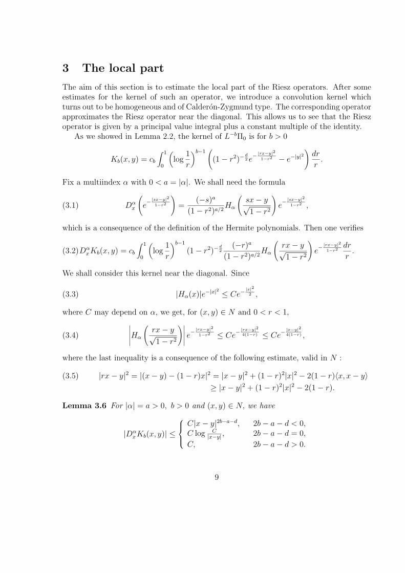
3 The local part

The aim of this section is to estimate the local part of the Riesz operators. After someestimates for the kernel of such an operator, we introduce a convolution kernel whichturns out to be homogeneous and of Calderon-Zygmund type. The corresponding operatorapproximates the Riesz operator near the diagonal. This allows us to see that the Rieszoperator is given by a principal value integral plus a constant multiple of the identity.

As we showed in Lemma 2.2, the kernel of L−bΠ0 is for b > 0

Kb(x, y) = cb

∫ 1

0

(log

1

r

)b−1(

(1− r2)−d2 e

− |rx−y|2

1−r2 − e−|y|2

)dr

r.

Fix a multiindex α with 0 < a = |α|. We shall need the formula

Dαx

(e− |sx−y|2

1−r2

)=

(−s)a

(1− r2)a/2Hα

(sx− y√1− r2

)e− |sx−y|2

1−r2 ,(3.1)

which is a consequence of the definition of the Hermite polynomials. Then one verifies

DαxKb(x, y) = cb

∫ 1

0

(log

1

r

)b−1

(1− r2)−d2

(−r)a

(1− r2)a/2Hα

(rx− y√1− r2

)e− |rx−y|2

1−r2dr

r.(3.2)

We shall consider this kernel near the diagonal. Since

|Hα(x)|e−|x|2 ≤ Ce−|x|22 ,(3.3)

where C may depend on α, we get, for (x, y) ∈ N and 0 < r < 1,∣∣∣∣∣Hα

(rx− y√1− r2

)∣∣∣∣∣ e− |rx−y|2

1−r2 ≤ Ce−|rx−y|24(1−r) ≤ Ce−

|x−y|24(1−r) ,(3.4)

where the last inequality is a consequence of the following estimate, valid in N :

|rx− y|2 = |(x− y)− (1− r)x|2 = |x− y|2 + (1− r)2|x|2 − 2(1− r)〈x, x− y〉(3.5)

≥ |x− y|2 + (1− r)2|x|2 − 2(1− r).

Lemma 3.6 For |α| = a > 0, b > 0 and (x, y) ∈ N, we have

|DαxKb(x, y)| ≤

C|x− y|2b−a−d, 2b− a− d < 0,C log C

|x−y| , 2b− a− d = 0,

C, 2b− a− d > 0.

9

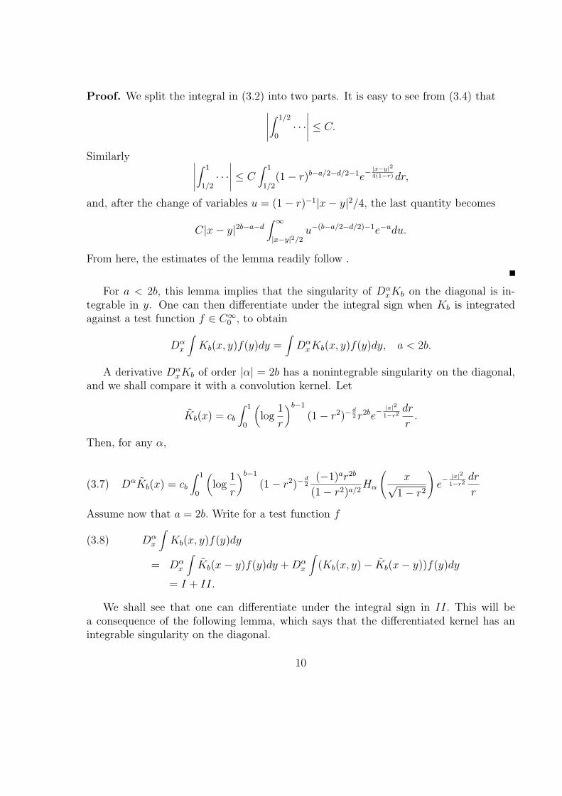
Proof. We split the integral in (3.2) into two parts. It is easy to see from (3.4) that∣∣∣∣∣∫ 1/2

0· · ·∣∣∣∣∣ ≤ C.

Similarly ∣∣∣∣∣∫ 1

1/2· · ·∣∣∣∣∣ ≤ C

∫ 1

1/2(1− r)b−a/2−d/2−1e−

|x−y|24(1−r)dr,

and, after the change of variables u = (1− r)−1|x− y|2/4, the last quantity becomes

C|x− y|2b−a−d∫ ∞

|x−y|2/2u−(b−a/2−d/2)−1e−udu.

From here, the estimates of the lemma readily follow .

For a < 2b, this lemma implies that the singularity of DαxKb on the diagonal is in-

tegrable in y. One can then differentiate under the integral sign when Kb is integratedagainst a test function f ∈ C∞

0 , to obtain

Dαx

∫Kb(x, y)f(y)dy =

∫Dα

xKb(x, y)f(y)dy, a < 2b.

A derivative DαxKb of order |α| = 2b has a nonintegrable singularity on the diagonal,

and we shall compare it with a convolution kernel. Let

Kb(x) = cb

∫ 1

0

(log

1

r

)b−1

(1− r2)−d2 r2be

− |x|2

1−r2dr

r.

Then, for any α,

DαKb(x) = cb

∫ 1

0

(log

1

r

)b−1

(1− r2)−d2

(−1)ar2b

(1− r2)a/2Hα

(x√

1− r2

)e− |x|2

1−r2dr

r(3.7)

Assume now that a = 2b. Write for a test function f

Dαx

∫Kb(x, y)f(y)dy(3.8)

= Dαx

∫Kb(x− y)f(y)dy +Dα

x

∫(Kb(x, y)− Kb(x− y))f(y)dy

= I + II.

We shall see that one can differentiate under the integral sign in II. This will bea consequence of the following lemma, which says that the differentiated kernel has anintegrable singularity on the diagonal.

10

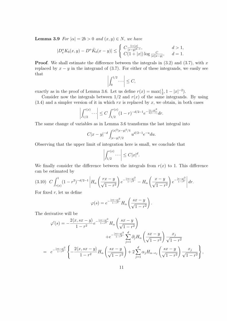
Lemma 3.9 For |α| = 2b > 0 and (x, y) ∈ N, we have

|DαxKb(x, y)−DαKb(x− y)| ≤

C 1+|x||x−y|d−1 , d > 1,

C(1 + |x|) log C|x||x−y| , d = 1.

Proof. We shall estimate the difference between the integrals in (3.2) and (3.7), with xreplaced by x − y in the integrand of (3.7). For either of these integrands, we easily seethat ∣∣∣∣∣

∫ 1/2

0· · ·∣∣∣∣∣ ≤ C,

exactly as in the proof of Lemma 3.6. Let us define r(x) = max(12, 1− |x|−2).

Consider now the integrals between 1/2 and r(x) of the same integrands. By using(3.4) and a simpler version of it in which rx is replaced by x, we obtain, in both cases∣∣∣∣∣

∫ r(x)

1/2· · ·∣∣∣∣∣ ≤ C

∫ r(x)

1/2(1− r)−d/2−1e−

|x−y|24(1−r)dr.

The same change of variables as in Lemma 3.6 transforms the last integral into

C|x− y|−d∫ |x|2|x−y|2/4

|x−y|2/2ud/2−1e−udu.

Observing that the upper limit of integration here is small, we conclude that∣∣∣∣∣∫ r(x)

1/2· · ·∣∣∣∣∣ ≤ C|x|d.

We finally consider the difference between the integrals from r(x) to 1. This differencecan be estimated by

C∫ 1

r(x)(1− r2)−d/2−1

∣∣∣∣∣Hα

(rx− y√1− r2

)e− |rx−y|2

1−r2 −Hα

(x− y√1− r2

)e− |x−y|2

1−r2

∣∣∣∣∣ dr.(3.10)

For fixed r, let us define

ϕ(s) = e− |sx−y|2

1−r2 Hα

(sx− y√1− r2

).

The derivative will be

ϕ′(s) = −2〈x, sx− y〉1− r2

e− |sx−y|2

1−r2 Hα

(sx− y√1− r2

)

+e− |sx−y|2

1−r2

d∑j=1

∂jHα

(sx− y√1− r2

)xj√

1− r2

= e− |sx−y|2

1−r2

−2〈x, sx− y〉1− r2

Hα

(sx− y√1− r2

)+ 2

d∑j=1

αjHα−ej

(sx− y√1− r2

)xj√

1− r2

,11

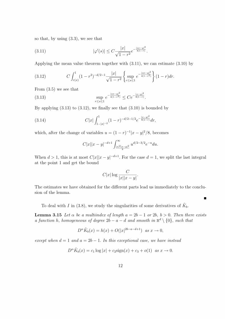
so that, by using (3.3), we see that

|ϕ′(s)| ≤ C|x|√1− r2

e−|sx−y|24(1−r) .(3.11)

Applying the mean value theorem together with (3.11), we can estimate (3.10) by

C∫ 1

r(x)(1− r2)−d/2−1 |x|√

1− r2

{sup

r≤s≤1e− |sx−y|2

4(1−r2)

}(1− r)dr.(3.12)

From (3.5) we see that

supr≤s≤1

e− |sx−y|2

4(1−r2) ≤ Ce−|x−y|28(1−r) .(3.13)

By applying (3.13) to (3.12), we finally see that (3.10) is bounded by

C|x|∫ 1

1−|x|−2(1− r)−d/2−1/2e−

|x−y|28(1−r)dr,(3.14)

which, after the change of variables u = (1− r)−1|x− y|2/8, becomes

C|x||x− y|−d+1∫ ∞

|x|2|x−y|28

ud/2−3/2e−udu.

When d > 1, this is at most C|x||x− y|−d+1. For the case d = 1, we split the last integralat the point 1 and get the bound

C|x| logC

|x||x− y|.

The estimates we have obtained for the different parts lead us immediately to the conclu-sion of the lemma.

To deal with I in (3.8), we study the singularities of some derivatives of Kb.

Lemma 3.15 Let α be a multiindex of length a = 2b− 1 or 2b, b > 0. Then there existsa function h, homogeneous of degree 2b− a− d and smooth in Rd \ {0}, such that

DαKb(x) = h(x) +O(|x|2b−a−d+1) as x→ 0,

except when d = 1 and a = 2b− 1. In this exceptional case, we have instead

DαKb(x) = c1 log |x|+ c2sign(x) + c3 + o(1) as x→ 0.

12

Proof. Write the integral in (3.7) as∫ 1/20 +

∫ 11/2. Clearly

∫ 1/2

0= c0 + o(1) as x→ 0,(3.16)

so that this part of DαKb verifies the conclusion of the lemma.In∫ 11/2 we observe that

(log 1/r)b−1r2b−1 = c(1− r2)b−1r(1 + (1− r)g(r)),

with g a bounded function in [1/2, 1], and expand the Hermite polynomial. Then∫ 11/2 is

seen to be a sum of terms

cδ

∫ 1

1/2(1− r2)b−1−d/2−a/2−|δ|/2xδe

− |x|2

1−r2 r(1 + (1− r)g(r))dr,(3.17)

taken over multiindices δ between 0 and α. The factor r here is introduced to facilitatethe change of variables s = (1− r2)/|x|2. If we neglect the term (1− r)g(r)for a moment,the expression (3.17) is transformed to

cxδ|x|2b−a−d−|δ|∫ 3/(4|x|2)

0sb−1−d/2−a/2−|δ|/2e−1/sds.(3.18)

In the main case 2b− a− d− |δ| < 0, the integral in (3.18) converges even if extended to+∞, and for small |x| its value is then c+O(|x|), for some c > 0. Then the expression in(3.18) is clearly

cxδ|x|2b−a−d−|δ| +O(|x|2b−a−d+1), as x→ 0.

The remaining, exceptional case 2b−a−d−|δ| = 0 occurs precisely when a = 2b−1, d =1, δ = 0. Then (3.18) is instead

c1 log |x|+ c2 + o(1).

The contribution from the term (1− r)g(r) can be transformed similarly, and is seento be no larger than

Q = C|x|2b−a−d+2∫ 3/(4|x|2)

0sb−d/2−a/2−|δ|/2e−1/sds.

If 2b− a < d+ |δ| − 2, the integral here converges at ∞, and Q = O(|x|2b−a−d+2), x→ 0.If 2b − a = d + |δ| − 2, we similarly find that Q = O(|x|2b−a−d+2 log 1/|x|). In these twocases, we thus have Q = O(|x|2b−a−d+1). If finally 2b−a > d+ |δ|−2, we get Q = O(|x||δ|).Then Q = O(|x|2b−a−d+1) again, provided |δ| ≥ 2b−a−d+1. This last inequality is easilyseen to be satisfied as soon as we are not in the exceptional case defined above. With

13

this sole exception, we thus have Q = O(|x|2b−a−d+1). In the exceptional case, we observeinstead directly that the contribution to (3.17) coming from the term (1− r)g(r) is∫ 1

1/2e− |x|2

1−r2 h(r)rdr,

for some bounded function h which does not depend on x. This expression is c+ o(1) asx→ 0. From this the lemma follows.

Consider now term I in (3.8), with |α| = 2b and f ∈ C∞0 . Let Dα = ∂jD

α′, for some

j and some α′ with |α′| = 2b− 1, and write P = Dα′Kb for short. Then

Dα(Kb ∗ f)(x) =∂

∂xj

∫P (y)f(x− y)dy

=∫P (y)f ′j(x− y)dy = − lim

ρ→0

∫|y|>ρ

P (y)∂

∂yj

f(x− y)dy.

We integrate by parts with respect to yj in the last integral. Let pj denote the projectionRd → Rd−1 obtained by deleting the jth coordinate. If y′ ∈ Rd−1 satisfies |y′| < ρ, the linep−1

j (y′) has two intersections with the sphere |y| = ρ denoted y+(y′) and y−(y′), wherethe subscript indicates the sign of the jth coordinate. We get

Dα(Kb ∗ f)(x)(3.19)

= limρ→0

(∫|y′|<ρ

(P (y+(y′))f(x− y+(y′))− P (y−(y′))f(x− y−(y′)))dy′

+∫|y|>ρ

∂jP (y)f(x− y)dy

).

From Lemma 3.15 it follows that the integral in y′ in the last expression tends to aαf(x)as ρ → 0. Here aα is a constant which is nonzero for instance when Dα = ∂2

j . Thus thelast integral converges, and its limit is a principal value.

Combining I and II, we finally get

Dαx

(∫RdKb(x, y)f(y)dy

)= aαf(x) + p.v.

∫RdDα

xKb(x, y)f(y)dy(3.20)

for |α| = 2b > 0.Off the diagonal, the operator Rα = DαL−bΠ0 is thus given by the smooth kernel

DαKb. In particular, we have a decomposition Rα = Rα,loc +Rα,glob, as defined in Section2.

Theorem 3.21 Let α be a multiindex with |α| = 2b > 0. Then Rα,loc is of weak type(1, 1) with respect to the Gaussian measure γ.

14

Proof. Let h be the homogeneous function obtained in Lemma 3.15. It then follows fromLemmas 3.9 and 3.15 that

Ψ(x, y) = DαKb(x, y)− h(x− y)

satisfies ∫(x,y)∈N

|Ψ(x, y)|dx ≤ C,

where C is independent of y. Thus the kernel Ψ(x, y)χN(x, y) defines a strong type (1, 1)operator both for Lebesgue measure and for γ.

The function h must have mean value 0 on the unit sphere, since the last integral in(3.19) has a limit for every test function f. Thus h is a Calderon-Zygmund kernel andconvolution by p.v. h defines an operator T of weak type (1, 1) for Lebesgue measure inRd. Hence, Theorem 2.7 implies that Tloc is of weak type (1, 1) for γ. It now follows thatthe operator Rα, loc, defined by the kernel

p.v. DαKb(x, y)χN(x, y)

is of weak type (1, 1) for γ.

15

4 The global part of the second-order operators

The major part of this section consists of the technical Lemma 4.3, giving size estimates forRiesz kernels of order 2. Then this lemma is applied, via the “forbidden regions”method,to obtain the weak type (1, 1) estimate of the corresponding Riesz operators.

Off the diagonal, the kernel of the second order Riesz operator Rjk = ∂j∂kL−1Π0 is

4c1

∫ 1

0(1− r2)−d/2−2r2(rxj − yj)(rxk − yk) exp

(−|rx− y|2

1− r2

)dr

r

−2δjk c1

∫ 1

0(1− r2)−d/2−1r2 exp

(−|rx− y|2

1− r2

)dr

r.

The absolute value of this kernel can be estimated by the positive kernel

K(x, y) =∫ 1

0ψ(r;x, y) e−φ(r;x,y) dr(4.1)

where

ψ(r;x, y) = r (1− r2)−d/2−1

(1 +

|rx− y|2

1− r2

)and φ(r;x, y) =

|rx− y|2

1− r2.(4.2)

In this section we shall prove that the global part Tglob of the integral operator with kernelK, i.e.

Tglobf(x) =∫K(x, y)χNc(x, y) f(y) dy,

is of weak type (1, 1). This clearly implies that the global part of any second order Rieszoperator is of weak type (1, 1).

We cover the set {x : |x| > 1} with nonoverlapping cubes Qi, i = 1, 2, ..., centred atpoints xi, |xi| ≥ 1 and of diameters di such that c/|xi| ≤ di < 1/(10|xi|), for some c > 0.This can clearly be done. We number the cubes in such a way that |xi| is nondecreasing.Let

K∗(x, y) = sup{K(x′, y) : x′ in the same Qi as x, or x′ = x}.For |y| > 1 we let η = |y| and write x = ξy/η + v, where ξ ∈ R and v ⊥ y. Define for

such a y regions Di = Di(y) by

D0 = {x : ξ < 0}D1 = {x : 0 < ξ < η, |x− y| > βη}D2 = {x : (x, y) ∈ N c, 0 < ξ < η, |x− y| < βη}D3 = {x : (x, y) ∈ N c, ξ > η, |x− y| < βη}D4 = {x : ξ > η, |x− y| > βη},

where β > 0 is sufficiently small.

16

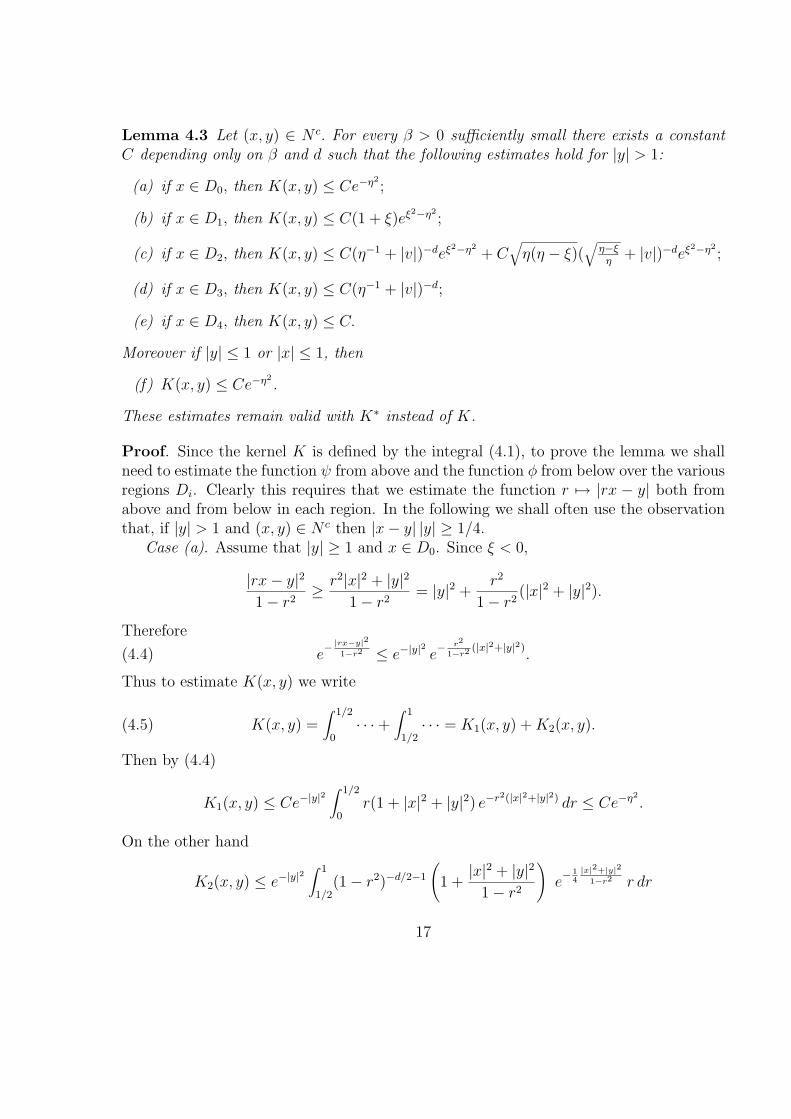
Lemma 4.3 Let (x, y) ∈ N c. For every β > 0 sufficiently small there exists a constantC depending only on β and d such that the following estimates hold for |y| > 1:

(a) if x ∈ D0, then K(x, y) ≤ Ce−η2;

(b) if x ∈ D1, then K(x, y) ≤ C(1 + ξ)eξ2−η2;

(c) if x ∈ D2, then K(x, y) ≤ C(η−1 + |v|)−deξ2−η2+ C

√η(η − ξ)(

√η−ξ

η+ |v|)−deξ2−η2

;

(d) if x ∈ D3, then K(x, y) ≤ C(η−1 + |v|)−d;

(e) if x ∈ D4, then K(x, y) ≤ C.

Moreover if |y| ≤ 1 or |x| ≤ 1, then

(f) K(x, y) ≤ Ce−η2.

These estimates remain valid with K∗ instead of K.

Proof. Since the kernel K is defined by the integral (4.1), to prove the lemma we shallneed to estimate the function ψ from above and the function φ from below over the variousregions Di. Clearly this requires that we estimate the function r 7→ |rx − y| both fromabove and from below in each region. In the following we shall often use the observationthat, if |y| > 1 and (x, y) ∈ N c then |x− y| |y| ≥ 1/4.

Case (a). Assume that |y| ≥ 1 and x ∈ D0. Since ξ < 0,

|rx− y|2

1− r2≥ r2|x|2 + |y|2

1− r2= |y|2 +

r2

1− r2(|x|2 + |y|2).

Therefore

e− |rx−y|2

1−r2 ≤ e−|y|2

e− r2

1−r2 (|x|2+|y|2).(4.4)

Thus to estimate K(x, y) we write

K(x, y) =∫ 1/2

0· · ·+

∫ 1

1/2· · · = K1(x, y) +K2(x, y).(4.5)

Then by (4.4)

K1(x, y) ≤ Ce−|y|2∫ 1/2

0r(1 + |x|2 + |y|2) e−r2(|x|2+|y|2) dr ≤ Ce−η2

.

On the other hand

K2(x, y) ≤ e−|y|2∫ 1

1/2(1− r2)−d/2−1

(1 +

|x|2 + |y|2

1− r2

)e− 1

4|x|2+|y|2

1−r2 r dr

17

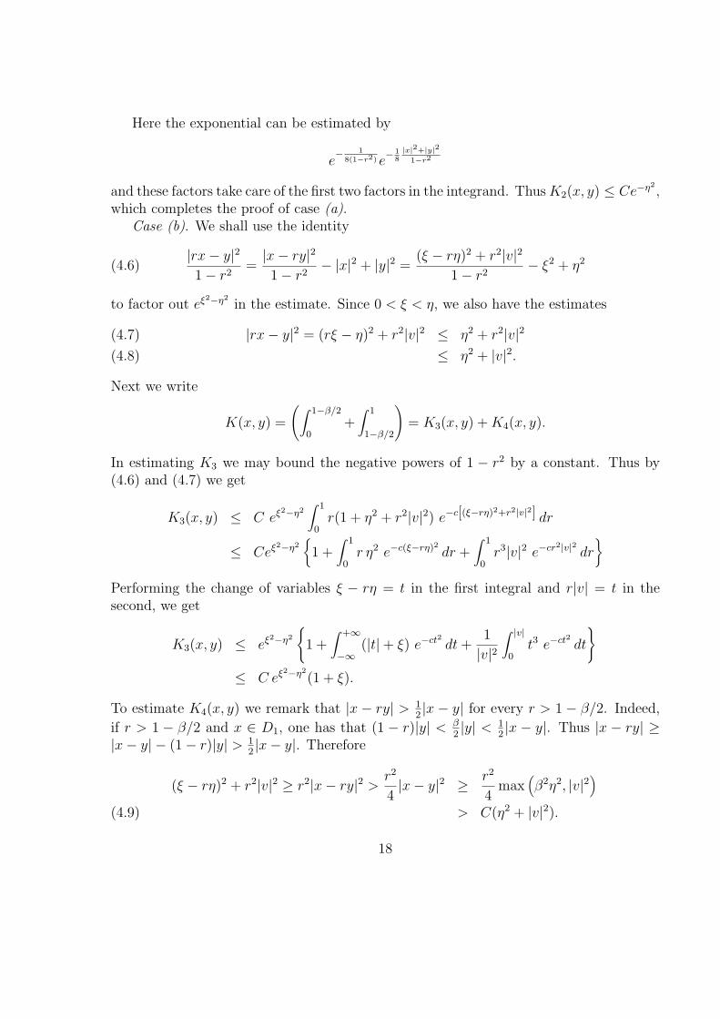
Here the exponential can be estimated by

e− 1

8(1−r2) e− 1

8|x|2+|y|2

1−r2

and these factors take care of the first two factors in the integrand. ThusK2(x, y) ≤ Ce−η2,

which completes the proof of case (a).Case (b). We shall use the identity

|rx− y|2

1− r2=|x− ry|2

1− r2− |x|2 + |y|2 =

(ξ − rη)2 + r2|v|2

1− r2− ξ2 + η2(4.6)

to factor out eξ2−η2in the estimate. Since 0 < ξ < η, we also have the estimates

|rx− y|2 = (rξ − η)2 + r2|v|2 ≤ η2 + r2|v|2(4.7)

≤ η2 + |v|2.(4.8)

Next we write

K(x, y) =

(∫ 1−β/2

0+∫ 1

1−β/2

)= K3(x, y) +K4(x, y).

In estimating K3 we may bound the negative powers of 1 − r2 by a constant. Thus by(4.6) and (4.7) we get

K3(x, y) ≤ C eξ2−η2∫ 1

0r(1 + η2 + r2|v|2) e−c[(ξ−rη)2+r2|v|2] dr

≤ Ceξ2−η2{1 +

∫ 1

0r η2 e−c(ξ−rη)2 dr +

∫ 1

0r3|v|2 e−cr2|v|2 dr

}Performing the change of variables ξ − rη = t in the first integral and r|v| = t in thesecond, we get

K3(x, y) ≤ eξ2−η2

{1 +

∫ +∞

−∞(|t|+ ξ) e−ct2 dt+

1

|v|2∫ |v|

0t3 e−ct2 dt

}≤ C eξ2−η2

(1 + ξ).

To estimate K4(x, y) we remark that |x − ry| > 12|x − y| for every r > 1 − β/2. Indeed,

if r > 1 − β/2 and x ∈ D1, one has that (1 − r)|y| < β2|y| < 1

2|x − y|. Thus |x − ry| ≥

|x− y| − (1− r)|y| > 12|x− y|. Therefore

(ξ − rη)2 + r2|v|2 ≥ r2|x− ry|2 > r2

4|x− y|2 ≥ r2

4max

(β2η2, |v|2

)> C(η2 + |v|2).(4.9)

18

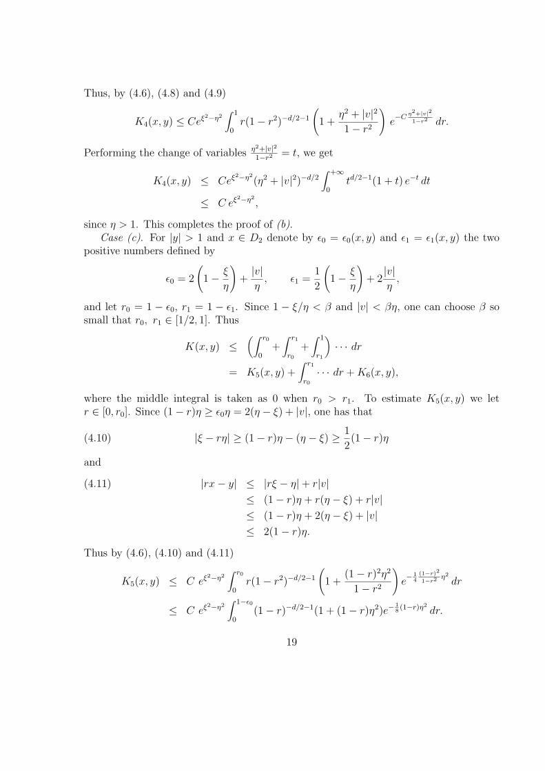
Thus, by (4.6), (4.8) and (4.9)

K4(x, y) ≤ Ceξ2−η2∫ 1

0r(1− r2)−d/2−1

(1 +

η2 + |v|2

1− r2

)e−C

η2+|v|2

1−r2 dr.

Performing the change of variables η2+|v|21−r2 = t, we get

K4(x, y) ≤ Ceξ2−η2

(η2 + |v|2)−d/2∫ +∞

0td/2−1(1 + t) e−t dt

≤ C eξ2−η2

,

since η > 1. This completes the proof of (b).Case (c). For |y| > 1 and x ∈ D2 denote by ε0 = ε0(x, y) and ε1 = ε1(x, y) the two

positive numbers defined by

ε0 = 2

(1− ξ

η

)+|v|η, ε1 =

1

2

(1− ξ

η

)+ 2

|v|η,

and let r0 = 1 − ε0, r1 = 1 − ε1. Since 1 − ξ/η < β and |v| < βη, one can choose β sosmall that r0, r1 ∈ [1/2, 1]. Thus

K(x, y) ≤(∫ r0

0+∫ r1

r0

+∫ 1

r1

)· · · dr

= K5(x, y) +∫ r1

r0

· · · dr +K6(x, y),

where the middle integral is taken as 0 when r0 > r1. To estimate K5(x, y) we letr ∈ [0, r0]. Since (1− r)η ≥ ε0η = 2(η − ξ) + |v|, one has that

|ξ − rη| ≥ (1− r)η − (η − ξ) ≥ 1

2(1− r)η(4.10)

and

|rx− y| ≤ |rξ − η|+ r|v|(4.11)

≤ (1− r)η + r(η − ξ) + r|v|≤ (1− r)η + 2(η − ξ) + |v|≤ 2(1− r)η.

Thus by (4.6), (4.10) and (4.11)

K5(x, y) ≤ C eξ2−η2∫ r0

0r(1− r2)−d/2−1

(1 +

(1− r)2η2

1− r2

)e− 1

4(1−r)2

1−r2 η2

dr

≤ C eξ2−η2∫ 1−ε0

0(1− r)−d/2−1(1 + (1− r)η2)e−

18(1−r)η2

dr.

19

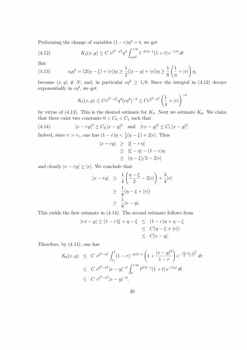
Performing the change of variables (1− r)η2 = t, we get

K5(x, y) ≤ C eξ2−η2

ηd∫ +∞

ε0η2t−d/2−1(1 + t) e−t/8 dt(4.12)

But

ε0η2 = (2(η − ξ) + |v|)η ≥ 1

2(|x− y|+ |v|)η ≥ 1

8

(1

η+ |v|

)η,(4.13)

because (x, y) 6∈ N ; and, in particular εη2 ≥ 1/8. Since the integral in (4.12) decaysexponentially in εη2, we get

K5(x, y) ≤ Ceξ2−η2

ηd(εη2)−d ≤ Ceξ2−η2

(1

η+ |v|

)−d

by virtue of (4.13). This is the desired estimate for K5. Next we estimate K6. We claimthat there exist two constants 0 < C0 < C1 such that

|x− ry|2 ≥ C0 |x− y|2 and |rx− y|2 ≤ C1 |x− y|2.(4.14)

Indeed, since r > r1, one has (1− r)η < 12(η − ξ) + 2|v|. Thus

|x− ry| ≥ |ξ − r η|≥ |ξ − η| − (1− r)η

≥ (η − ξ)/2− 2|v|and clearly |x− ry| ≥ |v|. We conclude that

|x− ry| ≥ 1

4

(η − ξ

2− 2|v|

)+

3

4|v|

≥ 1

8(η − ξ + |v|)

≥ 1

8|x− y|.

This yields the first estimate in (4.14). The second estimate follows from

|rx− y| ≤ (1− r)ξ + η − ξ ≤ (1− r)η + η − ξ

≤ C(η − ξ + |v|)≤ C|x− y|.

Therefore, by (4.14), one has

K6(x, y) ≤ C eξ2−η2∫ 1

r1

(1− r)−d/2−1

(1 +

|x− y|2

1− r

)e−

C02

|x−y|21−r dr

≤ C eξ2−η2|x− y|−d∫ +∞

0td/2−1(1 + t) e−C0t dt

≤ C eξ2−η2|x− y|−d.

20

Since |x − y| ≥ 1/2(|x − y| + |v|) ≥ C(η−1 + |v|) for (x, y) ∈ N c and |y| > 1, the lastestimate implies that

K6(x, y) ≤ C eξ2−η2

(1

η+ |v|

)−d

.

Finally, if r0 < r1, we have to estimate also the integral over the interval [r0, r1]. Noticethat r0 < r < r1 implies that ε1 < 1− r < ε0. Thus

|v| < 3

2(η − ξ) and

1

2

η − ξ

η< 1− r < 4

η − ξ

η,(4.15)

whence we get the estimates

|rx− y| ≤ η − rξ + |v| = (1− r)η + r(η − ξ) + |v| ≤ C(η − ξ)(4.16)

and|x− ry|2

1− r2=

(ξ − rη)2

1− r2+

|v|2

1− r2≥ 1

8

η(ξ − rη)2

η − ξ+

1

8

η|v|2

η − ξ.(4.17)

Define the new variable s by ξ − rη = ηs. Then by (4.15), (4.16) and (4.17)

∫ r1

r0

ψ e−φ dr ≤ C eξ2−η2

(η − ξ

η

)−d/2−1

(1 +η − ξ

ηη2) e−

18

ηη−ξ

|v|2∫

Re−

18

η3

η−ξs2

ds

≤ Cn eξ2−η2

(η − ξ

η

)−d/2+1/2 (1

η − ξ+ η

)(1 +

η

η − ξ|v|2

)−n

for each n > 0. By choosing n = d/2 we get

∫ r1

r0

ψ e−φ dr ≤ C eξ2−η2

(1

η − ξ+ η

)(η − ξ

η

)1/2 (η − ξ

η+ |v|2

)−d/2

.

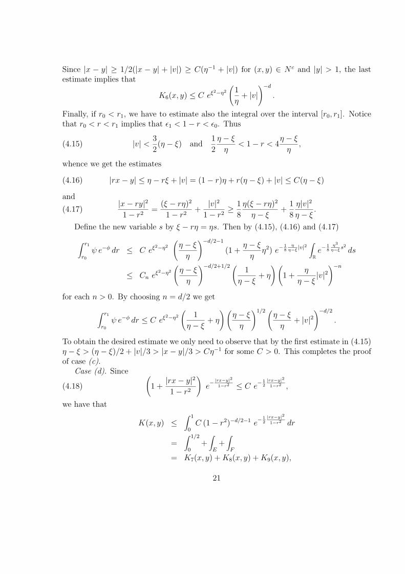
To obtain the desired estimate we only need to observe that by the first estimate in (4.15)η − ξ > (η − ξ)/2 + |v|/3 > |x− y|/3 > Cη−1 for some C > 0. This completes the proofof case (c).

Case (d). Since (1 +

|rx− y|2

1− r2

)e− |rx−y|2

1−r2 ≤ C e− 1

2|rx−y|2

1−r2 ,(4.18)

we have that

K(x, y) ≤∫ 1

0C (1− r2)−d/2−1 e

− 12|rx−y|2

1−r2 dr

=∫ 1/2

0+∫

E+∫

F

= K7(x, y) +K8(x, y) +K9(x, y),

21

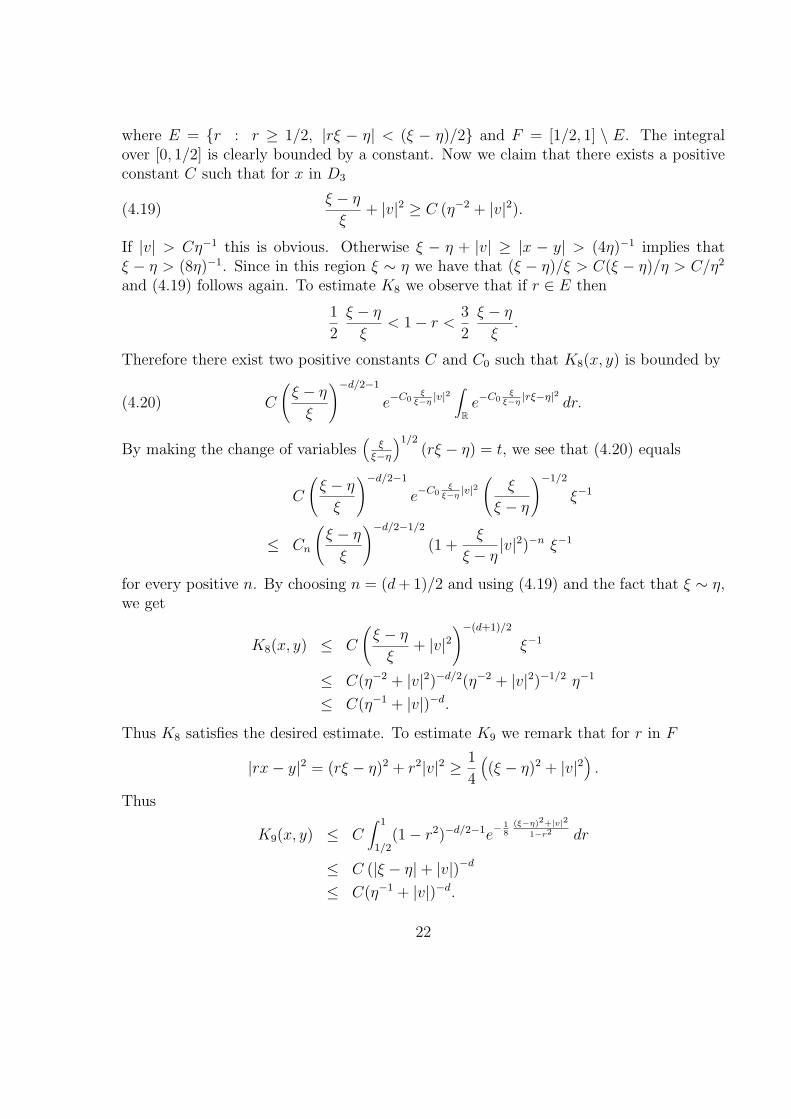
where E = {r : r ≥ 1/2, |rξ − η| < (ξ − η)/2} and F = [1/2, 1] \ E. The integralover [0, 1/2] is clearly bounded by a constant. Now we claim that there exists a positiveconstant C such that for x in D3

ξ − η

ξ+ |v|2 ≥ C (η−2 + |v|2).(4.19)

If |v| > Cη−1 this is obvious. Otherwise ξ − η + |v| ≥ |x − y| > (4η)−1 implies thatξ − η > (8η)−1. Since in this region ξ ∼ η we have that (ξ − η)/ξ > C(ξ − η)/η > C/η2

and (4.19) follows again. To estimate K8 we observe that if r ∈ E then

1

2

ξ − η

ξ< 1− r <

3

2

ξ − η

ξ.

Therefore there exist two positive constants C and C0 such that K8(x, y) is bounded by

C

(ξ − η

ξ

)−d/2−1

e−C0ξ

ξ−η|v|2∫

Re−C0

ξξ−η

|rξ−η|2 dr.(4.20)

By making the change of variables(

ξξ−η

)1/2(rξ − η) = t, we see that (4.20) equals

C

(ξ − η

ξ

)−d/2−1

e−C0ξ

ξ−η|v|2(

ξ

ξ − η

)−1/2

ξ−1

≤ Cn

(ξ − η

ξ

)−d/2−1/2

(1 +ξ

ξ − η|v|2)−n ξ−1

for every positive n. By choosing n = (d+ 1)/2 and using (4.19) and the fact that ξ ∼ η,we get

K8(x, y) ≤ C

(ξ − η

ξ+ |v|2

)−(d+1)/2

ξ−1

≤ C(η−2 + |v|2)−d/2(η−2 + |v|2)−1/2 η−1

≤ C(η−1 + |v|)−d.

Thus K8 satisfies the desired estimate. To estimate K9 we remark that for r in F

|rx− y|2 = (rξ − η)2 + r2|v|2 ≥ 1

4

((ξ − η)2 + |v|2

).

Thus

K9(x, y) ≤ C∫ 1

1/2(1− r2)−d/2−1e

− 18

(ξ−η)2+|v|2

1−r2 dr

≤ C (|ξ − η|+ |v|)−d

≤ C(η−1 + |v|)−d.

22

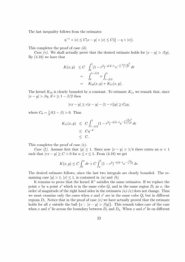
The last inequality follows from the estimates

η−1 + |v| ≤ C|x− y|+ |v| ≤ C(ξ − η + |v|).

This completes the proof of case (d).Case (e). We shall actually prove that the desired estimate holds for |x − y| > β|y|.

By (4.18) we have that

K(x, y) ≤ C∫ 1

0(1− r2)−d/2−1 e

− 12

|rx−y|2

1−r2 dr

=∫ 1−β/2

0+∫ 1

1−β/2

= K10(x, y) +K11(x, y).

The kernel K10 is clearly bounded by a constant. To estimate K11 we remark that, since|x− y| > βη, if r ≥ 1− β/2 then

|rx− y| ≥ r|x− y| − (1− r)|y| ≥ C0η,

where C0 = 12β(1− β) > 0. Thus

K11(x, y) ≤ C∫ 1

1−β/2(1− r2)−d/2−1e

− 12

C20η2

1−r2 dr

≤ Cη−d

≤ C.

This completes the proof of case (e).Case (f). Assume first that |y| ≤ 1. Since now |x − y| > 1/4 there exists an α < 1

such that |rx− y| ≥ C > 0 for α ≤ r ≤ 1. From (4.18) we get

K(x, y) ≤ C∫ α

0dr + C

∫ 1

α(1− r2)−d/2−1e

− C01−r2 dr.

The desired estimate follows, since the last two integrals are clearly bounded. The re-maining case |y| > 1, |x| ≤ 1, is contained in (a) and (b).

It remains to prove that the kernel K∗ satisfies the same estimates. If we replace thepoint x by a point x′ which is in the same cube Qi and in the same region Di as x, theorder of magnitude of the right hand sides in the estimates (a)-(e) does not change. Thuswe must examine only the cases when x and x′ are in the same cube Qi but in differentregions Di. Notice that in the proof of case (e) we have actually proved that the estimateholds for all x outside the ball {x : |x − y| > β|y|}. This remark takes care of the casewhen x and x′ lie across the boundary between D1 and D4. When x and x′ lie on different

23

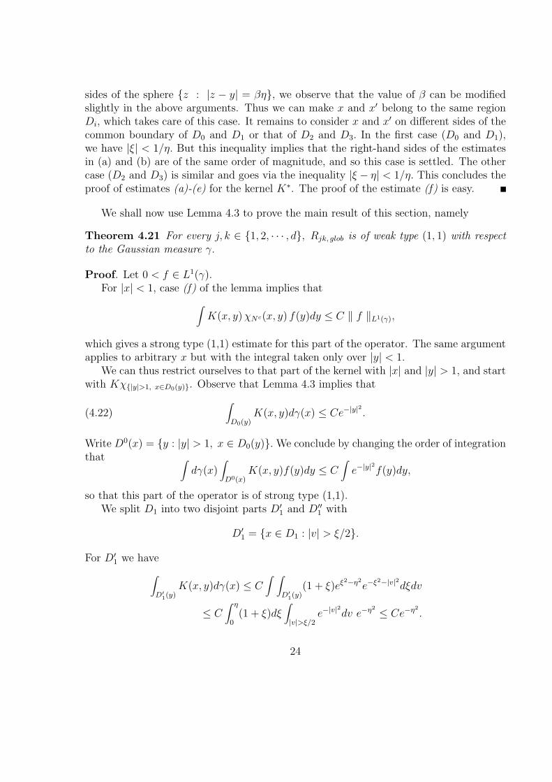
sides of the sphere {z : |z − y| = βη}, we observe that the value of β can be modifiedslightly in the above arguments. Thus we can make x and x′ belong to the same regionDi, which takes care of this case. It remains to consider x and x′ on different sides of thecommon boundary of D0 and D1 or that of D2 and D3. In the first case (D0 and D1),we have |ξ| < 1/η. But this inequality implies that the right-hand sides of the estimatesin (a) and (b) are of the same order of magnitude, and so this case is settled. The othercase (D2 and D3) is similar and goes via the inequality |ξ − η| < 1/η. This concludes theproof of estimates (a)-(e) for the kernel K∗. The proof of the estimate (f) is easy.

We shall now use Lemma 4.3 to prove the main result of this section, namely

Theorem 4.21 For every j, k ∈ {1, 2, · · · , d}, Rjk, glob is of weak type (1, 1) with respectto the Gaussian measure γ.

Proof. Let 0 < f ∈ L1(γ).For |x| < 1, case (f) of the lemma implies that∫

K(x, y)χNc(x, y) f(y)dy ≤ C ‖ f ‖L1(γ),

which gives a strong type (1,1) estimate for this part of the operator. The same argumentapplies to arbitrary x but with the integral taken only over |y| < 1.

We can thus restrict ourselves to that part of the kernel with |x| and |y| > 1, and startwith Kχ{|y|>1, x∈D0(y)}. Observe that Lemma 4.3 implies that∫

D0(y)K(x, y)dγ(x) ≤ Ce−|y|

2

.(4.22)

Write D0(x) = {y : |y| > 1, x ∈ D0(y)}. We conclude by changing the order of integrationthat ∫

dγ(x)∫

D0(x)K(x, y)f(y)dy ≤ C

∫e−|y|

2

f(y)dy,

so that this part of the operator is of strong type (1,1).We split D1 into two disjoint parts D′

1 and D′′1 with

D′1 = {x ∈ D1 : |v| > ξ/2}.

For D′1 we have∫

D′1(y)

K(x, y)dγ(x) ≤ C∫ ∫

D′1(y)

(1 + ξ)eξ2−η2

e−ξ2−|v|2dξdv

≤ C∫ η

0(1 + ξ)dξ

∫|v|>ξ/2

e−|v|2

dv e−η2 ≤ Ce−η2

.

24

The estimate thus obtained is similar to (4.22), and we can argue as above to take careof D′

1.When x ∈ D4, we observe that |y|/|x| < λ for some λ < 1, so that |x|2 > |y|2 + ε|x|2

where ε > 0 depends only on β. Together with Lemma 4.3, this implies that∫D4(y)

K(x, y)dγ(x) ≤ Ce−|y|2∫e−ε|x|2dx ≤ Ce−|y|

2

.

Thus we also control the D4 part of the operator.For the remaining regions D′′

1 , D2, and D3, we shall deduce the weak-type estimate.Fix y with |y| > 1, and let χy be the characteristic function of the union of those cubesQi which intersect D′′

1(y) ∪D2(y) ∪D3(y). Define K∗(x, y) = K∗(x, y)χy(x). Notice thatK∗(x, y) stays constant as x moves within a Qi. Our task is to estimate the level set

L = {x :∫K∗(x, y)f(y)dy > α}

for α > 0. We first observe that it would be enough to prove the inequality∫LK∗(x, y)dγ(x) ≤ Ce−|y|

2

, y ∈ Rd,(4.23)

Indeed, (4.23) implies

γ(L) ≤∫

Ldγ(x)

1

α

∫K∗(x, y)f(y)dy(4.24)

=1

α

∫f(y)dy

∫LK∗(x, y)dγ(x) ≤

C

α

∫f(y)dγ(y),

which is the desired estimate.However, (4.23) is false in general. We shall therefore construct a smaller set E ⊂ L

for which (4.23) holds, i.e., such that∫EK∗(x, y)dγ(x) ≤ Ce−|y|

2

, y ∈ Rd.(4.25)

Still E must be large enough so that

γ(E) ≥ cγ(L)(4.26)

for some c > 0. Given such a set E, we can carry through the argument (4.24) with Einstead of L and finish the proof.

We remark that our construction of E follows a method from Sjogren [12], also usedin [13].

Notice that L is a union of cubes Qi. We shall construct E as the union of some ofthese cubes. Roughly speaking, the reason why (4.23) fails is that L contains too many

25

cubes near each other. If we decide to include a cube in E, we should therefore notinclude its close neighbours. Still, (4.26) must be respected. To achieve this, we associatewith each cube Qi a forbidden region Fi, which is essentially a cone with vertex in Qi

and directed away from 0. More precisely, let Ci be the cone of vectors forming an angleof at most π/4 with the centre xi of Qi. We define Fi as the union of those cubes Qj

intersecting Qi + Ci. The inequality

γ(Fi) ≤ Cγ(Qi)(4.27)

is then rather easy to verify. One integrates first in each affine hyperplane orthogonal toxi, see [13, proof of formula (3.1)].

The procedure to construct E goes as follows. We consider the Qi, i = 1, 2, ..., in thisorder. For each Qi, we decide in the following way whether to select it, i.e., include it inE. The cube Qi is selected if and only if it is contained in L and is not contained in theforbidden region Fj of any Qj already selected. Then E is defined as the union of theselected Qi. Since L is covered by the selected cubes and their forbidden regions, (4.26)follows from (4.27).

Now it only remains to verify that the selected cubes are so sparse that (4.25) holds.We fix y with η = |y| > 1. An elementary geometric argument shows that K∗(x, y) can benonzero only when x is in the cone Cy of vectors forming an angle of at most π/4 with y.Consider a line ` parallel to y. We claim that the intersection of ` and Cy∩E is containedin at most one Qi. Indeed, any Qi intersecting this intersection is contained in E, and itsforbidden region contains the half-line of ` in the y direction starting at Qi.

We parametrise the lines ` by

`v = {x = ξy/η + v : ξ ∈ R},

where v ⊥ y. The observation we just made means that `v ∩ Cy ∩ E is contained in asegment corresponding to an interval in the parameter ξ given by ξv < ξ < ξv + ξ−1

v , forsome ξv > 1/2. Now we apply Fubini’s theorem to the integral in (4.25), getting

∫EK∗(x, y)dγ(x) ≤

∫e−|v|

2

dv∫ ξv+ξv

−1

ξv

e−ξ2

K∗(ξy/|y|+ v, y)dξ.

The integration in v is with respect to (d − 1)-dimensional Lebesgue measure in thehyperplane orthogonal to y. To estimate the right-hand side here, we insert the inequalitiesfrom Lemma 4.3 in the three regions we are considering.

For D′′1 , we get at most

C∫e−|v|

2

dv∫ ξv+ξv

−1

ξv

e−ξ2

(1 + |ξ|)eξ2−η2

dξ ≤ C∫e−|v|

2 1 + ξvξv

dv e−η2 ≤ Ce−η2

.

26

Using the estimates valid in D2, we get two terms. The first term is

C∫e−|v|

2

dv∫ ξv+ξv

−1

ξv

e−ξ2

(η−1 + |v|)−deξ2−η2

dξ ≤ C

ξv

∫(η−1 + |v|)−ddv e−η2 ≤ Ce−η2

,

where we used the fact that η ≤ Cξv here. The second term is

C∫e−|v|

2

dv∫ ξv+ξv

−1

ξv

e−ξ2√η(η − ξ)

(√η − ξ

η+ |v|

)−d

eξ2−η2

dξ.

If η − ξv ≤ 2/η, this is like the first term. If not, we can estimate this expression by

C∫e−|v|

2 1

ξv

√η(η − ξv)

(√η − ξvη

+ |v|)−d

dv e−η2 ≤ Ce−η2

,

almost as the first term.Using finally the estimates in D3, we get at most

C∫e−|v|

2

dv∫ ξv+ξv

−1

ξv

e−ξ2

(η−1 + |v|)−ddξ ≤ C∫ 1

ξve−ξ2

v(η−1 + |v|)−ddv

≤ Ce−η2 1

η

∫(η−1 + |v|)−ddv ≤ Ce−η2

.

These estimates together imply (4.25) and thus complete the proof of the theorem.

By putting together Theorems 3.21 and 4.21, we have finally proved Theorem 1.1.

27

5 A counterexample for operators of order at least

three

Theorem 5.1 Let a = |α| ≥ 3 and b > 0. Then the operator DαL−bΠ0 is not of weaktype (1, 1) with respect to the Gaussian measure γ.

Letting b = |α|/2 here, we clearly obtain Riesz operators of order at least 3.

Proof. We estimate the kernel DαxKb(x, y), as given in (3.2), for η = |y| large and

yi ≥ cη, i = 1, · · · , d and c > 0. Write x = ξy/η + v as before, with ξ ∈ R and v ⊥ y. Welet x be in the tube J defined by η/2 < ξ < 3η/4 and |v| < 1. Then for each i = 1, · · · , d,

− rxi − yi√1− r2

≥ cη√1− r2

≥ cη.

It follows that

(−1)aHα

(rx− y√1− r2

)> cηa.

In particular, the integrand in (3.2) is positive for 0 < r < 1. We observe that

e− |rx−y|2

1−r2 = eξ2−η2

e− |ξ−rη|2+r2|v|2

1−r2

so that for 1/4 < r < 3/4 and x ∈ J

e− |rx−y|2

1−r2 ≥ ceξ2−η2

e−C|ξ−rη|2 .

These estimates imply that

DαKb(x, y) ≥ cηaeξ2−η2∫ 3/4

1/4e−C(ξ−rη)2dr ≥ cηa−1eξ2−η2

.

Now let 0 ≤ f ∈ L1(γ) be a close approximation of a point mass at y, with norm 1 inL1(γ). Then

DαL−bΠ0f(x) =∫

RdDαKb(x, y)f(y)dy

will be close to eη2DαKb(x, y) when x ∈ J. We conclude that

DαL−bΠ0f(x) ≥ cηa−1eξ2 ≥ cηa−1e(η/2)2

for x ∈ J.Since γ(J) ≥ cη−1e−(η/2)2 , as is easily verified, the L1,∞(γ) quasi-norm of DαL−bΠ0f is

at least cηa−2 →∞ as η →∞ when a ≥ 3. This violates the weak type (1, 1) property.

28

References

[1] E. B. Fabes, C. E. Gutierrez and R. Scotto, Weak-type estimates for the Riesz trans-forms associated with the Gaussian measure, Rev. Mat. Iberoamericana 10 (1994).

[2] D. Feyel, Transformations de Hilbert-Riesz gaussiennes, C. R. Acad. Sci. Paris, Ser.I Math 310 (1990), 653-655.

[3] L. Forzani and R. Scotto, The higher order Riesz transform for Gaussian measureneed not be weak type (1, 1), to appear.

[4] R. F. Gundy, Sur les transformations de Riesz pour le semigroupe d’Ornstein-Uhlenbeck, C. R. Acad. Sci. Paris, Ser. I Math 303 (1986), 967-970.

[5] C. Gutierrez, On the Riesz transforms for Gaussian measures, J. of Funct. Anal.,120 (1) (1994), 107-134.

[6] C. Gutierrez, C. Segovia and J. L. Torrea, On higher Riesz transforms for Gaussianmeasures, to appear in J. of Fourier Anal. and Appl..

[7] T. Menarguez, S. Perez and F. Soria, Some remarks on harmonic analysis with respectto Gaussian measure, announcement.

[8] P. A. Meyer, Transformations de Riesz pour les lois Gaussiennes Springer LectureNotes in Mathematics, 1059 (1984), 179-193.

[9] B. Muckenhoupt, Hermite conjugate expansions, Trans. Amer. Math. Soc. 139(1969), 243-260.

[10] S. Perez, Estimaciones puntuales y en norma para operadores relacionados con elsemigrupo de Ornstein-Uhlenbeck Ph. D. Thesis Universidad Autonoma de Madrid,1996.

[11] G. Pisier, Riesz transforms: a simpler analytic proof of P. A. Meyer’s inequalitySpringer Lecture Notes in Mathematics, 1321 (1988), 485-501.

[12] P. Sjogren, Weak L1 characterizations of Poisson integrals, Green potentials and Hp

spaces, Trans. Amer. Math. Soc. 233 (1977), 179-196.

[13] P. Sjogren, On the maximal function for the Mehler kernel, in Harmonic Analysis,Cortona 1982, Springer Lecture Notes in Mathematics, 992 (1983), 73-82.

[14] P. Sjogren, Operators associated with the Hermite semigroup -A survey in Proceedingsof the 5th International Conference on Harmonic Analysis and Partial DifferentialEquations, El Escorial, Spain, June 1996.

29

[15] W. O. Urbina, On singular integrals with respect to the Gaussian measure, Ann.Scuola Norm. Sup. di Pisa, Classe di Scienze, Serie IV, Vol. XVIII, 4 (1990), 531-567.

30