Histogram equalization of the speech representation for robust speech recognition

2

Histogram Equalization for Robust Speech Recognition

Luz García, Jose Carlos Segura, Ángel de la Torre, Carmen Benítez and Antonio J. Rubio

University of Granada Spain

1. Introduction Optimal Automatic Speech Recognition takes place when the evaluation is done under circumstances identical to those in which the recognition system was trained. In the speech applications demanded in the actual real world this will almost never happen. There are several variability sources which produce mismatches between the training and test conditions. Depending on his physical or emotional state, a speaker will produce sounds with unwanted variations transmitting no acoustic relevant information. The phonetic context of the sounds produced will also introduce undesired variations. Inter-speaker variations must be added to those intra-speaker variations. They are related to the peculiarities of speakers’ vocal track, his gender, his socio-linguistic environment, etc. A third source of variability is constituted by the changes produced in the speaker’s environment and the characteristics of the channel used to communicate. The strategies used to eliminate the group of environmental sources of variation are called Robust Recognition Techniques. Robust Speech Recognition is therefore the recognition made as invulnerable as possible to the changes produced in the evaluation environment. Robustness techniques constitute a fundamental area of research for voice processing. The current challenges for automatic speech recognition can be framed within these work lines: • Speech recognition of coded voice over telephone channels. This task adds an

additional difficulty: each telephone channel has its own SNR and frequency response. Speech recognition over telephone lines must perform a channel adaptation with very few specific data channels.

• Low SNR environments. Speech Recognition during the 80’s was done inside a silent room with a table microphone. At this moment, the scenarios demanding automatic speech recognition are: • Mobile phones. • Moving cars. • Spontaneous speech. • Speech masked by other speech. • Speech masked by music. • Non-stationary noises.

• Co-channel voice interferences. Interferences caused by other speakers constitute a bigger challenge than those changes in the recognition environment due to wide band noises.

Speech Recognition, Technologies and Applications

24

• Quick adaptation for non-native speakers. Current voice applications demand robustness and adaptation to non-native speakers’ accents.

• Databases with realistic degradations. Formulation, recording and spreading of voice databases containing realistic examples of the degradation existing in practical environments are needed to face the existing challenges in voice recognition.

This chapter will analyze the effects of additive noise in the speech signal, and the existing strategies to fight those effects, in order to focus on a group of techniques called statistical matching techniques. Histogram Equalization –HEQ- will be introduced and analyzed as main representative of this family of Robustness Algorithms. Finally, an improved version of the Histogram Equalization named Parametric Histogram Equalization -PEQ- will be exposed.

2. Voice feature normalization 2.1 Effects of additive noise Within the framework of Automatic Speech Recognition, the phenomenon of noise can be defined as the non desired sound which distorts the information transmitted in the acoustic signal difficulting its correct perception. There are two main sources of distortion for the voice signal: additive noise and channel distortion. Channel distortion is defined as the noise convolutionally mixed with speech in the time domain. It appears as a consequence of the signal reverberations during its transmission, the frequency response of the microphone used, or peculiarities of the transmission channel such as an electrical filter within the A/D filters for example. The effects of channel distortion have been fought with certain success as they become linear once the signal is analyzed in the frequency domain. Techniques such as RASTA filtering, echo cancellation or Cepstral mean subtraction have proved to eliminate its effects. Additive noise is summed to the speech signal in the time domain and its effects in the frequency domain are not easily removed as it has the peculiarity to transform speech non-linearly in certain domains of analysis. Nowadays, additive noise constitutes the driving force of research in ASR: additive white noises, door slams, spontaneous overlapped voices, background music, etc. The most used model to analyze the effects of noise in the oral communication (Huang, 2001) represents noise as a combination of additive and convolutional noise following the expression:

[ ] [ ]* [ ] [ ]y m x m h m n m= + (1)

Assuming that the noise component n[m] and the speech signal x[m] are statistically independent, the resulting noisy speech signal y[m] will follow equation (2) for the ith channel of the filter bank:

2 2 2 2

( ) ( ) ( ) ( )i i i iY f X f H f N f≅ • + (2)

Taking logarithms in expression (2) and operating, the following approximation in the frequency domain can be obtained:

2 2 2 2 2 2ln ( ) ln ( ) ln ( ) ln(1 exp( ( ) ln ( ) ln ( ) ))i i i i i iY f X f H f N f X f H f≅ + + + − − (3)


25

In order to move expression (3) to the Cepstral domain with M+1 Cepstral coefficients, the following 4 matrixes are defined, using C() to denote the discrete cosine transform:

2 2 2

0 1

2 2 2

0 1

2 2 2

0 1

2 2 2

0 1

(ln ( ) ln ( ) .... ln ( ) )

(ln ( ) ln ( ) .... ln ( ) )

(ln ( ) ln ( ) .... ln ( ) )

(ln ( ) ln ( ) .... ln ( ) )

M

M

M

M

x C X f X f X f

h C H f H f H f

n C N f N f N f

y C Y f Y f Y f

=

=

=

=

(4)

The following expression can be obtained for the noisy speech signal y in the Cepstral domain combining equations (3) and (4):

^ ^ ^ ^ ^ ^

( )y x h g n x h= + + − − (5) being function g of equation (5) defined as:

1( )( ) (ln(1 ))C zg z C e−

= + (6)

Based on the relative facility to remove it (via linear filtering), and in order to simplify the analysis, we will consider absence of convolutional channel distortion, that is, we will consider H(f)=1. The expression of the noisy signal in the Cepstral domain becomes then:

ln(1 exp( ))y x n x= + + − (7)

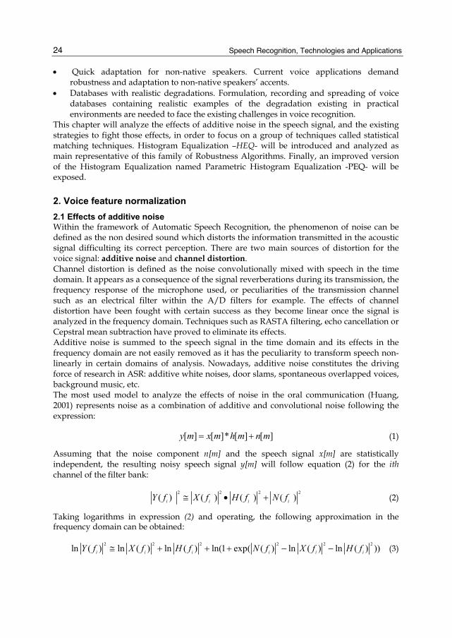
The relation between the clean signal x and the noisy signal y contaminated with additive noise is modelled in expression (7). There is a linear relation between both for high values of x, which becomes non linear when the signal energy approximates or is lower than the energy of noise. Figure 1 shows a numeric example of this behaviour. The logarithmic energy of a signal y contaminated with an additive Gaussian noise with average μn=3 and standard deviation σn=0,4 is pictured. The solid line represents the average transformation of the logarithmic energy, while the dots represent the transformed data. The average transformation can be inverted to obtain the expected value for the clean signal once the noisy signal is observed. In any case there will be a certain degree of uncertainty in the clean signal estimation, depending on the SNR of the transformed point. For values of y with energy much higher than noise the degree of uncertainty will be small. For values of y close to the energy of noise, the degree of uncertainty will be high. This lack of linearity in the distortion is a common feature of additive noise in the Cepstral domain.

Fig. 1. Transformation due to additive noise.


26

The analysis of the histograms of the MFCCs probability density function of a clean signal versus a noisy signal contaminated with additive noise shows the following effects of noise (De la Torre et al., 2002): • A shift in the mean value of the MFCC histogram of the contaminated signal. • A reduction in the variance of such histogram. • A modification in the histogram global shape. This is equivalent to a modification of the

histogram’s statistical higher order moments. This modification is especially remarkable for the logarithmic energy and the lower order coefficients C0 and C1.

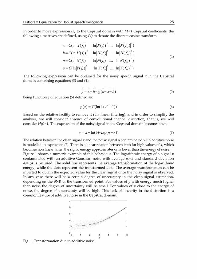
2.2 Robust speech recognition techniques There are several classifications of the existing techniques to make speech recognition robust against environmental changes and noise. A commonly used classification is the one that divides them into pre-processing techniques, feature normalization techniques and model adaptation techniques according to the point of the recognition process in which robustness is introduced (see Figure 2):

Fig. 2. Robust Recognition Strategies.

• Signal Pre-processing Techniques: their aim is to remove noise before the voice signal parameterization is done, in order to obtain a parameterization as close as possible to the clean signal parameterization. They are based on the idea that voice and noise are uncorrelated, and therefore they are additive in the time domain. Consequently their power spectrum of a noisy signal will be the sum of the voice and noise power spectra. The main techniques within this group are Linear Spectral Subtraction (Boll, 1979), Non-linear Spectral Subtraction (Lockwood & Boudy, 1992), Wiener Filtering (Wiener, 1949) or Ephraim Malah noise suppression rule (Ephraim & Malah, 1985).

• Feature Normalization Techniques: the environment distortion is eliminated once the voice signal has been parameterized. Through different processing techniques like high pass Cepstral filtering, models of the noise effects, etc., the clean voice features are recovered from the noisy voice features. Three sub-categories can be found within this group of techniques: • High Band Pass filtering techniques. They add a quite high level of robustness to

the recognizer with a low cost and therefore they are included in the most of the automatic recognition front-ends. Their objective is forcing the mean value of the Cepstral coefficients to be zero. With this condition they eliminate unknown linear filtering effects that the channel might have. The most important techniques within

Speech Signal

Speech Signal

Voice Features

Voice Features

Models

Models

Pre-processingStrategies

FeatureNormalization

ModelAdaptation

Training

Evaluation


27

this subgroup are RASTA filtering (Hermansky & Morgan, 1994) and CMN, Cepstral Mean Normalization- (Furui, 1981).

• Noise compensation with stereo data. This group of techniques compares the noisy voice features with those of clean stereo data. The result of such comparison is a correction of the environment which is added to the feature vector before entering the recognizer. RATZS –multivaRiate gAussian based cepsTral normaliZation- (Moreno et al., 1995) and SPLICE –Stereo-based Piecewise LInear Compensation for Environments- (Deng et al., 2000) are the most representative strategies in this group.

• Noise compensation based on an environment model. These techniques give an analytical expression of the environmental degradation and therefore need very few empirical data to normalize the features. (In contraposition to the compensation using stereo data). Degradation is defined as a filter and a noise such that when they are inversely applied, the probability of the normalized observations becomes the maximum. The most relevant algorithm within this category is VTS –Vector Taylor Series approach- (Moreno et al., 2006).

• Statistical Matching Algorithms. Set of algorithms for feature normalization which define linear and non-linear transformations in order to modify the statistics of noisy speech and make them equal to those of clean speech. Cepstral Mean Normalization, which was firstly classified as a high band pass filtering technique, corresponds as well to the definition of statistical matching algorithms. The most relevant ones are CMNV –Cepstral Mean and Variance Normalization- (Viiki et al., 1998), Normalization of a higher number of statistical moments (Khademul et al., 2004),(Chang Wen & Lin Shan, 2004),(Peinado & Segura, 2006) and Histogram Equalization (De la Torre et al., 2005),(Hilger & Ney, 2006). This group of strategies, and specially Histogram Equalization, constitute the core of this chapter and they will be analyzed in depth in order to see their advantages and to propose an alternative to overcome their limitations.

• Model Adaptation Techniques. They modify the classifier in order to make the classification optimal for the noisy voice features. The acoustic models obtained during the training phase are adapted to the test conditions using a set of adaptation data from the noisy environment. This procedure is used both for environment adaptation and for speaker adaptation. The most common adaptation strategies are MLLR –Maximum Likelihood Linear Regression- (Gales & Woodland, 1996) (Young et al. 1995), MAP –Mamixum a Posteriori Adaptation - (Gauvain & Lee, 1994), PMC- Parallel Model Combination (Gales & Young, 1993), and non linear model transformations like the ones performed using Neural Networks (Yuk et al., 1996) or (Yukyz & Flanagany, 1999).

The robust recognition methods exposed below work on the hypothesis of a stationary additive noise, that is, the noise power spectral density does not change with time. They are narrow-band noises. Other type of non-stationary additive noises with a big importance on robust speech recognition exist: door slams, spontaneous speech, the effect of lips or breath, etc. For the case of these transient noises with statistical properties changing with time, other techniques have been developed under the philosophy of simulating the human perception mechanisms: signal components with a high SNR are processed, while those components with low SNR are ignored. The most representative techniques within this group are the Missing Features Approach (Raj et al. 2001) (Raj et al. 2005), and Multiband Recognition (Tibrewala & Hermansky, 1997) (Okawa et al. 1999).


28

2.3 Statistical matching algorithms This set of features normalization algorithms define linear and non linear transforms in order to modify the noisy features statistics and make them equal to those of a reference set of clean data. The most relevant algorithms are: • CMVN: Cepstral Mean ad Variance Normalization (Viiki et al., 1998):

The additive effect of noise implies a shift on the average of the MFCC coefficients probability density function added to a scaling of its variance. Given a noisy Cepstral coefficient y contaminated with an additive noise with mean value h, and given the clean Cepstral coefficient x with mean value μx and variance σx, the contaminated MFCC y will follow expression (8), representing the variance scaling produced:

y x

y x

y x hh

αμ α μ

σ α σ

= ⋅ += ⋅ +

= ⋅

(8)

If we normalize the mean and variance of both coefficients x and y, their expressions will be:

x

x

xx

μσ

∧ −=

( ) ( )y x

y x

y x h hy x

μ α α μσ α σ

∧ ∧− ⋅ + − ⋅ += = =

⋅ (9)

Equation (9) shows that CMVN makes the coefficients robust against the shift and scaling introduced by noise.

• Higher order statistical moments normalization: A natural extension of CMVN is to normalize more statistical moments apart from the mean value and the variance. In 2004, Khademul (Khademul et al. 2004) adds the MFCCs first four statistical moments to the set of parameters to be used for automatic recognition obtaining some benefits in the recognition and making the system converge more quickly. Also in 2004 Chang Wen (Chang Wen & Lin Shan, 2004) proposes a normalization for the higher order Cepstral moments. His method permits the normalization of an eve or odd order moment added to the mean value normalization. Good results are obtained when normalizing moments with order higher than 50 in the original distribution. Prospection in this direction (Peinado & Segura J.C., 2006) is limited to the search of parametric approximations to normalize no more than 3 simultaneous statistical moments with a high computational cost that does not make them attractive when compared to the Histogram Equalization.

• Histogram Equalization: The linear transformation performed by CMNV only eliminates the linear effects of noise. The non-linear distortion produced by noise does not only affect the mean and variance of the probability density functions but it also affects the higher order moments. Histogram Equalization (De la Torre et al., 2005; Hilger & Ney, 2006) proposes generalizing the normalization to all the statistical moments by transforming


29

the Cepstral coefficients probability density function –pdf- in order to make it equal to a reference probability density function. The appeal of this technique is its low computational and storage cost, added to the absence of stereo data or any kind of supposition or model of noise. It is therefore a convenient technique to eliminate residual noise from other normalization techniques based on noise models like VTS (Segura et al., 2002). The objective of Section 3 will be to exhaustively analyze Histogram Equalization pointing at its advantages and limitations in order to overcome the last ones.

3. Histogram equalization 3.1 Histogram equalization philosophy Histogram Equalization is a technique frequently used in Digital Image Processing (Gonzalez & Wintz, 1987; Russ, 1995) in order to improve the image contrast and brightness and to optimize the dynamic range of the grayscale. With a simple procedure it automatically corrects the images too bright, too dark or with not enough contrast. The gray level values are adjusted within a certain margin and the image’s entropy is maximized. Since 1998 and due to the work of Balchandran (Balchandran & Mammone, 1998), Histogram Equalization –HEQ- started to be used for robust voice processing. HEQ can be located within the family of statistical matching voice feature normalization techniques. The philosophy underneath its application to speech recognition is to transform the voice features both for train and test in order to make them match a common range. This equalization of the ranges of both the original emission used to train the recognizer and the parameters being evaluated, has the following effect: the automatic recognition system based on the Bayes classifier becomes ideally invulnerable to the linear and non linear transformations originated by additive Gaussian noise in the test parameters once those test parameters have been equalized. One condition must be accomplished for this equalization to work: the transformations to which the recognizer becomes invulnerable must be invertible. In other words, recognition moves to a domain where any invertible transformation does not change the error of Bayes classifier. If CMN and CMNV normalized the mean and average of the Cepstral coefficients probability density functions, what HEQ does is normalizing the probability density function of the train and test parameters, transforming them to a third common pdf which becomes the reference pdf. The base theory (De la Torre et al., 2005) for this normalization technique is the property of the random variables according to which, a random variable x with probability density function px(x) and cumulative density function Cx(x) can be transformed into a random

variable )(xTx x=∧

with a reference probability density function )(xx∧φ preserving an

identical cumulative density function (∧

Φ= xxCx ()( )), as far as the transformation applied

)(xTx is invertible (Peyton & Peebles, 1993). The fact of preserving the cumulative density function provides a univocal expression of the invertible transformation )(xTx to be applied to the transformed variable )(xTx x=

∧ in order to obtain the desired probability density

function )(∧

xxφ :


30

( ) ( ) ( ( ))x xx C x T x∧

Φ = = Φ (10)

1( ) ( ( ))x xx

x T x C x∧

∧−= = Φ (11)

The transformation )(xTx defined in equation (11) is a non-decreasing monotonic function

that will be non linear in general. Expression (11) shows that the transformation is defined using de CDF of the variable being transformed. Once the random variables have been transformed, they become invulnerable to any linear or non-linear transformation applied to them as far as such transformation is reversible. Lets x be a random variable experimenting a generic reversible non linear transformation G to become the transformed random variable y=G(x). If both original and transformed variables are equalized to a reference pdf refφ , the equalized variables will follow the expressions:

1( ) ( ( ))x ref xx T x C x

∧−= = Φ (12)

1( ) ( ( ( )))y ref yy T y C G x∧

−= = Φ (13)

If G is an invertible function, then the CDFs of x and y=G(x) will be equal:

( ) ( ( ))x yC x C G x= (14)

And in the same way, the transformed variables will also be equal:

1 1( ) ( ( )) ( ( ( )))x ref x ref yx T x C x C G x y∧ ∧

− −= = Φ = Φ = (15)

Expression (15) points out that if we work with equalized variables, the fact of them being subject to an invertible distortion does not affect nor training nor recognition. Their value remains identical in the equalized domain. The benefits of this normalization method for robust speech recognition are based on the hypothesis that noise, denominated G in the former analysis, is an invertible transformation in the feature space. This is not exactly true. Noise is a random variable whose average effect can also be considered invertible (it can be seen in Figure 1). This average effect is the one that HEQ can eliminate. HEQ was first used for voice recognition by Balchandran and Mammone (Balchandran & Mammone, 1998). In this first incursion of equalization in the field of speech, it was used to eliminate the non-linear distortions of the LPC Cepstrum of a speaker identification system. In 2000 Dharanipragada (Dharanipragada & Padmanabhan, 2000) used HEQ to eliminate the environmental mismatch between the headphones and the microphone of a speech recognition system. He added an adaptation step using non-supervised MLLR and obtained good results summing the benefits of both techniques. Since that moment, Histogram Equalization has been widely used and incorporated to voice front-ends in noisy environments. Molau, Hilger and Herman Ney apply it since 2001 (Molau et al., 2001; Hilger & Ney, 2006) in the Mel Filter Bank domain. They implement HEQ together with other


31

techniques like LDA –Linear Discriminat Analysis- or VTLN –Vocal Track Length Normalization- obtaining satisfactory recognition results. De la Torre and Segura (De la Torre et al., 2002; Segura et al., 2004; De la Torre et al., 2005) implement HEQ in the Cepstral domain and analyse its benefits when using it together with VTS normalization.

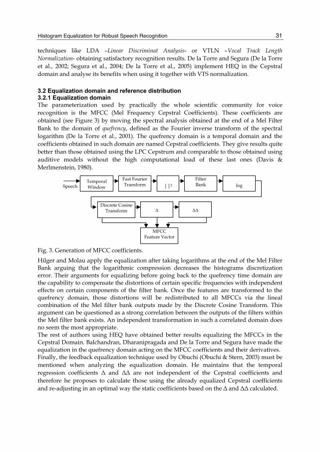
3.2 Equalization domain and reference distribution 3.2.1 Equalization domain The parameterization used by practically the whole scientific community for voice recognition is the MFCC (Mel Frequency Cepstral Coefficients). These coefficients are obtained (see Figure 3) by moving the spectral analysis obtained at the end of a Mel Filter Bank to the domain of quefrency, defined as the Fourier inverse transform of the spectral logarithm (De la Torre et al., 2001). The quefrency domain is a temporal domain and the coefficients obtained in such domain are named Cepstral coefficients. They give results quite better than those obtained using the LPC Cepstrum and comparable to those obtained using auditive models without the high computational load of these last ones (Davis & Merlmenstein, 1980).

Fig. 3. Generation of MFCC coefficients.

Hilger and Molau apply the equalization after taking logarithms at the end of the Mel Filter Bank arguing that the logarithmic compression decreases the histograms discretization error. Their arguments for equalizing before going back to the quefrency time domain are the capability to compensate the distortions of certain specific frequencies with independent effects on certain components of the filter bank. Once the features are transformed to the quefrency domain, those distortions will be redistributed to all MFCCs via the lineal combination of the Mel filter bank outputs made by the Discrete Cosine Transform. This argument can be questioned as a strong correlation between the outputs of the filters within the Mel filter bank exists. An independent transformation in such a correlated domain does no seem the most appropriate. The rest of authors using HEQ have obtained better results equalizing the MFCCs in the Cepstral Domain. Balchandran, Dharanipragada and De la Torre and Segura have made the equalization in the quefrency domain acting on the MFCC coefficients and their derivatives. Finally, the feedback equalization technique used by Obuchi (Obuchi & Stern, 2003) must be mentioned when analyzing the equalization domain. He maintains that the temporal regression coefficients Δ and ΔΔ are not independent of the Cepstral coefficients and therefore he proposes to calculate those using the already equalized Cepstral coefficients and re-adjusting in an optimal way the static coefficients based on the Δ and ΔΔ calculated.

Temporal Window

Fast Fourier Transform

||2

Filter Bank

log

Discrete Cosine Transform

Δ

ΔΔ

MFCC Feature Vector

Speech


32

3.2.2 Reference distribution analysis The election of the reference distribution

refΦ used as common CDF to equalize the random

variables is a relevant decision as the probability density function represents the global voice statistics. The analysis of equation (10) shows the relation between the original pdf and the reference pdf in the equalized domain:

dxxdTx

dxxdTxT

dxxTd

dxxdCxp xx

xxx

x)()()())(())(()()(

∧

==Φ

== φφ (16)

Dharanipragada explains in (Dharanipragada & Padmanabhan, 2000) the relation that the original and reference pdfs must satisfy in terms of information. He uses the Kullback-Liebler distance as a measure of the existing mutual information between the original pdf and the equalized domain reference pdf:

∫∧∧∧∧

=x xx xdxpxpD *))(log(*)()|( φφ (17)

to conclude that such distance will become null in case the condition expressed in equation (18) is satisfied:

)()(∧∧

= xpx xφ (18)

It is difficult to find a transformation )(xTx which satisfies equation (18) considering that x

and ∧

x are random variables with dimension N. If the simplification of independency between the dimensions of the feature vector is accepted, equation (18) can be one-dimensionally searched for. Two reference distributions have been used when implementing HEQ for speech recognition: • Gaussian distribution: When using a Gaussian pdf as reference distribution, the process

of equalization is called Gaussianization. It seems an intuitive distribution to be used in speech processing as the speech signal probability density function has a shape close to a bi-modal Gaussian. Chen and Gopinath (Chen S.S. and Gopinath R.A., 2000) proposed a Gaussianization transformation to model multi-dimensional data. Their transformation alternated linear transformations in order to obtain independence between the dimensions, with marginal one-dimensional Gaussianizations of those independent variables. This was the origin of Gaussianization as a probability distribution scaling technique which has been successfully applied by many authors (Xiang B. et al., 2002) (Saon G. et al., 2004), (Ouellet P. et al., 2005), (Pelecanos J. and Sridharan S., 2001), (De la Torre et al. 2001). Saon and Dharanipragada have pointed out the main advantage of its use: the most of the recognition systems use mixtures of Gaussians with diagonal covariance. It seems reasonable to expect that ”Gaussianizing” the features will strengthen that assumption.

• Clean Reference distribution: The election of the training clean data probability density function (empirically built using cumulative histograms) as reference pdf for the equalization has given better results than Gaussianization (Molau et al., 2001) (Hilger & Ney, 2006) (Dharanipragada


33

& Padmanabhan, 2000). It can be seen as the non-parametrical version of Gaussianization in which the shape of the pdf is calculated empirically. The only condition needed is counting on enough data not to introduce bias or errors in the global voice statistic that it represents.

3.3 HEQ implementation A computationally effective implementation of the Histogram Equalization can be done using quantiles to define the cumulative density function used. The algorithm is then called Quantile-Based Equalization –QBEQ- (Hilger & Ney, 2001) (Segura et al., 2004). Using this implementation, the equalization procedure for a sentence would be following one: i. The sentence’s order statistic is produced. If the total number of frames in the sentence

is 2*T+1, those 2*T+1 values will be ordered as equation (19) shows. The frame

)(rx represents the frame with the r-th position within the ordered sequence of frames:

(1) (2) ( ) (2 1)... ...r Tx x x x +≤ ≤ ≤ ≤ (19)

ii. The reference CDF set of quantiles are calculated. The number of quantiles per sample is chosen (NQ). The CDF values for each quantile probability value pr are registered:

1( ) ( )r rxQ p p∧

−= Φ (20)

0,5( ), 1,...,r QQ

rp r NN−

= ∀ = (21)

iii. The quantiles of the original data will follow expression (22) in which k and f denote the integer and decimal part operators of (1+2*Tpr) respectively:

1,

(2 1)

(1 ) 1 2*( )

2 1k k

x rT

f x fx k TQ p

x k T+

+

− + ≤ ≤⎧⎪= ⎨ = +⎪⎩ (22)

iv. Each pair of quantiles ( )(),( rx

rx pQpQ ∧) represents a point of the equalization

transformation that will be linearly approximated using the set of points obtained.

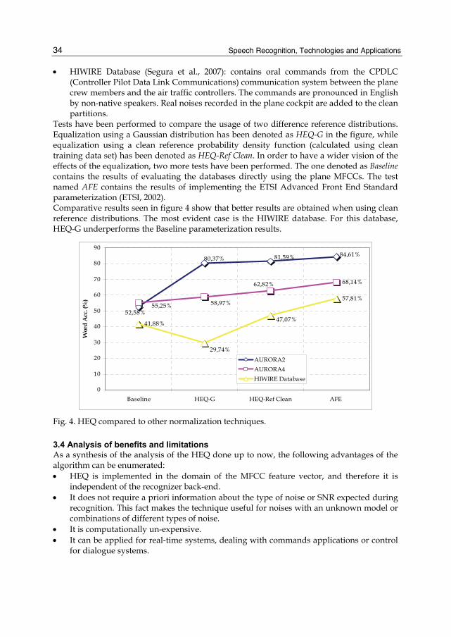
Figure 4. shows the results of implementing Histogram Equalization normalization using the QBEQ approximation, and performing the automatic speech recognition tasks for three databases: AURORA2, AURORA4 and HIWIRE: • AURORA2: database created (Pearce & Hirsch, 2000) adding four different types of

noise with 6 different SNRs to the clean database TIDigits (Leonard, 1984). It contains recording from adults pronouncing isolated and connected digits (up to seven) in English.

• AURORA4: Continuous speech database standardized (Hirsch, 2002) by the ETSI group STQ. It was built as a dictation task on texts from the Wall Street Journal with a size of 5000 words. It has 7 types of additive noises and convolutional channel noise to be put on top of them.


34

• HIWIRE Database (Segura et al., 2007): contains oral commands from the CPDLC (Controller Pilot Data Link Communications) communication system between the plane crew members and the air traffic controllers. The commands are pronounced in English by non-native speakers. Real noises recorded in the plane cockpit are added to the clean partitions.

Tests have been performed to compare the usage of two difference reference distributions. Equalization using a Gaussian distribution has been denoted as HEQ-G in the figure, while equalization using a clean reference probability density function (calculated using clean training data set) has been denoted as HEQ-Ref Clean. In order to have a wider vision of the effects of the equalization, two more tests have been performed. The one denoted as Baseline contains the results of evaluating the databases directly using the plane MFCCs. The test named AFE contains the results of implementing the ETSI Advanced Front End Standard parameterization (ETSI, 2002). Comparative results seen in figure 4 show that better results are obtained when using clean reference distributions. The most evident case is the HIWIRE database. For this database, HEQ-G underperforms the Baseline parameterization results.

84,61%81,59%80,37%

52,58%

68,14%

55,25%

62,82%

58,97%57,81%

47,07%

29,74%

41,88%

0

10

20

30

40

50

60

70

80

90

Baseline HEQ-G HEQ-Ref Clean AFE

Wor

d A

cc. (

%)

AURORA2 AURORA4HIWIRE Database

Fig. 4. HEQ compared to other normalization techniques.

3.4 Analysis of benefits and limitations As a synthesis of the analysis of the HEQ done up to now, the following advantages of the algorithm can be enumerated: • HEQ is implemented in the domain of the MFCC feature vector, and therefore it is

independent of the recognizer back-end. • It does not require a priori information about the type of noise or SNR expected during

recognition. This fact makes the technique useful for noises with an unknown model or combinations of different types of noise.

• It is computationally un-expensive. • It can be applied for real-time systems, dealing with commands applications or control

for dialogue systems.


35

Nevertheless a series of limitations exist which justify the development of new versions of HEQ to eliminate them: • The effectiveness of HEQ depends on the adequate calculation of the original and

reference CDFs for the features to be equalized. There are some scenarios in which sentences are not long enough to provide enough data to obtain a trustable global speech statistic. The original CDF is therefore miscalculated and it incorporates an error transferred to the equalization transformation defined on the basis of this original CDF.

• HEQ works on the hypothesis of statistical independence of the MFCCs. This is not exactly correct. The real MFCCs covariance matrix is not diagonal although it is considered as such for computational viability reasons.

4. Parametric histogram equalization 4.1 Parametric histogram equalization philosophy The two limitations of HEQ mentioned in section 3 have led to the proposal and analysis of a parametric version of Histogram Equalization (Garcia L. et al., 2006) to solve them. As we have just outlined in the former paragraph: 1. There is a minimum amount of data per sentence needed to correctly calculate statistics.

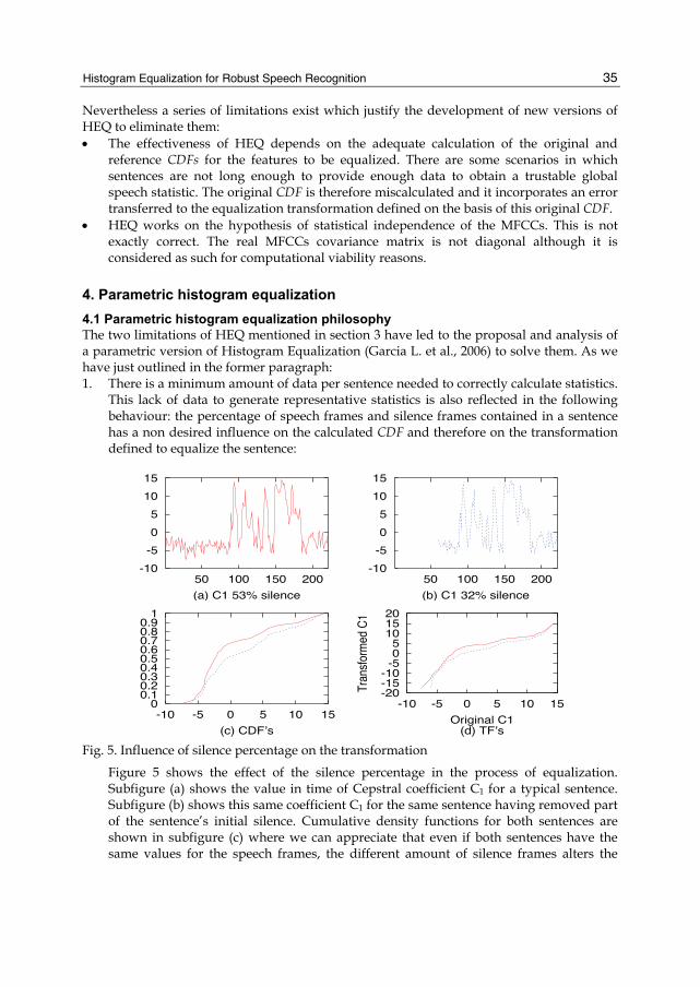
This lack of data to generate representative statistics is also reflected in the following behaviour: the percentage of speech frames and silence frames contained in a sentence has a non desired influence on the calculated CDF and therefore on the transformation defined to equalize the sentence:

-10

-5

0

5

10

15

50 100 150 200

(a) C1 53% silence

-10

-5

0

5

10

15

50 100 150 200

(b) C1 32% silence

00.10.20.30.40.50.60.70.80.9

1

-10 -5 0 5 10 15

(c) CDF’s

00.10.20.30.40.50.60.70.80.9

1

-10 -5 0 5 10 15

(c) CDF’s

-20-15-10-505

101520

-10 -5 0 5 10 15

Tran

sfor

med

C1

Original C1(d) TF’s

-20-15-10-505

101520

-10 -5 0 5 10 15

Tran

sfor

med

C1

Original C1(d) TF’s

Fig. 5. Influence of silence percentage on the transformation

Figure 5 shows the effect of the silence percentage in the process of equalization. Subfigure (a) shows the value in time of Cepstral coefficient C1 for a typical sentence. Subfigure (b) shows this same coefficient C1 for the same sentence having removed part of the sentence’s initial silence. Cumulative density functions for both sentences are shown in subfigure (c) where we can appreciate that even if both sentences have the same values for the speech frames, the different amount of silence frames alters the


36

shape of their global CDF. This difference in the CDF estimation introduces a non desired variation in the transformation calculated (see subfigure (d)). The existing strategies to face the short sentences producing non representative statistics are mainly the usage of a parametric expression for the CDF (Molau et al., 2002; Haverinen & Kiss, 2003; Liu et al., 2004). The usage of order statistics (Segura et al., 2004) can also improve slightly the CDF estimation.

2. The second limitation of HEQ is that due to the fact that equalization is done independently for each MFCC vector component, all the information contained in the relation between components is being lost. It would be interesting to capture this information, and in case noise has produced a rotation in the feature space it would be convenient to recover from it. This limitation has originated a whole family of techniques to capture relations between coefficients, using vector quantization with different criteria, or defining classes via Gaussian Mixture Models (Olsen et al., 2003) (Visweswariah & Gopinath, 2002; Youngjoo et al., 2007). In the group of vector quantization we must mention (Martinez P. et al., 2007) that does an equalization followed by a vector quantization of the Cepstral coefficient in a 4D space, adding temporal information. (Dat T.H. et al.,2005) (Youngjoo S. and Hoirin K.) must also be mentioned.

As an effective alternative to eliminate the exposed limitations, the author of this chapter has proposed (Garcia et al., 2006) to use a parametric variant of the equalization transformation based in modelling the MFCCs probability density function with a mixture of two Gaussians. In ideal clean conditions, speech has a distribution very close to a bi-modal Gaussian. For this reason, Sirko Molau proposes in (Molau S. et al., 2002) the usage of two independent histograms for voice and silence. In order to do so, he separates frames as speech or silence using a Voice Activity Detector. Results are not as good as expected, as the discrimination between voice and silence is quite aggressive. Bo Liu proposes in (Bo L. et al., 2004) to use two Gaussian cumulative histograms to define the pdf of each Cepstral coefficient. He solves the distinction between the classes of speech or silence using a weighing factor calculated with each class probability. The algorithm proposed in this work is named Parametric Equalization –PEQ-. It defines a parametric equalization transformation based on a two-Gaussians mixture model. The first Gaussian is used to represent the silence frames, and the second Gaussian is used to represent the speech frames. In order to map the clean and noisy domains, a parametric linear transformation is defined for each one of those two frame classes:

1, 2

, ,,

( ) ( )n xn x n y

n y

x yμ μ∧ Σ= + − ⋅

Σ being y a silence frame (23)

1, 2

, ,,

( ) ( )s xs x s y

s y

x yμ μ∧ Σ= + − ⋅

Σ being y a silence frame (24)

The terms of equations (23) and (24) are defined as follows: -

xn,μ and xn,Σ are the mean and variance of the clean reference Gaussian distributions for

the class of silence.


37

- xs,μ and

xs,Σ are the mean and variance of the clean reference Gaussian distributions for

the class of speech. -

yn,μ and yn,Σ correspond to the mean and variance of the noisy environment Gaussian

distributions for the class of silence. -

ys,μ and ys,Σ correspond to the mean and variance of the noisy environment Gaussian

distributions for the class of speech. Equations (23) and (24) transform the averages of the noisy environment

yn,μ and ys,μ into

clean reference averages xn,μ and

xs,μ . The noisy variances yn,Σ and

ys,Σ are transformed into clean reference averages

xn,Σ andxs,Σ .

The clean reference Gaussian parameters are calculated using the data of the clean training set. The noisy environment Gaussian parameters are individually calculated for every sentence in process of equalization. Before equalizing each frame we have to choose if it belongs to the speech or silence class. One possibility for taking this decision is to use a voice activity detector. That would imply binary election between both linear transformations (transformation according to voice class parameters or transformation according to silence class parameters). In the border between both classes taking a binary decision would create a discontinuity. In order to avoid it we have used a soft decision based on including the conditional probabilities of each frame to be speech or silence. Equation (25) shows the complete process of parametric equalization:

1 1, ,2 2

, , , ,, ,

( | ) ( ( ) ( ) ) ( | ) ( ( )( ) )n x s xn x n y s x s y

n y s y

x P n y y P s y yμ μ μ μ∧ Σ Σ= ⋅ + − ⋅ + ⋅ + −

Σ Σ (25)

The terms P(n|y) and P(s|y) of equation (25) are the posterior probabilities of the frame belonging to the silence or speech class respectively. They have been obtained using a 2-class Gaussian classifier and the logarithmic energy term (Cepstral coefficient C0) as classification threshold. Initially, the frames with a C0 value lower than the C0 average in the particular sentence are considered as noise. Those frames with a C0 value higher than the sentence average are considered as speech. Using this initial classification the initial values of the means, variances and priori probabilities of the classes are estimated. Using the Expected Maximization Algorithm –EM-, those values are later iterated until they converge. This classification originates the values of P(n|y) and P(s|y) added to the mean and covariance matrixes for the silence and speech classes in the equalization process

yn,μ ,ys,μ ,

yn,Σ and ys,Σ .

If we call n the number of silence frames in the sentence x and s the number of speech frames in the same sentence x being equalized, the mentioned parameters will be defined iteratively using EM:

( | )nx

n p n x x= ⋅∑

( | )sx

n p s x x= ⋅∑


38

1 ( | )nxn

p n xn

μ = ⋅∑

1 ( | )sxs

p s xn

μ = ⋅∑

1 ( | ) ( ) ( )Tn n nxn

p n x x xn

μ μ−

Σ = ⋅ ⋅ − ⋅ −∑

1 ( | ) ( ) ( )Ts s s

xs

p s x x xn

μ μ−

Σ = ⋅ ⋅ − ⋅ −∑ (26)

The posterior probabilities used in (26) have been calculated using the Bayes rule:

_

_ _

( ) ( ( , , ))( | )

( ) ( ( , , )) ( ) ( ( , , ))

nn

n sn s

p n N xp n x

p n N x p s N x

μ

μ μ

⋅ Σ=

⋅ Σ + ⋅ Σ

_

_ _

( ) ( ( , , ))( | )

( ) ( ( , , )) ( ) ( ( , , ))

ss

n sn s

p s N xp s x

p n N x p s N x

μ

μ μ

⋅ Σ=

⋅ Σ + ⋅ Σ (27)

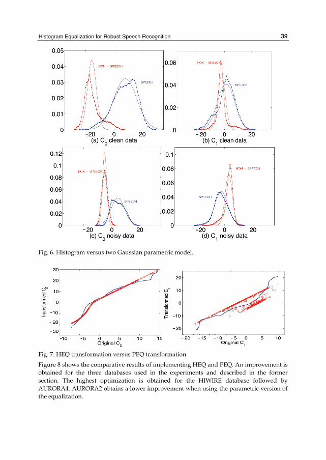
Subfigures (a) and (b) from Figure 6 show the two-Gaussian parametric model for the probability density functions of Cepstral coeficients C0 and C1, put on top of the cumulative histograms of speech and silences frames for a set of clean sentences. Subfigures (c) and (d) show the same models and histograms for a set of noisy sentences. The former figures show the convenience of using bi-modal Gaussians to approximate the two-class histogram, specially in the case of the coefficient C0. They also show how the distance between both Gaussians or both class histograms decreases when the noise increases.

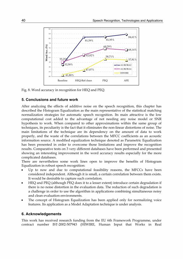
4.2 Histogram equalization versus parametric histogram equalization The solid line of Figure 7 represents the transformation defined for a noisy sentence according to Parametric Equalization in two classes, PEQ. The dotted line of the graph represents the equalization transformation for the same sentence defined with HEQ. Parametric equalization is based on the class probabilities P(n|y) and P(s|y) which depend on the level of the Cepstral coefficient C0. In the case of PEQ, equation (25) will define an

equalized variable ∧

x as a non-linear function of y tending to the linear mapping given by: • Equation (24) when the condition P(s|y) >> P(n|y) is fulfilled. • Equation (23) when the condition P(n|y)>>P(s|y) is fulfilled. The case of coefficient C1 contains a interesting difference when working with PEQ: as P(n|y) and P(s|y) depend on the value of C0, the relation between the clean and noisy data is not a monotonous function. A noisy value of C1 can originate different values of C1 equalized, depending on the value of C0 for the frame.


39

Fig. 6. Histogram versus two Gaussian parametric model.

Fig. 7. HEQ transformation versus PEQ transformation

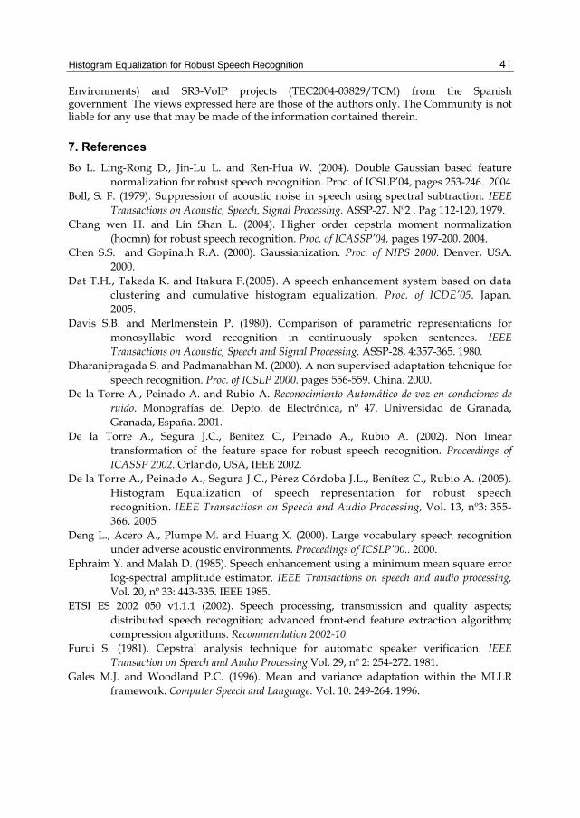
Figure 8 shows the comparative results of implementing HEQ and PEQ. An improvement is obtained for the three databases used in the experiments and described in the former section. The highest optimization is obtained for the HIWIRE database followed by AURORA4. AURORA2 obtains a lower improvement when using the parametric version of the equalization.


40

52,58%

81,59% 81,95%84,61%

68,14%69,29%

62,82%55,25%

41,88%

57,81%

47,07%

58,71%

40

4 5

50

55

60

6 5

70

75

80

8 5

90

Baseline HEQ-Ref clean PEQ AFE

Wor

d A

cc. (

%)

AURORA2

AURORA4

HIWIRE

Fig. 8. Word accuracy in recognition for HEQ and PEQ.

5. Conclusions and future work After analyzing the effects of additive noise on the speech recognition, this chapter has described the Histogram Equalization as the main representative of the statistical matching normalization strategies for automatic speech recognition. Its main attractive is the low computational cost added to the advantage of not needing any noise model or SNR hypothesis to work. When compared to other approximations within the same group of techniques, its peculiarity is the fact that it eliminates the non-linear distortions of noise. The main limitations of the technique are its dependency on the amount of data to work properly, and the waste of the correlations between the MFCC coefficients as an acoustic information source. A modified equalization technique denoted as Parametric Equalization has been presented in order to overcome those limitations and improve the recognition results. Comparative tests on 3 very different databases have been performed and presented showing an interesting improvement in the word accuracy results especially for the more complicated databases. There are nevertheless some work lines open to improve the benefits of Histogram Equalization in robust speech recognition: • Up to now and due to computational feasibility reasons, the MFCCs have been

considered independent. Although it is small, a certain correlation between them exists. It would be desirable to capture such correlation.

• HEQ and PEQ (although PEQ does it to a lesser extent) introduce certain degradation if there is no noise distortion in the evaluation data. The reduction of such degradation is a challenge in order to use the algorithm in applications combining simultaneous noisy and clean evaluation environments.

• The concept of Histogram Equalization has been applied only for normalizing voice features. Its application as a Model Adaptation technique is under analysis.

6. Acknowledgements This work has received research funding from the EU 6th Framework Programme, under contract number IST-2002-507943 (HIWIRE, Human Input that Works in Real


41

Environments) and SR3-VoIP projects (TEC2004-03829/TCM) from the Spanish government. The views expressed here are those of the authors only. The Community is not liable for any use that may be made of the information contained therein.

7. References Bo L. Ling-Rong D., Jin-Lu L. and Ren-Hua W. (2004). Double Gaussian based feature

normalization for robust speech recognition. Proc. of ICSLP’04, pages 253-246. 2004 Boll, S. F. (1979). Suppression of acoustic noise in speech using spectral subtraction. IEEE

Transactions on Acoustic, Speech, Signal Processing. ASSP-27. Nº2 . Pag 112-120, 1979. Chang wen H. and Lin Shan L. (2004). Higher order cepstrla moment normalization

(hocmn) for robust speech recognition. Proc. of ICASSP’04, pages 197-200. 2004. Chen S.S. and Gopinath R.A. (2000). Gaussianization. Proc. of NIPS 2000. Denver, USA.

2000. Dat T.H., Takeda K. and Itakura F.(2005). A speech enhancement system based on data

clustering and cumulative histogram equalization. Proc. of ICDE’05. Japan. 2005.

Davis S.B. and Merlmenstein P. (1980). Comparison of parametric representations for monosyllabic word recognition in continuously spoken sentences. IEEE Transactions on Acoustic, Speech and Signal Processing. ASSP-28, 4:357-365. 1980.

Dharanipragada S. and Padmanabhan M. (2000). A non supervised adaptation tehcnique for speech recognition. Proc. of ICSLP 2000. pages 556-559. China. 2000.

De la Torre A., Peinado A. and Rubio A. Reconocimiento Automático de voz en condiciones de ruido. Monografías del Depto. de Electrónica, nº 47. Universidad de Granada, Granada, España. 2001.

De la Torre A., Segura J.C., Benítez C., Peinado A., Rubio A. (2002). Non linear transformation of the feature space for robust speech recognition. Proceedings of ICASSP 2002. Orlando, USA, IEEE 2002.

De la Torre A., Peinado A., Segura J.C., Pérez Córdoba J.L., Benítez C., Rubio A. (2005). Histogram Equalization of speech representation for robust speech recognition. IEEE Transactiosn on Speech and Audio Processing, Vol. 13, nº3: 355-366. 2005

Deng L., Acero A., Plumpe M. and Huang X. (2000). Large vocabulary speech recognition under adverse acoustic environments. Proceedings of ICSLP’00.. 2000.

Ephraim Y. and Malah D. (1985). Speech enhancement using a minimum mean square error log-spectral amplitude estimator. IEEE Transactions on speech and audio processing, Vol. 20, nº 33: 443-335. IEEE 1985.

ETSI ES 2002 050 v1.1.1 (2002). Speech processing, transmission and quality aspects; distributed speech recognition; advanced front-end feature extraction algorithm; compression algorithms. Recommendation 2002-10.

Furui S. (1981). Cepstral analysis technique for automatic speaker verification. IEEE Transaction on Speech and Audio Processing Vol. 29, nº 2: 254-272. 1981.

Gales M.J. and Woodland P.C. (1996). Mean and variance adaptation within the MLLR framework. Computer Speech and Language. Vol. 10: 249-264. 1996.


42

Gales M.J. and Young S., (1993). Cepstral parameter compensation for the update of the parameters of a single mixture density hmm recognition in noise. Speech Communications.Vol 12: 231-239. 1993.

García L., Segura J.C., Ramírez J., De la Torre A. and Benítez C. (2006). Parametric Non-Linear Features Equalization for Robust Speech Recognition. Proc. of ICASSP’06. France. 2006.

Gauvain J.L. and Lee C.H. (1994). Maximum a posteriori estimation for multivariate Gaussian mixture observation of Markov chains. IEEE Transactions on speech and audio processing. Vol. 2, nº291-298. 1994.

González R.C. and Wintz P. (1987). Digital Image Processing. Addison-Wesley. 1987. Haverinen H. and Kiss I. (2003). On-line parametric histogram equalization techniques for

noise robust embedded speech recognition. Proc. of Eurospech’03. Switzerland. 2003.

Hermansky H. and Morgan N. (1991). Rasta Processing of Speech. IEEE Transactions on acoustic speech and signal processing. Vol. 2, nº 4: 578-589. 1991.

Hilger F. and Ney H. (2006). Quantile based histogram equalization for noise robust large vocabulary speech recognition. IEEE Transactions on speech and audio processing. 2006.

Hirsch H.G. (2002). Experimental framework for the performance evaluation of speech recognition front-ends of large vocabulary tasks. STQ AURORA DSR Working Group. 2002.

Leonard R.G. (1984). A database for independent digits recognitions. Proc. of ICASSP’84. United States. 1984.

Lockwood P. and Boudy J. (1992). Experiments with a Non Linear Spectral Subtractor (NSS), Hidden Markov Models and the projection, for robust speech recognition in cars. Speech Communications, Vol. 11. Issue 2-3, 1992.

Martinez P., Segura J.C. and García L. (2007). Robust distributed speech recognitio using histogram equalization and correlation information. Proc. of Interspeech’07. Belgium. 2007.

Molau S., Pitz M. and Ney H. (2001). Histogram based normalization in the acoustic feature space. Proc. of ASRU’01. 2001.

Molau S., Hilger F., Keyser D. and Ney H. (2002). Enhanced histogram equalization in the acoustic feature space. Proc. of ICSLP’02. pages 1421-1424. 2002.

Moreno P.J., Raj B., Gouvea E. and Stern R. (1995). Multivariate-gaussian-based Cepstral normalization for robust speech recognition. Proc. of ICASSP 1995. p. 137-140. 1995

Moreno P.J., Raj B. and Stern R. (1986). A Vector Taylor Series approach for environment-independent speech recognition. Proc. of ICASSP’96. USA. 1996.

Obuchi Y. and Stern R. (2003). Normalization of time-derivative parameters using histogram equalization. Proc. of EUROSPEECH’03. Geneva, Switzerland. 2003.

Olsen P., Axelrod S., Visweswariah K and Gopinath R. (2003). Gaussian mixture modelling with volume preserving non-linear feature space transforms. Proc. of ASRU’03. 2003.


43

Oullet P., Boulianne G. and Kenny P.(2005). Flavours of Gaussian Warping. Proc. of INTERSPEECH’05., pages 2957-2960. Lisboa, Portugal. 2005

Pearce O. and Hirsch H.G. (2000). The Aurora experimental framework for the performance evaluationo of speech recognition systems under noisy conditions. Proc. of ICSLP’00. China. 2000.

Peinado A. and Segura J.C. (2006). Robust Speech Recognition over Digital Channels. John Wiley , England. ISBN: 978-0-470-02400-3. 2006.

Pelecanos J. and Sridharan S., (2001). Feature Warping for robust speaker verification. Proceeding of Speaker Odyssey 2001 Conference. Greece. 2001

Peyton Z. and Peebles J.R. (1993). Probability, Random Variables and Random Signal Principles. Mac-Graw Hill. 1993.

Raj B., Seltser M. and Stern R. (2001). Robust Speech Recognition: the case for restoring missing feaures. Proc. of CRAC’01. pages 301-304. 2001.

Raj B., Seltser M. and Stern R. (2005). Missing Features Apporach in speech recognition. IEEE Signal Processing Magazine, pages 101-116. 2005.

Russ J.C.(1995). The Image Processing HandBook. BocaRatón. 1995. Saon G., Dharanipragada S. and Povey D. (2004). Feature Space Gaussianization. Proc. of

ICASSP’04, pages 329-332. Quèbec, Canada. 2004 Segura J.C., Benítez C., De Torre A, Dupont A. and Rubio A. (2002). VTS residual noise

compensation. Proc. of ICASSP’02, pages 409-412 .2002. Segura J.C., Benítez C., De la Torre A. and Rubio A. (2004). Cepstral domain segmental non-

linear feature transformations for robust speech recognition. IEEE Signal Processing Letters, 11, nº 5: 517-520. 2004.

Segura J.C., Ehrette T., Potamianos A. and Fohr D. (2007). The HIWIRE database, a noisy and non-native English speech Corpus for cockpit Communications. http://www.hiwire.org. 2007.

Viiki O., Bye B. and Laurila K. (1998). A recursive feature vector normalization approach for robust speech recognition in noise. Proceedings of ICASSP’98. 1998.

Visweswariah K. and Gopinath R. (2002). Feature adaptation using projections of Gaussian posteriors. Proc. of ICASSP’02. 2002.

Wiener, N. (1949). Extrapolation, Interpolation and Smoothing of temporary Time Series. New York, Wiley ISBN: 0-262-73005.

Xiang B., Chaudhari U.V., Navratil J., Ramaswamhy G. and Gopinath R. A. (2002). Short time Gaussianization for robust speaker verification. Proc. of ICASSP’2002, pages 197-200. Florida, USA. 2002.

Young S. et al. The HTK Book. Microsoft Corporation & Cambridge University Engineering Department. 1995.

Younjoo S., Mikyong J. and Hoiring K. (2006). Class-Based Histogram Equalization for robust speech recognition. ETRI Journal, Volume 28, pages 502-505. August 2006.

Younjoo S., Mikyong J. and Hoiring K. (2007). Probabilistic Class Histogram Equalization for Robust Speech Recognition. Signal Processing Letters, Vol. 14, nº 4. 2007


44

Yuk D., Che L. and Jin L. (1996). Environment independent continuous speech recognition using neural networks and hidden markov models. Proc. of ICASSP’96. USA (1996).

Yukyz D. and Flanagany J. (1999). Telephone speech recognition using neural networks and Hidden Markov models. Proceedings of ICASSP’99. 1999.

Documents

Histogram equalization of the speech representation for robust speech recognition