Hopf Galois Extensions and Forms ofCoalgebras and Hopf algebras

By

Darren B. Parker

A dissertation submitted in partial fulfillment of the

requirements for the degree of

Doctor of Philosophy

(Mathematics)

at the

UNIVERSITY OF WISCONSIN – MADISON

2005

i

Abstract

The results of this thesis are motivated by problems in the descent theory of

coalgebras and Hopf algebras. If H and H ′ are coalgebras (or Hopf algebras)

over the same field K, we attempt to find out when they are isomorphic after an

extension of the base field. In other words, when is L⊗K H ∼= L⊗K H ′ for some

field extension K ⊆ L? If H and H ′ are related in this way, they are said to be

L-forms of each other.

In the course of studying descent theory, it becomes apparent that the nature

of the field extension plays a key role. In the descent theory of Hopf algebras, this

leads us naturally to the notion of Hopf Galois extensions. Hopf Galois extensions

are generalizations of classical Galois field extensions, and are of interest in their

own right.

The first three chapters of this thesis are devoted primarily to background

material. Only 3.30 was previously unknown. Chapter 1 defines coalgebras and

Hopf algebras, and gives an introduction to some of the elementary results in Hopf

algebras. Chapter 2 contains the basic definitions of descent theory, and shows

how these concepts can be applied to coalgebras and Hopf algebras. Chapter 3

introduces Hopf algebra actions and coactions on associative algebras, and develops

these ideas to give us the definition of Hopf Galois extensions.

In Chapter 4, we begin the original results with the study of U(g)-Galois ex-

tensions. We use a result of Bell to construct a “PBW”-like basis for faithfully

ii

flat U(g)-Galois extensions under certain hypotheses. Even when these hypothe-

ses are not assumed, there are still close links between faithfully flat U(g)-Galois

extensions and U(g) itself. We then look at the case where the extension is not

faithfully flat. It appears that whether or not an extension is U(g)-Galois is related

to a certain function c defined in Section 4.2.

In Chapter 5, we turn to the descent theory of coalgebras and Hopf algebras.

In Section 5.1, we characterize the forms of grouplike coalgebras according to the

structure of their simple subcoalgebras. In Section 5.2, we show how to compute

the L-forms of an arbitrary K-Hopf algebra if the field extension K ⊆ L is W ∗-

Galois for a finite dimensional semisimple Hopf algebra W . They turn out to be

the invariant rings [L ⊗ H]W of certain actions of W on L ⊗ H. This result is

articulated in Theorem 5.18. We also propose a conjecture which strengthens this

result. This is given in Question 5.23.

Chapter 6 is devoted to computing examples using Theorem 5.18. In Sec-

tion 6.1, we characterize forms of enveloping algebras. We then compute the

L-forms for a specific Lie algebra g and field extension K ⊆ L, and we observe

that they satisfy the conjecture posed in Question 5.23. In Section 6.2, we turn our

attention to computing forms for the dual H∗ of a finite dimensional Hopf algebra

H. We show that, under certain hypotheses, there is a correspondence between

the L-forms of H satisfying Question 5.23 and the L-forms of H∗ satisfying Ques-

tion 5.23. We get a stronger result for group actions. Finally, in Section 6.3, we

compute an L-form for the dihedral group algebra KD2n using the adjoint action.

iii

Acknowledgements

I would first like to thank my thesis advisor, Donald Passman, who encouraged

my independence as a mathematician and gave me support. He is a terrific brain-

storming partner and mentor, and his deep insights into a field which is not his

own still bewilder me. I also enjoyed his dry sense of humor.

To my fiancee Stephanie Edwards, I owe more than can fit on this page. I will

always be grateful for the love and support she has given me. She is simply the

best.

Harry Mullikin has been family, friend, and teacher to me. He took especially

good care of me during my undergraduate years.

I would be remiss if I did not mention my loving parents, who supported their

son’s crazy idea to spend six extra years studying math. Plus, they might send me

to my room. Thanks, Mom and Dad!

I want to thank my brother Brent for his support and good humor through the

years. I do not think I would have been able to survive six years of graduate school

if he had not helped me learn not to take myself too seriously.

Thanks also to James Pate, my high school math teacher, who taught me about

the many joys of math, and the importance of drawing a picture.

I have had many friends who have helped me along the way. They have given

me emotional support, mathematical insights, and many happy memories. They

include Antonio Behn, John Caughman, Jonathan Celeste, Joan Hart, Jeff Hilde-

brand, Christopher Kribs, Rowan Littel, Chia-Hsin Liu, David Moulton, David

iv

Musicant, Jeff Riedl, Stephanie Wang, and Jennifer Ziebarth. Thank you all for

your warm friendship.

v

Contents

Abstract i

Acknowledgements iii

1 Preliminaries 1

1.1 Coalgebras and Hopf algebras . . . . . . . . . . . . . . . . . . . . . 1

1.2 Basic constructions . . . . . . . . . . . . . . . . . . . . . . . . . . . 6

1.3 Cosemisimplicity and the coradical . . . . . . . . . . . . . . . . . . 13

2 Theory of Descent 15

2.1 General descent theory . . . . . . . . . . . . . . . . . . . . . . . . . 15

2.2 Descent of coalgebras and Hopf algebras . . . . . . . . . . . . . . . 16

3 Actions, Coactions, and Galois Extensions 19

3.1 Hopf module algebras . . . . . . . . . . . . . . . . . . . . . . . . . . 19

3.2 Integrals and semisimplicity . . . . . . . . . . . . . . . . . . . . . . 21

3.3 Smash products and crossed products . . . . . . . . . . . . . . . . . 25

3.4 Comodules and Hopf comodule algebras . . . . . . . . . . . . . . . 27

3.5 Hopf Galois extensions . . . . . . . . . . . . . . . . . . . . . . . . . 31

3.6 Finite dimensional Hopf Galois extensions . . . . . . . . . . . . . . 35

4 Faithfully flat U(g)-Galois Extensions 38

4.1 U(g)-comodules . . . . . . . . . . . . . . . . . . . . . . . . . . . . . 38

vi

4.2 Faithfully flat H-Galois extensions . . . . . . . . . . . . . . . . . . 41

4.3 The role of c in the non-faithfully flat case . . . . . . . . . . . . . . 49

5 Descent theory of coalgebras and Hopf algebras 52

5.1 Forms of the Grouplike Coalgebra . . . . . . . . . . . . . . . . . . . 52

5.2 Hopf Algebra Forms . . . . . . . . . . . . . . . . . . . . . . . . . . 63

6 Applications of the Main Theorem 75

6.1 Forms of Enveloping Algebras . . . . . . . . . . . . . . . . . . . . . 75

6.2 Forms of Duals of Hopf Algebras . . . . . . . . . . . . . . . . . . . 84

6.3 Adjoint Forms . . . . . . . . . . . . . . . . . . . . . . . . . . . . . . 101

Bibliography 105

1

Chapter 1

Preliminaries

In this chapter, we investigate some of the elementary properties of coalgebras

and Hopf algebras. The first section is devoted to basic definitions and examples.

Next, we show how to construct new Hopf algebras out of old ones. Lastly, we

define cosemisimplicity and the coradical of a coalgebra.

1.1 Coalgebras and Hopf algebras

The basic references for the material here are [Mon93] and [Swe69]. The base ring

is always K, which we assume to be a field unless otherwise specified, and ⊗ is

always meant to be ⊗K , that is tensor product over K.

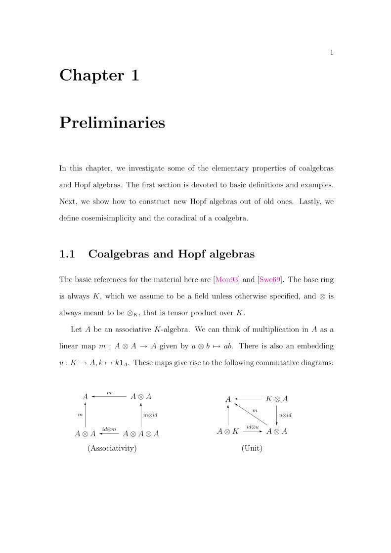
Let A be an associative K-algebra. We can think of multiplication in A as a

linear map m : A ⊗ A → A given by a ⊗ b 7→ ab. There is also an embedding

u : K → A, k 7→ k1A. These maps give rise to the following commutative diagrams:

A A⊗ A

A⊗ A A⊗ A⊗ A

¾ m

6m

6m⊗id

¾id⊗m

A K ⊗ A

A⊗K A⊗ A

¾

?u⊗id

6

-id⊗uQ

QQ

QQk

m

(Associativity) (Unit)

2

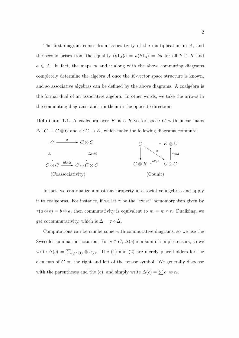
The first diagram comes from associativity of the multiplication in A, and

the second arises from the equality (k1A)a = a(k1A) = ka for all k ∈ K and

a ∈ A. In fact, the maps m and u along with the above commuting diagrams

completely determine the algebra A once the K-vector space structure is known,

and so associative algebras can be defined by the above diagrams. A coalgebra is

the formal dual of an associative algebra. In other words, we take the arrows in

the commuting diagrams, and run them in the opposite direction.

Definition 1.1. A coalgebra over K is a K-vector space C with linear maps

∆ : C → C ⊗ C and ε : C → K, which make the following diagrams commute:

C C ⊗ C

C ⊗ C C ⊗ C ⊗ C

-∆

?

∆

?

∆⊗id

-id⊗∆

C K ⊗ C

C ⊗K C ⊗ C

-

?

QQ

QQ

Qs

∆

¾id⊗ε

6ε⊗id

(Coassociativity) (Counit)

In fact, we can dualize almost any property in associative algebras and apply

it to coalgebras. For instance, if we let τ be the “twist” homomorphism given by

τ(a ⊗ b) = b ⊗ a, then commutativity is equivalent to m = m ◦ τ . Dualizing, we

get cocommutativity, which is ∆ = τ ◦∆.

Computations can be cumbersome with commutative diagrams, so we use the

Sweedler summation notation. For c ∈ C, ∆(c) is a sum of simple tensors, so we

write ∆(c) =∑

(c) c(1) ⊗ c(2). The (1) and (2) are merely place holders for the

elements of C on the right and left of the tensor symbol. We generally dispense

with the parentheses and the (c), and simply write ∆(c) =∑

c1 ⊗ c2.

3

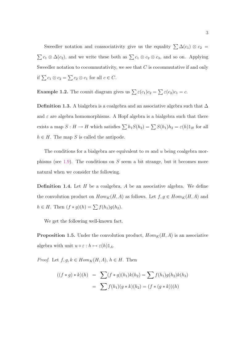
Sweedler notation and coassociativity give us the equality∑

∆(c1) ⊗ c2 =

∑c1 ⊗ ∆(c2), and we write these both as

∑c1 ⊗ c2 ⊗ c3, and so on. Applying

Sweedler notation to cocommutativity, we see that C is cocommutative if and only

if∑

c1 ⊗ c2 =∑

c2 ⊗ c1 for all c ∈ C.

Example 1.2. The counit diagram gives us∑

ε(c1)c2 =∑

ε(c2)c1 = c.

Definition 1.3. A bialgebra is a coalgebra and an associative algebra such that ∆

and ε are algebra homomorphisms. A Hopf algebra is a bialgebra such that there

exists a map S : H → H which satisfies∑

h1S(h2) =∑

S(h1)h2 = ε(h)1H for all

h ∈ H. The map S is called the antipode.

The conditions for a bialgebra are equivalent to m and u being coalgebra mor-

phisms (see 1.9). The conditions on S seem a bit strange, but it becomes more

natural when we consider the following.

Definition 1.4. Let H be a coalgebra, A be an associative algebra. We define

the convolution product on HomK(H, A) as follows. Let f, g ∈ HomK(H,A) and

h ∈ H. Then (f ∗ g)(h) =∑

f(h1)g(h2).

We get the following well-known fact.

Proposition 1.5. Under the convolution product, HomK(H, A) is an associative

algebra with unit u ◦ ε : h 7→ ε(h)1A.

Proof. Let f, g, k ∈ HomK(H, A), h ∈ H. Then

((f ∗ g) ∗ k)(h) =∑

(f ∗ g)(h1)k(h2) =∑

f(h1)g(h2)k(h3)

=∑

f(h1)(g ∗ k)(h2) = (f ∗ (g ∗ k))(h)

4

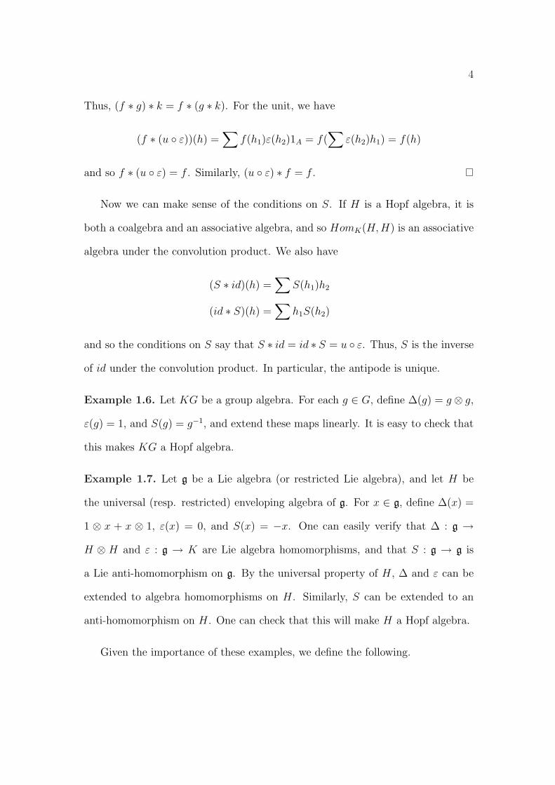
Thus, (f ∗ g) ∗ k = f ∗ (g ∗ k). For the unit, we have

(f ∗ (u ◦ ε))(h) =∑

f(h1)ε(h2)1A = f(∑

ε(h2)h1) = f(h)

and so f ∗ (u ◦ ε) = f . Similarly, (u ◦ ε) ∗ f = f .

Now we can make sense of the conditions on S. If H is a Hopf algebra, it is

both a coalgebra and an associative algebra, and so HomK(H, H) is an associative

algebra under the convolution product. We also have

(S ∗ id)(h) =∑

S(h1)h2

(id ∗ S)(h) =∑

h1S(h2)

and so the conditions on S say that S ∗ id = id ∗ S = u ◦ ε. Thus, S is the inverse

of id under the convolution product. In particular, the antipode is unique.

Example 1.6. Let KG be a group algebra. For each g ∈ G, define ∆(g) = g ⊗ g,

ε(g) = 1, and S(g) = g−1, and extend these maps linearly. It is easy to check that

this makes KG a Hopf algebra.

Example 1.7. Let g be a Lie algebra (or restricted Lie algebra), and let H be

the universal (resp. restricted) enveloping algebra of g. For x ∈ g, define ∆(x) =

1 ⊗ x + x ⊗ 1, ε(x) = 0, and S(x) = −x. One can easily verify that ∆ : g →H ⊗ H and ε : g → K are Lie algebra homomorphisms, and that S : g → g is

a Lie anti-homomorphism on g. By the universal property of H, ∆ and ε can be

extended to algebra homomorphisms on H. Similarly, S can be extended to an

anti-homomorphism on H. One can check that this will make H a Hopf algebra.

Given the importance of these examples, we define the following.

5

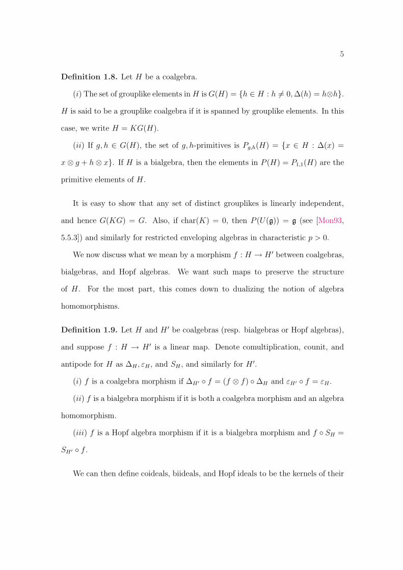
Definition 1.8. Let H be a coalgebra.

(i) The set of grouplike elements in H is G(H) = {h ∈ H : h 6= 0, ∆(h) = h⊗h}.H is said to be a grouplike coalgebra if it is spanned by grouplike elements. In this

case, we write H = KG(H).

(ii) If g, h ∈ G(H), the set of g, h-primitives is Pg,h(H) = {x ∈ H : ∆(x) =

x⊗ g + h⊗ x}. If H is a bialgebra, then the elements in P (H) = P1,1(H) are the

primitive elements of H.

It is easy to show that any set of distinct grouplikes is linearly independent,

and hence G(KG) = G. Also, if char(K) = 0, then P (U(g)) = g (see [Mon93,

5.5.3]) and similarly for restricted enveloping algebras in characteristic p > 0.

We now discuss what we mean by a morphism f : H → H ′ between coalgebras,

bialgebras, and Hopf algebras. We want such maps to preserve the structure

of H. For the most part, this comes down to dualizing the notion of algebra

homomorphisms.

Definition 1.9. Let H and H ′ be coalgebras (resp. bialgebras or Hopf algebras),

and suppose f : H → H ′ is a linear map. Denote comultiplication, counit, and

antipode for H as ∆H , εH , and SH , and similarly for H ′.

(i) f is a coalgebra morphism if ∆H′ ◦ f = (f ⊗ f) ◦∆H and εH′ ◦ f = εH .

(ii) f is a bialgebra morphism if it is both a coalgebra morphism and an algebra

homomorphism.

(iii) f is a Hopf algebra morphism if it is a bialgebra morphism and f ◦ SH =

SH′ ◦ f .

We can then define coideals, biideals, and Hopf ideals to be the kernels of their

6

respective morphisms. We get

Definition 1.10. (i) A coideal C of a coalgebra H is a subspace of H such that

∆(C) ⊆ C ⊗H + H ⊗ C and ε(C) = 0.

(ii) A biideal of a bialgebra H is a subspace of H that is both an ideal and a

coideal.

(iii) A Hopf ideal I of a Hopf algebra H is a biideal of H such that S(I) ⊆ I.

1.2 Basic constructions

We now proceed to show how one can construct Hopf algebras from other Hopf

algebras. We start with the tensor product.

Proposition 1.11. (i) Let (H, ∆H , εH) and (H ′, ∆H′ , εH′) be coalgebras. Then

H ⊗H ′ is a coalgebra with comultiplication and counit given by ∆H⊗H′(h⊗ h′) =

∑(h1 ⊗ h′1)⊗ (h2 ⊗ h′2), εH⊗H′(h⊗ h′) = εH(h)εH′(h′)

(ii) If H and H ′ are bialgebras, then so is H ⊗H ′. If, in addition, H and H ′

are Hopf algebras, then H ⊗H ′ is a Hopf algebra with antipode SH⊗H′(h ⊗ k) =

SH(h)⊗ SH′(k).

For our next construction, recall that, for any vector space H, we can construct

the dual space H∗ = HomK(H,K).

Proposition 1.12. [Mon93, 1.2.2, 1.2.4] (i) If H is a coalgebra, then H∗ is an

associative algebra with multiplication ∆∗ and unit ε. Also, if H is cocommutative,

then H∗ is commutative.

7

(ii) If H is a finite dimensional associative algebra, then H∗ is a coalgebra with

comultiplication ∆ = m∗ and counit ε = u∗. Also, if H is commutative, then H∗

is cocommutative.

(iii) If H is a finite dimensional bialgebra (resp. Hopf algebra), then H∗ is a

bialgebra (resp. Hopf algebra with antipode S∗).

Proof. For (i), assume H is a coalgebra. Now K is an associative K-algebra, so by

1.5, H∗ = HomK(H, K) is an associative algebra under the convolution product

with unit ε. It is a simple computation to show that f ∗g = (f⊗g)◦∆ = ∆∗(f⊗g).

Now suppose that H is cocommutative, so∑

h1⊗h2 =∑

h2⊗h1 for all h ∈ H.

Then

(f ∗ g)(h) =∑

f(h1)g(h2) =∑

f(h2)g(h1) = (g ∗ f)(h)

Thus, H∗ is commutative.

For (ii), suppose that H is a finite dimensional associative algebra. Then, for

all f ∈ H∗, we have ∆(f) = f ◦m ∈ (H ⊗H)∗ ∼= H∗⊗H∗ and ε(f) = f(1). Thus,

if ∆(f) =∑

fi ⊗ gi, then∑

fi(h)gi(k) = f(hk) for all h, k ∈ H. We need to show

that∑

fi ⊗∆(gi) =∑

∆(fi)⊗ gi to prove coassociativity. Let h, k, l ∈ H. Then

(∑

fi ⊗∆(gi))(h⊗ k ⊗ l) =∑

fi(h)∆(gi)(k ⊗ l)

=∑

fi(h)gi(kl)

= f(hkl)

=∑

fi(hk)gi(l)

=∑

∆(fi)(h⊗ k)gi(l)

= (∑

∆(fi)⊗ gi)(h⊗ k ⊗ l)

8

For the counit, we have (∑

ε(fi)gi)(h) =∑

fi(1)gi(h) = f(h), so∑

ε(fi)gi = f .

Similarly,∑

ε(gi)fi = f , so H∗ is a coalgebra.

Now suppose that H is commutative. Again write ∆(f) =∑

fi ⊗ gi. For all

h, k ∈ H,

(∑

fi ⊗ gi)(h⊗ k) =∑

fi(h)gi(k) = f(hk) = f(kh) = (∑

gi ⊗ fi)(h⊗ k)

and therefore H∗ is cocommutative.

For (iii), we need only show that ∆ and ε are algebra homomorphisms, and

that S∗ satisfies the required relations. Let f, g ∈ H∗, h, k ∈ H. Since ∆ is an

algebra homomorphism, then

∑[hk]1 ⊗ [hk]2 = ∆H(hk) = ∆H(h)∆H(k) =

∑h1k1 ⊗ h2k2

We get

∆(fg)(h⊗ k) = fg(hk)

=∑

f([hk]1)g([hk]2)

=∑

f(h1k1)g(h2k2)

=∑

∆(f)(h1 ⊗ k1)∆(g)(h2 ⊗ k2)

= (∆(f)∆(g))(h⊗ k)

Also, ∆(εH)(h⊗ k) = εH(hk) = εH(h)εH(k) = (εH ⊗ εH)(h⊗ k), so ∆(ε) = ε⊗ ε.

Thus, ∆ is an algebra homomorphism. To prove ε is an algebra homomorphism,

we have

ε(fg) = fg(1) = f(1)g(1) = ε(f)ε(g)

9

Now suppose H is a Hopf algebra. We need to show that, for all f ∈ H∗,∑

S∗(f1)f2 =∑

f1S∗(f2) = ε(f)εH . We have, for each h ∈ H,

(∑

S∗(f1)f2)(h) =∑

S∗(f1)(h1)f2(h2) =∑

f1(S(h1))f2(h2)

= f(∑

S(h1)h2) = εH(h)f(1) = ε(f)εH(h)

The other equality is similar.

For infinite dimensional Hopf algebras, H∗ will not, in general, be a Hopf

algebra. However, something can still be said. Let H◦ = {f ∈ H∗ : f(I) = 0 for

some I / H of finite codimension}.

Theorem 1.13. [Mon93, 9.1.1, 9.1.3] Let H be a bialgebra.

(i) If f ∈ H∗, then f ∈ H◦ if and only if m∗(f) ∈ H∗ ⊗H∗.

(ii) H◦ is a bialgebra with comultiplication m∗ and counit u∗. If H is a Hopf

algebra, then so is H◦ with antipode S∗.

Next, we characterize the grouplike elements in H◦

Proposition 1.14. [Mon93, 1.3] G(H◦) = Alg(H,K), where Alg(H,K) is the set

of K-algebra homomorphisms between H and K.

Proof. Let f ∈ G(H◦). Then, for all h, k ∈ H, we have

f(hk) = ∆(f)(h⊗ k) = (f ⊗ f)(h⊗ k) = f(h)f(k)

In particular, f(h) = f(h)f(1), and so, in addition, f(1) = 1. Thus, f is an algebra

homomorphism. The converse is similar.

Our last construction, in some sense, reverses the comultiplication of H. It is

dual to the notion of the opposite algebra Aop.

10

Definition 1.15. Let H be a coalgebra. Then the coopposite coalgebra Hcop is

H as a set, its counit ε is the same as for H, but its comultiplication is given by

∆′(h) =∑

h2 ⊗ h1.

It is easy to show that if H is a bialgebra, then so is Hcop. However, if H is a

Hopf algebra, Hcop is not necessarily a Hopf algebra. To find out when Hcop will

be a Hopf algebra, we will need a result about how multiplication and comultipli-

cation interact with the antipode of a Hopf algebra. Recall the examples of the

group algebra and the universal enveloping algebra. In each of these cases, the

antipode is an anti-homomorphism. This is true in general, along with a “dual”

anti-homomorphism property.

Proposition 1.16. [Swe69] Let H be a Hopf algebra.

(i) S is an algebra anti-homomorphism (i.e. S(hk) = S(k)S(h), and S(1) = 1).

(ii) ∆ ◦ S(h) =∑

S(h2)⊗ S(h1), ε ◦ S = ε.

A map that satisfies (ii) is called a coalgebra anti-morphism.

Proof. (i) First of all, we know∑

h1S(h2) = ε(h)1H . For h = 1, we have ∆(1) =

1⊗ 1, since ∆ is an algebra homomorphism. Thus, S(1) = 1.

Now consider the linear maps f : H ⊗H → H and g : H ⊗H → H given by

f(h ⊗ k) = S(hk), g(h ⊗ k) = S(k)S(h). We want to show that f = g. Let m

be the multiplication map on H. Since H ⊗H and H are Hopf algebras, we can

multiply these functions together via the convolution product. We have, for all

11

h, k ∈ H,

(f ∗m)(h⊗ k) =∑

f(h1 ⊗ k1)m(h2 ⊗ k2) =∑

S(h1k1)h2k2

=∑

S([hk]1)[hk]2 = ε(hk)1H

= ε(h)ε(k)1H = εH⊗H(h⊗ k)

(m ∗ g)(h⊗ k) =∑

m(h1 ⊗ k1)g(h2 ⊗ k2) =∑

h1k1S(k2)S(k1)

=∑

ε(k)h1S(h2) = ε(k)ε(h)

= εH⊗H(h⊗ k)

Thus, m is invertible, and in fact f = m−1 = g. This proves (i).

(ii) Our arguments here are dual to those above. First of all,

ε(S(h)) = ε(S(∑

ε(h1)h2)) =∑

ε(h1)ε(S(h2))

=∑

ε(h1S(h2)) = ε(ε(h))

= ε(h)ε(1) = ε(h)

Thus, ε ◦ S = ε.

Now define φ : H → H ⊗ H, γ : H → H ⊗ H by φ(h) = (∆ ◦ S)(h), γ(h) =

∑S(h2)⊗ S(h1). Our aim is to show that φ = γ. We have

(φ ∗∆)(h) =∑

φ(h1)∆(h2) =∑

∆(S(h1))∆(h2)

=∑

∆(S(h1)h2) = ∆(ε(h)) = ε(h)(1⊗ 1)

(∆ ∗ γ)(h) =∑

∆(h1)γ(h2) =∑

∆(h1)(S(h3)⊗ S(h2))

=∑

(h1 ⊗ h2)(S(h4)⊗ S(h3)) =∑

h1S(h4)⊗ h2S(h3)

=∑

ε(h2)h1S(h3)⊗ 1 =∑

h1S(h2)⊗ 1 = ε(h)(1⊗ 1)

This gives us φ = ∆−1 = γ, which completes the proof.

12

Proposition 1.17. [Mon93, 1.5.11] Let H be a bialgebra. Then Hcop is a Hopf

algebra if and only if H is a Hopf algebra and SH is invertible. Furthermore,

SHcop = S−1H (composition inverse).

Proof. Suppose that Hcop is a Hopf algebra. Let SH = S, SHcop = S. From 1.16,

both S and S are anti-homomorphisms and coalgebra anti-morphisms. Then

S(S(h)) =∑

ε(h1)S(S(h2)) =∑

h1S(h2)S(S(h3)) =∑

h1S(S(h3)h2)

=∑

ε(h2)h1S(1) = h

Similarly, S ◦ S = id, so S is invertible and S = S−1. For the converse,

we first show that S−1 is an algebra anti-homomorphism. Let h, h′ ∈ H. Write

l = S−1(h), l′ = S−1(h′), where l, l′ ∈ H. Then

S−1(hh′) = S−1(S(l)S(l′)) = S−1(S(l′l)) = l′l = S−1(h′)S−1(h)

Also, clearly S−1(1) = 1.

Now we need to show, for all h ∈ H that

∑S−1(h2)h1 =

∑h2S

−1(h1) = ε(h)1H

We know that∑

h1S(h2) =∑

S(h1)h2 = ε(h)1H . Simply apply S−1 to these

equations, and we get the desired result.

Corollary 1.18. [Mon93, 1.5.12] Let H be a commutative or cocommutative Hopf

algebra. Then S2 = id.

Proof. If H is cocommutative, then∑

h2S(h1) =∑

h1S(h2) = ε(h)1H . Similarly,

∑S(h2)h1 = ε(h)1H . Thus, S is an antipode for Hcop, and so S = S−1 by 1.17.

This implies S2 = id.

13

For the commutative case,∑

h2S(h1) =∑

S(h1)h2 = ε(h)1H . Similarly,

∑S(h2)h1 = ε(h)1H . As before, S2 = id.

1.3 Cosemisimplicity and the coradical

Now we dualize the notions of simplicity and semisimplicity of associative algebras.

Definition 1.19. Let H be a coalgebra.

(i) H is said to be simple if it has no proper nontrivial subcoalgebras.

(ii) The coradical H0 is the sum of all the simple subcoalgebras of H.

(iii) H is cosemisimple if H = H0.

These are indeed dual to their corresponding concepts in associative algebras,

since H is a simple coalgebra if and only if H∗ is a (finite dimensional) simple

algebra [Mon93, 5.1.4]. Also, J(H∗) = H⊥0 [Mon93, 5.2.9], so it is easy to see that

H is cosemisimple ⇔ H⊥0 = 0 ⇔ H∗ is semisimple. Note that by [Mon93, 5.1.2],

all simple coalgebras are finite dimensional.

In fact, more can be said about the coradical.

Proposition 1.20. [Swe69, 8.0.3, 8.0.6]

(i) Let H =∑

i Ci, where Ci are subcoalgebras. Then any simple subcoalgebra

lies in one of the Ci.

(ii) Let {Hi} be a set of distinct simple subcoalgebras. Then the sum of these

coalgebras is direct.

(iii) H0 = ⊕iHi, where the Hi are all the (distinct) simple subcoalgebras of H.

Definition 1.21. Let H be a coalgebra.

14

(i) H is said to be pointed if every simple subcoalgebra is one-dimensional.

(ii) H is said to be connected if H0 is one-dimensional.

Since H0 contains all the simple subcoalgebras of H, then any connected coal-

gebra is a pointed coalgebra. Also, it is easy to check that any one-dimensional

subcoalgebra of H must be of the form Kg, where g ∈ G(H). Thus, H is pointed

if and only if H0 = KG(H). Consequently, all group algebras are pointed. In

addition, by [Mon93, 5.5.3], we have that U(g) is connected.

The coradical has additional importance. Define inductively, for each n ≥ 1,

Hn = ∆−1(H ⊗Hn−1 + H0 ⊗H). The Hn form a coalgebra filtration, by which is

meant the following.

Theorem 1.22. [Mon93, 5.2.2] For all n ≥ 0, the family {Hn} satisfies

(i) Hn ⊆ Hn+1 and H =⋃

n≥0 Hn.

(ii) ∆(Hn) ⊆ ∑ni=0 Hi ⊗Hn−i.

15

Chapter 2

Theory of Descent

Given a K-coalgebra or Hopf algebra, one may ask what happens if the base field

is extended (e.g. to the algebraic closure of K). One may also ask whether or not

two coalgebras or Hopf algebras are isomorphic after extension of the base field.

Questions of these types are dealt with in descent theory.

In this chapter, we introduce the basic definitions of descent theory. Then we

describe how these definitions can be applied to coalgebras and Hopf algebras.

2.1 General descent theory

Much of the material and notation here comes from [Knu74]. Let K be a commuta-

tive ring, L a commutative K-algebra. Given a left K-module M , we can construct

the L-module ML = L ⊗M . Thus, we can take K-modules and “ascend” to L-

modules. The goal of descent theory is to say something about what happens when

we go in the other direction. In other words, if we start with L-modules, what

happens when we “descend” to K-modules?

An example of the type of problem encountered is the following. Given an

element y ∈ ML, what conditions will guarantee that y = 1L⊗ x for some x ∈ M?

This is a problem in descent of elements.

16

Example 2.1. Let K ⊆ L be a finite Galois field extension. Then K is a K-

module and KL = L ⊗ K ∼= L. So the descent of elements problem mentioned

above is equivalent to asking when an element a ∈ L is in K. Of course this

happens if and only if σ(a) = a for all σ ∈ Gal(L/K), the Galois group of L over

K.

Another problem we may consider is descent of modules. In other words, given

an L-module N , what are the K-modules M such that N ∼= ML? This same

question can be asked in other contexts and leads naturally to the notion of L-

forms.

Definition 2.2. Let L be a commutative K-algebra, H a K-object. A K-object

H ′ is an L-form of H if L⊗H ∼= L⊗H ′ as L-objects.

The word “object” above can be replaced with “associative algebra”, “Lie al-

gebra”, “module”, or any other category such that tensoring with L over K leaves

us in the same category, except that the base ring changes to L.

2.2 Descent of coalgebras and Hopf algebras

The central part of this thesis is concerned with computing L-forms of coalgebras

and Hopf algebras. But in order for these definitions to make sense in this context,

we must show that given H a K-coalgebra (or K-Hopf algebra), then L⊗H is an

L-coalgebra (resp. L-Hopf algebra).

Definition 2.3. Let K, L be as above, H a K-coalgebra. Then L ⊗ H is an

17

L-coalgebra with the following structure.

∆L⊗H(a⊗ h) =∑

(a⊗ h1)⊗L (1⊗ h2)

εL⊗H(a⊗ h) = εH(h)a

If H is a K-Hopf algebra, then L⊗H is an L-Hopf algebra with the antipode

given by SL⊗H(a⊗ h) = a⊗ SH(h).

Note: (L ⊗ H) ⊗L (L ⊗ H) ∼= L ⊗ H ⊗ H as L-vector spaces via the map given

by (a ⊗ h) ⊗L (b ⊗ k) 7→ ab ⊗ h ⊗ k. We use this identification for ∆L⊗H , so

∆L⊗H(a⊗ h) =∑

a⊗ h1 ⊗ h2.

Example 2.4. [HP86] Let K = R, and L = C. Let H = KA, where A is an

infinite cyclic group. Then H ′ = R[c, s : c2 + s2 = 1, cs = sc] has a Hopf algebra

structure

∆(c) = c⊗ c− s⊗ s, ∆(s) = s⊗ c + c⊗ s

ε(c) = 1, ε(s) = 0

S(c) = c, S(s) = −s

and it is called the trigonometric algebra. Let a = 1⊗ c + i⊗ s = c + is ∈ L⊗H ′.

Direct computation gives us a ∈ G(L ⊗ H ′) with a−1 = c − is. Furthermore, we

have a+ a−1 = 2c, so c ∈ L < a >. Similarly, a− a−1 = 2is, so s ∈ L < a >. Thus

L ⊗H ′ = L < a >∼= LA, so H and H ′ are L-forms. Note that H and H ′ are not

isomorphic over Q, since G(H) = A and G(H ′) = {1}.

We can extend the notion of forms to a slightly more general context.

18

Definition 2.5. Let X be a subcategory of the category of commutative K-

algebras. Given a K-object H, we say that a K-object H ′ is a form of H with

respect to X if H ′ is an L-form of H for some L ∈ X

This generalizes the term “form” used in [HP86], where a form was defined to

be an L-form for some L which is faithfully flat over K. In our terminology, this

would be called a form with respect to faithfully flat commutative K-algebras.

Two questions naturally arise.

Question 2.6. Given K, L as above, and a K-Hopf algebra H, what are all the

L-forms of H?

Question 2.7. Given a K-Hopf algebra H what are all the forms of H with respect

to X for a given category X of commutative K-algebras?

The first question is explored by Pareigis in [Par89] where he found L-forms of

group rings, which he called twisted group rings. He assumed the extension K ⊆ L

to be “F -Galois” for some group F and assumed L to be free as a K-module.

The second question is addressed by Haggenmuller and Pareigis in [HP86].

They restrict their attention to extensions K ⊆ L of commutative rings which are

faithfully flat. If G is a finitely generated group with finite automorphism group

F , they found a correspondence between forms of KG with respect to faithfully

flat commutative K-algebras and the set of “F -Galois extensions” of K. We will

address this more general notion of Galois extension in the next chapter.

19

Chapter 3

Actions, Coactions, and Galois

Extensions

In studying the descent theory of Hopf algebras and coalgebras, the nature of the

field extension K ⊆ L will be an important factor in computing L-forms. The

extensions we deal with are generalizations of classical Galois extensions. Instead

of having a field extension with a corresponding group, we will have an extension

of associative algebras with a corresponding Hopf algebra. Hopf Galois extensions

are helpful in descent theory, and are also of interest in their own right.

In this chapter, we begin by defining actions of Hopf algebras on associative

algebras, which will be the analogue of automorphism actions of groups and deriva-

tion actions of Lie algebras. We then give a link between invariants of Hopf algebra

actions and semisimplicity. After defining smash products and crossed products,

we move to coactions. This will lead us to Hopf Galois extensions.

3.1 Hopf module algebras

In classical Galois extensions, the Galois group acts as automorphisms on the field

extension. We must generalize this notion for Hopf algebras.

20

Definition 3.1. Let H be a Hopf algebra and let A be an associative algebra. We

say that A is an H-module algebra if A is an H-module, and for each a, b ∈ A and

h ∈ H we have

(i) h · (ab) =∑

(h1 · a)(h2 · b)(ii) h · 1A = ε(h)1A

If A and H merely satisfy (i) and (ii) (i.e. the map h⊗ a 7→ h · a is not necessarily

an H-module action), we say that H measures A.

Example 3.2. Let H = KG be a group algebra, and suppose that A is an H-

module algebra. For all a, b ∈ A, and g ∈ G, we have g · (ab) = (g · a)(g · b) and

g · 1A = 1A, so G acts as automorphisms on A.

Example 3.3. Let H = U(g) be a universal enveloping algebra, and suppose that

A is an H-module algebra. For x ∈ g and a, b ∈ A, we have x·(ab) = (x·a)b+a(x·b)and x · 1A = 0, so g acts as derivations on A.

Example 3.4. Let H be a Hopf algebra. The left adjoint action of H on itself is

given by h · h′ = (adlh)(h′) =∑

h1h′S(h2). We have, for all h, l, m ∈ H,

h · (lm) =∑

h1lmS(h2)

=∑

ε(h2)h1lmS(h3), by counit diagram

=∑

h1lε(h2)mS(h3)

=∑

h1lS(h2)h3mS(h4), by definition of S

=∑

(h1 · l)h2mS(h3) =∑

(h1 · l)(h2 ·m)

and so H is an H-module algebra.

21

Note that in the case H = KG, we get (adlg)(a) = gag−1 for g ∈ G and a ∈ H,

and for H an enveloping algebra, we get (adlx)(a) = xa − ax for x ∈ g, a ∈ H.

Thus, the left adjoint action corrresponds to the classical adjoint actions for groups

and Lie algebras.

Condition (ii) in Definition 3.1 says that, in some sense, H acts trivially on 1A.

This leads us to the notion of invariants.

Definition 3.5. (i) If M is an H-module, then the set of invariants of H in M is

MH = {m ∈ M : h ·m = ε(h)m, for all h ∈ H}.(ii) If we let H act on itself by left multiplication, then the invariants are called

left integrals, and are denoted by∫ l

H= {t ∈ H : ht = ε(h)t for all h ∈ H}.

The term invariant comes from group actions.

3.2 Integrals and semisimplicity

Integrals are an important tool in the study of Hopf algebras. Their importance

is highlighted in the following generalization of Maschke’s Theorem.

Theorem 3.6. [LS69] Let H be any finite dimensional Hopf algebra. Then H is

semisimple if and only if ε(∫ l

H) 6= 0.

Proof. Assume H is semisimple. Then every left H-module is completely reducible.

In particular, H is a completely reducible H-module under left multiplication.

We have that ker(ε) is an ideal of H, so there is some left ideal I such that

H = I⊕ker(ε). Let 0 6= t ∈ I. Since h− ε(h)1H ∈ ker(ε) for each h ∈ H, we have

ht = (h− ε(h)1H)t + ε(h)t ∈ I ⊕ ker(ε). Since I ⊕ ker(ε) is direct, and ht ∈ I, we

22

must have (h− ε(h)1H)t = 0. Then ht = ε(h)t, so t ∈ ∫ l

H. But t /∈ ker(ε), and so

ε(∫ l

H) 6= 0.

Now suppose ε(∫ l

H) 6= 0, and let M be any left H-module. It suffices to show

that M is completely reducible, so we need only prove that for each submodule

U ≤ M there is an H-projection M → U . Let t ∈ ∫ l

Hwith ε(t) = 1. Let π : M → U

be any K-linear projection, and define π : M → U by π(m) =∑

t1 · π(S(t2) ·m).

If u ∈ U , then π(u) =∑

t1 · (S(t2) · u) = ε(t)u = u. It then suffices to show that

π is an H-module map. First, note that

∑t1 ⊗ t2 ⊗ h = ∆(t)⊗ h =

∑∆((ε(h1)t)⊗ h2

=∑

∆(h1t)⊗ h2

=∑

∆(h1)∆(t)⊗ h2

=∑

h1t1 ⊗ h2t2 ⊗ h3 (3.1)

We have

π(h ·m) =∑

t1 · π(S(t2) · h ·m)

=∑

h1t1 · π(S(h2t2)h3 ·m), by Eqn. 3.1

=∑

h1t1 · π(S(t2)S(h2)h3 ·m)

=∑

h1t1 · π(S(t2)ε(h2) ·m)

= h ·∑

t1 · π(S(t2) ·m) = h · π(m)

Thus, π is a projection, and so M is completely reducible. The theorem is proved.

Note that if G is a finite group, then∫ l

KG= Kt, where t =

∑g∈G g, in which case

ε(t) = |G|. Thus, when H = KG, then we get the classical version of Maschke’s

23

Theorem. Also notice that∫ l

KGis one-dimensional. This is true in general for

finite dimensional Hopf algebras (see [Mon93, 2.1.3]).

An application of 3.6 to descent of Hopf algebras is the following.

Proposition 3.7. Let H be a finite dimensional K-Hopf algebra with K ⊆ L an

extension of fields. Then∫ l

L⊗H= L ⊗ ∫ l

H. In particular, if H ′ is an L-form of H,

then H ′ is semisimple if and only if H is semisimple.

Proof. By the above remarks, dimL(∫ l

L⊗H) = 1 and dimK(

∫ l

H) = 1. Thus, it suffices

to show that L ⊗ ∫ l

H⊆ ∫ l

L⊗H. Let 0 6= t ∈ ∫ l

H. Then for all a, b ∈ L and h ∈ H,

we have (a ⊗ t)(b ⊗ h) = ab ⊗ th = ε(t)ab ⊗ h = ε(a ⊗ t)(b ⊗ h). This gives us

the first statement. For the second statement, notice that εH(∫ l

H) 6= 0 if and only

if εL⊗H(L ⊗ ∫ l

H) 6= 0. Thus, H is semisimple if and only if L ⊗ H is semisimple.

By the same argument, H ′ is semisimple if and only if L⊗H ′ is semisimple. Since

L⊗H ∼= L⊗H ′, the theorem follows.

In [Chi92], Chin uses 3.6 to give an alternate proof of an old result of Hochschild [Hoc54].

This proof assumes the fact that if H is a finite dimensional semisimple Hopf al-

gebra, then any subHopfalgebra over which H is a free module is also semisim-

ple [Mon93, 2.2.2].

Theorem 3.8. [Hoc54] Let g be a finite dimensional restricted Lie algebra of

characteristic p 6= 0. Then u(g) is semisimple if and only if g is abelian and

g = Kgp.

Proof. Let E be the algebraic closure of K. It is easy to see that u(E⊗g) = E⊗u(g)

and that [E⊗ g]p = E⊗ g if and only if g = Kgp. Also,∫ l

E⊗u(g)= E⊗ ∫ l

u(g)by 3.7,

24

so E ⊗ u(g) is semisimple if and only if u(g) is semisimple. Thus, we may assume

that K is algebraically closed. In particular, g = Kgp if and only if g = gp.

First, assume that g is abelian with g = gp. Then u(g) = u(g)p, and so the

pth power map p : u(g) → u(g) is surjective. Since p is semilinear, and u(g) is

finite dimensional, then p is injective as well. Thus, u(g) has no nonzero nilpotent

elements, and so u(g) is semisimple.

Now suppose that H = u(g) is semisimple, and for the moment assume that

g =< x >= span{xpe: e ≥ 0}. By 3.6 there is some t ∈ ∫ l

Hsuch that ε(t) 6= 0.

Claim: x ∈< x >p.

Proof. Suppose dimK(< x >) = n. We have xpi ∈ g, so there is some nontrivial

polynomial f such that f(x) =∑n

i=0 aixpi

= 0. But dimK(u(g)) = pn by the

restricted PBW theorem, so f is actually the minimal polynomial for x. We can

uniquely write t = g(x) =∑pn−1

j=0 bjxj. Since xg(x) = xt = 0, then f(x) divides

xg(x). By comparison of degrees, xg(x) = αf(x), where α ∈ K. Note that

ε(t) =∑

bjε(xj) = b0, so b0 6= 0. But then also a0 6= 0 since xg(x) = αf(x). Thus,

x = −n∑

i=1

(ai

a0

)xpi ∈< x >p

In general, let x ∈ g. By the restricted PBW theorem, u(g) is a free module

over < x >. Then the remarks before the statement of the theorem imply that

< x > is semisimple. By the claim, x ∈< x >p⊆ gp, and so g = gp.

Since a0 6= 0 from the above, each x ∈ g satisfies a separable polynomial.

Hence, so does ad(x). Thus, the action of ad(x) on g is completely reducible. Let

25

y ∈ g be an eigenvector for ad(x). Then ad(x) acts on u(< y >), a commutative

ring. But ad(x) annihilates < y >p3 y, so [x, y] = 0. Since g is spanned by the

eigenvectors of ad(x), we conclude that [x, g] = 0. Thus, g is abelian.

Theorem 3.6 also makes determining the invariants under actions of semisimple

Hopf algebras extremely nice. We get the following well-known result.

Lemma 3.9. If M is an H-module, and 0 6= t ∈ ∫ l

H, then t ·M ⊆ MH . If H is

semisimple, then t ·M = MH .

Proof. Let m ∈ M . For all h ∈ H, we have h · (t ·m) = ht ·m = ε(h)(t ·m), and

so t ·M ⊆ MH .

If H is semisimple, let m ∈ MH . Since ε(t) 6= 0, we can assume, without loss

of generality, that ε(t) = 1. We then have t ·m = ε(t)m = m, so m ∈ t ·M , and

we are done.

3.3 Smash products and crossed products

Hopf module actions on associative algebras give rise to two important construc-

tions. The first is a generalization of skew group rings.

Definition 3.10. Let A be an H-module algebra. We can then construct the

associative algebra A#H, which is A ⊗H as a set. The element a ⊗ h is written

a#h, and multiplication is given by

(a#h)(b#k) =∑

a(h1 · b)#h2k

We often write a#h = ah.

26

It is easy to show that A#H is indeed an associative algebra with unit 1#1.

Notice that in the case of H = KG, we have, for all g, h ∈ G, (ag)(bh) = a(g ·b)gh,

which is the same as multiplication in in the skew group ring A ∗ G. The next

construction is a generalization of group crossed products.

Definition 3.11. Suppose H measures A (so A is not necessarily an H-module),

and let σ ∈ HomK(H ⊗ H, A) be invertible under the convolution product (i.e.

there exists τ ∈ HomK(H ⊗ H, A) such that σ ∗ τ = τ ∗ σ = u ◦ ε). Then we

construct A#σH. Again, A#σH = A⊗H as a set. Multiplication is given by

(a#h)(b#k) =∑

a(h1 · b)σ(h2, k1)#h3k2

For H = KG, we have (ag)(bh) = a(g · b)σ(g, h)gh, which gives us a group

crossed product. As in the case of group crossed products, we must have certain

conditions on the map σ and the manner in which H measures A in order for

A#σH to be an associative algebra.

Proposition 3.12. [DT86, BCM86] A#σH is an associative algebra with identity

1#1 if and only if for all h, k, m ∈ H and a ∈ A,

(i) h · (k · a) =∑

σ(h1, k1)(h2k2 · a)σ−1(h3, k3)

(ii) σ(h, 1) = σ(1, h) = ε(h)1A, and

∑[h1 · σ(k1, m1)]σ(h2, k2m2) =

∑σ(h1, k1)σ(h2, k2,m)

The proof of this is analogous to that of the proof of associativity for group

crossed products. It is quite tedious, and so it will be omitted. Note that σ−1 is

the inverse of σ under the convolution product (i.e. σ−1 = τ in 3.11).

27

3.4 Comodules and Hopf comodule algebras

One of the limitations in classical Galois theory is that it is difficult to define

infinite dimensional Galois extensions. Although it is most natural to think of

Galois extensions arising from module actions, we get the most generality when

we think of them as arising from coactions. These coactions are duals of actions.

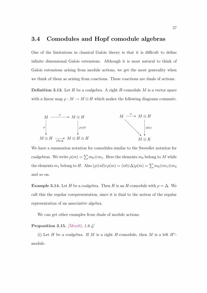
Definition 3.13. Let H be a coalgebra. A right H-comodule M is a vector space

with a linear map ρ : M → M ⊗H which makes the following diagrams commute.

M M ⊗H

M ⊗H M ⊗H ⊗H

-ρ

?

ρ

?

ρ⊗id

-id⊗∆

M M ⊗H

M ⊗K

-ρ

@@

@@

@R ?

id⊗ε

We have a summation notation for comodules similar to the Sweedler notation for

coalgebras. We write ρ(m) =∑

m0⊗m1. Here the elements m0 belong to M while

the elements m1 belong to H. Also (ρ⊗id)◦ρ(m) = (id⊗∆)ρ(m) =∑

m0⊗m1⊗m2

and so on.

Example 3.14. Let H be a coalgebra. Then H is an H-comodule with ρ = ∆. We

call this the regular corepresentation, since it is dual to the notion of the regular

representation of an associative algebra.

We can get other examples from duals of module actions.

Proposition 3.15. [Mon93, 1.6.4]

(i) Let H be a coalgebra. If M is a right H-comodule, then M is a left H∗-

module.

28

(ii) Let H be an associative algebra, M a left H-module. Then M is naturally a

right H◦-comodule algebra if and only if H ·m is finite dimensional for all m ∈ M .

(iii) If H is a finite dimensional bialgebra, then any H-module M is an H∗-

comodule and conversely. In particular, if {h1, · · · , hn} is a basis for H with

dual basis {h∗1, · · · , h∗n} in H∗, then the comodule structure is given by ρ(m) =

∑i(hi ·m)⊗ h∗i . The module structure is given by h ·m =

∑m1(h)m0.

Proof. For (i), let M be a right H-comodule, for H a coalgebra. For each f ∈ H∗

and m ∈ M , define f · m =∑

f(m1)m0. To show that this makes M a left

H∗-module, we have, for all f, g ∈ H∗ and m ∈ M ,

f · (g ·m) = f ·∑

g(m1)m0 =∑

g(m1)(f ·m0)

=∑

g(m2)f(m1)m0 =∑

fg(m1)m0

= (fg) ·m

For (ii), suppose that M is a left H-module, and let h ∈ H, m ∈ M . If H ·mis finite dimensional with basis {m1, · · · ,mn}, then h · m =

∑fi(h)mi for some

fi(h) ∈ K. Clearly, fi ∈ H∗. Moreover, fi ∈ H◦. For consider the homomorphism

φ : H → EndK(H ·m) given by φ(h)(k ·m) = hk ·m. Then I = kerφ is an ideal

of finite codimension since H ·m is finite dimensional. Furthermore, if h ∈ I, then

h ·m = 0, and so fi(h) = 0 for all i. Thus, fi(I) = 0, and so fi ∈ H◦. Now define

ρ(m) =∑

i mi ⊗ fi. We show that this makes M a right H◦-comodule. We have

ρ(m) =∑

i mi ⊗ fi. Since H · mi ⊆ H · m, then ρ(mi) =∑

j mj ⊗ gij for some

gij ∈ H◦.

Claim: ∆(fi) =∑

j gji ⊗ fj for all i.

29

Proof. For all h, k ∈ H and m ∈ M , we have

∑i

fi(hk)mi = hk ·m = h · (k ·m)

= h ·∑

j

fj(k)mj =∑i,j

fj(k)gji(h)mi

Since the mj are linearly independent, ∆(fi)(h⊗k) = fi(hk) = (∑

j gji⊗fj)(h⊗k).

This proves the claim.

We then have

((ρ⊗ id) ◦ ρ)(m) = (ρ⊗ id)(∑

i

mi ⊗ fi) =∑i,j

mj ⊗ gij ⊗ fi

=∑

j

mj ⊗∆(fj) = ((id⊗∆) ◦ ρ)(m)

For the converse, let M be an H◦-comodule algebra. If h ∈ H and m ∈ M ,

then h ·m =∑

m1(h)m0, so H ·m is contained in the span of {m0}, a finite set.

Thus, H ·m is finite dimensional.

Finally, (iii) follows directly from the constructions in (i) and (ii).

We can also dualize invariants.

Definition 3.16. If M is a right H-comodule, then the coinvariants of H in M

are the elements of M coH = {m ∈ M : ρ(m) = m⊗ 1}.

Proposition 3.17. [Mon93, 1.7.1]

(i) Let M be a right H-comodule with corresponding H∗-module structure.

Then MH∗= M coH .

(ii) If M is a left H-module such that it is also a right H◦-comodule, then

MH = M coH◦.

30

Proof. For (i), we have that m ∈ M coH if and only if ρ(m) = m ⊗ 1. But recall

that for all f ∈ H∗, f ·m =∑

f(m1)m0, and so m ∈ M coH if and only if f ·m =

f(1)m = ε(f)m. But this is equivalent to m ∈ MH∗

For (ii), we have that m ∈ MH if and only if h · m = ε(h)m for all h ∈ H.

But h ·m =∑

m1(h)m0, so this will be true if and only if ρ(m) = m⊗ ε. This is

equivalent to m ∈ M coH◦.

Our last dualization is of H-module algebras.

Definition 3.18. An associative algebra A is a right H-comodule algebra if it is a

right H-comodule, and we have, for all a, b ∈ A, ρ(ab) = ρ(a)ρ(b), and ρ(1) = 1⊗1.

Example 3.19. Let H be a Hopf algebra. Since ∆ is an algebra homomorphism,

the regular corepresentation makes H an H-comodule algebra.

Example 3.20. Let A be a KG-comodule algebra. For a ∈ A, suppose that

ρ(a) =∑

g∈G ag ⊗ g. Then we have

∑g∈G

ρ(ag)⊗ g = (ρ⊗ id) ◦ ρ(a) = (id⊗∆) ◦ ρ(a) =∑g∈G

ag ⊗ g ⊗ g

Thus, ρ(ag) = ag ⊗ g. We also have a =∑

ε(a1)a0 =∑

g ag. If we set Ag =

{b ∈ A : ρ(b) = b ⊗ g}, then a ∈ ⊕g∈G Ag and so A =

⊕g∈G Ag. Since ρ is

an algebra homomorphism, AgAh ⊆ Agh for all g, h ∈ G, and so KG-comodule

algebras are G-graded K-algebras. Conversely, if A =⊕

g∈G Ag is a G-graded,

associative algebra, then defining ρ(ag) = ag ⊗ g for each ag ∈ Ag and extending

linearly makes A a KG-comodule algebra, so KG-comodule algebras are precisely

G-graded associative K-algebras. Note that AcoKG = A1.

31

As in 3.15, if H is finite dimensional, then A is a left H-module algebra if and

only if it is a right H∗-comodule algebra.

3.5 Hopf Galois extensions

Now we are ready to define Hopf Galois extensions.

Definition 3.21. [KT81] Let H be a Hopf algebra, and suppose B ⊆ A is an

extension of right H-comodule algebras. This extension is right H-Galois if

(i) B = AcoH

(ii) The map β : A⊗B A → A⊗K H given by β(a⊗b) = (a⊗1)ρ(b) =∑

ab0⊗b1

is bijective.

Proposition 3.22. Let H be a Hopf algebra. Then K ⊆ H is an H-Galois

extension.

Proof. We first show that HcoH = K. Suppose that ∆(h) = h ⊗ 1. Then h =

∑ε(h1)h2 = ε(h)1H ∈ K.

From the comodule structure, we have that β : H⊗K H → H⊗K H is given by

β(h⊗k) =∑

hk1⊗k2. If, for h,m ∈ H, we define γ(h⊗m) =∑

hS(m1)⊗S(m2),

32

then

(γ ◦ β)(h⊗m) = γ(∑

hm1 ⊗m2) =∑

hm1S(m2)⊗m3

=∑

hε(m1)⊗m2 = h⊗ (∑

ε(h1)h2)

= h⊗m

(β ◦ γ)(h⊗m) = β(∑

hS(m1)⊗m2) =∑

hS(m1)m2 ⊗m3

=∑

hε(m1)⊗m2 = h⊗ (∑

ε(m1)m2)

= h⊗m

Thus, β is bijective and so K ⊆ H is H-Galois.

Example 3.23. Suppose that F ⊆ E is a classically Galois extension of fields,

with Galois group G = {x1, · · · , xn} and K ⊆ F . Let {p1, · · · , pn} ⊆ (KG)∗

be the dual basis to the {xi} ⊆ KG. The action of G on E gives us a coaction

ρ(a) =∑

i(xi · a)⊗ pi. From 3.17, we have F = EKG = Eco(KG)∗ . The Galois map

is β(a⊗ b) =∑

a(xi · b)⊗ pi. By comparisons of dimensions over K, we need only

show that β is injective. Let∑

j aj ⊗ bj ∈ ker(β), where {bj} is a basis of E over

F . Then∑

j aj(xi · bj) = 0 for each i. But Dedekind’s lemma on the independence

of automorphisms gives us that the matrix [xi · bj] is invertible, so aj = 0 for all

j. Thus, ker(β) = 0, and so β is injective. This makes β bijective, which makes

F ⊆ E (KG)∗-Galois.

Conversely, if F ⊆ E is (KG)∗-Galois, then β being bijective means that

dimF (E)2 = dimF (E ⊗K (KG)∗) = dimF (E ⊗F [F ⊗K (KG)∗])

= dimF (E) · |G|

Thus, dimF (E) = |G|, so F = EG ⊆ E is classically Galois.

33

Our next example considers KG-Galois extensions. Recall that KG-comodule

algebras are simply G-graded algebras. KG-Galois extensions must satisfy an

additional property.

Definition 3.24. A G-graded algebra A is said to be strongly graded if AgAh =

Agh for all g, h ∈ G.

Lemma 3.25. Let A be a G-graded algebra. Then the following are equivalent.

(i) A is strongly graded.

(ii) AgAg−1 = A1 for all g ∈ G.

(iii) For each g ∈ G, there exist agi ∈ Ag and bg−1

i ∈ Ag−1 which satisfy

∑i a

gi b

g−1

i = 1.

Proof. (i) ⇒ (ii) is obvious. Since 1 ∈ A1, then (ii) ⇒ (iii) is clear. It suffices

to show that (iii) ⇒ (i). Let g, h ∈ G. We know that AgAh ⊆ Agh, so it

suffices to show the other inclusion. Let a ∈ Agh. Assuming (iii), there exist

agi ∈ Ag, b

g−1

i ∈ Ag−1 such that∑

agi b

g−1

i = 1. Then

a = 1 · a =∑

agi (b

g−1

i a)

But agi ∈ Ag and bg−1

i a ∈ Ag−1Agh ⊆ Ah. Thus, a ∈ AgAh, which concludes the

proof.

Theorem 3.26. [Ulb81] Let A be a KG-comodule algebra. Then A1 ⊆ A is

KG-Galois if and only if A is strongly graded.

Proof. Assume that A1 ⊆ A is KG-Galois. Then for each g ∈ G there exist

ai, bi ∈ A such that β(∑

i ai ⊗ bi) = 1 ⊗ g. Since A is G-graded, we can write

34

ai =∑

u∈G aui , bi =

∑v∈G bv

i such that aui ∈ Au, b

vi ∈ Av. We then have 1 ⊗ g =

β(∑

i ai⊗ bi) =∑

u,v∈G(∑

i aui b

vi )⊗ v. This implies that

∑u∈G(

∑i a

ui b

gi ) = 1 ∈ A1.

But we have∑

i aui b

gi ∈ Aug. Also, as u runs over G, so does ug. Since the

sum of the Ag’s is direct, we conclude that∑

i aui b

gi = 0 unless u = g−1. Thus,

∑i a

g−1

i bgi = 1, and A is strongly graded.

Now suppose that A is strongly graded. Then for each g ∈ G, there exist

ag−1

i ∈ Ag−1 and bgi ∈ Ag such that

∑i a

g−1

i bgi = 1. We need only show that β is

bijective. Define γ : A⊗K KG → A⊗A1 A by γ(a⊗ g) =∑

i aag−1

i ⊗ bgi . We have

(β ◦ γ)(a⊗ g) = β(∑

i

aag−1

i ⊗ bgi )

=∑

i

aag−1

i bgi ⊗ g = a⊗ g

Finally, we need to show that for all a, b ∈ A, then (γ ◦β)(a⊗ b) = a⊗ b. Since

A =∑

g∈G Ag, then it suffices to show this for b ∈ Ag for each g ∈ G. We have

(γ ◦ β)(a⊗ b) = γ(ab⊗ g)

=∑

i

abag−1

i ⊗ bgi =

∑a⊗ bag−1

i bgi , since bag−1

i ∈ A1

= a⊗ b

which completes the proof.

One interpretation of this result is that a K-algebra must closely resemble KG

in order to be a KG-Galois extension. In this case, the group G is replaced by the

set of subspaces Ag which form a group under setwise multiplication. This group

is in fact isomorphic to the group G.

35

3.6 Finite dimensional Hopf Galois extensions

If H is finite dimensional, then H∗-Galois extensions are a bit easier to understand

since they can be defined in terms of actions of H on A (see 3.15). The following

results come from [KT81] and [Ulb82].

Theorem 3.27. Let H be a finite dimensional Hopf algebra, A a left H-module

algebra. The following are equivalent:

(i) AH ⊆ A is right H∗-Galois.

(ii) The map π : A#H → End(AAH ) given by π(a#h)(b) = a(h·b) is an algebra

isomorphism, and A is a finitely generated projective right AH-module.

(iii) If 0 6= t ∈ ∫ l

H, then the map [ , ] : A ⊗AH A → A#H given by [a, b] = atb

is surjective.

In particular, if our extension is a finite extension of fields K ⊆ L, then (ii)

becomes π : L#H → EndK(L) is bijective. In particular, |L : K| = dimK(H).

We get stronger results when A = D is a division algebra.

Theorem 3.28. [CFM90] Let D be a left H-module algebra, where D is a division

algebra, and H is a finite dimensional Hopf algebra. The following are equivalent:

(i) DH ⊆ D is H∗-Galois.

(ii) [D : DH ]r = dimK H or [D : DH ]l = dimK H

(iii) D#H is simple.

(iii) D ∼= DH#σH∗, for some 2-cocycle σ.

Example 3.29. Let K ⊆ L be a totally inseparable finite field extension of expo-

nent ≤ 1 (i.e. ap ∈ K for all a ∈ L). Since DerK(L) is finite dimensional over L,

36

there exists a finite p-basis of L over K [Jac64, p. 182]. In other words, there is a

finite set {a1, · · · , an} such that {am11 · · · amn

n : 0 ≤ mi < p} is a basis of L over K.

For each i, we can define a derivation δi such that δi(aj) = δi,j. We can think of

δi as the ith partial derivative with respect to the aj’s. It is easy to see that g =

span{δi : 1 ≤ i ≤ n} is a restricted Lie algebra, and in fact DerK(L) = Lg ∼= L⊗g.

In particular, DerK(L) is an abelian restricted Lie algebra. Clearly, K = Lu(g).

We also have dimK(u(g)) = pn = [L : K], and so K ⊆ L is a u(g)∗-Galois extension

by 3.28(ii).

In fact, more can be said.

Theorem 3.30. Suppose that K ⊆ L is a finite field extension of characteristic

p > 0. Then K ⊆ L is a u(g′)∗-Galois extension if and only if K ⊆ L is totally

inseparable of exponent≤ 1, and g′ is an L-form of g, where g is as in Example 3.29.

Proof. Suppose that K ⊆ L is a u(g′)∗-Galois extension, where g′ is some restricted

Lie algebra. Let a ∈ L and x ∈ g′. Since x acts as a derivation on L, we have

x · ap = pap−1(x · a) = 0. Thus, ap ∈ K and so K ⊆ L is totally inseparable of

exponent ≤ 1. Define f : L ⊗ g → EndK(L) by f(a⊗ x)(b) = a(x · b). Since f is

just π without the #, it follows from 3.27(ii) that f is injective. But one can check

that imf ⊆ DerK(L) and that f is in fact a Lie homomorphism. Furthermore,

dimK(u(g′)) = [L : K] = dimK(u(g))

and so dimK(g′) = dimK(g). Thus, f is actually a Lie isomorphism, which implies

g and g′ are L-forms.

Conversely, suppose that K ⊆ L is totally inseparable of exponent≤ 1, and that

φ : L⊗g′ → L⊗g ∼= DerK(L) is an L-isomorphism. We define an action of g′ on L

37

via x ·a = φ(x) ·a. This extends to an action of L⊗g′ on L. By 3.28, (ii), we need

only show that K = Lg′ . But this follows from K = Lg = LL⊗g = LL⊗g′ = Lg′ .

If we look ahead to 6.1, we see that u(g) and u(g′) are L-forms, and that all

the L-forms of u(g) are obtained from L-forms of g. Thus, 3.30 says that if K ⊆ L

is u(g)∗-Galois, it is also H∗-Galois for all forms H of u(g).

Question 3.31. If H is a finite dimensional Hopf algebra, and K ⊆ L is a finite

H∗-Galois field extension, is it also (H ′)∗-Galois for all L-forms H ′ of H?

A result from [GP87] puts this question in doubt. Specifically, it is shown that

if K ⊆ L is a separable H∗-Galois field extension, then H is an L-form of a group

algebra, where L is the normal closure of L. But the next example shows that a

separable H∗-Galois field extension does not have to be classically Galois.

Example 3.32. Let K = Q, L = K(ω), where ω is a real fourth root of 2. Then

K ⊆ L is H∗-Galois, where H = K < c, s : c2 + s2 = 1, cs = sc = 0 >. We have

g = c + is ∈ G(L ⊗H), and o(g) = 4. Thus, H is an L-form of KG, where G is

cyclic of order 4. But notice that g /∈ L ⊗H. In fact G(L ⊗H) = {1, g2}. Thus,

H is not an L-form of a group algebra.

Note that in the restricted enveloping algebra u(g) of Example 3.29 we have

δpi = 0 for all i, and so Kgp = 0. Thus, by 3.8, u(g) is not semisimple. Since u(g′)

is a form of u(g), then 3.7 implies that u(g′) is not semisimple either.

It should be noted that there are more equivalent conditions in 3.27 and 3.28

(see [Mon93, 8.3.3,8.3.7]).

38

Chapter 4

Faithfully flat U(g)-Galois

Extensions

In this chapter, we look at faithfully flat U(g)-Galois extensions, where g is an

arbitrary Lie algebra. What seems to be the case, as with KG-Galois extensions,

is that such extensions bear a fairly close resemblance to U(g). This is highlighted

in Theorem 4.14.

4.1 U(g)-comodules

Let us fix some notation for U(g). Let {xi : i ∈ I} be an ordered basis for g. We

use the “multi-index” notation as described in [Mon93, 5.5]. Consider all functions

n : I → Z≥0 with finite support. In other words, n(i) 6= 0 for only finitely many

i ∈ I. These functions can be thought of as ordered m-tuple (n(i1), · · · ,n(im)),

where i1 < · · · < im are the only elements in I which do not vanish under n. We

then allow the length of these tuples to be arbitrarily large (but finite). Define

xn = xn(i1)i1

· · ·xn(im)im

. Then the PBW basis for U(g) is {xn : n has finite support}.This gives us a shorthand for such a basis. We also define |n| = ∑

i∈I n(i).

We can use this notation to write the comultiplication on U(g) in a compact

39

manner. We first need some more notation. Define a partial order on these func-

tions, so that m ≤ n if m(i) ≤ n(i) for all i ∈ I. If m ≤ n, we can define a

generalized binomial coefficient(

nm

)=

∏i∈I

(n(i)m(i)

).

Lemma 4.1. [Mon93, 5.5] For all n : I → Z≥0 with finite support,

∆(xn) =∑m≤n

(n

m

)xm ⊗ xn−m.

Proof. Recall that ∆(xi) = xi⊗1+1⊗xi for all i ∈ I, and that ∆ is an algebra ho-

momorphism. The result then follows by induction on the degree of the monomial

xn. The details are left to the masochistic reader.

We now consider right U(g)-comodules. We approach such comodules in much

the same way as we approached KG-comodules. We take a U(g)-comodule M , and

an arbitrary element m ∈ M . Then we run this element through the commuting

diagrams for comodules. So let ρ denote the coaction on M . Then ρ(m) = m′ ⊗1 +

∑n>0 mn ⊗ xn, where only finitely many of the mn ∈ M are nonzero. We

have m =∑

ε(m1)m0 = m′, since ε(xn) = 0 for all n > 0 (this follows from

the fact that ε(xi) = 0 for all i ∈ I and ε is an algebra homomorphism). Thus,

ρ(m) = m⊗ 1 +∑

n>0 mn ⊗ xn. Since (ρ⊗ id) ◦ ρ = (id⊗∆) ◦ ρ, then

ρ(m)⊗ 1 +∑n>0

ρ(mn)⊗ xn = m⊗ 1⊗ 1 +∑n>0

∑

j≤n

(n

j

)mn ⊗ xn−j ⊗ xj (4.1)

For each fixed j, we get ρ(mj) =∑

n≥j

(nj

)mn ⊗ xn−j. If we adjust the indices,

this gives us

ρ(mn) =∑

k≥0

(n + k

n

)mn+k ⊗ xk (4.2)

This equality is also true for n = 0 if we let m0 = m.

40

Definition 4.2. Define Mn = {m ∈ M : ρ(m) ∈ M ⊗ Un}, where {Un} is the

standard filtration of U(g).

Lemma 4.3. Mn = {m ∈ M : ρ(m)−m⊗ 1 ∈ ⊕ni=1 Mi ⊗ gn−i}

Note: By gi, we mean the linear span of the monomials in elements of g of degree

i.

Proof. Let m ∈ Mn, and write ρ(m) = m ⊗ 1 +∑

i>0 mi ⊗ xi as in (4.1). It

suffices to show that for each i > 0, we have mi ∈ Mn−|i|, since we will then have

mi ⊗ xi ∈ Mn−|i| ⊗ g|i|.

Since m ∈ Mn, we have mi = 0 whenever |i| > n. By (4.2), we have that

ρ(mi) =∑

k≥0

(i+ki

)mi+k ⊗ xk. As mentioned above, we must have mi+k = 0

whenever n < |i + k| = |i| + |k|. It then follows that ρ(mi) ∈ M ⊗ Un−|i|, and so

mi ∈ Mn−|i|.

Lemma 4.4. (i) M =⋃∞

n=0 Mn

(ii) If M is a U(g)-comodule algebra, then MiMj ⊆ Mi+j

(iii) ρ(Mn) ⊆ ⊕ni=0 Mn−i ⊗ Ui

Proof. (i) is trivial. For (ii), we have, by the definition of comodule algebras, that

ρ is an algebra homomorphism. Thus, if a ∈ Mi, b ∈ Mj, then

ρ(ab) = ρ(a)ρ(b) ∈ (M ⊗ Ui)(M ⊗ Uj) ⊆ M ⊗ Ui+j

Thus, ab ∈ Mi+j. Finally, (iii) is a direct result of 4.3.

This makes {Mn} a comodule filtration of M . Notice that M0 = M coU(g).

41

4.2 Faithfully flat H-Galois extensions

Recall the following definition.

Definition 4.5. Let B ⊆ A be an extension of rings.

(i) The extension is left flat if, whenever 0 → M → M ′ → M ′′ → 0 is an exact

sequence of left B-modules, then 0 → A ⊗M → A ⊗M ′ → A ⊗M ′′ → 0 is also

exact.

(ii) The extension is left faithfully flat if it is flat, and if, for all nonzero left

B-modules M , we have A⊗M 6= 0.

The definitions are analogous for right flat and right faithfully flat.

In [Sch90], it is proven that if AcoH ⊆ A is a right H-Galois extension, then it

is right faithfully flat if and only if it is left faithfully flat. Thus, we can refer to

faithfully flat Galois extensions without reference to left or right.

Let A be a U(g)-comodule algebra. We now consider when AcoU(g) ⊆ A is a

faithfully flat U(g)-Galois extension. This was studied extensively in [Bel]. Before

we get to Bell’s result, a few preliminaries are in order.

Definition 4.6. (i) A total integral is a right H-comodule morphism φ : H → A

such that φ(1) = 1.

(ii) The extension AcoH ⊆ A is H-cleft if there exists a total integral which is

convolution invertible.

H-cleft extensions are important because of the following result.

Theorem 4.7. [Mon93, 7.2.2] The extension AcoH ⊆ A is H-cleft if and only if

A ∼= AcoH#σH for some 2-cocycle σ, and some crossed product action of H on

42

AcoH .

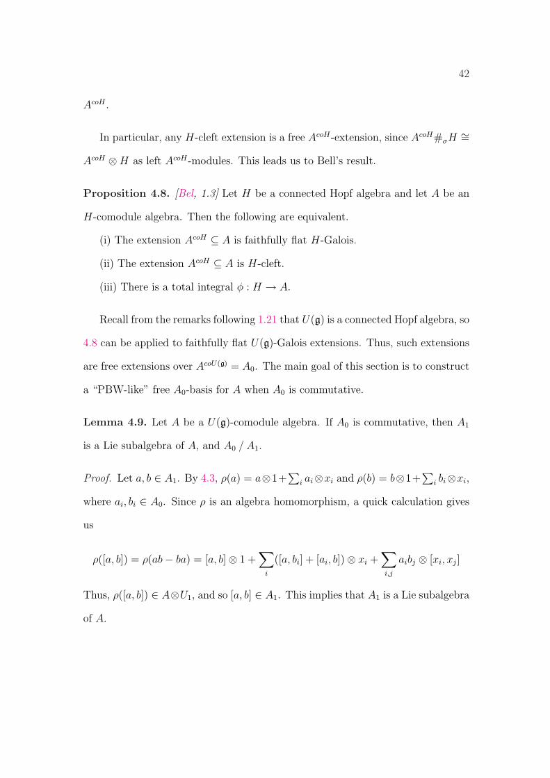
In particular, any H-cleft extension is a free AcoH-extension, since AcoH#σH∼=

AcoH ⊗H as left AcoH-modules. This leads us to Bell’s result.

Proposition 4.8. [Bel, 1.3] Let H be a connected Hopf algebra and let A be an

H-comodule algebra. Then the following are equivalent.

(i) The extension AcoH ⊆ A is faithfully flat H-Galois.

(ii) The extension AcoH ⊆ A is H-cleft.

(iii) There is a total integral φ : H → A.

Recall from the remarks following 1.21 that U(g) is a connected Hopf algebra, so

4.8 can be applied to faithfully flat U(g)-Galois extensions. Thus, such extensions

are free extensions over AcoU(g) = A0. The main goal of this section is to construct

a “PBW-like” free A0-basis for A when A0 is commutative.

Lemma 4.9. Let A be a U(g)-comodule algebra. If A0 is commutative, then A1

is a Lie subalgebra of A, and A0 / A1.

Proof. Let a, b ∈ A1. By 4.3, ρ(a) = a⊗1+∑

i ai⊗xi and ρ(b) = b⊗1+∑

i bi⊗xi,

where ai, bi ∈ A0. Since ρ is an algebra homomorphism, a quick calculation gives

us

ρ([a, b]) = ρ(ab− ba) = [a, b]⊗ 1 +∑

i

([a, bi] + [ai, b])⊗ xi +∑i,j

aibj ⊗ [xi, xj]

Thus, ρ([a, b]) ∈ A⊗U1, and so [a, b] ∈ A1. This implies that A1 is a Lie subalgebra

of A.

43

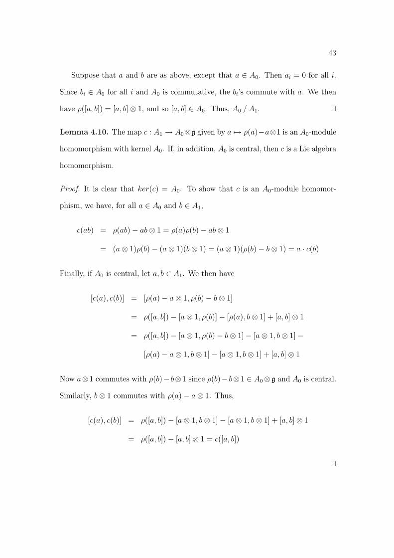
Suppose that a and b are as above, except that a ∈ A0. Then ai = 0 for all i.

Since bi ∈ A0 for all i and A0 is commutative, the bi’s commute with a. We then

have ρ([a, b]) = [a, b]⊗ 1, and so [a, b] ∈ A0. Thus, A0 / A1.

Lemma 4.10. The map c : A1 → A0⊗g given by a 7→ ρ(a)−a⊗1 is an A0-module

homomorphism with kernel A0. If, in addition, A0 is central, then c is a Lie algebra

homomorphism.

Proof. It is clear that ker(c) = A0. To show that c is an A0-module homomor-

phism, we have, for all a ∈ A0 and b ∈ A1,

c(ab) = ρ(ab)− ab⊗ 1 = ρ(a)ρ(b)− ab⊗ 1

= (a⊗ 1)ρ(b)− (a⊗ 1)(b⊗ 1) = (a⊗ 1)(ρ(b)− b⊗ 1) = a · c(b)

Finally, if A0 is central, let a, b ∈ A1. We then have

[c(a), c(b)] = [ρ(a)− a⊗ 1, ρ(b)− b⊗ 1]

= ρ([a, b])− [a⊗ 1, ρ(b)]− [ρ(a), b⊗ 1] + [a, b]⊗ 1

= ρ([a, b])− [a⊗ 1, ρ(b)− b⊗ 1]− [a⊗ 1, b⊗ 1]−

[ρ(a)− a⊗ 1, b⊗ 1]− [a⊗ 1, b⊗ 1] + [a, b]⊗ 1

Now a⊗1 commutes with ρ(b)− b⊗1 since ρ(b)− b⊗1 ∈ A0⊗g and A0 is central.

Similarly, b⊗ 1 commutes with ρ(a)− a⊗ 1. Thus,

[c(a), c(b)] = ρ([a, b])− [a⊗ 1, b⊗ 1]− [a⊗ 1, b⊗ 1] + [a, b]⊗ 1

= ρ([a, b])− [a, b]⊗ 1 = c([a, b])

44

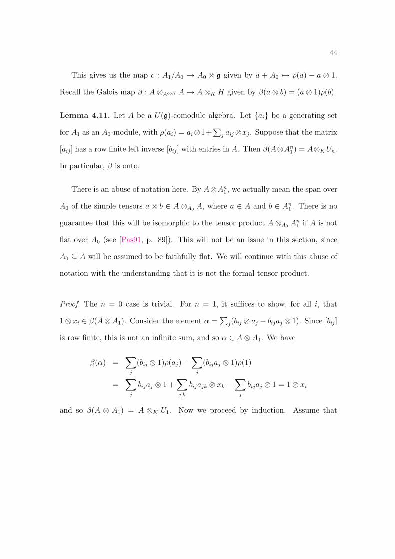
This gives us the map c : A1/A0 → A0 ⊗ g given by a + A0 7→ ρ(a) − a ⊗ 1.

Recall the Galois map β : A⊗AcoH A → A⊗K H given by β(a⊗ b) = (a⊗ 1)ρ(b).

Lemma 4.11. Let A be a U(g)-comodule algebra. Let {ai} be a generating set

for A1 as an A0-module, with ρ(ai) = ai⊗1+∑

j aij⊗xj. Suppose that the matrix

[aij] has a row finite left inverse [bij] with entries in A. Then β(A⊗An1 ) = A⊗K Un.

In particular, β is onto.

There is an abuse of notation here. By A⊗An1 , we actually mean the span over

A0 of the simple tensors a ⊗ b ∈ A ⊗A0 A, where a ∈ A and b ∈ An1 . There is no

guarantee that this will be isomorphic to the tensor product A⊗A0 An1 if A is not

flat over A0 (see [Pas91, p. 89]). This will not be an issue in this section, since

A0 ⊆ A will be assumed to be faithfully flat. We will continue with this abuse of

notation with the understanding that it is not the formal tensor product.

Proof. The n = 0 case is trivial. For n = 1, it suffices to show, for all i, that

1⊗ xi ∈ β(A⊗A1). Consider the element α =∑

j(bij ⊗ aj − bijaj ⊗ 1). Since [bij]

is row finite, this is not an infinite sum, and so α ∈ A⊗ A1. We have

β(α) =∑

j

(bij ⊗ 1)ρ(aj)−∑

j

(bijaj ⊗ 1)ρ(1)

=∑

j

bijaj ⊗ 1 +∑

j,k

bijajk ⊗ xk −∑

j

bijaj ⊗ 1 = 1⊗ xi

and so β(A ⊗ A1) = A ⊗K U1. Now we proceed by induction. Assume that

45

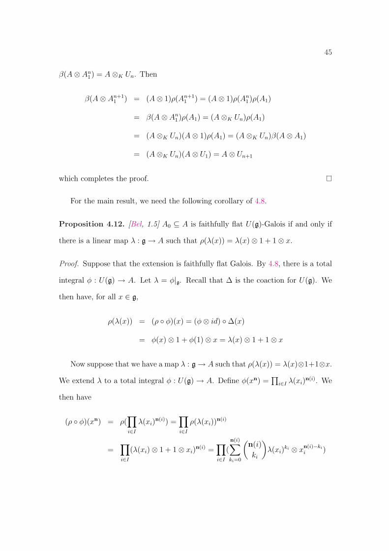
β(A⊗ An1 ) = A⊗K Un. Then

β(A⊗ An+11 ) = (A⊗ 1)ρ(An+1

1 ) = (A⊗ 1)ρ(An1 )ρ(A1)

= β(A⊗ An1 )ρ(A1) = (A⊗K Un)ρ(A1)

= (A⊗K Un)(A⊗ 1)ρ(A1) = (A⊗K Un)β(A⊗ A1)

= (A⊗K Un)(A⊗ U1) = A⊗ Un+1

which completes the proof.

For the main result, we need the following corollary of 4.8.

Proposition 4.12. [Bel, 1.5] A0 ⊆ A is faithfully flat U(g)-Galois if and only if

there is a linear map λ : g → A such that ρ(λ(x)) = λ(x)⊗ 1 + 1⊗ x.

Proof. Suppose that the extension is faithfully flat Galois. By 4.8, there is a total

integral φ : U(g) → A. Let λ = φ|g. Recall that ∆ is the coaction for U(g). We

then have, for all x ∈ g,

ρ(λ(x)) = (ρ ◦ φ)(x) = (φ⊗ id) ◦∆(x)

= φ(x)⊗ 1 + φ(1)⊗ x = λ(x)⊗ 1 + 1⊗ x

Now suppose that we have a map λ : g → A such that ρ(λ(x)) = λ(x)⊗1+1⊗x.

We extend λ to a total integral φ : U(g) → A. Define φ(xn) =∏

i∈I λ(xi)n(i). We

then have

(ρ ◦ φ)(xn) = ρ(∏i∈I

λ(xi)n(i)) =

∏i∈I

ρ(λ(xi))n(i)

=∏i∈I

(λ(xi)⊗ 1 + 1⊗ xi)n(i) =

∏i∈I

(

n(i)∑

ki=0

(n(i)

ki

)λ(xi)

ki ⊗ xn(i)−ki

i )

46

But if we define k(i) = ki and multiply everything out, we get

(ρ ◦ φ)(xn) =∑

k≤n

(∏i∈I

(n(i)

k(i)

)λ(xi)

k(i) ⊗ x(n−k)(i)i =

∑

k≤n

(n

k

)φ(xk)⊗ xn−k

= ((φ⊗ id) ◦∆)(xn)

Thus, φ is a comodule map. From its definition, we get that φ(1) = 1, and so φ is

a total integral. Thus, AcoH ⊆ A is faithfully flat Galois.

Corollary 4.13. A0 ⊆ A is faithfully flat U(g)-Galois if and only if c is an iso-

morphism.

Proof. Suppose A0 ⊆ A is faithfully flat U(g)-Galois. We already know that c

is injective by 4.10, so it suffices to prove that it is surjective. Let x ∈ g. By

4.12, there exists some ax ∈ A1 such that ρ(ax) = ax ⊗ 1 + 1 ⊗ x. We get

c(ax + A0) = 1⊗ x, and so c is surjective. Conversely, for each x ∈ g, let ax ∈ A1

such that c(ax + A0) = 1 ⊗ x. Then ρ(x) = ax ⊗ 1 + 1 ⊗ x, and thus A0 ⊆ A is

faithfully flat U(g)-Galois by 4.12

Notice for x ∈ g that λ(x) plays the same role in the comodule structure of

A as x plays in U(g) (where the coaction is given by ∆). Thus, faithfully flat

U(g)-Galois extensions bear a close resemblance to U(g) itself.

We can take this analogy even further. In A = U(g), we have A0 = K and

A1 = g ⊕K. Thus, we have g ∼= A1/A0. In fact, for all x ∈ g, we have x + A0 =

{a ∈ A : ρ(a) = a⊗ 1 + 1⊗ x}. Similarly, if A0 ⊆ A is faithfully flat U(g)-Galois,

then it is easy to check that ax + A0 = {a ∈ A : ρ(a) = a⊗ 1 + 1⊗ x}. This leads

us to the main theorem.

47

Theorem 4.14. Let A0 ⊆ A be a faithfully flat U(g)-Galois extension, with

{xi : i ∈ I} an ordered basis for g. Then

(i) If we define ai = λ(xi) as in 4.12, then {ai +A0} is a free A0-basis for A1/A0.

In particular, {1, ai} is a free basis for A1.

(ii) The set consisting of 1 and ordered monomials in {ai} is a free A0-basis for

the submodule of A it generates.

(iii) A =< A1 >.

(iv) If A1 is a Lie subalgebra of A, then the set consisting of 1 and ordered

monomials in {ai} form a free A0-basis for A. In particular, this holds when A0 is

commutative.

Proof. For (i), suppose that∑

i bi(ai + A0) = 0 for some bi ∈ A0. It follows that

∑i biai ∈ A0, so

∑i

biai ⊗ 1 = ρ(∑

i

biai) =∑

i

biai ⊗ 1 +∑

i

bi ⊗ xi

Thus,∑

i bi ⊗ xi = 0, and so bi = 0 for all i.

Now suppose a+A0 ∈ A1/A0. Then ρ(a) = a⊗1+∑

i bi⊗xi for some bi ∈ A0.

We then have

ρ(a−∑

i

biai) = (a⊗ 1 +∑

i

bi ⊗ xi)− (∑

i

(bi ⊗ 1)(ai ⊗ 1 + 1⊗ xi))

= (a−∑

i

biai)⊗ 1

Thus, a−∑i biai ∈ A0, and so a+A0 =

∑i bi(ai+A0). This gives us that {ai+A0}

is a free A0-basis for A1/A0.

For (ii), assume we have a nontrivial dependence relation∑

~i c~i ai1 · · · ain = 0,

ci ∈ A0, where i1 ≤ · · · ≤ in and n is the maximum degree of a monomial with a

48

nonzero coefficient. In order to allow for monomials of different lengths, we define

a0 = 1, so ij ∈ I ∪ {0}. We have

0 = ρ(∑

~i

c~i ai1 · · · ain)

=∑

~i

(c~i ⊗ 1)(ai1 ⊗ 1 + 1⊗ xi1) · · · (ain ⊗ 1 + 1⊗ xin)

=∑

|~i|=n

c~i ⊗ xi1 · · · xin + s

where s ∈ A⊗Un−1. By the PBW theorem, c~i = 0 for all |~i| = n. This contradicts

our assumption of the existence of a nontrivial dependence relation, and gives us

(ii).

For (iii), first note that A ⊗A0 An1 and A ⊗A0 An are naturally embedded in

A ⊗ A since the extension is faithfully flat. We have A =⋃

n An, so it suffices to

show that An1 = An for all n. We first show that A ⊗A0 An

1 = A ⊗A0 An. The

matrix {aij} from 4.11 is the identity matrix by 4.12, and is thus left invertible

with row finite left inverse. Also, {ai} generates A1 as an A0-module by (i), and

so 4.11 implies that β(A⊗A0 An1 ) = A⊗K Un, which gives us

β(A⊗A0 An1 ) ⊆ β(A⊗A0 An) ⊆ A⊗K Un = β(A⊗A0 An

1 )

Thus, β(A⊗A0 An) = β(A⊗A0 An1 ), and by the bijectivity of β, we get A⊗A0 An =

A⊗A0 An1 .

Now consider the exact sequence 0 → An1 → An → An/A

n1 → 0. By flatness,

we get the exact sequence 0 → A ⊗A0 An1 → A ⊗A0 An → A ⊗A0 (An/An

1 ) → 0.

But the second map in this sequence is the inclusion map, which is onto since

A⊗An1 = A⊗An, so A⊗A0 (An/A

n1 ) = 0. By faithful flatness, we get An/An

1 = 0,

and so An = An1 .

49

For (iv), we know by (i) that the ai form an A0 basis for A1. Then (iii) implies

that A is spanned by monomials in the ai. But A1 is a Lie subalgebra of A, and so

the monomials in ai are spanned by the ordered monomials in the ai. Finally, by

(ii), the ordered monomials are independent over A0, so they form a free basis.

4.3 The role of c in the non-faithfully flat case

Corollary 4.13 seems to indicate that the behavior of c is related to whether or not

A0 ⊆ A is U(g)-Galois. In this section, we attempt to generalize 4.13 to arbitrary

U(g)-Galois extensions. It appears that the correct map to consider in this more

general context is id⊗ c : A⊗A0 (A1/A0) → A⊗A0 (A0 ⊗K g) ∼= A⊗K g .

Proposition 4.15. (i) If id⊗ c is onto, then so is β.

(ii) If A0 ⊆ A is U(g)-Galois and β−1(A ⊗ U1) = A ⊗ A1, then id ⊗ c is an

isomorphism.

Proof. For (i), let {ai} be a generating set for A1 as an A0-module, and let {aij}be as in 4.11. Since id ⊗ c is onto, then for each i there exist bij ∈ A such that

1⊗xi = (id⊗ c)(∑

j bij ⊗ (aj +A0)). Notice that, for each i, there are only finitely

many j such that bij 6= 0, so the matrix [bij] is row finite. We also have

1⊗ xi =∑

j,k

bijajk ⊗ xk

and so∑

j bijajk = δi,k. Thus, [aij] has a row finite left inverse, and so β is onto

by 4.11.

Now we consider (ii). Since β−1(A⊗U1) = A⊗A1 and the ai’s generate A1 over

A0, then for each i, there exist bij ∈ A such that β−1(1⊗xi) =∑

j bij⊗aj. Since β−1

50

is A-linear, we have β−1(a⊗xi) =∑

j abij⊗aj. Define γ : A⊗K g → A⊗A0 (A1/A0)

by γ(a ⊗ xi) =∑

j abij ⊗ (aj + A0). For each a ∈ A and b ∈ A1, we have

ρ(b) = b⊗ 1 +∑

i bi ⊗ xi for some bi ∈ A0, and so

[γ ◦ (id⊗ c)](a⊗ (b + A0)) = γ(∑

i

abi ⊗ xi) =∑i,j

abibij ⊗ (aj + A0)

But we also have that

a⊗ b = β−1 ◦ β(a⊗ b) = β−1(ab⊗ 1 +∑

i

abi ⊗ xi)

= ab⊗ 1 +∑i,j

abibij ⊗ aj (4.3)

If we let π : A1 → A1/A0 be the canonical homomorphism, then, applying id ⊗ π

to both sides of (4.3) gives us a ⊗ (b + A0) =∑

i,j abibij ⊗ (aj + A0), and so

γ ◦ (id⊗ c) = id.

For the other direction, we have

[(id⊗ c) ◦ γ](a⊗ xi) = (id⊗ c)(∑

j

abij ⊗ (aj + A0))

=∑

j,k

abijajk ⊗ xk

But we have 1⊗xi = β◦β−1(1⊗xi) = β(∑

j bij⊗aj) =∑

j bijaj⊗1+∑

j,k bijajk⊗xk.

This implies that∑

j bijajk = δi,k, and thus∑

j,k abijajk ⊗ xk = a⊗ xi. This gives

us [(id ⊗ c) ◦ γ](a ⊗ xi) = a ⊗ xi, and so γ = (id ⊗ c)−1. Thus, id ⊗ c is an

isomorphism.

Note that we have a filtration of the A-module A⊗A0 A given by (A⊗A0 A)n =

A⊗An. Recall that a homomorphism f between two A-modules M and N are said

to have degree p if f(Mi) ⊆ Ni+p for all i. It is easy to see that β is a homomorphism

51

of degree 0 for any U(g)-comodule algebra. However, if β is bijective, it is not

necessarily true that β−1 is of degree zero. But if, in addition, id⊗ c is onto, then

4.15 implies that β|A⊗An is onto A ⊗ Un. In this case, β−1 is a homomorphism

of degree 0 as well. So (ii) implies that if A0 ⊆ A is U(g)-Galois, then β−1 is a

homomorphism of degree 0 if β−1(A⊗ U1) = A⊗A0 A1.

Proposition 4.15 leads one to consider what role id ⊗ c plays in determining

whether or not A0 ⊆ A is U(g)-Galois. We ask

Question 4.16. Is A0 ⊆ A a U(g)-Galois extension if and only if id ⊗ c is an

isomorphism?

If we knew that β−1 must be a homomorphism of degree 0 for any Galois

extension, or, equivalently, that β−1(A ⊗ U1) = A ⊗ A1, that would give us one

direction (⇒). The other direction seems more complicated.

52

Chapter 5

Descent theory of coalgebras and

Hopf algebras

In this chapter, we present two theorems on the descent theory of coalgebras and

Hopf algebras. The first theorem classifies all forms of the grouplike coalgebras

with respect to fields, and the second allows us to compute L-forms when K ⊆ L

is a finite dimensional Hopf Galois extension.

5.1 Forms of the Grouplike Coalgebra

We now consider the descent theory for coalgebras. In this section, we classify

all coalgebra forms of grouplike coalgebras with respect to fields according to the

structure of their simple subcoalgebras. Recall that a coalgebra is grouplike if it

is spanned by grouplike elements (i.e. elements g 6= 0 such that ∆(g) = g ⊗ g).

Suppose that C = KG is a grouplike coalgebra, where G = G(C). It is clear that

if we have a field extension K ⊆ L, then L ⊗ C ∼= LG. Thus, it is our goal to

characterize the coalgebras H such that L⊗H ∼= LG. We will denote the algebraic

closure of K by K.

53

To get started, we first consider the coalgebra structure of duals of finite ex-

tension fields. Let K ⊆ L be a finite field extension. Then L∗ is a K-coalgebra

by 1.12(ii). Let {α1, · · · , αn} be a basis for L over K with αjαk =∑

l cjklαl, where

cjkl ∈ K, and let {α∗1, · · · , α∗n} be the dual basis in L∗. For the comultiplicative

structure, let 1 ≤ r, s, l ≤ n. We have

∆(α∗l )(αr ⊗ αs) = α∗l (αrαs) =∑

t

crstα∗l (αt) = crsl = (

∑

j,k

cjklα∗j ⊗ α∗k)(αr ⊗ αs)

so ∆(α∗l ) =∑

j,k cjklα∗j ⊗ α∗k.

For the counit, let qi ∈ K such that∑

i qiαi = 1. Then for each j, we get

ε(α∗j ) = α∗j (1) =∑

i qiα∗i (αj) = qj. Thus, the ε(α∗i ) are the unique elements of

K such that∑

i ε(α∗i )αi = 1. This completes our description of the coalgebra

structure of L∗.

Lemma 5.1. Let K ⊆ L be a finite field extension. A coalgebra D is a morphic

image of L∗ if and only if D ∼= E∗ for some field E such that K ⊆ E ⊆ L. In

particular, any morphic image of L∗ is a simple coalgebra.

Proof. Suppose that φ : L∗ → D is an onto morphism of coalgebras. We can define

φ∗ : D∗ → L∗∗ ∼= L by φ∗(f) = f ◦ φ. It is then easy to show that φ∗ is an algebra

monomorphism. Let E be the image of D∗ in L. Then E is a finite dimensional

K-subalgebra of L, so E is a field. Furthermore, since E ∼= D∗ as fields, then

D ∼= E∗ as coalgebras.

Conversely, if D ∼= E∗ for E a field contained in L, then consider the inclusion

map i : E → L. Since i is a field monomorphism, i∗ : L∗ → E∗ ∼= D is an coalgebra

morphism. Since i is injective, one can show that i∗ is surjective.

54

Finally, let D be a morphic image of L∗. By the above, K ⊆ D∗ is a finite field

extension. Thus, D∗ is a finite dimensional simple K-algebra. By [Mon93, 5.1.4],

D is a simple coalgebra.

Some other facts will be important in helping us find forms of grouplike coalge-

bras. It is clear that any form H of KG must be cocommutative, since H ⊆ L⊗H

and L⊗H is cocommutative. Also, if L⊗H is grouplike, it must be pointed. The

following can be found in [Mon93, 5.6]. It says that pointedness will always occur

for a cocommutative coalgebra as long as we carefully choose our extension field.

Proposition 5.2. If H is a cocommutative K-coalgebra, and K is algebraically

closed, then H is pointed.

Thus, if we take L = K, then L ⊗ H is pointed when H is a cocommutative

coalgebra.

Proof. Let D be a simple subcoalgebra of H. Then D∗ is finite dimensional by

the remarks following 1.19. It is also a commutative, simple K-algebra, and so

K ⊆ D∗ is a finite field extension. Since K is algebraically closed, D∗ ∼= K, and

so dimK(D) = 1. Thus, H is pointed.

We will need a few technical results which will help us reduce the problem of

finding forms of KG to the case where L is algebraic over K. The first lemma tells

us that if we have a grouplike element g =∑

αi ⊗ hi, then in some sense the αi

and hi are dual to each other.

Lemma 5.3. Let g =∑

i αi ⊗ hi ∈ G(L⊗H).

55

(i) Suppose the αi are linearly independent, and that αiαj =∑

k cijkαk for all

i, j. Then ∆(hk) =∑

i,j cijkhi⊗hj for all k. In particular, D = span{hi} is a finite

dimensional subcoalgebra of H.

(ii) If we have the hypotheses in (i), and if the αi are algebraic over K, then D

is simple.

(iii) If the nonzero hi are linearly independent (write them as h1, · · · , hn), and

if ∆(hk) =∑n

i,j=1 dijkhi ⊗ hj, where dijk ∈ K, then αiαj =∑n

k=1 dijkαk for all

1 ≤ i, j ≤ n. In particular, K[α1, · · · , αn] is finite dimensional, and therefore is a

finite field extension.

(iv) Conversely, if we have {α′1, · · · , α′n} ∈ L and {h′1, · · · , h′n} such that α′iα′j =

∑k cijkα

′k and ∆(h′k) =

∑i,j cijkh

′i⊗h′j with cijk ∈ K, then

∑i α

′i⊗h′i ∈ G(L⊗H).

Proof. In general, we have

∑

k

αk ⊗∆(hk) = ∆(g) = g ⊗ g

=∑i,j

αiαj ⊗ hi ⊗ hj (5.1)

If αiαj =∑

k cijkαk, and the αi are linearly independent, then∑

i,j αiαj⊗hi⊗hj =

∑i,j,k cijkαk ⊗ hi ⊗ hj, and therefore ∆(hk) =

∑i,j cijkhi ⊗ hj by (5.1). This gives

us (i).

If the αi are algebraic over K, then let {α1, · · · , αn} be the αi such that hi 6= 0.

Since ε(g) = 1, then∑n

i=1 ε(hi)αi = 1. This and (i) imply that the hi satisfy the

same coalgebra relations as E∗, where E = K(α1, · · · , αn). Note that since the αi

are algebraic, E is finite dimensional, and so E∗ is indeed a coalgebra. Thus, D is

a morphic image of E∗, and so is simple by 5.1. This gives us (ii)

56

If ∆(hk) =∑

i,j dijkhi ⊗ hj and the hi are linearly independent, then we get

∑k αk⊗∆(hk) =

∑i,j,k dijkαk⊗hi⊗hj. Therefore, αiαj =

∑k dijkαk by (5.1) and

so we have (iii).

Finally, (iv) follows from a computation almost identical to those above. I will

leave this to the fastidious reader.

Lemma 5.4. Let K ⊆ L be any field extension. For each g ∈ G(L⊗H), there is

a simple subcoalgebra Hg ⊆ H such that g ∈ K ⊗Hg

Proof. Let g ∈ G(L ⊗ H), and let {αi} be a basis for L over K with αiαj =

∑k cijkαk, where cijk ∈ K. Then g =

∑i αi ⊗ hi for some hi ∈ H. Let D =

span{hi}. Then g ∈ L⊗D. Also, D is a finite dimensional coalgebra by 5.3(i).

Now let {v1, · · · , vn} be a basis for D. Then ∆(vk) =∑n

i,j=1 dijkvi⊗vj for some

dijk ∈ K. Write g =∑

i βi ⊗ vi with βi ∈ L. By 5.3(iii), K[β1, · · · , βn] is a finite

field extension, and so each βi is algebraic over K. Thus, g ∈ K ⊗D.

But now we can write g =∑

i γi⊗wi, where the γi are linearly independent in

K, γiγj =∑

k eijkγk with eijk ∈ K, and wi ∈ D. By 5.3(ii), we have that Hg =

span{wi} is a simple coalgebra. Since g ∈ K ⊗Hg, the proof is complete.

As a direct consequence, we get

Corollary 5.5. If a coalgebra H is an L-form of KG, then it is a K-form of KG.

Proof. If L ⊗H ∼= LG, then G ⊆ K ⊗H, by 5.4. Thus, KG ⊆ K ⊗H. Since G

spans L⊗H over L, G spans K ⊗H over K. Thus, K ⊗H = KG.

We now mention a fact from field theory.

57

Proposition 5.6. [McC66, Thm. 20] Let K ⊆ E be a finite field extension, with

L a normal extension of K containing E. Let n be the degree of separability of E

over K. Then there are exactly n distinct K-isomorphisms of E onto subfields of

L.

This leads us to the main theorem.

Theorem 5.7. Let H be a K-coalgebra, and suppose K ⊆ L is an extension of

fields. Then the following are equivalent.

(i) L⊗H is a grouplike L-coalgebra.

(ii) H is cocommutative, cosemisimple with separable coradical, and L contains

the normal closure of D∗ for each simple subcoalgebra D ⊆ H.

A coalgebra is said to have separable coradical if, for each simple subcoalgebra

D, we have that D∗ is a separable K-algebra. If D is cocommutative, this will

make D∗ a separable field extension.

Also notice that the above implies that H is a form of KG with respect to

fields if and only if H is cosemisimple with separable coradical.

Proof. Suppose that L⊗H is a grouplike coalgebra, and write G = G(L⊗H). By

5.5, we can assume that L is algebraic over K. By 5.4, each g ∈ G is contained in

L⊗Hg for some simple subcoalgebra Hg ⊆ H. We then have

L⊗H = LG ⊆∑g∈G

L⊗Hg = L⊗ (∑g∈G

Hg) ⊆ L⊗H0

and so H = H0. This implies that H is cosemisimple.

We now take care of the case where H is simple. By 5.1, H∗ is isomorphic

to some finite field extension of K in K. Let E ∼= H∗ be any such field, and

58

let {α1, · · · , αn} be a basis for E over K, {h1, · · · , hn} a basis for H such that

αiαj =∑

k cijkαk and ∆(hl) =∑

j,k cjklhj⊗hk. Then g =∑

i αi⊗hi is a grouplike

element of E⊗H by 5.3(iv). Since L⊗H is grouplike, g ∈ L⊗H. Also, the hi are

linearly independent, so αi ∈ L for all i. Thus, E ⊆ L, and so L contains every

isomorphic copy of H∗ in K. This implies that L contains the normal closure of

H∗ in K.

Now let E and {hi} be as above, and suppose that g′ =∑

j α′j ⊗ hj is any

grouplike element in H. By 5.3(iii), we have α′iα′j =

∑k cijkα

′k. But then the

map αj 7→ α′j extends to an isomorphism E → K(α′1, · · · , α′n). Thus, we get a

distinct grouplike element of L ⊗ H for every distinct isomorphism from E onto

subfields of L. Another way of saying this is that the number of grouplikes is the

same as the number of distinct isomorphisms of E onto subfields of L. Since L

contains the normal closure of H∗, 5.6 implies that the number of distinct grouplike

elements is the same as the degree of separability of H∗ over K. Since L⊗H has

dimK(H) = dimK(H∗) distinct grouplikes, the degree of separability of H∗ over K

is dimK(H∗). Therefore, H∗ is separable over K.

For the general case, since H is cosemisimple, we can write H = ⊕iHi, where

the Hi are the distinct simple subcoalgebras of H. Also recall from 5.3(ii) that each

grouplike element of L⊗H sits in some L⊗Hi. Thus, G(L⊗H) = ∪iG(L⊗Hi).

Since L⊗H is spanned by grouplike elements, it follows that each L⊗Hi is spanned

by grouplike elements. By the simple case, each H∗i is separable, and L contains

the normal closure of H∗i . Thus, if L ⊗ H is grouplike, then H is cosemisimple,

each simple subcoalgebra D is the dual of a finite separable extension field of K,

and L contains the normal closure of each such D.

59

Conversely, suppose that H is cosemisimple, each simple subcoalgebra is the

dual of a separable finite extension field, and L contains the normal closure of

D∗ for each simple subcoalgebra D ⊆ H. Since H is cosemisimple, H = ⊕iHi,

where each Hi is simple. It suffices to show that each Hi is spanned by grouplike

elements, and so, without loss of generality, H is simple. By the remarks following

1.19, H is finite-dimensional.

Since H∗ is separable, and L contains the normal closure of H∗, there are

dimK(H∗) distinct isomorphisms of H∗ onto subfields of L. By 5.3(iv), we get a

distinct grouplike element of L ⊗ H for each such isomorphism, and so there are

dimK(H∗) = dimK(H) distinct grouplike elements of L⊗H. Therefore, L⊗H is

a grouplike coalgebra, and the proof is complete.

If H is a cocommutative cosemisimple Hopf algebra, then so is L ⊗H, where

K ⊆ L is any field extension (see [Nic94, 1.2]). Since L⊗H is also pointed when

L is algebraically closed, any cocommutative cosemisimple Hopf algebra is a form

of a group algebra. By 5.7, H must have a separable coradical. This restricts

the coalgebra structure of such Hopf algebras. We can also say something about

semisimplicity in the finite dimensional case.

Corollary 5.8. Let H be a finite dimensional cocommutative cosemisimple Hopf

algebra. Then H is semisimple if and only if char(K) = 0 or char(K) does not

divide dimK(H).

Proof. Let L = K. By the above remarks, L⊗H ∼= LG, where G is a group. By

3.7, H is semisimple if and only if KG is. By Maschke’s theorem, this occurs if

and only if either char(K) = 0 or char(K) does not divide |G| = dimK(H).

60

Theorem 5.7 tells us which field L is the smallest one necessary in order for H

to be an L-form of a grouplike coalgebra. For each simple subcoalgebra D of H,

we need the normal closure of D∗ to be included in L. Thus, if H = ⊕Hi, where

the Hi are simple, and we let Li be the normal closure of H∗i , then L =

∏i Li is

the smallest field necessary for L ⊗ H to be grouplike. This leads us to another

result.

Corollary 5.9. Let H be an L-form of KG, where K ⊆ L is either a totally

inseparable or a purely transcendental extension. Then H ∼= KG.

Proof. Suppose K ⊆ L is totally inseparable. By the above remarks, any grouplike

element in L ⊗ H is contained in E ⊗ H where E is the separable closure of K

in L. Since K ⊆ L is totally inseparable, we have E = K. Thus, H ∼= K ⊗H is

spanned by grouplike elements, and so H ∼= KG.

If K ⊆ L is purely inseparable, then any grouplike element is contained in

E⊗H, where E is the algebraic closure of K in L by 5.4. But E = K since K ⊆ L

is purely transcendental. The result follows as before.

Corollary 5.10. Let H be a cocommutative coalgebra, and suppose that K ⊆ L

is such that L⊗H is pointed. Let {Hn}∞n=0 be the coradical filtration of H.

(i) [L⊗H]0 ⊆ L⊗H0.

(ii) Equality holds if and only if H has separable coradical.

(iii) If H has separable coradical, then L⊗Hn ⊆ [L⊗H]n for all n.

Proof. For (i), since L⊗H is pointed, [L⊗H]0 is spanned by grouplikes. Since each

grouplike g ∈ L⊗Hg ⊆ L⊗H0, where Hg is as in 5.4, we have [L⊗H]0 ⊆ L⊗H0.

61

For (ii), we first note that H0 is a cosemisimple, cocommutative coalgebra. If

H does not have separable coradical, then, by 5.7, L⊗H0 is not grouplike. Since

[L⊗H]0 is grouplike, equality cannot hold.

If H does have separable coradical, then 5.7 tells us that L ⊗H0 is grouplike,

and thus cosemisimple. Then L⊗H0 ⊆ [L⊗H]0, and we’re done by (i).

For (iii), we proceed by induction on n. The n = 0 case is (ii). Assume that

L⊗Hn ⊆ [L⊗H]n. We then look at L⊗Hn+1. We have

∆(L⊗Hn+1) = L⊗K ∆(Hn+1)

⊆ L⊗K (H ⊗K Hn + H0 ⊗K H)

⊆ (L⊗H)⊗L (L⊗Hn) + (L⊗H0)⊗L (L⊗H)

⊆ (L⊗H)⊗L (L⊗H)n + (L⊗H)0 ⊗L (L⊗H)

and so L⊗Hn+1 ⊆ [L⊗H]n+1, which completes the proof.

For the next corollary, we need the following.

Theorem 5.11. [Mon93, 2.3.1] Suppose that H is a finite dimensional commu-

tative semisimple Hopf algebra. Then there exists a group G and a separable

extension field E of K such that E ⊗H ∼= (EG)∗ as Hopf algebras.

Proof. By Wedderburn’s Theorem, H ∼= ⊕Ei, where each Ei is an extension field

of K. Since H is finite dimensional and semisimple, it is separable by [Mon93,

2.2.2], so each Ei is separable. Let E be a separable field containing all the Ei.

We have

E ⊗H ∼= E ⊗ (⊕Ei) ∼= ⊕(E ⊗ Ei) ∼= En

62

where n = dimKH, since E and the Ei’s are separable. Now let {pi} be a basis in

E ⊗H of orthogonal idempotents, and let G = {gi} be a dual basis in [E ⊗H]∗.

It is clear that the gi are algebra maps, so by 1.14 they are grouplike elements.

But then [E ⊗ H]∗ is generated by grouplikes, so [E ⊗ H]∗ ∼= EG, and thus

E ⊗H ∼= (EG)∗.

Lemma 5.12. Let C be a subspace of a K-Hopf algebra (or coalgebra) H, and

let K ⊆ L be a field extension.

(i) C is a subcoalgebra of H if and only if L⊗ C is a subcoalgebra of L⊗H.

(ii) C is a subHopfalgebra of H if and only if L ⊗ C is a subHopfalgebra of

L⊗H.

Proof. Suppose L ⊗ C is a subcoalgebra, and let c ∈ C. Then 1 ⊗ c ∈ L ⊗ C, so

1⊗∆(c) = ∆(1⊗ c) ∈ L⊗ C ⊗ C. But then

1⊗∆(c) ∈ (K ⊗H ⊗H) ∩ (L⊗ C ⊗ C) = K ⊗ (C ⊗ C)

so ∆(c) ∈ C⊗C, and C is a subcoalgebra. The other assertions follow similarly.

Corollary 5.13. Let H be a cocommutative Hopf algebra. If H has separable

coradical, then H0 is a subHopfalgebra. Conversely, if H0 is a finite dimensional

Hopf algebra, then H has separable coradical.

Proof. First suppose that H has separable coradical, and let L = K. Then L⊗H

is a pointed coalgebra, and so (L⊗H)0 is a group algebra. But this implies that

(L⊗H)0 is a Hopf algebra. By 5.10, L⊗H0 = (L⊗H)0. Since L⊗H0 is a Hopf

algebra, 5.12 implies that H0 is a Hopf algebra.

63

If H0 is a finite dimensional cocommutative Hopf algebra, then H∗0 is a finite

dimensional commutative semisimple Hopf algebra. By 5.11, L ⊗H∗0∼= (LG)∗ as

Hopf algebras. But L ⊗H∗0∼= (L ⊗H0)

∗, so L ⊗H0∼= LG. This implies, by 5.7,

that H0 has separable coradical, and thus so does H.

We get one final corollary.

Corollary 5.14. Suppose that K is a field of characteristic zero, and that H is a

K-Hopf algebra of prime dimension. Then H is semisimple and cosemisimple with

separable coradical.

Proof. Again, let L = K. By [Zhu94], since L ⊗ H is a Hopf algebra over an

algebraically closed field of characteristic zero, it is a group algebra. By 5.7, H is

cosemisimple with separable coradical. If we apply the above to H∗, then H∗ is

cosemisimple, and so H is semisimple.

5.2 Hopf Algebra Forms

In this section, we consider the descent theory of Hopf algebras. Here, we fix the

field extension K ⊆ L and search for the L-forms of a given Hopf algebra H.

More specifically, suppose that H and W are K-Hopf algebras, where W is finite

dimensional and semisimple. Also, let K ⊆ L be a right W ∗-Galois extension of

fields, and suppose that L⊗H is a W -module algebra, where the action restricted

to L is the Galois action. This, along with some other mild restrictions on the

action of W , will guarantee that [L ⊗ H]W is an L-form of H. Furthermore, all

L-forms of H can be obtained in this way.

64

Henceforth, L⊗H will be written as L ◦H and l ⊗ h will be written as lh for

convenience, where l ∈ L, and h ∈ H.

We start with a lemma on W -module algebras.

Lemma 5.15. Let W act on a field extension K ⊆ L such that K = LW , and

suppose that A is an associative K-algebra such that L◦A is a W -module algebra.

Then

(i) Any subset of [L ◦A]W that is linearly independent over K is linearly inde-

pendent over L.

(ii) [L ◦A]W ⊗K [L ◦A]W can be embedded in [L ◦A]⊗L [L ◦A] as K-algebras

by the map α⊗K β 7→ α⊗L β.

Proof. Let {αi} be a K-linearly independent set in [L ◦ A]W . Suppose that

∑ni=1 liαi = 0 is a nontrivial dependence relation of minimal length with li ∈ L.

Without loss of generality, we can assume that l1 = 1, and so α1 +∑

i>1 liαi = 0.

Let w ∈ W . By acting on the dependence relation by w and using the fact that

αi ∈ [L ◦ A]W , we get ε(w)α1 +∑

i>1(w · li)αi = 0. If we multiply the original

dependence relation by ε(w), we get ε(w)α1 +∑

i>1 ε(w)αi = 0. But if we subtract

these equations, we get∑i>0

(w · li − ε(w)li)αi = 0

Since this is a shorter dependence relation, we must have w · li−ε(w)li = 0 for each

i, so w · li = ε(w)li. Thus, li ∈ LW = K. Since the αi are K-linearly independent,

we have a contradiction. This gives us (i), and (ii) follows immediately.

This lemma allows us to view elements of [L ◦A]W ⊗ [L ◦A]W as belonging to

[L ◦ A] ⊗L [L ◦ A]. We can thus move elements of L through the tensor product

65

when looking at invariants. This will be important in our calculations for the main

theorem.

Before proving the main theorem, we need to say something about the action

of W on L.

Lemma 5.16. Let W be a finite dimensional K-Hopf algebra, and let K ⊆ L be

a W ∗-Galois extension. Let 0 6= t ∈ ∫ l

Wwith ∆(t) =

∑j tj ⊗ t′j, where {t′j} is a

basis for W . Let ai, bi ∈ L such that∑

i aitbi = 1 in L#H, as in 3.27(iii). Then

(i) For all w ∈ W , we have∑

i(w · ai)tbi = w in L#W .

(ii) For all j, k we have∑

i(t′j ·ai)(tk · bi) = δj,k. In particular, if we have t′1 = 1,

then∑

i ai(tj · bi) = δj,1.

Proof. Let w ∈ W . Then we have, by the definition of multiplication in L#W ,

w = w(∑

i

aitbi) =∑

i

(w1 · ai)w2tbi =∑

i

(w1 · ai)ε(w2)tbi =∑

i

(w · ai)tbi

This gives us (i). For (ii), we have from (i) and the expression for ∆(t) that for

all j,

t′j =∑

i

(t′j · ai)tbi =∑

i,k

(t′j · ai)(tk · bi)t′k

Since {t′k} is a basis, we have∑

i(t′j · ai)(tk · bi) = δj,k. This gives us (ii).

As mentioned before, only certain actions of W on L ◦ H will be considered.

We are looking for Hopf algebra forms, so we must take into consideration the

algebraic and coalgebraic structure of L ◦H, as well as the structure imposed by

the antipode. By making L ◦H a W -module algebra, we are choosing actions that

“respect” the algebraic structure of L ◦H. It thus makes sense to choose actions

that respect the rest of the Hopf algebra structure as well.

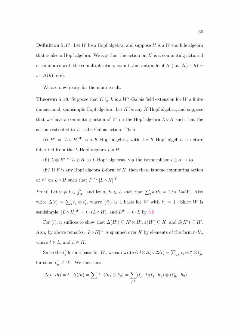
66

Definition 5.17. Let W be a Hopf algebra, and suppose H is a W -module algebra

that is also a Hopf algebra. We say that the action on H is a commuting action if

it commutes with the comultiplication, counit, and antipode of H (i.e. ∆(w · h) =

w ·∆(h), etc).

We are now ready for the main result.

Theorem 5.18. Suppose that K ⊆ L is a W ∗-Galois field extension for W a finite

dimensional, semisimple Hopf algebra. Let H be any K-Hopf algebra, and suppose

that we have a commuting action of W on the Hopf algebra L ◦H such that the

action restricted to L is the Galois action. Then

(i) H ′ = [L ◦ H]W is a K-Hopf algebra, with the K-Hopf algebra structure

inherited from the L-Hopf algebra L ◦H.

(ii) L⊗H ′ ∼= L⊗H as L-Hopf algebras, via the isomorphism l ⊗ α 7→ lα.

(iii) If F is any Hopf algebra L-form of H, then there is some commuting action

of W on L ◦H such that F ∼= [L ◦H]W

Proof. Let 0 6= t ∈ ∫ l

W, and let ai, bi ∈ L such that

∑i aitbi = 1 in L#W . Also

write ∆(t) =∑

j tj ⊗ t′j, where {t′j} is a basis for W with t′1 = 1. Since W is

semisimple, [L ◦H]W = t · (L ◦H), and LW = t · L by 3.9.

For (i), it suffices to show that ∆(H ′) ⊆ H ′⊗H ′, ε(H ′) ⊆ K, and S(H ′) ⊆ H ′.

Also, by above remarks, [L ◦H]W is spanned over K by elements of the form t · lh,

where l ∈ L, and h ∈ H.

Since the t′j form a basis for W , we can write (id⊗∆)◦∆(t) =∑

j,k tj⊗ t′j⊗ t′′jk

for some t′′jk ∈ W . We then have

∆(t · lh) = t ·∆(lh) =∑

t · (lh1 ⊗ h2) =∑

j,k

(tj · l)(t′j · h1)⊗ (t′′jk · h2)

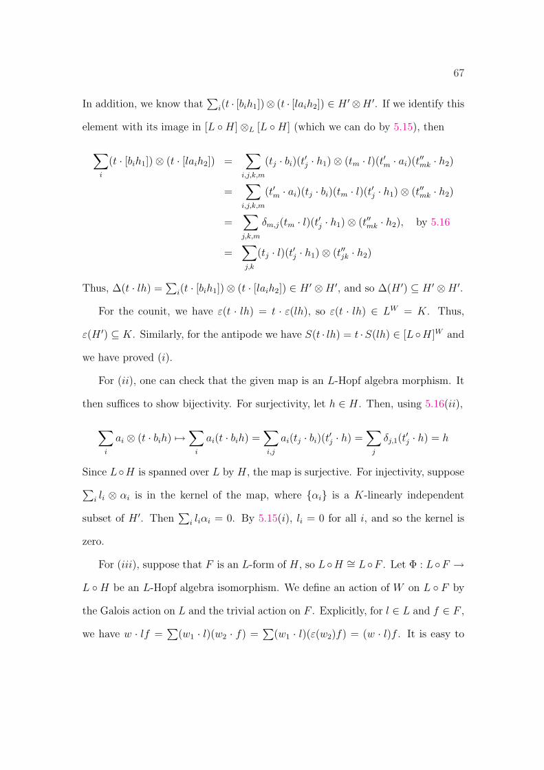
67

In addition, we know that∑

i(t · [bih1])⊗ (t · [laih2]) ∈ H ′⊗H ′. If we identify this

element with its image in [L ◦H]⊗L [L ◦H] (which we can do by 5.15), then

∑i

(t · [bih1])⊗ (t · [laih2]) =∑

i,j,k,m

(tj · bi)(t′j · h1)⊗ (tm · l)(t′m · ai)(t

′′mk · h2)

=∑

i,j,k,m

(t′m · ai)(tj · bi)(tm · l)(t′j · h1)⊗ (t′′mk · h2)

=∑

j,k,m

δm,j(tm · l)(t′j · h1)⊗ (t′′mk · h2), by 5.16

=∑

j,k

(tj · l)(t′j · h1)⊗ (t′′jk · h2)

Thus, ∆(t · lh) =∑

i(t · [bih1])⊗ (t · [laih2]) ∈ H ′ ⊗H ′, and so ∆(H ′) ⊆ H ′ ⊗H ′.

For the counit, we have ε(t · lh) = t · ε(lh), so ε(t · lh) ∈ LW = K. Thus,

ε(H ′) ⊆ K. Similarly, for the antipode we have S(t · lh) = t ·S(lh) ∈ [L◦H]W and

we have proved (i).

For (ii), one can check that the given map is an L-Hopf algebra morphism. It

then suffices to show bijectivity. For surjectivity, let h ∈ H. Then, using 5.16(ii),

∑i

ai ⊗ (t · bih) 7→∑

i

ai(t · bih) =∑i,j

ai(tj · bi)(t′j · h) =

∑j

δj,1(t′j · h) = h

Since L◦H is spanned over L by H, the map is surjective. For injectivity, suppose

∑i li ⊗ αi is in the kernel of the map, where {αi} is a K-linearly independent

subset of H ′. Then∑

i liαi = 0. By 5.15(i), li = 0 for all i, and so the kernel is

zero.

For (iii), suppose that F is an L-form of H, so L◦H ∼= L◦F . Let Φ : L◦F →L ◦H be an L-Hopf algebra isomorphism. We define an action of W on L ◦ F by

the Galois action on L and the trivial action on F . Explicitly, for l ∈ L and f ∈ F ,

we have w · lf =∑

(w1 · l)(w2 · f) =∑

(w1 · l)(ε(w2)f) = (w · l)f . It is easy to

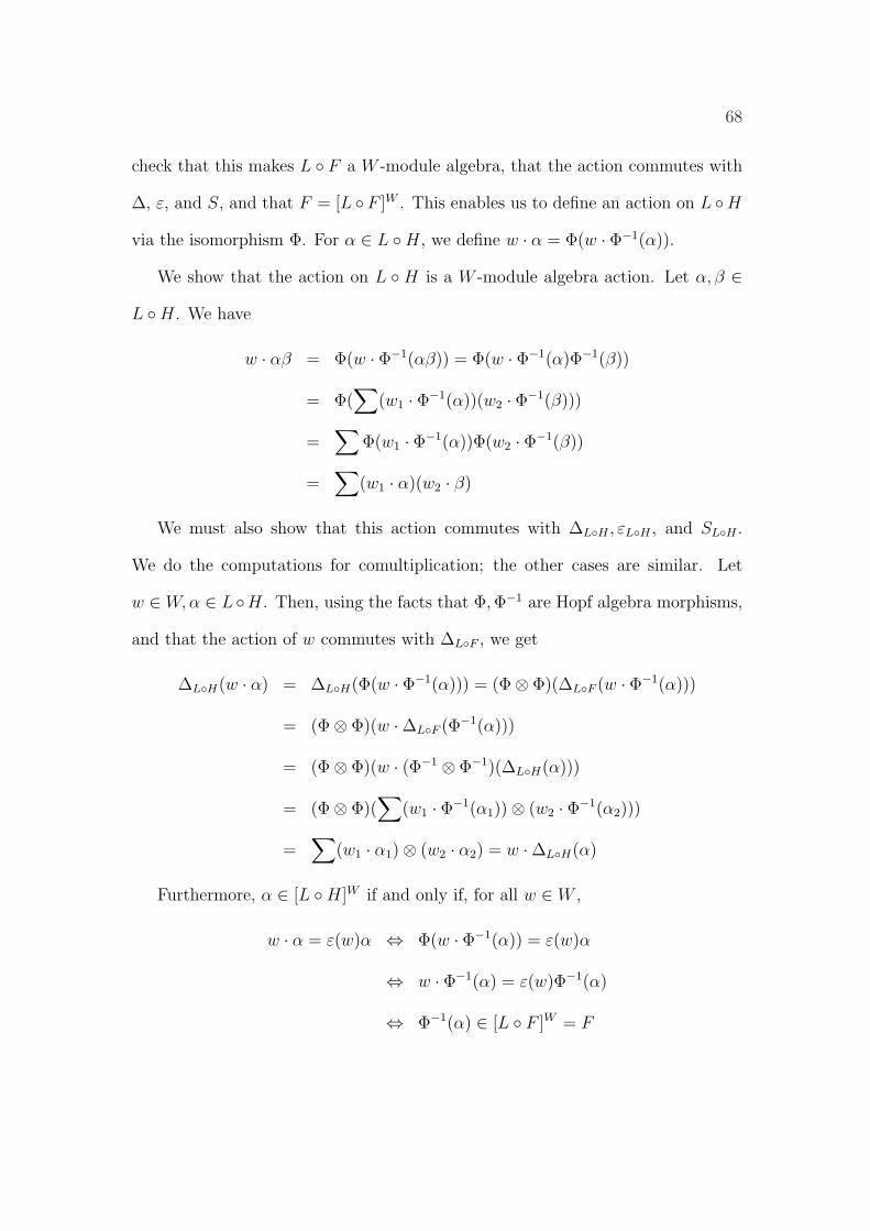
68

check that this makes L ◦ F a W -module algebra, that the action commutes with

∆, ε, and S, and that F = [L ◦F ]W . This enables us to define an action on L ◦H

via the isomorphism Φ. For α ∈ L ◦H, we define w · α = Φ(w · Φ−1(α)).

We show that the action on L ◦ H is a W -module algebra action. Let α, β ∈L ◦H. We have

w · αβ = Φ(w · Φ−1(αβ)) = Φ(w · Φ−1(α)Φ−1(β))

= Φ(∑

(w1 · Φ−1(α))(w2 · Φ−1(β)))

=∑

Φ(w1 · Φ−1(α))Φ(w2 · Φ−1(β))

=∑

(w1 · α)(w2 · β)

We must also show that this action commutes with ∆L◦H , εL◦H , and SL◦H .

We do the computations for comultiplication; the other cases are similar. Let

w ∈ W,α ∈ L ◦H. Then, using the facts that Φ, Φ−1 are Hopf algebra morphisms,

and that the action of w commutes with ∆L◦F , we get

∆L◦H(w · α) = ∆L◦H(Φ(w · Φ−1(α))) = (Φ⊗ Φ)(∆L◦F (w · Φ−1(α)))

= (Φ⊗ Φ)(w ·∆L◦F (Φ−1(α)))

= (Φ⊗ Φ)(w · (Φ−1 ⊗ Φ−1)(∆L◦H(α)))

= (Φ⊗ Φ)(∑

(w1 · Φ−1(α1))⊗ (w2 · Φ−1(α2)))

=∑

(w1 · α1)⊗ (w2 · α2) = w ·∆L◦H(α)

Furthermore, α ∈ [L ◦H]W if and only if, for all w ∈ W ,

w · α = ε(w)α ⇔ Φ(w · Φ−1(α)) = ε(w)α

⇔ w · Φ−1(α) = ε(w)Φ−1(α)

⇔ Φ−1(α) ∈ [L ◦ F ]W = F

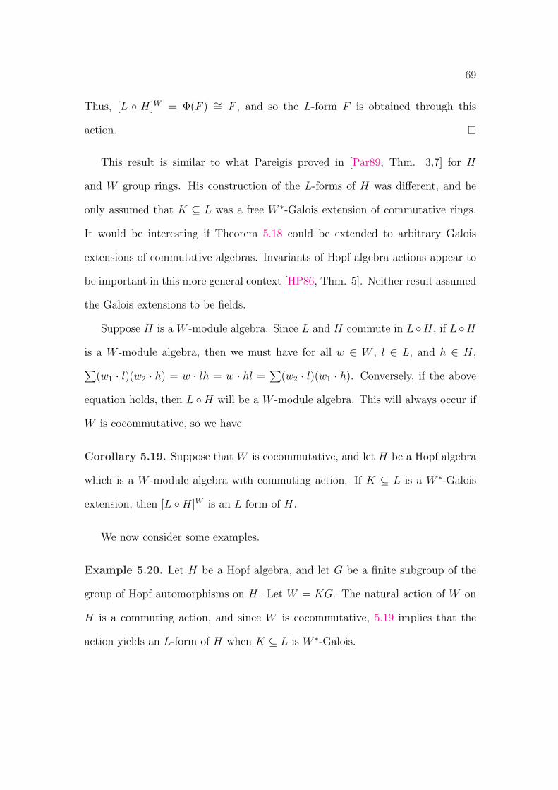
69

Thus, [L ◦ H]W = Φ(F ) ∼= F , and so the L-form F is obtained through this

action.

This result is similar to what Pareigis proved in [Par89, Thm. 3,7] for H

and W group rings. His construction of the L-forms of H was different, and he

only assumed that K ⊆ L was a free W ∗-Galois extension of commutative rings.

It would be interesting if Theorem 5.18 could be extended to arbitrary Galois

extensions of commutative algebras. Invariants of Hopf algebra actions appear to

be important in this more general context [HP86, Thm. 5]. Neither result assumed

the Galois extensions to be fields.

Suppose H is a W -module algebra. Since L and H commute in L ◦H, if L ◦H

is a W -module algebra, then we must have for all w ∈ W , l ∈ L, and h ∈ H,

∑(w1 · l)(w2 · h) = w · lh = w · hl =

∑(w2 · l)(w1 · h). Conversely, if the above

equation holds, then L ◦H will be a W -module algebra. This will always occur if

W is cocommutative, so we have

Corollary 5.19. Suppose that W is cocommutative, and let H be a Hopf algebra

which is a W -module algebra with commuting action. If K ⊆ L is a W ∗-Galois

extension, then [L ◦H]W is an L-form of H.

We now consider some examples.

Example 5.20. Let H be a Hopf algebra, and let G be a finite subgroup of the

group of Hopf automorphisms on H. Let W = KG. The natural action of W on

H is a commuting action, and since W is cocommutative, 5.19 implies that the

action yields an L-form of H when K ⊆ L is W ∗-Galois.

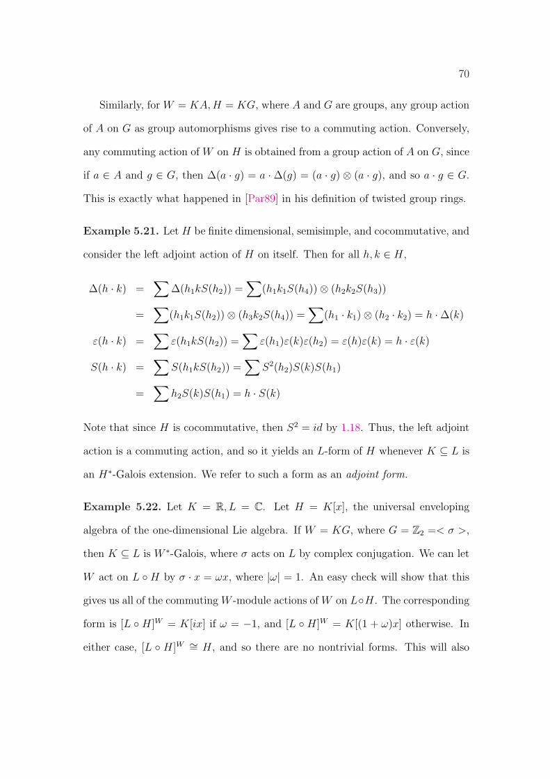
70

Similarly, for W = KA,H = KG, where A and G are groups, any group action

of A on G as group automorphisms gives rise to a commuting action. Conversely,

any commuting action of W on H is obtained from a group action of A on G, since

if a ∈ A and g ∈ G, then ∆(a · g) = a ·∆(g) = (a · g) ⊗ (a · g), and so a · g ∈ G.

This is exactly what happened in [Par89] in his definition of twisted group rings.

Example 5.21. Let H be finite dimensional, semisimple, and cocommutative, and

consider the left adjoint action of H on itself. Then for all h, k ∈ H,

∆(h · k) =∑

∆(h1kS(h2)) =∑

(h1k1S(h4))⊗ (h2k2S(h3))

=∑

(h1k1S(h2))⊗ (h3k2S(h4)) =∑

(h1 · k1)⊗ (h2 · k2) = h ·∆(k)

ε(h · k) =∑

ε(h1kS(h2)) =∑

ε(h1)ε(k)ε(h2) = ε(h)ε(k) = h · ε(k)

S(h · k) =∑

S(h1kS(h2)) =∑

S2(h2)S(k)S(h1)

=∑

h2S(k)S(h1) = h · S(k)

Note that since H is cocommutative, then S2 = id by 1.18. Thus, the left adjoint

action is a commuting action, and so it yields an L-form of H whenever K ⊆ L is

an H∗-Galois extension. We refer to such a form as an adjoint form.

Example 5.22. Let K = R, L = C. Let H = K[x], the universal enveloping

algebra of the one-dimensional Lie algebra. If W = KG, where G = Z2 =< σ >,

then K ⊆ L is W ∗-Galois, where σ acts on L by complex conjugation. We can let

W act on L ◦H by σ · x = ωx, where |ω| = 1. An easy check will show that this

gives us all of the commuting W -module actions of W on L◦H. The corresponding

form is [L ◦ H]W = K[ix] if ω = −1, and [L ◦ H]W = K[(1 + ω)x] otherwise. In

either case, [L ◦ H]W ∼= H, and so there are no nontrivial forms. This will also

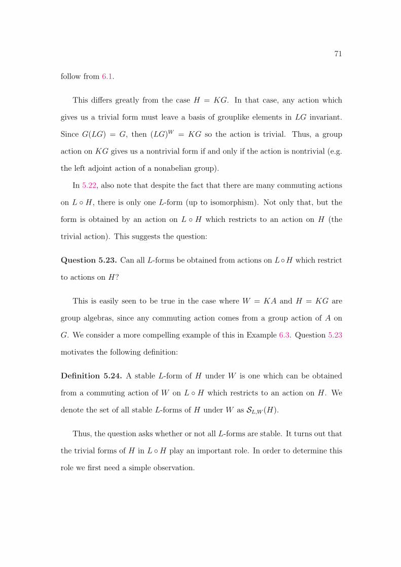
71

follow from 6.1.

This differs greatly from the case H = KG. In that case, any action which

gives us a trivial form must leave a basis of grouplike elements in LG invariant.

Since G(LG) = G, then (LG)W = KG so the action is trivial. Thus, a group

action on KG gives us a nontrivial form if and only if the action is nontrivial (e.g.

the left adjoint action of a nonabelian group).

In 5.22, also note that despite the fact that there are many commuting actions

on L ◦ H, there is only one L-form (up to isomorphism). Not only that, but the

form is obtained by an action on L ◦ H which restricts to an action on H (the

trivial action). This suggests the question:

Question 5.23. Can all L-forms be obtained from actions on L◦H which restrict

to actions on H?

This is easily seen to be true in the case where W = KA and H = KG are

group algebras, since any commuting action comes from a group action of A on

G. We consider a more compelling example of this in Example 6.3. Question 5.23

motivates the following definition:

Definition 5.24. A stable L-form of H under W is one which can be obtained

from a commuting action of W on L ◦ H which restricts to an action on H. We

denote the set of all stable L-forms of H under W as SL,W (H).

Thus, the question asks whether or not all L-forms are stable. It turns out that

the trivial forms of H in L ◦H play an important role. In order to determine this

role we first need a simple observation.

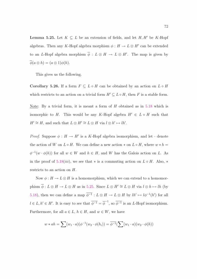
72

Lemma 5.25. Let K ⊆ L be an extension of fields, and let H, H ′ be K-Hopf

algebras. Then any K-Hopf algebra morphism φ : H → L ⊗H ′ can be extended

to an L-Hopf algebra morphism φ : L ⊗ H → L ⊗ H ′. The map is given by

φ(a⊗ h) = (a⊗ 1)φ(h).

This gives us the following.

Corollary 5.26. If a form F ⊆ L ◦ H can be obtained by an action on L ◦ H

which restricts to an action on a trivial form H ′ ⊆ L ◦H, then F is a stable form.

Note: By a trivial form, it is meant a form of H obtained as in 5.18 which is

isomorphic to H. This would be any K-Hopf algebra H ′ ∈ L ◦ H such that

H ′ ∼= H, and such that L⊗H ′ ∼= L⊗H via l ⊗ h′ 7→ lh′.

Proof. Suppose φ : H → H ′ is a K-Hopf algebra isomorphism, and let · denote

the action of W on L ◦H. We can define a new action ∗ on L ◦H, where w ∗ h =

φ−1(w · φ(h)) for all w ∈ W and h ∈ H, and W has the Galois action on L. As

in the proof of 5.18(iii), we see that ∗ is a commuting action on L ◦ H. Also, ∗restricts to an action on H.

Now φ : H → L⊗H is a homomorphism, which we can extend to a homomor-

phism φ : L ⊗H → L ⊗H as in 5.25. Since L ⊗H ′ ∼= L ⊗H via l ⊗ h 7→ lh (by

5.18), then we can define a map φ−1 : L ⊗ H → L ⊗ H by lh′ 7→ lφ−1(h′) for all

l ∈ L, h′ ∈ H ′. It is easy to see that φ−1 = φ−1

, so φ−1 is an L-Hopf isomorphism.

Furthermore, for all a ∈ L, h ∈ H, and w ∈ W , we have

w ∗ ah =∑

(w1 · a)(φ−1(w2 · φ(hi)) = φ−1(∑

(w1 · a)(w2 · φ(h))

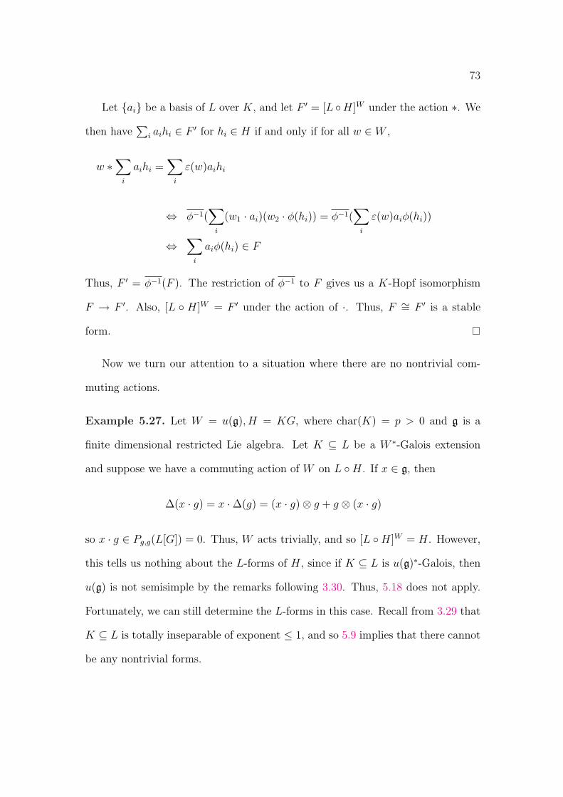
73

Let {ai} be a basis of L over K, and let F ′ = [L ◦H]W under the action ∗. We

then have∑

i aihi ∈ F ′ for hi ∈ H if and only if for all w ∈ W ,

w ∗∑

i

aihi =∑

i

ε(w)aihi

⇔ φ−1(∑

i

(w1 · ai)(w2 · φ(hi)) = φ−1(∑

i

ε(w)aiφ(hi))

⇔∑

i

aiφ(hi) ∈ F

Thus, F ′ = φ−1(F ). The restriction of φ−1 to F gives us a K-Hopf isomorphism

F → F ′. Also, [L ◦ H]W = F ′ under the action of ·. Thus, F ∼= F ′ is a stable

form.

Now we turn our attention to a situation where there are no nontrivial com-

muting actions.

Example 5.27. Let W = u(g), H = KG, where char(K) = p > 0 and g is a

finite dimensional restricted Lie algebra. Let K ⊆ L be a W ∗-Galois extension

and suppose we have a commuting action of W on L ◦H. If x ∈ g, then

∆(x · g) = x ·∆(g) = (x · g)⊗ g + g ⊗ (x · g)

so x · g ∈ Pg,g(L[G]) = 0. Thus, W acts trivially, and so [L ◦H]W = H. However,

this tells us nothing about the L-forms of H, since if K ⊆ L is u(g)∗-Galois, then

u(g) is not semisimple by the remarks following 3.30. Thus, 5.18 does not apply.

Fortunately, we can still determine the L-forms in this case. Recall from 3.29 that

K ⊆ L is totally inseparable of exponent ≤ 1, and so 5.9 implies that there cannot

be any nontrivial forms.

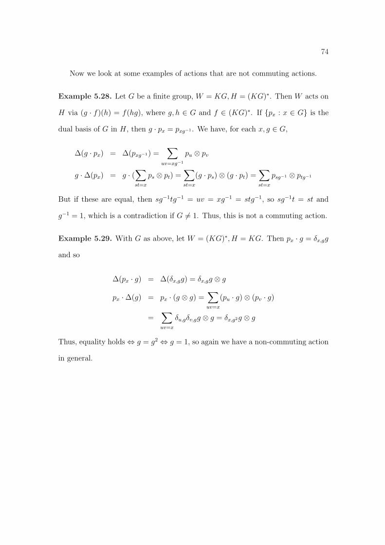
74

Now we look at some examples of actions that are not commuting actions.

Example 5.28. Let G be a finite group, W = KG,H = (KG)∗. Then W acts on

H via (g · f)(h) = f(hg), where g, h ∈ G and f ∈ (KG)∗. If {px : x ∈ G} is the

dual basis of G in H, then g · px = pxg−1 . We have, for each x, g ∈ G,

∆(g · px) = ∆(pxg−1) =∑

uv=xg−1

pu ⊗ pv

g ·∆(px) = g · (∑st=x

ps ⊗ pt) =∑st=x

(g · ps)⊗ (g · pt) =∑st=x

psg−1 ⊗ ptg−1

But if these are equal, then sg−1tg−1 = uv = xg−1 = stg−1, so sg−1t = st and

g−1 = 1, which is a contradiction if G 6= 1. Thus, this is not a commuting action.

Example 5.29. With G as above, let W = (KG)∗, H = KG. Then px · g = δx,gg

and so

∆(px · g) = ∆(δx,gg) = δx,gg ⊗ g

px ·∆(g) = px · (g ⊗ g) =∑uv=x

(pu · g)⊗ (pv · g)

=∑uv=x

δu,gδv,gg ⊗ g = δx,g2g ⊗ g

Thus, equality holds ⇔ g = g2 ⇔ g = 1, so again we have a non-commuting action

in general.

75

Chapter 6

Applications of the Main

Theorem

In this chapter, we use 5.18 to compute L-forms for various Hopf algebras. In

the first section, we characterize the L-forms of enveloping algebras, and give an

example of an enveloping algebra whose L-forms are all stable. Then we turn our

attention to L-forms of H∗, where H is a finite dimensional Hopf algebra. Finally,

we compute a form of KD2n via the adjoint action.

6.1 Forms of Enveloping Algebras

Our first result concerns the Hopf algebra forms of enveloping algebras. It turns

out that these forms are merely enveloping algebras of Lie algebras which are Lie

algebra forms of each other.

Proposition 6.1. Suppose that a K-Hopf algebra F is an L-form of U(g) in

characteristic zero or u(g) in characteristic p > 0. Then

(i) F is a universal enveloping algebra in characteristic zero and a restricted

enveloping algebra in characteristic p > 0.

(ii) If K ⊆ L is a W ∗-Galois field extension in characteristic zero for W a

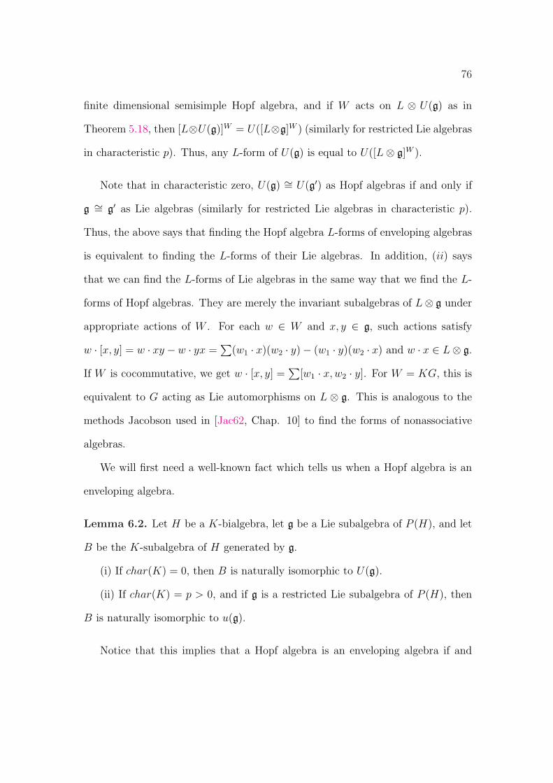
76

finite dimensional semisimple Hopf algebra, and if W acts on L ⊗ U(g) as in

Theorem 5.18, then [L⊗U(g)]W = U([L⊗g]W ) (similarly for restricted Lie algebras

in characteristic p). Thus, any L-form of U(g) is equal to U([L⊗ g]W ).

Note that in characteristic zero, U(g) ∼= U(g′) as Hopf algebras if and only if

g ∼= g′ as Lie algebras (similarly for restricted Lie algebras in characteristic p).

Thus, the above says that finding the Hopf algebra L-forms of enveloping algebras

is equivalent to finding the L-forms of their Lie algebras. In addition, (ii) says

that we can find the L-forms of Lie algebras in the same way that we find the L-

forms of Hopf algebras. They are merely the invariant subalgebras of L⊗ g under

appropriate actions of W . For each w ∈ W and x, y ∈ g, such actions satisfy

w · [x, y] = w · xy −w · yx =∑

(w1 · x)(w2 · y)− (w1 · y)(w2 · x) and w · x ∈ L⊗ g.

If W is cocommutative, we get w · [x, y] =∑

[w1 · x,w2 · y]. For W = KG, this is

equivalent to G acting as Lie automorphisms on L ⊗ g. This is analogous to the

methods Jacobson used in [Jac62, Chap. 10] to find the forms of nonassociative

algebras.

We will first need a well-known fact which tells us when a Hopf algebra is an

enveloping algebra.

Lemma 6.2. Let H be a K-bialgebra, let g be a Lie subalgebra of P (H), and let

B be the K-subalgebra of H generated by g.

(i) If char(K) = 0, then B is naturally isomorphic to U(g).

(ii) If char(K) = p > 0, and if g is a restricted Lie subalgebra of P (H), then

B is naturally isomorphic to u(g).

Notice that this implies that a Hopf algebra is an enveloping algebra if and

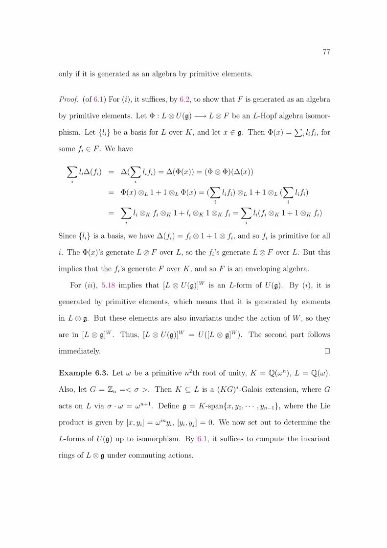
77

only if it is generated as an algebra by primitive elements.

Proof. (of 6.1) For (i), it suffices, by 6.2, to show that F is generated as an algebra

by primitive elements. Let Φ : L⊗ U(g) −→ L⊗ F be an L-Hopf algebra isomor-

phism. Let {li} be a basis for L over K, and let x ∈ g. Then Φ(x) =∑

i lifi, for

some fi ∈ F . We have

∑i

li∆(fi) = ∆(∑

i

lifi) = ∆(Φ(x)) = (Φ⊗ Φ)(∆(x))

= Φ(x)⊗L 1 + 1⊗L Φ(x) = (∑

i

lifi)⊗L 1 + 1⊗L (∑

i

lifi)

=∑

i

li ⊗K fi ⊗K 1 + li ⊗K 1⊗K fi =∑

i

li(fi ⊗K 1 + 1⊗K fi)

Since {li} is a basis, we have ∆(fi) = fi ⊗ 1 + 1⊗ fi, and so fi is primitive for all

i. The Φ(x)’s generate L⊗ F over L, so the fi’s generate L⊗ F over L. But this

implies that the fi’s generate F over K, and so F is an enveloping algebra.

For (ii), 5.18 implies that [L ⊗ U(g)]W is an L-form of U(g). By (i), it is

generated by primitive elements, which means that it is generated by elements

in L ⊗ g. But these elements are also invariants under the action of W , so they

are in [L ⊗ g]W . Thus, [L ⊗ U(g)]W = U([L ⊗ g]W ). The second part follows

immediately.

Example 6.3. Let ω be a primitive n2th root of unity, K = Q(ωn), L = Q(ω).

Also, let G = Zn =< σ >. Then K ⊆ L is a (KG)∗-Galois extension, where G

acts on L via σ · ω = ωn+1. Define g = K-span{x, y0, · · · , yn−1}, where the Lie

product is given by [x, yi] = ωinyi, [yi, yj] = 0. We now set out to determine the

L-forms of U(g) up to isomorphism. By 6.1, it suffices to compute the invariant

rings of L⊗ g under commuting actions.

78

Let 1 ≤ k ≤ n, and define an action of G on U(g) by σ ·x = ω−knx, σ ·yi = yi+k,

where we let yi+n = yi for all i. One can check that this is a commuting action,

and so it will yield a form gk = [L⊗ g]W .

We now compute a basis for gk. Let d = gcd(k, n), set l = nd, and consider the

elements r = ωkx, sjt =∑n−1

i=0 ωjk(in+1)yik+t, where 0 ≤ t ≤ d − 1, 0 ≤ j ≤ l − 1.

It is easy to check that r and the sjt’s are invariants. Moreover, they form a basis

for gk. To see this, note that since L ⊗ g ∼= L ⊗ gk, we have dim(gk) = dim(g) =

n + 1. It thus suffices to prove that {r, sjt} are linearly independent over K. Since

{x, yi : 0 ≤ i ≤ n − 1} is independent over K and r is a scalar multiple of x, it

suffices to show that the sjt’s are linearly independent over K.

Suppose∑

j,t cjtsjt = 0 with cjt ∈ K. Then

0 =∑j,t

cjtsjt =l−1∑j=0

d−1∑t=0

n−1∑i=0

cjtωjk(in+1)yik+t (6.1)

We look at the coefficients of yt for 0 ≤ t ≤ d − 1. It follows from (6.1) that

we get a contribution to the coefficient of yt from each coefficient of yik+t, where

ik + t = zn + t for some z ∈ Z. Thus, i = znk

= zlk/d

, so kd|zl. Since gcd(k

d, l) =

gcd(kd, n

d) = 1, we have k

d|z, so k|zd. Write zd = z′k. Then i = zn

k= zdl

k= z′kl

k= z′l.

In particular, z′ ≤ d− 1. We substitute i = z′l in the coefficient of yik+t to get the

coefficient of yt, which is

l−1∑j=0

d−1∑

z′=0

cjtωjk(z′ln+1) =

l−1∑j=0

d−1∑

z′=0

cjtωjk =

l−1∑j=0

dcjtωjk

since ωjkz′ln = 1. Now the ωjk are linearly independent over K, so cjt = 0, which

proves linear independence.

Thus, gk = span{r, sjt : 0 ≤ t ≤ d − 1, 0 ≤ j ≤ l − 1}. It is not difficult to

79

compute the Lie bracket relations. We get [r, sjt] = ωnts(j+1)t, [sjt, sj′t′ ] = 0, and

s(j+l)t = ωklsjt.

The remainder of this section will be devoted to showing that the gk are mu-

tually nonisomorphic as Lie algebras, and that they are all the L-forms of g. Let

I = span{sjt : 0 ≤ t ≤ d − 1, 0 ≤ j ≤ l − 1} and, for each 0 ≤ t ≤ d − 1, let It =

span{sjt : 0 ≤ j ≤ l − 1}. It is easy to show that I and It are Lie ideals of gk. It

is also clear that I is the unique abelian Lie ideal in gk of codimension 1, and that

I =⊕d−1

t=0 It.

Lemma 6.4. Let w /∈ I. Then

(i) For all 0 ≤ t ≤ d− 1, v ∈ It, v is an eigenvector for adl(w).

(ii) Let v ∈ I. If v is an eigenvector for ad(w)m, then m = 0 or m ≥ l.

Proof. We first reduce the problem a bit. Write w = ar +∑

j bjsjt. Since w /∈ I,

we have a 6= 0, so without loss of generality, a = 1. But then ad(w) = ad(r) on I,

since I is abelian, so we can assume that w = r. An easy induction gives us that

ad(r)m(sjt) = ωmnts(j+m)t for all m ≥ 0. Thus, if v =∑

j cjsjt, then

ad(r)l(v) =∑

j

ωlntcjs(j+l)t =∑

ωlnt+klcjsjt = ωlnt+klv

Thus, v is an eigenvector for ad(r)l, which gives us (i).

For (ii), we can again assume that w = r. We write v =∑d−1

t=0 vt, where vt ∈ It.

If ad(r)m(v) = av, we must have∑

t ad(r)m(vt) =∑

t avt. Since the sum of the

It’s is direct, we have ad(r)m(vt) = avt, and so each vt is an eigenvector for adm(r).

We can then assume that v ∈ It for some t.

Write v =∑l−1

j=0 cjsjt with cj ∈ K. By (i), v is an eigenvector for ad(r)l.

Let m > 0 be minimal such that v is an eigenvector for ad(r)m. Since v is an

80

eigenvector of ad(r)l, a simple number theoretic argument gives us m|l. Write

l = pm for some integer p ≥ 1. We have that ad(r)m(v) = av for some a ∈ K.

Also, a calculation gives us

ad(r)m(v) =∑

j

cjωmnts(j+m)t =

m−1∑j=0

ωkpm+mntcj+(p−1)msjt +

pm−1∑j=m

ωmntcj−msjt

If we equate the coefficients of ad(r)l(v) and av, we get

acj = ωkmp+mntcj+(p−1)m, 0 ≤ j ≤ m− 1 (6.2)

acj = ωmntcj−m, m ≤ j ≤ pm− 1 (6.3)

Let i be minimal such that ci 6= 0. If cj = 0 for all j < m, then (6.3) implies

that v = 0. Therefore, i < m. An easy induction gives us, using (6.3), that

for all integers 0 ≤ b ≤ p − 1, ci = ω−bmntabci+bm. Setting b = p − 1, we get

ci = ω−(p−1)mntap−1ci+(p−1)m. But (6.2) gives us that ci = 1aωkmp+mntci+(p−1)m.

Putting these together and simplifying, we get

ap = ωkmpωpmnt = ωkl+lnt

Now we take pth roots of both sides. Notice, since p|l and l|n, that all the pth roots

of unity are in K. We have a = ωkl+lnt

p · (pth root of unity), and so ωkl+lnt

p ∈ K. We

must then have n|kl+lntp

. Since p|l, we have n| lntp

. This forces n|klp. But kl = n(k

d),

so we must have p|kd.

But recall that gcd(nd, l) = 1. Since, p|l and p|k

d, it follows that p = 1, and so

m = l. This gives us (ii), and the proof is complete.

Proposition 6.5. Let K, L, g, gk be as above.

(i) The gk are mutually nonisomorphic K-Lie algebras.

81

(ii) The gk are all the L-forms of g up to isomorphism, and thus U(gk) are all

the L-forms of U(g).

Proof. Suppose that 1 ≤ k, k′ ≤ n, with gk∼= gk′ . Let d = gcd(n, k), d′ =

gcd(n, k′), l = nd, and l′ = n

d′ . Also define I ′ / gk′ similarly as for I / gk. Without

loss of generality, l ≤ l′. Let Φ : gk → gk′ be an isomorphism of Lie algebras. Since

I, I ′ are the unique abelian ideals of codimension 1 in their respective Lie algebras,

we must have Φ(I) = I ′. By 6.4(i), sjt is an eigenvector for adl(r). Since Φ is an

isomorphism, this makes Φ(sjt) an eigenvector for adl(Φ(r)). But Φ(r) /∈ I ′, so

6.4(ii) gives us l ≥ l′. Then l = l′, which implies that d = d′.

We now have gcd(n, k) = gcd(n, k′) = d. Thus,

gk = span{r, sjt : 0 ≤ j ≤ l − 1, 0 ≤ t ≤ d− 1}

gk′ = span{r′, s′jt : 0 ≤ j ≤ l − 1, 0 ≤ t ≤ d− 1}

Write Φ(s00) =∑

j,t bjts′jt, where bjt ∈ K, and the bjt are not all zero. Also write

Φ(r) = ar′ +∑

j,t ajts′jt, where a, ajt ∈ K. Since ad(Φ(r)) = ad(ar′) on I ′, an easy

induction gives us

ad(Φ(r))l(Φ(s00)) =∑j,t

alωlntbjts′(j+l)t =

∑j,t

alωlnt+k′lbjts′jt

But Φ is a homomorphism, so we get

ad(Φ(r))l(Φ(s00)) = Φ(ad(r)l(s00)) = Φ(sl0) = ωklΦ(s00) =∑j,t

ωklbjts′jt

This tells us that ωklbjt = alωlnt+k′lbjt for all j, t. Since not all the bjt are zero, we

have al = ωl(k−k′−nt) for some t. But then a = ωk−k′−nt · (lth root of unity), and

since a ∈ K, we must have k = k′. This gives us (i).

82

For (ii), we look at what an action of G on L⊗g must satisfy (keeping in mind

that G acts as Lie automorphisms on L⊗ g). After a bit of calculation, we get

σ · x = ω−knx +n−1∑j=1

bjyj, σ · yi = aiyi+k

for some 0 ≤ k ≤ n − 1, where the ai, bj ∈ L are chosen so that σn · x = x and

σn · yi = yi. We will show that [L⊗ g]KG ∼= gk.

To determine the form obtained from this action, we need only consider prim-

itive invariant elements. Suppose that α = ax +∑

j cjyj ∈ [L⊗ g]KG. Then

ax +∑

j

cjyj = (σ · a)ω−knx +∑

j

(σ · a)bjyj +∑

j

(σ · cj)ajyj+k

= (σ · a)ω−knx +∑

j

([σ · a]bj+k + [σ · cj]aj)yj+k

which yields a = (σ · a)ω−kn and cj+k = (σ · a)bj+k + (σ · cj)aj.

Write a =∑n−1

i=0 qiωi with qi ∈ K. The equation a = (σ · a)ω−kn yields

∑i

qiωi =

∑i

qiωin+i−kn =

∑i

qiω(i−k)nωi

Matching coefficients, we get qi = qiω(i−k)n, so qi = 0 or ω(i−k)n = 1. Thus, if

qi 6= 0, then n|i− k and so i = k. Therefore, a = qωk for some q ∈ K.

First, suppose that a = 0. We then have ct+k = (σ · ct)at. Once we are able

to define ct for 0 ≤ t ≤ d − 1, then we can define the rest of the ct inductively

using this relation and the fact that d = gcd{k, n}. The only restriction on ct

is that ct = ct+kl = (σl · ct)(σl−1 · at)(σ

l−2 · at+k) · · · at+(l−1)k = (σl · ct)At, where

At = (σl−1 · at)(σl−2 · at+k) · · · at+(l−1)k. For each 0 ≤ t ≤ d − 1, we then want to

find all of the elements ct ∈ L such that ct = (σl · ct)At with ct 6= 0 if possible. If c′t

is another such element, and ct 6= 0, then it is easy to show thatc′tct

is fixed by σl,

83

and soc′tct∈ Lσl

= K(ωk). Thus, if ct 6= 0, then the set {cjt = ωjkct : 0 ≤ j ≤ l−1}is a basis over K for the space of all c′t satisfying c′t = (σl · c′t)At. We then can

define cj(ik+t) for all 0 ≤ i ≤ l − 1 by defining, inductively, cj(t+k) = (σ · cjt)at. By

the way we have defined cj(ik+t), we get that sjt =∑l−1

i=0 cj(ik+t)yik+t ∈ [L ⊗ g]KG.

Furthermore, since the cjt span all possible coefficients of yt for elements in [L⊗g]KG

which have no nonzero x term, then the sjt span the space of all invariant elements

of the form∑

j cjyj.

If a = qωk 6= 0, then, substituting αq

for α, we can assume that a = ωk. Suppose

we have two sets of elements {b′t}, {b′′t } ⊆ L such that r = ωkx +∑

t b′tyt and

r′ = ωkx +∑

t b′′t yt are KG-invariants. Subtracting these, we get

∑t(b

′t − b′′t )yt ∈

[L ⊗ g]KG, so by the a = 0 case, r − r′ ∈ span{sjt}. Thus, r is unique modulo

span{sjt}.Putting these together, we get that [L⊗ g]KG is spanned by the set

{r, sjt : 0 ≤ t ≤ d− 1, 0 ≤ j ≤ l − 1}

Since dimK [L ⊗ g]KG = n + 1, these elements form a basis for [L ⊗ g]KG. In

particular, sjt 6= 0 for all j, t. We need only show that r and the sjt satisfy the

same Lie product relations as their counterparts in gk.

Claim: Let 0 ≤ t ≤ d− 1. Then cj(t+ik) = ωjk(in+1)c0(t+ik).

Proof. We induct on i. The definition of cjt gives us the i = 0 case. For the

inductive step, we have

cj(t+[i+1]k) = (σ · cj(t+ik))at+ik = (σ · [ωjk(in+1)c0(t+ik)])at+ik

= ωjk([i+1]n+1)(σ · c0(t+ik))at+ik = ωjk([i+1]n+1)c0(t+[i+1]k)

84

which completes the proof.

As an easy corollary, we get

c(j+1)(ik+t) = ω(j+1)k(in+1)c0(ik+t) = ωk(in+1)ωjk(in+1)c0(ik+t)

= ωk(in+1)cj(ik+t)

This gives us

[r, sjt] = [ωkx +∑

j

b′jyj,∑

i

cj(ik+t)yik+t] =∑

i

ωkcj(ik+t)[x, yik+t]

=∑

i

ωkcj(ik+t)ωn(ik+t)yik+t = ωnt

∑i

ωk(in+1)cj(ik+t)yik+t

= ωnt∑

i

c(j+1)(ik+t)yik+t = ωnts(j+1)t

Finally, a trivial computation shows that s(j+l)t = ωklsjt, and so [L ⊗ g]KG ∼= gk.

Thus, the gk are all the L-forms of g up to isomorphism, which gives us (ii).

Notice that all of the L-forms of U(g) are stable.

6.2 Forms of Duals of Hopf Algebras

We turn our attention to determining forms for duals of finite dimensional Hopf

algebras. This can be looked at from two perspectives. First, there is a natural

correspondence between L-forms of H and L-forms of H∗.

Proposition 6.6. Let H be a finite dimensional Hopf algebra over a field K with

K ⊆ L a field extension. Then

(i) L⊗H∗ ∼= (L⊗H)∗ as L-Hopf algebras.

(ii) The L-forms for H∗ are precisely the duals of the L-forms for H.

85

Proof. Define φ : L⊗H∗ → (L⊗H)∗ by φ(a⊗ f)(b⊗ h) = f(h)ab for all a, b ∈ L,

h ∈ H, and f ∈ H∗. We first show that φ is an algebra map. It is clear that

φ(1⊗ εH) = εL⊗H . Let a, b, c ∈ L, h ∈ H, and f, g ∈ H∗. We then have

(φ(a⊗ f)φ(b⊗ g))(c⊗ h) =∑

φ(a⊗ f)(c⊗ h1)φ(b⊗ g)(1⊗ h2)

=∑

abcf(h1)g(h2)

= abc(fg)(h) = φ(ab⊗ fg)(c⊗ h)

= φ([a⊗ f ][b⊗ g])(c⊗ h)

and so φ is an algebra homomorphism.

Now we show that φ is a Hopf algebra morphism. We have

(φ⊗ φ)∆(a⊗ f)([b⊗ h]⊗ [c⊗ h′]) =∑

φ(a⊗ f1)(b⊗ h)⊗ φ(1⊗ f2)(c⊗ h′)

=∑

abcf1(h)f2(h′)

= f(hh′)abc

= φ(a⊗ f)(bc⊗ hh′)

= (∆ ◦ φ(a⊗ f))([b⊗ h]⊗ [c⊗ h′])

and so ∆ ◦ φ = (φ⊗ φ) ◦∆. The other axioms follow similarly, and so φ is a Hopf

algebra morphism.

It remains to show that φ is bijective. By comparing dimensions over L, we

need only show that φ is injective. Let {hi} be a basis for H with dual basis {h∗i },and suppose that

∑i ai ⊗ h∗i ∈ kerφ. Then for all j, we have

0 =∑

i

φ(ai ⊗ h∗i )(1⊗ hj) = aj

and so kerφ = 0. This gives us (i).

86

For (ii), let H ′ be an L-form of H∗. Then

L⊗ (H ′)∗ ∼= (L⊗H ′)∗ ∼= (L⊗H∗)∗ ∼= L⊗H

Thus, (H ′)∗ is an L-form of H. Similarly, if H ′ is an L-form of H, then (H ′)∗ is

an L-form of H∗, and so (ii) follows.

We can also look at this question from the perspective of 5.18. In this context,

we restrict our attention to stable L-forms. Let H, W , and K ⊆ L be as before,

except we require H to be finite dimensional. The stable L-forms for H under W

are obtained by finding appropriate commuting actions of W on H. We attempt

to use these actions to help us compute forms of H∗. Our goal will be to find a

correspondence between stable L-forms of H under W and stable L-forms of H∗

under W cop. The first step in this direction is finding a correspondence between

W -actions on H and W cop-actions on H∗.

Proposition 6.7. If H is a left W -module algebra with a commuting action,

then H◦ is a left W cop-module with commuting action. Conversely, if H is finite

dimensional, then if H∗ is a left W cop-module algebra with commuting action, then

H is a left W -module algebra with commuting action.

Note that in the case where H is infinite dimensional, we can determine some

of the commuting actions of W cop on H◦ from the commuting actions of W on H,

but not necessarily all of them.

Proof. To avoid confusion, we distinguish between the Hopf algebra maps of H

and H◦ by writing them as ∆, ∆∗, etc. We first assume that H is a left W -module

87

algebra with commuting action. Then for all f ∈ H◦, define (w·f)(h) = f(S(w)·h).

We need to show that this is a left W cop-module algebra action on H∗, and that

the action commutes with the Hopf algebra maps of H◦.

We first prove that if f ∈ H◦, then w · f ∈ H◦. It suffices by 1.13 to show that

∆∗(w · f) ∈ H∗ ⊗H∗. Since f ∈ H◦, we can write ∆∗(f) =∑

f1 ⊗ f2, where all

the f1, f2 ∈ H◦, and for every h, h′ ∈ H, we have f(hh′) =∑

f1(h)f2(h′). We get

∆∗(w · f)(h⊗ h′) = (w · f)(hh′) = f(S(w) · hh′)

=∑

f([S(w2) · h][S(w1) · h′])

=∑

f1(S(w2) · h)f2(S(w1) · h′)

=∑

(w2 · f1)(h)(w1 · f2)(h′)

= (∑

(w2 · f1)⊗ (w1 · f2))(h⊗ h′)

so ∆∗(w · f) =∑

(w2 · f1)⊗ (w1 · f2) ∈ H∗ ⊗H∗, giving us w · f ∈ H◦. The above

also shows that the action of w commutes with comultiplication in W cop.

Now we show that this definition leads to an action on H◦. For all w, w′ ∈ W ,

f ∈ H◦, and h ∈ H, we have

(ww′ · f)(h) = f(S(ww′) · h) = f(S(w′)S(w) · h)

= (w′ · f)(S(w) · h) = (w · [w′ · f ])(h)

Thus, it is an action. For the remainder of the W -module algebra structure, we

88

note that

(w · ε)(h) = ε(S(w) · h) = ε(S(w))ε(h) = ε(w)ε(h) = (ε(w)ε)(h)

(w · fg)(h) = fg(S(w) · h) =∑

f([S(w) · h]1)g([S(w) · h]2)

=∑

f(S(w2) · h1)g(S(w1) · h2) =∑

(w2 · f)(h1)(w1 · g)(h2)

=∑

(w2 · f)(w1 · g)(h)

which gives us that W cop acts trivially on ε, and w · fg =∑

(w2 · f)(w1 · g).

Therefore, H◦ is a left W cop-module algebra.

Now we must prove that we have a commuting action. As shown above, the

action commutes with comultiplication in H◦. For the counit and antipode,

ε∗(w · f) = (w · f)(1H) = f(S(w) · 1H) = ε(w)ε∗(f)

S∗(w · f)(h) = (w · f)(S(h)) = f(S(w) · S(h)) = f(S(S(w) · h))

= (f ◦ S)(S(w) · h) = S∗(f)(S(w) · h) = (w · S∗(f))(h)

which gives us that the action commutes.

Conversely, suppose that H is finite dimensional and that H∗ is a left W cop-

module algebra with commuting action. Then S is bijective by [Mon93, 2.1.3(2)].

Let {h1, · · · , hn} be a basis for H, {h∗1, · · · , h∗n} the dual basis in H∗. Then for

each w ∈ W and 1 ≤ i ≤ n, we have w ·h∗i =∑

j aij(w)h∗j , where aij ∈ W ∗. Define

the action w · hi =∑

j aji(S−1(w))hj.

Claim: For all f ∈ H∗, w ∈ W,h ∈ H, we have (w · f)(h) = f(S(w) · h)

Proof. It suffices to prove the claim for f = h∗i and h = hk. We have

(w · h∗i )(hk) =∑

j

aij(w)h∗j(hk) = aik(w) = h∗i (∑

j

ajk(w)hj) = h∗i (S(w) · hk)

89

which proves the claim.

Let f ∈ H∗, h ∈ H, and w, w′ ∈ W . We will use the fact that S and S−1 are

algebra anti-homomorphisms and coalgebra anti-morphisms by 1.16. We have

f(ww′ · h) = (S−1(ww′) · f)(h) = (S−1(w′)S−1(w) · f)(h)

= (S−1(w) · f)(w′ · h) = f(w · [w′ · w′])

Since this is true for all f ∈ H∗, it follows that ww′ · h = w · (w′ · h), which implies

that we have a left action.

For the W -module algebra requirements, we have, for all f ∈ H∗,

f(ε(w) · 1H) = ε(w)f(1H) = ε(S−1(w))ε∗(f)

= ε∗(S−1(w) · f) = (S−1(w) · f)(1H) = f(w · 1H)

which implies that W acts trivially on 1H .

The multiplicative aspect of H being a W -module algebra requires a small fact.

Let w, f be as before, with h, h′ ∈ H, and let ∆∗(f) =∑

f1 ⊗ f2. Then using

the fact that we are acting on H∗ by W cop, as well as the fact that this action

commutes,

∆∗(S−1(w) · f)(h⊗ h′) = (S−1(w) ·∆∗(f))(h⊗ h′)

=∑

(S−1(w1) · f1 ⊗ S−1(w2) · f2)(h⊗ h′)

=∑

(S−1(w1) · f1)(h)(S−1(w2) · f2)(h′)

=∑

f1(w1 · h)f2(w2 · h′)

=∑

∆∗(f)(w1 · h⊗ w2 · h′)

90

We then have, for all f ∈ H∗,

f(w · [hh′]) = (S−1(w) · f)(hh′) = ∆∗(S−1(w) · f)(h⊗ h′)

=∑

∆∗(f)(w1 · h⊗ w2 · h′)

=∑

f([w1 · h][w2 · h′])

= f(∑

[w1 · h][w2 · h′])

and so w · (hh′) =∑

(w1 · h)(w2 · h′).Finally, we show that the action commutes. Let f, g ∈ H∗. Then

(f ⊗ g)(∆(w · h)) =∑

f([w · h]1)g([w · h]2) = fg(w · h)

= (S−1(w) · fg)(h) =∑

(S−1(w1) · f)(S−1(w2) · g)(h)

=∑

(S−1(w1) · f)(h1)(S−1(w2) · g)(h2)

=∑

f(w1 · h1)g(w2 · h2)

= (f ⊗ g)(w ·∆(h))

Thus, equality holds for all elements of H∗⊗H∗ = (H⊗H)∗, so ∆(w ·h) = w ·∆(h).

For the counit,

ε(w · h) = (S−1(w) · ε)(h) = (ε(S−1(w))ε)(h) = ε(w)ε(h)

Finally, for the antipode, we have for all f ∈ H∗,

f(w · S(h)) = (S−1(w) · f)(S(h)) = S∗(S−1(w) · f)(h)

= (S−1(w) · S∗(f))(h) = S∗(f)(w · h) = f(S(w · h))

so w · S(h) = S(w · h). This completes the proof.

91

Now we see how this fits in with the general theory of L-forms. Let H be a

finite dimensional K-Hopf algebra, K ⊆ L a W ∗-Galois extension of fields, such

that H is a W -module algebra with commuting action. Then, by 6.7, we have a

correspondence between commuting actions on H and commuting actions on H∗.

We would like this to give a correspondence between forms of H and forms of

H∗, but there are two items that must be addressed. First of all, we must figure

out what the (W cop)∗-Galois extensions are. This is answered in the following

proposition.

Proposition 6.8. An extension B ⊆ A of commutative K-algebras is right W ∗-

Galois if and only if it is right (W cop)∗-Galois.

Proof. Suppose B ⊆ A is a commutative W ∗-Galois extension. We show that the

action of W on L is a W cop-module algebra action as well. For w ∈ W and a, b ∈ A,

we have

w · (ab) = w · (ba) =∑

[w1 · b][w2 · a] =∑

[w2 · a][w1 · b]

so A is a W cop-module algebra. W cop clearly acts trivially on 1, and since the

action of W cop is the same as W , it is easy to see that K ⊆ L is (W cop)∗-Galois

by 3.27(ii). The converse follows similarly.

Thus, any correspondence we get would be between L-forms of H and L-forms

of H∗. The second issue involves the fact that 5.18 demands both that W have a

commuting action on H and that this action makes L ⊗H a W -module algebra.

As was mentioned just before 5.19, this will occur if and only if∑

(w1 · l)(w2 ·h) =

∑(w2 · l)(w1 · h). Of course, this is always true when W is cocommutative.

92

Question 6.9. If A ⊆ B is a W ∗-Galois extension of commutative algebras, must

W be cocommutative?

Greither and Pareigis showed this to be the case when K ⊆ L is a separable field

extension [GP87, 1.3]. Recall from the remarks following Question 3.31 that if

K ⊆ L is W ∗-Galois, then W has to be an L-form of a group algebra, where L is

the normal closure of L. The group involved is a subgroup G of G(L/K). Since KG

is cocommutative, so is W . Cohen makes an even stronger conjecture in [Coh94],

where she asks whether a noncommutative Hopf algebra can act faithfully on a

commutative algebra. She and Westreich get a negative answer to this question in

the case where A ⊆ B is an extension of fields and S2 6= id [CW93, 0.11].

Recall from 3.28(iv) that in the case where we have an extension of fields, we

can interpret Hopf Galois extensions in terms of crossed products. Here we get

L ∼= LH#σH∗ = Kσ(H∗), since the action of the crossed product is trivial. So

Question 6.9 becomes, replacing H∗ with H,

Question 6.10. If Kσ(H) is commutative, must H be commutative also?

We get a positive answer in the case of group crossed products, for if Kσ(G)

is commutative, then σ(g, h)gh = σ(h, g)hg for all g, h ∈ G. Thus, gh and hg are

scalar multiples of each other, and so gh = hg, making the group commutative.

The general case is more difficult, since Kσ(H) is commutative ⇔ for all h, k ∈ H

∑σ(h1, k1)#h1k1 =

∑σ(k1, h1)#k1h1 ⇔

∑σ(h1, k1)h1k1 =

∑σ(k1, h1)k1h1, and

so bases are not particularly helpful.

Let us return to the correspondence of stable L-forms. We can think of L-forms

of H in two ways. In light of 5.18, we can think of them as K-subspaces of L⊗H.

93

Another way is to think of them as Hopf-isomorphism classes of these subspaces.

Thus, we can approach the task of finding a correspondence between the stable L-

forms of H and H∗ from each of these perspectives. Let us begin by assuming that

SL,W (H) is the set of all subspaces of L⊗H which are stable L-forms of H under

W as in 5.18, and similarly for SL,W cop(H∗). To find a correspondence between

stable L-forms of H under W and stable L-forms of H∗ under W cop, we define

the map Φ : SL,W (H) → {subspaces of L ⊗ H∗} as follows. Let H ′ ∈ SL,W (H).

Then H ′ = [L ⊗H]W for some commuting action of W on L ⊗H which restricts

to an action on H. Since LH ′ = L⊗H, the (trivial) action of W on H ′ uniquely

determines the action of W on H, and so this action is unique. From 6.7 and

6.8, we have a corresponding commuting action of W cop on H∗ and K ⊆ L is

(W cop)∗-Galois. We define Φ([L⊗H]W ) = [L⊗H∗]Wcop

.

It is not clear that this map will be a correspondence of stable L-forms (as

subspaces). As was mentioned in Question 6.9, it is not certain that commuting

actions of W on H which make L⊗H a W -module algebra correspond to actions

of W cop on H∗ which make L⊗H∗ a W -module algebra. Thus, Φ(H ′) may not be

an L-form of H. Similarly, only the commuting actions on H which make L⊗H

a W -module algebra are considered, so it is possible that some forms of H∗ will

not lie in the image of Φ. Something can still be said in certain cases. We restrict

ourselves to a context which includes the case where W and H are both group

algebras.

Given a commuting action of W on H, suppose that there exists a basis for H

such that, for all w ∈ W , w and S(w) act as transpose matrices on H. This occurs

in the case where W and H are group algebras, since if g ∈ G(W ), then g acts

94

as a permutation of G(H), which is a basis for H. So if we let Ag be the matrix

representing the action of g on H, we get Atg = A−1

g = Ag−1 = AS(g), and so g and

S(g) act as transpose matrices with respect to the basis G(H).

So suppose that w and S(w) act as transpose matrices with respect to the

basis {h1, · · · , hn} of H, and let {h∗1, · · · , h∗n} be the dual basis in H∗. We then

have, for all w ∈ W , w · hi =∑

k aik(w)hk, where aik ∈ W ∗. By assumption,

S(w) · hi =∑

k aki(w)hk. If we consider what the corresponding action of W cop on

H∗ looks like, we have

(w · h∗i )(hj) = h∗i (S(w) · hj) =∑

k

akj(w)h∗i (hk) = aij(w) =∑

k

aik(w)h∗k(hj)

so w · h∗i =∑

k aik(w)h∗k.

Because of the nice relationship between the actions of W on H and W cop on

H∗, we get some interesting consequences:

Proposition 6.11. If w and S(w) act as transpose matrices with respect to some

basis {hi} of H for all w ∈ W , then an action of W on H makes L ⊗ H a W -

module algebra if and only if the corresponding action of W cop on H∗ makes L⊗H∗

a W cop-module algebra.

Proof. L⊗H is a W -module algebra ⇔ ∑(w1 · l)(w2 · hi) =

∑(w2 · l)(w1 · hi) for

all l ∈ L, w ∈ W , and 1 ≤ i ≤ n ⇔ ∑k(w1 · l)aik(w2)hk =

∑k aik(w1)(w2 · l)hk ⇔

∑aik(w2)(w1 · l) =

∑aik(w1)(w2 · l) for each i, k. The same calculations with h∗i in

place of hi give us the same equivalent conditions for L⊗H∗ being a W cop-module

algebra.

Putting this together with 6.7 gives us a one-to-one correspondence between

actions yielding L-forms of H and actions yielding L-forms of H∗. What makes this

95

especially nice is that we do not need the assumption that W is cocommutative.

Similar computations as in 6.11 give us the following:

Proposition 6.12. If w and S(w) act as transpose matrices with respect to the

basis {hi}, then∑

i lihi ∈ [L⊗H]W if and only if∑

i lih∗i ∈ [L⊗H∗]W

cop.

This leads us to the following bijection of subspaces.

Theorem 6.13. Suppose that for all commuting actions of W on H the elements

w and S(w) act as transpose matrices with respect to some basis of H for all

w ∈ W . Then the map Φ : SL,W (H) → SL,W (H∗) is a bijection, where we consider

SL,W (H) to be the invariant subspaces of L ⊗H arising from commuting actions

on H which make L⊗H a W -module algebra (similarly for SL,W cop(H∗)).

Proof. By 6.11, imΦ = SL,W cop(H∗). We thus need only prove injectivity. Recall

that Φ([L ⊗ H]W ) = [L ⊗ H∗]Wcop

. For clarity, if the action of W on H is given

by ·, then we write [L ⊗ H]W = [L ⊗ H]·W and similarly for H∗. Suppose there

are two actions · and ◦ on H such that the corresponding actions on H∗ give

[L⊗H∗]·Wcop

= [L⊗H∗]◦Wcop

. Let∑

i lihi ∈ [L⊗H]·W . By 6.12, we have∑

i lih∗i ∈

[L⊗H∗]·Wcop

= [L⊗H∗]◦Wcop

. Again by 6.12,∑

i lihi ∈ [L⊗H]◦W , so [L⊗H]·W ⊆[L ⊗ H]◦W . By symmetry, equality holds, and so Φ is injective, and the proof is

complete.

Now we address the question of whether Φ is bijective when considered as a

map between isomorphism classes of L-forms. In this case, it is not even clear

that Φ is well-defined, since Φ depends on the choice of action. In the case where

W = KG, something can be said if we assume the transpose condition above. In

96

this case, there is also a nice matching of actions of W on L⊗H and L⊗H∗ with

the correspondence of L-forms given by 6.6. But we first need a lemma.

Lemma 6.14. Let H be a finite dimensional Hopf algebra which is a W -module

algebra such that L ⊗ H is also a W -module algebra. Suppose further that w

and S(w) act as transpose matrices for all w ∈ W with respect to the basis {hi}of H. Let {h∗i } be the dual basis in H∗, and suppose that

∑i bihi ∈ [L ⊗ H]W ,

∑i cih

∗i ∈ [L ⊗H∗]W

cop. Finally, for each w ∈ W , let w · hi =

∑j aij(w)hj where

aij ∈ W ∗. Then

(i) ε(w)bi =∑

j aji(w2)(w1 · bj) =∑

j aji(w1)(w2 · bj)

(ii) ε(w)ci =∑

j aji(w2)(w1 · cj) =∑

j aji(w1)(w2 · cj)

(iii) δi,kε(w) =∑

j aji(w2)ajk(w1) =∑

j aij(w2)akj(w1)

Proof. For (i), let∑

i bihi ∈ [L⊗H]W . We have

∑i

ε(w)bihi = w ·∑

i

bihi =∑

j

(w1 · bj)(w2 · hj) =∑i,j

(w1 · bj)aji(w2)hi

Thus, ε(w)bi =∑

j aji(w2)(w1 · bj). If we do the same computations with the

equality ε(w)bihi =∑

j(w2 · bj)(w1 · hj), we get the second identity. (ii) follows

similarly.

For (iii), we have

ε(w)hi =∑

w1S(w2) · hi =∑

j

w1 · (aji(w2)hj) =∑

j,k

aji(w2)ajk(w1)hk

This gives us δi,kε(w) =∑

j aji(w2)ajk(w1), which is the first identity in (iii). If we

do the same calculations using ε(w) =∑

S(w1)w2, we get the second identity.

97

Theorem 6.15. Let W = KG with H and L as above, and suppose that w, S(w)

act as transpose matrices for all w ∈ W . Let H ′ = [L ⊗H]W with corresponding

L-form H ′ = [L⊗H∗]W of H∗. Then H ′ ∼= (H ′)∗.

Proof. Let α =∑

i bihi ∈ [L ⊗ H]W , f =∑

i cih∗i ∈ [L ⊗ H∗]W . Define the map

φ : H ′ → (H ′)∗ by φ(f)(α) =∑

i bici. It is clear that φ is just the restriction of

the isomorphism in 6.6 to H ′. We must first show that∑

i bici ∈ K. We have, for

each g ∈ G,

∑i

bici =∑

i,j,k

aji(g)aki(g)(g · bj)(g · ck), by 6.14(i), (ii)

=∑

j,k

δj,k(g · bj)(g · ck), by 6.14(iii)

= g · (∑

j

bjcj)

Thus,∑

i bici ∈ LW = K. The fact that φ is a K-Hopf algebra isomorphism follows

from the fact that the isomorphism in 6.6 is an L-Hopf algebra isomorphism.

Example 6.16. Let K = Q and L = Q(i), so K ⊆ L is W ∗-Galois, where

W = KZ2,Z2 =< τ >. Let H = KZn, with Zn =< σ >. Then the commuting

actions of W on H are given by τ · σ = σk, where k2 ≡ 1 (mod n). Let d =

gcd(k−1, n). Now [L⊗H]W is spanned by the elements (1+τ) ·σj and (1+τ) · iσj,

since 1 + τ ∈ ∫ l

W. A quick calculation shows that the fixed grouplike elements are

σtnd , where 0 ≤ t ≤ d− 1. The form becomes

Hk = span{σ tnd , σj + σkj, iσj − iσkj : 0 ≤ t ≤ d− 1, 0 ≤ j ≤ n− 1,

j 6= tn

d, j < kj}

where j < kj means that if we look at them mod n, we choose j to be the smaller

one. This weeds out redundant elements so that the above is a basis. To determine

98

the Hopf algebra structure, let cj = σj + σkj, sj = iσj − iσkj. Then

cjcm = cj+m + cj+km, cjsm = sj+m − sj+km, sjsm = −cj+m + cj+km

∆(cj) =1

2(cj ⊗ cj − sj ⊗ sj), ∆(sj) =

1

2(cj ⊗ sj + sj ⊗ cj)

ε(cj) = 2, ε(sj) = 0, S(cj) = cn−j, S(sj) = sn−j

We first show that the Hk are mutually nonisomorphic. If Hk∼= Hl, we must

then have G(Hk) ∼= G(Hl). In particular, they must have the same order. But if

we look at the basis above, this will only occur when gcd(k− 1, n) = gcd(l− 1, n),

since the grouplikes in Hk are contained in < σ >.

Let φ : Hk → Hl be an isomorphism. Define c′j ∈ Hl analogously as in Hk.

We claim that φ(cj) = c′γ(j), s′j = s′γ(j), where γ permutes the j’s mod n. Consider

id ⊗ φ : L ⊗ Hk → L ⊗ Hl. An easy computation shows that G(L ⊗ Hk) =

{12(cj + isj) : 1 ≤ j ≤ n} and similarly for G(L⊗Hl). Thus,

φ(cj) + iφ(sj) = (id⊗ φ)(cj + isj) = c′γ(j) + is′γ(j)

for some 1 ≤ γ(j) ≤ n, and the claim follows.

Now write n = 2rn1 · · ·nm, ni = psii , where the pi’s are distinct odd primes.

Since k2 ≡ l2 ≡ 1(mod n) then a well-known fact from number theory gives

us that k ≡ ±1(mod ni), l ≡ ±1(mod ni), k and l are odd when r = 1, and

k ≡ ±1(mod 2r−1), l ≡ ±1(mod 2r−1) when r > 1.

First, suppose that n is odd. If k ≡ 1(mod ni), then ni divides both k − 1

and n so ni|d. Thus, l ≡ 1(mod ni). This says that either k ≡ l ≡ 1(mod ni)

or k ≡ l ≡ −1(mod ni) for all i. In any case, k ≡ l(mod ni) for all i, and so

99

k ≡ l(mod n). Since 1 ≤ k, l < n, then k = l. A similar argument works for r = 1,

since we have k ≡ l ≡ 1(mod 2).

The final case is when r > 1. We assume, for contradiction, that k 6≡ l(mod

2r), since otherwise k ≡ l(mod n) by the above case. Suppose that k ≡ 1(mod

2r−1). As before, l ≡ 1(mod 2r−1). But there are only two possible congruences for

k and l mod 2r: 1 and 2r−1 + 1. Since k 6≡ l(mod 2r), one of them, say k, must be

congruent 1 mod 2r. But then 2r|k− 1, so since gcd(k− 1, n) = gcd(l− 1, n), and

2r|n, then 2r|l − 1. But this implies that k ≡ l(mod 2r), which is a contradiction.

We must then have k ≡ l ≡ −1(mod 2r−1).

Without loss of generality, k ≡ 2r−1 − 1(mod 2r) and l ≡ −1(mod 2r). Then

l + 1 = m2r, k + 1 = m′2r−1, where m,m′ ∈ Z and m′ is odd. Let c′j = φ(c1). We

have, by the multiplication tables and the fact that ck+1 = 2σk+1,

φ(c2) + 2φ(σk+1) = φ(c21) = c′2j = c′2j + 2σ(l+1)j

Therefore, φ(σk+1) = σ(l+1)j or φ(c2) = 2σ(l+1)j. In the first case, we have

|σk+1| = |σ(l+1)j|. But |σ(l+1)j| divides |σl+1| = |σm2r |, which divides |σ2r |, an

odd number. In contrast, |σk+1| = |σm′2r−1|, which is even since m′ is odd. This is

a contradiction.

Finally, φ(c2) = σ(l+1)j will only occur when 12c2 is grouplike. But this forces

nd|2, which implies that d = n

2or n. If d = n then we must have k = l = 1. If

d = n2, then since k, l < n, we must have k = l = n+2

2. In either case, k = l, so the

Hk are mutually nonisomorphic.

Now we look at the dual situation. If we let {pj} be the dual basis to {σj},then we have that W acts on H∗ via τ · pj = pkj where k2 ≡ 1 (mod n). Let d =

100

gcd(k − 1, n). We get the L-form

Hk = span{p tnd, pj + pkj, ipj − ipkj : 0 ≤ t ≤ d− 1, 0 ≤ j ≤ n− 1,

j /∈ (tn

d)Z, j < kj}

Define cj = pj + pkj, sj = ipj − ipkj. The multiplication is given by

cj cm = (δj,m + δkj,m)cm

cj sm = (δj,m + δkj,m)sm

sj sm = (δkj,m − δj,m)cm

Checking the rest of the Hopf algebra structure of Hk, we have

∆(ci) =1

2

∑j

cj ⊗ ci−j − sj ⊗ si−j, ∆(sj) =1

2

∑j

cj ⊗ si−j + sj ⊗ ci−j

ε(ci) = 2δi,0, ε(si) = 0, S(ci) = cn−i, S(si) = sn−i

By 6.15, we have that Hk∼= H∗

k . This is easy to compute directly. If we map

ci 7→ 2c∗i and si 7→ −2s∗i , then one can check that this gives us an isomorphism

HK → H∗k .

Most of the proof of 6.15 can be duplicated for general W . We need only show

that∑

i bici ∈ K. So we ask

Question 6.17. If∑

i bihi ∈ [L ⊗ H]W ,∑

i cih∗i ∈ [L ⊗ H∗]W

cop, does this imply

that∑

i bici ∈ K?

This is not obvious in the general case, since 6.14 does not seem to be helpful

when W is not a group algebra.

101

6.3 Adjoint Forms

As mentioned in 5.21, if H is a finite dimensional, semisimple, cocommutative Hopf

algebra, and if K ⊆ L is an H∗-Galois extension, then we can obtain a form for H

via the adjoint action of H on itself. In addition, we can find a form for H∗ using

the correspondence of actions given in 6.7. We demonstrate this on KD2n.

Example 6.18. Let ω be a primitive nth root of unity, and let α be a real nth root

of 2. Let K = Q(ω + ω−1) and L = K(α, ω). Let H = KD2n, where D2n is the

dihedral group of order 2n. Then D2n has a presentation

< σ, τ : σn = 1, τ 2 = 1, τστ−1 = σ−1 >

Furthermore, K ⊆ L is H∗-Galois, with the action of D2n on L given by

σ · α = ωα, σ · ω = ω, τ · α = α, τ · ω = ω−1

We obtain a form of H by letting H act on itself via the adjoint action, which

gives us σ · τ = σ2τ and τ · σ = σ−1. We then compute H ′ = [L⊗H]H to find an

L-form of H. Note that this action yields a nontrivial form, since the only group

action that yields a trivial form is the trivial action.

Consider the elements ek = 1n

∑n−1i=0 ωkiσi, e′k = 1

2α2kekτ . It is clear that σ fixes

ek, since σ fixes ω and σ. We have

τ · ek =1

n

n−1∑i=0

(τ · ω)ki(τ · σ)i =1

n

n−1∑i=0

ω−kiσ−i =1

n

n−1∑i=0

ωkiσi = ek

and so ek ∈ H ′. For the e′k, it is clear that they are fixed by τ , since τ fixes α, τ ,

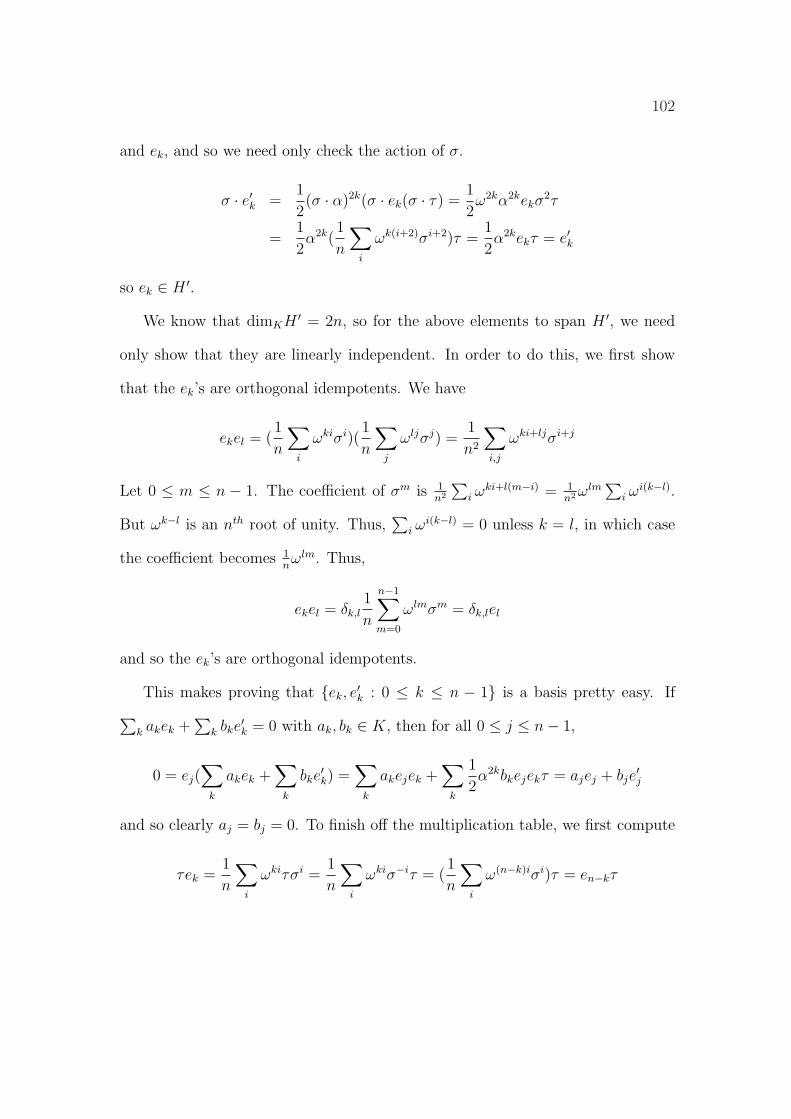
102

and ek, and so we need only check the action of σ.

σ · e′k =1

2(σ · α)2k(σ · ek(σ · τ) =

1

2ω2kα2kekσ

2τ

=1

2α2k(

1

n

∑i

ωk(i+2)σi+2)τ =1

2α2kekτ = e′k

so ek ∈ H ′.

We know that dimKH ′ = 2n, so for the above elements to span H ′, we need

only show that they are linearly independent. In order to do this, we first show

that the ek’s are orthogonal idempotents. We have

ekel = (1

n

∑i

ωkiσi)(1

n

∑j

ωljσj) =1

n2

∑i,j

ωki+ljσi+j

Let 0 ≤ m ≤ n − 1. The coefficient of σm is 1n2

∑i ω

ki+l(m−i) = 1n2 ω

lm∑

i ωi(k−l).

But ωk−l is an nth root of unity. Thus,∑

i ωi(k−l) = 0 unless k = l, in which case

the coefficient becomes 1nωlm. Thus,

ekel = δk,l1

n

n−1∑m=0

ωlmσm = δk,lel

and so the ek’s are orthogonal idempotents.

This makes proving that {ek, e′k : 0 ≤ k ≤ n − 1} is a basis pretty easy. If

∑k akek +

∑k bke

′k = 0 with ak, bk ∈ K, then for all 0 ≤ j ≤ n− 1,

0 = ej(∑

k

akek +∑

k

bke′k) =

∑

k

akejek +∑

k

1

2α2kbkejekτ = ajej + bje

′j

and so clearly aj = bj = 0. To finish off the multiplication table, we first compute

τek =1

n

∑i

ωkiτσi =1

n

∑i

ωkiσ−iτ = (1

n

∑i

ω(n−k)iσi)τ = en−kτ

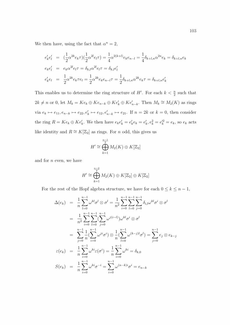
103

We then have, using the fact that αn = 2,

e′ke′l = (

1

2α2kekτ)(

1

2α2lelτ) =

1

4α2(k+l)eken−l =

1

4δk+l,nα2nek = δk+l,nek

eke′l = ekα

2lelτ = δk,lα2lelτ = δk,le

′l

e′kel =1

2α2kekτel =

1

2α2keken−lτ =

1

2δk+l,nα2kekτ = δk+l,ne′k

This enables us to determine the ring structure of H ′. For each k < n2

such that

2k 6= n or 0, let Mk = Kek ⊕Ken−k ⊕Ke′k ⊕Ke′n−k. Then Mk∼= M2(K) as rings

via ek 7→ e11, en−k 7→ e22, e′k 7→ e12, e

′n−k 7→ e21. If n = 2k or k = 0, then consider

the ring R = Kek ⊕Ke′k. We then have eke′k = e′kek = e′k, e

2k = e′2k = ek, so ek acts

like identity and R ∼= K[Z2] as rings. For n odd, this gives us

H ′ ∼=n−1

2⊕

k=1

M2(K)⊕K[Z2]

and for n even, we have

H ′ ∼=n−2

2⊕

k=1

M2(K)⊕K[Z2]⊕K[Z2]

For the rest of the Hopf algebra structure, we have for each 0 ≤ k ≤ n− 1,

∆(ek) =1

n

n−1∑

l=0

ωklσl ⊗ σl =1

n2

n−1∑i=0

n−1∑

l=0

n−1∑j=0

δi,lωklσi ⊗ σl

=1

n2

n−1∑i=0

n−1∑

l=0

(n−1∑j=0

ωj(i−l))ωklσi ⊗ σl

=n−1∑j=0

1

n(n−1∑i=0

ωjiσi)⊗ 1

n(n−1∑

l=0

ω(k−j)lσl) =n−1∑j=0

ej ⊗ ek−j

ε(ek) =1

n

n−1∑i=0

ωkiε(σi) =1

n

n−1∑i=0

ωki = δk,0

S(ek) =1

n

n−1∑i=0

ωkiσ−i =n−1∑i=0

ω(n−k)iσi = en−k

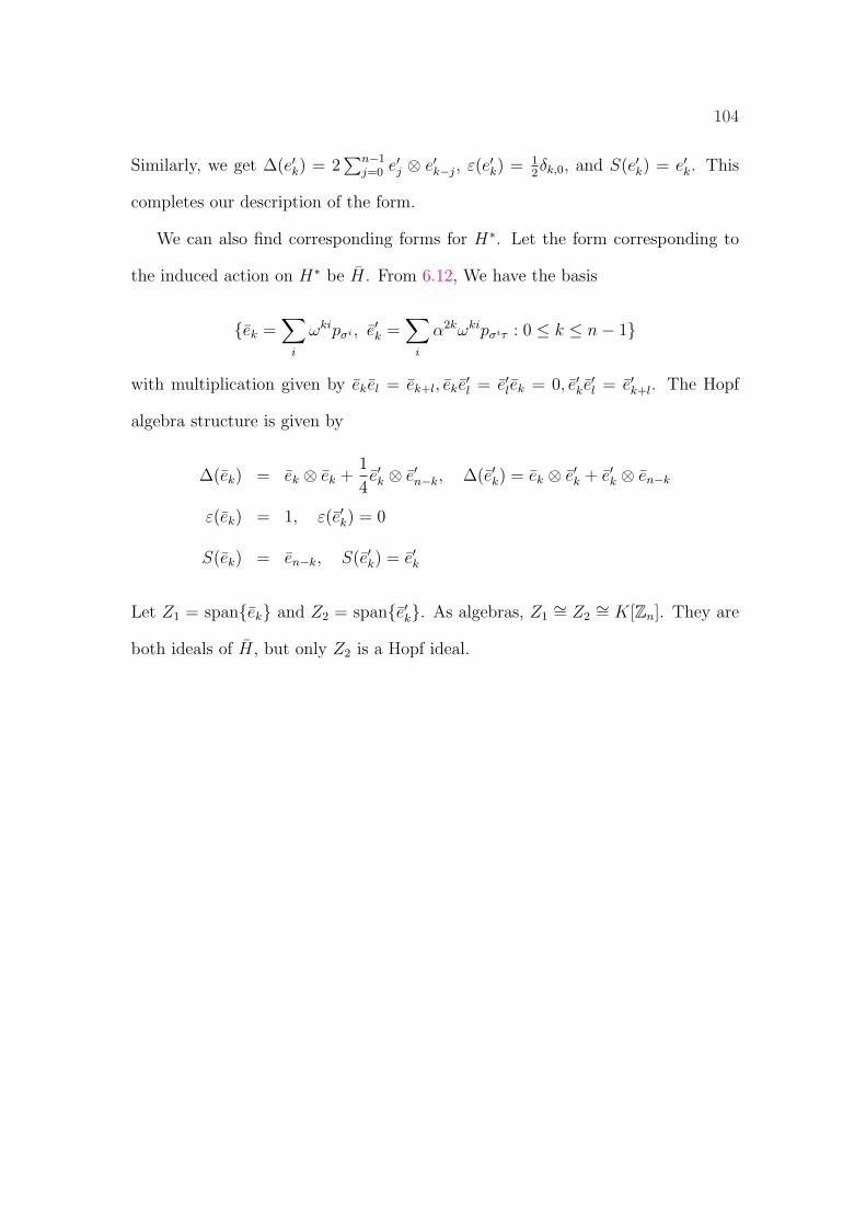
104

Similarly, we get ∆(e′k) = 2∑n−1

j=0 e′j ⊗ e′k−j, ε(e′k) = 12δk,0, and S(e′k) = e′k. This

completes our description of the form.

We can also find corresponding forms for H∗. Let the form corresponding to

the induced action on H∗ be H. From 6.12, We have the basis

{ek =∑

i

ωkipσi , e′k =∑

i

α2kωkipσiτ : 0 ≤ k ≤ n− 1}

with multiplication given by ekel = ek+l, eke′l = e′lek = 0, e′ke

′l = e′k+l. The Hopf

algebra structure is given by

∆(ek) = ek ⊗ ek +1

4e′k ⊗ e′n−k, ∆(e′k) = ek ⊗ e′k + e′k ⊗ en−k

ε(ek) = 1, ε(e′k) = 0

S(ek) = en−k, S(e′k) = e′k

Let Z1 = span{ek} and Z2 = span{e′k}. As algebras, Z1∼= Z2

∼= K[Zn]. They are

both ideals of H, but only Z2 is a Hopf ideal.

105

Bibliography

[BCM86] R.J. Blattner, M. Cohen, and S. Montgomery, Crossed Products and

inner actions of Hopf algebras, Trans. AMS 298 (1986), 671–711.

[Bel] A.D. Bell, Comodule algebras and Galois extensions relative to polyno-

mial algebras, free algebras, and enveloping algebras, Preprint.

[BM94] J. Bergen and S. Montgomery (eds.), Advances in Hopf Algebras, Marcel

Dekker, New York, 1994.

[CFM90] M. Cohen, D. Fischman, and S. Montgomery, Hopf Galois extensions, J.

Algebra 133 (1990), 351–372.

[Chi92] W. Chin, Crossed products of semisimple cocommutative Hopf algebras,

Proc. AMS 116 (1992), 321–327.

[Coh94] M. Cohen, Quantum commutativity and central invariants, in Bergen

and Montgomery [BM94], pp. 25–38.

[CW93] M. Cohen and S. Westreich, Central invariants of H-module algebras,

Comm. Alg. 21 (1993), no. 8, 2859–2883.

[DT86] Y. Doi and M. Takeuchi, Cleft comodule algebras for a bialgebra, Comm.

Alg. 14 (1986), 801–818.

[GP87] C. Greither and B. Pareigis, Hopf Galois theory for separable field ex-

tensions, J. Algebra 106 (1987), 239–258.

106

[Hoc54] G. Hochschild, Representations of restricted Lie algebras of characteristic

p, Proc. AMS 5 (1954), 603–605.

[HP86] R. Haggenmuller and B. Pareigis, Hopf algebra forms of the multiplicative

group and other groups, Manuscripta Math. 55 (1986), 121–136.

[Jac62] N. Jacobson, Lie algebras, Interscience, New York, 1962.

[Jac64] , Lectures in Abstract Algebra, vol. 3, D. Van Nostrand, Prince-

ton, 1964.

[Knu74] M.A. Knus, Theorie de la Descente et Algebres d’Azumaya, Springer-

Verlag, New York, 1974.

[KT81] H.F. Kreimer and M. Takeuchi, Hopf algebras and Galois extensions of

an algebra, Indiana Univ. Math. J. 30 (1981), 675–692.

[LS69] R.G. Larson and M. Sweedler, An associative orthogonal bilinear form

for Hopf algebras, Amer. J. Math. 91 (1969), 75–93.

[McC66] P.J. McCarthy, Algebraic Extensions of Fields, Blaisdell, Waltham,

Mass., 1966.

[Mon93] S. Montgomery, Hopf Algebras and Their Actions on Rings, AMS, Prov-

idence, R.I., 1993.

[Nic94] W.D. Nichols, Cosemisimple Hopf algebras, in Bergen and Montgomery

[BM94], pp. 135–151.

[Par89] B. Pareigis, Twisted group rings, Comm. Alg. 17 (1989), 2923–2939.

107

[Pas91] D.S. Passman, A Course in Ring Theory, Brooks/Cole, Belmont, CA,

1991.

[Sch90] H.J. Schneider, Principal homogeneous spaces for arbitrary Hopf alge-

bras, Israel J. Math 72 (1990), 167–195.

[Swe69] M.E. Sweedler, Hopf Algebras, Benjamin, New York, 1969.

[Ulb81] K.H. Ulbrich, Vollgraduierte Algebren, Abh. Math. Sem. Univ. Hamburg

51 (1981), 136–148.

[Ulb82] , Galois erweiterungen von nicht-kommutativen ringen, Comm.

Algebra 10 (1982), 655–672.

[Zhu94] Y. Zhu, Hopf algebras of prime dimension, Internat. Math. Res. Notices

1994 (1994), no. 1, 53–59.