Embed Size (px)
Citation preview
Hopf algebra of non-commutative eld theory
Adrian Tanasa(1),(2) and Fabien Vignes-Tourneret(3)
1Laboratoire de Physique Théorique, Bât. 210Université Paris XI, F-91405 Orsay Cedex, France
2Dep. Fizica Teoretica, Institul de Fizica si Inginerie Nucleara H. Hulubei,P. O. Box MG-6, 077125 Bucuresti-Magurele, Romania
e-mail: [email protected]
3IHÉSLe Bois-Marie, 35 route de ChartresF-91440 Bures-sur-Yvette, France
e-mail: [email protected]
Abstract
We contruct here the Hopf algebra structure underlying the process of renormal-
ization of non-commutative quantum eld theory.
1 Introduction and motivation
Hopf algebras (see for example [Kas95] or [DNR01]) are today one of the most studiedstructures in mathematics. In relation with quantum eld theories (QFT), Hopf algebraswere proven to be a natural framework for the description of the forest structure ofrenormalization - the Connes-Kreimer algebras [CK00, CK01]. Ever since there has beenan important amount of work with respect to this new class of Hopf algebras (for a generalreview see for example [Kre05]).However, this construction was realized so far only at the level of commuta-
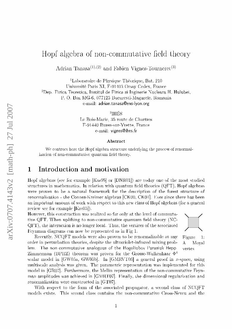
Figure 1:A Moyalvertex
tive QFT. When uplifting to non-commutative quantum eld theory (NC-QFT), the interaction is no longer local. Thus, the vertices of the associatedFeynman diagrams can now be represented as in Fig 1.
Recently, NCQFT models were also proven to be renormalizable at anyorder in perturbation theories, despite the ultraviolet-infrared mixing prob-lem. The non-commutative analogous of the Bogoliubov-Parasiuk-Hepp-Zimmerman (BPHZ) theorem was proven for the Grosse-Wulkenhaar Φ4
scalar model in [GW05a, GW05b]. In [GMRVT06] a general proof in x-space, usingmultiscale analysis was given. The parametric representation was implemented for thismodel in [GR07]. Furthermore, the Mellin representation of the non-commutative Feyn-man amplitudes was achieved in [GMRT07]. Finally, the dimensional regularization andrenormalization were constructed in [GT07].
With respect to the form of the associated propagator, a second class of NCQFTmodels exists. This second class contains the non-commutative Gross-Neveu and the
1
arX
iv:0
707.
4143
v2 [
mat
h-ph
] 2
7 Ju
l 200
7
Langmann-Szabo-Zarembo [LSZ04] models. The associate BPHZ theorem was proven in[VT07] for the non-commutative Gross-Neveu model. Moreover, the parametric represen-tation [RT07] and the Mellin representation [GMRT07] were also implemented for thisclass of models too. For a recent review on dierent issues of renormalizability of NCQFTthe interested reader may report himself to [Riv07].
Note that even though recent progress has been made in [DGWW07, GW07, BGS07],physicists do not yet have a renormalizable non-commutative gauge theory.
In this article we construct the Hopf algebra structure associated to the renormaliza-tion of these NCQFT models. The paper is organized as follows. In the next section wegive some insights on the renormalization of NCQFT with respect to renormalization ofcommutative QFT. The third section is devoted to the Hopf algebra structure of Feynmandiagrams. In the last section we state and prove our main result.
2 Renormalization of non-commutative quantum eld
theory
In this section we briey recall some features of both commutative and non-commutativeEuclidean renormalization. We will mainly focus on the Grosse-Wulkenhaar model [GW05b,GMRVT06] or non-commutative Φ4
4 theory. It consists in a scalar quantum eld theoryon the four-dimensional Moyal space. Its action is given by
S[φ] =
∫d4x(− 1
2φ(−∆)φ+
Ω2
2x2φ2 +
1
2m2 φ2 +
λ
4φ ? φ ? φ ? φ
)(x) (2.1)
with xµ = 2(Θ−1x)µ and Θ a four by four skew-symmetric matrix which encodes the non-commutative character of space time: [xµ, xν ]? = ıΘµν . It has been shown renormalizableto all orders of perturbation.
Furthermore, as already stated in the previous section, the same renormalization re-sults also hold for the non-commutative Gross-Neveu model [VT07] and the generalizedLSZ model [GMRVT06]:
SGN =
∫d2x[ψ(−i/∂ + Ω/x+m+ µγ5)ψ −
3∑A=1
gA4
(J A ? J A)(x)], (2.2)
J A =ψ ? ΓAψ, Γ1 = 1, Γ2 = γµ, Γ3 = γ5, , (2.3)
SgLSZ =
∫d4x[φ((−ı∂µ + Ω1xµ)2 + Ω2x
2 +m2)φ+
λ
2φ ? φ ? φ ? φ
](x). (2.4)
2.1 Topology and power counting
Let a graph G with V vertices and I internal lines. Interactions of quantum eld the-ories on the Moyal space are only invariant under cyclic permutation of the incom-ing/outcoming elds. This restriced invariance replaces the permutation invariance whichwas present in the case of local interactions.
A good way to keep track of such a reduced invariance is to draw Feynman graphsas ribbon graphs. Moreover there exists a basis for the Schwartz class functions where
2
the Moyal product becomes an ordinary matrix product [GW03, GBV88]. This furtherjusties the ribbon representation.
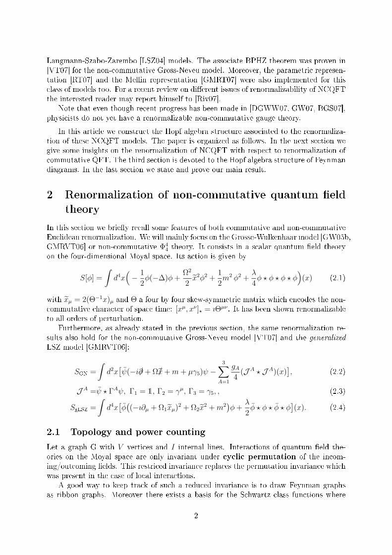
Let us consider the example of gure 2. Propagators in a ribbon graph are made of
−
+
−
+
+
−
+
−
−+
+−
(a) x-space repre-sentation
oo//
OO
//oo
//oo
OOOO
//oo
OO
OO
//
(b) Ribbon representa-tion
Figure 2: A graph with two broken faces
double lines. Let us call F the number of faces (loops made of single lines) of a ribbongraph. The graph of gure 2b has V = 3, I = 3, F = 2. Each ribbon graph can bedrawn on a manifold of genus g. The genus is computed from the Euler characteristicχ = F − I + V = 2− 2g. If g = 0 one has a planar graph, otherwise one has a non-planargraph. For example, the graph of gure 2b may be drawn on a manifold of genus 0. Notethat some of the F faces of a graph may be broken by external legs. In our example,both faces are broken. We denote the number of broken faces by B.
Furthermore let N the number of external legs of the graph. For the commutative φ4
model one has the following supercial degree of convergence ω = N − 4. Thus one hasto deal only with the renormalization of the two- and four-point functions. In the case ofthe Grosse-Wulkenhaar model, the situation is dierent. In [GW05a, GW05b, GR07] itwas proven that
ω = (N − 4) + 8g + 4(B − 1). (2.5)
Note that, as proven in [RT07] one has the same power counting for the LSZ like model(2.4). The one of the Gross-Neveu model (2.2) is more involved but leads to the sameconclusion: one has to deal only with the renormalization of the B = 1, planar two- andfour-point graphs hereafter qualied as planar regular.
2.2 Locality vs Moyality
A crucial aspect of the uplifting from commutative to non-commutative renormalization isthat the principle of locality of renormalized interactions of commutative QFT is replacedwith a new principle: renormalized interactions have a non-local Moyal vertex form.This is nothing but the analog of the locality phenomenon which occurs in commutativerenormalization. One can thus speak, in the case of non-commutative renormalization,of a new type of renormalization group, where the locality is just replaced by Moyality.The divergent parts of the planar regular two- and four-point graphs with one broken
3
face (the only divergent graphs) are proportional to the (1PI) tree level terms of theperturbative expansion. Such a new denition of locality was suggested in [Kre05], seeequation (62).
Let us also argue here that, despite this uplifting, the combinatorial backbone of renor-malization theory is almost the same when dealing with commutative or non-commutativeQFT. Thus the combinatorics of non-commutative renormalization will be shown to beencoded by a Hopf algebra.
2.3 Renormalization as a factorization issue
The basic operation for renormalization is the disentanglement of a graph Γ into pieces γand cograph Γ/γ. It is exactly this operation that was present at the level of commutativerenormalization and that gave rise to a Hopf algebra structure.
We now argue that this factorization process is also present at the level of non-commutative renormalization. Indeed, consider the dimensional renormalization schemefor the Grosse-Wulkenhaar model. The parametric representation constructed in [GR07]writes the Feynman amplitude φ(Γ) as
φ(Γ) = K
∫ 1
0
L∏`=1
[dt`(1− t2`)D2−1]HUG,V (t)−
D2 e−HVG
HUG , (2.6)
where K is some constant,
t` = tanhα`2, ` = 1, . . . , L, (2.7)
where α` are the parameters associated to any of the propagators of the graph. In [GR07]it was furthermore proved that HU and HV are polynomials in the set of variables t`.
Considering now a primitive divergent subgraph γ of Γ and rescaling the parameterst of its internal edges, it was proven in [GT07] that
HU lΓ = HU l
γ HUΓ/γ (2.8)
where by the index l we understand the leading terms under the rescaling. A similarfactorization theorem was also proven for the exponential part in (2.6) of the Feynmanamplitude φ(Γ).
Moreover, in [GMRVT06] an analogous phenomena of factorization was shown for theGrosse-Wulkenhaar model in position space namely the planar regular graphs contributeto the renormalization of the mass, wave-function, harmonic frequency Ω and couplingconstant, see Equation (2.1).
4
3 Hopf algebra structure of Feynman diagrams
3.1 Hopf algebra reminder
In this subsection we recall the general denition of a Hopf algebra (for further detailsone can refer for example to [Kas95, DNR01]).
Denition 3.1 (Algebra). A unital associative algebra A over a eld K is a K-linearspace endowed with two algebra homomorphisms:
• a product m : A⊗A → A satisfying the associativity condition:
∀Γ ∈ A, m (m⊗ id)(Γ) =m (id⊗m)(Γ), (3.1)
• a unit u : K→ A satisfying:
∀Γ ∈ A, m (u⊗ id)(Γ) =Γ = m (id⊗ u)(Γ). (3.2)
Denition 3.2 (Coalgebra). A coalgebra C over a eld K is a K-linear space endowedwith two algebra homomorphisms:
• a coproduct ∆ : C → C ⊗ C satisfying the coassociativity condition:
∀Γ ∈ C, (∆⊗ id) ∆(Γ) =(id⊗∆) ∆(Γ), (3.3)
• a counit ε : C → K satisfying:
∀Γ ∈ C, (ε⊗ id) ∆(Γ) =Γ = (id⊗ ε) ∆(Γ). (3.4)
Denition 3.3 (Bialgebra). A bialgebra B over a eld K is a K-linear space endowedwith both an algebra and a coalgebra structure (see Denitions 3.1 and 3.2) such that thecoproduct and the counit are unital algebra homomorphisms (or equivalently the productand unit are coalgebra homomorphisms):
∆ mB =mB⊗B (∆⊗∆), ∆(1) = 1⊗ 1, (3.5a)
ε mB =mK (ε⊗ ε), ε(1) = 1. (3.5b)
Denition 3.4 (Graded Bialgebra). A graded bialgebra is a bialgebra graded as a lin-ear space:
B =∞⊕n=0
B(n) (3.6)
such that the grading is compatible with the algebra and coalgebra structures:
B(n)B(m) ⊆ B(n+m) and ∆B(n) ⊆n⊕k=0
B(k) ⊗ B(n−k). (3.7)
5
Denition 3.5 (Connectedness). A connected bialgebra is a graded bialgebra B forwhich B(0) = u(K).
One can then dene a Hopf algebra:
Denition 3.6 (Hopf algebra). A Hopf algebra H over a eld K is a bialgebra over Kequipped with an antipode map S : H → H obeying:
m (S ⊗ id) ∆ =u ε = m (id⊗ S) ∆. (3.8)
Finally we remind a useful lemma:
Lemma 3.1 ([Man03]) Any connected graded bialgebra is a Hopf algebra whose antipodeis given by S(1) = 1 and recursively by any of the two following formulas for Γ 6= 1:
S(Γ) =− Γ−∑(Γ)
S(Γ′)Γ′′, (3.9a)
S(Γ) =− Γ−∑(Γ)
Γ′S(Γ′′) (3.9b)
where we used Sweedler's notation.
3.2 Locality and the residue map
In quantum eld theory, Feynman graphs are built from a certain set of edges and verticesR = RE ∪ RV . This set is given by the particle content of the model and by the type ofinteractions one wants to consider. For example, in the commutative φ4
4 theory (whichwill be our benchmark until section 4), RE contains only the scalar bosonic line while RV
contains the local four-point vertex and the two-point vertices corresponding to the massand wave-function renormalization:
RE = , RV = ,0
,1 .
In the following we will still write RV for the free algebra generated by the elements ofRV . Let us now consider the algebra H generated by a certain class of graphs (connected,1PI etc) made out of the set R.
Denition 3.7 (Subgraph). Let Γ ∈ H, Γ[1] its set of internal lines and Γ[0] its vertices.A subgraph γ of Γ, written γ ⊂ Γ, consists in a subset γ[1] of Γ[1] and the vertices of Γ[0]
hooked to the lines in γ[1]. Note that with such a denition, γ is truncated.
Denition 3.8 (Shrinkable subgraph). Let Γ ∈ H. A subgraph ∅ γ Γ is saidshrinkable if res(γ) ∈ RV . The set of shrinkable subgraphs of Γ will be denoted by Γ.
Note that until now we did not really dene what is the map res. We now do it. Firstwe assume that it is an algebra homomorphism from H to H∪RV . Then to compute thegraphical residue of a generator of H, we need the following remarks and denitions.
The coproduct of H (usually given by (3.15)) drives the combinatorial and algebraicaspects of renormalization if it corresponds to some analytical facts. Before we explainthis, let us recall the following denitions.
6
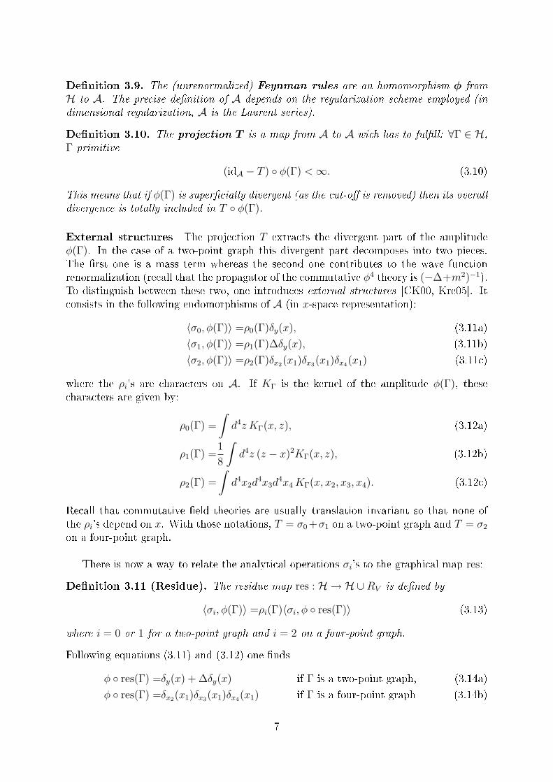
Denition 3.9. The (unrenormalized) Feynman rules are an homomorphism φ fromH to A. The precise denition of A depends on the regularization scheme employed (indimensional regularization, A is the Laurent series).
Denition 3.10. The projection T is a map from A to A wich has to fulll: ∀Γ ∈ H,Γ primitive
(idA − T ) φ(Γ) <∞. (3.10)
This means that if φ(Γ) is supercially divergent (as the cut-o is removed) then its overalldivergence is totally included in T φ(Γ).
External structures The projection T extracts the divergent part of the amplitudeφ(Γ). In the case of a two-point graph this divergent part decomposes into two pieces.The rst one is a mass term whereas the second one contributes to the wave functionrenormalization (recall that the propagator of the commutative φ4 theory is (−∆+m2)−1).To distinguish between these two, one introduces external structures [CK00, Kre05]. Itconsists in the following endomorphisms of A (in x-space representation):
〈σ0, φ(Γ)〉 =ρ0(Γ)δy(x), (3.11a)
〈σ1, φ(Γ)〉 =ρ1(Γ)∆δy(x), (3.11b)
〈σ2, φ(Γ)〉 =ρ2(Γ)δx2(x1)δx3(x1)δx4(x1) (3.11c)
where the ρi's are characters on A. If KΓ is the kernel of the amplitude φ(Γ), thesecharacters are given by:
ρ0(Γ) =
∫d4z KΓ(x, z), (3.12a)
ρ1(Γ) =1
8
∫d4z (z − x)2KΓ(x, z), (3.12b)
ρ2(Γ) =
∫d4x2d
4x3d4x4KΓ(x, x2, x3, x4). (3.12c)
Recall that commutative eld theories are usually translation invariant so that none ofthe ρi's depend on x. With those notations, T = σ0 +σ1 on a two-point graph and T = σ2
on a four-point graph.
There is now a way to relate the analytical operations σi's to the graphical map res:
Denition 3.11 (Residue). The residue map res : H → H∪RV is dened by
〈σi, φ(Γ)〉 =ρi(Γ)〈σi, φ res(Γ)〉 (3.13)
where i = 0 or 1 for a two-point graph and i = 2 on a four-point graph.
Following equations (3.11) and (3.12) one nds
φ res(Γ) =δy(x) + ∆δy(x) if Γ is a two-point graph, (3.14a)
φ res(Γ) =δx2(x1)δx3(x1)δx4(x1) if Γ is a four-point graph (3.14b)
7
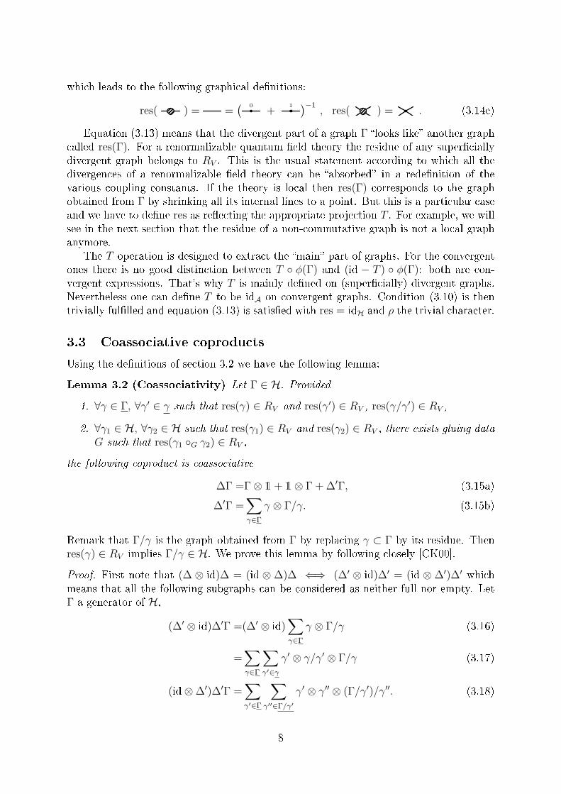
which leads to the following graphical denitions:
res( ) = =( 0
+1 )−1
, res( ) = . (3.14c)
Equation (3.13) means that the divergent part of a graph Γ looks like another graphcalled res(Γ). For a renormalizable quantum eld theory the residue of any superciallydivergent graph belongs to RV . This is the usual statement according to which all thedivergences of a renormalizable eld theory can be absorbed in a redenition of thevarious coupling constants. If the theory is local then res(Γ) corresponds to the graphobtained from Γ by shrinking all its internal lines to a point. But this is a particular caseand we have to dene res as reecting the appropriate projection T . For example, we willsee in the next section that the residue of a non-commutative graph is not a local graphanymore.
The T operation is designed to extract the main part of graphs. For the convergentones there is no good distinction between T φ(Γ) and (id − T ) φ(Γ): both are con-vergent expressions. That's why T is mainly dened on (supercially) divergent graphs.Nevertheless one can dene T to be idA on convergent graphs. Condition (3.10) is thentrivially fullled and equation (3.13) is satised with res = idH and ρ the trivial character.
3.3 Coassociative coproducts
Using the denitions of section 3.2 we have the following lemma:
Lemma 3.2 (Coassociativity) Let Γ ∈ H. Provided
1. ∀γ ∈ Γ, ∀γ′ ∈ γ such that res(γ) ∈ RV and res(γ′) ∈ RV , res(γ/γ′) ∈ RV ,
2. ∀γ1 ∈ H, ∀γ2 ∈ H such that res(γ1) ∈ RV and res(γ2) ∈ RV , there exists gluing dataG such that res(γ1 G γ2) ∈ RV ,
the following coproduct is coassociative
∆Γ =Γ⊗ 1 + 1⊗ Γ + ∆′Γ, (3.15a)
∆′Γ =∑γ∈Γ
γ ⊗ Γ/γ. (3.15b)
Remark that Γ/γ is the graph obtained from Γ by replacing γ ⊂ Γ by its residue. Thenres(γ) ∈ RV implies Γ/γ ∈ H. We prove this lemma by following closely [CK00].
Proof. First note that (∆ ⊗ id)∆ = (id ⊗ ∆)∆ ⇐⇒ (∆′ ⊗ id)∆′ = (id ⊗ ∆′)∆′ whichmeans that all the following subgraphs can be considered as neither full nor empty. LetΓ a generator of H,
(∆′ ⊗ id)∆′Γ =(∆′ ⊗ id)∑γ∈Γ
γ ⊗ Γ/γ (3.16)
=∑γ∈Γ
∑γ′∈γ
γ′ ⊗ γ/γ′ ⊗ Γ/γ (3.17)
(id⊗∆′)∆′Γ =∑γ′∈Γ
∑γ′′∈Γ/γ′
γ′ ⊗ γ′′ ⊗ (Γ/γ′)/γ′′. (3.18)
8
By the denitions 3.7, 3.8 and 3.11 it is clear that γ′ ∈ γ and γ ∈ Γ implies γ′ ∈ Γ. Thisimplicitly uses the fact that the residue of a graph is independant of the surrounding ofthis graph and really only depends on the graph itself: res(γ) is the same wether γ is asubgraph or not of another graph. Equation (3.17) can then be rewritten as
(∆′ ⊗ id)∆′Γ =∑γ′∈Γ
∑γ∈Γ|γ!γ′
γ′ ⊗ γ/γ′ ⊗ Γ/γ. (3.19)
It is now enough to prove equality between (3.18) and (3.19) at xed γ′ ∈ Γ. Let us rstx a subgraph γ ∈ Γ such that γ ! γ′ and prove that there exists a graph γ′′ ∈ Γ/γ′ suchthat γ/γ′⊗Γ/γ = γ′′⊗ (Γ/γ′)/γ′′. Of course the logical choice for γ′′ is γ/γ′ because then(Γ/γ′)/(γ/γ′) = Γ/γ.
We only have to prove that γ′′ = γ/γ′ ∈ Γ/γ′. It is clear that γ/γ′ is a subset of internallines of Γ/γ′. Then γ/γ′ ∈ Γ/γ′ if res(γ) ∈ RV and res(γ′) ∈ RV implies res(γ/γ′) ∈ RV
which we assumed.Conversely let us x γ′′ ∈ Γ/γ′ and prove that there exists γ ∈ Γ containing γ′
such that γ/γ′ ⊗ Γ/γ = γ′′ ⊗ (Γ/γ′)/γ′′. Let us write γ′ =⋃i∈I γ
′i for the connected
components of γ′. Some of these components led to vertices of γ′′, the others to verticesof (Γ/γ′) \ γ′′. We can then dene γ as (γ′′ GI1
⋃i∈I1 γ
′i)⋃j∈I2 γ
′j with I1 ∪ I2 = I.
It is clearly a subgraph of Γ and belongs to Γ if ∀γ1, γ2 ∈ H, res(γ1) ∈ RV , res(γ2) ∈RV there exists gluing data G such that res(γ1 G γ2) ∈ RV . We also assumed it. Thisends the proof of Lemma 3.2.
Let us now work out how Lemma 3.2 ts the commutative φ4 model. In this localeld theory the divergent graphs have two or four external legs. The residue of a givengraph is the one obtained by shrinking all its internal lines to a point (see section 3.2) andthen only depends on the number of external lines of the graph. Let us check condition2 of Lemma 3.2 for commutative φ4. We consider two graphs γ1 and γ2 with two orfour external legs. We consider γ0 = γ1 G γ2 for any gluing data G. Let Vi, Ii and Eithe respective numbers of vertices, internal and external lines of γi, i ∈ 0, 1, 2. For alli ∈ 0, 1, 2, we have
4Vi =2Ii + Ei (3.20a)
V0 =
V1 + V2 if E2 = 2
V1 + V2 − 1 if E2 = 4(3.20b)
I0 =
I1 + I2 + 1 if E2 = 2
I1 + I2 if E2 = 4(3.20c)
which proves that E = E1. Then as soon as res(γ1) ∈ RV so does res(γ0). Concerningcondition 1 note that γ′′ = γ/γ′ ⇐⇒ ∃G | γ = γ′′Gγ′ which allows to prove, in the case ofa local theory, that condition 1 also holds and that the coproduct (3.15) is coassociative.
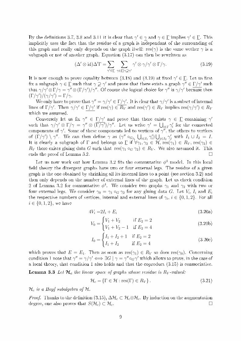
Lemma 3.3 Let Hc the linear space of graphs whose residue is RV -valued:
Hc = Γ ∈ H : res(Γ) ∈ RV . (3.21)
Hc is a Hopf subalgebra of H.
Proof. Thanks to the denition (3.15), ∆Hc ⊂ Hc⊗Hc. By induction on the augmentationdegree, one also proves that S(Hc) ⊂ Hc.
9
4 Hopf algebra for non-commutative Feynman graphs
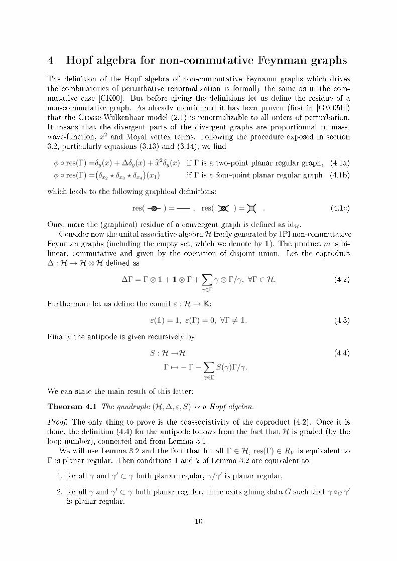
The denition of the Hopf algebra of non-commutative Feynamn graphs which drivesthe combinatorics of perturbative renormalization is formally the same as in the com-mutative case [CK00]. But before giving the denitions let us dene the residue of anon-commutative graph. As already mentionned it has been proven (rst in [GW05b])that the Grosse-Wulkenhaar model (2.1) is renormalizable to all orders of perturbation.It means that the divergent parts of the divergent graphs are proportionnal to mass,wave-function, x2 and Moyal vertex terms. Following the procedure exposed in section3.2, particularly equations (3.13) and (3.14), we nd
φ res(Γ) =δy(x) + ∆δy(x) + x2δy(x) if Γ is a two-point planar regular graph, (4.1a)
φ res(Γ) =(δx2 ? δx3 ? δx4
)(x1) if Γ is a four-point planar regular graph (4.1b)
which leads to the following graphical denitions:
res( ) = , res( ) = . (4.1c)
Once more the (graphical) residue of a convergent graph is dened as idH.Consider now the unital associative algebraH freely generated by 1PI non-commutative
Feynman graphs (including the empty set, which we denote by 1). The product m is bi-linear, commutative and given by the operation of disjoint union. Let the coproduct∆ : H → H⊗H dened as
∆Γ = Γ⊗ 1 + 1⊗ Γ +∑γ∈Γ
γ ⊗ Γ/γ, ∀Γ ∈ H. (4.2)
Furthermore let us dene the counit ε : H → K:
ε(1) = 1, ε(Γ) = 0, ∀Γ 6= 1. (4.3)
Finally the antipode is given recursively by
S : H →H (4.4)
Γ 7→ − Γ−∑γ∈Γ
S(γ)Γ/γ.
We can state the main result of this letter:
Theorem 4.1 The quadruple (H,∆, ε, S) is a Hopf algebra.
Proof. The only thing to prove is the coassociativity of the coproduct (4.2). Once it isdone, the denition (4.4) for the antipode follows from the fact that H is graded (by theloop number), connected and from Lemma 3.1.
We will use Lemma 3.2 and the fact that for all Γ ∈ H, res(Γ) ∈ RV is equivalent toΓ is planar regular. Then conditions 1 and 2 of Lemma 3.2 are equivalent to:
1. for all γ and γ′ ⊂ γ both planar regular, γ/γ′ is planar regular,
2. for all γ and γ′ ⊂ γ both planar regular, there exits gluing data G such that γ G γ′is planar regular.
10
1
2
3
4
(a) A vertex of γ1
1
1
2 2
3
3
44
1′
1′
2′ 2′
3′
3′
4′4′
(b) Insertion of γ2
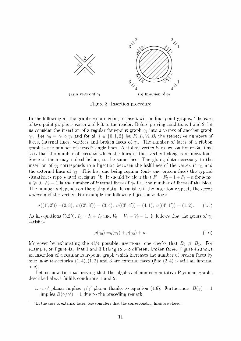
Figure 3: Insertion procedure
In the following all the graphs we are going to insert will be four-point graphs. The caseof two-point graphs is easier and left to the reader. Before proving conditions 1 and 2, letus consider the insertion of a regular four-point graph γ2 into a vertex of another graphγ1. Let γ0 = γ1 γ2 and for all i ∈ 0, 1, 2 let Fi, Ii, Vi, Bi the respective numbers offaces, internal lines, vertices and broken faces of γi. The number of faces of a ribbongraph is the number of closeda single lines. A ribbon vertex is drawn on gure 3a. Onesees that the number of faces to which the lines of that vertex belong is at most four.Some of them may indeed belong to the same face. The gluing data necessary to theinsertion of γ2 corresponds to a bijection between the half-lines of the vertex in γ1 andthe external lines of γ2. This last one being regular (only one broken face) the typicalsituation is represented on gure 3b. It should be clear that F = F2−1 +F1−n for somen > 0. F2 − 1 is the number of internal faces of γ2 i.e. the number of faces of the blob.The number n depends on the gluing data. It vanishes if the insertion respects the cyclicordering of the vertex. For example the following bijection σ does:
σ((1′, 2′)) =(2, 3), σ((2′, 3′)) = (3, 4), σ((3′, 4′)) = (4, 1), σ((4′, 1′)) = (1, 2). (4.5)
As in equations (3.20), I0 = I1 + I2 and V0 = V1 + V2 − 1. It follows that the genus of γ0
satises
g(γ0) =g(γ1) + g(γ2) + n. (4.6)
Moreover by exhausting the 4!/4 possible insertions, one checks that B0 > B1. Forexample, on gure 4a, lines 1 and 3 belong to two dierent broken faces. Figure 4b showsan insertion of a regular four-point graph which increases the number of broken faces byone: now trajectories (1, 4), (1, 2) and 3 are external faces (line (2, 4) is still an internalone).
Let us now turn to proving that the algebra of non-commutative Feynman graphsdescribed above fullls conditions 1 and 2.
1. γ, γ′ planar implies γ/γ′ planar thanks to equation (4.6). Furthermore B(γ) = 1implies B(γ/γ′) = 1 due to the preceding remark.
aIn the case of external faces, one considers that the corresponding lines are closed.
11
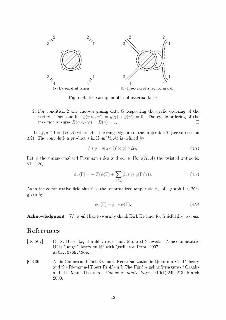
1
1
2 2
3
3
44(a) External situation
1
1
2 2
3
3
44(b) Insertion of a regular graph
Figure 4: Increasing number of external faces
2. For condition 2 one chooses gluing data G respecting the cyclic ordering of thevertex. Then one has g(γ G γ′) = g(γ) + g(γ′) = 0. The cyclic ordering of theinsertion ensures B(γ G γ′) = B(γ) = 1.
Let f, g ∈ Hom(H,A) where A is the range algebra of the projection T (see subsection3.2). The convolution product ∗ in Hom(H,A) is dened by
f ∗ g =mA (f ⊗ g) ∆H. (4.7)
Let φ the unrenormalized Feynman rules and φ− ∈ Hom(H,A) the twisted antipode:∀Γ ∈ H,
φ−(Γ) =− T(φ(Γ) +
∑γ∈Γ
φ−(γ) φ(Γ/γ)). (4.8)
As in the commutative eld theories, the renormalized amplitude φ+ of a graph Γ ∈ H isgiven by:
φ+(Γ) =φ− ∗ φ(Γ). (4.9)
Acknowledgment We would like to warmly thank Dirk Kreimer for fruitful discussions.
References
[BGS07] D. N. Blaschke, Harald Grosse, and Manfred Schweda. NoncommutativeU(1) Gauge Theory on R4 with Oscillator Term. 2007.ArXiv:0705.4205.
[CK00] Alain Connes and Dirk Kreimer. Renormalization in Quantum Field Theoryand the Riemann-Hilbert Problem I: The Hopf Algebra Structure of Graphsand the Main Theorem. Commun. Math. Phys., 210(1):249273, March2000.
12
[CK01] Alain Connes and Dirk Kreimer. Renormalization in Quantum Field The-ory and the RiemannHilbert Problem II: The ÿ-Function, Dieomorphismsand the Renormalization Group. Commun. Math. Phys., 216(1):215241,January 2001.
[DGWW07] Axel De Goursac, Jean-Christophe Wallet, and Raimar Wulkenhaar.Noncommutative Induced Gauge Theory. March 2007. Accepted byEur. Phys. J. C.ArXiv:hep-th/0703075.
[DNR01] Sorin D sc lescu, Constantin N st sescu, and erban Raianu. Hopf Alge-bras, An Introduction, volume 235 of Pure and applied mathematics. CRC,2001.
[GBV88] J. M. Gracia-Bondía and J. C. Várilly. Algebras of distributions suitable forphase space quantum mechanics. I. J. Math. Phys., 29:869879, 1988.
[GMRT07] R zvan Gur u, A. P. C. Malbouisson, Vincent Rivasseau, and AdrianTanasa. Non-Commutative Complete Mellin Representation for FeynmanAmplitudes. Accepted by Lett. Math. Phys., 2007.ArXiv:0705.3437.
[GMRVT06] Razvan Gurau, Jacques Magnen, Vincent Rivasseau, and Fabien Vignes-Tourneret. Renormalization of non-commutative φ4
4 eld theory in x space.Commun. Math. Phys., 267(2):515542, 2006.Journal link.ArXiv:hep-th/0512271.
[GR07] Razvan Gurau and Vincent Rivasseau. Parametric representation of non-commutative eld theory. Commun. Math. Phys., 272:811, 2007.ArXiv:math-ph/0606030.
[GT07] R zvan Gur u and Adrian Tanas . Dimensional regularization and renor-malization of non-commutative QFT. Submitted to Ann. H. Poincaré, 2007.ArXiv:0706.1147.
[GW03] Harald Grosse and Raimar Wulkenhaar. Renormalisation of φ4-theory onnoncommutative R2 in the matrix base. JHEP, 12:019, 2003.ArXiv:hep-th/0307017.
[GW05a] Harald Grosse and Raimar Wulkenhaar. Power-counting theorem for non-local matrix models and renormalisation. Commun. Math. Phys., 254(1):91127, 2005.ArXiv:hep-th/0305066.
[GW05b] Harald Grosse and Raimar Wulkenhaar. Renormalisation of φ4-theory onnoncommutative R4 in the matrix base. Commun. Math. Phys., 256(2):305374, 2005.ArXiv:hep-th/0401128.
13
[GW07] Harald Grosse and Michael Wohlgenannt. Induced Gauge Theory On ANoncommutative Space. March 2007.ArXiv:hep-th/0703169.
[Kas95] Christian Kassel. Quantum Groups, volume 155 of Graduate Texts in Math-ematics. Springer-Verlag, 1995.
[Kre05] Dirk Kreimer. Structures in Feynman Graphs - Hopf Algebras and Sym-metries. In Graphs and Patterns in Mathematics and Theoretical Physics,volume 73 of Proc. Symp. Pure Math., pages 4378, 2005.ArXiv:hep-th/0202110.
[LSZ04] E. Langmann, R. J. Szabo, and K. Zarembo. Exact solution of quantumeld theory on noncommutative phase spaces. JHEP, 01:017, 2004.ArXiv:hep-th/0308043.
[Man03] Dominique Manchon. Hopf algebras, from basics to applications to renor-malization. In Rencontres Mathématiques de Glanon, 2003.ArXiv:math.QA/0408405.
[Riv07] Vincent Rivasseau. Non-commutative renormalization. Poincare Seminar,updated and expanded version of hep-th/0702068, May 2007.ArXiv:0705.0705.
[RT07] Vincent Rivasseau and Adrian Tanasa. Parametric representation of crit-ical noncommutative QFT models. Submitted to Commun. Math. Phys.,January 2007.ArXiv:hep-th/0701034.
[VT07] Fabien Vignes-Tourneret. Renormalization of the orientable non-commutative Gross-Neveu model. Ann. H. Poincaré, 8(3):427474, June2007.Journal link.ArXiv:math-ph/0606069.
14


