NOTA DILAVORO15.2011

How CO2 Capture and Storage Can Mitigate Carbon Leakage

By Philippe Quirion, Julie Rozenberg,Olivier Sassi and Adrien Vogt-Schilb, Centre international de recherche sur l’environnement et le développement (CIRED)

The opinions expressed in this paper do not necessarily reflect the position of Fondazione Eni Enrico Mattei

Corso Magenta, 63, 20123 Milano (I), web site: www.feem.it, e-mail: working.papers@feem.it

SUSTAINABLE DEVELOPMENT Series Editor: Carlo Carraro

How CO2 Capture and Storage Can Mitigate Carbon Leakage By Philippe Quirion, Julie Rozenberg, Olivier Sassi and Adrien Vogt-Schilb, Centre international de recherche sur l’environnement et le développement (CIRED) Summary Most CO2 abatement policies reduce the demand for fossil fuels and therefore their price in international markets. If these policies are not global, this price decrease raises emissions in countries without CO2 abatement policies, generating “carbon leakage”. On the other hand, if the countries which abate CO2 emissions are net fossil fuel importers, they benefit from this price decrease, which reduces the abatement cost. In contrast, CO2 capture and storage (CCS) does not reduce fossil fuel demand, therefore it generates neither this type of leakage nor this negative feedback on abatement costs. We quantify these effects with the global hybrid general equilibrium model Imaclim-R and show that they are quantitatively important. Indeed, for a given unilateral abatement in OECD countries, leakage is more than halved in a scenario with CCS included among the abatement options, compared to a scenario prohibiting CCS. We show that the main reason for this difference in leakage is the above-mentioned international fossil fuel price feedback. This article does not intend to assess the desirability of CCS, which has many other pros and cons. It just identifies a consequence of CCS that should be taken into account, together with many others, when deciding to what extent CCS should be developed. Keywords: CO2 Capture and Storage, Carbon Leakage JEL Classification: Q5, Q58

Address for correspondence: Philippe Quirion CIRED 45 bis avenue de la belle Gabrielle F-94736 Nogent-sur-Marne cedex France Phone: +33 1 43 94 73 95 E-mail: quirion@centre-cired.fr

1

Philippe Quirion1*, Julie Rozenberg*, Olivier Sassi* and Adrien Vogt-Schilb*

*Centre international de recherche sur l’environnement et le développement (CIRED)

How CO2 capture and storage can mitigate carbon leakage

Abstract

Most CO2 abatement policies reduce the demand for fossil fuels and therefore their price in international markets. If these policies are not global, this price decrease raises emissions in countries without CO2 abatement policies, generating “carbon leakage”. On the other hand, if the countries which abate CO2 emissions are net fossil fuel importers, they benefit from this price decrease, which reduces the abatement cost. In contrast, CO2 capture and storage (CCS) does not reduce fossil fuel demand, therefore it generates neither this type of leakage nor this negative feedback on abatement costs. We quantify these effects with the global hybrid general equilibrium model Imaclim-R and show that they are quantitatively important. Indeed, for a given unilateral abatement in OECD countries, leakage is more than halved in a scenario with CCS included among the abatement options, compared to a scenario prohibiting CCS. We show that the main reason for this difference in leakage is the above-mentioned international fossil fuel price feedback. This article does not intend to assess the desirability of CCS, which has many other pros and cons. It just identifies a consequence of CCS that should be taken into account, together with many others, when deciding to what extent CCS should be developed.

1 Contact author. CIRED, 45 bis avenue de la belle Gabrielle, F-94736 Nogent-sur-Marne cedex, France. quirion@centre-cired.fr. Tel. 00 33 1 43 94 73 95.

2

1. Introduction

It is unusual – and generally inopportune – to start a paper by explaining what it does not deal with. Yet, when an article includes in its title both “CO2 capture and storage” (thereafter CCS) and “carbon leakage”, the reader may well think that it is about the risk of CO2 leaking from underground reservoirs to the atmosphere. This is not the case here: the carbon leakage we deal with is the increase in emissions in foreign countries due a unilateral – or at least non-global – climate policy (Manne and Rutherford, 1994; Paltsev, 2001; Kuik and Gerlagh, 2003). What is the connection between this kind of leakage and CCS? The main carbon leakage channel (at least in most economic models) is the so-called “international energy price channel”, which works as follows. Most CO2 emissions abatement options (energy savings, nuclear energy and renewable energies) reduce the demand for fossil fuels, hence their price in international markets. If these options are applied in only one part of the world, this increases the consumption of fossil fuels, hence emissions, in the rest of the world, creating carbon leakage. In contrast, CCS does not reduce the demand for fossil fuels. Furthermore, for a given amount of electricity generation, CCS increases fossil fuel consumption: in a survey of the technical literature about CCS in electricity generation, Kober and Blesl (2010) find an efficiency loss ranging from 3% to 14%, with an average of 8%. Therefore, the development of CCS in a part of the world, rather than generating leakage, might push the fossil fuel prices up, generating additional abatement in the rest of the world, i.e. a negative leakage. Admittedly, since CCS cannot abate all CO2 emissions, a climate policy which includes CCS will typically not generate a negative leakage; yet, leakage will likely be lower than under a climate policy which does not include CCS.

This potentially mitigating impact of CCS on leakage has already been mentioned in the literature by a few authors (Fölster and Nyström, 2010; Marschinski et al., 2009; Quirion, 2010a). Yet, to our knowledge, it has never been quantified. This is unfortunate since CCS accounts for an important share of abatement in many ambitious climate change mitigation scenarios (Fisher and Nakicenovic (eds.), 2007). Moreover, most published estimates of carbon leakage, surveyed e.g. by Dröge et al. (2009) or Gerlagh and Kuik (2007) are based on models which do not include CCS. These estimates are thus higher than what they would be, ceteris paribus, would CCS be included as a CO2 abatement option.

Moreover, be it in the EU, the US, Japan or Australia, the policy debate about leakage focuses on the “competitiveness channel”, which is due to the potential loss in market shares of domestic installations, which face a carbon price while their foreign competitors do not. Yet, in most economic models, the main carbon leakage channel is not the competitiveness channel but the international energy price channel (Gerlagh and Kuik, 2007). This conclusion is important since the main policy options adopted or proposed to tackle carbon leakage, like output-based allowances (Quirion, 2009) and border adjustments (Monjon and Quirion, 2010), can only mitigate the competitiveness leakage channel, not the international energy price channel. If policy makers are serious and consistent about tackling leakage, they should

3

also consider the international energy price channel and take into account, when choosing the technical options mobilised to abate emissions, their impact on leakage.

In the present paper, we quantify for the first time (at our knowledge) the influence of CCS on carbon leakage, using the global hybrid general equilibrium model Imaclim-R. This model has been used in several peer-reviewed articles in recent years: cf. Crassous et al. (2006), Guivarch et al. (2009, 2010), Hamdi-Cherif et al. (2010), Mathy and Guivarch (2010), Rozenberg et al. (2010) and Sassi et al. (2010).

In this aim, we compare a scenario with CCS to another without CCS. The scenarios are intentionally very stylised, in order to highlight the economic mechanisms at stake. Both scenarios assume a climate policy in OECD countries only, with the same emission trajectory. A price on CO2 emissions, which can be interpreted as a tax or as a cap-and-trade system, is calculated so as to fulfil this emission trajectory. It turns out that the scenario without CCS entails more than twice as much carbon leakage as the one allowing CCS. We show that this difference comes mainly from the above-mentioned international energy price leakage channel: when we exogenously set the fossil fuel prices at their business-as-usual level, which blocks this leakage channel, then both scenarios entail a similar and much lower leakage.

This article does not intend to assess the desirability of CCS, which has many other pros and cons. It focuses on a so far neglected dimension of CCS that should be taken into account, together with many others, when deciding to what extent CCS should be developed.

The rest of the article is structured as follows. In the second section, we present the scenarios. The results of the model with endogenous fossil fuel prices are presented in a third section, while section four presents the simulations with exogenous fossil fuel prices, and section five concludes. An appendix provides an overview of the model2.

2. The scenarios

For two reasons, we voluntarily favour simplicity over realism in the design of the scenarios. Firstly, the aim of the paper is to compare contrasted scenarios rather than to assess “realistic” climate policies. Secondly, the outcomes of climate negotiations are extremely difficult to forecast, so any climate policy scenario for the next decades is very uncertain.

We analyse two climate policies scenarios (one with CCS and one without CCS) and a business-as-usual scenario. In both scenarios, a climate policy is implemented only in OECD countries: the EU, the other Western European countries, Turkey, the USA, Canada, Japan, South Korea, Australia and New Zealand3. The climate policy takes the form of a uniform tax

2 More developed descriptions are available in the Electronic Supplementary Material of Rozenberg et al. (2010) and in Sassi et al. (2010). 3 We simulate no climate policy in Mexico and Chile although they are members of the OECD, because they are grouped with the rest of Latin America in the model. Also, we assume a climate policy in the entire EU although

4

(or a cap-and-trade system with auctioned emission allowances) on all CO2 emissions from fossil fuel combustion, from 2013 onwards. The tax rate trajectory is set in order to match the same emission trajectory in both scenarios. OECD emissions peak in 2013 and decrease thereafter until the end of the simulations in 2050, year in which they are halved compared to 2001 (Figure 1). Revenues from taxes on households’ direct emissions are rebated lump-sum to households, while revenues from taxes on each sector emissions are rebated to this sector as a production subsidy. This is not the least-cost way of using tax revenues, since using them to cut pre-existing tax distortions would be wiser (Goulder et al., 1997). However, this would require a specific approach in each region of the model and would complicate the scenarios and the interpretation of the results.

Finally, for simplicity, we assume out the climate policies that have already been implemented, like the EU ETS.

0

2

4

6

8

10

12

14

16

Gt C

O2

Figure 1. CO2 emissions in OECD countries

BAUno_CCSCCS

CCS does not apply to diffuse emissions from transport4 and heating, and is only one option mobilised among others (energy savings, renewable and nuclear energies) in our CCS scenario. In this scenario, over 2013-2050, 17% of OECD CO2 emissions are captured and stored, and CCS accounts for 43% of OECD abatement. These ratios increase progressively over the period: CCS starts in 2016 at a very low level and growths steadily so that 34% of OECD CO2 emissions are captured and stored in 2050.

some new Member States are not yet members of the OECD, since these countries also apply EU climate policies. 4 Except indirectly, since electricity produced in power stations equipped with CCS can be used in electric vehicles.

5

3. Quantification of leakage with and without CCS

As shown in Figure 2, when CCS is available, the CO2 price increases progressively to reach $100 around 2025 and stays at this level thereafter5. At this CO2 price, CCS becomes profitable enough to be applied at a large scale, which explains the price stability. Conversely, when CCS is prohibited, more costly options have to be applied and the CO2 price reaches $500/t CO2 around 2025. From 2025 to 2035 the CO2 price goes down because the old CO2-intensive capital is progressively replaced by new, less CO2-intensive capital so a lower CO2 price (around $200) is enough to fulfil the emission target.

0

100

200

300

400

500

600

$/t C

O2

Figure 2. CO2 price

BAUno_CCSCCS

Figure 3 displays the CO2 emissions in non-OECD countries. In both climate policy scenarios, these emissions are higher than in the BAU one, the difference being the absolute level of carbon leakage.

5 All costs are expressed in US dollars from year 2001, the calibration year of the model.

6

0

5

10

15

20

25

30

2010

2012

2014

2016

2018

2020

2022

2024

2026

2028

2030

2032

2034

2036

2038

2040

2042

2044

2046

2048

2050

Gt C

O2

Figure 3. CO2 emissions in non-OECD countries

BAUno_CCSCCS

The leakage-to-reduction ratio, or leakage rate, i.e. the increase in emissions in non-OECD countries (compared to the BAU scenario) divided by the emission decrease in OECD countries, averaged over 2013-2050, reaches 37% in the no_CCS scenario vs. 16% in the CCS scenario. In other words, leakage in the CCS scenario reaches only 44% (16/37) 6 of its value in the no_CCS scenario.

Although lower than in the CCS scenario, leakage is positive in no_CCS for two reasons. Firstly, as mentioned above, even in the CCS scenario CCS accounts for only 43% of OECD abatement. The rest of abatement is due to options that reduce fossil fuel consumption, mainly energy savings and renewable energies. These abatement options generate leakage through the international energy price channel. Secondly, a part of leakage comes from other leakage channels, including the competitiveness channel mentioned in the introduction.

Figure 4 displays the production and price of the three fossil fuels included in the model: coal, oil and natural gas. In both climate policy scenarios, coal production and price are lower than in BAU, but the difference is larger in no_CCS since the decrease in coal demand from OECD countries is higher. The same stands for oil price and production, although the difference among scenarios is lower, because more abatement takes place in coal-consuming sectors like electricity generation than in oil-consuming sectors like transportation.

The impact on the gas market is more complex: in the first decades, gas production is boosted by climate policies which generate a switch from coal to gas, but as the emission targets become more stringent, emissions from the combustion of natural gas have to be abated as well, pulling gas production below its BAU level.

6 We are allowed to do this simple calculation because abatement in the OECD is by construction the same in both scenarios.

7

Figure 4. Fossil fuels production and price 

0500

100015002000250030003500400045005000

Mto

e

Coal production

BAUno_CCSCCS

0

50

100

150

200

250

$/to

e

Coal price

0

20

40

60

80

100

120

Mill

ion

bl./d

ay

Oil production

0

20

40

60

80

100

120

140

160

$/bl

.

Oil price

0

500

1000

1500

2000

2500

3000

3500

4000

Mto

e

Natural gas production

0

50100

150200

250300

350400

450

$/to

e

Natural gas price

We now turn to the issue of abatement cost, approximated by GDP losses. The impact of CCS on the cost of emission reductions in OECD countries is not straightforward (Figure 5). Obviously, CCS reduces the abatement cost, as is apparent from the significantly lower CO2 price in the CCS scenario than in the no_CCS one. This explains why the aggregate cost for OECD countries, expressed in GDP loss, is significantly higher with no_CCS in the first decades. Yet, from 2033 onwards, the cost becomes lower with no_CCS. Moreover, from 2044 onwards, the cost with no_CCS becomes negative, meaning that GDP exceeds its BAU level. Hence, without discounting, the cumulated abatement cost is not very different: $65/t CO2 abated in the OECD with CCS, $72/t CO2 without (in US dollars from 2001, cf. Table 2, first line). When we compare the cost of the scenarios per tonne of CO2 abated worldwide, i.e. when we subtract leakage from the denominator, figures are higher and more different: $77/t CO2 abated with CCS vs. $114/t CO2 without. Of course, discounting would increase the cost difference between CCS and no_CCS.

8

-600

-400

-200

0

200

400

600

800

1000

1200bn

US

dol

lars

Figure 5. OECD cost of emission reduction

no_CCSCCS

The first explanation of the relatively low cost of the no_CCS scenario in the last decades is that OECD countries benefit from the decrease in fossil fuel prices, decrease which is stronger in no_CCS. The climate policy (especially without CCS) generates a rent transfer from fossil fuel exporters to fossil fuel importers, which reduces the cost of climate policies in the latter countries. The downside of the lower leakage entailed by CCS is that this option also lowers the rent transfer from the (mainly non-OECD) fossil fuel exporters to the (mainly OECD) importers.

The second explanation is that, in Imaclim-R, firms and households do not forecast the increases in the oil and coal prices that take place in the 2040s in the BAU scenario, increase which, for oil, is sharp around the date of the production peak, in 2041. More precisely, in the model, when firms and households make their investment decisions they assume that the fossil fuel prices will remain constant over the lifetime of the investment. If the fossil fuel price increases (which happens in the 2040s, especially in the BAU scenario), the productive capital of these firms is, ex post, too fossil-intensive. The CO2 price helps to correct this myopia by encouraging economic agents to buy less fossil-intensive capital goods.

As we have seen, in a general equilibrium model like Imaclim-R, carbon leakage goes through various channels. Moreover, since the model is non-linear, these channels are not additively separable. Yet, it is possible to assess the importance of some of these mechanisms by cancelling them. This is what the next section provides for the international energy price channel.

9

4. Setting exogenous fossil fuel prices in order to explain the difference in leakage between the scenarios

Two reasons explain the significantly higher leakage in the no_CCS scenario. Firstly, as explained above, CCS weakens the international energy price leakage channel. Secondly, the CO2 price is higher in this scenario, which reinforces the other leakage channels. In particular, with a higher CO2 price, OECD CO2-intensive industries lose more market shares, reinforcing the competitiveness leakage channel.

In order to disentangle these effects, in this section, we present simulations performed with the same scenarios but with a version of the model modified in order to switch off the international energy price leakage channel. In this version, the BAU scenario is ran with the same model as in the previous section, but in the other two scenarios, the fossil fuels (coal, oil and gas) price trajectories are exogenously set at the same level as in the BAU scenario. Therefore we label these scenarios no_CCS_exo and CCS_exo.

As displayed in Figure 6, the CO2 price is slightly lower than with endogenous prices, because in the latter case, the decrease in fossil fuel prices reduces emissions also in OECD countries, requiring a higher CO2 price to reach a given emission target.

050

100150200250300350400450500

2010

2012

2014

2016

2018

2020

2022

2024

2026

2028

2030

2032

2034

2036

2038

2040

2042

2044

2046

2048

2050

$/t C

O2

Figure 6. CO2 price with exogenous fossil fuel price

BAUno_CCS_exoCCS_exo

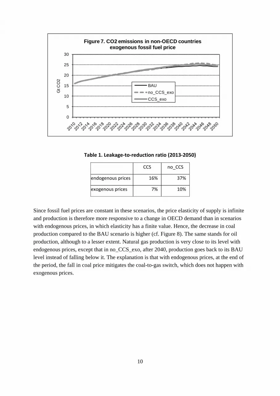
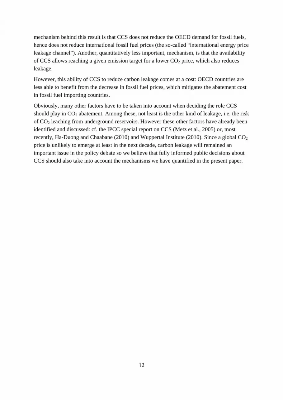
As shown in Figure 7, emissions in non-OECD countries are now very close to the BAU level, meaning that leakage is significantly reduced. Over 2013-2050, the leakage-to-reduction ratio reaches 7% in CCS_exo and 10% in no_CCS_exo (cf. Table 1, last line). In other words, leakage is divided by 2.2 in the CCS_exo scenario and by 3.9 in no_CCS_exo. The international energy price channel is thus the dominant leakage channel in our model, especially without CCS.

10

0

5

10

15

20

25

30G

t CO

2

Figure 7. CO2 emissions in non-OECD countries exogenous fossil fuel price

BAUno_CCS_exoCCS_exo

Table 1. Leakage‐to‐reduction ratio (2013‐2050) 

  CCS  no_CCS 

endogenous prices 16%  37% 

exogenous prices  7%  10% 

Since fossil fuel prices are constant in these scenarios, the price elasticity of supply is infinite and production is therefore more responsive to a change in OECD demand than in scenarios with endogenous prices, in which elasticity has a finite value. Hence, the decrease in coal production compared to the BAU scenario is higher (cf. Figure 8). The same stands for oil production, although to a lesser extent. Natural gas production is very close to its level with endogenous prices, except that in no_CCS_exo, after 2040, production goes back to its BAU level instead of falling below it. The explanation is that with endogenous prices, at the end of the period, the fall in coal price mitigates the coal-to-gas switch, which does not happen with exogenous prices.

11

Figure 8. Fossil fuels production, exogenous fossil fuel prices 

0500

100015002000250030003500400045005000

Mto

e

Coal production

BAUno_CCS_exoCCS_exo

0

20

40

60

80

100

120

2010

2012

2014

2016

2018

2020

2022

2024

2026

2028

2030

2032

2034

2036

2038

2040

2042

2044

2046

2048

2050

mill

ion

bl./d

ay

Oil production

0

500

1000

1500

2000

2500

3000

3500

4000

2010

2012

2014

2016

2018

2020

2022

2024

2026

2028

2030

2032

2034

2036

2038

2040

2042

2044

2046

2048

2050

Mto

e

Gas production

The abatement cost in OECD countries, measured by the GDP loss, is slightly higher than in the scenarios with endogenous prices. As a consequence, so is the cost per tonne abated in the OECD, but the cost per tonne abated worldwide (accounting for leakage) is slightly lower (cf. Table 2). In other words, the flexibility of the fossil fuel prices reduces the cost per tonne of CO2 abated if one does not take into account leakage but increases it if one takes leakage into account.

Table 2. Undiscounted average OECD abatement cost per tonne of CO2 over 2013‐2050 

(in US dollars from 2001) 

  per tonne of CO2 abated worldwide per tonne of CO2 abated in the OECD 

  CCS  no_CCS  CCS  no_CCS 

endogenous prices  77.3  113.7 64.9  71.8

exogenous prices  70.2  93.6 65.0  84.7

Conclusion

We have provided, at our knowledge, the first quantification of the impact of CCS on carbon leakage. Assuming a carbon tax (or a cap-and-trade system) only in OECD countries, we have compared two scenarios, one allowing and one prohibiting the use of CCS. The former more than halves carbon leakage to non-OECD countries, compared to the latter. The main

12

mechanism behind this result is that CCS does not reduce the OECD demand for fossil fuels, hence does not reduce international fossil fuel prices (the so-called “international energy price leakage channel”). Another, quantitatively less important, mechanism, is that the availability of CCS allows reaching a given emission target for a lower CO2 price, which also reduces leakage.

However, this ability of CCS to reduce carbon leakage comes at a cost: OECD countries are less able to benefit from the decrease in fossil fuel prices, which mitigates the abatement cost in fossil fuel importing countries.

Obviously, many other factors have to be taken into account when deciding the role CCS should play in CO2 abatement. Among these, not least is the other kind of leakage, i.e. the risk of CO2 leaching from underground reservoirs. However these other factors have already been identified and discussed: cf. the IPCC special report on CCS (Metz et al., 2005) or, most recently, Ha-Duong and Chaabane (2010) and Wuppertal Institute (2010). Since a global CO2 price is unlikely to emerge at least in the next decade, carbon leakage will remained an important issue in the policy debate so we believe that fully informed public decisions about CCS should also take into account the mechanisms we have quantified in the present paper.

13

Appendix: model description

A.1. General features

Imaclim-R is a hybrid recursive general equilibrium model of the global economy divided into 12 regions and 12 sectors (Table 3) and solved in a yearly time step (Sassi et al. 2010). The base year of the model (2001) is built on the GTAP-6 database, which provides a balanced Social Accounting Matrix (SAM) of the global economy. The original GTAP-6 dataset has been modified to (i) aggregate regions and sectors according to the Imaclim-R mapping, and (ii) accommodate the 2001 IEA energy balances, in an effort to base Imaclim-R on a set of hybrid energy-economy matrixes.

Table 3. Regional and sectoral disaggregation of the IMACLIM‐R model 

Regions   Sectors 

USA Canada Europe OECD Pacific (JP, AU, NZ, KR) Former Soviet Union China  India Brazil Middle‐East Countries Africa Rest of Asia Rest of Latin America 

Coal Oil Gas Liquid Fuels Electricity Air Water Other transports Construction Agriculture Energy‐intensive industry Composite (services and light industry) 

As a general equilibrium model, Imaclim-R provides a consistent macroeconomic framework to assess the energy-economy relationship through the clearing of commodity markets. Specific efforts have been devoted to building a modelling architecture allowing easy incorporation of technological information coming from bottom-up models and experts’ judgement within the simulated economic trajectories. The rigorous incorporating of information about how final demand and technical systems are transformed by economic incentives is allowed by the existence of physical variables that explicitly characterise equipments and technologies (e.g. the efficiency of cars, the intensity of production in transport, etc.). The economy is then described in both money-metric terms and physical quantities, the two dimensions being linked by a price vector. This dual vision of the economy is a precondition to guaranteeing that the projected economy is supported by a realistic technical background and, conversely, that any projected technical system corresponds to realistic economic flows and consistent sets of relative prices.

The full potential of this dual representation could not be exploited without abandoning the use of conventional aggregate production functions like nested CES functions: it is arguably

14

almost impossible to find mathematical functions flexible enough to cover large departures from the reference equilibrium and to encompass different scenarios of structural changes resulting from the interplay between consumption styles, technologies and localisation patterns (Hourcade 1993). In Imaclim-R the absence of formal production functions is compensated by a recursive structure that allows a systematic exchange of information between:

• An annual static equilibrium module with Leontief production functions (fixed equipment stocks and intensities of intermediary inputs, especially labour and energy; but a flexible utilisation rate). Solving this equilibrium at some year t provides a snapshot of the economy: information about relative prices, output levels, physical flows and profit rates for each sector and allocation of investments among sectors.

• Dynamic modules, including demography, capital dynamics and sector-specific reduced forms of technology-rich models, most of which assess the reactions of technical systems to the previous static equilibriums. These reactions are then sent back to the static module in the form of updated input-output coefficients to calculate year (t+1) equilibrium.

Between two equilibriums, technical choices are fully flexible for new capital only; the input-output coefficients and labour productivity are modified at the margin, because of fixed techniques embodied in existing equipment and resulting from past technical choices. This general putty-clay assumption is critical to representing the inertia in technical systems and the perverse effect of volatility in economic signals.

Imaclim-R thus generates economic trajectories by solving successive yearly static equilibriums of the economy interlinked by dynamic modules. Within the static equilibrium, in each region, the demand for each good derives from household consumption, government consumption, investment and intermediate uses from the production sectors. This demand can be provided either by domestic production or imports and all goods and services are traded on international markets. Domestic and international markets for all goods – excluding labour – are cleared by a unique set of relative prices that depend on the demand and supply behaviours of representative agents. The calculation of this equilibrium determines relative prices, wages, labour, quantities of goods and services, and value flows.

The dynamic modules shape the accumulation of capital and its technical content, they are driven by economic signals (such as prices or sectoral profitability) that emerge from former static equilibriums. They include the modelling of (i) the evolution of capital and energy equipment stock described in both vintage and physical units (such as number of cars, housing square meter, transportation infrastructure), (ii) of technological choices of economic agent described as discrete choices in explicit technology portfolios for key sectors such as electricity, transportation and alternative liquid fuels, or captured through reduced form of technology rich bottom up models, and (iii) of endogenous technical change for energy technologies (with learning curves).

15

In this framework, the main exogenous drivers of economic growth are population and labour productivity dynamics. However, international trade, particularly that of energy commodities, and imperfect markets for both labour (wage curve) and capital (constrained capital flows, varying utilisation rates of productive capacities), significantly impact on economic growth.

A.2. Energy markets and CCS in the Imaclim-R model

A.2.1. Oil

Oil markets are described in detail in Waisman et al. (2010). In particular, oil prices are related to the utilization rate of oil production capacity (Kauffmann et al., 2004), which in turn depends on the dynamics of both the supply and the demand side.

The main objective of the oil production module is to capture the drivers of short term scarcity generated by gaps between demand and production which cannot be bridged overnight given technical and economic inertia. Imaclim-R describes these determinants with a high level of site specific details that include the amount of ultimate resources, cost profiles of oil fields and the constraints on the deployment of production capacities.

To describe those deployment constraints, regional oil resources are distinguished according to their cost of exploration and exploitation. Once the decision to initiate investments in a given oil category is made, the pace of deployment of production capacities is determined by inertias affecting the efficiency of exploration7. In line with Rehrl and Friedrich (2006), we adopt the following dynamic equation to describe the deployment of production capacities Cap for a given category:

( )

0

0

( )

2( )

.( )1

b t t

b t t

Q beCap te

− −∞

− −=

+

This analytical expression corresponds to a bell-shaped symmetric Hubbert curve (Hubbert, 1962) differentiated across oil categories by its steepness and the area it delimits. The former characteristic measures the intensity of the constraints slowing down discoveries and is captured by parameter b (b=0.061). The latter one accounts for the amount of ultimate reserves through parameterQ∞ (=3.6Tb in these scenarios).

At a given point in time, oil production capacity thus depends upon two parameters, the previous decision to initiate exploration and the Hubbert curve that determines the geological constraints affecting the exploration process. In Imaclim-R, the utilization rate of those production capacities captures the level of tensions between supply and demand and affects the profit margin on any product: the higher the utilization rate, the higher the scarcity rent captured through a higher mark-up rate.

7 We assume a constant time-lag between discovery and production capacity

16

Contrary to most sectors for which high unitary profit margin triggers investment decisions, Middle-East oil producers have the latitude to refrain from investing, hence creating tensions through an overutilization of their producing capacity, in order to better fulfill long term objectives. This ‘swing producer’ behavior is coherent with past OPEC production which has no longer fit the discovery trend since the 1970s oil shocks. In our scenarios, OPEC aims at a short-term price of $80/bl. As for non-Middle-East producers (that are ‘fatal producers’), they cannot but act as followers: they observe the current oil prices, and decide to launch exploration campaigns of a category of oil as soon as it becomes profitable.

A.2.2. Gas

In the model, global gas production capacities answer to demand growth until ultimately recoverable resources enter a depletion process. Gas prices variations are indexed on that of oil prices via an indexation coefficient (0.68, see equation below) calibrated on the World Energy Model of the IEA (2007). When oil prices increase by 1%, gas prices increase by 0.68%. This indexation disappears when oil prices reach $80/bl.: beyond this threshold, the evolution of gas prices only depends on production costs and possibly on the depletion effect, which leads to a sharp price increase (due to an augmentation of the producer mark-up rate).

Gas price in each region at year t is equal to:

( ) ( )refgas gas gast tp p τ= ⋅

where: refgasp is the gas price in this region at year 1.

While gas depletion has not started, ( )gas tτ in each region is:

1 2 1( ) 0.68 ( ) ( 1)3 3gas oil oil ref

oil

t wp t wp twp

τ ⎛ ⎞= × × + × − ×⎜ ⎟⎝ ⎠

where:

( )oilwp t is the international oil price at year t;

refoilwp is the international oil price at year 1.

Moreover, if depletion has started in this region, ( )gas tτ increases by 5% each year, regardless

of oil prices.

A.2.3. Coal

Coal is treated in a different way than oil and gas because of the larger amount of available resources which prevents coal production from entering into a depletion process before the end of the 21st century. We describe price formation on the international coal market with a reduced functional form which relates price variation to production changes. This choice allows us to capture the cyclic behavior of this commodity market. In these scenarios, coal

17

price growth sensitivity with respect to coal production growth is quite high, so that the coal production growth cannot be absorbed without prices variations.

Coal price in year t is equal to:

( ) ( )refcoal coal coalt pp tτ⋅=

Where ( ) ( )refcoal coal coalt pp tτ⋅=

refcoalp is the coal price in this region at year 1.

( )coal tτ is defined as

( ) ( 1) ( ))(1coal coal i coal tt t gτ τ α= − ⋅ + ⋅

with lim( ) - ( -1)( -

-1)

( )

world worldcoal coal

coal worldcoal

Q QtQ

tt

gtg =

Where ( )worldcoalQ t is the international coal production at year t.

limg is the production growth rate that would not lead to price fluctuation (we set it to 0.05%).

We distinguish upwards and downwards movements of production growth, in order to introduce asymmetry in price response: we use 1α (=1) as the price growth elasticity to

production decrease when production growth is lower than limg and 2α (=4) when production

growth is greater than limg .

1.4. Carbon capture and storage

The CCS technology is represented in the electricity sector and Coal-To-Liquid production (see 1.5 below). The electricity supply module in Imaclim-R represents the evolution of power generation capacities over time, which depends on the amount of capital available for new investments and changes in fuel and factor prices. The model anticipates ten years forward the potential future electricity demand, taking into account past trends of demand, and computes an optimal mix of electricity productive capacities to face future needs at the lowest cost, expecting that fuel prices will stay at their current level. Three technologies can incorporate a CCS device: Combine Cycle Gas Turbine (CCGT), Supercritical coal plant, and Integrated coal Gasification Combined Cycle (IGCC). Each technology is characterized by a date of availability across each region, a level of energy efficiency, a capital cost when arriving to the market, a technology learning rate, and maximum socially and technically achievable market shares.

1.5. Biofuel and Coal-To-Liquid (CTL)

In our numerical exercises with the Imaclim-R modeling framework, biofuels (first and second generation) and Coal-To-Liquid fuels represent the main alternatives to refined oil over the 21st century.

18

Biofuels: The penetration of biofuels in energy supply is modeled according to worldwide supply curves published by the IEA (2006). They have been interpolated to integrate an annual continuum of the curves between 2001 and 2100 into the Imaclim-R model. Production potentials increase with time simultaneously with cost reductions thanks to constant technical progress. These production potential increases are mainly due to maturing, at middle term, of so-called second-generation technologies: the cellulosic-lignite branch for ethanol and the biomass liquefaction branch for biodiesel. The penetration of biofuels on the liquid fuels market depends on their competitiveness and availability. Both aspects are calculated by equaling out the marginal production costs of each type of biofuel and the price of fuel produced by the “classical” branch of refined crude oil, with an eventual increase due to a carbon tax in the case of climate policies.

Coal-To-Liquid (CTL): As soon as oil prices exceed a threshold value pCTL8, CTL producers

are willing to fill the gap between total liquid fuel demand D(t) and the total supply by other sources (refined oil and biofuels) S(t). Their production objective is then D(t)-S(t). But they may miss this objective because of insufficient delivery capacity at a given point in time as a result of past under-investments. Indeed, under imperfect foresight, a period of low oil prices affects the profitability prospects of CTL and suggests postponing the investments in this technology: CTL investments are driven by the current level of oil price at each date, and cumulative investments over time are then a function of the sum of past trends of oil price as follows

( )2010

( )t

cum oili

p t p i=

= ∑.

The share s of the targeted CTL production that is actually realized given the constraints on production investments is an increasing function of cumulative investments and, hence, of

( )cump t . As soon as oil price exceeds pCTL , CTL production is then given by:

( ) ( ) [ ]( ) . ( ) S( )cumCTL t s p t D t t= −

A share of CO2 emissions due to CTL production can be sequestrated, as a growing function of the carbon tax.

8 We take pCTL= $100/Bbl for all scenarios

19

References

Crassous, R., J.-C. Hourcade, and O. Sassi, 2006. Endogenous structural change and climate targets : modeling experiments with Imaclim-R, Energy Journal, Special Issue #1, Endogenous Technological Change

Dröge, S. et al., 2009. Tackling Leakage in a World of Unequal Carbon Prices, Climate Strategies Report, July. Available at http://www.climatestrategies.org/our-reports/category/32/257.html

Fisher, B. and N. Nakicenovic, 2007. Issues related to mitigation in the long-term context. Chapter 3 in IPCC Fourth Assessment Report, Working Group III, Cambridge U. Press

Fölster, S. and J. Nyström, 2010. Climate Policy to Defeat the Green Paradox. Ambio 39(3) Special Issue: 223-235

Gerlagh, R. and O. Kuik, 2007. Carbon Leakage with International Technology Spillovers, FEEM Working Paper 33.2007

Goulder, L.H., I.W.H. Parry and D. Burtraw, 1997. Revenue-Raising versus Other Approaches to Environmental Protection: The Critical Significance of Preexisting Tax Distortions. RAND Journal of economics, 28(4): 708-31

Guivarch, C., R. Crassous, O. Sassi and S. Hallegatte. 2010. The costs of climate policies in a second best world with labour market imperfections. Climate Policy (forthcoming)

Guivarch C., S. Hallegatte and R. Crassous, 2009. The Resilience of the Indian Economy to Rising Oil prices as a validation test for a Global Energy-Environment-Economy CGE model, 2009, Energy Policy 37, November

Ha-Duong, M. and N. Chaabane, 2010. Captage et stockage du CO2. Enjeux techniques et sociaux en France. Quae editions, Paris, ISBN 978-2-7592-0369-7, 164 pp.

Hamdi-Cherif, M., C. Guivarch and P. Quirion, 2010. Sectoral targets for developing countries: Combining "Common but differentiated responsibilities" with "Meaningful participation", Climate Policy, forthcoming

Hubbert, M.K. 1962. Energy from fossil fuels, energy resources. National Academy of Sciences, National Research Council publication 1000-D, p. 22-94.

Kaufmann, R.K., 2004. Does OPEC matter? An econometric analysis of oil prices. Energy Journal, 25(4): 67-90

Kober, T. and M. Blesl, 2010. Perspectives of CCS power plants in Europe, considering uncertain power plant parameters. International Energy Workshop, Stockholm, Sweden, http://www.kth.se/polopoly_fs/1.61926!D5_Kober.pdf

Kuik, O. and R. Gerlagh, 2003. Trade liberalization and carbon leakage. Energy Journal, 24(3): 97-120

20

Manne, A.S. and T.F. Rutherford, 1994. International trade in oil, gas and carbon emission rights – an intertemporal general equilibrium model. Energy Journal, 25, 162-176.

Marschinski, R., M. Jakob and O. Edenhofer, 2009. Analysis of Carbon Leakage in an Extended Ricardo-Viner Model. EAERE Conference, June 24-27, Amsterdam, Netherlands.

Mathy, S., Guivarch, C. 2010. Climate policies in a second-best world - A case study on India. Energy Policy 38(3): 1519-1528.

Metz, B., O. Davidson, H. de Coninck, M. Loos and L. Meyer (Eds.) , 2005. Carbon Dioxide Capture and Storage – IPCC Special Report. Cambridge University Press, UK. pp 431. http://www.ipcc.ch/pdf/special-reports/srccs/srccs_wholereport.pdf

Monjon, S. and P. Quirion, 2010. How to design a border adjustment for the European Union Emissions Trading System?, Energy Policy, 38(9): 5199-5207

Paltsev, S.V., 2001. The Kyoto Protocol: Regional and sectoral contributions to the carbon leakage. Energy Journal, 22(4): 53-79

Quirion, P., 2009. Historic versus output-based allocation of GHG tradable allowances: a survey, Climate Policy, 9: 575-592

Quirion, P., 2010a. Carbon leakage: beyond competitiveness. Berlin Seminar on Energy and Climate, 1st July, http://www.climatepolicyinitiative.org/news_berlin_bsec.html

Quirion, P., 2010b. Climate Change Policies, Competitiveness and Leakage. in Cerdá, E. and Labandeira, X. (eds.). Climate Change Policies: Global Challenges and Future Prospects. Edward Elgar Publishing, Cheltenham

Rehrl, T. and R. Friedrich, 2006. Modelling long-term oil price and extraction with a Hubbert approach: The LOPEX model. Energy Policy 34(15): 2413-2428

Rozenberg J., S. Hallegatte, A. Vogt-Schilb, O. Sassi, C. Guivarch, H. Waisman and J.-C. Hourcade, 2010. Climate policies as a hedge against the uncertainty on future oil supply. Climatic Change 101(3-4): 663-668

Sassi O., R. Crassous, J.-C. Hourcade, V. Gitz, H. Waisman and C. Guivarch, 2010. Imaclim-R: a modelling framework to simulate sustainable development pathways, International Journal of Global Environmental Issues 10(1): 5-24.

Waisman, H., J. Rozenberg, O. Sassi and J-.C. Hourcade, 2010. The Peak Oil through the lens of a general equilibrium assessment. CIRED Working Paper, http://www.centre-cired.fr/spip.php?article1144

Wuppertal Institute, 2010. Comparison of Renewable Energy Technologies with Carbon Dioxide Capture and Storage (CSS). Report for the German Federal Ministry of the Environment. http://www.wupperinst.org/uploads/tx_wiprojekt/RECCSplus_final_report.pdf

NOTE DI LAVORO DELLA FONDAZIONE ENI ENRICO MATTEI

Fondazione Eni Enrico Mattei Working Paper Series

Our Note di Lavoro are available on the Internet at the following addresses: http://www.feem.it/getpage.aspx?id=73&sez=Publications&padre=20&tab=1

http://papers.ssrn.com/sol3/JELJOUR_Results.cfm?form_name=journalbrowse&journal_id=266659 http://ideas.repec.org/s/fem/femwpa.html

http://www.econis.eu/LNG=EN/FAM?PPN=505954494 http://ageconsearch.umn.edu/handle/35978

http://www.bepress.com/feem/

NOTE DI LAVORO PUBLISHED IN 2011 SD 1.2011 Anna Alberini, Will Gans and Daniel Velez-Lopez: Residential Consumption of Gas and Electricity in the U.S.:

The Role of Prices and Income SD 2.2011 Alexander Golub, Daiju Narita and Matthias G.W. Schmidt: Uncertainty in Integrated Assessment Models of

Climate Change: Alternative Analytical Approaches SD 3.2010 Reyer Gerlagh and Nicole A. Mathys: Energy Abundance, Trade and Industry Location SD 4.2010 Melania Michetti and Renato Nunes Rosa: Afforestation and Timber Management Compliance Strategies in

Climate Policy. A Computable General Equilibrium Analysis SD 5,2011 Hassan Benchekroun and Amrita Ray Chaudhuri: “The Voracity Effect” and Climate Change: The Impact of

Clean Technologies IM 6.2011 Sergio Mariotti, Marco Mutinelli, Marcella Nicolini and Lucia Piscitell: Productivity Spillovers from Foreign

MNEs on Domestic Manufacturing Firms: Is Co-location Always a Plus? GC 7.2011 Marco Percoco: The Fight Against Geography: Malaria and Economic Development in Italian Regions GC 8.2011 Bin Dong and Benno Torgler: Democracy, Property Rights, Income Equality, and Corruption GC 9.2011 Bin Dong and Benno Torgler: Corruption and Social Interaction: Evidence from China SD 10.2011 Elisa Lanzi, Elena Verdolini and Ivan Haščič: Efficiency Improving Fossil Fuel Technologies for Electricity

Generation: Data Selection and Trends SD 11.2011 Stergios Athanassoglou: Efficient Random Assignment under a Combination of Ordinal and Cardinal

Information on Preferences SD 12.2011 Robin Cross, Andrew J. Plantinga and Robert N. Stavins: The Value of Terroir: Hedonic Estimation of

Vineyard Sale Prices SD 13.2011 Charles F. Mason and Andrew J. Plantinga: Contracting for Impure Public Goods: Carbon Offsets and

Additionality SD 14.2011 Alain Ayong Le Kama, Aude Pommeret and Fabien Prieur: Optimal Emission Policy under the Risk of

Irreversible Pollution SD 15.2011 Philippe Quirion, Julie Rozenberg, Olivier Sassi and Adrien Vogt-Schilb: How CO2 Capture and Storage Can

Mitigate Carbon Leakage