Hunger, Hiding, and Habitat: Observations and Game Theoretical Explorations of Foraging

and Burrowing

BY

HILARY BETH OSBORNE

B.S., Northeastern University, 2000

THESIS

Submitted as partial fulfillment of the requirements for the degree of Doctor of Philosophy in

Biological Sciences in the Graduate College of the University of Illinois at Chicago, 2016

Chicago, Illinois

Defense Committee:

Joel S. Brown, Chair and Advisor

Som B. Ale, Biological Sciences

Tanya Berger-Wolf, Computer Science

Thomas J. Park, Biological Sciences

Christopher J. Whelan, Biological Sciences and Illinois Natural History Survey

ii

ACKNOWLEDGEMENTS

A lot of people go into making a PhD, and they all deserve far more credit than just this page.

My parents have been supportive all along, including providing the only grants I was

good at getting, and getting me home early after my injury. Thanks for not asking about my

progress. Much.

My African parents, Retha and Ian Gaigher, along with their sons Emil and Stefan and

daughter-in-law Leslie for being there when my actual family could not, and for years

afterward.

The South African Mountain Rescue team, the South African Air Force, the staff of the

Limpopo Medi-Clinic in Polokwane, and my travel medical insurance company for literally

saving my life.

The good folks at SANParks for granting me a permit and forgetting to charge me

anything for living and working at Mapungubwe. The rangers and students at Mapungubwe,

especially Stefan, Sam, Ndwa, Solly, Daniel, Alek, and Fhatwhani.

Everyone at the Venetia Limpopo Nature Reserve. My time there was not particularly

fruitful, but it was rather nifty to be driven around in a DeBeers Land Rover.

VCA Aurora Animal Hospital for hiring me five times, even though I kept quitting to go to

South Africa. The ones we fix make it worth it.

Almost everyone at UIC. Joel, we had our differences (and how!), but always worked it

out in the end. Raghavan, the best professor I ever had (sorry Joel). Karin, for putting up with

my obsessiveness. Game Theory Club, especially Brian and Matt, for being supremely nerdy and

iii

working with me on what is now Chapter 6. And mostly Beth, without whom we’d all be forever

lost in the red tape.

Contribution of Authors

I wrote the entirety of all manuscripts presented in this document, including generating

all figures except where noted and the photograph in Chapter II, which was taken by Dr. Thom

Park and used with his permission. The experiments in Chapter II were carried out by Dr. Joel

Brown and Dr. Thom Park. The model in Chapter VI was a collaboration with Dr. Brian Powers

and Dr. Matthew Borque. Dr. Joel Brown assisted in preparing all chapters by offering advice

and critiques. None of the chapters have been previously published.

iv

TABLE OF CONTENTS CHAPTER PAGE I. INTRODUCTION ........................................................................................................................... 1

A. Personal Background ...................................................................................................... 1 B. Research .......................................................................................................................... 3 C. The chapters ................................................................................................................... 5

1. Field Work ........................................................................................................... 5 2. Game theory ....................................................................................................... 8 3. Naked mole-rats ................................................................................................ 11

D. Conclusion .................................................................................................................... 13 E. Literature cited .............................................................................................................. 13

II. NAKED MOLE-RATS ARE NOT AS COOPERATIVE AS THEY APPEAR .......................................... 16

A. Introduction .................................................................................................................. 16 1. Eusociality ......................................................................................................... 16 2. Naked mole-rats ................................................................................................ 17 3. Patch use ........................................................................................................... 18 4. Study design ...................................................................................................... 23 5. Predictions ........................................................................................................ 24

B. Methods ........................................................................................................................ 30 C. Results ........................................................................................................................... 28 D. Discussion ..................................................................................................................... 35 E. Conclusion ..................................................................................................................... 40 F. Literature cited .............................................................................................................. 40

III. DEMOGRAPHY AND DYNAMICS OF AARDVARK-DUG BURROWS ........................................... 43

A. Introduction ................................................................................................................. 43 B. Methods ........................................................................................................................ 46

1. Location ............................................................................................................. 46 2. Survey plots ....................................................................................................... 50 3. Plugs .................................................................................................................. 54

C. Results ........................................................................................................................... 55 1. Burrow density .................................................................................................. 57 2. Plugs .................................................................................................................. 62

D. Discussion ..................................................................................................................... 63 E. Conclusion ..................................................................................................................... 67 F. Literature cited .............................................................................................................. 68

IV. CAMERA TRAPS REVEAL THAT AARDVARKS ARE THE INADVERTENT CIVIL ENGINEERS OF

SOUTHERN AFRICA ............................................................................................................ 72 A. Introduction .................................................................................................................. 72

1. Ecosystem engineering ..................................................................................... 72 2. Aardvarks .......................................................................................................... 75

v

TABLE OF CONTENTS (continued) 3. Camera traps ..................................................................................................... 79 4. Study goals ........................................................................................................ 80

B. Methods ........................................................................................................................ 82 1. Location ............................................................................................................. 82 2. Habitat types ..................................................................................................... 84 3. Plot choice and camera placement ................................................................... 85

C. Results ........................................................................................................................... 91 1. Mopane ............................................................................................................. 92 2. Field and riverine .............................................................................................. 93

D. Discussion ................................................................................................................... 111 E. Conclusion ................................................................................................................... 122 F. Literature cited ............................................................................................................ 123

V. A MODEL OF BEHAVIORAL RESOURCE DEPRESSION AND SLOWLY REGENERATING

RESOURCES ..................................................................................................................... 128 A. Introduction ................................................................................................................ 128 B. The model Stage 0: the marginal value theorem ....................................................... 132 C. The model Stage 1: behavioral resource depression ................................................. 136 D. The model Stage 2: behavioral resource depression with slowly regenerating

resources, infinite patches .................................................................................. 141 E. The model Stage 3: behavioral resource depression with slowly regenerating

resources, limited patches .................................................................................. 147 F. Discussion and conclusion ........................................................................................... 151 G. Literature cited ........................................................................................................... 152

VI. THE ROLE OF HUNGER IN A PREDATOR-PREY FORAGING GAME ......................................... 154

A. Introduction ................................................................................................................ 154 1. Foraging........................................................................................................... 154 2. The real-world inspiration............................................................................... 155

B. The models .................................................................................................................. 157 1. Stage 1: the matrix .......................................................................................... 157 2. Stage 2: state dependence.............................................................................. 167 3. Stage 3: the asset protection principle ........................................................... 174

C. Conclusion ................................................................................................................... 179 D. Literature cited ........................................................................................................... 181

VITA ............................................................................................................................................. 183

vi

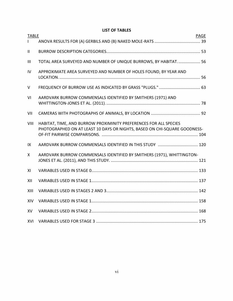
LIST OF TABLES TABLE PAGE I ANOVA RESULTS FOR (A) GERBILS AND (B) NAKED MOLE-RATS ........................................ 39

II BURROW DESCRIPTION CATEGORIES.................................................................................. 53

III TOTAL AREA SURVEYED AND NUMBER OF UNIQUE BURROWS, BY HABITAT. ................... 56

IV APPROXIMATE AREA SURVEYED AND NUMBER OF HOLES FOUND, BY YEAR AND LOCATION. ........................................................................................................................... 56

V FREQUENCY OF BURROW USE AS INDICATED BY GRASS "PLUGS." .................................... 63

VI AARDVARK BURROW COMMENSALS IDENTIFIED BY SMITHERS (1971) AND WHITTINGTON-JONES ET AL. (2011). .................................................................................. 78

VII CAMERAS WITH PHOTOGRAPHS OF ANIMALS, BY LOCATION ........................................... 92

VIII HABITAT, TIME, AND BURROW PROXIMINITY PREFERENCES FOR ALL SPECIES PHOTOGRAPHED ON AT LEAST 10 DAYS OR NIGHTS, BASED ON CHI-SQUARE GOODNESS-OF-FIT PAIRWISE COMPARISONS. .................................................................................... 104

IX AARDVARK BURROW COMMENSALS IDENTIFIED IN THIS STUDY ................................... 120

X AARDVARK BURROW COMMENSALS IDENTIFIED BY SMITHERS (1971), WHITTINGTON-JONES ET AL. (2011), AND THIS STUDY. ............................................................................ 121

XI VARIABLES USED IN STAGE 0 ............................................................................................. 133

XII VARIABLES USED IN STAGE 1 ............................................................................................. 137

XIII VARIABLES USED IN STAGES 2 AND 3................................................................................ 142

XIV VARIABLES USED IN STAGE 1 ............................................................................................. 158

XV VARIABLES USED IN STAGE 2 ............................................................................................. 168

XVI VARIABLES USED FOR STAGE 3 ......................................................................................... 175

vii

LIST OF FIGURES FIGURE PAGE

1 Relative proportions harvested by foragers using (A) fixed harvest rate, (B) fixed time, and

(C) fixed amount foraging strategies .................................................................................. 23

2 Schematic of the arena ....................................................................................................... 27

3 Author JSB setting up the test arena................................................................................... 28

4 Proportions of food harvested by gerbils in (Left) Mixed patches and (Right) Clustered patches. ............................................................................................................................... 31

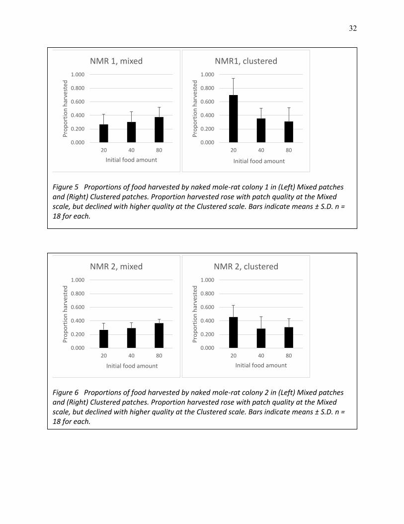
5 Proportions of food harvested by naked mole-rat colony 1 in (Left) Mixed patches and (Right) Clustered patches. .................................................................................................. 32

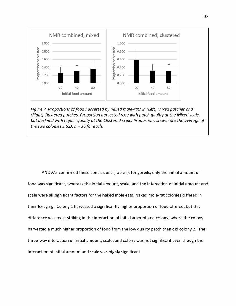
6 Proportions of food harvested by naked mole-rat colony 2 in (Left) Mixed patches and (Right) Clustered patches. .................................................................................................. 32

7 Proportions of food harvested by naked mole-rats in (Left) Mixed patches and (Right) Clustered patches. .............................................................................................................. 33

8 Official Map of Mapungubwe National Park, 2005 ............................................................. 47

9 Habitat types at Mapungubwe National Park, South Africa. ............................................. 49

10 Examples of aardvark burrows at Mapungubwe National Park, South Africa. .................. 53

11 An aardvark burrow in the riverine forest at Mapungubwe National Park, South Africa, after our grass "plug" had been pushed down by an animal. ............................................. 55

12 Burrow positions in two adjacent plots (left: plot H; right: plot G) in the field at Mapungubwe National Park, South Africa, in 2008. ........................................................... 58

13 Burrow C1, in a former agricultural field, at Mapungubwe National park in (A) 2008, (B) 2009, and (C) 2010. ............................................................................................................. 59

14 Distribution of the diameter of the soil fan or mound in front of burrows ....................... 60

15 Tunnel lengths .................................................................................................................... 61

16 Entry hole size (diameter) based on visual estimate ......................................................... 61

17 Bubble XY graphs for fan size vs. tunnel size ..................................................................... 62

18 Aardvarks at Mapungubwe National Park, South Africa .................................................... 76

viii

LIST OF FIGURES (continued)

19 Official map of Mapungubwe National Park, 2005. Park borders were unchanged as of this study. ................................................................................................................................... 82

20 Habitat types at Mapungubwe National Park, South Africa. .............................................. 85

21 Camera traps at Mapungubwe National Park ..................................................................... 87

22 (A) A starving aardvark exiting its burrow during the day. (B) The brown hyena that scavenged the aardvark. ..................................................................................................... 89

23 The number of photographs of identifiable species taken in the field and riverine habitats at Mapungubwe National Park, South Africa, in the winters of 2000–2010. ..................... 95

24 The number of photographs taken of the ten most-photographed species in the field and riverine habitats at Mapungubwe National Park, South Africa, in the winters of 2000–2010. .................................................................................................................................... 96

25 Total number of pictures per 100 camera-days and camera-nights of identifiable species taken in the field and riverine habitats at Mapungubwe National Park, South Africa, in the winters of 2000–2010. ........................................................................................................ 97

26 Number of photographs per 100 camera-days+nights of the 15 most-photographed species in the field and riverine habitats at Mapungubwe National Park, South Africa, in the winters of 2000–2010, stratified by habitat. ................................................................ 98

27 Number of photographs per 100 camera-days or camera-nights of the 15 most-photographed species in the field and riverine habitats at Mapungubwe National Park, South Africa, in the winters of 2000–2010. ........................................................................ 98

28 Number of photographs per 100 camera-days+nights of the 15 most-photographed species in the field and riverine habitats at Mapungubwe National Park, South Africa, in the winters of 2000–2010, stratified by Burrow–Away. ..................................................... 99

29 Species using aardvark burrows ........................................................................................ 101

30 Number of appearances by species .................................................................................. 102

31 Animals making use of aardvark burrows ay Mapungubwe National Park, South Africa. 106

32 Some of the visitors to and residents of burrow C1, located in a former agricultural field .................................................................................................................................... 108

33 Number of identified mammal species per camera location type ................................... 109

ix

LIST OF FIGURES (continued)

34 Number of mammal species versus the number of days (24-hour periods) monitored. . 110

35 General form of the changes in prey number over time using the Marginal Value Theorem (MVT) and Stage 1 Behavioral Resource Depression (BRD) .............................................. 140

36 General form of the prey numbers under behavioral resource depression (BRD) with slowly regenerating resources (SSR) ................................................................................. 146

37 General graph of behavioral resource depression (BRD) and slowly regenerating resources (SSR) with a limited number of patches. ........................................................................... 148

38 Summary schematic of prey numbers and movement between "available" and "hidden" pools .................................................................................................................................. 150

39 Payoff matrix for Stage 1 game ......................................................................................... 160

40 Example of gerbil and owl payoffs under the Stage 1 matrix model ................................ 173

41 Example of a Stage 2 game ............................................................................................... 178

42 Example of a Stage 3 game ............................................................................................... 174

x

LIST OF ABBREVIATIONS BRD Behavioral resource depression

MNP Mapungubwe National Park

NMR Naked mole-rats

SRR Slowly regenerating resources

TFCA Transfrontier Conservation Area

VLNR Venetia-Limpopo Nature Reserve

xi

SUMMARY

The challenges of living include the need for food and the risk of predation. This

dissertation explores several aspects of both finding food and hiding to avoid becoming food.

Naked mole-rats are subterranean eusocial rodents--or are they? We explored naked

mole-rat foraging patterns via a laboratory study measuring how naked mole-rats allocated

their foraging efforts when searching for hidden treats. We found that contrary to our

expectations of cooperative foraging, they appear to forage only for themselves, and may even

hide information about food patches from one another. This supports the idea that naked

mole-rat society is despotic rather than cooperative.

On the other end of the sociality spectrum is the solitary aardvark. Aardvarks do not live

fully underground like naked mole-rats, but they dig large burrows for themselves and feeding

digs large enough to serve as burrows for other animals. We traveled to Mapungubwe National

Park, South Africa, to look at the distribution of these burrows, how quickly they appear and

disappear, and how frequently they are used. We confirmed what many suspected: they are

distributed in a clumped pattern, and while these holes appear and collapse all the time, some

last for years. All have a good chance of being visited by some animal at any time.

We also monitored dozens of burrows with camera traps to determine the identity of

these burrow-users. It is not aardvarks. Instead, warthogs are king. This may reflect species

abundance, as warthogs are quite numerous at Mapungubwe. The distribution of these

burrows indicates that for their creators they are likely feeding digs, reflecting the clumped

distribution of ant and termite nests.

xii

We then considered what actually happens when an aardvark tears into a termite

mound. The termites can run away, send soldiers to defend the mound, or both. This means

that the food patch--in this case the mound--declines in food quantity at a rate higher than the

rate at which the aardvark feeds. We created and explored a model of how this additional

decline, a form of behavioral resource depression, affects the time the aardvark spends in the

patch and how much food they actually consume. We made the model more general than

aardvarks and ants/termites to account for other forms of behavioral resource depression, such

as induced plant chemical defenses, that reduce the quality, and thus effectively the quantity,

of plant biomass available to the herbivore. We also took the first step toward combining this

with the fact that food sources can take a long time to regenerate after being foraged, and how

a finite number of these patches can affect the forager’s long-term harvest from the patch.

Finally, we modeled how hunger may affect a forager’s willingness to risk predation and

the predator’s probability of hunting. Inspired by the well-studied gerbil–owl foraging game,

including empirical studies on this subject, we developed a model which shows that the

likelihood a predator will hunt increases with the forager’s hunger level.

I. INTRODUCTION

A. Personal Background

Nature is complex. Individual lives are complex. And so, my adventures leading up to

this document, and the document itself, are complex.

Once upon a time, I was a cynical kid. School was a horrible experience, not because of

the academics, but because of the combination of having to be up at ridiculously early hours of

the morning (who schedules physics for 7:30AM?) and having to be around teenagers. What

got me through was the promise that high school was as bad as it got, and that college would

be better. I hated English class most of all, but oddly enough some of my English teachers were

my favorites, and I clearly learned a thing or two. Misplaced apostrophes make me twitchy. I

also liked chemistry and never took biology.

Then college. At Northeastern University, chosen over Tufts for the simple reason of a

full scholarship, I started out in Chemical Engineering, but quickly discovered that I hated

engineering. I chose to switch to Biology for reasons unknown even to me. I did well, except for

Organic Chemistry. I knew I wanted to someday get a doctorate, but as I was burned out on

school and had no idea what I wanted my doctorate in, I went to work as a veterinary

technician. For five years I worked full-time in the incredibly stressful, but also incredibly

rewarding, specialty of Emergency and Critical Care.

After that, grad school seemed like a good idea. I ended up at UIC, with only a vague

idea of what I wanted to do. Burrowing mammals—check. Game theory—check. Anything more

specific—nope. I took some classes, had some ideas, then decided to head to South Africa, at a

2

private reserve owned by some people my adviser knew. They have aardvarks there. Aardvarks

are nifty, so why not?

My first attempt at a field season was a disaster. Within three days of arriving in

Johannesburg I was in an ICU in Polokwane recovering from life-threatening injuries. Turns out

that gravity works the same way in South Africa as it does in the USA.

I decided to try again the next year, only based in the Limpopo Valley instead of the

mountains. Mapungubwe National Park turned out to be perfect for me, having several habitat

types in close proximity, plenty of aardvark activity, and a wonderfully supportive set of

rangers. I spent a total of 9 months there over the next three years.

Like so much in my life, my research just kind of happened. I never had the detailed plan

other people did, but I think that let me accept whatever my results were. With no particular

attachment to a hypothesis, you don't mind seeing it disproven. It also helped while working in

South Africa, as the culture there is simply not as regimented as here. One goes with the

proverbial flow.

Throughout grad school, all 20 semesters, I was a Teaching Assistant. That of course had

its highs and lows, but I generally liked it. Students tended to either love me or hate me. I was

known as both “the mean one” and “the fun one,” depending on whether or not the students

followed my rules.

My desire to live comfortably instead of barely scraping by also led to taking more time

but gaining invaluable experience. Throughout grad school I worked part-time as a tech at a

veterinary ER. It's a mentally and physically exhausting job, but nothing beats the feeling of

3

saving a life. I also got to maintain my skills and keep on top of the rapidly changing standards

of veterinary medicine.

I also picked up some freelance editing work. I had no formal training, or even informal

training, but my mother had a book in progress that needed some resources checked for

completeness, and content that begged for snarky commentary. Later, she got a job re-writing

patient information for the American Academy of Ophthalmology, a project far too big for one

person to handle. She hired me, and together we re-wrote more than 80 documents in one

year. This means that I managed to have 80-something publications during grad school. Sure,

they're just a couple pages long, really repetitive, and don't have my name on them, but I'll take

it.

All that editing experience helped me qualify to take the exam for certification by the

Board of Editors in the Life Sciences, which I passed easily. I realized that while I find writing up

my own research painful, I love nit-picking others' work. Tearing it apart. And now I was

qualified to do so professionally.

B. Research

In all that time, when not working at any of my three jobs, I actually managed to get

some research done.

I began with an interest in burrowing mammals, especially the largest. That meant

wombats and aardvarks. My advisor had contacts in South Africa--aardvark territory--who

hosted undergraduate and graduate students studying the wildlife on their private conservation

land, Lajuma. It sounded like a good idea, so I signed up. Two days after arriving in the country,

4

while exploring the mountains, I fell and was severely injured. After nearly a week in the

hospital, I returned to do, well, nothing. I could not walk, and a deep depression prevented any

sedentary research. I did manage to make some contacts at South African National Parks

(SANParks), in particular a section ranger at Mapungubwe National Park named Stefan Cilliers.

So a year later, having completely recovered, I came up with a better idea. With the

appropriate permits in hand, I headed back to South Africa. This time, and the two years after, I

only visited Lajuma but worked at the non-mountainous Mapungubwe. I went four years

without experiencing summer.

At Mapungubwe, I spent countless hours walking around finding, describing, and

photographing holes in the ground. For the first two years I had Nature Conservation students

as assistants; the first year it was whoever was not assigned elsewhere, the second Samantha

McCulloch. My final field season we had no students, and I didn't know until I arrived how it

would work out. I ended up being accompanied every day by a ranger, Solly Zitha, who is also a

fantastic wire artist. With my assistants, I documented hundreds of aardvark-dug holes,

covering generally 8-10 km of ground a day. We set up camera traps all over the park, some of

which still worked by the end of it all. I sifted through a disturbingly large number of pictures of

grass to find the pictures of animals that form the basis for chapter 3. We revisited the same

burrows year after year to monitor their existence, and Solly and I spent a few weeks figuring

out how often these burrows were actually visited.

Back in Chicago, I built two game theory models. The first, an exploration of how

behavioral resource depression combines with slowly regenerating resources to affect patch

use in foraging. The second was developed along with some friends from the Math and Stats

5

department, and focuses on how hunger affects the decision of whether or not to forage for

food. Game theory allows me to be the math geek I truly am.

C. The chapters

1. Field work

The order of the chapters presented here is not the order in which they were conceived.

While my initial attraction to burrowing mammals was simply that they're awesome, I

had plenty of science to support actually studying them. I was intrigued by the concept of

organisms as "ecosystem engineers," a term coined by Jones et al. in 1994. Ecosystem

engineers work much like human civil and mechanical engineers, altering their environment to

benefit themselves and, as a side effect, impacting their entire ecosystem. The example known

even to the general public is the beaver, which creates massive and incredibly well-constructed

dams and turns streams into ponds--or rivers into lakes (Jones et al. 1994, 1997; Jones and

Gutiérrez 2007)

I was most intrigued by burrow-digging engineers. I don't know why. Perhaps I was

unconsciously influenced by one of modern history's most impressive engineering projects, the

Big Dig in my home town of Boston. The Big Dig involved putting a highway underneath an

existing city and the neighboring harbor, which required moving more than 12 million cubic

meters [24 million tonnes, assuming 2 tonnes/m3] of dirt (Commonwealth of Massachusetts).

Aardvarks don't move anywhere near that much dirt (or cost nearly as much), but for

individuals without machinery, their excavation work is impressive. To date, no one knows how

much soil aardvarks move in a year, as no one has fully documented the number and size of

6

burrows dug, but our data allows for a very conservative estimate of approximately 300 tonnes

per aardvark per year. Australia's hairy-nose wombat, another large solitary burrowing

mammal, has been estimated to move 276 m3/ha (552 tonnes/ha, assuming 2 tonnes/m3),

though no time frame was given (Bancroft et al. 2004).

One of my goals in South Africa, as seen in chapters 2 and 3, was to start to get a handle

on the size and nature of aardvarks’ impact. It turns out that another person, Gareth

Whittington-Jones, had similar ideas, and his Master's thesis (Whittington-Jones 2007) and later

paper (Whittington-Jones et al. 2011) cover areas that complement this dissertation.

Whittington-Jones surveyed the small rodents and insects in and around aardvark burrows in

several parks in South Africa with incidental sightings of larger animals; we focused on the

larger animals though the use of camera traps. He also described the microhabitat within the

burrows. We focused on the number, location, and external gross appearance of burrows.

My assistants and I, the royal "we," cataloged hundreds of aardvark excavations in three

habitat types. Location, visual estimates of size, pictures. We revisited many of our sites year

after year to see how things changed. Some burrows remained intact and in use for many years,

others collapsed almost as soon as they were dug; this variation exists within a soil and habitat

type, and undoubtedly varies among them.

At the same time, we used camera traps to figure out just who is actually using these

burrows. Camera-trap technology (like all technology) is improving rapidly (Rovero et al. 2013),

and even between field seasons we were able to switch to smaller yet higher-quality cameras.

Out of the 20 or so cameras I brought to South Africa, only four were functional by the end of

my final field season; I left them with the rangers to use for their own interests or to help catch

7

the poachers and smugglers that plague the park. Most of the rest were destroyed by hyenas,

elephants, or ants. One was stolen.

Camera-trapping started more than a century ago, when the method involved rigging up

a flashlight and a camera to be triggered by an animal tugging on a piece of food attached to a

wire (Carey 1926). Back then, they got one chance. Once film rolls were invented, camera traps

became more practical, and when the world went digital, camera traps became an easy and

useful way to survey the medium to large animals in an area (Rowcliffe and Carbone 2008),

though study designs are still being perfected (Tobler et al. 2008, Foster and Harmsen 2012,

Tobler and Powell 2013, Burton et al. 2015). Modern cameras can be left alone for months if in

a secure location, taking and storing thousands of pictures with a single set of batteries and a

memory card. Our cameras, made in 2008 or 2009, are not up to 2016's standards, but ours

were more than adequate for our purposes. One camera went missing, only to be found 11

months later, right where it had been left by a spotted hyena. It still worked.

I had the pleasure of sorting through tens of thousands of pictures to find just the ones

with animals and creating a spreadsheet database for them. There were already databases

created for this purpose (Tobler et al. 2008), but I chose to do it myself rather than navigate

new software.

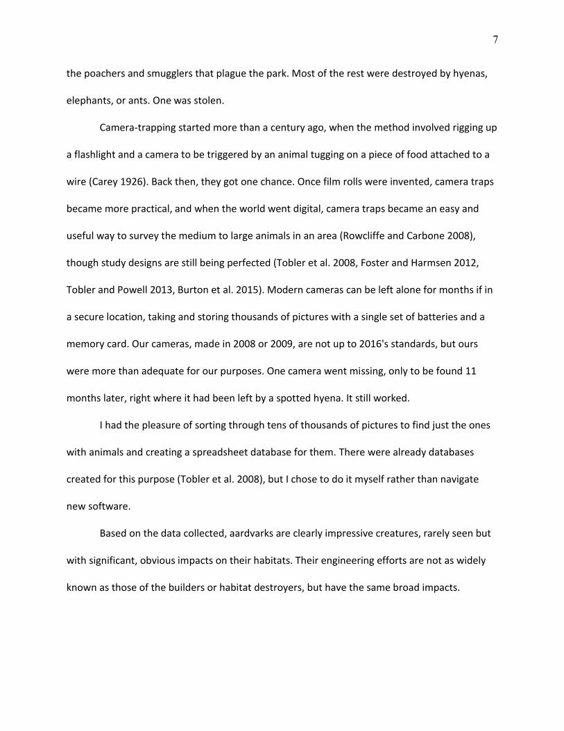
Based on the data collected, aardvarks are clearly impressive creatures, rarely seen but

with significant, obvious impacts on their habitats. Their engineering efforts are not as widely

known as those of the builders or habitat destroyers, but have the same broad impacts.

8

2. Game theory

At UIC, in Chicago, I took two game theory courses and a math-based population

ecology course. I decided to do some modeling.

When I was a kid, my dad (a health physicist) told me the terrible Spherical Cow joke

and for some reason it stuck in my head. As rendered on Wikipedia (Spherical Cow 2015):

Milk production at a dairy farm was low, so the farmer wrote to the local

university, asking for help from academia. A multidisciplinary team of

professors was assembled, headed by a theoretical physicist, and two

weeks of intensive on-site investigation took place. The scholars then

returned to the university, notebooks crammed with data, where the task

of writing the report was left to the team leader. Shortly thereafter the

physicist returned to the farm, saying to the farmer, "I have the solution,

but it only works in the case of spherical cows in a vacuum."

It's a terrible joke but a very useful metaphor. Models of the real world, whether

physics, economics, or biology, must be far simpler than the real world. Nature is complex. But

we can use rough approximations to try to understand things a little better. It's like an artist

drawing a cow. They don't start at the nose and try to get every little detail--they start with a

few big ovals. It doesn't take much more than that to end up with a picture we would recognize

as a cow. That is what we try to do with modeling. Not to get a realistic cow, but to end up with

something sufficiently cow-like to be useful.

Thanks to decades of theoretical and practical work, we know quite a bit about how

animals make foraging decisions. Each model and field study tends to focus on only one or two

9

factors, as the math and the number of variables and parameters can quickly become unwieldy

(e.g., Wood et al. 2013, Sunyer et al. 2014, Fortin et al. 2015). Furthermore, the point of

mathematical modeling is to discern how a particular factor may influence foraging. Including

too many factors makes this task impossible or unproductive. One must make many simplifying

assumptions so as to focus on the factor(s) of choice.

First up for my modeling was an exploration into behavioral resource depression

(Charnov et al. 1976). Behavioral resource depression occurs when a resource such as a food

supply, is depleted by means other than consumption. The simplest form of behavioral

resource depression is prey animals running away from their predators, where they still exist

but are not consumed. This concept applies to plants as well. Many plants have inducible

chemical defenses--when an animal begins chewing on them, the plant begins to release

noxious chemicals to render themselves less palatable or even toxic (Karban and Myers 1989).

Some plants even let each other know that an herbivore is present so they can build up

defenses before being eaten (Ueda et al. 2012).

Staying in defense mode may take a lot of resources (Neilson et al. 2013), and otherwise

interfere with other fitness-enhancing activities (foraging, reproducing, etc.). The plant or

animal which depresses its availability to predators needs time to return to its pre-predation

state.

In reading papers on foraging, I found that most ignored two realities of many systems:

sometimes the food runs away (i.e., behavioral resource depression) (e.g., Kotler 1992), and

sometimes it takes a long time to come back (Brown and Rosenzweig 1986, Watts 1998). Many

foraging studies use stationary food such as seeds, and the researcher replenishes the food

10

supply daily. My beloved aardvarks, however, eat ants and termites, which can both hide

deeper within the nest and send soldiers armed with pincers and poisons to defend the nest (da

Cunha et al. 2014). This encourages the aardvark to give up on the nest sooner, having done

less damage. Then nest rebuilding begins, a process which takes far longer than the seconds or

minutes the aardvark took to damage the nest. So I developed a model to explore how this

behavioral resource depression, coupled with slowly regenerating resources, affects foraging

behavior, giving-up densities (Brown 1988), and patch use. I used prey numbers, but the model

can easily be adapted for other metrics.

Because the phenomena of behavioral resource depression and slowly regenerating

resources exist in many systems, I kept the model, which I based on Charnov’s Marginal Value

Theorem (Charnov 1976), very general. Nevertheless, the model makes sense, and provides a

basis for more sophisticated models.

While sorting through all of this, I also met regularly with a few friends from the Math

and Stats department. We called it Game Theory Club. It was incredibly nerdy--we'd literally get

together to do game theory. We read papers (on learning algorithms) and started our own

model based on my idea. I was intrigued by the idea of state dependence, and that one's

strategy in a foraging game could be affected by, for example, how hungry one is. If you're

starving, you may be willing to head into a bad neighborhood if that’s where the food is. If

you're stuffed, even the kitchen may be too much effort (Clark 1994, Brown and Brooks 1991).

State dependence can be applied to pretty much any game where a player’s status may

determine their available strategies and their outcomes. For example, both body size and

11

burrow-resident status can affect the outcome of contests between juvenile signal crayfish

(Ranta and Lindström 1992).

Some work had been done in this area, and Game Theory Club's idea was sparked by

one paper in particular (Berger‐Tal et al. 2010). There was a simple model right in the paper,

but we chose to start from scratch, or as they say in science, from first principles. The result is

now chapter 5. Even with keeping our metaphorical cow pretty spherical (I'd say that it, like the

Earth, is kind of an oblate spheroid), we can see how the normal predator–prey game can be

affected by how hungry the prey is. While our models have some fatal flaws, they do indicate

that owl hunting behavior may be driven by gerbil hunger state. This model will need to be

altered before it is made more complex.

3. Naked Mole-rats

All throughout grad school I supported myself as a TA. At an end-of-semester lunch in

2014, one of the professors of the course I was TAing offered me a project. This professor,

Thom Park, worked with naked mole-rats. He studies their bizarre physiology, but that's not

what this project was. Way back in 1999 and 2000 he and my adviser, Joel Brown, had

conducted a short foraging behavior study with two colonies of naked mole-rats (and one of

gerbils, for comparison). They used Joel's favorite measurement, the giving-up density, or in

this case the related proportion harvested, to try to figure out if naked mole-rats forage like

they reproduce. Eusocially, that is.

Naked mole-rats are a weird species in many ways (Grimes et al. 2012). Physiologically,

they are nearly ectothermic (unlike all other mammals, which are endothermic), resistant to

12

some forms of pain, can withstand extreme hypoxia, do not get cancer, can live ten times as

long as other rodents their size, and show few signs of aging (though as the brilliant True Facts

video (True Facts About the Naked Mole-Rat 2013) points out, that feat is somewhat less

impressive when you're born looking like an old man). They are also one of the only mammals

considered to be eusocial.

Eusociality in insects, most notably ants and honeybees, means that the colony

effectively acts as a single organism. Individuals are literally born into their job, with little or no

opportunity to switch castes (Sherman et al. 1995). Eusocial colonies have one or a few

reproductive individuals, and non-reproductive members of the colony perform other tasks

such as foraging or nest building. Naked mole-rats were first described as eusocial in 1981

(Jarvis 1981). Over time it became clear that naked mole-rats are not fully eusocial like the

insects, and the popular definition for eusociality in mammals was restricted to “reproductive

altruism (which involves reproductive division of labor and cooperative alloparental brood

care), overlap of adult generations, and permanent (lifelong) philopatry,” (Burda et al. 2000)

and excluded things like fixed castes as criteria for eusociality.

But Thom and Joel had never really done anything with their data. Sure, they had

collected and partially analyzed it, and knew that naked mole-rats do not forage eusocially, but

had never gotten around to writing it up. They needed a grad student who knew them both. I fit

that criterion (and needed another chapter), and since this involved burrowing mammals and

eating, it was a perfect match. In this chapter, the royal "we" generally means "they," instead of

the usual "I" or, occasionally, "we."

13

D. Conclusion

Nature is complex, but the following chapters try to make little spherical cows out of some bits

of it.

E. Literature cited

Bancroft W, Hill D, Roberts J. 2004. A new method for calculating volume of excavated burrows: the geomorphic impact of Wedge Tailed Shearwater burrows on Rottnest Island. Functional Ecology 18: 752-59

Berger‐Tal O, Mukherjee S, Kotler BP, Brown JS. 2010. Complex state‐dependent games between owls and gerbils. Ecology Letters 13: 302-10

Brown GP, Brooks RJ. 1991. Thermal and behavioral responses to feeding in free-ranging turtles, Chelydra serpentina. Journal of Herpetology 25: 273-78

Brown JS. 1988. Patch use as an indicator of habitat preference, predation risk, and competition. Behavioral Ecology and Sociobiology 22: 37-47

Brown JS, Rosenzweig ML. 1986. Habitat selection in slowly regenerating environments. Journal of Theoretical Biology 123: 151-71

Burda H, Honeycutt RL, Begall S, Locker-Grütjen O, Scharff A. 2000. Are naked and common mole-rats eusocial and if so, why? Behavioral Ecology and Sociobiology 47: 293-303

Burton AC, Neilson E, Moreira D, Ladle A, Steenweg R, Fisher JT, Bayne E, Boutin S. 2015. Review: Wildlife camera trapping: a review and recommendations for linking surveys to ecological processes. Journal of Applied Ecology 52: 675-85

Carey HR. 1926. Camera-trapping: a novel device for wild animal photography. Journal of Mammalogy 7: 278-81

Charnov EL. 1976. Optimal foraging, the marginal value theorem. Theoretical Population Biology 9: 129-36

Charnov EL, Orians GH, Hyatt K. 1976. Ecological implications of resource depression. The American Naturalist 110: 247-59

Clark CW. 1994. Antipredator behavior and the asset-protection principle. Behavioral Ecology 5: 159-70

Commonwealth of Massachusetts. (n.d.). Facts & Figures. Retrieved July 1, 2015, from http://www.massdot.state.ma.us/highway/TheBigDig/FactsFigures.aspx

da Cunha HF, Carrijo TF, Prestes AC, Arruda LS, Rezende PB, Santos T, Brandão D. 2014. Food preference of giant anteater and collared anteater (Pilosa, Myrmecophagidae) regarding the termite defense strategies. Bioscience Journal 31: 234-41

Fortin D, Merkle JA, Sigaud M, Cherry SG, Plante S, Drolet A, Labrecque M. 2015. Temporal dynamics in the foraging decisions of large herbivores. Animal Production Science 55: 376-83

Foster RJ, Harmsen BJ. 2012. A critique of density estimation from camera‐trap data. The Journal of Wildlife Management 76: 224-36

14

Grimes KM, Lindsey ML, Gelfond JA, Buffenstein R. 2012. Getting to the heart of the matter: age-related changes in diastolic heart function in the longest-lived rodent, the naked mole rat. The Journals of Gerontology Series A: Biological Sciences and Medical Sciences 67: 384-94

Jarvis J. 1981. Eusociality in a mammal: cooperative breeding in naked mole-rat colonies. Science 212: 571-73

Jones CG, Gutiérrez JL. 2007. 1 On the purpose, meaning, and usage of the physical ecosystem engineering concept. Theoretical Ecology Series 4: 3-24

Jones CG, Lawton JH, Shachak M. 1994. Organisms as ecosystem engineers. Oikos 69: 373-86

Jones CG, Lawton JH, Shachak M. 1997. Positive and negative effects of organisms as physical ecosystem engineers. Ecology 78: 1946-57

Kotler BP. 1992. Behavioral resource depression and decaying perceived risk of predation in two species of coexisting gerbils. Behavioral Ecology and Sociobiology 30: 239-44

Neilson EH, Goodger JQ, Woodrow IE, Møller BL. 2013. Plant chemical defense: at what cost? Trends in Plant Science 18: 250-58

Ranta E, Lindström K. 1992. Power to hold sheltering burrows by juveniles of the signal crayfish, Pasifastacus leniusculus. Ethology 92: 217-26

Rovero F, Zimmermann F, Berzi D, Meek P. 2013. " Which camera trap type and how many do I need?" A review of camera features and study designs for a range of wildlife research applications. Hystrix, the Italian Journal of Mammalogy 24: 148-56

Rowcliffe J, Carbone C. 2008. Surveys using camera traps: are we looking to a brighter future? Animal Conservation 11: 185-86

Spherical Cow. (2015, April 22). Retrieved July 1, 2015, from https://en.wikipedia.org/wiki/Spherical_cow

Sunyer P, Espelta JM, Bonal R, Muñoz A. 2014. Seeding phenology influences wood mouse seed choices: the overlooked role of timing in the foraging decisions by seed-dispersing rodents. Behavioral Ecology and Sociobiology 68: 1205-13

Taylor WA, Skinner JD. 2003. Activity patterns, home ranges and burrow use of aardvarks (Orycteropus afer) in the Karoo. Journal of Zoology 261: 291-97

Tobler MW, Carrillo Percastegui SE, Leite Pitman R, Mares R, Powell G. 2008. An evaluation of camera traps for inventorying large and medium sized terrestrial rainforest mammals. Animal Conservation 11: 169-78

Tobler MW, Powell GV. 2013. Estimating jaguar densities with camera traps: problems with current designs and recommendations for future studies. Biological Conservation 159: 109-18

True facts about the naked mole rat. (2013, March 28). Retrieved July 1, 2015, from http://ashow.zefrank.com/episodes/114

Ueda H, Kikuta Y, Matsuda K. 2012. Plant communication: mediated by individual or blended VOCs? Plant Signaling & Behavior 7: 222-26

Watts DP. 1998. Long-term habitat use by mountain gorillas (Gorilla gorilla beringei). 2. Reuse of foraging areas in relation to resource abundance, quality, and depletion. International Journal of Primatology 19: 681-702

15

Whittington-Jones G, Bernard R, Parker D. 2011. Aardvark Burrows: A Potential Resource for Animals in Arid and Semi-Arid Environments. African Zoology 46: 362-70

Whittington-Jones GM. 2007. The role of aardvarks (Orycteropus afer) as ecosystem engineers in arid and semi-arid landscapes of South Africa. MSc Dissertation, Rhodes University, Grahamstown, South Africa.

Wood KA, Stillman RA, Wheeler D, Groves S, Hambly C, Speakman JR, Daunt F, O’Hare MT. 2013. Go with the flow: water velocity regulates herbivore foraging decisions in river catchments. Oikos 122: 1720-29

II. NAKED MOLE-RATS ARE NOT AS COOPERATIVE AS THEY APPEAR

A. Introduction

1. Eusociality

Animal social systems vary from totally solitary to completely eusocial. Eusocial animals

live in groups that have a reproductive division of labor, overlapping generations, and

cooperative rearing of the young (Jarvis 1981, Sherman et al. 1995, Burda et al. 2000, Wilson

and Hölldobler 2005, Jones 2014). Eusociality is most extreme in insects, in which individuals

may be permanently constrained to their roles and thus require the colony to perform other

tasks in order to survive as a unit; the colony is effectively a single organism and thus the unit of

selection.

While the generally accepted definition of eusociality in mammals only addresses

reproduction (Burda et al 2000), it is reasonable to expect that other aspects of their ecology

would be similarly group-oriented. For example, one would expect that a eusocially

reproducing group would also engage in eusocial foraging, in which individual foragers share

information about the best foraging opportunities. They would be willing to take risks and

subordinate their own returns for the good of the group.

Bees and ants, as the epitome of eusociality, engage in eusocial foraging. Honey bee

scouts seek possible nesting and foraging sites, then, rather than simply settling in to eat, will

fly back to the colony to tell the rest of the group (Seeley and Visscher 2003). Fire ants make

trails, signal their fellow scouts, and even provide samples of food to other ants. This allows the

17

colony to harvest and eat en masse rather than each individual foraging on its own (Cassill

2003).

Choices animals make while foraging can reveal a great deal about their perceptions of

their environment and their social cohesion. Social foraging may allow for protection from

predators through greater overall vigilance and safety in numbers. It can also allow the group to

find the best places to forage in a heterogeneous environment (Ale and Brown 2007). Eusocial

foraging is extreme social foraging. As a social unit, group benefits may outweigh the

individual’s risks associated with focusing on one's own food intake and safety.

2. Naked mole-rats

Little is known about naked mole-rat behavior in the wild. Their entirely fossorial

existence makes observation difficult at best. Even in the laboratory, naked mole-rat behavior

has not been described in great detail, and much of what we know in this area is based on

informal or incidental observations during the course of other studies.

Naked mole-rats (Heterocephalus glaber) are the most eusocial of mammals. They live in

large, closely related, multigenerational colonies in which a single female, the queen, is

responsible for all reproduction while other individuals work in tunnel maintenance and

foraging. Unlike insects, the division of labor is not fixed into castes, though transition between

roles is rare. The queen breeds with one to three designated males. The queen and breeding

males are in those roles for life, and other colony members fight to replace them upon their

deaths (van der Westhuizen et al. 2013).

18

Naked mole-rat scouts appear to recruit others to food patches by vocalizing when they

find high-quality food patches and by leaving an odor trail between the food and the main nest

(Judd and Sherman 1996). However, even in the same study, there was no obvious intentional

scent-marking observed. Naked mole-rats have also been observed tugging at food items held

by others (Schieffelin and Sherman 1995). This suggests that the “recruitment” may be

unintentional. Conflicts may arise between the interests of the individual mole-rat and those of

its colony.

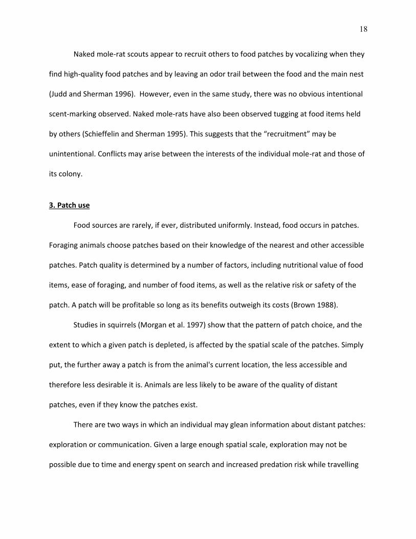
3. Patch use

Food sources are rarely, if ever, distributed uniformly. Instead, food occurs in patches.

Foraging animals choose patches based on their knowledge of the nearest and other accessible

patches. Patch quality is determined by a number of factors, including nutritional value of food

items, ease of foraging, and number of food items, as well as the relative risk or safety of the

patch. A patch will be profitable so long as its benefits outweigh its costs (Brown 1988).

Studies in squirrels (Morgan et al. 1997) show that the pattern of patch choice, and the

extent to which a given patch is depleted, is affected by the spatial scale of the patches. Simply

put, the further away a patch is from the animal's current location, the less accessible and

therefore less desirable it is. Animals are less likely to be aware of the quality of distant

patches, even if they know the patches exist.

There are two ways in which an individual may glean information about distant patches:

exploration or communication. Given a large enough spatial scale, exploration may not be

possible due to time and energy spent on search and increased predation risk while travelling

19

between patches. Communication with other conspecifics allows for information transfer

without increased individual risk. Communication may be via vocalizations, scent cues, or even

dances (e.g., Jackson and Ratnieks 2006, Seeley et al 2000).

One factor which can influence the amount harvested from a given patch is the forager's

information about, and ability to find and use, other patches. If there is only one food patch,

the forager has no options and must exploit it to the best of their ability. Conversely, if there

are many patches to choose among, a forager can explore them, using only the best patches

and only until they are no longer profitable. Not knowing about nearby patches is effectively

the same as these patches not existing. Animals vary widely in their communication about food,

from none whatsoever to complete information-sharing (Galef and Giraldeau 2001).

One way to “ask” foraging animals their opinion of a patch or set of patches is to

provide them with a variety of patches of known quality, allow them to forage for a time, and

then look at the absolute and relative quantities of food harvested—or not harvested. Patch

quality can be based on the type or quantity of food, the type and quantity of non-food items in

the patch, and how these are mixed.

Valone and Brown (1989) established methods of measuring patch assessment ability

using food patches and analyzing the patterns of food consumption. In this study, we used this

food-patch approach to determine if naked mole-rats are eusocial foragers. We varied food

patch quality and spatial distribution because closely spaced patches allow for exploration, but

more-separated patches force individuals to choose to explore to find better patches, to “make

do” with the first patch encountered, or to share information with one another.

20

A forager, or group of foragers, will stop using a given patch when the gains no longer

outweigh the costs. These costs include the metabolic costs of finding and handling the food

items, the risk of predation posed by the patch location, and missing opportunities from not

harvesting higher quality patches or engaging in other worthwhile endeavors. The quantity of

food remaining at the point a forager leaves a patch is known as the “giving-up density” (GUD),

and this measure is used in studies in which patches have similar starting quantities of food.

One can also compare the quantity or proportion of food eaten rather than what is left. Which

measure is used depends on the questions asked or hypotheses posed (Brown 1988).

Foraging experiments often use three spatial scales (Morgan et al. 1997): patch, station,

and site. Patches are individual foraging containers such as shallow trays in which a small

amount of food is mixed into a non-edible substrate such as sand. These patches are clustered

close together within a station. A site may contain several stations. Patch qualities can vary

among patches, stations, sites, or any combination of the three. For experimental purposes,

quality is held constant at two scales and varied at the remaining one.

When patches are close together, a forager can easily move between them, and thus

can obtain all of the information needed to forage efficiently. If the variation is at a larger

distance, such as at the station and site scales, movement may not be as easy or even possible.

When patches within a station have varying initial food quantities, the forager is able to

move among them freely, gaining information with negligible effort. It should consume food

until each patch has roughly the same quantity remaining--that is, to the same final patch

quality. This translates into a proportion harvested that increases with patch quality. To leave

21

10 items in a patch, a forager must consume only 10 items from a patch that started with 20

(50%), but 90 items from a patch that started with 100 (90%).

The quality of the patches in this study vary solely on the amount of food present, so

how much the animals eat is the only reliable measure of their foraging approach. To keep the

scale consistent between patches with varying initial food quantities, we use the proportion of

food eaten—the proportion harvested—as our metric.

We shall refer to our experimental set-up in which patch quality varies within a station

as the "mixed" spatial scale. All stations contain the same mix of patches.

If the patch types are spread far enough apart, complete exploration is difficult or

impossible due to time spent or danger incurred, and foraging decisions are more difficult.

What decisions are made will depend in part on communication between individuals within a

social foraging group—or lack thereof. In this scenario (which we call “clustered”), patches

within a station are equal to one another in quality, but stations differ in their patch quality.

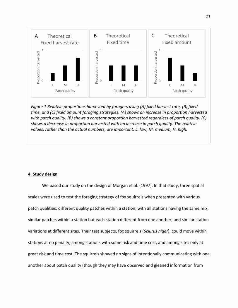
There are three general strategies foragers may use when food patches are distributed

in this clustered manner (Figure 1; see Valone and Brown 1989, Troxell-Smith et al. 2016):

1. Fixed quitting harvest rate (hereafter fixed harvest rate). In this strategy,

foragers will use a patch until it is no better than the average patch within the reachable

foraging area. This is the same strategy as when patches are mixed, and is most likely

the result of individuals sharing information, intentionally or otherwise. Accordingly, the

proportion harvested will increase with patch quality.

2. Fixed time. When foragers have no information about the available patches

other than their existence, the optimal strategy is to spend an equal amount of time

22

searching for food in each patch. Assuming the food items are not too difficult to find

and consume, foragers will harvest approximately the same proportion of food from

each patch type.

3. Fixed amount. If a forager has no information about other patches, faces

significant danger or other costs in getting to other patches, or simply needs very little

food, the patch encountered first will suffice. The forager will eat as needed without

exploring the area or seeking further information. When a group of foragers use this

strategy, they will harvest the same quantity of food from each patch type.

Consequently, the proportions harvested will decrease with increased patch quality.

23

4. Study design

We based our study on the design of Morgan et al. (1997). In that study, three spatial

scales were used to test the foraging strategy of fox squirrels when presented with various

patch qualities: different quality patches within a station, with all stations having the same mix;

similar patches within a station but each station different from one another; and similar station

variations at different sites. Their test subjects, fox squirrels (Sciurus niger), could move within

stations at no penalty, among stations with some risk and time cost, and among sites only at

great risk and time cost. The squirrels showed no signs of intentionally communicating with one

another about patch quality (though they may have observed and gleaned information from

Figure 1 Relative proportions harvested by foragers using (A) fixed harvest rate, (B) fixed time, and (C) fixed amount foraging strategies. (A) shows an increase in proportion harvested with patch quality. (B) shows a constant proportion harvested regardless of patch quality. (C) shows a decrease in proportion harvested with an increase in patch quality. The relative values, rather than the actual numbers, are important. L: low, M: medium, H: high.

24

others’ activities); that is, while they may have been foraging at the same time, they were

foraging as individuals.

Using this design as a basis, we tested the foraging strategy of two colonies of naked

mole-rats and one group of gerbils. Gerbil foraging behavior has been studied extensively, so

they served as a control of sorts. Several gerbils may forage at the same time, but they do so

independently (Kotler et al. 1991).

We varied patch quality (i.e., number of initial food items) at the patch and station

scales. Variation between patches within a station we call "mixed," as the patches within a

station are a mix of different qualities. In other trials, all of the patches within a station had the

same initial quality but this quality varied by station. We call this "clustered." We did not test

multiple sites.

5. Predictions

All animals should show a fixed harvest rate strategy on the "mixed" spatial scale. This is

because the patches are close enough to one another that every individual can sample and

explore all three patches within a station. Each animal should allocate time among patches so

as to equalize the end-of-foraging quality at all patches of a station. This translates into an

increase in proportion harvested with an increase in patch quality.

For the "clustered" scale, we expected the gerbils and naked mole-rats to exhibit

different strategies. Gerbils, as solitary foragers, were predicted to show a fixed time strategy,

which would be reflected as similar proportions harvested in each patch regardless of initial

quality. This is because the gerbils do not actively share information, and the cost of sampling

25

all patches at all stations may not be worth the effort to an individual gerbil. Why try to sample

patches that other gerbils are exploiting or have already exploited? Naked mole-rats were

expected to continue using a fixed harvest rate strategy, communicating with one another and

thus maximizing overall foraging efficiency. Alternately, the naked mole-rats could employ a

fixed time strategy, where each forager picked a patch and foraged it for a set period of time.

These strategies translate into proportions harvested which increase with patch quality or

remain the same regardless of patch quality, respectively.

B. Methods

We tested two colonies of naked mole-rats (n = 36, n = 27) and one family group

(parents and three litters of their offspring) of Mongolian gerbils (Meriones unguiculatus) (n =

20). The mole-rats were tested in their normal housing condition of dim red light, 30°C

temperature, and 45–65% relative humidity. The gerbils were housed and tested in a room kept

under a 12-hour light, 12-hour dark cycle, 22°C, and ambient relative humidity. Each colony was

housed in an artificial tunnel system constructed of two-inch diameter PVC piping and standard

laboratory mouse cages. The experimental protocol was approved by the University of Illinois at

Chicago Institutional Animal Care and Use Committee. All animals were given free access to

their normal laboratory diets in the home tunnel system. For naked mole-rats this was sweet

potato, and for gerbil’s rat chow and water.

During foraging experiments, the home tunnel system was connected to an open

foraging arena via a PVC pipe. This arena consisted of a central compartment with three

foraging stations connected via short lengths of PVC pipe. Each station, measuring

26

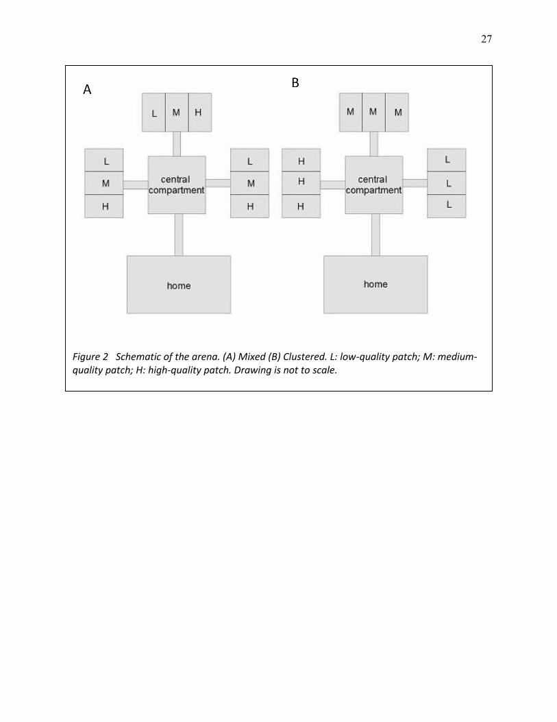
approximately 91 cm × 51 cm × 24 cm (l × w × d) and was further divided into three patches.

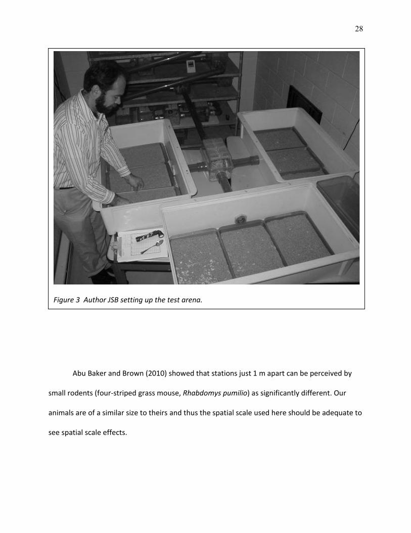
Figure 2 provides a schematic of the foraging arena; Figure 3 is a photograph of one of the

authors (JSB) setting up the actual arena. We initially tested our foraging arena with a cover

over it. In these tests, all patches were foraged to zero; that is, the naked mole-rats simply ate

everything everywhere. When left uncovered, the naked mole-rats foraged but considerably

less, likely due to a heightened sense of predation risk. Experiments were performed with the

arena uncovered.

27

Figure 2 Schematic of the arena. (A) Mixed (B) Clustered. L: low-quality patch; M: medium-quality patch; H: high-quality patch. Drawing is not to scale.

28

Abu Baker and Brown (2010) showed that stations just 1 m apart can be perceived by

small rodents (four-striped grass mouse, Rhabdomys pumilio) as significantly different. Our

animals are of a similar size to theirs and thus the spatial scale used here should be adequate to

see spatial scale effects.

Figure 3 Author JSB setting up the test arena.

29

We used fresh apples cut into very small pieces (approximately 0.1–0.2 g each) to test

naked mole-rat patch use behaviors. The naked mole rats prefer apples to their normal diet of

sweet potato (pers. obs.). We used millet seeds (approximately 0.006 g each) for the gerbils. As

gerbils are granivores, this food is sufficiently favored to ensure foraging within our food

patches.

We conducted a week of trials to allow both species to habituate to the trays and allow

us to establish the design of the patches and the quantity of substrate needed to achieve

intermediate GUDs. Naked mole-rats consumed the entire allotment of apple pieces when they

were offered in a single pile. All colonies (both gerbils and naked mole-rats) would eat all food

items if the foraging arenas were covered, indicating that when experimental foraging ended it

was not due to satiation. When the arena was uncovered, there was no difference between the

number of food items eaten whether the animals were given 24 or 48 hours to forage,

indicating that our choice of a 24-hour test period was adequate.

Prior to the experimental foraging rounds, we placed low, medium, or high quantities of

food in each of the nine food patches, varying placement between rounds in a Latin square

design while keeping average patch quality equal. We defined low as 20 food items, medium as

40 food items, and high as 80 food items (pieces of apple for the naked mole-rats, individual

millet seeds for the gerbils). We covered the food items with 4 L of coarse bank sand.

In the “mixed,” design, each of the three patches within each site contained a different

initial quantity of food items (20, 40, or 80). In the “clustered” scenario, each of the three

patches within a site contained the same initial food item quantity, with this number varying

between sites.

30

The animals were then given access to the foraging arena and allowed to forage for 24

hours. At the end of this time, the foraging arena was closed off and all animals restricted to

their home tunnel system. We counted the remaining food items in the experimental patches

and calculated the proportion harvested. Each colony was tested under each treatment (mixed

or clustered) for six trials.

We used SYSTAT 12 to test for effects of initial food quantity, spatial scale, and colony

(for naked mole-rats) via ANOVA, using proportions harvested as the dependent variable.

Effects were considered significant at p < 0.05. Naked mole-rat colonies were compared to each

other with chi-square goodness-of-fit tests. Graphs of proportions harvested were compared

(to one another and the theoretical graphs given above) visually and, in the case of naked mole-

rats, compared to an equal-harvest strategy with chi-square tests.

C. Results

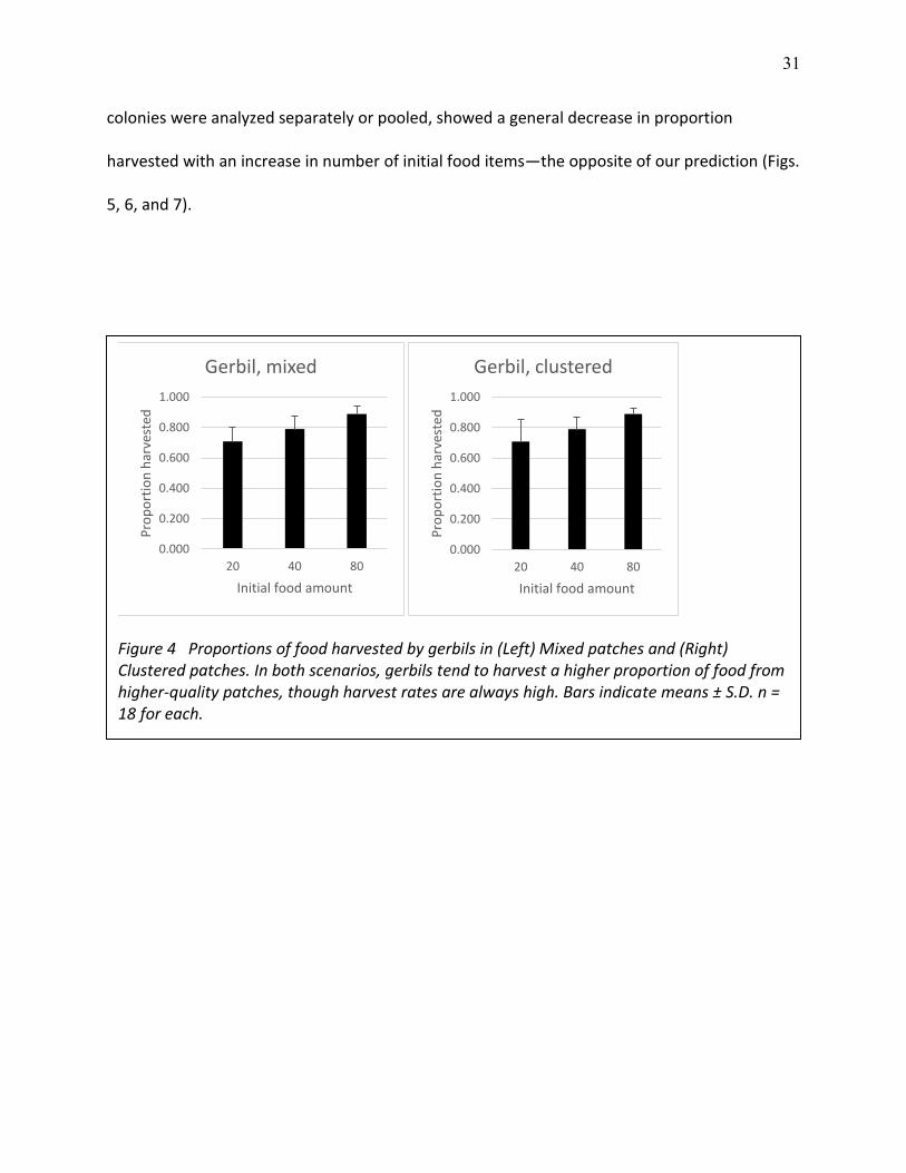
All colonies—both mole-rat and gerbil--performed as expected in the mixed-patch trials.

The proportion of food harvested increased with patch quality, supporting a tendency toward a

fixed quitting harvest rate strategy. The clustered patches, however, yielded some surprises. At

the clustered scale, the gerbils continued to show a fixed quitting harvest rate rather than the

expected fixed time strategy (Fig. 4). The two naked mole-rat colonies differed from one

another in their proportions harvested at this scale, particularly among different initial food

amounts. The colonies had different numbers of individuals (36 vs 27), and thus this is not

surprising. However, these differences were not significant (p = 0.638), so we also considered

the naked mole-rats as a single unit for analysis. Both colonies of naked mole-rats, whether

31

colonies were analyzed separately or pooled, showed a general decrease in proportion

harvested with an increase in number of initial food items—the opposite of our prediction (Figs.

5, 6, and 7).

Figure 4 Proportions of food harvested by gerbils in (Left) Mixed patches and (Right) Clustered patches. In both scenarios, gerbils tend to harvest a higher proportion of food from higher-quality patches, though harvest rates are always high. Bars indicate means ± S.D. n = 18 for each.

0.000

0.200

0.400

0.600

0.800

1.000

20 40 80

Pro

po

rtio

n h

arve

sted

Initial food amount

Gerbil, mixed

0.000

0.200

0.400

0.600

0.800

1.000

20 40 80

Pro

po

rtio

n h

arve

sted

Initial food amount

Gerbil, clustered

32

Figure 5 Proportions of food harvested by naked mole-rat colony 1 in (Left) Mixed patches and (Right) Clustered patches. Proportion harvested rose with patch quality at the Mixed scale, but declined with higher quality at the Clustered scale. Bars indicate means ± S.D. n = 18 for each.

0.000

0.200

0.400

0.600

0.800

1.000

20 40 80

Pro

po

rtio

n h

arve

sted

Initial food amount

NMR 1, mixed

0.000

0.200

0.400

0.600

0.800

1.000

20 40 80

Pro

po

rtio

n h

arve

sted

Initial food amount

NMR1, clustered

Figure 6 Proportions of food harvested by naked mole-rat colony 2 in (Left) Mixed patches and (Right) Clustered patches. Proportion harvested rose with patch quality at the Mixed scale, but declined with higher quality at the Clustered scale. Bars indicate means ± S.D. n = 18 for each.

0.000

0.200

0.400

0.600

0.800

1.000

20 40 80

Pro

po

rtio

n h

arve

sted

Initial food amount

NMR 2, mixed

0.000

0.200

0.400

0.600

0.800

1.000

20 40 80

Pro

po

rtio

n h

arve

sted

Initial food amount

NMR 2, clustered

33

ANOVAs confirmed these conclusions (Table I): for gerbils, only the initial amount of

food was significant, whereas the initial amount, scale, and the interaction of initial amount and

scale were all significant factors for the naked mole-rats. Naked mole-rat colonies differed in

their foraging. Colony 1 harvested a significantly higher proportion of food offered, but this

difference was most striking in the interaction of initial amount and colony, where the colony

harvested a much higher proportion of food from the low quality patch than did colony 2. The

three-way interaction of initial amount, scale, and colony was not significant even though the

interaction of initial amount and scale was highly significant.

Figure 7 Proportions of food harvested by naked mole-rats in (Left) Mixed patches and (Right) Clustered patches. Proportion harvested rose with patch quality at the Mixed scale, but declined with higher quality at the Clustered scale. Proportions shown are the average of the two colonies ± S.D. n = 36 for each.

0.000

0.200

0.400

0.600

0.800

1.000

20 40 80

Pro

po

rtio

n h

arve

sted

Initial food amount

NMR combined, mixed

0.000

0.200

0.400

0.600

0.800

1.000

20 40 80

Pro

po

rtio

n h

arve

sted

Initial food amount

NMR combined, clustered

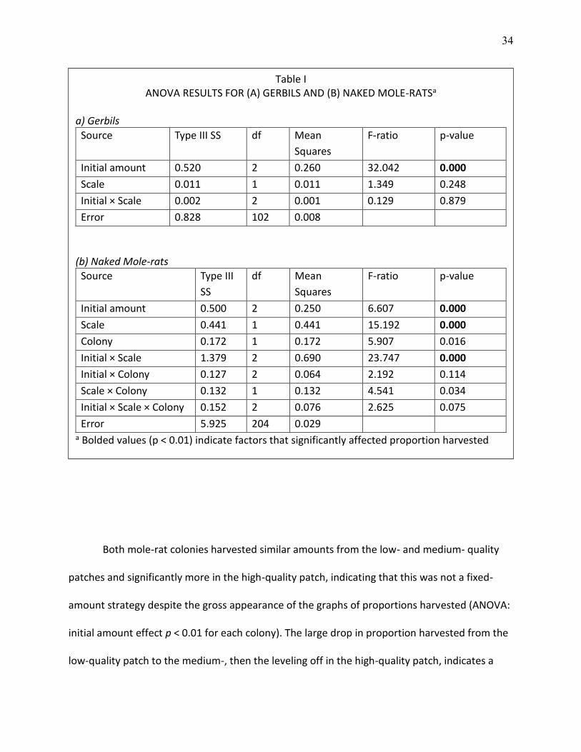
34

Both mole-rat colonies harvested similar amounts from the low- and medium- quality

patches and significantly more in the high-quality patch, indicating that this was not a fixed-

amount strategy despite the gross appearance of the graphs of proportions harvested (ANOVA:

initial amount effect p < 0.01 for each colony). The large drop in proportion harvested from the

low-quality patch to the medium-, then the leveling off in the high-quality patch, indicates a

Table I ANOVA RESULTS FOR (A) GERBILS AND (B) NAKED MOLE-RATSa

a) Gerbils

Source Type III SS df Mean

Squares

F‐ratio p‐value

Initial amount 0.520 2 0.260 32.042 0.000

Scale 0.011 1 0.011 1.349 0.248

Initial × Scale 0.002 2 0.001 0.129 0.879

Error 0.828 102 0.008

(b) Naked Mole-rats

Source Type III

SS

df Mean

Squares

F‐ratio p‐value

Initial amount 0.500 2 0.250 6.607 0.000

Scale 0.441 1 0.441 15.192 0.000

Colony 0.172 1 0.172 5.907 0.016

Initial × Scale 1.379 2 0.690 23.747 0.000

Initial × Colony 0.127 2 0.064 2.192 0.114

Scale × Colony 0.132 1 0.132 4.541 0.034

Initial × Scale × Colony 0.152 2 0.076 2.625 0.075

Error 5.925 204 0.029 a Bolded values (p < 0.01) indicate factors that significantly affected proportion harvested

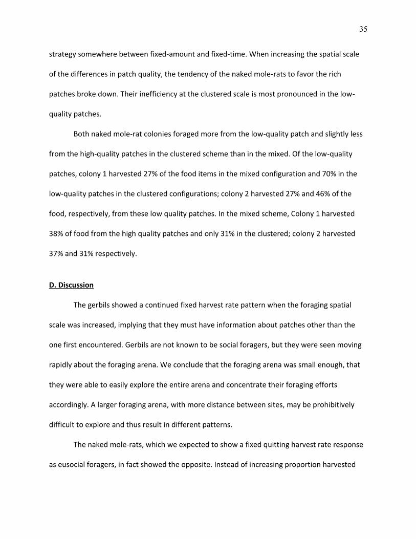
35

strategy somewhere between fixed-amount and fixed-time. When increasing the spatial scale

of the differences in patch quality, the tendency of the naked mole-rats to favor the rich

patches broke down. Their inefficiency at the clustered scale is most pronounced in the low-

quality patches.

Both naked mole-rat colonies foraged more from the low-quality patch and slightly less

from the high-quality patches in the clustered scheme than in the mixed. Of the low-quality

patches, colony 1 harvested 27% of the food items in the mixed configuration and 70% in the

low-quality patches in the clustered configurations; colony 2 harvested 27% and 46% of the

food, respectively, from these low quality patches. In the mixed scheme, Colony 1 harvested

38% of food from the high quality patches and only 31% in the clustered; colony 2 harvested

37% and 31% respectively.

D. Discussion

The gerbils showed a continued fixed harvest rate pattern when the foraging spatial

scale was increased, implying that they must have information about patches other than the

one first encountered. Gerbils are not known to be social foragers, but they were seen moving

rapidly about the foraging arena. We conclude that the foraging arena was small enough, that

they were able to easily explore the entire arena and concentrate their foraging efforts

accordingly. A larger foraging arena, with more distance between sites, may be prohibitively

difficult to explore and thus result in different patterns.

The naked mole-rats, which we expected to show a fixed quitting harvest rate response

as eusocial foragers, in fact showed the opposite. Instead of increasing proportion harvested

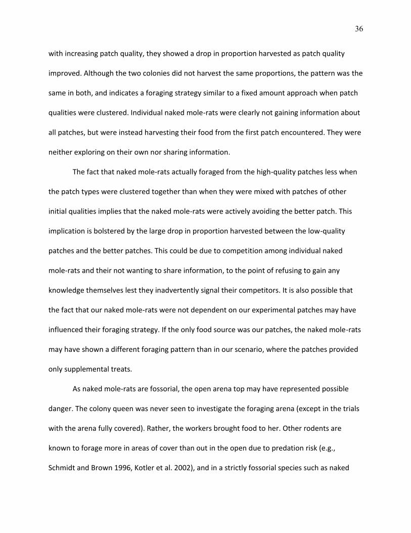
36

with increasing patch quality, they showed a drop in proportion harvested as patch quality

improved. Although the two colonies did not harvest the same proportions, the pattern was the

same in both, and indicates a foraging strategy similar to a fixed amount approach when patch

qualities were clustered. Individual naked mole-rats were clearly not gaining information about

all patches, but were instead harvesting their food from the first patch encountered. They were

neither exploring on their own nor sharing information.

The fact that naked mole-rats actually foraged from the high-quality patches less when

the patch types were clustered together than when they were mixed with patches of other

initial qualities implies that the naked mole-rats were actively avoiding the better patch. This

implication is bolstered by the large drop in proportion harvested between the low-quality

patches and the better patches. This could be due to competition among individual naked

mole-rats and their not wanting to share information, to the point of refusing to gain any

knowledge themselves lest they inadvertently signal their competitors. It is also possible that

the fact that our naked mole-rats were not dependent on our experimental patches may have

influenced their foraging strategy. If the only food source was our patches, the naked mole-rats

may have shown a different foraging pattern than in our scenario, where the patches provided

only supplemental treats.

As naked mole-rats are fossorial, the open arena top may have represented possible

danger. The colony queen was never seen to investigate the foraging arena (except in the trials

with the arena fully covered). Rather, the workers brought food to her. Other rodents are

known to forage more in areas of cover than out in the open due to predation risk (e.g.,

Schmidt and Brown 1996, Kotler et al. 2002), and in a strictly fossorial species such as naked

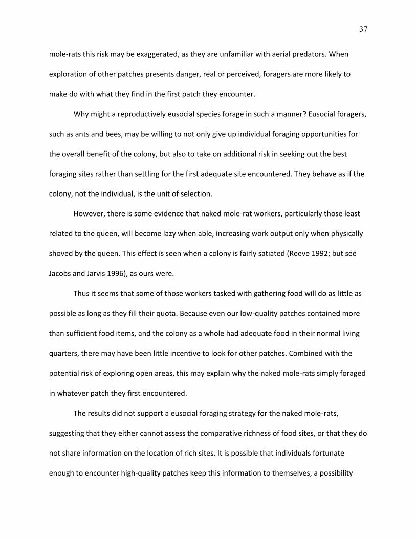
37

mole-rats this risk may be exaggerated, as they are unfamiliar with aerial predators. When

exploration of other patches presents danger, real or perceived, foragers are more likely to

make do with what they find in the first patch they encounter.

Why might a reproductively eusocial species forage in such a manner? Eusocial foragers,

such as ants and bees, may be willing to not only give up individual foraging opportunities for

the overall benefit of the colony, but also to take on additional risk in seeking out the best

foraging sites rather than settling for the first adequate site encountered. They behave as if the

colony, not the individual, is the unit of selection.

However, there is some evidence that naked mole-rat workers, particularly those least

related to the queen, will become lazy when able, increasing work output only when physically

shoved by the queen. This effect is seen when a colony is fairly satiated (Reeve 1992; but see

Jacobs and Jarvis 1996), as ours were.

Thus it seems that some of those workers tasked with gathering food will do as little as

possible as long as they fill their quota. Because even our low-quality patches contained more

than sufficient food items, and the colony as a whole had adequate food in their normal living

quarters, there may have been little incentive to look for other patches. Combined with the

potential risk of exploring open areas, this may explain why the naked mole-rats simply foraged

in whatever patch they first encountered.

The results did not support a eusocial foraging strategy for the naked mole-rats,

suggesting that they either cannot assess the comparative richness of food sites, or that they do

not share information on the location of rich sites. It is possible that individuals fortunate

enough to encounter high-quality patches keep this information to themselves, a possibility

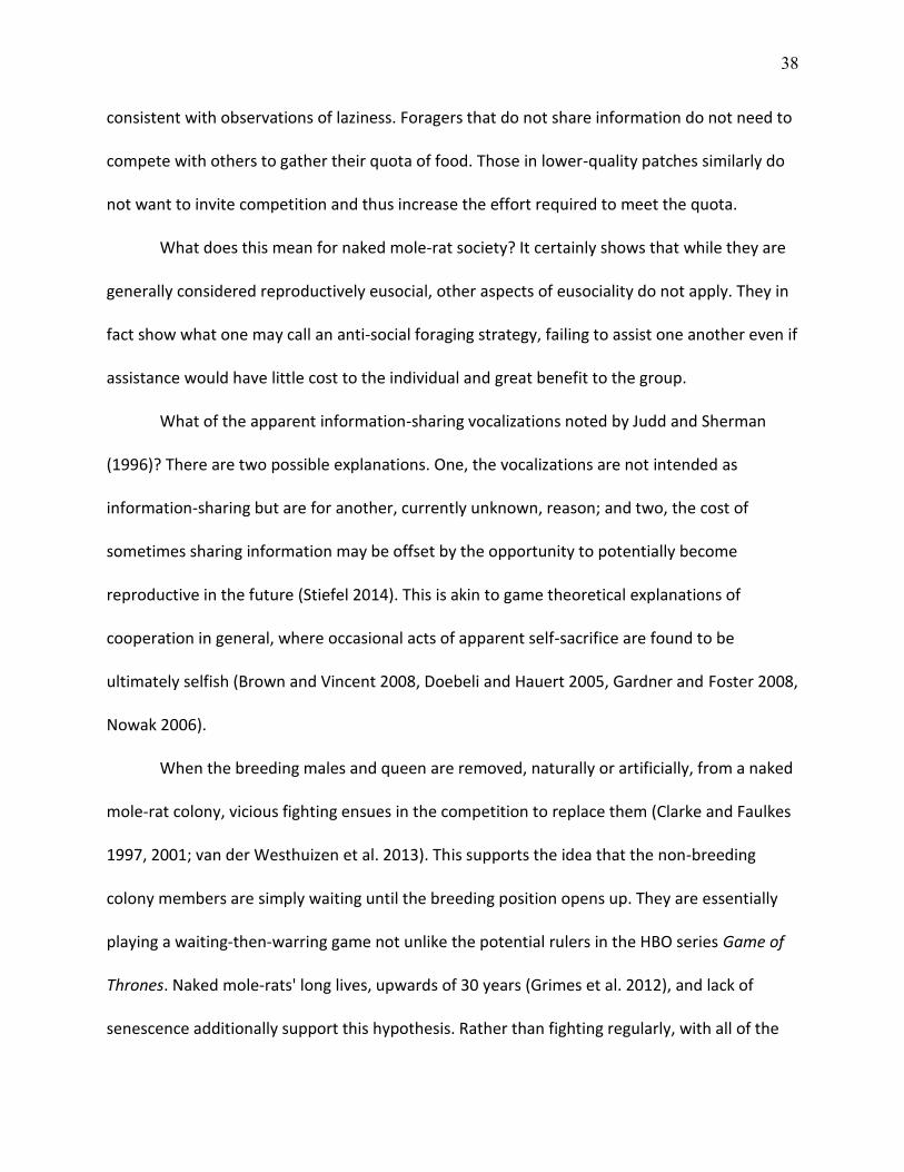
38

consistent with observations of laziness. Foragers that do not share information do not need to

compete with others to gather their quota of food. Those in lower-quality patches similarly do

not want to invite competition and thus increase the effort required to meet the quota.

What does this mean for naked mole-rat society? It certainly shows that while they are

generally considered reproductively eusocial, other aspects of eusociality do not apply. They in

fact show what one may call an anti-social foraging strategy, failing to assist one another even if

assistance would have little cost to the individual and great benefit to the group.

What of the apparent information-sharing vocalizations noted by Judd and Sherman

(1996)? There are two possible explanations. One, the vocalizations are not intended as

information-sharing but are for another, currently unknown, reason; and two, the cost of

sometimes sharing information may be offset by the opportunity to potentially become

reproductive in the future (Stiefel 2014). This is akin to game theoretical explanations of

cooperation in general, where occasional acts of apparent self-sacrifice are found to be

ultimately selfish (Brown and Vincent 2008, Doebeli and Hauert 2005, Gardner and Foster 2008,

Nowak 2006).

When the breeding males and queen are removed, naturally or artificially, from a naked

mole-rat colony, vicious fighting ensues in the competition to replace them (Clarke and Faulkes

1997, 2001; van der Westhuizen et al. 2013). This supports the idea that the non-breeding

colony members are simply waiting until the breeding position opens up. They are essentially

playing a waiting-then-warring game not unlike the potential rulers in the HBO series Game of

Thrones. Naked mole-rats' long lives, upwards of 30 years (Grimes et al. 2012), and lack of

senescence additionally support this hypothesis. Rather than fighting regularly, with all of the

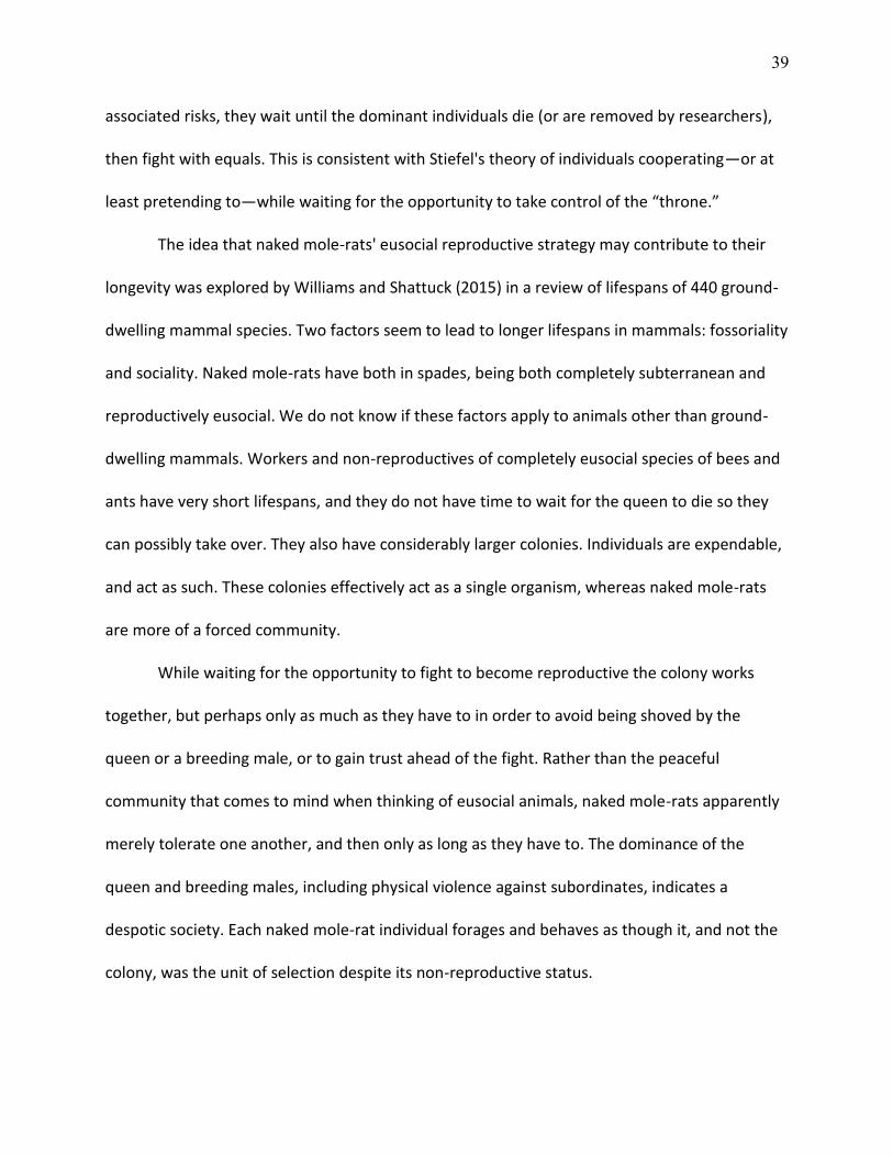
39

associated risks, they wait until the dominant individuals die (or are removed by researchers),

then fight with equals. This is consistent with Stiefel's theory of individuals cooperating—or at

least pretending to—while waiting for the opportunity to take control of the “throne.”

The idea that naked mole-rats' eusocial reproductive strategy may contribute to their

longevity was explored by Williams and Shattuck (2015) in a review of lifespans of 440 ground-

dwelling mammal species. Two factors seem to lead to longer lifespans in mammals: fossoriality

and sociality. Naked mole-rats have both in spades, being both completely subterranean and

reproductively eusocial. We do not know if these factors apply to animals other than ground-

dwelling mammals. Workers and non-reproductives of completely eusocial species of bees and

ants have very short lifespans, and they do not have time to wait for the queen to die so they

can possibly take over. They also have considerably larger colonies. Individuals are expendable,

and act as such. These colonies effectively act as a single organism, whereas naked mole-rats

are more of a forced community.

While waiting for the opportunity to fight to become reproductive the colony works

together, but perhaps only as much as they have to in order to avoid being shoved by the

queen or a breeding male, or to gain trust ahead of the fight. Rather than the peaceful

community that comes to mind when thinking of eusocial animals, naked mole-rats apparently

merely tolerate one another, and then only as long as they have to. The dominance of the

queen and breeding males, including physical violence against subordinates, indicates a

despotic society. Each naked mole-rat individual forages and behaves as though it, and not the

colony, was the unit of selection despite its non-reproductive status.

40

E. Conclusion

Whether naked mole-rats qualify as eusocial or not depends on your definition of

eusocial. If we define eusociality in mammals as requiring only cooperation in reproductive

matters (as in Burda et al 2000), then naked mole-rats are certainly eusocial. However, if we

require a group effort in other aspects of their ecology, like foraging for food, then naked mole-

rats are not. They fail the test of eusocial foraging.

F. Literature cited

Abu Baker MA, Brown JS. 2010. Islands of fear: effects of wooded patches on habitat suitability of the striped mouse in a South African grassland. Functional Ecology 24: 1313-22

Ale SB, Brown JS. 2007. The contingencies of group size and vigilance. Evolutionary Ecology Research 9: 1263-76

Brown JS. 1988. Patch use as an indicator of habitat preference, predation risk, and competition. Behavioral Ecology and Sociobiology 22: 37-47

Brown JS, Vincent TL. 2008. Evolution of cooperation with shared costs and benefits. Proceedings of the Royal Society B: Biological Sciences 275: 1985-94

Burda H, Honeycutt RL, Begall S, Locker-Grütjen O, Scharff A. 2000. Are naked and common mole-rats eusocial and if so, why? Behavioral Ecology and Sociobiology 47: 293-303

Cassill D. 2003. Rules of supply and demand regulate recruitment to food in an ant society. Behavioral Ecology and Sociobiology 54: 441-50

Clarke F, Faulkes C. 1997. Dominance and queen succession in captive colonies of the eusocial naked mole-rat, Heterocephalus glaber. Proceedings of the Royal Society of London. Series B: Biological Sciences 264: 993-1000

Clarke F, Faulkes C. 2001. Intracolony aggression in the eusocial naked mole-rat, Heterocephalus glaber. Animal Behaviour 61: 311-24

Doebeli M, Hauert C. 2005. Models of cooperation based on the Prisoner's Dilemma and the Snowdrift game. Ecology Letters 8: 748-66

Galef BG, Laland KN. 2005. Social learning in animals: empirical studies and theoretical models. Bioscience 55: 489-99

Gardner A, Foster KR. 2008. The evolution and ecology of cooperation–History and concepts. In: Ecology of Social Evolution, pp. 1-36: Springer

41

Grimes KM, Lindsey ML, Gelfond JA, Buffenstein R. 2012. Getting to the heart of the matter: age-related changes in diastolic heart function in the longest-lived rodent, the naked mole rat. The Journals of Gerontology Series A: Biological Sciences and Medical Sciences 67: 384-94

Jackson DE, Ratnieks FL. 2006. Communication in ants. Current Biology 16: R570-R74

Jacobs DS, Jarvis J. 1996. No evidence for the work-conflict hypothesis in the eusocial naked mole-rat (Heterocephalus glaber). Behavioral Ecology and Sociobiology 39: 401-09

Jarvis J. 1981. Eusociality in a mammal: cooperative breeding in naked mole-rat colonies. Science 212: 571-73

Jones CB. 2014. Multimale–Multifemale Groups and “Nested” Architectures: Collaboration Among Mammalian Males. In: The Evolution of Mammalian Sociality in an Ecological Perspective, pp. 37-45: Springer

Judd TM, Sherman PW. 1996. Naked mole-rats recruit colony mates to food sources. Animal Behaviour 52: 957-69

Kotler BP, Brown JS, Dall SR, Gresser S, Ganey D, Bouskila A. 2002. Foraging games between gerbils and their predators: temporal dynamics of resource depletion and apprehension in gerbils. Evolutionary Ecology Research 4: 495-518

Kotler BP, Brown JS, Hasson O. 1991. Factors affecting gerbil foraging behavior and rates of owl predation. Ecology 72: 2249-60

Morgan RA, Brown JS, Thorson JM. 1997. The effect of spatial scale on the functional response of fox squirrels. Ecology 78: 1087-97

Nowak MA. 2006. Five rules for the evolution of cooperation. Science 314: 1560

Reeve HK. 1992. Queen activation of lazy workers in colonies of the eusocial naked mole-rat. Nature 358: 147-49

Schieffelin JS, Sherman PW. 1995. Tugging contests reveal feeding hierarchies in naked mole-rat colonies. Animal Behaviour 49: 537-41

Schmidt KA, Brown JS. 1996. Patch assessment in fox squirrels: the role of resource density, patch size, and patch boundaries. American Naturalist: 360-80

Seeley TD, Mikheyev AS, Pagano GJ. 2000. Dancing bees tune both duration and rate of waggle-run production in relation to nectar-source profitability. Journal of Comparative Physiology A 186: 813-19

Seeley TD, Visscher PK. 2003. Choosing a home: how the scouts in a honey bee swarm perceive the completion of their group decision making. Behavioral Ecology and Sociobiology 54: 511-20

Sherman PW, Lacey EA, Reeve HK, Keller L. 1995. Forum The eusociality continuum. Behavioral Ecology 6: 102-08

Stiefel KM. 2014. Dishonest Signaling in Vertebrate Eusociality. Biological Theory 9: 325

Troxell-Smith SM, Tutka MJ, Albergo JM, Balu D, Brown JS, Leonard JP. 2016. Foraging decisions in wild versus domestic Mus musculus: What does life in the lab select for? Behavioural Processes 122: 43-50

Valone TJ, Brown JS. 1989. Measuring patch assessment abilities of desert granivores. Ecology 70: 1800-10

van der Westhuizen L, Jarvis JU, Bennett NC. 2013. A case of natural queen succession in a captive colony of naked mole-rats, Heterocephalus glaber. African Zoology 48: 56-63

42

Williams SA, Shattuck MR. 2015. Ecology, longevity and naked mole-rats: confounding effects of sociality? Proceedings of the Royal Society of London B: Biological Sciences 282: 20141664

Wilson EO, Hölldobler B. 2005. Eusociality: origin and consequences. Proceedings of The National Academy of Sciences of the United States of America 102: 13367-71

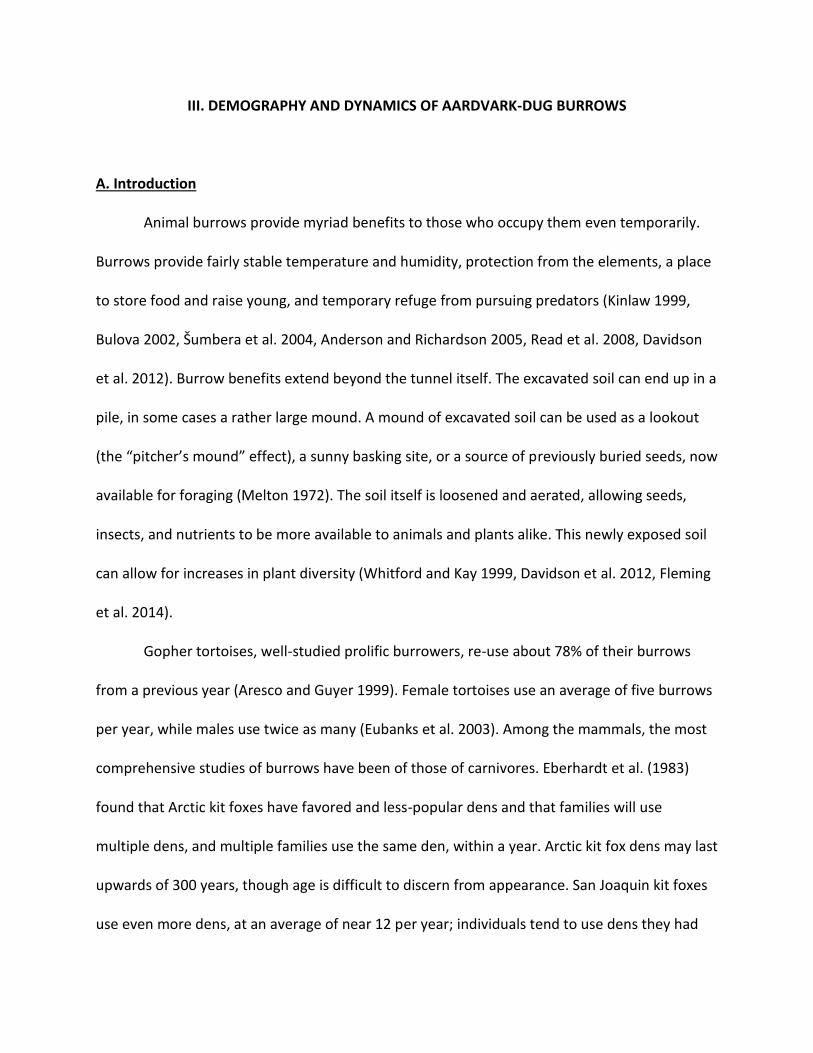
III. DEMOGRAPHY AND DYNAMICS OF AARDVARK-DUG BURROWS

A. Introduction

Animal burrows provide myriad benefits to those who occupy them even temporarily.

Burrows provide fairly stable temperature and humidity, protection from the elements, a place

to store food and raise young, and temporary refuge from pursuing predators (Kinlaw 1999,

Bulova 2002, Šumbera et al. 2004, Anderson and Richardson 2005, Read et al. 2008, Davidson

et al. 2012). Burrow benefits extend beyond the tunnel itself. The excavated soil can end up in a

pile, in some cases a rather large mound. A mound of excavated soil can be used as a lookout

(the “pitcher’s mound” effect), a sunny basking site, or a source of previously buried seeds, now

available for foraging (Melton 1972). The soil itself is loosened and aerated, allowing seeds,

insects, and nutrients to be more available to animals and plants alike. This newly exposed soil

can allow for increases in plant diversity (Whitford and Kay 1999, Davidson et al. 2012, Fleming

et al. 2014).

Gopher tortoises, well-studied prolific burrowers, re-use about 78% of their burrows

from a previous year (Aresco and Guyer 1999). Female tortoises use an average of five burrows

per year, while males use twice as many (Eubanks et al. 2003). Among the mammals, the most

comprehensive studies of burrows have been of those of carnivores. Eberhardt et al. (1983)

found that Arctic kit foxes have favored and less-popular dens and that families will use

multiple dens, and multiple families use the same den, within a year. Arctic kit fox dens may last

upwards of 300 years, though age is difficult to discern from appearance. San Joaquin kit foxes

use even more dens, at an average of near 12 per year; individuals tend to use dens they had

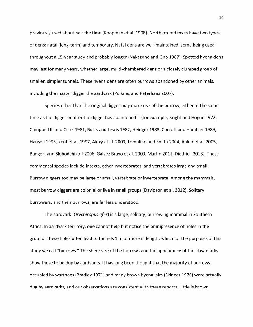
44

previously used about half the time (Koopman et al. 1998). Northern red foxes have two types

of dens: natal (long-term) and temporary. Natal dens are well-maintained, some being used

throughout a 15-year study and probably longer (Nakazono and Ono 1987). Spotted hyena dens

may last for many years, whether large, multi-chambered dens or a closely clumped group of

smaller, simpler tunnels. These hyena dens are often burrows abandoned by other animals,

including the master digger the aardvark (Poiknes and Peterhans 2007).

Species other than the original digger may make use of the burrow, either at the same

time as the digger or after the digger has abandoned it (for example, Bright and Hogue 1972,

Campbell III and Clark 1981, Butts and Lewis 1982, Heidger 1988, Cocroft and Hambler 1989,

Hansell 1993, Kent et al. 1997, Alexy et al. 2003, Lomolino and Smith 2004, Anker et al. 2005,

Bangert and Slobodchikoff 2006, Gálvez Bravo et al. 2009, Martin 2011, Diedrich 2013). These

commensal species include insects, other invertebrates, and vertebrates large and small.

Burrow diggers too may be large or small, vertebrate or invertebrate. Among the mammals,

most burrow diggers are colonial or live in small groups (Davidson et al. 2012). Solitary

burrowers, and their burrows, are far less understood.

The aardvark (Orycteropus afer) is a large, solitary, burrowing mammal in Southern

Africa. In aardvark territory, one cannot help but notice the omnipresence of holes in the

ground. These holes often lead to tunnels 1 m or more in length, which for the purposes of this

study we call “burrows.” The sheer size of the burrows and the appearance of the claw marks

show these to be dug by aardvarks. It has long been thought that the majority of burrows

occupied by warthogs (Bradley 1971) and many brown hyena lairs (Skinner 1976) were actually

dug by aardvarks, and our observations are consistent with these reports. Little is known

45

regarding the density of aardvark burrows, their primary utility to the aardvark, or how long

aardvark-dug burrows remain intact.

A single aardvark may dig in up to 200 places in a single night, resulting in anything from

shallow surface scratches to burrows 2 m deep (Taylor et al. 2002). Less frequent are larger

excavations used as sleeping burrows. Aardvarks move between burrows frequently, and will

re-use existing burrows within their home ranges (Taylor et al. 2002). Sleeping dens may exceed

12 m in tunnel length (Whittington-Jones et al. 2011). Reports of aardvark behavior are scarce

and largely anecdotal, so it is unknown if aardvarks dig or maintain burrows for other reasons,

such as as escape holes used to hide from predators. How long aardvarks maintain their

burrows (including re-excavating collapses) is also unknown. Maintenance, renovation, and

intentional destruction of burrows may also be performed by other species. While aardvarks

can only use the largest of their burrows as home dens, their larger feeding digs may provide

some benefit to other animals, especially those that are considerably smaller. Studies have

shown that dozens of species of animals use aardvark-dug burrows for their own purposes

(Smithers 1971, Whittington-Jones et al. 2011, Chapter 4 of this document).

We wanted to learn more about the burrows that aardvarks dig. Reports of burrowing

vertebrates and their commensals are numerous, but the burrows themselves are often

mentioned only as an afterthought. Studies on burrows proper, especially those dug by

mammals, are relatively rare. They include burrows of common wombats (Borchard et al.

2009), woodchucks (Merriam 1971), and Great gerbils (Wilschut et al. 2013). The size and shape

of burrows is studied relatively frequently, but methods tend to be destructive (e.g., Dentzien-

Dias and Figueiredo 2015, Šumbera et al 2012). Non-destructive methods have been used

46

(Martin 2011) but are not yet common, likely due to financial limitations. Changes in burrows

over time have gained some attention, particularly in recent years (Thomas et al. 2012, 2013).

What of the “demographics” and dynamics of the large and numerous burrows dug by

aardvarks? We surveyed aardvark-dug burrows in three distinct habitats within and near

Mapungubwe National Park, South Africa to learn more about these burrows. Specifically, we

asked: How does the density of burrows vary across habitats?; How long do burrows remain

usable?; How often do new burrows appear?; and is there evidence of active upkeep, whether

by aardvarks or other animals?

B. Methods

1. Location

The bulk of this work was done at Mapungubwe National Park (MNP) in South Africa

during the months of May-August of 2008, 2009, and 2010, which constitute the dry winter

season. The 20,000 ha park, founded in 2004, lies along the Limpopo River at the northernmost

point of South Africa, bordering Botswana (on the western side of the park), and Zimbabwe (on

the eastern) (Fig. 8). The park is discontinuous, with several working farms within its

boundaries, including farms that grow citrus and tomatoes. Sections of the northern border of

the park are unfenced or have only a simple electrified fence (erected in 2009) to reduce

elephant access without affecting other animals. The park is part of the Mapungubwe

Transfrontier Conservation Area, which includes both public and private lands in South Africa,

Botswana, and Zimbabwe. Animals are free to move among the countries, provided that the

Limpopo and Shashe Rivers that form the borders are low, as they often are in winter.

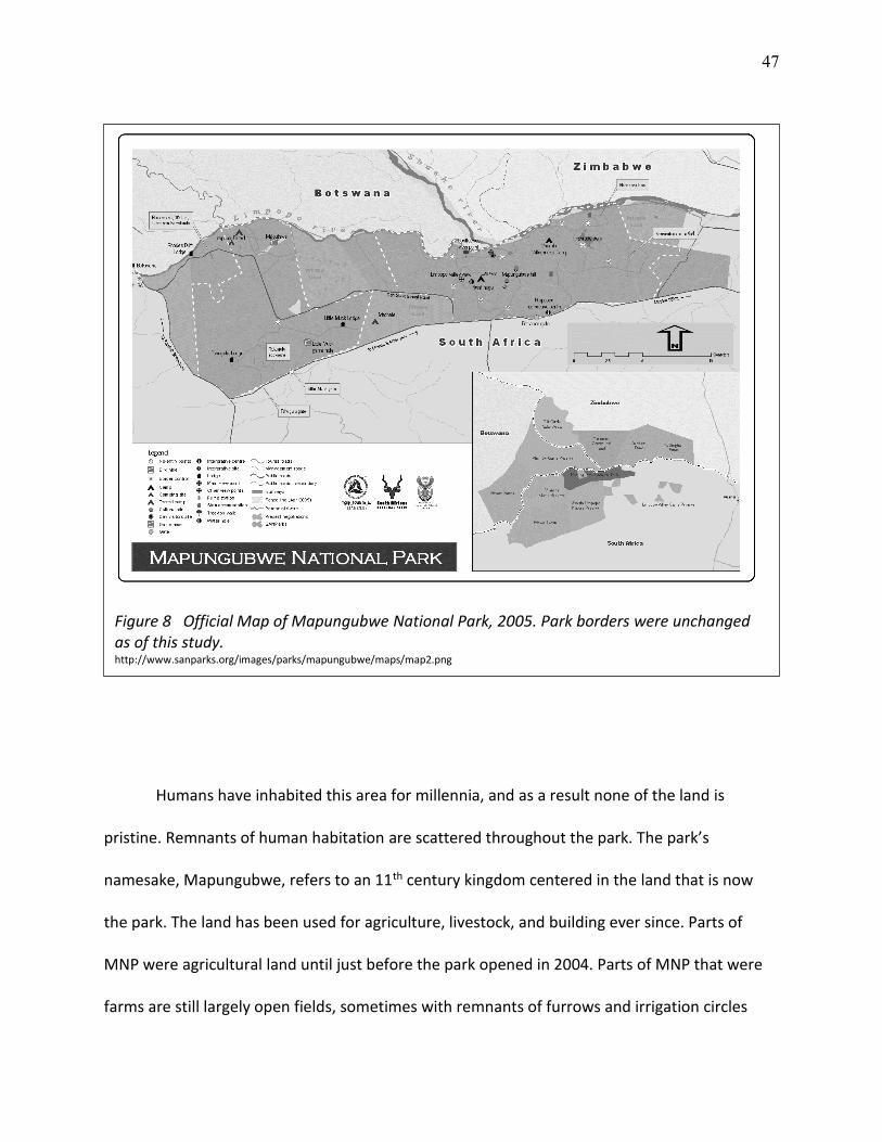
47

Humans have inhabited this area for millennia, and as a result none of the land is

pristine. Remnants of human habitation are scattered throughout the park. The park’s

namesake, Mapungubwe, refers to an 11th century kingdom centered in the land that is now

the park. The land has been used for agriculture, livestock, and building ever since. Parts of

MNP were agricultural land until just before the park opened in 2004. Parts of MNP that were

farms are still largely open fields, sometimes with remnants of furrows and irrigation circles

Figure 8 Official Map of Mapungubwe National Park, 2005. Park borders were unchanged as of this study. http://www.sanparks.org/images/parks/mapungubwe/maps/map2.png

48

visible on satellite images. One section of these fields was subject to an attempt at restoring the

natural riverine forest, but at the time of this study the restoration had yet to take effect.

Near the fields are patches of the endangered riverine forest habitat. Here too are signs

of human habitation, such as pieces of irrigation pipes and remnants of buildings. The forest

has largely recovered. The dominant trees are Combretum imberbe (leadwood), Lonchocarpus

capassa (apple leaf tree or rain tree), and Vachellia tortilis (umbrella thorn acacia), reaching a

crown height of > 7 m with 50% crown cover (Goetze et al. 2003). As of 2008, elephant

presence was notable, and there was considerable damage to the woody vegetation. During

our 2009 field season, SANParks erected a one-level electric fence in an effort to keep

elephants (and only elephants) out of this habitat. The effort was fairly successful, greatly

reducing elephant presence in the forest, stopping further destruction, and allowing plant

regrowth.

In addition to the field and riverine forest habitats, there are also areas of dense

mopane forests. Here, mopane trees (Colophospermum mopane) are a near monoculture. The

mopane woodlands were largely ignored by humans except for travel between other areas. The

soil in these mopane forests is often sandy and unsuitable for farming. Adjacent to and often

within the grasslands and mopane forests are rock outcroppings (kopjes) some of which form

extensive and contiguous tracks of rocky habitat (Fig. 9).

49

MNP offers suitable habitats for a diverse and growing animal population including

elephants, a wide variety of carnivores, and numerous antelopes. There is also a healthy

aardvark population, as evidenced by the large number of burrows throughout the non-rocky

areas of the park. A 2006 aerial census counted 114 elephants, 903 impala, 340 blue

wildebeest, 271 eland, 228 Burchell’s zebra, 88 greater kudu, 84 waterbuck, 48 giraffes, 20 red

hartebeest, 125 gemsbok, 8 tsessebe, 4 white rhinos, 2 sables, and 3 donkeys. The census also

Figure 9 Habitat types at Mapungubwe National Park, South Africa. (A) Former agricultural field with a kopje in the background; (B) Riverine forest; (C) Mopane forest

50

listed known but uncounted leopards, spotted hyenas, brown hyenas, black-backed jackals,

African wild cats, lions, bushbucks, klipspringers, common duikers, steenbok, bushpigs,

warthogs, baboons, vervet monkeys, mongooses, and unspecified rodents (Roerig 2006).

Species not mentioned above include many more mammals, at least 15 species of snakes, and

over 400 species of birds. In 2010, 165 elephants were counted within the park (Selier and Page

2010).

In 2009, we also surveyed the DeBeers-owned Venetia-Limpopo Nature Reserve (VLNR),

which is just south of MNP, for aardvark-dug burrows. Plots at VLNR included open fields,

mopane sandveld, and plots crossing both habitats. VLNR does not have riverine forest. These

plots proved to contain few aardvark burrows or signs of aardvark activity. For this reason, they

were not revisited.

2. Survey Plots

We chose plots haphazardly in each of the three habitats of open fields, riverine forest,

and mopane forest. All aardvark-dug burrows within these plots were found and measured, and

several randomly chosen burrows monitored with camera traps. The criteria for plot creation

included that the entire plot would be within one habitat type, the plot would not cross a road,

and the plot would not overlap others. We usually chose a corner point, then ran the plot east

and south from that point. Plots varied in size (0.02–21.74 ha, average 2.39 ha) and shape

(always quadrilaterals) depending on the continuity of the habitat type and ease of surveying.

In 2008 we surveyed 19 (total of 56 ha), 3 (9 ha) and 3 (9 ha) plots within the open field,

riverine and mopane habitats, respectively, at MNP. In 2009 we resurveyed 13 of the plots in

51

the open field, and added 12 more (total 49 ha). We did not resurvey the 2008 riverine and

mopane plots; instead we started 16 new riverine (23 ha) and 10 new mopane (10 ha) plots at

MNP, as well as 2 field (29 ha) and 5 mopane (23 ha) plots at VLNR. In the last year, 2010, we

resurveyed 15 of the field plots (38 ha), all 16 of the 2009 riverine (23 ha) and 2 of the mopane

plots (2 ha) at MNP; we did not return to VLNR.

For the purposes of this study, we called all aardvark-dug tunnels greater than 1 m in

length burrows. Such burrows, which can be attributed to aardvarks (Bradley 1971), are

potential burrows and dens for aardvarks and other animals. They appear in great numbers, far

disproportionate to the abundance of the aardvarks themselves. Clearly aardvarks are not

maintaining all or even a majority of these burrows. To do so would require considerable time

and effort. Aardvarks are constantly digging in new places to get at previously undiscovered ant

and termite tests. This, combined with the ease with which the aardvarks could re-excavate a

previous feeding burrow, means that they generally leave these burrows to the elements or

other animals.

Burrows are often associated with conspicuous “fans” or mounds of excavated soil. The

“fan” was defined as the area covered by soil removed from the burrow. In some cases, this

was a mound, in others it was spread out nearly flat, thus inspiring the terminology. A few

burrows that we believe to have been old had sunken areas just before the entrance, possible

the result of a soil fan being compressed or washed away by heavy rains. The size of the fan

should be related to the size of the tunnel, at least upon initial excavation. The amount of plant

debris and, even more, the amount of plant growth, provides a clue to how recently the burrow

has been maintained. When the soil is loose, even small rodents leave footprints, thus giving us

52

some indication of what type of animals have visited the area, and sometimes even if they went

inside. The size of the entrance is another possible clue to the burrow’s age. Aardvarks are large

animals and therefore dig large burrows. Entrances and tunnels may partially collapse or be

deliberately filled in. Smaller entrances should be older than larger ones. We noticed that many

entrance holes had grasses growing over them, cobwebs across part of the entry, or both.

These may provide clues as to recent activity. An entrance hole covered in grasses and cobwebs

does not likely lead to a current burrow. Finally, the approximate length of the tunnel can tell

us what kinds of animals may possibly make use of it. Large inhabitants, like aardvarks and

warthogs, require large tunnels. Smaller burrows are not suitable for these species to use as

sleeping dens, but could still provide temporary shelter.

For each burrow found, we recorded the GPS coordinates and several descriptors of the

burrow entrance (Table II). Figure 10 shows examples of typical burrow entrances. We

estimated the diameter of the soil fan in front of the entry hole, the diameter of the entry hole,

and the minimum tunnel length. All measurements were estimated visually; tunnel length is the

minimum based on visual inspection and measurements using fencing wire to probe the length.

Descriptions were also categorical. Fan debris and growth referred to loose plant material on

the surface and new plant growth on the fan, respectively.

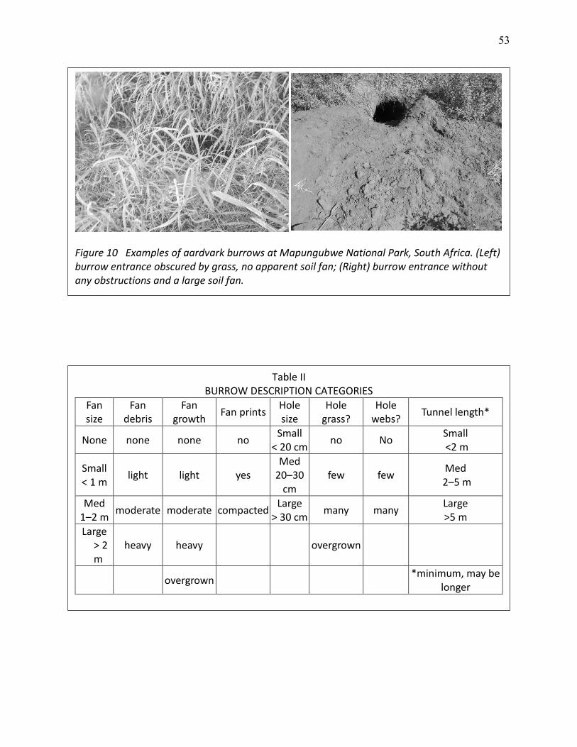
53

Figure 10 Examples of aardvark burrows at Mapungubwe National Park, South Africa. (Left) burrow entrance obscured by grass, no apparent soil fan; (Right) burrow entrance without any obstructions and a large soil fan.

Table II BURROW DESCRIPTION CATEGORIES

Fan size

Fan debris

Fan growth

Fan prints Hole size

Hole grass?

Hole webs?

Tunnel length*

None none none no Small

< 20 cm no No

Small <2 m

Small < 1 m

light light yes Med

20–30 cm

few few Med

2–5 m

Med 1–2 m

moderate moderate compacted Large

> 30 cm many many

Large >5 m

Large > 2 m

heavy heavy overgrown

overgrown *minimum, may be

longer

54

We used GPS Visualizer (gpsvisualizer.com) with Google Maps (maps.google.com) to

create a map of plot and burrow locations, color-coded by the years found. To examine the

spatial distribution pattern (random, clumped, or uniform), we used sub-plots of 1.0 +/- 0.05 ha

following the method described in Odum (1961). Plots less than 1 ha were not counted, 1 ha

plots were counted in their entirety, and larger plots were subdivided into 1-ha portions. We

kept the sub-plots as square as possible while fitting as many as possible. Generally, the

subplots were roughly the same shape as the larger plot. The method used to divide plots

depended on the shape of the plot and number of subplots needed, but was standard across

plots. We used Google Earth (Google, Mountain View, CA) with our maps to draw and measure

these sub-plots.

Within each plot of each habitat, we counted the number of burrows in the first year

that the plot was surveyed. As per Odum (1961), if the mean and the variance of the number of

burrows per unit space are equal, then burrows are randomly distributed; if the mean is greater

than the variance, then there is a uniform distribution; and if the mean is less than the variance,

then there is a clumped distribution. We expected a clumped distribution, or possibly a

seemingly random distribution on this fairly small scale, hypothesizing that the majority of

these burrows were dug for feeding purposes (reflecting clumped or random prey distributions)

rather than escape holes (which should have a uniform distribution).

3. Plugs

In 2010, to test for the frequency of use by any species, we loosely “plugged” the

entryways of 107 burrows (52 riverine, 55 field) with grasses (Fig. 11). We revisited those

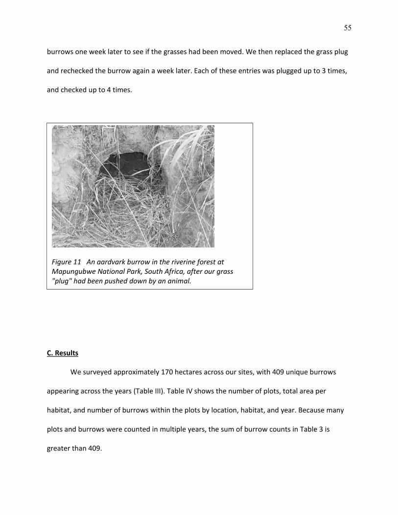
55

burrows one week later to see if the grasses had been moved. We then replaced the grass plug

and rechecked the burrow again a week later. Each of these entries was plugged up to 3 times,

and checked up to 4 times.

C. Results

We surveyed approximately 170 hectares across our sites, with 409 unique burrows

appearing across the years (Table III). Table IV shows the number of plots, total area per

habitat, and number of burrows within the plots by location, habitat, and year. Because many

plots and burrows were counted in multiple years, the sum of burrow counts in Table 3 is

greater than 409.

Figure 11 An aardvark burrow in the riverine forest at Mapungubwe National Park, South Africa, after our grass "plug" had been pushed down by an animal.

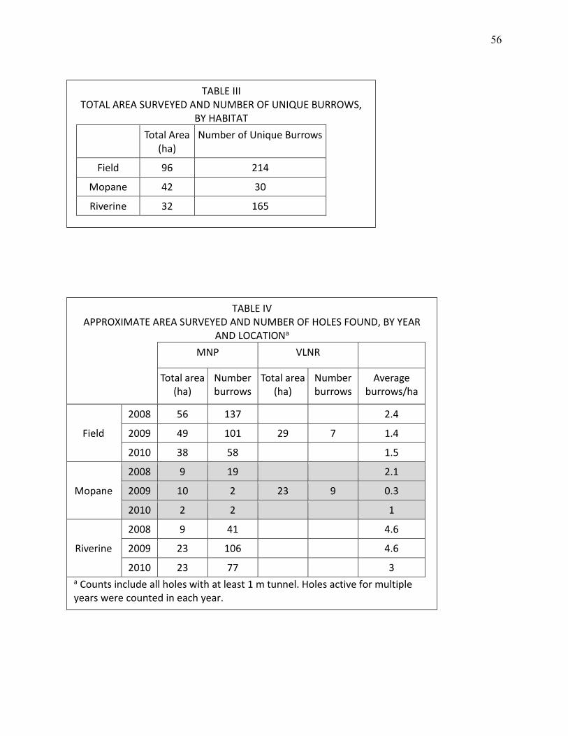
56

TABLE III TOTAL AREA SURVEYED AND NUMBER OF UNIQUE BURROWS,

BY HABITAT

Total Area (ha)

Number of Unique Burrows

Field 96 214

Mopane 42 30

Riverine 32 165

TABLE IV APPROXIMATE AREA SURVEYED AND NUMBER OF HOLES FOUND, BY YEAR

AND LOCATIONa

MNP VLNR

Total area (ha)

Number burrows

Total area (ha)

Number burrows

Average burrows/ha

Field

2008 56 137 2.4

2009 49 101 29 7 1.4

2010 38 58 1.5

Mopane

2008 9 19 2.1

2009 10 2 23 9 0.3

2010 2 2 1

Riverine

2008 9 41 4.6

2009 23 106 4.6

2010 23 77 3 a Counts include all holes with at least 1 m tunnel. Holes active for multiple years were counted in each year.

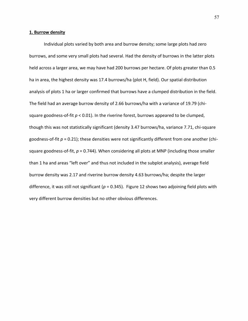
57

1. Burrow density

Individual plots varied by both area and burrow density; some large plots had zero

burrows, and some very small plots had several. Had the density of burrows in the latter plots

held across a larger area, we may have had 200 burrows per hectare. Of plots greater than 0.5

ha in area, the highest density was 17.4 burrows/ha (plot H, field). Our spatial distribution

analysis of plots 1 ha or larger confirmed that burrows have a clumped distribution in the field.

The field had an average burrow density of 2.66 burrows/ha with a variance of 19.79 (chi-

square goodness-of-fit p < 0.01). In the riverine forest, burrows appeared to be clumped,

though this was not statistically significant (density 3.47 burrows/ha, variance 7.71, chi-square

goodness-of-fit p = 0.21); these densities were not significantly different from one another (chi-

square goodness-of-fit, p = 0.744). When considering all plots at MNP (including those smaller

than 1 ha and areas “left over” and thus not included in the subplot analysis), average field

burrow density was 2.17 and riverine burrow density 4.63 burrows/ha; despite the larger

difference, it was still not significant (p = 0.345). Figure 12 shows two adjoining field plots with

very different burrow densities but no other obvious differences.

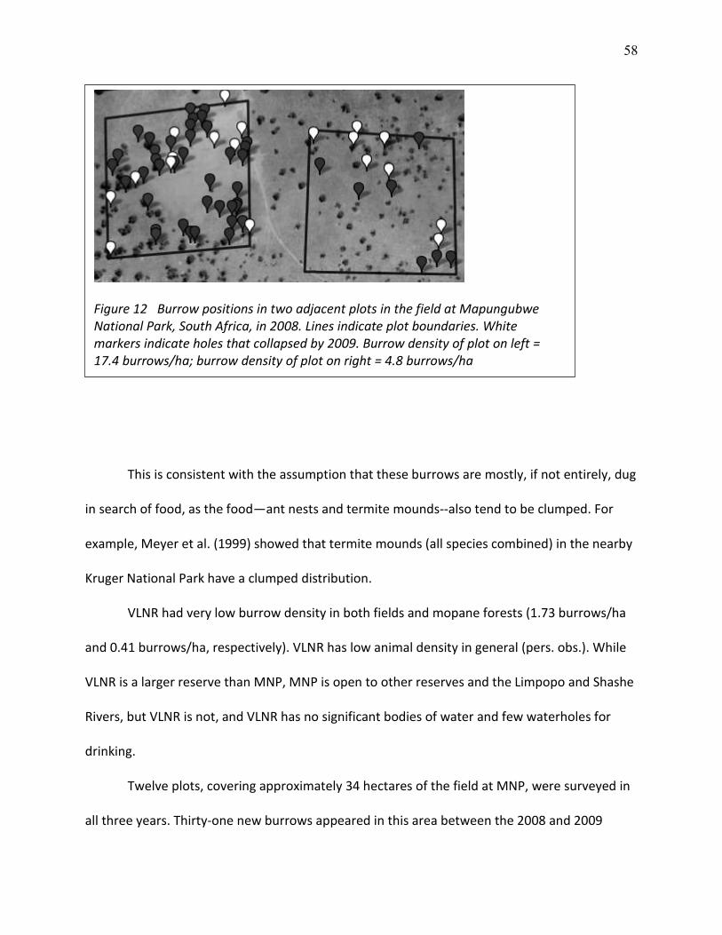
58

This is consistent with the assumption that these burrows are mostly, if not entirely, dug

in search of food, as the food—ant nests and termite mounds--also tend to be clumped. For

example, Meyer et al. (1999) showed that termite mounds (all species combined) in the nearby

Kruger National Park have a clumped distribution.

VLNR had very low burrow density in both fields and mopane forests (1.73 burrows/ha

and 0.41 burrows/ha, respectively). VLNR has low animal density in general (pers. obs.). While

VLNR is a larger reserve than MNP, MNP is open to other reserves and the Limpopo and Shashe

Rivers, but VLNR is not, and VLNR has no significant bodies of water and few waterholes for

drinking.

Twelve plots, covering approximately 34 hectares of the field at MNP, were surveyed in

all three years. Thirty-one new burrows appeared in this area between the 2008 and 2009

Figure 12 Burrow positions in two adjacent plots in the field at Mapungubwe National Park, South Africa, in 2008. Lines indicate plot boundaries. White markers indicate holes that collapsed by 2009. Burrow density of plot on left = 17.4 burrows/ha; burrow density of plot on right = 4.8 burrows/ha

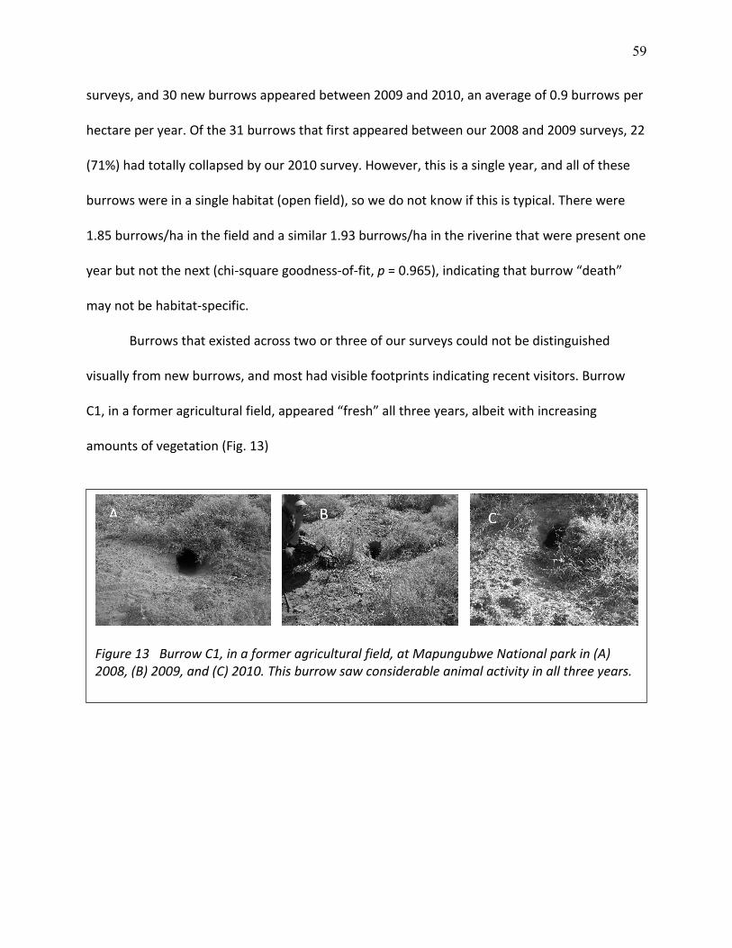
59

surveys, and 30 new burrows appeared between 2009 and 2010, an average of 0.9 burrows per

hectare per year. Of the 31 burrows that first appeared between our 2008 and 2009 surveys, 22

(71%) had totally collapsed by our 2010 survey. However, this is a single year, and all of these

burrows were in a single habitat (open field), so we do not know if this is typical. There were

1.85 burrows/ha in the field and a similar 1.93 burrows/ha in the riverine that were present one

year but not the next (chi-square goodness-of-fit, p = 0.965), indicating that burrow “death”

may not be habitat-specific.

Burrows that existed across two or three of our surveys could not be distinguished

visually from new burrows, and most had visible footprints indicating recent visitors. Burrow

C1, in a former agricultural field, appeared “fresh” all three years, albeit with increasing

amounts of vegetation (Fig. 13)

Figure 13 Burrow C1, in a former agricultural field, at Mapungubwe National park in (A) 2008, (B) 2009, and (C) 2010. This burrow saw considerable animal activity in all three years.

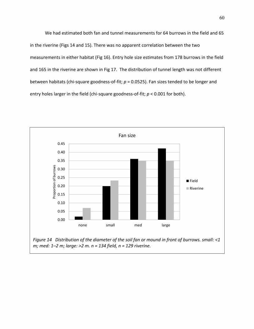
60

We had estimated both fan and tunnel measurements for 64 burrows in the field and 65

in the riverine (Figs 14 and 15). There was no apparent correlation between the two

measurements in either habitat (Fig 16). Entry hole size estimates from 178 burrows in the field

and 165 in the riverine are shown in Fig 17. The distribution of tunnel length was not different

between habitats (chi-square goodness-of-fit; p = 0.0525). Fan sizes tended to be longer and

entry holes larger in the field (chi-square goodness-of-fit; p < 0.001 for both).

Figure 14 Distribution of the diameter of the soil fan or mound in front of burrows. small: <1 m; med: 1–2 m; large: >2 m. n = 134 field, n = 129 riverine.

none small med large

0.00

0.05

0.10

0.15

0.20

0.25

0.30

0.35

0.40

0.45

Pro

po

rtio

n o

f b

urr

ow

s

Fan size

Field

Riverine

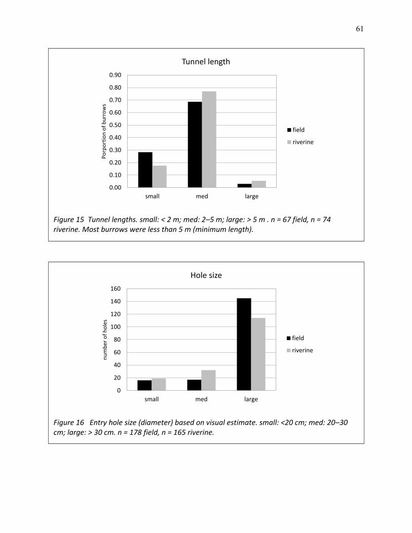
61

Figure 15 Tunnel lengths. small: < 2 m; med: 2–5 m; large: > 5 m . n = 67 field, n = 74 riverine. Most burrows were less than 5 m (minimum length).

small med large

0.00

0.10

0.20

0.30

0.40

0.50

0.60

0.70

0.80

0.90

Po

rpo

rtio

n o

f b

urr

ow

s

Tunnel length

field

riverine

Figure 16 Entry hole size (diameter) based on visual estimate. small: <20 cm; med: 20–30 cm; large: > 30 cm. n = 178 field, n = 165 riverine.

small med large

0

20

40

60

80

100

120

140

160

nu

mb

er o

f h

ole

s

Hole size

field

riverine

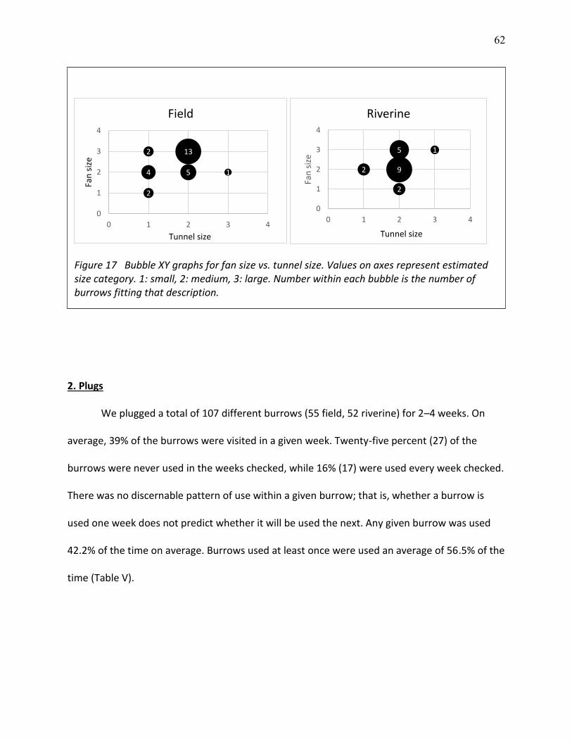
62

2. Plugs

We plugged a total of 107 different burrows (55 field, 52 riverine) for 2–4 weeks. On

average, 39% of the burrows were visited in a given week. Twenty-five percent (27) of the

burrows were never used in the weeks checked, while 16% (17) were used every week checked.

There was no discernable pattern of use within a given burrow; that is, whether a burrow is

used one week does not predict whether it will be used the next. Any given burrow was used

42.2% of the time on average. Burrows used at least once were used an average of 56.5% of the

time (Table V).

Figure 17 Bubble XY graphs for fan size vs. tunnel size. Values on axes represent estimated size category. 1: small, 2: medium, 3: large. Number within each bubble is the number of burrows fitting that description.

2

4 5 1

2 13

0

1

2

3

4

0 1 2 3 4

Fan

siz

e

Tunnel size

Field

2

2 9

5 1

0

1

2

3

4

0 1 2 3 4

Fan

siz

e

Tunnel size

Riverine

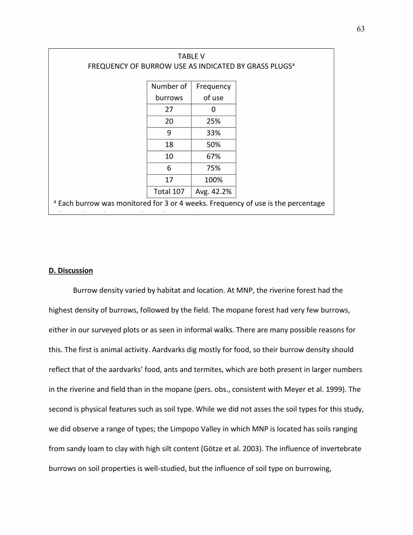
63

D. Discussion

Burrow density varied by habitat and location. At MNP, the riverine forest had the

highest density of burrows, followed by the field. The mopane forest had very few burrows,

either in our surveyed plots or as seen in informal walks. There are many possible reasons for

this. The first is animal activity. Aardvarks dig mostly for food, so their burrow density should

reflect that of the aardvarks’ food, ants and termites, which are both present in larger numbers

in the riverine and field than in the mopane (pers. obs., consistent with Meyer et al. 1999). The

second is physical features such as soil type. While we did not asses the soil types for this study,

we did observe a range of types; the Limpopo Valley in which MNP is located has soils ranging

from sandy loam to clay with high silt content (Götze et al. 2003). The influence of invertebrate

burrows on soil properties is well-studied, but the influence of soil type on burrowing,

TABLE V FREQUENCY OF BURROW USE AS INDICATED BY GRASS PLUGSa

Number of

burrows

Frequency

of use

27 0

20 25%

9 33%

18 50%

10 67%

6 75%

17 100%

Total 107 Avg. 42.2% a Each burrow was monitored for 3 or 4 weeks. Frequency of use is the percentage

of time those plugs were obviously moved.

64

particularly in larger animals, is largely unknown. Soil type, along with the density of tree roots,

can certainly affect the ease or difficulty of digging as well as structural stability. This has been

shown in small mammals (Laundre and Reynolds 1993) and southern hairy-nose wombats

(Walker et al. 2007). The variation in soil types undoubtedly affects the longevity of aardvark-

dug burrows as well, though the short time frame of this study was not enough to discern a

pattern in either habitat. Furthermore, soil type certainly affects the distribution of ants and

termites, and aardvark feeding digs would thus follow this pattern. Finally, the riverine forest

has significantly more water than the open fields, and this water affects both soil type and ant

and termite distribution.

Taylor and Skinner (2003) excavated two aardvark burrows that had been used as

sleeping dens. One of those burrows had two tunnels, the shorter 4.7 m long and ending in an

enlarged chamber, presumably for sleeping. Our method of measuring tunnel length was crude,

and only gave us a minimum length of a single tunnel. We had only 6 burrows with a minimum

length of 5 m out of the 149 measured; however, they could have been larger, and some of our

“medium” length tunnels were probably actually large enough to be sleeping dens.

Burrow attributes such as fan size and tunnel length did not appear to have any

correlations, but our methods were too crude to provide conclusive results. For example, we

did not test the depth or compaction of the soil fan, attributes that are vital in estimating the

volume of soil. For this reason, we make no conclusion about burrow attributes in relationship

to one another or their changes over time.

Burrow longevity, like burrow density at any one point in time, may be related to soil

type, aardvark density, ant/termite density, and the density of other animals performing

65

burrow upkeep or destruction. Aardvark-dug burrow longevity appears to be highly variable,

though our data do not permit calculation of averages. Of the burrows that appeared in the

fields between our 2008 and 2009 surveys, 71% (22 of 31) had collapsed by our 2010 survey. On

the other hand, there were 23 burrows in the same field that were dug sometime prior to our

2008 survey and were still viable at our 2010 survey. One of the few burrows found at VLNR

was at least 16 years old: an assistant recalled finding an aardvark dead of a snakebite at this

location 16 years prior to our visit, and camera-trap monitoring showed an aardvark using this

burrow. One burrow at MNP was used by a minimum of two different aardvarks during this

study: the first (which died in the burrow entry) in 2008, and at least one in 2009. An aardvark

was also photographed at this burrow in 2010, but we do not know if it was the same aardvark

as in 2009, as neither had distinctive markings. One burrow in the riverine forest (monitored by

a camera trap) was closed by a warthog. We do not know the reason for this or if that burrow

had other entrances.

We also do not know how much aardvarks contribute to this burrow upkeep as

compared with other species. (Taylor and Skinner 2003) found that aardvarks change sleeping

dens frequently; their observations found that a given burrow would be occupied for 1 to 38

days, with a mean of less than 10 days. They noted that there were many burrows available

within each aardvark’s home range and that aardvarks were not observed re-using any given

burrow within their study.

In our plots, new burrows appeared at a rate of about 0.9 per hectare per year.

Assuming an average of 1 m length and 30 cm diameter, that would mean about 0.7 m3 of

excavated soil per hectare per year, or about 1.4 tonnes per hectare per year (assuming an

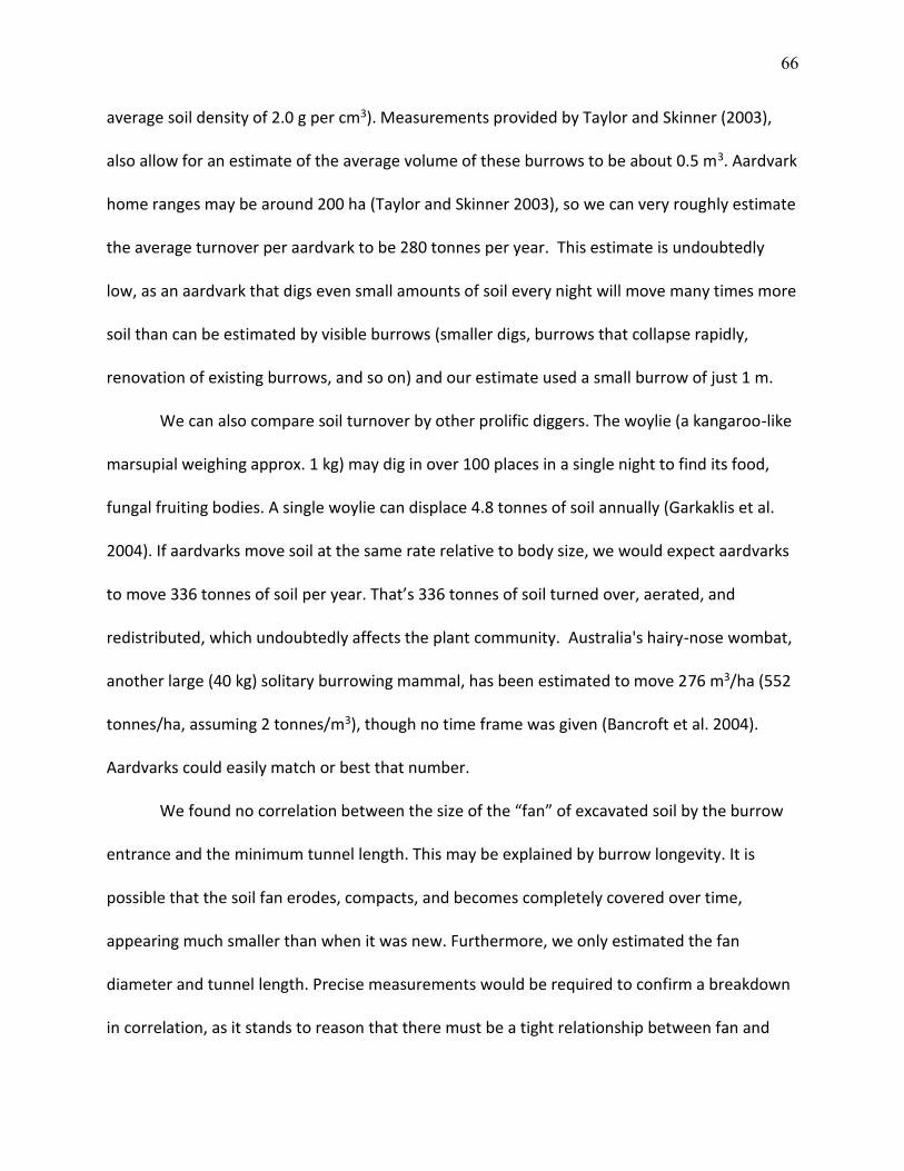
66

average soil density of 2.0 g per cm3). Measurements provided by Taylor and Skinner (2003),

also allow for an estimate of the average volume of these burrows to be about 0.5 m3. Aardvark

home ranges may be around 200 ha (Taylor and Skinner 2003), so we can very roughly estimate

the average turnover per aardvark to be 280 tonnes per year. This estimate is undoubtedly

low, as an aardvark that digs even small amounts of soil every night will move many times more

soil than can be estimated by visible burrows (smaller digs, burrows that collapse rapidly,

renovation of existing burrows, and so on) and our estimate used a small burrow of just 1 m.

We can also compare soil turnover by other prolific diggers. The woylie (a kangaroo-like

marsupial weighing approx. 1 kg) may dig in over 100 places in a single night to find its food,

fungal fruiting bodies. A single woylie can displace 4.8 tonnes of soil annually (Garkaklis et al.

2004). If aardvarks move soil at the same rate relative to body size, we would expect aardvarks

to move 336 tonnes of soil per year. That’s 336 tonnes of soil turned over, aerated, and

redistributed, which undoubtedly affects the plant community. Australia's hairy-nose wombat,

another large (40 kg) solitary burrowing mammal, has been estimated to move 276 m3/ha (552

tonnes/ha, assuming 2 tonnes/m3), though no time frame was given (Bancroft et al. 2004).

Aardvarks could easily match or best that number.

We found no correlation between the size of the “fan” of excavated soil by the burrow

entrance and the minimum tunnel length. This may be explained by burrow longevity. It is

possible that the soil fan erodes, compacts, and becomes completely covered over time,

appearing much smaller than when it was new. Furthermore, we only estimated the fan

diameter and tunnel length. Precise measurements would be required to confirm a breakdown

in correlation, as it stands to reason that there must be a tight relationship between fan and

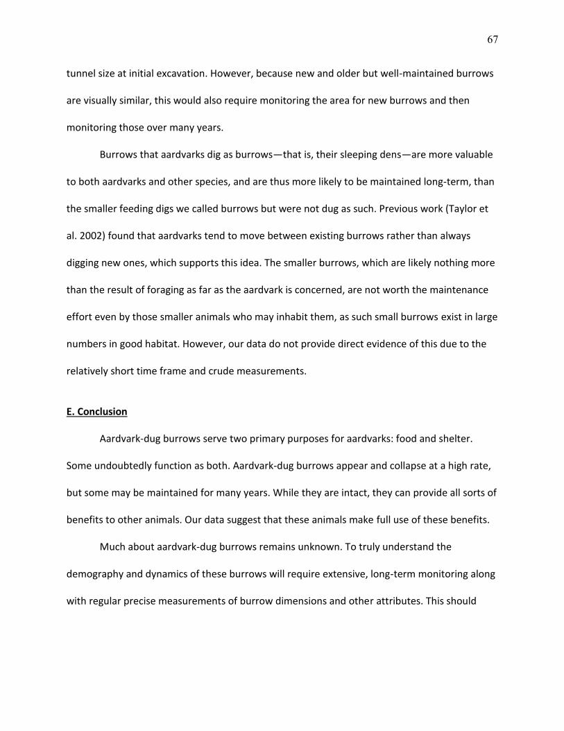
67

tunnel size at initial excavation. However, because new and older but well-maintained burrows

are visually similar, this would also require monitoring the area for new burrows and then

monitoring those over many years.

Burrows that aardvarks dig as burrows—that is, their sleeping dens—are more valuable

to both aardvarks and other species, and are thus more likely to be maintained long-term, than

the smaller feeding digs we called burrows but were not dug as such. Previous work (Taylor et

al. 2002) found that aardvarks tend to move between existing burrows rather than always

digging new ones, which supports this idea. The smaller burrows, which are likely nothing more

than the result of foraging as far as the aardvark is concerned, are not worth the maintenance

effort even by those smaller animals who may inhabit them, as such small burrows exist in large

numbers in good habitat. However, our data do not provide direct evidence of this due to the

relatively short time frame and crude measurements.

E. Conclusion

Aardvark-dug burrows serve two primary purposes for aardvarks: food and shelter.

Some undoubtedly function as both. Aardvark-dug burrows appear and collapse at a high rate,

but some may be maintained for many years. While they are intact, they can provide all sorts of

benefits to other animals. Our data suggest that these animals make full use of these benefits.

Much about aardvark-dug burrows remains unknown. To truly understand the

demography and dynamics of these burrows will require extensive, long-term monitoring along

with regular precise measurements of burrow dimensions and other attributes. This should

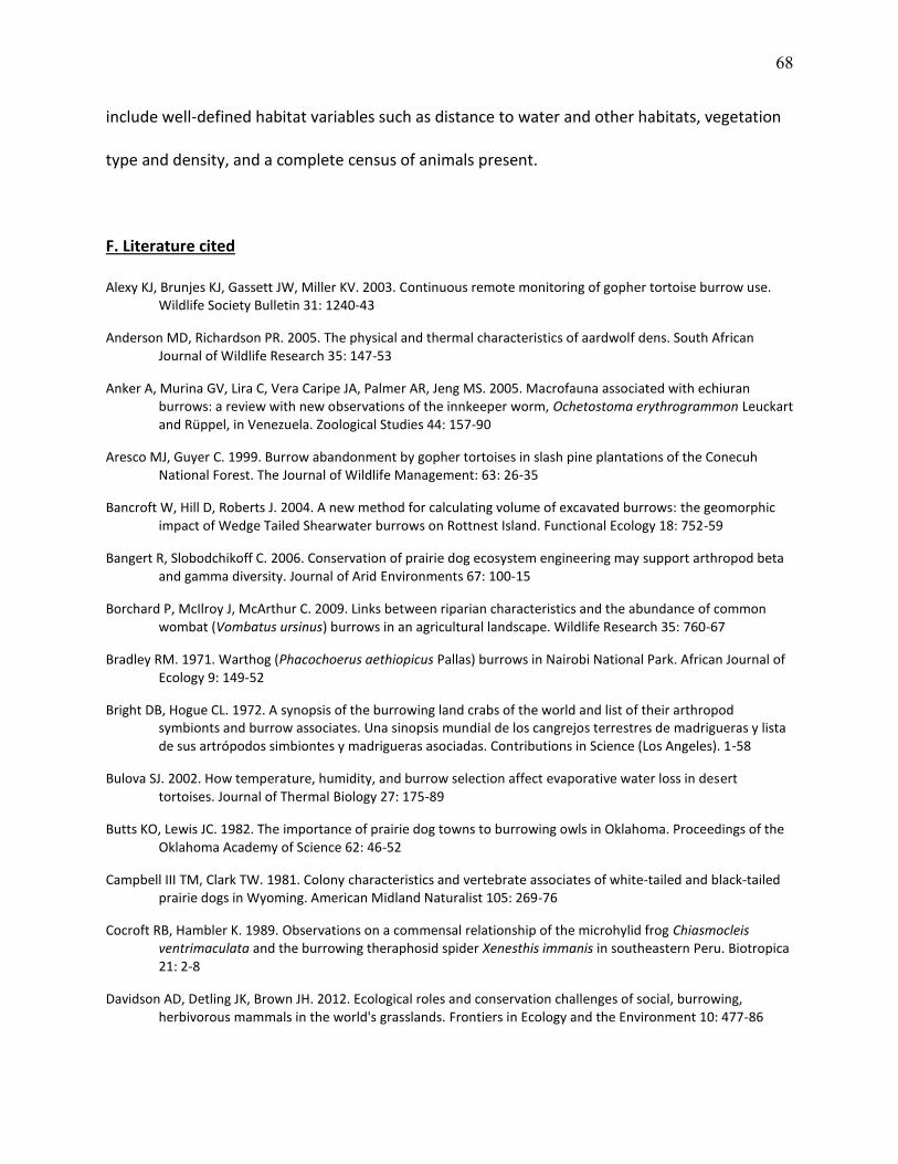
68

include well-defined habitat variables such as distance to water and other habitats, vegetation

type and density, and a complete census of animals present.

F. Literature cited

Alexy KJ, Brunjes KJ, Gassett JW, Miller KV. 2003. Continuous remote monitoring of gopher tortoise burrow use. Wildlife Society Bulletin 31: 1240-43

Anderson MD, Richardson PR. 2005. The physical and thermal characteristics of aardwolf dens. South African Journal of Wildlife Research 35: 147-53

Anker A, Murina GV, Lira C, Vera Caripe JA, Palmer AR, Jeng MS. 2005. Macrofauna associated with echiuran burrows: a review with new observations of the innkeeper worm, Ochetostoma erythrogrammon Leuckart and Rüppel, in Venezuela. Zoological Studies 44: 157-90

Aresco MJ, Guyer C. 1999. Burrow abandonment by gopher tortoises in slash pine plantations of the Conecuh National Forest. The Journal of Wildlife Management: 63: 26-35

Bancroft W, Hill D, Roberts J. 2004. A new method for calculating volume of excavated burrows: the geomorphic impact of Wedge Tailed Shearwater burrows on Rottnest Island. Functional Ecology 18: 752-59

Bangert R, Slobodchikoff C. 2006. Conservation of prairie dog ecosystem engineering may support arthropod beta and gamma diversity. Journal of Arid Environments 67: 100-15

Borchard P, McIlroy J, McArthur C. 2009. Links between riparian characteristics and the abundance of common wombat (Vombatus ursinus) burrows in an agricultural landscape. Wildlife Research 35: 760-67

Bradley RM. 1971. Warthog (Phacochoerus aethiopicus Pallas) burrows in Nairobi National Park. African Journal of Ecology 9: 149-52

Bright DB, Hogue CL. 1972. A synopsis of the burrowing land crabs of the world and list of their arthropod symbionts and burrow associates. Una sinopsis mundial de los cangrejos terrestres de madrigueras y lista de sus artrópodos simbiontes y madrigueras asociadas. Contributions in Science (Los Angeles). 1-58

Bulova SJ. 2002. How temperature, humidity, and burrow selection affect evaporative water loss in desert tortoises. Journal of Thermal Biology 27: 175-89

Butts KO, Lewis JC. 1982. The importance of prairie dog towns to burrowing owls in Oklahoma. Proceedings of the Oklahoma Academy of Science 62: 46-52

Campbell III TM, Clark TW. 1981. Colony characteristics and vertebrate associates of white-tailed and black-tailed prairie dogs in Wyoming. American Midland Naturalist 105: 269-76

Cocroft RB, Hambler K. 1989. Observations on a commensal relationship of the microhylid frog Chiasmocleis ventrimaculata and the burrowing theraphosid spider Xenesthis immanis in southeastern Peru. Biotropica 21: 2-8

Davidson AD, Detling JK, Brown JH. 2012. Ecological roles and conservation challenges of social, burrowing, herbivorous mammals in the world's grasslands. Frontiers in Ecology and the Environment 10: 477-86

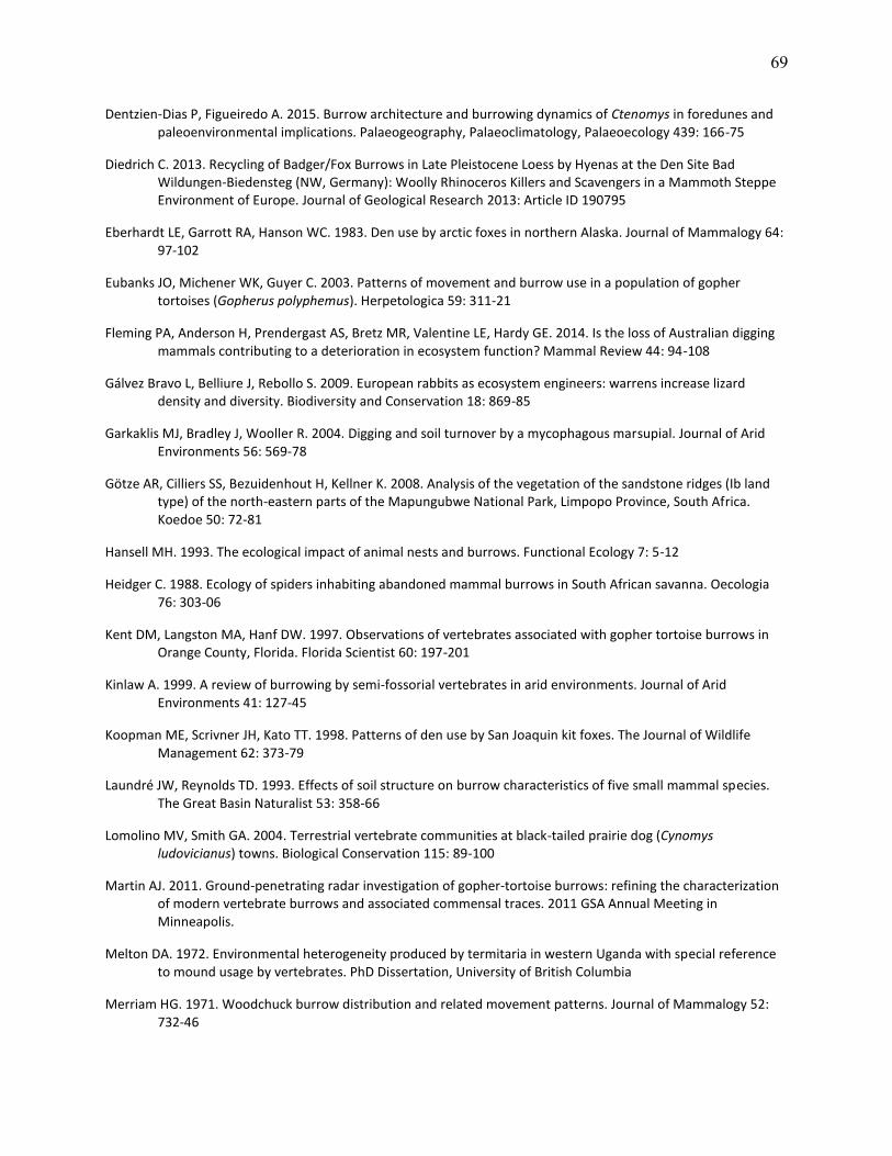
69

Dentzien-Dias P, Figueiredo A. 2015. Burrow architecture and burrowing dynamics of Ctenomys in foredunes and paleoenvironmental implications. Palaeogeography, Palaeoclimatology, Palaeoecology 439: 166-75

Diedrich C. 2013. Recycling of Badger/Fox Burrows in Late Pleistocene Loess by Hyenas at the Den Site Bad Wildungen-Biedensteg (NW, Germany): Woolly Rhinoceros Killers and Scavengers in a Mammoth Steppe Environment of Europe. Journal of Geological Research 2013: Article ID 190795

Eberhardt LE, Garrott RA, Hanson WC. 1983. Den use by arctic foxes in northern Alaska. Journal of Mammalogy 64: 97-102

Eubanks JO, Michener WK, Guyer C. 2003. Patterns of movement and burrow use in a population of gopher tortoises (Gopherus polyphemus). Herpetologica 59: 311-21

Fleming PA, Anderson H, Prendergast AS, Bretz MR, Valentine LE, Hardy GE. 2014. Is the loss of Australian digging mammals contributing to a deterioration in ecosystem function? Mammal Review 44: 94-108

Gálvez Bravo L, Belliure J, Rebollo S. 2009. European rabbits as ecosystem engineers: warrens increase lizard density and diversity. Biodiversity and Conservation 18: 869-85

Garkaklis MJ, Bradley J, Wooller R. 2004. Digging and soil turnover by a mycophagous marsupial. Journal of Arid Environments 56: 569-78

Götze AR, Cilliers SS, Bezuidenhout H, Kellner K. 2008. Analysis of the vegetation of the sandstone ridges (Ib land type) of the north-eastern parts of the Mapungubwe National Park, Limpopo Province, South Africa. Koedoe 50: 72-81

Hansell MH. 1993. The ecological impact of animal nests and burrows. Functional Ecology 7: 5-12

Heidger C. 1988. Ecology of spiders inhabiting abandoned mammal burrows in South African savanna. Oecologia 76: 303-06

Kent DM, Langston MA, Hanf DW. 1997. Observations of vertebrates associated with gopher tortoise burrows in Orange County, Florida. Florida Scientist 60: 197-201

Kinlaw A. 1999. A review of burrowing by semi-fossorial vertebrates in arid environments. Journal of Arid Environments 41: 127-45

Koopman ME, Scrivner JH, Kato TT. 1998. Patterns of den use by San Joaquin kit foxes. The Journal of Wildlife Management 62: 373-79

Laundré JW, Reynolds TD. 1993. Effects of soil structure on burrow characteristics of five small mammal species. The Great Basin Naturalist 53: 358-66

Lomolino MV, Smith GA. 2004. Terrestrial vertebrate communities at black-tailed prairie dog (Cynomys ludovicianus) towns. Biological Conservation 115: 89-100

Martin AJ. 2011. Ground-penetrating radar investigation of gopher-tortoise burrows: refining the characterization of modern vertebrate burrows and associated commensal traces. 2011 GSA Annual Meeting in Minneapolis.

Melton DA. 1972. Environmental heterogeneity produced by termitaria in western Uganda with special reference to mound usage by vertebrates. PhD Dissertation, University of British Columbia

Merriam HG. 1971. Woodchuck burrow distribution and related movement patterns. Journal of Mammalogy 52: 732-46

70

Meyer V, Braack L, Biggs H, Ebersohn C. 1999. Distribution and density of termite mounds in the northern Kruger National Park, with specific reference to those constructed by Macrotermes Holmgren (Isoptera: Termitidae). African Entomology 7: 123-30

Nakazono T, Ono Y. 1987. Den distribution and den use by the red fox Vulpes vulpes japonica in Kyushu. Ecological Research 2: 265-77

Odum EP, Pontin A. 1961. Population density of the underground ant, Lasius flavus, as determined by tagging with P-32. Ecology 42: 186-88

Pokines JT, Peterhans JCK. 2007. Spotted hyena (Crocuta crocuta) den use and taphonomy in the Masai Mara National Reserve, Kenya. Journal of Archaeological Science 34: 1914-31

Read JL, Carter J, Moseby K, Greenville A. 2008. Ecological roles of rabbit, bettong and bilby warrens in arid Australia. Journal of Arid Environments 72: 2124-30

Roerig J. 2006. Counting Game in Mapungubwe. https://www.sanparks.org/about/news/?id=371. Accessed September 23, 2016.

Selier SAJ, Page BR, Vanak AT, Slotow R. 2014. Sustainability of elephant hunting across international borders in southern Africa: A case study of the greater Mapungubwe Transfrontier Conservation Area. The Journal of Wildlife Management 78: 122-32

Skinner J. 1976. Ecology of the brown hyaena Hyaena brunnea in the Transvaal with a distribution map for southern Africa. South African Journal of Science 72: e269

Smithers RHN. 1971. The Mammals of Botswana. Trustees of the National Museums of Rhodesia.

Šumbera R, Chitaukali W, Elichová M, Kubová J, Burda H. 2004. Microclimatic stability in burrows of an Afrotropical solitary bathyergid rodent, the silvery mole‐rat (Heliophobius argenteocinereus). Journal of Zoology 263: 409-16

Šumbera R, Mazoch V, Patzenhauerová H, Lövy M, Šklíba J, et al. 2012. Burrow architecture, family composition and habitat characteristics of the largest social African mole-rat: the giant mole-rat constructs really giant burrow systems. Acta Theriologica 57: 121-30

Taylor WA, Lindsey PA, Skinner JD. 2002. The feeding ecology of the aardvark Orycteropus afer. Journal of Arid Environments 50: 135-52

Taylor WA, Skinner JD. 2003. Activity patterns, home ranges and burrow use of aardvarks (Orycteropus afer) in the Karoo. Journal of Zoology 261: 291-97

Thomas H, Scantlebury M, Swanepoel D, Bateman P, Bennett N. 2013. Seasonal changes in burrow geometry of the common mole rat (Rodentia: Bathyergidae). Naturwissenschaften 100: 1023-30

Thomas HG, Bateman PW, Scantlebury M, Bennett NC. 2012. Seasonal effects on digging activity and burrow architecture in the Cape dune mole-rat, Bathyergus suillus (Rodentia: Bathyergidae). African Zoology 47: 332-40

Walker FM, Taylor AC, Sunnucks P. 2007. Does soil type drive social organization in southern hairy nosed wombats? Molecular Ecology 16: 199-208

Whitford WG, Kay FR. 1999. Biopedturbation by mammals in deserts: a review. Journal of Arid Environments 41: 203-30

71

Whittington-Jones G, Bernard R, Parker D. 2011. Aardvark Burrows: A Potential Resource for Animals in Arid and Semi-Arid Environments. African Zoology 46: 362-70

Wilschut LI, Addink EA, Heesterbeek H, Heier L, Laudisoit A, et al. 2013. Potential corridors and barriers for plague spread in central Asia. International Journal of Health Geographics 12: 49

IV. CAMERA TRAPS REVEAL THAT AARDVARKS ARE THE INADVERTENT CIVIL ENGINEERS OF

SOUTHERN AFRICA

A. Introduction

1. Ecosystem engineering

Ecosystem engineering is the physical alteration of the environment by organisms,

whether via their bodies (e.g., corals, trees) or by building structures or destroying or otherwise

altering the landscape (Jones et al. 1994). The effects can be substantial: one study estimated

an average 25% increase in species diversity thanks to local engineering species (Romero et al.

2014). Ecosystem engineers include diverse taxa of plants and animals small and large. It can be

argued that all or almost all species alter their environments and therefore could be ecosystem

engineers (Hastings et al. 2007), but generally speaking, most people seem to reserve the term

for those with impacts disproportionate to their abundance in the community (Wright and

Jones 2006).

The direct and indirect effects of ecosystem engineers are still being documented, as

they are numerous and complex. In recent years, attempts have been made to better define

the types of ecosystem engineers and classify and quantify their effects (Romero et al. 2014).

Romero divided ecosystem engineering effects into three categories: bioturbation, habitat

forming, and habitat modification. Other authors have devised their own ecosystem

engineering classification schemes and others have challenged the usefulness of the term (e.g.,

Jones et al. 1997; Berke 2010), but the central idea remains.

The archetypal ecosystem engineer is the beaver (Castor spp.), which fells trees and

builds dams that turn rivers into ponds (e.g., Wright et al. 2002). For pure destructive power,

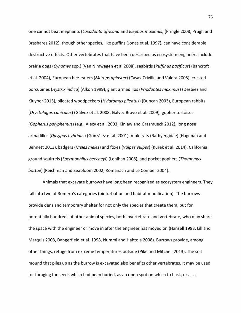
73

one cannot beat elephants (Loxodonta africana and Elephas maximus) (Pringle 2008; Prugh and

Brashares 2012), though other species, like puffins (Jones et al. 1997), can have considerable

destructive effects. Other vertebrates that have been described as ecosystem engineers include

prairie dogs (Cynomys spp.) (Van Nimwegen et al 2008), seabirds (Puffinus pacificus) (Bancroft

et al. 2004), European bee-eaters (Merops apiaster) (Casas-Criville and Valera 2005), crested

porcupines (Hystrix indica) (Alkon 1999), giant armadillos (Priodontes maximus) (Desbiez and

Kluyber 2013), pileated woodpeckers (Hylatomus pileatus) (Duncan 2003), European rabbits

(Oryctolagus cuniculus) (Gálvez et al. 2008; Gálvez Bravo et al. 2009), gopher tortoises

(Gopherus polyphemus) (e.g., Alexy et al. 2003, Kinlaw and Grasmueck 2012), long nose

armadillos (Dasypus hybridus) (González et al. 2001), mole rats (Bathyergidae) (Hagenah and

Bennett 2013), badgers (Meles meles) and foxes (Vulpes vulpes) (Kurek et al. 2014), California

ground squirrels (Spermophilus beecheyi) (Lenihan 2008), and pocket gophers (Thomomys

bottae) (Reichman and Seabloom 2002; Romanach and Le Comber 2004).

Animals that excavate burrows have long been recognized as ecosystem engineers. They

fall into two of Romero’s categories (bioturbation and habitat modification). The burrows

provide dens and temporary shelter for not only the species that create them, but for

potentially hundreds of other animal species, both invertebrate and vertebrate, who may share

the space with the engineer or move in after the engineer has moved on (Hansell 1993, Lill and

Marquis 2003, Dangerfield et al. 1998, Nummi and Hahtola 2008). Burrows provide, among

other things, refuge from extreme temperatures outside (Pike and Mitchell 2013). The soil

mound that piles up as the burrow is excavated also benefits other vertebrates. It may be used

for foraging for seeds which had been buried, as an open spot on which to bask, or as a

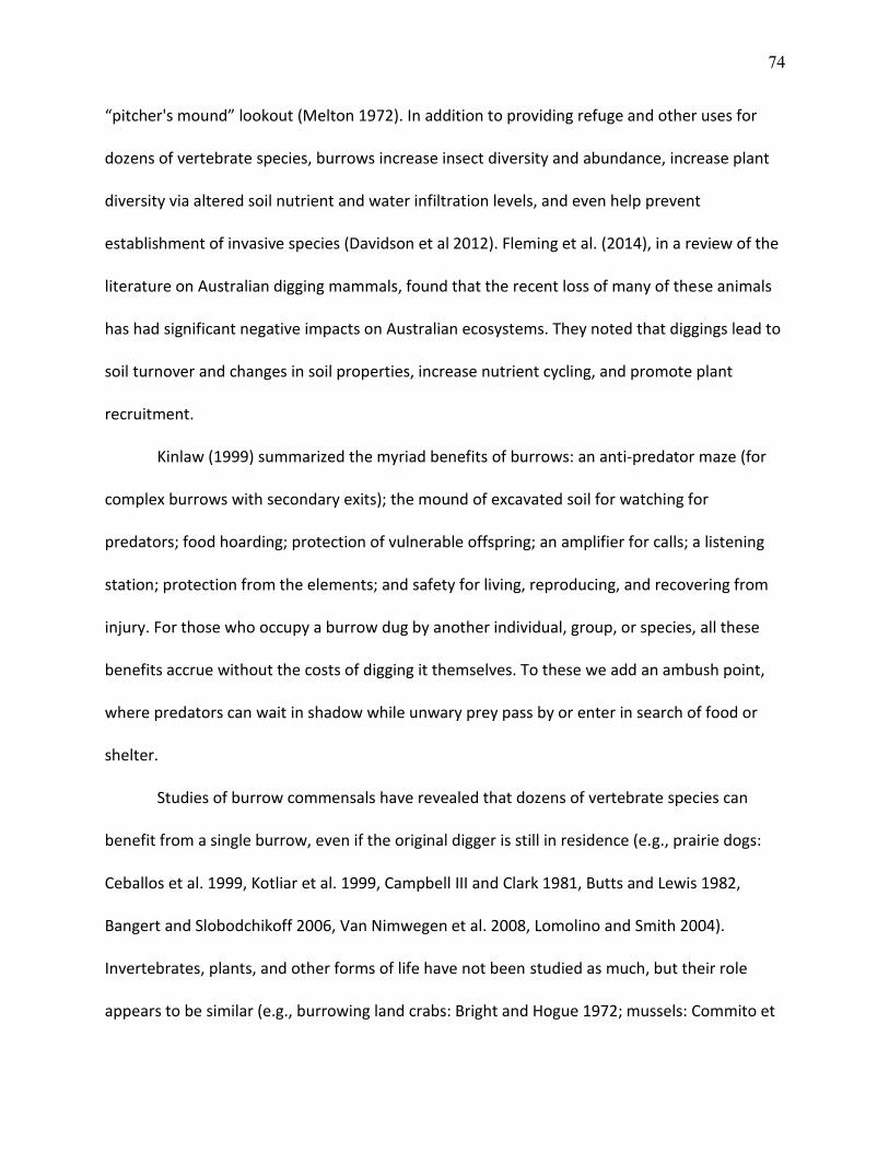
74

“pitcher's mound” lookout (Melton 1972). In addition to providing refuge and other uses for

dozens of vertebrate species, burrows increase insect diversity and abundance, increase plant

diversity via altered soil nutrient and water infiltration levels, and even help prevent

establishment of invasive species (Davidson et al 2012). Fleming et al. (2014), in a review of the

literature on Australian digging mammals, found that the recent loss of many of these animals

has had significant negative impacts on Australian ecosystems. They noted that diggings lead to

soil turnover and changes in soil properties, increase nutrient cycling, and promote plant

recruitment.

Kinlaw (1999) summarized the myriad benefits of burrows: an anti-predator maze (for

complex burrows with secondary exits); the mound of excavated soil for watching for

predators; food hoarding; protection of vulnerable offspring; an amplifier for calls; a listening

station; protection from the elements; and safety for living, reproducing, and recovering from

injury. For those who occupy a burrow dug by another individual, group, or species, all these

benefits accrue without the costs of digging it themselves. To these we add an ambush point,

where predators can wait in shadow while unwary prey pass by or enter in search of food or

shelter.

Studies of burrow commensals have revealed that dozens of vertebrate species can

benefit from a single burrow, even if the original digger is still in residence (e.g., prairie dogs:

Ceballos et al. 1999, Kotliar et al. 1999, Campbell III and Clark 1981, Butts and Lewis 1982,

Bangert and Slobodchikoff 2006, Van Nimwegen et al. 2008, Lomolino and Smith 2004).

Invertebrates, plants, and other forms of life have not been studied as much, but their role

appears to be similar (e.g., burrowing land crabs: Bright and Hogue 1972; mussels: Commito et

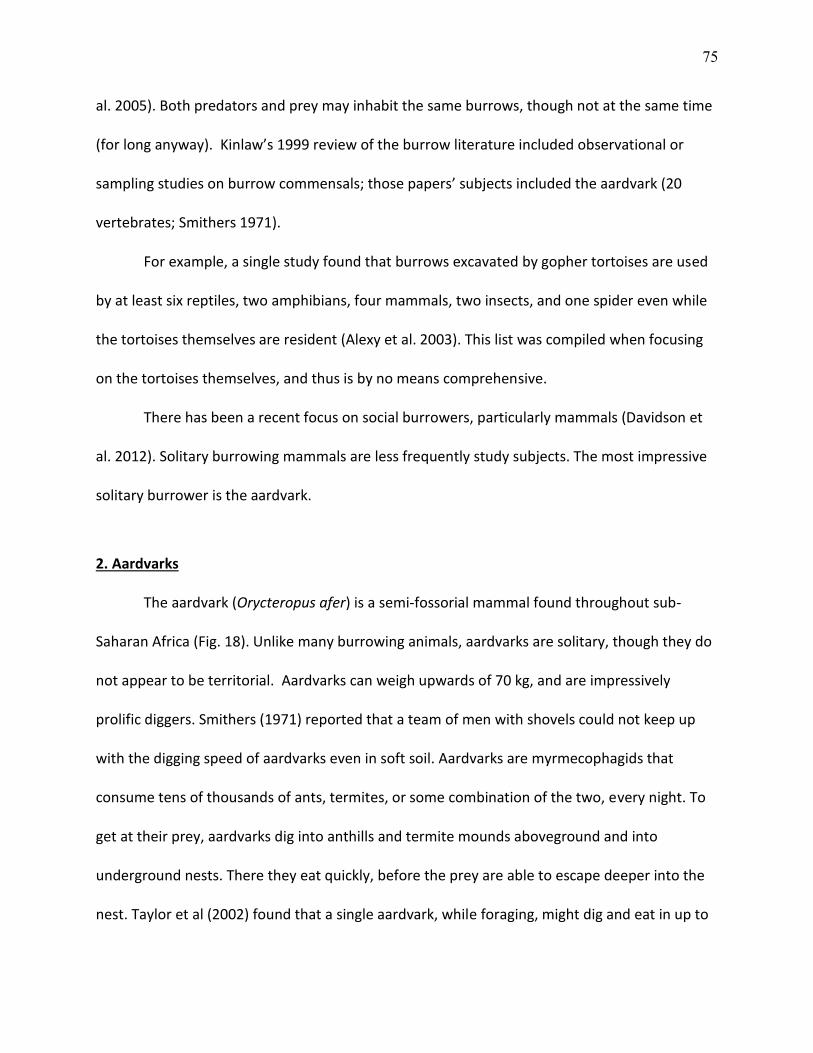
75

al. 2005). Both predators and prey may inhabit the same burrows, though not at the same time

(for long anyway). Kinlaw’s 1999 review of the burrow literature included observational or

sampling studies on burrow commensals; those papers’ subjects included the aardvark (20

vertebrates; Smithers 1971).

For example, a single study found that burrows excavated by gopher tortoises are used

by at least six reptiles, two amphibians, four mammals, two insects, and one spider even while

the tortoises themselves are resident (Alexy et al. 2003). This list was compiled when focusing

on the tortoises themselves, and thus is by no means comprehensive.

There has been a recent focus on social burrowers, particularly mammals (Davidson et

al. 2012). Solitary burrowing mammals are less frequently study subjects. The most impressive

solitary burrower is the aardvark.

2. Aardvarks

The aardvark (Orycteropus afer) is a semi-fossorial mammal found throughout sub-

Saharan Africa (Fig. 18). Unlike many burrowing animals, aardvarks are solitary, though they do

not appear to be territorial. Aardvarks can weigh upwards of 70 kg, and are impressively

prolific diggers. Smithers (1971) reported that a team of men with shovels could not keep up

with the digging speed of aardvarks even in soft soil. Aardvarks are myrmecophagids that

consume tens of thousands of ants, termites, or some combination of the two, every night. To

get at their prey, aardvarks dig into anthills and termite mounds aboveground and into

underground nests. There they eat quickly, before the prey are able to escape deeper into the

nest. Taylor et al (2002) found that a single aardvark, while foraging, might dig and eat in up to

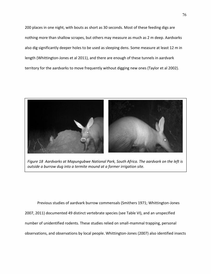
76

200 places in one night, with bouts as short as 30 seconds. Most of these feeding digs are

nothing more than shallow scrapes, but others may measure as much as 2 m deep. Aardvarks

also dig significantly deeper holes to be used as sleeping dens. Some measure at least 12 m in

length (Whittington-Jones et al 2011), and there are enough of these tunnels in aardvark

territory for the aardvarks to move frequently without digging new ones (Taylor et al 2002).

Previous studies of aardvark burrow commensals (Smithers 1971; Whittington-Jones

2007, 2011) documented 49 distinct vertebrate species (see Table VI), and an unspecified

number of unidentified rodents. These studies relied on small-mammal trapping, personal

observations, and observations by local people. Whittington-Jones (2007) also identified insects

Figure 18 Aardvarks at Mapungubwe National Park, South Africa. The aardvark on the left is outside a burrow dug into a termite mound at a former irrigation site.

77

from six orders, 30 families, and 50 morpho-species in a pitfall trap survey. He found that

aardvark burrows might increase overall plant diversity on a landscape scale, a finding

consistent with our observations in the field.

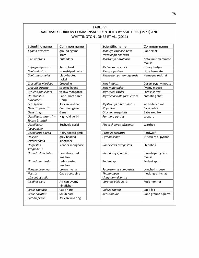
78

TABLE VI AARDVARK BURROW COMMENSALS IDENTIFIED BY SMITHERS (1971) AND

WHITTINGTON-JONES ET AL. (2011)

Scientific name Common name Scientific name Common name Agama aculeate ground agama

lizard Mabuya capensis now Trachylepis capensis

Cape skink

Bitis arietans puff adder Mastomys natalensis Natal mutimammate mouse

Bufo gariepensis Karoo toad Mellivora capensis Honey badger

Canis adustus side‐striped jackal Merops pusillus Little bee‐eater

Canis mesomelas black‐backed jackal

Michaelamys namaquensis Namaqua rock rat

Crocodilus niloticus Crocodile Mus indutus Desert pygmy mouse

Crocuta crocuta spotted hyena Mus minutoides Pygmy mouse

Cynictis panicillata yellow mongoose Myosorex varius Forest shrew

Desmodillus auricularis

Cape Short‐eared Gerbil

Myrmecocichla formicivora anteating chat

Felis lybica African wild cat Mystromys albicaudatus white‐tailed rat

Genetta genettta Common genet Naja nivea Cape cobra

Genetta sp. Genet Otocyon megalotis Bat‐eared fox

Gerbilliscus brantsii = Tatera brantsii

Highveld gerbil Panthera pardus Leopard

Gerbilliscus leucogaster

Bushveld gerbil Phacochoerus africanus Warthog

Gerbillurus paeba Hairy‐footed gerbil Proteles cristatus Aardwolf

Halcyon leucocephala

grey‐headed kingfisher

Python sebae African rock python

Herpestes sanguineus

slender mongoose Raphicerus campestris Steenbok

Hirundo dimidiate pearl‐breasted swallow

Rhabdomys pumilio four‐striped grass mouse

Hirundo semirufa red‐breasted swallow

Rodent spp. Rodent spp.

Hyaena brunnea brown hyena Saccostomus campestris pouched mouse

Hystrix africaeaustralis

Cape porcupine Thamnolaea cinnamomeiventris

mocking cliff‐chat

Ispidina picta African pygmy Kingfisher

Varanus albigularis Rock monitor

Lepus capensis Cape hare Vulpes chama Cape fox

Lepus saxatilis Scrub hare Xerus inauris Cape ground squirrel

Lycaon pictus African wild dog

79

These studies give us part of the picture, but can miss the larger, and potentially more

elusive, commensals. Furthermore, scattered stories do not provide information as to the

frequency with which various commensals will take advantage of these burrows.

Here we used camera traps to document the use or avoidance of aardvark burrows by

mid-sized and large animals, which is indirect evidence of aardvarks as ecosystem engineers—

namely, the extent to which other animals make use of aardvark-dug burrows. This too gives

only part of the overall picture, but when added to previous findings, we can get a general idea

of the importance of aardvark burrows in the community.

3. Camera Traps

Camera-trapping has given us the opportunity to remotely “observe” animals in the wild

for over a century (Carey 1926). In recent years, with advances in technology and decreases in

price, the popularity of camera-trapping has dramatically increased. This method has been

shown to be comparable to other census methods, only easier (Silveira et al. 2003, Yasuda

2004, Lyra-Jorge et al. 2008, Rowcliffe and Carbone 2008, Rowcliffe et al. 2008, Tobler et al.

2008, O'Connell et al. 2010). Camera-trap placement depends on the goal of the study, and

placement can affect population density estimates (Foster et al., 2012). Our camera placement,

as detailed below, was designed to capture animals both at aardvark burrows and in similar

small cleared areas. It cannot be assumed to represent actual animal density, only confirmation

of presence and relative activity.

80

4. Study goals

We sought to add to our knowledge of aardvarks as physical ecosystem engineers via

their extensive burrowing and the benefits these burrows provide. For the purposes of this

study, we defined a “burrow” as any aardvark-dug tunnel greater than 1 m in length. We used

camera-trapping to determine which species may be more likely to be in the vicinity of a

burrow for any reason, as well as those who may actively avoid them. We wanted to discern

the extent to which aardvark-dug holes and burrows (hereafter “burrows”) are an ecosystem

service for other animals. How extensively are these burrows used? What proportion of

burrows is in use at any given time? Can we determine from still photos how these burrows are

being used? Is it aardvarks that are primarily using their own burrows, or are they more likely to

be used by others? Which species derive benefit, directly or indirectly, from these burrows?

Which species avoid them?

Our predictions were of a general nature. Burrows should be used frequently, by

aardvarks and other species. Other species should include known burrow-dwellers such as

warthogs and porcupines. Partially collapsed or filled-in burrows no longer suitable for such

large animals may be home to smaller species such as springhares.

These burrows may provide dens or an escape from predators (“bolt holes”). If dens, we

would see the same animals repeatedly over several days, weeks, or longer. If bolt holes, we

would see only short visits. Our camera settings did not allow for detailed assessment of

whether an animal entered the burrow and left shortly afterward, nor if they were being

chased. Still pictures may give us some idea of how burrows are used, but this method is

81

limited. Not all use will be captured in a single photograph, as events may happen while the

camera is latent and resetting.

If aardvarks use the burrows they dug more than other species do, then such burrows

are less of an ecosystem service than it might otherwise seem, and function primarily as

aardvark feeding holes or dens. If we see more use by other species, then these burrows are

clearly performing a role in the community.

Known burrowing mammals such as warthogs and porcupines may favor aardvark

burrows for their size and ease of use. If these species avoid burrows, it may be that the

burrows are already occupied, or potentially occupied, by predators such as caracals, servals,

pythons, or hyenas. Non-burrow-dwellers may also use the burrows in search of food (e.g.,

insects or seeds in the disturbed soil) or escape (bolt holes). Predators may use them for cover

when ambushing prey. The soil mound that is a byproduct of burrow-digging may be favored by

some species as a vantage point (the pitcher’s mound effect). The plant species on aardvark

burrows and the associated soil mound may differ from those in the surrounding landscape

(Whittington-Jones 2007, pers. obs.), and thus may attract different herbivores. Antelope

species, giraffes, and elephants may avoid burrows if they are potential sources of injury or

loose footing (Kotler 2001, Abu Baker and Brown 2012). Avoidance of burrows would be shown

indirectly by a significantly higher number of photographs at sites other than at burrows.

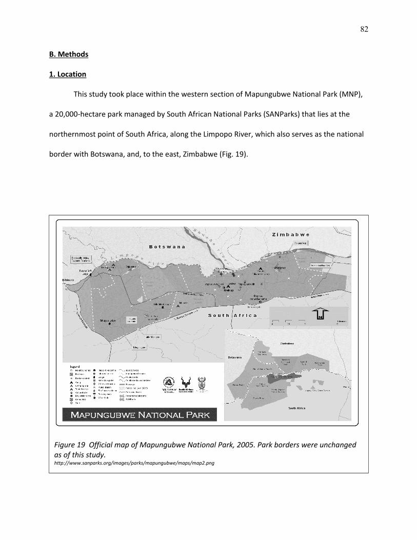
82

B. Methods

1. Location

This study took place within the western section of Mapungubwe National Park (MNP),

a 20,000-hectare park managed by South African National Parks (SANParks) that lies at the

northernmost point of South Africa, along the Limpopo River, which also serves as the national

border with Botswana, and, to the east, Zimbabwe (Fig. 19).

Figure 19 Official map of Mapungubwe National Park, 2005. Park borders were unchanged as of this study. http://www.sanparks.org/images/parks/mapungubwe/maps/map2.png

83

MNP was created beginning in 1999 and opened to the public in 2004, combining

former farmlands either long abandoned or recently in use with wild areas. At the time of this

study, working agricultural farms, growing primarily citrus or tomatoes, both abutted and

divided the park. Neighboring private reserves in South Africa and Botswana and public land in

Zimbabwe joined MNP as the Mapungubwe Transfrontier Conservation Area (TCFA). While part

of the northern border is lined with high, multi-layered fences, other areas have only a single

electrified wire elephant fence, a small barbed-wire fence, or no fence at all. Animals can move

freely between MNP and adjoining land in the rest of the TCFA. This is a rapidly changing area

and TFCA borders have been expanded since this study. This means that more animals now

have access to burrows, and our findings may underestimate current burrow use.

MNP, despite its small size, has several different habitats. We used primarily former

agricultural fields, a small portion of which were the site of experimental forest restoration, and

riverine forest. The forest is not pristine, but has been allowed to return to its wild state for

long enough that it is effectively so. In 2009, powerful electric fences were installed around

much of the riverine forest in an attempt to exclude elephants and thus preserve the forest.

These fences are just a few wires approximately one meter above the ground, so nearly all

other animals can easily go under or over them. These fences are effective in limiting elephant

movement, though elephants do break through on occasion. MNP also contains large areas of

mopane forest, which proved to have nearly no aardvark activity. Hence, the mopane habitat

represents only a small part of this study. The numerous rocky outcrops were not explored.

SANParks performs periodic aerial surveys by helicopter. The 2006 census counted 114

elephants, 903 impala, 340 blue wildebeest, 271 eland, 228 Burchell’s zebra, 88 greater kudu,

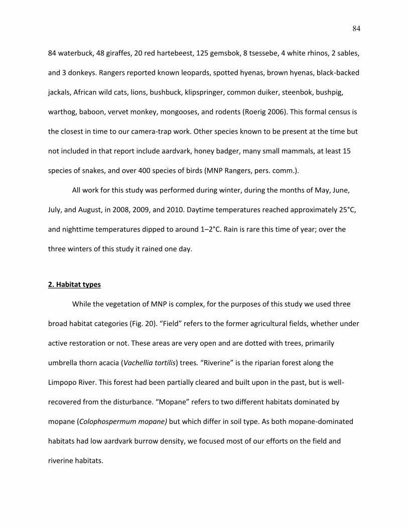
84

84 waterbuck, 48 giraffes, 20 red hartebeest, 125 gemsbok, 8 tsessebe, 4 white rhinos, 2 sables,

and 3 donkeys. Rangers reported known leopards, spotted hyenas, brown hyenas, black-backed

jackals, African wild cats, lions, bushbuck, klipspringer, common duiker, steenbok, bushpig,

warthog, baboon, vervet monkey, mongooses, and rodents (Roerig 2006). This formal census is

the closest in time to our camera-trap work. Other species known to be present at the time but

not included in that report include aardvark, honey badger, many small mammals, at least 15

species of snakes, and over 400 species of birds (MNP Rangers, pers. comm.).

All work for this study was performed during winter, during the months of May, June,

July, and August, in 2008, 2009, and 2010. Daytime temperatures reached approximately 25°C,

and nighttime temperatures dipped to around 1–2°C. Rain is rare this time of year; over the

three winters of this study it rained one day.

2. Habitat types

While the vegetation of MNP is complex, for the purposes of this study we used three

broad habitat categories (Fig. 20). “Field” refers to the former agricultural fields, whether under

active restoration or not. These areas are very open and are dotted with trees, primarily

umbrella thorn acacia (Vachellia tortilis) trees. “Riverine” is the riparian forest along the

Limpopo River. This forest had been partially cleared and built upon in the past, but is well-

recovered from the disturbance. “Mopane” refers to two different habitats dominated by

mopane (Colophospermum mopane) but which differ in soil type. As both mopane-dominated

habitats had low aardvark burrow density, we focused most of our efforts on the field and

riverine habitats.

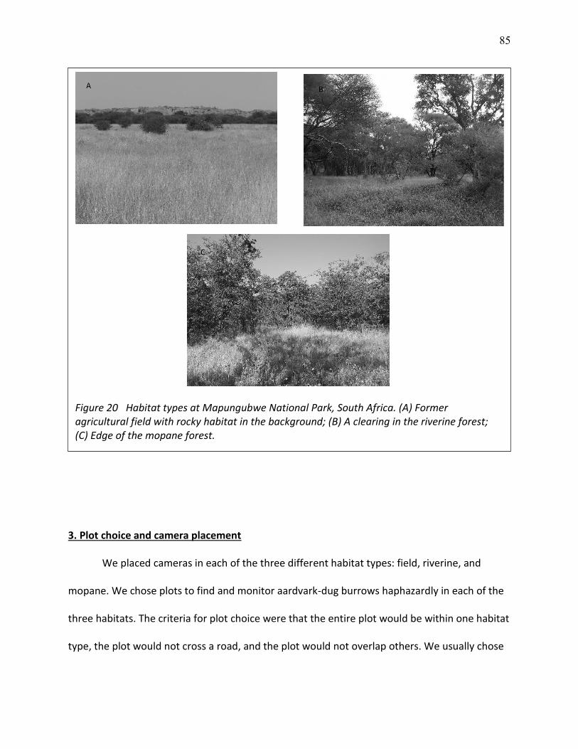
85

3. Plot choice and camera placement

We placed cameras in each of the three different habitat types: field, riverine, and

mopane. We chose plots to find and monitor aardvark-dug burrows haphazardly in each of the

three habitats. The criteria for plot choice were that the entire plot would be within one habitat

type, the plot would not cross a road, and the plot would not overlap others. We usually chose

Figure 20 Habitat types at Mapungubwe National Park, South Africa. (A) Former agricultural field with rocky habitat in the background; (B) A clearing in the riverine forest; (C) Edge of the mopane forest.

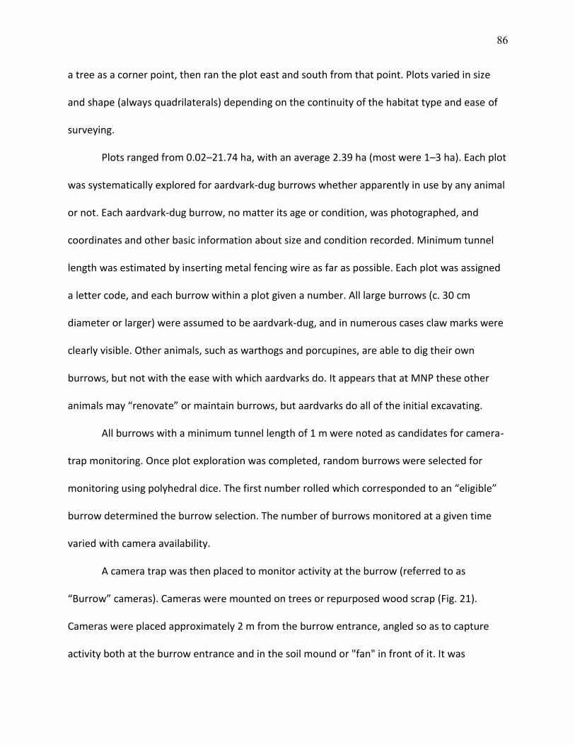
86

a tree as a corner point, then ran the plot east and south from that point. Plots varied in size

and shape (always quadrilaterals) depending on the continuity of the habitat type and ease of

surveying.

Plots ranged from 0.02–21.74 ha, with an average 2.39 ha (most were 1–3 ha). Each plot

was systematically explored for aardvark-dug burrows whether apparently in use by any animal

or not. Each aardvark-dug burrow, no matter its age or condition, was photographed, and

coordinates and other basic information about size and condition recorded. Minimum tunnel

length was estimated by inserting metal fencing wire as far as possible. Each plot was assigned

a letter code, and each burrow within a plot given a number. All large burrows (c. 30 cm

diameter or larger) were assumed to be aardvark-dug, and in numerous cases claw marks were

clearly visible. Other animals, such as warthogs and porcupines, are able to dig their own

burrows, but not with the ease with which aardvarks do. It appears that at MNP these other

animals may “renovate” or maintain burrows, but aardvarks do all of the initial excavating.

All burrows with a minimum tunnel length of 1 m were noted as candidates for camera-

trap monitoring. Once plot exploration was completed, random burrows were selected for

monitoring using polyhedral dice. The first number rolled which corresponded to an “eligible”

burrow determined the burrow selection. The number of burrows monitored at a given time

varied with camera availability.

A camera trap was then placed to monitor activity at the burrow (referred to as

“Burrow” cameras). Cameras were mounted on trees or repurposed wood scrap (Fig. 21).

Cameras were placed approximately 2 m from the burrow entrance, angled so as to capture

activity both at the burrow entrance and in the soil mound or "fan" in front of it. It was

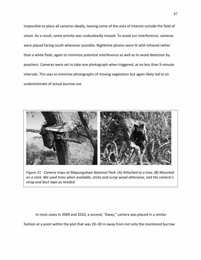
87

impossible to place all cameras ideally, leaving some of the area of interest outside the field of

vision. As a result, some activity was undoubtedly missed. To avoid sun interference, cameras

were placed facing south whenever possible. Nighttime photos were lit with infrared rather

than a white flash, again to minimize potential interference as well as to avoid detection by

poachers. Cameras were set to take one photograph when triggered, at no less than 5-minute

intervals. This was to minimize photographs of moving vegetation but again likely led to an

underestimate of actual burrow use.

In most cases in 2009 and 2010, a second, “Away,” camera was placed in a similar

fashion at a point within the plot that was 20–30 m away from not only the monitored burrow

Figure 21 Camera traps at Mapungubwe National Park. (A) Attached to a tree; (B) Mounted on a stick. We used trees when available, sticks and scrap wood otherwise, and the camera’s strap and duct tape as needed.

88

but any other burrow. Natural clearings or areas with little vegetation were chosen when

possible to emulate the lack of vegetation immediately around a burrow entrance and to

minimize the number of photographs triggered by swaying plants. When camera availability did

not allow for paired Burrow and Away cameras, we only monitored the burrow.

We cleared grasses and small branches from the area immediately in front of the

camera only as needed to get clear photographs. Cameras were not baited to attract animals,

but set to record the animals as they went about their usual activities.

Cameras remained in place for 3–76 days (average 12, mode 7). One burrow in the field,

known as C1, was monitored for a total of 219 days over the three field seasons, with its Away

point monitored 127 days (the discrepancy is due to not monitoring Away points in 2008 and

ants disabling the camera in 2010). In 2009 we added a long-term monitored burrow in the

riverine forest (97 days, 61 Away), but that burrow collapsed between seasons. A second

burrow in the same plot was chosen for long-term monitoring in 2010, but equipment shortage

meant it was only monitored 22 days and 22 nights, less than some other burrows.

We monitored a total of 85 burrows: 17 burrows in the mopane, 42 in the field, and 26

in the riverine. Away sites numbered 48: 6 mopane, 21 field, and 21 riverine. We gathered

information over a total of 2050 camera-days and 2025 camera-nights. The number of days and

nights are unequal due to camera malfunction or destruction. We ended up with a total of 3855

pictures with animals present.

Animals were identified to species, except for birds who were grouped to Family or

Order (ex: doves) and small rodents, which were only identified as small rodents. Sometimes an

animal could not be clearly identified. These subjects were classified simply as “antelope,”

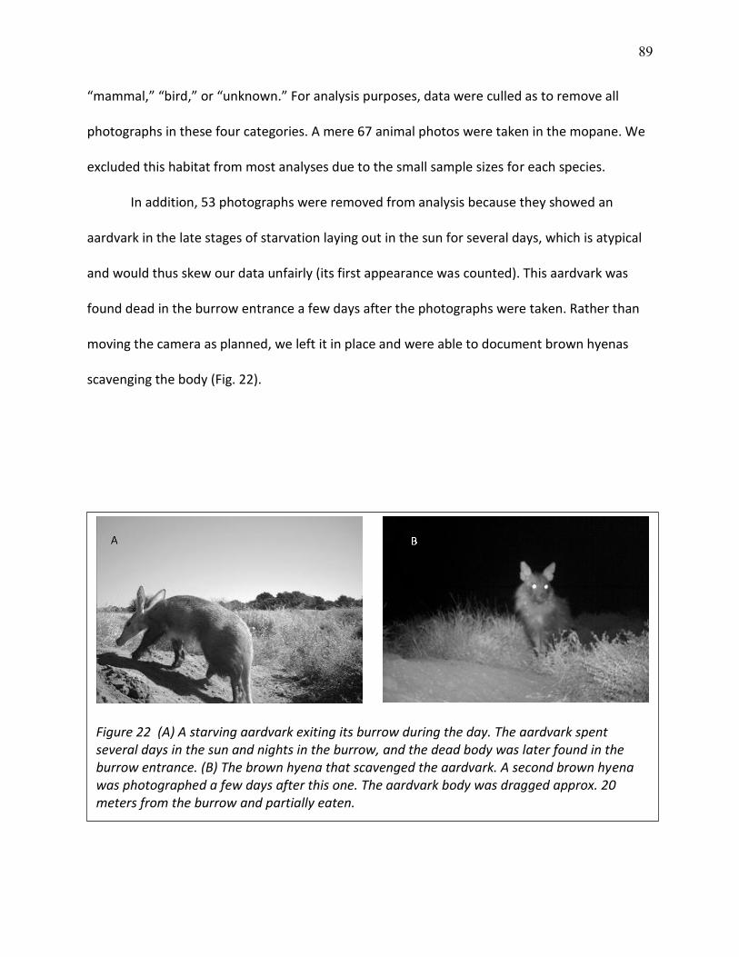
89

“mammal,” “bird,” or “unknown.” For analysis purposes, data were culled as to remove all

photographs in these four categories. A mere 67 animal photos were taken in the mopane. We

excluded this habitat from most analyses due to the small sample sizes for each species.

In addition, 53 photographs were removed from analysis because they showed an

aardvark in the late stages of starvation laying out in the sun for several days, which is atypical

and would thus skew our data unfairly (its first appearance was counted). This aardvark was

found dead in the burrow entrance a few days after the photographs were taken. Rather than

moving the camera as planned, we left it in place and were able to document brown hyenas

scavenging the body (Fig. 22).

Figure 22 (A) A starving aardvark exiting its burrow during the day. The aardvark spent several days in the sun and nights in the burrow, and the dead body was later found in the burrow entrance. (B) The brown hyena that scavenged the aardvark. A second brown hyena was photographed a few days after this one. The aardvark body was dragged approx. 20 meters from the burrow and partially eaten.

90

Because of unequal sampling effort, we normalized all counts to the number of

photographs per 100 camera-days. A camera-day is a unique combination of camera, date, and

either day or night designation. Some species may appear several times in a single location on a

single day, and therefore were counted multiple times. This reflects usage of the area. These

numbers give a general picture of what is going on, but are too biased for certain statistical

analyses.

To get at the question of how often a particular habitat, time of day, or burrow

proximity was chosen, we counted the number of camera-days on which a species was

photographed, regardless of the number of photographs of that species on that camera-day.

We called this unique combination of camera, day, and species an “appearance.“ This

eliminates the above bias of lingering.

For pairwise comparisons between habitats and Burrow–Away, all 3504 remaining

photographs were used. Eighty-seven photographs were taken at either dawn (34) or dusk (53)

and were therefore not included in day vs. night comparisons.

In our classification, there were 8 unique combinations of habitat, time of day, and

burrow proximity. Our sample sizes were not large enough to permit full detailed analysis of

these preferences and the interactions among them. We performed pairwise chi square

goodness-of-fit tests to test for preference of location and time when the number of camera-

day appearances would be expected to be at least 10 in each pair, (5 in each cell assuming

equal camera-trapping effort but here calculated to reflect actual trapping effort). Each species

could have a preference for habitat, time of day, and burrow proximity. Except for testing day

against night, both day and night appearances were counted; factors were pooled as above. For

91

those species with 10–19 appearances, we tested burrow vs away; those with 20–39

appearances were tested for burrow vs away and day vs night; those with 40 or more

appearances were tested for all three factors (burrow vs away, day vs night, and field vs

riverine). Expected values for the chi-square tests were calculated based on the proportion of

available camera-days and -nights and the total number of pictures.

We also noted whether these species were photographed definitely or apparently

“using” the burrow in some fashion, such as entering or exiting, foraging in the soil fan, or using

the mounded soil as a lookout.

C. Results

Only 71% of cameras located at burrows, in the mopane recorded any animal pictures,

at an average rate of 12.5 pictures/100 camera-days+nights. Only 4 of the six (67%) Away

cameras in the mopane had any animal pictures. By contrast, at least 90% of all other camera

locations obtained at least one animal picture. Field burrows had an overall average of 50.8

pictures/100 camera-days+nights, and riverine burrows saw 187.5 pictures/100 camera-

days+nights. In all habitats, fewer pictures were taken at the burrows than Away (Table VII).

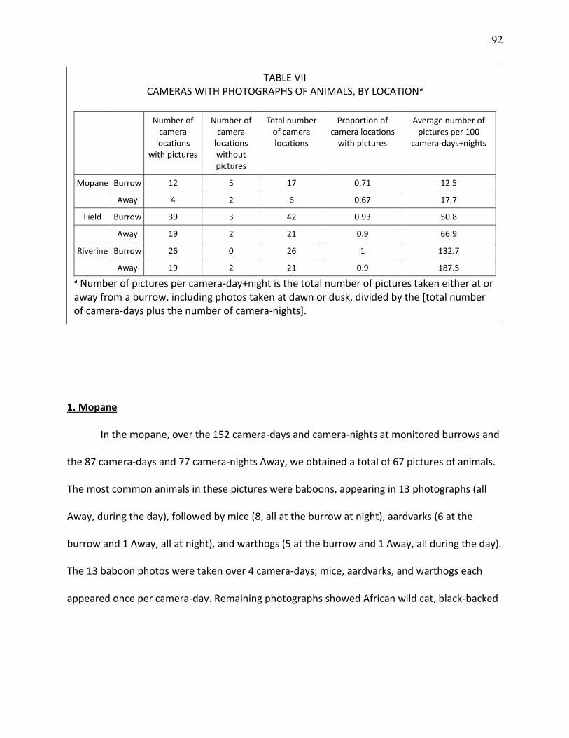
92

1. Mopane

In the mopane, over the 152 camera-days and camera-nights at monitored burrows and

the 87 camera-days and 77 camera-nights Away, we obtained a total of 67 pictures of animals.

The most common animals in these pictures were baboons, appearing in 13 photographs (all

Away, during the day), followed by mice (8, all at the burrow at night), aardvarks (6 at the

burrow and 1 Away, all at night), and warthogs (5 at the burrow and 1 Away, all during the day).

The 13 baboon photos were taken over 4 camera-days; mice, aardvarks, and warthogs each

appeared once per camera-day. Remaining photographs showed African wild cat, black-backed

TABLE VII CAMERAS WITH PHOTOGRAPHS OF ANIMALS, BY LOCATIONa

Number of camera

locations with pictures

Number of camera

locations without pictures

Total number of camera locations

Proportion of camera locations

with pictures

Average number of pictures per 100

camera‐days+nights

Mopane Burrow 12 5 17 0.71 12.5

Away 4 2 6 0.67 17.7

Field Burrow 39 3 42 0.93 50.8

Away 19 2 21 0.9 66.9

Riverine Burrow 26 0 26 1 132.7

Away 19 2 21 0.9 187.5

a Number of pictures per camera-day+night is the total number of pictures taken either at or away from a burrow, including photos taken at dawn or dusk, divided by the [total number of camera-days plus the number of camera-nights].

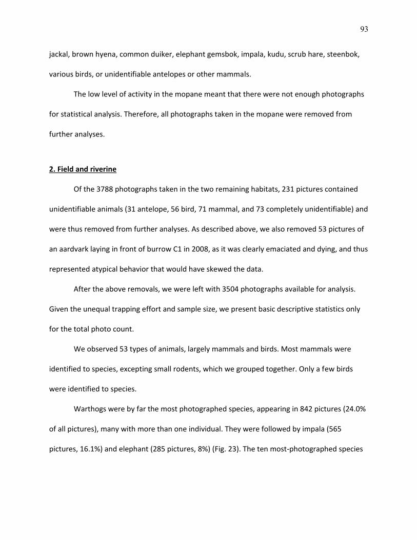
93

jackal, brown hyena, common duiker, elephant gemsbok, impala, kudu, scrub hare, steenbok,

various birds, or unidentifiable antelopes or other mammals.

The low level of activity in the mopane meant that there were not enough photographs

for statistical analysis. Therefore, all photographs taken in the mopane were removed from

further analyses.

2. Field and riverine

Of the 3788 photographs taken in the two remaining habitats, 231 pictures contained

unidentifiable animals (31 antelope, 56 bird, 71 mammal, and 73 completely unidentifiable) and

were thus removed from further analyses. As described above, we also removed 53 pictures of

an aardvark laying in front of burrow C1 in 2008, as it was clearly emaciated and dying, and thus

represented atypical behavior that would have skewed the data.

After the above removals, we were left with 3504 photographs available for analysis.

Given the unequal trapping effort and sample size, we present basic descriptive statistics only

for the total photo count.

We observed 53 types of animals, largely mammals and birds. Most mammals were

identified to species, excepting small rodents, which we grouped together. Only a few birds

were identified to species.

Warthogs were by far the most photographed species, appearing in 842 pictures (24.0%

of all pictures), many with more than one individual. They were followed by impala (565

pictures, 16.1%) and elephant (285 pictures, 8%) (Fig. 23). The ten most-photographed species

94

(warthog, impala, elephant, bushbuck, waterbuck, kudu, steenbok, porcupine, francolin, and

baboon) accounted for 75.0% of all photographs (Fig. 24).

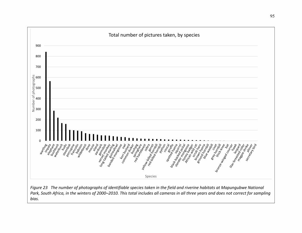
95

Figure 23 The number of photographs of identifiable species taken in the field and riverine habitats at Mapungubwe National Park, South Africa, in the winters of 2000–2010. This total includes all cameras in all three years and does not correct for sampling bias.

0

100

200

300

400

500

600

700

800

900

Nu

mb

er o

f p

ho

togr

aph

s

Species

Total number of pictures taken, by species

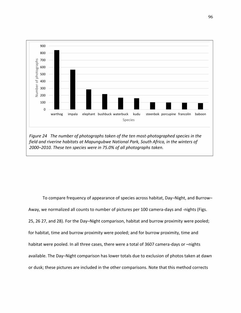
96

To compare frequency of appearance of species across habitat, Day–Night, and Burrow–

Away, we normalized all counts to number of pictures per 100 camera-days and -nights (Figs.

25, 26 27, and 28). For the Day–Night comparison, habitat and burrow proximity were pooled;

for habitat, time and burrow proximity were pooled; and for burrow proximity, time and

habitat were pooled. In all three cases, there were a total of 3607 camera-days or –nights

available. The Day–Night comparison has lower totals due to exclusion of photos taken at dawn

or dusk; these pictures are included in the other comparisons. Note that this method corrects

Figure 24 The number of photographs taken of the ten most-photographed species in the field and riverine habitats at Mapungubwe National Park, South Africa, in the winters of 2000–2010. These ten species were in 75.0% of all photographs taken.

0

100

200

300

400

500

600

700

800

900

warthog impala elephant bushbuck waterbuck kudu steenbok porcupine francolin baboon

Nu

mb

er o

f p

ho

togr

aph

s

Species

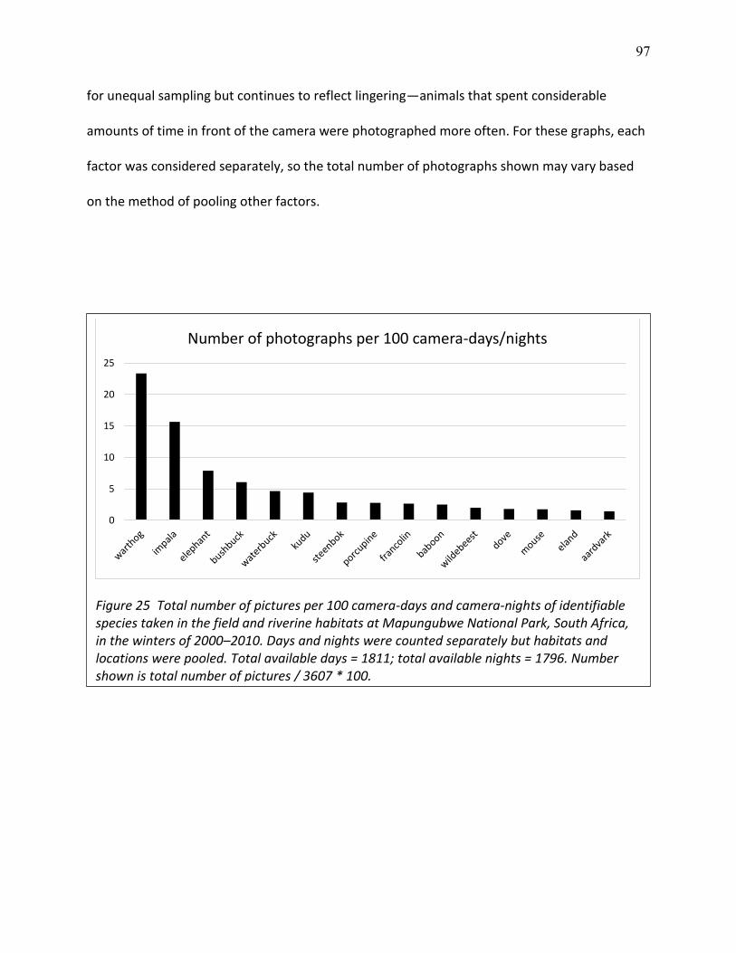
97

for unequal sampling but continues to reflect lingering—animals that spent considerable

amounts of time in front of the camera were photographed more often. For these graphs, each

factor was considered separately, so the total number of photographs shown may vary based

on the method of pooling other factors.

Figure 25 Total number of pictures per 100 camera-days and camera-nights of identifiable species taken in the field and riverine habitats at Mapungubwe National Park, South Africa, in the winters of 2000–2010. Days and nights were counted separately but habitats and locations were pooled. Total available days = 1811; total available nights = 1796. Number shown is total number of pictures / 3607 * 100.

0

5

10

15

20

25

Number of photographs per 100 camera-days/nights

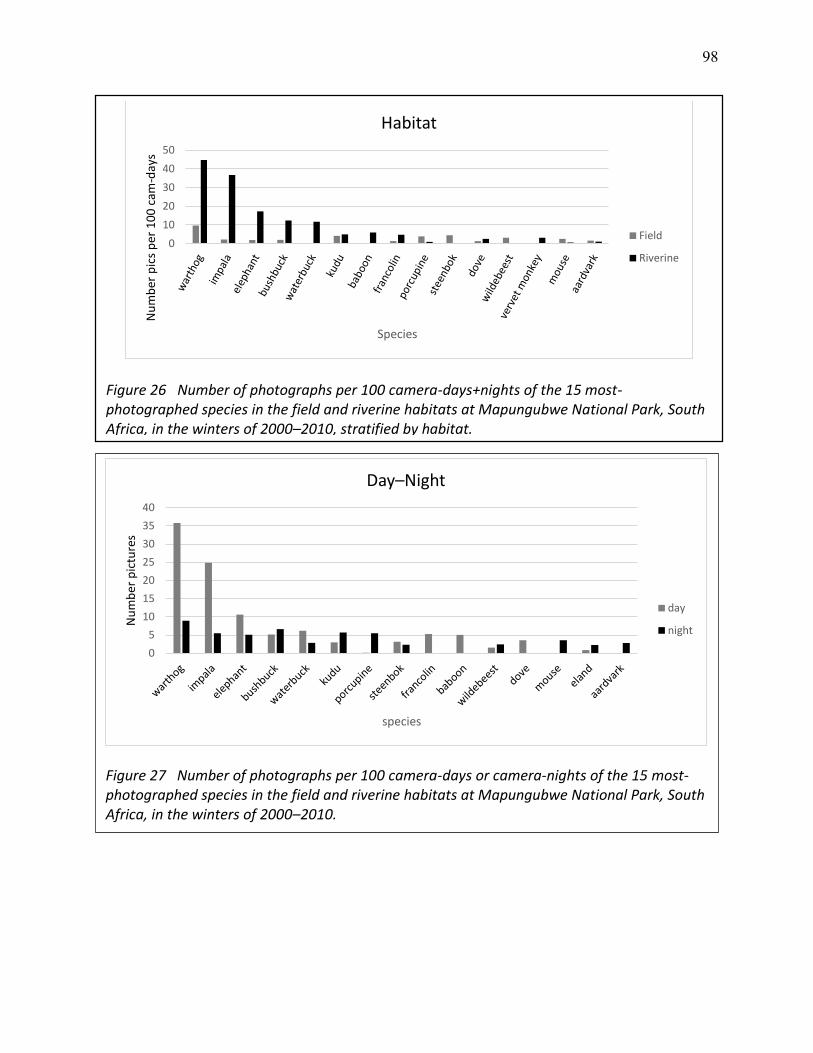
98

Figure 26 Number of photographs per 100 camera-days+nights of the 15 most-photographed species in the field and riverine habitats at Mapungubwe National Park, South Africa, in the winters of 2000–2010, stratified by habitat.

0

10

20

30

40

50N

um

ber

pic

s p

er 1

00

cam

-day

s

Species

Habitat

Field

Riverine

Figure 27 Number of photographs per 100 camera-days or camera-nights of the 15 most-photographed species in the field and riverine habitats at Mapungubwe National Park, South Africa, in the winters of 2000–2010.

0

5

10

15

20

25

30

35

40

Nu

mb

er p

ictu

res

species

Day–Night

day

night

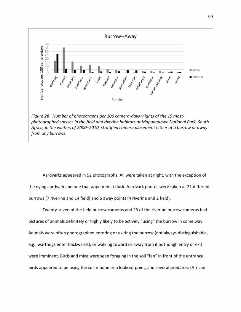
99

Aardvarks appeared in 52 photographs. All were taken at night, with the exception of

the dying aardvark and one that appeared at dusk. Aardvark photos were taken at 21 different

burrows (7 riverine and 14 field) and 6 away points (4 riverine and 2 field).

Twenty-seven of the field burrow cameras and 23 of the riverine burrow cameras had

pictures of animals definitely or highly likely to be actively “using” the burrow in some way.

Animals were often photographed entering or exiting the burrow (not always distinguishable,

e.g., warthogs enter backwards), or walking toward or away from it as though entry or exit

were imminent. Birds and mice were seen foraging in the soil “fan” in front of the entrance,

birds appeared to be using the soil mound as a lookout point, and several predators (African

Figure 28 Number of photographs per 100 camera-days+nights of the 15 most-photographed species in the field and riverine habitats at Mapungubwe National Park, South Africa, in the winters of 2000–2010, stratified camera placement either at a burrow or away from any burrows.

05

10152025303540

nu

mb

er p

ics

per

10

0 c

amer

a-d

ays

Species

Burrow--Away

away

burrow

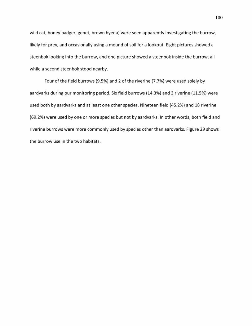
100

wild cat, honey badger, genet, brown hyena) were seen apparently investigating the burrow,

likely for prey, and occasionally using a mound of soil for a lookout. Eight pictures showed a

steenbok looking into the burrow, and one picture showed a steenbok inside the burrow, all

while a second steenbok stood nearby.

Four of the field burrows (9.5%) and 2 of the riverine (7.7%) were used solely by

aardvarks during our monitoring period. Six field burrows (14.3%) and 3 riverine (11.5%) were

used both by aardvarks and at least one other species. Nineteen field (45.2%) and 18 riverine

(69.2%) were used by one or more species but not by aardvarks. In other words, both field and

riverine burrows were more commonly used by species other than aardvarks. Figure 29 shows

the burrow use in the two habitats.

101

Figure 30 shows the total number of appearances (unique combination of species,

location, and day or night). As with total photographs, warthogs made the most appearances,

followed by bushbuck and impala.

Figure 29 Species using aardvark burrows. Numbers are the number of burrows used by that category (aardvark, non-aardvark, both, or neither) with percentages. The size of each circle reflects the unequal sample sizes but are not to scale. Total n for field = 42; n for riverine = 26.

1331.0%

49.5%

614.3%

1945.2%

Field

Not used Aardvark only Aardvark and other species Non-aardvark only

311%

28%

312%18

69%

Riverine

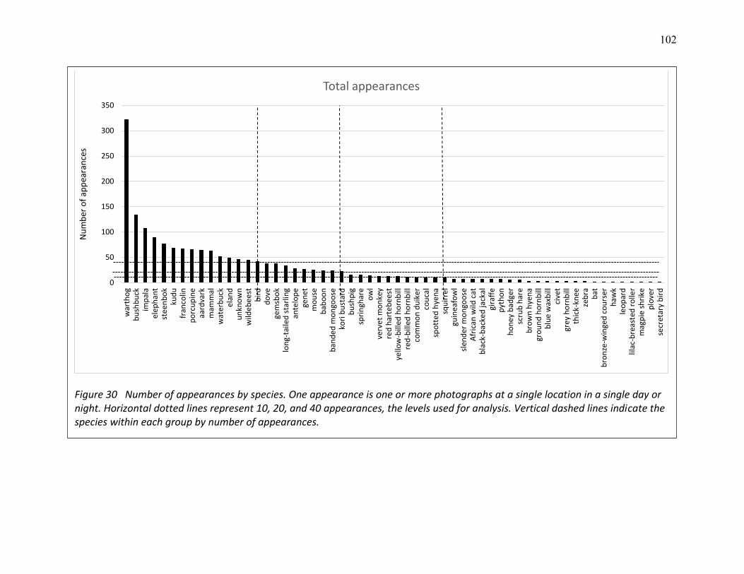
102

Figure 30 Number of appearances by species. One appearance is one or more photographs at a single location in a single day or night. Horizontal dotted lines represent 10, 20, and 40 appearances, the levels used for analysis. Vertical dashed lines indicate the species within each group by number of appearances.

0

50

100

150

200

250

300

350

war

tho

gb

ush

bu

ckim

pal

ael

eph

ant

ste

enb

ok

kud

ufr

anco

linp

orc

up

ine

aard

vark

mam

mal

wat

erb

uck

elan

du

nkn

ow

nw

ilde

be

est

bir

dd

ove

gem

sbo

klo

ng-

taile

d s

tarl

ing

ante

lop

ege

net

mo

use

bab

oo

nb

and

ed

mo

ngo

ose

kori

bu

star

db

ush

pig

spri

ngh

are

ow

lve

rve

t m

on

key

red

har

teb

ees

tye

llow

-bill

ed h

orn

bill

red

-bill

ed h

orn

bill

com

mo

n d

uik

erco

uca

lsp

ott

ed h

yen

asq

uir

rel

guin

eaf

ow

lsl

end

er m

on

goo

seA

fric

an w

ild c

atb

lack

-bac

ked

jack

algi

raff

ep

yth

on

ho

ne

y b

adge

rsc

rub

har

eb

row

n h

yen

agr

ou

nd

ho

rnb

illb

lue

wax

bill

cive

tgr

ey

ho

rnb

illth

ick-

knee

zeb

rab

atb

ron

ze-w

inge

d c

ou

rser

haw

kle

op

ard

lilac

-bre

aste

d r

olle

rm

agp

ie s

hri

kep

love

rse

cret

ary

bir

d

Nu

mb

er o

f ap

pea

ran

ces

Total appearances

103

Table VIII summarizes the results of our chi-square heterogeneity tests. None of the

daytime preferences is particularly surprising save for the confirmation that impala seem to

favor daytime over nighttime activity. Species that showed a significant nocturnal bias included

aardvark, eland, gemsbok, kudu, small rodents, African grass owl, and porcupine Large

antelopes such as eland, gemsbok and kudu favored the night. Bushbuck, elephant, steenbok,

and wildebeest were active both day and night.

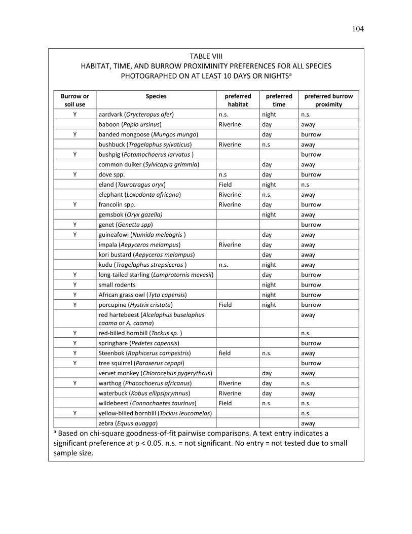
104

TABLE VIII HABITAT, TIME, AND BURROW PROXIMINITY PREFERENCES FOR ALL SPECIES

PHOTOGRAPHED ON AT LEAST 10 DAYS OR NIGHTSa

Burrow or soil use

Species preferred habitat

preferred time

preferred burrow proximity

Y aardvark (Orycteropus afer) n.s. night n.s.

baboon (Papio ursinus) Riverine day away

Y banded mongoose (Mungos mungo) day burrow

bushbuck (Tragelaphus sylvaticus) Riverine n.s away

Y bushpig (Potamochoerus larvatus ) burrow

common duiker (Sylvicapra grimmia) day away

Y dove spp. n.s day burrow

eland (Taurotragus oryx) Field night n.s

elephant (Loxodonta africana) Riverine n.s. away

Y francolin spp. Riverine day burrow

gemsbok (Oryx gazella) night away

Y genet (Genetta spp) burrow

Y guineafowl (Numida meleagris ) day away

impala (Aepyceros melampus) Riverine day away

kori bustard (Aepyceros melampus) day away

kudu (Tragelaphus strepsiceros ) n.s. night away

Y long‐tailed starling (Lamprotornis mevesii) day burrow

Y small rodents night burrow

Y African grass owl (Tyto capensis) night burrow

Y porcupine (Hystrix cristata) Field night burrow

red hartebeest (Alcelaphus buselaphus caama or A. caama)

away

Y red‐billed hornbill (Tockus sp. ) n.s.

Y springhare (Pedetes capensis) burrow

Y Steenbok (Raphicerus campestris) field n.s. away

Y tree squirrel (Paraxerus cepapi) burrow

vervet monkey (Chlorocebus pygerythrus) day away

Y warthog (Phacochoerus africanus) Riverine day n.s.

waterbuck (Kobus ellipsiprymnus) Riverine day away

wildebeest (Connochaetes taurinus) Field n.s. n.s.

Y yellow‐billed hornbill (Tockus leucomelas) n.s.

zebra (Equus quagga) away a Based on chi-square goodness-of-fit pairwise comparisons. A text entry indicates a significant preference at p < 0.05. n.s. = not significant. No entry = not tested due to small sample size.

105

Species that showed a significant preference for the field were eland, porcupine,

steenbok, and wildebeest. Species that showed a significant preference for the relatively dense

riverine were baboon, bushbuck, elephant (despite being largely excluded from the riverine in

2009), francolin, impala, warthog, and waterbuck. Aardvark, doves, and kudu showed no

significant habitat preference.

Of the species included in these tests, aardvark, banded mongoose, bushpig, doves,

francolin, genet, guineafowl, long-tailed starling, small rodents, African grass owl, porcupine,

red-billed hornbill, springhare, steenbok, tree squirrel, warthog, and yellow-billed hornbill were

photographed apparently or definitely “using” the burrow or its soil fan in some way (Fig. 31).

These uses included entering or exiting the burrow, foraging in the soil fan, or using a mound of

soil as a lookout. Other species photographed using burrows were African wild cat, brown

hyena, honey badger, rock python (the only reptile photographed), slender mongoose, and

spotted hyena. In all, 23 types of animals were photographed making use of the burrow or its

soil.

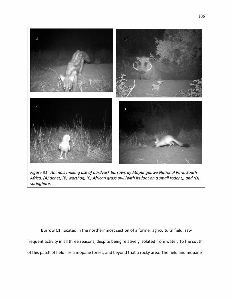
106

Burrow C1, located in the northernmost section of a former agricultural field, saw

frequent activity in all three seasons, despite being relatively isolated from water. To the south

of this patch of field lies a mopane forest, and beyond that a rocky area. The field and mopane

Figure 31 Animals making use of aardvark burrows ay Mapungubwe National Park, South Africa. (A) genet, (B) warthog, (C) African grass owl (with its foot on a small rodent), and (D) springhare.

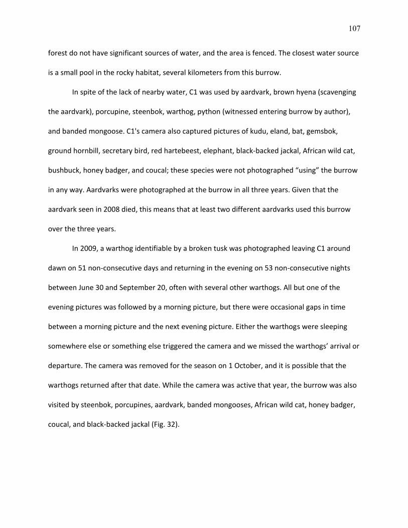
107

forest do not have significant sources of water, and the area is fenced. The closest water source

is a small pool in the rocky habitat, several kilometers from this burrow.

In spite of the lack of nearby water, C1 was used by aardvark, brown hyena (scavenging

the aardvark), porcupine, steenbok, warthog, python (witnessed entering burrow by author),

and banded mongoose. C1's camera also captured pictures of kudu, eland, bat, gemsbok,

ground hornbill, secretary bird, red hartebeest, elephant, black-backed jackal, African wild cat,

bushbuck, honey badger, and coucal; these species were not photographed “using” the burrow

in any way. Aardvarks were photographed at the burrow in all three years. Given that the

aardvark seen in 2008 died, this means that at least two different aardvarks used this burrow

over the three years.

In 2009, a warthog identifiable by a broken tusk was photographed leaving C1 around

dawn on 51 non-consecutive days and returning in the evening on 53 non-consecutive nights

between June 30 and September 20, often with several other warthogs. All but one of the

evening pictures was followed by a morning picture, but there were occasional gaps in time

between a morning picture and the next evening picture. Either the warthogs were sleeping

somewhere else or something else triggered the camera and we missed the warthogs’ arrival or

departure. The camera was removed for the season on 1 October, and it is possible that the

warthogs returned after that date. While the camera was active that year, the burrow was also

visited by steenbok, porcupines, aardvark, banded mongooses, African wild cat, honey badger,

coucal, and black-backed jackal (Fig. 32).

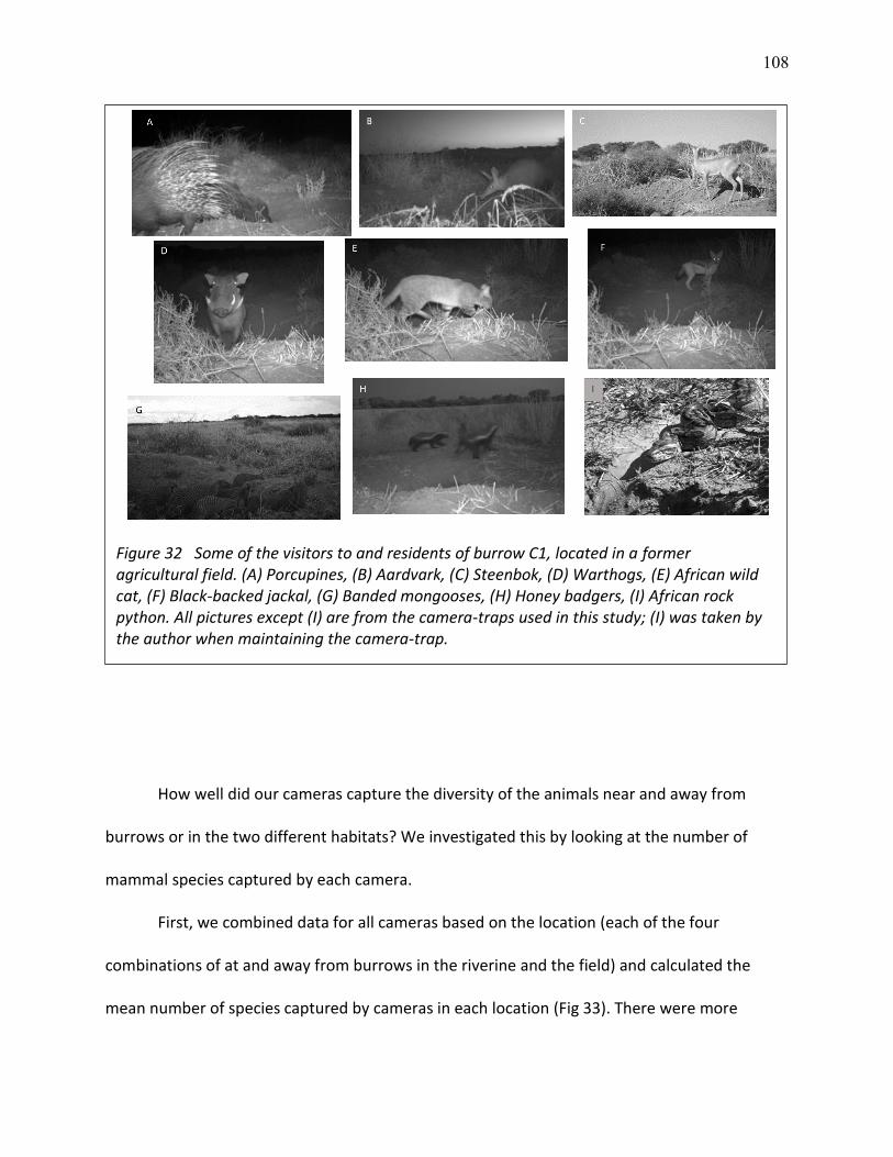
108

How well did our cameras capture the diversity of the animals near and away from

burrows or in the two different habitats? We investigated this by looking at the number of

mammal species captured by each camera.

First, we combined data for all cameras based on the location (each of the four

combinations of at and away from burrows in the riverine and the field) and calculated the

mean number of species captured by cameras in each location (Fig 33). There were more

Figure 32 Some of the visitors to and residents of burrow C1, located in a former agricultural field. (A) Porcupines, (B) Aardvark, (C) Steenbok, (D) Warthogs, (E) African wild cat, (F) Black-backed jackal, (G) Banded mongooses, (H) Honey badgers, (I) African rock python. All pictures except (I) are from the camera-traps used in this study; (I) was taken by the author when maintaining the camera-trap.

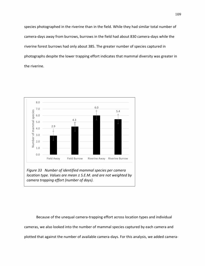
109

species photographed in the riverine than in the field. While they had similar total number of

camera-days away from burrows, burrows in the field had about 830 camera-days while the

riverine forest burrows had only about 385. The greater number of species captured in

photographs despite the lower trapping effort indicates that mammal diversity was greater in

the riverine.

Because of the unequal camera-trapping effort across location types and individual

cameras, we also looked into the number of mammal species captured by each camera and

plotted that against the number of available camera-days. For this analysis, we added camera-

Figure 33 Number of identified mammal species per camera location type. Values are mean ± S.E.M. and are not weighted by camera trapping effort (number of days).

2.9

4.3

6.05.4

0.0

1.0

2.0

3.0

4.0

5.0

6.0

7.0

8.0

Field Away Field Burrow Riverine Away Riverine Burrow

Nu

mb

er o

f m

amm

al s

pec

ies

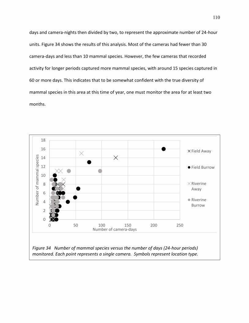
110

days and camera-nights then divided by two, to represent the approximate number of 24-hour

units. Figure 34 shows the results of this analysis. Most of the cameras had fewer than 30

camera-days and less than 10 mammal species. However, the few cameras that recorded

activity for longer periods captured more mammal species, with around 15 species captured in

60 or more days. This indicates that to be somewhat confident with the true diversity of

mammal species in this area at this time of year, one must monitor the area for at least two

months.

Figure 34 Number of mammal species versus the number of days (24-hour periods) monitored. Each point represents a single camera. Symbols represent location type.

0

2

4

6

8

10

12

14

16

18

0 50 100 150 200 250

Nu

mb

er o

f m

amm

al s

pec

ies

Number of camera-days

Field Away

Field Burrow

RiverineAway

RiverineBurrow

111

D. Discussion

Aardvark burrows are centers of bird and mammal activity. Nearly all of the cameras in

the riverine forest and former agricultural fields captured photographs of animals, and half of

those in the sparsely populated mopane forest did. It appears that most of the “burrows” are

mere byproducts of the aardvarks’ search for subterranean food (Chapter 3 of this document).

Aardvarks were not the species making most use of the benefits these burrows provide. Burrow

use at MNP can be summarized as “mostly warthogs.”

The majority of burrows, as defined here, were used on a weekly and sometimes daily

basis by a large number of species. Use of burrows was highly habitat-specific. In the riverine

habitat, 23 of 26 (88.5%) randomly monitored burrows showed use during the time we

monitored them. In the field, 29 of 42 (69.0%) had active use. In the mopane forest just 7 of 17

(41.1%) were used, and these were used infrequently compared to burrows in the other two

habitats. While the aardvarks who dug these burrows likely intended few if any as dens, our

hypothesis that they are widely used by other vertebrates is supported.

Many of our monitored burrows not only showed some animal use, but 13 in the

riverine (50.0% of the 26 monitored) and 15 in the field (35.7% of the 42 monitored) showed

use by more than one species, even in our generally short monitoring periods. The proportion

of burrows in use was not significantly different between the two habitats (chi-square

goodness-of-fit, p = 0.12). The most extensively monitored burrow, C1, saw definite use by

seven different species (aardvark, porcupine, warthog, banded mongoose, python, steenbok,

112

and brown hyena) and apparent interest by another four (African wild cat, honey badger, black-

backed jackal, and coucal), in its 219 days of monitoring across three winters.

Why are burrows in the riverine forest used so much more often than the other two

habitats? Part of this may reflect animal activity in general. It stands to reason that if there are

more animals present, more will be both attracted to and avoid aardvark burrows. The number

of burrows is a similarly obvious factor: more burrows means that the animals present have

more to potentially use (and less space in which to avoid them). Aardvark burrows are very

clumped in distribution, but are more numerous in the riverine forest than the fields or mopane

forest. We found that the mopane forest had about 1.1 burrows/ha, the field 1.8 burrows/ha,

and the riverine 4.1 burrows/ha (Chapter III). Yet despite the increased number of available

burrows, a higher proportion was used. This must be due to increased animal activity. While we

do not have complete census data on the species and numbers present in these habitats, our

cameras did appear to reflect the activity we observed. The riverine forest was relatively

crowded, the fields less so, and the mopane nearly deserted except for baboons and elephants.

Our camera trap setup limited our ability to definitively determine the full nature and

extent of burrow use. While we have many pictures of animals entering, exiting, and looking

into the burrow, it is highly likely that we missed other incidents of use. If the camera was

triggered, either by an animal or other motion, less than five minutes before the burrow use,

we would not have a picture of the activity or even the species. This undoubtedly led to an

underestimate of burrow use. For example, the warthog that spent much of our 2009 season

using burrow C1 was photographed entering the burrow on 53 non-consecutive nights but only

exiting on 51 mornings. On those days, other movement (such as that of vegetation) may have

113

triggered the camera just before he appeared, and thus we have no record of his exit.

Alternately, he may have actually spent the night elsewhere.

While still photos, especially those taken five minutes apart as ours were, do not always

provide direct evidence for why an animal chooses to be at or in the aardvark burrow, they can

be used to get a decent picture of what may be going on. Our cameras showed ten mammal

species, plus unidentified small rodents, definitely or likely using the burrows. Of these, five

showed a statistically significant preference to be at burrows. Aardvarks and warthogs

definitely use these burrows, but both are highly mobile and thus appeared in many Away

pictures as well. Several birds (including unidentified species of doves) were photographed

apparently foraging in the overturned soil (or hunting, as in the case of the grass owl in Fig.

4.14c), using mounded soil as a vantage point (e.g., coucal), or both (e.g., long-tailed starlings).

The burrows in this study did not appear to be used as bolt holes. Two pictures showed

an animal, one a springhare the other unidentifiable, entering the burrow so quickly as to

appear blurry; these may have been cases of the burrow being used as a bolt hole. Rather, the

protection offered by burrows is more as temporary shelter rather than emergency escape. This

makes sense. Predators could be hiding in the burrow as well as hunting out in the open.

Aardvark-dug burrows are large enough to hide many smaller predators such as genets or

snakes, and are easily modified into hyena or wild dog dens. Bolting into a burrow for

protection from one predator may result in bolting into the mouth of another.

Another possibility for the lack of apparent bolting was the high abundance of prey

animals relative to the predator populations. While many predators were photographed near

burrows (mongooses, genet, honey badger, brown hyena, spotted hyena, wild cat, jackal, and

114

python) and others known to live within the park (leopard, visiting wild dogs and lions), they

were greatly outnumbered by prey (warthogs, impala and other antelope, monkeys, and more).

To test this, the study should be repeated in a more predator-intensive/prey-poor

region. In 2009, we used the same methods to survey the field, mopane, and mixed field-

mopane habitats at the Venetia-Limpopo Nature Reserve (VLNR) that lies directly to the south

of MNP. The two were separated only by two fences and a two-lane paved road with little

traffic. VLNR was eliminated as a site for this study because of the low number of aardvark

burrows. This site also had relatively large predator numbers, including lions and wild dogs, and

few prey animals (pers. obs.). Because the climate and other factors are the same as at MNP, it

could serve as a comparison site.

There is little information on the long-term use of burrows of any species. Evans (2008)

found that common wombats (Vombatus ursinus) change sleeping burrows every 1–4 days; in

that study, burrows were twice as dense as wombats, yet because of wombat movement

burrows were used by an average of 2.2 wombats during the study. Finlayson et al (2005) found

that southern hairy-nosed wombats (Lasiorhinus latifrons) similarly moved frequently between

warrens (burrow complexes) and that they occupied 42% of the available warrens over a seven-

month period. Grant et al (1992) showed that platypuses frequently share “resting burrows,”

and do not seem to have a single “home” burrow. Merriam (1971) found that woodchucks

similarly move frequently. Holmes et al (2003) monitored burrowing owl (Athene cunicularia)

nests and burrows over three breeding seasons and found that burrows were reused

frequently, though they did not have data on the individual animals using them.

115

Taylor and Skinner (2003) radio-collared eight aardvarks and habituated two of them for

direct observation. They monitored burrow use by three of these, one for three months and

two for a year. The aardvarks spent 1–38 days in a given burrow (mean 6.9, 4.9, and 8.6 for the

three animals), and the authors noted that when an aardvark moved to a new burrow it usually

moved into an existing one within the home range rather than digging a new one. Aardvarks

were rarely observed returning to previously used burrows, indicating that there must have

been a surfeit of burrows to move among, though available burrows were not counted.

Aardvarks only used our monitored burrows occasionally. None of our monitored

burrows appeared to be aardvark sleeping dens at the time of monitoring, with the exception

of C1 and its dying occupant in 2008. Species other than aardvarks visited and inhabited the

burrows frequently. At least three were used as dens by families of warthogs while being

monitored. Given the low density of aardvarks relative to that of other species, and relative to

the number of burrows, this is not entirely surprising. Our results support the hypothesis that

most of these burrows were dug by aardvarks as onetime feeding digs and then left to be used

or not. While aardvarks may re-use feeding digs, the sheer number of burrows dug by aardvarks

suggests that few are actually re-used by the aardvarks for any reason. Taylor et al. (2002)

observed aardvarks digging short tunnels, up to 2 m in length, solely for feeding purposes,

which supports our conclusion that these “burrows,” as we have been using the term, are

nothing more than the remains of a meal as far as the aardvarks are concerned.

The proportions of burrows used by aardvarks, as compared to those used by any other

species, are undoubtedly skewed by the relative populations of the various species. If one were

to adjust for per-capita usage, the rates may be very different; however, we do not have the

116

census data to perform this calculation. An individual aardvark may well dig more burrows than

an individual of any other species, but the sheer number of others and the low population of

aardvarks makes it appear that aardvarks are not primary burrow users. However, this

reinforces the hypothesis that these burrows are of great importance to species other than

aardvarks.

Compared to expectations, aardvarks were underrepresented at burrows--they were

seen just as often “away” from their burrows as at them. A likely reason is their highly mobile

foraging. Another is the fact that a given burrow is probably neither the current den nor useful

for foraging because the ant or termite population has not yet recovered from a previous

aardvark attack. We do not know how often, if ever, aardvarks revisit previous feeding

locations, or visit those dug by other aardvarks. That aardvarks were not preferentially

photographed at burrows suggests that the majority of remnant burrows are unimportant to

aardvarks while very important to others, such as warthogs and porcupines, that did prefer

burrows.

Warthogs were by far the most numerous burrow-users at MNP, and the numbers are

even greater when one considers that warthogs live in family groups. Photographs often

showed multiple warthogs. Both porcupines and warthogs are capable of digging burrows, but

the large number of holes left behind by aardvarks frees these other animals from having to

make the effort. It would be interesting to know whether this public good simply makes life

easier for warthogs and porcupines or whether this promotes larger population sizes of the two

species.

117

Several antelope species significantly avoided aardvark burrows. The most likely reason

is simply that burrows are holes in the ground. As burrows provide no benefit to these animals,

the potential trip hazard is enough to make them avoid the immediate area. The trip hazard is

paramount when running from predators, a time when one cannot be picky about where they

place their feet.

Small rodents were only photographed in 2008. This was likely due to camera

positioning. In 2008, we tended to place cameras closer to the ground and burrow entrances

than in later years. Moving the cameras a little further away allowed for a more complete

survey of the burrow entrance, but may have been too far for such small animals to trigger the

cameras. Footprints of small rodents were a common sight at burrows with soft soil fans, and

the animals were undoubtedly present.

What we do not know is how applicable these findings are to other aardvark-inhabited

areas. MNP has a short history as a wildlife reserve and is bordered and interrupted by

agricultural farms. Predators actively avoid humans, while prey species may use us as a “shield”

and are quick to recolonize previously human-occupied areas (Berger 2007). One would

therefore expect, as we observed, that in a new park such as MNP predators would exist in

small numbers. The 2006 census did not count any predators, though rangers were aware of

them.

Of the thousands of photos obtained in this study, we only obtained five of brown

hyenas (which are mostly scavengers; Mills 1989), one of a leopard, 13 of a single python, 11 of

spotted hyenas, two of civets, 18 of genets, six of African wild cats, and seven of honey badgers.

Four of the five photos of brown hyenas were taken at the burrow entrance where an aardvark

118

died, in the week following the death. We found the aardvark remains some distance from the

burrow several days later. The skull was crushed and one leg was missing entirely, probably the

work of one or more of the brown hyenas.

Despite small numbers of predators overall, many of our photographs of them were

near burrows (all 13 pythons, nine of 11 spotted hyenas, one of two civets, all 18 genets, all six

African wild cats, two of seven honey badgers, and all five brown hyenas), and several of these

were photographed apparently hunting in or around the burrow. This could indicate that

burrows facilitate predator diversity as a potential prey source or a den; however, our sample

size was too small to determine this. The python was present on the same dates as a family of

porcupines, but it had recently eaten and so was not currently a threat. An aardvark had been

present four nights before our first picture of the porcupines, and during the day in the same

time period a pair of steenbok appeared to be investigating the burrow. There are anecdotes of

multiple species sharing aardvark burrows, but this has not been formally documented. We do

not know if these species were actually sharing the burrow or just taking turns.

Our cameras were not placed on trails or gathering places such as water holes, and were

not baited to attract animals. We placed cameras in places similar to aardvark burrow

locations—generally clearings or areas of low vegetation, but not trails. As we were looking at

burrow use and avoidance, a full census was not the goal and our inventory should not be taken

as such. Predators only appear incidentally in the Away pictures, or at burrows either

incidentally or if hunting. The lack of evidence at hunting at burrows in the form of photos or

other signs supports the idea that aardvark burrows are neither bolt holes nor ambush points,

or that these are minor uses.

119

Previous studies (Smithers 1971, Whittington-Jones et al. 2011) collectively named 49

vertebrate species or groups associated with aardvark burrows in Botswana (Smithers) or South

Africa (Whittington-Jones). We have expanded this list to 59, including the families of doves and

francolins. Vertebrate commensals identified in this study are shown in Table IX, and the

combined list in Table X. The species we added were mostly smaller mammals (mongooses,

squirrels, and springhares) and birds. These species may be quick to leave the area when

humans approach, too small to be noticed in the incidental observations employed by both

Smithers and Whittington-Jones, too large for the traps set by Whittington-Jones, or some

combination of the above. The only large animal we added was the bushpig, which may simply

be present in relatively low numbers or be misidentified as the more common warthog when

sighted.

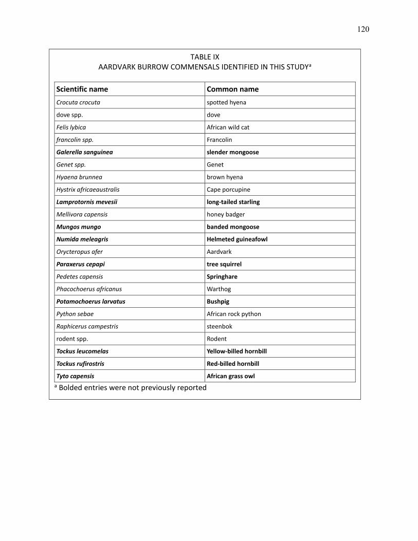
120

TABLE IX AARDVARK BURROW COMMENSALS IDENTIFIED IN THIS STUDYa

Scientific name Common name

Crocuta crocuta spotted hyena

dove spp. dove

Felis lybica African wild cat

francolin spp. Francolin

Galerella sanguinea slender mongoose

Genet spp. Genet

Hyaena brunnea brown hyena

Hystrix africaeaustralis Cape porcupine

Lamprotornis mevesii long-tailed starling

Mellivora capensis honey badger

Mungos mungo banded mongoose

Numida meleagris Helmeted guineafowl

Orycteropus afer Aardvark

Paraxerus cepapi tree squirrel

Pedetes capensis Springhare

Phacochoerus africanus Warthog

Potamochoerus larvatus Bushpig

Python sebae African rock python

Raphicerus campestris steenbok

rodent spp. Rodent

Tockus leucomelas Yellow-billed hornbill

Tockus rufirostris Red-billed hornbill

Tyto capensis African grass owl

a Bolded entries were not previously reported

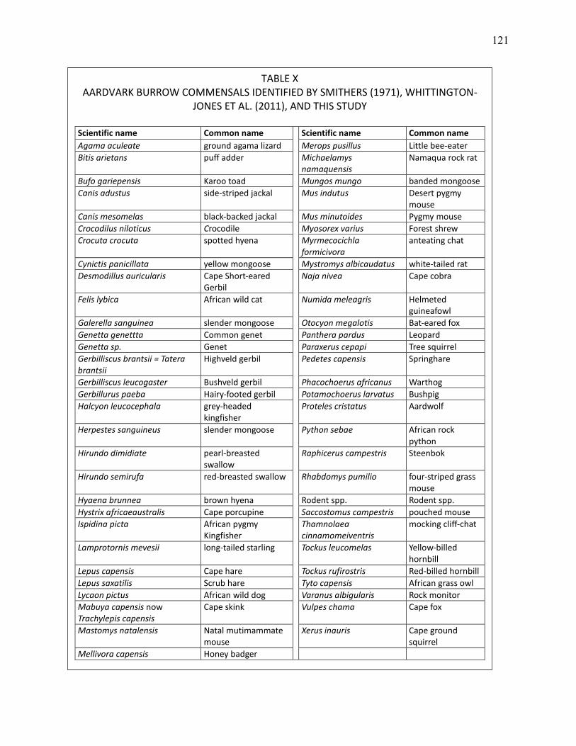
121

TABLE X AARDVARK BURROW COMMENSALS IDENTIFIED BY SMITHERS (1971), WHITTINGTON-

JONES ET AL. (2011), AND THIS STUDY

Scientific name Common name Scientific name Common name

Agama aculeate ground agama lizard Merops pusillus Little bee‐eater

Bitis arietans puff adder Michaelamys namaquensis

Namaqua rock rat

Bufo gariepensis Karoo toad Mungos mungo banded mongoose

Canis adustus side‐striped jackal Mus indutus Desert pygmy mouse

Canis mesomelas black‐backed jackal Mus minutoides Pygmy mouse

Crocodilus niloticus Crocodile Myosorex varius Forest shrew

Crocuta crocuta spotted hyena Myrmecocichla formicivora

anteating chat

Cynictis panicillata yellow mongoose Mystromys albicaudatus white‐tailed rat

Desmodillus auricularis Cape Short‐eared Gerbil

Naja nivea Cape cobra

Felis lybica African wild cat Numida meleagris Helmeted guineafowl

Galerella sanguinea slender mongoose Otocyon megalotis Bat‐eared fox

Genetta genettta Common genet Panthera pardus Leopard

Genetta sp. Genet Paraxerus cepapi Tree squirrel

Gerbilliscus brantsii = Tatera brantsii

Highveld gerbil Pedetes capensis Springhare

Gerbilliscus leucogaster Bushveld gerbil Phacochoerus africanus Warthog

Gerbillurus paeba Hairy‐footed gerbil Potamochoerus larvatus Bushpig

Halcyon leucocephala grey‐headed kingfisher

Proteles cristatus Aardwolf

Herpestes sanguineus slender mongoose Python sebae African rock python

Hirundo dimidiate pearl‐breasted swallow

Raphicerus campestris Steenbok

Hirundo semirufa red‐breasted swallow Rhabdomys pumilio four‐striped grass mouse

Hyaena brunnea brown hyena Rodent spp. Rodent spp.

Hystrix africaeaustralis Cape porcupine Saccostomus campestris pouched mouse

Ispidina picta African pygmy Kingfisher

Thamnolaea cinnamomeiventris

mocking cliff‐chat

Lamprotornis mevesii long‐tailed starling Tockus leucomelas Yellow‐billed hornbill

Lepus capensis Cape hare Tockus rufirostris Red‐billed hornbill

Lepus saxatilis Scrub hare Tyto capensis African grass owl

Lycaon pictus African wild dog Varanus albigularis Rock monitor

Mabuya capensis now Trachylepis capensis

Cape skink Vulpes chama Cape fox

Mastomys natalensis Natal mutimammate mouse

Xerus inauris Cape ground squirrel

Mellivora capensis Honey badger

122

We have no comparative data on the species that actively avoid burrows, either those

dug by aardvarks or those dug by any other species. The few studies which do survey burrow

commensals focus solely on these commensals. For a complete picture of the impact of

burrows, one would need to not only take a complete census of the burrow itself, using a

combination of techniques such as pitfall trapping and camera-trapping, but to repeat these

methods at some distance from the burrows. One would also need to not just identify species,

but to quantify individual numbers and document behaviors. Recording video rather than still

pictures, which we did not do due to memory card limitations, is increasingly practical thanks to

ever-increasing digital memory capacity at ever-decreasing costs. Most of the species we

identified as burrow-avoiders are those which cannot benefit from burrows, such as large

antelopes, elephants, and monkeys. Are there any animals that we would think may benefit

from aardvark burrows but instead avoid them?

There is always a chicken-egg scenario in studies like ours. Are there a lot of warthogs

because the predators have not yet moved in, because there are plenty of ready-made burrows

to hide in, or some combination? How much are warthogs maintaining the burrows, and how

would things change for other burrow commensals if the warthogs were to disappear? What

would happen if the aardvarks were to disappear? Further study would be required to answer

these questions.

E. Conclusion

Aardvarks dig a lot of holes large enough for vertebrates to use as a temporary shelter, a

long-term den, a food source, or a lookout point. However, the aardvarks themselves appear to

123

have little use for most of these diggings once they have finished the meal that inspired their

excavation. Aardvarks move among burrows frequently, and often re-use burrows they or other

individuals dug, but it seems that the majority of aardvark diggings are, as far as the aardvarks

ae concerned, just the remains of a meal.

Vertebrates that are not aardvarks, however, make much use of these leftovers.

Warthogs were especially numerous at MNP, though this is likely to be site-specific. Aardvarks

truly are the inadvertent civil engineers of the southern African plains and forests, creating a

public good by creating big holes in the ground that others can use.

The full extent of aardvarks’ effects on their community remain unknown, and while we

have expanded the list of commensal species, it too is likely incomplete. A full inventory of

vertebrate commensals would require more extensive camera trapping, physical trapping,

direct observations, and other census methods.

F. Literature cited

Abu Baker MA, Brown JS. 2012. Patch use behaviour of Elephantulus myurus and Micaelamys namaquensis: the role of diet, foraging substrates and escape substrates. African Journal of Ecology 50: 167-75

Alexy KJ, Brunjes KJ, Gassett JW, Miller KV. 2003. Continuous remote monitoring of gopher tortoise burrow use. Wildlife Society Bulletin 31: 1240-43

Alkon PU. 1999. Microhabitat to landscape impacts: crested porcupine digs in the Negev Desert highlands. Journal of Arid Environments 41: 183-202

Anker A, Murina GV, Lira C, Vera Caripe JA, Palmer AR, Jeng MS. 2005. Macrofauna associated with echiuran burrows: a review with new observations of the innkeeper worm, Ochetostoma erythrogrammon Leuckart and Rüppel, in Venezuela. Zoological Studies 44:157-90

Bangert R, Slobodchikoff C. 2006. Conservation of prairie dog ecosystem engineering may support arthropod beta and gamma diversity. Journal of Arid Environments 67: 100-15

Berger J. 2007. Fear, human shields and the redistribution of prey and predators in protected areas. Biology Letters 3: 620-23

Berke SK. 2010. Functional groups of ecosystem engineers: a proposed classification with comments on current issues. Integrative and Comparative Biology 50: 147

124

Bright DB, Hogue CL. 1972. A synopsis of the burrowing land crabs of the world and list of their arthropod symbionts and burrow associates. Una sinopsis mundial de los cangrejos terrestres de madrigueras y lista de sus artrópodos simbiontes y madrigueras asociadas. Contributions in Science (Los Angeles). 1-58

Butts KO, Lewis JC. 1982. The importance of prairie dog towns to burrowing owls in Oklahoma. Proceedings of the Oklahoma Academy of Science 62: 46-52

Campbell III TM, Clark TW. 1981. Colony characteristics and vertebrate associates of white-tailed and black-tailed prairie dogs in Wyoming. American Midland Naturalist 105: 269-76

Carey HR. 1926. Camera-trapping: a novel device for wild animal photography. Journal of Mammalogy 7: 278-81

Casas-Criville A, Valera F. 2005. The European bee-eater (Merops apiaster) as an ecosystem engineer in arid environments. Journal of Arid Environments 60: 227-38

Ceballos G, Pacheco J, List R. 1999. Influence of prairie dogs (Cynomys ludovicianus) on habitat heterogeneity and mammalian diversity in Mexico. Journal of Arid Environments 41: 161-72

Commito JA, Celano EA, Celico HJ, Como S, Johnson CP. 2005. Mussels matter: postlarval dispersal dynamics altered by a spatially complex ecosystem engineer. Journal of Experimental Marine Biology and Ecology 316: 133-47

Dangerfield J, McCarthy T, Ellery W. 1998. The mound-building termite Macrotermes michaelseni as an ecosystem engineer. Journal of Tropical Ecology 14: 507-20

Davidson AD, Detling JK, Brown JH. 2012. Ecological roles and conservation challenges of social, burrowing, herbivorous mammals in the world's grasslands. Frontiers in Ecology and the Environment 10: 477-86

Desbiez ALJ, Kluyber D. 2013. The Role of Giant Armadillos (Priodontes maximus) as Physical Ecosystem Engineers. Biotropica 45: 537-40

Duncan S. 2003. Coming home to roost: the pileated woodpecker as ecosystem engineer. Science Findings 57. Portland, OR: U.S. Department of Agriculture, Forest Service, Pacific Northwest Research Station.

Evans MC. 2008. Home range, burrow-use and activity patterns in common wombats (Vombatus ursinus). Wildlife Research 35: 455-62

Finlayson G, Shimmin G, Temple Smith P, Handasyde K, Taggart D. 2005. Burrow use and ranging behaviour of the southern hairy nosed wombat (Lasiorhinus latifrons) in the Murraylands, South Australia. Journal of Zoology 265: 189-200

Fleming PA, Anderson H, Prendergast AS, Bretz MR, Valentine LE, Hardy GE. 2014. Is the loss of Australian digging mammals contributing to a deterioration in ecosystem function? Mammal Review 44: 94-108

Foster RJ, Harmsen BJ. 2012. A critique of density estimation from camera‐trap data. The Journal of Wildlife Management 76: 224-36

Gálvez Bravo L, Belliure J, Rebollo S. 2009. European rabbits as ecosystem engineers: warrens increase lizard density and diversity. Biodiversity and Conservation 18: 869-85

Gálvez L, López-Pintor A, De Miguel JM, Alonso G, Rueda M, et al. 2008. Ecosystem Engineering Effects of European Rabbits in a Mediterranean Habitat. In: Lagomorph Biology: Evolution, Ecology, and Conservation, ed. PC Alves, N Ferrand, K Hackländer, pp. 125-39. Berlin, Heidelberg: Springer Berlin Heidelberg

González EM, Soutullo A, Altuna CA. 2001. The burrow of Dasypus hybridus (Cingulata: Dasypodidae). Acta Theriologica 46: 53-59

125

Grant T, Grigg GC, Beard L, Augee M. Movements and burrow use by platypuses, Ornithorhynchus anatinus, in the Thredbo River, New South Wales. In: Platypus and Echidnas pp. 263-267

Hagenah N, Bennett NC. 2013. Mole rats act as ecosystem engineers within a biodiversity hotspot, the Cape Fynbos. Journal of Zoology 289: 19-26

Hansell MH. 1993. The ecological impact of animal nests and burrows. Functional Ecology 7: 5-12

Hastings A, Byers JE, Crooks JA, Cuddington K, Jones CG, Lambrinos JG, Talley TS, Wilson WG. 2007. Ecosystem engineering in space and time. Ecology Letters 10: 153-64

Holmes AL, Green GA, Morgan RL, Livezey KB. 2003. Burrowing owl nest success and burrow longevity in north central Oregon. Western North American Naturalist 63: 244-50

Jones CG, Lawton JH, Shachak M. 1994. Organisms as ecosystem engineers. Oikos 69: 373-86

Jones CG, Lawton JH, Shachak M. 1997. Positive and negative effects of organisms as physical ecosystem engineers. Ecology 78: 1946-57

Kinlaw A. 1999. A review of burrowing by semi-fossorial vertebrates in arid environments. Journal of Arid Environments 41: 127-45

Kinlaw A, Grasmueck M. 2012. Evidence for and geomorphologic consequences of a reptilian ecosystem engineer: the burrowing cascade initiated by the gopher tortoise. Geomorphology 157: 108-21

Kotler BP, Brown J, Oldfield A, Thorson J, Cohen D. 2001. Foraging substrate and escape substrate: patch use by three species of gerbils. Ecology 82: 1781-90

Kotliar NB, Baker BW, Whicker AD, Plumb G. 1999. A critical review of assumptions about the prairie dog as a keystone species. Environmental Management 24: 177-92

Kurek P, Kapusta P, Holeksa J. 2014. Burrowing by badgers (Meles meles) and foxes (Vulpes vulpes) changes soil conditions and vegetation in a European temperate forest. Ecological research 29: 1-11

Lenihan CM. 2008. The ecological role of the California ground squirrel (Spermophilus beecheyi). PhD Dissertation, University of California, Davis

Lill JT, Marquis RJ. 2003. Ecosystem engineering by caterpillars increases insect herbivore diversity on white oak. Ecology 84: 682-90

Lomolino MV, Smith GA. 2004. Terrestrial vertebrate communities at black-tailed prairie dog (Cynomys ludovicianus) towns. Biological Conservation 115: 89-100

Lyra-Jorge MC, Ciocheti G, Pivello VR, Meirelles ST. 2008. Comparing methods for sampling large-and medium-sized mammals: camera traps and track plots. European Journal of Wildlife Research 54: 739-44

Melton DA. 1972. Environmental heterogeneity produced by termitaria in western Uganda with special reference to mound usage by vertebrates. PhD Dissertation, University of British Columbia

Merriam HG. 1971. Woodchuck burrow distribution and related movement patterns. Journal of Mammalogy 52: 732-46

Mills M. 1989. The comparative behavioral ecology of hyenas: the importance of diet and food dispersion. In: Carnivore Behavior, Ecology, and Evolution, pp. 125-42: Springer

Nummi P, Hahtola A. 2008. The beaver as an ecosystem engineer facilitates teal breeding. Ecography 31: 519-24

126

O'Connell AF, Nichols JD, Karanth UK, editors. 2010. Camera traps in animal ecology: Methods and analyses. Springer Science & Business Media

Pike D, Mitchell J. 2013. Burrow‐dwelling ecosystem engineers provide thermal refugia throughout the landscape. Animal Conservation 16: 694-703

Pringle RM. 2008. Elephants as agents of habitat creation for small vertebrates at the patch scale. Ecology 89: 26-33

Prugh LR, Brashares JS. 2012. Partitioning the effects of an ecosystem engineer: kangaroo rats control community structure via multiple pathways. Journal of Animal Ecology 81: 667-78

Reichman OJ, Seabloom EW. 2002. The role of pocket gophers as subterranean ecosystem engineers. Trends in Ecology & Evolution 17: 44-49

Roerig J. 2006. Counting Game in Mapungubwe. https://www.sanparks.org/about/news/?id=371. Accessed September 23, 2016.

Romanach SS, Le Comber SC. 2004. Measures of pocket gopher (Thomomys bottae) burrow geometry: correlates of fractal dimension. Journal of Zoology 262: 399-403

Romero GQ, Gonçalves‐Souza T, Vieira C, Koricheva J. 2014. Ecosystem engineering effects on species diversity across ecosystems: a meta‐analysis. Biological Reviews 90: 877-90

Rowcliffe J, Carbone C. 2008. Surveys using camera traps: are we looking to a brighter future? Animal Conservation 11: 185-86

Rowcliffe JM, Field J, Turvey ST, Carbone C. 2008. Estimating animal density using camera traps without the need for individual recognition. Journal of Applied Ecology 45: 1228-36

Silveira L, Jacomo ATA, Diniz-Filho JAF. 2003. Camera trap, line transect census and track surveys: a comparative evaluation. Biological Conservation 114: 351-55

Smithers RHN. 1971. The Mammals of Botswana. Trustees of the National Museums of Rhodesia.

Taylor WA, Lindsey PA, Skinner JD. 2002. The feeding ecology of the aardvark Orycteropus afer. Journal of Arid Environments 50: 135-52

Taylor WA, Skinner JD. 2003. Activity patterns, home ranges and burrow use of aardvarks (Orycteropus afer) in the Karoo. Journal of Zoology 261: 291-97

Tobler MW, Carrillo Percastegui SE, Leite Pitman R, Mares R, Powell G. 2008. An evaluation of camera traps for inventorying large and medium sized terrestrial rainforest mammals. Animal Conservation 11: 169-78

Van Nimwegen RE, Kretzer J, Cully Jr JF. 2008. Ecosystem engineering by a colonial mammal: how prairie dogs structure rodent communities. Ecology 89: 3298-305

Whittington-Jones G, Bernard R, Parker D. 2011. Aardvark Burrows: A Potential Resource for Animals in Arid and Semi-Arid Environments. African Zoology 46: 362-70

Whittington-Jones GM. 2007. The role of aardvarks (Orycteropus afer) as ecosystem engineers in arid and semi-arid landscapes of South Africa. MSc Dissertation, Rhodes University, Grahamstown, South Africa.

Wright JP, Jones CG. 2006. The concept of organisms as ecosystem engineers ten years on: progress, limitations, and challenges. Bioscience 56: 203-09

127

Wright JP, Jones CG, Flecker AS. 2002. An ecosystem engineer, the beaver, increases species richness at the landscape scale. Oecologia 132: 96-101

Yasuda M. 2004. Monitoring diversity and abundance of mammals with camera traps: a case study on Mount Tsukuba, central Japan. Mammal Study 29: 37-46

V. A MODEL OF BEHAVIORAL RESOURCE DEPRESSION AND SLOWLY REGENERATING

RESOURCES

A. Introduction

Foraging and depredating, the acts of searching for, finding, and consuming food involve

a number of steps and often complex, if unconscious, decision-making. Foragers and predators

must decide what, when, and where to eat as well as how much time and effort to devote to

this process, whether to forage with others or alone, and so on. Each facet is itself complex. Do

you opt for a higher quality food which may require more risk to acquire, or play it safe but

accept a lower-quality food? While it is true that these decisions are not conscious and even

made by those with no capacity for conscious thought (e.g., plants, O’Brien and Brown 2008),

they are nonetheless complex decisions that can be approximated with mathematical models.

The early bird is not doing calculus when deciding to go for the early worm, it just knows that

it’s time to hunt. The long history of natural selection has left organisms of all types with

adaptive foraging behaviors. Foragers behave as if they have done the math.

Food is never uniformly distributed; rather, it is clumped into patches. This is true

whether one seeks nutrients in soil, forages for plants, hunts animals, or shops at

supermarkets. The quantity and quality of food can vary among patches. Much of the existing

work on patch use, both theoretical and empirical, makes the assumption that the food source

is passive, politely remaining in place while it is eaten. The exceptions, of course, come when

one is looking at predator-prey situations. In these, the prey attempts to evade the predator.

But there are other cases in which the food source, be it plant or animal or otherwise, can make

itself harder to eat, such as by arming itself with spikes or toxins. Defenses can be permanent,

129

but defenses, like everything else, require regular energy inputs or incur other costs. It takes a

lot of food to avoid becoming food. Some species have instead turned to what we call

behavioral resource depression, which is the decrease in the amount or value of a resource

(here food) via its behavior. Examples of behavioral resource depression include animal prey

hiding or running away, altering behavior as to appear dead and therefore unappealing to a

given predator (Sargeant and Eberhardt 1975), and induced chemical responses in plants (e.g.,

Fraenkel 1959, Karban 1989, Harvell 1990, Walling 2000).

In 1976, Eric Charnov published a short but important paper defining the Marginal Value

Theorem (MVT). His model assumed a single predator foraging in a patchy environment with an

infinite number of two or more types of patches that the predator did not revisit. Foragers were

assumed to have knowledge of the quality of their current patch, the existence of other

patches, and the distribution of patch types in the environment (though not the quality of any

other individual patch), and thus were able to act optimally. It showed that under these

assumptions, a predator should leave a patch when the marginal rate of foraging drops to the

average for the environment. That is, once a patch drops below some threshold of quality, a

predator should forage elsewhere as the food availability is likely to be higher elsewhere.

The MVT has an important attribute in that the cost of foraging to an individual while in

a patch is the missed opportunity of not leaving the current patch and finding another. Hence

the benefit to a forager from a patch is the current harvest rate (marginal rate of return) and

the cost is the average rate of return from searching for and exploiting a new patch. The key

predictions are that a forager should spend more time in a rich patch than a poor patch, it

should spend less time in patches of a rich environment than a poor one, and patch residence

130

time should increase with the time taken to travel to a new patch. Studies of the applicability

and accuracy of the MVT followed. Nonacs (2001) noted that in most studies, foragers were

found to leave patches sooner than predicted by the MVT.

Charnov et al. (1976) explored the implications of resource depression, which

represents the decline in food availability in a patch because it is presently occupied by a

forager. They identified three forms of resource depression: exploitation depression, in which

prey is consumed by the predator; behavioral depression, in which the prey changes its

behavior in a way as to reduce its availability to the predator; and microhabitat depression, in

which prey move to another location to avoid predation. Microhabitat depression can be seen

as an alternative form of behavioral depression, when the behavior is movement.

Along with resource depression, one must consider recovery of the resource—prey

coming back to the location, reverting to pre-predation behavior, and increasing in population.

Plants must grow and prey must creep back, seeking the resources they need while trying to

avoid the predator. This recovery may be effectively instantaneous, very slow, or anywhere in

between. This factor is even more poorly understood than behavioral resource depression.

Foraging studies traditionally focus on the choice of a food patch and the food within, but do

not consider that patches may be predictably dynamic. In foraging studies, artificial food

patches are fully replenished daily, and while a given site may vary day to day, they do not do

so in any predictable pattern. In nature, however, food takes time to become available, and in

an environment with a limited number of food patches, this recovery time is as important as

the initial patch quality. Some work has been done in this area. Brown and Rosenzweig (1986)

modeled habitat selection in an environment with slowly regenerating resources, with the

131

assumption of a traditionally passive food source. Possingham (1992) provided a practical

application of the idea, using hummingbirds foraging on slowly produced nectar. However,

once the nectar was available it simply remained so. As a last example, Watts (1998) found that

gorillas will adjust the length of time between revisits to foraging areas to allow the vegetation

to recover from the previous visit.

Behavioral resource depression, including microhabitat depression, goes hand-in-hand

with slow regeneration of the patch. The decline in prey availability, above and beyond the

decline caused by food being eaten, should lead to a shorter foraging bout than if the prey just

stayed where and how it was. The rate of recovery to the pre-predation state determines when

the patch has recovered enough to be worth foraging again.

The models presented below begin to describe what may happen to prey numbers

during and after predation in a situation involving behavioral resource depression (BRD)

combined with a slowly regenerating resource (SRR). That is, what is actually happening when

food items make themselves unavailable and then take time to return. A major assumption in

our model is that prey will return at a predictable rate. We build a model in four stages,

beginning with the simplest situation, the Marginal Value Theorem, where a lone predator or

forager (we shall use the term “predator” for simplicity) travels among infinite food patches,

predating each until its quality is no longer greater than the average quality of all patches.

Because this is not a new model, we call this Stage 0. Stage 1 adds BRD, and reduces to Stage 0

when the BRD rate is set to 0. Stage 2 adds SRR with unlimited patches. It in turn reduces to

Stage 1 as infinite patches mean that the predator need not return to a patch that has not fully

recovered from previous depredation. Stage 3 introduces a limit to the number of patches such

132

that the predator may return at some point before the prey number has recovered to its initial

level. This is a true model of BRD with SRR, and shows that in time prey will maintain an

equilibrium population in hiding (or otherwise unavailable for predation) while available prey

numbers vacillate between the predator’s giving-up density (GUD, Brown 1988) and some

number sufficient for being predated again.

B. The model Stage 0: the marginal value theorem

One can express the Marginal Value Theorem (MVT) in any number of ways, and add

parameters as needed. Charnov’s model used variables of energy gain and loss along with the

proportion of patches of each type. Because our goals involve prey numbers rather than these

variables, we will build a new model that will result in the MVT in terms relevant to our

interests. We begin with an environment with an infinite number of distinct patches of prey,

such as ant hills. Within each patch is a population of prey individuals. There is a single predator

that encounters a patch, depredates it to some level, then moves on to another patch with

greater prey numbers.

We define the variables as follows: let t be the predation time, starting at 0 when the

predator enters the patch and maximizing at t*, the time when the predator leaves the patch

(quitting time); let T be the average time taken to travel between patches; and let N be the

number of prey; let h be the predator's instantaneous harvest rate, the rate at which the

predator is consuming prey at time t; let H be the average harvest rate for the set of patches

under consideration; let a be the attack rate (Hassell 1978; also called encounter probability,

Brown and Mitchell 1989), which is the probability that a predator will encounter and consume

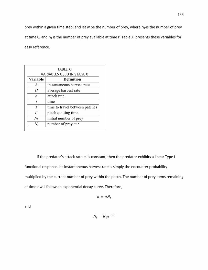
133

prey within a given time step; and let N be the number of prey, where N0 is the number of prey

at time 0, and Nt is the number of prey available at time t. Table XI presents these variables for

easy reference.

If the predator’s attack rate a, is constant, then the predator exhibits a linear Type I

functional response. Its instantaneous harvest rate is simply the encounter probability

multiplied by the current number of prey within the patch. The number of prey items remaining

at time t will follow an exponential decay curve. Therefore,

ℎ = 𝑎𝑁𝑡

and

𝑁𝑡 = 𝑁0𝑒−𝑎𝑡

TABLE XI VARIABLES USED IN STAGE 0

Variable Definition

h instantaneous harvest rate

H average harvest rate

a attack rate

t time

T time to travel between patches

t* patch quitting time

N0 initial number of prey

Nt number of prey at t

134

Under the assumption that patch depletion only occurs through the predator’s harvest

(no behavioral resource depression), the predator’s instantaneous harvest rate, h, is also

equivalent to the instantaneous rate of decline of prey items within the patch. Therefore,

ℎ = −𝑑𝑁𝑡

𝑑𝑡

The predator’s average harvest rate, H, includes both the time spent harvesting a patch,

t, and the time taken to travel to the patch, T. H, at time t, can be expressed as the number of

prey items consumed (the number of initial prey items minus those remaining at time t),

divided by the elapsed time (t plus the time taken to get to the patch, T).

𝐻 =𝑁0 − 𝑁𝑡

𝑡 + 𝑇

To maximize its average harvest rate, the predator should quit the patch when the

instantaneous harvest rate equals the average harvest rate for the entire area; that is, when h =

H. This time we call t*.

The MVT states that a predator should quit a patch when:

ℎ = −𝑑𝑁𝑡∗

𝑑𝑡=

𝑁0 − 𝑁𝑡∗

𝑡∗ + 𝑇= 𝐻

Note that we have not actually solved for t*. The best we can get is a fairly

uninformative transcendental equation. Remember that Nt is a function of t and therefore must

not be treated as a constant.

𝑡∗ =𝑁0 − 𝑁𝑡∗

𝑎𝑁𝑡∗− 𝑇

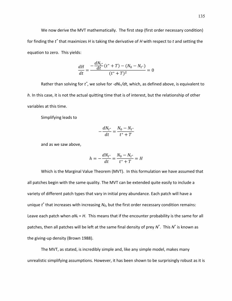
135

We now derive the MVT mathematically. The first step (first order necessary condition)

for finding the t* that maximizes H is taking the derivative of H with respect to t and setting the

equation to zero. This yields:

𝑑𝐻

𝑑𝑡=

−𝑑𝑁𝑡∗

𝑑𝑡(𝑡∗ + 𝑇) − (𝑁0 − 𝑁𝑡∗)

(𝑡∗ + 𝑇)2= 0

Rather than solving for t*, we solve for -dNt /dt, which, as defined above, is equivalent to

h. In this case, it is not the actual quitting time that is of interest, but the relationship of other

variables at this time.

Simplifying leads to

−𝑑𝑁𝑡∗

𝑑𝑡=

𝑁0 − 𝑁𝑡∗

𝑡∗ + 𝑇

and as we saw above,

ℎ = −𝑑𝑁𝑡∗

𝑑𝑡=

𝑁0 − 𝑁𝑡∗

𝑡∗ + 𝑇= 𝐻

Which is the Marginal Value Theorem (MVT). In this formulation we have assumed that

all patches begin with the same quality. The MVT can be extended quite easily to include a

variety of different patch types that vary in initial prey abundance. Each patch will have a

unique t* that increases with increasing N0, but the first order necessary condition remains:

Leave each patch when aNt = H. This means that if the encounter probability is the same for all

patches, then all patches will be left at the same final density of prey N*. This N* is known as

the giving-up density (Brown 1988).

The MVT, as stated, is incredibly simple and, like any simple model, makes many

unrealistic simplifying assumptions. However, it has been shown to be surprisingly robust as it is

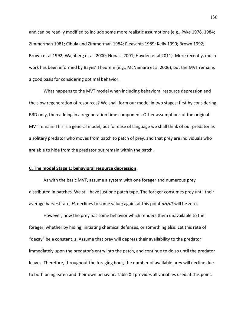
136

and can be readily modified to include some more realistic assumptions (e.g., Pyke 1978, 1984;

Zimmerman 1981; Cibula and Zimmerman 1984; Pleasants 1989; Kelly 1990; Brown 1992;

Brown et al 1992; Wajnberg et al. 2000; Nonacs 2001; Hayden et al 2011). More recently, much

work has been informed by Bayes’ Theorem (e.g., McNamara et al 2006), but the MVT remains

a good basis for considering optimal behavior.

What happens to the MVT model when including behavioral resource depression and

the slow regeneration of resources? We shall form our model in two stages: first by considering

BRD only, then adding in a regeneration time component. Other assumptions of the original

MVT remain. This is a general model, but for ease of language we shall think of our predator as

a solitary predator who moves from patch to patch of prey, and that prey are individuals who

are able to hide from the predator but remain within the patch.

C. The model Stage 1: behavioral resource depression

As with the basic MVT, assume a system with one forager and numerous prey

distributed in patches. We still have just one patch type. The forager consumes prey until their

average harvest rate, H, declines to some value; again, at this point dH/dt will be zero.

However, now the prey has some behavior which renders them unavailable to the

forager, whether by hiding, initiating chemical defenses, or something else. Let this rate of

“decay” be a constant, z. Assume that prey will depress their availability to the predator

immediately upon the predator's entry into the patch, and continue to do so until the predator

leaves. Therefore, throughout the foraging bout, the number of available prey will decline due

to both being eaten and their own behavior. Table XII provides all variables used at this point.

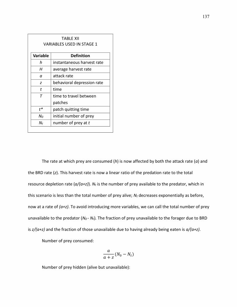
137

The rate at which prey are consumed (h) is now affected by both the attack rate (a) and

the BRD rate (z). This harvest rate is now a linear ratio of the predation rate to the total

resource depletion rate (a/(a+z)). Nt is the number of prey available to the predator, which in

this scenario is less than the total number of prey alive; Nt decreases exponentially as before,

now at a rate of (a+z). To avoid introducing more variables, we can call the total number of prey

unavailable to the predator (N0 - Nt). The fraction of prey unavailable to the forager due to BRD

is z/(a+z) and the fraction of those unavailable due to having already being eaten is a/(a+z).

Number of prey consumed:

𝑎

𝑎 + 𝑧(𝑁0 − 𝑁𝑡)

Number of prey hidden (alive but unavailable):

TABLE XII VARIABLES USED IN STAGE 1

Variable Definition

h instantaneous harvest rate

H average harvest rate

a attack rate

z behavioral depression rate

t time

T time to travel between

patches

t* patch quitting time

N0 initial number of prey

Nt number of prey at t

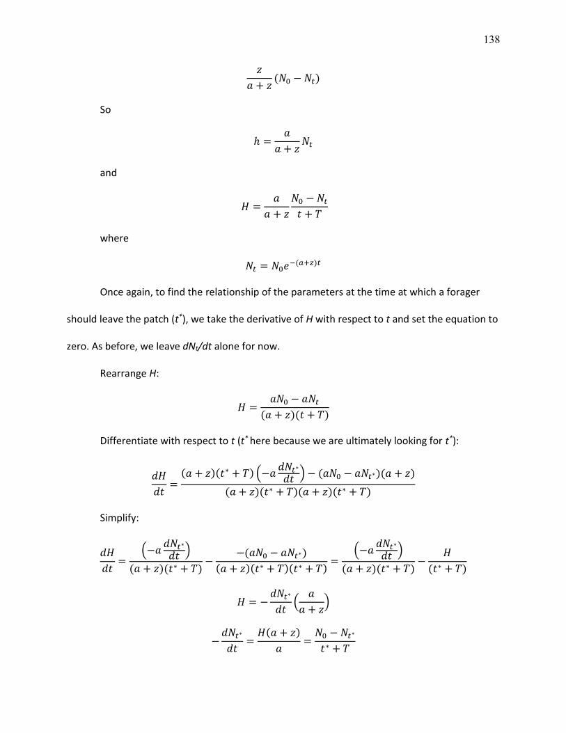
138

𝑧

𝑎 + 𝑧(𝑁0 − 𝑁𝑡)

So

ℎ =𝑎

𝑎 + 𝑧𝑁𝑡

and

𝐻 =𝑎

𝑎 + 𝑧

𝑁0 − 𝑁𝑡

𝑡 + 𝑇

where

𝑁𝑡 = 𝑁0𝑒−(𝑎+𝑧)𝑡

Once again, to find the relationship of the parameters at the time at which a forager

should leave the patch (t*), we take the derivative of H with respect to t and set the equation to

zero. As before, we leave dNt/dt alone for now.

Rearrange H:

𝐻 =𝑎𝑁0 − 𝑎𝑁𝑡

(𝑎 + 𝑧)(𝑡 + 𝑇)

Differentiate with respect to t (t* here because we are ultimately looking for t*):

𝑑𝐻

𝑑𝑡=

(𝑎 + 𝑧)(𝑡∗ + 𝑇) (−𝑎𝑑𝑁𝑡∗

𝑑𝑡) − (𝑎𝑁0 − 𝑎𝑁𝑡∗)(𝑎 + 𝑧)

(𝑎 + 𝑧)(𝑡∗ + 𝑇)(𝑎 + 𝑧)(𝑡∗ + 𝑇)

Simplify:

𝑑𝐻

𝑑𝑡=

(−𝑎𝑑𝑁𝑡∗

𝑑𝑡)

(𝑎 + 𝑧)(𝑡∗ + 𝑇)−

−(𝑎𝑁0 − 𝑎𝑁𝑡∗)

(𝑎 + 𝑧)(𝑡∗ + 𝑇)(𝑡∗ + 𝑇)=

(−𝑎𝑑𝑁𝑡∗

𝑑𝑡)

(𝑎 + 𝑧)(𝑡∗ + 𝑇)−

𝐻

(𝑡∗ + 𝑇)

𝐻 = −𝑑𝑁𝑡∗

𝑑𝑡(

𝑎

𝑎 + 𝑧)

−𝑑𝑁𝑡∗

𝑑𝑡=

𝐻(𝑎 + 𝑧)

𝑎=

𝑁0 − 𝑁𝑡∗

𝑡∗ + 𝑇

139

To find the actual patch quitting time, we substitute for -dNt /dt:

𝑑𝑁𝑡∗

𝑑𝑡= −𝑁0(𝑎 + 𝑧)(𝑒−(𝑎+𝑧)𝑡∗

)

Simplify to isolate t*. This equation is transcendental because Nt contains t, so it cannot

be solved analytically.

𝑡∗ =𝑁0 − 𝑁0𝑒−(𝑎+𝑧)𝑡∗

(𝑎 + 𝑧)𝑁0𝑒−(𝑎+𝑧)𝑡∗ − 𝑇

𝑡∗ =𝑁0 − 𝑁𝑡∗

𝑁𝑡∗(𝑎 + 𝑧)− 𝑇

We can use a spreadsheet to find close approximations for t* under various scenarios.

Using the same values, we can compare to the MVT. Figure 35 is a general graph of prey

consumed, still available, and in hiding over time, under both the MVT and our Stage 1 model.

The exact shapes of the curves vary with the values used, but this is the general form.

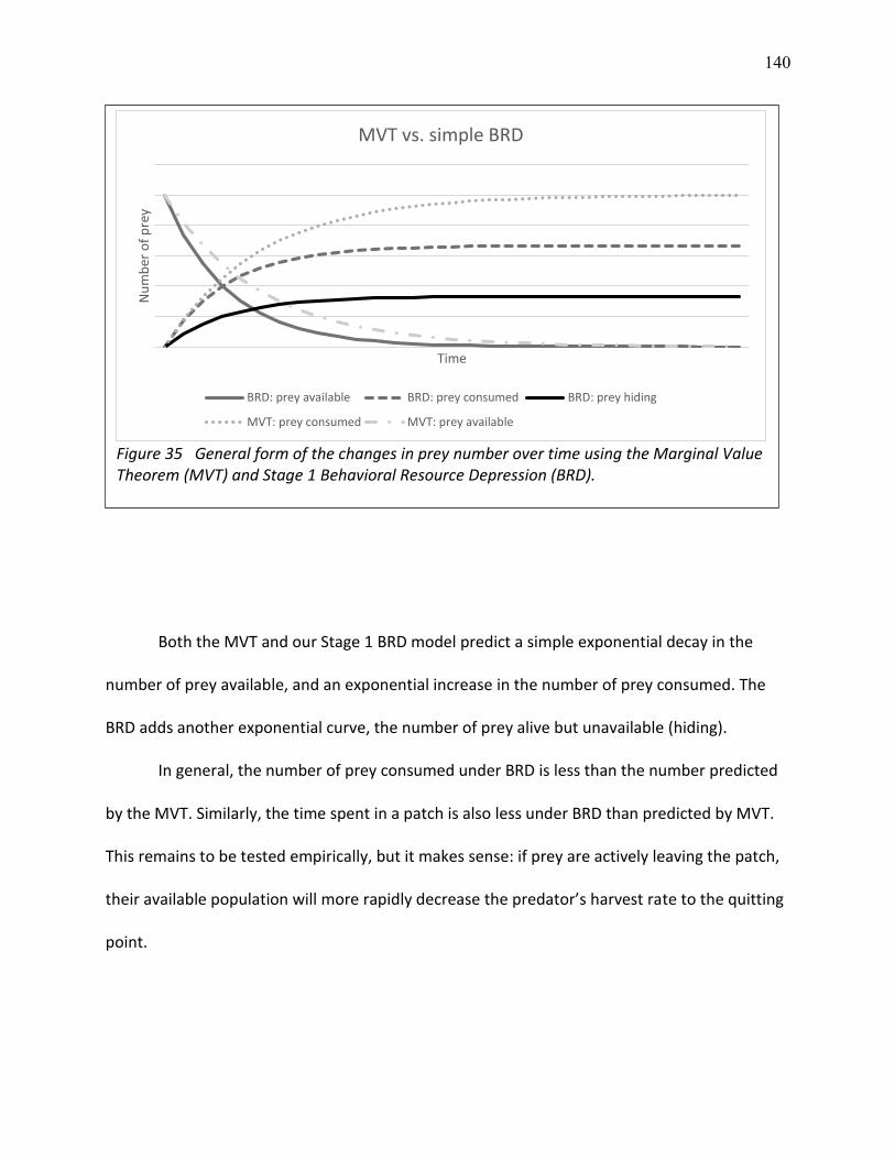
140

Both the MVT and our Stage 1 BRD model predict a simple exponential decay in the

number of prey available, and an exponential increase in the number of prey consumed. The

BRD adds another exponential curve, the number of prey alive but unavailable (hiding).

In general, the number of prey consumed under BRD is less than the number predicted

by the MVT. Similarly, the time spent in a patch is also less under BRD than predicted by MVT.

This remains to be tested empirically, but it makes sense: if prey are actively leaving the patch,

their available population will more rapidly decrease the predator’s harvest rate to the quitting

point.

Figure 35 General form of the changes in prey number over time using the Marginal Value Theorem (MVT) and Stage 1 Behavioral Resource Depression (BRD).

Nu

mb

er o

f p

rey

Time

MVT vs. simple BRD

BRD: prey available BRD: prey consumed BRD: prey hiding

MVT: prey consumed MVT: prey available

141

D. The model Stage 2: behavioral resource depression with slowly regenerating resources,

infinite patches

Stage 1 only covered what happens in a single patch during a single bout of foraging.

However, foragers do not just use one patch, and patches do not just get visited once. While

the forager moves on to a new patch, the recently exploited patch begins to recover. In most

cases, this recovery happens much more slowly. A foraging bout may last minutes or hours, but

recovery may take weeks or months. Therefore, the next stage of building our model is a patch

recovery time. The patch recovers in two ways: some of the prey that were unavailable return

to availability, and new prey are born or grown.

At the time the predator is done with the patch, t*, there are Nt* prey remaining

available to the predator. Because we are now considering time beyond that spent in the patch

along with the number of prey available at foraging's end, let us now call this N*.

The actual prey population size is N* plus the quantity of prey alive but unavailable to

the forager due to hiding.

𝑁 = 𝑁∗ +𝑧

𝑎 + 𝑧(𝑁0 − 𝑁∗)

What happens to the populations both available for foraging and in hiding as time

passes? Assume that during foraging, the prey can either be eaten or go into hiding. Once the

forager leaves the patch, the prey stop going into hiding (z = 0) and begin to return to being

available at some rate. Let r be the rate at which the prey return from hiding; They also begin

reproducing at a rate we shall call b. Let f represent the time since t*, and Nf be the number of

prey potentially available to predators at time f.

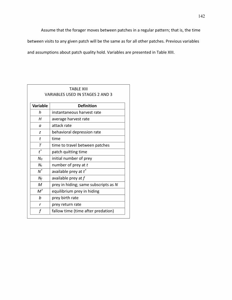
142

Assume that the forager moves between patches in a regular pattern; that is, the time

between visits to any given patch will be the same as for all other patches. Previous variables

and assumptions about patch quality hold. Variables are presented in Table XIII.

TABLE XIII VARIABLES USED IN STAGES 2 AND 3

Variable Definition

h instantaneous harvest rate

H average harvest rate

a attack rate

z behavioral depression rate

t time

T time to travel between patches

t* patch quitting time

N0 initial number of prey

Nt number of prey at t

N* available prey at t*

Nf available prey at f

M prey in hiding; same subscripts as N

M† equilibrium prey in hiding

b prey birth rate

r prey return rate

f fallow time (time after predation)

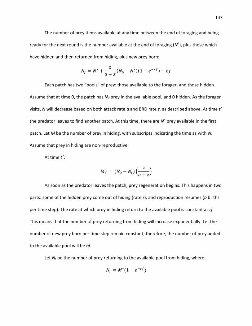
143

The number of prey items available at any time between the end of foraging and being

ready for the next round is the number available at the end of foraging (N*), plus those which

have hidden and then returned from hiding, plus new prey born:

𝑁𝑓 = 𝑁∗ +𝑧

𝑎 + 𝑧(𝑁0 − 𝑁∗)(1 − 𝑒−𝑟𝑓) + 𝑏𝑓

Each patch has two “pools” of prey: those available to the forager, and those hidden.

Assume that at time 0, the patch has N0 prey in the available pool, and 0 hidden. As the forager

visits, N will decrease based on both attack rate a and BRD rate z, as described above. At time t*

the predator leaves to find another patch. At this time, there are N* prey available in the first

patch. Let M be the number of prey in hiding, with subscripts indicating the time as with N.

Assume that prey in hiding are non-reproductive.

At time t*:

𝑀𝑡∗ = (𝑁0 − 𝑁𝑡) (𝑧

𝑎 + 𝑧)

As soon as the predator leaves the patch, prey regeneration begins. This happens in two

parts: some of the hidden prey come out of hiding (rate r), and reproduction resumes (b births

per time step). The rate at which prey in hiding return to the available pool is constant at rf.

This means that the number of prey returning from hiding will increase exponentially. Let the

number of new prey born per time step remain constant; therefore, the number of prey added

to the available pool will be bf.

Let Nr be the number of prey returning to the available pool from hiding, where:

𝑁𝑟 = 𝑀∗(1 − 𝑒−𝑟𝑓)

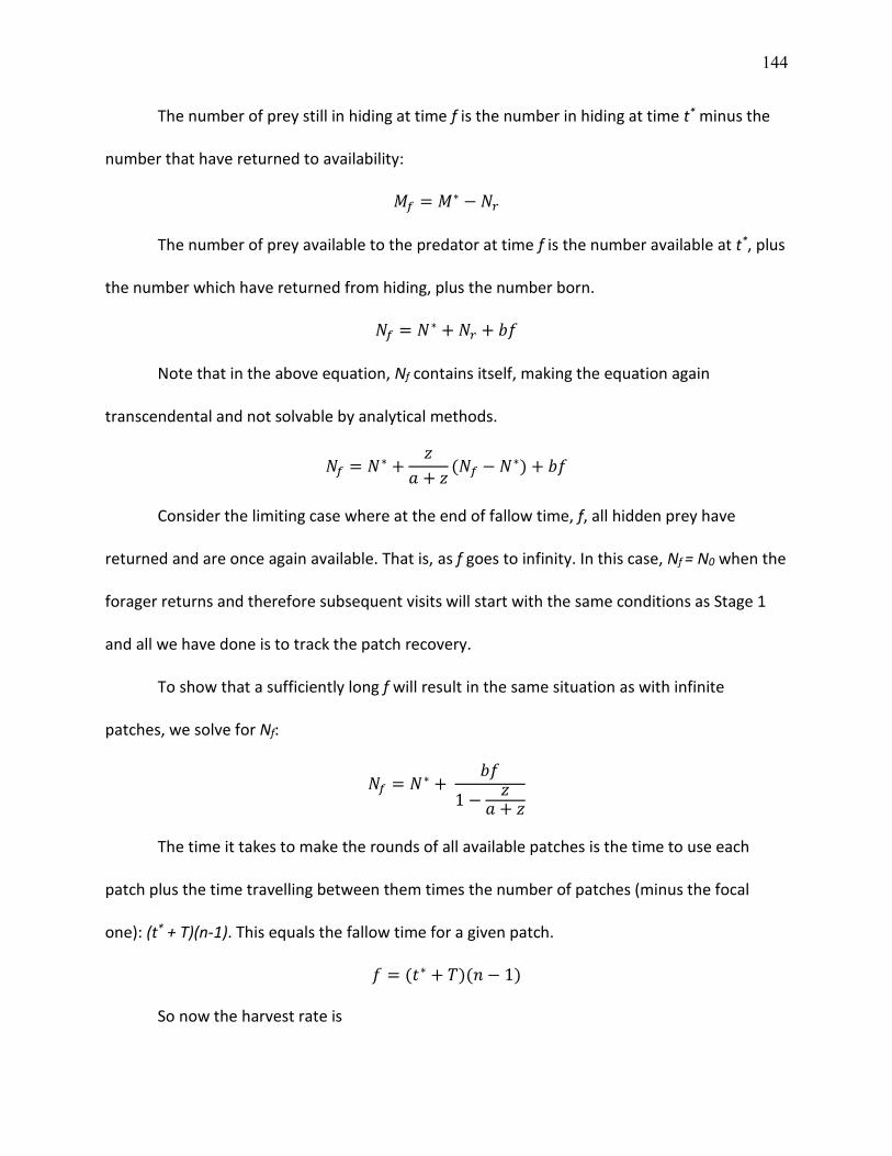
144

The number of prey still in hiding at time f is the number in hiding at time t* minus the

number that have returned to availability:

𝑀𝑓 = 𝑀∗ − 𝑁𝑟

The number of prey available to the predator at time f is the number available at t*, plus

the number which have returned from hiding, plus the number born.

𝑁𝑓 = 𝑁∗ + 𝑁𝑟 + 𝑏𝑓

Note that in the above equation, Nf contains itself, making the equation again

transcendental and not solvable by analytical methods.

𝑁𝑓 = 𝑁∗ +𝑧

𝑎 + 𝑧(𝑁𝑓 − 𝑁∗) + 𝑏𝑓

Consider the limiting case where at the end of fallow time, f, all hidden prey have

returned and are once again available. That is, as f goes to infinity. In this case, Nf = N0 when the

forager returns and therefore subsequent visits will start with the same conditions as Stage 1

and all we have done is to track the patch recovery.

To show that a sufficiently long f will result in the same situation as with infinite

patches, we solve for Nf:

𝑁𝑓 = 𝑁∗ + 𝑏𝑓

1 −𝑧

𝑎 + 𝑧

The time it takes to make the rounds of all available patches is the time to use each

patch plus the time travelling between them times the number of patches (minus the focal

one): (t* + T)(n-1). This equals the fallow time for a given patch.

𝑓 = (𝑡∗ + 𝑇)(𝑛 − 1)

So now the harvest rate is

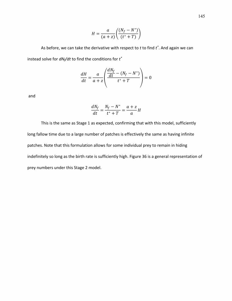
145

𝐻 =𝑎

(𝑎 + 𝑧)(

(𝑁𝑓 − 𝑁∗)

(𝑡∗ + 𝑇))

As before, we can take the derivative with respect to t to find t*. And again we can

instead solve for dNf/dt to find the conditions for t*

𝑑𝐻

𝑑𝑡=

𝑎

𝑎 + 𝑧(

𝑑𝑁𝑓

𝑑𝑡− (𝑁𝑓 − 𝑁∗)

𝑡∗ + 𝑇) = 0

and

𝑑𝑁𝑓

𝑑𝑡=

𝑁𝑓 − 𝑁∗

𝑡∗ + 𝑇=

𝑎 + 𝑧

𝑎𝐻

This is the same as Stage 1 as expected, confirming that with this model, sufficiently

long fallow time due to a large number of patches is effectively the same as having infinite

patches. Note that this formulation allows for some individual prey to remain in hiding

indefinitely so long as the birth rate is sufficiently high. Figure 36 is a general representation of

prey numbers under this Stage 2 model.

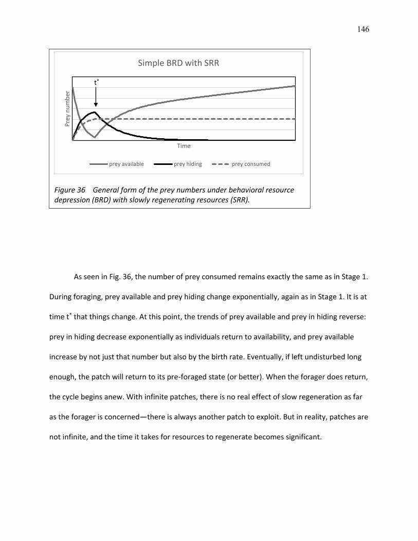
146

As seen in Fig. 36, the number of prey consumed remains exactly the same as in Stage 1.

During foraging, prey available and prey hiding change exponentially, again as in Stage 1. It is at

time t* that things change. At this point, the trends of prey available and prey in hiding reverse:

prey in hiding decrease exponentially as individuals return to availability, and prey available

increase by not just that number but also by the birth rate. Eventually, if left undisturbed long

enough, the patch will return to its pre-foraged state (or better). When the forager does return,

the cycle begins anew. With infinite patches, there is no real effect of slow regeneration as far

as the forager is concerned—there is always another patch to exploit. But in reality, patches are

not infinite, and the time it takes for resources to regenerate becomes significant.

Figure 36 General form of the prey numbers under behavioral resource depression (BRD) with slowly regenerating resources (SRR).

Pre

y n

um

ber

Time

Simple BRD with SRR

prey available prey hiding prey consumed

t*

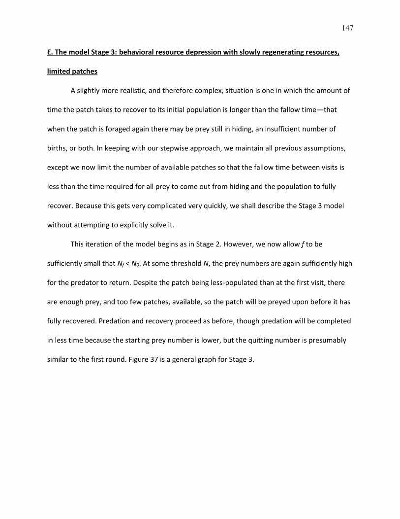
147

E. The model Stage 3: behavioral resource depression with slowly regenerating resources,

limited patches

A slightly more realistic, and therefore complex, situation is one in which the amount of

time the patch takes to recover to its initial population is longer than the fallow time—that

when the patch is foraged again there may be prey still in hiding, an insufficient number of

births, or both. In keeping with our stepwise approach, we maintain all previous assumptions,

except we now limit the number of available patches so that the fallow time between visits is

less than the time required for all prey to come out from hiding and the population to fully

recover. Because this gets very complicated very quickly, we shall describe the Stage 3 model

without attempting to explicitly solve it.

This iteration of the model begins as in Stage 2. However, we now allow f to be

sufficiently small that Nf < N0. At some threshold N, the prey numbers are again sufficiently high

for the predator to return. Despite the patch being less-populated than at the first visit, there

are enough prey, and too few patches, available, so the patch will be preyed upon before it has

fully recovered. Predation and recovery proceed as before, though predation will be completed

in less time because the starting prey number is lower, but the quitting number is presumably

similar to the first round. Figure 37 is a general graph for Stage 3.

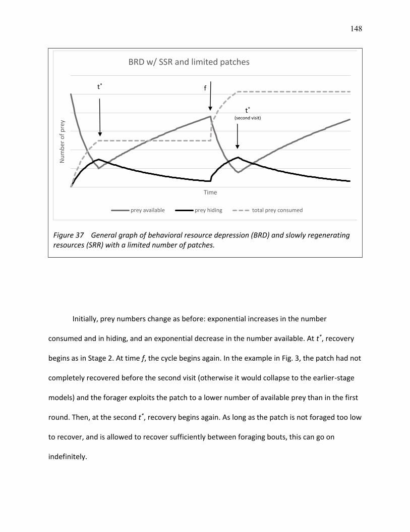
148

Initially, prey numbers change as before: exponential increases in the number

consumed and in hiding, and an exponential decrease in the number available. At t*, recovery

begins as in Stage 2. At time f, the cycle begins again. In the example in Fig. 3, the patch had not

completely recovered before the second visit (otherwise it would collapse to the earlier-stage

models) and the forager exploits the patch to a lower number of available prey than in the first

round. Then, at the second t*, recovery begins again. As long as the patch is not foraged too low

to recover, and is allowed to recover sufficiently between foraging bouts, this can go on

indefinitely.

Figure 37 General graph of behavioral resource depression (BRD) and slowly regenerating resources (SRR) with a limited number of patches.

Nu

mb

er o

f p

rey

Time

BRD w/ SSR and limited patches

prey available prey hiding total prey consumed

t*f

t*

(second visit)

149

At some point, the system should reach an equilibrium, which will include an

equilibrium M, which we call M†. That is, over time the patch will vary in available prey numbers

but the addition of new prey to the “hidden” pool will be balanced by those going back to the

“available” pool. As with all other outcomes, the number of rounds this will take will depend

upon all parameters.

Figure 38 is a simplified schematic of the prey pools at various times.

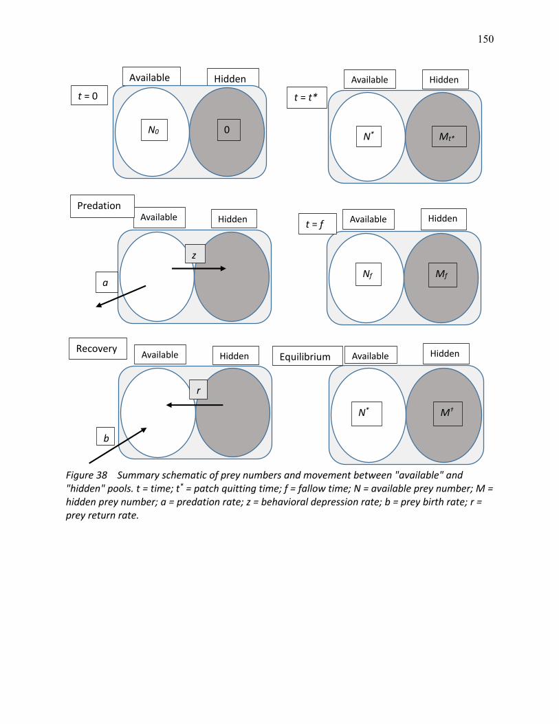
150

Figure 38 Summary schematic of prey numbers and movement between "available" and "hidden" pools. t = time; t* = patch quitting time; f = fallow time; N = available prey number; M = hidden prey number; a = predation rate; z = behavioral depression rate; b = prey birth rate; r = prey return rate.

Available Hidden

t = 0

N0 0

Available Hidden Predation

a

z

Available Hidden Recovery

b

r

Available Hidden

t = t*

N*

Available Hidden t = f

Nf Mf

Available Hidden Equilibrium

M† N*

Mt*

151

F. Discussion and Conclusion

Our models, based on simple additions to the Marginal Value Theorem, are a first-round

attempt at modelling the very complex system of foraging or predating in a patchy environment

where the prey actively make themselves unavailable or less desirable to the predator, then

take time to return to the previous state. These models assume that food patches do recover

from predation at a slow but predictable rate. Though it is not part of the model, there is also

the assumption that when the predator leaves the patch, there are enough remaining prey to

recover from predation; future expansion of the model should include this threshold population

explicitly.

The models presented here represent a very simplified idea of how behavioral resource

depression, coupled with slowly regenerating resources, can affect a foraging animal. There are

unlimited ways in which these models can be expanded. However, before creating more-

complex models and working through them, we should perform some empirical tests to see if

the above models generally hold. We can make numbers do anything, but prey is much more

difficult. This model was inspired by the system of aardvarks preying upon ants and termites.

The prey can both hide in deeper areas of the nest and replace some individuals with toxin-

laden soldiers. These soldiers are presumably a lower-quality food and thus the patch quality is

decreased. Once the aardvark leaves, the nest begins to return to normal. The recovery process

is much slower than the predation. Aardvark predation on ants lasts at most a few minutes

(Taylor et al. 2002), but ant nest recovery takes considerably longer. The figures generated here

compress the recovery time. In reality, f should be several orders of magnitude larger than t.

152

Along with a thorough exploration of the scenario presented in Stage 3, one could

create a dynamical game in which the prey modulates its behavioral depression, return from

hiding, or both, depending on the aggressiveness of the forager, and in which the forager

modulates its aggressiveness in response to prey behavior. One may also consider multiple prey

or patch types. Eventually, any good model must drop the assumption of optimality so as to

better reflect a world where no one is omniscient. This can be done using Bayes’ Theorem, in

which probabilities depend on previous observations rather than some external “true”

probabilities (McNamara et al 2006).

G. Literature cited

Brown JS. 1988. Patch use as an indicator of habitat preference, predation risk, and competition. Behavioral Ecology and Sociobiology 22: 37-47

Brown JS. 1992. Patch Use Under Predation Risk .1. Models and Predictions. Annales Zoologici Fennici 29: 301-09

Brown JS, Mitchell WA. 1989. Diet selection on depletable resources. Oikos 54: 33-43

Brown JS, Morgan RA, Dow BD. 1992. Patch use under predation risk 2. A test with fox squirrels, Sciurus niger. Annales Zoologici Fennici 29: 311-18

Brown JS, Rosenzweig ML. 1986. Habitat selection in slowly regenerating environments. Journal of Theoretical Biology 123: 151-71

Charnov EL. 1976. Optimal foraging, the marginal value theorem. Theoretical Population Biology 9: 129-36

Charnov EL, Orians GH, Hyatt K. 1976. Ecological implications of resource depression. The American Naturalist 110: 247-59

Cibula DA, Zimmerman M. 1984. The effect of plant density on departure decisions: testing the marginal value theorem using bumblebees and Delphinium nelsonii. Oikos 43: 154-58

Fraenkel GS. 1959. The raison d'etre of secondary plant substances Science 129.3361: 1466-70

Harvell CD. 1990. The ecology and evolution of inducible defenses. Quarterly Review of Biology 65: 323-40

Hassell MP. 1978. The dynamics of arthropod predator-prey systems. Princeton University Press.

Hayden BY, Pearson JM, Platt ML. 2011. Neuronal basis of sequential foraging decisions in a patchy environment. Nature Neuroscience 14: 933-39

153

Karban R, Myers JH. 1989. Induced plant responses to herbivory. Annual Review of Ecology and Systematics 20: 331-48

Kelly CK. 1990. Plant foraging: a marginal value model and coiling response in Cuscuta subinclusa. Ecology 71: 1916-25

McNamara JM, Green RF, Olsson O. 2006. Bayes’ theorem and its applications in animal behaviour. Oikos 112: 243-51

Nonacs P. 2001. State dependent behavior and the marginal value theorem. Behavioral Ecology 12: 71-83

O’Brien EE, Brown JS. 2008. Games roots play: effects of soil volume and nutrients. Journal of Ecology 96: 438-46

Pleasants JM. 1989. Optimal foraging by nectarivores: a test of the marginal-value theorem. American Naturalist: 51-71

Possingham HP. 1992. Habitat selection by two species of nectarivore: habitat quality isolines. Ecology 73: 1903-12

Pyke GH. 1978. Optimal foraging in hummingbirds: testing the marginal value theorem. American Zoologist 18: 739-52

Pyke GH. 1984. Optimal foraging theory: a critical review. Annual Review of Ecology and Systematics 15: 523-75

Sargeant AB, Eberhardt LE. 1975. Death feigning by ducks in response to predation by red foxes (Vulpes fulva). American Midland Naturalist: 108-19

Taylor WA, Lindsey PA, Skinner JD. 2002. The feeding ecology of the aardvark Orycteropus afer. Journal of Arid Environments 50: 135-52

Wajnberg E, Fauvergue X, Pons O. 2000. Patch leaving decision rules and the Marginal Value Theorem: an experimental analysis and a simulation model. Behavioral Ecology 11: 577-86

Walling LL. 2000. The myriad plant responses to herbivores. Journal of Plant Growth Regulation 19: 195-216

Watts DP. 1998. Long-term habitat use by mountain gorillas (Gorilla gorilla beringei). 2. Reuse of foraging areas in relation to resource abundance, quality, and depletion. International Journal of Primatology 19: 681-702

Zimmerman M. 1981. Optimal foraging, plant density and the marginal value theorem. Oecologia 49: 148-53

VI. THE ROLE OF HUNGER IN A PREDATOR-PREY FORAGING GAME

A. Introduction

1. Foraging

Few things are as important to an animal as food. Another is to avoid becoming food.

Foragers must constantly assess their situation, considering their own state (whether energy or

hunger), the potential for being preyed upon, the direct and indirect energetic and missed

opportunity costs of searching for and eating food, and the benefits of consuming the food.

What appears to be a simple decision—should I go eat something?—is actually complex,

though this complexity is not conscious (Sih 1980, Lima et al. 1985, Brown et al. 1999, Stephens

2008, McArthur et al. 2014). Researchers have been investigating how costs and benefits play

into a forager’s decisions of when, where, and how to forage, and for what and how long, with

both theoretical and empirical approaches (Stephens et al. 2007).

Theoretical approaches to foraging questions include mathematical models. Traditional

models begin with the optimization of a single factor, then build to include more complexity.

Generally, this means that all factors except the one under study remain static. Even when

multiple factors are considered, the model may remain static; that is, the values of each factor

do not change over the time covered.

Foraging, however, is not done in a vacuum. When a forager goes out in search of food,

it is not the only individual making decisions. The forager’s decisions and outcomes are

influenced by actions of other individuals—their prey, predators, or both. Foraging in fact is a

game with multiple players, each with multiple possible strategies; each player’s best strategy is

155

influenced by the strategies of the others, and strategies can change over time (see Vincent and

Brown 2005). Among the many factors that go into foraging decisions is hunger. Simply put,

hungry individuals will take greater risks than those who do not need to eat any time soon

(Lima and Valone 1986). Hunger can strongly affect immediate foraging decisions (e.g.,

Whitham and Mathis 2000) and even future decisions by affecting learning ability (Marsh et al.

2004).

Game theory allows us to develop and explore many ideas about how individuals and

populations may interact while making their own foraging decisions. As with traditional models,

one must begin with a very simple situation.

We developed a two-player game exploring how hunger affects immediate foraging

decisions made by a forager and its predator. We rely on simple assumptions to greatly

simplify the game and to permit analytic, generalizable results. As our model system, we use a

real, well-studied foraging game played every night—that between gerbils searching for seeds

and owls hunting for gerbils.

2. The real-world inspiration

In the deserts of the Middle East, foraging games in which gerbils forage for seeds and

both owls and snakes hunt for gerbils unfold every night (Brown et al. 2001). The gerbils are

safe in their burrows, but face danger from owls when foraging out in the open, and snakes

when foraging under bushes. The two predators essentially help one another: when gerbils hide

from owls, they are in snake territory, and when running from snakes they end up out in the

open, where owls can easily spot and capture them.

156

This game of predator facilitation (Kotler et al. 1992, 1993) has been explored for many

years, notably by Brown et al. (2001) who modeled a game between gerbils and their predators

with a focus on the pulsed (regularly renewed en masse) gerbil food. Bouskila (2001) explored

habitat selection of kangaroo rats facing the risk of predation by both owls and snakes. These

two papers followed a tradition of predator–prey games begun by Brown and Vincent (1992)

and Hugie and Dill (1993). The first predator–prey models were created in the early 20th century

by AJ Lotka and V Volterra; game theory was first applied to evolutionary biology in 1961 by

Lewontin, and Maynard Smith (1974) neatly outlined evolutionary game theory and thus paved

the way for these dynamic models, in which the players actively influence one another.

In our real-world example, gerbils who are not hungry will stay in the burrow, but

hungry gerbils must take the risk of foraging (e.g., Lima et al. 1985). In turn, the owls and snakes

expend energy and take risks in hunting gerbils, and have no reason to do so unless a) there are

gerbils to hunt, and b) they are sufficiently hungry so as to be willing to take the risks. As

implied by b), this is a state-dependent game, as the energetic state (hunger level) determines

the players’ motivation to forage and the payoffs associated with acquiring food (predator) or

suffering mortality (prey).

We created, from scratch, a model of the effects of hunger on foraging decisions. We

asked how the hunger level of foragers (prey gerbils and predator owls) dictate each other’s

foraging outcomes and fitness. While the game played in the gerbil–owl system has been the

basis for both practical and theoretical work, we chose to use this game as inspiration for a

more general foraging game in which the hunger state of the players is the primary driver of

foraging strategy decisions.

157

B. The models

Stage 1: The matrix

For this model, we assume a one-predator–one-prey system. For simplicity of

terminology, we have chosen to use owls as our example predator and gerbils as our example

prey. However, this model is not meant to apply specifically to this system, and is thus kept

general in form. For this game, payoffs are measured as net change in hunger state.

Evolutionary games generally have fitness, a measure of reproductive success, as the ultimate

payoff, but here we chose the more immediate payoff of survival until the next day.

We built our model one step at a time, beginning with no state-dependence. For this

stage, we used a two-player binary non-zero-sum matrix game. That is, there are two players

(owl and gerbil), each with two possible strategies (forage or do not forage), the sum of the

payoffs to each is variable, and the game can be described mathematically using a matrix.

Variables (see Table XIV for definitions) were not assigned variables or even ranges of

variables, with the exception of any probability variables, which were constrained between zero

and one (inclusive or exclusive depending on the variable). All other variables were assigned

values for simulations as needed to meet the assumptions of the model or the conditions of the

simulation; some values were chosen to create a representative graph of the expected

outcome.

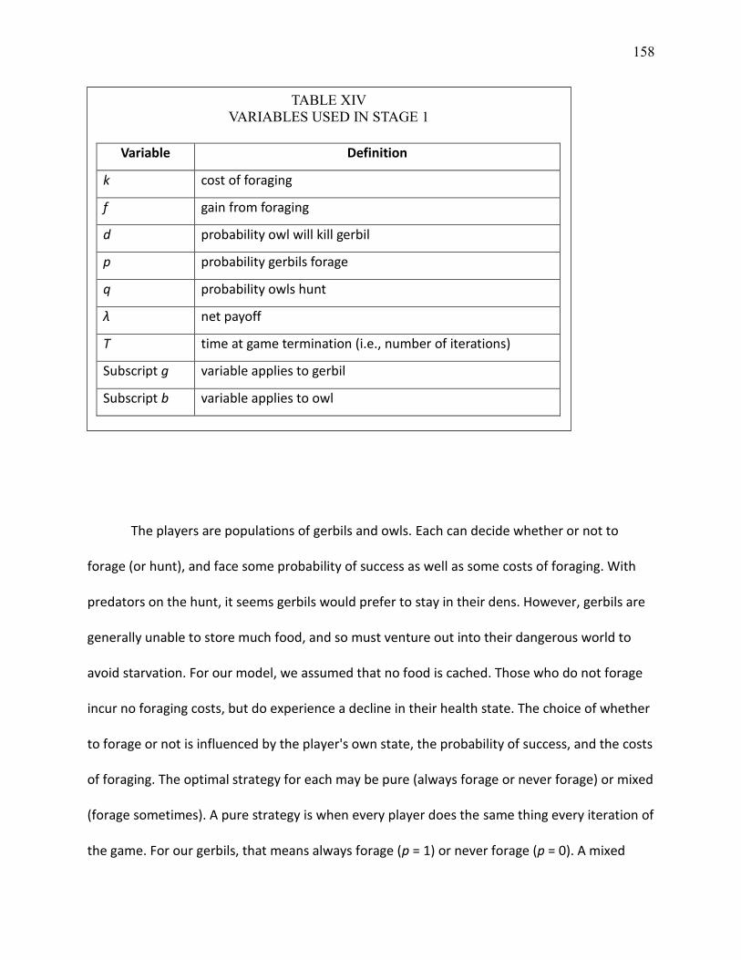
158

The players are populations of gerbils and owls. Each can decide whether or not to

forage (or hunt), and face some probability of success as well as some costs of foraging. With

predators on the hunt, it seems gerbils would prefer to stay in their dens. However, gerbils are

generally unable to store much food, and so must venture out into their dangerous world to

avoid starvation. For our model, we assumed that no food is cached. Those who do not forage

incur no foraging costs, but do experience a decline in their health state. The choice of whether

to forage or not is influenced by the player's own state, the probability of success, and the costs

of foraging. The optimal strategy for each may be pure (always forage or never forage) or mixed

(forage sometimes). A pure strategy is when every player does the same thing every iteration of

the game. For our gerbils, that means always forage (p = 1) or never forage (p = 0). A mixed

TABLE XIV

VARIABLES USED IN STAGE 1

Variable Definition

k cost of foraging

f gain from foraging

d probability owl will kill gerbil

p probability gerbils forage

q probability owls hunt

λ net payoff

T time at game termination (i.e., number of iterations)

Subscript g variable applies to gerbil

Subscript b variable applies to owl

159

strategy is when the player sometimes forages and sometimes does not, which means any

value of 0 < p < 1. A mixed strategy is represented by the proportion of time an individual plays

each of its available strategies. A mixed strategy can also be the proportion of a group of

players on the same “team” that are playing each strategy. In our scenario, gerbils and owls can

also be thought of as playing as teams; as long as each team divides its players in the right

proportions the game works the same way. This is because it’s not really players we are

concerned with but strategies. If the ESS requires that the gerbils be at p = 0.3, then gerbils

must, as a whole, forage 30% of the time. While it certainly matters for real gerbils,

mathematically it makes no difference whether 30% of individuals forage all the time and the

rest never forage, each individual forages 30% of the time, or something else. Because food is

needed by each individual, we can assume that in this model the mixed strategy applies to each

individual.

The net gain or loss is known as a payoff. To explore the game, we can construct a

payoff matrix with both players’ payoffs for each possible strategy. Here we use two matrices,

one with the payoffs to the gerbil, the other with the payoffs to the owl. The entry for each cell

of the matrix contains the payoff to the given player if the gerbil plays the row strategy and the

owl plays the column strategy. Therefore, the payoff to the gerbil when it does not forage and

the owl does not hunt is 0 (Fig. 39).

160

The expected payoff is the sum of the payoffs in each possible scenario (gerbil foraging,

owl not hunting; gerbil foraging, owl hunting; etc.) at the proportions of time at which each

occurs. Each player wants to maximize its own payoff, but their options are limited by what the

other player is doing. If the owls are hunting, the gerbils cannot get the payoff they would if

owls were not hunting.

The set of strategies at which the model will settle over time is known as the

evolutionarily stable strategy (ESS). When the system is at an ESS, neither player (or team) will

change their strategy; any slight change in strategy will lead to a poorer outcome. The set of

strategies at an ESS are said to be un-invadable, as a newcomer with a different strategy will be

unable to successfully invade the system (Vincent and Brown 2005).

(a) Owl strategy

Do not hunt Hunt

Gerbil strategy Do not forage 0 0

Forage fg - kg fg - kg - dg

(b) Owl strategy

Do not hunt Hunt

Gerbil strategy Do not forage 0 -kb

Forage 0 fb - kb

Figure 39 Payoff matrix for Stage 1 game. (a) Payoff to the owl; (b) payoff to the gerbil. Variables are as defined in Table XIV.

161

ESS always involve both players—gerbil strategies are influenced by owl strategies and

owl strategies are influenced by gerbil strategies. A strategy cannot be an ESS if the player

(team) could benefit by changing its strategy, assuming the opposing team doesn’t also change

strategies. An evolutionarily stable strategy is one that cannot be successfully invaded by a

slightly different strategy. If the gerbils would have a better payoff by foraging slightly more

often, then they were not at an ESS. When the system is at an ESS, gerbils foraging have the

same payoff as gerbils not foraging, and owls hunting have the same payoff as owls not

hunting.

Assume that gerbils that forage will do so successfully except when killed by an owl (that

is, there is always food available for the gerbils and they will find it). Owls are successful in

hunting at a rate of d as long as there are gerbils to be caught (that is, if the probability of

gerbils foraging is > 0). Assume that animals not out foraging or hunting have no gains or losses.

Owls that hunt when gerbils are all in hiding will bear the cost of foraging but no gain, as they

cannot catch what is not there. Gerbils have a probability of foraging of p, and therefore a

probability of not foraging of (1-p). Owls similarly have a hunting probability of q and a not-

hunting probability of (1-q). We assume an effectively infinite population.

If the gerbils do not forage, they have a payoff of zero regardless of the owl’s strategy,

as they remain in safety (no cost) but do not forage (no gain) (Table 6.2a). If they forage but the

owls are not hunting, the gerbil’s payoff is a simple gain of fg, minus the cost of foraging of kg. If

the gerbils forage and the owls hunt, the gerbils’ net payoff is the same as when the owls are

not hunting, minus the possibility of being killed by the owls. We assume this probability as an

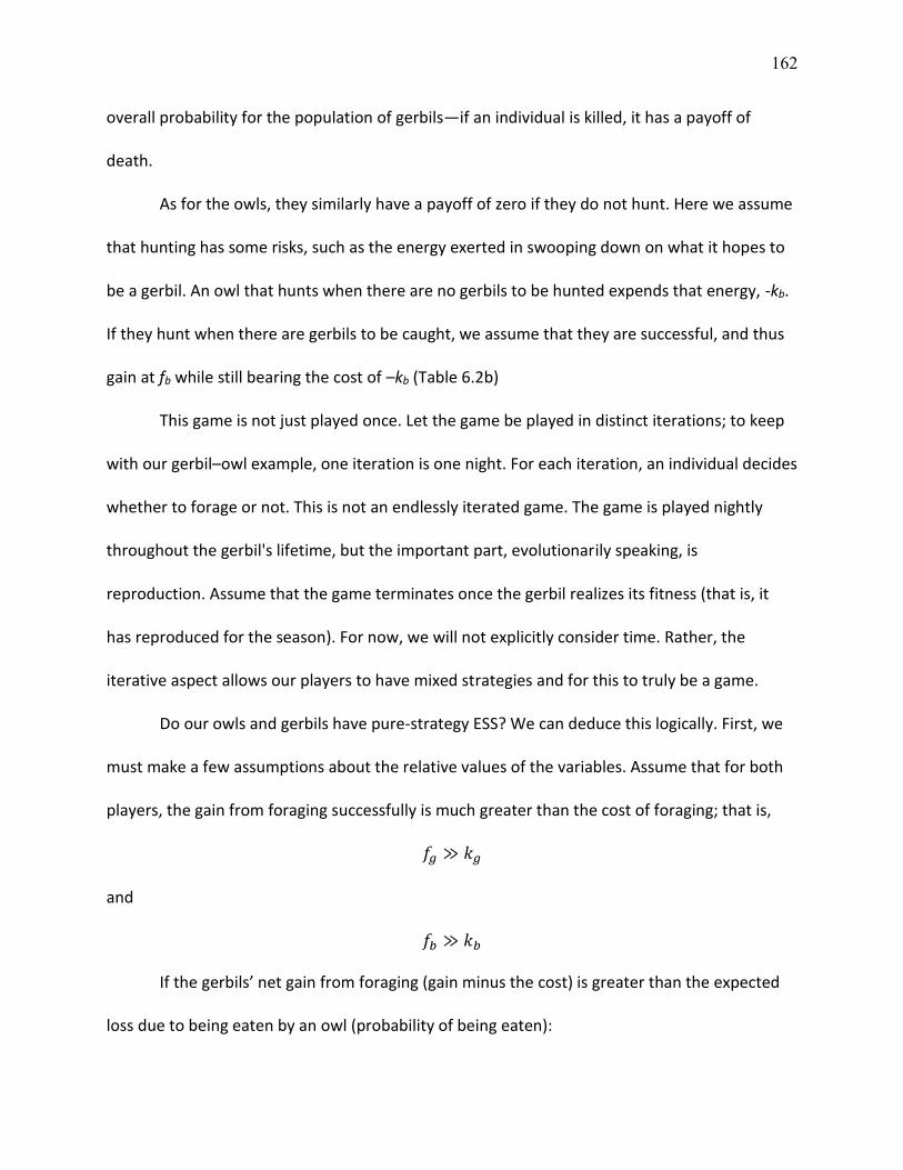
162

overall probability for the population of gerbils—if an individual is killed, it has a payoff of

death.

As for the owls, they similarly have a payoff of zero if they do not hunt. Here we assume

that hunting has some risks, such as the energy exerted in swooping down on what it hopes to

be a gerbil. An owl that hunts when there are no gerbils to be hunted expends that energy, -kb.

If they hunt when there are gerbils to be caught, we assume that they are successful, and thus

gain at fb while still bearing the cost of –kb (Table 6.2b)

This game is not just played once. Let the game be played in distinct iterations; to keep

with our gerbil–owl example, one iteration is one night. For each iteration, an individual decides

whether to forage or not. This is not an endlessly iterated game. The game is played nightly

throughout the gerbil's lifetime, but the important part, evolutionarily speaking, is

reproduction. Assume that the game terminates once the gerbil realizes its fitness (that is, it

has reproduced for the season). For now, we will not explicitly consider time. Rather, the

iterative aspect allows our players to have mixed strategies and for this to truly be a game.

Do our owls and gerbils have pure-strategy ESS? We can deduce this logically. First, we

must make a few assumptions about the relative values of the variables. Assume that for both

players, the gain from foraging successfully is much greater than the cost of foraging; that is,

𝑓𝑔 ≫ 𝑘𝑔

and

𝑓𝑏 ≫ 𝑘𝑏

If the gerbils’ net gain from foraging (gain minus the cost) is greater than the expected

loss due to being eaten by an owl (probability of being eaten):

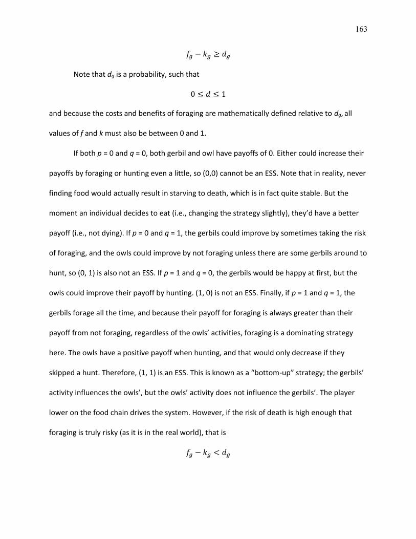
163

𝑓𝑔 − 𝑘𝑔 ≥ 𝑑𝑔

Note that dg is a probability, such that

0 ≤ 𝑑 ≤ 1

and because the costs and benefits of foraging are mathematically defined relative to dg, all

values of f and k must also be between 0 and 1.

If both p = 0 and q = 0, both gerbil and owl have payoffs of 0. Either could increase their

payoffs by foraging or hunting even a little, so (0,0) cannot be an ESS. Note that in reality, never

finding food would actually result in starving to death, which is in fact quite stable. But the

moment an individual decides to eat (i.e., changing the strategy slightly), they’d have a better

payoff (i.e., not dying). If p = 0 and q = 1, the gerbils could improve by sometimes taking the risk

of foraging, and the owls could improve by not foraging unless there are some gerbils around to

hunt, so (0, 1) is also not an ESS. If p = 1 and q = 0, the gerbils would be happy at first, but the

owls could improve their payoff by hunting. (1, 0) is not an ESS. Finally, if p = 1 and q = 1, the

gerbils forage all the time, and because their payoff for foraging is always greater than their

payoff from not foraging, regardless of the owls’ activities, foraging is a dominating strategy

here. The owls have a positive payoff when hunting, and that would only decrease if they

skipped a hunt. Therefore, (1, 1) is an ESS. This is known as a “bottom-up” strategy; the gerbils’

activity influences the owls’, but the owls’ activity does not influence the gerbils’. The player

lower on the food chain drives the system. However, if the risk of death is high enough that

foraging is truly risky (as it is in the real world), that is

𝑓𝑔 − 𝑘𝑔 < 𝑑𝑔

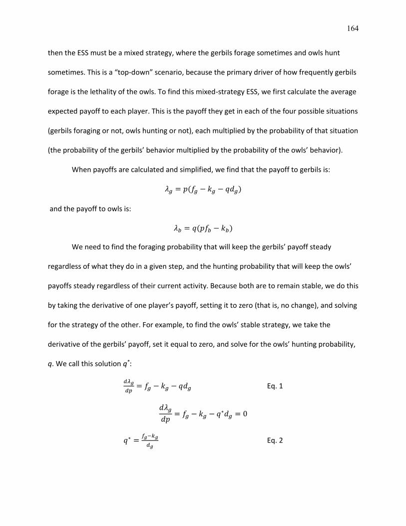
164

then the ESS must be a mixed strategy, where the gerbils forage sometimes and owls hunt

sometimes. This is a “top-down” scenario, because the primary driver of how frequently gerbils

forage is the lethality of the owls. To find this mixed-strategy ESS, we first calculate the average

expected payoff to each player. This is the payoff they get in each of the four possible situations

(gerbils foraging or not, owls hunting or not), each multiplied by the probability of that situation

(the probability of the gerbils’ behavior multiplied by the probability of the owls’ behavior).

When payoffs are calculated and simplified, we find that the payoff to gerbils is:

𝜆𝑔 = 𝑝(𝑓𝑔 − 𝑘𝑔 − 𝑞𝑑𝑔)

and the payoff to owls is:

𝜆𝑏 = 𝑞(𝑝𝑓𝑏 − 𝑘𝑏)

We need to find the foraging probability that will keep the gerbils’ payoff steady

regardless of what they do in a given step, and the hunting probability that will keep the owls’

payoffs steady regardless of their current activity. Because both are to remain stable, we do this

by taking the derivative of one player’s payoff, setting it to zero (that is, no change), and solving

for the strategy of the other. For example, to find the owls’ stable strategy, we take the

derivative of the gerbils’ payoff, set it equal to zero, and solve for the owls’ hunting probability,

q. We call this solution q*:

𝑑𝜆𝑔

𝑑𝑝= 𝑓𝑔 − 𝑘𝑔 − 𝑞𝑑𝑔 Eq. 1

𝑑𝜆𝑔

𝑑𝑝= 𝑓𝑔 − 𝑘𝑔 − 𝑞∗𝑑𝑔 = 0

𝑞∗ =𝑓𝑔−𝑘𝑔

𝑑𝑔 Eq. 2

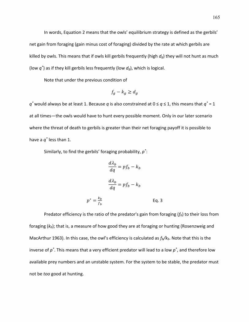
165

In words, Equation 2 means that the owls’ equilibrium strategy is defined as the gerbils’

net gain from foraging (gain minus cost of foraging) divided by the rate at which gerbils are

killed by owls. This means that if owls kill gerbils frequently (high dg) they will not hunt as much

(low q*) as if they kill gerbils less frequently (low dg), which is logical.

Note that under the previous condition of

𝑓𝑔 − 𝑘𝑔 ≥ 𝑑𝑔

q* would always be at least 1. Because q is also constrained at 0 ≤ q ≤ 1, this means that q* = 1

at all times—the owls would have to hunt every possible moment. Only in our later scenario

where the threat of death to gerbils is greater than their net foraging payoff it is possible to

have a q* less than 1.

Similarly, to find the gerbils’ foraging probability, p*:

𝑑𝜆𝑏

𝑑𝑞= 𝑝𝑓𝑏 − 𝑘𝑏

𝑑𝜆𝑏

𝑑𝑞= 𝑝𝑓𝑏 − 𝑘𝑏

𝑝∗ =𝑘𝑏

𝑓𝑏 Eq. 3

Predator efficiency is the ratio of the predator's gain from foraging (fb) to their loss from

foraging (kb); that is, a measure of how good they are at foraging or hunting (Rosenzweig and

MacArthur 1963). In this case, the owl’s efficiency is calculated as fb/kb. Note that this is the

inverse of p*. This means that a very efficient predator will lead to a low p*, and therefore low

available prey numbers and an unstable system. For the system to be stable, the predator must

not be too good at hunting.

166

The model (Stage 1), represented by Equations 1 and 2, reveals the point at which the

gerbil payoff crosses zero (q*) and the point at which the owl payoff crosses zero (p*). Figure 40

shows an example of how payoffs change depending on foraging probabilities. In general,

gerbils’ payoffs will be positive as long as owls are hunting at a rate below some threshold, and

negative if owls hunt more. The point at which gerbil payoffs are zero is the owl portion of the

ESS. Similarly, owl payoffs will be negative when gerbils are foraging below some threshold

rate, and positive above this rate. The rate at which gerbil foraging results in an owl payoff of

zero is their part of the ESS. In this most simple of games we see the owls and gerbils both

foraging quite often, the exact amount depending on what they gain as well as their basic risks.

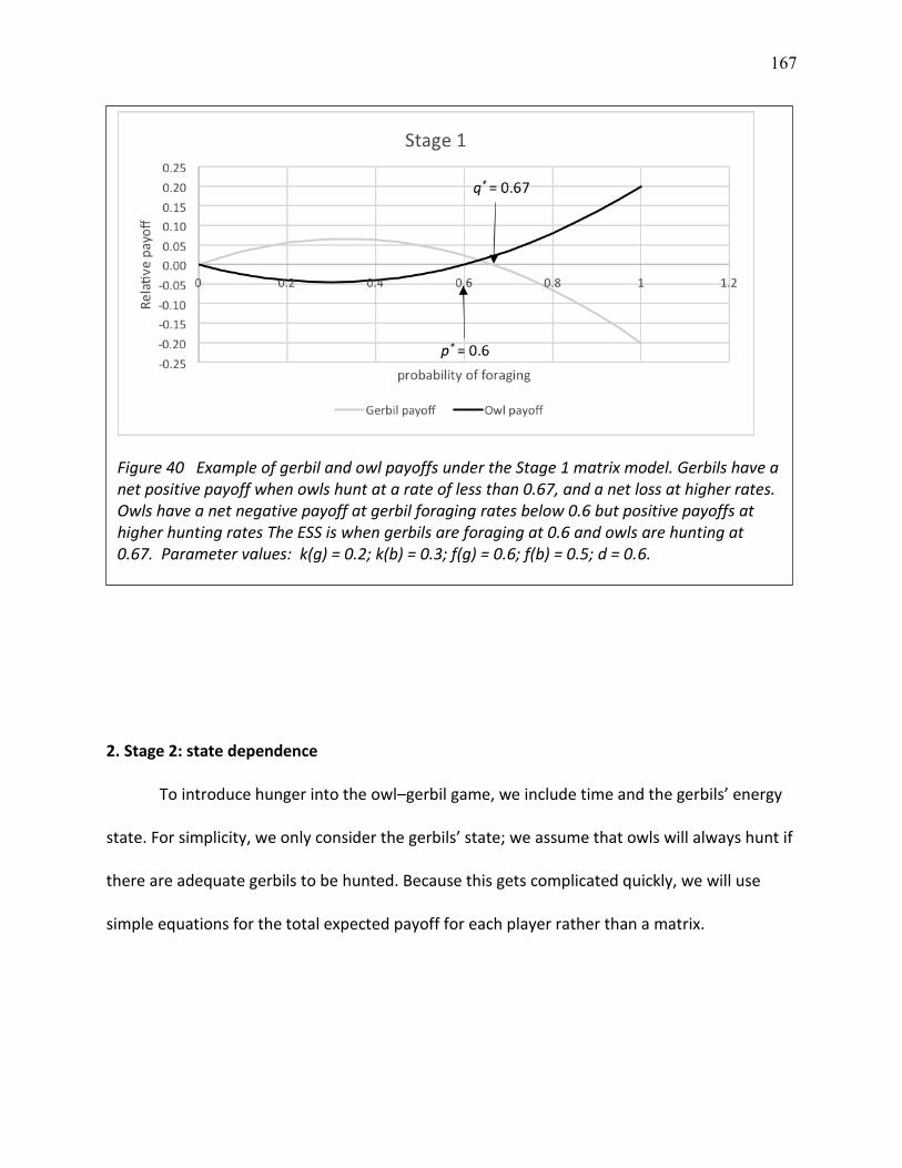
167

2. Stage 2: state dependence

To introduce hunger into the owl–gerbil game, we include time and the gerbils’ energy

state. For simplicity, we only consider the gerbils’ state; we assume that owls will always hunt if

there are adequate gerbils to be hunted. Because this gets complicated quickly, we will use

simple equations for the total expected payoff for each player rather than a matrix.

Figure 40 Example of gerbil and owl payoffs under the Stage 1 matrix model. Gerbils have a net positive payoff when owls hunt at a rate of less than 0.67, and a net loss at higher rates. Owls have a net negative payoff at gerbil foraging rates below 0.6 but positive payoffs at higher hunting rates The ESS is when gerbils are foraging at 0.6 and owls are hunting at 0.67. Parameter values: k(g) = 0.2; k(b) = 0.3; f(g) = 0.6; f(b) = 0.5; d = 0.6.

168

We will now consider the time (T) over which the game is played: the time until gerbil

reproduction. We add several more variables in this stage. Table XV summarizes all variables

used in Stage 2. The game starts anew after the breeding season.

TABLE XV VARIABLES USED IN STAGE 2

variable definition

k cost of foraging

f gain from foraging

d probability owl will kill gerbil

p probability gerbils forage

q probability owls hunt

λ net payoff

T time at game termination (i.e., number of iterations)

E0 initial energy state (gerbil)

ET terminal energy state (gerbil)

m metabolic cost of living

α scaling for effect of hunger state

Subscript g variable applies to gerbil

Subscript b variable applies to owl

169

The gerbil begins at some energy state E0. In the simplest case, assuming there are no

owls and the gerbil forages, the gerbil’s energy state at the next time step is

𝐸1 = 𝐸0 + 𝑓𝑔 − 𝑘𝑔

That is, the gerbils' energy state at time step 1 is their starting energy state at time zero,

plus any gains from foraging, minus the cost of foraging. If the individual does not forage, f and

k are zero, and E1 = E0. To find the gerbils' energy state at the termination of a game, time T, we

must consider the gain and loss from foraging in each time step.

𝐸𝑇 = 𝐸0 + (𝑓𝑔 − 𝑘𝑔)𝑝𝑇

Specifically, energy at time T is equal to starting energy plus the product of the net gain

from foraging, the proportion of time spent foraging, and time. In this formulation, there is no

penalty for not foraging, and foraging always results in a net energy gain (as defined earlier, f >>

k).

This is of course entirely unrealistic; if there were no energy lost by simply living, gerbils

would stay in their burrows, never seeing a decrease in energy state and never needing to take

the risks of foraging. However, not eating does decrease one’s energy state (or in other words,

increases one’s hunger). Let m be the metabolic cost of living, whether animals are foraging or

not. We had not considered m earlier as it is a fixed cost, unlike the variable cost of foraging k.

Now that we are considering energy state and the changes in state over time, m begins to

affect other variables (m itself is still assumed to be constant).

So now, energy at time T is equal to starting energy plus energy plus the product of the

net gain from foraging, the proportion of time spent foraging, and time minus the product of

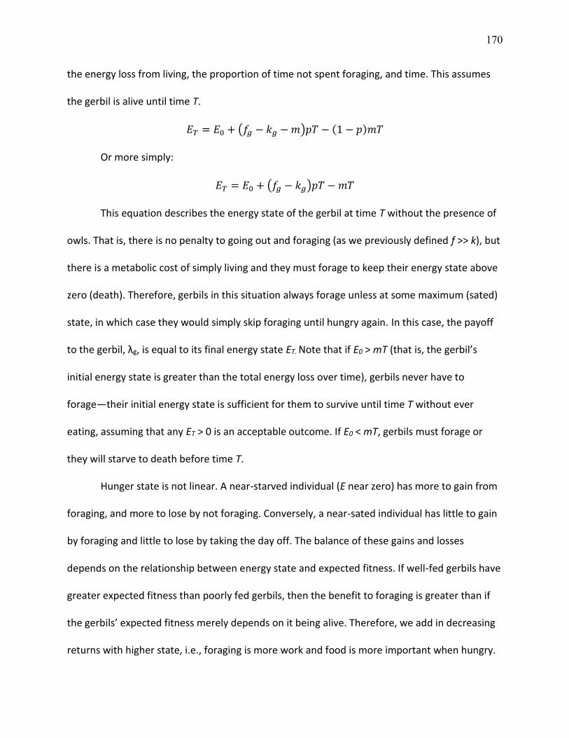
170

the energy loss from living, the proportion of time not spent foraging, and time. This assumes

the gerbil is alive until time T.

𝐸𝑇 = 𝐸0 + (𝑓𝑔 − 𝑘𝑔 − 𝑚)𝑝𝑇 − (1 − 𝑝)𝑚𝑇

Or more simply:

𝐸𝑇 = 𝐸0 + (𝑓𝑔 − 𝑘𝑔)𝑝𝑇 − 𝑚𝑇

This equation describes the energy state of the gerbil at time T without the presence of

owls. That is, there is no penalty to going out and foraging (as we previously defined f >> k), but

there is a metabolic cost of simply living and they must forage to keep their energy state above

zero (death). Therefore, gerbils in this situation always forage unless at some maximum (sated)

state, in which case they would simply skip foraging until hungry again. In this case, the payoff

to the gerbil, λg, is equal to its final energy state ET. Note that if E0 > mT (that is, the gerbil’s

initial energy state is greater than the total energy loss over time), gerbils never have to

forage—their initial energy state is sufficient for them to survive until time T without ever

eating, assuming that any ET > 0 is an acceptable outcome. If E0 < mT, gerbils must forage or

they will starve to death before time T.

Hunger state is not linear. A near-starved individual (E near zero) has more to gain from

foraging, and more to lose by not foraging. Conversely, a near-sated individual has little to gain

by foraging and little to lose by taking the day off. The balance of these gains and losses

depends on the relationship between energy state and expected fitness. If well-fed gerbils have

greater expected fitness than poorly fed gerbils, then the benefit to foraging is greater than if

the gerbils’ expected fitness merely depends on it being alive. Therefore, we add in decreasing

returns with higher state, i.e., foraging is more work and food is more important when hungry.

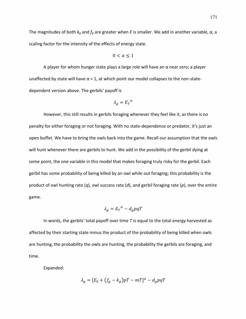
171

The magnitudes of both kg and fg are greater when E is smaller. We add in another variable, α, a

scaling factor for the intensity of the effects of energy state.

0 < 𝛼 ≤ 1

A player for whom hunger state plays a large role will have an α near zero; a player

unaffected by state will have α = 1, at which point our model collapses to the non-state-

dependent version above. The gerbils’ payoff is

𝜆𝑔 = 𝐸𝑇𝛼

However, this still results in gerbils foraging whenever they feel like it, as there is no

penalty for either foraging or not foraging. With no state-dependence or predator, it's just an

open buffet. We have to bring the owls back into the game. Recall our assumption that the owls

will hunt whenever there are gerbils to hunt. We add in the possibility of the gerbil dying at

some point, the one variable in this model that makes foraging truly risky for the gerbil. Each

gerbil has some probability of being killed by an owl while out foraging; this probability is the

product of owl hunting rate (q), owl success rate (d), and gerbil foraging rate (p), over the entire

game.

𝜆𝑔 = 𝐸𝑇𝛼 − 𝑑𝑔𝑝𝑞𝑇

In words, the gerbils’ total payoff over time T is equal to the total energy harvested as

affected by their starting state minus the product of the probability of being killed when owls

are hunting, the probability the owls are hunting, the probability the gerbils are foraging, and

time.

Expanded:

𝜆𝑔 = [𝐸0 + (𝑓𝑔 − 𝑘𝑔)𝑝𝑇 − 𝑚𝑇]𝛼 − 𝑑𝑔𝑝𝑞𝑇

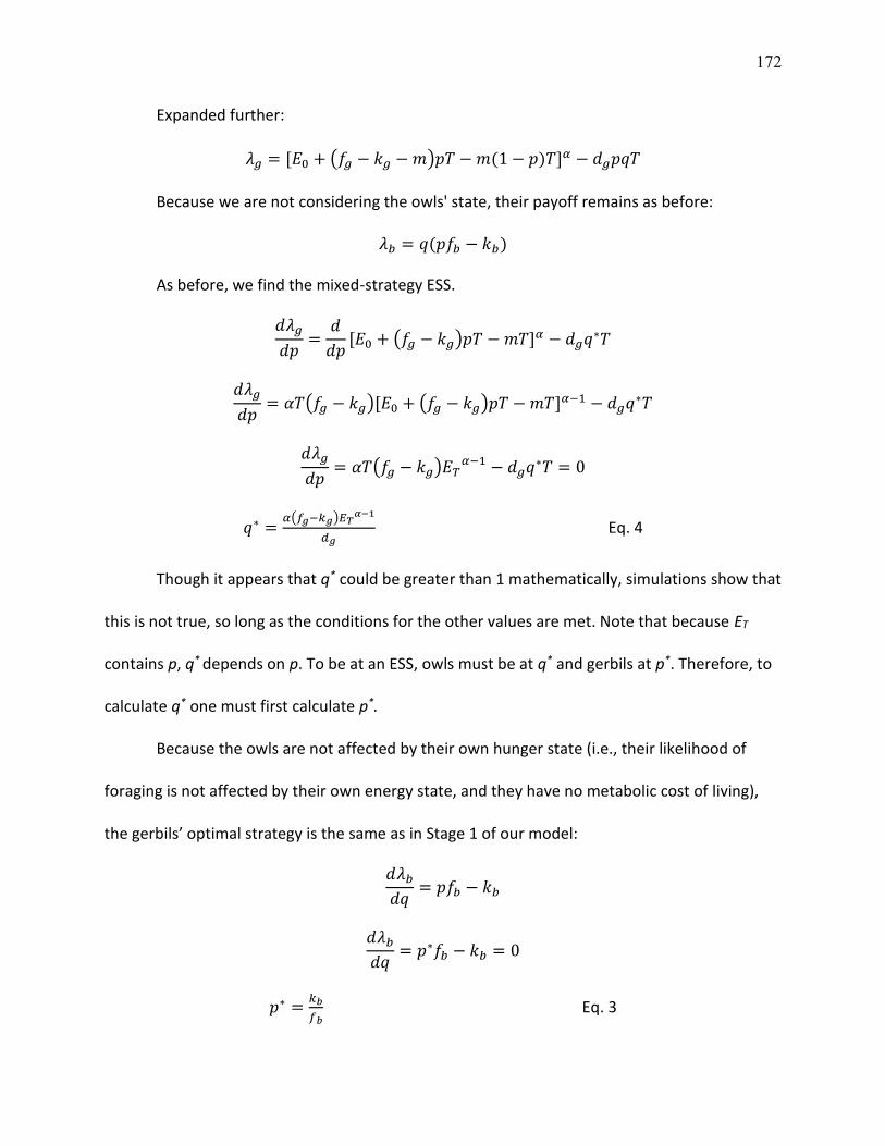
172

Expanded further:

𝜆𝑔 = [𝐸0 + (𝑓𝑔 − 𝑘𝑔 − 𝑚)𝑝𝑇 − 𝑚(1 − 𝑝)𝑇]𝛼 − 𝑑𝑔𝑝𝑞𝑇

Because we are not considering the owls' state, their payoff remains as before:

𝜆𝑏 = 𝑞(𝑝𝑓𝑏 − 𝑘𝑏)

As before, we find the mixed-strategy ESS.

𝑑𝜆𝑔

𝑑𝑝=

𝑑

𝑑𝑝[𝐸0 + (𝑓𝑔 − 𝑘𝑔)𝑝𝑇 − 𝑚𝑇]𝛼 − 𝑑𝑔𝑞∗𝑇

𝑑𝜆𝑔

𝑑𝑝= 𝛼𝑇(𝑓𝑔 − 𝑘𝑔)[𝐸0 + (𝑓𝑔 − 𝑘𝑔)𝑝𝑇 − 𝑚𝑇]𝛼−1 − 𝑑𝑔𝑞∗𝑇

𝑑𝜆𝑔

𝑑𝑝= 𝛼𝑇(𝑓𝑔 − 𝑘𝑔)𝐸𝑇

𝛼−1 − 𝑑𝑔𝑞∗𝑇 = 0

𝑞∗ =𝛼(𝑓𝑔−𝑘𝑔)𝐸𝑇

𝛼−1

𝑑𝑔 Eq. 4

Though it appears that q* could be greater than 1 mathematically, simulations show that

this is not true, so long as the conditions for the other values are met. Note that because ET

contains p, q* depends on p. To be at an ESS, owls must be at q* and gerbils at p*. Therefore, to

calculate q* one must first calculate p*.

Because the owls are not affected by their own hunger state (i.e., their likelihood of

foraging is not affected by their own energy state, and they have no metabolic cost of living),

the gerbils’ optimal strategy is the same as in Stage 1 of our model:

𝑑𝜆𝑏

𝑑𝑞= 𝑝𝑓𝑏 − 𝑘𝑏

𝑑𝜆𝑏

𝑑𝑞= 𝑝∗𝑓𝑏 − 𝑘𝑏 = 0

𝑝∗ =𝑘𝑏

𝑓𝑏 Eq. 3

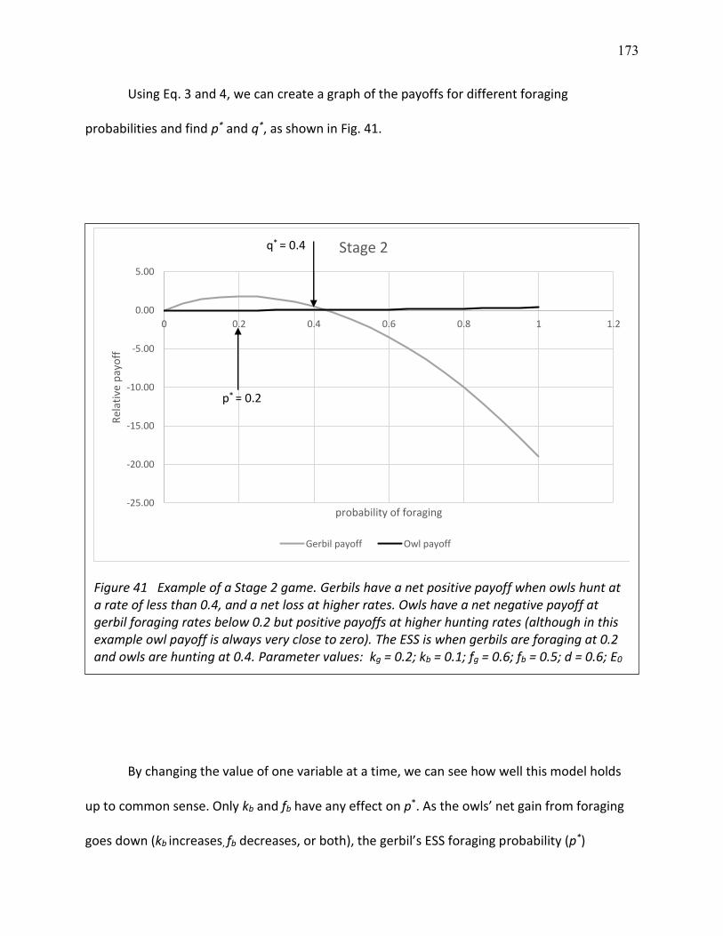
173

Using Eq. 3 and 4, we can create a graph of the payoffs for different foraging

probabilities and find p* and q*, as shown in Fig. 41.

By changing the value of one variable at a time, we can see how well this model holds

up to common sense. Only kb and fb have any effect on p*. As the owls’ net gain from foraging

goes down (kb increases, fb decreases, or both), the gerbil’s ESS foraging probability (p*)

Figure 41 Example of a Stage 2 game. Gerbils have a net positive payoff when owls hunt at a rate of less than 0.4, and a net loss at higher rates. Owls have a net negative payoff at gerbil foraging rates below 0.2 but positive payoffs at higher hunting rates (although in this example owl payoff is always very close to zero). The ESS is when gerbils are foraging at 0.2 and owls are hunting at 0.4. Parameter values: kg = 0.2; kb = 0.1; fg = 0.6; fb = 0.5; d = 0.6; E0 = 0.5; m = 0.01; α = 0.8; T = 50

-25.00

-20.00

-15.00

-10.00

-5.00

0.00

5.00

0 0.2 0.4 0.6 0.8 1 1.2

Rel

ativ

e p

ayo

ff

probability of foraging

Stage 2

Gerbil payoff Owl payoff

p* = 0.2

q* = 0.4

174

increases. The owls’ hunting probability (q*) increases when either players’ foraging gain or the

gerbils’ metabolic cost of living (fg, fb, and m respectively) increase. The last turns out to be a

very sensitive measure, and must be close to zero for the model to not fall apart. Increases in

kg, kb, d, E0, α, or T lead to a decrease in q*. If the owls incur a higher cost of foraging (kb), they

will hunt less. A higher kill rate (d) means that owls can get the same net gain while hunting less

frequently, and more time (T) has the same effect. A higher foraging cost to the gerbils (kg)

having an effect of decreasing owl hunting probability while not affecting gerbil foraging

probability offers no simple explanation. The gerbils’ initial energy state (E0) has only a small

effect on owl hunting, and here says that less-hungry gerbils lead to owls hunting more often.

Again, given that the model says that gerbil foraging rates are unaffected, this is not easily

resolved. Similar problems exist with the remaining variables. For example, as gerbils are more

state-dependent (α), they should react more to a change in initial state (E0), but this is not the

case.

There are two ways to resolve these problems. The first is to construct a complex

narrative including competing effects that perfectly negate one another. The second, which we

invoke, is that the model is simply flawed. While the reasoning behind it may have merit, this

model as it stands does not describe reality. Therefore, we shall discontinue this model for the

time being.

3. Stage 3: the asset protection principle

Clark (1994) took a somewhat different approach to state-dependence. He treated an

individual’s potential for future reproduction as an asset to protect. In short, this Asset

175

Protection Principle holds that when an individual is in a good physiological state, such as

having high weight, it has a lot to lose and therefore will be very cautious in its foraging habits.

If their state is near zero—that is, death—there is not much to lose but a lot to gain, so they will

take just about any risk necessary to attempt to better their state and thus protect their assets.

We used these ideas to create a population-level model for our gerbil–owl game, and perhaps

avoid the problems we encountered earlier. Many variables and assumptions are as before,

with the addition of gerbil and owl population sizes (Table XVI), but the approach to building

the model is different.

TABLE XVI

VARIABLES USED FOR STAGE 3

variable definition

k cost of foraging

f gain from foraging

d probability owl will kill gerbil

p probability gerbils forage

q probability owls hunt

λ net payoff

T time at game termination (i.e., number of iterations)

G gerbil population size

B owl population size

Subscript g variable applies to gerbil

Subscript b variable applies to owl

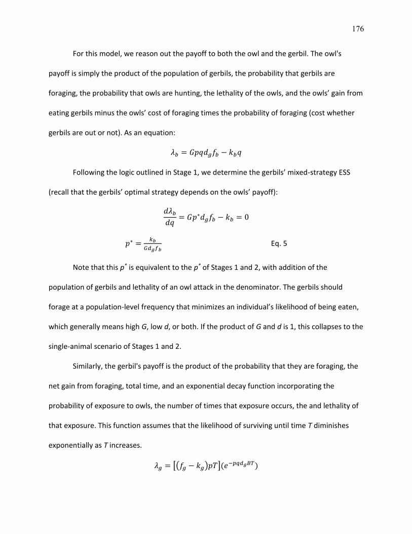
176

For this model, we reason out the payoff to both the owl and the gerbil. The owl's

payoff is simply the product of the population of gerbils, the probability that gerbils are

foraging, the probability that owls are hunting, the lethality of the owls, and the owls’ gain from

eating gerbils minus the owls’ cost of foraging times the probability of foraging (cost whether

gerbils are out or not). As an equation:

𝜆𝑏 = 𝐺𝑝𝑞𝑑𝑔𝑓𝑏 − 𝑘𝑏𝑞

Following the logic outlined in Stage 1, we determine the gerbils’ mixed-strategy ESS

(recall that the gerbils’ optimal strategy depends on the owls’ payoff):

𝑑𝜆𝑏

𝑑𝑞= 𝐺𝑝∗𝑑𝑔𝑓𝑏 − 𝑘𝑏 = 0

𝑝∗ =𝑘𝑏

𝐺𝑑𝑔𝑓𝑏 Eq. 5

Note that this p* is equivalent to the p* of Stages 1 and 2, with addition of the

population of gerbils and lethality of an owl attack in the denominator. The gerbils should

forage at a population-level frequency that minimizes an individual’s likelihood of being eaten,

which generally means high G, low d, or both. If the product of G and d is 1, this collapses to the

single-animal scenario of Stages 1 and 2.

Similarly, the gerbil's payoff is the product of the probability that they are foraging, the

net gain from foraging, total time, and an exponential decay function incorporating the

probability of exposure to owls, the number of times that exposure occurs, the and lethality of

that exposure. This function assumes that the likelihood of surviving until time T diminishes

exponentially as T increases.

𝜆𝑔 = [(𝑓𝑔 − 𝑘𝑔)𝑝𝑇](𝑒−𝑝𝑞𝑑𝑔𝐵𝑇)

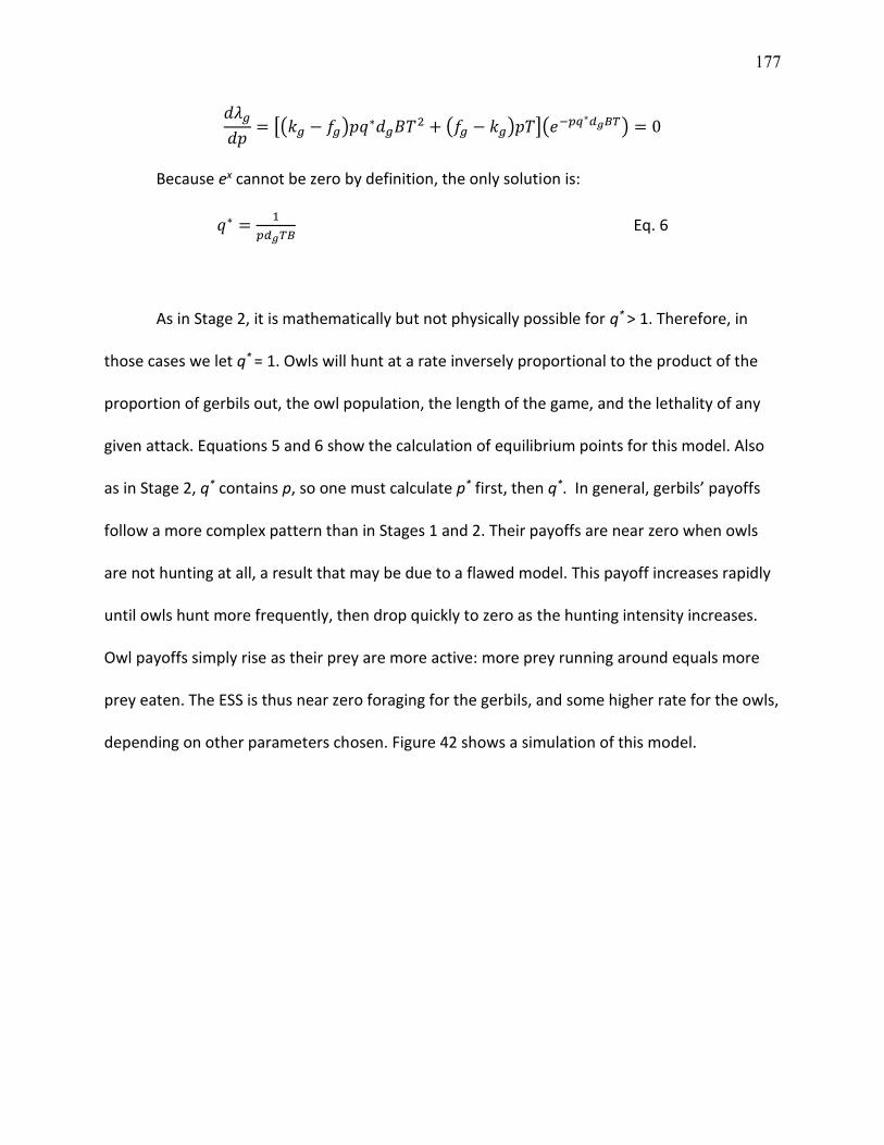
177

𝑑𝜆𝑔

𝑑𝑝= [(𝑘𝑔 − 𝑓𝑔)𝑝𝑞∗𝑑𝑔𝐵𝑇2 + (𝑓𝑔 − 𝑘𝑔)𝑝𝑇](𝑒−𝑝𝑞∗𝑑𝑔𝐵𝑇) = 0

Because ex cannot be zero by definition, the only solution is:

𝑞∗ =1

𝑝𝑑𝑔𝑇𝐵 Eq. 6

As in Stage 2, it is mathematically but not physically possible for q* > 1. Therefore, in

those cases we let q* = 1. Owls will hunt at a rate inversely proportional to the product of the

proportion of gerbils out, the owl population, the length of the game, and the lethality of any

given attack. Equations 5 and 6 show the calculation of equilibrium points for this model. Also

as in Stage 2, q* contains p, so one must calculate p* first, then q*. In general, gerbils’ payoffs

follow a more complex pattern than in Stages 1 and 2. Their payoffs are near zero when owls

are not hunting at all, a result that may be due to a flawed model. This payoff increases rapidly

until owls hunt more frequently, then drop quickly to zero as the hunting intensity increases.

Owl payoffs simply rise as their prey are more active: more prey running around equals more

prey eaten. The ESS is thus near zero foraging for the gerbils, and some higher rate for the owls,

depending on other parameters chosen. Figure 42 shows a simulation of this model.

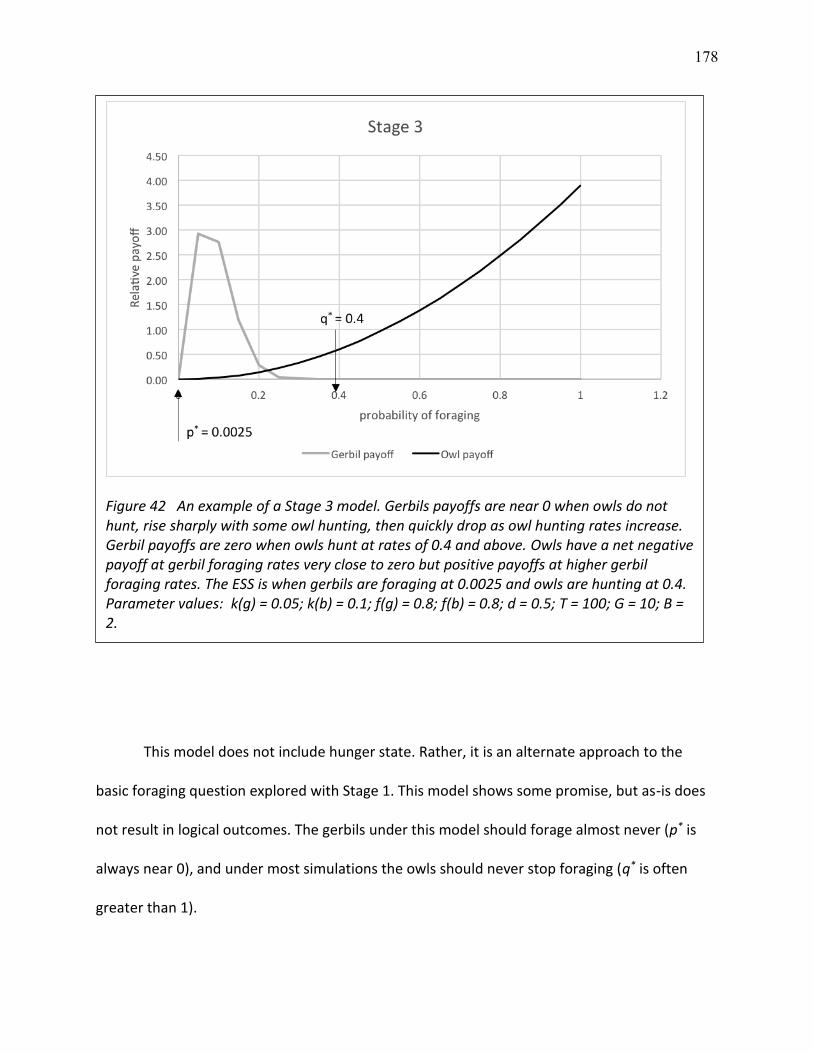
178

This model does not include hunger state. Rather, it is an alternate approach to the

basic foraging question explored with Stage 1. This model shows some promise, but as-is does

not result in logical outcomes. The gerbils under this model should forage almost never (p* is

always near 0), and under most simulations the owls should never stop foraging (q* is often

greater than 1).

Figure 42 An example of a Stage 3 model. Gerbils payoffs are near 0 when owls do not hunt, rise sharply with some owl hunting, then quickly drop as owl hunting rates increase. Gerbil payoffs are zero when owls hunt at rates of 0.4 and above. Owls have a net negative payoff at gerbil foraging rates very close to zero but positive payoffs at higher gerbil foraging rates. The ESS is when gerbils are foraging at 0.0025 and owls are hunting at 0.4. Parameter values: k(g) = 0.05; k(b) = 0.1; f(g) = 0.8; f(b) = 0.8; d = 0.5; T = 100; G = 10; B = 2.

179

Furthermore, when exploring the effects of changing single variables as in Stage 2, many

had effects that defy easy explanation or appear counterintuitive. For example, increasing the

owl population (B) has no effect on the gerbil foraging probability and decreases owl foraging

probability, which seems counterintuitive (owls should have to hunt more frequently to make

up for the increased competition with a stable prey pool).

For these reasons, we did not explore this model further. It is presented here as an

example of an alternate approach and thus a hint of the wide variety of models one may create

in an attempt to approximate reality.

C. Conclusion

Our models indicate that owls forage based on the gerbils’ hunger state (Eq. 4), but that

gerbils forage based only on the owls’ feeding efficiency (Eq. 3, which shows that gerbils’ stable

strategy is the inverse of owl predator efficiency; Eq. 5 shows a direct influence of the owls’

rate of killing gerbils). While we did not include owl hunger state in these models, it is clear that

the owls’ hunting behavior is driven by the gerbils’ behavior and hunger state, and the gerbils’

behavior is driven by the owls’ efficiency and effectiveness in hunting. Owl hunger may affect

their hunting efficiency, including the rate at which they kill gerbils, and thus drive gerbil

behavior. In this game one player’s behavior is driven more by the hunger state of the opposing

player than their own. That owl hunger should increase their hunting success rate is suggested

by studies in which hungry predators as varied as domestic cats, salmon, and jumping spiders

increased their attack rate and lethality (Gardner 1966, Biben 1979, Morgan and Ritz 1984, Hall

and Bradshaw 1998). Altwegg (2003) found that hungry predators killed both hungry and sated

180

prey, but that sated predators killed only hungry prey. Much as suggested by our game, the

hunger of the opponent was more of a factor than the players’ own, except when the players’

own hunger was extreme.

Berger-Tal et al. (2010) found, in a vivarium experiment, that owls base their activity on

their own hunger state, not the gerbils’; that gerbils responded to the owls’ state; and that

when they are hungry gerbils will forage no matter what the owls are doing. While our results

agree for the gerbils, they disagree when it comes to the owls. However, Embar et al. (2014)

conducted a vivarium gerbil–owl foraging game that effectively tested the ideas discussed here,

and found that owls can, and in some circumstances do, respond to gerbil energy state. They

found that hungry gerbils take more risks when foraging, and the owls focus their hunting

efforts on the hungry gerbils. The lack of a similar effect in Berger-Tal et al (2010) was

attributed to both the vivarium enclosure and the subtlety of the owls’ choices in most of the

tested scenarios. Our models show some promise in this outcome. We are confident that they

could form the basis of more robust models. These models should include the owls’ level of

hunger, which we did not consider here. One approach to owl hunger was the model of Brown

et al. (2001), which considered the predator’s energy state and the relative risk of injury

incurred when hunting and could be modified to fit our scenario.

The games played by foraging and hunting animals are complex, and the models

explored here do not, as they stand, provide much insight into the games played. However,

they do hint at the tradeoffs between the need to forage and the need to avoid being killed.

One could combine the above approaches with other models, existing or new, to build a model

to further explore the role hunger plays in the foraging game.

181

D. Literature cited

Altwegg R. 2003. Hungry predators render predator‐avoidance behavior in tadpoles ineffective. Oikos 100: 311-16

Berger‐Tal O, Mukherjee S, Kotler BP, Brown JS. 2010. Complex state‐dependent games between owls and gerbils. Ecology Letters 13: 302-10

Biben M. 1979. Predation and predatory play behaviour of domestic cats. Animal Behaviour 27: 81-94

Bouskila A. 2001. A habitat selection game of interactions between rodents and their predators. Annales Zoologici Fennici 38: 55-70

Brown JS, Kotler BP, Bouskila A. 2001. Ecology of fear: Foraging games between predators and prey with pulsed resources. Annales Zoologici Fennici 2001, 38: 71-87

Brown JS, Laundré JW, Gurung M. 1999. The ecology of fear: optimal foraging, game theory, and trophic interactions. Journal of Mammalogy 80: 385-99

Brown JS, Vincent TL. 1992. Organization of predator-prey communities as an evolutionary game. Evolution: 1269-83

Clark CW. 1994. Antipredator behavior and the asset-protection principle. Behavioral Ecology 5: 159-70

Embar K, Mukherjee S, Kotler BP. 2014. What do predators really want? The role of gerbil energetic state in determining prey choice by Barn Owls. Ecology 95: 280-85

Gardner BT. 1966. Hunger and characteristics of the prey in the hunting behavior of salticid spiders. Journal of Comparative and Physiological Psychology 62: 475

Hall SL, Bradshaw JW. 1998. The influence of hunger on object play by adult domestic cats. Applied Animal Behaviour Science 58: 143-50

Hugie DM, Dill LM. 1994. Fish and game: a game theoretic approach to habitat selection by predators and prey. Journal of Fish Biology 45: 151-69

Kotler BP, Blaustein L, Brown JS. 1992. Predator facilitation: the combined effect of snakes and owls on the foraging behavior of gerbils. Annales Zoologici Fennici 29: 199-206

Kotler BP, Brown JS, Slotow RH, Goodfriend WL, Strauss M. 1993. The influence of snakes on the foraging behavior of gerbils. Oikos 67: 309-16

Lewontin RC. 1961. Evolution and the theory of games. Journal of Theoretical Biology 1: 382-403

Lima SL, Valone TJ. 1986. Influence of predation risk on diet selection: a simple example in the grey squirrel. Animal Behaviour 34: 536-44

Lima SL, Valone TJ, Caraco T. 1985. Foraging-efficiency-predation-risk trade-off in the grey squirrel. Animal Behaviour 33: 155-65

Marsh B, Schuck-Paim C, Kacelnik A. 2004. Energetic state during learning affects foraging choices in starlings. Behavioral Ecology 15: 396-99

Maynard Smith J. 1974. The theory of games and the evolution of animal conflicts. Journal of Theoretical Biology 47: 209-21

182

McArthur C, Banks PB, Boonstra R, Forbey JS. 2014. The dilemma of foraging herbivores: dealing with food and fear. Oecologia 176: 677-89

Morgan W, Ritz D. 1984. Effect of prey density and hunger state on capture of krill, Nyctiphanes australis Sars, by Australian salmon, Arripis trutta (Bloch & Schneider). Journal of Fish Biology 24: 51-58

Rosenzweig ML, MacArthur RH. 1963. Graphical representation and stability conditions of predator-prey interactions. American Naturalist 97: 209-23

Sih A. 1980. Optimal behavior: can foragers balance two conflicting demands? Science 210: 1041-43

Stephens DW. 2008. Decision ecology: foraging and the ecology of animal decision making. Cognitive, Affective, & Behavioral Neuroscience 8: 475-84

Stephens DW, Brown JS, Ydenberg RC. 2007. Foraging: Behavior and Ecology. University of Chicago Press.

Vincent TL, Brown JS. 2005. Evolutionary game theory, natural selection, and Darwinian dynamics. Cambridge University Press.

Whitham J, Mathis A. 2000. Effects of hunger and predation risk on foraging behavior of graybelly salamanders, Eurycea multiplicata. Journal of Chemical Ecology 26: 1659-65

183

VITA

NAME: Hilary Beth Osborne

EDUCATION: B.S., Biological Sciences, Northeastern University, Boston, Massachusetts, 2000

Ph.D., Biological Sciences, University of Illinois at Chicago, Chicago, Illinois, 2016

TEACHING EXPERIENCE: Department of Biological Sciences, University of Illinois at Chicago,

Chicago, Illinois, Teaching Assistant (courses: Introductory Biology for Non-Science Majors; Introductory Ecology; Field Ecology; History of Life; Animal Behavior; Comparative Vertebrate Anatomy; Animal Physiology), 2005–2015

HONORS: Excellence in Teaching Award, 2006

PROFESSIONAL MEMBERSHIP: Board of Editors in the Life Sciences Council of Science Editors