Validation of Multiphase Validation of Multiphase CFD Models with RPT and CFD Models with RPT and

Tracer TechniquesTracer Techniques

IAEA/ RCA Regional Training Course on Validation of CFD Models of Multiphase Systems using Radiotracers: Goa, India , 01-05 December

2008

Shantanu RoyAssociate Professor

Department of Chemical Engineering

Indian Institute of Technology (IIT) Delhi

2

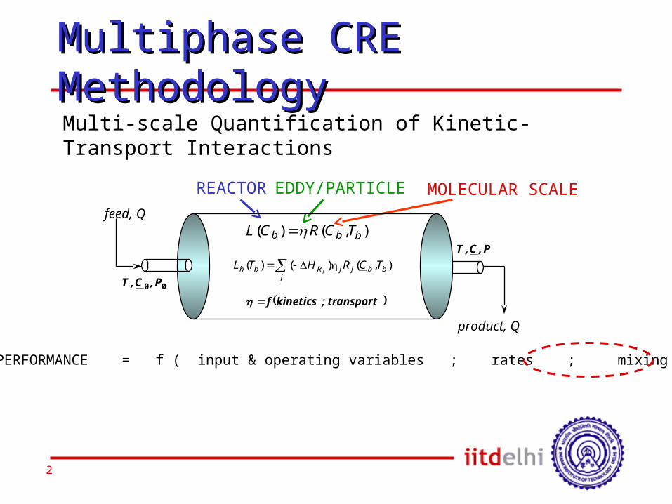
REACTOR PERFORMANCE = f ( input & operating variables ; rates ; mixing pattern )

REACTOR EDDY/PARTICLE MOLECULAR SCALE

),()( bbb TCRCL

j

bbjjRbh TCRHTLj

),()()(

transport;kineticsf00 P,C,T

P,C,T

product, Q

feed, Q

Multi-scale Quantification of Kinetic-Transport Interactions

Multiphase CRE Multiphase CRE MethodologyMethodology

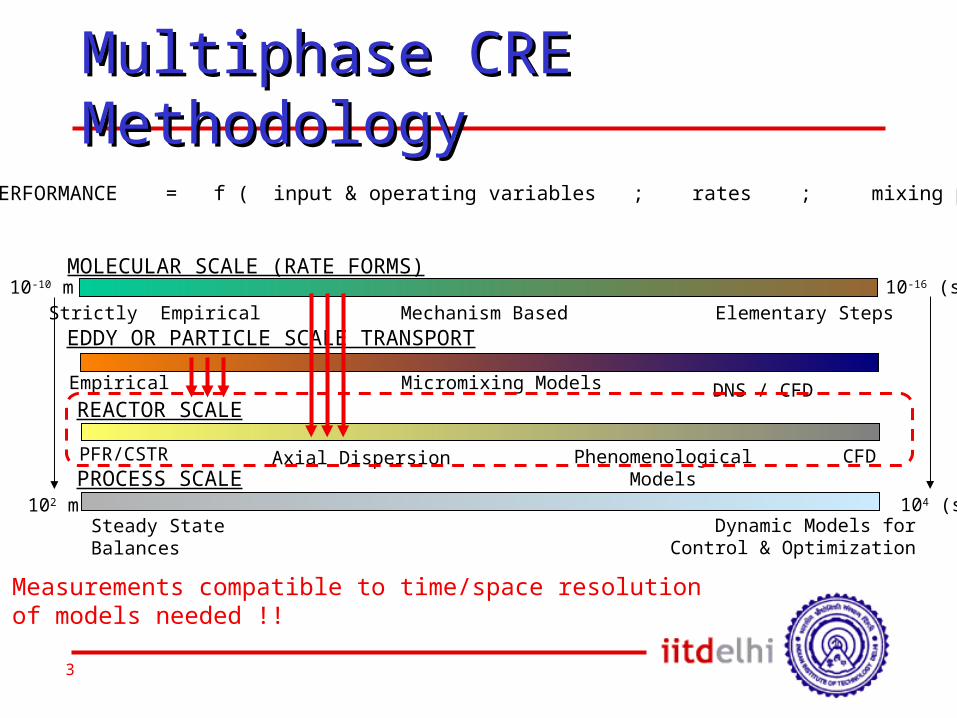
3

MOLECULAR SCALE (RATE FORMS)

Strictly Empirical Mechanism Based Elementary Steps

REACTOR SCALE

Axial Dispersion CFDPhenomenological Models

EDDY OR PARTICLE SCALE TRANSPORT

DNS / CFDEmpirical Micromixing Models

PROCESS SCALE

Steady State Balances

Dynamic Models forControl & Optimization

10-10 m

102 m

10-16 (s)

104 (s)

PFR/CSTR

REACTOR PERFORMANCE = f ( input & operating variables ; rates ; mixing pattern )

Multiphase CRE Multiphase CRE MethodologyMethodology

Measurements compatible to time/space resolution of models needed !!

4

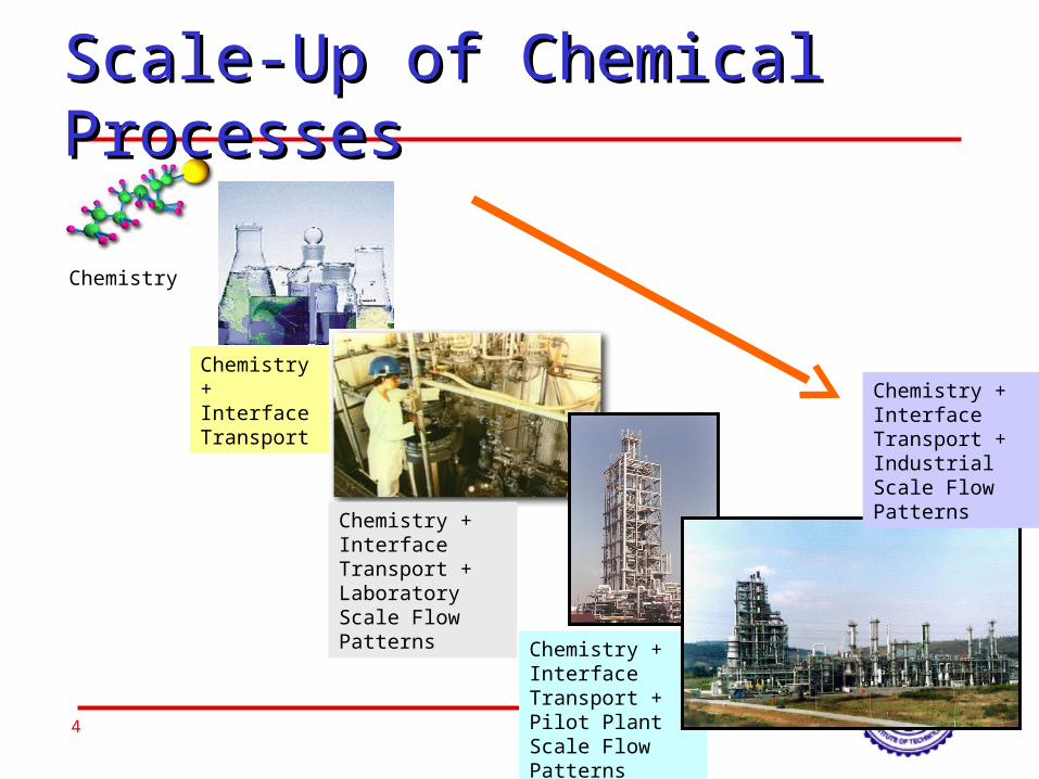
Chemistry

Scale-Up of Chemical Scale-Up of Chemical ProcessesProcesses

Chemistry + Interface Transport

Chemistry + Interface Transport + Laboratory Scale Flow Patterns Chemistry +

Interface Transport + Pilot Plant Scale Flow Patterns

Chemistry + Interface Transport + Industrial Scale Flow Patterns

5

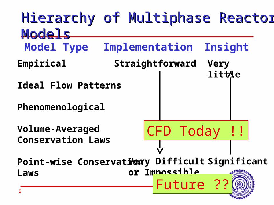
Hierarchy of Multiphase Reactor Hierarchy of Multiphase Reactor ModelsModels

Empirical

Ideal Flow Patterns

Phenomenological

Volume-AveragedConservation Laws

Point-wise ConservationLaws

StraightforwardImplementation Insight

Very little

Very Difficultor Impossible

Significant

Model Type

CFD Today !!

Future ??

6

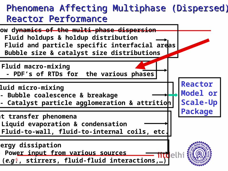
Phenomena Affecting Multiphase (Dispersed) Phenomena Affecting Multiphase (Dispersed) Reactor PerformanceReactor Performance

Flow dynamics of the multi-phase dispersion- Fluid holdups & holdup distribution- Fluid and particle specific interfacial areas- Bubble size & catalyst size distributions

Fluid macro-mixing- PDF’s of RTDs for the various phases

Fluid micro-mixing- Bubble coalescence & breakage- Catalyst particle agglomeration & attrition

Heat transfer phenomena- Liquid evaporation & condensation- Fluid-to-wall, fluid-to-internal coils, etc.

Energy dissipation- Power input from various sources(e.g., stirrers, fluid-fluid interactions,…)

ReactorModel or Scale-Up Package

7

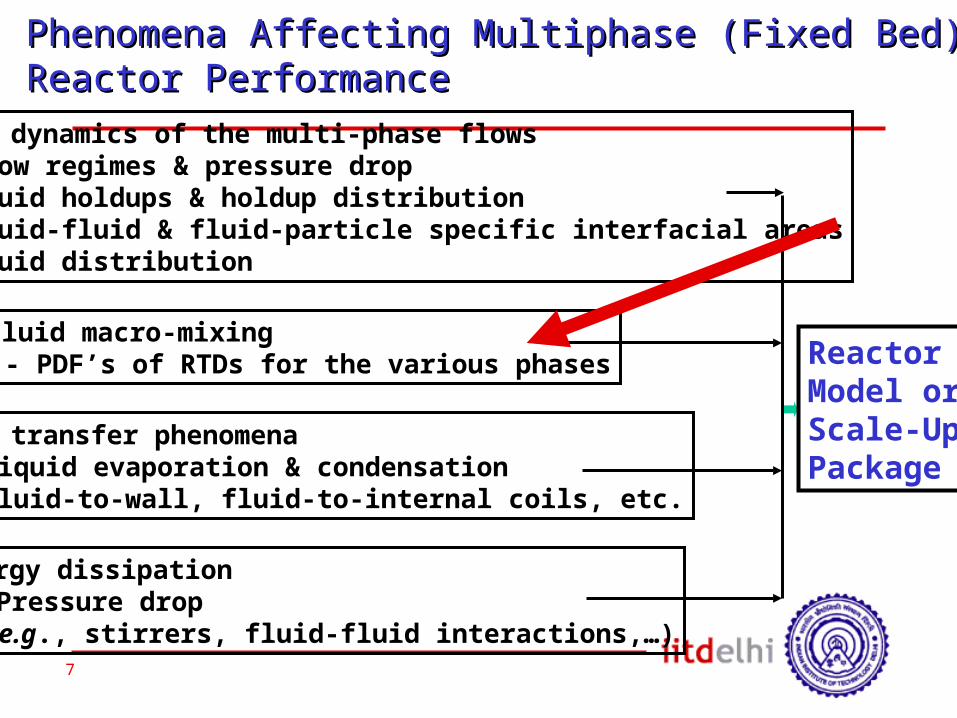
Fluid dynamics of the multi-phase flows- Flow regimes & pressure drop- Fluid holdups & holdup distribution- Fluid-fluid & fluid-particle specific interfacial areas- Fluid distribution

Fluid macro-mixing- PDF’s of RTDs for the various phases

Heat transfer phenomena- Liquid evaporation & condensation- Fluid-to-wall, fluid-to-internal coils, etc.

Energy dissipation- Pressure drop(e.g., stirrers, fluid-fluid interactions,…)

Phenomena Affecting Multiphase (Fixed Bed) Phenomena Affecting Multiphase (Fixed Bed) Reactor PerformanceReactor Performance

ReactorModel or Scale-Up Package

8

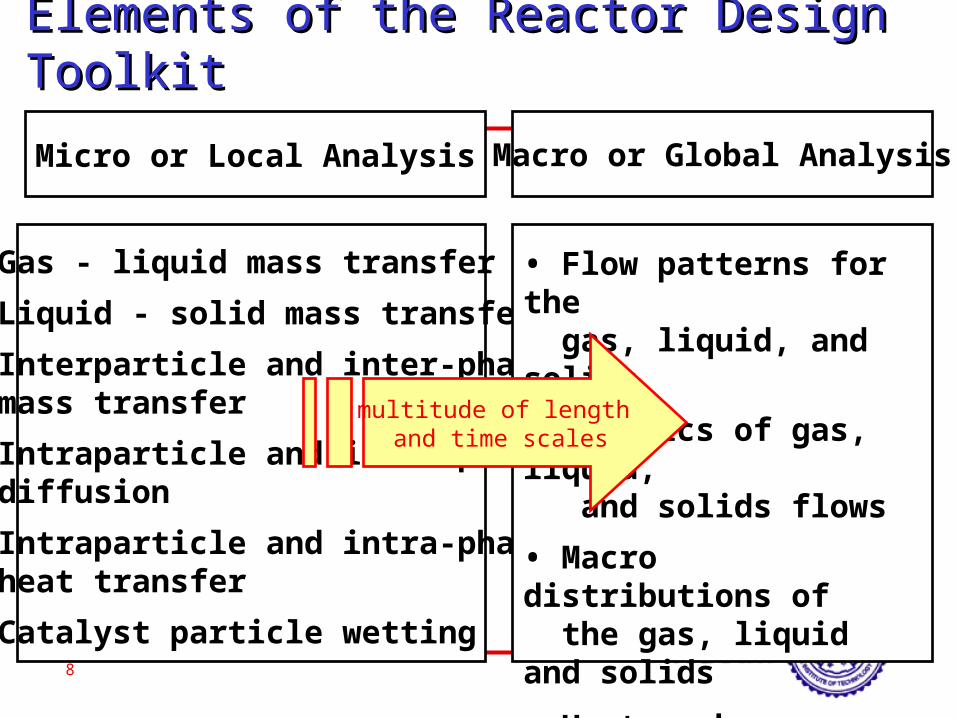
Elements of the Reactor Design Elements of the Reactor Design ToolkitToolkitMicro or Local Analysis Macro or Global Analysis

• Gas - liquid mass transfer• Liquid - solid mass transfer• Interparticle and inter-phase mass transfer• Intraparticle and intra-phase diffusion• Intraparticle and intra-phase heat transfer• Catalyst particle wetting

• Flow patterns for the gas, liquid, and solids• Dynamics of gas, liquid, and solids flows• Macro distributions of the gas, liquid and solids• Heat exchange • Other types of transport phenomena

multitude of length and time scales

9

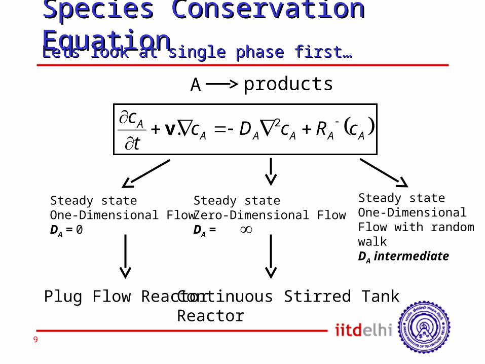
Species Conservation Species Conservation EquationEquation

AAAAAA cRcDct

c 2.v

A products

Steady stateOne-Dimensional FlowDA = 0

Plug Flow Reactor

Steady stateZero-Dimensional FlowDA =

Continuous Stirred Tank Reactor

Steady stateOne-Dimensional Flow with random walkDA intermediate

Lets look at single phase first…Lets look at single phase first…

10

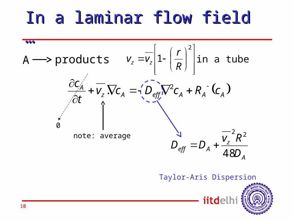
In a laminar flow field In a laminar flow field ……

AAAeffAzA cRcDcvt

c 2.

A products

0note: average

2

1Rrvv zz in a tube

A

zAeff D

RvDD 4822

Taylor-Aris Dispersion

11

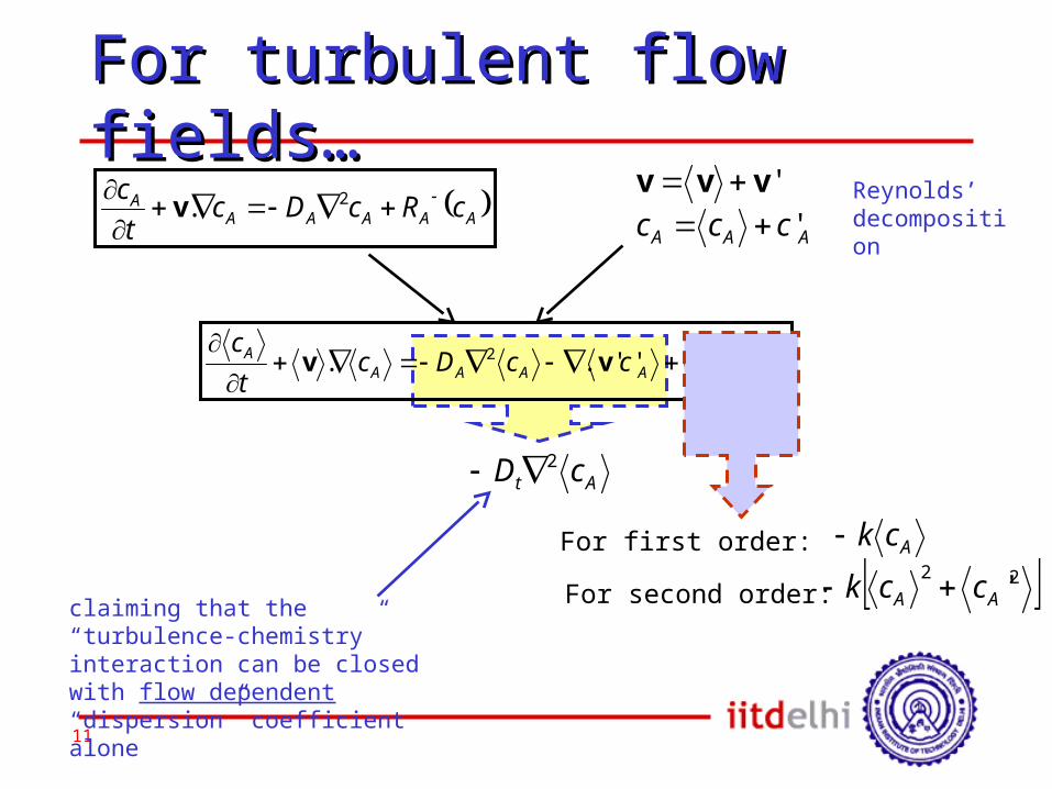
For turbulent flow For turbulent flow fields…fields…

At cD 2

AAAAAAA cRccDct

c

''.. 2 vv

AAAAAA cRcDct

c 2.v

'vvv

AAA ccc 'Reynolds’ decomposition

claiming that the “turbulence-chemistry” interaction can be closed with flow dependent “dispersion” coefficient alone

AckFor first order:For second order: 22 'AA cck

12

For understanding reactors For understanding reactors better…better…• The reactor design problem is known to good extent if we can measure v(x,t)

• It would be known completely if we can find the moments of fluctuations in velocity and concentration

13

What was done in the What was done in the past?past?• Danckwerts (1951) introduced the idea that if we cannot find v(x,t), let us try to find the distribution of residence times (macromixing)

• Later, Zwittering (1958) introduced a concept called micromixing to account for the effect of non-zero moments of the fluctuations and their correlations

14

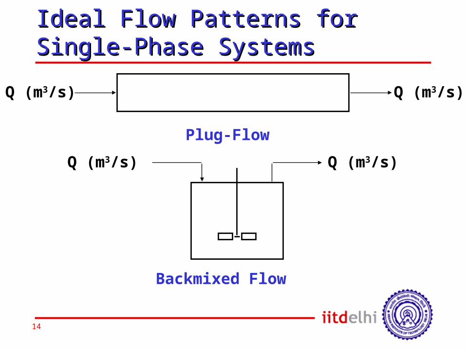
Ideal Flow Patterns for Ideal Flow Patterns for Single-Phase SystemsSingle-Phase Systems

Q (m3/s) Q (m3/s)

Q (m3/s) Q (m3/s)Plug-Flow

Backmixed Flow

15

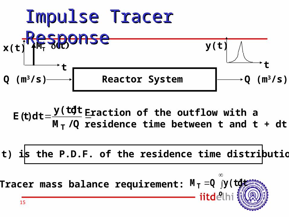
Q (m3/s) Q (m3/s)Reactor Systemt

x(t) MT tt

y(t)

Fraction of the outflow with aresidence time between t and t + dt

E(t) is the P.D.F. of the residence time distribution

Tracer mass balance requirement:

oT dt y(t) Q M

Q /Mdt y(t) dt )t(E

T

Impulse Tracer Impulse Tracer ResponseResponse

16

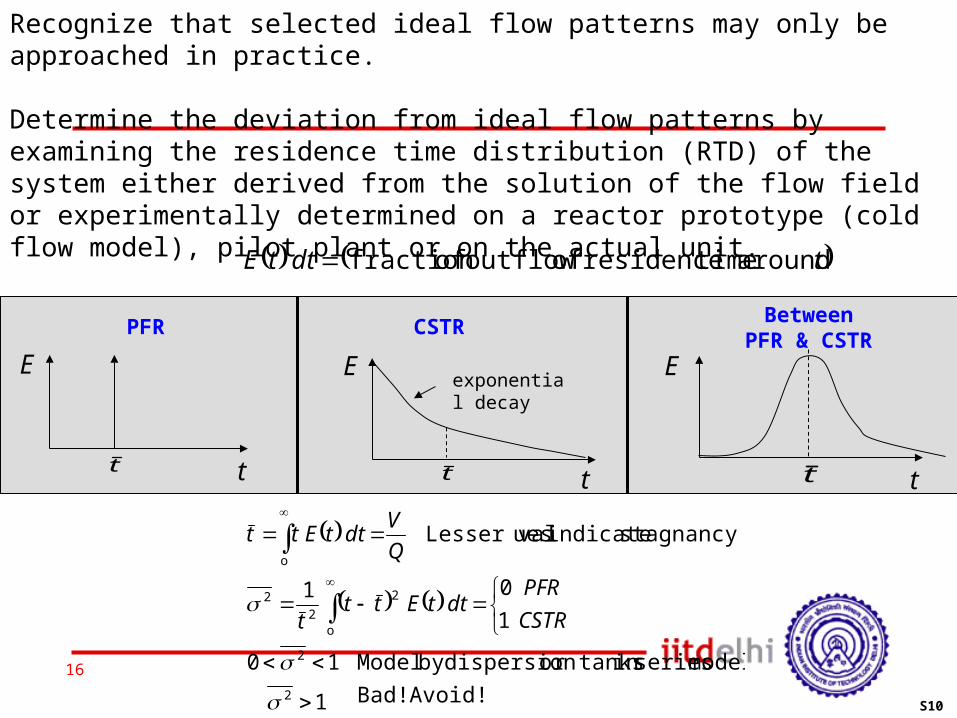
Avoid!Bad!model seriesin or tanks dispersionby Model

110

101

stagnancy indicate uesLesser val

2

2o

22

2

o

CSTRPFRdttEtt

t

QVdttEtt

Recognize that selected ideal flow patterns may only be approached in practice.

Determine the deviation from ideal flow patterns by examining the residence time distribution (RTD) of the system either derived from the solution of the flow field or experimentally determined on a reactor prototype (cold flow model), pilot plant or on the actual unit. tdttE around timeresidence of outflow offraction

tdttE about timeresidence of outflow offraction E

t

E

t

E

tt

PFR CSTR BetweenPFR & CSTR

exponential decay

tt

S10

17

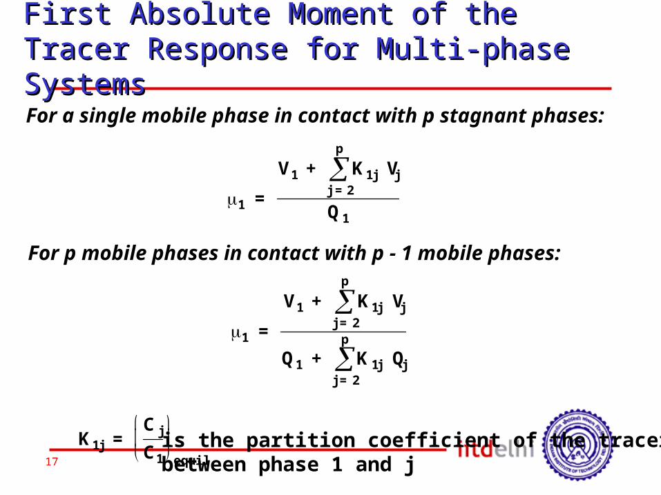
First Absolute Moment of theFirst Absolute Moment of theTracer Response for Multi-phase Tracer Response for Multi-phase SystemsSystemsFor a single mobile phase in contact with p stagnant phases:

1 = V1 + K 1j Vj

j = 2

p

Q 1

For p mobile phases in contact with p - 1 mobile phases:

1 = V1 + K 1j Vj

j = 2

p

Q 1 + K 1j Qjj = 2

p

K 1j = C jC1

equil.is the partition coefficient of the tracerbetween phase 1 and j

18

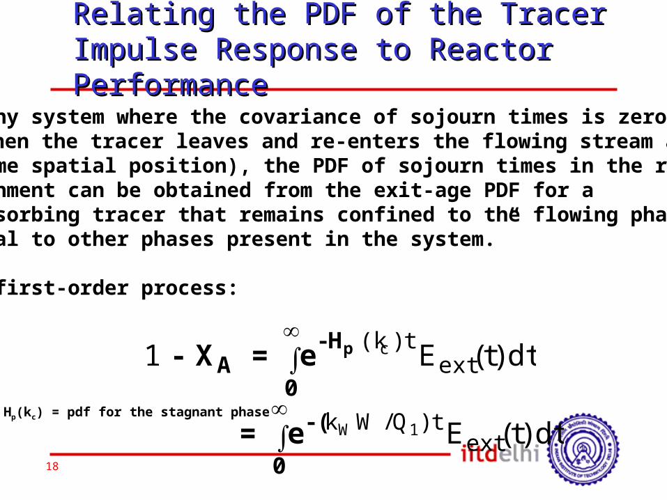
Relating the PDF of the Tracer Relating the PDF of the Tracer Impulse Response to Reactor Impulse Response to Reactor PerformancePerformance

“For any system where the covariance of sojourn times is zero(i.e., when the tracer leaves and re-enters the flowing stream atthe same spatial position), the PDF of sojourn times in the reactionenvironment can be obtained from the exit-age PDF for a non-adsorbing tracer that remains confined to the flowing phaseexternal to other phases present in the system.”

For a first-order process:

0

H -A

pe = X - dt )t(E 1 extt )(k c

0( -e = dt )t(E ext

t )Q/Wk 1WHp(kc) = pdf for the stagnant phase

19

oA

AoR R

C

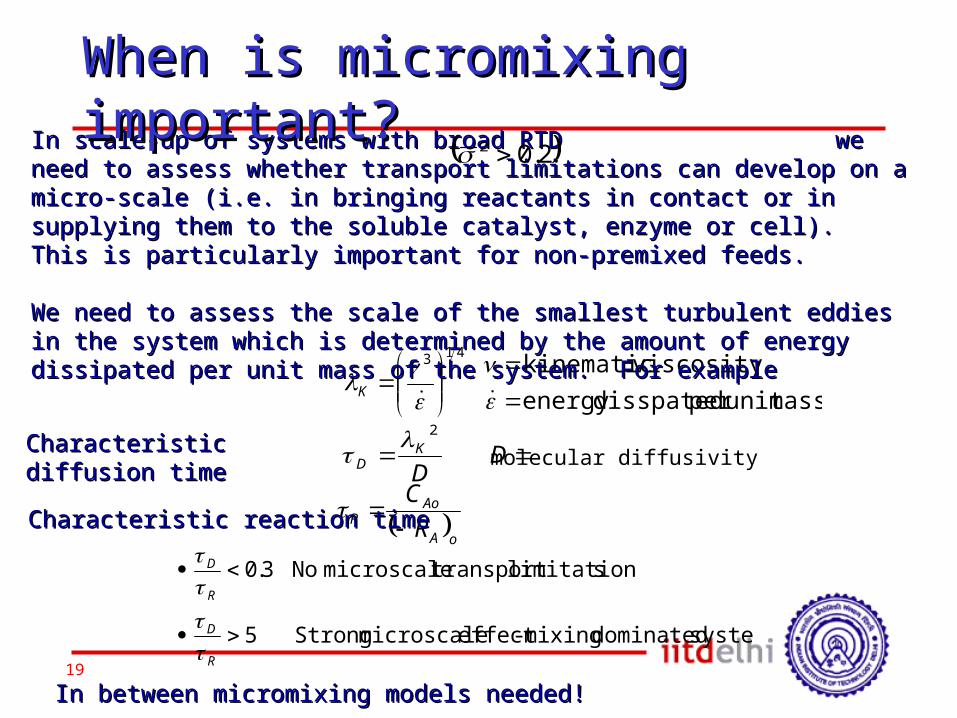
Characteristic reaction timeCharacteristic reaction time

system dominated mixing-effect microscale Strong5

slimitation transportmicroscale No3.0

R

D

R

D

massunit per disspatedenergy viscositykinematic413

K

In between micromixing models needed!In between micromixing models needed!

2

DDK

D

Characteristic Characteristic diffusion timediffusion time

In scale-up of systems with broad RTD we In scale-up of systems with broad RTD we need to assess whether transport limitations can develop on a need to assess whether transport limitations can develop on a micro-scale (i.e. in bringing reactants in contact or in micro-scale (i.e. in bringing reactants in contact or in supplying them to the soluble catalyst, enzyme or cell). supplying them to the soluble catalyst, enzyme or cell). This is particularly important for non-premixed feeds.This is particularly important for non-premixed feeds.

We need to assess the scale of the smallest turbulent eddies We need to assess the scale of the smallest turbulent eddies in the system which is determined by the amount of energy in the system which is determined by the amount of energy dissipated per unit mass of the system. For exampledissipated per unit mass of the system. For example

2.02

molecular diffusivity

When is micromixing When is micromixing important?important?

20

State-of-the-art?State-of-the-art?• Computational Fluid Dynamics (CFD) has been evolving as a way to predict v(x,t) as well as higher moments

• Problem is that CFD (like any modeling) incorporates “closures” whose validation is a challenge

• In any case, even without taking CFD into the picture, there is a need to understand the mixing patterns and dynamic effects for better scale-up

21

In Multiphase ReactorsIn Multiphase Reactors• In multiphase reactors, all the challenges of single phase reactors still hold – in fact now you have to account for mixing in two phases and their relative slip (distribution in time and space)

• In addition, the distribution of phases is a function of space and time and need to be determined

• In turn, dynamics of phase volume fraction also determines the time/space distribution of interfacial area

22

Further Issues in Further Issues in Multiphase ReactorsMultiphase Reactors• Most of them are highly dynamic (turbulent

or not)• Involve multitude of time and space scales• Most of them are opaque – why?• Theoretical “requirements” of RTD of other

measurements, such as “mixing cup conditions” are not easy to achieve

• Tracers distribute “between” phases – makes data interpretation difficult

• “Invasive” tools typically change the flow pattern itself, in many cases dramatically

23

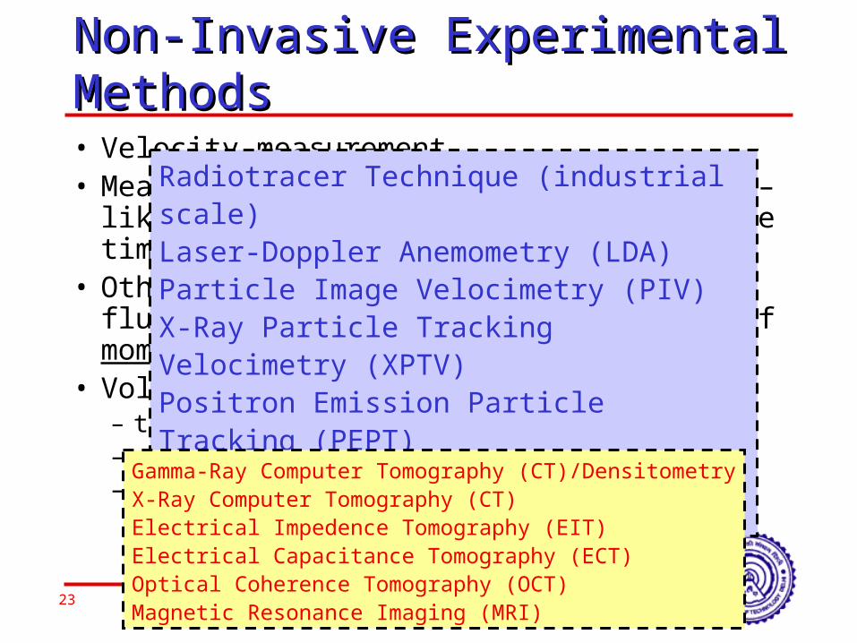
Non-Invasive Experimental Non-Invasive Experimental MethodsMethods• Velocity measurement• Measurement of mixing characteristics – like dispersion coefficients, residence time distributions

• Other parameters that quantify the fluid dynamical time series in terms of moments (integral domain)

• Volume fraction measurements – time-averaged– spatially resolved– temporally resolved

Radiotracer Technique (industrial scale)Laser-Doppler Anemometry (LDA)Particle Image Velocimetry (PIV)X-Ray Particle Tracking Velocimetry (XPTV)Positron Emission Particle Tracking (PEPT)Radioactive Particle Tracking (RPT)

Gamma-Ray Computer Tomography (CT)/DensitometryX-Ray Computer Tomography (CT)Electrical Impedence Tomography (EIT)Electrical Capacitance Tomography (ECT)Optical Coherence Tomography (OCT)Magnetic Resonance Imaging (MRI)

CFD and Need for CFD and Need for ValidationValidation

25

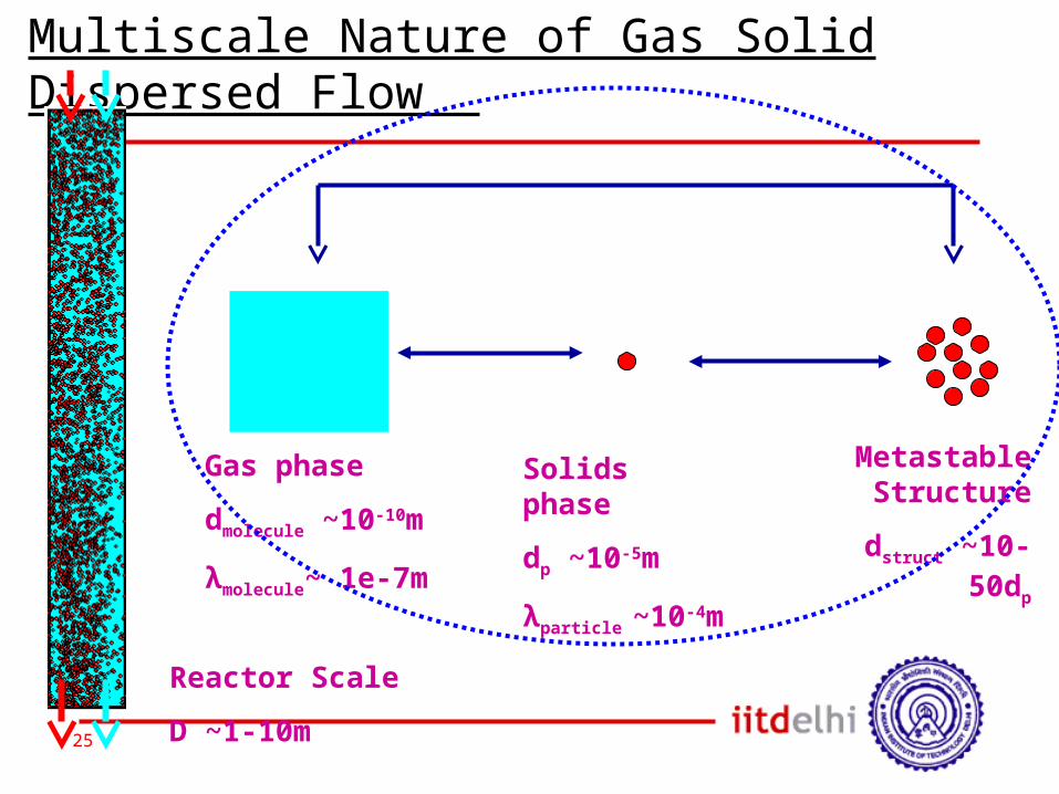
Multiscale Nature of Gas Solid Dispersed Flow

Gas phasedmolecule ~10-10mλmolecule~ 1e-7m

Solids phasedp ~10-5mλparticle ~10-4m

Metastable Structuredstruct ~10-

50dp

Reactor ScaleD ~1-10m

26

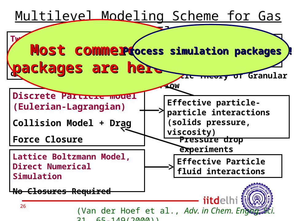
Lattice Boltzmann Model, Direct Numerical SimulationNo Closures Required

Effective Particle fluid interactions

Effective particle-particle interactions (solids pressure, viscosity)

Simulation of two phase flow at engineering scales

Kinetic Theory of Granular Flow

Two fluid model (Eulerian-Eularian)Drag + Pressure/ Viscosity closures

Discrete Particle model (Eulerian-Lagrangian)Collision Model + Drag Force Closure Pressure drop

experiments

Multilevel Modeling Scheme for Gas Solid Flow

(Van der Hoef et al., Adv. in Chem. Engng. Sci. 31, 65-149(2000))

Most commercial Most commercial packages are here !!packages are here !!

Process simulation packages !!Process simulation packages !!

27

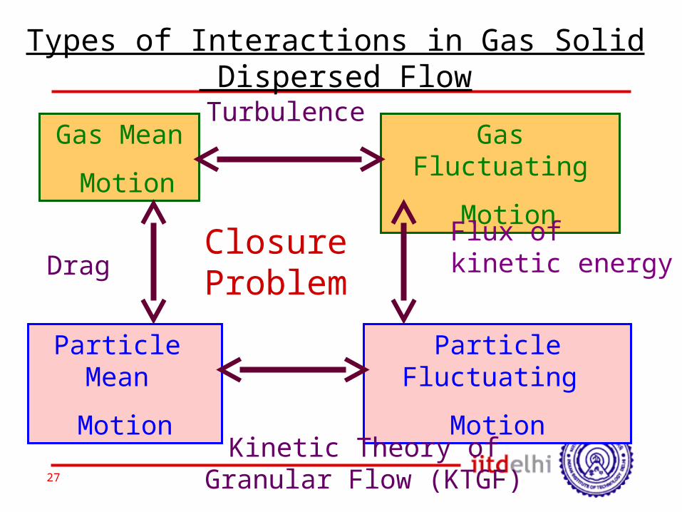
Gas Mean Motion

Gas Fluctuating Motion

Particle Mean Motion

Particle Fluctuating

Motion

Turbulence

Kinetic Theory of Granular Flow (KTGF)

DragFlux of kinetic energy

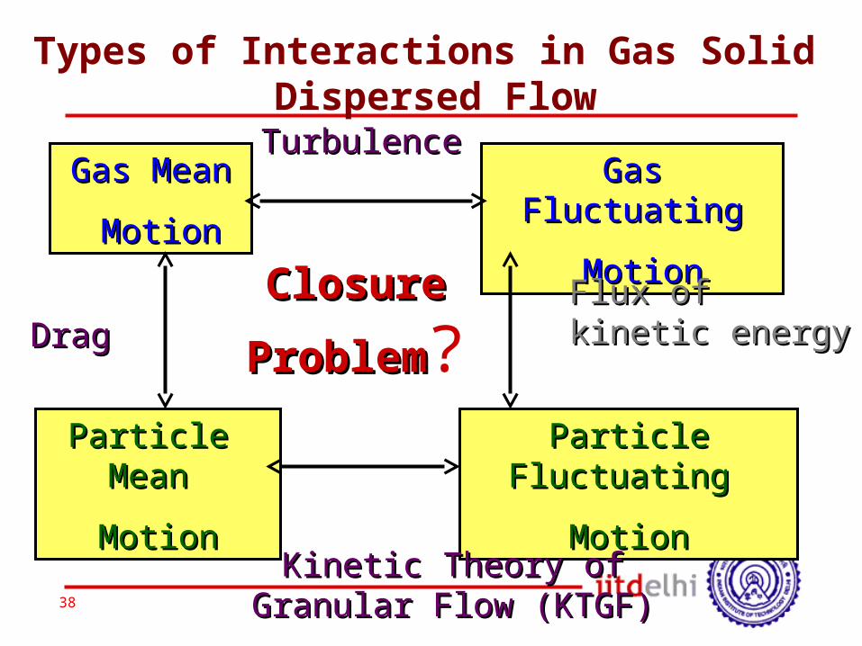
Types of Interactions in Gas Solid Dispersed Flow

Closure Problem

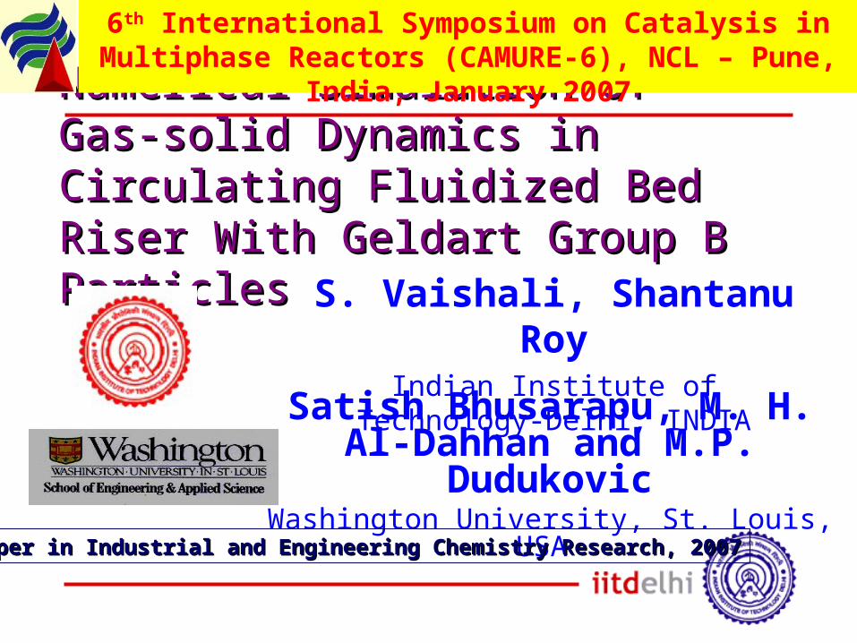
Numerical Simulation of Numerical Simulation of Gas-solid Dynamics in Gas-solid Dynamics in Circulating Fluidized Bed Circulating Fluidized Bed Riser With Geldart Group B Riser With Geldart Group B ParticlesParticles S. Vaishali, Shantanu

RoyIndian Institute of

Technology-Delhi, INDIA

6th International Symposium on Catalysis in Multiphase Reactors (CAMURE-6), NCL – Pune,

India, January 2007

Satish Bhusarapu, M. H. Al-Dahhan and M.P.

DudukovicWashington University, St. Louis,

USA Paper in Industrial and Engineering Chemistry Research, 2007Paper in Industrial and Engineering Chemistry Research, 2007

29

Motivation for studyMotivation for study Circulating Fluidized bed riser with Geldart group B particles finds application in combustion

CFD model is validated against non-invasive experimental data (CARPT-CT)

In addition to mean solids velocity field and solids density, second order moments, i.e., granular temperature profile has also been compared

30

Schematic Diagram of Schematic Diagram of CREL Riser CREL Riser

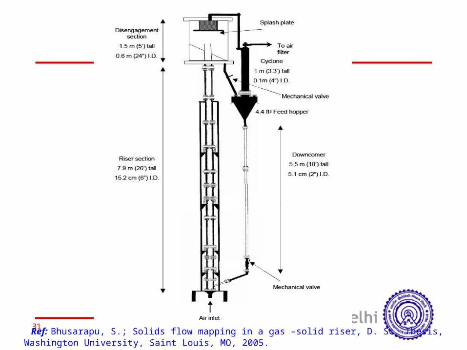
31 Ref: Bhusarapu, S.; Solids flow mapping in a gas –solid riser, D. Sc. Thesis, Washington University, Saint Louis, MO, 2005.

32

ExperimentalExperimental Non-Invasive Techniques:

Computer Automated Radioactive Particle Tracking (CARPT)

Computed Tomography (CT)

Independent Measurement of solids velocity, solids holdup as well as solids flux

First time implementation on relatively fast system

33Gas Solid

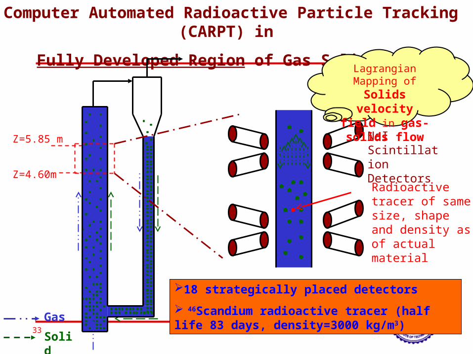
NaI Scintillation DetectorsRadioactive tracer of same size, shape and density as of actual material

Computer Automated Radioactive Particle Tracking (CARPT) in

Fully Developed Region of Gas Solid Riser

Z=5.85 m

Z=4.60m

Lagrangian Mapping of Solids velocity

field in gas-solids flow

18 strategically placed detectors 46Scandium radioactive tracer (half life 83 days, density=3000 kg/m3)

34

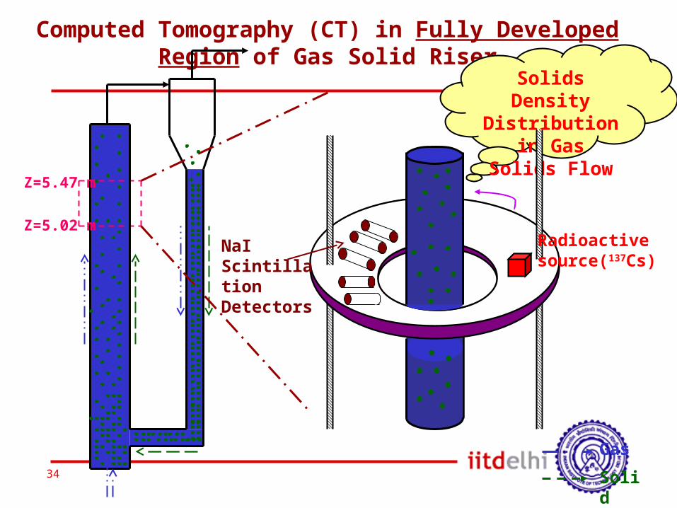
Computed Tomography (CT) in Fully Developed Region of Gas Solid Riser

Solids Density

Distribution in Gas

Solids Flow

Radioactive source(137Cs)

Z=5.47 m

Z=5.02 m

Gas Solid

NaI Scintillation Detectors

35

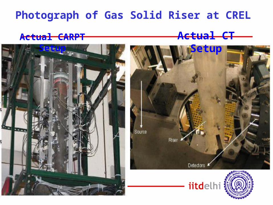
Actual CARPT Setup

Actual CT Setup

Photograph of Gas Solid Riser at CREL

36

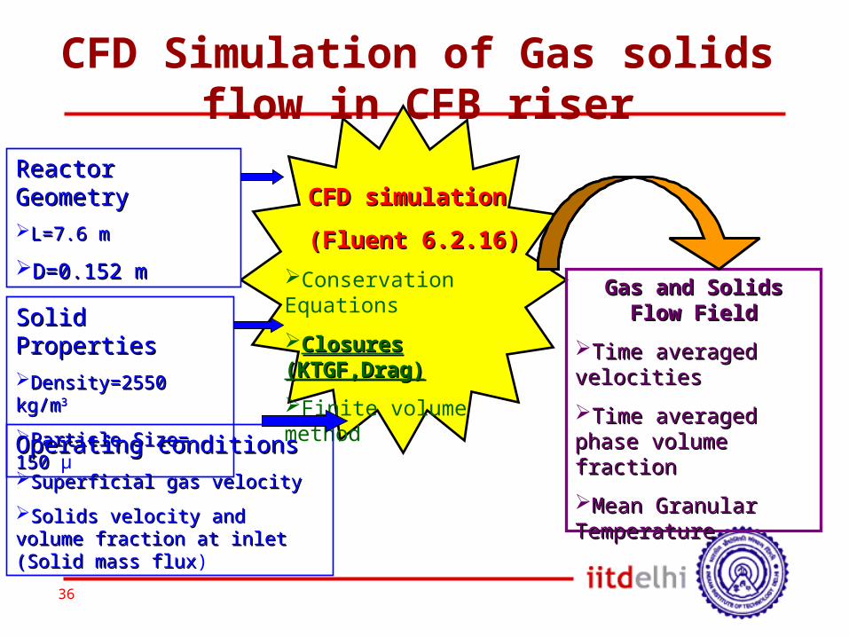
CFD simulation CFD simulation (Fluent 6.2.16)(Fluent 6.2.16)

Conservation EquationsClosures Closures (KTGF,Drag)(KTGF,Drag)Finite volume method

Solid Solid PropertiesPropertiesDensity=2550 Density=2550 kg/mkg/m33

Particle Size= Particle Size= 150150 μ

Reactor Reactor GeometryGeometryL=7.6 mL=7.6 mD=0.152 mD=0.152 m

Operating conditionsOperating conditionsSuperficial gas velocitySuperficial gas velocitySolids velocity and Solids velocity and volume fraction at inlet volume fraction at inlet (Solid mass flux(Solid mass flux)

Gas and Solids Gas and Solids Flow FieldFlow Field

Time averaged Time averaged velocitiesvelocitiesTime averaged Time averaged phase volume phase volume fractionfractionMean Granular Mean Granular TemperatureTemperature

CFD Simulation of Gas solids flow in CFB riser

37

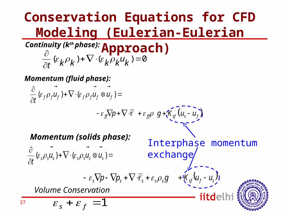
0)()(

kukkkkt

)()( fffffff uuut

ff ff sf s fp g K u u

)()( sssssss uuut

gpp sssss

sfsf uuK

Continuity (kth phase):

Conservation Equations for CFD Modeling (Eulerian-Eulerian

Approach)

Momentum (fluid phase):

Momentum (solids phase):

1 fs Volume Conservation

Interphase momentum exchange

38

Gas MeanGas Mean MotionMotion

Gas Gas FluctuatingFluctuating MotionMotion

Particle Particle Mean Mean MotionMotion

Particle Particle Fluctuating Fluctuating

MotionMotion

TurbulenceTurbulence

Kinetic Theory of Kinetic Theory of Granular Flow (KTGF)Granular Flow (KTGF)

DragDragFlux of Flux of kinetic energy kinetic energy

Types of Interactions in Gas Solid Dispersed Flow

Closure Closure ProblemProblem?

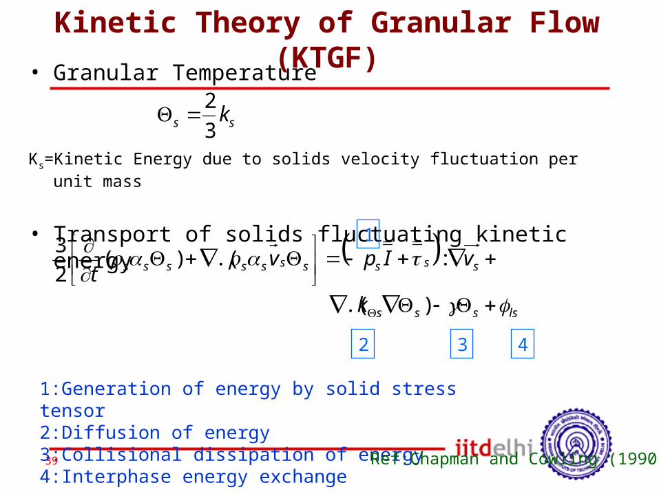
39

• Granular Temperature

Ks=Kinetic Energy due to solids velocity fluctuation per unit mass

• Transport of solids fluctuating kinetic energy

23s sk

lssss

ssssssssss

k

vIpvt

).(

:.()(23 1

2 3 4

1:Generation of energy by solid stress tensor2:Diffusion of energy 3:Collisional dissipation of energy 4:Interphase energy exchange

Ref:Chapman and Cowling (1990)

Kinetic Theory of Granular Flow (KTGF)

40

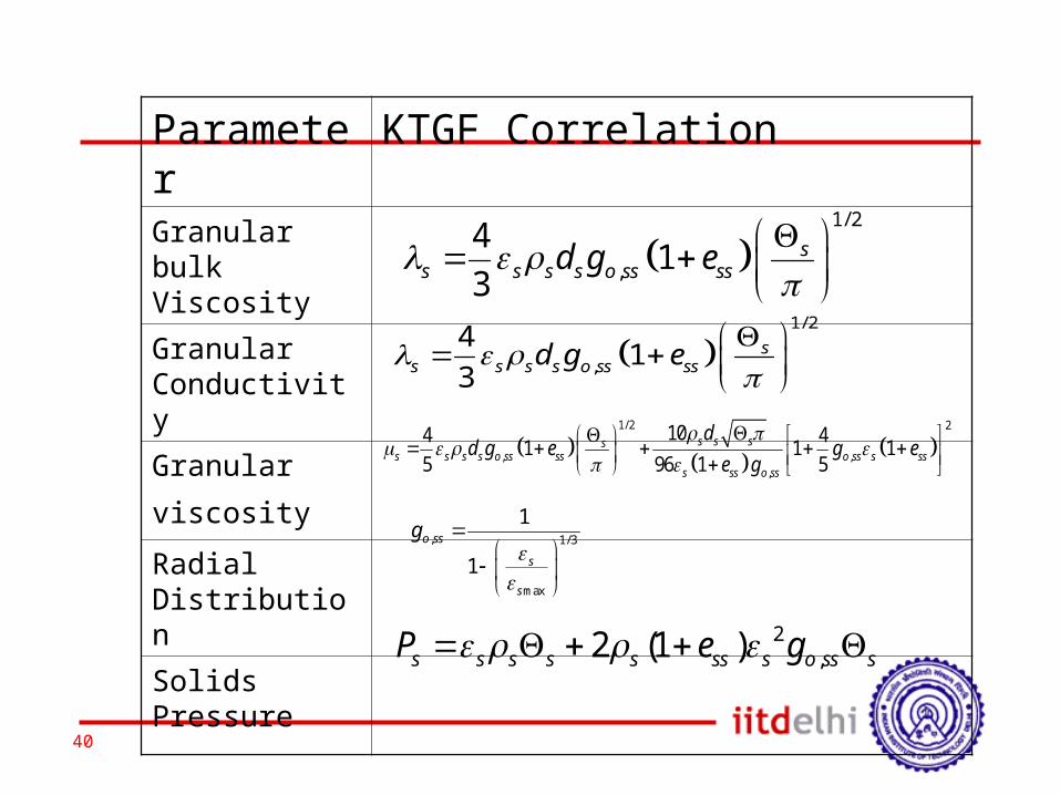
Parameter

KTGF Correlation

Granular bulk ViscosityGranular ConductivityGranular viscosity Radial DistributionSolids Pressure

1/2

,4 13

ss s s s o ss ssd g e

1/2

,4 13

ss s s s o ss ssd g e

1/2 2

, ,,

104 41 1 15 96 1 5s s ss

s s s s o ss ss o ss s sss ss o ss

dd g e g ee g

, 1/3

max

1

1o ss

s

s

g

2,2 (1 )s s s s s ss s o ss sP e g

41

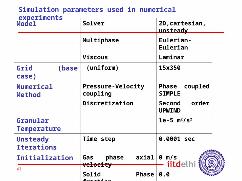
Model Solver 2D,cartesian, unsteady

Multiphase Eulerian- Eulerian

Viscous Laminar Grid (base case)

(uniform) 15x350

Numerical Method

Pressure-Velocity coupling

Phase coupled SIMPLE

Discretization Second order UPWIND

Granular Temperature

1e-5 m2/s2

Unsteady Iterations

Time step 0.0001 sec

Initialization Gas phase axial velocity

0 m/s

Solid Phase fraction

0.0

Simulation parameters used in numerical experiments

42

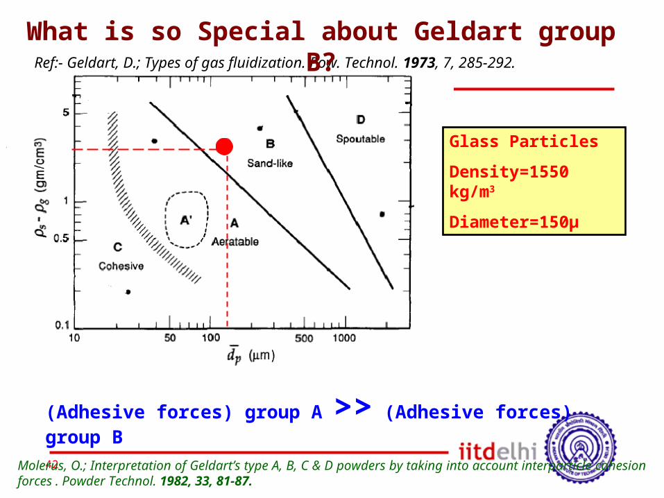
Ref:- Geldart, D.; Types of gas fluidization. Pow. Technol. 1973, 7, 285-292.

(Adhesive forces) group A >> (Adhesive forces) group B

What is so Special about Geldart group B?

Glass ParticlesDensity=1550 kg/m3

Diameter=150μ

Molerus, O.; Interpretation of Geldart’s type A, B, C & D powders by taking into account interparticle cohesion forces . Powder Technol. 1982, 33, 81-87.

43

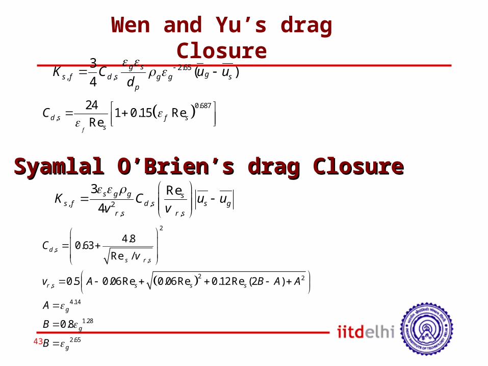
Syamlal O’Brien’s drag ClosureSyamlal O’Brien’s drag Closure, ,2

, ,

3 Re4

s g g ss f d s s g

r s r sK C u u

v v

2

,,

2 2,

4.14

1.28

2.65

4.80.63Re /

0.5 0.06Re 0.06Re 0.12Re (2 )

0.8

d ss r s

r s s s s

g

g

g

Cv

v A B A A

ABB

2.65, ,

3 ( )4g s

gs f d s g g sp

K C u ud

Wen and Yu’s drag Closure

0.687,24 1 0.15 ReRe

f

d s f ss

C

44

-0.5

0

0.5

1

1.5

2

-0.5 -0.3 -0.1 0.1 0.3 0.5 Radial Position (r/R)

Mean Solid Velocity (m/s)

W en and Yu's Drag closureSyam lal O ' Brien's Drag closureExp. Data (CARPT)

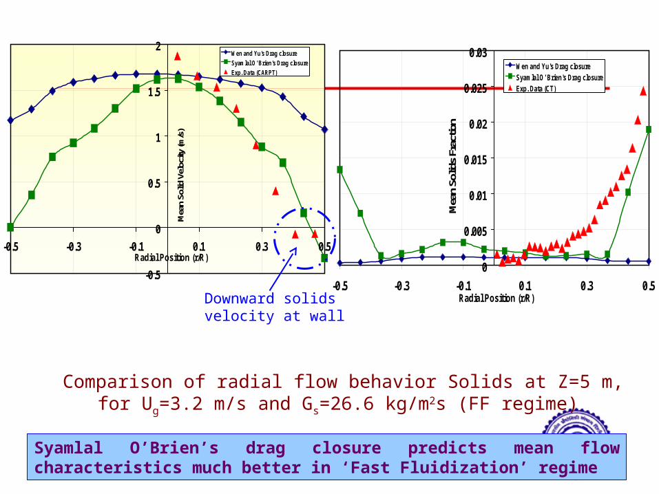
Comparison of radial flow behavior Solids at Z=5 m, for Ug=3.2 m/s and Gs=26.6 kg/m2s (FF regime)

0

0.005

0.01

0.015

0.02

0.025

0.03

-0.5 -0.3 -0.1 0.1 0.3 0.5 Radial Position (r/R)

Mean Solids Fraction

W en and Yu's Drag closureSyam lal O' Brien's Drag closureExp. Data (CT)

Syamlal O’Brien’s drag closure predicts mean flow characteristics much better in ‘Fast Fluidization’ regime

Downward solids velocity at wall

45

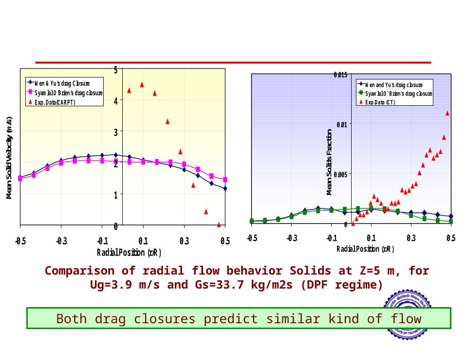
0

1

2

3

4

5

-0.5 -0.3 -0.1 0.1 0.3 0.5Radial Position (r/R)

Mean Solid Velocity (m/s)

W en & Yu's drag ClosureSyam lal O 'Brien's drag closureExp. Data(CARPT)

Both drag closures predict similar kind of flow

0

0.005

0.01

0.015

-0.5 -0.3 -0.1 0.1 0.3 0.5Radial Position (r/R)

Mean Solids Fraction

W en and Yu's drag closureSyam lal O' Brien's drag closureExp.Data (CT)

Comparison of radial flow behavior Solids at Z=5 m, for Ug=3.9 m/s and Gs=33.7 kg/m2s (DPF regime)

46

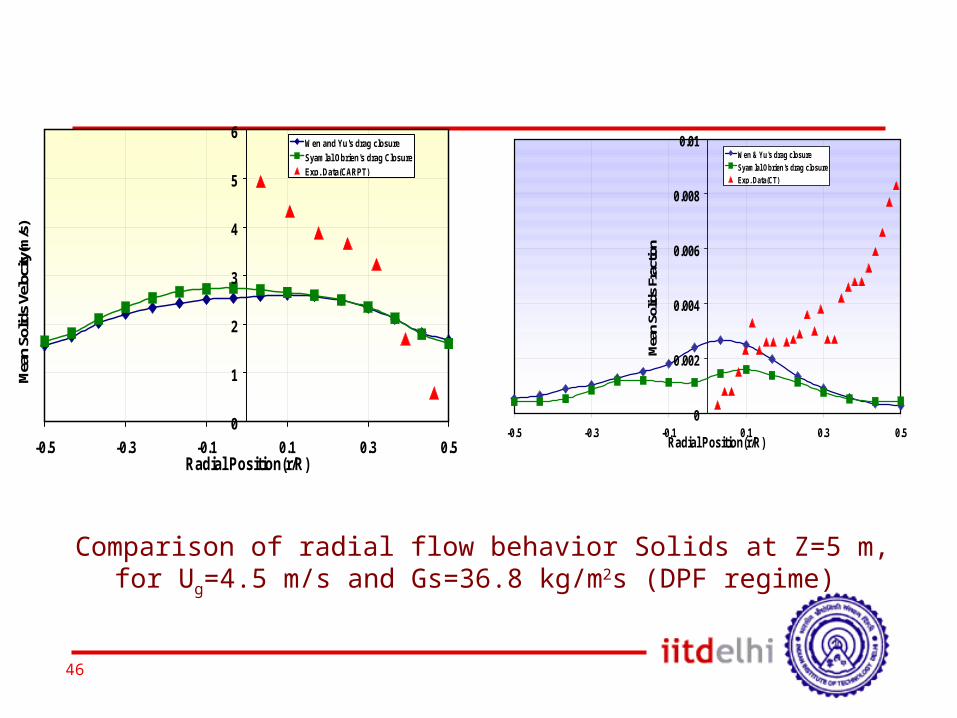
0

1

2

3

4

5

6

-0.5 -0.3 -0.1 0.1 0.3 0.5Radial Position(r/R)

Mean Solids Velocity(m/s)

W en and Yu's drag closureSyam lal Obrien's drag ClosureExp. Data(CARPT)

0

0.002

0.004

0.006

0.008

0.01

-0.5 -0.3 -0.1 0.1 0.3 0.5Radial Position(r/R)

Mean Solids Fraction

W en & Yu's drag closureSyam lal Obrien's drag closureExp. Data(CT)

Comparison of radial flow behavior Solids at Z=5 m, for Ug=4.5 m/s and Gs=36.8 kg/m2s (DPF regime)

47

Granular TemperatureGranular Temperature

48

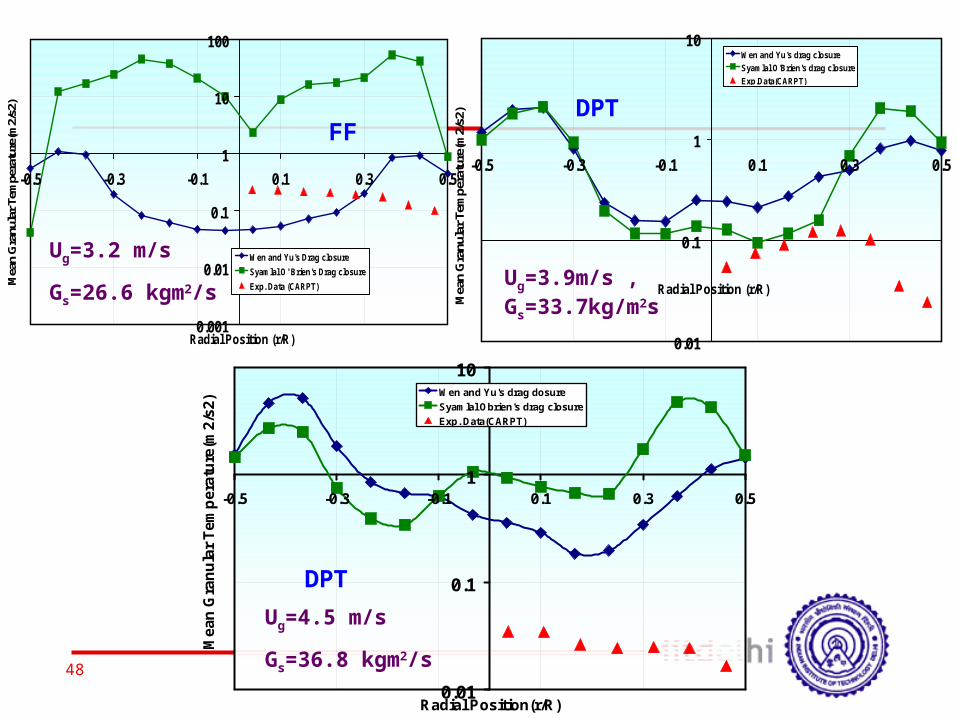
0.001

0.01

0.1

1

10

100

-0.5 -0.3 -0.1 0.1 0.3 0.5

Radial Position (r/R)

Mean Granular Temperature(m2/s2)

W en and Yu's Drag closureSyam lal O' Brien's Drag closureExp. Data (CARPT)

0.01

0.1

1

10

-0.5 -0.3 -0.1 0.1 0.3 0.5

Radial Position (r/R)

Mean Granular Tem

perature(m2/s2)

W en and Yu's drag closureSyam lal O'Brien's drag closureExp.Data(CARPT)

Ug=3.9m/s , Gs=33.7kg/m2s

Ug=3.2 m/sGs=26.6 kgm2/s

FFDPT

0.01

0.1

1

10

-0.5 -0.3 -0.1 0.1 0.3 0.5

Radial Position(r/R)

Mean Granular Tem

perature(m

2/s2) W en and Yu's drag dosure

Syam lal O brien's drag closureExp. Data(CARPT)

DPTUg=4.5 m/sGs=36.8 kgm2/s

49

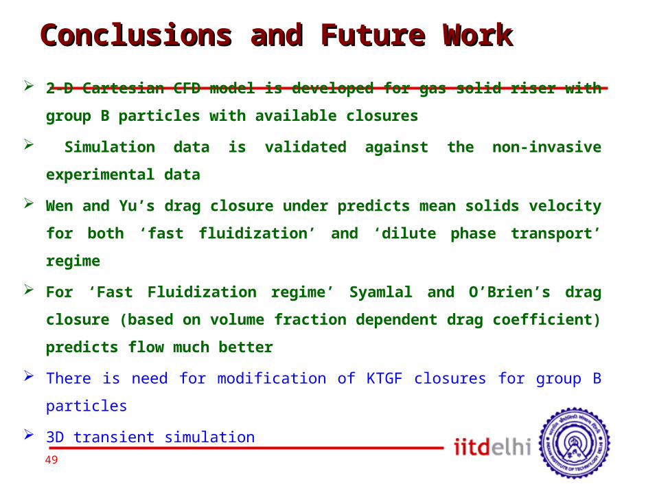
Conclusions and Future WorkConclusions and Future Work 2-D Cartesian CFD model is developed for gas solid riser with

group B particles with available closures Simulation data is validated against the non-invasive

experimental data Wen and Yu’s drag closure under predicts mean solids velocity

for both ‘fast fluidization’ and ‘dilute phase transport’ regime

For ‘Fast Fluidization regime’ Syamlal and O’Brien’s drag closure (based on volume fraction dependent drag coefficient) predicts flow much better

There is need for modification of KTGF closures for group B particles

3D transient simulation

RTD from CFD?RTD from CFD?

51

sigisiis

axsis

ssis

s RCCKxCD

xCu

tC

2

2

sis si s si ax

Cu C u C Dx

0siC

x

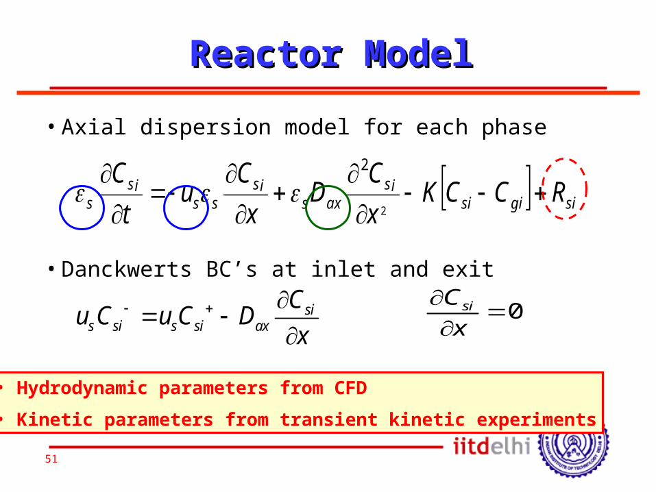
•Axial dispersion model for each phase

Reactor ModelReactor Model

•Danckwerts BC’s at inlet and exit

• Hydrodynamic parameters from CFD• Kinetic parameters from transient kinetic experiments

52

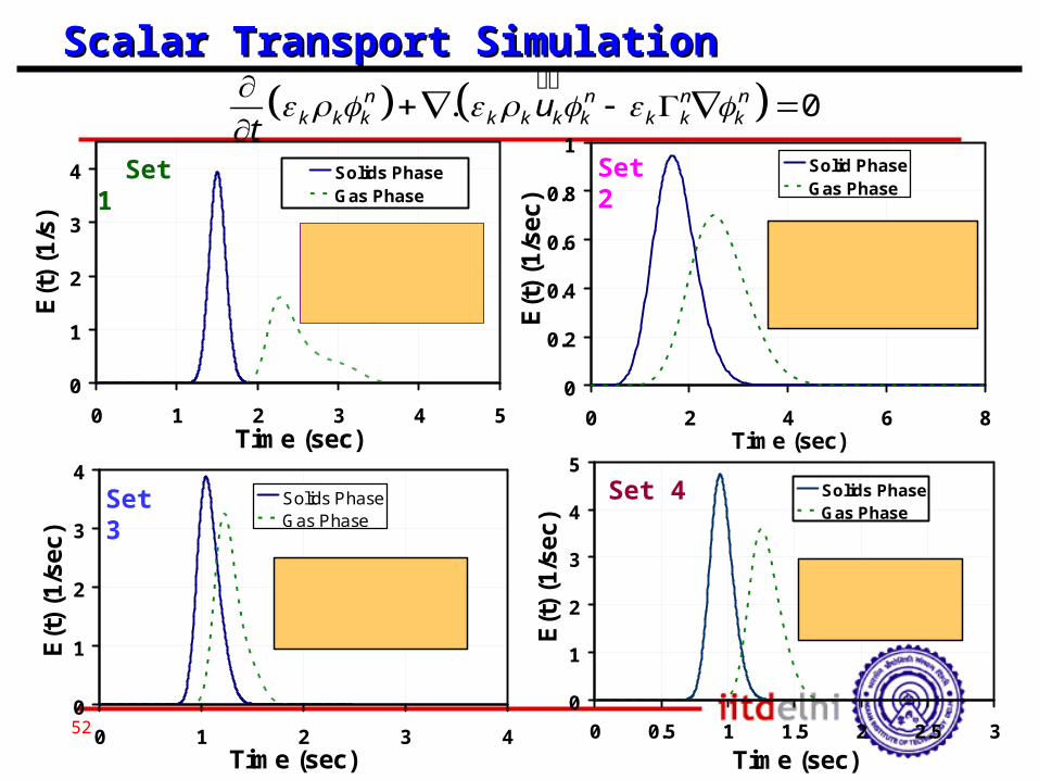
Scalar Transport SimulationScalar Transport Simulation

0

1

2

3

4

0 1 2 3 4 5Tim e (sec)

E(t) (1/s)

Solids PhaseG as Phase

Ug=3.7 m/s, Gs=49 kg/m2sSolids mean R.T.=1.50 secVariance (solids)= 0.0045Gas mean R.T.= 2.50 secVariance (gas)=0.018

0

1

2

3

4

0 1 2 3 4Tim e (sec)

E(t) (1/sec)

Solids PhaseG as Phase

Ug=7.2 m /s, G s=101kg/m 2sSolids m ean R.T.=1.08 secVariance (solids)= 0.0099Gas m ean R.T.= 1.28secVariance (gas)=0.00118

0

0.2

0.4

0.6

0.8

1

0 2 4 6 8Tim e (sec)

E(t) (1/sec)

Solid PhaseGas Phase

Ug=3.7 m /s, G s=101kg/m 2sSolids m ean R.T.=1.72 secVariance (solids)= 0.061Gas m ean R.T.= 2.61 secVariance (gas)=0.0488

0

1

2

3

4

5

0 0.5 1 1.5 2 2.5 3Tim e (sec)

E(t) (1/sec)

Solids PhaseGas Phase

Ug=7.2 m /s, Gs=208kg/m 2sSolids m ean R.T.=0.95 secVariance (solids)= 0.0082Gas m ean R.T.= 1.65secVariance (solids)=0.0079

. 0n n n nk k k k k k k k k ku

t

Set 1

Set 2

Set 3

Set 4

Future WorkFuture Work

54

X10-

3

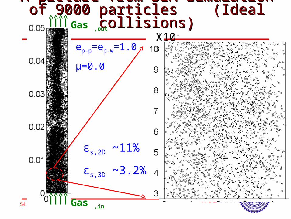
A picture from DEM Simulation A picture from DEM Simulation of 9000 particles (Ideal of 9000 particles (Ideal

collisions)collisions)

εs,2D ~11%εs,3D ~3.2%

ep-p=ep-w=1.0µ=0.0

Gas ,in

Gas ,out

55

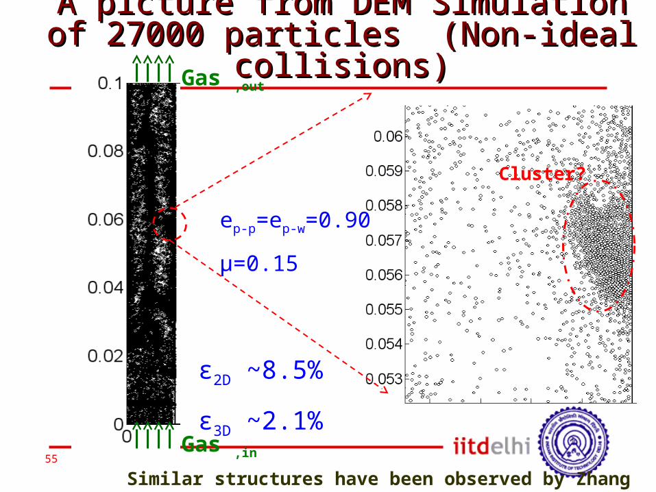
Similar structures have been observed by Zhang et al. 2000

ε2D ~8.5%ε3D ~2.1%

ep-p=ep-w=0.90µ=0.15

Cluster?

Gas ,in

A picture from DEM Simulation A picture from DEM Simulation of 27000 particles (Non-ideal of 27000 particles (Non-ideal

collisions)collisions)Gas ,out

56

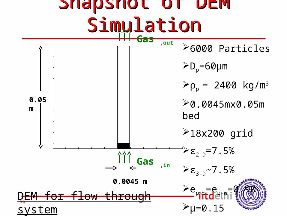
Snapshot of DEM Snapshot of DEM SimulationSimulation

0.05 m

0.0045 m

6000 ParticlesDp=60µmρp = 2400 kg/m3

0.0045mx0.05m bed18x200 gridε2-D=7.5%ε3-D~7.5%ep-p=ep-w=0.90µ=0.15

DEM for flow through system

Gas ,in

Gas ,out

57

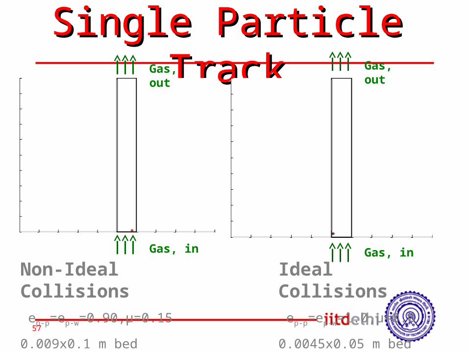
Single Particle Single Particle TrackTrack

Non-Ideal Collisions ep-p=ep-w=0.90,µ=0.150.009x0.1 m bed

Ideal Collisions ep-p=ep-w=1.0,µ=0.00.0045x0.05 m bed

Gas, in Gas, in

Gas, out

Gas, out