Identifying Heavy-Hitter Flows from Sampled Flow Statistics

IEICE TRANS. COMMUN., VOL.E90–B, NO.11 NOVEMBER 20073061

PAPER Special Section on Next Generation Network Management

Identifying Heavy-Hitter Flows from Sampled Flow Statistics∗

Tatsuya MORI†a), Tetsuya TAKINE††, Members, Jianping PAN†††, Nonmember, Ryoichi KAWAHARA†,Masato UCHIDA††††, and Shigeki GOTO†††††, Members

SUMMARY With the rapid increase of link speed in recent years,packet sampling has become a very attractive and scalable means in col-lecting flow statistics; however, it also makes inferring original flow char-acteristics much more difficult. In this paper, we develop techniques andschemes to identify flows with a very large number of packets (also knownas heavy-hitter flows) from sampled flow statistics. Our approach follows atwo-stage strategy: We first parametrically estimate the original flow lengthdistribution from sampled flows. We then identify heavy-hitter flows withBayes’ theorem, where the flow length distribution estimated at the firststage is used as an a priori distribution. Our approach is validated and eval-uated with publicly available packet traces. We show that our approachprovides a very flexible framework in striking an appropriate balance be-tween false positives and false negatives when sampling frequency is given.key words: network measurement, packet sampling, flow statistics, a prioridistribution, Bayes’ theorem

1. Introduction

For very high-speed links (e.g., OC-768+), collecting allpackets for on-line analysis is beyond the capability of mostexisting measurement equipments. For example, we haveonly 8 ns to process a 40-byte packet at a 40 Gb/s link.Thus the demands for CPU power, memory/storage capac-ity and access speed to conduct network measurement areoverwhelming. Being proposed as a candidate to meet thischallenge, packet sampling techniques in recent years haveattracted more and more attention from both industry and re-search communities [3], [4], [7], [12], [24]. Modern routersalready had these techniques embedded, e.g., NetFlow [16]and sFlow [21]. Also, the Packet Sampling (psamp) Work-ing Group [19] at IETF has been standardizing the tech-niques related to packet sampling. As being discussed in

Manuscript received February 28, 2007.Manuscript revised June 5, 2007.†The authors are with the NTT Service Integration Laborato-

ries, NTT Corporation, Musashino-shi, 180-8585 Japan.††The author is with the Department of Information and Com-

munication Technology, Graduate School of Engineering, OsakaUniversity, Suita-shi, 565-0871 Japan.†††The author is with the Department of Computer Science, Uni-

versity of Victoria, Victoria, BC, Canada.††††The author is with the Network Design Research Center, Kyu-

shu Institute of Technology, Kitakyushu-shi, 802-0001 Japan.†††††The author is with the Dept. of Information and Computer

Science, School of Science and Engineering, Waseda University,Tokyo, 169-8585 Japan.

∗An earlier version of this paper was presented at ACM IMC2004 [15].

a) E-mail: [email protected]: 10.1093/ietcom/e90–b.11.3061

[2], [5], [6], [11], although packet sampling techniques pro-vide greater scalability for network measurement, they alsomake inferring original flow characteristics much more dif-ficult.

In this paper, we attempt to answer the following ques-tion: How many (Y) sampled packets of a specific flowshould be collected to conjecture that the original flow hasmore than X packets in total? In particular, we are interestedin identifying flows with a very large number of packets, i.e.,heavy-hitter flows. Many ISPs need to regulate traffic gen-erated by heavy-hitters according to their cumulative trafficvolume over a certain time period, so a practical answer tothis question is very useful in choosing an adequate lengththreshold of sampled flows to identify heavy-hitters. Here,flow length is the number of packets in a flow, original flowlength means the number of packets in a flow that actuallyappear on a link during a certain time period, and sampledflow length means the number of sampled packets for a par-ticular flow.

To answer more than just the above question, in this pa-per we develop a framework to determine the length thresh-old of sampled flows for identifying flows of interest. Ourapproach follows a two-stage strategy: We first estimate theoriginal flow length distribution from sampled flow statis-tics. More specifically, we fit sampled flow statistics to atruncated Pareto distribution by means of maximum likeli-hood estimation (MLE). Next, we use Bayes’ theorem withthe estimated a priori distribution for identifying heavy-hitter flows from sampled flows. As we shall see, this ap-proach is very flexible in striking an appropriate balance be-tween false positives and false negatives when sampling fre-quencies are given. Although we use the usual 5-tuple def-inition (i.e., source/destination IP addresses and port num-bers and protocol identifier) for flows in this paper, our ap-proach is also applicable to aggregated flows defined bytheir IP prefixes or AS numbers.

The remainder of the paper is organized as follows.Section 2 reviews related work and compares it with ours.Section 3 explains how to characterize the original flowlength (i.e., a priori distribution) with a truncated Pareto dis-tribution. In Sect. 4, we discuss how to estimate the origi-nal flow length distribution from sampled flow statistics bymeans of MLE. In Sect. 5, we describe our framework to in-fer the original flow length from the sampled flow length.We also validate our approach by applying extensive packetsampling processes to real packet traces. In Sect. 6, we show

Copyright c© 2007 The Institute of Electronics, Information and Communication Engineers

3062IEICE TRANS. COMMUN., VOL.E90–B, NO.11 NOVEMBER 2007

how to identify heavy-hitter flows based on our framework.Section 7 discusses some related issues. In Sect. 8, we con-clude this paper with a brief summary.

2. Related Work

There are several papers addressing the problem of infer-ring original flow characteristics from sampled flow statis-tics. Duffield et al. [6] investigate how to estimate the orig-inal flow length distribution from sampled flow statistics.Their key idea is to use MLE for inference and additionalinformation in measured flow records, e.g., TCP SYN flag,which can be used to estimate the number of original flows.

On the other hand, the aim of our work is to develop away to infer the original flow length from the sampled flowlength without looking at each packet. To do so, we need thea priori length distribution of original flows. In contrast to[6], we adopt a parametric approach to estimating the origi-nal flow length distribution, since such an approach reducesoperation overhead significantly. As we shall see, our ap-proach works well in identifying heavy-hitters. Note alsothat this work goes beyond our previous work [15] by intro-ducing the above approach, i.e., the estimation of the origi-nal flow length distribution from the sampled flow statistics.

Hohn and Veitch [11] also study the related problem.Using a Poisson flow arrival model, they reveal that thereexists an inherent limit in recovering the original flow lengthdistribution from sampled flow statistics in a theoreticalfashion. They also show that asymptotic properties of theheavy-tailed flow length distribution can be recovered fromsampled flow statistics. Barakat et al. [2] study how to de-tect and rank the largest flows from sampled flow statistics.Through theoretical analysis and experiments with collectedpacket traces, they show that the ranking accuracy stronglydepends on the sampling frequency, e.g., accurate rankingof the largest (say, the 10 heaviest) flows requires samplingrate of 10% or greater. They also show that by applying aprotocol-aware ranking method, the required sampling fre-quency can be reduced by an order of magnitude.

There is another approach to tackling the problemof identifying heavy-hitter flows, i.e., the data reductionmethod. The aim of this approach is to reduce the amountof memory required for keeping flow statistics. Estanand Varghese [8] propose two novel techniques, sample-and-hold and multistage filters. Both techniques improvethe process of extracting flow statistics in high-speed net-works, while keeping memory consumption reasonably low.Kumar et al. [13] propose a new technique called space-codeBloom filter for extracting per-flow traffic statistics in high-speed networks. Their key ideas are the extension of thetraditional Bloom filter to a one with multiple sets of hashfunctions and the use of multi-resolution sampling. Theirapproach can capture flow statistics very well, while requir-ing a small amount of memory resources. Golab et al. [10]propose a deterministic algorithm to identify frequent itemsusing a memory-limited sliding window model. The pro-posed algorithm can fulfill its objective with limited mem-

ory resources. The main difference of these approaches fromours is their requirement of complex per-packet processing.That is, those approaches are based on non-sampling tech-niques, which look up all the coming packets instead of sam-pling them; thus it can keep rich information such as the rep-resentation of per-flow statistics. The approach has intrinsicconstraints to operate with small amount of memory space(such as SRAM) to keep up with per-packet processing. Italso requires to develop dedicated hardware to implementcomplexed operations such as hashing. In contrast, packetsampling schemes, which is our basis, have no requirementof per-packet processing and provide high scalability andlow implementation cost. Actually, packet sampling is to-day’s off-the-shelf measurement technique widely used inactual academic/commercial networks.

3. A priori Distribution of Original Flow Length

It is well known that the flow length distribution in the In-ternet is heavy-tailed [9], [14], [20], [22], [23], which is con-sidered as one of the invariant characteristics of the Internet.The Pareto distribution is a simple model for characteriz-ing heavy-tailed distributions. However, as we can see, theflow length distribution should always have an upper bound,which is dictated by the following facts. First, many Inter-net flows correspond to data files, and there is a limit on thefile/data size in most file systems. For example, the capacityof a regular DVD disc is 4.377 GB, and the FAT32 file sys-tem supports the maximum file size of 4 GB. Also, since themeasurement time period is always finite, the observed flowlength should be bounded by the number of total observedpackets, even if there exists only one flow. Thus, when weobserve the flow length distribution in a finite time period,there is always a cutoff length that truncates the heavy-taildistribution. Here, we adopt the truncated Pareto distribu-tion to approximate the flow length distribution. The trun-cation point can be estimated from the observed traffic in thefollowing way.

We assume that there are m flows observed, i.e., with-out sampling, during a certain time period. Let Xj ( j =1, 2, . . . ,m) denote the original flow length of the j-th flow,where a flow is defined by its 5-tuple identity throughout thispaper. We then assume that the distribution of Xj’s can beapproximated by a discrete, truncated Pareto distribution:

Pr[Xj = x

]=

x−θ − (x + 1)−θ

1 − (ν + 1)−θ(1 ≤ x ≤ ν),

Pr[Xj > x

]=

(x + 1)−θ − (ν + 1)−θ

1 − (ν + 1)−θ(0 ≤ x ≤ ν).

Note that Xj has its upper bound ν (i.e., Pr[Xj > ν] = 0),and every flow contains at least one packet (i.e., Pr[Xj ≥1] = 1). This truncated distribution is a modified versionof the original truncated Pareto distribution studied in [1].Note also that Xj is a discrete variable for flow length.

Given the observed flow length Xj ( j = 1, 2, . . . ,m),parameters ν and θ can be estimated by means of MLE. The

MORI et al.: IDENTIFYING HEAVY-HITTER FLOWS FROM SAMPLED FLOW STATISTICS3063

Fig. 1 A priori distribution estimated by the truncated Paretodistribution.

ML estimator ν of ν is given by

ν = max (X1, X2, . . . , Xm) , (1)

and the ML estimator θ of θ satisfies the following equation:

−mlog (ν + 1) (ν + 1)−θ

1 − (ν + 1)−θ

+

m∑j=1

−(log Xj

)X−θj +

{log

(Xj + 1

)} (Xj + 1

)−θX−θj −

(Xj + 1

)−θ = 0.

(2)

The proofs of Eqs. (1) and (2) are given in Appendix A.To evaluate the accuracy of the truncated Pareto ap-

proximation, we use a packet trace collected at an OC-48cbackbone link by the PMA project at NLANR [17]. Thetrace was collected from 10:50 to 11:00 on August 14, 2002.For easy handling, we use the first 107 packets that corre-spond to about 124 seconds of observed traffic. We refer tothis sliced packet trace as trace-I throughout this paper.The total number of flows in trace-I is 206, 299.

Figure 1 shows the Log-Log-Complementary-Distribution (LLCD) plots of the empirical distribution ofthe original flow lengths (circles) and the truncated Paretoapproximation for trace-I (curve). We observe that thetruncated Pareto model fits the empirical distribution fairlywell. Note that a rapidly decreasing tail is one of typicalfeatures in the truncated Pareto distribution.

In Fig. 2, we show the corresponding quantiles-quantiles (Q-Q) plot to further validate the accuracy of thetruncated Pareto approximation. The horizontal axis repre-sents the empirical quantiles, and the vertical axis representsthe quantiles of the approximate truncated Pareto distribu-tion. We observe that the curve is fairly close to a straightline with slope 1 over a wide quantile range, although thereare deviations in the middle of the support of the distribu-tion.

Fig. 2 Q-Q plot for the flow length distribution: empirical distributionvs. approximate distribution.

Table 1 Estimated parameters in the truncated Pareto distribution.

ν θ

244, 739 .891

Table 1 shows the estimated values of parameters ν andθ for trace-I. It is interesting to see that the estimatedshape parameter θ is less than 1, which does not imply theinfinite average of flow length. Since we adopt the truncateddistribution, the estimated flow length distribution alwayshas finite mean and variance.

Since the truncated Pareto distribution is characterizedby only two parameters, it is quite easy to estimate them.Thus the model offers higher feasibility in actual operation.Of course, the truncated Pareto distribution might not besufficient to characterize the flow length distribution in allcases. Some statistical metrics such as the weighted meanrelative difference [6], might be useful for quantitativelystudying the limitation of the truncated Pareto distribution.It is also for our further study. We believe, however, that theheavy-tailed characteristic is invariant in the Internet traffic,and the truncated Pareto distribution can capture this char-acteristic quite well. To support our claim, some examplesof parameter estimation for other packet traces are given inAppendix B.

4. Estimation of the a priori Distribution

In the preceding section, we showed that the original flowlength distribution could be well modeled by the truncatedPareto distribution. In this section, we show how to estimatethe unknown parameters ν and θ in the truncated Pareto dis-tribution from sampled flow statistics. Note that only the es-timated distribution will be used as the a priori distributionin estimating the original flow length in the next section.


4.1 MLE of the a priori Distribution

Suppose N packets appear during a certain time period, andeach of them is sampled independently with probability f .In other words, we consider random sampling from a pop-ulation of N packets with sampling frequency f . We de-fine Xj and Yj ( j = 1, 2, . . . ,m) as the original and sam-pled flow lengths of the j-th flow, respectively. By defini-tion, N = X1 + X2 + · · · + Xm. Let ni (i = 1, 2, . . . , ymax)denote the number of flows whose sampled flow length isequal to i, where ymax denotes the maximal sampled flowlength. We estimate parameters θ and ν from the observedn = (n1, n2, . . . , nymax ).

For simplicity, we assume that ν can be estimated in-dependent of θ. Recall that the ML estimator ν of ν is givenby max(Xj). Further the unbiased estimator of max(Xj) isgiven by max(Yj)/ f . Therefore it is possible to estimate νas

ν =ymax

f. (3)

As we shall see in Sect. 7, the estimation error in ν does notplay a crucial role in inferring the original flow length.

Due to random sampling, the conditional sampledprobability q(y | x) = Pr[Yj = y | Xj = x] is given by

q(y | x) =

⎧⎪⎪⎨⎪⎪⎩(xy

)· f y (1 − f )x−y , y = 0, 1, . . . , x,

0, otherwise.

Thus the probability r (y) = Pr[Yj = y] is given by

r(y) =ν∑

k=y

q (y | k) p (k, θ) ,

where

p (k, θ) = Pr[Xj = k

]=

k−θ − (k + 1)−θ

1 − (ν + 1)−θ. (4)

Given the observed data n = (n1, n2, . . . , nymax), the like-lihood function with parameter θ is given by

L (θ; n) =ymax∏i=1

(r (i)

1 − r (0)

)ni

,

since we cannot observe flows without sampled packets.The log likelihood function is then given by

L (θ) = log L (θ; n)

=

ymax∑i=1

ni log

⎛⎜⎜⎜⎜⎜⎜⎝ν∑

k=i

q (i | k) p (k, θ)

⎞⎟⎟⎟⎟⎟⎟⎠

−⎛⎜⎜⎜⎜⎜⎝ymax∑i=1

ni

⎞⎟⎟⎟⎟⎟⎠ log

⎛⎜⎜⎜⎜⎜⎜⎝1 −ν∑

k=1

q (0 | k) p (k, θ)

⎞⎟⎟⎟⎟⎟⎟⎠ .Thus, the ML estimator θ of parameter θ is given by a posi-tive solution of ∂L(θ)/∂θ = 0, i.e.,

Fig. 3 Estimated a priori distributions with f = 10−3 and f = 10−4.

⎛⎜⎜⎜⎜⎜⎝ymax∑i=1

ni

⎞⎟⎟⎟⎟⎟⎠∑ν

k=1 q (0 | k) ∂p(k,θ)∂θ

1 −∑νk=1 q (0 | k) p (k, θ)

+

ymax∑i=1

ni

∑νk=i q (i | k) ∂p(k,θ)

∂θ∑νk=i q (i | k) p (k, θ)

= 0,

where

∂p (k, θ)∂θ

=

{log (k + 1)

}(k + 1)−θ − (

log k)

k−θ

1 − (ν + 1)−θ

−{log(ν + 1)

}(ν + 1)−θ

{k−θ − (k + 1)−θ

}{1 − (ν + 1)−θ

}2.

We can numerically solve the equation by using a standardalgorithm such as the false position method.

4.2 Evaluation of the Estimation

To evaluate the accuracy of the estimation, we first applyrandom packet sampling† to trace-I and obtain the sam-pled flow statistics, i.e., n = (n1, n2, . . . , nymax), for samplingfrequency f = 10−3 and f = 10−4, respectively. Applyingthe MLE method described in the preceding subsection tothese data, we estimate parameters ν and θ. Figure 3 showsLLCD plots of the original a priori distribution (circles) andthe estimated distributions (dashed curves). For the sake ofcomparison, we also plot the truncated Pareto approxima-tion obtained from original flow data (solid curve). We ob-serve that the estimated distributions from sampled flows fitthe original a priori distribution and its approximate distri-bution fairly well. Figure 7 shows the corresponding Q-Qplots to further validate the accuracy of the estimation. We

†Throughout this paper, we use “uniform probabilistic sam-pling,” which is one of the packet sampling techniques standard-ized by IETF psamp WG [19]. That is, we independently samplepackets with a uniform probability p = f . We also confirmed thatother sampling processes such as systematic sampling give similarresults.


Table 2 Estimated parameters for sampling frequency f = 10−3 andf = 10−4.

ν θ

f = 10−3 232,000 .712f = 10−4 250,000 .860

Fig. 4 Sampled flow statistics n for sampling frequency f = 10−3 (left)and f = 10−4 (right).

Table 3 Estimated parameters from 10 random sampling processes.

min ν max ν ν min θ max θ θ

f = 10−3 225,000 266,000 244,800 .699 .716 .710f = 10−4 210,000 280,000 237,000 .831 .880 .851

observe that the curve is fairly close to a straight line withslope 1 over a wide range, although there are some devia-tions.

Table 2 shows the values of the estimated parameters νand θ. We note that the estimated distribution becomes moreheavy-tailed when f is higher, i.e., the estimated shape pa-rameter θ for f = 10−3 is smaller than that of f = 10−4.This behavior can be explained as follows. In Fig. 4, whichshows the measured n for each sampling frequency, we ob-serve that more sampled information comes from small i’s,such as 1 ≤ i ≤ 50 for f = 10−3 and 1 ≤ i ≤ 10 forf = 10−4. These i-packet (sampled) flows roughly corre-spond to i × 1, 000-packet (original) flows for f = 10−3 andi×10, 000-packet (original) flows for f = 10−4, respectively.Thus, for f = 10−4, the estimated flow length distribution re-flects larger original flows better than the case for f = 10−3.Since we parameterize the distribution with the truncatedPareto distribution, the estimated distribution for f = 10−4

fits the original downward curve better, and accordingly be-comes less heavy-tailed than the case for f = 10−3.

To confirm the above explanation, we then apply packetsampling to trace-I with different random seeds for 10times, and estimate the parameters for each sampled flowstatistics. Table 3 summarizes the results. As being indi-cated above, the estimated θ for f = 10−4 is larger than thatfor f = 10−3. We can also find that the estimated ν forf = 10−3 is relatively close to the estimated ν for originalflows without sampling (recall that ν = 244,739 in Table 1).

Thus, even though we take account of the non-sampledflows by introducing conditional probability, the estimated

flow length distribution is slightly skewed due to the infor-mation loss caused by packet sampling. As we shall showshortly, the difference in estimated flow length distributiondoes not affect the inference of the original flow length fromsampled flow statistics with small false probabilities. Someexamples of the estimation for other packet traces are givenin Appendix B.

5. Inferring Original Flow Length

In this section, we provide a framework to infer the originalflow length from the sampled flow length. Our approach isbased on Bayes’ theorem with the a priori distribution esti-mated in the preceding section.

5.1 Inference Framework

Recall that our task is to answer the following question:How many (Y) sampled packets of a specific flow shouldbe collected to conjecture that the original flow has morethan X packets in total? Let y′ = y′(x∗) denote the lengththreshold of sampled flows. Namely, if the sampled flowlength of a particular flow is no less than y′, we conjecturethat the flow contains at least x∗ packets. In what follows,we describe a way to find an appropriate value of y′.

To obtain an appropriate y′, we have to consider andbalance two kinds of false probabilities listed below.

FPR(y′) def= 1 − Pr

[Xj ≥ x∗ | Yj ≥ y′

],

FNR(y′) def= 1 − Pr

[Yj ≥ y′ | Xj ≥ x∗

].

Note that FPR(y′) denotes the false positive ratio, i.e., theconditional probability that the original flow length is lessthan x∗ given that the sampled flow length is not less thany′. On the other hand, FNR(y′) denotes the false negativeratio, i.e., the conditional probability that the sampled flowlength is less than y′ given that the original flow length isnot less than x∗.

According to Bayes’ theorem, the conditional proba-bility of Xj ≥ x∗ given Yj ≥ y′ is obtained to be

Pr[Xj ≥ x∗ | Yj ≥ y′

]

=

∑νk=x∗ Pr

[Yj ≥ y′ | Xj = k

]Pr

[Xj = k

]∑ν

k=1 Pr[Yj ≥ y′ | Xj = k

]Pr

[Xj = k

] ,

where Pr[Xj = k

]= p(k, θ) denotes the a priori distribution

(see Eq. (4) in Sect. 4) and

Pr[Yj ≥ y′ | Xj = k

]= 1 −

y′−1∑i=0

Pr[Yj = i | Xj = k

]

= 1 −y′−1∑i=0

q (i | k) .

Thus, we can calculate FPR(y′) by


FPR(y′) = 1 −∑ν

k=x∗(1 −∑y′−1

i=0 q (i | k))

Pr[Xj = k

]∑ν

k=1

(1 −∑y′−1

i=0 q (i | k))

Pr[Xj = k

] .(5)

Similarly, FNR(y′) can be calculated by

FNR(y′) = 1 −∑ν

k=x∗(1 −∑y′−1

i=0 q (i | k))

Pr[Xj = k

]∑ν

k=x∗ Pr[Xj = k

] .

(6)

Intuitively, for a fixed x∗, FPR(y′) will be a decreasingfunction of y′, while FNR(y′) will be an increasing func-tion of y′. That is, there is an intrinsic trade-off betweenfalse probabilities. Therefore it prevents us from choosingan arbitrary y′. Our framework allows us to quantify thistrade-off and make a proper choice, as we shall see shortly.

5.2 Evaluation of the Framework

To evaluate our framework, we use trace-I again (i.e., N =107) and compare FPR(y′) in Eq. (5) and FNR(y′) in Eq. (6)with various a priori distributions:

• the empirical distribution of original flows,• the truncated Pareto approximation of the empirical

distribution (given in Sect. 3),• the estimated truncated Pareto distribution from the

sampled flow statistics (given in Sect. 4), and• the uniform distribution, i.e., Pr[Xj = i] = 1/max(Xj)

(i = 1, 2, . . . ,max(Xj)).

The threshold x∗ is set to be 10, 000. FPR(y′) and FNR(y′)with the empirical distribution are considered as bench-marks. We plot false probabilities derived from 10 randomsampling processes, and false probabilities are calculated by

FPR(y′) = 1 −Nf

(Xj ≥ x∗, Yj ≥ y′

)Nf

(Yj ≥ y′

) , (7)

FNR(y′) = 1 −Nf

(Xj ≥ x∗, Yj ≥ y′

)Nf

(Xj ≥ x∗

) , (8)

where Nf (χ) denotes the number of sampled flows includedin event χ. We show the mean value with dashed error bar,which indicates the maximum and minimum values amongthose of 10 sampling processes.

In the case with the estimated truncated Pareto distri-bution, we use the sampled flow statistics derived from 10random packet sampling processes for sampling frequencyf = 10−3 and f = 10−4, respectively. Again, we plot themean value with error bar, which indicates the maximumand minimum values. The results are shown in Figs. 5 and6.

From these figures, we first observe that there are in-trinsic trade-offs between false probabilities. In all cases,an increase in y′ leads to a decrease in FPR(y′) and an in-crease in FNR(y′). We can also see that the trade-off is more

Fig. 5 False probabilities for sampling frequency f = 10−3: FPR (y′)(top) and FNR (y′) (bottom). Note that the uniform distribution modelfalsely underestimates the false probabilities.

critical at the lower sampling frequency, i.e., f = 10−4.Secondly, FPR’s derived from the approximate distri-

bution (i.e., without sampling) and the estimated distribu-tions (i.e., with sampling) fit the one obtained with the em-pirical distribution fairly well. Thus these FPR’s seem veryreliable. On the other hand, there exist relatively large dis-crepancies in FNR. These discrepancies are caused by thefact that the approximate distribution and the estimated dis-tribution are slightly different from the empirical distribu-tion in the tail quantiles (see Fig. 7). We can see that thediscrepancies become larger when sampling rate is equal to10−3, where the discrepancies in the tail quantiles also be-come larger. Thus this might indicate the limitation of thetruncated Pareto approximation. We also observe that thefalse probabilities derived from the estimated distributions(i.e., with or without sampling) have pretty small discrepan-cies; i.e., the results are still reliable.

Finally, we observe that the uniform distribution asthe a priori distribution yields quite different false proba-bilities. The uniform distribution model assumes that the


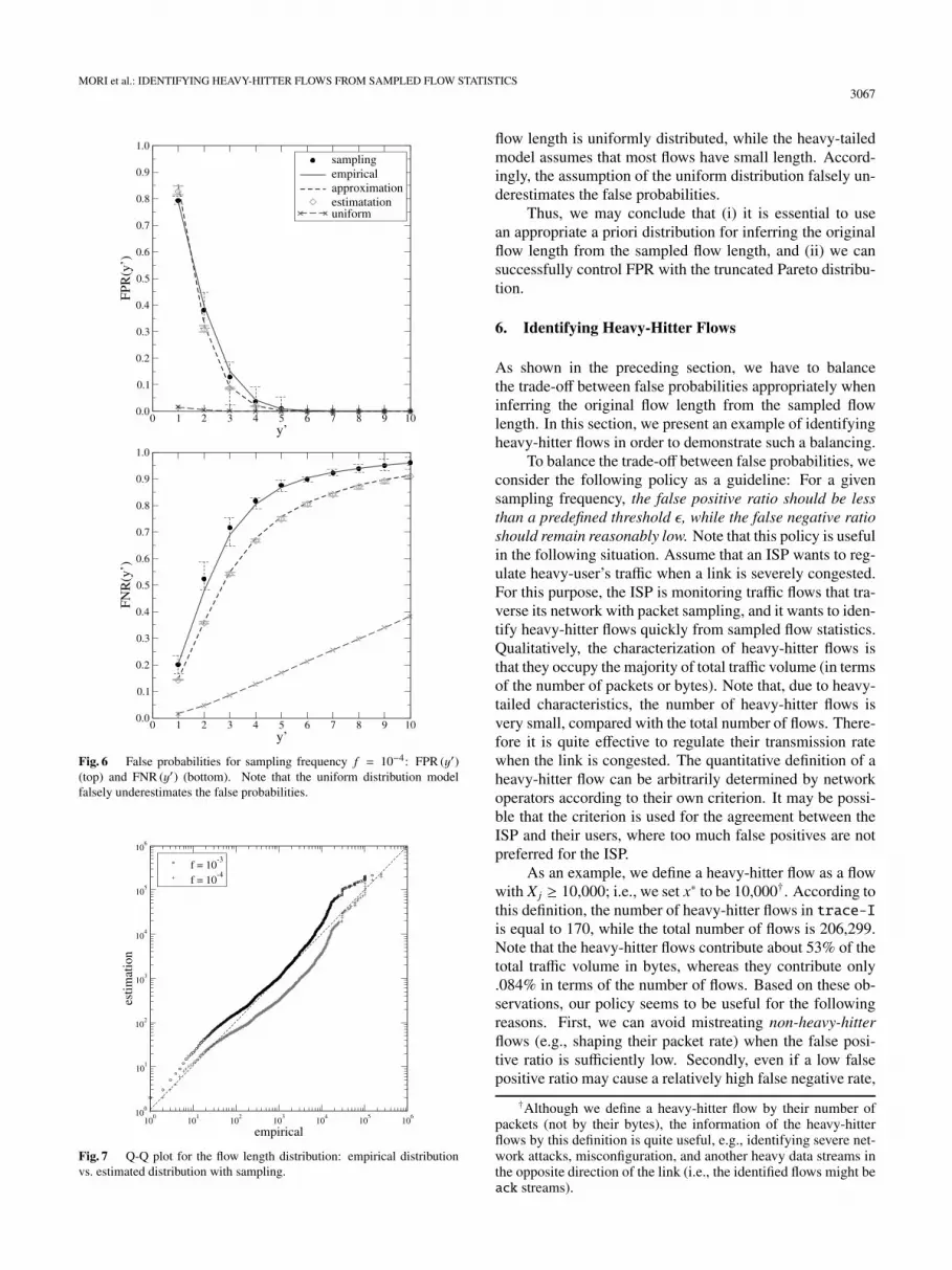
Fig. 6 False probabilities for sampling frequency f = 10−4: FPR (y′)(top) and FNR (y′) (bottom). Note that the uniform distribution modelfalsely underestimates the false probabilities.

Fig. 7 Q-Q plot for the flow length distribution: empirical distributionvs. estimated distribution with sampling.

flow length is uniformly distributed, while the heavy-tailedmodel assumes that most flows have small length. Accord-ingly, the assumption of the uniform distribution falsely un-derestimates the false probabilities.

Thus, we may conclude that (i) it is essential to usean appropriate a priori distribution for inferring the originalflow length from the sampled flow length, and (ii) we cansuccessfully control FPR with the truncated Pareto distribu-tion.

6. Identifying Heavy-Hitter Flows

As shown in the preceding section, we have to balancethe trade-off between false probabilities appropriately wheninferring the original flow length from the sampled flowlength. In this section, we present an example of identifyingheavy-hitter flows in order to demonstrate such a balancing.

To balance the trade-off between false probabilities, weconsider the following policy as a guideline: For a givensampling frequency, the false positive ratio should be lessthan a predefined threshold ε, while the false negative ratioshould remain reasonably low. Note that this policy is usefulin the following situation. Assume that an ISP wants to reg-ulate heavy-user’s traffic when a link is severely congested.For this purpose, the ISP is monitoring traffic flows that tra-verse its network with packet sampling, and it wants to iden-tify heavy-hitter flows quickly from sampled flow statistics.Qualitatively, the characterization of heavy-hitter flows isthat they occupy the majority of total traffic volume (in termsof the number of packets or bytes). Note that, due to heavy-tailed characteristics, the number of heavy-hitter flows isvery small, compared with the total number of flows. There-fore it is quite effective to regulate their transmission ratewhen the link is congested. The quantitative definition of aheavy-hitter flow can be arbitrarily determined by networkoperators according to their own criterion. It may be possi-ble that the criterion is used for the agreement between theISP and their users, where too much false positives are notpreferred for the ISP.

As an example, we define a heavy-hitter flow as a flowwith Xj ≥ 10,000; i.e., we set x∗ to be 10,000†. According tothis definition, the number of heavy-hitter flows in trace-Iis equal to 170, while the total number of flows is 206,299.Note that the heavy-hitter flows contribute about 53% of thetotal traffic volume in bytes, whereas they contribute only.084% in terms of the number of flows. Based on these ob-servations, our policy seems to be useful for the followingreasons. First, we can avoid mistreating non-heavy-hitterflows (e.g., shaping their packet rate) when the false posi-tive ratio is sufficiently low. Secondly, even if a low falsepositive ratio may cause a relatively high false negative rate,

†Although we define a heavy-hitter flow by their number ofpackets (not by their bytes), the information of the heavy-hitterflows by this definition is quite useful, e.g., identifying severe net-work attacks, misconfiguration, and another heavy data streams inthe opposite direction of the link (i.e., the identified flows might beack streams).


Table 4 y, FPR(y) and FNR(y) for trace-I (ε = .05, f = 10−3).

y FPR(y) FNR(y)13 .039 .178

y real FPR(y) real FNR(y)13 .057 .318

→ 14 .036 .376

Table 5 y, FPR(y) and FNR(y) for trace-I (ε = .05, f = 10−4).

y FPR(y) FNR(y)4 .020 .667

y real FPR(y) real FNR(y)3 .075 .712

→ 4 .000 .812

the amount of traffic volume generated by identified heavy-hitter flows is already significant. For example, the 10 heav-iest flows in trace-I account for about 17% of the totaltraffic volume.

According to this policy, our goal is to find y′ = y suchthat FPR(y) is no greater than ε. Because FPR(y) is a de-creasing function of y′, threshold y can be determined by

y = miny′

{y′ | FPR(y′) ≤ ε} . (9)

Note that Eq. (9) guarantees the lowest false negative ratiounder the constraint FPR(y′) ≤ ε, since FNR(y′) is an in-creasing function of y′.

To evaluate this policy, we apply a random samplingprocess to trace-I, and derive sampled flow statistics.Here, the sampling frequencies are set to be f = 10−3 andf = 10−4. We then estimate the flow length distributionfrom the sampled flow statistics. Using the estimated flowlength distributions and Eq. (9), we calculate y, FPR(y), andFNR(y) for each sampling frequency. Tables 4 and 5 listthese results, where ε is set to be .05. We also show thebenchmarks of these values, which are obtained throughEqs. (7) and (8), for the sake of comparison with the resultsfrom the sampled flow statistics.

When f = 10−3, y is estimated to be 13 with FPR(13) =.039. On the other hand, in this specific sampled data, thereal FPR for y = 13 is .057 and the real y is 14. Thus thereexists an estimation error. As we observed in the Sect. 5, theestimated FNR is smaller than the real value. When f =10−4, the estimated y is the same as the real value and thecorresponding FPR(y) = .020 is more conservative, i.e., itis greater than the real value 0. Apparently this result ispreferable according to our criteria. We observe, however,that FNR is underestimated again.

Before closing this section, we summarize the proce-dure for identifying heavy-hitter flows from sampled flowstatistics. We also give a guideline to set the initial parame-ters in Step 1.

Step 1: Determine (i) sampling frequency f , (ii) thresh-old x∗ defining a heavy-hitter flow, and (iii) threshold εthat FPR should satisfy.

Step 2: Estimate an a priori distribution of Xj from sam-pled flow statistics n according to Sect. 4.

Step 3: Calculate y according to Eq. (9).

Step 4: If the sampled flow length of a flow is not lessthan y, the flow is identified as a heavy-hitter flow.

Guideline of setting initial parameters

The initial parameters in Step 1 can be determined by net-work operators according to their policies and available re-sources. However, these parameters are not totally inde-pendent and there is a trade-off between cost and accuracy.As we have shown above, our framework is able to addressthis trade-off quantitatively, which makes possible for net-work operators to choose these parameters flexibly and ef-fectively. First, the network operators might want to setx∗ when they try to regulate traffic from heavy hitter flowswhose size exceeds certain threshold, x∗. Then, when theyset the sampling frequency f, they can refer to the perfor-mance of their network equipment. Through the discussionwith network operators, we have found that in most cases,they are using rule-of-thumb when they set the sampling fre-quency, e.g., f = 10−3, 10−4, etc, which we chose as exam-ples in this paper. However, we believe that it is possibleto set the sampling frequency more flexibly rather than us-ing the rule-of-thumb as we will show below. Finally, theoperators might want to set ε to be as small as possible inmany cases, however, it cannot be too small, since there isan instrinsic trade-off between FPR and FNR as shown inFig. 6 and Fig. 7. One can set ε to be small so that FNR doesnot increase too much. If one prefers both FPR and FNRto be small, it can be achieved by increasing the samplingfrequency as much as their resource allows.

7. Further Discussion

Influence of ν— In Sect. 4.1, we adopt ν = ymax/ f as anestimator of parameter ν (see Eq. (3)). Here we discuss howthe estimation error in ν affects our scheme.

Consider the situation where the j-th flow consists ofXj packets and Yj packets are sampled with sampling fre-quency f . As shown in [5], X j = Yj/ f is an unbiased estima-tor of Xj and the standard deviation σX j

of X j are bounded

above by√

Xj/ f . To see how the estimation error in X j af-fects our scheme, we consider the following ν∗1 and ν∗2.

ν∗1 = max Xj − 2√

max Xj/ f ,

ν∗2 = max Xj + 2√

max Xj/ f .

Roughly speaking, the estimated ν = ymax/ f lies in [ν∗1, ν∗2]

with probability .95.From the sampled flow statistics of trace-I used in

Sect. 4.2, we obtain two estimators θ1 and θ2 of parameters


Table 6 Estimated θ1 and θ2 for ν∗1 and ν∗2.

ν∗1 ν∗2 θ1 θ2

f = 10−3 214,356 276,027 .709 .712f = 10−4 145,796 343,681 .844 .867

Fig. 8 False probabilities for sampling frequency f = 10−3 (top) andf = 10−4 (bottom).

θ using ν∗1 and ν∗2, respectively. Table 6 summarizes the re-sults. Recall that max(Xj) = 244,739 for trace-I. We canobserve that the estimated θ1 and θ2 are quite close to eachother. Thus, we could confirm that the estimation error of νdoes not strongly affect the estimation of θ.

Next, we examine how the estimation error in ν af-fects our framework proposed in Sect. 5.1. Since FPR(y′) inEq. (5) and FNR(y′) in Eq. (6) are based on the a priori distri-bution Pr[Xj = x], it is possible that the estimation error in νaffects these false probabilities. We use the truncated Paretodistributions with sets of parameters (ν∗1, θ1) and (ν∗2, θ2) inTable 6 as a priori distributions, and calculate false prob-abilities for sampling frequency f = 10−3 and f = 10−4.Figure 8 shows the results. We observe that the false proba-

bilities in both cases are almost indistinguishable, especiallyfor FPR. Thus, we may conclude that the estimation of ν byEq. (3) is reasonable for our scheme.

8. Conclusions

In this paper, we developed techniques and schemes to eval-uate the original flow length from the sampled flows. Ourapproach consists of two stages. The first stage is to con-duct a parametric estimation of the original flow length dis-tribution from sampled flows. The second stage is to useBayes’ theorem with the estimated a priori distribution forinferring the original flow length from the sampled flowlength. We showed that our basic framework is very flex-ible in striking an appropriate balance between false posi-tive and false negative when sampling frequency was given.We further validated and evaluated our approach with somepublicly available traces. Our schemes are generic and re-quire no per-packet processing; hence, they allow a verycost-effective implementation for being deployed in large-scale high-speed networks.

Acknowledgment

The authors would like to thank the members of the PMAproject for making their packet traces publicly available tothe networking research community. We also wish to thankDr. Noriaki Kamiyama for providing valuable comments onthis paper, to Dr. Darryl Veitch for making a suggestion onthe heavy-tailed characteristics of the flow length distribu-tion, and to Mr. Hideaki Yoshino for helpful comments andsupport on this work.

References

[1] I.B. Aban, M.M. Meerscaert, and A.K. Panorska, “Parameter esti-mation for the truncated pareto distribution,” Journal of the Ameri-can Statistical Association: Theory and Methods, vol.101, no.473,pp.270–277(8), March 2006.

[2] C. Barakat, G. Iannacconne, and C. Diot, “Ranking flows from sam-pled traffic,” Proc. CoNEXT, pp.188–199, Touluse, Oct. 2005.

[3] K.C. Claffy, G.C. Polyzos, and H. Braun, “Application of samplingmethodologies to network traffic characterization,” Proc. ACM SIG-COMM, pp.194–203, San Francisco, CA, USA, Sept. 1993.

[4] N.G. Duffield, C. Lund, and M. Thorup, “Charging from samplednetwork usage,” ACM SIGCOMM Internet Measurement Work-shop, pp.245–256, California, Nov. 2001.

[5] N.G. Duffield, C. Lund, and M. Thorup, “Properties and predictionof flow statistics from sampled packet streams,” ACM SIGCOMMInternet Measurement Workshop, pp.159–171, Marseille, France,Nov. 2002.

[6] N.G. Duffield, C. Lund, and M. Thorup, “Estimating flow dis-tributions from sampled flow statistics,” Proc. ACM SIGCOMM,pp.325–336, Aug. 2003.

[7] N. Duffield, “Sampling for passive Internet measurement: A re-view,” Statistical Science, vol.19, no.3, pp.472–498, 2004.

[8] C. Estan and G. Varghese, “New directions in traffic measurementand accounting,” Proc. ACM SIGCOMM, pp.323–336, Aug. 2002.

[9] S.B. Fredj, T. Bonald, A. Proutiere, G. Regnie, and J. Roberts, “Sta-tistical bandwidth sharing: A study of congestion at flow level,”Proc. ACM SIGCOMM, pp.111–122, Aug. 2001.


[10] L. Golab, D. DeHaan, E. Demaine, and A. Lopez-Ortiz, “Identify-ing frequent items in sliding windows over on-line packet streams,”ACM SIGCOMM Internet Measurement Conference, pp.173–178,Florida, Oct. 2003.

[11] N. Hohn and D. Veitch, “Inverting sampled traffic,” Proc. ACMIMC, pp.222–233, FL, USA, Oct. 2003.

[12] J. Jedwab, P. Phaal, and B. Pinna, “Traffic estimation for thelargest sources on a network, using packet sampling with lim-ited storage,” HP Technical Report, Managemenr, Mathematicsand Security Department, HP Laboratories, Bristol, March 1992,http://www.hpl.hp.com/techreports/92/HPL-92-35.htm

[13] A. Kumar, J. Xu, J. Wang, O. Spatschek, and L. Li, “Space-codebloom filter for efficient per-flow traffic measurement,” Proc. IEEEINFOCOM, pp.1762–1773, Hong Kong, China, March 2004.

[14] T. Mori, R. Kawahara, S. Naito, and S. Goto, “On the characteristicsof Internet traffic variability: Spikes and elephants,” Proc. IEEE/IPSJSAINT, pp.99–106, Tokyo, Japan, Jan. 2004.

[15] T. Mori, M. Uchida, R. Kawahara, J. Pan, and S. Goto, “Identifyingelephant flows through periodically sampled packets,” Proc. ACMIMC, pp.115–120, Taormina, Italy, Oct. 2004.

[16] Cisco NetFlow,http://www.cisco.com/warp/public/732/netflow/index.html

[17] NLANR: Abilene-I data set,http://pma.nlanr.net/Traces/long/ipls1.html

[18] NLANR: Abilene-III data set,http://pma.nlanr.net/Special/ipls3.html

[19] IETF Packet Sampling (psamp) Working Group,http://www.ietf.org/html.charters/psamp-charter.html

[20] K. Papagiannaki, N. Taft, S. Bhattacharya, P. Thiran, K. Salamatian,and C. Diot, “On the feasibility of identifying elephants in Internetbackbone traffic,” Sprint ATL Technical Report TR01-ATL-110918,Sprint Labs, Nov. 2001.

[21] InMon sFlow Probe,http://www.inmon.com/products/probes.php

[22] K. Thompson, G.J. Miller, and R. Wilder, “Wide-area internet trafficpatterns and characteristics,” IEEE Netw., vol.11, no.6, pp.10–23,Nov./Dec. 1997.

[23] Y. Zhang, L. Breslau, V. Paxson, and S. Shenker, “On the charac-teristics and origins of Internet flow rates,” Proc. ACM SIGCOMM,pp.309–322, Aug. 2002.

[24] T. Zseby, “Deployment of sampling methods for SLA validationwith non-intrusive measurements,” Proc. Passive and Active Mea-surement Workshop, pp.84–94, Fort Collins, Colorado, USA March2002.

Appendix A: Parameter Estimation of the TruncatedPareto Distribution

This section proves Eqs. (1) and (2), which are ML estima-tors of parameters in the truncated Pareto distribution. Giventhe observed flow lengths X1, X2, ..., Xm, the likelihood func-tion L (ν, θ) is given by

L (ν, θ) =m∏

j=1

X−θj −(Xj + 1

)−θ1 − (ν + 1)−θ

.

Because L(ν, θ) is a decreasing function of ν and Xj ≤ ν <∞, we obtain ν = ν, where ν is given in Eq. (1).

Note here that the log likelihood function L(θ) is givenby

L (θ) = −m log{1 − (ν + 1)−θ

}+

∑j

log X−θj −(Xj + 1

)−θ.

Thus, θ = θ, which maximizes the log likelihood function,satisfies the following equation

∂L (θ)∂θ

= 0,

which yields Eq. (2). �

Appendix B: Examples of Parameter Estimation

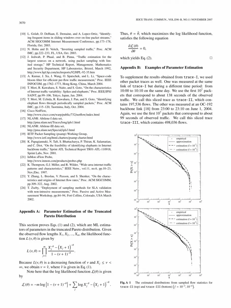
To supplement the results obtained from trace-I, we usedother packet traces as well. One was measured at the samelink of trace-I but during a different time period: from10:00 to 10:10 on the same day. We use the first 107 pack-ets that correspond to about 138 seconds of the observedtraffic. We call this sliced trace as trace-II, which con-tains 197,536 flows. The other was measured at an OC-192backbone link [18] from 23:00 to 23:10 on June 1, 2004.Again, we use the first 107 packets that correspond to about99 seconds of observed traffic. We call this sliced tracetrace-III, which contains 498,036 flows.

Fig. A· 1 The estimated distributions from sampled flow statistics fortrace-II (top) and trace-III (bottom)

(f = 10−3, 10−4

).


First, we approximate the original flow length distri-butions by the truncated Pareto distribution. We then applyrandom packet sampling to the trace-II and trace-III,with sampling frequency of f = 10−3 and f = 10−4. Fromthe obtained sampled flow statistics n, we estimate parame-ters ν and θ of the truncated Pareto distribution. Figure A· 1shows the results. We can observe that the approximate dis-tribution and the estimated distribution visually fit well tothe empirical distribution. Although the approximate andthe estimated distributions are slightly skewed from the em-pirical distributions, we confirmed that the difference did notplay a crucial role in determining the thresholds of sampledflow lengths, which identify the heavy-hitter flows.

Since our parametric model assumes that the flowlength distribution follows the truncated Pareto distribution,it would work well as far as the original flow distributionsfollow the heavy-tailed model. We believe that this assump-tion holds in most cases as reported in many measurement-based studies such as [9], [14], [20], [22], [23]. Moreover,the reason why the heavy-hitter flows exist among flowscomes from the fact that the distribution is heavy-tailed.However, it might be possible that the original flow lengthdistribution shows quite different characteristics. For suchdistributions, we might want to introduce another type ofdistribution model in our framework.

Tatsuya Mori received M.E. degree inapplied physics and Ph.D. degree in informa-tion science from the Waseda University, Tokyo,Japan, in 1999 and 2005, respectively. Sincejoining NTT corporation in 1999, he has beenengaged in the research of measurement andanalysis of the Internet. His recent research in-terests include algorithmic measurement tech-niques, data mining of network measurementdata, and the future of the Internet. From March2007 until March 2008, he is a visiting re-

searcher at the University of Wisconsin-Madison.

Tetsuya Takine is currently a Professor atthe Department of Information and Communi-cations Technology, Graduate School of Engi-neering, Osaka University, Suita, Japan. He wasborn in Kyoto, Japan, on November 28, 1961,and received B.Eng., M.Eng., and Dr.Eng. de-grees in applied mathematics and physics fromKyoto University, Kyoto, Japan, in 1984, 1986,and 1989, respectively. In April 1989, he joinedthe Department of Applied Mathematics andPhysics, Faculty of Engineering, Kyoto Univer-

sity, as an Assistant Professor. Beginning in November 1991, he spent oneyear at the Department of Information and Computer Science, Universityof California, Irvine, on leave of absence from Kyoto University. In April1994, he joined the Department of Information Systems Engineering, Fac-ulty of Engineering, Osaka University as a Lecturer, and from December1994 to March 1998, he was an Associate Professor at the same department.From April 1998 to May 2004, he was an Associate Professor at the Depart-ment of Applied Mathematics and Physics, Graduate School of Informatics,Kyoto University. His research interests include queueing theory, empha-sizing numerical computation, and its application to performance analysisof computer and communication networks. He is now serving as an areaeditor of Operations Research Letters and an associate editor of QueueingSystems. He received Telecom System Technology Award from TAF in2003 and Best Paper Awards from ORSJ, IEICE, and ISCIE in 1997, 2004,and 2006, respectively. Dr. Takine is a fellow of ORSJ and a member ofIEEE, IPSJ, and ISCIE.

Jianping Pan is currently an assistant pro-fessor of computer science at the University ofVictoria, British Columbia, Canada. He re-ceived his Bachelor’s and Ph.D. degrees in com-puter science from Southeast University, Nan-jing, China in 1994 and 1998, respectively.From 1999 to 2001, he was a postdoctoral fel-low and then a research associate at the Univer-sity of Waterloo, Ontario, Canada; from 2001to 2005, he was a member of research staff atFujitsu Labs and then a research scientist at NTT

MCL in Silicon Valley, California, USA. His area of specialization is dis-tributed systems and computer networks, and his recent research interestsinclude protocols for advanced networking, performance analysis of net-worked systems, and applied network security. He is a member of the ACMand the IEEE.

Ryoichi Kawahara received a B.E. inautomatic control, an M.E. in automatic con-trol, and a Ph.D. in telecommunication engineer-ing from Waseda University, Tokyo, Japan, in1990, 1992, and 2001, respectively. Since join-ing NTT in 1992, he has been engaged in re-search on traffic control for telecommunicationnetworks. He is currently working on teletrafficissues in IP networks in NTT Service IntegrationLaboratories. Dr. Kawahara received IEICE’sYoung Investigators’ Award in 1999 and Best

Paper Award in 2003. He is a member of the Operations Research Soci-ety of Japan.


Masato Uchida received the B.E., M.E. andD.E. degrees from Hokkaido University, Sap-poro, Hokkaido, in 1999, 2001, and 2005, re-spectively. In 2001, he joined NTT Service In-tegration Laboratories, Tokyo, Japan. Since Au-gust 2005, he has been an Associate Professorin Network Design Research Center, Kyushu In-stitute of Technology. He is a member of ACM.His research area includes teletraffic engineer-ing and statistical learning theory.

Shigeki Goto received B.S. and M.S. de-grees in mathematics from the University of To-kyo in 1971 and 1973, respectively. He workedfor NTT Laboratory for many years. He wasa visiting researcher at the Stanford Universityfrom 1984 to 1985. He received a Ph.D. in infor-mation engineering from the University of To-kyo in 1991. Currently, he is a professor inthe Department of Computer Science, Schoolof Science and Engineering, Waseda University.He is a member of ACM, IEEE, JSAI and a IPSJ

fellow. He is the chairman of APAN and the president of JPNIC.

Documents

Identifying Heavy-Hitter Flows from Sampled Flow Statistics