Western University Western University

Scholarship@Western Scholarship@Western

Electronic Thesis and Dissertation Repository

4-15-2020 9:30 AM

Impact-Generated Dykes and Shocked Carbonates from the Impact-Generated Dykes and Shocked Carbonates from the

Tunnunik and Haughton Impact Structures, Canadian High Arctic Tunnunik and Haughton Impact Structures, Canadian High Arctic

Jennifer D. Newman, The University of Western Ontario

Supervisor: Osinski, Gordon R., The University of Western Ontario

A thesis submitted in partial fulfillment of the requirements for the Doctor of Philosophy degree

in Geology

© Jennifer D. Newman 2020

Follow this and additional works at: https://ir.lib.uwo.ca/etd

Part of the Geology Commons

Recommended Citation Recommended Citation Newman, Jennifer D., "Impact-Generated Dykes and Shocked Carbonates from the Tunnunik and Haughton Impact Structures, Canadian High Arctic" (2020). Electronic Thesis and Dissertation Repository. 6950. https://ir.lib.uwo.ca/etd/6950

This Dissertation/Thesis is brought to you for free and open access by Scholarship@Western. It has been accepted for inclusion in Electronic Thesis and Dissertation Repository by an authorized administrator of Scholarship@Western. For more information, please contact wlswadmin@uwo.ca.

ii

Abstract

The Canadian High Arctic contains two impact structures created by hypervelocity impact

events in carbonate-rich target rocks. The remote locations of the Tunnunik and Haughton

impact structures means that there are aspects of these impact structures which have yet to be

fully investigated. This study characterizes the range of impact-generated dykes exposed from

both impact structures which include lithic breccias, impact melt-bearing breccias, and impact

melt rocks. Breccias may include silicate impact glass fragments and evidence for carbonate

melt. Impact melt rocks from the Haughton impact structure contain the rare terrestrial mineral

moissanite. This is only the third reported occurrence of moissanite associated with an impact

structure and the first to observe its presence in situ. Inclusions and variation of polytypes in

moissanite provide information regarding high temperatures present during crater formation.

The carbonate-rich rocks that form these impact structures contain well-developed shatter

cones as evidence of shock metamorphism. As a shock classification system does not currently

exist for carbonates, the effect of shock on the crystal structure of calcite and dolomite is

examined using X-ray diffraction to better understand the extent of strain in both these

minerals. Previous studies of shocked carbonates from terrestrial impact structures is limited

and the goal here is to assign numerical values to indicate strain and thereby better quantify

and compare shock in carbonates among impact structures.

The parallel studies of impact-generated dykes and shock at the Tunnunik and Haughton

impact structures allow for the comparison of two impact structures with similar diameters,

28-km for Tunnunik and 23-km for Haughton, in different states of preservation. The deeply

eroded Tunnunik impact structure and well-preserved Haughton impact structure provide

insights into complex crater formation in carbonate rich rocks that would otherwise not be

available by only studying one site. Results from this pair of impact sites has expanded the

knowledge of carbonate-rich impact structures and will help future investigations of other

known carbonate-rich impact sites and ones yet to be discovered.

iii

Keywords

Tunnunik impact structure, Haughton impact structure, impact cratering, impact breccia,

impact melt rock, dyke, carbonate, shocked carbonate, dolomite, calcite, lattice strain, Arctic,

X-ray diffraction, moissanite.

iv

Summary for Lay Audience

Impact craters form when a large projectile, typically a fragment from an asteroid or comet,

survives its transit through Earth’s atmosphere and strikes a solid rocky surface. The resulting

crater may be tens of metres to several hundred kilometres in diameter, depending on the size

and speed of the projectile. Examining the rocks affected and generated by impact events allow

the impact process to be better understood.

This study focuses on two remote impact sites in the Canadian High Arctic, the Tunnunik

impact structure and Haughton impact structure, that formed in carbonate rocks consisting

mainly of limestone and dolostone. Rocks affected by the shock created during the impact

often display shatter cones near the centre of the impact structures which appear as small

fractures or striation to the unaided eye. A technique called X-ray diffraction uses X-rays to

investigate the crystal structure of calcite and dolomite, the primary minerals in the carbonate

rocks that form the impact structures. Shock effects increase strain within the crystal structure

of these minerals and the strain values derived from the X-ray diffraction analyses are

compared among samples collected from different locations in each impact structure.

The rocks generated by the impact event examined in this study include impact breccias and

impact melt rocks found in impact-generated dykes. Breccias consist of fragments from one or

more different types of carbonate rock and are held together by finer fragments that are too

small to see without higher magnification. Breccias may also include small silicate glass

fragments or melted carbonate clasts. Impact melt rocks consist of fine-grained recrystallized

calcite, clasts from the limestone rocks adjacent to the dykes, and crystals of a rare mineral

called moissanite. Moissanite is rare due to very specific conditions required for it to form and

these conditions help identify temperatures reached in the impact melt rocks when they were

generated.

Comparing the results from the Tunnunik and Haughton impact structures has provided

insights into their formation and expanded the knowledge of carbonate-rich impact structures.

v

Co-Authorship Statement

Chapter 1. Literature review of information relevant to this work was completed and written

by Jennifer Newman. Comments and editing were provided by Dr. Gordon Osinski.

Chapter 2. Sample analysis, data collection, and data processing were completed by Jennifer

Newman. EPMA data collection was assisted by Marc Beauchamp. Chapter was written by

Jennifer Newman. Comments and editing were provided by Dr. Gordon Osinski.

Chapter 3. Sample analysis, data collection, and data processing were completed by Jennifer

Newman. EPMA data collection was assisted by Marc Beauchamp. Chapter was written by

Jennifer Newman. Comments and editing of were provided by Dr. Gordon Osinski.

Chapter 4. Sample preparation, analysis, and data processing for all suite 1 samples were

completed by Jennifer Newman. Powder X-ray diffraction data collection was assisted by

Alexandra Rupert. Rietveld analyses for suite 2 samples began as a class project in Earth Sci

9516b: Advanced Mineralogy and Crystallography (2017). Dr. Roberta Flemming provided

helpful and constructive discussions regarding sample processing and interpretation. I

reprocessed all suite 2 samples, so that all samples were refined in a manner consistent with

suite 1 samples. Ultimately all results presented in this chapter were processed and interpreted

by Jennifer Newman. Chapter was written by Jennifer Newman. Comments and editing were

provided by Dr. Gordon Osinski.

Chapter 5. Sample preparation, analysis, and data processing were completed by Jennifer

Newman. Powder X-ray diffraction data collection was assisted by Alexandra Rupert. Chapter

was written by Jennifer Newman. Comments and editing were provided by Dr. Gordon

Osinski.

Chapter 6. Sample analysis and data processing were completed by Jennifer Newman. Data

collection using the Raman spectrometer was assisted by Tianqi Xie. Chapter was written by

Jennifer Newman. Comments and editing were provided by Dr. Gordon Osinski.

Chapter 7. Summary of thesis was written by Jennifer Newman. Comments and edits were

provided by Dr. Gordon Osinski.

vi

Acknowledgements

As I cast my leaving shadow on this five year mission, it could not have been achieved without

the support and contribution of so many people. First, I would like to thank my supervisor Dr.

Gordon ‘Oz’ Osinski for his guidance and the opportunity to work on an incredible project that

included two amazing field seasons in the Arctic. I am grateful for field and research funding

support from NSERC, the Canadian Space Agency, the Northern Scientific Training Program,

and the OGS/QEII program from the Ontario government. The Polar Continental Shelf

Program is thanked for logistical field support.

When I started this journey, I did not have a sense of scope regarding the numerous aspects

this project would cover, let alone the unexpected mineral discovery from Haughton found as

I was nearing completion! The opportunity to participate in two CanMars Mars sample return

analogue missions through my NSERC CREATE/CSA fellowship and the CanMoon 2019

Lunar sample return analogue mission while at Western were great experiences and I hope to

put these experiences into practice. I am also grateful to Dr. Livio Tornabene for the

opportunity to participate in planning MRO/HiRISE cycle 301 with Sarah Simpson and Alyssa

Werynski, this was a valuable and amazing experience. My thesis committee is thanked for

their suggestions, collaborations, and guidance during this endeavour.

Racel Sopoco, Cassandra Marion, Taylor Haid, William Zylberman, Byung-Hun Choe,

Gordon Osinski, Livio Tornabene, Jeremy Hansen, Rob Misener and the rest of the Tunnunik

field team, thank you for your help collecting samples, fending off wildlife, and making camp

life enjoyable. Even when the weather didn’t cooperate with our field or flight plans, we

persevered through!

Thank you to Alexandra Pontefract, Rebecca Greenberger, Elise Harrington, Anna Grau,

Shamus Duff, Gordon Osinski, Livio Tornabene, Etienne Godin, Byung-Hun Choe, and the

rest of the Haughton field team who assisted with sample collection and made life around camp

fun despite the cold and all the rain. Whether we were getting stuck in the mud, sampling great

outcrops, climbing gullies, or racing to pack up camp early because the plane was on its way,

we made a great team.

vii

My lab work at Western would not have been a success without the assistance of Racel Sopoco,

Cassandra Marion, Marc Beauchamp, Dr. Roberta Flemming, Alexandra Rupert, Tianqi Xie,

Joshua Laughton, Peter Christoffersen, and Stephen Wood. Mati Raudsepp (UBC) and Jacob

Kabel (UBC) are thanked for their advice and insights regarding XRD sample mounting and

Rietveld refinement.

Thank you to the Spacerocks Team, Western and CPSX/Western Space friends, office mates,

and fellow planetary scientists I only see for a short time at conferences or field schools for

encouraging me during this time and for discussions on impact cratering, meteorites, and all

things space.

A special thanks and virtual high-fives to everyone who provided extra support and

encouragement during the COVID-19 pandemic to see a successful end to this journey (on

time!), albeit in a slightly modified and unexpected format.

Finally, I would like to thank my parents, Brad and Jayne, sister Melony, and the rest of my

family for their messages, support, and listening to my adventures and rock talk over the years.

I would also like to thank my extended family for fueling my DavidsTea obsession, my

cupboard was never empty and always had the perfect cuppa for any occasion. This journey

wasn’t always easy from a distance, but it meant a lot and could not have done this without

you.

Per conatus ad victoriam.

Victory through endeavour.

viii

Dedication

To my grandparents Joan and John Allen and Marshall Newman for their interest and support

when I began this journey but were not able to see its completion or join in the celebration.

And to my little Felis catus buddy Amber with her endless snuggles, you will be missed but

never forgotten.

ix

Table of Contents

Abstract ............................................................................................................................... ii

Keywords ........................................................................................................................... iii

Summary for Lay Audience ............................................................................................... iv

Co-Authorship Statement.................................................................................................... v

Acknowledgements ............................................................................................................ vi

Dedication ........................................................................................................................ viii

Table of Contents ............................................................................................................... ix

List of Tables ................................................................................................................... xiv

List of Figures .................................................................................................................. xvi

List of Appendices ....................................................................................................... xxviii

Chapter 1 ............................................................................................................................. 1

1 Introduction .................................................................................................................... 1

1.1 Impact cratering ...................................................................................................... 1

1.1.1 Complex crater formation ..............................................................................3

1.1.2 Sedimentary targets ........................................................................................6

1.1.3 Impactites .......................................................................................................7

1.1.4 Microscopic shock metamorphism ................................................................8

1.2 Arctic geology ......................................................................................................... 9

1.2.1 Arctic Archipelago .........................................................................................9

1.2.2 Victoria Island (Kiilineq) .............................................................................11

1.2.3 Devon Island (Tallurutit) .............................................................................14

1.3 X-ray diffraction ................................................................................................... 17

1.3.1 Powder X-ray diffraction theory ..................................................................18

1.3.2 Rietveld refinement ......................................................................................21

x

1.4 Thesis objectives ................................................................................................... 22

1.5 References ............................................................................................................. 22

Chapter 2 ........................................................................................................................... 33

2 Impact-generated breccia dykes of the Tunnunik impact structure, Canada ............... 33

2.1 Introduction ........................................................................................................... 33

2.2 Geologic setting .................................................................................................... 34

2.3 Samples and methods ............................................................................................ 35

2.4 Results ................................................................................................................... 36

2.4.1 Type 1 ..........................................................................................................37

2.4.2 Type 2 ..........................................................................................................50

2.4.3 Type 3 ..........................................................................................................51

2.4.4 Type 4 ..........................................................................................................58

2.5 Discussion ............................................................................................................. 60

2.5.1 Silicate impact glass .....................................................................................60

2.5.2 Evidence for melting of carbonates .............................................................62

2.5.3 Origin and emplacement of the Tunnunik dykes .........................................63

2.6 Conclusions ........................................................................................................... 69

2.7 References ............................................................................................................. 70

Chapter 3 ........................................................................................................................... 75

3 Impact-generated carbonate-rich dykes from the Haughton impact structure, Canada 75

3.1 Introduction ........................................................................................................... 75

3.2 Geologic setting .................................................................................................... 76

3.3 Samples and methods ............................................................................................ 76

3.4 Results ................................................................................................................... 79

3.4.1 Lithic breccia dykes .....................................................................................80

3.4.2 Quartz-cemented carbonate breccia dyke ....................................................84

xi

3.4.3 Sulfate-bearing polymict breccia .................................................................86

3.4.4 Impact melt rock dykes ................................................................................88

3.4.5 Chert .............................................................................................................95

3.5 Discussion ............................................................................................................. 97

3.5.1 Impact-related features .................................................................................97

3.5.2 Dyke formation ............................................................................................99

3.5.3 Clast-rich impact melt rocks ......................................................................101

3.5.4 Comparison with other impact structures ..................................................103

3.6 Conclusions ......................................................................................................... 105

3.7 References ........................................................................................................... 106

Chapter 4 ......................................................................................................................... 111

4 Shock effects in dolomite and calcite from the Haughton impact structure, Canada, using

X-ray diffraction and Rietveld refinement ................................................................. 111

4.1 Introduction ......................................................................................................... 111

4.2 Samples and methods .......................................................................................... 114

4.2.1 Suite 1: In situ carbonate target rocks ........................................................114

4.2.2 Suite 2: Shatter cone clasts from crater-fill and ballistic ejecta deposits ...116

4.2.3 Rietveld refinement ....................................................................................117

4.3 Results ................................................................................................................. 118

4.3.1 Powder X-ray diffraction ...........................................................................118

4.3.2 Rietveld refinement ....................................................................................120

4.3.3 Williamson-Hall plots ................................................................................123

4.4 Discussion ........................................................................................................... 126

4.4.1 Shock effects in calcite versus dolomite ....................................................126

4.4.2 Comparison with other craters in carbonate target rocks...........................128

4.4.3 Carbonates as shock indicators ..................................................................130

xii

4.5 Conclusions ......................................................................................................... 133

4.6 References ........................................................................................................... 134

Chapter 5 ......................................................................................................................... 140

5 An X-ray diffraction study of shocked carbonates from the deeply eroded Tunnunik

impact structure, Canada ............................................................................................ 140

5.1 Introduction ......................................................................................................... 140

5.2 Samples and methods .......................................................................................... 141

5.3 Results ................................................................................................................. 144

5.3.1 Powder X-ray diffraction ...........................................................................144

5.3.2 Rietveld refinement ....................................................................................145

5.3.3 Strain estimation ........................................................................................146

5.4 Discussion ........................................................................................................... 149

5.4.1 Peak broadening in X-ray diffraction patterns ...........................................149

5.4.2 Strain estimates and trends.........................................................................150

5.4.3 Practicality of strain estimation .................................................................152

5.5 Conclusions ......................................................................................................... 152

5.6 References ........................................................................................................... 153

Chapter 6 ......................................................................................................................... 156

6 Impact-generated moissanite (SiC) from the Haughton impact structure, Canada .... 156

6.1 Introduction ......................................................................................................... 156

6.2 Moissanite and polytypism background ............................................................. 157

6.3 Methods and results ............................................................................................ 159

6.3.1 Petrography ................................................................................................159

6.3.2 Electron probe microanalysis (EPMA) ......................................................161

6.3.3 Raman Spectroscopy ..................................................................................164

6.4 Discussion ........................................................................................................... 166

xiii

6.4.1 Natural versus synthetic SiC ......................................................................166

6.4.2 Moissanite formation .................................................................................167

6.4.3 Occurrence at terrestrial impact sites .........................................................169

6.5 Conclusions ......................................................................................................... 170

6.6 References ........................................................................................................... 170

Chapter 7 ......................................................................................................................... 174

7 Summary of results from two terrestrial hypervelocity impacts into carbonate target

sequences.................................................................................................................... 174

7.1 Carbonate-rich target sequences ......................................................................... 175

7.2 Deeply eroded versus well-preserved impact structures ..................................... 177

7.3 Dyke emplacement in the Tunnunik and Haughton impact structures ............... 178

7.4 Extent of shock ................................................................................................... 180

7.4.1 Strain versus distance from the centre of impact structures ......................180

7.4.2 Strain versus depth within impact structures .............................................181

7.4.3 Future shock-related research opportunities ..............................................181

7.5 Conclusions ......................................................................................................... 182

7.6 References ........................................................................................................... 183

Appendices ...................................................................................................................... 188

Curriculum Vitae ............................................................................................................ 339

xiv

List of Tables

Table 2-1. Electron microprobe WDS analyses of carbonates* for mineral grains and melt. 42

Table 2-2. Electron microprobe WDS analyses of silicate glass fragments in Type 1 breccia.

................................................................................................................................................. 48

Table 2-3. Breccia dyke summary. ......................................................................................... 69

Table 3-1. Compositions from the quartz-cemented carbonate breccia dyke. ........................ 86

Table 3-2. Electron probe microanalysis (WDS) of carbonate phases in impact melt rock dykes.

................................................................................................................................................. 93

Table 3-3. Electron probe microanalysis (WDS) of silicate glass. ......................................... 95

Table 4-1. Modal mineral proportions of samples in weight percent with crystal size and lattice

strain values for carbonates determined by Rietveld refinement of bulk rock powders from the

Haughton impact structure. ................................................................................................... 121

Table 4-2. Lattice strain values sorted by distance from the centre of the Haughton impact

structure for suite 1 carbonates. ............................................................................................ 122

Table 4-3. Lattice strain values sorted by distance from the centre of the Haughton impact

structure for suite 2 carbonates. ............................................................................................ 122

Table 4-4. Comparison of lattice strain measurements by Rietveld refinement from the

Haughton impact structure and experimentally shocked carbonates. ................................... 131

Table 5-1. Comparison of lattice strain values determined by two methods for samples from

the Haughton impact structure. ............................................................................................. 148

Table 5-2. Calculated lattice strain values for carbonate samples from the Tunnunik impact

structure sorted by distance from centre. .............................................................................. 148

Table 6-1. Distribution of moissanite crystals within impact melt rocks from the Haughton

impact structure. .................................................................................................................... 160

xv

Table 6-2. Electron probe microanalysis of silicate glass and moissanite using wavelength

dispersive spectrometry. ....................................................................................................... 162

Table 7-1. Comparison of physical features and properties at the Tunnunik and Haughton

impact structures. .................................................................................................................. 174

xvi

List of Figures

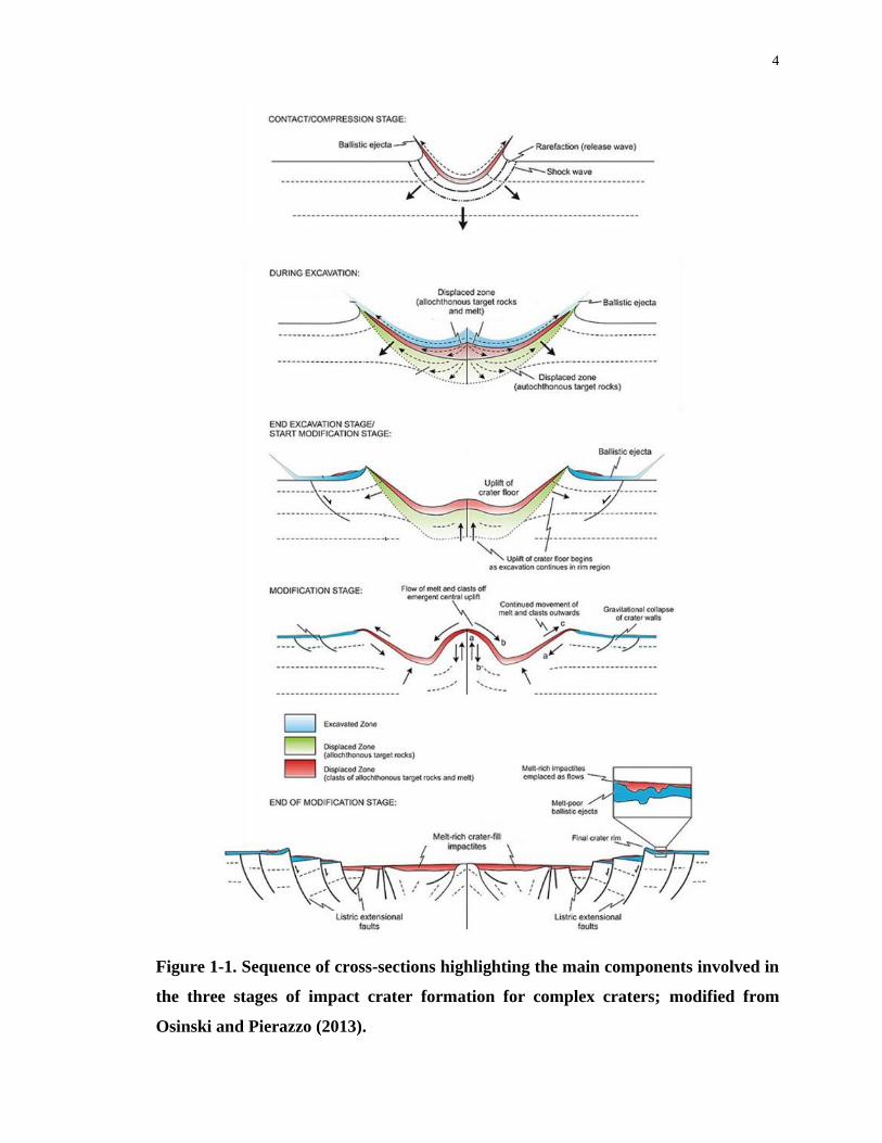
Figure 1-1. Sequence of cross-sections highlighting the main components involved in the three

stages of impact crater formation for complex craters; modified from Osinski and Pierazzo

(2013). ....................................................................................................................................... 4

Figure 1-2. The Canadian Arctic Archipelago with study site locations indicated. Base map

provided by d-maps.com. ........................................................................................................ 10

Figure 1-3. A) Google Earth (2018) image of Victoria Island; white square indicates the

location of inset image B) showing the Tunnunik impact structure, outlined by white dashed

circle. Coordinates for the centre of the Tunnunik impact structure are 72°27’16” N,

113°49’49” W (Impact Earth 2020). ....................................................................................... 13

Figure 1-4. A) Google Earth (2018) image of Devon Island; white square indicates the location

of inset image B) showing the Haughton impact structure. Coordinates for the centre of the

Haughton impact structure are 75°22’39” N, 89°39’13” W (Impact Earth 2020). ................ 15

Figure 1-5. Comparison of the unit cell for calcite and dolomite. View shown is looking

through the a-axes which are perpendicular to the c-axis. Representative carbonate (CO3) and

octahedral (CaO6 or MgO6) layers are indicated which include calcium (green), magnesium

(yellow), carbon (grey), and oxygen (red) atoms. Structural model visualizations obtained from

The Virtual Museum of Minerals and Molecules (Barak and Nater 2020). ........................... 18

Figure 1-6. Derivation and illustration of Bragg’s Law. Incident X-rays (A, B, C) diffract at

atoms within lattice planes (hkl), where d is the spacing between planes in the crystal structure,

at an angle (θ) to generate diffracted X-rays (A’, B’, C’). ...................................................... 19

Figure 1-7. X-ray diffraction patterns for unshocked calcite and dolomite. Positions of Miller

indices (hkl) for calcite are indicated by vertical green lines with diamond markers and

dolomite by vertical blue lines with square markers. ............................................................. 20

Figure 1-8. Illustration of peak broadening observed in diffraction patterns associated with

lattice strain (modified from Cullity 1978). The strained diffraction pattern can be thought of

xvii

as a series of small peaks (dashed) caused by slight differences in d-spacing in crystal lattice

that combine to generate one broad peak. ............................................................................... 21

Figure 2-1. Simplified geologic map of the Tunnunik impact structure indicating breccia dyke

localities examined in this study; Shatter Cone Canyon (SCC), Shaler Supergroup (SS), Big

Lake (BL), Big Lake south (BLs), Bouldering River (BR), West River (WR) and Rim Canyon

(RC). B) Shatter cone distribution within the Tunnunik impact structure. UTM grid with

Easting and Northing at 1000 m intervals for Zone 11 and Zone 12. ..................................... 35

Figure 2-2. Type 1 breccia dykes from Shatter Cone Canyon (A–C), Big Lake (D–E), and

Bouldering River (N) with dyke boundaries indicated by white dashed lines. A) Nearly vertical

dyke cuts through more horizontal bedding; breccia is fractured and fragments have fallen out

of place. B) Dyke is parallel to bedding planes with a dip of 49°. C) Narrow dyke that follows

the fold contour of the host rocks. D) Ground surface exposure of dyke has been strongly

affected by freeze-thaw action and is highly fractured like surrounding rock. Inset image from

top of dyke shows a location that was more resistant to freeze-thaw cycles. E) Similar to (D),

breccia in dyke has been severely fractured by frost action. Samples (F–K) represent variations

among T1 dykes. F) Breccia from Shatter Cone Canyon shows subtle banding in matrix with

elongated clasts oriented parallel to bands. G) Sample from dyke in (C) shows small clasts

oriented in horizontal direction. H) Bimodal clast size distribution in breccia from Big Lake.

I) Minimal alignment of larger rounded clasts in this Big Lake breccia sample. J) The most

diverse assemblage of clasts in any T1 breccia. K) Sample from dyke in (D) contains part of a

large 10 cm grey dolostone clast. L) Breccia sample from dyke in (B) showing alignment of

clasts parallel to green mudstone host rock along top of hand sample. M) Similar to (L) this

breccia from Shatter Cone Canyon also shows clasts oriented in same direction as green

mudstone host. N) Horizontal breccia dyke follows bedding planes of host dolostone. O) Close-

up of breccia near right edge of dyke shown in (N). .............................................................. 38

Figure 2-3. Type 1 breccia optical microscopy. A) Coarse, clast-supported area of breccia. B)

Small-scale clast orientation localized near host contact to right of image. C) Veins of coarse

calcite cut across matrix and clasts. D) Euhedral grains of dolomite in small vug. E) Rounded,

fine-grained calcite clast (pale grey) containing fine-grained dolomite (dark grey). F) Irregular-

xviii

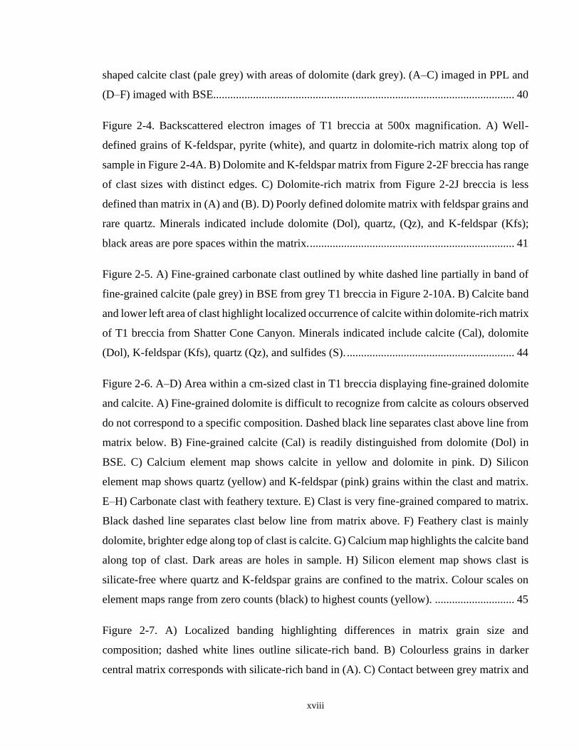
shaped calcite clast (pale grey) with areas of dolomite (dark grey). (A–C) imaged in PPL and

(D–F) imaged with BSE.......................................................................................................... 40

Figure 2-4. Backscattered electron images of T1 breccia at 500x magnification. A) Well-

defined grains of K-feldspar, pyrite (white), and quartz in dolomite-rich matrix along top of

sample in Figure 2-4A. B) Dolomite and K-feldspar matrix from Figure 2-2F breccia has range

of clast sizes with distinct edges. C) Dolomite-rich matrix from Figure 2-2J breccia is less

defined than matrix in (A) and (B). D) Poorly defined dolomite matrix with feldspar grains and

rare quartz. Minerals indicated include dolomite (Dol), quartz, (Qz), and K-feldspar (Kfs);

black areas are pore spaces within the matrix. ........................................................................ 41

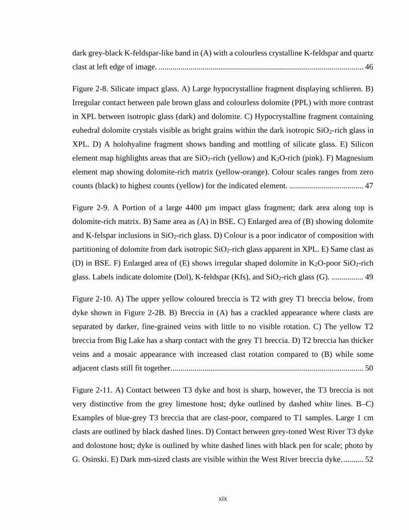
Figure 2-5. A) Fine-grained carbonate clast outlined by white dashed line partially in band of

fine-grained calcite (pale grey) in BSE from grey T1 breccia in Figure 2-10A. B) Calcite band

and lower left area of clast highlight localized occurrence of calcite within dolomite-rich matrix

of T1 breccia from Shatter Cone Canyon. Minerals indicated include calcite (Cal), dolomite

(Dol), K-feldspar (Kfs), quartz (Qz), and sulfides (S). ........................................................... 44

Figure 2-6. A–D) Area within a cm-sized clast in T1 breccia displaying fine-grained dolomite

and calcite. A) Fine-grained dolomite is difficult to recognize from calcite as colours observed

do not correspond to a specific composition. Dashed black line separates clast above line from

matrix below. B) Fine-grained calcite (Cal) is readily distinguished from dolomite (Dol) in

BSE. C) Calcium element map shows calcite in yellow and dolomite in pink. D) Silicon

element map shows quartz (yellow) and K-feldspar (pink) grains within the clast and matrix.

E–H) Carbonate clast with feathery texture. E) Clast is very fine-grained compared to matrix.

Black dashed line separates clast below line from matrix above. F) Feathery clast is mainly

dolomite, brighter edge along top of clast is calcite. G) Calcium map highlights the calcite band

along top of clast. Dark areas are holes in sample. H) Silicon element map shows clast is

silicate-free where quartz and K-feldspar grains are confined to the matrix. Colour scales on

element maps range from zero counts (black) to highest counts (yellow). ............................ 45

Figure 2-7. A) Localized banding highlighting differences in matrix grain size and

composition; dashed white lines outline silicate-rich band. B) Colourless grains in darker

central matrix corresponds with silicate-rich band in (A). C) Contact between grey matrix and

xix

dark grey-black K-feldspar-like band in (A) with a colourless crystalline K-feldspar and quartz

clast at left edge of image. ...................................................................................................... 46

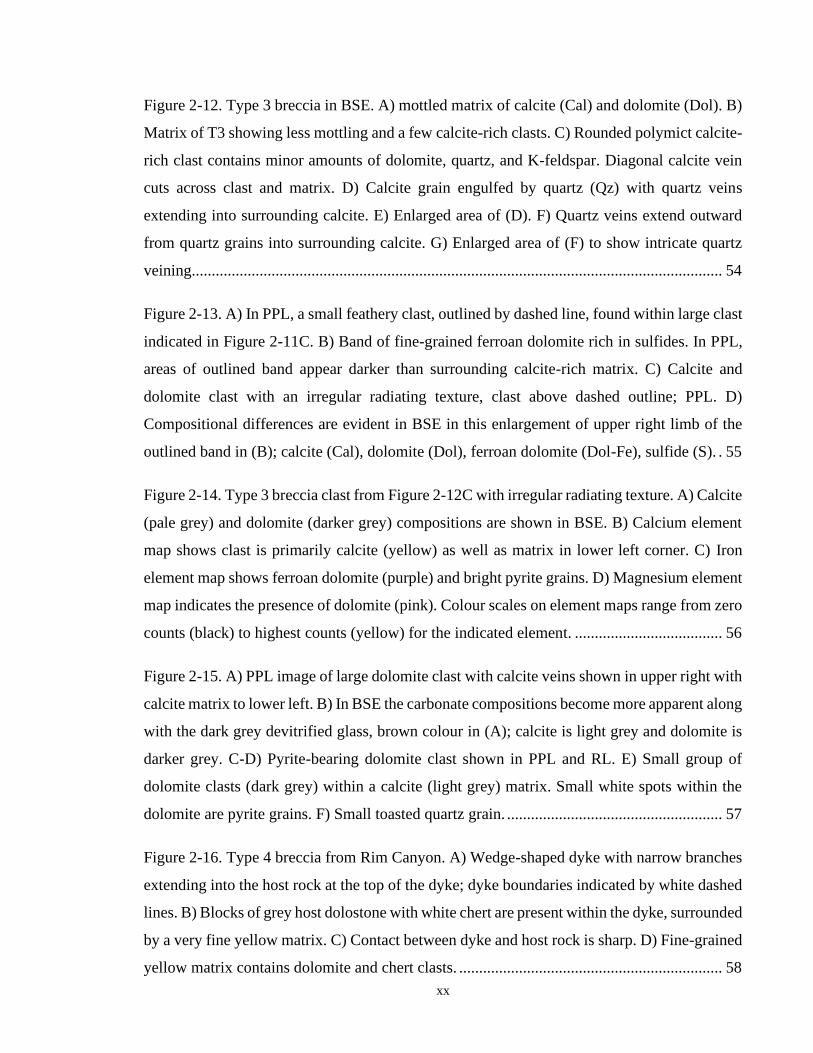
Figure 2-8. Silicate impact glass. A) Large hypocrystalline fragment displaying schlieren. B)

Irregular contact between pale brown glass and colourless dolomite (PPL) with more contrast

in XPL between isotropic glass (dark) and dolomite. C) Hypocrystalline fragment containing

euhedral dolomite crystals visible as bright grains within the dark isotropic SiO2-rich glass in

XPL. D) A holohyaline fragment shows banding and mottling of silicate glass. E) Silicon

element map highlights areas that are SiO2-rich (yellow) and K2O-rich (pink). F) Magnesium

element map showing dolomite-rich matrix (yellow-orange). Colour scales ranges from zero

counts (black) to highest counts (yellow) for the indicated element. ..................................... 47

Figure 2-9. A Portion of a large 4400 µm impact glass fragment; dark area along top is

dolomite-rich matrix. B) Same area as (A) in BSE. C) Enlarged area of (B) showing dolomite

and K-felspar inclusions in SiO2-rich glass. D) Colour is a poor indicator of composition with

partitioning of dolomite from dark isotropic SiO2-rich glass apparent in XPL. E) Same clast as

(D) in BSE. F) Enlarged area of (E) shows irregular shaped dolomite in K2O-poor SiO2-rich

glass. Labels indicate dolomite (Dol), K-feldspar (Kfs), and SiO2-rich glass (G). ................ 49

Figure 2-10. A) The upper yellow coloured breccia is T2 with grey T1 breccia below, from

dyke shown in Figure 2-2B. B) Breccia in (A) has a crackled appearance where clasts are

separated by darker, fine-grained veins with little to no visible rotation. C) The yellow T2

breccia from Big Lake has a sharp contact with the grey T1 breccia. D) T2 breccia has thicker

veins and a mosaic appearance with increased clast rotation compared to (B) while some

adjacent clasts still fit together. ............................................................................................... 50

Figure 2-11. A) Contact between T3 dyke and host is sharp, however, the T3 breccia is not

very distinctive from the grey limestone host; dyke outlined by dashed white lines. B–C)

Examples of blue-grey T3 breccia that are clast-poor, compared to T1 samples. Large 1 cm

clasts are outlined by black dashed lines. D) Contact between grey-toned West River T3 dyke

and dolostone host; dyke is outlined by white dashed lines with black pen for scale; photo by

G. Osinski. E) Dark mm-sized clasts are visible within the West River breccia dyke. .......... 52

xx

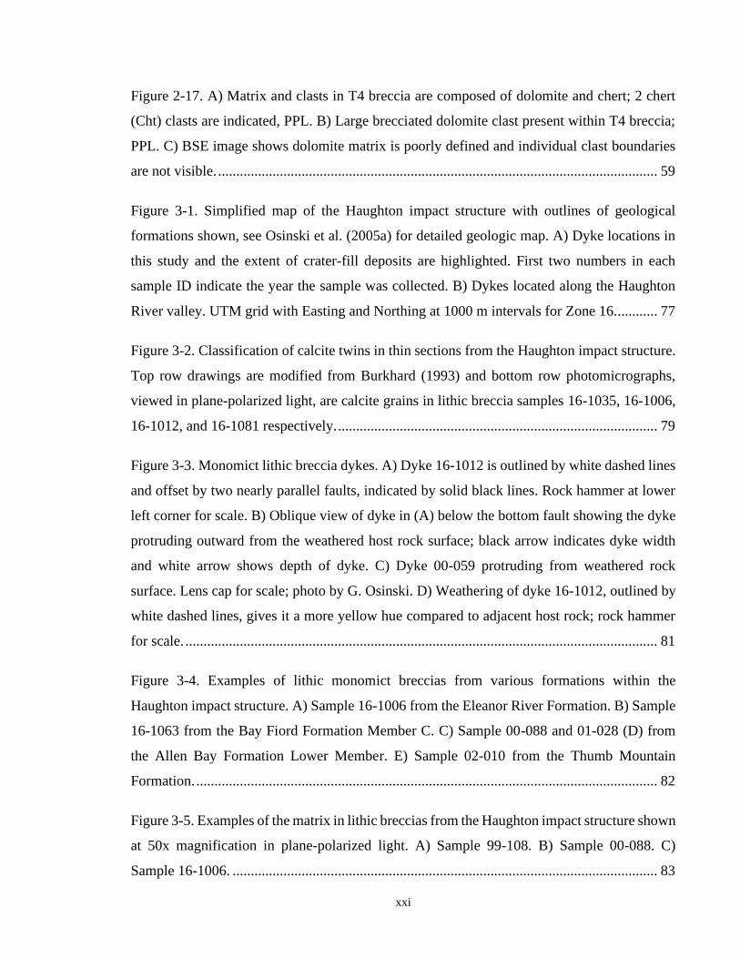
Figure 2-12. Type 3 breccia in BSE. A) mottled matrix of calcite (Cal) and dolomite (Dol). B)

Matrix of T3 showing less mottling and a few calcite-rich clasts. C) Rounded polymict calcite-

rich clast contains minor amounts of dolomite, quartz, and K-feldspar. Diagonal calcite vein

cuts across clast and matrix. D) Calcite grain engulfed by quartz (Qz) with quartz veins

extending into surrounding calcite. E) Enlarged area of (D). F) Quartz veins extend outward

from quartz grains into surrounding calcite. G) Enlarged area of (F) to show intricate quartz

veining..................................................................................................................................... 54

Figure 2-13. A) In PPL, a small feathery clast, outlined by dashed line, found within large clast

indicated in Figure 2-11C. B) Band of fine-grained ferroan dolomite rich in sulfides. In PPL,

areas of outlined band appear darker than surrounding calcite-rich matrix. C) Calcite and

dolomite clast with an irregular radiating texture, clast above dashed outline; PPL. D)

Compositional differences are evident in BSE in this enlargement of upper right limb of the

outlined band in (B); calcite (Cal), dolomite (Dol), ferroan dolomite (Dol-Fe), sulfide (S). . 55

Figure 2-14. Type 3 breccia clast from Figure 2-12C with irregular radiating texture. A) Calcite

(pale grey) and dolomite (darker grey) compositions are shown in BSE. B) Calcium element

map shows clast is primarily calcite (yellow) as well as matrix in lower left corner. C) Iron

element map shows ferroan dolomite (purple) and bright pyrite grains. D) Magnesium element

map indicates the presence of dolomite (pink). Colour scales on element maps range from zero

counts (black) to highest counts (yellow) for the indicated element. ..................................... 56

Figure 2-15. A) PPL image of large dolomite clast with calcite veins shown in upper right with

calcite matrix to lower left. B) In BSE the carbonate compositions become more apparent along

with the dark grey devitrified glass, brown colour in (A); calcite is light grey and dolomite is

darker grey. C-D) Pyrite-bearing dolomite clast shown in PPL and RL. E) Small group of

dolomite clasts (dark grey) within a calcite (light grey) matrix. Small white spots within the

dolomite are pyrite grains. F) Small toasted quartz grain. ...................................................... 57

Figure 2-16. Type 4 breccia from Rim Canyon. A) Wedge-shaped dyke with narrow branches

extending into the host rock at the top of the dyke; dyke boundaries indicated by white dashed

lines. B) Blocks of grey host dolostone with white chert are present within the dyke, surrounded

by a very fine yellow matrix. C) Contact between dyke and host rock is sharp. D) Fine-grained

yellow matrix contains dolomite and chert clasts. .................................................................. 58

xxi

Figure 2-17. A) Matrix and clasts in T4 breccia are composed of dolomite and chert; 2 chert

(Cht) clasts are indicated, PPL. B) Large brecciated dolomite clast present within T4 breccia;

PPL. C) BSE image shows dolomite matrix is poorly defined and individual clast boundaries

are not visible. ......................................................................................................................... 59

Figure 3-1. Simplified map of the Haughton impact structure with outlines of geological

formations shown, see Osinski et al. (2005a) for detailed geologic map. A) Dyke locations in

this study and the extent of crater-fill deposits are highlighted. First two numbers in each

sample ID indicate the year the sample was collected. B) Dykes located along the Haughton

River valley. UTM grid with Easting and Northing at 1000 m intervals for Zone 16. ........... 77

Figure 3-2. Classification of calcite twins in thin sections from the Haughton impact structure.

Top row drawings are modified from Burkhard (1993) and bottom row photomicrographs,

viewed in plane-polarized light, are calcite grains in lithic breccia samples 16-1035, 16-1006,

16-1012, and 16-1081 respectively. ........................................................................................ 79

Figure 3-3. Monomict lithic breccia dykes. A) Dyke 16-1012 is outlined by white dashed lines

and offset by two nearly parallel faults, indicated by solid black lines. Rock hammer at lower

left corner for scale. B) Oblique view of dyke in (A) below the bottom fault showing the dyke

protruding outward from the weathered host rock surface; black arrow indicates dyke width

and white arrow shows depth of dyke. C) Dyke 00-059 protruding from weathered rock

surface. Lens cap for scale; photo by G. Osinski. D) Weathering of dyke 16-1012, outlined by

white dashed lines, gives it a more yellow hue compared to adjacent host rock; rock hammer

for scale. .................................................................................................................................. 81

Figure 3-4. Examples of lithic monomict breccias from various formations within the

Haughton impact structure. A) Sample 16-1006 from the Eleanor River Formation. B) Sample

16-1063 from the Bay Fiord Formation Member C. C) Sample 00-088 and 01-028 (D) from

the Allen Bay Formation Lower Member. E) Sample 02-010 from the Thumb Mountain

Formation. ............................................................................................................................... 82

Figure 3-5. Examples of the matrix in lithic breccias from the Haughton impact structure shown

at 50x magnification in plane-polarized light. A) Sample 99-108. B) Sample 00-088. C)

Sample 16-1006. ..................................................................................................................... 83

xxii

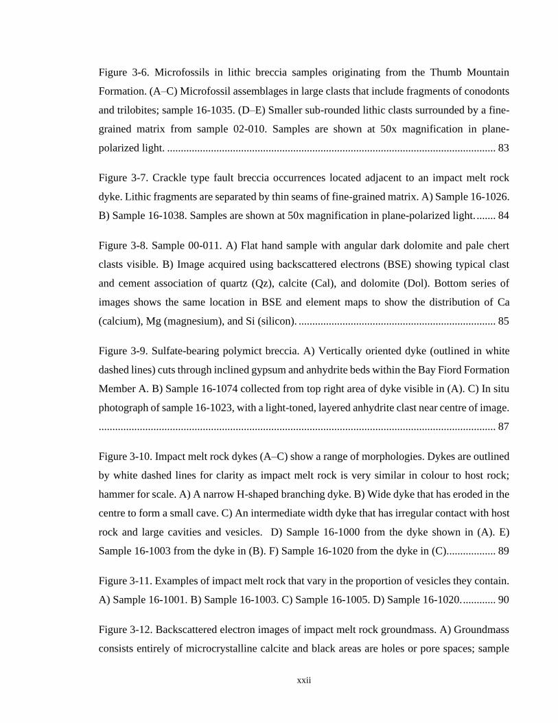
Figure 3-6. Microfossils in lithic breccia samples originating from the Thumb Mountain

Formation. (A–C) Microfossil assemblages in large clasts that include fragments of conodonts

and trilobites; sample 16-1035. (D–E) Smaller sub-rounded lithic clasts surrounded by a fine-

grained matrix from sample 02-010. Samples are shown at 50x magnification in plane-

polarized light. ........................................................................................................................ 83

Figure 3-7. Crackle type fault breccia occurrences located adjacent to an impact melt rock

dyke. Lithic fragments are separated by thin seams of fine-grained matrix. A) Sample 16-1026.

B) Sample 16-1038. Samples are shown at 50x magnification in plane-polarized light. ....... 84

Figure 3-8. Sample 00-011. A) Flat hand sample with angular dark dolomite and pale chert

clasts visible. B) Image acquired using backscattered electrons (BSE) showing typical clast

and cement association of quartz (Qz), calcite (Cal), and dolomite (Dol). Bottom series of

images shows the same location in BSE and element maps to show the distribution of Ca

(calcium), Mg (magnesium), and Si (silicon). ........................................................................ 85

Figure 3-9. Sulfate-bearing polymict breccia. A) Vertically oriented dyke (outlined in white

dashed lines) cuts through inclined gypsum and anhydrite beds within the Bay Fiord Formation

Member A. B) Sample 16-1074 collected from top right area of dyke visible in (A). C) In situ

photograph of sample 16-1023, with a light-toned, layered anhydrite clast near centre of image.

................................................................................................................................................. 87

Figure 3-10. Impact melt rock dykes (A–C) show a range of morphologies. Dykes are outlined

by white dashed lines for clarity as impact melt rock is very similar in colour to host rock;

hammer for scale. A) A narrow H-shaped branching dyke. B) Wide dyke that has eroded in the

centre to form a small cave. C) An intermediate width dyke that has irregular contact with host

rock and large cavities and vesicles. D) Sample 16-1000 from the dyke shown in (A). E)

Sample 16-1003 from the dyke in (B). F) Sample 16-1020 from the dyke in (C). ................. 89

Figure 3-11. Examples of impact melt rock that vary in the proportion of vesicles they contain.

A) Sample 16-1001. B) Sample 16-1003. C) Sample 16-1005. D) Sample 16-1020. ............ 90

Figure 3-12. Backscattered electron images of impact melt rock groundmass. A) Groundmass

consists entirely of microcrystalline calcite and black areas are holes or pore spaces; sample

xxiii

16-1003. B) Groundmass is microcrystalline calcite with small rounded quartz grains. Small

black spots are pore spaces; sample 16-1011. Magnification for both images is 500x. ......... 91

Figure 3-13. Sample 16-1011. A) Flat cut surface of impact melt rock sample with a heavily

weathered clast at its centre. B) Weathered clast showing analysis spots on the groundmass (C)

and clast (D). C) Magnified (7x) image of impact melt rock groundmass indicated in (B). D)

Magnified (7x) image of weathered clast indicated in (B). E) 2-D analysis of weathered clast

at location D. F) 2-D analysis of aphanitic groundmass at location C. .................................. 92

Figure 3-14. A) MgO-rich glass from 16-1020B. B) MgO-rich glass from 16-1003. C) MgO-

rich glass from 16-1020A. D) C4-like glass from 16-1020B. E) Cavity (white area) with silicate

glass remnants along the interior edge from 16-1020A. Images shown in plane-polarized light

with magnification of 200x (A, C, D), 100x (B), and 50x (E)................................................ 94

Figure 3-15. Occurrences of black chert in the Eleanor River Formation. A) Brecciated area

within the Haughton River valley with abundant black chert. B) Large rounded black chert

nodules are prominent within the middle layer. An impact melt rock dyke is directly below this

layer, outlined by black dashed lines. ..................................................................................... 96

Figure 3-16. Toasted chert has a brown appearance when observed in thin section. A–D)

Partially toasted chert clast viewed by different methods to highlight the differences between

the colourless untoasted areas and brown toasted areas of the clast as shown in plane-polarized

light (A); sample 16-1001. A) Plane-polarized light photomicrograph of chert surrounded by

calcite-rich groundmass. B) Cross-polarized light. C) Backscattered electron imagery shows a

slight texture change between the two areas of the clast. Box outlines view provided in (D). D)

Area corresponding to the toasted area of the clast is more pitted than the untoasted area. E)

Chert clast has a fully toasted appearance; sample 16-1038. F) Chert clast is toasted and

fractured; sample 16-1026. ..................................................................................................... 97

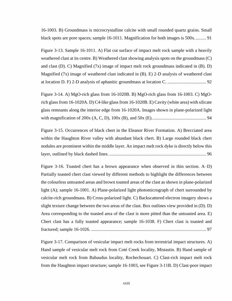
Figure 3-17. Comparison of vesicular impact melt rocks from terrestrial impact structures. A)

Hand sample of vesicular melt rock from Coté Creek locality, Mistastin. B) Hand sample of

vesicular melt rock from Babaudus locality, Rochechouart. C) Clast-rich impact melt rock

from the Haughton impact structure; sample 16-1003, see Figure 3-11B. D) Clast-poor impact

xxiv

melt rock from the Mistastin impact structure; sample MM 11-23A. E) Clast-poor impact melt

rock from the Rochechouart impact structure; sample RO-01-043. ..................................... 104

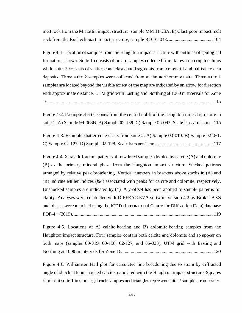
Figure 4-1. Location of samples from the Haughton impact structure with outlines of geological

formations shown. Suite 1 consists of in situ samples collected from known outcrop locations

while suite 2 consists of shatter cone clasts and fragments from crater-fill and ballistic ejecta

deposits. Three suite 2 samples were collected from at the northernmost site. Three suite 1

samples are located beyond the visible extent of the map are indicated by an arrow for direction

with approximate distance. UTM grid with Easting and Northing at 1000 m intervals for Zone

16........................................................................................................................................... 115

Figure 4-2. Example shatter cones from the central uplift of the Haughton impact structure in

suite 1. A) Sample 99-063B. B) Sample 02-139. C) Sample 06-093. Scale bars are 2 cm. . 115

Figure 4-3. Example shatter cone clasts from suite 2. A) Sample 00-019. B) Sample 02-061.

C) Sample 02-127. D) Sample 02-128. Scale bars are 1 cm. ................................................ 117

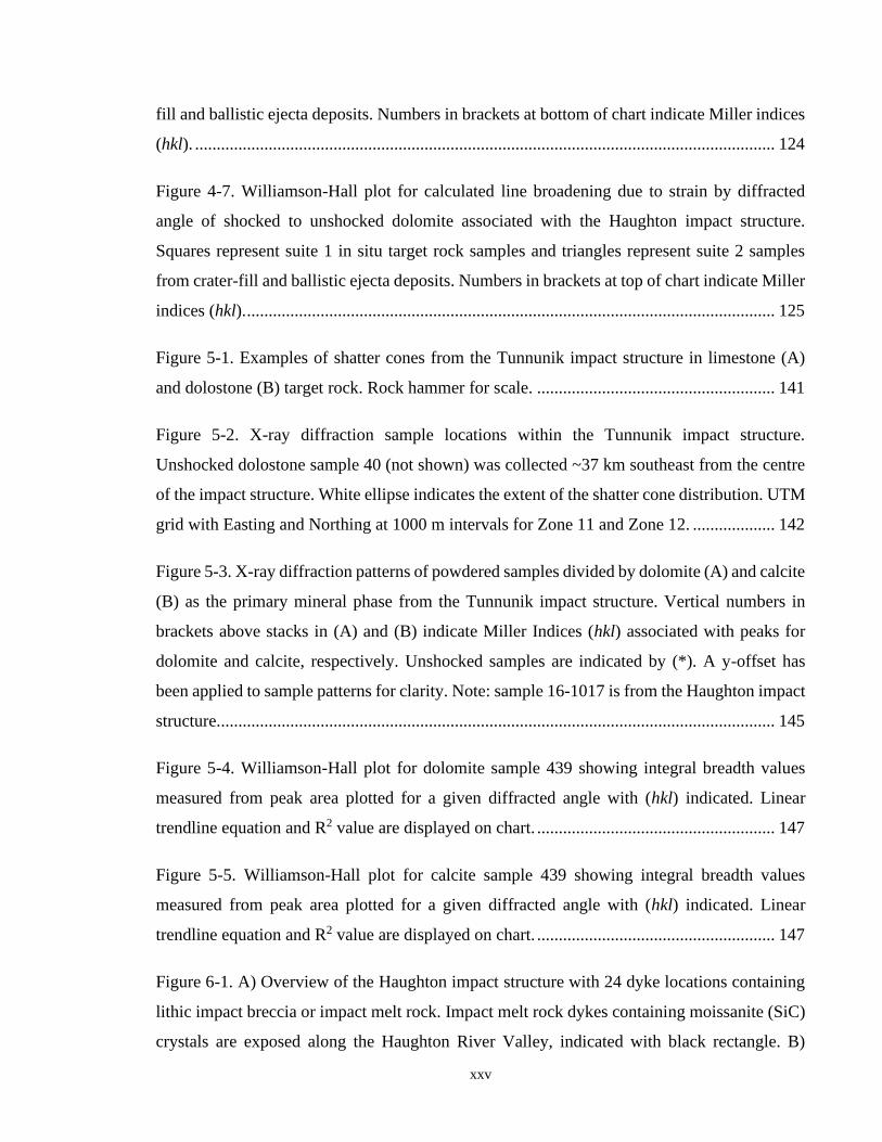
Figure 4-4. X-ray diffraction patterns of powdered samples divided by calcite (A) and dolomite

(B) as the primary mineral phase from the Haughton impact structure. Stacked patterns

arranged by relative peak broadening. Vertical numbers in brackets above stacks in (A) and

(B) indicate Miller Indices (hkl) associated with peaks for calcite and dolomite, respectively.

Unshocked samples are indicated by (*). A y-offset has been applied to sample patterns for

clarity. Analyses were conducted with DIFFRAC.EVA software version 4.2 by Bruker AXS

and phases were matched using the ICDD (International Centre for Diffraction Data) database

PDF-4+ (2019). ..................................................................................................................... 119

Figure 4-5. Locations of A) calcite-bearing and B) dolomite-bearing samples from the

Haughton impact structure. Four samples contain both calcite and dolomite and so appear on

both maps (samples 00-019, 00-158, 02-127, and 05-023). UTM grid with Easting and

Northing at 1000 m intervals for Zone 16. ........................................................................... 120

Figure 4-6. Williamson-Hall plot for calculated line broadening due to strain by diffracted

angle of shocked to unshocked calcite associated with the Haughton impact structure. Squares

represent suite 1 in situ target rock samples and triangles represent suite 2 samples from crater-

xxv

fill and ballistic ejecta deposits. Numbers in brackets at bottom of chart indicate Miller indices

(hkl). ...................................................................................................................................... 124

Figure 4-7. Williamson-Hall plot for calculated line broadening due to strain by diffracted

angle of shocked to unshocked dolomite associated with the Haughton impact structure.

Squares represent suite 1 in situ target rock samples and triangles represent suite 2 samples

from crater-fill and ballistic ejecta deposits. Numbers in brackets at top of chart indicate Miller

indices (hkl). .......................................................................................................................... 125

Figure 5-1. Examples of shatter cones from the Tunnunik impact structure in limestone (A)

and dolostone (B) target rock. Rock hammer for scale. ....................................................... 141

Figure 5-2. X-ray diffraction sample locations within the Tunnunik impact structure.

Unshocked dolostone sample 40 (not shown) was collected ~37 km southeast from the centre

of the impact structure. White ellipse indicates the extent of the shatter cone distribution. UTM

grid with Easting and Northing at 1000 m intervals for Zone 11 and Zone 12. ................... 142

Figure 5-3. X-ray diffraction patterns of powdered samples divided by dolomite (A) and calcite

(B) as the primary mineral phase from the Tunnunik impact structure. Vertical numbers in

brackets above stacks in (A) and (B) indicate Miller Indices (hkl) associated with peaks for

dolomite and calcite, respectively. Unshocked samples are indicated by (*). A y-offset has

been applied to sample patterns for clarity. Note: sample 16-1017 is from the Haughton impact

structure................................................................................................................................. 145

Figure 5-4. Williamson-Hall plot for dolomite sample 439 showing integral breadth values

measured from peak area plotted for a given diffracted angle with (hkl) indicated. Linear

trendline equation and R2 value are displayed on chart. ....................................................... 147

Figure 5-5. Williamson-Hall plot for calcite sample 439 showing integral breadth values

measured from peak area plotted for a given diffracted angle with (hkl) indicated. Linear

trendline equation and R2 value are displayed on chart. ....................................................... 147

Figure 6-1. A) Overview of the Haughton impact structure with 24 dyke locations containing

lithic impact breccia or impact melt rock. Impact melt rock dykes containing moissanite (SiC)

crystals are exposed along the Haughton River Valley, indicated with black rectangle. B)

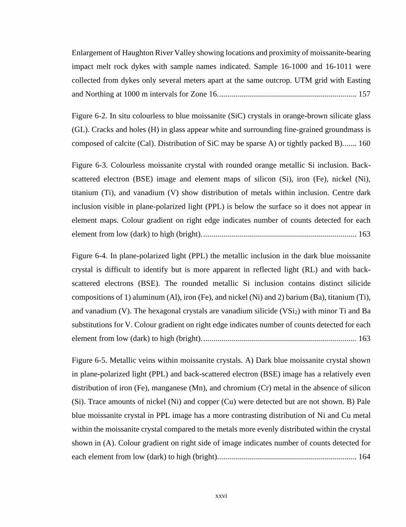
xxvi

Enlargement of Haughton River Valley showing locations and proximity of moissanite-bearing

impact melt rock dykes with sample names indicated. Sample 16-1000 and 16-1011 were

collected from dykes only several meters apart at the same outcrop. UTM grid with Easting

and Northing at 1000 m intervals for Zone 16. ..................................................................... 157

Figure 6-2. In situ colourless to blue moissanite (SiC) crystals in orange-brown silicate glass

(GL). Cracks and holes (H) in glass appear white and surrounding fine-grained groundmass is

composed of calcite (Cal). Distribution of SiC may be sparse A) or tightly packed B). ...... 160

Figure 6-3. Colourless moissanite crystal with rounded orange metallic Si inclusion. Back-

scattered electron (BSE) image and element maps of silicon (Si), iron (Fe), nickel (Ni),

titanium (Ti), and vanadium (V) show distribution of metals within inclusion. Centre dark

inclusion visible in plane-polarized light (PPL) is below the surface so it does not appear in

element maps. Colour gradient on right edge indicates number of counts detected for each

element from low (dark) to high (bright). ............................................................................. 163

Figure 6-4. In plane-polarized light (PPL) the metallic inclusion in the dark blue moissanite

crystal is difficult to identify but is more apparent in reflected light (RL) and with back-

scattered electrons (BSE). The rounded metallic Si inclusion contains distinct silicide

compositions of 1) aluminum (Al), iron (Fe), and nickel (Ni) and 2) barium (Ba), titanium (Ti),

and vanadium (V). The hexagonal crystals are vanadium silicide (VSi2) with minor Ti and Ba

substitutions for V. Colour gradient on right edge indicates number of counts detected for each

element from low (dark) to high (bright). ............................................................................. 163

Figure 6-5. Metallic veins within moissanite crystals. A) Dark blue moissanite crystal shown

in plane-polarized light (PPL) and back-scattered electron (BSE) image has a relatively even

distribution of iron (Fe), manganese (Mn), and chromium (Cr) metal in the absence of silicon

(Si). Trace amounts of nickel (Ni) and copper (Cu) were detected but are not shown. B) Pale

blue moissanite crystal in PPL image has a more contrasting distribution of Ni and Cu metal

within the moissanite crystal compared to the metals more evenly distributed within the crystal

shown in (A). Colour gradient on right side of image indicates number of counts detected for

each element from low (dark) to high (bright). ..................................................................... 164

xxvii

Figure 6-6. Micro-Raman spectra for the three moissanite polytypes identified (6H, 4H, and

15R) which are oriented parallel or close to parallel with respect to the c-axis. Major peak

values for each polytype are indicated and a Y-offset was applied between spectra for clarity.

............................................................................................................................................... 165

Figure 7-1. Visual estimation of erosion levels at the Haughton (H) and Tunnunik (T) impact

structures. Note the actual erosional surfaces of these impact structures are not flat horizontal

planes, this is only a representation. Complex crater cross-section image is modified from

Osinski and Pierazzo (2013); D = final rim-to-rim crater diameter, dt = true depth, da = apparent

depth, SU = structural uplift. ................................................................................................ 177

xxviii

List of Appendices

Appendix A: List of samples ................................................................................................ 188

Appendix B: EDS electron probe microanalysis data........................................................... 191

Appendix C: Powder X-ray diffraction (XRD) analysis data from the Tunnunik impact

structure................................................................................................................................. 193

Appendix D: Micro X-ray diffraction (µXRD) analysis data ............................................... 216

Appendix E: Detailed analytical methods and output values for Rietveld refinement of powder

X-ray diffraction (pXRD) scans from the Haughton impact structure ................................. 231

Appendix F: Raman spectroscopy analysis data ................................................................... 316

1

Chapter 1

1 Introduction

1.1 Impact cratering

Impact cratering is a ubiquitous process to all solid surfaces in our Solar System. On Earth

the terrestrial impact record is poorly preserved compared to the Moon or Mars due to

active surface processes such as plate tectonics, erosion, and burial. Currently there are 198

confirmed terrestrial impact structures (Impact Earth 2020) Despite the identification of

nearly 200 impact structures, there are still aspects that are not fully understood. This lack

in understanding is attributed, in part, to the inaccessibility of a large portion of terrestrial

impact structures as many are buried (63 are completely buried and 4 are partially buried)

or found in very remote locations (Impact Earth 2020). The preservation level of impact

structures can also affect what information can be acquired for a given impact site.

Impact cratering can occur on any solid surface, regardless of composition. The

composition of the target material can affect the formation of an impact structure, the shock

effects generated, and how well the structure and its components are preserved. Most

terrestrial craters are classified as simple or complex based on their morphology, which is

determined primarily by the size and speed of projectile that hits the surface during the

impact event. Projectiles are asteroid or cometary fragments that when they enter Earth’s

atmosphere, have enough mass and a diameter usually >20–50 m, such that little to no

deceleration occurs (French 1998). Without deceleration, the hypervelocity of the

projectile remains >11 km/s when it impacts the surface and depending on the projectile

diameter, a simple or complex crater will form (French 1998). Projectiles with a diameter

of a few metres or less will lose much of their velocity and may strike the surface as a

single projectile or disintegrate as it passes through the atmosphere, resulting in a low

velocity impact or impacts with little penetration into the surface (French 1998).

Simple terrestrial craters are less than ~2 km in apparent diameter, are bowl-shaped with a

raised rim, and have depth to diameter ratios between 1:3 and 1:5 (Melosh 1989). For

simple craters, the dimensions of the transient cavity are similar to the final apparent crater

2

dimensions. Complex craters are larger in apparent diameter than simple craters, ranging

from ~5 km to 300 km (Impact Earth 2020), contain a central uplift, wall terraces, and have

a shallower depth to diameter ratio between approximately 1:10 and 1:20 (Melosh 1989).

The transient cavity ratio is similar for complex and simple craters before the larger

unstable transient cavity of the complex crater collapses. In consolidated sedimentary rocks

the transition from simple to complex crater diameter is ~1.5–2 km and in crystalline rocks

the diameter increases to ~4 km (Dence et al. 1977). Examples of transitional terrestrial

craters include the 4 km Kärdla impact structure in Estonia (Puura and Suuroja 1992), the

4 km Mishina Gora impact structure in Russia (Shmayenok and Tikhomirov 1974), and the

3.2 km Zapadnaya impact structure in Ukraine (Gurov et al. 1985, 2002). On Earth, impact

craters are subject to water and wind erosion, plate tectonics, and burial which degrade or

destroy craters over time, and these factors are absent on other airless rocky planets and

moons in the Solar System (Melosh 1989). The term impact crater refers to the well-

formed circular feature resulting from a hypervelocity impact whereas impact structure is

a more generalized term that includes all impact-derived terrestrial structures regardless of

post-impact erosion or burial state (Baratoux and Reimold 2016; Stöffler and Grieve 2007).

Confirmation of a terrestrial impact structure requires the identification of one or more

features that include shatter cones, shock metamorphism, or meteorite fragments if the

projectile is small enough that it is not completely vapourized during the hypervelocity

impact and large enough to survive transit through the atmosphere (French and Koeberl

2010). Impact-related shock features are generated at different shock pressures during

impacts, so the resultant features are correlated, to a degree, with the apparent diameter of

the impact structure, size of projectile, and target material. The target material is a major

factor in determining what shock metamorphic effects can be generated. The ubiquity of

quartz in terrestrial crystalline rocks and the response of quartz to varying shock pressure

and subsequent ability to retain metamorphic effects to this pressure make it one of the

most studied minerals associated with terrestrial impact structures (Grieve et al. 1996). It

becomes a challenge, however, when hypervelocity impacts occur in targets where quartz-

bearing rocks are absent such as basalts, carbonates, or unconsolidated sediments as these

materials lack diagnostic shock effects or are indistinguishable from tectonic deformation

unrelated to impacts (French and Koeberl 2010).

3

This research focuses on complex craters in sedimentary targets, specifically targets

dominated by carbonates, to better understand the processes involved in generating craters

and to identify signs of shock in non-crystalline rocks.

1.1.1 Complex crater formation

The three recognized stages of the impact cratering process are contact and compression,

excavation, and modification (Fig. 1-1), which proceed as a continuum as there is no pause

or exact moment when one stage ends and the next begins (Gault et al. 1968; Melosh 1989).

The division of stages relates to the development of different physical processes that occur

during the impact event. The contact and compression stage begins when the incoming

projectile first contacts the solid target surface. The projectile penetrates up to twice its

diameter into the target, depending on the target material and the density of the projectile

(French 1998; Kieffer and Simonds 1980; O’Keefe and Ahrens 1982). The hypervelocity

contact transfers kinetic energy from the projectile into the target in the form of shock

waves that propagate through the projectile and the target material (Gault et al. 1968;

Melosh 1989). The largest pressures generated during an impact event occur during the

contact and compression stage where pressures at the point of impact can range from 100–

1,000 GPa (Melosh 1989; Shoemaker 1960). As the projectile penetrates the target

material, it becomes consumed by the shock wave. Once the shock wave reaches the upper

free surface of the projectile, it then reflects back through as a rarefaction wave (Gault et

al. 1968). Rarefaction is a means to decompress from the high impact pressure generated

to return to ambient pressure, resulting in the melting or vapourization of the projectile

(Gault et al. 1968). The rarefaction waves can also lead to melting, vapourization, and/or

shock metamorphism of target material (Ahrens and O’Keefe 1972; Grieve et al. 1977).

Shock waves also lose energy as they expand radially from the point of impact where

energy is lost as heat into the target rocks (French 1998). For projectiles 10 m to 1 km in

diameter, the contact and compression stage ranges from 10-3 to 10-1 seconds, the shortest

of the three stages (Gault et al. 1968).

4

Figure 1-1. Sequence of cross-sections highlighting the main components involved in

the three stages of impact crater formation for complex craters; modified from

Osinski and Pierazzo (2013).

5

The excavation stage continues with the propagation of a hemispherical shock wave

through the target material, outward from the penetration depth of the projectile. At this

point, the projectile itself is no longer involved in the crater-forming process as it was

melted and/or vapourized during the contact and compression stage (Melosh 1989).

Additional shock waves are directed upward and reach the free surface where they reflect

to produce rarefaction waves downward into the target material. Where the rarefaction

waves interact with the hemispherical shock wave, an interference zone is generated and

pressure here is reduced (Melosh 1989). Wave interaction in this zone produces an

‘excavation flow-field’ and generates a transient cavity of low to near ambient pressure

(Dence 1968; Gault et al. 1968; Grieve and Cintala 1992). Some of the energy from the

reflected rarefaction waves is converted back into kinetic energy, causing the transient

cavity to open up and expand while fractured target material is accelerated and ejected out

of the cavity (French 1998; Gault et al. 1968). The ejected material forms a continuous

ejecta blanket extending to about one crater radius beyond the rim of the bowl-shaped

transient cavity with ejecta becoming discontinuous to about 5 crater radii (French 1998;

Melosh 1989; Oberbeck 1975). The release in pressure within the transient cavity and

target material is also associated with fracturing and shattering within the target rock

(French 1998).

Until this point in crater-formation, the process for developing a simple or complex crater

has been essentially the same. The modification stage begins once the shock waves have

decayed beyond the crater rim so that they no longer affect crater development and this is

when different crater morphologies begin to develop based on the size of the excavated

transient crater (French 1998; Melosh 1989). Modification of simple craters with a

diameter less than a few kilometres is minor and they retain the stable and simple bowl-

shape morphology of the transient cavity (French 1998). On Earth, when a transient crater

reaches a diameter greater than ~2 km in sedimentary targets and ~4 km in crystalline

targets, the cavity becomes unstable and is modified by gravitational force and centripetal

movement (Dence 1968; French 1998). Gravity coupled with the strength and structure of

the target material cause significant movement and shearing of target rocks outward,

inward, and upward due to collapse, slumping, or faulting (French 1998). The resulting

complex crater morphology includes a central uplift, a flat internal floor, and terraces

6

around the periphery of the crater (French 1998; Melosh 1989). Craters larger than 140 km

in diameter develop an unstable central peak that collapses to form a peak ring, to resemble

Schrödinger Crater on the Moon (Melosh 1989).

To put the rapid nature of crater-forming processes into perspective, detailed calculations

project that the 1-km diameter simple crater Barringer (Meteor) Crater, Arizona formed in

approximately 6 seconds while a 200-km diameter complex crater requires closer to 90

seconds to form (French 1998).

1.1.2 Sedimentary targets

Currently, there are 82 terrestrial impacts listed out of 198 confirmed impact structures that

formed in completely sedimentary targets while another 54 formed in a mixed target of

sedimentary and crystalline rocks (Impact Earth 2020). This maintains a similar value of

~70% of impacts occurring in target sequences that contain sedimentary rocks as reported

over 10 years ago (Osinski et al. 2008). In 2007 there were 174 confirmed terrestrial impact

structures with 68 occurring in sedimentary targets and mixed is the same as the 2019 total

(Osinski et al. 2008). These numbers show the proportion of sedimentary rocks associated

with terrestrial impacts remains relatively consistent as new impact structures are

discovered and confirmed. The occurrence of sedimentary rocks is a significant portion

within the terrestrial impact record yet have been largely overlooked when theoretical

studies are carried out (Kieffer and Simonds 1980).

Sedimentary rocks add additional elements to the impact process as they often contain

rocks which are more porous and contain volatiles, when compared with crystalline targets

(Kieffer and Simonds 1980; Osinski et al. 2008). Porosity in sedimentary target rocks is

complex and varies between sandstones and carbonates as well as within each group

(Choquette and Pray 1970). The age of sedimentary rocks may also factor into porosity

where sandstones have initial porosity around 25–40% and carbonates 40–70% is common,

these decrease to 15–30% and none to <5%, respectively following diagenesis (Choquette

and Pray 1970). Porous rocks are able to hold groundwater (up to 20% or more pore space

filled by water) better than crystalline rocks, which tend to be non-porous leaving them to

hold only several percent water (Kieffer and Simonds 1980). The presence of groundwater

7

increases the portion of volatiles available during an impact event, and increases more

when the target sedimentary rocks contain carbonates (Kieffer and Simonds 1980). When

carbonates are involved, the production of carbon dioxide (CO2) during an impact could

play a factor; calcite (CaCO3) can decompose or devolatilize to produce CaO and CO2 (e.g.,

O’Keefe and Ahrens 1989). The effect and volume of carbon dioxide produced from an

impact event is not entirely understood. Estimates of carbon dioxide production from shock

experiments have suggested substantial amounts of carbon dioxide is released from impacts

into carbonate targets (e.g., Hörz et al. 2015; Kieffer and Simonds 1980; Lange and Ahrens

1986) and conversely, experiments have proposed the amount of carbon dioxide generated

has been overestimated (e.g., Bell 2016; Jones et al. 2000; Martinez et al. 1995). Production

of carbon dioxide during hypervelocity impacts is also related to research at terrestrial

impact sites as well as experiments and models have investigated the extent to which

carbonates melt (e.g., Graup 1999; Jones et al. 2000; Osinski et al. 2008, 2018) or

decompose (e.g., Hörz et al. 2015, 2019; O’Keefe and Ahrens 1989; Stöffler et al. 2013)

from the impact.

A consensus has yet to be reached regarding the fate of carbonates in hypervelocity impact

events. More time and information are required to determine the causes which can lead to

either or both outcomes while also reaching an agreement regarding these processes that

involve carbonates.

1.1.3 Impactites

Impactites is a broad term that refers to rocks affected by a hypervelocity impact event and

are categorized as proximal or distal based on where they are located with respect to the

impact structure (Stöffler and Grieve 2007). Proximal impactites are located within the

crater out to the farthest limit of the continuous ejecta blanket, or ~2.5 crater diameters,

and include shocked rocks, impact melt rocks, and impact breccias (Glass and Simonson

2012; Stöffler and Grieve 2007). Distal impactites occur beyond the continuous ejecta

blanket and include tektites, microtektites, and air fall beds (Stöffler and Grieve 2007).

Only the proximal group of impactites is relevant to this research and will be discussed

further as distal impactites are absent from both study sites.

8

Shocked rocks contain the effects of shock metamorphism and without any occurrence of

melt. Some of the most common shock effects or features of shocked target rocks include

quartz and feldspar with planar deformation features, diaplectic glass and other rock and

mineral glasses, and high temperature polymorphs such as coesite and stishovite (Stöffler

and Grieve 2007). These are discussed more in the following section as shock

metamorphism is the primary evidence that high pressures were generated during a

hypervelocity impact. Impact melt rocks are divided into three groups based on their clast

content which are clast-free, clast-poor, and clast-rich melt rocks (Stöffler and Grieve

2007). Impact breccias consist of monomict, lithic, and impact melt-bearing breccias or

suevites (Osinski et al. 2016; Stöffler and Grieve 2007). The term suevite originally

referred to impact breccias from the Ries impact structure that contained impact glass clasts

(Osinski et al. 2016 and references therein). Currently, a suevite is defined as an impact

breccia that has a particulate matrix and contains clasts of lithic and mineral exhibiting

shock metamorphism as well as impact glass fragments (Stöffler and Grieve 2007).

1.1.4 Microscopic shock metamorphism

Identification of shock metamorphism in rocks or mineral grains is a generally agreed upon

as a requirement to confirming a new impact structure (French and Koeberl 2010). Target

rocks and minerals associated with an impact event are subjected to short lived but intense

shock pressures, that may exceed 100 GPa, that can generate microscopic effects such as

planar fractures (PFs), planar deformation features (PDFs), or diaplectic glass in quartz or

feldspars (e.g., French 1998; Stöffler et al. 2018). Specifically in plagioclase (feldspar)

diaplectic glass is referred to as maskelynite (Stöffler et al. 2018). High-pressure

polymorphs can also be generated through shock metamorphism including coesite or

stishovite from quartz, ringwoodite from olivine, and diamond and lonsdaleite from

graphite (Frondel and Marvin 1967; Stöffler et al. 2018). These products of shock are

diagnostic of impact events and are used to confirm the origin of suspected impacts. When

hypervelocity impacts occur in silicate-bearing target rocks, at least some of these shock

metamorphic products should be generated, provided the scale of the impact is large

enough. With over a third of impacts occurring in sedimentary targets (Osinski et al. 2008)

9

many of these contain carbonates which do not display the typical diagnostic shock

products and effects listed above.

The ability to determine shock metamorphism in carbonates is not as straightforward as

identifying shock in quartz and feldspars. Optical microscopy does not reveal diagnostic

strain or shock effects in carbonates, however, studies using X-ray diffraction and Raman

spectroscopy have shown varying ability to detect crystallographic or spectroscopic

changes due to shock in carbonates. Shock effects in dolomite such as lower symmetry and

broader peaks in the dolomite Raman spectra were detected while the Raman spectra for

calcite remained unchanged making Raman spectroscopy a useful tool for identifying

shock in dolomite (Lindgren et al. 2009). X-ray diffraction studies on shock effects in

calcite (Skála and Jakeš 1999), calcite and dolomite (Huson et al. 2009), and dolomite

(Seeley and Milam 2018) show potential for identifying shock in carbonates when FWHM

values are derived using Rietveld refinements or peak broadening is examined. Rietveld

derived values indicate shock is more easily distinguished in dolomite than calcite (Huson

et al. 2009) so there may be additional differences to be uncovered for these two carbonate

minerals.

1.2 Arctic geology

1.2.1 Arctic Archipelago

The Arctic Archipelago (Fig. 1-2) is a group of more than 36,000 islands, of which 94 are

considered major islands having a land area greater than 130 km2, off the northern Canada

mainland (Hund 2014). The Arctic Archipelago is divided into seven geological provinces

including the Arctic Platform and the Canadian Shield (Thorsteinsson and Tozer 1970).

These geologic provinces consist largely of Phanerozoic-aged sedimentary rocks with

isolated occurrences of Precambrian-aged rocks (Daae and Rutgers 1975; Douglas et al.

1963; Thorsteinsson and Tozer 1970).

There are correlations of sedimentary units between adjacent islands within the Arctic

Archipelago and the extent of correlation can vary which is evident in geological maps

(e.g., Okulitch 1991). The abundance of carbonates within the Arctic Platform geologic

province indicates there was a vast continental shelf environment where local ocean

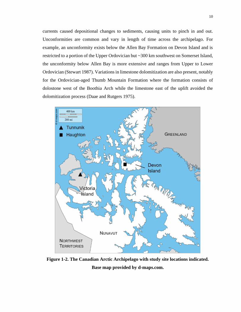
10

currents caused depositional changes to sediments, causing units to pinch in and out.

Unconformities are common and vary in length of time across the archipelago. For

example, an unconformity exists below the Allen Bay Formation on Devon Island and is

restricted to a portion of the Upper Ordovician but ~300 km southwest on Somerset Island,

the unconformity below Allen Bay is more extensive and ranges from Upper to Lower

Ordovician (Stewart 1987). Variations in limestone dolomitization are also present, notably

for the Ordovician-aged Thumb Mountain Formation where the formation consists of

dolostone west of the Boothia Arch while the limestone east of the uplift avoided the

dolomitization process (Daae and Rutgers 1975).

Figure 1-2. The Canadian Arctic Archipelago with study site locations indicated.

Base map provided by d-maps.com.

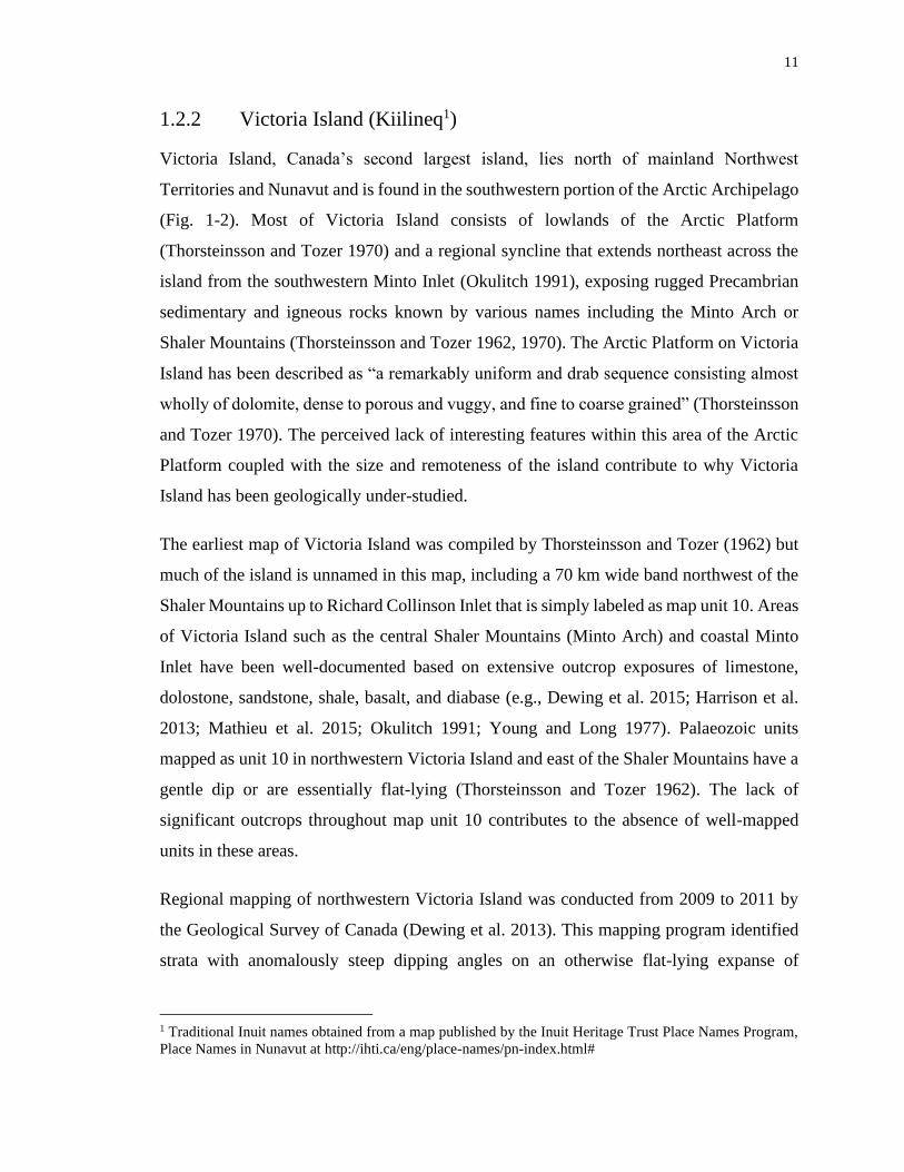
11

1.2.2 Victoria Island (Kiilineq1)

Victoria Island, Canada’s second largest island, lies north of mainland Northwest

Territories and Nunavut and is found in the southwestern portion of the Arctic Archipelago

(Fig. 1-2). Most of Victoria Island consists of lowlands of the Arctic Platform

(Thorsteinsson and Tozer 1970) and a regional syncline that extends northeast across the

island from the southwestern Minto Inlet (Okulitch 1991), exposing rugged Precambrian

sedimentary and igneous rocks known by various names including the Minto Arch or

Shaler Mountains (Thorsteinsson and Tozer 1962, 1970). The Arctic Platform on Victoria

Island has been described as “a remarkably uniform and drab sequence consisting almost

wholly of dolomite, dense to porous and vuggy, and fine to coarse grained” (Thorsteinsson

and Tozer 1970). The perceived lack of interesting features within this area of the Arctic

Platform coupled with the size and remoteness of the island contribute to why Victoria

Island has been geologically under-studied.

The earliest map of Victoria Island was compiled by Thorsteinsson and Tozer (1962) but

much of the island is unnamed in this map, including a 70 km wide band northwest of the

Shaler Mountains up to Richard Collinson Inlet that is simply labeled as map unit 10. Areas

of Victoria Island such as the central Shaler Mountains (Minto Arch) and coastal Minto

Inlet have been well-documented based on extensive outcrop exposures of limestone,

dolostone, sandstone, shale, basalt, and diabase (e.g., Dewing et al. 2015; Harrison et al.

2013; Mathieu et al. 2015; Okulitch 1991; Young and Long 1977). Palaeozoic units

mapped as unit 10 in northwestern Victoria Island and east of the Shaler Mountains have a

gentle dip or are essentially flat-lying (Thorsteinsson and Tozer 1962). The lack of

significant outcrops throughout map unit 10 contributes to the absence of well-mapped

units in these areas.

Regional mapping of northwestern Victoria Island was conducted from 2009 to 2011 by

the Geological Survey of Canada (Dewing et al. 2013). This mapping program identified

strata with anomalously steep dipping angles on an otherwise flat-lying expanse of

1 Traditional Inuit names obtained from a map published by the Inuit Heritage Trust Place Names Program,

Place Names in Nunavut at http://ihti.ca/eng/place-names/pn-index.html#

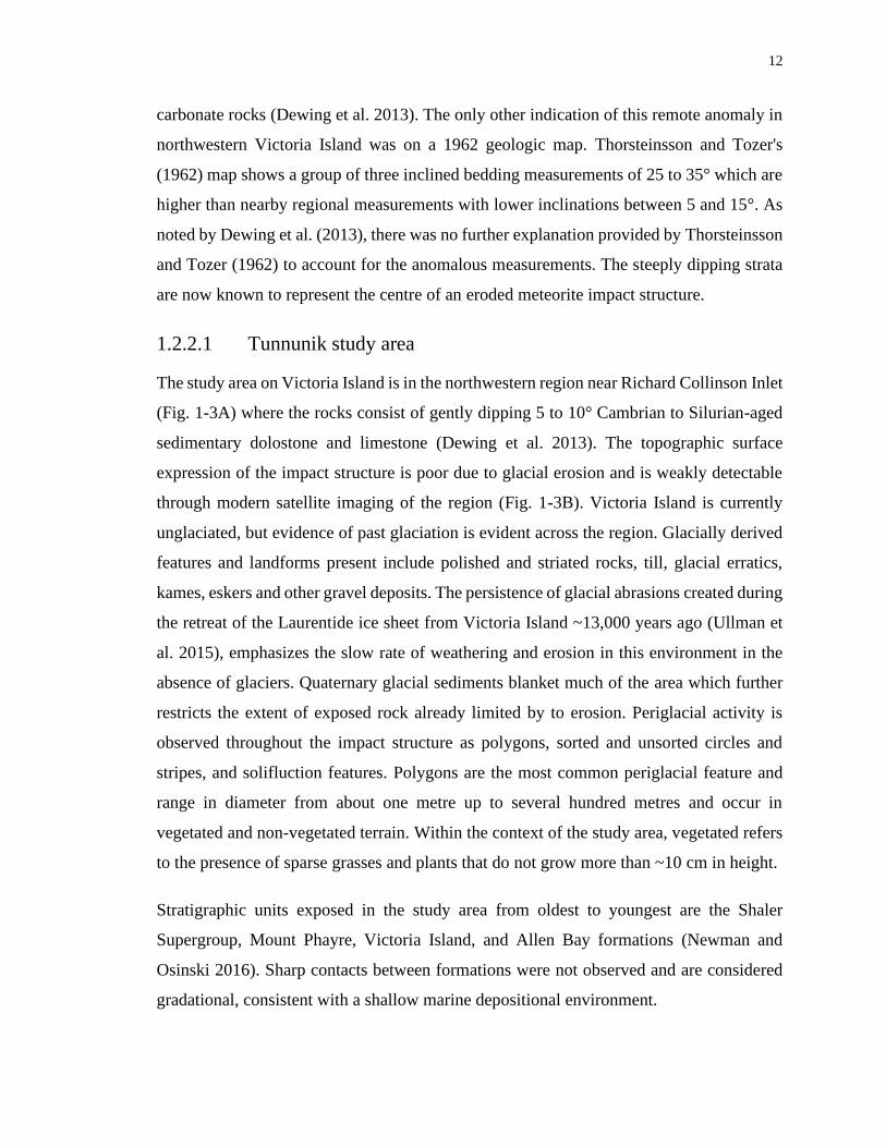
12

carbonate rocks (Dewing et al. 2013). The only other indication of this remote anomaly in

northwestern Victoria Island was on a 1962 geologic map. Thorsteinsson and Tozer's

(1962) map shows a group of three inclined bedding measurements of 25 to 35° which are

higher than nearby regional measurements with lower inclinations between 5 and 15°. As

noted by Dewing et al. (2013), there was no further explanation provided by Thorsteinsson

and Tozer (1962) to account for the anomalous measurements. The steeply dipping strata

are now known to represent the centre of an eroded meteorite impact structure.

1.2.2.1 Tunnunik study area

The study area on Victoria Island is in the northwestern region near Richard Collinson Inlet

(Fig. 1-3A) where the rocks consist of gently dipping 5 to 10° Cambrian to Silurian-aged

sedimentary dolostone and limestone (Dewing et al. 2013). The topographic surface

expression of the impact structure is poor due to glacial erosion and is weakly detectable

through modern satellite imaging of the region (Fig. 1-3B). Victoria Island is currently

unglaciated, but evidence of past glaciation is evident across the region. Glacially derived

features and landforms present include polished and striated rocks, till, glacial erratics,

kames, eskers and other gravel deposits. The persistence of glacial abrasions created during

the retreat of the Laurentide ice sheet from Victoria Island ~13,000 years ago (Ullman et

al. 2015), emphasizes the slow rate of weathering and erosion in this environment in the

absence of glaciers. Quaternary glacial sediments blanket much of the area which further

restricts the extent of exposed rock already limited by to erosion. Periglacial activity is

observed throughout the impact structure as polygons, sorted and unsorted circles and

stripes, and solifluction features. Polygons are the most common periglacial feature and

range in diameter from about one metre up to several hundred metres and occur in

vegetated and non-vegetated terrain. Within the context of the study area, vegetated refers

to the presence of sparse grasses and plants that do not grow more than ~10 cm in height.

Stratigraphic units exposed in the study area from oldest to youngest are the Shaler

Supergroup, Mount Phayre, Victoria Island, and Allen Bay formations (Newman and

Osinski 2016). Sharp contacts between formations were not observed and are considered

gradational, consistent with a shallow marine depositional environment.

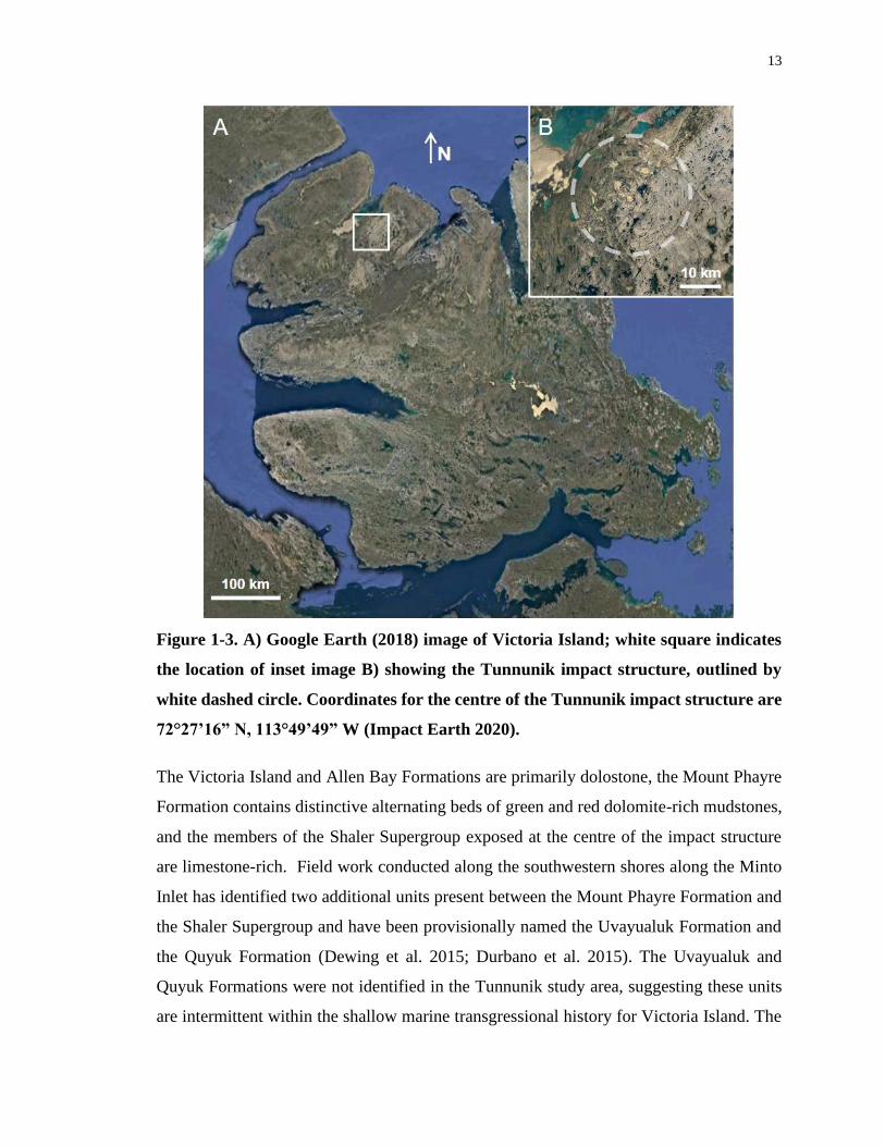
13

Figure 1-3. A) Google Earth (2018) image of Victoria Island; white square indicates

the location of inset image B) showing the Tunnunik impact structure, outlined by

white dashed circle. Coordinates for the centre of the Tunnunik impact structure are

72°27’16” N, 113°49’49” W (Impact Earth 2020).

The Victoria Island and Allen Bay Formations are primarily dolostone, the Mount Phayre

Formation contains distinctive alternating beds of green and red dolomite-rich mudstones,

and the members of the Shaler Supergroup exposed at the centre of the impact structure

are limestone-rich. Field work conducted along the southwestern shores along the Minto

Inlet has identified two additional units present between the Mount Phayre Formation and

the Shaler Supergroup and have been provisionally named the Uvayualuk Formation and

the Quyuk Formation (Dewing et al. 2015; Durbano et al. 2015). The Uvayualuk and

Quyuk Formations were not identified in the Tunnunik study area, suggesting these units

are intermittent within the shallow marine transgressional history for Victoria Island. The

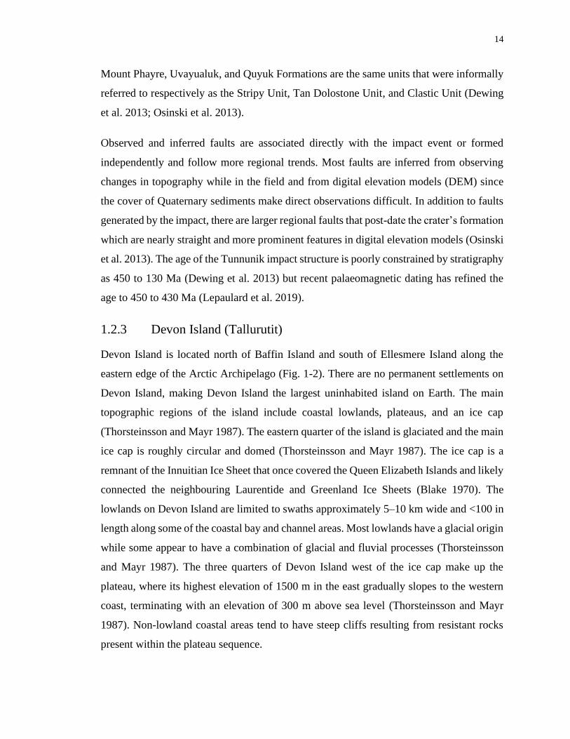
14

Mount Phayre, Uvayualuk, and Quyuk Formations are the same units that were informally

referred to respectively as the Stripy Unit, Tan Dolostone Unit, and Clastic Unit (Dewing

et al. 2013; Osinski et al. 2013).

Observed and inferred faults are associated directly with the impact event or formed

independently and follow more regional trends. Most faults are inferred from observing

changes in topography while in the field and from digital elevation models (DEM) since

the cover of Quaternary sediments make direct observations difficult. In addition to faults

generated by the impact, there are larger regional faults that post-date the crater’s formation

which are nearly straight and more prominent features in digital elevation models (Osinski

et al. 2013). The age of the Tunnunik impact structure is poorly constrained by stratigraphy

as 450 to 130 Ma (Dewing et al. 2013) but recent palaeomagnetic dating has refined the

age to 450 to 430 Ma (Lepaulard et al. 2019).

1.2.3 Devon Island (Tallurutit)

Devon Island is located north of Baffin Island and south of Ellesmere Island along the

eastern edge of the Arctic Archipelago (Fig. 1-2). There are no permanent settlements on

Devon Island, making Devon Island the largest uninhabited island on Earth. The main

topographic regions of the island include coastal lowlands, plateaus, and an ice cap

(Thorsteinsson and Mayr 1987). The eastern quarter of the island is glaciated and the main

ice cap is roughly circular and domed (Thorsteinsson and Mayr 1987). The ice cap is a

remnant of the Innuitian Ice Sheet that once covered the Queen Elizabeth Islands and likely

connected the neighbouring Laurentide and Greenland Ice Sheets (Blake 1970). The

lowlands on Devon Island are limited to swaths approximately 5–10 km wide and <100 in

length along some of the coastal bay and channel areas. Most lowlands have a glacial origin

while some appear to have a combination of glacial and fluvial processes (Thorsteinsson

and Mayr 1987). The three quarters of Devon Island west of the ice cap make up the

plateau, where its highest elevation of 1500 m in the east gradually slopes to the western

coast, terminating with an elevation of 300 m above sea level (Thorsteinsson and Mayr

1987). Non-lowland coastal areas tend to have steep cliffs resulting from resistant rocks

present within the plateau sequence.

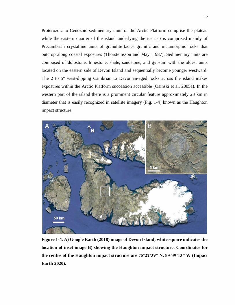
15

Proterozoic to Cenozoic sedimentary units of the Arctic Platform comprise the plateau

while the eastern quarter of the island underlying the ice cap is comprised mainly of

Precambrian crystalline units of granulite-facies granitic and metamorphic rocks that

outcrop along coastal exposures (Thorsteinsson and Mayr 1987). Sedimentary units are

composed of dolostone, limestone, shale, sandstone, and gypsum with the oldest units

located on the eastern side of Devon Island and sequentially become younger westward.

The 2 to 5° west-dipping Cambrian to Devonian-aged rocks across the island makes

exposures within the Arctic Platform succession accessible (Osinski et al. 2005a). In the

western part of the island there is a prominent circular feature approximately 23 km in

diameter that is easily recognized in satellite imagery (Fig. 1-4) known as the Haughton

impact structure.

Figure 1-4. A) Google Earth (2018) image of Devon Island; white square indicates the

location of inset image B) showing the Haughton impact structure. Coordinates for

the centre of the Haughton impact structure are 75°22’39” N, 89°39’13” W (Impact

Earth 2020).

16

The existence of this structure has been known since the 1950s and was confirmed to have

an impact origin after shatter cones were identified by Robertson and Mason (1975). Over

the past 30 years there have been numerous expeditions to the Haughton impact structure

that have studied various aspects of the structure including geology, impactites, shatter

cones, hydrothermal activity, geophysics, and geomicrobiology (e.g., Bischoff and

Oskierski 1988; Osinski et al. 2001, 2005a, 2005b; Pontefract et al. 2014; Redeker and

Stöffler 1988; Zylberman et al. 2017).

1.2.3.1 Haughton study area

The Haughton impact structure is approximately 80 km inland from the western coast of

Devon Island (Fig. 1-4). The western side of Devon Island is unglaciated, and the study

area consists of Ordovician to Silurian-aged sedimentary units of dolostones, limestones,

evaporites, and sandstones. Stratigraphic units exposed within the Haughton impact

structure from oldest to youngest are the Blanley Bay Formation, Eleanor River Formation,

Bay Fiord Formation, Thumb Mountain Formation, and Allen Bay Formation (Osinski et

al. 2005a). There are no outcrops of Precambrian crystalline rocks within the impact

structure, however, crystalline clasts of various gneisses, amphibolite, and diabase have

been identified within the impact melt rock crater-fill deposits and exhibit levels of shock

from pressures ranging from 15 to 60 GPa (Metzler et al. 1988). Gneiss clasts that display

higher shock metamorphism are poorly banded, paler in colour, and have a more vesicular

texture compared to unshocked gneiss (Frisch and Thorsteinsson 1978). In addition to the

crystalline clasts in the impact melt rock deposits, most of the lithic clasts present are

dolostone, limestone, gypsum, and anhydrite which reflects the target lithology (Osinski et

al. 2005b). The diverse assemblage of clasts within the crater-fill deposits show all

lithologies within the target sequence were affected during the impact event, down to and

including the crystalline basement.

Several areas within the impact structure the crater-fill deposits are overlain by the early

Miocene Haughton Formation, a post-impact depositional unit. The geographically

isolated Haughton Formation is the only source of Miocene biota and climate information

within the northern Arctic (Hickey et al. 1988). Quaternary glacial deposits and fluvial

deposits are also present within the impact structure and throughout the region. The

17

Haughton impact structure is relatively young geologically, and the Miocene-age deposits

within the structure help constrain the age. Radiometric dating has been performed in

separate experiments with the most recent age being 23.5 ± 2.0 Ma obtained through (U-

Th)/He dating of zircon (Young et al. 2013). Previous experiments using Ar-Ar dating

yielded 23.4 ± 1.0 Ma (Jessberger 1988) and 39.1 ± 1.7 Ma (Sherlock et al. 2005),

respectively, for this well-preserved impact structure.

1.3 X-ray diffraction

X-ray diffraction is a means by which information about a mineral’s crystal structure is

examined. It was discovered in 1912 that crystals diffract X-rays by Max von Laue when

he directed a beam of X-rays at a crystal of copper sulfate that was diffracted into spots on

a photographic plate (Cullity 1978). In the same year as von Laue’s discovery, the father

and son team of W. H. Bragg and W. L. Bragg completed successful experiments on

additional crystal structures while deriving a simpler mathematical form (Cullity 1978).

The crystal structure of calcite was determined the following year (Bragg 1914; Bragg and

Bragg 1913) and dolomite about ten years later (Wasastjerna 1924; Wyckoff and Merwin

1924).

The most common carbonate minerals, calcite (CaCO3) and dolomite (CaMg(CO3)2), have

a hexagonal crystal lattice but differ slightly in symmetry and their space groups; calcite is

R3̅c and dolomite is R3̅ (Reeder 1983). The unit cell for both minerals is similar with

carbonate (CO3) layers alternating with cation layers (Fig. 1-5). Dolomite preserves the

structure of calcite but magnesium (Mg) substitutes in alternating octahedral cation layers

for calcium (Ca). The substitution of Mg cations slightly modifies unit cell properties of

dolomite including bond lengths and introduces less distortion into the CaO6 octahedra

with the addition of MgO6 octahedra when compared to calcite since Mg and Ca cations

are different sizes, Ca being the larger cation (Reeder 1983). The ionic radius of Ca cations

is 1.00 Å compared to an ionic radius of 0.72 Å for Mg cations (Ross and Reeder 1992;

Shannon 1976).

The unit cell for any mineral is the smallest unique three-dimensional unit that repeats

along crystallographic axis directions to form larger crystals. The unit cell structure is

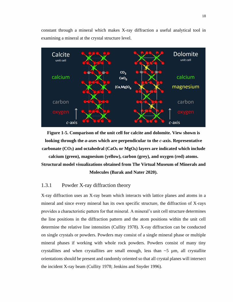
18

constant through a mineral which makes X-ray diffraction a useful analytical tool in

examining a mineral at the crystal structure level.

Figure 1-5. Comparison of the unit cell for calcite and dolomite. View shown is

looking through the a-axes which are perpendicular to the c-axis. Representative

carbonate (CO3) and octahedral (CaO6 or MgO6) layers are indicated which include

calcium (green), magnesium (yellow), carbon (grey), and oxygen (red) atoms.

Structural model visualizations obtained from The Virtual Museum of Minerals and

Molecules (Barak and Nater 2020).

1.3.1 Powder X-ray diffraction theory

X-ray diffraction uses an X-ray beam which interacts with lattice planes and atoms in a

mineral and since every mineral has its own specific structure, the diffraction of X-rays

provides a characteristic pattern for that mineral. A mineral’s unit cell structure determines

the line positions in the diffraction pattern and the atom positions within the unit cell

determine the relative line intensities (Cullity 1978). X-ray diffraction can be conducted

on single crystals or powders. Powders may consist of a single mineral phase or multiple

mineral phases if working with whole rock powders. Powders consist of many tiny

crystallites and when crystallites are small enough, less than ~5 µm, all crystallite

orientations should be present and randomly oriented so that all crystal planes will intersect

the incident X-ray beam (Cullity 1978; Jenkins and Snyder 1996).

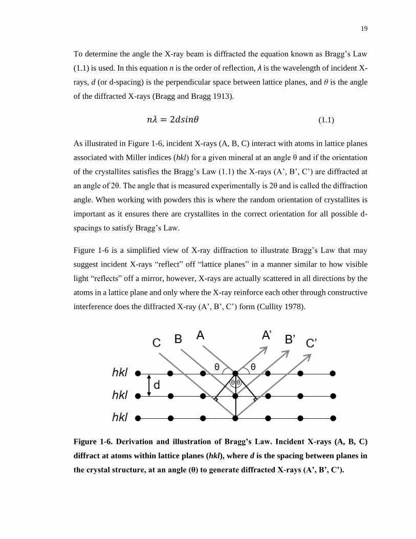
19

To determine the angle the X-ray beam is diffracted the equation known as Bragg’s Law

(1.1) is used. In this equation n is the order of reflection, λ is the wavelength of incident X-

rays, d (or d-spacing) is the perpendicular space between lattice planes, and θ is the angle

of the diffracted X-rays (Bragg and Bragg 1913).

𝑛𝜆 = 2𝑑𝑠𝑖𝑛𝜃 (1.1)

As illustrated in Figure 1-6, incident X-rays (A, B, C) interact with atoms in lattice planes

associated with Miller indices (hkl) for a given mineral at an angle θ and if the orientation

of the crystallites satisfies the Bragg’s Law (1.1) the X-rays (A’, B’, C’) are diffracted at

an angle of 2θ. The angle that is measured experimentally is 2θ and is called the diffraction

angle. When working with powders this is where the random orientation of crystallites is

important as it ensures there are crystallites in the correct orientation for all possible d-

spacings to satisfy Bragg’s Law.

Figure 1-6 is a simplified view of X-ray diffraction to illustrate Bragg’s Law that may

suggest incident X-rays “reflect” off “lattice planes” in a manner similar to how visible

light “reflects” off a mirror, however, X-rays are actually scattered in all directions by the

atoms in a lattice plane and only where the X-ray reinforce each other through constructive

interference does the diffracted X-ray (A’, B’, C’) form (Cullity 1978).

Figure 1-6. Derivation and illustration of Bragg’s Law. Incident X-rays (A, B, C)

diffract at atoms within lattice planes (hkl), where d is the spacing between planes in

the crystal structure, at an angle (θ) to generate diffracted X-rays (A’, B’, C’).

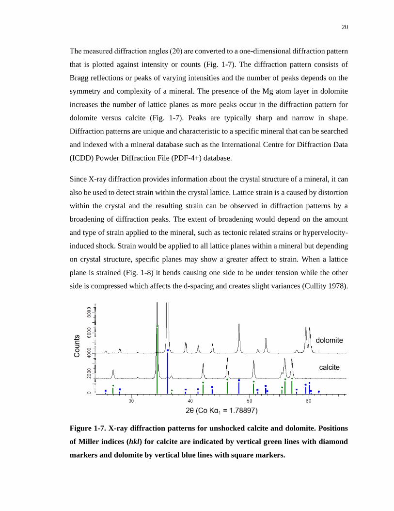
20

The measured diffraction angles (2θ) are converted to a one-dimensional diffraction pattern

that is plotted against intensity or counts (Fig. 1-7). The diffraction pattern consists of

Bragg reflections or peaks of varying intensities and the number of peaks depends on the

symmetry and complexity of a mineral. The presence of the Mg atom layer in dolomite

increases the number of lattice planes as more peaks occur in the diffraction pattern for

dolomite versus calcite (Fig. 1-7). Peaks are typically sharp and narrow in shape.

Diffraction patterns are unique and characteristic to a specific mineral that can be searched

and indexed with a mineral database such as the International Centre for Diffraction Data

(ICDD) Powder Diffraction File (PDF-4+) database.

Since X-ray diffraction provides information about the crystal structure of a mineral, it can

also be used to detect strain within the crystal lattice. Lattice strain is a caused by distortion

within the crystal and the resulting strain can be observed in diffraction patterns by a

broadening of diffraction peaks. The extent of broadening would depend on the amount

and type of strain applied to the mineral, such as tectonic related strains or hypervelocity-

induced shock. Strain would be applied to all lattice planes within a mineral but depending

on crystal structure, specific planes may show a greater affect to strain. When a lattice

plane is strained (Fig. 1-8) it bends causing one side to be under tension while the other

side is compressed which affects the d-spacing and creates slight variances (Cullity 1978).

Figure 1-7. X-ray diffraction patterns for unshocked calcite and dolomite. Positions

of Miller indices (hkl) for calcite are indicated by vertical green lines with diamond

markers and dolomite by vertical blue lines with square markers.

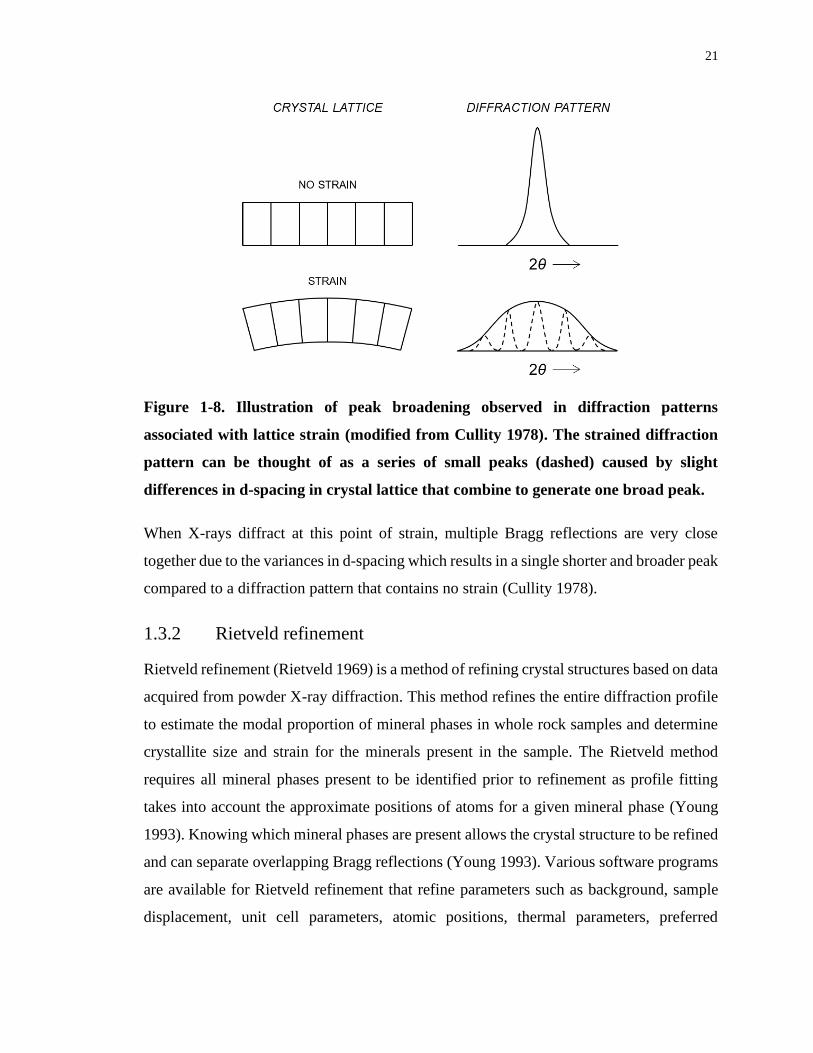
21

Figure 1-8. Illustration of peak broadening observed in diffraction patterns

associated with lattice strain (modified from Cullity 1978). The strained diffraction

pattern can be thought of as a series of small peaks (dashed) caused by slight

differences in d-spacing in crystal lattice that combine to generate one broad peak.

When X-rays diffract at this point of strain, multiple Bragg reflections are very close

together due to the variances in d-spacing which results in a single shorter and broader peak

compared to a diffraction pattern that contains no strain (Cullity 1978).

1.3.2 Rietveld refinement

Rietveld refinement (Rietveld 1969) is a method of refining crystal structures based on data

acquired from powder X-ray diffraction. This method refines the entire diffraction profile

to estimate the modal proportion of mineral phases in whole rock samples and determine

crystallite size and strain for the minerals present in the sample. The Rietveld method

requires all mineral phases present to be identified prior to refinement as profile fitting

takes into account the approximate positions of atoms for a given mineral phase (Young

1993). Knowing which mineral phases are present allows the crystal structure to be refined

and can separate overlapping Bragg reflections (Young 1993). Various software programs

are available for Rietveld refinement that refine parameters such as background, sample

displacement, unit cell parameters, atomic positions, thermal parameters, preferred

22

orientation, occupancy, crystallite size, and crystal strain. Here, the software program

TOPAS 5 by Bruker AXS was used.

1.4 Thesis objectives

The goals of this thesis are to understand the nature of impact-generated dykes in

sedimentary targets, specifically in dolostone and limestone, and identify effects of shock

in these carbonates as a product of hypervelocity impacts to help identify and verify

impacts in sedimentary targets. The two impact sites studied here are located in remote

Canadian Arctic locations and research from both sites include aspects that have not been

previously explored or reported. Field work at the Tunnunik and Haughton impact

structures involved documenting and collecting impact breccia and representative target

rock samples. Breccia and melt rock samples from dykes were characterized through

optical microscopy and electron probe microanalysis while shock effects in target rocks,

crater-fill deposits, and ballistic ejecta were investigated using X-ray diffraction of

powdered whole rock samples.

The similarity in diameter and target composition between the Tunnunik and Haughton

impact structures provides an excellent opportunity to compare the products and processes

of the events that generated these structures. The differing state of preservation between

the study sites allows for the upper and lower sections of complex craters to be examined

and compared, which could not be accomplished from studying only one of these impact

sites. While characterizing impact melt rocks from Haughton, the rare terrestrial mineral

moissanite was unexpectedly discovered. The presence of moissanite helps to better

constrain temperatures and conditions present during the impact event. The insights gained

from this research will improve the understanding of hypervelocity impacts into carbonate-

rich targets which can be applied to other impact sites where carbonates are present in

significant quantities.

1.5 References

Ahrens T. J., and O’Keefe J. D. 1972. Shock melting and vaporization of lunar rocks and

minerals. The Moon 4:214–249.

23

Barak P. and Nater E. A. The Virtual Museum of Minerals and Molecules. 2020.

http://virtual-museum.soils.wisc.edu (Accessed April 18, 2020).

Baratoux D., and Reimold W. U. 2016. The current state of knowledge about shatter cones:

Introduction to the special issue. Meteoritics & Planetary Science 51:1389–1434.

Bell M. S. 2016. CO2 release due to impact devolatilization of carbonate: Results of shock

experiments. Meteoritics & Planetary Science 51:619–646.

Bischoff L., and Oskierski W. 1988. The surface structure of the Haughton impact crater,

Devon Island, Canada. Meteoritics 23:209–220.

Blake W. J. 1970. Studies of glacial history in Arctic Canada. I. Pumice, radiocarbon dates,

and differential postglacial uplift in the eastern Queen Elizabeth Islands. Canadian

Journal of Earth Sciences 7:634–664.

Bragg W. H., and Bragg W. L. 1913. The reflection of X-rays by crystals. Proceedings of

the Royal Society of London. Series A, Containing Papers of a Mathematical and

Physical Character 88:428–438.

Bragg W. L. 1914. The analysis of crystals by the X-ray spectrometer. Proceedings of the

Royal Society of London. Series A, Containing Papers of a Mathematical and Physical

Character 89:468–489.

Choquette P. W., and Pray L. C. 1970. Geologic nomenclature and classification of

porosity in sedimentary carbonates. The American Association of Petroleum

Geologists Bulletin 54:207–250.

Cullity B. D. 1978. Elements of X-ray Diffraction, Second Ed. Reading: Addison-Wesley

Publishing Company, Inc.

Daae H. D., and Rutgers A. T. C. 1975. Geologic history of the Northwest Passage. Bulletin

of Canadian Petroleum Geology 23:84–108.

Dence M. R. 1968. Shock zoning at Canadian craters: Petrography and structural

24

implications. In Shock Metamorphism of Natural Materials, edited by French B. M.,

and Short N. M. Baltimore: Mono Book Corp. pp. 169–184.

Dence M. R., Grieve R. A. F., and Robertson P. B. 1977. Terrestrial impact structures:

Principal characteristics and energy considerations. In Impact and Explosion

Cratering, edited by Roddy D. J., Pepin R. O., and Merrill R. B. New York: Pergamon

Press. pp. 247–275.

Dewing K., Pratt B. R., Hadlari T., Brent T., Bédard J., and Rainbird R. H. 2013. Newly

identified “Tunnunik” impact structure, Prince Albert Peninsula, northwestern

Victoria Island, Arctic Canada. Meteoritics & Planetary Science 48:211–223.

Dewing K., Hadlari T., Rainbird R. H., and Bédard J. H. 2015. Phanerozoic geology,

northwestern Victoria Island, Northwest Territories; Geological Survey of Canada,

Canadian Geoscience Map 171 (preliminary). scale 1:500 000.

Douglas R. J. W., Norris D. K., Thorsteinsson R., and Tozer E. T. 1963. Geology and

petroleum potentialities of northern Canada, Paper 63-3. Geological Survey of

Canada.

Durbano A. M., Pratt B. R., Hadlari T., and Dewing K. 2015. Sedimentology of an early

Cambrian tide-dominated embayment: Quyuk formation, Victoria Island, Arctic

Canada. Sedimentary Geology 320:1–18.

French B. M. 1998. Traces of Catastrophe: A Handbook of Shock-Metamorphic Effects in

Terrestrial Meteorite Impact Structures, LPI Contribution No. 954, Lunar and

Planetary Science Institute, Houston.

French B. M., and Koeberl C. 2010. The convincing identification of terrestrial meteorite

impact structures: What works, what doesn’t, and why. Earth-Science Reviews

98:123–170.

Frisch T., and Thorsteinsson R. 1978. Haughton astrobleme: A mid-Cenozoic impact crater

Devon Island, Canadian Arctic Archipelago. Arctic 31:108–124.

25

Frondel C., and Marvin U. B. 1967. Lonsdaleite, a hexagonal polymorph of diamond.

Nature 214:587–589.

Gault D. E., Quaide W. L., and Oberbeck V. R. 1968. Impact cratering mechanics and

structures. In Shock Metamorphism of Natural Materials, edited by French B. M., and

Short N. M. Baltimore: Mono Book Corp. pp. 87–99.

Glass B. P., and Simonson B. M. 2012. Distal impact ejecta layers: Spherules and more.

Elements 8:43–48.

Graup G. 1999. Carbonate-silicate liquid immiscibility upon impact melting: Ries Crater,

Germany. Meteoritics & Planetary Science 34:425–438.

Grieve R. A. F., Dence M. R., and Robertson P. B. 1977. Cratering processes: As

interpreted from the occurrence of impact melts. In Impact and Explosion Cratering,

edited by Roddy D. J., Pepin R. O., and Merrill R. B. New York: Pergamon Press. pp.

791–814.

Grieve R. A. F., and Cintala M. J. 1992. An analysis of differential impact melt-crater

scaling and implications for the terrestrial impact record. Meteoritics 27:526–538.

Grieve R. A. F., Langenhorst F., and Stöffler D. 1996. Shock metamorphism of quartz in

nature and experiment: II. Significance in geoscience. Meteoritics & Planetary

Science 31:6–35.

Gurov E. P., Melnychuk E. V., Metalidi S. V., Ryabenko V. A., and Gurova E. P. 1985.

The characteristics of the geological structure of the eroded astrobleme in the western

part of the Ukrainian Shield. Dopovidi Akademii Nauk Ukrains’ koi RSR 8–11.

Gurov E. P., Gurova E. P., and Sokur T. M. 2002. Geology and petrography of the

Zapadnaya impact crater in the Ukranian Shield. In Impacts in Precambrian Shields,

edited by Plado J., and Pesonen L. J. Berlin: Springer. pp. 173–188.

Harrison J. C., Ford A., Miall A. D., Rainbird R. H., Hulbert L. J., Christie R. L., and

Campbell F. H. A. 2013. Geology, tectonic assemblage map of Aulavik, Banks Island

26

and northwestern Victoria Island, Northwest Territories; Geological Survey of

Canada, Canadian Geosciences Map 35 (preliminary). scale 1:500 000.

Hickey L. J., Johnson K. R., and Dawson M. R. 1988. The stratigraphy, sedimentology,

and fossils of the Haughton Formation: A post-impact crater-fill, Devon Island,

N.W.T., Canada. Meteoritics 23:221–231.

Hörz F., Archer P. D., Niles P. B., Zolensky M. E., and Evans M. 2015. Devolatilization

or melting of carbonates at Meteor Crater, AZ? Meteoritics & Planetary Science

50:1050–1070.

Hörz F., Cintala M. J., Thomas-Keprta K. L., Ross D. K., and Clemett S. J. 2019.

Unconfined shock experiments: A pilot study into the shock-induced melting and

devolatilization of calcite. Meteoritics & Planetary Science 28:1–28.

Hund A. J., ed. 2014. Antarctica and the Arctic Circle: A Geographic Encyclopedia of the

Earth’s Polar Regions, 2 volumes. ABC-CLIO.

Huson S. A., Foit F. F., Watkinson A. J., and Pope M. C. 2009. Rietveld analysis of X-ray

powder diffraction patterns as a potential tool for the identification of impact-

deformed carbonate rocks. Meteoritics & Planetary Science 44:1695–1706.

Impact Earth. Impact Earth Database. 2020. www.impactearth.com (Accessed February

18, 2020).

Jenkins R., and Snyder R. L. 1996. Introduction to X-ray Powder Diffractometry, New

York: John Wiley & Sons, Inc.

Jessberger E. K. 1988. 40Ar-39Ar dating of the Haughton impact structure. Meteoritics

23:233–234.

Jones A. P., Claeys P., and Heuschkel S. 2000. Impact melting of carbonates from the

Chicxulub Crater. In Impacts and the Early Earth, Lecture Notes in Earth Sciences,

edited by Gilmour I., and Koeberl C. Springer-Verlag, Berlin-Heidelberg-New York.

pp. 343–361.

27

Kieffer S. W., and Simonds C. H. 1980. The role of volatiles and lithology in the impact

cratering process. Reviews of Geophysics and Space Physics 18:143–181.

Lange M. A., and Ahrens T. J. 1986. Shock-induced CO2 loss from CaCO3; implications

for early planetary atmospheres. Earth and Planetary Science Letters 77:409–418.

Lepaulard C., Gattacceca J., Swanson-Hysell N., Quesnel Y., Demory F., and Osinski G.

R. 2019. A Paleozoic age for the Tunnunik impact structure. Meteoritics & Planetary

Science 1–12.

Lindgren P., Broman C., Holm N. G., Parnell J., Bowden S., Osinski G. R., and Lee P.

2009. The Raman signiture of shocked carbonates from the Haughton impact

structure, Devon Island, Canada. 40th Lunar and Planetary Science Conference. 1–2.

Martinez I., Deutsch A., Scharer U., Ildefonse P., Guyot F., and Agrinier P. 1995. Shock

recovery experiments on dolomite and thermodynamical calculation of impact

induced decarbonation. Journal of Geophysical Research 100:15465–15476.

Mathieu J., Kontak D. J., Turner E. C., Fayek M., and Layne G. 2015. Geochemistry of

Phanerozoic diagenesis on Victoria Island, NWT, Canada. Chemical Geology

415:47–69.

Melosh H. J. 1989. Impact Cratering: A Geologic Process, New York: Oxford University

Press.

Metzler A., Ostertag R., Redeker H. J., and Stoffler D. 1988. Composition of the crystalline

basement and shock metamorphism of crystalline and sedimentary target rocks at the

Haughton impact crater, Devon Island, Canada. Meteoritcs 23:197–207.

Newman J. D., and Osinski G. R. 2016. Geological mapping of the Tunnunik impact

structure, Victoria Island, Canadian High Arctic. 47th Lunar and Planetary Science

Conference Abstract #1591.

O’Keefe J. D., and Ahrens T. J. 1982. Cometary and meteorite swarm impact on planetary

surfaces. Journal of Geophysical Research 87:6668–6680.

28

O’Keefe J. D., and Ahrens T. J. 1989. Impact production of CO2 by the

Cretaceous/Tertiary extinction bolide and the resultant heating of the Earth. Nature

338:247–249.

Oberbeck V. R. 1975. The role of ballistic erosion and sedimentation in lunar stratigraphy.

Reviews of Geophysics and Space Physics 13:337–362.

Okulitch A. V. 1991. Geology of the Canadian Archipelago and North Greenland; Figure

2; in Innuitian Orogen and Arctic Platform: Canada and Greenland H.P. Trettin (ed.),

scale 1:2 000 000.

Osinski G. R., Spray J. G., and Lee P. 2001. Impact-induced hydrothermal activity within

the Haughton impact structure, Arctic Canada; generation of a transient, warm, wet

oasis. Meteoritics & Planetary Science 36:731–745.

Osinski G. R., Lee P., Spray J. G., Parnell J., Lim D. S. S., Bunch T. E., Cockell C. S., and

Glass B. 2005a. Geological overview and cratering model for the Haughton impact

structure, Devon Island, Canadian High Arctic. Meteoritics & Planetary Science

40:1759–1776.

Osinski G. R., Spray J. G., and Lee P. 2005b. Impactites of the Haughton impact structure,

Devon Island, Canadian High Arctic. Meteoritics & Planetary Science 40:1789–1812.

Osinski G. R., Spray J. G., and Grieve R. A. F. 2008. Impact melting in sedimentary target

rocks: An assessment. In The Sedimentary Record of Meteorite Impacts, Special

Paper 437, edited by Evans K. R., Horton W., King Jr. D. K., and Morrow J. R.

Geological Society of America, Boulder, CO. pp. 1–18.

Osinski G. R., and Pierazzo E. 2013. Ch 01 Impact cratering: processes and products. In

Impact Cratering: Processes and Products. pp. 1–20.

Osinski G. R., Abou-Aly S., Francis R., Hansen J., Marion C. L., Pickersgill A. E., and

Tornabene L. L. 2013. The Prince Albert structure, Northwest Territories, Canada: A

new 28-km diameter complex impact structure. 44th Lunar and Planetary Science

Conference Abstract #2099.

29

Osinski G. R., Grieve R. A. F., Chanou A., and Sapers H. M. 2016. The “suevite”

conundrum, Part 1: The Ries suevite and Sudbury Onaping Formation compared.

Meteoritics & Planetary Science 51:1–18.

Osinski G. R., Grieve R. A. F., Bleacher J. E., Neish C. D., Pilles E. A., and Tornabene L.

L. 2018. Igneous rocks formed by hypervelocity impact. Journal of Volcanology and

Geothermal Research 353:25–54.

Pontefract A., Osinski G. R., Cockell C. S., Moore C. A., Moores J. E., and Southam G.

2014. Impact-generated endolithic habitat within crystalline rocks of the Haughton

impact structure, Devon Island, Canada. Astrobiology 14:522–33.

Puura V., and Suuroja K. 1992. Ordovician impact crater at Kärdla, Hiiumaa Island,

Estonia. Tectonophysics 216:143–156.

Redeker H. J., and Stöffler D. 1988. The allochtonous polymict breccia layer of the

Haughton impact crater, Devon Island, Canada. Meteoritics 23:185–196.

Ross N. L., and Reeder R. J. 1992. High-pressure structural study of dolomite and ankerite.

American Mineralogist 77:412–421.

Reeder R. J. 1983. Crystal chemistry of the rhombohedral carbonates. In Reviews in

Mineralogy Volume 11 Carbonates: Mineralogy and Chemistry, edited by Reeder R.

J. Mineralogical Society of America. pp. 1–47.

Rietveld H. M. 1969. A profile refinement method for nuclear and magnetic structures.

Journal of Applied Crystallography 2:65–71.

Robertson P. B., and Mason G. D. 1975. Shatter cones from Haughton Dome, Devon

Island, Canada. Nature 255:393–394.

Seeley J. R., and Milam K. A. 2018. Optical and X-ray diffraction analyses of shock

metamorphosed dolostone at increasing depths within the central uplift of the Wells

Creeks impact structure. 49th Lunar and Planetary Science Conference Abstract

#2755.

30

Shannon R. D. 1976. Revised effective ionic radii and systematic studies of interatomic

distances in halides and chalcogenides. Acta Crystallographica A32:751–767.

Sherlock S. C., Kelley S. P., Parnell J., Green P., Lee P., Osinski G. R., and Cockell C. S.

2005. Re-evaluating the age of the Haughton impact event. Meteoritics & Planetary

Science 40:1777–1787.

Shmayenok A. I., and Tikhomirov S. N. 1974. The Mishina Gora explosive structure in the

Lake Chud area. Doklady Akademii Nauk SSSR 219:701–703.

Shoemaker E. M. 1960. Penetration Mechanics of High Velocity Meteorites, Illustrated by

Meteor Crater, Arizona. In International Geological Congress, Report of the Twenty-

First Session, Norden. Part XVIII, Structure of the Earth’s Crust and Deformation of

Rocks, edited by Kvale A., and Metzger A. Copenhagen: Det Berlingske Bogtrykkeri.

pp. 418–434.

Skála R., and Jakeš P. 1999. Shock-induced effects in natural calcite-rich targets as

revealed by X-ray powder diffraction. In Large Meteorite Impacts and Planetary

Evolution II, Special Paper 339, edited by Dressler B. O., and Sharpton V. L.

Geological Society of America (GSA), Boulder, CO. pp. 205–214.

Stewart W. D. 1987. Late Proterozoic to Early Tertiary stratigraphy of Somerset Island

and Northern Boothia Peninsula, District of Franklin, N.W.T., Paper 83-26,

Geological Survey of Canada.

Stöffler D., and Grieve R. A. F. 2007. Impactites. In Metamorphic Rocks: A Classification

and Glossary of Terms, Recommendations of the International Union of Geological

Sciences, edited by Fettes D., and Desmons J. Cambridge: Cambridge University

Press. pp. 82–92.

Stöffler D., Artemieva N. A., Wünnemann K., Reimold W. U., Jacob J., Hansen B. K., and

Summerson I. A. T. 2013. Ries crater and suevite revisited-Observations and

modeling Part I: Observations. Meteoritics & Planetary Science 48:515–589.

Stöffler D., Hamann C., and Metzler K. 2018. Shock metamorphism of planetary silicate

31

rocks and sediments: Proposal for an updated classification system. Meteoritics &

Planetary Science 49:5–49.

Thorsteinsson R., and Tozer E. T. 1962. Banks, Victoria, and Stefansson Islands, Arctic

Archipelago, Memoir 330. Geological Survey of Canada.

Thorsteinsson R., and Tozer E. T. 1970. Geology of the Arctic Archipelago. In Geology

and Economic Minerals of Canada, edited by Douglas R. J. W. Geological Survey of

Canada. pp. 547–590.

Thorsteinsson R., and Mayr U. 1987. The Sedimentary Rocks of Devon Island, Canadian

Arctic Archipelago, Memoir 411. Geological Survey of Canada.

Ullman D. J., Carlson A. E., Anslow F. S., LeGrande A. N., and Licciardi J. M. 2015.

Laurentide ice-sheet instability during the last deglaciation. Nature Geoscience

8:534–537.

Wasastjerna J. A. 1924. The crystal structure of dolomite. Societas Scientiarum Fennica

2:1–14.

Wyckoff R. W. G., and Merwin H. E. 1924. The crystal structure of dolomite. The

American Journal of Science 48:447–461.

Young G. M., and Long D. G. F. 1977. Carbonate sedimentation in a late Precambrian

Shelf Sea, Victoria Island, Canadian Arctic Archipelago. Journal of Sedimentary

Petrology 47:943–955.

Young R. A. 1993. Introduction to the Rietveld method. In The Rietveld Method, edited by

Young R. A. Oxford: Oxford University Press. pp. 1–38.

Young K. E., Van Soest M. C., Hodges K. V., Watson E. B., Adams B. A., and Lee P.

2013. Impact thermochronology and the age of Haughton impact structure, Canada.

Geophysical Research Letters 40:3836–3840.

32

Zylberman W., Quesnel Y., Rochette P., Osinski G. R., Marion C., and Gattacceca J. 2017.

Hydrothermally enhanced magnetization at the center of the Haughton impact

structure? Meteoritics & Planetary Science 52:2147–2165.

33

Chapter 2

2 Impact-generated breccia dykes of the Tunnunik impact

structure, Canada

2.1 Introduction

The Tunnunik impact structure is a deeply eroded impact structure located on northwestern

Victoria Island, Northwest Territories, Canada. It was discovered during regional mapping

of northwestern Victoria Island in 2010 by the Geological Survey of Canada (Dewing et

al. 2013). Dewing et al. (2013) identified tilted strata and an abundance of shatter cones

within the central area of the impact structure, thus confirming its origin. It is notable that

no impact breccias or impact melt rocks were documented by Dewing et al. (2013) during

their reconnaissance. The erosion of all the ejecta, crater-fill impactites, and most of the

topographic expression (i.e., rim and central uplift) of the original complex crater

morphology is consistent with this being an old impact structure with an age between 430

and 450 Ma (Lepaulard et al. 2019). Recent expeditions to this remote Arctic impact site

in 2012 and 2015 have studied the geology (Newman and Osinski 2016; Osinski et al.

2013), geophysics (Quesnel et al. 2020; Zylberman 2017), and palaeomagnetics (Lepaulard

et al. 2019) of the Tunnunik impact structure.

Approximately one third of known impact structures have carbonates present in their target

rock sequence (Osinski et al. 2008). Only a few of these structures are in completely

sedimentary targets where carbonates dominate the entire target sequence. The products

and processes of impacts into carbonates remains controversial, particularly with respect

to the importance of melting versus decomposition. Observations and experiments on the

response of carbonates to hypervelocity impact has been investigated for over 40 years and

a consensus has yet to be achieved (Stöffler et al. 2018, and references therein). The most

probable rocks in a given target sequence to preserve such clues are the rocks generated

during an impact, or impactites, which can be found in crater-fill deposits, breccia dykes,

and ejecta deposits.

For deeply eroded complex craters, such as Tunnunik, impact breccia dykes should be

present (Dressler and Reimold 2004; Lambert 1981); however, their distribution in deeply

34

eroded craters is often underestimated in the field, attributed in part to poor exposure of the

crater floor (Lambert 1981). Impact breccia dykes have been proposed to be emplaced to

depths of several km during the early stages of crater formation (Dence 1971; Dressler and

Sharpton 1997; Stöffler and Grieve 2007), thus potentially preserving crater-fill deposits

and fragments of overlying target rocks that are no longer present. As noted above,

allochthonous impactites were not documented at the Tunnunik impact structure in the

discovery paper (Dewing et al. 2013). Osinski et al. (2013) reported on the findings from

the 2012 Tunnunik expedition during which impact breccia dykes were discovered at four

locations. This contribution focuses on the field and laboratory investigation of impact

breccia dykes at the Tunnunik structure from the 2012 and 2015 field seasons. These dykes

represent the only preserved allochthonous impactites at this impact structure and provide

insight into the fate of carbonates during hypervelocity impact and how, and when, in the

cratering process, breccia dykes are emplaced.

2.2 Geologic setting

Northwestern Victoria Island consists of Cambrian to Silurian-aged sedimentary rocks,

dominated by carbonates, that dip gently from 5 to 10° and overlain by Quaternary

sediments (Dewing et al. 2013). The Tunnunik impact structure has an apparent diameter

of ~28 km and an age between 450 and 430 Ma (Lepaulard et al. 2019). Extensive erosion

at Tunnunik has removed at least ~1 km of the original structure (Dewing et al. 2013;

Quesnel et al. 2020; Zylberman 2017) such that no crater-fill deposits or ejecta are

preserved and only the deeper layers of the crater floor remain. An abundance of well-

preserved shatter cones helps define the limits of the central uplift in an elliptical area 10

by 12 km (Osinski and Ferrière 2016).

Four main stratigraphic units have been identified in the Tunnunik impact structure: from

oldest to youngest these are the Shaler Supergroup, Mount Phayre Formation, Victoria

Island Formation, and Allen Bay Formation (Fig. 2-1). Sharp contacts between formations

were not observed and are considered gradational, consistent with a shallow marine

depositional environment. The exposed section of the Shaler Supergroup is limestone that

avoided the regional dolomitization activity that affected the three overlying formations

which consist primarily of dolostone. An unconformity of ~200 Ma separates the

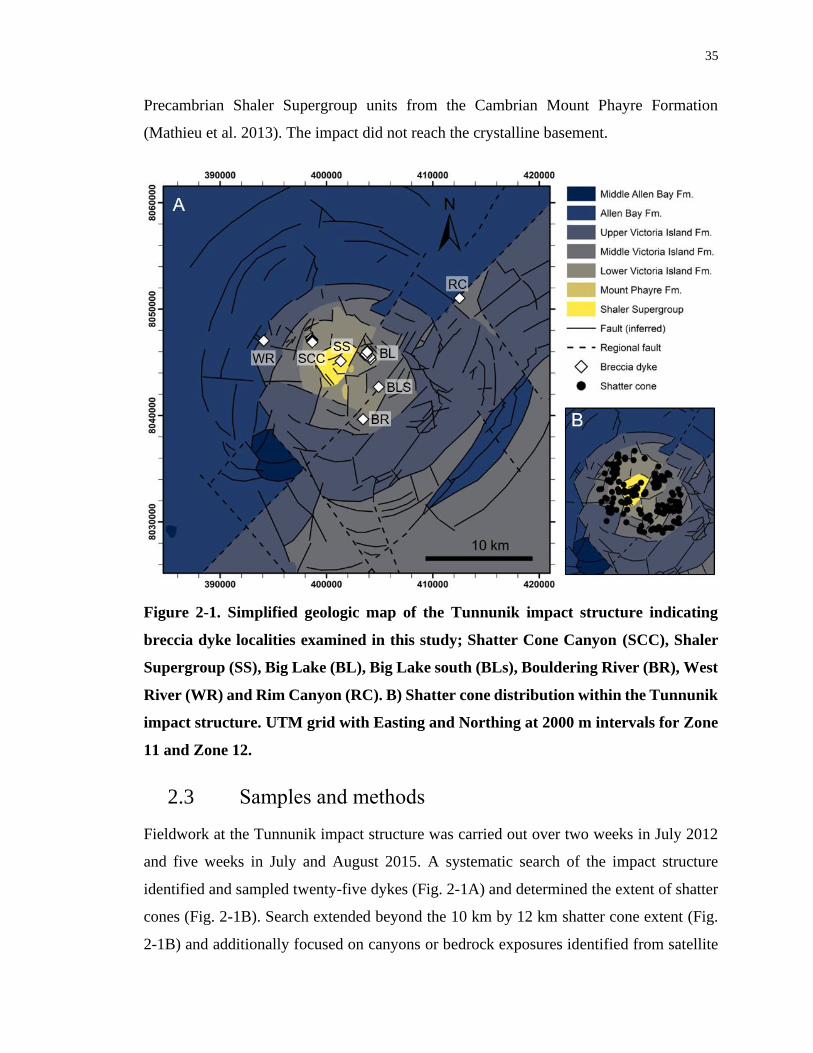
35

Precambrian Shaler Supergroup units from the Cambrian Mount Phayre Formation

(Mathieu et al. 2013). The impact did not reach the crystalline basement.

Figure 2-1. Simplified geologic map of the Tunnunik impact structure indicating

breccia dyke localities examined in this study; Shatter Cone Canyon (SCC), Shaler

Supergroup (SS), Big Lake (BL), Big Lake south (BLs), Bouldering River (BR), West

River (WR) and Rim Canyon (RC). B) Shatter cone distribution within the Tunnunik

impact structure. UTM grid with Easting and Northing at 2000 m intervals for Zone

11 and Zone 12.

2.3 Samples and methods

Fieldwork at the Tunnunik impact structure was carried out over two weeks in July 2012

and five weeks in July and August 2015. A systematic search of the impact structure

identified and sampled twenty-five dykes (Fig. 2-1A) and determined the extent of shatter

cones (Fig. 2-1B). Search extended beyond the 10 km by 12 km shatter cone extent (Fig.

2-1B) and additionally focused on canyons or bedrock exposures identified from satellite

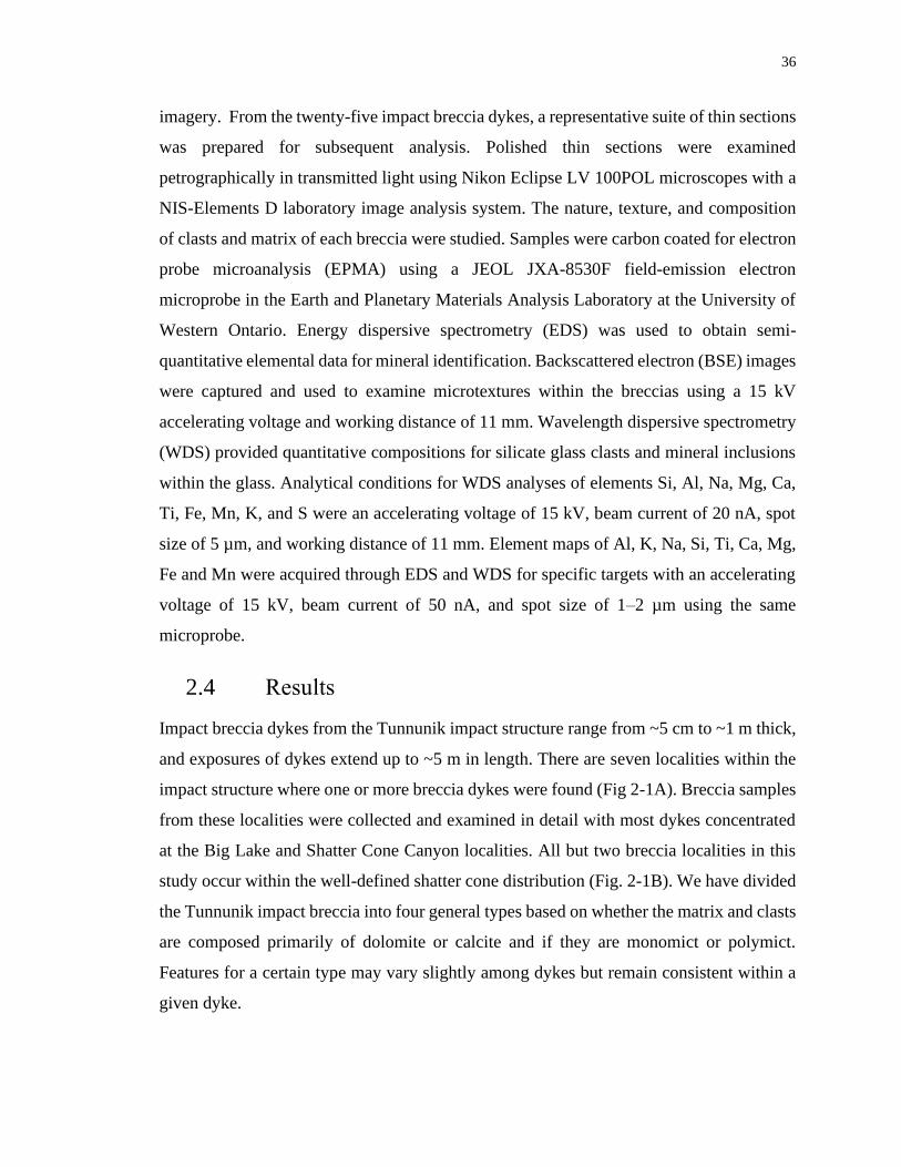
36

imagery. From the twenty-five impact breccia dykes, a representative suite of thin sections

was prepared for subsequent analysis. Polished thin sections were examined

petrographically in transmitted light using Nikon Eclipse LV 100POL microscopes with a

NIS-Elements D laboratory image analysis system. The nature, texture, and composition

of clasts and matrix of each breccia were studied. Samples were carbon coated for electron

probe microanalysis (EPMA) using a JEOL JXA-8530F field-emission electron

microprobe in the Earth and Planetary Materials Analysis Laboratory at the University of

Western Ontario. Energy dispersive spectrometry (EDS) was used to obtain semi-

quantitative elemental data for mineral identification. Backscattered electron (BSE) images

were captured and used to examine microtextures within the breccias using a 15 kV

accelerating voltage and working distance of 11 mm. Wavelength dispersive spectrometry

(WDS) provided quantitative compositions for silicate glass clasts and mineral inclusions

within the glass. Analytical conditions for WDS analyses of elements Si, Al, Na, Mg, Ca,

Ti, Fe, Mn, K, and S were an accelerating voltage of 15 kV, beam current of 20 nA, spot

size of 5 µm, and working distance of 11 mm. Element maps of Al, K, Na, Si, Ti, Ca, Mg,

Fe and Mn were acquired through EDS and WDS for specific targets with an accelerating

voltage of 15 kV, beam current of 50 nA, and spot size of 1–2 µm using the same

microprobe.

2.4 Results

Impact breccia dykes from the Tunnunik impact structure range from ~5 cm to ~1 m thick,

and exposures of dykes extend up to ~5 m in length. There are seven localities within the

impact structure where one or more breccia dykes were found (Fig 2-1A). Breccia samples

from these localities were collected and examined in detail with most dykes concentrated

at the Big Lake and Shatter Cone Canyon localities. All but two breccia localities in this

study occur within the well-defined shatter cone distribution (Fig. 2-1B). We have divided

the Tunnunik impact breccia into four general types based on whether the matrix and clasts

are composed primarily of dolomite or calcite and if they are monomict or polymict.

Features for a certain type may vary slightly among dykes but remain consistent within a

given dyke.

37

2.4.1 Type 1

2.4.1.1 Field observations

Breccia samples designated as Type 1 (T1) were collected from four localities within the

central uplift called Shatter Cone Canyon, Big Lake, Big Lake south, and Bouldering River

(Fig. 2-1A). Shatter Cone Canyon is ~4 km northwest of the centre of the impact structure

and is an exceptional feature within the impact crater. The walls of the canyon expose thrust

faults, inclined strata and an abundance of well-developed and well-preserved shatter cones

(Dewing et al. 2013; Osinski et al. 2013). Shatter Cone Canyon is one of the largest and

longest continuous exposures within the impact structure providing excellent access to

breccia dykes. The breccia dykes discovered in Shatter Cone Canyon occur in the Mount

Phayre Formation which is located at the southern end of the canyon and gradually grades

into the Victoria Island Formation northward about midway through the canyon. These

dykes are found along fractures or bedding planes and have sharp contacts with the host

rock (Figs. 2-2A–C). Larger clasts within several dykes have their long axes notably

oriented parallel with the longitudinal axis of the dyke (Figs. 2-2L–M). Weathered outer

surfaces of breccia are pale tan to yellow in colour for all dykes while fresh surfaces are

grey to grey-green or yellow in colour. The dykes with yellow matrix also have yellow

weathering but differences between shades of yellow are evident in hand samples.

The Big Lake breccia dykes are located ~3 km east from the centre of the impact structure

and the Big Lake south dyke is located ~3 km south-southeast from the main Big Lake

locality (Fig. 2-1B). The Big Lake breccia dykes are more difficult to identify than the

dykes in Shatter Cone Canyon due to the highly fractured nature of the surface rocks and

due to their occurrence on inclined slopes (Figs. 2-2D–E). The ground position of the dykes

as opposed to a vertical outcrop means they are strongly affected by annual freeze-thaw

cycles which has fractured not only the breccia dykes themselves but the surrounding host

rock as well. Within the fragmented dykes at Big Lake, some larger blocks of breccia exist

that are not completely broken apart while some large adjacent fragments fit together

further showing minimal movement of rocks in this area.

38

Figure 2-2. Type 1 breccia dykes from Shatter Cone Canyon (A–C), Big Lake (D–E),

and Bouldering River (N) with dyke boundaries indicated by white dashed lines. A)

Nearly vertical dyke cuts through more horizontal bedding; breccia is fractured and

fragments have fallen out of place. B) Dyke is parallel to bedding planes with a dip of

49°. C) Narrow dyke that follows the fold contour of the host rocks. D) Ground

surface exposure of dyke has been strongly affected by freeze-thaw action and is

highly fractured like surrounding rock. Inset image from top of dyke shows a location

that was more resistant to freeze-thaw cycles. E) Similar to (D), breccia in dyke has

been severely fractured by frost action. Samples (F–K) represent variations among

T1 dykes. F) Breccia from Shatter Cone Canyon shows subtle banding in matrix with

elongated clasts oriented parallel to bands. G) Sample from dyke in (C) shows small

clasts oriented in horizontal direction. H) Bimodal clast size distribution in breccia

from Big Lake. I) Minimal alignment of larger rounded clasts in this Big Lake breccia

sample. J) The most diverse assemblage of clasts in any T1 breccia. K) Sample from

dyke in (D) contains part of a large 10 cm grey dolostone clast. L) Breccia sample

from dyke in (B) showing alignment of clasts parallel to green mudstone host rock

along top of hand sample. M) Similar to (L) this breccia from Shatter Cone Canyon

also shows clasts oriented in same direction as green mudstone host. N) Horizontal

breccia dyke follows bedding planes of host dolostone. O) Close-up of breccia near

right edge of dyke shown in (N).

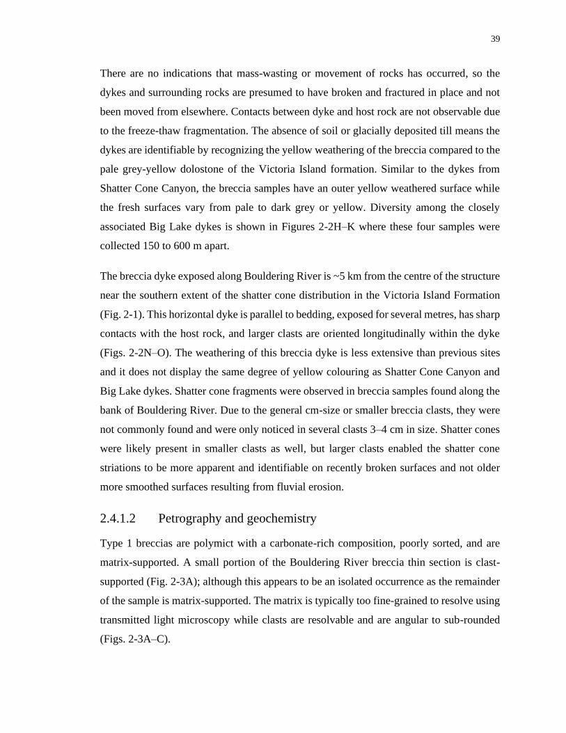
39

There are no indications that mass-wasting or movement of rocks has occurred, so the

dykes and surrounding rocks are presumed to have broken and fractured in place and not

been moved from elsewhere. Contacts between dyke and host rock are not observable due

to the freeze-thaw fragmentation. The absence of soil or glacially deposited till means the

dykes are identifiable by recognizing the yellow weathering of the breccia compared to the

pale grey-yellow dolostone of the Victoria Island formation. Similar to the dykes from

Shatter Cone Canyon, the breccia samples have an outer yellow weathered surface while

the fresh surfaces vary from pale to dark grey or yellow. Diversity among the closely

associated Big Lake dykes is shown in Figures 2-2H–K where these four samples were

collected 150 to 600 m apart.

The breccia dyke exposed along Bouldering River is ~5 km from the centre of the structure

near the southern extent of the shatter cone distribution in the Victoria Island Formation

(Fig. 2-1). This horizontal dyke is parallel to bedding, exposed for several metres, has sharp

contacts with the host rock, and larger clasts are oriented longitudinally within the dyke

(Figs. 2-2N–O). The weathering of this breccia dyke is less extensive than previous sites

and it does not display the same degree of yellow colouring as Shatter Cone Canyon and

Big Lake dykes. Shatter cone fragments were observed in breccia samples found along the

bank of Bouldering River. Due to the general cm-size or smaller breccia clasts, they were

not commonly found and were only noticed in several clasts 3–4 cm in size. Shatter cones

were likely present in smaller clasts as well, but larger clasts enabled the shatter cone

striations to be more apparent and identifiable on recently broken surfaces and not older

more smoothed surfaces resulting from fluvial erosion.

2.4.1.2 Petrography and geochemistry

Type 1 breccias are polymict with a carbonate-rich composition, poorly sorted, and are

matrix-supported. A small portion of the Bouldering River breccia thin section is clast-

supported (Fig. 2-3A); although this appears to be an isolated occurrence as the remainder

of the sample is matrix-supported. The matrix is typically too fine-grained to resolve using

transmitted light microscopy while clasts are resolvable and are angular to sub-rounded

(Figs. 2-3A–C).

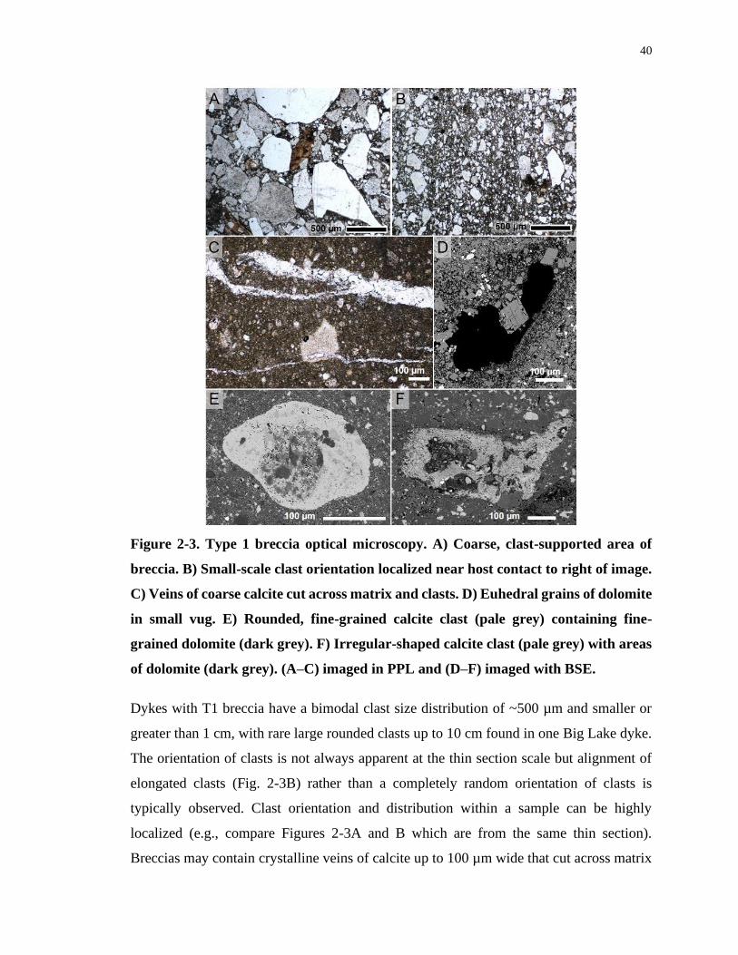
40

Figure 2-3. Type 1 breccia optical microscopy. A) Coarse, clast-supported area of

breccia. B) Small-scale clast orientation localized near host contact to right of image.

C) Veins of coarse calcite cut across matrix and clasts. D) Euhedral grains of dolomite

in small vug. E) Rounded, fine-grained calcite clast (pale grey) containing fine-

grained dolomite (dark grey). F) Irregular-shaped calcite clast (pale grey) with areas

of dolomite (dark grey). (A–C) imaged in PPL and (D–F) imaged with BSE.

Dykes with T1 breccia have a bimodal clast size distribution of ~500 µm and smaller or

greater than 1 cm, with rare large rounded clasts up to 10 cm found in one Big Lake dyke.

The orientation of clasts is not always apparent at the thin section scale but alignment of

elongated clasts (Fig. 2-3B) rather than a completely random orientation of clasts is

typically observed. Clast orientation and distribution within a sample can be highly

localized (e.g., compare Figures 2-3A and B which are from the same thin section).

Breccias may contain crystalline veins of calcite up to 100 µm wide that cut across matrix

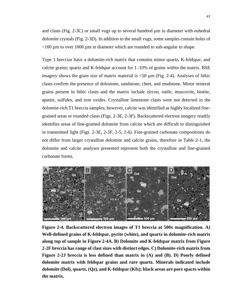
41

and clasts (Fig. 2-3C) or small vugs up to several hundred µm in diameter with euhedral

dolomite crystals (Fig. 2-3D). In addition to the small vugs, some samples contain holes of

~100 µm to over 1000 µm in diameter which are rounded to sub-angular in shape.

Type 1 breccias have a dolomite-rich matrix that contains minor quartz, K-feldspar, and

calcite grains; quartz and K-feldspar account for 1–10% of grains within the matrix. BSE

imagery shows the grain size of matrix material is <50 µm (Fig. 2-4). Analyses of lithic

clasts confirm the presence of dolostone, sandstone, chert, and mudstone. Minor mineral

grains present in lithic clasts and the matrix include zircon, rutile, muscovite, biotite,

apatite, sulfides, and iron oxides. Crystalline limestone clasts were not detected in the

dolomite-rich T1 breccia samples; however, calcite was identified as highly localized fine-

grained areas or rounded clasts (Figs. 2-3E, 2-3F). Backscattered electron imagery readily

identifies areas of fine-grained dolomite from calcite which are difficult to distinguished

in transmitted light (Figs. 2-3E, 2-3F, 2-5, 2-6). Fine-grained carbonate compositions do

not differ from larger crystalline dolomite and calcite grains, therefore in Table 2-1, the

dolomite and calcite analyses presented represent both the crystalline and fine-grained

carbonate forms.

Figure 2-4. Backscattered electron images of T1 breccia at 500x magnification. A)

Well-defined grains of K-feldspar, pyrite (white), and quartz in dolomite-rich matrix

along top of sample in Figure 2-4A. B) Dolomite and K-feldspar matrix from Figure

2-2F breccia has range of clast sizes with distinct edges. C) Dolomite-rich matrix from

Figure 2-2J breccia is less defined than matrix in (A) and (B). D) Poorly defined

dolomite matrix with feldspar grains and rare quartz. Minerals indicated include

dolomite (Dol), quartz, (Qz), and K-feldspar (Kfs); black areas are pore spaces within

the matrix.

42

Tab

le 2

-1. E

lect

ron

mic

rop

rob

e W

DS

an

aly

ses

of

carb

on

ate

s* f

or

min

era

l gra

ins

an

d m

elt.

* B

ack-c

alcu

late

d C

-co

nte

nt,

not

mea

sure

d b

y W

DS

.

n =

num

ber

of

po

ints

an

alyze

d;

wt%

= a

ver

age

min

eral

com

posi

tion i

n w

eight

%.

s.d.

= s

tand

ard

dev

iati

on;

b.d

. =

bel

ow

det

ecti

on.

Car

bonat

e-si

lica

te1 =

do

lom

ite

wit

h S

i.

Car

bonat

e-si

lica

te2 =

fer

roan

do

lom

ite

wit

h S

i.

Car

bonat

e-si

lica

te3 =

Mg-b

eari

ng

cal

cite

wit

h S

i.

Car

bonat

e-si

lica

te4 =

Mg

,Fe-

bea

rin

g c

alci

te w

ith S

i-A

l.

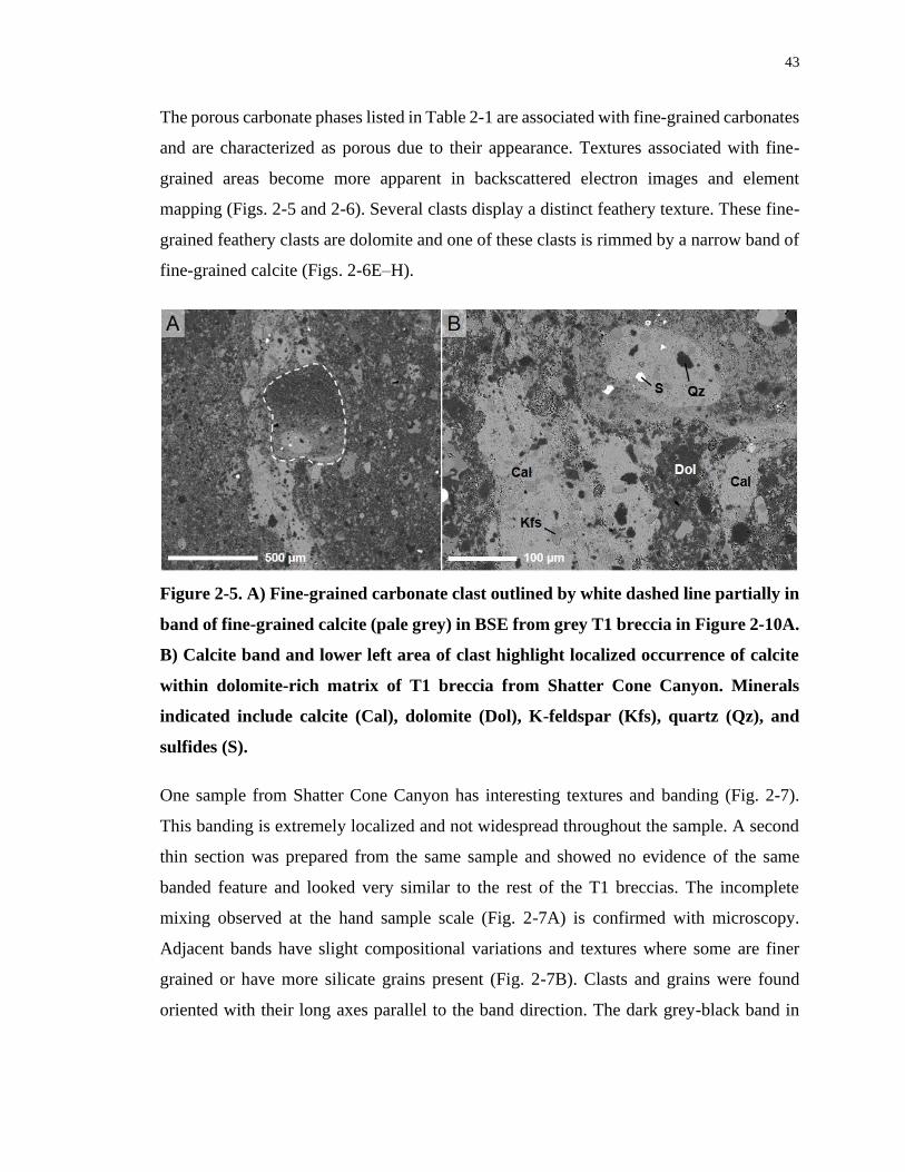
43

The porous carbonate phases listed in Table 2-1 are associated with fine-grained carbonates

and are characterized as porous due to their appearance. Textures associated with fine-

grained areas become more apparent in backscattered electron images and element

mapping (Figs. 2-5 and 2-6). Several clasts display a distinct feathery texture. These fine-

grained feathery clasts are dolomite and one of these clasts is rimmed by a narrow band of

fine-grained calcite (Figs. 2-6E–H).

Figure 2-5. A) Fine-grained carbonate clast outlined by white dashed line partially in

band of fine-grained calcite (pale grey) in BSE from grey T1 breccia in Figure 2-10A.

B) Calcite band and lower left area of clast highlight localized occurrence of calcite

within dolomite-rich matrix of T1 breccia from Shatter Cone Canyon. Minerals

indicated include calcite (Cal), dolomite (Dol), K-feldspar (Kfs), quartz (Qz), and

sulfides (S).

One sample from Shatter Cone Canyon has interesting textures and banding (Fig. 2-7).

This banding is extremely localized and not widespread throughout the sample. A second

thin section was prepared from the same sample and showed no evidence of the same

banded feature and looked very similar to the rest of the T1 breccias. The incomplete

mixing observed at the hand sample scale (Fig. 2-7A) is confirmed with microscopy.

Adjacent bands have slight compositional variations and textures where some are finer

grained or have more silicate grains present (Fig. 2-7B). Clasts and grains were found

oriented with their long axes parallel to the band direction. The dark grey-black band in

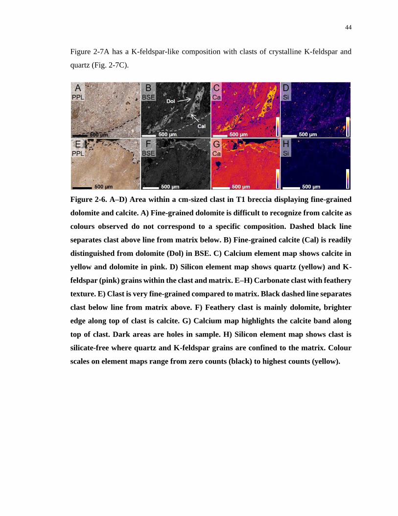
44

Figure 2-7A has a K-feldspar-like composition with clasts of crystalline K-feldspar and

quartz (Fig. 2-7C).

Figure 2-6. A–D) Area within a cm-sized clast in T1 breccia displaying fine-grained

dolomite and calcite. A) Fine-grained dolomite is difficult to recognize from calcite as

colours observed do not correspond to a specific composition. Dashed black line

separates clast above line from matrix below. B) Fine-grained calcite (Cal) is readily

distinguished from dolomite (Dol) in BSE. C) Calcium element map shows calcite in

yellow and dolomite in pink. D) Silicon element map shows quartz (yellow) and K-

feldspar (pink) grains within the clast and matrix. E–H) Carbonate clast with feathery

texture. E) Clast is very fine-grained compared to matrix. Black dashed line separates

clast below line from matrix above. F) Feathery clast is mainly dolomite, brighter

edge along top of clast is calcite. G) Calcium map highlights the calcite band along

top of clast. Dark areas are holes in sample. H) Silicon element map shows clast is

silicate-free where quartz and K-feldspar grains are confined to the matrix. Colour

scales on element maps range from zero counts (black) to highest counts (yellow).

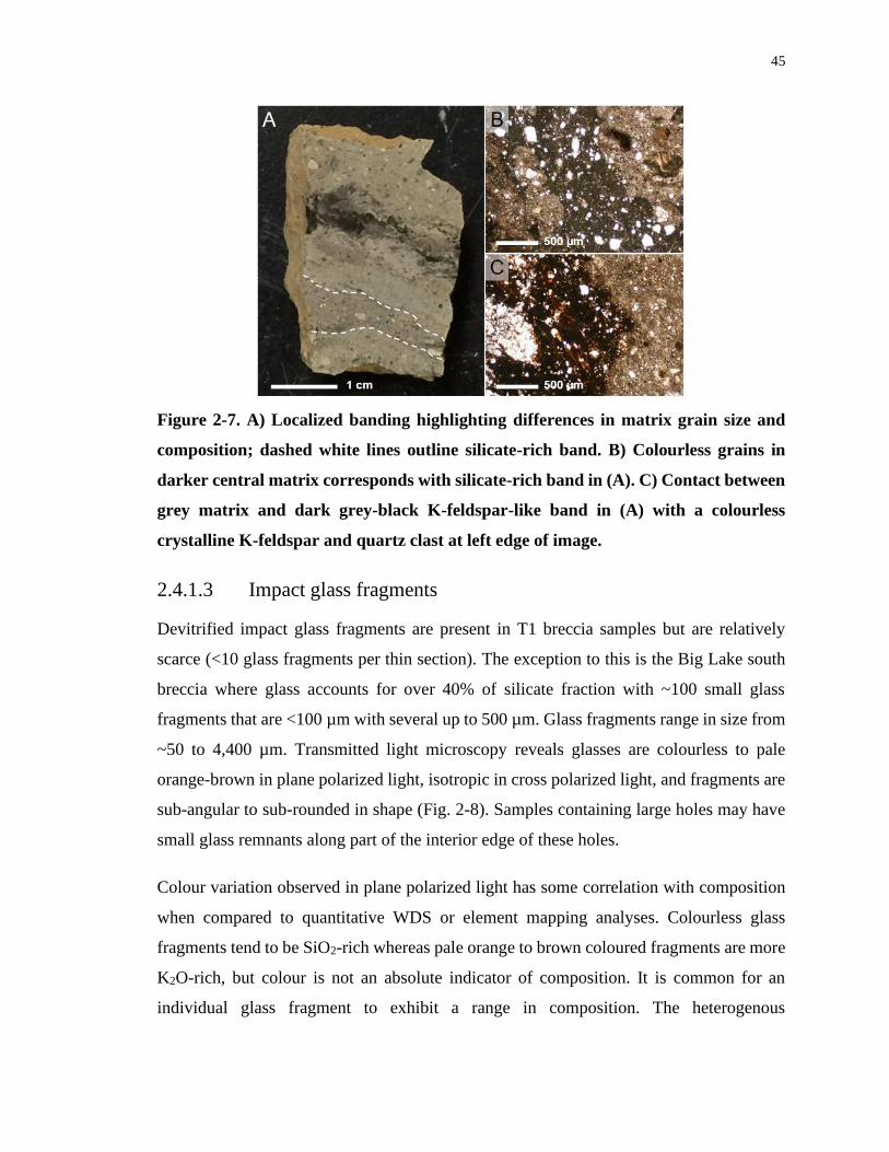
45

Figure 2-7. A) Localized banding highlighting differences in matrix grain size and

composition; dashed white lines outline silicate-rich band. B) Colourless grains in

darker central matrix corresponds with silicate-rich band in (A). C) Contact between

grey matrix and dark grey-black K-feldspar-like band in (A) with a colourless

crystalline K-feldspar and quartz clast at left edge of image.

2.4.1.3 Impact glass fragments

Devitrified impact glass fragments are present in T1 breccia samples but are relatively

scarce (<10 glass fragments per thin section). The exception to this is the Big Lake south

breccia where glass accounts for over 40% of silicate fraction with ~100 small glass

fragments that are <100 µm with several up to 500 µm. Glass fragments range in size from

~50 to 4,400 µm. Transmitted light microscopy reveals glasses are colourless to pale

orange-brown in plane polarized light, isotropic in cross polarized light, and fragments are

sub-angular to sub-rounded in shape (Fig. 2-8). Samples containing large holes may have

small glass remnants along part of the interior edge of these holes.

Colour variation observed in plane polarized light has some correlation with composition

when compared to quantitative WDS or element mapping analyses. Colourless glass

fragments tend to be SiO2-rich whereas pale orange to brown coloured fragments are more

K2O-rich, but colour is not an absolute indicator of composition. It is common for an

individual glass fragment to exhibit a range in composition. The heterogenous

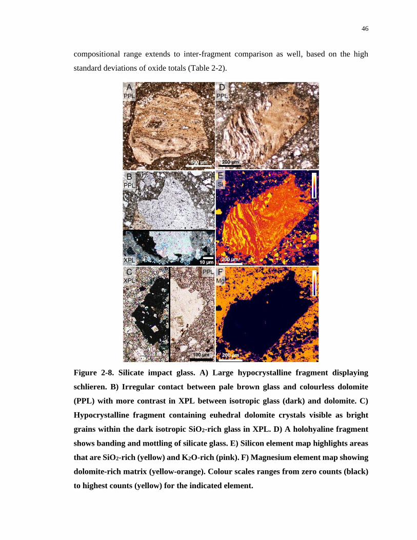
46

compositional range extends to inter-fragment comparison as well, based on the high

standard deviations of oxide totals (Table 2-2).

Figure 2-8. Silicate impact glass. A) Large hypocrystalline fragment displaying

schlieren. B) Irregular contact between pale brown glass and colourless dolomite

(PPL) with more contrast in XPL between isotropic glass (dark) and dolomite. C)

Hypocrystalline fragment containing euhedral dolomite crystals visible as bright

grains within the dark isotropic SiO2-rich glass in XPL. D) A holohyaline fragment

shows banding and mottling of silicate glass. E) Silicon element map highlights areas

that are SiO2-rich (yellow) and K2O-rich (pink). F) Magnesium element map showing

dolomite-rich matrix (yellow-orange). Colour scales ranges from zero counts (black)

to highest counts (yellow) for the indicated element.

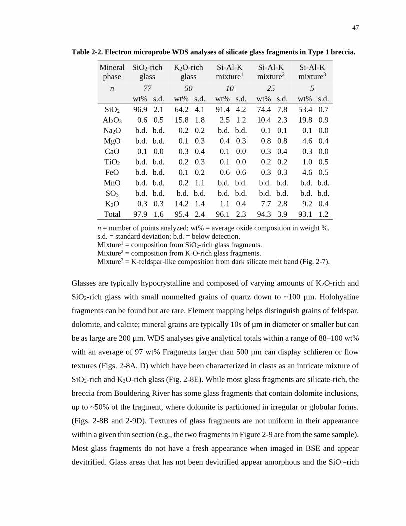
47

Table 2-2. Electron microprobe WDS analyses of silicate glass fragments in Type 1 breccia.

Mineral

phase

SiO2-rich

glass

K2O-rich

glass

Si-Al-K

mixture1

Si-Al-K

mixture2

Si-Al-K

mixture3

n 77 50 10 25 5

wt% s.d. wt% s.d. wt% s.d. wt% s.d. wt% s.d.

SiO2 96.9 2.1 64.2 4.1 91.4 4.2 74.4 7.8 53.4 0.7

Al2O3 0.6 0.5 15.8 1.8 2.5 1.2 10.4 2.3 19.8 0.9

Na2O b.d. b.d. 0.2 0.2 b.d. b.d. 0.1 0.1 0.1 0.0

MgO b.d. b.d. 0.1 0.3 0.4 0.3 0.8 0.8 4.6 0.4

CaO 0.1 0.0 0.3 0.4 0.1 0.0 0.3 0.4 0.3 0.0

TiO2 b.d. b.d. 0.2 0.3 0.1 0.0 0.2 0.2 1.0 0.5

FeO b.d. b.d. 0.1 0.2 0.6 0.6 0.3 0.3 4.6 0.5

MnO b.d. b.d. 0.2 1.1 b.d. b.d. b.d. b.d. b.d. b.d.

SO3 b.d. b.d. b.d. b.d. b.d. b.d. b.d. b.d. b.d. b.d.

K2O 0.3 0.3 14.2 1.4 1.1 0.4 7.7 2.8 9.2 0.4

Total 97.9 1.6 95.4 2.4 96.1 2.3 94.3 3.9 93.1 1.2

n = number of points analyzed; wt% = average oxide composition in weight %.

s.d. = standard deviation; b.d. = below detection.

Mixture1 = composition from SiO2-rich glass fragments.

Mixture2 = composition from K2O-rich glass fragments.

Mixture3 = K-feldspar-like composition from dark silicate melt band (Fig. 2-7).

Glasses are typically hypocrystalline and composed of varying amounts of K2O-rich and

SiO2-rich glass with small nonmelted grains of quartz down to ~100 µm. Holohyaline

fragments can be found but are rare. Element mapping helps distinguish grains of feldspar,

dolomite, and calcite; mineral grains are typically 10s of µm in diameter or smaller but can

be as large are 200 µm. WDS analyses give analytical totals within a range of 88–100 wt%

with an average of 97 wt% Fragments larger than 500 µm can display schlieren or flow

textures (Figs. 2-8A, D) which have been characterized in clasts as an intricate mixture of

SiO2-rich and K2O-rich glass (Fig. 2-8E). While most glass fragments are silicate-rich, the

breccia from Bouldering River has some glass fragments that contain dolomite inclusions,

up to ~50% of the fragment, where dolomite is partitioned in irregular or globular forms.

(Figs. 2-8B and 2-9D). Textures of glass fragments are not uniform in their appearance

within a given thin section (e.g., the two fragments in Figure 2-9 are from the same sample).

Most glass fragments do not have a fresh appearance when imaged in BSE and appear

devitrified. Glass areas that has not been devitrified appear amorphous and the SiO2-rich

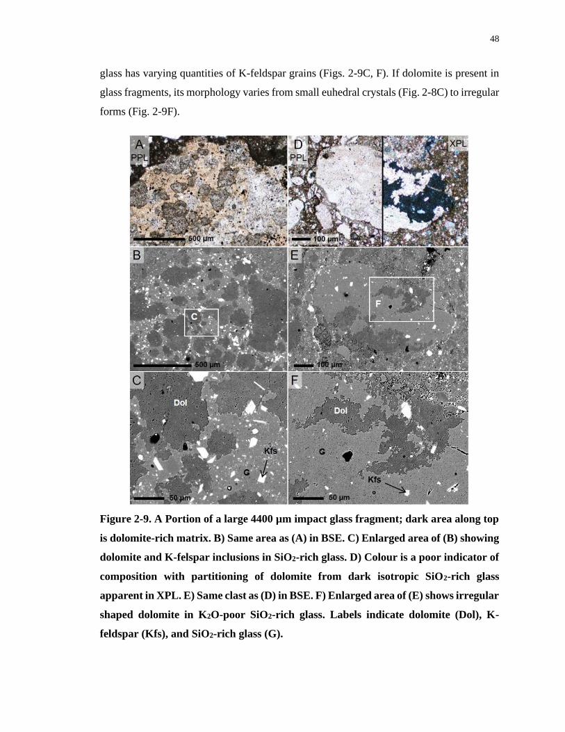
48

glass has varying quantities of K-feldspar grains (Figs. 2-9C, F). If dolomite is present in

glass fragments, its morphology varies from small euhedral crystals (Fig. 2-8C) to irregular

forms (Fig. 2-9F).

Figure 2-9. A Portion of a large 4400 µm impact glass fragment; dark area along top

is dolomite-rich matrix. B) Same area as (A) in BSE. C) Enlarged area of (B) showing

dolomite and K-felspar inclusions in SiO2-rich glass. D) Colour is a poor indicator of

composition with partitioning of dolomite from dark isotropic SiO2-rich glass

apparent in XPL. E) Same clast as (D) in BSE. F) Enlarged area of (E) shows irregular

shaped dolomite in K2O-poor SiO2-rich glass. Labels indicate dolomite (Dol), K-

feldspar (Kfs), and SiO2-rich glass (G).

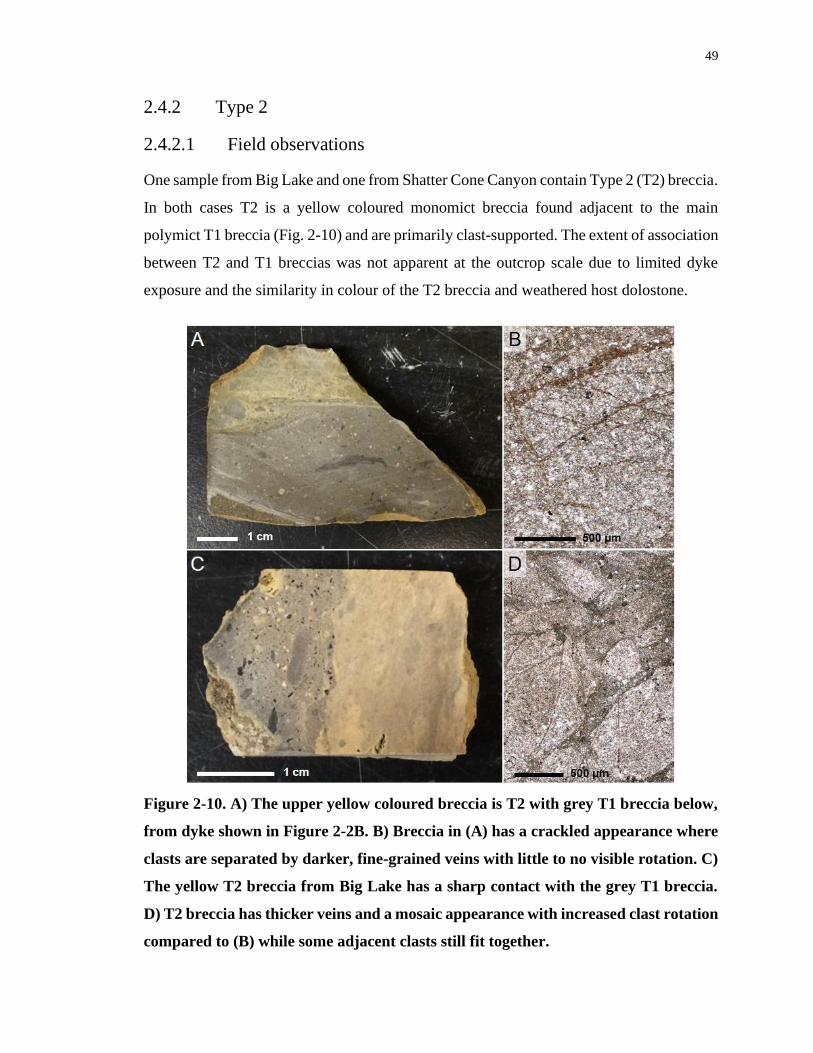
49

2.4.2 Type 2

2.4.2.1 Field observations

One sample from Big Lake and one from Shatter Cone Canyon contain Type 2 (T2) breccia.

In both cases T2 is a yellow coloured monomict breccia found adjacent to the main

polymict T1 breccia (Fig. 2-10) and are primarily clast-supported. The extent of association

between T2 and T1 breccias was not apparent at the outcrop scale due to limited dyke

exposure and the similarity in colour of the T2 breccia and weathered host dolostone.

Figure 2-10. A) The upper yellow coloured breccia is T2 with grey T1 breccia below,

from dyke shown in Figure 2-2B. B) Breccia in (A) has a crackled appearance where

clasts are separated by darker, fine-grained veins with little to no visible rotation. C)

The yellow T2 breccia from Big Lake has a sharp contact with the grey T1 breccia.

D) T2 breccia has thicker veins and a mosaic appearance with increased clast rotation

compared to (B) while some adjacent clasts still fit together.

50

2.4.2.2 Petrography and geochemistry

Cross-cutting relationships show some features of the monomict breccia are truncated by

the polymict T1 breccia (Fig. 2-10). The interface along the two breccias may be wavy or

straight and small T2 clasts are present along the contact but there is no indication of mixing

between the breccias. No impact glass fragments were found in T2 breccias. The matrix

and clasts in T2 breccia are dolomite which contain small grains of quartz, K-feldspar,

sulfides, and Fe-oxides.

The T2 breccia from Shatter Cone Canyon shows fracturing and brecciation with thin veins

of fine matrix (Fig. 2-10B). Many of the veins preferentially run parallel to the contact

between the monomict and polymict breccia. This monomict breccia is clast-supported and

most clasts do not display any significant rotation with respect to neighbouring clasts. A

few clasts appear distinct from the rest of the monomict package near the T1 contact; closer

inspection reveals they are unbrecciated T2 clasts and not clasts from the adjacent polymict

breccia (Fig. 2-10A). The contact between breccia types is relatively sharp and straight

with a slight offset and no mixing.

The Big Lake monomict breccia has regions with large sub-angular brecciated clasts that

are clast-supported and other sections that have unbrecciated clasts that are supported by a

fine-grained matrix (Fig. 2-10D). Smaller clasts display some rotation and alignment

relative to nearby clasts and these clasts tend to be more sub-rounded. The contact between

the monomict and polymict breccia is sharp but not straight (Fig. 2-10C) and do not appear

to have undergone any mixing. The similarity in composition between the matrix and clasts

make it difficult to readily discriminate them in BSE images.

2.4.3 Type 3

2.4.3.1 Field observations

Type 3 (T3) breccia is found within the Shaler Supergroup near the centre of the impact

structure and in one dyke near the West River (Fig. 2-1). The Shaler T3 dyke is not very

distinct from the surrounding blue-grey limestone and the bedding at this location differs

by 22° on either side of the dyke (Fig. 2-11A). The narrow grey T3 dyke along the West

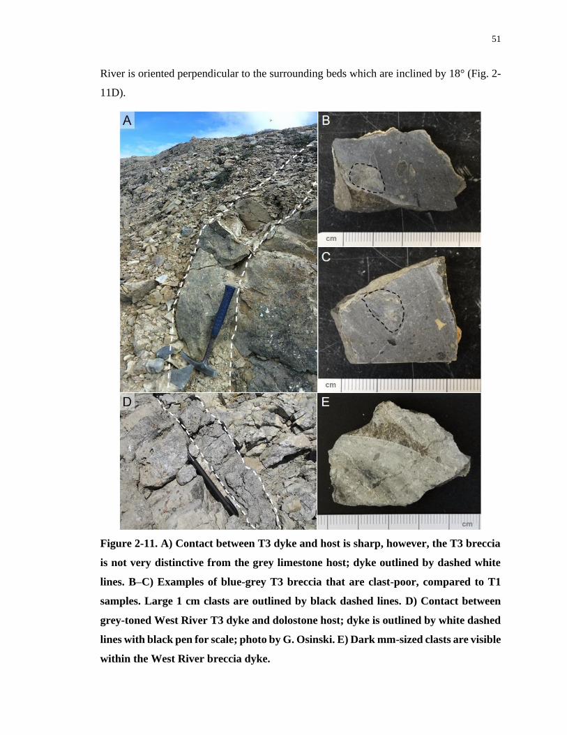
51

River is oriented perpendicular to the surrounding beds which are inclined by 18° (Fig. 2-

11D).

Figure 2-11. A) Contact between T3 dyke and host is sharp, however, the T3 breccia

is not very distinctive from the grey limestone host; dyke outlined by dashed white

lines. B–C) Examples of blue-grey T3 breccia that are clast-poor, compared to T1

samples. Large 1 cm clasts are outlined by black dashed lines. D) Contact between

grey-toned West River T3 dyke and dolostone host; dyke is outlined by white dashed

lines with black pen for scale; photo by G. Osinski. E) Dark mm-sized clasts are visible

within the West River breccia dyke.

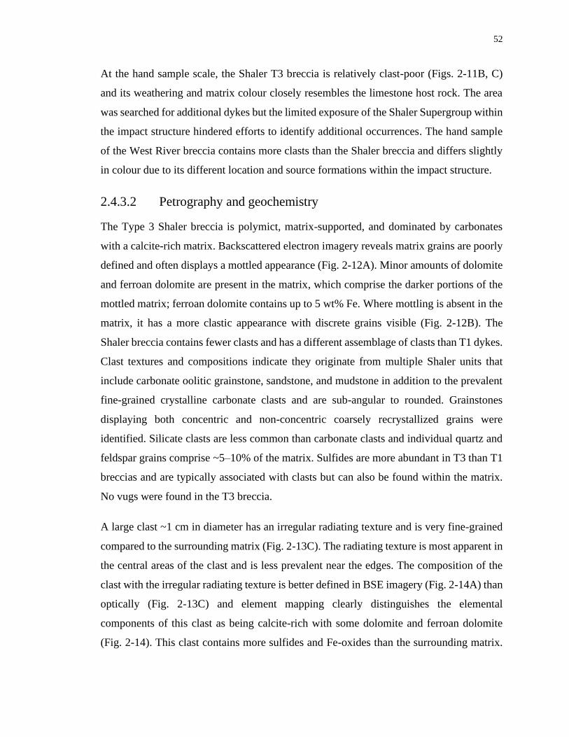
52

At the hand sample scale, the Shaler T3 breccia is relatively clast-poor (Figs. 2-11B, C)

and its weathering and matrix colour closely resembles the limestone host rock. The area

was searched for additional dykes but the limited exposure of the Shaler Supergroup within

the impact structure hindered efforts to identify additional occurrences. The hand sample

of the West River breccia contains more clasts than the Shaler breccia and differs slightly

in colour due to its different location and source formations within the impact structure.

2.4.3.2 Petrography and geochemistry

The Type 3 Shaler breccia is polymict, matrix-supported, and dominated by carbonates

with a calcite-rich matrix. Backscattered electron imagery reveals matrix grains are poorly

defined and often displays a mottled appearance (Fig. 2-12A). Minor amounts of dolomite

and ferroan dolomite are present in the matrix, which comprise the darker portions of the

mottled matrix; ferroan dolomite contains up to 5 wt% Fe. Where mottling is absent in the

matrix, it has a more clastic appearance with discrete grains visible (Fig. 2-12B). The

Shaler breccia contains fewer clasts and has a different assemblage of clasts than T1 dykes.

Clast textures and compositions indicate they originate from multiple Shaler units that

include carbonate oolitic grainstone, sandstone, and mudstone in addition to the prevalent

fine-grained crystalline carbonate clasts and are sub-angular to rounded. Grainstones

displaying both concentric and non-concentric coarsely recrystallized grains were

identified. Silicate clasts are less common than carbonate clasts and individual quartz and

feldspar grains comprise ~5–10% of the matrix. Sulfides are more abundant in T3 than T1

breccias and are typically associated with clasts but can also be found within the matrix.

No vugs were found in the T3 breccia.

A large clast ~1 cm in diameter has an irregular radiating texture and is very fine-grained

compared to the surrounding matrix (Fig. 2-13C). The radiating texture is most apparent in

the central areas of the clast and is less prevalent near the edges. The composition of the

clast with the irregular radiating texture is better defined in BSE imagery (Fig. 2-14A) than

optically (Fig. 2-13C) and element mapping clearly distinguishes the elemental

components of this clast as being calcite-rich with some dolomite and ferroan dolomite

(Fig. 2-14). This clast contains more sulfides and Fe-oxides than the surrounding matrix.

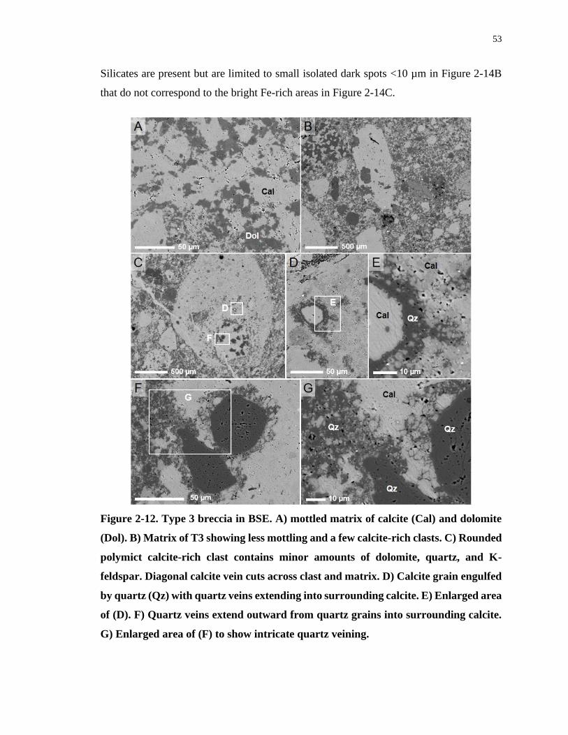
53

Silicates are present but are limited to small isolated dark spots <10 µm in Figure 2-14B

that do not correspond to the bright Fe-rich areas in Figure 2-14C.

Figure 2-12. Type 3 breccia in BSE. A) mottled matrix of calcite (Cal) and dolomite

(Dol). B) Matrix of T3 showing less mottling and a few calcite-rich clasts. C) Rounded

polymict calcite-rich clast contains minor amounts of dolomite, quartz, and K-

feldspar. Diagonal calcite vein cuts across clast and matrix. D) Calcite grain engulfed

by quartz (Qz) with quartz veins extending into surrounding calcite. E) Enlarged area

of (D). F) Quartz veins extend outward from quartz grains into surrounding calcite.

G) Enlarged area of (F) to show intricate quartz veining.

54

Another fine-grained 1 cm clast has a similar appearance with portions resembling the

radiating clast, but the pattern is less developed. Additionally, this clast contains a small

rounded carbonate clast with a fine-grained feathery texture (Fig. 2-13A), small grainstone

fragments, and wavy fine-grained carbonate bands rich in sulfide grains (Figs. 2-13B–D).

Figure 2-13. A) In PPL, a small feathery clast, outlined by dashed line, found within

large clast indicated in Figure 2-11C. B) Band of fine-grained ferroan dolomite rich

in sulfides. In PPL, areas of outlined band appear darker than surrounding calcite-

rich matrix. C) Calcite and dolomite clast with an irregular radiating texture, clast

above dashed outline; PPL. D) Compositional differences are evident in BSE in this

enlargement of upper right limb of the outlined band in (B); calcite (Cal), dolomite

(Dol), ferroan dolomite (Dol-Fe), sulfide (S).

Some clasts contain fine-grained, wavy or flow-like bands while others have fine veinlets

extending from the clasts into the surrounding matrix (Figs. 2-12C–G). Figure 2-12C is a

polymict breccia clast that contains small quartz grains that have thin veinlets of quartz

extending outward into the calcite matrix (Figs. 2-12F–G). Similar quartz veinlets are also

associated with quartz-rimmed calcite grains (Figs. 2-12D–E).

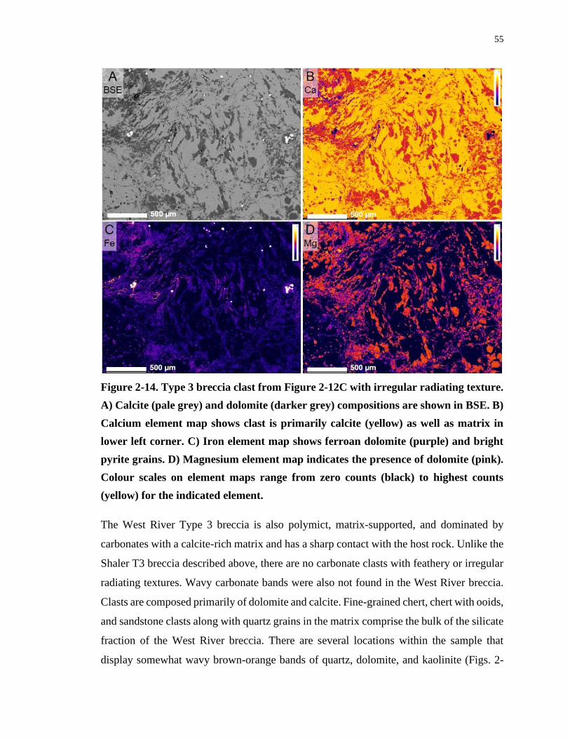
55

Figure 2-14. Type 3 breccia clast from Figure 2-12C with irregular radiating texture.

A) Calcite (pale grey) and dolomite (darker grey) compositions are shown in BSE. B)

Calcium element map shows clast is primarily calcite (yellow) as well as matrix in

lower left corner. C) Iron element map shows ferroan dolomite (purple) and bright

pyrite grains. D) Magnesium element map indicates the presence of dolomite (pink).

Colour scales on element maps range from zero counts (black) to highest counts

(yellow) for the indicated element.

The West River Type 3 breccia is also polymict, matrix-supported, and dominated by

carbonates with a calcite-rich matrix and has a sharp contact with the host rock. Unlike the

Shaler T3 breccia described above, there are no carbonate clasts with feathery or irregular

radiating textures. Wavy carbonate bands were also not found in the West River breccia.

Clasts are composed primarily of dolomite and calcite. Fine-grained chert, chert with ooids,

and sandstone clasts along with quartz grains in the matrix comprise the bulk of the silicate

fraction of the West River breccia. There are several locations within the sample that

display somewhat wavy brown-orange bands of quartz, dolomite, and kaolinite (Figs. 2-

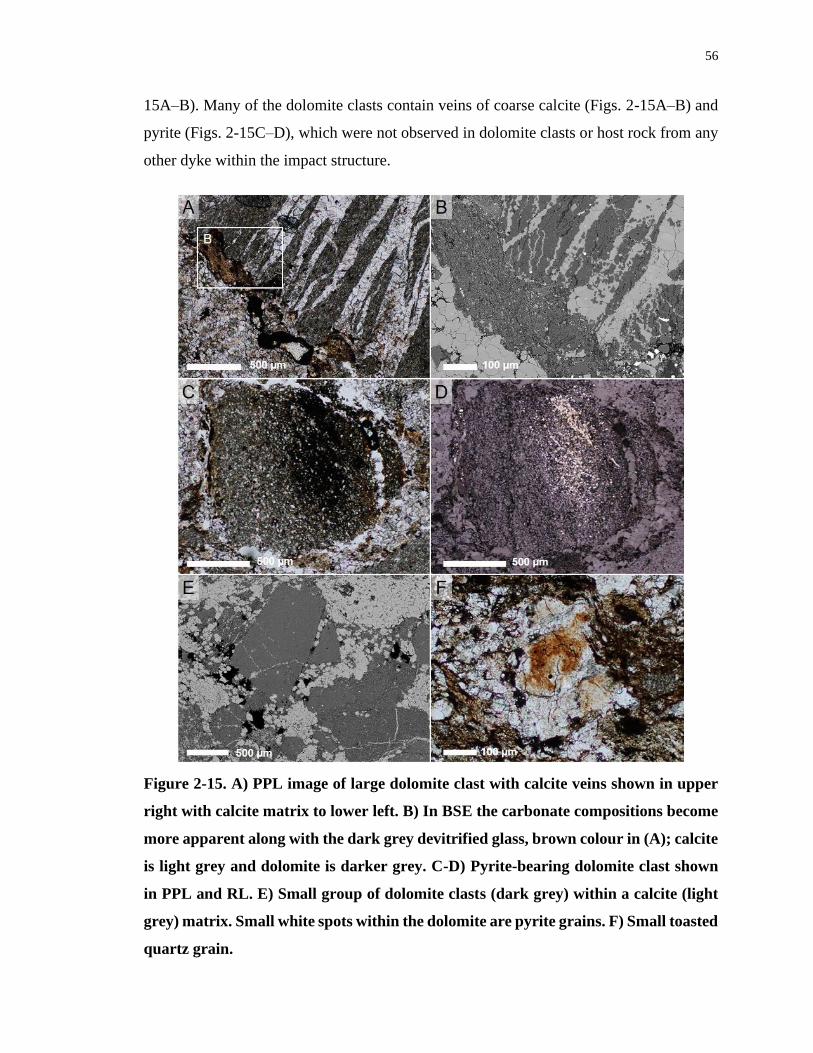
56

15A–B). Many of the dolomite clasts contain veins of coarse calcite (Figs. 2-15A–B) and

pyrite (Figs. 2-15C–D), which were not observed in dolomite clasts or host rock from any

other dyke within the impact structure.

Figure 2-15. A) PPL image of large dolomite clast with calcite veins shown in upper

right with calcite matrix to lower left. B) In BSE the carbonate compositions become

more apparent along with the dark grey devitrified glass, brown colour in (A); calcite

is light grey and dolomite is darker grey. C-D) Pyrite-bearing dolomite clast shown

in PPL and RL. E) Small group of dolomite clasts (dark grey) within a calcite (light

grey) matrix. Small white spots within the dolomite are pyrite grains. F) Small toasted

quartz grain.

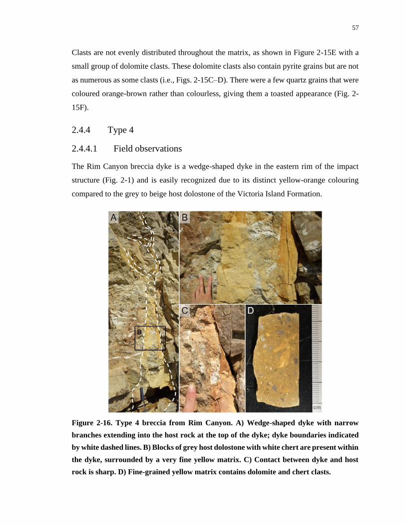
57

Clasts are not evenly distributed throughout the matrix, as shown in Figure 2-15E with a

small group of dolomite clasts. These dolomite clasts also contain pyrite grains but are not

as numerous as some clasts (i.e., Figs. 2-15C–D). There were a few quartz grains that were

coloured orange-brown rather than colourless, giving them a toasted appearance (Fig. 2-

15F).

2.4.4 Type 4

2.4.4.1 Field observations

The Rim Canyon breccia dyke is a wedge-shaped dyke in the eastern rim of the impact

structure (Fig. 2-1) and is easily recognized due to its distinct yellow-orange colouring

compared to the grey to beige host dolostone of the Victoria Island Formation.

Figure 2-16. Type 4 breccia from Rim Canyon. A) Wedge-shaped dyke with narrow

branches extending into the host rock at the top of the dyke; dyke boundaries indicated

by white dashed lines. B) Blocks of grey host dolostone with white chert are present within

the dyke, surrounded by a very fine yellow matrix. C) Contact between dyke and host

rock is sharp. D) Fine-grained yellow matrix contains dolomite and chert clasts.

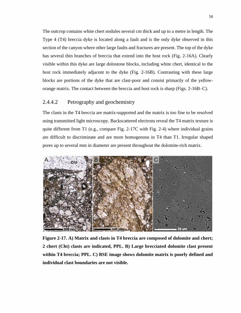
58

The outcrop contains white chert nodules several cm thick and up to a metre in length. The

Type 4 (T4) breccia dyke is located along a fault and is the only dyke observed in this

section of the canyon where other large faults and fractures are present. The top of the dyke

has several thin branches of breccia that extend into the host rock (Fig. 2-16A). Clearly

visible within this dyke are large dolostone blocks, including white chert, identical to the

host rock immediately adjacent to the dyke (Fig. 2-16B). Contrasting with these large

blocks are portions of the dyke that are clast-poor and consist primarily of the yellow-

orange matrix. The contact between the breccia and host rock is sharp (Figs. 2-16B–C).

2.4.4.2 Petrography and geochemistry

The clasts in the T4 breccia are matrix-supported and the matrix is too fine to be resolved

using transmitted light microscopy. Backscattered electrons reveal the T4 matrix texture is

quite different from T1 (e.g., compare Fig. 2-17C with Fig. 2-4) where individual grains

are difficult to discriminate and are more homogenous in T4 than T1. Irregular shaped

pores up to several mm in diameter are present throughout the dolomite-rich matrix.

Figure 2-17. A) Matrix and clasts in T4 breccia are composed of dolomite and chert;

2 chert (Cht) clasts are indicated, PPL. B) Large brecciated dolomite clast present

within T4 breccia; PPL. C) BSE image shows dolomite matrix is poorly defined and

individual clast boundaries are not visible.

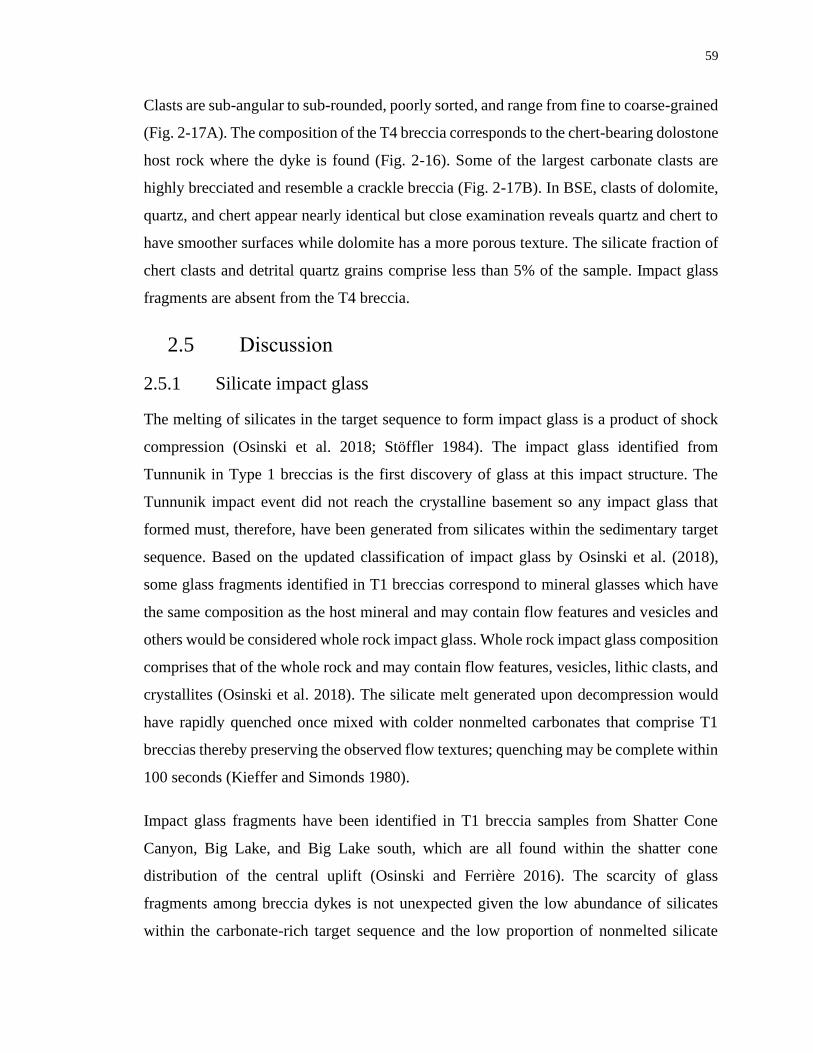
59

Clasts are sub-angular to sub-rounded, poorly sorted, and range from fine to coarse-grained

(Fig. 2-17A). The composition of the T4 breccia corresponds to the chert-bearing dolostone

host rock where the dyke is found (Fig. 2-16). Some of the largest carbonate clasts are

highly brecciated and resemble a crackle breccia (Fig. 2-17B). In BSE, clasts of dolomite,

quartz, and chert appear nearly identical but close examination reveals quartz and chert to

have smoother surfaces while dolomite has a more porous texture. The silicate fraction of

chert clasts and detrital quartz grains comprise less than 5% of the sample. Impact glass

fragments are absent from the T4 breccia.

2.5 Discussion

2.5.1 Silicate impact glass

The melting of silicates in the target sequence to form impact glass is a product of shock

compression (Osinski et al. 2018; Stöffler 1984). The impact glass identified from

Tunnunik in Type 1 breccias is the first discovery of glass at this impact structure. The

Tunnunik impact event did not reach the crystalline basement so any impact glass that

formed must, therefore, have been generated from silicates within the sedimentary target

sequence. Based on the updated classification of impact glass by Osinski et al. (2018),

some glass fragments identified in T1 breccias correspond to mineral glasses which have

the same composition as the host mineral and may contain flow features and vesicles and

others would be considered whole rock impact glass. Whole rock impact glass composition

comprises that of the whole rock and may contain flow features, vesicles, lithic clasts, and

crystallites (Osinski et al. 2018). The silicate melt generated upon decompression would

have rapidly quenched once mixed with colder nonmelted carbonates that comprise T1

breccias thereby preserving the observed flow textures; quenching may be complete within

100 seconds (Kieffer and Simonds 1980).

Impact glass fragments have been identified in T1 breccia samples from Shatter Cone

Canyon, Big Lake, and Big Lake south, which are all found within the shatter cone

distribution of the central uplift (Osinski and Ferrière 2016). The scarcity of glass

fragments among breccia dykes is not unexpected given the low abundance of silicates

within the carbonate-rich target sequence and the low proportion of nonmelted silicate

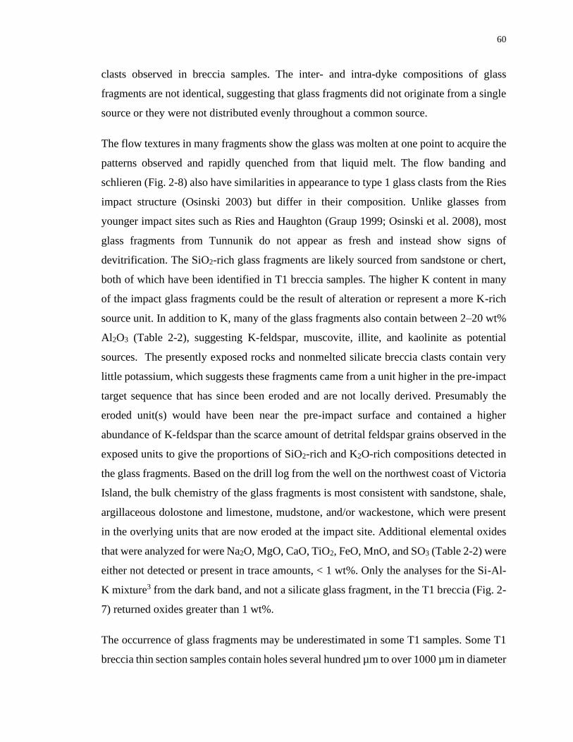
60

clasts observed in breccia samples. The inter- and intra-dyke compositions of glass

fragments are not identical, suggesting that glass fragments did not originate from a single

source or they were not distributed evenly throughout a common source.

The flow textures in many fragments show the glass was molten at one point to acquire the

patterns observed and rapidly quenched from that liquid melt. The flow banding and

schlieren (Fig. 2-8) also have similarities in appearance to type 1 glass clasts from the Ries

impact structure (Osinski 2003) but differ in their composition. Unlike glasses from

younger impact sites such as Ries and Haughton (Graup 1999; Osinski et al. 2008), most

glass fragments from Tunnunik do not appear as fresh and instead show signs of

devitrification. The SiO2-rich glass fragments are likely sourced from sandstone or chert,

both of which have been identified in T1 breccia samples. The higher K content in many

of the impact glass fragments could be the result of alteration or represent a more K-rich

source unit. In addition to K, many of the glass fragments also contain between 2–20 wt%

Al2O3 (Table 2-2), suggesting K-feldspar, muscovite, illite, and kaolinite as potential

sources. The presently exposed rocks and nonmelted silicate breccia clasts contain very

little potassium, which suggests these fragments came from a unit higher in the pre-impact

target sequence that has since been eroded and are not locally derived. Presumably the

eroded unit(s) would have been near the pre-impact surface and contained a higher

abundance of K-feldspar than the scarce amount of detrital feldspar grains observed in the

exposed units to give the proportions of SiO2-rich and K2O-rich compositions detected in

the glass fragments. Based on the drill log from the well on the northwest coast of Victoria

Island, the bulk chemistry of the glass fragments is most consistent with sandstone, shale,

argillaceous dolostone and limestone, mudstone, and/or wackestone, which were present

in the overlying units that are now eroded at the impact site. Additional elemental oxides

that were analyzed for were Na2O, MgO, CaO, TiO2, FeO, MnO, and SO3 (Table 2-2) were

either not detected or present in trace amounts, < 1 wt%. Only the analyses for the Si-Al-

K mixture3 from the dark band, and not a silicate glass fragment, in the T1 breccia (Fig. 2-

7) returned oxides greater than 1 wt%.

The occurrence of glass fragments may be underestimated in some T1 samples. Some T1

breccia thin section samples contain holes several hundred µm to over 1000 µm in diameter

61

and these samples typically have few glass fragments. Along the interior edge of several

larger holes are small glass remnants. These holes and glass remnants could indicate where

larger fragments existed which were more susceptible to weathering or were lost during

sample preparation.

2.5.2 Evidence for melting of carbonates

In thin section, very fine-grained areas or clasts too fine to resolve optically were found,

though many occurrences were quite subtle and only became apparent in BSE images.

Textural evidence that supports fine-grained carbonates were once melted include flow-

like bands and distinctive feathery textured clasts. Feathery clasts are interpreted as the

product of rapidly quenched carbonate melts (Jones et al. 2000). Feathery clasts are rare in

T1 and T3 breccias but are reported to comprise up to ~10 vol% of breccias at Chicxulub

(Jones et al. 2000). Feathery carbonate textures are also identified in the polymict breccia

associated with the Alamo Event in Nevada (Pinto and Warme 2008). Feathery clasts from

Chicxulub and Alamo have calcite compositions while the Tunnunik clasts are dolomite

showing that such textures can form in either limestone or dolostone-rich targets. Just as

rare as the feathery clasts are those with the irregular radiating texture found in T3 breccia

(Figs. 2-13A, C and 2-14). The 1 cm clasts containing the irregular radiating texture (Figs.

2-11B, C) could be a variation of feathery clast that did not quench quite as rapidly or were

only partially melted, resulting in the complex pattern of calcite and ferroan dolomite. This

texture has similarities to a calcite-carbocernaite spinifex quench texture in a carbonatite

dyke from Rajasthan, India (Wall et al. 1993). While the composition of the carbonatite

dyke is different and more complex than the T3 dyke from Tunnunik, it provides another

example showing carbonates forming intricate textures under the right conditions. The

radiating texture of the T3 quenched melt clasts are not observed in any other breccias

examined from this impact structure.

The smooth fine-grained carbonate bands identified in BSE images from T1 and T3

breccias vary in dolomite and calcite abundances. In dolomite-rich T1 breccia, bands of

calcite melt are more common (Figs. 2-5 and 2-6) and in calcite-rich T3 breccia the bands

are primarily dolomite (Fig. 2-13). In both cases the melt bands are not exclusively

62

dolomite or calcite, and often contain minor amounts of the other carbonate intermixed

along with small non-carbonate grains such as quartz, K-feldspar, or sulfides.

The mottled nature observed in areas of the matrix in the T3 breccia is not simply a mix of

different grains where changes in composition do not correspond to discreet grain

boundaries. The mottled texture of the matrix (Fig. 2-12A) is not quite the same as the

quenched carbonate melt clast textures (Fig. 2-14) but it is possible they formed in a similar

manner. The nature of the matrix is difficult to determine as it does not appear completely

clastic and its mottled texture, quenched carbonate clasts, and low number of clasts

suggests the matrix was partially melted. The scarcity of silicates to help identify

immiscible textures with carbonates (Osinski et al. 2008) makes it difficult to establish the

presence and extent of carbonate melt.

Macroscopic evidence of impact melt is not visible at hand sample scales so the extent

across the impact structure is difficult to determine. The localized occurrences of carbonate

melt present in crater floor breccia dykes suggests that more extensive carbonate melt could

have been found nearer to the surface before the crater was so deeply eroded. The eroded

crater-fill deposits at Tunnunik were likely similar to the impact melt breccia found in the

crater-fill deposits at the 23 km diameter Haughton impact structure, which formed in

similar target rocks ~800 km northeast from the Tunnunik site (e.g., Osinski et al. 2005).

The discussion regarding the response of carbonates during hypervelocity impacts as being

dominated by melting or decomposition continues as evidence for both processes exist

(e.g., Graup 1999; Hörz et al. 2015; Kieffer and Simonds 1980; Osinski et al. 2008; Sahoui

et al. 2016). We have not found any evidence for carbonate decomposition.

2.5.3 Origin and emplacement of the Tunnunik dykes

Crater formation processes are rapid, taking only seconds to minutes for all but the largest

structures (Melosh 1989). The deep erosion of the Tunnunik impact structure does not

provide a complete picture for this hypervelocity impact, but the examination of exposed

breccia dykes helps understand their formation.

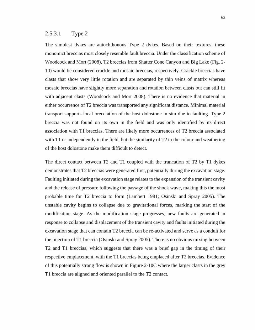
63

2.5.3.1 Type 2

The simplest dykes are autochthonous Type 2 dykes. Based on their textures, these

monomict breccias most closely resemble fault breccia. Under the classification scheme of

Woodcock and Mort (2008), T2 breccias from Shatter Cone Canyon and Big Lake (Fig. 2-

10) would be considered crackle and mosaic breccias, respectively. Crackle breccias have

clasts that show very little rotation and are separated by thin veins of matrix whereas

mosaic breccias have slightly more separation and rotation between clasts but can still fit

with adjacent clasts (Woodcock and Mort 2008). There is no evidence that material in

either occurrence of T2 breccia was transported any significant distance. Minimal material

transport supports local brecciation of the host dolostone in situ due to faulting. Type 2

breccia was not found on its own in the field and was only identified by its direct

association with T1 breccias. There are likely more occurrences of T2 breccia associated

with T1 or independently in the field, but the similarity of T2 to the colour and weathering

of the host dolostone make them difficult to detect.

The direct contact between T2 and T1 coupled with the truncation of T2 by T1 dykes

demonstrates that T2 breccias were generated first, potentially during the excavation stage.

Faulting initiated during the excavation stage relates to the expansion of the transient cavity

and the release of pressure following the passage of the shock wave, making this the most

probable time for T2 breccia to form (Lambert 1981; Osinski and Spray 2005). The

unstable cavity begins to collapse due to gravitational forces, marking the start of the

modification stage. As the modification stage progresses, new faults are generated in

response to collapse and displacement of the transient cavity and faults initiated during the

excavation stage that can contain T2 breccia can be re-activated and serve as a conduit for

the injection of T1 breccia (Osinski and Spray 2005). There is no obvious mixing between

T2 and T1 breccias, which suggests that there was a brief gap in the timing of their

respective emplacement, with the T1 breccias being emplaced after T2 breccias. Evidence

of this potentially strong flow is shown in Figure 2-10C where the larger clasts in the grey

T1 breccia are aligned and oriented parallel to the T2 contact.

64

2.5.3.2 Type 1

Allochthonous Type 1 breccia dykes are the most common type and the most visually

diverse. Looking beyond the visual differences in colour and clasts, there are similarities

among T1 breccias that indicate a similar origin. At the outcrop and hand sample scale, T1

breccias show a preferred orientation of larger clasts, especially if they are elongated (Fig.

2-2). This orientation roughly parallels the orientation of the contact with the host rock,

indicating that the direction of material transport followed the length of the dyke and the

flow regime was strong enough to maintain a constant movement of material. Type 1

breccias are polymict suggesting considerable transport. Breccias from Shatter Cone

Canyon occur within the Mount Phayre Formation and while some dolostone layers are

present, there is an abundance of mudstone beds in this unit. The degree to which mudstone

is present in the host rocks in Shatter Cone Canyon is not reflected in the composition of

T1 breccias. Mudstone clasts are a small fraction of the overall composition to the breccia

dyke indicating there is not a significant input of local material.

Silicate impact glass fragments have not been identified in the host rocks of T1 breccia

dykes, or in T2 breccias, so they must have been transported from elsewhere. Glass

fragments are not found in T3 breccia and the absence of crystalline limestone clasts

derived from the lower Shaler Supergroup unit within T1 breccias indicates that the glass

fragments and, therefore, breccia originated from a higher stratigraphic level. Incorporation

of glass material from the melt zone indicates a considerable transport distance of dyke

material, which requires a highly energetic process to generate the intrusion of dyke

material (Bischoff and Oskierski 1987; Lambert 1981; Stöffler 1977). Injection of impact

melt, including glasses, into the crater floor of complex craters has been observed at the

West Clearwater Lake and Ries impact structures (Dence 1971; Stöffler 1977). The

presence of glass fragments in polymict breccias from the crater floor of the Tunnunik

impact structure not only indicates the depth to which material was injected but is also

when these breccias formed and the timing of their injection.

The key evidence to determine this timing are the glass fragments since only the floor of

the impact structure remains without any overlying crater morphology, stratigraphy, ejecta,

or crater-fill. Temperature and pressure required for silicate glass melt to be generated

65

occurs upon decompression of the target material (Osinski et al. 2018). The faults generated

during the collapse of the transient cavity and re-activated faults that contain T2 breccias

create a network that facilitates the injection of T1 breccia, containing the glass fragments.

Recalling the relationship observed with T2 breccia, T1 breccia dykes were emplaced after

a brief pause following the formation of T2 dykes and suggests that the timing of T1 breccia

emplacement was early in the modification stage. Emplacement of T1 breccia dykes during

this phase of crater formation is comparable to the proposed timing of the emplacement of

impact melt-bearing breccia (suevite) dykes in the floor and walls of the Ries impact

structure near the end of transient cavity formation, after 15–20 s (Stöffler et al. 2013). The

observation in the field of shatter cone fragments within T1 breccias limits the timing

constraint further as shatter cones must have formed before the breccia in order to be

incorporated into the breccia; shatter cone formation is associated with the compression

stage (Osinski and Ferrière 2016).

2.5.3.3 Type 3

The parautochthonous Shaler type 3 breccia dyke is distinct from T1 and T2 dykes. Located

in the centre of the impact structure, it is the only breccia dyke found within a limestone-

rich section of the Shaler Supergroup. Clasts in the Shaler T3 breccia include crystalline

limestone, calcite-rich grainstone, and mudstone, but compared to T1 breccias, T3 breccia

is clast-poor. In addition to the dominant calcite composition of the T3 breccia, other

distinct features of this breccia include quenched carbonate melt clasts with a unique

radiating texture and matrix with a mottled texture (Fig. 2-14). The Shaler T3 breccia is

polymict and is comprised of clasts from several units within the Shaler Supergroup. The

polymict nature of the T3 breccia indicates transport and mixing of material has occurred,

but the displacement of material is much less extensive than in T1 so has formed more

locally within the Shaler Supergroup. Transport of material within the dyke is also evident

by the presence of the polymict clast (Figs. 2-12C–G) which appears to be a calcite-rich

breccia fragment that formed at a different location in the dyke. This exotic clast contains

quartz and quartz-rimmed calcite grains with small veinlets extending outward into the

clast. The composition of the mottled T3 matrix is a mix of calcite and ferroan dolomite

where the dolomite contains 1 to 5 wt% Fe. The occurrence of ferroan dolomite was not

66

detected within the overlying dolostone units and is therefore limited in extent to the Shaler

Supergroup.

The allochthonous West River T3 breccia is also distinct from T1 and T2 breccias in that

it is calcite-rich which makes it most similar to the Shaler T3 breccia compositionally,

however, the calcite associated with the West River breccia does not originate from the

Shaler Supergroup. The calcite-rich West River breccia dyke is emplaced in Allen Bay

dolostone, so the calcite was not locally derived. Based on regional geology, the most likely

source of the calcite is from the overlying Silurian-aged Cape Storm Formation which is a

transitional dolostone and limestone unit or from Douro Formation limestone (Kerr 1975;

Mallamo 1989). The occurrence of pyrite in the West River breccia could originate from

either the Douro or Cape Storm Formations. The pyrite source is based on drilling logs

from a site ~92 km west-northwest near the coast of Victoria Island at 72.75500° N and

117.18694° W (Batten 1975) as pyrite was not identified locally within the Allen Bay or

Victoria Island formations within the impact structure. The Douro and Cape Storm

Formations are equivalent to the Read Bay and Cape Phillips Formations, respectively as

reported in the drilling log (Batten 1975; Dewing et al. 2015). With the absence of shatter

cone clasts or association with T2 breccia, the timing of T3 breccias is more difficult to

constrain. However, based on the timing of T1 breccia and the presence of clasts from

multiple units, indicating material transport similar to T1, T3 breccias could have also been

emplaced during the modification stage.

The existence of the West River breccia dyke creates interesting implications regarding the

timing of the impact event more than any other breccia dyke within the impact structure.

Both the Cape Storm Formation and Douro Formation occur in the Early Ludlovian Stage

approximately 423 to 421 Ma and 421 to 418 Ma, respectively (Kerr 1975; Mallamo 1989;

Stewart 1987). The Cape Storm and Douro formations are mapped as an undivided unit

along with the Allen Bay Formation west of the Tunnunik impact structure on a recent

geologic map of Victoria Island (Dewing et al. 2015). The presence of a calcite-rich breccia

dyke within host dolostone indicates regional dolomitization of the Allen Bay and

underlying Victoria Island formations occurred before the impact event occurred,

otherwise any calcite present within the breccia, and the now exposed Shaler Supergroup

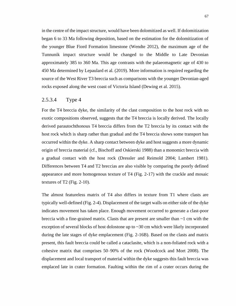
67

in the centre of the impact structure, would have been dolomitized as well. If dolomitization

began 6 to 33 Ma following deposition, based on the estimation for the dolomitization of

the younger Blue Fiord Formation limestone (Wendte 2012), the maximum age of the

Tunnunik impact structure would be changed to the Middle to Late Devonian

approximately 385 to 360 Ma. This age contrasts with the palaeomagnetic age of 430 to

450 Ma determined by Lepaulard et al. (2019). More information is required regarding the

source of the West River T3 breccia such as comparisons with the younger Devonian-aged

rocks exposed along the west coast of Victoria Island (Dewing et al. 2015).

2.5.3.4 Type 4

For the T4 breccia dyke, the similarity of the clast composition to the host rock with no

exotic compositions observed, suggests that the T4 breccia is locally derived. The locally

derived parautochthonous T4 breccia differs from the T2 breccia by its contact with the

host rock which is sharp rather than gradual and the T4 breccia shows some transport has

occurred within the dyke. A sharp contact between dyke and host suggests a more dynamic

origin of breccia material (cf., Bischoff and Oskierski 1988) than a monomict breccia with

a gradual contact with the host rock (Dressler and Reimold 2004; Lambert 1981).

Differences between T4 and T2 breccias are also visible by comparing the poorly defined

appearance and more homogenous texture of T4 (Fig. 2-17) with the crackle and mosaic

textures of T2 (Fig. 2-10).

The almost featureless matrix of T4 also differs in texture from T1 where clasts are

typically well-defined (Fig. 2-4). Displacement of the target walls on either side of the dyke

indicates movement has taken place. Enough movement occurred to generate a clast-poor

breccia with a fine-grained matrix. Clasts that are present are smaller than ~1 cm with the

exception of several blocks of host dolostone up to ~30 cm which were likely incorporated

during the late stages of dyke emplacement (Fig. 2-16B). Based on the clasts and matrix

present, this fault breccia could be called a cataclasite, which is a non-foliated rock with a

cohesive matrix that comprises 50–90% of the rock (Woodcock and Mort 2008). The

displacement and local transport of material within the dyke suggests this fault breccia was

emplaced late in crater formation. Faulting within the rim of a crater occurs during the

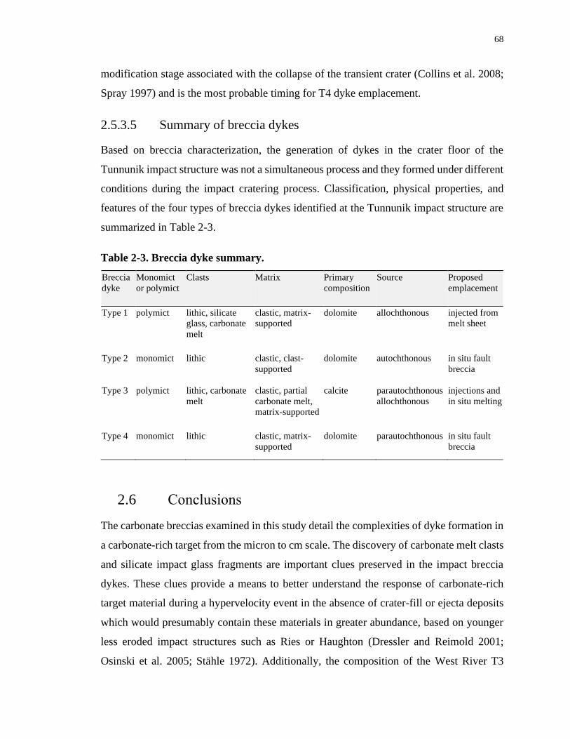
68

modification stage associated with the collapse of the transient crater (Collins et al. 2008;

Spray 1997) and is the most probable timing for T4 dyke emplacement.

2.5.3.5 Summary of breccia dykes

Based on breccia characterization, the generation of dykes in the crater floor of the

Tunnunik impact structure was not a simultaneous process and they formed under different

conditions during the impact cratering process. Classification, physical properties, and

features of the four types of breccia dykes identified at the Tunnunik impact structure are

summarized in Table 2-3.

Table 2-3. Breccia dyke summary.

Breccia

dyke Monomict

or polymict Clasts Matrix Primary

composition Source Proposed

emplacement

Type 1 polymict lithic, silicate

glass, carbonate

melt

clastic, matrix-

supported dolomite allochthonous injected from

melt sheet

Type 2 monomict lithic clastic, clast-

supported dolomite autochthonous in situ fault

breccia

Type 3 polymict lithic, carbonate

melt clastic, partial

carbonate melt,

matrix-supported

calcite parautochthonous

allochthonous injections and

in situ melting

Type 4 monomict lithic clastic, matrix-

supported dolomite parautochthonous in situ fault

breccia

2.6 Conclusions

The carbonate breccias examined in this study detail the complexities of dyke formation in

a carbonate-rich target from the micron to cm scale. The discovery of carbonate melt clasts

and silicate impact glass fragments are important clues preserved in the impact breccia

dykes. These clues provide a means to better understand the response of carbonate-rich

target material during a hypervelocity event in the absence of crater-fill or ejecta deposits

which would presumably contain these materials in greater abundance, based on younger

less eroded impact structures such as Ries or Haughton (Dressler and Reimold 2001;

Osinski et al. 2005; Stähle 1972). Additionally, the composition of the West River T3

69

breccia dyke is the only identified dyke within the impact structure that may have preserved

overlying formations that have been eroded due to post-impact glaciation events.

The results of this study warrant continued investigation into carbonate-rich breccias and

the response of carbonates during hypervelocity impact events since carbonates account

for the target material in approximately one third of impact structures (Osinski et al. 2008).

2.7 References

Batten W. H. R. 1975. Arctic well history report, Murphy Alminex Victoria Island F-36.

National Energy Board Report 063-11-09-024.

Bischoff L., and Oskierski W. 1987. Fractures, pseudotachylite veins and breccia dikes in

the crater floor of the Rochechouart impact structure, SW-France, as indicators of

crater forming processes. In Research in Terrestrial Impact Structures, edited by Pohl

J. pp. 5–29.

Bischoff L., and Oskierski W. 1988. The surface structure of the Haughton impact crater,

Devon Island, Canada. Meteoritics 23:209–220.

Collins G. S., Kenkmann T., Osinski G. R., and Wünnemann K. 2008. Mid-sized complex

crater formation in mixed crystalline-sedimentary targets: Insight from modeling and

observation. Meteoritics & Planetary Science 43:1955–1977.

Dence M. R. 1971. Impact melts. Journal of Geophysical Research 76:5552–5565.

Dewing K., Pratt B. R., Hadlari T., Brent T., Bédard J., and Rainbird R. H. 2013. Newly

identified “Tunnunik” impact structure, Prince Albert Peninsula, northwestern

Victoria Island, Arctic Canada. Meteoritics & Planetary Science 48:211–223.

Dewing K., Hadlari T., Rainbird R. H., and Bédard J. H. 2015. Phanerozoic geology,

northwestern Victoria Island, Northwest Territories; Geological Survey of Canada,

Canadian Geoscience Map 171 (preliminary). scale 1:500 000.

Dressler B. O., and Sharpton V. L. 1997. Breccia formation at a complex impact crater:

70

Slate Islands, Lake Superior, Ontario, Canada. Tectonophysics 275:285–311.

Dressler B. O., and Reimold W. U. 2001. Terrestrial impact melt rocks and glasses. Earth-

Science Reviews 56:205–284.

Dressler B. O., and Reimold W. U. 2004. Order or chaos? Origin and mode of emplacement

of breccias in floors of large impact structures. Earth-Science Reviews 67:1–54.

Graup G. 1999. Carbonate-silicate liquid immiscibility upon impact melting: Ries Crater,

Germany. Meteoritics & Planetary Science 34:425–438.

Hörz F., Archer P. D., Niles P. B., Zolensky M. E., and Evans M. 2015. Devolatilization

or melting of carbonates at Meteor Crater, AZ? Meteoritics & Planetary Science

50:1050–1070.

Jones A. P., Claeys P., and Heuschkel S. 2000. Impact melting of carbonates from the

Chicxulub Crater. In Impacts and the Early Earth, Lecture Notes in Earth Sciences,

edited by Gilmour I., and Koeberl C. Springer-Verlag, Berlin-Heidelberg-New York.

pp. 343–361.

Kerr J. W. 1975. Cape Storm Formation - A new Silurian unit in the Canadian Arctic.

Bulletin of Canadian Petroleum Geology 23:67–83.

Kieffer S. W., and Simonds C. H. 1980. The role of volatiles and lithology in the impact

cratering process. Reviews of Geophysics and Space Physics 18:143–181.

Lambert P. 1981. Breccia Dikes: Geological constraints on the formation of complex

craters. In Multi-ring Basins, Proc. Lunar Planet. Sci., edited by Schultz P. H., and

Merrill R. B. pp. 59–78.

Lepaulard C., Gattacceca J., Swanson-Hysell N., Quesnel Y., Demory F., and Osinski G.

R. 2019. A Paleozoic age for the Tunnunik impact structure. Meteoritics & Planetary

Science 1–12.

Mallamo M. P. Ordovician and Silurian stratigraphy, sedimentology, and paleoecology,

71

Central Canadian Arctic Islands. MSc thesis, University of Western Ontario, 1989.

Mathieu J., Turner E. C., and Rainbird R. H. 2013. Sedimentary architecture of a deeply

karsted Precambrian – Cambrian unconformity, Victoria Island, Northwest

Territories; Geological Survey of Canada, Current Research 2013-1. p. 15.

Melosh H. J. 1989. Impact Cratering: A Geologic Process, New York: Oxford University

Press.

Newman J. D., and Osinski G. R. 2016. Geological mapping of the Tunnunik impact

structure, Victoria Island, Canadian High Arctic. 47th Lunar and Planetary Science

Conference Abstract #1591.

Osinski G. R. 2003. Impact glasses in fallout suevites from the Ries impact structure,

Germany: An analytical SEM study. Meteoritics & Planetary Science 38:1641–1667.

Osinski G. R., Spray J. G., and Lee P. 2005. Impactites of the Haughton impact structure,

Devon Island, Canadian High Arctic. Meteoritics & Planetary Science 40:1789–1812.

Osinski G. R., and Spray J. G. 2005. Tectonics of complex crater formation as revealed by

the Haughton impact structure, Devon Island, Canadian High Arctic. Meteoritics &

Planetary Science 40:1813–1834.

Osinski G. R., Spray J. G., and Grieve R. A. F. 2008. Impact melting in sedimentary target

rocks: An assessment. In The Sedimentary Record of Meteorite Impacts, Special

Paper 437, edited by Evans K. R., Horton W., King Jr. D. K., and Morrow J. R.

Geological Society of America, Boulder, CO. pp. 1–18.

Osinski G. R., Abou-Aly S., Francis R., Hansen J., Marion C. L., Pickersgill A. E., and

Tornabene L. L. 2013. The Prince Albert structure, Northwest Territories, Canada: A

new 28-km diameter complex impact structure. 44th Lunar and Planetary Science

Conference Abstract #2099.

Osinski G. R., and Ferrière L. 2016. Shatter cones: (Mis)understood? Science Advances 2,

e160061:1–10.

72

Osinski G. R., Grieve R. A. F., Bleacher J. E., Neish C. D., Pilles E. A., and Tornabene L.

L. 2018. Igneous rocks formed by hypervelocity impact. Journal of Volcanology and

Geothermal Research 353:25–54.

Pinto J. A., and Warme J. E. 2008. Alamo Event, Nevada: Crater stratigraphy and impact

breccia realms. In The Sedimentary Record of Meteorite Impacts, Special Paper 437,

edited by Evans K. R., Horton W., King Jr. D. K., and Morrow J. R. Geological

Society of America, Boulder, CO. pp. 99–137.

Quesnel Y., Zylberman W., Rochette P., Uehara M., Gattacceca J., Osinski G. R.,

Dussouillez P., Lepaulard C., and Champollion C. 2020. Geophysical signature of the

Tunnunik impact structure, Northwest Territories, Canada. Meteoritics & Planetary

Science 55:480-495.

Sahoui R., Belhai D., and Jambon A. 2016. Impact-generated carbonate melts in the

Talemzane impact structure (Laghouat, Algeria). Arabian Journal of Geosciences

9:641.

Spray J. G. 1997. Superfaults. Geology 25:579–582.

Stähle V. 1972. Impact glasses from the suevite of the Nördlinger Ries. Earth and

Planetary Science Letters 17:275–293.

Stewart W. D. 1987. Late Proterozoic to Early Tertiary stratigraphy of Somerset Island

and Northern Boothia Peninsula, District of Franklin, N.W.T., Paper 83-26,

Geological Survey of Canada.

Stöffler D. 1977. Research drilling, Nördlingen 1973: Polymict breccias, crater basement

and cratering model of the Ries impact structure. Geologica Bavarica 75:443–458.

Stöffler D. 1984. Glasses formed by hypervelocity impact. Journal of Non-Crystalline

Solids 67:465–502.

Stöffler D., and Grieve R. A. F. 2007. Impactites. In Metamorphic Rocks: A Classification

and Glossary of Terms, Recommendations of the International Union of Geological

73

Sciences, edited by Fettes D., and Desmons J. Cambridge University Press,

Cambridge. pp. 82–92.

Stöffler D., Artemieva N. A., Wünnemann K., Reimold W. U., Jacob J., Hansen B. K., and

Summerson I. A. T. 2013. Ries crater and suevite revisited-Observations and

modeling Part I: Observations. Meteoritics & Planetary Science 48:515–589.

Stöffler D., Hamann C., and Metzler K. 2018. Shock metamorphism of planetary silicate

rocks and sediments: Proposal for an updated classification system. Meteoritics &

Planetary Science 49:5–49.

Wall F., Le Bas M. J., and Srivastava R. K. 1993. Calcite and carbocernaite exsolution and

cotectic textures in a Sr,REE-rich carbonatite dyke from Rajasthan, India.

Mineralogical Magazine 57:495–513.

Wendte J. C. 2012. Core, petrographic, and rock petrophysical evaluation of the Blue Fiord

Formation from wells in the Canadian Arctic Islands. Geological Survey of Canada,

Open File 6984:1–126.

Woodcock N. H., and Mort K. M. 2008. Classification of fault breccias and related fault

rocks. Geological Magazine 145:435–440.

Zylberman W. Geophysical Study of Complex Meteorite Impact Structures. PhD thesis,

University of Western Ontario, 2017, Electronic Thesis and Dissertation Repository

(5165).

74

Chapter 3

3 Impact-generated carbonate-rich dykes from the Haughton

impact structure, Canada

3.1 Introduction

The Haughton impact structure on Devon Island, Nunavut, is a well-preserved complex

impact structure 23 km in diameter (e.g., Osinski et al. 2005a; Robertson and Grieve 1978).

The Haughton structure is located in a carbonate-rich sedimentary sequence comprised of

limestone, dolostone, sandstone, shale, and sulfates, overlying gneiss and metagranite

(Osinski et al. 2008a). The preservation and exposure of this impact structure offers many

aspects for study from its geology, shatter cones, impactites, hydrothermal activity, to

geomicrobiology (e.g., Osinski and Spray 2001; Osinski et al. 2005a, 2005b; Pontefract et

al. 2014; Redeker and Stöffler 1988). The various allochthonous crater-fill impact melt

rocks have been studied in detail (Osinski and Spray 2001, 2003; Osinski et al. 2005b;

Redeker and Stöffler 1988); however, the one impactite that has not been studied in depth

at Haughton are impact-generated dykes. Bischoff and Oskierski (1988) provided the first

and only description of the occurrence of monomict and polymict impact breccia dykes

with a clastic matrix as part of their review of surface structures at Haughton, but these

lithologies were not described in any detail.

Breccia dykes are a prevalent feature in impact structures and their distribution can be

underestimated in the field due to erosion or poor exposure (Lambert 1981). The generation

of breccia dykes known to occur in carbonate-rich targets is limited to a few terrestrial

impact sites (Osinski et al. 2008a). The well-preserved state and exposure of the Haughton

impact structure provide an excellent opportunity to examine characteristics of dykes

formed within the near-surface portion of a complex impact crater. The diversity observed

among lithic breccias and impact melt rocks in this study of a well-preserved impact

structure highlight the complexity of dyke formation in the impact cratering process. Many

previous detailed studies of impact-generated dykes have been conducted at deeply eroded

impact structures such as Rochechouart, Slate Islands, Vredefort, Ile Rouleau, and

Tunnunik, which is described in Chapter 2 (Bischoff and Oskierski 1987; Caty et al. 1976;

75

Dressler and Reimold 2004; Dressler and Sharpton 1997; Lambert 1981). Examining dykes

at Haughton will provide insights into the products generated and present in a well-

preserved impact structure.

3.2 Geologic setting

The Haughton impact structure on Devon Island, Nunavut is located in a sedimentary target

sequence of limestone, dolostone, evaporites, and sandstone of Cambrian to Silurian age,

estimated to have been ~1880 m thick at the time of impact (Osinski et al. 2005a). The

formations exposed and associated with samples in this study include Eleanor River, Bay

Fiord, Thumb Mountain, and Allen Bay formations. These four formations can be

heterogenous and most contain multiple members which may consist of limestone,

dolostone, and/or anhydrite/gypsum. The Precambrian crystalline basement is not exposed

within the impact structure but is found as clasts in the crater-fill impact melt rock deposits

(Metzler et al. 1988; Osinski et al. 2005a, 2005b).

The crater-fill impact melt rocks cover the central area of the impact structure and are pale

grey in colour, with the groundmass consisting of microcrystalline calcite, silicate impact

melt glass, and anhydrite (Osinski and Spray 2001; Osinski et al. 2005b). These impact

melt rocks are clast-rich and contain shocked mineral and lithic clasts from all target

lithologies (Osinski et al. 2005b). Lithic breccias identified in dykes by Bischoff and

Oskierski (1988) were distinguished as monomict and polymict. The monomict breccias

consisted of a fine-grained dolomite or calcite matrix with clasts of dolostone or limestone,

corresponding to the matrix composition (Bischoff and Oskierski 1988). Polymict breccias

consisted primarily of limestone and dolostone clasts with fewer chert clasts and rare

gypsum (Bischoff and Oskierski 1988). The Haughton impact structure is ~23.5 Ma as

determined by U-Th/He dating of zircons (Young et al. 2013) and also preserves Miocene

crater lake deposits that overlies some of the crater-fill impact melt rocks (Hickey et al.

1988; Osinski et al. 2005a).

3.3 Samples and methods

Fieldwork related to this study was conducted over four weeks in July and August 2016 at

the Haughton impact structure. The primary field objective was to locate impact-generated

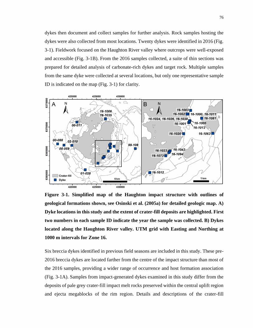
76

dykes then document and collect samples for further analysis. Rock samples hosting the

dykes were also collected from most locations. Twenty dykes were identified in 2016 (Fig.

3-1). Fieldwork focused on the Haughton River valley where outcrops were well-exposed

and accessible (Fig. 3-1B). From the 2016 samples collected, a suite of thin sections was

prepared for detailed analysis of carbonate-rich dykes and target rock. Multiple samples

from the same dyke were collected at several locations, but only one representative sample

ID is indicated on the map (Fig. 3-1) for clarity.

Figure 3-1. Simplified map of the Haughton impact structure with outlines of

geological formations shown, see Osinski et al. (2005a) for detailed geologic map. A)

Dyke locations in this study and the extent of crater-fill deposits are highlighted. First

two numbers in each sample ID indicate the year the sample was collected. B) Dykes

located along the Haughton River valley. UTM grid with Easting and Northing at

1000 m intervals for Zone 16.

Six breccia dykes identified in previous field seasons are included in this study. These pre-

2016 breccia dykes are located farther from the centre of the impact structure than most of

the 2016 samples, providing a wider range of occurrence and host formation association

(Fig. 3-1A). Samples from impact-generated dykes examined in this study differ from the

deposits of pale grey crater-fill impact melt rocks preserved within the central uplift region

and ejecta megablocks of the rim region. Details and descriptions of the crater-fill

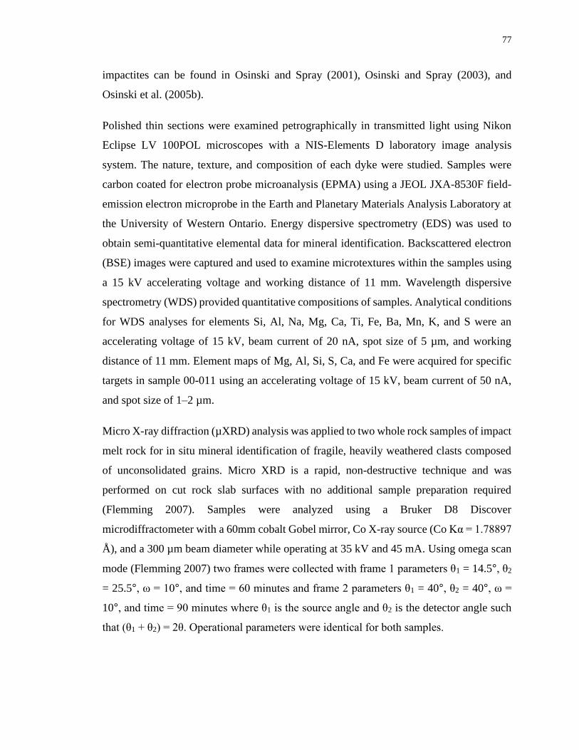
77

impactites can be found in Osinski and Spray (2001), Osinski and Spray (2003), and

Osinski et al. (2005b).

Polished thin sections were examined petrographically in transmitted light using Nikon

Eclipse LV 100POL microscopes with a NIS-Elements D laboratory image analysis

system. The nature, texture, and composition of each dyke were studied. Samples were

carbon coated for electron probe microanalysis (EPMA) using a JEOL JXA-8530F field-

emission electron microprobe in the Earth and Planetary Materials Analysis Laboratory at

the University of Western Ontario. Energy dispersive spectrometry (EDS) was used to

obtain semi-quantitative elemental data for mineral identification. Backscattered electron

(BSE) images were captured and used to examine microtextures within the samples using

a 15 kV accelerating voltage and working distance of 11 mm. Wavelength dispersive

spectrometry (WDS) provided quantitative compositions of samples. Analytical conditions

for WDS analyses for elements Si, Al, Na, Mg, Ca, Ti, Fe, Ba, Mn, K, and S were an

accelerating voltage of 15 kV, beam current of 20 nA, spot size of 5 µm, and working

distance of 11 mm. Element maps of Mg, Al, Si, S, Ca, and Fe were acquired for specific

targets in sample 00-011 using an accelerating voltage of 15 kV, beam current of 50 nA,

and spot size of 1–2 µm.

Micro X-ray diffraction (µXRD) analysis was applied to two whole rock samples of impact

melt rock for in situ mineral identification of fragile, heavily weathered clasts composed

of unconsolidated grains. Micro XRD is a rapid, non-destructive technique and was

performed on cut rock slab surfaces with no additional sample preparation required

(Flemming 2007). Samples were analyzed using a Bruker D8 Discover

microdiffractometer with a 60mm cobalt Gobel mirror, Co X-ray source (Co Kα = 1.78897

Å), and a 300 µm beam diameter while operating at 35 kV and 45 mA. Using omega scan

mode (Flemming 2007) two frames were collected with frame 1 parameters θ1 = 14.5°, θ2

= 25.5°, ω = 10°, and time = 60 minutes and frame 2 parameters θ1 = 40°, θ2 = 40°, ω =

10°, and time = 90 minutes where θ1 is the source angle and θ2 is the detector angle such

that (θ1 + θ2) = 2θ. Operational parameters were identical for both samples.

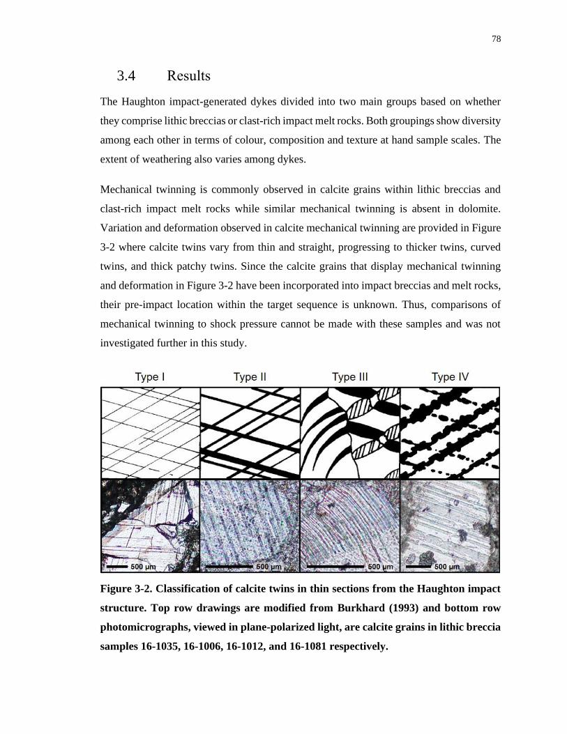
78

3.4 Results

The Haughton impact-generated dykes divided into two main groups based on whether

they comprise lithic breccias or clast-rich impact melt rocks. Both groupings show diversity

among each other in terms of colour, composition and texture at hand sample scales. The

extent of weathering also varies among dykes.

Mechanical twinning is commonly observed in calcite grains within lithic breccias and

clast-rich impact melt rocks while similar mechanical twinning is absent in dolomite.

Variation and deformation observed in calcite mechanical twinning are provided in Figure

3-2 where calcite twins vary from thin and straight, progressing to thicker twins, curved

twins, and thick patchy twins. Since the calcite grains that display mechanical twinning

and deformation in Figure 3-2 have been incorporated into impact breccias and melt rocks,

their pre-impact location within the target sequence is unknown. Thus, comparisons of

mechanical twinning to shock pressure cannot be made with these samples and was not

investigated further in this study.

Figure 3-2. Classification of calcite twins in thin sections from the Haughton impact

structure. Top row drawings are modified from Burkhard (1993) and bottom row

photomicrographs, viewed in plane-polarized light, are calcite grains in lithic breccia

samples 16-1035, 16-1006, 16-1012, and 16-1081 respectively.

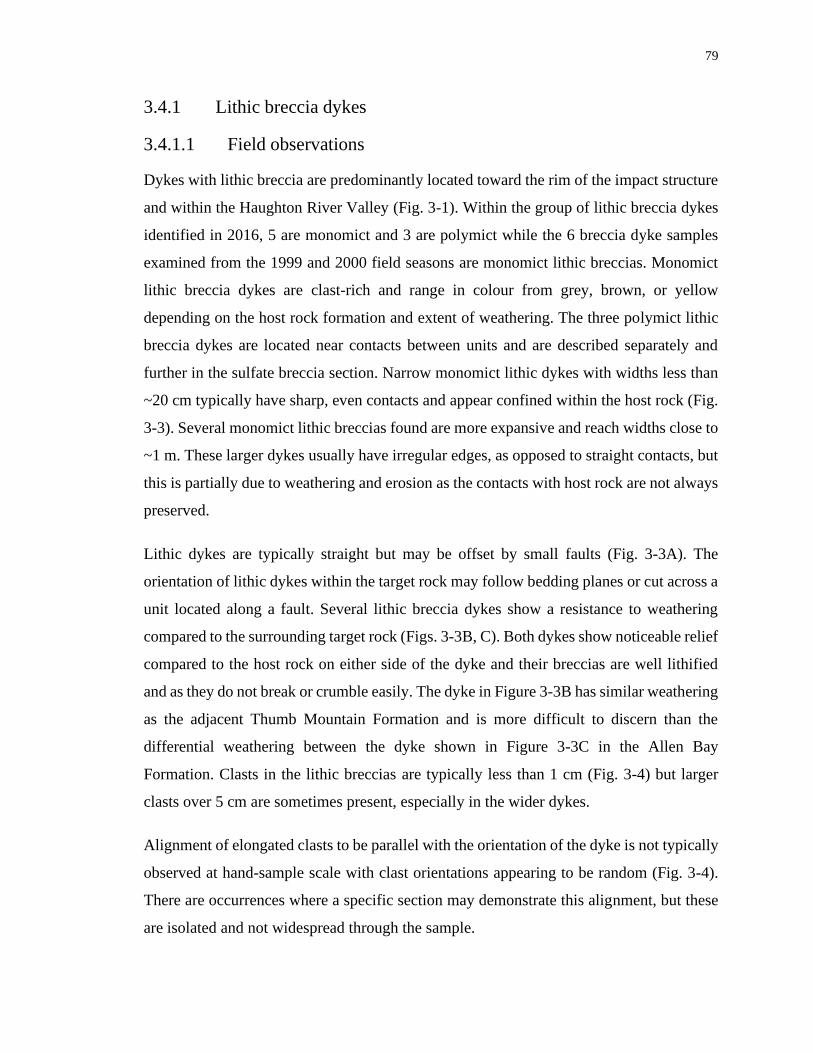
79

3.4.1 Lithic breccia dykes

3.4.1.1 Field observations

Dykes with lithic breccia are predominantly located toward the rim of the impact structure

and within the Haughton River Valley (Fig. 3-1). Within the group of lithic breccia dykes

identified in 2016, 5 are monomict and 3 are polymict while the 6 breccia dyke samples

examined from the 1999 and 2000 field seasons are monomict lithic breccias. Monomict

lithic breccia dykes are clast-rich and range in colour from grey, brown, or yellow

depending on the host rock formation and extent of weathering. The three polymict lithic

breccia dykes are located near contacts between units and are described separately and

further in the sulfate breccia section. Narrow monomict lithic dykes with widths less than

~20 cm typically have sharp, even contacts and appear confined within the host rock (Fig.

3-3). Several monomict lithic breccias found are more expansive and reach widths close to

~1 m. These larger dykes usually have irregular edges, as opposed to straight contacts, but

this is partially due to weathering and erosion as the contacts with host rock are not always

preserved.

Lithic dykes are typically straight but may be offset by small faults (Fig. 3-3A). The

orientation of lithic dykes within the target rock may follow bedding planes or cut across a

unit located along a fault. Several lithic breccia dykes show a resistance to weathering

compared to the surrounding target rock (Figs. 3-3B, C). Both dykes show noticeable relief

compared to the host rock on either side of the dyke and their breccias are well lithified

and as they do not break or crumble easily. The dyke in Figure 3-3B has similar weathering

as the adjacent Thumb Mountain Formation and is more difficult to discern than the

differential weathering between the dyke shown in Figure 3-3C in the Allen Bay

Formation. Clasts in the lithic breccias are typically less than 1 cm (Fig. 3-4) but larger

clasts over 5 cm are sometimes present, especially in the wider dykes.

Alignment of elongated clasts to be parallel with the orientation of the dyke is not typically

observed at hand-sample scale with clast orientations appearing to be random (Fig. 3-4).

There are occurrences where a specific section may demonstrate this alignment, but these

are isolated and not widespread through the sample.

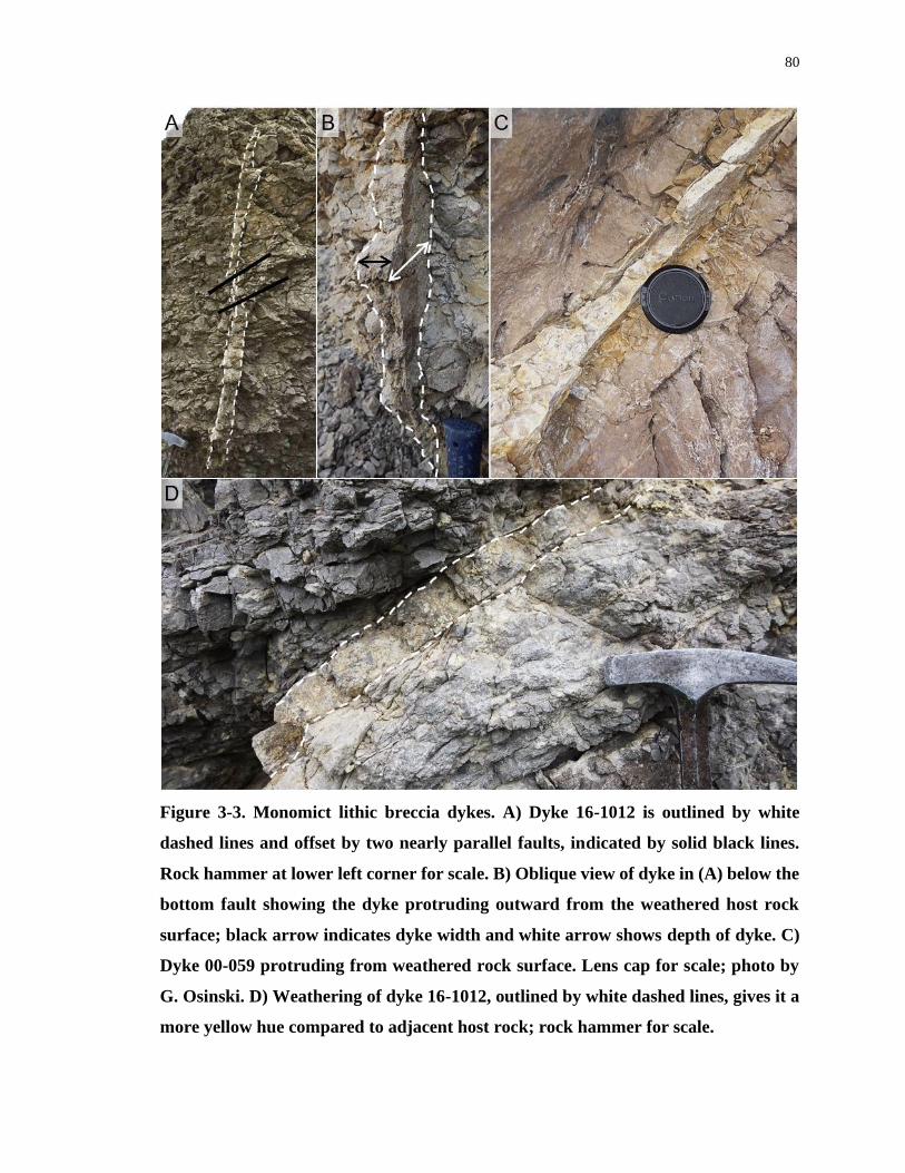
80

Figure 3-3. Monomict lithic breccia dykes. A) Dyke 16-1012 is outlined by white

dashed lines and offset by two nearly parallel faults, indicated by solid black lines.

Rock hammer at lower left corner for scale. B) Oblique view of dyke in (A) below the

bottom fault showing the dyke protruding outward from the weathered host rock

surface; black arrow indicates dyke width and white arrow shows depth of dyke. C)

Dyke 00-059 protruding from weathered rock surface. Lens cap for scale; photo by

G. Osinski. D) Weathering of dyke 16-1012, outlined by white dashed lines, gives it a

more yellow hue compared to adjacent host rock; rock hammer for scale.

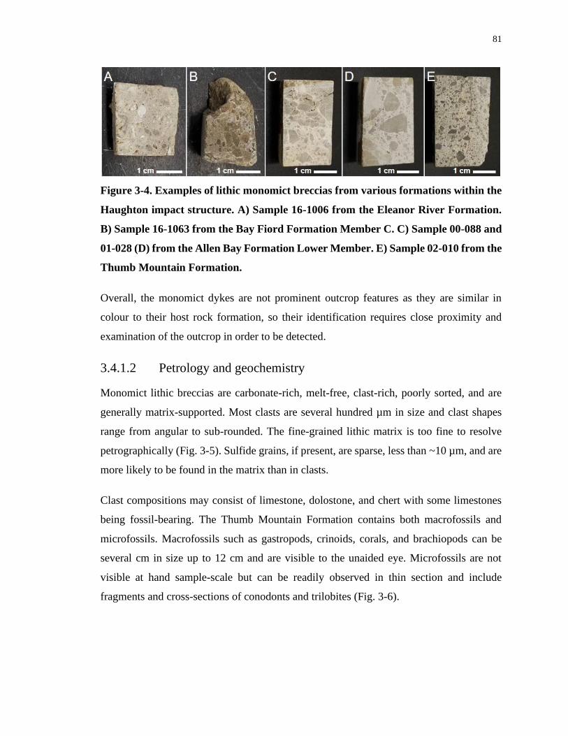
81

Figure 3-4. Examples of lithic monomict breccias from various formations within the

Haughton impact structure. A) Sample 16-1006 from the Eleanor River Formation.

B) Sample 16-1063 from the Bay Fiord Formation Member C. C) Sample 00-088 and

01-028 (D) from the Allen Bay Formation Lower Member. E) Sample 02-010 from the

Thumb Mountain Formation.

Overall, the monomict dykes are not prominent outcrop features as they are similar in

colour to their host rock formation, so their identification requires close proximity and

examination of the outcrop in order to be detected.

3.4.1.2 Petrology and geochemistry

Monomict lithic breccias are carbonate-rich, melt-free, clast-rich, poorly sorted, and are

generally matrix-supported. Most clasts are several hundred µm in size and clast shapes

range from angular to sub-rounded. The fine-grained lithic matrix is too fine to resolve

petrographically (Fig. 3-5). Sulfide grains, if present, are sparse, less than ~10 µm, and are

more likely to be found in the matrix than in clasts.

Clast compositions may consist of limestone, dolostone, and chert with some limestones

being fossil-bearing. The Thumb Mountain Formation contains both macrofossils and

microfossils. Macrofossils such as gastropods, crinoids, corals, and brachiopods can be

several cm in size up to 12 cm and are visible to the unaided eye. Microfossils are not

visible at hand sample-scale but can be readily observed in thin section and include

fragments and cross-sections of conodonts and trilobites (Fig. 3-6).

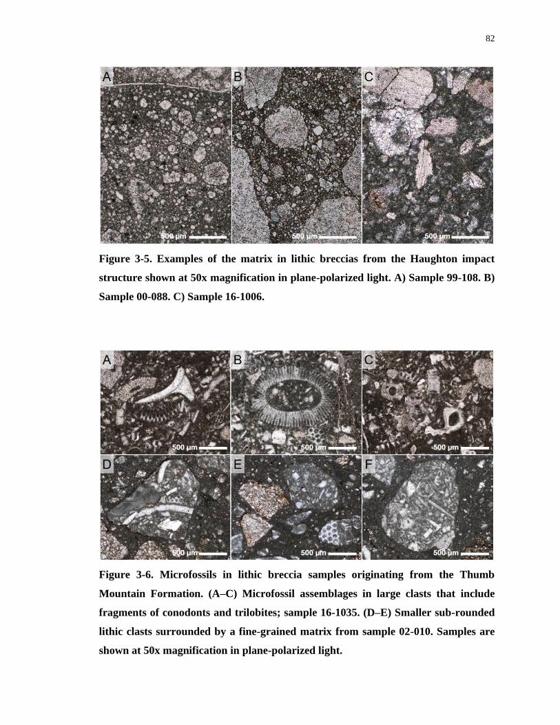
82

Figure 3-5. Examples of the matrix in lithic breccias from the Haughton impact

structure shown at 50x magnification in plane-polarized light. A) Sample 99-108. B)

Sample 00-088. C) Sample 16-1006.

Figure 3-6. Microfossils in lithic breccia samples originating from the Thumb

Mountain Formation. (A–C) Microfossil assemblages in large clasts that include

fragments of conodonts and trilobites; sample 16-1035. (D–E) Smaller sub-rounded

lithic clasts surrounded by a fine-grained matrix from sample 02-010. Samples are

shown at 50x magnification in plane-polarized light.

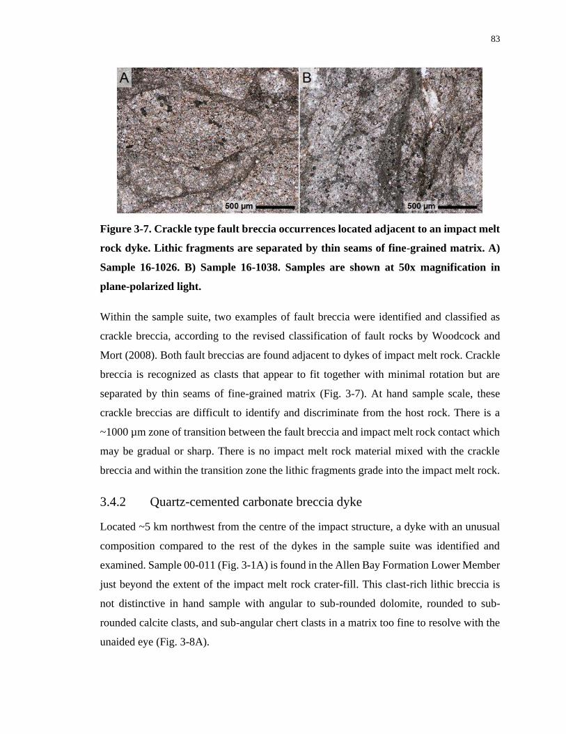
83

Figure 3-7. Crackle type fault breccia occurrences located adjacent to an impact melt

rock dyke. Lithic fragments are separated by thin seams of fine-grained matrix. A)

Sample 16-1026. B) Sample 16-1038. Samples are shown at 50x magnification in

plane-polarized light.

Within the sample suite, two examples of fault breccia were identified and classified as

crackle breccia, according to the revised classification of fault rocks by Woodcock and

Mort (2008). Both fault breccias are found adjacent to dykes of impact melt rock. Crackle

breccia is recognized as clasts that appear to fit together with minimal rotation but are

separated by thin seams of fine-grained matrix (Fig. 3-7). At hand sample scale, these

crackle breccias are difficult to identify and discriminate from the host rock. There is a

~1000 µm zone of transition between the fault breccia and impact melt rock contact which

may be gradual or sharp. There is no impact melt rock material mixed with the crackle

breccia and within the transition zone the lithic fragments grade into the impact melt rock.

3.4.2 Quartz-cemented carbonate breccia dyke

Located ~5 km northwest from the centre of the impact structure, a dyke with an unusual

composition compared to the rest of the dykes in the sample suite was identified and

examined. Sample 00-011 (Fig. 3-1A) is found in the Allen Bay Formation Lower Member

just beyond the extent of the impact melt rock crater-fill. This clast-rich lithic breccia is

not distinctive in hand sample with angular to sub-rounded dolomite, rounded to sub-

rounded calcite clasts, and sub-angular chert clasts in a matrix too fine to resolve with the

unaided eye (Fig. 3-8A).

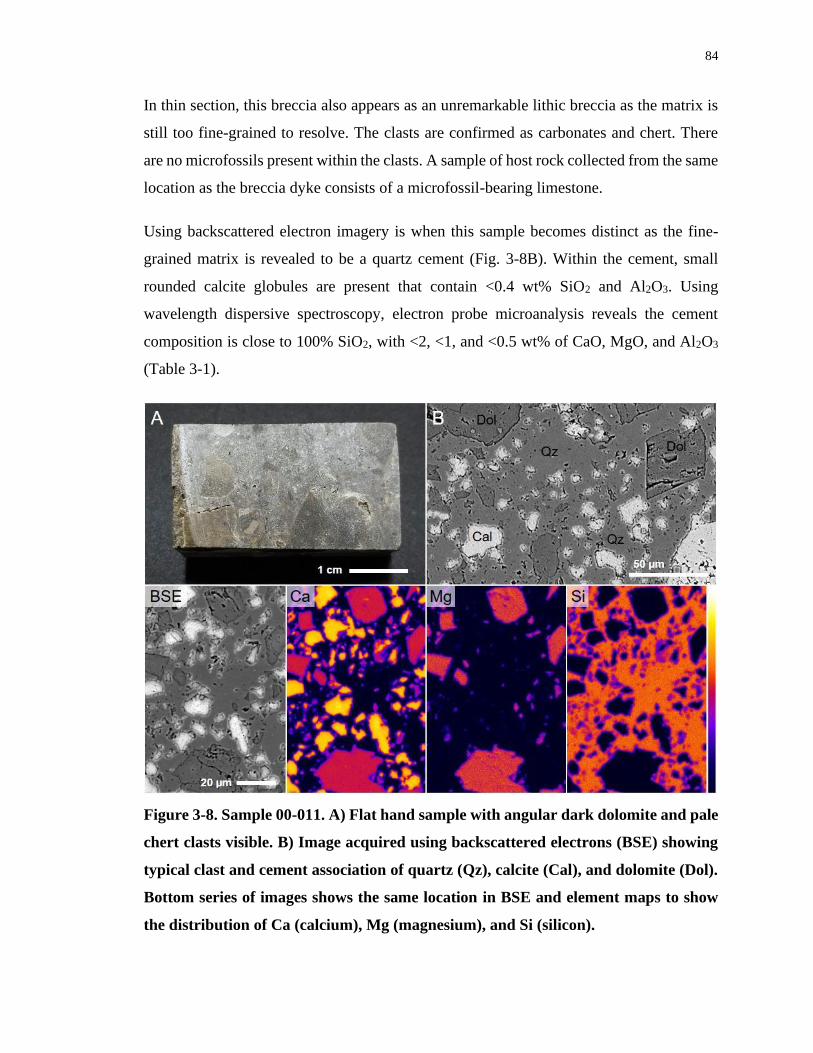
84

In thin section, this breccia also appears as an unremarkable lithic breccia as the matrix is

still too fine-grained to resolve. The clasts are confirmed as carbonates and chert. There

are no microfossils present within the clasts. A sample of host rock collected from the same

location as the breccia dyke consists of a microfossil-bearing limestone.

Using backscattered electron imagery is when this sample becomes distinct as the fine-

grained matrix is revealed to be a quartz cement (Fig. 3-8B). Within the cement, small

rounded calcite globules are present that contain <0.4 wt% SiO2 and Al2O3. Using

wavelength dispersive spectroscopy, electron probe microanalysis reveals the cement

composition is close to 100% SiO2, with <2, <1, and <0.5 wt% of CaO, MgO, and Al2O3

(Table 3-1).

Figure 3-8. Sample 00-011. A) Flat hand sample with angular dark dolomite and pale

chert clasts visible. B) Image acquired using backscattered electrons (BSE) showing

typical clast and cement association of quartz (Qz), calcite (Cal), and dolomite (Dol).

Bottom series of images shows the same location in BSE and element maps to show

the distribution of Ca (calcium), Mg (magnesium), and Si (silicon).

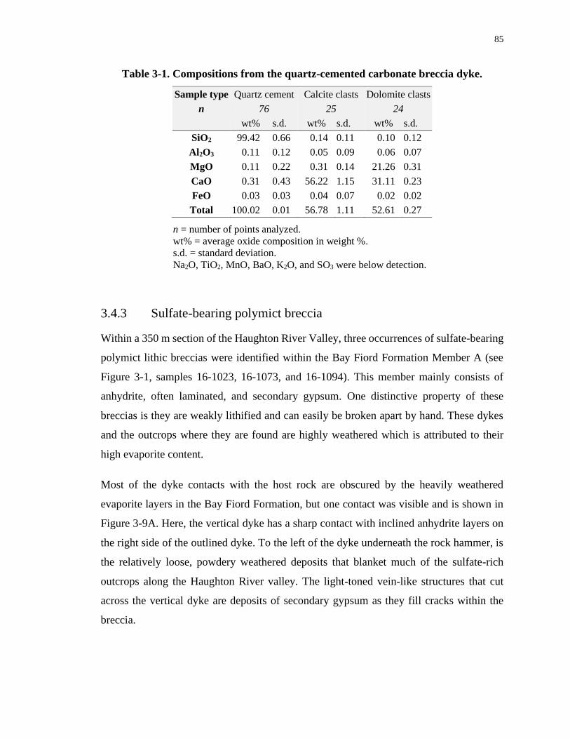
85

Table 3-1. Compositions from the quartz-cemented carbonate breccia dyke.

Sample type Quartz cement Calcite clasts Dolomite clasts

n 76 25 24

wt% s.d. wt% s.d. wt% s.d.

SiO2 99.42 0.66 0.14 0.11 0.10 0.12

Al2O3 0.11 0.12 0.05 0.09 0.06 0.07

MgO 0.11 0.22 0.31 0.14 21.26 0.31

CaO 0.31 0.43 56.22 1.15 31.11 0.23

FeO 0.03 0.03 0.04 0.07 0.02 0.02

Total 100.02 0.01 56.78 1.11 52.61 0.27

n = number of points analyzed.

wt% = average oxide composition in weight %.

s.d. = standard deviation.

Na2O, TiO2, MnO, BaO, K2O, and SO3 were below detection.

3.4.3 Sulfate-bearing polymict breccia

Within a 350 m section of the Haughton River Valley, three occurrences of sulfate-bearing

polymict lithic breccias were identified within the Bay Fiord Formation Member A (see

Figure 3-1, samples 16-1023, 16-1073, and 16-1094). This member mainly consists of

anhydrite, often laminated, and secondary gypsum. One distinctive property of these

breccias is they are weakly lithified and can easily be broken apart by hand. These dykes

and the outcrops where they are found are highly weathered which is attributed to their

high evaporite content.

Most of the dyke contacts with the host rock are obscured by the heavily weathered

evaporite layers in the Bay Fiord Formation, but one contact was visible and is shown in

Figure 3-9A. Here, the vertical dyke has a sharp contact with inclined anhydrite layers on

the right side of the outlined dyke. To the left of the dyke underneath the rock hammer, is

the relatively loose, powdery weathered deposits that blanket much of the sulfate-rich

outcrops along the Haughton River valley. The light-toned vein-like structures that cut

across the vertical dyke are deposits of secondary gypsum as they fill cracks within the

breccia.

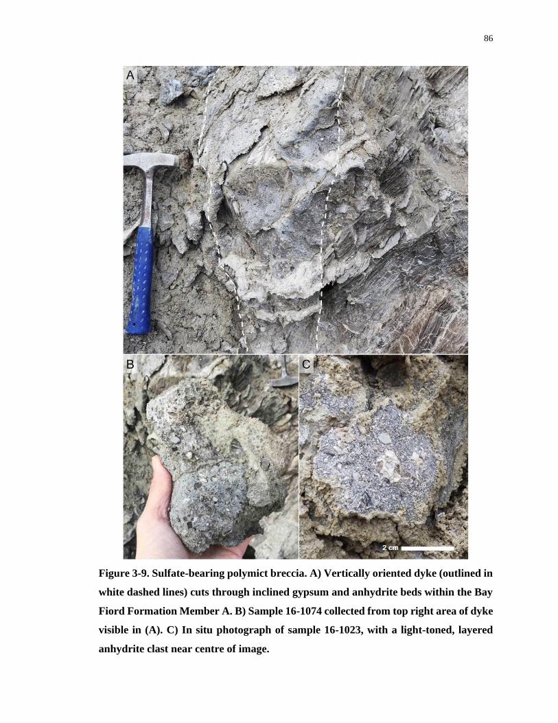
86

Figure 3-9. Sulfate-bearing polymict breccia. A) Vertically oriented dyke (outlined in

white dashed lines) cuts through inclined gypsum and anhydrite beds within the Bay

Fiord Formation Member A. B) Sample 16-1074 collected from top right area of dyke

visible in (A). C) In situ photograph of sample 16-1023, with a light-toned, layered

anhydrite clast near centre of image.

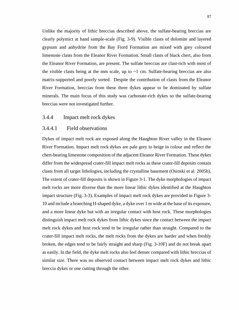
87

Unlike the majority of lithic breccias described above, the sulfate-bearing breccias are

clearly polymict at hand sample-scale (Fig. 3-9). Visible clasts of dolomite and layered

gypsum and anhydrite from the Bay Fiord Formation are mixed with grey coloured

limestone clasts from the Eleanor River Formation. Small clasts of black chert, also from

the Eleanor River Formation, are present. The sulfate breccias are clast-rich with most of

the visible clasts being at the mm scale, up to ~1 cm. Sulfate-bearing breccias are also

matrix-supported and poorly sorted. Despite the contribution of clasts from the Eleanor

River Formation, breccias from these three dykes appear to be dominated by sulfate

minerals. The main focus of this study was carbonate-rich dykes so the sulfate-bearing

breccias were not investigated further.

3.4.4 Impact melt rock dykes

3.4.4.1 Field observations

Dykes of impact melt rock are exposed along the Haughton River valley in the Eleanor

River Formation. Impact melt rock dykes are pale grey to beige in colour and reflect the

chert-bearing limestone composition of the adjacent Eleanor River Formation. These dykes

differ from the widespread crater-fill impact melt rocks as these crater-fill deposits contain

clasts from all target lithologies, including the crystalline basement (Osinski et al. 2005b).

The extent of crater-fill deposits is shown in Figure 3-1. The dyke morphologies of impact

melt rocks are more diverse than the more linear lithic dykes identified at the Haughton

impact structure (Fig. 3-3). Examples of impact melt rock dykes are provided in Figure 3-

10 and include a branching H-shaped dyke, a dyke over 1 m wide at the base of its exposure,

and a more linear dyke but with an irregular contact with host rock. These morphologies

distinguish impact melt rock dykes from lithic dykes since the contact between the impact

melt rock dykes and host rock tend to be irregular rather than straight. Compared to the

crater-fill impact melt rocks, the melt rocks from the dykes are harder and when freshly

broken, the edges tend to be fairly straight and sharp (Fig. 3-10F) and do not break apart

as easily. In the field, the dyke melt rocks also feel denser compared with lithic breccias of

similar size. There was no observed contact between impact melt rock dykes and lithic

breccia dykes or one cutting through the other.

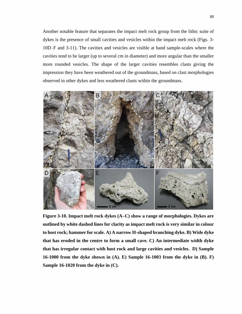
88

Another notable feature that separates the impact melt rock group from the lithic suite of

dykes is the presence of small cavities and vesicles within the impact melt rock (Figs. 3-

10D–F and 3-11). The cavities and vesicles are visible at hand sample-scales where the

cavities tend to be larger (up to several cm in diameter) and more angular than the smaller

more rounded vesicles. The shape of the larger cavities resembles clasts giving the

impression they have been weathered out of the groundmass, based on clast morphologies

observed in other dykes and less weathered clasts within the groundmass.

Figure 3-10. Impact melt rock dykes (A–C) show a range of morphologies. Dykes are

outlined by white dashed lines for clarity as impact melt rock is very similar in colour

to host rock; hammer for scale. A) A narrow H-shaped branching dyke. B) Wide dyke

that has eroded in the centre to form a small cave. C) An intermediate width dyke

that has irregular contact with host rock and large cavities and vesicles. D) Sample

16-1000 from the dyke shown in (A). E) Sample 16-1003 from the dyke in (B). F)

Sample 16-1020 from the dyke in (C).

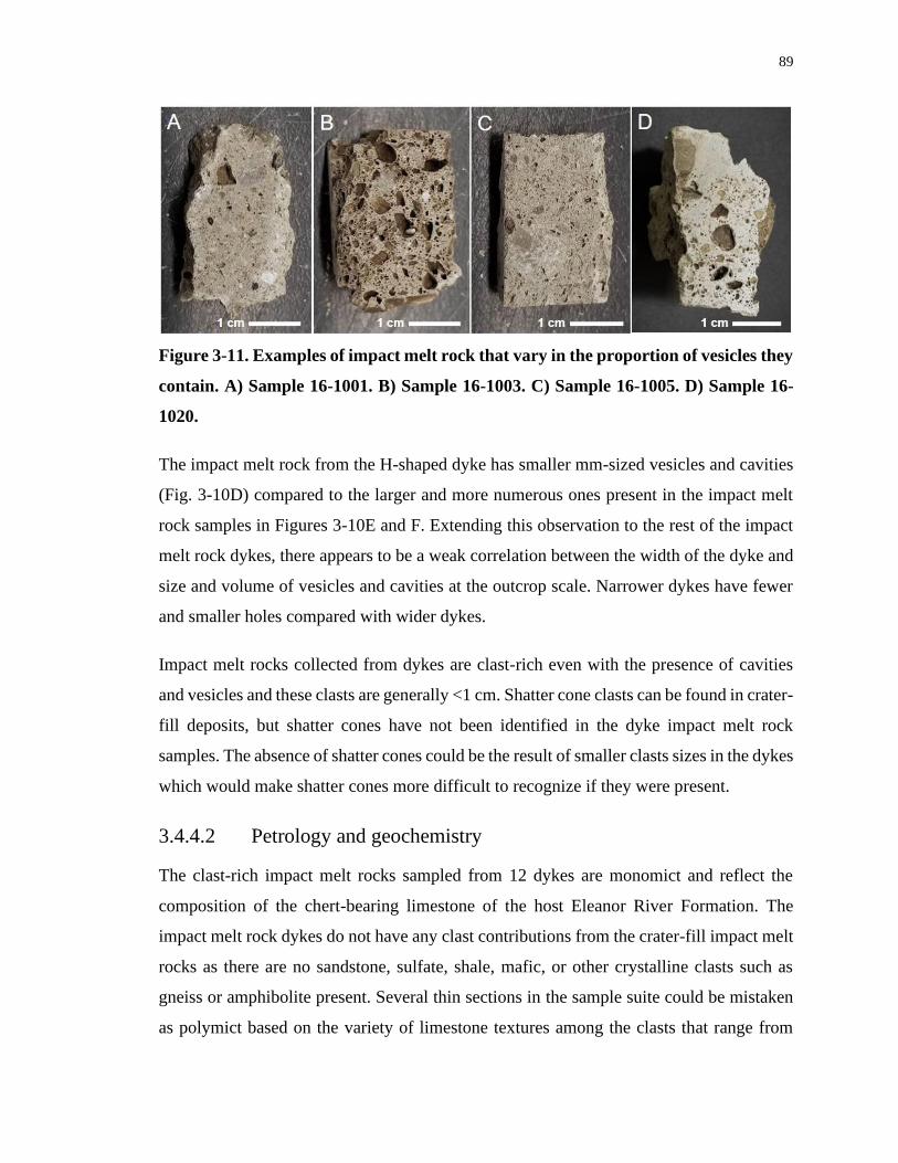
89

Figure 3-11. Examples of impact melt rock that vary in the proportion of vesicles they

contain. A) Sample 16-1001. B) Sample 16-1003. C) Sample 16-1005. D) Sample 16-

1020.

The impact melt rock from the H-shaped dyke has smaller mm-sized vesicles and cavities

(Fig. 3-10D) compared to the larger and more numerous ones present in the impact melt

rock samples in Figures 3-10E and F. Extending this observation to the rest of the impact

melt rock dykes, there appears to be a weak correlation between the width of the dyke and

size and volume of vesicles and cavities at the outcrop scale. Narrower dykes have fewer

and smaller holes compared with wider dykes.

Impact melt rocks collected from dykes are clast-rich even with the presence of cavities

and vesicles and these clasts are generally <1 cm. Shatter cone clasts can be found in crater-

fill deposits, but shatter cones have not been identified in the dyke impact melt rock

samples. The absence of shatter cones could be the result of smaller clasts sizes in the dykes

which would make shatter cones more difficult to recognize if they were present.

3.4.4.2 Petrology and geochemistry

The clast-rich impact melt rocks sampled from 12 dykes are monomict and reflect the

composition of the chert-bearing limestone of the host Eleanor River Formation. The

impact melt rock dykes do not have any clast contributions from the crater-fill impact melt

rocks as there are no sandstone, sulfate, shale, mafic, or other crystalline clasts such as

gneiss or amphibolite present. Several thin sections in the sample suite could be mistaken

as polymict based on the variety of limestone textures among the clasts that range from

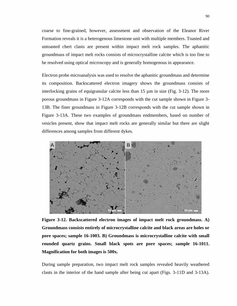
90

coarse to fine-grained, however, assessment and observation of the Eleanor River

Formation reveals it is a heterogenous limestone unit with multiple members. Toasted and

untoasted chert clasts are present within impact melt rock samples. The aphanitic

groundmass of impact melt rocks consists of microcrystalline calcite which is too fine to

be resolved using optical microscopy and is generally homogenous in appearance.

Electron probe microanalysis was used to resolve the aphanitic groundmass and determine

its composition. Backscattered electron imagery shows the groundmass consists of

interlocking grains of equigranular calcite less than 15 µm in size (Fig. 3-12). The more

porous groundmass in Figure 3-12A corresponds with the cut sample shown in Figure 3-

13B. The finer groundmass in Figure 3-12B corresponds with the cut sample shown in

Figure 3-13A. These two examples of groundmass endmembers, based on number of

vesicles present, show that impact melt rocks are generally similar but there are slight

differences among samples from different dykes.

Figure 3-12. Backscattered electron images of impact melt rock groundmass. A)

Groundmass consists entirely of microcrystalline calcite and black areas are holes or

pore spaces; sample 16-1003. B) Groundmass is microcrystalline calcite with small

rounded quartz grains. Small black spots are pore spaces; sample 16-1011.

Magnification for both images is 500x.

During sample preparation, two impact melt rock samples revealed heavily weathered

clasts in the interior of the hand sample after being cut apart (Figs. 3-11D and 3-13A).

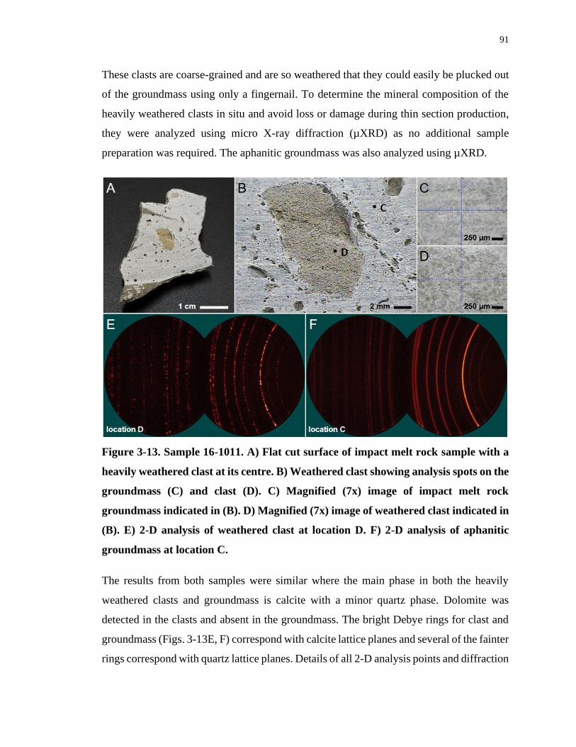
91

These clasts are coarse-grained and are so weathered that they could easily be plucked out

of the groundmass using only a fingernail. To determine the mineral composition of the

heavily weathered clasts in situ and avoid loss or damage during thin section production,

they were analyzed using micro X-ray diffraction (µXRD) as no additional sample

preparation was required. The aphanitic groundmass was also analyzed using µXRD.

Figure 3-13. Sample 16-1011. A) Flat cut surface of impact melt rock sample with a

heavily weathered clast at its centre. B) Weathered clast showing analysis spots on the

groundmass (C) and clast (D). C) Magnified (7x) image of impact melt rock

groundmass indicated in (B). D) Magnified (7x) image of weathered clast indicated in

(B). E) 2-D analysis of weathered clast at location D. F) 2-D analysis of aphanitic

groundmass at location C.

The results from both samples were similar where the main phase in both the heavily

weathered clasts and groundmass is calcite with a minor quartz phase. Dolomite was

detected in the clasts and absent in the groundmass. The bright Debye rings for clast and

groundmass (Figs. 3-13E, F) correspond with calcite lattice planes and several of the fainter

rings correspond with quartz lattice planes. Details of all 2-D analysis points and diffraction

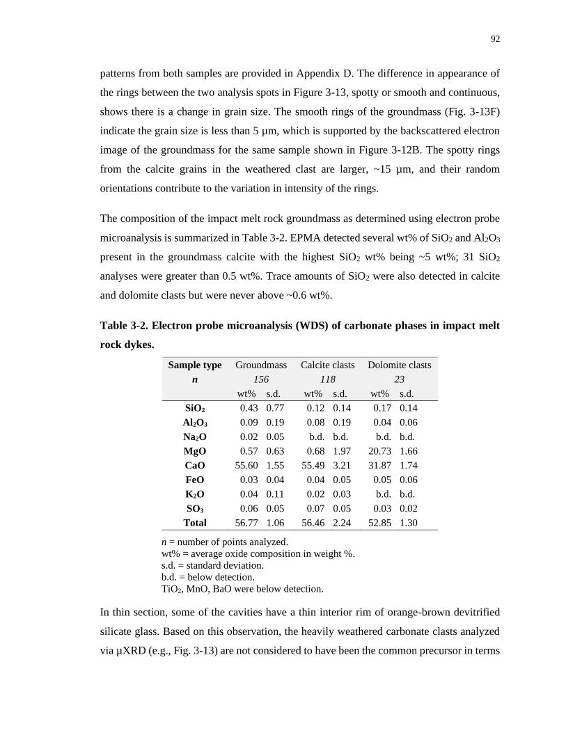
92

patterns from both samples are provided in Appendix D. The difference in appearance of

the rings between the two analysis spots in Figure 3-13, spotty or smooth and continuous,

shows there is a change in grain size. The smooth rings of the groundmass (Fig. 3-13F)

indicate the grain size is less than 5 µm, which is supported by the backscattered electron

image of the groundmass for the same sample shown in Figure 3-12B. The spotty rings

from the calcite grains in the weathered clast are larger, ~15 µm, and their random

orientations contribute to the variation in intensity of the rings.

The composition of the impact melt rock groundmass as determined using electron probe

microanalysis is summarized in Table 3-2. EPMA detected several wt% of SiO2 and Al2O3

present in the groundmass calcite with the highest SiO2 wt% being ~5 wt%; 31 SiO2

analyses were greater than 0.5 wt%. Trace amounts of SiO2 were also detected in calcite

and dolomite clasts but were never above ~0.6 wt%.

Table 3-2. Electron probe microanalysis (WDS) of carbonate phases in impact melt

rock dykes.

Sample type Groundmass Calcite clasts Dolomite clasts

n 156 118 23 wt% s.d. wt% s.d. wt% s.d.

SiO2 0.43 0.77 0.12 0.14 0.17 0.14

Al2O3 0.09 0.19 0.08 0.19 0.04 0.06

Na2O 0.02 0.05 b.d. b.d. b.d. b.d.

MgO 0.57 0.63 0.68 1.97 20.73 1.66

CaO 55.60 1.55 55.49 3.21 31.87 1.74

FeO 0.03 0.04 0.04 0.05 0.05 0.06

K2O 0.04 0.11 0.02 0.03 b.d. b.d.

SO3 0.06 0.05 0.07 0.05 0.03 0.02

Total 56.77 1.06 56.46 2.24 52.85 1.30

n = number of points analyzed.

wt% = average oxide composition in weight %.

s.d. = standard deviation.

b.d. = below detection.

TiO2, MnO, BaO were below detection.

In thin section, some of the cavities have a thin interior rim of orange-brown devitrified

silicate glass. Based on this observation, the heavily weathered carbonate clasts analyzed

via µXRD (e.g., Fig. 3-13) are not considered to have been the common precursor in terms

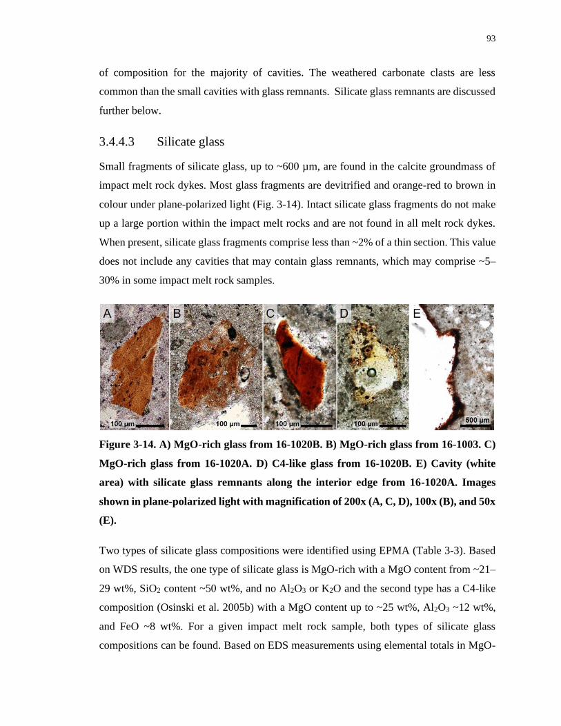
93

of composition for the majority of cavities. The weathered carbonate clasts are less

common than the small cavities with glass remnants. Silicate glass remnants are discussed

further below.

3.4.4.3 Silicate glass

Small fragments of silicate glass, up to ~600 µm, are found in the calcite groundmass of

impact melt rock dykes. Most glass fragments are devitrified and orange-red to brown in

colour under plane-polarized light (Fig. 3-14). Intact silicate glass fragments do not make

up a large portion within the impact melt rocks and are not found in all melt rock dykes.

When present, silicate glass fragments comprise less than ~2% of a thin section. This value

does not include any cavities that may contain glass remnants, which may comprise ~5–

30% in some impact melt rock samples.

Figure 3-14. A) MgO-rich glass from 16-1020B. B) MgO-rich glass from 16-1003. C)

MgO-rich glass from 16-1020A. D) C4-like glass from 16-1020B. E) Cavity (white

area) with silicate glass remnants along the interior edge from 16-1020A. Images

shown in plane-polarized light with magnification of 200x (A, C, D), 100x (B), and 50x

(E).

Two types of silicate glass compositions were identified using EPMA (Table 3-3). Based

on WDS results, the one type of silicate glass is MgO-rich with a MgO content from ~21–

29 wt%, SiO2 content ~50 wt%, and no Al2O3 or K2O and the second type has a C4-like

composition (Osinski et al. 2005b) with a MgO content up to ~25 wt%, Al2O3 ~12 wt%,

and FeO ~8 wt%. For a given impact melt rock sample, both types of silicate glass

compositions can be found. Based on EDS measurements using elemental totals in MgO-

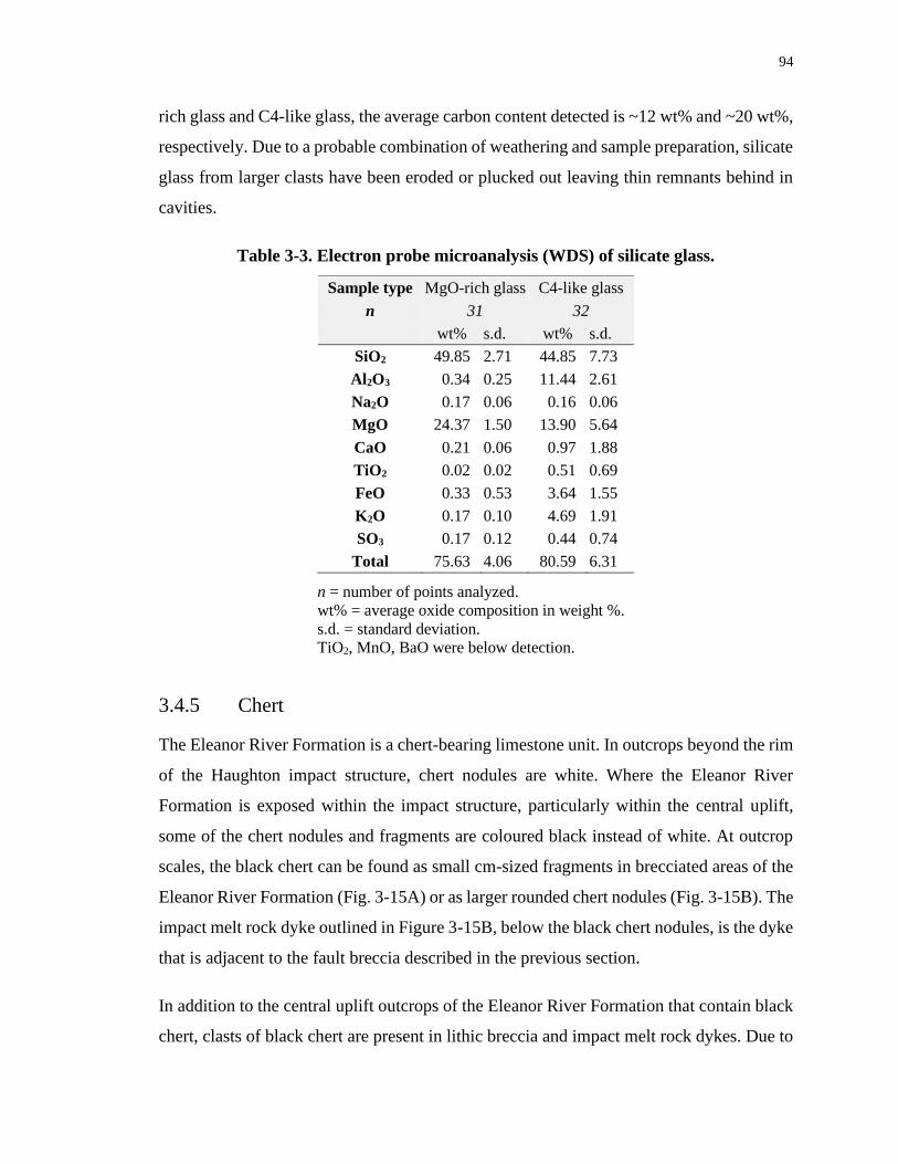
94

rich glass and C4-like glass, the average carbon content detected is ~12 wt% and ~20 wt%,

respectively. Due to a probable combination of weathering and sample preparation, silicate

glass from larger clasts have been eroded or plucked out leaving thin remnants behind in

cavities.

Table 3-3. Electron probe microanalysis (WDS) of silicate glass.

Sample type MgO-rich glass C4-like glass

n 31 32 wt% s.d. wt% s.d.

SiO2 49.85 2.71 44.85 7.73

Al2O3 0.34 0.25 11.44 2.61

Na2O 0.17 0.06 0.16 0.06

MgO 24.37 1.50 13.90 5.64

CaO 0.21 0.06 0.97 1.88

TiO2 0.02 0.02 0.51 0.69

FeO 0.33 0.53 3.64 1.55

K2O 0.17 0.10 4.69 1.91

SO3 0.17 0.12 0.44 0.74

Total 75.63 4.06 80.59 6.31

n = number of points analyzed.

wt% = average oxide composition in weight %.

s.d. = standard deviation.

TiO2, MnO, BaO were below detection.

3.4.5 Chert

The Eleanor River Formation is a chert-bearing limestone unit. In outcrops beyond the rim

of the Haughton impact structure, chert nodules are white. Where the Eleanor River

Formation is exposed within the impact structure, particularly within the central uplift,

some of the chert nodules and fragments are coloured black instead of white. At outcrop

scales, the black chert can be found as small cm-sized fragments in brecciated areas of the

Eleanor River Formation (Fig. 3-15A) or as larger rounded chert nodules (Fig. 3-15B). The

impact melt rock dyke outlined in Figure 3-15B, below the black chert nodules, is the dyke

that is adjacent to the fault breccia described in the previous section.

In addition to the central uplift outcrops of the Eleanor River Formation that contain black

chert, clasts of black chert are present in lithic breccia and impact melt rock dykes. Due to

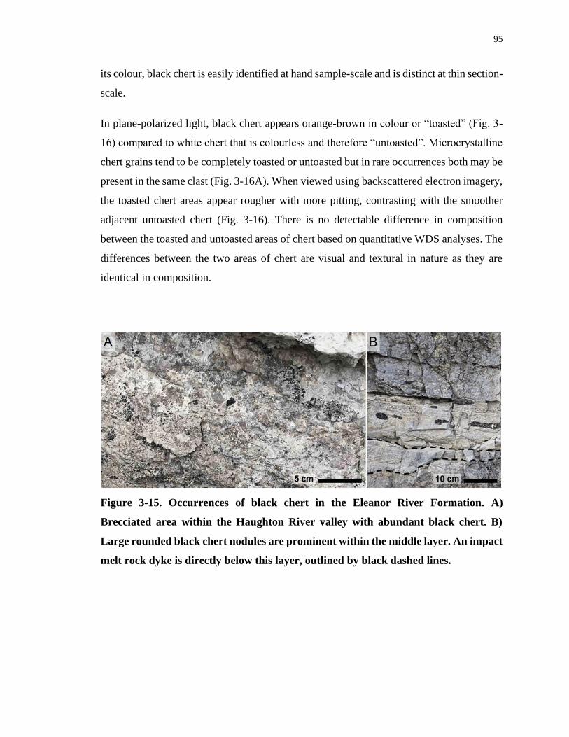
95

its colour, black chert is easily identified at hand sample-scale and is distinct at thin section-

scale.

In plane-polarized light, black chert appears orange-brown in colour or “toasted” (Fig. 3-

16) compared to white chert that is colourless and therefore “untoasted”. Microcrystalline

chert grains tend to be completely toasted or untoasted but in rare occurrences both may be

present in the same clast (Fig. 3-16A). When viewed using backscattered electron imagery,

the toasted chert areas appear rougher with more pitting, contrasting with the smoother

adjacent untoasted chert (Fig. 3-16). There is no detectable difference in composition

between the toasted and untoasted areas of chert based on quantitative WDS analyses. The

differences between the two areas of chert are visual and textural in nature as they are

identical in composition.

Figure 3-15. Occurrences of black chert in the Eleanor River Formation. A)

Brecciated area within the Haughton River valley with abundant black chert. B)

Large rounded black chert nodules are prominent within the middle layer. An impact

melt rock dyke is directly below this layer, outlined by black dashed lines.

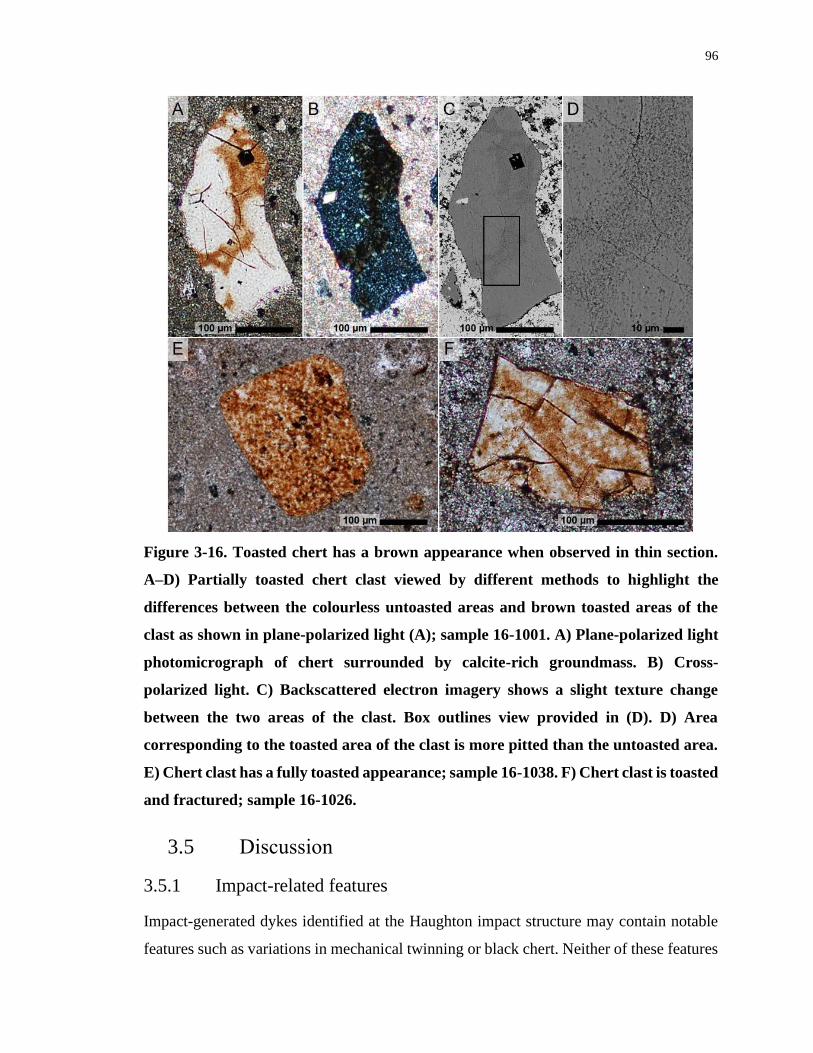
96

Figure 3-16. Toasted chert has a brown appearance when observed in thin section.

A–D) Partially toasted chert clast viewed by different methods to highlight the

differences between the colourless untoasted areas and brown toasted areas of the

clast as shown in plane-polarized light (A); sample 16-1001. A) Plane-polarized light

photomicrograph of chert surrounded by calcite-rich groundmass. B) Cross-

polarized light. C) Backscattered electron imagery shows a slight texture change

between the two areas of the clast. Box outlines view provided in (D). D) Area

corresponding to the toasted area of the clast is more pitted than the untoasted area.

E) Chert clast has a fully toasted appearance; sample 16-1038. F) Chert clast is toasted

and fractured; sample 16-1026.

3.5 Discussion

3.5.1 Impact-related features

Impact-generated dykes identified at the Haughton impact structure may contain notable

features such as variations in mechanical twinning or black chert. Neither of these features

97

are specific to a certain dyke material i.e., lithic breccia or impact melt rock, as they can be

found in both.

Variation in mechanical twinning of calcite has been examined and correlated with changes

in temperature (Burkhard 1993) and through experimental work by Lindgren et al. (2013)

that investigated the peak shock pressure threshold required to generate calcite twins and

found they begin to form ~110 to 480 MPa. As shown in samples from Haughton in Figure

3-2, calcite twins have a range of appearances. Type I calcite twins can form at

temperatures <200°C and with increasing temperature and deformation, Type IV calcite

twins can form at >250°C (Burkhard 1993). Twin formation can also depend on factors

such as grain size, crystallographic orientation, and porosity of the host rock (Burkhard

1993; Lindgren et al. 2013) so it is not a straightforward relationship. While the range in

appearance of calcite twins is interesting, mechanical twinning is not a reliable diagnostic

feature to identify shocked carbonates as twinning occurs naturally as a deformation

mechanism (Burkhard 1993).

The Eleanor River Formation on Devon Island is a limestone unit that can contain abundant

white chert nodules (Thorsteinsson and Mayr 1987). White chert nodules may also occur

in lower stratigraphic units, e.g., the Cape Clay Formation, or higher stratigraphic units

e.g., the Thumb Mountain Formation (Thorsteinsson and Mayr 1987). The abundance of

white chert nodules within the sedimentary target sequence of the Haughton impact

structure makes the occurrence of black chert within the Eleanor River Formation in the

central uplift region of the impact structure a curious observation. Compositional

difference was ruled out as the cause for colour change. In thin section under plane-

polarized light, the chert clasts that appear orange-brown in colour are described as toasted

which correspond with black chert clasts. Comparing the differences between the toasted

and untoasted or colourless chert there are parallel observations that can be made with

toasted quartz from other terrestrial impact structures.

Toasted quartz was first described in quartz from the Manson impact structure and thought

to be the result of fluid inclusions generated along the recrystallized glass of planar

deformation features, or PDFs (Short and Gold 1996; Whitehead et al. 2002). The fluid

98

inclusions enhance the scattering of transmitted light which results in a brown or orange-

brown colour to the quartz (Whitehead et al. 2002). The origin of toasted quartz was

revisited by Ferrière et al. (2009) and their conclusions suggested that toasted quartz

exhibits a higher quantity of vesicles compared with untoasted quartz that scatter

transmitted light, which is similar to previous findings. The main difference found by

Ferrière et al. (2009) in revisiting the origins of toasted quartz is that the vesicles are

unrelated to recrystallized glass associated with PDFs, as was proposed by Whitehead et

al. (2002).

In backscattered electron images, toasted chert from Haughton has a more porous texture

(Fig. 3-16) than untoasted chert which is consistent with the sponge-like texture observed

in toasted quartz (Ferrière et al. 2009). Shock metamorphism conditions required to

generate toasted quartz have previously been identified at Haughton as toasted quartz has

been reported in classes 2 through 4 of impact metamorphosed sandstones collected from

crater-fill impact melt rocks (Osinski 2007). Toasted quartz has been identified from at

least 26 terrestrial impact structures (Ferrière et al. 2009; Short and Gold 1996; Whitehead

et al. 2002) but this is the first report of toasted chert from an impact structure. In hand

samples, toasted quartz takes on a white chalky appearance but is not the same as milky

quartz (Short and Gold 1996; Whitehead et al. 2002). The colour change of chert from

white to black at Haughton could be an effect of grain size as chert is a microcrystalline

form of quartz. Based on the observations and parallels with toasted quartz, the black chert

in the central uplift suggests the colour change is a result of increased exposure to shock.

3.5.2 Dyke formation

Impact-generated dykes throughout the Haughton impact structure are diverse and this is

reflected in the composition and state (i.e., lithic breccia or impact melt rock) among dykes.

Dykes are exposed near the edge of the central uplift and toward the rim of the impact

structure (Fig. 3-1). Based on cratering models (e.g., Lambert 1981; Osinski and Spray

2005) and more eroded terrestrial impact structures, such as Tunnunik (Chapter 2), dykes

are found throughout the central uplift within the floor of an impact structure. Despite

extensive crater-fill deposits that blanket the central area of Haughton, many of the dykes

99

identified in this study were found within the central uplift (Fig. 3-1). The dykes examined

by Bischoff and Oskierski (1988) show a similar distribution as this study.

Several lithic breccia dykes are associated with faults or bedding planes within the target

rock. Faults can be initiated during several points during the impact cratering process. The

first faults are created during the excavation stage of crater formation which are related to

the expanding transient cavity and release of pressure following the shock wave (e.g.,

Lambert 1981). Subsequent collapse of the unstable transient cavity during the

modification stage creates new faults, especially toward the rim region of the crater. The

sharp, and generally straight, contact between lithic dykes and host rock indicate a dynamic

origin for lithic dykes (Bischoff and Oskierski 1988). The majority of lithic dykes

examined in this study are monomict, indicating the lithic material was not transported

great distances and were derived from a single unit within the target sequence. Overall, the

monomict breccias do not show preferred alignment within the dykes which suggests flow

within the dyke was not strong enough to orient clasts with elongated shapes. These

autochthonous dykes represent the uppermost portion of the dyke and as they continue

deeper into the crater floor, more clasts were likely incorporated into the dyke to change

the dyke from monomict to polymict. We suggest several dykes examined, specifically the

sulfate-bearing breccias, were determined to be polymict as a result of these dykes being

located near contacts between units and had a short transport distance.

From the single thin section from the quartz-cemented dyke, it is not clear if the quartz

cement is widespread throughout the dyke or just happened to be more localized where the

sample was collected. What can be inferred based on the clasts is there was more transport

within this dyke since the dolomite and calcite clasts do not match the microfossil-bearing

limestone host rock. The absence of microfossils within the calcite clasts makes this an

allochthonous breccia which differs from the autochthonous monomict breccias found

within the impact structure. The slight anomaly in calcite composition suggests the rounded

calcite clasts are actually melted calcite globules that had limited mixing with the

surrounding silicate cement (Osinski et al. 2008a). Quartz-cemented breccias have been

reported from other locations in the Haughton impact structure (Osinski et al. 2005c).

These occurrences are associated with hydrothermal activity and have a different

100

appearance in hand sample and thin section compared to sample 00-011, the quartz-

cemented carbonate breccia in this study. In hand sample and thin section, the quartz

cement is prominent with large interlocking crystals visible in thin section compared to

sample 00-011 where the cement is not resolvable even using optical microscopy.

Impact melt rocks are generated following the passage of the rarefaction wave and

decompression within the target (Grieve et al. 1977; Osinski et al. 2018). Dykes containing

impact melt rocks would then be emplaced during the excavation stage as impact melt is

injected downward and outward into fractures in the crater floor and walls (Osinski et al.

2018). At Haughton, the crater floor within the central uplift area is not exposed but the

Haughton River valley does expose impact melt rock dykes near the edge of the present-

day extent of crater-fill deposits. The contact between melt rock dykes and host rock is not

as sharp as the contacts observed with lithic breccia dykes and the edge of the melt rock

dykes are more irregular and less straight than the lithic dykes. This observation could be

due to the lower viscosity of carbonate-rich melt rocks (Jones et al. 2013) which would

allow the melts to fill irregular fractures with less erosion of the host rock. The monomict

clast composition within the melt rock dykes indicates the injection of these dykes is not

simply an extension of the crater-fill impact melt rock which contains clasts from the entire

target sequence. Since the impact melt rock dykes have only been identified within the

Eleanor River Formation to date, it remains unclear if the clasts within the dykes always

match the host formation. To answer this question, impact melt rock dykes would need to

be identified in additional locations around the edge of the crater-fill deposits where the

host formations include the Bay Fiord Formation, Thumb Mountain Formation, and Allen

Bay Formation (Osinski et al. 2005a).

3.5.3 Clast-rich impact melt rocks

Clast-rich impact melt rocks have been associated with the Haughton impact structure as

crater-fill impactite deposits since their re-examination and reclassification in 2001

(Osinski and Spray 2001). Before this time the Haughton crater-fill deposits were described

as fragmental or clastic breccia (Redeker and Stöffler 1988). The crater-fill impact melt

rocks at Haughton are carbonate-rich, unlike most impact melt rocks from terrestrial impact

structures which originate from crystalline target rocks. Deposits of impact melt rocks were

101

later identified in the crater rim region and interpreted as ejecta deposits by Osinski et al.

(2005b). This study has added a third occurrence of impact melt rocks at the Haughton

impact structure which are located in dykes exposed near the southeast edge of the crater-

fill deposits in the Haughton River valley (Fig. 3-1). Carbonate-rich melt rocks have been

reported from a number of impact sites including the Ries and Chicxulub impact structures

(e.g., Graup 1999; Jones et al. 2000; Osinski et al. 2008a).

The impact melt rocks described here from impact-generated dykes have similarities and

differences with the crater-fill deposits at Haughton. The primary difference is crater-fill

impactites contain clasts from all units in the target sequence down to and including the

crystalline basement (Osinski and Spray 2001) whereas impact melt rocks in the dykes

only contain clasts from the Eleanor River Formation. The crater-fill impactites are

currently found up to ~5 km from the centre of the impact structure and have a current

maximum thickness of ~125 m (Osinski and Spray 2001). The pale grey impact melt rocks

near the southwest rim of the impact structure are ejecta and have a resemblance to the

crater-fill impactites but are not identical and differ in groundmass and clast composition.

The groundmass of crater rim impactites is up to ~60 vol% calcite, <10 vol% impact melt

glass, and no anhydrite whereas the crater-fill impactites are more diverse with <10 to >50

vol% calcite, <0.5 to ~40 vol% silicate impact melt glass, and can have ~30 to 60 vol%

anhydrite (Osinski et al. 2005b). As previously noted, crater-fill impactites contain clasts

from the entire target sequence while the clasts in the crater rim impactites are mainly

limestone and dolostone with sandstone and evaporite clasts rare and crystalline clasts are

absent (Osinski et al. 2005b).

Based on these modal compositions, the dyke impact melt rocks more closely resemble the

pale grey crater rim impactites than the crater-fill deposits. While the dyke melt rocks are

more similar to the pale grey crater rim impactites with a calcite-rich groundmass but

without the impact melt glass (Table 3-2), several key differences remain. Clast-wise, the

dykes closely resemble the composition of the Eleanor River Formation where dolostone

clasts are rare and chert is more common compared to the crater rim impactites (Osinski et

al. 2005b). The overall texture and appearance of the impact melt rock dykes is the most

obvious difference, especially at hand sample-scale, with the presence of vesicles and

102

cavities in the groundmass of dyke impact melt rocks. Vesicles and cavities are rare in both

the crater rim and crater-fill impact melt rocks. The only mention of vesicles observed in

crater-fill or crater rim impactites are specifically within silicate impact melt glass and not

within the calcite groundmass (Osinski et al. 2005b).

Additional physical differences between dyke impact melt rocks and impact melt rocks

from crater-fill and crater rim deposits include 1) the groundmass in dyke melt rocks is

more difficult to break apart than crater-fill deposits, and 2) in thin section, the aphanitic

melt rock groundmass is finer in dykes than crater-fill or crater rim samples. These

differences could relate to the cooling rate of the melt rock at each location. Since the dyke

impact melt rocks are finer grained, it suggests they cooled more rapidly. Heat should

conduct more rapidly from the melt rock in the narrow dykes (Osinski et al. 2018).

Conversely, the thicker crater-fill impact melt rocks, originally ~200 m thick, would have

taken longer to cool to ambient temperatures on the order of several thousand years, based

on evidence from post-impact hydrothermal systems present within the Haughton impact

structure (Osinski et al. 2005c).

3.5.4 Comparison with other impact structures

The aphanitic texture of the impact melt rock dykes at Haughton is comparable to aphanitic

melt rocks described from other impact structures (Osinski et al. 2018). The Haughton

impact melt rock dykes also contain lithic and mineral clasts as well as shocked clasts in

the form of silicate glass and shocked chert. The main difference between the melt rocks

from Haughton and most other impact structures is composition, where the Haughton melt

rocks are carbonate-rich with the melt rock dykes being more specifically calcite-rich.

While calcite typically does not form igneous textures in impact structures, mantle-derived

carbonatites have a significant carbonate fraction and are the most comparable non-impact

source of igneous carbonates (Osinski et al. 2018). Textures observed in the impact melt

rock dykes are not as varied or complex in composition as can be found in carbonatites

(e.g. Chakhmouradian et al. 2016), especially when the bulk of the melt rock dyke

groundmass has a calcite composition.

What makes the dyke melt rocks most distinct from the crater-fill and crater rim melt rock

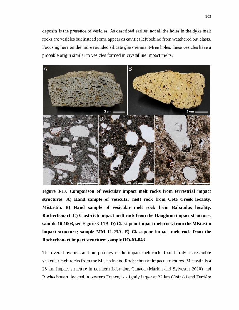
103

deposits is the presence of vesicles. As described earlier, not all the holes in the dyke melt

rocks are vesicles but instead some appear as cavities left behind from weathered out clasts.

Focusing here on the more rounded silicate glass remnant-free holes, these vesicles have a

probable origin similar to vesicles formed in crystalline impact melts.

Figure 3-17. Comparison of vesicular impact melt rocks from terrestrial impact

structures. A) Hand sample of vesicular melt rock from Coté Creek locality,

Mistastin. B) Hand sample of vesicular melt rock from Babaudus locality,

Rochechouart. C) Clast-rich impact melt rock from the Haughton impact structure;

sample 16-1003, see Figure 3-11B. D) Clast-poor impact melt rock from the Mistastin

impact structure; sample MM 11-23A. E) Clast-poor impact melt rock from the

Rochechouart impact structure; sample RO-01-043.

The overall textures and morphology of the impact melt rocks found in dykes resemble

vesicular melt rocks from the Mistastin and Rochechouart impact structures. Mistastin is a

28 km impact structure in northern Labrador, Canada (Marion and Sylvester 2010) and

Rochechouart, located in western France, is slightly larger at 32 km (Osinski and Ferrière

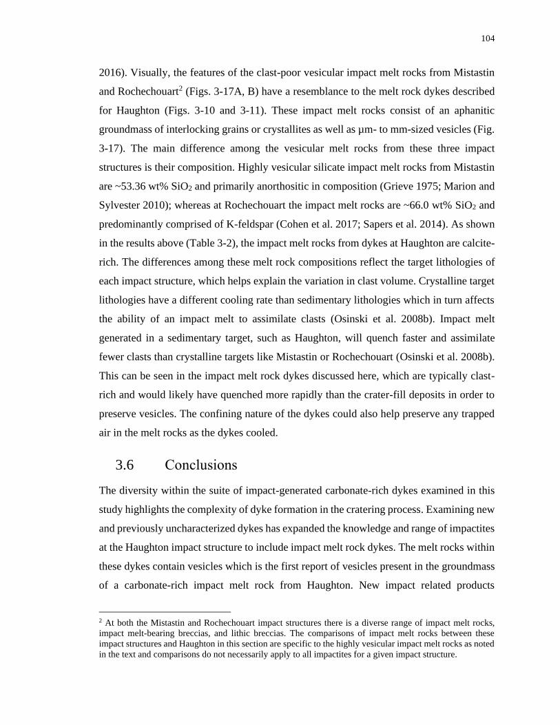
104

2016). Visually, the features of the clast-poor vesicular impact melt rocks from Mistastin

and Rochechouart2 (Figs. 3-17A, B) have a resemblance to the melt rock dykes described

for Haughton (Figs. 3-10 and 3-11). These impact melt rocks consist of an aphanitic

groundmass of interlocking grains or crystallites as well as µm- to mm-sized vesicles (Fig.

3-17). The main difference among the vesicular melt rocks from these three impact

structures is their composition. Highly vesicular silicate impact melt rocks from Mistastin

are ~53.36 wt% SiO2 and primarily anorthositic in composition (Grieve 1975; Marion and

Sylvester 2010); whereas at Rochechouart the impact melt rocks are ~66.0 wt% SiO2 and

predominantly comprised of K-feldspar (Cohen et al. 2017; Sapers et al. 2014). As shown

in the results above (Table 3-2), the impact melt rocks from dykes at Haughton are calcite-

rich. The differences among these melt rock compositions reflect the target lithologies of

each impact structure, which helps explain the variation in clast volume. Crystalline target

lithologies have a different cooling rate than sedimentary lithologies which in turn affects

the ability of an impact melt to assimilate clasts (Osinski et al. 2008b). Impact melt

generated in a sedimentary target, such as Haughton, will quench faster and assimilate

fewer clasts than crystalline targets like Mistastin or Rochechouart (Osinski et al. 2008b).

This can be seen in the impact melt rock dykes discussed here, which are typically clast-

rich and would likely have quenched more rapidly than the crater-fill deposits in order to

preserve vesicles. The confining nature of the dykes could also help preserve any trapped

air in the melt rocks as the dykes cooled.

3.6 Conclusions

The diversity within the suite of impact-generated carbonate-rich dykes examined in this

study highlights the complexity of dyke formation in the cratering process. Examining new

and previously uncharacterized dykes has expanded the knowledge and range of impactites

at the Haughton impact structure to include impact melt rock dykes. The melt rocks within

these dykes contain vesicles which is the first report of vesicles present in the groundmass

of a carbonate-rich impact melt rock from Haughton. New impact related products

2 At both the Mistastin and Rochechouart impact structures there is a diverse range of impact melt rocks,

impact melt-bearing breccias, and lithic breccias. The comparisons of impact melt rocks between these

impact structures and Haughton in this section are specific to the highly vesicular impact melt rocks as noted

in the text and comparisons do not necessarily apply to all impactites for a given impact structure.

105

associated with this impact site were identified and includes toasted chert. These impactites

and products provide further insights into the products generated during the impact event

and present in a well-preserved impact structure.

3.7 References

Bischoff L., and Oskierski W. 1987. Fractures, pseudotachylite veins and breccia dikes in

the crater floor of the Rochechouart impact structure, SW-France, as indicators of

crater forming processes. In Research in Terrestrial Impact Structures, edited by Pohl

J. Braunschweig: Friedrich Vieweg and Sohn. pp. 5–29.

Bischoff L., and Oskierski W. 1988. The surface structure of the Haughton impact crater,

Devon Island, Canada. Meteoritics 23:209–220.

Burkhard M. 1993. Calcite twins, their geometry, appearance and significance as stress-

strain markers and indicators of tectonic regime: a review. Journal of Structural

Geology 15:351–368.

Caty J.-L., Chown E. H., and Roy D. W. 1976. A new astrobleme: Ile Rouleau structure,

Lake Mistassini, Quebec. Canadian Journal of Earth Sciences 13:824–831.

Chakhmouradian A. R., Reguir E. P., Zaitsev A. N., and Chakhmouradian A. R. 2016.

Calcite and dolomite in intrusive carbonatites. I. Textural variations. Mineralogy and

Petrology 110:333–360.

Cohen B. E., Mark D. F., Lee M. R., and Simpson S. L. 2017. A new high-precision

40Ar/39Ar age for the Rochechouart impact structure: At least 5 Ma older than the

Triassic–Jurassic boundary. Meteoritics & Planetary Science 52:1600–1611.

Dressler B. O., and Sharpton V. L. 1997. Breccia formation at a complex impact crater:

Slate Islands, Lake Superior, Ontario, Canada. Tectonophysics 275:285–311.

Dressler B. O., and Reimold W. U. 2004. Order or chaos? Origin and mode of emplacement

of breccias in floors of large impact structures. Earth-Science Reviews 67:1–54.

106

Ferrière L., Koeberl C., Reimold W. U., Hecht L., and Bartosova K. 2009. The origin of

“toasted” quartz in impactites revisited. 40th Lunar and Planetary Science

Conference Abstract #1751.

Flemming R. L. 2007. Micro X-ray diffraction (µXRD): a versatile technique for

characterization of Earth and planetary materials. Canadian Journal of Earth Sciences

44:1333–1346.

Graup G. 1999. Carbonate-silicate liquid immiscibility upon impact melting: Ries Crater,

Germany. Meteoritics & Planetary Science 34:425–438.

Grieve R. A. F. 1975. Petrology and chemistry of the impact melt at Mistastin Lake crater,

Labrador. Geological Society of America Bulletin 86:1617–1629.

Grieve R. A. F., Dence M. R., and Robertson P. B. 1977. Cratering processes: As

interpreted from the occurrence of impact melts. In Impact and Explosion Cratering,

edited by Roddy D. J., Pepin R. O., and Merrill R. B. New York: Pergamon Press. pp.

79–814.

Hickey L. J., Johnson K. R., and Dawson M. R. 1988. The stratigraphy, sedimentology,

and fossils of the Haughton Formation: A post-impact crater-fill, Devon Island,

N.W.T., Canada. Meteoritics 23:221–231.

Jones A. P., Claeys P., and Heuschkel S. 2000. Impact melting of carbonates from the

Chicxulub Crater. In Impacts and the Early Earth, Lecture Notes in Earth Sciences,

edited by Gilmour I., and Koeberl C. Springer-Verlag, Berlin-Heidelberg-New York.

pp. 343–361.

Jones A. P., Genge M., and Carmody L. 2013. Carbonate melts and carbonatites. Reviews

in Mineralogy and Geochemistry 75:289–322.

Lambert P. 1981. Breccia Dikes: Geological constraints on the formation of complex

craters. In Multi-ring Basins, Proc. Lunar Planet. Sci., edited by Schultz P. H., and

Merrill R. B. pp. 59–78.

107

Lindgren P., Price M. C., Lee M. R., and Burchell M. J. 2013. Constraining the pressure

threshold of impact induced calcite twinning: Implications for the deformation history

of aqueously altered carbonaceous chondrite parent bodies. Earth and Planetary

Science Letters 384:71–80.

Marion C. L., and Sylvester P. J. 2010. Composition and heterogeneity of anorthositic

impact melt at Mistastin Lake crater, Labrador. Planetary and Space Science 58:552–

573.

Metzler A., Ostertag R., Redeker H. J., and Stoffler D. 1988. Composition of the crystalline

basement and shock metamorphism of crystalline and sedimentary target rocks at the

Haughton impact crater, Devon Island, Canada. Meteoritcs 23:197–207.

Osinski G. R., and Spray J. G. 2001. Impact-generated carbonate melts: Evidence from the

Haughton structure, Canada. Earth and Planetary Science Letters 194:17–29.

Osinski G. R., and Spray J. G. 2003. Evidence for the shock melting of sulfates from the

Haughton impact structure, Arctic Canada. Earth and Planetary Science Letters

215:357–370.

Osinski G. R., Lee P., Spray J. G., Parnell J., Lim D. S. S., Bunch T. E., Cockell C. S., and

Glass B. 2005a. Geological overview and cratering model for the Haughton impact

structure, Devon Island, Canadian High Arctic. Meteoritics & Planetary Science

40:1759–1776.

Osinski G. R., Spray J. G., and Lee P. 2005b. Impactites of the Haughton impact structure,

Devon Island, Canadian High Arctic. Meteoritics & Planetary Science 40:1789–1812.

Osinski G. R., and Spray J. G. 2005. Tectonics of complex crater formation as revealed by

the Haughton impact structure, Devon Island, Canadian High Arctic. Meteoritics &

Planetary Science 40:1813–1834.

Osinski G. R., Lee P., Parnell J., Spray J. G., and Baron M. 2005c. A case study of impact-

induced hydrothermal activity: The Haughton impact structure, Devon Island,

Canadian High Arctic. Meteoritics & Planetary Science 40:1859–1877.

108

Osinski G. R. 2007. Impact metamorphism of CaCO3‐bearing sandstones at the Haughton

structure, Canada. Meteoritics & Planetary Science 42:1945–1960.

Osinski G. R., Spray J. G., and Grieve R. A. F. 2008a. Impact melting in sedimentary target

rocks: An assessment. In The Sedimentary Record of Meteorite Impacts, Special

Paper 437, edited by Evans K. R., Horton W., King Jr. D. K., and Morrow J. R.

Geological Society of America, Boulder, CO. pp. 1–18.

Osinski G. R., Grieve R. A. F., Collins G. S., Marion C., and Sylvester P. 2008b. The effect

of target lithology on the products of impact melting. Meteoritics & Planetary Science

43:1939–1954.

Osinski G. R., and Ferrière L. 2016. Shatter cones: (Mis)understood? Science Advances 2,

e160061:1–10.

Osinski G. R., Grieve R. A. F., Bleacher J. E., Neish C. D., Pilles E. A., and Tornabene L.

L. 2018. Igneous rocks formed by hypervelocity impact. Journal of Volcanology and

Geothermal Research 353:25–54.

Pontefract A., Osinski G. R., Cockell C. S., Moore C. A., Moores J. E., and Southam G.

2014. Impact-generated endolithic habitat within crystalline rocks of the Haughton

impact structure, Devon Island, Canada. Astrobiology 14:522–33.

Redeker H. J., and Stöffler D. 1988. The allochtonous polymict breccia layer of the

Haughton impact crater, Devon Island, Canada. Meteoritics 23:185–196.

Robertson P. B., and Grieve R. A. F. 1978. The Haughton impact structure. Meteoritics

13:615–619.

Sapers H. M., Osinski G. R., Banerjee N. R., Ferrière L., Lambert P., and Izawa M. R. M.

2014. Revisiting the Rochechouart impact structure, France. Meteoritics & Planetary

Science 49:2152–2168.

Short N. M., and Gold D. P. 1996. Petrography of shocked rocks from the central peak at

the Manson impact structure edited by Koeberl C., and Anderson R. R. Special Paper

109

- Geological Society of America 302:245–265.

Thorsteinsson R., and Mayr U. 1987. The Sedimentary Rocks of Devon Island, Canadian

Arctic Archipelago, Memoir 411. Geological Survey of Canada.

Whitehead J., Spray J. G., and Grieve R. A. F. 2002. Origin of “toasted” quartz in terrestrial

impact structures. Geology (Boulder) 30:431–434.

Woodcock N. H., and Mort K. M. 2008. Classification of fault breccias and related fault

rocks. Geological Magazine 145:435–440.

Young K. E., Van Soest M. C., Hodges K. V., Watson E. B., Adams B. A., and Lee P.

2013. Impact thermochronology and the age of Haughton impact structure, Canada.

Geophysical Research Letters 40:3836–3840.

110

Chapter 4

4 Shock effects in dolomite and calcite from the Haughton

impact structure, Canada, using X-ray diffraction and

Rietveld refinement

4.1 Introduction

Shock metamorphism is a process that occurs in rocks that have been subjected to shock

pressures generated by hypervelocity impacts. Shock effects produced by shock

metamorphism are the primary identifiers used to confirm a new impact structure and these

effects are typically microscopic. The only macroscopic evidence of shock metamorphism

manifested in impact structures are shatter cones and depending on the erosion level or

target rock type, may not be well-preserved or exposed for a given impact structure. Shatter

cones develop in rocks associated with meteorite impact structures where shock waves

generated during the impact event generate striated conical fractures in the target rock (e.g.,

Baratoux and Reimold 2016; Dietz 1959; Osinski and Ferrière 2016). Microscopic

evidence of shock metamorphism is more abundant and includes planar fractures (PFs),

planar deformation features (PDFs), diaplectic glasses, and high-pressure mineral phases

(French and Koeberl 2010). These microscopic shock features are accepted as diagnostic

of the silicate minerals quartz and feldspar and represent shock pressures from ~2 GPa

(French 1998) up to ~50 GPa (Stöffler et al. 2018).

A range of shock effects have been identified and proposed for other silicate minerals to

identify reliable shock features to provide further proof of impact-induced shock

metamorphism (e.g., Cavosie et al. 2018; Černok et al. 2019; Stöffler et al. 2018).

Identification of shock is a necessary step to confirm a proposed new impact structure (e.g.,

French and Koeberl 2010) but not all impacts occur in targets with an abundance of silicate

minerals. Impact structures in sedimentary targets that are rich in carbonates are often poor

in silicates and, therefore, often do not contain any of the accepted microscopic evidence

listed above. Carbonates tend to be fine-grained which is conducive to shatter cone

formation from shock pressures in the 2–10 GPa range (French 1998). Fresh carbonate

surfaces display well-developed shatter cones in the field, however, identification can

111

become particularly difficult for carbonates as physical and chemical weathering from

dissolution of acidic rain waters and erosion can obscure shatter cones and consequently

any macroscopic evidence of shock (French and Koeberl 2010). Relying on shatter cones

as confirmation for impacts into carbonate-rich targets can result in an impact origin being

suggested but not confirmed for a number of sites where shatter cones have not been

observed, such as Jeptha Knob, Kentucky, USA (Cressman 1981). Having an alternative

shock effect other than shatter cone presence would be highly beneficial in helping to

confirm terrestrial impact structures. Shatter cones have also been identified in crystalline

rocks that have been exposed to pressures up to 30 to 45 GPa (Sharpton et al. 1996), so the

upper pressure limit for carbonate targets could also fall within this range; although this is

unclear at present.

At higher pressures, the relative importance of melting versus decomposition is also part

of an ongoing debate (e.g., Graup 1999; Hörz et al. 2015; Jones et al. 2000; O’Keefe and

Ahrens 1989; Osinski et al. 2008; Stöffler et al. 2013). Indeed, a recent review on shock

metamorphism of silicate rocks and sediments (Stöffler et al. 2018) highlights the lack of

consensus regarding shock in carbonates and cannot currently offer a classification scheme

for carbonates. It is clear more studies are required to fully understand shock metamorphic

and melting processes in carbonates.

A method that may offer a way to quantify shock in carbonates is through X-ray diffraction

(XRD). Several studies have shown that using XRD to measure lattice strain and strain-

related mosaicity in meteorites can help determine shock pressures experienced by the

meteorites using the minerals olivine and pyroxene (Izawa et al. 2011; Jenkins et al. 2019;

McCausland et al. 2010). The ability to quantify shock in carbonates without depending on

the presence of shatter cones would be a valuable tool as XRD would identify changes to

the crystal structure of carbonates as a result of exposure to elevated shock pressures. There

have been several previous studies that investigated terrestrial carbonate-rich impact

structures using XRD in slightly different manners. For example, early work began at the

Steinheim and Kara impact structures show increases in peak broadening in XRD patterns

by examining full width at half maximum values versus 2θ (Skála and Jakeš 1999). An

investigation at the Ries impact structure then determined peak broadening is the result of

112

a decrease in crystallite size in shocked calcite (Skála 2002). A study at the Sierra Madera

impact structure investigated if XRD patterns of shocked carbonates associated with the

impact structure could be distinguished from terrestrial tectonic processes (Huson et al.

2009). Most recently, at the Wells Creek impact structure, carbonates were studied via

XRD to determine if a relationship exists between shock and depth of samples recovered

from the central uplift (Seeley and Milam 2018).

The Haughton impact structure is located on Devon Island, NU, Canada and is a well-

preserved complex crater with a diameter of ~23 km (Osinski et al. 2005a). The age of the

Haughton impact structure is ~23.5 Ma based on thermochronology of zircon crystals from

impact melt rocks (Young et al. 2013). The sedimentary sequence at Haughton consists of

Ordovician to Silurian-aged rocks that include limestone, dolostone, sandstone, and

evaporites, with carbonates comprising ~75–80% of the target (Osinski et al. 2005a).

Limestone formations within the Haughton impact structure include Eleanor River, Thumb

Mountain, and Allen Bay Lower Member. Dolostone formations include Bay Fiord

Member C/D and Allen Bay Middle Member. For descriptions of formations and a detailed

geologic map of the Haughton impact structure see Thorsteinsson and Mayr (1987) and

Osinski et al. (2005). Older rocks down to the Precambrian crystalline basement have been

identified as clasts within the impact melt rocks of the crater-fill deposits (Osinski et al.

2005b). Crater-fill deposits cover most of the central uplift of the impact structure with

discontinuous deposits of impact melt rock present to a radius of ~7.5 km (Osinski and

Spray 2001). The well-preserved state of this impact structure includes the preservation of

megablocks and remnants of the continuous ejecta blanket near the rim (Osinski et al.

2005b).

Shatter cones at the Haughton impact structure are found in the target rocks of the central

uplift, megablocks in the ballistic ejecta blanket, and as clasts in the crater-fill impact melt

rocks (Osinski and Spray 2006). Within the central uplift, shatter cones are found in situ

up to approximately 4.5 km from the centre of the impact structure (Osinski and Ferrière

2016). Shatter cones present in ballistic ejecta and crater-fill deposits represent shock

pressures and conditions from their original position within the target sequence and not the

location where the sample was collected post-impact.

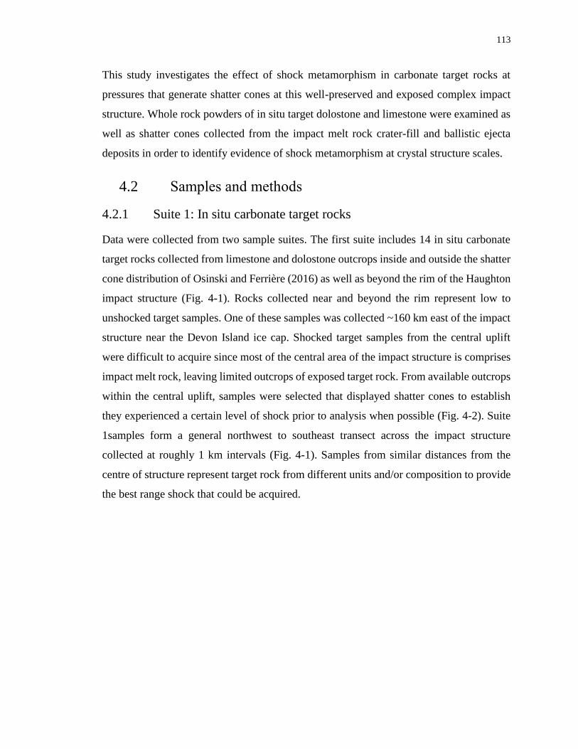
113

This study investigates the effect of shock metamorphism in carbonate target rocks at

pressures that generate shatter cones at this well-preserved and exposed complex impact

structure. Whole rock powders of in situ target dolostone and limestone were examined as

well as shatter cones collected from the impact melt rock crater-fill and ballistic ejecta

deposits in order to identify evidence of shock metamorphism at crystal structure scales.

4.2 Samples and methods

4.2.1 Suite 1: In situ carbonate target rocks

Data were collected from two sample suites. The first suite includes 14 in situ carbonate

target rocks collected from limestone and dolostone outcrops inside and outside the shatter

cone distribution of Osinski and Ferrière (2016) as well as beyond the rim of the Haughton

impact structure (Fig. 4-1). Rocks collected near and beyond the rim represent low to

unshocked target samples. One of these samples was collected ~160 km east of the impact

structure near the Devon Island ice cap. Shocked target samples from the central uplift

were difficult to acquire since most of the central area of the impact structure is comprises

impact melt rock, leaving limited outcrops of exposed target rock. From available outcrops

within the central uplift, samples were selected that displayed shatter cones to establish

they experienced a certain level of shock prior to analysis when possible (Fig. 4-2). Suite

1samples form a general northwest to southeast transect across the impact structure

collected at roughly 1 km intervals (Fig. 4-1). Samples from similar distances from the

centre of structure represent target rock from different units and/or composition to provide

the best range shock that could be acquired.

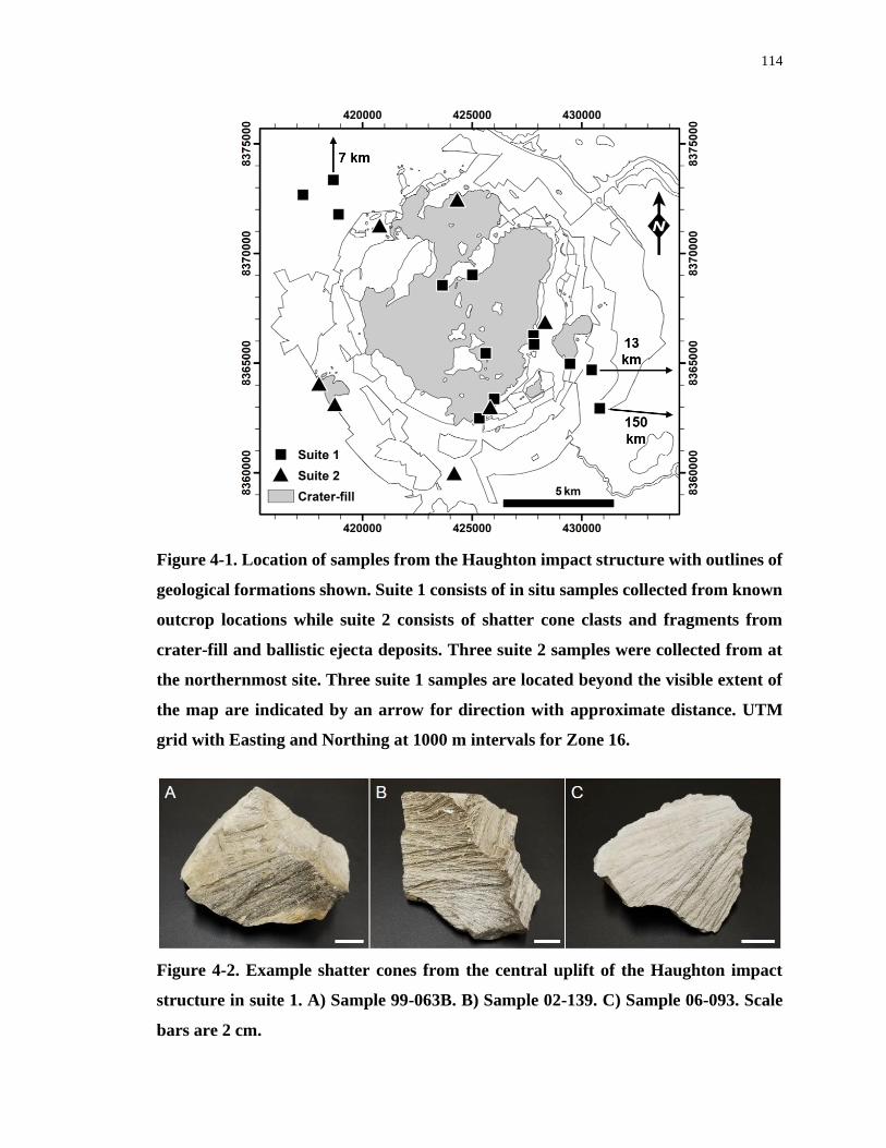
114

Figure 4-1. Location of samples from the Haughton impact structure with outlines of

geological formations shown. Suite 1 consists of in situ samples collected from known

outcrop locations while suite 2 consists of shatter cone clasts and fragments from

crater-fill and ballistic ejecta deposits. Three suite 2 samples were collected from at

the northernmost site. Three suite 1 samples are located beyond the visible extent of

the map are indicated by an arrow for direction with approximate distance. UTM

grid with Easting and Northing at 1000 m intervals for Zone 16.

Figure 4-2. Example shatter cones from the central uplift of the Haughton impact

structure in suite 1. A) Sample 99-063B. B) Sample 02-139. C) Sample 06-093. Scale

bars are 2 cm.

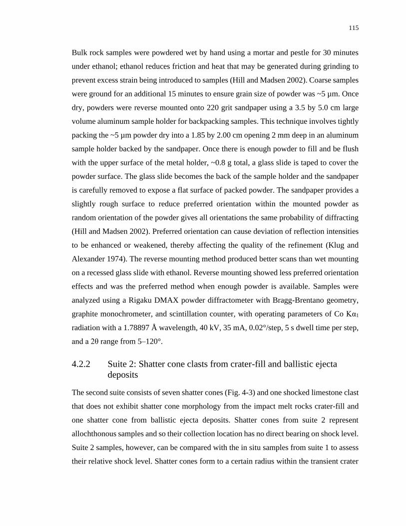
115

Bulk rock samples were powdered wet by hand using a mortar and pestle for 30 minutes

under ethanol; ethanol reduces friction and heat that may be generated during grinding to

prevent excess strain being introduced to samples (Hill and Madsen 2002). Coarse samples

were ground for an additional 15 minutes to ensure grain size of powder was ~5 µm. Once

dry, powders were reverse mounted onto 220 grit sandpaper using a 3.5 by 5.0 cm large

volume aluminum sample holder for backpacking samples. This technique involves tightly

packing the ~5 µm powder dry into a 1.85 by 2.00 cm opening 2 mm deep in an aluminum

sample holder backed by the sandpaper. Once there is enough powder to fill and be flush

with the upper surface of the metal holder, ~0.8 g total, a glass slide is taped to cover the

powder surface. The glass slide becomes the back of the sample holder and the sandpaper

is carefully removed to expose a flat surface of packed powder. The sandpaper provides a

slightly rough surface to reduce preferred orientation within the mounted powder as

random orientation of the powder gives all orientations the same probability of diffracting

(Hill and Madsen 2002). Preferred orientation can cause deviation of reflection intensities

to be enhanced or weakened, thereby affecting the quality of the refinement (Klug and

Alexander 1974). The reverse mounting method produced better scans than wet mounting

on a recessed glass slide with ethanol. Reverse mounting showed less preferred orientation

effects and was the preferred method when enough powder is available. Samples were

analyzed using a Rigaku DMAX powder diffractometer with Bragg-Brentano geometry,

graphite monochrometer, and scintillation counter, with operating parameters of Co Kα1

radiation with a 1.78897 Å wavelength, 40 kV, 35 mA, 0.02°/step, 5 s dwell time per step,

and a 2θ range from 5–120°.

4.2.2 Suite 2: Shatter cone clasts from crater-fill and ballistic ejecta

deposits

The second suite consists of seven shatter cones (Fig. 4-3) and one shocked limestone clast

that does not exhibit shatter cone morphology from the impact melt rocks crater-fill and

one shatter cone from ballistic ejecta deposits. Shatter cones from suite 2 represent

allochthonous samples and so their collection location has no direct bearing on shock level.

Suite 2 samples, however, can be compared with the in situ samples from suite 1 to assess

their relative shock level. Shatter cones form to a certain radius within the transient crater

116

during crater formation, based on shock pressures generated, which is where suite 2

samples originate. The exact radius of shatter cone formation within the transient crater is

not known, due to crater modification processes. What is known is the final distribution of

shatter cones which are found to a radius of ~4.5 km from the centre of the impact structure

(Osinski and Ferrière 2016). For comparison, all suite 2 samples were collected beyond the

current 4.5 km shatter cone distribution (Fig. 4-1).

Figure 4-3. Example shatter cone clasts from suite 2. A) Sample 00-019. B) Sample

02-061. C) Sample 02-127. D) Sample 02-128. Scale bars are 1 cm.

Bulk rock samples were powdered wet by hand using a mortar and pestle for 30 minutes

under ethanol. Once the powders were dry, powders were wet-mounted with ethanol onto

a recessed glass slide using ethanol rather than reverse mounting as done for suite 1 due to

limited sample volume. Suite 2 was analyzed using the same equipment and operating

parameters as suite 1.

4.2.3 Rietveld refinement

To determine the effects of shock pressures on rocks from both suites, Rietveld refinement

of crystal structures to quantify lattice strain were conducted using TOPAS 5 software by

Bruker AXS. Refined parameters include background intensity, sample displacement,

absorption, scale factor, unit cell dimensions, profile shape PV-TCHZ parameters U, V,

W, and X, Beq, Stephen’s model trigonal-high for calcite and dolomite, crystal size G

(Gaussian), and strain G (Gaussian). Mineral phases present in several wt%, up to ~5 wt%,

were not refined on Beq, Stephen’s model, crystal size G, or strain G as the errors for these

parameters increased significantly as the proportion of the mineral phase declined in the

bulk rock sample (e.g., Hill and Howard 1987; Turvey et al. 2018). All refinements were

fit from 16°–80° 2θ with fixed parameters including fifth-order background, and preferred

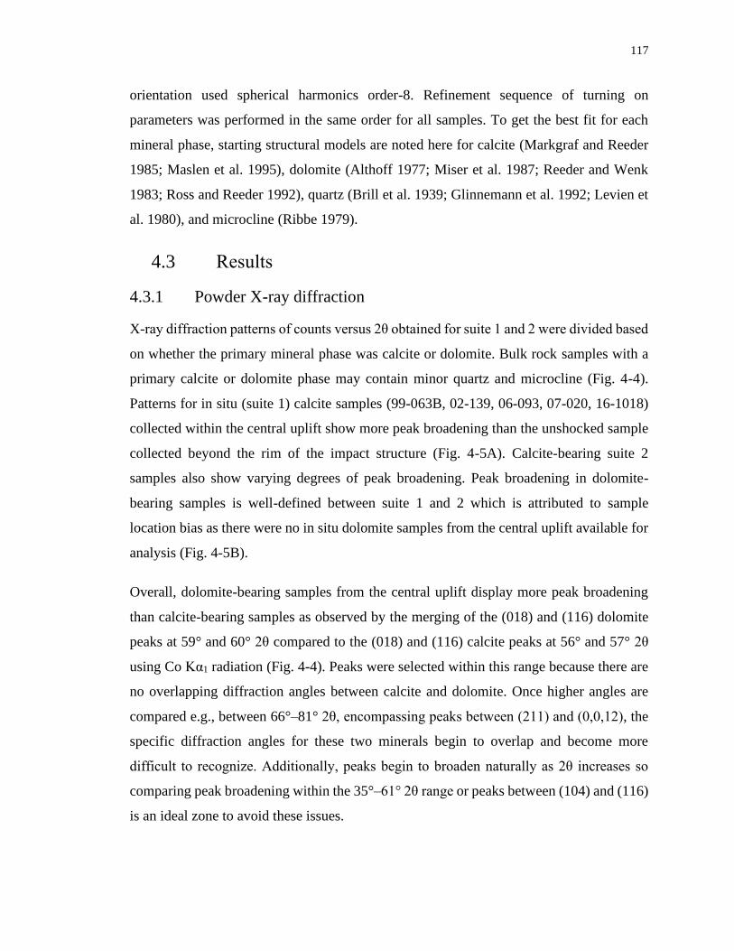
117

orientation used spherical harmonics order-8. Refinement sequence of turning on

parameters was performed in the same order for all samples. To get the best fit for each

mineral phase, starting structural models are noted here for calcite (Markgraf and Reeder

1985; Maslen et al. 1995), dolomite (Althoff 1977; Miser et al. 1987; Reeder and Wenk

1983; Ross and Reeder 1992), quartz (Brill et al. 1939; Glinnemann et al. 1992; Levien et

al. 1980), and microcline (Ribbe 1979).

4.3 Results

4.3.1 Powder X-ray diffraction

X-ray diffraction patterns of counts versus 2θ obtained for suite 1 and 2 were divided based

on whether the primary mineral phase was calcite or dolomite. Bulk rock samples with a

primary calcite or dolomite phase may contain minor quartz and microcline (Fig. 4-4).

Patterns for in situ (suite 1) calcite samples (99-063B, 02-139, 06-093, 07-020, 16-1018)

collected within the central uplift show more peak broadening than the unshocked sample

collected beyond the rim of the impact structure (Fig. 4-5A). Calcite-bearing suite 2

samples also show varying degrees of peak broadening. Peak broadening in dolomite-

bearing samples is well-defined between suite 1 and 2 which is attributed to sample

location bias as there were no in situ dolomite samples from the central uplift available for

analysis (Fig. 4-5B).

Overall, dolomite-bearing samples from the central uplift display more peak broadening

than calcite-bearing samples as observed by the merging of the (018) and (116) dolomite

peaks at 59° and 60° 2θ compared to the (018) and (116) calcite peaks at 56° and 57° 2θ

using Co Kα1 radiation (Fig. 4-4). Peaks were selected within this range because there are

no overlapping diffraction angles between calcite and dolomite. Once higher angles are

compared e.g., between 66°–81° 2θ, encompassing peaks between (211) and (0,0,12), the

specific diffraction angles for these two minerals begin to overlap and become more

difficult to recognize. Additionally, peaks begin to broaden naturally as 2θ increases so

comparing peak broadening within the 35°–61° 2θ range or peaks between (104) and (116)

is an ideal zone to avoid these issues.

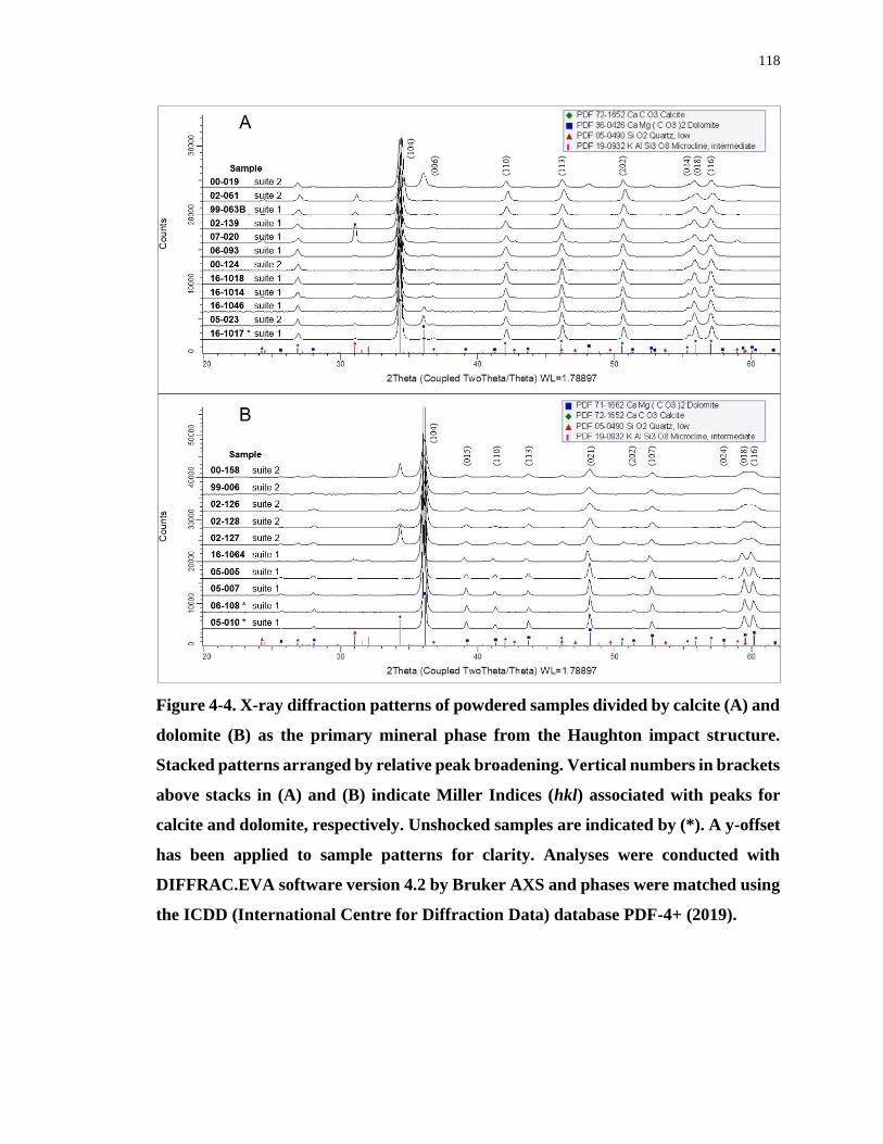
118

Figure 4-4. X-ray diffraction patterns of powdered samples divided by calcite (A) and

dolomite (B) as the primary mineral phase from the Haughton impact structure.

Stacked patterns arranged by relative peak broadening. Vertical numbers in brackets

above stacks in (A) and (B) indicate Miller Indices (hkl) associated with peaks for

calcite and dolomite, respectively. Unshocked samples are indicated by (*). A y-offset

has been applied to sample patterns for clarity. Analyses were conducted with

DIFFRAC.EVA software version 4.2 by Bruker AXS and phases were matched using

the ICDD (International Centre for Diffraction Data) database PDF-4+ (2019).

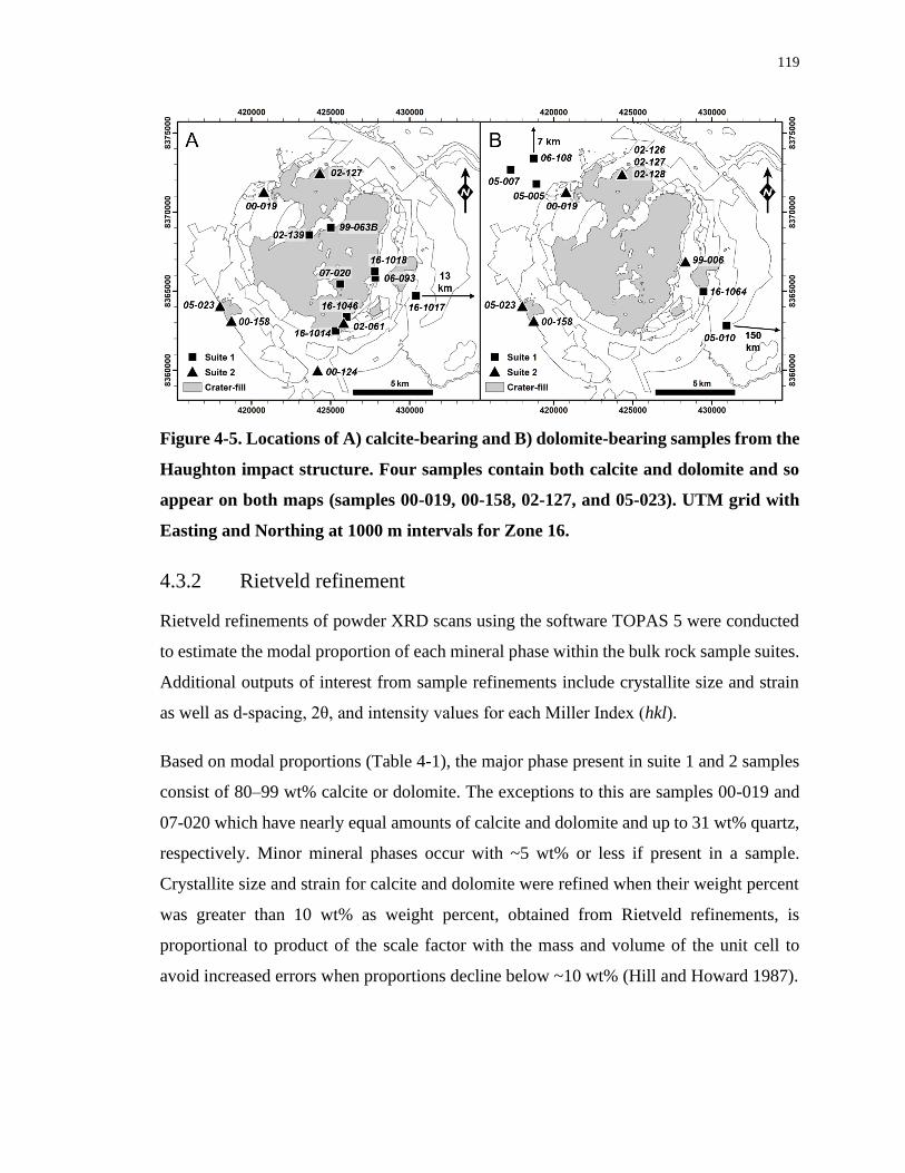
119

Figure 4-5. Locations of A) calcite-bearing and B) dolomite-bearing samples from the

Haughton impact structure. Four samples contain both calcite and dolomite and so

appear on both maps (samples 00-019, 00-158, 02-127, and 05-023). UTM grid with

Easting and Northing at 1000 m intervals for Zone 16.

4.3.2 Rietveld refinement

Rietveld refinements of powder XRD scans using the software TOPAS 5 were conducted

to estimate the modal proportion of each mineral phase within the bulk rock sample suites.

Additional outputs of interest from sample refinements include crystallite size and strain

as well as d-spacing, 2θ, and intensity values for each Miller Index (hkl).

Based on modal proportions (Table 4-1), the major phase present in suite 1 and 2 samples

consist of 80–99 wt% calcite or dolomite. The exceptions to this are samples 00-019 and

07-020 which have nearly equal amounts of calcite and dolomite and up to 31 wt% quartz,

respectively. Minor mineral phases occur with ~5 wt% or less if present in a sample.

Crystallite size and strain for calcite and dolomite were refined when their weight percent

was greater than 10 wt% as weight percent, obtained from Rietveld refinements, is

proportional to product of the scale factor with the mass and volume of the unit cell to

avoid increased errors when proportions decline below ~10 wt% (Hill and Howard 1987).

120

Table 4-1. Modal mineral proportions of samples in weight percent with crystal size

and lattice strain values for carbonates determined by Rietveld refinement of bulk

rock powders from the Haughton impact structure.

Sample

Calcite Dolomite Quartz Microcline

wt%

(error) *

crystal size §,

nm (error)

strain % †

(error)

wt%

(error)

crystal size,

nm (error)

strain %

(error)

wt%

(error)

wt%

(error)

99-006 2 4.7(3) – – 91.9(8) 56(8) 0.55(4) – 3.4(8)

99-063B 1 96.2(6) 51(7) 0.35(10) – – – 3.8(6) –

00-019 2 57.1(15) 52(2) 0.18(8) 42.9(15) 51(10) 0.73(10) – –

00-124 2 99.7(17) 64(6) 0.41(3) – – – 0.3(17) –

00-158 2 12.9(10) 85(8) 0.31(3) 87.1(10) 34.8(7) 0.43(3) – –

02-061 2 91.0(10) 71(5) 0.20(5) – – – 4.0(4) 5.0(10)

02-126 2 1.7(4) – – 95(2) 40(4) 0.46(8) 1.7(4) –

02-127 2 18.3(7) 72(7) 0.16(8) 81.7(7) 52(3) 0.42(3) – –

02-128 2 4.2(3) – – 95.8(3) 52(9) 0.60(6) – –

02-139 1 99.5(7) 55(6) 0.34(6) – – – 0.5(7) –

05-005 1 1.0(4) – – 98.1(18) 71(4) 0.16(3) 1.0(17) –

05-007 1 0.6(5) – – 97.7(18) 109(8) 0.19(4) 0.9(17) 0.9(4)

05-010 1 0.20(13) – – 99.7(4) 81(7) 0.20(3) 0.1(4) –

05-023 2 81(2) 80(6) 0.17(7) 13.6(18) 70(7) 0.40(4) 3.901(2) –

06-093 1 99.1(3) 59(5) 0.37(4) 0.52(19) – – 0.4(2) –

06-108 1 0.27(10) – – 99.5(4) 80(6) 0.11(9) 0.2(4) –

07-020 1 69.0(7) 53.7(15) 0.421(19) – – – 31.0(7) –

16-1014 1 96.6(3) 71(2) 0.282(9) 1.21(11) – – 2.2(2) –

16-1017 1 92.6(8) 54.2(10) 0.12(4) 3.2(5) – – 2.0(5) 2.2(3)

16-1018 1 98.0(11) 70(10) 0.32(4) – – – 1.3(11) 0.7(3)

16-1046 1 93.1(8) 60(7) 0.21(9) 5.9(4) – – 1.0(7) –

16-1064 1 0.14(13) – – 89.8(4) 91(7) 0.251(14) 3.2(4) 6.9(2)

1 Suite 1; in situ carbonate target rock. 2 Suite 2; shatter cone from crater-fill or ballistic ejecta deposit. * Standard error shown in parentheses corresponds to the last decimal place. § Crystal size = Gaussian crystal size. † Strain = Gaussian lattice strain.

Lattice strain values for shocked calcite samples range from 0.16% to 0.42% with the single

unshocked sample at 0.12% (Table 4-1). The range of lattice strain values for shocked

dolomite samples is slightly higher from 0.25% to 0.73% and low to unshocked samples

range from 0.11% to 0.20% (Table 4-1); low shock samples were collected near the crater

rim. The distance from the centre of the impact structure for each sample along with their

lattice strain values are provided in Table 4-2 for suite 1 samples and in Table 4-3 for suite

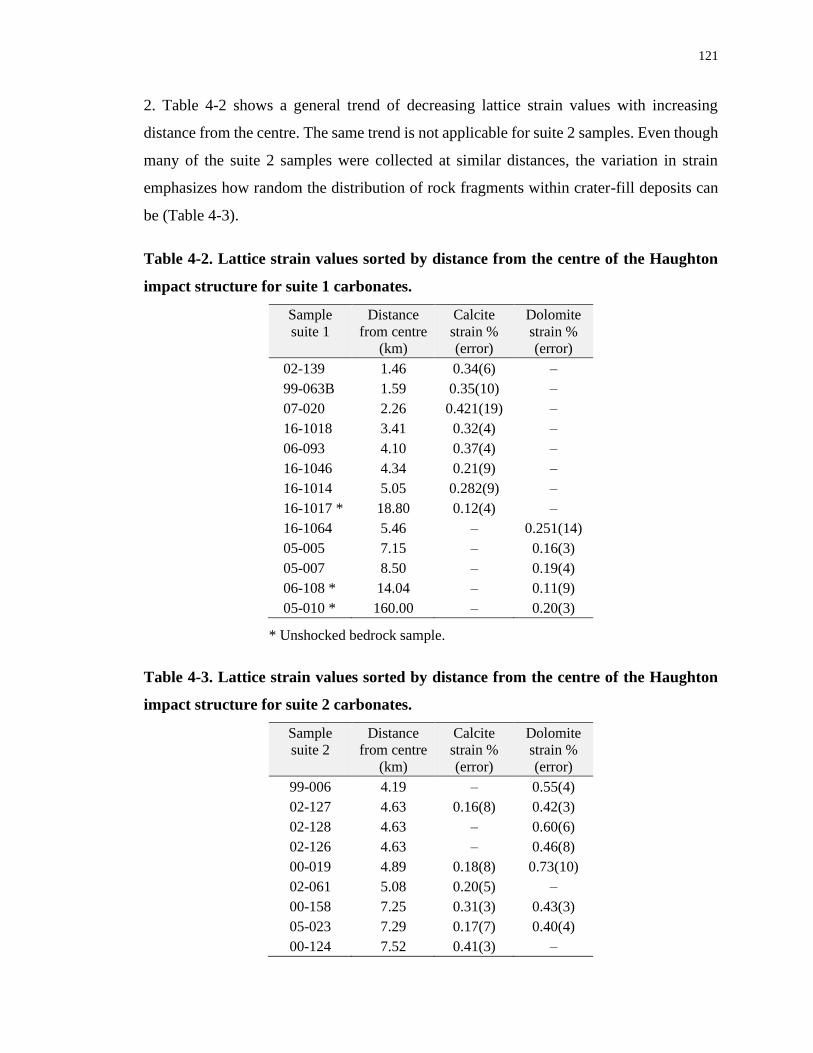
121

2. Table 4-2 shows a general trend of decreasing lattice strain values with increasing

distance from the centre. The same trend is not applicable for suite 2 samples. Even though

many of the suite 2 samples were collected at similar distances, the variation in strain

emphasizes how random the distribution of rock fragments within crater-fill deposits can

be (Table 4-3).

Table 4-2. Lattice strain values sorted by distance from the centre of the Haughton

impact structure for suite 1 carbonates.

Sample

suite 1

Distance

from centre

(km)

Calcite

strain %

(error)

Dolomite

strain %

(error)

02-139 1.46 0.34(6) –

99-063B 1.59 0.35(10) –

07-020 2.26 0.421(19) –

16-1018 3.41 0.32(4) –

06-093 4.10 0.37(4) –

16-1046 4.34 0.21(9) –

16-1014 5.05 0.282(9) –

16-1017 * 18.80 0.12(4) –

16-1064 5.46 – 0.251(14)

05-005 7.15 – 0.16(3)

05-007 8.50 – 0.19(4)

06-108 * 14.04 – 0.11(9)

05-010 * 160.00 – 0.20(3)

* Unshocked bedrock sample.

Table 4-3. Lattice strain values sorted by distance from the centre of the Haughton

impact structure for suite 2 carbonates.

Sample

suite 2

Distance

from centre

(km)

Calcite

strain %

(error)

Dolomite

strain %

(error)

99-006 4.19 – 0.55(4)

02-127 4.63 0.16(8) 0.42(3)

02-128 4.63 – 0.60(6)

02-126 4.63 – 0.46(8)

00-019 4.89 0.18(8) 0.73(10)

02-061 5.08 0.20(5) –

00-158 7.25 0.31(3) 0.43(3)

05-023 7.29 0.17(7) 0.40(4)

00-124 7.52 0.41(3) –

122

4.3.3 Williamson-Hall plots

Peak broadening evident in XRD patterns (Fig. 4-4) is the first evidence of strained crystal

lattices. Output values of interest from Rietveld refinements of shocked and unshocked

limestone and dolostone samples include lattice strain values and modal mineral

proportions (Table 4-1). To better visualize the effect of impact-induced strain within the

two sample suites, the strain values determined from Rietveld refinements were used to

create Williamson-Hall plots (Uchizono et al. 1999; Williamson and Hall 1953).

Williamson-Hall plots are typically used to derive lattice strain values from XRD data by

measuring the peak area for specific range of diffraction angles. Here, since lattice strain

(ε) has been determined through Rietveld refinement, line broadening is calculated instead

of measured in order to generate plots for calcite and dolomite. Williamson-Hall plots were

generated using equation 4.1 (Uchizono et al. 1999; Wilson 1962) to calculate the integral

breadth or line broadening due to strain (βs) using Gaussian crystal lattice strain (ε)

determined from Rietveld refinement and diffracted angles (θ).

𝛽𝑠 = 4𝜀𝑡𝑎𝑛𝜃 (4.1)

The strain value (ε) is responsible for the vertical spread of plotted samples. Samples that

contain more than 10 wt% of calcite and dolomite are found on both of the following

Williamson-Hall plots.

The Williamson-Hall plot for calcite (Fig. 4-6) shows a range of strain effects on peak

broadening where shocked samples result in slope values up to 1.7 compared to the

unshocked sample 16-1017 which has a slope of 0.5. All samples display a linear trend and

plot in order from lowest strain value (16-1017) to the highest (07-020). A notable small

gap exists in the middle of the plot that separates samples that have a strain value above

0.28% and below 0.21%. Six calcite-bearing samples from suite 1 plot above the gap (Fig.

4-6); all but one of these (16-1014) are located within 3.5 km from the centre of the impact

structure with sample 16-1014 being 5 km from the centre. The two suite 1 samples that

plot below the gap are 4.3 and 18.4 km from the centre, respectively.

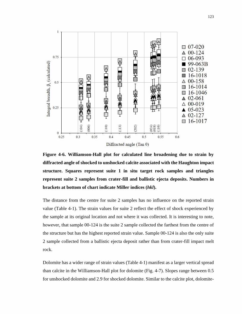
123

Figure 4-6. Williamson-Hall plot for calculated line broadening due to strain by

diffracted angle of shocked to unshocked calcite associated with the Haughton impact

structure. Squares represent suite 1 in situ target rock samples and triangles

represent suite 2 samples from crater-fill and ballistic ejecta deposits. Numbers in

brackets at bottom of chart indicate Miller indices (hkl).

The distance from the centre for suite 2 samples has no influence on the reported strain

value (Table 4-1). The strain values for suite 2 reflect the effect of shock experienced by

the sample at its original location and not where it was collected. It is interesting to note,

however, that sample 00-124 is the suite 2 sample collected the farthest from the centre of

the structure but has the highest reported strain value. Sample 00-124 is also the only suite

2 sample collected from a ballistic ejecta deposit rather than from crater-fill impact melt

rock.

Dolomite has a wider range of strain values (Table 4-1) manifest as a larger vertical spread

than calcite in the Williamson-Hall plot for dolomite (Fig. 4-7). Slopes range between 0.5

for unshocked dolomite and 2.9 for shocked dolomite. Similar to the calcite plot, dolomite-

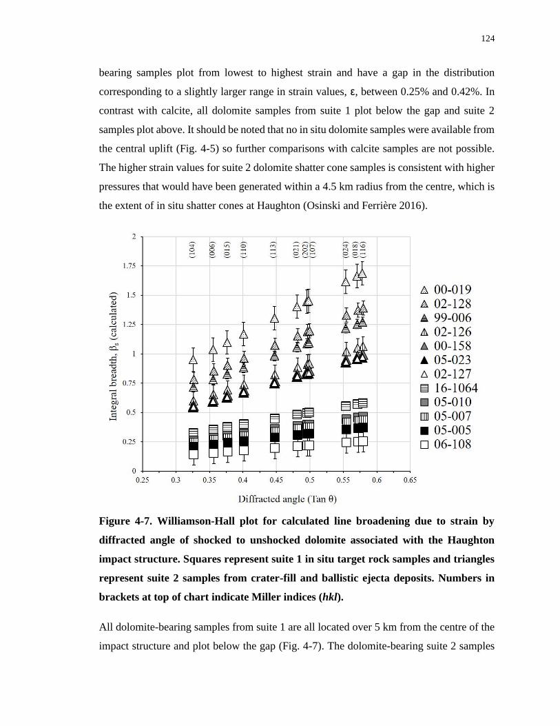
124

bearing samples plot from lowest to highest strain and have a gap in the distribution

corresponding to a slightly larger range in strain values, ε, between 0.25% and 0.42%. In

contrast with calcite, all dolomite samples from suite 1 plot below the gap and suite 2

samples plot above. It should be noted that no in situ dolomite samples were available from

the central uplift (Fig. 4-5) so further comparisons with calcite samples are not possible.

The higher strain values for suite 2 dolomite shatter cone samples is consistent with higher

pressures that would have been generated within a 4.5 km radius from the centre, which is

the extent of in situ shatter cones at Haughton (Osinski and Ferrière 2016).

Figure 4-7. Williamson-Hall plot for calculated line broadening due to strain by

diffracted angle of shocked to unshocked dolomite associated with the Haughton

impact structure. Squares represent suite 1 in situ target rock samples and triangles

represent suite 2 samples from crater-fill and ballistic ejecta deposits. Numbers in

brackets at top of chart indicate Miller indices (hkl).

All dolomite-bearing samples from suite 1 are all located over 5 km from the centre of the

impact structure and plot below the gap (Fig. 4-7). The dolomite-bearing suite 2 samples

125

like the equivalent calcite-bearing samples were displaced from their original location

within the target sequence by the impact event.

Samples containing both dolomite and calcite typically do not plot at similar positions on

their respective plots. Four bulk rock samples from suite 2 that contain both carbonate

phases with modal proportions greater than 10 wt% are 00-019, 00-158, 02-127, and 05-

023 (Figs. 4-6 and 4-7). First, 00-158 (81.7 wt% dolomite, 12.9 wt% calcite) sees both

carbonate minerals plot in the relatively same position just above the gap. Comparing 00-

158 with 02-127 which has nearly the same carbonate composition (81.7 wt% dolomite,

18.3 wt% calcite), dolomite plots at the same location above the gap whereas calcite plots

noticeably below the gap. Next, 05-023 has carbonate proportions reversed (81.0 wt%

calcite, 13.6 wt% dolomite) with dolomite plotting at the same position as 00-158 and 02-

127 and calcite plotting below the gap with 02-127. The final mixed carbonate, 00-019

(57.1 wt% calcite, 42.9 wt% dolomite) shows the widest spread in relative position between

the two plots with dolomite at the top while calcite falls below the gap near 05-023 and 02-

127.

4.4 Discussion

4.4.1 Shock effects in calcite versus dolomite

The sample suites in this study are all naturally occurring rocks where limestone and

dolostone are not necessarily pure and may contain up to several wt% of quartz or

microcline (Table 4-1). Dolomite and calcite are similar carbonate minerals with main

differences related to crystal symmetry and structure caused by Mg atoms substituting for

Ca atoms in alternating cation layers in dolomite (Reeder 1983). Mg has a smaller ionic

radius than Ca which leads to less distortion in CaO6 octahedra in dolomite than calcite and

the smaller Mg cation stabilizes the dolomite structure and prevents further octahedral

distortion under pressure (Ross and Reeder 1992; Shannon 1976). High pressure

experiments using diamond-anvil cells have shown the c-axis in carbonates is

approximately 3 times more compressible than the a-axis (Fiquet et al. 1994; Ross and

Reeder 1992). More specifically, compressibility only occurs within the CaO6 and MgO6

octahedral cation layers as the CO3 carbonate groups are rigid units and not affected by

126

increasing pressure (Ross and Reeder 1992). Compressibility is also controlled by the

polarizability of cations, decreasing from Ca to Mg, which supports the observed decrease

in compressibility for the calcite (CaCO3), dolomite (CaMg(CO3)2), and magnesite

(MgCO3) sequence (Fiquet et al. 1994).

Since CaO6 octahedra are more compressible and able to distort more than MgO6 octahedra

(Ross and Reeder 1992), we suggest calcite is able to accommodate impact-generated

shock pressures through distortion better than dolomite, resulting in less lattice strain.

When both minerals occur together, dolomite would experience more lattice strain

compared to calcite since it cannot distort as much when compressed. This is observed in

samples 05-023 and 00-019 where dolomite has the lower modal proportion and as the

proportion of dolomite increases from ~14 wt% to ~43 wt%, respectively, the spread

between relative strain in dolomite and calcite increases. With a set of only four samples,

care should be exercised in making definitive conclusions, but dolomite does appear to be

preferentially strained compared to calcite when both minerals are present in the same

target rock. Another important observation is that dolomite never has a lower relative strain

value compared to calcite in the same sample, further supporting this conclusion.

The sample with the highest strain value for calcite is 07-020 (Table 4-1) and this sample

plots at the top of Figure 4-6. Sample 07-020 is the third closest to the centre of the impact

structure but the reason for the high strain value may also relate to composition. Sample

07-020 contains 69 wt% calcite and 31 wt% quartz. Sample 07-020 is the only sample in

the suite with more than 4 wt% quartz so it is unclear how the proportion of quartz affects

strain in calcite. The increased presence of quartz could introduce impedance matching

between quartz and calcite, that contributes to increased shock metamorphism and the

elevated strain detected in calcite compared to samples collected closer to the centre of the

impact structure (e.g., Kenkmann et al. 2000). This observation also supports the above

conclusion for mixed carbonate samples in that distance from the centre of the impact

structure is not a linear relationship with strain and individual sample properties such as

composition are important factors.

127

Suite 1 samples 06-093 and 16-1014 also plot higher on the calcite Williamson-Hall plot

than their distance from the centre would suggest when compared with other suite 1

samples. A common aspect of these two samples is they were collected over 50 to 100 m

in elevation above the Haughton River channel. Currently, it is unclear how strain changes

vertically through an impact crater but this could be a potential factor. Seeley and Milam

(2018) began investigating this idea by analyzing dolostone at varying depths in a drill core

from the central uplift of the Wells Creek impact structure and is described further in the

following section.

The unshocked suite 1 sample 05-010 was collected ~160 km east of the impact structure

and, therefore, was not affected by the hypervelocity impact event. As such, this sample

would be expected to have the lowest lattice strain value, but it has the fourth lowest strain

value at 0.20% (Table 4-1). This could suggest that the area where sample 05-010 was

collected has experienced mild tectonic strain which has been shown to be detectable by

XRD (Huson et al. 2009).

4.4.2 Comparison with other craters in carbonate target rocks

There are currently 198 confirmed terrestrial impact structures and of these 82 formed in

completely sedimentary targets and 54 in a mixed sedimentary and crystalline target

sequence (Impact Earth 2020). From these sedimentary rock-bearing impact structures,

carbonates from only five have been investigated for the presence of shock in carbonates

using XRD and include the Ries, Kara, Steinheim, Sierra Madera, and Wells Creek impact

structures (Huson et al. 2009; Seeley and Milam 2018; Skála 2002; Skála and Jakeš 1999).

One common aspect that studies from these five impact structures highlight is the

occurrence of peak broadening in XRD patterns as an indicator that there has been a

decrease in crystallite size in shocked carbonates (Skála 2002). A main difference among

these studies is that each examined a different 2θ range, and within these ranges, reflections

or peaks for calcite, dolomite, and quartz often overlap. Identifying peak broadening is a

relatively quick qualitative method to visualize if further shock investigation is warranted

but becomes more difficult to compare between studies when different 2θ ranges are

reported.

128

In the studies by Skála and Jakeš (1999), Skála (2002) and Huson et al. (2009), peak

broadening observations from XRD patterns were further examined using Rietveld

refinement to derive full width half maximum (FWHM) values and regression curves,

which offer a better comparison than peak broadening alone. Data from Skála and Jakeš

(1999) show they were qualitatively able to estimate the level of shock in their samples and

state “the results obtained in this research are rather qualitative and require detailed

calibration using experimentally shocked calcite samples”. Skála and Jakeš (1999) showed

that Rietveld refinement data is more reliable than single-peak profile fitting, however,

their regression curves only display relative levels of shock among plotted samples. These

three studies provided FWHM values or curves versus 2θ which were stacked with other

samples in their respective sample suites. Each set of stacked sample suite curves from

Skála and Jakeš (1999), Skála (2002), and Huson et al. (2009) show variation between

shocked and unshocked rocks but is similar to the stacking of diffraction patterns to

compare peak broadening, where a single curve is more difficult to interpret. If the Rietveld

refinements by Skála and Jakeš (1999), Skála (2002), and Huson et al. (2009) had gone

one step further and determined strain values for their carbonate samples, the results could

be easier to compare among studies.

The preliminary summary by Seeley and Milam (2018) examined how peak broadening

changes with depth in a 401 m drill core from the central uplift of the Wells Creek impact

structure. From their diffraction patterns they suggest peak broadening does not appear to

directly correspond to an expected decrease with depth. Their results from comparing peak

broadening in diffraction patterns alone do not show a clear decrease in peak broadening

with depth, however, they intend to compare this to more robust data from Rietveld

refinements in the future (Seeley and Milam 2018). It is not mentioned if the Rietveld data

would then be used to create FWHM curves or if lattice strain values might be determined.

Determining lattice strain from a vertical sequence of samples at Wells Creek or any other

impact structure could reveal a clearer idea of the relationship between depth and strain.

The difference in 2θ ranges compared for peak broadening in diffraction patterns and the

qualitative display of stacked curves from peak fitting reveal a lack of directly comparable

parameters among previous studies and indicates that a different approach may be

129

necessary. To identify a more quantifiable method of identifying shock in carbonates, we

determined lattice strain for dolomite and calcite in samples from the Haughton impact

structure. Lattice strain values obtained from Rietveld refinement indicate there is a

detectable change in lattice strain associated with carbonates subjected to hypervelocity

impact at the Haughton impact structure (Table 4-1). Strain values offer a numerical

comparison between samples rather than a relative comparison of broadening in diffraction

patterns or FWHM curves. Having a consistent set of parameters would help work toward

a shock classification scheme for carbonates, which does not currently exist (Stöffler et al.

2018) and will be discussed in the following section.

4.4.3 Carbonates as shock indicators

In this study, specific shock pressures or classes cannot be assigned to individual carbonate

samples because they are not directly associated with other quartz-bearing rocks such as

sandstone where shock level can be determined through the presence of features such as

PDFs. Sandstone clasts from crater-fill deposits at Haughton have been divided into six

shock pressure classes ranging from 0 GPa to >30 GPa (Osinski 2007). The only visual

sign of shock metamorphism in carbonate samples is the occurrence of shatter cones at

hand sample scale.

Sample 07-020 contains the highest modal proportion of silicates, ~31 wt% quartz, and

based on the diffraction pattern for this sample, there are no peaks to indicate the presence

of stishovite or coesite. The peaks of these high pressure polymorphs of quartz are not

observed, however, their positions overlap with the large calcite peaks, so it is possible

they are obscured, especially if either are present in low proportions. Stishovite forms at

pressures between ~12–45 GPa and coesite forms between ~30–55 GPa (Stöffler 1971).

Strain values in this study cannot be directly quantified since lattice strain values from

experimentally shocked dolomite and calcite samples at known pressures have yet to be

measured. Such a pressure scale was suggested by Martinez et al. (1995) but has yet to be

produced. However, in the study by Martinez et al. (1995) they experimentally shocked

dolomitic rocks collected on Devon Island near the Haughton impact structure to 60 GPa.

They compared one unshocked sample and two samples from shock recovery experiments

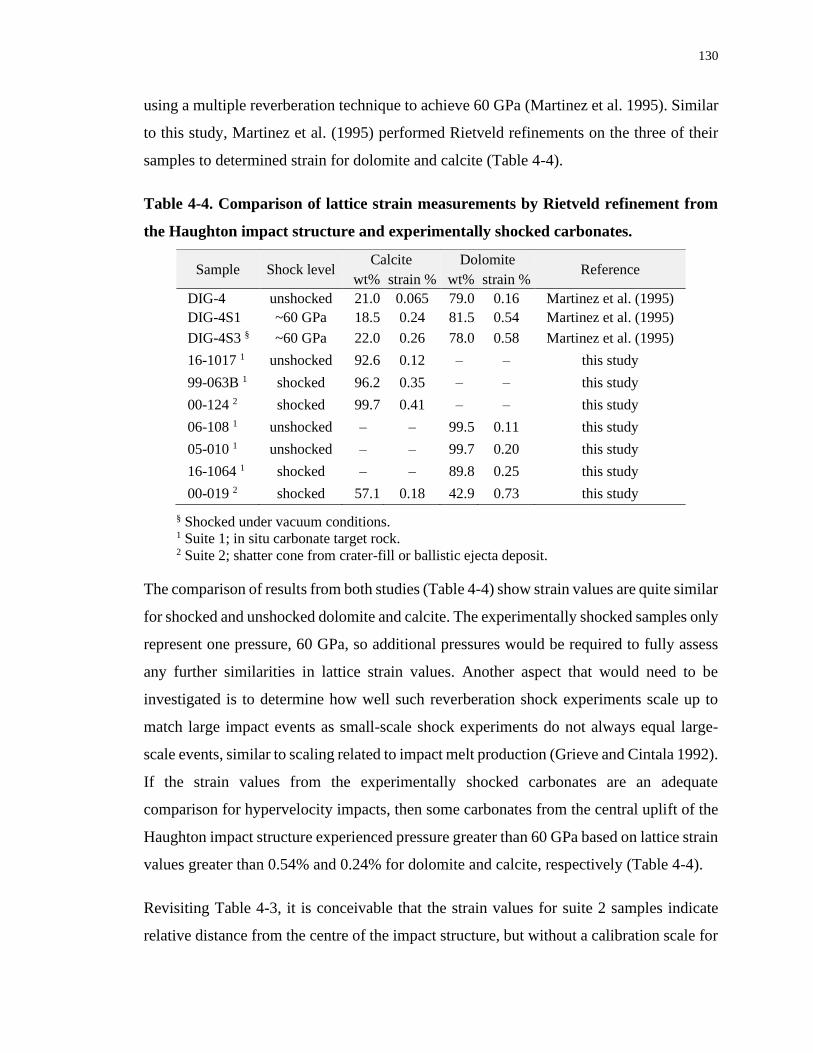
130

using a multiple reverberation technique to achieve 60 GPa (Martinez et al. 1995). Similar

to this study, Martinez et al. (1995) performed Rietveld refinements on the three of their

samples to determined strain for dolomite and calcite (Table 4-4).

Table 4-4. Comparison of lattice strain measurements by Rietveld refinement from

the Haughton impact structure and experimentally shocked carbonates.

Sample Shock level Calcite Dolomite

Reference wt% strain % wt% strain %

DIG-4 unshocked 21.0 0.065 79.0 0.16 Martinez et al. (1995)

DIG-4S1 ~60 GPa 18.5 0.24 81.5 0.54 Martinez et al. (1995)

DIG-4S3 § ~60 GPa 22.0 0.26 78.0 0.58 Martinez et al. (1995)

16-1017 1 unshocked 92.6 0.12 – – this study

99-063B 1 shocked 96.2 0.35 – – this study

00-124 2 shocked 99.7 0.41 – – this study

06-108 1 unshocked – – 99.5 0.11 this study

05-010 1 unshocked – – 99.7 0.20 this study

16-1064 1 shocked – – 89.8 0.25 this study

00-019 2 shocked 57.1 0.18 42.9 0.73 this study

§ Shocked under vacuum conditions. 1 Suite 1; in situ carbonate target rock. 2 Suite 2; shatter cone from crater-fill or ballistic ejecta deposit.

The comparison of results from both studies (Table 4-4) show strain values are quite similar

for shocked and unshocked dolomite and calcite. The experimentally shocked samples only

represent one pressure, 60 GPa, so additional pressures would be required to fully assess

any further similarities in lattice strain values. Another aspect that would need to be

investigated is to determine how well such reverberation shock experiments scale up to

match large impact events as small-scale shock experiments do not always equal large-

scale events, similar to scaling related to impact melt production (Grieve and Cintala 1992).

If the strain values from the experimentally shocked carbonates are an adequate

comparison for hypervelocity impacts, then some carbonates from the central uplift of the

Haughton impact structure experienced pressure greater than 60 GPa based on lattice strain

values greater than 0.54% and 0.24% for dolomite and calcite, respectively (Table 4-4).

Revisiting Table 4-3, it is conceivable that the strain values for suite 2 samples indicate

relative distance from the centre of the impact structure, but without a calibration scale for

131

strain associated with known pressures, this cannot be determined. What the strain values

from the two sample suites here do show is that strain values are higher near the centre of

the impact structure for in situ target samples and decrease toward the rim (Table 4-2). The

strain variation among the samples in this study indicates that the shatter cone-bearing

target rocks did not experience the same sample shock pressure during the impact event

and helps to support that lattice strain could be a proxy for shock pressure. If lattice strain

was not induced by shock pressure, then strain values for all samples within both sample

suites should have similar values. The ability to recognize strain in carbonates using XRD

and associate the strain with a shock pressure could be used to help identify and confirm

an impact structure in a sedimentary target.

X-ray diffraction data and subsequent strain derived from Williamson-Hall plots has shown

success in estimating shock pressure in forsterite (Uchizono et al. 1999). The calibration

curve generated by experimentally shocking forsterite up to 82 GPa was used to determine

shock pressures experienced by olivine in a LL6 chondrite meteorite (Uchizono et al.

1999). By measuring lattice strain of olivine in Martian meteorites Jenkins et al. (2019)

also produced strain values that are comparable to literature values for shock pressures,

giving further support to the value of lattice strain measurements.

As shock indicators, carbonates would not be as straightforward as silicates. Results here

show that rocks with a mixed carbonate composition result in preferential strain in dolomite

over calcite, likely due to crystal structure differences between the two minerals. Future

experiments need to consider this aspect of naturally occurring carbonates and not limit

experimental samples to pure calcite or dolomite. While pure limestone and dolostone

rocks will produce the best calibration scales for quantifying strain in experimentally

shocked samples, mixed carbonate rocks of known compositions will also reveal any

effects or trends that result from varying carbonate compositions. The effect of porosity

and grain size on strain in carbonates should also be explored in controlled experiments to

determine if they contribute to lattice strain caused by hypervelocity-generated shock

pressures, and if so to what extent do they contribute to strain.

132

When calcite and dolomite are both available to determine strain, dolomite appears to be

the better mineral for several reasons. First, in mixed carbonate samples its strain value has

less variation when considering modal abundance. Second, weakly shocked dolostone from

an impact event can be distinguished from tectonically strained dolostone whereas mildly

shocked calcite cannot make the same distinction (Huson et al. 2009). And third, dolomite

does not undergo displacive-type phase transformations at pressures below 5.0 GPa, unlike

calcite where this has been shown to occur at pressures around 1.5 GPa and 2.2 GPa (Ross

and Reeder 1992). Additional structural transformation in calcite has also been observed

between 7 GPa and 18.3 GPa (Fiquet et al. 1994). This study did not investigate the effect

of phase transformations so future experiments should determine the effect these

transformations have on lattice strain.

4.5 Conclusions

Peak broadening in X-ray diffraction patterns was observed in this study as well as in

previous studies of carbonates from impact events (Huson et al. 2009; Seeley and Milam

2018; Skála 2002; Skála and Jakeš 1999). Further assessment of XRD data by Rietveld

refinement show lattice strain variation in dolomite and calcite among shocked samples.

Both calcite and dolomite show variation in strain values with trends showing highest strain

within the central uplift and decreases toward the rim. Higher strain values for dolomite

show it is more affected by hypervelocity impact than calcite. This is supported by the

results from mixed carbonate samples that show strain is not evenly distributed through

calcite and dolomite with dolomite preferentially strained over calcite.

This study has shown promising results to identify shocked carbonates associated with

impact structures. Further study of naturally and experimentally shocked limestone and

dolostone samples will prove the reliability of using lattice strain measurement to identify

shock in dolomite and calcite. In the future, experimentally shocked carbonates could

produce a calibration scale where strain values could estimate impact-generated shock

pressures in an effort to initiate a reliable shock classification system for carbonates.

133

4.6 References

Althoff P. 1977. Structural refinements of dolomite and a magnesian calcite and

implications for dolomite formation in the marine environment. American

Mineralogist 62:772–783.

Baratoux D., and Reimold W. U. 2016. The current state of knowledge about shatter cones:

Introduction to the special issue. Meteoritics & Planetary Science 51:1389–1434.

Brill R., Hermann C., and Peters C. 1939. Studien über chemische Bindung mittels

Fourieranalyse III. Die Naturwissenschaften 27:677–678.

Cavosie A. J., Timms N. E., Ferrière L., and Rochette P. 2018. FRIGN zircon - The only

terrestrial mineral diagnostic of high-pressure and high-temperature shock

deformation. Geology 46:891–894.

Černok A., White L. F., Darling J., Dunlop J., and Anand M. 2019. Shock-induced

microtextures in lunar apatite and merrillite. Meteoritics & Planetary Science

54:1262–1282.

Cressman E. R. 1981. Surface geology of the Jeptha Knob cryptoexplosion structure,

Shelby County, Kentucky., Professional Paper 1151-B, United States Geological

Survey.

Dietz R. S. 1959. Shatter cones in cryptoexplosion structures (meteorite impact?). The

Journal of Geology 67:496–505.

Fiquet G., Guyot F., and Itie J. P. 1994. High-pressure X-ray diffraction study of

carbonates: MgCO3, CaMg(CO3)2, and CaCO3. American Mineralogist 79:15–23.

French B. M. 1998. Traces of Catastrophe: A Handbook of Shock-Metamorphic Effects in

Terrestrial Meteorite Impact Structures, LPI Contribution No. 954, Lunar and

Planetary Science Institute, Houston.

French B. M., and Koeberl C. 2010. The convincing identification of terrestrial meteorite

134

impact structures: What works, what doesn’t, and why. Earth-Science Reviews

98:123–170.

Glinnemann J., King Jr. H. E., Schulz H., Hahn T., La Placa S. J., and Dacol F. 1992.

Crystal structures of the low-temperature quartz-type phases of SiO2 and GeO2 at

elevated pressure. Zeitschrift für Kristallographie 198:177–212.

Graup G. 1999. Carbonate-silicate liquid immiscibility upon impact melting: Ries Crater,

Germany. Meteoritics & Planetary Science 34:425–438.

Grieve R. A. F., and Cintala M. J. 1992. An analysis of differential impact melt-crater

scaling and implications for the terrestrial impact record. Meteoritics 27:526–538.

Hill R. J., and Howard C. J. 1987. Quantitative phase analysis from neutron powder

diffraction data using the Rietveld method. Journal of Applied Crystallography

20:467–474.

Hill R. J., and Madsen I. C. 2002. Sample preparation, instrument selection and data

collection. In Structure Determination from Powder Diffraction Data, edited by

David W. I. F., Shankland K., McCusker L. B., and Baerlocher C. New York. pp. 98–

117.

Hörz F., Archer P. D., Niles P. B., Zolensky M. E., and Evans M. 2015. Devolatilization

or melting of carbonates at Meteor Crater, AZ? Meteoritics & Planetary Science

50:1050–1070.

Huson S. A., Foit F. F., Watkinson A. J., and Pope M. C. 2009. Rietveld analysis of X-ray

powder diffraction patterns as a potential tool for the identification of impact-

deformed carbonate rocks. Meteoritics & Planetary Science 44:1695–1706.

Impact Earth. Impact Earth Database. 2020. www.impactearth.com (Accessed February

18, 2020).

Izawa M. R. M., Flemming R. L., Banerjee N. R., and Mccausland P. J. A. 2011. Micro-

X-ray diffraction assessment of shock stage in enstatite chondrites. Meteoritics &

135

Planetary Science 46:638–651.

Jenkins L. E., Flemming R. L., and McCausland P. J. A. 2019. Quantitative in situ XRD

measurement of shock metamorphism in Martian meteorites using lattice strain and

strain-related mosaicity in olivine. Meteoritics & Planetary Science 54:902–918.

Jones A. P., Claeys P., and Heuschkel S. 2000. Impact melting of carbonates from the

Chicxulub Crater. In Impacts and the Early Earth, Lecture Notes in Earth Sciences,

edited by Gilmour I., and Koeberl C. Springer-Verlag, Berlin-Heidelberg-New York.

pp. 343–361.

Kenkmann T., Hornemann U., and Stöffler D. 2000. Experimental generation of shock-

induced pseudotachylites along lithological interfaces. Meteoritics & Planetary

Science 35:1275–1290.

Klug H. P., and Alexander L. E. 1974. X-Ray Diffraction Procedures for Polycrystalline

and Amorphous Materials, New York: John Wiley & Sons, Inc.

Levien L., Prewitt C. T., and Weidner D. J. 1980. Structure and elastic properties of quartz

at pressure. American Mineralogist 65:920–930.

Markgraf S. A., and Reeder R. J. 1985. High-temperature structure refinements of calcite

and magnesite. American Mineralogist 70:590–600.

Martinez I., Deutsch A., Scharer U., Ildefonse P., Guyot F., and Agrinier P. 1995. Shock

recovery experiments on dolomite and thermodynamical calculation of impact

induced decarbonation. Journal of Geophysical Research 100:15465–15476.

Maslen E. N., Streltsov V. A., Streltsova N. R., and Ishizawa N. 1995. Electron density

and optical anisotropy in rhombohedral carbonates. III. Synchrotron X‐ray studies of

CaCO3, MgCO3 and MnCO3. Acta Crystallographica Section B 51:929–939.

McCausland P. J. A., Flemming R. L., and Izawa M. R. M. 2010. Quantitative shock stage

assessment in olivine and pyroxene bearing meteorites via in situ micro-XRD.

American Geophysical Union, Fall Meeting 2010, abstract #P14C-03.

136

Miser D. E., Swinnea J. S., and Steinfink H. 1987. TEM observations and X-ray crystal-

structure refinement of a twinned dolomite with a modulated microstructure.

American Mineralogist 72:188–193.

O’Keefe J. D., and Ahrens T. J. 1989. Impact production of CO2 by the

Cretaceous/Tertiary extinction bolide and the resultant heating of the Earth. Nature

338:247–249.

Osinski G. R., and Spray J. G. 2001. Impact-generated carbonate melts: Evidence from the

Haughton structure, Canada. Earth and Planetary Science Letters 194:17–29.

Osinski G. R., Lee P., Spray J. G., Parnell J., Lim D. S. S., Bunch T. E., Cockell C. S., and

Glass B. 2005a. Geological overview and cratering model for the Haughton impact

structure, Devon Island, Canadian High Arctic. Meteoritics & Planetary Science

40:1759–1776.

Osinski G. R., Spray J. G., and Lee P. 2005b. Impactites of the Haughton impact structure,

Devon Island, Canadian High Arctic. Meteoritics & Planetary Science 40:1789–1812.

Osinski G. R., and Spray J. G. 2006. Shatter cones of the Haughton impact structure,

Canada. In Proceedings, 1st International Conference on Impact Cratering in the

Solar System, European Space Agency Special Publication SP-612. CD-ROM. pp.

95–99.

Osinski G. R. 2007. Impact metamorphism of CaCO3‐bearing sandstones at the Haughton

structure, Canada. Meteoritics & Planetary Science 42:1945–1960.

Osinski G. R., Spray J. G., and Grieve R. A. F. 2008. Impact melting in sedimentary target

rocks: An assessment. In The Sedimentary Record of Meteorite Impacts, Special

Paper 437, edited by Evans K. R., Horton W., King Jr. D. K., and Morrow J. R.

Geological Society of America, Boulder, CO. pp. 1–18.

Osinski G. R., and Ferrière L. 2016. Shatter cones: (Mis)understood? Science Advances 2,

e160061:1–10.

137

Reeder R. J., and Wenk H. R. 1983. Structure refinements of some thermally disordered

dolomites. American Mineralogist 68:769–776.

Reeder R. J. 1983. Crystal chemistry of the rhombohedral carbonates. In Reviews in

Mineralogy Volume 11 Carbonates: Mineralogy and Chemistry, edited by Reeder R.

J. Mineralogical Society of America. pp. 1–47.

Ribbe P. H. 1979. The structure of a strained intermediate microcline in cryptoperthitic

association with twinned plagioclase. American Mineralogist 64:402–408.

Ross N. L., and Reeder R. J. 1992. High-pressure structural study of dolomite and ankerite.

American Mineralogist 77:412–421.

Seeley J. R., and Milam K. A. 2018. Optical and X-ray diffraction analyses of shock

metamorphosed dolostone at increasing depths within the central uplift of the Wells

Creeks impact structure. 49th Lunar and Planetary Science Conference Abstract

#2755.

Shannon R. D. 1976. Revised effective ionic radii and systematic studies of interatomic

distances in halides and chalcogenides. Acta Crystallographica A32:751–767.

Sharpton V. L., Dressler B. O., Herrick R. R., Schnieders B., and Scott J. 1996. New

constraints on the Slate Islands impact structure, Ontario, Canada. Geology 24:851–

854.

Skála R., and Jakeš P. 1999. Shock-induced effects in natural calcite-rich targets as

revealed by X-ray powder diffraction. In Large Meteorite Impacts and Planetary

Evolution II, Special Paper 339, edited by Dressler B. O., and Sharpton V. L.

Geological Society of America (GSA), Boulder, CO. pp. 205–214.

Skála R. 2002. Shock-induced phenomena in limestones in the quarry near Ronheim, the

Ries Crater, Germany. Bulletin of the Czech Geological Survey 77:313–320.

Stöffler D. 1971. Coesite and stishovite in shocked crystalline rocks. Journal of

Geophysical Research 76:5474–5488.

138

Stöffler D., Artemieva N. A., Wünnemann K., Reimold W. U., Jacob J., Hansen B. K., and

Summerson I. A. T. 2013. Ries crater and suevite revisited - Observations and

modeling Part I: Observations. Meteoritics & Planetary Science 48:515–589.

Stöffler D., Hamann C., and Metzler K. 2018. Shock metamorphism of planetary silicate

rocks and sediments: Proposal for an updated classification system. Meteoritics &

Planetary Science 49:5–49.

Thorsteinsson R., and Mayr U. 1987. The Sedimentary Rocks of Devon Island, Canadian

Arctic Archipelago, Memoir 411. Geological Survey of Canada.

Turvey C. C., Hamilton J. L., and Wilson S. A. 2018. Comparison of Rietveld-compatible

structureless fitting analysis methods for accurate quantification of carbon dioxide

fixation in ultramafic mine tailings. American Mineralogist 103:1649–1662.

Uchizono A., Shinno I., Nakamuta Y., Nakamura T., and Sekine T. 1999. Characterization

of artificially shocked forsterites: (1) Diffraction profile analysis by Gandolfi camera.

Mineralogical Journal 21:15–23.

Williamson G. K., and Hall W. H. 1953. X-ray line broadening from filed aluminium and

wolfram. Acta Metallurgica 1:22–31.

Wilson A. J. C. 1962. X-Ray Optics: The Diffraction of X-rays by Finite and Imperfect

Crystals, London: Methuen & Co Ltd.

Young K. E., Van Soest M. C., Hodges K. V., Watson E. B., Adams B. A., and Lee P.

2013. Impact thermochronology and the age of Haughton impact structure, Canada.

Geophysical Research Letters 40:3836–3840.

139

Chapter 5

5 An X-ray diffraction study of shocked carbonates from the

deeply eroded Tunnunik impact structure, Canada

5.1 Introduction

Carbonates are an important component in sedimentary target sequences and sedimentary

rocks are present in approximately 70% of terrestrial impact craters (Osinski et al. 2008).

Despite the common occurrence of carbonates in hypervelocity impact structures, the

response of carbonates to these extreme events is poorly understood. The lack in

understanding is due, in part, to the absence of any reliable shock metamorphic features in

carbonates compared to silicates, such as planar fractures, planar deformation features, and

diaplectic glass – which are common in quartz or feldspar (French and Koeberl 2010).

This study focuses on the Tunnunik impact structure, a 28 km diameter structure located

on Victoria Island, Northwest Territories, Canada. The target sequence of the ~430 Ma

deeply eroded Tunnunik impact structure is entirely sedimentary and consists of

Precambrian limestone and Cambrian to Silurian dolostone units (Dewing et al. 2013;

Lepaulard et al. 2019). Much of what remains of the structure is covered by a blanket of

glacial till but outcrops across the structure may show impact-related features such as

inclined bedding planes, shatter cones, and impact-generated breccia dykes, with shatter

cones providing the only visual indicator of shock.

Shatter cones are macroscopic evidence of shock metamorphism in impact structures and

are found in all rock types, however, their forms are best developed in fine-grained rocks

such as carbonates (French 1998). At the Tunnunik impact structure, shatter cones are

found in the central uplift area in an ellipse approximately 10 km by 12 km (Osinski and

Ferrière 2016) in both dolostone and limestone target rocks (Fig. 5-1). Shatter cones are

typically generated from lower shock pressures of ~2–10 GPa (French 1998), but the

complete pressure range for developing shatter cones in all target types is reported as 1–45

GPa (Stöffler et al. 2018).

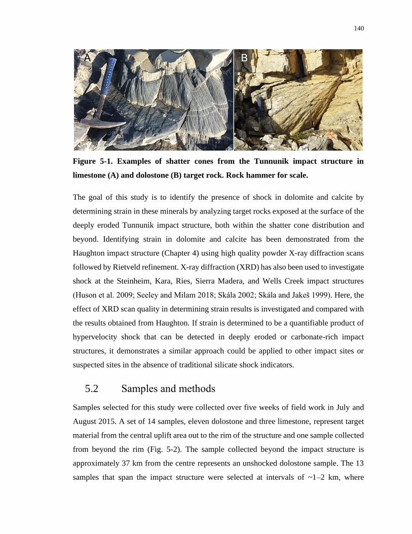
140

Figure 5-1. Examples of shatter cones from the Tunnunik impact structure in

limestone (A) and dolostone (B) target rock. Rock hammer for scale.

The goal of this study is to identify the presence of shock in dolomite and calcite by

determining strain in these minerals by analyzing target rocks exposed at the surface of the

deeply eroded Tunnunik impact structure, both within the shatter cone distribution and

beyond. Identifying strain in dolomite and calcite has been demonstrated from the

Haughton impact structure (Chapter 4) using high quality powder X-ray diffraction scans

followed by Rietveld refinement. X-ray diffraction (XRD) has also been used to investigate

shock at the Steinheim, Kara, Ries, Sierra Madera, and Wells Creek impact structures

(Huson et al. 2009; Seeley and Milam 2018; Skála 2002; Skála and Jakeš 1999). Here, the

effect of XRD scan quality in determining strain results is investigated and compared with

the results obtained from Haughton. If strain is determined to be a quantifiable product of

hypervelocity shock that can be detected in deeply eroded or carbonate-rich impact

structures, it demonstrates a similar approach could be applied to other impact sites or

suspected sites in the absence of traditional silicate shock indicators.

5.2 Samples and methods

Samples selected for this study were collected over five weeks of field work in July and

August 2015. A set of 14 samples, eleven dolostone and three limestone, represent target

material from the central uplift area out to the rim of the structure and one sample collected

from beyond the rim (Fig. 5-2). The sample collected beyond the impact structure is

approximately 37 km from the centre represents an unshocked dolostone sample. The 13

samples that span the impact structure were selected at intervals of ~1–2 km, where

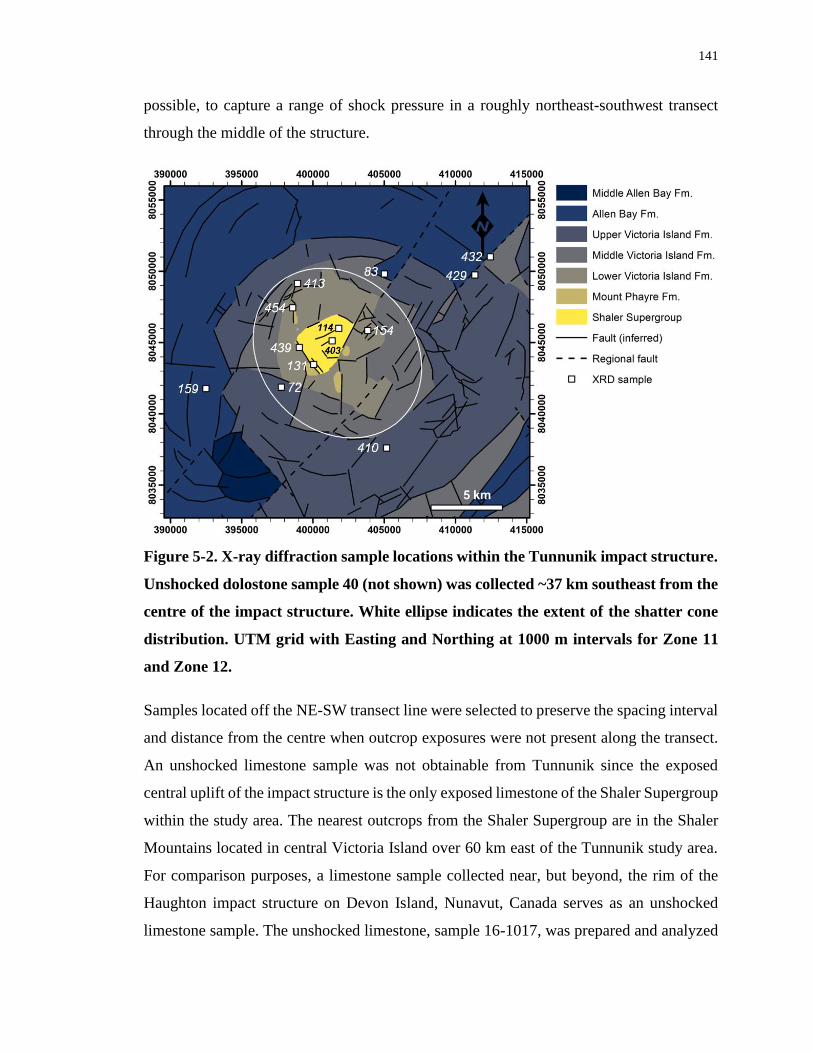
141

possible, to capture a range of shock pressure in a roughly northeast-southwest transect

through the middle of the structure.

Figure 5-2. X-ray diffraction sample locations within the Tunnunik impact structure.

Unshocked dolostone sample 40 (not shown) was collected ~37 km southeast from the

centre of the impact structure. White ellipse indicates the extent of the shatter cone

distribution. UTM grid with Easting and Northing at 1000 m intervals for Zone 11

and Zone 12.

Samples located off the NE-SW transect line were selected to preserve the spacing interval

and distance from the centre when outcrop exposures were not present along the transect.

An unshocked limestone sample was not obtainable from Tunnunik since the exposed

central uplift of the impact structure is the only exposed limestone of the Shaler Supergroup

within the study area. The nearest outcrops from the Shaler Supergroup are in the Shaler

Mountains located in central Victoria Island over 60 km east of the Tunnunik study area.

For comparison purposes, a limestone sample collected near, but beyond, the rim of the

Haughton impact structure on Devon Island, Nunavut, Canada serves as an unshocked

limestone sample. The unshocked limestone, sample 16-1017, was prepared and analyzed

142

during a similar investigation at the Haughton impact structure (see Chapter 4). The

unshocked limestone sample from Devon Island is from the late Ordovician Thumb

Mountain Formation, which falls within the age of the target sequence at Tunnunik but is

absent on Victoria Island due to an Ordovician-aged disconformity (Mallamo 1989;

Stewart 1987).

Bulk rock samples free of weathered surfaces were prepared by grinding in a mortar and

pestle for 30 minutes. Powders were mounted onto a recessed glass slide using 100%

ethanol then analyzed by a Rigaku DMAX powder diffractometer with Bragg-Brentano

geometry, graphite monochrometer, and scintillation counter. X-ray diffraction patterns

were collected using Co Kα1 radiation with a 1.78896 Å wavelength and operating

parameters of 40 kV, 35 mA, 0.02°/step, 1 s dwell time per step, and a 2θ range from 10–

90°.

It should be noted that powder preparation and analysis of the Tunnunik samples varies

slightly from Chapter 4. A total of 61 samples from the Tunnunik impact structure were

powdered for the purpose of mineral phase identification. There was no concern regarding

the potential introduction of excess strain into the samples by powdering them dry, as this

would not affect phase identification. The shorter dwell time and 2θ range for Tunnunik

samples compared to the high-quality Haughton scans, 1 s versus 5 s and 10–90° versus 5–

120°, favoured sample volume over data quality as this allowed a Tunnunik sample to be

analyzed in 1 hour compared to 8 hours for one Haughton sample. The shorter analysis

time did not affect the ability to detect main mineral phases within the bulk rock powders.

The software used to run the Rigaku diffractometer was MDI Data Scan 3.2. The data files

were converted to a raw format by the open source software ConveX. Analysis of raw data

files was conducted with DIFFRAC.EVA software version 4.2 by Bruker AXS and phases

were identified and matched using the ICDD (International Centre for Diffraction Data)

database PDF-4+ (2019).

Rietveld refinement for several samples was attempted by following the same procedure

used for Haughton samples in Chapter 4 to quantify lattice strain using TOPAS 5 software

by Bruker AXS. Refined parameters include background intensity, sample displacement,

143

absorption, scale factor, unit cell dimensions, profile shape PV-TCHZ parameters U, V,

W, and X, Beq, Stephen’s model trigonal-high for calcite and dolomite, crystal size G

(Gaussian), and strain G (Gaussian). Mineral phases present in several wt%, up to ~5 wt%,

were not refined on Beq, Stephen’s model, crystal size G, or strain G as the errors for these

parameters increased significantly as the proportion of the mineral phase declined in the

bulk rock sample (e.g., Hill and Howard 1987; Turvey et al. 2018). Refinements were fit

from 16°–80° 2θ with fixed parameters including fifth-order background, and preferred

orientation used spherical harmonics order-8. Refinement sequence of turning on

parameters was performed in the same order for all samples. To get the best fit for each

mineral phase, starting structural models are noted here for calcite (Maslen et al. 1995),

dolomite (Althoff 1977; Ross and Reeder 1992), microcline (Ribbe 1979) and quartz (Brill

et al. 1939).

5.3 Results

5.3.1 Powder X-ray diffraction

X-ray diffraction patterns of counts versus 2θ for the 14 bulk rock samples from Tunnunik

were divided based on whether the primary mineral phase was dolomite or calcite. Samples

with a primary dolomite phase may contain a minor quartz phase and samples with a

primary calcite phase may also contain minor dolomite, quartz, and orthoclase phases (Fig.

5-3).

Dolomite samples (Fig. 5-3A) are ordered by distance from the centre of the impact

structure with sample 439 the closest at ~2.6 km to sample 40 collected ~37 km away. The

greatest peak broadening is observed in sample 439 with broadening decreasing as distance

from the centre increases. Samples 439, 154, 454, 413, and 72 fall within the mapped

shatter cone distribution Tunnunik (Osinski and Ferrière 2016). Importantly, these samples

also show the greatest peak broadening. All three calcite samples (Fig. 5-3B) were

collected within 2 km from the centre of the impact structure and exhibit peak broadening

compared with the unshocked sample. Samples that display well-developed shatter cones

are 131, 439, 154, and 454.

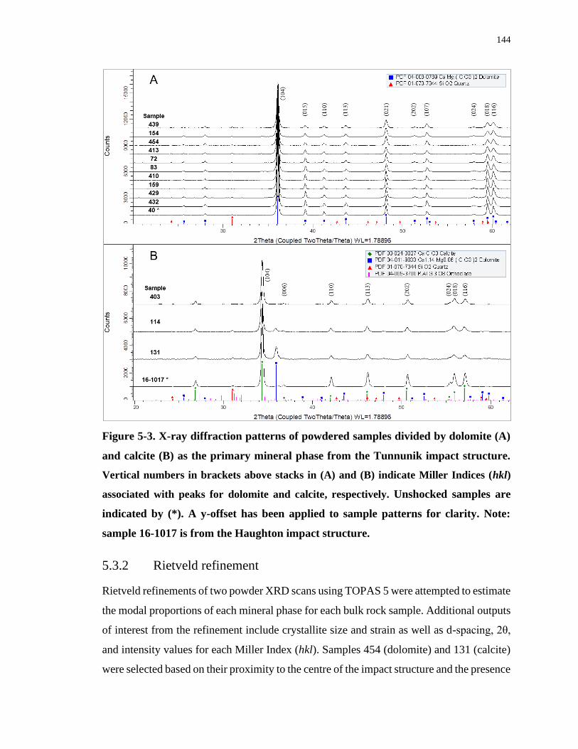
144

Figure 5-3. X-ray diffraction patterns of powdered samples divided by dolomite (A)

and calcite (B) as the primary mineral phase from the Tunnunik impact structure.

Vertical numbers in brackets above stacks in (A) and (B) indicate Miller Indices (hkl)

associated with peaks for dolomite and calcite, respectively. Unshocked samples are

indicated by (*). A y-offset has been applied to sample patterns for clarity. Note:

sample 16-1017 is from the Haughton impact structure.

5.3.2 Rietveld refinement

Rietveld refinements of two powder XRD scans using TOPAS 5 were attempted to estimate

the modal proportions of each mineral phase for each bulk rock sample. Additional outputs

of interest from the refinement include crystallite size and strain as well as d-spacing, 2θ,

and intensity values for each Miller Index (hkl). Samples 454 (dolomite) and 131 (calcite)

were selected based on their proximity to the centre of the impact structure and the presence

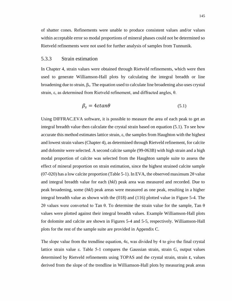
145

of shatter cones. Refinements were unable to produce consistent values and/or values

within acceptable error so modal proportions of mineral phases could not be determined so

Rietveld refinements were not used for further analysis of samples from Tunnunik.

5.3.3 Strain estimation

In Chapter 4, strain values were obtained through Rietveld refinements, which were then

used to generate Williamson-Hall plots by calculating the integral breadth or line

broadening due to strain, βs. The equation used to calculate line broadening also uses crystal

strain, ε, as determined from Rietveld refinement, and diffracted angles, θ.

𝛽𝑠 = 4𝜀𝑡𝑎𝑛𝜃 (5.1)

Using DIFFRAC.EVA software, it is possible to measure the area of each peak to get an

integral breadth value then calculate the crystal strain based on equation (5.1). To see how

accurate this method estimates lattice strain, ε, the samples from Haughton with the highest

and lowest strain values (Chapter 4), as determined through Rietveld refinement, for calcite

and dolomite were selected. A second calcite sample (99-063B) with high strain and a high

modal proportion of calcite was selected from the Haughton sample suite to assess the

effect of mineral proportion on strain estimation, since the highest strained calcite sample

(07-020) has a low calcite proportion (Table 5-1). In EVA, the observed maximum 2θ value

and integral breadth value for each (hkl) peak area was measured and recorded. Due to

peak broadening, some (hkl) peak areas were measured as one peak, resulting in a higher

integral breadth value as shown with the (018) and (116) plotted value in Figure 5-4. The

2θ values were converted to Tan θ. To determine the strain value for the sample, Tan θ

values were plotted against their integral breadth values. Example Williamson-Hall plots

for dolomite and calcite are shown in Figures 5-4 and 5-5, respectively. Williamson-Hall

plots for the rest of the sample suite are provided in Appendix C.

The slope value from the trendline equation, 4ε, was divided by 4 to give the final crystal

lattice strain value ε. Table 5-1 compares the Gaussian strain, strain G, output values

determined by Rietveld refinements using TOPAS and the crystal strain, strain ε, values

derived from the slope of the trendline in Williamson-Hall plots by measuring peak areas

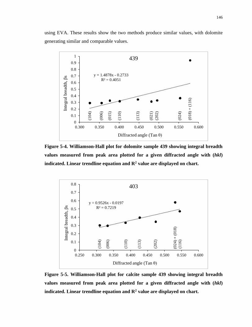
146

using EVA. These results show the two methods produce similar values, with dolomite

generating similar and comparable values.

Figure 5-4. Williamson-Hall plot for dolomite sample 439 showing integral breadth

values measured from peak area plotted for a given diffracted angle with (hkl)

indicated. Linear trendline equation and R2 value are displayed on chart.

Figure 5-5. Williamson-Hall plot for calcite sample 439 showing integral breadth

values measured from peak area plotted for a given diffracted angle with (hkl)

indicated. Linear trendline equation and R2 value are displayed on chart.

y = 1.4878x - 0.2733

R² = 0.4051

0

0.1

0.2

0.3

0.4

0.5

0.6

0.7

0.8

0.9

1

0.300 0.350 0.400 0.450 0.500 0.550 0.600

Inte

gra

l b

read

th, β

s

Diffracted angle (Tan θ)

439

(00

6)

(10

4)

(01

5)

(11

0)

(11

3)

(02

1)

(20

2)

(02

4)

(01

8)

+ (

11

6)

y = 0.9526x - 0.0197

R² = 0.7219

0

0.1

0.2

0.3

0.4

0.5

0.6

0.7

0.8

0.250 0.300 0.350 0.400 0.450 0.500 0.550 0.600

Inte

gra

l b

read

th, β

s

Diffracted angle (Tan θ)

403

(10

4)

(00

6)

(11

0)

(11

3)

(20

2)

(02

4)

+ (

01

8)

(11

6)

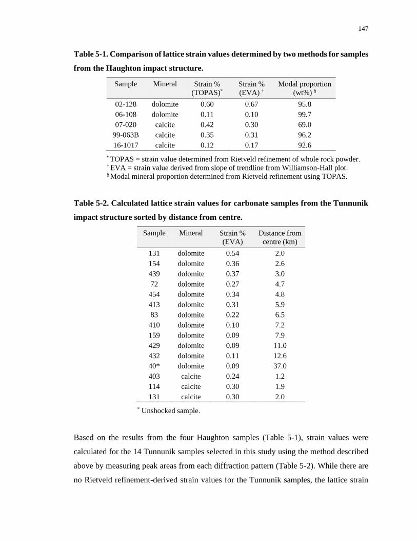
147

Table 5-1. Comparison of lattice strain values determined by two methods for samples

from the Haughton impact structure.

Sample Mineral Strain %

(TOPAS)*

Strain %

(EVA) †

Modal proportion

(wt%) §

02-128 dolomite 0.60 0.67 95.8

06-108 dolomite 0.11 0.10 99.7

07-020 calcite 0.42 0.30 69.0

99-063B calcite 0.35 0.31 96.2

16-1017 calcite 0.12 0.17 92.6

* TOPAS = strain value determined from Rietveld refinement of whole rock powder. † EVA = strain value derived from slope of trendline from Williamson-Hall plot. § Modal mineral proportion determined from Rietveld refinement using TOPAS.

Table 5-2. Calculated lattice strain values for carbonate samples from the Tunnunik

impact structure sorted by distance from centre.

Sample Mineral Strain %

(EVA)

Distance from

centre (km)

131 dolomite 0.54 2.0

154 dolomite 0.36 2.6

439 dolomite 0.37 3.0

72 dolomite 0.27 4.7

454 dolomite 0.34 4.8

413 dolomite 0.31 5.9

83 dolomite 0.22 6.5

410 dolomite 0.10 7.2

159 dolomite 0.09 7.9

429 dolomite 0.09 11.0

432 dolomite 0.11 12.6

40* dolomite 0.09 37.0

403 calcite 0.24 1.2

114 calcite 0.30 1.9

131 calcite 0.30 2.0

* Unshocked sample.

Based on the results from the four Haughton samples (Table 5-1), strain values were

calculated for the 14 Tunnunik samples selected in this study using the method described

above by measuring peak areas from each diffraction pattern (Table 5-2). While there are

no Rietveld refinement-derived strain values for the Tunnunik samples, the lattice strain

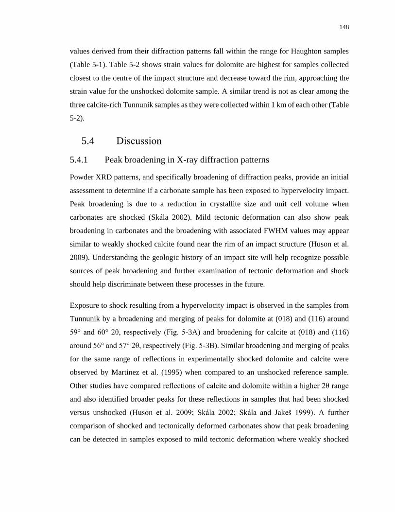
148

values derived from their diffraction patterns fall within the range for Haughton samples

(Table 5-1). Table 5-2 shows strain values for dolomite are highest for samples collected

closest to the centre of the impact structure and decrease toward the rim, approaching the

strain value for the unshocked dolomite sample. A similar trend is not as clear among the

three calcite-rich Tunnunik samples as they were collected within 1 km of each other (Table

5-2).

5.4 Discussion

5.4.1 Peak broadening in X-ray diffraction patterns

Powder XRD patterns, and specifically broadening of diffraction peaks, provide an initial

assessment to determine if a carbonate sample has been exposed to hypervelocity impact.

Peak broadening is due to a reduction in crystallite size and unit cell volume when

carbonates are shocked (Skála 2002). Mild tectonic deformation can also show peak

broadening in carbonates and the broadening with associated FWHM values may appear

similar to weakly shocked calcite found near the rim of an impact structure (Huson et al.

2009). Understanding the geologic history of an impact site will help recognize possible

sources of peak broadening and further examination of tectonic deformation and shock

should help discriminate between these processes in the future.

Exposure to shock resulting from a hypervelocity impact is observed in the samples from

Tunnunik by a broadening and merging of peaks for dolomite at (018) and (116) around

59° and 60° 2θ, respectively (Fig. 5-3A) and broadening for calcite at (018) and (116)

around 56° and 57° 2θ, respectively (Fig. 5-3B). Similar broadening and merging of peaks

for the same range of reflections in experimentally shocked dolomite and calcite were

observed by Martinez et al. (1995) when compared to an unshocked reference sample.

Other studies have compared reflections of calcite and dolomite within a higher 2θ range

and also identified broader peaks for these reflections in samples that had been shocked

versus unshocked (Huson et al. 2009; Skála 2002; Skála and Jakeš 1999). A further

comparison of shocked and tectonically deformed carbonates show that peak broadening

can be detected in samples exposed to mild tectonic deformation where weakly shocked

149

calcite is more difficult to distinguish from tectonically deformed calcite than more heavily

shocked dolomite (Huson et al. 2009).

5.4.2 Strain estimates and trends

When Rietveld quality powder XRD scans are not available to determine lattice strain

values, this study has shown that strain values obtained from Williamson-Hall plots are a

reasonable approximation. The comparison of strain values from Haughton samples (Table

5-1) demonstrates that relatively “pure” samples are more reliable in producing strain

values similar to the refined Rietveld values; pure here means the dominant mineral phase

in the sample is >90 wt%. The results from sample 07-020 (Table 5-1), which has the

largest difference between strain values, indicate that when the modal proportion of the

dominant mineral phase drops to ~70 wt%, this approximation method becomes less

effective. Based on this observation, bulk rock samples consisting of one dominant mineral

phase, over 90 wt%, are recommended rather than mixed samples, to achieve the best

results of strain estimation. It is difficult to compare this variation relating to modal mineral

proportions with previous studies as sample compositions in these studies appear to be

consistent within their respective sample suites. Composition of sample suites in previous

studies were reported as dominantly calcite by Skála and Jakeš (1999), the calcite samples

used by Skála (2002) were “more or less uniform” and “contents other than calcite end-

members are less than 5 mol%”, the calcite and dolomite samples used by Huson et al.

(2009) deviate slightly from stoichiometric values, and the dolomitic rocks used by

Martinez et al. (1995) were 79 ± 1% dolomite, 20 ± 1% calcite. The dolomitic rocks from

Martinez et al. (1995) have the most deviation from an ideal dolomite composition and

would have been interesting to see if there was a difference in strain values if they included

stoichiometric dolomite and calcite samples in their shock recovery experiments.

Modal proportions for mineral phases in the Tunnunik samples (Table 5-2) were not

determined because the quality of the original scans is not suitable for Rietveld refinement.

However, based on the XRD patterns for dolomite-rich samples (Fig. 5-3A), peaks

associated with calcite were not detected so dolomite is assumed to be the dominant

carbonate phase in these samples and, therefore, provide good approximations to Rietveld-

determined strain values. Calcite-rich samples 114 and 131 both indicate the presence of

150

dolomite (Fig. 5-3B) so these mixed carbonate samples may differ slightly in their

estimated strain values compared with Rietveld-determined values, depending on their

modal mineral proportions.

Other promising results from the Tunnunik strain values (Table 5-2) include both dolomite

and calcite strain falling within the range of strain values determined for Haughton samples

from Chapter 4 using Rietveld refinement. Several of the strain values for the low shocked

and the unshocked dolomite samples from Tunnunik are slightly lower than the Haughton

values, but remain comparable at 0.09% versus 0.11%, respectively. Since Tunnunik is

deeply eroded, the exposed target rocks within the impact structure would be expected to

have experienced lower overall shock pressures compared to the target rocks exposed

within the younger and well-preserved Haughton impact structure as the expanding

shockwave attenuates with depth (Melosh 1989). The estimated Tunnunik strain values

obtained support this expectation.

The highest dolomite strain value occurs within a calcite-rich mixed carbonate sample,

131, collected near the centre of the Tunnunik impact structure. Comparing the distance

from the centre to sample 131 and 439, the highest strain from a dolomite-rich sample, they

have similar distances and would be expected to have more similar strain values. The

difference is explained based on a trend observed for mixed carbonate samples from

Haughton (Chapter 4). The trend identified in Haughton mixed carbonate samples is that

dolomite is preferentially strained compared to calcite when both occur in bulk rock

powders, especially when dolomite is the carbonate present in lower proportion.

In Table 5-2, sample 72 appears to be out of place with respect to decreasing strain value

as distance from the centre of the impact structure increases as its value is less than sample

454 or 413 but is closer to the centre. This is explained by the elliptical distribution of

shatter cones (Fig. 5-2) where sample 72 is nearer to the edge of the distribution than 454

despite being closer to the centre. The elliptical shatter cone distribution has been suggested

to be the result of an oblique impact (Osinski and Ferrière 2016).

151

5.4.3 Practicality of strain estimation

Based on the results of XRD studies from the Tunnunik and Haughton impact structures,

Rietveld refinement of bulk rock powders provides better refined structural information

and is a more powerful tool than estimating peak areas from XRD patterns of short scan

durations to generate Williamson-Hall plots. This is not meant to diminish the usefulness

in generating Williamson-Hall plots for the purpose of measuring lattice strain as these

plots have been used successfully for other minerals (e.g., Jenkins et al. 2019; Uchizono et

al. 1999). There may be cases where it is more practical to collect a lower quality XRD

pattern to look for peak broadening, especially if there is a large sample volume and limited

analysis time. One-hour scans versus 8 hours or more could be a preferred option in this

case. If peak broadening is observed, Williamson-Hall plots can easily be generated to

estimate the lattice strain for that sample. If higher quality strain values are required, then

specific samples could be analyzed a second time to produce Rietveld quality data.

5.5 Conclusions

Building from the results and conclusions in Chapter 4, lattice strain in carbonates

generated by hypervelocity impact events is a measurable property. This study has shown

that good, low quality X-ray diffraction scans can generate lattice strain results that are

consistent with and fall within range of the lattice strain values determined when using

higher quality XRD data and structural refinement. The strain values from Tunnunik also

demonstrate the potential of using lattice strain values to estimate hypervelocity shock

pressure and allow for comparisons between carbonate-rich impact structures. Shock

pressure estimates could be determined from comparisons to lattice strain values in

dolomite and calcite derived from dolostone and limestone experimentally shocked to

known pressures with their strain values calculated. This could serve as the first steps in

generating a quantifiable shock classification system for carbonates as none currently exist

(Stöffler et al. 2018).

152

5.6 References

Althoff P. 1977. Structural refinements of dolomite and a magnesian calcite and

implications for dolomite formation in the marine environment. American

Mineralogist 62:772–783.

Brill R., Hermann C., and Peters C. 1939. Studien über chemische Bindung mittels

Fourieranalyse III. Die Naturwissenschaften 27:677–678.

Dewing K., Pratt B. R., Hadlari T., Brent T., Bédard J., and Rainbird R. H. 2013. Newly

identified “Tunnunik” impact structure, Prince Albert Peninsula, northwestern

Victoria Island, Arctic Canada. Meteoritics & Planetary Science 48:211–223.

French B. M. 1998. Traces of Catastrophe: A Handbook of Shock-Metamorphic Effects in

Terrestrial Meteorite Impact Structures, LPI Contribution No. 954, Lunar and

Planetary Science Institute, Houston.

French B. M., and Koeberl C. 2010. The convincing identification of terrestrial meteorite

impact structures: What works, what doesn’t, and why. Earth-Science Reviews

98:123–170.

Hill R. J., and Howard C. J. 1987. Quantitative phase analysis from neutron powder

diffraction data using the Rietveld method. Journal of Applied Crystallography

20:467–474.

Huson S. A., Foit F. F., Watkinson A. J., and Pope M. C. 2009. Rietveld analysis of X-ray

powder diffraction patterns as a potential tool for the identification of impact-

deformed carbonate rocks. Meteoritics & Planetary Science 44:1695–1706.

Jenkins L. E., Flemming R. L., and McCausland P. J. A. 2019. Quantitative in situ XRD

measurement of shock metamorphism in Martian meteorites using lattice strain and

strain-related mosaicity in olivine. Meteoritics & Planetary Science 54:902–918.

Lepaulard C., Gattacceca J., Swanson-Hysell N., Quesnel Y., Demory F., and Osinski G.

R. 2019. A Paleozoic age for the Tunnunik impact structure. Meteoritics & Planetary

153

Science 1–12.

Mallamo M. P. Ordovician and Silurian stratigraphy, sedimentology, and paleoecology,

Central Canadian Arctic Islands. MSc thesis, University of Western Ontario, 1989.

Martinez I., Deutsch A., Scharer U., Ildefonse P., Guyot F., and Agrinier P. 1995. Shock

recovery experiments on dolomite and thermodynamical calculation of impact

induced decarbonation. Journal of Geophysical Research 100:15465–15476.

Maslen E. N., Streltsov V. A., Streltsova N. R., and Ishizawa N. 1995. Electron density

and optical anisotropy in rhombohedral carbonates. III. Synchrotron X‐ray studies of

CaCO3, MgCO3 and MnCO3. Acta Crystallographica Section B 51:929–939.

Melosh H. J. 1989. Impact Cratering: A Geologic Process, New York: Oxford University

Press.

Osinski G. R., Spray J. G., and Grieve R. A. F. 2008. Impact melting in sedimentary target

rocks: An assessment. In The Sedimentary Record of Meteorite Impacts, Special

Paper 437, edited by Evans K. R., Horton W., King Jr. D. K., and Morrow J. R.

Geological Society of America, Boulder, CO. pp. 1–18.

Osinski G. R., and Ferrière L. 2016. Shatter cones: (Mis)understood? Science Advances 2,

e160061:1–10.

Ribbe P. H. 1979. The structure of a strained intermediate microcline in cryptoperthitic

association with twinned plagioclase. American Mineralogist 64:402–408.

Ross N. L., and Reeder R. J. 1992. High-pressure structural study of dolomite and ankerite.

American Mineralogist 77:412–421.

Seeley J. R., and Milam K. A. 2018. Optical and X-ray diffraction analyses of shock

metamorphosed dolostone at increasing depths within the central uplift of the Wells

Creeks impact structure. 49th Lunar and Planetary Science Conference Abstract

#2755.

154

Skála R., and Jakeš P. 1999. Shock-induced effects in natural calcite-rich targets as

revealed by X-ray powder diffraction. In Large Meteorite Impacts and Planetary

Evolution II, Special Paper 339, edited by Dressler B. O., and Sharpton V. L.

Geological Society of America (GSA), Boulder, CO. pp. 205–214.

Skála R. 2002. Shock-induced phenomena in limestones in the quarry near Ronheim, the

Ries Crater, Germany. Bulletin of the Czech Geological Survey 77:313–320.

Stewart W. D. 1987. Late Proterozoic to Early Tertiary stratigraphy of Somerset Island

and Northern Boothia Peninsula, District of Franklin, N.W.T., Paper 83-26,

Geological Survey of Canada.

Stöffler D., Hamann C., and Metzler K. 2018. Shock metamorphism of planetary silicate

rocks and sediments: Proposal for an updated classification system. Meteoritics &

Planetary Science 49:5–49.

Turvey C. C., Hamilton J. L., and Wilson S. A. 2018. Comparison of Rietveld-compatible

structureless fitting analysis methods for accurate quantification of carbon dioxide

fixation in ultramafic mine tailings. American Mineralogist 103:1649–1662.

Uchizono A., Shinno I., Nakamuta Y., Nakamura T., and Sekine T. 1999. Characterization

of artificially shocked forsterites: (1) Diffraction profile analysis by Gandolfi camera.

Mineralogical Journal 21:15–23.

155

Chapter 6

6 Impact-generated moissanite (SiC) from the Haughton

impact structure, Canada

6.1 Introduction

Moissanite (SiC) is a rare terrestrial mineral typically identified in mantle-derived sources

including kimberlites, carbonatites, and ultramafic rocks, as well as from crustal sources

such as granitoids, volcanic breccias, and carbonates (e.g., Machev et al. 2018; Shiryaev et

al. 2011). Here, we report the first documented in situ occurrence of moissanite crystals

from a meteorite impact crater – in clast-rich impact melt rocks from the Haughton impact

structure. The Haughton impact structure is a 23-km diameter complex crater located on

Devon Island in the Canadian Arctic, consisting of mixed target rocks of Cambrian to

Silurian-aged limestone, dolostone, evaporites, and sandstone overlying a Precambrian

basement of gneiss and metagranite (Osinski et al. 2005a). Moissanite is associated with

impact melt rocks present in 7 dykes within the chert-bearing limestone of the Eleanor

River Formation exposed along the Haughton River (Osinski et al. 2005a) within the

central uplift of the impact structure (Fig. 6-1).

The physical properties of moissanite include a hardness of 9.5, adamantine lustre,

conchoidal fracture, and range from colourless to dark blue or green (e.g., Lyakhovich

1980). Moissanite has a simple crystal structure consisting of stable silicon and carbon

tetrahedral layers. Variations in the number of repeated tetrahedral layers along the c-axis

in the unit cell give rise to the formation of polytypes associated with the hexagonal,

rhombohedral, and cubic lattice systems (Ramsdell 1947). The hexagonal polytypes 15R,

6H, and 4H were the first three polytypes identified, as well as the most common, and are

known as α-SiC, or true moissanite, while cubic polytypes are classed as β-SiC

(Lyakhovich 1980; Verma and Krishna 1966).

Moissanite has been reported in impactites from two other terrestrial impact structures, the

Ries impact structure, Germany (Hough et al. 1995) and the Popigai impact structure,

Russia (Gromilov et al. 2018). At both sites, moissanite crystals were not observed in situ

but were identified in acid-resistant residue from suevite melt rocks at the Otting quarry

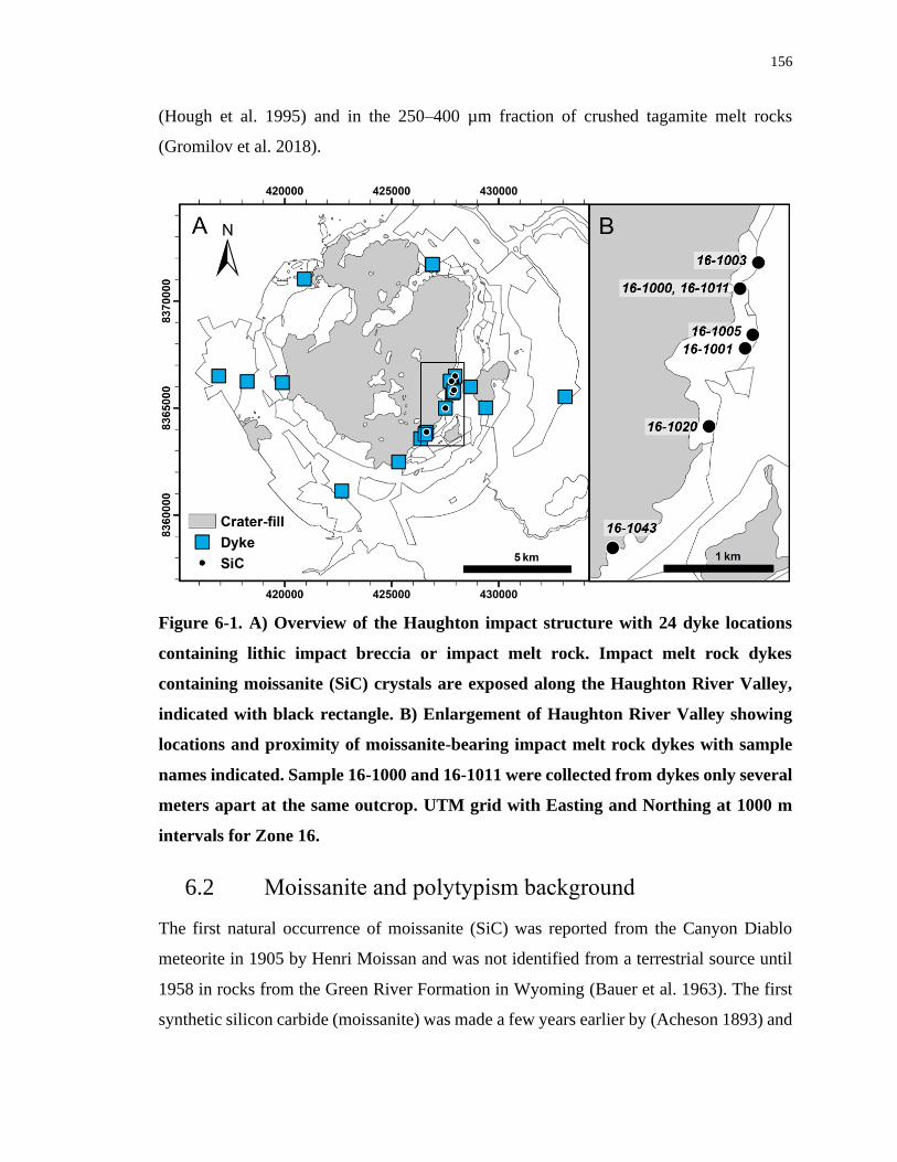
156

(Hough et al. 1995) and in the 250–400 µm fraction of crushed tagamite melt rocks

(Gromilov et al. 2018).

Figure 6-1. A) Overview of the Haughton impact structure with 24 dyke locations

containing lithic impact breccia or impact melt rock. Impact melt rock dykes

containing moissanite (SiC) crystals are exposed along the Haughton River Valley,

indicated with black rectangle. B) Enlargement of Haughton River Valley showing

locations and proximity of moissanite-bearing impact melt rock dykes with sample

names indicated. Sample 16-1000 and 16-1011 were collected from dykes only several

meters apart at the same outcrop. UTM grid with Easting and Northing at 1000 m

intervals for Zone 16.

6.2 Moissanite and polytypism background

The first natural occurrence of moissanite (SiC) was reported from the Canyon Diablo

meteorite in 1905 by Henri Moissan and was not identified from a terrestrial source until

1958 in rocks from the Green River Formation in Wyoming (Bauer et al. 1963). The first

synthetic silicon carbide (moissanite) was made a few years earlier by (Acheson 1893) and

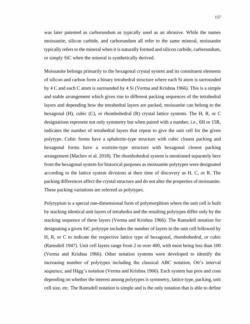
157

was later patented as carborundum as typically used as an abrasive. While the names

moissanite, silicon carbide, and carborundum all refer to the same mineral, moissanite

typically refers to the mineral when it is naturally formed and silicon carbide, carborundum,

or simply SiC when the mineral is synthetically derived.

Moissanite belongs primarily to the hexagonal crystal system and its constituent elements

of silicon and carbon form a binary tetrahedral structure where each Si atom is surrounded

by 4 C and each C atom is surrounded by 4 Si (Verma and Krishna 1966). This is a simple

and stable arrangement which gives rise to different packing sequences of the tetrahedral

layers and depending how the tetrahedral layers are packed, moissanite can belong to the

hexagonal (H), cubic (C), or rhombohedral (R) crystal lattice systems. The H, R, or C

designations represent not only symmetry but when paired with a number, i.e., 6H or 15R,

indicates the number of tetrahedral layers that repeat to give the unit cell for the given

polytype. Cubic forms have a sphalerite-type structure with cubic closest packing and

hexagonal forms have a wurtzite-type structure with hexagonal closest packing

arrangement (Machev et al. 2018). The rhombohedral system is mentioned separately here

from the hexagonal system for historical purposes as moissanite polytypes were designated

according to the lattice system divisions at their time of discovery as H, C, or R. The

packing differences affect the crystal structure and do not alter the properties of moissanite.

These packing variations are referred as polytypes.

Polytypism is a special one-dimensional form of polymorphism where the unit cell is built

by stacking identical unit layers of tetrahedra and the resulting polytypes differ only by the

stacking sequence of these layers (Verma and Krishna 1966). The Ramsdell notation for

designating a given SiC polytype includes the number of layers in the unit cell followed by

H, R, or C to indicate the respective lattice type of hexagonal, rhombohedral, or cubic

(Ramsdell 1947). Unit cell layers range from 2 to over 400, with most being less than 100

(Verma and Krishna 1966). Other notation systems were developed to identify the

increasing number of polytypes including the classical ABC notation, Ott’s interval

sequence, and Hägg’s notation (Verma and Krishna 1966). Each system has pros and cons

depending on whether the interest among polytypes is symmetry, lattice type, packing, unit

cell size, etc. The Ramsdell notation is simple and is the only notation that is able to define

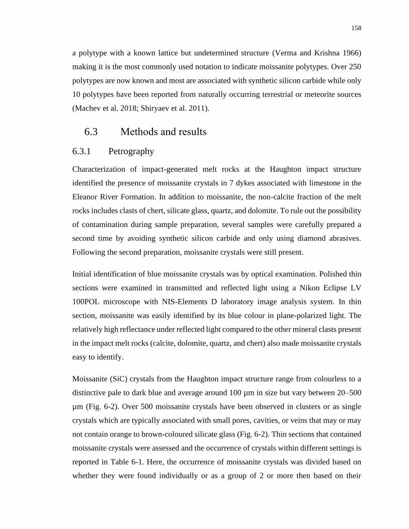
158

a polytype with a known lattice but undetermined structure (Verma and Krishna 1966)

making it is the most commonly used notation to indicate moissanite polytypes. Over 250

polytypes are now known and most are associated with synthetic silicon carbide while only

10 polytypes have been reported from naturally occurring terrestrial or meteorite sources

(Machev et al. 2018; Shiryaev et al. 2011).

6.3 Methods and results

6.3.1 Petrography

Characterization of impact-generated melt rocks at the Haughton impact structure

identified the presence of moissanite crystals in 7 dykes associated with limestone in the

Eleanor River Formation. In addition to moissanite, the non-calcite fraction of the melt

rocks includes clasts of chert, silicate glass, quartz, and dolomite. To rule out the possibility

of contamination during sample preparation, several samples were carefully prepared a

second time by avoiding synthetic silicon carbide and only using diamond abrasives.

Following the second preparation, moissanite crystals were still present.

Initial identification of blue moissanite crystals was by optical examination. Polished thin

sections were examined in transmitted and reflected light using a Nikon Eclipse LV

100POL microscope with NIS-Elements D laboratory image analysis system. In thin

section, moissanite was easily identified by its blue colour in plane-polarized light. The

relatively high reflectance under reflected light compared to the other mineral clasts present

in the impact melt rocks (calcite, dolomite, quartz, and chert) also made moissanite crystals

easy to identify.

Moissanite (SiC) crystals from the Haughton impact structure range from colourless to a

distinctive pale to dark blue and average around 100 µm in size but vary between 20–500

µm (Fig. 6-2). Over 500 moissanite crystals have been observed in clusters or as single

crystals which are typically associated with small pores, cavities, or veins that may or may

not contain orange to brown-coloured silicate glass (Fig. 6-2). Thin sections that contained

moissanite crystals were assessed and the occurrence of crystals within different settings is

reported in Table 6-1. Here, the occurrence of moissanite crystals was divided based on

whether they were found individually or as a group of 2 or more then based on their

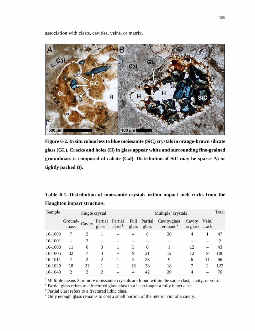
159

association with clasts, cavities, veins, or matrix.

Figure 6-2. In situ colourless to blue moissanite (SiC) crystals in orange-brown silicate

glass (GL). Cracks and holes (H) in glass appear white and surrounding fine-grained

groundmass is composed of calcite (Cal). Distribution of SiC may be sparse A) or

tightly packed B).

Table 6-1. Distribution of moissanite crystals within impact melt rocks from the

Haughton impact structure.

Sample Single crystal Multiple* crystals Total

Ground-

mass Cavity

Partial

glass †

Partial

clast §

Full

glass

Partial

glass

Cavity/glass

remnant #

Cavity

no glass

Vein/

crack

16-1000 7 2 1 – 4 8 20 4 1 47

16-1001 – 2 – – – – – – – 2

16-1003 11 6 3 1 3 6 1 12 – 43

16-1005 32 7 4 – 9 21 12 12 9 106

16-1011 7 2 2 1 5 23 9 6 11 66

16-1020 18 21 1 1 16 38 18 7 2 122

16-1043 2 2 2 – 4 42 20 4 – 76

* Multiple means 2 or more moissanite crystals are found within the same clast, cavity, or vein. † Partial glass refers to a fractured glass clast that is no longer a fully intact clast. § Partial clast refers to a fractured lithic clast. # Only enough glass remains to coat a small portion of the interior rim of a cavity.

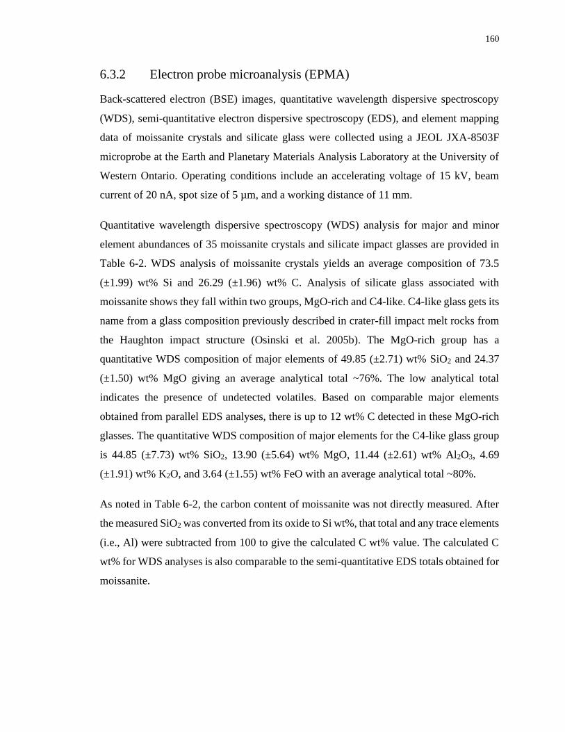
160

6.3.2 Electron probe microanalysis (EPMA)

Back-scattered electron (BSE) images, quantitative wavelength dispersive spectroscopy

(WDS), semi-quantitative electron dispersive spectroscopy (EDS), and element mapping

data of moissanite crystals and silicate glass were collected using a JEOL JXA-8503F

microprobe at the Earth and Planetary Materials Analysis Laboratory at the University of

Western Ontario. Operating conditions include an accelerating voltage of 15 kV, beam

current of 20 nA, spot size of 5 µm, and a working distance of 11 mm.

Quantitative wavelength dispersive spectroscopy (WDS) analysis for major and minor

element abundances of 35 moissanite crystals and silicate impact glasses are provided in

Table 6-2. WDS analysis of moissanite crystals yields an average composition of 73.5

(±1.99) wt% Si and 26.29 (±1.96) wt% C. Analysis of silicate glass associated with

moissanite shows they fall within two groups, MgO-rich and C4-like. C4-like glass gets its

name from a glass composition previously described in crater-fill impact melt rocks from

the Haughton impact structure (Osinski et al. 2005b). The MgO-rich group has a

quantitative WDS composition of major elements of 49.85 (±2.71) wt% SiO2 and 24.37

(±1.50) wt% MgO giving an average analytical total ~76%. The low analytical total

indicates the presence of undetected volatiles. Based on comparable major elements

obtained from parallel EDS analyses, there is up to 12 wt% C detected in these MgO-rich

glasses. The quantitative WDS composition of major elements for the C4-like glass group

is 44.85 (±7.73) wt% SiO2, 13.90 (±5.64) wt% MgO, 11.44 (±2.61) wt% Al2O3, 4.69

(±1.91) wt% K2O, and 3.64 (±1.55) wt% FeO with an average analytical total ~80%.

As noted in Table 6-2, the carbon content of moissanite was not directly measured. After

the measured SiO2 was converted from its oxide to Si wt%, that total and any trace elements

(i.e., Al) were subtracted from 100 to give the calculated C wt% value. The calculated C

wt% for WDS analyses is also comparable to the semi-quantitative EDS totals obtained for

moissanite.

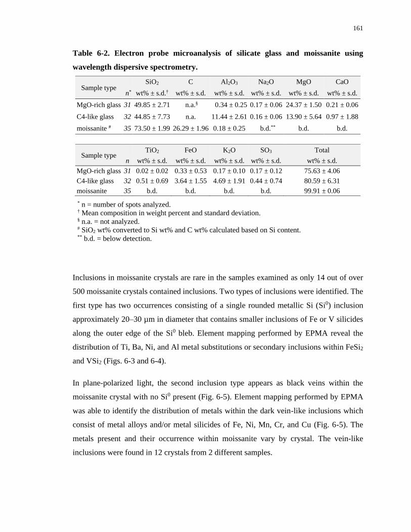
161

Table 6-2. Electron probe microanalysis of silicate glass and moissanite using

wavelength dispersive spectrometry.

Sample type

SiO2 C Al2O3 Na2O MgO CaO

n* wt% ± s.d.† wt% ± s.d. wt% ± s.d. wt% ± s.d. wt% ± s.d. wt% ± s.d.

MgO-rich glass 31 49.85 ± 2.71 n.a.§ 0.34 ± 0.25 0.17 ± 0.06 24.37 ± 1.50 0.21 ± 0.06

C4-like glass 32 44.85 ± 7.73 n.a. 11.44 ± 2.61 0.16 ± 0.06 13.90 ± 5.64 0.97 ± 1.88

moissanite # 35 73.50 ± 1.99 26.29 ± 1.96 0.18 ± 0.25 b.d.** b.d. b.d.

Sample type TiO2 FeO K2O SO3 Total

n wt% ± s.d. wt% ± s.d. wt% ± s.d. wt% ± s.d. wt% ± s.d.

MgO-rich glass 31 0.02 ± 0.02 0.33 ± 0.53 0.17 ± 0.10 0.17 ± 0.12 75.63 ± 4.06

C4-like glass 32 0.51 ± 0.69 3.64 ± 1.55 4.69 ± 1.91 0.44 ± 0.74 80.59 ± 6.31

moissanite 35 b.d. b.d. b.d. b.d. 99.91 ± 0.06

* n = number of spots analyzed. † Mean composition in weight percent and standard deviation. § n.a. = not analyzed. # SiO2 wt% converted to Si wt% and C wt% calculated based on Si content. ** b.d. = below detection.

Inclusions in moissanite crystals are rare in the samples examined as only 14 out of over

500 moissanite crystals contained inclusions. Two types of inclusions were identified. The

first type has two occurrences consisting of a single rounded metallic Si (Si0) inclusion

approximately 20–30 µm in diameter that contains smaller inclusions of Fe or V silicides

along the outer edge of the Si0 bleb. Element mapping performed by EPMA reveal the

distribution of Ti, Ba, Ni, and Al metal substitutions or secondary inclusions within FeSi2

and VSi2 (Figs. 6-3 and 6-4).

In plane-polarized light, the second inclusion type appears as black veins within the

moissanite crystal with no Si0 present (Fig. 6-5). Element mapping performed by EPMA

was able to identify the distribution of metals within the dark vein-like inclusions which

consist of metal alloys and/or metal silicides of Fe, Ni, Mn, Cr, and Cu (Fig. 6-5). The

metals present and their occurrence within moissanite vary by crystal. The vein-like

inclusions were found in 12 crystals from 2 different samples.

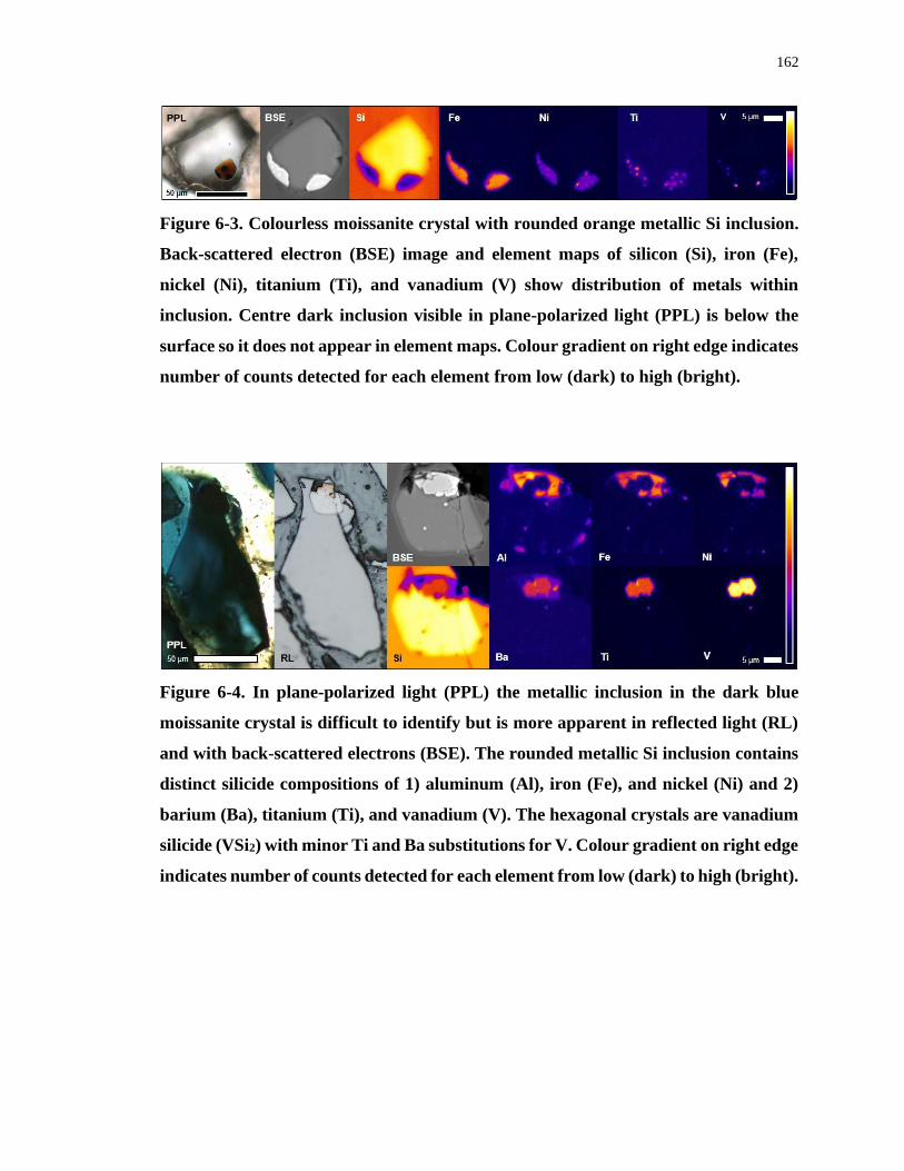
162

Figure 6-3. Colourless moissanite crystal with rounded orange metallic Si inclusion.

Back-scattered electron (BSE) image and element maps of silicon (Si), iron (Fe),

nickel (Ni), titanium (Ti), and vanadium (V) show distribution of metals within

inclusion. Centre dark inclusion visible in plane-polarized light (PPL) is below the

surface so it does not appear in element maps. Colour gradient on right edge indicates

number of counts detected for each element from low (dark) to high (bright).

Figure 6-4. In plane-polarized light (PPL) the metallic inclusion in the dark blue

moissanite crystal is difficult to identify but is more apparent in reflected light (RL)

and with back-scattered electrons (BSE). The rounded metallic Si inclusion contains

distinct silicide compositions of 1) aluminum (Al), iron (Fe), and nickel (Ni) and 2)

barium (Ba), titanium (Ti), and vanadium (V). The hexagonal crystals are vanadium

silicide (VSi2) with minor Ti and Ba substitutions for V. Colour gradient on right edge

indicates number of counts detected for each element from low (dark) to high (bright).

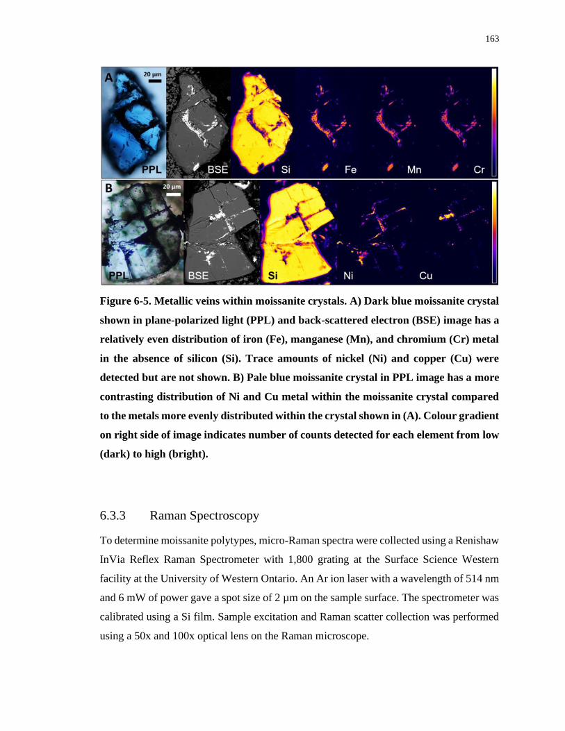
163

Figure 6-5. Metallic veins within moissanite crystals. A) Dark blue moissanite crystal

shown in plane-polarized light (PPL) and back-scattered electron (BSE) image has a

relatively even distribution of iron (Fe), manganese (Mn), and chromium (Cr) metal

in the absence of silicon (Si). Trace amounts of nickel (Ni) and copper (Cu) were

detected but are not shown. B) Pale blue moissanite crystal in PPL image has a more

contrasting distribution of Ni and Cu metal within the moissanite crystal compared

to the metals more evenly distributed within the crystal shown in (A). Colour gradient

on right side of image indicates number of counts detected for each element from low

(dark) to high (bright).

6.3.3 Raman Spectroscopy

To determine moissanite polytypes, micro-Raman spectra were collected using a Renishaw

InVia Reflex Raman Spectrometer with 1,800 grating at the Surface Science Western

facility at the University of Western Ontario. An Ar ion laser with a wavelength of 514 nm

and 6 mW of power gave a spot size of 2 µm on the sample surface. The spectrometer was

calibrated using a Si film. Sample excitation and Raman scatter collection was performed

using a 50x and 100x optical lens on the Raman microscope.

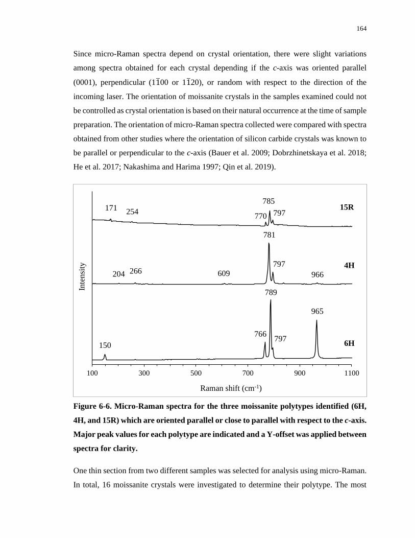
164

Since micro-Raman spectra depend on crystal orientation, there were slight variations

among spectra obtained for each crystal depending if the c-axis was oriented parallel

(0001), perpendicular (11̅00 or 11̅20), or random with respect to the direction of the

incoming laser. The orientation of moissanite crystals in the samples examined could not

be controlled as crystal orientation is based on their natural occurrence at the time of sample

preparation. The orientation of micro-Raman spectra collected were compared with spectra

obtained from other studies where the orientation of silicon carbide crystals was known to

be parallel or perpendicular to the c-axis (Bauer et al. 2009; Dobrzhinetskaya et al. 2018;

He et al. 2017; Nakashima and Harima 1997; Qin et al. 2019).

Figure 6-6. Micro-Raman spectra for the three moissanite polytypes identified (6H,

4H, and 15R) which are oriented parallel or close to parallel with respect to the c-axis.

Major peak values for each polytype are indicated and a Y-offset was applied between

spectra for clarity.

One thin section from two different samples was selected for analysis using micro-Raman.

In total, 16 moissanite crystals were investigated to determine their polytype. The most

100 300 500 700 900 1100

Inte

nsi

ty

Raman shift (cm-1)

6H

4H

15R

150

766

789

797

965

204 266 609

781

797

966

171254

770

785

797

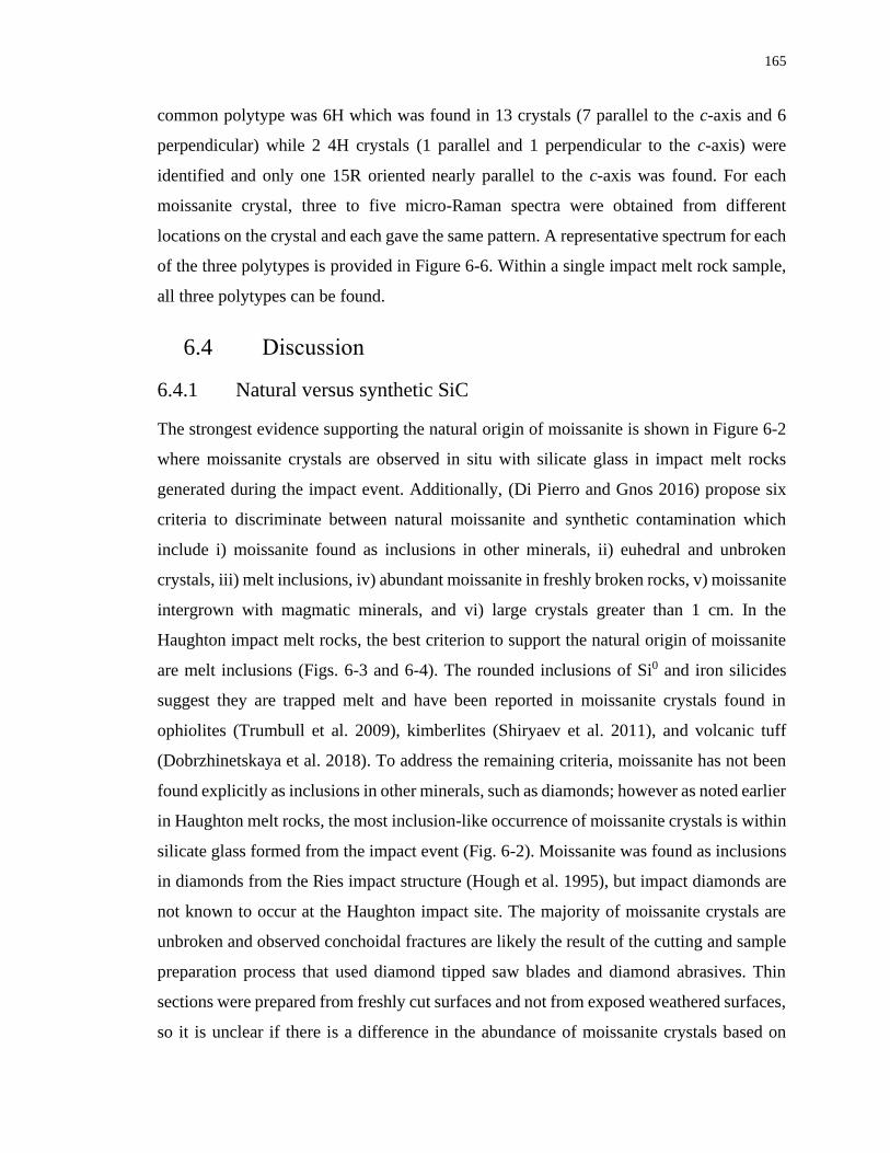
165

common polytype was 6H which was found in 13 crystals (7 parallel to the c-axis and 6

perpendicular) while 2 4H crystals (1 parallel and 1 perpendicular to the c-axis) were

identified and only one 15R oriented nearly parallel to the c-axis was found. For each

moissanite crystal, three to five micro-Raman spectra were obtained from different

locations on the crystal and each gave the same pattern. A representative spectrum for each

of the three polytypes is provided in Figure 6-6. Within a single impact melt rock sample,

all three polytypes can be found.

6.4 Discussion

6.4.1 Natural versus synthetic SiC

The strongest evidence supporting the natural origin of moissanite is shown in Figure 6-2

where moissanite crystals are observed in situ with silicate glass in impact melt rocks

generated during the impact event. Additionally, (Di Pierro and Gnos 2016) propose six

criteria to discriminate between natural moissanite and synthetic contamination which

include i) moissanite found as inclusions in other minerals, ii) euhedral and unbroken

crystals, iii) melt inclusions, iv) abundant moissanite in freshly broken rocks, v) moissanite

intergrown with magmatic minerals, and vi) large crystals greater than 1 cm. In the

Haughton impact melt rocks, the best criterion to support the natural origin of moissanite

are melt inclusions (Figs. 6-3 and 6-4). The rounded inclusions of Si0 and iron silicides

suggest they are trapped melt and have been reported in moissanite crystals found in

ophiolites (Trumbull et al. 2009), kimberlites (Shiryaev et al. 2011), and volcanic tuff

(Dobrzhinetskaya et al. 2018). To address the remaining criteria, moissanite has not been

found explicitly as inclusions in other minerals, such as diamonds; however as noted earlier

in Haughton melt rocks, the most inclusion-like occurrence of moissanite crystals is within

silicate glass formed from the impact event (Fig. 6-2). Moissanite was found as inclusions

in diamonds from the Ries impact structure (Hough et al. 1995), but impact diamonds are

not known to occur at the Haughton impact site. The majority of moissanite crystals are

unbroken and observed conchoidal fractures are likely the result of the cutting and sample

preparation process that used diamond tipped saw blades and diamond abrasives. Thin

sections were prepared from freshly cut surfaces and not from exposed weathered surfaces,

so it is unclear if there is a difference in the abundance of moissanite crystals based on

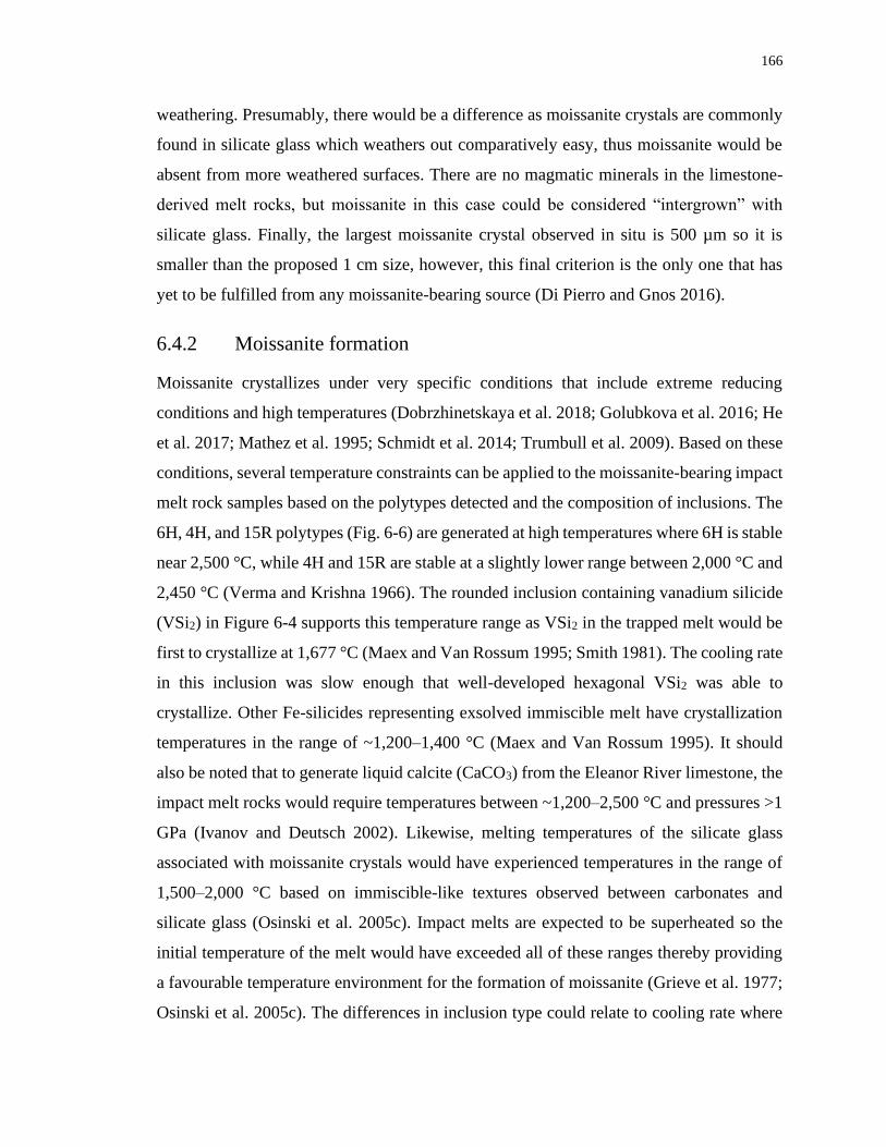
166

weathering. Presumably, there would be a difference as moissanite crystals are commonly

found in silicate glass which weathers out comparatively easy, thus moissanite would be

absent from more weathered surfaces. There are no magmatic minerals in the limestone-

derived melt rocks, but moissanite in this case could be considered “intergrown” with

silicate glass. Finally, the largest moissanite crystal observed in situ is 500 µm so it is

smaller than the proposed 1 cm size, however, this final criterion is the only one that has

yet to be fulfilled from any moissanite-bearing source (Di Pierro and Gnos 2016).

6.4.2 Moissanite formation

Moissanite crystallizes under very specific conditions that include extreme reducing

conditions and high temperatures (Dobrzhinetskaya et al. 2018; Golubkova et al. 2016; He

et al. 2017; Mathez et al. 1995; Schmidt et al. 2014; Trumbull et al. 2009). Based on these

conditions, several temperature constraints can be applied to the moissanite-bearing impact

melt rock samples based on the polytypes detected and the composition of inclusions. The

6H, 4H, and 15R polytypes (Fig. 6-6) are generated at high temperatures where 6H is stable

near 2,500 °C, while 4H and 15R are stable at a slightly lower range between 2,000 °C and

2,450 °C (Verma and Krishna 1966). The rounded inclusion containing vanadium silicide

(VSi2) in Figure 6-4 supports this temperature range as VSi2 in the trapped melt would be

first to crystallize at 1,677 °C (Maex and Van Rossum 1995; Smith 1981). The cooling rate

in this inclusion was slow enough that well-developed hexagonal VSi2 was able to

crystallize. Other Fe-silicides representing exsolved immiscible melt have crystallization

temperatures in the range of ~1,200–1,400 °C (Maex and Van Rossum 1995). It should

also be noted that to generate liquid calcite (CaCO3) from the Eleanor River limestone, the

impact melt rocks would require temperatures between ~1,200–2,500 °C and pressures >1

GPa (Ivanov and Deutsch 2002). Likewise, melting temperatures of the silicate glass

associated with moissanite crystals would have experienced temperatures in the range of

1,500–2,000 °C based on immiscible-like textures observed between carbonates and

silicate glass (Osinski et al. 2005c). Impact melts are expected to be superheated so the

initial temperature of the melt would have exceeded all of these ranges thereby providing

a favourable temperature environment for the formation of moissanite (Grieve et al. 1977;

Osinski et al. 2005c). The differences in inclusion type could relate to cooling rate where

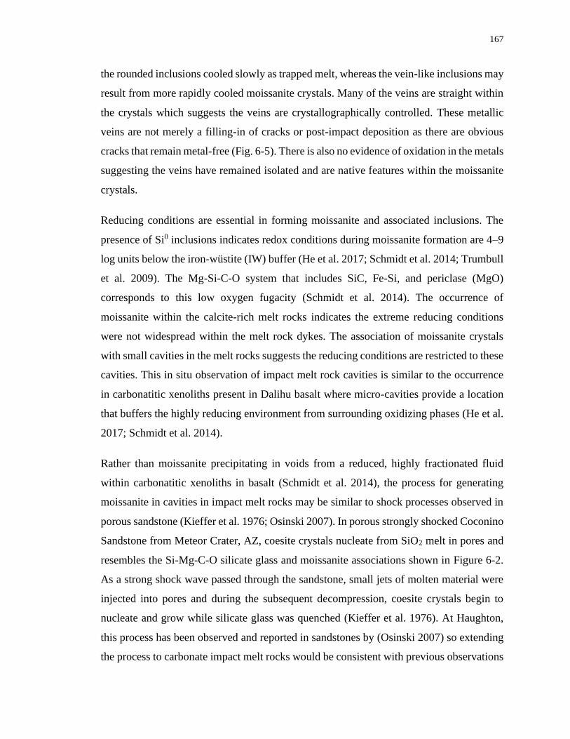
167

the rounded inclusions cooled slowly as trapped melt, whereas the vein-like inclusions may

result from more rapidly cooled moissanite crystals. Many of the veins are straight within

the crystals which suggests the veins are crystallographically controlled. These metallic

veins are not merely a filling-in of cracks or post-impact deposition as there are obvious

cracks that remain metal-free (Fig. 6-5). There is also no evidence of oxidation in the metals

suggesting the veins have remained isolated and are native features within the moissanite

crystals.

Reducing conditions are essential in forming moissanite and associated inclusions. The

presence of Si0 inclusions indicates redox conditions during moissanite formation are 4–9

log units below the iron-wüstite (IW) buffer (He et al. 2017; Schmidt et al. 2014; Trumbull

et al. 2009). The Mg-Si-C-O system that includes SiC, Fe-Si, and periclase (MgO)

corresponds to this low oxygen fugacity (Schmidt et al. 2014). The occurrence of

moissanite within the calcite-rich melt rocks indicates the extreme reducing conditions

were not widespread within the melt rock dykes. The association of moissanite crystals

with small cavities in the melt rocks suggests the reducing conditions are restricted to these

cavities. This in situ observation of impact melt rock cavities is similar to the occurrence

in carbonatitic xenoliths present in Dalihu basalt where micro-cavities provide a location

that buffers the highly reducing environment from surrounding oxidizing phases (He et al.

2017; Schmidt et al. 2014).

Rather than moissanite precipitating in voids from a reduced, highly fractionated fluid

within carbonatitic xenoliths in basalt (Schmidt et al. 2014), the process for generating

moissanite in cavities in impact melt rocks may be similar to shock processes observed in

porous sandstone (Kieffer et al. 1976; Osinski 2007). In porous strongly shocked Coconino

Sandstone from Meteor Crater, AZ, coesite crystals nucleate from SiO2 melt in pores and

resembles the Si-Mg-C-O silicate glass and moissanite associations shown in Figure 6-2.

As a strong shock wave passed through the sandstone, small jets of molten material were

injected into pores and during the subsequent decompression, coesite crystals begin to

nucleate and grow while silicate glass was quenched (Kieffer et al. 1976). At Haughton,

this process has been observed and reported in sandstones by (Osinski 2007) so extending

the process to carbonate impact melt rocks would be consistent with previous observations

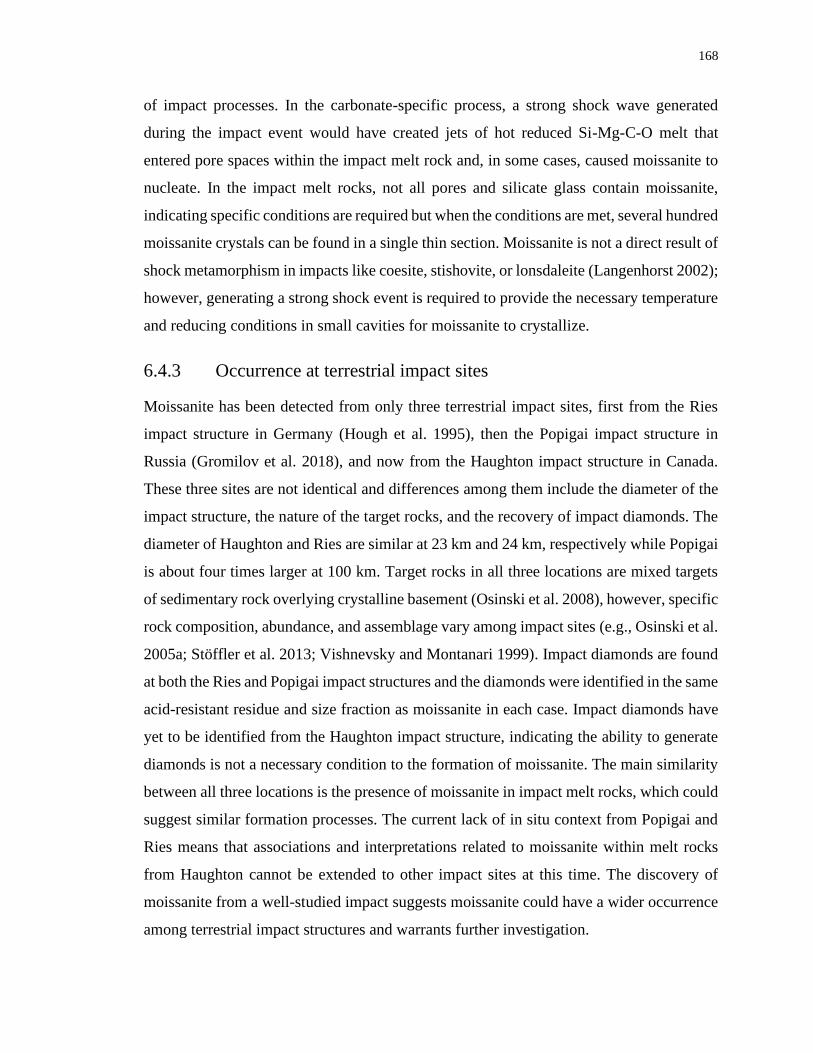
168

of impact processes. In the carbonate-specific process, a strong shock wave generated

during the impact event would have created jets of hot reduced Si-Mg-C-O melt that

entered pore spaces within the impact melt rock and, in some cases, caused moissanite to

nucleate. In the impact melt rocks, not all pores and silicate glass contain moissanite,

indicating specific conditions are required but when the conditions are met, several hundred

moissanite crystals can be found in a single thin section. Moissanite is not a direct result of

shock metamorphism in impacts like coesite, stishovite, or lonsdaleite (Langenhorst 2002);

however, generating a strong shock event is required to provide the necessary temperature

and reducing conditions in small cavities for moissanite to crystallize.

6.4.3 Occurrence at terrestrial impact sites

Moissanite has been detected from only three terrestrial impact sites, first from the Ries

impact structure in Germany (Hough et al. 1995), then the Popigai impact structure in

Russia (Gromilov et al. 2018), and now from the Haughton impact structure in Canada.

These three sites are not identical and differences among them include the diameter of the

impact structure, the nature of the target rocks, and the recovery of impact diamonds. The

diameter of Haughton and Ries are similar at 23 km and 24 km, respectively while Popigai

is about four times larger at 100 km. Target rocks in all three locations are mixed targets

of sedimentary rock overlying crystalline basement (Osinski et al. 2008), however, specific

rock composition, abundance, and assemblage vary among impact sites (e.g., Osinski et al.

2005a; Stöffler et al. 2013; Vishnevsky and Montanari 1999). Impact diamonds are found

at both the Ries and Popigai impact structures and the diamonds were identified in the same

acid-resistant residue and size fraction as moissanite in each case. Impact diamonds have

yet to be identified from the Haughton impact structure, indicating the ability to generate

diamonds is not a necessary condition to the formation of moissanite. The main similarity

between all three locations is the presence of moissanite in impact melt rocks, which could

suggest similar formation processes. The current lack of in situ context from Popigai and

Ries means that associations and interpretations related to moissanite within melt rocks

from Haughton cannot be extended to other impact sites at this time. The discovery of

moissanite from a well-studied impact suggests moissanite could have a wider occurrence

among terrestrial impact structures and warrants further investigation.

169

6.5 Conclusions

The discovery of moissanite in clast-rich impact melt rocks from the Haughton impact

structure is the first report of moissanite observed in situ and third occurrence from a

terrestrial impact structure. The existence of moissanite has provided new information such

as temperature constraints involved in generating moissanite-bearing impact melt rocks

and the mineral associations of moissanite at the Haughton impact structure. The specific

formation conditions of moissanite also offer insights into impact processes at the Earth’s

surface for a mineral typically associated with mantle sources.

6.6 References

Acheson E. G. 1893. On carborundum. Chemical News 68:179.

Bauer J., Fiala J., and Hrichova R. 1963. Natural a-silicon carbide. American Mineralogist

48:620–634.

Bauer M., Gigler A. M., Huber A. J., Hillenbrand R., and Stark R. W. 2009. Temperature-

depending Raman line-shift of silicon carbide. Journal of Raman Spectroscopy

40:1867–1874.

Dobrzhinetskaya L., Mukhin P., Wang Q., Wirth R., O’Bannon E., Zhao W., Eppelbaum

L., and Sokhonchuk T. 2018. Moissanite (SiC) with metal-silicide and silicon

inclusions from tuff of Israel: Raman spectroscopy and electron microscope studies.

Lithos 310–311:355–368.

Golubkova A., Schmidt M. W., and Connolly J. A. D. 2016. Ultra-reducing conditions in

average mantle peridotites and in podiform chromitites: a thermodynamic model for

moissanite (SiC) formation. Contributions to Mineralogy and Petrology 171.

Grieve R. A. F., Dence M. R., and Robertson P. B. 1977. Cratering processes: As

interpreted from the occurrence of impact melts. In Impact and Explosion Cratering,

edited by Roddy D. J., Pepin R. O., and Merrill R. B. New York: Pergamon Press. pp.

791–814.

170

Gromilov S. A., Afanasiev V. P., and Pokhilenko N. P. 2018. Moissanites of the Popigai

astrobleme. Doklady Earth Sciences 481:997–999.

He D., Liu Y., Gao C., Chen C., Hu Z., and Gao S. 2017. SiC-dominated ultra-reduced

mineral assemblage in carbonatitic xenoliths from the Dalihu basalt, Inner Mongolia,

China. American Mineralogist 102:312–320.

Hough R. M., Gilmour I., Pillinger C. T., Arden J. W., Gilkes K. W. R., Yuan J., and

Milledge H. J. 1995. Diamond and silicon carbide in impact melt rock from the Ries

impact crater. Nature 378:41–44.

Ivanov B. A., and Deutsch A. 2002. The phase diagram of CaCO3 in relation to shock

compression and decompression. Physics of the Earth and Planetary Interiors

129:131–143.

Kieffer S. W., Phakey P. P., and Christie J. M. 1976. Shock processes in porous quartzite:

Transmission electron microscope observations and theory. Contributions to

Mineralogy and Petrology 59:41–93.

Langenhorst F. 2002. Shock metamorphism of some minerals: Basic introduction and

microstructural observations. Bulletin of the Czech Geological Survey 77:265–282.

Lyakhovich V. V. 1980. Origin of accessory moissanite. International Geology Review

22:961–970.

Machev P., O’Bannon E. F., Bozhilov K. N., Wang Q., and Dobrzhinetskaya L. 2018. Not

all moissanites are created equal: New constraints on moissanite from metamorphic

rocks of Bulgaria. Earth and Planetary Science Letters 498:387–396.

Maex K., and Van Rossum M., eds. 1995. Properties of Metal Silicides, London: INSPEC,

the Institution of Electrical Engineers.

Mathez E. A., Fogel R. A., and Hutcheon I. D. 1995. Carbon isotopic composition and

origin of SiC from kimberlites of Yakutia, Russia. Geochimica et Cosmochimica Acta

59:781–791.

171

Nakashima S., and Harima H. 1997. Raman investigation of SiC polytypes. Physica Status

Solidi (A) Applied Research 162:39–64.

Osinski G. R., Lee P., Spray J. G., Parnell J., Lim D. S. S., Bunch T. E., Cockell C. S., and

Glass B. 2005a. Geological overview and cratering model for the Haughton impact

structure, Devon Island, Canadian High Arctic. Meteoritics & Planetary Science

40:1759–1776.

Osinski G. R., Spray J. G., and Lee P. 2005b. Impactites of the Haughton impact structure,

Devon Island, Canadian High Arctic. Meteoritics & Planetary Science 40:1789–1812.

Osinski G. R., Lee P., Parnell J., Spray J. G., and Baron M. 2005c. A case study of impact-

induced hydrothermal activity: The Haughton impact structure, Devon Island,

Canadian High Arctic. Meteoritics & Planetary Science 40:1859–1877.

Osinski G. R. 2007. Impact metamorphism of CaCO3‐bearing sandstones at the Haughton

structure, Canada. Meteoritics & Planetary Science 42:1945–1960.

Osinski G. R., Spray J. G., and Grieve R. A. F. 2008. Impact melting in sedimentary target

rocks: An assessment. In The Sedimentary Record of Meteorite Impacts, Special

Paper 437, edited by Evans K. R., Horton W., King Jr. D. K., and Morrow J. R.

Geological Society of America, Boulder, CO. pp. 1–18.

Di Pierro S., and Gnos E. 2016. Ca-Al-silicate inclusions in natural moissanite (SiC).

American Mineralogist 101:71–81.

Qin X., Li X., Chen X., Yang X., Zhang F., Xu X., Hu X., Peng Y., and Yu P. 2019. Raman

scattering study on phonon anisotropic properties of SiC. Journal of Alloys and

Compounds 776:1048–1055.

Ramsdell L. S. 1947. Studies on silicon carbide. American Mineralogist 32:64–82.

Schmidt M. W., Gao C., Golubkova A., Rohrbach A., and Connolly J. A. 2014. Natural

moissanite (SiC) – a low temperature mineral formed from highly fractionated ultra-

reducing COH-fluids. Progress in Earth and Planetary Science 1:1–14.

172

Shiryaev A. A., Griffin W. L., and Stoyanov E. 2011. Moissanite (SiC) from kimberlites:

Polytypes, trace elements, inclusions and speculations on origin. Lithos 122:152–164.

Smith J. F. 1981. The Si-V (Silicon-Vanadium) system. Bulletin of Alloy Phase Diagrams

2:42–48.

Stöffler D., Artemieva N. A., Wünnemann K., Reimold W. U., Jacob J., Hansen B. K., and

Summerson I. A. T. 2013. Ries crater and suevite revisited-Observations and

modeling Part I: Observations. Meteoritics & Planetary Science 48:515–589.

Trumbull R. B., Yang J. S., Robinson P. T., Di Pierro S., Vennemann T., and Wiedenbeck

M. 2009. The carbon isotope composition of natural SiC (moissanite) from the Earth’s

mantle: New discoveries from ophiolites. Lithos 113:612–620.

Verma A. R., and Krishna P. 1966. Polymorphism and polytypism in crystals, New York:

John Wiley & Sons, Inc.

Vishnevsky S., and Montanari A. 1999. Popigai impact structure (Arctic Siberia, Russia):

Geology, petrology, geochemistry, and geochronology of glass-bearing impactites. In

Large Meteorite Impacts and Planetary Evolution II, Special Paper 339, edited by

Dressler B. O., and Sharpton V. L. Geological Society of America (GSA), Boulder,

CO. pp. 19–59.

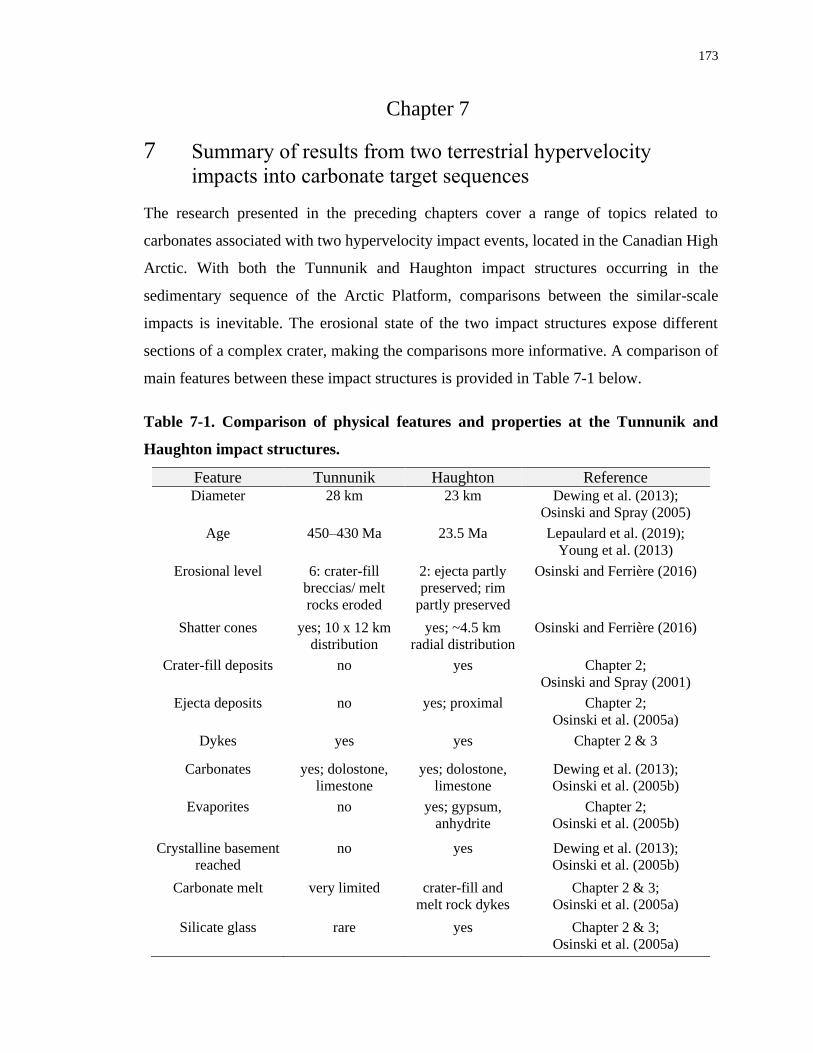
173

Chapter 7

7 Summary of results from two terrestrial hypervelocity

impacts into carbonate target sequences

The research presented in the preceding chapters cover a range of topics related to

carbonates associated with two hypervelocity impact events, located in the Canadian High

Arctic. With both the Tunnunik and Haughton impact structures occurring in the

sedimentary sequence of the Arctic Platform, comparisons between the similar-scale

impacts is inevitable. The erosional state of the two impact structures expose different

sections of a complex crater, making the comparisons more informative. A comparison of

main features between these impact structures is provided in Table 7-1 below.

Table 7-1. Comparison of physical features and properties at the Tunnunik and

Haughton impact structures.

Feature Tunnunik Haughton Reference Diameter 28 km 23 km Dewing et al. (2013);

Osinski and Spray (2005)

Age 450–430 Ma 23.5 Ma Lepaulard et al. (2019);

Young et al. (2013)

Erosional level 6: crater-fill

breccias/ melt

rocks eroded

2: ejecta partly

preserved; rim

partly preserved

Osinski and Ferrière (2016)

Shatter cones yes; 10 x 12 km

distribution

yes; ~4.5 km

radial distribution

Osinski and Ferrière (2016)

Crater-fill deposits no yes Chapter 2;

Osinski and Spray (2001)

Ejecta deposits no yes; proximal Chapter 2;

Osinski et al. (2005a)

Dykes yes yes Chapter 2 & 3

Carbonates yes; dolostone,

limestone

yes; dolostone,

limestone

Dewing et al. (2013);

Osinski et al. (2005b)

Evaporites no yes; gypsum,

anhydrite

Chapter 2;

Osinski et al. (2005b)

Crystalline basement

reached

no yes Dewing et al. (2013);

Osinski et al. (2005b)

Carbonate melt very limited crater-fill and

melt rock dykes

Chapter 2 & 3;

Osinski et al. (2005a)

Silicate glass rare yes Chapter 2 & 3;

Osinski et al. (2005a)

174

7.1 Carbonate-rich target sequences

The Arctic Platform consists of many sedimentary formations (Daae and Rutgers 1975;

Thorsteinsson and Tozer 1970) and the sequences present at both impact sites are

dominated by carbonates. Northwest Victoria Island has a thicker sedimentary sequence

than on Devon Island and as a result the Tunnunik impact event did not reach the crystalline

basement whereas the Haughton impact event did reach the crystalline basement of granitic

and metasedimentary rocks (Table 7-1). Presence of crystalline basement material,

evaporites, and sandstones leaves a target sequence comprised of ~75–80% carbonates at

the Haughton impact structure (Osinski et al. 2005a). Carbonates are even more abundant

at the Tunnunik impact structure where dolostone, limestone, and limited mudstone rocks

are exposed (Dewing et al. 2013). Limestone and dolostone are present in different amounts

at each site with Tunnunik exposing more dolostone than limestone while Haughton

exposes more equal portions of carbonate rocks overall.

When it comes to carbonate-rich target rocks, there are still questions to be answered and

relate to whether carbonates melt or decompose upon impact. The two carbonate-rich study

sites here provided an opportunity to identify if any melting or decomposition of carbonates

occurred during these impact events. While this was not a primary goal of this research,

evidence to support one or both processes had the potential to be identified through the

characterization of impact breccias and impact melt rocks collected from impact-generated

dykes.

Recalling the decomposition reactions of calcite (7.1) and dolomite (7.2) (e.g., Agrinier et

al. 2001), the main evidence for the decomposition or devolatilization of carbonates would

be the presence of CaO or MgO in impactites generated during the impact event (Osinski

et al. 2008).

𝐶𝑎𝐶𝑂3 → 𝐶𝑎𝑂 + 𝐶𝑂2 (7.1)

𝐶𝑎𝑀𝑔(𝐶𝑂3)2 → 𝐶𝑎𝑂 + 𝑀𝑔𝑂 + 2𝐶𝑂2 (7.2)

Neither CaO (lime) nor MgO (periclase) were identified in Tunnunik breccias or in

Haughton breccias or melt rocks. If either decomposition product had been generated

175

during the impact, then these impactites would be the most likely location to detect the

presence of these products.

As for melting, at Tunnunik there is limited evidence for melt in the form of thin isolated

bands of calcite that have a flow-like morphology and as irregular textures in clasts from

breccia from the central uplift (Chapter 2). At Haughton, melting has previously been

shown to occur in groundmass and associated with impact glass in the crater-fill impact

melt rock deposits (Osinski and Spray 2001; Osinski et al. 2005b) and as melt rocks found

in some dykes within the central uplift (Chapter 3).

Even within the last several years a consensus has yet to be reached regarding the fate of

carbonates associated with hypervelocity impacts. In a recent laboratory experiment a

small amount of carbonate melt was generated from a carbonate projectile, to the surprise

of the authors, as they were conducting unconfined shock experiments to support CO2

volatilization dominates in carbonate containing targets (Hörz et al. 2019). The volume of

melt generated in the unconfined experiments is not equivalent to what is observed at

terrestrial craters i.e., Haughton where the crater-fill impact melt rocks were estimated to

be >200 m thick (presently ~125 m thick) and cover an area of ~60 km2 (Osinski and Spray

2001). The Hörz et al. (2019) study could be a case where small scale shock experiments

do not scale up to simulate large terrestrial impact events (Grieve and Cintala 1992). It has

also been suggested that the amount of melt generated in sedimentary target sequences,

including carbonates, has been underestimated and the volume of melt generated in

sedimentary and crystalline targets is similar (e.g., Kieffer and Simonds 1980; Osinski et

al. 2018; Wünnemann et al. 2008).

While the research presented in the preceding chapters does not unequivocally provide

evidence that carbonate melting is the dominant process to affect carbonates during

hypervelocity impact events, it does contribute support.

The dykes at the Haughton impact structure that contain impact melt rocks also contain the

rare mineral moissanite (Chapter 6). Previously, moissanite has only been identified from

two terrestrial impact locations, the Ries and Popigai impact structures (Gromilov et al.

2018; Hough et al. 1995). The very specific crystallization setting related to temperature

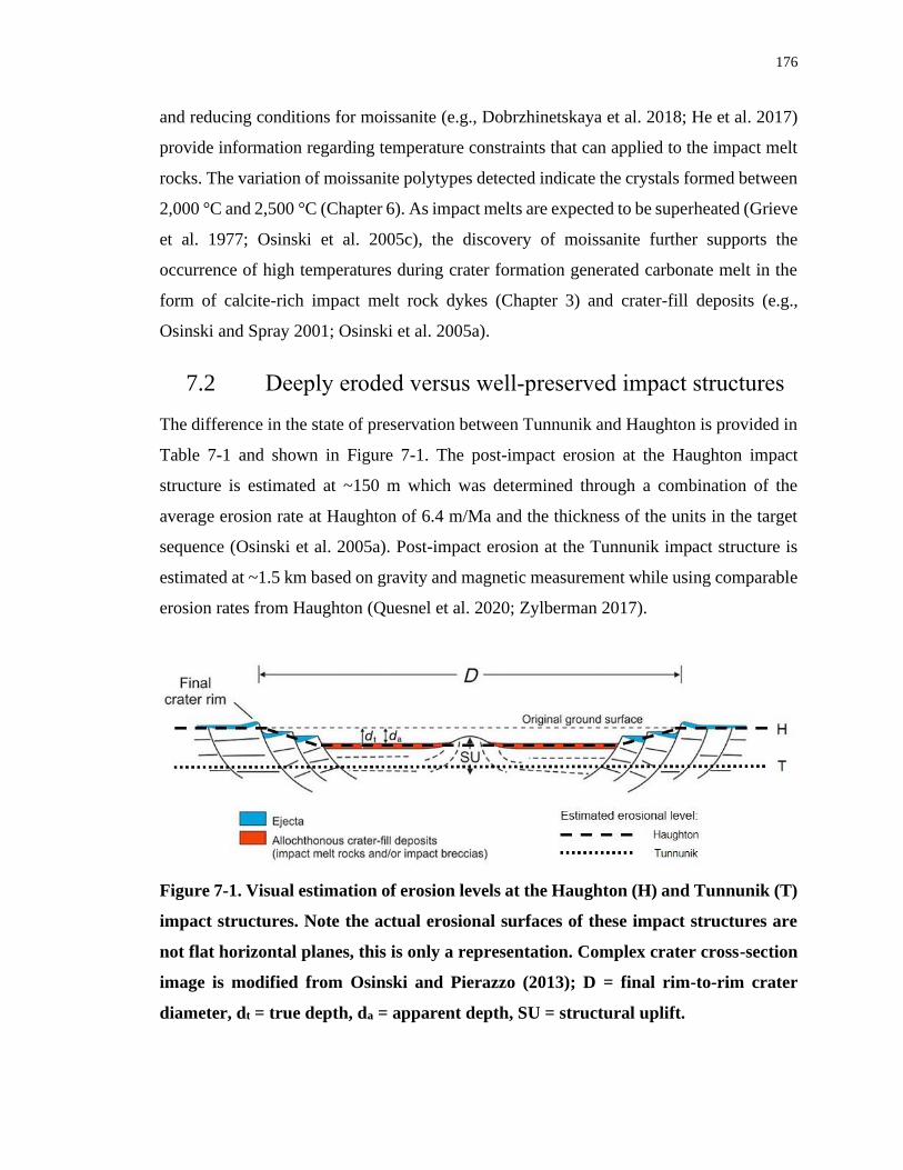
176

and reducing conditions for moissanite (e.g., Dobrzhinetskaya et al. 2018; He et al. 2017)

provide information regarding temperature constraints that can applied to the impact melt

rocks. The variation of moissanite polytypes detected indicate the crystals formed between

2,000 °C and 2,500 °C (Chapter 6). As impact melts are expected to be superheated (Grieve

et al. 1977; Osinski et al. 2005c), the discovery of moissanite further supports the

occurrence of high temperatures during crater formation generated carbonate melt in the

form of calcite-rich impact melt rock dykes (Chapter 3) and crater-fill deposits (e.g.,

Osinski and Spray 2001; Osinski et al. 2005a).

7.2 Deeply eroded versus well-preserved impact structures

The difference in the state of preservation between Tunnunik and Haughton is provided in

Table 7-1 and shown in Figure 7-1. The post-impact erosion at the Haughton impact

structure is estimated at ~150 m which was determined through a combination of the

average erosion rate at Haughton of 6.4 m/Ma and the thickness of the units in the target

sequence (Osinski et al. 2005a). Post-impact erosion at the Tunnunik impact structure is

estimated at ~1.5 km based on gravity and magnetic measurement while using comparable

erosion rates from Haughton (Quesnel et al. 2020; Zylberman 2017).

Figure 7-1. Visual estimation of erosion levels at the Haughton (H) and Tunnunik (T)

impact structures. Note the actual erosional surfaces of these impact structures are

not flat horizontal planes, this is only a representation. Complex crater cross-section

image is modified from Osinski and Pierazzo (2013); D = final rim-to-rim crater

diameter, dt = true depth, da = apparent depth, SU = structural uplift.

177

Erosion at Tunnunik has removed all proximal and distal ejecta, crater-fill, and nearly all

the surface expression of the impact structure, especially as seen from satellite imagery.

This extensive erosion has exposed the crater floor of the Tunnunik impact structure.

Together, these two impact structures could be thought of as two exposures of the same

crater based on their size and carbonate-rich target sequence. Since Tunnunik is much

older, it is logical that no crater-fill or ejecta deposits remain following the erosion from

repeated glaciation events. To get a sense of the appearance and distribution of such

deposits, the Haughton impact structure can be examined. While there is no way to verify

what a well-preserved Tunnunik impact structure looked like, Haughton would be a good

approximation. At Haughton, the crater-fill impact melt rocks cover much of the central

portion of the impact structure and obscure the target rocks of the central uplift as well as

features such as shatter cones. Where uplifted rocks are exposed within the central uplift

at Haughton, shatter cones are easily recognized and well-developed in fine-grained

limestone and dolostone (Osinski and Spray 2006). Similarly, the extent of shatter cones

was also determined at Tunnunik (Osinski and Ferrière 2016) despite the blanket of

Quaternary post-glacial sediments covering most of the flat-lying surfaces. The

preservation level of these craters shows differences in dykes based on where they were

emplaced during an impact event and is discussed further in the next section.

7.3 Dyke emplacement in the Tunnunik and Haughton

impact structures

The distribution of known dykes at the Tunnunik impact structure (Chapter 2) are the result

of a comprehensive survey of exposed outcrops conducted during 2012 and 2015. With

limited target rock exposure across the impact structure, additional exposed dykes are

expected to remain scarce. The distribution of dykes at the Haughton impact structure is

more widespread (Chapter 3) than Tunnunik but does remain limited within the central

uplift due to the coverage of impact melt rocks in the crater-fill deposits.

In complex craters, dyke distribution is also complex and the spatial distribution of dykes

can be difficult to assess or are underestimated in the field due to limited exposure (Lambert

1981; Reimold 1998). Reimold (1998) also notes that “the inherent lack of three-

178

dimensional geological understanding has generally prevented detailed mapping of

distribution and interrelationships of impact breccias”. On their own, the Tunnunik and

Haughton impact structures have their own cross-section through an ideal complex crater

(Fig. 7-1), but the occurrence of dykes throughout the rest of each structure is unknown.

At Tunnunik it is impossible to know the distribution of dykes in the now eroded rocks that

once overlaid the current exposure. At Haughton, it could be possible to drill into the target

rocks deep into the crater floor but would need to be extremely lucky to encounter any

dykes if such a depth was reached. In 2013 three locations in the central uplift were drilled,

the depths of these holes were ~4 m, ~5 m, and ~13 m (Zylberman et al. 2017). The material

recovered from these cores was limited but consist of several types of polymict impact melt

rock (Zylberman et al. 2017). By comparing the distribution of dykes between Haughton

and Tunnunik, this problem is addressed to some extent where one crater provides an

extended extent toward the other. Combined these impact structures do not generate a

complete “three-dimensional geological understanding” but allows for insights and

interpretations regarding impact processes that create impact-generated dykes and their

contents.

When comparing lithic breccia dykes, Haughton breccias are predominantly monomict

compared to Tunnunik which are mostly polymict (Type 1); see Chapters 2 and 3. This

suggests that transport distance of dyke contents was a main factor in the type of lithic

breccias found relative to their position within the impact structure. Injected Type 1 dykes

at Tunnunik were transported greater distances in order to be emplaced in the crater floor

and would have entrained clasts from all stratigraphic units the dykes cut across during

transport. Impact melt rock dykes are absent from the current exposure at Tunnunik but are

common within the central uplift at Haughton. Impact melt rock dykes were only identified

within one formation at Haughton, the Eleanor River Formation, and only contain clasts

from this formation indicating the impact melt rocks likely experienced little transport. If

impact melt rocks were only transported short distances, it corresponds with the lack of

melt rocks at the present exposure of Tunnunik. The presence of impact melt rocks at

Haughton does suggest, however, that similar melt rocks would have formed at Tunnunik

but have since been eroded. Several clasts of possible calcite melt (e.g., Fig. 2-5) could be

surviving clasts from Haughton-like impact melt rocks.

179

7.4 Extent of shock

Using X-ray diffraction (XRD) to identify shock effects in carbonates has not been

extensively examined in impact structures around the world. Outside of this study, analysis

of shocked carbonates with XRD has been conducted at the Kara and Steinheim (Skála and

Jakeš 1999), Ries (Skála 2002), Sierra Madera (Huson et al. 2009), and Wells Creek

(Seeley and Milam 2018) impact structures. There are 198 confirmed terrestrial impact

structures, 82 of which formed in sedimentary target rocks and 54 in mixed sedimentary

and crystalline rocks, so there are many potential candidates that remain to be examined

(Impact Earth 2020).

This study has added the Haughton and Tunnunik impact structures to this list as calcite

and dolomite from the target sequence at both structures were investigated. Lattice strain

values for these minerals were determined and represent varying degrees of shock. As more

information is collected about shocked calcite and dolomite, the better our understanding

will be about how these minerals respond to shock. An end goal would be to create a

classification scheme for carbonates as many already exist for silicate minerals (Stöffler et

al. 2018).

7.4.1 Strain versus distance from the centre of impact structures

Investigating lattice strain in shocked carbonates from Haughton (Chapter 4) and Tunnunik

(Chapter 5) has shown the highest strain values for dolomite and calcite are associated with

samples collected near the centre of the impact structure and decrease toward the rim. This

general trend applies to most samples from the two impact structures with several key

observations. The first observation is related to strain values from Tunnunik where strain

values are not simply correlated with distance from the centre, but also to the distribution

of shatter cones. The elliptical shatter cone distribution at Tunnunik is suggested to be

caused by an oblique impact (Osinski and Ferrière 2016) and if shock pressures were not

evenly distributed in all directions at the time of impact then the strain results appear to

support that the well-documented shatter cone distribution is indeed elliptical.

The second observation is that bulk rock sample composition may affect strain values when

a mixture of dolomite and calcite are present. The studies at Haughton and Tunnunik

180

worked with natural samples so compositions cannot be controlled and as a result, the

modal proportions of mineral phases from one sample to the next are not consistent. This

inconsistency has revealed potential trends associated with carbonate proportions related

to strain such as dolomite giving higher strain values and calcite lower values when both

are present in proportions >10 wt% in the same sample.

7.4.2 Strain versus depth within impact structures

Variation with depth at the Tunnunik and Haughton impact structures was not specifically

investigated in their respective studies. Exact elevation differences between samples was

not recorded but could vary up to a couple hundred metres. What can be compared with

respect to depth are the overall sample suites from each impact site. Recall that Figure 7-1

shows the relative difference in the exposed surface exposure for each impact structure.

Based on this figure alone, it would be expected that the more deeply eroded Tunnunik

impact structure would have a lower range of strain values than the Haughton impact

structure since shock waves weaken as they propagate downward into target rock (Melosh

1989). As expected, the lattice strain values from both sites appear to agree with this

statement. Even though the Tunnunik impact structure has been deeply eroded, it still

contains shatter cones. Shock evidence is present at Tunnunik regardless of strain values,

the values simply indicate the rocks experienced less shock compared to Haughton. The

initial study by Seeley and (Milam 2018) examined how shock changes within a drill core

from the central uplift of the Wells Creek impact structure. Peak broadening alone was not

able to provide a clear answer but when their study is complete a more definitive result

related to shock with depth could be achieved.

7.4.3 Future shock-related research opportunities

The lattice strain studies at Haughton and Tunnunik impact structures provide promising

results for identifying shock in carbonate rocks. Parallel investigations of calcite and

dolomite from additional carbonate-bearing impact structures are needed to determine if

the results from Chapter 4 and Chapter 5 are typical for terrestrial impact structures.

Tunnunik and Haughton are similar in diameter so additional lattice strain data from impact

structures with a range of diameters would be valuable.

181

To provide further meaning to lattice strain values obtained from carbonates shocked at

terrestrial impact structures, a pressure scale with associated strain values is required. A

scale like this was suggested by Martinez et al. (1995) but has yet to be generated. This

could be achieved by experimentally shocking limestone and dolostone to increasing levels

of known pressure, comparable to hypervelocity shock levels, followed by determining

lattice strain. This would allow strain values acquired from impact structures that are

without silicates to estimate shock levels or assist in confirming an impact into a carbonate

target where shatter cones or other physical crater features are absent.

7.5 Conclusions

This research has produced new information and insights into impact cratering processes

associated with carbonate-rich terrestrial environments. A significant contribution of this

research comes from the opportunity to study two impact structures of similar diameter,

and consequently the ability to compare what would have been similar cratering processes,

in different states of preservation.

Characterizing the impact-generated dykes exposed at the Tunnunik and Haughton impact

structures has identified the diversity of impact breccias and impact melt rocks present

these sites. The range of diversity within these dykes was previously unreported can be

used to compare with characteristics of dykes from other carbonate-rich impact structures.

The results of the X-ray diffraction studies of lattice strain related to shock is promising

and indicates more research is required to better understand how carbonates respond to

shock, which could help lead to a shock classification system for carbonates. It would be

interesting to determine if the occurrence of moissanite is truly rare where it has only been

identified at three impact structures or has been dismissed as contamination and was not

fully investigated further at other impact sites.

Based on the results presented in these studies, related future work would continue to

investigate and revisit previously studied carbonate-rich impact structures to determine

similarities or even variation related to this research conducted at the Tunnunik and

Haughton impact structures.

182

7.6 References

Agrinier P., Deutsch A., Schärer U., and Martinez I. 2001. Fast back-reactions of shock-

released CO2 from carbonates : An experimental approach. Geochimica et

Cosmochimica Acta 65:2615–2632.

Daae H. D., and Rutgers A. T. C. 1975. Geologic history of the Northwest Passage. Bulletin

of Canadian Petroleum Geology 23:84–108.

Dewing K., Pratt B. R., Hadlari T., Brent T., Bédard J., and Rainbird R. H. 2013. Newly

identified “Tunnunik” impact structure, Prince Albert Peninsula, northwestern

Victoria Island, Arctic Canada. Meteoritics & Planetary Science 48:211–223.

Dobrzhinetskaya L., Mukhin P., Wang Q., Wirth R., O’Bannon E., Zhao W., Eppelbaum

L., and Sokhonchuk T. 2018. Moissanite (SiC) with metal-silicide and silicon

inclusions from tuff of Israel: Raman spectroscopy and electron microscope studies.

Lithos 310–311:355–368.

Grieve R. A. F., Dence M. R., and Robertson P. B. 1977. Cratering processes: As

interpreted from the occurrence of impact melts. In Impact and Explosion Cratering,

edited by Roddy D. J., Pepin R. O., and Merrill R. B. New York: Pergamon Press. pp.

791–814.

Grieve R. A. F., and Cintala M. J. 1992. An analysis of differential impact melt-crater

scaling and implications for the terrestrial impact record. Meteoritics 27:526–538.

Gromilov S. A., Afanasiev V. P., and Pokhilenko N. P. 2018. Moissanites of the Popigai

astrobleme. Doklady Earth Sciences 481:997–999.

He D., Liu Y., Gao C., Chen C., Hu Z., and Gao S. 2017. SiC-dominated ultra-reduced

mineral assemblage in carbonatitic xenoliths from the Dalihu basalt, Inner Mongolia,

China. American Mineralogist 102:312–320.

Hörz F., Cintala M. J., Thomas-Keprta K. L., Ross D. K., and Clemett S. J. 2019.

Unconfined shock experiments: A pilot study into the shock-induced melting and

183

devolatilization of calcite. Meteoritics & Planetary Science 28:1–28.

Hough R. M., Gilmour I., Pillinger C. T., Arden J. W., Gilkes K. W. R., Yuan J., and

Milledge H. J. 1995. Diamond and silicon carbide in impact melt rock from the Ries

impact crater. Nature 378:41–44.

Huson S. A., Foit F. F., Watkinson A. J., and Pope M. C. 2009. Rietveld analysis of X-ray

powder diffraction patterns as a potential tool for the identification of impact-

deformed carbonate rocks. Meteoritics & Planetary Science 44:1695–1706.

Impact Earth. Impact Earth Database. 2020. www.impactearth.com (Accessed February

18, 2020).

Kieffer S. W., and Simonds C. H. 1980. The role of volatiles and lithology in the impact

cratering process. Reviews of Geophysics and Space Physics 18:143–181.

Lambert P. 1981. Breccia Dikes: Geological constraints on the formation of complex

craters. In Multi-ring Basins, Proc. Lunar Planet. Sci., edited by Schultz P. H., and

Merrill R. B. pp. 59–78.

Lepaulard C., Gattacceca J., Swanson-Hysell N., Quesnel Y., Demory F., and Osinski G.

R. 2019. A Paleozoic age for the Tunnunik impact structure. Meteoritics & Planetary

Science 1–12.

Martinez I., Deutsch A., Scharer U., Ildefonse P., Guyot F., and Agrinier P. 1995. Shock

recovery experiments on dolomite and thermodynamical calculation of impact

induced decarbonation. Journal of Geophysical Research 100:15465–15476.

Melosh H. J. 1989. Impact Cratering: A Geologic Process, New York: Oxford University

Press.

Osinski G. R., and Spray J. G. 2001. Impact-generated carbonate melts: Evidence from the

Haughton structure, Canada. Earth and Planetary Science Letters 194:17–29.

Osinski G. R., and Spray J. G. 2005. Tectonics of complex crater formation as revealed by

184

the Haughton impact structure, Devon Island, Canadian High Arctic. Meteoritics &

Planetary Science 40:1813–1834.

Osinski G. R., Spray J. G., and Lee P. 2005a. Impactites of the Haughton impact structure,

Devon Island, Canadian High Arctic. Meteoritics & Planetary Science 40:1789–1812.

Osinski G. R., Lee P., Spray J. G., Parnell J., Lim D. S. S., Bunch T. E., Cockell C. S., and

Glass B. 2005b. Geological overview and cratering model for the Haughton impact

structure, Devon Island, Canadian High Arctic. Meteoritics & Planetary Science

40:1759–1776.

Osinski G. R., Lee P., Parnell J., Spray J. G., and Baron M. 2005c. A case study of impact-

induced hydrothermal activity: The Haughton impact structure, Devon Island,

Canadian High Arctic. Meteoritics & Planetary Science 40:1859–1877.

Osinski G. R., and Spray J. G. 2006. Shatter cones of the Haughton Impact Structure,

Canada. In Proceedings, 1st International Conference on Impact Cratering in the

Solar System, European Space Agency Special Publication SP-612. CD-ROM. pp.

95–99.

Osinski G. R., Spray J. G., and Grieve R. A. F. 2008. Impact melting in sedimentary target

rocks: An assessment. In The Sedimentary Record of Meteorite Impacts, Special

Paper 437, edited by Evans K. R., Horton W., King Jr. D. K., and Morrow J. R.

Geological Society of America, Boulder, CO. pp. 1–18.

Osinski G. R., and Pierazzo E. 2013. Ch 01 Impact cratering: processes and products. In

Impact Cratering: Processes and Products. pp. 1–20.

Osinski G. R., and Ferrière L. 2016. Shatter cones: (Mis)understood? Science Advances 2,

e160061:1–10.

Osinski G. R., Grieve R. A. F., Bleacher J. E., Neish C. D., Pilles E. A., and Tornabene L.

L. 2018. Igneous rocks formed by hypervelocity impact. Journal of Volcanology and

Geothermal Research 353:25–54.

185

Quesnel Y., Zylberman W., Rochette P., Uehara M., Gattacceca J., Osinski G. R.,

Dussouillez P., Lepaulard C., and Champollion C. 2020. Geophysical signature of the

Tunnunik impact structure, Northwest Territories, Canada. Meteoritics & Planetary

Science 55:480-495.

Reimold W. U. 1998. Exogenic and endogenic breccias: a discussion of major

problematics. Earth Science Reviews 43:25–47.

Seeley J. R., and Milam K. A. 2018. Optical and X-ray diffraction analyses of shock

metamorphosed dolostone at increasing depths within the central uplift of the Wells

Creeks impact structure. 49th Lunar and Planetary Science Conference Abstract

#2755.

Skála R., and Jakeš P. 1999. Shock-induced effects in natural calcite-rich targets as

revealed by X-ray powder diffraction. In Large Meteorite Impacts and Planetary

Evolution II, Special Paper 339, edited by Dressler B. O., and Sharpton V. L.

Geological Society of America (GSA), Boulder, CO. pp. 205–214.

Skála R. 2002. Shock-induced phenomena in limestones in the quarry near Ronheim, the

Ries Crater, Germany. Bulletin of the Czech Geological Survey 77:313–320.

Stöffler D., Hamann C., and Metzler K. 2018. Shock metamorphism of planetary silicate

rocks and sediments: Proposal for an updated classification system. Meteoritics &

Planetary Science 49:5–49.

Thorsteinsson R., and Tozer E. T. 1970. Geology of the Arctic Archipelago. In Geology

and Economic Minerals of Canada, edited by Douglas R. J. W. Geological Survey of

Canada. pp. 547–590.

Wünnemann K., Collins G. S., and Osinski G. R. 2008. Numerical modelling of impact

melt production in porous rocks. Earth and Planetary Science Letters 269:529–538.

Young K. E., Van Soest M. C., Hodges K. V., Watson E. B., Adams B. A., and Lee P.

2013. Impact thermochronology and the age of Haughton impact structure, Canada.

Geophysical Research Letters 40:3836–3840.

186

Zylberman W. Geophysical Study of Complex Meteorite Impact Structures. PhD thesis,

University of Western Ontario, 2017, Electronic Thesis and Dissertation Repository

(5165).

Zylberman W., Quesnel Y., Rochette P., Osinski G. R., Marion C., and Gattacceca J. 2017.

Hydrothermally enhanced magnetization at the center of the Haughton impact

structure? Meteoritics & Planetary Science 52:2147–2165.

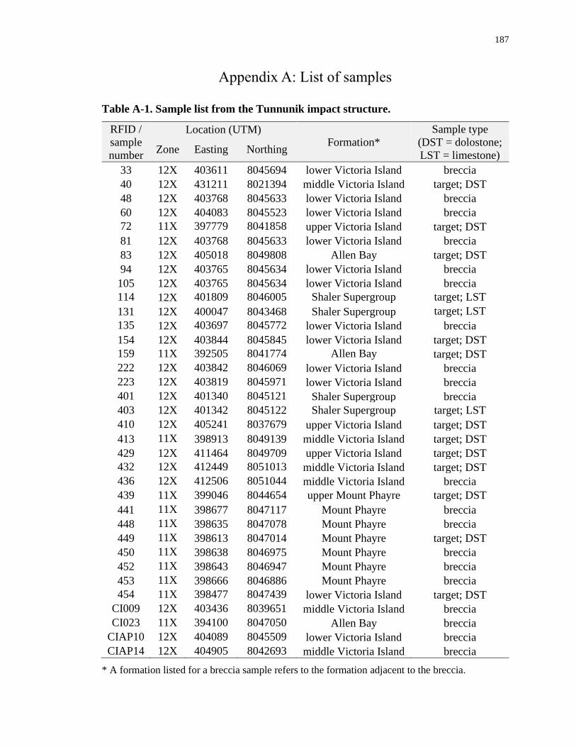
187

Appendix A: List of samples

Table A-1. Sample list from the Tunnunik impact structure.

RFID /

sample

number

Location (UTM) Formation*

Sample type

(DST = dolostone;

LST = limestone) Zone Easting Northing

33 12X 403611 8045694 lower Victoria Island breccia

40 12X 431211 8021394 middle Victoria Island target; DST

48 12X 403768 8045633 lower Victoria Island breccia

60 12X 404083 8045523 lower Victoria Island breccia

72 11X 397779 8041858 upper Victoria Island target; DST

81 12X 403768 8045633 lower Victoria Island breccia

83 12X 405018 8049808 Allen Bay target; DST

94 12X 403765 8045634 lower Victoria Island breccia

105 12X 403765 8045634 lower Victoria Island breccia

114 12X 401809 8046005 Shaler Supergroup target; LST

131 12X 400047 8043468 Shaler Supergroup target; LST

135 12X 403697 8045772 lower Victoria Island breccia

154 12X 403844 8045845 lower Victoria Island target; DST

159 11X 392505 8041774 Allen Bay target; DST

222 12X 403842 8046069 lower Victoria Island breccia

223 12X 403819 8045971 lower Victoria Island breccia

401 12X 401340 8045121 Shaler Supergroup breccia

403 12X 401342 8045122 Shaler Supergroup target; LST

410 12X 405241 8037679 upper Victoria Island target; DST

413 11X 398913 8049139 middle Victoria Island target; DST

429 12X 411464 8049709 upper Victoria Island target; DST

432 12X 412449 8051013 middle Victoria Island target; DST

436 12X 412506 8051044 middle Victoria Island breccia

439 11X 399046 8044654 upper Mount Phayre target; DST

441 11X 398677 8047117 Mount Phayre breccia

448 11X 398635 8047078 Mount Phayre breccia

449 11X 398613 8047014 Mount Phayre target; DST

450 11X 398638 8046975 Mount Phayre breccia

452 11X 398643 8046947 Mount Phayre breccia

453 11X 398666 8046886 Mount Phayre breccia

454 11X 398477 8047439 lower Victoria Island target; DST

CI009 12X 403436 8039651 middle Victoria Island breccia

CI023 11X 394100 8047050 Allen Bay breccia

CIAP10 12X 404089 8045509 lower Victoria Island breccia

CIAP14 12X 404905 8042693 middle Victoria Island breccia

* A formation listed for a breccia sample refers to the formation adjacent to the breccia.

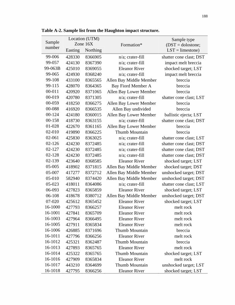
188

Table A-2. Sample list from the Haughton impact structure.

Sample

number

Location (UTM)

Zone 16X Formation*

Sample type

(DST = dolostone;

LST = limestone) Easting Northing

99-006 428330 8366905 n/a; crater-fill shatter cone clast; DST

99-057 424130 8367390 n/a; crater-fill impact melt breccia

99-063B 425010 8369055 Eleanor River shocked target; LST

99-065 424930 8368240 n/a; crater-fill impact melt breccia

99-108 433100 8365565 Allen Bay Middle Member breccia

99-115 428070 8364365 Bay Fiord Member A breccia

00-011 420920 8371065 Allen Bay Lower Member breccia

00-019 420780 8371305 n/a; crater-fill shatter cone clast; LST

00-059 418250 8366275 Allen Bay Lower Member breccia

00-088 416920 8366535 Allen Bay undivided breccia

00-124 424180 8360015 Allen Bay Lower Member ballistic ejecta; LST

00-158 418730 8363155 n/a; crater-fill shatter cone clast; DST

01-028 422670 8361165 Allen Bay Lower Member breccia

02-010 419890 8366225 Thumb Mountain breccia

02-061 425830 8363025 n/a; crater-fill shatter cone clast; LST

02-126 424230 8372485 n/a; crater-fill shatter cone clast; DST

02-127 424230 8372485 n/a; crater-fill shatter cone clast; DST

02-128 424230 8372485 n/a; crater-fill shatter cone clast; DST

02-139 423640 8368585 Eleanor River shocked target; LST

05-005 418902 8371815 Allen Bay Middle Member shocked target; DST

05-007 417277 8372712 Allen Bay Middle Member unshocked target; DST

05-010 582940 8374420 Allen Bay Middle Member unshocked target; DST

05-023 418011 8364086 n/a; crater-fill shatter cone clast; LST

06-093 427823 8365859 Eleanor River shocked target; LST

06-108 418678 8380712 Allen Bay Middle Member unshocked target; DST

07-020 425612 8365452 Eleanor River shocked target; LST

16-1000 427793 8366257 Eleanor River melt rock

16-1001 427841 8365709 Eleanor River melt rock

16-1003 427964 8366495 Eleanor River melt rock

16-1005 427911 8365834 Eleanor River melt rock

16-1006 426885 8371696 Thumb Mountain breccia

16-1011 427796 8366256 Eleanor River melt rock

16-1012 425321 8362487 Thumb Mountain breccia

16-1013 427893 8365765 Eleanor River melt rock

16-1014 425322 8365765 Thumb Mountain shocked target; LST

16-1016 427909 8365834 Eleanor River melt rock

16-1017 443210 8364699 Thumb Mountain unshocked target; LST

16-1018 427795 8366256 Eleanor River shocked target; LST

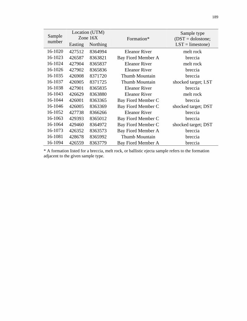
189

Sample

number

Location (UTM)

Zone 16X Formation*

Sample type

(DST = dolostone;

LST = limestone) Easting Northing

16-1020 427512 8364994 Eleanor River melt rock

16-1023 426587 8363821 Bay Fiord Member A breccia

16-1024 427904 8365837 Eleanor River melt rock

16-1026 427902 8365836 Eleanor River breccia

16-1035 426908 8371720 Thumb Mountain breccia

16-1037 426905 8371725 Thumb Mountain shocked target; LST

16-1038 427901 8365835 Eleanor River breccia

16-1043 426629 8363880 Eleanor River melt rock

16-1044 426001 8363365 Bay Fiord Member C breccia

16-1046 426005 8363369 Bay Fiord Member C shocked target; DST

16-1052 427738 8366266 Eleanor River breccia

16-1063 429393 8365012 Bay Fiord Member C breccia

16-1064 429460 8364972 Bay Fiord Member C shocked target; DST

16-1073 426352 8363573 Bay Fiord Member A breccia

16-1081 428678 8365992 Thumb Mountain breccia

16-1094 426559 8363779 Bay Fiord Member A breccia

* A formation listed for a breccia, melt rock, or ballistic ejecta sample refers to the formation

adjacent to the given sample type.

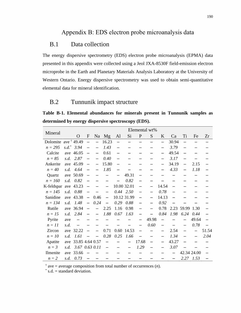
190

Appendix B: EDS electron probe microanalysis data

B.1 Data collection

The energy dispersive spectrometry (EDS) electron probe microanalysis (EPMA) data

presented in this appendix were collected using a Jeol JXA-8530F field-emission electron

microprobe in the Earth and Planetary Materials Analysis Laboratory at the University of

Western Ontario. Energy dispersive spectrometry was used to obtain semi-quantitative

elemental data for mineral identification.

B.2 Tunnunik impact structure

Table B-1. Elemental abundances for minerals present in Tunnunik samples as

determined by energy dispersive spectroscopy (EDS).

Mineral Elemental wt% O F Na Mg Al Si P S K Ca Ti Fe Zr

Dolomite ave † 49.49 – – 16.23 – – – – – 30.94 – – –

n = 295 s.d.* 3.94 – – 1.43 – – – – – 3.79 – – –

Calcite ave 46.05 – – 0.61 – – – – – 49.54 – – –

n = 85 s.d. 2.87 – – 0.40 – – – – – 3.17 – – –

Ankerite ave 45.09 – – 15.80 – – – – – 34.19 – 2.15 –

n = 40 s.d. 4.64 – – 1.85 – – – – – 4.33 – 1.18 –

Quartz ave 50.69 – – – – 49.31 – – – – – – –

n = 160 s.d. 0.82 – – – – 0.82 – – – – – – –

K-feldspar ave 43.23 – – – 10.00 32.01 – – 14.54 – – – –

n = 145 s.d. 0.88 – – – 0.44 2.50 – – 0.78 – – – –

Sanidine ave 43.38 – 0.46 – 10.12 31.99 – – 14.13 – – – –

n = 134 s.d. 1.48 – 0.24 – 0.29 0.88 – – 0.92 – – – –

Rutile ave 36.94 – – 2.25 1.16 0.98 – – 0.78 2.23 59.99 1.30 –

n = 15 s.d. 2.84 – – 1.88 0.67 1.63 – – 0.84 1.98 6.24 0.44 –

Pyrite ave – – – – – – – 49.98 – – – 49.64 –

n = 11 s.d. – – – – – – – 0.60 – – – 0.78 –

Zircon ave 32.22 – – 0.71 0.60 14.53 – – – 2.54 – – 51.54

n = 10 s.d. 1.61 – – 0.28 0.25 1.66 – – – 1.34 – – 2.04

Apatite ave 33.85 4.64 0.57 – – – 17.68 – – 43.27 – – –

n = 3 s.d. 3.67 0.63 0.11 – – – 1.29 – – 3.07 – – –

Ilmenite ave 33.66 – – – – – – – – – 42.34 24.00 –

n = 2 s.d. 0.73 – – – – – – – – – 2.27 1.53 –

† ave = average composition from total number of occurrences (n). * s.d. = standard deviation.

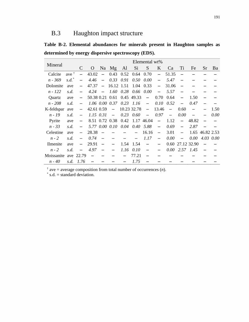
191

B.3 Haughton impact structure

Table B-2. Elemental abundances for minerals present in Haughton samples as

determined by energy dispersive spectroscopy (EDS).

Mineral Elemental wt% C O Na Mg Al Si S K Ca Ti Fe Sr Ba

Calcite ave † – 43.02 – 0.43 0.52 0.64 0.70 – 51.35 – – – –

n - 369 s.d.* – 4.46 – 0.33 0.91 0.50 0.00 – 5.47 – – – –

Dolomite ave – 47.37 – 16.12 1.51 1.04 0.33 – 31.06 – – – –

n - 122 s.d. – 4.24 – 1.60 0.28 0.66 0.00 – 5.57 – – – –

Quartz ave – 50.38 0.21 0.61 0.45 49.33 – 0.70 0.64 – 1.50 – –

n - 208 s.d. – 1.06 0.00 0.37 0.23 1.16 – 0.10 0.52 – 0.47 – –

K-feldspar ave – 42.61 0.59 – 10.23 32.78 – 13.46 – 0.60 – – 1.50

n - 19 s.d. – 1.15 0.31 – 0.23 0.60 – 0.97 – 0.00 – – 0.00

Pyrite ave – 8.51 0.72 0.38 0.42 1.17 46.04 – 1.12 – 48.82 – –

n - 33 s.d. – 5.77 0.00 0.10 0.04 0.40 5.88 – 0.69 – 2.87 – –

Celestine ave – 28.38 – – – – 16.16 – 3.01 – 1.65 46.82 2.53

n - 2 s.d. – 0.74 – – – – 1.17 – 0.00 – 0.00 4.03 0.00

Ilmenite ave – 29.91 – – 1.54 1.54 – – 0.60 27.12 32.90 – –

n - 2 s.d. – 4.97 – – 1.16 0.10 – – 0.00 2.57 1.45 – –

Moissanite ave 22.79 – – – – 77.21 – – – – – – –

n - 40 s.d. 1.76 – – – – 1.75 – – – – – – –

† ave = average composition from total number of occurrences (n). * s.d. = standard deviation.

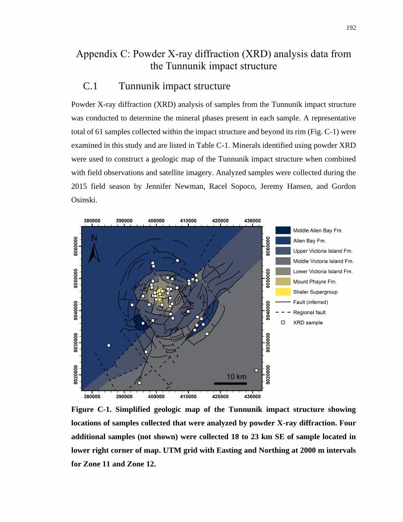
192

Appendix C: Powder X-ray diffraction (XRD) analysis data from

the Tunnunik impact structure

C.1 Tunnunik impact structure

Powder X-ray diffraction (XRD) analysis of samples from the Tunnunik impact structure

was conducted to determine the mineral phases present in each sample. A representative

total of 61 samples collected within the impact structure and beyond its rim (Fig. C-1) were

examined in this study and are listed in Table C-1. Minerals identified using powder XRD

were used to construct a geologic map of the Tunnunik impact structure when combined

with field observations and satellite imagery. Analyzed samples were collected during the

2015 field season by Jennifer Newman, Racel Sopoco, Jeremy Hansen, and Gordon

Osinski.

Figure C-1. Simplified geologic map of the Tunnunik impact structure showing

locations of samples collected that were analyzed by powder X-ray diffraction. Four

additional samples (not shown) were collected 18 to 23 km SE of sample located in

lower right corner of map. UTM grid with Easting and Northing at 2000 m intervals

for Zone 11 and Zone 12.

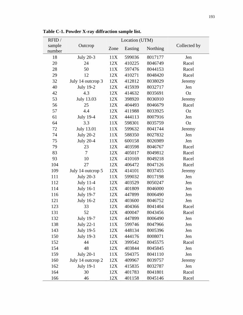
193

Table C-1. Powder X-ray diffraction sample list.

RFID /

sample

number

Outcrop Location (UTM)

Collected by Zone Easting Northing

18 July 20-3 11X 599036 8017177 Jen

20 24 12X 410225 8046749 Racel

28 50 11X 597476 8044153 Racel

29 12 12X 410271 8048420 Racel

32 July 14 outcrop 3 12X 412812 8038029 Jeremy

40 July 19-2 12X 415939 8032717 Jen

42 4.3 12X 414632 8035691 Oz

53 July 13.03 12X 398920 8036910 Jeremy

56 25 12X 404493 8046679 Racel

57 4.4 12X 411988 8033925 Oz

61 July 19-4 12X 444113 8007916 Jen

64 3.3 11X 598301 8035759 Oz

72 July 13.01 11X 599632 8041744 Jeremy

74 July 20-2 11X 588350 8027832 Jen

75 July 20-4 11X 600158 8026989 Jen

79 23 12X 403598 8046767 Racel

83 7 12X 405017 8049812 Racel

93 10 12X 410169 8049218 Racel

104 27 12X 406472 8047126 Racel

109 July 14 outcrop 5 12X 414101 8037455 Jeremy

111 July 20-3 11X 599032 8017198 Jen

112 July 11-4 12X 403529 8050247 Jen

114 July 16-1 12X 401809 8046000 Jen

116 July 19-7 12X 447899 8006490 Jen

121 July 16-2 12X 403600 8046752 Jen

123 33 12X 404366 8041404 Racel

131 52 12X 400047 8043456 Racel

132 July 19-7 12X 447899 8006490 Jen

138 July 22-1 11X 599746 8047966 Jen

143 July 19-5 12X 448134 8005396 Jen

150 July 19-3 12X 444176 8008071 Jen

152 44 12X 399542 8045575 Racel

154 48 12X 403844 8045845 Jen

159 July 20-1 11X 594375 8041110 Jen

160 July 14 outcrop 2 12X 409967 8039757 Jeremy

162 July 19-1 12X 415835 8032787 Jen

164 30 12X 401783 8041801 Racel

166 46 12X 401158 8045146 Racel

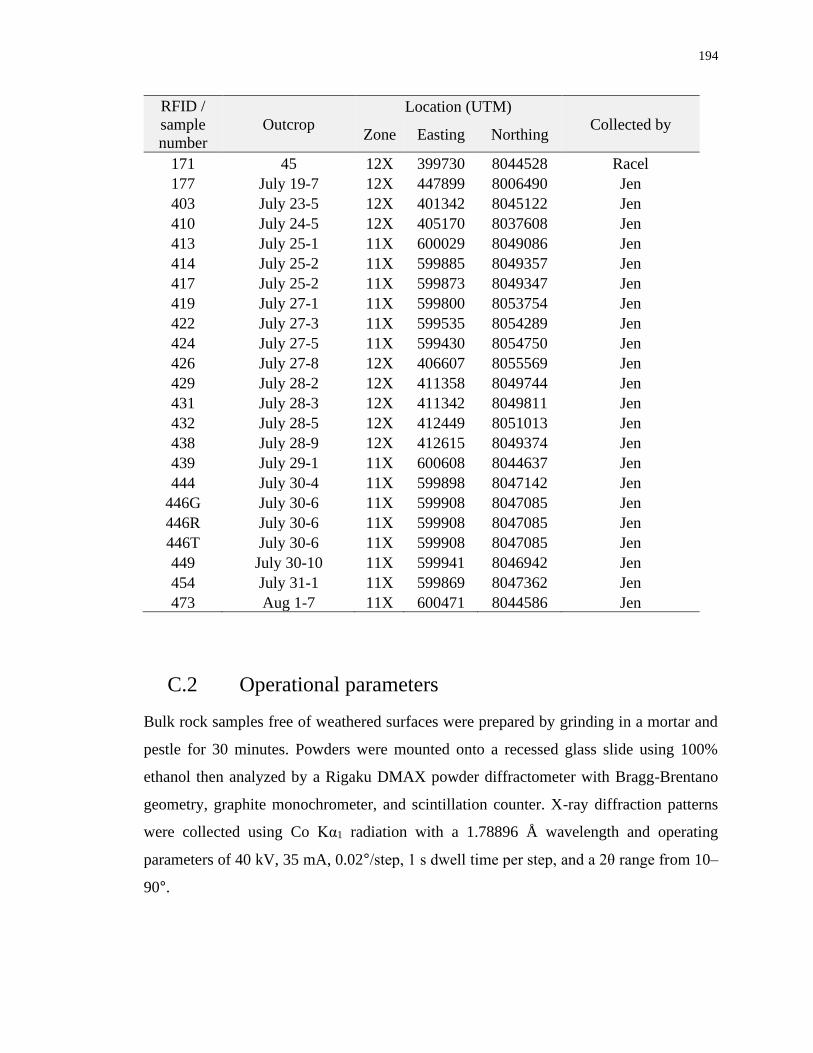
194

RFID /

sample

number

Outcrop Location (UTM)

Collected by Zone Easting Northing

171 45 12X 399730 8044528 Racel

177 July 19-7 12X 447899 8006490 Jen

403 July 23-5 12X 401342 8045122 Jen

410 July 24-5 12X 405170 8037608 Jen

413 July 25-1 11X 600029 8049086 Jen

414 July 25-2 11X 599885 8049357 Jen

417 July 25-2 11X 599873 8049347 Jen

419 July 27-1 11X 599800 8053754 Jen

422 July 27-3 11X 599535 8054289 Jen

424 July 27-5 11X 599430 8054750 Jen

426 July 27-8 12X 406607 8055569 Jen

429 July 28-2 12X 411358 8049744 Jen

431 July 28-3 12X 411342 8049811 Jen

432 July 28-5 12X 412449 8051013 Jen

438 July 28-9 12X 412615 8049374 Jen

439 July 29-1 11X 600608 8044637 Jen

444 July 30-4 11X 599898 8047142 Jen

446G July 30-6 11X 599908 8047085 Jen

446R July 30-6 11X 599908 8047085 Jen

446T July 30-6 11X 599908 8047085 Jen

449 July 30-10 11X 599941 8046942 Jen

454 July 31-1 11X 599869 8047362 Jen

473 Aug 1-7 11X 600471 8044586 Jen

C.2 Operational parameters

Bulk rock samples free of weathered surfaces were prepared by grinding in a mortar and

pestle for 30 minutes. Powders were mounted onto a recessed glass slide using 100%

ethanol then analyzed by a Rigaku DMAX powder diffractometer with Bragg-Brentano

geometry, graphite monochrometer, and scintillation counter. X-ray diffraction patterns

were collected using Co Kα1 radiation with a 1.78896 Å wavelength and operating

parameters of 40 kV, 35 mA, 0.02°/step, 1 s dwell time per step, and a 2θ range from 10–

90°.

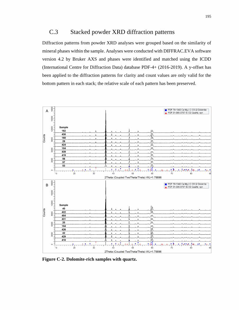
195

C.3 Stacked powder XRD diffraction patterns

Diffraction patterns from powder XRD analyses were grouped based on the similarity of

mineral phases within the sample. Analyses were conducted with DIFFRAC.EVA software

version 4.2 by Bruker AXS and phases were identified and matched using the ICDD

(International Centre for Diffraction Data) database PDF-4+ (2016-2019). A y-offset has

been applied to the diffraction patterns for clarity and count values are only valid for the

bottom pattern in each stack; the relative scale of each pattern has been preserved.

Figure C-2. Dolomite-rich samples with quartz.

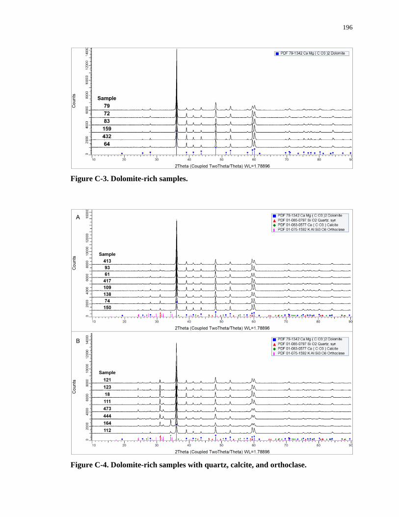
196

Figure C-3. Dolomite-rich samples.

Figure C-4. Dolomite-rich samples with quartz, calcite, and orthoclase.

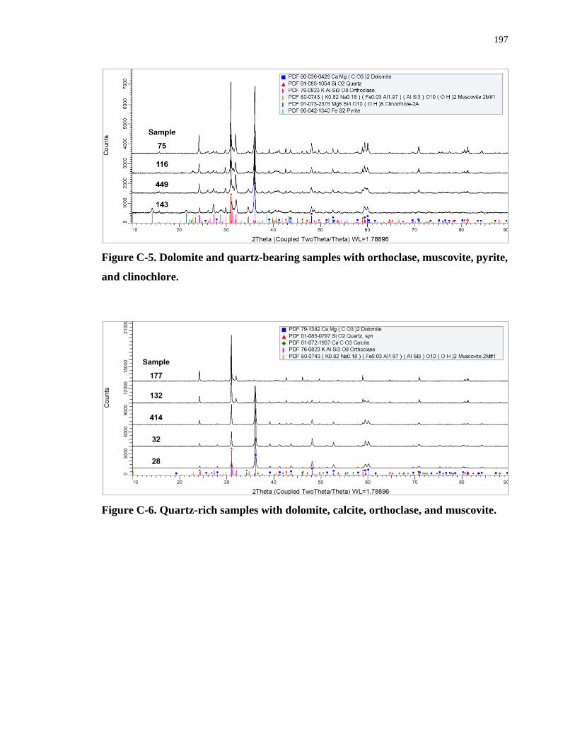
197

Figure C-5. Dolomite and quartz-bearing samples with orthoclase, muscovite, pyrite,

and clinochlore.

Figure C-6. Quartz-rich samples with dolomite, calcite, orthoclase, and muscovite.

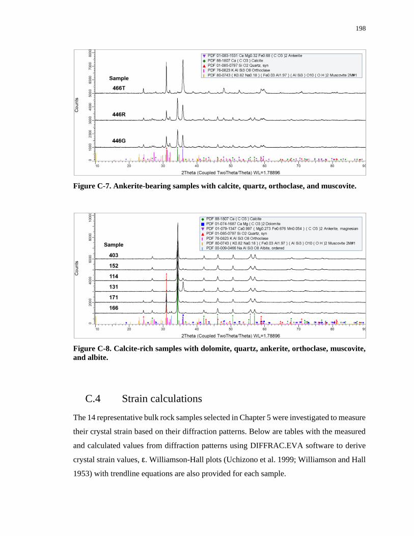
198

Figure C-7. Ankerite-bearing samples with calcite, quartz, orthoclase, and muscovite.

Figure C-8. Calcite-rich samples with dolomite, quartz, ankerite, orthoclase, muscovite,

and albite.

C.4 Strain calculations

The 14 representative bulk rock samples selected in Chapter 5 were investigated to measure

their crystal strain based on their diffraction patterns. Below are tables with the measured

and calculated values from diffraction patterns using DIFFRAC.EVA software to derive

crystal strain values, ε. Williamson-Hall plots (Uchizono et al. 1999; Williamson and Hall

1953) with trendline equations are also provided for each sample.

199

Table C-2. Measured 2θ and integral breadth values from diffraction pattern for

dolomite sample 439. Tan θ values derived from 2θ observed maximum value.

hkl 2θ

(observed

max)

θ

(degrees)

θ

(radians)

Tan θ Integral

breadth

104 36.100 18.050 0.315 0.326 0.291

006 39.150 19.575 0.342 0.356 0.290

015 41.250 20.625 0.360 0.376 0.326

110 43.695 21.848 0.381 0.401 0.318

113 48.170 24.085 0.420 0.447 0.344

021 51.367 25.684 0.448 0.481 0.313

202 52.714 26.357 0.460 0.495 0.330

024 57.934 28.967 0.506 0.554 0.364

116 * 60.120 30.060 0.525 0.579 0.937

* Area for (018) and (116) peak calculated together due to broadening and merging of peaks.

Figure C-9. Williamson-Hall plot for dolomite sample 439 showing integral breadth

values measured from peak area plotted for a given diffracted angle. Linear trendline

equation and R2 value are displayed on chart.

Crystal strain ε for sample 439 is 0.37%. Strain is derived from the slope of the trendline

equation (Fig. C-9) where ε equals 1.4878 divided by 4.

y = 1.4878x - 0.2733

R² = 0.4051

0

0.1

0.2

0.3

0.4

0.5

0.6

0.7

0.8

0.9

1

0.300 0.350 0.400 0.450 0.500 0.550 0.600

Inte

gra

l bre

adth

, β

s

Diffracted angle (Tan θ)

439

200

Table C-3. Measured 2θ and integral breadth values from diffraction pattern for

dolomite sample 154. Tan θ values derived from 2θ observed maximum value.

hkl 2θ

(observed

max)

θ

(degrees)

θ

(radians)

Tan θ Integral

breadth

104 36.098 18.049 0.315 0.326 0.270

006 39.148 19.574 0.342 0.356 0.249

015 41.254 20.627 0.360 0.376 0.312

110 43.687 21.844 0.381 0.401 0.280

113 48.168 24.084 0.420 0.447 0.334

021 51.352 25.676 0.448 0.481 0.287

202 52.721 26.361 0.460 0.496 0.313

024 57.944 28.972 0.506 0.554 0.368

116 * 60.121 30.061 0.525 0.579 0.858

* Area for (018) and (116) peak calculated together due to broadening and merging of peaks.

Figure C-10. Williamson-Hall plot for dolomite sample 154 showing integral breadth

values measured from peak area plotted for a given diffracted angle. Linear trendline

equation and R2 value are displayed on chart.

Crystal strain ε for sample 154 is 0.36%. Strain is derived from the slope of the trendline

equation (Fig. C-10) where ε equals 1.4411 divided by 4.

y = 1.4411x - 0.2794

R² = 0.454

0

0.1

0.2

0.3

0.4

0.5

0.6

0.7

0.8

0.9

1

0.300 0.350 0.400 0.450 0.500 0.550 0.600

Inte

gra

l bre

adth

, β

s

Diffracted angle (Tan θ)

154

201

Table C-4. Measured 2θ and integral breadth values from diffraction pattern for

dolomite sample 454. Tan θ values derived from 2θ observed maximum value.

hkl 2θ

(observed

max)

θ

(degrees)

θ

(radians)

Tan θ Integral

breadth

104 36.101 18.051 0.315 0.326 0.284

006 39.163 19.582 0.342 0.356 0.266

015 41.267 20.634 0.360 0.377 0.307

110 43.684 21.842 0.381 0.401 0.295

113 48.168 24.084 0.420 0.447 0.336

021 51.365 25.683 0.448 0.481 0.340

202 52.717 26.359 0.460 0.496 0.321

024 57.939 28.970 0.506 0.554 0.370

116 * 60.125 30.063 0.525 0.579 0.823

* Area for (018) and (116) peak calculated together due to broadening and merging of peaks.

Figure C-11. Williamson-Hall plot for dolomite sample 454 showing integral breadth

values measured from peak area plotted for a given diffracted angle. Linear trendline

equation and R2 value are displayed on chart.

Crystal strain ε for sample 454 is 0.34%. Strain is derived from the slope of the trendline

equation (Fig. C-11) where ε equals 1.3499 divided by 4.

y = 1.3499x - 0.2308

R² = 0.4783

0

0.1

0.2

0.3

0.4

0.5

0.6

0.7

0.8

0.9

0.300 0.350 0.400 0.450 0.500 0.550 0.600

Inte

gra

l bre

adth

, β

s

Diffracted angle (Tan θ)

454

202

Table C-5. Measured 2θ and integral breadth values from diffraction pattern for

dolomite sample 413. Tan θ values derived from 2θ observed maximum value.

hkl 2θ

(observed

max)

θ

(degrees)

θ

(radians)

Tan θ Integral

breadth

104 36.101 18.051 0.315 0.326 0.261

006 39.152 19.576 0.342 0.356 0.254

015 41.257 20.629 0.360 0.376 0.278

110 43.677 21.839 0.381 0.401 0.292

113 48.171 24.086 0.420 0.447 0.336

021 51.338 25.669 0.448 0.481 0.308

202 52.707 26.354 0.460 0.495 0.328

024 57.921 28.961 0.505 0.553 0.304

116 * 59.467 29.734 0.519 0.571 0.785

* Area for (018) and (116) peak calculated together due to broadening and merging of peaks.

Figure C-12. Williamson-Hall plot for dolomite sample 413 showing integral breadth

values measured from peak area plotted for a given diffracted angle. Linear trendline

equation and R2 value are displayed on chart.

Crystal strain ε for sample 413 is 0.31%. Strain is derived from the slope of the trendline

equation (Fig. C-12) where ε equals 1.226 divided by 4.

y = 1.226x - 0.1962

R² = 0.4131

0

0.1

0.2

0.3

0.4

0.5

0.6

0.7

0.8

0.9

1

0.300 0.350 0.400 0.450 0.500 0.550 0.600

Inte

gra

l bre

adth

, β

s

Diffracted angle (Tan θ)

413

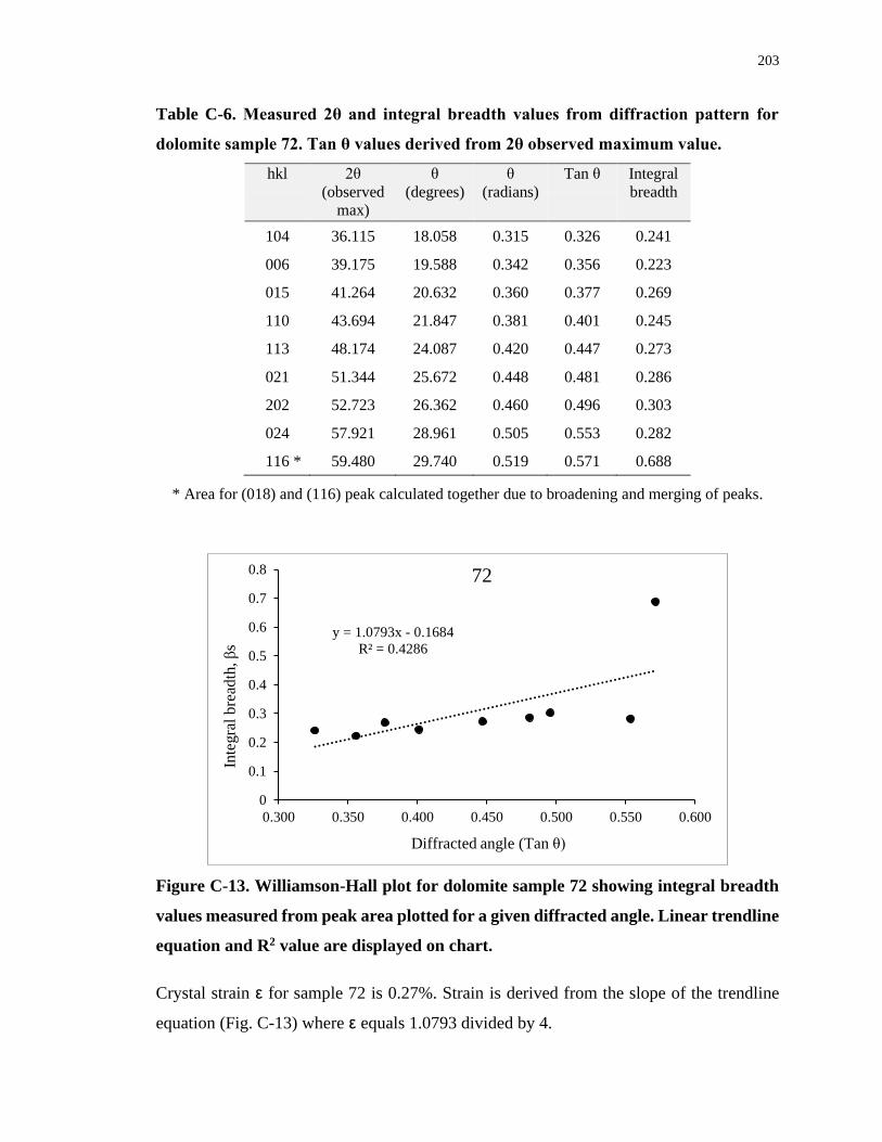
203

Table C-6. Measured 2θ and integral breadth values from diffraction pattern for

dolomite sample 72. Tan θ values derived from 2θ observed maximum value.

hkl 2θ

(observed

max)

θ

(degrees)

θ

(radians)

Tan θ Integral

breadth

104 36.115 18.058 0.315 0.326 0.241

006 39.175 19.588 0.342 0.356 0.223

015 41.264 20.632 0.360 0.377 0.269

110 43.694 21.847 0.381 0.401 0.245

113 48.174 24.087 0.420 0.447 0.273

021 51.344 25.672 0.448 0.481 0.286

202 52.723 26.362 0.460 0.496 0.303

024 57.921 28.961 0.505 0.553 0.282

116 * 59.480 29.740 0.519 0.571 0.688

* Area for (018) and (116) peak calculated together due to broadening and merging of peaks.

Figure C-13. Williamson-Hall plot for dolomite sample 72 showing integral breadth

values measured from peak area plotted for a given diffracted angle. Linear trendline

equation and R2 value are displayed on chart.

Crystal strain ε for sample 72 is 0.27%. Strain is derived from the slope of the trendline

equation (Fig. C-13) where ε equals 1.0793 divided by 4.

y = 1.0793x - 0.1684

R² = 0.4286

0

0.1

0.2

0.3

0.4

0.5

0.6

0.7

0.8

0.300 0.350 0.400 0.450 0.500 0.550 0.600

Inte

gra

l b

read

th, β

s

Diffracted angle (Tan θ)

72

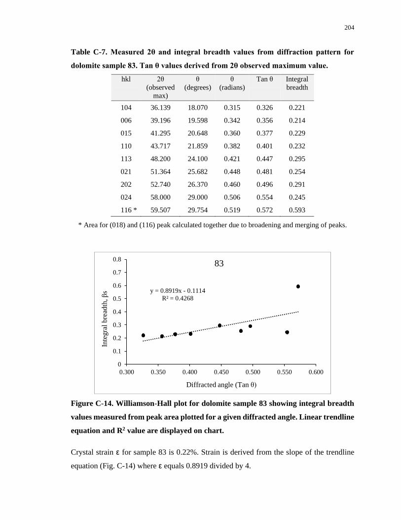
204

Table C-7. Measured 2θ and integral breadth values from diffraction pattern for

dolomite sample 83. Tan θ values derived from 2θ observed maximum value.

hkl 2θ

(observed

max)

θ

(degrees)

θ

(radians)

Tan θ Integral

breadth

104 36.139 18.070 0.315 0.326 0.221

006 39.196 19.598 0.342 0.356 0.214

015 41.295 20.648 0.360 0.377 0.229

110 43.717 21.859 0.382 0.401 0.232

113 48.200 24.100 0.421 0.447 0.295

021 51.364 25.682 0.448 0.481 0.254

202 52.740 26.370 0.460 0.496 0.291

024 58.000 29.000 0.506 0.554 0.245

116 * 59.507 29.754 0.519 0.572 0.593

* Area for (018) and (116) peak calculated together due to broadening and merging of peaks.

Figure C-14. Williamson-Hall plot for dolomite sample 83 showing integral breadth

values measured from peak area plotted for a given diffracted angle. Linear trendline

equation and R2 value are displayed on chart.

Crystal strain ε for sample 83 is 0.22%. Strain is derived from the slope of the trendline

equation (Fig. C-14) where ε equals 0.8919 divided by 4.

y = 0.8919x - 0.1114

R² = 0.4268

0

0.1

0.2

0.3

0.4

0.5

0.6

0.7

0.8

0.300 0.350 0.400 0.450 0.500 0.550 0.600

Inte

gra

l b

read

th, β

s

Diffracted angle (Tan θ)

83

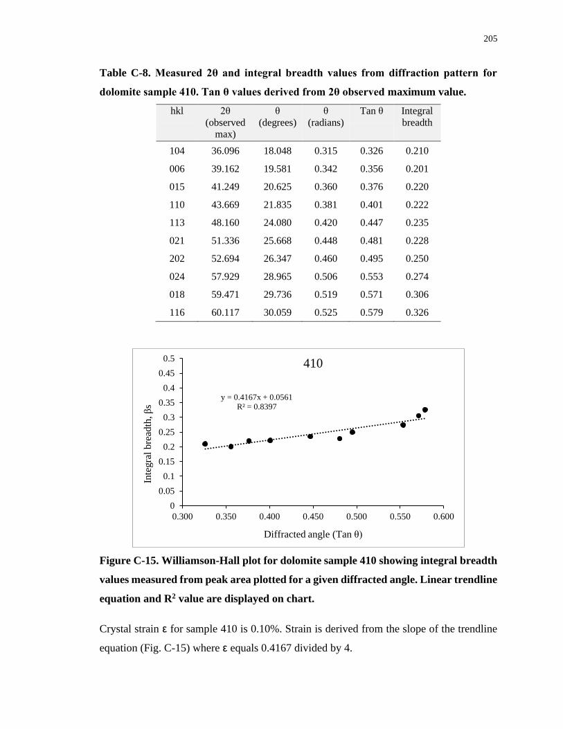
205

Table C-8. Measured 2θ and integral breadth values from diffraction pattern for

dolomite sample 410. Tan θ values derived from 2θ observed maximum value.

hkl 2θ

(observed

max)

θ

(degrees)

θ

(radians)

Tan θ Integral

breadth

104 36.096 18.048 0.315 0.326 0.210

006 39.162 19.581 0.342 0.356 0.201

015 41.249 20.625 0.360 0.376 0.220

110 43.669 21.835 0.381 0.401 0.222

113 48.160 24.080 0.420 0.447 0.235

021 51.336 25.668 0.448 0.481 0.228

202 52.694 26.347 0.460 0.495 0.250

024 57.929 28.965 0.506 0.553 0.274

018 59.471 29.736 0.519 0.571 0.306

116 60.117 30.059 0.525 0.579 0.326

Figure C-15. Williamson-Hall plot for dolomite sample 410 showing integral breadth

values measured from peak area plotted for a given diffracted angle. Linear trendline

equation and R2 value are displayed on chart.

Crystal strain ε for sample 410 is 0.10%. Strain is derived from the slope of the trendline

equation (Fig. C-15) where ε equals 0.4167 divided by 4.

y = 0.4167x + 0.0561

R² = 0.8397

0

0.05

0.1

0.15

0.2

0.25

0.3

0.35

0.4

0.45

0.5

0.300 0.350 0.400 0.450 0.500 0.550 0.600

Inte

gra

l bre

adth

, β

s

Diffracted angle (Tan θ)

410

206

Table C-9. Measured 2θ and integral breadth values from diffraction pattern for

dolomite sample 159. Tan θ values derived from 2θ observed maximum value.

hkl 2θ

(observed

max)

θ

(degrees)

θ

(radians)

Tan θ Integral

breadth

104 36.091 18.046 0.315 0.326 0.208

006 39.156 19.578 0.342 0.356 0.199

015 41.246 20.623 0.360 0.376 0.224

110 43.668 21.834 0.381 0.401 0.226

113 48.156 24.078 0.420 0.447 0.244

021 51.351 25.676 0.448 0.481 0.248

202 52.686 26.343 0.460 0.495 0.256

024 57.903 28.952 0.505 0.553 0.261

018 59.449 29.725 0.519 0.571 0.296

116 60.106 30.053 0.525 0.579 0.326

Figure C-16. Williamson-Hall plot for dolomite sample 159 showing integral breadth

values measured from peak area plotted for a given diffracted angle. Linear trendline

equation and R2 value are displayed on chart.

Crystal strain ε for sample 159 is 0.09%. Strain is derived from the slope of the trendline

equation (Fig. C-16) where ε equals 0.3923 divided by 4.

y = 0.3923x + 0.069

R² = 0.8575

0

0.05

0.1

0.15

0.2

0.25

0.3

0.35

0.4

0.45

0.5

0.300 0.350 0.400 0.450 0.500 0.550 0.600

Inte

gra

l bre

adth

, β

s

Diffracted angle (Tan θ)

159

207

Table C-10. Measured 2θ and integral breadth values from diffraction pattern for

dolomite sample 429. Tan θ values derived from 2θ observed maximum value.

hkl 2θ

(observed

max)

θ

(degrees)

θ

(radians)

Tan θ Integral

breadth

104 36.128 18.064 0.315 0.326 0.209

006 39.191 19.596 0.342 0.356 0.194

015 41.280 20.640 0.360 0.377 0.227

110 43.702 21.851 0.381 0.401 0.222

113 48.184 24.092 0.420 0.447 0.240

021 51.344 25.672 0.448 0.481 0.242

202 52.716 26.358 0.460 0.495 0.245

024 57.948 28.974 0.506 0.554 0.261

018 59.485 29.743 0.519 0.571 0.295

116 60.133 30.067 0.525 0.579 0.318

Figure C-17. Williamson-Hall plot for dolomite sample 429 showing integral breadth

values measured from peak area plotted for a given diffracted angle. Linear trendline

equation and R2 value are displayed on chart.

Crystal strain ε for sample 429 is 0.09%. Strain is derived from the slope of the trendline

equation (Fig. C-17) where ε equals 0.3765 divided by 4.

y = 0.3765x + 0.0726

R² = 0.8407

0

0.05

0.1

0.15

0.2

0.25

0.3

0.35

0.4

0.45

0.5

0.300 0.350 0.400 0.450 0.500 0.550 0.600

Inte

gra

l bre

adth

, β

s

Diffracted angle (Tan θ)

429

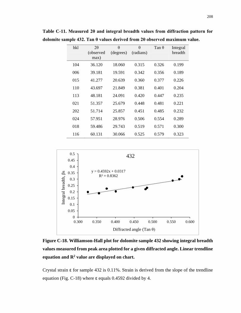
208

Table C-11. Measured 2θ and integral breadth values from diffraction pattern for

dolomite sample 432. Tan θ values derived from 2θ observed maximum value.

hkl 2θ

(observed

max)

θ

(degrees)

θ

(radians)

Tan θ Integral

breadth

104 36.120 18.060 0.315 0.326 0.199

006 39.181 19.591 0.342 0.356 0.189

015 41.277 20.639 0.360 0.377 0.226

110 43.697 21.849 0.381 0.401 0.204

113 48.181 24.091 0.420 0.447 0.235

021 51.357 25.679 0.448 0.481 0.221

202 51.714 25.857 0.451 0.485 0.232

024 57.951 28.976 0.506 0.554 0.289

018 59.486 29.743 0.519 0.571 0.300

116 60.131 30.066 0.525 0.579 0.323

Figure C-18. Williamson-Hall plot for dolomite sample 432 showing integral breadth

values measured from peak area plotted for a given diffracted angle. Linear trendline

equation and R2 value are displayed on chart.

Crystal strain ε for sample 432 is 0.11%. Strain is derived from the slope of the trendline

equation (Fig. C-18) where ε equals 0.4592 divided by 4.

y = 0.4592x + 0.0317

R² = 0.8362

0

0.05

0.1

0.15

0.2

0.25

0.3

0.35

0.4

0.45

0.5

0.300 0.350 0.400 0.450 0.500 0.550 0.600

Inte

gra

l bre

adth

, β

s

Diffracted angle (Tan θ)

432

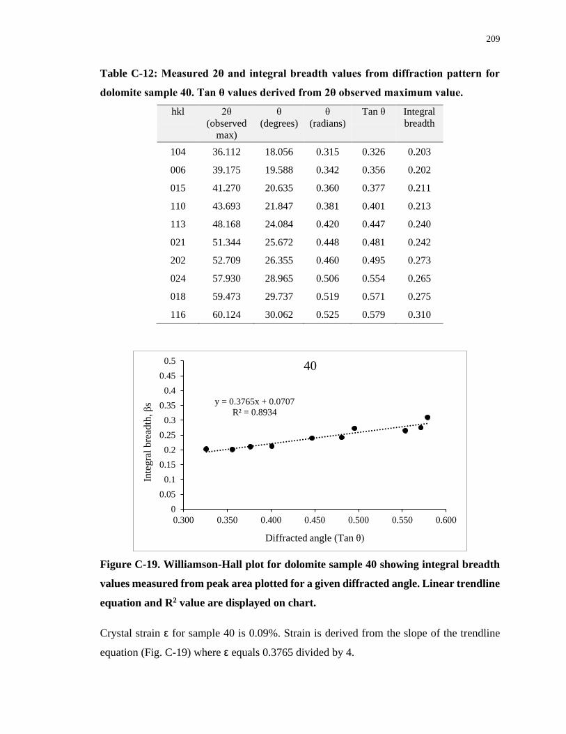
209

Table C-12: Measured 2θ and integral breadth values from diffraction pattern for

dolomite sample 40. Tan θ values derived from 2θ observed maximum value.

hkl 2θ

(observed

max)

θ

(degrees)

θ

(radians)

Tan θ Integral

breadth

104 36.112 18.056 0.315 0.326 0.203

006 39.175 19.588 0.342 0.356 0.202

015 41.270 20.635 0.360 0.377 0.211

110 43.693 21.847 0.381 0.401 0.213

113 48.168 24.084 0.420 0.447 0.240

021 51.344 25.672 0.448 0.481 0.242

202 52.709 26.355 0.460 0.495 0.273

024 57.930 28.965 0.506 0.554 0.265

018 59.473 29.737 0.519 0.571 0.275

116 60.124 30.062 0.525 0.579 0.310

Figure C-19. Williamson-Hall plot for dolomite sample 40 showing integral breadth

values measured from peak area plotted for a given diffracted angle. Linear trendline

equation and R2 value are displayed on chart.

Crystal strain ε for sample 40 is 0.09%. Strain is derived from the slope of the trendline

equation (Fig. C-19) where ε equals 0.3765 divided by 4.

y = 0.3765x + 0.0707

R² = 0.8934

0

0.05

0.1

0.15

0.2

0.25

0.3

0.35

0.4

0.45

0.5

0.300 0.350 0.400 0.450 0.500 0.550 0.600

Inte

gra

l b

read

th, β

s

Diffracted angle (Tan θ)

40

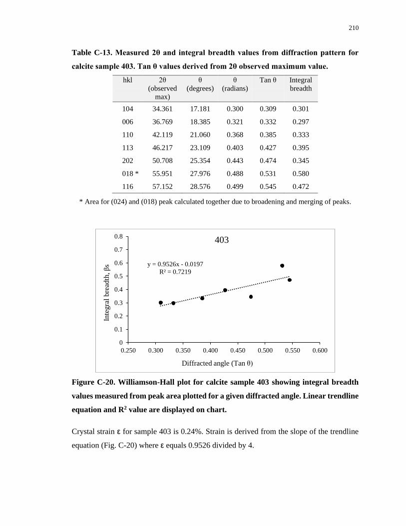
210

Table C-13. Measured 2θ and integral breadth values from diffraction pattern for

calcite sample 403. Tan θ values derived from 2θ observed maximum value.

hkl 2θ

(observed

max)

θ

(degrees)

θ

(radians)

Tan θ Integral

breadth

104 34.361 17.181 0.300 0.309 0.301

006 36.769 18.385 0.321 0.332 0.297

110 42.119 21.060 0.368 0.385 0.333

113 46.217 23.109 0.403 0.427 0.395

202 50.708 25.354 0.443 0.474 0.345

018 * 55.951 27.976 0.488 0.531 0.580

116 57.152 28.576 0.499 0.545 0.472

* Area for (024) and (018) peak calculated together due to broadening and merging of peaks.

Figure C-20. Williamson-Hall plot for calcite sample 403 showing integral breadth

values measured from peak area plotted for a given diffracted angle. Linear trendline

equation and R2 value are displayed on chart.

Crystal strain ε for sample 403 is 0.24%. Strain is derived from the slope of the trendline

equation (Fig. C-20) where ε equals 0.9526 divided by 4.

y = 0.9526x - 0.0197

R² = 0.7219

0

0.1

0.2

0.3

0.4

0.5

0.6

0.7

0.8

0.250 0.300 0.350 0.400 0.450 0.500 0.550 0.600

Inte

gra

l bre

adth

, β

s

Diffracted angle (Tan θ)

403

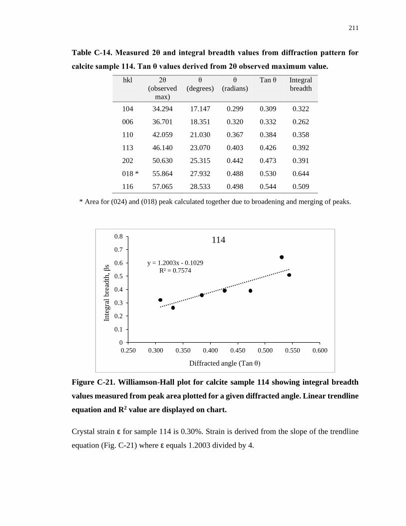
211

Table C-14. Measured 2θ and integral breadth values from diffraction pattern for

calcite sample 114. Tan θ values derived from 2θ observed maximum value.

hkl 2θ

(observed

max)

θ

(degrees)

θ

(radians)

Tan θ Integral

breadth

104 34.294 17.147 0.299 0.309 0.322

006 36.701 18.351 0.320 0.332 0.262

110 42.059 21.030 0.367 0.384 0.358

113 46.140 23.070 0.403 0.426 0.392

202 50.630 25.315 0.442 0.473 0.391

018 * 55.864 27.932 0.488 0.530 0.644

116 57.065 28.533 0.498 0.544 0.509

* Area for (024) and (018) peak calculated together due to broadening and merging of peaks.

Figure C-21. Williamson-Hall plot for calcite sample 114 showing integral breadth

values measured from peak area plotted for a given diffracted angle. Linear trendline

equation and R2 value are displayed on chart.

Crystal strain ε for sample 114 is 0.30%. Strain is derived from the slope of the trendline

equation (Fig. C-21) where ε equals 1.2003 divided by 4.

y = 1.2003x - 0.1029

R² = 0.7574

0

0.1

0.2

0.3

0.4

0.5

0.6

0.7

0.8

0.250 0.300 0.350 0.400 0.450 0.500 0.550 0.600

Inte

gra

l bre

adth

, β

s

Diffracted angle (Tan θ)

114

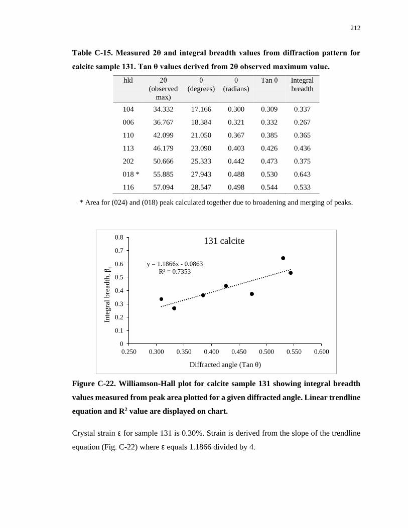
212

Table C-15. Measured 2θ and integral breadth values from diffraction pattern for

calcite sample 131. Tan θ values derived from 2θ observed maximum value.

hkl 2θ

(observed

max)

θ

(degrees)

θ

(radians)

Tan θ Integral

breadth

104 34.332 17.166 0.300 0.309 0.337

006 36.767 18.384 0.321 0.332 0.267

110 42.099 21.050 0.367 0.385 0.365

113 46.179 23.090 0.403 0.426 0.436

202 50.666 25.333 0.442 0.473 0.375

018 * 55.885 27.943 0.488 0.530 0.643

116 57.094 28.547 0.498 0.544 0.533

* Area for (024) and (018) peak calculated together due to broadening and merging of peaks.

Figure C-22. Williamson-Hall plot for calcite sample 131 showing integral breadth

values measured from peak area plotted for a given diffracted angle. Linear trendline

equation and R2 value are displayed on chart.

Crystal strain ε for sample 131 is 0.30%. Strain is derived from the slope of the trendline

equation (Fig. C-22) where ε equals 1.1866 divided by 4.

y = 1.1866x - 0.0863

R² = 0.7353

0

0.1

0.2

0.3

0.4

0.5

0.6

0.7

0.8

0.250 0.300 0.350 0.400 0.450 0.500 0.550 0.600

Inte

gra

l bre

adth

, β

s

Diffracted angle (Tan θ)

131 calcite

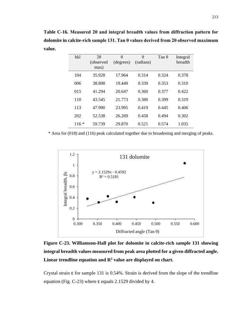
213

Table C-16. Measured 2θ and integral breadth values from diffraction pattern for

dolomite in calcite-rich sample 131. Tan θ values derived from 2θ observed maximum

value.

hkl 2θ

(observed

max)

θ

(degrees)

θ

(radians)

Tan θ Integral

breadth

104 35.928 17.964 0.314 0.324 0.378

006 38.898 19.449 0.339 0.353 0.310

015 41.294 20.647 0.360 0.377 0.422

110 43.545 21.773 0.380 0.399 0.319

113 47.990 23.995 0.419 0.445 0.406

202 52.538 26.269 0.458 0.494 0.302

116 * 59.739 29.870 0.521 0.574 1.035

* Area for (018) and (116) peak calculated together due to broadening and merging of peaks.

Figure C-23. Williamson-Hall plot for dolomite in calcite-rich sample 131 showing

integral breadth values measured from peak area plotted for a given diffracted angle.

Linear trendline equation and R2 value are displayed on chart.

Crystal strain ε for sample 131 is 0.54%. Strain is derived from the slope of the trendline

equation (Fig. C-23) where ε equals 2.1529 divided by 4.

y = 2.1529x - 0.4592

R² = 0.5181

0

0.2

0.4

0.6

0.8

1

1.2

0.300 0.350 0.400 0.450 0.500 0.550 0.600

Inte

gra

l bre

adth

, β

s

Diffracted angle (Tan θ)

131 dolomite

214

C.5 References

Uchizono A., Shinno I., Nakamuta Y., Nakamura T., and Sekine T. 1999. Characterization

of artificially shocked forsterites: (1) Diffraction profile analysis by Gandolfi camera.

Mineralogical Journal 21:15–23.

Williamson G. K., and Hall W. H. 1953. X-ray line broadening from filed aluminium and

wolfram. Acta Metallurgica 1:22–31.

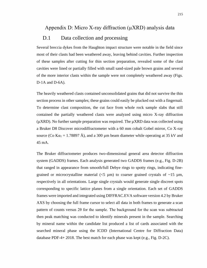
215

Appendix D: Micro X-ray diffraction (µXRD) analysis data

D.1 Data collection and processing

Several breccia dykes from the Haughton impact structure were notable in the field since

most of their clasts had been weathered away, leaving behind cavities. Further inspection

of these samples after cutting for thin section preparation, revealed some of the clast

cavities were lined or partially filled with small sand-sized pale brown grains and several

of the more interior clasts within the sample were not completely weathered away (Figs.

D-1A and D-6A).

The heavily weathered clasts contained unconsolidated grains that did not survive the thin

section process in other samples; these grains could easily be plucked out with a fingernail.

To determine clast composition, the cut face from whole rock sample slabs that still

contained the partially weathered clasts were analyzed using micro X-ray diffraction

(µXRD). No further sample preparation was required. The µXRD data was collected using

a Bruker D8 Discover microdiffractometer with a 60 mm cobalt Gobel mirror, Co X-ray

source (Co Kα1 = 1.78897 Å), and a 300 µm beam diameter while operating at 35 kV and

45 mA.

The Bruker diffractometer produces two-dimensional general area detector diffraction

system (GADDS) frames. Each analysis generated two GADDS frames (e.g., Fig. D-2B)

that ranged in appearance from smooth/full Debye rings to spotty rings, indicating fine-

grained or microcrystalline material (<5 µm) to coarser grained crystals of ~15 µm,

respectively in all orientations. Large single crystals would generate single discreet spots

corresponding to specific lattice planes from a single orientation. Each set of GADDS

frames were imported and integrated using DIFFRAC.EVA software version 4.2 by Bruker

AXS by choosing the full frame cursor to select all data in both frames to generate a scan

pattern of counts versus 2θ for the sample. The background for the scan was subtracted

then peak matching was conducted to identify minerals present in the sample. Searching

by mineral name within the candidate list produced a list of cards associated with the

searched mineral phase using the ICDD (International Centre for Diffraction Data)

database PDF-4+ 2018. The best match for each phase was kept (e.g., Fig. D-2C).

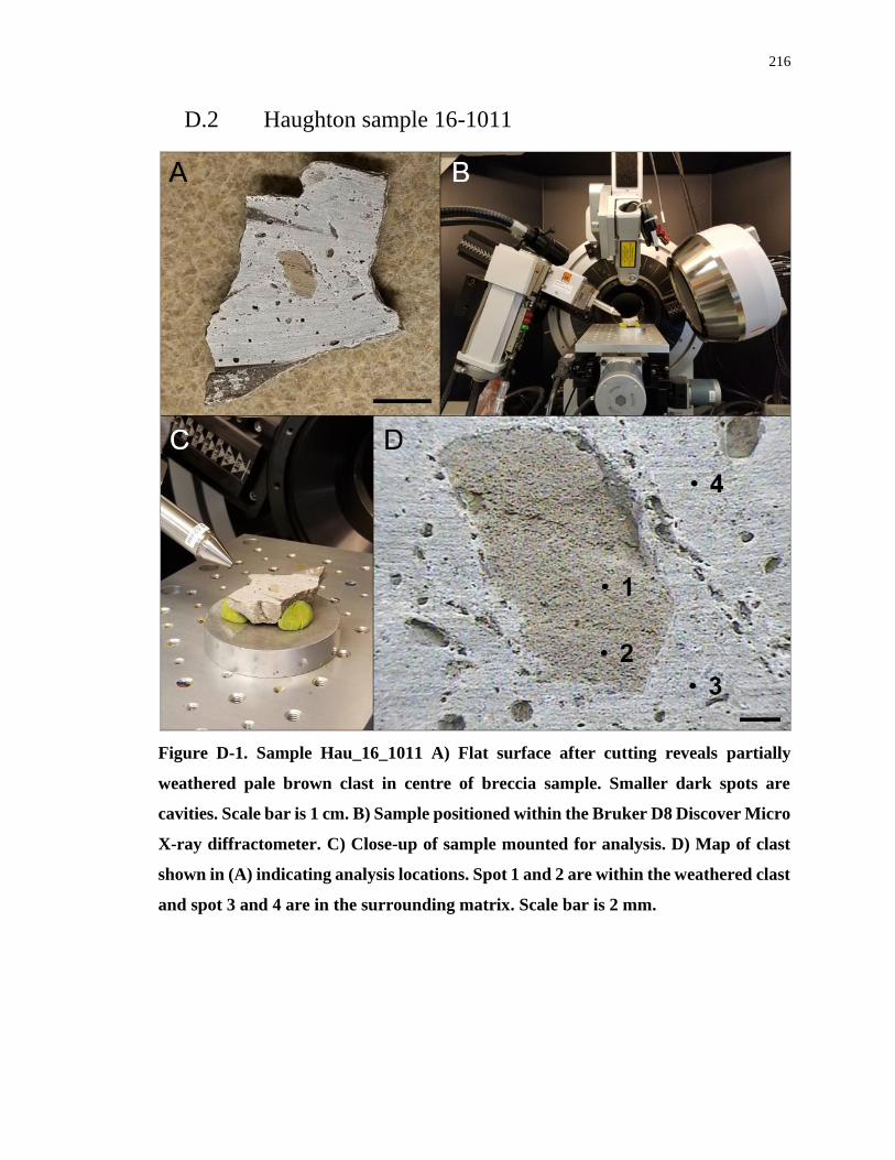
216

D.2 Haughton sample 16-1011

Figure D-1. Sample Hau_16_1011 A) Flat surface after cutting reveals partially

weathered pale brown clast in centre of breccia sample. Smaller dark spots are

cavities. Scale bar is 1 cm. B) Sample positioned within the Bruker D8 Discover Micro

X-ray diffractometer. C) Close-up of sample mounted for analysis. D) Map of clast

shown in (A) indicating analysis locations. Spot 1 and 2 are within the weathered clast

and spot 3 and 4 are in the surrounding matrix. Scale bar is 2 mm.

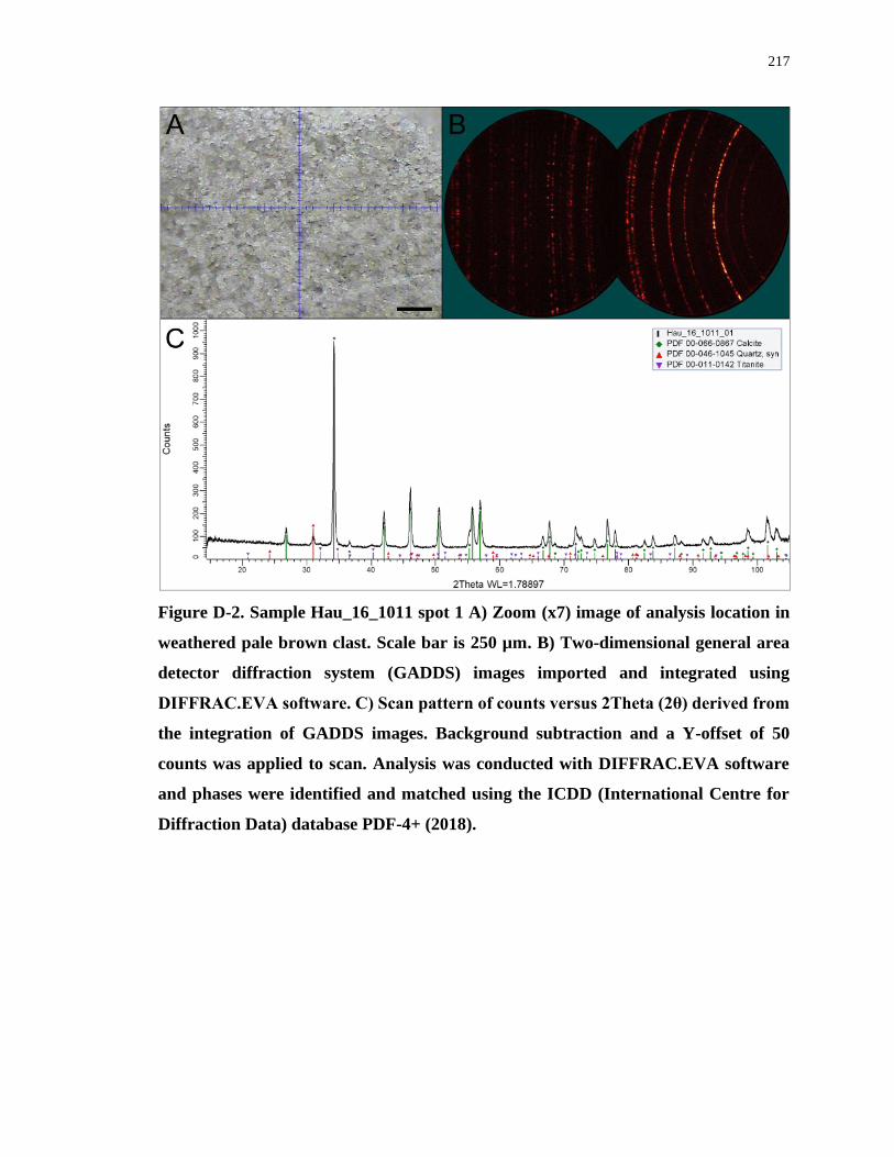
217

Figure D-2. Sample Hau_16_1011 spot 1 A) Zoom (x7) image of analysis location in

weathered pale brown clast. Scale bar is 250 µm. B) Two-dimensional general area

detector diffraction system (GADDS) images imported and integrated using

DIFFRAC.EVA software. C) Scan pattern of counts versus 2Theta (2θ) derived from

the integration of GADDS images. Background subtraction and a Y-offset of 50

counts was applied to scan. Analysis was conducted with DIFFRAC.EVA software

and phases were identified and matched using the ICDD (International Centre for

Diffraction Data) database PDF-4+ (2018).

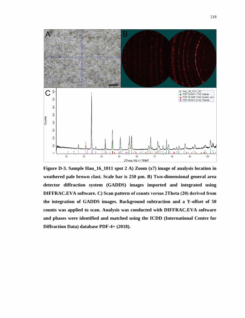
218

Figure D-3. Sample Hau_16_1011 spot 2 A) Zoom (x7) image of analysis location in

weathered pale brown clast. Scale bar is 250 µm. B) Two-dimensional general area

detector diffraction system (GADDS) images imported and integrated using

DIFFRAC.EVA software. C) Scan pattern of counts versus 2Theta (2θ) derived from

the integration of GADDS images. Background subtraction and a Y-offset of 50

counts was applied to scan. Analysis was conducted with DIFFRAC.EVA software

and phases were identified and matched using the ICDD (International Centre for

Diffraction Data) database PDF-4+ (2018).

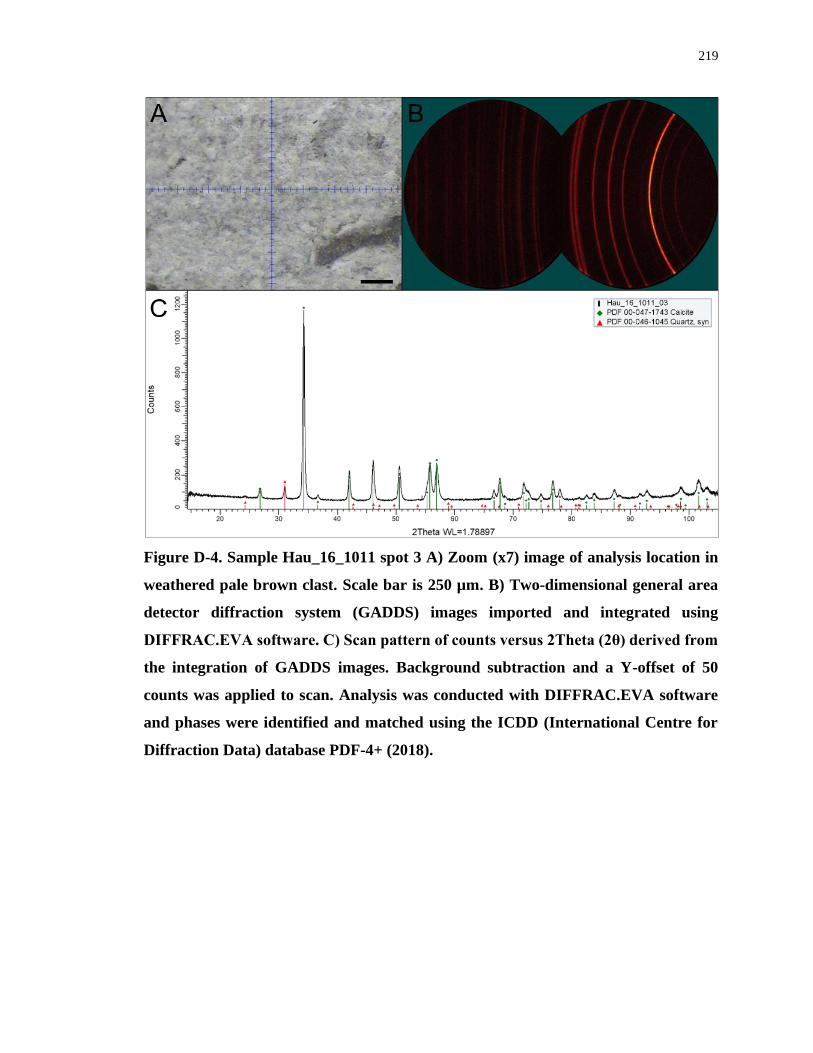
219

Figure D-4. Sample Hau_16_1011 spot 3 A) Zoom (x7) image of analysis location in

weathered pale brown clast. Scale bar is 250 µm. B) Two-dimensional general area

detector diffraction system (GADDS) images imported and integrated using

DIFFRAC.EVA software. C) Scan pattern of counts versus 2Theta (2θ) derived from

the integration of GADDS images. Background subtraction and a Y-offset of 50

counts was applied to scan. Analysis was conducted with DIFFRAC.EVA software

and phases were identified and matched using the ICDD (International Centre for

Diffraction Data) database PDF-4+ (2018).

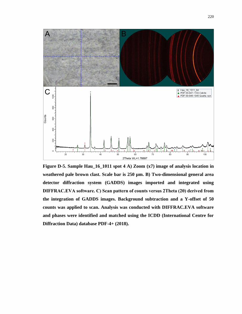
220

Figure D-5. Sample Hau_16_1011 spot 4 A) Zoom (x7) image of analysis location in

weathered pale brown clast. Scale bar is 250 µm. B) Two-dimensional general area

detector diffraction system (GADDS) images imported and integrated using

DIFFRAC.EVA software. C) Scan pattern of counts versus 2Theta (2θ) derived from

the integration of GADDS images. Background subtraction and a Y-offset of 50

counts was applied to scan. Analysis was conducted with DIFFRAC.EVA software

and phases were identified and matched using the ICDD (International Centre for

Diffraction Data) database PDF-4+ (2018).

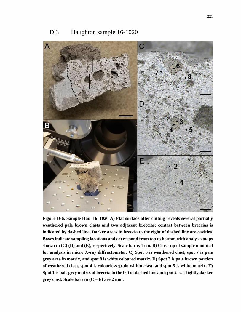
221

D.3 Haughton sample 16-1020

Figure D-6. Sample Hau_16_1020 A) Flat surface after cutting reveals several partially

weathered pale brown clasts and two adjacent breccias; contact between breccias is

indicated by dashed line. Darker areas in breccia to the right of dashed line are cavities.

Boxes indicate sampling locations and correspond from top to bottom with analysis maps

shown in (C) (D) and (E), respectively. Scale bar is 1 cm. B) Close-up of sample mounted

for analysis in micro X-ray diffractometer. C) Spot 6 is weathered clast, spot 7 is pale

grey area in matrix, and spot 8 is white coloured matrix. D) Spot 3 is pale brown portion

of weathered clast, spot 4 is colourless grain within clast, and spot 5 is white matrix. E)

Spot 1 is pale grey matrix of breccia to the left of dashed line and spot 2 is a slightly darker

grey clast. Scale bars in (C – E) are 2 mm.

222

Figure D-7. Sample Hau_16_1020 spot 1 A) Zoom (x7) image of analysis location in

weathered pale brown clast. Scale bar is 250 µm. B) Two-dimensional general area

detector diffraction system (GADDS) images imported and integrated using

DIFFRAC.EVA software. C) Scan pattern of counts versus 2Theta (2θ) derived from

the integration of GADDS images. Background subtraction and a Y-offset of 50

counts was applied to scan. Analysis was conducted with DIFFRAC.EVA software

and phases were identified and matched using the ICDD (International Centre for

Diffraction Data) database PDF-4+ (2018).

223

Figure D-8. Sample Hau_16_1020 spot 2 A) Zoom (x7) image of analysis location in

weathered pale brown clast. Scale bar is 250 µm. B) Two-dimensional general area

detector diffraction system (GADDS) images imported and integrated using

DIFFRAC.EVA software. C) Scan pattern of counts versus 2Theta (2θ) derived from

the integration of GADDS images. Background subtraction and a Y-offset of 50

counts was applied to scan. Analysis was conducted with DIFFRAC.EVA software

and phases were identified and matched using the ICDD (International Centre for

Diffraction Data) database PDF-4+ (2018).

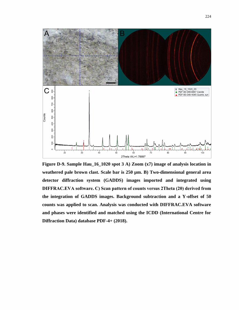
224

Figure D-9. Sample Hau_16_1020 spot 3 A) Zoom (x7) image of analysis location in

weathered pale brown clast. Scale bar is 250 µm. B) Two-dimensional general area

detector diffraction system (GADDS) images imported and integrated using

DIFFRAC.EVA software. C) Scan pattern of counts versus 2Theta (2θ) derived from

the integration of GADDS images. Background subtraction and a Y-offset of 50

counts was applied to scan. Analysis was conducted with DIFFRAC.EVA software

and phases were identified and matched using the ICDD (International Centre for

Diffraction Data) database PDF-4+ (2018).

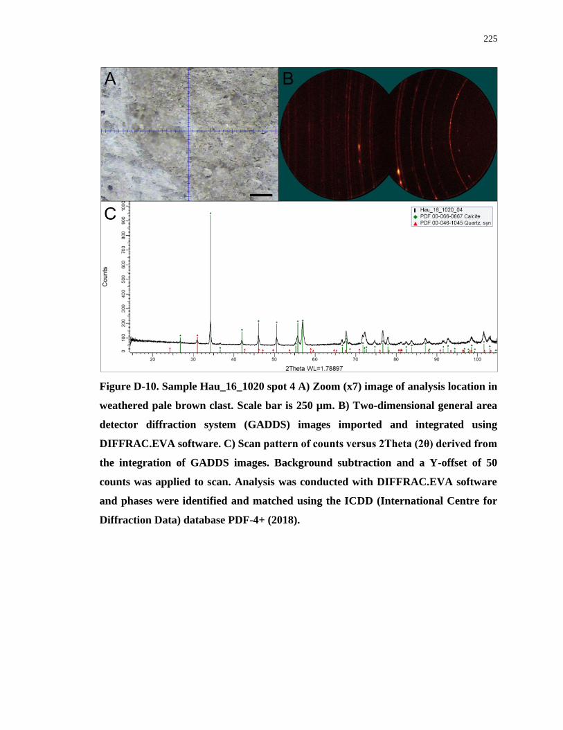
225

Figure D-10. Sample Hau_16_1020 spot 4 A) Zoom (x7) image of analysis location in

weathered pale brown clast. Scale bar is 250 µm. B) Two-dimensional general area

detector diffraction system (GADDS) images imported and integrated using

DIFFRAC.EVA software. C) Scan pattern of counts versus 2Theta (2θ) derived from

the integration of GADDS images. Background subtraction and a Y-offset of 50

counts was applied to scan. Analysis was conducted with DIFFRAC.EVA software

and phases were identified and matched using the ICDD (International Centre for

Diffraction Data) database PDF-4+ (2018).

226

Figure D-11. Sample Hau_16_1020 spot 5 A) Zoom (x7) image of analysis location in

weathered pale brown clast. Scale bar is 250 µm. B) Two-dimensional general area

detector diffraction system (GADDS) images imported and integrated using

DIFFRAC.EVA software. C) Scan pattern of counts versus 2Theta (2θ) derived from

the integration of GADDS images. Background subtraction and a Y-offset of 50

counts was applied to scan. Analysis was conducted with DIFFRAC.EVA software

and phases were identified and matched using the ICDD (International Centre for

Diffraction Data) database PDF-4+ (2018).

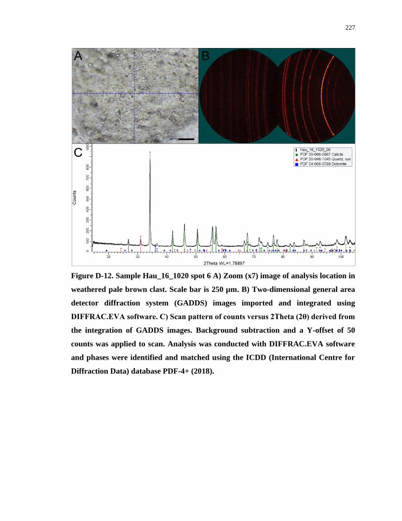
227

Figure D-12. Sample Hau_16_1020 spot 6 A) Zoom (x7) image of analysis location in

weathered pale brown clast. Scale bar is 250 µm. B) Two-dimensional general area

detector diffraction system (GADDS) images imported and integrated using

DIFFRAC.EVA software. C) Scan pattern of counts versus 2Theta (2θ) derived from

the integration of GADDS images. Background subtraction and a Y-offset of 50

counts was applied to scan. Analysis was conducted with DIFFRAC.EVA software

and phases were identified and matched using the ICDD (International Centre for

Diffraction Data) database PDF-4+ (2018).

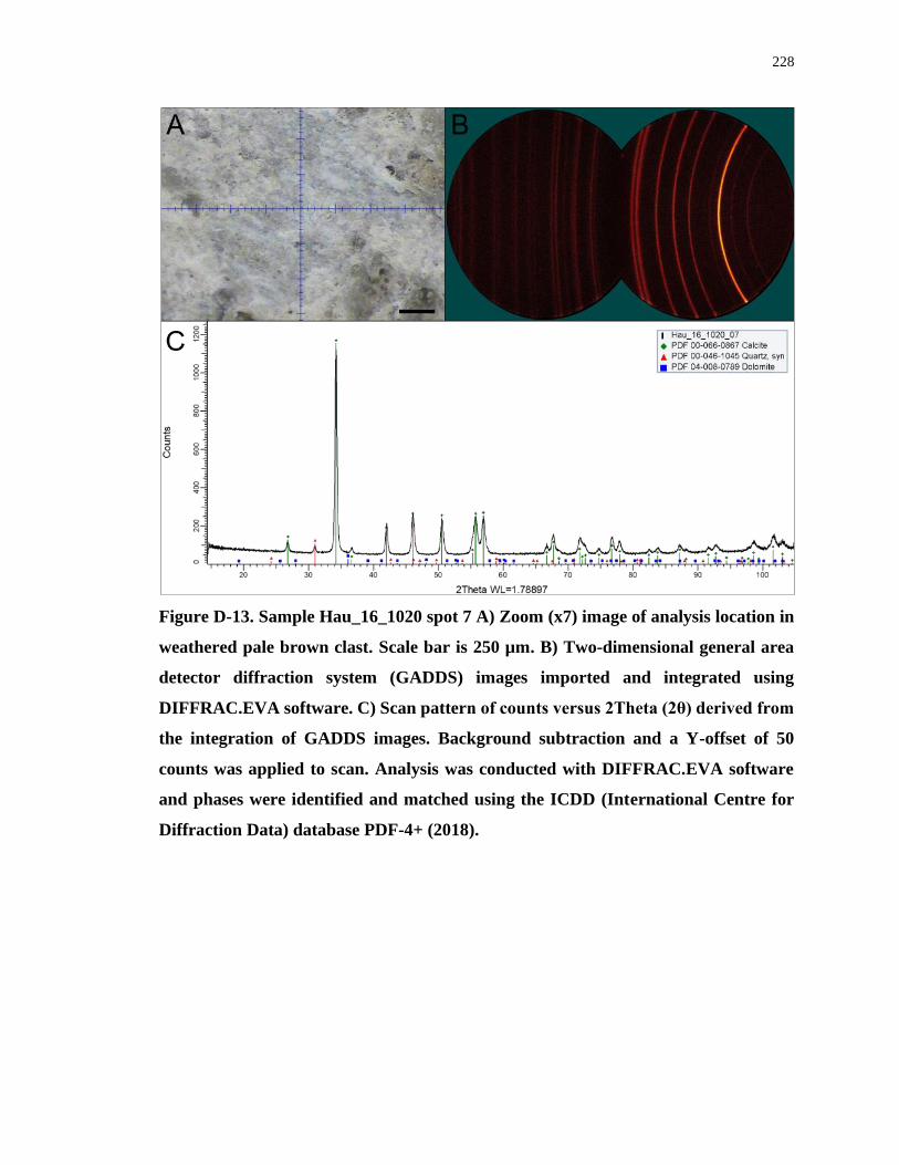
228

Figure D-13. Sample Hau_16_1020 spot 7 A) Zoom (x7) image of analysis location in

weathered pale brown clast. Scale bar is 250 µm. B) Two-dimensional general area

detector diffraction system (GADDS) images imported and integrated using

DIFFRAC.EVA software. C) Scan pattern of counts versus 2Theta (2θ) derived from

the integration of GADDS images. Background subtraction and a Y-offset of 50

counts was applied to scan. Analysis was conducted with DIFFRAC.EVA software

and phases were identified and matched using the ICDD (International Centre for

Diffraction Data) database PDF-4+ (2018).

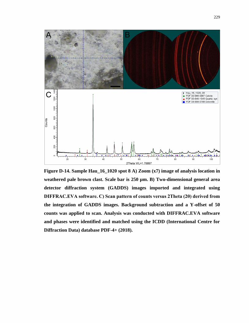
229

Figure D-14. Sample Hau_16_1020 spot 8 A) Zoom (x7) image of analysis location in

weathered pale brown clast. Scale bar is 250 µm. B) Two-dimensional general area

detector diffraction system (GADDS) images imported and integrated using

DIFFRAC.EVA software. C) Scan pattern of counts versus 2Theta (2θ) derived from

the integration of GADDS images. Background subtraction and a Y-offset of 50

counts was applied to scan. Analysis was conducted with DIFFRAC.EVA software

and phases were identified and matched using the ICDD (International Centre for

Diffraction Data) database PDF-4+ (2018).

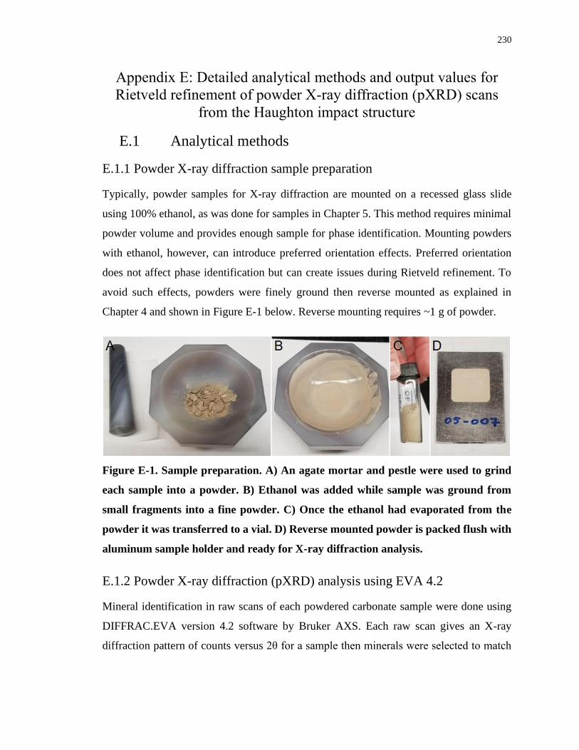
230

Appendix E: Detailed analytical methods and output values for

Rietveld refinement of powder X-ray diffraction (pXRD) scans

from the Haughton impact structure

E.1 Analytical methods

E.1.1 Powder X-ray diffraction sample preparation

Typically, powder samples for X-ray diffraction are mounted on a recessed glass slide

using 100% ethanol, as was done for samples in Chapter 5. This method requires minimal

powder volume and provides enough sample for phase identification. Mounting powders

with ethanol, however, can introduce preferred orientation effects. Preferred orientation

does not affect phase identification but can create issues during Rietveld refinement. To

avoid such effects, powders were finely ground then reverse mounted as explained in

Chapter 4 and shown in Figure E-1 below. Reverse mounting requires ~1 g of powder.

Figure E-1. Sample preparation. A) An agate mortar and pestle were used to grind

each sample into a powder. B) Ethanol was added while sample was ground from

small fragments into a fine powder. C) Once the ethanol had evaporated from the

powder it was transferred to a vial. D) Reverse mounted powder is packed flush with

aluminum sample holder and ready for X-ray diffraction analysis.

E.1.2 Powder X-ray diffraction (pXRD) analysis using EVA 4.2

Mineral identification in raw scans of each powdered carbonate sample were done using

DIFFRAC.EVA version 4.2 software by Bruker AXS. Each raw scan gives an X-ray

diffraction pattern of counts versus 2θ for a sample then minerals were selected to match

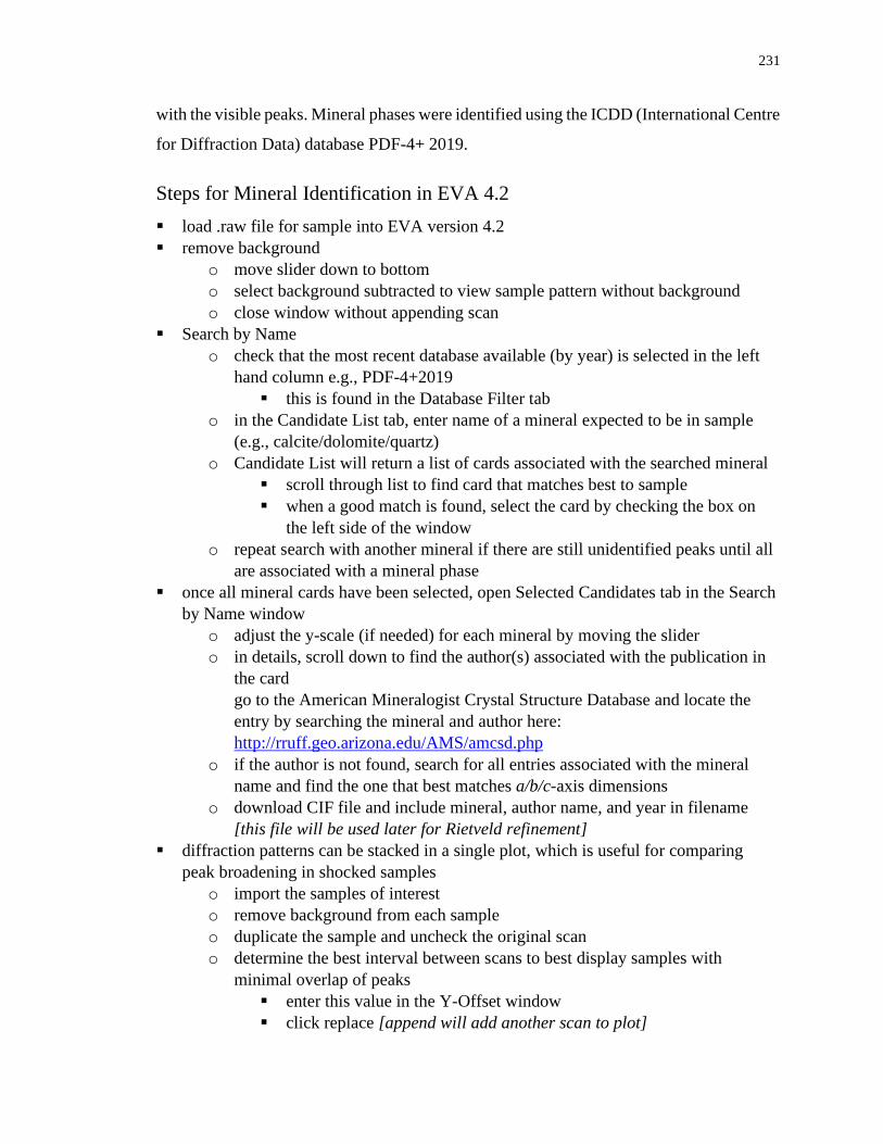
231

with the visible peaks. Mineral phases were identified using the ICDD (International Centre

for Diffraction Data) database PDF-4+ 2019.

Steps for Mineral Identification in EVA 4.2

▪ load .raw file for sample into EVA version 4.2

▪ remove background

o move slider down to bottom

o select background subtracted to view sample pattern without background

o close window without appending scan

▪ Search by Name

o check that the most recent database available (by year) is selected in the left

hand column e.g., PDF-4+2019

▪ this is found in the Database Filter tab

o in the Candidate List tab, enter name of a mineral expected to be in sample

(e.g., calcite/dolomite/quartz)

o Candidate List will return a list of cards associated with the searched mineral

▪ scroll through list to find card that matches best to sample

▪ when a good match is found, select the card by checking the box on

the left side of the window

o repeat search with another mineral if there are still unidentified peaks until all

are associated with a mineral phase

▪ once all mineral cards have been selected, open Selected Candidates tab in the Search

by Name window

o adjust the y-scale (if needed) for each mineral by moving the slider

o in details, scroll down to find the author(s) associated with the publication in

the card

go to the American Mineralogist Crystal Structure Database and locate the

entry by searching the mineral and author here:

http://rruff.geo.arizona.edu/AMS/amcsd.php

o if the author is not found, search for all entries associated with the mineral

name and find the one that best matches a/b/c-axis dimensions

o download CIF file and include mineral, author name, and year in filename

[this file will be used later for Rietveld refinement]

▪ diffraction patterns can be stacked in a single plot, which is useful for comparing

peak broadening in shocked samples

o import the samples of interest

o remove background from each sample

o duplicate the sample and uncheck the original scan

o determine the best interval between scans to best display samples with

minimal overlap of peaks

▪ enter this value in the Y-Offset window

▪ click replace [append will add another scan to plot]

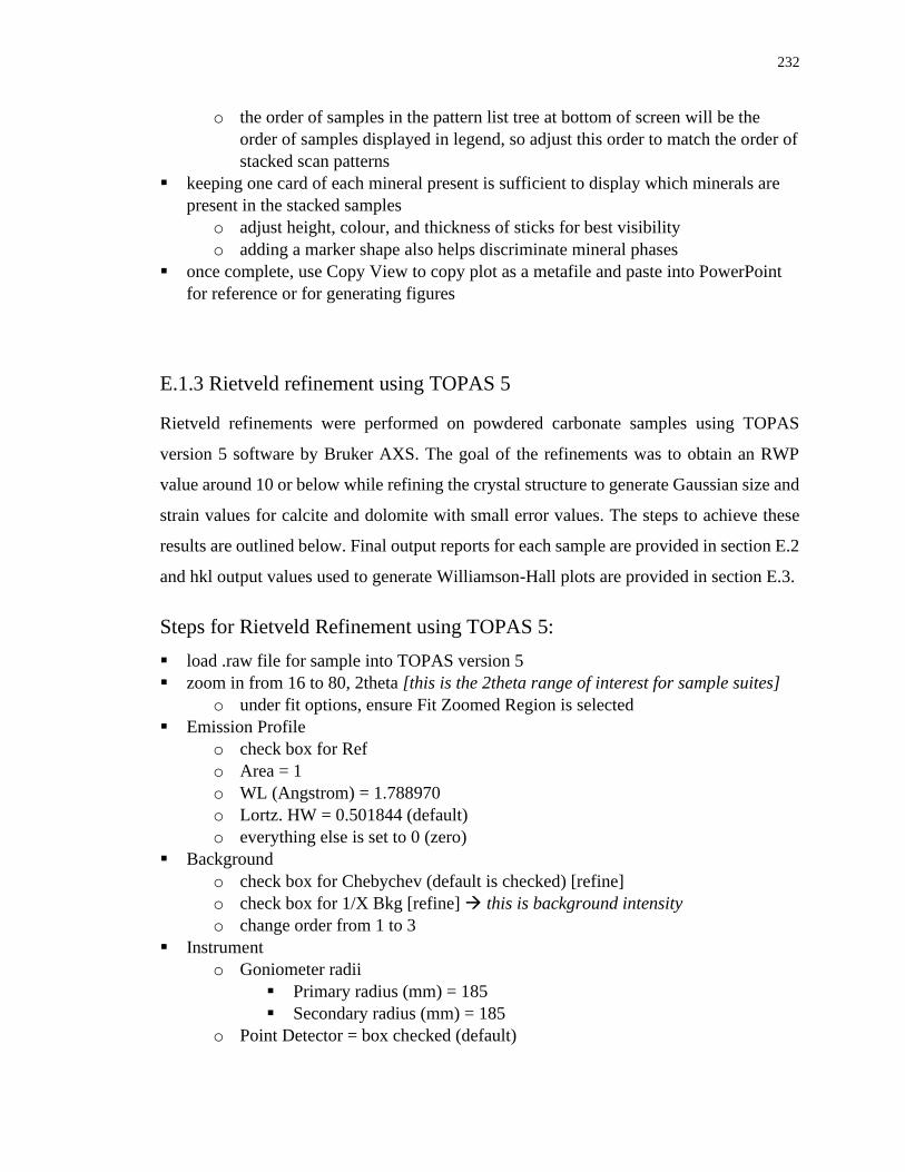
232

o the order of samples in the pattern list tree at bottom of screen will be the

order of samples displayed in legend, so adjust this order to match the order of

stacked scan patterns

▪ keeping one card of each mineral present is sufficient to display which minerals are

present in the stacked samples

o adjust height, colour, and thickness of sticks for best visibility

o adding a marker shape also helps discriminate mineral phases

▪ once complete, use Copy View to copy plot as a metafile and paste into PowerPoint

for reference or for generating figures

E.1.3 Rietveld refinement using TOPAS 5

Rietveld refinements were performed on powdered carbonate samples using TOPAS

version 5 software by Bruker AXS. The goal of the refinements was to obtain an RWP

value around 10 or below while refining the crystal structure to generate Gaussian size and

strain values for calcite and dolomite with small error values. The steps to achieve these

results are outlined below. Final output reports for each sample are provided in section E.2

and hkl output values used to generate Williamson-Hall plots are provided in section E.3.

Steps for Rietveld Refinement using TOPAS 5:

▪ load .raw file for sample into TOPAS version 5

▪ zoom in from 16 to 80, 2theta [this is the 2theta range of interest for sample suites]

o under fit options, ensure Fit Zoomed Region is selected

▪ Emission Profile

o check box for Ref

o Area = 1

o WL (Angstrom) = 1.788970

o Lortz. HW = 0.501844 (default)

o everything else is set to 0 (zero)

▪ Background

o check box for Chebychev (default is checked) [refine]

o check box for 1/X Bkg [refine] → this is background intensity

o change order from 1 to 3

▪ Instrument

o Goniometer radii

▪ Primary radius (mm) = 185

▪ Secondary radius (mm) = 185

o Point Detector = box checked (default)

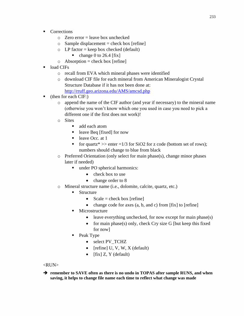
233

▪ Corrections

o Zero error = leave box unchecked

o Sample displacement = check box [refine]

o LP factor = keep box checked (default)

▪ change 0 to 26.4 [fix]

o Absorption = check box [refine]

▪ load CIFs

o recall from EVA which mineral phases were identified

o download CIF file for each mineral from American Mineralogist Crystal

Structure Database if it has not been done at:

http://rruff.geo.arizona.edu/AMS/amcsd.php

▪ (then for each CIF:)

o append the name of the CIF author (and year if necessary) to the mineral name

(otherwise you won’t know which one you used in case you need to pick a

different one if the first does not work)!

o Sites

▪ add each atom

▪ leave Beq [fixed] for now

▪ leave Occ. at 1

▪ for quartz* >> enter =1/3 for SiO2 for z code (bottom set of rows);

numbers should change to blue from black

o Preferred Orientation (only select for main phase(s), change minor phases

later if needed)

▪ under PO spherical harmonics:

• check box to use

• change order to 8

o Mineral structure name (i.e., dolomite, calcite, quartz, etc.)

▪ Structure

• Scale = check box [refine]

• change code for axes (a, b, and c) from [fix] to [refine]

▪ Microstructure

• leave everything unchecked, for now except for main phase(s)

• for main phase(s) only, check Cry size G [but keep this fixed

for now]

▪ Peak Type

• select PV_TCHZ

• [refine] U, V, W, X (default)

• [fix] Z, Y (default)

<RUN>

➔ remember to SAVE often as there is no undo in TOPAS after sample RUNS, and when

saving, it helps to change file name each time to reflect what change was made

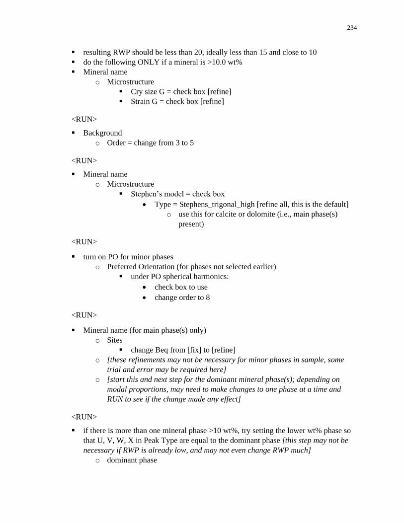
234

▪ resulting RWP should be less than 20, ideally less than 15 and close to 10

▪ do the following ONLY if a mineral is >10.0 wt%

▪ Mineral name

o Microstructure

▪ Cry size G = check box [refine]

▪ Strain G = check box [refine]

<RUN>

▪ Background

o Order = change from 3 to 5

<RUN>

▪ Mineral name

o Microstructure

▪ Stephen’s model = check box

• Type = Stephens_trigonal_high [refine all, this is the default]

o use this for calcite or dolomite (i.e., main phase(s)

present)

<RUN>

▪ turn on PO for minor phases

o Preferred Orientation (for phases not selected earlier)

▪ under PO spherical harmonics:

• check box to use

• change order to 8

<RUN>

▪ Mineral name (for main phase(s) only)

o Sites

▪ change Beq from [fix] to [refine]

o [these refinements may not be necessary for minor phases in sample, some

trial and error may be required here]

o [start this and next step for the dominant mineral phase(s); depending on

modal proportions, may need to make changes to one phase at a time and

RUN to see if the change made any effect]

<RUN>

▪ if there is more than one mineral phase >10 wt%, try setting the lower wt% phase so

that U, V, W, X in Peak Type are equal to the dominant phase [this step may not be

necessary if RWP is already low, and may not even change RWP much]

o dominant phase

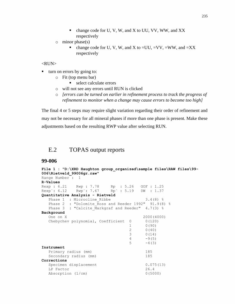
235

▪ change code for U, V, W, and X to UU, VV, WW, and XX

respectively

o minor phase(s)

▪ change code for U, V, W, and X to =UU, =VV, =WW, and =XX

respectively

<RUN>

▪ turn on errors by going to:

o Fit (top menu bar)

▪ select calculate errors

o will not see any errors until RUN is clicked

o [errors can be turned on earlier in refinement process to track the progress of

refinement to monitor when a change may cause errors to become too high]

The final 4 or 5 steps may require slight variation regarding their order of refinement and

may not be necessary for all mineral phases if more than one phase is present. Make these

adjustments based on the resulting RWP value after selecting RUN.

E.2 TOPAS output reports

99-006

File 1 : "D:\XRD Haughton group_organized\sample files\RAW files\99-

006\Rietveld_99006gr.raw"

Range Number : 1

R-Values

Rexp : 6.21 Rwp : 7.78 Rp : 5.26 GOF : 1.25

Rexp`: 6.12 Rwp`: 7.67 Rp` : 5.19 DW : 1.37

Quantitative Analysis - Rietveld

Phase 1 : Microcline_Ribbe 3.4(8) %

Phase 2 : "Dolomite_Ross and Reeder 1992" 91.9(8) %

Phase 3 : "Calcite_Markgraf and Reeder" 4.7(3) %

Background

One on X 2000(4000)

Chebychev polynomial, Coefficient 0 0(120)

1 0(90)

2 0(40)

3 0(14)

4 -9(5)

5 -4(3)

Instrument

Primary radius (mm) 185

Secondary radius (mm) 185

Corrections

Specimen displacement 0.075(13)

LP Factor 26.4

Absorption (1/cm) 0(5000)

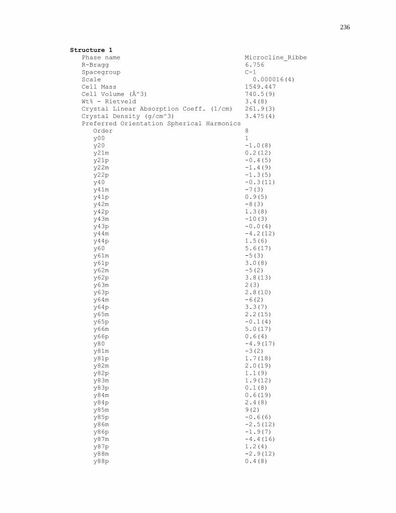
236

Structure 1

Phase name Microcline_Ribbe

R-Bragg 6.756

Spacegroup C-1

Scale 0.000016(4)

Cell Mass 1549.447

Cell Volume (Å^3) 740.5(9)

Wt% - Rietveld 3.4(8)

Crystal Linear Absorption Coeff. (1/cm) 261.9(3)

Crystal Density (g/cm^3) 3.475(4)

Preferred Orientation Spherical Harmonics

Order 8

y00 1

y20 -1.0(8)

y21m 0.2(12)

y21p -0.4(5)

y22m -1.4(9)

y22p -1.3(5)

y40 -0.3(11)

y41m -7(3)

y41p 0.9(5)

y42m -8(3)

y42p 1.3(8)

y43m -10(3)

y43p -0.0(4)

y44m -4.2(12)

y44p 1.5(6)

y60 5.6(17)

y61m -5(3)

y61p 3.0(8)

y62m -5(2)

y62p 3.8(13)

y63m 2(3)

y63p 2.8(10)

y64m -6(2)

y64p 3.3(7)

y65m 2.2(15)

y65p -0.1(4)

y66m 5.0(17)

y66p 0.6(4)

y80 -4.9(17)

y81m -3(2)

y81p 1.7(18)

y82m 2.0(19)

y82p 1.1(9)

y83m 1.9(12)

y83p 0.1(8)

y84m 0.6(19)

y84p 2.4(8)

y85m 9(2)

y85p -0.6(6)

y86m -2.5(12)

y86p -1.9(7)

y87m -4.4(16)

y87p 1.2(4)

y88m -2.9(12)

y88p 0.4(8)

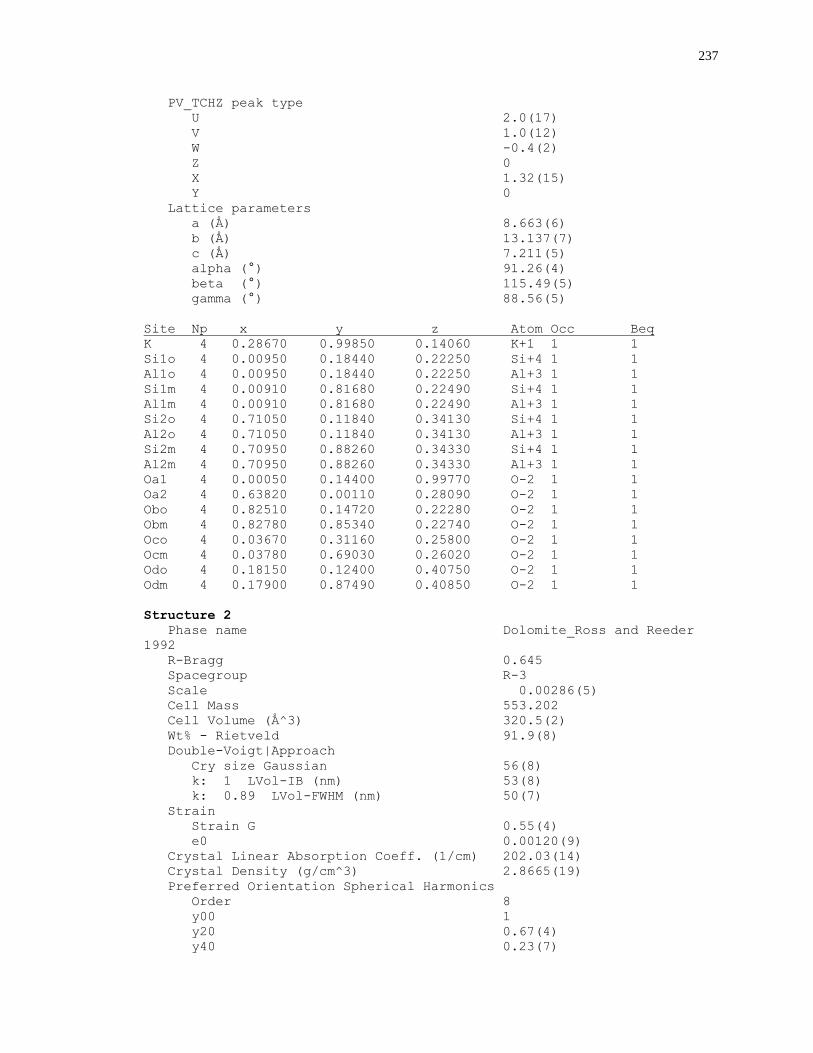
237

PV_TCHZ peak type

U 2.0(17)

V 1.0(12)

W -0.4(2)

Z 0

X 1.32(15)

Y 0

Lattice parameters

a (Å) 8.663(6)

b (Å) 13.137(7)

c (Å) 7.211(5)

alpha (°) 91.26(4)

beta (°) 115.49(5)

gamma (°) 88.56(5)

Site Np x y z Atom Occ Beq

K 4 0.28670 0.99850 0.14060 K+1 1 1

Si1o 4 0.00950 0.18440 0.22250 Si+4 1 1

Al1o 4 0.00950 0.18440 0.22250 Al+3 1 1

Si1m 4 0.00910 0.81680 0.22490 Si+4 1 1

Al1m 4 0.00910 0.81680 0.22490 Al+3 1 1

Si2o 4 0.71050 0.11840 0.34130 Si+4 1 1

Al2o 4 0.71050 0.11840 0.34130 Al+3 1 1

Si2m 4 0.70950 0.88260 0.34330 Si+4 1 1

Al2m 4 0.70950 0.88260 0.34330 Al+3 1 1

Oa1 4 0.00050 0.14400 0.99770 O-2 1 1

Oa2 4 0.63820 0.00110 0.28090 O-2 1 1

Obo 4 0.82510 0.14720 0.22280 O-2 1 1

Obm 4 0.82780 0.85340 0.22740 O-2 1 1

Oco 4 0.03670 0.31160 0.25800 O-2 1 1

Ocm 4 0.03780 0.69030 0.26020 O-2 1 1

Odo 4 0.18150 0.12400 0.40750 O-2 1 1

Odm 4 0.17900 0.87490 0.40850 O-2 1 1

Structure 2

Phase name Dolomite_Ross and Reeder

1992

R-Bragg 0.645

Spacegroup R-3

Scale 0.00286(5)

Cell Mass 553.202

Cell Volume (Å^3) 320.5(2)

Wt% - Rietveld 91.9(8)

Double-Voigt|Approach

Cry size Gaussian 56(8)

k: 1 LVol-IB (nm) 53(8)

k: 0.89 LVol-FWHM (nm) 50(7)

Strain

Strain G 0.55(4)

e0 0.00120(9)

Crystal Linear Absorption Coeff. (1/cm) 202.03(14)

Crystal Density (g/cm^3) 2.8665(19)

Preferred Orientation Spherical Harmonics

Order 8

y00 1

y20 0.67(4)

y40 0.23(7)

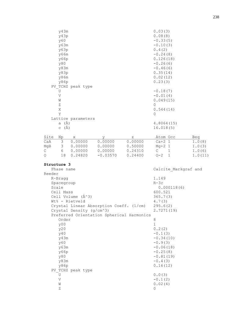
238

y43m 0.03(3)

y43p 0.08(8)

y60 -0.33(5)

y63m -0.10(3)

y63p 0.4(2)

y66m -0.24(8)

y66p 0.126(18)

y80 -0.26(6)

y83m -0.46(6)

y83p 0.35(14)

y86m 0.02(12)

y86p 0.23(3)

PV_TCHZ peak type

U -0.18(7)

V -0.01(4)

W 0.049(15)

Z 0

X 0.544(14)

Y 0

Lattice parameters

a (Å) 4.8064(15)

c (Å) 16.018(5)

Site Np x y z Atom Occ Beq

CaA 3 0.00000 0.00000 0.00000 Ca+2 1 1.0(8)

MgB 3 0.00000 0.00000 0.50000 Mg+2 1 1.0(3)

C 6 0.00000 0.00000 0.24310 C 1 1.0(6)

O 18 0.24820 -0.03570 0.24400 O-2 1 1.0(11)

Structure 3

Phase name Calcite_Markgraf and

Reeder

R-Bragg 1.149

Spacegroup R-3c

Scale 0.000118(6)

Cell Mass 600.521

Cell Volume (Å^3) 365.7(3)

Wt% - Rietveld 4.7(3)

Crystal Linear Absorption Coeff. (1/cm) 295.6(2)

Crystal Density (g/cm^3) 2.7271(19)

Preferred Orientation Spherical Harmonics

Order 8

y00 1

y20 0.2(2)

y40 -0.1(3)

y43m -0.34(10)

y60 -0.9(3)

y63m -0.06(18)

y66p -0.25(8)

y80 -0.81(19)

y83m -0.4(3)

y86p 0.16(12)

PV_TCHZ peak type

U 0.0(3)

V -0.1(2)

W 0.02(4)

Z 0

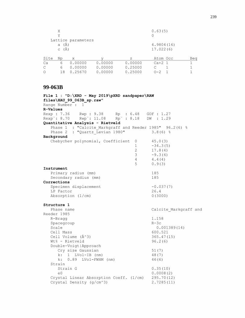
239

X 0.63(5)

Y 0

Lattice parameters

a (Å) 4.9804(16)

c (Å) 17.022(6)

Site Np x y z Atom Occ Beq

Ca 6 0.00000 0.00000 0.00000 Ca+2 1 1

C 6 0.00000 0.00000 0.25000 C 1 1

O 18 0.25670 0.00000 0.25000 O-2 1 1

99-063B

File 1 : "D:\XRD - May 2019\pXRD sandpaper\RAW

files\HAU_99_063B_sp.raw"

Range Number : 1

R-Values

Rexp : 7.36 Rwp : 9.38 Rp : 6.48 GOF : 1.27

Rexp`: 8.70 Rwp`: 11.08 Rp` : 8.18 DW : 1.29

Quantitative Analysis - Rietveld

Phase 1 : "Calcite_Markgraff and Reeder 1985" 96.2(6) %

Phase 2 : "Quartz_Levian 1980" 3.8(6) %

Background

Chebychev polynomial, Coefficient 0 45.0(3)

1 -34.3(5)

2 17.8(4)

3 -9.3(4)

4 4.4(4)

5 0.9(3)

Instrument

Primary radius (mm) 185

Secondary radius (mm) 185

Corrections

Specimen displacement -0.037(7)

LP Factor 26.4

Absorption (1/cm) 0(3000)

Structure 1

Phase name Calcite_Markgraff and

Reeder 1985

R-Bragg 1.158

Spacegroup R-3c

Scale 0.001389(14)

Cell Mass 600.521

Cell Volume (Å^3) 365.47(15)

Wt% - Rietveld 96.2(6)

Double-Voigt|Approach

Cry size Gaussian 51(7)

k: 1 LVol-IB (nm) 48(7)

k: 0.89 LVol-FWHM (nm) 46(6)

Strain

Strain G 0.35(10)

e0 0.0008(2)

Crystal Linear Absorption Coeff. (1/cm) 295.70(12)

Crystal Density (g/cm^3) 2.7285(11)

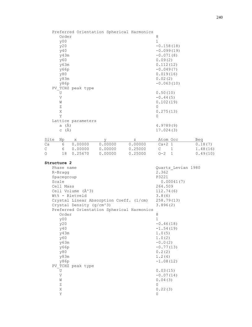
240

Preferred Orientation Spherical Harmonics

Order 8

y00 1

y20 -0.158(18)

y40 -0.099(19)

y43m -0.071(8)

y60 0.09(2)

y63m 0.112(12)

y66p -0.049(7)

y80 0.019(16)

y83m 0.02(2)

y86p -0.063(10)

PV_TCHZ peak type

U 0.50(10)

V -0.44(5)

W 0.102(19)

Z 0

X 0.275(13)

Y 0

Lattice parameters

a (Å) 4.9789(9)

c (Å) 17.024(3)

Site Np x y z Atom Occ Beq

Ca 6 0.00000 0.00000 0.00000 Ca+2 1 0.18(7)

C 6 0.00000 0.00000 0.25000 C 1 1.48(16)

O 18 0.25670 0.00000 0.25000 O-2 1 0.49(10)

Structure 2

Phase name Quartz_Levian 1980

R-Bragg 2.362

Spacegroup P3221

Scale 0.00041(7)

Cell Mass 264.509

Cell Volume (Å^3) 112.74(6)

Wt% - Rietveld 3.8(6)

Crystal Linear Absorption Coeff. (1/cm) 258.79(13)

Crystal Density (g/cm^3) 3.896(2)

Preferred Orientation Spherical Harmonics

Order 8

y00 1

y20 -0.46(18)

y40 -1.54(19)

y43m 1.0(5)

y60 1.0(2)

y63m -0.0(2)

y66p -0.77(13)

y80 0.2(2)

y83m 1.2(4)

y86p -1.08(12)

PV_TCHZ peak type

U 0.03(15)

V -0.07(14)

W 0.04(3)

Z 0

X 0.22(3)

Y 0

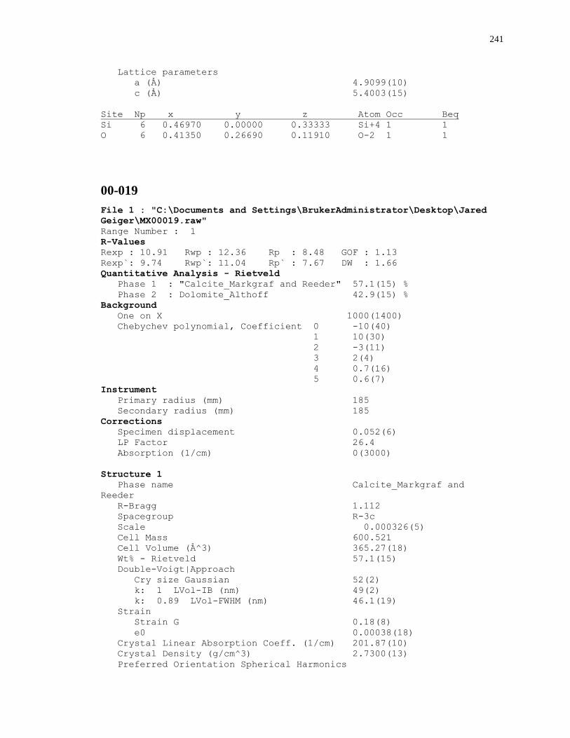
241

Lattice parameters

a (Å) 4.9099(10)

c (Å) 5.4003(15)

Site Np x y z Atom Occ Beq

Si 6 0.46970 0.00000 0.33333 Si+4 1 1

O 6 0.41350 0.26690 0.11910 O-2 1 1

00-019

File 1 : "C:\Documents and Settings\BrukerAdministrator\Desktop\Jared

Geiger\MX00019.raw"

Range Number : 1

R-Values

Rexp : 10.91 Rwp : 12.36 Rp : 8.48 GOF : 1.13

Rexp`: 9.74 Rwp`: 11.04 Rp` : 7.67 DW : 1.66

Quantitative Analysis - Rietveld

Phase 1 : "Calcite_Markgraf and Reeder" 57.1(15) %

Phase 2 : Dolomite_Althoff 42.9(15) %

Background

One on X 1000(1400)

Chebychev polynomial, Coefficient 0 -10(40)

1 10(30)

2 -3(11)

3 2(4)

4 0.7(16)

5 0.6(7)

Instrument

Primary radius (mm) 185

Secondary radius (mm) 185

Corrections

Specimen displacement 0.052(6)

LP Factor 26.4

Absorption (1/cm) 0(3000)

Structure 1

Phase name Calcite_Markgraf and

Reeder

R-Bragg 1.112

Spacegroup R-3c

Scale 0.000326(5)

Cell Mass 600.521

Cell Volume (Å^3) 365.27(18)

Wt% - Rietveld 57.1(15)

Double-Voigt|Approach

Cry size Gaussian 52(2)

k: 1 LVol-IB (nm) 49(2)

k: 0.89 LVol-FWHM (nm) 46.1(19)

Strain

Strain G 0.18(8)

e0 0.00038(18)

Crystal Linear Absorption Coeff. (1/cm) 201.87(10)

Crystal Density (g/cm^3) 2.7300(13)

Preferred Orientation Spherical Harmonics

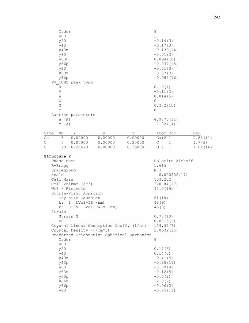
242

Order 8

y00 1

y20 -0.14(3)

y40 -0.17(3)

y43m -0.139(14)

y60 -0.01(3)

y63m 0.094(18)

y66p -0.037(15)

y80 -0.01(3)

y83m -0.07(3)

y86p -0.084(16)

PV_TCHZ peak type

U 0.19(4)

V -0.11(2)

W 0.014(5)

Z 0

X 0.372(10)

Y 0

Lattice parameters

a (Å) 4.9775(11)

c (Å) 17.024(4)

Site Np x y z Atom Occ Beq

Ca 6 0.00000 0.00000 0.00000 Ca+2 1 0.81(11)

C 6 0.00000 0.00000 0.25000 C 1 1.7(3)

O 18 0.25670 0.00000 0.25000 O-2 1 1.02(16)

Structure 2

Phase name Dolomite_Althoff

R-Bragg 1.615

Spacegroup R-3

Scale 0.000302(17)

Cell Mass 553.202

Cell Volume (Å^3) 320.84(17)

Wt% - Rietveld 42.9(15)

Double-Voigt|Approach

Cry size Gaussian 51(10)

k: 1 LVol-IB (nm) 48(9)

k: 0.89 LVol-FWHM (nm) 45(9)

Strain

Strain G 0.73(10)

e0 0.0016(2)

Crystal Linear Absorption Coeff. (1/cm) 139.37(7)

Crystal Density (g/cm^3) 2.8632(15)

Preferred Orientation Spherical Harmonics

Order 8

y00 1

y20 0.17(6)

y40 0.14(8)

y43m -0.41(5)

y43p -0.35(19)

y60 -0.39(8)

y63m -0.12(5)

y63p -0.5(2)

y66m -2.0(2)

y66p -0.06(3)

y80 -0.25(11)

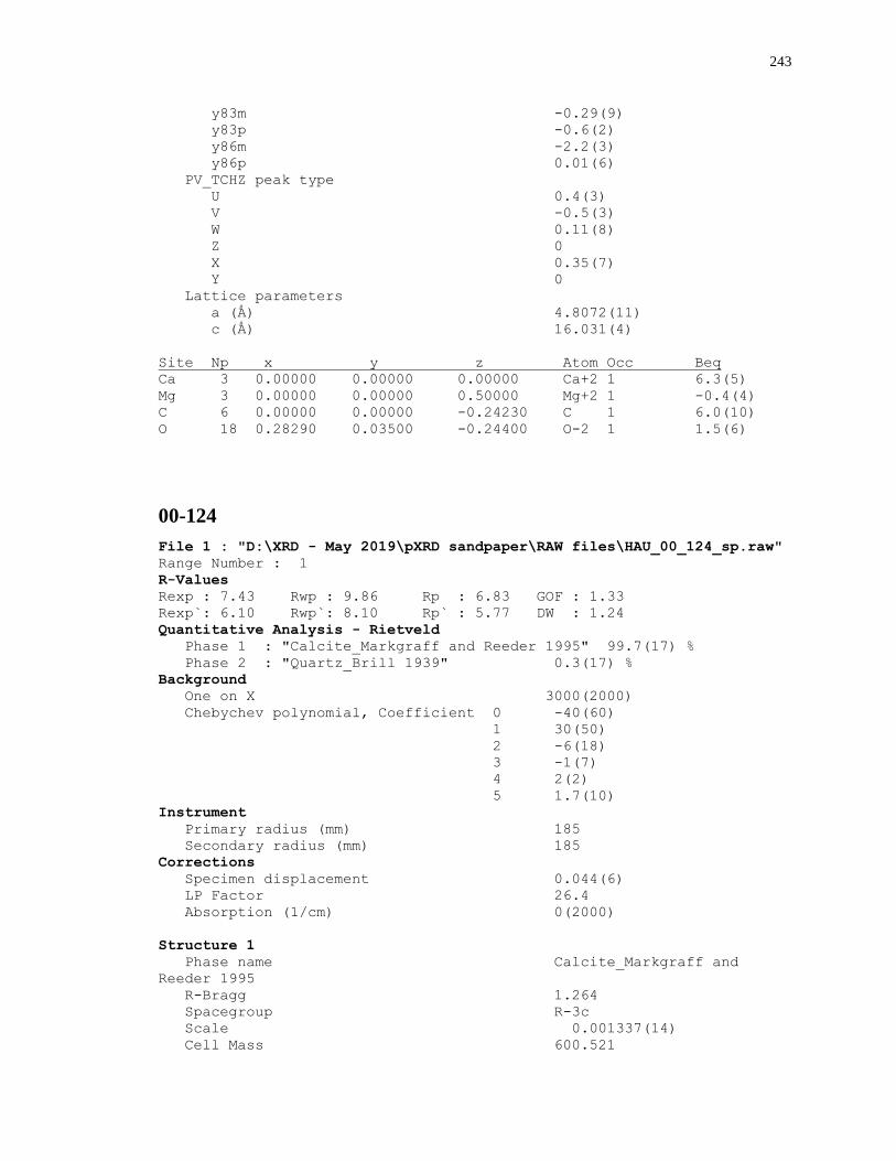
243

y83m -0.29(9)

y83p -0.6(2)

y86m -2.2(3)

y86p 0.01(6)

PV_TCHZ peak type

U 0.4(3)

V -0.5(3)

W 0.11(8)

Z 0

X 0.35(7)

Y 0

Lattice parameters

a (Å) 4.8072(11)

c (Å) 16.031(4)

Site Np x y z Atom Occ Beq

Ca 3 0.00000 0.00000 0.00000 Ca+2 1 6.3(5)

Mg 3 0.00000 0.00000 0.50000 Mg+2 1 -0.4(4)

C 6 0.00000 0.00000 -0.24230 C 1 6.0(10)

O 18 0.28290 0.03500 -0.24400 O-2 1 1.5(6)

00-124

File 1 : "D:\XRD - May 2019\pXRD sandpaper\RAW files\HAU_00_124_sp.raw"

Range Number : 1

R-Values

Rexp : 7.43 Rwp : 9.86 Rp : 6.83 GOF : 1.33

Rexp`: 6.10 Rwp`: 8.10 Rp` : 5.77 DW : 1.24

Quantitative Analysis - Rietveld

Phase 1 : "Calcite_Markgraff and Reeder 1995" 99.7(17) %

Phase 2 : "Quartz_Brill 1939" 0.3(17) %

Background

One on X 3000(2000)

Chebychev polynomial, Coefficient 0 -40(60)

1 30(50)

2 -6(18)

3 -1(7)

4 2(2)

5 1.7(10)

Instrument

Primary radius (mm) 185

Secondary radius (mm) 185

Corrections

Specimen displacement 0.044(6)

LP Factor 26.4

Absorption (1/cm) 0(2000)

Structure 1

Phase name Calcite_Markgraff and

Reeder 1995

R-Bragg 1.264

Spacegroup R-3c

Scale 0.001337(14)

Cell Mass 600.521

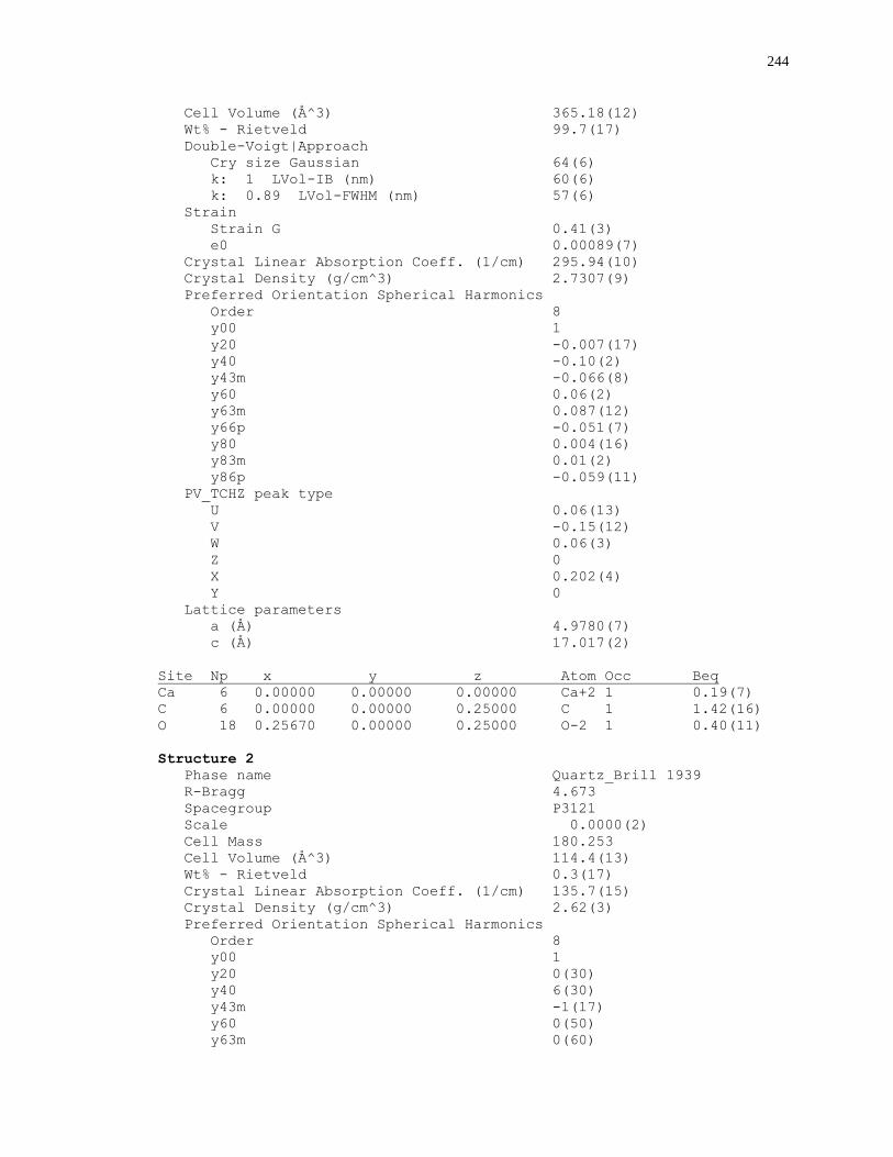
244

Cell Volume (Å^3) 365.18(12)

Wt% - Rietveld 99.7(17)

Double-Voigt|Approach

Cry size Gaussian 64(6)

k: 1 LVol-IB (nm) 60(6)

k: 0.89 LVol-FWHM (nm) 57(6)

Strain

Strain G 0.41(3)

e0 0.00089(7)

Crystal Linear Absorption Coeff. (1/cm) 295.94(10)

Crystal Density (g/cm^3) 2.7307(9)

Preferred Orientation Spherical Harmonics

Order 8

y00 1

y20 -0.007(17)

y40 -0.10(2)

y43m -0.066(8)

y60 0.06(2)

y63m 0.087(12)

y66p -0.051(7)

y80 0.004(16)

y83m 0.01(2)

y86p -0.059(11)

PV_TCHZ peak type

U 0.06(13)

V -0.15(12)

W 0.06(3)

Z 0

X 0.202(4)

Y 0

Lattice parameters

a (Å) 4.9780(7)

c (Å) 17.017(2)

Site Np x y z Atom Occ Beq

Ca 6 0.00000 0.00000 0.00000 Ca+2 1 0.19(7)

C 6 0.00000 0.00000 0.25000 C 1 1.42(16)

O 18 0.25670 0.00000 0.25000 O-2 1 0.40(11)

Structure 2

Phase name Quartz_Brill 1939

R-Bragg 4.673

Spacegroup P3121

Scale 0.0000(2)

Cell Mass 180.253

Cell Volume (Å^3) 114.4(13)

Wt% - Rietveld 0.3(17)

Crystal Linear Absorption Coeff. (1/cm) 135.7(15)

Crystal Density (g/cm^3) 2.62(3)

Preferred Orientation Spherical Harmonics

Order 8

y00 1

y20 0(30)

y40 6(30)

y43m -1(17)

y60 0(50)

y63m 0(60)

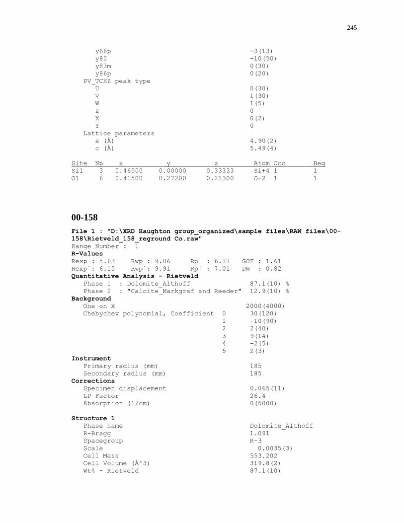
245

y66p -3(13)

y80 -10(50)

y83m 0(30)

y86p 0(20)

PV_TCHZ peak type

U 0(30)

V 1(30)

W 1(5)

Z 0

X 0(2)

Y 0

Lattice parameters

a (Å) 4.90(2)

c (Å) 5.49(4)

Site Np x y z Atom Occ Beq

Si1 3 0.46500 0.00000 0.33333 Si+4 1 1

O1 6 0.41500 0.27200 0.21300 O-2 1 1

00-158

File 1 : "D:\XRD Haughton group_organized\sample files\RAW files\00-

158\Rietveld_158_reground Co.raw"

Range Number : 1

R-Values

Rexp : 5.63 Rwp : 9.06 Rp : 6.37 GOF : 1.61

Rexp`: 6.15 Rwp`: 9.91 Rp` : 7.01 DW : 0.82

Quantitative Analysis - Rietveld

Phase 1 : Dolomite_Althoff 87.1(10) %

Phase 2 : "Calcite_Markgraf and Reeder" 12.9(10) %

Background

One on X 2000(4000)

Chebychev polynomial, Coefficient 0 30(120)

1 -10(90)

2 2(40)

3 9(14)

4 -2(5)

5 2(3)

Instrument

Primary radius (mm) 185

Secondary radius (mm) 185

Corrections

Specimen displacement 0.065(11)

LP Factor 26.4

Absorption (1/cm) 0(5000)

Structure 1

Phase name Dolomite_Althoff

R-Bragg 1.091

Spacegroup R-3

Scale 0.0035(3)

Cell Mass 553.202

Cell Volume (Å^3) 319.8(2)

Wt% - Rietveld 87.1(10)

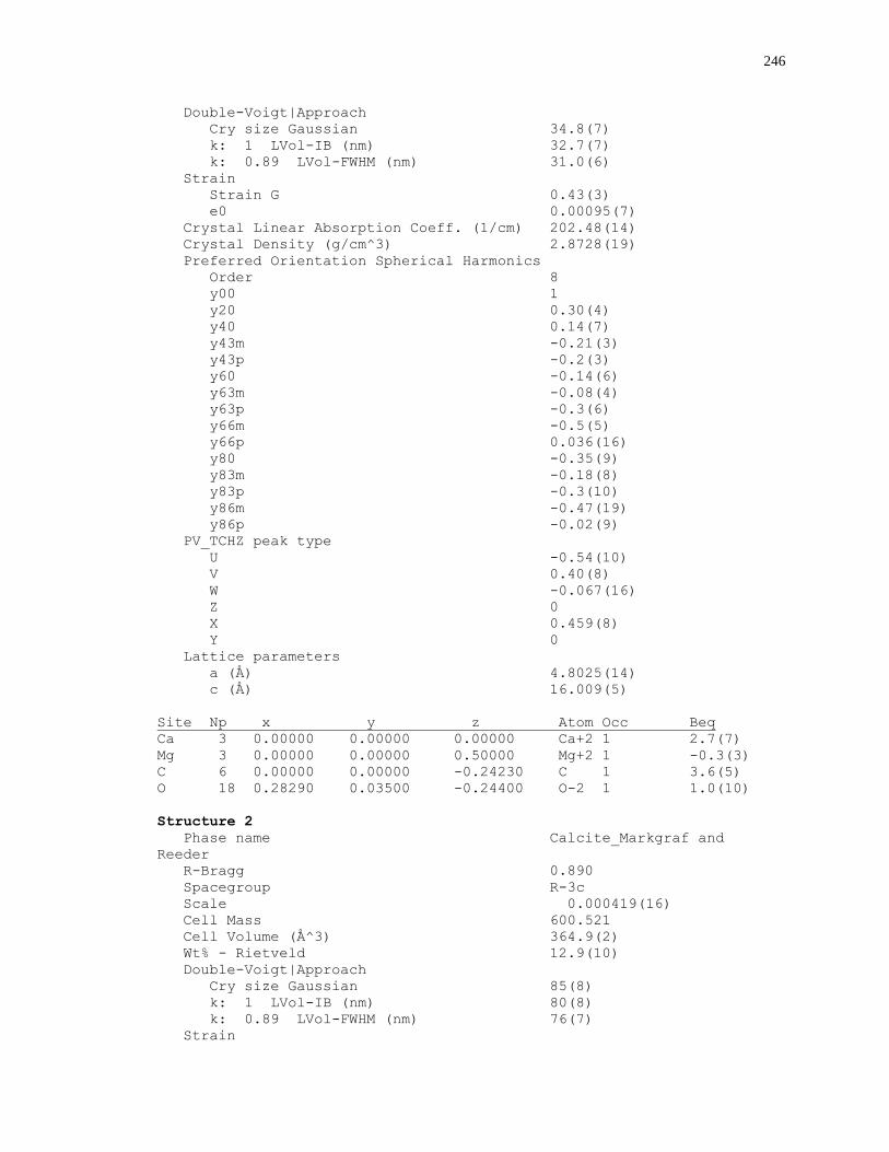
246

Double-Voigt|Approach

Cry size Gaussian 34.8(7)

k: 1 LVol-IB (nm) 32.7(7)

k: 0.89 LVol-FWHM (nm) 31.0(6)

Strain

Strain G 0.43(3)

e0 0.00095(7)

Crystal Linear Absorption Coeff. (1/cm) 202.48(14)

Crystal Density (g/cm^3) 2.8728(19)

Preferred Orientation Spherical Harmonics

Order 8

y00 1

y20 0.30(4)

y40 0.14(7)

y43m -0.21(3)

y43p -0.2(3)

y60 -0.14(6)

y63m -0.08(4)

y63p -0.3(6)

y66m -0.5(5)

y66p 0.036(16)

y80 -0.35(9)

y83m -0.18(8)

y83p -0.3(10)

y86m -0.47(19)

y86p -0.02(9)

PV_TCHZ peak type

U -0.54(10)

V 0.40(8)

W -0.067(16)

Z 0

X 0.459(8)

Y 0

Lattice parameters

a (Å) 4.8025(14)

c (Å) 16.009(5)

Site Np x y z Atom Occ Beq

Ca 3 0.00000 0.00000 0.00000 Ca+2 1 2.7(7)

Mg 3 0.00000 0.00000 0.50000 Mg+2 1 -0.3(3)

C 6 0.00000 0.00000 -0.24230 C 1 3.6(5)

O 18 0.28290 0.03500 -0.24400 O-2 1 1.0(10)

Structure 2

Phase name Calcite_Markgraf and

Reeder

R-Bragg 0.890

Spacegroup R-3c

Scale 0.000419(16)

Cell Mass 600.521

Cell Volume (Å^3) 364.9(2)

Wt% - Rietveld 12.9(10)

Double-Voigt|Approach

Cry size Gaussian 85(8)

k: 1 LVol-IB (nm) 80(8)

k: 0.89 LVol-FWHM (nm) 76(7)

Strain

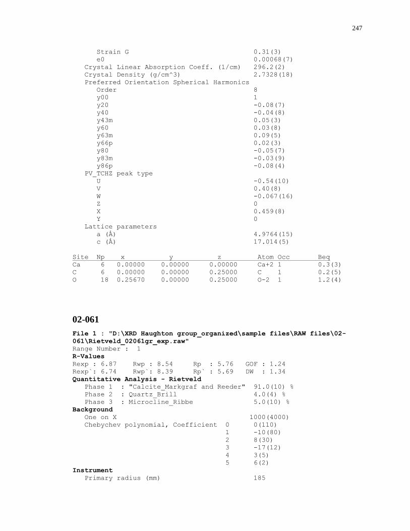
247

Strain G 0.31(3)

e0 0.00068(7)

Crystal Linear Absorption Coeff. (1/cm) 296.2(2)

Crystal Density (g/cm^3) 2.7328(18)

Preferred Orientation Spherical Harmonics

Order 8

y00 1

y20 -0.08(7)

y40 -0.04(8)

y43m 0.05(3)

y60 0.03(8)

y63m 0.09(5)

y66p 0.02(3)

y80 -0.05(7)

y83m -0.03(9)

y86p -0.08(4)

PV_TCHZ peak type

U -0.54(10)

V 0.40(8)

W -0.067(16)

Z 0

X 0.459(8)

Y 0

Lattice parameters

a (Å) 4.9764(15)

c (Å) 17.014(5)

Site Np x y z Atom Occ Beq

Ca 6 0.00000 0.00000 0.00000 Ca+2 1 0.3(3)

C 6 0.00000 0.00000 0.25000 C 1 0.2(5)

O 18 0.25670 0.00000 0.25000 O-2 1 1.2(4)

02-061

File 1 : "D:\XRD Haughton group_organized\sample files\RAW files\02-

061\Rietveld_02061gr_exp.raw"

Range Number : 1

R-Values

Rexp : 6.87 Rwp : 8.54 Rp : 5.76 GOF : 1.24

Rexp`: 6.74 Rwp`: 8.39 Rp` : 5.69 DW : 1.34

Quantitative Analysis - Rietveld

Phase 1 : "Calcite_Markgraf and Reeder" 91.0(10) %

Phase 2 : Quartz_Brill 4.0(4) %

Phase 3 : Microcline_Ribbe 5.0(10) %

Background

One on X 1000(4000)

Chebychev polynomial, Coefficient 0 0(110)

1 -10(80)

2 8(30)

3 -17(12)

4 3(5)

5 6(2)

Instrument

Primary radius (mm) 185

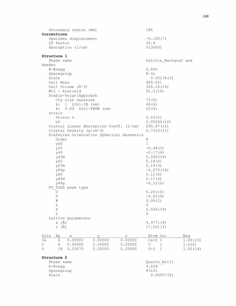
248

Secondary radius (mm) 185

Corrections

Specimen displacement -0.180(7)

LP Factor 26.4

Absorption (1/cm) 0(3000)

Structure 1

Phase name Calcite_Markgraf and

Reeder

R-Bragg 0.645

Spacegroup R-3c

Scale 0.00174(3)

Cell Mass 600.521

Cell Volume (Å^3) 365.14(14)

Wt% - Rietveld 91.0(10)

Double-Voigt|Approach

Cry size Gaussian 71(5)

k: 1 LVol-IB (nm) 66(4)

k: 0.89 LVol-FWHM (nm) 63(4)

Strain

Strain G 0.20(5)

e0 0.00044(12)

Crystal Linear Absorption Coeff. (1/cm) 295.97(12)

Crystal Density (g/cm^3) 2.7310(11)

Preferred Orientation Spherical Harmonics

Order 8

y00 1

y20 -0.48(3)

y40 -0.17(4)

y43m 0.006(16)

y60 0.18(4)

y63m 0.19(3)

y66p -0.075(14)

y80 0.11(4)

y83m 0.17(4)

y86p -0.12(2)

PV_TCHZ peak type

U 0.26(10)

V -0.25(9)

W 0.06(2)

Z 0

X 0.506(19)

Y 0

Lattice parameters

a (Å) 4.9771(9)

c (Å) 17.021(3)

Site Np x y z Atom Occ Beq

Ca 6 0.00000 0.00000 0.00000 Ca+2 1 1.00(13)

C 6 0.00000 0.00000 0.25000 C 1 1.0(2)

O 18 0.25670 0.00000 0.25000 O-2 1 1.00(14)

Structure 2

Phase name Quartz_Brill

R-Bragg 4.029

Spacegroup P3121

Scale 0.00057(5)

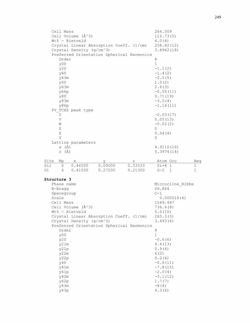
249

Cell Mass 264.509

Cell Volume (Å^3) 112.73(5)

Wt% - Rietveld 4.0(4)

Crystal Linear Absorption Coeff. (1/cm) 258.82(12)

Crystal Density (g/cm^3) 3.8962(18)

Preferred Orientation Spherical Harmonics

Order 8

y00 1

y20 -1.1(2)

y40 -1.4(2)

y43m -2.5(5)

y60 1.0(2)

y63m 2.6(3)

y66p -0.55(11)

y80 0.71(19)

y83m -3.5(4)

y86p -1.14(11)

PV_TCHZ peak type

U -0.03(17)

V 0.05(13)

W -0.02(2)

Z 0

X 0.54(4)

Y 0

Lattice parameters

a (Å) 4.9110(10)

c (Å) 5.3974(14)

Site Np x y z Atom Occ Beq

Si1 6 0.46500 0.00000 0.33333 Si+4 1 1

O1 6 0.41500 0.27200 0.21300 O-2 1 1

Structure 3

Phase name Microcline_Ribbe

R-Bragg 26.844

Spacegroup C-1

Scale 0.000018(4)

Cell Mass 1549.447

Cell Volume (Å^3) 736.6(8)

Wt% - Rietveld 5.0(10)

Crystal Linear Absorption Coeff. (1/cm) 263.3(3)

Crystal Density (g/cm^3) 3.493(4)

Preferred Orientation Spherical Harmonics

Order 8

y00 1

y20 -0.6(6)

y21m 4.4(13)

y21p 0.9(4)

y22m 6(2)

y22p 0.2(4)

y40 -0.6(11)

y41m -7.8(15)

y41p -2.0(4)

y42m -3.1(12)

y42p 1.7(7)

y43m -8(4)

y43p 4.3(6)

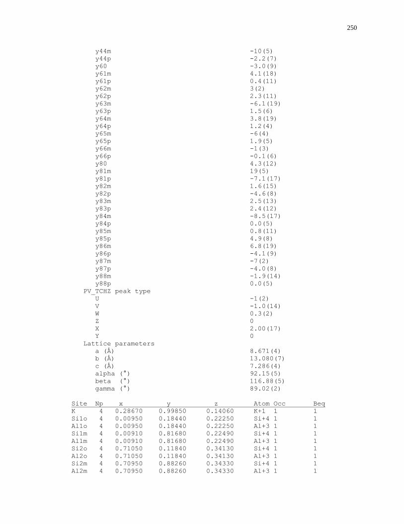
250

y44m -10(5)

y44p -2.2(7)

y60 -3.0(9)

y61m 4.1(18)

y61p 0.4(11)

y62m 3(2)

y62p 2.3(11)

y63m -6.1(19)

y63p 1.5(6)

y64m 3.8(19)

y64p 1.2(4)

y65m -6(4)

y65p 1.9(5)

y66m -1(3)

y66p -0.1(6)

y80 4.3(12)

y81m 19(5)

y81p -7.1(17)

y82m 1.6(15)

y82p -4.6(8)

y83m 2.5(13)

y83p 2.4(12)

y84m -8.5(17)

y84p 0.0(5)

y85m 0.8(11)

y85p 4.9(8)

y86m 6.8(19)

y86p -4.1(9)

y87m -7(2)

y87p -4.0(8)

y88m -1.9(14)

y88p 0.0(5)

PV_TCHZ peak type

U -1(2)

V -1.0(14)

W 0.3(2)

Z 0

X 2.00(17)

Y 0

Lattice parameters

a (Å) 8.671(4)

b (Å) 13.080(7)

c (Å) 7.286(4)

alpha (°) 92.15(5)

beta (°) 116.88(5)

gamma (°) 89.02(2)

Site Np x y z Atom Occ Beq

K 4 0.28670 0.99850 0.14060 K+1 1 1

Si1o 4 0.00950 0.18440 0.22250 Si+4 1 1

Al1o 4 0.00950 0.18440 0.22250 Al+3 1 1

Si1m 4 0.00910 0.81680 0.22490 Si+4 1 1

Al1m 4 0.00910 0.81680 0.22490 Al+3 1 1

Si2o 4 0.71050 0.11840 0.34130 Si+4 1 1

Al2o 4 0.71050 0.11840 0.34130 Al+3 1 1

Si2m 4 0.70950 0.88260 0.34330 Si+4 1 1

Al2m 4 0.70950 0.88260 0.34330 Al+3 1 1

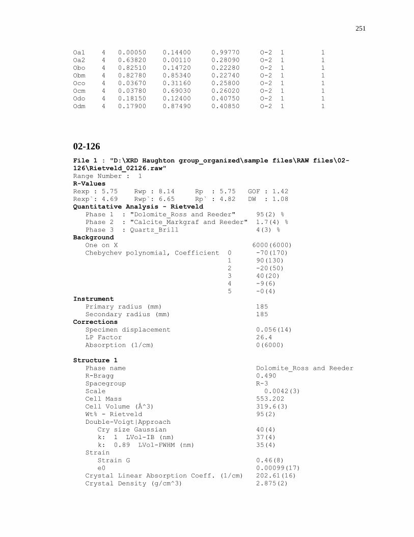
251

Oa1 4 0.00050 0.14400 0.99770 O-2 1 1

Oa2 4 0.63820 0.00110 0.28090 O-2 1 1

Obo 4 0.82510 0.14720 0.22280 O-2 1 1

Obm 4 0.82780 0.85340 0.22740 O-2 1 1

Oco 4 0.03670 0.31160 0.25800 O-2 1 1

Ocm 4 0.03780 0.69030 0.26020 O-2 1 1

Odo 4 0.18150 0.12400 0.40750 O-2 1 1

Odm 4 0.17900 0.87490 0.40850 O-2 1 1

02-126

File 1 : "D:\XRD Haughton group_organized\sample files\RAW files\02-

126\Rietveld_02126.raw"

Range Number : 1

R-Values

Rexp : 5.75 Rwp : 8.14 Rp : 5.75 GOF : 1.42

Rexp`: 4.69 Rwp`: 6.65 Rp` : 4.82 DW : 1.08

Quantitative Analysis - Rietveld

Phase 1 : "Dolomite_Ross and Reeder" 95(2) %

Phase 2 : "Calcite_Markgraf and Reeder" 1.7(4) %

Phase 3 : Quartz_Brill 4(3) %

Background

One on X 6000(6000)

Chebychev polynomial, Coefficient 0 -70(170)

1 90(130)

2 -20(50)

3 40(20)

4 -9(6)

5 -0(4)

Instrument

Primary radius (mm) 185

Secondary radius (mm) 185

Corrections

Specimen displacement 0.056(14)

LP Factor 26.4

Absorption (1/cm) 0(6000)

Structure 1

Phase name Dolomite_Ross and Reeder

R-Bragg 0.490

Spacegroup R-3

Scale 0.0042(3)

Cell Mass 553.202

Cell Volume (Å^3) 319.6(3)

Wt% - Rietveld 95(2)

Double-Voigt|Approach

Cry size Gaussian 40(4)

k: 1 LVol-IB (nm) 37(4)

k: 0.89 LVol-FWHM (nm) 35(4)

Strain

Strain G 0.46(8)

e0 0.00099(17)

Crystal Linear Absorption Coeff. (1/cm) 202.61(16)

Crystal Density (g/cm^3) 2.875(2)

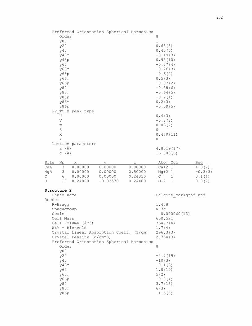
252

Preferred Orientation Spherical Harmonics

Order 8

y00 1

y20 0.63(3)

y40 0.40(5)

y43m -0.49(3)

y43p 0.95(10)

y60 -0.37(4)

y63m -0.26(3)

y63p -0.6(2)

y66m 0.5(3)

y66p -0.07(2)

y80 -0.88(6)

y83m -0.64(5)

y83p -0.2(4)

y86m 0.2(3)

y86p -0.09(5)

PV_TCHZ peak type

U 0.4(3)

V -0.3(3)

W 0.03(7)

Z 0

X 0.479(11)

Y 0

Lattice parameters

a (Å) 4.8019(17)

c (Å) 16.003(6)

Site Np x y z Atom Occ Beq

CaA 3 0.00000 0.00000 0.00000 Ca+2 1 4.8(7)

MgB 3 0.00000 0.00000 0.50000 Mg+2 1 -0.3(3)

C 6 0.00000 0.00000 0.24310 C 1 0.1(4)

O 18 0.24820 -0.03570 0.24400 O-2 1 0.8(7)

Structure 2

Phase name Calcite_Markgraf and

Reeder

R-Bragg 1.438

Spacegroup R-3c

Scale 0.000060(13)

Cell Mass 600.521

Cell Volume (Å^3) 364.7(4)

Wt% - Rietveld 1.7(4)

Crystal Linear Absorption Coeff. (1/cm) 296.3(3)

Crystal Density (g/cm^3) 2.734(3)

Preferred Orientation Spherical Harmonics

Order 8

y00 1

y20 -4.7(19)

y40 -10(3)

y43m -0.1(3)

y60 1.8(19)

y63m 5(2)

y66p -0.8(4)

y80 3.7(18)

y83m 6(3)

y86p -1.3(8)

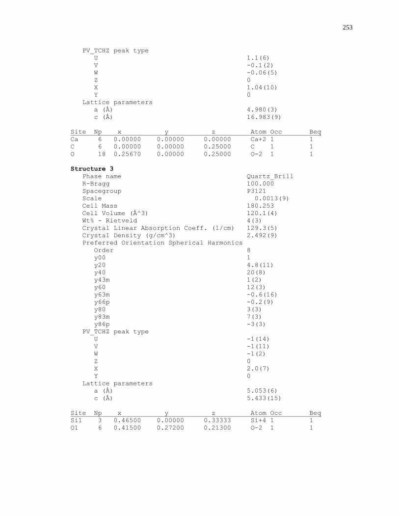
253

PV_TCHZ peak type

U 1.1(6)

V -0.1(2)

W -0.06(5)

Z 0

X 1.04(10)

Y 0

Lattice parameters

a (Å) 4.980(3)

c (Å) 16.983(9)

Site Np x y z Atom Occ Beq

Ca 6 0.00000 0.00000 0.00000 Ca+2 1 1

C 6 0.00000 0.00000 0.25000 C 1 1

O 18 0.25670 0.00000 0.25000 O-2 1 1

Structure 3

Phase name Quartz_Brill

R-Bragg 100.000

Spacegroup P3121

Scale 0.0013(9)

Cell Mass 180.253

Cell Volume (Å^3) 120.1(4)

Wt% - Rietveld 4(3)

Crystal Linear Absorption Coeff. (1/cm) 129.3(5)

Crystal Density (g/cm^3) 2.492(9)

Preferred Orientation Spherical Harmonics

Order 8

y00 1

y20 4.8(11)

y40 20(8)

y43m 1(2)

y60 12(3)

y63m -0.6(16)

y66p -0.2(9)

y80 3(3)

y83m 7(3)

y86p -3(3)

PV_TCHZ peak type

U -1(14)

V -1(11)

W -1(2)

Z 0

X 2.0(7)

Y 0

Lattice parameters

a (Å) 5.053(6)

c (Å) 5.433(15)

Site Np x y z Atom Occ Beq

Si1 3 0.46500 0.00000 0.33333 Si+4 1 1

O1 6 0.41500 0.27200 0.21300 O-2 1 1

254

02-127

File 1 : "D:\XRD Haughton group_organized\sample files\RAW files\02-

127\Rietveld_02127.raw"

Range Number : 1

R-Values

Rexp : 5.77 Rwp : 8.80 Rp : 6.10 GOF : 1.53

Rexp`: 5.99 Rwp`: 9.14 Rp` : 6.35 DW : 0.88

Quantitative Analysis - Rietveld

Phase 1 : "Dolomite_Ross and Reeder" 81.7(7) %

Phase 2 : "Calcite_Markgraf and Reeder" 18.3(7) %

Background

One on X 2000(4000)

Chebychev polynomial, Coefficient 0 20(100)

1 -10(80)

2 10(30)

3 -3(11)

4 0(4)

5 0(2)

Instrument

Primary radius (mm) 185

Secondary radius (mm) 185

Corrections

Specimen displacement 0.066(8)

LP Factor 26.4

Absorption (1/cm) 0(3000)

Structure 1

Phase name Dolomite_Ross and Reeder

R-Bragg 1.042

Spacegroup R-3

Scale 0.00319(13)

Cell Mass 553.202

Cell Volume (Å^3) 320.29(14)

Wt% - Rietveld 81.7(7)

Double-Voigt|Approach

Cry size Gaussian 52(3)

k: 1 LVol-IB (nm) 48(3)

k: 0.89 LVol-FWHM (nm) 46(2)

Strain

Strain G 0.42(3)

e0 0.00092(6)

Crystal Linear Absorption Coeff. (1/cm) 202.15(9)

Crystal Density (g/cm^3) 2.8681(12)

Preferred Orientation Spherical Harmonics

Order 8

y00 1

y20 0.53(2)

y40 0.22(3)

y43m -0.176(19)

y43p 0.39(15)

y60 -0.22(4)

y63m -0.088(15)

y63p 0.1(3)

y66m 0.6(2)

y66p 0.028(14)

y80 -0.36(4)

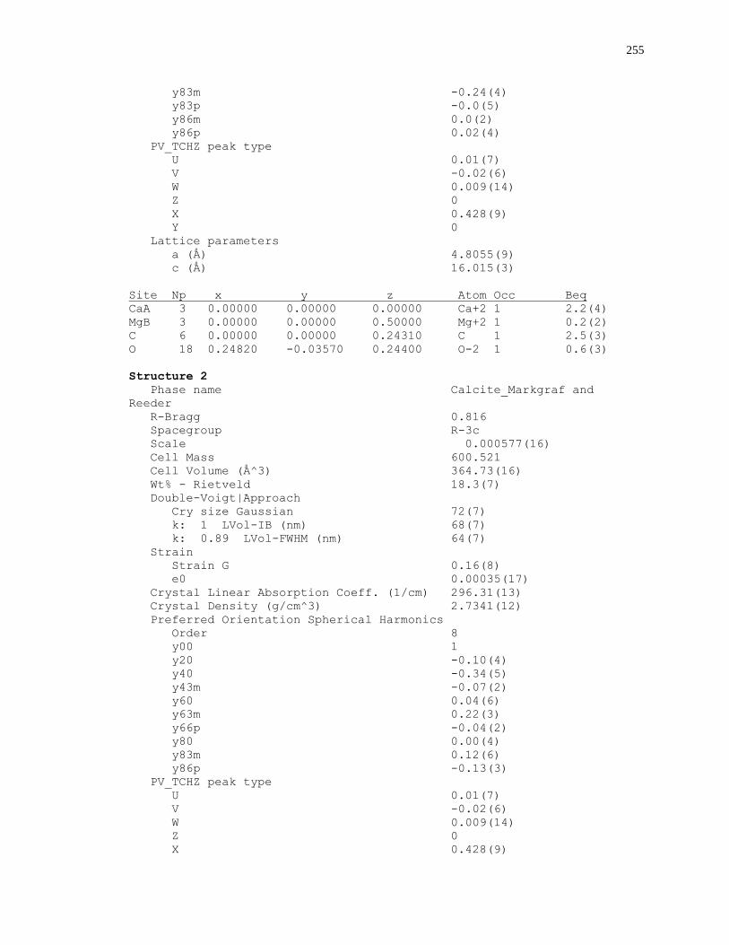
255

y83m -0.24(4)

y83p -0.0(5)

y86m 0.0(2)

y86p 0.02(4)

PV_TCHZ peak type

U 0.01(7)

V -0.02(6)

W 0.009(14)

Z 0

X 0.428(9)

Y 0

Lattice parameters

a (Å) 4.8055(9)

c (Å) 16.015(3)

Site Np x y z Atom Occ Beq

CaA 3 0.00000 0.00000 0.00000 Ca+2 1 2.2(4)

MgB 3 0.00000 0.00000 0.50000 Mg+2 1 0.2(2)

C 6 0.00000 0.00000 0.24310 C 1 2.5(3)

O 18 0.24820 -0.03570 0.24400 O-2 1 0.6(3)

Structure 2

Phase name Calcite_Markgraf and

Reeder

R-Bragg 0.816

Spacegroup R-3c

Scale 0.000577(16)

Cell Mass 600.521

Cell Volume (Å^3) 364.73(16)

Wt% - Rietveld 18.3(7)

Double-Voigt|Approach

Cry size Gaussian 72(7)

k: 1 LVol-IB (nm) 68(7)

k: 0.89 LVol-FWHM (nm) 64(7)

Strain

Strain G 0.16(8)

e0 0.00035(17)

Crystal Linear Absorption Coeff. (1/cm) 296.31(13)

Crystal Density (g/cm^3) 2.7341(12)

Preferred Orientation Spherical Harmonics

Order 8

y00 1

y20 -0.10(4)

y40 -0.34(5)

y43m -0.07(2)

y60 0.04(6)

y63m 0.22(3)

y66p -0.04(2)

y80 0.00(4)

y83m 0.12(6)

y86p -0.13(3)

PV_TCHZ peak type

U 0.01(7)

V -0.02(6)

W 0.009(14)

Z 0

X 0.428(9)

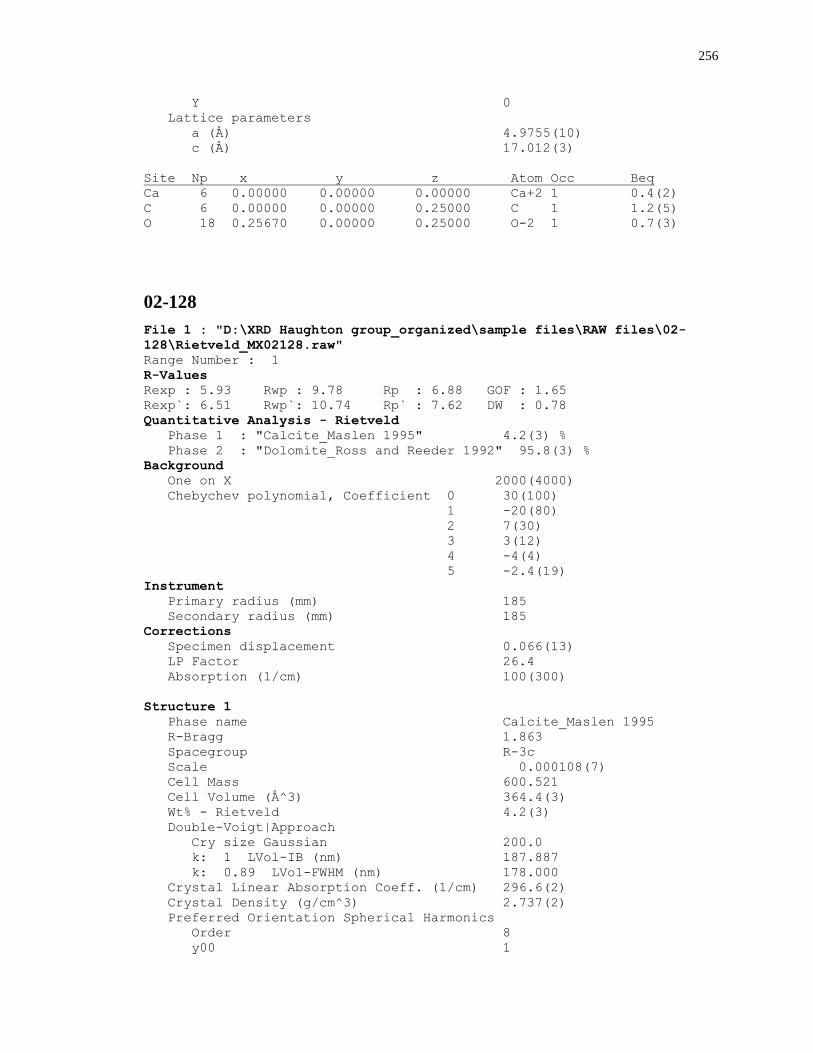
256

Y 0

Lattice parameters

a (Å) 4.9755(10)

c (Å) 17.012(3)

Site Np x y z Atom Occ Beq

Ca 6 0.00000 0.00000 0.00000 Ca+2 1 0.4(2)

C 6 0.00000 0.00000 0.25000 C 1 1.2(5)

O 18 0.25670 0.00000 0.25000 O-2 1 0.7(3)

02-128

File 1 : "D:\XRD Haughton group_organized\sample files\RAW files\02-

128\Rietveld_MX02128.raw"

Range Number : 1

R-Values

Rexp : 5.93 Rwp : 9.78 Rp : 6.88 GOF : 1.65

Rexp`: 6.51 Rwp`: 10.74 Rp` : 7.62 DW : 0.78

Quantitative Analysis - Rietveld

Phase 1 : "Calcite_Maslen 1995" 4.2(3) %

Phase 2 : "Dolomite_Ross and Reeder 1992" 95.8(3) %

Background

One on X 2000(4000)

Chebychev polynomial, Coefficient 0 30(100)

1 -20(80)

2 7(30)

3 3(12)

4 -4(4)

5 -2.4(19)

Instrument

Primary radius (mm) 185

Secondary radius (mm) 185

Corrections

Specimen displacement 0.066(13)

LP Factor 26.4

Absorption (1/cm) 100(300)

Structure 1

Phase name Calcite_Maslen 1995

R-Bragg 1.863

Spacegroup R-3c

Scale 0.000108(7)

Cell Mass 600.521

Cell Volume (Å^3) 364.4(3)

Wt% - Rietveld 4.2(3)

Double-Voigt|Approach

Cry size Gaussian 200.0

k: 1 LVol-IB (nm) 187.887

k: 0.89 LVol-FWHM (nm) 178.000

Crystal Linear Absorption Coeff. (1/cm) 296.6(2)

Crystal Density (g/cm^3) 2.737(2)

Preferred Orientation Spherical Harmonics

Order 8

y00 1

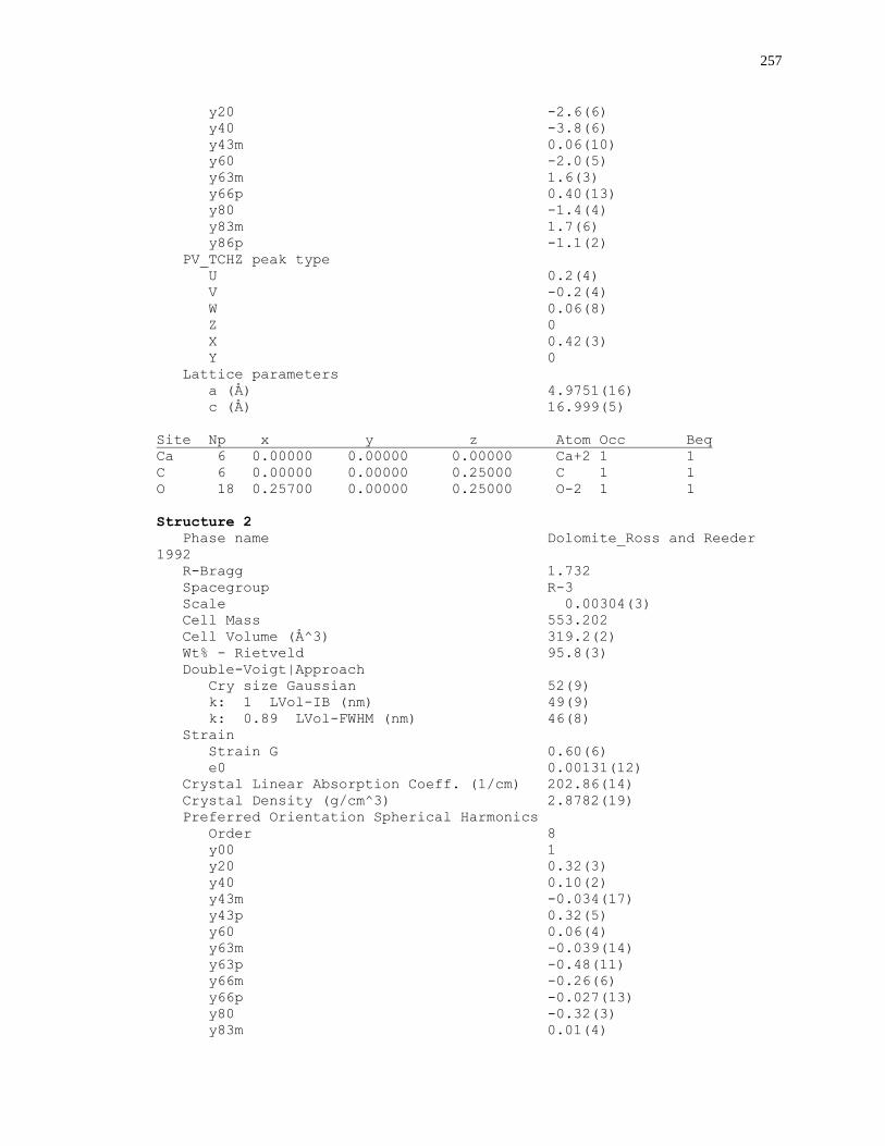
257

y20 -2.6(6)

y40 -3.8(6)

y43m 0.06(10)

y60 -2.0(5)

y63m 1.6(3)

y66p 0.40(13)

y80 -1.4(4)

y83m 1.7(6)

y86p -1.1(2)

PV_TCHZ peak type

U 0.2(4)

V -0.2(4)

W 0.06(8)

Z 0

X 0.42(3)

Y 0

Lattice parameters

a (Å) 4.9751(16)

c (Å) 16.999(5)

Site Np x y z Atom Occ Beq

Ca 6 0.00000 0.00000 0.00000 Ca+2 1 1

C 6 0.00000 0.00000 0.25000 C 1 1

O 18 0.25700 0.00000 0.25000 O-2 1 1

Structure 2

Phase name Dolomite_Ross and Reeder

1992

R-Bragg 1.732

Spacegroup R-3

Scale 0.00304(3)

Cell Mass 553.202

Cell Volume (Å^3) 319.2(2)

Wt% - Rietveld 95.8(3)

Double-Voigt|Approach

Cry size Gaussian 52(9)

k: 1 LVol-IB (nm) 49(9)

k: 0.89 LVol-FWHM (nm) 46(8)

Strain

Strain G 0.60(6)

e0 0.00131(12)

Crystal Linear Absorption Coeff. (1/cm) 202.86(14)

Crystal Density (g/cm^3) 2.8782(19)

Preferred Orientation Spherical Harmonics

Order 8

y00 1

y20 0.32(3)

y40 0.10(2)

y43m -0.034(17)

y43p 0.32(5)

y60 0.06(4)

y63m -0.039(14)

y63p -0.48(11)

y66m -0.26(6)

y66p -0.027(13)

y80 -0.32(3)

y83m 0.01(4)

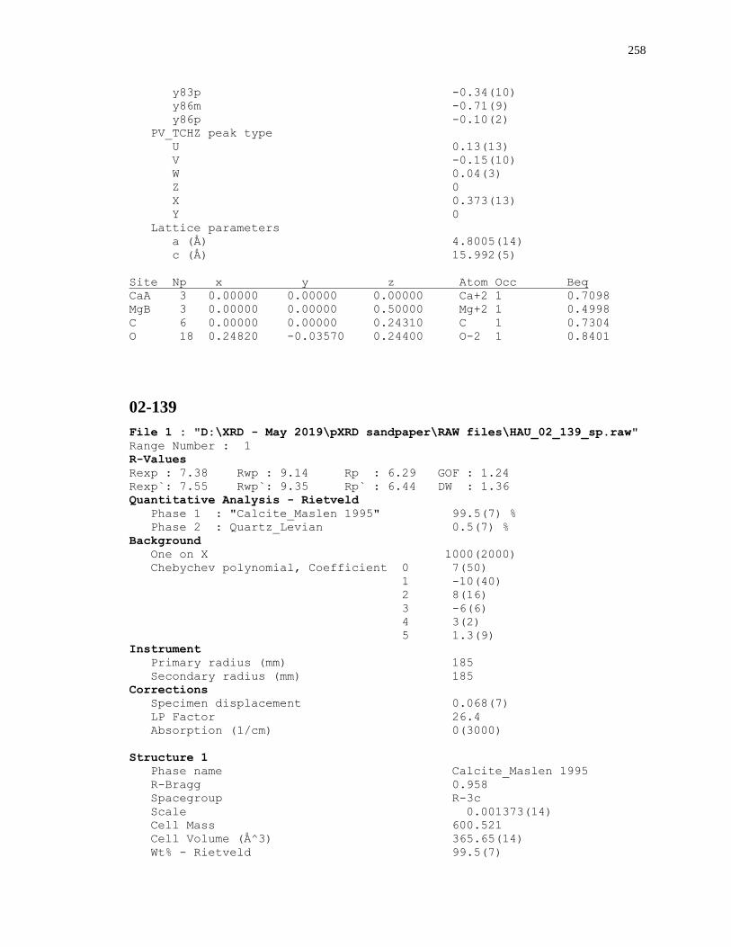
258

y83p -0.34(10)

y86m -0.71(9)

y86p -0.10(2)

PV_TCHZ peak type

U 0.13(13)

V -0.15(10)

W 0.04(3)

Z 0

X 0.373(13)

Y 0

Lattice parameters

a (Å) 4.8005(14)

c (Å) 15.992(5)

Site Np x y z Atom Occ Beq

CaA 3 0.00000 0.00000 0.00000 Ca+2 1 0.7098

MgB 3 0.00000 0.00000 0.50000 Mg+2 1 0.4998

C 6 0.00000 0.00000 0.24310 C 1 0.7304

O 18 0.24820 -0.03570 0.24400 O-2 1 0.8401

02-139

File 1 : "D:\XRD - May 2019\pXRD sandpaper\RAW files\HAU_02_139_sp.raw"

Range Number : 1

R-Values

Rexp : 7.38 Rwp : 9.14 Rp : 6.29 GOF : 1.24

Rexp`: 7.55 Rwp`: 9.35 Rp` : 6.44 DW : 1.36

Quantitative Analysis - Rietveld

Phase 1 : "Calcite_Maslen 1995" 99.5(7) %

Phase 2 : Quartz_Levian 0.5(7) %

Background

One on X 1000(2000)

Chebychev polynomial, Coefficient 0 7(50)

1 -10(40)

2 8(16)

3 -6(6)

4 3(2)

5 1.3(9)

Instrument

Primary radius (mm) 185

Secondary radius (mm) 185

Corrections

Specimen displacement 0.068(7)

LP Factor 26.4

Absorption (1/cm) 0(3000)

Structure 1

Phase name Calcite_Maslen 1995

R-Bragg 0.958

Spacegroup R-3c

Scale 0.001373(14)

Cell Mass 600.521

Cell Volume (Å^3) 365.65(14)

Wt% - Rietveld 99.5(7)

259

Double-Voigt|Approach

Cry size Gaussian 55(6)

k: 1 LVol-IB (nm) 52(5)

k: 0.89 LVol-FWHM (nm) 49(5)

Strain

Strain G 0.34(6)

e0 0.00074(14)

Crystal Linear Absorption Coeff. (1/cm) 295.56(11)

Crystal Density (g/cm^3) 2.7272(10)

Preferred Orientation Spherical Harmonics

Order 8

y00 1

y20 -0.107(17)

y40 -0.124(18)

y43m -0.069(8)

y60 0.074(19)

y63m 0.125(12)

y66p -0.056(7)

y80 0.038(15)

y83m 0.03(2)

y86p -0.072(10)

PV_TCHZ peak type

U 0.20(17)

V -0.27(15)

W 0.08(3)

Z 0

X 0.312(5)

Y 0

Lattice parameters

a (Å) 4.9797(8)

c (Å) 17.026(3)

Site Np x y z Atom Occ Beq

Ca 6 0.00000 0.00000 0.00000 Ca+2 1 0.14(7)

C 6 0.00000 0.00000 0.25000 C 1 1.61(17)

O 18 0.25700 0.00000 0.25000 O-2 1 0.49(11)

Structure 2

Phase name Quartz_Levian

R-Bragg 1.951

Spacegroup P3221

Scale 0.00005(7)

Cell Mass 264.509

Cell Volume (Å^3) 112.67(18)

Wt% - Rietveld 0.5(7)

Crystal Linear Absorption Coeff. (1/cm) 259.0(4)

Crystal Density (g/cm^3) 3.898(6)

Preferred Orientation Spherical Harmonics

Order 8

y00 1

y20 0.5(19)

y40 -0(3)

y43m -2(8)

y60 -1(3)

y63m -2(4)

y66p 0(2)

y80 0(2)

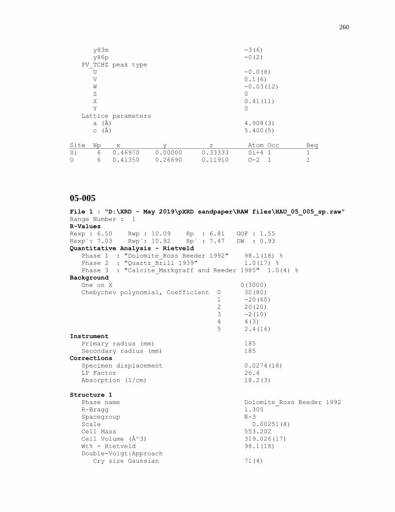
260

y83m -3(6)

y86p -0(2)

PV_TCHZ peak type

U -0.0(8)

V 0.1(6)

W -0.03(12)

Z 0

X 0.41(11)

Y 0

Lattice parameters

a (Å) 4.908(3)

c (Å) 5.400(5)

Site Np x y z Atom Occ Beq

Si 6 0.46970 0.00000 0.33333 Si+4 1 1

O 6 0.41350 0.26690 0.11910 O-2 1 1

05-005

File 1 : "D:\XRD - May 2019\pXRD sandpaper\RAW files\HAU_05_005_sp.raw"

Range Number : 1

R-Values

Rexp : 6.50 Rwp : 10.09 Rp : 6.81 GOF : 1.55

Rexp`: 7.03 Rwp`: 10.92 Rp` : 7.47 DW : 0.93

Quantitative Analysis - Rietveld

Phase 1 : "Dolomite_Ross Reeder 1992" 98.1(18) %

Phase 2 : "Quartz_Brill 1939" 1.0(17) %

Phase 3 : "Calcite_Markgraff and Reeder 1985" 1.0(4) %

Background

One on X 0(3000)

Chebychev polynomial, Coefficient 0 30(80)

1 -20(60)

2 20(20)

3 -2(10)

4 4(3)

5 2.4(16)

Instrument

Primary radius (mm) 185

Secondary radius (mm) 185

Corrections

Specimen displacement 0.0274(18)

LP Factor 26.4

Absorption (1/cm) 18.2(3)

Structure 1

Phase name Dolomite_Ross Reeder 1992

R-Bragg 1.305

Spacegroup R-3

Scale 0.00251(8)

Cell Mass 553.202

Cell Volume (Å^3) 319.026(17)

Wt% - Rietveld 98.1(18)

Double-Voigt|Approach

Cry size Gaussian 71(4)

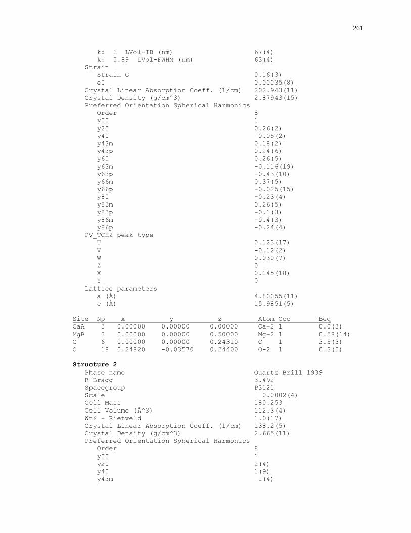
261

k: 1 LVol-IB (nm) 67(4)

k: 0.89 LVol-FWHM (nm) 63(4)

Strain

Strain G 0.16(3)

e0 0.00035(8)

Crystal Linear Absorption Coeff. (1/cm) 202.943(11)

Crystal Density (g/cm^3) 2.87943(15)

Preferred Orientation Spherical Harmonics

Order 8

y00 1

y20 0.26(2)

y40 -0.05(2)

y43m 0.18(2)

y43p 0.24(6)

y60 0.26(5)

y63m -0.116(19)

y63p -0.43(10)

y66m 0.37(5)

y66p -0.025(15)

y80 -0.23(4)

y83m 0.26(5)

y83p -0.1(3)

y86m -0.4(3)

y86p -0.24(4)

PV_TCHZ peak type

U 0.123(17)

V -0.12(2)

W 0.030(7)

Z 0

X 0.145(18)

Y 0

Lattice parameters

a (Å) 4.80055(11)

c (Å) 15.9851(5)

Site Np x y z Atom Occ Beq

CaA 3 0.00000 0.00000 0.00000 Ca+2 1 0.0(3)

MgB 3 0.00000 0.00000 0.50000 Mg+2 1 0.58(14)

C 6 0.00000 0.00000 0.24310 C 1 3.5(3)

O 18 0.24820 -0.03570 0.24400 O-2 1 0.3(5)

Structure 2

Phase name Quartz_Brill 1939

R-Bragg 3.492

Spacegroup P3121

Scale 0.0002(4)

Cell Mass 180.253

Cell Volume (Å^3) 112.3(4)

Wt% - Rietveld 1.0(17)

Crystal Linear Absorption Coeff. (1/cm) 138.2(5)

Crystal Density (g/cm^3) 2.665(11)

Preferred Orientation Spherical Harmonics

Order 8

y00 1

y20 2(4)

y40 1(9)

y43m -1(4)

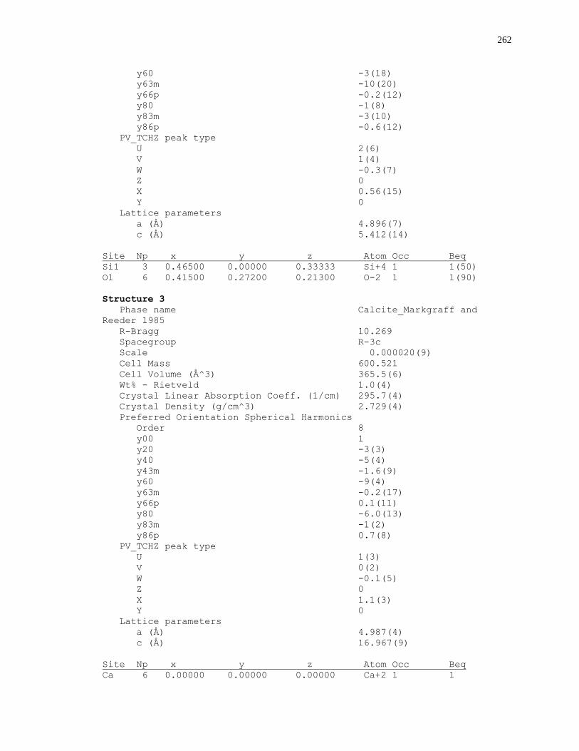
262

y60 -3(18)

y63m -10(20)

y66p -0.2(12)

y80 -1(8)

y83m -3(10)

y86p -0.6(12)

PV_TCHZ peak type

U 2(6)

V 1(4)

W -0.3(7)

Z 0

X 0.56(15)

Y 0

Lattice parameters

a (Å) 4.896(7)

c (Å) 5.412(14)

Site Np x y z Atom Occ Beq

Si1 3 0.46500 0.00000 0.33333 Si+4 1 1(50)

O1 6 0.41500 0.27200 0.21300 O-2 1 1(90)

Structure 3

Phase name Calcite_Markgraff and

Reeder 1985

R-Bragg 10.269

Spacegroup R-3c

Scale 0.000020(9)

Cell Mass 600.521

Cell Volume (Å^3) 365.5(6)

Wt% - Rietveld 1.0(4)

Crystal Linear Absorption Coeff. (1/cm) 295.7(4)

Crystal Density (g/cm^3) 2.729(4)

Preferred Orientation Spherical Harmonics

Order 8

y00 1

y20 -3(3)

y40 -5(4)

y43m -1.6(9)

y60 -9(4)

y63m -0.2(17)

y66p 0.1(11)

y80 -6.0(13)

y83m -1(2)

y86p 0.7(8)

PV_TCHZ peak type

U 1(3)

V 0(2)

W -0.1(5)

Z 0

X 1.1(3)

Y 0

Lattice parameters

a (Å) 4.987(4)

c (Å) 16.967(9)

Site Np x y z Atom Occ Beq

Ca 6 0.00000 0.00000 0.00000 Ca+2 1 1

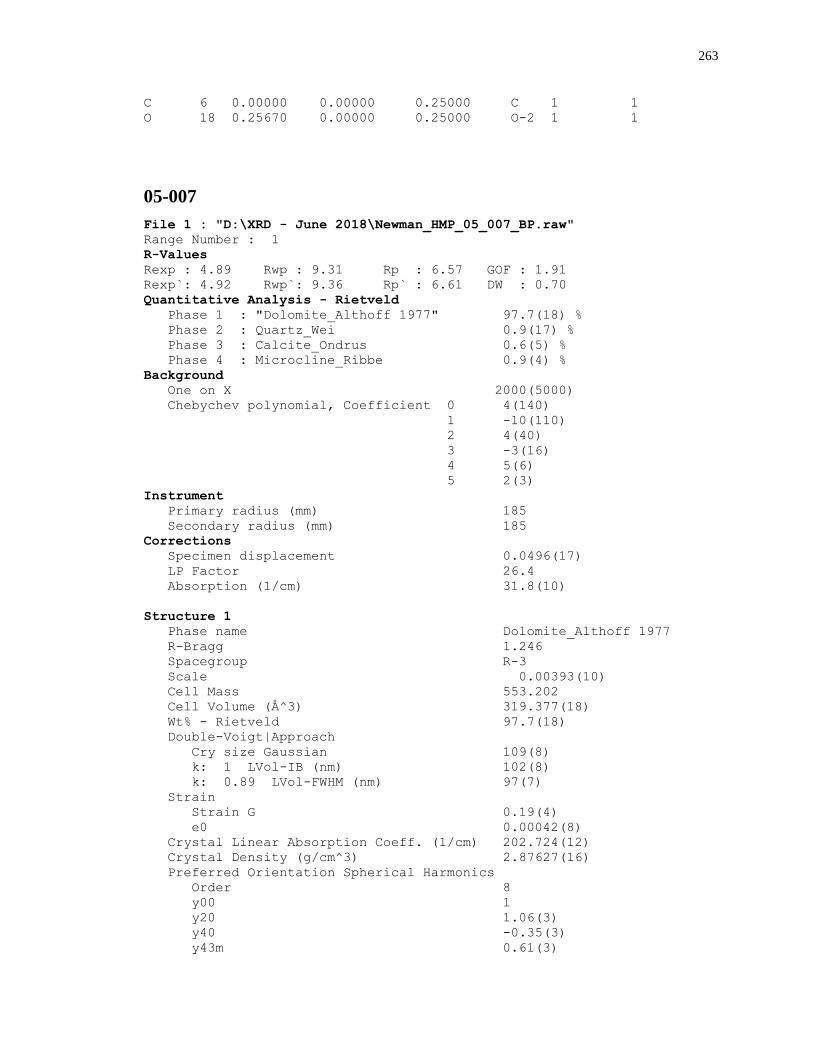
263

C 6 0.00000 0.00000 0.25000 C 1 1

O 18 0.25670 0.00000 0.25000 O-2 1 1

05-007

File 1 : "D:\XRD - June 2018\Newman_HMP_05_007_BP.raw"

Range Number : 1

R-Values

Rexp : 4.89 Rwp : 9.31 Rp : 6.57 GOF : 1.91

Rexp`: 4.92 Rwp`: 9.36 Rp` : 6.61 DW : 0.70

Quantitative Analysis - Rietveld

Phase 1 : "Dolomite_Althoff 1977" 97.7(18) %

Phase 2 : Quartz_Wei 0.9(17) %

Phase 3 : Calcite_Ondrus 0.6(5) %

Phase 4 : Microcline_Ribbe 0.9(4) %

Background

One on X 2000(5000)

Chebychev polynomial, Coefficient 0 4(140)

1 -10(110)

2 4(40)

3 -3(16)

4 5(6)

5 2(3)

Instrument

Primary radius (mm) 185

Secondary radius (mm) 185

Corrections

Specimen displacement 0.0496(17)

LP Factor 26.4

Absorption (1/cm) 31.8(10)

Structure 1

Phase name Dolomite_Althoff 1977

R-Bragg 1.246

Spacegroup R-3

Scale 0.00393(10)

Cell Mass 553.202

Cell Volume (Å^3) 319.377(18)

Wt% - Rietveld 97.7(18)

Double-Voigt|Approach

Cry size Gaussian 109(8)

k: 1 LVol-IB (nm) 102(8)

k: 0.89 LVol-FWHM (nm) 97(7)

Strain

Strain G 0.19(4)

e0 0.00042(8)

Crystal Linear Absorption Coeff. (1/cm) 202.724(12)

Crystal Density (g/cm^3) 2.87627(16)

Preferred Orientation Spherical Harmonics

Order 8

y00 1

y20 1.06(3)

y40 -0.35(3)

y43m 0.61(3)

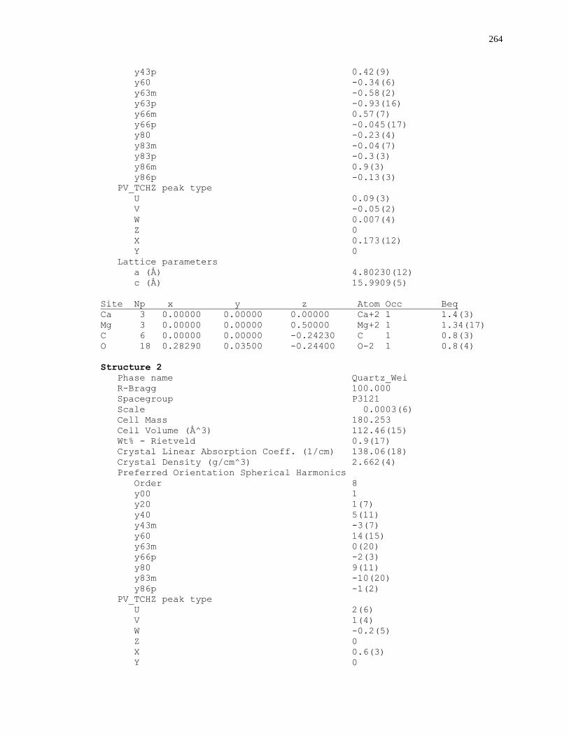
264

y43p 0.42(9)

y60 -0.34(6)

y63m -0.58(2)

y63p -0.93(16)

y66m 0.57(7)

y66p -0.045(17)

y80 -0.23(4)

y83m -0.04(7)

y83p -0.3(3)

y86m 0.9(3)

y86p -0.13(3)

PV_TCHZ peak type

U 0.09(3)

V -0.05(2)

W 0.007(4)

Z 0

X 0.173(12)

Y 0

Lattice parameters

a (Å) 4.80230(12)

c (Å) 15.9909(5)

Site Np x y z Atom Occ Beq

Ca 3 0.00000 0.00000 0.00000 Ca+2 1 1.4(3)

Mg 3 0.00000 0.00000 0.50000 Mg+2 1 1.34(17)

C 6 0.00000 0.00000 -0.24230 C 1 0.8(3)

O 18 0.28290 0.03500 -0.24400 O-2 1 0.8(4)

Structure 2

Phase name Quartz_Wei

R-Bragg 100.000

Spacegroup P3121

Scale 0.0003(6)

Cell Mass 180.253

Cell Volume (Å^3) 112.46(15)

Wt% - Rietveld 0.9(17)

Crystal Linear Absorption Coeff. (1/cm) 138.06(18)

Crystal Density (g/cm^3) 2.662(4)

Preferred Orientation Spherical Harmonics

Order 8

y00 1

y20 1(7)

y40 5(11)

y43m -3(7)

y60 14(15)

y63m 0(20)

y66p -2(3)

y80 9(11)

y83m -10(20)

y86p -1(2)

PV_TCHZ peak type

U 2(6)

V 1(4)

W -0.2(5)

Z 0

X 0.6(3)

Y 0

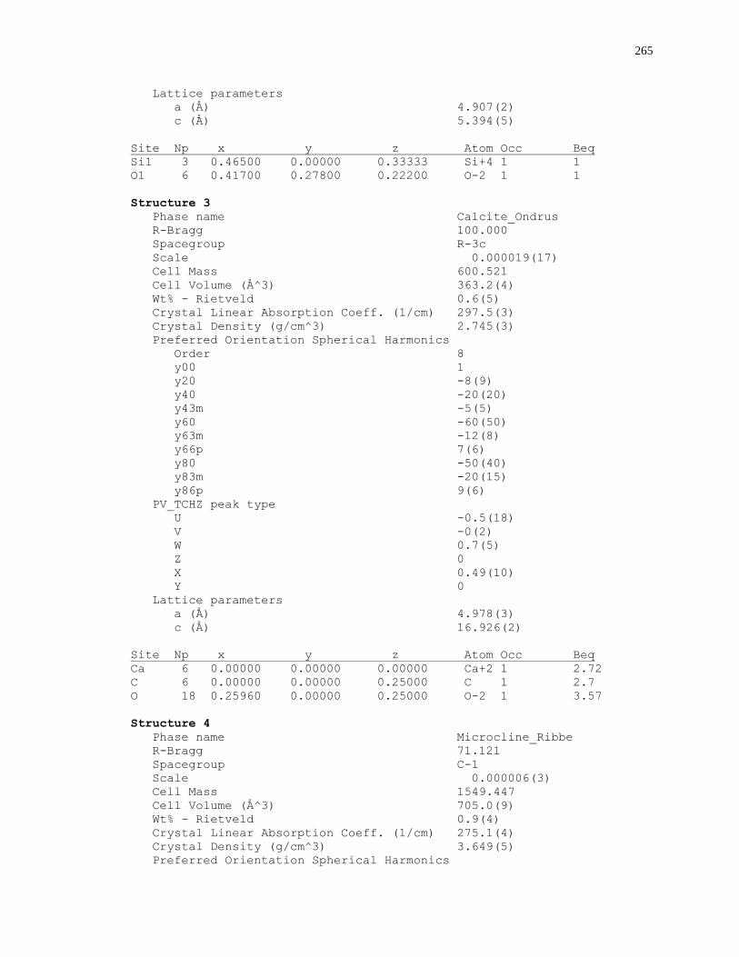
265

Lattice parameters

a (Å) 4.907(2)

c (Å) 5.394(5)

Site Np x y z Atom Occ Beq

Si1 3 0.46500 0.00000 0.33333 Si+4 1 1

O1 6 0.41700 0.27800 0.22200 O-2 1 1

Structure 3

Phase name Calcite_Ondrus

R-Bragg 100.000

Spacegroup R-3c

Scale 0.000019(17)

Cell Mass 600.521

Cell Volume (Å^3) 363.2(4)

Wt% - Rietveld 0.6(5)

Crystal Linear Absorption Coeff. (1/cm) 297.5(3)

Crystal Density (g/cm^3) 2.745(3)

Preferred Orientation Spherical Harmonics

Order 8

y00 1

y20 -8(9)

y40 -20(20)

y43m -5(5)

y60 -60(50)

y63m -12(8)

y66p 7(6)

y80 -50(40)

y83m -20(15)

y86p 9(6)

PV_TCHZ peak type

U -0.5(18)

V -0(2)

W 0.7(5)

Z 0

X 0.49(10)

Y 0

Lattice parameters

a (Å) 4.978(3)

c (Å) 16.926(2)

Site Np x y z Atom Occ Beq

Ca 6 0.00000 0.00000 0.00000 Ca+2 1 2.72

C 6 0.00000 0.00000 0.25000 C 1 2.7

O 18 0.25960 0.00000 0.25000 O-2 1 3.57

Structure 4

Phase name Microcline_Ribbe

R-Bragg 71.121

Spacegroup C-1

Scale 0.000006(3)

Cell Mass 1549.447

Cell Volume (Å^3) 705.0(9)

Wt% - Rietveld 0.9(4)

Crystal Linear Absorption Coeff. (1/cm) 275.1(4)

Crystal Density (g/cm^3) 3.649(5)

Preferred Orientation Spherical Harmonics

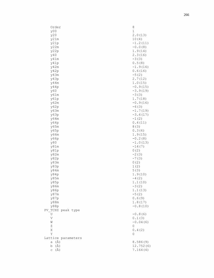
266

Order 8

y00 1

y20 2.0(13)

y21m 10(4)

y21p -1.2(11)

y22m -0.0(8)

y22p 1.9(14)

y40 2.3(16)

y41m -3(3)

y41p 0.5(8)

y42m -1.9(16)

y42p 0.6(16)

y43m -5(2)

y43p 2.7(12)

y44m 1.0(15)

y44p -0.9(15)

y60 -3.9(19)

y61m -3(3)

y61p 1.7(18)

y62m -0.9(16)

y62p -6(3)

y63m -1.7(19)

y63p -3.6(17)

y64m -1(2)

y64p 0.4(11)

y65m 8(3)

y65p 0.3(6)

y66m 1.9(15)

y66p -0.2(8)

y80 -1.0(13)

y81m -14(7)

y81p 0(2)

y82m -2(3)

y82p -7(3)

y83m 0(2)

y83p 1(2)

y84m 5(3)

y84p 1.9(10)

y85m -4(2)

y85p 1.1(10)

y86m -3(2)

y86p 1.1(13)

y87m -5(2)

y87p 0.6(9)

y88m 1.8(17)

y88p -0.8(10)

PV_TCHZ peak type

U -0.8(6)

V 0.1(3)

W -0.04(6)

Z 0

X 0.4(2)

Y 0

Lattice parameters

a (Å) 8.586(9)

b (Å) 12.752(6)

c (Å) 7.164(4)

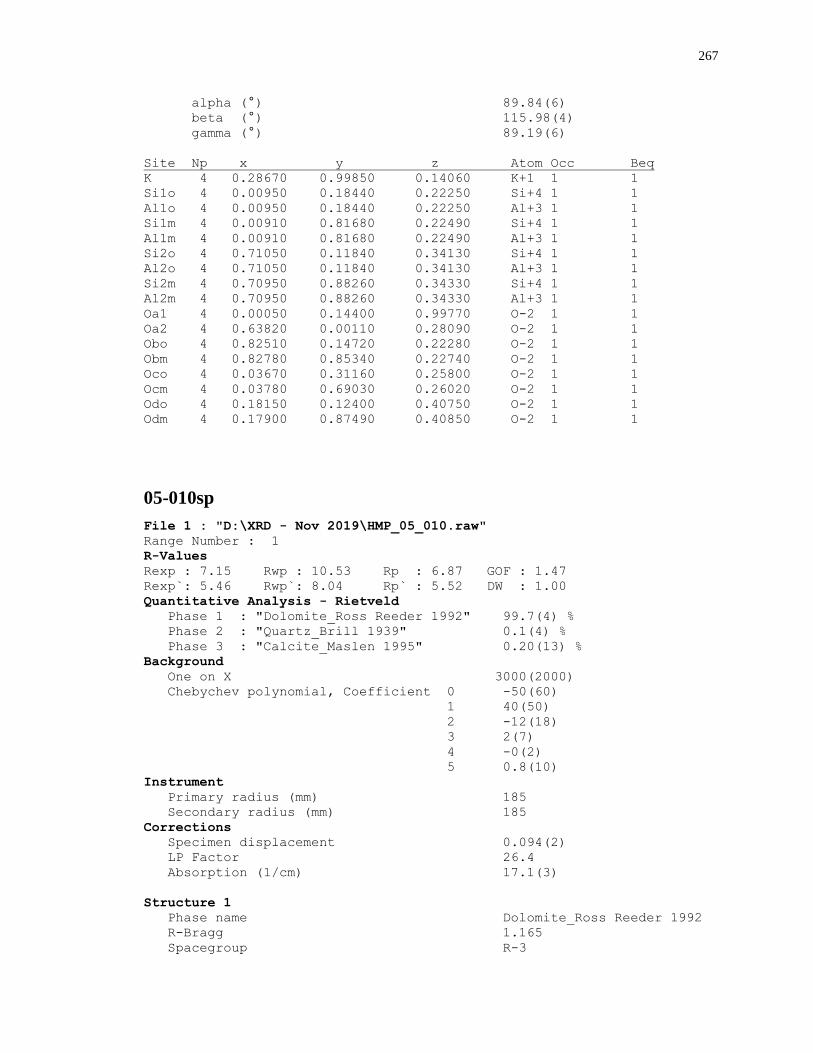
267

alpha (°) 89.84(6)

beta (°) 115.98(4)

gamma (°) 89.19(6)

Site Np x y z Atom Occ Beq

K 4 0.28670 0.99850 0.14060 K+1 1 1

Si1o 4 0.00950 0.18440 0.22250 Si+4 1 1

Al1o 4 0.00950 0.18440 0.22250 Al+3 1 1

Si1m 4 0.00910 0.81680 0.22490 Si+4 1 1

Al1m 4 0.00910 0.81680 0.22490 Al+3 1 1

Si2o 4 0.71050 0.11840 0.34130 Si+4 1 1

Al2o 4 0.71050 0.11840 0.34130 Al+3 1 1

Si2m 4 0.70950 0.88260 0.34330 Si+4 1 1

Al2m 4 0.70950 0.88260 0.34330 Al+3 1 1

Oa1 4 0.00050 0.14400 0.99770 O-2 1 1

Oa2 4 0.63820 0.00110 0.28090 O-2 1 1

Obo 4 0.82510 0.14720 0.22280 O-2 1 1

Obm 4 0.82780 0.85340 0.22740 O-2 1 1

Oco 4 0.03670 0.31160 0.25800 O-2 1 1

Ocm 4 0.03780 0.69030 0.26020 O-2 1 1

Odo 4 0.18150 0.12400 0.40750 O-2 1 1

Odm 4 0.17900 0.87490 0.40850 O-2 1 1

05-010sp

File 1 : "D:\XRD - Nov 2019\HMP_05_010.raw"

Range Number : 1

R-Values

Rexp : 7.15 Rwp : 10.53 Rp : 6.87 GOF : 1.47

Rexp`: 5.46 Rwp`: 8.04 Rp` : 5.52 DW : 1.00

Quantitative Analysis - Rietveld

Phase 1 : "Dolomite_Ross Reeder 1992" 99.7(4) %

Phase 2 : "Quartz_Brill 1939" 0.1(4) %

Phase 3 : "Calcite_Maslen 1995" 0.20(13) %

Background

One on X 3000(2000)

Chebychev polynomial, Coefficient 0 -50(60)

1 40(50)

2 -12(18)

3 2(7)

4 -0(2)

5 0.8(10)

Instrument

Primary radius (mm) 185

Secondary radius (mm) 185

Corrections

Specimen displacement 0.094(2)

LP Factor 26.4

Absorption (1/cm) 17.1(3)

Structure 1

Phase name Dolomite_Ross Reeder 1992

R-Bragg 1.165

Spacegroup R-3

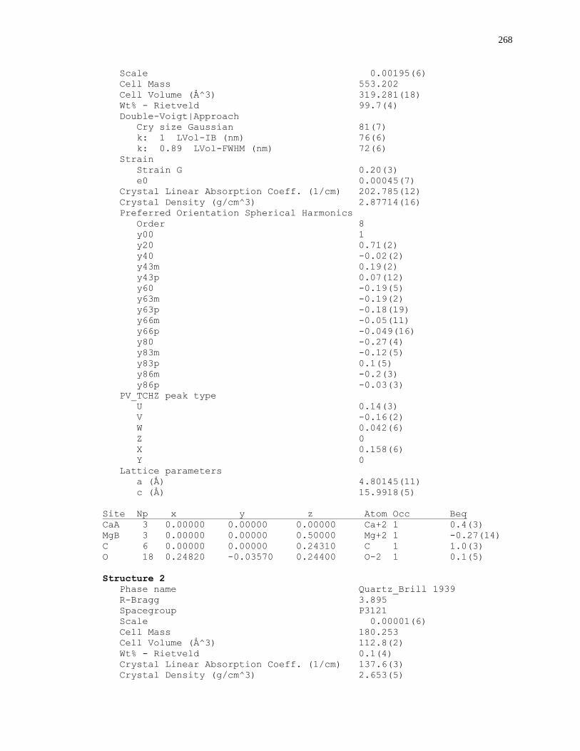
268

Scale 0.00195(6)

Cell Mass 553.202

Cell Volume (Å^3) 319.281(18)

Wt% - Rietveld 99.7(4)

Double-Voigt|Approach

Cry size Gaussian 81(7)

k: 1 LVol-IB (nm) 76(6)

k: 0.89 LVol-FWHM (nm) 72(6)

Strain

Strain G 0.20(3)

e0 0.00045(7)

Crystal Linear Absorption Coeff. (1/cm) 202.785(12)

Crystal Density (g/cm^3) 2.87714(16)

Preferred Orientation Spherical Harmonics

Order 8

y00 1

y20 0.71(2)

y40 -0.02(2)

y43m 0.19(2)

y43p 0.07(12)

y60 -0.19(5)

y63m -0.19(2)

y63p -0.18(19)

y66m -0.05(11)

y66p -0.049(16)

y80 -0.27(4)

y83m -0.12(5)

y83p 0.1(5)

y86m -0.2(3)

y86p -0.03(3)

PV_TCHZ peak type

U 0.14(3)

V -0.16(2)

W 0.042(6)

Z 0

X 0.158(6)

Y 0

Lattice parameters

a (Å) 4.80145(11)

c (Å) 15.9918(5)

Site Np x y z Atom Occ Beq

CaA 3 0.00000 0.00000 0.00000 Ca+2 1 0.4(3)

MgB 3 0.00000 0.00000 0.50000 Mg+2 1 -0.27(14)

C 6 0.00000 0.00000 0.24310 C 1 1.0(3)

O 18 0.24820 -0.03570 0.24400 O-2 1 0.1(5)

Structure 2

Phase name Quartz_Brill 1939

R-Bragg 3.895

Spacegroup P3121

Scale 0.00001(6)

Cell Mass 180.253

Cell Volume (Å^3) 112.8(2)

Wt% - Rietveld 0.1(4)

Crystal Linear Absorption Coeff. (1/cm) 137.6(3)

Crystal Density (g/cm^3) 2.653(5)

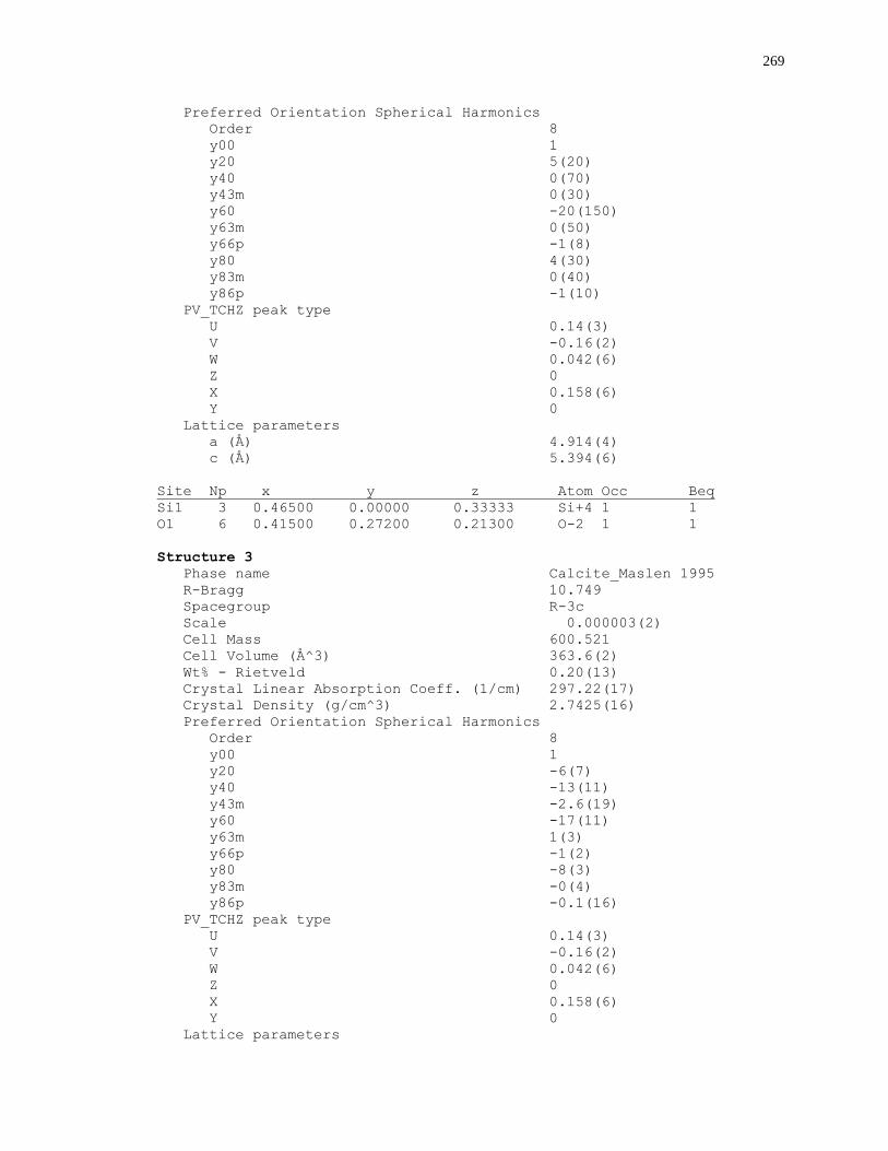
269

Preferred Orientation Spherical Harmonics

Order 8

y00 1

y20 5(20)

y40 0(70)

y43m 0(30)

y60 -20(150)

y63m 0(50)

y66p -1(8)

y80 4(30)

y83m 0(40)

y86p -1(10)

PV_TCHZ peak type

U 0.14(3)

V -0.16(2)

W 0.042(6)

Z 0

X 0.158(6)

Y 0

Lattice parameters

a (Å) 4.914(4)

c (Å) 5.394(6)

Site Np x y z Atom Occ Beq

Si1 3 0.46500 0.00000 0.33333 Si+4 1 1

O1 6 0.41500 0.27200 0.21300 O-2 1 1

Structure 3

Phase name Calcite_Maslen 1995

R-Bragg 10.749

Spacegroup R-3c

Scale 0.000003(2)

Cell Mass 600.521

Cell Volume (Å^3) 363.6(2)

Wt% - Rietveld 0.20(13)

Crystal Linear Absorption Coeff. (1/cm) 297.22(17)

Crystal Density (g/cm^3) 2.7425(16)

Preferred Orientation Spherical Harmonics

Order 8

y00 1

y20 -6(7)

y40 -13(11)

y43m -2.6(19)

y60 -17(11)

y63m 1(3)

y66p -1(2)

y80 -8(3)

y83m -0(4)

y86p -0.1(16)

PV_TCHZ peak type

U 0.14(3)

V -0.16(2)

W 0.042(6)

Z 0

X 0.158(6)

Y 0

Lattice parameters

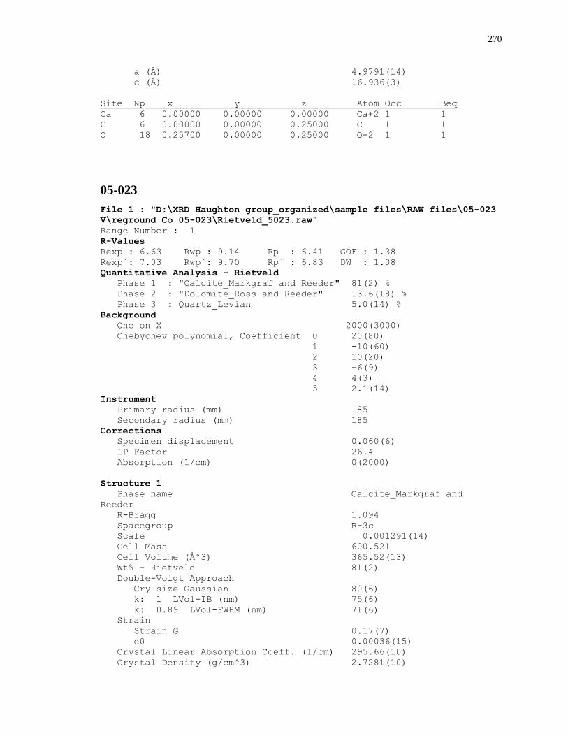
270

a (Å) 4.9791(14)

c (Å) 16.936(3)

Site Np x y z Atom Occ Beq

Ca 6 0.00000 0.00000 0.00000 Ca+2 1 1

C 6 0.00000 0.00000 0.25000 C 1 1

O 18 0.25700 0.00000 0.25000 O-2 1 1

05-023

File 1 : "D:\XRD Haughton group_organized\sample files\RAW files\05-023

V\reground Co 05-023\Rietveld_5023.raw"

Range Number : 1

R-Values

Rexp : 6.63 Rwp : 9.14 Rp : 6.41 GOF : 1.38

Rexp`: 7.03 Rwp`: 9.70 Rp` : 6.83 DW : 1.08

Quantitative Analysis - Rietveld

Phase 1 : "Calcite_Markgraf and Reeder" 81(2) %

Phase 2 : "Dolomite_Ross and Reeder" 13.6(18) %

Phase 3 : Quartz_Levian 5.0(14) %

Background

One on X 2000(3000)

Chebychev polynomial, Coefficient 0 20(80)

1 -10(60)

2 10(20)

3 -6(9)

4 4(3)

5 2.1(14)

Instrument

Primary radius (mm) 185

Secondary radius (mm) 185

Corrections

Specimen displacement 0.060(6)

LP Factor 26.4

Absorption (1/cm) 0(2000)

Structure 1

Phase name Calcite_Markgraf and

Reeder

R-Bragg 1.094

Spacegroup R-3c

Scale 0.001291(14)

Cell Mass 600.521

Cell Volume (Å^3) 365.52(13)

Wt% - Rietveld 81(2)

Double-Voigt|Approach

Cry size Gaussian 80(6)

k: 1 LVol-IB (nm) 75(6)

k: 0.89 LVol-FWHM (nm) 71(6)

Strain

Strain G 0.17(7)

e0 0.00036(15)

Crystal Linear Absorption Coeff. (1/cm) 295.66(10)

Crystal Density (g/cm^3) 2.7281(10)

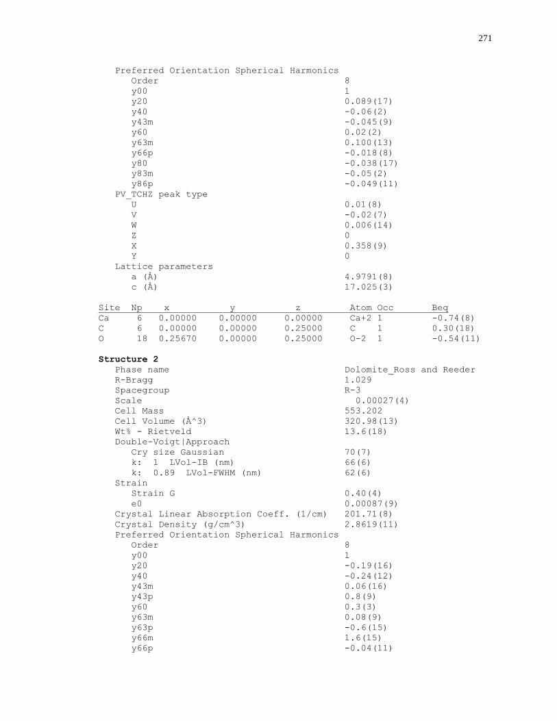
271

Preferred Orientation Spherical Harmonics

Order 8

y00 1

y20 0.089(17)

y40 -0.06(2)

y43m -0.045(9)

y60 0.02(2)

y63m 0.100(13)

y66p -0.018(8)

y80 -0.038(17)

y83m -0.05(2)

y86p -0.049(11)

PV_TCHZ peak type

U 0.01(8)

V -0.02(7)

W 0.006(14)

Z 0

X 0.358(9)

Y 0

Lattice parameters

a (Å) 4.9791(8)

c (Å) 17.025(3)

Site Np x y z Atom Occ Beq

Ca 6 0.00000 0.00000 0.00000 Ca+2 1 -0.74(8)

C 6 0.00000 0.00000 0.25000 C 1 0.30(18)

O 18 0.25670 0.00000 0.25000 O-2 1 -0.54(11)

Structure 2

Phase name Dolomite_Ross and Reeder

R-Bragg 1.029

Spacegroup R-3

Scale 0.00027(4)

Cell Mass 553.202

Cell Volume (Å^3) 320.98(13)

Wt% - Rietveld 13.6(18)

Double-Voigt|Approach

Cry size Gaussian 70(7)

k: 1 LVol-IB (nm) 66(6)

k: 0.89 LVol-FWHM (nm) 62(6)

Strain

Strain G 0.40(4)

e0 0.00087(9)

Crystal Linear Absorption Coeff. (1/cm) 201.71(8)

Crystal Density (g/cm^3) 2.8619(11)

Preferred Orientation Spherical Harmonics

Order 8

y00 1

y20 -0.19(16)

y40 -0.24(12)

y43m 0.06(16)

y43p 0.8(9)

y60 0.3(3)

y63m 0.08(9)

y63p -0.6(15)

y66m 1.6(15)

y66p -0.04(11)

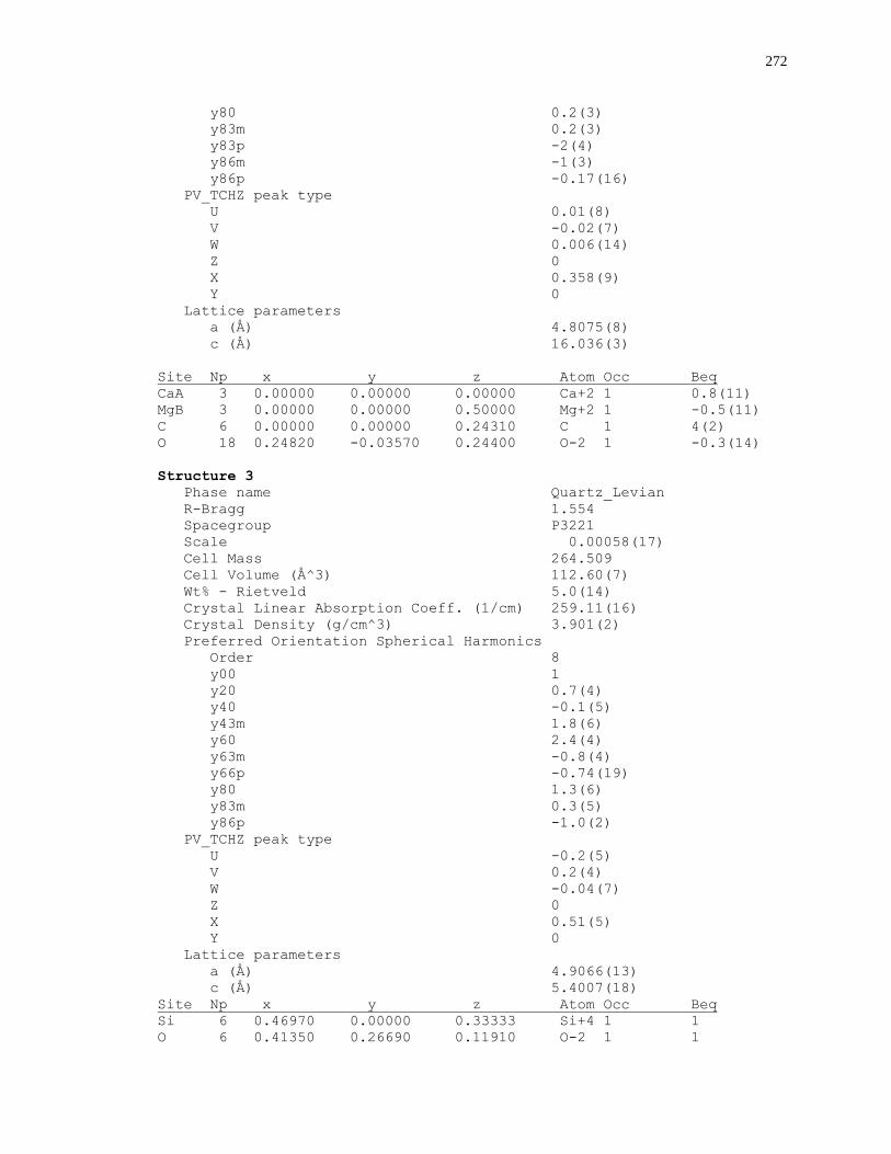
272

y80 0.2(3)

y83m 0.2(3)

y83p -2(4)

y86m -1(3)

y86p -0.17(16)

PV_TCHZ peak type

U 0.01(8)

V -0.02(7)

W 0.006(14)

Z 0

X 0.358(9)

Y 0

Lattice parameters

a (Å) 4.8075(8)

c (Å) 16.036(3)

Site Np x y z Atom Occ Beq

CaA 3 0.00000 0.00000 0.00000 Ca+2 1 0.8(11)

MgB 3 0.00000 0.00000 0.50000 Mg+2 1 -0.5(11)

C 6 0.00000 0.00000 0.24310 C 1 4(2)

O 18 0.24820 -0.03570 0.24400 O-2 1 -0.3(14)

Structure 3

Phase name Quartz_Levian

R-Bragg 1.554

Spacegroup P3221

Scale 0.00058(17)

Cell Mass 264.509

Cell Volume (Å^3) 112.60(7)

Wt% - Rietveld 5.0(14)

Crystal Linear Absorption Coeff. (1/cm) 259.11(16)

Crystal Density (g/cm^3) 3.901(2)

Preferred Orientation Spherical Harmonics

Order 8

y00 1

y20 0.7(4)

y40 -0.1(5)

y43m 1.8(6)

y60 2.4(4)

y63m -0.8(4)

y66p -0.74(19)

y80 1.3(6)

y83m 0.3(5)

y86p -1.0(2)

PV_TCHZ peak type

U -0.2(5)

V 0.2(4)

W -0.04(7)

Z 0

X 0.51(5)

Y 0

Lattice parameters

a (Å) 4.9066(13)

c (Å) 5.4007(18)

Site Np x y z Atom Occ Beq

Si 6 0.46970 0.00000 0.33333 Si+4 1 1

O 6 0.41350 0.26690 0.11910 O-2 1 1

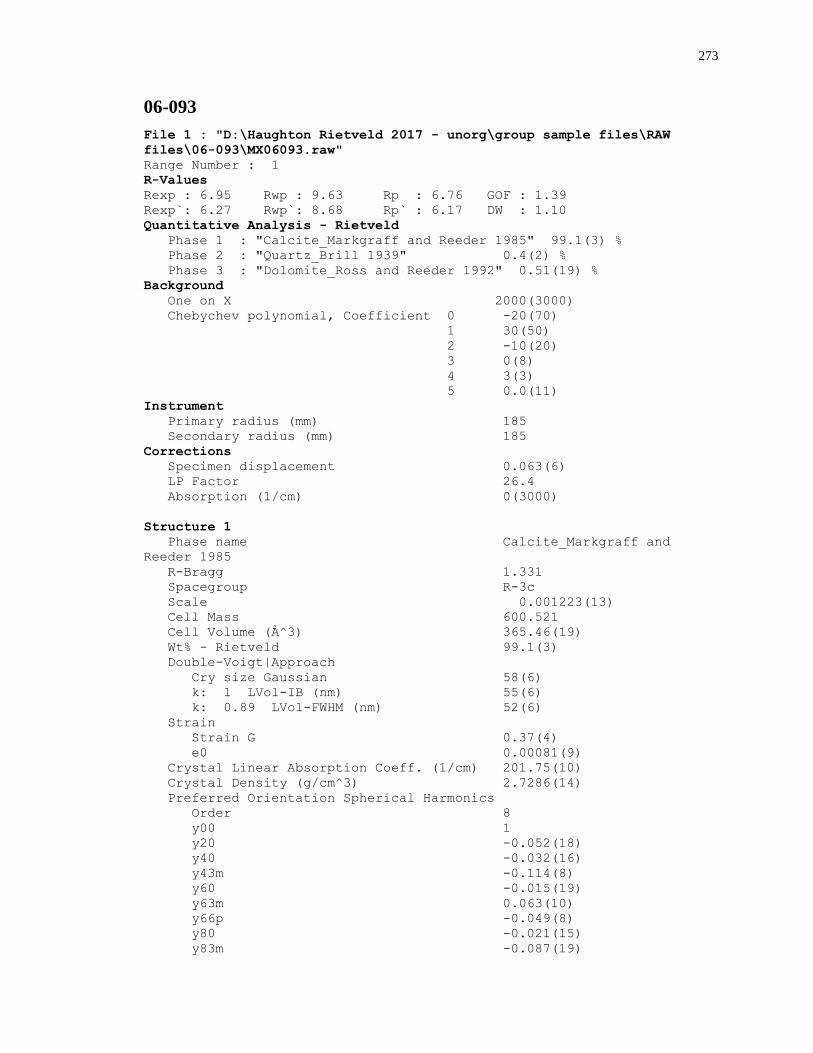
273

06-093

File 1 : "D:\Haughton Rietveld 2017 - unorg\group sample files\RAW

files\06-093\MX06093.raw"

Range Number : 1

R-Values

Rexp : 6.95 Rwp : 9.63 Rp : 6.76 GOF : 1.39

Rexp`: 6.27 Rwp`: 8.68 Rp` : 6.17 DW : 1.10

Quantitative Analysis - Rietveld

Phase 1 : "Calcite_Markgraff and Reeder 1985" 99.1(3) %

Phase 2 : "Quartz_Brill 1939" 0.4(2) %

Phase 3 : "Dolomite_Ross and Reeder 1992" 0.51(19) %

Background

One on X 2000(3000)

Chebychev polynomial, Coefficient 0 -20(70)

1 30(50)

2 -10(20)

3 0(8)

4 3(3)

5 0.0(11)

Instrument

Primary radius (mm) 185

Secondary radius (mm) 185

Corrections

Specimen displacement 0.063(6)

LP Factor 26.4

Absorption (1/cm) 0(3000)

Structure 1

Phase name Calcite_Markgraff and

Reeder 1985

R-Bragg 1.331

Spacegroup R-3c

Scale 0.001223(13)

Cell Mass 600.521

Cell Volume (Å^3) 365.46(19)

Wt% - Rietveld 99.1(3)

Double-Voigt|Approach

Cry size Gaussian 58(6)

k: 1 LVol-IB (nm) 55(6)

k: 0.89 LVol-FWHM (nm) 52(6)

Strain

Strain G 0.37(4)

e0 0.00081(9)

Crystal Linear Absorption Coeff. (1/cm) 201.75(10)

Crystal Density (g/cm^3) 2.7286(14)

Preferred Orientation Spherical Harmonics

Order 8

y00 1

y20 -0.052(18)

y40 -0.032(16)

y43m -0.114(8)

y60 -0.015(19)

y63m 0.063(10)

y66p -0.049(8)

y80 -0.021(15)

y83m -0.087(19)

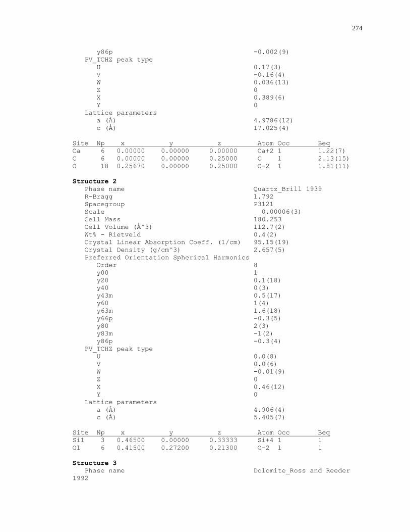
274

y86p -0.002(9)

PV_TCHZ peak type

U 0.17(3)

V -0.16(4)

W 0.036(13)

Z 0

X 0.389(6)

Y 0

Lattice parameters

a (Å) 4.9786(12)

c (Å) 17.025(4)

Site Np x y z Atom Occ Beq

Ca 6 0.00000 0.00000 0.00000 Ca+2 1 1.22(7)

C 6 0.00000 0.00000 0.25000 C 1 2.13(15)

O 18 0.25670 0.00000 0.25000 O-2 1 1.81(11)

Structure 2

Phase name Quartz_Brill 1939

R-Bragg 1.792

Spacegroup P3121

Scale 0.00006(3)

Cell Mass 180.253

Cell Volume (Å^3) 112.7(2)

Wt% - Rietveld 0.4(2)

Crystal Linear Absorption Coeff. (1/cm) 95.15(19)

Crystal Density (g/cm^3) 2.657(5)

Preferred Orientation Spherical Harmonics

Order 8

y00 1

y20 0.1(18)

y40 0(3)

y43m 0.5(17)

y60 1(4)

y63m 1.6(18)

y66p -0.3(5)

y80 2(3)

y83m -1(2)

y86p -0.3(4)

PV_TCHZ peak type

U 0.0(8)

V 0.0(6)

W -0.01(9)

Z 0

X 0.46(12)

Y 0

Lattice parameters

a (Å) 4.906(4)

c (Å) 5.405(7)

Site Np x y z Atom Occ Beq

Si1 3 0.46500 0.00000 0.33333 Si+4 1 1

O1 6 0.41500 0.27200 0.21300 O-2 1 1

Structure 3

Phase name Dolomite_Ross and Reeder

1992

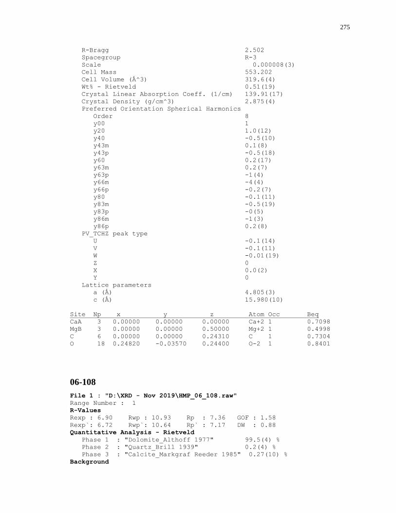
275

R-Bragg 2.502

Spacegroup R-3

Scale 0.000008(3)

Cell Mass 553.202

Cell Volume (Å^3) 319.6(4)

Wt% - Rietveld 0.51(19)

Crystal Linear Absorption Coeff. (1/cm) 139.91(17)

Crystal Density (g/cm^3) 2.875(4)

Preferred Orientation Spherical Harmonics

Order 8

y00 1

y20 1.0(12)

y40 -0.5(10)

y43m 0.1(8)

y43p -0.5(18)

y60 0.2(17)

y63m 0.2(7)

y63p -1(4)

y66m -4(4)

y66p -0.2(7)

y80 -0.1(11)

y83m -0.5(19)

y83p -0(5)

y86m -1(3)

y86p 0.2(8)

PV_TCHZ peak type

U -0.1(14)

V -0.1(11)

W -0.01(19)

Z 0

X 0.0(2)

Y 0

Lattice parameters

a (Å) 4.805(3)

c (Å) 15.980(10)

Site Np x y z Atom Occ Beq

CaA 3 0.00000 0.00000 0.00000 Ca+2 1 0.7098

MgB 3 0.00000 0.00000 0.50000 Mg+2 1 0.4998

C 6 0.00000 0.00000 0.24310 C 1 0.7304

O 18 0.24820 -0.03570 0.24400 O-2 1 0.8401

06-108

File 1 : "D:\XRD - Nov 2019\HMP_06_108.raw"

Range Number : 1

R-Values

Rexp : 6.90 Rwp : 10.93 Rp : 7.36 GOF : 1.58

Rexp`: 6.72 Rwp`: 10.64 Rp` : 7.17 DW : 0.88

Quantitative Analysis - Rietveld

Phase 1 : "Dolomite_Althoff 1977" 99.5(4) %

Phase 2 : "Quartz_Brill 1939" 0.2(4) %

Phase 3 : "Calcite_Markgraf Reeder 1985" 0.27(10) %

Background

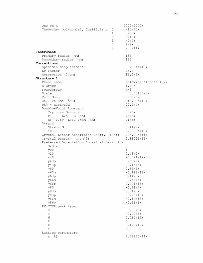
276

One on X 2000(2000)

Chebychev polynomial, Coefficient 0 -10(60)

1 8(50)

2 0(18)

3 -0(7)

4 2(2)

5 2.0(11)

Instrument

Primary radius (mm) 185

Secondary radius (mm) 185

Corrections

Specimen displacement -0.0344(19)

LP Factor 26.4

Absorption (1/cm) 16.3(2)

Structure 1

Phase name Dolomite_Althoff 1977

R-Bragg 1.485

Spacegroup R-3

Scale 0.00185(5)

Cell Mass 553.202

Cell Volume (Å^3) 318.935(18)

Wt% - Rietveld 99.5(4)

Double-Voigt|Approach

Cry size Gaussian 80(6)

k: 1 LVol-IB (nm) 75(5)

k: 0.89 LVol-FWHM (nm) 71(5)

Strain

Strain G 0.11(9)

e0 0.00024(19)

Crystal Linear Absorption Coeff. (1/cm) 203.005(11)

Crystal Density (g/cm^3) 2.88026(16)

Preferred Orientation Spherical Harmonics

Order 8

y00 1

y20 0.48(2)

y40 -0.021(19)

y43m 0.33(2)

y43p -0.14(5)

y60 0.35(5)

y63m -0.198(18)

y63p 0.41(9)

y66m -0.45(4)

y66p 0.001(13)

y80 -0.21(4)

y83m 0.34(5)

y83p -0.73(16)

y86m -0.14(13)

y86p -0.36(3)

PV_TCHZ peak type

U -0.08(6)

V -0.00(5)

W 0.015(12)

Z 0

X 0.126(12)

Y 0

Lattice parameters

a (Å) 4.79975(11)

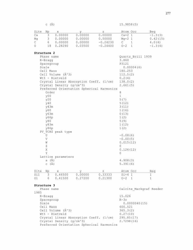
277

c (Å) 15.9858(5)

Site Np x y z Atom Occ Beq

Ca 3 0.00000 0.00000 0.00000 Ca+2 1 -1.3(3)

Mg 3 0.00000 0.00000 0.50000 Mg+2 1 0.42(15)

C 6 0.00000 0.00000 -0.24230 C 1 4.0(4)

O 18 0.28290 0.03500 -0.24400 O-2 1 -1.3(4)

Structure 2

Phase name Quartz_Brill 1939

R-Bragg 3.860

Spacegroup P3121

Scale 0.00004(6)

Cell Mass 180.253

Cell Volume (Å^3) 112.5(2)

Wt% - Rietveld 0.2(4)

Crystal Linear Absorption Coeff. (1/cm) 138.0(2)

Crystal Density (g/cm^3) 2.661(5)

Preferred Orientation Spherical Harmonics

Order 8

y00 1

y20 5(7)

y40 5(12)

y43m 3(11)

y60 1(16)

y63m 0(13)

y66p 1(2)

y80 5(9)

y83m 1(12)

y86p 1(2)

PV_TCHZ peak type

U -0.08(6)

V -0.00(5)

W 0.015(12)

Z 0

X 0.126(12)

Y 0

Lattice parameters

a (Å) 4.908(3)

c (Å) 5.391(6)

Site Np x y z Atom Occ Beq

Si1 3 0.46500 0.00000 0.33333 Si+4 1 1

O1 6 0.41500 0.27200 0.21300 O-2 1 1

Structure 3

Phase name Calcite_Markgraf Reeder

1985

R-Bragg 15.026

Spacegroup R-3c

Scale 0.0000040(15)

Cell Mass 600.521

Cell Volume (Å^3) 365.3(2)

Wt% - Rietveld 0.27(10)

Crystal Linear Absorption Coeff. (1/cm) 295.85(17)

Crystal Density (g/cm^3) 2.7298(16)

Preferred Orientation Spherical Harmonics

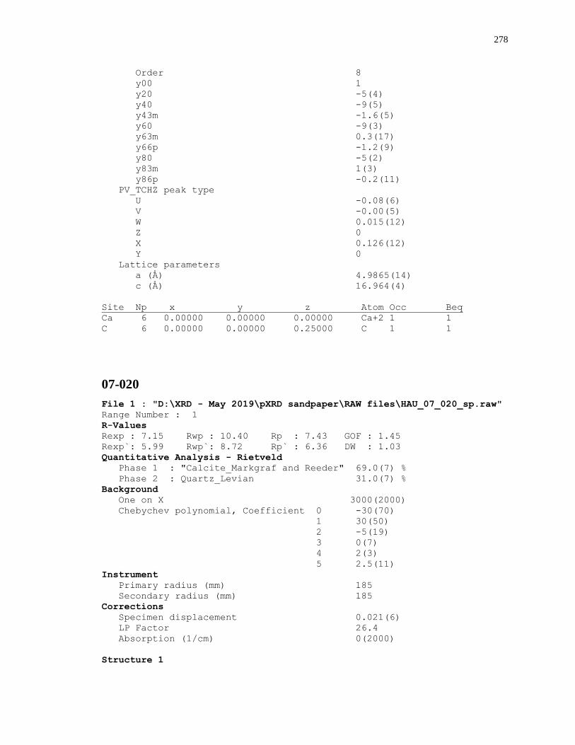
278

Order 8

y00 1

y20 -5(4)

y40 -9(5)

y43m -1.6(5)

y60 -9(3)

y63m 0.3(17)

y66p -1.2(9)

y80 -5(2)

y83m 1(3)

y86p -0.2(11)

PV_TCHZ peak type

U -0.08(6)

V -0.00(5)

W 0.015(12)

Z 0

X 0.126(12)

Y 0

Lattice parameters

a (Å) 4.9865(14)

c (Å) 16.964(4)

Site Np x y z Atom Occ Beq

Ca 6 0.00000 0.00000 0.00000 Ca+2 1 1

C 6 0.00000 0.00000 0.25000 C 1 1

07-020

File 1 : "D:\XRD - May 2019\pXRD sandpaper\RAW files\HAU_07_020_sp.raw"

Range Number : 1

R-Values

Rexp : 7.15 Rwp : 10.40 Rp : 7.43 GOF : 1.45

Rexp`: 5.99 Rwp`: 8.72 Rp` : 6.36 DW : 1.03

Quantitative Analysis - Rietveld

Phase 1 : "Calcite_Markgraf and Reeder" 69.0(7) %

Phase 2 : Quartz_Levian 31.0(7) %

Background

One on X 3000(2000)

Chebychev polynomial, Coefficient 0 -30(70)

1 30(50)

2 -5(19)

3 0(7)

4 2(3)

5 2.5(11)

Instrument

Primary radius (mm) 185

Secondary radius (mm) 185

Corrections

Specimen displacement 0.021(6)

LP Factor 26.4

Absorption (1/cm) 0(2000)

Structure 1

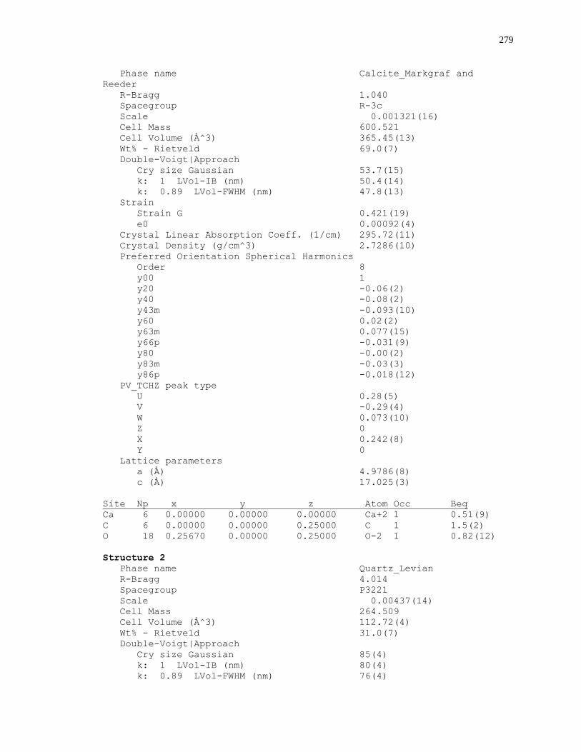
279

Phase name Calcite_Markgraf and

Reeder

R-Bragg 1.040

Spacegroup R-3c

Scale 0.001321(16)

Cell Mass 600.521

Cell Volume (Å^3) 365.45(13)

Wt% - Rietveld 69.0(7)

Double-Voigt|Approach

Cry size Gaussian 53.7(15)

k: 1 LVol-IB (nm) 50.4(14)

k: 0.89 LVol-FWHM (nm) 47.8(13)

Strain

Strain G 0.421(19)

e0 0.00092(4)

Crystal Linear Absorption Coeff. (1/cm) 295.72(11)

Crystal Density (g/cm^3) 2.7286(10)

Preferred Orientation Spherical Harmonics

Order 8

y00 1

y20 -0.06(2)

y40 -0.08(2)

y43m -0.093(10)

y60 0.02(2)

y63m 0.077(15)

y66p -0.031(9)

y80 -0.00(2)

y83m -0.03(3)

y86p -0.018(12)

PV_TCHZ peak type

U 0.28(5)

V -0.29(4)

W 0.073(10)

Z 0

X 0.242(8)

Y 0

Lattice parameters

a (Å) 4.9786(8)

c (Å) 17.025(3)

Site Np x y z Atom Occ Beq

Ca 6 0.00000 0.00000 0.00000 Ca+2 1 0.51(9)

C 6 0.00000 0.00000 0.25000 C 1 1.5(2)

O 18 0.25670 0.00000 0.25000 O-2 1 0.82(12)

Structure 2

Phase name Quartz_Levian

R-Bragg 4.014

Spacegroup P3221

Scale 0.00437(14)

Cell Mass 264.509

Cell Volume (Å^3) 112.72(4)

Wt% - Rietveld 31.0(7)

Double-Voigt|Approach

Cry size Gaussian 85(4)

k: 1 LVol-IB (nm) 80(4)

k: 0.89 LVol-FWHM (nm) 76(4)

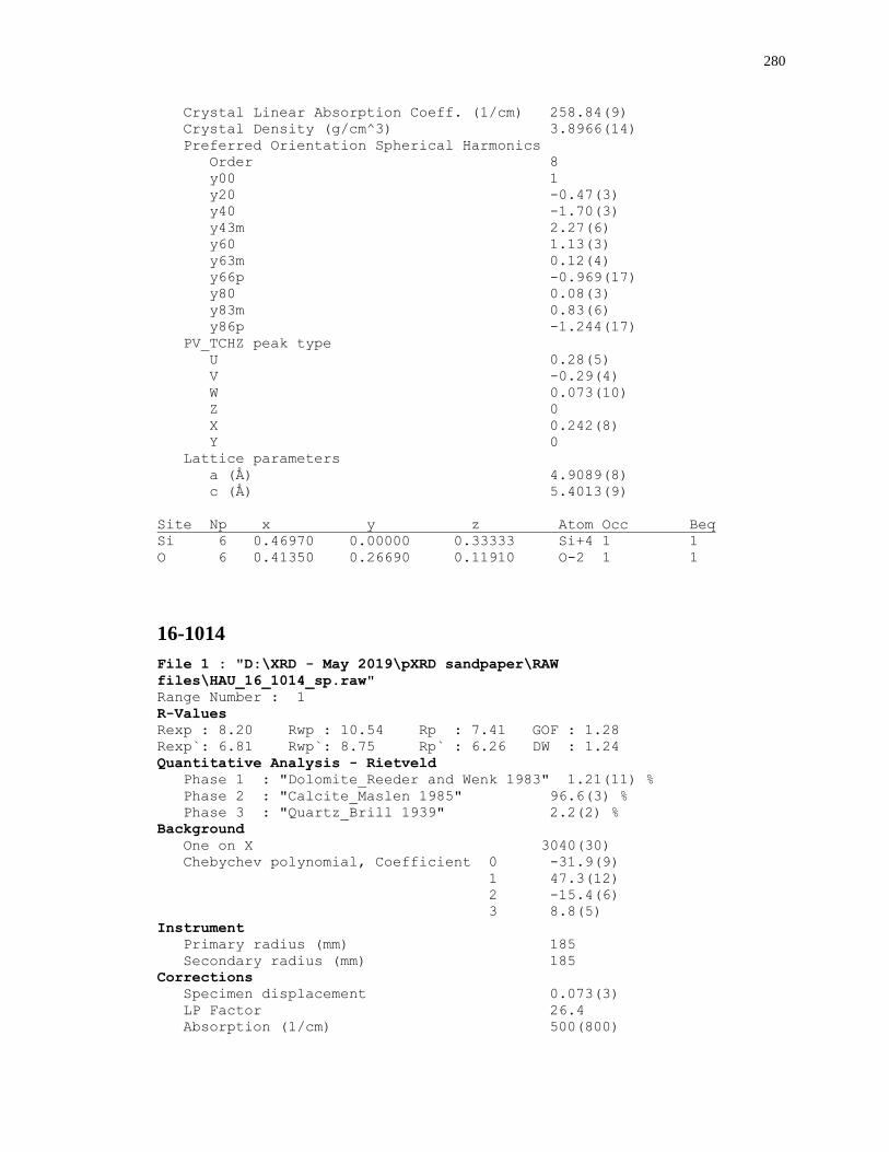
280

Crystal Linear Absorption Coeff. (1/cm) 258.84(9)

Crystal Density (g/cm^3) 3.8966(14)

Preferred Orientation Spherical Harmonics

Order 8

y00 1

y20 -0.47(3)

y40 -1.70(3)

y43m 2.27(6)

y60 1.13(3)

y63m 0.12(4)

y66p -0.969(17)

y80 0.08(3)

y83m 0.83(6)

y86p -1.244(17)

PV_TCHZ peak type

U 0.28(5)

V -0.29(4)

W 0.073(10)

Z 0

X 0.242(8)

Y 0

Lattice parameters

a (Å) 4.9089(8)

c (Å) 5.4013(9)

Site Np x y z Atom Occ Beq

Si 6 0.46970 0.00000 0.33333 Si+4 1 1

O 6 0.41350 0.26690 0.11910 O-2 1 1

16-1014

File 1 : "D:\XRD - May 2019\pXRD sandpaper\RAW

files\HAU_16_1014_sp.raw"

Range Number : 1

R-Values

Rexp : 8.20 Rwp : 10.54 Rp : 7.41 GOF : 1.28

Rexp`: 6.81 Rwp`: 8.75 Rp` : 6.26 DW : 1.24

Quantitative Analysis - Rietveld

Phase 1 : "Dolomite_Reeder and Wenk 1983" 1.21(11) %

Phase 2 : "Calcite_Maslen 1985" 96.6(3) %

Phase 3 : "Quartz_Brill 1939" 2.2(2) %

Background

One on X 3040(30)

Chebychev polynomial, Coefficient 0 -31.9(9)

1 47.3(12)

2 -15.4(6)

3 8.8(5)

Instrument

Primary radius (mm) 185

Secondary radius (mm) 185

Corrections

Specimen displacement 0.073(3)

LP Factor 26.4

Absorption (1/cm) 500(800)

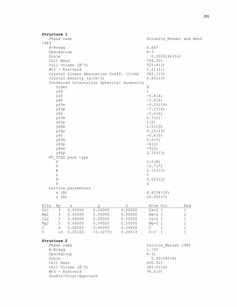
281

Structure 1

Phase name Dolomite_Reeder and Wenk

1983

R-Bragg 6.667

Spacegroup R-3

Scale 0.0000146(14)

Cell Mass 746.351

Cell Volume (Å^3) 321.8(3)

Wt% - Rietveld 1.21(11)

Crystal Linear Absorption Coeff. (1/cm) 382.3(3)

Crystal Density (g/cm^3) 3.851(3)

Preferred Orientation Spherical Harmonics

Order 8

y00 1

y20 -0.8(4)

y40 -3.0(5)

y43m -0.10(14)

y43p -7.2(16)

y60 -2.4(6)

y63m 0.7(2)

y63p 1(2)

y66m 1.6(19)

y66p 0.13(13)

y80 -0.6(5)

y83m 0.6(5)

y83p -6(2)

y86m -9(3)

y86p 0.70(13)

PV_TCHZ peak type

U 2.0(8)

V -0.7(7)

W 0.15(15)

Z 0

X 0.00(12)

Y 0

Lattice parameters

a (Å) 4.8104(18)

c (Å) 16.059(7)

Site Np x y z Atom Occ Beq

Ca1 3 0.00000 0.00000 0.00000 Ca+2 1 1

Mg1 3 0.00000 0.00000 0.00000 Mg+2 1 1

Ca2 3 0.00000 0.00000 0.50000 Ca+2 1 1

Mg2 3 0.00000 0.00000 0.50000 Mg+2 1 1

C 6 0.00000 0.00000 0.24420 C 1 1

O 18 0.25160 -0.02770 0.24514 O-2 1 1

Structure 2

Phase name Calcite_Maslen 1985

R-Bragg 1.720

Spacegroup R-3c

Scale 0.001282(6)

Cell Mass 600.521

Cell Volume (Å^3) 365.43(3)

Wt% - Rietveld 96.6(3)

Double-Voigt|Approach

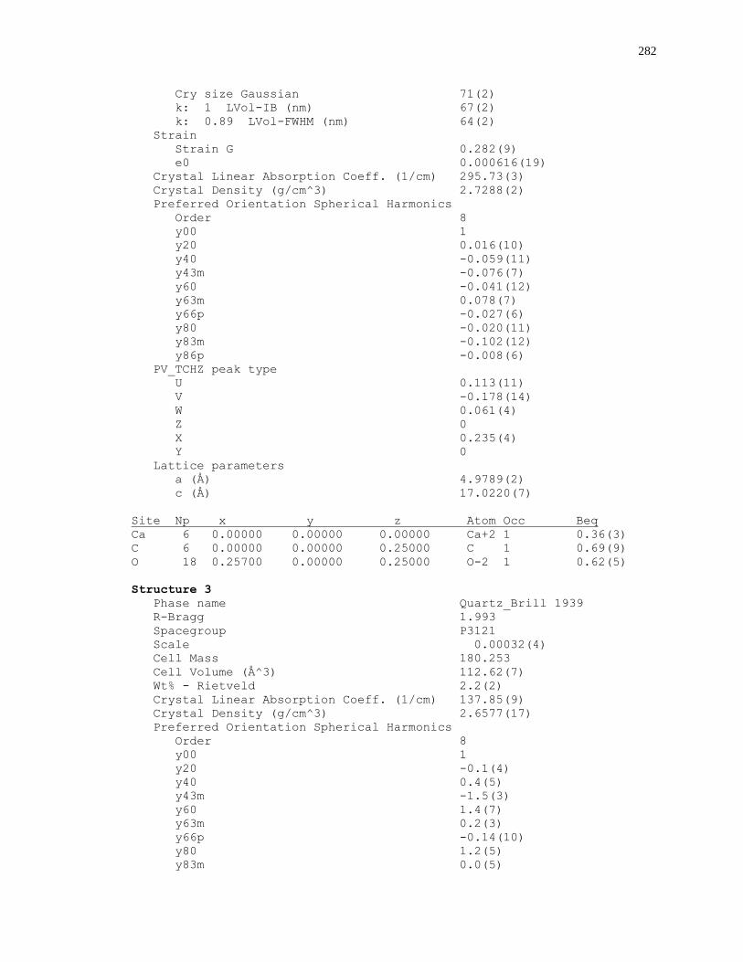
282

Cry size Gaussian 71(2)

k: 1 LVol-IB (nm) 67(2)

k: 0.89 LVol-FWHM (nm) 64(2)

Strain

Strain G 0.282(9)

e0 0.000616(19)

Crystal Linear Absorption Coeff. (1/cm) 295.73(3)

Crystal Density (g/cm^3) 2.7288(2)

Preferred Orientation Spherical Harmonics

Order 8

y00 1

y20 0.016(10)

y40 -0.059(11)

y43m -0.076(7)

y60 -0.041(12)

y63m 0.078(7)

y66p -0.027(6)

y80 -0.020(11)

y83m -0.102(12)

y86p -0.008(6)

PV_TCHZ peak type

U 0.113(11)

V -0.178(14)

W 0.061(4)

Z 0

X 0.235(4)

Y 0

Lattice parameters

a (Å) 4.9789(2)

c (Å) 17.0220(7)

Site Np x y z Atom Occ Beq

Ca 6 0.00000 0.00000 0.00000 Ca+2 1 0.36(3)

C 6 0.00000 0.00000 0.25000 C 1 0.69(9)

O 18 0.25700 0.00000 0.25000 O-2 1 0.62(5)

Structure 3

Phase name Quartz_Brill 1939

R-Bragg 1.993

Spacegroup P3121

Scale 0.00032(4)

Cell Mass 180.253

Cell Volume (Å^3) 112.62(7)

Wt% - Rietveld 2.2(2)

Crystal Linear Absorption Coeff. (1/cm) 137.85(9)

Crystal Density (g/cm^3) 2.6577(17)

Preferred Orientation Spherical Harmonics

Order 8

y00 1

y20 -0.1(4)

y40 0.4(5)

y43m -1.5(3)

y60 1.4(7)

y63m 0.2(3)

y66p -0.14(10)

y80 1.2(5)

y83m 0.0(5)

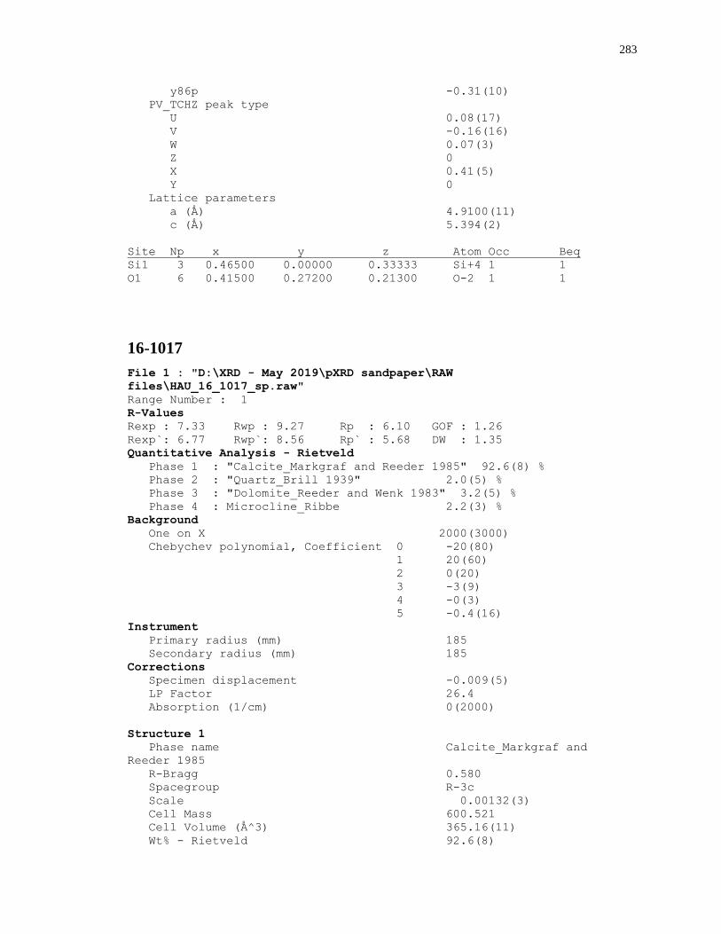
283

y86p -0.31(10)

PV_TCHZ peak type

U 0.08(17)

V -0.16(16)

W 0.07(3)

Z 0

X 0.41(5)

Y 0

Lattice parameters

a (Å) 4.9100(11)

c (Å) 5.394(2)

Site Np x y z Atom Occ Beq

Si1 3 0.46500 0.00000 0.33333 Si+4 1 1

O1 6 0.41500 0.27200 0.21300 O-2 1 1

16-1017

File 1 : "D:\XRD - May 2019\pXRD sandpaper\RAW

files\HAU_16_1017_sp.raw"

Range Number : 1

R-Values

Rexp : 7.33 Rwp : 9.27 Rp : 6.10 GOF : 1.26

Rexp`: 6.77 Rwp`: 8.56 Rp` : 5.68 DW : 1.35

Quantitative Analysis - Rietveld

Phase 1 : "Calcite_Markgraf and Reeder 1985" 92.6(8) %

Phase 2 : "Quartz_Brill 1939" 2.0(5) %

Phase 3 : "Dolomite_Reeder and Wenk 1983" 3.2(5) %

Phase 4 : Microcline_Ribbe 2.2(3) %

Background

One on X 2000(3000)

Chebychev polynomial, Coefficient 0 -20(80)

1 20(60)

2 0(20)

3 -3(9)

4 -0(3)

5 -0.4(16)

Instrument

Primary radius (mm) 185

Secondary radius (mm) 185

Corrections

Specimen displacement -0.009(5)

LP Factor 26.4

Absorption (1/cm) 0(2000)

Structure 1

Phase name Calcite_Markgraf and

Reeder 1985

R-Bragg 0.580

Spacegroup R-3c

Scale 0.00132(3)

Cell Mass 600.521

Cell Volume (Å^3) 365.16(11)

Wt% - Rietveld 92.6(8)

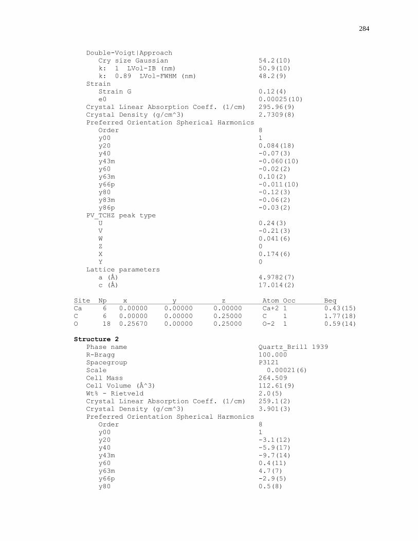
284

Double-Voigt|Approach

Cry size Gaussian 54.2(10)

k: 1 LVol-IB (nm) 50.9(10)

k: 0.89 LVol-FWHM (nm) 48.2(9)

Strain

Strain G 0.12(4)

e0 0.00025(10)

Crystal Linear Absorption Coeff. (1/cm) 295.96(9)

Crystal Density (g/cm^3) 2.7309(8)

Preferred Orientation Spherical Harmonics

Order 8

y00 1

y20 0.084(18)

y40 -0.07(3)

y43m -0.060(10)

y60 -0.02(2)

y63m 0.10(2)

y66p -0.011(10)

y80 -0.12(3)

y83m -0.06(2)

y86p -0.03(2)

PV_TCHZ peak type

U 0.24(3)

V -0.21(3)

W 0.041(6)

Z 0

X 0.174(6)

Y 0

Lattice parameters

a (Å) 4.9782(7)

c (Å) 17.014(2)

Site Np x y z Atom Occ Beq

Ca 6 0.00000 0.00000 0.00000 Ca+2 1 0.43(15)

C 6 0.00000 0.00000 0.25000 C 1 1.77(18)

O 18 0.25670 0.00000 0.25000 O-2 1 0.59(14)

Structure 2

Phase name Quartz_Brill 1939

R-Bragg 100.000

Spacegroup P3121

Scale 0.00021(6)

Cell Mass 264.509

Cell Volume (Å^3) 112.61(9)

Wt% - Rietveld 2.0(5)

Crystal Linear Absorption Coeff. (1/cm) 259.1(2)

Crystal Density (g/cm^3) 3.901(3)

Preferred Orientation Spherical Harmonics

Order 8

y00 1

y20 -3.1(12)

y40 -5.9(17)

y43m -9.7(14)

y60 0.4(11)

y63m 4.7(7)

y66p -2.9(5)

y80 0.5(8)

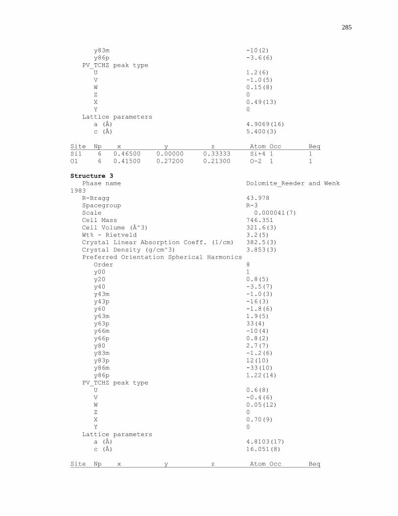
285

y83m -10(2)

y86p -3.6(6)

PV_TCHZ peak type

U 1.2(6)

V -1.0(5)

W 0.15(8)

Z 0

X 0.49(13)

Y 0

Lattice parameters

a (Å) 4.9069(16)

c (Å) 5.400(3)

Site Np x y z Atom Occ Beq

Si1 6 0.46500 0.00000 0.33333 Si+4 1 1

O1 6 0.41500 0.27200 0.21300 O-2 1 1

Structure 3

Phase name Dolomite_Reeder and Wenk

1983

R-Bragg 43.978

Spacegroup R-3

Scale 0.000041(7)

Cell Mass 746.351

Cell Volume (Å^3) 321.6(3)

Wt% - Rietveld 3.2(5)

Crystal Linear Absorption Coeff. (1/cm) 382.5(3)

Crystal Density (g/cm^3) 3.853(3)

Preferred Orientation Spherical Harmonics

Order 8

y00 1

y20 0.8(5)

y40 -3.5(7)

y43m -1.0(3)

y43p -16(3)

y60 -1.8(6)

y63m 1.9(5)

y63p 33(4)

y66m -10(4)

y66p 0.8(2)

y80 2.7(7)

y83m -1.2(6)

y83p 12(10)

y86m -33(10)

y86p 1.22(14)

PV_TCHZ peak type

U 0.6(8)

V -0.4(6)

W 0.05(12)

Z 0

X 0.70(9)

Y 0

Lattice parameters

a (Å) 4.8103(17)

c (Å) 16.051(8)

Site Np x y z Atom Occ Beq

286

Ca1 3 0.00000 0.00000 0.00000 Ca+2 1 1

Mg1 3 0.00000 0.00000 0.00000 Mg+2 1 1

Ca2 3 0.00000 0.00000 0.50000 Ca+2 1 1

Mg2 3 0.00000 0.00000 0.50000 Mg+2 1 1

C 6 0.00000 0.00000 0.24420 C 1 1

O 18 0.25160 -0.02770 0.24514 O-2 1 1

Structure 4

Phase name Microcline_Ribbe

R-Bragg 4.011

Spacegroup C-1

Scale 0.0000061(9)

Cell Mass 1549.447

Cell Volume (Å^3) 727.5(6)

Wt% - Rietveld 2.2(3)

Crystal Linear Absorption Coeff. (1/cm) 266.6(2)

Crystal Density (g/cm^3) 3.537(3)

Preferred Orientation Spherical Harmonics

Order 8

y00 1

y20 1.3(3)

y21m 1.0(3)

y21p 0.64(18)

y22m 0.60(19)

y22p -0.31(19)

y40 -1.3(5)

y41m -2.9(5)

y41p 0.5(2)

y42m 0.0(2)

y42p -1.9(4)

y43m -0.6(2)

y43p -0.9(2)

y44m -1.1(3)

y44p -0.4(3)

y60 -0.4(5)

y61m 3.0(7)

y61p 0.5(5)

y62m 1.0(3)

y62p 1.2(4)

y63m -0.1(3)

y63p -0.1(3)

y64m -3.8(5)

y64p 1.6(3)

y65m -0.9(2)

y65p 1.9(3)

y66m 1.3(3)

y66p 0.3(2)

y80 0.4(4)

y81m 0.3(5)

y81p 1.5(6)

y82m 1.3(5)

y82p 1.5(4)

y83m -2.4(4)

y83p -0.7(4)

y84m -1.5(4)

y84p 1.6(3)

y85m 2.4(5)

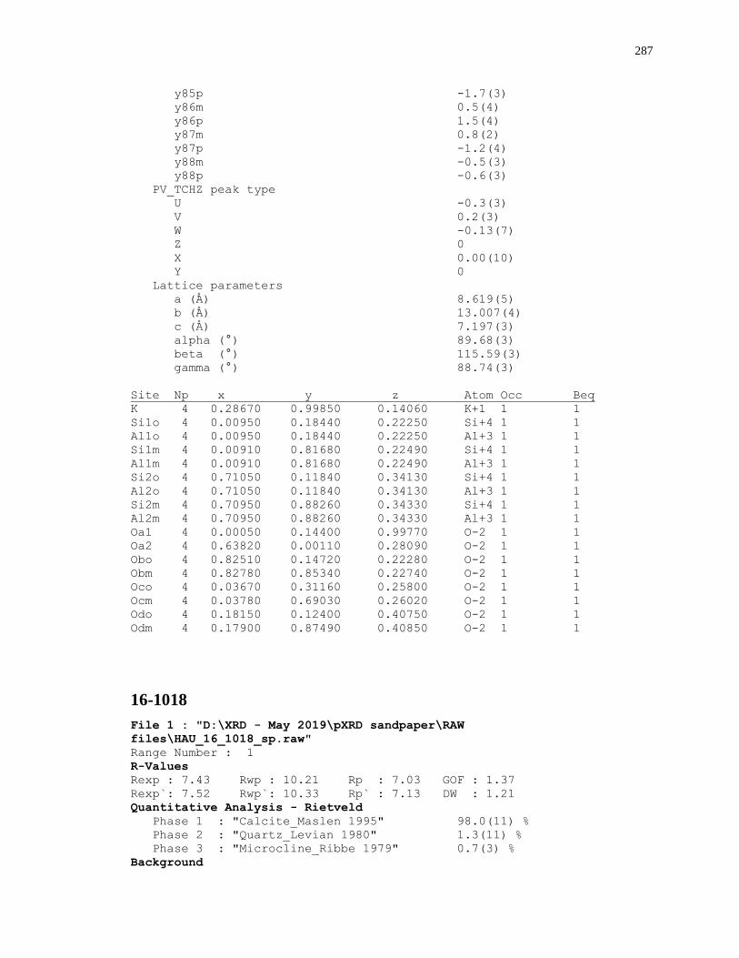
287

y85p -1.7(3)

y86m 0.5(4)

y86p 1.5(4)

y87m 0.8(2)

y87p -1.2(4)

y88m -0.5(3)

y88p -0.6(3)

PV_TCHZ peak type

U -0.3(3)

V 0.2(3)

W -0.13(7)

Z 0

X 0.00(10)

Y 0

Lattice parameters

a (Å) 8.619(5)

b (Å) 13.007(4)

c (Å) 7.197(3)

alpha (°) 89.68(3)

beta (°) 115.59(3)

gamma (°) 88.74(3)

Site Np x y z Atom Occ Beq

K 4 0.28670 0.99850 0.14060 K+1 1 1

Si1o 4 0.00950 0.18440 0.22250 Si+4 1 1

Al1o 4 0.00950 0.18440 0.22250 Al+3 1 1

Si1m 4 0.00910 0.81680 0.22490 Si+4 1 1

Al1m 4 0.00910 0.81680 0.22490 Al+3 1 1

Si2o 4 0.71050 0.11840 0.34130 Si+4 1 1

Al2o 4 0.71050 0.11840 0.34130 Al+3 1 1

Si2m 4 0.70950 0.88260 0.34330 Si+4 1 1

Al2m 4 0.70950 0.88260 0.34330 Al+3 1 1

Oa1 4 0.00050 0.14400 0.99770 O-2 1 1

Oa2 4 0.63820 0.00110 0.28090 O-2 1 1

Obo 4 0.82510 0.14720 0.22280 O-2 1 1

Obm 4 0.82780 0.85340 0.22740 O-2 1 1

Oco 4 0.03670 0.31160 0.25800 O-2 1 1

Ocm 4 0.03780 0.69030 0.26020 O-2 1 1

Odo 4 0.18150 0.12400 0.40750 O-2 1 1

Odm 4 0.17900 0.87490 0.40850 O-2 1 1

16-1018

File 1 : "D:\XRD - May 2019\pXRD sandpaper\RAW

files\HAU_16_1018_sp.raw"

Range Number : 1

R-Values

Rexp : 7.43 Rwp : 10.21 Rp : 7.03 GOF : 1.37

Rexp`: 7.52 Rwp`: 10.33 Rp` : 7.13 DW : 1.21

Quantitative Analysis - Rietveld

Phase 1 : "Calcite_Maslen 1995" 98.0(11) %

Phase 2 : "Quartz_Levian 1980" 1.3(11) %

Phase 3 : "Microcline_Ribbe 1979" 0.7(3) %

Background

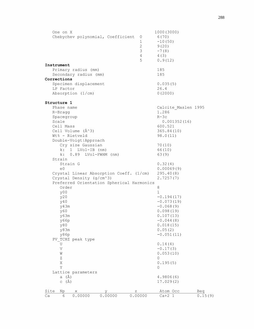
288

One on X 1000(3000)

Chebychev polynomial, Coefficient 0 6(70)

1 -10(50)

2 9(20)

3 -7(8)

4 4(3)

5 0.9(12)

Instrument

Primary radius (mm) 185

Secondary radius (mm) 185

Corrections

Specimen displacement 0.035(5)

LP Factor 26.4

Absorption (1/cm) 0(2000)

Structure 1

Phase name Calcite_Maslen 1995

R-Bragg 1.286

Spacegroup R-3c

Scale 0.001352(16)

Cell Mass 600.521

Cell Volume (Å^3) 365.84(10)

Wt% - Rietveld 98.0(11)

Double-Voigt|Approach

Cry size Gaussian 70(10)

k: 1 LVol-IB (nm) 66(10)

k: 0.89 LVol-FWHM (nm) 63(9)

Strain

Strain G 0.32(4)

e0 0.00069(9)

Crystal Linear Absorption Coeff. (1/cm) 295.40(8)

Crystal Density (g/cm^3) 2.7257(7)

Preferred Orientation Spherical Harmonics

Order 8

y00 1

y20 -0.194(17)

y40 -0.073(19)

y43m -0.068(9)

y60 0.098(19)

y63m 0.107(13)

y66p -0.044(8)

y80 0.018(15)

y83m 0.05(2)

y86p -0.051(11)

PV_TCHZ peak type

U 0.14(4)

V -0.17(3)

W 0.053(10)

Z 0

X 0.195(5)

Y 0

Lattice parameters

a (Å) 4.9806(6)

c (Å) 17.029(2)

Site Np x y z Atom Occ Beq

Ca 6 0.00000 0.00000 0.00000 Ca+2 1 0.15(9)

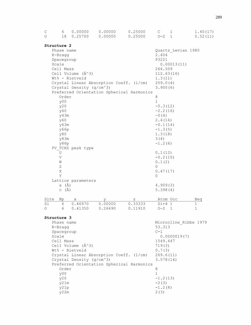
289

C 6 0.00000 0.00000 0.25000 C 1 1.40(17)

O 18 0.25700 0.00000 0.25000 O-2 1 0.52(11)

Structure 2

Phase name Quartz_Levian 1980

R-Bragg 2.404

Spacegroup P3221

Scale 0.00013(11)

Cell Mass 264.509

Cell Volume (Å^3) 112.63(16)

Wt% - Rietveld 1.3(11)

Crystal Linear Absorption Coeff. (1/cm) 259.0(4)

Crystal Density (g/cm^3) 3.900(6)

Preferred Orientation Spherical Harmonics

Order 8

y00 1

y20 -0.3(12)

y40 -2.2(16)

y43m -0(4)

y60 2.4(16)

y63m -0.1(14)

y66p -1.3(5)

y80 1.3(18)

y83m 3(4)

y86p -1.2(6)

PV_TCHZ peak type

U 0.1(12)

V -0.2(10)

W 0.1(2)

Z 0

X 0.47(17)

Y 0

Lattice parameters

a (Å) 4.909(3)

c (Å) 5.398(4)

Site Np x y z Atom Occ Beq

Si 6 0.46970 0.00000 0.33333 Si+4 1 1

O 6 0.41350 0.26690 0.11910 O-2 1 1

Structure 3

Phase name Microcline_Ribbe 1979

R-Bragg 53.313

Spacegroup C-1

Scale 0.0000019(7)

Cell Mass 1549.447

Cell Volume (Å^3) 719(3)

Wt% - Rietveld 0.7(3)

Crystal Linear Absorption Coeff. (1/cm) 269.6(11)

Crystal Density (g/cm^3) 3.578(14)

Preferred Orientation Spherical Harmonics

Order 8

y00 1

y20 -1.2(13)

y21m -2(3)

y21p -1.2(8)

y22m 2(3)

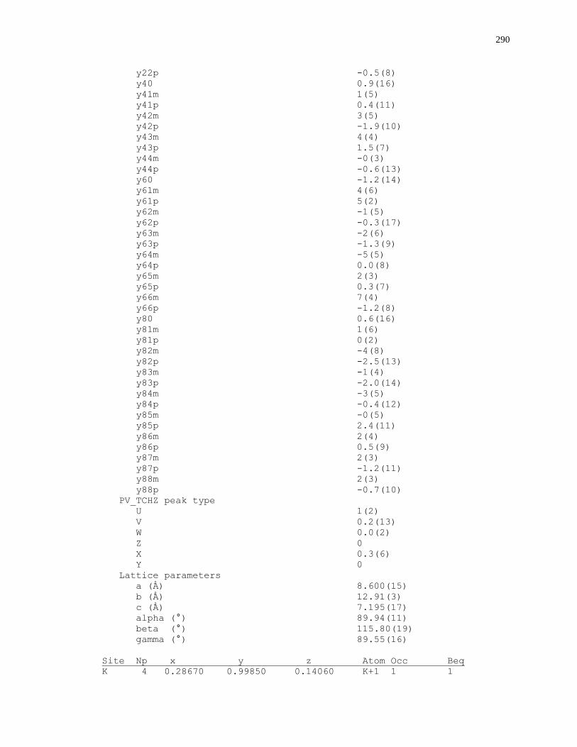
290

y22p -0.5(8)

y40 0.9(16)

y41m 1(5)

y41p 0.4(11)

y42m 3(5)

y42p -1.9(10)

y43m 4(4)

y43p 1.5(7)

y44m -0(3)

y44p -0.6(13)

y60 -1.2(14)

y61m 4(6)

y61p 5(2)

y62m -1(5)

y62p -0.3(17)

y63m -2(6)

y63p -1.3(9)

y64m -5(5)

y64p 0.0(8)

y65m 2(3)

y65p 0.3(7)

y66m 7(4)

y66p -1.2(8)

y80 0.6(16)

y81m 1(6)

y81p 0(2)

y82m -4(8)

y82p -2.5(13)

y83m -1(4)

y83p -2.0(14)

y84m -3(5)

y84p -0.4(12)

y85m -0(5)

y85p 2.4(11)

y86m 2(4)

y86p 0.5(9)

y87m 2(3)

y87p -1.2(11)

y88m 2(3)

y88p -0.7(10)

PV_TCHZ peak type

U 1(2)

V 0.2(13)

W 0.0(2)

Z 0

X 0.3(6)

Y 0

Lattice parameters

a (Å) 8.600(15)

b (Å) 12.91(3)

c (Å) 7.195(17)

alpha (°) 89.94(11)

beta (°) 115.80(19)

gamma (°) 89.55(16)

Site Np x y z Atom Occ Beq

K 4 0.28670 0.99850 0.14060 K+1 1 1

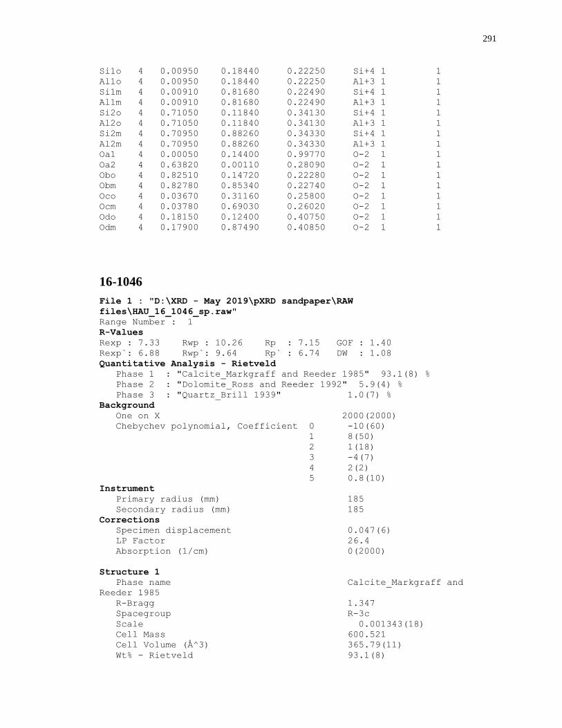
291

Si1o 4 0.00950 0.18440 0.22250 Si+4 1 1

Al1o 4 0.00950 0.18440 0.22250 Al+3 1 1

Si1m 4 0.00910 0.81680 0.22490 Si+4 1 1

Al1m 4 0.00910 0.81680 0.22490 Al+3 1 1

Si2o 4 0.71050 0.11840 0.34130 Si+4 1 1

Al2o 4 0.71050 0.11840 0.34130 Al+3 1 1

Si2m 4 0.70950 0.88260 0.34330 Si+4 1 1

Al2m 4 0.70950 0.88260 0.34330 Al+3 1 1

Oa1 4 0.00050 0.14400 0.99770 O-2 1 1

Oa2 4 0.63820 0.00110 0.28090 O-2 1 1

Obo 4 0.82510 0.14720 0.22280 O-2 1 1

Obm 4 0.82780 0.85340 0.22740 O-2 1 1

Oco 4 0.03670 0.31160 0.25800 O-2 1 1

Ocm 4 0.03780 0.69030 0.26020 O-2 1 1

Odo 4 0.18150 0.12400 0.40750 O-2 1 1

Odm 4 0.17900 0.87490 0.40850 O-2 1 1

16-1046

File 1 : "D:\XRD - May 2019\pXRD sandpaper\RAW

files\HAU_16_1046_sp.raw"

Range Number : 1

R-Values

Rexp : 7.33 Rwp : 10.26 Rp : 7.15 GOF : 1.40

Rexp`: 6.88 Rwp`: 9.64 Rp` : 6.74 DW : 1.08

Quantitative Analysis - Rietveld

Phase 1 : "Calcite_Markgraff and Reeder 1985" 93.1(8) %

Phase 2 : "Dolomite_Ross and Reeder 1992" 5.9(4) %

Phase 3 : "Quartz_Brill 1939" 1.0(7) %

Background

One on X 2000(2000)

Chebychev polynomial, Coefficient 0 -10(60)

1 8(50)

2 1(18)

3 -4(7)

4 2(2)

5 0.8(10)

Instrument

Primary radius (mm) 185

Secondary radius (mm) 185

Corrections

Specimen displacement 0.047(6)

LP Factor 26.4

Absorption (1/cm) 0(2000)

Structure 1

Phase name Calcite_Markgraff and

Reeder 1985

R-Bragg 1.347

Spacegroup R-3c

Scale 0.001343(18)

Cell Mass 600.521

Cell Volume (Å^3) 365.79(11)

Wt% - Rietveld 93.1(8)

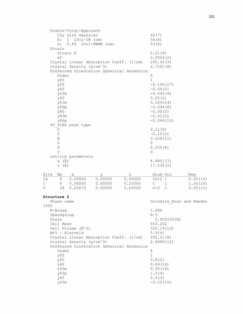
292

Double-Voigt|Approach

Cry size Gaussian 60(7)

k: 1 LVol-IB (nm) 56(6)

k: 0.89 LVol-FWHM (nm) 53(6)

Strain

Strain G 0.21(9)

e0 0.0004(2)

Crystal Linear Absorption Coeff. (1/cm) 295.45(9)

Crystal Density (g/cm^3) 2.7261(8)

Preferred Orientation Spherical Harmonics

Order 8

y00 1

y20 -0.195(17)

y40 -0.04(2)

y43m -0.045(9)

y60 0.05(2)

y63m 0.109(14)

y66p -0.044(8)

y80 -0.00(2)

y83m -0.01(2)

y86p -0.064(13)

PV_TCHZ peak type

U 0.11(6)

V -0.10(3)

W 0.026(11)

Z 0

X 0.225(6)

Y 0

Lattice parameters

a (Å) 4.9801(7)

c (Å) 17.030(2)

Site Np x y z Atom Occ Beq

Ca 6 0.00000 0.00000 0.00000 Ca+2 1 0.30(10)

C 6 0.00000 0.00000 0.25000 C 1 1.34(16)

O 18 0.25670 0.00000 0.25000 O-2 1 0.56(11)

Structure 2

Phase name Dolomite_Ross and Reeder

1992

R-Bragg 1.684

Spacegroup R-3

Scale 0.000105(8)

Cell Mass 553.202

Cell Volume (Å^3) 320.19(13)

Wt% - Rietveld 5.9(4)

Crystal Linear Absorption Coeff. (1/cm) 202.21(8)

Crystal Density (g/cm^3) 2.8689(12)

Preferred Orientation Spherical Harmonics

Order 8

y00 1

y20 0.8(2)

y40 0.64(14)

y43m 0.35(16)

y43p 1.0(4)

y60 0.4(3)

y63m -0.10(10)

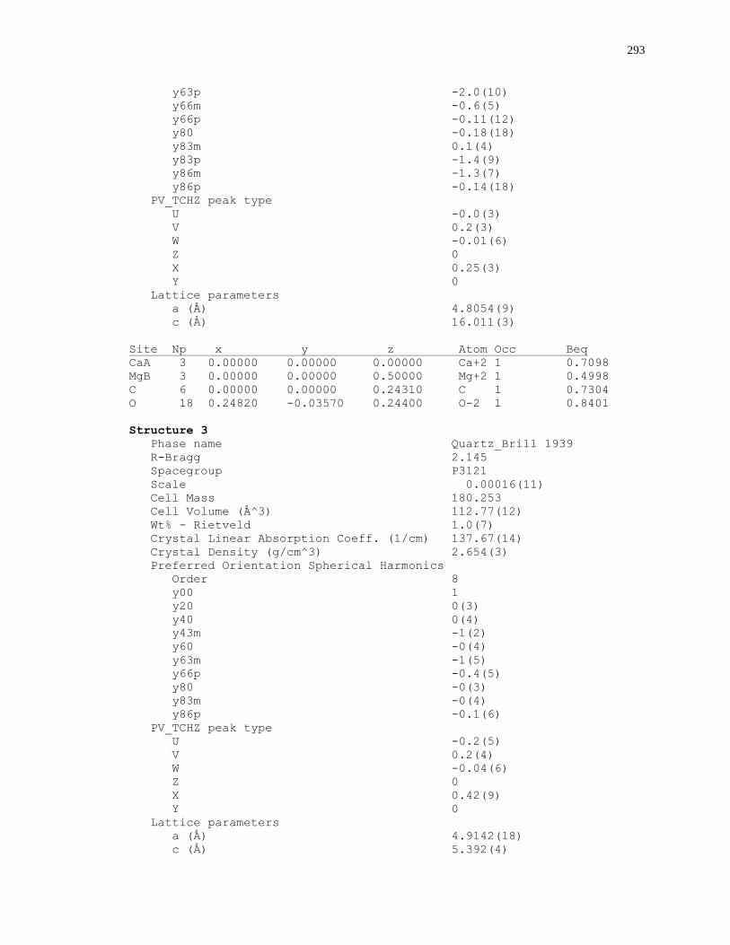
293

y63p -2.0(10)

y66m -0.6(5)

y66p -0.11(12)

y80 -0.18(18)

y83m 0.1(4)

y83p -1.4(9)

y86m -1.3(7)

y86p -0.14(18)

PV_TCHZ peak type

U -0.0(3)

V 0.2(3)

W -0.01(6)

Z 0

X 0.25(3)

Y 0

Lattice parameters

a (Å) 4.8054(9)

c (Å) 16.011(3)

Site Np x y z Atom Occ Beq

CaA 3 0.00000 0.00000 0.00000 Ca+2 1 0.7098

MgB 3 0.00000 0.00000 0.50000 Mg+2 1 0.4998

C 6 0.00000 0.00000 0.24310 C 1 0.7304

O 18 0.24820 -0.03570 0.24400 O-2 1 0.8401

Structure 3

Phase name Quartz_Brill 1939

R-Bragg 2.145

Spacegroup P3121

Scale 0.00016(11)

Cell Mass 180.253

Cell Volume (Å^3) 112.77(12)

Wt% - Rietveld 1.0(7)

Crystal Linear Absorption Coeff. (1/cm) 137.67(14)

Crystal Density (g/cm^3) 2.654(3)

Preferred Orientation Spherical Harmonics

Order 8

y00 1

y20 0(3)

y40 0(4)

y43m -1(2)

y60 -0(4)

y63m -1(5)

y66p -0.4(5)

y80 -0(3)

y83m -0(4)

y86p -0.1(6)

PV_TCHZ peak type

U -0.2(5)

V 0.2(4)

W -0.04(6)

Z 0

X 0.42(9)

Y 0

Lattice parameters

a (Å) 4.9142(18)

c (Å) 5.392(4)

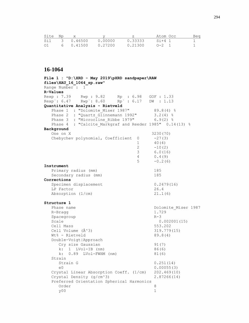
294

Site Np x y z Atom Occ Beq

Si1 3 0.46500 0.00000 0.33333 Si+4 1 1

O1 6 0.41500 0.27200 0.21300 O-2 1 1

16-1064

File 1 : "D:\XRD - May 2019\pXRD sandpaper\RAW

files\HAU_16_1064_sp.raw"

Range Number : 1

R-Values

Rexp : 7.39 Rwp : 9.82 Rp : 6.98 GOF : 1.33

Rexp`: 6.47 Rwp`: 8.60 Rp` : 6.17 DW : 1.13

Quantitative Analysis - Rietveld

Phase 1 : "Dolomite_Miser 1987" 89.8(4) %

Phase 2 : "Quartz_Glinnemann 1992" 3.2(4) %

Phase 3 : "Microcline_Ribbe 1979" 6.9(2) %

Phase 4 : "Calcite_Markgraf and Reeder 1985" 0.14(13) %

Background

One on X 3230(70)

Chebychev polynomial, Coefficient 0 -27(3)

1 40(4)

2 -10(2)

3 6.0(16)

4 0.4(9)

5 -0.2(6)

Instrument

Primary radius (mm) 185

Secondary radius (mm) 185

Corrections

Specimen displacement 0.2479(16)

LP Factor 26.4

Absorption (1/cm) 21.1(6)

Structure 1

Phase name Dolomite_Miser 1987

R-Bragg 1.729

Spacegroup R-3

Scale 0.002001(15)

Cell Mass 553.202

Cell Volume (Å^3) 319.779(15)

Wt% - Rietveld 89.8(4)

Double-Voigt|Approach

Cry size Gaussian 91(7)

k: 1 LVol-IB (nm) 86(6)

k: 0.89 LVol-FWHM (nm) 81(6)

Strain

Strain G 0.251(14)

e0 0.00055(3)

Crystal Linear Absorption Coeff. (1/cm) 202.469(10)

Crystal Density (g/cm^3) 2.87266(14)

Preferred Orientation Spherical Harmonics

Order 8

y00 1

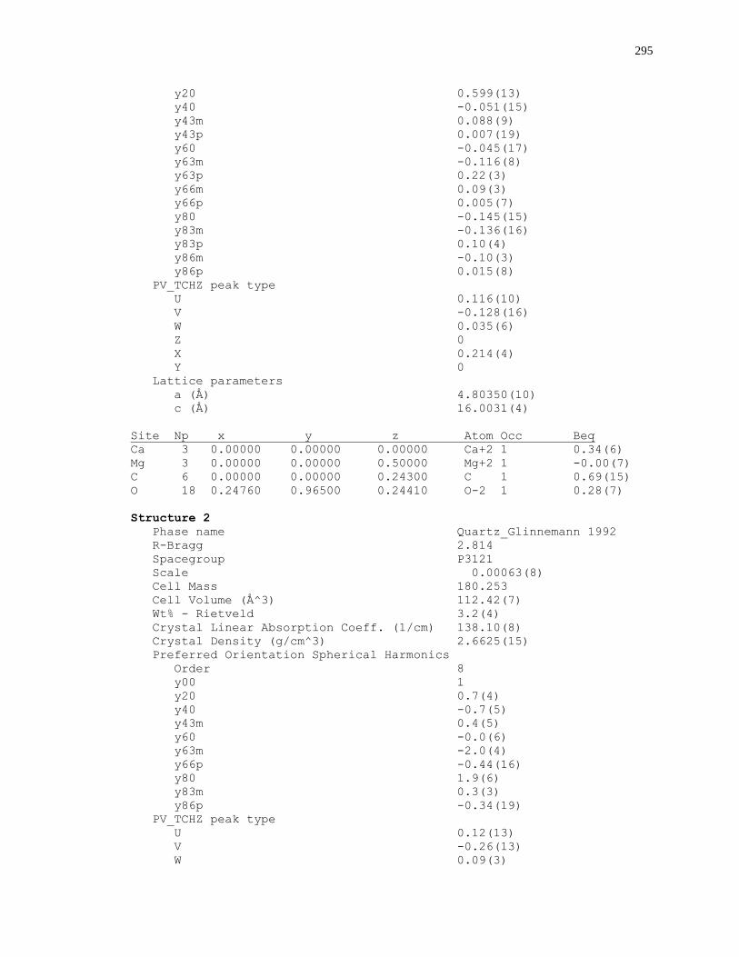
295

y20 0.599(13)

y40 -0.051(15)

y43m 0.088(9)

y43p 0.007(19)

y60 -0.045(17)

y63m -0.116(8)

y63p 0.22(3)

y66m 0.09(3)

y66p 0.005(7)

y80 -0.145(15)

y83m -0.136(16)

y83p 0.10(4)

y86m -0.10(3)

y86p 0.015(8)

PV_TCHZ peak type

U 0.116(10)

V -0.128(16)

W 0.035(6)

Z 0

X 0.214(4)

Y 0

Lattice parameters

a (Å) 4.80350(10)

c (Å) 16.0031(4)

Site Np x y z Atom Occ Beq

Ca 3 0.00000 0.00000 0.00000 Ca+2 1 0.34(6)

Mg 3 0.00000 0.00000 0.50000 Mg+2 1 -0.00(7)

C 6 0.00000 0.00000 0.24300 C 1 0.69(15)

O 18 0.24760 0.96500 0.24410 O-2 1 0.28(7)

Structure 2

Phase name Quartz_Glinnemann 1992

R-Bragg 2.814

Spacegroup P3121

Scale 0.00063(8)

Cell Mass 180.253

Cell Volume (Å^3) 112.42(7)

Wt% - Rietveld 3.2(4)

Crystal Linear Absorption Coeff. (1/cm) 138.10(8)

Crystal Density (g/cm^3) 2.6625(15)

Preferred Orientation Spherical Harmonics

Order 8

y00 1

y20 0.7(4)

y40 -0.7(5)

y43m 0.4(5)

y60 -0.0(6)

y63m -2.0(4)

y66p -0.44(16)

y80 1.9(6)

y83m 0.3(3)

y86p -0.34(19)

PV_TCHZ peak type

U 0.12(13)

V -0.26(13)

W 0.09(3)

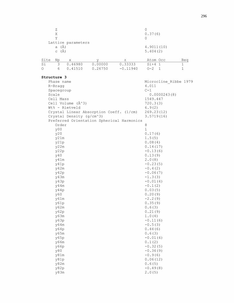
296

Z 0

X 0.37(6)

Y 0

Lattice parameters

a (Å) 4.9011(10)

c (Å) 5.404(2)

Site Np x y z Atom Occ Beq

Si 3 0.46980 0.00000 0.33333 Si+4 1 1

O 6 0.41510 0.26750 -0.11940 O-2 1 1

Structure 3

Phase name Microcline_Ribbe 1979

R-Bragg 4.011

Spacegroup C-1

Scale 0.0000243(8)

Cell Mass 1549.447

Cell Volume (Å^3) 720.3(3)

Wt% - Rietveld 6.9(2)

Crystal Linear Absorption Coeff. (1/cm) 269.23(12)

Crystal Density (g/cm^3) 3.5719(16)

Preferred Orientation Spherical Harmonics

Order 8

y00 1

y20 0.17(6)

y21m 1.5(5)

y21p 0.08(4)

y22m 0.14(17)

y22p -0.13(6)

y40 0.13(9)

y41m 2.0(8)

y41p -0.23(5)

y42m -0.4(2)

y42p -0.06(7)

y43m -1.3(3)

y43p -0.01(4)

y44m -0.1(2)

y44p 0.03(5)

y60 0.20(9)

y61m -2.2(9)

y61p 0.35(9)

y62m 0.6(3)

y62p 0.21(9)

y63m 1.0(4)

y63p -0.11(6)

y64m -0.5(3)

y64p 0.44(6)

y65m 0.6(3)

y65p -0.01(4)

y66m 0.1(2)

y66p -0.32(5)

y80 -0.36(9)

y81m -0.9(6)

y81p 0.06(12)

y82m 0.6(5)

y82p -0.49(8)

y83m 2.0(5)

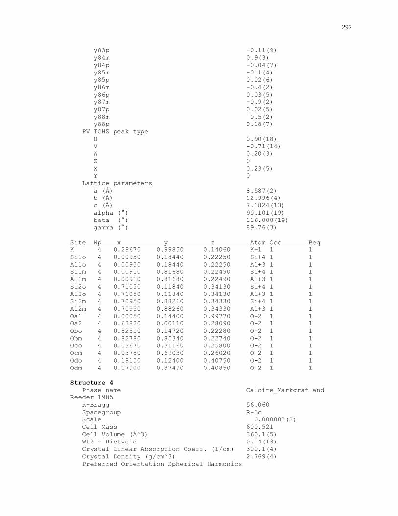
297

y83p -0.11(9)

y84m 0.9(3)

y84p -0.04(7)

y85m -0.1(4)

y85p 0.02(6)

y86m -0.4(2)

y86p 0.03(5)

y87m -0.9(2)

y87p 0.02(5)

y88m -0.5(2)

y88p 0.18(7)

PV_TCHZ peak type

U 0.90(18)

V -0.71(14)

W 0.20(3)

Z 0

X 0.23(5)

Y 0

Lattice parameters

a (Å) 8.587(2)

b (Å) 12.996(4)

c (Å) 7.1824(13)

alpha (°) 90.101(19)

beta (°) 116.008(19)

gamma (°) 89.76(3)

Site Np x y z Atom Occ Beq

K 4 0.28670 0.99850 0.14060 K+1 1 1

Si1o 4 0.00950 0.18440 0.22250 Si+4 1 1

Al1o 4 0.00950 0.18440 0.22250 Al+3 1 1

Si1m 4 0.00910 0.81680 0.22490 Si+4 1 1

Al1m 4 0.00910 0.81680 0.22490 Al+3 1 1

Si2o 4 0.71050 0.11840 0.34130 Si+4 1 1

Al2o 4 0.71050 0.11840 0.34130 Al+3 1 1

Si2m 4 0.70950 0.88260 0.34330 Si+4 1 1

Al2m 4 0.70950 0.88260 0.34330 Al+3 1 1

Oa1 4 0.00050 0.14400 0.99770 O-2 1 1

Oa2 4 0.63820 0.00110 0.28090 O-2 1 1

Obo 4 0.82510 0.14720 0.22280 O-2 1 1

Obm 4 0.82780 0.85340 0.22740 O-2 1 1

Oco 4 0.03670 0.31160 0.25800 O-2 1 1

Ocm 4 0.03780 0.69030 0.26020 O-2 1 1

Odo 4 0.18150 0.12400 0.40750 O-2 1 1

Odm 4 0.17900 0.87490 0.40850 O-2 1 1

Structure 4

Phase name Calcite_Markgraf and

Reeder 1985

R-Bragg 56.060

Spacegroup R-3c

Scale 0.000003(2)

Cell Mass 600.521

Cell Volume (Å^3) 360.1(5)

Wt% - Rietveld 0.14(13)

Crystal Linear Absorption Coeff. (1/cm) 300.1(4)

Crystal Density (g/cm^3) 2.769(4)

Preferred Orientation Spherical Harmonics

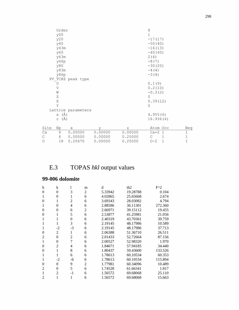
298

Order 8

y00 1

y20 -17(17)

y40 -50(40)

y43m -16(13)

y60 -40(40)

y63m 2(4)

y66p -8(7)

y80 -30(20)

y83m -4(4)

y86p -3(4)

PV_TCHZ peak type

U 0.1(9)

V 0.2(10)

W -0.3(2)

Z 0

X 0.39(12)

Y 0

Lattice parameters

a (Å) 4.955(4)

c (Å) 16.936(4)

Site Np x y z Atom Occ Beq

Ca 6 0.00000 0.00000 0.00000 Ca+2 1 1

C 6 0.00000 0.00000 0.25000 C 1 1

O 18 0.25670 0.00000 0.25000 O-2 1 1

E.3 TOPAS hkl output values

99-006 dolomite

h k l m d th2 F^2

0 0 3 2 5.33942 19.28788 0.104

1 0 1 6 4.02865 25.65668 2.674

0 1 2 6 3.69343 28.03082 4.794

1 0 4 6 2.88586 36.11301 272.360

0 0 6 2 2.66971 39.15112 19.455

0 1 5 6 2.53877 41.25981 21.056

1 1 0 6 2.40319 43.70361 39.759

1 1 3 6 2.19145 48.17986 10.589

1 -2 -3 6 2.19145 48.17986 37.713

0 2 1 6 2.06388 51.36710 26.511

2 0 2 6 2.01433 52.72664 87.156

1 0 7 6 2.00527 52.98320 1.970

0 2 4 6 1.84671 57.94185 34.440

0 1 8 6 1.80437 59.43600 133.526

1 1 6 6 1.78613 60.10534 60.353

1 -2 -6 6 1.78613 60.10534 115.894

0 0 9 2 1.77981 60.34096 10.489

2 0 5 6 1.74528 61.66341 1.817

1 2 -1 6 1.56572 69.68068 25.110

2 1 1 6 1.56572 69.68068 15.663

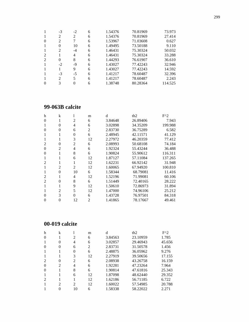
299

1 -3 -2 6 1.54376 70.81969 73.973

1 2 2 6 1.54376 70.81969 27.414

0 2 7 6 1.53967 71.03608 0.627

1 0 10 6 1.49495 73.50188 9.110

1 2 -4 6 1.46431 75.30324 50.032

2 1 4 6 1.46431 75.30324 33.288

2 0 8 6 1.44293 76.61907 36.610

1 -2 -9 6 1.43027 77.42243 32.946

1 1 9 6 1.43027 77.42243 14.592

1 -3 -5 6 1.41217 78.60487 32.396

1 2 5 6 1.41217 78.60487 2.243

0 3 0 6 1.38748 80.28364 114.525

99-063B calcite

h k l m d th2 F^2

0 1 2 6 3.84648 26.89406 7.943

1 0 4 6 3.02898 34.35209 199.988

0 0 6 2 2.83730 36.75289 6.582

1 1 0 6 2.48945 42.11571 41.129

1 1 3 12 2.27972 46.20359 77.412

2 0 2 6 2.08993 50.68108 74.184

0 2 4 6 1.92324 55.43244 36.488

0 1 8 6 1.90824 55.90612 116.311

1 1 6 12 1.87127 57.11084 137.265

2 1 1 12 1.62231 66.92142 31.948

1 2 2 12 1.60065 67.94920 100.810

1 0 10 6 1.58344 68.79081 11.416

2 1 4 12 1.52196 71.99081 60.106

2 0 8 6 1.51449 72.40165 28.222

1 1 9 12 1.50610 72.86973 31.894

1 2 5 12 1.47000 74.96106 25.212

0 3 0 6 1.43728 76.97501 84.318

0 0 12 2 1.41865 78.17667 49.461

00-019 calcite

h k l m d th2 F^2

0 1 2 6 3.84563 23.10959 1.785

1 0 4 6 3.02857 29.46943 45.656

0 0 6 2 2.83731 31.50578 1.456

1 1 0 6 2.48875 36.05962 9.276

1 1 3 12 2.27919 39.50656 17.155

2 0 2 6 2.08938 43.26758 16.159

0 2 4 6 1.92281 47.23264 7.964

0 1 8 6 1.90814 47.61816 25.343

1 1 6 12 1.87098 48.62440 29.352

2 1 1 12 1.62186 56.71185 6.722

1 2 2 12 1.60022 57.54985 20.788

1 0 10 6 1.58338 58.22022 2.271

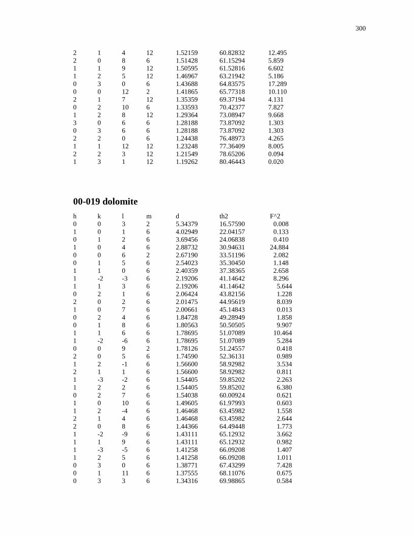
300

2 1 4 12 1.52159 60.82832 12.495

2 0 8 6 1.51428 61.15294 5.859

1 1 9 12 1.50595 61.52816 6.602

1 2 5 12 1.46967 63.21942 5.186

0 3 0 6 1.43688 64.83575 17.289

0 0 12 2 1.41865 65.77318 10.110

2 1 7 12 1.35359 69.37194 4.131

0 2 10 6 1.33593 70.42377 7.827

1 2 8 12 1.29364 73.08947 9.668

3 0 6 6 1.28188 73.87092 1.303

0 3 6 6 1.28188 73.87092 1.303

2 2 0 6 1.24438 76.48973 4.265

1 1 12 12 1.23248 77.36409 8.005

2 2 3 12 1.21549 78.65206 0.094

1 3 1 12 1.19262 80.46443 0.020

00-019 dolomite

h k l m d th2 F^2

0 0 3 2 5.34379 16.57590 0.008

1 0 1 6 4.02949 22.04157 0.133

0 1 2 6 3.69456 24.06838 0.410

1 0 4 6 2.88732 30.94631 24.884

0 0 6 2 2.67190 33.51196 2.082

0 1 5 6 2.54023 35.30450 1.148

1 1 0 6 2.40359 37.38365 2.658

1 -2 -3 6 2.19206 41.14642 8.296

1 1 3 6 2.19206 41.14642 5.644

0 2 1 6 2.06424 43.82156 1.228

2 0 2 6 2.01475 44.95619 8.039

1 0 7 6 2.00661 45.14843 0.013

0 2 4 6 1.84728 49.28949 1.858

0 1 8 6 1.80563 50.50505 9.907

1 1 6 6 1.78695 51.07089 10.464

1 -2 -6 6 1.78695 51.07089 5.284

0 0 9 2 1.78126 51.24557 0.418

2 0 5 6 1.74590 52.36131 0.989

1 2 -1 6 1.56600 58.92982 3.534

2 1 1 6 1.56600 58.92982 0.811

1 -3 -2 6 1.54405 59.85202 2.263

1 2 2 6 1.54405 59.85202 6.380

0 2 7 6 1.54038 60.00924 0.621

1 0 10 6 1.49605 61.97993 0.603

1 2 -4 6 1.46468 63.45982 1.558

2 1 4 6 1.46468 63.45982 2.644

2 0 8 6 1.44366 64.49448 1.773

1 -2 -9 6 1.43111 65.12932 3.662

1 1 9 6 1.43111 65.12932 0.982

1 -3 -5 6 1.41258 66.09208 1.407

1 2 5 6 1.41258 66.09208 1.011

0 3 0 6 1.38771 67.43299 7.428

0 1 11 6 1.37555 68.11076 0.675

0 3 3 6 1.34316 69.98865 0.584

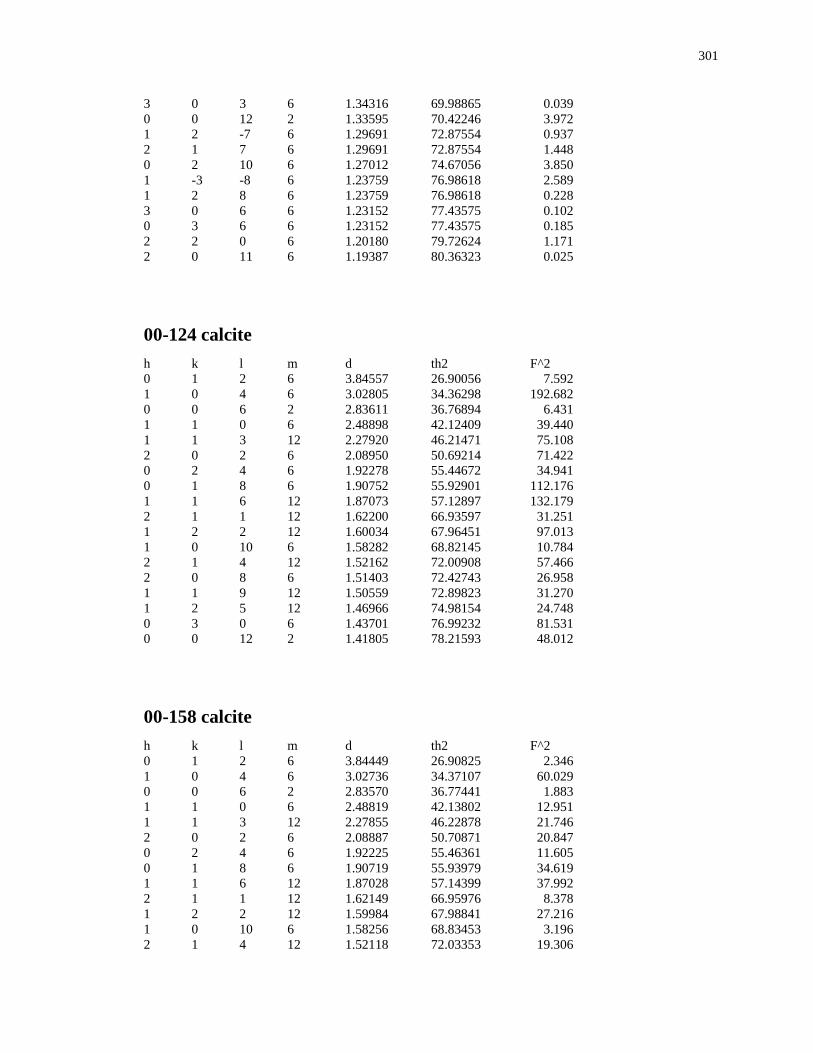
301

3 0 3 6 1.34316 69.98865 0.039

0 0 12 2 1.33595 70.42246 3.972

1 2 -7 6 1.29691 72.87554 0.937

2 1 7 6 1.29691 72.87554 1.448

0 2 10 6 1.27012 74.67056 3.850

1 -3 -8 6 1.23759 76.98618 2.589

1 2 8 6 1.23759 76.98618 0.228

3 0 6 6 1.23152 77.43575 0.102

0 3 6 6 1.23152 77.43575 0.185

2 2 0 6 1.20180 79.72624 1.171

2 0 11 6 1.19387 80.36323 0.025

00-124 calcite

h k l m d th2 F^2

0 1 2 6 3.84557 26.90056 7.592

1 0 4 6 3.02805 34.36298 192.682

0 0 6 2 2.83611 36.76894 6.431

1 1 0 6 2.48898 42.12409 39.440

1 1 3 12 2.27920 46.21471 75.108

2 0 2 6 2.08950 50.69214 71.422

0 2 4 6 1.92278 55.44672 34.941

0 1 8 6 1.90752 55.92901 112.176

1 1 6 12 1.87073 57.12897 132.179

2 1 1 12 1.62200 66.93597 31.251

1 2 2 12 1.60034 67.96451 97.013

1 0 10 6 1.58282 68.82145 10.784

2 1 4 12 1.52162 72.00908 57.466

2 0 8 6 1.51403 72.42743 26.958

1 1 9 12 1.50559 72.89823 31.270

1 2 5 12 1.46966 74.98154 24.748

0 3 0 6 1.43701 76.99232 81.531

0 0 12 2 1.41805 78.21593 48.012

00-158 calcite

h k l m d th2 F^2

0 1 2 6 3.84449 26.90825 2.346

1 0 4 6 3.02736 34.37107 60.029

0 0 6 2 2.83570 36.77441 1.883

1 1 0 6 2.48819 42.13802 12.951

1 1 3 12 2.27855 46.22878 21.746

2 0 2 6 2.08887 50.70871 20.847

0 2 4 6 1.92225 55.46361 11.605

0 1 8 6 1.90719 55.93979 34.619

1 1 6 12 1.87028 57.14399 37.992

2 1 1 12 1.62149 66.95976 8.378

1 2 2 12 1.59984 67.98841 27.216

1 0 10 6 1.58256 68.83453 3.196

2 1 4 12 1.52118 72.03353 19.306

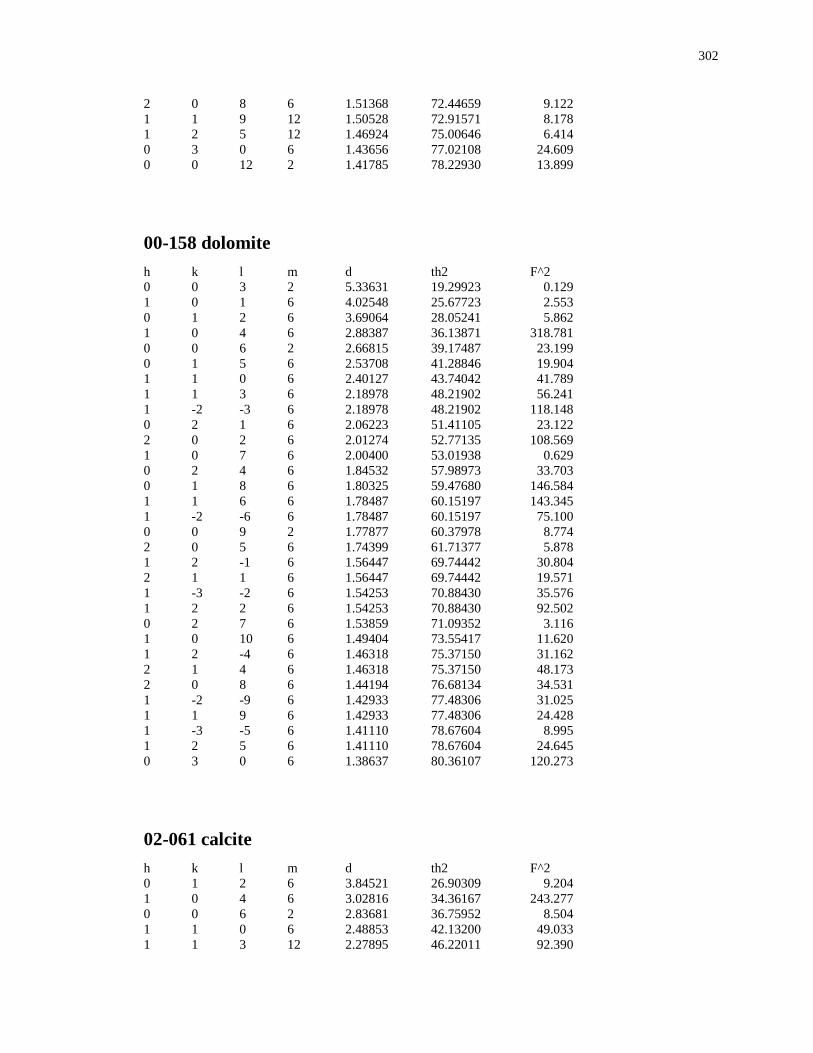
302

2 0 8 6 1.51368 72.44659 9.122

1 1 9 12 1.50528 72.91571 8.178

1 2 5 12 1.46924 75.00646 6.414

0 3 0 6 1.43656 77.02108 24.609

0 0 12 2 1.41785 78.22930 13.899

00-158 dolomite

h k l m d th2 F^2

0 0 3 2 5.33631 19.29923 0.129

1 0 1 6 4.02548 25.67723 2.553

0 1 2 6 3.69064 28.05241 5.862

1 0 4 6 2.88387 36.13871 318.781

0 0 6 2 2.66815 39.17487 23.199

0 1 5 6 2.53708 41.28846 19.904

1 1 0 6 2.40127 43.74042 41.789

1 1 3 6 2.18978 48.21902 56.241

1 -2 -3 6 2.18978 48.21902 118.148

0 2 1 6 2.06223 51.41105 23.122

2 0 2 6 2.01274 52.77135 108.569

1 0 7 6 2.00400 53.01938 0.629

0 2 4 6 1.84532 57.98973 33.703

0 1 8 6 1.80325 59.47680 146.584

1 1 6 6 1.78487 60.15197 143.345

1 -2 -6 6 1.78487 60.15197 75.100

0 0 9 2 1.77877 60.37978 8.774

2 0 5 6 1.74399 61.71377 5.878

1 2 -1 6 1.56447 69.74442 30.804

2 1 1 6 1.56447 69.74442 19.571

1 -3 -2 6 1.54253 70.88430 35.576

1 2 2 6 1.54253 70.88430 92.502

0 2 7 6 1.53859 71.09352 3.116

1 0 10 6 1.49404 73.55417 11.620

1 2 -4 6 1.46318 75.37150 31.162

2 1 4 6 1.46318 75.37150 48.173

2 0 8 6 1.44194 76.68134 34.531

1 -2 -9 6 1.42933 77.48306 31.025

1 1 9 6 1.42933 77.48306 24.428

1 -3 -5 6 1.41110 78.67604 8.995

1 2 5 6 1.41110 78.67604 24.645

0 3 0 6 1.38637 80.36107 120.273

02-061 calcite

h k l m d th2 F^2

0 1 2 6 3.84521 26.90309 9.204

1 0 4 6 3.02816 34.36167 243.277

0 0 6 2 2.83681 36.75952 8.504

1 1 0 6 2.48853 42.13200 49.033

1 1 3 12 2.27895 46.22011 92.390

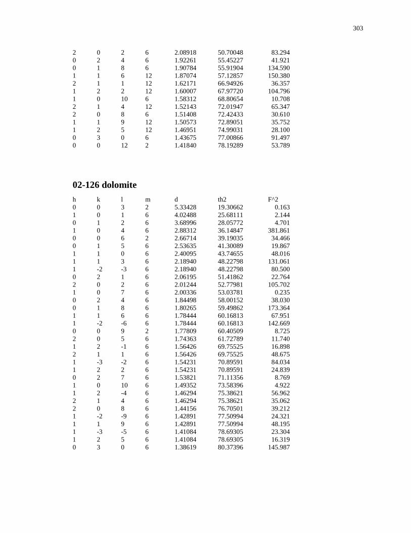
303

2 0 2 6 2.08918 50.70048 83.294

0 2 4 6 1.92261 55.45227 41.921

0 1 8 6 1.90784 55.91904 134.590

1 1 6 12 1.87074 57.12857 150.380

2 1 1 12 1.62171 66.94926 36.357

1 2 2 12 1.60007 67.97720 104.796

1 0 10 6 1.58312 68.80654 10.708

2 1 4 12 1.52143 72.01947 65.347

2 0 8 6 1.51408 72.42433 30.610

1 1 9 12 1.50573 72.89051 35.752

1 2 5 12 1.46951 74.99031 28.100

0 3 0 6 1.43675 77.00866 91.497

0 0 12 2 1.41840 78.19289 53.789

02-126 dolomite

h k l m d th2 F^2

0 0 3 2 5.33428 19.30662 0.163

1 0 1 6 4.02488 25.68111 2.144

0 1 2 6 3.68996 28.05772 4.701

1 0 4 6 2.88312 36.14847 381.861

0 0 6 2 2.66714 39.19035 34.466

0 1 5 6 2.53635 41.30089 19.867

1 1 0 6 2.40095 43.74655 48.016

1 1 3 6 2.18940 48.22798 131.061

1 -2 -3 6 2.18940 48.22798 80.500

0 2 1 6 2.06195 51.41862 22.764

2 0 2 6 2.01244 52.77981 105.702

1 0 7 6 2.00336 53.03781 0.235

0 2 4 6 1.84498 58.00152 38.030

0 1 8 6 1.80265 59.49862 173.364

1 1 6 6 1.78444 60.16813 67.951

1 -2 -6 6 1.78444 60.16813 142.669

0 0 9 2 1.77809 60.40509 8.725

2 0 5 6 1.74363 61.72789 11.740

1 2 -1 6 1.56426 69.75525 16.898

2 1 1 6 1.56426 69.75525 48.675

1 -3 -2 6 1.54231 70.89591 84.034

1 2 2 6 1.54231 70.89591 24.839

0 2 7 6 1.53821 71.11356 8.769

1 0 10 6 1.49352 73.58396 4.922

1 2 -4 6 1.46294 75.38621 56.962

2 1 4 6 1.46294 75.38621 35.062

2 0 8 6 1.44156 76.70501 39.212

1 -2 -9 6 1.42891 77.50994 24.321

1 1 9 6 1.42891 77.50994 48.195

1 -3 -5 6 1.41084 78.69305 23.304

1 2 5 6 1.41084 78.69305 16.319

0 3 0 6 1.38619 80.37396 145.987

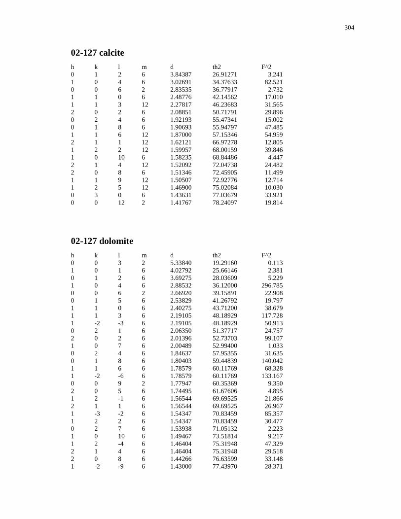
304

02-127 calcite

h k l m d th2 F^2

0 1 2 6 3.84387 26.91271 3.241

1 0 4 6 3.02691 34.37633 82.521

0 0 6 2 2.83535 36.77917 2.732

1 1 0 6 2.48776 42.14562 17.010

1 1 3 12 2.27817 46.23683 31.565

2 0 2 6 2.08851 50.71791 29.896

0 2 4 6 1.92193 55.47341 15.002

0 1 8 6 1.90693 55.94797 47.485

1 1 6 12 1.87000 57.15346 54.959

2 1 1 12 1.62121 66.97278 12.805

1 2 2 12 1.59957 68.00159 39.846

1 0 10 6 1.58235 68.84486 4.447

2 1 4 12 1.52092 72.04738 24.482

2 0 8 6 1.51346 72.45905 11.499

1 1 9 12 1.50507 72.92776 12.714

1 2 5 12 1.46900 75.02084 10.030

0 3 0 6 1.43631 77.03679 33.921

0 0 12 2 1.41767 78.24097 19.814

02-127 dolomite

h k l m d th2 F^2

0 0 3 2 5.33840 19.29160 0.113

1 0 1 6 4.02792 25.66146 2.381

0 1 2 6 3.69275 28.03609 5.229

1 0 4 6 2.88532 36.12000 296.785

0 0 6 2 2.66920 39.15891 22.908

0 1 5 6 2.53829 41.26792 19.797

1 1 0 6 2.40275 43.71200 38.679

1 1 3 6 2.19105 48.18929 117.728

1 -2 -3 6 2.19105 48.18929 50.913

0 2 1 6 2.06350 51.37717 24.757

2 0 2 6 2.01396 52.73703 99.107

1 0 7 6 2.00489 52.99400 1.033

0 2 4 6 1.84637 57.95355 31.635

0 1 8 6 1.80403 59.44839 140.042

1 1 6 6 1.78579 60.11769 68.328

1 -2 -6 6 1.78579 60.11769 133.167

0 0 9 2 1.77947 60.35369 9.350

2 0 5 6 1.74495 61.67606 4.895

1 2 -1 6 1.56544 69.69525 21.866

2 1 1 6 1.56544 69.69525 26.967

1 -3 -2 6 1.54347 70.83459 85.357

1 2 2 6 1.54347 70.83459 30.477

0 2 7 6 1.53938 71.05132 2.223

1 0 10 6 1.49467 73.51814 9.217

1 2 -4 6 1.46404 75.31948 47.329

2 1 4 6 1.46404 75.31948 29.518

2 0 8 6 1.44266 76.63599 33.148

1 -2 -9 6 1.43000 77.43970 28.371

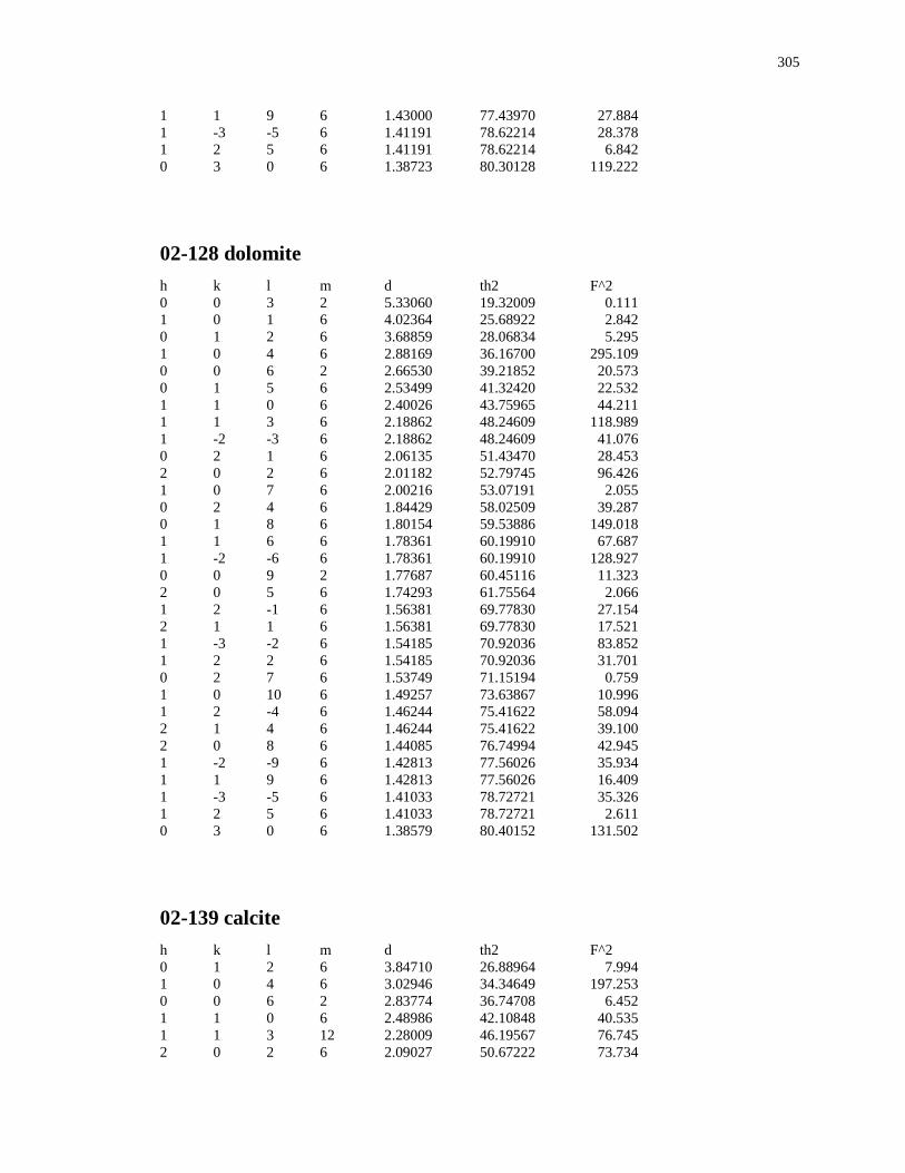
305

1 1 9 6 1.43000 77.43970 27.884

1 -3 -5 6 1.41191 78.62214 28.378

1 2 5 6 1.41191 78.62214 6.842

0 3 0 6 1.38723 80.30128 119.222

02-128 dolomite

h k l m d th2 F^2

0 0 3 2 5.33060 19.32009 0.111

1 0 1 6 4.02364 25.68922 2.842

0 1 2 6 3.68859 28.06834 5.295

1 0 4 6 2.88169 36.16700 295.109

0 0 6 2 2.66530 39.21852 20.573

0 1 5 6 2.53499 41.32420 22.532

1 1 0 6 2.40026 43.75965 44.211

1 1 3 6 2.18862 48.24609 118.989

1 -2 -3 6 2.18862 48.24609 41.076

0 2 1 6 2.06135 51.43470 28.453

2 0 2 6 2.01182 52.79745 96.426

1 0 7 6 2.00216 53.07191 2.055

0 2 4 6 1.84429 58.02509 39.287

0 1 8 6 1.80154 59.53886 149.018

1 1 6 6 1.78361 60.19910 67.687

1 -2 -6 6 1.78361 60.19910 128.927

0 0 9 2 1.77687 60.45116 11.323

2 0 5 6 1.74293 61.75564 2.066

1 2 -1 6 1.56381 69.77830 27.154

2 1 1 6 1.56381 69.77830 17.521

1 -3 -2 6 1.54185 70.92036 83.852

1 2 2 6 1.54185 70.92036 31.701

0 2 7 6 1.53749 71.15194 0.759

1 0 10 6 1.49257 73.63867 10.996

1 2 -4 6 1.46244 75.41622 58.094

2 1 4 6 1.46244 75.41622 39.100

2 0 8 6 1.44085 76.74994 42.945

1 -2 -9 6 1.42813 77.56026 35.934

1 1 9 6 1.42813 77.56026 16.409

1 -3 -5 6 1.41033 78.72721 35.326

1 2 5 6 1.41033 78.72721 2.611

0 3 0 6 1.38579 80.40152 131.502

02-139 calcite

h k l m d th2 F^2

0 1 2 6 3.84710 26.88964 7.994

1 0 4 6 3.02946 34.34649 197.253

0 0 6 2 2.83774 36.74708 6.452

1 1 0 6 2.48986 42.10848 40.535

1 1 3 12 2.28009 46.19567 76.745

2 0 2 6 2.09027 50.67222 73.734

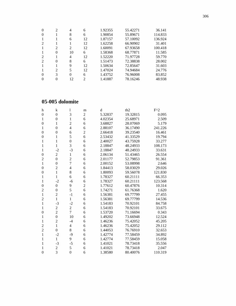
306

0 2 4 6 1.92355 55.42271 36.141

0 1 8 6 1.90854 55.89671 114.833

1 1 6 12 1.87157 57.10092 136.924

2 1 1 12 1.62258 66.90902 31.401

1 2 2 12 1.60091 67.93658 100.418

1 0 10 6 1.58368 68.77871 11.585

2 1 4 12 1.52220 71.97728 59.770

2 0 8 6 1.51473 72.38838 28.002

1 1 9 12 1.50634 72.85647 31.603

1 2 5 12 1.47024 74.94684 24.776

0 3 0 6 1.43752 76.96008 83.852

0 0 12 2 1.41887 78.16246 48.938

05-005 dolomite

h k l m d th2 F^2

0 0 3 2 5.32837 19.32815 0.095

1 0 1 6 4.02354 25.68971 2.509

0 1 2 6 3.68827 28.07069 5.179

1 0 4 6 2.88107 36.17490 241.226

0 0 6 2 2.66418 39.23540 16.461

0 1 5 6 2.53432 41.33529 19.794

1 1 0 6 2.40027 43.75928 33.277

1 1 3 6 2.18847 48.24933 108.173

1 -2 -3 6 2.18847 48.24933 33.631

0 2 1 6 2.06134 51.43465 26.554

2 0 2 6 2.01177 52.79853 91.361

1 0 7 6 2.00152 53.08998 2.646

0 2 4 6 1.84413 58.03029 29.026

0 1 8 6 1.80093 59.56078 121.830

1 1 6 6 1.78327 60.21111 66.353

1 -2 -6 6 1.78327 60.21111 123.568

0 0 9 2 1.77612 60.47876 10.314

2 0 5 6 1.74271 61.76368 1.620

1 2 -1 6 1.56381 69.77799 27.455

2 1 1 6 1.56381 69.77799 14.536

1 -3 -2 6 1.54183 70.92101 84.758

1 2 2 6 1.54183 70.92101 33.675

0 2 7 6 1.53720 71.16694 0.343

1 0 10 6 1.49202 73.66948 12.524

1 2 -4 6 1.46236 75.42052 45.205

2 1 4 6 1.46236 75.42052 29.112

2 0 8 6 1.44053 76.76910 32.653

1 -2 -9 6 1.42774 77.58459 34.892

1 1 9 6 1.42774 77.58459 15.058

1 -3 -5 6 1.41021 78.73418 35.556

1 2 5 6 1.41021 78.73418 2.047

0 3 0 6 1.38580 80.40076 110.319

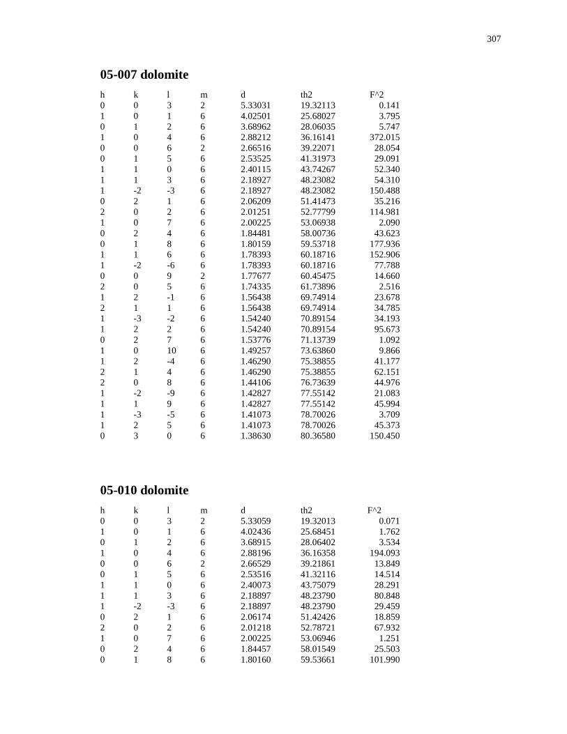
307

05-007 dolomite

h k l m d th2 F^2

0 0 3 2 5.33031 19.32113 0.141

1 0 1 6 4.02501 25.68027 3.795

0 1 2 6 3.68962 28.06035 5.747

1 0 4 6 2.88212 36.16141 372.015

0 0 6 2 2.66516 39.22071 28.054

0 1 5 6 2.53525 41.31973 29.091

1 1 0 6 2.40115 43.74267 52.340

1 1 3 6 2.18927 48.23082 54.310

1 -2 -3 6 2.18927 48.23082 150.488

0 2 1 6 2.06209 51.41473 35.216

2 0 2 6 2.01251 52.77799 114.981

1 0 7 6 2.00225 53.06938 2.090

0 2 4 6 1.84481 58.00736 43.623

0 1 8 6 1.80159 59.53718 177.936

1 1 6 6 1.78393 60.18716 152.906

1 -2 -6 6 1.78393 60.18716 77.788

0 0 9 2 1.77677 60.45475 14.660

2 0 5 6 1.74335 61.73896 2.516

1 2 -1 6 1.56438 69.74914 23.678

2 1 1 6 1.56438 69.74914 34.785

1 -3 -2 6 1.54240 70.89154 34.193

1 2 2 6 1.54240 70.89154 95.673

0 2 7 6 1.53776 71.13739 1.092

1 0 10 6 1.49257 73.63860 9.866

1 2 -4 6 1.46290 75.38855 41.177

2 1 4 6 1.46290 75.38855 62.151

2 0 8 6 1.44106 76.73639 44.976

1 -2 -9 6 1.42827 77.55142 21.083

1 1 9 6 1.42827 77.55142 45.994

1 -3 -5 6 1.41073 78.70026 3.709

1 2 5 6 1.41073 78.70026 45.373

0 3 0 6 1.38630 80.36580 150.450

05-010 dolomite

h k l m d th2 F^2

0 0 3 2 5.33059 19.32013 0.071

1 0 1 6 4.02436 25.68451 1.762

0 1 2 6 3.68915 28.06402 3.534

1 0 4 6 2.88196 36.16358 194.093

0 0 6 2 2.66529 39.21861 13.849

0 1 5 6 2.53516 41.32116 14.514

1 1 0 6 2.40073 43.75079 28.291

1 1 3 6 2.18897 48.23790 80.848

1 -2 -3 6 2.18897 48.23790 29.459

0 2 1 6 2.06174 51.42426 18.859

2 0 2 6 2.01218 52.78721 67.932

1 0 7 6 2.00225 53.06946 1.251

0 2 4 6 1.84457 58.01549 25.503

0 1 8 6 1.80160 59.53661 101.990

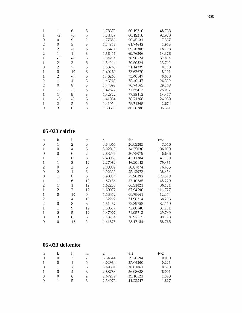
308

1 1 6 6 1.78379 60.19210 48.768

1 -2 -6 6 1.78379 60.19210 92.920

0 0 9 2 1.77686 60.45131 7.537

2 0 5 6 1.74316 61.74642 1.915

1 2 -1 6 1.56411 69.76306 18.708

2 1 1 6 1.56411 69.76306 14.376

1 -3 -2 6 1.54214 70.90524 62.814

1 2 2 6 1.54214 70.90524 23.712

0 2 7 6 1.53765 71.14339 0.718

1 0 10 6 1.49260 73.63670 8.191

1 2 -4 6 1.46268 75.40147 40.038

2 1 4 6 1.46268 75.40147 26.332

2 0 8 6 1.44098 76.74165 29.268

1 -2 -9 6 1.42822 77.55412 25.017

1 1 9 6 1.42822 77.55412 14.477

1 -3 -5 6 1.41054 78.71268 24.939

1 2 5 6 1.41054 78.71268 2.674

0 3 0 6 1.38606 80.38288 95.331

05-023 calcite

h k l m d th2 F^2

0 1 2 6 3.84665 26.89283 7.516

1 0 4 6 3.02913 34.35036 196.099

0 0 6 2 2.83746 36.75079 6.636

1 1 0 6 2.48955 42.11384 41.199

1 1 3 12 2.27982 46.20142 79.451

2 0 2 6 2.09002 50.67874 76.455

0 2 4 6 1.92333 55.42973 38.454

0 1 8 6 1.90834 55.90292 123.588

1 1 6 12 1.87136 57.10785 145.220

2 1 1 12 1.62238 66.91821 36.121

1 2 2 12 1.60072 67.94590 111.727

1 0 10 6 1.58352 68.78661 12.354

2 1 4 12 1.52202 71.98714 68.296

2 0 8 6 1.51457 72.39755 32.110

1 1 9 12 1.50617 72.86546 37.211

1 2 5 12 1.47007 74.95712 29.749

0 3 0 6 1.43734 76.97115 99.193

0 0 12 2 1.41873 78.17154 58.765

05-023 dolomite

h k l m d th2 F^2

0 0 3 2 5.34544 19.26594 0.010

1 0 1 6 4.02984 25.64900 0.221

0 1 2 6 3.69501 28.01861 0.520

1 0 4 6 2.88788 36.08688 26.001

0 0 6 2 2.67272 39.10521 1.928

0 1 5 6 2.54079 41.22547 1.867

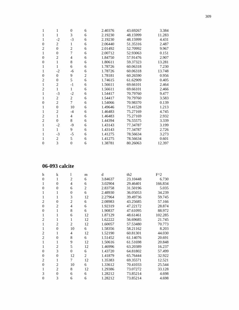
309

1 1 0 6 2.40376 43.69267 3.384

1 1 3 6 2.19230 48.15999 11.283

1 -2 -3 6 2.19230 48.15999 4.431

0 2 1 6 2.06440 51.35316 2.487

2 0 2 6 2.01492 52.70992 9.967

1 0 7 6 2.00712 52.93063 0.151

0 2 4 6 1.84750 57.91476 2.907

0 1 8 6 1.80611 59.37323 13.281

1 1 6 6 1.78726 60.06318 7.230

1 -2 -6 6 1.78726 60.06318 13.748

0 0 9 2 1.78181 60.26590 0.956

2 0 5 6 1.74615 61.62909 0.405

1 2 -1 6 1.56611 69.66101 2.464

2 1 1 6 1.56611 69.66101 2.466

1 -3 -2 6 1.54417 70.79760 9.477

1 2 2 6 1.54417 70.79760 3.583

0 2 7 6 1.54066 70.98370 0.139

1 0 10 6 1.49646 73.41528 1.213

1 2 -4 6 1.46483 75.27169 4.745

2 1 4 6 1.46483 75.27169 2.932

2 0 8 6 1.44394 76.55575 3.339

1 -2 -9 6 1.43143 77.34787 3.199

1 1 9 6 1.43143 77.34787 2.726

1 -3 -5 6 1.41275 78.56634 3.273

1 2 5 6 1.41275 78.56634 0.601

0 3 0 6 1.38781 80.26063 12.397

06-093 calcite

h k l m d th2 F^2

0 1 2 6 3.84637 23.10448 6.730

1 0 4 6 3.02904 29.46401 166.834

0 0 6 2 2.83758 31.50196 5.035

1 1 0 6 2.48930 36.05053 34.239

1 1 3 12 2.27964 39.49736 59.745

2 0 2 6 2.08983 43.25685 57.166

0 2 4 6 1.92319 47.22172 28.874

0 1 8 6 1.90837 47.61095 88.972

1 1 6 12 1.87129 48.61461 102.285

2 1 1 12 1.62222 56.69685 21.745

1 2 2 12 1.60057 57.53480 70.773

1 0 10 6 1.58356 58.21162 8.203

2 1 4 12 1.52190 60.81301 44.030

2 0 8 6 1.51452 61.14076 20.691

1 1 9 12 1.50616 61.51698 20.848

1 2 5 12 1.46996 63.20389 16.237

0 3 0 6 1.43720 64.81802 57.499

0 0 12 2 1.41879 65.76444 32.922

2 1 7 12 1.35383 69.35571 12.521

0 2 10 6 1.33612 70.41033 25.544

1 2 8 12 1.29386 73.07272 33.128

3 0 6 6 1.28212 73.85214 4.698

0 3 6 6 1.28212 73.85214 4.698

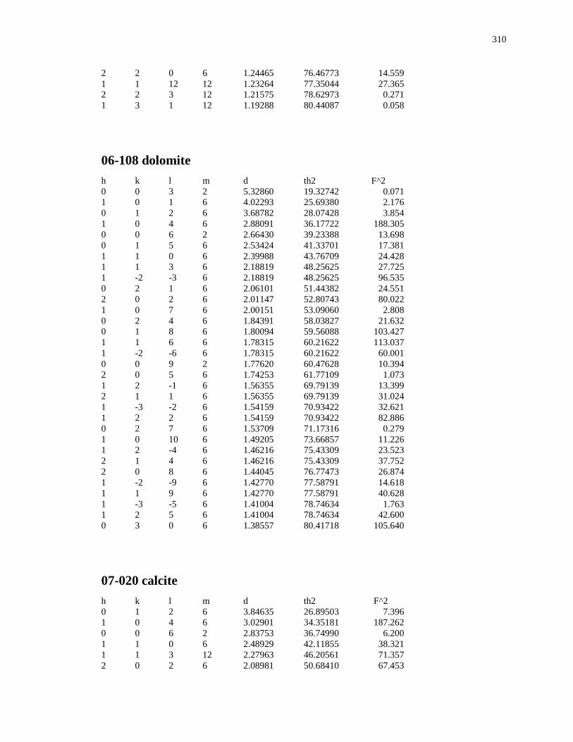
310

2 2 0 6 1.24465 76.46773 14.559

1 1 12 12 1.23264 77.35044 27.365

2 2 3 12 1.21575 78.62973 0.271

1 3 1 12 1.19288 80.44087 0.058

06-108 dolomite

h k l m d th2 F^2

0 0 3 2 5.32860 19.32742 0.071

1 0 1 6 4.02293 25.69380 2.176

0 1 2 6 3.68782 28.07428 3.854

1 0 4 6 2.88091 36.17722 188.305

0 0 6 2 2.66430 39.23388 13.698

0 1 5 6 2.53424 41.33701 17.381

1 1 0 6 2.39988 43.76709 24.428

1 1 3 6 2.18819 48.25625 27.725

1 -2 -3 6 2.18819 48.25625 96.535

0 2 1 6 2.06101 51.44382 24.551

2 0 2 6 2.01147 52.80743 80.022

1 0 7 6 2.00151 53.09060 2.808

0 2 4 6 1.84391 58.03827 21.632

0 1 8 6 1.80094 59.56088 103.427

1 1 6 6 1.78315 60.21622 113.037

1 -2 -6 6 1.78315 60.21622 60.001

0 0 9 2 1.77620 60.47628 10.394

2 0 5 6 1.74253 61.77109 1.073

1 2 -1 6 1.56355 69.79139 13.399

2 1 1 6 1.56355 69.79139 31.024

1 -3 -2 6 1.54159 70.93422 32.621

1 2 2 6 1.54159 70.93422 82.886

0 2 7 6 1.53709 71.17316 0.279

1 0 10 6 1.49205 73.66857 11.226

1 2 -4 6 1.46216 75.43309 23.523

2 1 4 6 1.46216 75.43309 37.752

2 0 8 6 1.44045 76.77473 26.874

1 -2 -9 6 1.42770 77.58791 14.618

1 1 9 6 1.42770 77.58791 40.628

1 -3 -5 6 1.41004 78.74634 1.763

1 2 5 6 1.41004 78.74634 42.600

0 3 0 6 1.38557 80.41718 105.640

07-020 calcite

h k l m d th2 F^2

0 1 2 6 3.84635 26.89503 7.396

1 0 4 6 3.02901 34.35181 187.262

0 0 6 2 2.83753 36.74990 6.200

1 1 0 6 2.48929 42.11855 38.321

1 1 3 12 2.27963 46.20561 71.357

2 0 2 6 2.08981 50.68410 67.453

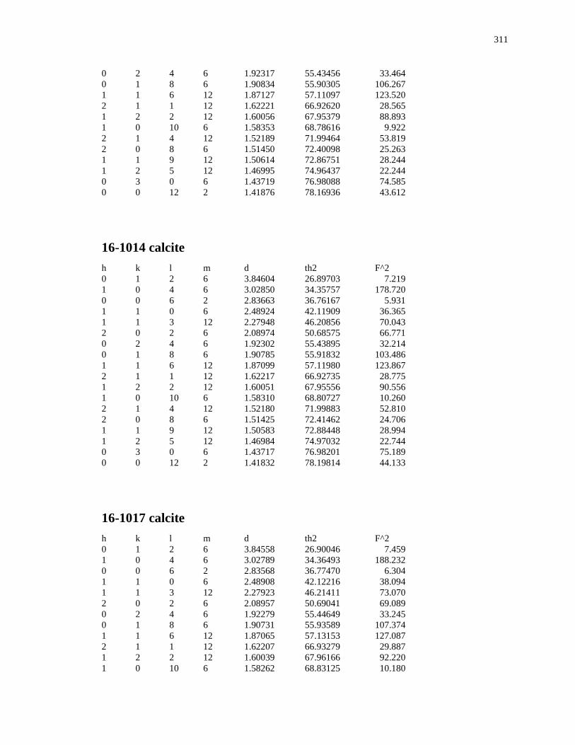
311

0 2 4 6 1.92317 55.43456 33.464

0 1 8 6 1.90834 55.90305 106.267

1 1 6 12 1.87127 57.11097 123.520

2 1 1 12 1.62221 66.92620 28.565

1 2 2 12 1.60056 67.95379 88.893

1 0 10 6 1.58353 68.78616 9.922

2 1 4 12 1.52189 71.99464 53.819

2 0 8 6 1.51450 72.40098 25.263

1 1 9 12 1.50614 72.86751 28.244

1 2 5 12 1.46995 74.96437 22.244

0 3 0 6 1.43719 76.98088 74.585

0 0 12 2 1.41876 78.16936 43.612

16-1014 calcite

h k l m d th2 F^2

0 1 2 6 3.84604 26.89703 7.219

1 0 4 6 3.02850 34.35757 178.720

0 0 6 2 2.83663 36.76167 5.931

1 1 0 6 2.48924 42.11909 36.365

1 1 3 12 2.27948 46.20856 70.043

2 0 2 6 2.08974 50.68575 66.771

0 2 4 6 1.92302 55.43895 32.214

0 1 8 6 1.90785 55.91832 103.486

1 1 6 12 1.87099 57.11980 123.867

2 1 1 12 1.62217 66.92735 28.775

1 2 2 12 1.60051 67.95556 90.556

1 0 10 6 1.58310 68.80727 10.260

2 1 4 12 1.52180 71.99883 52.810

2 0 8 6 1.51425 72.41462 24.706

1 1 9 12 1.50583 72.88448 28.994

1 2 5 12 1.46984 74.97032 22.744

0 3 0 6 1.43717 76.98201 75.189

0 0 12 2 1.41832 78.19814 44.133

16-1017 calcite

h k l m d th2 F^2

0 1 2 6 3.84558 26.90046 7.459

1 0 4 6 3.02789 34.36493 188.232

0 0 6 2 2.83568 36.77470 6.304

1 1 0 6 2.48908 42.12216 38.094

1 1 3 12 2.27923 46.21411 73.070

2 0 2 6 2.08957 50.69041 69.089

0 2 4 6 1.92279 55.44649 33.245

0 1 8 6 1.90731 55.93589 107.374

1 1 6 12 1.87065 57.13153 127.087

2 1 1 12 1.62207 66.93279 29.887

1 2 2 12 1.60039 67.96166 92.220

1 0 10 6 1.58262 68.83125 10.180

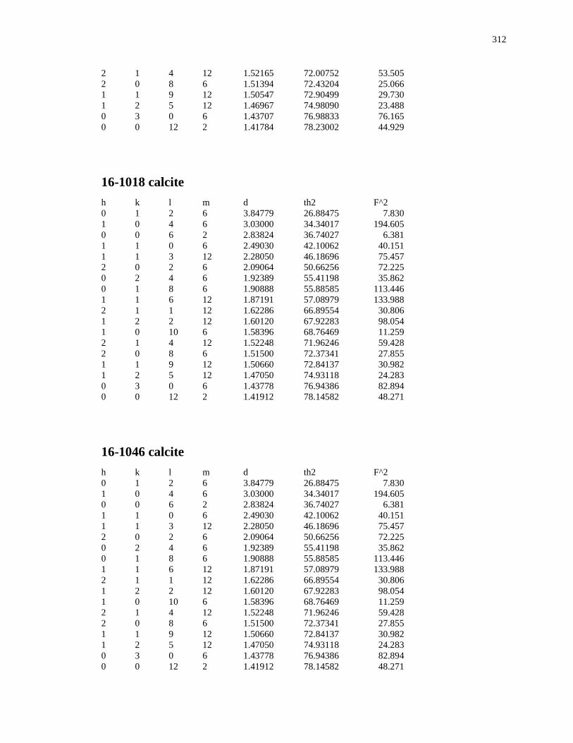
312

2 1 4 12 1.52165 72.00752 53.505

2 0 8 6 1.51394 72.43204 25.066

1 1 9 12 1.50547 72.90499 29.730

1 2 5 12 1.46967 74.98090 23.488

0 3 0 6 1.43707 76.98833 76.165

0 0 12 2 1.41784 78.23002 44.929

16-1018 calcite

h k l m d th2 F^2

0 1 2 6 3.84779 26.88475 7.830

1 0 4 6 3.03000 34.34017 194.605

0 0 6 2 2.83824 36.74027 6.381

1 1 0 6 2.49030 42.10062 40.151

1 1 3 12 2.28050 46.18696 75.457

2 0 2 6 2.09064 50.66256 72.225

0 2 4 6 1.92389 55.41198 35.862

0 1 8 6 1.90888 55.88585 113.446

1 1 6 12 1.87191 57.08979 133.988

2 1 1 12 1.62286 66.89554 30.806

1 2 2 12 1.60120 67.92283 98.054

1 0 10 6 1.58396 68.76469 11.259

2 1 4 12 1.52248 71.96246 59.428

2 0 8 6 1.51500 72.37341 27.855

1 1 9 12 1.50660 72.84137 30.982

1 2 5 12 1.47050 74.93118 24.283

0 3 0 6 1.43778 76.94386 82.894

0 0 12 2 1.41912 78.14582 48.271

16-1046 calcite

h k l m d th2 F^2

0 1 2 6 3.84779 26.88475 7.830

1 0 4 6 3.03000 34.34017 194.605

0 0 6 2 2.83824 36.74027 6.381

1 1 0 6 2.49030 42.10062 40.151

1 1 3 12 2.28050 46.18696 75.457

2 0 2 6 2.09064 50.66256 72.225

0 2 4 6 1.92389 55.41198 35.862

0 1 8 6 1.90888 55.88585 113.446

1 1 6 12 1.87191 57.08979 133.988

2 1 1 12 1.62286 66.89554 30.806

1 2 2 12 1.60120 67.92283 98.054

1 0 10 6 1.58396 68.76469 11.259

2 1 4 12 1.52248 71.96246 59.428

2 0 8 6 1.51500 72.37341 27.855

1 1 9 12 1.50660 72.84137 30.982

1 2 5 12 1.47050 74.93118 24.283

0 3 0 6 1.43778 76.94386 82.894

0 0 12 2 1.41912 78.14582 48.271

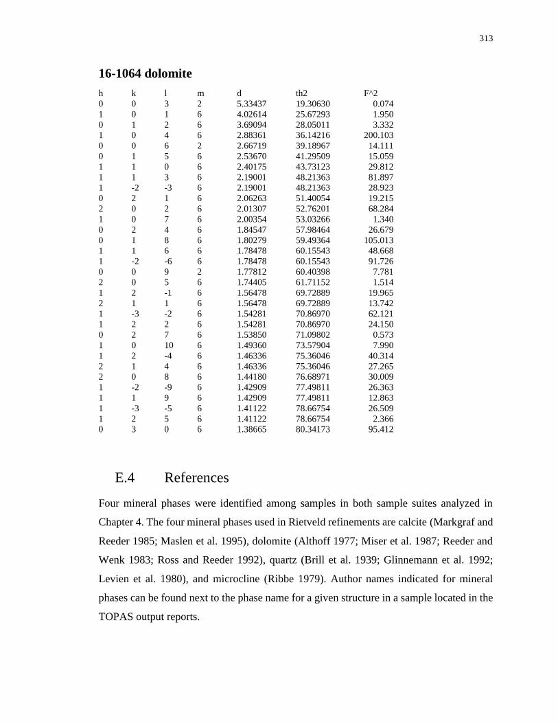
313

16-1064 dolomite

h k l m d th2 F^2

0 0 3 2 5.33437 19.30630 0.074

1 0 1 6 4.02614 25.67293 1.950

0 1 2 6 3.69094 28.05011 3.332

1 0 4 6 2.88361 36.14216 200.103

0 0 6 2 2.66719 39.18967 14.111

0 1 5 6 2.53670 41.29509 15.059

1 1 0 6 2.40175 43.73123 29.812

1 1 3 6 2.19001 48.21363 81.897

1 -2 -3 6 2.19001 48.21363 28.923

0 2 1 6 2.06263 51.40054 19.215

2 0 2 6 2.01307 52.76201 68.284

1 0 7 6 2.00354 53.03266 1.340

0 2 4 6 1.84547 57.98464 26.679

0 1 8 6 1.80279 59.49364 105.013

1 1 6 6 1.78478 60.15543 48.668

1 -2 -6 6 1.78478 60.15543 91.726

0 0 9 2 1.77812 60.40398 7.781

2 0 5 6 1.74405 61.71152 1.514

1 2 -1 6 1.56478 69.72889 19.965

2 1 1 6 1.56478 69.72889 13.742

1 -3 -2 6 1.54281 70.86970 62.121

1 2 2 6 1.54281 70.86970 24.150

0 2 7 6 1.53850 71.09802 0.573

1 0 10 6 1.49360 73.57904 7.990

1 2 -4 6 1.46336 75.36046 40.314

2 1 4 6 1.46336 75.36046 27.265

2 0 8 6 1.44180 76.68971 30.009

1 -2 -9 6 1.42909 77.49811 26.363

1 1 9 6 1.42909 77.49811 12.863

1 -3 -5 6 1.41122 78.66754 26.509

1 2 5 6 1.41122 78.66754 2.366

0 3 0 6 1.38665 80.34173 95.412

E.4 References

Four mineral phases were identified among samples in both sample suites analyzed in

Chapter 4. The four mineral phases used in Rietveld refinements are calcite (Markgraf and

Reeder 1985; Maslen et al. 1995), dolomite (Althoff 1977; Miser et al. 1987; Reeder and

Wenk 1983; Ross and Reeder 1992), quartz (Brill et al. 1939; Glinnemann et al. 1992;

Levien et al. 1980), and microcline (Ribbe 1979). Author names indicated for mineral

phases can be found next to the phase name for a given structure in a sample located in the

TOPAS output reports.

314

Althoff P. 1977. Structural refinements of dolomite and a magnesian calcite and

implications for dolomite formation in the marine environment. American

Mineralogist 62:772–783.

Brill R., Hermann C., and Peters C. 1939. Studien über chemische Bindung mittels

Fourieranalyse III. Die Naturwissenschaften 27:677–678.

Glinnemann J., King Jr. H. E., Schulz H., Hahn T., La Placa S. J., and Dacol F. 1992.

Crystal structures of the low-temperature quartz-type phases of SiO2 and GeO2 at

elevated pressure. Zeitschrift für Kristallographie 198:177–212.

Levien L., Prewitt C. T., and Weidner D. J. 1980. Structure and elastic properties of quartz

at pressure. American Mineralogist 65:920–930.

Markgraf S. A., and Reeder R. J. 1985. High-temperature structure refinements of calcite

and magnesite. American Mineralogist 70:590–600.

Maslen E. N., Streltsov V. A., Streltsova N. R., and Ishizawa N. 1995. Electron density

and optical anisotropy in rhombohedral carbonates. III. Synchrotron X‐ray studies of

CaCO3, MgCO3 and MnCO3. Acta Crystallographica Section B 51:929–939.

Miser D. E., Swinnea J. S., and Steinfink H. 1987. TEM observations and X-ray crystal-

structure refinement of a twinned dolomite with a modulated microstructure.

American Mineralogist 72:188–193.

Reeder R. J., and Wenk H. R. 1983. Structure refinements of some thermally disordered

dolomites. American Mineralogist 68:769–776.

Ribbe P. H. 1979. The structure of a strained intermediate microcline in cryptoperthitic

association with twinned plagioclase. American Mineralogist 64:402–408.

Ross N. L., and Reeder R. J. 1992. High-pressure structural study of dolomite and ankerite.

American Mineralogist 77:412–421.

315

Appendix F: Raman spectroscopy analysis data

F.1 Data collection and processing

A subset of the suite of impact dykes consisting of carbonate melt rocks characterized from

the Haughton impact structure contain blue crystals of moissanite (SiC). Moissanite is a

rare terrestrial mineral and the composition of the crystals was identified by electron probe

microanalysis using wavelength dispersive spectroscopy (WDS). Naturally occurring and

synthetic moissanite crystals have a range of polytypes that belong to the cubic, hexagonal,

and rhombohedral crystal classes where the resulting polytype depends on factors present

during crystal growth including temperature and pressure.

To determine the polytypes of moissanite crystals in thin sections prepared from Haughton

clast-bearing impact melt rocks, micro-Raman spectra were collected using a Renishaw

InVia Reflex Raman Spectrometer with 1800 grating at the Surface Science Western

facility at the University of Western Ontario. An argon-ion laser with a wavelength of 514

nm was used as the exciting source and the spectrometer was calibrated using a Si film.

The sample excitation and Raman scatter collection were performed using a 50x and 100x

optical lens on the Raman microscope. An energy of 6 mW was transferred to the sample

surface with a spot size of 2 µm. The spectra were analyzed by WiRE software developed

by Renishaw.

To confirm moissanite crystals were not the result of contamination during thin section

preparation, two thin sections were re-made by avoiding the use of any silicon carbide-

containing abrasives; only diamond abrasives were used during grinding and polishing.

After this careful preparation, moissanite crystals were still observed within the melt rock

samples, thus confirming the in situ identification of moissanite.

The orientation of moissanite crystals within the thin sections examined are random. Based

on individual crystal spectral patterns, a parallel or perpendicular orientation relative to the

c-axis for one of the three identified polytypes (6H, 4H, and 15R) are indicated in Figures

F-1 to F-4 and stacked vertically for comparison when needed.

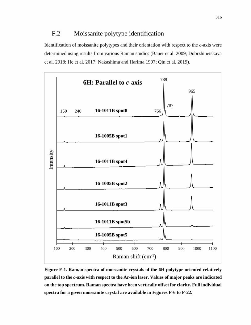
316

F.2 Moissanite polytype identification

Identification of moissanite polytypes and their orientation with respect to the c-axis were

determined using results from various Raman studies (Bauer et al. 2009; Dobrzhinetskaya

et al. 2018; He et al. 2017; Nakashima and Harima 1997; Qin et al. 2019).

Figure F-1. Raman spectra of moissanite crystals of the 6H polytype oriented relatively

parallel to the c-axis with respect to the Ar-ion laser. Values of major peaks are indicated

on the top spectrum. Raman spectra have been vertically offset for clarity. Full individual

spectra for a given moissanite crystal are available in Figures F-6 to F-22.

100 200 300 400 500 600 700 800 900 1000 1100

Inte

nsi

ty

Raman shift (cm-1)

6H: Parallel to c-axis

150 766

789

797

965

16-1011B spot8

16-1005B spot1

16-1011B spot4

16-1005B spot2

16-1011B spot3

16-1011B spot5b

16-1005B spot5

240

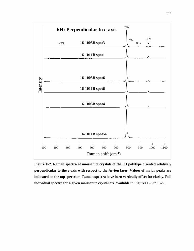
317

Figure F-2. Raman spectra of moissanite crystals of the 6H polytype oriented relatively

perpendicular to the c-axis with respect to the Ar-ion laser. Values of major peaks are

indicated on the top spectrum. Raman spectra have been vertically offset for clarity. Full

individual spectra for a given moissanite crystal are available in Figures F-6 to F-22.

100 200 300 400 500 600 700 800 900 1000 1100

Inte

nsi

ty

Raman shift (cm-1)

6H: Perpendicular to c-axis

969797

787

239 16-1005B spot3

16-1011B spot1

16-1005B spot6

16-1011B spot6

16-1005B spot4

16-1011B spot5a

887

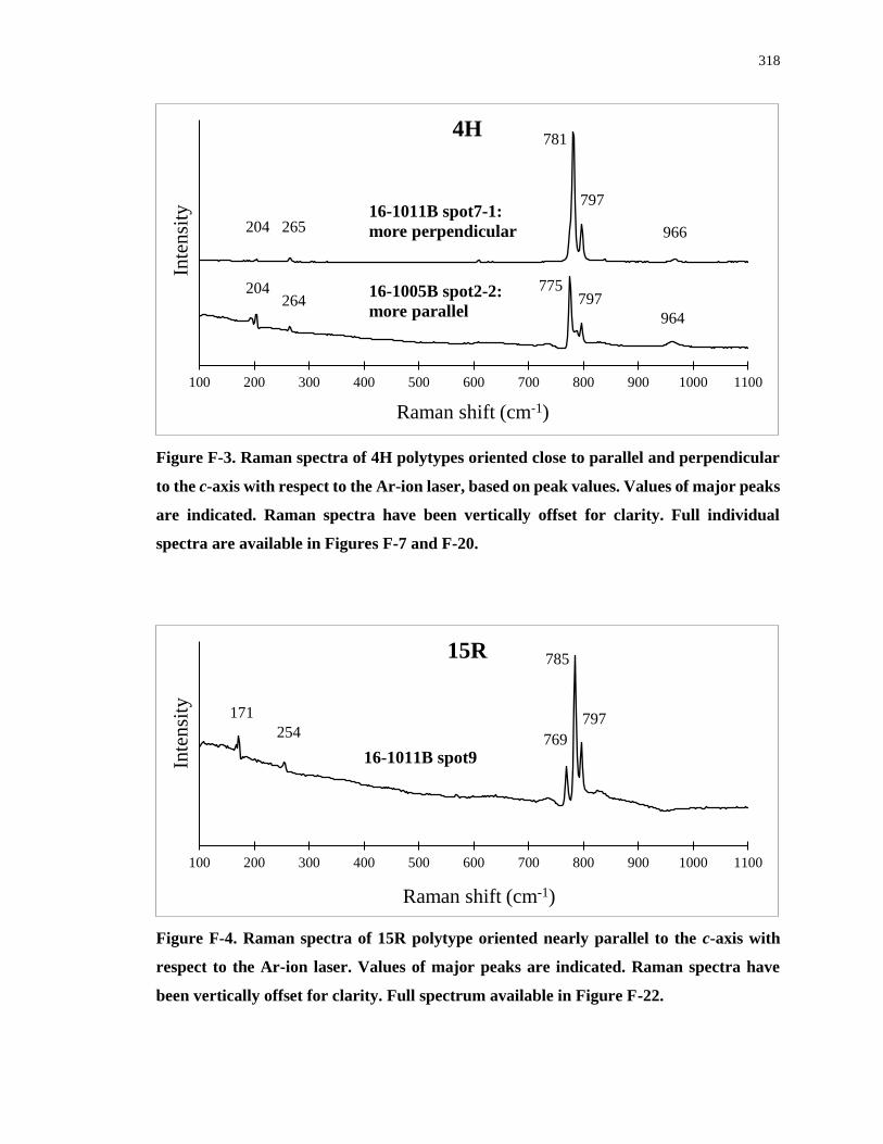
318

Figure F-3. Raman spectra of 4H polytypes oriented close to parallel and perpendicular

to the c-axis with respect to the Ar-ion laser, based on peak values. Values of major peaks

are indicated. Raman spectra have been vertically offset for clarity. Full individual

spectra are available in Figures F-7 and F-20.

Figure F-4. Raman spectra of 15R polytype oriented nearly parallel to the c-axis with

respect to the Ar-ion laser. Values of major peaks are indicated. Raman spectra have

been vertically offset for clarity. Full spectrum available in Figure F-22.

100 200 300 400 500 600 700 800 900 1000 1100

Inte

nsi

ty

Raman shift (cm-1)

4H

16-1005B spot2-2:

more parallel

16-1011B spot7-1:

more perpendicular

204264

775797

964

204 265

781

797

966

100 200 300 400 500 600 700 800 900 1000 1100

Inte

nsi

ty

Raman shift (cm-1)

15R

16-1011B spot9

171

254769

785

797

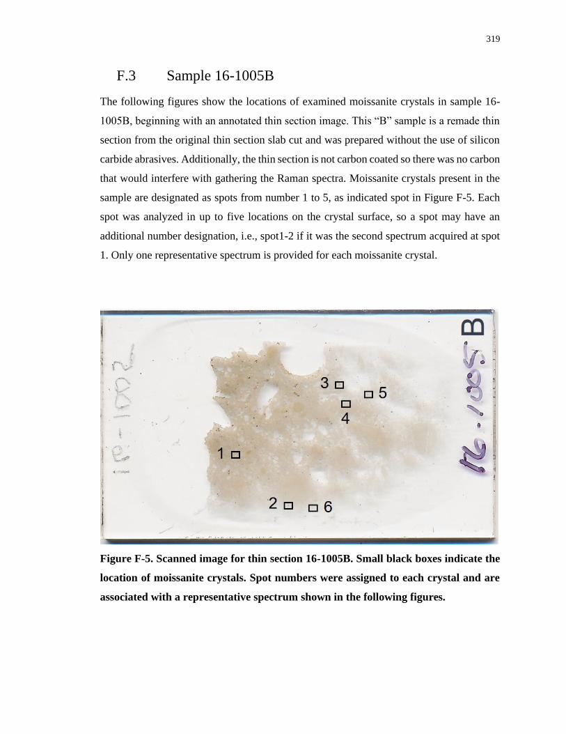
319

F.3 Sample 16-1005B

The following figures show the locations of examined moissanite crystals in sample 16-

1005B, beginning with an annotated thin section image. This “B” sample is a remade thin

section from the original thin section slab cut and was prepared without the use of silicon

carbide abrasives. Additionally, the thin section is not carbon coated so there was no carbon

that would interfere with gathering the Raman spectra. Moissanite crystals present in the

sample are designated as spots from number 1 to 5, as indicated spot in Figure F-5. Each

spot was analyzed in up to five locations on the crystal surface, so a spot may have an

additional number designation, i.e., spot1-2 if it was the second spectrum acquired at spot

1. Only one representative spectrum is provided for each moissanite crystal.

Figure F-5. Scanned image for thin section 16-1005B. Small black boxes indicate the

location of moissanite crystals. Spot numbers were assigned to each crystal and are

associated with a representative spectrum shown in the following figures.

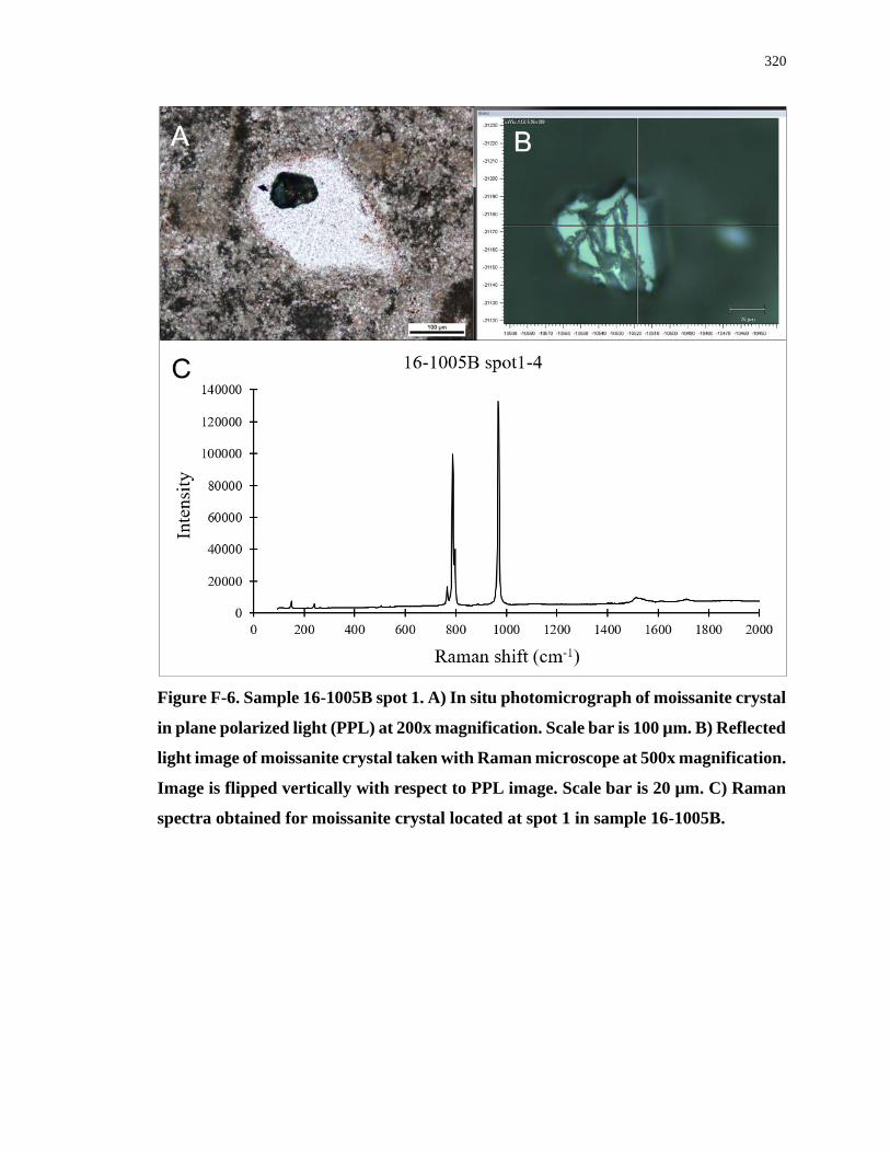
320

Figure F-6. Sample 16-1005B spot 1. A) In situ photomicrograph of moissanite crystal

in plane polarized light (PPL) at 200x magnification. Scale bar is 100 µm. B) Reflected

light image of moissanite crystal taken with Raman microscope at 500x magnification.

Image is flipped vertically with respect to PPL image. Scale bar is 20 µm. C) Raman

spectra obtained for moissanite crystal located at spot 1 in sample 16-1005B.

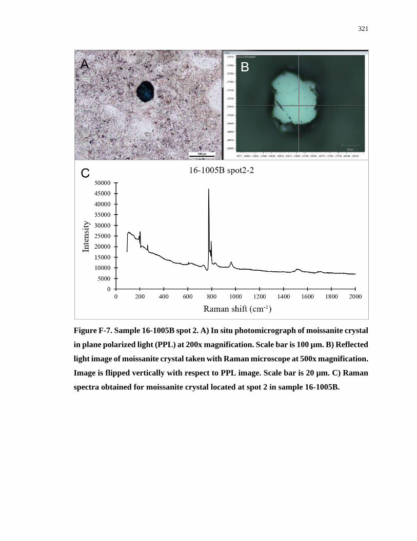
321

Figure F-7. Sample 16-1005B spot 2. A) In situ photomicrograph of moissanite crystal

in plane polarized light (PPL) at 200x magnification. Scale bar is 100 µm. B) Reflected

light image of moissanite crystal taken with Raman microscope at 500x magnification.

Image is flipped vertically with respect to PPL image. Scale bar is 20 µm. C) Raman

spectra obtained for moissanite crystal located at spot 2 in sample 16-1005B.

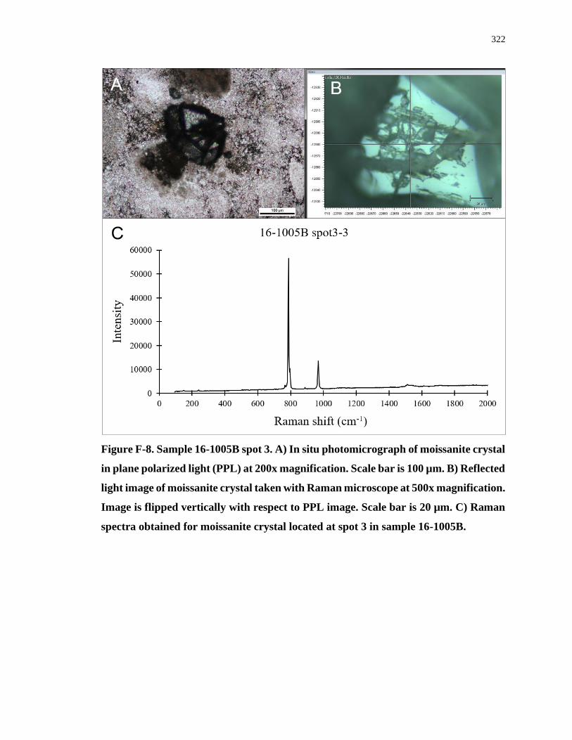
322

Figure F-8. Sample 16-1005B spot 3. A) In situ photomicrograph of moissanite crystal

in plane polarized light (PPL) at 200x magnification. Scale bar is 100 µm. B) Reflected

light image of moissanite crystal taken with Raman microscope at 500x magnification.

Image is flipped vertically with respect to PPL image. Scale bar is 20 µm. C) Raman

spectra obtained for moissanite crystal located at spot 3 in sample 16-1005B.

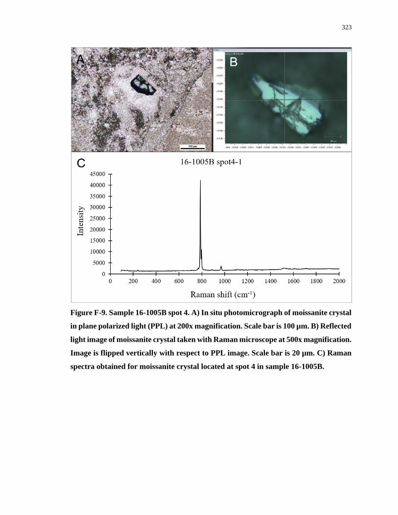
323

Figure F-9. Sample 16-1005B spot 4. A) In situ photomicrograph of moissanite crystal

in plane polarized light (PPL) at 200x magnification. Scale bar is 100 µm. B) Reflected

light image of moissanite crystal taken with Raman microscope at 500x magnification.

Image is flipped vertically with respect to PPL image. Scale bar is 20 µm. C) Raman

spectra obtained for moissanite crystal located at spot 4 in sample 16-1005B.

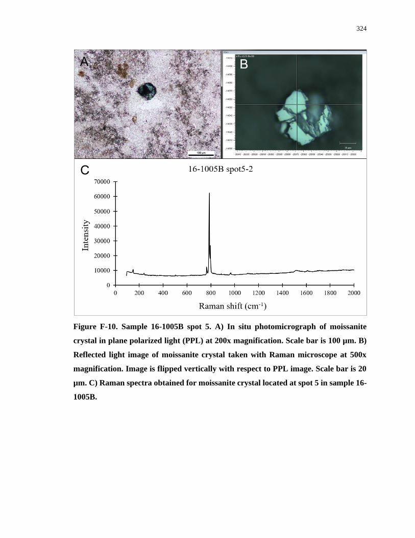
324

Figure F-10. Sample 16-1005B spot 5. A) In situ photomicrograph of moissanite

crystal in plane polarized light (PPL) at 200x magnification. Scale bar is 100 µm. B)

Reflected light image of moissanite crystal taken with Raman microscope at 500x

magnification. Image is flipped vertically with respect to PPL image. Scale bar is 20

µm. C) Raman spectra obtained for moissanite crystal located at spot 5 in sample 16-

1005B.

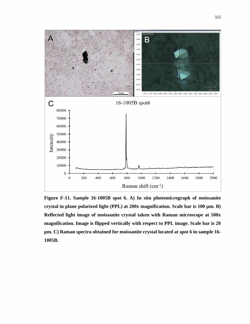
325

Figure F-11. Sample 16-1005B spot 6. A) In situ photomicrograph of moissanite

crystal in plane polarized light (PPL) at 200x magnification. Scale bar is 100 µm. B)

Reflected light image of moissanite crystal taken with Raman microscope at 500x

magnification. Image is flipped vertically with respect to PPL image. Scale bar is 20

µm. C) Raman spectra obtained for moissanite crystal located at spot 6 in sample 16-

1005B.

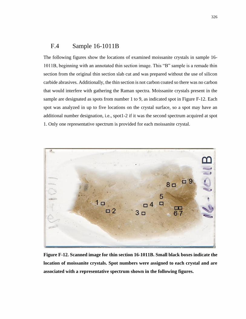
326

F.4 Sample 16-1011B

The following figures show the locations of examined moissanite crystals in sample 16-

1011B, beginning with an annotated thin section image. This “B” sample is a remade thin

section from the original thin section slab cut and was prepared without the use of silicon

carbide abrasives. Additionally, the thin section is not carbon coated so there was no carbon

that would interfere with gathering the Raman spectra. Moissanite crystals present in the

sample are designated as spots from number 1 to 9, as indicated spot in Figure F-12. Each

spot was analyzed in up to five locations on the crystal surface, so a spot may have an

additional number designation, i.e., spot1-2 if it was the second spectrum acquired at spot

1. Only one representative spectrum is provided for each moissanite crystal.

Figure F-12. Scanned image for thin section 16-1011B. Small black boxes indicate the

location of moissanite crystals. Spot numbers were assigned to each crystal and are

associated with a representative spectrum shown in the following figures.

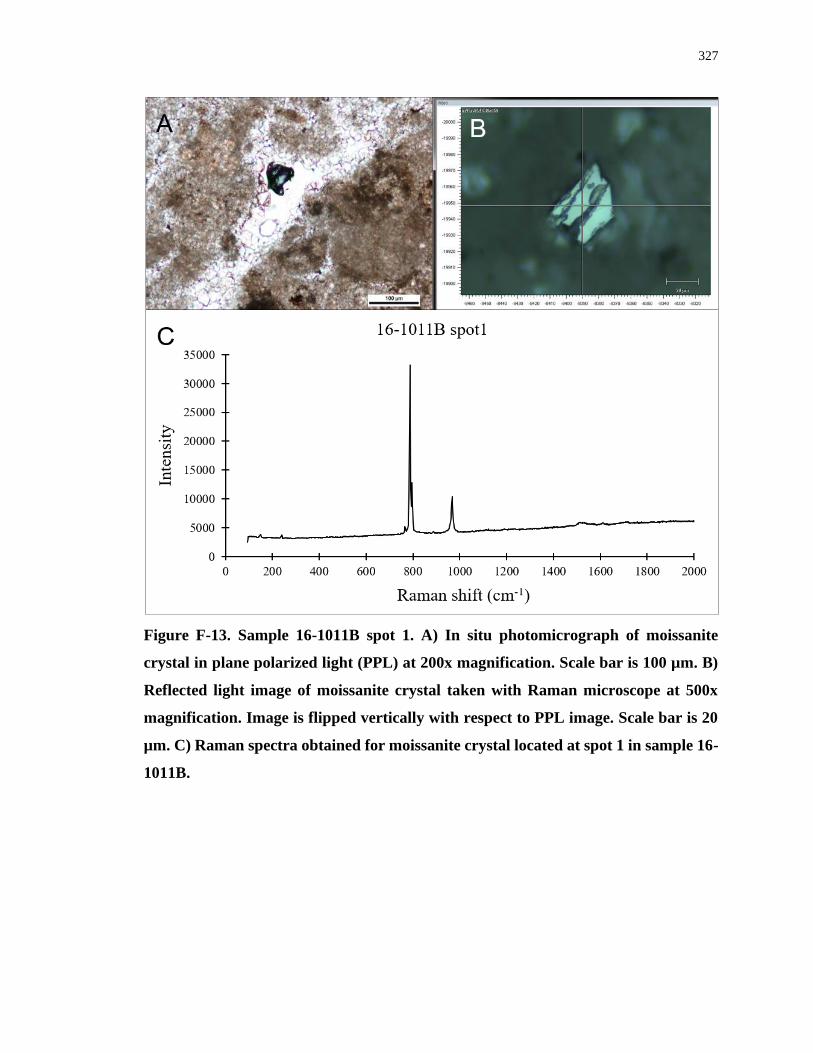
327

Figure F-13. Sample 16-1011B spot 1. A) In situ photomicrograph of moissanite

crystal in plane polarized light (PPL) at 200x magnification. Scale bar is 100 µm. B)

Reflected light image of moissanite crystal taken with Raman microscope at 500x

magnification. Image is flipped vertically with respect to PPL image. Scale bar is 20

µm. C) Raman spectra obtained for moissanite crystal located at spot 1 in sample 16-

1011B.

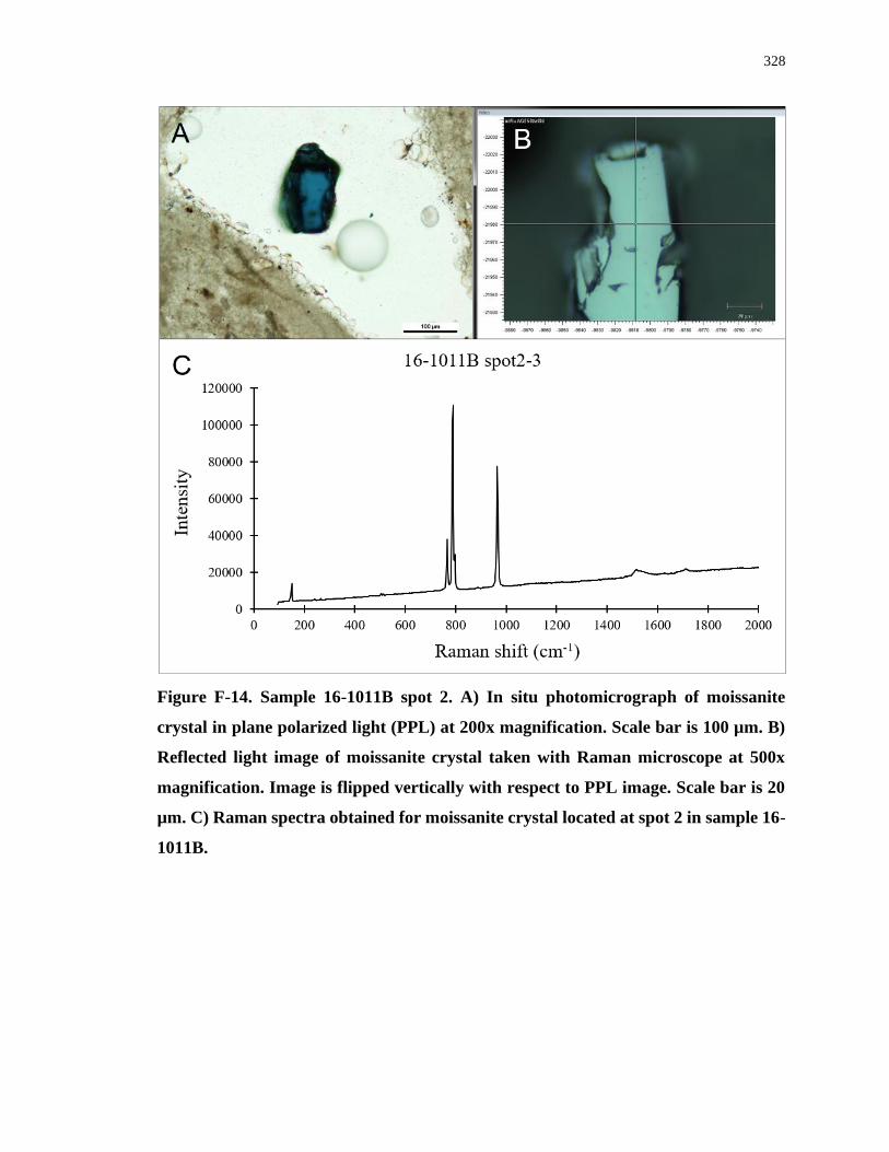
328

Figure F-14. Sample 16-1011B spot 2. A) In situ photomicrograph of moissanite

crystal in plane polarized light (PPL) at 200x magnification. Scale bar is 100 µm. B)

Reflected light image of moissanite crystal taken with Raman microscope at 500x

magnification. Image is flipped vertically with respect to PPL image. Scale bar is 20

µm. C) Raman spectra obtained for moissanite crystal located at spot 2 in sample 16-

1011B.

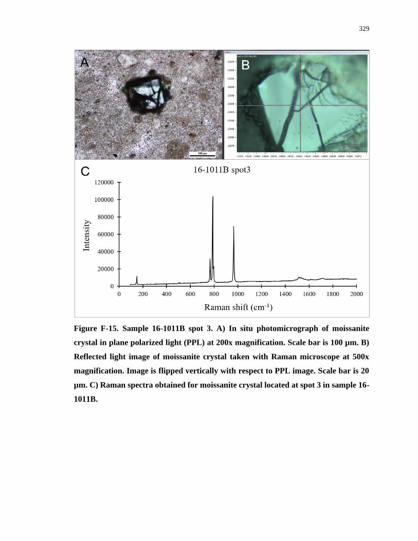
329

Figure F-15. Sample 16-1011B spot 3. A) In situ photomicrograph of moissanite

crystal in plane polarized light (PPL) at 200x magnification. Scale bar is 100 µm. B)

Reflected light image of moissanite crystal taken with Raman microscope at 500x

magnification. Image is flipped vertically with respect to PPL image. Scale bar is 20

µm. C) Raman spectra obtained for moissanite crystal located at spot 3 in sample 16-

1011B.

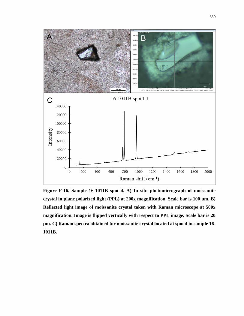
330

Figure F-16. Sample 16-1011B spot 4. A) In situ photomicrograph of moissanite

crystal in plane polarized light (PPL) at 200x magnification. Scale bar is 100 µm. B)

Reflected light image of moissanite crystal taken with Raman microscope at 500x

magnification. Image is flipped vertically with respect to PPL image. Scale bar is 20

µm. C) Raman spectra obtained for moissanite crystal located at spot 4 in sample 16-

1011B.

331

Figure F-17. Sample 16-1011B spot 5a. A) In situ photomicrograph of moissanite

crystal in plane polarized light (PPL) at 200x magnification. Scale bar is 100 µm. B)

Reflected light image of moissanite crystal taken with Raman microscope at 500x

magnification. Image is flipped vertically with respect to PPL image. Scale bar is 20

µm. C) Raman spectra obtained for moissanite crystal located at spot 5a in sample

16-1011B.

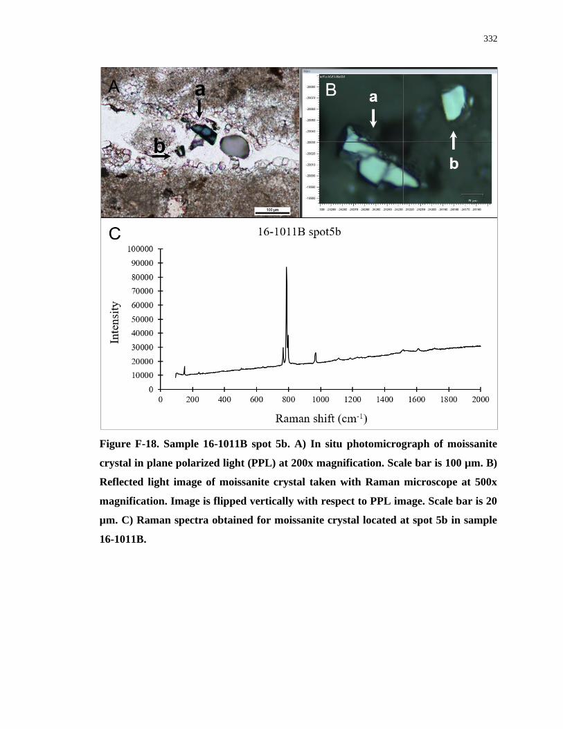
332

Figure F-18. Sample 16-1011B spot 5b. A) In situ photomicrograph of moissanite

crystal in plane polarized light (PPL) at 200x magnification. Scale bar is 100 µm. B)

Reflected light image of moissanite crystal taken with Raman microscope at 500x

magnification. Image is flipped vertically with respect to PPL image. Scale bar is 20

µm. C) Raman spectra obtained for moissanite crystal located at spot 5b in sample

16-1011B.

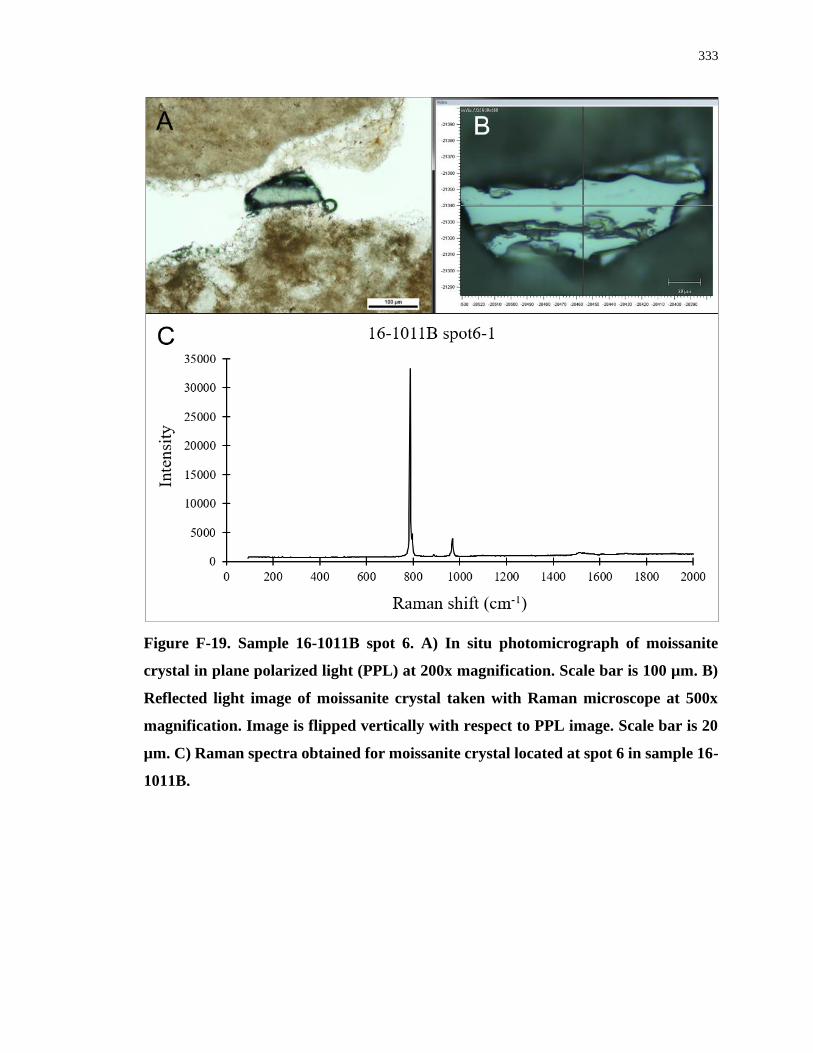
333

Figure F-19. Sample 16-1011B spot 6. A) In situ photomicrograph of moissanite

crystal in plane polarized light (PPL) at 200x magnification. Scale bar is 100 µm. B)

Reflected light image of moissanite crystal taken with Raman microscope at 500x

magnification. Image is flipped vertically with respect to PPL image. Scale bar is 20

µm. C) Raman spectra obtained for moissanite crystal located at spot 6 in sample 16-

1011B.

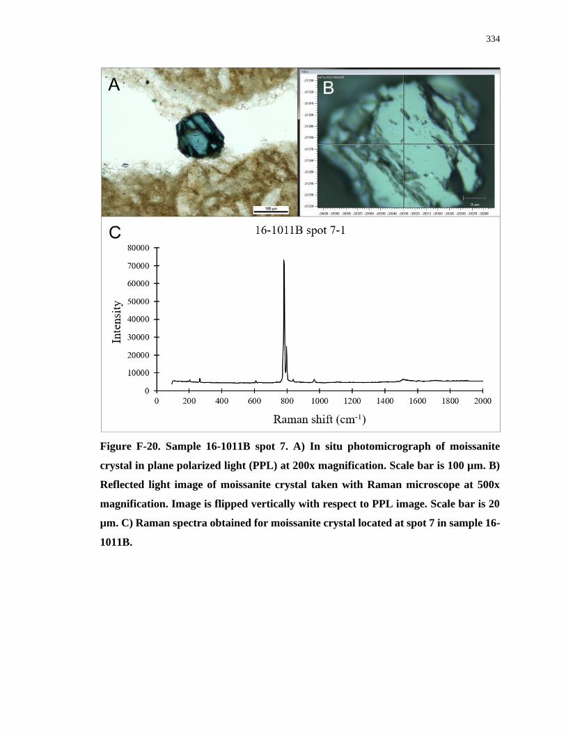
334

Figure F-20. Sample 16-1011B spot 7. A) In situ photomicrograph of moissanite

crystal in plane polarized light (PPL) at 200x magnification. Scale bar is 100 µm. B)

Reflected light image of moissanite crystal taken with Raman microscope at 500x

magnification. Image is flipped vertically with respect to PPL image. Scale bar is 20

µm. C) Raman spectra obtained for moissanite crystal located at spot 7 in sample 16-

1011B.

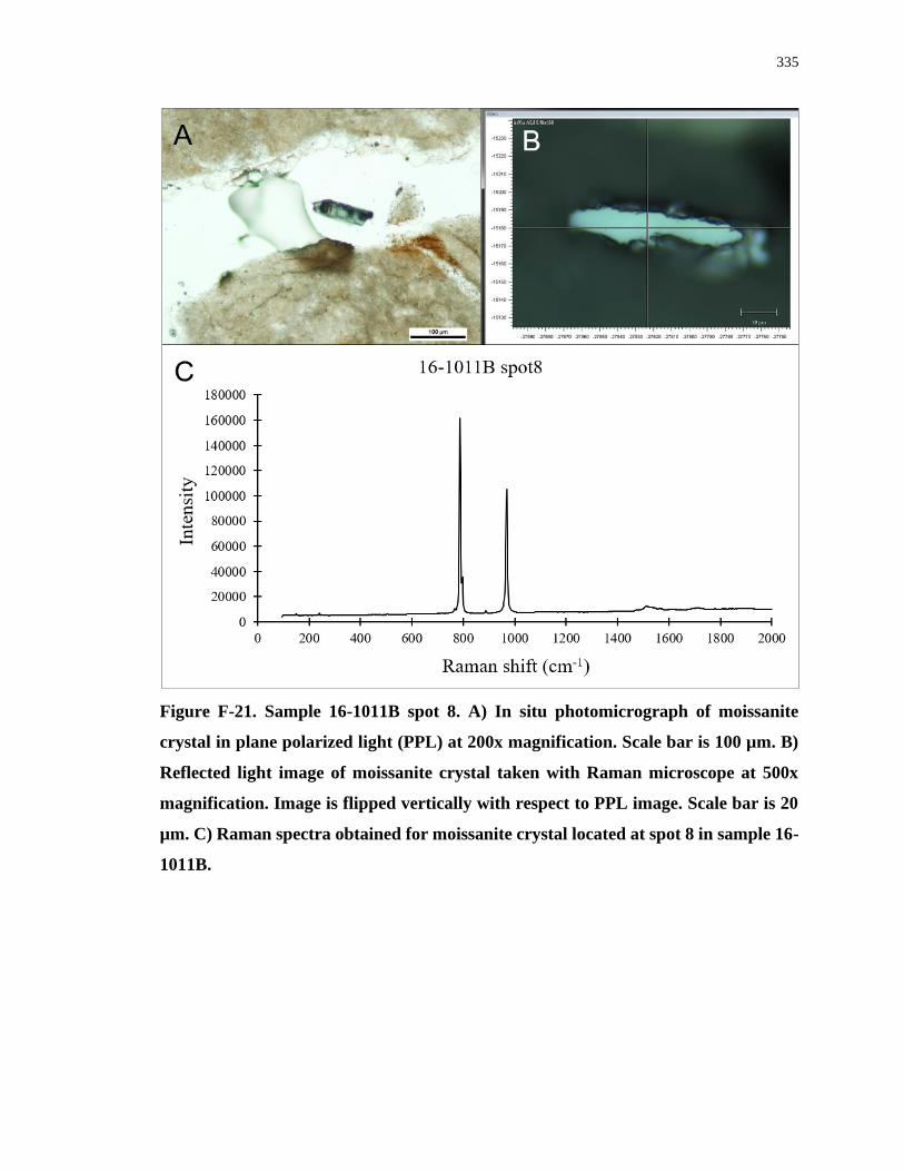
335

Figure F-21. Sample 16-1011B spot 8. A) In situ photomicrograph of moissanite

crystal in plane polarized light (PPL) at 200x magnification. Scale bar is 100 µm. B)

Reflected light image of moissanite crystal taken with Raman microscope at 500x

magnification. Image is flipped vertically with respect to PPL image. Scale bar is 20

µm. C) Raman spectra obtained for moissanite crystal located at spot 8 in sample 16-

1011B.

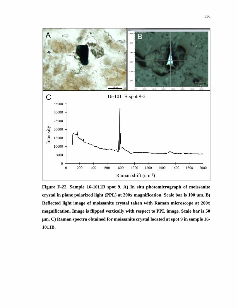
336

Figure F-22. Sample 16-1011B spot 9. A) In situ photomicrograph of moissanite

crystal in plane polarized light (PPL) at 200x magnification. Scale bar is 100 µm. B)

Reflected light image of moissanite crystal taken with Raman microscope at 200x

magnification. Image is flipped vertically with respect to PPL image. Scale bar is 50

µm. C) Raman spectra obtained for moissanite crystal located at spot 9 in sample 16-

1011B.

337

F.5 References

Bauer M., Gigler A. M., Huber A. J., Hillenbrand R., and Stark R. W. 2009. Temperature-

depending Raman line-shift of silicon carbide. Journal of Raman Spectroscopy

40:1867–1874.

Dobrzhinetskaya L., Mukhin P., Wang Q., Wirth R., O’Bannon E., Zhao W., Eppelbaum

L., and Sokhonchuk T. 2018. Moissanite (SiC) with metal-silicide and silicon

inclusions from tuff of Israel: Raman spectroscopy and electron microscope studies.

Lithos 310–311:355–368.

He D., Liu Y., Gao C., Chen C., Hu Z., and Gao S. 2017. SiC-dominated ultra-reduced

mineral assemblage in carbonatitic xenoliths from the Dalihu basalt, Inner Mongolia,

China. American Mineralogist 102:312–320.

Nakashima S., and Harima H. 1997. Raman investigation of SiC polytypes. Physica Status

Solidi (A) Applied Research 162:39–64.

Qin X., Li X., Chen X., Yang X., Zhang F., Xu X., Hu X., Peng Y., and Yu P. 2019. Raman

scattering study on phonon anisotropic properties of SiC. Journal of Alloys and

Compounds 776:1048–1055.

338

Curriculum Vitae

Name: Jennifer Diane Newman

Post-secondary University of Western Ontario

Education and London, Ontario, Canada

Degrees: 2015-2020 Ph.D. Geology & Planetary Science and Exploration

University of Alberta

Edmonton, Alberta, Canada

2011-2014 M.Sc. Earth and Atmospheric Sciences

University of Alberta

Edmonton, Alberta, Canada

2005-2007 B.Sc. Specialization in Environmental Earth Science

University of Alberta

Edmonton, Alberta, Canada

2000-2004 B.Sc. Biological Sciences major Earth Sciences minor

Honours and Natural Sciences and Engineering Research Council of Canada

Awards: Alexander Graham Bell Canada Graduate Scholarship-Doctoral

(NSERC CGS-D)

University of Western Ontario

2017-2019

Doctoral Excellence Research Award

University of Western Ontario

2016-2019

Centre for Planetary Science and Exploration (CPSX)

Certificate of Appreciation for outstanding contributions towards

the CPSX Outreach Program

2016-2017

Queen Elizabeth II Graduate Scholarship in Science and

Technology (QEII-GSST)

University of Western Ontario

2016-2017 (declined – could not hold concurrently with NSERC)

Natural Sciences and Engineering Research Council of Canada

Postgraduate Scholarship-Doctoral (NSERC PGS-D)

University of Western Ontario

2016-2017

339

Western Graduate Research Scholarship

University of Western Ontario

2016

Polar Knowledge Canada (POLAR) Northern Scientific Training

Program Award

University of Western Ontario

2016

Queen Elizabeth II Graduate Scholarship in Science and

Technology (QEII-GSST)

University of Western Ontario

2015-2016

PhD Fellowship: NSERC CREATE “Technologies and Techniques

for Earth and Space Exploration”

University of Western Ontario

2015-2017

Graduate Students’ Association Professional Development Grant

University of Alberta

2013

ASTRO/CPSX Graduate Student Travel Award

University of Alberta

2013

Graduate Student Scholarship

University of Alberta

2013

Related Work Teaching Assistant

Experience University of Western Ontario

2015-2020

Research Assistant

University of Western Ontario

2015-2019

Lab Assistant

University of Alberta

2014

Teaching Assistant

University of Alberta

2011-2013

340

Planetary Mission High Resolution Imaging Science Experiment (HiRISE) on the

Involvement 2005 Mars Reconnaissance Orbiter (MRO) [PI: Dr. Alfred

McEwen]: Science and operations planning for Cycle 301 (under

Science Team Member Dr. Livio L. Tornabene), University of

Western Ontario

23 April to 30 May 2018

Certificate of Canadian Space Agency

Operation Lunar Exploration Analogue Deployment (LEAD)

Science Support in the HOPE-2 CSA/ESA Joint Experiment

13-19 June 2019

Analogue Mission CanMoon 2019 Lunar Sample Return Analogue Mission

Involvement Planning Lead, Planning Team, University of Western Ontario

2019

CanMars 2016 Mars Sample Return Analogue Mission

Sequencing Integrator, Planning Team, University of Western

Ontario

2016

CanMars 2015 Mars Sample Return Analogue Mission

Localization Lead, Science Team, University of Western Ontario

2015

Concept Study Canadian Space Agency Contract 9F050-170252/A: Space

Involvement Exploration Concept Studies for Planetary Exploration and Space

Astronomy Science Priorities – “Miniaturized in situ X-ray

diffractometer for mineralogical characterization of planetary

surfaces”.

Student Collaborator, University of Western Ontario

2018-2020

Publications

Morse Z. R., Harrington E., Hill P. J. A., Christoffersen P., Newman J., Choe B-H.,

Tornabene L. L., Caudill C., Osinski G. R. 2019. The use of GIS, mapping, and immersive

technologies in the CanMars Mars Sample Return analogue mission: Advantages for

science interpretation and operational decision-making. Planetary and Space Science 168:

15-26.

Osinski G. R., Battler M., Caudill C. M., Francis R., Haltigin T., Hipkin V. J., Kerrigan

M., Pilles E. A., Pontefract A., Tornabene L. L., … Newman J., et al. 2019. The CanMars

Mars Sample Return Analogue Mission. Planetary and Space Science 166: 110-130.

341

Pilles E. A., Cross M., Caudill C. M., Francis R., Osinski G. R., Newman J., Battler M.,

Bourassa M., Haltigin T., Hipkin V., Kerrigan M., McLennan S., Silber E. A., Williford

K. 2019. Exploring new models for improving planetary rover operations efficiency

through the 2016 CanMars Mars Sample Return (MSR) analogue deployment. Planetary

and Space Science 165: 250-259.

Choe B-H., Tornabene L. L., Osinski G. R., and Newman J. D. 2019. Remote predictive

mapping of the Tunnunik impact structure in the Canadian Arctic using multispectral and

polarimetric SAR data fusion. Canadian Journal of Remote Sensing 44: 513-531.

Newman, J. D. and Herd, C. D. K. 2015. Mineralogy, petrology and distribution of

meteorites at the Whitecourt Crater, Alberta, Canada. Meteoritics & Planetary Science 50:

305-317.

Conference Abstracts

Newman J. D., Flemming R. L., and Osinski G. R. 2020. Shock Effects in Carbonates

from the Haughton Impact Structure using X-Ray Diffraction. 51st Lunar and Planetary

Science Conference, Woodlands, TX, abstract #2284.

Newman J. D., Pilles E. A., Morse Z. R., Marion C. L., Christoffersen P. A., Hill P. J. A.,

Osinski G. R., Cloutis E. A., Andres C. N., Bourassa M., Caudill C. M., Cross M., Dicecca

A., Doerksen K., Hibbard S., Hopkins R., Kollewyn J., Pascual A., Ratcliffe K., Roberts

A., Rodriguez Sanchez-Vahamonde C. D., Ryan C., Shah J., Tolometti G., Tornabene L.

L., and Vlachopoulos O. 2020. Planning Team Operations for the CanMoon Lunar Sample

Return Analogue Mission. 51st Lunar and Planetary Science Conference, Woodlands, TX,

abstract #2196.

Andres C. N., Ratcliffe K., Newman J. D., Osinski G. R., Cloutis E. A., Marion C. L., and

Pilles E. A. 2020. Rover Command Sequencing and Instrument Utilization during the

CanMoon Analogue Mission. 51st Lunar and Planetary Science Conference, Woodlands,

TX, abstract #2584.

Osinski G. R., Grieve R. A. F., Hill P. J. A., Newman J. D., Patel P., and Tolometti G. D.

2020. Impact Earth – A Resource for Public Outreach and Teaching at the K-12,

Undergraduate, and Graduate Level. 51st Lunar and Planetary Science Conference,

Woodlands, TX, abstract #2111.

Flemming R. L., Rupert A. N., Field J., Pilles E. A., Sabarinathan J., Veinberg S. L.,

Leftwich K., Shaw A., Dickinson C., Berger J. A., Bourassa M., Gellert R., Hiemstra D.

M., McCausland P. J. A., McIsaac K. A., Osinski G. R., Schmidt M. E., Tornabene L. L.,

Vukotic V. N., Bakhtazad A., Cao F., Li Y., Jenkins L. E., McCraig M. A., Newman J.

D., Pentesco J. T., Posnov N. M., Simpson S. L., Svenson M. J. O. 2020. In Situ X-ray

Diffraction (ISXRD) for Exploring Mars Mineralogy and Geology. 51st Lunar and

Planetary Science Conference, Woodlands, TX, abstract #2965.

342

Shah J., Andres C. N., Pilles E. A., Roberts A., Rodriguez Sanchez-Vahamonde C. D.,

Vlachopoulos O., Yingling W., Marion C. L., Osinski G. R., Cloutis E. A., Morse Z. R.,

Newman J. D., Caudill C. 2020. CanMoon Analogue Mission Operations: GIS,

Localization, and Rover Traverse Planning and Monitoring. 51st Lunar and Planetary

Science Conference, Woodlands, TX, abstract #2222.

Marion C. L., Morse Z. R., Newman J. D., Pilles E. A., Hill P. J. A., Osinski G. R., Cloutis

E. A., Caudill C. M., Simpson S. L., Xie T. and the 2019 CanMoon Team. 2020. Shift

Handovers for Real-Time Lunar Operations: Methods from the CanMoon Analogue

Mission. 51st Lunar and Planetary Science Conference, Woodlands, TX, abstract #2400.

Marion C. L., Osinski G. R., Bourassa M., Caudill C. M., Cloutis E. A., Christoffersen P.,

Hill P. J. A., Morse Z. R., Newman J. D., Pilles E. A., Simpson S. L., Tornabene L. L.,

and Xie T. 2020. Overview of the CanMoon Lunar Sample Return Analogue Mission. 51st

Lunar and Planetary Science Conference, Woodlands, TX, abstract #2349.

Morse Z. R., Hill P. J. A., Osinski G. R., Cloutis E. A., Marion C. L., Newman J. D.,

Caudill C. M., Christoffersen P., Pilles E. A., Simpson S. L., Tornabene L. L., and Xie T.

2020. CanMoon Analogue Mission Tactical Science Team: Scientific Instrumentation and

Decision Making during a High Fidelity Realtime Lunar Analogue Mission. 51st Lunar and

Planetary Science Conference, Woodlands, TX, abstract #1253.

Hill P. J. A., Simpson S. L., Xie T., Morse Z. R., Sacks L. E., Osinski G. R., Cloutis E. A.,

Caudill C. M., Christoffersen P., Marion C. L., Newman J. D., Pilles E. A., Tornabene L.

L. 2020. CanMoon Science Interpretation Team: Insights into Volcanic Flows in Lanzarote

Spain. 51st Lunar and Planetary Science Conference, Woodlands, TX, abstract #2152.

Newman J. D., Pilles E. A., Morse Z. R., Marion C. L., Osinski G. R., Cloutis E. A.,

Caudill C. M., Hill P. J. A., Simpson S. L., Tornabene L. L., and Xie T. Planning Team

Operational Structure for the 2019 CanMoon Lunar Sample Return Analogue Mission.

2019 Annual Meeting of the Lunar Exploration Analysis Group, Washington, D. C.,

abstract #5041.

Osinski G. R., Marion C., Cloutis E., Morse Z., Newman J., Caudill C., Christoffersen P.,

Cross M., Hill P., Pilles E., Simpson S., Tornabene L. L., and Xie T. 2019. The Role of

Analogue Missions in Preparing to Return to the Moon: Lessons and Recommendations

from CanMoon. 2019 Annual Meeting of the Lunar Exploration Analysis Group,

Washington, D. C., abstract #5018.

Morse Z. R., Hill P. J. A., Osinski G. R., Cloutis E. A., Caudill C. M., Christoffersen P.,

Marion C. L., Newman J. D., Pilles E. A., Simpson S. L., Tornabene L. L., and Xie T.

2019. 2019 CanMoon Tactical Science Team: Real-Time Instrument Use and Coordination

During a Lunar Sample Return Analogue Mission. 2019 Annual Meeting of the Lunar

Exploration Analysis Group, Washington, D. C., abstract #5047.

343

Hill P. J. A., Simpson S. L., Xie T., Osinski G. R., Cloutis E. A., Caudill C. M.,

Christoffersen P., Marion C. L., Morse Z. R., Newman J. D., Pilles E. A., and Tornabene

L. L. 2019. 2019 CanMoon Science Interpretation Team: Insights into Volcanic Flows in

Lanzarote, Spain. 2019 Annual Meeting of the Lunar Exploration Analysis Group,

Washington, D. C., abstract #5048.

Newman J. D. and Osinski G. R. 2019. Impact-Generated Dykes from the Haughton

Impact Structure, Canada. 50th Lunar and Planetary Science Conference, Woodlands, TX,

abstract #1558.

Osinski G. R., Grieve R. A. F., Hill P., Newman J., Patel P., and Tolometti G. 2019. Impact

Earth – New Insights into the Terrestrial Impact Record and Cratering Processes. 50th

Lunar and Planetary Science Conference, Woodlands, TX, abstract #2472.

Tornabene L. L., Block K., Pilles E., Baugh N., McEwen A. S., Hansen C., Espinoza A.,

Osinski G. R., Bina A., Bourassa M., Capitan R., Caudill C., Hansen K., Harrington E.,

Hibbard S., Hopkins R., Kissi-Ameyaw J., Morse Z., Newman J., Pritchard I., Silber E.,

Simpson S., Tolometti G., and Werynski A. 2019. Mission Science/Operations Support

and Training for Spacecraft Payloads: Building the Next Generation of Planetary Mission

Professionals. 50th Lunar and Planetary Science Conference, Woodlands, TX, abstract

#2962.

Newman J. D. and Osinski G. R. 2018. Investigation of Carbonate-rich Breccias and their

Emplacement in the Central Uplift of the Decaturville Impact Structure, Missouri. 49th

Lunar and Planetary Science Conference, Woodlands, TX, abstract #2880.

Flemming R. L., Newman J. D., Botor R. J., Cao F., Caudill C. M., Galarneau M. R.,

Geiger J., Houde V. L., Jenkins L. E., Li Y., Maris J. M., Tolometti G. D., Rupert A. N.,

McCraig M. A., and Osinski G. R. 2018. Preliminary Investigation of Shocked Carbonates

from the Haughton Impact Structure, Devon Island, NU using X-Ray Diffraction and

Rietveld Refinement. 49th Lunar and Planetary Science Conference, Woodlands, TX,

abstract #3000.

Newman J. D. and Osinski G. R. 2017. Characterization of breccia dykes in the deeply

eroded Tunnunik impact structure, Canada. 80th Annual Meeting of the Meteoritical

Society, Santa Fe, NM, abstract #6248.

Newman J. D., Cross M. D. G., Pilles E. A., Francis R., and Osinski G. R. 2017. Resource

Utilization and Efficiency for the CanMars 2016 Mars Sample Return Analogue Mission.

48th Lunar and Planetary Science Conference, Woodlands, TX, abstract #2521.

Pilles E. A., Francis R. Newman J., Cross M., Battler M., and Osinski G. R. 2017. To Hel

and Back – Strategic Planning for the CanMars 2016 Mars Sample Return Analogue

Mission. 48th Lunar and Planetary Science Conference, Woodlands, TX, abstract #2022.

Newman, J. D. and Osinski, G. R. (2016) Geological mapping of the Tunnunik impact

structure, Victoria Island, Canadian High Arctic. 47th Lunar and Planetary Science

Conference, Woodlands, TX, abstract #1591.

344

Christoffersen, P. A., Newman, J. D., Morse, Z. R., Tornabene, L. L., and Osinski, G. R.

(2016) Geologic map and stratigraphy of the Yggdrasil quadrangle from the 2015 CanMars

MSR Analogue Mission. 47th Lunar and Planetary Science Conference, Woodlands, TX,

abstract #2225.

Newman, J. D. and Herd, C. D. K. (2013) Possible impact origin of amorphous carbon

spherules found in the soil surrounding the Whitecourt Meteorite Impact Crater. 76th

Annual Meteoritical Society Meeting, Edmonton, AB, abstract #5332.

Newman, J. D. and Herd, C. D. K. (2013) Whitecourt Meteorite Impact Crater:

Distribution, texture, and mineralogy of meteorites and the discovery of carbon spherules

possibly associated with the impact event. 44th Lunar and Planetary Science Conference,

Woodlands, TX, abstract #2316.