European Conference on Computational Fluid DynamicsECCOMAS CFD 2006

P. Wesseling, E. Onate and J. Periaux (Eds)c TU Delft, The Netherlands, 2006

IMPLICIT-EXPLICIT RUNGE-KUTTA METHOD FORCOMBUSTION SIMULATION

E. Lindblad1;2, D.M. Valiev2, B. Muller1, J. Rantakokko1;3, P. Lotstedt1,M.A. Liberman2

1Department of Information Technology, Uppsala University, Box 337, 751 05 Uppsala, Swedene-mail: erik.lindblad@it.uu.se

web page: http://www.it.uu.se/katalog/erikl2Department of Physics, Uppsala University, Box 530, 751 21 Uppsala, Sweden

e-mail: damir.valiev@fysik.uu.se3UPPMAX, Uppsala University, Box 337, 751 05 Uppsala, Sweden

web page: http://www.uppmax.uu.se

Key words: Semi-implicit methods, stiff problems, combustion, deflagration-to-detonationtransition

Abstract. New high order implicit-explicit Runge-Kutta methods have been developed andimplemented into a finite volume code to solve the Navier-Stokes equations for reacting gasmixtures. The resulting nonlinear systems in each stage are solved by Newton’s method.If only the chemistry is treated implicitly, the linear systems in each Newton iterationare simple and solved directly. If in addition certain convection or diffusion terms aretreated implicitly as well, the sparse linear systems in each Newton iteration are solvedby preconditioned GMRES. Numerical simulations of deflagration-to-detonation transition(DDT) show the potential of the new time integration for computaional combustion.

1 INTRODUCTION

The distinctive feature of premixed combustion is its ability to propagate as a self-sustained wave of the exothermic chemical reaction spreading through a homogeneouscombustible mixture either as a subsonic deflagration (premixed flame) or supersonicdetonation. Thus, both deflagration and detonation appear to be stable attractors eachbeing linked to its own base of initial data.

In unconfined obstacle-free systems the concrete realization of the specific propagationmode is controlled by the ignition conditions. Normally, deflagrations are initiated by amild energy discharge, i.e. by a spark, while detonations are provoked by shock wavesvia localized explosions. It is known, however, that in the presence of obstacles or con-finement (tube walls, wire screens, porous matrix, etc.) the initially formed deflagrationundergoes gradual acceleration abruptly converting into detonation [1, 2, 3, 4, 5]. In spite

1

E. Lindblad, D.M. Valiev, B. Muller, J. Rantakokko, P. Lotstedt and M.A. Liberman

of numerous efforts, the basic mechanisms controlling the spontaneous transition from de-flagrative to detonative combustion (DDT) is still remaining a major unsolved challengeof the combustion theory [6, 7, 8, 9].

The classical explanation of DDT [1, 2, 3] was due to flame acceleration in a tubecaused by the flame interaction with the nonuniform flow ahead of the flame front, whichis formed by the flame pushing the unburned gas in a tube with adhesive walls. Thenonuniform flow stretches the flame, so that the shape of the flame mimics the veloc-ity profile in the flow ahead. This increases the flame surface area, thus acceleratingthe reaction wave propagation and the flow. This flame-acceleration phenomenon is pre-sumably enhanced by the flame interaction with turbulence generated in the boundarylayer formed in the flow ahead of the flame [1, 2, 10]. Indeed, it has recently been real-ized [11] that the hydraulic resistance alone is capable of triggering the transition evenif the multi-dimensional effects, such as the flame acceleration due to folding, are com-pletely suppressed and the system is regarded as effectively one-dimensional. The basicpredictions of the one-dimensional model were recently corroborated by direct numericalsimulations of premixed gas combustion in thin channels, where the hydraulic resistance isincorporated through the no-slip boundary condition rather than through the volumetricdrag-force [12]. It was also recently shown [13, 14] that a similar effect is observed inwide channels and in the channels with rough walls. For both no-slip and rough wallsthe transition is triggered predominantly by hydraulic resistance inducing formation ofan extended preheat zone ahead of the advancing flame, and thereby creating conditionspertinent to Zeldovich’s mechanism of soft initiation. The detonation first develops in thenear-wall mixture adjacent to the flame, corroborating many experimental observations(e.g. [7]).

Deflagration-to-detonation transition in unconfined systems is more problematic. Thereare reports claiming that in highly sensitive oxygen-based mixtures the transition may betriggered by outwardly propagating ’free-space’ flames [15]. In this description, the tran-sition is commonly attributed to the flame acceleration induced by the Darrieus-Landau(DL) instability (spontaneous flame wrinkling). Yet, the acceleration resulting from thewrinkling seems to be a rather weak effect whose ability to cause the transition is not atall obvious. In the foreword to Nettleton’s monograph on gaseous detonation [3], whendiscussing the problem of transition, Zel’dovich wrote, ”The role of the internal instabilityof the plane slow flame (Landau, Darrieus) is still not clear.”

As is now well known, (e.g. [16, 17, 18, 19, 20, 21]) in wide channels the DL instabilityresults in the formation of wrinkled flames and the flame speed enhancement due to theincrease of the flame area. The wrinkled flame generates a shock with a Mach number ofabout 1.2 - 1.5, which is too low to trigger detonation. Yet, as has recently been shown [13,14, 22, 23], there is another previously overlooked aspect of the DL instability. The foldedreaction zone creates a low-gradient preheating (preconditioning) of the fresh mixturetrapped within the fold interior. This, under favorable conditions, may invoke autoignitiontriggering the transition. The mechanism of the transition is the temperature increase

2

E. Lindblad, D.M. Valiev, B. Muller, J. Rantakokko, P. Lotstedt and M.A. Liberman

due to the influx of heat from the folded reaction zone, followed by autoignition. Thetransition occurs when the pressure elevation at the accelerating reaction front becomeshigh enough to produce a shock capable of supporting detonation. This requires the foldto be sufficiently narrow and deep. The effect was found to be sensitive to the flame’snormal speed and the reaction rate pressure-dependency, favoring fast flames and high-order reactions. In the context of colliding elliptic flames the folding induced transitionwas reported also in [24] and for flame initiated by corrugated walls in [25].

A central issue in simulations of combustion is to ensure that the computations resolveall the most important flow and chemical time and space scales. To simulate combustionprocesses from first principles, it is necessary to resolve the relevant scales from the sizeof the system to the flame thickness, a range that can cover up to twelve orders ofmagnitude. This computational challenge in the development of numerical algorithms forsolving coupled partial and ordinary differential equations resulted in the development ofseveral numerical methods, including adaptive mesh refinement to deal with multiscalephenomena, domain decomposition, and multiresolution methods using wavelets.

The present work is aimed at gaining further improvement of the numerical code per-formance for modeling complex combustion processes. The present simulations were per-formed using a parallel version of the code developed by L.-E. Eriksson [26]. This codesolves the Navier-Stokes equations for reacting gas mixtures using a third-order upwind-biased finite volume method for the inviscid fluxes and a second-order central discretiza-tion of the viscous fluxes with an explicit second order Runge-Kutta time integrationmethod. The code has been successfully used for solving physics problems of flame insta-bility in wide tubes [16, 18, 20] and gaining deeper understanding of DDT in wide tubeswith thermoisolated (adiabatic boundary conditions) and rough walls [13, 14, 22, 23].Further steps in the DDT studies will include investigation of heat losses to the walls,influence of complex chemistry and flame-turbulence interaction, and simulations in 3D.These additions increase the stiffness of the governing equations and therefore the timestepping method must be improved.

In the present study, new time integration methods have been implemented into thecombustion code, namely second and fourth order implicit-explicit Runge-Kutta methods[28] [29], as well as a third order implicit-explicit Runge-Kutta method [36]. Whereas theinviscid and viscous fluxes are treated explictly, the chemistry is treated implicitly. Sinceonly the species continuity equations have nonzero chemistry terms, the resulting nonlin-ear systems only involve the species densities and are quickly solved by Newton’s method.Other classifications of non-stiff and stiff parts of the equations have been investigatedas well. Then, the resulting nonlinear systems are solved using efficient Jacobian matrixcalculations and GMRES. The systems are preconditioned using incomplete LU factor-izations. Preliminary results show that the increased stability of the implicit methodcombined with the efficiency of the explicit method will be an efficient solver for theintended combustion problems.

3

E. Lindblad, D.M. Valiev, B. Muller, J. Rantakokko, P. Lotstedt and M.A. Liberman

2 NAVIER-STOKES EQUATIONS FOR REACTING GAS

2.1 Thermodynamic, Transport and Chemical Models

We consider a thermally perfect gas mixture of n species Mi with the molecular weightsWi and the densities i. The mass fraction of species i (meaning Mi) is the ratio of themass of species i and the mass of the mixture, i.e.Yi =

i ; (1)

where is the density of the mixture. Details of the thermodynamic model we used aregiven by Kuo [30].

Viscosity, molecular diffusion and heat conduction are described by simplified transportmodels. For the viscosity , we use the Sutherland law. The Schmidt numbersS i =

Di (2)

of all species are assumed to be equal and constant. Di denotes the diffusion coefficientof species Mi and is determined from equation (2) by the specified Schmidt number andthe computed density and viscosity. The Prandtl numberPr =

p (3)

is assumed to be constant. p and are the specific heat at constant pressure and theheat conduction coefficient of the mixture, respectively.

We consider a chemical reaction mechanism with m reactions [30]. A reaction h (hereh is an index for reactions and not the enthalpy) is of the formnXk=1

0k;hMk ! nXk=1

00k;hMk; (4)

where 0k;h and 00k;h are the stoichiometric coefficients of reaction h for species k appearingas a reactant and as a product, respectively. The reaction rate of reaction h iskh nYk=1

kWk0k;h (5)

with Wk the molecular weight of species k and the Arrhenius termkh = AhT hexpEahRuT ; (6)

4

E. Lindblad, D.M. Valiev, B. Muller, J. Rantakokko, P. Lotstedt and M.A. Liberman

where Ah and h are constants and Eah is the activation energy of reaction h. Ru is theuniversal gas constant, and T is the temperature. The backward reaction of reaction (5)is khKCh ! nYk=1

kWk00k;h : (7)

The equilibrium constants KCh =nYk=1

kWk(00k;h0k;h)equilibrium (8)

are functions of temperature, and tables exist for most of them [31]. With the definitionsabove, the production rate !i of species i is given by!i = Wi mXh=1

( 00i;h 0i;h)kh nYk=1

kWk0k;h 1KCh nYk=1

kWk00k;h! : (9)

2.2 Navier-Stokes equations

In Cartesian coordinates, the 2D compressible Navier-Stokes equations for reacting gasflow read in conservative form [30, 17]Ut +

(F Fv)x +(GGv)y = S; (10)

where U is the vector of the conservative variables, F = F1 and G = F2 are the inviscidflux vectors for the x- and y-directions, and Fv = Fv1 and G

v= Fv2 are the viscous flux

vectors for the x- and y-directions. Let the Cartesian coordinates and velocity componentsbe denoted by (x1; x2)T = (x; y)T and (u1; u2)

T = (u; v)T . The pressure, the total energyper unit mass, the total enthalpy, and the enthalpy of species k are denoted by p, E, H,and hk, respectively. Then the conservative variables, the inviscid and viscous flux vectorsare

U =

0BBBBBBBBBBBu1u2EY1...Yn1

1CCCCCCCCCCCA ;Fj =

0BBBBBBBBBBBuju1uj + pÆ1ju2uj + pÆ2jHuj1uj...n1uj

1CCCCCCCCCCCA ;Fvj =

0BBBBBBBBBBBBB01j2jP2l=1 ullj + Txj + Pnk=1

Dkhk Ykxj D1Y1xj...Dn1Yn1xj

1CCCCCCCCCCCCCA(11)

5

E. Lindblad, D.M. Valiev, B. Muller, J. Rantakokko, P. Lotstedt and M.A. Liberman

and S is the source term

ST = (0; 0; 0; 0; !1; : : : ; !n1) :For a Newtonian fluid, the components of the shear stress tensor areij = uixj +

ujxi! 2

3 2Xk=1

ukxk! Æijwhere Æij = 1 if i = j and Æij = 0 if i 6= j.

Integrating equation (10) over a control volume Ω (actually a surface in 2D) withthe boundary Ω and the outer normal unit vector n = (nx; ny)T and using the Gausstheorem, we obtain the integral form of the 2D Navier-Stokes equations for a reacting gasflow Z

Ω

Ut dV +ZΩ

(F Fv)nxdA +ZΩ

(GGv)nydA =Z

ΩSdV: (12)

3 FINITE VOLUME METHOD

With the finite volume method, equation (12) is discretized for each grid cell by ap-proximating dUi;jdt V oli;j +

NXs=1

[(F Fv)nxA + (GGv)nyA]s = Si;jV oli;j: (13)

where Ui;j is the volume averaged vector of the conservative variables in the cell Ωi;jand Si;j the volume averaged source vector. V oli;j is the area of the cell. Since weconsider structured grids with quadrilaterals as control volumes, the cells have N = 4sides. As is the length of the cell interface s. The cell averages Ui;j are the unknownsin the cell-centered finite volume method. Therefore, we have to approximate the fluxvectors at the cell interfaces. The inviscid flux vectors are discretized by a third-orderupwind-biased approximation of the characteristic variables and using a total variationdiminishing (TVD) limiter [26] [27]. Central discretizations are employed for the viscousfluxes at the cell interfaces. The volume averaged nonlinear source term is approximatedby

Si;j S(Ui;j): (14)

After the finite volume discretization of equation (13), we have a system of ordinarydifferential equations (ODEs) for the time dependent cell averages Ui;jy0 = f(y) + g(y) ; (15)

where y denotes the vector of all Ui;j, f(y) the vector of all inviscid and viscous fluxcontributions, i.e. all 1V oli;j PNs=1[(F

nFnv )nxA + (GnGnv )nyA]s, and g(y) the vector

6

E. Lindblad, D.M. Valiev, B. Muller, J. Rantakokko, P. Lotstedt and M.A. Liberman

of all source terms Si;j. Thereby, we classify the right hand side of the ODE (15) intoa non-stiff part f and a stiff part g. Other classifications are possible and discussed insection 6.2.

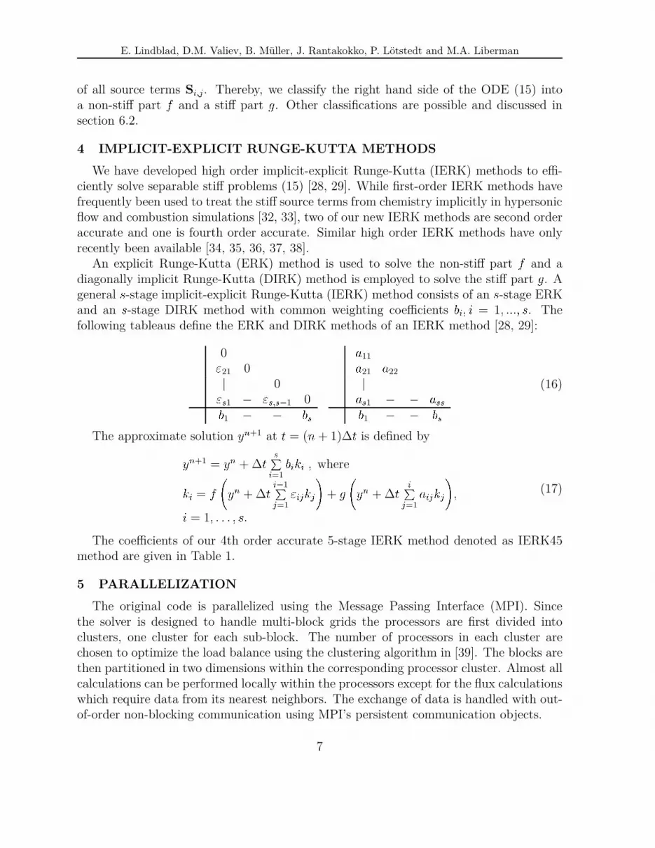
4 IMPLICIT-EXPLICIT RUNGE-KUTTA METHODS

We have developed high order implicit-explicit Runge-Kutta (IERK) methods to effi-ciently solve separable stiff problems (15) [28, 29]. While first-order IERK methods havefrequently been used to treat the stiff source terms from chemistry implicitly in hypersonicflow and combustion simulations [32, 33], two of our new IERK methods are second orderaccurate and one is fourth order accurate. Similar high order IERK methods have onlyrecently been available [34, 35, 36, 37, 38].

An explicit Runge-Kutta (ERK) method is used to solve the non-stiff part f and adiagonally implicit Runge-Kutta (DIRK) method is employed to solve the stiff part g. Ageneral s-stage implicit-explicit Runge-Kutta (IERK) method consists of an s-stage ERKand an s-stage DIRK method with common weighting coefficients bi; i = 1; :::; s. Thefollowing tableaus define the ERK and DIRK methods of an IERK method [28, 29]:

0"21 0j 0"s1 "s;s1 0b1 bs a11a21 a22jas1 assb1 bs (16)

The approximate solution yn+1 at t = (n + 1)∆t is defined byyn+1 = yn + ∆t sPi=1biki ; whereki = f yn + ∆t i1Pj=1"ijkj!+ g yn + ∆t iPj=1

aijkj!;i = 1; : : : ; s: (17)

The coefficients of our 4th order accurate 5-stage IERK method denoted as IERK45method are given in Table 1.

5 PARALLELIZATION

The original code is parallelized using the Message Passing Interface (MPI). Sincethe solver is designed to handle multi-block grids the processors are first divided intoclusters, one cluster for each sub-block. The number of processors in each cluster arechosen to optimize the load balance using the clustering algorithm in [39]. The blocks arethen partitioned in two dimensions within the corresponding processor cluster. Almost allcalculations can be performed locally within the processors except for the flux calculationswhich require data from its nearest neighbors. The exchange of data is handled with out-of-order non-blocking communication using MPI’s persistent communication objects.

7

E. Lindblad, D.M. Valiev, B. Muller, J. Rantakokko, P. Lotstedt and M.A. Liberman

Table 1: Coefficients for fourth order implicit-explicit Runge-Kutta method IERK4521 = 0:39098372452428 a11 = 1=431 = 1:09436646160460 a21 = 0:3411470572973932 = 0:33181504274704 a22 = 1=441 = 0:14631668003312 a31 = 0:8045872078976342 = 0:69488738277516 a32 = 0:0709526215454043 = 0:46893381306619 a33 = 1=451 = 1:33389883143642 a41 = 0:5293260732910352 = 2:90509214801204 a42 = 1:1513763849425353 = 1:06511748457024 a43 = 0:8024826323780354 = 0:27210900509137 a44 = 1=4b1 = a51 a51 = 0:11933093090075b2 = a52 a52 = 0:55125531344927b3 = a53 a53 = 0:1216872844994b4 = a54 a54 = 0:20110104014943b5 = a55 a55 = 1=4

The solver has been tested on a Sun Fire 15k server with UltraSparcIIIcu processorsrunning at 900MHz. The largest partition of the machine has 36 processors and 36GBRAM. Each processor has 64KB L1-cache and 8MB L2-cache. We have run several testcases with different problem sizes (600x200 to 1000x200 grid points) and different numbersof blocks (1 to 5 blocks in the multi-block case). All cases show excellent scaling withsuperlinear speedup up to full machine size, i.e., speedup close to 40 on 36 processors,cf. Figure 1 [40]. The superlinear speedup is due to better cache utilization as data isdivided into smaller pieces when running on multiple processors.

6 RESULTS

6.1 Deflagration to Detonation Transition (DDT)

One of the typical pictures of the transition due to formation of the appropriate flamefold is shown in Fig. 2, where the sequence of zonal images depicting the square ofpressure gradient gives a cinematic impression of the dynamics of the flame front duringthe incipient stage of the transition from deflagration to detonation [14]. These imagesresemble the schlieren photographs of laboratory experiments, though the latter visualizegradients of the density rather than of the pressure.

The numerical resolution is 10 cells per flame width. The time instants of Fig. 2 arenot evenly spaced but rather clustered around the transition point. The earlier imagesdepicting the incipient phase of the flame evolution in the vicinity of the tube’s closedend, are not shown.

8

E. Lindblad, D.M. Valiev, B. Muller, J. Rantakokko, P. Lotstedt and M.A. Liberman

Figure 1: Speedup versus number of processors for 3 blocks running on a SunFire 15k, ideal speedup,:: 1D decomposition of each block separately, ::: 2D decomposition of each block separately, dividingthe processors among the blocks [40]

A zoomed view of the flame fold dynamics near the transition point is shown in Fig.3 [14]. The associated profiles of temperature, density, flow velocity, and pressure alongthe fold axis are plotted on Fig. 4 [14]. Here one readily observes (i) formation of thelarge-scale preheat zone (preconditioning) in the unreacted gas trapped within the foldinterior, (ii) acceleration of the fold-tip, and (iii) the pressure elevation and formationof a high pressure peak. The transition occurs when the pressure peak becomes highenough to produce a shock capable of supporting detonation. This requires the fold to benarrow and deep enough; otherwise one ends up with a moderately strong pressure waveinsufficient for triggering the transition. This mechanism of transition by an appropriatenon-uniformity in the temperature field (preconditioning) may naturally be associatedwith Zel’dovich’s theory of soft initiation [41, 42].

6.2 Test of IERK Methods

To show the advantages of using IERK methods for combustion a series of DDT sim-ulations have been performed. The flux is calculated using the combustion code of [26].The original code uses a second order explicit Runge-Kutta method known as Gary’smethod [43] for the time stepping. For our tests it has been replaced by implicit-explicitRunge-Kutta methods of order 2, 3 and 4. The third order method is derived in [36],and the second and fourth order methods are derived in [28, 29]. Simulations showingorder of accuracy and applications of IERK methods to various model problems are alsopresented in the cited source papers.

9

E. Lindblad, D.M. Valiev, B. Muller, J. Rantakokko, P. Lotstedt and M.A. Liberman

6.2.1 Static implicit treatment of chemistry

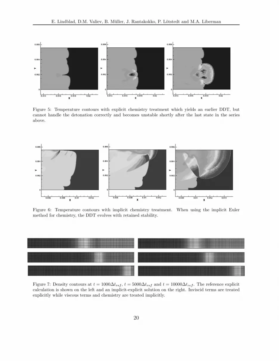
As stated above the code by [26] has been successfully used for combustion calculations.The need for implicit treatment of the chemistry becomes evident when studying thetransition from deflagration to detonation for a propagating flame. Fig. 5 shows thetemperature contours of the DDT simulation obtained using the original explicit code.Soon after the transition the solution becomes unstable.

Since the chemical source term (14) only depends on cell data, the implicit iterationcan be performed by solving a (3 + n) (3 + n) system per cell where n is the numberof species. In the present simulations a mixture of two species representing burned andunburned fuel is used. The production rate of the fuel is given by an Arrhenius expression,cf. (9) and (6). !1 = Am1Y expEaRuT ; (18)

where Y is the mass fraction of the fuel, A the reaction rate constant, and Ea theactivation energy. Here m denotes the reaction order. The temperature T is dependenton Y and given by T =

E H0 12

(u2 + v2)Cv (19)

where E is the total energy per unit mass, is the density and u and v are velocitiesin x and y directions, respectively. The enthalpy of formation H0 and the specific heat atconstant volume Cv for a mixture of n species are given byH0 =

nXi=1

YiH0i (20)Cv =nXi=1

YiCvi (21)H0i and Cvi are corresponding values for species i. For the present case n = 2, Cv1= Cv2

and H02= 0 and (19) thus reduces toT =

E Y H01 1

2(u2 + v2)Cv1

(22)

This reduces the implicit treatment of the source term (18) to a scalar equation whichcan be solved using scalar Newton iteration without having to solve any linear systems orcompute Jacobians. The overhead for solving the chemistry implicitly is therefore verysmall. Fig. 6 shows the temperature contours obtained for the same setup as the explicitcase above but using the first order implicit Euler method for the chemistry treatment.Here the solution remains stable during the transition.

10

E. Lindblad, D.M. Valiev, B. Muller, J. Rantakokko, P. Lotstedt and M.A. Liberman

The DDT for the implicit-explicit code occurs after roughly twice the time as for theexplicit code. This is because of the chaotic behaviour of the perturbations on the flamefront that cause the cusps and thereby trigger the DDT. Therefore direct comparisonscannot be made between the two cases, but the main observation is that the explicitcode becomes unstable shortly after the DDT when choosing the time step based on thestability conditions for the inviscid and viscous parts.

6.2.2 Flexible treatment of flux terms using ”switch” technique

Although the implicit treatment of the chemistry term proves efficient to retain stabilityduring DDT, apart from being more efficient than fully implicit methods, the real bene-fits come from being able to configure the explicit and implicit treatment more flexibly.Consider an ODE or a semi-discretized PDE consisting of several separable terms:U 0(t) =

lXi=1

Fi (t; U) : (23)

For a given problem some of the Fi terms will be non-stiff and some will be stiff. EveryFi will yield an upper limit on the time step for an explicit method to remain stable, thestiffer the term the smaller the limiting time step. When using an explicit method themost restrictive time step will be used for all Fi terms, resulting in unnecessary evaluationsof the other terms. When the stiffness varies significantly among the Fi terms the useof IERK methods can be more efficient than fully explicit or implicit methods, as shownabove.

The stiffness can vary in the course of a simulation, both in time and space. For combus-tion simulations the flux gradients are steepest near the flame, which moves continuously.Depending on the specific problem cell shapes, grid configurations and boundary layereffects greatly affect which Fi term will yield the most restrictvie time step.

For these situations it is beneficial to be able to freely choose which Fi terms aretreated implicitly. In the Navier-Stokes example the Fi consists of three terms, inviscidflux, viscous flux and chemical source term. In the next example, a flame propagating in atube similar to the case described above, the limiting time step for the inviscid and viscousfluxes are calculated in each step, the chemical source term is always treated implicitly.For this problem the viscous terms yield a more than 100 times smaller limiting timestep than the inviscid terms. This small step size is not needed to maintain accuracy andtherefore we choose to treat also the viscous terms implicitly. This enables us to use atime step limited only by the inviscid terms.

To investigate the impact of a larger time step a reference solution is computed ex-plicitly using a time step ∆tref = 4 1011 s, calculated from the stability condition ofthe viscous terms. This is compared with the solutions obtained when using a time step∆tIERK = 4 109 and treating the viscous terms and chemistry implicitly.

11

E. Lindblad, D.M. Valiev, B. Muller, J. Rantakokko, P. Lotstedt and M.A. Liberman

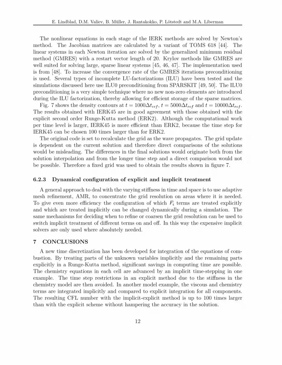
The nonlinear equations in each stage of the IERK methods are solved by Newton’smethod. The Jacobian matrices are calculated by a variant of TOMS 618 [44]. Thelinear systems in each Newton iteration are solved by the generalized minimum residualmethod (GMRES) with a restart vector length of 20. Krylov methods like GMRES arewell suited for solving large, sparse linear systems [45, 46, 47]. The implementation usedis from [48]. To increase the convergence rate of the GMRES iterations preconditioningis used. Several types of incomplete LU-factorizations (ILU) have been tested and thesimulations discussed here use ILU0 preconditioning from SPARSKIT [49, 50]. The ILU0preconditioning is a very simple technique where no new non-zero elements are introducedduring the ILU factorization, thereby allowing for efficient storage of the sparse matrices.

Fig. 7 shows the density contours at t = 1000∆tref , t = 5000∆tref and t = 10000∆tref .The results obtained with IERK45 are in good agreement with those obtained with theexplicit second order Runge-Kutta method (ERK2). Although the computational workper time level is larger, IERK45 is more efficient than ERK2, because the time step forIERK45 can be chosen 100 times larger than for ERK2.

The original code is set to recalculate the grid as the wave propagates. The grid updateis dependent on the current solution and therefore direct comparisons of the solutionswould be misleading. The differences in the final solutions would originate both from thesolution interpolation and from the longer time step and a direct comparison would notbe possible. Therefore a fixed grid was used to obtain the results shown in figure 7.

6.2.3 Dynamical configuration of explicit and implicit treatment

A general approach to deal with the varying stiffness in time and space is to use adaptivemesh refinement, AMR, to concentrate the grid resolution on areas where it is needed.To give even more efficiency the configuration of which Fi terms are treated explicitlyand which are treated implicitly can be changed dynamically during a simulation. Thesame mechanisms for deciding when to refine or coarsen the grid resolution can be used toswitch implicit treatment of different terms on and off. In this way the expensive implicitsolvers are only used where absolutely needed.

7 CONCLUSIONS

A new time discretization has been developed for integration of the equations of com-bustion. By treating parts of the unknown variables implicitly and the remaining partsexplicitly in a Runge-Kutta method, significant savings in computing time are possible.The chemistry equations in each cell are advanced by an implicit time-stepping in oneexample. The time step restrictions in an explicit method due to the stiffness in thechemistry model are then avoided. In another model example, the viscous and chemistryterms are integrated implicitly and compared to explicit integration for all components.The resulting CFL number with the implicit-explicit method is up to 100 times largerthan with the explicit scheme without hampering the accuracy in the solution.

12

E. Lindblad, D.M. Valiev, B. Muller, J. Rantakokko, P. Lotstedt and M.A. Liberman

ACKNOWLEDGEMENTS

Fellowships for E. Lindblad by EU and Goran Gustafsson Foundation are gratefullyacknowledged by M. Liberman and B. Muller, respectively.

REFERENCES

[1] Schelkin, K. I. and Troshin, Ya. K., Gasdynamics of Combustion, Mono Book Corp.Baltimore, 1965.

[2] Zel’dovich, Ya. B., Kompaneets, A.S., Theory of Detonation, Academic press, NewYork, 1960.

[3] Nettleton, M. A., Gaseous Detonation, Chapman and Hall, London, 1987.

[4] Urtiew, P., and Oppenheim, A. K., Experimental observation of the transition todetonation in an explosive gas, Proc. Roy. Soc. Lond. Ser. A, 295, 13-28. (1966).

[5] Oppenheim, K. and Soloukhin, R. I., Experiments in gasdynamics of explosion, Ann.Rev. Fluid Mech. 5, 31-58 (1973).

[6] Lee, J.H.S. and Moen, I., The mechanism of transition from deflagration to detona-tion in vapor cloud explosion, Prog. Energy Combust. Sci., 6, 359-389 (1980).

[7] Shepherd, J. E., and Lee, J. H. S., On the transition from deflagration to detonation,in Major Research Topics in Combustion, (M. Y. Hussaini, A. Kumar, and R. G.Voigt, eds), Springer-Verlag, New York, 439-487, 1992.

[8] Buckmaster, J., Clavin, P., Linan, A.,Matalon, M., Peters, N., Sivashinsky, G.,Williams, F. A., Some developments in Combustion Theory, Proc. Combust. Inst.,30, 1-14, (2005).

[9] Sivashinsky, G. I., Some developments in premixed combustion modeling, Proc. Com-bust. Inst., 29, 1737 (2002).

[10] Kuznetsov, M., Alekseev, V., Matsukov, I., and Dorofeev, S., DDT in a smooth tubefilled with a hydrogen-oxygen mixture, Shock Waves, 14, 205-215 (2005).

[11] Brailovsky, I., and Sivashinsky, G. I., Hydraulic Resistance as a Mechanism forDeflagration-to-Detonation Transition, Combust. Flame, 122, 492-499 (2000).

[12] Kagan, L., and Sivashinsky, G., The transition from deflagration to detonation inthin channels, Combust. Flame, 134, 389-397 (2003).

13

E. Lindblad, D.M. Valiev, B. Muller, J. Rantakokko, P. Lotstedt and M.A. Liberman

[13] Liberman, M. A., Sivashinsky, G. I., Valiev, D. M. and Eriksson, L-E., HydrodynamicInstability as a Mechanism for Deflagration-to-Detonation Transition, 20th Interna-tional Colloquium on the Dynamics of Explosions and Reactive Systems (ICDERS),Montreal, 2005.

[14] Liberman, M. A., Sivashinsky, G. I., Valiev, D. M. and Eriksson, L-E., NumericalSimulation of Deflagration-to-Detonation Transition: The Role of HydrodynamicFlame Instability, Int. J. Transport Phenomena (2006) to appear.

[15] Sokolik, A. S. Self-Ignition, Flame and Detonation in Gases, Israel Program forScientific Translations, NASA TTF-125OTS-63-1179, Jerusalem, 1963.

[16] Liberman, M. A., Golberg, S. M., Bychkov, V. V., and Eriksson, L.-E., Numericalstudies of hydrodynamically unstable flame propagation in 2D channels, Combust.Sci. Tech., 136, 221-242 (1998).

[17] Bychkov, V. V. and Liberman, M. A., Dynamics and stability of premixed flames,Physics Reports, 325, 115-237 (2000).

[18] Travnikov, O.Yu., Bychkov, V.V. and Liberman, M.A., Influence of compressibilityon propagation of curved flames, Physics of Fluids, 11, 2657-2666 (1999).

[19] Kazakov, K. A. and Liberman, M. A., Nonlinear equation for curved stationaryflames, Physics of Fluids, 14, 1166-1180 (2002).

[20] Liberman, M. A., Ivanov, M. F., Peil, O. E., Valiev, D. M., and Eriksson, L.-E.,Numerical modeling of flame propagation in wide tube, Combust. Theory Modeling,7, 653-676 (2003).

[21] Kadowaki, S. and Hasegawa, T., Numerical simulation of dynamics of premixedflames: flame instability and vortex-flame dynamics, Progr. Energy Combust. Sci.,31, 193-241 (2005).

[22] Liberman, M. A., Sivashinsky, G. I., Valiev, D. M., Numerical Simulation ofDeflagration-to-Detonation Transition: The Role of Hydrodynamic Flame Instability,ECCOMAS Thematic Conference on Computational Combustion, Lisbon, Portugal,(2005).

[23] Liberman, M. A., Sivashinsky, G. I., Valiev, D. M. and Eriksson, L-E., The Darrieus-Landau Instability as a Mechanism for Deflagration-to-Detonation Transition Com-bust. Theory and Modeling (2006) to appear.

[24] Oran, E. S., and Gamezo, V. N., Flame acceleration and detonation transition innarrow tubes, Proc. 20th ICDERS, Montreal, Canada (CD) (2005).

14

E. Lindblad, D.M. Valiev, B. Muller, J. Rantakokko, P. Lotstedt and M.A. Liberman

[25] Kagan L. LibermanM. Sivashinsky G, Detonation initiation by hot corrugated walls,ECCOMAS Thematic Conference on Computational Combustion, Lisbon, Portugal,21-(2005).

[26] Eriksson, L.-E., Development and validation of highly modular flow solver versionsin G2DFLOW and G3DFLOW series for compressible viscous reacting flow, Tech.Report, 9970-1162, Volvo Aero Corporation, Trollhattan, Sweden, 1995.

[27] Andersson, N., Eriksson, L.-E. and Davidson, L., Large-Eddy Simulation of subsonicturbulent jets and their radiated sound. AIAA Journal, 43(9), 1899–1912, (2005).

[28] Lindblad, E., High order semi-implicit Runge-Kutta methods for separable stiff prob-lems, Master’s Thesis, Uppsala University, Sweden, Dec. 2004.

[29] Lindblad, E. and Muller, B., High order implicit-explicit Runge-Kutta methods forseparable stiff problems. Submitted to BIT, Aug. 2005.

[30] Kuo, K.K., Principles of Combustion. John Wiley & Sons, New York, 1986.

[31] Kee, R.J., Rupley, F.M. and Miller, J.A., CHEMKIN-II: A Fortran chemical kineticspackage for the analysis of gas-phase chemical kinetics. SANDIA Report, SAND89-8009B, 1991.

[32] Bussing, T.R.A. and Murman, E.M., Finite-volume methods for the calculation ofcompressible chemically reactive flows. AIAA J., 26 (9), 1070–1078, (1988).

[33] Eriksson, L.-E., Time-marching Euler and Navier-Stokes solution for nozzle flowswith finite rate chemistry. Tech. Report, 9370-794, Volvo Flygmotor AB, Trollhattan,Sweden, 1993.

[34] Ascher, U.M., Ruuth, S.J. and Spiteri, R.J., Implict-explicit Runge-Kutta methodsfor time-dependent partial differential equations, Appl. Numer. Math., 25, 151–167,(1997).

[35] Pareschi, L. and Russo, G., Implicit-explicit Runge-Kutta schemes and applicationsto hyperbolic systems with relaxation, J. Scientific Comp., 25 (1/2), 129–155, (2005).

[36] Yoh, J.J. and Zhong, X., New hybrid Runge-Kutta methods for unsteady reactiveflow simulation, AIAA J., 42 (8), 1593–1600, (2004).

[37] Yoh, J.J. and Zhong, X., New hybrid Runge-Kutta methods for unsteady reactiveflow simulation: Applications, AIAA J., 42 (8), 1601–1611, (2004).

[38] Kennedy, C.A. and Carpenter, M.H., Additive Runge-Kutta schemes for convection-diffusion-reaction equations, Appl. Numer. Math., 44, 139–181, (2003).

15

E. Lindblad, D.M. Valiev, B. Muller, J. Rantakokko, P. Lotstedt and M.A. Liberman

[39] Rantakokko, J., Partitioning Strategies for Structured Multiblock Grids, ParallelComputing, 26 (12), 1661-1680, (2000).

[40] Myklebust, E., Parallelization of a combustion code, Master’s Thesis, Uppsala Uni-versity, Sweden, July 2004.

[41] Zel’dovich, Ya.B., Librovich, V. B., Makhviladze, G. M., and Sivashinsky, G. I., Onthe development of detonation in non-uniformly preheated gas Astronautica Acta,15, 313-321, (1970).

[42] Zel’dovich, Ya.B., Regime classification of an exothermic reaction with nonuniforminitial conditions, Combust. Flame, 39, 211-226, (1980).

[43] Gary, J., On certain finite difference schemes for hyperbolic systems, Math. Comp.,18, 1–18, (1964).

[44] Coleman, T.F., Garbow, B.S. and More, J.J., Algorithm 618: FORTRAN subrou-tines for estimating sparse Jacobian Matrices, ACM Transaction on MathematicalSoftware, 10 (3), 346-347, (1984).

[45] Knoll, D.A. and Keyes, D.E., Jacobian-free Newton-Krylov methods: a survey ofapproaches and applications, J. Comput. Phys., 193, 357-397, (2004).

[46] Banas, K., A Newton-Krylov solver with multiplicative Schwarz preconditioning forfinite element compressible flow simulations, Commun. Numer. Meth. Engng., 18,269-275, (2002).

[47] Pernice, M. and Tocci, M.D., A multigrid-preconditioned Newton-Krylov method forthe incompressible Navier-Stokes equations, SIAM J. Sci. Comput., 23 (2), 398-418,(2001).

[48] Fraysse, V., Giraud, L., Gratton, S. and Langou, J., A set of GMRES rou-tines for real and complex arithmetics on high performance computers, CER-FACS Technical Report TR/PA/03/0, 2003, public domain software available onwww.cerfacs/fr/algor/Softs.

[49] Saad, Y., SPARSKIT: a basic tool kit for sparse matrix computa-tions (version 2), Report, 1994, public domain software available onwww-users.cs.umn.edu/saad/software/SPARSKIT/sparskit.html.

[50] Saad, Y., Iterative Methods for Sparse Linear Systems, 2nd ed., SIAM, Philadelphia,2003.

16

E. Lindblad, D.M. Valiev, B. Muller, J. Rantakokko, P. Lotstedt and M.A. Liberman

Figure 2: Time sequence of images for the flame/shock dynamics near the transition point. Strongershading corresponds to higher pressure gradient. The time and distance are referred to Lf=Uf0

and Lfrespectively. Lf = u=(PruUf0

) is the flame width, where Uf0is the incipient velocity of the planar

flame, u and u the density and dynamic viscosity, respectively, of the unburnt fuel. The incipientvelocity of the planar flame Uf0

corresponds to the Mach number Mf0= Uf0

= u = 0:05, where u isthe speed of sound in the unburnt fuel. Reaction order m = 2, tube width D = 70Lf , dimensionlessactivation energy = Ea=(RuTb) = 8, expansion ratio Θ = Tb=Tu = 10. Tu and Tb are the temperaturesof the unburnt and burnt gases, respectively.

17

E. Lindblad, D.M. Valiev, B. Muller, J. Rantakokko, P. Lotstedt and M.A. Liberman

Figure 3: Time sequence of zoomed temperature contours for the flame dynamics near the transitionpoint for the conditions of Fig. 2. Lighter shading corresponds to higher temperature.

18

E. Lindblad, D.M. Valiev, B. Muller, J. Rantakokko, P. Lotstedt and M.A. Liberman

Figure 4: Temperature, density, flow velocity and pressure profiles for the fold dynamics of Fig. 3.

19

E. Lindblad, D.M. Valiev, B. Muller, J. Rantakokko, P. Lotstedt and M.A. Liberman

Figure 5: Temperature contours with explicit chemistry treatment which yields an earlier DDT, butcannot handle the detonation correctly and becomes unstable shortly after the last state in the seriesabove.

Figure 6: Temperature contours with implicit chemistry treatment. When using the implicit Eulermethod for chemistry, the DDT evolves with retained stability.

Figure 7: Density contours at t = 1000∆tref , t = 5000∆tref and t = 10000∆tref . The reference explicitcalculation is shown on the left and an implicit-explicit solution on the right. Inviscid terms are treatedexplicitly while viscous terms and chemistry are treated implicitly.

20