A Runge-Kutta Type Boundary Value ODE Solverwith Defect ControlW.H. Enright and Paul MuirTechnical Report No. 267/93June 1993.Department of Computer ScienceUniversity of TorontoToronto, Ontario, Canada M5S 1A4Copyright W.H. Enright and Paul MuirJune 1993.Abstract. A popular approach for the numerical solution of boundary value ODEproblems involves the use of collocation methods. Such methods can be naturallyimplemented so as to provide a continuous approximation to the solution over theentire problem interval. On the other hand, several authors have suggested asan alternative, certain subclasses of the implicit Runge-Kutta formulas, known asmono-implicit Runge-Kutta (MIRK) formulas, which can be implemented substan-tially more e�ciently than the collocation methods. These latter formulas do nothave a natural implementation that provides a continuous approximation to thesolution; rather only a discrete approximation at certain points within the probleminterval is obtained. However recent work in the area of initial value problems hasdemonstrated the possibility of generating inexpensive interpolants for any explicitRunge-Kutta formula. These ideas have recently been extended to develop inter-polants for the MIRK formulas. In this paper, we describe our investigation of theuse of continuous MIRK formulas in a code for the numerical solution of boundaryvalue ODE problems. A primary thrust of this investigation is to consider defectcontrol, based on these interpolants, as an alternative to the standard use of globalerror estimates, as the basis for termination and mesh redistribution criteria.Keywords: Runge-Kutta methods, ordinary di�erential equations, interpolationAMS Subject Classi�cations: 65L05, 65L10This work was supported by the Natural Sciences and EngineeringResearch Council of Canada and the Information TechnologyResearch Center of Ontario. Author addresses: W.H.Enright, University of Toronto, Toronto, Ontario, Canada, M5S 1A4(e-mail: enright@na.toronto.edu); Paul Muir, Saint Mary's University, Halifax, Nova Scotia, Canada, B3H 3C3. (e-mail:muir@husky1.stmarys.ca)

1. IntroductionA popular approach for the numerical solution of boundary value ODE (BVODE) prob-lems involves the use of collocation formulas based on, for example, Gauss or Lobatto points.The Gauss point formulas have been implemented in the widely used code, COLSYS [As-cher, Christiansen, and Russell 1981] and its descendant, COLNEW [Bader and Ascher1987]. These approaches have been shown to be particularly e�ective in the solution ofsti� or singularly perturbed BVODEs [Ascher and Weiss 1983, 1984a, 1984b], [Ascher 1985,1986], [Ascher and Bader 1986], and [Ascher and Jacobs 1989], For many numerical methodsfor BVODE problems, one obtains an approximation to the solution at a discrete set of meshpoints which partition the problem interval. An advantage of the collocation approach isthat a continuous approximation to the solution over the entire problem interval is obtainedas a natural consequence of the standard implementation of these methods. For a meshwith subintervals of size h and collocation based on Gauss points with s collocation pointsper subinterval, the continuous solution provides an approximation with global error O(hs),while the associated discrete solution at the mesh points has a global error that is (in theabscence of order reduction phenomenon) O(h2s), a property known as super-convergence.The continuous solution approximation can be very useful, for example, when the user re-quires solution information throughout the problem interval. Furthermore it can also beuseful within the numerical software package, itself, for example, for error estimation, meshre�nement and redistribution, and generation of initial iterates for Newton iterations.It is well known ([Weiss 1974]) that the collocation formulas, when applied to �rst ordersystems of ODEs, can be viewed as equivalent to certain subclasses of the implicit Runge-Kutta formulas. Recently, several authors have suggested, as an alternative to the collocationformulas, other subclasses of implicit Runge-Kutta formulas for use in the numerical solutionof BVODE problems. These formulas are known as mono-implicit Runge-Kutta (MIRK)formulas [vanBokhoven 1980], [Cash and Singhal 1982a]. A recent investigation of MIRKformulas is presented in [Burrage, Chipman, and Muir 1993], where families of order 1through 6 are characterized. An advantage of these formulas over the collocation formulas,is that the formula calculations on each subinterval can be implemented substantially moree�ciently [Cash and Singhal 1982b], [Gupta 1985], [Enright and Muir 1986], [Cash 1986,1988]. The most recent work using these formulas [Cash and Wright 1990, 1991], makesuse of three speci�c MIRK formulas of orders 4, 6, and 8 within a software package forthe numerical solution of BVODEs, called HAGRON. An early software e�ort, describedin [Gupta 1985], involved modifying the PASVA code, [Lentini and Pererya 1977], to useMIRK formulas. The approaches used in the HAGRON code and in the modi�ed PASVAcode are fundamantally di�erent from those we consider in this paper. Both of those codesuse deferred correction to provide error estimation in order to obtain a discrete solutionapproximation, while we use continuous MIRK schemes to provide defect control. As wellthe nonlinear iteration and the mesh selection algorithms are di�erent.Unlike the collocation formulas, the MIRK formulas do not directly provide a continuousapproximation to the solution. The idea of extending the discrete solution approximation toa continuous one has received considerable attention over the last few years, primarily in thearea of initial value ODE problems. In that context, a number of authors have demonstratedthe possibility of generating inexpensive interpolants for general explicit Runge-Kutta for-mulas; see, for example, [Enright et al. 1986], [Gladwell et al. 1987], [Owren and Zennaro1991,1992] and [Verner 1990]. These interpolants are obtained by performing extra derivativeevaluations, within the current step, thus preserving the one-step nature of the formula. The2

usefulness of these interpolants has been demonstrated in error estimation and defect control[Enright 1989a, 1989b] and in detection of discontinuities [Enright et al. 1988]. Recently,[Muir and Owren 1993], have developed continuous versions of the MIRK formulas. In ad-dition to presenting a general analysis, they establish order barriers for continuous MIRK(CMIRK) schemes of orders 1 through 6, and provide characterizations of CMIRK familiesof these orders.For BVODEs, the question of extending a discrete solution to obtain a continuous onehas received substantially less attention. Most BVODE codes do not provide a continuoussolution approximation. Examples of such codes are the PASVA code and the modi�edversion mentioned above, some experimental codes based on special one-sided Runge-Kuttaschemes [Kreiss, Nichols, and Brown 1986], [Brown and Lorenz 1988], and the HAGRONcode mentioned earlier.In this paper, we investigate the use of continuous solution approximations based onCMIRK formulas for the numerical solution of BVODEs. A primary thrust of the investiga-tion involves the use of defect control as an alternative to the standard global error estimatecontrol, for use in both mesh selection and accuracy control. The quality of the continuoussolution is assessed by examining the defect, which is de�ned as the amount by which thecomputed continuous solution fails to satisfy the system of di�erential equations. It is, ina sense, a more natural choice for control than estimates of the global error, since it is thedefect which arises in the analysis of the mathematical conditioning of the underlying prob-lem where appropriate condition numbers are introduced to quantify the sensitivity of theglobal error to perturbations of the ODEs. See [Ascher, Mattheij, and Russell 1988, Chap.3, Sec. 4]This paper is organized as follows. In Section 2 we describe the use of discrete andcontinuous MIRK schemes in the numerical solution of BVODEs. In Section 3 we brie ydiscuss the class of CMIRK formulas [Muir and Owren 1993] and describe the speci�c con-tinuous formulas we have chosen to implement. In Section 4, we present our investigationsof implementations of a modi�ed Newton iteration, mesh selection algorithms, and defectcontrol using CMIRK schemes. In section 5, we demonstrate the e�ectiveness of a numericalsoftware package we have written based on the ideas discussed in the previous sections of thepaper. We apply this package to some families of test problems chosen from the literature,and provide corresponding results from the COLNEW code in order to demonstrate thee�ectiveness of our approach. We close, in Section 6, with our conclusions and a summaryof our plans for future work in this area.2. The numerical solution of BVODEs using MIRK schemesIn this section we review the basic algorithm for solving a system of BVODEs with aMIRK scheme as the underlying discretization formula and then how a continuous version ofthe discrete MIRK scheme is used to provide defect control and mesh selection capabilities.The basic approach is to use the MIRK formulas to determine a non-linear discrete systemwhich can then be solved with a Newton iteration to obtain a discrete solution. Only afterthis solution is obtained is a CMIRK scheme employed to provide a continuous solutionapproximation over the problem interval for use in the computation of defect estimates,mesh redistribution, and initial guesses for subsequent Newton iterates.We assume that the boundary value ODEs to be solved can be expressed in the generalform, y0(t) = f(t; y(t)); t 2 [a; b];3

where y 2Rn and f :R�Rn !Rn, and where we assume for convenience of implementationthat we have separated boundary conditions,g(y(a); y(b)) = g0(y(a))g1(y(b))!= 0;where g0 : Rn ! Rn0 and g1 : Rn ! Rn1 and n0 + n1 = n: (The non-separated case can betreated at the cost of doubling the size of the ABD system, although it may be possible toavoid this by adapting some of the recently developed algorithms for the parallel solution ofABD systems.)A standard approach for employing a Runge-Kutta scheme to solve such problems canbe described in terms of a two-level iteration scheme:(0) Prior to beginning the two-level iteration we determine a suitable initial mesh and asso-ciated discrete solution approximation (often provided by the user).(1) The �rst step of the upper-level iteration is the setup and solution of a discrete system,�(Y ) = 0, where � is the \residual function" and Y is a vector whose i-th component, yi,is an approximation to the exact solution evaluated at the i-th point of an N + 1 pointmesh which partitions the problem interval into subintervals. The residual function hasN +1 components, each of size n: one component associated with the boundary conditions,g0 and g1, and N components, �i, i = 0; : : : ;N � 1, where �i is associated with the useof the Runge-Kutta scheme on the (i + 1)-st subinterval. We solve this discrete systemusing a modi�ed Newton iteration, which constitutes the lower-level iteration. The Jacobianof the Newton system has an almost block diagonal structure with blocks B0 = @g1@y0 andB1 = @g1@yN at the top and bottom positions of the block diagonal, and blocks Li = @�i@yi ; andRi = @�i@yi+1 ; i = 0; : : : ;N � 1, across the ith block row of the block diagonal. The blocksLi, Ri, and the block [B0;B1]T ; are all of size n by n. When a MIRK scheme is used as theunderlying discretization the ith component of the residual function takes the form,�i = yi+1 � yi � hi sXr=1 brKr; (2:1)where, the stages, Kr, are given by,Kr = f(ti+ crhi; (1� vr)yi+ vryi+1+ hi r�1Xj=1xrjKj); r = 1; : : : ; s: (2:2)Because the stages are de�ned explicitly in terms of the unknowns yi and yi+1, these methodscan be implemented quite e�ciently. The corresponding partial derivatives are also easilycomputed. The expressions for Li and Ri follow simply by di�erentiating �i with respect toyi and yi+1, respectively. This yieldsLi = �I � hi sXr=1 br �@Kr@yi � and Ri = I � hi sXr=1 br � @Kr@yi+1� ; (2:3)4

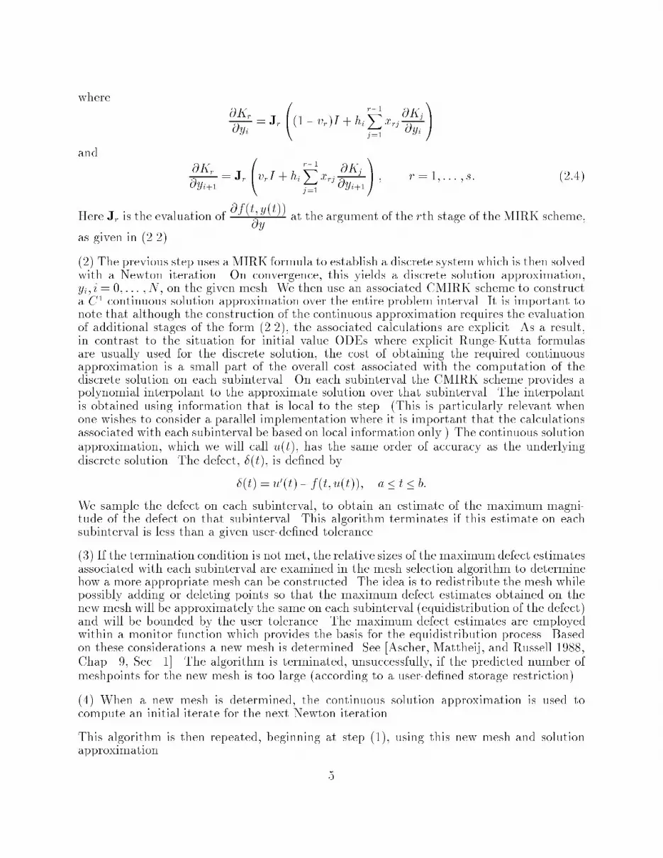
where @Kr@yi = Jr 0@(1 � vr)I + hi r�1Xj=1xrj @Kj@yi 1Aand @Kr@yi+1 = Jr0@vrI + hi r�1Xj=1xrj @Kj@yi+11A ; r = 1; : : : ; s: (2:4)Here Jr is the evaluation of @f(t; y(t))@y at the argument of the rth stage of the MIRK scheme,as given in (2.2).(2) The previous step uses a MIRK formula to establish a discrete system which is then solvedwith a Newton iteration. On convergence, this yields a discrete solution approximation,yi; i= 0; : : : ;N , on the given mesh. We then use an associated CMIRK scheme to constructa C1 continuous solution approximation over the entire problem interval. It is important tonote that although the construction of the continuous approximation requires the evaluationof additional stages of the form (2.2), the associated calculations are explicit. As a result,in contrast to the situation for initial value ODEs where explicit Runge-Kutta formulasare usually used for the discrete solution, the cost of obtaining the required continuousapproximation is a small part of the overall cost associated with the computation of thediscrete solution on each subinterval. On each subinterval the CMIRK scheme provides apolynomial interpolant to the approximate solution over that subinterval. The interpolantis obtained using information that is local to the step. (This is particularly relevant whenone wishes to consider a parallel implementation where it is important that the calculationsassociated with each subinterval be based on local information only.) The continuous solutionapproximation, which we will call u(t), has the same order of accuracy as the underlyingdiscrete solution. The defect, �(t), is de�ned by�(t) = u0(t)� f(t; u(t)); a � t � b:We sample the defect on each subinterval, to obtain an estimate of the maximum magni-tude of the defect on that subinterval. This algorithm terminates if this estimate on eachsubinterval is less than a given user-de�ned tolerance.(3) If the termination condition is not met, the relative sizes of the maximumdefect estimatesassociated with each subinterval are examined in the mesh selection algorithm to determinehow a more appropriate mesh can be constructed. The idea is to redistribute the mesh whilepossibly adding or deleting points so that the maximum defect estimates obtained on thenew mesh will be approximately the same on each subinterval (equidistribution of the defect)and will be bounded by the user tolerance. The maximum defect estimates are employedwithin a monitor function which provides the basis for the equidistribution process. Basedon these considerations a new mesh is determined. See [Ascher, Mattheij, and Russell 1988,Chap. 9, Sec. 1]. The algorithm is terminated, unsuccessfully, if the predicted number ofmeshpoints for the new mesh is too large (according to a user-de�ned storage restriction).(4) When a new mesh is determined, the continuous solution approximation is used tocompute an initial iterate for the next Newton iteration.This algorithm is then repeated, beginning at step (1), using this new mesh and solutionapproximation. 5

We will discuss further details of the Newton iteration, defect estimation, and meshselection algorithms in section 4. In the next section we employ the work of [Muir andOwren 1993] on CMIRK schemes to derive the speci�c CMIRK formulas which we haveimplemented in our code.3. CMIRK Schemes3.1. OverviewIn the paper [Muir and Owren 1993], the class of CMIRK schemes is investigated.We now brie y summarize their work and discuss how it is applied in the computation ofcontinuous solution approximations for BVODE problems. As mentioned in the previoussection, the CMIRK scheme is employed only after the discrete solution has been obtainedfor the current mesh. By saving the stages from the MIRK scheme that were computed foreach subinterval during the computation of the discrete solution, we can save some of thecomputational cost associated with the construction of the stages for the CMIRK scheme foreach subinterval. For the ith subinterval, the basic form of a CMIRK scheme is a polynomialin �, (where � = t�tihi ),u(t) = u(ti+ �hi) = yi+ hi s�Xr=1 br(�)Kr; 0 � � � 1; ti � t � ti+1; s� � s; (3:1)with stages Kr = f(ti+ crhi; (1� vr)yi+ vryi+1+ hi r�1Xj=1xrjKj); r = 1; : : : ; s�: (3:2)Observe that the stage values, (3.2), have the same structure as for the discrete MIRKscheme, (2.2); in fact the �rst s stages are precisely those of the discrete MIRK scheme usedduring the computation of the discrete solution. The remaining s� � s stages are de�ned bydetermining appropriate sets of new coupling coe�cients xrj; r = s+1; : : : ; s�; j = 1; : : : ; r �1. The de�nition of the CMIRK is completed with the determination of the s� weightpolynomials, br(�); r = 1; : : : ; s�. These are polynomials of maximum degree p, where pis the order of accuracy of the discrete MIRK scheme. The extra stages and the weightpolynomials are constructed to satisfy continuous order conditions up to and including orderp so that on each subinterval, the CMIRK scheme satis�esmax0���1 jjy(ti+ �hi)� u(ti+ �hi)jj= O(hp+1i ); (3:3)where y(t) is the exact solution to the local initial value ODE,y0(t) = f(t; y(t)); y(ti) = yi;y(ti) = u(ti), and jj � jj is any norm on Rn. For all CMIRK schemes, u(ti) = yi, and for thosesatisfying an additional condition known as the C(3) stage order condition, u(ti+1) = yi+1.Included in [Muir and Owren 1993] is a presentation of multi-parameter families ofCMIRK stages having a minimal number of stages for each order p = 1; : : : ;6. Similarly,6

a portion of the [Burrage, Chipman and Muir 1993] paper is devoted to the presentationof multi-parameter families of (discrete) MIRK schemes having a minimal number of stagesfor each order p = 1; : : : ;6. Throughout this paper, we will refer to CMIRK and MIRKschemes having a minimal number of stages for a given order as optimal schemes. It is ofcourse always the case that the number of stages needed to get a discrete MIRK schemeis less than or equal to that for the associated CMIRK scheme. In this section, we willchoose optimal discrete MIRK schemes from the families presented in [Burrage, Chipman,and Muir 1993] and then attempt to embed the discrete schemes in optimal CMIRK schemes.The CMIRK schemes will be determined by employing the additional stage coe�cients andweight polynomials according to the characterizations given in [Muir and Owren 1993].Since the families of schemes given in [Burrage, Chipman, and Muir 1993] and [Muirand Owren 1993] involve several parameters, there is usually substantial freedom in thechoice of a particular MIRK scheme and the associated CMIRK scheme. An open problemis to determine appropriate criteria for the determination of good MIRK schemes and goodCMIRK schemes for use in the numerical solution of boundary value ODEs with defectcontrol. In the current paper, where the selection of the MIRK and CMIRK schemes is onlyone component of the project, we have selected schemes which are e�cient, have satisfactoryaccuracy properties, and have been demonstrated to work well on several test problems. Itshould be noted that the focus of this paper is to investigate the potential advantages of usingMIRK and CMIRK schemes in a software package for the numerical solution of boundaryvalue ODEs, rather than to develop optimal schemes of these types. We will pursue thislatter investigation in a subsequent study.We next present the particular MIRK and CMIRK schemes which have been imple-mented with our code. The coe�cients de�ning a MIRK scheme, (2.1),(2.2) are usuallypresented in the form of a tableau as in Table 3.1.Table 3:1c1 v1 0 0 : : : 0 0c2 v2 x21 0 : : : 0 0... ... ... ... ... ... ...cs�1 vs�1 xs�1;1 xs�1;2 : : : 0 0cs vs xs;1 xs;2 : : : xs;s�1 0b1 b2 : : : bs�1 bsLater in the paper, we will use the following compact notation for the above scheme:c = [c1; c2; : : : ; cs]T , v = [v1; v2; : : : ; vs]T , b = [b1; b2; : : : ; bs]T , and X is the s � s matrixwhose (i; j)th component is xij. For a CMIRK scheme, as given by (3.1),(3.2), the tableauhas the form shown in Table 3.1 but the bottom row will consist of weight polynomials,b1(�); b2(�); : : : ; bs(�), and we will use the notation, b(�) = [b1(�); b2(�); : : : ; bs(�)]T . Here wepresent two MIRK/CMIRK schemes, one of order 4, the other of order 6.7

3.2. MIRK/CMIRK schemes of 4th orderThe most general form of a 4th order CMIRK scheme is given in [Muir and Owren1993]. It uses 4 stages and has free parameters c3, c4, and v4. We will attempt to embedthe optimal, 3-stage, 4th order discrete MIRK scheme within the CMIRK scheme. That is,the �rst 3 stages of the CMIRK scheme will be the same as those of the MIRK scheme, andthe values of the continuous weight polynomials at � = 1 will be the weights of the discretescheme. If we choose the free parameter c3 = 12 then the �rst three stages of this CMIRKscheme correspond to the unique 3-stage, 4th order MIRK, and the expressions for the 4thstage and the weight polynomials become more restricted. In Table 3.2 we give the tableaufor this restricted CMIRK scheme. Table 3:20 0 0 0 0 01 1 0 0 0 012 12 18 � 18 0 0c4 v4 �v46 �3c422 + c4 + 2c433 �c422 �v46 + 2c433 2c42�4c433 �2v43 0b1(�) b2(�) b3(�) b4(�)whereb1(�) = � (6 c4 � 9 �c4 � 3 �+6 �2+4 �2c4 � 3 �3)6 c4 ; b2(�) = �2 (2 � � 3 c4+4 �c4 � 3 �2)6(c4 � 1) ;b3(�) = �2 �2 (4 �c4 � 6 c4+4 � � 3 �2)3(2 c4 � 1) ; b4(�) = �2 (� � 1)22 c4 (2 c4 � 1) (c4 � 1) ;with the restrictions that c4 6= 0;1; 12. Also b1(1) = 16, b2(1) = 16, b3(1) = 23, and b4(1) = 0.A careful analysis to determine suitable optimization criteria based, for example, on min-imizing the error coe�cients of the dominant error terms followed by a thorough numericalinvestigation will be needed to determine optimal values for the remaining free parametersc4 and v4. Here, in order to exhibit a speci�c CMIRK scheme, we have arbitrarily chosenc4 = 34 and v4 = 2732. With these choices we get the 4th order CMIRK scheme, given in Table3.3. Table 3:30 0 0 0 0 01 1 0 0 0 012 12 18 �18 0 034 2732 364 �964 0 0b1(�) b2(�) b3(�) b4(�)8

where b1(�) = �� (2 � � 3) (2 �2 � 3 �+2)6 ; b2(�) = �2 (9 � 20 �+12 �2)6 ;b3(�) = 2 �2 (9� 14 �+6 �2)3 ; b4(�) = �16 �2 (� � 1)23 :This is the 4th order CMIRK scheme, with embedded MIRK scheme we have implemented.3.3. MIRK/CMIRK schemes of 6th orderA particular family of 6th order CMIRK schemes is given in [Muir and Owren 1993].Although the family has 9 free parameters c3; c4; c5, c6; c7; v7, c8; v8; x81, it does not necessarilyrepresent all possible 8-stage, 6th order CMIRK schemes. As in the previous subsection, ourplan will be to attempt to construct a particular CMIRK scheme which contains a speci�c, 5-stage, 6th order discrete MIRK scheme as an embedded scheme, i.e. the tableau will containthe stages of the discrete scheme, and the weights evaluated at � = 1 are the weights of thediscrete scheme. If we choose the free parameters c3 = 14, c4 = 34 , and c5 = 12 this completelyde�nes the �rst 5 rows of the CMIRK scheme and the expressions for the remaining 4 stagesand the weight polynomials become more restricted. The remaining free parameters for thisfamily are c6; c7; c8, v7; v8, and x81. We give the tableau for this CMIRK scheme in Section1 of the Appendix. Unfortunately, this family of CMIRK schemes does not include thestandard optimal 5-stage, 6th order discrete MIRK scheme, often quoted in the literature.(See, for example, [Van Bokhoven 1980], Method VIII.) The 5th stage of our CMIRK familyis di�erent than Method VIII, and more signi�cantly, the 3rd and 4th weights of our CMIRKscheme are identically zero, while the corresponding weights of Method VIII are not.We consider whether or not our CMIRK family contains a di�erent optimal 5-stage,6th order discrete MIRK scheme. (The 5-stage, 6th order MIRK scheme of [Van Bokhoven1980] is easily shown to be non-unique.) The remaining free parameters are all associatedwith de�ning the extra stages (6 through 8) required by the CMIRK scheme. We arbitrarilychoose c6 = 18 , c7 = 78, v7 = 34794096 (chosen so that x76 = 0), c8 = v8 = 38, and x81 = 524. Thisgives a CMIRK scheme with the tableau given in Table 3.4.Table 3:40 0 0 0 0 0 0 0 0 01 1 0 0 0 0 0 0 0 014 532 964 �364 0 0 0 0 0 034 2732 364 �964 0 0 0 0 0 012 12 124 �124 16 �16 0 0 0 018 6174096 151924576 �38524576 491536 �491536 �1472048 0 0 078 34794096 38524576 �151924576 491536 �491536 1472048 0 0 038 38 524 �2711344 11471920 �11471920 �37576 �980920160 15672880 0b1(�) b2(�) b3(�) b4(�) b5(�) b6(�) b7(�) b8(�)9

where the weight polynomials areb1(�) = �� (4665 � +5120 �5 � 17664 �4 + 23400 �3 � 14900 �2 � 630)630 ;b2(�) = �2 (63 � 580 � +1800 �2 � 2304 �3 +1024 �4)210 ; b3(�) = 0; b4(�) = 0;b5(�) = 2 �2 (315 � 2690 � +7140 �2 � 7296 �3 +2560 �4)135 ;b6(�) = 32 �2 (315 � 1430 � +2595 �2 � 2112 �3 +640 �4)945 ;b7(�) = �16 �2 (45 � 410 �+1245 �2 � 1536 �3 + 640 �4)945 ;b8(�) = �16 �2 (128 �2 � 128 �+ 21) (� � 1)245 :If we evaluate these polynomials at � = 1 we get a 6th order 7-stage discrete MIRK schemewith 5 non-zero weights, as follows,b1 = b2 = 170 ; b3 = b4 = 0; b5 = 58135 ; b6 = b7 = 256945 ; b8 = 0:The above discussion demonstrates a fundamental contrast between the 4th and the6th order cases. In the 4th order case, the number of stages needed to get a 4th ordercontinuous extension of a given optimal discrete MIRK is the same as the optimal number ofstages for a continuous CMIRK scheme of order 4, namely 4, and the discrete scheme can beembedded in the continuous family. This follows from the observation that the continuousfamily of CMIRK schemes of 4th order given in [Muir and Owren 1993] is complete. Inthe 6th order case, the optimal number of stages for a 6th order CMIRK scheme is 8. Theparticular CMIRK family exhibited in [Muir and Owren 1993] is based on two additionalassumptions about the stage order of some of the stages of the schemes and thus is not likelyto be complete. In fact it is substantially restrictive since it must have b3(�) = b4(�) = 0. Itis then impossible for this family to include any optimal discrete MIRK scheme having only5 stages, since there would then have to be only 3 stages with non-zero weights which fromconsideration of the quadrature conditions, we know is not possible. In the above derivation,the result is a discrete scheme with only 5 non-zero weights but requiring 7 stages.For the optimal 5-stage, 6th order discrete scheme of [Van Bokhoven 1980], it appears,from an analysis of the continuous order conditions, that 4 additional stages must be addedin order to produce a 6th order continuous scheme. That is, the continuous extension of thegiven optimal 5-stage, 6th order discrete scheme requires one more stage than that requiredby an optimal continuous CMIRK scheme of 6th order. We thus have the choice of an optimal8-stage CMIRK scheme with a non-optimal embedded 7-stage, 6th order MIRK scheme, ora non-optimal 9-stage CMIRK scheme with an optimal embedded 5-stage, 6th order MIRKscheme. Because an important factor in the computational costs is the number of stagesin the discrete MIRK scheme, we choose the latter option for our implementation. Theabove discussion suggests the need for a theoretical investigation of optimal CMIRK schemescontaining embedded optimal discrete MIRK schemes. We plan to study this question in asubsequent investigation. 10

In Table 3.5, we present a 9-stage, 6th order CMIRK scheme, which has the abovementioned 5-stage, 6th order discrete MIRK scheme embedded within it. The �rst 5 stagesof the CMIRK scheme are the stages of this MIRK scheme. The �rst 5 weight polynomialsevaluated at � = 1 are the weights of this MIRK scheme, while the last 4 weight polynomialsare 0 when evaluated at � = 1. Table 3:50 0 0 0 0 0 0 0 0 0 01 1 0 0 0 0 0 0 0 0 014 532 964 �364 0 0 0 0 0 0 034 2732 364 �964 0 0 0 0 0 0 012 12 524 �524 23 �23 0 0 0 0 0716 716 154732768 �122532768 7494096 �2872048 �86116384 0 0 0 018 18 831536 �13384 2831536 �1671536 �49512 0 0 0 0916 916 122532768 �154732768 2872048 �7494096 86116384 0 0 0 038 38 2333456 �191152 0 0 0 �572 772 �17216 0b1(�) b2(�) b3(�) b4(�) b5(�) b6(�) b7(�) b8(�) b9(�)whereb1(�) = � (334530 � 1287315 � � 1662100 �2 + 10043400 �3 � 11467776 �4 +4065280 �5)334530 ;b2(�) = �2 (3083913 � 25341580 � + 62657400 �2 � 62874624 �3 +22657024 �4)2341710 ;b3(�) = �16 �2 (8505 � 69430 � +168780 �2 � 164352 �3 +56320 �4)7965 ;b4(�) = �16 �2 (8505 � 69430 � +168780 �2 � 164352 �3 +56320 �4)7965 ;b5(�) = �2 �2 (8505 � 69430 � + 168780 �2 � 164352 �3 + 56320 �4)2655 ;b6(�) = �1024 �2 (45568 �2 � 45856 � +7533) (� � 1)233453 ;b7(�) = 128 �2 (128 �2 � 128 �+ 21) (� � 1)215 ;b8(�) = 1024 �2 (134144 �2 � 132128 � +21609) (� � 1)2234171 ; b9(�) = �16384 �3 (� � 1)3441 :11

Evaluating these weight polynomials at � = 1 givesb1(1) = b2(1) = 790 ; b3(1) = b4(1) = 3290 ; b5(1) = 1290 ; b6(1) = b7(1) = b8(1) = b9(1) = 0:These 5 non-zero weights plus the �rst 5 stages from Table 3.5 de�ne the optimal 5-stage,6th order MIRK scheme, embedded within the 9-stage, 6th order CMIRK scheme, which wehave implemented.4. Practical Aspects of MIRK Schemes in a Defect-Controlled BVODE CodeIn this section we discuss the development, implementation, and analysis of algorithmsfor various parts of a software package for the numerical solution of BVODEs, based onMIRK schemes and defect control, for which the general algorithm was given in Section 2.We will include a presentation of the results of an exploration of several of the heuristicstrategies employed within the code. We will discuss the modi�ed Newton iteration used tosolve the non-linear systems arising from the discretization of the ODE system, the detailsof the implementation of defect control (including estimation of the defect through defectsampling), and the results of our investigation of some of the controlling parameters in themesh re�nement and redistribution algorithm.4.1. The Modi�ed Newton Iteration4.1.1. Damped Newton and �xed Jacobian iterationsTo solve the system, �(Y ) = 0, described in section 2, we have employed a modi�edNewton iteration, modelled on that discussed in [Ascher, Mattheij, and Russell 1988, Chap.8]. This includes the implementation of a damped Newton iteration, and a �xed Jacobianiteration, as well as a scheme for switching between these two modes of iteration. Theswitching scheme involves monitoring the rate of decrease of a function known as the \naturalcriterion function", jjJ�1(Y (q))�(Y (q+1))jj, where Y (q) is the qth iterate, �(Y ) is the residualfunction de�ned in section 2, and J(Y ) is the Jacobian of �(Y ). The code begins with afull Newton step and continues with damped Newton steps until it has taken a step withthe damping factor equal to 1 (i.e. a full Newton step) and there has been a su�cientdecrease in the size of the natural criterion function. When these conditions arise the codeswitches to �xed Jacobian steps, continuing these as long as su�cient decreases in the valueof the natural criterion function continue. Our numerical experiments indicate that thecomputational costs of �xed Jacobian steps are relatively negligible compared to the costsof setting up and factoring the full Jacobian. Thus we have found it worthwhile to be fairlyliberal in allowing the code to attempt to take �xed Jacobian steps.In addition to monitoring the size of the natural criterion function to check for a su�cientrate of convergence, we have also found it useful to use the size of the natural criterionfunction to allow early termination of divergent or slowly converging iterations. When thenatural criterion function value exceeds a certain threshold value this usually signi�es that thecorresponding Newton correction is also large, and we terminate the Newton iteration since alarge Newton correction indicates that the current iterate is not close to the true solution ofthe current discrete system. In the context of solving BVODE problems, it may be preferableto employ the option of restarting with a new discrete system based on a �ner mesh. Anopen question here is to determine a suitable value for the threshold value bounding the sizeof the natural criterion function values. A somewhat related point concerns determination12

of the appropriate upper limit on the maximum number of iterations that should be allowedfor each Newton iteration. Even if the natural criterion function values remain boundedthe rate of convergence may be su�ciently slow that convergence will not be achieved formany steps. Also divergent iterations can be detected in this way. As mentioned above, areasonable strategy may be to set the maximum number of iterations limit fairly low, withthe idea that it would be better to start over on a �ner mesh than to continue on the currentmesh.An additional consideration, mentioned in [AMR 1988], is to have the size of the systemcontribute to deciding when to switch to a �xed Jacobian iteration: for smaller systemswhich usually arise during the initial iterations (where the mesh is coarse and may not bewell adapted to the solution behavior) it may be better to simply employ full or dampedNewton iterations, and avoid any consideration of �xed Jacobian steps until the systemsbecome larger and more substantial savings can be expected. We have not implemented thisidea, but are considering it for further testing to evaluate its importance. Another interestingaspect of the e�cient implementation of this algorithm has been the need for careful datamanagement to ensure that no duplicate calculations are performed. Some of the quantitiescomputed by the natural criterion function to assess the quality of the most recent iteratecan be used in the next Newton step, even when the current step is rejected.We conducted a numerical evaluation of the damped Newton iteration compared with asimpler approach where a full Newton iteration was used for every step. As expected, for verydi�cult discrete systems where we used poor initial estimates of the solution, the dampedNewton iteration achieved convergence in cases where the full Newton iteration did not.This usually occurred during the early part of the execution of the code where the mesh wascoarse and the solution information from the previous mesh was nonexistent or not relevant.However for somewhat less di�cult discrete systems, again on coarse meshes with poor initialinformation for the solution, the full Newton iteration sometimes achieved convergence whenthe damped iteration gave up too soon. Thus it is not clear that the damped Newton iterationwill always behave in a superior fashion. Furthermore, when solving the nonlinear systemsarising in BVODEs, it may not be a good strategy to employ a damped Newton iterationand devote substantial computational e�ort to obtaining a converged solution to a discretesystem derived from a coarse mesh. Rather, it may be better to just restart on a �ner meshwhere convergence may be obtained more quickly. Of course, as is noted in [Ascher, Mattheij,and Russell, 1988], the primary bene�t of the damped Newton iteration in this context maybe that it allows early termination of a divergent or too slowly converging iteration.4.1.2. Approximate Jacobian evaluationsHere we make note of an important point associated with the evaluation of the Jacobianmatrix arising during the damped Newton iteration. The Jacobian, @�@Y , as described insection 2, has an almost block diagonal structure, with blocks based on the partial derivativesof the components of � associated with each subinterval. The expressions for the blocks aregiven in (2.3) and (2.4). The literature for MIRK schemes for both initial and boundaryvalue ODEs suggests that (2.4) can be approximated by evaluating @f@y at only one pointon each subinterval, with this one value being used in place of each instance of Jr arisingin (2.4). We implemented this suggestion in the module which constructs the Jacobianblocks, and compared the performance with that obtained using a similar module where sJacobian evaluations were done for each subinterval, as in (2.4). We found major di�erencesin performance between the two approaches, especially when applied to di�cult nonlinearproblems. When using single Jacobian evaluations per subinterval approach, we found somesavings in the cost of computing the Jacobian blocks, but the resultant degradation in the13

performance of the Newton iteration more than o�set these savings. Not only was the rate ofconvergence for the single Jacobian evaluation approach much slower, but also the likelyhoodof achieving convergence was much lower as well. This suggests that on some problems it iscritical to incur the extra cost of using exact Jacobian values on each subinterval, in orderto achieve a lower overall cost.4.1.3. Solution and mesh continuation over the discrete problem sequenceWe conducted a set of experiments in which we investigated the standard approach usedin the numerical solution of boundary value problems in which the code begins with a coarsemesh and possibly poor solution approximation, sets up and solves a discrete system basedon this information, and then proceeds to construct a more appropriate mesh and estimateof the solution for the next discrete system, (based on the solution information from thecurrent step). When the code begins execution under such circumstances, it was oftendi�cult to obtain convergence of the Newton iteration. Furthermore, in those instanceswhere convergence was obtained on the initial mesh (after many iterations, and possiblyusing a sequence of damped steps), and the resulting continuous solution used for the initialguess for the next discrete system (based on a mesh obtained by halving the previous one),we often observed that the Newton iteration for the new discrete problem would often notconverge at all. In fact, we sometimes observed that we could get better convergence resultsby ignoring the computed solution from the previous coarse mesh, and simply providingthe original initial solution approximation for the re�ned mesh. The di�culty here is thatthe solution to the discrete system on a coarse mesh may not be closely related to thesolution for the discrete system on the re�ned mesh, so it is not particularly helpful toprovide the computed solution from the coarse system as the initial solution estimate forthe re�ned system. The implication for strategies for monitoring the Newton iteration isthat, if we observe convergence di�culty for a discrete system on a coarse mesh, it may notbe worthwhile to invest much computational e�ort in �nding a solution to this system. Abetter strategy might be to simply \fail" on that coarse system, and restart with a re�nedmesh and a larger discrete system. We found that by monitoring the size of the defect wecould generally detect whether the solution from a coarse discrete system would be usefulas the initial solution estimate for the next re�ned system. A large defect signaled that thesolution to the coarse system would probably not be useful. We are presently conductingfurther investigation of an optimal choice for the maximum size of an acceptable defect.A related consideration here is that the appropriate threshold value for the size ofthe defect of the numerical solution may be di�erent depending on how we intend to usethe defect. We have found that in some cases, where the defect is of intermediate size, itmay be worthwhile to use the defect estimates for each subinterval as input for the meshredistribution algorithm but it is not appropriate to use the corresponding numerical solutionas the initial guess for the Newton iterate for the discrete system derived from the new mesh.This suggests that two thresholds may be needed, one for acceptance of the defect for usein the mesh redistribution process, and another for acceptance of the numerical solutionfor use as the initial Newton iterate. We are currently investigating the determination ofappropriate threshold values.4.1.4. The tolerance for the Newton iterationA �nal issue in this area is to determine the appropriate size for the tolerance to beapplied to the Newton correction vector at each step of the Newton iteration in order todetermine convergence of the iteration. It is clear that the Newton tolerance should be lessthan the user-de�ned tolerance in order to ensure that the discretization errors will dominatein the determination of the defect, and thus in the mesh redistribution process. We have14

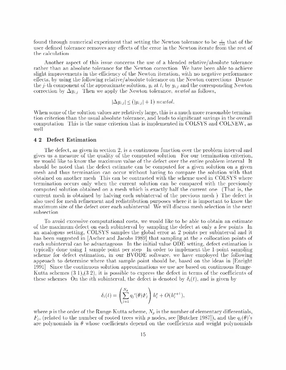
found through numerical experiment that setting the Newton tolerance to be 1100 that of theuser-de�ned tolerance removes any e�ects of the error in the Newton iterate from the rest ofthe calculation.Another aspect of this issue concerns the use of a blended relative/absolute tolerancerather than an absolute tolerance for the Newton correction. We have been able to achieveslight improvements in the e�ciency of the Newton iteration, with no negative performancee�ects, by using the following relative/absolute tolerance on the Newton corrections. Denotethe j-th component of the approximate solution, yi at ti by yi;j and the corresponding Newtoncorrection by �yi;j. Then we apply the Newton tolerance, newtol as follows,j�yi;jj � (jyi;jj+1) newtol:When some of the solution values are relatively large, this is a muchmore reasonable termina-tion criterion than the usual absolute tolerance, and leads to signi�cant savings in the overallcomputation. This is the same criterion that is implemented in COLSYS and COLNEW, aswell.4.2. Defect EstimationThe defect, as given in section 2, is a continuous function over the problem interval andgives us a measure of the quality of the computed solution. For our termination criterion,we would like to know the maximum value of the defect over the entire problem interval. Itshould be noted that the defect estimate can be computed for a given solution on a givenmesh and thus termination can occur without having to compare the solution with thatobtained on another mesh. This can be contrasted with the scheme used in COLSYS wheretermination occurs only when the current solution can be compared with the previouslycomputed solution obtained on a mesh which is exactly half the current one. (That is, thecurrent mesh is obtained by halving each subinterval of the previous mesh.) The defect isalso used for mesh re�nement and redistribution purposes where it is important to know themaximum size of the defect over each subinterval. We will discuss mesh selection in the nextsubsection.To avoid excessive computational costs, we would like to be able to obtain an estimateof the maximum defect on each subinterval by sampling the defect at only a few points. Inan analogous setting, COLSYS samples the global error at 2 points per subinterval and ithas been suggested in [Ascher and Jacobs 1989] that sampling at the s collocation points ofeach subinterval can be advantageous. In the initial value ODE setting, defect estimation istypically done using 1 sample point per step. In order to implement the 1-point samplingscheme for defect estimation, in our BVODE software, we have employed the followingapproach to determine where that sample point should be, based on the ideas in [Enright1991]. Since the continuous solution approximations we use are based on continuous Runge-Kutta schemes (3.1),(3.2), it is possible to express the defect in terms of the coe�cients ofthese schemes. On the ith subinterval, the defect is denoted by �i(t), and is given by�i(t) = 0@ NpXj=1 qj 0(�)Fj1Ahpi +O(hp+1i );where p is the order of the Runge-Kutta scheme,Np is the number of elementary di�erentials,Fj, (related to the number of rooted trees with p nodes, see [Butcher 1987]), and the qj(�)'sare polynomials in � whose coe�cients depend on the coe�cients and weight polynomials15

of the continuous Runge-Kutta scheme. Thus the size of the defect is determined by thecoe�cient of the hpi term in the above expression, for hi su�ciently small. We introduce afurther approximation by considering only the term that remains when linear ODE problemsare considered. In this case the only non-zero qj(�), which we write without a subscript, isq(�) = bT (�)(X + vb(1)T)p�2c� �pp! :For a particular continuous MIRK schemewe can examine the behavior of q0(�) over 0 � � � 1and determine where it reaches it maximum. We will then choose the defect sample point,��, at this location. For the 4th order continuous MIRK scheme given in the previous section,the above analysis led us to choose �� � 0:226. For the 6th order CMIRK given at the endof the previous section, we found that �� � 0:716. The estimate of the maximum defect foreach subinterval is de�ned to be the max-norm of the defect vector (of length n) generatedby sampling the exact defect expression at this single sample point. We will refer to this asthe absolute defect estimate.As we saw in the previous subsection for Newton iterations, it is more practical toconsider using a relative/absolute de�nition of the defect for use in termination criteria andin mesh redistribution. The use of the scaled defect, ��i(t), on each subinterval, de�ned by,��i(t) � �i(t)(jf(t; u(t))j+1)has proven, in our numerical experiments, to lead to substantial savings in the computationalcosts. Since the defect is a perturbation of the original ODE system, it is clearly moreappropriate to consider the size of the defect relative to the size of f , when f is large.We performed numerical experiments to determine the reliability of the above approachto defect sampling. Using the family of test problems, Swirling Flow III, [Ascher, Mattheij,Russell, 1980, Pg. 23], (see the Appendix, Section 2, for the corrected form of this problem),we assessed the reliability of three defect estimation schemes. We considered several problemsfrom this family, each characterized by a particular value of the parameter value, epsilon. Weconsidered a sequence of meshes and used a tolerance of 10�6. We examined the reliabilityof estimation of the maximum absolute defect using 1-point sampling, estimation of themaximumscaled defect using 1-point sampling, and estimation of the maximumscaled defectusing 2-point sampling, with the second sample point chosen to be 1 � ��. We comparedthe estimate for each subinterval with a \true" value obtained by sampling the defect at 11points on the subinterval to get a good estimate of the true maximum value. We computedthe ratio of the estimated maximum to the true maximum and de�ned a deception to occurwhen the estimate of the maximumwas less than 15 of the true maximum. We then computedthe percentage of deceptions with respect to the total number of estimates performed overall discrete problems considered by the code in arriving at the �nal solution. We used theBVODE code to solve each problem beginning with an initial uniform mesh of 5 subintervals,and and initial guess consisting of straight lines through the boundary conditions. The codethen worked through a sequence of discrete problems, choosing new meshes based on defectinformation, until it obtained a solution with a satisfactory defect or until it found it couldnot �nd a solution using fewer than the maximumnumber of subintervals we allowed, namely300. For each discrete problem for which a solution was obtained, the code computed defectestimates according to one of the above schemes: absolute defect with 1-point sampling,scaled defect with 1-point sampling, or scaled defect with 2-point sampling. (Note that when16

applied as the termination criterion, the absolute defect requirement is more severe than thescaled defect requirement, so a BVODE code would have to work much harder in the formercase. The point of this particular experiment is to examine the reliability of the estimationschemes and rather than compare their e�ciency within the BVODE software.) We usedthe defect to control both termination and mesh redistribution. In Tables 4.2.1 and 4.2.2 wereport the percentage of deceptions for the the 4th and 6th order MIRK/CMIRK schemes,for each of the three estimation schemes which we will identify as follows: I: Absolute Defect,1-point sampling; II: Scaled Defect, 1-point sampling; III: Scaled Defect, 2-point sampling.Also, note that a '*' indicates that the problem could not be solved using within a limit of300 subintervals; we will refer to this as a failure.Table 4:2:1 : 4th order MIRK=CMIRK scheme : Percentage of Deceptions�) 0:01 0:005 0:001 0:0005 0:0001 AverageI 8:5 4:7 � � � 6:3II 17:6 11:8 2:3 0:6 � 4:5III 0:3 0:9 0:8 0:3 � 0:6Table 4:2:2 : 6th order MIRK=CMIRK scheme : Percentage of Deceptions�) 0:01 0:005 0:001 0:0005 0:0001 AverageI 0:0 0:0 0:8 0:2 � 0:3II 0:0 0:8 2:4 0:8 0:8 1:0III 0:0 0:0 1:2 1:2 0:2 0:5It is clear from Tables 4.2.1 and 4.2.2, that 2-point sampling can yield substantialimprovements over 1-point sampling, particularly in the 4th order case. It is worthwhileconsidering how much extra this more robust scheme costs in terms of e�ciency. The speci�ccost of 2-point sampling is about twice that of one point sampling but the contribution tothe overall cost is less clear. We performed some timings of schemes II and III for the 4thand 6th order MIRK/CMIRK schemes on a SPARC station IPC. The results are given inTable 4.2.3. The table entry is the overall cost for solving the problem in seconds.17

Table 4:2:3 : Execution Times for Defect Sampling Schemes�) 0:01 0:005 0:001 0:0005 0:0001 AverageII; 4th 5:9 9:7 26:2 31:2 � 73:0III; 4th 6:2 10:7 24:2 23:8 � 64:9II; 6th 4:5 6:9 12:8 21:2 81:1 126:5III; 6th 5:2 8:1 13:4 13:9 110:4 151:0While computing the times for the above table, we also monitored the execution timesspeci�cally associated with the defect estimation module and found, as expected, that theexecution times for that module were approximately doubled when 2-point sampling wasused instead of 1-point sampling. It is interesting to note, in Table 4.2.3, however, thatthe overall execution costs for the BVODE code are roughly the same. This occurs becausethe availability of a sharper estimate of the defect pro�le over the mesh subintervals allowsthe mesh redistribution algorithm to obtain meshes that are better suited to the underlyingsolution behavior, thus leading to a �nal solution more quickly.In conclusion, 1-point sampling for a scaled defect provides a reasonably robust estima-tion scheme. Sampling at 2 points provides substantially more reliability, and overall, thecosts are not substantially increased.4.3. Mesh SelectionWe refer the reader to [AMR 1988, Chap. 9] for an overview of mesh selection algorithmsfor boundary value codes. The mesh selection algorithm we have implemented is modelledon that given in [AMR 1998, Pg 369-70] but it uses scaled defect estimates rather than globalerror estimates as the basis for the equidistribution process. The mesh selection process hasas its kernel a mesh redistribution algorithm which, when given the defect estimate for eachsubinterval of the current mesh, produces a new mesh which approximately equidistributesthat estimate over the subintervals of the new mesh. The other major part of the meshselection process is an algorithm which examines the degree of non-uniformity of the defectestimate over the subintervals of the current mesh to establish whether or not a redistributionof the mesh points could be expected to be of much help. Both these strategies depend onsome parameters whose values can have a signi�cant e�ect on the overall performance of thecode.One of these parameters, which we will call �, is used to monitor the ratio of themaximum to the average value of a quantity which depends on the relative size of the scaleddefect, maxi hi � j��ijTOL� 1p1N PNi=1hi � j��ijTOL� 1p ; (4:1)where p is the order of the Runge-Kutta scheme, TOL is the user de�ned tolerance, �i isthe defect estimate for the ith subinterval, and hi is the width of the ith subinterval. Meshre�nement is performed only if the above ratio is greater than �. When the ratio is less than18

or equal to �, the new mesh is obtained simply by halving each subinterval of the currentmesh. In COLSYS, the value used for � is 2. This means that if all the subintervals areabout the same size then the maximum value of this quantity must be 2p times the averagevalue before a redistribution is performed. The result is that for COLSYS, redistributionsare infrequent. We have pro�led our code and noted that the execution costs associatedwith the mesh re�nement algorithm are small compared to some other parts of the code, soe�ciency concerns over execution costs directly associated with the mesh selection modulesare not particularly relevant, and redistribution can be considered more often, if desired.Later in this section we will present some results describing the values we considered for thisparameter.Another parameter that arises within the mesh selection algorithm predicts the numberof points a new mesh would need in order to lead to a solution having a defect satisfying theuser-requested tolerance. We have performed some numerical investigations of this parameterand have found that it usually provides good predictions for the number of points which willbe needed in the �nal mesh. A di�culty with the approach described here is that the meshredistribution is only invoked if the distribution of the defect estimates is su�ciently non-uniform. That is, if the distribution is fairly uniform, the mesh redistribution algorithm isnever invoked. This is unfortunate because there are times when the distribution of meshpoints over the problem interval is satisfactory but the resultant solution is not satisfactorysimply because the mesh is not �ne enough to lead to a solution which meets the tolerance.We would like to be able to switch to a mesh with the same distribution but with morepoints. We can control the frequency with which mesh redistribution takes place by choosinga smaller value for �. For example, choosing � = 1 implies that the mesh will be redistributedwith possibly new points added or taken away, every time the check is performed.We have also experimented with applying a \safety factor" to the parameter determiningthe predicted number of points for a new mesh. We multiply the prediction parameter by asafety factor slightly bigger than 1 with the reasoning that it would be preferable to performthe next set of computations using a slightly larger number of meshpoints than necessaryrather than fail on the current mesh because the number of meshpoints was slightly toosmall to provide the required accuracy. Shortly, we will present some results comparing theperformances associated with several choices of the safety factor parameter.The �nal two parameters control the width of the window of possible values for thenew number of mesh points, compared to the current number of mesh points. In COLSYSthe number of points in the new mesh can be no greater than the number of points in thecurrent mesh, and no smaller than half the number of points in the current mesh. We haveexperimented with the factors controlling how much smaller or larger the number of newmeshpoints should be allowed to change with respect to the old mesh, and report the resultsbelow.In the Table 4.3.1, we summarize the results of our investigations of these parameters.We again used the Swirling Flow III problem family from [AMR 1988, Pg. 23], with atolerance value of 10�6. The 6th order MIRK/CMIRK scheme was used. A uniform mesh of5 subintervals was provided as the initial mesh for each problem. The code worked througha sequence of discrete problems based on meshes determined using the mesh redistributionalgorithm for each of the mesh algorithm parameters. Termination occured when a solutionwith a scaled defect satisfying the tolerance was obtained, or when the code determined thatmore than 300 subintervals would be needed to obtain a solution.The process for computing the solution for a particular problem usually requires thecode to solve a sequence of discrete problems. For each problem, we noted the number19

of meshes used, the size of each, and the number of Newton iterations performed to getconvergence. One important unit of computational cost is the work per subinterval involvedin setting up and factoring the Newton systems. Thus, in Table 4.3.1, for each value of �,and each set of mesh algorithm parameter choices, we record the total number of subintervalcomputations treated by the code. This cost measure is Pqj=1NjIj, where q is the numberof di�erent meshes used to solve the problem, Nj is the number of mesh intervals associatedwith the jth mesh, and Ij is the number of full or damped Newton iterations (i.e. Jacobiansetup and factorizations) performed on the discrete problem derived from that mesh. Thesafety factor is sf and w is the window for the new mesh sizes. If the current mesh has Nsubintervals, then w = [�;�] means the new mesh must have at least �N subintervals, andat most �N subintervals. We will de�ne a failure to occur when a given problem cannot besolved using no more than a maximum number of subintervals, chosen for this experimentto be 300. In the event of a failure, we doubled the number of subintervals in the �nalmesh and contributed this value to the overall cost for that combination of mesh algorithmparameters. We have summed up the above cost measures over all discrete problems and �values in order to arrive at an overall cost for each parameter combination.Table 4:3:1 : Number of subinterval computations per problemsf + �; w ) 2:0; [ 12; 2] 2:0; [ 12; 4] 1:5; [ 12; 2] 1:5; [ 12; 4] 1:0; [ 12; 2] 1:0; [ 12; 4]1:1 5999 5999 5856 5725 5462 53731:2 5989 5998 6302 6209 6033 53731:3 5944 5974 5672 5847 5459 5427We see from this table that savings in overall costs of about 10% are possible for particularchoices of the mesh parameters. In particular, choosing � = 1:0 and w = [12 ;4] appears to givethe best results overall, independent of the choice of safety factor. The results for � = 1:0and w = [12;2] with sf = 1:1 or 1.3, are not much worse.Another important consideration here is the frequency of occurences of failure. Thereare no failures in the above table for any problem with �= 1:5 or 1.0, while 7 failures occurredover the two cases with � = 2:0. This latter choice for � severely restricts the ability of thecode to adapt the mesh to the solution pro�le because the mesh redistribution algorithm isinvoked only when the defect pro�le is very non-uniform. In contrast, the choice of � = 1:0forces the code to perform a mesh redistribution after every solved discrete problem, evenwhen the defect pro�le is not particularly non-uniform. This allows the code to introducemore points into a mesh in order to meet accuracy requirements, more quickly than is possibleif only mesh doubling is allowed.5. Overall performance analysis5.1. OverviewIn this section we present some results on the performance of our BVODE solver whichuse MIRK formulas with Defect Control, and which we will call MIRKDC. We will present a20

preliminary demonstration of the performance of this code on a two families of test problemschosen from the literature. We will also present performance results for the COLNEWcode. It is not the purpose of this paper to compare these codes. Comparison of boundaryvalue software is very di�cult under any circumstances. The fact that these two codes areattempting to produce solutions that satisfy di�erent criterion (i.e. defect control vs. globalerror control) makes a detailed comparison impossible. Also, COLNEW is able to handledirectly mixed order BVODE systems, while MIRKDC, because it uses standard Runge-Kutta formulas, can only handle �rst order BVODE systems. Our point in presenting resultsfrom COLNEW is to demonstrate that the performance exhibited by our code MIRKDC iscomparable to that of state-of-the-art software in this area.We shall assess the performance of a code according to several criteria. For each testproblem, we will �rst present what we will call a \performance pro�le". This pro�le willtrace the sequence of discrete problems that each code considered in its attempt to arriveat a �nal solution. The performance pro�le will consist of a list of ordered pairs, (n; q),one pair for each discrete system, where n is the number of subintervals in the mesh fromwhich the discrete system was derived, and q is the number of full Newton steps (alsothe number of Jacobian evaluations and factorizations). Such a pro�le gives a concise yetreliable indication of the di�culty encountered by the code in attempting to solve the givenproblem. In addition to the pro�le, our assessment of the performance of each code ona given problem will include the CPU time (obtained on a Micro-VAX 3800), the globalerror of the computed solution (measured in a relative/absolute sense), and the defect ofthe solution (again measured in a relative/absolute sense, as explained in section 4.2). Theglobal error will be obtained by comparing the computed solution, SOLC, with a highlyaccurate numerical solution SOLACC , obtained by COLNEW. The relative/absolute globalerror, GEREL is given by GEREL � jjSOLC �SOLACC jj(jjSOLACC jj+1) :In order to have the codes perform approximately the same task for each test problem,we have chosen to ask each code to return a solution for which the global error (in therelative/absolute sense mentioned above) is within a certain tolerance. Since COLNEWis designed to control the global error in this relative/absolute sense, it is straightforwardto make this speci�cation to COLNEW - one simply sets the tolerances for each solutioncomponent. On the other hand MIRKDC controls the defect (in a relative/absolute sense)so a slightly di�erent strategy is employed. For each test problem, using MIRKDC, we selecta constant tolerance to be applied to the components of the defect that will yield a solutionwhose global error in a relative/absolute sense is within the desired tolerance. The tolerancethat must be applied for the defect will usually not be the same as the tolerance for theglobal error, and the relationship between these values is problem and method dependent.For each test problem we experimentally determined a tolerance for the defect that wouldlead to a solution whose global error satis�ed the requested global error tolerance. Thusthe codes will both produce solutions with global errors satisfying a given tolerance but themanner in which they do this will be fundamentally di�erent.Since MIRKDC can only handle �rst order systems, our set of test problems will bepresented as �rst order systems. The importance of this restriction has not been fully dis-cussed in the current literature. The ability of a code to handle mixed order systems directlyhas fundamental implications for the e�ciency of that code on such problems. Whenevera mixed order system must be converted to a �rst order system, the result is a substantialincrease in the sizes of the blocks of the almost block diagonal systems arising in the Newton21

matrices. Since the factorization costs for these matricies depend on the cube of the size ofthese blocks, any increase in this size can lead to substantial increases in the computationalcost of a BVODE solver employing them. Although the larger blocks in the almost blockdiagonal systems arising from the conversion of a mixed order system to a �rst order sys-tem do exhibit some structure which perhaps could be exploited by some specially designedfactorization software, no such software currently exists, and BVODE codes rely upon moregeneral purpose almost block diagonal system software to perform the factorizations. This isan important area for future work in the use of Runge-Kutta methods for BVODEs. In theAppendix, Section 3, we give the results of a numerical experiment in which we compare theperformance of COLNEW on mixed and �rst order system versions of a BVODE system todemonstrate the signi�cant di�erences. As an alternative to designing special purpose soft-ware to handle the Jacobian blocks from �rst order system, an alternative approach whichwe plan to investigate involves developing extensions of the MIRK and CMIRK formulas forthe direct treatment of higher order ODE systems (analogous to the situation with initialvalue ODE problems where Runge-Kutta-Nystrom formulas have been available for sometime.)5.2. Numerical results for problem 1The �rst problem for which we present results is the Swirling Flow III problem from[AMR 1988, pg. 23], (with the correction as noted in the Appendix, Section 2) which weused as a test problem family in section 4. We consider two tolerance values. Our goalhere is to have both codes produce solutions which, in the usual relative/absolute sense,have global errors of less than 10�6 or 10�8. Thus for each set of tests, we simply providedCOLNEW with a tolerance of 10�6 and 10�8 for each component. For MIRKDC, for eachproblem (i.e. value of �) we list the tolerances values that were supplied in order to obtainsolutions with the desired global errors. We provide results for both 4th and 6th ordermethods. A '*' indicates that the Newton iteration for a discrete problem did not converge.A failure is indicated (by the entry FAIL) if a code signaled that it required more than2000 subintervals to solve the problem. For MIRKDC, we use 2-point defect sampling, andset the mesh selection parameters of section 4.3 as � = 1:0, sf = 1:3, w = [12 ;4]. Also, thethreshold strategies for monitoring the size of the defect, as discussed in Section 4, are not22

used here since the appropriate values for the thresholds are currently under investigation.Table 5:2:1 : COLNEW on Problem 1 : 4th order; tol = 10�6� ) 1:0 0:1 0:05 0:01 0:005 0:001 0:0005Pro�le (5;2) (5;2) (5;3) (5;�) (5;�) (5;�)(160;1) (5;�)(110;1)(10;1) (10;1) (10;1) (10;5) (10;6) (10;9)(320;1) (10;�)(220;1)(20;1) (20;1) (20;1) (10;1) (10;2) (20;�)(440;1)(40;1) (40;1) (40;1) (20;1) (20;2) (40;10)(80;1) (80;1) (40;1) (20;1) (40;1)(58;1) (80;1) (40;1) (40;1)(116;1) (71;1) (40;1) (80;1)(142;1) (80;1) (160;1)Time(sec) 0:078 0:313 0:645 1:415 1:697 2:963 6:869Error 8:3 � 10�7 2:3 � 10�7 6:2 � 10�8 1:6 � 10�7 1:8 � 10�7 1:2 � 10�7 2:4 � 10�8Defect 1:0 � 10�4 2:1 � 10�4 1:5 � 10�4 9:4 � 10�4 2:0 � 10�3 3:9 � 10�3 2:1 � 10�3Table 5:2:2 : MIRKDC on Problem 1 : 4th order; error = 10�6� ) 1:0 0:1 0:05 0:01 0:005 0:001 0:0005tol ) 6 � 10�7 8 � 10�6 2 � 10�6 2 � 10�6 3 � 10�6 4 � 10�6 3 � 10�7Pro�le (5;1) (5;1) (5;1) (5;2) (5;�) (5;�) (5;5)(16;1) (20;1) (20;1) (20;2) (10;2) (10;4) (20;�)(21;1) (29;1) (45;1) (80;1) (40;1) (40;�) (40;5)52;1) (111;1) (104;1) (80;4) (160;1)(125;1) (153;1) (323;1)(175;1) (373;1)(192;1)Time(sec) 0:059 0:078 0:169 0:358 0:468 1:468 1:667Error 3:7 � 10�7 9:6 � 10�7 7:6 � 10�7 7:2 � 10�7 8:9 � 10�7 8:4 � 10�7 8:0 � 10�7Defect 3:5 � 10�7 4:3 � 10�6 1:5 � 10�6 3:0 � 10�6 4:5 � 10�6 9:7 � 10�6 2:0 � 10�623

Table 5:2:3 : COLNEW on Problem 1 : 4th order; tol = 10�8� ) 1:0 0:1 0:05 0:01 0:005 0:001 0:0005Pro�le (5;2) (5;3) (5;3) (5;�) (5;�) (5;�)(320;1) (5;�)(320;1)(10;1) (10;1) (10;1) (10;6) (10;7) (10;9)(640;1) (10;�)(640;1)(20;1) (20;1) (20;1) (20;1) (10;1) (10;2)(325;1) (20;�)(40;1) (40;1) (40;1) (40;1) (20;1) (20;2)(650;1) (40;10)(80;1) (80;1) (80;1) (40;1) (20;1) (40;2)(160;1) (160;1) (80;1) (80;1) (40;1) (40;2)(160;1) (80;1) (40;1) (80;2)(320;1) (160;1) (80;1) (160;1)(320;1) (320;1) (160;1) (160;1)Time(sec) 0:28 1:13 1:15 3:00 3:13 9:73 9:26Error 2:5 � 10�9 8:6 � 10�10 4:1 � 10�9 2:2 � 10�9 6:3 � 10�9 1:0 � 10�9 5:4 � 10�9Defect 1:8 � 10�6 3:4 � 10�6 1:9 � 10�5 4:6 � 10�5 1:8 � 10�4 2:3 � 10�4 6:8 � 10�4Table 5:2:4 : MIRKDC on Problem 1 : 4th order; error = 10�8� ) 1:0 0:1 0:05 0:01 0:005 0:001 0:0005tol ) 7 � 10�9 8 � 10�8 1 � 10�8 3 � 10�8 3 � 10�8 3 � 10�8 3 � 10�9Pro�le (5;1) (5;1) (5;1) (5;3) (5;5) (5;�) (5;5)(20;1) (20;1) (20;1) (20;2) (10;2) (10;4) (20;�)(52;1) (71;1) (80;1) (80;1) (40;1) (40;�) (40;5)(92;1) (168;1) (256;1) (160;1) (80;4) (160;1)(323;1) (341;1) (320;1) (640;1)(397;1) (536;1) (1071;1)(595;1) (1186;1)Time(sec) 0:106 0:259 0:393 1:000 1:390 2:821 4:852Error 1:0 � 10�8 9:5 � 10�9 7:0 � 10�9 9:9 � 10�9 9:1 � 10�9 9:0 � 10�9 9:1 � 10�9Defect 9:3 � 10�9 5:3 � 10�8 1:3 � 10�8 2:7 � 10�8 2:4 � 10�8 2:8 � 10�8 3:4 � 10�924

Table 5:2:5 : COLNEW on Problem 1 : 6th order; tol = 10�6� ) 1:0 0:1 0:05 0:01 0:005 0:001 0:0005Pro�le (5;2) (5;3) (5;3) (5;�) (5;�) (5;�) (5; �)(10;1) (10;1) (10;1) (10;5) (10;5) (10;9) (10;11)(20;1) (20;1) (20;1) (10;1) (10;1)(40;1) (40;1) (20;1) (20;1)(80;1) (20;1) (20;1)(40;1) (40;1)(80;1) (80;1)Time(sec) 0:178 0:183 0:410 1:053 1:875 2:557 2:646Error 2:2 � 10�10 9:6 � 10�8 1:1 � 10�8 3:6 � 10�8 5:0 � 10�9 2:3 � 10�8 1:3 � 10�7Defect 4:3 � 10�8 1:3 � 10�5 6:4 � 10�6 9:4 � 10�5 3:8 � 10�5 4:1 � 10�4 2:7 � 10�3Table 5:2:6 : MIRKDC on Problem 1 : 6th order; error = 10�6� ) 1:0 0:1 0:05 0:01 0:005 0:001 0:0005tol ) 1 � 10�4 6 � 10�5 1 � 10�4 1 � 10�5 9 � 10�6 5 � 10�6 7 � 10�6Pro�le (5;1) (5;1) (5;1) (5;2) (5;3) (5;14) (5;11)(10;1) (12;1) (20;1) (20;�) (20;�) (20;�)(12;1) (15;1) (38;1) (40;3) (40;4) (40;5)(42;1) (49;1) (74;1) (82;1)(53;1) (82;1) (90;1)(90;1)Time(sec) 0:015 0:074 0:090 0:310 0:933 1:232 1:118Error 6:1 � 10�7 7:0 � 10�7 9:5 � 10�7 5:7 � 10�7 6:6 � 10�7 4:9 � 10�7 9:4 � 10�7Defect 4:5 � 10�6 1:1 � 10�5 2:6 � 10�5 2:6 � 10�6 1:8 � 10�5 3:7 � 10�6 8:1 � 10�625

Table 5:2:7 : COLNEW on Problem 1 : 6th order; tol = 10�8� ) 1:0 0:1 0:05 0:01 0:005 0:001 0:0005Pro�le (5;2) (5;3) (5;3) (5;�) (5;�) (5;�) (5;�)(10;1) (10;1) (10;1) (10;6) (10;6) (10;10) (10;11)(20;1) (20;1) (20;1) (20;1) (10;1) (10;�)(40;1) (40;1) (40;1) (20;1) (20;3)(80;1) (80;1) (20;1) (20;1)(160;1) (160;1) (40;1) (40;1)(80;1) (80;1)(160;1) (160;1)Time(sec) 0:169 0:348 0:778 1:955 3:589 4:212 4:702Error 2:2 � 10�10 1:4 � 10�9 1:6 � 10�10 5:0 � 10�10 8:7 � 10�11 5:2 � 10�10 2:5 � 10�9Defect 4:3 � 10�8 4:8 � 10�7 2:3 � 10�7 3:5 � 10�6 1:3 � 10�6 1:5 � 10�5 1:0 � 10�4Table 5:2:8 : MIRKDC on Problem 1 : 6th order; error = 10�8� ) 1:0 0:1 0:05 0:01 0:005 0:001 0:0005tol ) 5 � 10�7 8 � 10�7 6 � 10�7 1 � 10�7 1 � 10�7 7 � 10�8 7 � 10�8Pro�le (5;1) (5;1) (5;1) (5;3) (5;3) (5;14) (5;11)(9;1) (18;1) (20;1) (20;1) (20;�) (20;�) (20;�)(23;1) (32;1) (72;1) (40;3) (40;4) (40;5)(87;1) (92;1) (135;1) (150;1)(104;1) (162;1) (183;1)(178;1) (201;1)Time(sec) 0:039 0:125 0:161 0:541 1:178 1:886 2:160Error 6:9 � 10�9 7:2 � 10�9 8:6 � 10�9 8:5 � 10�9 8:6 � 10�9 8:1 � 10�9 8:8 � 10�9Defect 8:4 � 10�8 2:1 � 10�7 2:9 � 10�7 3:6 � 10�8 3:6 � 10�8 2:0 � 10�8 3:6 � 10�85.3. Numerical results for problem 2The second problem for which we present results is the Swirling Flow I problem from[AMR 1988, Pg. 22] (see the Appendix, Section 2.) All other aspects of the testing procedure26

and the software con�gurations are the same as for the previous section.Table 5:3:1 : COLNEW on Problem 2 : 4th order; tol = 10�6 ) 0:0 5:0 10:0 20:0 50:0 100:0Pro�le (5;7) (5;5) (5;6) (5;10) (5;14)(80;1) (5;13)(40;1)(10;1) (10;2) (10;2) (10;3) (10;7)(160;1) (10;8)(80;1)(10;1) (10;1) (10;1) (10;2) (10;2)(320;1) (10;6)(160;1)(20;1) (20;1) (20;1) (20;1) (20;1) (10;2)(320;1)(40;1) (40;1) (40;1) (40;1) (20;1) (20;1)(160;1)(80;1) (80;1) (80;1) (20;1) (20;1)(320;1)(160;1) (160;1) (160;1) (40;1) (20;1)(320;1) (40;1) (40;1)Time(sec) 0:304 0:988 1:015 1:998 2:360 3:763Error 2:4 � 10�7 4:7 � 10�8 6:0 � 10�7 4:8 � 10�8 8:1 � 10�8 5:2 � 10�8Defect 7:5 � 10�5 1:9 � 10�4 1:6 � 10�3 1:5 � 10�3 2:5 � 10�3 8:2 � 10�3Table 5:3:2 : MIRKDC on Problem 2 : 4th order; error = 10�6 ) 0:0 5:0 10:0 20:0 50:0 100:0tol) 5 � 10�7 1 � 10�6 6 � 10�7 3 � 10�7 6 � 10�7 1 � 10�7Pro�le (5;5) (5;3) (5;5) (5;6) (5;�) (5;�)(20;1) (20;1) (20;2) (20;2) (10;6) (10;7)(36;1) (80;1) (80;1) (80;1) (40;2) (40;3)(111;1) (163;1) (234;1) (160;1) (160;1)(282;1) (282;1) (459;1)(313;1) (554;1)(334;1) (609;1)Time(sec) 0:151 0:730 0:623 0:884 2:303 2:161Error 9:9 � 10�7 7:1 � 10�7 8:9 � 10�7 7:9 � 10�7 7:9 � 10�7 7:0 � 10�7Defect 6:0 � 10�7 9:4 � 10�7 1:2 � 10�6 3:1 � 10�7 5:3 � 10�7 1:6 � 10�727

Table 5:3:3 : COLNEW on Problem 2 : 4th order; tol = 10�8 ) 0:0 5:0 10:0 20:0 50:0 100:0Pro�le (5;7) (5;6) (5;7) (5;11) (5;14)(320;1) (5;13)(320;1)(10;1) (10;2) (10;2) (10;3) (10;7)(320;1) (10;8)(320;1)(10;1) (10;1) (10;2) (10;2) (10;3)(640;1) (10;7)(320;1)(20;1) (20;1) (20;1) (20;1) (20;2) (10;2)(640;1)(40;1) (40;1) (40;1) (40;1) (20;1) (20;�)(80;1) (80;1) (80;1) (80;1) (20;1) (40;3)(160;1) (160;1) (160;1) (160;1) (40;1) (40;1)(320;1) (320;1) (320;1) (80;1) (40;1)(640;1) (268;1) (80;1) (80;1)(536;1) (160;1) (160;1)Time(sec) 0:887 1:948 3:706 4:176 5:096 6:423Error 9:1 � 10�10 3:7 � 10�9 2:1 � 10�9 1:5 � 10�9 2:0 � 10�9 3:3 � 10�9Defect 1:3 � 10�6 2:4 � 10�5 2:5 � 10�5 5:3 � 10�5 1:9 � 10�4 6:7 � 10�4Table 5:3:4 : MIRKDC on Problem 2 : 4th order; error = 10�8 ) 0:0 5:0 10:0 20:0 50:0 100:0tol ) 4 � 10�9 1 � 10�8 7 � 10�9 3 � 10�9 5 � 10�9 9 � 10�10Pro�le (5;5) (5; 3) (5;5) (5;6) (5;�) (5;�)(20;1) (20;1) (20;2) (20;2) (10;6) (10;7)(80;1) (80;1) (80;1) (80;1) (40;2) (40;3)(124;1) (278;1) (320;1) (320;1) (160;1) (160;1)(356;1) (516;1 (752;1) (640;1) (640;1)(888;1) (949;1) (1508;1)(1043;1) (1783;1)(1961;1)Time(sec) 0:235 1:053 1:044 1:713 3:351 3:233Error 9:0 � 10�9 6:6 � 10�9 9:2 � 10�9 8:3 � 10�9 9:2 � 10�9 6:4 � 10�9Defect 3:6 � 10�9 8:0 � 10�9 7:9 � 10�9 2:5 � 10�9 3:9 � 10�9 9:0 � 10�1028

Table 5:3:5 : COLNEW on Problem 2 : 6th order; tol = 10�6 ) 0:0 5:0 10:0 20:0 50:0 100:0Pro�le (5;7) (5;5) (5;7) (5;11) (5;19) (5;�)(10;1) (10;1) (10;1) (10;2) (10;2) (10;�)(20;1) (20;1) (20;1) (20;1) (10;1) (20;�)(40;1) (14;1) (40;1) (20;1) (40;�)(28;1) (80;1) (40;1) (80;�)(21;1) (160;�)(42;1) (320;�)(640;�)(1280;�)Time(sec) 0:433 0:644 0:760 1:524 1:671 FAILError 7:4 � 10�8 1:2 � 10�7 1:1 � 10�7 6:1 � 10�9 1:7 � 10�7 �Defect 9:6 � 10�6 2:5 � 10�5 4:4 � 10�4 4:0 � 10�4 3:6 � 10�3 �Table 5:3:6 : MIRKDC on Problem 2 : 6th order; error = 10�6 ) 0:0 5:0 10:0 20:0 50:0 100:0tol) 1 � 10�5 1 � 10�5 3 � 10�5 1 � 10�5 3 � 10�5 5 � 10�6Pro�le (5;5) (5;9) (5;�) (5;�) (5;�) (5;�)(12;1) (20;13) (10;5) (10;�) (10;�) (10;�)(14;1) (35;1) (34;1) (20;5) (20;�) (20;�)(38;1) (41;1) (52;1) (40;20) (40;12)(61;1) (63;1) (89;1)(67;1) (69;1) (97;1)(75;1) (106;1)(116;1)Time(sec) 0:106 0:624 0:318 0:901 2:013 1:791Error 4:7 � 10�7 2:0 � 10�7 8:5 � 10�7 4:0 � 10�7 6:5 � 10�7 6:0 � 10�7Defect 2:4 � 10�6 2:8 � 10�6 1:9 � 10�5 3:8 � 10�6 2:0 � 10�5 3:2 � 10�629

Table 5:3:7 : COLNEW on Problem 2 : 6th order; tol = 10�8 ) 0:0 5:0 10:0 20:0 50:0 100:0Pro�le (5;7) (5;5) (5;7) (5;12) (5;19) (5;�)(10;1) (10;1) (10;1) (10;2) (10;3) (10;�)(20;1) (20;1) (20;1) (10;1) (10;2) (20;�)(10;1) (40;1) (20;1) (20;1) (20;1) (40;�)(20;1) (23;1) (40;1) (40;1) (40;1) (80;�)(46;1) (80;1) (80;1) (40;1) (160;�)(160;1) (80;1) (320;�)(640;�)(1280;�)Time(sec) 0:541 1:039 1:354 2:592 2:460 FAILError 1:0 � 10�9 1:5 � 10�9 5:5 � 10�10 1:1 � 10�10 2:6 � 10�9 �Defect 3:3 � 10�7 2:3 � 10�6 6:0 � 10�6 1:8 � 10�5 2:0 � 10�4 �Table 5:3:8 : MIRKDC on Problem 2 : 6th order; error = 10�8 ) 0:0 5:0 10:0 20:0 50:0 100:0tol) 2 � 10�7 5 � 10�7 5 � 10�7 1 � 10�7 2 � 10�7 5 � 10�8Pro�le (5;5) (5;9) (5;�) (5;�) (5;�) (5;�)(20;1) (20;13) (10;5) (10;�) (10;�) (10;�)(25;1) (53;1) (40;1) (20;5) (20;�) (20;�)(61;1) (75;1) (80;1) (40;20) (40;12)(82;1) (125;1) (121;1) (160;1)(137;1) (143;1) (201;1)(157;1) (221;1)(243;1)Time(sec) 0:152 0:756 0:627 1:224 2:586 2:880Error 8:5 � 10�9 9:1 � 10�9 9:4 � 10�9 4:6 � 10�9 8:9 � 10�9 6:7 � 10�9Defect 7:0 � 10�8 1:6 � 10�7 1:3 � 10�7 2:7 � 10�8 9:2 � 10�8 3:3 � 10�85.4. Discussion of resultsThese results demonstrate that the observed performance of MIRKDC can be compa-30

rable to that of COLNEW over a range of accuracy requests and problem di�culties. Themesh selection strategy and stopping criterion of COLNEW are conservative and force aniteration on a �nal mesh of N subintervals (where N is the number of subintervals reportedin the performance pro�les). This �nal iteration, required primarily to obtain a reliable errorestimate (after a convergent solution on N/2 subintervals has been determined), can result ina solution that is more accurate than requested at a cost that is higher than necessary. Thisbehaviour leads to costs being very sensitive to small changes in the accuracy request (or toany other problem parameter) and therefore makes direct comparison of results very di�-cult. This must be kept in mind when interpreting our numerical results. The error controlstrategy and mesh selection strategy of MIRKDC are more exible than that of COLNEW(allowing a more �nely adapted selection of an appropriate mesh) and leads to a generallysmoother relationship between the cost and requested accuracy.An overview of the relative performance of the two methods on the two families of testproblems is provided in �gures 1-8 (see the Appendix, Section 4). For problem 1 the sevenlevels of di�culty (associated with the x-axis of �gures 1-4) correspond to the seven valuesof '�' reported in the detailed performance pro�les of tables 5.2.1-5.2.8. For problem 2 thesix levels of di�culty (associated with the x-axis of �gures 5-8) correspond to the six valuesof ' ' reported in the detailed performance pro�les of tables 5.3.1-5.3.8.From these �gures (especially those associated with problem 1) one can observe thatMIRKDC is at least as e�cient and exhibits smoother and more predictable behaviouras the problem become more di�cult. For problem 2 this trend is also observable butthere are also a few instances (for both methods) where the cost is unexpectedly largeor no results are available. By studying the corresponding performance pro�les we seethat the former behaviour is usually the result of a large number of Newton iterationsassociated with a coarse-mesh approximate solution, while the latter behaviour is the resultof a Newton iteration failure at all attempted meshes. In practical applications these tworelated di�culties are not uncommon and special method-independent techniques are oftenused to overcome them. For example, when the Newton iteration fails to converge for anymesh one can obtain more accurate initial guesses by employing continuaton with respect tothe problem parameter that quanti�es the level of di�culty.Note that the rather large defects observed in the performance pro�les associated withCOLNEW should not be interpreted as a de�ciency. This code was not designed to controlthis quantity and a di�erent interpolating strategy would lead to a much improved relation-ship between the size of the defect and the requested accuracy. This statistic is only reportedto con�rm that MIRKDC is controlling the defect in the way that is intended.6. Conclusions and Future WorkIn this paper we have discussed an alternative approach for the numerical solution ofBVODE problems. The major new aspects are the use of MIRK formulas rather thancollocation formulas and the use of defect control rather than global error estimation foraccuracy control and mesh selection. The algorithms for this alternate approach have beenimplemented in a software package called MIRKDC which, in some preliminary testinghas demonstrated performance comparable to that a widely used collocation formula basedsoftware package, COLNEW. The results are su�ciently encouraging to indicate that furtherwork in the development of the MIRKDC package is worthwhile. Further testing of thepackage on a larger set of test problems is now proceeding.There are several aspects of the new approach and software that require substantial31

further investigation. Foremost among these is the need to explore the space of availableMIRK formulas to select speci�c optimal formulas of each order. A related question involvesa theoretical analysis of the development of continuous MIRK formulas containing optimalembedded discrete MIRK formulas. We believe that the order barriers in such a case maybe di�erent than those of [Muir and Owren 1993], where the restriction of an embeddedoptimal discrete formula is not included. Subsequent to the characterization of optimalCMIRK formulas with optimal embedded discrete MIRK formulas, a study to explore theparameter space of the CMIRK families to discover appropriate speci�c formulas is needed.Additional areas of investigation include examining some of the parameters which con-trol the Newton iteration for the solution of the discrete non-linear problems arising fromRunge-Kutta discretization. Some of these have been explored elsewhere, and some in sec-tion 4 of this paper, but further work is needed. The overall e�ciency and robustness ofa BVODE code is very much dependent on the quality of the Newton iteration algorithmand associated controlling parameters. Other areas where further investigation of controllingparameters is required is in the mesh redistribution algorithm, and in the software control-ling continuation of solution and mesh over the discrete problem sequences, as indicated insection 4.1.3. Finally, a number of questions remain to be answered concerning the use ofdefect control in the numerical solution of BVODE problems. A variety of defect estimationschemes are available, and the most appropriate choice for the BVODE context remains tobe established.7. ReferencesU. Ascher, Two families of symmetric di�erence schemes for singular perturbation problems,, in NumericalBoundary Value ODEs, U. Ascher and R.D. Russell (eds.), Birkhauser, Boston (1985).U. Ascher, Collocation for two-point boundary value problems revisited, SIAM J. Numer. Anal. 23 (1986),596{609.U. Ascher and G. Bader, Stability of collocation at Gaussian points, SIAM J. Numer. Anal. 23 (1986),412{422.U. Ascher, J. Christiansen, and R.D. Russell, Collocation software for boundary value ODEs, Trans. onMath. Software 7 (1981), 209{222.U. Ascher, R.M.M. Mattheij, and R. Russell, \Numerical solution of boundary value problems for ordinarydi�erential equations," Prentice Hall, New Jersey, 1988.U. Ascher and S. Jacobs, On collocation implementation for singularly perturbed two-point problems, SIAMJ. Sci. Stat. Comput. 10 (1989), 533{549. 32

U. Ascher and R. Weiss, Collocation for singular perturbation problems I: �rst order systems with constantcoe�cients, SIAM J. Numer. Anal. 20 (1983), 537{557.U. Ascher and R. Weiss, Collocation for singular perturbation problems II: linear �rst order systems withoutturning points, Math. Comp. 43 (1984a), 157{187.U. Ascher and R. Weiss, Collocation for singular perturbation problems III: nonlinear problems withoutturning points, SIAM J. Sci. Stat. Comp. 5 (1984b), 811{829.G. Bader and U. Ascher, A new basis implementation for a mixed order boundary value ode solver, SIAMJ. Sci. Stat. Comp. 8 (July 1987), 483{500.G.K. Batchelor, A note on a class of solutions of the Navier-Stokes equations representing rotationallysymmetric ow, Quart. J. Mech. Appl. Math. 4 (1951), 29{41.W. M. G. van Bokhoven, E�cient higher order implicit one-step methods for integration of sti� di�erentialequations, BIT 20 (1980), 34{43.D.L. Brown and J. Lorenz, A high-order method for sti� boundary value problems with turning points,SIAM J. Sci. Stat. Comp. 8 (1987), 790{808.K. Burrage, F. Chipman, and P. Muir, Order Results for Mono-Implicit Runge-Kutta Methods, submittedto SIAM J. Numer. Anal. (1993).J. C. Butcher, \The Numerical Analysis of Ordinary Di�erential Equations," John Wiley & Sons, Toronto,1987.J. R. Cash, On the numerical integration of nonlinear two-point boundary value problems using iterateddeferred corrections, Part 1: A survey and comparison of some one-step formulae, Comput. Math. Appl.12a (1986), 1029{1048.J. R. Cash, On the numerical integration of nonlinear two-point boundary value problems using iterateddeferred corrections, Part 2: The development and analysis of highly stable deferred correction formulae,SIAM J. Numer. Anal. 25 (1988), 862{882.J. R. Cash and A. Singhal, Mono-implicit Runge-Kutta formulae for the numerical integration of sti�di�erential systems, IMA J. Numer. Anal. 2 (1982a), 211{227.33

J. R. Cash and A. Singhal, High order methods for the numerical solution of two-point boundary valueproblems, BIT 22 (1982b), 184{199.J. R. Cash and M. H. Wright, Implementation issues in solving nonlinear equations for two-point boundaryvalue problems, Computing 45 (1990), 17{37.J. R. Cash and M. H. Wright, A deferred correction method for nonlinear two-point boundary value prob-lems: implementation and numerical evaluation, SIAM J. Sci. Stat. Comput. 12 pages 971{989 (1991).W. H. Enright, A new error-control for initial value solvers, Appl. Math. and Comp. 31 (1989a), 288{301.W. H. Enright, Analysis of error control strategies for continuous Runge-Kutta methods, SIAM J. Numer.Anal. 26 (1989b), 588{599.W.H. Enright, K.R. Jackson, S.P. N�rsett, and P.G. Thomsen, Interpolants for Runge-Kutta formulas,ACM Trans. Math. Softw. 12 (1986), 193{218.W.H. Enright, K.R. Jackson, S.P. N�rsett, and P.G. Thomsen, E�ective solution of discontinuous IVPsusing a Runge-Kutta formula pair with interpolants, Appl. Math. and Comp. 27 (1988), 313{335.W. H. Enright and P. H. Muir, E�cient classes of Runge-Kutta methods for two-point boundary valueproblems, Computing 37 (1986), 315{334.I. Gladwell, L. F. Shampine, L. S. Baca, and R. W. Brankin, Practical aspects of interpolation inRunge-Kutta codes, SIAM J. Sci. Stat. Comp. 8 (1987), 322{341.S. Gupta, An adaptive boundary value Runge-Kutta solver for �rst order boundary value problems, SIAMJ. Numer. Anal. 22 (1985), 114{126.H.-O. Kreiss, N. K. Nichols, and D. L. Brown, Numerical methods for sti� two-point boundary valueproblems, SIAM J. Numer. Anal. 23 (1986), 325{368.M. Lentini and V. Pereyra, An adaptive �nite di�erence solver for nonlinear two-point boundary valueproblems with mild boundary layers, SIAM J. Numer. Anal. 14 (1977), 91{111.P.H. Muir and B. Owren, Order barriers and characterizations of continuous mono-implicit Runge-Kuttaschemes, to appear Math. Comp. (1993).B. Owren and M. Zennaro, Order barriers for continuous explicit Runge-Kutta methods, Math. Comp. 5634

(1991), 645{661.B. Owren and M. Zennaro, Derivation of optimal continuous explicit Runge-Kutta methods, to appear inSIAM J. Stat. Sci. Comp. (1992).J. Verner, Di�erentiable interpolants for high-order Runge-Kutta methods,, Technical Report 1990-9,Queen's University (1990).R. Weiss, The application of implicit Runge-Kutta and collocation methods to boundary value problems,Math. Comp. 28 (1974), 449{464.8. Appendix8.1. MIRK/CMIRK schemes of 6th orderA family of 6th order CMIRK schemes from [Muir and Owren 1991] with c3 = 14 , c4 = 34 , and c5 = 12 ,and free parameters c6; c7; c8, v7; v8, and x81:0 0 0 0 0 0 0 0 0 01 1 0 0 0 0 0 0 0 014 532 964 �364 0 0 0 0 0 034 2732 364 �964 0 0 0 0 0 012 12 124 �124 16 �16 0 0 0 0c6 v6 x61 x62 x63 x64 x65 0 0 0c7 v7 x71 x72 x73 x74 x75 x76 0 0c8 v8 x81 x82 x83 x84 x85 x86 x87 0b1(�) b2(�) b3(�) b4(�) b5(�) b6(�) b7(�) b8(�)where for the 6th stage we have,v6 = � �50 c6 � 60 c26 + 24 c36 � 15� c26; x61 = c6 �12 c26 � 10 c6 + 3� (c6 � 1)23 ;x62 = c26 (c6 � 1) �12 c26 � 14 c6 + 5�3 ; x63 = 8 c26 (c6 � 1)23 ; x64 = �8 c26 (c6 � 1)23 ;x65 = 8 c26 (2 c6 � 1) (c6 � 1)2 :35

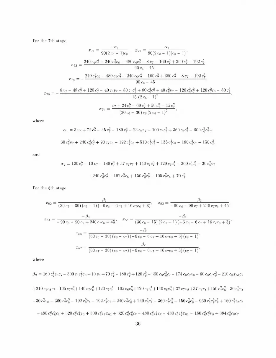
For the 7th stage, x71 = ��190(2 c6 � 1)c6 ; x72 = �290(2 c6 � 1)(c6 � 1) ;x73 = 240 c6c47 + 240 c27c6 � 480 c6c37 � 8 v7 � 160 c37 + 360 c47 � 192 c5790 c6 � 45x74 = �240 c27c6 � 480 c6c37 + 240 c6c47 � 160 c37 + 360 c47 � 8 v7 � 192 c5790 c6 � 45 ;x75 = �8 v7 � 48 c57 + 120 c47 � 40 c6v7 � 80 c6c37 + 80 c26c37 + 40 c26v7 � 120 c26c27 + 120 c27c6 � 80 c3715 (2 c6 � 1)2 ;x76 = v7 + 24 c57 � 60 c47 + 50 c37 � 15 c27(30 c6 � 30) c6 (2 c6 � 1)2 ;where �1 = 3 v7 + 72 c57 � 45 c27 � 180 c47 � 23 c6v7 � 100 c6c37 + 360 c6c47 � 600 c26c37+30 c26v7 + 240 c26c47 + 90 c7c6 � 192 c57c6 + 510 c26c27 � 135 c27c6 � 180 c26c7 + 150 c37;and �2 = 120 c57 � 10 v7 � 180 c47 + 37 c6v7 + 140 c6c37 + 120 c6c47 � 360 c26c37 � 30 c26v7+240 c26c47 � 192 c57c6 + 150 c26c27 � 105 c27c6 + 70 c37:For the 8th stage,x82 = �2(30 c7 � 30) (c6 � 1) (�6 c6 � 6 c7 + 16 c7c6 + 3) ; x83 = �3�90 c6 � 90 c7 + 240 c7c6 + 45 ;x84 = ��4�90 c6 � 90 c7 + 240 c7c6 + 45 ; x85 = ��5(30 c6 � 15) (2 c7 � 1) (�6 c6 � 6 c7 + 16 c7c6 + 3) ;x86 = ��6(60 c6 � 30) (c6 � c7) (�6 c6 � 6 c7 + 16 c7c6 + 3) (c6 � 1) ;x87 = �7(60 c7 � 30) (c6 � c7) (�6 c6 � 6 c7 + 16 c7c6 + 3) (c7 � 1) ;where�2 = 160 c26v8c7�300 c6c27c8�10 v8+70 c38�180 c48+120 c58�360 c6c38c7�174 c6c7v8�60 c6c7c28�210 c6x81c7+210 c6c8c7�105 c7c28+140 c7c38+120 c7c48�105 c6c28+120 c6c48+140 c6c38+37 c7v8+37 c6v8+150 c27c28�30 c26v8�30 c27v8 � 360 c27c38 � 192 c58c6 � 192 c58c7 + 240 c27c48 + 240 c26c48 � 360 c26c38 + 150 c26c28 � 960 c26c27c28+ 160 c27v8c6�480 c27c48c6 + 320 c27c38c6 + 300 c26c7x81 + 320 c26c38c7 � 480 c26c48c7 � 480 c26c27x81 � 160 c26c27v8 + 384 c58c6c736

+300 c6c27x81 + 300 c26c7c28 + 640 c26c38c27 � 300 c26c8c7 + 300 c27c28c6 + 480 c26c8c27;�3 = 320 c6c38c7�80 c6c7v8�720 c6c7c28�480 c6x81c7�240 c7c28+480 c7c38+480 c6c8c7�240 c7c48+8 v8�240 c6c28�240 c6c48 + 160 c38 + 480 c6c38 � 360 c48 + 192 c58;�4 = 320 c6c38c7�80 c6c7v8�720 c6c7c28�480 c6x81c7�240 c7c28+480 c7c38+480 c6c8c7�240 c7c48+8 v8�240 c6c28�240 c6c48 + 160 c38 + 480 c6c38 � 360 c48 + 192 c58�5 = 720 c6c27c8�680 c26v8c7+24 v8�240 c38+360 c48�144 c58+240 c6c38c7+672 c6c7v8+720 c6x81c7�720 c6c8c7+360 c7c28 � 240 c7c38 + 360 c6c28 � 240 c6c38 � 120 c7v8 � 120 c6v8 � 360 c27c28 + 120 c26v8 + 120 c27v8 + 240 c27c38+240 c26c38 � 360 c26c28 � 1920 c26c27c28 � 680 c27v8c6 � 960 c27c48c6 + 1280 c27c38c6 � 720 c26c7x81+1280 c26c38c7 � 960 c26c48c7 + 640 c26c27v8 + 768 c58c6c7 � 720 c6c27x81 � 360 c26c7c28+1280 c26c38c27 + 720 c26c8c7 � 360 c27c28c6 � 960 c48c6c7�6 = 360 c7c48 � 23 c7v8 + 3 v8 + 72 c58 + 150 c38 � 180 c48 � 100 c7c38 � 135 c7c28 + 510 c27c28 + 30 c27v8 � 600 c27c38�192 c58c7 + 240 c27c48 + 90 c7c8 � 90 c7x81 � 45 c28 + 180 c27x81 � 180 c8c27�7 = 360 c6c48 + 3 v8 + 72 c58 + 150 c38 � 23 c6v8 � 180 c48 � 100 c6c38 � 135 c6c28 + 30 c26v8 � 192 c58c6 + 240 c26c48�600 c26c38 + 510 c26c28 � 90 c6x81 + 90 c6c8 � 45 c28 + 180 c26x81 � 180 c26c8:The weight polynomials areb1(�) = ��160 c7c6c8 b2(�) = ��2(60 c7 � 60) (c6 � 1) (c8 � 1) ; b3(�) = 0; b4(�) = 0;b5(�) = �5(30 c8 � 15) (2 c7 � 1) (2 c6 � 1) ; b6(�) = �660 c6 (c6 � c8) (c6 � c7) (c6 � 1) (2 c6 � 1) ;b7(�) = ��760 c7 (c7 � c8) (c7 � 1) (c6 � c7) (2 c7 � 1) ; b8(�) = �8(60 c8 � 60) (c7 � c8) (c6 � c8) (2 c8 � 1) c8 ;where�1 = �(20 �5�60 c7c6c8�36 �4+15 �3+45 �3c6+45 �3c7+45 �3c8�24 �4c6�24 �4c7�24 �4c8�20 �2c6�20 �2c7�20 �2c8 � 60 �2c7c6 � 60 �2c6c8 � 60 �2c7c8 + 30 �3c7c6 + 30 �3c6c8 + 30 �3c7c8+30 �c7c6 + 30 �c6c8 + 30 �c7c8 + 90 �c7c6c8 � 40 �2c7c6c8)�2 = �2(30 c7c6c8 � 20 �c7c6 � 20 �c6c8 � 20 �c7c8 � 40 �c7c6c8 + 15 �2c6 + 15 �2c8 + 15 �2c7 + 30 �2c6c837

+30 �2c7c6 + 30 �2c7c8 � 12 �3 � 24 �3c6 � 24 �3c8 � 24 �3c7 + 20 �4);�5 = 8 �2(30 c7c6c8 � 20 �c7c6c8 � 20 �c7c6 � 20 �c6c8 � 20 �c7c8 + 15 �2c7c6 + 15 �2c6c8 + 15 �2c6+15 �2c7c8 + 15 �2c7 + 15 �2c8 � 12 �3c6 � 12 �3c7 � 12 �3c8 � 12 �3 + 10 �4);�6 = �2(45 �2c8�60 �c7c8+45 �2c7+30 �2c7c8�36 �3�24 �3c8�24 �3c7+20 �4+30 c7c8�20 �c7�20 �c8+15 �2);�7 = �2(45 �2c6�60 �c6c8+45 �2c8+30 �2c6c8�36 �3�24 �3c6�24 �3c8+20 �4+30 c6c8�20 �c6�20 �c8+15 �2);�8 = �2(45 �2c6�60 �c7c6+45 �2c7+30 �2c7c6�36 �3�24 �3c6�24 �3c7+20 �4+30 c7c6�20 �c6�20 �c7+15 �2);8.2. Detailed descriptions of the test problemsThe swirling ow III family of test problems is given in [AMR 1988, Pg. 23]. The versionof the problem given there is slightly incorrect. The corrected version of the problem, whichhas been studied extensively in a large number of papers for some time, can be found, in aslightly modi�ed form, in, for example, [Batchelor 1951], and has the following form,�f 0000+ ff 000+ gg0 = 0; �g00+ fg0 � f 0g = 0;with f(0) = f(1) = f 0(0) = f 0(1) = 0; g(0) = 0; g(1) = 1:In this paper we consider the following �rst order system form,y01 = y2; �y02 = y1y4 � y2y3; y03 = y4; y04 = y5; y05 = y6; y06 = �y3y6 � y1y2;y3(0) = y4(0) = y3(1) = y4(1) = 0; y1(0) = 0; y1(1) = 1:No closed form solution exists in general. For our testing, we chose 0 = 1 and 1 = �1,and consider values of the parameter �= 1.0, 0.1, 0.05, 0.01, 0.005, 0.001, 0.0005. The initialguesses for the solution are chosen to be straight lines through the boundary conditions.The swirling ow I family of test problems is given in [AMR 1988, Pg. 22], and has thefollowing �rst order system form,y01 = y2; y02 = y3; y03 = 2 � 2y1y3+ y22 � y24; y04 = y5; y05 = 2y2y4 � 2y1y5;with y1(0) = y2(0) = 0; y4(0) = 1; y2(1) = 0; y4(1) = :No closed form solution exists in general. For our testing, we chose L = 10:0 . The values of we consider are 0.0, 5.0, 10.0, 20.0, 50.0, 100.0, and the initial conditions are straight linesthrough the boundary conditions.8.3. Mixed vs. First Order BVODE systemsIn the Table 7.3.1, we show the results from comparing the performance of COLNEWapplied to a mixed order BVODE system with COLNEW applied to the equivalent �rstorder BVODE system, using collocation polynomials o� order 4 and 6 (which we will callCO for collocation order.). We used the swirling ow III problem family as the set of test38

problems. We expressed the family in its original form, as above, with a 4th order equationand a 2nd order equation, and also in terms of an equivalant �rst order system form with 6�rst order equations. We requested a tolerance on every component of 10�8, and imposed anupper bound of 300 subintervals. Note that a '*' indicates that the code failed to convergeusing no more than 300 subintervals.Table 7:3:1 : COLNEW on a Mixed and First Order systemCO) 4th 4th 6th 6th� + Mixed Order First Order Mixed Order First Order1:0 0:12 0:28 0:05 0:160:1 0:49 1:13 0:11 0:390:05 0:48 1:15 0:22 0:720:01 1:34 3:31 0:48 1:820:005 1:38 3:38 0:94 3:310:001 � � 1:09 3:930:0005 � � � 4:59Note that for the last value of �= 0:0005, the �rst order system version of the problem couldbe solved by COLNEW within 300 subintervals, while the mixed order system version couldnot. In general, substantial savings in execution time are obtained by applying COLNEWdirectly to a mixed order system. 39

8.4. Graphs for Tables 5.1.1-5.1.8 and 5.2.1-5.2.8

40

41