Impostor Finding

Faculteit Betawetenschappen

Impostor FindingUsing Stylometry and Network Analysis

Master’s Thesis

Laurisa Maagendans

Artificial Intelligence

Supervisors:

Dr. Marijn Schraagen First SupervisorInformation and computing sciences

Dr. T. Deoskar Second SupervisorHumanities, ILTS

Dr. J.P. Mense Daily SupervisorNational Police, National Unit

December 30, 2020

Abstract

This work presents research on the pair-wise impostor finding problem: ‘Given a pairof user accounts (and optionally, messages sent by either user account), can one reliablydetermine whether this pair is controlled by the same actual author?’. The specific domainfor which this thesis aims to solve the pair-wise problem is social networks in which shortconversational texts are sent between nodes.

Two approaches to this problem are evaluated. The first is the combination of stylo-metric authorship attribution methods with the Doppelganger Finder. Three stylometricauthorship attribution methods and various stylometric feature sets are compared on theirperformance on the authorship attribution task on short conversational text: Cosine Delta,SVM and CNN. The CNN model achieves the highest scores on all datasets used, and for allthree methods, character 3-grams and word 1-grams prove to capture the most characteristicinformation.

The second approach to the pair-wise problem is a direct network analysis-based method,which is an original contribution of this thesis. This method is evaluated on the OpsahlFacebook-like Social Network dataset, where the edges have been injected with Tweets fromthe Sentiment140 Twitter dataset. The network analysis-based method does not attainnotable results when used with only network features or stylometric features. However,with stylometric and network features combined, it reaches a weighted F1-score of 0.7 onthe pair-wise problem.

To compare the two approaches, the SVM model is applied to the injected subset ofthe Sentiment140 Twitter dataset on the authorship attribution task. The DoppelgangerFinder is applied to the predictions of the SVM model to answer the pair-wise problem.The resulting scores are no higher than 0.5, which is unremarkable on the binary pair-wiseproblem, but also lower than the 0.7 attained by the network analysis-based method.

i CONTENTS

Contents

1 Introduction 11.1 Relevance for AI . . . . . . . . . . . . . . . . . . . . . . . . . . . . . . . . . . 3

2 Related work 42.1 Stylometric authorship attribution . . . . . . . . . . . . . . . . . . . . . . . . 4

2.1.1 Burrows’ Delta . . . . . . . . . . . . . . . . . . . . . . . . . . . . . . . 52.1.2 Support vector machines . . . . . . . . . . . . . . . . . . . . . . . . . . 62.1.3 Convolutional neural network . . . . . . . . . . . . . . . . . . . . . . . 82.1.4 Comparison to other authorship attribution methods . . . . . . . . . . 9

2.2 Finding impostors using AA . . . . . . . . . . . . . . . . . . . . . . . . . . . . 102.3 Network-based methods . . . . . . . . . . . . . . . . . . . . . . . . . . . . . . 112.4 Feature sets for AA . . . . . . . . . . . . . . . . . . . . . . . . . . . . . . . . . 12

2.4.1 Lexical . . . . . . . . . . . . . . . . . . . . . . . . . . . . . . . . . . . . 122.4.2 Character-based . . . . . . . . . . . . . . . . . . . . . . . . . . . . . . 132.4.3 Syntactic . . . . . . . . . . . . . . . . . . . . . . . . . . . . . . . . . . 132.4.4 Semantic . . . . . . . . . . . . . . . . . . . . . . . . . . . . . . . . . . 142.4.5 Choice of feature sets . . . . . . . . . . . . . . . . . . . . . . . . . . . 14

3 Methods 153.1 Authorship attribution methods on short conversational texts . . . . . . . . . 15

3.1.1 Feature extraction . . . . . . . . . . . . . . . . . . . . . . . . . . . . . 153.1.2 Feature selection . . . . . . . . . . . . . . . . . . . . . . . . . . . . . . 163.1.3 Delta . . . . . . . . . . . . . . . . . . . . . . . . . . . . . . . . . . . . 163.1.4 SVM . . . . . . . . . . . . . . . . . . . . . . . . . . . . . . . . . . . . . 163.1.5 CNN . . . . . . . . . . . . . . . . . . . . . . . . . . . . . . . . . . . . . 173.1.6 Doppelganger Finder . . . . . . . . . . . . . . . . . . . . . . . . . . . . 19

3.2 Network Analysis . . . . . . . . . . . . . . . . . . . . . . . . . . . . . . . . . . 203.2.1 Synthesizing impostor accounts . . . . . . . . . . . . . . . . . . . . . . 213.2.2 Injecting stylometric information . . . . . . . . . . . . . . . . . . . . . 223.2.3 Creating pair-wise datapoints . . . . . . . . . . . . . . . . . . . . . . . 23

4 Data and data preparation 254.1 Datasets . . . . . . . . . . . . . . . . . . . . . . . . . . . . . . . . . . . . . . . 25

4.1.1 SMS datasets and Twitter dataset . . . . . . . . . . . . . . . . . . . . 254.1.2 Network datasets: The Opsahl Social Network . . . . . . . . . . . . . 27

4.2 Data preparation . . . . . . . . . . . . . . . . . . . . . . . . . . . . . . . . . . 284.2.1 Author selection . . . . . . . . . . . . . . . . . . . . . . . . . . . . . . 28

ii CONTENTS

4.2.2 Tagging . . . . . . . . . . . . . . . . . . . . . . . . . . . . . . . . . . . 304.2.3 Message grouping . . . . . . . . . . . . . . . . . . . . . . . . . . . . . . 31

5 Experiment setup 335.1 AA experiments . . . . . . . . . . . . . . . . . . . . . . . . . . . . . . . . . . 335.2 Network analysis-based experiments . . . . . . . . . . . . . . . . . . . . . . . 335.3 Comparison of the two sets of results . . . . . . . . . . . . . . . . . . . . . . . 33

6 Results and discussion 356.1 AA . . . . . . . . . . . . . . . . . . . . . . . . . . . . . . . . . . . . . . . . . . 35

6.1.1 Message grouping . . . . . . . . . . . . . . . . . . . . . . . . . . . . . . 356.1.2 Feature sets . . . . . . . . . . . . . . . . . . . . . . . . . . . . . . . . . 366.1.3 Delta vs SVM vs CNN . . . . . . . . . . . . . . . . . . . . . . . . . . . 396.1.4 Twitter AA results . . . . . . . . . . . . . . . . . . . . . . . . . . . . . 40

6.2 Network analysis . . . . . . . . . . . . . . . . . . . . . . . . . . . . . . . . . . 416.2.1 Overlap% . . . . . . . . . . . . . . . . . . . . . . . . . . . . . . . . . . 416.2.2 Feature sets . . . . . . . . . . . . . . . . . . . . . . . . . . . . . . . . . 42

6.3 AA versus Network analysis . . . . . . . . . . . . . . . . . . . . . . . . . . . . 43

7 Further research and conclusion 447.1 Limitations and further research . . . . . . . . . . . . . . . . . . . . . . . . . 44

7.1.1 From pair-wise to group-wise . . . . . . . . . . . . . . . . . . . . . . . 447.1.2 Comparing CNN to Delta and SVM . . . . . . . . . . . . . . . . . . . 457.1.3 Comparing the network analysis-based method to AA combined with

the Doppelganger Finder . . . . . . . . . . . . . . . . . . . . . . . . . 457.1.4 Applying the network analysis-based method to other networks . . . . 467.1.5 One user account, multiple authors . . . . . . . . . . . . . . . . . . . . 47

7.2 Conclusion . . . . . . . . . . . . . . . . . . . . . . . . . . . . . . . . . . . . . 47References . . . . . . . . . . . . . . . . . . . . . . . . . . . . . . . . . . . . . . . . . 49

A Message grouping I

B Authorship attribution results IVB.1 Delta . . . . . . . . . . . . . . . . . . . . . . . . . . . . . . . . . . . . . . . . . IVB.2 SVM . . . . . . . . . . . . . . . . . . . . . . . . . . . . . . . . . . . . . . . . . VIB.3 CNN . . . . . . . . . . . . . . . . . . . . . . . . . . . . . . . . . . . . . . . . . VIII

C Network analysis results XI

1 CHAPTER 1. INTRODUCTION

Chapter 1

Introduction

Imagine a detective faced with the task to investigate a criminal organisation. At theirdisposal is a dataset consisting of a large amount of mobile messages that are suspected tobe related to members of the criminal organisation. However, criminals are known to useburners - disposable phones that are used for the sake of anonymity. This not only meansthat one cannot link one phone number to a specific person, but also that one person maybe behind multiple phone numbers.

Being able to identify groups of phone numbers with the underlying people would pro-vide the detective with more coherent information about these people. For example, anygeolocation information of the phones used by a specific person can be used to construe apath that the person has traveled. Another example is that some conversations this per-son has held with other individuals might be spread out over multiple phones, and can bere-constructed with this newfound information.

Finding groups of phone numbers (or other electronic identifiers such as Twitter IDs)that are used by one person is what this thesis is concerned with. More specifically, themain research question of this thesis is:

Given a dataset of messages from a number of user accounts, can one reliably find groupsof user accounts that are controlled by the same actual author?

To simplify the main question, it can be expressed in terms of the question

Given a pair of user accounts (and optionally, messages sent by either user account), canone reliably determine whether this pair is controlled by the same actual author?

A method that can (reliably) find whether a pair of user accounts is controlled by thesame actual author can be used to find groups of user accounts controlled by the sameactual author. Therefore, this thesis is concerned with proposing and evaluating methodsthat solve the simpler pair-wise research question to answer the main research question inextension. Some options for the translation from the pair-wise to the main research questionare discussed in Section 7.1.4.

To answer the pair-wise research question, there are two approaches that will be discussedin this thesis. One is a combination of existing authorship attribution methods with amethod called the Doppelganger Finder. The other is a newly-proposed network analysis-based method.

The authorship attribution task, to be shortened to AA, can be defined as follows:


Given a text of unknown authorship, the authorship attribution task is to identify themost likely author of this text out of a set of candidate authors of whom text samples are

available.

AA, and consequently methods that solve AA, have been relevant for a long time. TheDonation of Constantine[19] is a Roman imperial decree by which authority over Rome andthe western part of the Roman empire was transferred from Constantine the Great, a fourth-century emperor, to the Pope. Although its authenticity had been repeatedly contested sincethe beginning of the 11th century[65], it took until the 15th century for its forgery to beproven by Lorenzo Valla - the convincing evidence being that the form of Latin used in thedecree cannot possibly date back to the fourth century[61]. The forgery of the Donation ofConstantine was of big importance to the people living in Medieval Europe - it allowed forjuridical resistance against papal power, most prominently within Italy.

The method used to solve the AA problem of the Donation of Constantine made use ofstylometric features - features of text that describe writing style. Contrary to this example,the majority of AA methods employed nowadays are automated, but at the same timethey still mainly perform analysis on the basis of stylometric features. In 2015, Boyd andPennebaker[6] used stylometric features to train a couple of classifiers to study the authorshipof Double Falsehood[58], a play officially published as the original work of Lewis Theobald.The conclusion was that it was likely written by Shakespeare and Fletcher instead.

Another change that came with recent times is the type of text on which AA is to besolved, as in the detective example. Instead of long, literary text, it is short conversationaltext that concerns recent AA-related problems. Some examples of short conversationaltext are WhatsApp messages, SMS messages and Twitter Tweets. As stated earlier, AAmethods can be used to answer the pair-wise problem, but this needs to be done on shortconversational text. This gives rise to a sub-question:

How well do existing AA methods perform the AA task on short conversational text?

The lengthiness and plentifulness of literary texts seems to be a requirement for AA,as 5000 words per text is the minimum requirement for any AA method to be performedon prose with an accuracy of at least 80%, regardless of language.[15] While this is onliterary text, it poses a problem for AA on short conversational text. Another problemwith dealing with conversational short texts is that, unlike in (relatively heavily regulated)literary texts, a larger number of texts contain more than one language. Over 50% of theworld’s population speaks more than one language (semi-)fluently[3]. This large percentageof bilingual people is reflected in language use on Twitter and many other social media[31].

To answer the pair-wise problem, methods that solve AA can be paired with the Dop-pelganger Finder. This is a method introduced by Afroz et al.[1] that uses the predictionsof an AA method to solve the pair-wise problem - it translates the output of an AA methodto a solution to the pair-wise problem. This translation allows for comparison of the perfor-mance of AA methods (combined with the Doppelganger Finder) with that of other methodsthat solve the pair-wise problem.

In the example where a detective is tracking a criminal organisation, one type of datathat can be used is network data. If the senders and recipients of the messages in thedataset are known, the dataset itself describes a network. Here, the nodes are the uniquephone numbers and the edges are connections over which messages are sent between phonenumbers. It is probable that patterns can be found in the comparison of connectivity dataof mobile phones that indicate that two phones are used by the same person. For example,


this could be a set of common contacts the two phones share, that none of the other phonesshare.

The goal is to use network information as a supplement to stylometric information tosolve the pair-wise problem. Unfortunately, AA methods are author classifiers that do noteasily support the addition of network information without data leakage. To circumventsuch problems, a method that can use such network information to directly solve the pair-wise problem is proposed and evaluated in this thesis. This means the method is novel intwo ways. Firstly, it can use network information. Secondly, it is a direct solution to thepair-wise problem, in contrast to AA methods, which need the addition of the DoppelgangerFinder to form a solution to the pair-wise problem.

To summarize, the research in this thesis can be split into three parts. Firstly, it eval-uates the applicability of existing AA methods on short conversational text. Secondly, theapplicability of the network analysis-based method will be evaluated on short conversationaltext. And thirdly, it concerns a comparison of AA in combination with the DoppelgangerFinder with the network analysis-based method.

1.1 Relevance for AI

The relevance of this thesis research project to the field of AI is threefold.Firstly, this thesis shows the applicability of AI-based methods to relevant real-world

problems. To answer the research question, this thesis explores multiple approaches thatare rooted in the field of AI. With the exception of the family of Delta methods, all methodsdiscussed belong to the family of machine/deep learning methods, or are used in combi-nation with such a method. These methods are examined on their applicability to shortconversational text. This specific type of text is of increasing abundance in the past years,and of increasing relevance is the search for patterns in such text, for example in the problemof imposter finding.

Secondly, this thesis introduces a novel AI-based approach. The network analysis-basedmethod is a novel approach to the AA-related field of imposter finding, that combines ideasfrom two AI-related fields: AA and node similarity on graphs.

Thirdly, the research has interdisciplinary relevance. Some of the methods discussed,including the network analysis-based method, can give insight into the types of featuresin short conversational text that are most characteristic for the classification of authors.This could be interesting for a linguist that wishes to compare the subconscious stylometricbehaviour of people in short conversational text to that in other types of text.

4 CHAPTER 2. RELATED WORK

Chapter 2

Related work

As stated before, there are two routes to solving the main research question of this thesis.The first is to use AA methods in combination with methods that determine similaritybetween any two user accounts based on the AA method’s output. The second is to use anetwork analysis-based classifier to directly identify whether any two user accounts are usedby the same author.

This section serves as a literature review of related work on the topic of the researchquestion and the two routes to solving the question stated above. Firstly, various methodsused in the field of AA are discussed. In particular Burrows’ Delta, SVM and CNN. Thesethree methods will be compared on their accuracy on the AA task on short conversationaltexts. Secondly, two methods for finding impostors using the predictions of any AA methodfrom the literature will be discussed: the Doppelganger Finder and the Impostor Method.The first will be applied to the predictions of an SVM model trained on the AA task.Thirdly, network analysis methods from the literature will be discussed that have inspiredthe network analyis-based method proposed in this thesis. Finally, the available options forfeature sets for the AA methods are discussed.

2.1 Stylometric authorship attribution

The set of automated AA methods can be divided into two main categories; non-trainedmethods and machine learning methods[63]. Both methods make use of a distance metricto determine the distance between a given document and the already identified documentsof any of the candidate authors. Non-trained methods are given a static distance metric.Machine learning methods learn different weights that tie into a distance metric. Theyuse the already identified documents of candidate authors as training data to construct aclassifier. This classifier can then be used to classify a given document as most likely havingbeen written by one specific candidate author.

Both non-trained methods and machine learning methods (in particular the ones dis-cussed in this thesis - Delta, SVM and CNN) come with their strengths and weaknesses.Due to the general simplicity of non-trained methods, their explainability often surpassesthat of machine learning methods. When the results of an AA method are the only con-cern, this explainability is barely of interest, but one should not forgo the fact that it isinvaluable to AA research. It offers an insight into what constitutes an authorial fingerprint,and what does not. However, this explainability is a double-edged sword, as the distance


metric of a non-trained method is subject to human bias. The distance metric is based onwhat intuitively makes a document similar in writing style to another. Even if this distancemetric is based on a number of properties, or features, of a document, the weights of thesefeatures are picked by hand. On the other hand, machine learning methods learn theseweights by fitting them to a training set. Deep learning methods are even more capableof finding the intricacies that determine an authorial fingerprint, due to the integration offeature extraction in a deep network. An added advantage of non-trained methods is thatprecisely because they are non-trained, they are domain-independent. No model needs tobe trained with data specific to a domain in order to apply it to other data from the samedomain. For trained methods, domain-specific training is necessary and unavoidable, whichmakes such models domain-dependent.

The following section will provide an overview of Burrows’ Delta, a non-trained similarity-based method. After that, support vector machines, a machine learning-based method, willbe discussed, followed by convolutional neural networks, a deep learning-based method.These sections include a brief introduction to the methods and notable research using thesemethods, as well as what makes these methods of interest to our research. Finally, a fewother AA methods that will not be used in this research will be discussed briefly to motivatethe choice of methods.

2.1.1 Burrows’ Delta

One notable non-trained similarity-based method is Burrows’ Delta method[7]. Burrows’Delta method checks for similarity of word distributions of most frequent words. Thismethod has initially been developed to transform the problem of identifying the author ofa given text out of a large number of candidate authors (‘open game’) into the problemwhere the set of candidates is small (‘closed game’). By doing so, an open game could beapproached by first transforming it into a closed game, which in turn is easier to solve byexisting AA methods.

As Delta is a similarity-based method, it works by using a distance metric to determinethe distance between a document and a set of documents that are known to be writtenby some candidate author. By calculating the distance between a document (of which itsauthor is to be identified) with the document sets of each of the candidate authors, itbecomes possible to rank the most probable authors of this document. This ranking isexactly what allows Delta to transform an open game into a closed game - by selecting thetop n candidates. While Burrows’ Delta is designed with this transformation in mind, itcan also be used directly as an AA method by selecting the single top ranking candidate.

As part of calculating Delta, the application of a distance metric is preceded by a numberof steps. First, the occurrence of each word within each document is counted. For eachdocument, these word counts are transformed to relative frequencies, to account for differentdocument lengths. For efficiency purposes, the n most frequent words over the whole corpusare chosen, of which the relative frequencies can be represented as a documents × wordsmatrix. These word frequencies are then standardized such that, over the whole corpus, themean of each word is 0 and its standard deviation is 1. On the final frequency matrix, theManhattan distance can be used to determine the distance between a document and thedocument set of any candidate author.

Burrows is the first to use Delta for AA[7], or more accurately, to the related problemof likely authorship attribution; to find the n most likely authors of a text. For this, heused Delta on a dataset of 200 English poems from the late seventeenth century. Out of 25


candidate authors, the top 5 most likely authors contain the actual author in 67 out of 100poems of at most 500 words. For poems of more than 500 words and at most 1000 words,the actual author was within the top 5 for 32 out of 40 poems, and within the top 10 for allof the 40 poems. This ratio increases further as the poem length increases.

Hoover[27] made several modifications to Burrows’ Delta, of which the most notable isthe use of a cosine distance metric. Smith and Aldridge[62] showed that Hoover’s CosineDelta is capable of forming a top 5 that includes the actual author with an accuracy of over85% for poems of at least 800 words long, while Burrows’ Delta obtains an accuracy of 70%on the same task.

As mentioned before, one big advantage of using similarity-based methods, such as Delta,is their explainability due to their transparency. Because Delta uses only a subset of allwords, it gives insight into what part of an author’s vocabulary accounts for their authorialfingerprint[17]. Moreover, by using a bag-of-words approach, the effectiveness of Delta showsthat sequential data in text becomes less influential to AA as sample length increases[7].For our research, it is a benefit that Delta has rarely been applied to non-literary texts, asthis allows us to utilize its explainability in a novel domain.

One possible downside to Delta is that its minimal sample size for reliable AA was shownby Eder (2015) to be 5000[16]. However, Eder (2017) later re-evaluated the minimal samplesize to be 1500 words[17]. Furthermore, when used for reducing the set of candidate authors(to 5), Cosine Delta performs with 85% accuracy on poems of even 800 words long[62]. Thisindicates that Delta can be used for AA(-related) tasks on short texts. However, note thatthe short conversational texts investigated in this thesis are tweets and mobile messages.These are closer to 30 words than the 800 words of the texts investigated by Smith. For anoverview of the data, refer to Section 4.1.

In short, Burrows’ Delta and its related Delta methods are still studied today for itsexplainability. Despite early indications of Delta’s minimal sample length for reliable AA,recent research shows Delta’s potential as an AA method for use on short texts.

2.1.2 Support vector machines

While Delta is a similarity-based AA method, support vector machine (SVM) classifiers forma family of supervised machine learning-based methods. In AA research, SVM classifiershave been used frequently[12, 56, 59].

The principle behind SVM is to construct a hyperplane that best splits two classes ofdata points in an n-dimensional space, where the dimensions represent features such as wordn-grams[11]. SVM receives its name from the fact that only a small set of training examples,called the support vectors, is needed to determine the best hyperplane, or decision surface.While SVM is in principle a binary classifier, most AA problems concern the attributionof an author from a set of more than two candidates. For these AA problems, multiclassSVMs can be used, which reduce the multiclass problem to a set of binary problems to besolved by a regular SVM[28].

Diederich et al.[12] were the first to apply an SVM to AA. Previously, SVMs had beenproven to be effective when applied to other text classification problems[32, 13]. SVMs hadonly recently been gaining popularity in the learning community at the time of Diederich etal.’s research[64]. One of the reasons for this surge in popularity, as well as the main reasonDiederich et al. decided to use SVMs for AA, was SVM’s ability to process hundreds ofthousands of features. This allowed for the frequencies of all words in a text to directly beused as features. In that research the SVM is used on a dataset of the texts of the seven


authors with most documents from the Berliner Zeitung, a daily newspaper in Berlin. Theirresults show that SVMs using only word frequency features consistently achieve results thatare comparable to, or better than, those achieved with methods that use more intricatefeature selection. Do note that this specific case concerned only seven authors. If thereare many authors, like in most domains that concern short conversational texts, featureselection might still be necessary or beneficial in terms of computational costs.

Schwartz et al.[56] used libsvm’s MATLAB implementation of the multi-class SVM[8]with a linear kernel on Twitter tweets, using libsvm’s option to return probability estimates.The selected author is the one with the highest probability estimate for a given text, if thisprobability estimate is higher than a given threshold. This threshold allows for the SVM toreturn ‘don’t know’ as a result, increasing classification precision at the cost of recall. Asfeatures, Schwartz et al. used character 4-grams and word n-grams, where 2 ≤ n ≤ 5. On adataset of 50 authors with 500 tweets per author, Schwartz et al.’s implementation obtainedan accuracy of 66%.

Sharma et al.[59] published an investigation of supervised learning methods for AA ona dataset of short Hinglish (a blend of Hindi and English) texts. One of the methods theylooked at was SVM, using only character and word n-grams as features. As character n-grams, n-grams were used where 3 ≤ n ≤ 5. As word n-grams, only unigrams (n = 1)and bigrams (n = 2) were considered. Compared to the other methods used in this study(Naive Bayes, conditional tree and random forest), the SVM classifier achieved the bestresults with a test accuracy between 90.514% and 95.079% on word unigrams and charactern-grams. Since Hinglish is a macaronic language, meaning that it is a language in whichtwo languages are used interchangeably, it contains distinctive features such as its idiolecticspellings. This means that differences in the spelling of specific words frequently occur atthe level of an individual speaker of that language. Sharma et al. have shown that this isreflected in their Hinglish text data by showing that the top distinctive word unigrams ofauthors contain many words that are slight variants of one another.

Comparing these three studies utilizing SVM classifiers, one can see that SVM classifiersowe their popularity within the field of AA to a number of advantages they have over otherAA methods. Section 2.1.4 will provide a more comprehensive comparison between the AAmethods discussed in this thesis. As mentioned previously, the ability of SVMs to processhundreds of thousands of features eliminates the need of feature selection[57]. Another bigadvantage is that SVMs are fairly robust to overfitting and are highly suitable for high-dimensional input, such as text[57]. As such, SVM’s do not require term selection. Otherpositive attributes of SVM that are not specific to its usage in AA include its guaranteedglobal minimum and memory-efficiency[45]. Furthermore, SVM’s popularity as a supervisedlearning method and its wide applicability has given rise to many SVM implementations inmany languages, for example; libsvm[8], PyStruct[44] and SVMStruct[33].

One of the disadvantages of using SVMs is that SVMs become more prone to overfittingas there is increasing overlap between classes[45]. What this could mean for AA is that itbecomes harder to train an SVM on datasets when authors exhibit a plethora of writingstyles, of which some overlap with those of other authors.

All in all, SVM classifiers continue to be used in AA today. This wide usage can beattributed to the fact that SVMs do not require feature nor term selection, minimizingany selection efforts to be done by hand, as well as any loss in information that could berepresented by features. These practical bonuses outweigh potential costs.


2.1.3 Convolutional neural network

Convolutional neural networks (CNN) are frequently used within the field of computervision. Its application to NLP tasks is not straightforward, and as such it has only firstbeen applied to AA in 2015[54]. Other approaches that are commonly used for NLP tasksinclude LSTMs and RNNs. In Section 2.1.4 it will be explained why CNNs are chosenover these. As a deep learning-based approach, CNNs can be categorized as a machinelearning-based approach to AA.

To briefly explain the workings of a CNN, the first focus is on the convolutional operation.This operation takes an n-dimensional matrix, which could be a 2D image or a sentencethat is represented as the concatenation of the word vectors of its words. Suppose that theinput is a 2D greyscale image, represented as a 2D matrix containing the brightness valuesfor each pixel. The convolutional operation uses a filter, for example a 3× 3 identity matrixrepresenting a diagonal line, and checks for each cell (or pixel) in the input matrix to whatextent this diagonal line is present. This is done by a cellwise multiplication of the filterwith the 3× 3 matrix surrounding the cell in question, after which the results are summedup. After performing this on all cells, the result is a matrix of similar size to the inputmatrix, now called a feature map. In a similar fashion, the convolutional operation can beapplied using multiple filters, after which the resulting feature maps are stacked. The layerin which the convolutional operation takes place is called the convolutional layer. The 3× 3matrix in this example is a filter that has a filter size of 3 × 3. The sizes of the filters aredependent on the specific architecture of the CNN used.

A convolutional layer is often followed by a threshold layer, which enables learning ofnon-linear maps by applying a non-linear function such as ReLU[4]. After that comes apooling layer that downsamples the output of the threshold layer by applying a poolingfunction. A common pooling function is max-pooling, which divides the input matrix intoequally-sized (n-dimensional) cubes to preserve only the maximum value of each cube[53].While there exists no cookie cutter architecture for a CNN, the feature extraction part ofa basic CNN consists of a number of subsequent sequences of convolutional, threshold andpooling layers (in this order). Often, this includes a normalization step after the poolinglayer. To turn a CNN into a classifier, the feature extraction part is to be followed by aflattening layer, a fully connected layer and a softmax layer. Training of a CNN happensthrough a process called backpropagation of error, where the content of the filters are theweights to be trained[70].

Rhodes[54] was the first to apply CNNs to AA, using Kalchbrenner et al.’s approachto using a CNN for modelling sentences[34]. Rhodes used pre-trained word vectors with adimensionality of 300, derived from co-occurrence in a dataset of Google News articles[42].By producing word vectors for every word in a sentence, Rhodes represented each sentenceas the concatenation of its word vectors. The sentence is padded with 0s at both ends,such that the convolutional operation would be as sensitive to words near the edge of asentence as it is to words in the centre. For the convolutional step, he uses word n-gramfilters in the form of a concatenation of n word vectors. A positive consequence of this useof word vectors is that the CNN is more robust to the scenario where different words sharesimilar semantics. To ensure constant sized output of the convolutional layers, Rhodes usedmax-over-time pooling[10]. On a dataset of eight books on the highly specific subject of lifein Canada during the 19th century, written by six different authors, Rhodes obtained a testaccuracy of about 76%.

To perform AA on short texts specifically, Shrestha et al. employed a CNN[60]. Instead


of using a sequence of words or characters, they use a sequence of character n-grams asinput. The CNN model consists of a character embedding module, a convolutional moduleand a fully-connected softmax module. The character embedding module learns a vectorrepresentation of the character n-grams. In the convolutional module, filters of varyingwidth are used to capture patterns involving anything from morphemes to words, followedby max-over-time pooling[10]. On Schwartz et al.’s dataset of 9000 Twitter users with 1000tweets each[56], Shrestha et al. compared the performance of their own CNN models toa number of models. Schwarz et al.’s SVM model, an LSTM trained on bigrams, logisticregression with character n-grams, and a CNN trained on word sequences. Both CNN-2, their CNN trained on character bigrams, and CNN-1, their CNN trained on characterunigrams, outperform any of the other tested methods. This holds true even when varyingthe number of authors and tweets. For 50 authors with 1000 tweets each, CNN-2 achievesan accuracy of 76.1%. These results show that CNNs are at least as promising as SVMson short texts. In addition to introducing an approach to CNNs for AA, Shrestha et al.employed a method for interpreting the patterns their CNN captures. The saliency scoreS(e) of an embedding e is defined by Li et al. as

S(e) =∣∣w(e)

∣∣ , w(e) =δ(Sc)

δ(e)

where Sc represents the output of the CNN[40]. The saliency score indicates the con-tribution of an n-gram to the final decision. Using saliency scores, uncommon versions ofemoticons were found to be among the highest contributing bigrams.

The increased interpretability due to saliency scores forms an advantage of using CNNs.The semantic robustness gained by using word vectors, like in Rhodes’ research[54], couldbe an advantage of CNNs for AA on texts where specific semantics are highly correlatedwith specific authors. A more intrinsic property of CNNs is their preservation of sequentialdata. A consequence is a CNN’s proneness to picking up syntactic features. While stylisticfeatures may reside at a syntactic level[60], many syntactic features are the result of thelanguage being used, rather than being an indicator of the author themselves[7].

To summarize, CNNs are a relatively novel deep learning-based method for AA, withpromising results compared to other AA methods such as SVMs, LSTMs and logistic re-gression models.

2.1.4 Comparison to other authorship attribution methods

Having discussed Delta, SVM and CNN, there exist many other AA methods that will notbe investigated any further as part of this thesis. To support the choice for Delta, SVMand CNN, these AA methods will be briefly introduced in this section and compared to thechosen AA methods.

Note that this selection of methods includes both similarity-based and machine learning-based methods, of which CNN can be categorized as a deep-learning method. By selectingthe best candidate method of each of these categories, the aim is to not only illustrate thestrengths and weaknesses of each method on short conversational texts, but also to extrap-olate these findings to their category. To assess whether Burrows’ Delta, SVM and CNNare indeed the best candidate methods within their categories, it is paramount to introduceselection criteria. This includes a method’s known potential for high AA performance onshort (conversational) texts and its well-establishedness as an AA method.


Besides the family of Delta methods, another similarity-based AA method is n-gramtracing[23]. This novel method counts the distinct word unigrams and character n-grams.The distance metric is the percentage of overlap between the document and each author inthe corpus. In contrast to Delta, the frequency of these n-grams does not contribute to thedistance. n-gram tracing is designed for use on short texts. However, a comparative studyby Proisl et al. shows that, on (shortened) English, French and German novels, Cosine Deltaperforms at least as well as n-gram tracing, regardless of text length[52]. Delta’s performanceon short non-literary texts has not previously been studied. Even so, it has been shown thatDelta is reliable for AA on literary texts containing at least 1500 words[17]. Proisl et al.’sstudy indicates that the minimal sample size for n-gram tracing is comparable to thatof Cosine Delta. The hypothesis is that, for both Delta and n-gram tracing, this minimalsample size will be lower on conversational texts, due to the presence of highly characteristicstylistic markers such as uncommon abbreviations, smileys and systematic misspellings[60].Because of Delta’s superior performance and its well-establishedness compared to n-gramtracing, Delta seems to be a better representative of similarity-based AA methods.

Besides the machine learning-based methods SVM and CNN, there exist other methodssuch as LSTM and logistic regression. These have been used before in the context of AA.Long short-term memory (LSTM) networks are variations on the recurrent neural network(RNN), where RNN units (or nodes in the neural network) are replaced by LSTM units[22].For the machine learning-based methods, each method will be evaluated on their knownpotential for high AA performance on short (conversational) texts. Both SVMs and CNNshave been previously applied to datasets of Tweets[60, 56]. In addition to introducing aCNN-based approach to AA, Shrestha et al. compared the results thereof on a datasetof Tweets to that of methods including Schwartz et al.’s SVM method for short texts[56],logistic regression and LSTMs[60]. In this study, both of their CNN models on characterunigrams and bigrams, as well as Schwartz et al.’s SVM approach, outperformed the logisticregression and LSTM-based methods.

Thus, by choosing Delta, SVM and CNN for the comparative study, the results of thestudy will give insight into the strengths and weaknesses of similarity-based methods versusmachine learning-based methods.

2.2 Finding impostors using AA

The impostor finding problem can be viewed as an extension of the regular AA problem.With AA, one can figure out what documents of author A get classified as belonging toauthor B, and vice-versa. The next question is how big such an overlap should be toconclude that author A and B are the same person.

Afroz et al.’s Doppelganger Finder is built upon the same principle[1]. First, one calcu-lates the probability of author A being identified as author B, and vice-versa. Then, theseprobabilities are either summed, multiplied or taken the square average of. The result ofthis operation is check against a pre-determined threshold, to conclude whether author Aand B are the same person upon passing the check.

Another method for finding impostors is Koppel and Winter’s Impostor Method (IM)[38].IM has been further adapted by Seidman for the PAN’ 13 authorship identification com-petition. GenIM, the adapted method, ranked 1st overall. The original IM works by firstcreating n impostors of a document Y, for example by picking n random documents outof the whole dataset. Each of these impostor documents is compared to the documents


of author X using a distance metric. The percentage of impostors that are less similar toauthor X than document Y is shows how similar author X is to the author of document Y.On blog posts of 500 words each, IM achieves an accuracy of around 86%.

2.3 Network-based methods

An overview of the related literature does not reveal any network analysis-based methodsthat answer the research question of this thesis. Few attempts exist at AA that concernan analysis of social networks, let alone the combination of social network data and thedirected text sent along the edges of such a network.

However, a related topic within network analysis of interest to the method proposedin this thesis is the topic of node similarity within a network. User accounts correlate tonodes of a network, and text sent between user accounts to metadata on the edges betweennodes. Therefore, it is not hard to fathom that there could be a link between node similarityand impostor similarity - when two user accounts are ‘impostor similar’, they are controlledby the same author. Inspiration from methods used to compute node similarity can betaken for the method proposed in this thesis. In particular, these methods use measuresthat use features that contain characteristic information for the node similarity of a pair ofnodes. Despite that node similarity is not necessarily and not likely the same as impostorsimilarity, these features can still be useful for finding impostor pairs. In the case of theproposed method, and in contrary to one type of node similarity computation method, nopre-defined measure is used, but rather implicitly trained through an SVM.

Li et al.[41] have made the distinction between neighborhood-based and path-basedmeasures. Neighborhood-based measures define the similarity between nodes in terms ofthe overlap between the neighborhoods of both nodes. These measures differ in the waythey calculate the overlap. One example of such a measure is the Jaccard Index[30] thatnormalizes the number of shared nodes between the two neighborhoods by the union of theneighborhoods. Another is cosine similarity[55], that normalizes the number of shared nodesby the cosine of the angle between the characteristic vectors of the two neighborhoods. Path-based measures are more varied, but they all share that they incorporate paths betweenpairs of nodes into their measure. One such measure is proposed by Chen et al.[9], whodefine a so-called relation strength between two nodes. In short, the relation strength is anasymmetric property that increases when A and B are adjacent, and A has relatively fewerdirect neighbours. When the two nodes are not adjacent, the relation strength is defined interms of the relation strengths of the nodes on any path between A and B of a pre-specifiedmaximal length. To look at another example, Li et al.[41] propose a measure that is basedon the idea that the similarity of two nodes is negatively correlated with the informationloss that results from merging the two nodes. The information loss is defined in terms ofweights of edges on paths between all nodes of the network. Another group of examples isgiven by Fouss et al.[18]. They propose measures that use properties of a number of randomwalks between a pair of nodes. One example of such a measure derived from random walksis ‘average commute-time’ which is the average number of steps that a random walker takesto travel from starting node A to ending node B and the other way around.

Two criteria for the feature sets used are scalability and extensibility to the particularcase of combination with stylometric features. For both criteria the features used in theneighborhood-based measures are a better fit. When representing the direct neighborhoodof a node, the size of the representation is O(n) where n is the number of nodes in the


network. For features used in path-based measures the representation would require O(n2)space. This is because the feature set that would contain the required information forlearning based on path-based quantities would include the connectivity data between everypair of nodes. Direct neighborhoods can be represented by the connectivity data betweentwo nodes and all nodes in the network. To combine network-based features with stylometricfeatures, it is important to note that the analysis performed on the stylometric features isthat of AA. This means that it should be performed on texts originating from a user accountwhen one wants to investigate the author fingerprint of that user account. Direct (directed)neighborhoods of a node A have the property that it consists of nodes that have a directedconnection originating from A - there is a 1-to-1 mapping of all edges A has sent text over toall nodes A has an outgoing edge to. When combining direct neighborhood information withstylometric information, this stylometric information would be descriptive of the informationsent along the edges of the direct neighborhood. Path-based features concern edges thatdo not all directly originate from A. Adding stylometric information that solely originatesfrom A would be possible with path-based features, but it would not be descriptive of theinformation encoded by the path-based features, while for direct neighborhood informationit would be.

2.4 Feature sets for AA

For machine learning-based AA methods, there exists a plethora of commonly used features.These features can be categorized into lexical, character-based, syntactic and semantic fea-tures. This section lists features that have previously been used in AA methods, as well asthe tools that are required to extract these features. Any features that have been shown tocapture especially author-specific information, or require specifics, will be pointed out anddiscussed in text.

2.4.1 Lexical

A list of lexical features, i.e. features concerning words, can be seen in Table 2.1.

Feature Required tools

Word length TokenizerSentence length (words) Tokenizer, sentence splitter

Sentence length (characters) sentence splitterVocabulary richness Tokenizer, stemmer

Word n-grams TokenizerSpelling errors Tokenizer, spell checker

Table 2.1: Lexical features used in AA and the tools required to obtain these features[63].

In particular, vocabulary richness is the feature that lies at the heart of the family of Deltamethods. Prior to the invention of Burrows’ Delta, in the year 1949 Zipf observed that α(f),the number of words that occur exactly f times, is given as α(f) = fγ , where γ ≈ 2[73]. Hefurther conjectured that γ varies depending on the age and intelligence of the author[72], thuscapturing author-specific information. Later in 1964, Mosteller and Wallace[43] had the ideato count function words such as ‘while’ and ‘upon’ to discriminate between authors. Burrows’


Delta can be viewed as a generalized version of this method; counting the occurrences ofall words instead of being limited to function words. This illustrates that the underlyingprinciple of vocabulary richness has been thought to contribute to an author’s characteristicsfor over half a century.

To give an explanation of the required tools, a tokenizer takes a text input and convertsit into a stream of tokens, where a token can be a word, URL, date, etc.[51]. The (straight-forwardly named) sentence splitter splits an input text into its individual sentences[25]. Astemmer reduces inflected words to their word stem, and a spell checker determines whethera presented word forms a correct spelling. All of these tools are available in a wide array oflanguages. For macaronic languages like Hinglish and Singlish, it is difficult to find stem-mers and spell checkers of established reliability. For English, there exist stemmers with anaccuracy of about 97%[29].

2.4.2 Character-based

Table 2.2 contains character-based features and the tools required to extract those features.


Character types (letters, digits, special characters, etc.) Character dictionaryCharacter n-grams -

Table 2.2: Character-based features used in AA and the tools required to obtain thesefeatures[63].

2.4.3 Syntactic

Table 2.3 shows a list of syntactic features and their required tools.


POS tags Tokenizer, sentence splitter, POS taggerFlexible patterns Tokenizer, HFW/CW tagger

Table 2.3: Syntactic features used in AA and the tools required to obtain these features[63,56].

A part-of-speech (POS) tag is a tag given to a word in a sentence that indicates thesyntactic role of the word, such as ‘noun’, ‘verb’ or ‘adjective’[24]. POS taggers are toolsthat assign POS tags to words in the input text. POS taggers are available for mostlanguages and even for mixes of languages like Hinglish and Chinese-English[66, 71].

A concept introduced by Schwarz et al.[56] are flexible patterns, which are a type of wordn-gram. Every flexible pattern is composed of high-frequency words (HFW), i.e. words thatappear in more than 0.01% of the corpus, and content words (CW), i.e. words that appearin less than 0.1% of the corpus. This also means that words that occur in more than 0.01%but less than 0.1% of the corpus can act as both HFW and CW. Each flexible patternshould start and end with an HFW and contain at least one CW. An example of a flexiblepattern is ‘the CW of the’. A document matches a flexible pattern if it contains the flexiblepattern sequence, which is the case when the document contains the sequence ‘the king ofthe hill’. Partial matches, such as ‘the great king of the’ count with a weight of 0.5∗HFWfound

HFWexpected.


Through the inclusion of flexible patterns, Schwarz et al.’s SVM model on Tweets gainedan averaged 2.9% improvement in accuracy across varying numbers of tweets and authors.

2.4.4 Semantic

Several semantic features are listed in Table 2.4, along with any required tools.


Word embedding n-grams Tokenizer, Word embedding modelSentence-level sentiment Sentence splitter, Sentence-level sentiment analysis method

Table 2.4: Semantic features used in AA and the tools required to obtain these features[63].

Word embedding n-grams are similar to word n-grams, except that the words themselvesare represented as word vectors. Converting words to word vectors involves the use of aword embedding model, such as Word2Vec[21]. The previously discussed study by Rhodesuses word embeddings as features of his CNN[54].

Using sentence-level sentiment as a feature involves the use of sentiment analysis todetermine the emotional state represented by each sentence. The underlying idea is that,for example, some authors have a tendency to write text that has a sad tone[49].

2.4.5 Choice of feature sets

The choice of feature sets to use in this thesis is any combination of word unigrams and/orcharacter uni-, bi-, or trigrams. This means that a lot of feature sets are not used. The setof unused feature sets can be divided into two groups. For each of these groups, there arereasons to not use them in combination with word and character n-grams. The first groupconsists of features that are partially implicit in the combinations of character and wordn-grams. For example, average sentence length per message can be extracted from the totalmessage length found via word unigrams or character unigrams and total count of periods,question marks and other sentence markers. Average word length, and vocabulary richness,are also implicit. The second group consists of features that would require any pre-trainedmodel or dictionary. For example, counting spelling errors would require a dictionary to beable to identify misspelled words. These dictionaries are inevitably domain specific. Giventhe diversity in datasets used in this thesis, in particular in the languages present, it ispreferable to use features that don’t introduce dependencies on domain specific models ordictionaries. A combination of word and character n-grams is both an informationally densefeature set, as well as being independent of external information to the investigated texts.

15 CHAPTER 3. METHODS

Chapter 3

Methods

This section consists of two parts. The first part, Section 3.1, details the approach where anAA method is paired with the Doppelganger Finder to answer the research question. TheAA methods used are Delta, SVM and CNN. Since there are commonalities between thefeature extraction used to make the data applicable for each of these methods, the specificfeature extraction used will first be discussed. The second part, Section 3.2, introduces anapproach where network features are combined with stylometric data to answer the researchquestion directly.

Certain data-specific pre-processing steps will be discussed in conjunction with the dis-cussion of the specific datasets themselves in Section 4.1 and not in this section.

3.1 Authorship attribution methods on short conversa-tional texts

3.1.1 Feature extraction

In order for most AA methods to become applicable to author-linked texts, the featuresby which these methods profile an author should first be extracted from these texts. Thissection details the feature extraction methods used for AA.

Analysing texts: N-grams

This thesis uses both word and character n-grams as the main stylometric features, whichare groups of n subsequent words and characters respectively. The experiments in this thesisuse character 1, 2 and 3-grams, and word 1-grams.

Word n-grams are extracted from each text by the NLTK ngrams function[5], usingwhitespace as the separator. Since tags are pre-processed to be surrounded by whitespace,these are also treated as individual words. Likewise, newlines are treated as individual words.The underlying idea is to better capture newline-specific author characteristics such as theirfrequency of using newlines. Since generally, punctuation marks are not surrounded bywhitespace, these punctuation marks are added to the word 1-gram. The consequences arethat some occurrences of words will not be counted as such because they are appended witha punctuation mark. However, compared to literary text that is reviewed for correct usageof punctuation, short conversational text is not. This means that the use of punctuation


becomes a stylometric marker. For example, some people tend to add whitespace before apunctuation mark.

For extracting character n-grams, the texts are split by character and processed by thesame NLTK ngrams function. Tags are treated as single characters.

Delta and SVM For Delta and SVM, n-grams are counted per message. The inputfor these methods becomes a count matrix where each row represents a message and eachcolumn a unique n-gram.

CNN For the CNN model, each message is split up into word or character n-grams, forany combination of n-grams types (e.g. character 3-grams and word unigrams). The resultis a list of n-grams for each of the n-gram types of interest. For example, when character3-gram and word unigram features are desired, the message ‘Hi dude’ becomes a list of listscontaining [‘Hi ’, ‘i d’, ‘ du’, ‘dud’, ‘ude’] and [‘Hi’, ‘dude’]. These lists are padded such thatthe lists’ lengths correspond to the length of the longest list of that specific n-gram type (e.g.lists of character 3-grams are as long as the longest list of character 3-grams in the dataset).These n-gram lists are then concatenated to form a long list containing all n-grams of thedesired types. The CNN thus uses a sequence of n-gram information, whereas for SVM andDelta, sequential information is not retained.

3.1.2 Feature selection

Feature selection is performed on all datasets using scikit-learn’s χ2 function[50]. Thisfunction performs the χ2 test to measure the dependence between features and classes toretain the n most class-dependent features.

In each of the experiments, on all datasets top-2000 χ2 feature selection is performedprior to applying any of the methods. This is done to improve computational efficiency. Ona test set, the evaluation scores are largely unaffected by the top-2000 feature selection.

3.1.3 Delta

As mentioned in Section 2.1.1, there exist different versions of the Delta method, basedon different metrics. In this thesis, the Cosine Delta method will be used, because of itssuperior performance as shown by Smith and Aldridge [62].

Burrows’ Delta method is originally crafted for use on word unigrams. However, themethod can easily be generalized for use on any combination of n-gram features. To allowfor a fair comparison to SVM and CNN, that are both general methods with respect tofeature input, this thesis proposes and implements this generalized version of Cosine Delta.

Whether the effectiveness of such a generalization can be supported theoretically, isanother question. Intuitively however, it is no big stretch to hypothesize that if authors canbe identified by the similarity of word frequencies across their works (or messages), they canalso be identified by the similarity of n-gram frequencies across their works.

3.1.4 SVM

For the SVM, this thesis uses the SVM with a linear kernel from scikit-learn[50], using itsdefault settings. A linear kernel is a special case of the more general RBF (Gaussian) kernel.Although there always exists a Gaussian kernel for which the SVM is at least as optimal as


with a linear kernel, there is a preference for the linear kernel because of it superior timeefficiency[35].

3.1.5 CNN

Architecture

The architecture of the CNN model used in this thesis is based on Kim’s CNN architecturefor sentence classification[36]. Figure 3.1 shows this architecture.

The whole architecture will be discussed in this section. Choices that are not standard toCNNs will be explained in further detail, while the standard elements will only be mentioned.In addition, hyperparameters that deviate significantly from Kim’s model[36] will also bedefended. For the sake of explanation, the architecture is split into three modules: theembedding, convolutional and classification modules.

Embedding module The input the embedding module receives is a sequence of anypre-specified combination of character and word n-grams, as detailed in Section 3.1.1 asthe result of preprocessing. This preprocessing, prior to embedding, is similar to that forDelta and SVM and thus allows for comparison of results between these methods and theCNN. For each of the input n-grams, the embedding module learns a d-dimensional vectorrepresentation.

Convolutional module The convolutional module consists of the convolution, non-linear,and pooling layers. The architecture contains three groups of convolutional, non-linearand pooling layers - each for a different filter size. This deviates from a standard CNNarchitecture that has only one such group for one predetermined filter size.

Filters are used in the convolutional layer of the CNN to find patterns in the embed-ded input of the convolutional layer, for each of the filters of a specific filter size. In theconvolutional layer, a filter of size k would check for the extent to which a pattern, that isrepresented by the filter, is found in all subsequences of k n-grams in the input data.

The filter sizes used are 3, 4, and 5. The reasoning behind using multiple filter sizes isto capture patterns present in a variety of local filter sizes. Since the CNN performs theconvolution operation on a sequence of n-gram embeddings, the actual filter size is two-dimensional like in the example in Section 2.1.3, and its second dimension is as large as theembedding size. For the sake of simplicity, a filter size of 3 will refer to an actual filter sizeof 3 × d, where d denotes the embedding size. The presence of filter sizes larger than 3 inthis CNN model has impact on its comparability with the SVM model and Delta. This willbe further explored in Section 7.1.2.

For the non-linear layer, a ReLU layer is used, after which the data is fed to a max-pooling layer. This is in accordance with standard CNN architecture.

Classification module The classification module consists of matrix multiplication, soft-max cross-entropy and argmax layers, all of which have been implemented according tostandard CNN architecture. The flattened and reshaped output of the max-pooling layer isthe input for the dropout layer. This dropout layer has a dropout keep percentage of 70%and is added for regularization. Then, scores are computed through a matrix multiplicationwith the weights and bias. This is equivalent to a fully-connected layer, which is a standard


Figure 3.1: Architecture of the CNN. The text in each of the blocks specifies the dimensionsof the data at that specific step in the architecture. b = batch size, s = max sequencelength, d = embedding dimensionality.


layer in CNN applications. From the scores, predictions are made using an argmax functionfor each of the samples, and the loss is computed through softmax cross-entropy.

Training

To optimize the loss function, the Adam optimizer is used, which is a built-in stochasticgradient descent optimizer in Tensorflow[37]. Training is done in batches of batch size 4,over 30 epochs.

Hyperparameters

The CNN is provided with hyperparameters of the following values. It has 3 filter windows ofsizes 3, 4 and 5, with 128 filters each. For regularization, the dropout keep probability is 70%and the L2 constraint is 0.001. The L2 constraint regularizes the weights by introducingweight decay for each optimization step based on the sum of squared weights and theL2 parameter. The batch size has been set to 4 to accommodate memory constraints.Training is done over 30 epochs to accommodate runtime constraints. Most of these valuesare identical to that of Kim’s model[36], or are close to theirs. The exception is the L2constraint, which is 3 in their model. This lower value was decided on because Zhang andWallace showed showed that the L2 value has little to no effect on the outcomes of thisspecific sentence classification model[69].

3.1.6 Doppelganger Finder

To find impostor pairs, a variation of the method introduced in Doppelganger Finder[1] isused, which has previously been mentioned in Section 2.2. This method uses a probabilityscore that determines the probability that two users share the same actual author based onthe frequencies of which the first user is classified as the second user, and vice-versa, by anyAA method.

To explain the probability score calculation approaches that are proposed in DoppelgangerFinder, define Pr(A→ B) as the probability score that a text from user account A is clas-sified as a text from user account B, by any AA model. These probability score calculationapproaches can then be defined as:

Pravg(A,B) =Pr(A→ B) + Pr(B → A)

2

Prmul(A,B) = Pr(A→ B)Pr(B → A)

Prsq(A,B) =Pr(A→ B)2 + Pr(B → A)2

2

Respectively, Pravg, Prmul and Prsq are the average, multiplication and square averageprobability score calculation approaches.

One conceptual problem with these approaches is that it does not take into account theaccuracy of the AA method. Intuitively, if Pr(A → A) is high, it makes sense to assign ahigher weight to Pr(A→ B), for any pair of user accounts A and B. If Pr(A→ A) is low, alower weight should be assigned to Pr(A→ B). This is because if an AA model is generally


accurate with regards to class (user account) A, then in the case of a message from A beingmisclassified, the class it has been misclassified as is likely more similar to A than in thecase that the AA model is inaccurate with regards to class A.

To take this into account, modified versions of the probability score calculation ap-proaches are proposed in this thesis. In these modified versions, Pr(A→ B) is replaced bythe product Pr(A → B)Pr(A → A), and Pr(B → A) by Pr(B → A)Pr(B → B). Theresulting formula is then multiplied by a scalar to ensure that the range of the resulting prob-ability score is [0, 1]. The substitution changes this range since both Pr(A→ B)Pr(A→ A)and Pr(B → A)Pr(B → B) are within

[0, 14

]. The resulting modified probability score cal-

culation approaches are:

Pr∗avg(A,B) = 4Pr(A→ B)Pr(A→ A) + Pr(B → A)Pr(B → B)

2

Pr∗mul(A,B) = 16(Pr(A→ B)Pr(A→ A)Pr(B → A)Pr(B → B))

Pr∗sq(A,B) = 16(Pr(A→ B)Pr(A→ A))2 + (Pr(B → A)Pr(B → B))2

2

Through comparing the resulting probability score with a hand-chosen threshold value,one can decide whether a pair of users is controlled by the same actual author. How thisthreshold is determined, and how each of the probability score calculation approaches areto be compared, is detailed in Section 5.

Note that Pr(A→ B) is not the same as Pr(B → A). For example, when user accountsA and B are an impostor pair, A’s stylometric footprint might be so typical that its messagesnever get misidentified. Whereas B’s messages might occasionally be identified as belongingto A.

3.2 Network Analysis

Previously, the research question was stated as:

Given a pair of user accounts (and optionally, messages sent by either useraccount), can one reliably determine whether this pair is controlled by the same

actual author?

One approach to answering this research question would be to apply the impostor methodto any of the previously discussed AA methods. Another is a network analysis-based ap-proach that is original to this thesis. It utilizes both network connectivity information, aswell as stylometric information to directly determine whether two user accounts are con-trolled by the same actual author. This method can be used either with only networkfeatures, only stylometric features or a combination of network and stylometric features.Both will be used in the experiments.

To use this method, two dataset requirements to be met are:

1. For each user account (represented by a node) in the dataset, its actual author shouldbe identifiable. In addition, there should be multiple groups of accounts that sharethe same actual author.


2. The dataset should be a network dataset that contains stylometric information aboutthe text sent over its edges. This text should be short and conversational in nature.

Unfortunately, neither of these requirements are met by any dataset available for this the-sis. However, there are enough normal network datasets available that can be transformedinto datasets that fit these requirements.

This section will detail each of the aspects of the network analysis method. First, each ofthe users in the network dataset is split into two new users, to act as a user pair controlledby the same actual author. Then, the data is prepared by injecting stylometric informationinto the edges of the network dataset. Next, data points are made for arbitrary pairs ofusers by combining adjacency and stylometric information from the network dataset, inorder to directly determine whether the user pair is controlled by the same actual author.And finally, the method of classification is discussed.

3.2.1 Synthesizing impostor accounts

Since there is no network dataset available with true author identity labels, such labelsshould be fabricated. A true author identity label is different from a user ID. A true authoridentity label is a label that can be attributed to a multitude of user accounts, that refersto the one person that sends messages using those accounts. A true author is called animposter when its label is attributed to more than one unique user account. It is assumedabout the dataset that there is a 1-1 mapping of authors and user accounts. It cannot beguaranteed that there is no actual impostor pair among the dataset’s user accounts. It seemsfair to assume that the number of actual impostor pairs is low compared to the number ofall possible user account pairs in the dataset. Using this 1-1 mapping, each of the nodesis provided a true author identity label. From this basis imposters can be generated. Thiscan be done by creating two (or more) synthesized nodes out of every node that representsa user in the original network dataset. Since both synthesized nodes are affiliated with thesame original node, the original node’s true author identity label will be attributed to eithersynthesized node. The synthesized nodes will be dubbed impostors with respect to oneanother. First, the concrete details of the underlying synthesis method will be explained.After that, the method itself will be critically discussed in terms of scientific plausibility.

The impostor synthesis method operates on node level, and is applied to every node ofthe given original network dataset. For any node A, two copies A1 and A2 are made. A1

and A2 share all incoming edges, but only n% of all of A’s outgoing edges (where A1

and A2 sharing an edge means that for an edge (A1, B), there exists an edge (A2, B) withidentical edge attributes, and vice-versa). The number n will be referred to as overlap%.

To determine which of A’s outgoing edges are distributed to A1 and A2 respectively, arandom percentage in [n, 1] of A’s outgoing edges is given to A1 at random. A2 is givenall edges of A that are not given to A1, in addition to m randomly selected edges that aregiven to A. Here, m is n% of A’s total number of outgoing edges, where n is the selectedoverlap%.

As an example, Figure 3.2 shows the result of applying impostor synthesis on node A,with an overlap% of 50. Here, the edges (A,B), (A,C), (A,D), (A,E) are transformed into(A1, B), (A1, D), (A1, E) and (A2, B), (A2, C), (A2, D). Edges ’shared’ by A1 and A2 are(A∗, B) and (A∗, D).


Figure 3.2: An example of impostor synthesis on node A with 50% overlap.

A question one might ask is: Are these synthesized impostors good representations ofactual impostors? An actual impostor might show different stylometric and network-basedpatterns across their user accounts than a synthesized impostor would.

The parameter that is introduced when fabricating impostors is the overlap%. It isunknown whether there is a characteristic overlap% for real impostor pairs, or whether theedges they share are uniformly distributed with regards to the contents of those edges. Whatcan be investigated however, is how the overlap% influences the classification accuracy inthe end. This should give an indication of how accurate the network analysis-based methodwill be on a dataset, if one can determine the characteristic overlap% of impostors in thatdataset.

Another question might be: Why are impostors synthesized for every single networknode? The main reason is to maximize the number of impostor pairs for the classificationpart of this method. Precisely two impostors are created out of every node to avoid anybias towards specific nodes and their degrees. In a dataset with real impostors, high degreesmight be a characteristic of an impostor pair, but such information is not available.

After making impostors of all network nodes, self-loops are added to each one of thesenodes to avoid zero columns in the classification part of this method.

3.2.2 Injecting stylometric information

The second dataset requirement was stated as:

The dataset should be a network dataset that contains stylometric informationabout the text sent over its edges. This text should be short and conversationalin nature.

To make the network dataset that already underwent impostor synthesis meet this re-quirement, tweets are injected into each of the edges of the network dataset. For this, eachnetwork node is paired with a Twitter user, and only tweets by the same Twitter user are in-jected on the outgoing edges of the corresponding node. To keep the stylometric fingerprintof impostor pairs consistent, any impostor pair nodes are paired with the same Twitter user.In practice, there might be more discrepancy in stylometric features between user accountsused by the same author. However, to check on this, one would need a dataset as describedin Section 3.2. But as stated, such a dataset is not available. There is no information on the


extent and specifics of this possible discrepancy between stylometric features of accountscontrolled by the same author. This injection is done as if the overlap between impostors is100%, to keep the mapping of tweets onto edges the same between runs, as well as to avoidunnecessarily executing tweet injection too many times Any specific overlap% is enforcedupon the impostor pairs of the dataset after tweet injection.

For this, tweets from the Sentiment140 dataset are injected into the edges of the network[20].These tweets are first filtered to contain only tweets starting with ‘@’, followed by any user-name. These ‘@username ’ strings are then removed from the message. The underlyingreason is to distill messages that are conversational in nature, rather than picking any typeof tweet. For example, a tweet that is meant to promote a product would not be a perfect fitfor a dataset that is meant to be conversational. Since tweets in this dataset contain at most140 characters, these are short conversational texts. This is important for the comparisonof the results of AA on the Twitter dataset to that on the other SMS datasets. NER isused to replace any remaining hyper-personal information with placeholders. This processwill be explained in Section 4.2.2. As with AA, tweets are converted into n-gram counts.The specific n-gram counts that are injected into the edges can contain any combination ofn-grams, which is up to the user’s specification.

Similar to AA, χ2 feature selection is performed on these n-gram features. To conservecomputational resources and limit memory usage, χ2 is performed on the AA task, insteadof the task of identifying whether a pair of users has the same actual author. This meansthat through χ2, the 2000 n-grams are selected that χ2 deems most characteristic to pairingthe injected tweets to the Twitter users corresponding to nodes of the network dataset. Thisis justified under the assumption that a high performance in the AA task translates to ahigh performance in the impostor pair identification task.

3.2.3 Creating pair-wise datapoints

After impostor synthesis and tweet injection, the data still needs to be transformed todirectly answer the question whether any arbitrary pair of user accounts is controlled by thesame actual author, or not.

First, pairs are to be made from the current nodes in the dataset. When considering allpossible pairs of nodes in a network with n nodes originally, and when not pairing nodeswith themselves, the resulting number of data points would be n(2n − 1), which is O(n2).This is not scalable, and enlarges the problem of class imbalance as n increases. As analternative, the method retains all pairs with the same actual author. Out of the pairs thatdo not share their author, it picks as many as there are same-author pairs, at random. Theresulting number of data points is 2n, which is O(n). Instead of picking 1 times as manynot-same-author pairs as there are same-author pairs, the choice could have been made topick more than that. However, picking too high of a number would be out of scope in termsof computational resources.

Then, for each of these pairs, data points are made. These data points should containadjacency data for both nodes of the pair, as well as stylometric data. For a user pair (A,B),this is done through the following procedure:

First, it finds direct neighbourhoods of A and B. These neighbourhoods can be repre-sented as adjacency vectors. Each of these adjacency vectors is a row in the full network’sadjacency matrix. The adjacency vectors of A and B are summed.

Then, for both A and B, the n-gram counts of the tweets injected into their outgoingedges are summed. The result is a vector containing the sum of all n-gram count vectors


contained in all outgoing edges of A and B. This vector is appended to the adjacency vectorof the previous step to form the data point, which is then fed into an SVM.

It is important to mention that the shape of the adjacency vectors is formed with regardto the entire network dataset, instead of only the train or the test subset. This is becausethe features represented in these adjacency vectors correspond to nodes in the network. Thisonly works for directed networks, since the train-test split is made on the set of nodes, andany outgoing edge of a node in the train set will never be the outgoing edge of a node inthe test set, and vice-versa.

As an example, let the adjacency matrix in Table 3.1 be the adjacency matrix for theentire network dataset. In this example, the nodes A and B belong to the train set, and Cand D to the test set. The adjacency vector of A will be the row labeled A. And similarly,the adjacency vector of node C is row C.

This is done since the features that are trained on should be present in the test data inorder to apply the model. This could pose a problem for the applicability of the model, sinceit becomes completely unusable in the attempt to apply it to a network that is completelyunrelated to the network it has been trained on. In such a case, a mapping is to be madeof the nodes of the new network to those of the network the model is trained on. Whichnodes are mapped onto which nodes is entirely random, with the exception of perhapstrying to match the degrees of the nodes as closely as possible. To show the influence ofsuch a mapping, an experiment one could do is to use this method on a number of randommappings of the same dataset. This issue is further discussed in Section 7.1.4.

A B C D

A 1 1 1 0B 1 1 0 1C 0 0 1 0D 1 0 1 1

Table 3.1: Adjacency matrix example.

25 CHAPTER 4. DATA AND DATA PREPARATION

Chapter 4

Data and data preparation

In this section two important preparatory steps for the thesis will be discussed. The first isthe choice and description of the datasets used, which will be discussed in Section 4.1. Thesecond is the description of relevant preprocessing methods that need to be applied to thedatasets, including their implementation details. This will be discussed in Section 4.2.

4.1 Datasets

In this thesis a number of datasets will be used. The AA methods require textual datawhereas the network analysis-based method requires connectivity data combined with tex-tual data. Unfortunately, it is difficult to find data concerning short conversational textsthat both contains this textual data and represents a sufficiently large and interconnectednetwork for both AA and network analysis to be applicable. Therefore, four SMS datasetsare used for the AA portion of this thesis as well as a Twitter dataset. This Twitter datasetwill also be injected into both network datasets to serve as the textual data that is notpresent in any network dataset.

4.1.1 SMS datasets and Twitter dataset

Table 5 serves as an overview of the SMS datasets and the Twitter dataset to be used inthis thesis.

SMS4Science

The SMS4Science Swiss SMS Corpus is a collection of donated SMS messages collectedbetween 2011 and 2014[14]. The SMS messages are directly forwarded from the phones.Compared to other collection methods such as transcription, there is no loss of informationdue to typos. However, the SMS donor does have full control over the set of messages thatis forwarded, possibly introducing bias. Since the collection of the SMS4Science Swiss SMSCorpus was limited to Switzerland, the corpus reflects the multilingualism of its population.41% of all entries are in Swiss German, 28% in non-dialectal German, 18% in French, 6% inItalian, and 4% in Romansh. The multilingual nature of the dataset is useful for testing theAA methods’ robustness to cross-lingual AA. In total, the dataset contains 2784 authorsand 25947 messages.


Mobile Forensics Text Message Corpus

The Mobile Forensics Text Message (MFTM) Corpus is a dataset of text messages wheretext messages are labeled as drug-related when anything drug-related is mentioned in thetext message. For this thesis however, these labels can be disregarded. The dataset consistsof 4934 messages either written or received by any of the 112 authors. Since this dataset ismissing sender user-IDs for incoming messages, only outgoing messages are considered forAA. The collection method of this corpus is unspecified and all messages are in English,including slang.

NUS SMS Corpus

The National University of Singapore (NUS) SMS Corpus is composed out of 67093 SMSmessages from 686 Singaporean students. The dataset consists of an English and a Chineseset, but since Singaporeans speak Singlish, a macaronic language, influences of Chinese leakinto their use of English and vice-versa. The SMS messages were collected either throughtranscription or by directly exporting all messages on a phone. As mentioned earlier, bothof these collection methods can introduce bias. On top of that, transcription has the addeddanger of introducing typos.

Spanish-English Bilingual Youth Texts

The Spanish-English Bilingual Youth Texts (BYTs) Corpus consists of 44597 messages di-rectly downloaded from the phones of 15 authors. The dataset contains all incoming andoutgoing messages for these 15 authors, possibly meaning that not all incoming messagesare written by one of these 15 authors. Because of this, only the subset of outgoing messagesis to be used for the AA task. The dataset is not split up into English messages and Spanishmessages, but shows a high intermingling of the two languages within messages.

Sentiment140 dataset of Tweets

The Sentiment140 dataset is a dataset of 1.6 million Tweets. 106922 out of these Tweetsare directed. Only these directed Tweets are used because these Tweets are closer to theconversational nature of the messages in the other datasets. The Tweets are exclusively inEnglish. Not all directed messages in the dataset will be used for injection, as explainedin Section 3.2.2. Only the Tweets of as many authors as there are nodes in the networkare used, and as many Tweets of these authors as is needed for the outgoing edges of thecorresponding nodes.


Language #authors #messages Collectionmethod

Collectionyear

MFTM Corpus English 112 4934 Unknown Published2013

NUS SMS Corpus SingaporeanEnglish,SingaporeanChinese

686 67093 Transcribedor directlyexported

Published2015

Spanish-EnglishBYTs

English,Spanish

15 44597 Directlydown-loaded

Published2016

SMS4Science Swiss-German,German,French,Italian,Romansh

2784 25947 Forwarded 2011-2014

Sentiment140 English 2927 106922 TwitterAPI

2009

Table 4.1: SMS datasets and Twitter dataset.

4.1.2 Network datasets: The Opsahl Social Network

Due to computational limitations, this thesis limits itself to the use of one network dataset:the Opsahl Facebook-like Social Network. For a summarized view of the social networkdataset specifications, please consult Table 2. Degree distributions for the Opsahl datasetcan be found in Figure 4.1.

Opsahl: Social Network

The other network dataset is the Facebook-like Social Network collected by Opsahl.[48] Thisdataset features a network of 1899 (active) users on an online community for students atUniversity of California. Two nodes are connected by a directed edge when at least onemessage has been sent between the users, weighted by both the number of messages andcharacters sent in that direction.

Although unlike the other datasets, the communication did not (primarily) take placeon mobile phones, the nature of this dataset is still a close enough match - the messages areconversational and feature one-on-one conversations.

In addition, with a mean message length of 108.99 ± 0.30 (95% confidence interval)characters, the messages can definitely be called short. This is despite the fact that, whencompared to the datasets used in the comparative study of AA methods, the messages inOpsahl’s network dataset are considerably longer. The SMS4Science and NUS datasetshave a mean message length of 51.87 ± 0.99 and 55.98 ± 0.45 characters, respectively.For the Hispanic BYTs dataset, the messages are even shorter, averaging on 26.7 ± 0.23characters per message. Precisely because the message length in the Hispanic BYTs datasetsis much shorter compared to the other datasets, the message length of 108.99 characters forOpsahl’s network dataset can also be excused. In addition, with an average word length


of 4.7 characters[46] and considering spaces as characters, the average message in Opsahl’snetwork dataset contains about 19 words. For all intents and purposes, these are shortmessages. This means that the Opsahl dataset is representative for a network in whichshort conversational texts are sent between nodes.

#Nodes #Edges Directed Weighted Collectionyear

Opsahl 1899 20296 Yes #messages,#characters

Published2009

Table 4.2: Social network datasets.

Figure 4.1: Degree distributions over all nodes in the Opsahl Social Network dataset.

4.2 Data preparation

4.2.1 Author selection

As with most SMS datasets, the distribution of the number of messages sent per author isnot uniform within each of the datasets used in this thesis. The extent of this imbalancecan be seen in Figure 4.2.

These sorts of properties of datasets are problematic for AA, since, firstly, they willgenerate a tendency to overfit to authors/classes that make up a large percentage of allmessages. Secondly, a high number of classes leads to longer training, validation and testingtimes. Training on all classes proved to be prohibitive within the constraints of computa-tional resources available in this project. This adds up even if these classes are small.


Figure 4.2: Number of messages per user in the four SMS datasets, sorted descendingly.

To avoid these problems, users with less than n or more than m messages are left out.However, since the range of messages sent per user varies wildly per dataset, these n andm are picked for each of the datasets individually. For the MFTM Corpus, only users withat least 20 messages are considered, without a maximum number of messages. For theSMS4Science dataset, users should have at least 20 and at most 109 messages. For the NUSSMS Corpus, the accepted range of messages per user is between 114 and 1244. For theHispanic BYTs dataset, this range is between 152 and 1289 messages.

Additionally, since k-fold cross validation is performed using stratified k-folds, any userswith less than k conversations will not be present in all of the train-test splits, when messagesare grouped by conversation. k is either 5 or 10 depending on the size of the dataset, andspecified in the captions of the experiment results. Message grouping has not been mentionedup until this point. For more on message grouping, refer to Section 4.2.3. To nullify anyinfluence of this on the results, these users are preemptively filtered out of the Hispanic BYTsdataset. This is the only dataset that will have conversation-level message grouping lateron in this thesis, because this is the only dataset that comes with conversation identifiers.

After author selection, the specifications of each of the SMS datasets are as described inTable 4.2.1.


#authorspreviously

#messagespreviously

#authors #messages

MFTM Corpus 112 4934 29 1959NUS SMS Corpus 686 67093 44 21552Spanish-English BYTs 15 44597 8 5501SMS4Science 2784 25947 192 6756

Table 4.3: Number of authors and messages per SMS dataset, both after and prior to authorselection.

4.2.2 Tagging

Messages often contain hyper-personalised data like names, email addresses and phone num-bers. In AA, the idea is to capture stylometric fingerprints of authors, and use these finger-prints to detect authors. When feeding messages containing uncensored names into an AAmethod, this fingerprint becomes more reliant on the specific name(s) mentioned, ratherthan stylometric information. Especially when searching for authors that try to hide theiridentity, it is rather unhelpful that the AA method has learnt to rely on hyper-personaliseddata.

For avoiding overfitting to hyper-personalised data, while retaining information thatis captured in the frequency of mentioning such information and the placement thereof,replacing this data with placeholders can be a solution. To know where to place placeholders,one needs to know the location of words that contain such hyper-personalised information.The method of finding such words is called named entity recognition. The process of placingtags that represent such hyper-personalised information will be called tagging in this thesis.A placeholder can then be placed to conceal a name, phone number, etc. To show anexample, the message ‘Heya John! Your new phone number was +316 123 4567 right?’would become ‘Heya <N>! Your new phone number was <#> right?’

For the Hispanic BYTs dataset, tags are already given for names, phone numbers andlocations. In addition, it contains emoticon tags that serve as identifiers for unique emoti-cons. Since emoticons do not contain hyper-personalised information like names, they can betreated as stylometric data, much like other word or character n-grams. In other datasets,such emoticon tags are not given. If AA were to be applied to the combination of alldatasets, this could pose a problem - the presence of emoticons would be a unique identifierfor the authors from the Hispanic BYTs dataset. However, AA will not be applied to thecombination of all datasets as part of this thesis. For the application of AA to solely theHispanic BYTs dataset, the presence of emoticons poses no problem, as emoticon tags arepresent for all users within the dataset.

To tag the other datasets, SpaCy’s named entity recognition models for English, Spanish,French, German and Multilingual texts are used to determine tag positions for names andlocations.[26, 67] To determine which of the models to use on each of the messages, themain language used in the given message needs to be known. To retrieve this information,language detection is used on all of the datasets except for SMS4Science, which comeswith language tags per message, and the MFTM Corpus, which is comprised primarily ofEnglish messages. For language detection, PYCLD2[2], a Python wrapper for CLD2[47] isused, using hint languages English and Spanish for the Hispanic BYTs dataset and English,Chinese and Malay for the NUS SMS Corpus.

For each of the datasets, a default language is chosen in case that a message has no


language tag that corresponds with one of the aforementioned SpaCy NER models. Thisdefault is Spanish for the Hispanic BYTs dataset, Multilingual for the SMS4Science dataset,English for MFTM Corpus and English for the NUS SMS Corpus.

Email address positions are found by locating space-delimited substrings containing atleast one ‘.’ and one ‘@’. Substrings are tagged as webpages when they contain either‘www’, ‘http’, ‘://’, or any combination of these.

Once the tag locations are found through NER, placeholders are placed with a formatas described in Table 4.4.

Tag Description<N> Name<#> Phone number<W#> Webpage, where # is an integer identifier<P> Place/location<I> Image<E> Email address<E#> Emoticon, where # is an integer identifier

Table 4.4: Placeholders and their descriptions as used to preprocess text data for AA.

These placeholder formats are chosen for their uniformity - they all start with a < andend in a >. This makes it easy to detect a placeholder to treat that placeholder as anindividual character when extracting character n-grams. Parsing a placeholder character-by-character could be problematic. The sequence of characters that makes up a placeholderdoes not hold any syntactic nor semantic information, like the sequence ‘<N’. On top ofthat, it could give rise to sequences like ‘>:’, which might be used elsewhere as a sadtext emoticon. Hence, placeholders are treated as individual characters when extractingcharacter n-grams. Likewise, placeholders are also treated as individual words in wordn-grams, since the information represented by a placeholder forms a semantic unit.

To ensure proper handling, the datasets have been checked to not already contain anysubstring enclosed by < and >. The tagged words in the pre-tagged Hispanic BYTs datasethave been replaced by placeholders in this format. Any identifiers that came with the tagshave been removed, with the exception of emoticon and webpage tags. Image pre-tags donot have such an identifier.

4.2.3 Message grouping

So far, this thesis has dealt with the AA problem on short conversational texts. However,in practice, messages are often given as a conversation - a set of messages that acts as adialogue between two authors. Given that such a conversation is indeed between two authors(i.e. assuming that none of the user IDs are used by two or more authors), messages of thisconversation sent by either user ID can be grouped. By grouping, the AA problem morphsinto an AA problem on not-so-short conversational texts.

However, for the datasets used in this thesis, grouping messages by conversation wouldresult in a low number of data points per user ID. In practice, this is also bound to be thecase - a person’s total number of conversations often does not reach high numbers. Anotherdownside of grouping by conversation, and a result of low sample size, would be that theremight be overfitting to ‘how user A speaks to their friends’ in particular. The AA methods


would then have trouble classifying a sample of user A speaking to their mother. Thechances of this happening are heightened by the low sample size.

This does not necessarily imply that AA on individual messages is preferred over AAon grouped messages. Individual messages come with the very problem this thesis has beentrying to deal with. They are short. To try and get the best of both worlds, a betterapproach might be to group the messages from each conversation into x groups, if theconversation contains more than x messages.

For the Hispanic BYTs, experiments will be performed to show the effects of messagegrouping on the AA task. The AA task will be performed on individual messages andgrouped messages, separately, where the contribution of an author to each conversation issplit into 1, 3, 5 or 10 groups. The results of this are discussed in Section 6.1.1.

33 CHAPTER 5. EXPERIMENT SETUP

Chapter 5

Experiment setup

5.1 AA experiments

Experiments have been set up for the authorship attribution task to evaluate the perfor-mance of the three AA methods on short conversational text using different feature sets.The methods evaluated are the three AA methods discussed in Section 3.1, which are Delta,SVM and CNN. Experiments are run for each of these three methods on each of the fourSMS datasets described in Section 4.1. In these experiments, the features sets used consistof n-gram features, as described in Section 3.1.1. The feature sets experiments are run onconsist of all combinations of character 1-, 2-, 3-grams and word 1-grams. This results in15 different feature sets.

5.2 Network analysis-based experiments

For the network analysis-based method, several experiments are run to evaluate the methodon performance on different feature sets and overlap%. The experiments cover a total of 7feature sets, which are: character 1-grams, character 1-, 2-, and 3-grams, and word 1-gramswith character 2-grams, with or without network features, or exclusively network features.This should provide insight into whether combining network and stylometric features hasany added value compared to using either of these separately. A choice in specific stylometricfeatures has been made because of computational limitations. This choice includes two of thetop-performing feature sets in the AA experiments (character 1-, 2-, and 3-grams, and word1-grams with character 2-grams) and one of the worst-performing feature sets (character1-grams). Overlap% as a variable is discussed in Section 3.2.1. The three overlap% valuesused in the experiments are 20%, 50%, and 80%, to provide insight into the influence ofoverlap% on the performance of the network analysis-based method on a relatively broadrange.

5.3 Comparison of the two sets of results

To evaluate whether the network analysis-based method performs better than the combi-nation of an AA method with any of the Doppelganger Finder probability score formulas,a fair comparison between the two has to be made. Because the network analysis-based

34 CHAPTER 5. EXPERIMENT SETUP

method is presented as many not-same-author pairs as there are same-author pairs, such acomparison is not straight-forward. For a text from a user account, the AA methods arepresented with all user accounts as classification candidates. This is a significantly hardertask that would result in an unfair comparison.

For a fairer comparison, only user account pairs that are used in the network analysis-based method are considered for the Doppelganger Finder. This not only means that theseare the exact user account pairs that the Doppelganger Finder is applied to, but also thatwhen calculating Pr(A → B), for two user accounts A and B, only user accounts that Aforms a pair with are considered.

The process of translating the output of any of the AA methods to an accuracy score thatcan be compared to the network analysis-based method’s output then becomes as follows:For each of the 5-fold cross-validation folds of the network analysis experiments, the userpairs in the test set are selected to apply the Doppelganger Finder to. This results in 5sets of user pairs. For each of these sets, one of the Doppelganger Finder probability scorecalculation approaches is applied to the pairs within these sets, considering only pairs thatbelong to the set. The resulting probability scores for each pair are held against a thresholdvalue to form predictions for those pairs - either they are the same author, or not. Fromthese predictions and the true labels, an accuracy score can be computed. The threshold ispicked such that it achieves the highest accuracy, mimicking the procedure as described inthe paper introducing the Doppelganger Finder[1]. Finally, the accuracy scores for each ofthe cross-validation folds are averaged and compared to the average scores from the networkanalysis-based method.

35 CHAPTER 6. RESULTS AND DISCUSSION

Chapter 6

Results and discussion

The full results of Delta, the SVM model, and the CNN model on all four SMS datasetsare displayed in Appendix B. The full results of the network analysis-based method can befound in Appendix C. On each of these runs, top-2000 feature selection is performed on thestylometric features using χ2. All AA and network analysis results shown in the appendicesare the averaged results of 5- or 10-fold cross-validation, as specified in the captions. Thefigures shown in this chapter include results that are averaged over specific parameters toillustrate specific points.

6.1 AA

6.1.1 Message grouping

In Section 4.2.3, message grouping on the basis of conversations was introduced. Experi-ments have been run where either the contribution of an author to a conversation is splitinto 1, 3, 5 or 10 groups, or no message grouping is applied. Instead of messages, the groupsresulting from message grouping become the data points used in the AA task - given agroup of messages, the author behind the messages is to be attributed to this group. Toevaluate which of these groupings is best, each of the AA methods discussed is applied tothe Hispanic BYTs dataset in each of the three forms (per message, per conversation andthe hybrid grouping). Figure 6.1 shows the average, maximal, and minimal results.


Figure 6.1: Mean scores of the SVM model on the Hispanic BYTs dataset over all featuresets. The error bars illustrate the maximal and minimal scores achieved over all feature sets.The horizontal axis lists the message grouping sizes that are applied. Each of these labelsdetails the number of groups each user account’s contribution to a conversation is split upinto. The only exception is ‘msg’, which has no message grouping applied and consists ofindividual messages.

Since the Hispanic BYTs dataset contains 8 authors, the results are significantly higherthan random classification, which would on average achieve scores of 1

8 . No direct correlationbetween message group number and SVM performance scores on the Hispanic BYTs datasetcan be derived from these results. Moreover, the confidence intervals of the maximal resultsfor each of the message groupings overlap significantly, as can be seen in the full resultplots in Appendix A. Because of these two reasons, none of the message groupings can beconcluded as superior over the other. Therefore, it is justified to compare the performanceof the AA methods on all datasets on the basis of individual messages, without any messagegrouping - not only because out of the datasets, the Hispanic BYTs dataset is the only onewhere message grouping is at all possible.

6.1.2 Feature sets

To gain insight into how well each of the three AA methods perform on each of the featureset types, the results of the AA methods have been averaged over all of the four SMSdatasets. This averaging is not weighted and is performed to provide a clearer overview.The insights provided in this subsection are also present in all dataset-specific results, whichcan be found in Appendix B. The averaged results for Delta, SVM, and CNN are shown inFigure 6.2, Figure 6.3, and Figure 6.4 respectively.


Figure 6.2: Mean weighted scores of the Cosine Delta method, averaged over all datasets.The error bars indicate 95% confidence intervals.

From Figure 6.2, it can be concluded that character 1-grams and 2-grams lead to rel-atively low results when not used in combination with other types of n-grams. Character3-grams and word 1-grams lead to relatively high results when used on their own. Usingword 1-grams in combination with character 1-grams and/or 2-grams leads to scores thatare generally higher than when word 1-grams are not included. The same holds true forcharacter 3-grams. However, none of the scores achieved through the addition of character3-grams to other n-grams are significantly higher than the scores achieved on character 3-grams alone. For word 1-grams however, the scores achieved from the combination of word1-grams and character 2-grams is significantly higher than either of the two n-gram typeson their own. But this the only combination with this property. That this property is notpresent for other n-gram combination can possibly be explained by the fact that top-2000feature selection is performed on the data through χ2 prior to using Delta. The restrictionto 2000 features potentially introduces a maximal cap to the scores. χ2 does not necessarilysee the same features as most distinctive as Delta would, sometimes leading to slight declinesin scores when n-gram types are combined.


Figure 6.3: Mean weighted scores of the SVM model, averaged over all datasets. The errorbars indicate 95% confidence intervals.

Similarly to Delta, the features that contribute most to the SVM model’s ability toachieve high scores are character 3-grams and word 1-grams, as can be seen in Figure 6.3.However, contrary to Delta’s results, character 2-grams on their own also lead to relativelyhigh scores. The behaviour observed in Delta’s scores when adding n-gram types to thefeature set is also present in the SVM scores, and can also be explained by the applicationof top-2000 χ2 feature selection, albeit with a higher maximal score cap.

Figure 6.4: Mean weighted scores of the CNN model, averaged over all datasets. The errorbars indicate 95% confidence intervals.

Contrary to Delta and the SVM model, the CNN model does not show significant vari-ation in scores when varying the feature set, as can be seen in Figure 6.4. This can be


explained because the CNN model discovers sequential patterns through the variety of filtersizes (3, 4, 5). This means that for char 1-grams, the CNN implicitly finds character 3-, 4-and 5-grams in which to express the patterns it finds in the data.

The implications are that for the AA task on short conversational texts, no more inputfeatures than character 1-grams are needed for the CNN model to achieve optimal results.The SMS dataset with the highest number of character 1-grams has only 130 character1-grams. This means that in this case, having only 130 features is sufficient instead of 2000,which is the number of features present for all other feature sets due to feature selection.This also raises the suspicion that, at least for the CNN model, the scores are not maximallycapped because of the top-2000 feature selection.

6.1.3 Delta vs SVM vs CNN

Figure 6.5: Mean weighted F1 scores of Delta, the SVM model, and the CNN model onall SMS datasets, averaged over all feature sets. The error bars illustrate 95% confidenceintervals.

In Figure 6.5, weighted F1 scores are shown for Delta, SVM and CNN over the four SMSdatasets. The CNN model achieves the highest scores on all datasets, followed by the SVMmodel.

That the CNN model performs so well on short conversational text can be explained by(other than that it is a deep learning model) how it retains sequential information. Whilen-gram features are inherently sequential (with the exception of 1-grams), both Delta andSVM use n-gram counts, instead of a sequence of n-grams like CNN does. This is especiallyhelpful in short texts, since this type of text does not hold the same amount of stylometricinformation a longer text would.


6.1.4 Twitter AA results

Figure 6.6: Weighted scores of the SVM model on the Sentiment 140 Twitter dataset,achieved through 5-fold cross-validation and preceded by top-2000 feature selection usingχ2.

On the Twitter dataset, the SVM model achieves extremely low scores. This might lead oneto think that Twitter data is less suited for the AA task. However, Layton et al.[39] achievesan accuracy of 70% on the AA task on a Twitter dataset using the SCAP methodology,when replacing @username mentions by @ and using only character 3-grams. This suggeststhat the low scores are not a result of the type of data (Tweets).

A possible reason for the low scores could be the number of conversations per user andthe number of messages per conversation. A group of messages is said to belong to thesame conversation when they share their sender and recipient. For the Twitter dataset,users partake in an average of 30.4 conversations, with an average of 1.9 messages each. ForNUS, these averages are 15.9 and 30.2 respectively, and 23.6 and 29.1 for the Hispanic BYTsdataset. The number of conversations per user is highest for the Twitter dataset, and thenumber of messages per conversation is lowest. It seems likely that this is a reason behindthe low scores, since intuitively, one expects some stylometric properties to be conversation-specific. Many people do not use the same writing style they use with their friends whentexting their mother. A high number of conversations per user would potentially leadto a wider spread of conversation-specific stylometric features, which might make author-specific stylometric features harder to pick up on. This is not in accordance with commonassumptions in stylometry, where writing style is assumed to be domain-independent.

Layton et al. report that their method uses 50 Twitter users with 200 Tweets each. Inthe subset of the Twitter dataset used in this thesis, there are 213 users with an average of 60Tweets each. This difference in users and Tweet count per user could be one of the reasonswhy the Twitter scores in this thesis are so low. To compare the number of users to thatof the other SMS datasets, the Hispanic BYTs dataset, the MFTM Corpus and the NUSSMS Corpus all contain less than 50 users. However, the Twitter dataset is comparablewith the SMS4Science dataset in terms of number of users and number of messages per


user. SMS4Science has 192 users with around 35 messages each. The SVM model does notnecessarily achieve low results on the SMS4Science dataset. Therefore, the number of usersand messages per user are likely not the sole reason behind the low scores on the Twitterdataset, but could still potentially be one of the reasons.

6.2 Network analysis

To evaluate the network analysis-based method, a couple of parameters have been chosen tovary across the experiments, as discussed in Section 5.2. These parameters are overlap% andfeature sets. For overlap%, the values 20%, 50% and 80% are used. The stylometric featuresets used are character 1-grams, character 1-, 2- and 3-grams, and finally word 1-grams andcharacter 2-grams. Experiments are run for each stylometric feature set, the combinationof each of the stylometric feature sets with network features, and network features on theirown, for each of the overlap% values.

6.2.1 Overlap%

Figure 6.7: Mean weighted scores of the network analysis-based method on the injectedOpsahl dataset, averaged over all feature sets. The error bars indicate the maximal andminimal scores achieved over all feature sets.

Figure 6.7 shows that the scores do not vary significantly with the different overlap% values.This leads to the conclusion that the scores of the network analysis-based method is invariantover the overlap%.

It is worth mentioning however, that overlap% here is a very specific property of thedataset used, as it is the percentage of shared direct neighbours of two nodes forming asame-author pair. This percentage is in relation to the union of the direct neighborhoods ofthe two nodes. The overlap% property is dataset-wide, meaning that the overlap% of eachsame-author pair is constant across the dataset, with some slight variation as a result ofthe size of some direct neighborhood unions not being perfectly divisible. This is a highlyspecific dataset property that is unlikely to surface in real-world problem data.


One might have expected that higher overlap% would contain more useful network infor-mation, as it would allow the classifier to identify same-author pairs on the basis of sharedneighbours. However, the results suggest that when the overlap% is uniform, or close touniform, across the whole dataset, the influence of the specific overlap% value is minimal.This is a sign of robustness to dataset variation. However, note that the overlap% parameterhas only been tested on 3 specific values. This leaves the possibility that the method showsnot to be robust to overlap% when other ranges are inspected.

6.2.2 Feature sets

Figure 6.8: Mean weighted scores of the network analysis-based method on the injectedOpsahl dataset, averaged over the overlap% parameter (20%, 50% and 80%). The errorbars indicate 95% confidence intervals. The red line indicates a score of 0.5 that is expectedwhen randomly assigning classes on a binary classification problem.

What is immediately evident from the results shown in Figure 6.8 is that stylometric featurescombined with network features achieve higher results than stylometric or network featureson their own.

The network features on their own achieve drastically low results. Since the method isapplied to a binary classification problem, one would expect scores of at least 0.5 on allscoring metrics. The results when using only stylometric features are also not impressive.Only when using character 1-grams is are all scores significantly higher than 0.5. Addingnetwork features significantly improves the scores on each of the stylometry-only featuresets. This is an interesting observation especially because network features on their ownlead to drastically low scores, and the scores achieved using only stylometric features donot improve upon random classification. Yet, the presence of a combination of network andstylometric features prove to be valuable for solving the pair-wise problem.

When comparing the results across the stylometric feature sets, both with and withoutnetwork features, the resulting scores indicate no significant differences. This suggests thatthe specific stylometric features used are not as important as having both stylometric and


network features. A consequence is that, as for stylometric features, no more than thecharacter 1-gram features seem to be needed. This feature set is computationally favorablebecause it is relatively small.

6.3 AA versus Network analysis

To answer the pair-wise research question, two approaches are evaluated in this thesis. Thefirst is the direct network analysis-based method. The second is the combination of an AAmethod, SVM specifically, with the Doppelganger Finder.

For some feature sets, the network analysis-based method can achieve an accuracy sig-nificantly higher than the 50% one would expect when predicting randomly on the Twitterdataset. This is the case when using both stylometric and network data, achieving around70% accuracy.

Application of the Doppelganger Finder to the predictions of the SVM model on theSentiment140 Twitter data has proven to provide results that are no better than randomguessing. For each cross-validation fold, only 0 to 4 of the test pairs have a DoppelgangerFinder score higher than 0, roughly symmetrical across same- and not-same-author pairs, outof the 200 test pairs. Therefore, the best threshold choice is 0, in all cross-validation foldsand for each Doppelganger Finder probability score calculation method. This essentiallyrenders it a majority classifier, and results in roughly 50% accuracy. This means that forthe pair-wise problem, the network analysis-based method that uses both stylometric andnetwork data is seems to be strongly preferred as a method.

That most Doppelganger probability scores are no higher than 0 is likely a consequenceof the low AA results on the Twitter dataset. Conceptually, it makes sense that low AAresults lead to low results on detecting the same author if they are hiding behind a differentname. In the Twitter dataset, the impostors are fabricated and do not show the samebehavior of an impostor that is actively trying to mask their stylometric footprint. Forreal-world applications, the Doppelganger Finder would likely be even less useful, since itrelies on the AA method being able to accurately identify an author.

When the AA method does achieve good results, this might lead to better results on thepair-wise problem through the Doppelganger Finder. Since the CNN model achieves higherscores than the SVM model on the AA task, using the CNN model can be an alternative thatmight potentially lead to better scores on the pair-wise problem. However, such experimentshave not been conducted as part of this thesis due to time constraints. Not just for AAmethods, but also for datasets on which higher AA task accuracy is expected, the conclusionthat the network analysis-based method performs better than AA with the DoppelgangerFinder can also not be made yet.

One drawback of the network analysis-based method is that, even when only usingstylometric information, the network analysis-based method is dependent on the availabilityof network data. The alternative, the combination of an AA method with the DoppelgangerFinder, is not.

On the other hand, the network analysis-based method is not dependent on having textthat belongs to a specific author and is identified as such in the training set. The approachusing an AA method with the Doppelganger Finder is dependent on this being the case.

The conclusion is that whenever network data is available for a dataset, and the AAtask accuracy is low on that dataset, the network analysis-based method is preferred overthe use of an AA method in combination with the Doppelganger Finder.

44 CHAPTER 7. FURTHER RESEARCH AND CONCLUSION

Chapter 7

Further research and conclusion

7.1 Limitations and further research

This section is dedicated to discussing open issues related to, but falling outside of the scopeof, this research. This includes, but is not limited to, suggestions for further research tosolve these issues.

7.1.1 From pair-wise to group-wise

An unsolved problem for this thesis is the translation from a solution to the pair-wiseproblem to one to the group-wise problem. The two main types of approaches discussedare aimed at solving the pair-wise problem. These two types are AA methods combinedwith the Doppelganger Finder and the network analysis-based method. In the case of thedetective from the introduction, a solution to the group-wise problem is desired - in the end,they wish to find what groups of phone numbers share the same author. This subsectionwill visit a number of approaches to translate a pair-wise solution to a group-wise solution.

Given that for any pair of user accounts, one can reliably find whether they share thesame author or not, one could evaluate this for each pair of user accounts in question. Fromthese results, a graph can be made with the user accounts as its nodes, which share an edgeif and only if the user accounts are determined to be controlled by the same actual author.

The groups of user accounts that concern the main question can then be found using aheuristic on this graph. For example, one can choose to pick only maximal fully-connectedsubgraphs as groups. Another heuristic could be picking maximal fully-connected subgraphsof which each node is connected to at least n% of the remaining nodes of the subgraph itbelongs to.

Which one of these two heuristics is chosen reflects upon the accuracy of the methodused to solve the pair-wise problem. If the method is fully accurate, the resulting groupswill be equal for either heuristic. Each node that belongs to a group would be connectedwith all other nodes belonging to that group. While the maximal fully-connected subgraphheuristic lessens the influence of false positives, the maximal subgraph heuristic does so forfalse negatives. Whichever one of the two heuristics performs better in practice, where fullaccuracy of a pair-wise method cannot be guaranteed, is something that requires furtherresearch.


7.1.2 Comparing CNN to Delta and SVM

While the results on the AA task show that the CNN achieves higher scores than both Deltaand SVM, a potential worry about the comparability of these results remains. Despite usingthe same n-gram data, the CNN implicitly finds character 3-, 4-, and 5-grams in character1-gram features, because of its filter sizes. When other n-gram types are given as input,these sequences become even longer. This means that the shortest implicit character n-gramlengths for which the CNN has been tested are character 3-, 4-, and 5-grams.

Delta and the SVM model on the other hand, have only been tested with character 1-,2-, and 3-grams. This raises the suspicion that the comparison between the CNN resultsand that of Delta and SVM cannot be made. However, the CNN receives the same n-gramtypes as input. The CNN’s filter sizes are part of its architecture, and therefore the fact thatcharacter 3-, 4-, and 5-grams are implicitly found by the CNN is an inherent property ofthe CNN method. This means that the comparison is fair on the grounds of n-gram types.

However, the real difference between the inputs for CNN compared to Delta and SVM isthat the CNN input is sequential. It is an inherent property of the CNN method to work onsequential information, whereas Delta and SVM both do not, and cannot take sequentialityinto account.

Despite the fairness of the comparison, there remains a chance that the characteristicstylometric information is captured in character 4- or 5-grams. In that case, additionalexperiments would be required where character 4- and/or 5-grams are given as input toDelta and SVM. The results of this experiment would show that character 4- and/or 5-grams are very characteristic for AA, or would confirm that the CNN model is superiorwith regards to the AA task.

7.1.3 Comparing the network analysis-based method to AA com-bined with the Doppelganger Finder

In Section 6.1.4, low scores on the AA task on the Sentiment140 Twitter dataset are reported.The SVM model achieves an accuracy score of about 0.003 on this dataset that containsmessages from 213 users. This is lower than the accuracy score a random classifier wouldachieve on average, which is about 0.005. The F1- and precision scores are even lower.These low scores make it harder for the Doppelganger Finder to find impostors, forcing itto become a majority classifier to achieve an average accuracy of 50% on the binary pair-wise impostor finding task. The network analysis-based method achieves 70% accuracy onthe same task, when using both stylometric and network features. The question remainswhether the network analysis-based method still achieves higher scores than the SVM modelwith Doppelganger Finder on the pair-wise task when the accuracy on the AA task is notexceptionally low.

The low scores on the Sentiment140 Twitter dataset raise the suspicion that the AA taskis much harder on Twitter data compared to SMS data. However, Layton et al.[39] reportan accuracy of 53% on the AA task on a Twitter dataset using the SCAP methodology.This means that the SCAP methodology is far superior compared to the SVM model, orthat the AA task is easier on their specific Twitter dataset.

Further research could test whether the network analysis-based method remains superioron the pair-wise impostor finding task when AA accuracy is higher. This can be done byperforming the AA task followed by Doppelganger Finder on Layton et al.’s Twitter datasetusing the SCAP methodology. The resulting scores can be compared to that of the network


analysis-based method on a network dataset that is injected with directed tweets fromLayton et al.’s Twitter dataset. For a fair comparison, the SCAP methodology should beapplied to precisely those tweets that are injected into the network. The same can be doneusing the SVM model instead of the SCAP methodology to either confirm or rule out thatthe AA task is easier on Layton et al.’s Twitter dataset.

7.1.4 Applying the network analysis-based method to other net-works

As stated in Section 3.2.3, there is a problem to the applicability of the network analysis-based method. This problem originates from the fact that the features that the networkanalysis-based method uses are specific to its training data, since they are derived fromthe adjacency matrix. Each of these features represents a node in the network. Nodesof a pair to be evaluated might be both (dis)connected to, or might have precisely one ofthe pair’s nodes connected to the node represented by a feature. Inherently, the networkanalysis-based method seems to be extremely domain-specific.

However, whether this is actually the case has yet to be proven. In this subsection, away of evaluating the robustness of the network analysis-based method to application toother networks will be proposed. In addition, a solution to make the network analysis-basedmethod applicable across different networks is proposed.

Evaluating robustness to network variation

To evaluate whether the network analysis-based method can be applied when the trainingnetwork is not the same as the network it is applied to, it is paramount to check its robustnessto network variation.

One approach to evaluating this robustness would be to first train the method on anetwork dataset with stylometric data, as is usual. As the next step, the method is evaluatedon a number of variations of the test set, where the node identifiers of the network nodesare shuffled randomly. The variance of the resulting scores is an indicator of the method’srobustness to network variation. However, this might vary greatly depending on the general(dis)similarity between nodes of this specific network. When presented with a network whereall nodes are relatively similar in their connections (e.g. the network is fully-connected),shuffling the nodes’ identifiers does not change such properties significantly. Therefore, onewould expect a lower variance in the resulting scores.

Graph matching

If the network analysis-based method is not sufficiently robust against network variation,one alternative is to make a network, that one wishes to apply the method to, look like thetraining network. Given a new network, the aim is to map its nodes onto the nodes of thetraining network such that the change in the relations between the nodes is minimized.

To do this, it can be helpful to explore the subject of graph similarity, or more specifically,approaches to graph matching. Zager et al.[68] propose a similarity measure that generatesboth node and edge similarity scores. This similarity measure is then applied to the graphmatching task to find an optimal matching of nodes and edges from one graph onto another.

Their approach also considers different types of edges. This is important for the networkanalysis-based method, since it is best used with both stylometric and network data. Some


edges are connections between spouses, while others are between friends or family members.For each of these types of connections, one would expect different stylometric properties.

One drawback of their approach is that it assumes that the graph to be mapped ontoanother graph is smaller than, or equal in size to the other. If graph mapping using their ap-proach is performed prior to the network analysis-based method, it would limit the method’sapplicability to networks smaller than the training set.

7.1.5 One user account, multiple authors

One problem that presents itself in domains with short conversational text is that of shareduser accounts. Some user accounts might have more than one author writing their mes-sages. For the pair-wise methods, as well as most AA methods when combined with theDoppelganger Finder, this poses a problem. This is because these methods implicitly as-sume that each user account amounts to one singular author. This leads to the followingproblem to be solved:

Given a set of short conversational messages sent by one user account, and optionally, adataset of candidate authors, are these messages all written by the same author or more

than one author?

If there is a reliable solution to this problem, the dataset to be used for the AA or thenetwork analysis-based method can be filtered to only contain user accounts controlled byone and the same author.

However, a consequence of such an approach to filtering the data is that it potentiallyleads to a considerable loss in usable data. An alternative would be to find a method thatsolves the problem posed in the following question:

Given a set of short conversational messages sent by one user account, and a dataset ofverified messages from candidate authors, are these message all written by the same author

or more than one of these authors? And if so, which authors are responsible for whichsubset of the account’s messages?

This is a harder problem to solve, as it requires high accuracy on the AA task on useraccount-level. The existence of a reliable solution would provide the option to split eachof these multi-author accounts into however many authors it is used by. Messages of thisaccount would be split accordingly. This would preserve the information that is lost whenotherwise dropping shared accounts. However, it introduces a heavy dependency of thepair-wise method to the accuracy of the method used to find authors on shared accounts.

7.2 Conclusion

To find a solution to the main research question, this research had three main aims. The firstaim was to evaluate the performance of three AA methods (Delta, SVM and CNN) on shortconversational text. The second to propose and evaluate a network analysis-based methodto directly solve the pair-wise problem. And finally, the third aim was to evaluate AAwith the Doppelganger Finder against the network analysis-based method on the pair-wiseproblem.

When evaluating and comparing the performance of Delta, SVM and CNN on shortconversational text, the CNN model has shown to achieve the highest scores. Character


3-grams and word 1-grams are most indicative of writing style among the tested stylometricfeature sets on short conversational text. However, when using the CNN model, character1-grams are sufficient.

The network analysis-based method has shown to be useful when using it with a com-bination of stylometric and network features. Using such a combination, it achieves around70% accuracy on the pair-wise task. When using solely stylometric or network features, thenetwork analysis-based method does not achieve considerably good results on this binaryclassification task.

Applying the Doppelganger Finder to the predictions of the SVM model has proven tobe useless on the Twitter dataset. The hypothesis is that the performance of the Dop-pelganger Finder is heavily dependent on the performance of the AA method on the datasetin question. Further research using other AA methods and other datasets is necessary todraw a conclusion. On the other hand, the network analysis-based method can make usablepredictions, albeit with an accuracy of 70%. However, this method requires both stylometricand network features to achieve this score. But, it is usable when either the AA methodaccuracy is low on the dataset in question, or when the dataset is missing author labelsfor its messages. The approach where an AA method is combined with the DoppelgangerFinder is not usable in these cases.

Further research is needed to translate any solution to the pair-wise problem to a solutionto the group-wise problem. In addition, whether the network analysis-based method isapplicable to networks other than the training network is yet to be confirmed. However,some suggestions have been given for evaluating its applicability, as well as an approachthat could make it more applicable to other networks.

49 BIBLIOGRAPHY

Bibliography

[1] Sadia Afroz, Aylin Caliskan Islam, Ariel Stolerman, Rachel Greenstadt, and DamonMcCoy. Doppelganger finder: Taking stylometry to the underground. In 2014 IEEESymposium on Security and Privacy, pages 212–226. IEEE, 2014.

[2] Rami Alfrou and Brad Solomon. Pycld2. https://github.com/aboSamoor/pycld2,2015.

[3] Ana Ines Ansaldo, Karine Marcotte, Lilian Scherer, and Gaelle Raboyeau. Languagetherapy and bilingual aphasia: Clinical implications of psycholinguistic and neuroimag-ing research. Journal of Neurolinguistics, 21(6):539–557, 2008.

[4] Raman Arora, Amitabh Basu, Poorya Mianjy, and Anirbit Mukherjee. Understandingdeep neural networks with rectified linear units. arXiv preprint arXiv:1611.01491, 2016.

[5] Steven Bird. NLTK: The natural language toolkit. In Proceedings of COLING 2006,page 69. ACL, 2006.

[6] Ryan L. Boyd and James W. Pennebaker. Did Shakespeare write Double False-hood? Identifying individuals by creating psychological signatures with text analy-sis. Psychological Science, 26(5):570–582, 2015. doi: 10.1177/0956797614566658. URLhttps://doi.org/10.1177/0956797614566658. PMID: 25854277.

[7] John Burrows. ‘Delta’: a measure of stylistic difference and a guide to likely authorship.Literary and linguistic computing, 17(3):267–287, 2002.

[8] Chih-Chung Chang and Chih-Jen Lin. LIBSVM: A library for support vector machines.ACM transactions on intelligent systems and technology (TIST), 2(3):1–27, 2011.

[9] Hung-Hsuan Chen, Liang Gou, Xiaolong Luke Zhang, and C Lee Giles. Predictingrecent links in FOAF networks. In International Conference on Social Computing,Behavioral-Cultural Modeling, and Prediction, pages 156–163. Springer, 2012.

[10] Ronan Collobert, Jason Weston, Leon Bottou, Michael Karlen, Koray Kavukcuoglu,and Pavel Kuksa. Natural language processing (almost) from scratch. Journal ofmachine learning research, 12(Aug):2493–2537, 2011.

[11] Corinna Cortes and Vladimir Vapnik. Support-vector networks. Machine learning, 20(3):273–297, 1995.

[12] Joachim Diederich, Jorg Kindermann, Edda Leopold, and Gerhard Paass. Authorshipattribution with support vector machines. Applied intelligence, 19(1-2):109–123, 2003.

https://github.com/aboSamoor/pycld2

https://doi.org/10.1177/0956797614566658

50 BIBLIOGRAPHY

[13] Susan Dumais, John Platt, David Heckerman, and Mehran Sahami. Inductive learningalgorithms and representations for text categorization. In Proceedings of the seventhinternational conference on Information and knowledge management, pages 148–155,1998.

[14] Christa Durscheid and Elisabeth Stark. sms4science: An international corpus-basedtexting project and the specific challenges for multilingual Switzerland. Digital Dis-course: language in the new media, pages 299–320, 2011.

[15] Maciej Eder. Does size matter? Authorship attribution, small samples, big problem.Digital Scholarship in the Humanities, 30(2):167–182, 2013.

[16] Maciej Eder. Does size matter? authorship attribution, small samples, big problem.Digital Scholarship in the Humanities, 30(2):167–182, 2015.

[17] Maciej Eder. Short samples in authorship attribution: A new approach. In DH, 2017.

[18] Francois Fouss, Alain Pirotte, Jean-Michel Renders, and Marco Saerens. Random-walkcomputation of similarities between nodes of a graph with application to collaborativerecommendation. IEEE Transactions on knowledge and data engineering, 19(3):355–369, 2007.

[19] J. Fried. ”Donation of Constantine” and ”Constitutum Constantini”: The Misin-terpretation of a Fiction and its Original Meaning. With a contribution by WolframBrandes: ”The Satraps of Constantine”. Millennium-Studien / Millennium Studies.De Gruyter, 2012. ISBN 9783110902235. URL https://books.google.nl/books?id=

i5ZVVdNTRowC.

[20] Alec Go, Richa Bhayani, and Lei Huang. Twitter sentiment classification using distantsupervision. CS224N Project Report, Stanford, 1(12):2009, 2009.

[21] Yoav Goldberg and Omer Levy. word2vec explained: deriving Mikolov et al.’s negative-sampling word-embedding method. arXiv preprint arXiv:1402.3722, 2014.

[22] Klaus Greff, Rupesh K Srivastava, Jan Koutnık, Bas R Steunebrink, and JurgenSchmidhuber. LSTM: A search space odyssey. IEEE transactions on neural networksand learning systems, 28(10):2222–2232, 2016.

[23] Jack Grieve, Isobelle Clarke, Emily Chiang, Hannah Gideon, Annina Heini, AndreaNini, and Emily Waibel. Attributing the Bixby Letter using n-gram tracing. DigitalScholarship in the Humanities, 34(3):493–512, 2019.

[24] David Guthrie, Ben Allison, Wei Liu, Louise Guthrie, and Yorick Wilks. A closer lookat skip-gram modelling. In LREC, pages 1222–1225, 2006.

[25] Nitin Hardeniya, Jacob Perkins, Deepti Chopra, Nisheeth Joshi, and Iti Mathur. Nat-ural Language Processing: Python and NLTK. Packt Publishing Ltd, 2016.

[26] Matthew Honnibal and Ines Montani. Spacy 2: Natural language understanding withbloom embeddings, convolutional neural networks and incremental parsing. To appear,7(1), 2017.

https://books.google.nl/books?id=i5ZVVdNTRowC

https://books.google.nl/books?id=i5ZVVdNTRowC

51 BIBLIOGRAPHY

[27] David L Hoover. Testing Burrows’s Delta. Literary and linguistic computing, 19(4):453–475, 2004.

[28] Chih-Wei Hsu and Chih-Jen Lin. A comparison of methods for multiclass supportvector machines. IEEE transactions on Neural Networks, 13(2):415–425, 2002.

[29] Mohd Shahid Husain. An unsupervised approach to develop stemmer. InternationalJournal on Natural Language Computing (IJNLC), 1(2):15–23, 2012.

[30] Paul Jaccard. Etude comparative de la distribution florale dans une portion des Alpeset des Jura. Bull Soc Vaudoise Sci Nat, 37:547–579, 1901.

[31] Iqra Javed, Hammad Afzal, Awais Majeed, and Behram Khan. Towards creation oflinguistic resources for bilingual sentiment analysis of Twitter data. 06 2014. ISBN978-3-319-07983-7. doi: 10.1007/978-3-319-07983-7 32.

[32] Thorsten Joachims. Making large-scale SVM learning practical. Technical report,Technical Report, 1998.

[33] Thorsten Joachims. SVMstruct: Support vector machine for complex outputs, 2008.

[34] Nal Kalchbrenner, Edward Grefenstette, and Phil Blunsom. A convolutional neuralnetwork for modelling sentences. arXiv preprint arXiv:1404.2188, 2014.

[35] S Sathiya Keerthi and Chih-Jen Lin. Asymptotic behaviors of support vector machineswith Gaussian kernel. Neural computation, 15(7):1667–1689, 2003.

[36] Yoon Kim. Convolutional neural networks for sentence classification, 2014.

[37] Diederik P. Kingma and Jimmy Ba. Adam: A method for stochastic optimization,2017.

[38] Moshe Koppel and Yaron Winter. Determining if two documents are written by thesame author. Journal of the Association for Information Science and Technology, 65(1):178–187, 2014.

[39] Robert Layton, Paul Watters, and Richard Dazeley. Authorship attribution for Twitterin 140 characters or less. In 2010 Second Cybercrime and Trustworthy ComputingWorkshop, pages 1–8. IEEE, 2010.

[40] Guanbin Li and Yizhou Yu. Visual saliency detection based on multiscale deep CNNfeatures. IEEE transactions on image processing, 25(11):5012–5024, 2016.

[41] Yongli Li, Peng Luo, and Chong Wu. A new network node similarity measure methodand its applications. arXiv preprint arXiv:1403.4303, 2014.

[42] Tomas Mikolov, Ilya Sutskever, Kai Chen, Greg S Corrado, and Jeff Dean. Distributedrepresentations of words and phrases and their compositionality. In Advances in neuralinformation processing systems, pages 3111–3119, 2013.

[43] Frederick Mosteller and David Wallace. Inference and disputed authorship: The Fed-eralist.(1964), 1964.

52 BIBLIOGRAPHY

[44] Andreas C Muller and Sven Behnke. Pystruct: Learning structured prediction inPython. The Journal of Machine Learning Research, 15(1):2055–2060, 2014.

[45] Andrew Ng. Cs229 lecture notes.

[46] Peter Norvig. English letter frequency counts: Mayzner revisited. Modern version ofthe letter frequency analysis by Mayzner and Tresselt (1965), based on data from theGoogle books N-gram corpus (Michel et al., 2011), URL http://norvig. com/mayzner.html, 2013.

[47] J Ooms and D Sites. cld2: Google’s compact language detector 2. Retrieved Feburary,7:2019, 2018.

[48] Tore Opsahl and Pietro Panzarasa. Clustering in weighted networks. Social networks,31(2):155–163, 2009.

[49] Braja Gopal Patra, Somnath Banerjee, Dipankar Das, and Sivaji Bandyopadhyay. Feel-ing may separate two authors: Incorporating sentiment in authorship identificationtask. Small, 26:72, 2013.

[50] F. Pedregosa, G. Varoquaux, A. Gramfort, V. Michel, B. Thirion, O. Grisel, M. Blondel,P. Prettenhofer, R. Weiss, V. Dubourg, J. Vanderplas, A. Passos, D. Cournapeau,M. Brucher, M. Perrot, and E. Duchesnay. Scikit-learn: Machine learning in Python.Journal of Machine Learning Research, 12:2825–2830, 2011.

[51] Jacob Perkins. Python text processing with NLTK 2.0 cookbook. Packt Publishing Ltd,2010.

[52] Thomas Proisl, Stefan Evert, Fotis Jannidis, Christof Schoch, Leonard Konle, andSteffen Pielstrom. Delta vs. n-gram tracing: Evaluating the robustness of authorshipattribution methods. In Proceedings of the Eleventh International Conference on Lan-guage Resources and Evaluation (LREC 2018), 2018.

[53] Marc’Aurelio Ranzato, Y-Lan Boureau, and Yann L Cun. Sparse feature learning fordeep belief networks. In Advances in neural information processing systems, pages1185–1192, 2008.

[54] D. Rhodes. Author attribution with CNN’s. 2015.

[55] Gerald Salton. Automatic text analysis. Science, 168(3929):335–343, 1970.

[56] Roy Schwartz, Oren Tsur, Ari Rappoport, and Moshe Koppel. Authorship attributionof micro-messages. In Proceedings of the 2013 Conference on Empirical Methods inNatural Language Processing, pages 1880–1891, 2013.

[57] Fabrizio Sebastiani. Machine learning in automated text categorization. ACM comput-ing surveys (CSUR), 34(1):1–47, 2002.

[58] W. Shakespeare and B. Hammond. Double Falsehood: Third Series. Arden Shake-speare (Arden Shakespeare).: Third series. Bloomsbury Academic, 2010. ISBN9781903436776. URL https://books.google.nl/books?id=GM4BsMgjgNUC.

https://books.google.nl/books?id=GM4BsMgjgNUC

53 BIBLIOGRAPHY

[59] Abhay Sharma, Ananya Nandan, and Reetika Ralhan. An investigation of supervisedlearning methods for authorship attribution in short Hinglish texts using char & wordn-grams. arXiv preprint arXiv:1812.10281, 2018.

[60] Prasha Shrestha, Sebastian Sierra, Fabio Gonzalez, Manuel Montes, Paolo Rosso, andThamar Solorio. Convolutional neural networks for authorship attribution of shorttexts. In Proceedings of the 15th Conference of the European Chapter of the Associationfor Computational Linguistics: Volume 2, Short Papers, pages 669–674, 2017.

[61] P.E. Sigmund and Nicholas of Cusa. Nicholas of Cusa: The Catholic Concordance.Cambridge Texts in the History of Political Thought. Cambridge University Press, 1995.ISBN 9780521567732. URL https://books.google.nl/books?id=ZURD9uKGZbUC.

[62] Peter W.H. Smith and W. Aldridge. Improving authorship attribution: OptimizingBurrows’ Delta method. Journal of Quantitative Linguistics, 18(1):63–88, 2011.

[63] Efstathios Stamatatos. A survey of modern authorship attribution methods. Journalof the American Society for information Science and Technology, 60(3):538–556, 2009.

[64] Vladimir N Vapnik. An overview of statistical learning theory. IEEE transactions onneural networks, 10(5):988–999, 1999.

[65] A. Vauchez and A. Walford. Encyclopedia of the Middle Ages. Number v. 1 in Ency-clopedia of the Middle Ages. Fitzroy Dearborn Publishers, 2000. ISBN 9781579582821.URL https://books.google.nl/books?id=qtgotOF0MKQC.

[66] Yogarshi Vyas, Spandana Gella, Jatin Sharma, Kalika Bali, and Monojit Choudhury.POS-tagging of English-Hindi code-mixed social media content. In Proceedings of the2014 Conference on Empirical Methods in Natural Language Processing (EMNLP),pages 974–979, 2014.

[67] Ralph Weischedel, Martha Palmer, Mitchell Marcus, Eduard Hovy, Sameer Pradhan,Lance Ramshaw, Nianwen Xue, Ann Taylor, Jeff Kaufman, Michelle Franchini, et al.Ontonotes release 5.0 ldc2013t19. Linguistic Data Consortium, Philadelphia, PA, 23,2013.

[68] Laura A Zager and George C Verghese. Graph similarity scoring and matching. Appliedmathematics letters, 21(1):86–94, 2008.

[69] Ye Zhang and Byron Wallace. A sensitivity analysis of (and practitioners’ guide to)convolutional neural networks for sentence classification, 2016.

[70] Zhifei Zhang. Derivation of backpropagation in convolutional neural network (CNN).University of Tennessee, Knoxville, TN, 2016.

[71] Jiayi Zhao, Xipeng Qiu, Shu Zhang, Feng Ji, and Xuanjing Huang. Part-of-speech tag-ging for Chinese-English mixed texts with dynamic features. In Proceedings of the 2012Joint Conference on Empirical Methods in Natural Language Processing and Computa-tional Natural Language Learning, pages 1379–1388, Jeju Island, Korea, July 2012. As-sociation for Computational Linguistics. URL https://www.aclweb.org/anthology/

D12-1126.

https://books.google.nl/books?id=ZURD9uKGZbUC

https://books.google.nl/books?id=qtgotOF0MKQC

https://www.aclweb.org/anthology/D12-1126

https://www.aclweb.org/anthology/D12-1126

54 BIBLIOGRAPHY

[72] George K Zipf. Observations of the possible effect of mental age upon the frequency-distribution of words, from the viewpoint of dynamic philology. The Journal of Psy-chology, 4(1):239–244, 1937.

[73] George Kingsley Zipf. Human behavior and the principle of least effort. 1949.

I APPENDIX A. MESSAGE GROUPING

Appendix A

Message grouping

All plots are results of the SVM model on the Hispanic BYTs dataset achieved through 5-foldcross-validation, with top-2000 feature selection through chi-squared. For the plot on theright, word unigram features are used along with the character n-gram features mentionedin the labels on the x-axis. Error bars indicate a confidence interval of 95%.

The plots vary in the number of groups each conversation is split into.

Figure A.1: No message grouping. Individual messages.

II APPENDIX A. MESSAGE GROUPING

Figure A.2: 10 groups per conversation.



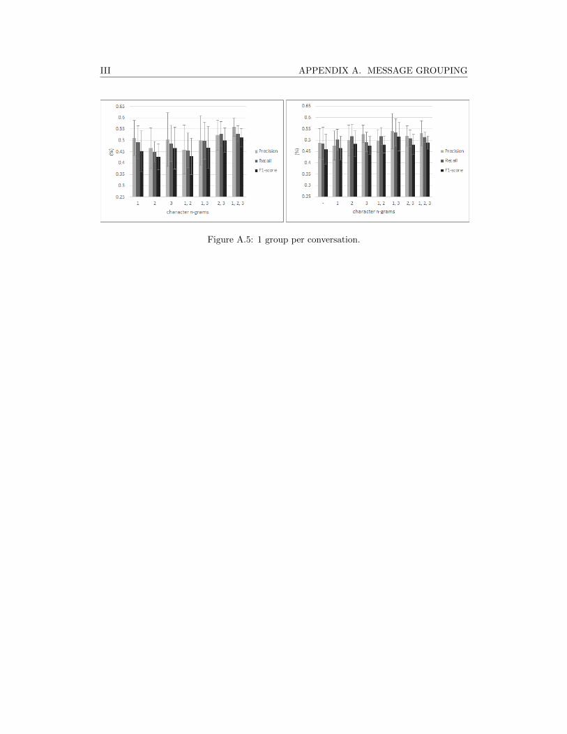
III APPENDIX A. MESSAGE GROUPING

Figure A.5: 1 group per conversation.

IV APPENDIX B. AUTHORSHIP ATTRIBUTION RESULTS

Appendix B

Authorship attribution results

B.1 Delta

Figure B.1: Results of the Cosine Delta model on the MFTM Corpus achieved through 5-fold cross-validation, with top-2000 feature selection through chi-squared, without messagegrouping. Error bars indicate a confidence interval of 95%.

V APPENDIX B. AUTHORSHIP ATTRIBUTION RESULTS

Figure B.2: Results of the Cosine Delta model on the NUS SMS Corpus achieved through 5-fold cross-validation, with top-2000 feature selection through chi-squared, without messagegrouping. Error bars indicate a confidence interval of 95%.

Figure B.3: Results of the Cosine Delta model on the SMS4Science dataset achieved through5-fold cross-validation, with top-2000 feature selection through chi-squared, without messagegrouping. Error bars indicate a confidence interval of 95%.

VI APPENDIX B. AUTHORSHIP ATTRIBUTION RESULTS

Figure B.4: Results of the Cosine Delta model on the Hispanic BYTs dataset achievedthrough 5-fold cross-validation, with top-2000 feature selection through chi-squared, withoutmessage grouping. Error bars indicate a confidence interval of 95%.

B.2 SVM

Figure B.5: Results of the SVM model on the MFTM Corpus achieved through 5-fold cross-validation, with top-2000 feature selection through chi-squared, without message grouping.Error bars indicate a confidence interval of 95%.

VII APPENDIX B. AUTHORSHIP ATTRIBUTION RESULTS

Figure B.6: Results of the SVM model on the NUS SMS Corpus achieved through 5-fold cross-validation, with top-2000 feature selection through chi-squared, without messagegrouping. Error bars indicate a confidence interval of 95%.

Figure B.7: Results of the SVM model on the SMS4Science dataset achieved through 5-fold cross-validation, with top-2000 feature selection through chi-squared, without messagegrouping. Error bars indicate a confidence interval of 95%.

VIII APPENDIX B. AUTHORSHIP ATTRIBUTION RESULTS

Figure B.8: Results of the SVM model on the Hispanic BYTs dataset achieved through 5-fold cross-validation, with top-2000 feature selection through chi-squared, without messagegrouping. Error bars indicate a confidence interval of 95%.

B.3 CNN

Figure B.9: Results of the CNN model on the MFTM Corpus achieved through 5-fold cross-validation, without message grouping. Error bars indicate a confidence interval of 95%.

IX APPENDIX B. AUTHORSHIP ATTRIBUTION RESULTS

Figure B.10: Results of the CNN model on the NUS SMS Corpus achieved through 5-foldcross-validation, without message grouping. Error bars indicate a confidence interval of95%.

Figure B.11: Results of the CNN model on the SMS4Science dataset achieved through 10-fold cross-validation, without message grouping. Error bars indicate a confidence intervalof 95%.

X APPENDIX B. AUTHORSHIP ATTRIBUTION RESULTS

Figure B.12: Results of the CNN model on the Hispanic BYTs dataset achieved through5-fold cross-validation, without message grouping. Error bars indicate a confidence intervalof 95%.

XI APPENDIX C. NETWORK ANALYSIS RESULTS

Appendix C

Network analysis results

Figure C.1: Results of the network analysis-based method on the Opsahl dataset achievedthrough 5-fold cross-validation. Error bars indicate a confidence interval of 95%.

Documents

Impostor Finding