arX

iv:0

804.

2089

v2 [

hep-

ex]

7 A

ug 2

008

BABAR-PUB-08/006SLAC-PUB-132090804.2089 [hep-ex]

Improved measurement of the CKM angle γ in B∓ → D(∗)K(∗)∓ decays

with a Dalitz plot analysis of D decays to K0Sπ+π− and K0

SK+K−

B. Aubert,1 M. Bona,1 Y. Karyotakis,1 J. P. Lees,1 V. Poireau,1 E. Prencipe,1 X. Prudent,1 V. Tisserand,1

J. Garra Tico,2 E. Grauges,2 L. Lopez,3 A. Palano,3 M. Pappagallo,3 G. Eigen,4 B. Stugu,4 L. Sun,4 G. S. Abrams,5

M. Battaglia,5 D. N. Brown,5 J. Button-Shafer,5 R. N. Cahn,5 R. G. Jacobsen,5 J. A. Kadyk,5 L. T. Kerth,5

Yu. G. Kolomensky,5 G. Kukartsev,5 G. Lynch,5 I. L. Osipenkov,5 M. T. Ronan,5, ∗ K. Tackmann,5 T. Tanabe,5

W. A. Wenzel,5 C. M. Hawkes,6 N. Soni,6 A. T. Watson,6 H. Koch,7 T. Schroeder,7 D. Walker,8 D. J. Asgeirsson,9

T. Cuhadar-Donszelmann,9 B. G. Fulsom,9 C. Hearty,9 T. S. Mattison,9 J. A. McKenna,9 M. Barrett,10

A. Khan,10 M. Saleem,10 L. Teodorescu,10 V. E. Blinov,11 A. D. Bukin,11 A. R. Buzykaev,11 V. P. Druzhinin,11

V. B. Golubev,11 A. P. Onuchin,11 S. I. Serednyakov,11 Yu. I. Skovpen,11 E. P. Solodov,11 K. Yu. Todyshev,11

M. Bondioli,12 S. Curry,12 I. Eschrich,12 D. Kirkby,12 A. J. Lankford,12 P. Lund,12 M. Mandelkern,12

E. C. Martin,12 D. P. Stoker,12 S. Abachi,13 C. Buchanan,13 J. W. Gary,14 F. Liu,14 O. Long,14 B. C. Shen,14, ∗

G. M. Vitug,14 Z. Yasin,14 L. Zhang,14 V. Sharma,15 C. Campagnari,16 T. M. Hong,16 D. Kovalskyi,16

M. A. Mazur,16 J. D. Richman,16 T. W. Beck,17 A. M. Eisner,17 C. J. Flacco,17 C. A. Heusch,17 J. Kroseberg,17

W. S. Lockman,17 T. Schalk,17 B. A. Schumm,17 A. Seiden,17 L. Wang,17 M. G. Wilson,17 L. O. Winstrom,17

C. H. Cheng,18 D. A. Doll,18 B. Echenard,18 F. Fang,18 D. G. Hitlin,18 I. Narsky,18 T. Piatenko,18 F. C. Porter,18

R. Andreassen,19 G. Mancinelli,19 B. T. Meadows,19 K. Mishra,19 M. D. Sokoloff,19 F. Blanc,20 P. C. Bloom,20

W. T. Ford,20 A. Gaz,20 J. F. Hirschauer,20 A. Kreisel,20 M. Nagel,20 U. Nauenberg,20 A. Olivas,20 J. G. Smith,20

K. A. Ulmer,20 S. R. Wagner,20 R. Ayad,21, † A. M. Gabareen,21 A. Soffer,21, ‡ W. H. Toki,21 R. J. Wilson,21

D. D. Altenburg,22 E. Feltresi,22 A. Hauke,22 H. Jasper,22 M. Karbach,22 J. Merkel,22 A. Petzold,22 B. Spaan,22

K. Wacker,22 V. Klose,23 M. J. Kobel,23 H. M. Lacker,23 W. F. Mader,23 R. Nogowski,23 K. R. Schubert,23

R. Schwierz,23 J. E. Sundermann,23 A. Volk,23 D. Bernard,24 G. R. Bonneaud,24 E. Latour,24 Ch. Thiebaux,24

M. Verderi,24 P. J. Clark,25 W. Gradl,25 S. Playfer,25 J. E. Watson,25 M. Andreotti,26 D. Bettoni,26 C. Bozzi,26

R. Calabrese,26 A. Cecchi,26 G. Cibinetto,26 P. Franchini,26 E. Luppi,26 M. Negrini,26 A. Petrella,26 L. Piemontese,26

V. Santoro,26 F. Anulli,27 R. Baldini-Ferroli,27 A. Calcaterra,27 R. de Sangro,27 G. Finocchiaro,27 S. Pacetti,27

P. Patteri,27 I. M. Peruzzi,27, § M. Piccolo,27 M. Rama,27 A. Zallo,27 A. Buzzo,28 R. Contri,28 M. Lo Vetere,28

M. M. Macri,28 M. R. Monge,28 S. Passaggio,28 C. Patrignani,28 E. Robutti,28 A. Santroni,28 S. Tosi,28

K. S. Chaisanguanthum,29 M. Morii,29 R. S. Dubitzky,30 J. Marks,30 S. Schenk,30 U. Uwer,30 D. J. Bard,31

P. D. Dauncey,31 J. A. Nash,31 W. Panduro Vazquez,31 M. Tibbetts,31 P. K. Behera,32 X. Chai,32 M. J. Charles,32

U. Mallik,32 J. Cochran,33 H. B. Crawley,33 L. Dong,33 W. T. Meyer,33 S. Prell,33 E. I. Rosenberg,33 A. E. Rubin,33

Y. Y. Gao,34 A. V. Gritsan,34 Z. J. Guo,34 C. K. Lae,34 A. G. Denig,35 M. Fritsch,35 G. Schott,35 N. Arnaud,36

J. Bequilleux,36 A. D’Orazio,36 M. Davier,36 J. Firmino da Costa,36 G. Grosdidier,36 A. Hocker,36 V. Lepeltier,36

F. Le Diberder,36 A. M. Lutz,36 S. Pruvot,36 P. Roudeau,36 M. H. Schune,36 J. Serrano,36 V. Sordini,36

A. Stocchi,36 W. F. Wang,36 G. Wormser,36 D. J. Lange,37 D. M. Wright,37 I. Bingham,38 J. P. Burke,38

C. A. Chavez,38 J. R. Fry,38 E. Gabathuler,38 R. Gamet,38 D. E. Hutchcroft,38 D. J. Payne,38 C. Touramanis,38

A. J. Bevan,39 K. A. George,39 F. Di Lodovico,39 R. Sacco,39 M. Sigamani,39 G. Cowan,40 H. U. Flaecher,40

D. A. Hopkins,40 S. Paramesvaran,40 F. Salvatore,40 A. C. Wren,40 D. N. Brown,41 C. L. Davis,41 K. E. Alwyn,42

N. R. Barlow,42 R. J. Barlow,42 Y. M. Chia,42 C. L. Edgar,42 G. D. Lafferty,42 T. J. West,42 J. I. Yi,42

J. Anderson,43 C. Chen,43 A. Jawahery,43 D. A. Roberts,43 G. Simi,43 J. M. Tuggle,43 C. Dallapiccola,44

S. S. Hertzbach,44 X. Li,44 E. Salvati,44 S. Saremi,44 R. Cowan,45 D. Dujmic,45 P. H. Fisher,45 K. Koeneke,45

G. Sciolla,45 M. Spitznagel,45 F. Taylor,45 R. K. Yamamoto,45 M. Zhao,45 S. E. Mclachlin,46, ∗ P. M. Patel,46

S. H. Robertson,46 A. Lazzaro,47 V. Lombardo,47 F. Palombo,47 J. M. Bauer,48 L. Cremaldi,48 V. Eschenburg,48

R. Godang,48 R. Kroeger,48 D. A. Sanders,48 D. J. Summers,48 H. W. Zhao,48 S. Brunet,49 D. Cote,49 M. Simard,49

P. Taras,49 F. B. Viaud,49 H. Nicholson,50 G. De Nardo,51 L. Lista,51 D. Monorchio,51 C. Sciacca,51 M. A. Baak,52

G. Raven,52 H. L. Snoek,52 C. P. Jessop,53 K. J. Knoepfel,53 J. M. LoSecco,53 G. Benelli,54 L. A. Corwin,54

K. Honscheid,54 H. Kagan,54 R. Kass,54 J. P. Morris,54 A. M. Rahimi,54 J. J. Regensburger,54 S. J. Sekula,54

Q. K. Wong,54 N. L. Blount,55 J. Brau,55 R. Frey,55 O. Igonkina,55 J. A. Kolb,55 M. Lu,55 R. Rahmat,55

2

N. B. Sinev,55 D. Strom,55 J. Strube,55 E. Torrence,55 G. Castelli,56 N. Gagliardi,56 M. Margoni,56 M. Morandin,56

M. Posocco,56 M. Rotondo,56 F. Simonetto,56 R. Stroili,56 C. Voci,56 P. del Amo Sanchez,57 E. Ben-Haim,57

H. Briand,57 G. Calderini,57 J. Chauveau,57 P. David,57 L. Del Buono,57 O. Hamon,57 Ph. Leruste,57 J. Ocariz,57

A. Perez,57 J. Prendki,57 L. Gladney,58 M. Biasini,59 R. Covarelli,59 E. Manoni,59 C. Angelini,60 G. Batignani,60

S. Bettarini,60 M. Carpinelli,60, ¶ A. Cervelli,60 F. Forti,60 M. A. Giorgi,60 A. Lusiani,60 G. Marchiori,60

M. Morganti,60 N. Neri,60 E. Paoloni,60 G. Rizzo,60 J. J. Walsh,60 J. Biesiada,61 D. Lopes Pegna,61 C. Lu,61

J. Olsen,61 A. J. S. Smith,61 A. V. Telnov,61 E. Baracchini,62 G. Cavoto,62 D. del Re,62 E. Di Marco,62 R. Faccini,62

F. Ferrarotto,62 F. Ferroni,62 M. Gaspero,62 P. D. Jackson,62 L. Li Gioi,62 M. A. Mazzoni,62 S. Morganti,62

G. Piredda,62 F. Polci,62 F. Renga,62 C. Voena,62 M. Ebert,63 T. Hartmann,63 H. Schroder,63 R. Waldi,63

T. Adye,64 B. Franek,64 E. O. Olaiya,64 W. Roethel,64 F. F. Wilson,64 S. Emery,65 M. Escalier,65 L. Esteve,65

A. Gaidot,65 S. F. Ganzhur,65 G. Hamel de Monchenault,65 W. Kozanecki,65 G. Vasseur,65 Ch. Yeche,65 M. Zito,65

X. R. Chen,66 H. Liu,66 W. Park,66 M. V. Purohit,66 R. M. White,66 J. R. Wilson,66 M. T. Allen,67 D. Aston,67

R. Bartoldus,67 P. Bechtle,67 J. F. Benitez,67 R. Cenci,67 J. P. Coleman,67 M. R. Convery,67 J. C. Dingfelder,67

J. Dorfan,67 G. P. Dubois-Felsmann,67 W. Dunwoodie,67 R. C. Field,67 S. J. Gowdy,67 M. T. Graham,67

P. Grenier,67 C. Hast,67 W. R. Innes,67 J. Kaminski,67 M. H. Kelsey,67 H. Kim,67 P. Kim,67 M. L. Kocian,67

D. W. G. S. Leith,67 S. Li,67 B. Lindquist,67 S. Luitz,67 V. Luth,67 H. L. Lynch,67 D. B. MacFarlane,67

H. Marsiske,67 R. Messner,67 D. R. Muller,67 H. Neal,67 S. Nelson,67 C. P. O’Grady,67 I. Ofte,67 A. Perazzo,67

M. Perl,67 B. N. Ratcliff,67 A. Roodman,67 A. A. Salnikov,67 R. H. Schindler,67 J. Schwiening,67 A. Snyder,67

D. Su,67 M. K. Sullivan,67 K. Suzuki,67 S. K. Swain,67 J. M. Thompson,67 J. Va’vra,67 A. P. Wagner,67

M. Weaver,67 C. A. West,67 W. J. Wisniewski,67 M. Wittgen,67 D. H. Wright,67 H. W. Wulsin,67 A. K. Yarritu,67

K. Yi,67 C. C. Young,67 V. Ziegler,67 P. R. Burchat,68 A. J. Edwards,68 S. A. Majewski,68 T. S. Miyashita,68

B. A. Petersen,68 L. Wilden,68 S. Ahmed,69 M. S. Alam,69 R. Bula,69 J. A. Ernst,69 B. Pan,69 M. A. Saeed,69

S. B. Zain,69 S. M. Spanier,70 B. J. Wogsland,70 R. Eckmann,71 J. L. Ritchie,71 A. M. Ruland,71 C. J. Schilling,71

R. F. Schwitters,71 B. W. Drummond,72 J. M. Izen,72 X. C. Lou,72 S. Ye,72 F. Bianchi,73 D. Gamba,73

M. Pelliccioni,73 M. Bomben,74 L. Bosisio,74 C. Cartaro,74 G. Della Ricca,74 L. Lanceri,74 L. Vitale,74 V. Azzolini,75

N. Lopez-March,75 F. Martinez-Vidal,75 D. A. Milanes,75 A. Oyanguren,75 J. Albert,76 Sw. Banerjee,76

B. Bhuyan,76 H. H. F. Choi,76 K. Hamano,76 R. Kowalewski,76 M. J. Lewczuk,76 I. M. Nugent,76 J. M. Roney,76

R. J. Sobie,76 T. J. Gershon,77 P. F. Harrison,77 J. Ilic,77 T. E. Latham,77 G. B. Mohanty,77 H. R. Band,78

X. Chen,78 S. Dasu,78 K. T. Flood,78 Y. Pan,78 M. Pierini,78 R. Prepost,78 C. O. Vuosalo,78 and S. L. Wu78

(The BABAR Collaboration)1Laboratoire de Physique des Particules, IN2P3/CNRS et Universite de Savoie, F-74941 Annecy-Le-Vieux, France

2Universitat de Barcelona, Facultat de Fisica, Departament ECM, E-08028 Barcelona, Spain3Universita di Bari, Dipartimento di Fisica and INFN, I-70126 Bari, Italy

4University of Bergen, Institute of Physics, N-5007 Bergen, Norway5Lawrence Berkeley National Laboratory and University of California, Berkeley, California 94720, USA

6University of Birmingham, Birmingham, B15 2TT, United Kingdom7Ruhr Universitat Bochum, Institut fur Experimentalphysik 1, D-44780 Bochum, Germany

8University of Bristol, Bristol BS8 1TL, United Kingdom9University of British Columbia, Vancouver, British Columbia, Canada V6T 1Z1

10Brunel University, Uxbridge, Middlesex UB8 3PH, United Kingdom11Budker Institute of Nuclear Physics, Novosibirsk 630090, Russia12University of California at Irvine, Irvine, California 92697, USA

13University of California at Los Angeles, Los Angeles, California 90024, USA14University of California at Riverside, Riverside, California 92521, USA15University of California at San Diego, La Jolla, California 92093, USA

16University of California at Santa Barbara, Santa Barbara, California 93106, USA17University of California at Santa Cruz, Institute for Particle Physics, Santa Cruz, California 95064, USA

18California Institute of Technology, Pasadena, California 91125, USA19University of Cincinnati, Cincinnati, Ohio 45221, USA20University of Colorado, Boulder, Colorado 80309, USA

21Colorado State University, Fort Collins, Colorado 80523, USA22Technische Universitat Dortmund, Fakultat Physik, D-44221 Dortmund, Germany

23Technische Universitat Dresden, Institut fur Kern- und Teilchenphysik, D-01062 Dresden, Germany24Laboratoire Leprince-Ringuet, CNRS/IN2P3, Ecole Polytechnique, F-91128 Palaiseau, France

25University of Edinburgh, Edinburgh EH9 3JZ, United Kingdom26Universita di Ferrara, Dipartimento di Fisica and INFN, I-44100 Ferrara, Italy

27Laboratori Nazionali di Frascati dell’INFN, I-00044 Frascati, Italy28Universita di Genova, Dipartimento di Fisica and INFN, I-16146 Genova, Italy

3

29Harvard University, Cambridge, Massachusetts 02138, USA30Universitat Heidelberg, Physikalisches Institut, Philosophenweg 12, D-69120 Heidelberg, Germany

31Imperial College London, London, SW7 2AZ, United Kingdom32University of Iowa, Iowa City, Iowa 52242, USA

33Iowa State University, Ames, Iowa 50011-3160, USA34Johns Hopkins University, Baltimore, Maryland 21218, USA

35Universitat Karlsruhe, Institut fur Experimentelle Kernphysik, D-76021 Karlsruhe, Germany36Laboratoire de l’Accelerateur Lineaire, IN2P3/CNRS et Universite Paris-Sud 11,

Centre Scientifique d’Orsay, B. P. 34, F-91898 ORSAY Cedex, France37Lawrence Livermore National Laboratory, Livermore, California 94550, USA

38University of Liverpool, Liverpool L69 7ZE, United Kingdom39Queen Mary, University of London, E1 4NS, United Kingdom

40University of London, Royal Holloway and Bedford New College, Egham, Surrey TW20 0EX, United Kingdom41University of Louisville, Louisville, Kentucky 40292, USA

42University of Manchester, Manchester M13 9PL, United Kingdom43University of Maryland, College Park, Maryland 20742, USA

44University of Massachusetts, Amherst, Massachusetts 01003, USA45Massachusetts Institute of Technology, Laboratory for Nuclear Science, Cambridge, Massachusetts 02139, USA

46McGill University, Montreal, Quebec, Canada H3A 2T847Universita di Milano, Dipartimento di Fisica and INFN, I-20133 Milano, Italy

48University of Mississippi, University, Mississippi 38677, USA49Universite de Montreal, Physique des Particules, Montreal, Quebec, Canada H3C 3J7

50Mount Holyoke College, South Hadley, Massachusetts 01075, USA51Universita di Napoli Federico II, Dipartimento di Scienze Fisiche and INFN, I-80126, Napoli, Italy

52NIKHEF, National Institute for Nuclear Physics and High Energy Physics, NL-1009 DB Amsterdam, The Netherlands53University of Notre Dame, Notre Dame, Indiana 46556, USA

54Ohio State University, Columbus, Ohio 43210, USA55University of Oregon, Eugene, Oregon 97403, USA

56Universita di Padova, Dipartimento di Fisica and INFN, I-35131 Padova, Italy57Laboratoire de Physique Nucleaire et de Hautes Energies,

IN2P3/CNRS, Universite Pierre et Marie Curie-Paris6,Universite Denis Diderot-Paris7, F-75252 Paris, France

58University of Pennsylvania, Philadelphia, Pennsylvania 19104, USA59Universita di Perugia, Dipartimento di Fisica and INFN, I-06100 Perugia, Italy

60Universita di Pisa, Dipartimento di Fisica, Scuola Normale Superiore and INFN, I-56127 Pisa, Italy61Princeton University, Princeton, New Jersey 08544, USA

62Universita di Roma La Sapienza, Dipartimento di Fisica and INFN, I-00185 Roma, Italy63Universitat Rostock, D-18051 Rostock, Germany

64Rutherford Appleton Laboratory, Chilton, Didcot, Oxon, OX11 0QX, United Kingdom65DSM/Dapnia, CEA/Saclay, F-91191 Gif-sur-Yvette, France

66University of South Carolina, Columbia, South Carolina 29208, USA67Stanford Linear Accelerator Center, Stanford, California 94309, USA

68Stanford University, Stanford, California 94305-4060, USA69State University of New York, Albany, New York 12222, USA

70University of Tennessee, Knoxville, Tennessee 37996, USA71University of Texas at Austin, Austin, Texas 78712, USA

72University of Texas at Dallas, Richardson, Texas 75083, USA73Universita di Torino, Dipartimento di Fisica Sperimentale and INFN, I-10125 Torino, Italy

74Universita di Trieste, Dipartimento di Fisica and INFN, I-34127 Trieste, Italy75IFIC, Universitat de Valencia-CSIC, E-46071 Valencia, Spain

76University of Victoria, Victoria, British Columbia, Canada V8W 3P677Department of Physics, University of Warwick, Coventry CV4 7AL, United Kingdom

78University of Wisconsin, Madison, Wisconsin 53706, USA(Dated: August 7, 2008)

We report on an improved measurement of the Cabibbo-Kobayashi-Maskawa CP -violating phase γthrough a Dalitz plot analysis of neutral D meson decays to K0

Sπ+π− and K0SK+K− produced in

the processes B∓ → DK∓, B∓ → D∗K∓ with D∗ → Dπ0, Dγ, and B∓ → DK∗∓ with K∗∓ →

K0Sπ∓. Using a sample of 383 million BB pairs collected by the BABAR detector, we measure

γ = (76± 22± 5± 5)◦ (mod 180◦), where the first error is statistical, the second is the experimentalsystematic uncertainty and the third reflects the uncertainty on the description of the Dalitz plotdistributions. The corresponding two standard deviation region is 29◦ < γ < 122◦. This result hasa significance of direct CP violation (γ 6= 0) of 3.0 standard deviations.

4

PACS numbers: 13.25.Hw, 12.15.Hh, 14.40.Nd, 11.30.Er

I. INTRODUCTION AND OVERVIEW

In the Standard Model (SM) the phase in the Cabibbo-Kobayashi-Maskawa (CKM) quark-mixing matrix [1] isthe sole source of CP violation in the quark sector ofthe electroweak interactions. This phase can be directlydetermined using a variety of methods, involving eitherthe interference between decays with and without mixingin time-dependent CP asymmetries in neutral B mesondecays, or interference between neutral B (self-tagged)or charged B decays yielding the same final state (di-rect CP violation). These multiple determinations inCP -violating tree-level processes as well as in decays in-volving penguin diagrams test the CKM mechanism, thusprobing the presence of physics beyond the SM [2].

D0�us K��u

B� b W�B� b u

� K��D0

�u s�u W�FIG. 1: Main Feynman diagrams contributing to the B− →

D0K− decay. The left diagram proceeds via b → cus transi-tion, while the right diagram proceeds via b → ucs transitionand is color suppressed.

Among these determinations, the measurement of theangle γ, defined as arg [−VudV

∗ub/VcdV

∗cb ], where Vij are

the elements of the CKM matrix, is one of the most dif-ficult to achieve and constitutes an important goal ofpresent and future B physics experiments. Several meth-ods have been proposed to extract γ. However, thoseusing B∓ → D(∗)0K(∗)∓ decays [3, 4] (the symbol D(∗)0

indicates either a D(∗)0 or a D(∗)0 meson) are theoreti-cally clean and are unlikely to be affected by new physicsbecause the main contributions to the amplitudes comefrom tree-level diagrams, as shown in Fig. 1. This is animportant distinction from most of other direct measure-ments of phases of CKM elements. The decay amplitudesfor the color allowed B− → D(∗)0K(∗)− (b → cus) andthe color suppressed B− → D(∗)0K(∗)− (b → ucs) tran-

sitions [5] differ by a factor r(∗)B ei(δ

(∗)B

∓γ). Here, r(∗)B is

the magnitude of the ratio of the amplitudes A(B− →

∗Deceased†Now at Temple University, Philadelphia, Pennsylvania 19122,

USA‡Now at Tel Aviv University, Tel Aviv, 69978, Israel§Also with Universita di Perugia, Dipartimento di Fisica, Perugia,

Italy¶Also with Universita di Sassari, Sassari, Italy

D(∗)0K−) and A(B− → D(∗)0K−) and δ(∗)B is their rel-

ative strong phase. The weak phase γ leads to differentB− and B+ decay rates (direct CP violation) and, whenthe D(∗)0 and D(∗)0 decay to a common final state [6–9], the phases become observable. The uncertainty in γ

scales roughly as 1/r(∗)B . From the ratio of CKM matrix

elements we expect r(∗)B ≈ cF | VcsV

∗ub | / | VusV

∗cb | to be

approximately in the range 0.1−0.2, where cF ∼ 0.2−0.4is the color suppression factor [10, 11].

When the neutral D meson is reconstructed in athree-body final state, like K0

Sπ+π−, the distribution

in the Dalitz plot [12] depends on the interference be-tween Cabibbo allowed, doubly-Cabibbo suppressed, andCP -eigenstate decay amplitudes of D0 (from B∓ →D(∗)0K(∗)∓) and D0 (from B∓ → D(∗)0K(∗)∓). Thedominant interfering amplitudes in the K0

Sπ+π− final

state are D0 → K∗−π+, D0 → K∗+π−, and D0 →K0

Sρ(770)0 [5, 13]. Neglecting effects from D0 − D0

mixing and CP asymmetries in neutral D decays thatare 1% or less [14–16], the B∓ → D(∗)0K∓, with

D∗0 → D0π0, D0γ, D0 → K0Sπ+π− decay chain ampli-

tude A(∗)∓ (m2

−, m2+) can be written as

A(∗)∓ (m2

−, m2+) ∝ AD∓ + λr

(∗)B ei(δ

(∗)B

∓γ)AD± , (1)

where m2− and m2

+ are the squared invariant masses ofthe K0

Sπ− and K0

Sπ+ combinations, respectively, and

AD∓ ≡ AD(m2∓, m2

±), with AD− (AD+) the amplitude

of the D0 → K0Sπ+π− (D0 → K0

Sπ−π+) decay. For con-

venience, m20 is defined analogously for the π+π− com-

bination. The factor λ in Eq. (1) takes the value −1 for

the decay B∓ → D∗0[D0γ]K∓ and +1 for the remainingB decays. This relative sign arises due to charge conju-gation and angular momentum conservation in the D∗0

decay [17]. The corresponding decay rate Γ(∗)∓ (m2

−, m2+)

can therefore be written as

Γ(∗)∓ (m2

−, m2+) ∝ |AD∓|

2 + r(∗)B

2|AD±|

2 +

2λ[

x(∗)∓ ℜ{AD∓A

∗D±

} + y(∗)∓ ℑ{AD∓A

∗D±}

]

, (2)

where we introduce the CP parameters [18] x(∗)∓ =

r(∗)B cos(δ

(∗)B ∓ γ) and y

(∗)∓ = r

(∗)B sin(δ

(∗)B ∓ γ), where

x(∗)∓

2+ y

(∗)∓

2= r

(∗)B

2.

Decays B∓ → D0K∗∓ with K∗∓ → K0Sπ∓ [4] are

also used in this analysis. For these, Eq. (2) requires the

replacements Γ(∗)∓ → Γs∓, r

(∗)B → rs, δ

(∗)B → δs, x

(∗)∓ →

xs∓ = κrs cos(δs ∓ γ), and y(∗)∓ → ys∓ = κrs sin(δs ∓ γ),

where x2s∓ + y2

s∓ = κ2r2s , where [11]

r2s =

∫

A2u(p)dp

∫

A2c(p)dp

, κeiδs =

∫

Ac(p)Au(p)eiδ(p)dp√

∫

A2c(p)dp

∫

A2u(p)dp

. (3)

5

Here, Ac(p) and Au(p) are the magnitudes of the b → cand b → u amplitudes as a function of the B∓ →D0K0

Sπ∓ phase space position p, and δ(p) is the relative

strong phase. The parameter κ accounts for the interfer-ence between B∓ → D0K∗∓ and other B∓ → D0K0

Sπ∓

amplitudes with 0 < κ < 1 in the most general case.This effective parameterization also accounts for effi-ciency variations as a function of the kinematics of theB decay.

In this paper we present an improved measurement ofγ based on the analysis of the Dalitz plot distribution ofD0 → K0

Sπ+π− and, for the first time, D0 → K0

SK+K−,

using a sample of 351 fb−1 of integrated luminosityrecorded at the Υ (4S) resonance, corresponding to 383million BB pairs. We analyze a total of seven sig-nal samples (also referred to as CP samples), B− →

D(∗)0K− and B− → D0K∗−, with D∗0 → D0π0, D0γ,D0 → K0

Sπ+π−, K0

SK+K−, K∗− → K0

Sπ− [5]. Due

to lack of statistics, the decay B− → D0K∗− withD0 → K0

SK+K− has been excluded from the analysis.

We also reconstruct high statistics control samples, onefor each signal B decay channel: B− → D(∗)0π− and (for

B− → D0K∗−) B− → D0a−1 with a−

1 → π−π+π− [5, 19].We exploit the same dataset to determine AD∓ for D0 →K0

Sπ+π− and D0 → K0

SK+K− decays from analyses of

the respective Dalitz plots for high-statistics samples offlavor-tagged D0 mesons from D∗+ → D0π+ decays [5],produced in e+e− → cc events. Additional improve-ments compared to our previous publication [18] includea higher reconstruction efficiency, an optimized treat-ment of the e+e− → qq, q = u, d, s, c background andan improved D0 → K0

Sπ+π− description of the Dalitz

plot distribution (referred to hereafter as Dalitz model),resulting in significant decrease of statistical, systematicand model uncertainties. This measurement supersedesour previous result based on 227 million BB pairs [18].

The paper is organized as follows. In Sec. II we de-scribe the reconstruction and selection of the signal andcontrol samples. Sec. III is devoted to the determinationof AD∓ for D0 → K0

Sπ+π− and D0 → K0

SK+K− de-

cays. In Sec. IV we describe the simultaneous maximum

likelihood fit to the distributions Γ(∗)− and Γ

(∗)+ for the

B∓ → D(∗)0K∓ samples and to the analogous distribu-tions for B∓ → D0K∗∓, to determine the CP parameters

x(∗)∓ , y

(∗)∓ , xs∓, and ys∓. In that section we also present

the experimental results, including systematic uncertain-ties. We extract these CP parameters since they have a

good Gaussian behavior for small values of r(∗)B ,κrs and

relatively low statistics samples, independent of their val-

ues and precisions, in contrast to γ, r(∗)B , δ

(∗)B , κrs, and δs.

Finally, in Sec. V, we interpret the experimental results

and extract the physically relevant quantities γ, r(∗)B , δ

(∗)B ,

κrs and δs, using a statistical (frequentist) analysis.

II. EVENT SELECTION

A. BABAR detector

This analysis is based on a data sample collected by theBABAR detector at the Stanford Linear Accelerator Cen-ter PEP-II e+e− asymmetric-energy storage ring. TheBABAR detector is described in detail elsewhere [20]. Wesummarize briefly the components that are crucial to thisanalysis. Charged-particle tracking is provided by a five-layer silicon vertex tracker (SVT) and a 40-layer driftchamber (DCH). In addition to providing precise spacecoordinates for tracking, the SVT and DCH also mea-sure the specific ionization (dE/dx), which is used forparticle identification of low-momentum charged parti-cles. At higher momenta (p > 0.7 GeV/c) pions andkaons are identified by Cherenkov radiation detected ina ring-imaging device (DIRC). The typical separation be-tween pions and kaons varies from 8σ at 2 GeV/c to 2.5σat 4 GeV/c, where σ denotes here the standard deviation.The position and energy of photons are measured withan electromagnetic calorimeter (EMC) consisting of 6580thallium-doped CsI crystals. These systems are mountedinside a 1.5-T solenoidal super-conducting magnet. Weuse a GEANT4-based Monte Carlo (MC) simulation tomodel the response of the detector, taking into accountthe varying accelerator and detector conditions, and togenerate large samples of signal and background for theCP and control modes considered in the analysis.

B. Event reconstruction and selection

The B− candidates are formed by combining a D(∗)0

candidate with a track identified as a kaon [20] or witha K∗− candidate formed as a combination of a K0

Sand

a negatively charged pion, with an invariant mass within55 MeV/c2 of the nominal K∗− mass. Here and in thefollowing, nominal mass values are taken from [21]. The

D0 candidates are selected by requiring the K0Sπ+π− or

K0SK+K− invariant mass to be within 12 MeV/c2 of the

nominal D0 mass, and the momentum in the center-of-mass (CM) frame to be greater than 1.3 GeV/c. The

K∓ tracks in D0 → K0SK+K− are required to be pos-

itively identified as kaons in the DCH and DIRC. Theπ0 candidates from D∗0 → D0π0 decays are formedfrom pairs of photons with invariant mass in the range[115, 150] MeV/c2, and with photon energy greater than

30 MeV. Photon candidates from D∗0 → D0γ decays areselected if their energy is greater than 100 MeV. The D0

candidates are combined with a π0 (γ) to form the D∗0

candidate, and are required to have a D∗0-D0 mass dif-ference within 2.5 (10) MeV/c2 of its nominal value. TheK0

Scandidates are reconstructed from pairs of oppositely-

charged pions constrained to originate from the samepoint and with an invariant mass within 9 MeV/c2 ofthe K0

Snominal mass. The cosine of the collinearity an-

6

gle between the K0S

momentum and the line connecting

its parent particle (the D0 or the K∗−) and the K0S

decaypoints in the plane transverse to the beam, is required tobe larger than 0.990 (0.997 for K0

Sfrom K∗− decays).

This cut helps to significantly reduce background con-tributions from D0 → ππππ decays and from a−

1 mis-reconstructed as K∗−. The kinematic variables of theD(∗)0, K0

S, and π0 when forming the B−, D0, and D∗0,

respectively, are fitted with masses constrained to nom-inal values. For B− → D0K∗− decays we also require| cos θH | ≥ 0.35, where θH is the angle between the mo-mentum of the K∗− daughter pion and the parent B− inthe K∗− rest frame. The distribution of cos θH is propor-tional to cos2 θH for B− → D0K∗− while it is approx-imately flat for e+e− → qq, q = u, d, s, c (continuum)background.

We characterize B mesons using two almost inde-pendent variables, the beam-energy substituted mass,mES =

√

(E∗20 /2 + p0 · pB)2/E2

0 − p2B, and the energy

difference ∆E = E∗B − E∗

0/2, with p = (E,p), where thesubscripts 0 and B refer to the initial e+e− system andthe B candidate, respectively, and the asterisk denotesthe CM frame. The signal events peak at the B mass inmES and at zero in ∆E. The mES resolution is about2.6 MeV/c2 and does not depend on the decay mode oron the nature of the prompt particle (K− or K∗− can-didate). In contrast, the ∆E resolution depends on themomentum resolution of the D(∗)0 meson and the promptparticle, and ranges between 15 MeV and 18 MeV, de-pending on the decay mode. We select events withmES > 5.2 GeV/c2 and −80 MeV < ∆E < 120 MeV.We discriminate against the main background contribu-tion coming from continuum events through the fit to thedata, as described in Sec. II C.

For events in which multiple B candidates satisfy theselection criteria, the one whose measured D0 mass dif-fers from the nominal value by the least number of stan-dard deviations, is accepted as signal candidate. ForB− → D0K∗− decays we select the candidate with thesmallest value for the sum of the squares of the differ-ences from nominal values, in standard deviations, ofboth K∗− and D0 masses. The fraction of events inwhich we reconstruct more than one candidate is lessthan 1% for B− → D(∗)0K− samples and about 6% forB− → D0K∗−. The cross-feed among the different sam-ples is negligible except for B− → D∗0[D0γ]K−, where

the background from B− → D∗0[D0π0]K− is below 5%

of the signal yield. If both B− → D∗0[D0π0]K− and

B− → D∗0[D0γ]K− candidates are selected in the same

event, only the B− → D∗0[D0π0]K− is kept. This con-tamination has a negligible effect on the measurement ofthe CP parameters.

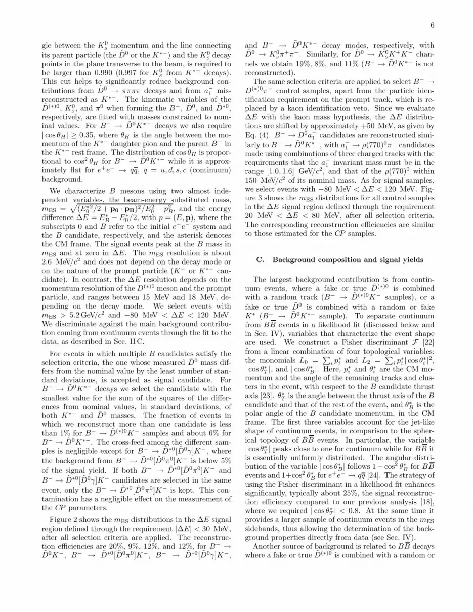
Figure 2 shows the mES distributions in the ∆E signalregion defined through the requirement |∆E| < 30 MeV,after all selection criteria are applied. The reconstruc-tion efficiencies are 20%, 9%, 12%, and 12%, for B− →D0K−, B− → D∗0[D0π0]K−, B− → D∗0[D0γ]K−,

and B− → D0K∗− decay modes, respectively, withD0 → K0

Sπ+π−. Similarly, for D0 → K0

SK+K− chan-

nels we obtain 19%, 8%, and 11% (B− → D0K∗− is notreconstructed).

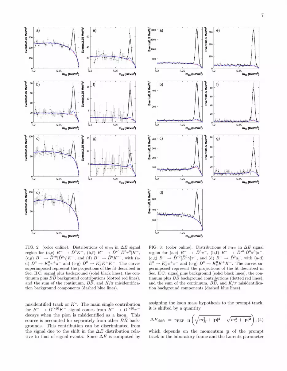
The same selection criteria are applied to select B− →D(∗)0π− control samples, apart from the particle iden-tification requirement on the prompt track, which is re-placed by a kaon identification veto. Since we evaluate∆E with the kaon mass hypothesis, the ∆E distribu-tions are shifted by approximately +50 MeV, as given byEq. (4). B− → D0a−

1 candidates are reconstructed simi-

larly to B− → D0K∗−, with a−1 → ρ(770)0π− candidates

made using combinations of three charged tracks with therequirements that the a−

1 invariant mass must be in therange [1.0, 1.6] GeV/c2, and that of the ρ(770)0 within150 MeV/c2 of its nominal mass. As for signal samples,we select events with −80 MeV < ∆E < 120 MeV. Fig-ure 3 shows the mES distributions for all control samplesin the ∆E signal region defined through the requirement20 MeV < ∆E < 80 MeV, after all selection criteria.The corresponding reconstruction efficiencies are similarto those estimated for the CP samples.

C. Background composition and signal yields

The largest background contribution is from contin-uum events, where a fake or true D(∗)0 is combinedwith a random track (B− → D(∗)0K− samples), or a

fake or true D0 is combined with a random or fakeK∗ (B− → D0K∗− sample). To separate continuumfrom BB events in a likelihood fit (discussed below andin Sec. IV), variables that characterize the event shapeare used. We construct a Fisher discriminant F [22]from a linear combination of four topological variables:the monomials L0 =

∑

i p∗i and L2 =∑

i p∗i | cos θ∗i |2,

| cos θ∗T |, and | cos θ∗B|. Here, p∗i and θ∗i are the CM mo-mentum and the angle of the remaining tracks and clus-ters in the event, with respect to the B candidate thrustaxis [23]. θ∗T is the angle between the thrust axis of the Bcandidate and that of the rest of the event, and θ∗B is thepolar angle of the B candidate momentum, in the CMframe. The first three variables account for the jet-likeshape of continuum events, in comparison to the spher-ical topology of BB events. In particular, the variable| cos θ∗T | peaks close to one for continuum while for BB itis essentially uniformly distributed. The angular distri-bution of the variable | cos θ∗B| follows 1− cos2 θ∗B for BBevents and 1+cos2 θ∗B for e+e− → qq [24]. The strategy ofusing the Fisher discriminant in a likelihood fit enhancessignificantly, typically about 25%, the signal reconstruc-tion efficiency compared to our previous analysis [18],where we required | cos θ∗T | < 0.8. At the same time itprovides a larger sample of continuum events in the mES

sidebands, thus allowing the determination of the back-ground properties directly from data (see Sec. IV).

Another source of background is related to BB decayswhere a fake or true D(∗)0 is combined with a random or

7

)2 (GeV/cESm5.2 5.25

2E

ven

ts/2

.25

MeV

/c

0

100

200

300

)2 (GeV/cESm5.2 5.25

2E

ven

ts/2

.25

MeV

/c

0

100

200

300

a)

)2 (GeV/cESm5.2 5.25

2E

ven

ts/2

.25

MeV

/c

0

20

40

60

)2 (GeV/cESm5.2 5.25

2E

ven

ts/2

.25

MeV

/c

0

20

40

60

e)

)2 (GeV/cESm5.2 5.25

2E

ven

ts/2

.25

MeV

/c

0

20

40

60

80

)2 (GeV/cESm5.2 5.25

2E

ven

ts/2

.25

MeV

/c

0

20

40

60

80 b)

)2 (GeV/cESm5.2 5.25

2E

ven

ts/2

.25

MeV

/c

0

5

10

15

)2 (GeV/cESm5.2 5.25

2E

ven

ts/2

.25

MeV

/c

0

5

10

15f)

)2 (GeV/cESm5.2 5.25

2E

ven

ts/2

.25

MeV

/c

0

50

100

)2 (GeV/cESm5.2 5.25

2E

ven

ts/2

.25

MeV

/c

0

50

100c)

)2 (GeV/cESm5.2 5.25

2E

ven

ts/2

.25

MeV

/c

0

5

10

15

)2 (GeV/cESm5.2 5.25

2E

ven

ts/2

.25

MeV

/c

0

5

10

15 g)

)2 (GeV/cESm5.2 5.25

2E

ven

ts/2

.25

MeV

/c

0

50

100

)2 (GeV/cESm5.2 5.25

2E

ven

ts/2

.25

MeV

/c

0

50

100 d)

FIG. 2: (color online). Distributions of mES in ∆E signal

region for (a,e) B− → D0K−, (b,f) B− → D∗0[D0π0]K−,

(c,g) B− → D∗0[D0γ]K−, and (d) B− → D0K∗−, with (a-

d) D0 → K0Sπ+π− and (e-g) D0 → K0

SK+K−. The curvessuperimposed represent the projections of the fit described inSec. IIC: signal plus background (solid black lines), the con-tinuum plus BB background contributions (dotted red lines),and the sum of the continuum, BB, and K/π misidentifica-tion background components (dashed blue lines).

misidentified track or K∗. The main single contributionfor B− → D(∗)0K− signal comes from B− → D(∗)0π−

decays when the pion is misidentified as a kaon. Thissource is accounted for separately from other BB back-grounds. This contribution can be discriminated fromthe signal due to the shift in the ∆E distribution rela-tive to that of signal events. Since ∆E is computed by

)2 (GeV/cESm5.2 5.25

2E

ven

ts/1

.5 M

eV/c

0

500

1000

1500

2000

)2 (GeV/cESm5.2 5.25

2E

ven

ts/1

.5 M

eV/c

0

500

1000

1500

2000 a)

)2 (GeV/cESm5.2 5.25

2E

ven

ts/1

.5 M

eV/c

0

100

200

300

)2 (GeV/cESm5.2 5.25

2E

ven

ts/1

.5 M

eV/c

0

100

200

300 e)

)2 (GeV/cESm5.2 5.25

2E

ven

ts/1

.5 M

eV/c

0

200

400

)2 (GeV/cESm5.2 5.25

2E

ven

ts/1

.5 M

eV/c

0

200

400

b)

)2 (GeV/cESm5.2 5.25

2E

ven

ts/1

.5 M

eV/c

0

20

40

60

80

)2 (GeV/cESm5.2 5.25

2E

ven

ts/1

.5 M

eV/c

0

20

40

60

80f)

)2 (GeV/cESm5.2 5.25

2E

ven

ts/1

.5 M

eV/c

0

100

200

300

400

)2 (GeV/cESm5.2 5.25

2E

ven

ts/1

.5 M

eV/c

0

100

200

300

400 c)

)2 (GeV/cESm5.2 5.25

2E

ven

ts/1

.5 M

eV/c

0

20

40

60

80

)2 (GeV/cESm5.2 5.25

2E

ven

ts/1

.5 M

eV/c

0

20

40

60

80 g)

)2 (GeV/cESm5.2 5.25

2E

ven

ts/1

.5 M

eV/c

0

200

400

600

)2 (GeV/cESm5.2 5.25

2E

ven

ts/1

.5 M

eV/c

0

200

400

600

d)

FIG. 3: (color online). Distributions of mES in ∆E signal

region for (a,e) B− → D0π−, (b,f) B− → D∗0[D0π0]π−,

(c,g) B− → D∗0[D0γ]π−, and (d) B− → D0a−1 , with (a-d)

D0 → K0Sπ+π− and (e-g) D0 → K0

SK+K−. The curves su-perimposed represent the projections of the fit described inSec. IIC: signal plus background (solid black lines), the con-tinuum plus BB background contributions (dotted red lines),and the sum of the continuum, BB, and K/π misidentifica-tion background components (dashed blue lines).

assigning the kaon mass hypothesis to the prompt track,it is shifted by a quantity

∆Eshift = γPEP−II

(

√

m2K + |p|2 −

√

m2π + |p|2

)

, (4)

which depends on the momentum p of the prompttrack in the laboratory frame and the Lorentz parameter

8

γPEP−II characterizing the boost of the CM relative tothe laboratory frame, estimated from the PEP-II beamenergies. For B− → D0K∗− signal the main BB back-ground source comes from B− → D0a−

1 decays. Sincethis contribution is highly suppressed by the cut on thecosine of the collinearity angle at 0.997, it is not treatedseparately from other BB backgrounds. Non-K∗ decayscontributing to the B− → D0K∗− sample are consideredas signal, and their effect is accounted for by the factorκ defined in Eq. (3).

We fit the seven signal samples B− → D(∗)0K− andB− → D0K∗−, and their control samples B− → D(∗)0π−

and B− → D0a−1 , using an unbinned extended maxi-

mum likelihood method to extract signal and backgroundyields, and probability density functions (PDFs) for thevariables mES, ∆E, and the F discriminant, in the ∆Eselection region. Three different background componentsare considered: continuum events, K/π misidentification

(for B− → D(∗)0K− and B− → D(∗)0π− samples only),and other Υ (4S) → BB decays. The log-likelihood foreach of the CP and control samples is

lnL = −η +∑

j

ln

[

∑

c

NcPc(uj)

]

, (5)

where uj = {mES, ∆E,F}j characterizes the event j.Here, Pc(u) = Pc(mES)Pc(∆E)Pc(F) is the combinedselection PDF, verifying the normalization condition∫

Pc(u)du = 1, Nc the event yield for signal or back-ground component c, and η =

∑

c Nc.The signal mES distributions for each CP sample and

its corresponding control sample are parameterized usinga common single Gaussian. Similarly, the F PDF makesuse of a double Gaussian with different widths for theleft and right parts of the curve (bifurcated Gaussian),and is assumed common for all CP and control samples.The signal ∆E distribution for B− → D(∗)0K− events isparameterized with a double Gaussian function, while forB− → D(∗)0π− events we use the same function, shiftedevent-by-event using Eq. (4). For B− → D0K∗− and

B− → D0a−1 signal events a common double Gaussian is

used instead.The continuum background in the mES distribution

is described by a threshold function [25] while the con-tinuum ∆E distribution is described using a first orderpolynomial parameterization. The free parameters aredifferent for each CP sample but common to the corre-sponding control sample. The F distribution for contin-uum background is parameterized with the sum of twoGaussian functions and assumed common for all samples.

The shape of the mES distribution for Υ (4S) → BBbackground (excluding the K/π misidentification contri-bution, as indicated previously) is taken from generic BBsimulated events for each CP and control sample inde-pendently, and uses a threshold function [25] to describethe combinatorial component plus a bifurcated Gaus-sian to parameterize the contribution peaking at the Bmass. The fraction of the peaking contribution is ex-

tracted directly from the fit to the data, except for theD0 → K0

SK+K− CP samples, where it is taken from

the generic BB MC due to lack of statistics. The ∆Edistribution for BB background is taken similarly fromsimulation and is parameterized with the sum of a secondorder polynomial and an exponential function that takesinto account the increase of combinatorial backgroundat negative ∆E values. A Gaussian function is also in-cluded to account for potential ∆E peaking background,although we find no significant peaking structure in anyof our samples. The F distributions for signal and con-trol samples, and for the generic BB background, areassumed to be the same as found in the simulation.

The selection fit yields, respectively, 610±34, 156±17,114 ± 16, and 110 ± 15 signal candidates, for B− →D0K−, B− → D∗0[D0π0]K−, B− → D∗0[D0γ]K−, and

B− → D0K∗− reconstructed in the D0 → K0Sπ+π−

mode, in agreement with expectations based on mea-sured branching fractions and efficiencies estimated fromMonte Carlo simulation. Similarly, for D0 → K0

SK+K−

channels we obtain, respectively, 132 ± 14, 35 ± 7, and16 ± 6. The corresponding signal yields for control sam-ples are 8262± 105, 2227± 55, 1446± 53, and 2321± 75,for D0 → K0

Sπ+π− decay modes, and 1402±41, 350±20,

and 236 ± 20, for D0 → K0SK+K−. All errors are sta-

tistical only. The curves in Fig. 2 and Fig. 3 representthe fit projections on the mES variable, for the ∆E signalregion.

III. D0→ K0

Sπ+π− AND D0→ K0

SK+K−

AMPLITUDES

A. Selection of flavor-tagged D0 mesons

The D0 → K0Sπ+π− and D0 → K0

SK+K− (referred

to hereafter collectively as D0 → K0Sh+h−) decay am-

plitudes are determined from Dalitz plot analyses of D0

mesons from D∗+ → D0π+ decays produced in e+e− →cc events. The charge of the low momentum π+ fromthe D∗+ decay identifies (“tags”) the flavor of the D0.Reconstruction and selection of D0 → K0

Sh+h− candi-

dates from D∗+ → D0π+ decays are similar to thosefrom B− → D(∗)0K− decays, the only exception be-ing the kaon identification of only one charged kaon forD0 → K0

SK+K−. The D∗+ candidates are formed by

combining the D0 with the low momentum charged track.The two D∗+ decaying daughters are constrained to orig-inate from the same point inside the PEP-II luminous re-gion. To reduce combinatorial background and contami-nation from BB decays, the D0 candidates are requiredto have a CM momentum greater than 2.2 GeV/c.

Each D0 sample is characterized by the distributions oftwo variables, the invariant mass of the D0 candidate mD

and the ∆m = D∗+ − D0 mass difference. We select D0

candidates within ±0.64 MeV/c2 and ±0.61 MeV/c2, cor-responding to ±2 standard deviations, around the nom-inal ∆m [21], for D0 → K0

Sπ+π− and D0 → K0

SK+K−,

9

respectively. Figure 4 shows the resulting D0 → K0Sh+h−

mass distributions. The mD lineshape is described usinga two Gaussian function for the signal and a linear back-ground, as also shown in Fig. 4. The mD resolutions are6.7 MeV/c2 and 3.9 MeV/c2, for D0 → K0

Sπ+π− and

D0 → K0SK+K−. The mass resolution for the latter

is better than that of the former because of the muchsmaller Q-value involved. The signal purity in the signalbox (±2σ cutoff on mD, where σ stands for the mD reso-lution) is 97.7% and 99.3%, with about 487000 and 69000candidates, for D0 → K0

Sπ+π− and D0 → K0

SK+K−.

The Dalitz plot distributions for these events are shownin Fig. 5, with m2

∓ = m2K0

Sh∓ and m2

0 = m2h+h− .

)2 (GeV/cDm

1.84 1.86 1.88 1.9

2E

ven

ts /

1.6

MeV

/c

0

20000

40000

)2 (GeV/cDm

1.84 1.86 1.88 1.9

2E

ven

ts /

1.6

MeV

/c

0

20000

40000

a)

)2 (GeV/cDm

1.84 1.86 1.88 1.9

2E

ven

ts /

1.6

MeV

/c

0

5000

10000

)2 (GeV/cDm

1.84 1.86 1.88 1.9

2E

ven

ts /

1.6

MeV

/c

0

5000

10000

b)

FIG. 4: (color online). D0 mass distributions after all selec-tion criteria, for (a) D∗+ → D0π+, D0 → K0

Sπ+π− and (b)D∗+ → D0π+, D0 → K0

SK+K−. The curves superimposedrepresent the result from the mD fit (solid blue lines) and thelinear background contribution (dotted red lines).

FIG. 5: (color online). Dalitz plot distributions for (a) D0 →

K0Sπ+π− and (b) D0 → K0

SK+K− from D∗+ → D0π+ eventsafter all selection criteria, in the D0 mass signal signal region.The contours (solid red lines) represent the kinematical limitsof the D0 → K0

Sπ+π− and D0 → K0SK+K− decays.

B. Dalitz plot analysis

Three-body charm decays are expected to proceedthrough intermediate quasi-two body modes [26] and thisis the observed pattern. We therefore use, as a baselinemodel to describe AD(m2

∓, m2±), an isobar approach con-

sisting of a coherent sum of two-body amplitudes (sub-

script r) and a “non-resonant” (subscript NR) contribu-tion [27],

AD(m) =∑

r

areiφrAr(m) + aNReiφNR , (6)

where we have introduced the notation m ≡ (m2−, m2

+).The parameters ar (aNR) and φr (φNR) are the magni-tude and phase of the amplitude for component r (NR).The function Ar = FD × Fr × Tr × Wr is a Lorentz-invariant expression that describes the dynamic prop-erties of the D0 meson decaying into K0

Sh+h− through

an intermediate resonance r, as a function of position inthe Dalitz plane. Here, FD (Fr) is the Blatt-Weisskopfcentrifugal barrier factor for the D (resonance) decayvertex [28] with radius R = 1.5 GeV−1hc ≡ 0.3 fm,Tr is the resonance propagator, and Wr describes theangular distribution in the decay. For Tr we use arelativistic Breit-Wigner (BW) parameterization withmass-dependent width [27], except for r = ρ(770)0 andρ(1450)0 resonances where we use the Gounaris-Sakuraifunctional form [29]. The angular dependence Wr isdescribed using either Zemach tensors [30, 31] wheretransversality is enforced or the helicity formalism [32–34] when we allow for a longitudinal component in theresonance propagator (see Ref. [27] for a comprehensivesummary). Mass and width values are taken from [21],unless otherwise specified.

The complex ππ S-wave dynamics in the D0 →K0

Sπ+π− reaction [35], with the presence of several broad

and overlapping scalar resonances, is more adequatelydescribed through the use of a K-matrix formalism [36]with the P-vector approximation [37]. This approach of-fers a direct way of imposing the unitarity constraint ofthe scattering matrix, not guaranteed in the case of theisobar model. The Dalitz plot amplitude AD(m) givenby Eq. (6) is then modified as

AD(m) = F1(s) +∑

r 6=(ππ)L=0

areiφrAr(m) + aNReiφNR , (7)

where F1(s) is the contribution of ππ S-wave states writ-ten in terms of the K-matrix formalism,

Fu(s) =∑

l

[I − iK(s)ρ(s)]−1uv Pv(s). (8)

Here, s = m20 is the squared invariant mass of the π+π−

system, I is the identity matrix, K is the matrix describ-ing the S-wave scattering process, ρ is the phase-spacematrix, and P is the initial production vector (P-vector).The index u (and similarly v) represents the uth channel(1 = ππ, 2 = KK, 3 = ππππ, 4 = ηη, 5 = ηη′). In thisframework, the production process can be viewed as theinitial preparation of several states, which are then prop-agated by the [I − iK(s)ρ(s)]

−1term into the final one.

The propagator can be described using scattering data,

10

provided that the two-body system in the final state isisolated and does not interact with the rest of the finalstate in the production process. The P-vector has to bedetermined from the data themselves since it depends onthe production mechanism. Only the F1 amplitude ap-pears in Eq. (7) since we are describing the ππ channel.See Sec. III C for more details.

The decay amplitude AD(m) is then determined froma maximum likelihood fit to the D0 → K0

Sh+h− Dalitz

plot distribution m in a ±2σ cutoff region of the D0 mass,with log-likelihood function

lnL =∑

j

ln [fsigDsig,∓(mj) + (1 − fsig)Dbkg,∓(mj)] ,(9)

where fsig represents the fraction of signal obtained fromthe fit to the mass spectrum, and Dsig(bkg),∓(mj) is thesignal (background) Dalitz plot PDF for event j, sat-isfying the condition

∫

Dsig(bkg),∓(m)dm = 1. For D0

signal events, Dsig,+(m) = |AD(m)|2ǫ(m), while for D0,Dsig,−(m) = |AD(m)|2ǫ(m), with m ≡ (m2

+, m2−). Here

ǫ(m) represents the efficiency variations on the Dalitzplot, evaluated using high statistics signal MC samples.These are generated according to a uniform distributionand parameterized using third-order polynomial func-tions in two dimensions, symmetric for D0 → K0

Sπ+π−

and asymmetric for D0 → K0SK+K− to account for pos-

sible charge asymmetries in the K− and K+ detectionefficiencies. The Dalitz plot distributions for the back-ground, Dbkg,∓(m), are determined using D0 mass side-band data.

For each contribution r we evaluate the fit fractionas the normalized integral of a2

r|Ar(m)|2 over the Dalitzplane [27],

fr =a2

r

∫

|Ar(m)|2dm∑

r

∑

r′ ara∗r′

∫

Ar(m)A∗r′(m)dm

. (10)

The sum of fit fractions does not necessarily add up tounity because of interference effects among the ampli-tudes.

C. D0 → K0Sπ+π− Dalitz model

The P- and D-waves of the D0 → K0Sπ+π− decay am-

plitude are described using a total of 6 resonances leadingto 8 two-body decay amplitudes: the Cabibbo allowed(CA) K∗(892)−, K∗(1680)−, K∗

2 (1430)−, the doubly-Cabibbo suppressed (DCS) K∗(892)+, K∗

2 (1430)+, andthe CP eigenstates ρ(770)0, ω(782), and f2(1270). Sincethe Kπ P-wave is largely dominated by the K∗(892)∓,the mass and width of this resonance are simultane-ously determined from our fit to the tagged D0 sam-ple, MK∗(892)∓ = 893.61± 0.08 MeV/c2 and ΓK∗(892)∓ =

46.34 ± 0.16 MeV/c2 (errors are statistical only). Themass and width values of the K∗(1680)− are takenfrom [38], where the interference between the Kπ S- andP-waves is properly accounted for.

We adopt the same parameterizations for K, ρ, and Pin Eq. (8) as in Refs. [27, 39, 40]. For the K matrix wehave

Kuv(s) =

(

∑

α

gαugα

v

m2α − s

+ f scattuv

1 − sscatt0

s − sscatt0

)

fA0(s), (11)

where gαu is the coupling constant of the K-matrix pole

mα to the uth channel. The parameters f scattuv and sscatt

0

describe the slowly-varying part of the K-matrix. Thefactor

fA0(s) =1 − sA0

s − sA0

(

s − sA

m2π

2

)

, (12)

suppresses the false kinematical singularity at s = 0 inthe physical region near the ππ threshold (the Adlerzero [41]). The parameter values used in this analysis arelisted in Table I, and are obtained from a global analy-sis of the available ππ scattering data from threshold upto 1900 MeV/c2 [39]. The parameters f scatt

uv , for u 6= 1,are all set to zero since they are not related to the ππscattering process. Similarly, for the P vector we have

Pv(s) =∑

α

βαgαv

m2α − s

+ fprod1v

1 − sprod0

s − sprod0

. (13)

Note that the P-vector has the same poles as the K-matrix, otherwise the F1 vector would vanish (diverge)at the K-matrix (P-vector) poles. The parameters βα,

fprod1v and sprod

0 of the initial P-vector are obtained fromour fit to the tagged D0 → K0

Sπ+π− data sample.

TABLE I: K-matrix parameters from a global analysisof the available ππ scattering data from threshold up to1900 MeV/c2 [39]. Masses and coupling constants are givenin GeV/c2.

mα gαπ+π− gα

KKgα4π gα

ηη gαηη′

0.65100 0.22889 −0.55377 0.00000 −0.39899 −0.346391.20360 0.94128 0.55095 0.00000 0.39065 0.315031.55817 0.36856 0.23888 0.55639 0.18340 0.186811.21000 0.33650 0.40907 0.85679 0.19906 −0.009841.82206 0.18171 −0.17558 −0.79658 −0.00355 0.22358sscatt0 f scatt

11 f scatt12 f scatt

13 f scatt14 f scatt

15

−3.92637 0.23399 0.15044 −0.20545 0.32825 0.35412sA0 sA

−0.15 1

For the Kπ S-wave contribution to Eq. (7) we use a pa-rameterization extracted from scattering data [38] whichconsists of a K∗

0 (1430)− or K∗0 (1430)+ BW (for CA or

DCS contribution, respectively) together with an effec-tive range non-resonant component with a phase shift,

AKπ L=0(m) = F sin δF eiδF + R sin δReiδRei2δF , (14)

11

with

δR = φR + tan−1

[

MΓ(m2Kπ)

M2 − m2Kπ

]

,

δF = φF + cot−1

[

1

aq+

rq

2

]

. (15)

The parameters a and r play the role of a scatteringlength and effective interaction length, respectively, F(φF ) and R (φR) are the amplitudes (phases) for the non-resonant and resonant terms, and q is the momentumof the spectator particle in the Kπ system rest frame.Note that the phases δF and δR depend on m2

Kπ. Mand Γ(m2

Kπ) are the mass and running width of the res-onant term. This parameterization corresponds to a K-matrix approach describing a rapid phase shift comingfrom the resonant term and a slow rising phase shift gov-erned by the non-resonant term, with relative strengthsR and F [42]. The parameters M , Γ, F , φF , R, φR,a and r are determined from our fit to the tagged D0

sample, along with the other parameters of the model.Other recent experimental efforts to improve the descrip-tion of the Kπ S-wave using K-matrix and model inde-pendent parameterizations from high-statistics samplesof D+ → K−π+π+ decays are described in Ref. [43].

Table II summarizes the values obtained for all free pa-rameters of the D0 → K0

Sπ+π− Dalitz model: CA, DCS,

and CP eigenstates complex amplitudes areiφr , π+π− S-

wave P-vector parameters, and Kπ S-wave parameters,along with the fit fractions. The non-resonant term ofEq. (7) has not been included since the ππ and Kπ S-wave parameterizations naturally account for their re-spective non-resonant contributions. The fifth P-vectorchannel and pole have also been excluded since the ηη′

threshold and the pole mass m5 are both far beyondour ππ kinematic range, and thus there is little sensi-

tivity to the associated parameters, fprod15 and β5, re-

spectively. The amplitudes are measured with respect toD0 → K0

Sρ(770)0 which gives the second largest contri-

bution. We report statistical errors only for the ampli-tudes, but for the fit fractions we also include system-atic uncertainties (see Sec. III E), which largely dom-inate. The Kπ and ππ P-waves dominate the decay,but significant contributions from the corresponding S-waves are also observed (above 6 and 4 standard devi-ations, respectively). We obtain a sum of fit fractionsof (103.6 ± 5.2)%, and the goodness of fit is estimatedthrough a two-dimensional χ2 test performed binning theDalitz plot into square regions of size 0.015 GeV2/c4,yielding a reduced χ2 of 1.11 (including statistical er-rors only) for 19274 degrees of freedom. The variation ofthe contribution to the χ2 as a function of the Dalitz plotposition is approximately uniform. Figure 6(a,b,c) showsthe Dalitz fit projections overlaid with the data distribu-tions. The Dalitz plot distributions are well reproduced,with some small discrepancies in low and high mass re-gions of the m2

0 projection, and in the ρ(770)0 − ω(782)interference region.

TABLE II: CA, DCS, and CP eigenstates complex ampli-tudes are

iφr , ππ S-wave P-vector parameters, Kπ S-waveparameters, and fit fractions, as obtained from the fit ofthe D0 → K0

Sπ+π− Dalitz plot distribution from D∗+ →

D0π+. P-vector parameters f′prod1v , for v 6= 1, are defined as

fprod1v /fprod

11 . Errors for amplitudes are statistical only, whilefor fit fractions include statistical and systematic uncertain-ties, largely dominated by the latter. Upper limits on fit frac-tions are quoted at 95% confidence level.

Component ar φr (deg) Fraction (%)

K∗(892)− 1.740 ± 0.010 139.0 ± 0.3 55.7 ± 2.8K∗

0 (1430)− 8.2 ± 0.7 153 ± 8 10.2 ± 1.5K∗

2 (1430)− 1.410 ± 0.022 138.4 ± 1.0 2.2 ± 1.6K∗(1680)− 1.46 ± 0.10 −174 ± 4 0.7 ± 1.9K∗(892)+ 0.158 ± 0.003 − 42.7 ± 1.2 0.46 ± 0.23K∗

0 (1430)+ 0.32 ± 0.06 143 ± 11 < 0.05K∗

2 (1430)+ 0.091 ± 0.016 85 ± 11 < 0.12ρ(770)0 1 0 21.0 ± 1.6ω(782) 0.0527 ± 0.0007 126.5 ± 0.9 0.9 ± 1.0f2(1270) 0.606 ± 0.026 157.4 ± 2.2 0.6 ± 0.7β1 9.3 ± 0.4 − 78.7 ± 1.6β2 10.89 ± 0.26 −159.1 ± 2.6β3 24.2 ± 2.0 168 ± 4β4 9.16 ± 0.24 90.5 ± 2.6

fprod11 7.94 ± 0.26 73.9 ± 1.1

f′prod12 2.0 ± 0.3 − 18 ± 9

f′prod13 5.1 ± 0.3 33 ± 3

f′prod14 3.23 ± 0.18 4.8 ± 2.5

sprod0 −0.07 ± 0.03

ππ S-wave 11.9 ± 2.6

M ( GeV/c2) 1.463 ± 0.002Γ ( GeV/c2) 0.233 ± 0.005F 0.80 ± 0.09φF 2.33 ± 0.13R 1φR −5.31 ± 0.04a 1.07 ± 0.11r −1.8 ± 0.3

As a cross-check, we alternatively parameterize the ππand Kπ S-waves using the isobar approximation with thefollowing BW amplitudes (plus the non-resonant contri-bution): the CA K∗

0 (1430)−, the DCS K∗0 (1430)+, and

the CP eigenstates f0(980), f0(1370), σ and an ad hocσ′. This model is very similar to that used in our pre-vious measurement of γ [18], except that the K∗(1410)−

and ρ(1450)0 resonances have been removed because oftheir negligible fit fractions. Masses and widths of the σand σ′ scalars are obtained from the fit, Mσ = 528 ± 5,Γσ = 512 ± 9, Mσ′ = 1033 ± 4, and Γσ′ = 99 ± 6, givenin MeV/c2. Mass and width values for the K∗

0 (1430)∓,f0(980), and f0(1370) are taken from [44, 45]. We ob-tain a sum of fit fractions of 122.5%, and a reduced χ2

of 1.20 (with statistical errors only) for 19274 degrees offreedom, which strongly disfavors the isobar approach incomparison to the K-matrix formalism.

12

)4/c2 (GeV2-m

1 2 3

4/c2

Eve

nts

/ 0.

014

GeV

0

10000

20000

30000

)4/c2 (GeV2-m

1 2 3

4/c2

Eve

nts

/ 0.

014

GeV

0

10000

20000

30000 a)

)4/c2 (GeV2+m

1 2 3

4/c2

Eve

nts

/ 0.

014

GeV

0

2000

4000

6000

)4/c2 (GeV2+m

1 2 3

4/c2

Eve

nts

/ 0.

014

GeV

0

2000

4000

6000b)

)4/c2 (GeV20m

0 0.5 1 1.5 2

4/c2

Eve

nts

/ 0.

01 G

eV

0

2000

4000

6000

)4/c2 (GeV20m

0 0.5 1 1.5 2

4/c2

Eve

nts

/ 0.

01 G

eV

0

2000

4000

6000 c)

)4/c2 (GeV2-m

1 1.2 1.4 1.6 1.8

4/c2

Eve

nts

/ 0.

0094

GeV

0

500

1000

1500

2000

)4/c2 (GeV2-m

1 1.2 1.4 1.6 1.8

4/c2

Eve

nts

/ 0.

0094

GeV

0

500

1000

1500

2000 d)

)4/c2 (GeV2+m

1 1.2 1.4 1.6 1.8

4/c2

Eve

nts

/ 0.

0094

GeV

0

500

1000

1500

2000

)4/c2 (GeV2+m

1 1.2 1.4 1.6 1.8

4/c2

Eve

nts

/ 0.

0094

GeV

0

500

1000

1500

2000 e)

)4/c2 (GeV20m

1 1.2 1.4 1.6 1.8

4/c2

Eve

nts

/ 0.

0047

GeV

0

5000

10000

)4/c2 (GeV20m

1 1.2 1.4 1.6 1.8

4/c2

Eve

nts

/ 0.

0047

GeV

0

5000

10000 f)

FIG. 6: (color online). D0 → K0Sh+h− Dalitz plot projections from D∗+ → D0π+ events on (a,d) m2

−, (b,e) m2+, and (c,f) m2

0,for (a,b,c) D0 → K0

Sπ+π− and (d,e,f) D0 → K0SK+K−. The curves are the reference model fit projections.

D. D0 → K0SK+K− Dalitz model

The description of the D0 → K0SK+K− decay ampli-

tude uses Eq. (6) and consists of five distinct resonancesleading to 8 two-body decays: K0

Sa0(980)0, K0

Sφ(1020),

K−a0(980)+, K0Sf0(1370), K+a0(980)−, K0

Sf2(1270)0,

K0Sa0(1450)0, and K−a0(1450)+. This isobar model is

essentially identical to that used in our previous analy-sis of the same reaction [46], but for the addition of thea0(1450) scalar, whose contribution is strongly supportedby the much larger data sample, as well as of a D-wavecontribution parameterized with the f2(1270) tensor. At-tempts to improve the model quality by adding othercontributions (including the non-resonant term) did notgive better results.

The φ(1020) resonance is described using a relativisticBW, with mass and width left free in our fit to the D0

tagged sample in order to account for mass resolution ef-fects. The a0(980) resonance has a mass very close to theKK threshold and decays mostly to ηπ. Therefore it isdescribed using a coupled channel BW [27, 46], wherethe mass pole and coupling constant to ηπ are takenfrom [47], while the coupling constant to KK, gKK , isdetermined from our fit.

Table III summarizes the values obtained for all freeparameters of the D0 → K0

SK+K− Dalitz model, the

complex amplitudes areiφr , the mass and width of the

φ(1020) and the coupling constant gKK , together withthe fit fractions. The value of gKK is consistent withour previous result [46], and differs significantly from themeasurement reported in [47]. All amplitudes are mea-sured with respect to D0 → K0

Sa0(980)0, which gives the

largest contribution. The sum of fit fractions is 152.3%,and the reduced χ2 is 1.09 (with statistical errors only)for 6856 degrees of freedom, estimated from a binning ofthe Dalitz plot into square regions of size 0.045 GeV2/c4.The variation of the contribution to the χ2 as a functionof the Dalitz plot position is approximately uniform inthe regions where most of the decay dynamics occurs.Figure 6(d,e,f) shows the fit projections overlaid with thedata distributions. The Dalitz plot distributions are wellreproduced, with some small discrepancies at the peaksof the m2

− and m2+ projections.

E. Systematic uncertainties

Systematic uncertainties on AD(m) are evaluated byrepeating the fit to the tagged D0 samples with alter-native assumptions to those adopted in the referenceD0 → K0

Sπ+π− and D0 → K0

SK+K− amplitude analy-

ses. These uncertainties can then be directly propagatedto the measurement of the CP parameters, as discussed inSec. IVB, and the total systematic error can be obtained

13

TABLE III: CP eigenstates, CA, and DCS complex ampli-tudes are

iφr and fit fractions, obtained from the fit of theD0 → K0

SK+K− Dalitz plot distribution from D∗+ → D0π+.The mass and width of the φ(1020), and the gKK couplingconstant are simultaneously determined in the fit, yieldingMφ(1020) = 1.01943 ± 0.00002 GeV/c2, Γφ(1020) = 4.59319 ±

0.00004 MeV/c2, and gKK = 0.550±0.010 GeV/c2. Errors foramplitudes are statistical only. Uncertainties (largely domi-nated by systematic contributions) are not estimated for thefit fractions.

Component ar φr (deg) Fraction (%)

K0Sa0(980)

0 1 0 55.8K0

Sφ(1020) 0.227 ± 0.005 − 56.2 ± 1.0 44.9K0

Sf0(1370) 0.04 ± 0.06 − 2 ± 80 0.1K0

Sf2(1270) 0.261 ± 0.020 − 9 ± 6 0.3K0

Sa0(1450)0 0.65 ± 0.09 − 95 ± 10 12.6

K−a0(980)+ 0.562 ± 0.015 179 ± 3 16.0

K−a0(1450)+ 0.84 ± 0.04 97 ± 4 21.8

K+a0(980)− 0.118 ± 0.015 138 ± 7 0.7

from the sum square of the individual contributions. Inthis paper we have also propagated these systematic un-certainties to the measurement of the D0 → K0

Sπ+π− fit

fractions, as reported in Table II. In general, each of theconsidered alternative models has a reduced χ2 poorerthan that of the reference. Therefore, our systematic un-certainties do not include potential contributions due tothe residual poor quality of the reference model fit, asreported in Secs. III C and III D.

1. Model contributions

Dalitz model systematic uncertainties on AD(m) arerelated to the model dependence of the strong charm de-cay phase as a function of the Dalitz plot position whenit is determined from the Dalitz plot density, which onlydepends on decay rates.

We use alternative models where the BW parametersare varied according to their uncertainties or changed byvalues measured by other experiments. This is the case ofthe f0(1370), where the reference values [44] are replacedby alternative measurements [48], and the K∗(1680)−,where the reference parameters [38] are replaced by thosefrom [21]. We also build models using alternative param-eterizations, as in the case of the ρ(770)0 where the refer-ence Gounaris-Sakurai form is replaced by the standardrelativistic BW.

To estimate the ππ S-wave systematic error we replacethe reference K-matrix solution (Table I) by all alter-native solutions analyzed in Ref. [39]. Analogously, theuncertainty on the parameterization of the Kπ S-waveis estimated using a standard relativistic BW describingthe K∗

0 (1430)∓ with parameters taken either from [44] orsimultaneously determined from our fit to the D0 sample.Additionally, the isobar model is used as a cross-check ofthe combined ππ and Kπ S-wave effect.

Uncertainties due to our choice of the angular depen-dence are estimated by replacing the reference Zemachtensors by the helicity formalism. The effect is neg-ligible for S-waves, very small for P-waves, but largerfor D-waves [31]. Other alternative models are builtby changing the Blatt-Weisskopf radius between 0 and3 GeV−1hc, and removing and adding resonances withsmall or negligible fit fractions. For D0 → K0

Sπ+π−,

we added ρ(1450)0 and CA K∗(1410)−. Similarly, forD0 → K0

SK+K−, we removed all the a0(1450) charged

states and the f2(1270), and added the f0(980) and thecharged DCS a0(1450). The f0(980) resonance is de-scribed using a coupled channel BW with parameterstaken from a variety of experiments [45, 48, 49].

2. Experimental contributions

Experimental systematic errors come from uncertain-ties in the knowledge of variations of the reconstruc-tion efficiency on the Dalitz plot, background Dalitz plotshapes, mass resolution, mistag rate, and binning.

The uncertainty from the efficiency variations on theDalitz plot ǫ(m) has been evaluated assuming the effi-ciency to be flat. Tracking efficiency studies in data andMC show that this method gives a conservative estimateof the imperfections of the detector simulation, which ap-pear mainly at the boundaries of the phase space becauseof the presence of very low momentum tracks.

Systematic errors related to the background Dalitz plotprofile Dbkg,∓(m) are determined assuming a flat shape,which gives the largest effect among other alternativeprofiles obtained using either the mD sideband from con-tinuum MC, or the mD signal region from continuum MCafter removal of true D0 mesons.

All the resonances, except for the ω(782) and φ(1020),have intrinsic width significantly larger than possible biason invariant mass measurement and resolution. We esti-mate the systematic uncertainty associated with ω(782)by repeating the model fit using an overall width result-ing from adding in quadrature its natural width and themass resolution in the 782 MeV/c2 ππ mass region. Nosystematic error is assigned for the φ(1020), since the ref-erence model has been extracted with its mass and widthas free parameters.

The uncertainty due to a wrong identification of theflavor of the D0 (D0) meson from the D∗+ → D0π+

(D∗− → D0π−) decay, due to the association of the Dmeson with a random soft pion of incorrect charge hasbeen evaluated taking into account explicitly the rate ofmistags observed in the MC, at 0.7% level.

Effects from limited numerical precision in the com-putation of normalization integrals and binning in theDalitz plane have been evaluated using coarser and thin-ner bins.

14

IV. DALITZ PLOT ANALYSIS OF

B−

→ D(∗)K− AND B−

→ DK∗− DECAYS

Once the decay amplitudes AD(m) for D0 → K0Sπ+π−

and D0 → K0SK+K− are known, they are fed into

Γ(∗)∓ (m) and Γs∓(m). The extraction of the CP -violating

parameters x(∗)∓ , y

(∗)∓ , xs∓, and ys∓ is then performed

through a simultaneous unbinned maximum likelihood

fit (referred to hereafter as the CP fit) to the Γ(∗)∓ (m)

and Γs∓(m) Dalitz plot distributions of the seven sig-nal modes, in the ∆E signal region defined as |∆E| <30 MeV. Figures 7 and 8 show these distributions sep-arately for B− and B+ decays in a region enriched insignal through the requirements mES > 5.272 GeV/c2

and F > −0.1. The efficiency of the Fisher cut in the|∆E| < 30 MeV and mES > 5.272 GeV/c2 region isaround 70% for signal events, while for continuum back-ground events it is below 1%.

The log-likelihood function for each of the seven CPsamples generalizes Eq. (5) to include the Dalitz plotdistributions,

lnL = −η +∑

j

ln

[

∑

c

Nc

2(1 ± Ac)Pc(uj)Dc,∓(mj)

]

. (16)

Here, Dc,∓(mj) is the Dalitz plot PDF for event j satisfy-ing the normalization condition

∫

Dc,∓(m)dm = 1, andAc accounts for any asymmetry in the absolute numberof B− and B+ candidates (charge asymmetry) for com-ponent c.

For B∓ → D0K∓ signal, Dsig,∓(m) = Γ∓(m)ǫ(m),where the efficiency map in the Dalitz plot ǫ(m) is de-termined as for D∗+ → D0π+ events (Sec. III B). Wereplace r2

B in Eq. (2) by r2B∓ = x2

∓ + y2∓. The physical

condition rB− = rB+ is recovered in the statistical pro-cedure to extract γ from x∓, y∓, as discussed in Sec. V.The same procedure is applied analogously to the othersignal samples.

We consider the same background components as inthe selection fit, with some important modifications.First, events falling into the continuum and BB back-ground components are divided into events with a realor a fake (combinatorial) D0 meson. Dalitz plot shapes

for fake D0 mesons from continuum are extracted asdescribed in Sec. III B, using events in the continuumenriched region (mES and mD sideband regions), whilethose from BB are determined from MC events. Eventscontaining a real D0 are further divided into “right-sign”and “wrong-sign” flavor categories depending on whetherthey are combined with a negative or positive kaon (orK∗). We pay special attention to this charge-flavor cor-relation in the background since it can mimic either theb → c or the b → u signal component. Second, we haveincluded a background contribution due to signal eventswhere the kaon (or K∗) comes from the other B decay;

this amounts to 9% of the B− → D0K∗− signal, but isnegligible for B− → D(∗)0K−.

) 4/c2 (GeV2-m

1 2 3

)

4/c2

(G

eV2 +

m

1

2

3 a)

) 4/c2 (GeV2+m

1 2 3

)

4/c2

(G

eV2 -

m

1

2

3 b)

) 4/c2 (GeV2-m

1 2 3

)

4/c2

(G

eV2 +

m

1

2

3 c)

) 4/c2 (GeV2+m

1 2 3

)

4/c2

(G

eV2 -

m

1

2

3 d)

) 4/c2 (GeV2-m

1 2 3

)

4/c2

(G

eV2 +

m

1

2

3 e)

) 4/c2 (GeV2+m

1 2 3

)

4/c2

(G

eV2 -

m

1

2

3 f)

) 4/c2 (GeV2-m

1 2 3

)

4/c2

(G

eV2 +

m

1

2

3 g)

) 4/c2 (GeV2+m

1 2 3

)

4/c2

(G

eV2 -

m

1

2

3 h)

FIG. 7: (color online). D0 → K0Sπ+π− Dalitz plot dis-

tributions for (a) B− → D0K−, (b) B+ → D0K+, (c)

B− → D∗0[D0π0]K−, (d) B+ → D∗0[D0π0]K+, (e) B− →

D∗0[D0γ]K−, (f) B+ → D∗0[D0γ]K+, (g) B− → D0K∗−,

and (h) B+ → D0K∗+, for the ∆E signal region. The require-ments mES > 5.272 GeV/c2 and F > −0.1 have been appliedto reduce the background contamination, mainly from con-tinuum events. The contours (solid red lines) represent the

kinematical limits of the D0 → K0Sπ+π− decay.

The mES, ∆E, and F PDF parameters in the CPfit are the same as those used in or obtained from theselection fit, except for the mES peaking fractions forD0 → K0

Sπ+π− channels, which are allowed to vary

since their values depend on the ∆E region used forthe fit. Other parameters simultaneously determined

15

) 4/c2 (GeV2+m

1 1.2 1.4 1.6 1.8

)

4/c2

(G

eV2 0

m

1

1.2

1.4

1.6

1.8 a)

) 4/c2 (GeV2-m

1 1.2 1.4 1.6 1.8

)

4/c2

(G

eV2 0

m

1

1.2

1.4

1.6

1.8 b)

) 4/c2 (GeV2+m

1 1.2 1.4 1.6 1.8

)

4/c2

(G

eV2 0

m

1

1.2

1.4

1.6

1.8 c)

) 4/c2 (GeV2-m

1 1.2 1.4 1.6 1.8

)

4/c2

(G

eV2 0

m

1

1.2

1.4

1.6

1.8 d)

) 4/c2 (GeV2+m

1 1.2 1.4 1.6 1.8

)

4/c2

(G

eV2 0

m

1

1.2

1.4

1.6

1.8 e)

) 4/c2 (GeV2-m

1 1.2 1.4 1.6 1.8

)

4/c2

(G

eV2 0

m

1

1.2

1.4

1.6

1.8 f)

FIG. 8: (color online). D0 → K0SK+K− Dalitz plot dis-

tributions for (a) B− → D0K−, (b) B+ → D0K+, (c)

B− → D∗0[D0π0]K−, (d) B+ → D∗0[D0π0]K+, (e) B− →

D∗0[D0γ]K−, and (f) B+ → D∗0[D0γ]K+, for the ∆E signalregion. The requirements mES > 5.272 GeV/c2 and F > −0.1have been applied to reduce the background contamination,mainly from continuum events. The contours (solid red lines)

represent the kinematical limits of the D0 → K0SK+K− de-

cay.

from the fit, along with the CP -violating parameters

x(∗)∓ , y

(∗)∓ , xs∓, and ys∓, are: signal and background

yields, signal charge asymmetries, and fractions of trueD0 mesons for all decay modes and right-sign fractionsfor D0 → K0

Sπ+π− channels in continuum background.

Right-sign fractions for the modes with D0 → K0SK+K−

are fixed from MC simulation due to lack of statisticsand the limited discriminating power between D0 andD0 Dalitz plot distributions. Similarly, fractions of trueD0 mesons and charge-flavor correlation for the BB com-ponent are determined using MC events, because of thelack of BB background statistics.

A. Results and cross-checks

We find 600±31, 133±15, 129±16, and 118±18 signalevents, for B− → D0K−, B− → D∗0[D0π0]K−, B− →

D∗0[D0γ]K−, and B− → D0K∗− decay modes, respec-

tively, with D0 → K0Sπ+π−. Similarly, for the D0 →

K0SK+K− channels we obtain 112±13, 32±7, and 21±7

signal events, for B− → D0K−, B− → D∗0[D0π0]K−,

and B− → D∗0[D0γ]K−. Errors are statistical only.No statistically significant charge asymmetries are ob-

served. The results for the CP -violating parameters x(∗)∓ ,

y(∗)∓ , xs∓, and ys∓, are summarized in Table IV. The

only non-zero statistical correlations involving the CPparameters are for the pairs (x−, y−), (x+, y+), (x∗

−, y∗−),

(x∗+, y∗

+), (xs−, ys−), (xs+, ys+), which amount to 0.4%,3.5%, −14.0%, −5.6%, −29.9%, and 6.8%, respectively.Figure 9 shows the 39.3% and 86.5% 2-dimensionalconfidence-level (CL) contours in the (x∓, y∓), (x∗

∓, y∗∓),

and (xs∓, ys∓) planes, corresponding to one- and two-standard deviation regions (statistical only). The sepa-ration of the B− and B+ positions in the (x, y) plane isequal to 2rB| sinγ| and is a measurement of direct CP vi-olation. The angle between the lines connecting the B−

and B+ centers with the origin (0, 0) is equal to 2γ.

A variety of studies using data, parameterized fastMonte Carlo, and full GEANT4-simulated samples havebeen performed to test the consistency of the results andto verify the analysis chain and fitting procedure, as de-scribed below.

The CP fit to the B− → D(∗)0K− samples has beenperformed separately for D0 → K0

Sπ+π− and D0 →

K0SK+K− samples. Figure 10 shows the resulting one-

and two-standard deviation regions in the (x(∗)∓ , y

(∗)∓ )

planes. We find statistically consistent results betweenthe different subsets. The same fitting procedure hasbeen applied to the B− → D(∗)0π− control samples. In

this case we expect r(∗)B,π ≈| VcdV

∗ub | / | VudV

∗cb | cF

to be approximately 0.01. Since the experimental resolu-

tions on (x(∗)∓,π , y

(∗)∓,π) are expected to have the same order

of magnitude, the (x(∗)∓,π , y

(∗)∓,π) contours for B− and B+

decays should be close to the origin up to ∼ 0.01. De-viations from this pattern could be an indication thatthe Dalitz plot distributions are not well described bythe models. Figure 11 shows the resulting one- and

two-standard deviation regions for (x(∗)∓,π, y

(∗)∓π), consis-

tent with the expected values. Moreover, we find sta-tistically consistent results between the D0 → K0

Sπ+π−

and D0 → K0SK+K− samples.

An additional test of the fitting procedure is performedwith parameterized MC simulations consisting of about500 experiments generated with a sample size and com-position corresponding to that of the data. The CP pa-rameters are generated with values close to those foundin the data and the reference CP fit is performed on eachof these experiments. The r.m.s. of the residual distri-butions for all the CP parameters (where the residual is

16

TABLE IV: CP -violating parameters x(∗)∓ , y

(∗)∓ , xs∓, and ys∓, as obtained from the CP fit. The first error is statistical, the

second is experimental systematic uncertainty and the third is the systematic uncertainty associated with the Dalitz models.

Parameters B− → D0K− B− → D∗0K− B− → D0K∗−

x− , x∗− , xs− 0.090 ± 0.043 ± 0.015 ± 0.011 −0.111 ± 0.069 ± 0.014 ± 0.004 0.115 ± 0.138 ± 0.039 ± 0.014

y− , y∗− , ys− 0.053 ± 0.056 ± 0.007 ± 0.015 −0.051 ± 0.080 ± 0.009 ± 0.010 0.226 ± 0.142 ± 0.058 ± 0.011

x+ , x∗+ , xs+ −0.067 ± 0.043 ± 0.014 ± 0.011 0.137 ± 0.068 ± 0.014 ± 0.005 −0.113 ± 0.107 ± 0.028 ± 0.018

y+ , y∗+ , ys+ −0.015 ± 0.055 ± 0.006 ± 0.008 0.080 ± 0.102 ± 0.010 ± 0.012 0.125 ± 0.139 ± 0.051 ± 0.010

±x-0.5 0 0.5

±y

-0.5

0

0.5

a)

±x*-0.5 0 0.5

±y*

-0.5

0

0.5

b)

±sx-0.5 0 0.5

±sy

-0.5

0

0.5

c)

FIG. 9: (color online). Contours at 39.3% (dark) and 86.5% (light) 2-dimensional confidence-level (CL) in the (a) (x∓, y∓), (b)(x∗

∓, y∗∓), and (c) (xs∓, ys∓) planes, corresponding to one- and two-standard deviation regions (statistical only), for B− (thick

and solid lines) and B+ (thin and dotted lines) decays.

defined as the difference between the fitted and generatedvalues) is found to be consistent with the mean (Gaus-sian) statistical errors reported by the fits. The mean val-ues of the residual distributions are consistent with zero.Only for xs∓ and ys∓ we observe small biases (at 10%level of the statistical uncertainty), as a consequence ofthe non-Gaussian behavior of samples with small statis-tics. This small deviation from Gaussian behavior is alsoobserved in the data, as shown in Fig. 9(c). The sta-tistical errors on the CP parameters and the calculatedcorrelation coefficients among them extracted from thefit are consistent with the range of values obtained fromthese experiments. We also observe that the fit errors areindependent of the truth values.

Finally, samples of signal and background GEANT4-simulated MC events with a full detector simulation areused to validate the measurement. We performed fits tosignal samples, using the true and reconstructed B mesoncharge and D0 Dalitz plot distributions, obtaining in allcases results consistent with those generated.

B. Systematic uncertainties

1. Dalitz model contributions

Dalitz model uncertainties are evaluated by repeatingthe fit to the tagged D0 samples with alternative assump-tions to those adopted in the reference D0 → K0

Sπ+π−

and D0 → K0SK+K− amplitude analyses (Sec. III E),

and then are propagated to the CP parameters. Topropagate each systematic uncertainty on AD(m) to theCP parameters we have generated samples of B− →D(∗)0K− and B− → D0K∗− signal events that are onehundred times larger than each measured signal yield indata. These virtually infinite samples reduce to a negligi-ble level statistical differences between the models. TheD0 Dalitz plot distributions are generated according tothe reference models and to CP parameters consistentwith the values found in data. The CP parameters arethen extracted by fitting the generated Dalitz plot dis-tributions using the reference or one of the alternativemodels. The difference is taken as the systematic uncer-tainty associated with each alternative model, and thesign of the variation is used to estimate whether thedifferent contributions are positively or negatively cor-related (Appendix A). When two alternative models arebuilt from an up and down variation of the same param-

17

±x-0.5 0 0.5

±y

-0.5

0

0.5

a)

±x*-0.5 0 0.5

±y*

-0.5

0

0.5

b)

±x-0.5 0 0.5

±y

-0.5

0

0.5

c)

±x*-0.5 0 0.5

±y*

-0.5

0

0.5

d)

FIG. 10: (color online). Contours at 39.3% (dark) and86.5% (light) 2-dimensional confidence-level (CL) in the (a,c)(x∓, y∓) and (b,d) (x∗

∓, y∗∓) planes, corresponding to one- and

two-standard deviation regions (statistical only), for B− →

D(∗)0K− (thick and solid lines) and B+ → D(∗)0K+ (thin

and dotted lines) decays, for (a,b) D0 → K0Sπ+π− and (c,d)

D0 → K0SK+K− only decay modes.

π,±x-0.1 0 0.1

π,±y

-0.1

0

0.1

a)

π,±x*-0.1 0 0.1

π,±y*

-0.1

0

0.1

b)

FIG. 11: (color online). Contours at 39.3% (dark) and86.5% (light) 2-dimensional confidence-level (CL) in the (a)(x∓,π, y∓,π) and (b) (x∗

∓,π, y∗∓,π) planes, corresponding to

one- and two-standard deviation regions (statistical only), for

B− → D(∗)0π− (thick and solid lines) and B+ → D(∗)0π+

(thin and dotted lines) control sample decays. Note the dif-ferences in scale when comparing to Figs. 9 and 10.

eter, we take the maximum variation as the systematicerror. Assuming the contributions are uncorrelated, wesum in quadrature to obtain the total systematic uncer-tainty.

The statistical errors in the Dalitz model parametersobtained from the tagged D0 samples have been propa-gated to the CP parameters by repeating the CP fit withthose parameters randomized according to their covari-ance matrix.

Table V summarizes the main contributions fromall the alternative models considered and discussed inSec. III E. Contributions from other models are found tobe negligible.

We have also evaluated the effect on the measured CPparameters when we parameterize the ππ and Kπ S-waves in D0 → K0

Sπ+π− using the isobar model instead

of the K-matrix model (plus the non-resonant contribu-tion), as described in Sec. III C. The variations are foundto be smaller than the sum of the ππ and Kπ S-wave sys-tematic uncertainties, and are used as a cross-check of theprocedure adopted for assigning this contribution to thetotal Dalitz model error.

2. Experimental contributions

Experimental systematic uncertainties arise from sev-eral sources and their main contributions are summarizedin Table VI. They are small compared to the statisticalprecision, and their sum is similar to the Dalitz modeluncertainty. Other sources of experimental systematicuncertainty, e.g. the assumption of perfect mass reso-lution for the Dalitz plot variables m, are found to benegligible.

Statistical uncertainties due to the mES, ∆E, and FPDF parameters for signal and background extractedfrom the selection fit (fixed in the reference CP fit) areestimated by repeating the CP fit with PDF parametersrandomized according to their covariance matrix. Possi-ble bias due to differences in the mES and F shapes forcontinuum and BB background events between the ∆Eselection and signal regions are evaluated applying theselection fit in the ∆E signal region. Other PDF param-eters, such as the mES end-point, BB ∆E peaking frac-tions, mES BB peaking fractions for D0 → K0

SK+K−

channels, and PEP-II boost are varied by one standarddeviation. We account for mES and ∆E differences inBB background for true and fake D mesons, while forcontinuum events we do not observe differences. We alsofind the effect of the small correlation between mES, ∆E,and F variables negligible.

The uncertainties related to the knowledge of the D0

fractions for the small BB background are estimatedfrom the maximum variations of the CP parameters whenthe fractions are varied one σ up and down from their MCestimates, or replaced by the values found for the con-tinuum background, or assumed to be zero. Similarly,the uncertainties due to our knowledge of the right-signfractions for D0 → K0

SK+K− continuum events and BB

events are evaluated from the maximum variations of theCP parameters after varying these fractions according totheir MC values or assuming that the D0 is randomly

18

TABLE V: Summary of the main contributions to the Dalitz model systematic error on the CP parameters.

Source x− y− x+ y+ x∗− y∗

− x∗+ y∗

+ xs− ys− xs+ ys+

Mass and width of Breit-Wigner’s 0.001 0.001 0.001 0.002 0.001 0.002 0.001 0.003 0.003 0.001 0.002 0.002ππ S-wave K-matrix solutions 0.003 0.012 0.003 0.001 0.003 0.007 0.002 0.009 0.001 0.001 0.013 0.003Kπ S-wave parameterization 0.001 0.001 0.002 0.004 0.001 0.003 0.001 0.003 0.005 0.001 0.004 0.002Angular dependence 0.001 0.001 0.001 0.001 0.001 0.001 0.002 0.001 0.003 0.001 0.003 0.001Blatt-Weisskopf radius 0.001 0.001 0.001 0.001 0.001 0.001 0.001 0.001 0.002 0.001 0.001 0.003Add/remove resonances 0.001 0.001 0.001 0.001 0.001 0.002 0.001 0.002 0.001 0.001 0.001 0.002Dalitz plot efficiency 0.006 0.004 0.008 0.001 0.002 0.004 0.002 0.003 0.008 0.001 0.008 0.004Background Dalitz plot shape 0.003 0.002 0.004 0.001 0.001 0.001 0.001 0.001 0.004 0.001 0.004 0.002Normalization and binning 0.001 0.001 0.001 0.002 0.001 0.001 0.001 0.002 0.002 0.001 0.003 0.001Mistag rate 0.008 0.006 0.006 0.005 0.002 0.001 0.002 0.003 0.008 0.010 0.004 0.007Dalitz plot complex amplitudes 0.002 0.002 0.003 0.004 0.001 0.001 0.002 0.006 0.003 0.003 0.004 0.002Total Dalitz model 0.011 0.015 0.011 0.008 0.004 0.010 0.005 0.012 0.014 0.011 0.018 0.010

TABLE VI: Summary of the main contributions to the experimental systematic error on the CP parameters.

Source x− y− x+ y+ x∗− y∗

− x∗+ y∗

+ xs− ys− xs+ ys+

mES, ∆E, F shapes 0.001 0.001 0.001 0.002 0.002 0.004 0.004 0.005 0.003 0.002 0.001 0.004Real D0 fractions 0.001 0.001 0.001 0.001 0.001 0.001 0.004 0.001 0.002 0.004 0.001 0.001Charge-flavor correlation 0.002 0.002 0.001 0.001 0.002 0.002 0.002 0.001 0.001 0.002 0.001 0.001Efficiency in the Dalitz plot 0.002 0.002 0.002 0.002 0.001 0.001 0.001 0.001 0.002 0.003 0.001 0.005Background Dalitz plot shape 0.012 0.007 0.013 0.003 0.010 0.007 0.007 0.007 0.014 0.006 0.012 0.005B− → D∗0K− cross-feed – – – – 0.003 0.002 0.007 0.001 – – – –CP violation in Dπ and BB bkg 0.001 0.001 0.001 0.001 0.005 0.001 0.001 0.004 0.006 0.002 0.003 0.001

Non-K∗ B− → D0K0Sπ− decays – – – – – – – – 0.035 0.058 0.025 0.045

Total experimental 0.015 0.007 0.014 0.006 0.014 0.009 0.014 0.010 0.039 0.058 0.028 0.051

associated either with a negatively- or positively-chargedkaon (absence of correlation).

The effect due to reconstruction efficiency variations ofthe signal across the Dalitz plane, ǫ(m), has been evalu-ated by varying randomly the coefficients of the polyno-mial parameterization according to their covariance ma-trix, including the statistical errors due to the limited MCstatistics as well as systematic uncertainties arising fromthe imperfections of the detector simulation, as discussedin Sec. III E 2.

The uncertainty associated with the knowledge of theDalitz plot distributions of continuum background eventsis taken to be the difference in the CP parameters us-ing background Dalitz plot shapes from sideband datainstead of signal region backgrounds from MC. We alsoaccount for statistical uncertainties adding in quadraturethe r.m.s. of the distributions of CP parameters when thetwo sets of profile distributions are randomized. Uncer-tainties due to the Dalitz plot shapes of combinatorial Dmesons in BB background are conservatively estimatedfrom the variation of CP parameters when the referenceshapes are replaced by a flat profile.

The effect of the remaining cross-feed of B− →D∗0[D0π0]K− events into the B− → D∗0[D0γ]K− sam-ple (5% of the signal yield) has been evaluated by includ-ing in the CP fit an additional background component tothe latter sample with Pc(mj) identical to that of thesignal component of the former.

Possible CP -violating effects in the background havebeen evaluated by setting the CP parameters of theB− → D(∗)0π− background component to the valuesobtained from a CP fit to the B− → D(∗)0π− controlsamples, and by floating an independent set of CP pa-rameters for the mixture of BB background.

The B− → D0K∗− sample has two additional sourcesof uncertainty. The first one comes from signal eventswhere the prompt K∗− is replaced by a combinatorialK∗− (about 9% of the signal), with either the same oropposite charge. This systematic uncertainty, evaluatedby changing by ±10% the fraction of these events andneglecting the charge-flavor correlation, has been foundto be negligible.

The second additional uncertainty is due to our knowl-edge of the parameter κ, as defined in Eq. (3), which ac-

counts for the interference between B− → D0K∗− andother B− → D0K0

Sπ− (higher K∗ resonances plus non-

resonant) decays. Since this parameter cannot be ex-tracted from the CP fit and no experimental data analysisis available on the B− → D0K0

Sπ− decay, we study a B−

Dalitz (isobar) model including K∗(892)−, K∗0 (1410)−,

K∗2 (1430)−, D∗(2010)−, D∗

2(2460)− and non-resonantterms, and randomly varying phases in the range [0, 2π]and magnitudes [50]. The magnitude of the contributionfrom b → c transitions relative to b → u was fixed tobe around 3, while the magnitude of the non-resonantcontribution was varied between 0 and 1. Since our

19

model has a large uncertainty we made several alterna-tive models adding/removing resonances and changingranges for b → u amplitudes, keeping the K∗ pollution(defined as the non-K∗ fit fraction) below 5-10%, sincefrom earlier studies with very similar selection criteriawe estimate that, neglecting higher resonances, the non-resonant K∗ decays contribute about 5% of the signalevents [51]. Evaluating κ from Eq. (3) for the regionwithin 55 MeV/c2 of the K∗ mass and | cos θH | ≥ 0.35we find quite narrow distributions, centered around 0.9and with r.m.s. not larger than 0.1, in agreement withprevious studies [52]. For this reason we have fixed thevalue of κ to 0.9 in the reference CP fit, and varied itbetween 0.8 and 1.

V. INTERPRETATION OF RESULTS

A frequentist procedure [21] has been adoptedto transform the measurement of the CP parame-ters z∓ ≡ (x∓, y∓, x∗

∓, y∗∓, xs∓, ys∓) into the mea-

surement of the physically relevant quantities p ≡(γ, rB, r∗B , κrs, δB, δ∗B, δs).

Using a large number of pseudo-experiments withprobability density functions and parameters as obtainedfrom the fit to the data but with different values ofthe CP parameters, we construct a multivariate Gaus-sian likelihood function L(p|z, C) relating the experimen-tally measured observables z ≡ {z+, z−} (reported inTable IV) and their 12 × 12 statistical and systematiccovariance matrices C with the corresponding true valuescalculated using their definition in terms of the quanti-ties p. The matrices C are constructed from the uncer-tainties summarized in Table IV and the statistical andsystematic correlation coefficients given in Sec. IVA andAppendix A, respectively. For a single B decay channelthe procedure is identical to that outlined here but witha reduced space of measured and truth parameters. Forexample, for B− → D0K−, z± ≡ (x±, y±), C is the cor-responding 4× 4 covariance matrix, and p ≡ (γ, rB, δB).

We evaluate the confidence level (CL) as a function ofthe true value for a given parameter µ from p ≡ {µ,q},minimizing the function χ2(p|z, C) ≡ −2 lnL(p|z, C)with respect to the parameters q. For each given valueµ0 of µ, between its minimum and maximum value, thefit provides a minimum chi-square χ2(µ0,q0), where q0

are the best parameters for the given µ0 and the actualz measurements with covariance matrix C. Then we takethe values pbest ≡ {µbest,qbest} for which χ2(µbest,qbest)is minimum and compute the χ2-difference ∆χ2(µ0) =χ2(µ0,q0) − χ2(µbest,qbest)

In a purely Gaussian situation for the truth parametersp, the CL can be obtained by computing the probabilitythat this value is exceeded for a χ2-distribution with onedegree of freedom, CL = 1 − α = F (∆χ2(µ0); ν = 1),where F (∆χ2(µ0); ν = 1) is the corresponding cumu-lative distribution function. In a non-Gaussian situa-tion one has to consider ∆χ2(µ0) as a test statistic,

and has to rely on a Monte Carlo simulation to ob-tain its expected distribution. This Monte Carlo sim-ulation is built by generating a large number of sam-ples with truth values p0 ≡ {µ0,q0} as determined fromthe actual data analysis, and then counting the numberof experiments for which ∆χ′2(µ0) < ∆χ2(µ0), where∆χ′2(µ0) = χ′2(µ0,q

′0) − χ′2(µ′

best,q′best) is determined

by letting the q parameters free to vary for each of thegenerated (primed) samples. The one- (two-) standarddeviation region of the CP parameters is defined as theset of µ0 values for which α is greater than 31.7% (4.6%).

This technique to obtain the physical parameterstakes into account unphysical regions of the parameterspace [53], which may arise since in the z measurementswe allow B− and B+ events to have different rB− andrB+ values, while the space of true values is built usinga common rB parameter. Moreover, this approach pro-vides 1-dimensional intervals that include the true valueas implied by the confidence level, while in previous mea-surements [18, 54] the 1-dimensional intervals were de-termined from projections of the multidimensional confi-dence regions onto each of the parameters.

Figure 12 shows α = 1 − CL as a function of the pa-rameter γ, for each of the three B decay channels sepa-rately and their combination. As expected from Eq. (2),the method has a two-fold ambiguity in the weak and

strong phases, (γ; δ(∗)B , δs) → (γ + 180◦; δ

(∗)B + 180◦, δs +

180◦). For the combination of all decay modes we ob-tain γ = (76+23

−24)◦ {5, 5}◦ (mod 180◦), where the error

includes statistical, experimental and Dalitz model sys-tematic uncertainties. The values inside brackets indi-cate the parabolic contributions to the total error com-ing from experimental and Dalitz model systematic un-certainties. The corresponding two-standard-deviationinterval is [29, 122]◦. The central value is taken at thepoint of maximum α, including all sources of uncertain-ties. Considering only D0 → K0

Sπ+π− samples we obtain

γ = (63+30−28)

◦ {8, 7}◦ [5, 125]◦ (mod 180◦).

Similarly, Fig. 13 shows α as a function of the ampli-tude ratios rB , r∗B , and κrs, and the strong phases δB,δ∗B, and δs. We obtain rB = 0.086±0.035 {0.010, 0.011},

r∗B = 0.135 ± 0.051 {0.011, 0.005}, κrs = 0.163+0.088−0.105

{0.037, 0.021} (rs = 0.181+0.100−0.118), δB =

(

109+28−31

)◦

{4, 7}◦, δ∗B =(

−63+28−30

)◦{5, 4}◦, and δs =

(

104+43−41

)◦

{17, 5}◦. The results of the strong phases correspondto the solution for γ in the sheet [0, 180]◦. The cor-responding two-standard-deviation intervals are rB <0.157, r∗B ∈ [0.011, 0.237], κrs < 0.338 (rs < 0.377),δB ∈ [40, 166]◦, and δ∗B ∈ [−125,−9]◦. No constraint onδs is achieved at the two-standard deviation level.

The significance of direct CP violation is obtained byevaluating the CL = 1−α for the most probable CP con-serving point, i.e. the set of coordinates of p with mini-mum CL and γ = 0. Including statistical and systematicuncertainties, we obtain CL = 0.971, 0.989 and 0.871,corresponding to 2.2, 2.5, and 1.5 standard deviations,for B− → D0K−, B− → D∗0K−, and B− → D0K∗− de-

20

(deg)γ-150 -100 -50 0 50 100 150

1 -

CL

0

0.2

0.4

0.6

0.8

1

σ1

σ2

± DK→ ±B± D*K→ ±B± DK*→ ±B

Combined

FIG. 12: (color online). α = 1 − CL as a function of γ for

B− → D0K−, B− → D∗0K−, and B− → D0K∗− decaysseparately, and their combination, including statistical andsystematic uncertainties and their correlations. The dashed(upper) and dotted (lower) horizontal lines correspond to theone- and two-standard deviation intervals, respectively.

cays, respectively. For the combined analysis of the threecharged B → DK decay modes we obtain CL = 0.997,corresponding to 3.0 standard deviations.

VI. CONCLUSION

In summary, using 383 million BB decays recorded bythe BABAR detector, we have performed a new measure-

ment of the direct CP -violating parameters (x(∗)∓ , y

(∗)∓ )

and (xs∓, ys∓) in B− → D(∗)0K− and B− → D0K∗−

decays, respectively, using a Dalitz plot analysis of D0 →K0

Sπ+π− and D0 → K0

SK+K−. Compared to our pre-

vious analysis based on 227 million BB decays [18],this measurement takes advantage of significant improve-ments in reconstruction efficiencies, treatment of e+e− →qq, q = u, d, s, c background, and Dalitz models, alongwith the use, for the first time, of D0 → K0

SK+K− de-

cays. These upgrades result in reduced experimental andDalitz model systematic uncertainties, and statistical un-certainties improved beyond the increase in data samplesize. The results, summarized in Table IV are consistentwith, and improve significantly, the previous measure-ments from BABAR and Belle [18, 54].

A significant reduction in Dalitz model systematic un-certainties has been achieved through the detailed studyof high-statistics samples of e+e− → cc → D∗+ → D0π+

decays, where the D0 is reconstructed in the K0Sπ+π−

and K0SK+K− final states. We have adopted a K-matrix

srκ,(*)Br

0 0.1 0.2 0.3 0.4 0.5

1 -

CL

0

0.2

0.4

0.6

0.8

1

σ1

σ2

± DK→ ±B± D*K→ ±B± DK*→ ±B

(deg)sδ,(*)Bδ

-150 -100 -50 0 50 100 150

1 -

CL

0

0.2

0.4

0.6

0.8

1

σ1

σ2

± DK→ ±B± D*K→ ±B± DK*→ ±B

FIG. 13: α = 1−CL as a function of (a) rB, r∗B, and κrs, and

(b) δB , δ∗B , and δs, for B− → D0K−, B− → D∗0K−, and

B− → D0K∗− decays, including statistical and systematicuncertainties and their correlations. The dashed (upper) anddotted (lower) horizontal lines correspond to the one- andtwo-standard deviation intervals, respectively.

formalism to describe the complex ππ and Kπ S-wavedynamics in D0 → K0

Sπ+π−. For this decay, the fit

fractions measured and reported in Table II, show thatthe Kπ and ππ P-waves dominate, but for the first timesignificant contributions from the corresponding S-wavesare observed (above 6 and 4 standard deviations, respec-tively).

Using a frequentist analysis we interpret the (x(∗)∓ , y

(∗)∓ )

and (xs∓, ys∓) experimental results in terms of the weakphase γ, the amplitude ratios rB , r∗B , and rs, and thestrong phases δB, δ∗B, and δs. We obtain γ = (76 ± 22 ±5±5)◦ (mod 180◦), where the first error is statistical, the

21

second is the experimental systematic uncertainty andthe third reflects the uncertainty on the D decay Dalitzmodels (parabolic errors). The corresponding two stan-dard deviation region is 29◦ < γ < 122◦. The combinedsignificance of direct CP violation (i.e. γ 6= 0) is 99.7%,corresponding to 3.0 standard deviations. This directdetermination of γ supersedes and significantly improvesour previous constraint [18], and is consistent with thatreported by the Belle Collaboration [54]. The latter hasa slightly better precision in spite of a larger uncertaintyon the measured CP parameters because the error on γ

scales roughly as 1/r(∗)B (1/rs) and our tighter r

(∗)B , κrs

constraints favor smaller values.

VII. ACKNOWLEDGMENTS

We are grateful for the extraordinary contributions ofour PEP-II colleagues in achieving the excellent luminos-ity and machine conditions that have made this work pos-sible. The success of this project also relies critically onthe expertise and dedication of the computing organiza-tions that support BABAR. The collaborating institutionswish to thank SLAC for its support and the kind hospi-tality extended to them. This work is supported by theUS Department of Energy and National Science Foun-dation, the Natural Sciences and Engineering ResearchCouncil (Canada), the Commissariat a l’Energie Atom-ique and Institut National de Physique Nucleaire et dePhysique des Particules (France), the Bundesministerium

fur Bildung und Forschung and Deutsche Forschungsge-meinschaft (Germany), the Istituto Nazionale di FisicaNucleare (Italy), the Foundation for Fundamental Re-search on Matter (The Netherlands), the Research Coun-cil of Norway, the Ministry of Education and Science ofthe Russian Federation, Ministerio de Educacion y Cien-cia (Spain), and the Science and Technology FacilitiesCouncil (United Kingdom). Individuals have receivedsupport from the Marie-Curie IEF program (EuropeanUnion) and the A. P. Sloan Foundation.

APPENDIX A: CORRELATION MATRICES

Averaging x(∗)∓ , y

(∗)∓ , xs∓, ys∓ measurements be-

tween different methods and experiments, and tran-forming into the physically relevant quantities p ≡(γ, rB, r∗B , κrs, δB, δ∗B, δs) requires a complete evaluationof the different sources of uncertainties and their cor-relations. The statistical correlation coefficients are ex-tracted from the fit and are reported in Sec. IVA. Theexperimental systematic and Dalitz model systematiccorrelation coefficients for the measurement vector

z ≡ (x−, y−, x+, y+, x∗−, y∗

−, x∗+, y∗

+, xs−, ys−, xs+, ys+),

are defined in the usual way as ρij = Cij/√

CiiCjj , where

Cij = (z − zbest)i(z − zbest)j , with zbest the vector ofbest measurements, and equal to (only diagonal andlower off-diagonal terms are written, in %):

[1] N. Cabibbo, Phys. Rev. Lett. 10, 531 (1963);M. Kobayashi and T. Maskawa, Prog. Theor. Phys. 49,652 (1973).

[2] A. Hocker, Z. Ligeti, Ann. Rev. Nucl. Part. Sci. 56, 501(2006); J. Charles et al., Eur. Phys. Jour. C 41, 1 (2005);A. Hocker et al., Eur. Phys. Jour. C 21, 225 (2001)and updates at http://ckmfitter.in2p3.fr/; M. Bona etal., JHEP 507, 28 (2005), JHEP 603, 080 (2006),and updates at http://www.utfit.org/; F. J. Botella,G. C. Branco, M. Nebot, Nucl. Phys. B 768, 1 (2007).

[3] The symbols D(∗) (K(∗)) refer to either a D (K) or a D∗

(K∗) meson.[4] K∗∓ (and K∗) refers to K∗(892)∓.[5] Reference to the charge-conjugate state is implied here

and throughout the text unless otherwise specified.[6] M. Gronau and D. London, Phys. Lett. B 253, 483

(1991); M. Gronau and D. Wyler, Phys. Lett. B 265,172 (1991).

[7] D. Atwood, I. Dunietz and A. Soni, Phys. Rev. Lett. 78,3257 (1997); Phys. Rev. D 63, 036005 (2001).

[8] A. Giri, Y. Grossman, A. Soffer and J. Zupan, Phys. Rev.D 68, 054018 (2003).

[9] A. Poluetkov et al. (Belle Collaboration), Phys. Rev.D 70, 072003 (2004).

[10] T. E. Browder, K. Honscheid, D. Pedrini, Ann. Rev.Nucl. Part. Sci. 46, 395 (1996).

[11] M. Gronau, Phys. Lett. B 557, 198 (2003).[12] R. H. Dalitz, Phil. Mag. 44, 1068 (1953).[13] H. Muramatsu et al. (CLEO Collaboration), Phys. Rev.

Lett. 89, 251802 (2002); Erratum-ibid: 90 059901(2003).

[14] B. Aubert et al. (BABAR Collaboration), Phys. Rev. Lett.98, 211802 (2007); M. Staric et al. (Belle Collaboration),Phys. Rev. Lett. 98, 211803 (2007).

[15] Y. Grossman, A. Soffer, J. Zupan, Phys. Rev. D 72,031501 (2005).

[16] L. M. Zhang et al. (Belle Collaboration), Phys. Rev. Lett.99, 131803 (2007).

[17] A. Bondar and T. Gershon, Phys. Rev. D 70, 091503(2004).

[18] B. Aubert et al. (BABAR Collaboration), Phys. Rev. Lett.95, 121802 (2005).

[19] a−1 refers to a1(1260)

−.[20] B. Aubert et al. (BABAR Collaboration), Nucl. Instrum.

Methods Phys. Res., Sect. A 479, 1 (2002).[21] Particle Data Group, W.-M. Yao et al., J. Phys. G 33, 1

(2006).[22] R. A. Fisher, Annals Eugen. 7, 179 (1936).[23] S. Brandt, C. Peyrou, R. Sosnowski and A. Wroblewski,

Phys. Lett. 12, 57 (1964); E. Farhi, Phys. Rev. Lett. 39,1587 (1977).

[24] M. E. Peskin and D. V. Schroeder, “An Introduction To

22

ρexp =

0

B

B

B

B

B

B

B

B

B

B

B

B

B

B

B

B

B

@

100−2.2 100

8.1 1.9 10022.4 3.4 12.7 1005.2 −3.2 1.3 5.8 100

−6.8 1.4 −3.6 −9.8 −8.0 100−0.7 −1.9 −2.0 1.3 29.2 −26.8 100−6.8 −0.2 −3.3 −8.6 −29.5 6.5 −15.8 100

0.0 −1.0 −0.4 −2.2 6.2 −0.4 −0.2 −6.4 1000.9 0.0 0.9 1.4 −1.9 −0.5 −1.4 1.8 6.5 100

−4.0 −1.0 −2.5 −7.3 3.8 2.6 −0.4 −1.8 −1.9 −6.9 100−0.3 −0.7 −0.5 −1.3 1.7 1.9 0.3 −0.2 −4.4 −7.8 5.1 100

1

C

C

C

C

C

C

C

C

C

C

C

C

C

C

C

C

C

A

ρmodel =

0

B

B

B

B

B

B

B

B

B

B

B

B

B

B

B

B

B

@

10071.6 10090.5 64.9 10039.1 12.3 30.4 100

−30.1 −54.1 −2.0 −13.3 100−52.0 −83.1 −50.7 33.9 40.8 100−7.1 −33.9 −29.8 28.7 −36.5 42.8 10051.2 77.4 45.0 −22.9 −48.7 −86.2 −30.0 10083.5 43.2 85.6 55.2 6.4 −14.4 −14.5 15.7 10059.3 28.4 34.6 57.4 −51.3 −0.9 55.4 12.6 43.4 10073.6 86.3 77.6 15.0 −24.9 −70.7 −50.1 62.9 61.6 8.3 10042.6 39.2 19.8 64.6 −66.2 1.3 41.2 10.3 30.8 68.9 26.9 100

1

C

C

C

C

C

C

C

C

C

C

C

C

C

C

C

C

C

A

Quantum Field Theory”, Addison-Wesley (1995).[25] H. Albrecht et al. (ARGUS Collaboration), Z. Phys.

C 48, 543 (1990).[26] M. Bauer et al., Z. Phys. C 34, 103 (1987).[27] Review on Dalitz Plot Analysis Formalism in Ref. [21].[28] J. M. Blatt and V. F. Weisskopf, “Theoretical Nuclear

Physics”, John Wiley & Sons, New York (1952).[29] G.J. Gounaris and J.J. Sakurai, Phys. Rev. Lett. 21, 244

(1968).[30] C. Zemach, Phys. Rev. 133, B1201 (1964), Phys. Rev.

140, B97 (1965).[31] V. Filippini, A. Fontana and A. Rotondi, Phys. Rev.

D 51, 2247 (1995).[32] M. Jacob and G. C. Wick, Annals Phys. 7, 404 (1959);

S. U. Chung et al., Phys. Rev. D 48, 1225 (1993).[33] S. Kopp et al. (CLEO Collaboration), Phys. Rev. D 63,

092001 (2001).[34] The labels A and B should be swapped in Eq. (6) of

Ref. [33].[35] Review on Scalar Mesons in Ref. [21].[36] E. P. Wigner, Phys. Rev. 70, 15 (1946); S. U. Chung et

al., Ann. Phys. 4, 404 (1995).[37] I. J. R. Aitchison, Nucl. Phys. A 189, 417 (1972).[38] D. Aston et al. (LASS Collaboration), Nucl. Phys. B 296,

493 (1988).[39] V. V. Anisovich and A. V. Sarantsev, Eur. Phys. Jour.

A16, 229 (2003).[40] J. M. Link et al. (FOCUS Collaboration), Phys. Lett.

B 585, 200 (2004).[41] S. L. Adler, Phys. Rev. 137, B1022 (1965).

[42] Y. P. Lau, Ph. D. dissertation, Princeton University,2007.

[43] E.M. Aitala et al. (E791 Collaboration), Phys. Rev. D 73,032004 (2006); J. M. Link et al. (FOCUS Collaboration),Phys. Lett. B 653, 1 (2007); G. Bonvicini et al. (CLEOCollaboration), arXiv:0802.4214 [hep-ex], submitted toPhys. Rev. D.

[44] E. M. Aitala et. al. (E791 Collaboration), Phys. Rev.Lett. 89, 121801 (2002).

[45] E.M. Aitala et al. (E791 Collaboration), Phys. Rev. Lett.86, 765 (2001).

[46] B. Aubert et al. (BABAR Collaboration), Phys. Rev.D 72, 052008 (2005).

[47] A. Abele et al. (Crystall Barrel Collaboration), Phys.Rev. D 57, 3860 (1998).

[48] M. Ablikim et al. (BES Collaboration), Phys. Lett.B 607, 243 (2005).

[49] T. A. Armstrong et al. (WA76 Collaboration), Z. Phys.C 51, 351 (1991).

[50] R. Aleksan, T. C. Petersen and A. Soffer, Phys. Rev.D 67, 096002 (2003).

[51] B. Aubert et al. (BABAR Collaboration), Phys. Rev.D 73, 111104 (2006).

[52] B. Aubert et al. (BABAR Collaboration), Phys. Rev.D 72, 071103 (2005); Phys. Rev. D 72, 071104 (2005).

[53] G. J. Feldman and R. D. Cousins, Phys. Rev. D 57, 3873(1998).

[54] A. Poluetkov et al. (Belle Collaboration), Phys. Rev.D 73, 112009 (2006).