Embed Size (px)
Citation preview

Pattern Recognition 36 (2003) 1233–1250www.elsevier.com/locate/patcog
Improving mine recognition through processing andDempster–Shafer fusion of ground-penetrating radar data
Nada Milisavljevi(ca;b, Isabelle Blochb;∗, Sebastiaan van den Broekc, Marc AcheroyaaSignal and Image Centre-Royal Military Academy, Av. de la Renaissance 30, 1000, Brussels, Belgium
bEcole Nationale Sup!erieure des T!el!ecommunications, Department TSI-CNRS URA 820, 46 rue Barrault, 75013, Paris, FrancecTNO Physics and Electronics Laboratory, P.O.Box 96864, 2509 JG, The Hague, The Netherlands
Received 18 December 2001; accepted 1 August 2002
Abstract
A method for modeling and combination of measures extracted from a ground-penetrating radar (GPR) in terms of belieffunctions within the Dempster–Shafer framework is presented and illustrated on a real GPR data set. A starting point in theanalysis is a preprocessed C-scan of a sand-lane containing some mines and false alarms. In order to improve the selectionof regions of interest on such a preprocessed C-scan, a method for detecting suspected areas is developed, based on regionanalysis around the local maxima. Once the regions are selected, a detailed analysis of the chosen measures is performed foreach of them. Two sets of measures are extracted and modeled in terms of belief functions. Finally, for every suspected region,masses assigned by each of the measures are combined, leading to a 7rst guess on whether there is a mine or a non-dangerousobject in the region. The region selection method improves detection, while the combination method results in signi7cantimprovements, especially in eliminating most of the false alarms.? 2002 Pattern Recognition Society. Published by Elsevier Science Ltd. All rights reserved.
Keywords: Humanitarian mine detection; Ground-penetrating radar; Dempster–Shafer framework; Mass assignment; Randomized Houghtransform for hyperbola detection
1. Introduction
Despite decades of great e<orts of research centers all overthe world, the humanitarian mine detection problem is stillunsolved, mainly due to the necessarily high detection ratethat is requested, as well as a large variety of types of minesand of scenarios where mines can be found. A conventionalmetal detector (MD) is the oldest mine detection sensor, andin reality, it is still the one that is most often used by thedeminers. Unfortunately, there are situations where MD can-not be used, due to either soil type (ferrous soils), metallic
∗ Corresponding author. Tel.: +33-1-45-817585; fax: +33-1-45-813794.
E-mail addresses: [email protected] (N. Milisavljevi(c),[email protected] (I. Bloch), [email protected](S. van den Broek), [email protected] (M. Acheroy).
debris, that often remain on old battle7elds, or, nowadays,plastic or low-metal content mines, for which MD is prac-tically useless. In these cases, other sensors are preferable,and one most often reaches for a GPR. Namely, GPR de-tects any object below the soil surface if it di<ers from thesurrounding medium [1,2] in: the conductivity (metallictargets), the permittivity or the dielectric constant (plasticand non-conducting targets), or the permeability (ferrousmetals).
Earth materials are mostly non-magnetic, and the changein conductivity mainly a<ects absorption of the GPR signalby the medium, so it is usually the contrast in the per-mittivity that leads to a reGection of the electromagneticwaves radiated by the transmit antenna of the GPR [3], andconsequently, the detection of backscattered echoes by itsreceiving antenna. GPR also has two main drawbacks [4]: itcannot see through a water table if the water is highlyconductive, and mineralogic clays at frequencies below
0031-3203/03/$30.00 ? 2002 Pattern Recognition Society. Published by Elsevier Science Ltd. All rights reserved.PII: S0031 -3203(02)00251 -0

1234 N. Milisavljevi!c et al. / Pattern Recognition 36 (2003) 1233–1250
400 MHz drastically decrease its performance. Otherwise,this sensor is very promising from the mine detection pointof view and it attracts a lot of attention within the demi-ning community [3,5–7]. However, a lot of research is alsodevoted to GPR because:
• the data it provides are often very diIcult to interpret,• various types of clutter can signi7cantly increase false
alarms,• di<erent GPR technologies exist [5,8], and• the acquired data are strongly scenario dependent.
As a consequence, di<erent data sets need di<erent pro-cessing and interpretation methods [9,10].
In this paper, a method for analyzing GPR data isdescribed, as a part of a work done within the BelgianHUDEM project [11]. In Section 2 GPR data presentationin the form of A-, B- and C-scans is brieGy described, andpreprocessing based on time-varying gain and backgroundremoval [5] applied on A-scans is presented. A way forprojecting the energy of each preprocessed A-scan thatresults in one C-scan is introduced. Taking into accountsome characteristics of the GPR data in general as wellas the way that the preprocessing is done, a method forselecting suspected regions is proposed in Section 3 basedon the analysis of regions around the local maxima. Oncethe possibly dangerous regions are selected, a detailedanalysis of each of the regions is performed, in order toextract measures that can give information about the truenature of the alarm. Section 4 discusses measures extractedfrom the preprocessed A- and C-scan data. Measures canalso be extracted from B-scans, and more precisely fromhyperbolae detected by the randomized Hough transform(RHT) [12] (Section 5). After that, as shown in Section 6each extracted piece of information is modeled in terms ofbelief functions and modeled measures are then combinedwithin the Dempster–Shafer (DS) framework [13,14]. Thenon-probabilistic interpretation [15] of the DS method ischosen, on the one hand, to compensate for the fact thatthe data are not numerous enough for a reliable statisticallearning, and on the other hand, to be able to easily includeand model existing partial knowledge about the mines andthe GPR sensor itself. A simple way of making decisionsor guesses about the true identity of each region is also pro-posed. Finally, results obtained by applying the proposedmethod on GPR data acquired in a sand lane at the TNOtest facilities [16] within the Dutch HOM-2000 project aregiven and discussed in Section 7.
2. A-scan preprocessing and resulting C-scan
2.1. Types of GPR data presentations
A common presentation of the signals obtained by GPRis in the form of scans: A-, B- and C-scans (adopted from
acoustic terminology), and data processing can be appliedto any of them. A single amplitude-time waveform, with theGPR antennas at a given 7xed position, is referred to as anA-scan. A B-scan presents an ensemble of A-scans gatheredalong one axis, or, in other words, it is a two-dimensional(2D) image representing a vertical slice in the ground. Notethat reGections from a point scatterer located below the sur-face are present in a broad region of a B-scan, due to the poordirectivity of the transmitting and the receiving antenna.Finally, a C-scan is a 3D data set resulting from collectingmultiple parallel B-scans, hence recording the data over aregular grid in the soil surface plane. Usually, a C-scan isrepresented as a horizontal slice of this 3D data set by plot-ting its amplitudes at a given time.
2.2. A-scan preprocessing methods
In order to use the information on energy contained in anA-scan, the weakening of the signal with the depth should becompensated. Another problem that should be overcome isthe strong reGection at the air/ground interface, that, besidesstrongly biasing the energy contained in each A-scan, oftenhides reGections from objects buried just below or placedjust above the surface.
2.2.1. Time-varying gainWhile propagating from the transmitter towards a buried
object and being scattered back to the receiver, the electro-magnetic waves of the GPR are subject to some losses [3,5].In particular, the deeper the object is buried, the higher thelosses introduced by the soil are. In order to compensate forthese attenuations in function of R or, more directly, of timet, a TVG is introduced, by which a 7xed gain of X dBs/s(or /m) is added to the raw signal s, so the ampli7ed signalin the time-domain is
sTVG(t) = s(t)10Xt=20: (1)
The optimal value of TVG strongly depends on the type ofGPR used, on the type and characteristics of the soil, on thelevel of moisture and on the depth range of interest, so itis usually chosen to meet the operational requirements. Itsvalues can typically vary from 0:1 dB=ns up to 100 dB=ns.
2.2.2. Background removal by @nding average valueswithin sliding windows
We discuss here a background removal method whichaims at reducing clutter 1 and eliminating strong air/groundinterface reGections. Within regions where the soil surfaceis not rough, where the electromagnetic properties of thesoil are unchanged and where the antenna distance from theground is kept constant, it can be expected that the positionat which these strong reGections occur remains constant. In
1 That is why this method is often referred to as clutter reduction[5].

N. Milisavljevi!c et al. / Pattern Recognition 36 (2003) 1233–1250 1235
addition, in such regions it can be assumed that some back-ground disturbances a<ect the neighboring A-scans approx-imately equally. That is often the case for smaller regions.A simple way for removing the background consists then inchoosing a window within which for each sample number,the mean of neighboring A-scans is found and subtractedfrom the value of a central A-scan at that sample number.Usually, this sliding window within which the mean is cal-culated is in the direction of scanning
snew(x; y; t) = sTVG(x; y; t)− 12n+ 1
n∑i=−n
sTVG(x; y − i; t);
(2)
where sTVG is a signal after the TVG and before backgroundremoval, snew is the same signal after background removal,x is the cross-track coordinate, y is the scanning directioncoordinate, and n is the half-width of the sliding window.The choice of n should be a compromise between the ex-pectable size of the objects, the distance between two neigh-boring objects, and the possible change of the height of theantennas. If the range of expected sizes of objects and theirdistances is not known, if surfaces are rough or if the heightof the antennas is not constant, this type of background re-moval is not really useful. An ideal solution would be tohave a “known-to-be-empty” region for the background es-timation, for which the GPR distance from the soil surfaceis somehow (if possible) kept the same as for the measur-ing region, but this request is rarely met in reality. Finally,if neither of the above requirements for background estima-tion by 7nding the mean of several neighboring A-scans ismet, more complicated ways for background removal wouldhave to be investigated.
2.3. C-scan containing energy projections of preprocessedA-scans
The advantage of GPR in providing 3D information canbe a drawback too, in terms of data quantity. In order toreduce the amount of GPR data, we choose to project theinformation contained in A-scans in one plane. Another im-portant reason for creating a unique C-scan from 3D data isin using it later both to select possibly dangerous regions aswell as to fuse it with other sensors that give 2D images ofthe regions, such as an imaging metal detector or an infraredcamera [17].
Several possibilities for creating such C-scans as projec-tions of A-scans exist, of which we 7nd as the most usefulone to sum square values of each A-scan, i.e. to represent itby its real energy. Namely, once TVG and background re-moval are applied to the data, the signal attenuation e<ectsof the depth and the strength of the air/ground interface re-Gection are suppressed to some level. It allows to projectthe energy contained in one A-scan in one point, as wellas to put together all such points in one plane and by thatindirectly induce comparison between di<erent A-scans, be-longing either to objects at various depths or simply to the
background. In other words, each A-scan snew(x; y; jOT ),where j is the sample number, and OT is the sampling time,is represented by its energy Es(x; y):
Es(x; y) =N∑j=1
s2new(x; y; jOT ): (3)
Since the peak energy is proportional, amongst other, tothe volume of the object seen from that point, the result-ing C-scan is a good start for selection of regions possiblycontaining (dangerous) objects.
3. Region selection by local maxima analysis
A simple way for region selection is to threshold pro-jected A-scans. This gives good results, even without TVG[18]. Still, a potential general problem introduced by thismethod is that deeper buried objects have weaker signalsand, accordingly, weaker energies. Therefore, it can happenthat they are not detected if the threshold is not low enough,while a threshold that is too low leads to an increase inthe number of false alarms. Even if TVG is applied, sucha simple thresholding can rarely work well enough in caseof humanitarian mine detection, which demands the highestpossible detection rates. As shown in Section 2, the prob-lem of correctly choosing the appropriate TVG is subtle,and strongly depends on a variety of factors. Consequently,it is practically impossible to be sure the chosen TVG is theright one.
In order to preserve weaker signals, possibly belongingto deeper buried objects, without causing a strong increasein the number of false alarms, we propose a simple methodfor the region selection. The idea is to 7nd local maximaand analyze their neighborhood by grouping together all thepoints within some window around each of them, the valueof which is close to the value of that local maximum. As aresult, we get a “blob” within a window around every localmaximum. Note that a blob belonging to one local maximumcan actually be a group of blobs, and not just one connectedblob, since within a window around a local maximum therecould be some regions with higher and some with lowerenergies than the chosen threshold (on percentage of themaximum decrease of a local maximum value) allows.
This means the local maxima method needs three piecesof information as input. The 7rst one is the size of the win-dow around the local maxima within which the points areanalyzed. Again (see Section 2), it must be larger than thesize of the largest expectable object convolved with the GPRantenna opening and smaller than the minimum expectabledistance between two objects in a lane. If this interval doesnot exist, mistakes can hardly be avoided—either an objectthat is too large could be detected twice, or a few closelyplaced objects could be detected as a single object. A wayto deal with this problem is shown in Section 7.7. A sec-ond input the local maxima method asks for is the mini-mum value of local maxima that should still be detected

1236 N. Milisavljevi!c et al. / Pattern Recognition 36 (2003) 1233–1250
(thr1). Obviously, this value a<ects the number of detectedregions. Finally, the minimum percentage of the local max-imum value so that neighboring pixels are grouped with it(thr2) has to be chosen too. The choice of this value shouldnot be critical, since it should inGuence sizes of all obtainedblobs similarly.
4. Choice of A- and C-scans measure and theirextraction
The selection of regions that possibly contain mines isusually the end of the detection process, resulting in a lotof false alarms in reality. Therefore, we are looking forsome useful and reliable measures that can be relativelyeasily extracted from GPR data, and that should give moreinformation regarding the true identity of objects within eachof these regions.
The acquisition step in the cross-track direction is oftenaround the size of a typical AP mine. Consequently, depend-ing on its position in comparison with the gathered B-scans,the same mine can appear on one, two or, in a limit case, 2
even three successive B-scans. In such cases, both size andshape of the 2D projection are useless. In order to overcomethis problem and still extract some information from the pre-processed C-scan, two assumptions have to be made. The7rst one is that the objects are not prolonged in one direction,so that the dimension in the scanning direction can give anidea about the object size. Taking into account that GPR an-tennas are usually close to the ground during the acquisitionand that analyzed objects are not too deeply buried, it can bealso assumed that the antenna opening does not change sig-ni7cantly with the actual object depth (so-called near-7eldassumption), meaning that the dimension of a region alongthe scanning direction does not depend on burial depth. Un-der these two assumptions, a 7rst measure is chosen: thewidth of each selected region in the scanning direction, ysize.Since the analyzed C-scan is obtained from energy pro-
jected A-scans preprocessed by means of TVG and back-ground removal, if the di<erence in material and shapes isignored, it can be said that the energy of a local maximumis proportional to the volume of the corresponding object.This is the second chosen measure, E.The reGection of GPR signal on the interface causes peaks
in A-scans, the strength of which depends mainly on thetype of material of the object. Once the background is re-moved, the 7rst peak should correspond to the position ofthe top surface of the object, i.e. to its depth. That is thethird chosen measure, expressed in number of time samplesand obtained as the sample number of the 7rst maximumin snew. We convert the depth n1, expressed in numbers ofsamples, to d1 in centimeters through proportionalities, by
2 The 7nite antenna opening should be taken into account aswell, i.e. the fact that antennas typically have a poor directivity, soobjects appear larger than they really are.
locating an object with a known depth in a calibration area,and assuming that electromagnetic properties of the sandremain constant within the lane, as well as that the soil ishomogeneous and isotropic [19]. For such an object buriedat the depth of dref, the 7rst maximum in its A-scan ap-pears at the sample number nref. Analyzing the raw A-scans,it can be seen that the air/ground interface appears aroundthe sample number nsurf. This means that for buried ob-jects (n1 ¿nsurf), one can estimate the depth in centimetersby
d1 =−dref(n1 − nsurf)nref − nsurf
: (4)
The soil surface is taken as the reference point for the depth,and the negative sign is chosen to indicate depths in theground. In case that an object is surface-laid (n1 ¡nsurf),the height of its top above the surface could be estimatedtaking antennas as the reference object, and knowing itsheight. Unfortunately, it is not possible to determine whichsample number the antenna position corresponds to, sincein practice, sample number 0 is chosen in an arbitraryway. This makes distance estimations above the surfaceunreliable. Still, the real power of GPR is in its subsur-face detection abilities, and for surface-laid objects variousother sensors could be used in combination with this sen-sor. Therefore, we choose to assign all positive depths tozero.
5. B-scan hyperbola detection and chosen measures
5.1. Hyperbola detection on B-scans by RHT
Another way for getting useful measures fromGPR data isto analyze B-scans obtained from A-scans preprocessed bythe TVG and background removal methods. Namely, whileA-scans can give local information at the position of a lo-cal maximum only, B-scans can provide more global infor-mation about its neighborhood. An interesting way to gaininformation about the size of an object, its 3D position andthe propagation velocity of electromagnetic waves above theobject is by analyzing characteristic hyperbolic shapes onB-scans [12]. These shapes result from the poor directivityof GPR antennas, due to which reGections of a small object,approximated by a point scatterer, are smeared out [3] overa broad region in B-scans.
The geometry of GPR data acquisition can be presentedas given in Fig. 1, for a given displacement of the antennasfrom the starting position of a B-scan line. Yt denotes thedisplacement for the transmitting (T) and Yr for the receiv-ing (R) antenna, where their di<erence, OY = Yr − Yt isa characteristic of the GPR. The lateral distance of the ob-served object from the same starting point is Y0. Height ofthe antennas above the soil surface is H , and it is assumedto be constant. It is assumed that the size of the object, d,is comparable to the wavelength of the GPR signal, �, so

N. Milisavljevi!c et al. / Pattern Recognition 36 (2003) 1233–1250 1237
D
RT
H
(B-scan line)yθ1
θ4 w1
4w
θ2
θ3
w w
Y
Y
Y
oY
23
t
r
d~λ
air
ground
∆
Fig. 1. The geometry of GPR data acquisition.
that it can be approximated by a point scatterer. 3 Its burialdepth is equal to D. The path of electromagnetic waves trav-eling from T to the object consists of two parts, one throughthe air (w1) and another through the soil (w2). At the in-terface between the two media waves are refracted so thata change of path angle occurs, from 1 to 2, with respectto the soil surface. Similarly, the path of waves reGectedfrom the object and traveling back to the GPR receiver con-sists of two parts, w3 through the soil and w4 through theair, with corresponding angles 3 and 4. A detailed analy-sis of this situation and corresponding complex calculationscan be found in Ref. [17]. In the following, we introducesome simpli7cations of the geometry of GPR data acquisi-tion, leading to simpli7ed calculations that can be found in,e.g., Ref. [12]. There are several arguments in favor of thesesimpli7cations:
• the main interest in GPR is for subsurface imaging,• it is easy to determine the air/ground interface on A- or
B-scans, due to the strong reGection at such interfaces,• GPR antennas often operate very close to the ground,• the distance between T and R is often negligible in com-
parison with other distances.
Accordingly, at a 7rst approximation, it can be said thatH = 0 and OY = 0, and, consequently, Yr = Yt = Ya, whereYa is the distance of the central point between T and R fromthe starting position in a B-scan line. It further means thatw1 = w4 = 0 and w2 = w3 = w, with w being the (one-way)wave-path between the antennas and the object:
w =√
D2 + (Ya − Y0)2: (5)
3 This assumption is valid for AP mines and standard GPRfrequencies.
Finally, the round-trip travel-time or time-of-Gight (TOF)can be found as
TOF = 2wv= 2
√D2 + (Ya − Y0)2
v(6)
with v being the propagation velocity of the electromagneticwaves through the soil (assuming that it is a constant value).TOF is usually expressed in discrete values, as a number oftime samples j taken every OT :
TOF = jOT: (7)
The data is stored in such a way that the y-axis is alsodiscretized:
Ya = iaOY; (8)
Y0 = i0OY: (9)
Here, OY presents the acquisition step in the y-direction,while i is the number of samples, ia being the sample num-ber in y-direction corresponding to one A-scan collectingposition of antennas in a B-scan line, and i0 being the dis-cretized lateral position (y-coordinate) of the object. Sub-stituting Eqs. (7), (8) and (9) in Eq. (6), we come to thefollowing:
j2 = A+ B(ia − C)2 (10)
with
A=(
2DvOT
)2
; (11)
B =(2OYvOT
)2
; (12)
C = i0: (13)
Eq. (10) is the parametric equation of a hyperbola, showingthat indeed, due to a poor directivity of T and R, objects

1238 N. Milisavljevi!c et al. / Pattern Recognition 36 (2003) 1233–1250
appear as hyperbolae in B-scans: moving the antennas duringthe acquisition of a B-scan, their position ia changes, andone small object leaves a hyperbola in the acquired image.
As a next step, a way to detect or extract hyperbolae fromB-scans has to be found. For that, the RHT [20,21] for hy-perbola detection [12] can be of a great help. In the follow-ing, we only brieGy describe this idea which is discussedin detail in Ref. [22], and which is based on modifying apreviously developed method for ellipse detection by RHT[23,24]. Firstly, we randomly choose three foreground pix-els in an image containing edges of a thresholded B-scanimage (after TVG and background removal). Then, we 7ndthe three parameters (A; B; C) of the hyperbola that containsthese points by substituting their coordinates in Eq. (10). Ifthe obtained parameters are realistic [22], they are stored asa potential 7nal solution. This process is repeated a presetnumber of times, chosen as a compromise between speedand accuracy. Whenever a new hyperbola is found, it has tobe checked whether it is already found, and if it is the case,the number of times it was found increases. At the end, twopossibilities exist for deciding which hyperbolae are the realsolutions, by ranking them based either on the number oftimes each of them was found, or on the number of fore-ground pixels each of them contains. If the number of timesthe RHT is performed is high enough, the two ways shouldgive the same results. If the number of times is not veryhigh, the second way leads to better results.
If the detection is performed in an automated way, an-other question is how to determine how many highly rankedhyperbolae to preserve. It depends on how many objectscan be expected in a scene. While estimating that number,one should not forget that depth is still a free dimension, sothat there can be a few objects, placed one below the other.Therefore, in case there is no certain information regardingthe possible number of objects in the scene, the safest isto choose several hyperbolae and eliminate some of themlater, on the basis of how realistic the measures estimatedfrom each of them are (Section 6). If human interaction isenvisaged, the problem can be simply solved by visuallyestimating how many hyperbolae indeed exist in the scene.
5.2. Chosen B-scan measures
Eqs. (12), (11) and (13) can be rewritten, respectively,in the following forms:
v =2OY
OT√B; (14)
D =vOT
√A
2; (15)
i0 = C: (16)
Therefore, once the typical hyperbolic shape is extractedfrom a B-scan, the propagation velocity in the medium abovethe object, the burial depth of the object and its cross-track
coordinate xy-position (in other words, its 3D position) canbe estimated. In addition, the hyperbola opening is propor-tional to the size of the object d [12]:
d= kAB
(17)
with k being the characteristic of the scattering function thatdepends on object shape. Since we do not have informationabout the shapes of objects, we assume that their scatteringfunctions are approximately the same.
There are two ways of 7nding the burial depth, not alwaysleading to the same results, so we use two notations in thefollowing, D∗ and D. Taking into account that
√A is the
position of the top of hyperbola, D∗ is the depth obtainedfrom it through proportionalities, as explained in Section 4for depths below the soil surface (see Eq. (4)), i.e. for values√A¿nsurf. If this condition is not satis7ed, meaning that
the top of such an object is found to be above the surface,D∗ is set to 0 (see Section 4). D is the depth that is foundfrom the velocity using Eq. (15), taking into account, onceagain, where the top of the obtained hyperbola (
√A) is in
comparison with the position of the air/ground interface. If√A¿nsurf is satis7ed, Eq. (15) is modi7ed to
D =vOT (nsurf −√
A)2
: (18)
In this case, D presents the depth measured from theair/ground interface and it has a negative sign. If
√A6 nsurf,
Eq. (15) is applied, giving the distance between the topof hyperbola and the sample number 0. As said in Section4, this number does not say much, except that its positivesign means that such an object is laid above the surface.Consequently, D∗ and D must not be compared directlyabove the surface. Below the soil surface, D∗ and D ideallyshould be equal. In reality, their di<erences result from theway they are estimated, since D∗ assumes that v remainsthe same everywhere and equal to the one that is foundfor the reference object. If v estimated from hyperbolaedi<ers signi7cantly from that reference value, the value ofD will be a<ected. The antennas of the GPR are generallynot optimized for detection above the surface, which di-minishes the need for a precise depth estimation there. Theonly important information in that case is its positive sign,indicating that such an object is above the surface.
The propagation velocity calculated from Eq. (14) shouldhave a value within a known range of values for that typeof soil if the object is buried below the soil surface (if Dis negative). If the object is placed above the soil surface(positive D), ideally, v should be equal to the propagationvelocity in the air, c = 3× 10⁸ m=s.
Based on the above, we select the following independentmeasures extracted by hyperbola detection for further mod-eling:
• depth information given by D∗;• propagation velocity v together with the sign of D;• ratio between object size and its scattering function, d=k.

N. Milisavljevi!c et al. / Pattern Recognition 36 (2003) 1233–1250 1239
Fig. 2. Masses assigned by ysize measure (left) and by E measure (right).
6. Modeling and combination of measures in terms ofbelief functions
In real mine detection situations, the acquired data arefar from numerous enough for reliable statistical learning.Besides, they are highly variable depending on the contextand conditions [25]. Furthermore, not every possible object,neither mines nor objects that can be confused with them,can be modeled. On the other hand, some general knowl-edge exists regarding AP mines, their sizes, shapes, burialdepths, etc., as well as regarding GPR detection possibili-ties. For these reasons, we decide to model and combine theGPR measures in terms of belief functions within the DStheory, since in this framework ignorance, partial knowl-edge, uncertainty and ambiguity can be appropriately mod-eled [13,14].
In the following, the frame of discernment * consistsof two classes of objects: M (mine), and F (friendly, i.e.non-dangerous object, including background). The model-ing step aims at de7ning a mass function for each measureexpressing the information provided by this measure on thepresence of a mine. Note that the mass function is the dis-tribution of an initial unitary amount of belief among thesubsets of * [15].
6.1. A-scan and preprocessed C-scan measures
ysize mass assignment: This measure is extracted as thewidth of a region selected by the local maxima method.It cannot provide information about mines alone. Althoughwe know the approximate range of sizes of AP mines, still,whenever an object has a size within that range, it can besomething else as well. Therefore, in that range, masses
should be mainly assigned to the full set, *. If the object istoo large or too small, it is far more likely that it is not adangerous one, and a large part of mass should be given tofriendly objects. Therefore, it makes sense to model massesas given in Fig. 2 (left). The position of the center and thewidth of the central interval, where masses go mainly tothe full set, depend on the available information. If there isno information regarding expectable mine size, or if a widerange of sizes can be expected, these curves should be quitenon-informative, so the central interval should be very wide.If it is known which types of mines can be expected in amine7eld and their size is similar, the curves, and accord-ingly, this measure, become very selective (narrow centralinterval).
E mass assignment: Similarly to ysize, whenever the en-ergy is as expected for mines, it can be any other object aswell, assigning masses mainly to *. Otherwise, it is likelythat an object is friendly, so masses can be modeled as shownin Fig. 2 (right). The remaining reasoning is the same as forthe previous measure.
d1 mass assignment: If an object is buried too deep, it ispossibly a non-dangerous one. Otherwise, it can be anything.Following this logic, masses can be modeled as shown inFig. 3 (left).
6.2. B-scan (hyperbolae) measures
D∗ mass assignment: Since its meaning is the same asthat of d1, D∗ is modeled as given in the left side of Fig. 3.
v mass assignment: As said earlier, the value of the prop-agation velocity depends on the medium, so, in the case ofthe soil, it should be around the values for this medium, andif it is the air, it should be close to c. In order to decide which

1240 N. Milisavljevi!c et al. / Pattern Recognition 36 (2003) 1233–1250
Fig. 3. Masses assigned by the depth measure (left) and by velocity measure (right).
model should be used, the sign of D is used as indicator.If the value of v is expectable for a particular medium, anobject that gives that estimation of v can be anything. If vdi<ers signi7cantly from expected values for that medium,it can be expected that it is something friendly or simplybackground. This reasoning is illustrated in the right side ofFig. 3.
d=k mass assignment: If this measure is within a rangeof values that can be expected for mines, such an objectcan be anything from the full set. For very low or highvalues of this parameter, it is quite certain that the objectis non-dangerous. Along this idea, masses are modeled asshown in the left side of Fig. 4.
6.3. Discounting
As pointed out already, the behavior of the GPR isstrongly scenario-dependent (see also [26]), referring to:
• the quality of the acquired data,• GPR reliability/detection ability for a particular type of
soil, moisture, depth, etc.,• types of objects under analysis.
Because of that, we use the possibility o<ered by the DSframework to give di<erent importances to masses using dis-counting [13,27,28]. Discounting factors have been provento be useful in the context of mine detection [26], and wespecify them here for GPR measures. For a measure l, thediscounting factor dl consists of three types of parameters:
• gl—con7dence level of GPR in its assessment when judg-ing this measure l (0—not con7dent at all, 1—completelycon7dent);
• bl—level of importance of the measure l (1—very low,bscale—very high, where bscale is the scale for the bparameter);
• s—deminer’s con7dence into GPR (1—very low, sscale—very high, where sscale is the scale for the s parameter.) 4
Due to the fact that a main factor that inGuences performanceof a standard GPR is depth, gl is the same function of depth,g (such as the one shown in the right side of Fig. 4) forall measures. Other factors, such as moisture, type of thesoil, etc. are diIcult to measure or quantify and for themoment, they are included in the model via the deminer’scon7dence in the GPR within a particular scenario. Sincethese factors inGuence the maximum depth range of a GPRas well, the shape of g can be adjusted to the scenario.For example, our preliminary analysis shows that for thisparticular type of GPR and for relatively dry sand, thereis no need for heavy discounting. Note that the reliabilityregarding the depth information depends on the used GPRand the scenario at hand, so in practice, for some GPR, itis known in which situations it makes sense to include thediscounting in function of the depth.
Each discounting parameter can simply be used in a suc-cessive discounting, and then the global discounting factoris their product:
dl = gs
sscalebl
bscale: (19)
4 As discussed in Ref. [26], the choice of bscale and sscale valuesshould be left to the deminer, depending whether he prefers a wideror a narrower scale.

N. Milisavljevi!c et al. / Pattern Recognition 36 (2003) 1233–1250 1241
Fig. 4. Masses assigned by the d=k measure (left), discounting factor g as a function of the depth (right).
Using these coeIcients, initial masses,ml, assigned for eachmeasure l are modi7ed into new masses, mlNEW :
• ∀A ⊂ *, A �= *:
mlNEW (A) = dl ml(A); (20)
• for the full set:
mlNEW (*) = dl ml(*) + 1− dl: (21)
In the following, we compare the combination obtained frommasses without discounting and from masses with discount-ing. We assume that the deminer does not intervene so thatall measures are equally important and that there is a fullcon7dence in GPR (s= sscale; b=bscale). In other words, theonly discounting parameter that will be included is g.
6.4. Combination of measures
Masses that are calculated for each measure of GPR canbe combined using the well-known Dempster’s rule [13] inunnormalized form [14]:
m(A) =∑
Ai∩Bj···∩Ck=A
m1(Ai)m2(Bj) : : : mn(Ck); (22)
where m1; m2; : : : ; mn are basic mass assignments corre-sponding to n measures extracted from GPR data, andtheir focal elements are A1; A2; : : : ; Al; B1; B2; : : : ; Bp; : : : ; C1;C2; : : : ; Cq, respectively. A general idea, discussed in Refs.[25,26], for using unnormalized instead of more usual nor-malized form is to preserve conGict. Here, due to the chosenmeasures and their modeling linked with some speci7citiesof GPR data, there is no possibility of having conGict, sounnormalized and normalized DS rules, actually, give thesame results. Indeed, focal elements are always F and *and therefore never contradict.
6.5. Guesses
The last step in the fusion process is decision making.Since the 7nal decision has to be taken by the deminer inthis type of application, to avoid confusion, we use the term“guess” for the 7rst decision made automatically from thenumerical combination results. This section aims at de7ningthese guesses. The application is very special in comparisonto other fusion applications in the sense that the di<erentpossible hypotheses do not have the same impact: minescannot be missed, so false recognition of a mine as a friendlyobject is incomparably worse than false recognition of afriendly object as a mine. Therefore in case of ambiguity,it is safer to choose M. Here, due to the fact that GPRis an anomaly detector (not restricted to mines), the massmodel we proposed focuses on F and * only, and M neverappears as a focal element. Namely, whenever an objectcan be a mine, from the point of view of GPR, it can besomething else as well. Since mines must not be missed, itis necessary to be cautious [26], so the mass assigned to thefull set is treated as the possibility that an object is a mine.On the basis of this reasoning, guesses are determined bysimply comparing which mass is larger, i.e. the one assignedto friendly objects (in that case, our guess is “F”, friendlyobject), or to the full set (the guess is “M”, mine). Notethat this could not have been done at the modeling step.For instance, if we decide for each measure that everythingassigned to * is put on M (for sake of cautiousness), thenthe fusion will have to face conGicts with F , while keepingthe mass on * really means both F and M are possible, andanother measure decides.
It is possible to derive direct links between the guessesand belief (Bel) and plausibility (Pls) functions [14]. Takinginto account that the focal elements are here only F and *,we have for each measure and after combination (since no

1242 N. Milisavljevi!c et al. / Pattern Recognition 36 (2003) 1233–1250
conGict occurs with this simple model):
m(*) = 1− m(F) = Pls(M); (23)
Bel(F) = m(F): (24)
The general decision rule we proposed [17] is as follows:
G(M) = Pls(M); (25)
G(F) = Bel(F); (26)
G(∅) = m(∅): (27)
The last term aims at dealing with the open-world as-sumption and is useful when combining several sensors thatcan for instance focus on di<erent objects [17]. Here onlyGPR measures are considered, and this case cannot occur.The decision rule is then as follows:
if m(F)¿m(*); then F; (28)
if m(*)¿m(F); then M; (29)
which is equivalent to
if Bel(F)¿Pls(M); then F;
if Pls(M)¿Bel(F); then M: (30)
The equivalence in terms of plausibility of M for m(*) andof belief of F for m(F) illustrates the cautiousness require-ment in this type of application.
7. Results
7.1. Speci@cities of the acquired data and of thepreprocessed C-scan
The used data were acquired in a part of a lane 7lled withsand at the TNO test facilities [16]. The analyzed part of thelane is actually its upper part (see Figs. 8 and 9). It containsseveral types of antipersonnel (AP) mines buried at various
Fig. 5. An example of a raw A-scan (left), and after the TVG of 1 dB=ns (right).
depths, as well as some false alarms. The area reservedfor one object is approximately 45 cm × 45 cm. Objectsare buried in lines. These lines are also the direction ofcollecting B-scans. The data acquisition step in this directionwas around 9 mm, while in the cross-track direction, it was10 cm. In depth, presenting wave travel-time proportionalto it, the sampling time was 50 ps. The non-analyzed partof the lane, containing antitank (AT) mines and some falsealarms, was used for testing, TVG estimation and derivationof models.
7.2. Choice of TVG
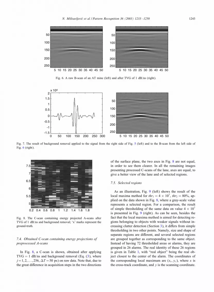
An example of a raw A-scan belonging to a target buriedat around 30 cm below the surface is given in the left sideof Fig. 5, where the x-axis is expressed in number of timesamples, so directly proportional to t. The position of the7rst maximum, around time-sample number 38, correspondsto the air/ground interface. The result of applying the TVGof 1 dB=ns is given on the right side of Fig. 5. This value ofTVG is our 7nal choice, based on the analysis of energiesof one object buried at di<erent depths, aimed to preserveapproximately the same energy regardless the depth. To givea more global illustration of inGuence of TVG on the data,a raw B-scan and the same scan after TVG are shown inFig. 6, in case of a deeper buried AT mine.
7.3. Results of background removal
The number of targets in our data as well as their separa-tion decrease the usefulness of the method to some extent,so some other, more sophisticated and complex methodsfor background removal would probably give better results.Nevertheless, we are looking for a realistic, simple, fastand automated method, and since it gives satisfactory re-sults, this method is accepted as our 7nal choice. A resultof sliding window mean background removal applied onthe A-scan from the right side of Fig. 5 is shown in Fig. 7(left), while the B-scan from the right side of Fig. 6 afterbackground removal is shown in Fig. 7 (right).
N. Milisavljevi!c et al. / Pattern Recognition 36 (2003) 1233–1250 1243
Fig. 6. A raw B-scan of an AT mine (left) and after TVG of 1 dB=ns (right).
Fig. 7. The result of background removal applied to the signal from the right side of Fig. 5 (left) and to the B-scan from the left side ofFig. 6 (right).
Fig. 8. The C-scan containing energy projected A-scans afterTVG of 1 dB=ns and background removal; ‘x’ marks represent theground-truth.
7.4. Obtained C-scan containing energy projections ofpreprocessed A-scans
In Fig. 8, a C-scan is shown, obtained after applyingTVG = 1 dB=ns and background removal (Eq. (3), wherej=1; 2; : : : ; 256, OT =50 ps) on raw data. Note that, due tothe great di<erence in acquisition steps in the two directions
of the surface plane, the two axes in Fig. 8 are not equal,in order to see them clearer. In all the remaining imagespresenting processed C-scans of the lane, axes are equal, togive a better view of the lane and of selected regions.
7.5. Selected regions
As an illustration, Fig. 9 (left) shows the result of thelocal maxima method for thr1 = 4 × 10⁷, thr2 = 80%, ap-plied on the data shown in Fig. 8, where a gray-scale valuerepresents a selected region. For a comparison, the resultof simple thresholding of the same data on value 4 × 10⁷
is presented in Fig. 9 (right). As can be seen, besides thefact that the local maxima method is aimed for detecting re-gions belonging to objects with weaker signals without in-creasing clutter detection (Section 3), it di<ers from simplethresholding in two other points. Namely, size and shape ofseparate regions are di<erent, and several selected regionsare grouped together as corresponding to the same object.Instead of having 72 thresholded areas or alarms, they aregrouped in 26 alarms. The real identity of these 26 regionsis given in Table 1, with “real object” being the real ob-ject closest to the center of the alarm. The coordinates ofthe corresponding local maximum are (xc; yc), where x isthe cross-track coordinate, and y is the scanning coordinate.

1244 N. Milisavljevi!c et al. / Pattern Recognition 36 (2003) 1233–1250
Fig. 9. Ground truth information (x) and the regions selected by: (a) left—the local maxima method applied to the data from the left sideof Fig. 8, for thr1 = 4× 10⁷, thr2 = 80%, window half-size 20 cm (in the cross-track direction) and 25 cm (in the scanning direction); (b)right—simply thresholding the data from the left side of Fig. 8, for the threshold level equal to 4× 10⁷.
Table 1The real identity of 26 selected regions
Region xc (m) yc (m) Real object Identity
1 1.85 7.1 Waterlevel tube F2 0.85 5.27 Iron fragment, 10 cm depth F3 1.85 5.59 Al can, 0 depth F4 1.45 6.89 NR24, with ring (metallic, small), 0 depth M5 1.45 4.8 M14 (low metal, small), 0 depth M6 0.55 7.36 Wooden AP (low metal, medium), 10 cm depth M7 1.85 6.18 Brick, 10 cm depth F8 0.55 5.95 PMN2 (metallic, medium), 10 cm depth M9 1.35 6.45 PMN (metallic, medium), 0 depth M10 0.45 6.42 PMN, 10 cm depth M11 1.55 5.68 NR24, no ring (no metal, small), 0 depth M12 0.95 7.08 PFM-1 butterGy (metallic, small), above the surface M13 1.35 5.93 PMN2, 0 depth M14 1.45 5.07 M14, 0 depth M15 1.05 4.89 Nothing F16 0.25 7.27 Nothing F17 0.65 4.93 M14, 10 cm depth M18 0.95 5.84 Iron fragment, 0 depth F19 0.25 7.53 Nothing F20 1.75 5.09 Iron fragment, above the surface F21 1.35 7.36 Wooden AP, 0 depth M22 0.35 4.81 Nothing F23 0.25 5.25 Nothing F24 0.55 7.1 NR24 with ring, 10 cm depth M25 1.75 4.72 Nothing F26 0.95 6.19 PFM-1 butterGy, 10 cm depth M

N. Milisavljevi!c et al. / Pattern Recognition 36 (2003) 1233–1250 1245
Table 2Measures extracted from the preprocessed C-scan after local max-ima detection (Fig. 9, left) and A-scans after TVG and backgroundremoval, for each of the selected regions from Table 1
Region ysize (cm) E(107) n1 (Sample no:) d1 (cm)
1 2.76 17.3 57 −5:72 17.48 14.6 49 −3:33 4.6 14.6 41 −0:94 3.68 13.4 32 05 10.12 12.3 29 06 3.68 12.2 58 −67 3.68 11.4 89 −15:38 3.68 11.2 71 −9:99 2.76 10.51 52 −4:2
10 3.68 9.41 77 −11:711 11.04 8.56 59 −6:312 2.76 8.48 30 013 2.76 7.81 32 014 16.56 7.51 30 015 21.16 7.44 46 −2:416 25.76 7.39 40 −0:617 3.68 0.23 71 −9:918 25.76 6.59 55 −5:119 2.76 5.70 41 −0:920 18.4 5.69 42 −1:221 3.68 5.67 47 −2:722 18.4 5.49 33 023 16.56 5.27 240 −60:624 12.88 5.13 32 025 14.72 4.67 48 −326 12.88 4.22 47 −2:7
Most of these regions contain objects, but some are simplyclutter. These alarms are the basis for the extraction, model-ing and combination of measures presented in the following.The regions are ordered by the values of their local max-ima, with the highest one on the top. Note that a depth of0 means that an object is buried just below the surface. Itcan be seen that the regions 5 and 14 possibly refer to thesame object, meaning that, although the chosen size of thewindow around the objects works satisfactory for most ofthe objects, in this case it was too small.
7.6. Extracted A- and C-scans measure
The three chosen measures, ysize, E and d1, correspondingto 26 selected regions, are given in Table 2. In our case:dref = 30 cm, nref = 138, nsurf = 38 (see Section 4).
7.7. Extracted measures from B-scans
Table 3 contains measures that are found from hyperbolaedetected in B-scans corresponding to each of 26 selectedregions. Here, X0 presents the x-coordinate of a B-scan, Y0 isfound from theC parameter of a detected hyperbola (through
Eqs. (9) and (13)), while d=k, v, D and D∗ are determinedas discussed in Section 5.2. Several important conclusionscan be made by analyzing Table 3. For example, comparingthe parameters of regions 5 and 14 (their xy-coordinatesas a 7rst indicator), it can be easily concluded that it is,actually, the same object split in two regions. Therefore,even if the arrangement of objects and their sizes are suchthat it makes it diIcult to determine the optimum size ofthe window for local maxima analysis, so that one object isdetected twice, these errors can be corrected at the momenteach of the regions is analyzed in more detail. It can befurther concluded that a similar e<ect would occur if thesize of the window is too large, so that at the beginning, oneselected region contains a few objects. In that case, a fewhyperbolae would be detected in the corresponding B-scan.
Another important piece of information can be obtainedby analyzing results for the propagation velocities, v. Forsandy soils, v ranges typically from 5:5 × 10⁷ to 1:73 ×108 m=s [12]. Using the information about the true identityof objects in each of the regions given in Table 1, it canbe seen that in case of buried objects, v has indeed valueswithin the given range, while for surface-laid objects, it isclose to c. Note also that in cases of false alarms, v oftenreaches unreasonable values, sometimes even higher thanin free space. This is a good indicator that there is reallynothing in that region, and that the obtained hyperbola iscaused by some artifacts or simply clutter.
Finally, the measure d=k also shows that there is a range ofvalues that describes most objects, and that extreme valuesmainly belong to background.
7.8. Combination of A-scan and preprocessed C-scanmeasures
Once masses are assigned for each of the measures givenin Table 2, they are combined either immediately or afterbeing discounted (See Sections 6.3 and 6.4). The results aregiven in Table 4. False alarms are written in italic.
Observing the part concerning non-discounted masses,and taking into account real identities of the objects(Table 1), it can be seen that clutter is mainly discarded(except in two cases: regions 19 and 25). Furthermore, forseveral mines (regions 6, 7, 11, 21, as the most criticalones) the masses assigned to friends and to the full set arevery close, meaning that, although correctly classi7ed here,in case of slight changes in the model, they could be easilymisclassi7ed. If the discounting is included, it means thatsome part of the mass initially assigned to friends goes tothe full set, so the sensitivity of some masses is decreased.However, some non-dangerous objects, the two masses ofwhich are close to each other and that are well classi7edwithout discounting, can also become potential mines (suchas regions 20 and 22). The danger of this type of misclassi-7cation is in slowing down the mine removal process, sincethe non-dangerous objects will have to be removed too.However, this is much less important than the danger of

1246 N. Milisavljevi!c et al. / Pattern Recognition 36 (2003) 1233–1250
Table 3Measures extracted from the preprocessed B-scans after hyperbola detection, for each of the selected regions from Table 1
Region X0 (m) Y0 (m) D∗ (cm) (d=k)[(y-dir: sample no:)2] v(108 m=s) D (cm)
1 1.85 7.1 −4:5 486 1.48 −5:542 0.85 5.29 −2:4 363 1.53 −3:073 1.85 5.62 0 244 1.53 04 1.45 6.95 0 768 2.95 25.615 1.45 5.02 0 548 3.13 21.66 0.55 7.35 −6:3 471 1.44 −6:447 1.85 6.17 −13:8 586 10.6 −12:38 0.55 5.96 −6 556 1.51 −7:59 1.35 6.46 −2:7 371 1.5 −3:54
10 0.45 6.44 −10:8 542 1.17 −10:4411 1.55 5.75 −0:6 265 1.51 −0:7512 0.95 7.09 0 469 2.52 20.0313 1.35 5.95 −2:4 393 1.6 −3:1714 1.45 5.03 0 562 3.15 21.9115 1.05 5.07 −0:6 1245 3.26 −1:6316 0.25 7.18 0 1099 4.37 30.717 0.65 4.95 −9:3 839 1.55 −12:0718 0.95 5.85 −5:4 730 1.78 −7:919 0.25 7.4 0 1285 3.8 33.2120 1.75 5.09 0 493 3.04 20.5521 1.35 7.37 0 575 2.79 22.1522 0.35 4.79 0 178 1.59 12.3323 0.25 5.13 −15:9 15 0.16 −2:0924 0.55 6.91 −7:5 645 1.49 −9:3225 1.75 4.69 0 1407 4.48 34.6926 0.95 6.16 −8:1 362 1.08 −7:3
the opposite situation, where some mines are not removedbecause they are classi7ed as non-dangerous objects. There-fore, when the chosen measures do not distinguish wellbetween mines and friends, the safest way is to apply dis-counting, and by that increase con7dence in the 7nal guess(although possibly slightly increasing the number of falsealarms).
In the discounted case, note that 5 of 12 non-dangerousobjects are still discarded, which is a good improvementwhen compared with the starting situation, meaning thatwithout further analysis of the regions, all 26 regions wouldbe treated as dangerous. Also, it can be seen that the strongestdiscounting occurs in the case of region 23, due to the factthat the extracted depth was around −60 cm.
Finally, it must be repeated that there is no rejection ofmines. Although our goal is to decrease both number of falserejections and of false alarms, it must not be forgotten that,taking into account the problemwe are dealing with, false re-jections have an incomparably higher importance than falsealarms.
Note that discounting parameters s and b are not included.It can be expected that these already good results can befurther improved once the deminer’s knowledge and expe-rience is included in the reasoning process. It is out of thescope of this paper to discuss the way the deminer would
reason for each detected region, since that process can bequite subjective.
7.9. Combination of B-scan (hyperbolae) measures
After assigning masses to measures extracted from de-tected hyperbolae (Table 3), they are combined in two ways,without being discounted and after discounting. Masses af-ter their combination are given in Table 5, together with 7rstguesses on object identities. As can be seen, discountingdoes not have any inGuence on the 7nal guesses this time,indicating that we can be more con7dent in obtained results,i.e. that chosen measures and their models are well-suitedfor the data and robust. Also, looking back to the real iden-tities of the regions, shown in Table 1, it can be seen thatall the alarms corresponding to background are classi7ed asnon-dangerous (regions 15, 16, 19, 22, 23, 25), and, in ad-dition, with a high con7dence in most of the cases.
On the other hand, from the placed false alarms, onlyone of them is well classi7ed (region 3, aluminum can),but this result is a direct consequence of the fact that thismethod actually detects whether there is an object, regardlesswhether it is a mine or not.
Nevertheless, it has to be pointed out that this method isvery promising for several reasons. Namely, clutter, which

N. Milisavljevi!c et al. / Pattern Recognition 36 (2003) 1233–1250 1247
Table 4Resulting masses after combination of masses assigned by chosen A-scan and C-scan measures, without and with discounting, for each ofthe selected regions from Table 1; values of discounting parameters are also given
Region No discounting g With discounting
m(F) m(*G) Guess m(F) m(*G) Guess
1 0.78 0.22 F 0.98 0.77 0.23 F2 0.62 0.38 F 0.91 0.58 0.42 F3 0.52 0.48 F 0.71 0.39 0.61 M4 0.48 0.52 M 0.6 0.31 0.69 M5 0.18 0.82 M 0.6 0.11 0.89 M6 0.41 0.59 M 0.99 0.4 0.6 M7 0.46 0.54 M 0.8 0.4 0.6 M8 0.37 0.63 M 0.96 0.36 0.64 M9 0.39 0.61 M 0.95 0.37 0.63 M10 0.35 0.65 M 0.91 0.32 0.68 M11 0.05 0.95 M 1 0.05 0.95 M12 0.38 0.62 M 0.6 0.23 0.77 M13 0.39 0.61 M 0.6 0.24 0.76 M14 0.34 0.66 M 0.6 0.21 0.79 M15 0.67 0.33 F 0.85 0.57 0.43 F16 0.88 0.12 F 0.68 0.61 0.39 F17 0.36 0.64 M 0.96 0.34 0.66 M18 0.89 0.11 F 0.97 0.87 0.13 F19 0.47 0.53 M 0.71 0.35 0.65 M20 0.54 0.46 F 0.75 0.42 0.58 M21 0.41 0.59 M 0.87 0.36 0.64 M22 0.55 0.45 F 0.6 0.35 0.65 M23 1 1.1e-4 F 0.03 0.01 0.99 M24 0.28 0.72 M 0.6 0.18 0.82 M25 0.39 0.61 M 0.89 0.36 0.64 M26 0.36 0.64 M 0.87 0.32 0.68 M
is typically the most signi7cant cause of false alarms in caseof GPR, is almost completely discarded here. In addition,slight modi7cations of the way measures are modeled andinclusion or not of the discounting factors do not a<ect 7nalresults, meaning that the chosen measures and models allowfor a good and reliable discrimination. Finally, there are nofalse rejections.
Table 6 summarizes all results discussed here and in theprevious subsection.
The results obtained by this method and by a votingmethod are compared in Ref. [29] on a part of the data usedhere. In that paper, we both analyzed performance of eachof the sensors as well as combined the following three sen-sors: infrared camera, metal detector, and GPR. RegardingGPR results using belief functions, we analyzed only resultsobtained by B-scan measures. For this sensor, both methodsclassi7ed well all mines (12 of them). The real power ofbelief functions was seen in case of clutter-caused alarms,where 6 out of 7 were correctly classi7ed (so rejected) bybelief functions, while all 7 were misclassi7ed (so becamefalse alarms) using voting. The conclusion was that withoutadditional knowledge, which is the case of voting, all alarms
are treated as mines, leading to a high false alarm rate, whilein the belief function framework, knowledge helps in de-creasing the false alarm rate without decreasing the resultof mine detection.
7.10. Combination of A-, B- and C-scans measures
Finally, we address the combination of A-, B- and C-scanmeasures, which may appear as a promising solution. Firstly,it should be noted that it cannot be done straightforward, dueto some dependencies between measures (such as two burialdepth measures, one per set). Therefore, we performed pre-liminary tests on combination by excluding one of the twoburial depth measures. These tests show that there is no sig-ni7cant improvement in the 7nal results. The combinationof all measures is therefore not useful. Moreover, it is highlyquestionable how realistic this way would be in humanitar-ian mine detection context, due to the di<erent types of pro-cessing that each of them requests. A potential solution, thatwill be analyzed in detail in our future work, is in 7ndingways for selecting a subset of the two sets containing mostdiscriminant and cognitively independent measures.

1248 N. Milisavljevi!c et al. / Pattern Recognition 36 (2003) 1233–1250
Table 5Resulting masses after combination of masses assigned by chosen B-scan measures, without and with discounting, for each of the selectedregions from Table 1; values of discounting parameters are also given
Region No discounting g With discounting
m(F) m(*G) Guess m(F) m(*G) Guess
1 0.14 0.86 M 0.96 0.14 0.86 M2 0.3 0.7 M 0.85 0.25 0.75 M3 0.94 0.06 F 0.6 0.65 0.35 F4 0.07 0.93 M 0.6 0.04 0.96 M5 0.12 0.88 M 0.6 0.07 0.93 M6 0.15 0.85 M 0.99 0.14 0.86 M7 0.2 0.8 M 0.85 0.17 0.83 M8 0.11 0.89 M 0.99 0.11 0.89 M9 0.28 0.72 M 0.87 0.24 0.76 M10 0.12 0.88 M 0.94 0.11 0.89 M11 0.42 0.58 M 0.68 0.29 0.71 M12 0.26 0.74 M 0.6 0.16 0.84 M13 0.29 0.71 M 0.85 0.25 0.75 M14 0.12 0.88 M 0.6 0.07 0.93 M15 0.99 0.01 F 0.68 0.82 0.18 F16 0.96 0.04 F 0.6 0.68 0.32 F17 0.21 0.79 M 0.98 0.21 0.79 M18 0.28 0.72 M 0.98 0.27 0.73 M19 0.89 0.11 F 0.6 0.65 0.35 F20 0.12 0.88 M 0.6 0.07 0.93 M21 0.06 0.94 M 0.6 0.04 0.96 M22 0.94 0.06 F 0.6 0.67 0.33 F23 0.95 0.05 F 0.77 0.85 0.15 F24 0.08 0.92 M 0.99 0.08 0.92 M25 0.99 0.01 F 0.6 0.79 0.21 F26 0.3 0.7 M 0.99 0.3 0.7 M
Table 6Number of correct and wrong classi7cations over total number of mines (14) or friendly objects (6 placed and 6 clutter-caused), per analyzedset of measures, with or without discounting
A- and C-scans measure B-scan measure
No disc. With disc. No disc. With disc.
Mine detection 14/14 14/14 14/14 14/14Mine rejection 0/14 0/14 0/14 0/14Correctly recognized placed F 5/6 3/6 1/6 1/6Placed F recognized as a mine 1/6 3/6 5/6 5/6Correctly recognized clutter-caused F 4/6 2/6 6/6 6/6Clutter-caused F recognized as a mine 2/6 4/6 0/6 0/6
8. Conclusion
In this paper, we investigate a method based on GPR datafor humanitarian mine detection. This study is motivated bythe fact that GPR has very useful features for this type ofapplication. In particular, it is able to provide 3D informa-tion about the subsurface structure, in contrary to most othersensors. The diIculty of interpreting GPR data calls for
speci7c processing relying on the speci7cities of the sensorcharacteristics. Our contribution in this direction is twofold.Firstly, we develop tools for processing A- and C-scans, forextracting useful measures from local maxima, and for de-tection and measuring hyperbolas in B-scans. Secondly, wepropose an appropriate model of the extracted measures interms of belief functions and discounting factors, which in-cludes knowledge about the sensor and the context of the ap-

N. Milisavljevi!c et al. / Pattern Recognition 36 (2003) 1233–1250 1249
plication. The fusion of these measures leads to informationon the presence of a friendly object or of any (undi<erenti-ated) object. We derive a decision rule adapted to this resultand to the constraint of the application (no mine should bemissed).
Normally, after selecting suspicious regions, the processof detection is 7nished and the mine removal operationsbegin. Still, both in general as well as in our case, a lot ofnon-dangerous objects and clutter are selected as well, whichmeans that the removal proceeds slowly. To deal with that,we propose a way for further analysis of suspected regionsthrough choosing discriminative measures, their modelingand combination in terms of belief functions within the DSframework. Two sets of measures are separately analyzed,one extracted from preprocessed A-scans and a C-scan onwhich regions are selected, and the other extracted fromhyperbolae detected on preprocessed B-scans correspondingto the selected regions. For each of these measures, massesare modeled and assigned either to friendly objects or to thefull set, i.e. both mines and friendly objects, due to the factthat GPR, as well as a great majority of other mine detectionsensors, is not aimed for mine but for anomaly detection.
Reasons for eventual discounting of measures before theircombination are also discussed here, and assigned massesare combined both without being discounted as well as af-ter discounting. It is shown that in cases when the measuresdo not give a good discrimination between friendly objectsand the full set, it is safer (taking into account the extremedanger in misclassifying mines) to make 7nal guesses aboutthe true object identity based on results of combining dis-counted masses. Here, such situations correspond to the caseof combining A- and C-scans measures. On the other hand,B-scan measures extracted from detected hyperbolae show agreat potential in discarding alarms caused by clutter, whichis often the largest problem for GPR. Also, these measuresdiscriminate well between friendly objects and the full set,so there is no need for further discounting. Both sets ofmeasures have a 100% of detection of mines. Note that theanalyzed data set contains 14 mines, all of them are small,most have little metal, and some have no metal at all.
A careful analysis and choice of most selective and in-dependent measures from the two sets together, taking intoaccount the processing aspect, could be a good solution forfurther improvements of the results, and it will certainly bedone in future.
The methodology presented here can be applied to othermine detection sensors (where only the choice of measuresand their modeling would be di<erent, i.e. would be a func-tion of the operational principles) and their fusion, as shownin Ref. [29]. In addition, various steps of the methodologycan be useful themselves, such as A-, B- and C-scans pro-cessing, which can be useful to various other areas of GPRapplication besides mine detection, where visualization ofa shallow subsurface using close-range GPR data is impor-tant, such as road inspection. Finally, the proposed regionselection method can provide an important improvement in
fastening any detection process, where a coarser acquisitionstep could be used for an initial observation of a whole ter-rain, to which the region selection can be applied, and thena 7ner acquisition step can be applied only to the selectedregions. This method can be used for other sensors (such asmetal detector or infrared camera) and for other applicationsthat involve terrain inspection than mine detection.
Acknowledgements
We are thankful to the TNO Physics and Electronics Lab-oratory for giving us the permission and great opportunityto work on the data gathered on their test facilities withinthe Dutch HOM-2000 project. Also, we thank Bart Scheersfrom the Royal Military Academy for useful comments andsuggestions.
References
[1] C.E. Baum (Ed.), Detection and Identi7cation of VisuallyObscured Targets. Taylor & Francis, Philadelphia, USA, 1999.
[2] J.D. Young, L. Peters Jr., A brief history of GPR fundamentalsand applications, in: Proceedings of Sixth InternationalConference on Ground Penetrating Radar (GPR’96), Sendai,Japan, 1996, pp. 5–14.
[3] B. Scheers, Ultra-wideband ground penetrating radar, withapplication to the detection of anti personnel landmines, Ph.D.Thesis, Universit(e Catholique de Louvain, Louvain-La-Neuve,Belgium, 2001.
[4] G.R. Olhoeft, Application of ground penetrating radar, in:Proceedings of Sixth International Conference on GroundPenetrating Radar (GPR’96), Sendai, Japan, 1996, pp. 1–3.
[5] D.J. Daniels, Surface-Penetrating Radar, The Institution ofElectrical Engineers, London, UK, 1996.
[6] K.B. Jakobsen, H.B.D. Sorensen, O. Nymann, Stepped-frequency ground-penetrating radar for detection of smallnon-metallic buried objects, in: Proceedings of SPIEConference on Detection Technologies for Mines andMinelike Targets, Vol. 3079, Orlando, USA, 1997, pp. 538–542.
[7] G.D. Sower, S.P. Cave, Detection and identi7cation of minesfrom natural magnetic and electromagnetic resonances, in:Proceedings of SPIE Conference on Detection Technologiesfor Mines and Minelike Targets, Vol. 2496, Orlando, USA,1995, pp. 1015–1024.
[8] D.J. Daniels, Ground probing radar techniques for minedetection, in: Proceedings of Seventh International Conferenceon Ground Penetrating Radar (GPR’98), Vol. 1, Lawrence,Kansas, USA, 1998, pp. 319–323.
[9] L. van Kempen, H. Sahli, Ground penetrating radar dataprocessing: a selective survey of the state of the art literature,Technical Report IRIS-TR-0060, Vrije Universiteit Brussel,Brussels, Belgium, 1999.
[10] T.R. Witten, Present state-of-the-art in ground penetratingradars for mine detection, in: Proceedings of SPIE Conferenceon Detection Technologies for Mines and Minelike Targets,Vol. 3392, Orlando, USA, 1998, pp. 576–585.

1250 N. Milisavljevi!c et al. / Pattern Recognition 36 (2003) 1233–1250
[11] N. Milisavljevi(c, M. Acheroy, Overview of mine detectionsensors and ideas for their estimation and fusion in the scopeof HUDEM project, in: Proceedings of Australian–AmericanJoint Conference on the Technologies of Mines and MineCountermeasures, Sydney, Australia, 1999.
[12] L. Capineri, P. Grande, J.A.G. Temple, Advancedimage-processing technique for real-time interpretation ofground penetrating radar images, Int. J. Imaging SystemsTechnol. 9 (1998) 51–59.
[13] G. Shafer, A Mathematical Theory of Evidence, PrincetonUniversity Press, Princeton, NJ, 1976.
[14] P. Smets, What is Dempster–Shafer’s model? in: R.R. Yager,M. Fedrizzi, J. Kacprzyk (Eds.), Advances in the Dempster–Shafer Theory of Evidence,Wiley, NewYork, 1994, pp. 5–34.
[15] P. Smets, R. Kennes, The transferable belief model, Artif.Intell. 66 (1994) 191–234.
[16] W. de Jong, H.A. Lensen, Y.H.L. Janssen, Sophisticatedtest facility to detect landmines, in: Proceedings of SPIEConference on Detection Technologies for Mines andMinelike Targets, Vol. 3710, Orlando, USA, 1999, pp.1409–1418.
[17] N. Milisavljevi(c, Analysis and fusion using belief functiontheory of multisensor data for close-range humanitarian minedetection, Ph.D. Thesis, (Ecole Nationale Sup(erieure desT(el(ecommunications, Paris, France, 2001.
[18] M.G.J. Breuers, P.B.W. Schwering, S.P. van den Broek,Sensor fusion algorithms for the detection of land mines, in:Proceedings of SPIE Conference on Detection Technologiesfor Mines and Minelike Targets, Vol. 3710, Orlando, USA,1999, pp. 1160–1166.
[19] G.R. Olhoeft, Electrical, magnetic and geometric propertiesthat determine ground penetrating radar performance, in:Proceedings of Seventh International Conference on GroundPenetrating Radar (GPR’98), Vol. 1, Lawrence, Kansas, USA,1998, pp. 177–182.
[20] V.F. Leavers, Shape Detection in Computer Vision Using theHough Transform, Springer, London, 1992.
[21] L. Xu, Randomized Hough transform (RHT): basicmechanisms, algorithms, and computational complexities,CVGIP: Image Understanding 57 (2) (1993) 131–154.
[22] N. Milisavljevi(c, I. Bloch, M. Acheroy, Application of therandomized Hough transform to humanitarian mine detection,in: Proceedings of the Seventh IASTED InternationalConference on Signal and Image Processing (SIP2001),Honolulu, Hawaii, USA, 2001, pp. 149–154.
[23] R.A. McLaughlin, Randomized Hough transform: improvedellipse detection with comparison, Technical Report TR97-01,The University of Western Australia, CIIPS, 1997.
[24] N. Milisavljevi(c, Comparison of three methods for shaperecognition in the case of mine detection, Pattern RecognitionLett. 20 (11–13) (1999) 1079–1083.
[25] N. Milisavljevi(c, I. Bloch, M. Acheroy, A 7rst steptowards modeling and combining mine detection sensorswithin Dempster–Shafer framework, in: Proceedings of2000 International Conference on Arti7cial Intelligence(IC-AI’2000), Vol. II, Las Vegas, USA, 2000, pp. 745–751.
[26] N. Milisavljevi(c, I. Bloch, M. Acheroy, Characterization ofmine detection sensors in terms of belief functions and theirfusion, 7rst results, in: Proceedings of the Third InternationalConference on Information Fusion (FUSION 2000), Vol. II,Paris, France, 2000, pp. ThC3.15–ThC3.22.
[27] D. Dubois, M. Grabisch, H. Prade, P. Smets, Assessing thevalue of a candidate, in: 15th Conference on Uncertainty inArti7cial Intelligence (UAI’99), Stockholm, Sweden, MorganKaufmann, San Francisco, 1999, pp. 170–177.
[28] P. Smets, Belief functions: the disjunctive rule of combinationand the generalized Bayesian theorem, Int. J. Approx.Reasoning (9) (1993) 1–35.
[29] N. Milisavljevi(c, S.P. van den Broek, I. Bloch, P.B.W.Schwering, H.A. Lensen, M. Acheroy, Comparison of belieffunctions and voting method for fusion of mine detectionsensors, Proceedings of SPIE Conference on Detection andRemediation Technologies for Mines and Minelike TargetsVI, Vol. 4394, 2001, pp. 1011–1022.
About the Author—NADAMILISAVLJEVI (C is a researcher at the Signal and Image Centre of the RMA. She graduated from the Universityof Novi Sad, Yugoslavia, in Electrical Engineering (Electronics and Telecommunications) in 1992. She received the M.Sc. degree in OpticalElectronics and Laser Technics from the University of Belgrade, Yugoslavia, in 1996, and her Ph.D. degree from ENST in Paris, France,in 2001. Her current research interests include data fusion, evidence theory, humanitarian mine detection and pattern recognition.
About the Author—ISABELLE BLOCH is a professor at ENST (Signal and Image Processing Department). She graduated from Ecoledes Mines de Paris in 1986, received Ph.D from ENST Paris in 1990, and the “Habilitation Diriger des Recherches” from University Paris 5in 1995. Her research interests include 3D image and object processing, 3D and fuzzy mathematical morphology, discrete 3D geometry andtopology, decision theory, information fusion in image processing, fuzzy set theory, evidence theory, structural pattern recognition, spatialreasoning, medical imaging.
About the Author—SEBASTIAANVANDEN BROEK received his Ph.D. in physics in 1997 at the University of Twente (The Netherlands),where he did work on numerical modeling of electromagnetic activity in the human brain. Since 1998 he works as a researcher at TNOPhysics and Electronics Laboratory in the 7eld of electro-optics. His research interests are in image processing, sensor fusion and automatictarget detection and tracking.
About the Author—MARC ACHEROY is an ordinary professor at the Faculty of Applied Sciences of the RMA in Brussels, Belgium, andfounder and director of the Signal and Image Centre of the RMA. He received his degree of civil engineering in mechanics and transportfrom the RMA, the degree of civil engineering in control and automation (in 1981) and his Ph.D. degree in Applied Sciences (in 1983) fromthe Universit(e libre de Bruxelles. His main research interests include pattern recognition, humanitarian demining, and image restoration andcompression.


