This article was downloaded by: [Kwang Bin Bae]On: 27 March 2015, At: 18:29Publisher: RoutledgeInforma Ltd Registered in England and Wales Registered Number: 1072954Registered office: Mortimer House, 37-41 Mortimer Street, London W1T 3JH,UK

Click for updates

Local Government StudiesPublication details, including instructions for authorsand subscription information:http://www.tandfonline.com/loi/flgs20

Income Inequality andRedistributive Spending:Evidence from Panel Data ofTexas CountiesKwang Bin Baea

a School of Economic, Political and Policy Sciences,University of Texas at Dallas, Dallas, TX, USAPublished online: 25 Mar 2015.

To cite this article: Kwang Bin Bae (2015): Income Inequality and RedistributiveSpending: Evidence from Panel Data of Texas Counties, Local Government Studies, DOI:10.1080/03003930.2015.1020373

To link to this article: http://dx.doi.org/10.1080/03003930.2015.1020373

PLEASE SCROLL DOWN FOR ARTICLE

Taylor & Francis makes every effort to ensure the accuracy of all theinformation (the “Content”) contained in the publications on our platform.However, Taylor & Francis, our agents, and our licensors make norepresentations or warranties whatsoever as to the accuracy, completeness, orsuitability for any purpose of the Content. Any opinions and views expressedin this publication are the opinions and views of the authors, and are not theviews of or endorsed by Taylor & Francis. The accuracy of the Content shouldnot be relied upon and should be independently verified with primary sourcesof information. Taylor and Francis shall not be liable for any losses, actions,claims, proceedings, demands, costs, expenses, damages, and other liabilitieswhatsoever or howsoever caused arising directly or indirectly in connectionwith, in relation to or arising out of the use of the Content.

This article may be used for research, teaching, and private study purposes.Any substantial or systematic reproduction, redistribution, reselling, loan, sub-licensing, systematic supply, or distribution in any form to anyone is expresslyforbidden. Terms & Conditions of access and use can be found at http://www.tandfonline.com/page/terms-and-conditions

Dow

nloa

ded

by [

Kw

ang

Bin

Bae

] at

18:

29 2

7 M

arch

201

5

Income Inequality and RedistributiveSpending: Evidence from Panel Dataof Texas Counties

KWANG BIN BAESchool of Economic, Political and Policy Sciences, University of Texas at Dallas, Dallas, TX, USA

ABSTRACT The relationship between redistributive spending and income inequality hasbeen of interest to researchers for several decades. Existing literature has largely focusedon country-level studies and may be broadly divided into two groups: studies that find apositive relationship between the two and studies that find a negative relationship. Thepositive association is usually explained through the median voter theory and the negativeassociation through the social insurance theory.This study offers a test of the median voter and social insurance hypotheses by

examining the relationship between economic inequality, voter turnout and redistributivespending at the sub-national level among the 50 largest counties in Texas over years 2006to 2012. One of the advantages of using a regional sample is that counties are relativelymore homogeneous and allow for the collection of better records across time. Randomeffects models suggest that income inequality is positively associated with redistributivespending. The study improves our understanding of the patterns of redistribution at thesub-national level and highlights the importance of careful inter-temporal modelling ofrelationships between redistributive spending and inequality.

KEY WORDS: Income inequality, voter turnout, redistributive spending, median votertheory, social insurance theory

Introduction

Over the past few decades, the US government has increased spending onwelfare programmes and other categories of social support. At the same time,national income inequality and poverty rate have also gone up.1 This positiveassociation may be interpreted in a variety of perspectives. For example, it maybe viewed as a sign of ineffectiveness of government spending in alleviatingpoverty and inequality, or it may be viewed as a feature of a healthy democraticstate, where the levels of public spending reflect preferences of the majority, inthis case, a growing majority of citizens with lower income who favour redis-tribution. This study tests two orthogonal theories developed by political

Correspondence Address: Mr Kwang Bin Bae, School of Economic, Political and Policy Sciences,University of Texas at Dallas, Dallas, TX 75252, USA. E-mail: kxb124730@utdallas.edu

Local Government Studies, 2015http://dx.doi.org/10.1080/03003930.2015.1020373

© 2015 Taylor & Francis

Dow

nloa

ded

by [

Kw

ang

Bin

Bae

] at

18:

29 2

7 M

arch

201

5

economists to explain the relationship between public assistance expendituresand inequality: the median voter theory, which accounts for a positive associationbetween redistributive spending and inequality, and the social insurance theory,which predicts a negative relationship between the two. This study also examinesthe relationship between turnout and redistributive expenditures.

This study offers a test of these theories using longitudinal sub-national data inthe United States, which sets this study apart from the majority of existing workthat generally make cross-country and cross-sectional comparisons. Althoughthere have been a number of studies that examine the relationship betweeninequality and redistribution, most research has relied on cross-sectional(Finseraas 2009) or year average data (Moene and Wallerstein 2001;Schwabish et al. 2003; De Mello and Tiongson 2006; Kenworthy andMcCall 2008). A few exceptions are studies which have analysed the relationshipbetween inequality and social expenditure across a 30-year period(Milanovic 2000; Mohl and Pamp 2009). This study uses a panel data set offinancial, economic and socio-demographic records to test the relationshipbetween inequality and redistributive expenditures.

Further, I offer a test of the median voter theory using data on Texas counties.Previous studies have analysed the relationship between inequality and redis-tribution spending using data from the OECD (Lindert 1996; Milanovic 2000;Moene and Wallerstein 2001; Schwabish et al. 2003; Kenworthy andMcCall 2008; Mohl and Pamp 2009), European countries (Finseraas 2009) andother countries (FiGini 1998; Bassett, Burkett, and Putterman 1999;Tanninen 1999; De Mello and Tiongson 2006). Since each country uses itsown currency and has a different method of measuring redistribution, compar-ison among nations is unfeasible. Inequality can also vary according to acountry’s economic development and political system. A few studies haveanalysed the relationship between redistribution and inequality using US statepanel data (Gouveia and Masia 1998) and US state average data(Rodrigiuez 1999, Panizza 2002). This study is the first research to examinethe effect of inequality to redistribution spending with county-level data. Theadvantage of regional analysis is that regional samples tend to be more homo-geneous and comparable than those of countries because data are sampled from apopulation that shares more common characteristics. Regional data can alsoexamine the causal effect of income inequality on redistributive spending bycontrolling variables such as regulations and policies that are difficult to quantifyand compare across countries (Barro et al. 1991).

The article is organised as follows. I start with reviewing existing theoreticalmodels that explain the relationship between public assistance spending andincome inequality. Next, I will formulate the hypotheses and discuss the expecta-tions in the model tested on sub-national data. I will then describe the data foranalysis and present the models. In Results, I will overview the findings.Conclusion summarises the findings and highlights directions for future researchon redistributive spending and income inequality at the sub-national level.

2 K.B. Bae

Dow

nloa

ded

by [

Kw

ang

Bin

Bae

] at

18:

29 2

7 M

arch

201

5

Inequality and redistributive policy

Previous studies have conflicting perspectives on the effects of income inequalityon redistributive spending. Several studies state that income inequality leads toan increase in redistribution (Meltzer and Richard 1981; Bassett, Burkett, andPutterman 1999). A theoretical model that supports the positive effect of incomeinequality on social expenditure is based on the median voter theory (Meltzerand Richard 1981). The theory was developed by A. Downs in 1957 to analyseelectoral competition (Downs 1957). Downs showed that under a set of assump-tions – primarily unidimensional voting and single-peaked voter preferences –policies or party platforms that win elections reflect policy preferences of themedian voter. Meltzer and Richard (1981) popularised the median voter theory asan explanation of income redistribution through fiscal policy. This theoryassumes that individuals are rational actors who maximise their utility and voteto maximise their predicted income. Income distribution in a modern economy isgenerally skewed to the right, with a relatively small number of earners at the tophaving very high incomes. As a result, the median income of a country is usuallybelow the mean (Larcinese 2007). When the median voter’s income is below themean, the median voter will favour redistribution and higher taxes because thiswill increase income after redistributive policies are in place. The median votertheory predicts that an increasing gap between the median and mean income willlead to a rise in redistributive spending because the median voter will benefitfrom redistribution and because government spending will follow the voter’spreference.

Easterly and Rebelo (1993) examined the median voter theory using anaverage of cross-county data from 1970 to 1988 and found a positive associationbetween income inequality and social expenditure. Milanovic (2000) alsoreached a conclusion supporting the median voter theory, which states that socialexpenditure increases as inequality increases, using the Luxembourg IncomeStudy time series data. The research questioned whether the middle classwould receive benefits from government transfer eventually, if not immediately.Using inequality resources, the study verified that social expenditure increasesalong with inequality. Similar positive results were derived from Alesina andRodrik (1994) and Persson and Tabellini (1994).

Sharp and Maynard-Moody (1991) also explained the relationship betweeninequality and redistributive spending in local governments. They mentioned thatredistributive expenditure is greater in higher poverty communities with the needresponsiveness model. According to this model, social problems such as povertyand income inequality lead to local government responses through redistributivespending. Empirical studies, however, have showed mixed results. Chamlin(1987) and Pack (1998) found a positive relationship between the two, whileIsaac and Kelly (1981) and Sharp and Maynard-Moody (1991) did not find anyrelationship.

In contrast, others studies have suggested that income inequality has anegative association with redistributive spending (Milanovic 2000; Moene

Evidence from Panel Data of Texas Counties 3

Dow

nloa

ded

by [

Kw

ang

Bin

Bae

] at

18:

29 2

7 M

arch

201

5

and Wallerstein 2001; De Mello and Tiongson 2006). This relationship isgenerally interpreted in light of the social insurance theory (Moene andWallerstein 2001; Bradley et al. 2003; Cantillon, Marx, and Bosch 2002).The median voter theory assumes that individuals are rational actors whomaximise their utility. Social insurance theory, however, have pointed out thebounds of rationality. Moene and Wallerstein (2001) stated that welfareexpenditures are not only redistributive but also provide insurance againstincome loss. They argued that by increasing income, the demand for insur-ance rises while the demand for redistribution decreases. When a medianvoter’s income decreases, the demand for insurance decreases, whereas thedesire for redistribution increases. Higher inequality in pre-tax earnings isrelated to lower levels of spending on policies. According to the socialinsurance theory, a welfare policy is a public supply of social insurance; avoter will support a welfare policy that protects against the risk of privateinsurance failure (Moene and Wallerstein 2001). If insurance is a normalgood with other conditions equal, demand will be reduced because of adecrease in income resulting from an increase in income inequality. Adecrease in insurance demand will eventually lead to a decrease in socialexpenditure because the model assumes social expenditure as a public supplyof insurance.

The studies which support social insurance theory have examined a negativerelationship between income inequality and social expenditure (Moene andWallerstein 2001; Cantillon, Marx, and Bosch 2002; Bradley et al. 2003).Bassett, Burkett, and Putterman (1999) questioned the relationship betweeninequality and government transfer; their findings verified that they are, in fact,negatively related. Moene and Wallerstein (2001) and Bradley et al. (2003) alsoconcluded that these two variables have a significant negative relationship. DeMello and Tiongson (2006) were interested in comparing social expenditures ofunequal versus equal societies. Using cross-country data, they found that socie-ties with low inequality have greater social expenditure using the ordinary leastsquare and Tobit models. Cantillon, Marx, and Bosch (2002) found a strongnegative relationship between social expenditure and poverty and verified thatincidences of inequality decreases when social expenditure increases. Existingresearch has shown mixed results on the association between income inequalityand social expenditure.

Schneider (1987) examined the negative relationship between income inequal-ity and redistributive spending at the city level. He wrote ‘in heterogeneouscommunities, better-off residents will resist social welfare commitments becausesuch programmes visibly transfer wealth from one segment of the community toanother’ (Schneider 1987, 40). According to Schneider (1987), a high level ofinequality implies a high level of heterogeneity, and this condition leads to alower level of redistributive spending.

Table 1 summarises the main findings and samples of different empiricalstudies.

4 K.B. Bae

Dow

nloa

ded

by [

Kw

ang

Bin

Bae

] at

18:

29 2

7 M

arch

201

5

Tab

le1.

Sum

maryof

previous

literature

Inequalityandredistributio

n

Authors

Sam

ple

Period

Datastructure

Correlatio

nSignificance

Meltzer

andRichard

(198

1)USaverage

1937–197

7Tim

eseries

Positive

Significant

Lindert(199

6)14

OECD

countries

1962–198

1Panel

Negative

Generally

insignificant

FiGini(199

8)Upto

63coun

tries

1970–1990

Cross-country

average

Nonlin

ear

Significant

Gou

veia

andMasia

(199

8)50

USstates

1979–199

1Panel

Generally

negativ

eGenerally

sign

ificant

Bassett,

Burkett,

andPutterm

an(199

9)Upto

54coun

tries

1970–1985

Cross-country

average

Generally

negativ

eInconsistent

Rod

rigiuez(199

9)50

USstates

1984–1994

Tim

eseries

andcross-stateaverage

Inconsistent

Inconsistent

Tanninen

(199

9)Upto

45coun

tries

1970–1988

Cross-country

average

Inconsistent

Significant

Milano

vic(200

0)24

mostly

OECD

coun

tries

1967–199

7Panel

Positive

Significant

Moene

andWallerstein

(200

1)18

mostly

OECD

coun

tries

1980–1995

Cross-country

average

Negative

Significant

Panizza

(200

2)46

USstates

1970–1980

Cross-state

average

Generally

positiv

eInconsistent

Schwabishet

al.(200

3)17

OECD

countries

1981–1998

Cross-country

average

Negative

Generally

significant

DeMello

andTiong

son(200

6)Upto

56coun

tries

1981–1998

Cross-country

average

Negative

Significant

KenworthyandMcC

all(200

8)8OECD

countries

1980–1990

Cross-country

average

Positive

Inconsistent

Finseraas

(200

9)22

Europeancountries

2002

Cross-country

average

Positive

Significant

MohlandPam

p(200

9)23

OECD

countries

1971–2005

Panel

Inconsistent

Inconsistent

HustedandKenny

(199

7)46

USstates

1950–198

8Panel

Positive

Significant

Moene

andWallerstein

(200

1)18

OECD

countries

1980–199

5Panel

Negative

Significant

IversenandSoskice

(200

6)14

OECD

countries

1967–1997

Panel

Negative

Inconsistent

KenworthyandPontusson

(200

5)15

OECD

countries

1980–1990

Panel

Positive

Inconsistent

MahlerandJesuit(200

6)13

OECD

countries

1970–200

0Panel

Positive

Significant

Larcinese

(200

7)41

countries

1972–199

8Panel

Positive

Significant

Finseraas

(200

8)13

OECD

countries

Panel

Positive

Significant

Mahler(200

8)13

OECD

countries

1979–200

0Panel

Positive

Significant

Galbraith

andHale(2008)

50USstates

1992–200

4Panel

Negative

Significant

Barnes(201

3)50

USstates

1978–2002

Panel

Negative

Inconsistent

Note:

Sou

rces

forTable1includeDeMello

andTiong

son(200

6).The

remaining

literaturewas

addedby

theauthor.

Evidence from Panel Data of Texas Counties 5

Dow

nloa

ded

by [

Kw

ang

Bin

Bae

] at

18:

29 2

7 M

arch

201

5

Turnout and redistributive policy

Recent studies have begun to include the turnout variable to analyse the relation-ship between inequality and redistributive spending (Franzese 1998, 2002;Larcinese 2007; Barnes 2013). The median voter theory assumes that all poten-tial voters within a nation actually vote (Meltzer and Richard 1981). This impliesthat when everyone votes, the median voter and median income would be equal.The voter turnout, however, has varied across countries and over time in realelection. Furthermore, voter turnout systematically differs by demographic back-ground and policy preferences. Thus, when a democratic policy-making mechan-ism represents the preferences of voters, voter turnout will affect policyoutcomes. Wolfinger and Rosnstone (1980) showed that voter turnout wasinfluenced by region, education, income, age, marital status and occupation.This study needs to consider regional characteristics because this research usesdata of counties within the state of Texas. According to the US Census Bureau(2012b), African Americans showed the highest voter turnout rate at 63.1%followed by Anglos at 60.9% in Texas in the 2012 presidential election.Furthermore, while the age group over 65 shows a 72% voter turnout, the agegroup from 18 to 24 remains at 25%. This result shows that the AfricanAmerican population and the older group are active voters in Texas.

Empirical studies have examined the role of turnout on inequality and redis-tributive spending. Moene and Wallerstein (2001, 2003) reported a significantnegative relationship between voter turnout and social spending, supporting thesocial insurance theory. They pointed out that the effect of inequality depends onthe employed or those without earnings.

Larcinese (2007), however, found a positive relationship between turnout andsocial spending using data from 41 countries. Larcinese (2007) mentioned thatwhen the median voter’s income is higher than that of the median income person,the demand for redistributive policies is decreased compared to when everyonevotes. Mahler (2008) not only examined the effect of turnout on income, but alsothe effect of that on redistributive spending. This study finds that turnoutpositively affects redistribution spending due to the different levels of turnoutby different income distributions. On the other hand, Hicks and Swank (1992)found that turnout, as well as left governments, increase redistributive spending.They also explore that relatively neo-corporatist, centralised and traditionalisticgovernments spend more on welfare policies. Boix (2003) also argues that theincrease in turnout is associated with the extension of transition to democracy,which leads to larger redistributive spending.

Barnes (2013) examined the relationship between inequality, electoral turnoutand redistributive spending using the Current Population Survey, but did not finda significant relationship among them. Franzese (2002) explored the interactioneffect of turnout and inequality on redistributive spending and found a relation-ship in advanced democracies. However, other studies have not found significantinteraction effects on redistributive spending (Boix 2003; Ansell and

6 K.B. Bae

Dow

nloa

ded

by [

Kw

ang

Bin

Bae

] at

18:

29 2

7 M

arch

201

5

Samuels 2010). Finseraas (2009) found no evidence on the interaction termbetween inequality and turnout on redistributive spending.

Redistributive expenditure in Texas

Expenditure in the state of Texas is categorised into public assistance spending,inter-governmental spending, inter-fund transfers, payment on principal debtservices and salaries and wages (Texas Comptroller of Public Accounts 2012).Public assistance expenditures can be classified as redistributive spending inTexas because these include expenditures for cash assistance under theTemporary Assistance for Needy Families (TANF) programmes, and other cashassistance such as state supplements to the Supplemental Security Incomeprogramme, and general or emergency assistance (National Association ofState Budget Officers 2012). Spending on public assistance in Texas totalled$34.9 billion in FY 2012 and represented 37% of total state expenditures, thehighest amount of Texas state expenditures in 2012. Public assistance expendi-tures decreased by 2.8% from FY 2011 to FY 2012 with total state expendituresdecreasing by 1.3% (Texas Comptroller of Public Accounts 2012). Spending onpublic assistance spending reached $14.5 billion in FY 2000 and increased by140% from FY 2000 to FY 2012. The largest supply of public assistance fundingfor FY 2011 include general funds at 56.4% followed by federal funds at 43.6%.General funds represent 68% of the total with federal funds following at 32% forFY 2012 (National Association of State Budget Officers 2012).

Empirical analysis

Data

This study includes information on county demographics, inequality and govern-ment finances from multiple sources. Our data on government finances are fromthe Texas State Expenditures by County reports published by the TexasComptroller of Public Accounts for FY 2006 to FY 2012. Income inequality,which is used as the independent variable, and county demographics used as thecontrol variables are from the American Community Survey from 2006 to 2012.To estimate the effects of income inequality on redistributive expenditure, thisstudy includes additional control variables such as population, income per capita,percentage of population over 65, percentage of blacks and percentage of highschool graduates from US Census Bureau for years 2006 to 2012. The dichot-omous variable which shows counties that voted for the Democratic Party in thepresidential, senator or governor elections and turnout are from Texas Secretaryof State Election Division. This study chooses counties within Texas as the unitof analysis because the state of Texas is ranked ninth in inequality among the 51states of the US based on the Gini index, of which the Gini index for Texas is0.469, equal to the Gini index for the whole United States. Table 2 shows publicassistance expenditures in dollars as a share of total expenditure for the 50

Evidence from Panel Data of Texas Counties 7

Dow

nloa

ded

by [

Kw

ang

Bin

Bae

] at

18:

29 2

7 M

arch

201

5

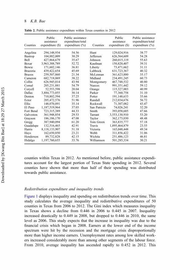
counties within Texas in 2012. As mentioned before, public assistance expendi-tures account for the largest portion of Texas State spending in 2012. Severalcounties have shown that more than half of their spending was distributedtowards public assistance.

Redistribution expenditure and inequality trends

Figure 1 displays inequality and spending on redistribution trends over time. Thisstudy calculates the average inequality and redistributive expenditures of 50counties in Texas from 2006 to 2012. The Gini index which measures inequalityin Texas shows a decline from 0.446 in 2006 to 0.445 in 2007. Inequalityincreased drastically to 0.449 in 2008, but dropped to 0.446 in 2010, the samelevel as 2006. This study expects that the increase in inequality was due to thefinancial crisis which began in 2008. Earners at the lower end of the incomespectrum were hit by the recession and the mortgage crisis disproportionallymore than higher income earners. Unemployment rates among low skilled work-ers increased considerably more than among other segments of the labour force.From 2010, average inequality has ascended rapidly to 0.452 in 2012. This

Table 2. Public assistance expenditure within Texas counties in 2012

Counties

Publicassistance

expenditure ($)

Public assistanceexpenditure/totalexpenditure (%) Counties

Publicassistance

expenditure ($)

Public assistanceexpenditure/totalexpenditure (%)

Angelina 294,148,934 54.56 Hunt 129,024,916 38.77Bastrop 104,882,009 30.29 Jefferson 626,564,609 54.28Bell 427,864,679 35.67 Johnson 260,015,119 55.63Bexar 3,963,388,789 52.72 Kaufman 150,820,407 39.31Bowie 171,602,146 36.81 Liberty 73,471,662 31.11Brazoria 439,422,654 45.69 Lubbock 631,723,367 40.32Brazos 259,507,860 21.34 McLennan 361,623,880 35.17Cameron 682,718,069 38.22 Midland 234,491,245 60.73Collin 626,945,014 43.94 Montgomery 467,748,532 40.80Comal 205,231,881 54.79 Nueces 991,351,442 59.12Coryell 52,553,598 20.04 Orange 115,327,003 40.99Dallas 3,884,773,055 30.14 Parker 77,360,758 31.10Denton 710,802,594 37.25 Potter 191,148,633 35.66Ector 205,472,576 51.96 Randall 212,034,676 56.72Ellis 148,070,891 35.14 Rockwall 71,307,082 43.47El Paso 1,187,519,964 37.03 San Patricio 74,026,241 32.20Fort Bend 723,315,389 44.33 Smith 393,058,685 47.66Galveston 361,948,854 29.53 Tarrant 3,553,130,910 53.20Grayson 186,186,170 47.08 Taylor 362,173,030 48.48Gregg 387,940,094 61.20 Tom Green 363,835,777 57.18Guadalupe 132,516,465 42.91 Travis 1,895,464,879 23.55Harris 8,118,133,907 51.18 Victoria 165,048,448 49.34Hays 162,650,850 23.21 Webb 311,856,422 31.06Henderson 89,732,828 42.15 Wichita 251,486,123 46.81Hidalgo 1,197,760,655 33.76 Williamson 501,285,334 30.21

8 K.B. Bae

Dow

nloa

ded

by [

Kw

ang

Bin

Bae

] at

18:

29 2

7 M

arch

201

5

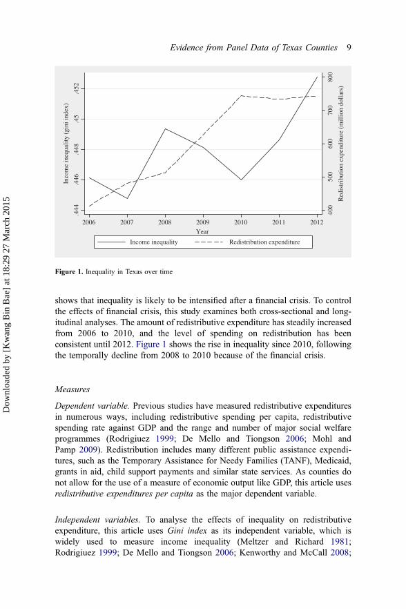
shows that inequality is likely to be intensified after a financial crisis. To controlthe effects of financial crisis, this study examines both cross-sectional and long-itudinal analyses. The amount of redistributive expenditure has steadily increasedfrom 2006 to 2010, and the level of spending on redistribution has beenconsistent until 2012. Figure 1 shows the rise in inequality since 2010, followingthe temporally decline from 2008 to 2010 because of the financial crisis.

Measures

Dependent variable. Previous studies have measured redistributive expendituresin numerous ways, including redistributive spending per capita, redistributivespending rate against GDP and the range and number of major social welfareprogrammes (Rodrigiuez 1999; De Mello and Tiongson 2006; Mohl andPamp 2009). Redistribution includes many different public assistance expendi-tures, such as the Temporary Assistance for Needy Families (TANF), Medicaid,grants in aid, child support payments and similar state services. As counties donot allow for the use of a measure of economic output like GDP, this article usesredistributive expenditures per capita as the major dependent variable.

Independent variables. To analyse the effects of inequality on redistributiveexpenditure, this article uses Gini index as its independent variable, which iswidely used to measure income inequality (Meltzer and Richard 1981;Rodrigiuez 1999; De Mello and Tiongson 2006; Kenworthy and McCall 2008;

400

500

600

700

800

Red

istr

ibut

ion

expe

nditu

re (

mill

ion

dolla

rs)

.444

.446

.448

.45

.452

Inco

me

ineq

ualit

y (g

ini i

ndex

)

2006 2007 2008 2009 2010 2011 2012

Year

Income inequality Redistribution expenditure

Figure 1. Inequality in Texas over time

Evidence from Panel Data of Texas Counties 9

Dow

nloa

ded

by [

Kw

ang

Bin

Bae

] at

18:

29 2

7 M

arch

201

5

Finseraas 2009; Mohl and Pamp 2009). Gini index is derived from the AmericanCommunity Survey conducted by the US Census Bureau from 2006 to 2012.Gini index varies between 0 and 1. A value of 1 indicates maximum inequality inwhich only one household possesses all the income. A value of 0 indicatesperfect equality, in which all households have equal income. This study usesvoter turnout in presidential, senator and governor elections in 2006, 2008, 2010and 2012 as other independent variables.

Control variables. This article controls for Log population as measured bylogarithm of the population of each county from 2006 to 2012. De Mello andTiongson (2006) included GDP per capita as a control variable, but this articleuses income per capita as a proxy variable to reflect the economic condition andwealth status of each county. As overall income level rises, the demand forredistribution is also anticipated to increase. In addition to the support forredistribution, the models carry over the proportion of population over age 65and the proportion of blacks as control variables. Moene and Wallerstein (2001)selected the proportion of over age 65 as a control variable and found that whenthe population of over age 65 increases the size of redistributive expenditure alsoincreases. This study also suggests that when the population of blacks increases,redistributive expenditure will also increase. Education level measured by thepercentage with a bachelor’s degree or higher is closely related to redistributiveexpenditure. Unemployment rate would also affect redistributive expenditure andDemocrat has been used as a dummy variable to reflect differences in countiesthat have voted for the Democratic Party in the presidential and governorelections from 2006 to 2012.

Methods

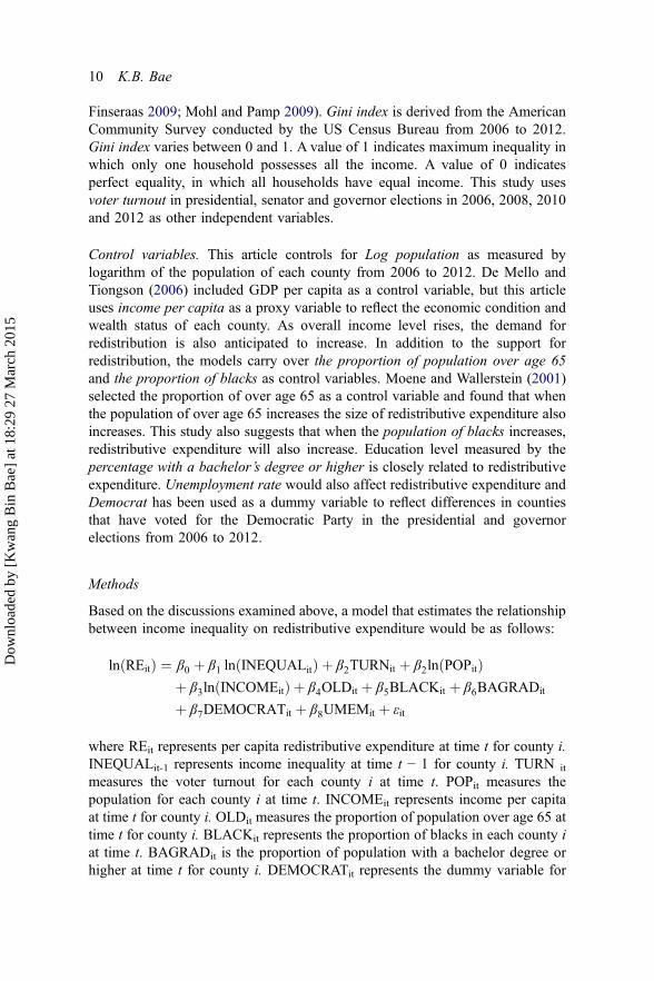
Based on the discussions examined above, a model that estimates the relationshipbetween income inequality on redistributive expenditure would be as follows:

ln REitð Þ ¼ β0 þ β1 ln INEQUALitð Þ þ β2TURNit þ β2ln POPitð Þþ β3ln INCOMEitð Þ þ β4OLDit þ β5BLACKit þ β6BAGRADit

þ β7DEMOCRATit þ β8UMEMit þ εit

where REit represents per capita redistributive expenditure at time t for county i.INEQUALit-1 represents income inequality at time t − 1 for county i. TURN it

measures the voter turnout for each county i at time t. POPit measures thepopulation for each county i at time t. INCOMEit represents income per capitaat time t for county i. OLDit measures the proportion of population over age 65 attime t for county i. BLACKit represents the proportion of blacks in each county iat time t. BAGRADit is the proportion of population with a bachelor degree orhigher at time t for county i. DEMOCRATit represents the dummy variable for

10 K.B. Bae

Dow

nloa

ded

by [

Kw

ang

Bin

Bae

] at

18:

29 2

7 M

arch

201

5

counties that voted for the democratic party at time t for county i, UNEMit

represents the unemployment rate at time t for county i, and εit represents errorterms. This article estimates a random effects model with robust standard errors.

Results

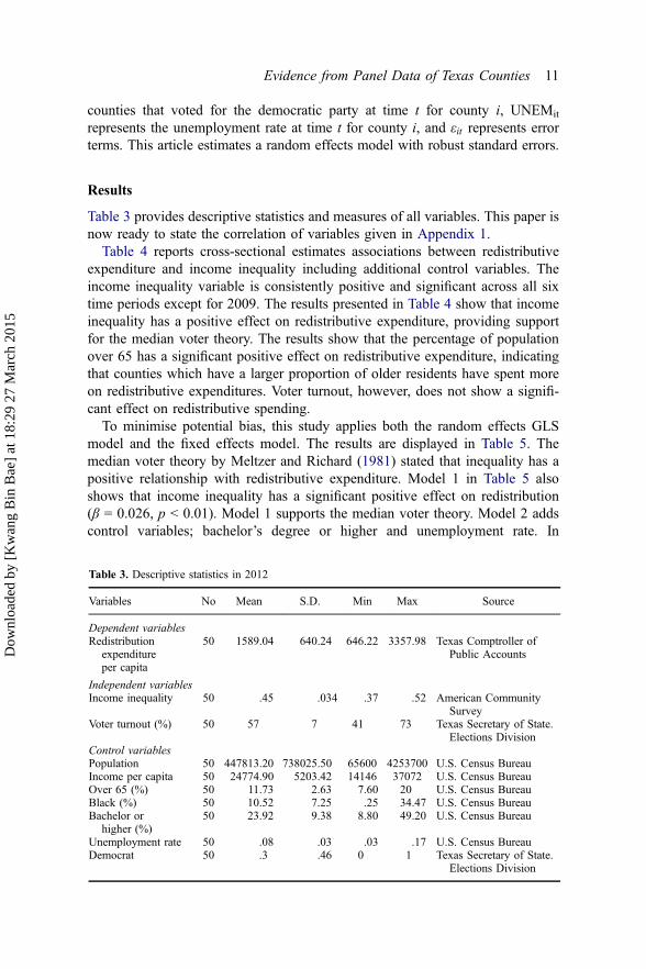
Table 3 provides descriptive statistics and measures of all variables. This paper isnow ready to state the correlation of variables given in Appendix 1.

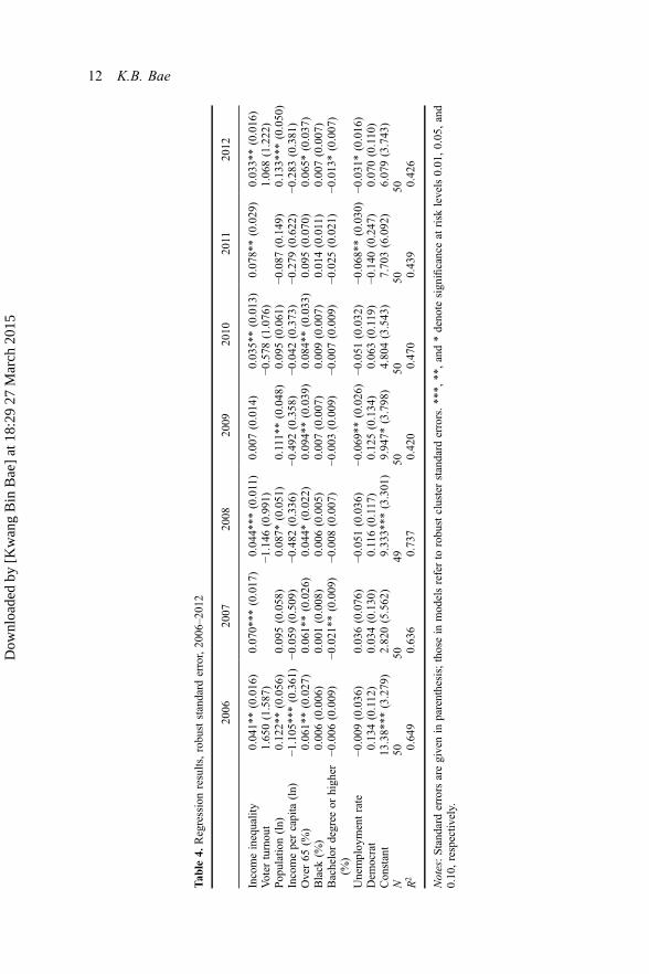
Table 4 reports cross-sectional estimates associations between redistributiveexpenditure and income inequality including additional control variables. Theincome inequality variable is consistently positive and significant across all sixtime periods except for 2009. The results presented in Table 4 show that incomeinequality has a positive effect on redistributive expenditure, providing supportfor the median voter theory. The results show that the percentage of populationover 65 has a significant positive effect on redistributive expenditure, indicatingthat counties which have a larger proportion of older residents have spent moreon redistributive expenditures. Voter turnout, however, does not show a signifi-cant effect on redistributive spending.

To minimise potential bias, this study applies both the random effects GLSmodel and the fixed effects model. The results are displayed in Table 5. Themedian voter theory by Meltzer and Richard (1981) stated that inequality has apositive relationship with redistributive expenditure. Model 1 in Table 5 alsoshows that income inequality has a significant positive effect on redistribution(β = 0.026, p < 0.01). Model 1 supports the median voter theory. Model 2 addscontrol variables; bachelor’s degree or higher and unemployment rate. In

Table 3. Descriptive statistics in 2012

Variables No Mean S.D. Min Max Source

Dependent variablesRedistribution

expenditureper capita

50 1589.04 640.24 646.22 3357.98 Texas Comptroller ofPublic Accounts

Independent variablesIncome inequality 50 .45 .034 .37 .52 American Community

SurveyVoter turnout (%) 50 57 7 41 73 Texas Secretary of State.

Elections DivisionControl variablesPopulation 50 447813.20 738025.50 65600 4253700 U.S. Census BureauIncome per capita 50 24774.90 5203.42 14146 37072 U.S. Census BureauOver 65 (%) 50 11.73 2.63 7.60 20 U.S. Census BureauBlack (%) 50 10.52 7.25 .25 34.47 U.S. Census BureauBachelor or

higher (%)50 23.92 9.38 8.80 49.20 U.S. Census Bureau

Unemployment rate 50 .08 .03 .03 .17 U.S. Census BureauDemocrat 50 .3 .46 0 1 Texas Secretary of State.

Elections Division

Evidence from Panel Data of Texas Counties 11

Dow

nloa

ded

by [

Kw

ang

Bin

Bae

] at

18:

29 2

7 M

arch

201

5

Tab

le4.

Regressionresults,robuststandard

error,2006–201

2

2006

2007

2008

2009

2010

2011

2012

Incomeinequality

0.04

1**(0.016

)0.070*

**(0.017

)0.044*

**(0.011)

0.00

7(0.014

)0.035*

*(0.013

)0.078*

*(0.029

)0.033*

*(0.016

)Voter

turnou

t1.65

0(1.587

)−1.146(0.991

)−0.578(1.076

)1.068(1.222

)Pop

ulation(ln)

0.12

2**(0.056

)0.095(0.058

)0.087*

(0.051

)0.111*

*(0.048

)0.095(0.061

)−0.087(0.149

)0.133*

**(0.050

)Incomepercapita

(ln)

−1.105

***(0.361

)−0.059(0.509

)−0.482(0.336

)−0

.492

(0.358

)−0.042(0.373

)−0.279(0.622

)−0.283(0.381

)Over65

(%)

0.06

1**(0.027

)0.061*

*(0.026

)0.044*

(0.022

)0.09

4**(0.039

)0.084*

*(0.033

)0.095(0.070

)0.065*

(0.037

)Black

(%)

0.00

6(0.006

)0.001(0.008

)0.006(0.005

)0.00

7(0.007

)0.009(0.007

)0.014(0.011)

0.007(0.007

)Bachelordegree

orhigh

er(%

)−0

.006

(0.009

)−0.021*

*(0.009

)−0.008(0.007

)−0

.003

(0.009

)−0.007(0.009

)−0.025(0.021

)−0.013*

(0.007

)

Unemploy

mentrate

−0.009

(0.036

)0.036(0.076

)−0.051(0.036

)−0

.069

**(0.026

)−0.051(0.032

)−0.068*

*(0.030

)−0.031*

(0.016

)Dem

ocrat

0.13

4(0.112

)0.034(0.130

)0.116(0.117

)0.12

5(0.134

)0.063(0.119

)−0.140(0.247

)0.070(0.110

)Con

stant

13.38*

**(3.279

)2.820(5.562

)9.333*

**(3.301

)9.94

7*(3.798

)4.804(3.543

)7.703(6.092

)6.079(3.743

)N

5050

4950

5050

50R2

0.64

90.636

0.737

0.42

00.470

0.439

0.426

Notes:Standarderrors

aregivenin

parenthesis;thosein

modelsreferto

robustclusterstandard

errors.***,

**,and*denote

significanceat

risk

levels0.01

,0.05

,and

0.10,respectiv

ely.

12 K.B. Bae

Dow

nloa

ded

by [

Kw

ang

Bin

Bae

] at

18:

29 2

7 M

arch

201

5

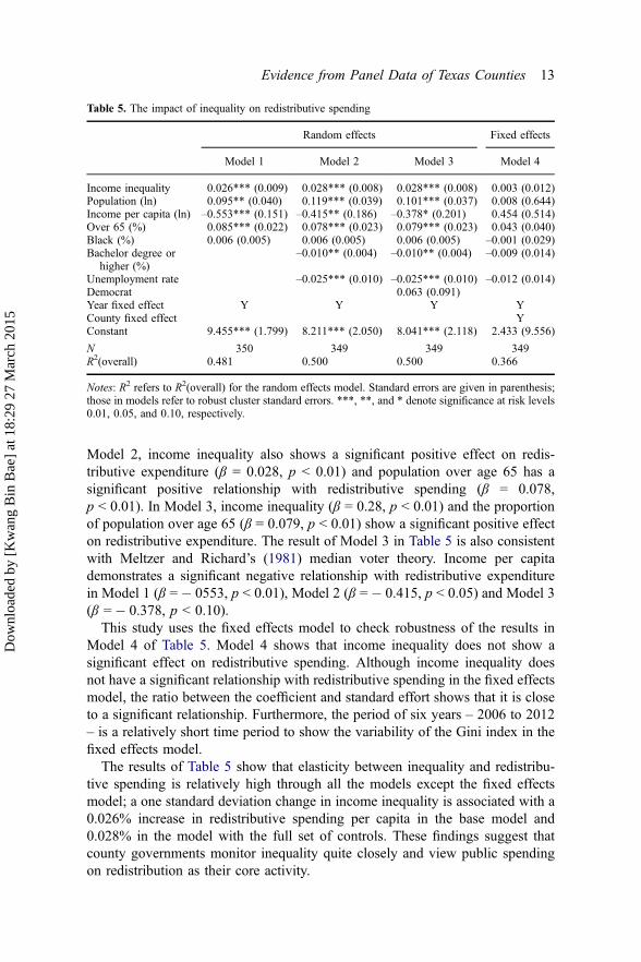
Model 2, income inequality also shows a significant positive effect on redis-tributive expenditure (β = 0.028, p < 0.01) and population over age 65 has asignificant positive relationship with redistributive spending (β = 0.078,p < 0.01). In Model 3, income inequality (β = 0.28, p < 0.01) and the proportionof population over age 65 (β = 0.079, p < 0.01) show a significant positive effecton redistributive expenditure. The result of Model 3 in Table 5 is also consistentwith Meltzer and Richard’s (1981) median voter theory. Income per capitademonstrates a significant negative relationship with redistributive expenditurein Model 1 (β =� 0553, p < 0.01), Model 2 (β =� 0.415, p < 0.05) and Model 3(β =� 0.378, p < 0.10).

This study uses the fixed effects model to check robustness of the results inModel 4 of Table 5. Model 4 shows that income inequality does not show asignificant effect on redistributive spending. Although income inequality doesnot have a significant relationship with redistributive spending in the fixed effectsmodel, the ratio between the coefficient and standard effort shows that it is closeto a significant relationship. Furthermore, the period of six years – 2006 to 2012– is a relatively short time period to show the variability of the Gini index in thefixed effects model.

The results of Table 5 show that elasticity between inequality and redistribu-tive spending is relatively high through all the models except the fixed effectsmodel; a one standard deviation change in income inequality is associated with a0.026% increase in redistributive spending per capita in the base model and0.028% in the model with the full set of controls. These findings suggest thatcounty governments monitor inequality quite closely and view public spendingon redistribution as their core activity.

Table 5. The impact of inequality on redistributive spending

Random effects Fixed effects

Model 1 Model 2 Model 3 Model 4

Income inequality 0.026*** (0.009) 0.028*** (0.008) 0.028*** (0.008) 0.003 (0.012)Population (ln) 0.095** (0.040) 0.119*** (0.039) 0.101*** (0.037) 0.008 (0.644)Income per capita (ln) –0.553*** (0.151) –0.415** (0.186) –0.378* (0.201) 0.454 (0.514)Over 65 (%) 0.085*** (0.022) 0.078*** (0.023) 0.079*** (0.023) 0.043 (0.040)Black (%) 0.006 (0.005) 0.006 (0.005) 0.006 (0.005) –0.001 (0.029)Bachelor degree or

higher (%)–0.010** (0.004) –0.010** (0.004) –0.009 (0.014)

Unemployment rate –0.025*** (0.010) –0.025*** (0.010) –0.012 (0.014)Democrat 0.063 (0.091)Year fixed effect Y Y Y YCounty fixed effect YConstant 9.455*** (1.799) 8.211*** (2.050) 8.041*** (2.118) 2.433 (9.556)

N 350 349 349 349R2(overall) 0.481 0.500 0.500 0.366

Notes: R2 refers to R2(overall) for the random effects model. Standard errors are given in parenthesis;those in models refer to robust cluster standard errors. ***, **, and * denote significance at risk levels0.01, 0.05, and 0.10, respectively.

Evidence from Panel Data of Texas Counties 13

Dow

nloa

ded

by [

Kw

ang

Bin

Bae

] at

18:

29 2

7 M

arch

201

5

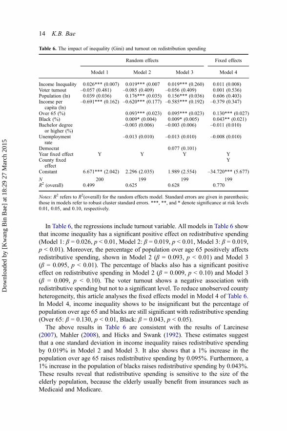
In Table 6, the regressions include turnout variable. All models in Table 6 showthat income inequality has a significant positive effect on redistributive spending(Model 1: β = 0.026, p < 0.01, Model 2: β = 0.019, p < 0.01, Model 3: β = 0.019,p < 0.01). Moreover, the percentage of population over age 65 positively affectsredistributive spending, shown in Model 2 (β = 0.093, p < 0.01) and Model 3(β = 0.095, p < 0.01). The percentage of blacks also has a significant positiveeffect on redistributive spending in Model 2 (β = 0.009, p < 0.10) and Model 3(β = 0.009, p < 0.10). The voter turnout shows a negative association withredistributive spending but not to a significant level. To reduce unobserved countyheterogeneity, this article analyses the fixed effects model in Model 4 of Table 6.In Model 4, income inequality shows to be insignificant but the percentage ofpopulation over age 65 and blacks are still significant with redistributive spending(Over 65: β = 0.130, p < 0.01, Black: β = 0.043, p < 0.05).

The above results in Table 6 are consistent with the results of Larcinese(2007), Mahler (2008), and Hicks and Swank (1992). These estimates suggestthat a one standard deviation in income inequality raises redistributive spendingby 0.019% in Model 2 and Model 3. It also shows that a 1% increase in thepopulation over age 65 raises redistributive spending by 0.095%. Furthermore, a1% increase in the population of blacks raises redistributive spending by 0.043%.These results reveal that redistributive spending is sensitive to the size of theelderly population, because the elderly usually benefit from insurances such asMedicaid and Medicare.

Table 6. The impact of inequality (Gini) and turnout on redistribution spending

Random effects Fixed effects

Model 1 Model 2 Model 3 Model 4

Income Inequality 0.026*** (0.007) 0.019*** (0.007 0.019*** (0.260) 0.011 (0.008)Voter turnout –0.057 (0.481) –0.085 (0.409) –0.056 (0.409) 0.001 (0.536)Population (ln) 0.039 (0.036) 0.176*** (0.035) 0.156*** (0.036) 0.606 (0.403)Income per

capita (ln)–0.691*** (0.162) –0.620*** (0.177) –0.585*** (0.192) –0.379 (0.347)

Over 65 (%) 0.093*** (0.023) 0.095*** (0.023) 0.130*** (0.027)Black (%) 0.009* (0.004) 0.009* (0.005) 0.043** (0.021)Bachelor degree

or higher (%)–0.003 (0.006) –0.003 (0.006) –0.011 (0.010)

Unemploymentrate

–0.013 (0.010) –0.013 (0.010) –0.008 (0.010)

Democrat 0.077 (0.101)Year fixed effect Y Y Y YCounty fixed

effectY

Constant 6.671*** (2.042) 2.296 (2.035) 1.989 (2.554) –34.720*** (5.677)

N 200 199 199 199R2 (overall) 0.499 0.625 0.628 0.770

Notes: R2 refers to R2(overall) for the random effects model. Standard errors are given in parenthesis;those in models refer to robust cluster standard errors. ***, **, and * denote significance at risk levels0.01, 0.05, and 0.10, respectively.

14 K.B. Bae

Dow

nloa

ded

by [

Kw

ang

Bin

Bae

] at

18:

29 2

7 M

arch

201

5

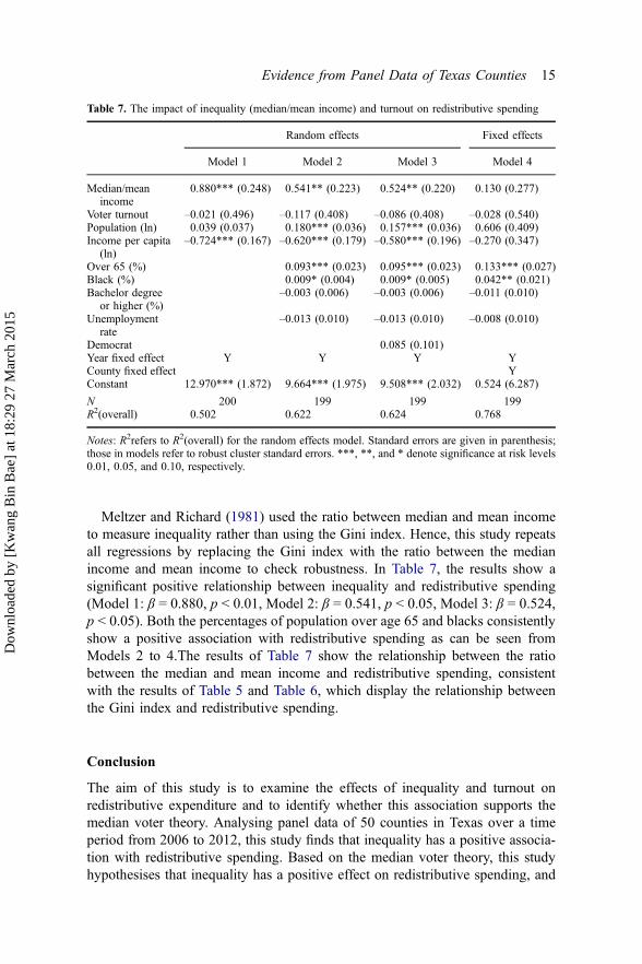
Meltzer and Richard (1981) used the ratio between median and mean incometo measure inequality rather than using the Gini index. Hence, this study repeatsall regressions by replacing the Gini index with the ratio between the medianincome and mean income to check robustness. In Table 7, the results show asignificant positive relationship between inequality and redistributive spending(Model 1: β = 0.880, p < 0.01, Model 2: β = 0.541, p < 0.05, Model 3: β = 0.524,p < 0.05). Both the percentages of population over age 65 and blacks consistentlyshow a positive association with redistributive spending as can be seen fromModels 2 to 4.The results of Table 7 show the relationship between the ratiobetween the median and mean income and redistributive spending, consistentwith the results of Table 5 and Table 6, which display the relationship betweenthe Gini index and redistributive spending.

Conclusion

The aim of this study is to examine the effects of inequality and turnout onredistributive expenditure and to identify whether this association supports themedian voter theory. Analysing panel data of 50 counties in Texas over a timeperiod from 2006 to 2012, this study finds that inequality has a positive associa-tion with redistributive spending. Based on the median voter theory, this studyhypothesises that inequality has a positive effect on redistributive spending, and

Table 7. The impact of inequality (median/mean income) and turnout on redistributive spending

Random effects Fixed effects

Model 1 Model 2 Model 3 Model 4

Median/meanincome

0.880*** (0.248) 0.541** (0.223) 0.524** (0.220) 0.130 (0.277)

Voter turnout –0.021 (0.496) –0.117 (0.408) –0.086 (0.408) –0.028 (0.540)Population (ln) 0.039 (0.037) 0.180*** (0.036) 0.157*** (0.036) 0.606 (0.409)Income per capita

(ln)–0.724*** (0.167) –0.620*** (0.179) –0.580*** (0.196) –0.270 (0.347)

Over 65 (%) 0.093*** (0.023) 0.095*** (0.023) 0.133*** (0.027)Black (%) 0.009* (0.004) 0.009* (0.005) 0.042** (0.021)Bachelor degree

or higher (%)–0.003 (0.006) –0.003 (0.006) –0.011 (0.010)

Unemploymentrate

–0.013 (0.010) –0.013 (0.010) –0.008 (0.010)

Democrat 0.085 (0.101)Year fixed effect Y Y Y YCounty fixed effect YConstant 12.970*** (1.872) 9.664*** (1.975) 9.508*** (2.032) 0.524 (6.287)

N 200 199 199 199R2(overall) 0.502 0.622 0.624 0.768

Notes: R2refers to R2(overall) for the random effects model. Standard errors are given in parenthesis;those in models refer to robust cluster standard errors. ***, **, and * denote significance at risk levels0.01, 0.05, and 0.10, respectively.

Evidence from Panel Data of Texas Counties 15

Dow

nloa

ded

by [

Kw

ang

Bin

Bae

] at

18:

29 2

7 M

arch

201

5

find results to support the median voter theory both through cross sectional andpanel data. This study also finds a positive association between the proportion ofpopulation over age 65 and redistributive spending. Furthermore, income percapita has a significant negative relationship with redistributive expenditure, andfinally, the proportion of blacks shows a significant positive effect on redistribu-tive expenditure.

Based on these results, this study finds that unequal counties spend more onredistributing towards their low-income population. People with below-averageincome favour higher taxes and more redistribution, whereas people with above-average income support lower taxes and less redistribution. When the number ofpeople with relatively low income increases, the number of people favouringtaxes and redistribution will rise. Counties with a higher income per capita spendless on redistribution compared to those with a lower income per capita.Furthermore, this research has found that counties with a higher proportion ofold aged residents show higher redistributive spending.

This study has several limitations. Although the local government plays a rolein the decision-making process of redistributive spending, the federal and statelevel governments also exert influence on this process. It is therefore necessary totake into consideration the effects of intergovernmental grants on redistributivespending when interpreting the results of this research. The federal governmentfinancially supports state and local governments by means of intergovernmentalgrants, and local governments follow the policy priorities of the federal govern-ment to receive these grants. Furthermore, federal grants may be allocatedtowards redistributive spending, which include programmes such as Medicaid,CHIP, TANF, and grants for the education of disadvantaged children. Therefore,federal grants may be greater in counties in which an older or low incomepopulation is larger compared to those with a relatively younger or high incomepopulation. Future studies need to analyse the median voter and voter turnouttheories by controlling the effects of intergovernmental grants on localgovernments.

Second, this research mainly uses the data of 50 counties within Texas, a statethat is considered to be conservative. The majority of residents in Texas supportsthe conservative party and do not support the increase in tax rates. Furthermore,the voter turnout of the younger generation is relatively low compared to theolder generation. The preference of the older generation is likely to be reflectedin policies because they tend to participate in elections more actively than theyounger generation. Future studies need to extend the scope of research intovarious different counties within the US states.

Third, the amount of data used for the fixed effects model is not sufficient todraw a significant result. This study uses data from the American CommunitySurvey from 2006 to 2012 because of data availability. Furthermore, thisresearch uses the voter turnout of presidential, senator and governor electionsin years 2006, 2008, 2010 and 2012. This may be a short period to examine anaccurate relationship.

16 K.B. Bae

Dow

nloa

ded

by [

Kw

ang

Bin

Bae

] at

18:

29 2

7 M

arch

201

5

Finally, this article uses the random effects GLS model and the fixed effectsmodel with county level data to mitigate endogeneity; however, there remainsdoubt as to whether they are sufficient. To identify a clear causal effect betweeninequality and redistributive expenditure, future research would require either afield experiment or a well-designed quasi-experiment. Considering the continu-ing debates on increasing inequality, research on inequality and spending onredistribution would need further attention. When policy makers consider redu-cing inequality, it is essential to identify the causal relationship between redis-tribution spending and inequality.

Acknowledgements

I thank Dr. Evgenia Gorina at the University of Texas at Dallas for her insightfulcomments towards the development of this paper. I am also grateful to thereviewers and Editor for providing excellent feedback and guidance.

Disclosure statement

No potential conflict of interest was reported by the author.

Notes on contributor

Kwang Bin Bae is a PhD candidate of Public Affairs at the University of Texas atDallas. His primarily interests are human resource management, social policy,and nonprofit finance. His articles have appeared in Public PersonnelManagement, KEDI Journal of Education Policy, and International Review ofPublic Administration.

Note

1. The Gini index, a most commonly used nationwide measure of income inequality, rosefrom 0.462 in 2000 to 0.477 in 2011. National poverty rate increased from 11.3% in2000 to 15.1% in 2010 (U.S. Census Bureau 2012a).

References

Alesina, A., and D. Rodrik. 1994. “Distributive Politics and Economic Growth.” TheQuarterly Journal of Economics 109: 465–490. doi:10.2307/2118470.

Ansell, B. W., and D. J. Samuels, 2010. “Democracy and Redistribution, 1880–1930:Reassessing the Evidence.” Paper presented to the annual conference of the AmericanPolitical Science Association, Washington, DC.

Barnes, L. 2013. “Does Median Voter Income Matter? The Effects of Inequality andTurnout on Government Spending.” Political Studies 61 (1): 82–100. doi:10.1111/j.1467-9248.2012.00952.x.

Barro, R. J., X. Sala-i-Martin, O. J. Blanchard, and R. E. Hall. 1991. “Convergence acrossStates and Regions.” Brookings Papers on Economic Activity 1991 (1): 107–182.doi:10.2307/2534639

Evidence from Panel Data of Texas Counties 17

Dow

nloa

ded

by [

Kw

ang

Bin

Bae

] at

18:

29 2

7 M

arch

201

5

Bassett, W. F., J. P. Burkett, and L. Putterman. 1999. “Income Distribution, GovernmentTransfers, and the Problem of Unequal Influence.” European Journal of PoliticalEconomy 15 (2): 207–228. doi:10.1016/S0176-2680(99)00004-X.

Boix, C. 2003. Democracy and Redistribution. New York: Cambridge University Press.Bradley, D., E. Huber, S. Moller, F. Nielsen, and J. Stephens. 2003. “Distribution andRedistribution in Post-Industrial Democracies.” World Politics 55: 193–228.doi:10.1353/wp.2003.0009.

Cantillon, B., I. Marx, and K. V. Bosch. 2002. The Puzzle of Egalitarianism: About theRelationships between Employment, Wage Inequality, Social Expenditures and Poverty.Luxembourg Income Study Working Paper, 337. Syracuse: Syracuse University.

Chamlin, M. B. 1987. “General Assistance among Cities: An Examination of the Need,Economic Threat, and Benign Neglect Hypotheses.” Social Science Quarterly 68: 834–846.

De Mello, L., and E. R. Tiongson. 2006. “Income Inequality and RedistributiveGovernment Spending.” Public Finance Review 34 (3): 282–305. doi:10.1177/1091142105284894.

Downs, A. 1957. “An Economic Theory of Political Action in a Democracy.” The Journalof Political Economy 65 (2): 135–150. doi:10.1086/257897.

Easterly, W., and S. Rebelo. 1993. “Fiscal Policy and Economic Growth.” Journal ofMonetary Economics 32 (3): 417–458. doi:10.1016/0304-3932(93)90025-B.

FiGini, P. 1998. Inequality and Growth Revisited. Dublin: Trinity College Press.Finseraas, H. 2008. “What If Robin Hood Is a Non-voter? An Empirical Analysis of theEffect of Income Inequality and Voter Turnout of Redistribution.” In workshop onPolitical Economy, Harvard University.

Finseraas, H. 2009. “Income Inequality and Demand for Redistribution: A MultilevelAnalysis of European Public Opinion.” Scandinavian Political Studies 32 (1): 94–119.doi:10.1111/j.1467-9477.2008.00211.x.

Franzese, R. 1998. “Political Participation, Income Distribution, and Public Transfers inDeveloped Democracies.” Paper presented to the American Political ScienceAssociation, September.

Franzese, R. 2002. Macroeconomic Policies of Developed Democracies. New York:Cambridge University Press.

Gouveia, M., and N. A. Masia. 1998. “Does the Median Voter Model Explain the Size ofGovernment?: Evidence from the States.” Public Choice 97: 159–177. doi:10.1023/A:1004973610506.

Hicks, A. M., and D. H. Swank. 1992. “Politics, Institutions, and Welfare Spending inIndustrialized Democracies, 1960-82.” The American Political Science Review 86 (3):658–674. doi:10.2307/1964129.

Husted, T. A., and L. W. Kenny. 1997. “The Effect of the Expansion of the VotingFranchise on the Size of Government.” Journal of Political Economy 105 (1): 54–82.doi:10.1086/262065.

Isaac, L., and W. R. Kelly. 1981. “Racial Insurgency, the State, and Welfare Expansion:Local and National Level Evidence from the Postwar United States.” American Journalof Sociology 86: 1348–305. doi:10.1086/227388.

Iversen, T., and D. Soskice. 2006. “Electoral Institutions and the Politics of Coalitions:Why Some Democracies Redistribute More than Others.” American Political ScienceReview 100 (2): 165–181.

Kenworthy, L., and L. McCall. 2008. “Inequality, Public Opinion and Redistribution.”Socio-Economic Review 6 (1): 35–68. doi:10.1093/ser/mwm006.

Kenworthy, L., and J. Pontusson. 2005. “Rising Inequality and the Politics ofRedistribution in Affluent Countries.” Perspectives on Politics 3 (3): 449–471.doi:10.1017/S1537592705050292.

Larcinese, V. 2007. “Voting over Redistribution and the Size of theWelfare State: The Role ofTurnout.” Political Studies 55 (3): 568–585. doi:10.1111/j.1467-9248.2007.00658.x.

18 K.B. Bae

Dow

nloa

ded

by [

Kw

ang

Bin

Bae

] at

18:

29 2

7 M

arch

201

5

Lindert, P. H. 1996. “What Limits Social Spending?” Explorations in Economic History33 (1): 1–34. doi:10.1006/exeh.1996.0001.

Mahler, V. A. 2008. “Electoral Turnout and Income Redistribution by the State: A Cross-National Analysis of the Developed Democracies.” European Journal of PoliticalResearch 47 (2): 161–183. doi:10.1111/j.1475-6765.2007.00726.x.

Mahler, V. A., and D. K. Jesuit. 2006. “Fiscal Redistribution in the Developed Countries:New Insights from the Luxembourg Income Study.” Socio-Economic Review 4 (3):483–511. doi:10.1093/ser/mwl003.

Meltzer, A. H., and S. F. Richard. 1981. “A Rational Theory of the Size of Government.”The Journal of Political Economy 89 (5): 914–927. doi:10.1086/261013.

Milanovic, B. 2000. “The Median-Voter Hypothesis, Income Inequality, and IncomeRedistribution: An Empirical Test with the Required Data.” European Journal ofPolitical Economy 16 (3): 367–410. doi:10.1016/S0176-2680(00)00014-8.

Moene, K. O., and M. Wallerstein. 2001. “Inequality, Social Insurance, andRedistribution.” American Political Science Review 95 (4): 859–874.

Moene, K. O., and M. Wallerstein. 2003. “Earnings Inequality and Welfare Spending:A Disaggregated Analysis.” World Politics 55 (4): 485–516. doi:10.1353/wp.2003.0022.

Mohl, P., and O. Pamp. 2009. “Income Inequality and Redistributional Spending: An EmpiricalInvestigation of Competing Theories.” Public Finance and Management 9 (2): 179–234.

National Association of State Budget Officers. 2012. “State Expenditure Report:Examining Fiscal 2010–2012 State Spending” Accessed December 1, 2014. http://www.nasbo.org/publications-data/state-expenditure-report/archives

Pack, J. R. 1998. “Poverty and Urban Public Expenditures.” Urban Studies 35 (11): 1995–2019. doi:10.1080/0042098983980.

Panizza, U. 2002. “Income Inequality and Economic Growth: Evidence from AmericanData.” Journal of Economic Growth 7 (1): 25–41. doi:10.1023/A:1013414509803.

Persson, T., and G. Tabellini. 1994. “Is Inequality Harmful for Growth?” AmericanEconomic Review 84 (3): 600–621.

Rodrigiuez, F. C. 1999. “Does Distributional Skewness Lead to Redistribution? Evidence fromthe United States.” Economics & Politics 11 (2): 171–199. doi:10.1111/1468-0343.00057.

Schneider, M. 1987. “Income Homogeneity and the Size of Suburban Government.” TheJournal of Politics 49 (1): 36–53. doi:10.2307/2131133.

Schwabish, J. A., T. M. Smeeding, L. Osberg, M. Eriksen, and J. Marchand. 2003. IncomeDistribution and Social Expenditures: A Cross-National Perspective. New York:Maxwell School of Citizenship and Public Affairs, Syracuse University.

Sharp, E. B., and S. Maynard-Moody. 1991. “Theories of the Local Welfare Role.”American Journal of Political Science 35 (4): 934–950. doi:10.2307/2111500.

Tanninen, H. 1999. “Income Inequality, Government Expenditures and Growth.” AppliedEconomics 31 (9): 1109–1117. doi:10.1080/000368499323599.

Texas Comptroller of Public Accounts. 2012. “Texas State Expenditures by CountyReports.” Accessed December 1, 2014. http://www.texastransparency.org/State_Finance/Budget_Finance/Reports/Expenditures_by_County/

Texas Secretary of State Elections Division. 2012. “General Election 11/6/2012 President/Vice President.” Accessed March 3, 2014. http://elections.sos.state.tx.us/elchist.exe

U.S. Census Bureau, 2012a. “Income, Poverty, and Health Insurance Coverage in theU.S.” Accessed December 1, 2014. http://www.census.gov/prod/2012pubs/p60-243.pdf

U.S. Census Bureau, 2012b. “The Current Population Survey in the U.S.” AccessedDecember 1, 2014. http://www.census.gov/hhes/www/socdemo/voting/publications/p20/2012/index.html

Wolfinger, R. E., and S. J. Rosnstone. 1980. Who Votes? New Haven, CT: Yale UniversityPress.

Evidence from Panel Data of Texas Counties 19

Dow

nloa

ded

by [

Kw

ang

Bin

Bae

] at

18:

29 2

7 M

arch

201

5

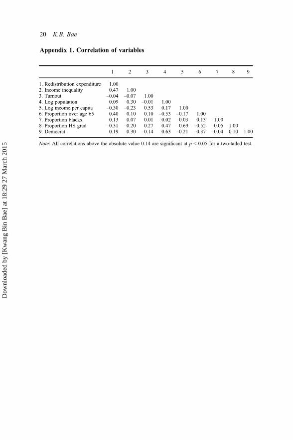
Appendix 1. Correlation of variables

1 2 3 4 5 6 7 8 9

1. Redistribution expenditure 1.002. Income inequality 0.47 1.003. Turnout –0.04 –0.07 1.004. Log population 0.09 0.30 –0.01 1.005. Log income per capita –0.30 –0.23 0.53 0.17 1.006. Proportion over age 65 0.40 0.10 0.10 –0.53 –0.17 1.007. Proportion blacks 0.13 0.07 0.01 –0.02 0.03 0.13 1.008. Proportion HS grad –0.31 –0.20 0.27 0.47 0.69 –0.52 –0.05 1.009. Democrat 0.19 0.30 –0.14 0.63 –0.21 –0.37 –0.04 0.10 1.00

Note: All correlations above the absolute value 0.14 are significant at p < 0.05 for a two-tailed test.

20 K.B. Bae

Dow

nloa

ded

by [

Kw

ang

Bin

Bae

] at

18:

29 2

7 M

arch

201

5