An “Ideal” Kyoto Protocol: Emissions Trading, Redistributive Transfers and Global Participation

By

Arthur J. Caplan Department of Economics, Utah State University, 3530 Old Main Hill, Logan, UT 84322-3530, USA.

Richard C. Cornes School of Economics, University of Nottingham, University Park, Nottingham NG7 2RD, UK.

and

Emilson C. D. Silva Department of Economics, Tulane University, New Orleans, LA 70118-5698, USA.

May 10, 2002

Abstract: We demonstrate that an interregional policy scheme featuring trading of carbon dioxide emissions, redistributive resource transfers and global participation, a scheme which we call “Ideal Kyoto Protocol,” yields an efficient equilibrium allocation for a global economy. An altruistic international agency – say, the Global Environment Facility – should operate the resource transfer mechanism. In addition, regional governments should be able to make independent policy commitments regarding how to control regional emissions of carbon dioxide in anticipation of the redistributive transfers. Our efficiency result suggests that the USA should be “bribed” to reverse its decision of not participating in the Kyoto Protocol.

Acknowledgements: We would like to thank Daniel Arce, Harvey Lapan, Todd Sandler and two anonymous referees for very helpful comments and suggestions, which greatly improved the paper. Silva also wishes to thank the Tulane Committee on Research Summer Fellowships for partially funding this research.

1

1. Introduction

The Kyoto Protocol to the United Nations Framework Convention on Climate Change, completed on

December 10, 1997, called for the creation of three mechanisms to effectively control global greenhouse

gas emissions. There should be an emissions trading mechanism,1 which in its initial phase would include a

subset of OECD and Eastern European countries (referred to as Annex I countries), a “clean development”

mechanism, which in a later stage would allow developing countries to participate in emissions trading, and

a financial mechanism, which would facilitate transfers of income, technology and other valuable resources

from rich to poor countries. The idea behind the clean development mechanism is articulated in Article 11

of the Protocol, whereby (1) “[developing] countries will benefit from project activities resulting in

certified emissions reductions,” and (2) “[developed countries] may use the certified emissions reductions

accruing from such project activities to contribute to compliance with part of their quantified emission

limitation and reduction commitments.” As for the financial mechanism, the Conference of the Parties to

the United Nations Framework Convention on Climate Change, which represents the supreme body of the

Convention, has delegated the responsibility of operating such a mechanism to the Global Environment

Facility (GEF). The GEF was established in 1990 by the World Bank, the United Nations Development

Program (UNDP) and the United Nations Environment Program (UNEP).

The Kyoto Protocol motivates us to study the efficiency properties of an interregional policy

scheme which features both resource transfers and trading of carbon dioxide emissions. In doing so, we are

also motivated by the USA’s decision to not ratify the Kyoto Protocol, which occurred shortly after the

Bush administration took office in 2001. Whether or not the USA’s government was justified in

“withdrawing” from the Kyoto Protocol is beyond the scope of this paper. We are mostly interested in

investigating the potential implications for the allocation of resources in the global economy if all regions

but one decide to participate in the interregional policy scheme.2

1 The call for emissions trading was, no doubt, motivated by the effectiveness of marketable permit programs in the USA (see, e.g., Hahn (1989) and Stavins (1998)). Furthermore, an impressive amount of research and experience underscores the benefits and costs associated with emissions trading programs (see, e.g., Maloney and Yandle (1984), Coggins and Swinton (1996) and references therein). 2 We do explore the interesting issue of coalition formation in this paper. For good examples of papers that examine endogenous participation in international agreements, see Barrett (1994) and Black et. al (1993).

2

We show that the equilibrium allocation for a global economy implied by an interregional policy

scheme in which one region – the USA – does not participate is inefficient because resources are not

transferred from or to the USA and the USA’s government neglects the negative effects that its carbon

dioxide emissions cause to the rest of the world. For a similar global economy, we also show that the

equilibrium allocation implied by an interregional policy scheme which includes all regions in the globe – a

scheme which we refer to as “Ideal Kyoto Protocol” – is Pareto efficient. The intuition for this important

finding is simple and straightforward. The redistributive interregional transfer mechanism operated by an

interregional agency – say, the GEF – makes every regional government realize that it is in its best interest

to maximize global income. Every government knows, therefore, that its policy choice should internalize

all externalities caused by its region’s carbon dioxide emissions.

This paper is closely related to a set of game-theoretic papers that use sequential games to study

provision of public goods (see, e.g., Arce (2001), Caplan et al. (2000) and Caplan and Silva (2002)). None

of these papers, however, combines emissions trading and transfers. To our knowledge the only other

article that features such a combination is Chichilnisky, et al. (2000). The authors demonstrate that equity

and efficiency go hand in hand whenever carbon dioxide emissions are globally traded. In their framework,

a market for emissions allocates resources efficiently if and only if international transfers are made in order

to equalize social marginal utilities of consumption. They also show that this resource redistribution

condition can be satisfied by an appropriate initial distribution of emission permits. Although our paper’s

message is fully consistent with theirs, our approach differs from theirs in two crucial ways in what

respects the resource redistribution: (1) it is endogenous; and, more importantly, (2) it takes place after the

regional governments choose their most desired emission quotas. It is the anticipation of the interregional

resource transfers implemented by the GEF that makes the regional governments behave efficiently.

The paper is organized as follows. Section 2 builds the basic model. Section 3 characterizes a

Pareto efficient allocation. Section 4 examines regional and interregional policy schemes. In subsection 4.1,

we consider a policy setting in which regional governments, acting independently, simultaneously

determine their environmental policy agendas. We characterize the equilibrium allocation of resources for

the global economy in this arrangement and then demonstrate that it is inefficient. Next, we investigate two

interregional policy regimes. Motivated by the USA’s decision to withdraw from the Kyoto Protocol, in

3

subsection 4.2 we consider a policy scheme in which all regions but one in the globe participate in it. The

USA is excluded from both interregional emissions trading and transfer mechanisms, but it is able to

announce – i.e., commit to – a regional policy scheme before the other regions make their own policy

commitments under the Protocol. In the policy scheme of subsection 4.3, all regions participate in both

mechanisms and make their policy commitments simultaneously. In both interregional policy settings, the

GEF implements transfers after it observes the policy commitments of all regions. Section 5 concludes the

paper.

2. Basic Model

Imagine a global economy consisting of J politically autonomous regions and governments, indexed by j, j

= 1,...,J. There are two globally traded consumption commodities, a commodity whose production

generates emissions of carbon dioxide (e.g., an industrial good) and a commodity whose production is

harmed by emissions of carbon dioxide (e.g., an agricultural good). Let jY be region j’s industrial product

and E be the global quantity of carbon dioxide emitted in the atmosphere. We assume that ∑=

≡J

1j

jYE ; that

is, production of a unit of the industrial good leads to the emission of a unit of carbon dioxide.

The industrial sector in region j is competitive and consists of a large number of identical

producers. Let jI be the (fixed) number of industrial producers in region j. Each industrial producer utilizes

an input quantity 0x j ≤ of the agricultural good to produce ( )jj xf units of the industrial good. We assume

that jf is decreasing and strictly concave.3 Define jjj xIX ≡ as the total amount of the agricultural good

demanded as input by region j’s industrial sector and ( ) ( )jjj

jjj IXfIXF ≡ as this sector’s production

function. Hence, ( )jj

j XFY = . If we let Xp and Yp denote the prices of the agricultural and industrial

goods, respectively, the profit of the industrial sector in region j is jxjY XpYp + .

The agricultural sector in region j is also competitive. Let jA be region j’s (fixed) number of

agricultural producers. Each agricultural producer utilizes an input quantity 0y j ≤ of the industrial good to

produce ( )E,yg jj units of the agricultural good. We assume that jg is decreasing in both arguments and

3 Throughout the analysis, we use superscripts to index functions.

4

strictly concave. Let jjj yAY ≡ and ( ) ( )

≡

∑∑==

J

1ii

ijj

jj

J

1ii

ij

j XF,AYgAXF,YG . Hence, region j’s

agricultural product is ( )

= ∑=

J

1ii

ij

jj XF,YGX and its profit is jYjX YpXp + .

Region j is populated by jn immobile consumers. Consumers within each region are identical in

that they possess identical preferences and incomes. Let ( )jjj y,xU be the utility function of a consumer in

region j who consumes jx units of the agricultural good and jy units of the industrial good.4 This function

is assumed to be increasing in both arguments, quasiconcave and twice continuously differentiable.

Both industrial and agricultural goods are freely traded in global markets. Let 0jX and 0

jY denote

region j’s initial endowments of agricultural and industrial goods, respectively. In any equilibrium for the

global economy, ( )∑=

=−−−J

1jjj

0jjj 0XXXxn and ( ) 0YYYyn

J

1jjj

0jjj =−−−∑

=

; namely, the global

markets must clear. To keep things simple, we henceforth normalize the price of the agricultural good to

one. This normalization will enable us to ignore the market clearing condition for the agricultural good,

since it is automatically satisfied whenever the other conditions that characterize an equilibrium allocation

are satisfied. The normalization also allows us to set ppY ≡ .

3. Pareto Efficiency

Before we examine regional and interregional environmental policy making, it is useful to derive the set of

Pareto efficiency conditions for our economy. A Pareto efficient allocation can be obtained as follows.

Choose { }J,...,1jjjjjjj Y,X,Y,X,y,x

= to maximize ( )11

1 y,xU subject to ( ) k

kk

k Uy,xU ≥ , J,...,2k = ,

( )jj

j XFY ≤ , ( )

≤ ∑=

J

1ii

ij

jj XF,YGX , ( )∑

=

≤−−−J

1iii

0iii 0XXXxn , ( ) 0YYYyn

J

1iii

0iii ≤−−−∑

=

,

0Y, 0X, 0, Y0, X0, y0x jjjjjj ≤≤≥≥≥≥ , J ..., ,1j = . An interior solution satisfies:

( ) k

kk

k Uy,xU = , J,...,2k = , (1a)

4 For expositional ease, we assume that utility does not depend directly on E. It can be shown that, for a large family of utility functions, the results of our analysis would remain qualitatively the same if E entered as an arguments in the utility function. A proof of this claim is available from the authors upon request.

5

( ) 0XFY jj

j >= , ( ) 0XF,YGXJ

1ii

ij

jj >

= ∑=

, J ..., ,1j = , (1b)

( )∑=

=−−−J

1iii

0iii 0XXXxn , ( ) 0YYYyn

J

1iii

0iii =−−−∑

=

, (1c)

kx

k

y

1x

1

y

U

U

U

U= , J,...,2k = , (1d)

jYj

x

j

y GU

U−= , J,...,1j = , (1e)

∑=

+=J

1i

iEj

X

jY G

F1

G , J,...,1j = . (1f)

Equations (1a) state that the utility constraints bind. Each region k reaches the exogenously given

level of per capita welfare, kU . Equations (1b) tell us that each region produces positive quantities of both

commodities. Equations (1c) inform us that resources are fully employed. Equations (1d) state that

individual marginal rates of substitution between industrial and agricultural goods must be equal across

regions. Equations (1e) tell us that in each region the individual marginal rate of substitution between

industrial and agricultural goods must be equal to the marginal rate of transformation for the agricultural

good. Equations (1f) inform us that in each region the marginal rate of transformation for the agricultural

good must be equal to the marginal rate of transformation for the industrial good. The marginal rate of

transformation for the industrial good in each region includes the negative production effects brought about

by global emissions of carbon dioxide.

For future reference, it is worth noting that Pareto efficiency requires satisfaction of three

important conditions. First, marginal agricultural products must be equalized across regions:

k

Y

1

Y GG = , J,...,2k = . (2a)

Second, marginal industrial products must also be equalized across regions:

kX

1X FF = , J,...,2k = . (2b)

Third, there must be interregional resource transfers. To see this, observe that we obtain the Pareto

efficiency conditions (1a) – (1f) if and only if:

k

kxk

1

1x

n

U

n

U λ=µ= , J,...,2k = , (2c)

6

where µ is the Lagrangian multiplier associated with the resource feasibility constraint for the agricultural

commodity and kλ is the Lagrangian multiplier associated with the utility constraint for region k.

Equations (2c) tell us how the agriculture commodity (our numeraire) should be allocated across regions.

One unit of the numeraire good transferred to region 1 from some region k, increases region 1’s per capita

utility by an amount 11x nU , since the extra unit is shared by 1n residents. Per capita utility in region k is

decreased by k

k

xk nUλ , since kλ is the shadow cost of the utility constraint and the unit shortfall is shared

by kn residents. Hence, equations (2c) inform us that interregional transfers of the numeraire good are

implemented up to the point where the marginal shadow transfer benefit (of each recipient region) equates

the marginal shadow transfer cost (of each remitter region).

4. Regional and Interregional Policy Making

We start our analysis of regional and interregional policy making by considering a situation in which all

regions independently decide how to control their emissions of carbon dioxide. We call this regime

“Regional Environmental Policy Making.” We later study two interregional policy schemes, denoted “Ideal

Kyoto Protocol” and “Kyoto Protocol without the USA.” All regions in the globe participate in the “Ideal

Kyoto Protocol.” This is a scenario which apparently accords well with the Kyoto Protocol envisioned by

its founders. All regions, except the USA, participate in the other interregional policy scheme, “Kyoto

Protocol without the USA.” This setting corresponds to a fairly optimistic view of the current situation,

whereby all regions in the world, except the USA, will decide to participate. We do not consider other

possible interregional policy schemes, characterized by fewer participating regions, because it does not

seem likely that the Kyoto Protocol will survive if another country withdraws.5 It is not unreasonable to

assume that yet another defection will trigger a chain of defections, which will eventually completely

undermine the Protocol.

5 At this stage, the Kyoto Protocol can be implemented only if most of the 33 Annex I countries that remain decide to participate in it. A requirement for the Protocol to be enacted is that the set of participating countries contains countries that accounted for a share greater or equal to 55% of the total carbon dioxide emitted by the original 34 Annex I countries in 1990. The participation rates of the USA, Russia, Japan and Germany in the total emissions of Annex I countries in 1990 were 36.1%, 17.4%, 8.5% and 7.4%, respectively. If, in addition to the USA, Russia decides to withdraw, the Protocol will necessarily fail. If either Japan or Germany follows the USA’s lead, the Protocol will not necessarily fail, but its chance of survival will be slim. Although defection of any other Annex I country will not be as harmful in a first instance, it is likely that it will eventually invite others to defect, undermining the Protocol’s viability.

7

4.1. Regional Environmental Policy Making

Suppose that there is a separate market for emission permits within each region. This will facilitate

comparison with the subsequent arrangements. The regional government in region j – henceforth called

“regulator j” – sets a quota, jQ , of emission permits that can be sold. Regulator j endows each consumer

in the region with jjj nQq ≡ emission permits. Since consumption activities do not emit carbon dioxide,

consumers are sellers in each regional market for emission permits. Every industrial producer in region j

must purchase at a cost 0c j ≥ an emission permit per unit of the industrial good he produces.

The representative consumer in region j sells js emission permits, jj qs0 ≤≤ , and earn jjsc units

of income. Hence, his budget constraint is

j

j

0

j

0

j

jjjj n

pYXscpyx

Π+++=+ ,

where jΠ corresponds to the sum of industry’s and agriculture’s regional profits. This consumer chooses

nonnegative quantities { }jjj s,y,x to maximize ( )jjj y,xU subject to both his budget constraint and jj qs ≤ ,

taking p , jc and { } jj0j

0j npYX Π++ as given. First, note that it is optimal for this consumer to sell jq

pollution permits. Setting jj qs = , the budget constraint becomes

j

j

0

j

0

j

jjjj n

pYXqcpyx

Π+++=+ . (3a)

Assuming that the consumer finds it optimal to consume strictly positive amounts of both agriculture and

industrial commodities, the solution to his problem satisfies (3a) and the following tangency condition:

pU

Ujx

j

y = . (3b)

Equation (3b) demonstrates that in each region the representative individual's marginal rate of substitution

between industrial and agricultural goods must be equal to the (relative) price of the industrial good. Let

{ } jj0j

0jjjj npYXqcm Π+++≡ . We can now use equations (3) to implicitly define the demand functions

of the representative individual in region j, ( )jj m,px and ( )j

j m,py .

8

The industrial sector in region j chooses { }jX to maximize ( ) ( ) jjj

j XXFcp +− subject to 0X j ≤ ,

taking p and jc as given. Assuming that jcp > , the industrial sector of each region maximizes profit if

and only if

( ) 1Fcp jXj =−− , J,...,1j = (4a)

that is, the realized value of the regional marginal industrial product (left side) must be equal to the regional

marginal input cost (right side). Let jj cpr −≡ denote the price of the industrial good net of the marginal

regulatory cost, jc . Equations (4a) enables us to implicitly define the input demand functions ( )jj rX ,

J,...,1j = . Hence, the industrial sectors’ supply functions are ( ) ( )( )jjj

jj rXFrY ≡ , J,...,1j = .

The agricultural sector in region j chooses { }jY to maximize ( ) jjj YpE,YG + subject to 0Yj ≤ ,

taking p and E as given. The agricultural sector of each region maximizes profit if and only if

pG jY =− , J,...,1j = , (4b)

that is, the regional marginal agricultural product must be equal to the regional marginal input cost.

Equations (4b) enable us to implicitly define the input demand functions ( )E,pY j , J,...,1j = . Then, the

agricultural sectors’ supply functions are ( ) ( )( )E,E,pYGE,pX jjj ≡ , J,...,1j = .

Given jr , the industrial sector in region j demands ( )jj rY emission permits. Then, the regional

market for permits clears if and only if

( ) jjj QrY = . (5a)

Since jj cpr −≡ , we can use equation (5a) to implicitly define ( )jj Q,pc . It follows that 0Y1c j

rjQ <−= ,

where j

jj

Q Qcc ∂∂≡ and j

jj

r drdYY ≡ . Since, in equilibrium, equation (5a) holds for each j, we have

( )( ) jjjj QQ,pcpY =− , J,...,1j = . (5b)

We now turn our attention to the problems facing regional regulators. First, we need to compute

regional per capita incomes and then later derive the indirect utility functions of the regional representative

individuals. Each regulator chooses a quota level of regional permits that maximizes the utility of his

region’s representative consumer.

9

Given equations (5b), we can write the total profits of the industrial and agricultural sectors in

region j, as ( )( ) ( )( ) ( )( )jjj

jjj

jj Q,pcpXQ,pcpYQ,pcp −+−− and

+

∑∑==

J

1ii

jJ

1ii

j Q,pYpQ,pX ,

respectively. Note that equations (5b) imply that ∑=

=J

1j

jQE . Let ∑=

≡J

1j

jQQ . Adding up the profits of both

sectors, we have ( ) ( )( ) ( )( ) ( )( ){ } ( ) ( ){ }Q,pYpQ,pXQ,pcpXQ,pcpYQ,pcpQ,Q,p jjj

jjj

jjj

jj

j ++−+−−≡Π .

This enables us to write regional per capita income as a function of p , jQ and Q as follows:

( ) ( ) ( )j

jj

j

j

j0

j

0

j

jj

n

QQ,pcQ,Q,ppYXQ,Q,pm

+Π++≡ . (6)

Regulator j chooses { }jQ to maximize ( ) ( )( ) ( )( )( )Q,Q,pm,py,Q,Q,pm,pxUQ,Q,pV jjj

jjjj

jj ≡

subject to: (6), ∑≠

+=J

jkkj QQQ and 0Q j ≥ , taking p and kQ , jk ≠∀ , as given. Assuming an interior

solution, the first order condition for maximization of ( )Q,Q,pV jj is

( ) { } ( )0

dQ

Q,Q,pdmyUxU

dQ

Q,Q,pdV

j

j

j

jm

jy

jm

jx

j

j

j

=+= . (7a)

Since the solution to the utility maximization problem for the representative individual implies that

1pyxyU

Ux j

mjm

jmj

x

jyj

m =+=+ ,

the second equation in (7a) can be rewritten as

( )0

dQ

Q,Q,pdm

j

j

j

= . (7b)

Equation (7b) clearly shows that each regulator seeks to maximize regional per capita income. From

equation (6), we obtain:

( ) ( )( ) ( )( ){ } 0ccQGYpGcYcX1Frn

1

dQ

Q,Q,pdmjj

QjjE

jE

jY

jQ

jjQ

jr

jXj

jj

j

j

=+++++−+−= . (7c)

Given equations (4a), (4b) and (5a), equation (7c) reduces to

( ) ( )( ) 0Q,Q,pYGQ,pc jjEj

j =+ . (7d)

Differentiating the first order condition (7d) with respect to jQ yields

10

( ) ( )0

G

GGGcG

G

GcGYGc

jYY

2jEY

jEE

jYYj

QjEEj

YY

2jEYj

QjEE

jE

jEY

jQ <

−+≡+−≡++ . (7e)

The sign of the second order condition (7e) follows from strict concavity of jG and the fact that 0c jQ < .

Hence, the per capita income function (6) is strictly concave and the first order condition (7d) is not only

necessary but also sufficient for an interior maximum.

Assuming that equation (7d) holds for all j in the Nash equilibrium, we obtain:

( ) ( )( )Q,Q,pYGQ,pc jjEj

j −= , J,...,1j = . (8)

Equations (8) inform us that each regulator finds it optimal to supply emission permits at the level

in which the regional price of the permit equals the regional marginal damage caused by carbon dioxide

emissions. Equations (8) also clearly demonstrate that in equilibrium regional supplies of emission permits

become functions of p . Let ( )pQ j and ( ) ( )∑=

≡J

1i

i pQpQ denote the quota functions for region j and the

globe as a whole. Now define ( ) ( ) ( )( )pQ,pQ,pmpm jjj ≡ , ( ) ( )( )pm,pypy jjj ≡ , ( ) ( )( )pQ,pcppr jjj −≡ and

( ) ( )( )pQ,pYpY jj ≡ . Given these definitions, we may write the market clearing condition for the industrial

good as follows:

( ) ( )( ) ( )( ) 0pYprYYpynJ

1j

jjj0j

jj =−−−∑

=

. (9)

The price of the industrial good, p , is determined endogenously by equation (9).

In this setting, the equilibrium allocation for the global economy is given by conditions (3a), (3b),

(4a), (4b), (5b), (8) and (9). Comparing these conditions with the Pareto efficiency conditions immediately

reveals that regional policy making is inefficient. There are two sources of inefficiency: (1) the absence of

interregional income transfers, since regional marginal shadow utilities of income are not necessarily

equalized; and (2) the presence of interregional external effects associated with regional production of the

industrial commodity, since every regulator neglects the negative effects that production of the industrial

commodity in his region cause to every other region in the globe.

For future reference, let jDV denote region j’s per capita utility level realized in the global

equilibrium allocation described above.

11

4.2 Kyoto Protocol without the USA

Suppose that all regions in the globe, except for the USA, participate in an interregional policy scheme –

denoted “KP-USA” for notational simplicity – in which an interregional market for carbon dioxide

emissions coexists with an interregional transfer mechanism. Motivated by current events, we postulate that

the USA commits to an environmental policy before the KP-USA regions commit to their own

environmental policies. In addition, the Global Environmental Facility (GEF) is only able to implement

interregional transfers after it observes the policy choices of the KP-USA regions. Hence, it seems natural

to model the game played by the USA, the KP-USA regions and the GEF as a three-stage game. The USA

chooses its environmental policy in the first stage of the game. The KP-USA regions observe the USA’s

policy choice and simultaneously choose their own policies in the second stage of the game. Finally, in the

third stage, the GEF, having already observed the policy choices of all regions, implements interregional

income transfers across the KP-USA regions. The equilibrium concept for the game is subgame perfection.

Before we analyze the three-stage policy game described above, let us examine how consumers

and regional industrial and agricultural sectors behave in this regime. Let the USA be region 1 and 1m

denote its per capita income. The representative consumer’s demand functions are ( )11 m,px and

( )11 m,py . This consumer’s indirect utility function is ( ) ( ) ( )( )1

11

111

1 m,py,m,pxUm,pV ≡ .

As for the KP-USA regions, the GEF redistributes per capita incomes through its interregional

transfer mechanism. Let kT denote the quantity of income (in terms of the agricultural good) the GEF

transfers to region k, if positive, or receives from region k, if negative. Interpreting km as before, let

kkkk nTmw +≡ denote per capita income in region k after the income transfer is made. The

representative consumer’s demand functions are ( )kk w,px and ( )k

k w,py . This consumer’s indirect utility

function is ( ) ( ) ( )( )kk

kkk

kk w,py,w,pxUw,pV ≡ .

Letting 1c denote the price of a permit in the USA and assuming that 1cp > , the industrial sector

in the USA maximizes profit if and only if

( ) 1Fcp 1X1 =−− . (10a)

Let 11 cpr −≡ . This industry’s input demand and supply functions are ( )11 rX and ( )1

1 rY , respectively.

12

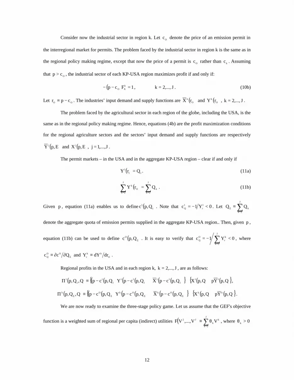
Consider now the industrial sector in region k. Let Oc denote the price of an emission permit in

the interregional market for permits. The problem faced by the industrial sector in region k is the same as in

the regional policy making regime, except that now the price of a permit is Oc rather than kc . Assuming

that Ocp > , the industrial sector of each KP-USA region maximizes profit if and only if:

( ) 1Fcp kXO =−− , J,...,2k = . (10b)

Let OO cpr −≡ . The industries’ input demand and supply functions are ( )Ok rX and ( )O

k rY , J,...,2k = .

The problem faced by the agricultural sector in each region of the globe, including the USA, is the

same as in the regional policy making regime. Hence, equations (4b) are the profit maximization conditions

for the regional agriculture sectors and the sectors’ input demand and supply functions are respectively

( )E,pY j and ( )E,pX j , J,...,1j = .

The permit markets – in the USA and in the aggregate KP-USA region – clear if and only if

( ) 11

1 QrY = . (11a)

( ) ∑∑==

=J

2k

k

J

2k

Ok QrY . (11b)

Given p , equation (11a) enables us to define ( )1

1 Q,pc . Note that 0Y1c 1r

1Q <−= . Let ∑

=Σ ≡

J

2k

kQQ

denote the aggregate quota of emission permits supplied in the aggregate KP-USA region.. Then, given p ,

equation (11b) can be used to define ( )ΣQ,pcO . It is easy to verify that ∑=

<−=J

2k

kr

OQ 0Y1c , where

Σ∂∂≡ Qcc OOQ and O

hh

r drdYY ≡ .

Regional profits in the USA and in each region k, J,...,2k = , are as follows:

( ) ( )( ) ( )( ) ( )( ){ } ( ) ( ){ }Q,pYpQ,pXQ,pcpXQ,pcpYQ,pcpQ,Q,p 111

111

111

11

1 ++−+−−≡Π ,

( ) ( )( ) ( )( ) ( )( ){ } ( ) ( ){ }Q,pYpQ,pXQ,pcpXQ,pcpYQ,pcpQ,Q,p kkOkOkOk ++−+−−≡Π ΣΣΣΣ .

We are now ready to examine the three-stage policy game. Let us assume that the GEF's objective

function is a weighted sum of regional per capita (indirect) utilities ( ) ∑=

θ≡J

2k

kk

J2 VV,...,VF , where 0k >θ

13

for every k and 1J

2k

k ≡θ∑=

. The weights are exogenously given. We postulate that they are implied by the

equilibrium of a political bargaining game, which takes place before the regions commit to participating in

the KP-USA. We do not, however, attempt to formalize such a game here. This is an interesting avenue for

future work.

Consider the third stage of the policy game. Given p , ( )J1 Q,...,Q≡Q and ( )J1 m,...,m≡m , the

GEF chooses interregional income transfers { } J,...,2kkT = to maximize ( )h

J

2h

hh w,pV∑

=

θ subject to

hhhh nTmw +≡ and ∑=

=J

2hh 0T . Let kkk wnW ≡ and kkk mnM ≡ , J,...,2k = . Given these definitions,

the GEF’s problem can be alternatively expressed as the choice of { } J,...,2kkW = to maximize

( )kk

J

2k

kk nW,pV∑

=

θ subject to ∑∑==

=J

2k

k

J

2k

k MW . The first order conditions for maximization can be

written as follows:

( ) ( )( )ν=

θ

k

kkk

kkkk

xk

n

nW,py,nW,pxU, J,...,2k = , (12a)

∑∑==

=J

2k

k

J

2k

k MW , (12b)

where 0>ν is the Lagrangian multiplier associated with the feasibility constraint (12b). Equations (12a)

tell us that the GEF redistributes income across the KP-USA regions in order to equate individuals’

marginal utilities of income.

Let ∑=

Σ ≡J

2k

kMM denote the KP-USA’s aggregate income level. Close inspection of equations

(12a) and (12b) reveals that we can define regional incomes as functions of the price of the industrial good

and the KP-USA’s aggregate income level, ( )ΣM,pW k , J,...,2k = . Inserting these functions and ΣM into

equation (12b), we obtain

( ) Σ=

Σ =∑ MM,pWJ

2k

k . (12c)

Differentiating equation (12c) with respect to ΣM yields

14

1WJ

2k

kM =∑

=

, (12d)

where Σ∂∂≡ MWW kk

M , for J,...,2k = .

The KP-USA’s aggregate income level is given by the sum of initial endowments and profits over

all KP-USA regions. Hence,

( ) ( )( )∑=

ΣΣΣΣ Π+++=J

2h

h0h

0h

O Q,Q,ppYXQQ,pcM , (13)

where one should remember that ∑=

Σ ≡J

2hhQQ .

In the second stage of the game, regulator k wishes to maximize ( )( )kkk nM,pW,pV Σ . However,

one can easily check that ( )( )kkk nM,pW,pV Σ is maximized if and only if regional income, ( )ΣM,pW k ,

is maximized. This implies that regulator k chooses nonnegative { }kQ to maximize ( )ΣM,pW k subject to

equation (13) and ∑=

Σ ≡J

2hhQQ , taking p and every other regulator’s choice as given. Assuming that the

solution of each regulator’s problem is interior, the first order conditions that characterize the Nash

equilibrium in the second stage of the game are

0GcWJ

2h

hE

OkM =

+ ∑

=

, J,...,2k = . (14a)

Given equation (12d), we obtain the following result when we add up the J-1 equations (14a):

0GcWGcJ

2h

hE

OJ

2k

kM

J

2h

hE

O =

+=

+ ∑∑∑

===

,

or

( ) ( )( )∑=

Σ −=J

2h

hhE

O Q,Q,pYGQ,pc . (14b)

Equation (14b) is the equilibrium condition that determines the KP-USA’s aggregate quota level.

It states that all regulators within the aggregate KP-USA region agree on a emission permit price equal to

the sum of the marginal damages caused by carbon dioxide emissions to all KP-USA regions. As each

regulator’s maximization problem makes it clear, the transfers implemented by the GEF induce each

regulator to choose a quota level which maximizes the KP-USA aggregate income level. Hence, each

15

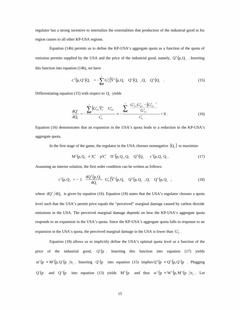
regulator has a strong incentive to internalize the externalities that production of the industrial good in his

region causes to all other KP-USA regions.

Equation (14b) permits us to define the KP-USA’s aggregate quota as a function of the quota of

emission permits supplied by the USA and the price of the industrial good, namely, ( )1Q,pQΣ . Inserting

this function into equation (14b), we have

( )( ) ( )( ) ( )( )∑=

ΣΣΣ ++−=J

2k

1111kk

E1O QQQ,QQQ,pYGQQ,pc . (15)

Differentiating equation (15) with respect to 1Q yields

( ) ( )

0c

G

GGG

c

GYG

dQ

dQo

Q

J

2kkYY

2kYE

kEE

kYY

o

Q

J

2k

kEE

kE

kYE

1

<

−

−≡+

−=∑∑

==Σ

. (16)

Equation (16) demonstrates that an expansion in the USA’s quota leads to a reduction in the KP-USA’s

aggregate quota.

In the first stage of the game, the regulator in the USA chooses nonnegative { }1Q to maximize

( ) ( )( ) ( ) 111

11110

1011

1 QQ,pcQQQ,Q,ppYXQ,pM ++Π++≡ Σ . (17)

Assuming an interior solution, the first order condition can be written as follows:

( ) ( ) ( )( ) ( )( )111111

E

1

11

1 Q,pQQ,Q,pQQ,pYGdQ

Q,pdQ1Q,pc ΣΣ

Σ

++

+−= , (18)

where 1dQdQΣ is given by equation (16). Equation (18) states that the USA’s regulator chooses a quota

level such that the USA’s permit price equals the “perceived” marginal damage caused by carbon dioxide

emissions in the USA. The perceived marginal damage depends on how the KP-USA’s aggregate quota

responds to an expansion in the USA’s quota. Since the KP-USA’s aggregate quota falls in response to an

expansion in the USA’s quota, the perceived marginal damage in the USA is lower than 1EG .

Equation (18) allows us to implicitly define the USA’s optimal quota level as a function of the

price of the industrial good, ( )pQ1 . Inserting this function into equation (17) yields

( ) ( )( ) 1

111 npQ,pMpm ≡ . Inserting ( )pQ1 into equation (15) implies ( ) ( )( )pQ,pQpQ 1ΣΣ ≡ . Plugging

( )pQ1 and ( )pQΣ into equation (13) yields ( )pMΣ and thus ( ) ( )( ) k

kk npM,pWpw Σ≡ . Let

16

( ) ( )( )pm,pypy 111 ≡ , ( ) ( )( )pw,pypy kkk ≡ , ( ) ( )( )pQ,pcppr 111 −≡ , ( ) ( )( )pQ,pcppr 1OO −≡ ,

( ) ( )( )pQ,pYpY 11 ≡ , ( ) ( )( )pQ,pYpY kk ≡ and ( ) ( ) ( )pQpQpQ 1 Σ+≡ . Then, the price of the industrial

good is determined by:

( ) ( )( ) ( )( ) ( )( )∑∑ ∑== =

+++=J

2k

Ok11J

1j

J

1j

j0j

jj prYprYpYYpyn . (19)

The equilibrium allocation of resources for the global economy in this setting is characterized by

equations (3b), (4b), (10a), (10b), (11a), (11b), (12a), (12b), (13), (14a), (14b), (17), (18), (19) and the

budget constraints, 111 mpyx =+ and kkk wpyx =+ , k = 2,...,J. Combining equations (4b), (10b) and

(14b) yields

∑=

+=J

2h

kEk

X

kY G

F1

G . J,...,2k = . (20a)

Combining equations (4b), (10a) and (18), we obtain

1E

11X

1Y G

dQ

dQ1

F

1G

++=

Σ

. (20b)

Now consider the Pareto efficiency conditions (1f) for j = 2,…,J. Equations (20a) differ from their

Pareto efficiency counterparts only in that they do not include the marginal damages caused to the USA.

Equation (20b) differs from its Pareto efficiency counterpart in that it is perceived marginal damage does

not correspond to the global marginal damage. It is also worth noting that the equilibrium conditions that

tell us how interregional transfers are made do not correspond to their Pareto efficiency counterparts

because the equilibrium conditions do not include transfers from or to the USA while Pareto efficiency

requires interregional transfers be made across all regions in the globe.

For future reference, let 1jV be region j’s per capita utility level realized in the global equilibrium

allocation described in this section.

4.3. Ideal Kyoto Protocol

Suppose now that all regions in the globe, including the USA, participate in the Kyoto Protocol (KP).

Regulators and the GEF play a two-stage game, whereby regulators commit to their environmental policies

before the GEF implements interregional transfers. The equilibrium concept for the two-stage game is

again subgame perfection.

17

Let c denote the global price of an emission permit. Assuming that cp > , each region’s industrial

sector maximizes profit if and only if

( ) 1Fcp jX =−− , J,...,1j = . (21)

Let cpr −≡ . Equations (21) enable us to define ( )rX j , J,...,1j = . Hence, ( ) ( )( )rXFrY jjj ≡ , J,...,1j = .

As before, equations (4b) yield the regional agricultural sectors’ input functions ( )Q,pY j , J,...,1j = . Thus,

( ) ( )( )Q,Q,pYGQ,pX jjj ≡ , J,...,1j = .

The global market for emission permits clears if and only if

( ) QrYJ

1j

j =∑=

. (22)

Equation (22) permits us to define ( )Q,pc . It is easy to verify that ∑=

<−=J

1j

jrQ 0Y1c . We can now define

( ) ( )( ) ( )( ) ( )( ){ } ( ) ( ){ }Q,pYpQ,pXQ,pcpXQ,pcpYQ,pcpQ,p jjjjj ++−+−−≡Π , the total profit in region j..

Let jjjj nTmw +≡ be per capita income in region j. The redistribution constraint for the

interregional transfers is now ∑=

=J

1j

j 0T . The demand functions for the representative consumer in region j

are ( )jj w,px and ( )j

j w,py . His indirect utility function is ( ) ( ) ( )( )jj

jjj

jj w,py,w,pxUw,pV ≡ .

Taking p , ( )J1 Q,...,Q≡Q and ( )J1 m,...,m≡m as given, the GEF chooses { }J,...,1jjW

= to

maximize ( )jjj

J

1j

j nW,pV∑=

θ subject to:

MMWJ

1j

j

J

1j

j ≡= ∑∑==

, (23a)

where 0j >θ for all j and 1J

1j

j ≡θ∑=

. Besides equation (23a), the first order conditions for maximization

can be written as follows:

( ) ( )( )η=

θ

j

jj

j

jj

jj

xj

n

nW,py,nW,pxU, J,...,1j = , (23b)

18

where 0>η is the Lagrangian multiplier associated with constraint (23a). Equations (23b) demonstrate

that the GEF implements transfers in order to equalize individual marginal utilities of income across all

regions in the globe. These conditions, therefore, satisfy the Pareto efficiency requirement that the

individual marginal shadow utilities of income be equalized across all regions of the globe. Note that

equations (23b) are identical to equations (2c) provided that 1kk θθ=λ , J,...,2k = .

Equations (23) enable us to define ( )M,pW j , J,...,1j = . Plugging these functions into equation

(23a) yields

( ) MM,pWJ

1j

j =∑=

. (23c)

Differentiating equation (23c) with respect to M , we obtain

1WJ

1j

jM =∑

=

, (24c)

where MWW jj

M ∂∂≡ , J,...,1j = .

The global income level, M , is the sum of all regions’ initial endowments and profits. Then,

( ) ( )( )∑=

Π+++=J

1j

j0j

0j Q,ppYXQQ,pcM . (25)

In the first stage of the game, regulator j chooses nonnegative { }jQ to maximize ( )M,pW j

subject to equation (25), taking p and the choice of every other regulator as given. Assuming that the

solution to each regulator’s problem is interior, the first order conditions that characterize the Nash

equilibrium in the first stage of the game are

0GcWJ

1i

iE

jM =

+ ∑

=

, J,...,1j = . (26a)

Given equation (24c), we obtain the following result when we add up equations (26a) over all j:

0GcWGcJ

1i

iE

J

1j

jM

J

1i

iE =

+=

+ ∑∑∑

===

,

or

( ) ( )( )Q,Q,pYGQ,pc iJ

1i

iE∑

=

−= . (26b)

19

Equation (26b) determines the equilibrium global quota level. It shows that each regulator agrees

on a price of permits equal to the global marginal damages caused by carbon dioxide emissions. The

interregional transfers implemented by the GEF induces each regulator to choose a regional quota level that

maximizes global income. Hence, each regulator finds it desirable to acknowledge the negative effects

brought about by production of the industrial good in his region.

Equation (26b) enables us to define the global quota of emission permits as a function of the price

of the industrial good, ( )pQ . Inserting this function into equation (25), we obtain ( )pM . Hence, we can

define ( ) ( )( ) jjj npM,pWpw ≡ and ( ) ( )( )pw,pypy jjj ≡ . Let ( ) ( )( )pQ,pcppr j −≡ and ( ) ( )( )prYpY jjj ≡ .

Let also ( ) ( )( )pQ,pYpY jj ≡ . Hence, the price of the industrial good is determined by the following market

clearing condition:

( ) ( ) ( )( )∑ ∑= =

++=J

1j

J

1j

jj0j

jj pYpYYpyn . (27)

The global equilibrium allocation of resources in this setting is characterized by equations (3b),

(4b), (21), (22), (23a), (23b), (25), (26a), (26b), (27) and the budget constraints, jjj wpyx =+ , J,...,1j = .

Equations (3b) and (4b) imply that the equilibrium allocation satisfies the Pareto efficiency conditions (1d)

and (1e), respectively. Furthermore, equations (4b), (21) and (26b) together yield the Pareto efficiency

conditions (1f). Since we have already established that the equilibrium allocation satisfies the Pareto

efficiency conditions underlying interregional transfers, we can state this paper’s main result as follows:

Theorem 1: Provided that all regions in the globe participate in the Kyoto Protocol and 0Q j > for all j in

the subgame perfect equilibrium for the policy game played by the regional regulators and the GEF, the

implied equilibrium allocation of resources for the global economy is Pareto efficient.

Theorem 1 is extremely important in light of the USA’s decision to withdraw from the Kyoto

Protocol and the current set of events, in which some countries, such as Russia and Japan, are still unsure

whether or not they should ratify the Protocol. The efficiency properties of the Ideal Kyoto Protocol

scheme, clearly described in Theorem 1, imply that there is potential for each region in the globe to

20

improve its welfare level relative to what it obtains in the status quo. To see this formally, let *JV denote

region j’s welfare level in the equilibrium described in this section. Because the equilibrium allocation

implied by the Ideal Kyoto Protocol scheme is Pareto efficient and the equilibrium allocations implied by

regional policy making and the KP-USA scheme are inefficient, we have

∑∑==

>J

1j

0jj

J

1j

*jj VnVn , (28a)

∑∑==

>J

1j

1jj

J

1j

*jj VnVn . (28b)

Inequality (28a) tell us that the Ideal Kyoto Protocol scheme can satisfy all regions’ participation

constraints if the status quo is characterized by regional policy making – i.e., if the Kyoto Protocol fails.

Similarly, inequality (28b) states that all regions’ participation constraints can also be satisfied by the Ideal

Kyoto Protocol scheme if the status quo is characterized by a setting in which the USA is the only region

that does not participate in the Kyoto Protocol. An interesting implication of inequality (28) is that there is

scope for bribing the USA to reverse its withdraw decision. The bribe would have to satisfy

11*1 VV ≥ (29a)

while, at the same time, not violating

1k*k VV ≥ , J,...,2k = . (29b)

Now, notice that inequality (28b) implies that inequality (29a) as well as the set of J-1 inequalities (29b)

can all be satisfied slack. Not only would the USA be better off by reversing its withdraw decision, but also

every other region in the globe would benefit from conceding to terms – i.e., the bribe – that would

persuade the USA to reverse its decision!

Our global economy does not explicitly distinguish developed from developing regions. How does

our analysis then capture the Kyoto Protocol’s intention of transferring resources from developed to

developing regions? Since the levels of per capita income are higher in developed regions than in

developing regions, the marginal utilities of income are lower in developed regions. Given the exogenous

weights assigned to regional welfare levels, the redistributive transfer mechanism operated by the GEF

transfers resources from regions whose weighted marginal utilities of income are low to regions whose

weighted marginal utilities of income are high. If, for example, the weights are equal across all regions, the

21

transfer mechanism will necessarily transfer resources from developed to developing regions. Indeed, it can

be shown that there is a large number of weight allocations that would imply resource transfers from

developed to developing regions without violating the participation constrains (29a) and (29b).

It must also be stressed that our efficiency result depends crucially on the timing of the policy

game played by regional regulators and the GEF.6 It is, for example, straightforward to show that if the

timing of the game were changed so that the GEF “moved” first and the regional regulators “moved” last,

the implied subgame perfect equilibrium would not feature condition (26b) because the regulators would

not attempt to maximize global income. Since they would essentially treat the GEF transfers as lump-sum

transfers, their decisions would not depend on such transfers. Each regulator would choose a policy that

maximizes regional income, neglecting therefore the negative externalities caused by regional emissions.

Fortunately, our assumption about the timing of the policy game appears to be consistent with

reality. The GEF cannot possibly be a Stackelberg leader. Because it is incapable of punishing nations for

not complying with environmental standards, it lacks political and economical powers to design and

enforce interregional schemes to control emissions of carbon dioxide. Not surprisingly, design and

enforcement of the Kyoto Protocol are responsibilities of the participating nations. As we mentioned in the

introduction, the Conference of the Parties to the United Nations Framework Convention on Climate

Change, which represents the supreme body of the Convention, delegated authority to the GEF to operate

the financial mechanism. Therefore, it appears quite reasonable to postulate that the GEF is a common

Stackelberg follower in the policy game played with regional regulators.

5. Conclusion

In this paper, we demonstrate that there is a combination of emissions trading and transfer mechanisms that

yields an efficient allocation of resources for a global economy. The transfer mechanism should be

redistributive and operated after the regional governments make their policy commitments regarding how

to control regional emissions of carbon dioxide. Furthermore, there should be global participation in both

mechanisms. An interregional scheme featuring global participation and the efficient mix of mechanisms

and timing of operations described above is what an ideal Kyoto Protocol should look like.

6 Our efficiency result, however, does not depend on our game being a quantity leadership game rather than a price leadership game. Changing the strategy space would not alter the incentives of regulators of maximizing global income in the first stage of the game.

22

References

Arce, Daniel, 2001, "Leadership and the Aggregation of International Collective Action," Oxford Economic Papers, 53: 114-137.

Barrett, Scott, 1994, "Self-Enforcing International Environmental Agreements," Oxford Economic Papers,

46: 878-894. Black, Jane, Maurice D. Levi, and David De Meza, 1993, "Creating a Good Atmosphere: Minimum

Participation for Tackling the 'Greenhouse Effect'", Economica, 60: 281-293. Caplan, Arthur J. and Emilson C. D. Silva, 2002, "An Equitable, Efficient and Implementable Scheme to

Control Global Carbon Dioxide Emissions," unpublished manuscript. Caplan, Arthur J., Richard C. Cornes and Emilson C. D. Silva, 2000, "Pure Public Goods and Income

Redistribution in a Federation with Decentralized Leadership and Imperfect Labor Mobility, Journal of Public Economics, 77: 265-284.

Chichilnisky, G., G. Heal and D. Starrett, 2000, "Equity and Efficiency in Environmental Markets: Global

Trade in Carbon Dioxide Emissions," in Environmental Markets: Equity and Efficiency, G. Chilchinisky and G. Heal (eds.), Columbia University Press, New York

Coggins, Jay S. and John R. Swinton, 1996, “The Price of Pollution: A Dual Approach to Valuing SO2

Allowances,” Journal of Environmental Economics and Management, 30: 58-72. Hahn, Robert W., 1989, “Economic Prescriptions For Environmental Problems: How the Patient Followed

the Doctor’s Orders,” Journal of Economic Perspectives, 3(2): 95-114. Kyoto Protocol to the United Nations Framework Convention on Climate Change, December 10, 1997. Maloney, Michael T. and Bruce Yandle, 1984, “Estimation of the Cost of Air Pollution Control

Regulation,” Journal of Environmental Economics and Management, 11: 244-263. Stavins, Robert N., 1998, “What Can We Learn from the Grand Policy Experiment? Lessons from SO2

Allowance Trading,” Journal of Economic Perspectives, 12(3): 69-88.