Embed Size (px)
Citation preview

http://smm.sagepub.com
Statistical Methods in Medical Research
DOI: 10.1177/0962280206075310 2007; 16; 457 originally published online Jul 26, 2007; Stat Methods Med Res
Caroline Beunckens, Geert Molenberghs, Herbert Thijs and Geert Verbeke Incomplete hierarchical data
http://smm.sagepub.com The online version of this article can be found at:
Published by:
http://www.sagepublications.com
can be found at:Statistical Methods in Medical Research Additional services and information for
http://smm.sagepub.com/cgi/alerts Email Alerts:
http://smm.sagepub.com/subscriptions Subscriptions:
http://www.sagepub.com/journalsReprints.navReprints:
http://www.sagepub.com/journalsPermissions.navPermissions:
http://smm.sagepub.com/cgi/content/refs/16/5/457SAGE Journals Online and HighWire Press platforms):
(this article cites 70 articles hosted on the Citations
© 2007 SAGE Publications. All rights reserved. Not for commercial use or unauthorized distribution. at PENNSYLVANIA STATE UNIV on February 6, 2008 http://smm.sagepub.comDownloaded from

Statistical Methods in Medical Research 2007; 16: 457–492
Incomplete hierarchical dataCaroline Beunckens, Geert Molenberghs, Herbert Thijs Center for Statistics, HasseltUniversity, Diepenbeek, Belgium and Geert Verbeke Biostatistical Centre, KatholiekeUniversiteit Leuven, Leuven, Belgium
The researcher collecting hierarchical data is frequently confronted with incompleteness. Since the pro-cesses governing missingness are often outside the investigator’s control, no matter how well the experimenthas been designed, careful attention is needed when analyzing such data. We sketch a standard frameworkand taxonomy largely based on Rubin’s work. After briefly touching upon (overly) simple methods, we turnto a number of viable candidates for a standard analysis, including direct likelihood, multiple imputationand versions of generalized estimating equations. Many of these require so-called ignorability. With thelatter condition not necessarily satisfied, we also review flexible models for the outcome and missingnessprocesses at the same time. Finally, we illustrate how such methods can be very sensitive to modelingassumptions and then conclude with a number of routes for sensitivity analysis. Attention will be given tothe feasibility of the proposed modes of analysis within a regulatory environment.
1 Introduction
Longitudinal data are common in biomedical research and beyond. A typical study,for instance, would consist of observing a metric outcome or a characteristic over time,taken in relation to covariates of interest. Data arising from such investigations, however,are more often than not prone to incompleteness or missingness. In the context oflongitudinal studies, missingness predominantly occurs in the form of dropouts, in whichsubjects fail to complete the study for one reason or another. In other studies, such ashierarchically designed surveys, missingness can take more general forms.
The nature of the missingness mechanism can affect the resulting analysis of incom-plete data. Since once can never be certain about the precise form of the non-responseprocess, certain assumptions have to be made. Therefore, when referring to the missing-ness process, we will use the terminology introduced by Rubin1. A non-response processis said to be missing completely at random (MCAR) if the missingness is independent ofboth unobserved and observed data, and missing at random (MAR) if, conditional on theobserved data, the missingness is independent of the unobserved measurements. A pro-cess that is neither MCAR nor MAR is termed non-random (MNAR). In the context oflikelihood inference, and when the parameters describing the measurement process arefunctionally independent of the parameters describing the missingness process, MCARand MAR are ignorable, while an MNAR process is non-ignorable. This is not the case
Address for correspondence: Caroline Beunckens, Center for Statistics, Hasselt University, Agoralaan 1,B3590 Diepenbeek, Belgium. E-mail: [email protected]
© 2007 SAGE Publications 10.1177/0962280206075310Los Angeles, London, New Delhi and Singapore
© 2007 SAGE Publications. All rights reserved. Not for commercial use or unauthorized distribution. at PENNSYLVANIA STATE UNIV on February 6, 2008 http://smm.sagepub.comDownloaded from

458 C Beunckens et al.
for frequentist inference, where the stronger condition of MCAR is required to ensureignorability.
In this article, we will describe a number of methods to deal with incompletehierarchical data. After introducing a leading case study from opthalmology, the age-related macular degeneration (ARMD) trial, in Section 2, and the necessary notationalframework in Section 3, a variety of analysis methods are described next. Simple meth-ods, finding their roots in the past decades, are reviewed and criticized in Section 4,while a set of more modern and, under MAR, broadly valid methods are presentedin Section 5. These methods are applied in Section 6 to the ARMD trial. Methodsdesigned to cope with MNAR and sensitivity analysis tools are discussed in Sections 7and 8, respectively. Sensitivity analysis results on the ARMD trial are reported inSections 9.
2 ARMD trial
These data arise from a randomized multicentric clinical trial comparing an experimen-tal treatment (interferon-α) to a corresponding placebo in the treatment of patients withARMD. Throughout the analyses, we focus on the comparison between placebo andthe highest dose (six million units daily) of interferon-α (Z), but the full results of thistrial have been reported elsewhere (Pharmacological Therapy for Macular Degenera-tion Study Group 1997). Patients with macular degeneration progressively lose vision.In the trial, the patients’ visual acuity was assessed at different time points (4, 12, 24and 52 weeks) through their ability to read lines of letters on standardized vision charts.These charts display lines of five letters of decreasing size, which the patient must readfrom top (largest letters) to bottom (smallest letters). Each line with at least four let-ters correctly read is called one ‘line of vision’. The patient’s visual acuity is the totalnumber of letters correctly read. The primary endpoint of the trial was the loss of atleast three lines of vision at 1 year, compared with their baseline performance (a binaryendpoint). The secondary endpoint of the trial was the visual acuity at 1 year (treatedas a continuous endpoint).
Table 1 shows the visual acuity (mean and standard error) by the treatment group atbaseline and at the four measurement occasions after baseline.
Table 1 ARMD trial
Time point Placebo Active Total
Baseline 55.3 (1.4) 54.6 (1.4) 55.0 (1.0)4 weeks 54.0 (1.5) 50.9 (1.5) 52.5 (1.1)12 weeks 52.9 (1.6) 48.7 (1.7) 50.8 (1.2)24 weeks 49.3 (1.8) 45.5 (1.8) 47.5 (1.3)1 year (52 weeks) 44.4 (1.8) 39.1 (1.9) 42.0 (1.3)
Note: Mean (standard error) of visual acuity at baseline, at 4,12, 24 and 52 weeks according to randomized treatment group(placebo versus interferon-α).
© 2007 SAGE Publications. All rights reserved. Not for commercial use or unauthorized distribution. at PENNSYLVANIA STATE UNIV on February 6, 2008 http://smm.sagepub.comDownloaded from

Incomplete hierarchical data 459
Table 2 ARMD trial
Measurement occasion Number %
4 weeks 12 weeks 24 weeks 52 weeks
CompletersO O O O 188 78.33
DropoutsO O O M 24 10.00O O M M 8 3.33O M M M 6 2.50M M M M 6 2.50
Non-monotone missingnessO O M O 4 1.67O M M O 1 0.42M O O O 2 0.83M O M M 1 0.42
Note: Overview of missingness patterns and the frequencies with which they occur.‘O’ indicates observed and ‘M’ indicates missing.
Visual acuity can be measured in several ways. First, one can record the number ofletters read. Alternatively, dichotomized versions (at least three lines of vision lost versusless than three lines of vision lost) can be used as well.
Regarding missingness in the ARMD data set, an overview of the different dropoutpatterns is given in Table 2. Clearly, both intermittent missingness and dropout occurs.It is observed that 188 of the 240 profiles are complete, which is a percentage of 78.33%,while 18.33% (44 subjects) exhibit monotone missingness. Out of the latter group, 2.5%or six subjects have no follow-up measurements. The remaining 3.33%, representingeight subjects, have intermittent missing values. Although the group of dropouts isof considerable magnitude, the ones with intermittent missingness is much smaller.Nevertheless, it is cautious to include all into the analyses.
Both the original quasi-continuous and a dichotomized version of the incompletelongitudinal outcome will be analyzed. The data analyses can be found in Sections 6and 9.
3 Data setting and modeling framework
Assume that for subject i = 1, . . . , N in the study, a sequence of responses Yij is designedto be measured at occasions j = 1, . . . , n. The outcomes are grouped into a vector Yi =(Yi1, . . . , Yin)
′. In addition, define a dropout indicator Di for the occasion at whichdropout occurs and make the convention that Di = n + 1 for a complete sequence. It isoften necessary to split the vector Yi into observed (Yo
i ) and missing (Ymi ) components,
respectively. Note that dropout is a particular case of monotone missingness. In orderto have a monotone pattern of missingness, there has to exist a permutation of themeasurement components such that a measurement earlier in the permuted sequenceis observed for at least those subjects that are observed at later measurements. For thisdefinition to be meaningful, we need to have a balanced design in the sense of a common
© 2007 SAGE Publications. All rights reserved. Not for commercial use or unauthorized distribution. at PENNSYLVANIA STATE UNIV on February 6, 2008 http://smm.sagepub.comDownloaded from
460 C Beunckens et al.
set of measurement occasions for all subjects. Other patterns are called non-monotoneor intermittent missingness. When intermittent missingness occurs, one should use avector of binary indicators Ri = (Ri1, . . . , Rin)
′ rather than the dropout indicator Di.In principle, one would like to consider the density of the full data f ( yi, di|θ , ψ),
where the parameter vectors θ and ψ describe the measurement and missingness pro-cesses, respectively. Covariates are assumed to be measured but, for notational simplicity,suppressed from notation.
To analyze the full data different routes can be taken. The first one is the selectionmodel framework, on which the taxonomy, constructed by Rubin1, further developed inLittle and Rubin2, is based. Selection modeling makes use of the factorization
f ( yi, di|θ , ψ) = f ( yi|θ)f (di|yi, ψ) (1)
where the first factor is the marginal density of the measurement process and thesecond one is the density of the missingness process, conditional on the outcomes. Thesecond factor corresponds to the (self-)selection of individuals into ‘observed’ and ‘miss-ing’ groups. An alternative taxonomy can be built based on so-called pattern-mixturemodels.3,4 These are based on the reversed factorization
f ( yi, di|θ , ψ) = f ( yi|di, θ)f (di|ψ) (2)
Indeed, Equation (2) can be seen as a mixture of different populations characterized bythe observed pattern of missingness. Finally, a third modeling framework that can beused to analyze the full data is called a shared parameter model. In such a model, themeasurement and dropout process are assumed to be independent, given a certain set ofshared parameters.
Most strategies used to analyze such data are, implicitly or explicitly, based on twochoices.
3.1 Model for measurementsA choice has to be made regarding the modeling approach to the measurement
sequence. Several views are possible.
View 1. One can choose to analyze the entire longitudinal profile, irrespective ofwhether interest focusses on the entire profile (e.g., difference in slope betweengroups) or on a specific time point (e.g., the last planned occasion). In the lattercase, one would make inferences about such an occasion within the positedmodel.
View 2. One states the scientific question in terms of the outcome at a well-definedpoint in time. Several choices are possible:View 2a. The scientific question is defined in terms of the last planned occa-
sion. In this case, one can either accept the dropout as it is or useone or other strategy (e.g., imputation and direct likelihood) toincorporate the missing outcomes.
View 2b. One can choose to define the question and the correspondinganalysis in terms of the last observed measurement.
© 2007 SAGE Publications. All rights reserved. Not for commercial use or unauthorized distribution. at PENNSYLVANIA STATE UNIV on February 6, 2008 http://smm.sagepub.comDownloaded from

Incomplete hierarchical data 461
While Views 1 and 2a necessitate reflection on the missing data mechanism, View 2bavoids the missing data problem because the question is couched completely in termsof observed measurements. Thus, under View 2b, a last observation carried forward(LOCF) analysis might be acceptable, provided it matched the scientific goals, but isthen better described as a last observation analysis because nothing is carried forward.Such an analysis should properly be combined with an analysis of time to dropout,perhaps in a survival analysis framework. Of course, an investigator should reflect verycarefully on whether View 2b represents a relevant and meaningful scientific question5.
3.2 Method for handling missingnessA choice has to be made regarding the modeling approach for the missingness pro-
cess. Under certain assumptions, this process can be ignored (e.g., a likelihood-basedignorable analysis). Some simple methods, such as a complete case (CC) analysis andLOCF, do not explicitly address the missingness process either.
We first describe the measurement and missingness models in turn, then formallyintroduce and comment on ignorability.
The measurement model will depend on whether or not a full longitudinal analysis isdone. When the focus is on the last observed measurement or on the last measurementoccasion only, one typically opts for classical two- or multi-group comparisons (t-test,Wilcoxon, and so on). When a longitudinal analysis is deemed necessary, the choicedepends on the nature of the outcome. A variety of methods will be discussed in Section 5.
Assume that incompleteness is due to dropout only, and that the first measurementYi1 is obtained for everyone. Under the selection modeling framework, a possible modelfor the dropout process is a logistic regression for the probability of dropout at occasionj, given that the subject is still in the study. We denote this probability by g(hij, yij) inwhich hij is a vector containing all responses observed up to but not including occasionj, as well as relevant covariates. We then assume that g(hij, yij) satisfies6
logit[g(hij, yij)] = logit[pr(Di = j|Di ≥ j, yi)] = hijψ + ωyij, i = 1, . . . , N (3)
When ω equals zero, the dropout model is MAR, and all parameters can be estimatedusing standard software since the measurement model for which we use a linear mixedmodel, and the dropout model, assumed to follow a logistic regression, can then befitted separately. If ω �= 0, the posited dropout process is MNAR. Model (3) provides thebuilding blocks for the dropout process f (di|yi, ψ). While it has been used, in particular,by Diggle and Kenward6, it is, at this stage, quite general and allows for a wide varietyof modeling approaches.
Rubin1 and Little and Rubin2 have shown that, under MAR and the condition thatparameters θ and ψ are functionally independent, likelihood-based inference remainsvalid when the missing data mechanism is ignored7. Practically speaking, the likelihoodof interest is then based upon the factor f (yo
i |θ). This is called ignorability. The practicalimplication is that a software module with likelihood estimation facilities and with theability to handle incompletely observed subjects, manipulates the correct likelihood,providing valid parameter estimates and likelihood ratio values. Note that the estimands
© 2007 SAGE Publications. All rights reserved. Not for commercial use or unauthorized distribution. at PENNSYLVANIA STATE UNIV on February 6, 2008 http://smm.sagepub.comDownloaded from

462 C Beunckens et al.
are the parameters of Equation (6), which is a model for complete data, correspondingto what one would expect to see in the absence of dropouts.
A few cautionary remarks are warranted. First, when at least part of the scientificinterest is directed towards the non-response process, obviously both processes needto be considered. Under MAR, both processes can be modeled and parameters esti-mated separately. Second, likelihood inference is often surrounded with references tothe sampling distribution (e.g., to construct measures of precision for estimators and forstatistical hypothesis tests8). However, the practical implication is that standard errorsand associated tests, when based on the observed rather than the expected informationmatrix and given that the parametric assumptions are correct, are valid. Third, it may behard to rule out the operation of an MNAR mechanism. This point was brought up inthe introduction and will be discussed further in Section 8. Fourth, such an analysis canproceed only under View 1, that is, a full longitudinal analysis is necessary, even wheninterest lies, for example, in a comparison between the two treatment groups at the lastoccasion. In the latter case, the fitted model can be used as the basis for inference at thelast occasion. A common criticism is that a model needs to be considered with the risk ofmodel misspecification. However, it should be noted that in many clinical trial settings,the repeated measures are balanced in the sense that a common (and often limited) setof measurement times is considered for all subjects, allowing the a priori specificationof a saturated model (e.g., full group by time interaction model for the fixed effectsand unstructured variance–covariance matrix). Such an ignorable linear mixed modelspecification is termed (mixed-model random missingness MMRM) by Mallinckrodtet al. 9,10 Thus, MMRM is a particular form of a linear mixed model, fitting within theignorable-likelihood paradigm. Such an approach is a promising alternative to the oftenused simple methods such as CC analysis or LOCF. These will be described in the nextsection and further studied in subsequent sections.
4 Simple methods
We will briefly review a number of relatively simple methods that still are commonlyused. For the validity of many of these methods, MCAR is required. For others, such asLOCF, MCAR is necessary but not sufficient. The focus will be on the CC method forwhich data are removed, and on imputation strategies where data are filled in. Regardingimputation, one distinguishes between single and multiple imputation. In the first case,a single value is substituted for every ‘hole’ in the data set and the resulting data set isanalyzed as if it represented the true complete data. Multiple imputation acknowledgesthe uncertainty stemming from filling in missing values rather than observing them.11,12
LOCF will be discussed within the context of imputation strategies, although LOCF canbe placed in other frameworks as well.
A CC analysis includes only those cases for which all measurements were recorded.This method has obvious advantages. The method is simple since it restores balance, inthe sense that a rectangular data matrix is obtained. Consequently, standard statisticalsoftware can be used to analyze the CCs. However, the drawbacks surpass the advantages.Apart from considerable information loss, leading to inefficient estimates and tests with
© 2007 SAGE Publications. All rights reserved. Not for commercial use or unauthorized distribution. at PENNSYLVANIA STATE UNIV on February 6, 2008 http://smm.sagepub.comDownloaded from

Incomplete hierarchical data 463
less than optimal power, severe bias can result when the missingness mechanism is MARbut not MCAR. A CC analysis can be conducted when Views 1 and 2a of Section 3 areadopted. It, obviously is not a reasonable choice with View 2b.
Alternatively, balance can be restored by filling in rather than deleting2. The observedvalues are used to impute values for the missing observations. There are several waysto use the observed information. First, one can use the information on the same sub-ject (e.g., LOCF). Second, information can be borrowed from other subjects (e.g., meanimputation). Finally, both within and between subject information can be used (e.g.,conditional mean imputation and hot deck imputation). The practical advantages arethe same as with CC, indeed, complete data software can be used to analyze the obtainedimputed data set. However, many issues arise when using such an imputation method.First of all, filled-in values are used as if it were actual data. The imputation modelcould be wrong, leading to biased point estimates. Further, even for a correct impu-tation model, the uncertainty from missingness is ignored. Indeed, even when one isreasonably sure about the mean value the unknown observation would have had, theactual stochastic realization, depending on both the mean and error structures, is stillunknown. In addition, most methods require the MCAR assumption to hold and someeven require additional and often unrealistically strong assumptions.
As stated above, a method that has received considerable attention9,10,13 is LOCF. Inthe LOCF method, whenever a value is missing, the last observed value is substituted.The technique is typically applied in settings where incompleteness is due to attrition,but can also be used in case of non-monotone missingness.
LOCF can, but does not have to be, regarded as an imputation strategy, dependingon which of the views of Section 3 is taken. The choice of viewpoint has a number ofconsequences. Either when we consider a longitudinal analysis (View 1) or when thescientific question is in terms of the last planned occasion (View 2a), one has to believethat a subjects measurement stays at the same level from the moment of dropout onwards(or during the period they are unobserved in the case of intermittent missingness). Ina clinical trial setting, one might believe that the response profile changes as soon as apatient goes off treatment and even that it would flatten. However, the constant profileassumption is even stronger.
The situation, in which the scientific question is in terms of the last observed mea-surement (View 2b), is often considered to be the real motivation for LOCF. However insome cases, the question, defined as such, has a very unrealistic and adhoc flavor. Clearly,measurements at (self-selected) dropout times are lumped together with measurementsmade at the (investigator defined) end of the study.
Several pieces of criticism have been brought forward. Molenberghs et al.14 andBeunckens et al.15 have shown that the bias resulting from LOCF can both be con-servative and liberal, contradicting common believe that the appeal of the method liesin it being conservative for the assessment of treatment effect in superiority trials.
Further, it is often quoted that LOCF or CC, while problematic for parameter esti-mation, produce randomization-valid hypothesis testing, but this too is questionable.First, in a CC analysis, partially observed data are selected out with probabilities thatmay depend on post-randomization outcomes, thereby undermining any randomizationjustification. Second, if the focus is on one particular time point, for example, the last one
© 2007 SAGE Publications. All rights reserved. Not for commercial use or unauthorized distribution. at PENNSYLVANIA STATE UNIV on February 6, 2008 http://smm.sagepub.comDownloaded from

464 C Beunckens et al.
scheduled, then LOCF plugs in data. Such imputations, apart from artificially inflatingthe information content, may deviate in complicated ways from the underlying data.In contrast, a likelihood-based MAR analysis uses all available data, with the need forneither deletion nor imputation, which suggests that a likelihood-based MAR analysiswould usually be the preferred one for testing as well. Third, although the size of arandomization-based LOCF test may reach its nominal size under the null hypothesisof no difference in treatment profiles, there will be other regions of the alternative spacewhere the power of the LOCF test procedure is equal to its size, which is completelyunacceptable.
These and other arguments have led these authors to prefer such methods as will beintroduced in Section 5.
We will briefly describe two other imputation methods. The idea behind unconditionalmean imputation2 is to replace a missing value with the average of the observed valueson the same variable over the other subjects. Thus, the term unconditional refers tothe fact that one does not use (i.e, condition on) information on the subject for whichan imputation is generated. Since values are imputed that are unrelated to a subject’sother measurements, all aspects of a model, such as a linear mixed model, are typicallydistorted.16 In this sense, unconditional mean imputation can be as damaging as LOCF.
Buck’s method or conditional mean imputation2,17 is similar in complexity to meanimputation. Consider, for example, a single multivariate normal sample. The first stepis to estimate the mean vector μ and the covariance matrix � from the CCs, assumingthat Yi ∼ N(μ, �). For a subject with missing components, the regression of the missingcomponents (Ym
i ) on the observed ones (yoi ) is
Ymi |yo
i ∼ N(μm + �mo(�oo)−1(yoi − μo
i ), �mm − �mo(�oo)−1�om) (4)
The second step calculates the conditional mean from the regression of the missingcomponents on the observed components, and substitutes the conditional mean for thecorresponding missing values. In this way, ‘vertical’ information (estimates for μ and�) is combined with ‘horizontal’ information (Yo
i ). Buck17 showed that under mildconditions, the method is valid under MCAR mechanisms. Little and Rubin2 added thatthe method is also valid under certain MAR mechanisms. Even though the distribu-tion of the observed components is allowed to differ between complete and incompleteobservations, it is very important that the regression of the missing components on theobserved ones is constant across missingness patterns. Again, this method shares withother single imputation strategies that, although point estimation may be consistent,the precision will be overestimated. There is a connection between the concept of condi-tional mean imputation and a likelihood-based ignorable analysis, in the sense that thelatter analysis produces expectations for the missing observations that are formally equalto those obtained under a conditional mean imputation. However, in likelihood-basedignorable analyses, no explicit imputation takes place, hence the amount of informationin the data is not overestimated and important model elements, such as mean structureand variance components, are not distorted.
Historically, an important motivation behind the simpler methods was their simplicity,that is, predominantly their computational convenience. Currently, with the availability
© 2007 SAGE Publications. All rights reserved. Not for commercial use or unauthorized distribution. at PENNSYLVANIA STATE UNIV on February 6, 2008 http://smm.sagepub.comDownloaded from

Incomplete hierarchical data 465
of commercial software tools such as, for example, the SAS procedures MIXED,GLIMMIX and NLMIXED, the SPlus and R nlme libraries and the SPSS-based GLAMMpackage, this motivation no longer applies. Arguably, an MAR analysis is the preferredchoice. Of course, the correctness of an MAR analysis rests upon the truth of the MARassumption, which is, in turn, never completely verifiable. Purely resorting to MNARanalyses is not satisfactory either since important sensitivity issues then arise. These andrelated issues are briefly discussed in the next section.7
5 Standard methods
In this section, we will present standard modeling frameworks for longitudinal data.First, the continuous case will be treated where the linear mixed model undoubtedlyoccupies the most prominent role. Then, we switch to the discrete setting, where impor-tant distinctions exist between three model families: the marginal, random-effects andconditional model family. The mixed model parameters, both in the continuous anddiscrete cases, are usually estimated using maximum likelihood-based methods whichimplies that the results are valid under MAR. A commonly encountered marginalapproach to non-Gaussian data is generalized estimating equations (GEEs)18 whichhas a frequentist foundation. It is valid only under MCAR,18 necessitating the need forextensions, such as weighted GEE,19 multiple-imputation based GEE20 and so on, whichwill be discussed as well.
5.1 Continuous longitudinal dataFor continuous outcomes, one typically assumes a linear mixed-effects model, perhaps
with serial correlation7
Yi = Xiβ + Zibi + W i + εi (5)
where Yi is the n-dimensional response vector for subject i, 1 ≤ i ≤ N, N is the num-ber of subjects, Xi and Zi are (n × p) and (n × q) known design matrices, β is thep-dimensional vector containing the fixed effects, bi ∼ N(0, D) is the q-dimensionalvector containing the random effects, εi ∼ N(0, σ 2Ini) is a n-dimensional vector of mea-surement error components and b1, . . . , bN, ε1, . . . , εN are assumed to be independent.Serial correlation is captured by the realization of a Gaussian stochastic process, W i,which is assumed to follow a N(0, τ 2Hi) law. The serial covariance matrix Hi onlydepends on i through the number n of observations and through the time points tij atwhich measurements are taken. The structure of the matrix Hi is determined through theauto-correlation function ρ(tij − tik). This function decreases such that ρ(0) = 1 andρ(u) → 0 as u → ∞. Finally, D is a general (q × q) covariance matrix with (i, j) elementdij = dji. Inference is based on the marginal distribution of the response Yi which, afterintegrating over random effects, can be expressed as
Yi ∼ N(Xiβ, ZiDZi′ + �i) (6)
© 2007 SAGE Publications. All rights reserved. Not for commercial use or unauthorized distribution. at PENNSYLVANIA STATE UNIV on February 6, 2008 http://smm.sagepub.comDownloaded from

466 C Beunckens et al.
Here, �i = σ 2Ini + τ 2Hi is a (n × n) covariance matrix combining the measurementerror and serial components.
5.2 Discrete longitudinal dataWhereas the linear mixed model is seen as a unifying parametric framework for Gaus-
sian repeated measures,7 there are many more options available in the non-Gaussiansetting. In a marginal model, marginal distributions are used to describe the outcomevector, given a set of predictor variables. The correlation among the components of theoutcome vector can then be captured either by adopting a fully parametric approachor by means of working assumptions, such as in the semiparametric approach of Liangand Zeger.18 Alternatively, in a random-effects model, the predictor variables are sup-plemented with a vector of random effects, conditional upon which the components ofthe response vector are usually assumed to be independent. Finally, a conditional modeldescribes the distribution of the components of the outcome vector, conditional on thepredictor variables but also conditional on (a subset of) the other components of theresponse vector. Well-known members of this class of models are log-linear models.21 Letus give a simple example of each for the case of Gaussian outcomes, or more generallyfor models with a linear mean structure.
A marginal model is characterized by a marginal mean function of the form
E(Yij|xij) = x′ijβ (7)
where xij is a vector of covariates for subject i at occasion j and β is a vector of regressionparameters.
In a random-effects model, we focus on the expectation, additionally conditioningupon a random-effects vector bi
E(Yij|bi, xij) = x′ijβ + z′
ijbi (8)
Finally, a third family of models conditions a particular outcome on the other responsesor a subset thereof. In particular, a simple first-order stationary transition model focusseson expectations of the form
E(Yij|Yi,j−1, . . . , Yi1, xij) = x′ijβ + αYi,j−1 (9)
Alternatively, one might condition upon all outcomes except the one being modeled
E(Yij|Yik,k �=j, xij) = x′ijβ + αYij
where Yij represents Yi with the jth component omitted.As shown by Verbeke and Molenberghs7 and seen in the previous section, random-
effects models imply a simple marginal model in the linear mixed model case. This is dueto the elegant properties of the multivariate normal distribution. In particular, expec-tation (7) follows from Equation (8) by either 1) marginalizing over the random effectsor by 2) conditioning upon the random-effects vector bi = 0. Hence, the fixed-effects
© 2007 SAGE Publications. All rights reserved. Not for commercial use or unauthorized distribution. at PENNSYLVANIA STATE UNIV on February 6, 2008 http://smm.sagepub.comDownloaded from

Incomplete hierarchical data 467
parameters β have a marginal and a hierarchical model interpretation at the same time.Finally, certain auto-regressive models in which later-time residuals are expressed interms of earlier ones lead to particular instances of the general linear mixed effectsmodel as well and hence have a marginal function of the form (7).
Since the linear mixed model has marginal, hierarchical and conditional aspects, it isclear why it provides a unified framework in the Gaussian setting. However, there doesnot exist such a close connection when outcomes are of a non-Gaussian type, such asbinary, categorical or discrete.
We will consider the marginal and random-effects model families in turn and thenpoint to some particular issues arising within them or when comparisons are madebetween them. The conditional models are less useful in the context of longitudinal dataand will not be discussed here.22
5.3 Marginal modelsThorough discussions on marginal modeling can be found in Diggle et al. 23 and in
Molenberghs and Verbeke.22 For the sake of completeness, we list a few full-likelihoodmethods. Bahadur24 proposed a marginal model, accounting for the association viamarginal correlations. Ashford and Sowden25 considered the multivariate probit model,for repeated ordinal data, thereby extending univariate probit regression. Molenberghsand Lesaffre26 and Long and Agresti27 have proposed models which parameterize theassociation in terms of marginal odds ratios. Dale28 defined the bivariate global oddsratio model, based on a bivariate Plackett distribution.29 Molenberghs and Lesaffre,26,30
Lang and Agresti27 and Glonek and McCullagh31 extended this model to multivariateordinal outcomes. They generalize the bivariate Plackett distribution in order to establishthe multivariate cell probabilities.
Apart from these full-likelihood approaches, non-likelihood approaches, such asGEEs18 or pseudo-likelihood32,33 have been considered.
While full-likelihood methods are appealing because of their flexible ignorabilityproperties (Section 3), their use for non-Gaussian outcomes can be problematic due toprohibitive computational requirements. Therefore, GEE is a viable alternative withinthis family. Since GEE is motivated by frequentist considerations, the missing datamechanism needs to be MCAR for it to be ignorable. This motivates the proposalof so-called weighted generalized estimating equations (WGEE). We will discuss thesein turn.
5.3.1 Generalized estimating equationsLet us introduce more formally the classical form of GEE.18,22 The score equations
for a non-Gaussian outcome are
S(β) =N∑
i=1
∂μi
∂β ′ (A1/2i CiA
1/2i )−1(yi − μi) = 0 (10)
Although Ai = Ai(β) follows directly from the marginal mean model, β commonlycontains no information about Ci. Therefore, the correlation matrix Ci typically iswritten in terms of a vector α of unknown parameters, Ci = Ci(α).
© 2007 SAGE Publications. All rights reserved. Not for commercial use or unauthorized distribution. at PENNSYLVANIA STATE UNIV on February 6, 2008 http://smm.sagepub.comDownloaded from

468 C Beunckens et al.
Liang and Zeger18 dealt with this set of nuisance parameters α by allowing forspecification of an incorrect structure or so-called working correlation matrix. Assumingthat the marginal mean μi has been correctly specified as h(μi) = Xiβ, they showed that,under mild regularity conditions, the estimator β̂ obtained from solving Equation (10)is asymptotically normally distributed with mean β and with covariance matrix
Var(β̂) = I−10 I1I−1
0 (11)
where
I0 =( N∑
i=1
∂μ′i
∂βV−1
i∂μi
∂β ′
), I1 =
( N∑
i=1
∂μ′i
∂βV−1
i Var(yi)V−1i
∂μi
∂β ′
)
Consistent estimates can be obtained by replacing all unknown quantities in Equa-tion (11) by consistent estimates. Observe that, when Ci would be correctly specified,Var(Yi) = V i, and thus I1 = I0. As a result, the expression for the covariance matrix (11)would reduce to I−1
0 , corresponding to full likelihood, that is, when the first and secondmoment assumptions would be correct. Thus, when the working correlation structureis correctly specified, it reduces to full likelihood, although generally it differs from it.There is no price to pay in terms of consistency of asymptotic normality, but there maybe efficiency loss when the working correlation structure differs strongly from the trueunderlying structure.
Two further specifications are necessary before GEE is operational: Var(Yi) on theone hand and Ci(α), with in particular estimation of α, on the other hand. Full modelingwill not be an option, since we would then be forced to do what we want to avoid. Inpractice, Var(yi) in Equation (11) is replaced by (yi − μi)(yi − μi)
′, which is unbiasedon the sole condition of correct mean specification. One also needs estimates of thenuisance parameters α. Liang and Zeger18 proposed moment-based estimates for theworking correlation. To this end, deviations of the form
eij = yij − πij√πij(1 − πij)
are used. Note that eij = eij(β) through μij = μij(β) and therefore also through v(μij),the variance at time j and hence the jth diagonal element of Ai.
Some of the more popular choices for the working correlations are independence(Corr(Yij, Yik) = 0, j �= k), exchangeability (Corr(Yij, Yik) = α, j �= k), AR(1) (Corr(Yij, Yi,j+t) = αt, t = 0, 1, . . . , ni − j) and unstructured (Corr(Yij, Yik) = αjk, j �= k).
An overdispersion parameter could be included as well, but we have suppressed it forease of exposition. The standard iterative procedure to fit GEE, based on Liang andZeger18 is then as follows: 1) compute initial estimates for β using a univariate GLM(i.e., assuming independence); 2) compute Pearson residuals eij; 3) compute estimatesfor α; 4) compute Ci(α); 5) compute Vi(β, α) = A1/2
i (β)Ci(α)A1/2i (β); 6) update the
© 2007 SAGE Publications. All rights reserved. Not for commercial use or unauthorized distribution. at PENNSYLVANIA STATE UNIV on February 6, 2008 http://smm.sagepub.comDownloaded from

Incomplete hierarchical data 469
estimate for β:
β(t+1) = β(t) −[ N∑
i=1
∂μ′i
∂βV−1
i∂μi
∂β
]−1 [ N∑
i=1
∂μ′i
∂βV−1
i (yi − μi)
]
Steps 2–6 are iterated until convergence.
5.3.2 Weighted generalized estimating equationsAs Liang and Zeger18 pointed out, GEE-based inferences are valid only under MCAR,
because of the fact that they are based on frequentist considerations. An importantexception, mentioned by these authors, is the situation where the working correlationstructure, happens to be correct, since then the estimates and model-based standarderrors are valid under the weaker MAR. In that case, the estimating equations canbe interpreted as likelihood equations. In general, of course, the working correlationstructure will not be correctly specified. Therefore, Robins et al.19 proposed a class ofWGEEs to allow for MAR, by extending GEE.
The idea of WGEE is to weight each subject’s contribution in the GEEs by the inverseprobability that a subject drops out at the time he dropped out. The incorporationof these weights is expected to reduce possible bias of the estimates of the regressionparameters, β̂. Such a weight can be calculated as
νij ≡ P[Di = j] =j−1∏
k=2
(1 − P[Rik = 0|Ri2 = · · · = Ri,k−1 = 1])
× P[Rij = 0|Ri2 = · · · = Ri,j−1 = 1]I{j≤ni}
if dropout occurs by time j or we reach the end of the measurement sequence, and
νij ≡ P[Di = j] =di−1∏
k=2
(1 − P[Rik = 0|Ri2 = · · · = Ri,k−1 = 1])
otherwise.An alternative mode of analysis, generally overlooked but proposed by Schafer,20
would consist in multiply imputing the missing outcomes using a parametric model, forexample, of a random-effects or conditional type, followed by conventional GEE andconventional multiple-imputation inference on the so-completed sets of data. A detailedcomparison has been made by Beunckens et al.34
5.4 Random-effects modelsUnlike for correlated Gaussian outcomes, the parameters of the random-effects
and population-averaged models for correlated binary data describe different typesof effects of the covariates on the response probabilities.35 Therefore, the choice
© 2007 SAGE Publications. All rights reserved. Not for commercial use or unauthorized distribution. at PENNSYLVANIA STATE UNIV on February 6, 2008 http://smm.sagepub.comDownloaded from

470 C Beunckens et al.
between population-averaged and random-effects strategies should heavily depend onthe scientific goals. Population-averaged models evaluate the success probability as afunction of covariates only. With a subject-specific approach, the response is modeled asa function of covariates and parameters, specific to the subject. In such models, interpre-tation of fixed-effects parameters is conditional on a constant level of the random-effectsparameter. Population-averaged comparisons, on the other hand, make no use of withincluster comparisons for cluster varying covariates and are therefore not useful to assesswithin-subject effects.36
Whereas the linear mixed model is unequivocally, the most popular choice in the case ofnormally distributed response variables, there are more options in the case of non-normaloutcomes. Stiratelli et al.37 assume the parameter vector to be normally distributed. Thisidea has been carried further in the work on so-called generalized linear mixed models38
which is closely related to linear and non-linear mixed models. Alternatively, Skellam39
introduced the beta-binomial model, in which the response probability of any responseof a particular subject comes from a beta distribution. Hence, this model can also beviewed as a random-effects model. We will consider generalized linear mixed models.
A general formulation of mixed-effects models is as follows. Assume that Yi (possiblyappropriately transformed) satisfies
Yi|bi ∼ Fi(θ , bi) (12)
that is, conditional on bi, Yi follows a pre-specified distribution Fi, possibly dependingon covariates and parameterized through a vector θ of unknown parameters, commonto all subjects. Further, bi is a q-dimensional vector of subject-specific parameters, calledrandom effects, assumed to follow a so-called mixing distribution G which may dependon a vector ψ of unknown parameters, that is, bi ∼ G(ψ). The bi reflect the between-unitheterogeneity in the population with respect to the distribution of Yi. In the presence ofrandom effects, conditional independence is often assumed, under which the componentsYij in Yi are independent, conditional on bi. The distribution function Fi in Equation (12)then becomes a product over the ni independent elements in Yi.
In general, unless a fully Bayesian approach is followed, inference is based on themarginal model for Yi which is obtained from integrating out the random effects, overtheir distribution G(ψ). Let fi(yi|bi) and g(bi) denote the density functions correspond-ing to the distributions Fi and G, respectively, we have that the marginal density functionof Yi equals
fi( yi) =∫
fi( yi|bi)g(bi) dbi (13)
which depends on the unknown parameters θ and ψ . Assuming independence of theunits, estimates of θ̂ and ψ̂ can be obtained from maximizing the likelihood functionbuilt from Equation (13), and inferences immediately follow from classical maximum-likelihood theory.
It is important to realize that the random-effects distribution G is crucial in the calcula-tion of the marginal model (13). One often assumes G to be of a specific parametric form,such as a (multivariate) normal. Depending on Fi and G, the integration in Equation (13)
© 2007 SAGE Publications. All rights reserved. Not for commercial use or unauthorized distribution. at PENNSYLVANIA STATE UNIV on February 6, 2008 http://smm.sagepub.comDownloaded from

Incomplete hierarchical data 471
may or may not be possible analytically. Proposed solutions are based on Taylor seriesexpansions of fi(yi|bi), or on numerical approximations of the integral, such as (adaptive)Gaussian quadrature.
A general formulation of GLMM is as follows. Conditionally on random effects bi, itassumes that the elements Yij of Yi are independent, with density function usually basedon a classical exponential family formulation, that is, with mean E(Yij|bi) = a′(ηij) =μij(bi) and variance Var(Yij|bi) = φa′′(ηij), and where, apart from a link function h (e.g.,the logit link for binary data or the Poisson link for counts), a linear regression modelwith parameters β and bi is used for the mean, that is, h(μi(bi)) = Xiβ + Zibi. Notethat the linear mixed model is a special case with identity link function. The randomeffects bi are again assumed to be sampled from a (multivariate) normal distributionwith mean 0 and covariance matrix D. Usually, the canonical link function is used, thatis, h = a′−1, such that ηi = Xiβ + Zibi. When the link function is chosen to be of thelogit form and the random effects are assumed to be normally distributed, the familiarlogistic-linear GLMM follows.
5.5 Marginal versus random-effects modelsNote that there is an important difference with respect to the interpretation of the fixed
effects β. Under the classical linear mixed model,7 we have E(Yi) equals Xiβ, such thatthe fixed effects have a subject-specific as well as a population-averaged interpretation.Under non-linear mixed models, however, this does no longer hold in general. The fixedeffects now only reflect the conditional effect of covariates and the marginal effect is noteasily obtained anymore as E(Yi) is given by
E(Yi) =∫
yi
∫fi(yi|bi)g(bi) dbi dyi.
The interpretation of the parameters in both types of model (marginal or random-effects) is completely different. A schematic display is given in Figure 1. Depending
Figure 1 Representation of model families and corresponding inference. A superscript ‘M’ stands formarginal, ‘RE’ for random effects. A parameter between quotes indicates that marginal functions but nodirect marginal parameters are obtained, since they result from integrating out the random effects from thefitted hierarchical model.
© 2007 SAGE Publications. All rights reserved. Not for commercial use or unauthorized distribution. at PENNSYLVANIA STATE UNIV on February 6, 2008 http://smm.sagepub.comDownloaded from

472 C Beunckens et al.
on the model family (marginal or random-effects), one is led to either marginal orhierarchical inference. It is important to realize that in the general case, the parameterβM resulting from a marginal model is different from the parameter βRE even whenthe latter is estimated using marginal inference. Some of the confusion surrounding thisissue may result from the equality of these parameters in the very special linear mixedmodel case. When a random-effects model is considered, the marginal mean profile canbe derived, but it will generally not produce a simple parametric form. In Figure 1, thisis indicated by putting the corresponding parameter between quotes.
6 Analysis of ARMD trial
We will now perform a longitudinal analysis, the data of the ARMD study introducedin Section 2. Both the continuous outcome, visual acuity and the binary outcome, thedichotomizations of the numbers of letters lost, are analyzed using first the simplemethods and secondly the standard methods, described in Sections 4 and 5, respectively.
Since at least one measurement should be taken, the six subjects without anyfollow-up measurement, cannot be included for analysis. Neither will the subjects withnon-monotone profiles be taken into account, although one could monotonize the miss-ingness patterns by means of multiple imputation. This results in a data set of 226 outof 240 subjects, or 94.17%.
First, longitudinal analyses were performed for the continuous outcome on the com-pleters only (CC) and on the LOCF imputed data, as well as on the observed data.To this purpose, the linear mixed model was used, which assumes different interceptsand treatment effects for each of the four time points, and an unstructured variancecovariance matrix. Let Yij be the visual acuity of subject i = 1, . . . , 240 at time pointj = 1, . . . , 4 and Ti the treatment assignment for subject i, then the mean model takesthe following form
E(Yij) = βj1 + βj2Ti
Results of these three analyses are displayed in Table 3. From the parameter estimates, itis clear that the treatment effects are underestimated when considering the completersonly. Whereas for all observed data treatment effect at weeks 12 and 52 are borderlinesignificant, both turn insignificant when deleting subjects with missing values. For theLOCF analysis, going from week 4 to the end of the study, the underestimation of thetreatment effect increases. Therefore, the effect at week 12 is borderline significant, butat week 52 it becomes insignificant again.
Turning attention to the binary outcome, again analyses performed on the completersonly (CC) and on the LOCF imputed data, as well as on the observed data, were com-pared. For the observed, partially incomplete data, GEE is supplemented with WGEE.Further, a random-intercepts GLMM is considered, based on numerical integration.The GEE analyses are reported in Table 4 and the random-effects models in Table 5.
For GEE, a working exchangeable correlation matrix is considered. The model hasfour intercepts and four treatment effects. Precisely, the marginal regression model takes
© 2007 SAGE Publications. All rights reserved. Not for commercial use or unauthorized distribution. at PENNSYLVANIA STATE UNIV on February 6, 2008 http://smm.sagepub.comDownloaded from
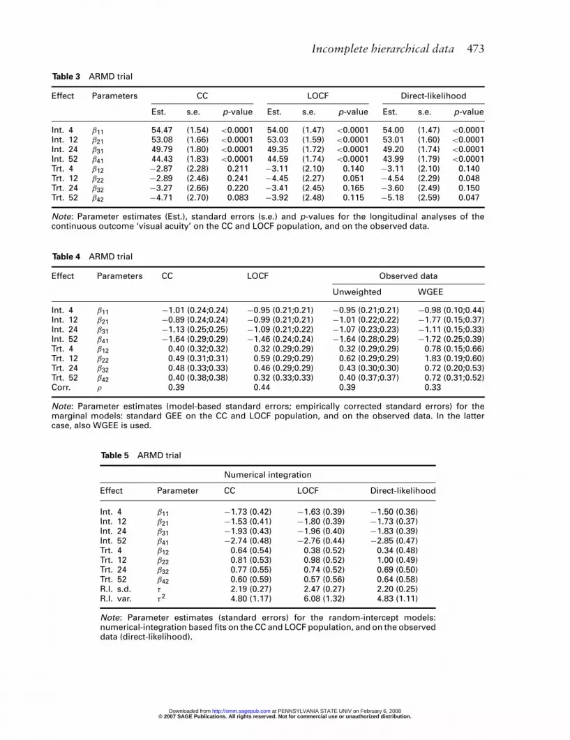
Incomplete hierarchical data 473
Table 3 ARMD trial
Effect Parameters CC LOCF Direct-likelihood
Est. s.e. p-value Est. s.e. p-value Est. s.e. p-value
Int. 4 β11 54.47 (1.54) <0.0001 54.00 (1.47) <0.0001 54.00 (1.47) <0.0001Int. 12 β21 53.08 (1.66) <0.0001 53.03 (1.59) <0.0001 53.01 (1.60) <0.0001Int. 24 β31 49.79 (1.80) <0.0001 49.35 (1.72) <0.0001 49.20 (1.74) <0.0001Int. 52 β41 44.43 (1.83) <0.0001 44.59 (1.74) <0.0001 43.99 (1.79) <0.0001Trt. 4 β12 −2.87 (2.28) 0.211 −3.11 (2.10) 0.140 −3.11 (2.10) 0.140Trt. 12 β22 −2.89 (2.46) 0.241 −4.45 (2.27) 0.051 −4.54 (2.29) 0.048Trt. 24 β32 −3.27 (2.66) 0.220 −3.41 (2.45) 0.165 −3.60 (2.49) 0.150Trt. 52 β42 −4.71 (2.70) 0.083 −3.92 (2.48) 0.115 −5.18 (2.59) 0.047
Note: Parameter estimates (Est.), standard errors (s.e.) and p-values for the longitudinal analyses of thecontinuous outcome ‘visual acuity’ on the CC and LOCF population, and on the observed data.
Table 4 ARMD trial
Effect Parameters CC LOCF Observed data
Unweighted WGEE
Int. 4 β11 −1.01 (0.24;0.24) −0.95 (0.21;0.21) −0.95 (0.21;0.21) −0.98 (0.10;0.44)Int. 12 β21 −0.89 (0.24;0.24) −0.99 (0.21;0.21) −1.01 (0.22;0.22) −1.77 (0.15;0.37)Int. 24 β31 −1.13 (0.25;0.25) −1.09 (0.21;0.22) −1.07 (0.23;0.23) −1.11 (0.15;0.33)Int. 52 β41 −1.64 (0.29;0.29) −1.46 (0.24;0.24) −1.64 (0.28;0.29) −1.72 (0.25;0.39)Trt. 4 β12 0.40 (0.32;0.32) 0.32 (0.29;0.29) 0.32 (0.29;0.29) 0.78 (0.15;0.66)Trt. 12 β22 0.49 (0.31;0.31) 0.59 (0.29;0.29) 0.62 (0.29;0.29) 1.83 (0.19;0.60)Trt. 24 β32 0.48 (0.33;0.33) 0.46 (0.29;0.29) 0.43 (0.30;0.30) 0.72 (0.20;0.53)Trt. 52 β42 0.40 (0.38;0.38) 0.32 (0.33;0.33) 0.40 (0.37;0.37) 0.72 (0.31;0.52)Corr. ρ 0.39 0.44 0.39 0.33
Note: Parameter estimates (model-based standard errors; empirically corrected standard errors) for themarginal models: standard GEE on the CC and LOCF population, and on the observed data. In the lattercase, also WGEE is used.
Table 5 ARMD trial
Numerical integration
Effect Parameter CC LOCF Direct-likelihood
Int. 4 β11 −1.73 (0.42) −1.63 (0.39) −1.50 (0.36)Int. 12 β21 −1.53 (0.41) −1.80 (0.39) −1.73 (0.37)Int. 24 β31 −1.93 (0.43) −1.96 (0.40) −1.83 (0.39)Int. 52 β41 −2.74 (0.48) −2.76 (0.44) −2.85 (0.47)Trt. 4 β12 0.64 (0.54) 0.38 (0.52) 0.34 (0.48)Trt. 12 β22 0.81 (0.53) 0.98 (0.52) 1.00 (0.49)Trt. 24 β32 0.77 (0.55) 0.74 (0.52) 0.69 (0.50)Trt. 52 β42 0.60 (0.59) 0.57 (0.56) 0.64 (0.58)R.I. s.d. τ 2.19 (0.27) 2.47 (0.27) 2.20 (0.25)R.I. var. τ2 4.80 (1.17) 6.08 (1.32) 4.83 (1.11)
Note: Parameter estimates (standard errors) for the random-intercept models:numerical-integration based fits on the CC and LOCF population, and on the observeddata (direct-likelihood).
© 2007 SAGE Publications. All rights reserved. Not for commercial use or unauthorized distribution. at PENNSYLVANIA STATE UNIV on February 6, 2008 http://smm.sagepub.comDownloaded from

474 C Beunckens et al.
the formlogit[P(Yij = 1|Ti)] = βj1 + βj2Ti
with notational conventions as before, except that Yij is now the indicator for whetheror not letters of vision have been lost for subject i at time j, relative to baseline. Theadvantage of having separate treatment effects at each time is that particular attentioncan be given at the treatment effect assessment at the last planned measurement occasion,that is, after one year.
From Table 4 it is clear that the model-based and empirically corrected standard errorsagree extremely well. This is due to the unstructured nature of the full time by treatmentmean structure. However, we do observe differences in the WGEE analyses. Not onlyare the parameter estimates mildly different between the two GEE versions, there is adramatic difference between the model-based and empirically corrected standard errors.Nevertheless, the two sets of empirically corrected standard errors agree very closely,which is reassuring.
When comparing parameter estimates across CC, LOCF and observed data analyses,it is clear that LOCF has the effect of artificially increasing the correlation betweenmeasurements. The effect is mild in this case. The parameter estimates of the observed-data GEE are close to the LOCF results for earlier time points and close to CC for latertime points. This is to be expected, as at the start of the study, the LOCF and observedpopulations are virtually the same, with the same holding between CC and observedpopulations near the end of the study. Note also that the treatment effect under LOCF,especially at 12 weeks and after one year, is biased downward in comparison to the GEEanalyses. To properly use the information in the missingness process, WGEE can be used.To this end, a logistic regression for dropout, given covariates and previous outcomes,needs to be fitted. Parameter estimates and standard errors are given in Table 6.
Covariates of importance are treatment assignment, the level of lesions at baseline(a four-point categorical variable, for which three dummies are needed), and time atwhich dropout occurs. For the latter covariates, there are three levels, since dropout canoccur at times 2, 3 or 4. Hence, two dummy variables are included. Finally, the previousoutcome does not have a significant impact, but will be kept in the model nevertheless.In spite of there being no strong evidence for MAR, the results between GEE and WGEE
Table 6 ARMD trial
Effect Parameter Estimate (s.e.)
Intercept ψ0 0.13 (0.49)Previous outcome ψ1 0.04 (0.38)Treatment ψ2 −0.87 (0.37)Lesion level 1 ψ31 −1.82 (0.49)Lesion level 2 ψ32 −1.89 (0.52)Lesion level 3 ψ33 −2.79 (0.72)Time 2 ψ41 −1.73 (0.49)Time 3 ψ42 −1.36 (0.44)
Note: Parameter estimates (standard errors) for a logis-tic regression model to describe dropout.
© 2007 SAGE Publications. All rights reserved. Not for commercial use or unauthorized distribution. at PENNSYLVANIA STATE UNIV on February 6, 2008 http://smm.sagepub.comDownloaded from

Incomplete hierarchical data 475
differ quite a bit. It is noteworthy that at 12 weeks, a treatment effect is observed withWGEE which goes unnoticed with the other marginal analyses. This finding is mildlyconfirmed by the random-intercept model, when the data as observed are used.
The results for the random-effects models are given in Table 5. We observe the usualrelationship between the marginal parameters of Table 4 and their random-effectscounterparts. Note also that the random-intercepts variance is largest under LOCF,underscoring again that this method artificially increases the association between mea-surements on the same subject. In this case, unlike for the marginal models, LOCF andin fact also CC, slightly to considerably overestimates the treatment effect at certaintimes, in particular at 4 and 24 weeks.
7 Full selection MNAR model
In the selection model framework, even though the assumption of likelihood ignorabilityencompasses the MAR and not only the more stringent and often implausible MCARmechanisms, it is difficult to exclude the option of a more general MNAR mechanism.One solution for continuous outcomes is to fit a full selection model which is valid underMNAR, as proposed by Diggle and Kenward.6 In the discrete case, Molenberghs et al.40
considered a global odds ratio (Dale) model. Within the selection model framework,models have been proposed for non-monotone missingness as well,41 and further anumber of proposals have been made for non-Gaussian outcomes.22
However, as pointed out in the introduction and by several authors (discussion to Dig-gle and Kenward,6 Verbeke and Molenberghs7,(Ch. 18)), one has to be extremely carefulwith interpreting evidence for or against MNAR in a selection model context, especiallyin large studies with a lot of power. We will return to these issues in Section 8. We firstdescribe the Diggle and Kenward model for continuous longitudinal data. We also give abrief perspective on counterparts for discrete data. Molenberghs and Verbeke22 providea comprehensive overview of such models.
7.1 Diggle and Kenward model for continuous longitudinal dataIn agreement with notation introduced in Section 3, we assume a vector of outcomes Yi
is designed to be measured. If dropout occurs, Yi is only partially observed. We denote theoccasion at which dropout occurs by Di > 1, and Yi is split into the (Di − 1)-dimensionalobserved component Yo
i and the (ni − Di + 1)-dimensional missing component Ymi . In
case of no dropout, we let Di = ni + 1 and Yi equals Yoi . The likelihood contribution
of the ith subject, based on the observed data (yoi , di), is proportional to the marginal
density function
f (yoi , di|θ , ψ) =
∫f (yi, di|θ , ψ) dym
i =∫
f (yi|θ)f (di|yi, ψ) dymi (14)
in which a marginal model for Yi is combined with a model for the dropout process,conditional on the response – since we are considering the selection model framework –and where θ and ψ are vectors of unknown parameters in the measurement model anddropout model, respectively.
© 2007 SAGE Publications. All rights reserved. Not for commercial use or unauthorized distribution. at PENNSYLVANIA STATE UNIV on February 6, 2008 http://smm.sagepub.comDownloaded from

476 C Beunckens et al.
Let hij = (yi1, . . . , yi; j−1) denote the observed history of subject i up to time ti,j−1. TheDiggle–Kenward model for the dropout process allows the conditional probability fordropout at occasion j, given that the subject was still observed at the previous occasion,to depend on the history hij and the possibly unobserved current outcome yij, but not onfuture outcomes yik, k > j. These conditional probabilities P(Di = j|Di ≥ j, hij, yij, ψ)can now be used to calculate the probability of dropout at each occasion
P(Di = j|yi, ψ) = P(Di = j|hij, yij, ψ)
=
⎧⎪⎪⎪⎪⎪⎪⎪⎪⎪⎪⎨
⎪⎪⎪⎪⎪⎪⎪⎪⎪⎪⎩
P(Di = j|Di ≥ j, hij, yij, ψ), j = 2
P(Di = j|Di ≥ j, hij, yij, ψ)
×j−1∏
k=2
[1 − P(Di = k|Di ≥ k, hik, yik, ψ)], j = 3, . . . , ni
ni∏
k=2
[1 − P(Di = k|Di ≥ k, hik, yik, ψ)], j = ni + 1
Diggle and Kenward6 combine a multivariate normal model for the measurement processwith a logistic regression model for the dropout process. More specifically, the measure-ment model assumes that the vector Yi of repeated measurements for the ith subjectsatisfies the linear regression model Yi ∼ N(Xiβ, Vi) (i = 1, . . . , N). The matrix Vi canbe left unstructured or assumed to be of a specific form, for example, resulting from alinear mixed model (Section 5.1).
The logistic dropout model can, for example, take the form
logit[P(Di = j | Di ≥ j, hij, yij, ψ)] = ψ0 + ψ1yi,j−1 + ψ2yij (15)
More general models can easily be constructed by including the complete history hij =(yi1, . . . , yi; j−1), as well as external covariates, in the above conditional dropout model.Note also that, strictly speaking, one could allow dropout at a specific occasion tobe related to all future responses as well. However, this is rather counter-intuitive inmany cases. Moreover, including future outcomes seriously complicates the calculationssince computation of the likelihood (14) then requires evaluation of a possibly high-dimensional integral. Note also that special cases of model (15) are obtained from settingψ2 = 0 or ψ1 = ψ2 = 0, respectively. In the first case, dropout is no longer allowed todepend on the current measurement, implying MAR. In the second case, dropout isindependent of the outcome, which corresponds to MCAR.
Diggle and Kenward6 obtained parameter and precision estimates by maximum like-lihood. The likelihood involves marginalization over the unobserved outcomes Ym
i .Practically, this involves relatively tedious and computationally demanding forms ofnumerical integration. This, combined with likelihood surfaces tending to be ratherflat, makes the model difficult to use. These issues are related to the problems to bediscussed next.
© 2007 SAGE Publications. All rights reserved. Not for commercial use or unauthorized distribution. at PENNSYLVANIA STATE UNIV on February 6, 2008 http://smm.sagepub.comDownloaded from

Incomplete hierarchical data 477
7.2 Models for discrete longitudinal dataMolenberghs et al.40 proposed a model for longitudinal ordinal data with non-random
dropout, that is, the missingness mechanism was assumed to be MNAR, which com-bines the multivariate Dale model for longitudinal ordinal data with a logistic regressionmodel for dropout. The resulting likelihood can be maximized relatively simply, usingthe fact that all stochastic outcomes are of a categorical type, using the expectation-maximization (EM) algorithm. It means that the integration over the missing data,needed to maximize the likelihood of Diggle and Kenward,6 is replaced by finite summa-tion. This is certainly not the only model available. The work on incomplete categoricaldata is vast. Baker and Laird42 develop the original work of Fay43 and give a thoroughaccount of the modeling of contingency tables in which there is one response dimen-sion and an additional dimension indicating whether the response is absent. Baker andLaird use log-linear models and the EM algorithm for the analysis. They pay partic-ular attention to the circumstances in which no solution exists for the non-randomdropout models. Such non-estimability is also a feature of the models we use below,but the more complicated setting makes a systematic account more difficult. Stasny44
and Conaway45,46 consider non-random missingness models for categorical longitudi-nal data. Baker47 allows for intermittent missingness in repeated categorical outcomes.Baker et al.48 present a method for incomplete bivariate binary outcomes with generalpatterns of missingness. The model was adapted for the use of covariates by Jansenet al.49
8 Sensitivity analysis
Even though the assumption of likelihood ignorability encompasses both MAR and themore stringent and often implausible MCAR mechanisms, it is difficult to exclude theoption of a more general missingness mechanism. One solution is to fit an MNAR model,such as discussed in the previous section. However, as pointed out by several authors(discussion to Diggle and Kenward,6 Verbeke and Molenberghs7,(Ch. 18), Molenberghsand Verbeke22), one has to be extremely careful with interpreting evidence for or againstMNAR using only the data under study. A detailed treatment of the issue is provided inJansen et al.49
A sensible compromise between blindly shifting to MNAR models or ignoring themaltogether is to make them a component of a sensitivity analysis. It is important toconsider the effect on key parameters such as treatment effect. In many instances, asensitivity analysis can strengthen one’s confidence in the MAR model.50,51
Informally, we could define a sensitivity analysis as one in which several statisticalmodels are considered simultaneously and/or where a statistical model is further scru-tinized using specialized tools (such as diagnostic measures). This rather loose and verygeneral definition encompasses many useful approaches. The simplest procedure is tofit a selected number of MNAR models that are all deemed plausible or one in which apreferred (primary) analysis is supplemented with a number of variations. The extentto which conclusions (inferences) are stable across such ranges provides an indication
© 2007 SAGE Publications. All rights reserved. Not for commercial use or unauthorized distribution. at PENNSYLVANIA STATE UNIV on February 6, 2008 http://smm.sagepub.comDownloaded from

478 C Beunckens et al.
about the belief one can put into them. Variations to a basic model can be constructedin different ways. The most obvious strategy is to consider various dependencies ofthe missing data process on the outcomes and/or covariates. Alternatively, the distribu-tional assumptions of the model can be changed. Thus clearly, several routes to sensitivityanalysis are possible.
To begin with, a sensitivity analysis can be conducted within the selection modelfamily itself. A perspective is given below. A promising tool, proposed by Verbeke et al.,51
and employed by Thijs et al.52 and Molenberghs et al.,50 is based on local influence.53
These authors considered the Diggle and Kenward6 model as their starting point. Theseideas have been developed for categorical data as well. Van Steen et al.54 developed alocal influence-based sensitivity analysis for the MNAR Dale model. Related ideas havebeen developed for the general Baker et al.48 model by Jansen et al.49 Hens et al.55
developed kernel weighted influence measures.Although classical inferential procedures account for the imprecision resulting from
the stochastic component of the model and for finite sampling, less attention is devotedto the uncertainty arising from (unplanned) incompleteness in the data, even thoughthe majority of studies in humans suffer from incomplete follow-up. Molenberghset al.50 acknowledge both the status of imprecision, due to (finite) random samplingand ignorance, due to incompleteness. Both can be combined into uncertainty.56
Yet another option is to consider pattern-mixture models as a complement to selectionmodels.57,58
While it is impossible to provide a complete overview of sensitivity analysis methodswithin the scope of this article, a few methods will be presented in detail. In Sec-tion 8.1, local influence methods are described. Section 8.2 is devoted to sensitivityanalysis methods based on pattern-mixture methods. These are applied to the ARMDtrial in Section 9.
8.1 Selection models and local influenceLet us return to the Diggle and Kenward6 selection model, as described in Section 7.1
and consider dropout model (3). When ω equals zero, the dropout model is random,and all the parameters can be estimated using standard software since the measurementmodel for which we use a linear mixed model and the dropout model, assumed to follow alogistic regression, can then be fitted separately. If ω �= 0, the dropout process is assumedto be non-random.
Let us now shift attention to sensitivity and influence analysis issues. Whereas a globalinfluence approach is based on case-deletion, a local influence-based sensitivity assess-ment of the relevant quantities, such as treatment effect or time evolution parameters,with respect to assumptions about the dropout model is based on the following perturbedversion of Equation (15)
logit[P(Di = j | Di ≥ j, hij, yij, ψ)] = hijψ + ωiyij, i = 1, . . . , N (16)
in which different subjects give different weights to the response at time tij to predictdropout at time tij. If all ωi equal zero, the model reduces to a MAR model. HenceEquation (16) can be seen as an extension of the MAR model, which allows some
© 2007 SAGE Publications. All rights reserved. Not for commercial use or unauthorized distribution. at PENNSYLVANIA STATE UNIV on February 6, 2008 http://smm.sagepub.comDownloaded from
Incomplete hierarchical data 479
individuals to dropout in a ‘less random’ way (|ωi| large) than others (|ωi| small). Ithas to be noted that, even when ωi is large, we still cannot conclude that the dropoutmodel for these subjects is non-random. Rather, it is a way of pointing to subjects which,because of their strong influence, are able to distort the model parameters such that theycan produce, for example, a dropout mechanism which is seemingly non-random. Inreality, many different characteristics of such an individual’s profile might be responsiblefor this effect. As mentioned earlier, such sensitivity has been alluded to by many authors,such as Laird59 and Rubin.60
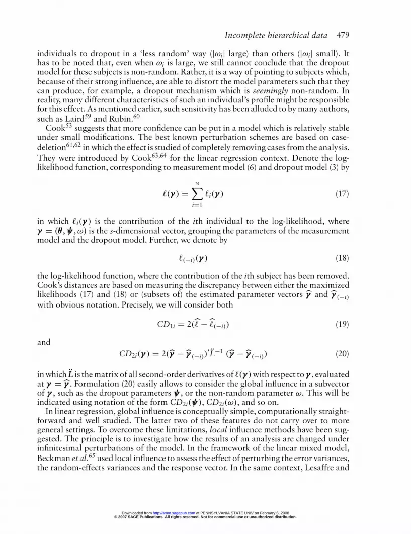
Cook53 suggests that more confidence can be put in a model which is relatively stableunder small modifications. The best known perturbation schemes are based on case-deletion61,62 in which the effect is studied of completely removing cases from the analysis.They were introduced by Cook63,64 for the linear regression context. Denote the log-likelihood function, corresponding to measurement model (6) and dropout model (3) by
�(γ ) =N∑
i=1
�i(γ ) (17)
in which �i(γ ) is the contribution of the ith individual to the log-likelihood, whereγ = (θ , ψ , ω) is the s-dimensional vector, grouping the parameters of the measurementmodel and the dropout model. Further, we denote by
�(−i)(γ ) (18)
the log-likelihood function, where the contribution of the ith subject has been removed.Cook’s distances are based on measuring the discrepancy between either the maximizedlikelihoods (17) and (18) or (subsets of) the estimated parameter vectors γ̂ and γ̂ (−i)with obvious notation. Precisely, we will consider both
CD1i = 2(�̂ − �̂(−i)) (19)
andCD2i(γ ) = 2(γ̂ − γ̂ (−i))
′L̈−1 (γ̂ − γ̂ (−i)) (20)
in which L̈ is the matrix of all second-order derivatives of �(γ )with respect toγ , evaluatedat γ = γ̂ . Formulation (20) easily allows to consider the global influence in a subvectorof γ , such as the dropout parameters ψ , or the non-random parameter ω. This will beindicated using notation of the form CD2i(ψ), CD2i(ω), and so on.
In linear regression, global influence is conceptually simple, computationally straight-forward and well studied. The latter two of these features do not carry over to moregeneral settings. To overcome these limitations, local influence methods have been sug-gested. The principle is to investigate how the results of an analysis are changed underinfinitesimal perturbations of the model. In the framework of the linear mixed model,Beckman et al.65 used local influence to assess the effect of perturbing the error variances,the random-effects variances and the response vector. In the same context, Lesaffre and
© 2007 SAGE Publications. All rights reserved. Not for commercial use or unauthorized distribution. at PENNSYLVANIA STATE UNIV on February 6, 2008 http://smm.sagepub.comDownloaded from

480 C Beunckens et al.
Verbeke66 have shown that the local influence approach is also useful for the detection ofinfluential subjects in a longitudinal data analysis. Moreover, since the resulting influencediagnostics can be expressed analytically, they often can be decomposed in interpretablecomponents, which yield additional insights in the reasons why some subjects are moreinfluential than others.
Verbeke et al.51 studied the influence of the non-randomness of dropout exerts on themodel parameters. Let us briefly sketch the principles of local influence and then applythem to our MNAR problem.
We denote the log-likelihood function corresponding to model (16) by
�(γ |ω) =N∑
i=1
�i(γ |ωi) (21)
in which �i(γ |ωi) is the contribution of the ith individual to the log-likelihood, whereγ = (θ , ψ) is the s-dimensional vector, grouping the parameters of the measurementmodel and the dropout model, not including the N × 1 vector ω = (ω1, ω2, . . . , ωN)′of weights defining the perturbation of the MAR model. Let γ̂ be the maximum-likelihood estimator for γ , obtained by maximizing �(γ |ω0), and let γ̂ ω denote themaximum-likelihood estimator for γ under �(γ |ω). Cook53 proposed to measurethe distance between γ̂ ω and γ̂ by the so-called likelihood displacement, defined byLD(ω) = 2(�(γ̂ |ω0) − �(γ̂ ω|ω)). Since this quantity can only be depicted when N = 2,Cook53 proposed to look at local influence, that is, at the normal curvatures Ch of ξ(ω)
in ω0, in the direction of some N-dimensional vector h of unit length. It can be shownthat a general form is given by
Ch(θ) = −2h′[
∂2�iω
∂θ ∂ωi
∣∣∣∣ωi=0
]′L̈−1
(θ)
[∂2�iω
∂θ ∂ωi
∣∣∣∣ωi=0
]h
Ch(ψ) = −2h′[
∂2�iω
∂ψ ∂ωi
∣∣∣∣ωi=0
]′L̈−1
(ψ)
[∂2�iω
∂ψ ∂ωi
∣∣∣∣ωi=0
]h
evaluated at γ = γ̂ , where indeed the influence for the measurement and dropout modelparameters split, since the second-derivative matrix of the log-likelihood, L̈ is block-diagonal with blocks L̈(θ) and L̈(ψ). Verbeke et al.51 decomposed local influence intomeaningful and interpretable components.
8.2 Pattern-mixture models and sensitivity analysisLittle3,4,67 has been promoting the use of pattern-mixture models as a viable alternative
to selection models. His work is based on, for example, Rubin,68 where the idea was usedin a sensitivity analysis within a fully Bayesian framework. Further references includeGlynn et al.,69 Little and Rubin2 and Rubin.11 In 1989, an entire issue of the Journal of
© 2007 SAGE Publications. All rights reserved. Not for commercial use or unauthorized distribution. at PENNSYLVANIA STATE UNIV on February 6, 2008 http://smm.sagepub.comDownloaded from

Incomplete hierarchical data 481
Educational Statistics was devoted to this theme. A key reference is Hogan and Laird.70
Several authors have contrasted selection models and pattern-mixture models. Thisis done either 1) to answer the same scientific question, such as marginal treatmenteffect or time evolution, based on these two rather different modeling strategies or2) to gain additional insight by supplementing the selection model results with thosefrom a pattern-mixture approach. Examples include Verbeke et al.71 or Michiels et al.58
for continuous outcomes, and Molenberghs et al.72 or Michiels et al.73 for categoricaloutcomes. Further references include Cohen and Cohen,74 Muthén et al.,75 Allison,76
McArdle and Hamagami,77 Little and Wang,78 Hedeker and Gibbons,79 Ekholm andSkinner,80 Molenberghs et al.,81 Park and Lee82 and Thijs et al.57
An important issue is that pattern-mixture models are by construction under-identified, that is, overspecified. Little34 solves this problem through the use of identifyingrestrictions: inestimable parameters of the incomplete patterns are set equal to (func-tions of) the parameters describing the distribution of the completers. Although someauthors perceive this under-identification as a drawback, we believe it is an asset becauseit forces one to reflect on the assumptions made. This can serve as a starting point forsensitivity analysis, as outlined in Verbeke and Molenberghs7,(Ch. 20) and Molenberghsand Verbeke22,(Ch. 31).
Fitting pattern-mixture models can be approached in several ways. It is importantto decide whether pattern-mixture and selection modeling are to be contrasted withone another or rather the pattern-mixture modeling is the central focus. In the lattercase, it is natural to conduct an analysis, and preferably a sensitivity analysis, within thepattern-mixture family. Basically, we will consider three strategies to deal with underidentification.
1) Strategy 1. Little3,4 advocated the use of identifying restrictions and presented anumber of examples. A general framework for identifying restrictions is discussedin more detail in Thijs et al.57 with complete-case missing value restrictions (CCMV)(introduced by Little3), available-case missing value restrictions (ACMV) and neigh-boring case missing value restrictions (NCMV) as important special cases. Note thatACMV is the natural counterpart of MAR in the pattern-mixture model (PMM)framework83. This provides a way to compare ignorable selection models with theircounterpart in the pattern-mixture setting.
2) Strategy 2. As opposed to identifying restrictions, model simplification can be donein order to identify the parameters. The advantage is that the number of parametersdecreases, which is desirable since the length of the parameter vector is a generalissue with pattern-mixture models. Indeed, Hogan and Laird70 noted that in orderto estimate the large number of parameters in general pattern-mixture models, onehas to make the awkward requirement that each dropout pattern occurs sufficientlyoften. Broadly, we distinguish between two types of simplifications.a) Strategy 2a. Trends can be restricted to functional forms supported by the
information available within a pattern. For example, a linear or quadratic timetrend is easily extrapolated beyond the last obtained measurement. One onlyneeds to provide an ad hoc solution for the first or the first few patterns. Inorder to fit such models, one simply has to carry out a model building exercisewithin each of the patterns separately.
© 2007 SAGE Publications. All rights reserved. Not for commercial use or unauthorized distribution. at PENNSYLVANIA STATE UNIV on February 6, 2008 http://smm.sagepub.comDownloaded from

482 C Beunckens et al.
b) Strategy 2b. Next, one can let the parameters vary across patterns in a controlledparametric way. Thus, rather than estimating a separate time trend withineach pattern, one could for example assume that the time evolution withina pattern is unstructured, but parallel across patterns. This is effectuated bytreating pattern as a covariate. The available data can be used to assess whethersuch simplifications are supported within the time ranges for which there isinformation.
Although the second strategy is computationally simple, it is important to note thatthere is a price to pay. Indeed, simplified models, qualified as assumption rich by Sheineret al.84 also make untestable assumptions, just as in the selection model case. From atechnical point of view, Strategy 2 only requires to either consider ‘pattern’ as an extracovariate in the model, or to conduct an analysis ‘by pattern,’ such that a separateanalysis is obtained for each of the dropout patterns. In the identifying restrictionssetting on the other hand (Strategy 1), the assumptions are clear from the start. Preciselyfor these reasons it is stated in Thijs et al.57 that the use of simplified models is not thebest strategy and can be rather dangerous as well.
Pattern-mixture models do not always automatically provide estimates and standarderrors of marginal quantities of interest, such as overall treatment effect or overall timetrend. Hogan and Laird70 provided a way to derive selection model quantities from thepattern-mixture model. An example of such a marginalization is given by Thijs et al.57
See also Verbeke and Molenberghs7 and Molenberghs and Verbeke.22
Pattern-mixture models can be of use in the context of sensitivity analysis. Given thereare several, quite distinct, strategies to formulate such models, one can consider onestrategy as a sensitivity analysis for another one. For example, the sensitivity of simple,identified models can be checked using identifying restrictions. Also, a set of identifyingrestrictions can be considered, rather than a single one, by way of sensitivity analysis.Thijs et al.57 and Molenberghs et al.14 discuss strategies for fitting pattern-mixturemodels. Obviously, one can formulate selection models for one’s primary analysis, andthen fit pattern-mixture models to assess sensitivity. Michiels et al.58 followed this route.Molenberghs et al.81 formulated models that combine aspects of both selection modelsand pattern-mixture models, and used pseudo-likelihood ideas to fit such models.
A final observation, applying to both strategies, is that pattern-mixture models donot always automatically provide estimates and standard errors of marginal quantitiesof interest, such as overall treatment effect or overall time trend. Hogan and Laird70
provided a way to derive selection model quantities from the pattern-mixture model.Several authors have followed this idea to formally compare the conclusions from aselection model with the selection model parameters in a pattern-mixture model.73,85
9 Sensitivity analysis for ARMD trial
A sensitivity analysis of the ARMD trial will be performed making use of models andsensitivity tools within both the selection and pattern-mixture framework. Results ofthese analyses will be discussed in turn.
© 2007 SAGE Publications. All rights reserved. Not for commercial use or unauthorized distribution. at PENNSYLVANIA STATE UNIV on February 6, 2008 http://smm.sagepub.comDownloaded from

Incomplete hierarchical data 483
9.1 Selection models and local influence for the ARMD trialIn this section, the visual acuity in the ARMD trial is first analyzed using the full
selection model proposed by Diggle and Kenward,6 discussed in Section 7.1. Apart frommodeling the three missing data mechanisms MCAR, MAR and MNAR, explicitly, anignorable MAR analysis is also conducted. For the measurement model, again, the linearmixed model was used, assuming different intercepts and treatment effects for each ofthe four time points, next to an unstructured variance covariance matrix. In the fullselection models, the dropout is modeled by Equation (15). Parameter estimates andcorresponding standard errors of the fixed effects of the measurement model and of thedropout model parameters are given in Table 7.
As expected, the parameter estimates and standard errors coincide for the ignorabledirect-likelihood analysis and the selection models under MCAR and MAR, except forsome numerical noise.
Since main interest lies in the treatment effect at one year, the corresponding p-valuesare displayed in Table 7. In all four cases, this treatment effect is significant.
Note that for the MNAR analysis, the estimates of the ψ1 and ψ2 parameter aremore or less of the same magnitude, but with a different sign. This is in line withthe argument of Molenberghs et al.,50 stating that the dropout oftentimes depends onthe increment yij − yi,j−1. This is because two subsequent measurements are usuallypositively correlated. By rewriting the fitted dropout model in terms of the increment,
logit[pr(Di = j|Di ≥ j, yi)
] = −1.81 − 0.026yi,j−1 − 0.042(yij − yi,j−1)
Table 7 ARMD trial
All subjects Ignorable MCAR MAR MNARParameters
Est. (s.e) Est. (s.e.) Est. (s.e.) Est. (s.e.)
Measurement modelInt. 4 : β11 54.00 (1.47) 54.00 (1.46) 54.00 (1.47) 54.00 (1.47)Int. 12: β21 53.01 (1.60) 53.01 (1.59) 53.01 (1.60) 52.98 (1.60)Int. 24: β31 49.20 (1.74) 49.20 (1.73) 49.19 (1.74) 49.06 (1.74)Int. 52: β41 43.99 (1.79) 43.99 (1.78) 43.99 (1.79) 43.52 (1.82)Trt. 4 : β12 −3.11 (2.10) −3.11 (2.07) −3.11 (2.09) −3.11 (2.10)Trt. 12: β22 −4.54 (2.29) −4.54 (2.25) −4.54 (2.29) −4.67 (2.29)Trt. 24: β32 −3.60 (2.49) −3.60 (2.46) −3.60 (2.50) −3.80 (2.50)Trt. 52: β42 −5.18 (2.59) −5.18 (2.57) −5.18 (2.62) −5.71 (2.63)
Dropout modelψ0 −2.79 (0.17) −1.86 (0.46) −1.81 (0.47)ψ1 −0.020 (0.009) 0.016 (0.022)ψ2 −0.042 (0.023)
−2 log-likelihood 6488.7 6782.7 6778.4 6775.9
Trt. at 1 year: p-value 0.046 0.044 0.048 0.030
Note: Parameter estimates (standard errors) assuming ignorability, as well as explicitly modeling the missingdata mechanism under MCAR, MAR and MNAR assumptions, for all data.
© 2007 SAGE Publications. All rights reserved. Not for commercial use or unauthorized distribution. at PENNSYLVANIA STATE UNIV on February 6, 2008 http://smm.sagepub.comDownloaded from

484 C Beunckens et al.
We find that the probability of dropout increases with larger negative increments; thatis, those patients who showed or would have shown a greater decrease in visual acuityfrom the previous visit are more likely to dropout.
Let us now switch to local influence. Figure 2 displays overall Ci and influences forsubvectors θ , β, α and ψ . In addition, the direction hmax, corresponding to maximallocal influence, is given. The main emphasis should be put on the relative magnitudes.We observe that patients 10, 27, 28, 114, 139 and 154 have larger Ci values compared
100 150 200
0 10
0000
200
000
3000
00 4
0000
0
# 10
# 27
# 28
# 114
# 139
# 154
Ci
0 50 100 150 200 0
100
200
300
400
500
# 68
# 185
Ci(θ)
100 150 200
0.0
0.1
0.2
0.3
0.4
0.5
0.6
Ci(β)
0 50
0 50
0 50
0 50
0 50
100 150 200
0 10
0 20
0 30
0 40
0 50
0
# 68
# 185
Ci(α)
100 150 200
0 10
0000
200
000
3000
00 4
0000
0
# 10
# 27
# 28
# 114
# 139
# 154
Ci(ψ)
100 150 200
-1.0
-0
.5
0.0
0.5
1.0
# 10
# 27
# 28 # 114
# 139
# 154
hmax,i
Figure 2 ARMD trial. Index plots of Ci , Ci (θ), Ci (α), Ci (β), Ci (ψ) and of the components of the direction hmax,iof maximal curvature.
© 2007 SAGE Publications. All rights reserved. Not for commercial use or unauthorized distribution. at PENNSYLVANIA STATE UNIV on February 6, 2008 http://smm.sagepub.comDownloaded from

Incomplete hierarchical data 485
with other patients, which means they can be considered influential. Virtually the samepicture holds for Ci(ψ).
Turning attention to the influence on the measurement model, we see that for Ci(β),there are no strikingly high peaks, whereas Ci(α) reveals two considerable peak forpatients 68 and 185. Note that both patients do not have a high peak for the overall Ci.This is due to the fact that the scale for Ci(α) is relatively small, comparing to the overallCi. Nevertheless, these patients can still be considered influential. Finally, the directionof maximum curvature depicts the same six influential patients as the overall Ci.
In Figure 3, the individual profiles of the influential observations are highlighted. Letus take a closer look at these cases. The six patients, which are influencing the dropoutmodel parameters, are those that dropout after the first measurement is taken at week4. All of these patients are in the active treatment arm, except for no. 27. On the otherhand, the two patients influential for the measurement model parameters, stay in thestudy up to week 24 and have no observation for the last measurement occasion at oneyear. Patient 68 received the active treatment, and its visual acuity decreases a lot afterweek 4, but stayed more or less the same after week 12. Opposite, patient 185 belongedto the placebo treatment arm and its visual acuity increases after week 4, and decreasesa little bit after week 12.
It is interesting to consider an analysis without these influential observations. There-fore, we applied the selection model on three subsets of the data. To obtain the firstsubset, all the eight influential patients mentioned above were removed. In the secondsubset of the data, patients 10, 27, 28, 114, 139, and 154 were removed, since these areoverall the most influential ones. Finally patients 68 and 185, which seemed to be influ-encing the measurement model the most, were removed, resulting in the third subset.Result of these analyses are shown in Table 8. Let us compare the results of the MARand MNAR analyses.
After removing the patients, who have large overall Ci and Ci(ψ) values, the estimatesof the dropout model parameters ψ1 and ψ2 are approximately the same, whereasthe estimate of ψ0 decreases from −1.86 to −1.90 under MAR, and from −1.81 to−1.85 under MNAR. The same can be seen after removing all patients. Considering thetreatment effect at one year, its estimate under the MAR analysis increases from −5.18to −5.06, yielding a slightly increased borderline p-value, whereas under the MNAR
# 10
# 28
# 114
# 139
# 154
# 68# 27
# 185
Weeks4 12 5224 4 12 5224
Active
Weeks
Vis
ual A
cuity
020
4060
8010
0
Vis
ual A
cuity
020
4060
8010
0
Placebo
Figure 3 ARMD trial. Individual profiles for both treatment arms, with influential subjects highlighted.
© 2007 SAGE Publications. All rights reserved. Not for commercial use or unauthorized distribution. at PENNSYLVANIA STATE UNIV on February 6, 2008 http://smm.sagepub.comDownloaded from

486 C Beunckens et al.
Ta
ble
8A
RM
Dtr
ial
Su
bje
ctre
mo
ved
(10,
27,2
8,11
4,13
9,15
4,68
,185
)(1
0,27
,28,
114,
139,
154)
(68,
185)
Par
amet
erM
AR
MN
AR
MA
RM
NA
RM
AR
MN
AR
Est
.(s
.e.)
Est
.(s
.e.)
Est
.(s
.e.)
Est
.(s
.e.)
Est
.(s
.e.)
Est
.(s
.e.)
Mea
sure
men
tm
od
elIn
t.4
:β
1154
.14
(1.5
1)54
.15
(1.4
9)54
.30
(1.4
7)54
.30
(1.4
6)53
.84
(1.4
8)53
.84
(1.4
7)In
t.12
:β
2153
.09
(1.6
4)53
.06
(1.6
2)53
.16
(1.5
9)53
.13
(1.5
9)52
.94
(1.6
0)52
.91
(1.5
9)In
t.24
:β
3149
.56
(1.7
7)49
.46
(1.7
5)49
.31
(1.7
4)49
.20
(1.7
2)49
.44
(1.7
3)49
.31
(1.7
2)In
t.52
:β
4144
.40
(1.8
2)43
.97
(1.8
4)44
.00
(1.7
9)43
.58
(1.8
2)44
.38
(1.7
8)43
.90
(1.8
2)Tr
t.4
:β
12−3
.13
(2.1
7)−3
.13
(2.1
1)−3
.28
(2.0
8)−3
.28
(2.0
6)−2
.95
(2.0
7)−2
.95
(2.0
5)Tr
t.12
:β
22−4
.48
(2.3
6)−4
.63
(2.2
9)−4
.55
(2.2
6)−4
.69
(2.2
4)−4
.47
(2.2
6)−4
.60
(2.2
3)Tr
t.24
:β
32−3
.80
(2.5
6)−4
.04
(2.4
9)−3
.55
(2.4
8)−3
.79
(2.4
4)−3
.85
(2.4
4)−4
.04
(2.4
2)Tr
t.52
:β
42−5
.45
(2.6
6)−6
.12
(2.6
6)−5
.06
(2.5
9)−5
.72
(2.6
1)−5
.56
(2.5
5)−6
.09
(2.5
8)
Dro
po
ut
mo
del
ψ0
−1.9
0(0
.47)
−1.8
5(0
.49)
−1.9
0(0
.47)
−1.8
5(0
.49)
−1.8
5(0
.46)
−1.8
1(0
.47)
ψ1
−0.0
19(0
.010
)0.
018
(0.0
22)
−0.0
19(0
.010
)0.
017
(0.0
22)
−0.0
20(0
.009
)0.
017
(0.0
22)
ψ2
−0.0
44(0
.024
)−0
.043
(0.0
24)
−0.0
43(0
.024
)
−2lo
g-l
ikel
iho
od
6535
.365
32.7
6606
.966
04.4
6706
.467
03.8
Trt.
at1
year
:p-v
alu
e0.
040
0.02
10.
051
0.02
80.
029
0.01
8
No
te:P
aram
eter
esti
mat
es(s
tan
dar
der
rors
)ex
plic
itly
mo
del
ing
the
mis
sin
gd
ata
mec
han
ism
un
der
MA
Ran
dM
NA
Ras
sum
pti
on
s,af
ter
rem
ovi
ng
the
follo
win
gsu
bse
tso
fsu
bje
cts
(10,
27,2
8,11
4,13
9,15
4,68
,185
),(1
0,27
,28,
114,
139,
154)
and
(68,
185)
.
© 2007 SAGE Publications. All rights reserved. Not for commercial use or unauthorized distribution. at PENNSYLVANIA STATE UNIV on February 6, 2008 http://smm.sagepub.comDownloaded from

Incomplete hierarchical data 487
analysis it decreases with 0.01 and together with a decreased standard error this yieldsa small decrease in the p-value.
There is no impact on the likelihood ratio test for MAR against MNAR after removingpatients 10, 27, 28, 114, 139 and 154, or all influential patients, G2 remains 2.5. If thislikelihood ratio test would follow a standard χ2
1 -distribution, we would fail to rejectthe null hypothesis, which leads us to the MAR assumption. However, the test of MARagainst MNAR is non-standard and it cannot be used as such.49,86
Finally, we perform the same analyses on the third subset with patients 68 and 185removed. For both the MAR and MNAR analysis, again the estimate of the treatmenteffect at one year decreases quite a lot, from −5.18 to −5.56 and from −5.71 to −6.09,respectively. Consequently, the p-value also drops down from 0.048 to 0.029 under MARand from 0.030 to 0.018 under the MNAR analysis. The deviance for the likelihood ratiotest for MAR changes from 2.5 to 2.6.
9.2 Pattern-mixture models for ARMD trialLet us turn to pattern-mixture models. As mentioned before the main issue in deal-
ing with pattern-mixture models is solving the problem of under identification. Onthe basis of the discussion in Section 8.2, we will apply the first strategy making useof CCMV, NCMV and ACMV identification restrictions. With respect to the secondstrategy, Thijs et al.57 advised against its use.
The procedure to apply identifying restrictions in the context of pattern-mixturemodels is discussed in full detail in Thijs et al.57 The key steps are as follows:
1) Fit a model to the pattern-specific identifiable densities: ft(y1, . . . , yt). This resultsin a set parameter estimates βp for each pattern p.
2) Select an identification method of choice (ACMV, CCMV, NCMV).3) Using this identification method, determine the conditional distributions of the
unobserved outcomes, given the observed ones: ft(yt+1, . . . , yt|y1, . . . , yt).4) Using standard multiple-imputation methodology,7,11,12 draw multiple imputations
for the unobserved components, given the observed outcomes and the correctpattern-specific density.
5) Analyze the multiple-imputed sets of data using the method of choice. This canbe another pattern-mixture model, but also a selection model or any other desiredmodel.
6) Inferences can be conducted in the standard multiple-imputation way.
The results for the three types of restrictions are shown in Table 9. From the estimates,it is clear that the three different strategies do not differ much among each other andalso compared with the other analyses, the results show a similar trend. With respect tostandard errors, we notice a slight increase for later time points. This can be explainedas a result from the imputation which is known to increase the variability.
Taking a closer look at the treatment effect at 52 weeks, we must conclude that there isno significant treatment effect any more neither under CCMV nor NCMV nor ACMV.In comparison with the selection models the results are contradictory.
In the pattern-mixture approach, we use information from different patterns to mul-tiply impute new values whenever the observations are missing. Borrowing information
© 2007 SAGE Publications. All rights reserved. Not for commercial use or unauthorized distribution. at PENNSYLVANIA STATE UNIV on February 6, 2008 http://smm.sagepub.comDownloaded from

488 C Beunckens et al.
Table 9 ARMD trial
Effect Parameter ACMV CCMV NCMV
Est. (s.e.) p-value Est. (s.e.) p-value Est. (s.e.) p-value
Int. 4 β11 54.00 (1.47) 54.00 (1.47) 54.00 (1.47)Int. 12 β21 52.87 (1.68) <0.0001 52.92 (1.61) <0.0001 52.86 (1.63) <0.0001Int. 24 β31 48.65 (2.00) <0.0001 49.16 (1.87) <0.0001 48.77 (1.78) <0.0001Int. 52 β41 44.19 (2.14) <0.0001 44.69 (2.54) <0.0001 44.00 (1.80) <0.0001Trt. 4 β12 −3.11 (2.10) −3.11 (2.10) −3.11 (2.10)Trt. 12 β22 −4.18 (2.48) 0.092 −4.07 (2.30) 0.077 −4.40 (2.42) 0.069Trt. 24 β32 −4.36 (3.83) 0.271 −5.14 (3.61) 0.173 −4.19 (2.62) 0.110Trt. 52 β42 −5.04 (3.86) 0.211 −2.33 (4.93) 0.647 −4.89 (2.70) 0.071
Note: Parameter estimates (standard errors) and p-values resulting from the pattern-mixture model usingidentifying restrictions ACMV, CCMV and NCMV.
from more distant patterns, such as the CCs, may introduce extra variability, depend-ing on the nature of the conditional distributions sampled from. It is not unexpected,therefore, for the variability to be smallest when applying NCMV. Considering the p-values for the treatment effect also provides some extra evidence for this reasoningin the fact that the p-value for the treatment effect in the case with NCMV restric-tions is closest to the one from the selection models. On the other hand, we know thatACMV is equivalent to MAR. The results from the pattern-mixture approach beingin contradiction with the earlier methods can be interpreted as evidence against theMAR assumption and therefore caution for a strong conclusion regarding the treatmenteffect.
10 Concluding remarks
In summary, we have seen that likelihood-based inference is valid under MAR, provided afew mild regularity conditions hold. For example, a linear mixed model or a generalizedlinear mixed model fitted to incomplete data is valid, and it is as simple to conductas it would be in contexts where data are complete. The situation is a little differentwith GEEs. However, the mild extension of GEE to weighted GEE comes to the rescue.Indeed, fitting WGEE only necessitates the construction of a model for the dropoutprobabilities, given covariates and previous, observed measurements. This can routinelybe done using logistic regression. Thus, a number of frequently used tools for correlateddata are valid in the important MAR setting. One conclusion from this is that there islittle or no need for the simple methods such as CC analysis or LOCF. On the otherhand, though one can hardly ever rule out the possibility of missing data to be MNAR.This implies that the need may exist to consider MNAR models.
A sensible compromise between blindly shifting to MNAR models or ignoring themaltogether, is to make them a component of a sensitivity analysis. In that sense, it isimportant to consider the effect on key parameters. One such route is to consider aselection model of the Diggle and Kenward6 type, and to build in devices to explorethe effect of (small) changes from the posited MAR model, which is the basis of local
© 2007 SAGE Publications. All rights reserved. Not for commercial use or unauthorized distribution. at PENNSYLVANIA STATE UNIV on February 6, 2008 http://smm.sagepub.comDownloaded from

Incomplete hierarchical data 489
influence. A further route for sensitivity analysis is to consider pattern-mixture modelsas a complement to selection models.57,58
Acknowledgements
We gratefully acknowledge support from Belgian IUAP/PAI network ‘StatisticalTechniques and Modeling for Complex Substantive Questions with Complex Data.’
References
1 Rubin DB. Inference and missing data.Biometrika 1976; 63: 581–92.
2 Little RJA, Rubin DB. Statistical analysiswith missing data. Wiley, 1987.
3 Little RJA. Pattern-mixture models formultivariate incomplete data. Journal of theAmerican Statistical Association 1993; 88:125–34.
4 Little RJA. Informative dropout inlongitudinal data analysis (discussion toDiggle PJ, Kenward MG). Applied Statistics1994; 43: 78.
5 Shih WJ, Quan H. Testing for treatmentdifferences with dropouts present in clinicaltrials – a composite approach. Statistics inMedicine 1997; 16: 1225–39.
6 Diggle PD, Kenward MG. Informativedropout in longitudinal data analysis (withdiscussion). Applied Statistics 1994; 43:49–93.
7 Verbeke G, Molenberghs G. Linear mixedmodels for longitudinal data. Springer-Verlag,2000.
8 Kenward MG, Molenberghs G. Likelihoodbased frequentist inference when data aremissing at random. Statistical Science 1998;12: 236–47.
9 Mallinckrodt CH, Clark WS, Carroll RJ,Molenberghs G. Assessing response profilesfrom incomplete longitudinal clinical trialdata under regulatory considerations. Journalof Biopharmaceutical Statistics 2003; 13:179–90.
10 Mallinckrodt CH, Sanger TM, Dube S,Debrota DJ, Molenberghs G, Carroll RJ,Zeigler Potter WM, Tollefson GD. Assessingand interpreting treatment effects inlongitudinal clinical trials with missing data.Biological Psychiatry 2003; 53(8):754–60.
11 Rubin DB. Multiple imputation fornonresponse in surveys. John Wiley & Sons,1987.
12 Schafer JL. Analysis of incompletemultivariate data. Chapman & Hall, 1997.
13 Siddiqui O, Ali MW. A comparison of therandom-effects pattern mixture model withlast observation carried forward (LOCF)analysis in longitudinal clinical trials withdropouts. Journal of BiopharmaceuticalStatistics 1998; 8: 545–63.
14 Molenberghs G, Thijs H, Jansen I,Beunckens C, Kenward MG, Mallinckrodt C,Carroll RJ. Analyzing incompletelongitudinal clinical trial data. Biostatistics2004; 5: 445–64.
15 Beunckens C, Molenberghs G, Kenward MG.Tutorial: direct likelihood analysis versussimple forms of imputation for missing datain randomized clinical trials. Clinical Trials2005; 2: 379–86.
16 Verbeke G, Molenberghs G. Linear MixedModels in Practice: A SAS-OrientedApproach. Lecture Notes in Statistics.Volume 126. Springer-Verlag, 1997.
17 Buck SF. A method of estimation of missingvalues in multivariate data suitable for usewith an electronic computer. Journal of theRoyal Statistical Society, Series B 1960; 22:302–6.
18 Liang K-Y, Zeger SL. Longitudinal dataanalysis using generalized linear models.Biometrika 1986; 73: 13–22.
19 Robins JM, Rotnitzky A, Zhao LP. Analysisof semiparametric regression models forrepeated outcomes in the presence of missingdata. Journal of the American StatisticalAssociation 1995; 90: 106–121.
20 Schafer JL. Multiple imputation inmultivariate problems when the imputation
© 2007 SAGE Publications. All rights reserved. Not for commercial use or unauthorized distribution. at PENNSYLVANIA STATE UNIV on February 6, 2008 http://smm.sagepub.comDownloaded from

490 C Beunckens et al.
and analysis models differ. StatisticaNeerlandica 2003; 57: 19–35.
21 Agresti A. Categorical data analysis, secondedition. John Wiley & Sons, 2002.
22 Molenberghs G, Verbeke G. Models fordiscrete longitudinal data. Springer-Verlag,2005.
23 Diggle PJ, Heagerty P, Liang K-Y, Zeger SL.Analysis of longitudinal data. OxfordUniversity Press, 2002.
24 Bahadur RR. A representation of the jointdistribution of responses to n dichotomousitems. In Solomon H ed. Studies in ItemAnalysis and Prediction. StanfordMathematical Studies in the Social SciencesVI. Stanford University Press, 1961.
25 Ashford JR, Sowden RR. Multivariate probitanalysis. Biometrics 1970; 26: 535–46.
26 Molenberghs G, Lesaffre E. Marginalmodelling of correlated ordinal data using amultivariate Plackett distribution. Journal ofthe American Statistical Association 1994; 89:633–44.
27 Lang JB, Agresti A. Simultaneouslymodelling joint and marginal distributions ofmultivariate categorical responses. Journal ofthe American Statistical Association 1994; 89:625–32.
28 Dale JR. Global cross-ratio models forbivariate, discrete, ordered responses.Biometrics 1986; 42: 909–17.
29 Plackett RL. A class of bivariate distributions.Journal of the American StatisticalAssocication 1965; 60: 516–22.
30 Molenberghs G, Lesaffre E. Marginalmodelling of multivariate categorical data.Statistics in Medicine 1999; 18: 2237–55.
31 Glonek GFV, McCullagh P. Multivariatelogistic models. Journal of the RoyalStatistical Society, Series B 1995; 81: 477–82.
32 le Cessie S, van Houwelingen JC. Logisticregression for correlated binary data. AppliedStatistics 1994; 43: 95–108.
33 Geys H, Molenberghs M, Lipsitz, SR. A noteon the comparison of pseudo-likelihood andgeneralized estimating equations for marginalodds ratio models. Journal of the StatisticalComputation and Simulation 1998; 62: 45–72.
34 Beunckens C, Sotto C, Molenberghs G. Asimulation study comparing weightedestimating equations with multipleimputation based estimating equations. 2006.Submitted for publication.
35 Neuhaus JM. Statistical methods forlongitudina, clustered designs with binary
responses. Statistical Methods in MedicalResearch 1992; 1: 249–73.
36 Neuhaus JM, Kalbfleisch JD, Hauck WW. Acomparison of cluster-specific andpopulation-averaged approaches foranalyzing correlated binary data.International Statistical Review 1991; 59:25–35.
37 Stiratelli R, Laird N, Ware J. Random effectsmodels for serial observations withdichotomous response. Biometrics 1984; 40:961–72.
38 Breslow NE, Clayton DG. Approximateinference in generalized linear mixed models.Journal of the American StatisticalAssociation 1993; 88: 9–25.
39 Skellam JG. A probability distribution derivedfrom the binomial distribution by regardingthe probability of success as variable betweenthe sets of trials. Journal of the RoyalStatistical Society, Series B 1948; 10: 257–61.
40 Molenberghs G, Kenward MG, Lesaffre E.The analysis of longitudinal ordinal datawith non-random dropout. Biometrika 1997;84: 33–44.
41 Jansen I, Molenberghs G. A flexible marginalmodeling strategy for non-monotone missingdata. 2006. Submitted for publication.
42 Baker SG, Laird NM. Regression analysis forcategorical variables with outcome subject tonon-ignorable non-response. Journal of theAmerican Statistical Association, 1988; 83:62–9.
43 Fay RE. Causal models for patterns ofnonresponse. Journal of the AmericanStatistical Association 1986; 81: 354–65.
44 Stasny EA. Estimating gross flows using paneldata with nonresponse: an example from theCanadian Labour Force Survey. Journal of theAmerican Statistical Association 1986; 81:42–7.
45 Conaway MR. The analysis of repeatedcategorical measurements subject tononignorable nonresponse. Journal of theAmerican Statistical Association 1992; 87:817–24.
46 Conaway MR. Non-ignorable non-responsemodels for time-ordered categorical variables.Applied Statistics 1993; 42: 105–15.
47 Baker SG. Marginal regression for repeatedbinary data with outcome subject tonon-ignorable non-response. Biometrics1995; 51: 1042–52.
48 Baker SG, Rosenberger WF, DerSimonian R.Closed-form estimates for missing counts in
© 2007 SAGE Publications. All rights reserved. Not for commercial use or unauthorized distribution. at PENNSYLVANIA STATE UNIV on February 6, 2008 http://smm.sagepub.comDownloaded from

Incomplete hierarchical data 491
two-way contingency tables. Statistics inMedicine 1992; 11: 643–57.
49 Jansen I, Hens N, Molenberghs G, Aerts M,Verbeke G, Kenward MG. The nature ofsensitivity in monotone missing not atrandom models. Computational Statisticsand Data Analysis 2006; 50: 830–58.
50 Molenberghs G, Verbeke G, Thijs H, LesaffreE, Kenward MG. Mastitis in dairy cattle:local influence to assess sensitivity of thedropout process. Computational Statisticsand Data Analysis 2001; 37: 93–113.
51 Verbeke G, Molenberghs G, Thijs H, LesaffreE, Kenward MG. Sensitivity analysis fornon-random dropout: a local influenceapproach. Biometrics 2001; 57: 43–50.
52 Thijs H, Molenberghs G, Verbeke G. Themilk protein trial: influence analysis of thedropout process. Biometrical Journal 2000;42: 617–46.
53 Cook RD. Assessment of local influence.Journal of the Royal Statistical Society, SeriesB 1986; 48: 133–69.
54 Van Steen K, Molenberghs G, Verbeke G,Thijs H. A local influence approach tosensitivity analysis of incomplete longitudinalordinal data. Statistical Modelling: AnInternational Journal 2001; 1: 125–42.
55 Hens N, Aerts M, Molenberghs G, Thijs H,Verbeke G. Kernel weighted influencemeasures. Computational Statistics & DataAnalysis 2005; 48:467–87.
56 Kenward MG, Molenberghs G,Goetghebeur E. Sensitivity analysis forincomplete categorical data. StatisticalModelling 2001; 1: 31–48.
57 Thijs H, Molenberghs G, Michiels B, VerbekeG, Curran D. Strategies to fit pattern-mixturemodels. Biostatistics 2002; 3: 245–65.
58 Michiels B, Molenberghs G, Bijnens L,Vangeneugden T, Thijs H. Selection modelsand pattern-mixture models to analyzelongitudinal quality of life data subject todropout. Statistics in Medicine 2002; 21:1023–41.
59 Laird NM. (discussion to Diggle PJ, KenwardMG) Informative dropout in longitudinaldata analysis. Applied Statistics 1994; 43: 84.
60 Rubin DB. Informative dropout inlongitudinal data analysis (discussion toDiggle PJ, Kenward MG). Applied Statistics1994; 43: 80–2.
61 Cook RD, Weisberg S. Residuals andinfluence in regression. Chapman & Hall,1982.
62 Chatterjee S, Hadi AS. Sensitivity analysis inlinear regression. John Wiley & Sons, 1988.
63 Cook RD. Detection of influentialobservations in linear regression.Technometrics 1977; 19: 15–18.
64 Cook RD. Influential observations in linearregression. Journal of the AmericanStatistical Association 1979; 74: 169–74.
65 Beckman RJ, Nachtsheim CJ, Cook RD.Diagnostics for mixed-model analysis ofvariance. Technometrics 1987; 29: 413–26.
66 Lesaffre E, Verbeke G. Local influence inlinear mixed models. Biometrics 1998; 54:570–82.
67 Little RJA. Modeling the drop-outmechanism in repeated measures studies.Journal of the American StatisticalAssociation 1995; 90: 1112–21.
68 Rubin DB. Formalizing subjective notionsabout the effect of nonrespondents in samplesurveys. Journal of the American StatisticalAssociation 1977; 72: 538–43.
69 Glynn RJ, Laird NM, Rubin DB. Selectionmodelling versus mixture modelling withnonignorable nonresponse. In Wainer, H ed.Drawing Inferences from Self-SelectedSamples. Springer Verlag 1986; 115–42.
70 Hogan JW, Laird NM. Mixture models forthe joint distribution of repeated measuresand event times. Statistics in Medicine 1997;16: 239–58.
71 Verbeke G, Lesaffre E, Spiessens B. Thepractical use of different strategies to handledropout in longitudinal studies. DrugInformation Journal 2001; 35: 419–34.
72 Molenberghs G, Michiels B, Lipsitz SR.Selection models and pattern-mixture modelsfor incomplete categorical data withcovariates. Biometrics 1999; 55: 978–83.
73 Michiels B, Molenberghs G, Lipsitz SR.A pattern-mixture odds ratio model forincomplete categorical data.Communications in Statistics: Theory andMethods 1999; 28: 2843–69.
74 Cohen J, Cohen P. Applied multipleregression/correlation analysis for thebehavioral sciences, second edition. Erlbaum,1983.
75 Muthén B, Kaplan D, Hollis M. On structuralequation modeling with data that are notmissing completely at random.Psychometrika 1987; 52: 431–62.
76 Allison PD. Estimation of linear models withincomplete data. Sociology Methodology1987; 71–103.
© 2007 SAGE Publications. All rights reserved. Not for commercial use or unauthorized distribution. at PENNSYLVANIA STATE UNIV on February 6, 2008 http://smm.sagepub.comDownloaded from

492 C Beunckens et al.
77 McArdle JJ, Hamagami F. Modelingincomplete longitudinal and crosssectionaldata using latent growth structural models.Experimental Aging Research 1992; 18:145–66.
78 Little RJA, Wang Y. Pattern-mixture modelsfor multivariate incomplete data withcovariates. Biometrics 1996; 52: 98–111.
79 Hedeker D, Gibbons RD. Application ofrandom-effects pattern-mixture models formissing data in longitudinal studies.Psychological Methods 1997; 2:64–78.
80 Ekholm A, Skinner C. The muscatinechildren’s obesity data reanalysed usingpattern mixture models. Applied Statistics1998; 47: 251–63.
81 Molenberghs G, Michiels B, Kenward MG.Pseudo-likelihood for combined selection andpattern-mixture models for missing dataproblems. Biometrical Journal 1998; 40:557–72.
82 Park T, Lee S-L. Simple pattern-mixturemodels for longitudinal data with missingobservations: analysis of urinaryincontinence data. Statistics in Medicine1999; 18: 2933–41.
83 Molenberghs G, Michiels B, Kenward MG,Diggle PJ. Missing data mechanisms andpattern-mixture models. StatisticaNeerlandica 1998; 52: 153–61.
84 Sheiner LB, Beal SL, Dunne A. Analysis ofnonrandomly censored ordered categoricallongitudinal data from analgesic trials.Journal of the American StatisticalAssociation 1997; 92: 1235–44.
85 Verbeke, Lesaffre, Spiessens B. (2001) Thepractical use of different strategies to handledropout in longitudinal studies. DrugInformation Journal 35: 419–34.
86 Rotnitzky A, Cox DR, Bottai M, Robins J.Likelihood-based inference with singularinformation matrix. Bernouilli 2000; 6:243–84.
© 2007 SAGE Publications. All rights reserved. Not for commercial use or unauthorized distribution. at PENNSYLVANIA STATE UNIV on February 6, 2008 http://smm.sagepub.comDownloaded from


![[BAIL APPLICATIONS] [ORDERS (INCOMPLETE MATTERS](https://img.pdfslide.net/doc/110x75/63298450c7728c9bbd0a340c/bail-applications-orders-incomplete-matters-.jpg)


