Embed Size (px)
Citation preview

A Hierarchical Model of Data Locality ∗
Chengliang Zhang Chen DingMitsunori Ogihara
Computer Science DepartmentUniversity of Rochester
734 Computer Studies BldgRochester, NY 14627
zhangchl,cding,[email protected]
Yutao ZhongComputer Science Department
George Mason UniversityMSN 4A5
4400 University DriveFairfax, VA 22030
Youfeng WuProgramming Systems Research Lab
Intel labs2200 Mission College Blvd
Santa Clara, CA [email protected]
AbstractIn POPL 2002, Petrank and Rawitz showed a universal result—finding optimal data placement is not only NP-hard but also impos-sible to approximate within a constant factor if P 6= NP . Here westudy a recently published concept called reference affinity, whichcharacterizes a group of data that are always accessed together incomputation. On the theoretical side, we give the complexity forfinding reference affinity in program traces, using a novel reductionthat converts the notion of distance into satisfiability. We also provethat reference affinity automatically captures the hierarchical lo-cality in divide-and-conquer computations including matrix solversand N-body simulation. The proof establishes formal links betweencomputation patterns in time and locality relations in space.
On the practical side, we show that efficient heuristics exist. Inparticular, we present a sampling method and show that it is moreeffective than the previously published technique, especially fordata that are often but not always accessed together. We show theeffect on generated and real traces. These theoretical and empiricalresults demonstrate that effective data placement is still attainablein general-purpose programs because common (albeit not all) lo-cality patterns can be precisely modeled and efficiently analyzed.
Categories and Subject Descriptors D.3.4 [Programming Lan-guages]: Processors—optimization, compilers
General Terms Theory, Algorithms, Performance
Keywords Hierarchical data placement, program locality, refer-ence affinity, volume distance, NP-complete, N-body simulation
1. IntroductionData placement becomes increasingly important to programminglanguage design as programmers routinely improve performance orenergy efficiency by better utilizing the cache memory in proces-sors, disks, and networks. Different memory levels come with dif-ferent sizes and configurations. The hardware configuration, how-
∗ This research has been supported by DOE (DE-FG02-02ER25525) andNSF (CCR-0238176)
Permission to make digital or hard copies of all or part of this work for personal orclassroom use is granted without fee provided that copies are not made or distributedfor profit or commercial advantage and that copies bear this notice and the full citationon the first page. To copy otherwise, to republish, to post on servers or to redistributeto lists, requires prior specific permission and/or a fee.POPL’06 January 11–13, 2006, Charleston, South Carolina, USA.Copyright c© 2006 ACM 1-59593-027-2/06/0001. . . $5.00.
ever, may not be fully visible to a user. In addition, a program mayrun on machines with different configurations. As the program-ming for specific memory levels becomes increasingly untenable,solutions for hierarchical data placement are developed in separateapplication domains including matrix solvers [16], wavelet trans-form [7], N-body simulation [30], and search trees [3], where theprogram data are recursively decomposed into smaller blocks. Byexploiting the inherent locality in computation, hierarchical dataplacement optimizes for any and all cache sizes. While most stud-ies examined specific computation tasks, in this work we show thata general model can be used to derive the hierarchical data place-ment from program traces without user’s knowledge of the meaningof the program.
While the data placement is sensitive to a machine, it is firstand foremost driven by the computation order. In fact, any layoutis perfect if the program traverses the data contiguously. Given anarbitrary data access trace, we say a group of data have referenceaffinity if they are always accessed together in the trace [44]. Thecloseness is parameterized by the volume distance (denoted byk), which is the volume of data between two accesses in a trace.We also call it the reuse distance if the two accesses are to thesame datum. Changing k, reference affinity gives a hierarchicalpartition of program data. We show an example here and givethe formal definitions in the next section. Figure 1 (a) shows atrace, where different letters represent accesses to different data,and “. . .” means accesses to data other than those shown in thetrace.
k
w x y z u v
1
2
3
0
8
w x w x u y z . . . z y y z v x w x w . . .
(a) Example data access seqeuence over time
(b) The reference affinity gives
a hierarchical relation in data
Figure 1. An example reference affinity hierarchy

Reference affinity gives a hierarchical relation shown as a den-drogram in Figure 1(b). The top of the hierarchy (k = ∞) is theset of all data u, v, w, x, y, z, which have the weakest affinity.The group w, x, y, z have stronger affinity than they do with uand v (when k = 3). Inside this group, w, x have closer affinity(k = 2), so do y, z. At the bottom of the hierarchy (k = 0),each data element becomes an affinity group. The affinity hierar-chy enables the hierarchical data placement, which is simply theorder (or its reverse) of the leaves in the dendrogram. The hierar-chical placement improves the spatial locality for all cache configu-rations. When a data element is loaded, the following computationaccesses more likely the neighboring data than the distant data. Asshown by this example, reference affinity converts a computationtrace to a hierarchical data layout.
In this paper we first present two theoretical results on referenceaffinity. The first is the complexity of finding reference affinity. Wegive polynomial-time algorithms for cases k = 1 and k = 2. Weprove that the problems are either NPC or NP-hard when k ≥ 3.Second, we prove that reference affinity automatically capturesthe hierarchical locality in divide-and-conquer type computationsincluding blocked matrix solvers and N-body simulation. The proofholds even when data are divided into non-uniform sections andtraversed in any order.
Despite of the theoretical complexity, efficient heuristics exist.We present a new analysis method based on sampling. We showthrough experiments that the new technique is more accurate thanthe previously published approximation method [44], especiallyfor partial reference affinity where a group of data is often butnot always accessed together. We show two new uses of referenceaffinity. The first is finding hierarchical data layout in recursivematrix multiplication, and the second is improving the code layoutof seven SPEC 2000 applications.
The volume distance has been difficult for theoretical analy-sis because data may appear in different orders with different fre-quencies while still yielding the same volume distance. It raisesinteresting problems different from those in traditional graph andstreaming domains. In this work, we present two new proof tech-niques that link between the volume distance of memory referencesand the affinity of data groups. The first contains a reduction thatconverts the problem of data volume into formal logic. The sec-ond contains a construction that connects the recursive structure ofcomputation and the hierarchical relation of data.
In POPL 2002, Petrank and Rawitz showed a universal result—finding optimal data placement is not only NP-hard but also im-possible to approximate within a constant factor if P 6= NP . Thiswork shows a finer partition. On the one hand, good data placementis possible because reference affinity exists in most programs. Thisexplains the effective heuristics developed by many earlier studies.On the other hand, the optimal placement is still unreachable for ar-bitrary access patterns. The paper shows a division between a fewsolvable or approximable sub-cases and the general case governedby the Petrank-Rawitz theorems.
2. Reference AffinityAn address trace or reference string is a sequence of accesses to aset of data elements. If we assign a logical time to each access, theaddress trace is a vector indexed by the logical time. We use letterssuch as x, y, z to represent data elements, subscripted symbols suchas ax, a′
x to represent accesses to a particular data element x, andthe array index T [ax] to represent the logical time of the access ax
on a trace T . We use sequence and trace interchangeably.
DEFINITION 1. Volume distance. The volume distance betweentwo accesses, ax and ay , at times T [ax] and T [ay]) in a traceT , is one less than the number of distinct data elements accessed
in times between (and including) T [ax] and T [ay]. We write it asdis(ax, ay).
According to the definition, dis(ax, ax) = 0 and dis(ax, ay) =dis(ay, ax). In addition, the triangle inequality holds—dis(ax, ay) + dis(ay, az) ≥ dis(ax, az), because the cardinalityof the union of two sets is no greater than the sum of the cardinalityof each set. For example, in the trace abbbc, the volume distancefrom the first a and to the last c is 2 and vice versa. The symmetryis important because the closeness is the same no matter whichaccess happens first. Next we define the condition that a group ofdata elements are accessed close together.
DEFINITION 2. Linked path. A linked path in a trace is param-eterized by the volume distance k. There is a linked path fromax to ay (x 6= y) if and only if there exist t accesses, ax1
,ax2
, . . ., axt, such that (1) dis(ax, ax1
) ≤ k∧ dis(ax1, ax2
) ≤k ∧ . . . ∧ dis(axt
, ay) ≤ k and (2) x1, x2, . . . , xt, x and y aredifferent (pairwise distinct) data elements.
In words, a linked path has a sequence of hops, each hop landson a different data element and has a volume distance no greaterthan k. We call k the link length. We will later restrict the hops,x1, x2, . . . , xt, to be members of some set S and say that there is ak-linked path from ax to ay with respect to set S.
For example consider the first part of the trace in Figure 1(a),wxwxuyz. The closeness between the first w and the last z isdefined by the linked path with a minimal k, which is the path thatjumps to the second x and then steps through each one in uyz. Eachhop has a volume distance of 1 so is the link length. If we restrictthe path to the set w, x, y, z, the link length becomes 2 since anypath has to jump over u.
DEFINITION 3. Reference affinity group. Given an address trace,a set G of data elements is a reference affinity group (i.e. they havethe reference affinity) with the link length k if and only if
1. for any x ∈ G, all its accesses ax must have a linked pathfrom ax to some ay for each other member y ∈ G, that is,there exist different elements x1, x2, . . . , xt ∈ G such thatdis(ax, ax1
) ≤ k∧dis(ax1, ax2
) ≤ k∧. . .∧dis(axt, ay) ≤ k
2. adding any other element to G will make Condition (1) impos-sible to hold
Reference affinity is a communal bond. All members of an affin-ity group must be accessed in the trace wherever one member isaccessed. Each access is linked to some access of every other mem-ber in the group, and the linked path can go through only membersof the group. We can now explain the hierarchy in Figure 1 fully.When k = ∞, any access in the trace is linked to any other access,so all data belong to one group. When k = 0, no two accesses canbe linked, so each data element is a group. Now consider the groupw, x, y, z, which are access in both parts of the trace. Its linklength is 3 because in trace zyyzvxwxw, no linked path can wadefrom the first z to an access of x without hopping through four dif-ferent data elements around v. The path cannot land on the secondz because it starts from z. Neither can it land on v because it is nota member of the group. When we reduce k, the group w, x, y, zis partitioned into two sub-groups with closer affinity.
The initial purpose of this complex definition is for referenceaffinity to give a unique and hierarchical partition of data, as shownin the following three properties [44].
1. Unique partition Given an address trace and a fixed link lengthk, the affinity groups form a unique partition of program data.

2. Hierarchical structure Given an address trace and two dis-tances k and k′ (k < k′), the affinity groups at k form a finerpartition of the affinity groups at k′.
3. Bounded access range Given an address trace with an affinitygroup G at the link length k, any time an element x of G isaccessed at ax, there exists a section of the trace that includesax and at least one access to all other members of G. Thevolume distance between the two sides of the section is nogreater than 2k|G| + 1, where |G| is the number of elementsin the affinity group.
Having the definition of reference affinity, the problems ofchecking and finding reference affinity groups can be formulatedas the following:
DEFINITION 4. Checking reference affinity groups Given an ad-dress trace and k, check if a given group of data elements belongsto the same reference affinity group with link length k.
DEFINITION 5. Finding reference affinity groups Given an ad-dress trace and k, find all reference affinity groups with link lengthk.
A related decision problem with checking reference affinitygroups is to test if two accesses is k-linked with each other:DEFINITION 6. Given an address trace, a volume distance k ≥ 0and two data accesses ax and ay , the Point-wise k-Linked AffinityProblem (Pw-k -Aff , for short) is the problem of testing whetherax and ay are k-linked in the trace.
3. Hardness of Finding Reference AffinityThe following theorems give the complexity of the linking, check-ing, and finding problems for different k. We include the basic ideasof the proofs and leave the full version in the appendix.
THEOREM 1. For each k ≥ 3, Pw-k -Aff is NP-complete.
We prove it by making a polynomial-time many-one reductionfrom a variant of 3-SAT problem, where every variable appears atmost three times (an NP-complete problem, see, e.g., [31]) to thelinking problem. The proof constructs a three-part reference trace.The first part forces a linked path to go through a set of elementswe call “separators”, which cannot be used as hops in the nexttwo parts. The second part prepares a set of data triples to modelthe truth values of the logical variables in a 3-SAT expression.Since two data elements may represent opposite values of a logicalvariable, the construction ensures that the elements cannot be bothincluded in a possible linked path. A linked path can land ondifferent places and can even go backwards—the only constraint isthat the volume distance of the longest hop. The critical moment ofthe construction is when the freedom of the linked path is containedwithin seven cases, and each is shown to have the needed property.
The third part of the sequence models all 3-SAT expressions. Alinked path exists if and only if there is a truth value assignment tosatisfy all expressions. To design a trace that enforces the logicalconsistency, we learned that we need to use multiple data accessesto represent logical variables instead of using data to representthem. The full proof is more than a page long and given in theappendix. From Theorem 1, we can easily prove two corollaries.COROLLARY 1. For k ≥ 3, the problem of checking referenceaffinity groups is NP-complete.
COROLLARY 2. For k ≥ 3, the problem of finding reference affin-ity groups is NP-hard.
THEOREM 2. Pw-2 -Aff is NL-complete.
Using the same polynomial-time reduction from Theorem 1, wecan show that 2 -CNF-SAT can be reduced to Pw-2 -Aff . The ex-act proof is in the appendix. This theorem shows that a polynomialalgorithm exists for Pw-2 -Aff . Then we have the following result,proved by the algorithm that follows.
THEOREM 3. For k = 2, the problem of finding reference affinitygroups is in P .
ALGORITHM 1. Finding reference affinity groups when k=2procedure FindReferenceAffinityGroup 2(T)
1: T is the trace, the link length k = 22: initially no affinity groups3: while there exist elements not yet grouped do4: put all such elements into a set G and pick one x randomly
from this set;5: repeat6: if there is an element z not 2-linked to x with respect to
G then7: remove z from G;8: else9: if there exist two elements y, z ∈ G such that an
access of y is not 2-linked to any access of z withrespect to G then
10: remove z from group G.11: end if12: end if13: until G is unchanged14: output reference affinity group G.15: end whileendFindReferenceAffinityGroup 2
Algorithm 1 is polynomial time. From Theorem 2, the linkingproblem, that is, testing whether a 2-linked path exists between twodata accesses, can be solved in polynomial time. This algorithmneeds a polynomial number of such tests. The algorithm gives cor-rect reference affinity groups. First, it is easy to see that the groupsfound by this algorithm satisfy the first condition of reference affin-ity. To show every group is the largest possible, we show that thealgorithm removes z correctly, so that G still includes only the ref-erence affinity group that x belongs to. Removing z at step 7 isstraightforward. The correctness of the removal of z at step 10 canbe proved by contradiction. Suppose z belongs to the same groupas x and should not be removed, we can construct a 2-linked pathfrom every access of y to an access of z. This contradicts with thetest at line 9. The full proof is given in the appendix.
From Theorem 3, we can get the following corollary.
COROLLARY 3. For k = 2, the problem of checking referenceaffinity groups is in P .
The complexity for k = 1 is as follows.THEOREM 4. Pw-1 -Aff can be solved in linear time.
THEOREM 5. For k = 1, there is a polynomial-time solution forfinding reference affinity groups.
Here we give a naive method. Since k = 1, all of the groupsappear in the sequence continuously, and two groups do not over-lap. We sort the data elements according to their order of appear-ance in the trace. Then for every t (from the number of data ele-ments to 1) consecutive data elements starting from the first dataelement, we check if it is a reference affinity group. Similarly, wefind other affinity groups. The algorithm is given in the appendix.Finally, from Theorem 5, we haveCOROLLARY 4. For k = 1, the problem of checking referenceaffinity groups can be solved in polynomial time.

Compute(D1, D2, ..., Dn) beginif the input data is above a threshold size
divide D1, D2, ..., Dn into sub-blocksfor some set of sub-block combinations
Compute(subblocki(D1), subblockj(D2),..., subblockk(Dn))
end forelse process without sub-division
end ifend
Figure 2. The general form of the divide-and-conquer algorithm
4. Reference Affinity in Divide-and-ConquerComputations
The divide-and-conquer type of computations we consider areblocked and recursive algorithms for dense matrix operations, N-body and mesh simulation, and wavelet transform. The generalform is given in Figure 2. The procedure takes a set of data suchas matrices. It then divides the input data into smaller blocks andprocesses all or subsets of their combinations. For each subset, ifthe blocks are still large, it makes a recursive call to itself. Thecomputation is hierarchical, so is its locality.
We show that reference affinity can reconstruct the hierarchicaldata locality from an execution trace, if the following two require-ments are met by the hierarchical computation. First, once a blockof Datai is accessed, all its sub-blocks are accessed before movingto the next block of Datai. Second, the access order of sub-blocksis the same for the same block. For example, consider the multi-plication of two matrices A and B. The computation, if startingfrom the left sub-matrix of A, must access all elements of the leftsub-matrix of A at least once before accessing any element fromthe right sub-matrix of A. Still, it is free to access B or other dataat the same time. The traversal order within A is the same, for ex-ample, Morton order. The traversal order in B can be different. Inaddition, non-nesting blocks in the same matrix can have differenttraversal orders.
We use N-body simulation as an example, which calculateshow particles interact and move in space. Most computation isspent on computing the direct interaction between each particle andits neighbors within a specific radius. The typical implementationdivides the space into basic units. For ease of presentation, weassume each unit contains the same number of particles, and theprogram computes the interaction between all unit pairs. Our mainresult, Theorem 7, holds when units contain a different number ofparticles, and when interactions are limited within a radius.
In the following analysis, we assume a one-dimensional space.Higher dimensions can be linearized by using a space-fittingcurve [30]. For simplicity, we assume that the space has n = 2t
units, where integer t is non-negative. The N-body simulation traceis then of size 22t+1. As an example, we give the trace that followsthe Morton space filling curve when computing the interactionsbetween all pairs of four molecule data, shown in Figure 3 (a). Thelocality is in the recursive structure of computation. The data accesstrace is given in Figure 3 (b). We show that reference affinity canidentify the locality structure by examining only the data accesstrace.
We call each data a unit and divide units into sections. We callthe set of units i ∗m + 1 to i ∗m + m an m-section of data, wherem is a power of 2 and i is a non-negative integer. As the examplein Figure 3 (a) shows, the rows and columns of the matrix are dataunits, and the Morton space filling curve gives the execution order.The interaction between an m-section and another m-section iscomputed at their product area in the graph, a block of size m by
m. We call it an m-block of computation. In a divide-and-conquercomputation, each m-block contains a contiguous sequence of thecomputation trace.
We will prove the exact structure of the reference affinity hier-archy for divide-and-conquer computations. As a shorter exercise,we first show that the reference-affinity hierarchy has more thana constant number of levels when the size of data n is arbitrarilylarge.
THEOREM 6. For one-dimensional N-body simulation in the Mor-ton order, the reference affinity has more than a constant number oflevels when n is arbitrarily large.
Proof Given a k that is a power of 2, we show that (a) every k2
-section of data belongs to a k-affinity group but (b) some m-sectionof data does not all belong to a k-affinity group. We prove part (a)first. Every use of a k
2-section data is contained in a k
2-block of
computation, which contains at most k distinct data. It is obviousthat a k-linked path exists from any access to any other access inthe k
2-block, therefore a k
2-section belongs to a k-affinity group.
We prove part(b) by contradiction. Suppose for any m, an m-section of data belongs to a k-affinity group. We denote the first andthe last data elements of the m-section as d1 and dm. According tothe definition of reference affinity, there must be a k-linked pathfrom the first access of d1 to some access of dm, the path has atmost m − 1 links, and the volume distance of each link is no morethan k. The trace from the first access of d1 to the first access of dm
includes at least a m2
-block, which has a length m2
4. Hence the path
of m−1 links spans at least m2
4data accesses, and there must exist
a link that spans at least m4
accesses. However, when m is largeenough, it is impossible to bound the number of distinct data in m
4
contiguous accesses on the trace. The volume distance of the linkmust be greater than k. A contradiction. Therefore, the reference-affinity hierarchy has more than a constant number of levels whenn can be arbitrarily large.
Next we prove the exact structure of the reference affinity hier-archy. First, we give a key lemma needed by the final theorem. Wecall it the insertion lemma. It shows that the insertion of a new dataaccess converts a link of length k into two shorter links.
LEMMA 1. Insertion Lemma Given two different data elements uand v; their accesses au and av where the volume distance from au
to av is exactly k; and a third access ax, which happens betweenau and av in the trace; then there exists an access a′
x between au
and av such that the volume distance from au to a′x and the volume
distance from a′x to av are both less than k.
The insertion lemma states that a link from au to av of length kcan be divided into two shorter links. In particular, for any dataelement x accessed along the path, there exists an access of xsuch that it breaks the link into two shorter links. Not all accessesto x can be the breaking point. The proof considers all possibleconfigurations of u, v, x, au, av and shows the placement of x ineach case. The proof is mechanical and long due to the number ofcases. We include a sketch of the proof in the appendix.
The following theorem gives the exact structure of the reference-affinity hierarchy. It is the most important theoretical result, estab-lishing the link between the linear, flexible concept of linked pathsin a computation trace and the hierarchical structure of locality inspace.
THEOREM 7. Given N-body simulation of 2s particles imple-mented using the divide-and-conquer technique or a space-fittingcurve, the reference affinity hierarchy contains s + 1 levels, whereeach 2i-section belongs to an i-level affinity group.
The proof is straightforward after proving the following lemma.

1
2
3
4
1 2 5 6
3 4 7 8
9 10 13 14
11 12 15 16
1 2 3 4
(a) The Morton order for com-puting all interactions betweenall pairs of four molecule data
(1,1) (1,2) (2,1) (2,2)
(1,3) (1,4) (2,3) (2,4)
(3,1) (3,2) (4,1) (4,2)
(3,3) (3,4) (4,3) (4,4)
(b) The trace of the access to data
Figure 3. An example 4-body simulation
LEMMA 2. Separation Lemma For any m-section, there exists ak, such that the m-section is a k-affinity group, but the 2m-sectiondoes not all belong to the k-affinity group.
Proof Let k be the smallest reuse distance such that the m-sectionbelongs to an affinity group. Without loss of generality, we assumethe m-section and 2m-section are the first such sections in the dataspace, as shown in Figure 4(a). Suppose the 2m-section also be-longs to the k-affinity group, we derive a contradiction by showingthat the m-section belongs to a k − 1-affinity group, for which itsuffices to show that there is a k−1-linked path from the first accessof 1 to the first access of m.
Because the 2m-section is in a k-affinity group, there is a k-linked path from the first access of element 1 to some access ofelement m + 1, as shown in Figure 4(a). The path is linked by atmost one access of elements 2 to m. Now consider the two m-blocks of computation in the figure marked with U and V . Theydivide the path into two parts. By adding an ending point at the firstaccess of m in the U block, and a starting point at the first access of1 in the V block, we cut the k-linked path from 1 to m+1 into twok-linked paths from an access of 1 to an access of m. The two pathsare shown at the bottom of Figure 4(a). The intermediate links inthe two paths are u1, . . . , us and v1, . . . , vt. We map the vi path inthe V block to the U block. We now have two k-linked paths fromthe first access of 1 to the first accesses of m. The links are accessesto different data elements.
We construct a k − 1 linked path from the first access of 1 tothe first access of m in U block in Figure 4(a). Consider each linkon the ui path, say from ui to ui+1. If the link length is not exactlyk, then we are done. If the length is k, and some vj happens inbetween, then from the insertion lemma, the k-link can be dividedinto two shorter links by moving vj . If no vj happens betweenui and ui+1, there must exist vj and vj+1 that include ui andui+1 in between. Since the volume distance from ui to ui+1 isk, vj and vj+1 must appear between ui−1 and ui+2, forming thesequence shown in Figure 4(c). If the volume distance from ui−1 tovj is smaller than k, then using the insertion lemma, the link fromvj to ui+1 can be divided into two smaller links by moving ui,and the link from ui+1 to ui+2 can be divided into two smallerlinks by moving vj+1. Similarly we can construct smaller linkswhen the volume distance between vj+1 and ui+2 is less than k.Otherwise, ui−1, ui, ui+1, ui+2, are exactly k-linked. We continueto consider elements of vj−1, vj−2, . . . , v1 and vj+2, vj+3, . . . , vt
through similar steps. If we can not get a k − 1 linked path afterexamining all elements, it means that the path 1, u1, · · · , us, m areexactly k-linked. This is impossible, since the original linked path
m 2m 3m 4m1
m
2m
1 1
m+1
1 u1 u2 ... us m
1 v1 v2 ... vt m
1
mm
U V
(a) Given that a k-link path exists from1 to m + 1, we want to show that a (k-1)-link path exists from 1 to m. The k-link path is broken into two and placedin parallel at the bottom.
ui-1 vj ui ui+1 vj+1 ui+2
If the top 3 are exactly k-linked
Then the bottom 2 are exactly k-linked
(b) When no links of length k can be broken intosmaller links, all links must have exactly the lengthk, and the last link must be k+1, which contradictsto the assumption.
Figure 4. An illustration for the proof of Separation Lemma
goes from the first access of 1 to an access of m + 1. The last linkconnecting to the access of m + 1 must have a length greater thank. A contradiction.
We make two observations. First, the proofs do not assumewhat, when, and whether a section of data is used. It requires onlythat a section is used together as a block. In N-body simulation, theinteractions are calculated within a radius. In this case, an affinity

group cannot cross the boundary of a radius. The proofs assumethe Morton order for the convenience of illustration, but it remainsvalid as long as all data are traversed in some order. The ordermay change when the same block is accessed at a different time.Hence the theorems can be extended to general divide-and-conqueralgorithms. Second, the proofs are for the existence of k. The exactsize of the data sections may change the value of k but not theexistence of k. Therefore, the affinity hierarchy exists when datasections are divided into non-uniform sections.
Given Theorem 1, a natural question is whether the referenceaffinity in divide-and-conquer algorithms can be efficiently discov-ered. While the answer requires a systematic study that is beyondthe scope of this paper, we note that our initial experiments in Sec-tion 6 show good results for recursive matrix multiplication. Onereason is that in divide-and-conquer algorithms, the elements ofthe same affinity group are accessed in a similar order, while thereduction in the NP-complete proof requires data be accessed in allpossible orders.
5. Affinity Analysis Through SamplingGiven a trace, an affinity group G, and x, y ∈ G, if there is awindow of the trace covering at least an access for ax and an accessfor ay , and the length of the section is no greater than k(|G|−1)+1,then we call it a witness window for x and y. We consider thataffinity holds for ax and ay if there a witness window 1.
A sampling window of size w is a window of the trace wherethe volume distance between the two boundaries is w. We estimateaffinity groups by finding elements that are frequently accessedtogether in sampling windows.
The sampling method is given by Algorithm 5. It first estimatesthe upper bound for the size of affinity groups. Suppose it is g.The size of the sampling window is set accordingly to l = 2gk.For a pair of data elements, x, y, the sampling method measuresthe affinity by what percent of the sampling windows have both xand y. Since they may appear in a different number of windows,the smaller number is used as the denominator. If the value isbigger than some threshold θ′, then we consider x and y haveaffinity. The pairwise relation is extended into a group relation bytaking the transitive closure. To reduce the number of data elementsconsidered in the analysis, we may exclude infrequently accesseddata element, i.e. the number of appearances fewer than ε, in asimilar fashion as association rule mining [21].
ALGORITHM 2. Sampling method for reference affinity analysisInput: A trace; window size w; sample rate δ; threshold ε;
Affinity threshold θ.Output: the reference affinity groups.Method:
Let S be the number of sampled windows every single dataelement appears;Let P be the number of sampled windows where each pair ofdata elements appear;Sample windows of size w from the given trace, according to thesampling rate δ.for each window do
for each distinct data element x doincrease S[x] by 1.
end forfor every distinct pair of data element x, y do
Increase P [x, y] by 1end for
end for
1 This is an approximation because the bounded appearance is a necessarybut not sufficient condition for reference affinity.
Ignore those data elements x with S[x] < ε.Construct a graph with the data elements not ignored as vertices.for two vertices x, y do
if (confidence(x, y) = P [x, y]/min(S[x], S[y])) > θthen
Add an edge between x and yend if
end forOutput every connected subgraph as a group.
Suppose M is the number of distinct data elements, L bethe length of the trace. The time complexity of this algorithm isO(Lδw2). The space complexity is O(M 2).
THEOREM 8. For any data element x in the reference affinitygroup, there exists a y in the same group and their expected confi-dence (defined in the algorithm 2) is greater than 1
2.
Proof Suppose the upper bound for the affinity group size is g.Consider reference affinity group G. Clearly, |G| ≤ g . For anydata access to x ∈ G, from the definition of reference affinity, wecan find an access to y ∈ G, where their volume distance is withink(|G|−1)+1. The sample size is 2kg . Hence the sampling windowhas
1 −k(|G| − 1) + 1 − 1
2kg≥ 1 −
k|G|
2kg≥ 1 −
kg
2kg=
1
2
probability of covering x and y, given it covers x.Since the windows are sampled independent of x and y, the
confidence value for x and y is at least 1
2
By Theorem 8, we know that if we set the threshold θ to be 1
2,
we can ensure the data elements in the same group remain in thesame group found by Algorithm 2. Notice that in the algorithm, thewindow size, instead of the confidence threshold, is dependent ofthe reuse distance k.
The previous algorithm finds one level of reference affinity.For practice use, we can vary the sampling window size w in alogarithmic scale to find affinity groups at different levels.
Pairwise affinity has been used to reduce cache conflicts forcode and data. Thabit [38] modeled the pairwise affinity of arraysin a proximity graph and showed that optimal packing is NP-hard. Gloy and Smith [19] studied procedure placement and usedprofiling to find the frequency a pair of procedures are called withina distance smaller than the cache size 2. Similar profiling methodsare used for placing dynamic program data by Calder et al. [5] andChilimibi et al [9].
The goal of the sampling method is to find reference affinityrather than to minimize cache conflicts. It is unique in at least threeaspects. First, the pairwise frequency is the percentage of accesses.Consider the access sequence abcabc..abc. The percentage weightbetween all three data is 100%, so they belong to an affinity group.Now consider the sequence abab..ab ... bcbc..bc ... acac..ac. Thepercentage frequency is no more than 0.5 on average, so they donot have affinity, despite that access frequency of data pairs can bearbitrarily high. Petrank and Rawitz showed that for any placementmethod, a trace exists that has the same pairwise frequency but thedata layout given by the method is at least a factor of k − 3 awayfrom the optimal layout, where k is the cache size. The samplingmethod alleviates this problem to a degree because the high per-centage from the first example implies the affinity pattern in the ac-cess sequence, while the frequency from the second example doesnot contain enough information to ensure a good data layout. Thisshows the gist of the theory of reference affinity—it identifies a
2 If a procedure p is called and the reuse distance after the previous call p′
is no greater than twice of the cache size, the frequency is incremented forall pairs between p and all procedures called between p and p′.
specific access pattern and provides a better solution to the limitedproblem.
Two other differences are also significant. The size of the sam-pling window is proportional to the group size rather than the cachesize. Since the useful group size is the size of cache blocks, it ismuch smaller than the cache size, and the smaller window allowsmore efficient analysis and in turn larger traces and finer granular-ity. Finally, the data transformation is simple, which is to groupmembers of the same affinity group. It is no problem if groupmembers have different sizes. In contrast, previous methods solveweighted data packing problems and must reconcile between differ-ent size data. The difference is due to the fact that reference affin-ity is transitive but the pairwise frequency is not. The placementbetween affinity groups is still a problem of packing, and the gen-eral complexity is given by Petrank and Rawitz. Still, the solutionwithin an affinity group is clear.
As a heuristic, the sampling method is not accurate for severalreasons. First, it may miss an affinity group when not enoughwitness widows are sampled. Second, it may find false groupsthat are not accessed together as often as they do in samplingwindows. While in general one cannot guarantee without a prioriknowledge about the distribution of data accesses in a trace, we canuse a higher sampling rate to improve the statistical coverage andaccuracy. In fact, we can sample every window in profiling analysis.Finally, it needs an upper bound for the group size. This preventsthe method from finding large affinity groups. However, if we targetspecific hardware, the size of the storage unit, for example, the sizeof cache blocks, can be used as the upper bound for the group size.
6. Evaluations of The Sampling Method6.1 Comparisons with K-distance Analysis
We first review the k-distance analysis based on reuse signa-ture [44]. K-distance analysis targets only groups of data that arealways accessed together. It first measures the reuse signature of ev-ery data element, which is the histogram of the reuse distance of allaccesses of the element. Then it computes the Manhattan distancebetween the reuse signature of every data pair x, y as follows.
d =B
X
i=1
|Avgxi − Avgy
i | (1)
where Avgxi is the average distance for bin i, B is the number of
bins considered. If their access pattern is near identical, |Avgxi −
Avgyi | is smaller than k in every bin. Hence if d ≤ k ∗B, then x, y
are in the same affinity group.K-distance builds the affinity hierarchy incrementally. Initially
every data element is a group. Then it merges two groups if thedistance between a member in one group and a member in the othergroup is the smallest among all cross-group distances.
Compared with the sampling method, k-distance tends to clusterirrelevant data elements into one group, especially for those singledata elements which occur randomly. The second problem is thatthe vector may not be the same for data elements in the same strictreference affinity group because of the partition boundaries whencollecting the histogram. Finally, it does not work well for partialreference affinity where groups of data are often but not alwaysaccessed together. Their reuse signatures may differ by an averageof more than k.
We first compare the two methods using generated traces. A di-rect measure is the number of perfect matches between the affinitygroups we use to generate the trace and the affinity groups foundby an analysis method. We call it the match rate of the analysis.A more complex metric, accuracy, measures the quality of im-perfect matches. Let an affinity group G be separated into pieces
P ′1, P
′2, . . . , P
′n and scattered into groups G′
1, G′2, . . . , G
′n found
by an analysis method. We define the accuracy for this affinitygroup as
accuracy(G) =
Pn
i=1
|P ′
i|
|G′
i|
n2.
The more pieces a group is separated into, the lower the accuracyis. Same is true when a small group is clustered into a bigger group.We use n2 instead of n as the denominator. Consider the followingsituation: if G is scattered into exactly |G| trivial groups, then theaccuracy would be 1 if we used n as the denominator. The overallaccuracy is the average accuracy of all affinity groups. We use boththe match rate and the accuracy in the following comparison. Whenthe affinity groups are correctly recognized, both the match rate andthe accuracy are 1. Otherwise the accuracy is in general higher thanthe match rate because the former includes partially recognizedgroups.
The results presented here are an average of simulating 20traces. The variances of the accuracy and the miss rate are verysmall and we don’t report them here. The size of the trace is200,000 by default or a length in which every affinity group occursroughly 400 times. In every figure except Figure 7, the link lengthk is set to 1, which is the best case for k-distance analysis. Fig-ure 7 will show that when k increases, the accuracy of k-distancedrops much faster than the sampling method does. For every exper-iment, the sample rate is set to be 0.001. For lack of space, we omitparameters of the trace generation that are not essential to the pre-sentation. A more detailed description can be found in a technicalreport [42].
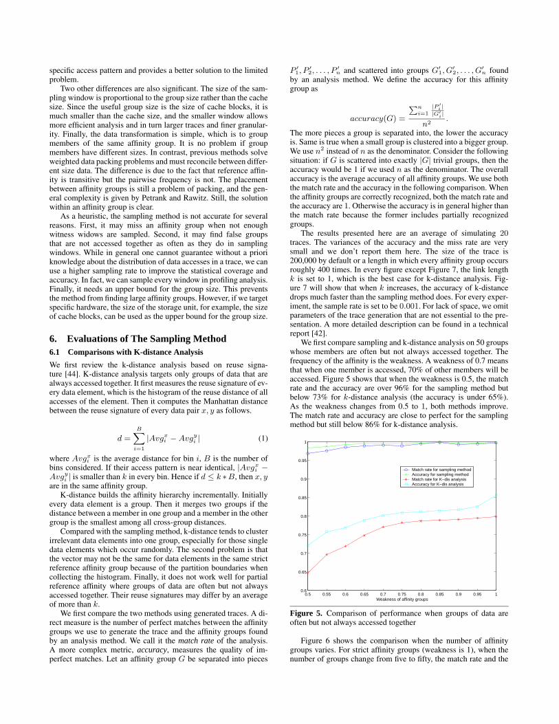
We first compare sampling and k-distance analysis on 50 groupswhose members are often but not always accessed together. Thefrequency of the affinity is the weakness. A weakness of 0.7 meansthat when one member is accessed, 70% of other members will beaccessed. Figure 5 shows that when the weakness is 0.5, the matchrate and the accuracy are over 96% for the sampling method butbelow 73% for k-distance analysis (the accuracy is under 65%).As the weakness changes from 0.5 to 1, both methods improve.The match rate and accuracy are close to perfect for the samplingmethod but still below 86% for k-distance analysis.
0.5 0.55 0.6 0.65 0.7 0.75 0.8 0.85 0.9 0.95 10.6
0.65
0.7
0.75
0.8
0.85
0.9
0.95
1
Weakness of affinity groups
Match rate for sampling methodAccuracy for sampling methodMatch rate for K−dis analysisAccuracy for K−dis analysis
Figure 5. Comparison of performance when groups of data areoften but not always accessed together
Figure 6 shows the comparison when the number of affinitygroups varies. For strict affinity groups (weakness is 1), when thenumber of groups change from five to fifty, the match rate and the

accuracy are stable (around 85%) for the sampling method but dropsignificantly for k-distance, from 86% to 67% for the match rateand from 78% to 50% for the accuracy. The match rate of thesampling method is not only much higher but also much closerto the accuracy, compared with k-distance. The upper two curvesdiffer by no more than 5%, showing that most affinity groups aredetected in whole by the sampling method.
5 10 15 20 25 30 35 40 45 500.6
0.65
0.7
0.75
0.8
0.85
0.9
0.95
1
Number of non−naive affinity groups
Match rate for sampling methodAccuracy for sampling methodMatch rate for K−dis analysisAccuracy for K−dis analysis
Figure 6. Comparison of performance when the number of affinitygroups varies
We now compare the effect of k, which is the closeness betweenaccesses to data of the same affinity group. As k increases, thecomplexity of finding affinity groups increases, from polynomialtime to NP-hard as shown in theory in earlier sections. Figures 7shows the result for 200 strict affinity groups. The match rate of thesampling method is perfect when k is 1 and 2 and drops to around80% when k increases from 3 to 10. K-distance analysis has muchworse performance from the beginning (around 85%) followed bya steep drop (to below 20%). The sampling method detects mostaffinity groups in whole but k-distance does not.
1 2 3 4 5 6 7 8 9 100
0.1
0.2
0.3
0.4
0.5
0.6
0.7
0.8
0.9
1
K
Match rate for sampling methodAccuracy for sampling methodMatch rate for K−dis analysisAccuracy for K−dis analysis
Figure 7. Comparison of performance when k (the closeness) ofthe affinity group varies
Last we test different sizes of the sampling window using affin-ity groups of size 20. Figure 8 shows that the performance is bestwhen the window size is 20, comparable to kg, where k = 1 and
g = 20. Since accesses are randomly scattered, the average dis-tance is about half of kg. Thus using only kg, we can get enoughconfidence. The performance varies by less than 2% for windowsizes between 10 and 30 and less than 8% between 5 and 50. Thematch rate and the accuracy are always higher than 92%. There-fore, the sampling method tolerates a wide range of window sizeswhen targeting groups of specific sizes.
5 10 15 20 25 30 35 40 45 500.92
0.93
0.94
0.95
0.96
0.97
0.98
0.99
1
Sample size
Match rate Accuracy
Figure 8. The performance of the sampling method for differentwindow sizes
The two methods can be combined. We first run K-distanceanalysis to find approximate affinity groups, estimate the size ofthe affinity groups, and then use the sampling method to refineand improve the results. The estimate from K-distance analysisalso reduces the memory requirement of the analysis. We haveleft out results from other experiments based on generated tracesbecause of the limited space. In all cases, the sampling methodgives efficient and accurate analysis for a wide range of affinitygroups. Next we look at real program traces.
6.2 Recursive Matrix Multiplication
We test affinity analysis on recursive matrix multiplication. Giventwo square matrices, each has 256 elements (16*16), the programrecursively divides the matrices into four parts and calculates theirproduct. The length of data access trace is 12288 (3 ∗ 163). Ac-cording to Theorem 7, there are five levels of reference affinity in16*16, 8*8, 4*4, 2*2, and 1*1 sub-matrices. When we set the sam-pling window to be volume distance 12 and the affinity thresholdto be 0.6, the sampling method correctly identifies affinity groupsin 2*2 blocks. Figure 9 shows one of the input matrix, with affinitygroups drawn in different shades of gray. Figure 10 shows that k-distance analysis identifies half of the 2*2 blocks but groups othersinto 4*4 blocks, which is not as accurate as the sampling method.
This is a simple experiment, but it demonstrates that samplinganalysis can uncover the high-level locality structure despite that itexamines only the data access trace of the complex computation,and that the general problem is NP-hard.
The affinity analysis can be used in a profiling tool for a userto see the locality structure in program data. Some of the datatransformations can be automated, for example, structure splittingand array regrouping. Some cannot, for example, the recursivedata layout in complex computations, so user support is currentlyneeded. It may be possible for dynamic data transformation. Aprogram can often analyzes its run-time data access and reorganizesthe data for better locality, as demonstrated by many studies forarray data in scientific programs or objects managed by a garbage

2 4 6 8 10 12 14 16
2
4
6
8
10
12
14
16
Figure 9. All 2*2 affinity groups are identified by the samplingmethod
2 4 6 8 10 12 14 16
2
4
6
8
10
12
14
16
Figure 10. Half of the 2*2 affinity groups are identified by k-distance analysis
collector. Reference affinity should be profitable if its analysis canbe made efficient enough.
6.3 Affinity-based Code Layout
We use profiling to collect the trace of basic block references,apply reference affinity analysis, and then reorganize code layoutby placing basic blocks of the same group sequentially in memory.The sim-cache module of SimpleScalar is modified to simulate theinstruction cache and measure the cache miss rate. We comparethese affinity groups with the original code layout and the coderegions formed by checking transition frequencies between basicblocks [22], a common method in profiling-based code layout. Forlack of space, we briefly describe only the main setup and the result.The purpose is to demonstrate the applicability of reference affinityand the sampling method. We do not intend in this work to designa complete compiler technique nor evaluate it against the existingliterature.
We test seven integer programs from SPEC 2000 3. We use com-plete traces, which contain up to one billion basic blocks and 10 bil-lion references. K-distance method is based on the reuse signature
3 Bzip2, Crafty, Gap, Mcf, Perlbmk, Twolf, and Vpr
from long-distance reuses, so it ignores many basic blocks, whichare only accessed once with a short reuse distance. It suffers morefrom false positives because the reuse signature lacks the timing in-formation. In experiments, k-distance tends to produce one or twovery large groups, containing up to 50% of all basic blocks. Thesampling method overcomes these drawbacks. For complete cover-age in profiling, the sampling rate is 100%. The exact comparisondepends on the thresholds and parameters for both sampling andthe frequency-based method. A detailed comparison is too long toinclude. However, the best affinity-based layout always has betterlocality than the best frequency-based layout, as shown in Figure 11for two different cache configurations. Compared with the unopti-mized code layout on 8KB direct-mapped cache, the affinity-basedlayout reduces the cache miss rate for six of the seven programsby up to a factor of more than 3. When 16KB 2-way set associativecache is used, the miss rate of the three of the seven programs dropsto near zero. The affinity-based layout improves the locality in allother four programs. The largest relative improvement is on Twolf,a circuit placement and global routing program using simulated an-nealing. The miss rate drops from 0.4% by more than a factor of 10by the affinity-based layout. In comparison, the frequency-basedlayout reduces the miss rate by a factor of about 2.
7. Related WorkThabit showed that data packing for a given block size using pair-wise frequency is NP-hard [38]. Kennedy and Kremer gave a gen-eral model that includes run-time data transformation (among othertechniques) and showed that the problem is NP-hard [23]. Pe-trank and Rawitz showed the strongest theoretical result to date—ifP 6= NP , no polynomial time method can guarantee a data layoutwhose number of cache misses is within O(n1−ε) of that of theoptimal data layout, where n is the length of the trace. In addition,if only pair-wise information is used, no algorithm can guarantee adata layout whose number of cache misses is within O(k − 3) ofthat of the optimal data layout, where k is the size of cache. Theresults hold even when the computation sequence is completelyknown, objects have the same size, and the cache is set associa-tive [32]. These general results, however, do not preclude effectiveoptimization targeting specific (rather than all) data access patterns.In fact, one can easily construct traces for which it is trivial to findthe optimal data layout.
Zhong et al. defined reference affinity and used a heuristic calledk-distance analysis in structure splitting and array regrouping [44].The earlier work does not give the computational complexity ofreference affinity, nor is it used in hierarchical data placement. Inaddition, as shown in Section 6, k-distance analysis does not workwell for partial reference affinity.
Hierarchical data layout is first used for matrix multiplicationand QR factorization by Frens and Wise [16, 17], Cholesky fac-torization (based on data shackling [25]) and wavelet transform byChatterjee et al. [7], and N-body and mesh simulation by Mellor-Crummey et al [30]. We show that reference affinity can help aprogrammer to analyze data locality in these and other programs(without knowing the structure of the computation).
Bender et al. used the recursive van Emde Boas layout fordynamic search trees and proved the asymptotic optimality if theinput consists of random searches [3]. Reference affinity cannotyet give the van Emde Boas layout because the affinity hierarchyis flat (two levels) for any constant k. The extension for variable-distance affinity groups is a subject of future work. On the otherhand, if the input is not random search and has reference affinity,for example, a group of tree nodes are often searched together, thenreference affinity is directly applicable and in principle may yieldbetter locality than the van Emde Boas layout does.

0.0%
0.5%
1.0%
1.5%
2.0%
2.5%
3.0%
3.5%
4.0%
4.5%
Bzip2
Crafty
Gap Mcf
Perlb
mkTw
olf Vpr
benchmark
cach
e m
iss
rate
orig min-freq min-aff
(a) 8KB direct-mapped cache, cache blocksize 64 bytes
0.0%
0.2%
0.4%
0.6%
0.8%
1.0%
1.2%
1.4%
1.6%
1.8%
Bzip2
Crafty
Gap Mcf
Perlb
mkTw
olf Vpr
benchmark
cach
e m
iss
rate
orig min-freq min-aff
(b) 16KB 2-way set associative cache, cacheblock size 32 bytes
Figure 11. Comparison of cache performance of the original and the best of frequency- and affinity-based code layout for seven SPEC2Kinteger benchmarks
Wolf and Lam [40] and McKinley et al. [29] used compileranalysis to identify groups of memory references in loop nests.Our work is related to trace-based pairwise affinity models, as dis-cussed in Section 5. Hang and Tseng used pairwise (connection)models for scientific data and found that hierarchical clustering wasmore cost-effective than general graph partitioning [20]. Chilimbidefined hot data streams, which are sequences of repeated data ac-cesses and are not limited by pairwise affinity [8]. When a pro-gram has good computation locality, simple data packing (first-touch ordering) improves the data layout, as shown by several stud-ies [12, 30, 36, 39]. Recently, Strout and Hovland introduced mod-els based on hyper-graphs [37]. Most of these techniques are in-tended for on-line adaptation and do not model hierarchical local-ity.
Earlier studies have established the locality upper bound (thebest possible locality) for specific computing problems. Hong andKung used a graph model to prove the tight lower bound of I/O forFFT, matrix multiply, and sorting. Aggarwal et al. gave a hierarchi-cal memory model (HMM), where the cost for access location xwas dlog xe [1]. They showed that the maximal slowdown factor(O(log n)) could be avoided for some computations (FFT, matrixmultiply, and sorting) but not for others (list search and circuit sim-ulation). They also studied other convex cost functions. Alpern etal. extended the hierarchical model with explicit transfer cost andgave a set of threshold functions when computations (FFT, matrixmultiply, matrix transpose, and parallel matrix multiply) becamecommunication bound [2]. Frigo et al. refined the cache model toconsider cache size Z and block size L. They gave recursive al-gorithms that yielded the best asymptotic locality for FFT, matrixmultiply, and sorting for any Z and L (Z = Ω(L2)) [18]. The al-gorithms are cache oblivious because they do not depend on Z andL. Yi et al. showed that a compiler can automatically convert loopsinto recursive subroutines to exploit hierarchical locality [41].
The ordering of general computations has been studied as aclustering problem in loop fusion and computation regrouping.Kennedy and McKinley [24] showed that fusion for locality wasNP-hard because it could be reduced to the problem of k-waycut [10]. Ding and Kennedy proved a similar result for a refinedmodel, where hyper graphs were used to represent data reusesamong multiple computations [13]. Darte gave complexity resultsfor a larger class of fusion problems [11]. These results suggestthat efficient, hierarchical models are unlikely for general-purposecomputations.
In 1970, Mattson et al. first defined reuse distance (named LRU-stack distance) [28]. The distribution of all reuse distances (whichwe call the reuse signature) gives the temporal locality of an execu-tion. Snir and Yu recently disproved the possibility of a more com-pact metric by showing that temporal locality could not be char-acterized by one or few parameters [35]. Indeed, reuse signaturehas been widely used in virtual memory and cache design. Build-ing on decades of development by others, our earlier work reducedthe measurement cost to near linear time [14] and used reuse dis-tance patterns for program locality prediction [33, 43], data struc-ture transformation [44], and locality phase prediction [34]. Reuse-distance based models are found useful for program analysis byan increasing number of studies (three appeared in 2005), includ-ing cache miss rate prediction across inputs by Marin and Mellor-Crummey [26, 27], per-reference miss rate prediction by Fang etal. [15] and Beyls and D’Hollander [4], and cache interferenceprediction for parallel processes by Chandra et al [6]. This paperpresents a formal theory for reuse distance. The proof for Theo-rem 1 gives a reduction between reuse distance and formal logic.The proof of Theorem 7 connects the structure in computation withthe locality in data. These formal connections serve as a theoret-ical basis for current and future reuse-distance based models andtechniques.
8. SummaryIn this paper we have given a complete characterization of the com-plexity of reference affinity. We have proved that when k = 1 ork = 2, finding reference affinity grooups can be done within poly-nomial time and when k = 3, finding reference affinity groups isa NP-hard problem. We have extended the hierarchical locality todivide-and-conquer computations such as matrix solvers, factoriza-tion, wavelet transform, N-body and mesh simulation, where theresults confirms the previous empirical solutions. The theoreticalresults have established formal links between the computation, thedata reuse, and the locality. In practical use side, We don’t knowa real use for cases k = 1 or k = 2. The hardness of findingthe reference affinity groups when k > 2 implies that it is hard tofind any polynomial algorithms. Instead, we have presented a sam-pling method and shown through experiments that it is more accu-rate than the previously published technique, especially for groupsgreater in number and complexity and weaker in their affinity. Wehave shown two new uses of reference affinity. The first is finding

hierarchical data layout in a recursive program, and the second isimproving the code layout of seven SPEC 2K applications.
In POPL 2002, Petrank and Rawitz precisely characterized thetheoretical difficulty of the general data placement. Reference affin-ity side steps this limitation by targeting a common pattern ratherthan all patterns of data access. Since the volume distance is widelyused in experimental algorithms, the theoretical findings in this pa-per may help the development of other distance-based locality the-ories.
A. Proofs
Theorem 1 For each k ≥ 3, Pw-k -Aff is NP-complete.
Proof It is obvious that the problem is in NP. We will prove its NP-hardness by constructing a polynomial-time many-one reductionto Pw-k -Aff from 3-SAT, which is the problem of testing, givena formula of conjunctive normal form in which each clause hasat most 3 literals, whether the formula is satisfiable. We considerthe variant of this problem in which each variable appears as aliteral (positively or negatively) at most three times. This problemis also known to be NP-complete (see, e.g., [31]). Without loss ofgenerality, we can assume that all variables appear both positivelyand negatively in the formula. If a variable appears only positively(respectively, negatively) then we can create a simpler, equivalentformula by setting the value of the variable to true (respectively,false).
Let ϕ be a CNF formula of N variables and M clauses in whicheach clause has at most 3 literals and each variable appears at mostthree times. Let x1, . . . , xN be the variables of ϕ and C1, . . . , CM
be the clauses of ϕ.Let λin and λout be two distinct labels. We will define a se-
quence T whose first label is λin and whose last label is λout. λout
appears nowhere else in the sequence. We will consider the prob-lem of creating a k-linked path between the two. The sequence isof the form
λinΣΓ1 · · ·ΓNΘ1 · · ·ΘMλout.
The sequence Σ is the k repetitions of ν1 · · · νk separated byk− 1 λin’s. where ν1, . . . , νk are k pairwise distinct labels. Recallthat for a pair of positions to be k-linked there must be a set ofintermediate points with pairwise distinct labels in which the reusedistance between each neighboring intermediate points is at most k.To create such a path between our two end points, the subsequenceΣ must be traversed without visiting a same label more than once sothat the distance between the two neighboring visited points havereuse distance at most k. The only way to construct such a path isto visit every (k+1)st element of Σ besides the first λin, exiting atthe first element after Σ. This path visits ν1, . . . , νk exactly once.This means that any k-link path between our two endpoints shouldnot visit any one of ν1, . . . , νk+1 again.
For each xi appeared in the formula, 1 ≤ i ≤ N , Γi if of formαi,1γi,1γi,2γi,3ν1 · · · νk−2γi,1αi,2ν1 · · · νk−1.
The α’s here appear nowhere else in the sequence. Each γ appearsat most once elsewhere. If it does indeed, it appears in one of theΘ’s. Suppose that a k-linked path between the two endpoints landson αi,1. Then the path can only be threaded in Γi using one of thefollowing paths:1. [γi,3, αi,2],2. [γi,3, γi,1, αi,2],3. [γi,2, γi,3, αi,2],4. [γi,2, γi,3, γi,1, αi,2],5. [γi,2, γi,1, αi,2],
6. [γi,1, γi,2, γi,3, αi,2], and7. [γi,1, γi,3, αi,2].
Consider the set of all γ’s that has not been visited yet. The set is1. γi,1, γi,2,2. γi,2,3. γi,1,4. ∅,5. γi,3,6. ∅,7. γi,2.
Two crucial observations here are that (a) there is no set thatcontains γi,3 and one extra element and (b) that the first set has bothγi,1 and γi,2. Suppose that xi appears three times in the formula,twice as xi and once as xi. Then we use γi,1 to denote the firstoccurrence of xi, γi,2 to denote the second occurrence of xi, andγi,3 to denote xi. In the case when xi appears twice and xi appearsonce, we use γi,1 to denote the first occurrence of xi, γi,2 to denotethe second occurrence of xi, and γi,3 to denote xi. In the case whenboth xi and xi appear only once, we use γi,1 to denote the uniqueoccurrence of xi and γi,3 to denote the unique occurrence of xi.Note that all of these possible paths must land the first elementafter Γi.
For each i, 1 ≤ i ≤ M , such that Ci has exactly two literals,Θi is of the form
βi,1θi,1θi,2ν3 · · · νk.βi,2ν2 · · · νk,
and for each i, 1 ≤ i ≤ M , such that Ci has exactly three literals,we construct Θi as
βi,1θi,1θi,2θi,3ν4 · · · νk.βi,2ν2 · · · νk,
where θi,l is the lth literal of Ci. Note here that the literals in theclause are replaced using γ’s in the sequence according to the rulesin the construction of Γ’s. Suppose that the k-linked path betweenour two endpoints land on βi,1. Since there are k labels betweenβi,1 and βi,2 and none of the ν’s can be visited again, the k-linkedpath can only be extended if one of the θ literals is visited. Thesegment after βi,2 forces the path to land on the element right afterΘi.
we can see that Σ is of length k(k + 1) − 1, for each i,1 ≤ i ≤ N , Γi has length 2k + 3, and for each i, 1 ≤ i ≤ M , Θi
has length 2k + 1. So, the total length of the sequence, includingthe two endpoints, is
2 + k(k + 1) − 1 + N(2k + 3) + M(2k + 1),
which is equal to k(2N + 2M + k + 1) + 3N + M + 1, whichis polynomial of the size of the CNF formula. So the constructioncan be done in polynomial time.
We view the literals that are visited in Θi as those satisfiedby the assignment represented by the path. For such a path to bevalid, the selections in the Θ sections have to be made so that theliterals satisfying the clauses are still available. Suppose that ϕ issatisfiable. Let A be a satisfying assignment of ϕ. Construct thepath within Θ’s so that the those that are visited are precisely thosethat are satisfied by A. Then it is possible to select the paths inΓ so that none of those visited in Θ are visited in Γ. So, the twoendpoints are k-lined.
On the other hand, suppose that ϕ is not satisfiable. Take anypotentially k-linked path π in the Θ’s. There exist at least one vari-able, xi for which both one occurrence of xi and one occurrence ofxi is selected. Then it is not possible to construct a k-linked pathwithin Γi, so there is no k-linked path between the two endpoints.

We note here that the set of labels, Λ, which is the part of theinstance is the set of all labels that we’ve defined. By now, we haveconstructed a polynomial-time many-one reduction from 3-SAT toPw-k -Aff . Since Pw-k -Aff apparently belongs to NP, we provethat Pw-k -Aff is a NP-complete problem.
Corollary 1 For k ≥ 3, the problem of checking referenceaffinity groups is NP-complete.
Proof Suppose the group of data elements is G. First, let’s showthat this problem belongs to NP. This can be done by first guessingthe possible supersets of G, say G′. For every two different dataelements x, y ∈ G′, for every ax, we guess it can be connected tothe nearest ay located left-side or right-side, and then we guess alink-path between them and then verify if this is a link path of link-length k. If it is, then continue to check other ax’s and then otherpairs of data elements. But if not, it will just refuse to accept. Wecan check for all of the pairs and all accesses of x in a sequentialway. If every pairs and every accesses are checked to be linkedsuccessfully, then accept.
By the definition of reference affinity group, for any x, y ∈ G,for all ax, we need to check if there exists an ay , such that ax anday are k-linked. The only way is to check if there is a k-linkedpath from ax to the left-side or right-side nearest ay . So we can seethat if there is a polynomial-time algorithm for checking referenceaffinity problem, then there is a polynomial-time algorithm forPw-k -Aff problem. Thus we have proved that for k ≥ 3,checkingreference affinity group problem is NP-complete problem.
Corollary 2 For k ≥ 3, the problem of finding referenceaffinity groups is NP-hard.
Proof The proof is quite straightforward. If there is a polynomial-time solution that can find out the reference affinity groups, thenwe can solve the problem of checking reference affinity groups inpolynomial time. This contradicts with Corollary 1.
Theorem 2 For k = 2, Pw-k -Aff is NL-complete.
Proof 2 -CNF-SAT is the problem of testing whether a givenconjunctive normal form formula with two literals per clause issatisfiable. This problem is the standard NL-complete problem. Byfollowing the proof of Theorem 1 with k = 2, we can show thatthe 2 -CNF-SAT is reducible to Pw-k -Aff for k = 2.
To prove that PWkAff belongs to NL for k = 2, supposethat a set of labels Λ, a sequence Σ = σi
Mi≥1 over Λ, an integer
k ≥ 0, and two integers I and J , 1 ≤ I ≤ J ≤ M are given asan instance to the problem. We wish to test whether I and J arek-linked.
Since the elements before the Ith entry and those after the J th
are irrelevant to the problem at hand, we may assume, Without lossof generality, that I = 1 and J = M . Also, if the ith entry and the(i + 1)st entry are the same, at most one of the two can be visited,and if one is visited at all which one doesn’t matter. So, one of themcan be safely removed. This means that, for all i, 2 ≤ i ≤ M − 2,σi 6= σi+1.
For each i, 2 ≤ i ≤ M −1, let yi be the variable that representswhether the ith element is visited. We construct a formula ϕ byjoining the following size-two clauses:• for each i, 2 ≤ i ≤ M − 2, (yi ∨ yi+1), and• for all ρ ∈ Σ and for all i and j such that 2 ≤ i < j ≤ M − 1
and σi = σj = ρ, (yi ∨ yj).Suppose that this formula is satisfiable. Let A be a satisfyingassignment of the formula. Then A clearly defines a k-linked path,since only those belonging to Σ are visited, no element in Σ isvisited more than once, and there is at most one entry between any
two neighbors on the path. Similarly, if there is a k-linked path, thenby setting the truth value of each variable according to whether thenode is included in the path, we can satisfy the formula. So, thesatisfiability of the formula is equivalent to the existence of a k-linked path.
Theorem 3 For k = 2, the problem of finding referenceaffinity groups is in P .
Algorithm 1 can be found in Section 3. Here we present thedetailed proof.Proof First let us show this is a polynomial-time algorithm. ByTheorem 2, we need polynomial time to test whether two dataaccesses are 2-linked. Hence, testing if two data elements is 2-linked with respect to a given group can be done in polynomialtime. Constructing the graph G needs only polynomial time. Forthe reference affinity group that x belongs to, we remove at mostm data elements from the group, where m is the number of dataelements in the trace. There are at most m reference affinity groups.Therefore, the algorithm takes polynomial time.
Next we prove the correctness. First, it is easy to see that thegroups found by this algorithm satisfy the first condition of refer-ence affinity. Second, let us show every group is the maximal sizepossible. We show that the algorithm removes z correctly. Remov-ing z at step 7 is straightforward. The correctness of the removal ofz at step 10 can be proved by contradiction. Suppose z and x be-long to the same group G1. We have y /∈ G1. From the algorithm,an access ay cannot be 2-linked to any access of z. Since x and yare 2-linked, there are some accesses of x that is 2-linked to ay . Wepick the nearest one as ax. Without loss of generality, we assumeax appears at the right side of ay . Similarly, we choose az , whichis 2-linked to and nearest to the ax. This az can not appear on theleft side of ax. Otherwise, we have two cases. First, if az appearsbetween ay and ax, then the path from ay to ax must pass the verydata element at the right side of az , since k = 2. Then the ay canbe 2-linked to this az by replacing the very data element with az ,which is a contradiction. Second, if az appears on the left side ofay , since x and z are in the same group, a path exists from ax to az
without passing ay . This path must land on the very data elementat the right side of ay , since k = 2. Then we can replace the verydata element with ay and get a new path from ay to az , which isalso a contradiction.
Now let’s select the leftmost data element in G1 that appears onthe section of trace between the ay and az . Suppose it is al. This isshown in Sequence (2).
...y...l...x...z... (2)We first show that a path exists from ay to al with respect to
(G − G1)S
l. Since ay is 2-linked to ax with respect to groupG, there is a path π connecting them. If π does not pass al, it mustpass the very data element at the left side of al, since k = 2. A newpath π1can be generated from ay to al by first reaching the verydata element and then one step further to al. If π passes al, then wepick the segment from ay to al as π1. All of the data elements onthe path π1 is in G − G1 except for l.
Since l is in the same group with z, there is a path π2 from al toaz with respect to G1. We get a new path π′ by merging paths π1
and π2. Now π′ is a 2-linked path without duplicated data elementsfrom ay to az , which is a contradiction with step 9.
Theorem 5 For k = 1, there is a polynomial-time solution forfinding reference affinity groups.
ALGORITHM 3. Finding reference affinity groups when k=1procedure FindReferenceAffinityGroup 1(T)
1: T is the trace, k = 1

2: encode the data elements according to the order of appearancein the trace. Suppose there are m distinct data elements.
3: while there exist data not yet grouped do4: pick the smallest not yet grouped datum s.5: for t=m to s step −1 do6: if IsAGroup(T,s,t) then7: break;8: end if9: end for
10: output elements in s, . . . , t as a group.11: end while
endFindReferenceAffinityGroup 1procedure IsAGroup(T,s,t)
1: for i from 1 to |T | do2: if T[i] is within s and t then3: if The elements T[i] can be 1-linked to with respect to
s, . . . , t can not cover set s, . . . , t then4: return false;5: end if6: end if7: end for8: return true;
endIsAGroup
It is straightforward to show that the algorithm is polynomialtime and can output the correct reference affinity groups.Lemma 1 Given two different data elements u and v; theiraccesses au and av where the volume distance from au to av isexactly k; and a third access ax, which happens between au andav in the trace; then there exists an access a′
x between au andav such that the volume distance from au to a′
x and the volumedistance from a′
x to av are both less than k.
Proof The element u is either earlier or later than v in the dataspace. Because a link and a path are not directed, the two casesare symmetrical. Without loss of generality, we assume u is beforev. Consider the smallest m-block that contains u, v, au, av . Theelement x must be in the data section of the block; otherwise thepath from au to av does not go through x. There are two casesshown by the two graphs in Figure 12, each has six sub-cases. Thelocation of ax is given for each sub-case in the figure. In most cases,ax splits the k-link from au to av into two shorter links of less thank. The first case is when au and av are in upper and lower halfblocks. In the first sub-case of the first case, we need to use oneof the two locations, marked by a′
x and a′′x . Then we use the au
to break the link from the access of x to av and treat the access tox as au. The last sub-case of the first case is similar. The secondcase happens when au and av are both in the upper or lower halfblock. Figure 12 shows the three out of the six sub-cases when bothaccesses are in the upper half block. The other three sub-cases aresymmetrical. In sub-case 1 and 3, we pick a′
x to be in the middleon the same side of ax. In sub-case 2, we use one of the two middlepoints depending on the position of ax.
References[1] A. Aggarwal, B. Alpern, A. Chandra, and M. Snir. A model for
hierarchical memory. In Proceedings of the ACM Conference onTheory of Computing, New York, NY, 1987.
[2] B. Alpern, L. Carter, E. Feig, and T. Selker. The uniform memoryhierarchy model of computation. Algorithmica, 12(2/3):72–109,1994.
[3] M. A. Bender, E. D. Demaine, and M. Farach-Colton. Cache-oblivious b-trees. In Proceedings of Symposium on Foundationsof Computer Science, November 2000.
(au) au
(av) av
case 1
case 2
case 3
case 4
case 5
case 6
ax
a‘xa‘’x
a‘xa‘x a‘’x
a‘x
a‘x
a‘x
(a)
au
av
case 1
case 2
case 3ax
a‘x
(b)
Figure 12. Cases in proving the insertion lemma. au and av showthe possible positions in the trace. a′
x, and a′′x show the possible
targets of moving x to split trace between au and av . The arrowsshow the destination of moving x. For every case, there is a solutionfor x to break the k-link in the old path.
[4] K. Beyls and E. D’Hollander. Reuse distance-based cache hintselection. In Proceedings of the 8th International Euro-ParConference, Paderborn, Germany, August 2002.
[5] B. Calder, C. Krintz, S. John, and T. Austin. Cache-conscious dataplacement. In Proceedings of the Eighth International Conferenceon Architectural Support for Programming Languages and OperatingSystems (ASPLOS-VIII), San Jose, Oct 1998.
[6] D. Chandra, F. Guo, S. Kim, and Y. Solihin. Predicting inter-thread cache contention on a chip multi-processor architecture. InProceedings of the International Symposium on High PerformanceComputer Architecture (HPCA), 2005.
[7] S. Chatterjee, V. V. Jain, A. R. Lebeck, S. Mundhra, and M. Thot-tethodi. Nonlinear array layouts for hierarchical memory systems. InProceedings of International Conference on Supercomputing, 1999.
[8] T. M. Chilimbi. Efficient representations and abstractions forquantifying and exploiting data reference locality. In Proceedingsof ACM SIGPLAN Conference on Programming Language Designand Implementation, Snowbird, Utah, June 2001.
[9] T. M. Chilimbi, M. D. Hill, and J. R. Larus. Cache-consciousstructure layout. In Proceedings of ACM SIGPLAN Conferenceon Programming Language Design and Implementation, Atlanta,Georgia, May 1999.

[10] E. Dahlhaus, D. S. Johnson, C. H. Papadimitriou, P. D. Seymour, andM. Yannakakis. The complexity of multiway cuts. In Proceedings ofthe 24th Annual ACM Symposium on the Theory of Computing, May1992.
[11] A. Darte. On the complexity of loop fusion. Parallel Computing,26(9):1175–1193, 2000.
[12] C. Ding and K. Kennedy. Improving cache performance in dynamicapplications through data and computation reorganization at run time.In Proceedings of the SIGPLAN ’99 Conference on ProgrammingLanguage Design and Implementation, Atlanta, GA, May 1999.
[13] C. Ding and K. Kennedy. Improving effective bandwidth throughcompiler enhancement of global cache reuse. Journal of Parallel andDistributed Computing, 64(1):108–134, 2004.
[14] C. Ding and Y. Zhong. Predicting whole-program locality with reusedistance analysis. In Proceedings of ACM SIGPLAN Conference onProgramming Language Design and Implementation, San Diego, CA,June 2003.
[15] C. Fang, S. Carr, S. Onder, and Z. Wang. Instruction basedmemory distance analysis and its application to optimization. InProceedings of International Conference on Parallel Architecturesand Compilation Techniques, St. Louis, MO, 2005.
[16] J. D. Frens and D. S. Wise. Auto-blocking matrix-multiplication ortracking BLAS3 performance with source code. In Proceedings ofthe ACM SIGPLAN Symposium on Principles Practice of ParallelProgramming, Las Vegas, NV, 1997.
[17] J. D. Frens and D. S. Wise. QR factorization with Morton-orderedquadtree matrices for memory re-use and parallelism. In Proceedingsof the ACM SIGPLAN Symposium on Principles Practice of ParallelProgramming, San Diego, CA, 2003.
[18] M. Frigo, C. E. Leiserson, H. Prokop, and S. Ramachandran. Cache-oblivious algorithms. In Proceedings of Symposium on Foundationsof Computer Science, October 1999.
[19] N. Gloy and M. D. Smith. Procedure placement using temporal-ordering information. ACM Transactions on Programming Languagesand Systems, 21(5), September 1999.
[20] H. Han and C. W. Tseng. Locality optimizations for adaptive irregularscientific codes. Technical report, Department of Computer Science,University of Maryland, College Park, 2000.
[21] J. Han and M. Kamber. Data Mining: Concepts and Techniques.Morgan Kaufmann Publishers, 2000.
[22] R. E. Hank, W. W. Hwu, and B. R. Rau. Region-based compilation:An introduction and motivation. In Proceedings of the AnnualInternational Symposium on Microarchitecture, 1995.
[23] K. Kennedy and U. Kremer. Automatic data layout for distributedmemory machines. ACM Transactions on Programming Languagesand Systems, 20(4), 1998.
[24] K. Kennedy and K. S. McKinley. Typed fusion with applicationsto parallel and sequential code generation. Technical Report TR93-208, Dept. of Computer Science, Rice University, Aug. 1993. (alsoavailable as CRPC-TR94370).
[25] I. Kodukula, N. Ahmed, and K. Pingali. Data-centric multi-levelblocking. In Proceedings of the SIGPLAN ’97 Conference onProgramming Language Design and Implementation, Las Vegas,NV, June 1997.
[26] G. Marin and J. Mellor-Crummey. Cross architecture performancepredictions for scientific applications using parameterized models. InProceedings of Joint International Conference on Measurement andModeling of Computer Systems, New York City, NY, June 2004.
[27] G. Marin and J. Mellor-Crummey. Scalable cross-architecturepredictions of memory hierarchy response for scientific applications.
In Proceedings of the Symposium of the Las Alamo s ComputerScience Institute, Sante Fe, New Mexico, 2005.
[28] R. L. Mattson, J. Gecsei, D. Slutz, and I. L. Traiger. Evaluationtechniques for storage hierarchies. IBM System Journal, 9(2):78–117,1970.
[29] K. S. McKinley, S. Carr, and C.-W. Tseng. Improving data localitywith loop transformations. ACM Transactions on ProgrammingLanguages and Systems, 18(4):424–453, July 1996.
[30] J. Mellor-Crummey, D. Whalley, and K. Kennedy. Improving memoryhierarchy performance for irregular applications. InternationalJournal of Parallel Programming, 29(3), June 2001.
[31] C. H. Papadimitriou. Computational Complexity. Addison Wesley,1994.
[32] E. Petrank and D. Rawitz. The hardness of cache conscious dataplacement. In Proceedings of ACM Symposium on Principles ofProgramming Languages, Portland, Oregon, January 2002.
[33] X. Shen, Y. Zhong, and C. Ding. Regression-based multi-modelprediction of data reuse signature. In Proceedings of the 4th AnnualSymposium of the Las Alamos Computer Science Institute, Sante Fe,New Mexico, November 2003.
[34] X. Shen, Y. Zhong, and C. Ding. Locality phase prediction. InProceedings of the Eleventh International Conference on Architectural Support for Programming Languages and Operating Systems(ASPLOS XI), Boston, MA, 2004.
[35] M. Snir and J. Yu. On the theory of spatial and temporal locality.Technical Report DCS-R-2005-2564, Computer Science Dept., Univ.of Illinois at Urbana-Champaign, July 2005.
[36] M. M. Strout, L. Carter, and J. Ferrante. Compile-time compositionof run-time data and iteration reorderings. In Proceedings ofACM SIGPLAN Conference on Programming Language Design andImplementation, San Diego, CA, June 2003.
[37] M. M. Strout and P. Hovland. Metrics and models for reorderingtransformations. In Proceedings of the 2nd ACM SIGPLAN Workshopon Memory System Performance, Washington DC, June 2004.
[38] K. O. Thabit. Cache Management by the Compiler. PhD thesis, Dept.of Computer Science, Rice University, 1981.
[39] B. S. White, S. A. McKee, B. R. de Supinski, B. Miller, D. Quinlan,and M. Schulz. Improving the computational intensity of unstructuredmesh applications. In Proceedings of the 19th ACM InternationalConference on Supercomputing, Cambridge, MA, June 2005.
[40] M. E. Wolf and M. Lam. A data locality optimizing algorithm.In Proceedings of the SIGPLAN ’91 Conference on ProgrammingLanguage Design and Implementation, Toronto, Canada, June 1991.
[41] Q. Yi, V. Adve, and K. Kennedy. Transforming loops to recursion formulti-level memory hierarchies. In Proceedings of ACM SIGPLANConference on Programming Language Design and Implementation,Vancouver, Canada, June 2000.
[42] C. Zhang, Y. Zhong, C. Ding, and M. Ogihara. Finding referenceaffinity groups in trace using sampling method. Technical ReportTR 842, Department of Computer Science, University of Rochester,July 2004. presented at the 3rd Workshop on Mining Temporal andSequential Data, in conjunction with ACM SIGKDD 2004.
[43] Y. Zhong, S. G. Dropsho, and C. Ding. Miss rate prediction across allprogram inputs. In Proceedings of the 12th International Conferenceon Parallel Architectures and Compilation Techniques, New Orleans,Louisiana, September 2003.
[44] Y. Zhong, M. Orlovich, X. Shen, and C. Ding. Array regroupingand structure splitting using whole-program reference affinity.In Proceedings of ACM SIGPLAN Conference on ProgrammingLanguage Design and Implementation, June 2004.


