Inflated mixture models: Applications to multimodality in loss given default

Mauro R de Oliveira Jr1

Caixa Econmica Federal and Federal University of Sao Carlos

Francisco Louzada

University of Sao Paulo

Gustavo Pereira

Federal University of Sao Carlos

Fernando Moreira

University of Edinburgh Business School

Raffaella Calabrese

University of Essex Business Scholl

Abstract

In this paper, we propose an inflated mixture model to deal with multimodality in loss given default data.We propose a mixed of degenerate distributions, to handle zeros and ones excess, with a mixture of to-be-chosen bounded distributions for non-zeros and non-ones proportions. By applying the methodologyin four retail portfolios of a large Brazilian commercial bank, we show that the inflated mixture of betadistributions plays better role minimizing model risk in fitting an inadequate model, in comparison withothers considered competitive models. We explore the use of maximum likelihood estimation procedure.Monte Carlo simulations are carried out in order to check its finite sample performance.

Keywords: Basel II, inflated model, MLE, mixture, multimodality, retail exposures.

1. Introduction

Since the Basel II publications in the mid-2000s, recommending central banks to allow banks to useinternal data to calculate credit risk measures of their portfolios, much has been proposed in the literatureon probability of default, loss given default and exposure at default. See for example [5, 9, 17]. Theimportance is justified as these parameters comprise the main ingredients of regulatory capital calculation,what banks must set aside to cope with unexpected losses from credit portfolios.

According to Basel rules for corporate, sovereign and bank exposures (see [1], paragraphs 286 and 297),loss given default (LGD) is measured as the proportion of unrecovered debt, compared to total counterpartyoverdue debt. However, despite the simplicity in setting it, there are distinctions about the treatmentthat should be given to different types of portfolios (see [15]). For instance, in case of the aforementionedportfolios, corporate, sovereign and bank exposures, banks must provide an individual estimate of LGD foreach exposure and, for that reason, a different approach that has been applied to retail portfolios.

In fact, as retail exposures typically represent majority of loan portfolios of commercial banks, it wouldbe impossible to give an individualized treatment for each exposure. That is why, even before Basel recom-mendations, bank risk managers relied on automated scoring models. This means that, mostly, modellingcredit risk involves estimating parametric statistical models (see [13]). However, as expected, an exaggerated

1Corresponding author: mauroexatas@gmail.com

Preprint submitted to Elsevier 24th September 2015

dependence on complex statistical models may lead to new sources of risks. In this case, the model risk, inother words, the risk of not choosing the best model in the light of the available data.

An attempt to draw attention to model risk, and encourage mitigation of this source of risk, has alreadybeen addressed by the Basel Committee, as stated in [2], p. 2, ”Supervisors should be cautious againstover-reliance on internal models for credit risk management and regulatory capital. Where appropriate,simple measures could be evaluated in conjunction with sophisticated modelling to provide a more completepicture”.

Regarding the modelling of LGD, BCBS [1] also recommends that its calculation must consider all relevantfactors that impact in the loss triggered by the event of default. Strictly following the paragraph 460, thecalculation must include all material discount effects and all material direct and indirect costs associatedwith collecting on the defaulted loan.

Since it is known that LGD has considerable impact on the regulatory capital amount, small differencescan lead to major distortions in its calculation. For this reason, when dealing with large retail portfolioswithout sufficient evidence of the impact of each direct and indirect recovery cost, in order to proceed anreliable estimate, we must opt for models that bring a extra dose of conservatism.

In the foregoing context, i.e., concerning to the loss given default modelling, in this paper we aim toextend the established framework already proposed to accommodate multimodality in LGD data. Therefore,basically, we attempt to minimize model risk in fitting an inadequate distribution to LGD data. For that, wecomplement the work done by Hlawatsch & Ostrowski [7], which, despite dealing with simulated bimodality,do not address the occurrence of zeros and ones excesses in bimodal LGD data.

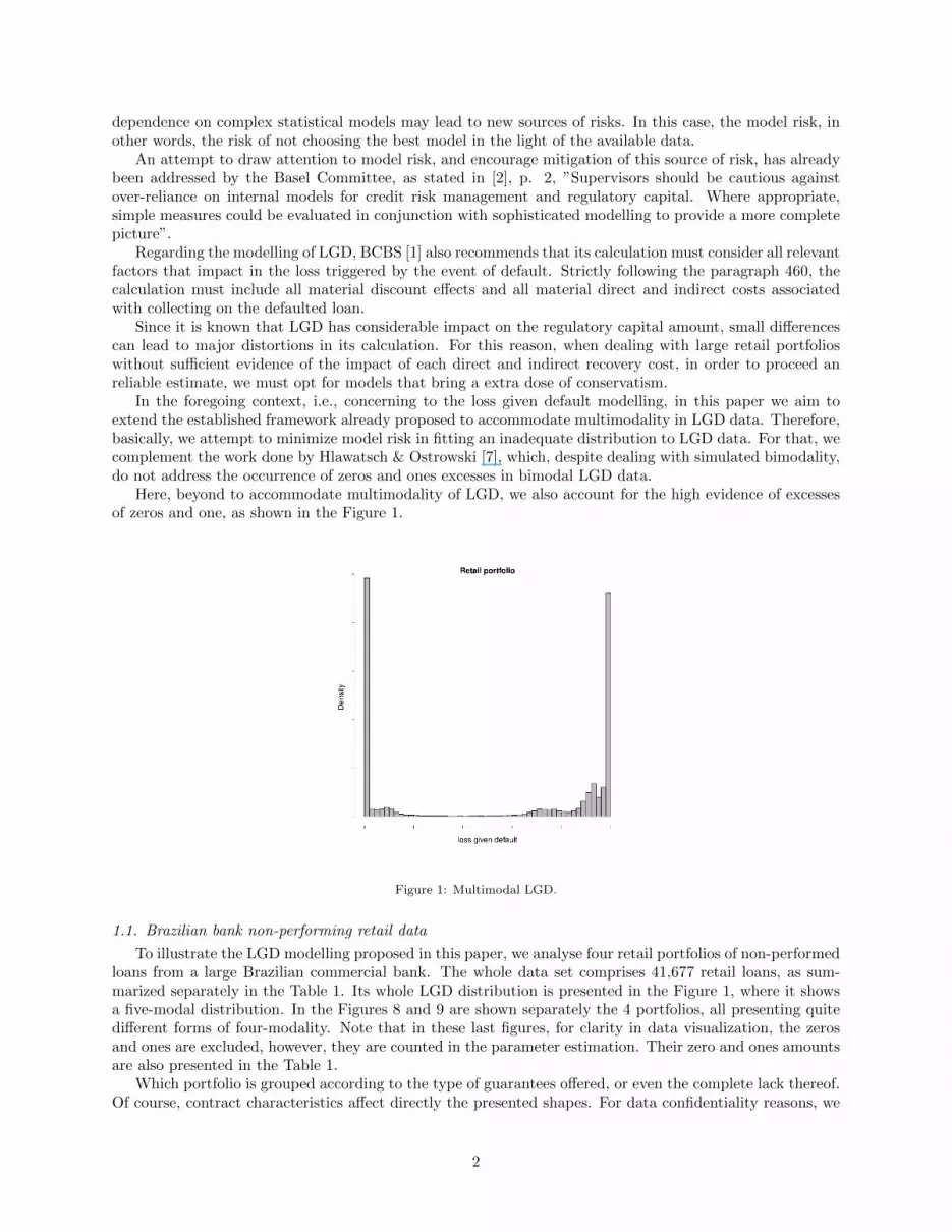
Here, beyond to accommodate multimodality of LGD, we also account for the high evidence of excessesof zeros and one, as shown in the Figure 1.

Figure 1: Multimodal LGD.

1.1. Brazilian bank non-performing retail data

To illustrate the LGD modelling proposed in this paper, we analyse four retail portfolios of non-performedloans from a large Brazilian commercial bank. The whole data set comprises 41,677 retail loans, as sum-marized separately in the Table 1. Its whole LGD distribution is presented in the Figure 1, where it showsa five-modal distribution. In the Figures 8 and 9 are shown separately the 4 portfolios, all presenting quitedifferent forms of four-modality. Note that in these last figures, for clarity in data visualization, the zerosand ones are excluded, however, they are counted in the parameter estimation. Their zero and ones amountsare also presented in the Table 1.

Which portfolio is grouped according to the type of guarantees offered, or even the complete lack thereof.Of course, contract characteristics affect directly the presented shapes. For data confidentiality reasons, we

2

do not explain the features of each loan making up each portfolio, we can only mention these are retailexposures, as defined in [1], paragraph 231.

Table 1: Summary of observed LGD data.

Portfolio Qtd Mean Median SD #0 #11 15,295 0.52195 0.7272 0.4746 5722 66342 22,951 0.59814 0.9093 0.4596 8349 83983 440 0.32945 0.7466 0.4004 232 444 2,991 0.72060 0.9175 0.3810 510 265

Although Calabrese [3] has dealt with excess of zeros and ones in a real LGD data on Italian bank loans,the author has not presented real situations of multimodality (without considering the excess of zeros andones), assuming an arbitrary mixture of two betas to encourage the forecasting of two distinct periods,one with higher and another with lower mean intensity for the random variable LGD. In this sense, wecomplement the work made in [3] by applying our methodology in a variety of real bank loan portfolios.In addition, we perform a simulation study to assess estimation performance of the inflated mixture model,what was not carried out in that referred paper.

Notwithstanding the bimodality and zeros and ones excess has been partially accounted for in the recentliterature, [7, 16, 3], to the best of our knowledge, the full configuration of the aforestated data has notbeen wholly incorporated into any model. Thereby, by assuming a mixed of degenerate distributions tohandle all zeros and ones excess, together with a mixture of distributions to account for multimodal losses,along with the already mentioned variety of real applications and simulation studies, here, we fill this gap byintroducing a simple statistical tool for credit risk managers deal, as effectively as possible, with loss givendefault multi-shape data.

Summing up, the first novelty of this paper is to present an application of the inflated mixture modelson a wide range of multimodality shapes, accompanied by a simulation study, which, at our knowledge, hasnot been presented in the literature. The second novelty is the presentation of the model considering theinfluence of a set of co-variables, i.e., presenting a regression model version, thus, allowing to measure howcustomer and loan features impact on LGD results.

The paper is organized as follows. In Section 2, we formulate the inflated mixture model and its regressionversion. Section 3 introduces maximum likelihood estimation. A simulation study with different vectorparameters (with and without covariates) is presented in Section 4. An application to a real variety of retailportfolios of a large Brazilian bank is presented in Section 5. General remarks are presented in Section 6.

2. Model specification

Here, we propose an inflated mixture model to handle multimodality in the loss given default framework.To present in a more didactic way, without compromising general understanding of ideas, we only deal withbeta distributions and consider the sum of two distributions in the mixture model. Other mixtures beyondthe number of two, and the use of others bounded distributions that appear in the application section, i.e.,Kumaraswamy, truncated normal and logit-normal distributions, can be easily implemented computationally,since there are a lot of statistical packages available in R and, also, a comprehensive amount of academicmaterials about them in the statistical literature.

2.1. The Inflated mixture of beta distributions

Inflated models are a way to incorporate degenerate points that do not belong to original distribution,assign to them probability to occur. Thereby, we firstly define what is mixture of two beta distributions,and consequently, it leads us naturally to our main definition, the inflated mixture of beta distributions.

The well-known beta distribution, as appears in [6], has mean parameter µ ∈ (0, 1), and precisionparameter φ > 0. Defined only for y ∈ (0, 1), beta distribution has density function as following:

f(y;µ, φ) =Γ(φ)

Γ(µφ)Γ((1− µ)φ)y(µφ−1)(1− y)(1−µ)φ−1, (1)

3

where Γ(.) is gamma function.Given f1(. ;µ1, φ1) and f2(. ;µ2, φ2), beta distributions, we set a mixture of two beta distributions, with

a 5-parameters density function given by fm2b = πf1 + (1− π)f2. The parameter π is commonly known asmixing proportion. Roughly, this means for the probability of y ∈ (0, 1) be more suitable accommodate byf1, while 1− π stands for the probability of y ∈ (0, 1) be more accommodate by f2.

Now, let Y be a random variable with support in {0, 1}∪(0, 1). The Y distribution is said to be a inflated(in zeros and ones) mixture of two beta distributions, with a 7-parameters ϑ = (δ0, δ1, π, µ1, φ1, µ2, φ2), if itsdensity function is given by:

fim2b(y;ϑ) =

δ0, if y = 0(1− δ0 − δ1)fm2b, if 0 < y < 1δ1, if y = 1,

(2)

where fm2b follows a mixture of two beta distributions.Note that α = δ0+δ1 is a mixing proportion and, mathematically, these parameters, δ0, δ1 and α, account

for, respectively, P [y = 0], P [y = 1] and P [y /∈ (0, 1)].As we will see in the application section, the average estimate is an important decision-making criteria for

the best LGD model. In fact, according to the Basel II agreement, it is advised to avoid a non-conservativeestimate given practical circumstances of lack of informations (see [1], paragraph 460). What is our case,once the Bank has made available a database records of accounting losses rather than economic losses. Forthat, we present the first moment (mean) of Y, given by E[Y ] = (1− δ0 − δ1)(πµ1 + (1− π)µ2) + δ1.

2.2. The Inflated mixture of beta regression models

Here, we introduce an approach to accommodate covariates in a regression setting. In the applicationsection, we discuss the applications of both models to a real retail portfolios, i.e., the inflated mixture modeland the inflated mixture regression model and, likewise, simulations studies are performed for both cases.

Therefore, we propose to connect the set of 4 average related parameters, (δ0, δ1, µ1, µ2), with a set of4-covariate vectors, x1, x2,x3 and x4, respectively. These covariate vectors, as occurs in practice, may bethe same, i.e., x1 = x2 = x3 = x4.

Following [12], the regression version of the inflated mixture of beta distributions is defined by 2, and bythe following components, also known as link functions:

(δ0i, δ1i) =(

ex>1iβ1

1+ex>1iβ1+ex

>2iβ2, ex

>2iβ2

1+ex>1iβ1+ex

>2iβ2

)µ1i = ex

>3iβ3

1+ex>3iβ3

µ2i = ex>4iβ4

1+ex>4iβ4,

(3)

where βj ’s are 4 vectors of regression coefficients to be estimated.Note that the inflated mixture of beta regression model can be viewed as an extension of the inflated

beta regression model introduced by Martınez [10] and Ospina & Ferrari [11].

3. Inference

Parameter estimation is performed by straightforward use of maximum likelihood estimation (MLE).Despite the existence of competitive methods, see for example expectation-maximization (EM) algorithm in[8], the simulation studies support simple application of MLE approach.

The likelihood function of the inflated mixture model fim2b, as defined in 2, with a vector 7-parameterϑ = (δ0, δ1, π, µ1, φ1, µ2, φ2), as well as the increased parameter version of the regression model, is based ona sample of n observations, D = {yi}, independent and identically distributed:

L(ϑ;D) ∝∏

fim2b(yi; δ0, δ1, π, µ1, φ1, µ2, φ2).

The maximum likelihood estimates ϑ, of the parameter vector ϑ, are obtained through maximization ofL(ϑ;D) or `(ϑ;D) = log{L(ϑ;D)}. Under suitable regularity conditions, the asymptotic distribution of the

4

maximum likelihood estimates (MLEs), ϑ, is a multivariate normal with mean vector ϑ and covariance matrix,

which can be estimated by {−∂2`(ϑ)/∂ϑ∂ϑT }−1, evaluated at ϑ = ϑ, where the required second derivativesare computed numerically. There are many software and routines available for numerical maximization. Wechoose the method ”BFGS” for maximizing, see [14], which comes within the R routine optim.

Different models can be compared by using the Akaike information criteria. The model with the smallestvalue of AIC is commonly chosen as the preferred for describing a given dataset. In the application section,we compare the proposed model configured with four different density functions and, through the applicationin four different real portfolios, the combination of the best results of AIC, along with the most conservativeestimates of LGD, will decide which model better meet the Basel II conservative recommendations.

4. Simulation Studies

We proceed a parameter estimation based on a maximum likelihood principle and use the R routineoptim() for that. In order to assess the performance of the maximum likelihood estimates with respect tosample size, we perform Monte Carlo simulations, where each sample is replicate 1000 times and the samplesize varies as n = 100, 500, 1000, 2500, 5000. Two simulation studies are performed for the inflated mixturebeta model in 2, and three simulation studies for the regression version introduced by the link functions in3.

First we present the results of simulation studies without the presence of covariates. Tables 2 and 3describe the average estimates, biases and root mean square errors for two different vectors of 7-parametersunder the inflated mixture beta model. In the first scenario we set 11% of zeros and ones (δ0 + δ1), and thelast 55% of zeros and ones. As expected, the bias and the root MSE of the estimators of the continuouscomponent increases with the expected proportion of zeros and ones increases.

For the continuous component, we set up the first scene with two beta peaks away from each other,µ1 = 0.05 and µ2 = 0.85, while in the second scenario the peaks are closer, µ1 = 0.72 and µ2 = 0.95. Weproceed in such a way to simulate a real situation that occurs in real data sets. The outcomes show that inboth cases the biases and root mean square errors decrease as sample size increases, as expected. Thus, weobtain a promising outcome, since in credit risk analysis we always deal with large data sets.

Table 2: Estimates of bias, root mean square error (RMSE) and mean parameters ( ) of a inflated mixture of two betadistributions obtained from a Monte Carlo simulation with 1000 replications and increasing sample size (n).

δ0 = 0.05 δ1 = 0.06 π = 0.4 µ1 = 0.05 φ1 = 15 µ2 = 0.85 φ2 = 35n Bias RMSE Bias RMSE Bias RMSE Bias RMSE Bias RMSE Bias RMSE Bias RMSE

100 0.017 0.000 0.019 0.001 0.042 0.054 0.007 0.000 3.705 5.191 0.006 0.000 6.11 8.004

δ0 = 0.050 δ1 = 0.060 π = 0.396 µ1 = 0.050 φ1 = 16.600 µ2 = 0.850 φ2 = 36.983500 0.008 0.000 0.009 0.000 0.018 0.031 0.003 0.000 1.517 1.936 0.003 0.000 2.45 3.168

δ0 = 0.050 δ1 = 0.060 π = 0.400 µ1 = 0.050 φ1 = 15.322 µ2 = 0.850 φ2 = 35.4361000 0.005 0.000 0.006 0.000 0.014 0.000 0.002 0.000 0.945 1.200 0.002 0.000 1.71 2.154

δ0 = 0.050 δ1 = 0.060 π = 0.400 µ1 = 0.050 φ1 = 15.110 µ2 = 0.850 φ2 = 35.1802500 0.004 0.000 0.004 0.000 0.008 0.000 0.001 0.000 0.676 0.840 0.001 0.000 1.04 1.319

δ0 = 0.050 δ1 = 0.060 π = 0.400 µ1 = 0.050 φ1 = 15.102 µ2 = 0.850 φ2 = 35.1415000 0.003 0.000 0.003 0.000 0.006 0.000 0.001 0.000 0.448 0.571 0.001 0.000 0.78 0.969

δ0 = 0.050 δ1 = 0.060 π = 0.400 µ1 = 0.050 φ1 = 15.010 µ2 = 0.850 φ2 = 35.025

5

Table 3: Estimates of bias, root mean square error (RMSE) and mean parameters ( ) of a inflated mixture of two betadistributions obtained from a Monte Carlo simulation with 1000 replications and increasing sample size (n).

δ0 = 0.25 δ1 = 0.30 π = 0.35 µ1 = 0.72 φ1 = 31 µ2 = 0.95 φ2 = 35n Bias RMSE Bias RMSE Bias RMSE Bias RMSE Bias RMSE Bias RMSE Bias RMSE

100 0.034 0.044 0.037 0.044 0.077 0.100 0.025 0.031 28.23 23.72 0.009 0.000 19.84 17.80

δ0 = 0.247 δ1 = 0.300 π = 0.355 µ1 = 0.722 φ1 = 52.421 µ2 = 0.950 φ2 = 47.619500 0.015 0.000 0.017 0.000 0.029 0.031 0.010 0.000 5.90 7.798 0.003 0.000 5.32 6.92

δ0 = 0.251 δ1 = 0.300 π = 0.351 µ1 = 0.721 φ1 = 32.428 µ2 = 0.950 φ2 = 36.5711000 0.012 0.000 0.012 0.000 0.023 0.031 0.007 0.000 4.17 5.271 0.003 0.000 3.83 4.79

δ0 = 0.251 δ1 = 0.299 π = 0.351 µ1 = 0.720 φ1 = 32.120 µ2 = 0.950 φ2 = 35.5012500 0.007 0.000 0.007 0.000 0.013 0.000 0.004 0.000 2.53 3.210 0.002 0.000 2.32 2.88

δ0 = 0.249 δ1 = 0.300 π = 0.350 µ1 = 0.720 φ1 = 31.331 µ2 = 0.950 φ2 = 35.2575000 0.005 0.000 0.005 0.000 0.009 0.000 0.003 0.000 1.74 2.188 0.001 0.000 1.62 2.02

δ0 = 0.250 δ1 = 0.300 π = 0.350 µ1 = 0.720 φ1 = 31.114 µ2 = 0.950 φ2 = 35.171

Finally, we present the estimates of bias, root mean square error (RMSE) and the average parameterestimates of the inflated mixture of two beta regression models, obtained from a Monte Carlo simulation, with1000 replications and increasing sample size. For covariate simulation, we consider an intercept covariatex1 = 1, and we assume x2 as a binary covariate with values drawn from a Bernoulli distribution withparameter 0.5.

The following graphs 2 to 6 show the decrease to zero of the biases and RMSE for three different parametersettings, each with around 10%, 25% and 50% of excess of zeros and ones. In the Table 4, we present only thescenario with around 45% of zero and ones excess (δ0+δ1). These settings are chosen by represent the realityof available data regarding to the amount of excess zeros and ones. In the regression model simulation, asexpect, the biases and root mean square errors decrease as sample size increases.

6

Table 4: Estimates of bias, root mean square error (RMSE) and mean parameters ( ) of a inflated mixture of two beta regressionmodels obtained from a Monte Carlo simulation with 1000 replications and increasing sample size (n).

δ0 = 0.257 δ1 = 0.200 πβ11 = −1.00 β12 = 0.50 β21 = −1.50 β22 = 1.00 π = 0.60

n Bias RMSE Bias RMSE Bias RMSE Bias RMSE Bias RMSE100 0.433 0.555 0.691 0.879 0.520 0.652 0.832 1.069 0.234 0.289

β11 = −1.089 β12 = 0.538 β21 = −1.659 β22 = 1.202 π = 0.609250 0.225 0.299 0.411 0.514 0.300 0.376 0.540 0.652 0.159 0.192

β11 = −1.047 β12 = 0.499 β21 = −1.528 β22 = 0.985 π = 0.597500 0.174 0.219 0.295 0.389 0.186 0.227 0.311 0.378 0.104 0.123

β11 = −1.044 β12 = 0.552 β21 = −1.516 β22 = 0.987 π = 0.6011000 0.123 0.150 0.215 0.267 0.144 0.181 0.239 0.308 0.078 0.096

β11 = −1.002 β12 = 0.519 β21 = −1.542 β22 = 1.074 π = 0.6042000 0.095 0.112 0.154 0.189 0.101 0.133 0.163 0.215 0.053 0.067

β11 = −0.990 β12 = 0.477 β21 = −1.510 β22 = 0.998 π = 0.599

µ1 = 0.366 φ1 µ2 = 0.786 φ2β31 = −0.80 β32 = 0.50 φ1 = 30 β41 = 1.00 β42 = 0.60 φ2 = 50

n Bias RMSE Bias RMSE Bias RMSE Bias RMSE Bias RMSE Bias RMSE100 0.098 0.129 0.180 0.228 0.234 0.290 0.111 0.142 0.205 0.271 0.325 0.443

β31 = −0.786 β32 = 0.471 φ1 = 32.678 β41 = 1.026 β42 = 0.572 φ2 = 59.794250 0.075 0.094 0.137 0.166 0.130 0.176 0.069 0.088 0.115 0.142 0.157 0.199

β31 = −0.802 β32 = 0.493 φ1 = 31.050 β41 = 0.995 β42 = 0.604 φ2 = 53.606500 0.041 0.051 0.071 0.088 0.086 0.110 0.052 0.068 0.099 0.129 0.133 0.165

β31 = −0.800 β32 = 0.499 φ1 = 30.409 β41 = 0.990 β42 = 0.610 φ2 = 49.9031000 0.032 0.040 0.055 0.066 0.064 0.080 0.035 0.045 0.065 0.082 0.094 0.116

β31 = −0.798 β32 = 0.491 φ1 = 30.317 β41 = 0.998 β42 = 0.591 φ2 = 51.0782000 0.023 0.030 0.039 0.051 0.049 0.059 0.024 0.029 0.043 0.052 0.065 0.083

β31 = −0.795 β32 = 0.494 φ1 = 30.192 β41 = 0.998 β42 = 0.607 φ2 = 50.584

Figure 2: Estimates of bias, root mean square error for theparameters β11 and β12.

Figure 3: Estimates of bias, root mean square error for theparameters β21 and β22.

7

Figure 4: Estimates of bias, root mean square error for theparameters β31 and β32.

Figure 5: Estimates of bias, root mean square error for theparameters β41 and β42.

Figure 6: Estimates of bias, root mean square error for the parameters π, φ1 and φ2.

5. Application

In this section we illustrate some applications of the models presented in this paper, i.e., the inflatedmixture model defined in 2, and the regression version reached by the link functions considered in 3.

First, we compare the fit of four competitive inflated mixture models: The inflated mixture of betadistributions, the inflated mixture of Kumaraswamy distributions, the inflated mixture of (0, 1)−truncated

8

normal distributions and, finally, the inflated mixture of logit-normal distributions. These distributions havebeen chosen for comparison because are limited to the same support.

As mentioned, we opt to use the values of the AIC (Akaike information criterion) for model selectioncriteria, along with the choice of the most conservative estimates for LGD, in order to decide which modelbetter meet the Basel II conservative recommendations. A goal for future research would be to proposemeasures of predictive power for the regression models here introduced.

5.1. Inflated mixture of beta models

Here, we consider the four portfolios described in the introduction section 1.1. As our goal is to selectthe best modelling LGD portfolio, so we present only the results obtained for the average estimated foreach model, which we compared with the average appearing in the table 1, along with the AIC obtained inadjusting the model to the data.

Given the relative differences between the mean values estimated with the observed values of LGD, seeTable 5, the model considering the beta distribution has a slight advantage due to have been presented themost conservative measure.

Table 5: Expected mean LGD by portfolio and by model.

Portfolio Expected lgdbeta Kumaraswamy Truncated normal Logit-normal

1 0.52205 0.52173 0.52187 0.522722 0.59810 0.59817 0.59814 0.597893 0.33187 0.33129 0.32993 0.330884 0.72072 0.72021 0.72060 0.71841

Relativedifference % 0.1912% 0.1167% 0.0330% 0.0590%

Regarding the measure of AIC, we must define a criterion for choosing the best model taking into accountthe adjustment of the four scenarios/portfolios. Thus, although the beta model, individually, has not thelowest AIC value, we see, with the graph 7 helps, that the beta model overall performance is better than theother models.

Figure 7: AIC values for Model selection criteria.

9

Table 6: AIC values for the fitted distributions.

Model Beta Kumaraswamy Truncated normal Logit-normalPortfolio 1 27999.30 28147.77 27350.50 28332.28Portfolio 2 36870.90 36765.73 36903.02 37074.51Portfolio 3 612.13 613.06 624.38 609.52Portfolio 4 -1840.22 -1804.26 -1946.01 -1388.19

For illustration, following, we present the graphs of the LGD shapes, and their respective adjustments ofthe each considered model.

(a) Portfolio 1 (b) Portfolio 2

Figure 8: Fitted distributions for portfolio 1 and portfolio 2.

(a) Portfolio 3 (b) Portfolio 4

Figure 9: Fitted distributions for portfolio 3 and portfolio 4.

5.2. Inflated mixture of beta regression models

In this section we illustrate the regression model taking in consideration two covariates made availableby the bank. For this purpose, a sample of the portfolio 1, with two variables and containing 5000 retailloans is considered for modelling purposes.

10

Let (x1,x2,x3) be the vector of covariates, where x1 stands for the interceptor parameter, i.e., x1 = 1,and two others are real covariates. Both real variables are categorized into two classes.

The first, x2 represents two client groups according to the behavioural risk presented. The bank has itsbehaviour score model and segregated their customers into two groups, roughly, x2 = 0 to customers withpoor credit risk and x2 = 1 with better credit risk. The second variable is related to the loan characteristics.The loan classified as x3 = 0, represents a group of loans with term relatively shorter than the group withx3 = 1.

Thus, we use the following setting of the link functions:

δ0i = e(β11x1i+β12x2i+β13x3i)

1+e(β11x1i+β12x2i+β13x3i)+e(β21x1i+β22x2i+β23x3i)

δ1i = e(β21x1i+β22x2i+β23x3i)

1+e(β11x1i+β12x2i+β13x3i)+e(β21x1i+β22x2i+β23x3i)

µ1i = e(β31x1i+β32x2i+β33x3i)

1+e(β31x1i+β32x2i+β33x3i)

µ2i = e(β41x1i+β42x2i+β43x3i)

1+e(β41x1i+β42x2i+β43x3i)

(4)

The results summarized in Table 7 corroborate the following findings that shorter term loans held bylower credit risk customers have a much lower loss given default that the remaining group.

Table 7: Summary of average LGD estimated by the inflated mixture of two beta regression model

Portfolio 1 Subgroups Qtd Observed Estimatedx2 = 0 x3 = 0 1,266 0.6325 0.6383

mean lgd x3 = 1 1,269 0.6324 0.6255= 0.5216 x2 = 1 x3 = 0 1,234 0.4262 0.4265

x3 = 1 1,231 0.3890 0.4101

The standard deviation of the estimator of is calculated using the delta method with a first-order Taylorapproximation (see [4]).

Table 8: Maximum likelihood estimation results for the inflated mixture of two beta regression models

Parameter Estimative (est) Standard error (se) |est|/ seβ11 0.1890 0.0707 2.6731β12 0.8122 0.0809 10.0333β13 0.0851 0.0802 1.0599β21 0.9171 0.0641 14.3059β22 -0.2448 0.0786 3.1132β23 0.0013 0.0777 0.0173π 0.5784 0.0828 6.9789β31 -0.7320 0.1005 7.2790β32 -0.2577 0.1086 2.3727β33 0.0728 0.1079 0.6750φ1 1.1757 0.0538 21.8377β41 1.1076 0.0293 37.7084β42 -0.1125 0.0349 3.2177β43 -0.0508 0.0351 1.4478φ2 62.8578 0.1110 566.0437

11

6. Concluding remarks

We have proposed two novelties in this paper. The first is present the inflated of zeros and ones mixturemodels fitting 4 different real databases, made available by a large Brazilian commercial bank. We alsopresent a simulation study to evaluate the asymptotic performance of the estimation method proposed, thatis, the behaviour of estimates regarding to the increased sample size.

The second novelty presented is the version of the regression model, where we propose a simple and easyto apply methodology. Our simulation studies and application in a real database show how the model canbe useful for application in modelling LGD data sets.

A future research is to propose measures of predictive power for the regression models here introduced.

Acknowledgement

The research was sponsored by CAPES - Process number: BEX 10583/14-9, Brazil.

References

[1] BCBS (2006). International Convergence of Capital Measurement and Capital Standards: A RevisedFramework, Comprehensive Version (June 2006 Revision). Basel Committee on Banking Supervision.

[2] BCBS (2015). Developments in credit risk management across sectors: current practices and recommend-ations. Basel Committee on Banking Supervision.

[3] Calabrese, R. (2014). Downturn loss given default: Mixture distribution estimation. European Journalof Operational Research, 237(1), 271–277.

[4] Efron, B. & Efron, B. (1982). The jackknife, the bootstrap and other resampling plans, volume 38. SIAM.

[5] Engelmann, B. & Rauhmeier, R. (2011). The Basel II Risk Parameters: Estimation, Validation, StressTesting with Applications to Loan Risk Management . Springer Science & Business Media.

[6] Ferrari, S. & Cribari-Neto, F. (2004). Beta regression for modelling rates and proportions. Journal ofApplied Statistics, 31(7), 799–815.

[7] Hlawatsch, S. & Ostrowski, S. (2011). Simulation and estimation of loss given default. The Journal ofCredit Risk , 7(3), 39.

[8] Ji, Y., Wu, C., Liu, P., Wang, J. & Coombes, K. R. (2005). Applications of beta-mixture models inbioinformatics. Bioinformatics, 21(9), 2118–2122.

[9] Loterman, G., Brown, I., Martens, D., Mues, C. & Baesens, B. (2012). Benchmarking regression al-gorithms for loss given default modeling. International Journal of Forecasting , 28, 161–170.

[10] Martınez, R. O. (2008). Modelos de regressao beta inflacionados. Ph.D. thesis, Universidade de SaoPaulo.

[11] Ospina, R. & Ferrari, S. L. (2012). A general class of zero-or-one inflated beta regression models.Computational Statistics & Data Analysis, 56(6), 1609–1623.

[12] Pereira, G. H., Botter, D. A. & Sandoval, M. C. (2013). A regression model for special proportions.Statistical Modelling , 13(2), 125–151.

[13] Porath, D. (2011). Scoring models for retail exposures. In The Basel II Risk Parameters, pages 25–36.Springer.

[14] R Core Team (2015). R: A Language and Environment for Statistical Computing . R Foundation forStatistical Computing, Vienna, Austria.

[15] Schuermann, T. (2004). What do we know about loss given default?

12

[16] Tong, E. N., Mues, C. & Thomas, L. (2013). A zero-adjusted gamma model for mortgage loan lossgiven default. International Journal of Forecasting , 29(4), 548–562.

[17] Yashkir, O. & Yashkir, Y. (2013). Loss given defult: a comparative analysis. Journal of Risk ModelValidation, 7(1), 25–59.

13