Embed Size (px)
Citation preview
PhD Thesis
Information Loss in Deterministic Systems
Connecting Information Theory, Systems Theory, and SignalProcessing
conducted at theSignal Processing and Speech Communications Laboratory
Graz University of Technology, Austria
byDipl.-Ing. Bernhard C. Geiger
Supervisor:Univ-.Prof. Dipl.-Ing. Dr. Gernot Kubin
Assessors/Examiners:Univ.-Prof. Dipl.-Ing. Dr.techn. Gernot KubinProf. Dr.sc.techn. Gerhard Kramer, TU Munich
Graz, June 3, 2014


Affidavit
I declare that I have authored this thesis independently, that I have not used other than thedeclared sources/resources, and that I have explicitly marked all material which has been quotedeither literally or by content from the used sources. The text document uploaded to TUGRA-Zonline is identical to the present doctoral dissertation.
Eidesstattliche Erklarung
Ich erklare an Eides statt, dass ich die vorliegende Arbeit selbststandig verfasst, andere alsdie angegebenen Quellen/Hilfsmittel nicht benutzt, und die den benutzten Quellen wortlichund inhaltlich entnommene Stellen als solche kenntlich gemacht habe. Das in TUGRAZonlinehochgeladene Textdokument ist mit der vorliegenden Dissertation identisch.
date (signature)

Information Loss in Deterministic Systems
Contents
Abstract 9
Acknowledgments 11
Preface 13
1 Introduction 15
1.1 Motivation . . . . . . . . . . . . . . . . . . . . . . . . . . . . . . . . . . . . . . . 15
1.2 Five Influential PhD Theses . . . . . . . . . . . . . . . . . . . . . . . . . . . . . . 16
1.3 Contributions and Outline . . . . . . . . . . . . . . . . . . . . . . . . . . . . . . . 18
2 Information Loss 21
2.1 What Is Information Loss? – The Discrete Case . . . . . . . . . . . . . . . . . . . 21
2.2 Generalization to Continuous Random Variables . . . . . . . . . . . . . . . . . . 23
2.3 Information Loss in Piecewise Bijective Functions . . . . . . . . . . . . . . . . . . 27
2.3.1 Elementary Properties . . . . . . . . . . . . . . . . . . . . . . . . . . . . . 27
2.3.2 Bounds on the Information Loss . . . . . . . . . . . . . . . . . . . . . . . 30
2.3.3 Reconstruction Error and Information Loss . . . . . . . . . . . . . . . . . 33
2.3.4 Example: Third-Order Polynomial . . . . . . . . . . . . . . . . . . . . . . 37
2.3.5 Example: Accumulator . . . . . . . . . . . . . . . . . . . . . . . . . . . . 39
2.4 Relative Information Loss . . . . . . . . . . . . . . . . . . . . . . . . . . . . . . . 41
2.4.1 Elementary Properties . . . . . . . . . . . . . . . . . . . . . . . . . . . . . 41
2.4.2 Relative Information Loss for System Reducing the Dimensionality of Con-tinuous Random Variables . . . . . . . . . . . . . . . . . . . . . . . . . . . 43
2.4.3 A Bound on the Relative Information Loss . . . . . . . . . . . . . . . . . 45
2.4.4 Reconstruction Error and Relative Information Loss . . . . . . . . . . . . 46
2.4.5 Relative Information Loss for 1D-Systems of Mixed Random Variables . . 49
2.5 Application: Multi-Channel Autocorrelation Receiver . . . . . . . . . . . . . . . . 50
2.6 Application: Principal Components Analysis . . . . . . . . . . . . . . . . . . . . 53
2.6.1 PCA with Population Covariance Matrix . . . . . . . . . . . . . . . . . . 54
2.6.2 PCA with Sample Covariance Matrix . . . . . . . . . . . . . . . . . . . . 55
2.6.3 Information Propagation in PCA . . . . . . . . . . . . . . . . . . . . . . . 58
2.7 Open Questions . . . . . . . . . . . . . . . . . . . . . . . . . . . . . . . . . . . . . 58
3 Information Loss Rate 61
3.1 What Is Information Loss for Stochastic Processes? – The Discrete Case . . . . . 61
3.2 Information Loss Rate for Markov Chains . . . . . . . . . . . . . . . . . . . . . . 63
3.2.1 Preliminaries . . . . . . . . . . . . . . . . . . . . . . . . . . . . . . . . . . 64
3.2.2 Equivalent Conditions for Information-Preservation . . . . . . . . . . . . . 65
3.2.3 Excursion: k-lumpability of Markov Chains . . . . . . . . . . . . . . . . . 66
3.2.4 Sufficient Conditions for Information-Preservation and k-Markovity . . . . 68
3.2.5 An Algorithm for Obtaining SFS(2)-Lumpings . . . . . . . . . . . . . . . 74
3.2.6 Application: n-gram models . . . . . . . . . . . . . . . . . . . . . . . . . . 78
June 3, 2014 – iii –
3.3 Information Loss Rate for Continuous Processes . . . . . . . . . . . . . . . . . . . 79
3.3.1 Upper Bounds on the Information Loss Rate . . . . . . . . . . . . . . . . 81
3.3.2 Excursion: Lumpability of Continuous Markov Processes . . . . . . . . . 82
3.3.3 Example: AR(1)-Process in a Rectifier . . . . . . . . . . . . . . . . . . . . 84
3.3.4 Example: Cyclic Random Walk in a Rectifier . . . . . . . . . . . . . . . . 85
3.4 Relative Information Loss Rate for Continuous Processes . . . . . . . . . . . . . 87
3.5 Application: Multirate Signal Processing & Sampling . . . . . . . . . . . . . . . . 88
3.6 Outlook: Information Loss Rate in Systems with Memory . . . . . . . . . . . . . 91
3.6.1 Partially Invertible Systems . . . . . . . . . . . . . . . . . . . . . . . . . . 94
3.6.2 Example: Fixed-Point Implementation of a Linear Filter . . . . . . . . . . 96
3.7 Open Questions . . . . . . . . . . . . . . . . . . . . . . . . . . . . . . . . . . . . . 98
4 Relevant Information Loss 101
4.1 The Problem of Relevance - A General Definition . . . . . . . . . . . . . . . . . . 101
4.1.1 Elementary Properties . . . . . . . . . . . . . . . . . . . . . . . . . . . . . 103
4.1.2 A Simple Upper Bound . . . . . . . . . . . . . . . . . . . . . . . . . . . . 106
4.2 Signal Enhancement and the Information Bottleneck Method . . . . . . . . . . . 107
4.3 Application: Markov Chain Aggregation . . . . . . . . . . . . . . . . . . . . . . . 111
4.3.1 Contributions and Related Work . . . . . . . . . . . . . . . . . . . . . . . 111
4.3.2 Preliminaries . . . . . . . . . . . . . . . . . . . . . . . . . . . . . . . . . . 112
4.3.3 An Information-Theoretic Aggregation Method . . . . . . . . . . . . . . . 114
4.3.4 Interpreting the KLDR as Information Loss . . . . . . . . . . . . . . . . . 119
4.3.5 Employing the Information-Bottleneck Method for Aggregation . . . . . . 120
4.3.6 Example: Models of Bio-Molecular Systems . . . . . . . . . . . . . . . . . 122
4.4 Application: PCA with Specific Signal Models . . . . . . . . . . . . . . . . . . . 123
4.5 Relevant Information Loss in Inaccurate Functions . . . . . . . . . . . . . . . . . 127
4.6 Open Questions . . . . . . . . . . . . . . . . . . . . . . . . . . . . . . . . . . . . . 130
5 Relevant Information Loss Rate 133
5.1 A Definition, its Properties, and a Simple Upper Bound . . . . . . . . . . . . . . 133
5.2 Application: Anti-Aliasing Filter Design . . . . . . . . . . . . . . . . . . . . . . . 135
5.2.1 A Gaussian Bound for Non-Gaussian Processes . . . . . . . . . . . . . . . 137
5.2.2 FIR Solutions for Information Maximization . . . . . . . . . . . . . . . . 139
5.3 Application: Filtering Prior to Quantization . . . . . . . . . . . . . . . . . . . . . 141
5.3.1 Optimal Prefilters for Quantization . . . . . . . . . . . . . . . . . . . . . . 142
5.3.2 FIR Prefilters for Quantization . . . . . . . . . . . . . . . . . . . . . . . . 144
5.4 Open Questions . . . . . . . . . . . . . . . . . . . . . . . . . . . . . . . . . . . . . 148
6 Discussion 149
A Proofs from Chapter 2 153
A.1 Proof of Theorem 2.2 . . . . . . . . . . . . . . . . . . . . . . . . . . . . . . . . . . 153
A.2 Proof of Proposition 2.3 . . . . . . . . . . . . . . . . . . . . . . . . . . . . . . . . 154
A.3 Proof of Proposition 2.4 . . . . . . . . . . . . . . . . . . . . . . . . . . . . . . . . 155
A.4 Proof of Theorem 2.3 . . . . . . . . . . . . . . . . . . . . . . . . . . . . . . . . . . 156
A.5 Proof of Proposition 2.7 . . . . . . . . . . . . . . . . . . . . . . . . . . . . . . . . 157
A.6 Proof of Proposition 2.10 . . . . . . . . . . . . . . . . . . . . . . . . . . . . . . . 157
A.7 A Sketch for Conjecture 2.1 . . . . . . . . . . . . . . . . . . . . . . . . . . . . . . 158
A.8 PCA: Information Dimension of the Input Matrix given the Output Matrix . . . 160

B Proofs from Chapter 3 161B.1 Proof of Theorem 3.1 . . . . . . . . . . . . . . . . . . . . . . . . . . . . . . . . . . 161
B.1.1 The information-preserving case . . . . . . . . . . . . . . . . . . . . . . . 161B.1.2 The lossy case . . . . . . . . . . . . . . . . . . . . . . . . . . . . . . . . . 162
B.2 Proof of Proposition 3.2 . . . . . . . . . . . . . . . . . . . . . . . . . . . . . . . . 164B.3 Proof of Proposition 3.3 . . . . . . . . . . . . . . . . . . . . . . . . . . . . . . . . 164B.4 Proof of Proposition 3.14 . . . . . . . . . . . . . . . . . . . . . . . . . . . . . . . 165B.5 Proof of Corollary 3.3 . . . . . . . . . . . . . . . . . . . . . . . . . . . . . . . . . 166B.6 Proof of Proposition 3.16 . . . . . . . . . . . . . . . . . . . . . . . . . . . . . . . 167B.7 Proof of Lemma 3.3 . . . . . . . . . . . . . . . . . . . . . . . . . . . . . . . . . . 168B.8 Proof of Lemma 3.4 . . . . . . . . . . . . . . . . . . . . . . . . . . . . . . . . . . 169B.9 Proof of Theorem 3.3 . . . . . . . . . . . . . . . . . . . . . . . . . . . . . . . . . . 170
C Proofs from Chapter 4 174C.1 Proof of Proposition 4.5 . . . . . . . . . . . . . . . . . . . . . . . . . . . . . . . . 174C.2 Proof of Theorem 4.1 . . . . . . . . . . . . . . . . . . . . . . . . . . . . . . . . . . 175C.3 Proof of Theorem 4.2 . . . . . . . . . . . . . . . . . . . . . . . . . . . . . . . . . . 176C.4 Proof of Theorem 4.3 . . . . . . . . . . . . . . . . . . . . . . . . . . . . . . . . . . 176
D Proofs from Chapter 5 178D.1 Proof of Lemma 5.2 . . . . . . . . . . . . . . . . . . . . . . . . . . . . . . . . . . 178D.2 Proof of Theorem 5.1 . . . . . . . . . . . . . . . . . . . . . . . . . . . . . . . . . . 178D.3 Proof of Theorem 5.2 . . . . . . . . . . . . . . . . . . . . . . . . . . . . . . . . . . 181D.4 Proof of Lemma 5.3 . . . . . . . . . . . . . . . . . . . . . . . . . . . . . . . . . . 181


Information Loss in Deterministic Systems
Abstract
A fundamental theorem in information theory – the data processing inequality – states that de-terministic processing cannot increase the amount of information contained in a random variableor a stochastic process. The task of signal processing is to operate on the physical representationof information such that the intended user can access this information with little effort. In thelight of the data processing inequality, this can be viewed as the task of removing irrelevantinformation, while preserving as much relevant information as possible.This thesis defines information loss for memoryless systems processing random variables or
stochastic processes, both with and without a notion of relevance. These definitions are thebasis of an information-theoretic systems theory, which complements the currently prevailingenergy-centered approaches. The results thus developed are used to analyze various systems inthe signal processor’s toolbox: polynomials, quantizers, rectifiers, linear filters with and withoutquantization effects, principal components analysis, multirate systems, etc. The analysis not onlyfocuses on the information processing capabilities of these systems: It also highlights differencesand similarities between design principles based on information-theoretic quantities and thosebased on energetic measures, such as the mean-squared error. It is shown that, at least in somecases, simple energetic design can be justified information-theoretically.As a side result, this thesis presents two approaches to model complexity reduction for time-
homogeneous, finite Markov chains. While one approach preserves full model information withthe cost of losing the (first-order) Markov property, the other approach yields a Markov chain on asmaller state space with reduced model information. Finally, this thesis presents an information-theoretic characterization of strong lumpability, the case where the function of a Markov chainis Markov (of some order).
June 3, 2014 – 9 –


Information Loss in Deterministic Systems
Acknowledgments
A lot of persons directly or indirectly influenced this thesis, and this is the perfect opportunityto say thank you.First and foremost, I want to thank you, Gernot, for being the best PhD advisor I could wish
for: During the many discussions we had, you always treated me like a peer, not like a student.You granted me the freedom to find (and pursue!) my own research ideas and to present myresults as I liked – and you always had great research ideas when I was lacking them and youmade sense of my results when I couldn’t. Every time we met you astonished me with yourimmense knowledge in every field relevant for our joint work. I sincerely hope we can continueresearching together some time in the future.Thank you, Klaus, for teaching me how to write papers, and for supervising my Master’s
thesis. Without you, I would probably not have become a member of this lab. Thank you,Christian V., for teaching me how to write papers, for employing me as a study assistant in2007, and for the beers. Thank you particularly for the many chats we had about (scientific)life, the universe, and everything. Thank you, Christian F., for your open door during thedifficult first months of my thesis. I really appreciate the time you spent explaining things tome.I want to thank all the SPSC lab members I met during these four-and-a-half years – you’re
a great bunch, I really had a lot of fun with you! Particularly, I want to thank the members ofthe 2-pm-coffee-party: Paul, my office “roomie”, Shuli, Andi P., Erik, Kathi, Michi S., Shahzad,and Stefan M. Thank you for all the technical and, more importantly, non-technical chats!Thank you, Christoph, Tanja, and Georg, for collaborating with me despite the distance that
separated us: From you, I learned (again) writing papers, and how mathematicians, computerscientists, and information-theorists think. I hope we will stay in contact!I also want to thank all the students that attended my classes: You were a great source of
motivation for me. Most importantly, I want to thank my excellent Master’s students Erik,Gebhard, and Christian K. It was a pleasure working with all of you!Thank you, Mum, Berni, Peter, and Michi, for your endless support: I always knew you
would never let me down if I needed your help. You always stood behind my decisions, and Iam extremely grateful for that. Thank you, Berni, for tolerating our almost entirely disgustingmeals at Mensa!Finally, I want to thank you, Babsi, for being there for me the last ten years. Thank you
for patiently listening to my mathematical stories of success and failure – they must have beeninfinitely boring for you! Thank you for sharing my joy when I succeeded, and for cheering meup when I failed. You all did this while you were struggling with your own thesis, and I reallyappreciate that. You are one of the strongest women I know, be proud of yourself. I love youand I look forward to our future together.
June 3, 2014 – 11 –


Information Loss in Deterministic Systems
Preface
A typical PhD thesis is a highly specialized piece of work: Metaphorically speaking, the scientisthas to climb a mountain (the scientific field), find a tree on this mountain (the research topic),and pick some tasty fruits (the contribution). This PhD thesis is different: Instead of a deepinvestigation of a narrow field, this thesis is broad and, consequently, rather shallow. Stickingto the metaphor of the tree, my journey during the last four years may be described as follows:After an equally demanding and exhausting ascent halfway up the Mountain of Information
Theory (I never hoped for getting higher), I saw a tree with small, sour fruits, that have notbeen touched by previous scientists on their way to the top: This tree represents informationloss in deterministic functions. I climbed it, to harvest my first fruits, and from one of itsbranches I discovered a beautiful orchard in a valley, surrounded by the Mountains of SignalProcessing, Machine Learning, Control Theory, and Mathematics. I ventured into this orchardand discovered lots of trees, hybrids of the one I just climbed and of seeds blown down fromthe surrounding mountains. And so I came to analyzing the effect of deterministic processing invarious disciplines from an information-theoretic point-of-view. Admittedly, I grabbed mainlythe low-hanging, exotic fruits, but there were many of them, and there are still many of themleft for future scientists.The topics considered in my thesis range from anti-aliasing filters, over lumpability of Markov
chains, to Renyi’s information dimension, the information bottleneck method, and principalcomponents analysis. It was astonishing for me that information can play a fundamental rolein so many disciplines, but in hindsight this is only natural: Nowadays information is one ofthe most important entities one has to consider in the design and the application of systems.While for communications, this importance was recognized more than 60 years ago, other areasare only recently getting aware of this concept. I can only hope that my thesis makes otherscientists eager to wander through the same valley that I have wandered, and to pick the fruitsfor which I was simply too small.
June 3, 2014 – 13 –

Information Loss in Deterministic Systems
1Introduction
“Information is information,not matter or energy.”
– Norbert Wiener, “Cybernetics”
1.1 Motivation
Information is everywhere. All there is to know about the world is already in it, we just haveto discover it. And signal processing helps us in discovering it, by processing the signals, thephysical carriers of information, in such a way that we can access this information with littleeffort. The information in a string of zeros and ones is the same as in the digital image, or inthe snippet of recorded speech transmitted from one cell phone to the other. But it is signalprocessing which makes this information usable to the person in front of the computer screen,or to the one holding the cell phone.Signal processing is usually done by deterministic systems, taking an input signal and re-
sponding with an output signal. And the systems used today come in great variety: Takingthe example of the cell phone, there is an antenna converting the electromagnetic wave to anelectronic signal, a sampler and a quantizer converting this electronic signal into a string ofzeros and ones, some digital filters removing noise and suppressing interference, a demodulatorand a decoder, and again a system converting the resulting string of zeros and ones first againinto an electronic signal, and then into acoustic waves travelling into our ear. Of course, thislist is not exhaustive, but it suggests that there are lots of systems involved when it comes topreparing information for its sink, i.e., the human listener in this case. Thus, signal processingand systems theory are closely related disciplines.But neither signal processing nor systems theory provide means to quantify the information
contained in these signals; they provide quantitative measures for its physical representation, andfor how the systems act on it, though. This physical representation is either energetic or material,but – and this is the link to the quote of Norbert Wiener at the beginning of this chapter – therepresentation is not identical to the represented information. Information theory does provide ameasure of information – entropy – but is often not concerned with deterministic systems. Thus,there are two large, flourishing disciplines which have been largely developed independently fromone another, but which pursue – should pursue – the same goal: Transmission and processingof information. Only recently, information theory embraced concepts from signal processing,
June 3, 2014 – 15 –
1 Introduction
e.g., [43,67,155], and only recently signal processing based on information-theoretic cost functionshas been gaining momentum, e.g., [8, 9, 35, 36].
That information theory is not concerned with deterministic systems at all is not entirely true:All textbooks on information theory include the well-known data-processing inequality, statingin one way or another that deterministic processing of random variables or stochastic processescannot increase information, but decreases it or at best leaves it unmodified. In fact, thisdata-processing inequality for functions and/or deterministic systems is a direct consequence ofShannon’s third axiom characterizing entropy [138]. Nevertheless, aside from this theorem, thequestion how much information is lost during deterministic processing has not been answeredyet. Generally, despite recent advances mentioned above, the link between information theory,deterministic signal processing, and systems theory is weak. In fact, Johnson mentioned in [81]that “classic information theory is silent on how to use information theoretic measures (or ifthey can be used) to assess actual system performance”. It is exactly the purpose of this workto make information theory speak up in this regard, for, as will be seen below, it has a lot tosay.
Among the few published results about the information processing behavior of deterministicinput-output systems are Pippenger’s analysis of the information lost by multiplying two integerrandom variables [117] and the work of Watanabe and Abraham concerning the rate of informa-tion loss caused by feeding a discrete-time, finite-alphabet stationary stochastic process througha static, non-injective function [161]. All these works, however, focus only on finite-alphabetrandom variables and stochastic processes.
Slightly larger, but still focused on discrete random variables only, is the field concerninginformation-theoretic cost functions for the design of intelligent systems: The infomax princi-ple [100], the information bottleneck method [145] using the Kullback-Leibler divergence as adistortion function, and system design by minimizing the error entropy (e.g., [120]) are just a fewexamples of this recent trend. Additionally, Lev’s approach to aggregating accounting data [96],and, although not immediately evident, the work about macroscopic descriptions of multi-agentsystems [93] belong to that category.
A systems theory for neural information processing has been proposed by Johnson in [81].The assumptions made there (information need not be stochastic, the same information canbe represented by different signals, information can be seen as a parameter of a probabilitydistribution, etc.) suggest the Kullback-Leibler divergence as a central quantity. Althoughthese assumptions are incompatible with the ones in this work, some similarities exist (e.g., theinformation transfer ratio of a cascade in [81] and Proposition 2.2).
Another, completely different connection between information theory and systems theory isin the field of autonomous dynamical systems or iterated maps. There, different measuresfor information flow within these systems have been proposed, e.g., [97, 103, 153, 164], mostnotably the definition of transfer entropy in [84, 135]. This connection clearly follows the spiritof Kolmogorov and Sinaı, who characterized dynamical systems exhibiting chaotic behavior withentropy [91, 92, 141], cf. [31].
1.2 Five Influential PhD Theses
During his work, the author this theses drew from a vast literature – but it is probably thefollowing five PhD theses that had most influence. Therefore, this section gives a short overviewof these works, and indicates which tools they provided or which research ideas they sparked.The discussion in Chapter 6 contains the counterpart: A list of contributions, and in which sensethey complement, generalize, or extend these five PhD theses.
A very influential text was the PhD thesis of Yihong Wu [168, 169], submitted 2011 atPrinceton University. He analyzed compressed sensing from the viewpoint of analog compres-
– 16 – June 3, 2014
1.2 Five Influential PhD Theses
sion, i.e., of representing a set of real numbers by another, smaller set of real numbers, withrestricted encoder and decoder (e.g., linear encoder, Lipschitz decoder). He showed that themeasurement rate (or the ratio of the mentioned set cardinalities) is closely related to the Renyiinformation dimension [123] of the input random variables; thus, aside from discussing manyof its properties, he gave information dimension an operational characterization. In this work,especially in Sections 2.4 and 3.4, information dimension is used to characterize the relativeinformation loss (rate) in deterministic systems. Many results from [168, Chapter 2] served asa basis for the results developed in this work.William S. Evans used information theory to analyze system design in his thesis [37, 38],
submitted at the University of California in Berkeley in 1994. In particular, he analyzed the ratioof information transferred over a noisy circuit with binary input and m-ary output, m ≥ 2. This“signal strength ratio” is large if the information at the input of the circuit is small; hence, thegreatest information loss occurs at the beginning of a cascade of noisy circuits. These resultsconnect to the measures of relative information loss proposed in Section 2.4, to the resultsabout cascades of systems, and to this work’s general approach of using information theory forsystem analysis and design. With his results, Evans gave lower bounds on the depth and size ofelectronic circuits to ensure reliable computation.A connection between information theory and automatic control has been made by Kun
Deng, who submitted his dissertation [26,27] at the University of Illinois at Urbana-Champaignin 2012. His topic was the aggregation of Markov chains, i.e., defining a Markov chain on asmaller state space which is close to the original Markov chain in terms of the Kullback-Leiblerdivergence rate. He showed that the problem of bi-partitioning the state space is solved byspectral theory, at least for nearly completely decomposable Markov chains. In addition to thisspectral-based aggregation, he introduced a simulation-based aggregation, which requires onlya single realized sequence of the Markov chain for aggregation. For hidden Markov models, hesuggested to reduce the state space by keeping the Kullback-Leibler divergence rate between theobservation processes small. In the present work, the Kullback-Leibler divergence rate is usedfor Markov chain aggregation too, although its computation is done differently; see Section 4.3.As a particular application of his theoretical results, Deng considered reducing the complexityof thermal models of buildings.Connected also to Chapter 4 in this work, but to a different section and a completely different
topic is the PhD thesis [131,132] of Manuel Antonio Sanchez-Montanes, submitted in 2003at the Universidad Autonoma de Madrid. In his work, he proposed an effective information-processing measure trading model complexity for preservation of information relevant for a spe-cific task. The motivation comes from neuro-biological systems, e.g., the auditory system, whichare known not only to communicate, but to actually process information already at very earlystages. This information-processing measure does not rule out non-Shannon information mea-sures a priori; e.g., Bayes’ error could very well take the place of Shannon entropy according toSanchez-Montanes. His work, which is very similar to the information bottleneck method [145],is strongly connected to this work’s Sections 4.2 and 4.4: Also here, the trade-off between preser-vation of relevant information and reduction of spurious information is an important concept;the author even believes that this trade-off is equivalent to the problem of signal enhancementor signal processing, not only for biological systems, but essentially for all systems which are de-signed to prepare an information-bearing signal for its sink. As applications, Sanchez-Montanesanalyzed, e.g., linear systems with linear objectives (to which the principal components analysisis the optimal solution) and induction of decision trees.Similar in concept is the thesis [72, 73] of Gustav Eje Henter, submitted to the KTH
Royal Institute of Technology in 2013. He discussed the general problem of solving tasks (e.g.,classification, synthesis, etc.) using data, and quantifying the performance using loss or costfunctions. The solution of a task is in many cases the definition of a proper model for thedata, be it the estimate of just a single parameter (e.g., the maximum likelihood estimate), ormore complicated, generative or discriminative models. To get such a model, features have to
June 3, 2014 – 17 –
1 Introduction
be extracted out of the data, which Henter adequately called information removal : Redundantinformation has to be removed, and the remaining information has to be transformed to allowefficient model identification – these are exactly the two steps required for signal enhancement,too, and Section 4.2 makes this explicit. Specifically, in [73] Henter used an information-theoreticformulation to reduce the complexity of stationary stochastic processes: Minimize the process’entropy rate while keeping the Kullback-Leibler divergence rate to the original process small. Hepresented closed-form solutions for Gaussian and Markov processes, and showed that the formerare related to Wiener filtering. Henter applied his results to speech and language models.
1.3 Contributions and Outline
The contributions of this work are all motivated by Wiener’s quote: Information is information,not matter or energy. Therefore, whenever we build a system to process information, the ob-jective function shall capture the information-processing capabilities of the system. Since thesystems we build are usually deterministic, information loss lends itself as an appropriate mea-sure. But Wiener’s quote also allows a second interpretation in the light of this work: More thanonce it will be shown that standard “energetic” system design, i.e., design based on energeticcost functions such as the mean-squared error, fails information-theoretically.
The larger part of Chapter 2 provides general results on information loss, assuming thatthe input to the system is a multidimensional random variable. The system there is describedeither by a function which has a countable preimage for each output value, or by projections tolower dimensions. Both classes are important, and, although not exhaustive, allow an analysis ofmany practically important systems. As an example the principal components analysis (PCA)is considered. It is shown that PCA in general does not lead to a reduction of information loss,if it is, as usual, used prior to dimensionality reduction. This marks the first of many instancesin this work where common design practices are overthrown because information-theoretic andenergetic designs differ. Moreover, while Chapter 2 is closest to systems theory in its generaltreatment of systems, the section on PCA represents a first connection to machine learning.
Extending information loss from random variables to stationary stochastic processes is thefocus of Chapter 3. Because this more general case is also more difficult to treat, the re-sults presented there are focused on more specific scenarios than those of the previous chapter.In particular, and representing a connection to applied probability, finite-state Markov chainsare characterized from an information-theoretic point-of-view. Not only equivalent conditionsfor information-preserving lumpings, i.e., state space reductions, are presented, but also aninformation-theoretic formulation of strong lumpability. One of the fruits mentioned in the pref-ace has the flavor of natural language processing, since the presented theory is applied to statespace reduction of a letter bi-gram model. After presenting some results for continuous-valuedprocesses, multirate signal processing is considered: Section 3.5 proves that anti-aliasing filterscannot reduce the amount of information lost in the subsequent downsampling device. In anal-ogy to PCA, this is another instance where an energetically optimal system fails to have superiorperformance in terms of information theory. The end of Chapter 3 contains a brief outlook tosystems with memory, showing, quite counterintuively, that digital filter implementations withround-off errors need not lose information.
The large discrepancy between energy and information, particularly for the PCA and anti-aliasing filtering example, is resolved by bringing the notion of relevance into the game inChapter 4: Considering again random variables only, not all information in a data vector isrelevant. By focusing only on the relevant information in the data vector, a new information-processing measure is suggested. And indeed, this measure is shown to best correspond to thesignal processor’s task of signal enhancement, i.e., of preparing the signal such that the sink can
– 18 – June 3, 2014

1.3 Contributions and Outline
retrieve the relevant information with least effort. The connection to machine learning is madeby showing that the information bottleneck method exactly minimizes relevant informationloss. As a consequence, PCA is better understood by showing that, under specific signal modelassumptions, it minimizes the relevant information loss in the following dimensionality reduction.Moreover, relevant information loss is also shown to be an adequate cost function for state spacereduction of Markov chains, where this time the focus is not on preserving all information, buton obtaining a good first-order Markov model on a smaller state space. Possible applicationsfor this type of state space reduction lie in the field of automatic control.Finally, Chapter 5 extends results of the previous chapter from random variables to stochas-
tic processes. For this most general case, only few specific results could be obtained. Andagain, the connection to signal processing is strong: By introducing a specific signal model ofdata superimposed by a Gaussian noise process, anti-aliasing filters are justified information-theoretically, resolving the counterintuivity from Section 3.5. As a second example, filter designprior to quantization is analyzed, essentially justifying linear prediction under specific assump-tions. That this chapter discusses mainly filter design is no accident: Especially filter design,an elementary tool of the signal processor, is often based on energetic considerations. It is,therefore, of prime importance to know when, and when not, this energetic design coincideswith the information-theoretic optimum.
Naturally, this thesis is by no means complete. There are many open questions, the mostimmediate of which are mentioned at the end of each chapter. Chapter 6 finally points atlarger areas left uncovered, and suggests the most fruitful – or most important – directions forfuture research.
June 3, 2014 – 19 –

Information Loss in Deterministic Systems
2Information Loss
The results of this chapter have almost exclusively been obtained by the author, owing to fruitfuldiscussions with Christian Feldbauer and Gernot Kubin. The results about piecewise bijectivefunctions in Section 2.3 have been partly published in [49] and [51]. Relative information loss(Section 2.4) and its application to principal components analysis (Section 2.6) was treatedin [52]. Furthermore, parts of this chapter constitute [46].The result that the sub-optimal reconstructor coincides with the maximum a-posteriori re-
constructor in the example in Section 2.3.4 is due to the author’s student Stefan Wakolbinger.The significance of Theorem 2.2 in the light of chaotic systems was investigated by the author’sstudent Gebhard Wallinger.
2.1 What Is Information Loss? – The Discrete Case
What is information loss? In order to analyze the central quantity of this work one needsto define it properly. And in defining a quantity one typically has two options: The first is topresent a definition for the general case and then apply it to each special case. The second, moreinstructive option – the one taken up in this work – is to define the quantity for a special case andcontinue with generalizing it to larger and larger classes, making sure that the generalizationsare consistent.Intuitively, the information loss in a deterministic system is the same as the water loss in a
system of (possibly corroded) pipes1: Water that flows into the system at the well may eitherleave it at the faucet (the desired output), or through holes or leaking adaptors. The waterloss – for the person trying to wash its hands – is just the difference between the amountof water leaving the well and the amount of water flowing out of the faucet. In analogy, theinformation loss in a deterministic input-output system may be defined as the difference betweenthe information at its input and the information at its output.To make this precise, let (Ω,A,Pr) be a probability space and let X: Ω → X be a discrete
random variable, taking values from a finite set X ⊂ N. It induces a new probability space(X ,P(X ), PX), where P(X ) is the power set of X and where
∀B ∈ P(X ): PX(B) = Pr(X−1[B]). (2.1)
1 This analogy is not new; in his thesis [37], Evans writes: “[For functions,] Pippenger first showed that the totalinformation sent is bounded by the sum of the information sent over each path [...] This supports the viewof information as a kind of fluid which flows from the input X to the output [...] At each gate, several pathscombine, but the fluid flowing out of the gate is no more than the sum of the fluid flowing in.”
June 3, 2014 – 21 –
2 Information Loss
XInput
g
Memoryless System
YOutput
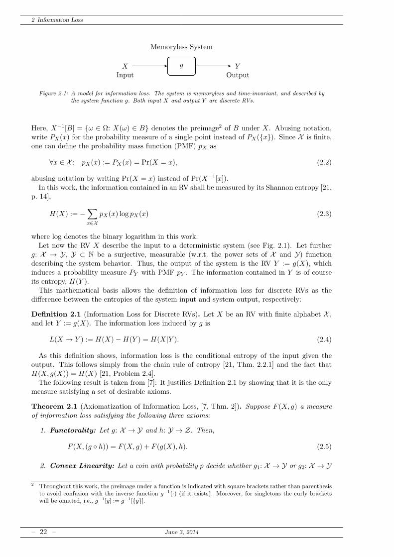
Figure 2.1: A model for information loss. The system is memoryless and time-invariant, and described bythe system function g. Both input X and output Y are discrete RVs.
Here, X−1[B] = ω ∈ Ω: X(ω) ∈ B denotes the preimage2 of B under X. Abusing notation,write PX(x) for the probability measure of a single point instead of PX(x). Since X is finite,one can define the probability mass function (PMF) pX as
∀x ∈ X : pX(x) := PX(x) = Pr(X = x), (2.2)
abusing notation by writing Pr(X = x) instead of Pr(X−1[x]).In this work, the information contained in an RV shall be measured by its Shannon entropy [21,
p. 14],
H(X) := −∑
x∈XpX(x) log pX(x) (2.3)
where log denotes the binary logarithm in this work.Let now the RV X describe the input to a deterministic system (see Fig. 2.1). Let further
g: X → Y, Y ⊂ N be a surjective, measurable (w.r.t. the power sets of X and Y) functiondescribing the system behavior. Thus, the output of the system is the RV Y := g(X), whichinduces a probability measure PY with PMF pY . The information contained in Y is of courseits entropy, H(Y ).This mathematical basis allows the definition of information loss for discrete RVs as the
difference between the entropies of the system input and system output, respectively:
Definition 2.1 (Information Loss for Discrete RVs). Let X be an RV with finite alphabet X ,and let Y := g(X). The information loss induced by g is
L(X → Y ) := H(X)−H(Y ) = H(X|Y ). (2.4)
As this definition shows, information loss is the conditional entropy of the input given theoutput. This follows simply from the chain rule of entropy [21, Thm. 2.2.1] and the fact thatH(X, g(X)) = H(X) [21, Problem 2.4].The following result is taken from [7]: It justifies Definition 2.1 by showing that it is the only
measure satisfying a set of desirable axioms.
Theorem 2.1 (Axiomatization of Information Loss, [7, Thm. 2]). Suppose F (X, g) a measureof information loss satisfying the following three axioms:
1. Functorality: Let g: X → Y and h: Y → Z. Then,
F (X, (g h)) = F (X, g) + F (g(X), h). (2.5)
2. Convex Linearity: Let a coin with probability p decide whether g1: X → Y or g2: X → Y
2 Throughout this work, the preimage under a function is indicated with square brackets rather than parenthesisto avoid confusion with the inverse function g−1(·) (if it exists). Moreover, for singletons the curly bracketswill be omitted, i.e., g−1[y] := g−1[y].
– 22 – June 3, 2014
2.2 Generalization to Continuous Random Variables
describes the system. Then,
F (X, pg1 ⊕ (1− p)g2) = pF (X, g1) + (1− p)F (X, g2). (2.6)
3. Continuity: Let (Xn) be a sequence of RVs with alphabets (Xn) and PMFs (pXn) and let(gn: Xn → Yn) be a sequence of system functions. Let for sufficiently large n, Xn = X ,Yn = Y, and gn(x) = g(x) for all x ∈ X . Let further pXn → pX and pYn → pY (pointwise).Then,
F (Xn, gn)→ F (X, g). (2.7)
Then, there exists a constant c ≥ 0 such that F (X, g) = cL(X → g(X)).
The property of functorality will be dealt with later; it will be shown that it not only holdsfor discrete RVs with finite alphabets, but for all scenarios investigated in this work. The othertwo properties, while interesting, are not generalized here. Particularly, one cannot expect thatcontinuity still holds for countable alphabets, due to the discontinuity of entropy [75].
2.2 Generalization to Continuous Random Variables
Let X still be an RV, and let Y := g(X). Thus, still H(Y |X) = 0. Assume now, however,that X is not discrete, but an N -dimensional RV taking values from X ⊆ RN . Its probabilitymeasure, PX , need not be supported on a countable set, but may, generally, decompose3 into adiscrete, atomic component P d
X , a singularly continuous component P scX , and a component P ac
X
absolutely continuous w.r.t. the N -dimensional Lebesgue measure λN . If PX consists only ofthe latter, which is denoted by PX ≪ λN , it possesses a probability density function (PDF) fX ,the Radon-Nikodym derivative of PX w.r.t. λN .Assume that g: X → Y is measurable w.r.t. the Borel-algebras BX and BY of X and Y,
respectively. Then, the probability distribution of Y is
∀B ∈ BY : PY (B) = PX(g−1[B]). (2.9)
As soon as PX has a non-atomic component, it follows that H(X) =∞, and the same holdsfor H(Y ). Computing the information loss as the difference between the entropy of the inputand the entropy of the output fails. As a remedy, the following approach is proposed: QuantizeX by partitioning its alphabet X uniformly; this defines
X(n) :=⌊2nX⌋2n
(2.10)
where the floor operation is taken element-wise. The elements X (n)k , k ∈ Z, of the induced
partition Pn of X are N -dimensional hypercubes4 of side length 12n . Obviously, the partitions
refine with increasing n, i.e., Pn ≻ Pn+1.
3 To be specific, according to the Lebesgue decomposition theorem [128, pp. 121] every (probability) measurecan be decomposed into
PX = P acX + P sc
X + P dX (2.8)
with P acX (X )+P sc
X (X )+P dX(X ) = 1. Here, P ac
X ≪ λN while the other two measures are singular to λN . P dX is
a discrete probability measure, i.e., it consists of point masses, while P scX is called singular continuous (single
points have zero probability, but the probability mass is concentrated on a Lebesgue null set). In the one-dimensional case, P sc
X would account for, e.g., fractal probability measures such as, e.g., the Cantor distribution;in higher dimensions P sc
X also accounts for probability masses concentrated on smooth submanifolds of RN oflower dimensionality.
4 Specifically, for N = 1 the element X (n)k corresponds to the interval [ k
2n, k+1
2n).
June 3, 2014 – 23 –
2 Information Loss
X g Y
X(n)
Q PnI(Xn;X)
I(Xn;Y )
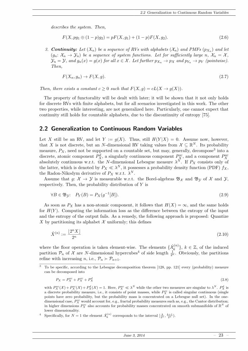
Figure 2.2: Model for computing the information loss of a memoryless input-output system g. Q is a quan-tizer with partition Pn. The input X is not necessarily discrete.
One can now measure the mutual information between X and its quantization X(n), as well asthe mutual information between the system output Y and X(n) (see Fig. 2.2). While the formeris an approximation of the information available at the system input, the latter approximatesthe information at the system output. By the data processing inequality [21, p. 35], the formerquantity cannot be smaller than the latter. Moreover, the finer the quantization, the better arethese approximations. This leads to
Definition 2.2 (Information Loss). Let X be an RV with alphabet X , and let Y := g(X). Theinformation loss induced by g is
L(X → Y ) := limn→∞
(
I(X(n);X)− I(X(n);Y ))
= H(X|Y ). (2.11)
Before addressing the second equality, note that for a bijective system the two mutual in-formations are equal for all n, and that thus the information loss evaluates to zero: bijectivefunctions describe lossless systems.For the second equality, note that with [66, Lem. 7.20]
I(X(n);X)− I(X(n);Y ) = H(X(n))−H(X(n)|X)−H(X(n)) +H(X(n)|Y ) (2.12)
= H(X(n)|Y ) (2.13)
since Xn is a function of X. Since furthermore H(Xn|Y = y)ր H(X|Y = y) monotonically [66,Lem. 7.18], the second equality follows.For a discrete input RV X one obtains L(X → Y ) = H(X) − H(Y ). Thus, the extension
to general RVs does not conflict with Definition 2.1 and remains justified by [7]. Clearly, for adiscrete input RV (with finite entropy) the information loss will always be a finite quantity. Thesame does not hold for a continuous input X:
Proposition 2.1 (Infinite Information Loss). Let PX have an absolutely continuous componentP acX ≪ λN which is supported on X . If there exists a set B ⊆ Y of positive PY -measure such
that the preimage g−1[y] is uncountable for every y ∈ B, then
L(X → Y ) =∞. (2.14)
Proof.
L(X → Y ) = H(X|Y ) =
∫
YH(X|Y = y)dPY (y) ≥
∫
BH(X|Y = y)dPY (y) (2.15)
since B ⊆ Y. Since, for all y ∈ B, g−1[y] is uncountable and since PX has an absolutelycontinuous component on X , the conditional probability measure PX|Y=y cannot be supportedon a countable set of points; thus one obtains H(X|Y = y) = ∞ [116, Ch. 2.4] for all y ∈ B.The proof follows from PY (B) > 0.
– 24 – June 3, 2014
2.2 Generalization to Continuous Random Variables
Now let PX ≪ λN and take y∗ ∈ Y. Since PY (y∗) = PX(g−1[y∗]), PY (y
∗) > 0 is only possibleif g−1[y∗] is uncountable (it cannot be a λN null set). This proves
Corollary 2.1. Let PX ≪ λN . If there exists a point y∗ ∈ Y such that PY (y∗) > 0, then
L(X → Y ) =∞.
Example 1: Quantizer.Look at the information loss of a scalar quantizer, i.e., of a system described by a function
g(x) = ⌊x⌋. (2.16)
With the notation introduced above, Y = g(X) = X(0). Assuming PX ≪ λ, which isfulfilled by every univariate distribution described by a PDF, there will be at least one pointy∗ for which Pr(Y = y∗) = PY (y
∗) = PX([y∗, y∗ + 1)) > 0. The conditions of Corollary 2.1are fulfilled and one obtains
L(X → X(0)) =∞. (2.17)
Note that due to the continuity of the input distribution, H(X) =∞, while in all practically
relevant cases H(Y ) < ∞. Thus, in this case the information loss truly corresponds to the
difference between input and output entropies.
There obviously exists a class of systems with finite information transfer (I(X;Y ) <∞) andinfinite information loss. Contrarily, Section 2.3 treats systems with finite information loss forwhich I(X;Y ) =∞; finally, Section 2.4 analyzes systems for which both quantities are infinite.As the next example shows, not every function with an uncountable preimage leads to infiniteinformation loss:
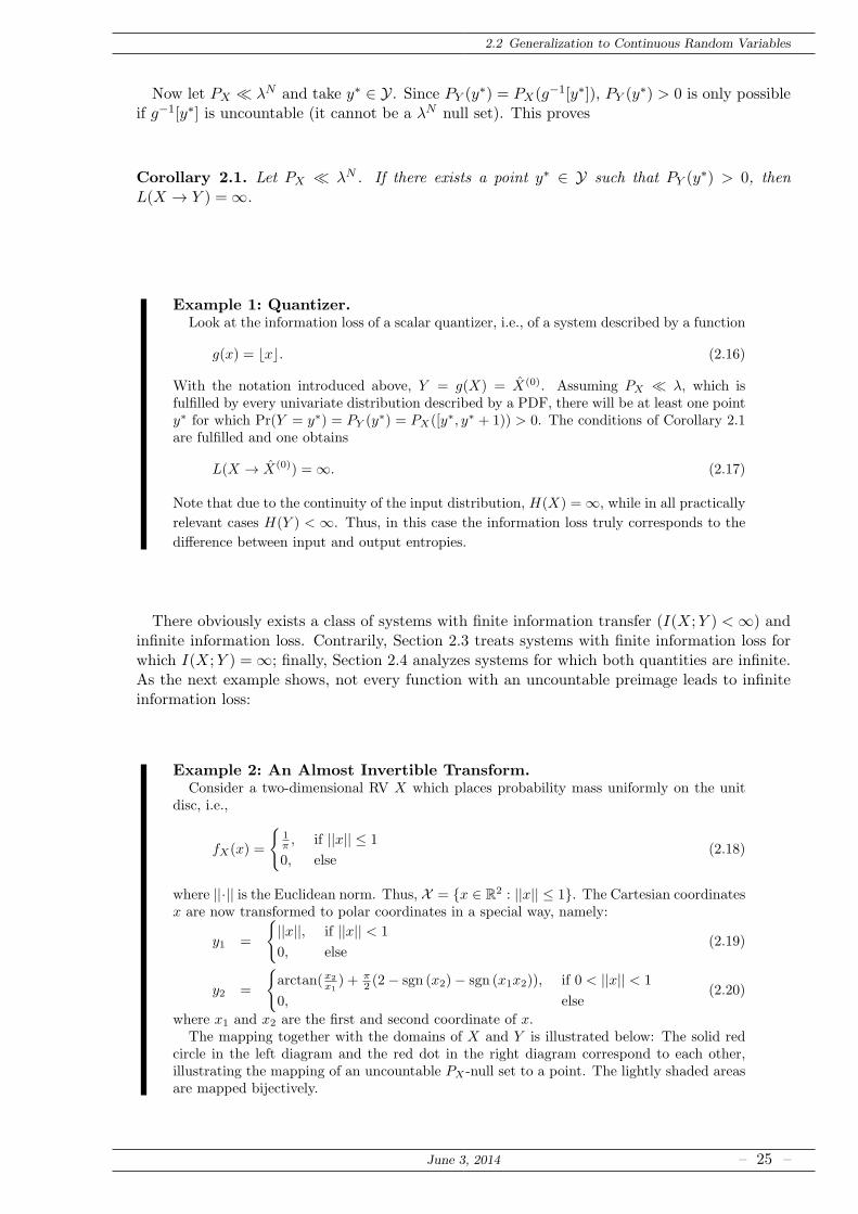
Example 2: An Almost Invertible Transform.Consider a two-dimensional RV X which places probability mass uniformly on the unit
disc, i.e.,
fX(x) =
1π, if ||x|| ≤ 1
0, else(2.18)
where ||·|| is the Euclidean norm. Thus, X = x ∈ R2 : ||x|| ≤ 1. The Cartesian coordinatesx are now transformed to polar coordinates in a special way, namely:
y1 =
||x||, if ||x|| < 1
0, else(2.19)
y2 =
arctan(x2
x1) + π
2 (2− sgn (x2)− sgn (x1x2)), if 0 < ||x|| < 1
0, else(2.20)
where x1 and x2 are the first and second coordinate of x.The mapping together with the domains of X and Y is illustrated below: The solid red
circle in the left diagram and the red dot in the right diagram correspond to each other,illustrating the mapping of an uncountable PX -null set to a point. The lightly shaded areasare mapped bijectively.
June 3, 2014 – 25 –
2 Information Loss
x1
x21
y1
y22π
1
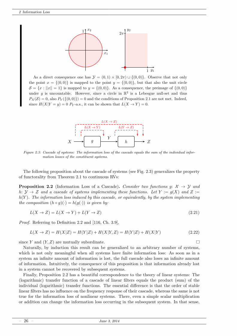
As a direct consequence one has Y = (0, 1) × [0, 2π) ∪ (0, 0). Observe that not only
the point x = (0, 0) is mapped to the point y = (0, 0), but that also the unit circle
S = x : ||x|| = 1 is mapped to y = (0, 0). As a consequence, the preimage of (0, 0)under g is uncountable. However, since a circle in R2 is a Lebesgue null-set and thus
PX(S) = 0, also PY ((0, 0)) = 0 and the conditions of Proposition 2.1 are not met. Indeed,
since H(X|Y = y) = 0 PY -a.s., it can be shown that L(X → Y ) = 0.
X g h ZY
L(X → Y ) L(Y → Z)
L(X → Z)
Figure 2.3: Cascade of systems: The information loss of the cascade equals the sum of the individual infor-mation losses of the constituent systems.
The following proposition about the cascade of systems (see Fig. 2.3) generalizes the propertyof functorality from Theorem 2.1 to continuous RVs:
Proposition 2.2 (Information Loss of a Cascade). Consider two functions g: X → Y andh: Y → Z and a cascade of systems implementing these functions. Let Y := g(X) and Z :=h(Y ). The information loss induced by this cascade, or equivalently, by the system implementingthe composition (h g)(·) = h(g(·)) is given by:
L(X → Z) = L(X → Y ) + L(Y → Z) (2.21)
Proof. Referring to Definition 2.2 and [116, Ch. 3.9],
L(X → Z) = H(X|Z) = H(Y |Z) +H(X|Y, Z) = H(Y |Z) +H(X|Y ) (2.22)
since Y and (Y, Z) are mutually subordinate.
Naturally, by induction this result can be generalized to an arbitrary number of systems,which is not only meaningful when all systems have finite information loss: As soon as in asystem an infinite amount of information is lost, the full cascade also loses an infinite amountof information. Intuitively, the consequence of this proposition is that information already lostin a system cannot be recovered by subsequent systems.
Finally, Proposition 2.2 has a beautiful correspondence to the theory of linear systems: The(logarithmic) transfer function of a cascade of linear filters equals the product (sum) of theindividual (logarithmic) transfer functions. The essential difference is that the order of stablelinear filters has no influence on the frequency response of their cascade, whereas the same is nottrue for the information loss of nonlinear systems. There, even a simple scalar multiplicationor addition can change the information loss occurring in the subsequent system. In that sense,
– 26 – June 3, 2014
2.3 Information Loss in Piecewise Bijective Functions
nonlinear systems do not necessarily commute w.r.t. information loss, while stable linear systemsdo w.r.t., e.g., the frequency response. Consequently, while post-processing cannot recoverinformation already lost, pre-processing can prevent it from getting lost, cf. [81]. A significantpart of this work deals with designing such pre-processing systems for this very purpose.
2.3 Information Loss in Piecewise Bijective Functions
As Example 1 showed, there certainly exist functions for which the information loss is infinite;for these, our measure of information loss will be of little help, and other, yet to be developedmeasures shall be applied. However, as we show in this section, quite a large class of systemsloses only a finite amount of information. As a prime example, take the recitfier: Stripping thesign off a number cannot destroy more than 1 bit of information.Throughout this section, let the probability distribution of the system input X satisfy PX ≪
λN for some N , and let Xi be a partition of X into non-null sets, i.e., for all i, PX(Xi) > 0.The class of systems considered in this section is described by
Definition 2.3 (Piecewise Bijective Function). A piecewise bijective function (PBF) g: X → Y,X ,Y ⊆ RN , is a surjective function defined in a piecewise manner:
g(x) =
g1(x), if x ∈ X1
g2(x), if x ∈ X2
...
(2.23)
where gi: Xi → Yi bijectively. The Jacobian matrix Jg(·) exists on the closures of Xi, and itsdeterminant, detJg(·), is non-zero PX -a.s.
2.3.1 Elementary Properties
A direct consequence of Definition 2.3 is that the preimage g−1[y] is countable for all y ∈ Y andthat the probability measure of the output Y satisfies PY ≪ λN and has a PDF
fY (y) =∑
xi∈g−1[y]
fX(xi)
|detJg(xi)|(2.24)
by the method of transformation [114, p. 244].One of the main results of this work is the following, connecting information loss with differ-
ential entropies. The differential entropy of an RV X with PDF fX is given as
h(X) := −∫
XfX(x) log fX(x)dx (2.25)
provided that the (N -dimensional) integral exists. It equals the N -dimensional entropy ofX [123].
Theorem 2.2 (Information Loss and Differential Entropy). Let PX ≪ λN and let g be a PBF.The information loss induced by g is
L(X → Y ) = h(X)− h(Y ) + E (log |detJg(X)|) (2.26)
provided the quantities on the right exist.
Proof. See Appendix A.1.This result is interesting because it connects a quantity which is invariant under a change of
variables (the information loss is defined via mutual information, which exhibits this invariance)
June 3, 2014 – 27 –
2 Information Loss
and a quantity which is not: differential entropy changes under a bijective variable transformand can thus not be regarded as a measure of information5. As such, the difference h(X)−h(Y )is meaningless: Changing g to c · g with c being a real number changes the aforementioneddifference. The third term, the expected logarithmic differential gain E (log |detJg(X)|), however,compensates for this variation – the effect from shaping the PDF is mitigated, what remains isa measure of information loss.From a different point-of-view, Theorem 2.2 extends [114, pp. 660], which claims that the
differential entropy of a function g of an RV X is bounded by
h(Y ) ≤ h(X) + E (log |detJg(X)|) (2.27)
where equality holds if and only if g is bijective: Theorem 2.2 explains the difference between theright-hand side and the left-hand side of (2.27) as the information lost due to data processingfor functions which are only piecewise bijective.It is also worth noting that Theorem 2.2 has a tight connection to the theory of iterated
function systems. In particular, [164] analyzed the information flow in one-dimensional maps,which is the difference between information generation via stretching (corresponding to the terminvolving the Jacobian determinant) and information reduction via folding (corresponding to in-formation loss). Ruelle [129] later proved that for a restricted class of systems the folding entropyL(X → Y ) cannot fall below the information generated via stretching, and therefore speaks ofpositivity of entropy production. He also established a connection to the Kolmogorov-Sinaı en-tropy rate. In [82], both components constituting information flow in iterated function systemsare described as ways a dynamical system can lose information. This highly interesting con-nection was recently investigated in a Master’s thesis for one-dimensional, discrete-time chaoticsystems [160].
Example 3: Square-Law Device and Gaussian Input.Let X be a zero-mean, unit variance Gaussian RV and let Y = X2. Switching to nats,
the differential entropy of X is h(X) = 12 ln(2πe). The output Y is a χ2-distributed RV with
one degree of freedom, for which the differential entropy can be computed as [156]
h(Y ) =1
2(1 + lnπ − γ) (2.28)
where γ is the Euler-Mascheroni constant [3, pp. 3]. The Jacobian determinant degeneratesto the derivative, and using some calculus yields
E (ln |g′(X)|) = E (ln |2X|) = 1
2(ln 2− γ) . (2.29)
With Theorem 2.2 it follows that L(X → Y ) = ln 2, which after changing the base of the
logarithm amounts to one bit. Indeed, the information loss induced by a square-law device
is always one bit if the PDF of the input RV has even symmetry [49].
Intuitively, the information loss is due to the non-injectivity of g, which, employing Defini-tion 2.3, is only invertible if the partition Xi from which the input X originated is already known.The following statements will put this intuition on solid ground.
Definition 2.4 (Partition Indicator). The partition indicator W is a discrete RV which satisfies
W = i if X ∈ Xi (2.30)
5 In fact, this invariance under a variable change tempted Edwin T. Jaynes to write “[...] that the entropy of acontinuous probability distribution is not an invariant. This is due to the historical accident that in his originalpapers, Shannon assumed, without calculating, that the analog of
∑pi log pi was
∫w logwdx [...] we have
realized that mathematical deduction from the uniqueness theorem, instead of guesswork, yields [an] invariantinformation measure” [78, p. 202].
– 28 – June 3, 2014
2.3 Information Loss in Piecewise Bijective Functions
for all i. In other words, W is obtained by quantizing X according to the partition Xi.
Proposition 2.3. The information loss is identical to the uncertainty about the set Xi fromwhich the input was taken, i.e.,
L(X → Y ) = H(W |Y ). (2.31)
Proof. See Appendix A.2.
The mathematical justification of the intuition-based claim is actually contained in
Corollary 2.2. System output Y and partition indicator W together are a sufficient statistic ofthe system input X, i.e.,
H(X|Y,W ) = 0. (2.32)
Proof. Since W is a function of X,
L(X → Y ) = H(X|Y ) = H(X,W |Y ) = H(X|W,Y )+H(W |Y ) = H(X|W,Y )+L(X → Y )
(2.33)
from which H(X|Y,W ) = 0 follows.
Knowing the output value, and the element of the partition from which the input originated,perfect reconstruction is possible. In all other cases, reconstruction will fail with some proba-bility, cf. Section 2.3.3.
While the information loss in most practically relevant PBFs will be a finite quantity, thisdoes not always have to be the case:
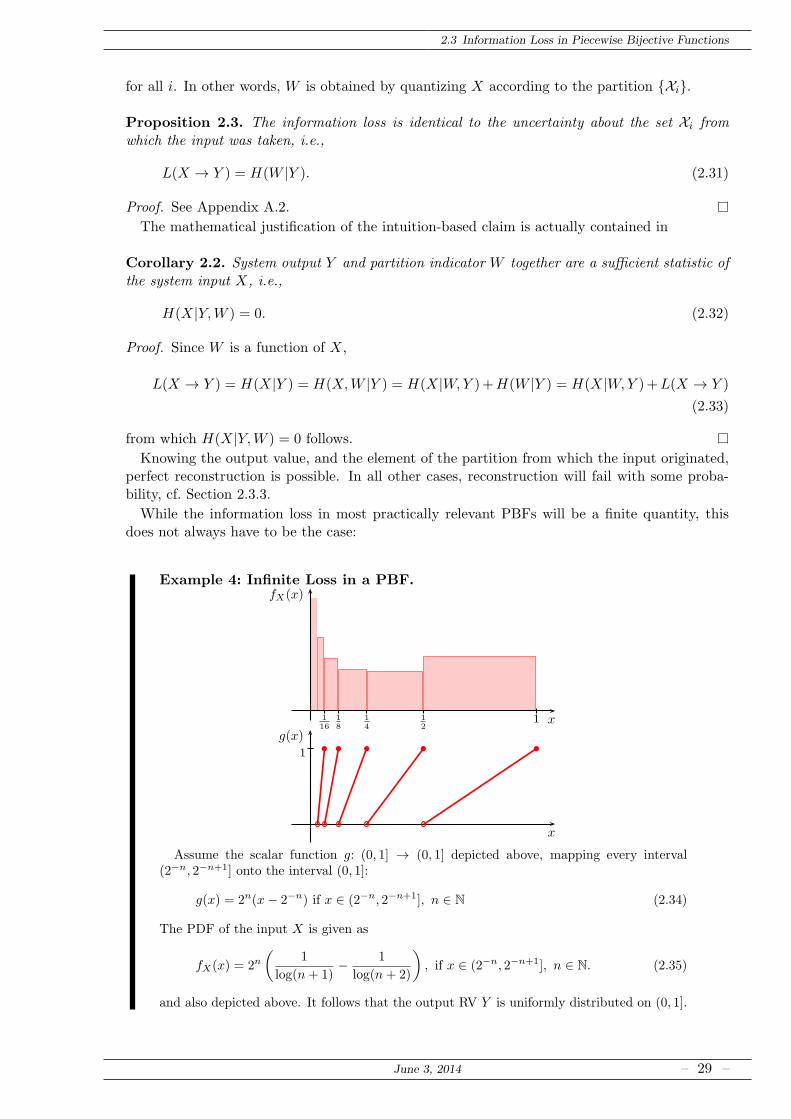
Example 4: Infinite Loss in a PBF.
112
14
18
116
x
fX(x)
x
g(x)
1
Assume the scalar function g: (0, 1] → (0, 1] depicted above, mapping every interval(2−n, 2−n+1] onto the interval (0, 1]:
g(x) = 2n(x− 2−n) if x ∈ (2−n, 2−n+1], n ∈ N (2.34)
The PDF of the input X is given as
fX(x) = 2n(
1
log(n+ 1)− 1
log(n+ 2)
)
, if x ∈ (2−n, 2−n+1], n ∈ N. (2.35)
and also depicted above. It follows that the output RV Y is uniformly distributed on (0, 1].
June 3, 2014 – 29 –
2 Information Loss
To apply Proposition 2.3, one needs
Pr(W = n|Y = y) = Pr(W = n) =1
log(n+ 1)− 1
log(n+ 2). (2.36)
For this distribution, the entropy is known to be infinite [6], and thus
L(X → Y ) = H(W |Y ) = H(W ) =∞. (2.37)
2.3.2 Bounds on the Information Loss
In many cases one cannot directly evaluate the information loss according to Theorem 2.2, sincethe differential entropy of Y involves the logarithm of a sum. This section therefore presentsupper bounds on the information loss which are comparably easy to evaluate.A particularly simple example for an upper bound – which is exact in Examples 3 and 4 –
is the following corollary to Proposition 2.3, which is due to the fact that conditioning reducesentropy:
Corollary 2.3. L(X → Y ) ≤ H(W ).
More interesting is the following list of inequalities: All of these involve the cardinality of thepreimage of the output. The further down one moves in this list, the simpler is the expressionto evaluate; the last two bounds do not require any knowledge about the PDF of the input X.Nevertheless, the bounds are tight, as Examples 3 and 4 show.
Proposition 2.4 (Upper Bounds on Information Loss). The information loss induced by a PBFcan be upper bounded by the following ordered set of inequalities:
L(X → Y ) ≤∫
YfY (y) log card(g
−1[y])dy (2.38)
≤ log
(∑
i
∫
Yi
fY (y)dy
)
(2.39)
≤ ess supy∈Y
log card(g−1[y]) (2.40)
≤ log card(Xi) (2.41)
where card(B) is the cardinality of the set B. Bound (2.38) holds with equality if and only if
∑
xk∈g−1[g(x)]
fX(xk)
|detJg(xk)||detJg(x)|fX(x)
PX -a.s.= card(g−1[g(x)]). (2.42)
If and only if this expression is constant PX-a.s., bounds (2.39) and (2.40) are tight. Bound (2.41)holds with equality if and only if additionally PY (Yi) = 1 for all i.
Proof. See Appendix A.3.If the PDF of X and the absolute value of the Jacobian determinant (but not necessarily
the cardinality of the preimage) are constant on X , the first bound (2.38) holds with equality(cf. [51, conference version, Sect. VI.A]). But also two other scenarios, where these bounds holdwith equality, are worth mentioning: First, for functions g: R→ R equality holds if g is relatedto the cumulative distribution function FX of the input RV such that, for all x, |g′(x)| = fX(x).From this immediately follows that g assumes, for all i,
gi(x) = biFX(x) + ci (2.43)
– 30 – June 3, 2014
2.3 Information Loss in Piecewise Bijective Functions
x
FX(x), g(x), h(x)
1
Z
Y1Y2
Y3
X1 X2 X3
b
b
b
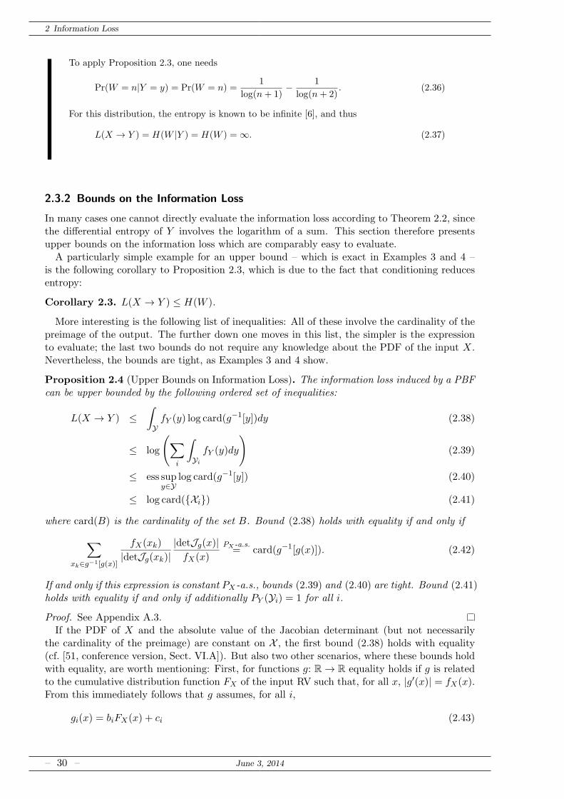
Figure 2.4: Piecewise bijective functions with card(Xi) =: L = 3 illustrating tightness of Proposition 2.4.The black curve is the cumulative distribution function FX of X. The function in blue, h: X →Y, renders (2.42) piecewise constant but not constant due to improper setting of the constantsci. Tightness is achieved in the smallest bound, (2.38), only. The function in red, g: X → Z,satisfies all conditions (i.e., (2.42) is constant and Zl = Z for all l) and thus achieves equalityin the largest bound (2.41). The constants for g are (bi) = (−1, 1, 1) and (ci) = (1/3, 1/3, 2/3).Note that the elements Xi are chosen such that each contains the same probability mass.
where bi ∈ 1,−1 and ci ∈ R are multiplicative and additive constants which may differ oneach element of the partition Xi. The function h: X → Y depicted in Fig. 2.4 satisfies thiscondition.
The constants ci and the probability masses in each interval are constrained if equality in (2.41)is desired. Specifically, in (2.42) card(g−1[g(x)]) = card(Xi) =: L shall hold PX -a.s., essentiallystating that the image of every Xi has to coincide with Y except on a set of measure zero.Assuming that Xi are intervals containing the same probability mass, i.e., PX(Xi) = 1/L for alli, (2.41) holds with equality for additive constants
ci = −i−1∑
l=1
PX(Xl) = −i− 1
L(2.44)
for bi = 1 and
ci = −i
L(2.45)
for bi = −1, respectively. A function g: X → Z satisfying these requirements is shown in Fig. 2.4.
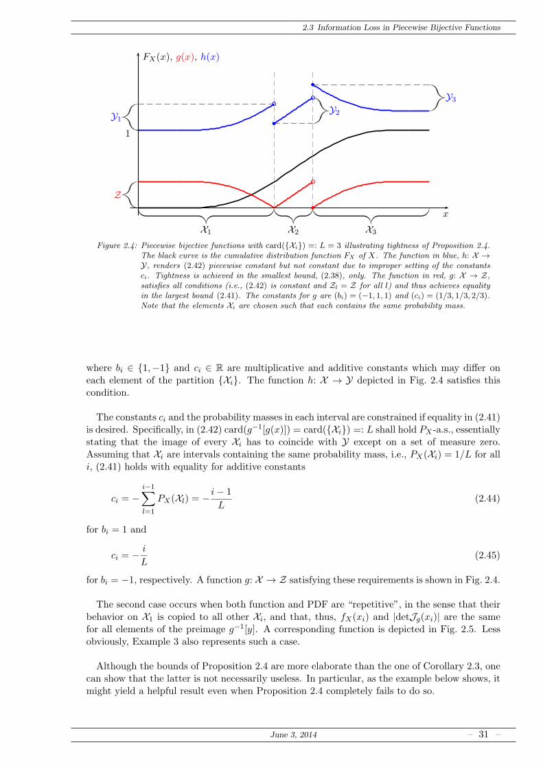
The second case occurs when both function and PDF are “repetitive”, in the sense that theirbehavior on X1 is copied to all other Xi, and that, thus, fX(xi) and |detJg(xi)| are the samefor all elements of the preimage g−1[y]. A corresponding function is depicted in Fig. 2.5. Lessobviously, Example 3 also represents such a case.
Although the bounds of Proposition 2.4 are more elaborate than the one of Corollary 2.3, onecan show that the latter is not necessarily useless. In particular, as the example below shows, itmight yield a helpful result even when Proposition 2.4 completely fails to do so.
June 3, 2014 – 31 –
2 Information Loss
x
fX(x), g(x), FX(x)
X1 X2 X3
Y
b
bb
x
g(x)
Figure 2.5: Piecewise bijective function with L = 3 satisfying all conditions of Proposition 2.4. The black andthe grey functions are the PDF fX and cumulative distribution function FX of X, respectively.The function g: X → Y consists of L shifted copies of the prototype function g, possibly modifiedwith different signs bi on different sets Xi. Moreover, the PDF fX is identical on all elementsXi (equal probability mass in each interval). Note that in this example X is not an interval.
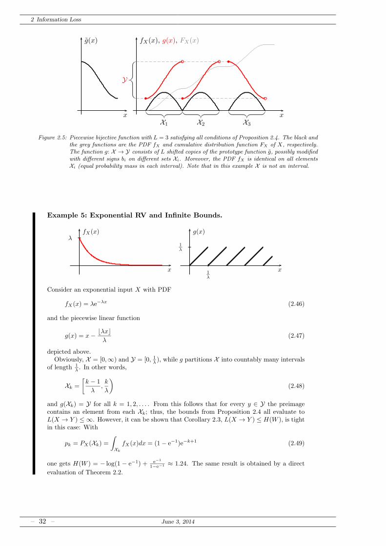
Example 5: Exponential RV and Infinite Bounds.
x
fX(x)λ
x
g(x)
1λ
1λ
Consider an exponential input X with PDF
fX(x) = λe−λx (2.46)
and the piecewise linear function
g(x) = x− ⌊λx⌋λ
(2.47)
depicted above.Obviously, X = [0,∞) and Y = [0, 1
λ), while g partitions X into countably many intervals
of length 1λ. In other words,
Xk =
[k − 1
λ,k
λ
)
(2.48)
and g(Xk) = Y for all k = 1, 2, . . . . From this follows that for every y ∈ Y the preimagecontains an element from each Xk; thus, the bounds from Proposition 2.4 all evaluate toL(X → Y ) ≤ ∞. However, it can be shown that Corollary 2.3, L(X → Y ) ≤ H(W ), is tightin this case: With
pk = PX(Xk) =
∫
Xk
fX(x)dx = (1− e−1)e−k+1 (2.49)
one gets H(W ) = − log(1 − e−1) + e−1
1−e−1 ≈ 1.24. The same result is obtained by a direct
evaluation of Theorem 2.2.
– 32 – June 3, 2014
2.3 Information Loss in Piecewise Bijective Functions
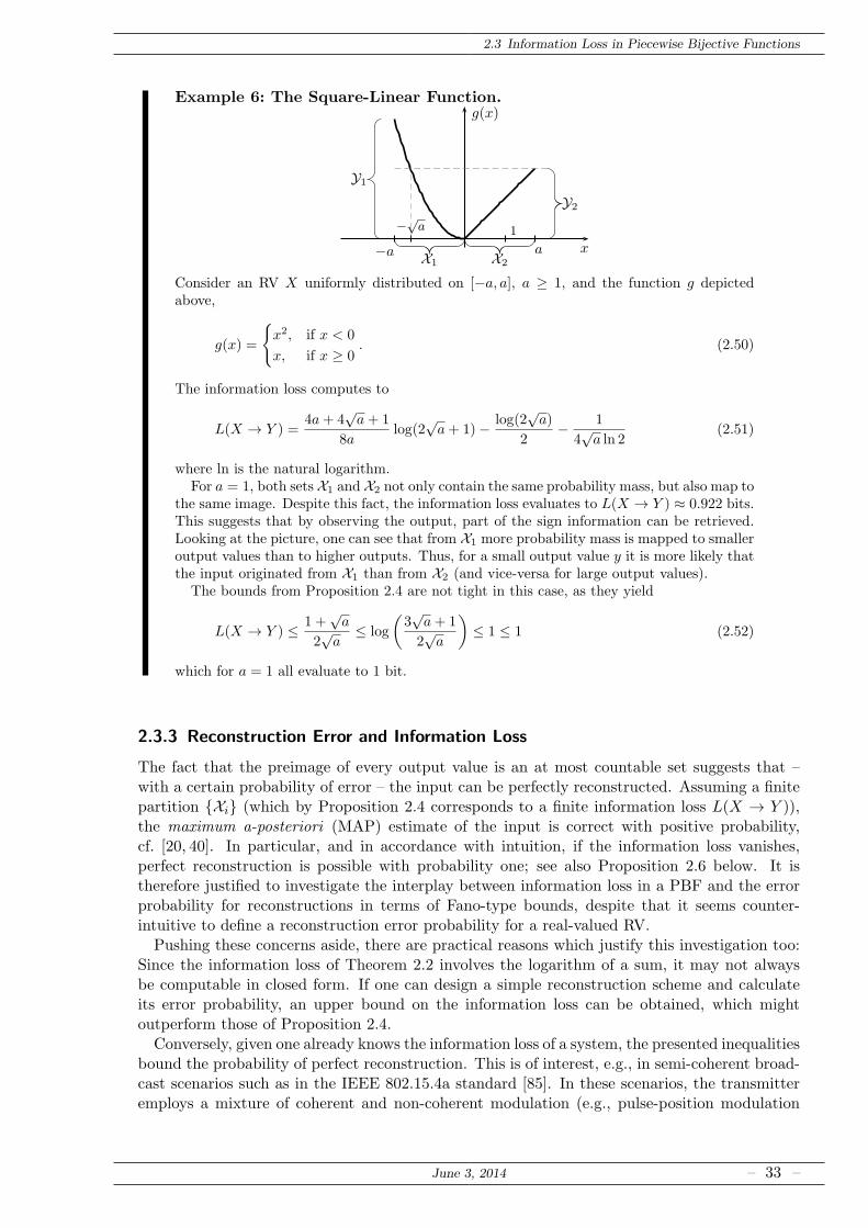
Example 6: The Square-Linear Function.
x
g(x)
−a a
1−√a
Y2Y1
X1 X2
Consider an RV X uniformly distributed on [−a, a], a ≥ 1, and the function g depictedabove,
g(x) =
x2, if x < 0
x, if x ≥ 0. (2.50)
The information loss computes to
L(X → Y ) =4a+ 4
√a+ 1
8alog(2
√a+ 1)− log(2
√a)
2− 1
4√a ln 2
(2.51)
where ln is the natural logarithm.For a = 1, both sets X1 and X2 not only contain the same probability mass, but also map to
the same image. Despite this fact, the information loss evaluates to L(X → Y ) ≈ 0.922 bits.This suggests that by observing the output, part of the sign information can be retrieved.Looking at the picture, one can see that from X1 more probability mass is mapped to smalleroutput values than to higher outputs. Thus, for a small output value y it is more likely thatthe input originated from X1 than from X2 (and vice-versa for large output values).
The bounds from Proposition 2.4 are not tight in this case, as they yield
L(X → Y ) ≤ 1 +√a
2√a≤ log
(3√a+ 1
2√a
)
≤ 1 ≤ 1 (2.52)
which for a = 1 all evaluate to 1 bit.
2.3.3 Reconstruction Error and Information Loss
The fact that the preimage of every output value is an at most countable set suggests that –with a certain probability of error – the input can be perfectly reconstructed. Assuming a finitepartition Xi (which by Proposition 2.4 corresponds to a finite information loss L(X → Y )),the maximum a-posteriori (MAP) estimate of the input is correct with positive probability,cf. [20, 40]. In particular, and in accordance with intuition, if the information loss vanishes,perfect reconstruction is possible with probability one; see also Proposition 2.6 below. It istherefore justified to investigate the interplay between information loss in a PBF and the errorprobability for reconstructions in terms of Fano-type bounds, despite that it seems counter-intuitive to define a reconstruction error probability for a real-valued RV.Pushing these concerns aside, there are practical reasons which justify this investigation too:
Since the information loss of Theorem 2.2 involves the logarithm of a sum, it may not alwaysbe computable in closed form. If one can design a simple reconstruction scheme and calculateits error probability, an upper bound on the information loss can be obtained, which mightoutperform those of Proposition 2.4.Conversely, given one already knows the information loss of a system, the presented inequalities
bound the probability of perfect reconstruction. This is of interest, e.g., in semi-coherent broad-cast scenarios such as in the IEEE 802.15.4a standard [85]. In these scenarios, the transmitteremploys a mixture of coherent and non-coherent modulation (e.g., pulse-position modulation
June 3, 2014 – 33 –
2 Information Loss
and phase-shift keying). A non-coherent receiver, such as the energy detector, might undercertain circumstances be able to decode also part of the coherently transmitted message; thepresented inequalities can yield performance bounds.
To simplify analysis and to avoid the peculiarities of entropy pointed out in [75], the focus ison PBFs with finite partition. For a possible generalization to countable partitions the reader isrefered to [74]. While the results in this section were derived with PBFs in mind, they are alsovalid for the more general case where the cardinality of the reconstruction alphabet depends onthe observed output.
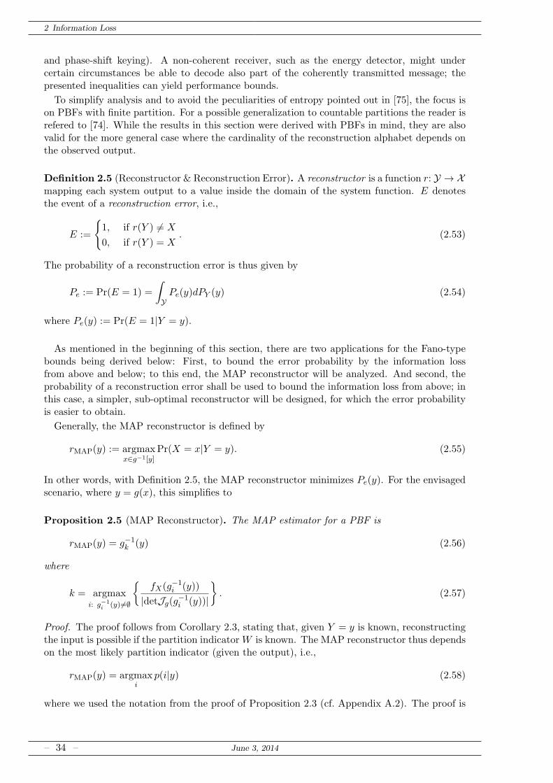
Definition 2.5 (Reconstructor & Reconstruction Error). A reconstructor is a function r: Y → Xmapping each system output to a value inside the domain of the system function. E denotesthe event of a reconstruction error, i.e.,
E :=
1, if r(Y ) 6= X
0, if r(Y ) = X. (2.53)
The probability of a reconstruction error is thus given by
Pe := Pr(E = 1) =
∫
YPe(y)dPY (y) (2.54)
where Pe(y) := Pr(E = 1|Y = y).
As mentioned in the beginning of this section, there are two applications for the Fano-typebounds being derived below: First, to bound the error probability by the information lossfrom above and below; to this end, the MAP reconstructor will be analyzed. And second, theprobability of a reconstruction error shall be used to bound the information loss from above; inthis case, a simpler, sub-optimal reconstructor will be designed, for which the error probabilityis easier to obtain.
Generally, the MAP reconstructor is defined by
rMAP(y) := argmaxx∈g−1[y]
Pr(X = x|Y = y). (2.55)
In other words, with Definition 2.5, the MAP reconstructor minimizes Pe(y). For the envisagedscenario, where y = g(x), this simplifies to
Proposition 2.5 (MAP Reconstructor). The MAP estimator for a PBF is
rMAP(y) = g−1k (y) (2.56)
where
k = argmaxi: g−1
i (y) 6=∅
fX(g−1
i (y))
|detJg(g−1i (y))|
. (2.57)
Proof. The proof follows from Corollary 2.3, stating that, given Y = y is known, reconstructingthe input is possible if the partition indicator W is known. The MAP reconstructor thus dependson the most likely partition indicator (given the output), i.e.,
rMAP(y) = argmaxi
p(i|y) (2.58)
where we used the notation from the proof of Proposition 2.3 (cf. Appendix A.2). The proof is
– 34 – June 3, 2014
2.3 Information Loss in Piecewise Bijective Functions
completed with
p(i|y) =
fX(g−1i (y))
|detJg(g−1i (y))|fY (y)
, if g−1i (y) 6= ∅
0, if g−1i (y) = ∅
. (2.59)
As a direct consequence, for the MAP reconstructor one has rMAP(y) ∈ g−1[y]. Therefore, forthis and any other reconstructor choosing the reconstruction from the preimage of the output,Fano’s inequality holds and one gets [21, pp. 39]
L(X → Y ) ≤ H2(Pe) + Pe log (card(Xi)− 1) (2.60)
where H2(p) := −p log p − (1 − p) log(1 − p) is the entropy of a Bernoulli-p random variable.Trivially, one can exchange the cardinality of the partition Xi by the essential supremum overall preimage cardinalities (cf. Appendix A.4), i.e.,
L(X → Y ) ≤ H2(Pe) + Pe log
(
ess supy∈Y
card(g−1[y])− 1
)
. (2.61)
Definition 2.6 (Bijective Part). Xb is the maximal set which is mapped injectively by g, andYb is its image under g. Thus, g: Xb → Yb bijectively, where
Xb := x ∈ X : card(g−1[g(x)]) = 1. (2.62)
Then Pb := PX(Xb) = PY (Yb) denotes the bijectively mapped probability mass.
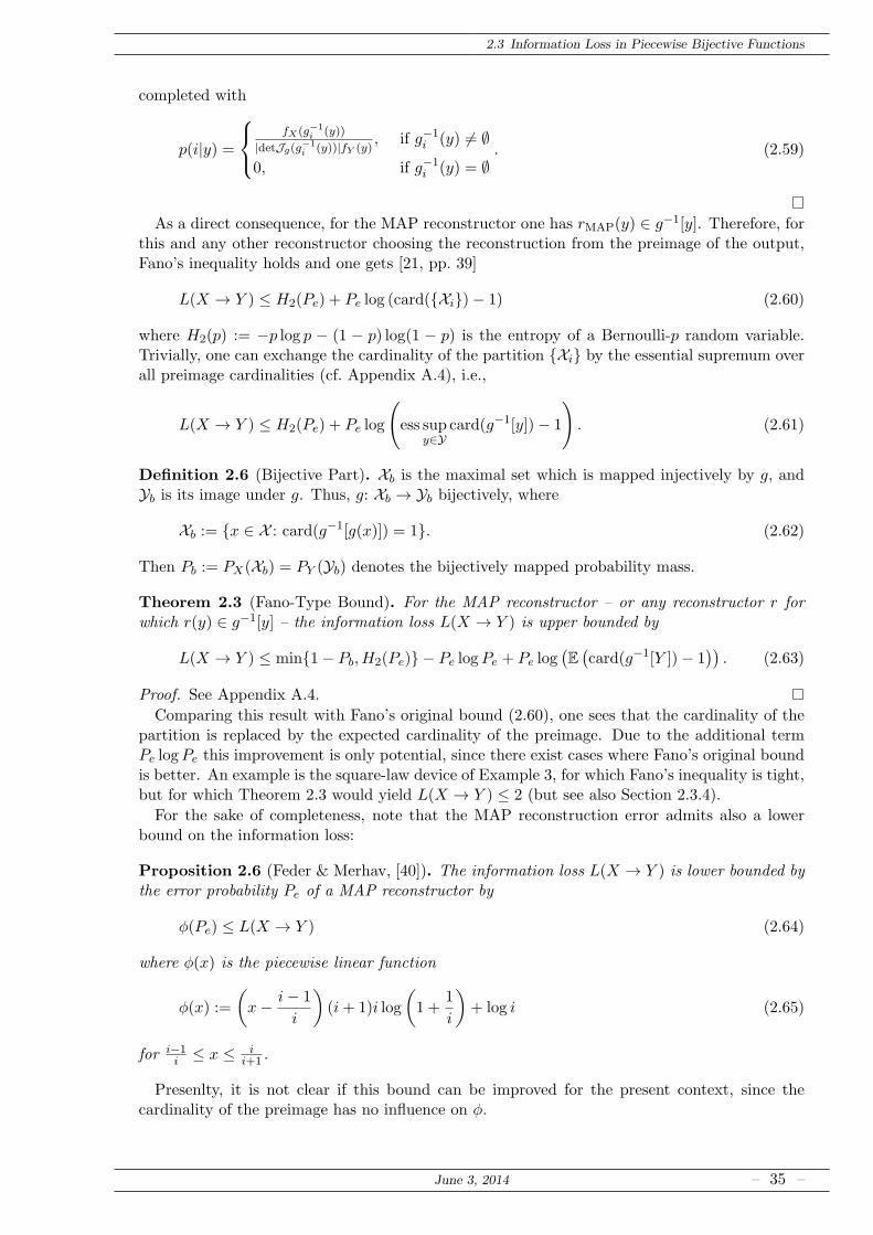
Theorem 2.3 (Fano-Type Bound). For the MAP reconstructor – or any reconstructor r forwhich r(y) ∈ g−1[y] – the information loss L(X → Y ) is upper bounded by
L(X → Y ) ≤ min1− Pb, H2(Pe) − Pe logPe + Pe log(E(card(g−1[Y ])− 1
)). (2.63)
Proof. See Appendix A.4.
Comparing this result with Fano’s original bound (2.60), one sees that the cardinality of thepartition is replaced by the expected cardinality of the preimage. Due to the additional termPe logPe this improvement is only potential, since there exist cases where Fano’s original boundis better. An example is the square-law device of Example 3, for which Fano’s inequality is tight,but for which Theorem 2.3 would yield L(X → Y ) ≤ 2 (but see also Section 2.3.4).
For the sake of completeness, note that the MAP reconstruction error admits also a lowerbound on the information loss:
Proposition 2.6 (Feder & Merhav, [40]). The information loss L(X → Y ) is lower bounded bythe error probability Pe of a MAP reconstructor by
φ(Pe) ≤ L(X → Y ) (2.64)
where φ(x) is the piecewise linear function
φ(x) :=
(
x− i− 1
i
)
(i+ 1)i log
(
1 +1
i
)
+ log i (2.65)
for i−1i ≤ x ≤ i
i+1 .
Presenlty, it is not clear if this bound can be improved for the present context, since thecardinality of the preimage has no influence on φ.
June 3, 2014 – 35 –
2 Information Loss
In concrete examples, the MAP reconstructor is not always easy to find. For bounding theinformation loss of a system (rather than reconstructing the input), it is therefore desirable tointroduce a simpler, sub-optimal reconstructor:
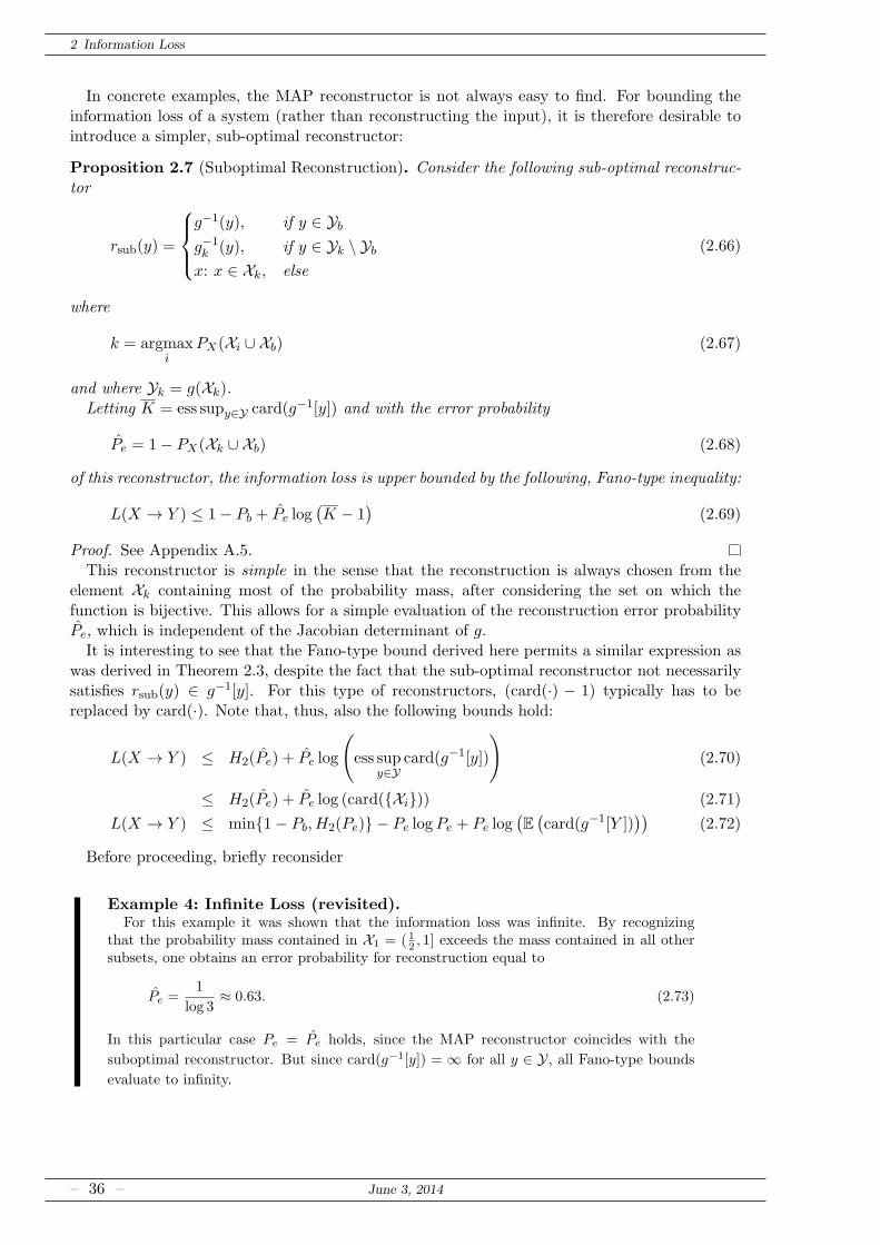
Proposition 2.7 (Suboptimal Reconstruction). Consider the following sub-optimal reconstruc-tor
rsub(y) =
g−1(y), if y ∈ Ybg−1k (y), if y ∈ Yk \ Ybx: x ∈ Xk, else
(2.66)
where
k = argmaxi
PX(Xi ∪ Xb) (2.67)
and where Yk = g(Xk).Letting K = ess supy∈Y card(g−1[y]) and with the error probability
Pe = 1− PX(Xk ∪ Xb) (2.68)
of this reconstructor, the information loss is upper bounded by the following, Fano-type inequality:
L(X → Y ) ≤ 1− Pb + Pe log(K − 1
)(2.69)
Proof. See Appendix A.5.This reconstructor is simple in the sense that the reconstruction is always chosen from the
element Xk containing most of the probability mass, after considering the set on which thefunction is bijective. This allows for a simple evaluation of the reconstruction error probabilityPe, which is independent of the Jacobian determinant of g.It is interesting to see that the Fano-type bound derived here permits a similar expression as
was derived in Theorem 2.3, despite the fact that the sub-optimal reconstructor not necessarilysatisfies rsub(y) ∈ g−1[y]. For this type of reconstructors, (card(·) − 1) typically has to bereplaced by card(·). Note that, thus, also the following bounds hold:
L(X → Y ) ≤ H2(Pe) + Pe log
(
ess supy∈Y
card(g−1[y])
)
(2.70)
≤ H2(Pe) + Pe log (card(Xi)) (2.71)
L(X → Y ) ≤ min1− Pb, H2(Pe) − Pe logPe + Pe log(E(card(g−1[Y ])
))(2.72)
Before proceeding, briefly reconsider
Example 4: Infinite Loss (revisited).For this example it was shown that the information loss was infinite. By recognizing
that the probability mass contained in X1 = ( 12 , 1] exceeds the mass contained in all othersubsets, one obtains an error probability for reconstruction equal to
Pe =1
log 3≈ 0.63. (2.73)
In this particular case Pe = Pe holds, since the MAP reconstructor coincides with the
suboptimal reconstructor. But since card(g−1[y]) = ∞ for all y ∈ Y, all Fano-type bounds
evaluate to infinity.
– 36 – June 3, 2014
2.3 Information Loss in Piecewise Bijective Functions
g(x), y
x, rMAP(y)
− 10√3
10√3
20√3
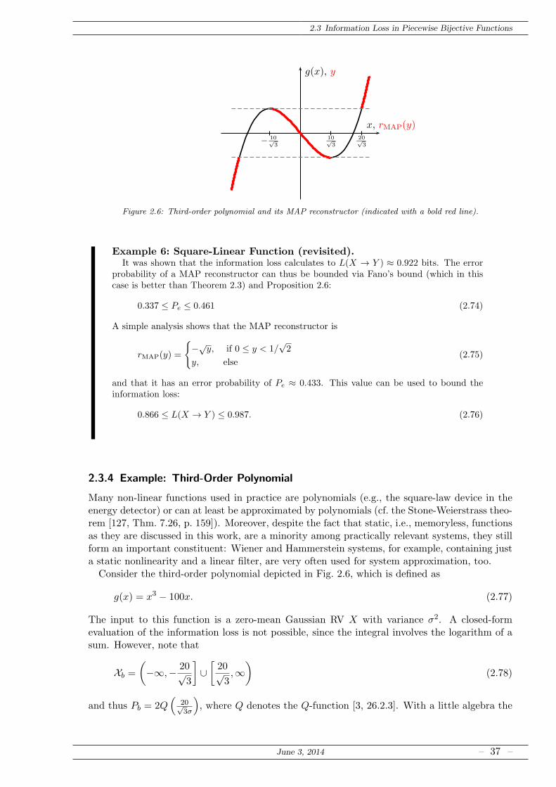
Figure 2.6: Third-order polynomial and its MAP reconstructor (indicated with a bold red line).
Example 6: Square-Linear Function (revisited).It was shown that the information loss calculates to L(X → Y ) ≈ 0.922 bits. The error
probability of a MAP reconstructor can thus be bounded via Fano’s bound (which in thiscase is better than Theorem 2.3) and Proposition 2.6:
0.337 ≤ Pe ≤ 0.461 (2.74)
A simple analysis shows that the MAP reconstructor is
rMAP(y) =
−√y, if 0 ≤ y < 1/√2
y, else(2.75)
and that it has an error probability of Pe ≈ 0.433. This value can be used to bound theinformation loss:
0.866 ≤ L(X → Y ) ≤ 0.987. (2.76)
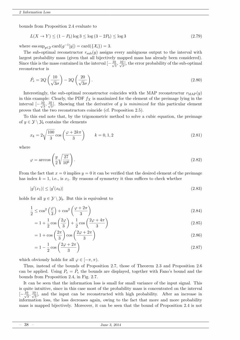
2.3.4 Example: Third-Order Polynomial
Many non-linear functions used in practice are polynomials (e.g., the square-law device in theenergy detector) or can at least be approximated by polynomials (cf. the Stone-Weierstrass theo-rem [127, Thm. 7.26, p. 159]). Moreover, despite the fact that static, i.e., memoryless, functionsas they are discussed in this work, are a minority among practically relevant systems, they stillform an important constituent: Wiener and Hammerstein systems, for example, containing justa static nonlinearity and a linear filter, are very often used for system approximation, too.Consider the third-order polynomial depicted in Fig. 2.6, which is defined as
g(x) = x3 − 100x. (2.77)
The input to this function is a zero-mean Gaussian RV X with variance σ2. A closed-formevaluation of the information loss is not possible, since the integral involves the logarithm of asum. However, note that
Xb =
(
−∞,− 20√3
]
∪[20√3,∞)
(2.78)
and thus Pb = 2Q(
20√3σ
)
, where Q denotes the Q-function [3, 26.2.3]. With a little algebra the
June 3, 2014 – 37 –
2 Information Loss
bounds from Proposition 2.4 evaluate to
L(X → Y ) ≤ (1− Pb) log 3 ≤ log (3− 2Pb) ≤ log 3 (2.79)
where ess supy∈Y card(g−1[y]) = card(Xi) = 3.
The sub-optimal reconstructor rsub(y) assigns every ambiguous output to the interval withlargest probability mass (given that all bijectively mapped mass has already been considered).Since this is the mass contained in the interval [− 10√
3, 10√
3], the error probability of the sub-optimal
reconstructor is
Pe = 2Q
(10√3σ
)
− 2Q
(20√3σ
)
. (2.80)
Interestingly, the sub-optimal reconstructor coincides with the MAP reconstructur rMAP(y)in this example: Clearly, the PDF fX is maximized for the element of the preimage lying in theinterval [− 10√
3, 10√
3]. Showing that the derivative of g is minimized for this particular element
proves that the two reconstructors coincide (cf. Proposition 2.5).
To this end note that, by the trigonometric method to solve a cubic equation, the preimageof y ∈ Y \ Yb contains the elements
xk = 2
√
100
3cos
(ϕ+ 2kπ
3
)
k = 0, 1, 2 (2.81)
where
ϕ = arccos
(
y
2
√
27
106
)
. (2.82)
From the fact that x = 0 implies y = 0 it can be verified that the desired element of the preimagehas index k = 1, i.e., is x1. By reasons of symmetry it thus suffices to check whether
|g′(x1)| ≤ |g′(x0)| (2.83)
holds for all y ∈ Y \ Yb. But this is equivalent to
1
2≤ cos2
(ϕ
3
)
+ cos2(ϕ+ 2π
3
)
(2.84)
= 1 +1
2cos
(2ϕ
3
)
+1
2cos
(2ϕ+ 4π
3
)
(2.85)
= 1 + cos
(2π
3
)
cos
(2ϕ+ 2π
3
)
(2.86)
= 1− 1
2cos
(2ϕ+ 2π
3
)
(2.87)
which obviously holds for all ϕ ∈ [−π, π).Thus, instead of the bounds of Proposition 2.7, those of Theorem 2.3 and Proposition 2.6
can be applied. Using Pe = Pe the bounds are displayed, together with Fano’s bound and thebounds from Proposition 2.4, in Fig. 2.7.
It can be seen that the information loss is small for small variance of the input signal. Thisis quite intuitive, since in this case most of the probability mass is concentrated on the interval[− 10√
3, 10√
3], and the input can be reconstructed with high probability. After an increase in
information loss, the loss decreases again, owing to the fact that more and more probabilitymass is mapped bijectively. Moreover, it can be seen that the bound of Proposition 2.4 is not
– 38 – June 3, 2014
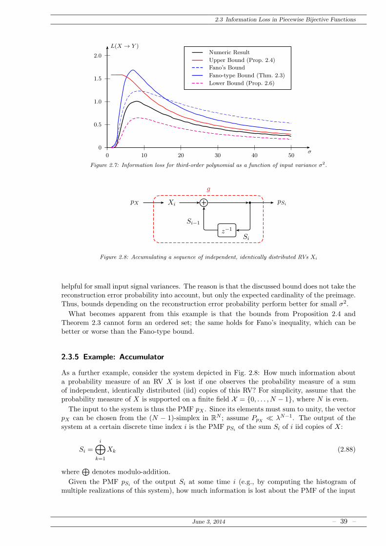
2.3 Information Loss in Piecewise Bijective Functions
0
0.5
1.0
1.5
2.0
0 10 20 30 40 50σ
L(X → Y )Numeric Result
Upper Bound (Prop. 2.4)
Fano’s Bound
Fano-type Bound (Thm. 2.3)
Lower Bound (Prop. 2.6)
Figure 2.7: Information loss for third-order polynomial as a function of input variance σ2.
pX pSiXi
z−1
b
Si−1
Si
g
Figure 2.8: Accumulating a sequence of independent, identically distributed RVs Xi
helpful for small input signal variances. The reason is that the discussed bound does not take thereconstruction error probability into account, but only the expected cardinality of the preimage.Thus, bounds depending on the reconstruction error probability perform better for small σ2.
What becomes apparent from this example is that the bounds from Proposition 2.4 andTheorem 2.3 cannot form an ordered set; the same holds for Fano’s inequality, which can bebetter or worse than the Fano-type bound.
2.3.5 Example: Accumulator
As a further example, consider the system depicted in Fig. 2.8: How much information abouta probability measure of an RV X is lost if one observes the probability measure of a sumof independent, identically distributed (iid) copies of this RV? For simplicity, assume that theprobability measure of X is supported on a finite field X = 0, . . . , N − 1, where N is even.
The input to the system is thus the PMF pX . Since its elements must sum to unity, the vectorpX can be chosen from the (N − 1)-simplex in RN ; assume PpX ≪ λN−1. The output of thesystem at a certain discrete time index i is the PMF pSi
of the sum Si of i iid copies of X:
Si =
i⊕
k=1
Xk (2.88)
where⊕
denotes modulo-addition.
Given the PMF pSiof the output Si at some time i (e.g., by computing the histogram of
multiple realizations of this system), how much information is lost about the PMF of the input
June 3, 2014 – 39 –
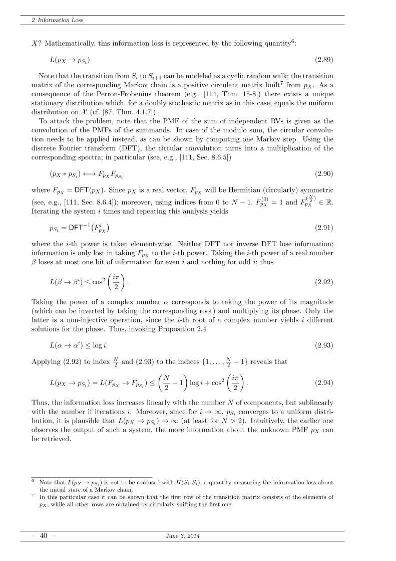
2 Information Loss
X? Mathematically, this information loss is represented by the following quantity6:
L(pX → pSi) (2.89)
Note that the transition from Si to Si+1 can be modeled as a cyclic random walk; the transitionmatrix of the corresponding Markov chain is a positive circulant matrix built7 from pX . As aconsequence of the Perron-Frobenius theorem (e.g., [114, Thm. 15-8]) there exists a uniquestationary distribution which, for a doubly stochastic matrix as in this case, equals the uniformdistribution on X (cf. [87, Thm. 4.1.7]).To attack the problem, note that the PMF of the sum of independent RVs is given as the
convolution of the PMFs of the summands. In case of the modulo sum, the circular convolu-tion needs to be applied instead, as can be shown by computing one Markov step. Using thediscrete Fourier transform (DFT), the circular convolution turns into a multiplication of thecorresponding spectra; in particular (see, e.g., [111, Sec. 8.6.5])
(pX ∗ pSi)←→ FpXFpSi
(2.90)
where FpX = DFT(pX). Since pX is a real vector, FpX will be Hermitian (circularly) symmetric
(see, e.g., [111, Sec. 8.6.4]); moreover, using indices from 0 to N − 1, F(0)pX = 1 and F
(N2)
pX ∈ R.Iterating the system i times and repeating this analysis yields
pSi= DFT
−1(F ipX
)(2.91)
where the i-th power is taken element-wise. Neither DFT nor inverse DFT lose information;information is only lost in taking FpX to the i-th power. Taking the i-th power of a real numberβ loses at most one bit of information for even i and nothing for odd i; thus
L(β → βi) ≤ cos2(iπ
2
)
. (2.92)
Taking the power of a complex number α corresponds to taking the power of its magnitude(which can be inverted by taking the corresponding root) and multiplying its phase. Only thelatter is a non-injective operation, since the i-th root of a complex number yields i differentsolutions for the phase. Thus, invoking Proposition 2.4
L(α→ αi) ≤ log i. (2.93)
Applying (2.92) to index N2 and (2.93) to the indices 1, . . . , N2 − 1 reveals that
L(pX → pSi) = L(FpX → FpSi
) ≤(N
2− 1
)
log i+ cos2(iπ
2
)
. (2.94)
Thus, the information loss increases linearly with the number N of components, but sublinearlywith the number if iterations i. Moreover, since for i → ∞, pSi
converges to a uniform distri-bution, it is plausible that L(pX → pSi
) → ∞ (at least for N > 2). Intuitively, the earlier oneobserves the output of such a system, the more information about the unknown PMF pX canbe retrieved.
6 Note that L(pX → pSi) is not to be confused with H(S1|Si), a quantity measuring the information loss about
the initial state of a Markov chain.7 In this particular case it can be shown that the first row of the transition matrix consists of the elements of
pX , while all other rows are obtained by circularly shifting the first one.
– 40 – June 3, 2014
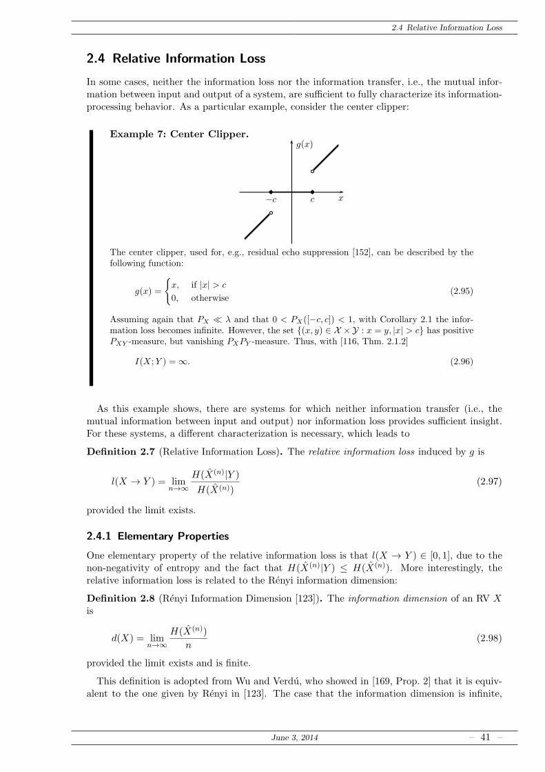
2.4 Relative Information Loss
2.4 Relative Information Loss
In some cases, neither the information loss nor the information transfer, i.e., the mutual infor-mation between input and output of a system, are sufficient to fully characterize its information-processing behavior. As a particular example, consider the center clipper:
Example 7: Center Clipper.
x
g(x)
c−c
The center clipper, used for, e.g., residual echo suppression [152], can be described by thefollowing function:
g(x) =
x, if |x| > c
0, otherwise(2.95)
Assuming again that PX ≪ λ and that 0 < PX([−c, c]) < 1, with Corollary 2.1 the infor-mation loss becomes infinite. However, the set (x, y) ∈ X ×Y : x = y, |x| > c has positivePXY -measure, but vanishing PXPY -measure. Thus, with [116, Thm. 2.1.2]
I(X;Y ) =∞. (2.96)
As this example shows, there are systems for which neither information transfer (i.e., themutual information between input and output) nor information loss provides sufficient insight.For these systems, a different characterization is necessary, which leads to
Definition 2.7 (Relative Information Loss). The relative information loss induced by g is
l(X → Y ) = limn→∞
H(X(n)|Y )
H(X(n))(2.97)
provided the limit exists.
2.4.1 Elementary Properties
One elementary property of the relative information loss is that l(X → Y ) ∈ [0, 1], due to thenon-negativity of entropy and the fact that H(X(n)|Y ) ≤ H(X(n)). More interestingly, therelative information loss is related to the Renyi information dimension:
Definition 2.8 (Renyi Information Dimension [123]). The information dimension of an RV Xis
d(X) = limn→∞
H(X(n))
n(2.98)
provided the limit exists and is finite.
This definition is adopted from Wu and Verdu, who showed in [169, Prop. 2] that it is equiv-alent to the one given by Renyi in [123]. The case that the information dimension is infinite,
June 3, 2014 – 41 –
2 Information Loss
which may occur if H(X(0)) =∞ [169, Prop. 1], is excluded here. Conversely, if the informationdimension of an RVX exists, it is guaranteed to be finite ifH(X(0)) <∞ [123] or if E (|X|ǫ) <∞for some ǫ > 0 [169]. Aside from that, the information dimension exists for discrete RVs and RVswith probability measures absolutely continuous w.r.t. the Lebesgue measure on a sufficientlysmooth manifold [123], for mixtures of RVs with existing information dimension [123, 144, 169],and self-similar distributions generated by iterated function systems [169]. Finally, the informa-tion dimension exists if the MMSE dimension exists [170, Thm. 8]. The remainder of this workis based on the assumption that the information dimension of all considered RVs exists and isfinite.
Proposition 2.8 (Relative Information Loss and Information Dimension). Let X be an N -dimensional RV with positive information dimension d(X) and finite H(X(0)). If d(X|Y = y)and H(X(0)|Y = y) exist and are finite PY -a.s., the relative information loss equals
l(X → Y ) =d(X|Y )
d(X)(2.99)
where d(X|Y ) =∫
Y d(X|Y = y)dPY (y).
Proof. From Definition 2.7,
l(X → Y ) = limn→∞
H(X(n)|Y )
H(X(n))(2.100)
= limn→∞
∫
Y H(X(n)|Y = y)dPY (y)
H(X(n))(2.101)
= limn→∞
∫
YH(X(n)|Y=y)
n dPY (y)
H(X(n))n
. (2.102)
By assumption, the limit of the denominator and of the expression under the integral both existand correspond to d(X) and d(X|Y = y), respectively. By assumption, H(X(0)|Y = y) is finitePY -a.s., thus, with [123, eq. (11)], the expression under the integral is finite for all n ≥ 1:
H(X(n)|Y = y)
n≤ H(X(0)|Y = y) +N(n+ 1)
n< H(X(0)|Y = y) + 2N <∞ (2.103)
The latter is an integrable function, integrating to H(X(0)|Y ) + 2N ≤ H(X(0)) + 2N < ∞.One can thus apply Lebesgue’s dominated convergence theorem (e.g., [128, Thm. 1.34, p. 26])to exchange the order of the limit and the integral:
l(X → Y ) =limn→∞
∫
YH(X(n)|Y=y)
n dPY (y)
d(X)=
∫
Y d(X|Y = y)dPY (y)
d(X)=
d(X|Y )
d(X). (2.104)
This completes the proof.
The relative information loss shall be accompanied by its logical complement, the relativeinformation transfer:
Definition 2.9 (Relative Information Transfer). The relative information transfer through thesystem g is
t(X → Y ) = limn→∞
I(X(n);Y )
H(X(n))= 1− l(X → Y ) (2.105)
provided the limit exists.
– 42 – June 3, 2014
2.4 Relative Information Loss
The relative information loss was introduced to characterize systems for which the absoluteinformation loss from Definition 2.2 is infinite. The following result shows that, at least forinput RVs with infinite entropy, an infinite absolute information loss is a prerequisite for positiverelative information loss:
Proposition 2.9 (Positive Relative Loss leads to Infinite Absolute Loss). Let X be such thatH(X) =∞ and let l(X → Y ) > 0. Then, L(X → Y ) =∞.
Proof. The proposition is proved by contradiction: Assume that L(X → Y ) = H(X|Y ) = κ <∞. Thus,
l(X → Y ) = limn→∞
H(X(n)|Y )
H(X(n))(2.106)
(a)
≤ limn→∞
H(X|Y )
H(X(n))(2.107)
(b)= 0 (2.108)
where (a) is due to data processing and (b) follows from H(X|Y ) = κ <∞ and from H(X(n))→H(X) =∞ (e.g., [66, Lem. 7.18]).
Note that the converse is not true: There exist examples where an infinite amount of informa-tion is lost, but for which the relative information loss nevertheless vanishes, i.e., l(X → Y ) = 0(see Example 4).
2.4.2 Relative Information Loss for System Reducing the Dimensionality ofContinuous Random Variables
Systems for which the information loss L(X → Y ) is infinite subsume, among others, thosewhich reduce the dimensionality of the input signal, e.g., by dropping coordinates or by keepingthe function constant on a subset of its domain. This section is devoted to an investigation ofthis particular class of systems. Interestingly, a reduction of the dimension of the support X doesnot necessarily lead to a positive relative information loss, nor does its preservation guaranteevanishing relative information loss.
Assume that X ⊆ RN and PX ≪ λN , thus d(X) = N . Assume further that g is piecewisedefined, as in Definition 2.3. Here, however, gi: Xi → Yi are not necessarily bijective, butprojections.
Proposition 2.10 (Relative Information Loss in Dimensionality Reduction). Let Xi be apartition of X . Let g be such that gi = g|Xi
are projections to Mi coordinates. Then, the relativeinformation loss is
l(X → Y ) =K∑
i=1
PX(Xi)N −Mi
N. (2.109)
Proof. See Appendix A.6.
As it is argued in the proof, the result can be generalized to submersions, i.e., smooth functionsbetween smooth manifolds whose pushforward is surjective everywhere (see, e.g., [95]). Thisgeneralization is, however, not carried out in this work.
Corollary 2.4. Let g be any projection of X onto M of its coordinates. Then, the relativeinformation loss is
l(X → Y ) =N −M
N. (2.110)
June 3, 2014 – 43 –
2 Information Loss
Corollary 2.5. Let g be constant on a set A ⊆ X with positive PX-measure. Let furthermore gbe such that card(g−1[y]) <∞ for all y /∈ g(A). Then, the relative information loss is
l(X → Y ) = PX(A). (2.111)
The first of these two corollaries will be applied to principal components analysis in Section 2.6,while the second solves Example 7 (center clipper): While both the information loss and theinformation transfer are infinite, the relative information loss corresponds to the probabilitymass contained in the clipping region, i.e., l(X → Y ) = PX([−c, c]). Yet another illustration ofthese corollaries is given in
Example 8: Adding Two RVs.Consider two N -dimensional input RVs X1 and X2, and assume that the output of the
system under consideration is
Y = X1 +X2 (2.112)
i.e., the sum of these two RVs.For the moment, assume that X1 and X2 have a joint probability measure PX1,X2
≪ λ2N .As it can be shown rather easily by transforming X1, X2 invertibly to X1+X2, X1, droppingthe second coordinate leads to
l(X1, X2 → Y ) =1
2. (2.113)
Things look different if the joint probability measure PX1,X2is supported on some lower-
dimensional submanifold of R2N . Consider, e.g., the case where X2 = −X1, thus Y ≡ 0,and l(X1, X2 → Y ) = 1. In contrary to this, assume that both input variables are one-dimensional, and that X2 = −0.01X3
1 . Then, as it turns out,
Y = X1 − 0.01X31 = −0.01(X3
1 − 100X1) (2.114)
which is a piecewise bijective function. As the analysis of the third-order polynomial in
Section 2.3.4 shows, l(X1, X2 → Y ) = 0 in this case.
The somewhat surprising consequence of these results is that the shape of the PDF (if oneexists) has no influence on the relative information loss; whether the PDF is peaky in the clippingregion or flat, or whether the omitted coordinates are highly correlated to the preserved onesdoes neither increase nor decrease the relative information loss. As Example 8 shows, thingsbecome more complicated when the distribution of the input does not have a PDF: The choiceof the set on which the probability mass is supported (be it either of the same or of a smallerdimension as the function’s domain) can have a large influence on the relative information loss.
Proposition 2.10 permits another corollary, one which is of great interest and which is alsoproved in Appendix A.6:
Corollary 2.6. In the setting of Proposition 2.10,
t(X → Y ) =d(Y )
N. (2.115)
Indeed, the author believes that this behavior is the “general” behavior for functions reducingthe dimensionality of the data. This leads to the following
Conjecture 2.1 (Relative Information Transfer and Information Dimension). Let X be an RVwith positive information dimension d(X) and let g be a Lipschitz function. Then, the relative
– 44 – June 3, 2014
2.4 Relative Information Loss
information transfer through this function is
t(X → Y ) =d(Y )
d(X). (2.116)
The author is currently not able to prove this conjecture, but a possible line of reasoning isoutlined in Appendix A.7. Moreover, this conjecture suggests that, at least for a restricted classof functions,
d(X) = d(X,Y ) = d(X|Y ) + d(Y ) (2.117)
holds. This complements the results of [22], where it was shown that the point-wise informa-tion dimension satisfies this chain rule (second equality) given that the conditional probabilitymeasure satisfies a Lipschitz property. Moreover, the first equality was shown to hold for thepoint-wise information dimension given that Y is a Lipschitz function of X; for non-Lipschitzfunctions, the point-wise information dimension of (X,Y ) may exceed the one of X. If the sameholds for the information dimension (which is the expectation over the point-wise informationdimension) is an interesting question for future research.
A corollary to Conjecture 2.1 is the counterpart of Proposition 2.2 for relative informationloss:
Conjecture 2.2 (Relative Information Loss of a Cascade). Consider two Lipschitz functionsg: X → Y and h: Y → Z and a cascade of systems implementing these functions. Let Y := g(X)and Z := h(Y ). For the cascade of these systems the relative information transfer and relativeinformation loss are
t(X → Z) = t(X → Y )t(Y → Z) (2.118)
and
l(X → Z) = l(X → Y ) + l(Y → Z)− l(X → Y )l(Y → Z) (2.119)
respectively.
This conjecture about cascades can be proved for cascades of projections (with absolutelycontinuous inputs) and also for discrete RVs.
2.4.3 A Bound on the Relative Information Loss
Complementing the results from Section 2.3.2, this subsection presents a bound for the relativeinformation loss. Clearly, from the trivial bounds on the information dimension (d(X) ∈ [0, N ]if X is a subset of the N -dimensional Euclidean space or a sufficiently smooth N -dimensionalmanifold) simple bounds on the relative information loss can be computed. The bound on therelative information loss presented here for an N -dimensional input RV is formulated by thecorresponding coordinate-wise quantities.
Proposition 2.11 (Upper Bound on the Relative Information Loss). Let X be an N -dimensionalRV with a probability measure PX ≪ λN and let Y be N -dimensional. Then,
l(X → Y ) ≤ 1
N
N∑
i=1
l(Xi → Y ) ≤ 1
N
N∑
i=1
l(Xi → Yi) (2.120)
where Xi and Yi are the i-th coordinates of X and Y , respectively.
June 3, 2014 – 45 –
2 Information Loss
Proof. The proof follows from the fact that d(X) = N and, for all i, d(Xi) = 1. From thedefinition of relative information loss,
l(X → Y ) = limn→∞
H(X(n)1 , . . . , X
(n)N |Y )
H(X(n)1 , . . . , X
(n)N )
(2.121)
= limn→∞
∑Ni=1H(X
(n)i |X
(n)1 , . . . , X
(n)i−1, Y )
H(X(n)1 , . . . , X
(n)N )
(2.122)
≤ limn→∞
∑Ni=1H(X
(n)i |Y )
H(X(n)1 , . . . , X
(n)N )
(2.123)
Exchanging limit and summation yields
l(X → Y ) ≤∑N
i=1 d(Xi|Y )
d(X)=
∑Ni=1 d(Xi|Y )
N. (2.124)
But since N = Nd(Xi) for all i, this is equivalent to
l(X → Y ) ≤ 1
N
N∑
i=1
d(Xi|Y )
d(Xi)=
1
N
N∑
i=1
l(Xi → Y ). (2.125)
This proves the first inequality. The second is obtained by removing conditioning again in (2.123),since Y = Y1, . . . , YN.
Example 9: Projection.Let X be an N -dimensional RV with probability measure PX ≪ λN and let Xi denote
the i-th coordinate of X. Let g be a projection onto the first M < N coordinates. Theinformation loss is given as
l(X → Y ) =N −M
N(2.126)
by Corollary 2.4. Note that l(Xi → Y ) = 0 for i ∈ 1, . . . ,M, while l(Xi → Y ) = 1 for
i ∈ M + 1, . . . , N. This shows tightness of Proposition 2.11.
Example 8: Adding Two RVs (revisited).Take the adder Y = X1+X2 with PX1,X2
≪ λ2: Since in the general case the probability
measure PXi|Y=y possesses a density, one gets l(Xi → Y ) = 1 for i = 1, 2. The bound thus
evaluates to 1 and the inequality is strict, since l(X → Y ) = 12 < 1.
2.4.4 Reconstruction Error and Relative Information Loss
Complementing Section 2.3.3, this subsection presents a Fano-type relation between the relativeinformation loss and the probability of a reconstruction error. While for piecewise bijectivefunctions this relation was justified by the fact that for every output value the preimage under thesystem function is a countable set, the case is completely different here: Quantizers, for example,characterized by relative information loss, are typically evaluated based on energetic measures(e.g., the mean-squared reconstruction error). As the following example shows, the relativeinformation loss does not permit a meaningful interpretation in energetic terms, underlining theintrinsically different behavior of information and energy measures.
– 46 – June 3, 2014
2.4 Relative Information Loss
Example 1: Quantizer (revisited).Consider a continuous one-dimensional RV X (PX ≪ λ) and the quantizer introduced in
Section 2.2. Since the quantizer is constant PX -a.s., one obtains with Corollary 2.5
l(X → Xn) = 1. (2.127)
In other words, the quantizer destroys 100% of the information available at its input. This
naturally holds for all n, so a finer partition Pn cannot decrease the relative information
loss. Contrarily, the mean-squared reconstruction error decreases with increasing n.
Definition 2.10 (Minkowski Dimension). The Minkowski or box-counting dimension of a com-pact set X ⊂ RN is
dB(X ) = limn→∞
log card(Pn)n
(2.128)
where the partition Pn is induced by a uniform vector quantizer with quantization interval 12n .
The Minkowski dimension of a set equals the information dimension of a uniform distributionon that set (e.g., [39]), and is a special case of Renyi information dimension where the entropyis replaced with the Renyi entropy of zeroth order [64].
Proposition 2.12. Let X be an RV with probability measure PX with positive informationdimension d(X). Let the support X ⊂ RN of PX be compact and have positive Minkowskidimension dB(X ). Then, the error probability bounds the relative information loss from aboveby
l(X → Y ) ≤ PedB(X )d(X)
. (2.129)
Proof. Note that by the compactness of X the quantized input X(n) has a finite alphabet, whichallows employing Fano’s inequality
H(X(n)|Y ) ≤ H2(Pe,n) + Pe,n log card(Pn) (2.130)
where
Pe,n = Pr(r(Y ) 6= X(n)). (2.131)
Since Fano’s inequality holds for arbitrary reconstructors, let r be the composition of the MAPreconstructor rMAP and the quantizer introduced in Section 2.2. Consequently, Pe,n is theprobability that rMAP(Y ) and X do not lie in the same quantization bin. Since the bin volumeshrinks with increasing n, Pe,n increases monotonically to Pe. Thus, with H2(p) ≤ 1 for 0 ≤ p ≤1,
H(X(n)|Y ) ≤ 1 + Pe log card(Pn). (2.132)
With the introduced definitions,
l(X → Y ) = limn→∞
H(X(n)|Y )
H(X(n))≤ lim
n→∞1 + Pe log card(Pn)
H(X(n))
(a)= Pe
dB(X )d(X)
(2.133)
where (a) is obtained by dividing both numerator and denominator by n and evaluating thelimit. This completes the proof.
June 3, 2014 – 47 –
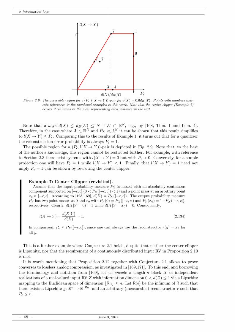
2 Information Loss
Pe
l(X → Y )
1
1
d(X)/dB(X )
b 7
b 7 b 7b 9
b 1
b 4b 3
Figure 2.9: The accessible region for a (Pe, l(X → Y ))-pair for d(X) = 0.6dB(X ). Points with numbers indi-cate references to the numbered examples in this work. Note that the center clipper (Example 7)occurs three times in the plot, representing each instance in the text.
Note that always d(X) ≤ dB(X ) ≤ N if X ⊂ RN , e.g., by [168, Thm. 1 and Lem. 4].Therefore, in the case where X ⊂ RN and PX ≪ λN it can be shown that this result simplifiesto l(X → Y ) ≤ Pe. Comparing this to the results of Example 1, it turns out that for a quantizerthe reconstruction error probability is always Pe = 1.
The possible region for a (Pe, l(X → Y ))-pair is depicted in Fig. 2.9. Note that, to the bestof the author’s knowledge, this region cannot be restricted further. For example, with referenceto Section 2.3 there exist systems with l(X → Y ) = 0 but with Pe > 0. Conversely, for a simpleprojection one will have Pe = 1 while l(X → Y ) < 1. Finally, that l(X → Y ) = 1 need notimply Pe = 1 can be shown by revisiting the center clipper:
Example 7: Center Clipper (revisited).Assume that the input probability measure PX is mixed with an absolutely continuous
component supported on [−c, c] (0 < PX([−c, c]) < 1) and a point mass at an arbitrary pointx0 /∈ [−c, c]. According to [123, 169], d(X) = PX([−c, c]). The output probability measurePY has two point masses at 0 and x0 with PY (0) = PX([−c, c]) and PY (x0) = 1−PX([−c, c]),respectively. Clearly, d(X|Y = 0) = 1 while d(X|Y = x0) = 0. Consequently,
l(X → Y ) =d(X|Y )
d(X)= 1. (2.134)
In comparison, Pe ≤ PX([−c, c]), since one can always use the reconstructor r(y) = x0 for
all y.
This is a further example where Conjecture 2.1 holds, despite that neither the center clipperis Lipschitz, nor that the requirement of a continuously distributed input RV in Proposition 2.10is met.
It is worth mentioning that Proposition 2.12 together with Conjecture 2.1 allows to proveconverses to lossless analog compression, as investigated in [169,171]. To this end, and borrowingthe terminology and notation from [169], let us encode a length-n block X of independentrealizations of a real-valued input RV Z with information dimension 0 < d(Z) ≤ 1 via a Lipschitzmapping to the Euclidean space of dimension ⌊Rn⌋ ≤ n. Let R(ǫ) be the infimum of R such thatthere exists a Lipschitz g: Rn → R⌊Rn⌋ and an arbitrary (measurable) reconstructor r such thatPe ≤ ǫ.
– 48 – June 3, 2014
2.4 Relative Information Loss
Conjecture 2.3 (Converse for Lipschitz Encoders; connection to [169], [171, eq. (26)]). For amemoryless source with compactly supported marginal distribution PZ and information dimen-sion 0 < d(Z) ≤ 1, and a Lipschitz encoder function g,
R(ǫ) ≥ d(Z)− ǫ. (2.135)
Proof. Since X is the collection of n real-valued, independent RVs Zi with probability measurePZ supported on Z, it follows that Zn ⊂ Rn and dB(Zn) = n. With Proposition 2.12 it thusfollows
nPe ≥ d(X)l(X → Y ) (2.136)
(a)= d(X)− d(Y ) (2.137)
(b)= nd(Z)− d(Y ) (2.138)
where (a) is due to Conjecture 2.1 and (b) is due to the fact that the information dimensionof a set of independent RVs is the sum of the individual information dimensions (see, e.g., [22]or [168, Lem. 3]). Since Y is an R⌊Rn⌋-valued RV, d(Y ) ≤ ⌊Rn⌋. Thus,
nPe ≥ nd(Z)− ⌊Rn⌋ ≥ nd(Z)− Rn. (2.139)
Dividing by the block length n and rearranging the terms completes the proof.While this result – compared with those presented in [169, 171] – is rather weak, it suggests
that the presented theory has relationships with different topics in information theory, such ascompressed sensing. Note further that the reconstructor is arbitrary, since already the encoder– the function g – loses information. The restriction of Lipschitz continuity cannot be dropped,since, as stated in [169], there are non-Lipschitz bijections from Rn to R.
2.4.5 Relative Information Loss for 1D-Systems of Mixed Random Variables
Briefly consider the case where X ,Y ⊂ R, but where not necessarily PX ≪ λ. Instead, let PX bea mixture of continuous and discrete probability measures, i.e., assume that PX has no singularcontinuous component. Thus, [128, pp. 121]
PX = P acX + P d
X . (2.140)
According to [123, 169] the information dimension of X equals the probability mass with abso-lutely continuous distribution, d(X) = P ac
X (X ).Proposition 2.13 (Relative Information Loss for Mixed RVs). Let X be a mixed RV with aprobability measure PX = P ac
X + P dX , 0 < P ac
X (X ) ≤ 1. Let Xi be a finite partition of X ⊆ R
into compact sets. Let g be a bounded function such that g|Xiis either injective or constant. The
relative information loss is given as
l(X → Y ) =P acX (A)
P acX (X ) (2.141)
where A is the union of sets Xi on which g is constant.
Proof. Since the partition is finite, using [169, Thm. 2] yields
d(X|Y = y) =∑
i
d(X|Y = y,X ∈ Xi)PX|Y=y(Xi). (2.142)
If g is injective on Xi, the intersection g−1[y]∩Xi is a single point8, thus d(X|Y = y,X ∈ Xi) = 0.
8 We do not consider the case here that the preimage of y does not intersect Xi, since in this case PX|Y =y(Xi) = 0.
June 3, 2014 – 49 –
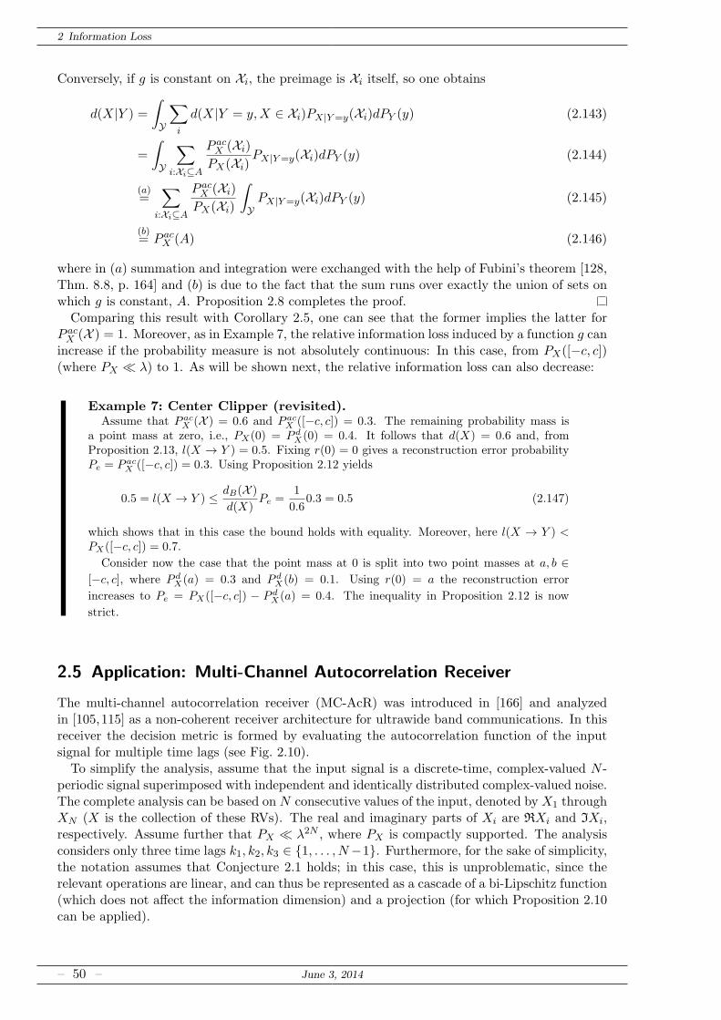
2 Information Loss
Conversely, if g is constant on Xi, the preimage is Xi itself, so one obtains
d(X|Y ) =
∫
Y
∑
i
d(X|Y = y,X ∈ Xi)PX|Y=y(Xi)dPY (y) (2.143)
=
∫
Y
∑
i:Xi⊆A
P acX (Xi)
PX(Xi)PX|Y=y(Xi)dPY (y) (2.144)
(a)=
∑
i:Xi⊆A
P acX (Xi)
PX(Xi)
∫
YPX|Y=y(Xi)dPY (y) (2.145)
(b)= P ac
X (A) (2.146)
where in (a) summation and integration were exchanged with the help of Fubini’s theorem [128,Thm. 8.8, p. 164] and (b) is due to the fact that the sum runs over exactly the union of sets onwhich g is constant, A. Proposition 2.8 completes the proof.Comparing this result with Corollary 2.5, one can see that the former implies the latter for
P acX (X ) = 1. Moreover, as in Example 7, the relative information loss induced by a function g can
increase if the probability measure is not absolutely continuous: In this case, from PX([−c, c])(where PX ≪ λ) to 1. As will be shown next, the relative information loss can also decrease:
Example 7: Center Clipper (revisited).Assume that P ac
X (X ) = 0.6 and P acX ([−c, c]) = 0.3. The remaining probability mass is
a point mass at zero, i.e., PX(0) = P dX(0) = 0.4. It follows that d(X) = 0.6 and, from
Proposition 2.13, l(X → Y ) = 0.5. Fixing r(0) = 0 gives a reconstruction error probabilityPe = P ac
X ([−c, c]) = 0.3. Using Proposition 2.12 yields
0.5 = l(X → Y ) ≤ dB(X )d(X)
Pe =1
0.60.3 = 0.5 (2.147)
which shows that in this case the bound holds with equality. Moreover, here l(X → Y ) <PX([−c, c]) = 0.7.
Consider now the case that the point mass at 0 is split into two point masses at a, b ∈[−c, c], where P d
X(a) = 0.3 and P dX(b) = 0.1. Using r(0) = a the reconstruction error
increases to Pe = PX([−c, c]) − P dX(a) = 0.4. The inequality in Proposition 2.12 is now
strict.
2.5 Application: Multi-Channel Autocorrelation Receiver
The multi-channel autocorrelation receiver (MC-AcR) was introduced in [166] and analyzedin [105,115] as a non-coherent receiver architecture for ultrawide band communications. In thisreceiver the decision metric is formed by evaluating the autocorrelation function of the inputsignal for multiple time lags (see Fig. 2.10).To simplify the analysis, assume that the input signal is a discrete-time, complex-valued N -
periodic signal superimposed with independent and identically distributed complex-valued noise.The complete analysis can be based on N consecutive values of the input, denoted by X1 throughXN (X is the collection of these RVs). The real and imaginary parts of Xi are RXi and IXi,respectively. Assume further that PX ≪ λ2N , where PX is compactly supported. The analysisconsiders only three time lags k1, k2, k3 ∈ 1, . . . , N−1. Furthermore, for the sake of simplicity,the notation assumes that Conjecture 2.1 holds; in this case, this is unproblematic, since therelevant operations are linear, and can thus be represented as a cascade of a bi-Lipschitz function(which does not affect the information dimension) and a projection (for which Proposition 2.10can be applied).
– 50 – June 3, 2014
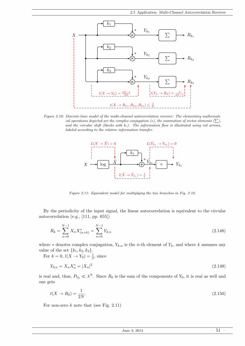
2.5 Application: Multi-Channel Autocorrelation Receiver
X b
b
b
b
b
k1
k2
k3
∗
∗
∗
∑
∑
∑
Rk1
Rk2
Rk3
Yk1
Yk2
Yk3
t(X → Yk) =2N−12N
t(Yk → Rk) =2
2N−1
t(X → Rk1 , Rk2 , Rk3) ≤ 3N
Figure 2.10: Discrete-time model of the multi-channel autocorrelation receiver: The elementary mathemati-cal operations depicted are the complex conjugation (∗), the summation of vector elements (
∑),
and the circular shift (blocks with ki). The information flow is illustrated using red arrows,labeled according to the relative information transfer.
X log b
k1
∗e Yk1
X Yk1
L(X → X) = 0 L(Yk1 → Yk1) = 0
l(X → Yk1) =12
Figure 2.11: Equivalent model for multiplying the two branches in Fig. 2.10.
By the periodicity of the input signal, the linear autocorrelation is equivalent to the circularautocorrelation (e.g., [111, pp. 655])
Rk =N−1∑
n=0
XnX∗(n+k) =
N−1∑
n=0
Yk,n (2.148)
where ∗ denotes complex conjugation, Yk,n is the n-th element of Yk, and where k assumes anyvalue of the set k1, k2, k3.For k = 0, l(X → Y0) =
12 , since
Y0,n = XnX∗n = |Xn|2 (2.149)
is real and, thus, PY0 ≪ λN . Since R0 is the sum of the components of Y0, it is real as well andone gets
t(X → R0) =1
2N. (2.150)
For non-zero k note that (see Fig. 2.11)
June 3, 2014 – 51 –
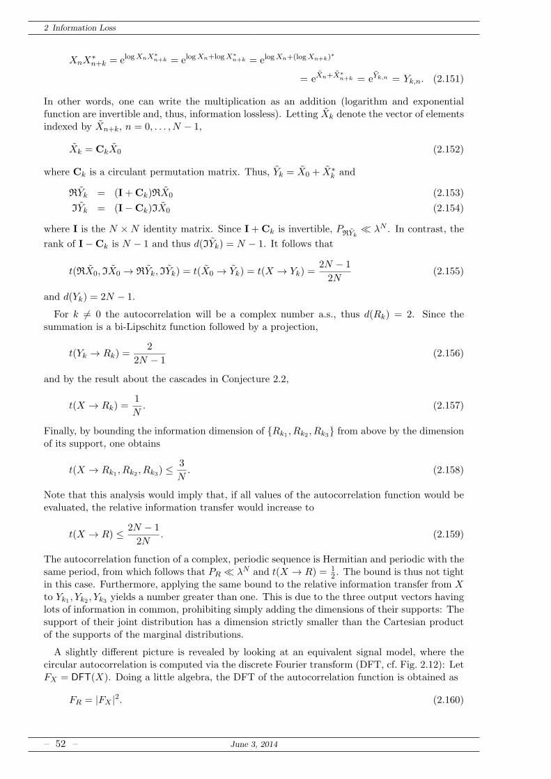
2 Information Loss
XnX∗n+k = elogXnX∗
n+k = elogXn+logX∗n+k = elogXn+(logXn+k)
∗
= eXn+X∗n+k = eYk,n = Yk,n. (2.151)
In other words, one can write the multiplication as an addition (logarithm and exponentialfunction are invertible and, thus, information lossless). Letting Xk denote the vector of elementsindexed by Xn+k, n = 0, . . . , N − 1,
Xk = CkX0 (2.152)
where Ck is a circulant permutation matrix. Thus, Yk = X0 + X∗k and
RYk = (I+Ck)RX0 (2.153)
IYk = (I−Ck)IX0 (2.154)
where I is the N ×N identity matrix. Since I+Ck is invertible, PRYk≪ λN . In contrast, the
rank of I−Ck is N − 1 and thus d(IYk) = N − 1. It follows that
t(RX0, IX0 → RYk, IYk) = t(X0 → Yk) = t(X → Yk) =2N − 1
2N(2.155)
and d(Yk) = 2N − 1.
For k 6= 0 the autocorrelation will be a complex number a.s., thus d(Rk) = 2. Since thesummation is a bi-Lipschitz function followed by a projection,
t(Yk → Rk) =2
2N − 1(2.156)
and by the result about the cascades in Conjecture 2.2,
t(X → Rk) =1
N. (2.157)
Finally, by bounding the information dimension of Rk1 , Rk2 , Rk3 from above by the dimensionof its support, one obtains
t(X → Rk1 , Rk2 , Rk3) ≤3
N. (2.158)
Note that this analysis would imply that, if all values of the autocorrelation function would beevaluated, the relative information transfer would increase to
t(X → R) ≤ 2N − 1
2N. (2.159)
The autocorrelation function of a complex, periodic sequence is Hermitian and periodic with thesame period, from which follows that PR ≪ λN and t(X → R) = 1
2 . The bound is thus not tightin this case. Furthermore, applying the same bound to the relative information transfer from Xto Yk1 , Yk2 , Yk3 yields a number greater than one. This is due to the three output vectors havinglots of information in common, prohibiting simply adding the dimensions of their supports: Thesupport of their joint distribution has a dimension strictly smaller than the Cartesian productof the supports of the marginal distributions.
A slightly different picture is revealed by looking at an equivalent signal model, where thecircular autocorrelation is computed via the discrete Fourier transform (DFT, cf. Fig. 2.12): LetFX = DFT(X). Doing a little algebra, the DFT of the autocorrelation function is obtained as
FR = |FX |2. (2.160)
– 52 – June 3, 2014
2.6 Application: Principal Components Analysis
X DFT | · |2 IDFT Π
Rk1
Rk2
Rk3
FX FR R
L(X → FX) = 0 L(FR → R) = 0
t(FX → FR) =12
t(R → Rk1 , Rk2 , Rk3) ≤ 6N
Figure 2.12: Equivalent model of the MC-AcR of Fig. 2.10, using the DFT to compute the circular auto-correlation. IDFT denotes the inverse DFT and Π a projection onto a subset of coordinates.The information flow is indicated by red arrows labeled according to the relative informationtransfer.
Since the DFT is an invertible transform, one has d(FX) = d(X) = 2N . The squaring ofthe magnitude can be written as a cascade of a coordinate transform (from Cartesian to polarcoordinates; invertible), a dimensionality reduction (the phase information is dropped), and asquaring function (invertible, since the magnitude is a non-negative quantity). It follows that
l(X → R) = l(FX → FR) =1
2. (2.161)
since the inverse DFT is again invertible.
Since FR is a real RV and thus PFR≪ λN , it follows that also PR ≪ λN , despite the fact that
R is a vector of N complex numbers. The probability measure of this RV is concentrated on anN -dimensional submanifold of R2N defined by the periodicity and Hermitian symmetry of R.Choosing three coordinates of R as the final output of the system amounts to upper boundingthe information dimension of the output by
d(Rk1 , Rk2 , Rk3) ≤ 6. (2.162)
Thus,
t(X → Rk1 , Rk2 , Rk3) ≤3
N(2.163)
where equality is achieved if, e.g., all time lags are distinct and smaller than N2 . The information
flow for this example – computed from the relative information loss and information transfer –is depicted in Figs. 2.10 and 2.12.
2.6 Application: Principal Components Analysis
As another illustration for the results about the relative information loss in systems whichreduce the dimensionality of the data, this section investigates the information loss in principalcomponents analysis (PCA). In particular, it will be shown that – without any specific signalmodel in mind – PCA is not a transform which minimizes the information loss occurring insubsequent dimensionality reduction (although this statement can be qualified by assuming asignal model, as in Section 4.4). Furthermore, in case of PCA based on data samples, informationis lost even without deliberately reducing the dimensionality of the data.
June 3, 2014 – 53 –
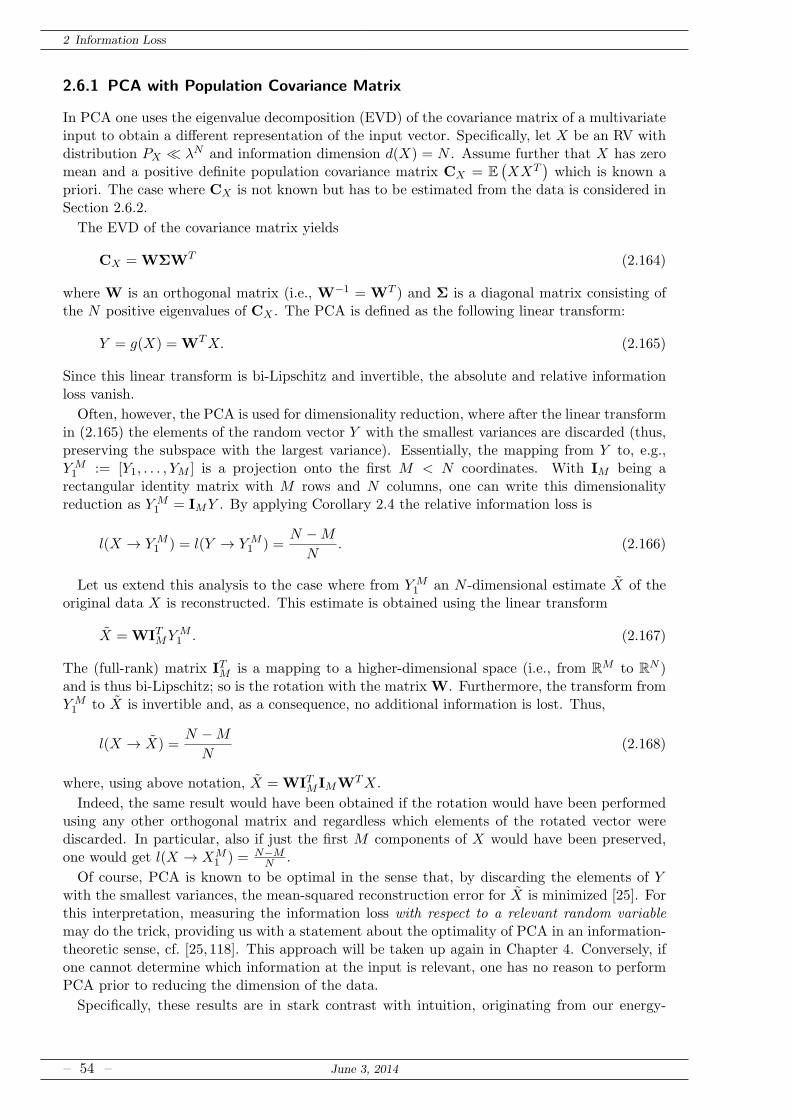
2 Information Loss
2.6.1 PCA with Population Covariance Matrix
In PCA one uses the eigenvalue decomposition (EVD) of the covariance matrix of a multivariateinput to obtain a different representation of the input vector. Specifically, let X be an RV withdistribution PX ≪ λN and information dimension d(X) = N . Assume further that X has zeromean and a positive definite population covariance matrix CX = E
(XXT
)which is known a
priori. The case where CX is not known but has to be estimated from the data is considered inSection 2.6.2.
The EVD of the covariance matrix yields
CX = WΣWT (2.164)
where W is an orthogonal matrix (i.e., W−1 = WT ) and Σ is a diagonal matrix consisting ofthe N positive eigenvalues of CX . The PCA is defined as the following linear transform:
Y = g(X) = WTX. (2.165)
Since this linear transform is bi-Lipschitz and invertible, the absolute and relative informationloss vanish.
Often, however, the PCA is used for dimensionality reduction, where after the linear transformin (2.165) the elements of the random vector Y with the smallest variances are discarded (thus,preserving the subspace with the largest variance). Essentially, the mapping from Y to, e.g.,Y M1 := [Y1, . . . , YM ] is a projection onto the first M < N coordinates. With IM being a
rectangular identity matrix with M rows and N columns, one can write this dimensionalityreduction as Y M
1 = IMY . By applying Corollary 2.4 the relative information loss is
l(X → Y M1 ) = l(Y → Y M
1 ) =N −M
N. (2.166)
Let us extend this analysis to the case where from Y M1 an N -dimensional estimate X of the
original data X is reconstructed. This estimate is obtained using the linear transform
X = WITMY M1 . (2.167)
The (full-rank) matrix ITM is a mapping to a higher-dimensional space (i.e., from RM to RN )and is thus bi-Lipschitz; so is the rotation with the matrix W. Furthermore, the transform fromY M1 to X is invertible and, as a consequence, no additional information is lost. Thus,
l(X → X) =N −M
N(2.168)
where, using above notation, X = WITMIMWTX.
Indeed, the same result would have been obtained if the rotation would have been performedusing any other orthogonal matrix and regardless which elements of the rotated vector werediscarded. In particular, also if just the first M components of X would have been preserved,one would get l(X → XM
1 ) = N−MN .
Of course, PCA is known to be optimal in the sense that, by discarding the elements of Ywith the smallest variances, the mean-squared reconstruction error for X is minimized [25]. Forthis interpretation, measuring the information loss with respect to a relevant random variablemay do the trick, providing us with a statement about the optimality of PCA in an information-theoretic sense, cf. [25, 118]. This approach will be taken up again in Chapter 4. Conversely, ifone cannot determine which information at the input is relevant, one has no reason to performPCA prior to reducing the dimension of the data.
Specifically, these results are in stark contrast with intuition, originating from our energy-
– 54 – June 3, 2014
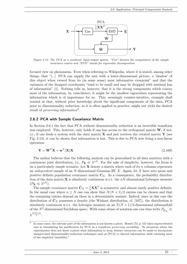
2.6 Application: Principal Components Analysis
X Σ
Y
b Cov EVD
W
1nXXT
W
PCA
Figure 2.13: The PCA as a nonlinear input-output system. “Cov” denotes the computation of the samplecovariance matrix and “EVD” stands for eigenvalue decomposition.
focused view on phenomena. Even when referring to Wikipedia, where it is stated, among otherthings, that “[...] PCA can supply the user with a lower-dimensional picture, a ’shadow’ ofthis object when viewed from its (in some sense) most informative viewpoint” and that thevariances of the dropped coordinates “tend to be small and may be dropped with minimal lossof information” [1]. Nothing tells us, however, that it is the strong components which conveymost of the information; by coincidence, it might be the smallest eigenvalues representing theinformation which is of importance for us. This, seemingly counter-intuitive, example shallremind us that, without prior knowledge about the significant components of the data, PCAprior to dimensionality reduction, as it is often applied in practice, might not yield the desiredresult of preserving information9.
2.6.2 PCA with Sample Covariance Matrix
In Section 2.6.1 the fact that PCA without dimensionality reduction is an invertible transformwas employed. This, however, only holds if one has access to the orthogonal matrix W; if not,i.e., if one feeds a system with the data matrix X and just receives the rotated matrix Y (seeFig. 2.13), it can be shown that information is lost. This is due to PCA now being a non-linearoperation:
Y = WTX = wT (X)X (2.169)
The author believes that the following analysis can be generalized to all data matrices with acontinuous joint distribution, i.e., PX ≪ λnN . For the sake of simplicity, however, the focus ison a particularly simple scenario: Let X denote a matrix where each of its n columns representsan independent sample of an N -dimensional Gaussian RV X. Again, let X have zero mean andpositive definite population covariance matrix CX . As a consequence, the probability distribu-tion of the data matrix X is absolutely continuous w.r.t. the nN -dimensional Lebesgue measure(PX ≪ λnN ).The sample covariance matrix CX = 1
nXXT is symmetric and almost surely positive definite.In the usual case where n ≥ N one can show that N(N + 1)/2 entries can be chosen and thatthe remaining entries depend on these in a deterministic manner. Indeed, since in this case thedistribution of CX possesses a density (the Wishart distribution, cf. [107]), the distribution isabsolutely continuous w.r.t. the Lebesgue measure on an N(N + 1)/2-dimensional submanifoldof the N2-dimensional Euclidean space. With some abuse of notation one can thus write P
CX≪
λN(N+1)
2 .
9 In some cases, the relevant part of the information is not known a priori. Henter [72, p. 54] takes unprecedentedcare in formulating his justification for PCA as a transform preserving variability : “In situations where theexperimenter does not know a-priori what information to keep, feature extractors can be made to incorporateunsupervised dimensionality-reduction techniques such as [PCA] to discard information while retaining mostof the empirical variability.”
June 3, 2014 – 55 –
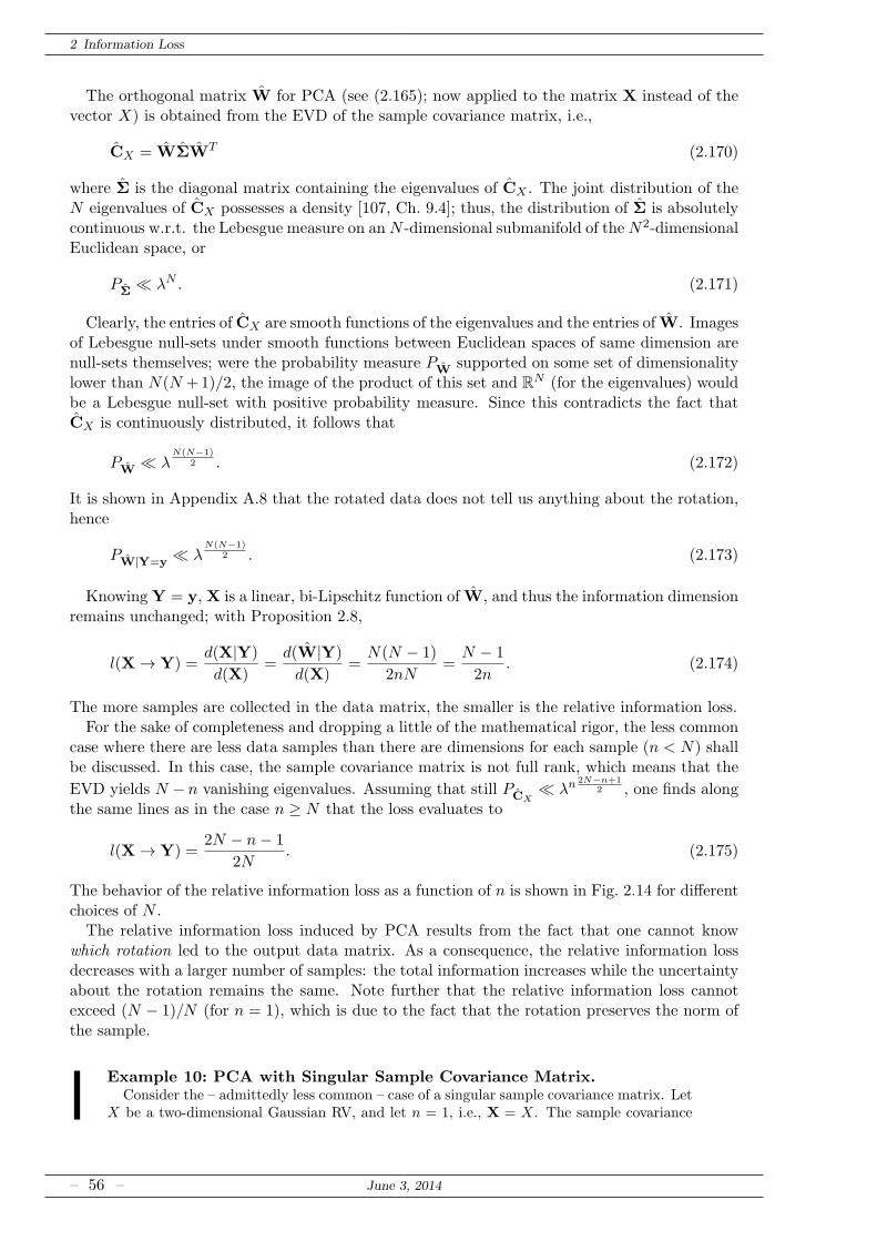
2 Information Loss
The orthogonal matrix W for PCA (see (2.165); now applied to the matrix X instead of thevector X) is obtained from the EVD of the sample covariance matrix, i.e.,
CX = WΣWT (2.170)
where Σ is the diagonal matrix containing the eigenvalues of CX . The joint distribution of theN eigenvalues of CX possesses a density [107, Ch. 9.4]; thus, the distribution of Σ is absolutelycontinuous w.r.t. the Lebesgue measure on anN -dimensional submanifold of theN2-dimensionalEuclidean space, or
PΣ≪ λN . (2.171)
Clearly, the entries of CX are smooth functions of the eigenvalues and the entries of W. Imagesof Lebesgue null-sets under smooth functions between Euclidean spaces of same dimension arenull-sets themselves; were the probability measure P
Wsupported on some set of dimensionality
lower than N(N +1)/2, the image of the product of this set and RN (for the eigenvalues) wouldbe a Lebesgue null-set with positive probability measure. Since this contradicts the fact thatCX is continuously distributed, it follows that
PW≪ λ
N(N−1)2 . (2.172)
It is shown in Appendix A.8 that the rotated data does not tell us anything about the rotation,hence
PW|Y=y
≪ λN(N−1)
2 . (2.173)
KnowingY = y, X is a linear, bi-Lipschitz function of W, and thus the information dimensionremains unchanged; with Proposition 2.8,
l(X→ Y) =d(X|Y)
d(X)=
d(W|Y)
d(X)=
N(N − 1)
2nN=
N − 1
2n. (2.174)
The more samples are collected in the data matrix, the smaller is the relative information loss.For the sake of completeness and dropping a little of the mathematical rigor, the less common
case where there are less data samples than there are dimensions for each sample (n < N) shallbe discussed. In this case, the sample covariance matrix is not full rank, which means that the
EVD yields N − n vanishing eigenvalues. Assuming that still PCX≪ λn 2N−n+1
2 , one finds alongthe same lines as in the case n ≥ N that the loss evaluates to
l(X→ Y) =2N − n− 1
2N. (2.175)
The behavior of the relative information loss as a function of n is shown in Fig. 2.14 for differentchoices of N .The relative information loss induced by PCA results from the fact that one cannot know
which rotation led to the output data matrix. As a consequence, the relative information lossdecreases with a larger number of samples: the total information increases while the uncertaintyabout the rotation remains the same. Note further that the relative information loss cannotexceed (N − 1)/N (for n = 1), which is due to the fact that the rotation preserves the norm ofthe sample.
Example 10: PCA with Singular Sample Covariance Matrix.Consider the – admittedly less common – case of a singular sample covariance matrix. Let
X be a two-dimensional Gaussian RV, and let n = 1, i.e., X = X. The sample covariance
– 56 – June 3, 2014
2.6 Application: Principal Components Analysis
n
l(X→ Y)
1
5 10 20
Figure 2.14: Relative information loss in the PCA with sample covariance matrix as a function of the numbern of independent measurements. The cases N = 5 (black), N = 10 (red), and N = 20 (blue) areshown. The dashed lines indicate the conjectured loss for singular sample covariance matrices.
matrix is given by
CX =
[
X21 X1X2
X1X2 X22
]
(2.176)
and has eigenvalues |X|2 and 0. The corresponding (normalized) eigenvectors are then givenby
p1 =
[X1
|X| ,X2
|X|
]T
(2.177)
and
p2 =
[
−X2
|X| ,X1
|X|
]T
. (2.178)
Performing the rotation Y = WTX with W = [p1, p2] one obtains
Y = [|X|, 0]T . (2.179)
The fact that the second component of Y is zero regardless of the entries of X makes it
obvious that exactly one half of the information is lost, i.e., l(X → Y ) = 12 .
The PCA with sample covariance matrix also allows different interpretations of informationloss, in addition to the information lost in the rotation: First, by the fact that the sample covari-ance matrix of Y is a diagonal matrix, the possible values of Y are restricted to a submanifold ofdimensionality smaller than nN . Naturally, this also restricts the amount of information whichcan be conveyed in the output. In contrary to this, in PCA using the population covariancematrix the sample covariance matrix of Y (almost surely) does not contain zeros, so the entriesof Y will not be restricted deterministically.
Finally, it is interesting to observe that in this case the absolute information loss in the PCAis infinite (see Proposition 2.9), even if no additional dimensionality reduction is performed.Moreover, this analysis not only holds for the PCA, but for any rotation which depends on theinput data in a similar manner – in this sense, the PCA is not better than any other rotation.In fact, there is no rotation to be preferred, because doing nothing at least does not destroyvaluable information. In practice, however, this advice is often ignored: In many cases, datais analyzed by performing PCA to see how the principal components behave. In the particularcase where the rotation itself is the data relevant to the recipient, such an approach is fatal.
June 3, 2014 – 57 –
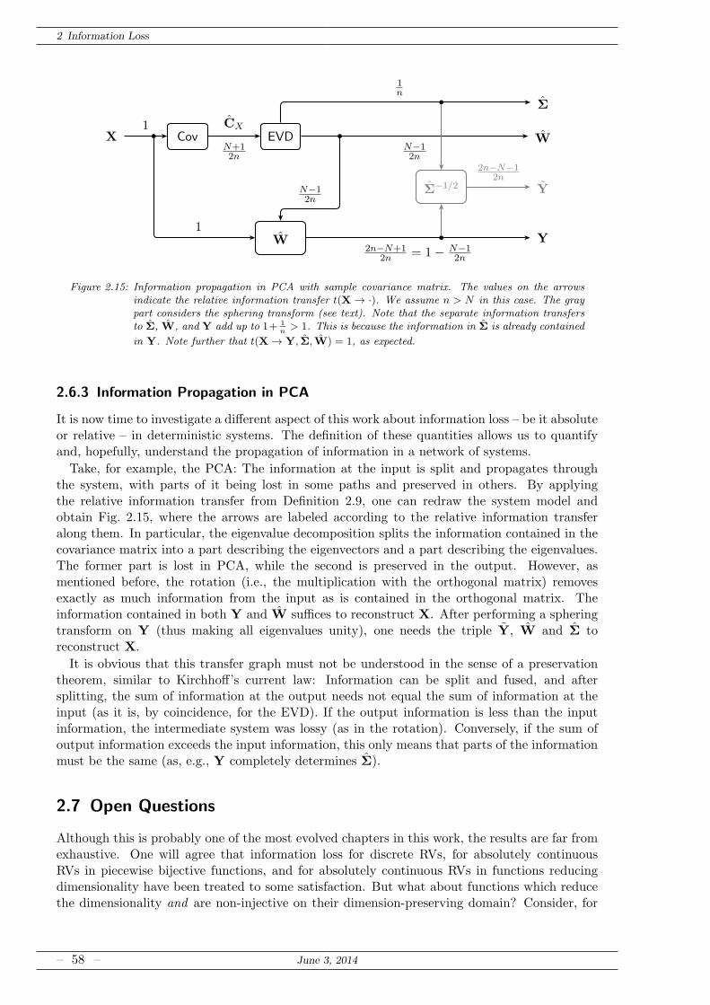
2 Information Loss
X W
Σ
Y
b Cov EVD
W
b
b
b
1
N+12n
CX
N−12n
2n−N+12n = 1− N−1
2n
1
1n
N−12n
YΣ−1/2
2n−N−12n
Figure 2.15: Information propagation in PCA with sample covariance matrix. The values on the arrowsindicate the relative information transfer t(X → ·). We assume n > N in this case. The graypart considers the sphering transform (see text). Note that the separate information transfersto Σ, W, and Y add up to 1+ 1
n> 1. This is because the information in Σ is already contained
in Y. Note further that t(X → Y, Σ,W) = 1, as expected.
2.6.3 Information Propagation in PCA
It is now time to investigate a different aspect of this work about information loss – be it absoluteor relative – in deterministic systems. The definition of these quantities allows us to quantifyand, hopefully, understand the propagation of information in a network of systems.
Take, for example, the PCA: The information at the input is split and propagates throughthe system, with parts of it being lost in some paths and preserved in others. By applyingthe relative information transfer from Definition 2.9, one can redraw the system model andobtain Fig. 2.15, where the arrows are labeled according to the relative information transferalong them. In particular, the eigenvalue decomposition splits the information contained in thecovariance matrix into a part describing the eigenvectors and a part describing the eigenvalues.The former part is lost in PCA, while the second is preserved in the output. However, asmentioned before, the rotation (i.e., the multiplication with the orthogonal matrix) removesexactly as much information from the input as is contained in the orthogonal matrix. Theinformation contained in both Y and W suffices to reconstruct X. After performing a spheringtransform on Y (thus making all eigenvalues unity), one needs the triple Y, W and Σ toreconstruct X.
It is obvious that this transfer graph must not be understood in the sense of a preservationtheorem, similar to Kirchhoff’s current law: Information can be split and fused, and aftersplitting, the sum of information at the output needs not equal the sum of information at theinput (as it is, by coincidence, for the EVD). If the output information is less than the inputinformation, the intermediate system was lossy (as in the rotation). Conversely, if the sum ofoutput information exceeds the input information, this only means that parts of the informationmust be the same (as, e.g., Y completely determines Σ).
2.7 Open Questions
Although this is probably one of the most evolved chapters in this work, the results are far fromexhaustive. One will agree that information loss for discrete RVs, for absolutely continuousRVs in piecewise bijective functions, and for absolutely continuous RVs in functions reducingdimensionality have been treated to some satisfaction. But what about functions which reducethe dimensionality and are non-injective on their dimension-preserving domain? Consider, for
– 58 – June 3, 2014
2.7 Open Questions
example, a symmetrized version of the center clipper (cf. Example 7): Is the statement “Thesystem destroys 25% of the information plus one bit” satisfactory?One of the most pressing needs is, of course, a proof of Conjecture 2.1 and its corollaries.
That such a proof exists is strongly suggested by intuition.Furthermore, the case where the input probability measure is neither discrete nor absolutely
continuous has been treated only marginally. Not only input measures supported on a lower-dimensional manifold of the domain (e.g., on a line in R2), but also fractal input measures, likethe Cantor measure, would be interesting to investigate – both for piecewise bijective functionsand for systems reducing dimensionality.While information loss was given an operational meaning by its connection to the reconstruc-
tion error, the operational meaning of relative information loss is not as clear. A connection tothe reconstruction error was found in Section 2.4.4, but the problem of reconstruction and – inparticular – the definition of a reconstruction error, seems ill-posed.Whether the information measures proposed in this work suffice to develop a theory of in-
formation propagation in deterministic systems remains an open question. “Information flowgraphs” or “information link budgets” may be the results; a hint in this direction was given inSection 2.6, where the PCA was analyzed.Also interesting, but probably not at the core of information or systems theory, is the question
whether relative information loss can be given an interpretation in thermodynamics, similar toabsolute information loss – Landauer’s principle shall be named here. Speaking about Landauer’sprinciple, it is worth investigating where exactly, in, e.g., a rectifier, the one bit of informationloss is converted to thermodynamical entropy – or if this principle applies at all. Closely related isalso the connection between information loss and the Kolmogorov-Sinaı entropy rate in iteratedfunction systems: Also this connection has not been investigated to its full extent, at least inthe opinion of the author.
June 3, 2014 – 59 –

Information Loss in Deterministic Systems
3Information Loss Rate
The signal model and the mathematical preliminaries, the style of which is strongly influencedby Tatjana Petrov, were taken from [47] unless noted otherwise. The results of Section 3.2were obtained in collaboration with Christoph Temmel, and partly published in [48, 58]; a partof its introduction is taken from a joint work with Tatjana Petrov, Heinz Koppl, and GernotKubin [47], cf. Section 4.3. Christoph Temmel devised the characterization for the lossless caseand the current proof idea is due to him; the sufficient criteria for lumpability and losslesscompression are due to the present author. In both cases, the results were obtained jointly. Theresults of Section 3.2.6 are mainly due to the present author, while the idea to use the adjacencymatrix of a graph for the characterization was again from Christoph Temmel. Sections 3.3and 3.4 have been derived by the present author, thanks to suggestions from Gernot Kubin;they have been published on arXiv [54]. The contents of Section 3.5 constitute part of [56]and [53]. Finally, [50] comprises Section 3.6, where again Gernot Kubin made many suggestions(to investigate finite-precision effects in digital filters).
3.1 What Is Information Loss for Stochastic Processes? – The
Discrete Case
In extending information loss from random variables to stochastic processes, it is instructiveto take up the water analogy from Section 2.1; indeed, the analogy is even more appropriatehere. Observing the flow of the liquid (the stochastic process) through the pipes (the system),one can measure the amount of liquid lost per time unit. Depending on the flow rate (theprocess’ entropy rate) and the viscosity of the liquid (the process’ correlation or redundancy),the corrosion of the pipes will lead to a larger or smaller loss. As the loss rate of the liquid isjust the difference between the flow rates at the input and the output of the pipe system, theinformation loss rate shall be defined likewise: as the difference between the information ratesat the input and the output of the system under consideration.
This shall be made precise now. A discrete-time, one-sided random process X is a sequenceof RVs X0, X1, X2, . . . defined on a common probability space. Each RV Xi shall take valuesfrom the same finite alphabet X .For a finite index set I ⊂ N0, the joint PMF of XI = Xii∈I is
∀zI ∈ X card(I): pXI(zI) := Pr(Xi = xi, i ∈ I). (3.1)
June 3, 2014 – 61 –
3 Information Loss Rate
In particular, for I = m,m+ 1, . . . , n, XI is abbreviated by Xnm := Xm, Xm+1, . . . , Xn and
pXnm(znm) := Pr(Xm = zm, . . . , Xn = zn). (3.2)
Along the same lines one obtains the marginal PMF pXn of Xn and the conditional PMFpXn|Xn−1
1of Xn given its past, Xn−1
1 , where the latter is assumed to be well-defined (i.e., the
conditioning event has positive probability).The random processes considered in this work are stationary, i.e., for an arbitrary, finite I the
corresponding joint PMF is shift-invariant,
∀k ∈ N0: pXI= pXI+k
. (3.3)
In particular, stationarity implies that the marginal distribution of Xk is equal for all k and shallbe denoted as pX . For simplicity, whenever a quantity depends only on the marginal distributionof the process, it shall be given as a function of an RV X with PMF pX . In particular, due tostationarity,
∀k ∈ N0: H(Xk) = H(X). (3.4)
The information conveyed by a stationary, stochastic process per time unit is measured by itsentropy rate [21, Thm. 4.2.1]
H (X) := limn→∞
1
nH(Xn
1 ) = limn→∞
H(Xn|Xn−11 ). (3.5)
By the fact that conditioning reduces entropy, one always has H (X) ≤ H(X), with equality ifX is a sequence of independent, identically distributed (iid) RVs. The difference between thesetwo quantities leads to the definition of redundancy:
Definition 3.1 (Redundancy Rate). The redundancy rate of a stationary stochastic process Xis
R(X) := H(X)−H (X). (3.6)
The redundancy rate is a measure of statistical dependence between the current sample and itspast: For an iid processH (X) = H(X) and R(X) = 0. Conversely, for a completely predictableprocess H (X) = 0 and R(X) = H(X). In other words, the higher the redundancy rate, thelower the entropy rate and, thus, the less information is conveyed by the process in each timestep.Let X be the stochastic process at the input of a system described by a measurable function
g: X → Y. The output of the system is again a stochastic process Y, whose n-th sample isYn := g(Xn). From stationarity of X it follows that Y is stationary (and jointly stationary withX). The information Y conveys in each time unit is measured by its entropy rate H (Y).These preliminaries admit a definition of the information lost per time unit for discrete-time,
discrete-valued stationary stochastic processes:
Definition 3.2 (Information Loss Rate, [161]). Let X be a stationary stochastic process withfinite alphabet X , and let Y be defined via Yn := g(Xn). The information loss induced by g ineach time unit is
L(X→ Y) := limn→∞
1
nL(Xn
1 → Y n1 ) =H (X)−H (Y). (3.7)
For the last equality, combine Definition 2.1 with the definition of entropy rate given in (3.5).Before proceeding, it is worth mentioning that this quantity was defined by Watanabe andAbraham in [161], albeit using non-standard notation. That above difference is non-negative
– 62 – June 3, 2014
3.2 Information Loss Rate for Markov Chains
was observed by Pinsker (cf. [116, eq. (6.3.4)]), thus establishing a data processing inequalityfor stochastic processes. Another interesting result from [161] shall be reproduced here:
Lemma 3.1 (Upper Bound on the Information Loss Rate [161, Thm. 3]). The information lossrate is bounded from above by the information loss, i.e.,
L(X→ Y) ≤ L(X → Y ) (3.8)
where X is distributed according to the marginal distribution of X.
Proof. The proof follows from the chain rule of entropy, conditioning, and stationarity:
L(X→ Y) = limn→∞
1
n(H(Xn
1 )−H(Y n1 )) (3.9)
= limn→∞
1
nH(Xn
1 |Y n1 ) (3.10)
= limn→∞
1
n
n∑
i=1
H(Xi|Xi−11 , Y n
1 ) (3.11)
≤ limn→∞
1
n
n∑
i=1
H(Xi|Yi) (3.12)
= L(X → Y ) (3.13)
It seems as if redundancy in the process can help prevent information from being lost, com-pared to the case where the process has no redundancy. This is intuitive, since part of theinformation is stored in the temporal structure of the process. However, one should not con-clude that a process with a higher redundancy rate suffers from less information loss than aprocess with a lower redundancy rate: The redundancy has to be matched to the function inorder to be effective. This parallels coding theory, where the code has to be matched to thechannel in order to reduce the bit error rate. Example 18 shows that a process with higherredundancy can suffer from higher information loss; since the considered processes are Markovchains, the example is deferred to the end of Section 3.2.4.
3.2 Information Loss Rate for Markov Chains
This section starts with a particularly simple class of stochastic processes: Markov chains.Markov models are ubiquitous in scientific and engineering disciplines, for example, to under-stand chemical reaction systems, to perfprm speech recognition and to model data sources, orin Markov decision processes in automated control. The popularity of these models arises be-cause the Markov property often renders model analysis tractable and their simulation efficient.However, the state space of a Markov model (i.e., its alphabet) is sometimes too large to permitsimulation, even when harnessing today’s computing power. Indeed, in stochastic modeling incomputational biology [165], or in n-gram word models in speech recognition [102], dealing withthe state space explosion is a major challenge. Also in control theory, particularly for nearlycompletely decomposable Markov chains, state space reduction is an important topic [5, 27].Feeding the Markov chain through a function will be called a lumping here, referring to the fact
that the non-injective function g lumps together states of the chain’s transition graph. Assumingstationarity, the resulting (stationary) lumped stochastic process is also called a functional hiddenMarkov model [33]. One can transform an arbitrary hidden Markov model on finite state andobservation spaces into this setting [33, Section IV.E]. In general, the lumped process loses theMarkov property [68, 87] and has a lower entropy rate than the original Markov chain due tothe aggregation of states [116,161].
June 3, 2014 – 63 –
3 Information Loss Rate
The present section investigates the structure of information-preserving lumpings of stationaryMarkov chains over a finite state space. The central result characterizes information preservationin two ways. First, by a structural property of the transition graph associated with the Markovchain. Second, by the growth of the cardinality of the realizable preimage of a realization ofthe lumped process. This analysis reveals a strong dichotomy between the preservation and losscase: In the former, the information loss of sequences of arbitrary length is finitely bounded, andthe cardinality of the realizable preimage has finite growth a.s. In the latter, the informationloss grows linearly in the sequence length and the cardinality of the realizable preimage growsexponentially a.s.In particular, a positive transition matrix always implies information loss for a non-trivial
lumping. For Markov chains with non-positive transition matrices, a sufficient condition for alumping to preserve information is presented. Carlyle [16] investigated the representation of afinite-state stationary stochastic process as a lumping of a Markov chain on an at most countablestate space; his representation fulfills the sufficient condition for information preservation.Preserving the Markov property during lumping is highly desirable from a simulation point-
of-view. It is shown that lumpings resulting in higher-order Markov chains are characterized byequality in natural entropic bounds on the entropy rate of the lumped process. The equalityholding only for entropies depending on the lumped process is equivalent to weak lumpability,i.e., the lumped process is a higher-order Markov chain in the stationary setting. A secondequality involving also entropies using the underlying Markov chain in the stationary case isequivalent to strong lumpability, i.e., the lumped process is a higher-order Markov chain for everyinitial distribution. This characterization is an information-theoretic complement to Gurvits &Ledoux’s [68] linear algebraic approach to characterize lumpability.Finally, a sufficient condition on a lumping of a Markov chain to preserve the entropy rate
and be strongly k-lumpable is given. The condition is fulfilled on non-trivial lower-dimensionalsubspaces of the space of transition matrices10. The latter condition will be employed for losslesscompression of letter n-gram models in Section 3.2.6.A different notion of information loss is worth mentioning, namely the loss of information
about the initial state X0 (or its distribution) occuring over time. Lindqvist quantified theamount of information about X0 contained in the observation of Xn without using information-theoretic methods in [98]. If instead of Xn only a function Yn := g(Xn) is observed, theinformation about X0 is decreased further (although in some cases this additional loss decreasesas a function of n) [99]. In case the distribution of X0 can be inferred by the joint distribution ofY0, Y1, Y2, . . . , the lumping is called g-observable (see [68, Section 3] and the references therein).However, neither g-observability nor Lindqvist’s results appear to have a direct correspondencein this work.
3.2.1 Preliminaries
Let X be an irreducible, aperiodic, time-homogeneous Markov chain on the finite state space X .It has transition matrix P = Pij with an invariant probability vector µ satisfying µT = µTP.Assume that X is stationary, i.e., X0 ∼ µ. The function g shall in this section be called thelumping function; it is non-trivial, i.e., 2 ≤ card(Y) < card(X ). Without loss of generality,the function g is extended to X n → Yn coordinate-wise, for arbitrary n ∈ N. The stationarystochastic process Y defined by Yn := g(Xn) shall be called the lumped process, and the totalsetup is referred to as the lumping (P, g).The lumping of course induces an information loss rate L(X→ Y). The main question is
whetherL(X→ Y) is positive or zero (speaking of information loss or information preservation,respectively). Note that information preservation does not imply that the original process canbe reconstructed from the lumped process (see Example 13).
10 This does not conflict with Gurvits & Ledoux’s [68] result that lumpings having higher-order Markov behaviorare nowhere dense.
– 64 – June 3, 2014
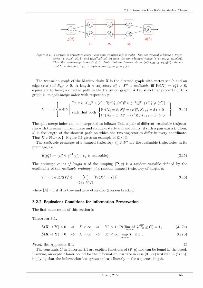
3.2 Information Loss Rate for Markov Chains
x
x′1
x′′1
x′2
x′′2
x′3
x′′3
x
y1 y2 y3
g(x) g(x)
Figure 3.1: A section of trajectory space, with time running left-to-right. The two realizable length-5 trajec-tories (x, x′
1, x′2, x
′3, x) and (x, x′′
1 , x′′2 , x
′′3 , x) have the same lumped image (g(x), y1, y2, y3, g(x)).
Thus the split-merge index K ≤ 3. Note that the lumped states g(x), y1, y2, y3, g(x) do notneed to be distinct; e.g., it might be that y1 = y2 = g(x).
The transition graph of the Markov chain X is the directed graph with vertex set X and anedge (x, x′) iff Pxx′ > 0. A length n trajectory xn1 ∈ X n is realizable, iff Pr(Xn
1 = xn1 ) > 0,equivalent to being a directed path in the transition graph. A key structural property of thisgraph is its split-merge index with respect to g:
K := inf
n ∈ N
∣∣∣∣∣
∃x, x ∈ X , yn1 ∈ Yn : ∃(x′)n1 , (x′′)n1 ∈ g−1[yn1 ], (x′′)n1 6= (x′)n1 :
such that both
Pr(X0 = x, Xn1 = (x′)n1 , Xn+1 = x) > 0
Pr(X0 = x, Xn1 = (x′′)n1 , Xn+1 = x) > 0
. (3.14)
The split-merge index can be interpreted as follows: Take a pair of different, realizable trajecto-ries with the same lumped image and common start- and endpoints (if such a pair exists). Then,K is the length of the shortest path on which the two trajectories differ in every coordinate.Thus K ∈ N ∪ ∞. Figure 3.1 gives an example of K ≤ 3.
The realizable preimage of a lumped trajectory yn1 ∈ Yn are the realizable trajectories in itspreimage, i.e.
R(yn1 ) := xn1 ∈ g−1[yn1 ] : xn1 is realizable . (3.15)
The preimage count of length n of the lumping (P, g) is a random variable defined by thecardinality of the realizable preimage of a random lumped trajectory of length n:
Tn := card(R(Y n1 )) =
∑
xn1∈g−1[Y n
1 ]
⌈Pr(Xn1 = xn1 )⌉ , (3.16)
where [A] = 1 if A is true and zero otherwise (Iverson bracket).
3.2.2 Equivalent Conditions for Information-Preservation
The first main result of this section is
Theorem 3.1.
L(X→ Y) > 0 ⇔ K <∞ ⇔ ∃C > 1 : Pr(lim infn→∞
n√
Tn ≥ C) = 1 , (3.17a)
L(X→ Y) = 0 ⇔ K =∞ ⇔ ∃C <∞ : supn→∞
Tn ≤ C . (3.17b)
Proof. See Appendix B.1.
The constants C in Theorem 3.1 are explicit functions of (P, g) and can be found in the proof.Likewise, an explicit lower bound for the information loss rate in case (3.17a) is stated in (B.15),implying that the information loss grows at least linearly in the sequence length.
June 3, 2014 – 65 –
3 Information Loss Rate
Theorem 3.1 reveals a dichotomy in the information-theoretic behavior of the lumping. If Kis infinite, then no split-merge situations as in Figure 3.1 occur. Thus, all finite trajectories ofX can be reconstructed from their lumped image and knowledge of their endpoints. Therefore,the only information loss occurs at those endpoints and is finite. This yields uniform finitebounds on the conditional block entropies, i.e., the information loss, and the preimage count. IfK is finite, then at least two different, realizable length-(K+ 2) trajectories of X with the samelumped image split and merge (see Figure 3.1). Such a split-merge leads to a finite informationloss. The ergodic theorem ensures that this situation occurs linearly often in the block length,thus leading to a linear growth of the information loss. This in turn implies an informationloss rate greater than zero. In particular, the information loss of a lumping can never exhibitsublinear (unbounded) growth.If no split-merge situation occurs, then realisable trajectories with the same lumped image
move in parallel and their number is constrained. This yields a uniform bound on the conditionalblock entropies for lengths smaller than K:Proposition 3.1.
∀n : n− 2 < K ⇒ L(Xn1 → Y n
1 ) ≤ 2 log(card(X )− card(Y) + 1) . (3.18)
Proof. See Appendix B.1.1.An information-preserving lumping of course needs to have an output alphabet sufficiently
large to represent the information of the process. This motivates the necessary condition pre-sented in
Proposition 3.2. An information-preserving lumping (P, g) satisfies
card(Y) ≥ mini
di (3.19)
where di :=∑N
j=1⌈Pij⌉ is the out-degree of state i.
Proof. See Appendix B.2.Since for a positive transition matrix P the out-degree of the associated transition graph is
card(X ) for all states, there is no (non-trivial) lumping which can preserve information:
Corollary 3.1. If P is positive, i.e., all its entries are positive, then L(X→ Y) > 0.
Thus, information preserving lumpings must have sufficiently sparse transition matrices P.Conversely, for a sufficiently sparse transition matrix P one can hope to find a more compactrepresentation of the original Markov chain.
3.2.3 Excursion: k-lumpability of Markov Chains
Functions of Markov chains have been considered in the literature for a long time: Kemeny &Snell [87] coined the term lumpability for retaining the Markov property and presented necessaryand sufficient conditions. Burke and Rosenblatt [15] analyzed the Markovity of a function ofa Markov chain without requiring that the resulting process is a homogeneous Markov chain.They stated that the condition in [87] is sufficient for all stationary, regular Markov chains witharbitrary initial probability, but necessary only for reversible chains with an initial distributionequal to the invariant distribution. Also Rogers and Pitman worked on basic results on lumpa-bility [124]. Higher-order lumpability, as it used in this section, has been analyzed by Gurvitsand Ledoux [68], and they showed that the class of Markov chains being lumpable is nowheredense.Abdel-Moneim and Leysieffer [2] extended the work by Kememy and Snell [87] on weakly
lumpable Markov chains, i.e., where the derived process is Markov only for a specific set ofinitial conditions. Their work was later extended and corrected by Rubino and Sericola [126].
– 66 – June 3, 2014
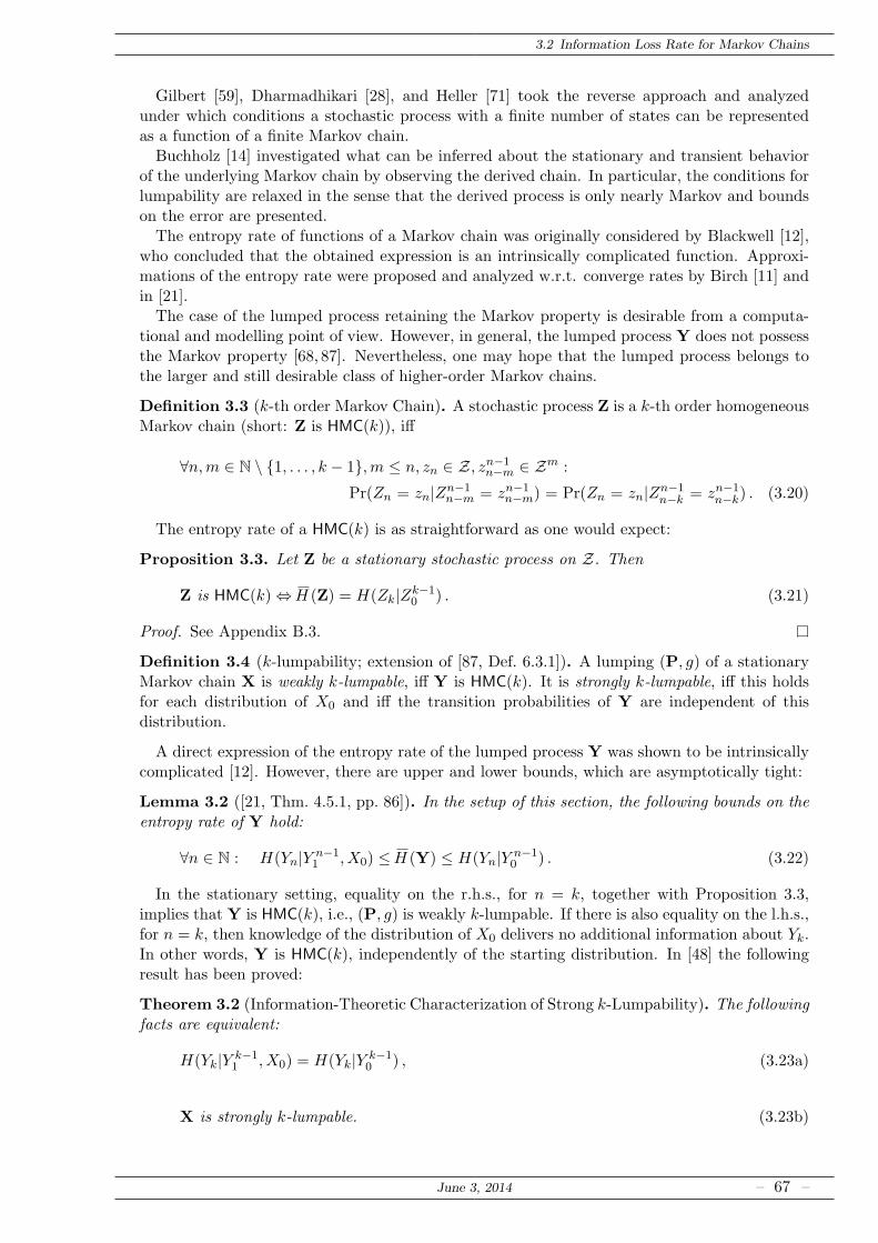
3.2 Information Loss Rate for Markov Chains
Gilbert [59], Dharmadhikari [28], and Heller [71] took the reverse approach and analyzedunder which conditions a stochastic process with a finite number of states can be representedas a function of a finite Markov chain.Buchholz [14] investigated what can be inferred about the stationary and transient behavior
of the underlying Markov chain by observing the derived chain. In particular, the conditions forlumpability are relaxed in the sense that the derived process is only nearly Markov and boundson the error are presented.The entropy rate of functions of a Markov chain was originally considered by Blackwell [12],
who concluded that the obtained expression is an intrinsically complicated function. Approxi-mations of the entropy rate were proposed and analyzed w.r.t. converge rates by Birch [11] andin [21].The case of the lumped process retaining the Markov property is desirable from a computa-
tional and modelling point of view. However, in general, the lumped process Y does not possessthe Markov property [68, 87]. Nevertheless, one may hope that the lumped process belongs tothe larger and still desirable class of higher-order Markov chains.
Definition 3.3 (k-th order Markov Chain). A stochastic process Z is a k-th order homogeneousMarkov chain (short: Z is HMC(k)), iff
∀n,m ∈ N \ 1, . . . , k − 1,m ≤ n, zn ∈ Z, zn−1n−m ∈ Zm :
Pr(Zn = zn|Zn−1n−m = zn−1
n−m) = Pr(Zn = zn|Zn−1n−k = zn−1
n−k) . (3.20)
The entropy rate of a HMC(k) is as straightforward as one would expect:
Proposition 3.3. Let Z be a stationary stochastic process on Z. Then
Z is HMC(k)⇔H (Z) = H(Zk|Zk−10 ) . (3.21)
Proof. See Appendix B.3.
Definition 3.4 (k-lumpability; extension of [87, Def. 6.3.1]). A lumping (P, g) of a stationaryMarkov chain X is weakly k-lumpable, iff Y is HMC(k). It is strongly k-lumpable, iff this holdsfor each distribution of X0 and iff the transition probabilities of Y are independent of thisdistribution.
A direct expression of the entropy rate of the lumped process Y was shown to be intrinsicallycomplicated [12]. However, there are upper and lower bounds, which are asymptotically tight:
Lemma 3.2 ([21, Thm. 4.5.1, pp. 86]). In the setup of this section, the following bounds on theentropy rate of Y hold:
∀n ∈ N : H(Yn|Y n−11 , X0) ≤H (Y) ≤ H(Yn|Y n−1
0 ) . (3.22)
In the stationary setting, equality on the r.h.s., for n = k, together with Proposition 3.3,implies that Y is HMC(k), i.e., (P, g) is weakly k-lumpable. If there is also equality on the l.h.s.,for n = k, then knowledge of the distribution of X0 delivers no additional information about Yk.In other words, Y is HMC(k), independently of the starting distribution. In [48] the followingresult has been proved:
Theorem 3.2 (Information-Theoretic Characterization of Strong k-Lumpability). The followingfacts are equivalent:
H(Yk|Y k−11 , X0) = H(Yk|Y k−1
0 ) , (3.23a)
X is strongly k-lumpable. (3.23b)
June 3, 2014 – 67 –
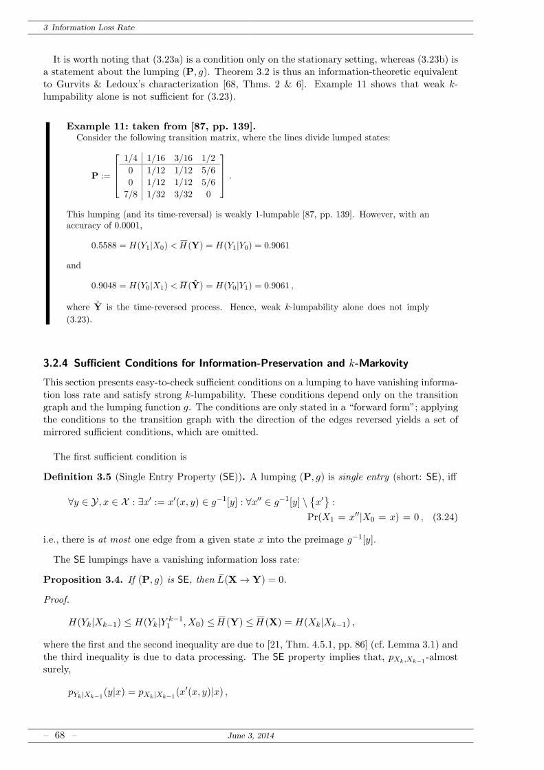
3 Information Loss Rate
It is worth noting that (3.23a) is a condition only on the stationary setting, whereas (3.23b) isa statement about the lumping (P, g). Theorem 3.2 is thus an information-theoretic equivalentto Gurvits & Ledoux’s characterization [68, Thms. 2 & 6]. Example 11 shows that weak k-lumpability alone is not sufficient for (3.23).
Example 11: taken from [87, pp. 139].Consider the following transition matrix, where the lines divide lumped states:
P :=
1/4 1/16 3/16 1/2
0 1/12 1/12 5/6
0 1/12 1/12 5/6
7/8 1/32 3/32 0
.
This lumping (and its time-reversal) is weakly 1-lumpable [87, pp. 139]. However, with anaccuracy of 0.0001,
0.5588 = H(Y1|X0) <H (Y) = H(Y1|Y0) = 0.9061
and
0.9048 = H(Y0|X1) <H (Y) = H(Y0|Y1) = 0.9061 ,
where Y is the time-reversed process. Hence, weak k-lumpability alone does not imply
(3.23).
3.2.4 Sufficient Conditions for Information-Preservation and k-Markovity
This section presents easy-to-check sufficient conditions on a lumping to have vanishing informa-tion loss rate and satisfy strong k-lumpability. These conditions depend only on the transitiongraph and the lumping function g. The conditions are only stated in a “forward form”; applyingthe conditions to the transition graph with the direction of the edges reversed yields a set ofmirrored sufficient conditions, which are omitted.
The first sufficient condition is
Definition 3.5 (Single Entry Property (SE)). A lumping (P, g) is single entry (short: SE), iff
∀y ∈ Y, x ∈ X : ∃x′ := x′(x, y) ∈ g−1[y] : ∀x′′ ∈ g−1[y] \x′:
Pr(X1 = x′′|X0 = x) = 0 , (3.24)
i.e., there is at most one edge from a given state x into the preimage g−1[y].
The SE lumpings have a vanishing information loss rate:
Proposition 3.4. If (P, g) is SE, then L(X→ Y) = 0.
Proof.
H(Yk|Xk−1) ≤ H(Yk|Y k−11 , X0) ≤H (Y) ≤H (X) = H(Xk|Xk−1) ,
where the first and the second inequality are due to [21, Thm. 4.5.1, pp. 86] (cf. Lemma 3.1) andthe third inequality is due to data processing. The SE property implies that, pXk,Xk−1
-almostsurely,
pYk|Xk−1(y|x) = pXk|Xk−1
(x′(x, y)|x) ,
– 68 – June 3, 2014

3.2 Information Loss Rate for Markov Chains
where x′(x, y) is from (3.24). Thus, the outer terms in the above chain of inequalities coincide,yieldingH (Y) =H (X).The following and Example 17 show that SE is not necessary for entropy rate preservation:
Example 12: SE is not necessary for entropy rate preservation.
a
b1
b2
c1
c2
d1
d2
fB D
A F
C1
C2
The transition graph of a Markov chain with the lumping represented by red boxes. The
lumping is neither SE (violated by transitions from a into B) nor its mirror condition for
the time-reversed process (violated by transitions from D to f). On the other hand, the
existence of the uniquely represented states C1 and C2 allows to distinguish between the
trajectories (a, b1, c1, d1, f) and (a, b2, c2, d2, f). Therefore the lumping preserves the entropy
rate. Furthermore, this lumping is weakly 1-lumpable and strongly 2-lumpable. Hence it
shows that SE is neither necessary for entropy rate preservation nor for weak k-lumpability.
This also applies to SFS(k) (see Definition 3.6), which is a subclass of SE.
Corollary 3.2. If (P, g) is SE and weakly k-lumpable, then it is strongly k-lumpable.
Proof. The proof of Proposition 3.4 shows that SE implies equality on the l.h.s. of (3.22), for alln. Weak k-lumpability implies equality on the r.h.s. of (3.22) for n = k. Therefore, Theorem 3.2applies.
There is one interesting result about SE-lumpings, which is similar to the one in Proposi-tion 3.2:
Proposition 3.5. An SE-lumping satisfies
card(Y) ≥ maxi
di (3.25)
where di is the out-degree of state i.
In particular, this implies that a transition matrix with at least one positive row does notadmit an SE-lumping.
Proof. Evaluate the rows of P separately: All states x2 accessible from state x1 are characterizedby Px1,x2 > 0. Any two states accessible from x1 cannot be merged, since this would contradictDefinition 3.5. Thus, all states accessible from x1 must have different images, implying card(Y) ≥dx1 . The result follows by considering all states x1.
Example 13: An SE lumping.
b1
b2
a1
a2
B A
June 3, 2014 – 69 –
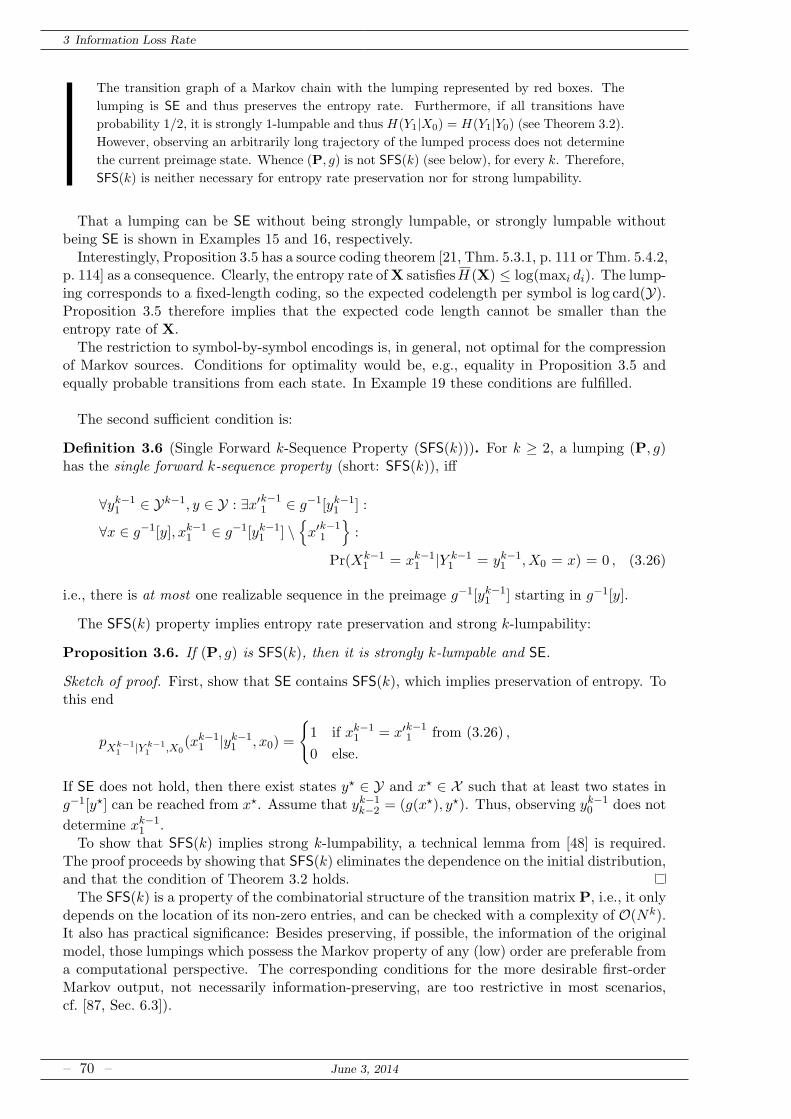
3 Information Loss Rate
The transition graph of a Markov chain with the lumping represented by red boxes. The
lumping is SE and thus preserves the entropy rate. Furthermore, if all transitions have
probability 1/2, it is strongly 1-lumpable and thus H(Y1|X0) = H(Y1|Y0) (see Theorem 3.2).
However, observing an arbitrarily long trajectory of the lumped process does not determine
the current preimage state. Whence (P, g) is not SFS(k) (see below), for every k. Therefore,
SFS(k) is neither necessary for entropy rate preservation nor for strong lumpability.
That a lumping can be SE without being strongly lumpable, or strongly lumpable withoutbeing SE is shown in Examples 15 and 16, respectively.Interestingly, Proposition 3.5 has a source coding theorem [21, Thm. 5.3.1, p. 111 or Thm. 5.4.2,
p. 114] as a consequence. Clearly, the entropy rate ofX satisfiesH (X) ≤ log(maxi di). The lump-ing corresponds to a fixed-length coding, so the expected codelength per symbol is log card(Y).Proposition 3.5 therefore implies that the expected code length cannot be smaller than theentropy rate of X.The restriction to symbol-by-symbol encodings is, in general, not optimal for the compression
of Markov sources. Conditions for optimality would be, e.g., equality in Proposition 3.5 andequally probable transitions from each state. In Example 19 these conditions are fulfilled.
The second sufficient condition is:
Definition 3.6 (Single Forward k-Sequence Property (SFS(k))). For k ≥ 2, a lumping (P, g)has the single forward k-sequence property (short: SFS(k)), iff
∀yk−11 ∈ Yk−1, y ∈ Y : ∃x′k−1
1 ∈ g−1[yk−11 ] :
∀x ∈ g−1[y], xk−11 ∈ g−1[yk−1
1 ] \
x′k−11
:
Pr(Xk−11 = xk−1
1 |Y k−11 = yk−1
1 , X0 = x) = 0 , (3.26)
i.e., there is at most one realizable sequence in the preimage g−1[yk−11 ] starting in g−1[y].
The SFS(k) property implies entropy rate preservation and strong k-lumpability:
Proposition 3.6. If (P, g) is SFS(k), then it is strongly k-lumpable and SE.
Sketch of proof. First, show that SE contains SFS(k), which implies preservation of entropy. Tothis end
pXk−11 |Y k−1
1 ,X0(xk−1
1 |yk−11 , x0) =
1 if xk−11 = x′k−1
1 from (3.26) ,
0 else.
If SE does not hold, then there exist states y⋆ ∈ Y and x⋆ ∈ X such that at least two states ing−1[y⋆] can be reached from x⋆. Assume that yk−1
k−2 = (g(x⋆), y⋆). Thus, observing yk−10 does not
determine xk−11 .
To show that SFS(k) implies strong k-lumpability, a technical lemma from [48] is required.The proof proceeds by showing that SFS(k) eliminates the dependence on the initial distribution,and that the condition of Theorem 3.2 holds.The SFS(k) is a property of the combinatorial structure of the transition matrix P, i.e., it only
depends on the location of its non-zero entries, and can be checked with a complexity of O(Nk).It also has practical significance: Besides preserving, if possible, the information of the originalmodel, those lumpings which possess the Markov property of any (low) order are preferable froma computational perspective. The corresponding conditions for the more desirable first-orderMarkov output, not necessarily information-preserving, are too restrictive in most scenarios,cf. [87, Sec. 6.3]).
– 70 – June 3, 2014
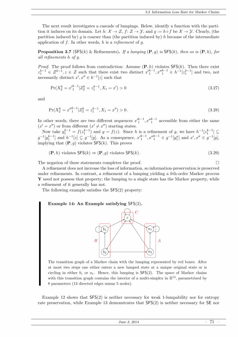
3.2 Information Loss Rate for Markov Chains
The next result investigates a cascade of lumpings. Below, identify a function with the parti-tion it induces on its domain. Let h: X → Z, f : Z → Y, and g := hf be X → Y. Clearly, (thepartition induced by) g is coarser than (the partition induced by) h because of the intermediateapplication of f . In other words, h is a refinement of g.
Proposition 3.7 (SFS(k) & Refinements). If a lumping (P, g) is SFS(k), then so is (P, h), forall refinements h of g.
Proof. The proof follows from contradiction: Assume (P, h) violates SFS(k). Then there existzk−11 ∈ Zk−1, z ∈ Z such that there exist two distinct x′k−1
1 , x′′k−11 ∈ h−1[zk−1
1 ] and two, notnecessarily distinct x′, x′′ ∈ h−1[z] such that
Pr(Xk2 = x′k−1
1 |Zk2 = zk−1
1 , X1 = x′) > 0 (3.27)
and
Pr(Xk2 = x′′k−1
1 |Zk2 = zk−1
1 , X1 = x′′) > 0 . (3.28)
In other words, there are two different sequences x′k−11 , x′′k−1
1 accessible from either the same(x′ = x′′) or from different (x′ 6= x′′) starting states.
Now take yk−11 = f(zk−1
1 ) and y = f(z). Since h is a refinement of g, we have h−1[zk−11 ] ⊆
g−1[yk−11 ] and h−1[z] ⊆ g−1[y]. As a consequence, x′k−1
1 , x′′k−11 ∈ g−1[yn1 ] and x′, x′′ ∈ g−1[y],
implying that (P, g) violates SFS(k). This proves
(P, h) violates SFS(k)⇒ (P, g) violates SFS(k) . (3.29)
The negation of these statements completes the proof.
A refinement does not increase the loss of information, so information-preservation is preservedunder refinements. In contrast, a refinement of a lumping yielding a kth-order Markov processY need not possess that property; the lumping to a single state has the Markov property, whilea refinement of it generally has not.
The following example satisfies the SFS(2) property:
Example 14: An Example satisfying SFS(2).
b1
b2
c
a1
a2
B A
C
The transition graph of a Markov chain with the lumping represented by red boxes. After
at most two steps one either enters a new lumped state at a unique original state or is
circling in either b1 or a1. Hence, this lumping is SFS(2). The space of Markov chains
with this transition graph contains the interior of a multi-simplex in R13, parametrized by
8 parameters (13 directed edges minus 5 nodes).
Example 12 shows that SFS(2) is neither necessary for weak 1-lumpability nor for entropyrate preservation, while Example 13 demonstrates that SFS(2) is neither necessary for SE nor
June 3, 2014 – 71 –
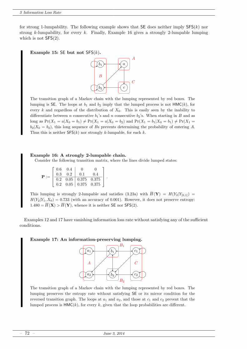
3 Information Loss Rate
for strong 1-lumpability. The following example shows that SE does neither imply SFS(k) norstrong k-lumpability, for every k. Finally, Example 16 gives a strongly 2-lumpable lumpingwhich is not SFS(2).
Example 15: SE but not SFS(k).
b1
b2
a
c
B
A
C
The transition graph of a Markov chain with the lumping represented by red boxes. The
lumping is SE. The loops at b1 and b2 imply that the lumped process is not HMC(k), for
every k and regardless of the distribution of X0. This is easily seen by the inability to
differentiate between n consecutive b1’s and n consecutive b2’s. When starting in B and as
long as Pr(X1 = a|X0 = b1) 6= Pr(X1 = a|X0 = b2) and Pr(X1 = b1|X0 = b1) 6= Pr(X1 =
b2|X0 = b2), this long sequence of Bs prevents determining the probability of entering A.
Thus this is neither SFS(k) nor strongly k-lumpable, for each k.
Example 16: A strongly 2-lumpable chain.Consider the following transition matrix, where the lines divide lumped states:
P :=
0.6 0.4 0 00.3 0.2 0.1 0.40.2 0.05 0.375 0.3750.2 0.05 0.375 0.375
.
This lumping is strongly 2-lumpable and satisfies (3.23a) with H (Y) = H(Y2|Y[0,1]) =
H(Y2|Y1, X0) = 0.733 (with an accuracy of 0.001). However, it does not preserve entropy:
1.480 =H (X) >H (Y), whence it is neither SE nor SFS(2).
Examples 12 and 17 have vanishing information loss rate without satisfying any of the sufficientconditions.
Example 17: An information-preserving lumping.
a1
a2
b1
b2
c1
c2
A C
B1
B2
The transition graph of a Markov chain with the lumping represented by red boxes. The
lumping preserves the entropy rate without satisfying SE or its mirror condition for the
reversed transition graph. The loops at a1 and a2, and those at c1 and c2 prevent that the
lumped process is HMC(k), for every k, given that the loop probabilities are different.
– 72 – June 3, 2014
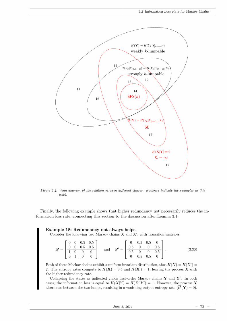
3.2 Information Loss Rate for Markov Chains
SFS(k)
SE
H (Y) = H(Yk|Y[k−1], X0)
K =∞H (X|Y) = 0
strongly k-lumpable
H(Yk|Y[0,k−1]) = H(Yk|Y[k−1], X0)
weakly k-lumpable
H (Y) = H(Yk|Y[0,k−1])
15
12
12
14
13
16
11
17
Figure 3.2: Venn diagram of the relation between different classes. Numbers indicate the examples in thiswork.
Finally, the following example shows that higher redundancy not necessarily reduces the in-formation loss rate, connecting this section to the discussion after Lemma 3.1.
Example 18: Redundancy not always helps.Consider the following two Markov chains X and X′, with transition matrices
P =
0 0 0.5 0.50 0 0.5 0.51 0 0 00 1 0 0
and P′ =
0 0.5 0.5 00.5 0 0 0.50.5 0 0 0.50 0.5 0.5 0
. (3.30)
Both of these Markov chains exhibit a uniform invariant distribution, thusH(X) = H(X ′) =2. The entropy rates compute to H (X) = 0.5 and H (X′) = 1, leaving the process X withthe higher redundancy rate.
Collapsing the states as indicated yields first-order Markov chains Y and Y′. In bothcases, the information loss is equal to H(X|Y ) = H(X ′|Y ′) = 1. However, the process Yalternates between the two lumps, resulting in a vanishing output entropy rate (H (Y) = 0).
June 3, 2014 – 73 –
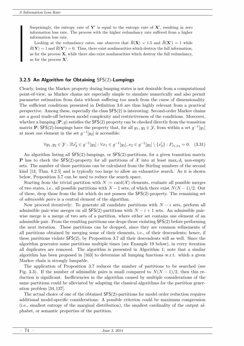
3 Information Loss Rate
Surprisingly, the entropy rate of Y′ is equal to the entropy rate of X′, resulting in zeroinformation loss rate. The process with the higher redundancy rate suffered from a higherinformation loss rate.
Looking at the redundancy rates, one observes that R(X) = 1.5 and R(X′) = 1 while
R(Y) = 1 and R(Y′) = 0. Thus, there exist nonlinearities which destroy the full information,
as for the process X, while there also exist nonlinearities which destroy the full redundancy,
as for the process X′.
3.2.5 An Algorithm for Obtaining SFS(2)-Lumpings
Clearly, losing the Markov property during lumping states is not desirable from a computationalpoint-of-view, as Markov chains are especially simple to simulate numerically and also permitparameter estimation from data without suffering too much from the curse of dimensionality.The sufficient conditions presented in Definition 3.6 are thus highly relevant from a practicalperspective. Among these, especially the class SFS(2) is interesting: Second-order Markov chainsare a good trade-off between model complexity and restrictiveness of the conditions. Moreover,whether a lumping (P, g) satisfies the SFS(2) property can be checked directly from the transitionmatrix P; SFS(2)-lumpings have the property that, for all y1, y2 ∈ Y, from within a set g−1[y1]at most one element in the set g−1[y2] is accessible:
∀y1, y2 ∈ Y : ∃!x′2 ∈ g−1[y2] : ∀x1 ∈ g−1[y1], x2 ∈ g−1[y2] \ x′2 : Px1,x2 = 0. (3.31)
An algorithm listing all SFS(2)-lumpings, or SFS(2)-partitions, for a given transition matrixP has to check the SFS(2)-property for all partitions of X into at least maxi di non-emptysets. The number of these partitions can be calculated from the Stirling numbers of the secondkind [13, Thm. 8.2.5] and is typically too large to allow an exhaustive search. As it is shownbelow, Proposition 3.7 can be used to reduce the search space.
Starting from the trivial partition with N := card(X ) elements, evaluate all possible mergesof two states, i.e., all possible partitions with N − 1 sets, of which there exist N(N − 1)/2. Outof these, drop those from the list which do not possess the SFS(2)-property. The remaining setof admissible pairs is a central element of the algorithm.
Now proceed iteratively: To generate all candidate partitions with N − i sets, perform alladmissible pair-wise merges on all SFS(2)-partitions with N − i + 1 sets. An admissible pair-wise merge is a merge of two sets of a partition, where either set contains one element of anadmissible pair. From the resulting partitions one drops those violating SFS(2) before performingthe next iteration. These partitions can be dropped, since they are common refinements ofall partitions obtained by merging some of their elements, i.e., of their descendents; hence, ifthese partitions violate SFS(2), by Proposition 3.7 all their descendents will as well. Since thealgorithm generates some partitions multiple times (see Example 19 below), in every iterationall duplicates are removed. The algorithm is presented in Algorithm 1; note that a similaralgorithm has been proposed in [163] to determine all lumping functions w.r.t. which a givenMarkov chain is strongly lumpable.
The application of Proposition 3.7 reduces the number of partitions to be searched (seeFig. 3.3). If the number of admissible pairs is small compared to N(N − 1)/2, then this re-duction is significant. Inefficiencies in the algorithm caused by multiple considerations of thesame partitions could be alleviated by adapting the classical algorithms for the partition gener-ation problem [34,137].
The actual choice of one of the obtained SFS(2)-partitions for model order reduction requiresadditional model-specific considerations: A possible criterion could be maximum compression(i.e., smallest entropy of the marginal distribution), the smallest cardinality of the output al-phabet, or semantic properties of the partition.
– 74 – June 3, 2014

3.2 Information Loss Rate for Markov Chains
Algorithm 1 Algorithm for listing all SFS(2)-lumpings
1: function ListLumpings(P)2: admPairs← GetAdmissiblePairs(P)3: Lumpings(1)← merge(admPairs) ⊲ Convert pairs to functions4: n← 15: while notEmpty(Lumpings(n)) do6: n← n+ 17: Lumpings(n)← [ ]8: for h ∈ Lumpings(n− 1) do9: for i1, i2 ∈ admPairs do
10: g ← h11: g(h−1(h(i2)))← g(i1) ⊲ i1 and i2 have same image.12: if g is SFS(2) then13: Lumpings(n)← [Lumpings(n); g]14: end if15: end for16: end for17: Remove duplicates from Lumpings18: end while19: return Lumpings20: end function
21: function GetAdmissiblePairs(P)22: Pairs← [ ]23: N ← dim(P)24: for i1 = 1 : N − 1 do25: for i2 = i1 : N do26: f ← merge(i1, i2) ⊲ f merges i1 and i227: if f is SFS(2) then28: Pairs← [Pairs; i1, i2]29: end if30: end for31: end for32: return Pairs33: end function
In practice, if N is large and if the number of admissible pairs is of the same order as N(N −1)/2, listing all SFS(2)-partitions might be computationally expensive. One can trade optimalityfor speed by greedy selection of the best h in line 8, given a specific criterion, or by evaluatingonly a (random) subset of admissible pairs in line 9 (cf. Fig. 3.3).
June 3, 2014 – 75 –
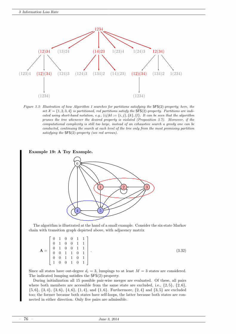
3 Information Loss Rate
1234
(12)34 (13)24 (14)23 1(23)4 1(24)3 12(34)
(123)4 (12)(34) (124)3 (124)3 (134)2 (14)(23) (12)(34) (134)2 1(234)
(1234) (1234)
Figure 3.3: Illustration of how Algorithm 1 searches for partitions satisfying the SFS(2)-property; here, theset X = 1, 2, 3, 4 is partitioned, red partitions satisfy the SFS(2)-property. Partitions are indi-cated using short-hand notation, e.g., (ij)kl := i, j, k, l. It can be seen that the algorithmprunes the tree whenever the desired property is violated (Proposition 3.7). Moreover, if thecomputational complexity is still too large, instead of an exhaustive search a greedy one can beconducted, continuing the search at each level of the tree only from the most promising partitionsatisfying the SFS(2)-property (see red arrows).
Example 19: A Toy Example.
6
1 2 3
4 5
The algorithm is illustrated at the hand of a small example. Consider the six-state Markovchain with transition graph depicted above, with adjacency matrix
A =
0 1 0 0 1 10 1 0 0 1 10 1 0 0 1 10 0 1 1 0 10 0 1 1 0 11 0 0 1 0 1
. (3.32)
Since all states have out-degree di = 3, lumpings to at least M = 3 states are considered.The indicated lumping satisfies the SFS(2)-property.
During initialization all 15 possible pair-wise merges are evaluated. Of these, all pairswhere both members are accessible from the same state are excluded, i.e., 2, 5, 2, 6,5, 6, 3, 4, 3, 6, 4, 6, 1, 4, and 1, 6. Furthermore, 2, 4 and 3, 5 are excludedtoo; the former because both states have self-loops, the latter because both states are con-nected in either direction. Only five pairs are admissible.
– 76 – June 3, 2014
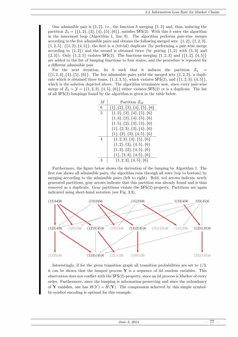
3.2 Information Loss Rate for Markov Chains
One admissible pair is 1, 2, i.e., the function h merging 1, 2 and, thus, inducing thepartition Z5 = 1, 2, 3, 4, 5, 6, satisfies SFS(2). With this h enter the algorithmin the innermost loop (Algorithm 1, line 9). The algorithm performs pair-wise mergesaccording to the five admissible pairs and obtains the following merged sets: 1, 2, 1, 2, 3,1, 2, 5, 1, 2, 4, 5; the first is a (trivial) duplicate (by performing a pair-wise mergeaccording to 1, 2) and the second is obtained twice (by pairing 1, 2 with 1, 3 and2, 3). Only 1, 2, 5 violates SFS(2). The functions merging 1, 2, 3 and 1, 2, 4, 5are added to the list of lumping functions to four states, and the procedure is repeated fora different admissible pair.
For the next iteration, fix h such that it induces the partition Z4 =1, 2, 3, 4, 5, 6. The five admissible pairs yield the merged sets 1, 2, 3, a dupli-cate which is obtained three times, 1, 2, 3, 5, which violates SFS(2), and 1, 2, 3, 4, 5,which is the solution depicted above. The algorithm terminates now, since every pair-wisemerge of Z3 = Y = 1, 2, 3, 4, 5, 6 either violates SFS(2) or is a duplicate. The listof all SFS(2)-lumpings found by the algorithm is given in the table below.
M Partition ZM
6 1, 2, 3, 4, 5, 65 1, 2, 3, 4, 5, 6
1, 3, 2, 4, 5, 61, 5, 2, 3, 4, 61, 2, 3, 3, 4, 61, 2, 3, 4, 5, 6
4 1, 2, 3, 4, 5, 61, 2, 3, 4, 5, 61, 3, 2, 4, 5, 61, 2, 3, 4, 5, 6
3 1, 2, 3, 4, 5, 6
Furthermore, the figure below shows the derivation of the lumping by Algorithm 1. Thefirst row shows all admissible pairs, the algorithm runs through all rows (top to bottom) bymerging according to the admissible pairs (left to right). Bold, red arrows indicate newlygenerated partitions, gray arrows indicate that this partition was already found and is thusremoved as a duplicate. Gray partitions violate the SFS(2)-property. Partitions are againindicated using short-hand notation (see Fig. 3.3).
(12)3456 (13)2456 (15)2346 1(23)456 123(45)6
(123)456 (125)346 (12)3(45)6 (135)246 (13)2(45)6 (15)(23)46 (145)236 1(23)(45)6
(1235)46 (123)(45)6 (12, 5)36 (1345)26 (23)(145)6
Interestingly, if for the given transition graph all transition probabilities are set to 1/3,
it can be shown that the lumped process Y is a sequence of iid random variables. This
observation does not conflict with the SFS(2)-property, since an iid process is Markov of every
order. Furthermore, since the lumping is information-preserving and since the redundancy
of Y vanishes, one has H(Y ) = H (Y). The compression achieved by this simple symbol-
by-symbol encoding is optimal for this example.
June 3, 2014 – 77 –
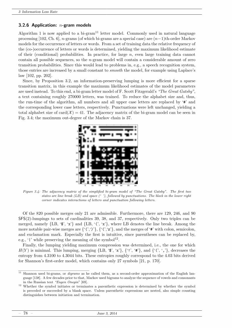
3 Information Loss Rate
3.2.6 Application: n-gram models
Algorithm 1 is now applied to a bi-gram11 letter model. Commonly used in natural languageprocessing [102, Ch. 6], n-grams (of which bi-grams are a special case) are (n−1)th-order Markovmodels for the occurrence of letters or words. From a set of training data the relative frequency ofthe (co-)occurrence of letters or words is determined, yielding the maximum likelihood estimateof their (conditional) probabilities. In practice, for large n, even large training data cannotcontain all possible sequences, so the n-gram model will contain a considerable amount of zerotransition probabilities. Since this would lead to problems in, e.g., a speech recognition system,those entries are increased by a small constant to smooth the model, for example using Laplace’slaw [102, pp. 202].Since, by Proposition 3.2, an information-preserving lumping is more efficient for a sparse
transition matrix, in this example the maximum likelihood estimates of the model parametersare used instead. To this end, a bi-gram letter model of F. Scott Fitzgerald’s “The Great Gatsby”,a text containing roughly 270000 letters, was trained. To reduce the alphabet size and, thus,the run-time of the algorithm, all numbers and all upper case letters are replaced by ‘#’ andthe corresponding lower case letters, respectively. Punctuations were left unchanged, yielding atotal alphabet size of card(X ) = 41. The adjacency matrix of the bi-gram model can be seen inFig. 3.4; the maximum out-degree of the Markov chain is 37.
5 10 15 20 25 30 35 40
5
10
15
20
25
30
35
40
Figure 3.4: The adjacency matrix of the simplified bi-gram model of “The Great Gatsby”. The first twostates are line break (LB) and space (‘ ’), followed by punctuations. The block in the lower rightcorner indicates interactions of letters and punctuation following letters.
Of the 820 possible merges only 21 are admissible. Furthermore, there are 129, 246, and 90SFS(2)-lumpings to sets of cardinalities 39, 38, and 37, respectively. Only two triples can bemerged, namely LB, ‘$’, ‘x’ and LB, ‘(’, ‘x’, where LB denotes the line break. Among themore notable pair-wise merges are ‘(’,‘)’, ‘(’,‘z’, and the merges of ‘#’ with colon, semicolon,and exclamation mark. Especially the first is intuitive, since parentheses can be replaced by,e.g., ‘|’ while preserving the meaning of the symbol12.Finally, the lumping yielding maximum compression was determined, i.e., the one for which
H(Y ) is minimal. This lumping, merging LB, ‘$’, ‘x’, ‘!’, ‘#’, and ‘(’, ‘,’, decreases theentropy from 4.3100 to 4.3044 bits. These entropies roughly correspond to the 4.03 bits derivedfor Shannon’s first-order model, which contains only 27 symbols [21, p. 170].
11 Shannon used bi-grams, or digrams as he called them, as a second-order approximation of the English lan-guage [138]. A few decades prior to that, Markov used bigrams to analyze the sequence of vowels and consonantsin the Russian text “Eugen Onegin” [69].
12 Whether the symbol initiates or terminates a parenthetic expression is determined by whether the symbolis preceded or succeeded by a blank space. Unless parenthetic expressions are nested, also simple countingdistinguishes between initiation and termination.
– 78 – June 3, 2014
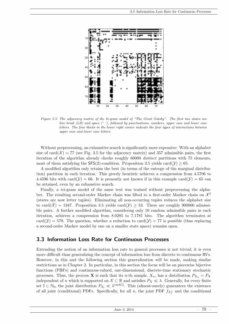
3.3 Information Loss Rate for Continuous Processes
10 20 30 40 50 60 70
10
20
30
40
50
60
70
Figure 3.5: The adjacency matrix of the bi-gram model of “The Great Gatsby”. The first two states areline break (LB) and space (‘ ’), followed by punctuations, numbers, upper case and lower caseletters. The four blocks in the lower right corner indicate the four types of interactions betweenupper case and lower case letters.
Without preprocessing, an exhaustive search is significantly more expensive: With an alphabetsize of card(X ) = 77 (see Fig. 3.5 for the adjacency matrix) and 357 admissible pairs, the firstiteration of the algorithm already checks roughly 60000 distinct partitions with 75 elements,most of them satisfying the SFS(2)-condition. Proposition 3.5 yields card(Y) ≥ 65.
A modified algorithm only retains the best (in terms of the entropy of the marginal distribu-tion) partition in each iteration. This greedy heuristic achieves a compression from 4.5706 to4.4596 bits with card(Y) = 66. It is presently not known if in this example card(Y) = 65 canbe attained, even by an exhaustive search.
Finally, a tri-gram model of the same text was trained without preprocessing the alpha-bet. The resulting second-order Markov chain was lifted to a first-order Markov chain on X 2
(states are now letter tuples). Eliminating all non-occurring tuples reduces the alphabet sizeto card(X ) = 1347. Proposition 3.5 yields card(Y) ≥ 53. There are roughly 900000 admissi-ble pairs. A further modified algorithm, considering only 10 random admissible pairs in eachiteration, achieves a compression from 8.0285 to 7.1781 bits. The algorithm terminates atcard(Y) = 579. The question, whether a reduction to card(Y) < 77 is possible (thus replacinga second-order Markov model by one on a smaller state space) remains open.
3.3 Information Loss Rate for Continuous Processes
Extending the notion of an information loss rate to general processes is not trivial; it is evenmore difficult than generalizing the concept of information loss from discrete to continuous RVs.However, in this and the following section this generalization will be made, making similarrestrictions as in Chapter 2. In particular, in this section the focus will be on piecewise bijectivefunctions (PBFs) and continuous-valued, one-dimensional, discrete-time stationary stochasticprocesses. Thus, the process X is such that its n-th sample, Xn, has a distribution PXn = PX
independent of n which is supported on X ⊂ R and satisfies PX ≪ λ. Generally, for every finiteset I ⊂ N0, the joint distribution PXI
≪ λcard(I). This (almost-surely) guarantees the existenceof all joint (conditional) PDFs. Specifically, for all n, the joint PDF fXn
1and the conditional
June 3, 2014 – 79 –
3 Information Loss Rate
PDF fXn|Xn−11
exist.
Additionally, it shall be assumed that the joint differential entropy of an arbitrary collectionof RVs exists and is finite, and that, thus, also the differential entropy rate [114, Thm. 14.7]
h(X) := limn→∞
h(Xn|Xn−11 ) = lim
n→∞1
nh(Xn
1 ) (3.33)
exists and is finite.
The system under consideration shall be described by a PBF satisfying Definition 2.3. Theoutput process Y is obtained by feeding X through this system, i.e., Yn := g(Xn), and is jointlystationary with X. The information loss occurring in this system per sample shall be quantifiedby
Definition 3.7 (Information Loss Rate). Let X be a continuous-valued, one-dimensional,discrete-time stationary stochastic process, and let Y be a jointly stationary process defined byYn := g(Xn). The information loss rate induced by g is
L(X→ Y) := limn→∞
1
nL(Xn
1 → Y n1 ) (3.34)
where L(· → ·) follows Definition 2.2.
It can be shown that many properties of information loss for PBFs can be generalized also tothe information loss rate. Most surprisingly, the information loss rate allows a simple expressionin terms of the differential entropy rates of the input and output processes:
Proposition 3.8 (Information Loss Rate and Differential Entropy Rate). The information lossrate induced by feeding a stationary stochastic process through a PBF is
L(X→ Y) = h(X)−h(Y) + E(log |g′(X)|
). (3.35)
Proof. For the proof note that the RVs X1, . . . , Xn can be interpreted as a single, n-dimensionalRV; similarily, one can define an extended function gn: X n → Yn, applying g coordinate-wise.The Jacobian matrix of gn is a diagonal matrix constituted by the elements g′(xi). With Theo-rem 2.2,
L(Xn1 → Y n
1 ) = h(Xn1 )− h(Y n
1 ) + E
(
log
∣∣∣∣∣
n∏
i=1
g′(Xi)
∣∣∣∣∣
)
= h(Xn1 ) − h(Y n
1 ) + nE(log∣∣g′(X)
∣∣)
(3.36)
where the first line is because the determinant of a diagonal matrix is the product of its diagonalelements, and where stationarity of X yields the second line. Dividing by n and taking the limitcompletes the proof.
Proposition 2.2 shows that the information loss of a cascade of systems equals the sum of theinformation losses induced in the systems constituting the cascade. Indeed, this result carriesover to the information loss rate as well:
Proposition 3.9 (Cascade of Systems). Consider two functions g: X → Y and h: Y → Z anda cascade of systems implementing these functions. Let Yn := g(Xn) and Zn := h(Yn), whereXn are samples from a continuous-valued stationary stochastic process X. The informationloss rate induced by this cascade, or equivalently, by the system implementing the composition(h g)(·) = h(g(·)) is given as the sum of the individual information loss rates:
L(X→ Z) =L(X→ Y) +L(Y → Z). (3.37)
– 80 – June 3, 2014
3.3 Information Loss Rate for Continuous Processes
Proof. The proof follows from the fact that the cascade is described by the function h g, andthat
E(log |(h g)′(X)|
)= E
(log |g′(X)h′(g(X))|
)= E
(log |g′(X)|
)+ E
(log |h′(Y )|
). (3.38)
Finally, an extension of Proposition 2.3 is possible: To this end, let the stationary stochasticprocess W be given according to Definition 2.4, applied to each sample pair (Xn,Wn).
Proposition 3.10. Let W be a stationary stochastic process defined by Wn := i if Xn ∈ Xi.Then,
L(X→ Y) =H (W|Y). (3.39)
Proof. Again, treat Xn1 as an n-dimensional RV; gn induces a partition of its domain X n, which
is equivalent to the n-fold product of the partition Xi. Letting W be the RV obtained byquantizing Xn
1 according to this partition, it is easy to see that Wn1 is equivalent to W . Thus,
with Proposition 2.3,
H(Xn1 |Y n
1 ) = H(W |Y n1 ) = H(Wn
1 |Y n1 ) (3.40)
for all n. The proof is completed with H (W|Y) := limn→∞ 1nH(Wn
1 |Y n1 ).
3.3.1 Upper Bounds on the Information Loss Rate
It is often not possible to obtain closed-form expressions for the information loss rate inducedby a system. Moreover, estimating the information loss rate by simulations soon suffers thecurse of dimensionality, as, in principle, infinitely long random sequences have to be drawnand averaged. Much simpler is an estimation of the information loss, since a single realized,sufficiently long sequence allows for an estimation of the latter. As the next proposition shows,this relatively simple estimation delivers an upper bound on the information loss rate, and thusextends Lemma 3.1 to continuous-valued processes.
Proposition 3.11 (Loss ≥ Loss Rate). Let X be a stationary stochastic process and X anRV distributed according to the process’ marginal distribution. The information loss induced byfeeding X through a PBF g is an upper bound on the information loss rate induced by passingX through g, i.e.,
L(X→ Y) ≤ L(X → Y ). (3.41)
Proof. The inequality holds trivially if L(X → Y ) =∞. The rest of the proof follows along thesame lines as in Lemma 3.1.Clearly, this bound is tight whenever the input process X is an iid process. Moreover, it is
trivially tight whenever the function is bijective, i.e., when L(X → Y ) = 0. Example 20 rendersthis bound tight in a more general case.Intuitively, this bound suggests that redundancy of a process, i.e., the statistical dependence of
its samples, reduces the amount of information lost per sample when fed through a deterministicsystem. The same connection between information loss and information loss rate has alreadybeen observed in [161] for stationary stochastic processes with finite alphabets.The next bound extends Corollary 2.3, bounding the information loss rate by the entropy
rate of a stationary stochastic process on an at most countable alphabet. As such, it presents adifferent way to estimate the information loss rate efficiently using numerical simulations.
Proposition 3.12 (Upper Bound). Let W be as in Proposition 3.10. Then,
L(X→ Y) ≤H (W). (3.42)
June 3, 2014 – 81 –
3 Information Loss Rate
The proof follows from the fact that conditioning reduces entropy.
For the case that the input process is a stationary Markov process, i.e., if fXn|Xn−11
=
fXn|Xn−1= fX2|X1
PXn−11
-a.s. for all n, an additional, sharper, upper bound can be presented:
Proposition 3.13 (Upper Bound for Markovian X). Let X be a stationary Markov process,and let W be as in Proposition 3.10. Then, for finite L(X → Y ),
L(X→ Y) ≤ H(W2|X1). (3.43)
Proof. Applying the chain rule, Markovity of X, and the fact that conditioning reduces entropyyields
H(Xn1 |Y n
1 ) ≤ H(X1|Y1) +n∑
i=2
H(Xi|Xi−1, Yi). (3.44)
With stationarity and with H(X1|Y1) = L(X → Y ) <∞ one can continue
L(X→ Y) = limn→∞
1
nH(Xn
1 |Y n1 ) (3.45)
≤ H(X2|X1, Y2) (3.46)
(a)= H(W2|X1, Y2) (3.47)
≤ H(W2|X1) (3.48)
where (a) holds due to Proposition 2.3 since, for all x ∈ X , H(X2|Y2, X1 = x) = H(W2|Y2, X1 =x). The last inequality is due to conditioning [21, Thm. 2.6.5] and completes the proof.
That the bound is sharper than the one of Proposition 3.12 follows from observing that
H(Wn|Xn−1) = limn→∞
H(Wn|Xn−11 ) ≤ lim
n→∞H(Wn|Wn−1
1 ) =H (W). (3.49)
The interpretation of this result is that a function destroys little information if the processis such that, given the current sample Xn−1, the next sample Xn falls within some element ofthe partition with a high probability. The question whether, and under which conditions, thisbound is tight is related to the phenomenon of lumpability and will be answered in the followingsection.
3.3.2 Excursion: Lumpability of Continuous Markov Processes
It is well-known that the function of a Markov process need not possess the Markov propertyitself. However, as it is known for Markov chains (see Section 3.2), there exist conditions on thefunction and/or the chain such that the output is Markov. While most results are given for finiteMarkov chains (e.g., [15, 124]) relatively little is known in the general case of an uncountablealphabet (see [125] for an exception). This section is a small contribution to this field of researchby presenting sufficient conditions for lumpability of continuous-valued Markov processes.
Let fXn|Xn−11
= fXn|Xn−1= fX2|X1
for all n, i.e., let X be a stationary Markov process.
Proposition 3.14. If
∀y21 ∈ Y2 : ∀x ∈ g−1[y1] : fY2,X1(y2, x) > 0⇒ fY2|X1(y2|x) = fY2|Y1
(y2|y1) (3.50)
then X is lumpable w.r.t. g, i.e., Y is Markov.
Proof. See Appendix B.4.
– 82 – June 3, 2014
3.3 Information Loss Rate for Continuous Processes
As a corollary, the conditions on the function g, the marginal distribution fX , and the condi-tional distribution fX2|X1
can be made explicit. By adding a further condition, Proposition 3.13becomes tight:
Corollary 3.3. If for all y21 ∈ Y2 and all x, x′ ∈ g−1[y1] such that fX(x) > 0 and fX(x′) > 0the following holds
∑
x2∈g−1[y2]
fX2|X1(x2|x)
|g′(x2)|=
∑
x2∈g−1[y2]
fX2|X1(x2|x′)
|g′(x2)|(3.51)
then the condition of Proposition 3.14 is fulfilled and Y is Markov.
Let, additionally, for all y ∈ Y, all x within the support X of fX , and all w,w′ with Pr(W2 =w|X1 = x) > 0 and Pr(W2 = w′|X1 = x) > 0
fX2|X1(g−1
w (y2)|x)|g′(g−1
w (y2))|=
fX2|X1(g−1
w′ (y2)|x)|g′(g−1
w′ (y2))|(3.52a)
and
Pr(W2 = w′|X1 = x) = Pr(W2 = w|X1 = x). (3.52b)
Then, the bound of Proposition 3.13 holds with equality.
Proof. See Appendix B.5.
Example 20: An Example for Tightness of the Bounds.The following example illustrates the tightness of the presented bounds and also sat-
isfies the condition of lumpability. Assume that X is a Markov process with conditionaldistribution
fX2|X1(x2|x1) =: fM (x2|x1) =
1
2
I[1,2)(x2) + I[3,4)(x2), x1 ∈ [0, 1) ∪ [2, 3)
I[0,1)(x2) + I[2,3)(x2), x1 ∈ [1, 2) ∪ [3, 4)(3.53)
where IA(x) = 1 iff x ∈ A. The stationary distribution is the uniform distribution on [0, 4),thus, h(X) = log 4 = 2 and h(X) = 1.
The system maps the interval X2 = [2, 4) onto the interval X1 = [0, 2), i.e.,
g(x) =
x, x ∈ [0, 2)
x− 2, x ∈ [2, 4)(3.54)
which yields the conditional distribution of Y2 given X1,
fY2|X1(y2|x1) =
I[1,2)(y2), x1 ∈ [0, 1) ∪ [2, 3)
I[0,1)(y2), x1 ∈ [1, 2) ∪ [3, 4). (3.55)
The derivative of g is identical to one, the stationary distribution of the output process Yis the uniform distribution on [0, 2); thus, h(Y ) = log 2 = 1 and L(X → Y ) = 1.
The output process Y can be shown to be Markov: Assuming X1 = x ∈ [0, 1), it followsthat x′ ∈ [2, 3); since these conditions are equivalent in the definition of fM , (3.51) holds.
From fM one can see that Pr(W2 = 1|X1 = x) = Pr(W2 = 2|X1 = x) = 12 regardless of
x, which satisfies (3.52b) and renders the upper bound from Proposition 3.13 as
H(W2|X1) = 1. (3.56)
The bound can be shown to be tight, since also (3.52a) is fulfilled: Given, e.g., X1 = x ∈ [0, 1)
June 3, 2014 – 83 –
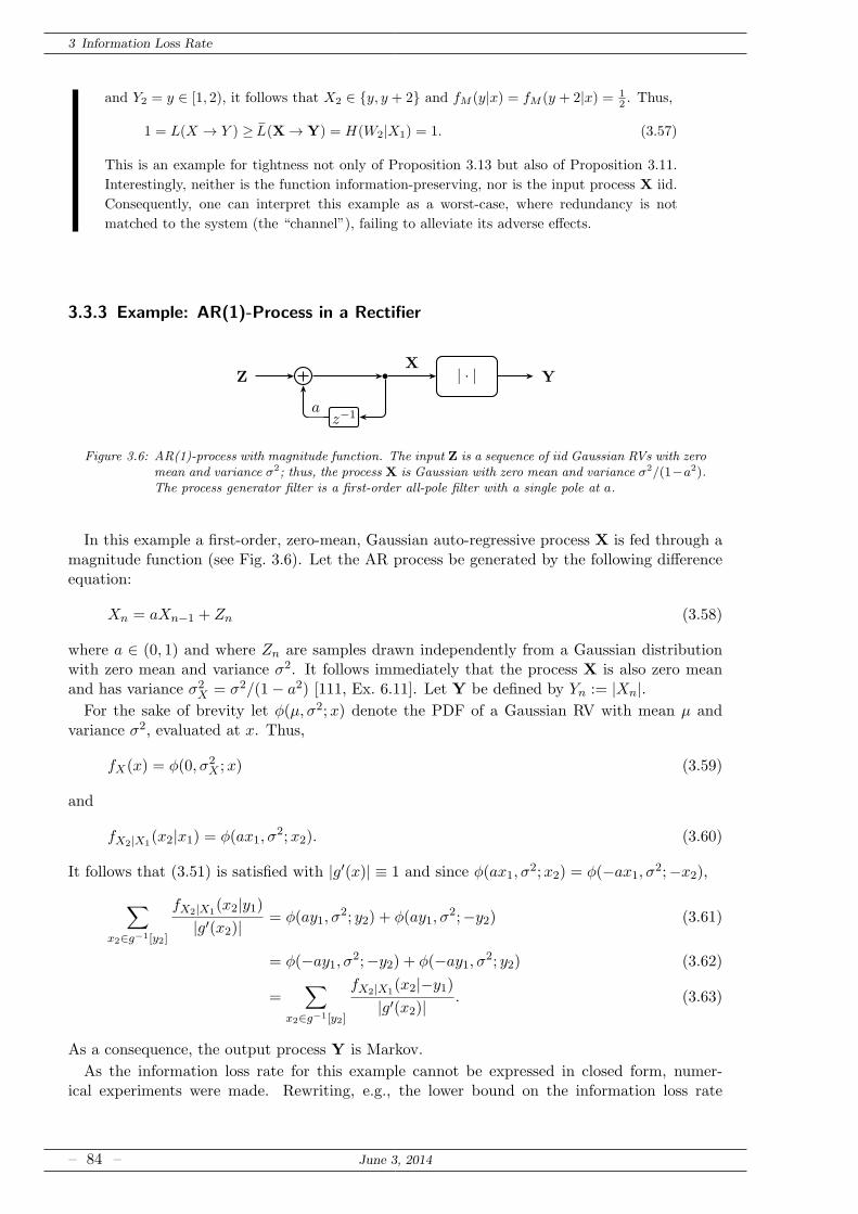
3 Information Loss Rate
and Y2 = y ∈ [1, 2), it follows that X2 ∈ y, y + 2 and fM (y|x) = fM (y + 2|x) = 12 . Thus,
1 = L(X → Y ) ≥L(X→ Y) = H(W2|X1) = 1. (3.57)
This is an example for tightness not only of Proposition 3.13 but also of Proposition 3.11.
Interestingly, neither is the function information-preserving, nor is the input process X iid.
Consequently, one can interpret this example as a worst-case, where redundancy is not
matched to the system (the “channel”), failing to alleviate its adverse effects.
3.3.3 Example: AR(1)-Process in a Rectifier
Z b | · |
z−1a
YX
Figure 3.6: AR(1)-process with magnitude function. The input Z is a sequence of iid Gaussian RVs with zeromean and variance σ2; thus, the process X is Gaussian with zero mean and variance σ2/(1−a2).The process generator filter is a first-order all-pole filter with a single pole at a.
In this example a first-order, zero-mean, Gaussian auto-regressive process X is fed through amagnitude function (see Fig. 3.6). Let the AR process be generated by the following differenceequation:
Xn = aXn−1 + Zn (3.58)
where a ∈ (0, 1) and where Zn are samples drawn independently from a Gaussian distributionwith zero mean and variance σ2. It follows immediately that the process X is also zero meanand has variance σ2
X = σ2/(1− a2) [111, Ex. 6.11]. Let Y be defined by Yn := |Xn|.For the sake of brevity let φ(µ, σ2;x) denote the PDF of a Gaussian RV with mean µ and
variance σ2, evaluated at x. Thus,
fX(x) = φ(0, σ2X ;x) (3.59)
and
fX2|X1(x2|x1) = φ(ax1, σ
2;x2). (3.60)
It follows that (3.51) is satisfied with |g′(x)| ≡ 1 and since φ(ax1, σ2;x2) = φ(−ax1, σ2;−x2),
∑
x2∈g−1[y2]
fX2|X1(x2|y1)
|g′(x2)|= φ(ay1, σ
2; y2) + φ(ay1, σ2;−y2) (3.61)
= φ(−ay1, σ2;−y2) + φ(−ay1, σ2; y2) (3.62)
=∑
x2∈g−1[y2]
fX2|X1(x2|−y1)
|g′(x2)|. (3.63)
As a consequence, the output process Y is Markov.
As the information loss rate for this example cannot be expressed in closed form, numer-ical experiments were made. Rewriting, e.g., the lower bound on the information loss rate
– 84 – June 3, 2014
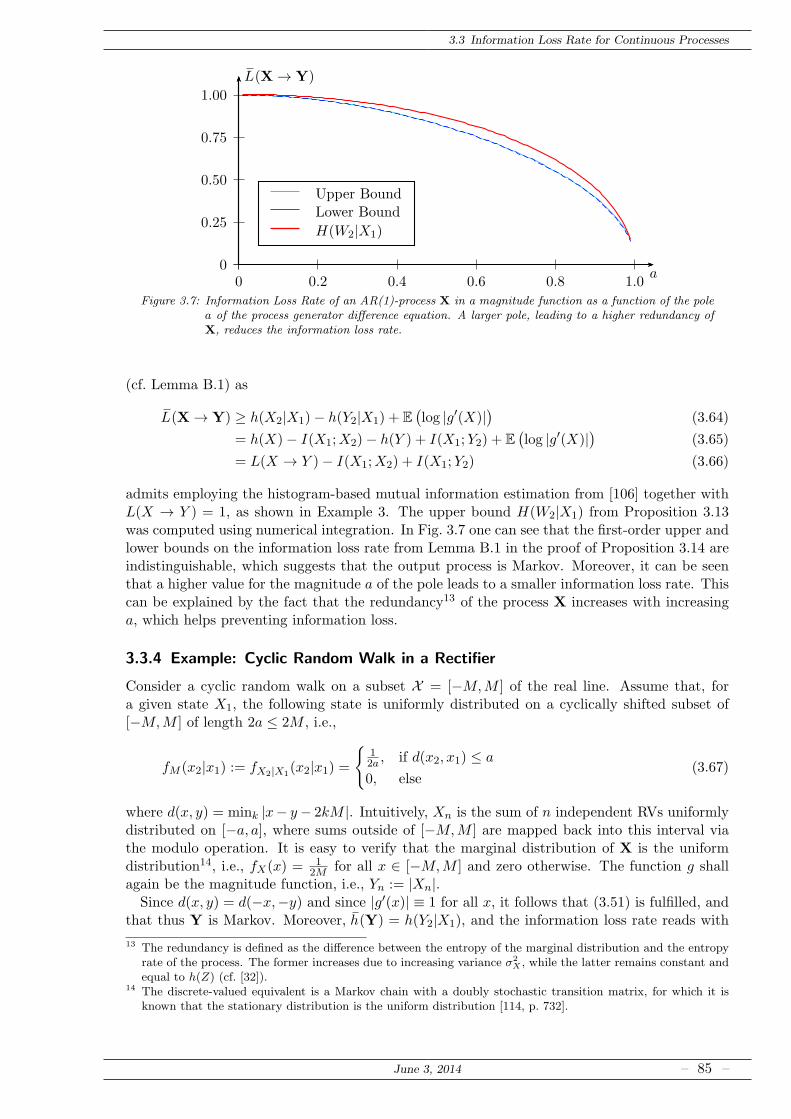
3.3 Information Loss Rate for Continuous Processes
0
0.25
0.50
0.75
1.00
0 0.2 0.4 0.6 0.8 1.0a
L(X→ Y)
Upper BoundLower Bound
H(W2|X1)
Figure 3.7: Information Loss Rate of an AR(1)-process X in a magnitude function as a function of the polea of the process generator difference equation. A larger pole, leading to a higher redundancy ofX, reduces the information loss rate.
(cf. Lemma B.1) as
L(X→ Y) ≥ h(X2|X1)− h(Y2|X1) + E(log |g′(X)|
)(3.64)
= h(X)− I(X1;X2)− h(Y ) + I(X1;Y2) + E(log |g′(X)|
)(3.65)
= L(X → Y )− I(X1;X2) + I(X1;Y2) (3.66)
admits employing the histogram-based mutual information estimation from [106] together withL(X → Y ) = 1, as shown in Example 3. The upper bound H(W2|X1) from Proposition 3.13was computed using numerical integration. In Fig. 3.7 one can see that the first-order upper andlower bounds on the information loss rate from Lemma B.1 in the proof of Proposition 3.14 areindistinguishable, which suggests that the output process is Markov. Moreover, it can be seenthat a higher value for the magnitude a of the pole leads to a smaller information loss rate. Thiscan be explained by the fact that the redundancy13 of the process X increases with increasinga, which helps preventing information loss.
3.3.4 Example: Cyclic Random Walk in a Rectifier
Consider a cyclic random walk on a subset X = [−M,M ] of the real line. Assume that, fora given state X1, the following state is uniformly distributed on a cyclically shifted subset of[−M,M ] of length 2a ≤ 2M , i.e.,
fM (x2|x1) := fX2|X1(x2|x1) =
12a , if d(x2, x1) ≤ a
0, else(3.67)
where d(x, y) = mink |x− y− 2kM |. Intuitively, Xn is the sum of n independent RVs uniformlydistributed on [−a, a], where sums outside of [−M,M ] are mapped back into this interval viathe modulo operation. It is easy to verify that the marginal distribution of X is the uniformdistribution14, i.e., fX(x) = 1
2M for all x ∈ [−M,M ] and zero otherwise. The function g shallagain be the magnitude function, i.e., Yn := |Xn|.Since d(x, y) = d(−x,−y) and since |g′(x)| ≡ 1 for all x, it follows that (3.51) is fulfilled, and
that thus Y is Markov. Moreover, h(Y) = h(Y2|X1), and the information loss rate reads with
13 The redundancy is defined as the difference between the entropy of the marginal distribution and the entropyrate of the process. The former increases due to increasing variance σ2
X , while the latter remains constant andequal to h(Z) (cf. [32]).
14 The discrete-valued equivalent is a Markov chain with a doubly stochastic transition matrix, for which it isknown that the stationary distribution is the uniform distribution [114, p. 732].
June 3, 2014 – 85 –
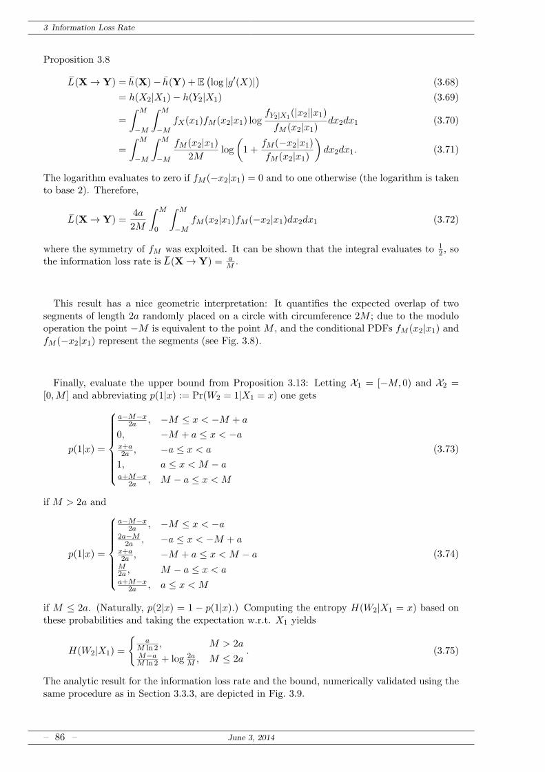
3 Information Loss Rate
Proposition 3.8
L(X→ Y) = h(X)−h(Y) + E(log |g′(X)|
)(3.68)
= h(X2|X1)− h(Y2|X1) (3.69)
=
∫ M
−M
∫ M
−MfX(x1)fM (x2|x1) log
fY2|X1(|x2||x1)
fM (x2|x1)dx2dx1 (3.70)
=
∫ M
−M
∫ M
−M
fM (x2|x1)2M
log
(
1 +fM (−x2|x1)fM (x2|x1)
)
dx2dx1. (3.71)
The logarithm evaluates to zero if fM (−x2|x1) = 0 and to one otherwise (the logarithm is takento base 2). Therefore,
L(X→ Y) =4a
2M
∫ M
0
∫ M
−MfM (x2|x1)fM (−x2|x1)dx2dx1 (3.72)
where the symmetry of fM was exploited. It can be shown that the integral evaluates to 12 , so
the information loss rate is L(X→ Y) = aM .
This result has a nice geometric interpretation: It quantifies the expected overlap of twosegments of length 2a randomly placed on a circle with circumference 2M ; due to the modulooperation the point −M is equivalent to the point M , and the conditional PDFs fM (x2|x1) andfM (−x2|x1) represent the segments (see Fig. 3.8).
Finally, evaluate the upper bound from Proposition 3.13: Letting X1 = [−M, 0) and X2 =[0,M ] and abbreviating p(1|x) := Pr(W2 = 1|X1 = x) one gets
p(1|x) =
a−M−x2a , −M ≤ x < −M + a
0, −M + a ≤ x < −ax+a2a , −a ≤ x < a
1, a ≤ x < M − aa+M−x
2a , M − a ≤ x < M
(3.73)
if M > 2a and
p(1|x) =
a−M−x2a , −M ≤ x < −a
2a−M2a , −a ≤ x < −M + a
x+a2a , −M + a ≤ x < M − aM2a , M − a ≤ x < aa+M−x
2a , a ≤ x < M
(3.74)
if M ≤ 2a. (Naturally, p(2|x) = 1 − p(1|x).) Computing the entropy H(W2|X1 = x) based onthese probabilities and taking the expectation w.r.t. X1 yields
H(W2|X1) =
a
M ln 2 , M > 2aM−aM ln 2 + log 2a
M , M ≤ 2a. (3.75)
The analytic result for the information loss rate and the bound, numerically validated using thesame procedure as in Section 3.3.3, are depicted in Fig. 3.9.
– 86 – June 3, 2014
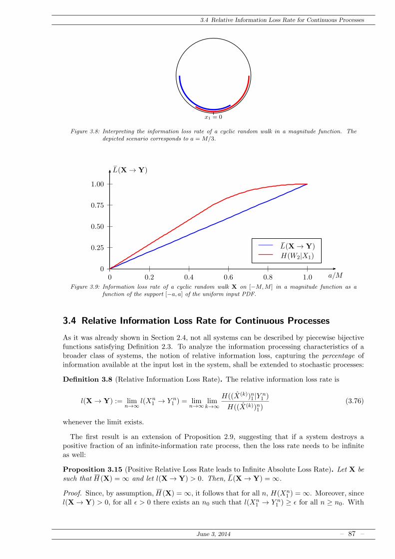
3.4 Relative Information Loss Rate for Continuous Processes
x1 = 0
Figure 3.8: Interpreting the information loss rate of a cyclic random walk in a magnitude function. Thedepicted scenario corresponds to a = M/3.
0
0.25
0.50
0.75
1.00
0 0.2 0.4 0.6 0.8 1.0 a/M
L(X→ Y)
L(X→ Y)
H(W2|X1)
Figure 3.9: Information loss rate of a cyclic random walk X on [−M,M ] in a magnitude function as afunction of the support [−a, a] of the uniform input PDF.
3.4 Relative Information Loss Rate for Continuous Processes
As it was already shown in Section 2.4, not all systems can be described by piecewise bijectivefunctions satisfying Definition 2.3. To analyze the information processing characteristics of abroader class of systems, the notion of relative information loss, capturing the percentage ofinformation available at the input lost in the system, shall be extended to stochastic processes:
Definition 3.8 (Relative Information Loss Rate). The relative information loss rate is
l(X→ Y) := limn→∞
l(Xn1 → Y n
1 ) = limn→∞
limk→∞
H((X(k))n1 |Y n1 )
H((X(k))n1 )(3.76)
whenever the limit exists.
The first result is an extension of Proposition 2.9, suggesting that if a system destroys apositive fraction of an infinite-information rate process, then the loss rate needs to be infiniteas well:
Proposition 3.15 (Positive Relative Loss Rate leads to Infinite Absolute Loss Rate). Let X besuch that H (X) =∞ and let l(X→ Y) > 0. Then, L(X→ Y) =∞.
Proof. Since, by assumption,H (X) =∞, it follows that for all n, H(Xn1 ) =∞. Moreover, since
l(X→ Y) > 0, for all ǫ > 0 there exists an n0 such that l(Xn1 → Y n
1 ) ≥ ǫ for all n ≥ n0. With
June 3, 2014 – 87 –
3 Information Loss Rate
Proposition 2.9 it follows that L(Xn1 → Y n
1 ) =∞. Since this holds for all n ≥ n0, this completesthe proof.For the results following below, let us again assume that the stationary process X is such
that all joint and conditional PDFs exist, cf. Section 3.3. Thus, d(Xn1 ) = nd(X) = n, for all n.
Clearly, if X is iid, so is Y, and l(X→ Y) = l(X → Y ). In general, from stationarity, existenceof the joint PDFs, and Proposition 2.11 the following holds for all n:
l(Xn1 → Y n
1 ) ≤ 1
n
n∑
i=1
l(Xi → Yi) = l(X → Y ) (3.77)
Therefore one can show15 that l(X→ Y) ≤ l(X → Y ), complementing Proposition 3.11. Inmany cases, this inequality is tight, as presented in the following
Proposition 3.16 (Redundancy won’t help). Let X be a stationary stochastic process and Xan RV distributed according to the process’ marginal distribution. Let further g be defined on afinite partition Xi of X into non-empty sets as in Definition 2.3, where gi is either bi-Lipschitzor constant (i.e., gi(x) = ci for all x ∈ Xi). Then,
l(X→ Y) = l(X → Y ) = PX(Xc) (3.78)
where Xc is the union of all elements Xi of the partition on which g is constant.
Proof. See Appendix B.6Indeed, the author conjectures that equality is indeed the “usual” case, prevailing in most
practical scenarios. Thus, while redundancy can help reduce information loss, it may be uselesswhen it comes to relative information loss. Applications of this result may be the scalar quanti-zation of a stochastic process (leading to a relative information loss rate of 1, i.e., 100% of theinformation is lost, cf. Example 1) and system blocks for multirate signal processing. The latterapplication is discussed in the next section.
3.5 Application: Multirate Signal Processing & Sampling
Consider the system depicted in Fig. 3.10, i.e., a decimation system consisting of a linear filterH and an M -fold downsampler. The statements below will make it clear that no linear filter H– regardless whether it is stable and causal or not – can reduce the amount of information lostin such a system. While this is surprising in itself (in general, pre-processing a signal shouldbe able to reduce the amount of information lost in a consecutive system; cf. channel coding),it suggests that all linear filters are equivalent in this sense: Whether an ideal low-pass filteris employed or no filter at all, the relative information loss rate remains unchanged. This insome sense parallels the analysis of PCA in Section 2.6. Again, the reason for this seeminglycounter-intuitive behavior is that every bit of input information is treated equally. As soon asone assumes a portion of the input process being relevant, the counter-intuitivity is removedand filtering does make sense (cf. Section 5.2).The stochastic processes dealt with here satisfy
Assumption 1. Z is stationary, has finite marginal differential entropy h(Zn) = h(Z), finiteShannon entropy of the quantized RV ⌊Zn⌋, and finite differential entropy rate h(Z).
Lemma 3.3 (Finite differential entropy (rate) and information dimension). Let X be a station-ary stochastic process satisfying Assumption 1. Then, for every finite set J, d(XJ) = card(J).
15 Note that also Watanabe and Abraham defined the fractional information loss for stochastic processes onfinite alphabets [161]; for these types of processes, however, the relative information loss rate can be smalleror larger than the relative information loss.
– 88 – June 3, 2014
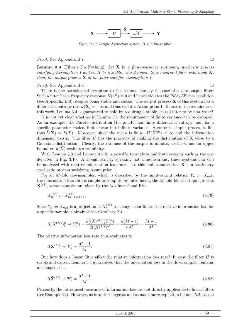
3.5 Application: Multirate Signal Processing & Sampling
X H ↓M YX
Figure 3.10: Simple decimation system. H is a linear filter.
Proof. See Appendix B.7.
Lemma 3.4 (Filter’s Do Nothing). Let X be a finite-variance stationary stochastic processsatisfying Assumption 1 and let H be a stable, causal linear, time invariant filter with input X;then, the output process X of the filter satisfies Assumption 1.
Proof. See Appendix B.8.There is one pathological exception to this lemma, namely the case of a zero-output filter:
Such a filter has a frequency response H(eθ) ≡ 0 and hence violates the Paley-Wiener condition(see Appendix B.8), despite being stable and causal. The output process X of this system has adifferential entropy rateh(X) = −∞ and thus violates Assumption 1. Hence, in the remainder ofthis work, Lemma 3.4 is guaranteed to hold by requiring a stable, causal filter to be non-trivial.It is not yet clear whether in Lemma 3.4 the requirement of finite variance can be dropped:
As an example, the Pareto distribution [45, p. 145] has finite differential entropy and, for aspecific parameter choice, finite mean but infinite variance. Assume the input process is iid,thus h(X) = h(X). Moreover, since the mean is finite, H(X(0)) < ∞ and the informationdimension exists. The filter H has the property of making the distribution of X close to aGaussian distribution. Clearly, the variance of the output is infinite, so the Gaussian upperbound on h(X) evaluates to infinity.With Lemma 3.3 and Lemma 3.4 it is possible to analyze multirate systems such as the one
depicted in Fig. 3.10. Although strictly speaking not time-invariant, these systems can stillbe analyzed with relative information loss rates. To this end, assume that X is a stationarystochastic process satisfying Assumption 1.For an M -fold downsampler, which is described by the input-output relation Yn := XnM ,
the information loss rate is simple to compute by introducing the M -fold blocked input processX(M ), whose samples are given by the M -dimensional RVs
X(M )n := XnM
(n−1)M+1. (3.79)
Since Yn := XnM is a projection of X(M )n to a single coordinate, the relative information loss for
a specific sample is obtained via Corollary 2.4
l((X(M))n1 → Y n1 ) =
d((X(M))n1 |Y n1 )
d((X(M))n1 )=
n(M − 1)
nM=
M − 1
M. (3.80)
The relative information loss rate thus evaluates to
l(X(M ) → Y) =M − 1
M. (3.81)
But how does a linear filter affect the relative information loss rate? In case the filter H isstable and causal, Lemma 3.4 guarantees that the information loss in the downsampler remainsunchanged, i.e.,
l(X(M ) → Y) =M − 1
M. (3.82)
Presently, the introduced measures of information loss are not directly applicable to linear filters(see Example 22). However, as intuition suggests and as made more explicit in Lemma 5.2, causal
June 3, 2014 – 89 –
3 Information Loss Rate
and stable filters do not change the information content of the signal. Thus, one can abusenotation and exchange stochastic processes (or collections of stochastic processes) if they areequivalent from an informational perspective. In particular, this abuse will be made wheneverthere is a bijection16 between the two processes. As a consequence, also for a stable and causalfilter H one has
l(X(M ) → Y) = l(X(M ) → Y) =M − 1
M. (3.83)
The question remains whether an ideal anti-aliasing low-pass filter (or any filter violating thePaley-Wiener condition17) can eliminate, or at least reduce, the relative information loss rate.Clearly, as an ideal anti-aliasing filter limits the bandwidth of the process, the downsamplerwill not cause any information loss. In this case, however, the information is lost already in thefilter:
Theorem 3.3 (Anti-Aliasing Filters are Useless). Let X be a finite-variance, Gaussian sta-tionary stochastic process satisfying Assumption 1. The relative information loss rate in themultirate system depicted in Fig. 3.10 is
l(X→ Y) ≥ M − 1
M(3.84)
for all linear, time-invariant filters H with finitely many stop-bands.
Proof. See Appendix B.9.Note that a general filter can destroy an arbitrarily large amount of information, hence the
inequality: Taking the pathological zero-output filter, for example, the relative information lossrate evaluates to 100% for every downsampling factor M .While the proof is given only for Gaussian processes, the author believes that Theorem 3.3
is valid for all finite-variance processes satisfying Assumption 1. The proof in Appendix B.9discusses a promising way to prove this result.The intuition behind this result is that the ideal anti-aliasing low-pass eliminates a relative
fraction of (M − 1)/M of the spectral components18 of X, which yields the according relative
16 Note that a stable and causal linear filter may not have a stable and causal inverse. A particularly simpleexample to illustrate this claim is when H has a rational transfer function: The inverse transfer function maynot be stable if required to be causal, but a non-causal, stable inverse will always exist. Thus, taking thecomplete process X, it is possible to infer the input process X. Only zeros in the frequency response leadto components which cannot be reconstructed. However, isolated zeros in the frequency response cancel onlycomplex exponentials with corresponding frequencies; components which do not contribute to the entropy rateof the process.
17 If the PSD SX(eθ) of a stationary process violates the Paley-Wiener condition, according to Martin Schet-zen [134, p. 169]: “[The future of the signal violating]
1
2π
∫ π
−π
lnSX(eθ)dθ > −∞
can be completely determined from its own past with arbitrarily small error [...] If the future of your speechwaveform were predictable with arbitrary small error, then all that you will say in the future is predeterminedand you would not be able to change it. Thus your free will would be definitely limited.” Schetzen thusconcludes that the PSD of our speech waveform cannot be nonzero in any band. The author of this work isnot sure whether he agrees with this conclusion.
18 An interesting aspect of these spectral considerations is the following: Eliminating spectral components leadsto a band-limited process, for which the differential entropy rate evaluates to −∞. In other words, the processbecomes predictable [134, p. 169]. This suggests that the information dimension of n consecutive samplesof the process will be strictly smaller than n, for n large enough. One might now ask if the concept ofinformation dimension introduced by Renyi [123] can be generalized to stochastic processes, e.g., by d(X) :=limn→∞ d(Xn
1 )/n. Furthermore, is there a relation between the information dimension of the process and itsbandwidth, at least if the process is Gaussian? Simple examples (a predictable, sinusoidal process or an ideallylow-pass filtered process) at least suggest so.
– 90 – June 3, 2014

3.6 Outlook: Information Loss Rate in Systems with Memory
information loss rate. Although no information is lost in the downsampler, the total relativeinformation loss rate stays the same: Here, information is already lost in the linear filter.The consequence of these considerations is quite interesting, and parallels the reasoning for
the PCA example in Section 2.6: When no signal model is available for the stochastic processX, i.e., when it is not clear which part of the input information is relevant, anti-aliasing low-passfiltering is completely neutral in information-theoretic terms. The following example makes thisexplicit and summarizes the previous analysis:
Example 21: Anti-Aliasing Filters are Useless.
θ
SX(eθ)
π−π
σ2
θ
|H(eθ)|
π −π θ
|H(eθ)|
π −π θ
|H(eθ)|
π −π
Let X be a stationary Gaussian process with PSD SX(eθ) = σ2 + 1 + cos(θ) depictedabove. It shall be the input process to the multirate system in Fig. 3.10 with M = 2. Tominimize the information loss rate across the downsampler, H can be any of the followingthree options (see above):
(a) An ideal anti-aliasing low-pass filter with cut-off frequency θc =π2 ,
(b) An FIR low-pass filter satisfying the Paley-Wiener conditions,
(c) A direct connection, i.e., H(eθ) = 1 for all θ.
Energetic considerations would rank the three options in the given order; however, all areequivalent in terms of the relative information loss rate, which equals
l(X(2) → Y) =1
2(3.85)
in all cases.
While the results of this section focus on discrete-time processes and decimation systems, theanalysis can be extended to sampling continuous-time processes as well. This extension may bebased on the sampling expansion of a bandlimited input process and successive downsampling.If the input process is not bandlimited, it is the author’s conjecture that the relative informationloss rate is unity, i.e., that 100% of the information is lost.
3.6 Outlook: Information Loss Rate in Systems with Memory
The measures of information loss presented in this work are not directly applicable to systemswith memory, as the following example shows:
June 3, 2014 – 91 –
3 Information Loss Rate
Example 22: Linear Filters and Information Loss Rate.Consider the simple FIR filter given by the input-output difference equation Yn = aXn−1+
Xn, where |a| < 1. Assume that the input process X is iid, and that the marginal probabilitymeasure, supported on R, satisfies PX ≪ λ. First, note that
H(Xn0 |Y n
1 ) = H(X0|Y n1 , Xn
1 ) +H(Xn1 |Y n
1 ) (3.86)
(a)= H(X0|Y1, X
n1 ) +H(Xn
1 |Y n1 ) (3.87)
(b)= H(Xn
1 |Y n1 ) (3.88)
where (a) follows from the definition of the output and where (b) follows from the fact thatX0 can be computed from Y1 and X1. But the mapping from Xn
0 to Y n1 is a mapping from
Rn+1 to Rn, and can be written as the cascade of a linear map and a projection. Therefore,and by the assumption that X is iid and has a marginal PDF,
l(Xn0 → Y n
1 ) =1
n+ 1> 0. (3.89)
By Proposition 2.9 it follows that H(Xn0 |Y n
1 ) =∞ and, therefore,
H(Xn1 |Y n
1 ) = L(Xn1 → Y n
1 ) =∞ (3.90)
for all n, and hence L(X→ Y) = ∞. But this naturally conflicts with the intuition that
stable and causal filters do not change the information content of a signal (cf. Lemma 5.2).
Moreover, it conflicts with the fact that the filter is minimum-phase and has, therefore, a
stable and causal inverse (invertable systems cannot induce an information loss). Hence, the
proposed measures of information loss rate cannot immediately be applied to system with
memory, e.g., linear filters.
At least in case the involved processes have finite or countable alphabets, some preliminaryresults on the information loss rate can be presented. To this end, letX be a two-sided stationarystochastic process with finite alphabet X . Consider the following class of systems:
Definition 3.9 (Finite-Dimensional Dynamical System). Let Yn = f(Xnn−N , Y n−1
n−M ), 0 ≤M,N <∞, be the RV of the n-th output sample of a dynamical system with a finite-dimensional statevector subject to the input process X. Here, f : XN+1 × YM → Y is a function such that thesequence of output samples, Yn, constitutes a two-sided stochastic process Y jointly stationarywith X.
Lemma 3.5. Let X and Y be jointly stationary stochastic processes related as in Definition 3.9.Then, for M <∞,
H (X) = limn→∞
1
nH(Xn
1 |Y M1 ) = lim
n→∞1
nH(Xn
1 , YM1 ). (3.91)
Proof. Clearly,
H(Xn1 |Y M
1 ) ≤ H(Xn1 ) ≤ H(Xn
1 , YM1 ) (3.92)
for all n, thus also in the limit. Now, since H(Xn1 , Y
M1 ) = H(Xn
1 |Y M1 ) +H(Y M
1 ) and since allinvolved entities are non-negative,
H (X) ≤ limn→∞
1
nH(Xn
1 |Y M1 ) + lim
n→∞1
nH(Y M
1 )︸ ︷︷ ︸
→0
(3.93)
if the first limit exists. But by assumption and (3.5), H(Xn1 |Y M
1 ) ≥ H(Xn1 |XM
−∞) = (n −
– 92 – June 3, 2014
3.6 Outlook: Information Loss Rate in Systems with Memory
M)H (X), and therfore the limit exists:
limn→∞
n−M
nH (X) ≤ lim
n→∞1
nH(Xn
1 |Y M1 ) ≤H (X) (3.94)
Thus, in the limit the upper and lower bound are equal and the proof is completed.Intuitively, one would suspect that for dynamical systems, i.e., systems with memory, the last
equality of Definition 3.2, stating that L(X→ Y) =H (X)−H (Y) would not hold. As the nextresult shows, this intuition is wrong:
Proposition 3.17. Let X and Y be jointly stationary processes related as in Definition 3.9.Then, the information loss rate is given by the difference of entropy rates:
L(X→ Y) =H (X)−H (Y). (3.95)
Proof. The proof follows with Definition 3.2,
L(X→ Y) = limn→∞
1
nH(Xn
1 |Y n1 ) = lim
n→∞1
nH(Xn
1 )− limn→∞
1
nH(Y n
1 ) (3.96)
where the second equality needs to be proved. Consider that, for n > maxM,N
H(Xn1 , Y
n1 ) = H(Yn, X
n1 , Y
n−11 ) (3.97)
= H(f(Xnn−N , Y n−1
n−M ), Xn1 , Y
n−11 ) (3.98)
= H(Xn1 , Y
n−11 ) (3.99)
...
= H(Xn1 , Y
maxM,N1 ). (3.100)
Lemma 3.5 and the chain rule complete the proof.This result is interesting since it allows to employ Proposition 3.9 to the cascade of two or more
systems also to the case where the systems are dynamic. In general, however, the computation ofentropy rates is a non-trivial problem, where closed-form solutions exist only for simple processes(e.g., Markov chains). Since even functions of Markov chains only rarely allow such a simplifiedtreatment (cf. Section 3.2), the availability of bounds is of great importance.
Proposition 3.18 (Upper Bound). Let X and Y be jointly stationary processes related as inDefinition 3.9. Then, the information loss rate is bounded by
L(X→ Y) ≤ max(x,θ)∈X×T
log card(f−1θ [fθ(x)]) (3.101)
where T = XN ×YM , θ ∈ T are the possible values of the RV Θn = Xn−1n−N , Y n−1
n−M, and f−1θ [·]
denotes the preimage under fθ, an instantiation of the function fΘn(·) = f(·,Θn).
Proof.
L(X→ Y) = limn→∞
1
nH(Xn
1 |Y n1 ) (3.102)
(a)= lim
n→∞1
n
n∑
i=1
H(Xi|Xi−11 , Y n
1 ) (3.103)
(b)
≤ limn→∞
1
n
n∑
i=1
H(Xi|Xi−11 , Y i
1 ) (3.104)
where (a) is due to the chain rule of entropy and (b) is due to conditioning. The expressionunder the sum in (3.104) is a non-negative decreasing sequence in i and thus has a limit. Its
June 3, 2014 – 93 –
3 Information Loss Rate
Cesaro mean exists [21, Thm. 4.2.3, p. 76], and one obtains
L(X→ Y) ≤ limn→∞
H(Xn|Xn−11 , Y n
1 ) (3.105)
≤ H(Xn|Xn−1n−N , Y n
n−M ) (3.106)
= H(Xn|Yn,Θn). (3.107)
One can now write Yn = f(Xn,Θn) = fΘn(Xn) by treating the collection of all previous RVsinfluencing Yn as a (random) parameter Θn of the function. This approach interprets thedynamical system as a parameterized static system fΘn : X → Y, where Θn takes values θ fromT = XN × YM .
L(X→ Y) ≤ H(Xn|fΘn(Xn),Θn) (3.108)
=∑
(x,θ)∈X×TH(Xn|fΘn(Xn) = fθ(x),Θn = θ)Pr(Xn = x,Θn = θ) (3.109)
(c)
≤∑
(x,θ)∈X×Tlog card(f−1
θ [fθ(x)])Pr(Xn = x,Θn = θ) (3.110)
≤ max(x,θ)∈X×T
log card(f−1θ [fθ(x)]) (3.111)
where (c) is due the maximum entropy property of the uniform distribution over an alphabet sizeequal to the cardinality of the preimage under fθ. Maximizing over all possible x and parametervalues θ completes the proof.
3.6.1 Partially Invertible Systems
To investigate yet another class of systems, consider an additional restriction on the systemfunction in Definition 3.9. This additional restriction defines a class for which the informationloss rate can be shown to vanish.
Definition 3.10 (Partially invertible system). A system satisfying Definition 3.9 is partiallyinvertible if there exists a function finv such that
Xn = finv(Xn−1n−N , Y n
n−M ) = finv(Yn,Θn) = f−1Θn
(Yn). (3.112)
In other words, a system is partially invertible if its parameterized static function fΘn is invertiblefor all possible parameter values θ ∈ T .It will next be shown that partially invertible systems are information lossless. To this end,
consider
Definition 3.11 (Information-Lossless System). A system satisfying Definition 3.9 is calledinformation-lossless, if and only if L(X→ Y) = 0 for all stationary stochastic processes Xtaking values from the set X , for which the system responds with an output process Y jointlystationary with X.
Proposition 3.19. Partially invertible systems are information-lossless, i.e.,
L(X→ Y) = 0. (3.113)
Proof. For all θ ∈ T , the parameterized function fθ is invertible at all points of the image of X(which may be a strict subset of Y in this case). Thus, card(f−1
θ [fθ(x)]) = 1 for all x ∈ X andθ ∈ T . Proposition 3.18 completes the proof.Note that the converse is not true, i.e., there exist information-lossless systems which are
not partially invertible. For example, let f be such that, for all input processes X on X , the
– 94 – June 3, 2014
3.6 Outlook: Information Loss Rate in Systems with Memory
sequence of M consecutive output samples Y n−1n−M takes values from a strict subset of YM . As
a consequence, the parameterized function fθ needs not be invertible for all parameters θ ∈ T ,but only for values which are achievable:
Example 23: Information Lossless but not Partially Invertible.Consider a linear filter described by the difference equation
Yn = Xn + αYn−1 (3.114)
with α > 0.5 and an input process X taking values from the set X = [−a, a] ∩ Q. Con-sequently, the output process takes values from the set Y = [ −a
1−α, a1−α
]. However, themaximum amount by which two consecutive output values can differ is given by
max |Yn − Yn−1| = 2a <a
1− α. (3.115)
By Definition 3.10, the linear filter described by (3.114) is partially invertible, thus alsoinformation-lossless. However, let us now modify the system equation such that the outputis given as
Yn = fY n−1n−2
(Xn) =
Xn + αYn−1, if |Yn−1 − Yn−2| ≤ 2a
0, else. (3.116)
Since the condition above is always (i.e., for all possible input processes and initial valuesof the system states) fulfilled, the system is information-lossless; however, the system isnot partially invertible, since there exist points in Y2 for which the parameter values θ ofΘn = Y n−1
n−2 have a difference greater than 2a. And since for these parameter values thefunction delivers zero as output regardless of the input, the preimage is not a singleton.
Next, consider the following system:
Yn =
Xn + αYn−1, if |Yn−1 − Yn−2| ≤ 2a
Yn−2, else(3.117)
Again, this system is not partially invertible, since for some parameter values the system
responds with a single value regardless of the input. However, depending on the initial
conditions the system may not even be information-lossless: Assume that initially |Yn−1 −Yn−2| > 2a. Then, as it can be verified easily, the output oscillates between these two
initial values and all information is lost. This suggests a connection between preservation of
information and the stability properties (asymptotic stability, input-to-state stability, etc.)
of the nonlinear system.
Indeed, the class of partially invertible systems not only proves to have vanishing informationloss rate, but also finite absolute information loss: By observing a sequence of output samplesY n1 , the total information loss corresponds to the uncertainty about the initial values of the
corresponding input sequence. Indeed, for n > maxM,N, it turns out that [50, Thm. 4]
H(Xn1 |Y n
1 ) = H(XmaxM,N1 |Y n
1 ). (3.118)
Note that even though fΘn is invertible for all parameter values θ, this does not mean thatH(Xn|fΘn(Xn)) = 0; however, H(Xn|fΘn(Xn),Θn) = 0 holds. This is due to the fact that, forn < maxM,N, Θn is unknown.
The class of information lossless systems contains the class of systems which permit perfectreconstruction of the input as a proper subclass: While the possibility of perfect reconstructionautomatically yields a vanishing information loss rate, the converse is not true, even if recon-struction errors are allowed in the first maxM,N samples. The following example illustrates
June 3, 2014 – 95 –
3 Information Loss Rate
this fact:
Example 24: Multiplying Consecutive Inputs.The following system can be shown to be partially invertible in the sense of Definition 3.10:
Yn = XnXn−1 (3.119)
The partial inverse is Xn = Yn
Xn−1if Xn−1 6= 0, while for Xn−1 = 0 no such inverse exists.
Therefore, this example represents a class of systems whose partial invertibility depends onthe alphabet X of the stochastic process. If the process X is such that X does not containthe element 0, the partial inverse exists and one obtains for Xn, n > 1:
Xn =
X1
∏n−12
k=1Y2k+1
Y2k, for odd n
Yn
X1
∏n2 −1
k=1Y2k
Y2k+1, for even n
(3.120)
Indeed, since all Xn, n > 1, can be computed from X1 and Y n1 , it follows that H(Xn
1 |Y n1 ) =
H(X1|Y n1 ). Reconstruction of X is thus possible up to an unknown X1. Note, however, that
this unknown sample influences the whole reconstructed sequence as shown in (3.120). Thus,
even though the information loss rate vanishes, perfect reconstruction of any subsequence
of X is impossible by observing the corresponding output sequence only.
The notion of partial invertibility might play a role in the equalization or linearization of mildlynonlinear Volterra systems [77, 110]. In particular, [77] presented a sufficient condition for aniterative equalization method to converge. To fulfill the condition, the linear part of the Volterrasystem needs to be dominant and invertible. It can be shown that the sufficient condition of [77]is sufficient but not necessary for partial invertibility according to Definition 3.10.
3.6.2 Example: Fixed-Point Implementation of a Linear Filter
An important subclass of discrete-time stable causal linear filters falls in the category of partiallyinvertible systems, as long as the input and output alphabets are countable. An example wherethe latter condition is satisfied is given if the input process and the coefficients take values fromthe field of rational numbers. This subclass, powerful enough to cover most applications [29],comprises filters with a finite-dimensional state vector described by constant-coefficient differenceequations:
Yn =N∑
k=0
bkXn−k +M∑
l=1
alYn−l (3.121)
As noted in [113], stability of the filter guarantees that for a stationary input process the outputprocess is stationary and that Definition 3.9 applies. By rearranging the terms in (3.121) itcan be verified that this subclass of linear systems satisfies the definition of partially invertiblesystems and, thus, has a vanishing information loss rate.
It is noteworthy that this property is independent of the minimum-phase property (cf. [111,pp. 280]) of linear filters, which ensures that the filter has a stable and causal inverse. Indeed, forfilters which are not minimum-phase, the partial inverse function finv in Definition 3.10 describesa causal, but unstable linear filter. As a consequence, to an arbitrary stationary stochastic inputprocess, the inverse filter described by finv may respond with a non-stationary output process;however, the response to Y will be X.
A signal space model may effectively illustrate these considerations: Let X∞ and Y∞ be thespaces of stationary input and output processes X and Y, respectively, and let F· be the(linear) operator mapping each element of X∞ to Y∞. By restricting our attention to regular
– 96 – June 3, 2014
3.6 Outlook: Information Loss Rate in Systems with Memory
stochastic processes, i.e., processes which cannot have periodic components, the operator F·is injective. As a consequence, for each element of Y∞ there exists at most one element inX∞ such that Y = FX. Note, however, that there are stationary stochastic processes inY∞ which are not images of elements in X∞. Only if F· is such that it describes a stable,causal minimum-phase system, i.e., has a stable and causal inverse, Y∞ contains only images ofelements from X∞.Linear filters, if stable and causal, can thus be assumed to be lossless from an information-
theoretic point-of-view. It is surprising, though, that even filters with finite precision, i.e.,non-linear filters, can preserve information:
Example 25: Finite-Precision Linear Filters.In many practical applications in digital signal processing linear filters are implemented
with finite-precision number representations only. Thus assume that both input process andfilter coefficients take values from a finite set. For example, X may be a finite subset of therational numbers Q, closed under modulo-addition. Multiplying two values from that set,e.g., by multiplying an input sample with a filter coefficient, typically yields a result notrepresentable in X . As a consequence, after every multiplication a quantizer is necessary,essentially truncating the additional bits resulting from multiplication. Let the quantizerbe described by a function Q: R → X with Q (a+Xn) = Q (a) ⊕Xn if Xn ∈ X , where ⊕denotes modulo-addition (e.g., [111, pp. 373]). With this, (3.121) changes to
Yn =N⊕
k=0
Q (bkXn−k)⊕M⊕
l=1
Q (alYn−l) (3.122)
or
Yn = Q
(N⊕
k=0
bkXn−k ⊕M⊕
l=1
alYn−l
)
(3.123)
depending whether quantization is performed after multiplication or after accumulation (inthe latter case, the intermediate results are represented in a larger set X ′). Note that dueto modulo-addition the result Yn remains in X .
Focus on filters with b0 = 1. For filters with infinite precision this can be done without lossof generality by considering a constant gain factor b0 and by normalizing all bk coefficients.However, this gain normalization poses a restriction in the finite-precision case since bk/b0is not necessarily an element of X . With b0 = 1, (3.122) and (3.123) change to
Yn = Xn ⊕(
N⊕
k=1
Q (bkXn−k)⊕M⊕
l=1
Q (alYn−l)
)
(3.124)
and
Yn = Xn ⊕Q
(N⊕
k=1
bkXn−k −M⊕
l=1
alYn−l
)
(3.125)
by the property of the quantizer. From this it can be seen that either implementation
is partially invertible (the terms in parentheses in (3.124) and (3.125) are both in X , andmodulo-addition has an inverse element). Consequently, even filters with nonlinear elements
can be shown to preserve information under certain circumstances despite the fact that the
quantizer function is non-injective.
How does the fact that linear filters – finite-precision or not – preserve information connect toExample 22, which claims that even an invertible filter destroys an infinite amount of informationin each time unit? The answer is that Example 22 just illustrated that the proposed measureof information loss rate is not suitable for systems with memory in the general case. It is well-
June 3, 2014 – 97 –
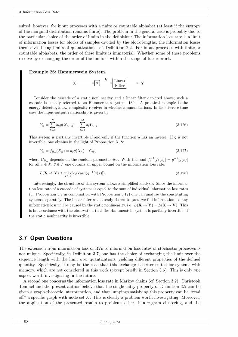
3 Information Loss Rate
suited, however, for input processes with a finite or countable alphabet (at least if the entropyof the marginal distribution remains finite). The problem in the general case is probably due tothe particular choice of the order of limits in the definition: The information loss rate is a limitof information losses for blocks of samples divided by the block lengths; the information lossesthemselves being limits of quantizations, cf. Definition 2.2. For input processes with finite orcountable alphabets, the order of these limits is immaterial. Whether some of these problemsresolve by exchanging the order of the limits is within the scope of future work.
Example 26: Hammerstein System.
X g LinearFilter
YV
Consider the cascade of a static nonlinearity and a linear filter depicted above; such acascade is usually referred to as Hammerstein system [139]. A practical example is theenergy detector, a low-complexity receiver in wireless communications. In the discrete-timecase the input-output relationship is given by
Yn =
N∑
k=0
bkg(Xn−k) +
M∑
l=1
alYn−l. (3.126)
This system is partially invertible if and only if the function g has an inverse. If g is notinvertible, one obtains in the light of Proposition 3.18:
Yn = fΘn(Xn) = b0g(Xn) + CΘn
(3.127)
where CΘndepends on the random parameter Θn. With this and f−1
θ [fθ(x)] = g−1[g(x)]for all x ∈ X , θ ∈ T one obtains an upper bound on the information loss rate:
L(X→ Y) ≤ maxx∈X
log card(g−1[g(x)]) (3.128)
Interestingly, the structure of this system allows a simplified analysis: Since the informa-
tion loss rate of a cascade of systems is equal to the sum of individual information loss rates
(cf. Proposition 3.9 in combination with Proposition 3.17) one can analyze the constituting
systems separately. The linear filter was already shown to preserve full information, so any
information loss will be caused by the static nonlinearity, i.e.,L(X→ Y) =L(X→ V). This
is in accordance with the observation that the Hammerstein system is partially invertible if
the static nonlinearity is invertible.
3.7 Open Questions
The extension from information loss of RVs to information loss rates of stochastic processes isnot unique. Specifically, in Definition 3.7, one has the choice of exchanging the limit over thesequence length with the limit over quantizations, yielding different properties of the definedquantity. Specifically, it may be the case that this exchange is better suited for systems withmemory, which are not considered in this work (except briefly in Section 3.6). This is only oneaspect worth investigating in the future.
A second one concerns the information loss rate in Markov chains (cf. Section 3.2). ChristophTemmel and the present author believe that the single entry property of Definition 3.5 can begiven a graph-theoretic interpretation, and that lumpings satisfying this property can be “readoff” a specific graph with node set X . This is clearly a problem worth investigating. Moreover,the application of the presented results to problems other than n-gram clustering, and the
– 98 – June 3, 2014
3.7 Open Questions
improvement of the algorithm should be part of future work. The present author also founddifferent sufficient conditions for 2-lumpability, which should be investigated; in particular, theinterplay between these conditions and the SFS(2)-property should be analyzed. Furthermore,performance bounds for SFS(2)-lumpings and a complexity analysis of the algorithm as a functionof the graph degree could be developed. Finally, the optimality of SFS(k)- lumpings in terms ofcompression, and the generalization to non-stationary, time-homogeneous Markov chains wouldbe important.A connection between the information loss rate and the probability of reconstruction error
would give the former quantity an operational meaning. Reconstruction of nonlinearly distortedsequences is difficult, and performance bounds would be helpful in this regard.In Section 3.5, relative information loss was employed for analyzing decimation systems. The
generalization to sampling devices was hinted at, but not thoroughly analyzed. Future work shallfill this gap, which will probably need an information measure for continuous-time, continuous-amplitude stochastic processes. It is also of great interest if there are systems and/or processes,for which the relative information loss rate is strictly smaller than the relative information loss,cf. Proposition 3.16.Another interesting question is whether, at least for discrete-time Gaussian processes, the
definition of an information dimension rate makes sense, and if it is connected to the bandwidthof the process. The tools for such an analysis might be, again, a filterbank decomposition,Renyi’s information dimension, and the Paley-Wiener theorem.Paralleling the analysis of sample covariance-based PCA in Section 2.6.2, it might be interest-
ing if similar results can be obtained for adaptive filters, i.e., filters which depend on the inputsignal. In other words, assuming that the adapted filter coefficients are not transmitted, whatis the (relative) information loss (rate) in, e.g., and LMS-adapted linear predictor?Of course, the extension to systems with memory is of great importance, but, as the author
believes, also one of great difficulty. Probably, results can be obtained for restricted classes ofsystems, such as Volterra systems. The relevance of these results in practical applications (e.g.,linearization or equalization of systems, as mentioned in Section 3.6) shall also be investigated.
June 3, 2014 – 99 –

Information Loss in Deterministic Systems
4Relevant Information Loss
The notion of relevant information loss was first employed in [55]; an essentially identical quan-tity was introduced earlier by Plumbley in [118]. The idea for this metric was written downsimultaneously by the present author and Gernot Kubin, although the latter had had it in mindprobably much longer. It was essentially his idea to apply this quantity for signal enhancement;the present author found its connection to the information bottleneck method, as indicated inSection 4.2.The part on Markov chain aggregation in Section 4.3 was developed in cooperation with
Tatjana Petrov, Gernot Kubin, and Heinz Koppl [47]. In particular, the theoretic results havemainly been discovered by the present author; much of the notation is due to Dr. Petrov.The example on bio-molecular systems in Section 4.3.6 has also been written by her, while thesimulations have been carried out together with the present author.The results on PCA in Section 4.4, again influenced by Gernot Kubin, are published in [55].
Inaccurate function knowledge was considered by the main author only; the results of the cor-responding Section 4.5 are unpublished.
4.1 The Problem of Relevance - A General Definition
As the examples in Sections 2.6 and 3.5 showed, both the absolute and the relative definition ofinformation loss have their shortcomings, especially when it comes to systems g used for signalenhancement: Since the expressions only consider the RV X at the input of the system, they donot take into account that not all of the information contained in X is relevant, often leadingto counter-intuitive results. The main contribution of this chapter lies thus in analyzing theimplications of
Definition 4.1 (Relevant Information Loss). Let X be an RV with alphabet X , and let Y =g(X). Let S be another RV with alphabet S representing relevant information. The informationloss relevant w.r.t. S is
LS(X → Y ) = limn→∞
(
I(S(n);X)− I(S(n);Y ))
= I(X;S|Y ). (4.1)
The last equality holds because Y is a function of X and, thus,
limn→∞
(
I(S(n);X)− I(S(n);Y ))
= limn→∞
(
I(S(n);X,Y )− I(S(n);Y ))
(4.2)
= limn→∞
I(S(n);X|Y ) (4.3)
June 3, 2014 – 101 –
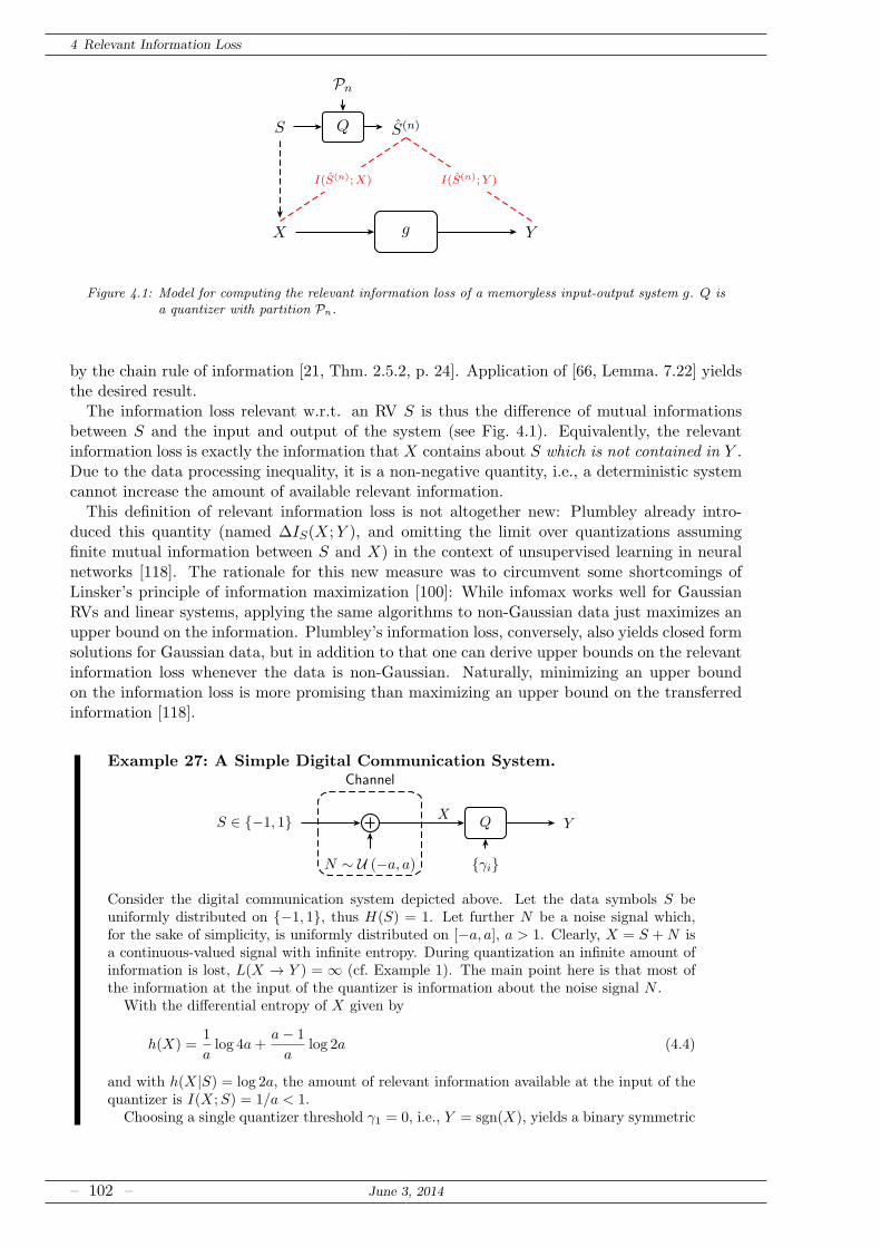
4 Relevant Information Loss
X g Y
S
Pn
Q S(n)
I(S(n);X) I(S(n);Y )
Figure 4.1: Model for computing the relevant information loss of a memoryless input-output system g. Q isa quantizer with partition Pn.
by the chain rule of information [21, Thm. 2.5.2, p. 24]. Application of [66, Lemma. 7.22] yieldsthe desired result.The information loss relevant w.r.t. an RV S is thus the difference of mutual informations
between S and the input and output of the system (see Fig. 4.1). Equivalently, the relevantinformation loss is exactly the information that X contains about S which is not contained in Y .Due to the data processing inequality, it is a non-negative quantity, i.e., a deterministic systemcannot increase the amount of available relevant information.This definition of relevant information loss is not altogether new: Plumbley already intro-
duced this quantity (named ∆IS(X;Y ), and omitting the limit over quantizations assumingfinite mutual information between S and X) in the context of unsupervised learning in neuralnetworks [118]. The rationale for this new measure was to circumvent some shortcomings ofLinsker’s principle of information maximization [100]: While infomax works well for GaussianRVs and linear systems, applying the same algorithms to non-Gaussian data just maximizes anupper bound on the information. Plumbley’s information loss, conversely, also yields closed formsolutions for Gaussian data, but in addition to that one can derive upper bounds on the relevantinformation loss whenever the data is non-Gaussian. Naturally, minimizing an upper boundon the information loss is more promising than maximizing an upper bound on the transferredinformation [118].
Example 27: A Simple Digital Communication System.
S ∈ −1, 1
N ∼ U (−a, a)
Q
γi
Y
Channel
X
Consider the digital communication system depicted above. Let the data symbols S beuniformly distributed on −1, 1, thus H(S) = 1. Let further N be a noise signal which,for the sake of simplicity, is uniformly distributed on [−a, a], a > 1. Clearly, X = S +N isa continuous-valued signal with infinite entropy. During quantization an infinite amount ofinformation is lost, L(X → Y ) = ∞ (cf. Example 1). The main point here is that most ofthe information at the input of the quantizer is information about the noise signal N .
With the differential entropy of X given by
h(X) =1
alog 4a+
a− 1
alog 2a (4.4)
and with h(X|S) = log 2a, the amount of relevant information available at the input of thequantizer is I(X;S) = 1/a < 1.
Choosing a single quantizer threshold γ1 = 0, i.e., Y = sgn(X), yields a binary symmetric
– 102 – June 3, 2014
4.1 The Problem of Relevance - A General Definition
channel with cross-over probability Pe =a−12a . With H2(·) being the binary entropy function
the mutual information thus computes to I(Y ;S) = 1−H2(Pe) [21, p. 187]. Consequently,one gets a relevant information loss of
LS(X → Y ) = H2(a− 1
2a)− a− 1
a. (4.5)
Using two quantizer thresholds γ1 = 1 − a and γ2 = a − 1 yields a ternary outputRV Y . Interpreting any value γ1 ≤ X ≤ γ2 as an erasure, one obtains a binary erasurechannel with erasure probability a−1
a. The corresponding mutual information computes to
I(Y ;S) = 1a[21, p. 188], and the relevant information loss vanishes.
As this example shows, while the quantizer destroys an infinite amount of information
(to be precise, the relative information loss is 100%), the relevant information loss can still
be zero. Signal enhancement, in the sense of removing irrelevant information, was thus
successful.
4.1.1 Elementary Properties
Before proceeding, the elementary properties of relevant information loss will be analyzed:
Proposition 4.1 (Elementary Properties). The relevant information loss from Definition 4.1satisfies the following properties:
1. LS(X → Y ) ≤ I(S;X) ≤ H(S)
2. LS(X → Y ) ≥ LY (X → Y ) = 0
3. LS(X → Y ) ≤ LX(X → Y ) = L(X → Y ), with equality if X is a function of S.
4. LS(X → Y ) = H(S|Y ) if S is a function of X.
Proof. The first property results immediately from the definition, while the second property isdue to the fact that Y is a function of X. The third property results from making X the relevantRV, thus making Definition 4.1 equal to Definition 2.2. Note that, with L(X → Y ) = H(X|Y ),
LS(X → Y ) = I(S;X|Y ) = H(X|Y )−H(X|Y, S) ≤ L(X → Y ) (4.6)
with equality if X is a function of S. For S = f(X), the last property follows by expandingI(X;S|Y ) as H(S|Y )−H(S|Y,X) = H(S|Y ).
The third property is of particular interest. Essentially, it states that the relevant informa-tion loss cannot exceed the total information loss, so upper bounds (e.g., those presented inSection 2.3.2) for the latter can be used for the former as well.
Since by Definition 4.1 relevant information loss is represented by a conditional mutual infor-mation, it inherits all of its properties. In particular, a data processing inequality holds:
Proposition 4.2 (Data Processing Inequality). Let V −W −X − Y be a Markov tuple. Then,
LW (X → Y ) ≥ LV (X → Y ). (4.7)
Proof. The proof follows along the same lines as the proof of the data processing inequality formutual information in [21, Thm. 2.8.1, p. 34]. Expanding I(X;W,V |Y ) yields
I(X;W,V |Y ) = I(X;V |Y ) + I(X;W |V, Y ) (4.8)
= I(X;W |Y ) + I(X;V |W,Y ) (4.9)
= I(X;W |Y ) (4.10)
June 3, 2014 – 103 –
4 Relevant Information Loss
where the last line follows from the fact that V and X are conditionally independent given W .With Definition 4.1 one then obtains
LW (X → Y ) = I(X;W |Y ) (4.11)
= I(X;V |Y ) + I(X;W |V, Y ) (4.12)
= LV (X → Y ) + I(X;W |V, Y ) (4.13)
≥ LV (X → Y ) (4.14)
which completes the proof.
The usefulness of this data processing inequality (especially in the context of this work) relieson the fact that both S −X − g(X) and f(S) − S −X are Markov tuples. Comparing this toProposition 4.2 one is tempted to believe that the direction of the inequality depends on thefact whether f(S)−S−X −Y or S− f(S)−X −Y is a Markov tuple. The following corollary,a generalization of the third property of Proposition 4.1, resolves this complication.
Corollary 4.1. Let f be a measurable function defined on the sample space of S. Then,
LS(X → Y ) ≥ Lf(S)(X → Y ) (4.15)
with equality if S − f(S)−X − Y is a Markov tuple.
Proof. The corollary follows immediately from [116, Thm. 3.7.1]. Specifically, if f(S)−S−X−Yis a Markov tuple, the case is trivial. For S− f(S)−X−Y being a Markov tuple, one gets withthe proof of Proposition 4.2
Lf(S)(X → Y ) = LS(X → Y ) + I(X; f(S)|S, Y ) = LS(X → Y ). (4.16)
Inherited from the properties of mutual information, also the relevant information loss obeysa chain rule:
Lemma 4.1 (Chain Rule of Information Loss). The information loss LSn1(X → Y ) induced by
a function g, relevant w.r.t. a collection Sn1 = S1, . . . , Sn of RVs, satisfies
LSn1(X → Y ) =
n∑
i=1
LSi|Si−11
(X → Y ). (4.17)
The proof follows immediately from the chain rule of (conditional) information and is thusomitted. More interestingly, this chain rule justifies our intuitive understanding of the nature ofinformation loss:
Corollary 4.2. The information loss L(X → Y ) induced by a function g can be split intorelevant (w.r.t. S) and irrelevant information loss:
L(X → Y ) = LS(X → Y ) + LX|S(X → Y ) (4.18)
Proof. The proof follows from Lemma 4.1 and from the fact that LXS(X → Y ) = L(X → Y ),since S and Y are conditionally independent given X.
Note that even in a simple scenario with additive noise, i.e., X = S +N , it is not straightfor-ward to just identify the noise N with the irrelevant information:
Example 27: A Simple Digital Communication System (revisited).In this example it is tempting to identify the noise variable N with the irrelevant infor-
mation X|S. However, this not necessarily leads to a correct result:
– 104 – June 3, 2014

4.1 The Problem of Relevance - A General Definition
X
S
g h ZY
LS(X → Y ) LS(Y → Z)
LS(X → Z)
Figure 4.2: Cascade of two systems: The relevant information loss of the cascade is the sum of relevantinformation losses of the constituting systems.
To this end, substitute the quantizer in the system by a magnitude device, i.e., Y ′ =|X|. By the fact that the probability density function of X has even symmetry, one hasL(X → Y ′) = H(X|Y ′) = 1. Further, since the marginal distribution of Y ′ coincides withthe conditional distributions Y |S = −1 and Y |S = 1, the mutual information I(Y ′;S) = 0.Thus, LS(X → Y ′) = 1
aand LX|S(X → Y ′) = a−1
a.
Let us now determine the information loss relevant w.r.t. N . Showing that LN (X →Y ′) 6= LX|S(X → Y ′) proves that noise and irrelevant information are not identical. Observethat
LN (X → Y ′) = I(X;N |Y ′) (4.19)
= H(X|Y ′)−H(X|N,Y ′) (4.20)
= 1−H(S +N |N,Y ′) (4.21)
= 1−H(S|N, |S +N |). (4.22)
Given N , S is uncertain only if |S +N | yields the same value for both S = 1 and S = −1.In other words, only for |N − 1| = |N + 1|. Squaring both sides translates to requiringN = −N , which is fulfilled only for N = 0. Since Pr(N = 0) = 0 (N is a continuous RV),it follows that
LN (X → Y ′) = 1 6= a− 1
a= LX|S(X → Y ′). (4.23)
The reason why one cannot identify the noise with the irrelevant information can be re-lated to N and S not being conditionally independent given X. The findings are summarizedin the table below.
Loss Y = sgn(X) Y = |X|L(X → Y ) ∞ 1
LS(X → Y ) H2(a−12a )− a−1
a1a
LX|S(X → Y ) ∞ a−1a
LN (X → Y ) ∞ 1
LX|N (X → Y ) a−12a 0
A final property worth presenting concerns the cascade of systems (see Fig. 4.2). Assume thatthe output Y of the first system g is used as the input to a second system h, which respondswith the RV Z. In Proposition 2.2 it was shown that the information loss of this cascade isadditive, i.e.,
L(X → Z) = L(X → Y ) + L(Y → Z). (4.24)
The same holds for the relevant information loss, as Plumbley showed in [118]:
Proposition 4.3 (Information Loss in a Cascade is Additive, [118]). Consider two functionsg: X → Y and h: Y → Z and a cascade of systems implementing these functions. Let Y := g(X)and Z := h(Y ). The relevant information loss w.r.t. S induced by this cascade, or equivalently,
June 3, 2014 – 105 –
4 Relevant Information Loss
by the system implementing the composition (h g)(·) = h(g(·)) is given by
LS(X → Z) = LS(X → Y ) + LS(Y → Z). (4.25)
Proof. Note that with Definition 4.1 one gets
LS(X → Z)(a)= I(S;X,Y |Z) (4.26)
(b)= I(S;X|Y, Z) + I(S;Y |Z) (4.27)
(a)= I(S;X|Y ) + I(S;Y |Z) (4.28)
where (a) is due to the fact that Y = g(X) and Z = h(Y ), respectively, and (b) is the chain ruleof information.
4.1.2 A Simple Upper Bound
It was already mentioned that, by the fact LS(X → Y ) ≤ L(X → Y ), the upper bounds ofSection 2.3 can also act as upper bounds on the relevant information loss. In addition to these,the relevant information loss can – under specific assumptions – be upper bounded by lookingat the joint second-order statistics only.
Definition 4.2 (Negentropy). Let X be an RVs with distribution PX ≪ λ, and let XG be aGaussian RVs with the same first and second moments. The negentropy of X is
J(X) := D(fX ||fXG) = h(XG)− h(X) (4.29)
whenever the quantity exists.
Clearly, negentropy is non-negative; it is commonly used as a measure of Gaussianity, as it iszero if and only if X is Gaussian.
Proposition 4.4 (Gaussian Upper Bound). Let S and X be jointly Gaussian RVs and letY := g(X), where g is piecewise bijective. Let further YG (YG, S) be a Gaussian RV with thesame (joint) first and second moments as Y (Y, S). Then,
LS(X → Y ) ≤ LS(X → YG). (4.30)
Proof. By the chain rule of relative entropy [21, Thm. 2.5.3, p. 24] and Gaussianity of S,
J(S, Y ) = D(fS,Y ||fS,YG) (4.31)
= E(D(fS|Y (·|Y )||fS|YG
(·|Y )))+ J(Y ) (4.32)
= E(D(fY |S(·|S)||fYG|S(·|S))
)+ J(S) (4.33)
= E(D(fY |S(·|S)||fYG|S(·|S))
)(4.34)
= h(YG|S)− h(Y |S) =: J(Y |S) (4.35)
from which follows that J(Y ) ≤ J(Y |S). The proof is completed with Definitions 4.2 and 4.1,
LS(X → Y ) = I(S;X)− I(S;Y ) (4.36)
= I(S;X)− h(Y ) + h(Y |S) (4.37)
= I(S;X) + J(Y )− h(YG)− J(Y |S) + h(YG|S) (4.38)
≤ I(S;X)− I(S;YG) = LS(X → YG). (4.39)
Note that the requirement of piecewise bijectivity of g in general cannot be dropped, sinceit guarantees that Y has a PDF. One could extend the previous result to let X and S have
– 106 – June 3, 2014
4.2 Signal Enhancement and the Information Bottleneck Method
arbitrary distribution and qualify the bound as being an upper or a lower bound by refering tothe negentropy of the involved RVs. This does not yield general results, however, since a given(non-linear) function g can both increase or decrease negentropy.
4.2 Signal Enhancement and the Information Bottleneck Method
Consider the discrete case: X and S are RVs with finitely many states, and one is interestedin a lossy compression Y of X which contains as much information about S as possible. Com-pression is related to removing irrelevant information, while preserving relevant information. Infact, this goal is not unique to compression, but is also found in signal enhancement: Often, theinformation one wants to use is not directly available, but only through some corrupted obser-vation. Information-carrying signals are affected by noise, distorted through nonlinear systems,or time-varying, dynamic effects. It is essentially the goal of the signal processing engineer tomitigate all these adverse effects; to improve the quality of the observation such that as muchinformation as possible can be retrieved from it with little effort. Quite similar is the problem offeature extraction from data for, e.g., model identification, cf. [72, p. 53] or pattern recognition.As the data processing inequality dictates, signal enhancement does not mean that one in-
creases the amount of information in the observation. At best, one can build a system whichpreserves as much information as possible. Conversely, noise, distortion, and other irrelevantcomponents of the observation should be removed such that the relevant information can beretrieved easily19.This is where relevant information loss comes in: When S is the information carrying signal
and X its corrupted observation, the goal is to find a system g such that the relevant informationloss is minimized while simultaneously maximizing the irrelevant information loss. One may castthe resulting optimization problem as follows:
maxg
LX|S(X → Y )
s.t. LS(X → Y ) ≤ C (4.40)
where C is some constant. Alternatively, one may minimize the relevant information loss subjectto a lower bound on the reduction of irrelevant information, or use a variational formulation.Let us now investigate whether a particular, variational formulation for maximizing relevant
information can help to solve the abovementioned problem. Consider the following formulationof the information bottleneck method (IB) [145]
minp(y|x)
I(Y ;X)− βI(S;Y ) (4.41)
where the minimization is performed over all relations between the (discrete) RVs Y and X andwhere β is a design parameter20 trading compression for preservation of relevant information,I(S;Y ). While in principle the relation p(y|x) can be stochastic, in many cases an algorithm isused for (hard) clustering using a deterministic function. By the definition of relevant informa-tion loss,
I(S;Y ) = I(S;X)− LS(X → Y ) (4.42)
19 Note that compression often removes redundancy, especially when the compression is lossless. Redundancycan, however, be quite important when it comes to retrieving relevant information: While a bit stream mightcontain almost the same relevant information as a speech waveform, the human listener can extract thisinformation more easily from the latter, redundant, representation. Hence, relevance and redundancy are notinterchangable in this context.
20 By the fact that S −X − Y is a Markov chain and by the data processing inequality, I(X;Y ) ≥ I(S;Y ). As aconsequence, equation (4.41) is lower bounded by (1− β)I(X;Y ), which is a non-negative quantity for β < 1.For this parameter choice the minimum is thus achieved for Y being independent of X, i.e., I(X;Y ) = 0. Thiscan be achieved, for example, by Y being constant. Hence, in this work it is assumed that β > 1.
June 3, 2014 – 107 –
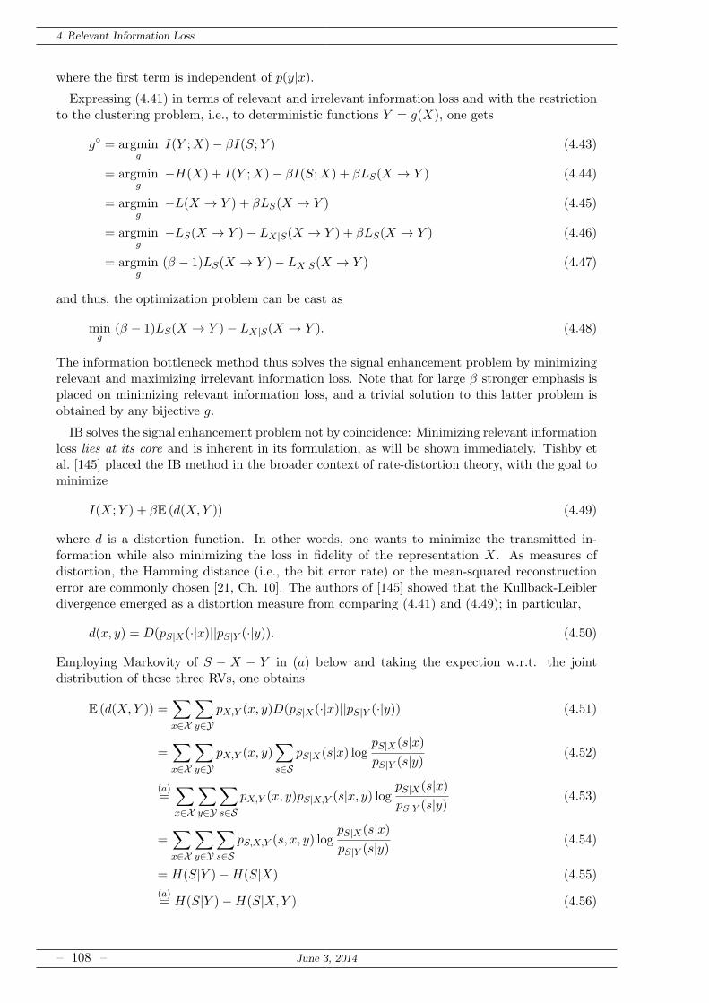
4 Relevant Information Loss
where the first term is independent of p(y|x).Expressing (4.41) in terms of relevant and irrelevant information loss and with the restriction
to the clustering problem, i.e., to deterministic functions Y = g(X), one gets
g = argming
I(Y ;X)− βI(S;Y ) (4.43)
= argming
−H(X) + I(Y ;X)− βI(S;X) + βLS(X → Y ) (4.44)
= argming
−L(X → Y ) + βLS(X → Y ) (4.45)
= argming
−LS(X → Y )− LX|S(X → Y ) + βLS(X → Y ) (4.46)
= argming
(β − 1)LS(X → Y )− LX|S(X → Y ) (4.47)
and thus, the optimization problem can be cast as
ming
(β − 1)LS(X → Y )− LX|S(X → Y ). (4.48)
The information bottleneck method thus solves the signal enhancement problem by minimizingrelevant and maximizing irrelevant information loss. Note that for large β stronger emphasis isplaced on minimizing relevant information loss, and a trivial solution to this latter problem isobtained by any bijective g.
IB solves the signal enhancement problem not by coincidence: Minimizing relevant informationloss lies at its core and is inherent in its formulation, as will be shown immediately. Tishby etal. [145] placed the IB method in the broader context of rate-distortion theory, with the goal tominimize
I(X;Y ) + βE (d(X,Y )) (4.49)
where d is a distortion function. In other words, one wants to minimize the transmitted in-formation while also minimizing the loss in fidelity of the representation X. As measures ofdistortion, the Hamming distance (i.e., the bit error rate) or the mean-squared reconstructionerror are commonly chosen [21, Ch. 10]. The authors of [145] showed that the Kullback-Leiblerdivergence emerged as a distortion measure from comparing (4.41) and (4.49); in particular,
d(x, y) = D(pS|X(·|x)||pS|Y (·|y)). (4.50)
Employing Markovity of S − X − Y in (a) below and taking the expection w.r.t. the jointdistribution of these three RVs, one obtains
E (d(X,Y )) =∑
x∈X
∑
y∈YpX,Y (x, y)D(pS|X(·|x)||pS|Y (·|y)) (4.51)
=∑
x∈X
∑
y∈YpX,Y (x, y)
∑
s∈SpS|X(s|x) log
pS|X(s|x)pS|Y (s|y)
(4.52)
(a)=∑
x∈X
∑
y∈Y
∑
s∈SpX,Y (x, y)pS|X,Y (s|x, y) log
pS|X(s|x)pS|Y (s|y)
(4.53)
=∑
x∈X
∑
y∈Y
∑
s∈SpS,X,Y (s, x, y) log
pS|X(s|x)pS|Y (s|y)
(4.54)
= H(S|Y )−H(S|X) (4.55)
(a)= H(S|Y )−H(S|X,Y ) (4.56)
– 108 – June 3, 2014
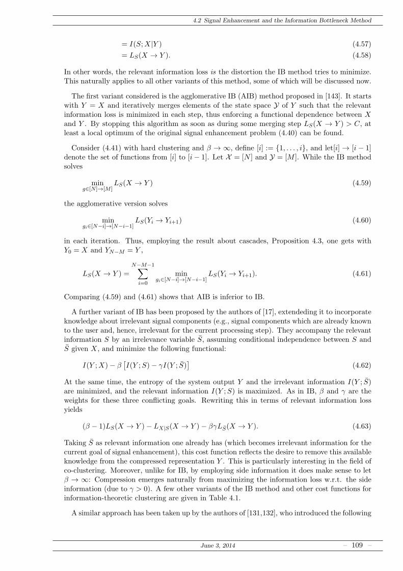
4.2 Signal Enhancement and the Information Bottleneck Method
= I(S;X|Y ) (4.57)
= LS(X → Y ). (4.58)
In other words, the relevant information loss is the distortion the IB method tries to minimize.This naturally applies to all other variants of this method, some of which will be discussed now.
The first variant considered is the agglomerative IB (AIB) method proposed in [143]. It startswith Y = X and iteratively merges elements of the state space Y of Y such that the relevantinformation loss is minimized in each step, thus enforcing a functional dependence between Xand Y . By stopping this algorithm as soon as during some merging step LS(X → Y ) > C, atleast a local optimum of the original signal enhancement problem (4.40) can be found.
Consider (4.41) with hard clustering and β → ∞, define [i] := 1, . . . , i, and let[i] → [i − 1]denote the set of functions from [i] to [i− 1]. Let X = [N ] and Y = [M ]. While the IB methodsolves
ming∈[N ]→[M ]
LS(X → Y ) (4.59)
the agglomerative version solves
mingi∈[N−i]→[N−i−1]
LS(Yi → Yi+1) (4.60)
in each iteration. Thus, employing the result about cascades, Proposition 4.3, one gets withY0 = X and YN−M = Y ,
LS(X → Y ) =N−M−1∑
i=0
mingi∈[N−i]→[N−i−1]
LS(Yi → Yi+1). (4.61)
Comparing (4.59) and (4.61) shows that AIB is inferior to IB.
A further variant of IB has been proposed by the authors of [17], extendeding it to incorporateknowledge about irrelevant signal components (e.g., signal components which are already knownto the user and, hence, irrelevant for the current processing step). They accompany the relevantinformation S by an irrelevance variable S, assuming conditional independence between S andS given X, and minimize the following functional:
I(Y ;X)− β[I(Y ;S)− γI(Y ; S)
](4.62)
At the same time, the entropy of the system output Y and the irrelevant information I(Y ; S)are minimized, and the relevant information I(Y ;S) is maximized. As in IB, β and γ are theweights for these three conflicting goals. Rewriting this in terms of relevant information lossyields
(β − 1)LS(X → Y )− LX|S(X → Y )− βγLS(X → Y ). (4.63)
Taking S as relevant information one already has (which becomes irrelevant information for thecurrent goal of signal enhancement), this cost function reflects the desire to remove this availableknowledge from the compressed representation Y . This is particularly interesting in the field ofco-clustering. Moreover, unlike for IB, by employing side information it does make sense to letβ → ∞: Compression emerges naturally from maximizing the information loss w.r.t. the sideinformation (due to γ > 0). A few other variants of the IB method and other cost functions forinformation-theoretic clustering are given in Table 4.1.
A similar approach has been taken up by the authors of [131,132], who introduced the following
June 3, 2014 – 109 –
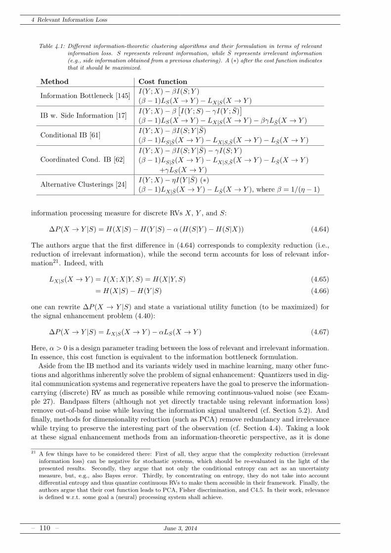
4 Relevant Information Loss
Table 4.1: Different information-theoretic clustering algorithms and their formulation in terms of relevantinformation loss. S represents relevant information, while S represents irrelevant information(e.g., side information obtained from a previous clustering). A (∗) after the cost function indicatesthat it should be maximized.
Method Cost function
Information Bottleneck [145]I(Y ;X)− βI(S;Y )
(β − 1)LS(X → Y )− LX|S(X → Y )
IB w. Side Information [17]I(Y ;X)− β
[I(Y ;S)− γI(Y ; S)
]
(β − 1)LS(X → Y )− LX|S(X → Y )− βγLS(X → Y )
Conditional IB [61]I(Y ;X)− βI(S;Y |S)(β − 1)LS|S(X → Y )− LX|S,S(X → Y )− LS(X → Y )
Coordinated Cond. IB [62]I(Y ;X)− βI(S;Y |S)− γI(S;Y )
(β − 1)LS|S(X → Y )− LX|S,S(X → Y )− LS(X → Y )
+γLS(X → Y )
Alternative Clusterings [24]I(Y ;X)− ηI(Y |S) (∗)(β − 1)LX|S(X → Y )− LS(X → Y ), where β = 1/(η − 1)
information processing measure for discrete RVs X, Y , and S:
∆P (X → Y |S) = H(X|S)−H(Y |S)− α (H(S|Y )−H(S|X)) (4.64)
The authors argue that the first difference in (4.64) corresponds to complexity reduction (i.e.,reduction of irrelevant information), while the second term accounts for loss of relevant infor-mation21. Indeed, with
LX|S(X → Y ) = I(X;X|Y, S) = H(X|Y, S) (4.65)
= H(X|S)−H(Y |S) (4.66)
one can rewrite ∆P (X → Y |S) and state a variational utility function (to be maximized) forthe signal enhancement problem (4.40):
∆P (X → Y |S) = LX|S(X → Y )− αLS(X → Y ) (4.67)
Here, α > 0 is a design parameter trading between the loss of relevant and irrelevant information.In essence, this cost function is equivalent to the information bottleneck formulation.Aside from the IB method and its variants widely used in machine learning, many other func-
tions and algorithms inherently solve the problem of signal enhancement: Quantizers used in dig-ital communication systems and regenerative repeaters have the goal to preserve the information-carrying (discrete) RV as much as possible while removing continuous-valued noise (see Exam-ple 27). Bandpass filters (although not yet directly tractable using relevant information loss)remove out-of-band noise while leaving the information signal unaltered (cf. Section 5.2). Andfinally, methods for dimensionality reduction (such as PCA) remove redundancy and irrelevancewhile trying to preserve the interesting part of the observation (cf. Section 4.4). Taking a lookat these signal enhancement methods from an information-theoretic perspective, as it is done
21 A few things have to be considered there: First of all, they argue that the complexity reduction (irrelevantinformation loss) can be negative for stochastic systems, which should be re-evaluated in the light of thepresented results. Secondly, they argue that not only the conditional entropy can act as an uncertaintymeasure, but, e.g., also Bayes error. Thirdly, by concentrating on entropy, they do not take into accountdifferential entropy and thus quantize continuous RVs to make them accessible in their framework. Finally, theauthors argue that their cost function leads to PCA, Fisher discrimination, and C4.5. In their work, relevanceis defined w.r.t. some goal a (neural) processing system shall achieve.
– 110 – June 3, 2014
4.3 Application: Markov Chain Aggregation
in this work, is essential; not only for a better understanding of these methods, but also for animproved design of information processing systems.
4.3 Application: Markov Chain Aggregation
This section is again devoted to reduction of Markov models, but the approach here is inherentlydifferent from the one in Section 3.2: There, a function of a Markov chain – a lumping –was analyzed, and conditions were presented such that the resulting process is Markov (ofhigher order) and/or information-preserving. The approach here is different: Here, the reduced-complexity model is required to be a first-order Markov chain, which makes it necessary toaccept some information loss. Clearly, only in very limited cases a bijection between the originalMarkov chain and the Markov chain on a smaller state space will be possible. However, as willbe shown later, one can define a reduced-complexity Markov model which minimizes informationloss relevant in a specific aspect.One way of reducing large Markov chains is state space aggregation. More precisely, the
transition graph of the original Markov chain is aggregated to a smaller graph with a givennumber of nodes, through a lumping function. The aggregated process, or aggregation, canbe any Markov process over this smaller transition graph, depending on how the transitionprobabilities are computed. The stochastic process obtained by projecting realizations of theoriginal chain through the lumping function shall be called the lumped process. Ideally, theaggregated and lumped process should coincide. However, as the lumped process is generallynot Markov, the aggregation “closest” to it is sought instead, where closeness has to be definedappropriately.For the problem treated in this section, closeness is defined via the Kullback-Leibler divergence
rate (KLDR) between the lumped and the aggregated process, which acts a cost function.Although, for a given lumping function, the optimal aggregation is easy to obtain (cf. [27]or Lemma 4.4 in this work), finding the optimal lumping function remains computationallyexpensive because it requires both an exhaustive search among all lumping functions to a givenalphabet size, and an exact evaluation of the aggregation cost for each candidate function.Here, the problem is relaxed to minimizing an upper bound on the aggregation cost instead
of the exact cost. More precisely, the aggregated Markov chain is lifted to the original alphabet,and then compared to the original Markov chain. The KLDR between these Markov chains canbe evaluated analytically [27, 121]. Further relaxing the problem allows its expression in termsof the information bottleneck method [145]. The latter method can be employed for finding a(sub-)optimal lumping function.
4.3.1 Contributions and Related Work
In control theory, state space aggregation of Markov models is an important topic: For ex-ample, White et al. analyzed aggregation of Markov and hidden Markov models in [163]. Inparticular, they presented a linear algebraic condition for lumpable chains (see Definition 3.4)and determined, for a given lumping function, the best aggregation in terms of the Frobeniusnorm. For a given transition matrix of the original Markov chain, they obtained a bi-partitionof the state space via alternating projection. Aldhaheri and Khalil considered optimal control ofnearly completely decomposable Markov chains and adapted Howard’s algorithm to work on anaggregated model [5]. The work of Jia considers state aggregation of Markov decision processesoptimal w.r.t. the value function and provides algorithms which perform this aggregation [80].Aggregation of Markov chains with information-theoretic cost functions was considered by Denget al. [27] and Vidyasagar [158], the first reference being the main inspiration of this section.The idea of lifting the aggregated chain to the original state space, was used in, e.g., Deng
et al. [27] and Katsoulakis et al. [86]. In [86], the authors realized that the Kullback-Leiblerdivergence between the resulting Markov chains provides an upper bound on the reduction
June 3, 2014 – 111 –
4 Relevant Information Loss
cost; however, their work is focused on continuous-time Markov chains, which makes a detailedcomparison with our work difficult. Compared to [27], the approach in this work is different in thedefinition of the lifting and its consequences. More precisely, the lifting used here incorporatesthe one-step transition probabilities of the original chain, while the authors of [27] define liftingbased only on the stationary distribution of the original chain. Consequently, while Deng et al.maximize the redundancy of the aggregated Markov chain, the lifting proposed here leads toa minimization of information loss. Moreover, the upper bound in this section is better thanthe upper bound obtained in [27], and it is tight in the special case where the original chain islumpable.The connection to spectral graph theory observed in [27] does not apply for the proposed
method, to the best of the author’s knowledge. More precisely, for Markov chains with stronglyinteracting groups of states (sometimes called nearly completely decomposable), the optimalpartition of the alphabet is known to be determined by the sign structure of the Fiedler vector.Despite spectral graph theory being employed for model reduction and Markov chain aggrega-tion for some time (e.g., [104, 130]), the authors of [27] first showed a connection between thiseigenvalue-based aggregation method and an information-theoretic cost function.In summary, by introducing a different lifting, the connection to eigenvalue-based aggregation
is lost, but instead the following is obtained:
1. The lifting that minimizes an upper bound on the KLDR between the lumped processand the aggregation, subject to the requirement that the lifted chain is lumpable. Theaggregation turns out to be the best Markov approximation for the lumped process.
2. The upper bound is tight in the special case where the original chain is strongly lumpable.
3. Minimizing the proposed upper bound minimizes information loss in a well-defined sense;Moreover, this minimization, loosely speaking, yields the partition w.r.t. which the originalchain is “most lumpable”.
4. A slight relaxation of the cost function allows the application of the information bottleneckmethod for Markov chain aggregation.
The connection to the information bottleneck method is most interesting: Recently, Vidyasagarinvestigated a metric between distributions on sets of different cardinalities, a problem verysimilar to the one considered in this work [159]. He proposed an information-theoretic metriccalled the variation of information, and showed that the optimal reduced-order distribution ona set of given cardinality is obtained by aggregating the original distribution. Specifically, thereduced-order distribution should have maximal entropy, which is equivalent to requiring thatthe lumping function induces the minimum information loss; a sub-optimal solution to thisproblem is given by the information bottleneck method (cf. Section 4.2).In works related to (graph) clustering, information-theoretic cost functions are often used
for error quantification. In particular, in [122], the authors use the information bottleneckmethod for partitioning a graph via assuming continuous-time graph diffusion. Moreover, in [146]and [44] pairwise distance measures between data points were used to define a stationary Markovchain, whose statistics are then used for clustering the data points. While [146] applies theinformation bottleneck method and obtains a result very similar to the one presented here, theauthors do not describe its importance for Markov chain aggregation. In [44], the authors employthe same cost function as [27] and present an iterative algorithm similar to the agglomerativeinformation bottleneck method. While their work focuses on pairwise clustering, they concludeby stating that their results can be employed for Markov chain aggregation as well.
4.3.2 Preliminaries
Let X = 1, . . . , N be the alphabet of a stationary, irreducible and aperiodic Markov chain Xwith transition matrix P and invariant distribution µ, i.e., X ∼ Mar(X ,P, µ). Let g: X → Y,
– 112 – June 3, 2014
4.3 Application: Markov Chain Aggregation
where Y = 1, . . . ,M, be the lumping function. Projecting X through the function, i.e.,Yn := g(Xn), defines another stochastic process Y, the lumped process X (see Fig. 4.3).
It is well known that Y is not necessarily Markov, except when X is lumpable (see Defini-tion 3.4 with k = 1). In the latter case, Y is a Markov chain on Y with transition matrix Qand invariant distribution ν, i.e., Y ∼ Mar(Y,Q, ν).
Let V be an N ×M matrix with Vij := 1 if i ∈ g−1[j] and zero otherwise (thus, every rowcontains exactly one 1). Furthermore, Uπ is an M ×N matrix with zeros in the same positionsas VT , but with otherwise positive row entries which sum up to one. In other words, with πbeing a positive probability vector,
Uπij :=
πj∑
k∈g−1[i] πk(4.68)
if j ∈ g−1[i] and zero otherwise. If the superscript is omitted, let π be arbitrary.
Lemma 4.2 (Conditions for Lumpability). A stationary Markov chain X ∼ Mar(X ,P, µ) islumpable w.r.t. g if either
VUPV = PV (4.69)
or
UµPVUµ = UµP. (4.70)
In both cases, Y ∼ Mar(Y,Q, ν) with νT = µTV and
Q = UµPV. (4.71)
Since, by assumption, X is stationary (i.e., its initial distribution equals the invariant dis-tribution) one needs not distinguish between strong and weak lumpability: A chain which isweakly lumpable is also lumpable if its initial distribution is the invariant distribution (cf. [87,Thm. 6.4.3]). The corresponding result for continuous-time Markov chains on a countable al-phabet has been proven in [41, Thm. 2].
Proof. For the first condition – the condition for strong lumpability in the sense of [87] – see [87,Thm. 6.3.5 & Example 6.3.3].
For the second condition, assume that
UµPVUµ = UµP. (4.72)
is fulfilled. By [87, Thm. 6.4.4], it follows that the Markov chain X with transition matrix P isweakly lumpable w.r.t. g and that thus, if the initial distribution among the states equals theinvariant distribution, the projected process Y is a Markov chain with transition matrix [87,Thm. 6.4.3]
Q = UµPV. (4.73)
Doing a little algebra
νT = νTQ = νTUµPV = µTPV = µTV (4.74)
establishes the result about the invariant distribution.
For the development of the results another definition is needed:
June 3, 2014 – 113 –
4 Relevant Information Loss
Definition 4.3 (Kullback-Leibler Divergence Rate). The Kullback-Leibler divergence rate (KLDR)between two stationary stochastic processes Z and Z′ on the same finite alphabet Z is [66, Ch. 10]
D(Z||Z′) := limn→∞
1
nD(pZn
1||pZ′n
1) = lim
n→∞1
n
∑
zn1 ∈Zn
pZn1(zn1 ) log
pZn1(zn1 )
pZ′n1(zn1 )
(4.75)
whenever the limit exists and if pZn1≪ pZ′n
1for all n.
The limit exists, e.g., between a stationary stochastic process and a time-homogeneous Markovchain [66] as well as between Markov chains (not necessarily stationary or irreducible) [121]:
D(X||X′) =∑
i,j∈XµiPij log
Pij
P ′ij
(4.76)
if P ′ij = 0 implies Pij = 0 (P≪ P′).
Roughly speaking, the KLDR between a process Z and its model Z′ quantifies the numberof bits necessary per time step to correct the model distribution to arrive at the true processdistribution. The KLDR also satisfies a data processing inequality:
Lemma 4.3. Let X and X′ be stationary, time-homogeneous, regular Markov chains with tran-sistion matrices P and P′ on the same alphabet X . Let P≪ P′. Define two processes Y and Y′
by Yn := g(Xn) and Y ′n := g(X ′
n), g: X → Y. Let additionally X′ be lumpable w.r.t. g. Then,
D(X||X′) ≥ D(Y||Y′). (4.77)
Proof. All involved processes are stationary. Since P≪ P′, D(X||X′) exists and equals (4.76).Since X′ is lumpable, Y′ is a regular, time-homogeneous Markov chain. Moreover, from P≪ P′
and, thus, PX ≪ PX′ , it follows that PY ≪ PY′ . This ensures the existence of D(Y||Y′) [66,Lem. 10.1].
The proof is completed by the fact that the Kullback-Leibler divergence reduces under mea-surements (e.g., [66, Cor. 3.3] or [116, Ch. 2.4]), i.e., that for all n,
D(pXn1||pX′n
1) ≥ D(pY n
1||pY ′n
1). (4.78)
4.3.3 An Information-Theoretic Aggregation Method
In order to make the notation more specific, let Yg be the lumped process obtained by projectingthe Markov chain X through the lumping function g, i.e., Yg,n := g(Xn).
Definition 4.4 (M -partition problem). Given X, the M -partition problem searches for thelumping function g such that the KLDR between the g-lumping of X and its best Markovapproximation is minimal, i.e., it solves
argming∈[X→Y]
minY′D(Yg ||Y′) | Y′ is Markov. (4.79)
For a fixed partition function g, this optimal Y′, i.e., the “best” Markov approximation (inthe sense of the KLDR) of the lumped process Yg can be found analytically:
Lemma 4.4. Given X, let Y′g denote the best Markov approximation of Yg in the sense of the
KLDR, i.e.,
Y′g := argmin
Y′D(Yg ||Y′) | Y′ is Markov. (4.80)
– 114 – June 3, 2014
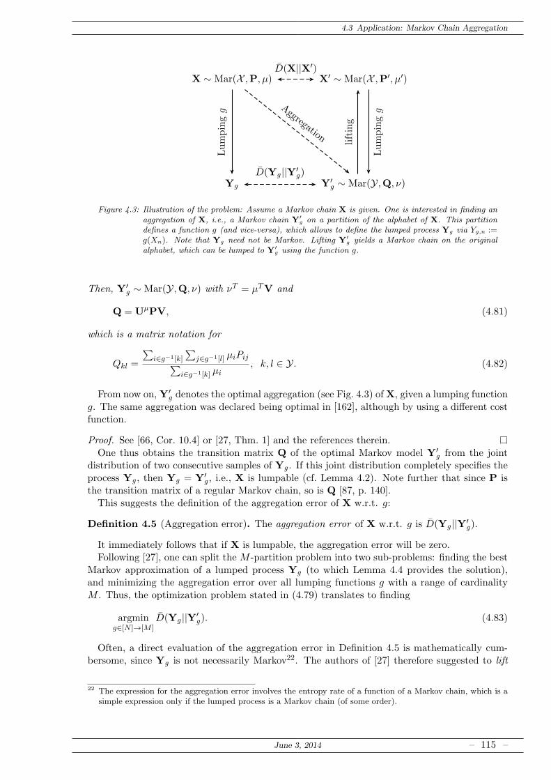
4.3 Application: Markov Chain Aggregation
X ∼ Mar(X ,P, µ)
Yg Y′g ∼ Mar(Y,Q, ν)
X′ ∼ Mar(X ,P′, µ′)
Lumpingg Aggregation
lifting
Lumpingg
D(Yg ||Y′g)
D(X||X′)
Figure 4.3: Illustration of the problem: Assume a Markov chain X is given. One is interested in finding anaggregation of X, i.e., a Markov chain Y
′g on a partition of the alphabet of X. This partition
defines a function g (and vice-versa), which allows to define the lumped process Yg via Yg,n :=g(Xn). Note that Yg need not be Markov. Lifting Y
′g yields a Markov chain on the original
alphabet, which can be lumped to Y′g using the function g.
Then, Y′g ∼ Mar(Y,Q, ν) with νT = µTV and
Q = UµPV, (4.81)
which is a matrix notation for
Qkl =
∑
i∈g−1[k]
∑
j∈g−1[l] µiPij∑
i∈g−1[k] µi, k, l ∈ Y. (4.82)
From now on, Y′g denotes the optimal aggregation (see Fig. 4.3) ofX, given a lumping function
g. The same aggregation was declared being optimal in [162], although by using a different costfunction.
Proof. See [66, Cor. 10.4] or [27, Thm. 1] and the references therein.One thus obtains the transition matrix Q of the optimal Markov model Y′
g from the jointdistribution of two consecutive samples of Yg . If this joint distribution completely specifies theprocess Yg , then Yg = Y′
g , i.e., X is lumpable (cf. Lemma 4.2). Note further that since P isthe transition matrix of a regular Markov chain, so is Q [87, p. 140].This suggests the definition of the aggregation error of X w.r.t. g:
Definition 4.5 (Aggregation error). The aggregation error of X w.r.t. g is D(Yg ||Y′g).
It immediately follows that if X is lumpable, the aggregation error will be zero.Following [27], one can split the M -partition problem into two sub-problems: finding the best
Markov approximation of a lumped process Yg (to which Lemma 4.4 provides the solution),and minimizing the aggregation error over all lumping functions g with a range of cardinalityM . Thus, the optimization problem stated in (4.79) translates to finding
argming∈[N ]→[M ]
D(Yg ||Y′g). (4.83)
Often, a direct evaluation of the aggregation error in Definition 4.5 is mathematically cum-bersome, since Yg is not necessarily Markov22. The authors of [27] therefore suggested to lift
22 The expression for the aggregation error involves the entropy rate of a function of a Markov chain, which is asimple expression only if the lumped process is a Markov chain (of some order).
June 3, 2014 – 115 –
4 Relevant Information Loss
the aggregation Y′g to a Markov chain X′ over the alphabet X , which subsequently allows a
computation of the KLDR (an equivalent lifting method is suggested in [162] and [157,158]):
Definition 4.6 (π-lifting [27, Def. 2]). Let Y′g ∼ Mar(Y,Q, ν) be as in Lemma 4.4 and let π be
a positive probability distribution over the alphabet X . The π-lifting of Y′g w.r.t. g, denoted
by X′πg , is a Markov chain over the alphabet X with transition matrix
P′ := VQUπ, (4.84)
which is a matrix notation for
P ′ij =
πj∑
k∈g−1[g(j)] πkQg(i)g(j), i, j ∈ X . (4.85)
Proposition 4.5 (Properties of π-lifting). The π-lifting X′πg satisfies
1. X′πg is lumpable w.r.t. g (and Y′
g is the resulting g-projection);
2. The invariant distribution of X′µg is µ;
3. µ = argminπ D(X||X′πg );
4. P′ ≫ P;
5. D(Yg ||Y′g) ≤ D(X||X′µ
g ).
Properties 1), 2), and 3) appear also in [27].
Proof. See Appendix C.1.The last property of the previous proposition shows that the KLDR between X and the µ-
lifting23 X′µg provides an upper bound on the aggregation error for a given lumping function
g. Unfortunately, the bound is loose in the sense that for D(Yg ||Y′g) = 0, one may have
D(X||X′µg ) > 0; see also [158]. One of the reasons for this disadvantage of π-lifting is that, by
construction, the lifted process X′πg does not contain information about the transition probabil-
ities between states of X. To remove this problem, consider
Definition 4.7 (P-lifting). The P-lifting of Y′g w.r.t. g, denoted by X′P
g , is a Markov chain
over the alphabet X with a transition matrix P given by
Pij :=
Pij∑k∈g−1(g(j)) Pik
Qg(i)g(j), if∑
k∈g−1(g(j))
Pik > 0
1card(g−1(g(j)))
Qg(i)g(j), if∑
k∈g−1(g(j))
Pik = 0. (4.86)
Theorem 4.1 (Properties of P-lifting). The P-lifting X′Pg satisfies
1. X′Pg is lumpable w.r.t. g (and Y′
g is the resulting lumped process);
2. P≫ P;
3. X′Pg = arg min
X:Y′g is lumping of X
D(X||X)
4. D(Yg ||Y′g) ≤ D(X||X′P
g ) ≤ D(X||X′µg )
23 i.e., the π-lifting obtained by chosing π to be the invariant distribution µ of X
– 116 – June 3, 2014
4.3 Application: Markov Chain Aggregation
5. If X is strongly lumpable w.r.t. g, then
D(Yg ||Y′g) = 0⇔ D(X||X′P
g ) = 0. (4.87)
Proof. See Appendix C.2.The tightness result follows from the fact that for a strongly lumpable X, the P-lifting yields
P = P; as a direct consequence, in this case also the invariant distribution of P trivially coincideswith µ, the invariant distribution of P. In general, however, the invariant distribution of P differsfrom µ, contrasting the corresponding result for π-lifing (cf. Proposition 4.5, property 2).Interestingly, the restriction to strongly lumpable chains for the tightness result cannot be
dropped: There are Markov chains X which are weakly lumpable (i.e., not for all initial distri-butions but, e.g., for the invariant distribution) for which consequently the aggregation errorvanishes, but for which the P-lifting does not yield P = P. A simple example for a transitionmatrix of such a chain is
Example 28: A weakly lumpable Markov chain.Taking the example from [87, pp. 139] shows that the upper bound on the aggregation
error is not tight in general, but only for strongly lumpable X. To this end, let
P =
14
14
12
0 16
56
78
18 0
. (4.88)
This chain is lumpable w.r.t. the partition 1, 2, 3, but not strongly lumpable; i.e.,the matrix fulfils (4.70) but not (4.69). To show that the bound is not tight, observe thatD(Yg ||Y′
g) = 0 but that, with
P =
14
14
12
712
572
2572
712
512 0
6= P (4.89)
one gets D(X||X′Pg ) = 0.347 > 0.
As this theorem shows, P-lifting yields the best upper bound on the aggregation error achiev-able for Markov chains over the alphabet X . This can also be explained intuitively, by expandingthe KLDR as
D(X||X′Pg ) =
∑
i,j∈XµiPij log
Pij
Pij
(4.90)
=∑
i,j∈XµiPij log
∑
k∈SjPik
Qg(i)g(j)(4.91)
(a)=∑
i,j∈XµiPij log
(∑
k∈Siµk
) (∑
l∈SjPil
)
∑
k∈Siµk∑
l∈SjPkl
(4.92)
= H(Yg,n|Yg,n−1)−H(Yg,n|Xn−1) (4.93)
where (a) is due to Lemma 4.4. Note that the last line corresponds to the difference between theupper and lower bounds on the entropy rate of a function of a Markov chain [21, Thm. 4.5.1];according to Theorem 3.2, equality of these bounds implies Markovity of Yg , i.e., strong lumpa-bility of X w.r.t. g. In other words, minimizing this cost function yields the function g for whichthe projected process Yg is “as Markov as possible”.
June 3, 2014 – 117 –

4 Relevant Information Loss
Example 29: Comparison of the two lifting methods.Consider the transition matrix given in [27, Section V.A]
P =
0.97 0.01 0.020.02 0.48 0.500.01 0.75 0.24
(4.94)
and use three different functions g inducing the following partitions of X : 1, 2, 3,1, 3, 2, and 1, 2, 3.
For all the resulting aggregations one can compute upper bounds on the aggregation errorusing both the µ-lifting and the P-lifting. In addition to that, the invariant distributions µ ofthe P-lifted Markov chains X′P
g are computed and compared to µ, the invariant distributionof the original chain X. The results are shown in the table below.
Partition D(X||X′µg ) D(X||X′P
g ) µ
bit/sample bit/sample [0.347, 0.388, 0.265]T
1, 2, 3 0.823 0.185 [0.077, 0.658, 0.265]T
1, 3, 2 0.808 0.317 [0.065, 0.388, 0.546]T
1, 2, 3 0.037 0.001 [0.347, 0.388, 0.265]T
As it can be seen, the partition 1, 2, 3 yields the best results in terms of KLDR.
Moreover, it can be seen that the KLDR using P-lifting is smaller than the KLDR using
µ-lifting in all three cases, as suggested by Theorem 4.1. However, while the µ-lifting yields
the same invariant distribution as the original chain has, P-lifting obtains quite different
values. An exception is the optimal partition, where Yg and Y′g are very close in terms of
the KLDR, i.e., where X is “nearly” lumpable w.r.t. g.
Example 30: A “nearly” periodic Markov chain.In another bi-partition problem the Markov chain X has a highly periodic structure:
P =
0.03 0.92 0.00 0.050.92 0.03 0.05 0.000.00 0.05 0.03 0.920.05 0.00 0.92 0.03
(4.95)
Consider two different functions g and h, inducing the partitions 1, 2, 3, 4 and1, 4, 2, 3. Both partitions lead to Markov chains, i.e., the original Markov chain Xis strongly lumpable w.r.t. both g and h. However, the former partition leads to a nearlydecomposable chain Y′
g , while the latter leads to a chain Y′h with highly periodic structure
(cf. [27, Section. V.C]). The resulting transition matrices are given by
Qg =
[0.95 0.050.05 0.95
]
, Qh =
[0.03 0.970.97 0.03
]
. (4.96)
Since the aggregation error is zero for both functions and since the upper bound obtainedvia P-lifting is tight in this particular case, one obtains
D(X||X′Pg ) = D(X||X′P
h ) = 0 (4.97)
i.e., both aggregations are equivalent. The µ-lifting, however, is in favor of the function h,for which one obtains D(X||X′µ
h ) = 0.716 compared to D(X||X′µg ) = 0.808.
The reason why one function is preferred w.r.t. the other is not clear at present, except
that the partition w.r.t. h leads to a Markov chain which has a higher redundancy. In
addition to that, the bi-partition does not admit an interpretation via the spectral theory of
Markov chains: the aggregation via h does not correspond to the Fiedler vector, but to the
– 118 – June 3, 2014
4.3 Application: Markov Chain Aggregation
eigenvector associated with the eigenvalue with the second largest magnitude (cf. [27]).
4.3.4 Interpreting the KLDR as Information Loss
There is a connection between the KLDR of the original process and a lifted process (be it eitherby π- or P-lifting) and the information loss induced by the lumping function g. In particular,the cost function from π-lifting is – except for its connection to spectral theory [27] – counter-intuitive, since it maximizes information loss. Contrarily, the cost function induced by P-liftingminimizes information loss relevant in a specific aspect.Since for the π-lifting exclusively the minimizer π = µ is used (cf. Proposition 4.5), this section
will also refer to it as µ-lifting. Recall that the goal is to find a partition of the original alphabetX (induced by a functiom g) such that the KLDR is minimized:
g := argming
D(X||X′µg )
(a)= argmax
gR(Y′
g) (4.98)
where (a) is due to [27, Lem. 3]: A minimization of D(X||X′µg ) can be stated as a maximization
of R(Y′g), since the redundancy rate of X is independent of g.
Note that H(Y ′g) = H(Yg) since Yg and Y′
g have the same marginal distribution. However,
H(Y′g) = H(Yg,1|Yg,0) ≥ H(Yg) (4.99)
by the fact that conditioning reduces entropy [21, Thm. 2.6.5]. With Definition 3.1, a maxi-mization of R(Y′
g) minimizes an upper bound on the entropy rate H(Yg) of the lumped processYg while simultaneously maximizing its marginal entropy. Since the entropy rate of a processis a measure of the average amount of information the process conveys in each time step, thesolution to above minimization problem yields a function g with as little information at itsoutput as possible. In other words, one tries to maximize information loss. This is in line withthe reasoning in [27], where the optimal solution was characterized as the model that is most“predictable”. Note further that essentially the same cost function was suggested by Friedmanand Goldberger [44], although the focus of their work was on pairwise clustering.Despite this counter-intuitivity of the cost function, the model reduction method proposed
by [27] works and, given some assumptions on the eigenstructure of the transition matrix24, hasa justification in spectral theory. In particular, the bi-partition problem is sub-optimally solvedemploying the sign structure of the eigenvector associated to the second-largest eigenvalue, theFiedler vector. The authors of [27] then solve the M -partition problem by recursively applyingthe bi-partition problem, i.e., by refining the partitions iteratively.To analyze the P-lifting, one needs the definition of relevant information loss. In addition, let
g• := argming
D(X||X′Pg ). (4.100)
Recall from (4.93) that
D(X||X′Pg ) = H(Yg,n|Yg,n−1)−H(Yg,n|Xn−1) (4.101)
which, by adding and subtracting H(Yg,n) can be rewritten as
D(X||X′Pg ) = I(Yg,n;Xn−1)− I(Yg,n;Yg,n−1) = LYg,n(Xn−1 → Yg,n−1) (4.102)
where LYg,n(Xn−1 → Yg,n−1) is the information loss relevant w.r.t. Yg,n induced by projecting
24 to be precise, on its additive reversibilization
June 3, 2014 – 119 –
4 Relevant Information Loss
the previous sample Xn−1 through the function g. Finding the optimal function g• thus amountsto minimizing information loss.
To the present date, the author could not verify if this cost function has an interpretation inspectral theory. However, as mentioned above, it minimizes the difference between first-orderupper and lower bounds on the entropy rate of the lumped process Yg . Upper and lower boundsare equal if and only if the original process is strongly lumpable w.r.t. g (cf. Theorem 3.2). Min-imizing this cost function thus amounts to making the lumped process as Markov as possible.
4.3.5 Employing the Information-Bottleneck Method for Aggregation
This section shows that the model reduction problem can be solved by the information bottleneckmethod [145]. Specifically, one needs to connect the results from Section 4.2, where it was shownthat the information bottleneck method can be used to minimize relevant information loss, withthose of Section 4.3.4. Unfortunately, in the cost function (4.102), the relevant information Yg,ndepends on g, i.e., on the object to be optimized. Since in such a case the IB method is notapplicable directly, let us relax the problem by applying Proposition 4.2:
LYg,n(Xn−1 → Yg,n−1) ≤ LXn(Xn−1 → Yg,n−1) (4.103)
Instead of minimizing D(X||X′Pg ), one minimizes an upper bound given by (4.103), and thus
gets
gIB := argming
LXn(Xn−1 → Yg,n−1). (4.104)
The possibility to apply the IB method and its algorithms (e.g., AIB) for model order reductioncomes at the cost of optimality. This cost is not as high as one would expect, since the obtainedupper bound is still better than D(X||X′µ
g ):
LXn(Xn−1 → Yg,n−1) = H(Xn|Yg,n−1)−H(Xn|Xn−1) (4.105)
= H(Xn, Yg,n|Yg,n−1)−H (X) (4.106)
= H(Xn|Yg,n, Yg,n−1) +H(Yg,n|Yg,n−1)︸ ︷︷ ︸
=H(Y′g )
−H (X) (4.107)
≤ H(Xn|Yg,n) +H (Y′g)−H (X) (4.108)
= H(X)−H(Y ′g) +H (Y′
g)−H (X) (4.109)
= R(X)− R(Y′g) (4.110)
= D(X||X′µg ) (4.111)
where the last line is due to [27, Lem. 3].
The solution of the relaxed problem might not coincide with the solution of the originalproblem. To be specific: Even if a Markov chain X is lumpable, neither the AIB nor theIB method implementing the relaxed optimization problem necessarily find the optimal M -partition:
Example 31: Sub-Optimality of the Relaxation.Let X be a Markov chain with state space X , N = 3, and transition matrix
P =
0.0475 0.9025 0.050.9025 0.0475 0.050.95 0.05 0
. (4.112)
Consider the bi-partition problem (i.e., M = 2). Since this chain is lumpable for the partition
– 120 – June 3, 2014
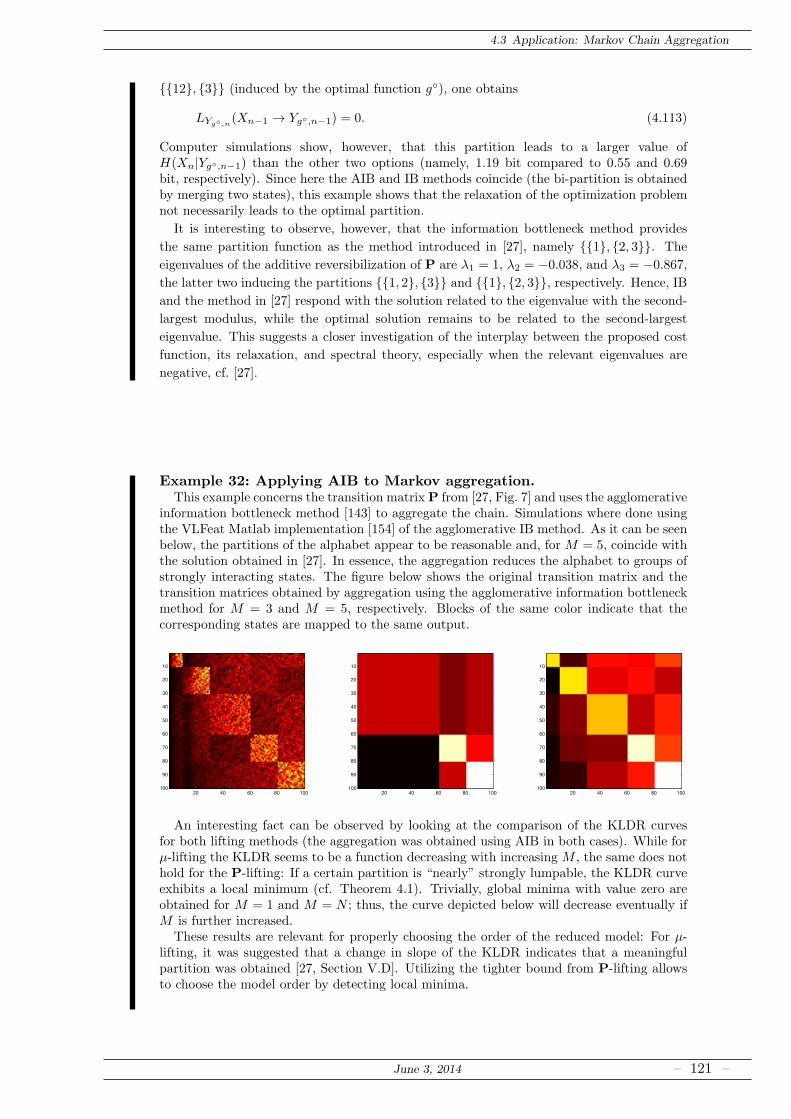
4.3 Application: Markov Chain Aggregation
12, 3 (induced by the optimal function g), one obtains
LYg,n(Xn−1 → Yg,n−1) = 0. (4.113)
Computer simulations show, however, that this partition leads to a larger value ofH(Xn|Yg,n−1) than the other two options (namely, 1.19 bit compared to 0.55 and 0.69bit, respectively). Since here the AIB and IB methods coincide (the bi-partition is obtainedby merging two states), this example shows that the relaxation of the optimization problemnot necessarily leads to the optimal partition.
It is interesting to observe, however, that the information bottleneck method provides
the same partition function as the method introduced in [27], namely 1, 2, 3. The
eigenvalues of the additive reversibilization of P are λ1 = 1, λ2 = −0.038, and λ3 = −0.867,the latter two inducing the partitions 1, 2, 3 and 1, 2, 3, respectively. Hence, IBand the method in [27] respond with the solution related to the eigenvalue with the second-
largest modulus, while the optimal solution remains to be related to the second-largest
eigenvalue. This suggests a closer investigation of the interplay between the proposed cost
function, its relaxation, and spectral theory, especially when the relevant eigenvalues are
negative, cf. [27].
Example 32: Applying AIB to Markov aggregation.This example concerns the transition matrixP from [27, Fig. 7] and uses the agglomerative
information bottleneck method [143] to aggregate the chain. Simulations where done usingthe VLFeat Matlab implementation [154] of the agglomerative IB method. As it can be seenbelow, the partitions of the alphabet appear to be reasonable and, for M = 5, coincide withthe solution obtained in [27]. In essence, the aggregation reduces the alphabet to groups ofstrongly interacting states. The figure below shows the original transition matrix and thetransition matrices obtained by aggregation using the agglomerative information bottleneckmethod for M = 3 and M = 5, respectively. Blocks of the same color indicate that thecorresponding states are mapped to the same output.
20 40 60 80 100
10
20
30
40
50
60
70
80
90
100
20 40 60 80 100
10
20
30
40
50
60
70
80
90
100
20 40 60 80 100
10
20
30
40
50
60
70
80
90
100
An interesting fact can be observed by looking at the comparison of the KLDR curvesfor both lifting methods (the aggregation was obtained using AIB in both cases). While forµ-lifting the KLDR seems to be a function decreasing with increasing M , the same does nothold for the P-lifting: If a certain partition is “nearly” strongly lumpable, the KLDR curveexhibits a local minimum (cf. Theorem 4.1). Trivially, global minima with value zero areobtained for M = 1 and M = N ; thus, the curve depicted below will decrease eventually ifM is further increased.
These results are relevant for properly choosing the order of the reduced model: For µ-lifting, it was suggested that a change in slope of the KLDR indicates that a meaningfulpartition was obtained [27, Section V.D]. Utilizing the tighter bound from P-lifting allowsto choose the model order by detecting local minima.
June 3, 2014 – 121 –
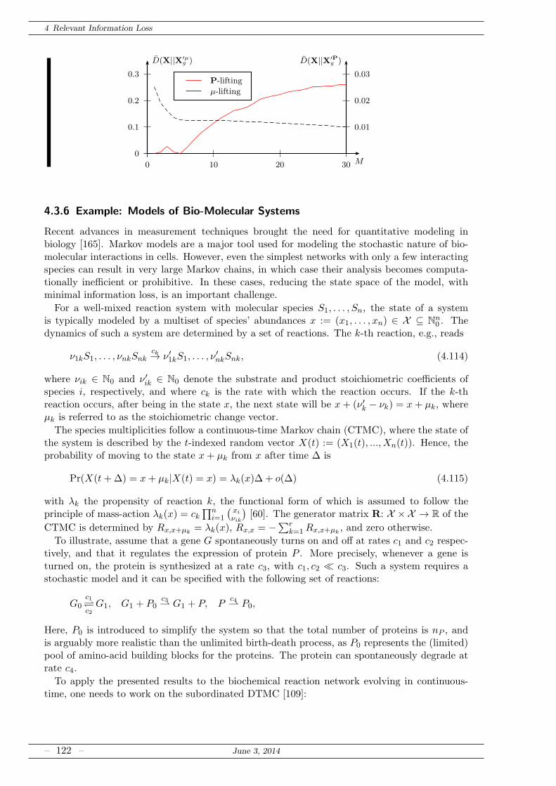
4 Relevant Information Loss
0
0.1
0.2
0.3
0 10 20 30 M
D(X||X′µg )
0.01
0.02
0.03
D(X||X′Pg )
P-lifting
µ-lifting
4.3.6 Example: Models of Bio-Molecular Systems
Recent advances in measurement techniques brought the need for quantitative modeling inbiology [165]. Markov models are a major tool used for modeling the stochastic nature of bio-molecular interactions in cells. However, even the simplest networks with only a few interactingspecies can result in very large Markov chains, in which case their analysis becomes computa-tionally inefficient or prohibitive. In these cases, reducing the state space of the model, withminimal information loss, is an important challenge.
For a well-mixed reaction system with molecular species S1, . . . , Sn, the state of a systemis typically modeled by a multiset of species’ abundances x := (x1, . . . , xn) ∈ X ⊆ Nn
0 . Thedynamics of such a system are determined by a set of reactions. The k-th reaction, e.g., reads
ν1kS1, . . . , νnkSnkck→ ν ′1kS1, . . . , ν
′nkSnk, (4.114)
where νik ∈ N0 and ν ′ik ∈ N0 denote the substrate and product stoichiometric coefficients ofspecies i, respectively, and where ck is the rate with which the reaction occurs. If the k-threaction occurs, after being in the state x, the next state will be x+ (ν ′k − νk) = x+ µk, whereµk is referred to as the stoichiometric change vector.
The species multiplicities follow a continuous-time Markov chain (CTMC), where the state ofthe system is described by the t-indexed random vector X(t) := (X1(t), ..., Xn(t)). Hence, theprobability of moving to the state x+ µk from x after time ∆ is
Pr(X(t+∆) = x+ µk|X(t) = x) = λk(x)∆ + o(∆) (4.115)
with λk the propensity of reaction k, the functional form of which is assumed to follow theprinciple of mass-action λk(x) = ck
∏ni=1
(xi
νik
)[60]. The generator matrix R: X ×X → R of the
CTMC is determined by Rx,x+µk= λk(x), Rx,x = −∑r
k=1Rx,x+µk, and zero otherwise.
To illustrate, assume that a gene G spontaneously turns on and off at rates c1 and c2 respec-tively, and that it regulates the expression of protein P . More precisely, whenever a gene isturned on, the protein is synthesized at a rate c3, with c1, c2 ≪ c3. Such a system requires astochastic model and it can be specified with the following set of reactions:
G0c1c2
G1, G1 + P0c3 G1 + P, P
c4 P0,
Here, P0 is introduced to simplify the system so that the total number of proteins is nP , andis arguably more realistic than the unlimited birth-death process, as P0 represents the (limited)pool of amino-acid building blocks for the proteins. The protein can spontaneously degrade atrate c4.
To apply the presented results to the biochemical reaction network evolving in continuous-time, one needs to work on the subordinated DTMC [109]:
– 122 – June 3, 2014
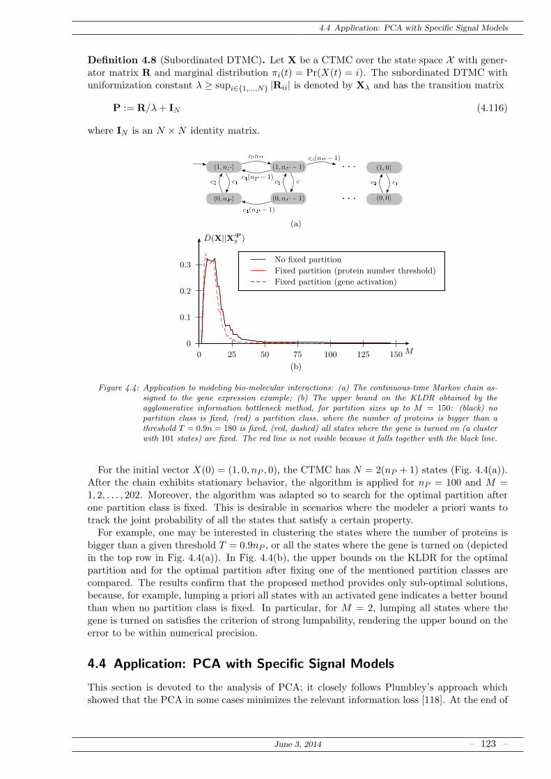
4.4 Application: PCA with Specific Signal Models
Definition 4.8 (Subordinated DTMC). Let X be a CTMC over the state space X with gener-ator matrix R and marginal distribution πi(t) = Pr(X(t) = i). The subordinated DTMC withuniformization constant λ ≥ supi∈1,...,N |Rii| is denoted by Xλ and has the transition matrix
P := R/λ+ IN (4.116)
where IN is an N ×N identity matrix.
(a)
0
0.1
0.2
0.3
0 25 50 75 100 125 150 M
D(X||X′Pg )
No fixed partition
Fixed partition (protein number threshold)
Fixed partition (gene activation)
(b)
Figure 4.4: Application to modeling bio-molecular interactions: (a) The continuous-time Markov chain as-signed to the gene expression example; (b) The upper bound on the KLDR obtained by theagglomerative information bottleneck method, for partition sizes up to M = 150: (black) nopartition class is fixed, (red) a partition class, where the number of proteins is bigger than athreshold T = 0.9n = 180 is fixed, (red, dashed) all states where the gene is turned on (a clusterwith 101 states) are fixed. The red line is not visible because it falls together with the black line.
For the initial vector X(0) = (1, 0, nP , 0), the CTMC has N = 2(nP + 1) states (Fig. 4.4(a)).After the chain exhibits stationary behavior, the algorithm is applied for nP = 100 and M =1, 2, . . . , 202. Moreover, the algorithm was adapted so to search for the optimal partition afterone partition class is fixed. This is desirable in scenarios where the modeler a priori wants totrack the joint probability of all the states that satisfy a certain property.For example, one may be interested in clustering the states where the number of proteins is
bigger than a given threshold T = 0.9nP , or all the states where the gene is turned on (depictedin the top row in Fig. 4.4(a)). In Fig. 4.4(b), the upper bounds on the KLDR for the optimalpartition and for the optimal partition after fixing one of the mentioned partition classes arecompared. The results confirm that the proposed method provides only sub-optimal solutions,because, for example, lumping a priori all states with an activated gene indicates a better boundthan when no partition class is fixed. In particular, for M = 2, lumping all states where thegene is turned on satisfies the criterion of strong lumpability, rendering the upper bound on theerror to be within numerical precision.
4.4 Application: PCA with Specific Signal Models
This section is devoted to the analysis of PCA; it closely follows Plumbley’s approach whichshowed that the PCA in some cases minimizes the relevant information loss [118]. At the end of
June 3, 2014 – 123 –
4 Relevant Information Loss
this section, Plumbley’s result will be slightly extended; eventually, it will be shown that evenlossless dimensionality reduction is possible in some cases.To this end, define the PCA as
Y M1 = g(X) = IMY = IMWTX (4.117)
where X is an N -dimensional continuous-valued input RV, Y M1 an M -dimensional output RV
(composed of the first M elements of Y ), and W the matrix of eigenvectors of the covariancematrix of X, CX = E
(XXT
). Thus, detW = 1 and W−1 = WT . Furthermore, let IM be
an (M ×N)-matrix with ones in the main diagonal. The PCA is used here for dimensionalityreduction and, assuming that one has perfect knowledge of the rotation matrix W, the relativeinformation loss equals (N − M)/N , while the absolute information loss is infinite (cf. Sec-tion 2.6).It is known that among all rotations prior to dimensionality reduction, the PCA minimizes
the mean squared error for a reconstruction X = WITMY M1 of X [25]. In addition to that, as
Linsker pointed out in [100], given that X is an observation of a Gaussian RV S corrupted by iidGaussian noise, the PCA maximizes the mutual information I(S;Y ). For non-Gaussian S (andiid Gaussian noise), the PCA not only maximizes an upper bound on the mutual information,but also minimizes an upper bound on the relevant information loss [25, 118].This section generalizes these results such that non-spherical and non-Gaussian noise is taken
into account as well. Let
X = S +N (4.118)
where S and N are the relevant information and the noise, respectively, with covariance matricesCS and CN . Assume further that S and N are independent and, as a consequence, CX =CS +CN . Let λi νi, and µi be the sets of eigenvalues of CX , CS , and CN , respectively.Let the eigenvalues be ordered descendingly, i.e.,
λ1 ≥ λ2 ≥ · · · ≥ λN . (4.119)
One can now write
Y M1 = IMWTX = IMWTS + IMWTN = SM
1 + NM1 . (4.120)
As mentioned before, Y M1 is composed of the first M elements of the vector Y , which is a sum
of the rotated signal vector S and the rotated noise vector N . Conversely, let Y NM+1, S
NM+1, and
NNM+1 denote the last N −M elements of the corresponding vectors. The covariance matrix of
Y M1 is a diagonal matrix with the M largest eigenvalues of CX .
Lemma 4.5. For above signal model, the relevant information loss in the PCA is given by
LS(X → Y M1 ) = h(Y N
M+1|Y M1 )− h(NN
M+1|NM1 ). (4.121)
Proof. Note that LS(X → Y M1 ) = LS(Y → Y M
1 ) since Y and X are related by an invertibletransform. Thus,
LS(Y → Y M1 ) = I(Y ;S)− I(Y M
1 ;S) (4.122)
= h(Y )− h(Y |S)− h(Y M1 ) + h(Y M
1 |S) (4.123)
= h(Y NM+1|Y M
1 )− h(WTS +WTN |S) + h(IMWTS + IMWTN |S)(4.124)
(a)= h(Y N
M+1|Y M1 )− h(WTN) + h(IMWTN) (4.125)
= h(Y NM+1|Y M
1 )− h(NNM+1|NM
1 ) (4.126)
– 124 – June 3, 2014
4.4 Application: PCA with Specific Signal Models
where (a) is due to independence of S and N . This completes the proof.
Definition 4.9 (Conditional Divergence). Let X and Y be continuous RVs with arbitrarycontinuous (joint) distribution, and let XG and YG be Gaussian RVs with same (joint) first andsecond moments. The conditional divergence is
J(X|Y ) := E(D(fX|Y (·|Y )||fXG|YG
(·|Y )))= h(XG|YG)− h(X|Y ). (4.127)
Clearly, this quantity inherits all its properties from the Kullback-Leibler divergence, e.g.,non-negativity, and can be considered as a measure of Gaussianity. Despite the similarity, thisquantity is not to be confused with negentropy. For negentropy, instead of using a jointlyGaussian distribution for (XG, YG) for computing h(XG|YG), one uses a Gaussian distributionfor XG|Y = y to compute h(XG|Y = y) before taking the expectation w.r.t. the true marginaldistribution of Y .While most results about the optimality of the PCA are restricted to the Gaussian case,
conditional divergence can be employed to generalize some of these results. In particular, oneobtains
Theorem 4.2. Let X = S+N , with N and S independent, and let Y M1 be obtained by perform-
ing dimensionality-reducing PCA. If N is iid (i.e., CN is a scaled identity matrix) and moreGaussian than Y in the sense
J(NNM+1|NM
1 ) ≤ J(Y NM+1|Y M
1 ) (4.128)
then the PCA minimizes the Gaussian upper bound on the relevant information loss LS(X →Y M1 ).
Proof. See Appendix C.3.This theorem generalizes the result by Plumbley [25, 118], who claimed that PCA minimizes
the Gaussian upper bound on the information loss for iid Gaussian noise (i.e., for Gaussian Nwith CN being a scaled identity matrix). In addition to that, it justifies the use of informationloss instead of information transfer; an upper bound on the latter would not be useful in thesignal enhancement problem.As a next step, assume that the relevant information is concentrated on an L ≤M -dimensional
subspace, and drop the requirement that N is iid. It is still assumed, however, that CN (and,thus, CX) is full rank. Note that due to these assumptions λi > 0 and µi > 0 for all i, whileνi = 0 for i > L.
Theorem 4.3 (Bounds for the PCA). Assume that S has covariance matrix CS with at mostrank M , and assume that N is independent of S and has (full-rank) covariance matrix CN . Letfurther N be more Gaussian than Y in the sense
J(NNM+1|NM ) ≤ J(Y N
M+1|Y M1 ) (4.129)
where Y M1 is obtained by employing the PCA for dimensionality reduction. Then, the relevant
information loss in nats is bounded from above by
LS(X → Y M1 ) ≤ 1
2ln
(N∏
i=M+1
µ1
µi
)
(4.130)
where µi is the set of decreasing eigenvalues of CN and where ln is the natural logarithm.
Proof. See Appendix C.4.Note that this upper bound is non-negative, since – by assumption on the ordering of the
eigenvalues – any term in the product cannot be smaller than one. Along the same lines a lower
June 3, 2014 – 125 –
4 Relevant Information Loss
bound can be derived; by similar reasons, this bound is non-positive and thus inactive (therelevant information loss is a non-negative quantity).
The previous theorem shows that there are cases where, despite the fact that the dimension-ality of the data is reduced, all of the relevant information can be preserved:
Corollary 4.3. Assume that S has covariance matrix CS with at most rank M , and assumethat N is zero-mean Gaussian noise independent of S with covariance matrix σ2
NI. Let Y M1 be
obtained by employing PCA for dimensionality reduction. Then, the relevant information lossLS(X → Y M
1 ) vanishes.
Proof. The proof follows from the fact that as CN = σ2NI, all eigenvalues µ1 = · · · = µN =
σ2N .
As mentioned before, due to dimensionality reduction the absolute information loss L(X →Y M1 ) is infinite; a direct consequence is that the irrelevant information loss, LX|S(X → Y M
1 ),is infinite as well. Given the assumptions of Corollary 4.3 hold, PCA is a good solution to thesignal enhancement problem:
Example 33: PCA with Non-Gaussian Data.Assume that two independent data sources, S1 and S2, are observed with three sensors
which are corrupted by independent, unit-variance Gaussian noise Ni, i = 1, 2, 3. The sensorsignals shall be defined as
X1 = S1 +N1, (4.131)
X2 = S1 + S2 +N2, and (4.132)
X3 = S2 +N3. (4.133)
Assume further that the data sources have variances σ21 and σ2
2 and are non-Gaussian, butthat they still can be described by a (joint) probability density function. The covariancematrix of X = [X1, X2, X3]
T is
CX =
σ1 + 1 σ1 0σ1 σ1 + σ2 + 1 σ2
0 σ2 σ2 + 1
. (4.134)
Performing the eigenvalue decomposition yields three eigenvalues,
λ1, λ2, λ3 = σ1 + σ2 + 1 + C, σ1 + σ2 + 1− C, 1 (4.135)
where C =√
σ21 + σ2
2 − σ1σ2.Let us reduce the dimension of the output vector Y from N = 3 to M = 2 by dropping
the component corresponding to the smallest eigenvalue. By Corollary 4.3 no relevant infor-mation is lost since the relevant information is concentrated on a two-dimensional subspace.
Note that N is iid Gaussian, and thus h(N3|N21 ) = h(N3). By assumption, CN = I, and
by the orthogonality of the transform,
h(N3) =1
2ln(2πe). (4.136)
Conversely, by the maximum entropy property of the Gaussian distribution,
h(Y3|Y 21 ) ≤ h(Y3,G|(Y 2
1 )G) = h(Y3,G) =1
2ln(2πeλ3). (4.137)
With λ3 = 1 and Lemma 4.5 one thus gets
LS(X → Y 21 ) ≤ 0. (4.138)
The relevant information loss vanishes. Indeed, the eigenvector corresponding to the
– 126 – June 3, 2014
4.5 Relevant Information Loss in Inaccurate Functions
smallest eigenvalue is given as p3 = 1√3[1,−1, 1]T ; thus, for Y3 one would obtain
Y3 =X1 +X3 −X2√
3=
N1 +N3 −N2√3
. (4.139)
Since this component does not contain any relevant signal component, dropping it does not
lead to a loss of relevant information.
Note that in case the noise sources Ni do not have the same variances, the application of PCAmay lead to a loss of information, even though the relevant information is still concentrated ona subspace of lower dimensionality. This is made precise in the next example.
Example 34: PCA with Large Noise Variances.Again assume that three sensors observe two independent, non-Gaussian data sources
which are corrupted by independent Gaussian noise:
X1 = S1 +N1, (4.140)
X2 = S2 +N2, and (4.141)
X3 = N3 (4.142)
This time, however, assume that the data sources have unit variance, and that the varianceof noise source Ni is i, thus µ1, µ2, µ3 = 3, 2, 1. With this, the covariance matrix of Xis given as
CX =
1 + 1 0 00 1 + 2 00 0 3
=
2 0 00 3 00 0 3
(4.143)
and has eigenvalues λ1, λ2, λ3 = 3, 3, 2.Since CX is already diagonal, PCA only leads to an ordering w.r.t. the eigenvalues;
dropping the component of Y corresponding to the smallest eigenvalue, i.e., dimensionalityreduction from N = 3 to M = 2, yields Y1 = N3 and Y2 = S2 + N2. Since the outputdoes not depend on S1 anymore, information is lost – in fact, PCA suggested to drop thecomponent of X with the highest SNR.
With Lemma 4.5 one can compute the Gaussian upper bound on the relevant informationloss: Following the proof of Theorem 4.2,
LS(X → Y 21 ) ≤ h(Y3,G)− h(N1) =
1
2ln 2. (4.144)
The bound obtained from Theorem 4.3 is loose here, evaluating to LS(X → Y 21 ) <
12 ln 3.
Since the noise is not iid, the condition of Theorem 4.2 is not fulfilled, thus the Gaussian
upper bound is not minimized by the PCA. By preserving X1 and X2 (and dropping X3)
the relevant information loss would vanish.
4.5 Relevant Information Loss in Inaccurate Functions
In this section, the results of Section 2.3 will be extended to a practically relevant scenario: Tothe case where the piecewise bijective function g is not exactly known. Clearly, in such a case,which corresponds in some sense to adding noise to the signals at the system’s input or output,the information loss for a continuous input RV will be infinite. If the input needs to be knownonly with a specific accuracy, one can at least provide bounds on the information loss relevantw.r.t. the accuracy requirements.
June 3, 2014 – 127 –
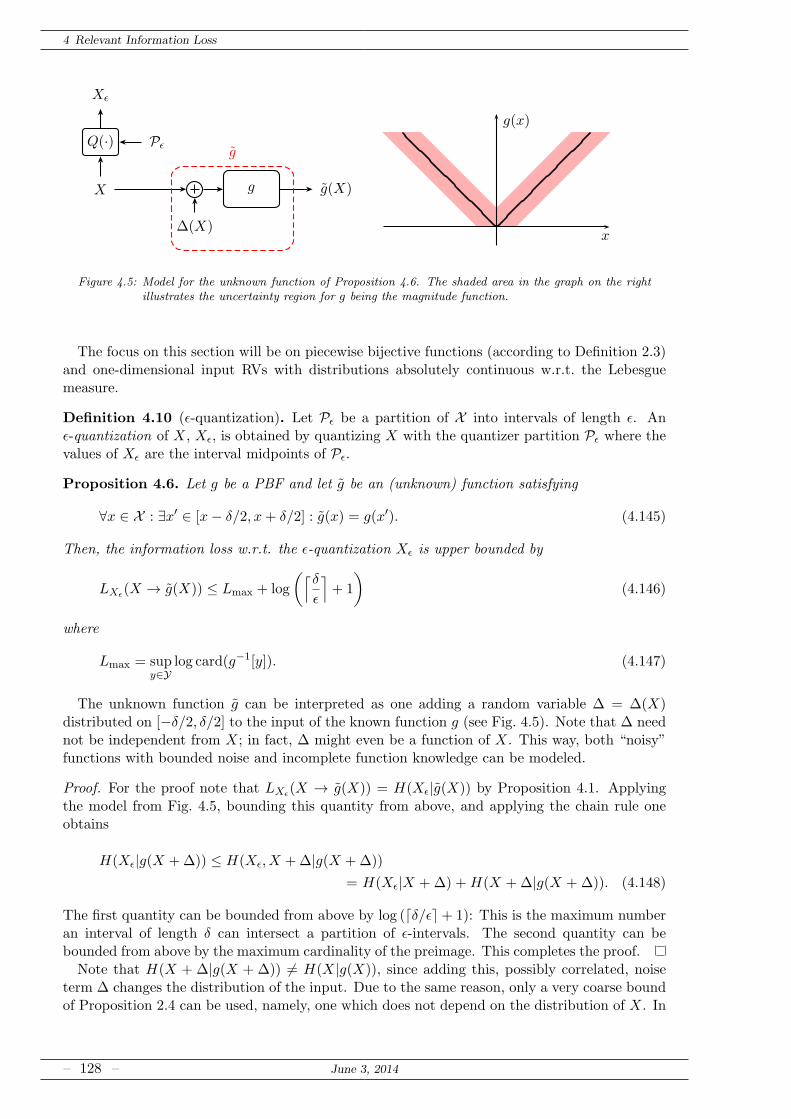
4 Relevant Information Loss
X g g(X)
∆(X)
g
Xǫ
PǫQ(·)
x
g(x)
Figure 4.5: Model for the unknown function of Proposition 4.6. The shaded area in the graph on the rightillustrates the uncertainty region for g being the magnitude function.
The focus on this section will be on piecewise bijective functions (according to Definition 2.3)and one-dimensional input RVs with distributions absolutely continuous w.r.t. the Lebesguemeasure.
Definition 4.10 (ǫ-quantization). Let Pǫ be a partition of X into intervals of length ǫ. Anǫ-quantization of X, Xǫ, is obtained by quantizing X with the quantizer partition Pǫ where thevalues of Xǫ are the interval midpoints of Pǫ.
Proposition 4.6. Let g be a PBF and let g be an (unknown) function satisfying
∀x ∈ X : ∃x′ ∈ [x− δ/2, x+ δ/2] : g(x) = g(x′). (4.145)
Then, the information loss w.r.t. the ǫ-quantization Xǫ is upper bounded by
LXǫ(X → g(X)) ≤ Lmax + log
(⌈δ
ǫ
⌉
+ 1
)
(4.146)
where
Lmax = supy∈Y
log card(g−1[y]). (4.147)
The unknown function g can be interpreted as one adding a random variable ∆ = ∆(X)distributed on [−δ/2, δ/2] to the input of the known function g (see Fig. 4.5). Note that ∆ neednot be independent from X; in fact, ∆ might even be a function of X. This way, both “noisy”functions with bounded noise and incomplete function knowledge can be modeled.
Proof. For the proof note that LXǫ(X → g(X)) = H(Xǫ|g(X)) by Proposition 4.1. Applyingthe model from Fig. 4.5, bounding this quantity from above, and applying the chain rule oneobtains
H(Xǫ|g(X +∆)) ≤ H(Xǫ, X +∆|g(X +∆))
= H(Xǫ|X + ∆) +H(X + ∆|g(X + ∆)). (4.148)
The first quantity can be bounded from above by log (⌈δ/ǫ⌉+ 1): This is the maximum numberan interval of length δ can intersect a partition of ǫ-intervals. The second quantity can bebounded from above by the maximum cardinality of the preimage. This completes the proof.Note that H(X + ∆|g(X + ∆)) 6= H(X|g(X)), since adding this, possibly correlated, noise
term ∆ changes the distribution of the input. Due to the same reason, only a very coarse boundof Proposition 2.4 can be used, namely, one which does not depend on the distribution of X. In
– 128 – June 3, 2014
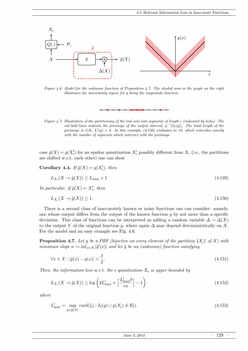
4.5 Relevant Information Loss in Inaccurate Functions
X g g(X)
∆(X)
g
Xǫ
PǫQ(·)
x
g(x)
Figure 4.6: Model for the unknown function of Proposition 4.7. The shaded area in the graph on the rightillustrates the uncertainty region for g being the magnitude function.
Figure 4.7: Illustration of the partitioning of the real axis into segments of length ǫ (indicated by ticks). Thered bold lines indicate the preimage of the output interval, g−1[Iδ(y)]. The total length of thepreimage is 2.8ǫ, L′(y) = 4. In this example, (4.156) evaluates to 10, which coincides exactlywith the number of segments which intersect with the preimage.
case g(X) = g(X ′ǫ) for an epsilon quantization X ′
ǫ possibly different from Xǫ (i.e., the partitionsare shifted w.r.t. each other) one can show
Corollary 4.4. If g(X) = g(X ′ǫ), then
LXǫ(X → g(X)) ≤ Lmax + 1. (4.149)
In particular, if g(X) = X ′ǫ, then
LXǫ(X → g(X)) ≤ 1. (4.150)
There is a second class of inaccurately known or noisy functions one can consider: namely,one whose output differs from the output of the known function g by not more than a specificdeviation. This class of functions can be interpreted as adding a random variable ∆ = ∆(X)to the output Y of the original function g, where again ∆ may depend deterministically on X.For the model and an easy example see Fig. 4.6.
Proposition 4.7. Let g be a PBF (bijective on every element of the partition Xj of X ) withminimum slope κ := infx∈X |g′(x)| and let g be an (unknown) function satisfying
∀x ∈ X : |g(x)− g(x)| < δ
2. (4.151)
Then, the information loss w.r.t. the ǫ-quantization Xǫ is upper bounded by
LXǫ(X → g(X)) ≤ log
(
2L′max +
⌈L′maxδ
ǫκ
⌉
− 1
)
(4.152)
where
L′max = sup
y∈g(X )card(j : Iδ(y) ∪ g(Xj) 6= ∅). (4.153)
June 3, 2014 – 129 –

4 Relevant Information Loss
L′(y) = 4
Figure 4.8: Illustration of the impact of unknown functions. If y assumes the value indicated by the red line,the preimage may intersect up to four elements Xi of the partition upon which g is piecewisebijective, thus L′(y) = L′
max = 4. Contrarily, Lmax = 2.
Proof. For the proof let λ denote the Lebesgue measure. By knowing the output y = g(x), oneknows the output g(x) with an accuracy of ±δ/2. One can now look at the preimage of theinterval Iδ(y) := [y − δ/2, y + δ/2], g−1[Iδ(y)]. If the preimage is an interval itself, i.e., if g isinvertible on Iδ(y), then the preimage intersects with at most
⌈λ(g−1[Iδ(y)])
ǫ
⌉
+ 1 (4.154)
ǫ-quantization intervals. If the preimage consists of multiple intervals, the total Lebesgue mea-sure of the preimage remains λ(g−1[Iδ(y)]), but this might now be spread over L′(y) intervals,where
L′(y) := card(j : Iδ(y) ∪ g(Xj) 6= ∅). (4.155)
The maximum number of intersections with the ǫ-quantization intervals is then given by (seeFigs. 4.7 and 4.8)
⌈λ(g−1[Iδ(y)])
ǫ
⌉
+ 1 + 2(L′(y)− 1). (4.156)
One further has, with gj being the restriction of g to Xj ,
λ(g−1[Iδ(y)]) =∑
j
λ(g−1j [Iδ(y)]) ≤ L′(y)
δ
κ(4.157)
by the fact that the slope is bounded from below. With L′max = supy∈g(X ) L
′(y) one thus gets
H(Xǫ|g(X)) ≤ log
(
2L′max +
⌈L′maxδ
ǫκ
⌉
− 1
)
. (4.158)
In particular, above result holds if g(X) is a δ-quantization of g(X). If g(X) = X ′ǫ, the result
of Corollary 4.4 is recovered with δ = ǫ, L′max = 1, and κ = 1 (g(x) = x). Note, finally, that
L′max ≥ Lmax, since the former degenerates to the latter for δ = 0 only.
4.6 Open Questions
Relevant information loss was introduced as a measure for signal enhancement, connecting theproblem to clustering methods developed by the machine learning community. However, verylittle signal enhancement was done in this chapter, except of course in the application of PCA inSection 4.4. The reason is that most other signal enhancement methods work on processes, not
– 130 – June 3, 2014
4.6 Open Questions
random variables, so part of this topic was deferred to (and almost exclusively constitutes) thefollowing chapter. However, the author fears that the importance of relevant information lossfor signal enhancement is presently underestimated in the field of signal processing, and thatsignificant examples of its usability have to be given in the near future.Markov chain aggregation by employing the information bottleneck method is one of the main
contributions of the present author. However, the method can still be improved by applying theinformation bottleneck method in some iterative scheme, where the relevant signal is exchangedafter every iteration; this way, part of the sub-optimality pointed out in Section 4.3.5 can beovercome. Moreover, it would be interesting if the new cost function – the relevant informationloss – has an interpretation in terms of spectral theory of Markov chains.Lindqvist [98] analyzed the information lost about the initial state of a Markov chain if the
chain is observed at some later time, although he did not quantify this loss in information-theoretic terms. For a specific type of Markov chain this was also considered in Section 2.3.5,where the information loss in an accumulator was analyzed. Lindqvist also analyzed the casein which only a function of a Markov chain is observed [99]. To complement his statisticalanalysis with an information-theoretic one, the notion of relevant information loss could beused. Specifically, the quantities of interest could be LpX0
(pXn → pYn) or LX0(Xn → Yn), if oneis interested in the additional loss incurred by the function. If, and how, these quantities relateto the statistical measures used by Lindqvist would be of great interest.Yet another open question is the applicability of PCA to non-additive signal models; while
PCA was shown to be a smart choice for data superimposed with iid Gaussian noise, the samemay not be the case if the data is affected by multiplicative noise or nonlinear distortion.Since PCA is a widely used method, finding signal models in which this method is justifiedfrom an information-theoretic point-of-view is of great importance. Equally interesting is aninformation-theoretic analysis of nonlinear methods for dimensionality reduction, such as kernelPCA, independent components analysis [25], or Kohonen’s self-organizing feature maps.
June 3, 2014 – 131 –

Information Loss in Deterministic Systems
5Relevant Information Loss Rate
The contents of this section have been exclusively developed by the present author – the in-spiration for it mainly coming from Gernot Kubin, who from the very beginning desired aninformation-theoretic analysis of the Wiener filter. In Section 5.3, which constitutes a large por-tion of [57], the Wiener filter is briefly analyzed in Example 38. The results of Section 5.2 arealso available in [56] and [53] and have been presented at the IEEE Forum on Signal Processingfor Radio Frequency Systems 2013 in Linz.
5.1 A Definition, its Properties, and a Simple Upper Bound
This section contains the last generalization of information loss in this work: The generalizationof relevant information loss from random variables to stationary stochastic processes. This mostgeneral scenario is clearly the one where one needs to take greatest care to guarantee that theintroduced quantities exist. Moreover, while it is also the scenario with the greatest practicalimportance, it is hard to obtain results for large classes of systems, as in Chapters 2 and 3.Therefore, in what follows, only two specific applications are considered: That of anti-aliasingfiltering in Section 5.2 and that of prefiltering for quantizers in Section 5.3. This focus on designof linear filters gives an information-theoretic justification for the standard, i.e., linear filteringapproach to the problem of signal enhancement. At least, this justification will be given inspecific signal model scenarios.
Before presenting a definition of relevant information loss rate, the notion of information rateshall be introduced, cf. [66, 116]:
Definition 5.1 (Information Rate). The information rate between two jointly stationary stochas-tic processes X and Y is
I(X;Y) := limn→∞
1
nI(Xn
1 ;Yn1 ) (5.1)
whenever the limit exists.
The limit exists, e.g., when at least one of the process alphabets is finite, or when at least oneof the processes has a finite redundancy rate limn→∞ I(Xn;X
n−11 ), cf. [66, Thm. 8.3, p. 229].
Definition 5.2 (Relevant Information Loss Rate). Let S and X be jointly stationary stochasticprocesses with at least one of them having finite redundancy rate, and let Y be a process defined
June 3, 2014 – 133 –
5 Relevant Information Loss Rate
by Yn := g(Xn). Then, if I(S;Y) <∞, the information loss rate relevant w.r.t. S is
LS(X→ Y) := limn→∞
1
nLSn
1(Xn
1 → Y n1 ) = I(S;X)− I(S;Y). (5.2)
If S has finite redundancy rate, then both involved information rates exist. If X has finiteredundancy rate, then so hasY (see [161] for the discrete-alphabet case; in general, the result canbe obtained via the data processing inequality) – again, both information rates exist. Because,by assumption, the limit 1
nI(Sn1 ;Y
n1 ) exists and is finite, the limit of the difference equals the
difference of limits; hence the second equality.The relevant information loss rate inherits many properties from relevant information loss dis-
cussed in Section 4.1.1. In particular, LS(X→ Y) ≤L(X→ Y), and the property for cascadesfrom Proposition 4.3.It is currently not clear whether also the information loss rate can be split into a relevant and
an irrelevant portion, similar to Corollary 4.2. The reason is that the irrelevant process, X|S,need not be stationary for all conditioning events. Moreover, it is not yet clear whether thefollowing result holds for all jointly stationary processes S and X:
Lemma 5.1. Let S and X be two jointly stationary processes satisfying Assumption 1 onpage 88, and let them be connected by a memoryless channel, i.e., Sn
1 − Si − Xi − Xn1 is a
Markov tuple for all n and 1 ≤ i ≤ n. Then, for Yn := g(Xn),
LS(X→ Y) ≤ LS(X → Y ) (5.3)
where S, X, and Y are RVs with the same joint distribution as Sn, Xn, and Yn for arbitrary n.
Proof. The assumption that Si−11 −Si−Xi is a Markov tuple and the fact that Y i−1
1 is a functionof Xi−1
1 gives equality in (a) below
LSn1(Xn
1 → Y n1 ) = I(Xn
1 ;Sn1 |Y n
1 ) =n∑
i=1
I(Xi;Sn1 |Xi−1
1 , Y n1 )
(a)=
n∑
i=1
I(Xi;Si|Xi−11 , Y n
i ). (5.4)
Since Si −Xi −Xn1 − (Xi−1
1 , Y ni )− Yi is a Markov tuple, for all 0 ≤ i ≤ n,
I(Xi;Si|Xi−11 , Y n
i ) = I(Si;Xi1, Y
ni )− I(Si;X
i−11 , Y n
i ) (5.5)
= I(Si;Xi)− I(Si;Xi−11 , Y n
i ) (5.6)
≤ I(Si;Xi)− I(Si;Yi) (5.7)
= LS(X → Y ). (5.8)
Thus LSn1(Xn
1 → Y n1 ) ≤ nLS(X → Y ), which completes the proof.
The larger portion of this chapter is devoted to the case where the involved processes – Sand X – have an absolutely continuous distribution. Specifically, it is assumed that both S andX satisfy Assumption 1 on page 88, i.e., they have finite differential entropy, finite differentialentropy rate, and finite Shannon entropy of their quantized samples. From this assumption itimmediately follows that the redundancy rate
R(X) := limn→∞
I(Xn;Xn−11 ) = h(X)−h(X) (5.9)
exists and is finite. Moreover, Lemma 3.4 can be extended to a more meaningful version,essentially proving that linear filters do not change the information content of a signal, giventhat they are stable and causal:
Lemma 5.2 (Filters don’t hurt). Let S and X be two jointly stationary stochastic processessatisfying Assumption 1, and let H be a stable, causal linear, time-invariant (LTI) filter. Then,
– 134 – June 3, 2014
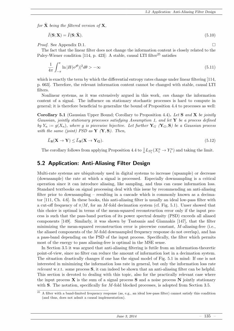
5.2 Application: Anti-Aliasing Filter Design
for X being the filtered version of X,
I(S;X) = I(S; X). (5.10)
Proof. See Appendix D.1.The fact that the linear filter does not change the information content is closely related to the
Paley-Wiener condition [114, p. 423]: A stable, causal LTI filter25 satisfies
1
4π
∫ π
−πln |H(eθ)|2dθ > −∞ (5.11)
which is exactly the term by which the differential entropy rates change under linear filtering [114,p. 663]. Therefore, the relevant information content cannot be changed with stable, causal LTIfilters.Nonlinear systems, as it was extensively argued in this work, can change the information
content of a signal. The influence on stationary stochastic processes is hard to compute ingeneral; it is therefore beneficial to generalize the bound of Proposition 4.4 to processes as well:
Corollary 5.1 (Gaussian Upper Bound; Corollary to Proposition 4.4). Let S and X be jointlyGaussian, jointly stationary processes satisfying Assumption 1, and let Y be a process definedby Yn := g(Xn), where g is piecewise bijective. Let further YG (YG,S) be a Gaussian processwith the same (joint) PSD as Y (Y,S). Then,
LS(X→ Y) ≤LS(X→ YG). (5.12)
The corollary follows from applying Proposition 4.4 to 1nLSn
1(Xn
1 → Y n1 ) and taking the limit.
5.2 Application: Anti-Aliasing Filter Design
Multi-rate systems are ubiquitously used in digital systems to increase (upsample) or decrease(downsample) the rate at which a signal is processed. Especially downsampling is a criticaloperation since it can introduce aliasing, like sampling, and thus can cause information loss.Standard textbooks on signal processing deal with this issue by recommending an anti-aliasingfilter prior to downsampling – resulting in a cascade which is commonly known as a decima-tor [111, Ch. 4.6]. In these books, this anti-aliasing filter is usually an ideal low-pass filter witha cut-off frequency of π/M , for an M -fold decimation system (cf. Fig. 5.1). Unser showed thatthis choice is optimal in terms of the mean-squared reconstruction error only if the input pro-cess is such that the pass-band portion of its power spectral density (PSD) exceeds all aliasedcomponents [149]. Similarly, it was shown by Tsatsanis and Giannakis [147], that the filterminimizing the mean-squared reconstruction error is piecewise constant, M -aliasing-free (i.e.,the aliased components of the M -fold downsampled frequency response do not overlap), and hasa pass-band depending on the PSD of the input process. Specifically, the filter which permitsmost of the energy to pass aliasing-free is optimal in the MSE sense.In Section 3.5 it was argued that anti-aliasing filtering is futile from an information-theoretic
point-of-view, since no filter can reduce the amount of information lost in a decimation system.The situation drastically changes if one has the signal model of Fig. 5.1 in mind: If one is notinterested in minimizing the information loss rate in general, but only the information loss raterelevant w.r.t. some process S, it can indeed be shown that an anti-aliasing filter can be helpful.This section is devoted to dealing with this topic, also for the practically relevant case wherethe input process X is the sum of a signal process S and a noise process N jointly stationarywith S. The notation, specifically for M -fold blocked processes, is adopted from Section 3.5.
25 A filter with a band-limited frequency response (as, e.g., an ideal low-pass filter) cannot satisfy this condition(and thus, does not admit a causal implementation).
June 3, 2014 – 135 –
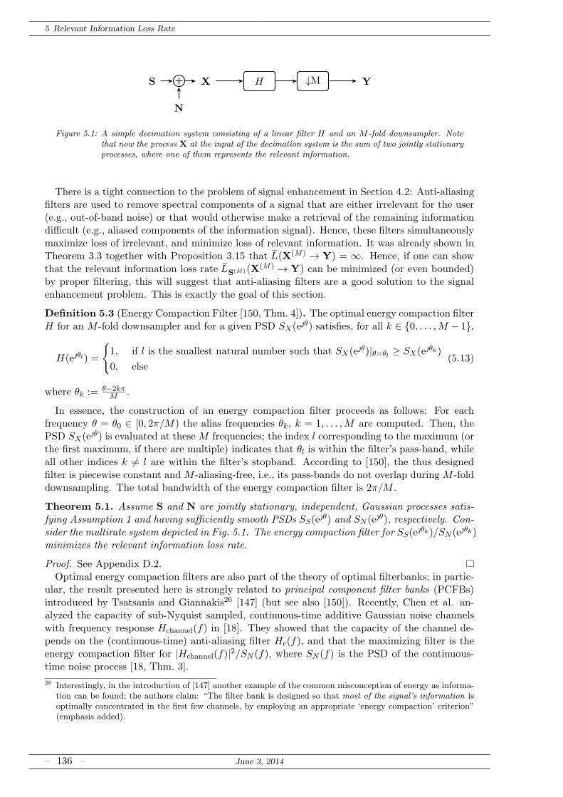
5 Relevant Information Loss Rate
S
N
X H ↓M Y
Figure 5.1: A simple decimation system consisting of a linear filter H and an M-fold downsampler. Notethat now the process X at the input of the decimation system is the sum of two jointly stationaryprocesses, where one of them represents the relevant information.
There is a tight connection to the problem of signal enhancement in Section 4.2: Anti-aliasingfilters are used to remove spectral components of a signal that are either irrelevant for the user(e.g., out-of-band noise) or that would otherwise make a retrieval of the remaining informationdifficult (e.g., aliased components of the information signal). Hence, these filters simultaneouslymaximize loss of irrelevant, and minimize loss of relevant information. It was already shown inTheorem 3.3 together with Proposition 3.15 that L(X(M ) → Y) = ∞. Hence, if one can showthat the relevant information loss rate LS(M )(X(M ) → Y) can be minimized (or even bounded)by proper filtering, this will suggest that anti-aliasing filters are a good solution to the signalenhancement problem. This is exactly the goal of this section.
Definition 5.3 (Energy Compaction Filter [150, Thm. 4]). The optimal energy compaction filterH for an M -fold downsampler and for a given PSD SX(eθ) satisfies, for all k ∈ 0, . . . ,M − 1,
H(eθl) =
1, if l is the smallest natural number such that SX(eθ)|θ=θl ≥ SX(eθk)
0, else(5.13)
where θk := θ−2kπM .
In essence, the construction of an energy compaction filter proceeds as follows: For eachfrequency θ = θ0 ∈ [0, 2π/M) the alias frequencies θk, k = 1, . . . ,M are computed. Then, thePSD SX(eθ) is evaluated at these M frequencies; the index l corresponding to the maximum (orthe first maximum, if there are multiple) indicates that θl is within the filter’s pass-band, whileall other indices k 6= l are within the filter’s stopband. According to [150], the thus designedfilter is piecewise constant and M -aliasing-free, i.e., its pass-bands do not overlap during M -folddownsampling. The total bandwidth of the energy compaction filter is 2π/M .
Theorem 5.1. Assume S and N are jointly stationary, independent, Gaussian processes satis-fying Assumption 1 and having sufficiently smooth PSDs SS(e
θ) and SN (eθ), respectively. Con-sider the multirate system depicted in Fig. 5.1. The energy compaction filter for SS(e
θk)/SN (eθk)minimizes the relevant information loss rate.
Proof. See Appendix D.2.Optimal energy compaction filters are also part of the theory of optimal filterbanks; in partic-
ular, the result presented here is strongly related to principal component filter banks (PCFBs)introduced by Tsatsanis and Giannakis26 [147] (but see also [150]). Recently, Chen et al. an-alyzed the capacity of sub-Nyquist sampled, continuous-time additive Gaussian noise channelswith frequency response Hchannel(f) in [18]. They showed that the capacity of the channel de-pends on the (continuous-time) anti-aliasing filter Hc(f), and that the maximizing filter is theenergy compaction filter for |Hchannel(f)|2/SN (f), where SN (f) is the PSD of the continuous-time noise process [18, Thm. 3].
26 Interestingly, in the introduction of [147] another example of the common misconception of energy as informa-tion can be found; the authors claim: “The filter bank is designed so that most of the signal’s information isoptimally concentrated in the first few channels, by employing an appropriate ‘energy compaction’ criterion”(emphasis added).
– 136 – June 3, 2014
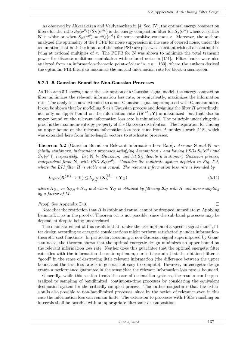
5.2 Application: Anti-Aliasing Filter Design
As observed by Akkarakaran and Vaidyanathan in [4, Sec. IV], the optimal energy compactionfilters for the ratio SS(e
θk)/SN (eθk) is the energy compaction filter for SS(eθ) whenever either
N is white or when SN (eθ) = cSS(eθ) for some positive constant c. Moreover, the authors
analyzed the optimality of the PCFB for noise suppression in the case of colored noise, under theassumption that both the input and the noise PSD are piecewise constant with all discontinuitieslying at rational multiples of π. The PCFB for N was shown to minimize the total transmitpower for discrete multitone modulation with colored noise in [151]. Filter banks were alsoanalyzed from an information-theoretic point-of-view in, e.g., [133], where the authors derivedthe optimum FIR filters to maximize the mutual information rate for block transmission.
5.2.1 A Gaussian Bound for Non-Gaussian Processes
As Theorem 5.1 shows, under the assumption of a Gaussian signal model, the energy compactionfilter minimizes the relevant information loss rate, or equivalently, maximizes the informationrate. The analysis is now extended to a non-Gaussian signal superimposed with Gaussian noise.It can be shown that by modelling S as a Gaussian process and designing the filterH accordingly,not only an upper bound on the information rate I(S(M );Y) is maximized, but that also anupper bound on the relevant information loss rate is minimized. The principle underlying thisproof is the maximum-entropy property of the Gaussian distribution. The inspiration for findingan upper bound on the relevant information loss rate came from Plumbley’s work [118], whichwas extended here from finite-length vectors to stochastic processes.
Theorem 5.2 (Gaussian Bound on Relevant Information Loss Rate). Assume S and N arejointly stationary, independent processes satisfying Assumption 1 and having PSDs SS(e
θ) andSN (eθ), respectively. Let N be Gaussian, and let SG denote a stationary Gaussian process,independent from N, with PSD SS(e
θ). Consider the multirate system depicted in Fig. 5.1,where the LTI filter H is stable and causal. The relevant information loss rate is bounded by
LS(M )(X(M ) → Y) ≤LS(M )G
(X(M )G → YG) (5.14)
where XG,n := SG,n +Nn, and where YG is obtained by filtering XG with H and downsamplingby a factor of M .
Proof. See Appendix D.3.
Note that the restriction thatH is stable and causal cannot be dropped immediately: ApplyingLemma D.1 as in the proof of Theorem 5.1 is not possible, since the sub-band processes may bedependent despite being uncorrelated.
The main statement of this result is that, under the assumption of a specific signal model, fil-ter design according to energetic considerations might perform satisfactorily under information-theoretic cost functions. In particular, assuming a non-Gaussian signal superimposed by Gaus-sian noise, the theorem shows that the optimal energetic design minimizes an upper bound onthe relevant information loss rate. Neither does this guarantee that the optimal energetic filtercoincides with the information-theoretic optimum, nor is it certain that the obtained filter is“good” in the sense of destroying little relevant information (the difference between the upperbound and the true loss rate is in general not easy to compute). However, an energetic designgrants a performance guarantee in the sense that the relevant information loss rate is bounded.
Generally, while this section treats the case of decimation systems, the results can be gen-eralized to sampling of bandlimited, continuous-time processes by considering the equivalentdecimation system for the critically sampled process. The author conjectures that the exten-sion is also possible to non-bandlimited processes, since by the notion of relevance even in thiscase the information loss can remain finite. The extension to processes with PSDs vanishing onintervals shall be possible with an appropriate filterbank decomposition.
June 3, 2014 – 137 –
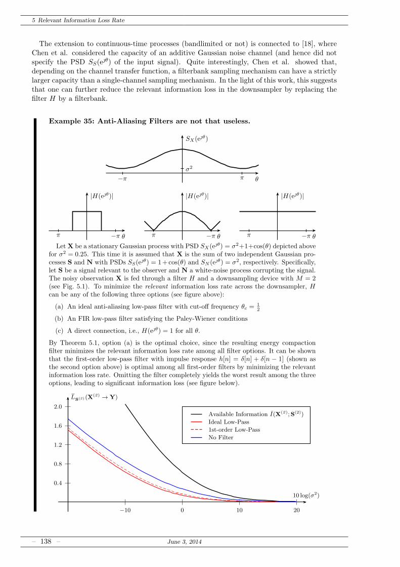
5 Relevant Information Loss Rate
The extension to continuous-time processes (bandlimited or not) is connected to [18], whereChen et al. considered the capacity of an additive Gaussian noise channel (and hence did notspecify the PSD SS(e
θ) of the input signal). Quite interestingly, Chen et al. showed that,depending on the channel transfer function, a filterbank sampling mechanism can have a strictlylarger capacity than a single-channel sampling mechanism. In the light of this work, this suggeststhat one can further reduce the relevant information loss in the downsampler by replacing thefilter H by a filterbank.
Example 35: Anti-Aliasing Filters are not that useless.
θ
SX(eθ)
π−πσ2
θ
|H(eθ)|
π −π θ
|H(eθ)|
π −π θ
|H(eθ)|
π −πLetX be a stationary Gaussian process with PSD SX(eθ) = σ2+1+cos(θ) depicted above
for σ2 = 0.25. This time it is assumed that X is the sum of two independent Gaussian pro-cesses S and N with PSDs SS(e
θ) = 1+cos(θ) and SN (eθ) = σ2, respectively. Specifically,let S be a signal relevant to the observer and N a white-noise process corrupting the signal.The noisy observation X is fed through a filter H and a downsampling device with M = 2(see Fig. 5.1). To minimize the relevant information loss rate across the downsampler, Hcan be any of the following three options (see figure above):
(a) An ideal anti-aliasing low-pass filter with cut-off frequency θc =12
(b) An FIR low-pass filter satisfying the Paley-Wiener conditions
(c) A direct connection, i.e., H(eθ) = 1 for all θ.
By Theorem 5.1, option (a) is the optimal choice, since the resulting energy compactionfilter minimizes the relevant information loss rate among all filter options. It can be shownthat the first-order low-pass filter with impulse response h[n] = δ[n] + δ[n − 1] (shown asthe second option above) is optimal among all first-order filters by minimizing the relevantinformation loss rate. Omitting the filter completely yields the worst result among the threeoptions, leading to significant information loss (see figure below).
0.4
0.8
1.2
1.6
2.0
−10 0 10 20
10 log(σ2)
LS(2)(X(2) → Y)
Available Information I(X(2);S(2))
Ideal Low-Pass
1st-order Low-Pass
No Filter
– 138 – June 3, 2014
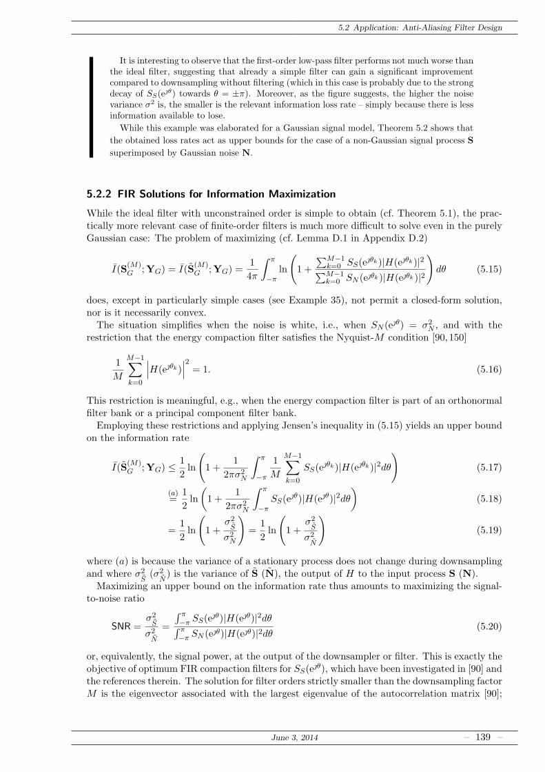
5.2 Application: Anti-Aliasing Filter Design
It is interesting to observe that the first-order low-pass filter performs not much worse thanthe ideal filter, suggesting that already a simple filter can gain a significant improvementcompared to downsampling without filtering (which in this case is probably due to the strongdecay of SS(e
θ) towards θ = ±π). Moreover, as the figure suggests, the higher the noisevariance σ2 is, the smaller is the relevant information loss rate – simply because there is lessinformation available to lose.
While this example was elaborated for a Gaussian signal model, Theorem 5.2 shows that
the obtained loss rates act as upper bounds for the case of a non-Gaussian signal process S
superimposed by Gaussian noise N.
5.2.2 FIR Solutions for Information Maximization
While the ideal filter with unconstrained order is simple to obtain (cf. Theorem 5.1), the prac-tically more relevant case of finite-order filters is much more difficult to solve even in the purelyGaussian case: The problem of maximizing (cf. Lemma D.1 in Appendix D.2)
I(S(M)G ;YG) = I(S
(M)G ;YG) =
1
4π
∫ π
−πln
(
1 +
∑M−1k=0 SS(e
θk)|H(eθk)|2∑M−1
k=0 SN (eθk)|H(eθk)|2
)
dθ (5.15)
does, except in particularly simple cases (see Example 35), not permit a closed-form solution,nor is it necessarily convex.The situation simplifies when the noise is white, i.e., when SN (eθ) = σ2
N , and with therestriction that the energy compaction filter satisfies the Nyquist-M condition [90, 150]
1
M
M−1∑
k=0
∣∣∣H(eθk)
∣∣∣
2= 1. (5.16)
This restriction is meaningful, e.g., when the energy compaction filter is part of an orthonormalfilter bank or a principal component filter bank.Employing these restrictions and applying Jensen’s inequality in (5.15) yields an upper bound
on the information rate
I(S(M)G ;YG) ≤
1
2ln
(
1 +1
2πσ2N
∫ π
−π
1
M
M−1∑
k=0
SS(eθk)|H(eθk)|2dθ
)
(5.17)
(a)=
1
2ln
(
1 +1
2πσ2N
∫ π
−πSS(e
θ)|H(eθ)|2dθ)
(5.18)
=1
2ln
(
1 +σ2S
σ2N
)
=1
2ln
(
1 +σ2S
σ2N
)
(5.19)
where (a) is because the variance of a stationary process does not change during downsamplingand where σ2
S(σ2
N) is the variance of S (N), the output of H to the input process S (N).
Maximizing an upper bound on the information rate thus amounts to maximizing the signal-to-noise ratio
SNR =σ2S
σ2N
=
∫ π−π SS(e
θ)|H(eθ)|2dθ∫ π−π SN (eθ)|H(eθ)|2dθ (5.20)
or, equivalently, the signal power, at the output of the downsampler or filter. This is exactly theobjective of optimum FIR compaction filters for SS(e
θ), which have been investigated in [90] andthe references therein. The solution for filter orders strictly smaller than the downsampling factorM is the eigenvector associated with the largest eigenvalue of the autocorrelation matrix [90];
June 3, 2014 – 139 –
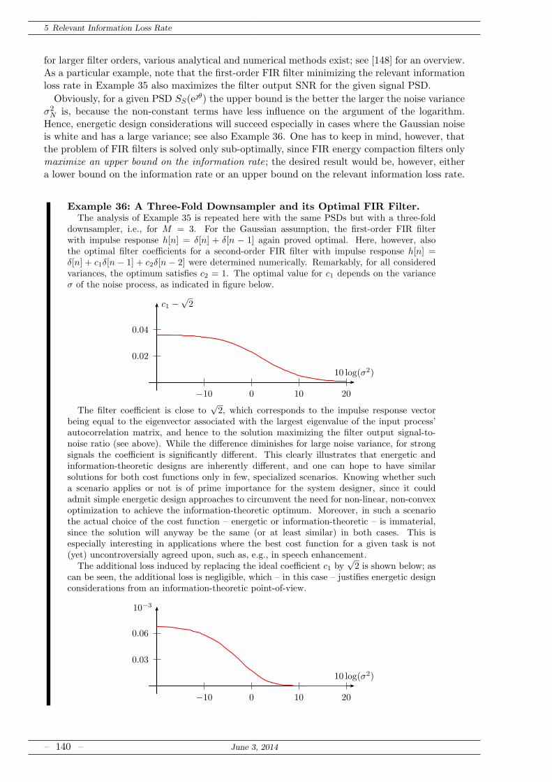
5 Relevant Information Loss Rate
for larger filter orders, various analytical and numerical methods exist; see [148] for an overview.As a particular example, note that the first-order FIR filter minimizing the relevant informationloss rate in Example 35 also maximizes the filter output SNR for the given signal PSD.
Obviously, for a given PSD SS(eθ) the upper bound is the better the larger the noise variance
σ2N is, because the non-constant terms have less influence on the argument of the logarithm.
Hence, energetic design considerations will succeed especially in cases where the Gaussian noiseis white and has a large variance; see also Example 36. One has to keep in mind, however, thatthe problem of FIR filters is solved only sub-optimally, since FIR energy compaction filters onlymaximize an upper bound on the information rate; the desired result would be, however, eithera lower bound on the information rate or an upper bound on the relevant information loss rate.
Example 36: A Three-Fold Downsampler and its Optimal FIR Filter.The analysis of Example 35 is repeated here with the same PSDs but with a three-fold
downsampler, i.e., for M = 3. For the Gaussian assumption, the first-order FIR filterwith impulse response h[n] = δ[n] + δ[n − 1] again proved optimal. Here, however, alsothe optimal filter coefficients for a second-order FIR filter with impulse response h[n] =δ[n] + c1δ[n − 1] + c2δ[n − 2] were determined numerically. Remarkably, for all consideredvariances, the optimum satisfies c2 = 1. The optimal value for c1 depends on the varianceσ of the noise process, as indicated in figure below.
0.02
0.04
−10 0 10 20
10 log(σ2)
c1 −√2
The filter coefficient is close to√2, which corresponds to the impulse response vector
being equal to the eigenvector associated with the largest eigenvalue of the input process’autocorrelation matrix, and hence to the solution maximizing the filter output signal-to-noise ratio (see above). While the difference diminishes for large noise variance, for strongsignals the coefficient is significantly different. This clearly illustrates that energetic andinformation-theoretic designs are inherently different, and one can hope to have similarsolutions for both cost functions only in few, specialized scenarios. Knowing whether sucha scenario applies or not is of prime importance for the system designer, since it couldadmit simple energetic design approaches to circumvent the need for non-linear, non-convexoptimization to achieve the information-theoretic optimum. Moreover, in such a scenariothe actual choice of the cost function – energetic or information-theoretic – is immaterial,since the solution will anyway be the same (or at least similar) in both cases. This isespecially interesting in applications where the best cost function for a given task is not(yet) uncontroversially agreed upon, such as, e.g., in speech enhancement.
The additional loss induced by replacing the ideal coefficient c1 by√2 is shown below; as
can be seen, the additional loss is negligible, which – in this case – justifies energetic designconsiderations from an information-theoretic point-of-view.
0.03
0.06
−10 0 10 20
10 log(σ2)
10−3
– 140 – June 3, 2014
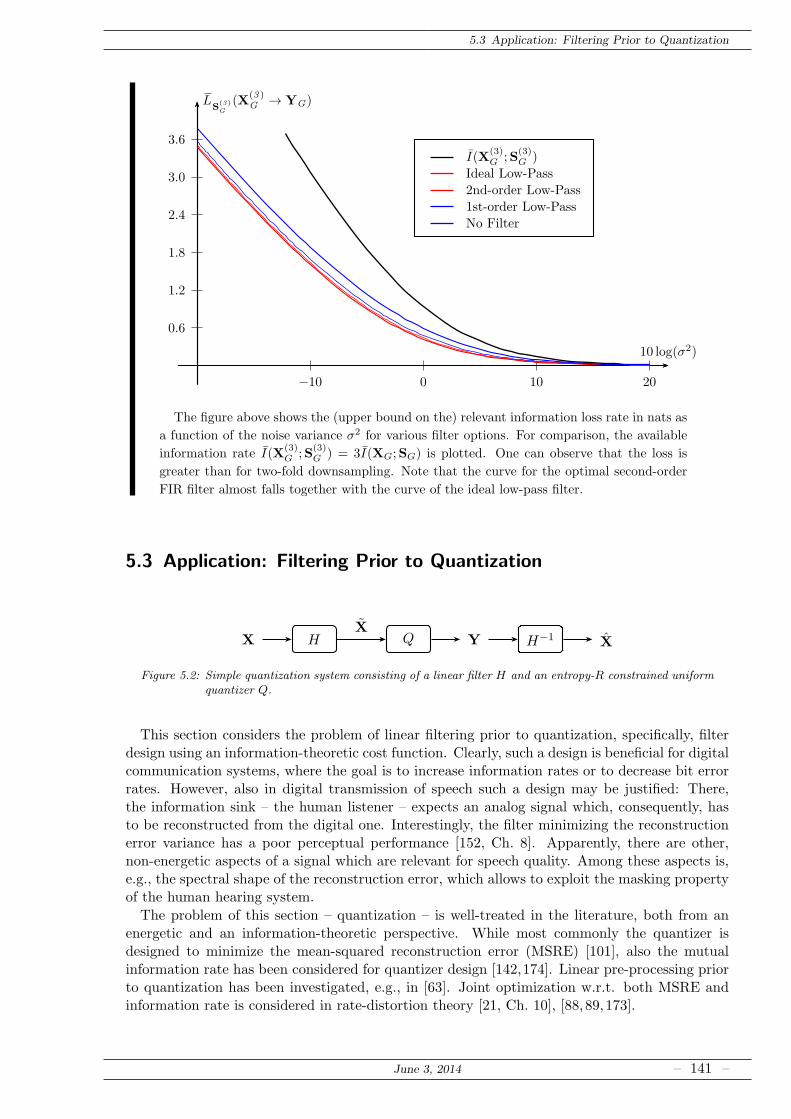
5.3 Application: Filtering Prior to Quantization
0.6
1.2
1.8
2.4
3.0
3.6
−10 0 10 20
10 log(σ2)
LS
(3)G
(X(3)G → YG)
I(X(3)G ;S
(3)G )
Ideal Low-Pass
2nd-order Low-Pass
1st-order Low-Pass
No Filter
The figure above shows the (upper bound on the) relevant information loss rate in nats as
a function of the noise variance σ2 for various filter options. For comparison, the available
information rate I(X(3)G ;S
(3)G ) = 3I(XG;SG) is plotted. One can observe that the loss is
greater than for two-fold downsampling. Note that the curve for the optimal second-order
FIR filter almost falls together with the curve of the ideal low-pass filter.
5.3 Application: Filtering Prior to Quantization
X H Q YX
H−1 X
Figure 5.2: Simple quantization system consisting of a linear filter H and an entropy-R constrained uniformquantizer Q.
This section considers the problem of linear filtering prior to quantization, specifically, filterdesign using an information-theoretic cost function. Clearly, such a design is beneficial for digitalcommunication systems, where the goal is to increase information rates or to decrease bit errorrates. However, also in digital transmission of speech such a design may be justified: There,the information sink – the human listener – expects an analog signal which, consequently, hasto be reconstructed from the digital one. Interestingly, the filter minimizing the reconstructionerror variance has a poor perceptual performance [152, Ch. 8]. Apparently, there are other,non-energetic aspects of a signal which are relevant for speech quality. Among these aspects is,e.g., the spectral shape of the reconstruction error, which allows to exploit the masking propertyof the human hearing system.
The problem of this section – quantization – is well-treated in the literature, both from anenergetic and an information-theoretic perspective. While most commonly the quantizer isdesigned to minimize the mean-squared reconstruction error (MSRE) [101], also the mutualinformation rate has been considered for quantizer design [142,174]. Linear pre-processing priorto quantization has been investigated, e.g., in [63]. Joint optimization w.r.t. both MSRE andinformation rate is considered in rate-distortion theory [21, Ch. 10], [88, 89, 173].
June 3, 2014 – 141 –
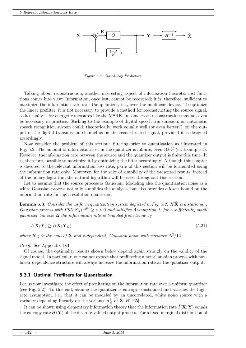
5 Relevant Information Loss Rate
X−
Q b
1−HH
YE
H−1 X
Figure 5.3: Closed-loop Prediction.
Talking about reconstruction, another interesting aspect of information-theoretic cost func-tions comes into view: Information, once lost, cannot be recovered; it is, therefore, sufficient tomaximize the information rate over the quantizer, i.e., over the nonlinear device. To optimizethe linear prefilter, it is not necessary to provide a method for reconstructing the source signal,as it usually is for energetic measures like the MSRE. In some cases reconstruction may not evenbe necessary in practice: Sticking to the example of digital speech transmission, an automaticspeech recognition system could, theoretically, work equally well (or even better?) on the out-put of the digital transmission channel as on the reconstructed signal, provided it is designedaccordingly.
Now consider the problem of this section: filtering prior to quantization as illustrated inFig. 5.2. The amount of information lost in the quantizer is infinite, even 100% (cf. Example 1).However, the information rate between the source and the quantizer output is finite this time. Itis, therefore, possible to maximize it by optimizing the filter accordingly. Although this chapteris devoted to the relevant information loss rate, parts of this section will be formulated usingthe information rate only. Moreover, for the sake of simplicity of the presented results, insteadof the binary logarithm the natural logarithm will be used throughout this section.
Let us assume that the source process is Gaussian. Modeling also the quantization noise as awhite Gaussian process not only simplifies the analysis, but also provides a lower bound on theinformation rate for high-resolution quantizers:
Lemma 5.3. Consider the uniform quantization system depicted in Fig. 5.2. If X is a stationaryGaussian process with PSD SX(eθ) ≥ ǫ > 0 and satisfies Assumption 1, for a sufficiently smallquantizer bin size ∆ the information rate is bounded from below by
I(X;Y) ≥ I(X;YG) (5.21)
where YG is the sum of X and independent, Gaussian noise with variance ∆2/12.
Proof. See Appendix D.4.
Of course, the optimality results shown below depend again strongly on the validity of thesignal model. In particular, one cannot expect that prefiltering a non-Gaussian process with non-linear dependence structure will always increase the information rate at the quantizer output.
5.3.1 Optimal Prefilters for Quantization
Let us now investigate the effect of prefiltering on the information rate over a uniform quantizer(see Fig. 5.2). To this end, assume the quantizer is entropy-constrained and satisfies the high-rate assumption, i.e., that it can be modeled by an uncorrelated, white noise source with avariance depending linearly on the variance σ2
Xof X, cf. [65].
It can be shown using elementary information theory that the information rate I(X;Y) equalsthe entropy rateH (Y) of the discrete-valued output process. For a fixed marginal distribution of
– 142 – June 3, 2014
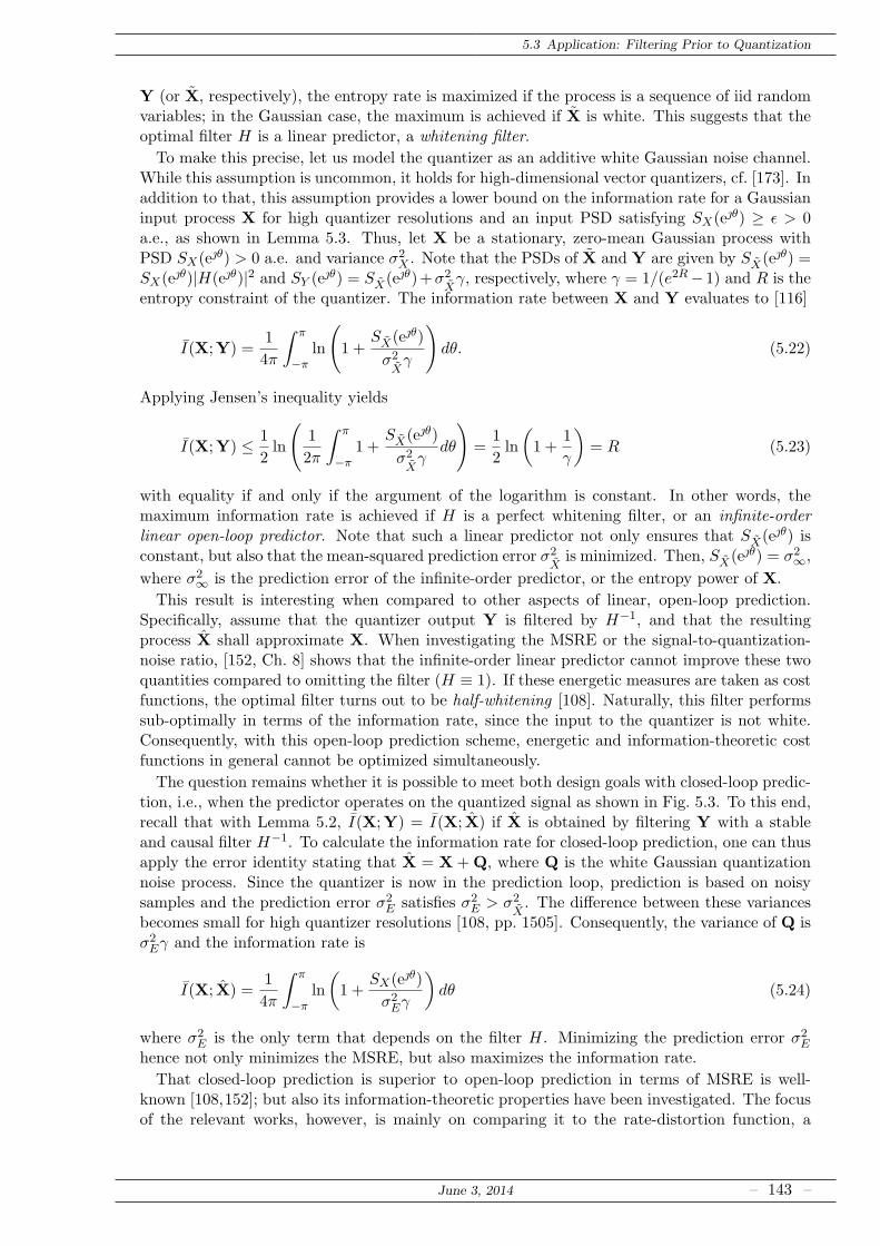
5.3 Application: Filtering Prior to Quantization
Y (or X, respectively), the entropy rate is maximized if the process is a sequence of iid randomvariables; in the Gaussian case, the maximum is achieved if X is white. This suggests that theoptimal filter H is a linear predictor, a whitening filter.
To make this precise, let us model the quantizer as an additive white Gaussian noise channel.While this assumption is uncommon, it holds for high-dimensional vector quantizers, cf. [173]. Inaddition to that, this assumption provides a lower bound on the information rate for a Gaussianinput process X for high quantizer resolutions and an input PSD satisfying SX(eθ) ≥ ǫ > 0a.e., as shown in Lemma 5.3. Thus, let X be a stationary, zero-mean Gaussian process withPSD SX(eθ) > 0 a.e. and variance σ2
X . Note that the PSDs of X and Y are given by SX(eθ) =SX(eθ)|H(eθ)|2 and SY (e
θ) = SX(eθ)+σ2Xγ, respectively, where γ = 1/(e2R−1) and R is the
entropy constraint of the quantizer. The information rate between X and Y evaluates to [116]
I(X;Y) =1
4π
∫ π
−πln
(
1 +SX(eθ)
σ2Xγ
)
dθ. (5.22)
Applying Jensen’s inequality yields
I(X;Y) ≤ 1
2ln
(
1
2π
∫ π
−π1 +
SX(eθ)
σ2Xγ
dθ
)
=1
2ln
(
1 +1
γ
)
= R (5.23)
with equality if and only if the argument of the logarithm is constant. In other words, themaximum information rate is achieved if H is a perfect whitening filter, or an infinite-orderlinear open-loop predictor. Note that such a linear predictor not only ensures that SX(eθ) isconstant, but also that the mean-squared prediction error σ2
Xis minimized. Then, SX(eθ) = σ2
∞,
where σ2∞ is the prediction error of the infinite-order predictor, or the entropy power of X.
This result is interesting when compared to other aspects of linear, open-loop prediction.Specifically, assume that the quantizer output Y is filtered by H−1, and that the resultingprocess X shall approximate X. When investigating the MSRE or the signal-to-quantization-noise ratio, [152, Ch. 8] shows that the infinite-order linear predictor cannot improve these twoquantities compared to omitting the filter (H ≡ 1). If these energetic measures are taken as costfunctions, the optimal filter turns out to be half-whitening [108]. Naturally, this filter performssub-optimally in terms of the information rate, since the input to the quantizer is not white.Consequently, with this open-loop prediction scheme, energetic and information-theoretic costfunctions in general cannot be optimized simultaneously.
The question remains whether it is possible to meet both design goals with closed-loop predic-tion, i.e., when the predictor operates on the quantized signal as shown in Fig. 5.3. To this end,recall that with Lemma 5.2, I(X;Y) = I(X; X) if X is obtained by filtering Y with a stableand causal filter H−1. To calculate the information rate for closed-loop prediction, one can thusapply the error identity stating that X = X +Q, where Q is the white Gaussian quantizationnoise process. Since the quantizer is now in the prediction loop, prediction is based on noisysamples and the prediction error σ2
E satisfies σ2E > σ2
X. The difference between these variances
becomes small for high quantizer resolutions [108, pp. 1505]. Consequently, the variance of Q isσ2Eγ and the information rate is
I(X; X) =1
4π
∫ π
−πln
(
1 +SX(eθ)
σ2Eγ
)
dθ (5.24)
where σ2E is the only term that depends on the filter H. Minimizing the prediction error σ2
E
hence not only minimizes the MSRE, but also maximizes the information rate.
That closed-loop prediction is superior to open-loop prediction in terms of MSRE is well-known [108,152]; but also its information-theoretic properties have been investigated. The focusof the relevant works, however, is mainly on comparing it to the rate-distortion function, a
June 3, 2014 – 143 –
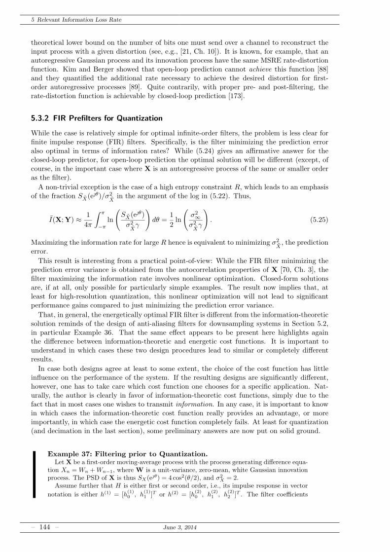
5 Relevant Information Loss Rate
theoretical lower bound on the number of bits one must send over a channel to reconstruct theinput process with a given distortion (see, e.g., [21, Ch. 10]). It is known, for example, that anautoregressive Gaussian process and its innovation process have the same MSRE rate-distortionfunction. Kim and Berger showed that open-loop prediction cannot achieve this function [88]and they quantified the additional rate necessary to achieve the desired distortion for first-order autoregressive processes [89]. Quite contrarily, with proper pre- and post-filtering, therate-distortion function is achievable by closed-loop prediction [173].
5.3.2 FIR Prefilters for Quantization
While the case is relatively simple for optimal infinite-order filters, the problem is less clear forfinite impulse response (FIR) filters. Specifically, is the filter minimizing the prediction erroralso optimal in terms of information rates? While (5.24) gives an affirmative answer for theclosed-loop predictor, for open-loop prediction the optimal solution will be different (except, ofcourse, in the important case where X is an autoregressive process of the same or smaller orderas the filter).
A non-trivial exception is the case of a high entropy constraint R, which leads to an emphasisof the fraction SX(eθ)/σ2
Xin the argument of the log in (5.22). Thus,
I(X;Y) ≈ 1
4π
∫ π
−πln
(
SX(eθ)
σ2Xγ
)
dθ =1
2ln
(
σ2∞
σ2Xγ
)
. (5.25)
Maximizing the information rate for large R hence is equivalent to minimizing σ2X, the prediction
error.
This result is interesting from a practical point-of-view: While the FIR filter minimizing theprediction error variance is obtained from the autocorrelation properties of X [70, Ch. 3], thefilter maximizing the information rate involves nonlinear optimization. Closed-form solutionsare, if at all, only possible for particularly simple examples. The result now implies that, atleast for high-resolution quantization, this nonlinear optimization will not lead to significantperformance gains compared to just minimizing the prediction error variance.
That, in general, the energetically optimal FIR filter is different from the information-theoreticsolution reminds of the design of anti-aliasing filters for downsampling systems in Section 5.2,in particular Example 36. That the same effect appears to be present here highlights againthe difference between information-theoretic and energetic cost functions. It is important tounderstand in which cases these two design procedures lead to similar or completely differentresults.
In case both designs agree at least to some extent, the choice of the cost function has littleinfluence on the performance of the system. If the resulting designs are significantly different,however, one has to take care which cost function one chooses for a specific application. Nat-urally, the author is clearly in favor of information-theoretic cost functions, simply due to thefact that in most cases one wishes to transmit information. In any case, it is important to knowin which cases the information-theoretic cost function really provides an advantage, or moreimportantly, in which case the energetic cost function completely fails. At least for quantization(and decimation in the last section), some preliminary answers are now put on solid ground.
Example 37: Filtering prior to Quantization.Let X be a first-order moving-average process with the process generating difference equa-
tion Xn = Wn +Wn−1, where W is a unit-variance, zero-mean, white Gaussian innovationprocess. The PSD of X is thus SX(eθ) = 4 cos2(θ/2), and σ2
X = 2.Assume further that H is either first or second order, i.e., its impulse response in vector
notation is either h(1) = [h(1)0 , h
(1)1 ]T or h(2) = [h
(2)0 , h
(2)1 , h
(2)2 ]T . The filter coefficients
– 144 – June 3, 2014
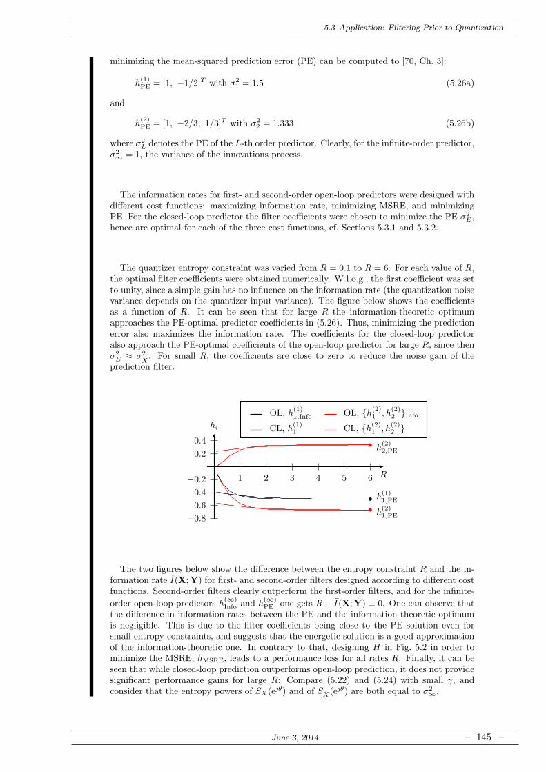
5.3 Application: Filtering Prior to Quantization
minimizing the mean-squared prediction error (PE) can be computed to [70, Ch. 3]:
h(1)PE = [1, −1/2]T with σ2
1 = 1.5 (5.26a)
and
h(2)PE = [1, −2/3, 1/3]T with σ2
2 = 1.333 (5.26b)
where σ2L denotes the PE of the L-th order predictor. Clearly, for the infinite-order predictor,
σ2∞ = 1, the variance of the innovations process.
The information rates for first- and second-order open-loop predictors were designed withdifferent cost functions: maximizing information rate, minimizing MSRE, and minimizingPE. For the closed-loop predictor the filter coefficients were chosen to minimize the PE σ2
E ,hence are optimal for each of the three cost functions, cf. Sections 5.3.1 and 5.3.2.
The quantizer entropy constraint was varied from R = 0.1 to R = 6. For each value of R,the optimal filter coefficients were obtained numerically. W.l.o.g., the first coefficient was setto unity, since a simple gain has no influence on the information rate (the quantization noisevariance depends on the quantizer input variance). The figure below shows the coefficientsas a function of R. It can be seen that for large R the information-theoretic optimumapproaches the PE-optimal predictor coefficients in (5.26). Thus, minimizing the predictionerror also maximizes the information rate. The coefficients for the closed-loop predictoralso approach the PE-optimal coefficients of the open-loop predictor for large R, since thenσ2E ≈ σ2
X. For small R, the coefficients are close to zero to reduce the noise gain of the
prediction filter.
0.2
0.4
−0.2−0.4−0.6−0.8
1 2 3 4 5 6 R
hi
OL, h(1)1,Info OL, h(2)
1 , h(2)2 Info
CL, h(1)1 CL, h(2)
1 , h(2)2
bh(2)2,PE
bh(2)1,PE
b h(1)1,PE
The two figures below show the difference between the entropy constraint R and the in-formation rate I(X;Y) for first- and second-order filters designed according to different costfunctions. Second-order filters clearly outperform the first-order filters, and for the infinite-
order open-loop predictors h(∞)Info and h
(∞)PE one gets R− I(X;Y) ≡ 0. One can observe that
the difference in information rates between the PE and the information-theoretic optimumis negligible. This is due to the filter coefficients being close to the PE solution even forsmall entropy constraints, and suggests that the energetic solution is a good approximationof the information-theoretic one. In contrary to that, designing H in Fig. 5.2 in order tominimize the MSRE, hMSRE, leads to a performance loss for all rates R. Finally, it can beseen that while closed-loop prediction outperforms open-loop prediction, it does not providesignificant performance gains for large R: Compare (5.22) and (5.24) with small γ, andconsider that the entropy powers of SX(eθ) and of SX(eθ) are both equal to σ2
∞.
June 3, 2014 – 145 –
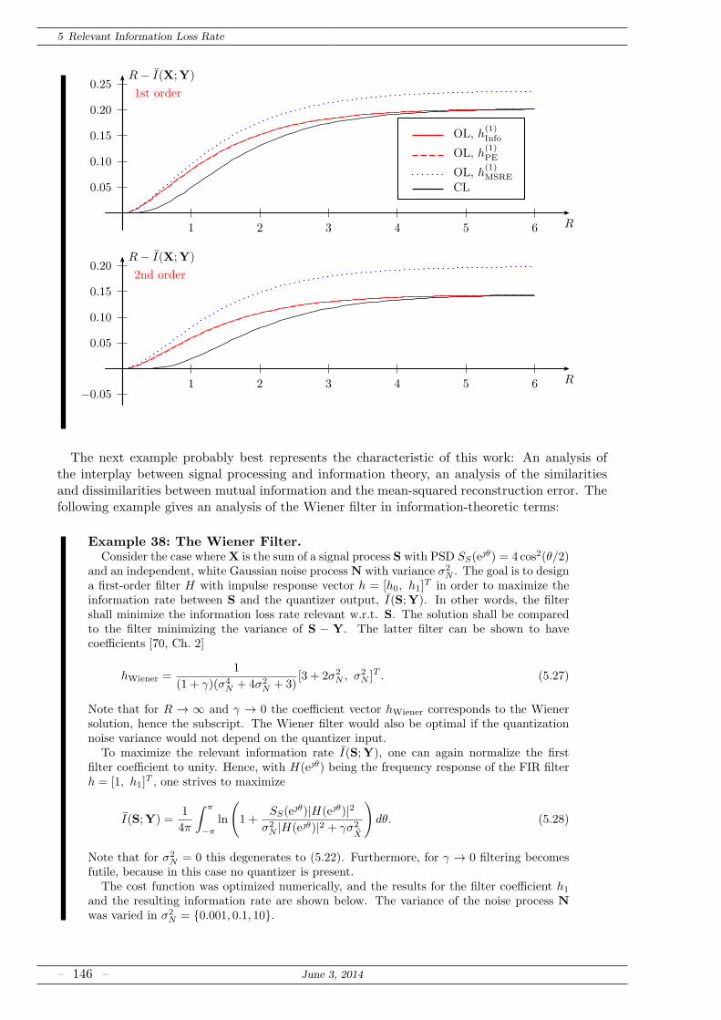
5 Relevant Information Loss Rate
1st order
0.05
0.10
0.15
0.20
0.25
1 2 3 4 5 6 R
R− I(X;Y)
OL, h(1)Info
OL, h(1)PE
OL, h(1)MSRE
CL
2nd order
0.05
0.10
0.15
0.20
−0.051 2 3 4 5 6 R
R− I(X;Y)
The next example probably best represents the characteristic of this work: An analysis ofthe interplay between signal processing and information theory, an analysis of the similaritiesand dissimilarities between mutual information and the mean-squared reconstruction error. Thefollowing example gives an analysis of the Wiener filter in information-theoretic terms:
Example 38: The Wiener Filter.Consider the case whereX is the sum of a signal process S with PSD SS(e
θ) = 4 cos2(θ/2)and an independent, white Gaussian noise process N with variance σ2
N . The goal is to designa first-order filter H with impulse response vector h = [h0, h1]
T in order to maximize theinformation rate between S and the quantizer output, I(S;Y). In other words, the filtershall minimize the information loss rate relevant w.r.t. S. The solution shall be comparedto the filter minimizing the variance of S − Y. The latter filter can be shown to havecoefficients [70, Ch. 2]
hWiener =1
(1 + γ)(σ4N + 4σ2
N + 3)[3 + 2σ2
N , σ2N ]T . (5.27)
Note that for R → ∞ and γ → 0 the coefficient vector hWiener corresponds to the Wienersolution, hence the subscript. The Wiener filter would also be optimal if the quantizationnoise variance would not depend on the quantizer input.
To maximize the relevant information rate I(S;Y), one can again normalize the firstfilter coefficient to unity. Hence, with H(eθ) being the frequency response of the FIR filterh = [1, h1]
T , one strives to maximize
I(S;Y) =1
4π
∫ π
−π
ln
(
1 +SS(e
θ)|H(eθ)|2σ2N |H(eθ)|2 + γσ2
X
)
dθ. (5.28)
Note that for σ2N = 0 this degenerates to (5.22). Furthermore, for γ → 0 filtering becomes
futile, because in this case no quantizer is present.The cost function was optimized numerically, and the results for the filter coefficient h1
and the resulting information rate are shown below. The variance of the noise process Nwas varied in σ2
N = 0.001, 0.1, 10.
– 146 – June 3, 2014
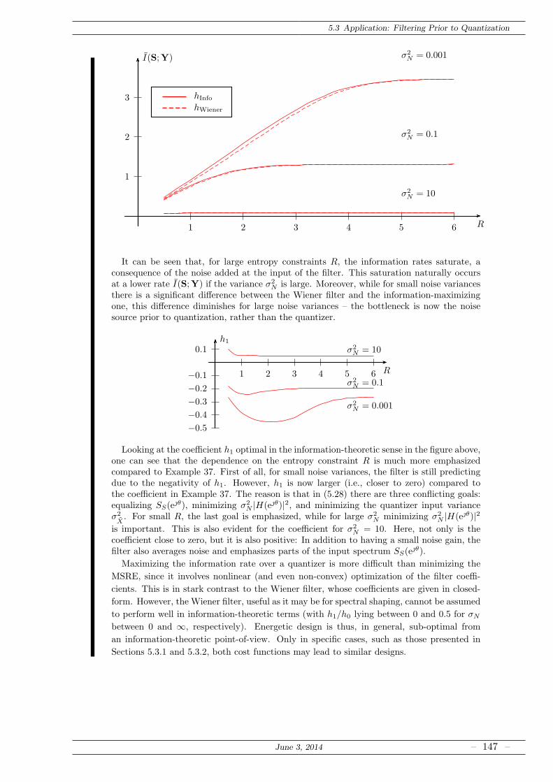
5.3 Application: Filtering Prior to Quantization
1
2
3
1 2 3 4 5 6 R
I(S;Y)
hInfo
hWiener
σ2N = 0.001
σ2N = 0.1
σ2N = 10
It can be seen that, for large entropy constraints R, the information rates saturate, aconsequence of the noise added at the input of the filter. This saturation naturally occursat a lower rate I(S;Y) if the variance σ2
N is large. Moreover, while for small noise variancesthere is a significant difference between the Wiener filter and the information-maximizingone, this difference diminishes for large noise variances – the bottleneck is now the noisesource prior to quantization, rather than the quantizer.
0.1
−0.1−0.2−0.3−0.4−0.5
1 2 3 4 5 6 R
h1
σ2N = 10
σ2N = 0.1
σ2N = 0.001
Looking at the coefficient h1 optimal in the information-theoretic sense in the figure above,one can see that the dependence on the entropy constraint R is much more emphasizedcompared to Example 37. First of all, for small noise variances, the filter is still predictingdue to the negativity of h1. However, h1 is now larger (i.e., closer to zero) compared tothe coefficient in Example 37. The reason is that in (5.28) there are three conflicting goals:equalizing SS(e
θ), minimizing σ2N |H(eθ)|2, and minimizing the quantizer input variance
σ2X. For small R, the last goal is emphasized, while for large σ2
N minimizing σ2N |H(eθ)|2
is important. This is also evident for the coefficient for σ2N = 10. Here, not only is the
coefficient close to zero, but it is also positive: In addition to having a small noise gain, thefilter also averages noise and emphasizes parts of the input spectrum SS(e
θ).
Maximizing the information rate over a quantizer is more difficult than minimizing the
MSRE, since it involves nonlinear (and even non-convex) optimization of the filter coeffi-
cients. This is in stark contrast to the Wiener filter, whose coefficients are given in closed-
form. However, the Wiener filter, useful as it may be for spectral shaping, cannot be assumed
to perform well in information-theoretic terms (with h1/h0 lying between 0 and 0.5 for σN
between 0 and ∞, respectively). Energetic design is thus, in general, sub-optimal from
an information-theoretic point-of-view. Only in specific cases, such as those presented in
Sections 5.3.1 and 5.3.2, both cost functions may lead to similar designs.
June 3, 2014 – 147 –

5 Relevant Information Loss Rate
5.4 Open Questions
Extending the notion of relevant information loss to stochastic processes allowed its applica-tion to filter design, both for anti-aliasing filters and filters prior to quantization. This clearlymarks the success and importance of the introduced measures: They can be applied to makesystems better. However, the processes considered here as still restricted to be non-bandlimited(in discrete time) and absolutely continuous, restrictions which should be overcome in the fu-ture. Particularly, the signal process containing the relevant information should be allowed to bediscrete-valued or non-stationary: This would eventually permit the analysis of digital commu-nication systems with discrete-valued data signals. More difficult will be the extension to lettingS be a sequence of continuous-valued pulses representing finitely many symbols: S will neitherbe stationary, nor will the joint distribution of any of its samples be absolutely continuous.A logical extension of the anti-aliasing filtering problem is of course the case where the relevant
information is not additive in the observed process. For example, the relevant information mightbe the sign of the observation, or it enters the observation via a noisy, nonlinear function. Afirst step into this direction has been made in [53]A different application of the relevant information loss rate may be clustering of hidden Markov
models: The relevant process can either be the discrete-valued state process (clustering theobservation process) or the discrete- or continuous-valued observation process (clustering thestate process). This might be of importance for, e.g., speech models, where, for different statesthe observation, or for different observations the underlying state may be the same.
– 148 – June 3, 2014
Information Loss in Deterministic Systems
6Discussion
The reader will by now agree with the author’s statements in the preface: The contents of thiswork are more diverse and less deep than those of other theses. And in hindsight, the maincontributions of this work are threefold:
1. Establishing a foothold for an information theory for deterministic systems.Deterministic systems can only destroy, at best preserve, information, hence informationloss is an adequate measure for the information-processing capabilities of such systems.This work introduces such measures for memoryless systems fed with either RVs or sta-tionary stochastic processes, both without and with considering a relevant aspect of theinput signal. Especially the last option is important for practical systems, since the notionof relevance allows to cast the signal enhancement problem in information-theoretic terms.
2. Pointing at the difference between energetic and information-theoretic design.Throughout the literature, various design problems are solved with energetic cost func-tions in mind, mainly because of their simplicity. This work shows, however, that withouta specific signal model, many of these design practices fail from an information-theoreticperspective: E.g., neither PCA nor anti-aliasing filtering can prevent or reduce informa-tion loss. Contrarily, both PCA and anti-aliasing filters can be justified information-theoretically under specific assumption on the signal model and by introducing the notionof relevance. Hence, if one knows which aspect of a signal is relevant, deterministic process-ing can be applied successfully to retrieve as much of this relevant information as possible.Similarily, for filters prior to quantization it was shown that the information-theoreticoptimum coincides with the energetic one, at least under specific assumptions. Systemdesign benefits from knowing in which situations these two different design objectives leadto different, or to similar solutions.
3. Providing information-theoretic methods for model complexity reduction forMarkov chains. There are two ways of reducing the state space of a Markov chainby deterministic functions: First, by defining a new Markov chain on groups of statesof the original chain. This method is called aggregation in this work and was shownto be connected to the notion of relevant information loss. The information bottleneckmethod was, to the best of the author’s knowledge, applied the first time for aggregationof Markov chains. The second method relies on defining a new, possibly non-Markovprocess by projecting (random) realizations of sequences coordinate-wise through a non-injective function, again essentially grouping states together. This is called lumping in
June 3, 2014 – 149 –
6 Discussion
this work, and a large body of literture analyzes the conditions under which this newprocess is Markov (at least of higher order). In this work, not only is this latter propertyof lumpability characterized with information theory, but also the information loss rateis used to determine classes of information-preserving lumpings. This result is closelyrelated to lossless symbol-by-symbol compression, and the author assumes that certainclasses of such information-preserving lumpings can be characterized with the asymptoticequipartition property.
It is also interesting to compare the present work with the five PhD theses mentioned in theintroduction. For example, Dr. Wu’s work [168,169] had great influence on the present thesis,at least on its methodological aspects. Information dimension, which Wu employed for “almost”lossless analog compression, is a fundamental quantity in the proposed measures of relativeinformation loss (rate). The present work, however, is not focused on lossless compression,but permits information loss and, thus, strictly positive reconstruction error. The link betweeninformation loss and error probability made in Proposition 2.12 allows to present a converse toanalog compression, as outlined in Conjecture 2.3. Thus, the theory presented here is generalenough to also apply to compressed sensing, at least to some aspects of it. What is missingis a more detailed analysis of information dimension: Does it satisfy a chain rule, how is itaffected by more general, non-Lipschitz functions, and in which cases does the relation to relativeinformation transfer mentioned in Conjecture 2.1 hold? These are questions which should beanswered in future work.
The present work extends the one of Dr. Evans [37, 38] by defining relative informationtransfer not only for binary, but for general, even continuous-valued random variables (cf. Def-inition 2.9), and to connect this measure to the reconstruction error probability in Proposi-tion 2.12. That most information is lost in the first elements of a cascade was also shownimplicitly in Conjecture 2.2, which holds for discrete RVs and continuous RVs processed byprojections. The work of Evans also suggests that the analysis of noisy systems is highly impor-tant. What is, for example, the relative information loss in an amplifier with an unknown gainoffset? Assuming continuous inputs and a continuous distribution of the gain offset, the relativeinformation loss will be 1 for a single measurement, but 1/N for N consecutive measurements,since the only uncertain element is a single, scalar RV. Thus, especially the case of noise with alower-dimensional distribution is of interest and shall be considered in future work.
Comparing the author’s work to the one of Dr. Deng [26, 27], the significant contributionlies not only in shedding light on the lifting method proposed there, but also in providing analternative, which is optimal and, thus, better in a well-defined sense. Moreover, that thenewly introduced P-lifting admits solving the aggregation problem sub-optimally by using theinformation bottleneck method illustrates its practical significance. But this comparison alsoreveals several new lines of investigation: First of all, it should be investigated if there is aconnection between P-lifting and spectral theory of Markov chains. Secondly, the aggregationof hidden Markov models is of great interest, both when it comes to reducing the state and theobservation space. The author has the feeling that the relevant information loss rate might be amore suitable cost function, compared to the Kullback-Leibler divergence rate proposed by Dr.Deng. On a more application- oriented level, it would of course be interesting if aggregating thethermal model of a building by employing the information bottleneck method has any advantagesin terms of energy efficient control for heating, ventilation, and air conditioning.
The work of Dr. Sanchez-Montanes [131, 132] suggested that Shannon entropy can beexchanged by a different uncertainty measure, such as Bayes’ error, which would consequentlyyield different solutions to the signal enhancement problem. Instead of investigating these dif-ferent uncertainty measures, the author suggests to apply the theory to different applicationscenarios and design problems. This has been done in this work, e.g., in justifying PCA andanti-aliasing filters from an information-theoretic perspective, and in Example 27, where thereceiver of a digital communication system is analyzed. These examples provide evidence for
– 150 – June 3, 2014
the author’s claim that the trade-off between maximizing irrelevant information loss (removalof spurious information) and minimizing relevant information loss (preservation of relevant in-formation) is equivalent to the problem of signal enhancement; not only for biological systemssuch as those in [131,132], but for all signal processing systems. However, there are many other(adaptive) systems which could also benefit from an information-centered design: beamformers,frequency estimators, channel equalizers (cf. [43]), etc. Lossy compression of images could be afurther example, which would require knowledge about which part of the image is irrelevant forthe human observer. Yet another would be speech enhancement: From an information-theoreticpoint-of-view, the most suitable objective function for a speech enhancement system would bethe word error rate (or sentence error rate?) of an automatic speech recognition system workingexactly as the intended sink: the human27. That information-theoretic concepts slowly enterspeech processing recently (e.g. [79] and the references therein) justifies further investigation ofthis claim.Dr. Henter also shares the author’s opinion that signal enhancement and feature extraction
are essentially a trade-off between complexity of the representation and its accuracy, cf. [72].His work on four-gram word models in [73] is complemented by the author’s work on bi-gramletter models in Section 3.2.6, although the cost function was quite different: Henter minimizedthe entropy rate of the model while preserving its state space and keeping the Kullback-Leiblerdivergence rate to the original chain small; in this work, the model is information-preservingon a smaller state space, but with a higher Markov order. The trade-off between accuracy andcomplexity for Markov model reduction is attractive, and future work could investigate whethera variational formulation of the results in Sections 3.2 or 4.3 is advantageous. Henter also con-sidered complexity reduction of Gaussian processes, something which has not been analyzedin this work. Interestingly, he was able to show that under a specific signal-plus-noise-model,his variational formulation of entropy rate and Kullback-Leibler divergence rate to the signalprocess has the Wiener filter as solution. Whether the relevant information loss rate of Chap-ter 5 can also justify the Wiener filter in specific scenarios is within the scope of future work, too.
It can be seen as another contribution of this work, directly related to the first one listedabove, that it posed more questions than it answered. Aside from the many open issues hintedat in the last paragraphs, or in the last section of each chapter, the author has the feeling thatat least two or three PhD theses could continue where he had to stop: Systems with memory, forexample, are almost completely neglected in this work, despite their great importance. At leastfor a restricted class of systems with memory, such as Volterra systems or affine-input systems,results should be obtainable, albeit with a different definition of information loss. Secondly, asmentioned before, hidden Markov models deserve more attention: Reducing the state and/orthe observation space should be possible also by employing information-theoretic cost functions,drawing heavily from the main contribution listed above. Eventually, specifically for speechprocessing, also continuous observations should be considered. And finally, most importantly,information-theoretic system design should be analyzed more deeply. Maybe a proper analysiswill reveal that the information bottleneck method and its variants can be used for system de-sign as well, bringing signal processing and machine learning much closer together. Maybe thiswill turn over long-established design principles, surpassing the second contribution of this work.
There is (at least) one chapter missing: One interpreting the information lost in a system in abroader context. What does it mean, if “information is lost”? Where does it go? If informationis not matter or energy, what is it? If information is lost somewhere, where did it come from?
27 It might be the case that this speech recognition system requires a high redundancy in the incoming signal, toallow easy retrieval of the information contained in the signal (“listeing comfort”). A proper model of such asystem needs to include the fact that humans are prone to fatigue and, hence, the word or sentence error rateincreases stronger if the enhanced speech signal does not sound natural or has lots of artifacts.
June 3, 2014 – 151 –

6 Discussion
These questions need not be impossible to answer, as a look into the literature reveals: Lan-dauer [94], for example, claimed that information loss can be interpreted as a conversion ofinformation-theoretic entropy to thermodynamical entropy. This interpretation could also re-move the conflict between the second law of thermodynamics and gedankenexperiments likeMaxwell’s demon or Szilard’s engine (e.g., [175] and the references therin). And if this conver-sion can go in one direction, can it also go into the other? Can one interpret information sourcesas systems in which some form of free energy is converted into information-theoretic entropy?And what are these sources? For example, it is known that chaotic systems reveal informationabout their initial state in samples of time series; systems are chaotic if they have a positiveKolmogorov-Sinaı entropy. Moreover, noise is a source of information, although one of littlepractical use. Most importantly, the human being is a source – and a sink – of information.Schrodinger wrote that the human being feeds on “negative entropy” to sustain its life [136] –does this mean that we feed on information? And is the creation of information within ourselvesjust a conversion from some other form of energy? Is information equivalent (but not identical)to matter and energy, so that it can be the principle of a monism?These questions are not only philosophical, but also part of the realms of physics, information
theory, and mathematics in general. It is not an easy task to give satisfactory answers – but it’san interesting one!
– 152 – June 3, 2014
Information Loss in Deterministic Systems
AProofs from Chapter 2
A.1 Proof of Theorem 2.2
Recall that Definition 2.2 states
L(X → Y ) := limn→∞
(
I(X(n);X)− I(X(n);Y ))
. (A.1)
Let X(n) = xk if x ∈ X (n)k . The conditional probability measure satisfies PX|X(n)=xk
≪ λN andthus possesses a density
fX|X(n)(x, xk) =
fX(x)p(xk)
, if x ∈ X (n)k
0, else(A.2)
where p(xk) = PX(X (n)k ) > 0. Also, PY |X(n)=xk
≪ λN , and its PDF if given by the method of
transformation. With [21, Ch. 8.5],
L(X → Y ) = limn→∞
(
h(X)− h(X|X(n))− h(Y ) + h(Y |X(n)))
= h(X) − h(Y ) + limn→∞
(
h(Y |X(n))− h(X|X(n)))
. (A.3)
The latter difference can be written as
h(Y |X(n))− h(X|X(n)) =∑
xk
p(xk)(
h(Y |X(n) = xk)− h(X|X(n) = xk))
. (A.4)
Since [114, Thm. 5-1]
h(Y |X(n) = xk) = −∫
YfY |X(n)(y, xk) log fY |X(n)(y, xk)dy (A.5)
= −∫
XfX|X(n)(x, xk) log fY |X(n)(g(x), xk)dx (A.6)
= − 1
p(xk)
∫
X (n)k
fX(x) log fY |X(n)(g(x), xk)dx (A.7)
June 3, 2014 – 153 –
A Proofs from Chapter 2
one obtains
h(Y |X(n))− h(X|X(n)) =∑
k
∫
X (n)k
fX(x) logfX|X(n)(x, xk)
fY |X(n)(g(x), xk)dx
=
∫
XfX(x) log
fX|X(n)(x, q(n)(x))
fY |X(n)(g(x), q(n)(x))dx (A.8)
where q(n)(x) = xk if x ∈ X (n)
kand where, by the method of transformation,
fY |X(n)(g(x), q(n)(x)) =
∑
xi∈g−1[g(x)]
fX|X(n)(xi, q(n)(x))
|detJg(xi)|. (A.9)
Since the preimage of g(x) is a set separated by neighborhoods28, there exists an n0 such that
∀n ≥ n0: k = k : x ∈ X (n)
k: g−1[g(x)] ∩ X (n)
k = x (A.10)
i.e., such that from this index on, the element of the partition under consideration, X (n)k , contains
just a single element of the preimage, x. Since fX|X(n) is non-zero only for arguments in X (n)k ,
in this case (A.9) degenerates to
fY |X(n)(g(x), q(n)(x)) =
fX|X(n)(x, q(n)(x))
|detJg(x)|. (A.11)
Consequently, the ratio
fX|X(n)(x, q(n)(x))
fY |X(n)(g(x), q(n)(x))ր |detJg(x)| (A.12)
monotonically (the number of positive terms in the sum in the denominator reduces with n).Applying the monotone convergence theorem, e.g., [128, pp. 21], yields
limn→∞
h(Y |X(n))− h(X|X(n)) =
∫
XfX(x) log |detJg(x)|dx = E (log |detJg(X)|) . (A.13)
This completes the proof.
A.2 Proof of Proposition 2.3
Note that
H(W |Y ) =
∫
YH(W |Y = y)dPY (y) = −
∫
Y
∑
i
p(i|y) log p(i|y)fY (y)dy (A.14)
where p(i|y) = Pr(W = i|Y = y) = PX|Y=y(Xi). For the sake of simplicity, permit the Diracdelta distribution δ as a PDF for discrete (atomic) probability measures. Following [19], onecan write for the conditional PDF of Y given X = x,
fY |X(x, y) = δ(y − g(x)) =∑
xi∈g−1[y]
δ(x− xi)
|detJg(xi)|. (A.15)
28 The space RN is Hausdorff, so any two distinct points are separated by neighborhoods.
– 154 – June 3, 2014
A.3 Proof of Proposition 2.4
Applying Bayes’ theorem for densities yields
p(i|y) =∫
Xi
fX|Y (x, y)dx (A.16)
=
∫
Xi
fY |X(x, y)fX(x)
fY (y)dx (A.17)
=1
fY (y)
∫
Xi
∑
xk∈g−1[y]
δ(x− xk)
|detJg(xk)|fX(x)dx (A.18)
=
fX(g−1i [y])
|detJg(g−1i [y])|fY (y)
, if y ∈ Yi0, if y /∈ Yi
(A.19)
by the properties of the delta distribution (e.g., [112]) and since, by Definition 2.3, at most oneelement of the preimage of y lies in Xi.
One can rewrite (A.14) as
H(W |Y ) = −∑
i
∫
Yi
p(i|y) log p(i|y)fY (y)dy (A.20)
after exchanging the order of summation and integration with the help of Tonelli’s theorem [42,Thm. 2.37] and by noticing that p(i|y) = 0 if y /∈ Yi. Inserting the expression for p(i|y) andchanging the integration variables by substituting x = g−1
i [y] in each integral yields
H(W |Y )
= −∑
i
∫
Yi
fX(g−1i [y])
|detJg(g−1i [y])|
logfX(g−1
i [y])
|detJg(g−1i [y])|fY (y)
dy (A.21)
= −∑
i
∫
Xi
fX(x) logfX(x)
|detJg(x)|fY (g(x))dx (A.22)
= −∫
XfX(x) log
fX(x)
|detJg(x)|fY (g(x))dx (A.23)
(a)= h(X)− h(Y ) + E (log |detJg(X)|) (A.24)
= L(X → Y ) (A.25)
where (a) is due to splitting the logarithm and applying [114, Thm. 5-1].
A.3 Proof of Proposition 2.4
The proof depends in parts on the proof of Proposition 2.3, where it is shown that
L(X → Y ) =
∫
YH(W |Y = y)fY (y)dy. (A.26)
The first inequality (2.38) is due to the maximum entropy property of the uniform distribution,i.e., H(W |Y = y) ≤ log card(g−1[y]) with equality if and only if p(i|y) = 1/card(g−1[y]) for all ifor which g−1
i [y] 6= ∅. But this translates to
card(g−1[y]) =|detJg(g−1
i [y])|fY (y)fX(g−1
i [y]). (A.27)
June 3, 2014 – 155 –
A Proofs from Chapter 2
Inserting the expression for fY and substituting x for g−1i [y] (it is immaterial which i is chosen,
as long as the preimage of y is not the empty set) one obtains
card(g−1[g(x)]) =∑
xk∈g−1[g(x)]
fX(xk)
|detJg(xk)||detJg(x)|fX(x)
. (A.28)
The second inequality (2.39) is due to Jensen [21, 2.6.2],
E(log card(g−1[Y ])
)≤ logE
(card(g−1[Y ])
)= log
∫
Ycard(g−1[y])dPY (y)
= log
∫
Y
∑
i
card(g−1i [y])dPY (y) = log
∑
i
∫
Yi
dPY (y) (A.29)
since card(g−1i [y]) = 1 if y ∈ Yi and zero otherwise. Equality is achieved if and only if
card(g−1[y]) is constant PY -a.s. In this case also the third inequality (2.40) is tight, whichis obtained by replacing the expected value of the cardinality of the preimage by its essentialsupremum.
Finally, the cardinality of the preimage cannot be larger than the cardinality of the partitionused in Definition 2.3, which yields the last inequality (2.41). Equality holds if and only if,assuming that all previous requirements for equality in the other bounds are fulfilled, PY (Yi) = 1for all i. This completes the proof.
A.4 Proof of Theorem 2.3
The proof follows closely the proof of Fano’s inequality [21, pp. 38], which starts by applyingthe chain rule
H(X|Y ) = H(E|Y ) +H(X|E, Y ). (A.30)
The first term, H(E|Y ) can be upper bounded by H(E) = H2(Pe), as in Fano’s inequality.However, also
H(E|Y ) =
∫
YH2(Pe(y))dPY (y) =
∫
Y\Yb
H2(Pe(y))dPY (y) ≤∫
Y\Yb
dPY (y) = 1−Pb (A.31)
since H2(Pe(y)) = Pe(y) = 0 if y ∈ Yb and since H2(Pe(y)) ≤ 1 otherwise. Thus,
H(E|Y ) ≤ minH2(Pe), 1− Pb. (A.32)
For the second part note that H(X|E = 0, Y = y) = 0, hence one gets
H(X|E, Y ) =
∫
YH(X|E = 1, Y = y)Pe(y)dPY (y). (A.33)
Upper bounding the entropy by log(card(g−1[y])− 1
)yields
H(X|E, Y ) ≤ Pe
∫
Ylog(card(g−1[y])− 1
) Pe(y)
PedPY (y) (A.34)
(a)
≤ Pe log
(∫
Y
(card(g−1[y])− 1
) Pe(y)
PedPY (y)
)
(A.35)
(b)
≤ Pe log
(∫
Y
(card(g−1[y])− 1
)dPY (y)
)
+ Pe log1
Pe(A.36)
– 156 – June 3, 2014
A.5 Proof of Proposition 2.7
where (a) is Jensen’s inequality (Pe(y)/Pe acts as a PDF) and (b) holds since Pe(y) ≤ 1 and dueto splitting the logarithm. This completes the proof.
A.5 Proof of Proposition 2.7
By construction, rsub(y) = x whenever x ∈ Xk ∪ Xb, and conversely, rsub(y) 6= x wheneverx /∈ Xk ∪ Xb. This yields Pe = 1− PX(Xk ∪ Xb).
For the Fano-type bound, notice again that
H(X|Y ) = H(E|Y ) +H(X|E, Y ). (A.37)
The first term can be written as
H(E|Y ) =
∫
YH2(Pe(y))dPY (y) =
∫
Yk\Yb
H2(Pe(y))dPY (y) ≤ PY (Yk \ Yb) (A.38)
since Pe(y) = 0 for y ∈ Yb and Pe(y) = 1 for y ∈ Y \ (Yk ∪ Yb).For the second term one can write
H(X|E, Y ) =
∫
YH(X|Y = y,E = 1)Pe(y)dPY (y) (A.39)
≤∫
Yk\Yb
log(K − 1)Pe(y)dPY (y) +
∫
Y\(Yk∪Yb)logKdPY (y) (A.40)
Now note that
Pe = PY (Y \ (Yk ∪ Yb)) +∫
Yk\Yb
Pe(y)dPY (y) (A.41)
which can be used above to get
H(X|E, Y ) ≤(
Pe − PY (Y \ (Yk ∪ Yb)))
log(K − 1) + PY (Y \ (Yk ∪ Yb)) logK. (A.42)
Rearranging and using
Pb + PY (Y \ (Yk ∪ Yb)) + PY (Yk \ Yb) = 1 (A.43)
yields
H(X|Y ) ≤ 1− Pb + Pe log(K − 1) + PY (Y \ (Yk ∪ Yb))(
logK
K − 1− 1
)
. (A.44)
The fact 0 ≤ log KK−1
≤ 1 completes the proof.
A.6 Proof of Proposition 2.10
By assumption, g|Xi: Xi → Yi is a projection, which preserves exactly Mi of the N original
coordinates. Assume, w.l.o.g., that the firstMi coordinates are preserved, and that the remainingN −Mi coordinates are dropped. It follows that Yi = Xi ∩ (RMi × ∅N−Mi), which is an Mi-dimensional set. Moreover, the preimage of a set A ⊂ Yi is given by
g|−1Xi
[A] = Xi ∩ (A× RN−Mi) = A× (Xi ∩ (∅M × RN−Mi)). (A.45)
From PX|X∈Xi≪ λN immediately follows that PY |X∈Xi
≪ λMi , since the distribution of X
June 3, 2014 – 157 –
A Proofs from Chapter 2
possesses a PDF and the PDF of Y is obtained by marginalization. It needs to be shown thatthe distribution on the preimage of a singleton is absolutely continuous w.r.t. the (N −Mi)-dimensional Lebesgue measure.
To this end, take A ⊆ Yi such that PY |X∈Xi(A) > 0, thus λMi(A) > 0. Then, assume that
there exists a B ⊆ Xi ∩ (∅M × RN−Mi) with λN−Mi(B) = 0 and, PY |X∈Xi-a.s.,
∀y ∈ A : PX|Y=y,X∈Xi(B) > 0. (A.46)
Now, one can compute
PX|X∈Xi(A×B) =
∫
APX|Y=y,X∈Xi
(B)dPY |X∈Xi(y) > 0 (A.47)
while λN (A × B) = λMi(A)λN−Mi(B) = 0, which contradicts the assumption that PX|X∈Xi≪
λN . Consequently, d(X|Y = y,X ∈ Xi) = N −Mi, PY |X∈Xi-a.s.
With [144,169],
d(X|Y = y) =K∑
i=1
d(X|Y = y,X ∈ Xi)PX|Y=y(Xi) =K∑
i=1
(N −Mi)PX|Y=y(Xi) (A.48)
and
d(X|Y ) =K∑
i=1
(N −Mi)
∫
YPX|Y=y(Xi)dPY (y) =
K∑
i=1
(N −Mi)PX(Xi). (A.49)
The fact d(X) = N completes the proof.
For Corollary 2.6 note that d(Y |X ∈ Xi) = Mi, and
d(X|Y ) =K∑
i=1
(N −Mi)PX(Xi) = N −K∑
i=1
MiPX(Xi) = d(X)− d(Y ). (A.50)
The author believes that a generalization to submersions is possible (but not necessary for thiswork): By the submersion theorem [95, Cor. 5.25] for every point y ∈ Y =
⋃Ki=1 Yi, the preimage
under g|Xiis either the empty set (if y /∈ Yi) or an (N−Mi)-dimensional embedded submanifold
of Xi. Moreover, preimages of λMi-null sets are λN -null sets [119], thus PY |X∈Xi≪ λMi , and
d(Y |X ∈ Xi) = Mi. Finally, with [140, Thm. 8.1] it follows that the conditional probabilitymeasures supported on the preimages of y under g|Xi
are smooth and possess a density.
A.7 A Sketch for Conjecture 2.1
Lemma A.1. Let X and Y be the input and output of a Lipschitz function g: X → Y, X ⊆ RN ,Y ⊆ RM . Then,
limn→∞
H(Y (n)|X(n))
n= 0. (A.51)
Proof. By showing that H(Y (n)|X(n) = xk) is uniformly bounded for all n and for all xk, itimmediately follows that
limn→∞
H(Y (n)|X(n))
n= lim
n→∞1
n
∑
k
H(Y (n)|X(n) = xk)PX(X (n)k ) = 0. (A.52)
– 158 – June 3, 2014
A.7 A Sketch for Conjecture 2.1
To this end, note that the conditional probability measure PX|X(n)=xkis supported on X (n)
k ,
and that, thus, PY |X(n)=xkis supported on g(X (n)
k ). Since g is Lipschitz, there exists a constant
λ such that for all a, b ∈ X (n)k
|g(a)− g(b)| ≤ λ|a− b|. (A.53)
Choose a and b such that the term on the left is maximized, i.e.,
supa,b|g(a)− g(b)| = |g(a)− g(b)| ≤ λ|a − b| ≤ λ sup
a,b|a− b| (A.54)
or, in other words,
diam(g(X (n)k )) ≤ λdiam(X (n)
k ) ≤ λ√N
2n. (A.55)
The latter inequality follows since X (n)k is inside an N -dimensional hypercube of side length 1
2n
(one may have equality in the last statement if X (n)k is a subset of X ).
The support of PY |X(n)=xkcan be covered by an M -dimensional hypercube of side length
diam(g(X (n)k )), which can again be covered by
⌈
2ndiam(g(X (n)k )) + 1
⌉M(A.56)
M -dimensional hypercubes of side length 12n . By the maximum entropy property of the uniform
distribution,
H(Y (n)|X(n) = xk) ≤ log⌈
2ndiam(g(X (n)k )) + 1
⌉M
≤ M log
⌈
2nλ√N
2n+ 1
⌉
= M log⌈
λ√N + 1
⌉
< ∞. (A.57)
This completes the proof.For the conjecture29, note that by expanding the relative information transfer as
t(X → Y ) = limn→∞
I(X(n); Y (n)) + I(X(n);Y |Y (n))
H(X(n))(A.58)
= limn→∞
I(X(n); Y (n))/n+ I(X(n);Y |Y (n))/n
H(X(n))/n(A.59)
= limn→∞
H(Y (n))/n+ I(X(n);Y |Y (n))/n
H(X(n))/n(A.60)
due to Lemma A.1 the proof boils down to showing that
1
nI(X(n);Y |Y (n))→ 0. (A.61)
Writing X(n) = X1, . . . , Xn and Y = Y1, . . . , Y∞ one gets
1
nI(X(n);Y |Y (n)) =
1
nI(X1, . . . , Xn; Y1, . . . , Y∞|Y1, . . . , Yn) (A.62)
29 The author is indebted to Siu-Wai Ho and, particularly, Tobias Koch for fruitful discussions about this problem.
June 3, 2014 – 159 –
A Proofs from Chapter 2
=1
nI(X1, . . . , Xn; Yn+1, . . . , Y∞|Y1, . . . , Yn) (A.63)
=1
n
n∑
k=1
I(Xk; Yn+1, . . . , Y∞|Y1, . . . , Yn, X1, . . . , Xn−1)︸ ︷︷ ︸
=:ak,n
(A.64)
Obviously, ak,n → 0 for n→∞, since one can express it again via the chain rule of a conditionalmutual information. The latter is bounded by one, thus the remainder of the series needs toapproach 0. Consequently, also an,n → 0. But neither of these two facts is sufficient to showthat the Cesaro sum converges to 0, too: While ak,n is bounded for all k, it is not sure whetherit is uniformly bounded. This is the missing part of the proof.
A.8 PCA: Information Dimension of the Input Matrix given the
Output Matrix
It was already shown that PW≪ λ
N(N−1)2 . Furthermore, since the sample covariance matrix of
Y is a diagonal matrix, the corresponding equations
1 ≤ i < j ≤ N : (CY )ij =1
n
n∑
k=1
YikYjk = 0 (A.65)
restrict the possible values of Y from an nN -dimensional to an M -dimensional subspace with
M = nN − N(N − 1)
2. (A.66)
In fact, it can be shown that M elements of Y are random while the remaining (nN − M)depend on these in a deterministic manner, i.e., one can determine Yij from the equation for
(CY )ij .
Since X = WY, X is a smooth function from RN(N−1)
2 × RM (the ranges of the values of Wand Y) to RnN (the range of values of X), thus from RnN to RnN . Since this smooth mappingmaps null-sets to null-sets [95, Lem. 6.2],
P(W,Y) ≪ λnN . (A.67)
(Note that W and Y together have more than nN entries, but only nN of those can be chosenfreely. In other words, the graph of the functions defining the remaining entries of Y and W isan nN -dimensional submanifold of RN(n+N) [95, Lem. 5.9].) The joint distribution of (W,Y)thus possesses a density, and, by marginalizing and conditioning, so does W|Y = y. As aconsequence,
PW|Y=y
≪ λN(N−1)
2 . (A.68)
Note further that this does not imply that W is independent of Y – it only implies that thesetwo quantities are at least not related deterministically.The final step is taken by recognizing that if one knows Y = y, then X|Y = y is a linear
function of W|Y = y. Since Y has full rank, the linear function maps the N2-dimensional spaceof W (on which the probability mass is concentrated on an N(N − 1)/2-dimensional subspace)to the N2-dimensional linear subspace of RnN . With [172, Remark 28.9] this transform is bi-Lipschitz and preserves the information dimension. Thus,
d(X|Y = y) =N(N − 1)
2. (A.69)
– 160 – June 3, 2014
Information Loss in Deterministic Systems
BProofs from Chapter 3
B.1 Proof of Theorem 3.1
The theorem follows from the mutually exclusive and collectively exhaustive implications
K <∞⇒L(X→ Y) > 0 , (B.1a)
K =∞⇒L(X→ Y) = 0 (B.1b)
and
K <∞⇒ ∃C > 0 : Pr(lim infn→∞
n√
Tn ≥ C) = 1 , (B.2a)
K =∞⇒ ∃C > 0 : supn→∞
Tn ≤ C . (B.2b)
The proofs of implications (B.1b) and (B.2b) and of Proposition 3.1 are in Section B.1.1 andthe proofs of implications (B.1a) and (B.2a) are sketched in Section B.1.2.
B.1.1 The information-preserving case
The definition of K in (3.14) implies that lumped trajectories of length n less than K + 2 havea unique preimage contingent on the endpoints, i.e., if n− 2 < K, then ∀x, x ∈ X , yn1 ∈ Yn:
Pr(X1 = x, Y n1 = yn1 , Xn = x) > 0
⇒ ∃!xn−12 ∈ X n−2 : Pr(Xn−1
2 = xn−12 |X1 = x, Y n
1 = yn1 , Xn = x) = 1 . (B.3)
Proof of Proposition 3.1. Assume n − 2 < K. The unique preimage (B.3) implies that theconditional entropy of the interior of a block, given its lumped image and the states at its ends,is zero:
H(Xn−12 |X1, Xn, Y
n1 )
=∑
yn1 ∈Yn
x,x∈X
Pr(X1 = x, Xn = x, Y n1 = yn1 )H(Xn−1
2 |X1 = x, Xn = x, Y n1 = yn1 )
︸ ︷︷ ︸
=0 by (B.3)
= 0 . (B.4)
Apply the chain rule of entropy to decompose the conditional block entropy into its interior andits boundary. The interior vanishes by (B.4) and the entropy at the endpoints is maximal for
June 3, 2014 – 161 –
B Proofs from Chapter 3
the uniform distribution:
L(Xn1 → Y n
1 ) = H(Xn−12 |X1, Xn, Y
n1 ) +H(X1, Xn|Y n
1 )
≤ 0 +H(X1, Xn|Y1, Yn)≤ H(X1|Y1) +H(Xn|Yn)≤ 2maxlog card(g−1[y]) : y ∈ Y≤ 2 log(card(X )− card(Y) + 1) .
Proof of (B.1b). As K =∞, the bound from Proposition 3.1 holds uniformly for all n. Thus
L(X→ Y) = limn→∞
1
nL(Xn
1 → Y n1 ) ≤ lim
n→∞2 log(card(X )− card(Y) + 1)
n= 0 .
Proof of (B.2b). Let tn be a realization of the preimage count Tn (i.e., for Y n1 = yn1 ). Then,
tn =∑
xn1∈g−1[yn1 ]
⌈Pr(Xn1 = xn1 )⌉
=∑
xn1∈Xn
⌈Pr(Xn1 = xn1 |Y n
1 = yn1 )⌉
=∑
xn1∈Xn
⌈Pr(X1 = x1, Xn = xn|Y n1 = yn1 )⌉
× ⌈Pr(Xn−12 = xn−1
2 |Y n1 = yn1 , X1 = x1, Xn = xn)⌉
(a)=
∑
x1∈g−1[y1]xn∈g−1[yn]
⌈Pr(X1 = x1, Xn = xn|Y n1 = yn1 )⌉
≤ card(X )2 <∞
where (a) is due to (B.3). While this holds for all yn1 with positive probability, the realization ofthe corresponding preimage count for yn1 with zero probability is trivially zero. Since this holdsfor all n, the proof is completed.
B.1.2 The lossy case
Let us start with some derivations common to the proof of (B.1a) and (B.2a). For K <∞, (3.14)is equivalent to the existence of x, x ∈ X , yK1 ∈ YK, xK1 ∈ g−1[yK1 ] with
0 < Pr(X0 = x, XK1 = xK1 , XK+1 = x) < Pr(X0 = x, Y K
1 = yK1 , XK+1 = x) . (B.5)
The unreconstructable set of trajectories H is
H := x × g−1[yK1 ]× x . (B.6)
– 162 – June 3, 2014
B.1 Proof of Theorem 3.1
Equation (3.14) implies that H contains at least two elements with positive probability. Passingthrough H incurs an information loss30 L:
L := H(XK1 |XK+1
0 ∈ H) > 0 . (B.7)
Let I be the random set of indices marking the start of non-overlapping runs of Xn1 through H,
that is
I :=
i ∈ 1, . . . , n−K − 1 :Xi+K+1
i ∈ Hand
∀j ∈ i+ 1, . . . , i+K + 1 : Xj+K+1j 6∈ H
, (B.8)
where lower indices are selected greedily.The proof of (B.1a) and (B.2a) is based on the fact that the random set I almost-surely
increases linearly with n, in other words, there exists an α > 0 such that
limn→∞
Pr(card(I) ≥ αn) = 1. (B.9)
The proof that such an α exists is technically complicated and is a direct consequence of theergodic theorem for Markov chains [167, Thm 3.55, p. 69]. The interested reader is referredto [48].
Sketch of the proof of (B.1a). Clearly,
L(Xn1 → Y n
1 ) ≥ Pr(card(I) ≥ αn)H(Xn1 |Y n
1 , card(I) ≥ αn) (B.10)
= Pr(card(I) ≥ αn)∑
I⊆1,...,ncard(I)≥αn
Pr(I = I|card(I) ≥ αn)H(Xn1 |Y n
1 , I = I).
(B.11)
It now rests to analyze H(Xn1 |Y n
1 , I = I). Again, the analysis is technically cumbersome andcan be found in [48]. However, the intuition behind the result is quite simple: Given the indiceswhere the non-overlapping runs through H start, with the help of the Markov property and thefact that this property is retained for Cartesian conditioning, one can ensure that
H(Xn1 |Y n
1 , I = I) ≥ Lcard(I) (B.12)
where L is from (B.7). Thus,
L(Xn1 → Y n
1 ) ≥ Pr(card(I) ≥ αn)∑
I⊆1,...,ncard(I)≥αn
Pr(I = I|card(I) ≥ αn)Lcard(I) (B.13)
≥ αnLPr(card(I) ≥ αn)∑
I⊆1,...,ncard(I)≥αn
Pr(I = I|card(I) ≥ αn) (B.14)
= αnLPr(card(I) ≥ αn) (B.15)
Since, by the ergodic theorem, in the limit n → ∞ the probability evaluates to one, the infor-mation loss rate is bounded from below by αL > 0.
30 A similar quantity, namely the entropy of a Markov trajectory given its start- and endpoints, was also consideredin [83]. The difference is, however, that the length of the trajectory is defined in this work, while in [83] onlystart- and endpoints are defined. Loosely speaking, while Kafsi et al. consider the randomness of paths fromx to x, this work considers only such paths of length n.
June 3, 2014 – 163 –

B Proofs from Chapter 3
Proof of (B.2a). Since for each run through H there are at least two realizable elements in thepreimage, it follws that
Tn ≥ 2card(I) . (B.16)
Thus, (B.16) and the ergodic theorem imply that there exists an α > 0 such that
lim infn→∞
n√
Tn ≥ lim infn→∞
exp((log 2)1
ncard(I))
= exp((log 2) lim infn→∞
1
ncard(I))
Pr−a.s.≥ exp((log 2)α) = 2α > 1 . (B.17)
B.2 Proof of Proposition 3.2
The proof employs elementary results from graph theory: Let A denote the adjacency matrixof the Markov chain, i.e., Ai,j = ⌈Pi,j⌉. The number of closed walks of length k on the graphdetermined by A is given as [23, p. 24]
N∑
i=1
λki (B.18)
where λiNi=1 is the set of eigenvalues of A.Let tkX denote the number of sequences xk1 ∈ X k of X with positive probability, i.e.,
tkX =∑
xk1∈Xk
⌈Pr(Xk1 = xk1)⌉ . (B.19)
Clearly, tkX ≥∑N
i=1 λki . Furthermore, defining tkY similarily one gets tkY ≤ card(Y)k. With λmax
denoting the largest eigenvalue of A,
tkXtkY≥∑N
i=1 λki
card(Y)k ≥(
λmax
card(Y)
)k
. (B.20)
If λmax > card(Y), then the ratio of possible length-k sequences of X to those of Y increasesexponentially. Then, the pigeon-hole-principle implies that also the preimage count Tn is un-bounded. Thus,
L(X→ Y) = 0⇒ card(Y) ≥ λmax . (B.21)
Finally, the Perron-Frobenius theorem for non-negative matrices [76, Cor. 8.3.3] bounds thelargest eigenvalue of A from below by the minimum out-degree of the associated transitiongraph.
B.3 Proof of Proposition 3.3
The r.h.s. of (3.21) is equivalent to
0 = H(Zk|Zk−10 )−H (Z)
= H(Zk|Zk−10 )− lim
n→∞H(Zn|Zn−1
0 )
= limn→∞
(H(Zn|Zn−1
n−k)−H(Zn|Zn−10 )
)
– 164 – June 3, 2014
B.4 Proof of Proposition 3.14
= limn→∞
I(Zn;Zn−k−10 |Zn−1
n−k) .
By stationarity, the sequence in the last limit increases monotonically in n. A limit value of zerois equivalent to, for all n ∈ N:
pZn|Zn−1n−k
(·|z)pZn−k−10 |Zn−1
n−k(·|z)
= pZn,Zn−k−10 |Zn−1
n−k(·|z)
= pZn|Zn−10
(·|·, z)pZn−k−10 |Zn−1
n−k(·|z) ,
where the first equality holds pZn−1n−k
-a.s. The equality between the first and last line is equivalent
to the higher-order Markov property (3.20).
B.4 Proof of Proposition 3.14
A possible definition of Markovity is
Definition B.1 (Markov Process [30, II.6, p. 80]). A process X is a Markov process iff for alli ∈ N, a ∈ R, and integers n1 < n2 < · · · < ni < n, with probability one,
Pr(Xn ≤ a|Xn1 = xn1 , . . . , Xni= xni
) = Pr(Xn ≤ a|Xni= xni
). (B.22)
Clearly, a process is Markov if, for all n,
fXn|Xn−11
a.e.= fXn|Xn−1
(B.23)
holds PXn−11
-a.s. because (B.22) results from integrating the densities over (−∞, a].
The proof of the proposition follows along the same lines as the proof for Markov chains givenin [48], and is built on the following Lemma, which is an extension of [21, Thm. 4.5.1]:
Lemma B.1 (Bounds on the differential entropy rate). Let X be a stationary Markov processwith differential entropy rate h(X) = h(X2|X1) and let Y be a stationary process derived fromX by Yn := g(Xn), where g is piecewise bijective. Then,
h(Yn|Y n−12 , X1) ≤ h(Y) ≤ h(Yn|Y n−1
1 ). (B.24)
Proof. The upper bound follows from the fact that conditioning reduces entropy, so only thelower bound has to be shown. By Markovity of X,
h(Yn|Y n−12 , X1) = h(Yn|Y n−1
2 , X1k) (B.25)
for all k < 1. Let Uk = (Y n−12 , X1
k) and Vk = Y n−1k . Obviously, there exists a function f such
that Vk = f(Uk), namely the function which is the identity function on the last n− 2, and thefunction g on the first 2− k elements. By showing that
h(Yn|Uk) ≤ h(Yn|Vk) (B.26)
the lower bound is proved by [114, Thm. 14.7]
h(Yn|Y n−12 , X1) = lim
k→−∞h(Yn|Uk) ≤ lim
k→−∞h(Yn|Vk) = h(Y). (B.27)
To show the inequality,
h(Yn|Vk)− h(Yn|Uk) = h(Yn, Vk)− h(Vk)− h(Yn, Uk) + h(Uk) (B.28)
June 3, 2014 – 165 –
B Proofs from Chapter 3
(a)= H(Uk|Vk)− E (log |detJf (Uk)|)−H(Uk, Yn|Vk, Yn) + E (log |detJf (Uk)|) (B.29)
= H(Uk|Vk)−H(Uk|Vk, Yn) (B.30)
≥ 0 (B.31)
where (a) is due to Theorem 2.2 and since the determinant of the Jacobian matrix is the samefor the function f , and for a function which applies f to some, and the identity function to therest of the elements. This completes the proof.
Proof of Proposition 3.14. Note that the assumption implies that
∫
X
∫
YfY2,X1(y, x) log
(fY2|X1
(y|x)fY2|Y1
(y|g(x))
)
dydx = h(Y2|Y1)− h(Y2|X1) = 0 (B.32)
which renders the upper bounds of Lemma B.1 equal for n = 2. Thus, h(Y) = h(Yn|Y n−11 ) =
h(Y2|Y1) for all n. By stationarity,
0 = h(Yn|Yn−1)− h(Yn|Y n−11 ) (B.33)
= I(Yn;Yn−21 |Yn−1) (B.34)
= E
(
log
(fYn,Y
n−21 |Yn−1
(Y n1 )
fYn|Yn−1(Y n
n−1)fY n−21 |Yn−1
(Y n−11 )
))
(B.35)
= E
(
log
(fYn|Y n−1
1(Y n
1 )
fYn|Yn−1(Y n
n−1)
))
(B.36)
= E
(
D(fYn|Y n−11
(·, Y n−11 )||fYn|Yn−1
(·, Yn−1)))
(B.37)
where D(·||·) is the Kullback-Leibler divergence and where in the last line the expectation istaken w.r.t. Y n−1
1 .
The expectation of a non-negative RV, such as the Kullback-Leibler divergence above, canonly be zero if this RV is almost surely zero. Together with the fact that the Kullback-Leiblerdivergence between two PDFs vanishes iff the PDFs are equal almost everywhere, the assumptionof the proposition implies that
fYn|Y n−11
a.e.= fYn|Yn−1
(B.38)
PY n−11
-a.s. But this implies Markovity by Definition B.1 (cf. (B.23)) and completes the proof.
B.5 Proof of Corollary 3.3
Note that (3.51) implies fY2|X1(y2|x) = fY2|X1
(y2|x′) for all x, x′ within the support of fX . Now
fY2|Y1(y2|y1) =
1
fY (y1)
∑
x1∈g−1[y1]
fY2|X1(y2|x1)fX(x1)
|g′(x1)|. (B.39)
Let g−1+ [y1] := x ∈ g−1[y1] : fX(x) > 0 and let x be an arbitrary element of this set.
fY2|Y1(y2|y1) =
1
fY (y1)
∑
x1∈g−1+ [y1]
fY2|X1(y2|x1)fX(x1)
|g′(x1)|(B.40)
– 166 – June 3, 2014
B.6 Proof of Proposition 3.16
(a)=
fY2|X1(y2|x)
fY (y1)
∑
x1∈g−1+ [y1]
fX(x1)
|g′(x1)|(B.41)
= fY2|X1(y2|x) (B.42)
where (a) is due to (3.51). Since fY2,X1 = fY2|X1fX , one can apply Proposition 3.14 to complete
the first part of the proof.For the second part, note that with Proposition 3.14
h(Y) = h(Y2|X1) (B.43)
and thus, with Proposition 3.8 and Theorem 2.2,
L(X→ Y) = h(X2|X1)− h(Y2|X1) + E(log |g′(X)|
)= H(X2|X1, Y2). (B.44)
It remains to show that (3.52) implies equality in (3.48) in the proof of Proposition 3.13. Tothis end, observe that
H(W2|X1)−H(W2|X1, Y2) = I(W2;Y2|X1) (B.45)
vanishes if for all y ∈ Y and all x ∈ X such that fX(x) > 0, and for all w such that Pr(W2 =w|X1 = x) > 0,
fY2|X1(y|x) = fY2|W2,X1
(y|w, x). (B.46)
But
fY2|W2,X1(y|w, x) =
fX2|X1(g−1
w (y)|x)p(w|x)|g′(g−1
w (y))|(B.47)
where p(w|x) := Pr(W2 = w|X1 = x). Let, for a given x, w satisfy p(w|x) > 0. The proof iscompleted by recognizing that
fY2|X1(y|x) =
∑
w
p(w|x)fY2|W2,X1(y|w, x) (B.48)
=∑
w
fX2|X1(g−1
w (y)|x)|g′(g−1
w (y))|(B.49)
(a)=
fX2|X1(g−1
w (y)|x)|g′(g−1
w (y))|∑
w
[p(w|x) > 0] (B.50)
=fX2|X1
(g−1w (y)|x)
|g′(g−1w (y))|
card(w : p(w|x) > 0) (B.51)
(b)=
fX2|X1(g−1
w (y)|x)|g′(g−1
w (y))|1
p(w|x) (B.52)
= fY2|W2,X1(y|w, x) (B.53)
where (a) is due to (3.52a) and (b) is due to (3.52b).
B.6 Proof of Proposition 3.16
That l(X → Y ) = PX(Xc) follows from Proposition 2.10 or Corollary 2.5.Now take a finite sequence Xn
1 obtained from the stochastic process X and look at the relativeinformation loss incurred in g. Similarly as in the proof of Proposition 3.12, gn induces a
June 3, 2014 – 167 –
B Proofs from Chapter 3
finite partition of X n. Moreover, for every element of this partition, gn is a composition ofa bi-Lipschitz function (which does not influence the information dimension) and, possibly, aprojection. One can thus apply Proposition 2.10 which leads to
l(Xn1 → Y n
1 ) = PXn1(X n
c )
+n− 1
nPXn
1(X n−1
c ×Xc) +n− 1
nPXn
1(X n−2
c ×Xc ×Xc) + · · ·+n− 1
nPXn
1(Xc ×X n−1
c )
...
+1
nPXn
1(Xc ×Xc
n−1) +
1
nPXn
1(Xc ×Xc ×Xc
n−2) + · · ·+ 1
nPXn
1(Xc
n−1 × Xc)
+0
nPXn
1(Xc
n)
(B.54)
where Xc = X \ Xc. Compactly written this yields
l(Xn1 → Y n
1 ) =1
n
n∑
i=1
iPr(card(Xj ∈ Xn1 : Xj ∈ Xc) = i). (B.55)
Defining
Vn :=
1, if Xn ∈ Xc
0, else(B.56)
and Zn :=∑n
j=1 Vj , and with the linearity of expectation one obtains
l(Xn1 → Y n
1 ) =1
n
n∑
i=1
iPr(n∑
j=1
Vj = i) (B.57)
=1
n
n∑
i=1
iPr(Zn = i) (B.58)
=1
nE (Zn) (B.59)
=1
n
n∑
j=1
E (Vj) (B.60)
(a)= E (V ) (B.61)
= PX(Xc) (B.62)
where (a) is due to stationarity of X. This completes the proof.
B.7 Proof of Lemma 3.3
By assumption, |h(X)| < ∞ and |h(X)| < ∞. But since h(X) = limn→∞ h(Xn|Xn−11 ) it also
follows from conditioning [21, Cor. to Thm. 8.6.1, p. 253] that
−∞ <h(X) ≤ h(Xn|Xn−11 ) ≤ h(X) <∞ (B.63)
and similarly, by the chain rule of differential entropy [21, Thm. 8.6.2, p. 253]
−∞ < nh(X) ≤ h(Xn1 ) ≤ nh(X) <∞. (B.64)
– 168 – June 3, 2014
B.8 Proof of Lemma 3.4
Now take XJ := Xj : j ∈ J. By conditioning and the chain rule,
−∞ < card(J)h(X) ≤ h(XJ) ≤ card(J)h(X) <∞. (B.65)
By the assumption that H(X(0)) <∞ it follows that the information dimension of X exists (andsimilarly for any finite collection XJ of samples). But h(XJ) is the card(J)-dimensional entropyof XJ, which can only be finite31 if d(XJ) = card(J) [123]. This completes the proof.
B.8 Proof of Lemma 3.4
If the filter is stable (i.e., the impulse response is absolutely summable [111, Ch. 2.4, p. 59] and,thus, square summable) and causal, it follows by the Paley-Wiener theorem [112, p. 215] that
1
2π
∫ π
−πln |H(eθ)|dθ > −∞. (B.66)
Moreover, since the filter is stable, one has by Jensen’s inequality:
1
4π
∫ π
−πln |H(eθ)|2dθ =
1
2E
(
ln |H(eθ)|2)
(B.67)
≤ 1
2ln(
E
(
|H(eθ)|2))
(B.68)
=1
2lnG <∞ (B.69)
where the expectation is taken assuming the frequency variable θ is uniformly distributed on[−π, π] and where the noise gain G is
G :=1
2π
∫ π
−π|H(eθ)|2dθ. (B.70)
The last (strict) inequality follows by assuming stability (square summability of the impulseresponse and Parseval’s theorem [111, Tab. 2.2, p. 86]).According to [114, p. 663], the differential entropy rate at the output of the filter H is given
by
h(X) = h(X) +1
2π
∫ π
−πln |H(eθ)|dθ (B.71)
and thus, by assumption, finite.With [114, (9-190), p. 421], one has for the autocorrelation function of the output of a linear
filter
rXX [m] = (rXX ∗ ρ) [m] (B.72)
where
ρ[m] =∑
k
h[m+ k]h∗[k]. (B.73)
31 If d(X) < d, the d-dimensional entropy of X will be −∞; if d(X) > d, the d-dimensional entropy of X will be∞.
June 3, 2014 – 169 –
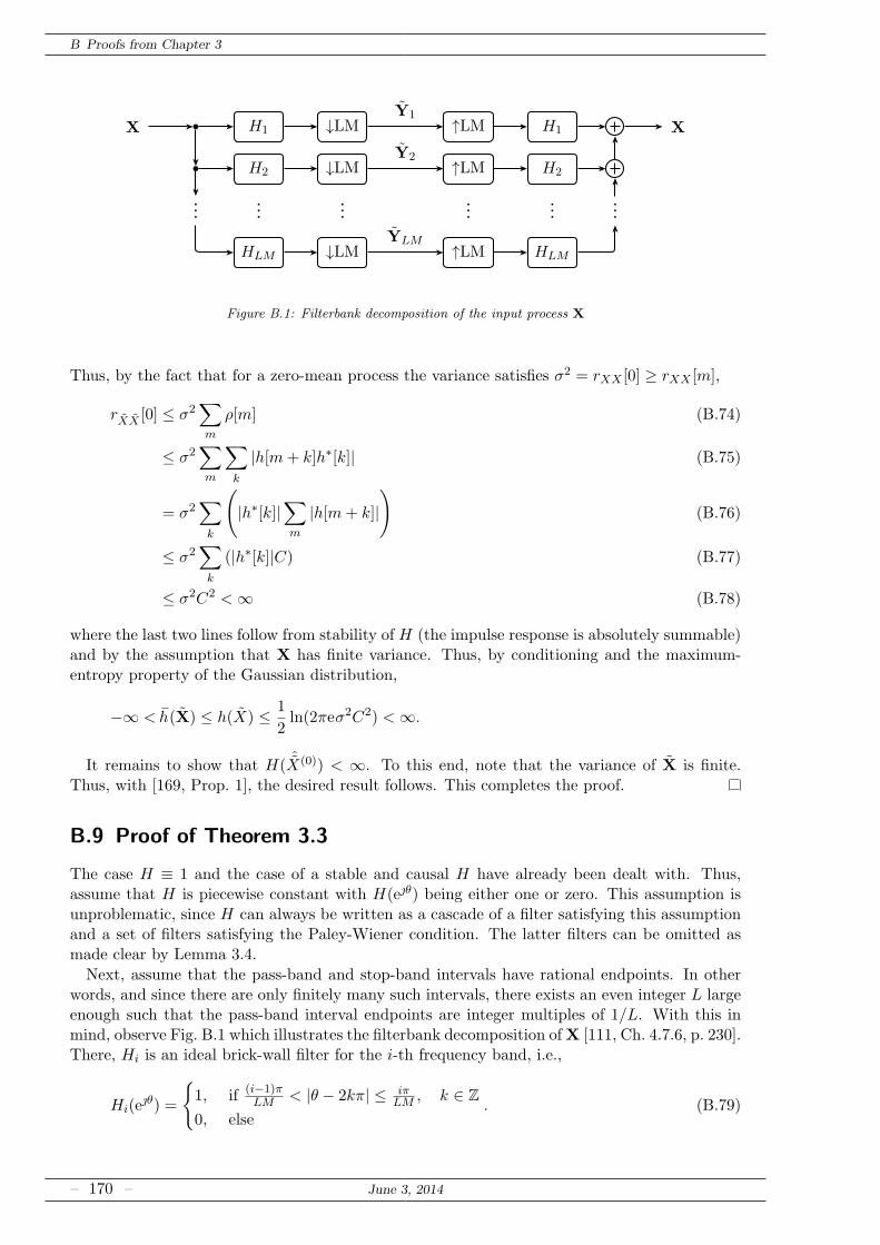
B Proofs from Chapter 3
X b
b
H1
H2
HLM
↓LM
↓LM
↓LM
↑LM
↑LM
↑LM
H1
H2
HLM
X
b
b
b
b
b
b
b
b
b
b
b
b
b
b
b
b
b
b
Y1
Y2
YLM
Figure B.1: Filterbank decomposition of the input process X
Thus, by the fact that for a zero-mean process the variance satisfies σ2 = rXX [0] ≥ rXX [m],
rXX [0] ≤ σ2∑
m
ρ[m] (B.74)
≤ σ2∑
m
∑
k
|h[m+ k]h∗[k]| (B.75)
= σ2∑
k
(
|h∗[k]|∑
m
|h[m+ k]|)
(B.76)
≤ σ2∑
k
(|h∗[k]|C) (B.77)
≤ σ2C2 <∞ (B.78)
where the last two lines follow from stability of H (the impulse response is absolutely summable)and by the assumption that X has finite variance. Thus, by conditioning and the maximum-entropy property of the Gaussian distribution,
−∞ <h(X) ≤ h(X) ≤ 1
2ln(2πeσ2C2) <∞.
It remains to show that H( ˆX(0)) < ∞. To this end, note that the variance of X is finite.Thus, with [169, Prop. 1], the desired result follows. This completes the proof.
B.9 Proof of Theorem 3.3
The case H ≡ 1 and the case of a stable and causal H have already been dealt with. Thus,assume that H is piecewise constant with H(eθ) being either one or zero. This assumption isunproblematic, since H can always be written as a cascade of a filter satisfying this assumptionand a set of filters satisfying the Paley-Wiener condition. The latter filters can be omitted asmade clear by Lemma 3.4.
Next, assume that the pass-band and stop-band intervals have rational endpoints. In otherwords, and since there are only finitely many such intervals, there exists an even integer L largeenough such that the pass-band interval endpoints are integer multiples of 1/L. With this inmind, observe Fig. B.1 which illustrates the filterbank decomposition ofX [111, Ch. 4.7.6, p. 230].There, Hi is an ideal brick-wall filter for the i-th frequency band, i.e.,
Hi(eθ) =
1, if (i−1)πLM < |θ − 2kπ| ≤ iπ
LM , k ∈ Z
0, else. (B.79)
– 170 – June 3, 2014
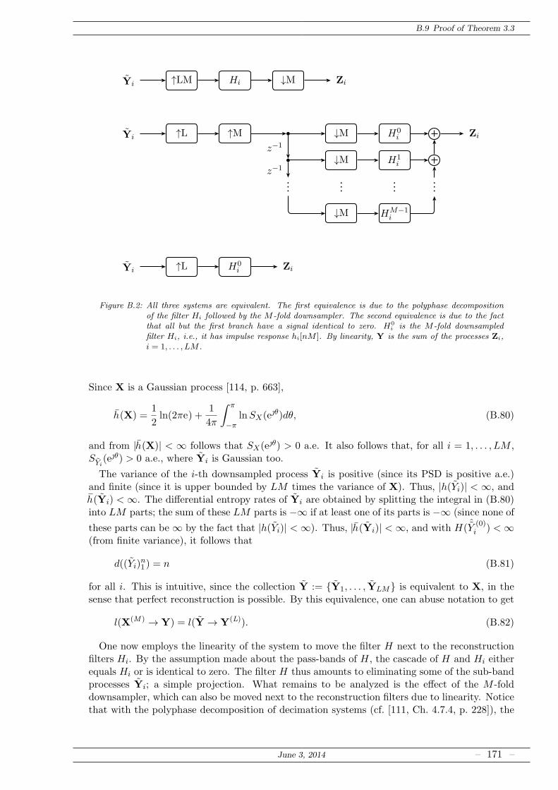
B.9 Proof of Theorem 3.3
Yi ↑LM Hi ↓M Zi
Yib
b
↑L ↑M ↓M
↓M
↓M
H0i
H1i
HM−1i
Zi
b
b
b
b
b
b
b
b
b
b
b
b
z−1
z−1
Yi ↑L H0i Zi
Figure B.2: All three systems are equivalent. The first equivalence is due to the polyphase decompositionof the filter Hi followed by the M-fold downsampler. The second equivalence is due to the factthat all but the first branch have a signal identical to zero. H0
i is the M-fold downsampledfilter Hi, i.e., it has impulse response hi[nM ]. By linearity, Y is the sum of the processes Zi,i = 1, . . . , LM .
Since X is a Gaussian process [114, p. 663],
h(X) =1
2ln(2πe) +
1
4π
∫ π
−πlnSX(eθ)dθ, (B.80)
and from |h(X)| < ∞ follows that SX(eθ) > 0 a.e. It also follows that, for all i = 1, . . . , LM ,SYi
(eθ) > 0 a.e., where Yi is Gaussian too.
The variance of the i-th downsampled process Yi is positive (since its PSD is positive a.e.)and finite (since it is upper bounded by LM times the variance of X). Thus, |h(Yi)| <∞, andh(Yi) <∞. The differential entropy rates of Yi are obtained by splitting the integral in (B.80)into LM parts; the sum of these LM parts is −∞ if at least one of its parts is −∞ (since none of
these parts can be∞ by the fact that |h(Yi)| <∞). Thus, |h(Yi)| <∞, and with H( ˆY(0)i ) <∞
(from finite variance), it follows that
d((Yi)n1 ) = n (B.81)
for all i. This is intuitive, since the collection Y := Y1, . . . , YLM is equivalent to X, in thesense that perfect reconstruction is possible. By this equivalence, one can abuse notation to get
l(X(M ) → Y) = l(Y → Y(L)). (B.82)
One now employs the linearity of the system to move the filter H next to the reconstructionfilters Hi. By the assumption made about the pass-bands of H, the cascade of H and Hi eitherequals Hi or is identical to zero. The filter H thus amounts to eliminating some of the sub-bandprocesses Yi; a simple projection. What remains to be analyzed is the effect of the M -folddownsampler, which can also be moved next to the reconstruction filters due to linearity. Noticethat with the polyphase decomposition of decimation systems (cf. [111, Ch. 4.7.4, p. 228]), the
June 3, 2014 – 171 –
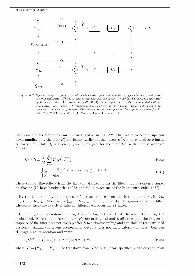
B Proofs from Chapter 3
Y1
Y2L+1
b
b
b
b
b
b
Y(M−1)L+1
c2L+1
c1
c(M−1)L+1
b
b
b
YL
Y3L
YML
b
b
b
b
b
b
c3L
cL
cML
↑L H01
↑L H0L
b
b
b
b
b
b
b
b
b
YY1
YL
Figure B.3: Equivalent system for a decimation filter with a piecewise constant H (pass-band intervals withrational endpoints). The constants ci indicate whether or not the sub-band process is eliminatedby H, i.e., ci ∈ 0, 1. Note that with (B.84) the interpolator outputs can be added withoutinformation loss. Thus, information loss only occurs by eliminating and/or adding sub-bandprocesses – a cascade of an intertible linear map and a projection. The system is shown for Modd. Note that Yi depends on Yi, Y2L−i+1, Y2L+i, Y4L−i+1, . . . .
i-th branch of the filterbank can be rearranged as in Fig. B.2. Due to the cascade of up- anddownsampling only the filter H0
i is relevant, while all other filters H li will have an all-zero input.
In particular, while Hi is given by (B.79), one gets for the filter H0i , with impulse response
hi[nM ],
H0i (e
θ) =1
M
M∑
m=1
Hi(e θ−2mπ
M ) (B.83)
=
1M , if (i−1)π
L < |θ − 2kπ| ≤ iπL , k ∈ Z
0, else(B.84)
where the last line follows from the fact that downsampling the filter impulse response causesno aliasing (Hi have bandwidths 1/LM and fall in exact one of the bands with width 1/M).
By the 2π-periodicity of the transfer functions, the sequence of filters is periodic with 2L,i.e., H0
i = H0i+2L. Moreover, H0
L+k = H0L−k+1, k = 1, . . . , L, by the symmetry of the filter.
Therefore, there are exactly L different filters, each occurring M times.
Combining the last system from Fig. B.2 with Fig. B.1 and (B.84) the schematic in Fig. B.3is obtained. Note that since the filters H0
i are orthogonal and L-aliasfree (i.e., the frequencyresponse of the filter does not overlap after L-fold downsampling and can thus be reconstructedperfectly), adding the reconstruction filter outputs does not incur information loss. One canthus again abuse notation and write
l(X(M ) → Y) = l(Y → Y(L)) = l(Y → Y) (B.85)
where Y := Y1, . . . , YL. The transform from Y to Y is linear, specifically, the cascade of an
– 172 – June 3, 2014
B.9 Proof of Theorem 3.3
intertible linear map and a projection. One can therefore apply Proposition 2.10 and gets
l(Y n1 → Y n
1 ) = 1− d(Y n1 )
d(Y n1 )
= 1− d(Y n1 )
nML. (B.86)
The information dimension of Y n1 =: (Y1)n1 , . . . , (YL)n1 is bounded from above by the number
of its scalar components, which is nL. This completes the proof for filters H with rationalendpoints of the pass-band intervals.Assume now that one of the interval endpoints is an irrational ai. Then, for a fixed L, there
exists Ai ∈ N0 such that Ai/L < ai < (Ai + 1)/L. Obviously, the filter with the irrational end-point replaced by either of these two rational endpoints destroys either more or less information(either the corresponding coefficient cm in Fig. B.3 is zero or one). For both of these filters,however, the information dimension of Y n
1 cannot exceed nL, and above analysis holds. Thiscompletes the proof.Note also that the proof suggests how to measure the exact relative information loss rate for
the decimation system by evaluating the information dimension of Y n1 . For rational endpoints
of the pass-band intervals this is simple since d((Yi)n1 ) ∈ 0, n. For irrational endpoints one
can always wedge the filter H between one which destroys more and one which destroys lessinformation; for L sufficiently large, the resulting difference in the relative information loss ratewill be small, and eventually vanish in the limit.Moreover, the result should also hold for non-Gaussian processes satisfying Assumption 1. The
intuition behind this is due to a bottleneck consideration: Since the filterbank decompositionis perfectly invertible, the information dimension of the input and output process need to beidentical for all time windows 1, . . . , n. The Gaussian assumption was needed to show thatthe information dimension (for a given time window) of each sub-band process is related tothe information dimension of the input process (in the same time window) and the number offilterbank channels. The author believes that the Gaussian assumption can be removed by thefact that all operations in the model are Lipschitz, and that therefore the information dimensioncannot increase. As a consequence, it is not possible that the information dimension of the sub-band processes is smaller than in the Gaussian case, since in this case the information dimensionof the (reconstructed) output would be smaller than the information dimension of the input – acontradiction.
June 3, 2014 – 173 –
Information Loss in Deterministic Systems
CProofs from Chapter 4
C.1 Proof of Proposition 4.5
For the first property, note that with P′ = VQUπ the condition
VUP′V = P′V (C.1)
from Lemma 4.2 can be written as
VUVQUπV = VQUπV. (C.2)
Since UπV = I for all positive probability vectors π, equality is achieved and the first resultis proved. By the same line of argument follows that UP′V = Q. Note in passing that thisactually proved strong lumpability of X′π
g (cf. [87]).
For the second property (cf. [27, Thm. 2, Property 3]) note that with P′ = VQUµ,
µTP′ = µTVQUµ = νTQUµ = νTUµ = µT (C.3)
where the second and third equality are due to Lemma 4.2; the last one follows from the definitionof Uµ in (4.68).
For the third property the reader is referred to [27, Thm. 1].
Next, observe that Qg(i)g(j) = 0 implies Pij = 0; see (4.82), combined with the fact that µ ispositive [87, Thm. 4.1.4]. The entries of the lifted matrix are given as
P ′ij =
πj∑
k∈g−1[g(j)] πkQg(i)g(j). (C.4)
Since π is positive, it follows that P ′ij = 0 implies Pij = 0, or equivalently, P′ ≫ P.
The last property immediately follows from Lemma 4.3; the lemma can be applied becauseX′µ
g is lumpable to Y′g (property 1) and P′ ≫ P (property 4). This completes the proof.
– 174 – June 3, 2014
C.2 Proof of Theorem 4.1
C.2 Proof of Theorem 4.1
For the proof note that another condition for lumpability is given by the entries of the matrixR = PV. In particular, if and only if for all h, l ∈ Y the elements
Ril :=∑
j∈g−1[l]
Pij (C.5)
are the same for all i ∈ g−1[h], the chain is strongly lumpable w.r.t. g [87]. Using this with (4.86)one gets
Ril =∑
j∈g−1[l]
Pij = Qhl. (C.6)
Clearly, Ril assumes the same values for all i ∈ g−1[h], as required. This completes the proof ofthe first statement32. Again, strong lumpability in the sense of [87] was proved.The second statement is obvious from the definition of P-lifting and from the proof of property
4 of Proposition 4.5.For the third statement, introduce an arbitrary lifting
Pij = bijQg(i)g(j) (C.7)
subject to∑
j∈g−1[l] bij = 1 for all l ∈ Y and all i ∈ X . With (C.5), this condition is necessary
and sufficient for strong lumpability of the lifted chain X with transition matrix P. Now writefor the KLDR
D(X||X) =∑
i,j∈XµiPij log
Pij
Pij
(C.8)
=∑
i,j∈XµiPij log
Pij
bijQg(i)g(j)(C.9)
=H (Y′g)−H (X) +
∑
i,j∈XµiPij log
1
bij. (C.10)
The last sum can be written as
∑
i,j∈XµiPij log
1
bij=∑
i∈Xµi
∑
l∈YRil
∑
j∈g−1[l]
Pij
Rillog
1
bij. (C.11)
Here, the last term on the right is a cross-entropy, since both bij andPij
Rilare probability vectors
on g−1[l]. The cross-entropy is minimized33 if and only if for all j ∈ g−1[l]
bij =Pij
Ril=
Pij∑
k∈g−1[l] Pik. (C.12)
Since the sums over i and l are expecations, the minimum is achieved if and only if abovecondition holds also for all i ∈ X and all l ∈ Y for which µiRil > 0.To show that the P-lifting indeed yields a better bound, observe that with H(Yg,n|Yg,n−1) =
32 Note that this statement holds for all stochastic matrices used for lifting, i.e., the lifting matrix does not haveto be equal to the transition matrix of the original chain.
33 This is a direct consequence of the fact that the Kullback-Leibler divergence vanishes if and only if theconsidered probability mass functions are equal [21, pp. 31].
June 3, 2014 – 175 –
C Proofs from Chapter 4
H (Y′g) and with (4.93)
D(X||X′µg )− D(X||X′P
g ) = H(X)−H (X)−H(Y ′g) +H(Yg,n|Xn−1) (C.13)
= H(Xn)−H(Xn|Xn−1)−H(Yg,n) +H(Yg,n|Xn−1) (C.14)
= I(Xn;Xn−1)− I(Yg,n;Xn−1) (C.15)
≥ 0 (C.16)
by the data processing inequality. D(X||X′Pg ) ≥ D(Yg ||Y′
g) is obtained by Lemma 4.3, whichcan be applied by properties 1 and 2.
For the fifth property, note that the sufficient and necessary condition for strong lumpabil-ity (4.69), namely that
Ril =∑
j∈g−1[l]
Pij = Qhl (C.17)
is the same for all i ∈ g−1[h], can be used in the definition of P:
Pij =Pij
∑
k∈SjPik
Qg(i)g(j) =Pij
∑
k∈SjPik
Rig(j) = Pij (C.18)
This proves the “⇒” part. The “⇐” part follows from Lemma 4.3. This completes the proof.
C.3 Proof of Theorem 4.2
By Lemma 4.5 and Definition 4.9,
LS(X → Y M1 ) = h(Y N
M+1|Y M1 )− h(NN
M+1|NM ) (C.19)
= h((Y NM+1)G|(Y M
1 )G)− J(Y NM+1|Y M
1 ) (C.20)
− h((NNM+1)G|(NM
1 )G) + J(NNM+1|NM
1 ) (C.21)
≤ h((Y NM+1)G|(Y M
1 )G)− h((NNM+1)G|(NM
1 )G) (C.22)
(a)= h((Y N
M+1)G)− h((NNM+1)G|(NM
1 )G) (C.23)
(b)= h((Y N
M+1)G)− h((NNM+1)G) (C.24)
=1
2ln
(N∏
i=M+1
λi
µ
)
. (C.25)
Here, (a) is due to the fact that the PCA decorrelates the output data Y and thus leads toindependence of (Y N
M+1)G and (Y M1 )G (in the sense of Definition 4.9). By similar reasons (b)
follows from the fact that N is iid (CN is a scaled identity matrix, with all eigenvalues beingequal µi = µ). Since the PCA ensures that the product contains the N −M smalles eigenvaluesλi of CY , the last line (obtained with [21, Thm. 8.4.1] and [10, Fact 5.10.14]) represents thesmallest Gaussian upper bound and completes the proof.
C.4 Proof of Theorem 4.3
Recapitulate (C.23) from the proof of Theorem 4.2:
LS(X → Y M1 ) ≤ h((Y N
M+1)G)− h((NNM+1)G|(NM
1 )G) (C.26)
= h((Y NM+1)G)− h(NG) + h((NM
1 )G). (C.27)
– 176 – June 3, 2014
C.4 Proof of Theorem 4.3
With [21, Thm. 8.4.1] and [10, Fact 5.10.14],
h(NG) =1
2ln
(
(2πe)NN∏
i=1
µi
)
(C.28)
and
h((Y NM+1)G) =
1
2ln
(
(2πe)N−MN∏
i=M+1
λi
)
. (C.29)
If CN denotes the (M ×M)-covariance matrix of NM1 (and, thus, of (NM
1 )G) and µi the setof eigenvalues of CN , one will obtain
LS(X → Y M1 ) ≤ 1
2ln
(∏Ni=M+1 λi
∏Mi=1 µi
∏Ni=1 µi
)
. (C.30)
The proof is completed by providing upper bounds on the eigenvalues in the numerator.It is easy to verify that CN is the top left principal submatrix of WTCNW (which, by theorthogonality of W, has the same eigenvalues as CN ). As a consequence, one can employCauchy’s interlacing inequality [10, Thm. 8.4.5]:
µi+N−M ≤ µi ≤ µi (C.31)
The second bound, λi ≤ µ1, is derived from Weyl’s inequality [10, Thm. 8.4.11]
λi ≤ νi + µ1 (C.32)
and by noticing that νj = 0 for all j > M . Combining this yields an upper bound on theinformation loss
LS(X → Y M1 ) ≤ 1
2ln
(∏Ni=M+1 λi
∏Mi=1 µi
∏Ni=1 µi
)
(C.33)
≤ 1
2ln
(∏Ni=M+1 µ1
∏Mi=1 µi
∏Ni=1 µi
)
(C.34)
=1
2ln
(N∏
i=M+1
µ1
µi
)
. (C.35)
June 3, 2014 – 177 –
Information Loss in Deterministic Systems
DProofs from Chapter 5
D.1 Proof of Lemma 5.2
The proof is provided for jointly Gaussian processes S and X only; since the effect of linearfilters is independent of the process statistics (cf. [114, p. 663]), the result can be extended tothe general case.
First, note that a stable, causal LTI filter satisfies the Paley-Wiener condition (cf. Section 3.5),and that thus H(eθ) > 0 a.e. From [114, Cor. to Thm. 9-4, p. 412] one gets SX(eθ) =|H(eθ)|2SX(eθ). Since X has a finite entropy rate, SX(eθ) > 0 a.e., and, thus, SX(eθ) > 0 a.e.That for the cross-power spectral density SXS(e
θ) = H(eθ)SXS(eθ) holds can be shown easily.
From [116, Thm. 10.2.1, p. 175],
I(X;S) = − 1
4π
∫ π
−πlog(
1− |ρXS(eθ)|2
)
dθ (D.1)
where
|ρXS(eθ)|2 =
|SXS(eθ)|2
SX(eθ)SS(eθ), if SXS(e
θ) 6= 0
0, else. (D.2)
With above reasoning one gets
|ρXS(eθ)|2 =
|H(eθ)|2|SXS(eθ)|2
|H(eθ)|2SX(eθ)SS(eθ), if H(eθ)SXS(e
θ) 6= 0
0, else(D.3)
which is a.e. equal to |ρXS(eθ)|2 since H(eθ) > 0 a.e. This completes the proof.
D.2 Proof of Theorem 5.1
The proof requires a lemma similar to Lemma 5.2, but for the specific problem at hand. Inparticular, let H be the (yet-to-be-designed) anti-aliasing filter and let S be the Gaussian signalprocess S filtered by H. Then,
– 178 – June 3, 2014
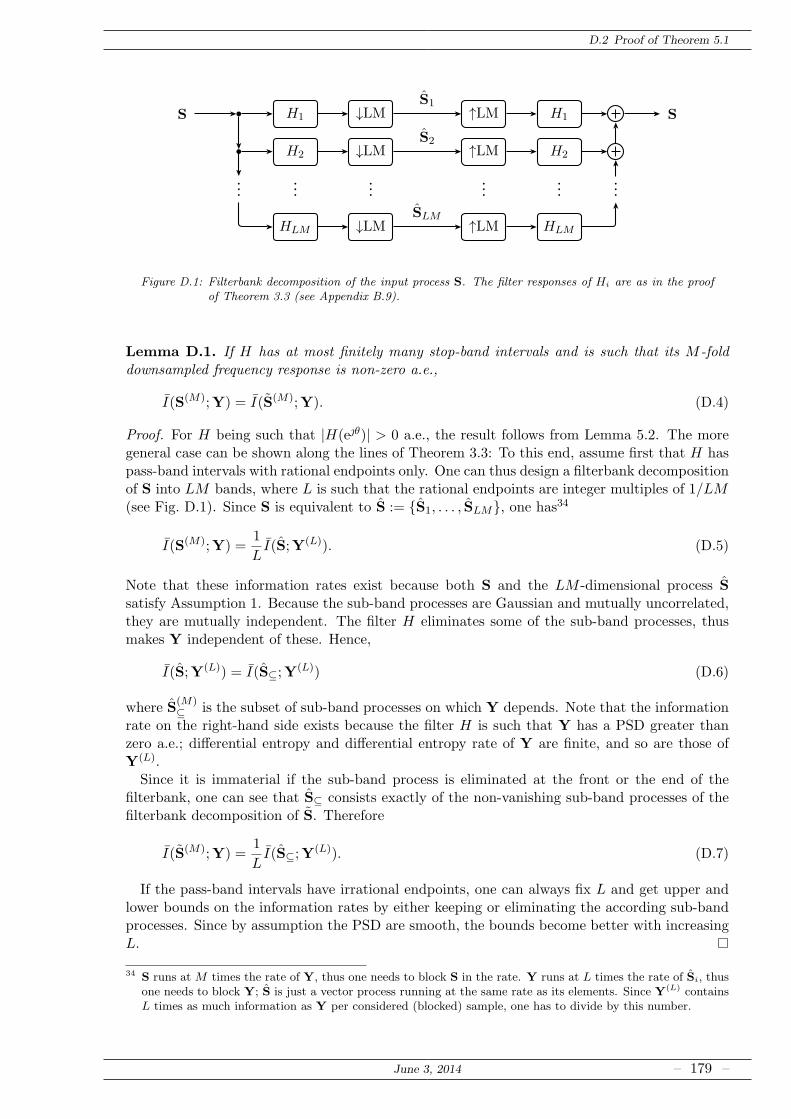
D.2 Proof of Theorem 5.1
S b
b
H1
H2
HLM
↓LM
↓LM
↓LM
↑LM
↑LM
↑LM
H1
H2
HLM
S
b
b
b
b
b
b
b
b
b
b
b
b
b
b
b
b
b
b
S1
S2
SLM
Figure D.1: Filterbank decomposition of the input process S. The filter responses of Hi are as in the proofof Theorem 3.3 (see Appendix B.9).
Lemma D.1. If H has at most finitely many stop-band intervals and is such that its M -folddownsampled frequency response is non-zero a.e.,
I(S(M);Y) = I(S(M);Y). (D.4)
Proof. For H being such that |H(eθ)| > 0 a.e., the result follows from Lemma 5.2. The moregeneral case can be shown along the lines of Theorem 3.3: To this end, assume first that H haspass-band intervals with rational endpoints only. One can thus design a filterbank decompositionof S into LM bands, where L is such that the rational endpoints are integer multiples of 1/LM(see Fig. D.1). Since S is equivalent to S := S1, . . . , SLM, one has34
I(S(M);Y) =1
LI(S;Y(L)). (D.5)
Note that these information rates exist because both S and the LM -dimensional process Ssatisfy Assumption 1. Because the sub-band processes are Gaussian and mutually uncorrelated,they are mutually independent. The filter H eliminates some of the sub-band processes, thusmakes Y independent of these. Hence,
I(S;Y(L)) = I(S⊆;Y(L)) (D.6)
where S(M)⊆ is the subset of sub-band processes on which Y depends. Note that the information
rate on the right-hand side exists because the filter H is such that Y has a PSD greater thanzero a.e.; differential entropy and differential entropy rate of Y are finite, and so are those ofY(L).Since it is immaterial if the sub-band process is eliminated at the front or the end of the
filterbank, one can see that S⊆ consists exactly of the non-vanishing sub-band processes of thefilterbank decomposition of S. Therefore
I(S(M);Y) =1
LI(S⊆;Y
(L)). (D.7)
If the pass-band intervals have irrational endpoints, one can always fix L and get upper andlower bounds on the information rates by either keeping or eliminating the according sub-bandprocesses. Since by assumption the PSD are smooth, the bounds become better with increasingL.
34S runs at M times the rate of Y, thus one needs to block S in the rate. Y runs at L times the rate of Si, thusone needs to block Y; S is just a vector process running at the same rate as its elements. Since Y
(L) containsL times as much information as Y per considered (blocked) sample, one has to divide by this number.
June 3, 2014 – 179 –
D Proofs from Chapter 5
Proof of Theorem 5.1. Instead of minimizing LS(M )(X(M ) → Y) one can maximize I(S(M);Y),since this is the only component depending on H.
Assume w.l.o.g. that H is such that its M -fold downsampled frequency response is nonzeroa.e.: Were it not so, then one can always split H into a filter H ′ which is, and a filter H ′′
following the downsampling device which is piecewise constant; i.e., H = H ′ ·H ′′. Let Y be theprocess obtained by using H ′ as filter, and let Y be the process obtained by filtering Y withH ′′. By data processing (combine [116, Thm. 7.4.2, p. 110] with [116, Thm. 7.2.1, (7), p. 95]and the fact that S is such that the information rate with a jointly stationary process exists),
I(S(M);Y) ≥ I(S(M); Y). (D.8)
Thus, it is safe to assume that H is such that its M -fold downsampled frequency response isnonzero a.e. In addition, assume that H has finitely many pass-bands. By Lemma D.1 it followsthat it suffices to maximize I(S(M);Y). Thus,
I(S(M);Y) = limn→∞
1
nI(SnM
1 ;Y n1 ) = lim
n→∞1
n
(
h(Y n1 )− h(Y n
1 |SnM1 )
)
(D.9)
The first term converges toh(Y). For the latter, note that by linearity, Yn = XnM = SnM+NnM ,where N is the noise process filtered by H. Consequently, and by the fact that S and N areindependent, h(Y n
1 |SnM1 ) = h(NM , . . . , NnM ).
Since S and N are Gaussian processes, one obtains
I(S(M);Y) =1
4π
∫ π
−πln
(∑M−1k=0 SN (eθk)|H(eθk)|2 + SS(e
θk)|H(eθk)|2∑M−1
k=0 SN (eθk)|H(eθk)|2
)
dθ (D.10)
where θk := θ−2kπM . This can be rearranged to
I(S(M);Y) =1
4π
∫ π
−πln
(
1 +
∑M−1k=0 SS(e
θk)|H(eθk)|2∑M−1
k=0 SN (eθk)|H(eθk)|2
)
dθ (D.11)
=1
4π
∫ π
−πln
1 +
∑M−1k=0
SS(eθk )
SN (eθk )SN (eθk)|H(eθk)|2
∑M−1k=0 SN (eθk)|H(eθk)|2
dθ (D.12)
=1
4π
∫ π
−πln
1 +
∑M−1k=0
SS(eθk )
SN (eθk )Hk(e
θ)∑M−1
k=0 Hk(eθ)
dθ (D.13)
where Hk(eθ) := SN (eθk)|H(eθk)|2. Maximizing the integral amounts to maximizing the frac-
tion inside the logarithm for every value of θ. Since the fraction is a weighted average of theratio SS(e
θk)/SN (eθk), the weights satisfying, for all k ∈ 0, . . . ,M − 1,
Hl(eθ) =
1, if l is the smallest natural number such that SS(eθ)
SN (eθ)|θ=θl ≥
SS(eθk )
SN (eθk )
0, else(D.14)
maximize the integral.
H is thus related to the piecewise constant functions Hl(eθ) via
|H(eθk)|2 = 1
SN (eθk)Hk(e
θ) (D.15)
where the relation has to be satisfied for all k = 0, . . . ,M − 1. Since, by assumption, SN (eθ) issuch that its square root corresponds to the magnitude response of a causal, stable filter (the
– 180 – June 3, 2014
D.3 Proof of Theorem 5.2
differential entropy rate h(N) is finite), and since Lemma 5.2 holds, one can choose H to bepiecewise constant. The assumption that the PSDs are smooth guarantees that the resultingfilter H has finitely many pass-bands.
That H is identical to the optimal energy compaction filter for SS(eθ)/SN (eθ) is evident
from Definition 5.3.
D.3 Proof of Theorem 5.2
For the proof note that, with Lemma 5.2,
LS(M )(X(M ) → Y) = I(S(M); X(M))− I(S(M);Y) = I(S(M); X(M))− I(S(M);Y) (D.16)
where X is obtained by filtering X with H. Since Xn = Sn+ Nn, and since Yn = XnM , one gets
LS(M )(X(M ) → Y) = limn→∞
1
n
(
h(XnM1 )− h(XnM
1 |SnM1 )− h(Y n
1 ) + h(Y n1 |SnM
1 ))
(D.17)
= limn→∞
1
n
(
h(XnM1 )− h(NnM
1 )− h(XM , . . . , XnM ) + h(NM , . . . , NnM ))
(D.18)
= limn→∞
1
nh(XM−1
1 , X2M−1M+1 , . . . , XnM−1
(n−1)M+1|XM , X2M , . . . , XnM )
− limn→∞
1
nh(NnM
1 ) + limn→∞
1
nh(NM , . . . , NnM ). (D.19)
The first conditional differential entropy is always upper bounded by the corresponding expres-sion for Gaussian RVs XG,1, . . . , XG,mM with the same joint first and second order moments asthe original RVs (cf. [21, Thm. 8.6.5, p. 254]). Replacing S by SG yieldsXG andYG Gaussian (byGaussianity of N) and achieves this upper bound with equality. Hence, with Xn,G = Sn,g + Nn
and Yn,G = XnM,G,
LS(M )(X(M ) → Y)
≤ limn→∞
1
nh((XM−1
1 , X2M−1M+1 , . . . , XnM−1
(n−1)M+1)G|(XM , X2M , . . . , XnM )G)
− limn→∞
1
nh(NnM
1 ) + limn→∞
1
nh(NM , . . . , NnM ) (D.20)
= limn→∞
1
n
(
h((XnM1 )G)− h((XnM
1 )G|(SnM1 )G)− h((Y n
1 )G) + h((Y n1 )G|(SnM
1 )G))
(D.21)
= I(S(M)G ; X
(M)G )− I(S
(M)G ;YG) (D.22)
=LS(M )G
(X(M )G → YG). (D.23)
D.4 Proof of Lemma 5.3
The mutual information rate is
I(X;Y)(a)= lim
n→∞1
nI(Xn
1 ;Yn1 ) (D.24)
= limn→∞
1
n
(
h(Xn1 )− h(Xn
1 |Y n1 ))
(D.25)
(b)= h(X)− lim
n→∞1
nh(Xn
1 |Y n1 ) (D.26)
June 3, 2014 – 181 –
D Proofs from Chapter 5
(c)=
1
2ln(2πe) +
1
4π
∫ π
−πlnSX(eθ)dθ − lim
n→∞1
nh(Xn
1 |Y n1 ) (D.27)
(d)=
1
2ln(2πeσ2
∞)− limn→∞
1
nh(Xn
1 |Y n1 ) (D.28)
(e)
≥ 1
2ln(2πeσ2
∞)− h(X1|Y1) (D.29)
(f)
≥ 1
2ln(2πeσ2
∞)− ln∆ (D.30)
=1
2ln(2πeσ2
∞/∆2) (D.31)
where (a) and (b) are the definitions of information rate and differential entropy rate, respectively,(c) is the differential entropy rate of a Gaussian process [114, p. 663], and (d) is the definitionof entropy power σ2
i nfty [21, Ch. 12.5]. Inequality (e) follows from the chain rule of differentialentropy, conditioning, and stationarity:
h(Xn1 |Y n
1 ) =n∑
i=1
h(Xi|Xi−11 , Y n
1 ) ≤n∑
i=1
h(Xi|Yi) = nh(X1|Y1) (D.32)
Finally, the differential entropy of a random variable supported on a finite interval is boundedby the entropy of the uniform distribution over this interval. Therefore, since X1|Y1 = y issupported on an interval of length ∆ for all y, it follows that h(X1|Y1) ≤ ln∆ in (f).Next, consider the case of high-rate quantization, where the quantization noise is modeled as
uncorrelated noise with variance ∆2/12. Assuming that X and YG are jointly Gaussian withthe same joint first and second moments as X and Y, one gets
I(X;YG) =1
4π
∫ π
−πln
(
1 +SX(eθ)
∆2/12
)
dθ. (D.33)
For high resolutions (i.e., for sufficiently small ∆) and if SX(eθ) is bounded away from zero, theone in the argument becomes negligible, and one has
I(X;YG) ≈1
2ln(12σ2
∞/∆2). (D.34)
Subtracting this from (D.31) yields
I(X;Y)− I(X;YG) '1
2ln
(2πe
12
)
> 0. (D.35)
– 182 – June 3, 2014
Information Loss in Deterministic Systems
Bibliography
[1] (2012, Oct.) Principle component analysis. [Online]. Available:http://en.wikipedia.org/wiki/Principle components analysis
[2] A. M. Abdel-Moneim and F. W. Leysieffer, “Weak lumpability in finite Markov chains,”J. Appl. Prob., vol. 19, no. 3, pp. 685–691, Sep. 1982.
[3] M. Abramowitz and I. A. Stegun, Eds., Handbook of Mathematical Functions with For-mulas, Graphs, and Mathematical Tables, 9th ed. New York, NY: Dover Publications,1972.
[4] S. Akkarakaran and P. P. Vaidyanathan, “Results on principal component filter banks:colored noise suppression and existence issues,” IEEE Trans. Inf. Theory, vol. 47, no. 3,pp. 1003–1020, 2001.
[5] R. W. Aldhaheri and H. K. Khalil, “Aggregation of the policy iteration method for nearlycompletely decomposable Markov chains,” IEEE Trans. Autom. Control, vol. 36, no. 2,pp. 178–187, Feb. 1991.
[6] M. Baer, “A simple countable infinite-entropy distribution,” 2008. [Online]. Available:https://hkn.eecs.berkeley.edu/∼calbear/research/Hinf.pdf
[7] J. C. Baez, T. Fritz, and T. Leinster, “A characterization of entropy in terms of informationloss,” Entropy, vol. 13, no. 11, pp. 1945–1957, Nov. 2011.
[8] H.-P. Bernhard, “The mutual information function and its application to signal process-ing,” Ph.D. dissertation, Technische Universitat Wien, Dec. 1997.
[9] ——, “Tight upper bound on the gain of linear and nonlinear predictors,” IEEE Trans.Signal Process., vol. 46, no. 11, pp. 2909–2917, Nov. 1998.
[10] D. S. Bernstein, Matrix Mathematics. Princeton, NJ: Princeton University Press, 2005.
[11] J. J. Birch, “Approximation for the entropy for functions of Markov chains,” Ann. Math.Statist., vol. 33, pp. 930–938, 1962.
[12] D. Blackwell, “The entropy of functions of finite-state Markov chains,” in Transactions ofthe first Prague conference on information theory, Statistical decision functions, randomprocesses held at Liblice near Prague from November 28 to 30, 1956. Prague: PublishingHouse of the Czechoslovak Academy of Sciences, 1957, pp. 13–20.
[13] R. A. Brualdi, Introductory Combinatorics, 5th ed. Upper Saddle River, NJ: PearsonEducation, 2010.
[14] P. Buchholz, “Exact and ordinary lumpability in finite Markov chains,” J. Appl. Prob.,vol. 31, pp. 59–75, 1994.
[15] C. J. Burke and M. Rosenblatt, “A Markovian function of a Markov chain,” Ann. Math.Statist., vol. 29, pp. 1112–1122, 1958.
June 3, 2014 – 183 –
Bibliography
[16] J. W. Carlyle, “Identification of state-calculable functions of finite Markov chains,” Ann.Math. Statist., vol. 38, pp. 201–205, 1967.
[17] G. Chechik and N. Tishby, “Extracting relevant structures with side information,” inAdvances in Neural Information Processing Systems (NIPS), 2002, pp. 857–864.
[18] Y. Chen, Y. C. Eldar, and A. J. Goldsmith, “Shannon meets Nyquist: Capacity of sampledGaussian channels,” IEEE Trans. Inf. Theory, vol. 59, no. 8, pp. 4889–4914, Aug. 2013.
[19] A. Chi and T. Judy, “Transforming variables using the Dirac generalized function,” TheAmerican Statistician, vol. 53, no. 3, pp. 270–272, Aug. 1999.
[20] J. T. Chu and J. C. Chueh, “Inequalities between information measures and error proba-bility,” J. Franklin Inst., vol. 282, pp. 121–125, Aug. 1966.
[21] T. M. Cover and J. A. Thomas, Elements of Information Theory, 2nd ed. Hoboken, NJ:Wiley Interscience, 2006.
[22] C. D. Cutler, “Computing pointwise fractal dimension by conditioning in multivariatedistributions and time series,” Bernoulli, vol. 6, no. 3, pp. 381–399, Jun. 2000.
[23] D. M. Cvetkovic, P. Rowlinson, and S. Simic, Eigenspaces of graphs, ser. Encyclopedia ofMathematics and its Applications. Cambridge: Cambridge University Press, 1997.
[24] X.-H. Dang and J. Bailey, “A hierarchical information theoretic technique for the discov-ery of non linear alternative clusterings,” in Proc. of the ACM Int. Conf. on KnowledgeDiscovery and Data Mining (SIGKDD), Washington, D.C., Jul. 2010, pp. 573–582.
[25] G. Deco and D. Obradovic, An Information-Theoretic Approach to Neural Computing.New York, NY: Springer, 1996.
[26] K. Deng, “Model reduction of Markov chains with applications to building systems,” Ph.D.dissertation, University of Illinois at Urbana-Champaign, 2012.
[27] K. Deng, P. G. Mehta, and S. P. Meyn, “Optimal Kullback-Leibler aggregation via spectraltheory of Markov chains,” IEEE Trans. Autom. Control, vol. 56, no. 12, pp. 2793–2808,Dec. 2011.
[28] S. W. Dharmadhikari, “Sufficient conditions for a stationary process to be a function of afinite Markov chain,” Ann. Math. Stat., vol. 34, pp. 1033–1041, 1963.
[29] P. S. R. Diniz, E. A. B. da Silva, and S. L. Netto, Digital Signal Processing: SystemAnalysis and Design, 2nd ed. Cambridge: Cambridge University Press, 2010.
[30] J. L. Doob, Stochastic Processes, ser. Wiley Classics Library. New York, NY: WileyInterscience, 1990.
[31] T. Downarowicz, Entropy in Dynamical Systems. Cambridge: Cambridge UniversityPress, 2011.
[32] M. Dumitrescu and G. Popovici, “Entropy invariance for autoregressive processes con-structed by linear filtering,” International Journal of Computer Mathematics, vol. 88,no. 4, pp. 864–880, Mar. 2011.
[33] Y. Ephraim and N. Merhav, “Hidden Markov processes,” IEEE Trans. Inform. Theory,vol. 48, no. 6, pp. 1518–1569, 2002, special issue on Shannon theory: perspective, trends,and applications. [Online]. Available: http://dx.doi.org/10.1109/TIT.2002.1003838
– 184 – June 3, 2014
Bibliography
[34] M. C. Er, “A fast algorithm for generating set partitions,” The Computer Journal, vol. 31,no. 3, pp. 283–284, 1988.
[35] D. Erdogmus, R. Agrawal, and J. C. Principe, “A mutual information extension to thematched filter,” Signal Processing, vol. 85, no. 5, pp. 927–935, May 2005.
[36] D. Erdogmus and J. C. Principe, “From linear adaptive filtering to nonlinear informationprocessing,” IEEE Signal Process. Mag., vol. 23, no. 6, pp. 14–33, Nov. 2006.
[37] W. S. Evans, “Information theory and noisy computation,” Ph.D. dissertation, Univ. Calif.Berkeley, Nov. 1994.
[38] W. S. Evans and L. J. Schulman, “Signal propagation and noisy circuits,” IEEE Trans.Inf. Theory, vol. 45, no. 7, pp. 2367–2373, Nov. 1999.
[39] J. D. Farmer, E. Ott, and J. A. Yorke, “The dimension of chaotic attractors,” Physica D,vol. 7, pp. 153–180, May 1983.
[40] M. Feder and N. Merhav, “Relations between entropy and error probability,” IEEE Trans.Inf. Theory, vol. 40, no. 1, pp. 259–266, Jan. 1994.
[41] J. Feret, T. Henzinger, H. Koeppl, and T. Petrov, “Lumpability abstractions of rule-basedsystems,” Electronic Proceedings in Theoretical Computer Science, vol. 40, pp. 142–161,Aug. 2010.
[42] G. B. Folland, Real Analysis. Modern Techniques and Their Applications, 2nd ed. NewYork, NY: Wiley Interscience, 1999.
[43] G. D. Forney, Jr., “Shannon meets Wiener: On MMSE estimation in successive decodingschemes,” in Proc. Allerton Conf. on Communication, Control, and Computing, Monti-cello, IL, Sep. 2004, pp. 923–932.
[44] A. Friedman and J. Goldberger, “Information theoretic pairwise clustering,” in SIMBAD,ser. LNCS, E. Hancock and M. Pelillo, Eds. Berlin: Springer, 2013, vol. 7953, pp. 106–119.
[45] J. Galambos, Advanced Probability Theory, 2nd ed., ser. Probability: Pure and Applied.New York, NY: Marcel Dekker, Inc., 1995.
[46] B. C. Geiger and G. Kubin, “Information measures for deterministic input-output sys-tems,” Mar. 2013, in preparation; preprint available: arXiv:1303.6409 [cs.IT].
[47] B. C. Geiger, T. Petrov, G. Kubin, and H. Koeppl, “Optimal Kullback-Leibler aggrega-tion via information bottleneck,” Apr. 2013, submitted to IEEE Trans. Autom. Control;preprint available: arXiv:1304.6603 [cs.SY].
[48] B. C. Geiger and C. Temmel, “Lumpings of Markov chains, entropy rate preservation,and higher-order lumpability,” Dec. 2012, accepted in J. Appl. Prob.; preprint available:arXiv:1212.4375 [cs.IT].
[49] B. C. Geiger, C. Feldbauer, and G. Kubin, “Information loss in static nonlinearities,” inProc. IEEE Int. Sym. Wireless Communication Systems (ISWSC), Aachen, Nov. 2011,pp. 799–803, extended version available: arXiv:1102.4794 [cs.IT].
[50] B. C. Geiger and G. Kubin, “Some results on the information loss in dynamical systems,”in Proc. IEEE Int. Sym. Wireless Communication Systems (ISWSC), Aachen, Nov. 2011,pp. 794–798, extended version available: arXiv:1106.2404 [cs.IT].
June 3, 2014 – 185 –
Bibliography
[51] ——, “On the information loss in memoryless systems: The multivariate case,” in Proc.Int. Zurich Seminar on Communications (IZS), Zurich, Feb. 2012, pp. 32–35, extendedversion available: arXiv:1109.4856 [cs.IT].
[52] ——, “Relative information loss in the PCA,” in Proc. IEEE Information The-ory Workshop (ITW), Lausanne, Sep. 2012, pp. 562–566, extended version available:arXiv:1204.0429 [cs.IT].
[53] ——, “Information loss and anti-aliasing filters in multirate systems,” Oct. 2013, in prepa-ration; preprint available: arXiv:1310.8487 [cs.IT].
[54] ——, “On the rate of information loss in memoryless systems,” Apr. 2013,arXiv:1304.5057 [cs.IT].
[55] ——, “Signal enhancement as minimization of relevant information loss,” in Proc. ITGConf. on Systems, Communication and Coding, Munich, Jan. 2013, pp. 1–6, extendedversion available: arXiv:1205.6935 [cs.IT].
[56] ——, “Information loss and anti-aliasing filters in multirate systems,” in Proc. Int. ZurichSeminar on Communications (IZS), Zurich, Feb. 2014, pp. 148–151.
[57] ——, “Information-maximizing prefilters for quantization,” in Proc. IEEE Int. Conf. onAcoustics, Speech and Signal Processing (ICASSP), Florence, May 2014, pp. 5001–5005.
[58] B. C. Geiger and C. Temmel, “Information-preserving Markov aggregation,” in Proc. IEEEInformation Theory Workshop (ITW), Seville, Sep. 2013, pp. 258–262, extended version:arXiv:1304.0920 [cs.IT].
[59] E. J. Gilbert, “On the identifiability problem for functions of finite Markov chains,” Ann.Math. Stat., vol. 30, pp. 688–697, 1959.
[60] D. T. Gillespie, “Stochastic Simulation of Chemical Kinetics,” Annual Review of PhysicalChemistry, vol. 58, no. 1, pp. 35–55, 2007.
[61] D. Gondek and T. Hofmann, “Conditional information bottleneck clustering,” in IEEE Int.Conf. on Data Mining (ICDM), Workshop on Clustering Large Data Sets, Melbourne, FL,Nov. 2003, pp. 36–42.
[62] ——, “Non-redundant data clustering,” in Proc. IEEE Int. Conf. on Data Mining (ICDM),Nov. 2004, pp. 75 – 82.
[63] V. K. Goyal, J. Zhuang, and M. Vetterli, “Transform coding with backward adaptiveupdates,” IEEE Trans. Inf. Theory, vol. 46, no. 4, pp. 1623–1633, Jul. 2000.
[64] P. Grassberger, “Generalized dimensions of strange attractors,” Physics Letters, vol. 97A,no. 6, pp. 227–230, Sep. 1983.
[65] R. M. Gray and D. L. Neuhoff, “Quantization,” IEEE Trans. Inf. Theory, vol. 44, no. 6,pp. 2325–2383, Oct. 1998.
[66] R. M. Gray, Entropy and Information Theory. New York, NY: Springer, 1990.
[67] D. Guo, S. S. Shamai, and S. Verdu, “Mutual information and minimum mean-squareerror in Gaussian channels,” IEEE Trans. Inf. Theory, vol. 51, no. 4, pp. 1261–1282, Apr.2005.
[68] L. Gurvits and J. Ledoux, “Markov property for a function of a Markov chain: a linearalgebra approach,” Linear Algebra Appl., vol. 404, pp. 85–117, 2005. [Online]. Available:http://dx.doi.org/10.1016/j.laa.2005.02.007
– 186 – June 3, 2014
Bibliography
[69] B. Hayes, “First links in the Markov chain,” America Scientist, vol. 101, pp. 92–97, 2013.
[70] S. Haykin, Adaptive Filter Theory, 5th ed. Upper Saddle River, NJ: Pearson, 2014.
[71] A. Heller, “On stochastic processes derived from Markov chains,” Ann. Math. Stat., vol. 36,no. 4, pp. 1286–1291, Aug. 1965.
[72] G. E. Henter, “Probabilistic sequence models with speech and language applications,”Ph.D. dissertation, KTH Royal Institute of Technology, Dec. 2013.
[73] G. E. Henter and W. B. Kleijn, “Minimum entropy rate simplification of stochastic pro-cesses,” submitted to IEEE Trans. Pattern Anal.
[74] S.-W. Ho and S. Verdu, “On the interplay between conditional entropy and error proba-bility,” IEEE Trans. Inf. Theory, vol. 56, no. 12, pp. 5930–5942, Dec. 2010.
[75] S.-W. Ho and R. Yeung, “On the discontinuity of the Shannon information measures,”IEEE Trans. Inf. Theory, vol. 55, no. 12, pp. 5362 –5374, Dec. 2009.
[76] R. A. Horn and C. R. Johnson, Matrix Analysis, 2nd ed. Cambridge: Cambridge Uni-versity Press, 2013.
[77] M. Hotz and C. Vogel, “Linearization of time-varying nonlinear systems using a modifiedlinear iterative method,” Nov. 2013, submitted to IEEE Trans. Sig. Proc.
[78] E. T. Jaynes, “Information theory and statistical mechanics,” in Statistical Physics, ser.Brandeis University Summer Institute Lectures in Theoretical Physics, K. W. Ford, Ed.New York, NY: W. A. Benjamin, Inc., 1963, vol. 3, pp. 181–218.
[79] J. Jensen and C. H. Taal, “Speech intelligibility prediction based on mutual information,”IEEE Audio, Speech, Language Process., vol. 22, no. 2, pp. 430–440, Feb. 2014.
[80] Q.-S. Jia, “On state aggregation to approximate complex value functions in large-scaleMarkov decision processes,” IEEE Trans. Autom. Control, vol. 56, no. 2, pp. 333–344,Feb. 2011.
[81] D. H. Johnson, “Information theory and neural information processing,” IEEE Trans. Inf.Theory, vol. 56, no. 2, pp. 653–666, Feb. 2010.
[82] J. Jost, Dynamical Systems: Examples of Complex Behavior. New York, NY: Springer,2005.
[83] M. Kafsi, M. Grossglauser, and P. Thiran, “The entropy of conditional Markov trajecto-ries,” IEEE Trans. Inf. Theory, vol. 59, no. 9, pp. 5577–5583, Sep. 2013.
[84] A. Kaiser and T. Schreiber, “Information transfer in continuous processes,” Physica D,vol. 166, pp. 43–62, Jun. 2002.
[85] E. Karapistoli, F.-N. Pavlidou, I. Gragopoulos, and I. Tsetsinas, “An overview of the IEEE802.15.4a standard,” IEEE Commun. Mag., vol. 48, no. 1, pp. 47–53, Jan. 2010.
[86] M. A. Katsoulakis and J. Trashorras, “Information loss in coarse-graining of stochasticparticle dynamics,” J. Stat. Phys., vol. 122, no. 1, pp. 115–135, 2006.
[87] J. G. Kemeny and J. L. Snell, Finite Markov Chains, 2nd ed. Springer, 1976.
[88] K. T. Kim and T. Berger, “Sending a lossy version of the innovations process is suboptimalin QG rate-distortion,” in Proc. IEEE Int. Sym. on Information Theory (ISIT), 2005, pp.209–213.
June 3, 2014 – 187 –
Bibliography
[89] ——, “The degree of suboptimality of sending a lossy version of the innovations process inGauss-Markov rate-distortion,” in Proc. IEEE Int. Sym. on Information Theory (ISIT),2006, pp. 808–812.
[90] A. Kirac and P. Vaidyanathan, “Theory and design of optimum FIR compaction filters,”IEEE Trans. Signal Process., vol. 46, no. 4, pp. 903–919, Apr. 1998.
[91] A. N. Kolmogorov, “A new metric invariant of transient dynamical systems and automor-phisms in Lebesgue spaces,” Dokl. Akad. Nauk. SSSR, vol. 119, pp. 861–864, 1958.
[92] ——, “Entropy per unit time as a metric invariant of automorphisms,” Dokl. Akad. Nauk.SSSR, vol. 124, pp. 754–755, 1959.
[93] R. Lamarche-Perrin, Y. Demazeau, and J.-M. Vincent, “How to build the bestmacroscopic description of your multi-agent system?” Laboratoire d’Informatiquede Grenoble, Tech. Rep., Jan. 2013. [Online]. Available: http://rr.liglab.fr/researchreport/RR-LIG-035 orig.pdf
[94] R. Landauer, “Irreversibility and heat generation in the computing process,” IBM Journalof Research and Development, vol. 5, pp. 183–191, 1961.
[95] J. M. Lee, Introduction to Smooth Manifolds, ser. Graduate Texts in Mathematics. NewYork, NY: Springer, 2003.
[96] B. Lev, “The aggregation problem in financial statements: An informational approach,”Journal of Accounting Research, vol. 6, no. 2, pp. 247–261, Autumn 1968.
[97] X. S. Liang and R. Kleeman, “Information transfer between dynamical system compo-nents,” Physical Review Letters, vol. 95, pp. 244 101–1–244 101–4, Dec. 2005.
[98] B. Lindqvist, “How fast does a Markov chain forget the initial state? A decisiontheoretical approach,” Scandinavian Journal of Statistics, vol. 4, no. 4, pp. pp. 145–152,1977. [Online]. Available: http://www.jstor.org/stable/4615670
[99] ——, “On the loss of information incurred by lumping states of a Markov chain,”Scandinavian Journal of Statistics, vol. 5, no. 2, pp. 92–98, 1978. [Online]. Available:http://www.jstor.org/stable/4615693
[100] R. Linsker, “Self-organization in a perceptual network,” IEEE Computer, vol. 21, no. 3,pp. 105–117, Mar. 1988.
[101] S. Lloyd, “Least squares quantization in PCM,” IEEE Trans. Inf. Theory, vol. 28, no. 2,pp. 129–137, Mar. 1982.
[102] C. D. Manning and H. Schutze, Foundations of Statistical Natural Language Processing,2nd ed. Cambridge, MA: MIT Press, 2000.
[103] K. Matsumoto and I. Tsuda, “Calculation of information flow rate from mutual informa-tion,” J. Phys. A, vol. 21, pp. 1405–1414, 1988.
[104] M. Meila and J. Shi, “Learning segmentation by random walks,” in Advances in NeuralInformation Processing Systems (NIPS), Denver, CO, Nov. 2000, pp. 1–7.
[105] P. Meissner and K. Witrisal, “Analysis of a noncoherent UWB receiver for multichannelsignals,” in Proc. IEEE Vehicular Technology Conf. (VTC-Spring), Taipei, May 2010, pp.1–5.
– 188 – June 3, 2014
Bibliography
[106] R. Moddemeijer. (2010, June) Matlab library. [Online]. Available:http://www.cs.rug.nl/∼rudy/matlab/
[107] R. J. Muirhead, Aspects of Multivariate Statistical Theory, ser. Wiley Series in Probabilityand Mathematical Statistics. Hoboken, NJ: Wiley Interscience, 1982.
[108] P. Noll, “On predictive quantization schemes,” Bell System Technical Journal, vol. 57,no. 5, pp. 1499–1532, May 1978.
[109] J. R. Norris, Markov chains. Cambridge university press, 1998, no. 2008.
[110] R. D. Nowak and B. D. V. Veen, “Volterra filter equalization: A fixed point approach,”IEEE Trans. Signal Process., vol. 45, no. 2, pp. 377–387, Feb. 1997.
[111] A. V. Oppenheim and R. W. Schafer, Discrete-Time Signal Processing, 3rd ed. UpperSaddle River, NJ: Pearson Higher Ed., 2010.
[112] A. Papoulis, The Fourier Integral and its Applications. McGraw Hill, 1962.
[113] ——, “Maximum entropy and spectral estimation: A review,” IEEE Trans. Acoust.,Speech, Signal Process., vol. ASSP-29, no. 6, pp. 1176–1186, Dec. 1981.
[114] A. Papoulis and U. S. Pillai, Probability, Random Variables and Stochastic Processes,4th ed. New York, NY: McGraw Hill, 2002.
[115] A. Pedross and K. Witrisal, “Analysis of nonideal multipliers for multichannel autocor-relation UWB receivers,” in Proc. IEEE Int. Conf. on Ultra-Wideband (ICUWB), Sep.2012, pp. 140–144.
[116] M. S. Pinsker, Information and Information Stability of Random Variables and Processes.San Francisco, CA: Holden Day, 1964.
[117] N. Pippenger, “The average amount of information lost in multiplication,” IEEE Trans.Inf. Theory, vol. 51, no. 2, pp. 684–687, Feb. 2005.
[118] M. Plumbley, “Information theory and unsupervised neural networks,” Cambridge Uni-versity Engineering Department, Tech. Rep. CUED/F-INFENG/TR. 78, 1991.
[119] S. P. Ponomarev, “Submersions and preimages of sets of measure zero,” Siberian Mathe-matical Journal, vol. 28, no. 1, pp. 153–163, Jan. 1987.
[120] J. C. Principe, Information Theoretic Learning: Renyi’s Entropy and Kernel Perspectives,ser. Information Science and Statistics. New York, NY: Springer, 2010.
[121] Z. Rached, F. Alajaji, and L. L. Campbell, “The Kullback-Leibler divergence rate betweenMarkov sources,” IEEE Trans. Inf. Theory, vol. 50, no. 5, pp. 917–921, May 2004.
[122] A. Raj and C. H. Wiggins, “An information-theoretic derivation of min-cut-based cluster-ing,” IEEE Trans. Pattern Anal. Mach. Intell., vol. 32, no. 6, pp. 988–995, Jun. 2010.
[123] A. Renyi, “On the dimension and entropy of probability distributions,” Acta MathematicaHungarica, vol. 10, no. 1-2, pp. 193–215, Mar. 1959.
[124] L. C. G. Rogers and J. W. Pitman, “Markov functions,” Ann. Prob., vol. 9, no. 4, pp.573–582, 1981.
[125] M. Rosenblatt, “Functions of a Markov process that are Markovian,” in Selected Works ofMurray Rosenblatt, ser. Selected Works in Probability and Statistics, R. A. Davis, K.-S.Lii, and D. N. Politis, Eds. Springer, 2011, pp. 134–146.
June 3, 2014 – 189 –
Bibliography
[126] G. Rubino and B. Sericola, “On weak lumpability in Markov chains,” J. Appl. Prob.,vol. 26, no. 3, pp. 446–457, Sep. 1989.
[127] W. Rudin, Principles of Mathematical Analysis, 3rd ed., ser. Int. Series in Pure and Ap-plied Mathematics. New York, NY: McGraw Hill, 1976.
[128] ——, Real and Complex Analysis, 3rd ed. New York, NY: McGraw-Hill, 1987.
[129] D. Ruelle, “Positivity of entropy production in nonequilibrium statistical mechanics,” J.Stat. Phys., vol. 85, pp. 1–23, 1996.
[130] T. Runolfsson and Y. Ma, “Model reduction of nonreversible Markov chains,” in Proc.IEEE Conf. on Decision and Control (CDC), New Orleans, LA, Dec. 2007, pp. 3739–3744.
[131] M. A. Sanchez-Montanes, “A theory of information processing for adaptive systems: In-spiration from biology, formal analysis and application to artificial systems,” Ph.D. dis-sertation, Universidad Autonoma de Madrid, Jun. 2003.
[132] M. A. Sanchez-Montanes and F. J. Corbacho, “A new information processing measure foradaptive complex systems,” IEEE Trans. Neural Netw., vol. 15, no. 4, pp. 917–927, Jul.2004.
[133] A. Scaglione, S. Barbarossa, and G. B. Giannakis, “Filterbank transceivers optimizing in-formation rate in block transmissions over dispersive channels,” IEEE Trans. Inf. Theory,vol. 45, no. 3, pp. 1019–1032, Apr. 1999.
[134] M. Schetzen, Linear Time-Invariant Systems. Piscataway, NJ: IEEE Press, 2003.
[135] T. Schreiber, “Measuring information transfer,” Physical Review Letters, vol. 85, no. 2,pp. 461–464, Jul. 2000.
[136] E. Schrodinger, What is Life? with Mind and Matter and Autobiographical Sketches.Cambridge University Press, 1992.
[137] I. Semba, “An efficient algorithm for generating all partitions of the set 1, 2, . . . , n,”Journal of information processing, vol. 7, no. 1, pp. 41–42, Mar. 1984.
[138] C. E. Shannon, “A mathematical theory of communication,” Bell Systems Technical Jour-nal, vol. 27, pp. 379–423, 623–656, Oct. 1948.
[139] Y. S. Shmaliy, Continuous-Time Systems. Dordrecht: Springer, 2007.
[140] D. Simmons, “Conditional measures and conditional expectation; Rohlin’s disintegrationtheorem,” Discrete and Continuous Dynamical Systems - Series A, vol. 32, no. 7, pp.2565–2582, Jul. 2012.
[141] Y. Sinai, “On the concept of entropy for a dynamic system,” Dokl. Akad. Nauk. SSSR,vol. 124, pp. 768–771, 1959.
[142] J. Singh, O. Dabeer, and U. Madhow, “On the limits of communication with low-precisionanalog-to-digital conversion at the receiver,” vol. 57, no. 12, pp. 3629–3639, Dec. 2009.
[143] N. Slonim and N. Tishby, “Agglomerative information bottleneck,” in Advances in NeuralInformation Processing Systems (NIPS). MIT Press, 1999, pp. 617–623.
[144] M. Smieja and J. Tabor, “Entropy of the mixture of sources and entropy dimension,”IEEE Trans. Inf. Theory, vol. 58, no. 5, pp. 2719–2728, May 2012.
– 190 – June 3, 2014
Bibliography
[145] N. Tishby, F. C. Pereira, and W. Bialek, “The information bottleneck method,” in Proc.Allerton Conf. on Communication, Control, and Computing, Monticello, IL, Sep. 1999,pp. 368–377.
[146] N. Tishby and N. Slonim, “Data clustering by Markovian relaxation and the informationbottleneck method,” in Advances in Neural Information Processing Systems (NIPS), 2001.[Online]. Available: http://citeseer.ist.psu.edu/viewdoc/summary?doi=10.1.1.24.3488
[147] M. Tsatsanis and G. Giannakis, “Principal component filter banks for optimal multireso-lution analysis,” IEEE Trans. Signal Process., vol. 43, no. 8, pp. 1766–1777, Aug. 1995.
[148] J. Tuqan and P. Vaidyanathan, “A state space approach to the design of globally optimalFIR energy compaction filters,” IEEE Trans. Signal Process., vol. 48, no. 10, pp. 2822–2838, 2000.
[149] M. Unser, “On the optimality of ideal filters for pyramid and wavelet signal approxima-tion,” IEEE Trans. Signal Process., vol. 41, no. 12, pp. 3591–3596, Dec. 1993.
[150] P. Vaidyanathan, “Theory of optimal orthonormal subband coders,” IEEE Trans. SignalProcess., vol. 46, no. 6, pp. 1528–1543, 1998.
[151] P. Vaidyanathan, Y.-P. Lin, S. Akkarakaran, and S.-M. Phoong, “Discrete multitone mod-ulation with principal component filter banks,” Circuits and Systems I: Fundamental The-ory and Applications, IEEE Transactions on, vol. 49, no. 10, pp. 1397–1412, 2002.
[152] P. Vary and R. Martin, Digital speech transmission: Enhancement, coding and error con-cealment. Chichester: John Wiley & Sons, 2006.
[153] J. A. Vastano and H. L. Swinney, “Information transport in spatiotemporal systems,”Physical Review Letters, vol. 60, no. 18, pp. 1773–1776, May 1988.
[154] A. Vedaldi and B. Fulkerson, “VLFeat: An open and portable library of computer visionalgorithms,” http://www.vlfeat.org/, 2008.
[155] S. Verdu, “Information measures and estimation theory,” Plenary Talk at IEEE Int. Conf.on Acoustics, Speech, and Signal Processing (ICASSP), May 2013.
[156] A. C. Verdugo Lazo and P. N. Rathie, “On the entropy of continuous probability distri-butions,” IEEE Trans. Inf. Theory, vol. IT-24, no. 1, pp. 120–122, Jan. 1978.
[157] M. Vidyasagar, “Kullback-Leibler divergence rate between probability distributions on setsof different cardinalities,” in Proc. of the IEEE Conf. on Decision and Control, Atlanta,GA, Dec. 2010, pp. 948–953.
[158] ——, “Reduced-order modeling of Markov and hidden Markov processes via aggregation,”in Proc. IEEE Conf. on Decision and Control (CDC), Atlanta, GA, Dec. 2010, pp. 1810–1815.
[159] ——, “A metric between probability distributions on finite sets of different cardinalitiesand applications to order reduction,” IEEE Trans. Autom. Control, vol. 57, no. 10, pp.2464–2477, Oct. 2012.
[160] G. J. Wallinger, “Information loss and chaotic systems,” Master’s Thesis, Graz Universityof Technology, Nov. 2013.
[161] S. Watanabe and C. T. Abraham, “Loss and recovery of information by coarse observationof stochastic chain,” Information and Control, vol. 3, no. 3, pp. 248–278, Sep. 1960.
June 3, 2014 – 191 –
Bibliography
[162] E. Weinan, L. Tiejun, and E. Vanden-Eijnden, “Optimal partition and effective dynamicsof complex networks,” PNAS, vol. 105, no. 23, pp. 7907–7912, Jun. 2008.
[163] L. B. White, R. Mahony, and G. D. Brushe, “Lumpable hidden Markov models–modelreduction and reduced complexity filtering,” IEEE Trans. Autom. Control, vol. 45, no. 12,pp. 2297–2306, Dec. 2000.
[164] W. Wiegerinck and H. Tennekes, “On the information flow for one-dimensional maps,”Physics Letters A, vol. 144, no. 3, pp. 145–152, Feb. 1990.
[165] D. Wilkinson, Stochastic Modelling for Systems Biology, ser. Chapman & Hall/CRC Math-ematical & Computational Biology. Boca Raton, FL: Taylor & Francis, 2006.
[166] K. Witrisal, “Noncoherent autocorrelation detection of orthogonal multicarrier UWB sig-nals,” in IEEE Int. Conf. on Ultra-Wideband (ICUWB), Hannover, Sep. 2008, pp. 161–164.
[167] W. Woess, Denumerable Markov chains, ser. EMS Textbooks in Mathematics. EuropeanMathematical Society (EMS), Zurich, 2009, generating functions, boundary theory,random walks on trees. [Online]. Available: http://dx.doi.org/10.4171/071
[168] Y. Wu, “Shannon theory for compressed sensing,” Ph.D. dissertation, Princeton Univer-sity, 2011.
[169] Y. Wu and S. Verdu, “Renyi information dimension: Fundamental limits of almost losslessanalog compression,” IEEE Trans. Inf. Theory, vol. 56, no. 8, pp. 3721–3748, Aug. 2010.
[170] ——, “MMSE dimension,” IEEE Trans. Inf. Theory, vol. 57, no. 8, pp. 4857–4879, Aug.2011.
[171] ——, “Optimal phase transitions in compressed sensing,” IEEE Trans. Inf. Theory, vol. 58,no. 10, pp. 6241–6263, Oct. 2012.
[172] J. Yeh, Lectures on real analysis. Singapore: World Scientific Publishing, 2000.
[173] R. Zamir, Y. Kochman, and U. Erez, “Achieving the Gaussian rate distortion function byprediction,” IEEE Trans. Inf. Theory, vol. 54, no. 7, pp. 3354–3364, 2008.
[174] G. Zeitler, A. C. Singer, and G. Kramer, “Low-precision A/D conversion for maximuminformation rate in channels with memory,” vol. 60, no. 9, pp. 2511–2521, Sep. 2012.
[175] W. H. Zurek, “Algorithmic information content, Church-Turing thesis, physical entropy,and Maxwell’s demon,” in Proc. Information Dynamics, H. Atmanspacher and H. Schein-graber, Eds., Irsee, 1991, pp. 245–259.
– 192 – June 3, 2014


