INFORMATION TO USERS

This manuscn'pt has been reproduced from the microfilm master. UMI films

the text di- fFMn ttm original or copy suknitbed, Thus, soma thesis and dissertation copies are in typenrriter face, whüe ottieris may be from any type of cornputer pn'nter,

The quality d thb mpmdudion b dependent upon the qurlity of the

copy submïtted. Broken or indisünd @nt, cdored or poor quality i l l ~ ~ r n s

and photographs, print bleedthmugh, substandard margins, a d improper

alignment can adverse& aSlied reproductiori.

In the unlikely event that the author did not send UMI a cmplete manuscript

and there are missing pages, these will be noted. Also, if unauthorized

copyright material had to be remaved, a note will indicade the deletion.

Oversize materials (e-g., maps, d-ngs, charts) are repmduced by

sectioning the original, beginning at the upper left-hand amer and continuing

from left to nght in equal sec!i~ns with srnatl werlaps

Photographs inciuded in the original manu--pt have bem reproduced

xemgraphically in this copy. Higher quality 6' x W bbdc and white

photographie prints are availabie for any photographs or iIlustmtions appeaing

in this wpy for an additional charge. Contact UMI direcüy to order.

Bell & Howell Infomiation and Learning 300 North Zeeb Road, Ann Arbor, MI 481-1346 USA

800-521-0800

Gerard Lynch

-4 thesis submitted in conformity with the requirements for the degee of Master of Science

Graduate Department of Computer Science University of Toronto

Copyright @ 1999 by Gerard Lynch

National Library Bibliothèque nationale du Canada

Acquisitions and Acquisitions et Bibliog raphic Services services bibliographiques

395 Weîlington Street 395. rurr WOHingtorr Otiawa ON K1A ON4 W O N KlAûN4 Canada Canaoa

The author has granted a non- exclusive licence aiiowing the National Library of Canada to reproduce, loan, distribute or seil copies of this thesis in microform, paper or electronic formats.

The author retains ownership of the copyright in this thesis. Neither the thesis nor substantial extracts fiom it may be printed or othenMse reproduced without the author's permission.

L'auteur a accordé une licence non exclusive permettant à la Bibliothèque nationale du Canada de reproduire, prêter, distnibuer ou vendre des copies de cette thèse sous la forme de microfiche/film, de reproduction sur papier ou sur fomat électronique.

L'auteur conserve la propriété du droit d'auteur qui protège cette thèse. Ni la thèse ni des extraits substantiels de celle-ci ne doivent être imprimés ou autrement reproduits sans son autorisation.

Abstract

Parallel Job Scheduling on Heterogeneous Networks of Multiprocessor Workstations

Gerard Lynch

Master of Science

Graduate Department of Computer Science

University of Toronto

1999

Parallel job scheduling has been heavily st udied on various architectures, from vector

supercornputers to networks of w-orkstations. -4 common assumption of this previous work

has been that ail processors in the system have quai processing power. We investigate

paralle1 job scheduling on heterogeneow networks of multiprocessor nodes, where the

machines in the network can vary in processor speed and node size (nurnber of processors

per node).

T w o dynamic scheduling policies and two adaptive scheduling policies are simulated

in this framework. We provide some evidence that a network's coeficient of variation

(standard deviation over mean) of processor speed or node size is a good predictor of job

mean response time for t hese algori t hms. As well, processor-speed heterogneity is found

to have a greater effect on job mean response time than node-size heterogeneity. In some

cases, the adaptive algorithrns can outperform the more flexible dynamic algorithrns due

to job imbalances created by dynamically reassigning processors.

Acknowledgement s

I would like to thank my supervisor, Prof. G. Scott Graham, for his advice and

encouragement over the p s t two years. Thesis drafts were reviewed by both Scott

and Prof. Ken Sevcik: their comments helped to improve the quality of the thesis.

.As wll, the -supportn provided to me by the good fo lk at Corel Corporation c a n o t

be underest imated, as wi t hout i t. my simulation experiments would likely have proved

infeasible. Finally, fruitful discussions with my officemates Andrew, Jenn, Kal and Nataia

helped distract me from usefd work aod prolong my stay in the groves of academe.

i l I f lies and jest: still, a man heurs what he wants to heur and disregards the rest.

Simon & Garfunkel, The Boxer

Contents

1 Introduction 1 . . . . . . . . . . . . . . . . . . . . . . 1.0.1 Heterogeneity Background 8

. . . . . . . . . . . . . . . . . . . . . . . . . . . . . . 1.1 Thesis Organization 10

2 Background 11 . . . . . . . . . . . . . . . . . . . . . . . . . . . . . . . . . . . 2.1 Scheduling 12

. . . . . . . . . . . . . . . . . . . . . . . . . . . . . . . 2.1.1 Dehitions 12 . . . . . . . . . . . . . . . . . . . . . . . . Speedup and Efficiency 12

. . . . . . . . . . . . . . . . . . . . . . . . . . . . . . . . Metrics 14 . . . . . . . . . . . . . . . . . . . . . . . . . 2.1.2 Uniprocessor Results 15

. . . . . . . . . . . 2.1.3 Classification Schemes for On-Lne Scheduling 16 . . . . . . . . . . . . . . . . . . . . . . Single-Level vs . Two-Level 16

. . . . . . . . . . . . . . . . . . Thread-Orïented vs . Job-Oriented 16 . . . . . . . . . . . . . . . . . . . . . . . . . . Dynarnic vs . Static 18 . . . . . . . . . . . . . . . . . . . . . . . . . . 2.1.4 Space Partitioning 19 . . . . . . . . . . . . . . . . . . . . . . . . . . Fixed Partitioning 20 . . . . . . . . . . . . . . . . . . . . . . . . . Variable Partitioning 21 . . . . . . . . . . . . . . . . . . . . . . . . .4 daptivepartitioning 21

. . . . . . . . . . . . . . . . . . . . . . . . . Dynamic Partitioning 23 . . . . . . . . . . . . . . . . . . . . . . . . . . . . . . 2 . 5 Time Slicing 28

. . . . . . . . . . . . . . . . . 2.1.6 Networks of Workstations (NOWs) 31 2.1.7 Non-Uniform Memory Access (NUMA) Machines . . . . . . . . . 32

. . . . . . . . . . . . . . . . . . . . . 2.1.8 Scheduling Research Lessons 33 . . . . . . . . . . . . . . . . . . . . . . . . . . 2.2 Workload Characterization 34

. . . . . . . . . . . . . . . . . . . . . . . . 2.2.1 JobInter-arrivaiTime 35 . . . . . . . . . . . . . . . . . . . . . . . . . . . . . 2.2.3 Job Runtime 36

. . . . . . . . . . . . . . . . . . . . . . . . . . . . . . . 2.2.3 Parallelism 38 . . . . . . . . . . . . . . . . . . . . . . . . . . 2.2.1 Workload Summary 39

3 System and Workload Mode1 40 . . . . . . . . . . . . . . . . . . . . . . . . . . . . . . . . . 3.1 System Mode1 40

. . . . . . . . . . . . . . . . . . . . . . . . . . . . . . . . . . . 3.2 Job ~Model 41 . . . . . . . . . . . . . . . . . . . . . . . . . . . . . . . 3.3 Workload Mode1 43

. . . . . . . . . . . . . . . . . . . . . . . . . . . . 3.4 Communication Mode1 35 . . . . . . . . . . . . . . . . . . . . . . . . . . . . . . 3.5 Summary of Models 49

4 Scheduling Policies and Experiments 51 . . . . . . . . . . . . . . . . . . . . . . . . . . . 3.1 Two Levels of Allocation 31

. . . . . . . . . . . . . . . . . . . . . . . . . . . . . . . . . . 3-2 The Policies 52 . . . . . . . . . . . . . . . . . . . . . . . . . . . 4.2.1 Adaptive Policies .Y 2 . . . . . . . . . . . . . . . . . . . . . . . . . . . 4-22 Dynamic Policies M

. . . . . . . . . . . . . . . . . . . . . . . . . . . . . . . 1.3 The Experiments 55

5 Results 57 . . . . . . . . . . . . . . . . . . . . . . . . . . . 5- 1 The Homogeneous Case 58

. . . . . . . . . . . . . . . . . . . . . . . . . . . . . 5.2 Speed Heterogeneity 60 . . . . . . . . . . . . . . . . . . . . . . . . . . . 5.3 Node-Size Heterogeneity 64

. . . . . . . . . . . . . . . . . . . . . . . 5.4 Effect of the Spanning Factor a 68

. . . . . . . . . . . . . . . . . . . . . . . 5.5 CV As a Performance Predictor i f - . . . . . . . . . . . . . . . . . . . . . . . . . . 5.5.1 Size Heterogeneity i 2 . . . . . . . . . . . . . . . . . . . . . . . . . 5 - 5 2 SpeedHeterogeneity 73

6 Conclusions and Future Work 76 . . . . . . . . . . . . . . . . . . . . . . . . . . . . . . . . . . 6.1 Conclusions 76 . . . . . . . . . . . . . . . . . . . . . . . . . . . . . . . . . . 6.2 Future Work 79

Bibliography 83

A Nctwork Configurations 92

B Workload Mode1 Code 96

C Arriva1 Process Code 102

Chapter 1

Introduction

Traditionally, parallel processing bas been performed on large, expensive supercomput-

ers. However. steady growt h in processing power and network bandwidth have resulted

in an alternative: networks of workstations (NOWs). In theory as powerful as large su-

percomputing platforms. but at a lower cost. NOWs have been c d e d Ythe poor man's

supercomputer". Much tirne and effort have been devoted to researching parallel job

scheduling in networked environments, and progress has been made with approaches

such as load balancing, communication libraries to facilitate parallel communication.

and different scheduling techniques.

.A common assumption of research in this area has b e n that al1 machines in the

network are equal in capability. This ideal situation is not always achievable in the

real world, since many networks are not created al1 at once. More often, a string of

purchases a t different times will create a network that is heterogeneous, as the machines

are not al1 identical. The flexibility and low cost of assembling such a "poorer man's

supercomputer~ is attractive, so it is Likely that such systems will continue to exist and

be used for high-performance computing.

Figure 1.1 illustrates where heterogeneous computing fits into the spectrum of high-

performance computing platforms. The possible architectures range from traditional

High

Figure 1.1: The cost versus benefit for various high performance computing architectures. Adapted /rom [DRSSSS].

vector supercornputers, to massively parailel processors (MPPs) with varying d e g r e s of

memory coherence and processor coupling, down t o workstations on a LAN, and h d y

to geographically distributed sites connected through the Internet. The type of system

we describe above, and consider in this thesis, fits into the "Networks of Workstationsn

category, although it is farther to the right than the left of this section.

In much of the computer science Literature, the term heterogeneous computing refers to

computing wit h loosely-coupled, geographically distributed meta-systems such as those

on the far right of Figure 1.1. The issues that arise in this area are legion, and constitute

an interesting body of systems reçearch; however, in Our research, we will assume a

network of workstations of similar architecture, connected by a fast network. This allows

us to ignore the rnechanisms involved in getting jobs to run. and concentrate on policy

issues for selecting where and when they should run.

We have restricted the problem domain by limit ing ourselves t o networks of worksta-

tions, but by dlowing the workstat ions to differ from one anot her, we are still confronted

by a dizzying array of possible areas of heterogeneity. The processors in the network

could have different clock speeds, memory sizes, network cards, cache sizes, disks, or

many ot her things that could cause them to behave differently. Separating out how each

of these factors affect job perforinance alone or in combination is a large task.

As a result, we restrict the problem further, and focus our investigation on only two

dimensions of heterogeneity: processor speed and node size. It is obvious that a heteroge-

neous network can vary in processor speed. We hypothesize that future networks wil1 also

vary in the number of processors at each workstat ion. SmaU-scale shared-memory mult i-

processors (SMPs) have already been seen in the high-performance computing field. and

impressive performance results have b e n reported when factors such as cache mernories

and differential communication latencies are taken into account [Woo96]. It is a reason-

able assumption that future heterogeneous networks will contain a mix of uniprocessor

and mult iprocessor nodes; in fact , the term "Clumps" ( CLUsters of Mult iProcessors ) has

been proposed for such networks [Lum98]. Our model of this type of network is explained

in greater detail in Chapter 3, where we introduce notation as well.

In this thesis, we attempt to determine how scheduling performance is affected by

varying the degree of heterogeneity in the network. The problem is approached through

simulation of scheduling algorithms on various networks that vary in our chosen dimen-

sions of heterogeneity: processor speed and node size. As mentioned above, these are

not the only aspects of a system that could be heterogeneous. However, we believe that

speed and size are the two most prominent attributes of a network of multiprocessors,

and have the added virtue of being easier to model than ot her attributes.

W e intend to compare networks that differ in heterogeneity. To Our knowledge, this

has not been done before, so we must decide on some measure that will effectively dif-

ferent iate between networks t hat have different degrees of heterogeneity. Alt hough no

forma1 method exists, we can see that there must be some intuitive sense of what consti-

tutes a situation of greater or lesser heterogeneity, where 'lesser" heterogeneity is closer

to being hornogeneous than &greater9 heterogeneity. Looking a t Figure 1.2, we can see

that the network in 1.2(b) is more speed-heterogeneous than the network in 1.2(a).

LVe believe that this Uintuition" of the degree of heterogeneity really cornes down to an

estimate of the distribution of the attribute in question (here, processor speed), and so

(a) Less heterogneneous (b) More heterogeneous

Figure 1.2: Speed-heterogeneous networks

Table 1.1: The algorithms studied in this thesis, divided b y category.

Adaptive Dynamic

our decision has been to use the coefficient of variation or CV (standard deviation over

mean) of the dimension in question as a numeric measure of heterogeneity. Since Our

work is primarily experimental rather than theoretical. we do not spend time developing

this concept. but simply use it as a tool to characterize the possible networks in Our

model.

By increasing the CV of either node size or processor speed, we are able to create

heterogeneous networks in either dimension. We use networks created in this way to

examine the performance of four scheduling algori t hms. The algorit hms are explained in

detail in Chapter 4' but we will briefly describe thern here. They are subdivided along two

axes. dynamic/adapt ive and spanning/non-spanning, as illustrated in Table 1.1. There

are two adaptive algorithms. Never-Span (NS) and Span-Sometimes (SS), of which NS

is non-spanning and SS is spanning. and two dynamic algorithms, Dynamic Never-Span

(DNS) and Dynamic Span-Sometimes (DSS), of which DNS is non-spanning and DSS is

spanning,

Non-Spanning Never-Span (NS)

Dynamic Never-Span (DNS)

The classification of algorithms as adaptive or dynamic is part of a larger division

Spanning Span-Sometimes (SS)

' Dynamic Span-Sornetimes (DSS)

into space-part it ioning and t ime-slicing algorithms. Space-part itioning policies divide

the available processors among the competing jobs and time-slicing algorithms rotate

the processors arnong the compet ing jobs. Space-part it ioning algorit hms can be classi-

fied as fixed. variabie, adaptive or dynarnic. Fixed partitioning uses a number of perma-

nent subdivisions of the available procesors. Variable partitioning assigns the number

of processors requested by a job when they become available. Fixed partitioning has

been shown to be insufficiently flexible for most workloads. and variable partitioning is

interesting only in restricted architectures. As a result, rve consider only adaptive and

dynamic algorithms in our study.

Dynamic algorithms ailow running jobs to have t heir processor allocation changed at

any t irne (jobs are malleable) while adapt ive algorit hms can set any processor allocation

for a job when it begins to run, but this alkocation is fwed for the lifetime of the job

(jobs are moldable) . Dynarnic scheduling aigorit hrns provide the most flexibili ty to the

scheduler, and thus are preferred when the architecture can support them. Adaptive

schernes are usually rnost appropriate when the pre-emption and data re-partitioning of

a dynarnic technique is expensive, and for this reason have been considered more often

in dist ri buted environments such as NOCVs. Our use of muitiprocessor workstations,

however. allows pre-empt ion and re-allocat ion of processors belonging to a workstat ion

to be done cheaply, and so we consider algorithms that are dynarnic in this way. These

are not fully dynarnic, as jobs cannot be assigned any processor allocation, so we use the

term semi-dynarnic to describe them.

Spanning refers to whether or not a job is allowed to execute on more than one

workstation: the spanning algorithms allow a job to execute on more than one workstation

at a tirne? while the non-spanning algorithms restrict each job to running on a single

workstation. Although it seems intuitive that a job would benefit from using more than

one workstation a t a time, this is not a foregone conclusion. We allow multiprocessor

workstâtions, so a certain arnount of parallelism can sometimes be exploited by a job even

wi t hout spanning. Communication between t hreads on the same workstat ion is much

cheaper than between threads on different workstations, so a much larger communication

overhead is incurred by a spanning job. As well, the fact that our workstations may be

of different speeds and node sizes can affect a spanning job's performance, as it is not

obvious that adding a very slow processor to a job that already has a number of fast

processors will actually improve performance.

Ali of our algorithms attempt to divide the processing power of the system somewhat

eveniy between the competing jobs, as this has been shown in previous work to be a

good strategy when other characteristics of the jobs are not known. In a homogeneous

system, this is accomplished by giving each job a roughly equd nurnber of processors. In

our beterogeneous system, this is not directly applicable, as the processors have difierent

speeds. W e t herefore introduce the concept of the capacity of a set of processors, and

define it as the sum of the speeds of the processors in the set. We then attempt to divide

the available capacity of the system equally between the ruming jobs.

LVe evaluate the algorithms through simulation, allowing us to easily vary the archi-

tecture of the network. This decision makes it necessary to model some parameters of

the workloado the most important of which are: job inter-arriva1 time, job parailelism,

job runtime. and communication cost. The type of workload in which we are primarily

interested consists rnainly of traditional high-performance pardel applications, such as

scientific computing and engineering work. This is not to Say that the job mix is entirely

large parallel jobs, but that we are interested in the workloads of sites that perform these

kinds of computations. In fact, as is explained further in Section 2.2, workloads of this

type often have a substantid fraction of seguential jobs.

W e represent job parallelism (number of threads per job) and runtime with a model

developed by Feitelson and Jette [FJ97]. This model is based on several studies of job

traces from supercomputing sites, and is in our opinion consistent with most published

empirical studies of parallel workloads.

We have designed our own model of communication based on data from the SP LAS H-

2 parailei benchmark suite [WOT+SS]. Although we would prefer to have used data from

job traces, this type of information was not aMilable in any of the workload studies of

which we are aware. Our model relates the amount of communication performed by a

job to the job parallelism with a logarithmic function, and assumes that communication

demand is equally distributed both across all threads and throughout the lifetime of

the job. Admittedly, this is a simple model that dues not capture the wide variation

in communication patterns that would be present in a tme p d l e l workload. Its value

for Our purposes will be in simpliciQr. -4 more complex model would have to account for

different types of communication such as barriers, nearest-neighbours or global exchange,

and the distribution and frequency of occurrence of each type. Without reliable workload

data from job traces. such a complex model would be as Likely to be misleading as helpful.

We do not attempt to mode1 the network itself explicitly, as we feel that this is a

level of complexity not warranted in a study of t his type. ,Modern switched networks can

provide point-tepoint communication Iatencies that are relatively constant for different

levels of network loads, allowing us to concentrate on the amount of communication

performed by a job, instead of the way in which the communication is performed.

Parallel workload rnodelling is discussed in more detail in Section 2.2, and Feitelson's

model and our communication model are covered in Chapter 3.

We intend the primary contribution of the thesis to be an increased understanding of

the ways in which heterogeneity (in the restricted sense described above) affects known

approaches to parallel job scheduling. We are l e s interested in finding a very good parallel

job scheduling algorithm for a heterogeneous environment than we are in determining why

aspects of known approaches do or do not pedorm well in our model. Of course, practical

and useful algorithms are a desired offshoot of this work, and we would hope that further

investigation would eventually produce practical algorithms suitable for heterogeneous

systems. Our purpose in doing this research is to provide some guidelines for future

CHAPTER 1. INTRODUCTION

designers of sucb algorit hms.

1 .O. 1 Heterogeneity Background

The word heterogeneity has been heavily used in computer science, to the point where it

can mean many different things, in different contexts, to different people. W'hile al1 of

these meanings corne down to the fact that not aU of the constituent parts making up

a system are identical, they often describe quite different fields of research. Some areas

often described as heterogeneous computing that we do not consider here include:

m heterogeneous task placement

This is the problem of matching segments of a parailel program described by a

directed acyclic graph to minimize the execution tirne, as in work by Watson et

al. [WASf 961.

0 network heterogeneity

This is the idea of optimizing execution by u t ilizing different network protocols for

different message types and sizes, as in work by Kim and Lilja [KLgi].

This assumes machines of different architectures, where a program binary is not

guaranteed to run identically or a t aU a t a different place in the network, as in work

by Berman e t al. [SBWS99].

m wide-area computing

This involves using the Internet or some other lmsely-coupled system to perform

cornputation, such as the Legion system [GWSf].

A taxonomy of heterogeneous systems has been suggested by Eshaghian [Esh96], and

is shown in Figure 1.3.

c w- -8 -prtliis - -8 =mprthg

A rnuithmdo m ï x ~ m o d e munnirdihm A mïxodinachlri.

Figure 1.3: A tazonomy of heterogeneous computing. Adapted /rom [Esh96].

a System Heterogeneous Computing (SHC)

System heterogeneous computing describes systems where a single autonomous

multiprocessor can operate in both single-instruction-multipledata (SIMD ) and

multiple-instruction-multiple-data (MIMD) modes. .A mufti-mode system can op-

erate in both modes simultaneously~ while a mïzed-mode system will switch back

and forth between S M D and MIMD.

0 Network Heterogeneous Computing (NHC)

Network heterogeneous cornputing utilizes a collection of autonomous machines to

perform parallel or distributed cornputing. Multi-machine networks are a collection

of identical machines. In mixed-machine computing, the cornputers in the network

may be different. .Multi-machine is a special case of mixed-machine.

Our work falls into the category of rnixed-machine NHC, since Our mode1 is a collection

of autonomous machines. Our feeling is that hiture heterogeneous systems are more likely

to be collections of workstations connected by a fast network.

-4lthough we would like t o present a breakdowu of scheduling approaches in heteroge-

neous systems similar to ours, we are unable to, as we know of dmost no work applicable

to ours. We feel that this provides sufficient motivation for our work, especially since we

believe that this type of heterogeneous network is Iikely to become more commonly used

for high-performance computing.

The remainder of the thesis is organized in the following way.

In Chapter 2, ao overview of research in mrious relevant areas is presented. We discuss

parallel job scheduling and classify different approaches and models used in the field. An

overview of workload characterization is given to motivate the workload assumptions we

malie in our own experiments.

In Chapter 3, we describe the system model in which our experiments are performed,

and present the workload model we use for generating simulated jobs.

In Chapter 4. the scheduling policies we use are defined, and we present an explanation

of our experiments and their implementation through simulation.

In Chapter 5 , the results of our simulation experiments are presented graphically and

discussed.

In Chapter 6, we present Our conclusions and discuss avenues for future work.

Chapter 2

Background

In this chapter we present some definitions, terminology. and previous work that is rele-

vant to Our research.

First we present background material in the area of parallel job scheduling. This field

is impossible to cover ~omple te ly~ so we concentrate on areas closely related to Our work,

especially space-parti t ioning algorit hms and networks of workst at ions. Some terms and

definitions are provided to guide the reader, and we also introduce some basic policies

t hrough a discussion of uniprocessor scheduling.

As well, we discuss previous work in the area of parallel workload characterizatian.

Since our study is carried out through simulation, we are interested in motivating the

distributions of the parameters used in our experiments. Many previous studies have

used somewhat arbitrary choices for their system and job parameters. We try to avoid

this by using data based on studies of actual job traces whenever possibie.

2.1 Scheduling

21.1 Definitions

-4 wide variation exists in the terminology used by various authors, in scheduling, and in

the computer science literature in general. In this thesis the following definitions will be

used.

A processor is an entity that performs some computation a t a given speed. A node

is a collection of processors of the same speed. -4 thread is a program that is executed

by a processor, usually consisting of an address space, although on a shared memory

architecture the address space couid be shared with other threads. A job consists of one

or more threads, and corresponds to an execution of an application on a given input.

Xote that different executions of the same application will produce different jobs.

Scheduling is the act of deciding which threads should be assigned to which processors

at any given time.

Speedup and Efficiency

One useful thing to h o w about a job is how efficiently it is likely to use any extra

processors it is allocated. For this purpose we define speedup and esifiency. Let

to be the time required to execute job j on i processors. For clarity, we will omit

the superscripted j in the following discussion, but bear in mind that these application

characteristics are different for every job. The speedup of an application mnning on p

processors is:

Technically. this is the relative speedup , as opposed to the absolute speedup, where Tl

is the execution time of the best known sequential algorithm. However, in most of the

literat ure, %peedup" refers to relative speedup.

A speedup that increases unit-linearly with p is desirable, and in t heory is the max-

imum attainable. In most cases, this is unrealistic, as not al1 work can be parallelized,

and overheads such as communication medium contention and congestion will grow with

the number of processors. Some super-linear speedup has been reported, but this is gen-

erally due to the increase in cache memory or some other resource as extra processors

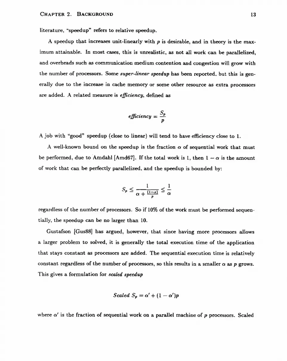
are added. -4 related measure is eficiency, d e h e d as

A job with "good' speedup (close to linear) will tend to have efficiency close to 1.

.A well-known bound on the speedup is the fraction a of sequential work that must

be performed, due to ~ m d a h l [Amd67]. If the total work is 1, t hen 1 - a is the amount

of work that can be perfectly parallelized, and the speedup is bounded by:

regardless of the number of processors. So if 10% of the work must be performed sequen-

tially, the speedup can be no larger than 10.

Gust afson [Gus881 bas argued, however, t hat since having more processors allows

a larger problem to solved, it is generally the total execution time of the application

that stays constant as processors are added. The sequential execution time is relatively

constant regardless of the number of processors, so this results in a smaller a as p grows.

This gives a formulation for scaled speedup

Scaled S, = of + (1 - af ) p

where af is the fraction of sequential work on a parallel machine of p processors. Scaled

CHAPTER 2 . BACKGROUND

speedup is bounded only by p.

Met rics

Many different metrics are available with which tu evaluate a scheduling algorithm. Mie

define some metrics here that we use later in the thesis.

A common metric is the mean msponse time (MEYT). For n jobs, where job j i(i =

1 ... n ) arrives in the system a t time si and leaves the systern at time t ; , the mean response

time is defined as

CLl(&- - si) rnean response time =

n

Another standard metric is the makespan. Informdly, this is how long it takes to

finish-a11 n jobs. FormalIy, assurning we started at time O, this can be defined as the

finish time of the last job:

makespan = m g ti L<r<n

The point a t which the system satuates is known as the level of sustainable through-

put. This is the job arrival rate at which the expected mean response time becornes

infinite, since jobs are arriving faster than they can be serviced.

Power is mean response time divided by throughput [Kleigj. At low load, throughput

is the same as the arrival rate, and at high load, the mean response time will tend to

infinity, so power will tend to zero a t both low and high arrivai rates. The maximum

point reached by the power curve is the arrival rate a t which the tradeoff between mean

response time and t hroughput provides the most overall benefit.

2.1.2 Uniprocessor Results

To understand the development of mdtiprocessor scheduling algorithms, we will first

consider some well-known results concerning single processor scheduling. A further dis-

cussion can be found in [DeiSO].

Scheduling policies for a single processor can be classified by how much information

is available to the scheduler, If the service demands of alt jobs are known e-xplicitly,

then Shortest Job First (SJF), running the jobs in increasing order of service demand,

is the best policy for minimizing mean response time, since the short jobs wiH run first

and finish quickly. If pre-emption of running jobs is allowed and is free, then Shortest

Remaining Processing Time First (SRPT) will minimize the mean response time.

Priority scheduling assigns a priority to each job, and mns the job with the highest

priority, with jobs of equal priority being scheduled in FCFS order. This can allow queues

of jobs with different resource requirements to execute at different priorities, e-g., short

interactive jobs a t high priority and long batch jobs at low priority.

Since it is often difficult to tell what type of job one is dealing with, many uniprocessor

schedulers use a multi-level feedback scheduling policy- -4 high priority is assigned to new

jobs, but as a job acquires processing time, its priority is gradually lowered. Studies of

typical workloads indicate t hat the variance in the distribution of job service times is high.

There tend to be many short jobs, and a few very long jobs, implying that newly arrived

jobs are more likely to be short jobs. Due to their high priority, they are run soon after

t hey arrive. unt il t hey reveal t hemselves as long non-interact ive jobs (by cont inuing to

run and not blocking on [/O), and cause their priority to drop. This is an approximation

of SRPT, as the high-priority jobs have a shorter expected remaining processing time.

If the coefficient of variation of job runtime is known, then the optimal scheduler can

be chosen. If the CV is less than 1, then FCFS is optimal, as a job with some acquired

processing time is expected to finish before a newly anived job. If the CV is greater than

1, t hen a feedback policy that approximates SRPT will perform best.

If no information about the job runtimes is available, then Round-Robin (RR) is a

good compromise policy, as it gives al1 jobs equd service. However. the quantum length

must be setected carehlly, as a long quantum will degenerate to first-corne-first-served

scheduling, and a short quantum will have excessive context switch overhead.

2.1.3 Classification Schemes for On-line Scheduling

Scheduling algorithms can be subdivided in a number of ways. In t his section we briefly

discusç the differences between dgorithmç that are single-level or twdevel algorithms,

thread-oriented or job-oriented, and dynarnic or static-

Single-Level vs. Two-Level

A well-known division in classi&ing scheduling disciplines is the difference between singie-

level and two-ievel scheduling. Single-level schedulers allocate processors to jobs, and

also control the allocation of specific threads of the job to specific processors. In a t w c ~

level scheduling polic_v, the scheduler allocates a set of processors to a job, but then

the scheduling of threads is done separately, perhaps by the application itself, Iower-

level operating system code, or the use of a runtime Iibrary. The second, lower level

of scheduling d o w s job-specific optirnizations to be made, and avoids the expensive

overhead of rnanaging every thread in the system.

Alt hough the two levels of scheduling seem quite different , most scheduling algori t hms

could be used a t either level in different situations [Fei95].

Thread-Oriented vs. Job-Oriented

Closely related to single-level and twelevel scheduling is the difference between thread-

oriented and job-oriented dispatching. A t hread-oriented discipline does not distinguish

between t hreads based on the job to which they belong. A FCFS global queue of threads

is a simple example. A job-oriented discipline, on the other hand, schedules jobs rather

t han t hreads. Alt hough a singie-level scheduler is not necessari ly t hread-oriented or

job-oriented, the top level of a twdevel scheduler is job-oriented. in general, a thread-

oriented scheduler c m achieve good performance if the threads of jobs in the workload

tend to perform unrelated work, and thus do not synchronize often. However, it has long

been known that if threads of a job communicate often, a fonn of thrashing can occur

due to excessive context switching [Ous82], so some form of coordination between the

threads of a job is required in this case.

Early mult i programmed mult iprocessor scheduling research concent rated on compar-

isons between t hread and job-oriented policies t hrough simple extensions of weil-known

uniprocessor algorithms [MEBSS]. For workioads that showed correlation between job

demand and number of processes (as is often the case, see Section 2.2), t hread-oriented

policies such as RR (between threads) aod FCFS resulted in higher mean response times

than job-oriented policies such as SJF, SRPT and Srnailest Nurnber of Processes First

(SNP F). Since t hread-oriented policies favour jobs wit h more t hreads, t hey were also

favouring jobs with greater service demands, causing the mean response time to increase.

This is different from uniprocessor scheduiing, where RR is known to be insensitive to job

demand distributions. However, for workloads with low variability in job parallelism and

high variability in job dernand, RR still performed as well as the job-oriented policies,

confirming the uniprocessor result .

Leutenegger and Vernon [LV90] attempted to counteract this effect with the job-

oriented policy RRJob, which time-slices jobs, and during a job's time quantum, time-

slices the threads of the job. They compared RRJob and an equipartition policy (see

Section 1.1.4) with the thread-oriented policies studied by Majumdar et al. [MEB88] and

found that the job-oriented policies gave lower mean response times under most workload

assurnpt ions.

Dynarnic vs, Static

Scheduling algorithms can be classified by whether a job's processor allocation is h e d by

the application, set at runtime, or changes as the application executes. There are some

differences in the terminology used by different authors for this distinction, especially

in earlier work. Where appropriate, we will note the differences for clarification. but

ot herwise the following taxonomy due to Feitelson [Fei951 will be used.

0 rigid the number of desîred processors is set by the application before running.

The job will not nin on less, and cannot utilize more. These types of jobs, as weil

as algorithms assuming these types of jobs, are often known as static.

moldable the number of processors can be set at the beginning of the job. but

cannot be changed during execution. This is often implemented as a parameter to

the application. Moldable jobs are somet imes called adaptiue jobs.

0 evolving the application goes through a number of phases of varying parallelism,

controlied by and/or communicated to the scheduler by the job as it executes.

0 malleable the application can have its processor allocation changed at any time in

response to a request by the scheduler. Malleable jobs are not a generally supported

programming model, since often significant prograrnming effort and execution over-

head must be expended to change a job's processor allocation during execution. In

a distributed memory environment especially, the costs of data repartitioning can

overwhelm the scheduling benefits realized by malleable job support. The program-

ming model known as "workpile of chores* is often assumed in studies of malkable

jobs. In this model, a global queue of work is maintained, and any number of

worker threads pick up work from the queue. This allows threads to be started

and stopped at (almost) any time. Malleable jobs can also be "faked" through a

technique known as folding, introduced by Zahorjan and McCann [MZ94]. Threads

of a job are multiplexed onto fewer processors than there are threads- When the

number of processors does not dîvide the number of threads, the extra processors

are "rotated" to give equd average efficiency-

The type of job assumed by the scheduler determines what kind of preernption the

scheduler can perform. The various degrees of pre-emption have received different names

as well. For exarnple, Parsons [Par971 uses this taxonomy:

0 run-to-completion (RTC) ali jobs run untii they are f i shed.

a simple preemption jobs c m be stopped so that their processors can be made

available to other jobs, but they must be restarted on the same set of processors.

0 migratable preemption jobs can be stopped and restarted on any set of proces-

sors, but the number of processors cannot change.

a malleable preemption jobs can be stopped and restarted on any number of

processors. As the name suggests, the jobs must be malleable.

Most schedulers currently used in production parallel environments use some f o m of

run-to-completion discipline [FRSC97]. wit h fixed partitions (see Section 2.1.4) Although

it stems intuitive that the flexibility allowed by a preemptive discipline would give better

performance, RTC can be attractive for other reasons. The time when a job wiil finish is

often quite predictable. A popular scheduling algorithm of this type is EASY [SCZL96]?

which guarantees that jobs will never be delayed by jobs submitted after them. How-

ever, research has dernonstrated the desirability of more adaptable disciplines and job

models [PS97].

Algorit hms t hat di vide the available processors among the competing jobs wit hout explic-

i t ly t ime-slici ng processors among jobs are known as space-sharing or space partitioning.

They can be classifiai similarly to the type of job mode1 that they assume (see Sec-

tion 21.3): into fixed, variable, adaptive and dynamic partitioning. As mentioned in

Chapter 1, the algorithms that we study in our work are adaptive and dparn ic parti-

tioning algorithms; t hus Our discussion of t hese two areas is longer than that for fixed

and variable part itioning.

Fixed Partitioning

In fixed partitioning, the system is permanently subdivided into partitions of fixed size.

These are generally set by the system administrator, and require reconfiguration and

perhaps downtime t o be changed. Often machines wilI have a small partition for de-

velopment and testing, and reserve a number of larger partitions for production work.

The partitions can be associated wit h different sizes of jobs t hrough job queues. Interna1

fragmentation can be a problern with this scheme if jobs are able to utilize a number of

processors that does not correspond to an existing partition size.

The ut ility of dividing the available processors into equal-sized partit ions has been

studied wit h analytic models [Sev89, MEB91, ST930 SST931, compared wit h adapt ive

policies [Sev89, MEB91, GST91 RSD*94, ST931, compared with timeslicing policies [SST93],

and compared with both adaptive and dynamic policies [NSS93b7 NSS93a7 NSS971. The

general conclusion is that h e d partitioning can perform well if the workload is well-

understood and jobs tend to have low variation in parallelism and service times. In

many cases, a particular size of fixed partitioning outperforms all other policies for a

particular system load and workload, but will perform poorly in other situations. This

has led to research into adaptive policies, which attempt to find an appropriate partition

size given the current load and perhaps other system and application information.

Variable Partitioning

Variable partit ioning refers to partit ioning the processors in response to requests from

applications for certain numbers of processors. The problem is uninteresting in terms of

scheduling udess there are speciai architectural problems that make it difficult to find

a partition of a given size. For example, hypercube architectures generally require that

partition sizes are multiples of powers of two, which has given rise to a luge body of

literature on finding and uniting sub-cubes of various sizes. Mesh architectures can have

requirements for rectangular allocations or thread adjacency, which m o t i ~ t e d the use of

schemes such as the buddy system.

If a given partition size cannot be allocated, the job must be queued. This leads to

some questions about the order in which to run the jobs in the queue. If job runtime

is correlated with job size, Smallest Job First c m perform well [Fei95]. but this is not

always the case.

Furt her discussion of miab le partitioning and the associated literat ure can be found

in the survey by Feitelson [Feigj].

Adapt ive Part itioning

Adaptive partitioning assumes that the jobs submitted to the system are moldable (see

Section 2.1.3), and thus will execute on any numberof processors assigned by the schedul-

ing discipline. Adaptive policies are useful in environments where the benefit of changiog

a job's processor allocation during execution can be offset by the overhead of doing so.

Dist ributed memory environments are an example. since the overhead of redistri buting

data structures c m be high.

Work on adaptive partitioning algorithms has concentrated on reducing the sizes of

processor allocations under high ioad conditions to improve mean response times, while

running applications on the partition size that gives the greatest executioa efficiency.

Sevcik [SevS9] compares adaptive policies that utilize information derived from a job's

parallelism profile to decide on the appropriate processor allocation. The policy called

.-\+&miCl gave lower mean response times using system load and the average, minimum,

maximum and variance in pardlelism, beating other rules using only one or two of these

characteristics.

Ghosal et al. [GSTSL] introduce a concept known as the "processor working set"

( pws). They use a rneasure called *efficacyn ~ ( p ) , defined as

where the cost function C(p) is defined as

and t hus

The pws is the minimum value of p which maximizes ~ ( p ) . Tt is shown that for the cost

function used, pws is the same as the number of processors associated with the h e e

of the execution tirne-efficiency profile [EZL89]. Some adaptive policies utilizing pws

were investigated. Among them, the best power was observed with a simple strategy

of allocating a job's pws when possible. If no jobs in the queue can be dIocated their

pws, the free processors are allocated to the first job in the queue. This has the effect of

allocat ing srnalier partition sizes at high loads.

Majumdar et al. [MEBglJ investigate a scheme where the number of processors per

job changed with the number of jobs in the system. They found substantial improvements

over a fixed partitioning scheme when using as few as three different sizes of processot

allocation.

Rosti et al. [RSD+94] compare a range of adaptive policies that differed in the speed

with which they would change the target partition size in reaction to a burst of arrivals

or a long period of no arrivds. This family of adaptive policies was found to be more

robust across workloads and system loads than both an equipartition policy and a non-

work-conserving policy that attempted t o leave some free processors for use by future

arrivals. The most robust policy, known as AP4, increases the target partition size onty

when there are two free partitions of the previous size, and decreases it whenever the

queue Iengt h increases.

Adaptive Static Partitioning (ASP), introduced by Setia and Tripathi [ST93], at-

tempts to decrease processor partition sizes under heavy load. If t here are free proces-

sors, an arriving job is allocated the minimum of the number of available processors and

the job's maximum parallelism. If no processors are free, the job is queued. On job

departures, the newly freed processors are divided evenly between the jobs in the queue

in FCFS order, subject to no job exceeding its maximum parallelism. ASP was found to

outperform two variations of the pws policy [GST91] and a fixed partitioning policy.

A variation on ASP is studied by Naik et al. [NSS93b], where the allocation size is also

Iimited by a system-wide minimum. This policy performed nearly as well as fixed policies

at part icu t â r loads, but was more consistent across different configurations. A dynamic

policy allowing limited pre-emption was also studied, but it tended to perform poorly a t

high load. Further study by the same authon [NSS93a] showed that the dynamic policy

handled tansieot bursts of arrivals much better than the k e d policies.

Chiang et al. [CMV94] compare adaptive policies that use application characteristics

such as average parallelism and pws with various versions of ASP. They find that for RTC

policies to perforrn well, it is crucial to have a maximum allocation limit as well as reduce

allocation under high load. The best results were found with the policy ASP-rnax+, a

version of ASP with a maximum allocation limit that decreases as load increases- This

policy consistently gave lower mean response times for workloads with high variability,

beating rules using average parallelism and pws information. The intuitive explanation

presented for this behaviour is the fact that these characteristics, although useful in

determining the optimal execution point for jobs in isolation, are poor predictors of job

demand. Long jobs can still acquire a large nurnber of processors and hold up short jobs.

Anastasiadis and Sevci k [AS971 study various adaptive policies, using execut ion t ime

funct ions based on measurements performed by Wu [Wu93], and comparing the difference

T ( p ) - T ( p + L), for p 2 1 for al1 waiting jobs to see which jobs would benefit most

from receiving another processor. They were able to surpass even the performance of

dynarnic equipartition at very high load levels (although not at Iower load Ievels). The

improvement was rnainly caused by improved queue ordering due to the application

knowledge.

Although adaptive policies will adapt to changing system conditions such as load,

they do so at a slower rate than dynarnic policies. One proposed solution is leaving some

processors in reserve for future arrivals to allow more flexibility in allocation decisions.

Policies like t his are called non-work-consenring if t hey leave idle processors when t here

are jobs in the queue. Smirni e t al. [SRS+95] study policies that attempted to retain

some memory of previous load conditions, hoping that p s t load would accurately predict

current load. They found that saving processors could have some benefit when any of

the following conditions held: the workload has poor speedup (in this case there tends

to be l e s benefit in assigning the idle processors to currently running jobs), the system

load is high, the system size is large, or job arrivals tend to be bursty. Although this

result seems at odds with results that Say equipartition can perform well, it does rnakes

sense. since saving processors for future use allows fewer processors to be allocated t o the

running jobs, and thus will tend to decrease t heir allocation sizes at higher loads.

Further study of non-work-conserving policies was carried out by Rosti et al. [RSSD95].

They compared a version of ASP-MAX and a processor-saving policy. Their results

tended to confirm that non-work-conserving policies perform best when irregularities

such as arriva1 bursts, multi-class workloads and processor failures exist in the system,

as well as when the workload has poor speedup. Further results reported by Rosti et

al. [RSD+98] indicate that these policies can aiso perform better when the workload has

irregular execut ion t imes, and when the system size is increased.

Dynamic Partitioning

Dynamic partitioning poiicies allow the scheduler to change the processor doca t ion of a

job after it has been started. Varying degrees of Bexibility can be used here, corresponding

to the Ievels of preemption discussed in Section '2-1.3. The cost of a preernption or

migration assumed for a particular system usually influences the type of dynamic policy

considered. It is easy to see that a tightly coupled shared memory machine will have less

overhead for t hread migration t han a dist ributed network of workstat ions.

A heavily studied form of dynamic partitioning is equipartitioning (EQ). where al1

jobs in the system are given an equal share of processing power. True equipartitioning

is only a theoretical concept, as it requires perfect processor sharing, Le., no context

switch overhead, cache refreshing time or other problems. The approximation most often

used first calculates a target allocation t (number of processors over nurnber of jobs),

and assigns t processors to each job in increasing order of maximum parallelism. if the

maximum parallelism of a job (Mi) is less than t , the job is assigned &.fj processors, and

t is recomputed using the remaining jobs and processors. Non-integer d u e s of t rnay

be possible if the study is theoretical; otherwise some further decisions may have to be

made to assign fract ional parts of processors. Equipart it ion based algori t hms have been

shown to perform well in many studies [TG89. ZM90, CMV94, AS971 although their

frequent reparti tioning may result in high overheads. For this reason EQ is often used as

an idealized baseline policy in studies of adaptive policies that attempt to approach its

performance while limiting overhead costs. Since equipartitioning gives (roughly) equal

service to al1 jobs, it is insensitive to the job service time distribution, and can be looked

upon as a multiprocessor analogue to round-robin scheduling. If more application or

workload knowledge is available, it is possible to improve upon EQ [Sev94, PS95, PS96,

AS97].

The earliest work on equipartitioning is by Tucker and Gupta [TG891 under the name

Process Controf. Their work focuses on the practical aspects of st ructuring applications

to create and destroy threads to keep the number of threads per job equal to the number

of processors per job. Jobs were able to suspend and create threads so that the number

of threads always matched the number of procesors, reducing context-switch overhead

and resource content ion.

Leutenegger and Vernon [LV90] study the dynamic partitioning scheme in cornparison

with some simple policies such as FCFS, Shortest Number of Processes First, RR, and

RRJob (described in Section 2.1.3). They h d that dynamic partitioning (processors

are split evenly, with no job receiving more than its maximum parallelism) and RRJob

perform better than the other policies. Both give a roughly equal share of processing

power to al1 jobs, whereas the other policies tended to favour one class of jobs at the

expense of anot her.

Crovella et al. [CDDf 9 11 study tirneslicing, coscheduling, and space partitioning in

a NUMA environment. They find that giving applications exclusive use of a smaller

number of processors is more efficient than uncoordinated timesharing or coscheduling.

Even wit h multiple threads of the sarne application timesliced on a partit ion, applications

did not experience as large of a slowdown as expected.

Zahorjaa and McCann [ZM90] compare an adaptive policy that used execution time

functions (similar to Anastasiadis and Sevcik [AS97], as described above in Section 2.1.4)

and a dynarnic policy. The dynamic policy is actually closer to a variable partitioning

policy, as the job rnodel is evolving (see Section 2.1.3), allowing jobs to request and release

processors according to their parallelism demands. The dynarnic policy gave lower mean

response times, except when context switch overhead was very high. In later work,

McCann et al. [MVZ93] compare a version of the above dynamic policy with RRJob and

equipartitioning. They find that the dynamic policy performs best with respect to mean

response time, fairness, and response to short, interactive jobs. This is mainly due to

the fact t hat the dynarnic policy is able to use processors more efficiently than the ot her

policies. since applications wili give up any processors they cannot use.

-4 policy called Folding is introduced by McCann and Zahorjan [MZ94]. The policy is

intended for mesh-coanected parailel computers, so much work is done to preserve adja-

cency relationships between threads when changing job partition sizes. On job arrivais,

the Iaxgest existing partition is split in two, the existing job's threads are -foldeci" onto

half of their previous allocation, and the other half is given to the new job. Processors

are rotated between differently sized partitions to give equal average service rates to dl

jobs. This folding policy is compared with a version of equipartitioning that attempts

to allocate partitions with at least one power-of-two dimension, and performs m a s red-

locations on every job arriva1 and departure. Although folding tends to perforrn better

when the number of jobs in the system is a power of two (rotations are minimized), it

out performs equipart it ioning in an analytic model, a Markovian birt h-deat h model, and

a simulation.

Padhye and Dowdy [PD961 compaxe adaptive and dynamic policies. An adapt ive a l p

rit hm (RA) based on those studied by Rosti et al. [RSD+94] is compared with a dynamic

EQ policy and a folding policy similar to that studied by McCann and Zahorjan [MZ94]

(described above). Using a synthetic workload running on an Intel Paragon, they found

that folding outperformed EQ. Folding also gave a better MRT than the RA poiicy when

the workload had poor speedup and variabIe demand, but not if the workload had good

speedup and less variability in demand.

The impact of repartitioning overheads on dynamic equipartit ioning policies is inves-

tigated by Islam et al. [IPS96]. They implement a malleable job system on NOW and

an IB b1 S P-2, bot h distributed memory systems where repartitioning could be expected

to be expensive. Measurements of this system are then used to create an analytic model

tbat includes the repartitioning overhead of equipartitioning- To simulate an adaptive

policy, a static partitioning policy is simdated for different partition sizes and load levels,

and the best partition size for each load level is used when comparing against the EQ

policy. Even given these overheads, the dynamic policy tended to outperform the static,

except when the workload was dominated by small. short jobs, for which the overhead of

frequent repartit ioning was not warranted. EQ's relative performance benefit increased

with higher system loads and arriva1 burstiness.

The study by Naik et al. [WSS97] compares a Kved partitioning policy, an adaptive

policy and a dynamic policy. The policies are based on those developed by Naik et

al. [NSSOJb]. and discussed in Section 2.1.4. Jobs are classified as srnd, mediumor large.

The st at ic policy divides the processors arnong the job classes and t hen assigns equal-sized

partitions to jobs according to their class. The adaptive policy also divides the processors

into 3 pools (for large, medium and small jobs) classes, but wit hin the pools the partition

size grows and shrinks with system load. The dparnic policy will reconfigure large and

medium-sized jobs to different processor allocations when processors are needed or when

t here are enough free processors anilable- The adaptive policies tended to perform as

well as the fixed policies, and provided more flexibility, as they performed well for a wider

range of workloads and arriva1 rates. The dynamic policy outperformed the ot hers w.r.t.

MRT for dl loads. The overhead of application reconfiguration is explicitly modeled, and

does not change the qualitative results until it is increased by a factor of 4.

2.1.5 Time Slicing

Partitioning dong the axis of time rat her than space is known as time-slicing. Generally,

there are few algorithms that perform any kind of time-slicing in a distributed system

such we are considering in this thesis. The ability to time-slice is desirable, however,

as mean response time can be greatly reduced by the abifity to pre-empt running jobs

so newly arrived short jobs can finish quickly. This bas inspired some researchers to

Figure 2.1 : Co-scheduling with 5 mws: scheduling rounds continue through, giuing each row a quantum, and then repeat. Each pattern in the figure is a diflerent job, white space is packing loss. New jobs fonn new rows ifthey don't fit into existing ones, and departing jobs will cause rous to be collapsed together if possible.

implement forms of time-slicing in NOW environments [DAC96, ADCM98, SPWC98].

Time-slicing techniques can be distinguished by whether they use a global queue for

the entire system, or local queues on each processor. Local queues are more cornmon

in dist ri buted memory machines, because of the communication overhead involved in

maintaining a shared giobd queue. A major issue when using local queues is how to

balance the load between processors, since there is no global CO-ordination. This can

be performed by intelligent initial placement, or by migrating t hreads from heavily-

loaded processors to lightly-loaded ones. A global queue is simple to implement if shared

memory is available, and does not have any load balancing issues. It c m become a central

bottleneck, however, so is more likely to be seen in srnaller scde machines.

Co-ordinated timeslicing refers to job-oriented time-slicing policies. There are two

main types of ceordinated time slicing, gang scheduling and static quantum-based schedul-

ing.

Gang Scheduling Early work by Ousterhout [Ous82] established that if threads of a

job communicate often, performance could be undermined due to the large number of

context switches caused by threads blocking when sending messages to threads t hat were

not scheduled. He proposed CO-scheduling, which attempted to schedule threads of the

same jobs together whenever possible. A matrix algorithm was used. which rnaintained

rows of jobs which were scheduled together, as in Figure 2.1.

Although the term gang scheduling is often used interchaogeably with CO-scheduling,

it is claimed by Feitelson at least, that gang scheduling means t hat threads of a job

are always scheduled toget her, as opposed to cescheduling, w hich will schedule t hreads

together when possible [Fei96]. Gang scheduling is something of a cross between space-

slicing and time-slicing. Al1 t hreads have a processor each. so the processors are parti-

tioned by job, but jobs are also time-sliced with other jobs. This reduces the thrashing

due to excessive context-switching described by Ousterhout, since al1 threads in the job

are scheduled at the same time. The time-slicing of jobs allows mean response time to

be kept low, as short jobs will get a chance to run quickly.

Achieving gang scheduling c m be difficult unless special hardware exists to perform

sirnultanmus context switching across all of the processors. In a tightly coupled MPP, t his

is easier to accomplish than in a distributed system. However, some have implernented

mechanisms for gang scheduling across a network of workstations. These approaches are

the most applicable to our work. and are described in Section 2.1.6.

Static Quantum-Based Policies Parsons and Sevcik [PS95] study what they cal1

stat ic quantum-based algorithms. The policies investigated are based on the rnult ilevel

feedback queue scheduling used for uniprocessors. They generalize the well-known a d a p

tive space partitioning disciplines ASP [ST93] and PWS [GSTSl] to feedback preemptive

disciplines, FB-PWS and FB-ASP. Every quantum, the jobs with the least acquired pro-

cessing time are selected to run. In workloads with high CV of job demand these jobs

are expected to finish first. The partition sizes allocated decrease as load on the system

increases. The feedback versions of the policies performed much better, according to

mean response time, than the RTC versions for al1 choices of workload and offered load,

with more pronounced tendencies as the CV of job demand rose. In the case of CV = 70,

the difference was two orders of magnitude. The F E P WS d s o policy came close to, and

in some cases surpassed an idealized equipartit ion policy wit h no overhead penalties.

Chiang and Vernon [CV96] follow up on this work using different workload models.

The results of Parsons and Sevcik [PS95] are corroborated for workloads with a large

number of inefficient jobs, but it is found that for workloads where large jobs tend to

have a t l e s t moderate efficiencies, EQ still outperforrns the feedback policies. A new

policy called EQS-PWS is presented that combines the approaches of the pwsbased

policy and EQ. hstead of allocating min(t, Mi) processors, min( t, pws ) processors are

allocated. This policy performs as well or better than the FB-PWS and EQ for al1 of the

workloads examined.

2.1.6 Networks of Workstations (NOWs)

Networks of commodity workstations have a much lower cost per processor than large

parallei cornputers. For this reason, they have b e n touted as the parailel computing plat-

form of the future [ACP95]. There is certainly evidence that parallel computing is feasi-

ble on this type of platform [CADAD+97]. Much research [ADCM98, DAC96, ADC97,

WZ97, KL97, LS93, ADV+95, SPWC98, DZ97, AS97, AFKT981 has been devoted to

determining how to schedule parallel applications effectively in a NOW environment.

In theory a NOW could be as powerful as a large, tightly coupled parallel machine,

but t here are some problems with the architecture that tend to limit performance. The

communication medium is generally orders of magnitude slower. Gang scheduling is

difficult to support directly, as hardware for c ~ r d i n a t e d context switching does not

exist . Alt hough implementations of dist ri buted shared memory [ACD+96, S BIS981 allow

s hared-mernory applications to execute on a NO W, they are s t iil generally out-performed

by applications optimized for message-passing. In particular, recent improvements in

processor speed have not b e n matched by improvements in network latencies, Limiting

the speedups achievable [PBSg?].

Sobalvarro et al. [SPWC98] study coscheduling on workstation clusters. They use a

mechanism known as dynamic CO-scheduling ( first st udied by Sobalvarro et al. [S W95] )

to achieve strong cescheduling behaviour. Threads that are not running when a mes-

sage ârrives are awakened and run. Transitive message-passing relationships can tend

to ceschedule groups of communicating processes without explicit identification of the

communicating groups. This approach has been successfuily implemented in both the

Solaris and Windows NT operating systems [BC9?].

-4 related idea is implicit CO-scheduling, studied by Dusseau et al. [DAC96, ADCM98I.

"Two-phase spin blocking" is used. Instead of blocking when waiting for a message, the

process will spin for a certain amount of time before blocking, in hopes of receiving the

message reply and avoiding the context switch overhead. The length of the spin period is

dependent on the amount and type of messages received and sent by a process. Processes

t hat are communicating often will increase their spin time. They give results showing

this mechanism to be competitive with explicit coscheduling; a maximum slowdown of

30% is observed-

Parsons and Sevcik [PS97] have doue work implementing a range of scheduling dis-

ciplines on a 16-node NOW. The scheduler is implemented on top of the commercial

load-balancing system LSF. They show that despite high preemption and reconfigu-

ration overheads (over a minute for preemption), adaptive and preernptive disciplines

out perform run-to-complet ion stat ic scheduling for bot h MRT and makespan.

2.1.7 Non-Uniform Memory Access (NUMA) Machines

Somewhere in between networks of workstations and shared memory machines lies the

NUMA model. Machines of this type have g l o b d y shared memory, but the memory is

organized hierarchically, so that access times to different areas of memory are not always

equal. Examples of this type of machine include Hector [VSLW91], developed at the

University of Toronto, and MIT'S Alewife [ABC+99].

In a NUMA environment, as in our heterogeneous model, not al1 processors are cre-

ated equal. Thus in addition to the classic allocation problem (how many processors t o

allocate), we are also faced with the placement problem (which processors to dlocate),

Work by Zhou and Brecht [ZB91, Bre971 established that placing threads close to their

data and to other threads in the job is cruciaI to performance. They used a construct

called a "processor pool" to group processors for allocations. Unsurprisingly, the best

performance was found ni th pool sizes that matched the underlying architecture; in this

case a hierarchical design with four "stations" of four processors each. This restricted

jobs to executing within a single station, making al1 data accesses local. As well, they

found that a "Worst-Fit* policy of placing jobs in the least-loaded pool performed best,

as jobs then had the most available room to expand.

2.1.8 Scheduling Research Lessons

We have presented a large amount of materiai related to parallel job scheduling in this

section. From this mass of information, we can distill a few principles that we will use

to guide us in our design of algorithms for a heterogeneous environment.

1. Among the dynarnic disciplines, equipartitioning performs well when workload

knowledge such as demand or speedup is not available.

'2. Among adaptive disciplines, the best results have been found with disciplines that

reduce processor allocations under hi& loads.

3. Some form of ceordinated scheduling kmong job threads is necessary to allow

forward progress.

4. Any knowledge of the job's service demand, even approximate, can improve schedul-

ing t hrough better queue ordering.

These are fairly hasic guidelines that have corne out of the research done over the past

few years. Given more specific workload or system knowledge, it is possible to improve

on t hese suggestions. However, since we are experimenting wit h a relatively new model,

we will start from these assumptions and attempt to find out where they may break down

in a heterogeneous system.

2.2 Workload C haracterizat ion

Over the past ten years, parallel job scheduling research has been hampered by a chronic

lack of data concerning the nature of workloads from parallel computing sites. Many

studies have used workloads consisting of a small number of parallel programs obtained

from benchmark suites or indust ry, or synt hetically generated workloads wit h somewhat

arbi t rary distributions. However, the situation has improved in recent years, and a

clearer picture of workload distributions has begun to emerge. The major job pararn-

eters of interest in our study are inter-arrivai time, runtime, degree of parallelismt and

communication demand. We use the words "shortn and "long" when contrasting job

runtirnes, and "smailn and "largen when describing job parallelism.

The Ieast well understood of these parameters is communication overhead. None

of the existing studies have attempted to characterize the communication patterns of

general parallel workloads, dthough much research exists on the problem of modeling

and optimizing the communication of individual p a r d e l prograrns. We have therefore

used Our own model of communication demand, based on data from the SPLASH-2

parallel benchmark suite [WOT+95], and explaineci in more detail in Chapter 4. The

ot her parameters are discussed below.

2.2.1 Job Int er-arriva1 T h e

The most popular choice for modeling job arrivals has been a Poisson process. Numerous

studies have used this distribution [MEBSS, LV90, ZM901 GST9 1, CMV94, PS95, CV96,

Fei96. Dow971, alt hough some have experimented witb the hyper-exponentid distribu-

t ion [RS D+S8. CV96, IPS961.

An exponential distribution is known to have a CV of 1. However, studies of workload

traces from parallel computing sites have tended to find inter-arriva1 CV's considerabiy

larger than 1. In the k s t widely cited in-depth stuciy of a parallel job trace, Feitel-

son [FN95] reports that inter-arriva1 times from NASA Ames had a relatively high CV,

which indicates that a hyper-exponential distribution may be more correct. The arrival

rate varied throughout the day: the daytime CV was 3.56, the night-time was -.IL, and

the weekend was 2.83.

The NASA Ames workload waç compared with one from the San Diego Supercom-

puter Center (SDSC) by Windisch et al. [WLM+96a]. They conclude that the inter-arriva1

time is the most regular of the workload parameters studied, and could be modeled by

'simpler probabiiistic functions". Based on comments by the same authors in [LMW98],

one would assume that this means an exponential distribution. The distributions at bot h

machines were quite similar. Due to some limitations in the trace data, the actud data

studied were job start times, rather than job arrival times. For interactive jobs, these

times are the same. However, for batch jobs, the scheduling policy can affect how soon

the submitted job actually runs. Nevertheless, the trends were similar: the daytime CV

\vas 3.0, the night-time was 5.8, and the weekend was 3.13. (These numbers are from the

technical report version of the paper [WLM+96b]).

In studying a workload from the Cornell Theory Center, Jann et al. [JPF+97] use a

method that fits a Hyper Erlang distribution to the workload data. This distribution

is a generalization of the hyper-exponential and Erlang distributions, wit h two branches

and a number of stages in each branch. They found that the inter-arriva1 times were

too dispersive to be captured by an exponential distribution, and a hyper-exponential

distribution was required tu fit the data.

Daily Cycle Some studies [FN95, WLMC96a] have found significant fluctuations in

the arriva1 rate according to the time of day. When users go home at night, the arriva1

rate drops off sharply, and many of the large queued jobs are able to finish.

2.2.2 Job Runtime

Job runt imes have usually been modeled wit h a hyper-exponential distribution [PS95]

and workload studies tend to support this practice. Reported CV's from workload traces

are generally in the range of 2-10, dthough numbers as high as 70 have been reported

[CMV94, FN9.5. WLM+96a, JPFf971.

A more interesting and less well-understood question is whether job runtimes are

correlated with job sizes. -4 weak positive correlation (Le., larger jobs run longer) has

been reported by several authors [FN95, WLW+96a, Hot96, Fei96, LMW98], but few

researchen have modeled this. One slight exception is a study of data from the Corne11

Theory Center (CTC)? where Kotovy [Hot961 reports a two-phase distribution of job

durat ion. Jobs using from 2- 16 processors had decreasing runt imes associated wi t h more

processors, but jobs using more than 16 processors tended to use more resources as their

parallelism increased.

Many studies [FN95. SSG95, Hot96, SGS96, WMKS961 have also noted the large

numbers of small, short jobs - often over half the total number of jobs. -4s well, they

have al1 found that these small jobs consume a small fraction of the total resources, e.g.,

node-seconds or CPU cycles.

Downey [Dow971 proposes a mode1 where the sequential lifetime L (runtime of a job

on a single processor) is used to calculate the speedup of a job, and thus the runtime

on n processors. Since L is generally not knowo, T (the wall-dock time multiplied by

the cluster size) is used as an estimator. T will generally over-estimate L, since most

prograrns have sub-iinear speedup. Based on trace data from the Corneil Theory Center,

Downey rnodels T as linear in log space, or "uniforrn-logn. The cumulative distribution

function is of the form

where 40, pi are intercept and slope of the Line in log space.

Jann et al. [JPF+97] reported that their fitting procedure for total CPU tirne was

unable to fit a hyper-exponential distribution to the runtimes for a workload a t the

Corne11 Theory Center. A Hyper Erlang distribution of higher order was required in

most cases to fit the data.

Lo et al. [LiMW98] attempt to determine what effect the use of different synthetic

rnodels has compared to real job traces with respect to simulations evaluating scheduling

disciplines. They compare two "naive" synt hetic models, two synthet ic models derived

frorn analysis of job traces (due t o Feitelson [Fei961 and Downey [Dow97]), and four

workload traces. Although the relative ranking of al1 scheduiing algorithms was not

d e c t e d by the particular mode1 used, some other aspects of the models were found to be

important, in particular the proportion of power-of-two job sizes and the correlation of

runtime with job size. System utilization tended to rise as the nurnber of power-of-two

job sizes increased. Real workload traces were found in most cases to have a weak positive

correlation between job size and runtime, with the correlation coefficient running between

0.13 and 0.35. Xlgorit hms that performed well on positively correlated workloads tended

to perform poorly on negat ively correlated workloads, and vice-versa.

The job size parameter has received the most widely varying treatrnent in the Literature.

This is due not only to the lack of information concerning the true distribution, but as

well to the difficulty of modeling the data that does exist. The reported data in workload

studies are difficult to characterize succinctly- They have a high discrete component, and

tend to vary considerably from site to site.

Feitelson's early study [FN95] found a roughiy uniform distribution of parallel jobs

(those using more than one processor). The number of single-node jobs was much higher

than any of the other sizes. The trace data was from a 138-node hypercube architecture

(an Intel iPSC/860), so all of the job sizes are powers of two. There is a large number of

32-node jobs, for which no explanation is posited.

Later studies [SSG95, WLMC96a, Hot96, SGS96, Fei96, Dow971 have tended to find

t hat the workload contains a high number of power-of-two sized jobs, although they are

not required by the architecture in any of these cases. There has been speculation that

the organization of the queueing system has encouraged the submission of jobs sized by

powers of two [WLM+96a, Dow971. However, in at least one study [Hot96], there does

not appear to be any encouragement to have jobs of these sizes. The subrnittal queues

are organized by estimated runtime, not number of processors. and the machine st udied

is an IBM SP2, which has no performance degradation for irregularly-sized jobs.

Feitelson [Fei961 studies 6 traces from different machines, some of which had been

used in other studies already. Again, small jobs were more common than large jobs.

Powers of two were common in a11 of the workloads. Other cornmonly occurring sizes,

termed "interesting sizes", were squares, multiples of 10, and the full system size. This

tended to create strong discrete components in the distribution. The author models this

by using an harmonic distribution, which is adjusted by hand to account for more small

jobs and interesting sizes.

2.2.4 Workload Summary

Some points emerge from the above discussion as being generally acceptai, or consistent

across studies. These are the main points to which we have attempted to be faithful

when selecting input distributions for our simulations.

1. Arriva1 processes have higher variability than the traditional Poisson process. and

are probably better rnodelled with a hyper-exponential distribution.

2. Job runtimes are highly variable, with many short jobs that require relatively few

resources, and a few long jobs that use a large portion of the total resources.

3. Job runtimes show a slight positive correlation with job parallelism.

4. Job sizes tend to be multiples of powers-of-two, even when they are not required by

the architecture. Ot her common sizes usually have sorne numerical or architectural

significance, such as 1, squares, multiples of ten, and the f u U machine size.

Discussion of the workload mode1 which we have used in our experiments is contained

in Chapter 3.

Chapter 3

System and Workload Model

3.1 System Model

The system under consideration is a network of rnultiprocessor nodes. Processors within

a node are the same speed, but processors in different nodes may have different speeds.

Nodes may be of different sizes, Le-, they may have different numbers of processors (see

Figure 3.1).

More formally, the network consists of a set S of nodes, Si, i = 1, . . . , [SI. Each node

Si has lSil processon, each of speed s(Si).

A subset of the processors belonging to a node is called a node partition. The proces-

sors of a node partition can be dedicated t o a single job j , in which case a partition N!

denotes a set of processors from node Si, belonging to job j .

We define capacity of a set G of processors g;, i = 1,. . . , lGl to be the sum of the

speeds of the processors in the set, and use K(G) to denote this quantity:

The capacity describes the computational power of a set of processors. Tt can be looked

at as an analogue to the number of processors in a homogeneous system.

CHAPTER 3. SYSTEM AND WORKLOAD MODEL

w Figure 3.1: Heterogeneous network of multïprocessors

We assume the nodes are connectecl by a fast network, so that communication between

any two nodes has the sarne cost. Network contention and congestion are not modelled.

W e will assume that communication between processors iri the same node (local corn-

municat ion j is much less expensive t han communication between processors in different

nodes (network communication), so that local cornmunicat ion effectively has zero cost .

Further, memory is shared inside the node, but is not shared between nodes (at least at

the hardware level.) The model is thus closer to that of a network of workstations than,

Say, a NUMA machine,

As far as we know, this model has not been studied in the Iiterature before. Previous

work in scheduling on networks of workstations has always assumed t hat nodes are single

processors, each of equal power. The assumptions concerning equal communication cost

between nodes are common in simulation studies in NOW environments.

3.2 Job Mode1

In the terminology of Chapter 2, a distinction is made between rnoldable jobs that cannot

change t heir processor ailocation after starting, and malleable jobs that can change their

processor allocation a t any time. Since memory is shared at a node, jobs in our model

CHAPTER 3. SYSTEM AND WORKLOAD MODEL

(a) Speedup curves for different degrada- (b) Slowdown curves for different degrada- tions due to multiplexing of job threads. tions due to multiplexing of job threads.

Figure 3.2: Efect of diflerent values of $.

may change their processor allocation within a node at any time, but are unable to change

t heir node allocation. These jobs are malleable in a restricted sense.

Malleable jobs are not a generally supported programming model, ço we will achieve

malleability by folding t hreads when necessary. Due to context switch overhead and

ot her factors, there is a performance cost to this option. We assume that if t threads are

running on k processors of speed S. where k < t, then the rate of service of the threads

can be modeled as

where ~ is a constant. A value of t,b = 0.91 has been used in previous work [GSTSl,

Pargï]. Speedup curves for different values of 11 are shown in Figure 3.2(a). The curves

are not completely accurate, as they represent the drop from the perfect speedup that the

job will have at its maximum allocation. Perhaps mole accurate is a graph of slowdown

for different shown in Figure 3.2(b). (Slowdown is defùied as the factor by which

execution increases when the number of processors is decreased.)

W e need to assume that it is possible for local node schedulers to create indepen-

dent partitions on a single node. Although general operating systems do not have this

CHAPTER 3. SYSTEM AND WORKLOAD IO DEL

capability, it is not difficult to irnplernent using a nurnber of queues.

The minimum parallelism of all jobs is 1, as al1 threads of a job could be multiplexed

onto a single processor. The maximum pardelism is set a t runtime as the number of

threads requested by the job.

We assume the jobs are programmed in single-program-multiple-data (SPWD) style

and al1 threads will have identical service demands. The threads synchronize "fre-

quently". (This is imprecise. but assume it is often enough that the progress of the

job will be Iimited by the slowest thread.) The finish time of a job is then the finish

time of its most slowly progressing thread. This load imbalance will not be modelled

explicitly, Le., no processors belonging to the job will be freed until al1 of the threads

belonging to the job have finished.

3.3 Workload Mode1

As discussed in Section 2.2, parallel workload modelling has advanced considerably in

the past few years. and studies of workload traces from supercomputing centres have

allowed some general conclusions to be made about parallel workloads. Our workload

assumpt ions have been guided by t hese points whenever possible.

We have chosen to mode1 the arrivai process wit h a hyper-exponential distribution

with CV of 8. The method of Sevcik et al. [SLTZï?] is used to create a distribution with

the required CV. Code is inchded in Appendix C.

In the interests of modelling job runtimes and job sizes, we have selected a parallel

workload generator based on that used by Feitelson and Jette [FJ97], and implemented

based on code supplied by Feitelson from his Parallel Workloads Archive l. The adapted

code used in our experiments is listed in Appendix B.

Feitelson's workload uses an harmonic distribution of order 2.5 for the job sizes, which

' http://www.cs.huji.ac.il/labs/parallel/workload

CHAPTER 3. SYSTEM AND WORKLOAD MODEL

(a) Cumuiative distribution function of (b) Cumulative distribution fnnction of the job size distribution used in Feitet- the job repetition distribution used in son's distribution. Feitelson's distribution. Note that the

y-axis scale starts at 0.85.

Figure 3.3: Repetition and size d i s t ebu tions.

is adjusted by hand to add extra weight for srnall jobs and interest ing sizes such as powers-

of-two, squares, multiples of ten, and the full machine size. The cumulative distribution

function of the job size distribution is shown in Figure 3.3(a). The job runtime is chosen

from a three-stage hyper-exponential distribution, with branches of mean 50, 900, and

10000. The probability of choosing a particular branch is based on the job size, to give

a slight positive correlation between job size and mntime. A scatterplot of 100,000 jobs,

with runtime plotted against job size, is shown in Figure 3.4. The predominance of

the interesting sizes can be clearly seen. For the sample of jobs shown, the correlation

coefficient between job size and job runtime is 0.187.

Feitelson's distribution also includes a distribution for the nurnber of times that a

job is repeated. This is modeled as an harmonic distribution of order 1.5, for which the

cumulative distribution function is shown in Figure 3.3(b). This has the effect of skewing

the average job demand by the number of times that a job is repeated, since these job

repetitions are not new arrivals - it is as if there is one arrival with a total demand equal

to the demand mult iplied by the number of repetitions. This total demand must be used

when calculating arrival rates that correspond to different system load factors.

CHAPTER 3. SYSTEM AND WORKLOAD MODEL

. to*

I

Figure 3.4: Scatterplot O/ 100,000 jobs, showing runtime plotted against job size.

3.4 Communication Mode1

As discussed in Section 2.2, there is Little existing work on the statistical distribution

of communication behaviour in parallel programs. For this reason, we have developed a

simple model based on data from the SPLASH-2 parallel benchmarks [WOTf 951.

-4 graph characterizing the ratio of communication to cornputation in the SPLASH-2

benchmark suite is presented in Figure 3.5. (This graph was generated from the online

database of SPLASH-2 data2.) The SPLASH-2 suite consists of shared memory applica-

tions; however this gross approximation of communication requirements is useful. Given

a distributed shared memory implementation [ACD+96, SBIS981, it is even possible to

implement these applications in a model such as ours, although the added overhead of

maintaining the DSM environment would make Our assumpt ions opt imist ic.

Discounting the local traffic, the average number of bytes communicated per instruc-

tion for each size of processor is given in Table 3.1. If we graph this table with the

number of processors on a logarithmic scale as in Figure 3.6(a), then we see a roughly

'ht~p://www-flash.staaford.edu

CHAPTER 3. SYSTEM AND w-ORKLOAD MODEL

R SM Flemote Capacii Remoîe Cold Remte W ~ R e ~ ûrerhead Remte Local Data

Figure 3 . 5 : Communic~tion/cornputation ratio in the SPLASH-8 suite (generated using the online database at the SPLASH-2 website, http://wuw-flash.stanford.edu).

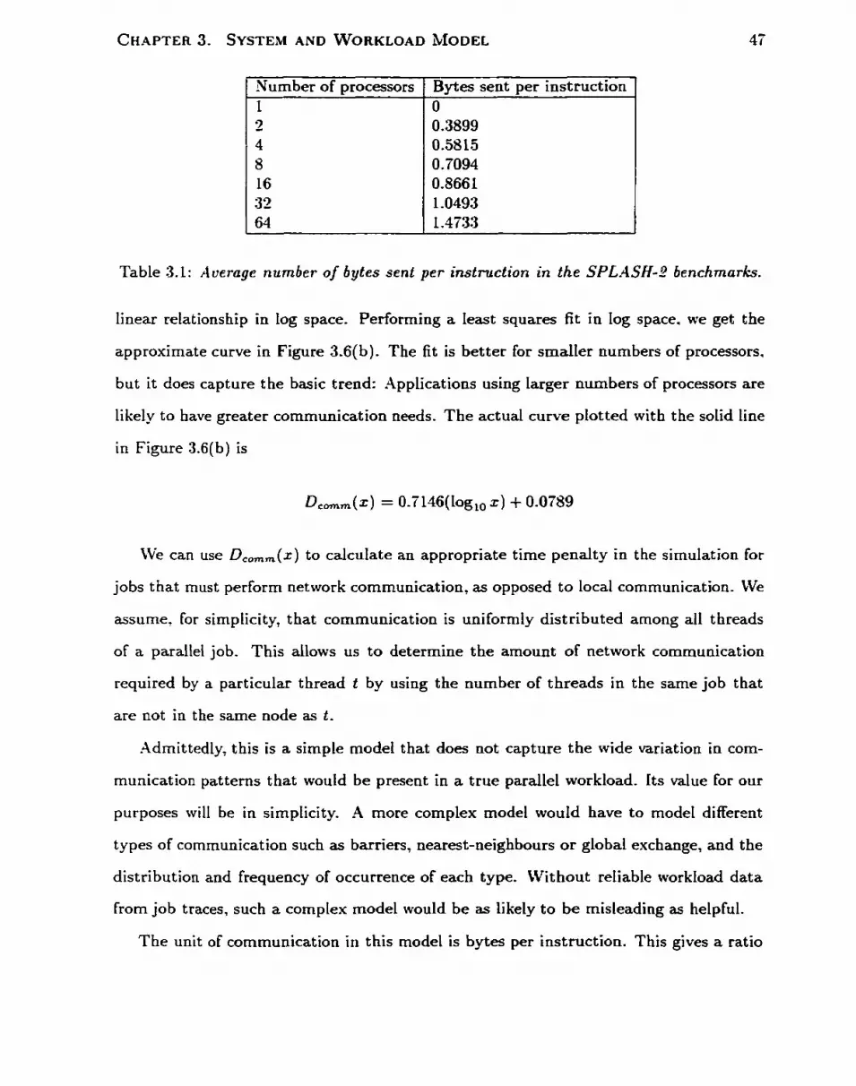
Number of processors Bytes sent per instruction O 0.3899 0.5815 O. 7094 0.8661 1.0493 1.4'733

Table 3.1: Average number of bytes sent per instruction in the SPLASH-2 benchmarks

linear relationship in Iog space, Performing a least squares fit in log space. we get the

approximate curve in Figure 3.6(b). The fit is better for srnaller numbers of processors,

but it does capture the basic trend: Applications using Iarger numbers of processors are

likely to have greater communication needs. The actual curve pLotted with the solid line

in Figure 3.6(b) is

Ive can use D,,,,(x) to calculate an appropriate time penalty in the simulation for

jobs that must perform network communication, as opposed to local communication. CVe

assume, for simplicity, that communication is unifomly distributed among al1 threads

of a parallel job. This allows us to determine the amount of network communication

required by a particular thread t by using the number of threads in the same job that

are not in the same node as t.

-Admittedly, this is a simple model that does not capture the wide variation in corn-

munication patterns that would be present in a true parallel workload. its value for our

purposes will be in simplicity. A more complex model would have to model differcnt

types of communication such as barriers, nearest-neighbours o r global exchange, and the

distribution and frequency of occurrence of each type. Without reliable workfoad data

from job traces, such a cornptex mode1 would be as likely to be misleading as helpful.

The unit of communication in this model is bytes per instruction. This gives a ratio

CHAPTER 3. SYSTEM AND WORKLOAD IO DEL

(a) Average number of bytes sent per fb) Least squares fit in log-space to instruction in SPLASH-2 benchmarks. the SPL.4SE-I-2 average communication (Note that number of processors is needs. grapbed on a logarithrnic scale.)

Figure 3.6: Derivation oJ the communication distribution.

of the amount of communication to the arnount of computation, but unfortunately does

not include how to convert the communication into a time penalty expressed in units of

computation. As a first approximation, we use a ratio of c = 2 for communication to

computation. Using Feitelson7s workload model as described in Section 3.3, this gives a

relationship like that in Figure 3.7. The data in the figure assume that each thread is

on a separate node, and so must perform network communication with al! other threads

in the job. This could be reduced by placing sorne threads in the same node? so the

figure represents the worst case communication time. Different communication workloads

can be modelled by varying the ratio c, as well by varying the shape of the curve in

Figure 3.6(b).

For some insight into this model of communication, we coüsider a simple system with

8 uniprocessor nodes of the same speed and fractional thread distribution. Figure 3.8

shows the response time of a single job with 8 threads for various values of c and different

nurnbers of processors. If the communication cost is rnuch higher relative to the compu-

tat ion cost, we see that even using the rnaximum number of processors does not greatly

improve the response time over just executing the job sequentially on one processor with

CHAPTER 3. SYSTEM AND WORKLOAD MO DEL

Job S i

Figure 3.7: Average cornputation and communication time for 10,000,000 jobs with a communication to computation ratio of.?, assuming each thread of the job is on a separate node. Note the cornfations between size and computation as tue11 as communication.

no communication costs. However. for a smaller ratio, some improvement is always found

as processors are added.

3.5 Summary of Models

LVe have motivated and developed rnodels for the system, jobs, and workload under

considerat ion.

The system consists of a network of multiprocessor nodes. each of which can be a

different speed and contain a different number of processors. Jobs are malleable in a

rest ricted sense: t heir processor allocations wit hin a node can be changed at any time,

but their allocation of nodes cannot change once the job has started. Jobs are composed

of threads, the number of which is requested by the job and stays constant throughout

the job. This requires that malleability be achieved by folding threads when there are

more threads than processors; a performance penalty relative to the ratio of threads to

CHAPTER 3. SYSTEM AND WORKLOAD MODEL

I

2 3 4 5 6 7 8 Number of F'mesxm

Figure 3.8: Response time of a job with 8 threads for diflerent ualues of c as processors are added. Work per thread is 1, so the fmtest possible response time is 1.

processors is applied when folding occurs.

The workload parameters are modeiied as follows: Job inter-arriva1 t imes are hyper-

exponentially distributed with a CV of 8, job sizes are from a harmonic distribution of

order 2.5 that has been hand-adjusted to add weight a t common sizes, job runtimes are

from a t hree-stage hyper-exponential distribution and bave a slight positive correlation

with the job size, and job repetitions are from a harmonic distribution of order 1.3.

The communication mode1 is developed based on data from the SPLASH-2 parallel

benchmark suite. Communication demand is related logarit hmically to the job size, and

we define a pararneter c that is the ratio between units of communication and units of

work. This ratio is set as c = 2 for our experiments.

Chapter 4

Scheduling Policies and Experiments

In this chapter we define the policies that we use to investigate scheduling in heteroge-

neous environments. As well, we describe the experimentd environment and the simula-

tion assumptions and decisions that we have made.

4.1 Two Levels of Allocation

Scheduling in a heterogeneous environment raises an additional problem not encountered

in t radi tional scheduling problems. Most algorithms previously st udied give al1 proces-

sors the same weight (alt hough t here are location-dependent considerations in variable

partitioning). Thus the problem is: How many processors should a given job have a t any

one time? In the model we consider, processors may differ in speed and node size, and

so the problem becomes not only How many?, but WJiich ones? as weU.

An addit ional problem in our model is t hread placement. After we have solved Which

ones?, rve need to decide how many threads should be assigned to each node. We would

Iike to minimize the completion time of each job. Since each thread has an equal demand,

this is accomplished if al1 threads progress at the same rate. If allocation of fractional

threads were allowed, then an equal rate of progress is achieved by assigning to each

procnsor a number of threads proportional to the processor's speed over the capacity of

CHAPTER 4. SCHEDULING POLIC~ES AND EXPERIMENTS 52

ail of the job's processors. Define the number of t hreads of job j assigned to a processor p

as e ( j , p ) . If a job j has t j threads to be assigned t o a s e t of processon G = {gil i = l...IGI},

we assign to processor gi a nurnber of t hreads equal to

Wit h integer constraints? we cannot achieve this exactly. We approximate this as closely

as possible by using the folIowing a lgo r i t h :

1. Assign to each partition N! a number of threads equal to the Eloor of the sum of

the perfect thread allocation for aii of the processors in Ni':

2. Each partition's thread allocation now differs from the ideal by less than 1 thread,

so there must be fewer unassigned threads than nodes. Now Ive assign the leftover

threads one a t a t ime to the partitions that have the greatect difference between

their actual and their ideal allocation-

3. Any partitions that have fewer assigned threads than processors have their sizes

reduced so there is one processor per thread. Any unused processors are returned

to the pool of free processors.

4.2 The Policies

4.2.1 Adaptive Policies

Never-Span (NS) Never-Span attempts to maximize locality benefits by always run-

ning al1 t hreads of a job in the same node. Newly arrived jobs a r e run on the node whose

set of free processors will give the fastest service rate. If there are no free processors, the

job is queued. On job departures, the newly freed processors are allocated one a t a time

to the jobs in the queue, not going over the maximum paralleiism for any job. So, if a

job using 5 processors ends, and there are two jobs in the queue, the first job will receive

:3 processors and the second job will receive 2.

Span-Sometimes (SS) Span-Sometimes attempts to utilize some of the supposed

benefits of allowing jobs to span nodes and decrease their level of timeslicing.

Define a target job capacity FC,,,,,~:

- -1 .(si> Ktorgct - number of jobs

where the number of jobs includes al1 jobs in the system, including running and queued

jobs. Algorithms using this definition of the number of jobs have tended to outperform

those that used just the number of running jobs [AS97].

To control the degree to which jobs will tend to span nodes, we define a spanning

factor. denoted al which controls the attractiveness of choosing a processor in another

node. This allows us to formulate an alternative definitioa of capacity, which subtracts

some amount to compensate for the increased overhead due to communication.

This basically calculates the used capacity of the job, with something subtracted at each

node that is relative to the amount of capacity at other nodes (and thus the amount of

communication t h e job will have to perform a t that node).

The size of the spanning factor, between O and 1, allows the policy to range between

uncontrolled node-spanning when O = O and no node spanning when a = 1.

Span-Sometimes assigns one processor a t a time to a newly arrived job, until the

CHAPTER 4, SCHEDULING POLICIES AND EXPERIMENTS 54

capacity of the job is as close to nt,,,t as possible. For each free processor p, the benefit

of adding this processor to the job's ailocation is calculated in the following way:

The free processor for which benefit is the greatest is selected and added to the job. The

process is continued until benefit is negative for all free processors, the maximum number

of processors have been assigned, or there are no more free processors. On job departures,

jobs in the queue are treated as new anivals in FCFS order.

4.2.2 Dynamic Policies

Dynamic Never-Span (DNS) On new arrivals, find the node for which equally par-

titioning all processors among the jobs in the node (plus the new job) will bring the

average capacity over al1 jobs dosest to Ktarget-

If al1 jobs are running on a single processor, then no further partitioning is possible,

and the job is queued.

On job departures, the same process is followed for jobs in the queue, as if t hey were

new arrivals. If there are no jobs in the queue, the newly freed processors are divided as

evenly as possible arnong the remaining jobs in the node.

Dynamic Span-Sometimes (DSS) We extend the Span-Sometimes policy by allow-

ing jobs to steal processors from currently running jobs. Lnstead of only considering free

processors, processors belonging to running jobs are ais0 considered. If job jthie is a new

arrival. and processor p belongs to job jvidim. then the benefit of taking p away from

j,;,t;, and giving it to jthie/ is calculated as:

This arnounts to adding up the benefit for the victim and the thief. Should the benefit of

removing p from jvidim be negative (thus in fact a detriment), and be larger in absolute

magnitude than the benefit gained by jthiell then the o v e r d benefit will be negative,

and p will not be re-assigned. Free processors compete with assigned processors, using

the definition of benefit for free processors from the adaptive Span-Sometimes algorithm-

Processors that are the only processor in a aode belonging to a job are not considered. As

in the adaptive Span-Sometirnes policy, processors continue to be assigned to a new job

until the benefit is negative for ail processors, the job cannot utilize any more processors,

or there are no more processors that are eligible to be stolen from running jobs.

4.3 The Experiments

The polices above were compared using a discrete-event simulation, consisting of about

15.000 lines of C++. Our initid decision was to write the simulation from scratch to allow

the greater flexibility and avoid the learning curve of a simulation package. However, in

retrospect, the use of a simulation language such as CSIM might have shortened Our

development t ime.

Job inter-arriva1 times were generated using a hyper-exponential distribution with a

CV of 8, and 7 different means corresponding to system load factors between O and 1.

Job work, paraltelisrn, and repetitions were generated using t he distributions of Feitelson,

described in Chapter 3. Simulations were run until 200000 jobs had completed, except

CHAPTER 4. SCHEDULING POLICIES AND EXPERIMENTS 56

if the queue length increased to greater than 150000 jobs, in wbch case the run was

terminated early. This was done to cope with rare situations in which very long queue

lengt hs overwhelmed the memory of the simulation machine. The resuits for the first 500

jobs of each run were not counted, to allow a w-armup period for the scheduling policies.

Runs were replicated 50 times with 50 different random number seeds. Cornmon random

numbers were used for each sequence of runs, and al1 job parameters were calculated

on job arrival, ensuring that each policy and network was evaluated with the sarne job

arrivais. In most cases, this gave 95% confidence intervals with a half-width of l a s than

5% of the mean. However, some intervais are Iarger: especially at higher loads, due

to the high variability inherent in the workload. We note that previous users of t his

workload [FJ97] have reported difficulty achieving tight confidence i n t e r d s as well.

Chapter 5

Results

In this section we compare the algorithms from the previous chapter on a variety of

networks with different ciegrees and types of heterogeneity. We constrain al1 of the

networks to have the same total capacity of 12800, so that cornparisons of response

time between networks can be made meaningfully. A network with no communication

costs is used as the baseline cornparison,

We begin by comparing non-heterogeneous, i.e. homogeneous, networks that fit into

our model, to see how a few, fast processors compare against a larger number of slow

processors. The algorithms are then evaluated on networks that vary in processor speed,

followed by networks varying in node size. As well, we compare some random samples of

networks with the same CV of speed or size, to vaiidate our use of the CV as a basis for

describing heterogeneity. To reduce the number of figures in this chapter, al1 networks

are shown in bar graphs in Appendix A.

Our results, especially a t lower loads, tend to have 93% confidence intervals with half-

widths less than 5% of the mean. These intervals are shown on al1 graphs of rnean response

time. In general, where we describe similarities and differences in mean response tirne*

t hese characteristics are defined as overlapping and non-overlapping confidence intervals

respect ively.

Syam Lod

Figure 5.1: Mean response times in the homogeneous ivetwork 1

5.1 The Homogeneous Case

We first compare our algorithms using a basic network, which we denote hereafter as

Yetwork 1. This network consists of one 128-processor node of speed 100. Since al1

processors are of the same speed, and al1 nodes are of the sarne size, this is a condition

of zero heterogeneity. Network 1 was chosen as it has neit her communication costs nor

overhead for switching threads between processors. This allows dynamic algorithms to

make full use of the network with no added cost- Performance on Network 1 can be used

as a benchmark ideal situation against which to compare perfumance in other networks.

Mean response times for the four algorithms in Network 1 are shown in Figure 5.1.

The two dynamic algorithms, DNS and DSS, perform much better than the adaptive

algorithms NS and SS. This is not surprising, as both of the dynamic algorithms reduce

to variants of equipartitioning in this network, and it is well known that equipartitioning

can perform well if overheads are low and no other workload information is available.

The two dynamic aigorithms are nearly identical in performance. Between the adaptive

algorithms, SS performs somewhat better than MS. This is because NS will assign as

many free processors as possible to a new arrival, while SS will only assign a capacity up

to rctaVet, making a long wait in the queue more likely with NS.

To investigate the effect of adding communication costs on performance, we ne-- com-

pare the algorit hms using various configurations of homogeneous networks wit h 16 nodes.

These networks are numbered 3540, and their configurations are shown in Table 5.1.

Each network has 16 nodes and a total capacity of 12800, giving each node a capacity of

800 to be divided among its processors. This causes the total number of processors to

n r y from netrvork to network, dthough the to td capacity is constant.

Table 5.1: Node sizes and processor speeds of the 6 hornogeneous networks. Ail networks have 16 nodes and a total capacity of 12800.

W e graph the performance of the four algorithms on these networks in Figures 5.2 and

5.3. -411 four algorithms saturate faster on the networks with fewer processors- At higher

load, there are not enough processors to sustain throughput when large, long jobs corne

along. In Figure 5.2 we see that at low loads, the NS algorithms show little difference

across networks, while the performance of the Span-Sometimes algorit hms (Figure 6.3)

improves as the networks have fewer processors. Although these networks have fewer

processors, the ones t hey have are faster. Thus if t here are only a few jobs in the system,

the spanning algorithms are able to utilize more of the faster processors and allow jobs

to complete sooner, without holding up many jobs in the queue. This effect is more

noticeable with the adaptive spanning algorithm SS than it is with DSS. The dynamic

Network 33 36 37 38 39 40

Processor Speed 800 400 200 100 80 50

Node Size 1 2 4 8 10 16

Number of Processors 16 32 64 128 160 256

spanning algorithm shows the same basic trend at high load, but at medium load it is

the in-between networks, 37 and 38, that perforrn the best.

Results Summary After simulation of our algorithrns on a number of homogeneous

networks. we find that a t low toads, the spanning algorithms perform better on networks

wit h fewer, faster processors, but the non-spanning algorit hms show little difference across

networks. However, at high loads, dl four algorithms degrade much faster on the networks

with fewer processors t han t hose with a larger number of slower processors.

5.2 Speed Heterogeneity

The first dimension of heterogeneity we investigate is that of processor speed. If we

hold the node size fixed, and vary the speed of the different nodes in the network, what

happeus to the relative ranliing of the algorithms? How do the algorithms themselves

vary as the speed-heterogenei ty is increased?

AS a measure of heterogeneity, we use the CV of processor speed. The node size is

fixed at 8, and processor speed is varied to get three networks, numbered L 1, 12, and

13, which have low, medium and high speed-heterogeneity respectively. Graphs of the

processor speeds are shown in Figure A.1. The three networks have node-speed CV's of

approximately 0.19, 0.43 and 0.86, respect ively-

Algorithm performance on Networks 11, 12, and 13 is shown in Figures 5.4 and 5.5.

Interest ingly, NS actually performs better in t hese speed-heterogeneous networks t han in

the hornogeneous case of Network 1. This is likely due to the fact that NS is a greedy

algorithm, which will assign as many free processors as possible to an arriving job. In

Network 1. this allowed jobs to monopolize large nurnbers of processors tvithout releasing

them. In the multi-node case, NS wiH limit jobs to the size of a node, leaving more

processors free for other jobs.

The other three algorithms, DNS, SS, and DSS show performance degradations for

(a) Never-Span (b) Dynamic Never-Span

Figure 5.2: Mean response time of the Never-Span algorithm on the homogeneous Net- works 35-40.

(a) S pan-Sometimes (b) Dynamic Span-Sornetimes

Figure 5.3: Mean response time of the Span-Sometimes algorithms on the homogeneous Networks 35-40.

the speed-heterogeneous networks compared to Network 1. In the case of NS and DNS

at low loads, the more speed-heterogeneous the network, the better the rnean response

time. At medium to high ioads, this situation is reversed: higher mean response times

are observed as the speed-heterogeneity of the network increases. At low loads, there

tend to be so few jobs in the system that most jobs end up using the faster processors

in the higher end of the network. As load increases, more and more jobs are forced to

execute on the slower processors, increasing mean response t ime.

We do not observe this crossover effect with SS and DSSt shown in Figure 5.5. For

al1 loads, the mean response time is the sarne (statisticdy speaking) or greater as we

increase the speed-heterogeneity.

The next question is how the performance of the algorithms relative to each other

is affected by the increasing speed heterogeneity. Figures 5.6 and 5.7 compare the per-

formance of the algorithms on Networks 1, 11, 12 and 13. (Figure 5.6(a) is identical to

Figure 5.1, but is shown again for ease of cornparison.) In the homogeneous case, the

split in performance was between static and dynamic policies. However, in the speed-

heterogeneous networks, NS goes from being the worst policy to one of the best policies,

while DSS, which had good performance in Network L, has relatively poor performance

in Ketworks 11-13. This makes the split occur between policies that are node-spanning

or not. while in Network 1 it was between policies that were dynamic or not. The mag-

nitude of the difference in performance between node-spanning and non-node-spanning

algorithms increases with the degree of speed-heterogeneity. One somewhat inexplicable

result is the fact t hat as the networks become more speed-heterogeneous, NS rnoves frorn

sIight ly underperforming DNS in Network 1 1 to outperforming i t in Network 13.

The dynamic spanning algorit hm, DSS, outperforms its adaptive version, SS, for low

and medium loads, but at high Ioads t heir performance becomes indistinguishable. The

gap between the two algorit hms at low to medium load increases wit h the degree of speed

heterogencity. This is because the performance of SS degrades faster with increasing

(a) Never-Span (b) Dynamic Never-Spa

Figure 5.4: Mean response t ime of the Never-Span algorithrns on Networks 1 , I l , 12, and 1 S.

(a) S pan-Sornetimes (b) Dynamic Span-Sometimes

Figure 5.5: Mean response t h e of the Span-Sometimes algorithms on Networks 1,11,12, and 13.

speed heterogeneity than does DSS, as can be seen by comparing Figures W(a) and (b).

Results Summary Our investigation of speed-heterogeneous networks shows that the

non-spanning algorithms exhi bit a crossover effect, where they perform bet ter on more

speed-heterogeneous networks at low loads, but worse on more speed-heterogeneous net-

works at high loads. The node-spanning algorithms do not show this effect, but instead

have worsening performance at al1 loads as the speed-heterogeneity increased. As well,

the non-spanning algorithms match or outperform the spanning aigorithms at d loads.

5.3 Node-Size Heterogeneity

The next dimension of heterogeneity that we investigate is the oumber of processors per

node. Sirnilady to the previous section, we create three networks where al1 nodes are

speed 100, but the size of the nodes are varied. These three networks are numbered

14-16. and are shown in Figure A.2. They exhibit low, medium and hi& degrees of size-

heterogeneity, wit h node-speed CV's of approximately 0.48, 0.83 and 1.2 1, respect ively.

The results of comparing the performance of the four algorit hms on Networks 1 and

14-16 are shown in Figures 5.8 and 5.9. As in the speed-heterogeneous networks, NS

performs better in the size-heterogeneous case than the homogeneous case due to the

limitation of node size. There is also a slight tendency at low load for NS and DNS

to perform bet ter on more size-heterogeneous networks. This also parallels the speed-

heterogeneous case, and is presumably due to more jobs utilizing the larger nodes when

the system is Lightly loaded.

However, unlike the speed-heterogeneous case, at medium load there is almost no

difference in relative performance for the algorithms across different degrees of size-

heterogeneity. The exception to this rule is DSS, which has equal performance a t low

load for al1 t hree networks, but shows decreasing petformance as the size-heterogeneity

increases at medium and high loads. The Fact that three of four algorithms show almost

(a) Network 1 (b) Network I l

Figure 5.6: Mean response time of al1 four algorithm on Networks 1 and 11. Note that in a ) , it is DNS-and DSS that have the best performance, but in b ) it is NS and DNS.

(a) Network 12 (b) Network 13

Figure 5.7: Mean response time of all four algodhms on Networks 12 and 13.

(a) Never-Span [ b) Dynarnic Never-Span

Figure 5.8: Mean response time of the Neuer-Span algorithms on Networks 1,14.15, and 1 6.

(a) Span-Sometimes (b) Dynamic Span-Sometimes

Figure 5.9: Mean response time 01 the Span-Sometimes algorithms on Networks 1,l4,l5, and 16.

(a) Network 14 (b) Network 15 (c) Network 16

Figure 5.10: Relative performance of all four algorithrns on Networks 1,14,15, and 16.

no difference in mean response time is interesting, as the degree of node-size heterogene-

ity is high? especially in Network 16, which has a CV of around 1.2, and a range of 32.

Note especially the case of SS in Figure 5.9(a), where performance is identical on ail three

networks, ciespite this hi& heterogeneity.

Kext we tum to the relative performance of the algorithms on the different s ize

heterogeneous networks. The ordering of the algorithms is shown for the three networks

14.15,16 in Figure 5-10. At low loads, the algorithrn ordering is the same as for the

speed-heterogeneous networks, i.e., NS and DNS are best, followed by DSS and then SS.

However. while in the speed-heterogeneous networks, DSS and SS have similar perfor-

mance at high loads, in the size-heterogeneous networks SS actually outperforms DSS

at high loads. The magnitude of this difference increases as the networks become more

heterogeneous. This is an interesting result, as we would expect a dynamic algorithm to

outperform its adaptive counterpart a t aU loads.

Results Sumrnary We determine from experimenting with size-heterogeneous net-

works t hat there is little or no statistically significant differences in performance across

the networks for three of the four aigorithms. The fourth algorithrn, DSS, shows worsen-

ing performance as the networks become more size-heterogeneous, resulting in DSS being

outperformed by its adaptive counterpart SS at medium to high loads.

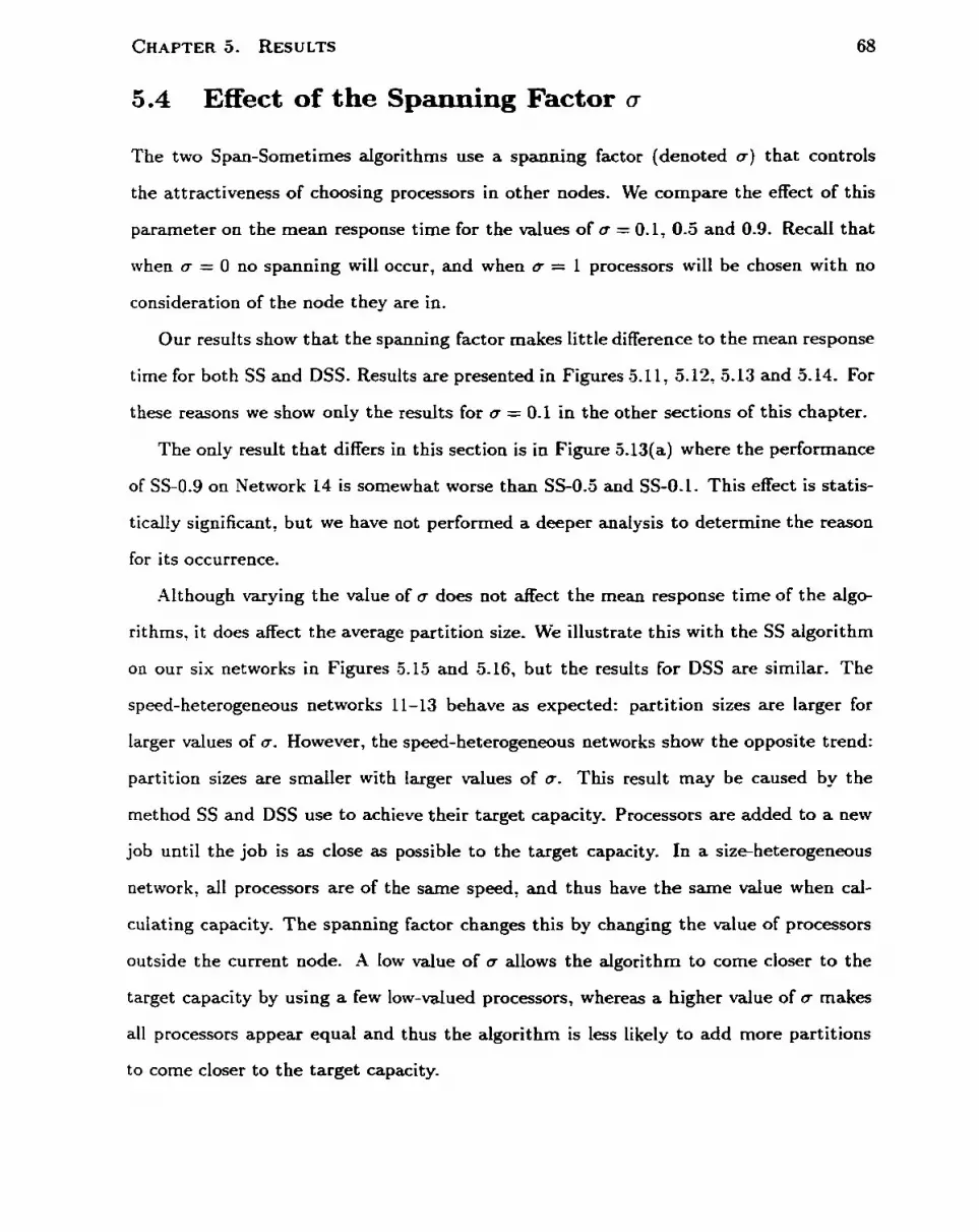
5.4 Effect of the Spanning Factor a

The two Span-Sometimes algorithms use a spanning factor (denoted a) that controls

the attractiveness of choosing processors in other nodes. We compare the effect of this

parameter on the mean response time for the values of a = 0.1, 0.5 and 0.9. Recall that

when a = O no spanning will occur, and when a = 1 processors will be chosen with no

consideration of the node they are in.

Our results show t hat the spanning factor makes little difference to the mean response

time for both SS and DSS. Results axe presented in Figures 5.11, 5.12? 5.13 and 5 14. For

t hese reasons we show only the results for a = 0.1 in the other sections of this chapter.

The only resuit that differs in this section is in Figure 5.13(a) where the performance

of SS-0.9 on Network L4 is somewhat worse than SS-0.5 and SS-0.1. This effect is statis-

tically significant, but we have not perforrned a deeper analysis to determine the reason

for i ts occurrence.

.4lthough varying the value of a does not affect the mean response time of the algo-

rithms, it does affect the average partition size- We illustrate this with the SS algorithm

on Our six networks in Figures 5.15 and 5.16, but the resuits for DSS are similar. The

speed-heterogeneous networks 11-13 behave as expected: partition sizes are larger for

Iarger values of a. However, the speed-heterogeneous networks show the opposite trend:

partition sizes are smaiier with larger values of o. This result may be caused by the

method SS and DSS use to achieve their target capacity. Processors are added to a new

job until the job is as close as possible to the target capacity. In a six-heterogeneous

network, al1 processors are of the same speed, and thus have the same value when cal-

culating capacity. The spanning factor changes this by changing the value of processors

outside the current node. A low value of a allows the algorithm to come closer to the

target capacity by using a few low-valued processors, whereas a higher value of a makes

al1 processors appear equal and thus the algorithm is less likely to add more partitions

to come closer to the target capacity.

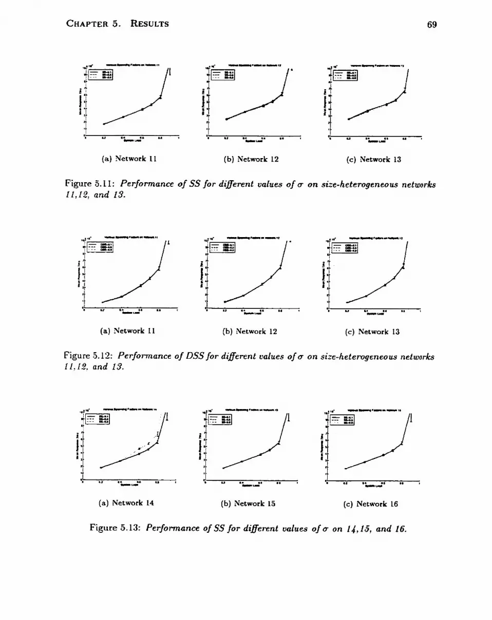
(a) Network 11 (b) Network 12 (c ) Network 13

Figure 5-11: Performance of SS for diflerent values of a on size-heterogeneous networks I l , I Y , and 13.

(a) Network 11 (b) Network 12 (c) Ketwork 13

Figure 5-12: Performance of DSS for different values of a on size-heterogeneous networks I l ? 12, and 13.

(a) Network 14 (b) Network 15 ( c ) Network 16

Figure 5.13: Performance of SS for diflerent ualues of a on l4,15, and 16.

(a) Network 14 (b) Network 15 (c ) Network 16

Figure 0.14: Performance of DSS for diferent uahes of 0 on l4,15, and 16.

(a) Network 11 (b) Network 12 (c ) Network 13

Figure 5.15: Mean number of partitions per job on the speed-heterogeneous nettuorks 11- IS for the SS algorithm.

(a) Network 14 (b) Network 15 (c) Network 16

Figure 5.16: Mean number ofpartitions per job on the size-heterogeneous networks 14-16 Jor the SS algorithm.

Results Summary Simulation of different values of the spanning factor show that it

has no effect on scheduling performance. Although it does affect the mean partition sizes

allocated to jobs, this happens in unexpected ways: a high spanning factor results in a

larger mean partition size on the speed-heterogeneous networks, but in a smaller mean

partition size on the size-heterogeneous networks.

5.5 CV As a Performance

In the experiments of the previous sections,

Predictor

we invest igated performance on networks

that have different CV's of speed and size. This involves an implicit assurnption that

the CV is a useful measure for differentiating between networks. However, it is possible

for two networks with the same CV to have different characteristics, and thus perhaps

di fferent performance.

To investigate this, we randomly selected networks with the same CV and capacity,

and used them to compare our algorithms' performance. Since there are an infinite

number of networks having any given CV and capacity, we reduced the search space

by considering only a Limited number of possible speeds and sizes, and constraining ail

networks to have exactly 16 nodes. We hypothesize that higher moments could describe

different types of network configurations, so we calculated the skewnessL for al1 networks

as well. The distribution of possible speed- and size-heterogeneous networks is shown in

Figure 5.17, with the CV of node size or speed graphed against skewness. The constraints

of 16 nodes and a total capacity of 12800 tend to create patterns in t h e distribution.

To compare otherwise different networks of equal CV, we randomly selected networks

from vertical cross-sections of t hese graphs. Figures A.3-A.8 show t h e resulting networks.

The relative range of possible node sizes (1-32) was much larger than that for processor

'using the formula: C s . , when is the sarnple mean, d is the sample variance, and n is the sample size.

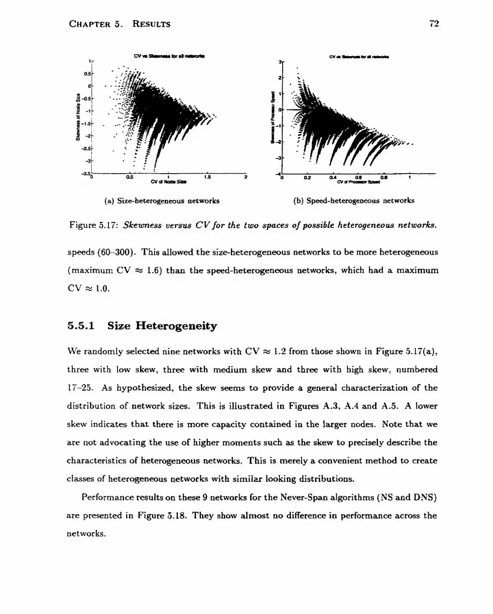
(a) Size-heterogeneous networks (b) Speed-heterogeneous networks

Figure 5.17: Skeumess versas CVfor the two spaces of possible heterogeneous networks.

speeds (60-300). This allowed the size-heterogeneous networks to be more heterogeneous

(maximum CV =r 1.6) than the speed-heterogeneous networks, which had a maximum

CV x 1.0.

5.5.1 Size Heterogeneity

We randomly selected nine networks with CV x 1.2 from those shown in Figure .5.17(a),

three with low skew, three with medium skew and three with high skew, numbered

17-25. As hypothesized, the skew seems t o provide a general characterization of the

distribution of network sizes. This is illustrated in Figures A.3, A 4 and A.5. A lower

skew indicates that there is more capacity contained in the larger nodes. Note that we

are not advocating the use of higher moments such as the skew to precisely describe the

characteristics of heterogeneous networks. This is merely a convenient method to create

c h s e s of heterogeneous networks with s imi lu looking distributions.

Performance results on these 9 networks for the Never-Span algorithms (NS and DNS)

are presented in Figure 5.18. They show almost no difference in performance across the

networks.

Results for the two Span-Sometimes aigorithms are shown in Figure 5.19. The a d a p

t ive algorit hm SS shows similar results to the NS aigorithms: there is alrnost no variation

among the networks. The dynamic version, DSS, does show a small difference: Networks

3 - 2 5 perform better a t low and medium loads than the other networks. These networks

have higher (less negative) skewness, and thus a higher proportion of larger nodes. How-

ever, the difference is not s tat is t icdy significant. We mention it here oniy because it is

the only case where the results are l e s t han identical.

5.5.2 Speed Heterogeneity

As in the previous section, we begin by selecting 9 networks with processor-speed CV of

0.6 from the space of possible 16-node networks having a total capacity of 12800, depicted

in in Figure 5.17(b).

Three of these networks have low skewness, three medium skewness, and three high

skewness. They are numbered Networks 26-34 and are shorvn in Figures -4.6, A.7 and

-4.8.

Results of the four algorithms on Networks 26-34 are presented in Figures 5.20 and

-5.21. As in the six-heterogeneous case, there is almost no difference in performance for

any of the algorithms, validating our use of the CV as a basis for network cornparison.

Results Summary Simulation on samples of speed-heterogeneous and size-heterogeneous

networks indicate that the CV is a good predictor of scheduling performance for our al-

gorithms. Although far from conclusive proof, we feel this offers some support for the

comparisons made in our study.

(a) Never-Span (b) Dynamic Never-Span

Figure 5.18: Performance of NS and DNS on networks with high CV of node size and uarying skewness-

(a) Span-Sometimes (b) Dynamic Span-Sometimes

Figure 5.19: Performance of SS and DSS on networks with high CV of node size and varying ske wness.

(a) Never-S pan (b) Dynamic Never-Span

Figure 5.20: Performance of NS and DNS on networks with medium CV of node speed and varying skewness.

(a) S pan-Somet imes (b) Dynamic Span-Sometirnes

Figure 5.21: Pef irmance of SS and DSS on networks with medium CV of node speed and va rying skeum ess.

Chapter 6

Conclusions and Future Work

6.1 Conclusions

Ini t idly, we compared various homogeneous networks having the same overall capacity

and nurnber of nodes, but varying in the number of processors per node, and thus the

total number of processors. Since the total network capacity was limited (to 12800),

networks with a larger number of processors had slower processors. We found that at low

loads, the spanning algorithms benefited from the façter processors, and so performed

better on the networks with fewer, but faster, processors. As load increased, both the

adaptive and the dynamic algorithms saturated much faster on the networks with fewer

processors.

This Ieads us to believe that it may be beneficial to construct a heterogeneous network,

using a few fast processors and a large number of slow processors. Networks coataining

only fast or only slow processors both perforrned weil, but at different loads, suggesting

that a heterogeneous network made up of some of each kind might be able to perform

well at both low and high load. Older, slow processors are often scrapped in favour of

new ones, but this argument might present some reasons for keeping them in a network,

if only to alleviate the pressure at high loads.

CHAPTER 6. CONCLUSIONS AND FUTURE WORK 77

Some previous work has had similar results. Sauer and Chandy (SC811 performed a

queueing analysis of a two-processor system versus a one-processor system, where the

dual processors have half the processing speed of the single processor. They found that

a job with a long service time interfered less in the two-processor case, as throughput

couid still be maintained on the other processor. Classical queueing t heory results due to

Kleinrock [Me761 indicate that as servers are added (with total system capacity remaining

the same), mean waiting time decreases, but mean processing time increaseç (where

response time is the sum of waiting and processing times), Although our result seems

counter-intuitive in light of classical results, our intuition is that it is likely due to the

specifics of the worktoad in question, which has large numbers of srnall, short jobs, and

a few very long, very Iarge jobs. With a large network, short jobs are hast always able

to run, albeit a t a slower rate. In a s m d network, it is easy for a Iarge. long job to tie

up al1 of the processors in the network for a long period of time, forcing many short jobs

to wait. The tradeoff is tbat the extra waiting time due to queueing is not made up by

the faster processing speed for many jobs, causing the overall response time to increase.

When we held the node size fixed, and varied the processor s p e d in the network,

we found t hat a t low load, the non-spanning algorithrns performed better on the more

speed-heterogeneous networks, but a t medium to high loads, the trend was reversed, with

better performance on the less speed-heterogeneous networks- The spanning algorithms

did not have this crossover tendency, but instead had worsening performance at al1 loads

as the speed- heterogenei ty increased.

We then investigated node-size heterogeneity by fixing the processor speed and vary-

ing the number of processors per node. The non-spanning algorithms showed a very slight

tendency to perform better on more heterogeneous networks at low load, but worse a t

higher loads. This is similar to the results for speed-heterogeneous networks, although

the magnitude of the effect is less pronounced. At medium load, there is little or no

stat k t ically significant di fference for al1 algorit hms except DSS, which had higher mean

CHAPTER 6 , CONCLUSIONS AND FUTURE WORK 78

response tirnes as the node-size heterogeneity increases, The performance of DSS is

actually worse than that of SS on the more size-heterogeneous networks.

The precedi ng two paragraphs provide evidence t hat the increased speed or size avail-

able in the high end of a heterogeneous network is beneficial at Iow loads, but at higher

loads, the increased use of the slower or srnaller end of the network becomes detrimental.

To support Our use of the CV as a basis for comparing network heterogeneity, we

sampled from the space of heterogeneous networks of a given CV with 16 nodes and a

capacity of 12800, Wë found that al1 of the dgorithms perform nearly identically on

networks with sirnilar CV's, even when the actual distribution is different, as indicated

by the skewness. This result was observed for buth speed and node-size heterogeneity,

providing some evidence that the CV is a good predictor of scheduling policy performance

for t hese algorit hms in Our rnodel.

We note that for al1 networks studied, the simple non-spanning algorithms NS and

DNS outperformed the more complex spanning algorithms SS and DSS. This was some-

what unexpected. as our original hypothesis was that node-spanning would be beneficial

in some cases. Bowever, this does not show that spanning is detrimental, only that

our approach to spanning does not work as well as desired. -4s well, our communication

rnodel incurred fairly high overheads for comrnunicating jobs. In the Future Work section

below, we discuss how furt her st udy wi t h different communication models and various

overheads could shed more light in this area.

The better performance of the non-spanning algorithms recalls the results of Brecht

in a NUM.4 environment [Breg'ij, where the best performance was found by restricting

jobs to pools that matched the underlying architecture* This effectively amounted to

using a non-spanning algorithm, alt hough in a sbared-memory environment rat her t han

a message-passing one.

Our observations indicate that processor-speed heterogeneity has a greater effect on

scheduling than node-size heterogeneity. This may be due to some limitations in our

CHAPTER 6. CONCLUSIONS AND FUTURE WORK 79

model, since we do not model bott lenecks at the network interface or memory bus level.

Leaving that aside, we find that trends existing in situations of low heterogeneity are often

magnified by increased heterogeneity (as measured by the CV of speed or node size). We

conclude that heterogeneity cannot be ignored when designing scheduling algorithms.

-4s well, the most dynamic and flexible algorithm, Dynarnic Span-Sometimes, faiied

to perform as well as expected. At higher loads, DSS was as bad or worse than its

adapt ive counterpart SS. for bot h size-heterogeneous and speed-heterogeneous networks.

This unexpected result indicates that the careful balancing of threads perforrned by SS

may be more important than the pre-emptive flexibility given by DSS. At higher loads.

when DSS steals processors from running jobs and causes them to be unbalanced, this

may offset the benefit gained from starting some jobs earlier. This result is interesting, as

the dynarnic algorithm is outperformed by the adaptive algorithm for a difTerent reason

than usual. Normaily, one would expect a dynamic algorithm to outperform a similar

adaptive algorithm whenever the costs of pre-ernption are not too high. In this case,

the pre-emption performed is cheap, but it is the upsetting of the balancing scherne of

t hreads to processors t hat is the cause of the dynamic poiicy's performance degradat ion,

6.2 Future Work

The field of heterogeneous scheduling remains largely unexplored. We have investigated

only two of the possible dimensions of heterogeneity, and only in isolation. In this section

we list some areas and approaches that would be reasonable directions to extend Our work-

-4 truly heterogeneous network would probably vary in more than the single dimen-

sions investigated here. It would be interesting to see if any of our results hold o n

networks that vary both in processor speed and node size. For example, we noted a

small effect on networks that vary only in node size: does this change when the network

also varies in processor speed? Our approach in this thesis involved enumerating many of

CHAPTER 6 . CONCLUSIONS AND FUTURE WORK 80

the possible networks composed of certain sizes or speeds, and t hen randomly choosing

a subset wit h which to experirnent. This method is probably computationally infeasible

if the network is heterogeneous in two or more dimensions. Therefore, we would likely

have better success with r andody generating networks until we have a sufficiently large

subset within a certain tolerance of the desired point.

Our work provides some evidence that the CV is a good predictor of scheduling

performance. at least for the networks, algorithms, and workloads considered. However,

more extensive work is required to prove or disprove t f i s hypothesis. Consideration of

more types of scheduling algorithms and a wider range of possible networks would make

this result much more useful to future system designers. It would also be interesting

to see if other measures of variation, Say inter-quartile range, or simpler ones such as

minimum and maximum provide any kind of scheduling predictive power.

As well, experiment a t ion wit h networks t hat are heterogeneous in rnult i ple dimensions

would also require the use of more than one CV to describe the heterogeneity of the

network, an approach that does seem unlikely to scale as more dimensions of heterogeneity

are added. It is difficult to believe that an n-tuple of CVs would effectively describe

scheduling performance in these networks. Future work would be needed to determine if

it is possible to compare networks in any meaningful way when the number of variables

becomes larger.

The results of our experiments with homogeneous networks suggest that a network

with many slow processors c m outpedonn a network with a smaller number of fast

processors, especially at high loads. This suggests the use of heterogeneous networks

cornposed of a small number of fast processors and a group of slow processors. Hopefdy

the fast processors could be used at low loads, while at high loads, small, short jobs

could be executed on the slow processors. Useful future work could include attempts

to quantify this somehow, giving some guidelines as t o how many slow processors are

needed before a difference in performance is seen.

CHAPTER 6. CONCLUSIONS AND FUTURE WORK 81

We compareci two node-spanning algorithms with two non-spanning algorithms, and

in al1 cases except the singie-node Network 1, the spanning algorithms were outperformed

by non-spanning algurithms. More experimentation is required to determine if this is a

property of al1 spanning algorithms in our model, or if it is just that our chosen algorithms

are particularly bad. Some of our observations indicated that thread baiancing is more

important than preemption, especidy a t higher Ioads- Since our dynamic spanning

algorit hm, DNS, made no attempt to re-balance the threads. or to pre-empt in a manner

that rninimized imbdance, we specdate that a dynamic algorithm that did do so rnight

perforrn better.

The most weakly supported part of our model is the communication overhead. Al-

t hou& the paucity of data in this area is partly to blarne, we could increase the validity

of our results by attempting our experiments with different communication models. One

possible approach is to design parameterized models of different communication patterns,

e.g. nearest-neighbour, barrier synchronization. Experiments could then be run using

different proportions of these models in the job mix. One further limitation due to the

communication model is that the amount of communication is constant, given a job's

runtime and number of processors. This almost certainly does not reflect the true situa-

tion, so any future model must include some variability in the arnount of communication

for a job.

We have rest ricted ourselves to space-partitioning algori t hms, as t hey are the tradi-

tional approach in Ioosely-coupled systerns such as a network of workstations. However,

in the same manner that we adopted algorithms that are somewhat dynamic, we might

also attempt sorne algorithms that do some time-slicing between jobs at the Level of a

single node. If a job is running on a single node, then it could be useful to timeslice it

with other jobs on the same node.

Our use of a performance penalty for multiplexing a number of threads onto a fewer

number of processors created speedup curves for the applications that are monotonically

CHAPTER 6. CONCLUSIONS AND FUTURE w O ~ ~

increasing with the number of processors. This is more an artifact of Our job model than a

deliberate choice for a speedup model - nevertheless, speedup curves for real applications

tend to have more convex shapes. Speedup will increase up to a point, and then level

off or decline thereafter. Use of these types of speedup curves in our simulations would

most likely affect our results, making this another area for future work in heterogeneous

scheduling. Our current model d o w s srnail changes in processor allocations to be made

without severe consequnces in response time, but more complex speedup curves would

probably neccesit ate scheduling algorithrns t hat atternpted to find the optimal execut ion

point for a job in terms of the nurnber of processors doca ted .

Bibliography

[.ABCC99] A. Agamral, R. Bianchini, D. Chaiken, F. T. Chong. K. L. Johnson. D. Kranz, J. D- Kubiatowicz, B-H. Lim, K. ~Mackenzie, and D. Yeung. The MIT alewife machine. Proc. of the IEEE, Special Issue on Distributed Shared Memory, 87(3):430344, March 1999.

[ACDf 961 Cristiana Amza, Alan L. Cox, Sandhya Dwarkadas, Pete Keleher, Honghui Lu, Rarnakrishnan Rajamony, Weimin Yu, and Willy Zwaenepoel. Tread- -Marks: shared memory computing on networks of workstations. Com- puter, 29(2):18-28, February 1996.

[.AC P 951 T. E. Anderson, D, E. Culler, and D. A. Patterson. A case for NOW (Networks of Workstations). IEEE Micro, 15(1):54-64, Febmary 1995.

[A DCW] Andrea C . Arpaci-Dusseau and David E. Culler. Extending proport ional- share scheduling to a network of workstations. Ln Proceedings of the In- ternational Conference on Parallel and Distributed Processing Techniques and Applications (PDPTA'97), June 1997.

[.4DCM9S] Andrea C. Arpaci-Dusseau, David E. Culler, and Alan M. Wainwaring. Scheduling wi t h implicit information in distributed systems. In Proceedings of 1998 ACM Sigmetn'cs hternational Conference on Measurernent and Modeiing of Cornputer Systems, pages 233-243, 1998.

[ADVf 951 Remzi H. Arpaci, Andrea C. Dusseau, Amin M. Vahdat, Lok T. Liu, Thomas E. Anderson, and David A. Patterson. The Interaction of Paral- le1 and Sequential WorWoads on a Network of Workstatiuns. In Proceed- ings of ACM S1GMETRICS795/PERFORMANCEY5 Joint International Con ference on Measurement and Modeling of Corn puter Systems, pages 267-278, May 1995-

[AFKTgB] Olaf Arndt, Bernd Freisleben, Thilo Kielrnann, and Frank Thilo. Scheduling Parallel Applications in Networks of Mixed Uniproces- sor/Multiprocessor Workstations. In Proc. ISCA 1 l th International Conference on Paraflel and Distributed Cornpvting Systerns (PDCS-9131, September 1998. to appear.

[ AmdG?] G . Arndahl. The validity of the single processor approach to achïeving large scale comput ing capabilit ies- In A FIPS con ference proceedings, Spring Joint Computing Conference, volume 30, pages 483-485, 1967.

[AS971 Stergios V. Anastasiadis and Kenneth C . Sevcik. Parailel application scheduling on networks of workstations. Journal of Parallel and Dis- tributed Computing, 43(2):109-124, June 199'7.

[BC97] Matt Buchanan and Andrew A. Chien. Coordinated thread scheduling for workstation clusters under Windows NT. In The USENIX Windows NT Workshop 1997, A ugust 1 1-1 3, 1997. Seattle, Wdshington, pages 47-53, Berkeley, CA, US& August 1997- USENIX.

[Bregi] T. B. Brecht. An Experimental Evaiuat ion of Processor Pool-Based Scheduling for S hared--Memory NUMA Muit iprocessors. In Dror G . Fei- telson and Lamy Rudolph, editors, Job Scheduling Strategies for Parullel Pmcessing - IPPS '97 Workshop, volume 1291 of Lecture Notes in Corn- puter Science, pages 139-165, New York, NY, USA, 1997. Springer-Verlag hc .

[CA D ADf 971 David E. Culler, Andrea Arpaci-Dusseau, Rernzi Arpaci-Dusseau, Brent Chun, S teven Lumet ta, Alan Mainwaring, Richard Martin, Chad Yoshikawa, and Frederick Wong. Parallel comput ing on the Berkeley NOW. ln Proceedings of the 9th Joint Symposium on Parallel Process- ing, 1997.

M- Crovella, P. Das, C. Dubnicki, T. LeBlanc, and E. hlarkatos. Multipr* gramming on multiprocessors. h Proc. 3rd lEEE Symposium on Parallel and Distributed Processing, pages 590-597, December 199 1.

Su-Hui Chiang, Rajesh K. Mansharamani, and Mary K. Vernon. Use of .4pplication Characteristics and Limited Preemption for Run-To- Completion Parallel Processor Scheduling Policies. In Proceedings of the 1994 ACM SfGMETRfCS Conference, pages 35-44, February 1994.

S.-H. Chiang and M. Vernon. Dynamic vs. static quant um-based parallel processor allocation. Lecture Notes in Compu ter Science, 1 162200-323, 1996.

Andrea C . Dusseau, Remzi H. Arpaci, and David E. Culler. Effective Dist ributed Scheduling of Parallel Workloads. ln Proceedings of 1996 ACM Sigmetrics International Conference on Measurement and hfodeling of Cornputer Systems, 1996-

Harvey M. Deitel. An lntroduction to Operating Systems. Addison-Wesley, Boston, 1990.

Allen B. Downey. Using queue t ime predict ions for processor allocation. En Dror G. Feitelson and Larry Rudolph, editors, Job Scheduling Stmtegies for Parallel Processing, pages 35-57. S pringer Verlag, 1997. Lect . Notes Comput. Sci. vol. 1291.

L.W. Dowdy, E. Rosti, G. Serazzi, and E. Smirni. Scheduling issues in high-performance computing. Performance Eualvation Review , (Special issue on Parallel Scheduling), March 1999. to appear.

Xing Du and Xiaodong Zhang. Coordinating parailel processes on net- works of workstations. Journal of Parafiel and Distributed Computing, 46(2):125-135, 1 November 1997.

Mary Mehrnoosh Eshaghian. An introduction to heterogeneous comput- ing. In Mary M. Eshaghian, editor, Heterogeneous Computing, chapter 1, pages 1-15. Artech House Publishing, 1996.

Derek L. Eager, John Zahorjan, and Edward D. Lazowsh. Speedup ver- sus Efficiency in Parallel Systems. IEEE Transactions on Comput ers, 38(3):408-23, March L989.

Dror G . Feitelson. A S w e y of Scheduling in Multiprograrnmed Parallel Systems. Research report rc 19790 (87657), IBM T.J. Watson Research Center, Yorktown Heights, 'NY, February 1995. revised August 1997.

Dror G. Feitelson. Packing Schemes for Gang Scheduiing. h Dror G. Feitelson and Larry Rudolph, editors, Job Scheduling Strategies for Par- allel Processing - IPPS '96 Workshop Proceedings, volume 1 162 of Lecture Notes in Computer Science, pages 89-1 10, Honolulu, Hawaii, April 1996. S pringer.

Dror G. Feitelson and Morris A. Jette. Improved Utilization and Respon- siveness with Gang Scheduling. In Dror G. Feitelson and Larry Rudolph, editors, Job Scheduling Strategiesjor Parallel Processing - IPPS '97 Work- shop, volume L29l of Lecture Notes in Computer Science, pages 238-261, New York, NY, USA, 1997. Springer-Verlag Inc.

Dror G. Fei telson and Bill Nitzberg. Job characterist ics of a production parailel scientific workload on the NASA ames iPSC/t360. In Dror G . Fei- telson and Larry Rudolph, editors, Job Scheduling Strategies for Parallel Processing - IPPS '95 Workshop, volume 949 of Lecture Notes in Computer Science, pages 337-360. Springer-Verlag, 1995.

Dror G. Feitelson, Larry Rudolph, Uwe Schwiegelshohn, Kenneth C . Sev- cik, and Parkson Wong. Theory and Practice in Parallel Job Scheduling. In Dror G . Feitelson and La.rry Rudolph, editors, Job Scheduling Strate- gies for Parallel Processing - P P S '97 Worbhop, volume 1291 of Lec- ture Notes in Computer Science, pages 1-34, New York, NY, USA, 1997. Springer-Verlag Inc.

[LM W98j

Dipak G hosal, Giuseppe Serazzi, and Sat ish K. Tripat hi. The Processor Working Set and Its Use in Scheduling Multiprocessor Systems. IEEE Transactions on Software Engineering, 17(5):443-453, May 199 1.

John L. Gustafion. Reevaiuating Amdahl's law. Communications of the .4CM, 3 1 (5):53Z-a33, May 1988.

Andrew S. Grimshaw and William A. Wulf. The Legion vision of a world- wide virtud computer. Cornmunications of the AChf, 40(1):39-43, Jan- uary 1997.

Steven Hotovy. Workload evolution on the Cornell Theory Center IBM SP2- in Dror G. Feitelson and Lamy Rudolph, editors, Job Schedul- ing Stra tegies for Parallet Processing, pages 27-40. Springer-Verlag, 1996. Lect. Notes Comput. Sci. vol. 1162.

N. Islam, A. Prodromidis, and *M. S. Squillante. Dynarnic partitioning in different dist ributed-mernory environments. Lecture Notes in Cornputer Science, 1 162244-370, 1996.

Joefon Jann, Pratap Pattnaik, Hubertus Franke, Fang Wang, Joseph Skovira, and Joseph Riodan. Modeling of workload in MPPs. In Dror G. Feitelson and La.rry Rudolph, editors, Job Scheduling Strutegies for Parai- le1 Processing, pages 95-1 16. Springer Verlag, 1991. Lect . Notes Comput. Sci. vol. 1'291.

JunSeong Kim and David J. Lilja. Utilizing heterogeneous networks in distributed parallel computing systems. In international Conference on High- Performance Distribut ed Computing, pages 336-345, August 1997.

L. Kleinrock. Queueing Systems, Volume 2: Cornputer Appfications. John Wiley &. Sons, New York, NY, 1976.

L. Kleinrock- Power and deterministic rules of thumb for probabilistic problems in computer communications. Conference Record of the Interna- tional Conference on Communications (ICC); IEEEE; Boston, MA, pages 43.1.1-43.1.10, 1979.

V. Lo, J. Mache, and K. Windisch. A comparative study of red work- load traces and synthetic workload rnodels for parallel job scheduling. In Dror G . Feitelson and Larry Rudolph, editors, Job Scheduling Strutegies for Paralle1 Processing. Springer-Verlag, 1998. Lect. Notes Cornput. Sci. vol. .

Scott T. Leutenegger and Xian-He Sun. Distributed Computing Feasibility in a Non-Dedicated Homogenous Distributed System. In Proceedings of Su~ercorn~ut ino '93. Daeres 143-152. 1993.

Steven Lumetta. Design and Eualuation of Multi-Protocol Cornmunication on a Cluster of SMP 's. PhD thesis, University of California at Berkeley, September 1998.

Scott T. Leutenegger and Mary K. Vernon. The Performance of Mult iprw grammed Mult iprocessor Scheduling Policies. In Proceedings of the 1990 A CM SIGMETRICS Conference, pages 326-36, May 1990.

S. Majumdar, D. L. Eager, and R. B B u t . Scheduling in multipro- grammed parallel systems. In Proc. ACM SIGMETRICS Con f. on Mea- surement and Modeling of Computer Systems, pages 104-1 13, May 1988.

S. Majumdar, D. Eager? and R Bunt. Characterisation of Prograrns for Scheduling in Mult iprogrammed Parallel Sys tems. Performance Evalua- tion, 13(2):109-130, October 1991.

C. McCann, R. Vaswani, and John Zahorjan, A Dynarnic Processor A11e cation Policy for ~Mult i-programrned Shared-Memory Mui t i processors. In ACM Transactions on Computer Systems, voiume 11, pages 146-178, May 1993.

Cathy McCann and John 2ahorja.n. Processor Allocation Policies for -YI essagePassing Parallel Cornputers. Ln Proceedings of the 1994 A C M SIGMETRICS Conference, pages 19-33, February 1994.

Vijay K. Naik, Sanjeev K. Setia, and Mark S. Squillante. Performance Analysis of Job Scheduling Policies in Parallel Supercomputing Environ- ments. In Proceedings O/ Supercomputing '93, pages 824-833, November 1993.

Vjay K. Naik, Sanjeev K. Setia, and Mark S. Squillante, Scheduling of large scientific applications on distributed memory muitiprocessor systems. In Linda R. Petzold Richard F. Sincovec, David E. Keyes, Michael R- Leuze and Daniel A. Reed, editors, Proceedings of the 6th SIAM Conference on Parallel Processing for Scientific Compu t ing, pages 9 13-923, Norfolk, VI, March 1993, SIAM Press.

Vijay K. Naik, Sanjeev K. Setia, and Mmk S. Squillante. Processor alloca- tion in multiprogrammed distributed-mernory parallel cornputer systems. Journal of Parallel and D i s t d ~ t e d Cornputing, 46(1):28-47, October 1997.

John K. Ousterhout . Scheduling Techniques for Concurrent Systems. In Third international Conference on Distributed Cornputing Systems, pages 23-30? May 1982.

Eric Parsons. Using Knowledge of Job Characteristics in 1Multiprogrammed Mvltiprocessor Scheduling. PhD thesis, University of Toronto, March 1997. Also appears as Technical Report CSRI-361.

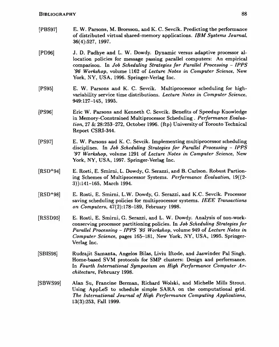
[PBS97]

[PD961

[PSgj]

[PS96]

[PS97]

[RS D+94]

[RS D+98]

[RSSDgq

[SB 1S98]

[SBWS99]

E- W. Parsons, M. Brorsson, and K. C . Sevcik. Predicting the performance of distributed virtual stiared-memory applications. IBM Systems Journal, 36(4):527, 1997.

J. D. Padhye and L. W. Dowdy. Dynarnic versus adaptive processor al- location policies for message passing parallel computerç: An empirical corn parison. In Job Schedu Ling Strategies for Parallel Processing - IPPS '96 Workshop, volume 1162 of Lecture Notes in Computer Science, New York, NY, USA. 1996. Springer-Verlag Inc.

E. W. Parsons and K. C. Sevcik. Multiprocessor scheduling for high- variability service time distributions. Lecture Notes in Computer Science' 949:127-145, 1995-

Eric W. Parsons and Kemeth C. Sevcik. Benefits of Speedup Knowledge in Memory-Cons t rained Md t iprocessor Scheduling . Perfornance Evalua- tion, 27 & 28953-272, October 1996. (ftp) University of Toronto Technicd Report CSRI-344.

E- W. Parsons and K. C. Sevcik. Implementing multiprocessor scheduling disciplines. In Job Schedvling Strategies for Parallel Processing - [PPS Y7 Workshop, volume 1291 of Lecture Notes in Computer Science, New York, NY, USA, 1997. Springer-Verlag Inc.

E. Rosti, E, Smirni, L. Dowdy, G . Serazzi, and B. Carlson. Robust Partion- ing Schemes of -Multiprocessor Systems, Performance Eualuation, 19((2- 3)):141-165, March 1994.

E. Rosti, E. Smirni, L. W. Dowdy, G. Serazzi, and K.C. Sevcik. Processor saving scheduling policies for multiprocessor systems. IEEE Transactions on Cornputers, 47(2): L78-189, February 1998.

E. Rosti, E- Srnirni, G. Serazzi, and L. W. Dowdy. Analysis of non-work- conserving processor partitioning policies. In Job Scheduling Strategies for Pamllel Processing - IPPS '95 Workshop, volume 949 of Lecture Notes in Computer Science, pages 163-181, New York, NY, USA, 1995. Springer- Verlag Inc.

Rudrajit Samanta, AngeIos Bilas, Liviu Iftode, and Jaswinder Pal Singh. Home-based SVM protocois for SMP clusters: Design and performance. In Fourth hternational Symposium on High Performance Computer .4r- chitecture, February 1998.

Alan Su, Francine Berman, Richard Wolski, and Michelle Mills Strout. Using AppLeS to schedule simple SARA on the computational grid. The International Journal of High Performunce Cornputing Applications, L3(3):253, Fa11 1999.

[SC8 11

[SC Z LSG]

[Sev89]

[Sev94]

[SGS96]

[S LTZ771

[S P WC981

[S RS+95]

[SSG95]

[SST93]

C. H. Sauer and K. M. Chaody. Computer Systems Performance Mod- elling. Prentice Hall, 1981.

Joseph Skovira, Waiman Chan, Honbo Zhou, and David Lifka. The EASY - LoadLeveler API Project. In Job Scheduling Strategies for Parallel Pro- cessing - IPPS'96 Workshop Proceedings, volume 1161 of Lecture Notes in Computer Science, pages 41-47, New York, NY, USA, 1996. Springer- Verlag Inc.

Kenneth C. Sevcik. Characterizations of Parailelism in Applications and t heir Use in Scheduling. In Proceedings of the 1989 A CM SIGMETRICS and PERFORMA.NCE Conference on lCfeasurement and Modeling of Com- pater Systerns, pages 171-180, May 1989.

K. C. Sevcik. Application scheduiing and processor allocation in multi- prograrnmed parallel processing systems. Performance Evaluation North Holland, 19, 2-3:107-140, 1994.

Jaspal Subhlok, Thomas Gross, and T h h i Suzuoka. Impact of job mix on optimizations for space sharing schedulers. In ACM, editor, Supercom- puling '96 Conference Proceedings: Nouember 17-22, Pittsburgh, PA, New York, NY 10036, USA and 1109 Spring Street, Suite 300, Silver Spring, &MD 20910, US.4, 1996. ACM Press and IEEE Computer Society Press.

K. C. Sevcik, A. 1. Levy. S. K. Tripathi, and J. L. Zahorjan. Improving approximations for aggregated queuing network subsystems. Computer Performance, pages 1-22, 19R.

Patrick G. Sobaltarro, Scott Pakin, William E. Weihi, and Andrew A Chien. Dynarnic Coscheduling on Workstation Clusters. In Proceedings O/

the IPPS '98 Workshop on Jo6 Sched uling Strategies for Parallel Process- ing, volume 1459 of Lecture Notes in Computer Science, pages 231-256, New York, NY, USA, March 1998. Springer-Verlag h c .

E. Smirni, E. Rosti? G. Serazzi, L. W. Dowdy, and K. C . Sevcik. Per- formance gains from leaving idle processors in mult iprocessor systerns. h Pmceedings of the 24th international Conference on Parallel Processing, pages 111203-210, Oconomowoc, WI, August 1995.

T. Suzuoka, J. Subhlok, and T. Gross. Evaluating job scheduling tech- niques for highly parallel computers. Computer Science CMU-CS-9*5-149, Department of Computer Science, Carnegie Melion University, 1995.

Sanjeev K. Setia, Mark S. Squillante, and Satish K. Tripathi. Processor scheduling on multiprogramrned, distributed memory parallel computers. In Blaine D. Gaither, editor, Proceedings of the ACM Sigmetrics Confer- ence on Measurement and Modeling of Computer Systems, volume 21-1

of Performance Evaluation Reoiew, pages 158-170, New York, NY, USA, May 1993. ACM Press.

S. Setia and S. Tripathi. A Compaiative Analysis of Static Processor Part itioning Policies for Parallel Cornputers. In International Workshop on ModeLing and Simulation of Computer and Telecommunicution Systems (MASCOTS), pages 383386, January 1993.

Patrick G . Sobalvarro and William E. Weihl. Demand-based Coscheduling of Paralle1 Jobs on Multiprogrammed Multiprocessors. In Proceedings of the IPPS '95 Workshop on Job Scheduiing Strategies for Parallel Process- ing, pages 63-75, April t995.

Andy Tucker and Anoop Gupta. Process Control and Scheduling issues for Multiprogrammed Shared-Memory Multiprocessors. Operating Systems Reuiew, 23(5):159-66, 1989.

Zvonko G . Vranesic, Michael Stumm, David M. Lewis, and Ron White- Hector: A hierarchically structured shaxed-memory mult iprocessor. Com- puter, 24(1):72-79, January 1991.

Daniel W. Watson, John K. Antonio, Howard Jay Siegel, Rohit Gupta, and Mikhail J. Atallah. Static matching of ordered program segments to dedicated machines in a heterogeneous computing environment. In Proceedings of 5th Heterogeneous Cornputing Workshop (HC W '96), pages 24-37, April 1996. sponsor: IEEE Computer Society.

K. Windisch, V. Lo, R. Moore, D. Feitelson, and B. Nitzberg. A com- parison of workload traces from two production paraIIel machines. In 6th Symp. Frontiers Massively Parallel Comput., pages 3 19-336, Oct 1996.

K. Windisch, V. Lo, R. Moore, D. Feitelson, and B. Nitzberg. A compar- ison of workload traces from two production parallel machines. Technical Report CIS-TR-96-06, Depart ment of Computer and Informat ion Science, University of Oregon, April 1996.

Michael Wan, Reagan Moore, George Kremenek? and Ken Steube. A batch scheduier for the Intel Paragon with a non-contiguous node allocation al- gorithrn. In Dror G. Feitelson and Lamy Rudolph, editors, Job Schedul- ing Strategies for Purallel Processing, pages 48-64. Springer-Verlag, 1996. Lect. Notes Comput. Sci. vol. 1162.

Paul R. Woodward. Perspective on supercomputing: Three decades of change. Computer, 29(10):99-111, October 1996.

Steven Cameron Woo, Moriyoshi Ohara, Evan Torrie, Jaswinder Pal Shingh, and Anoop Gupta. The SPLASH-2 programs: C haracterizat ion and methodological considerations. ln Proceedings of the 22nd Annuai

International Symposium on Computer Architecture, pages 24-36, Santa Margherita Ligure, Itaiy, June 22-24, 1995. ACM SIGARCH and [EEE Computer Society TCCA.

C.S. Wu. Processor Scheduiing in rnul tiprogrammed shared memory NUMA multiprocessors. Master's thesis, University of Toronto, 1993. Technical Report CS RI-34 1 , Depart ment of Computer Science.

Jon B. Weissman and Xin Zhao. Run-time Support for Scheduiing Parallel Applications in Heterogeneous NO Ws. Ln Sizth international Symposium on High Performance Distnbuted Computing (HPDC-6), August 1997.

Songnian Zhou and Timot hy Brecht. Processor pool-based scheduling for largescale NUMA multiprocessors. In Proceedings of the 1992 ACM SIGMETRlCS Conj'rence on Measurernent and Modeling of Computer Systems, pages 133-142, May 91.

J Zahorjan and C . McCann. Processor scheduling in shared memory mul- tiprocessors. Performance Evaluation Reuiew, 18(1):214-225, May 1990. Proc. 1990 ACM Sigrnetrics Conf. on Meas. and Mod. of Comp. Syst.

Appendix A

Network Configurations

(a) Network 1 1 (b) Network 12 (c) Network 13

Figure A. 1: Speed-hetemgeneous networks

92

(a) Network 14 (b) Network 15 (c) Network 16

Figure A.2: Size-hete rogeneous net works

(a) Network

Figure

Li (b) Network 18 (c) Network

A.3: Size-heterogeneous networks with skewness x -2.0

(a) Network 20 (b) Network 21

Figure A.4: Size-heterogeneous networks

(c) Network

with skewness -1.5

(a) Xetwork 23 (b) Network 24 (c ) Network

Figure A.5: Size-heterogeneous netzuorks uith skewness sz -0.9

- m u r -

(a) Xetwork 26

Figure A.6:

(b) Network 27 (c) Network 28

Speed-heterogeneous networks with shumess z - 1.0

(a) Network 29 (b) Network 30 (c) Network

Figure Ai: Speed-heterogeneous networks with skewness % -1.9

(a) Xetwork 32 (b) Network 33 (c) Network 34

Figure A.8: Speed-heterogeneous networks with skewness x -2.5

Appendix B

Workload Mode1 Code

The code used to generate the workload:

/* * generate workload based on s t a t i s t i c a l mode1 *

f o r each job, decide the s i z e (number of nodes used) , t h e runtime, * and the repet i t ion count (hou many times it w i l l b e run). * t h e output is one l i n e per job, with these 3 values. * * t h e s ize is based on a cornplex discret9 distribution. * the nintime is hyperexponential, based on the size- * the repet i t ion is generalized Zipf Charmonid * * the arrivai process is not modeled, and should be pa r t of the * simulation t h a t uses this workload as input. */

# inchde <math. Il, #indude <stdio . h> # include (assert. h> #indude " u t i l s .hl' ainclude "randlib/randl ib .hl' t include "f eitelson/ulf eitelson96 .hla

#if def ,,cplusplus extern "C" { ltendif

#def ine W I N T Oxïf f f f f f f

#define U N 300000 /* jobs generated */

#define TIME-LI?! 64800 /* longest job alloved - 18 hr */ #define FACTOR 9 /* about HAX-TIHE / log(TI!fE,LII¶) */

#define MX-SIZE 128 /* machine s i z e */ tdefine IZAX-REP 1000 /* far upper bound on number of repe t i t ions */ #define MAX-TIHE 100 /* f o r d i s t r ibu t ion of runtimes */

i n t g%narSize ; /* user-set max s i z e ( <= IUX-SIZE) */ f loa t size-dist [ HM-SIZE 1 ; /* cummulative d i s t r ibu t ion of s i zes */ i n t time,dist[: )(AX,TIHE 3 ; /* c d a t i v e d i s t r ibu t ion of runtimes */ f l o a t rep-distc M J E P 1 ; /* cumulat ive d i s t r ibu t ion of repe t i t ions */

/* f lag t o indicate t h a t i n t i a l i za t ion has been done */ s t a t i c Bool-T b h i t i a l i z e d = FALSE;

#i f def MAICE-PLOTS char f ilename [ 20 3 ;

i n t size-hist [ MX-SIZE 1 ; f l oa t tirne-hist [ MAX-SIZE 1 ; i n t rep-hist [ W J E P 1 ;

GenJob-T jobs C LEN ] ;

/* I n i t JobGeneration * s e t s up the cumulative d is t r ibu t ions needed t o generate the jobs. */

void InitJobCeneration(int nHaxJobSize) €

i n t i, j; f loa t sum;

/* no point i n doing t h i s twice */ if ( b h i t i a l i z e d )

return;

/* f i r s t c rea te a semi-hawonic d is t r ibu t ion */ size-dist [O] = 1; f o r ( i = i ; i<ghnaxSize ; i++) {

size-dist Ci3 = (f l o a t ) 1/ (f l oa t ) sqrt < (double) il ; 3

/* add weight at povers of 2 */ for (i=l ; i<=gLnaxSize ; i<<=l) < size-dist Ci-11 += 35 + 1.5*i;

3

/* add weight at squaes */ for (i=2, j=i*i ; j<=gbnaxSize ; i++, j=i*i) < size-distcj-11 += 5;

> /* add weight at multiples of 10 */ for (i=lO ; i<+ginaxSize ; i+=lO) < size-dist [j-11 += 5;

3

/* reduce weight at 1,2,4 */ size-dist [O] /= 4; size,dist[l] /= 4; size-dist C3] /= 3; /* add weight at 3,s-7 */ size-dist [2] += 5; size-dist f41 += 7; size-dist [5] += 5; size-dist [6] += 3;

/* impose a harmonic envelope to emphasize small sizes */ /* for non-special sizes, this becomes harmonic of order 1.5 */ for (i=i ; i<ghnaxSize ; i++) (

/* size-dist [il /= (f 1oat)sqrt ((double) i) ; semi-harmonic - no good */ size-dist Ci] /= (f loat) i; /* size-dist Ci] /= (f loat)exp(i) ; erponentiaï decreasing - no good*/

/* normalize */ sum = O; for (i=O ; i<gknaxSize ; i++) < sum += size-dist [il ;

3 for (i=O ; i<gknéuSize ; i++) < size-dist Ci] /= sum;

3

/* accumulate */ for (i=l ; i<gHarSize ; i++) < size-dist Ci] += size-dist Ci-l] ;

1

/* create harmonic repet i t ion distr ibution of order 2.5 */ sum = O; for (i=O ; i<)(AX,REP ; i++) {

rep-dist C i ] = ((f loa t ) l)/(float)porr(Cdouble) (i+i) , (double) 2 - 5 ) ; sum += rep-dist C i l ;

> /* normalize */ f o r ( i = O ; i<HAX,REP ; i++) C

rep-dist fi] /= sum; > /* accumulate */ fo r ( i = l ; i<W,REP ; i++) {

rep-dist C i l += rep-dist C i - 1 J ; >

/* CenerateJob * - get the next job i n t h i s sequence- * - the random number generator used is in "randlib". * - the specif ic random number Stream used depends on the seed being * se t by s e t a l 1 0 * - t h i s code is l i f t e d from the original Feitelson code in GenRunFile * and code was added t o generate a hyperexponential inter-arriva1 t h e */

Gen Job-T Generat eNert Job (1 €

GenJob-T genjob; in t i, s ize , rep; f loat p, runtime, m;

/* check tha t in i t i a l i za t ion has been done */ if ( ! bInitialized) € assert (FALSE) ; return genjob;

/* choose s i ze from distr ibution +/ p = ((float)ignlgiO)/)(AXINT; i = O;

LOO

uhile (p > size-dist [il i++ ;

size = i;

/* assign runtime */

* in the improved model, runtimes are from a three-stage * hyperexponential distribution, and the probability of * choosing each branch depends on the size. in addition, * there is an upper bound on the runtime. */

vhile Cl) C p = ((float)ignlgi())/WIHT; if (p < (0.90 - 0.65*( sqrt (((double)size)/gkn~Size) ))) m = 50;

else if (p < (0.97 - 0.37*( sqrt(((double)size)/ghna~~Size) ))) mi = 900;

else m = 20000;

if ((size == 2) 1 1 (size == 4) I l (size = 8) 1 1 (size == 16) 1 1 (size == 32) 1 1 (size == 64) I 1 (size == 128) )

rn *= 2; runtime = -m rn (f1oat)logC ((double) ignlgio) / WINT ) ;

if (nintime < TIHE-LIH) break;

1

/* assign repetition */ p = ( (f loat) ignlgi O ) /KAXINT; i = O; while (p > rep-dist Ci]) i++ ;

rep = i;

/* assign the job fields */ genjob.rtime = ruatime; genjob.rep = rep + 1; genjob.size = size + 1;

return genjob; 3

Appendix C

Arriva1 Process Code

The code used to generate the arriva1 process:

// Work1oad::SetArrivalP~ams // set the mean and the coefficient of variation for the // hypererponential arrivai process and calculate some constants. void Workload::SetArrivalParams(double Mean, double dCV) C clArrivalMean = dnean;

// CV-2 is actually required by the formulae dArrivaïCVsq = dCV * dm;

// these parameters are from the paper "Improving Approximations // of Subsystems" by Sevcik et al., 1977, Computer Performance // North-Holland, ed. KI H. Chandy and U. Reiser. a = 0.5 * (1 - sqrt( (MrrivalCVsq - 1.0) / (dArrivalCVsq + 1.0) )) ;

assert(a > 0-0 && a <= 1.0); r = dnean / (2.0 *a); s = ciMean / (2 .0 * (1.0-a));

// set flag that this has been done - just for a sanity check b ArrivalInit ialized = TRUE ;

>

// Work1oad::GenerateA~rivalTime // Inter-arriva1 times are hyper-exponent iaily distributed // vith a vaqing mean and Cv set at program startup. // See the comments in Workload::SetArrivalParams for the // paper ref erence. Tirne-T Workload : : CenerateArrivalTime €

// generate unif orm variate. double dU = CenerateUnif orinTime (0 - O, 1 -0) ;

// f l i p a random coin double dCoin = Generateunif ormTime (0.0, 1.0) ; T h e - T the;

// 2-stage hypererponential - choose one branch with // probability a and the other with prob. (1-a) if (dCoin <= a) < time = C-r) log(dU1;

3 else < t h e = (-s) 4 log(dU1;

3

return time; 1