Embed Size (px)
Citation preview

arX
iv:h
ep-p
h/03
0506
9 v1
7
May
200
3BARI-TH 461/03
CERN-TH/2003-082
Inhomogeneous Superconductivity in Condensed Matter and QCD
Roberto Casalbuoni∗†
TH-Division, CERN, CH-1211 Geneva 23, Switzerland
Giuseppe Nardulli‡
Department of Physics, University of Bari, I-70124 Bari, Italy and
INFN, Bari, Italy
(Dated: June 5, 2005)
Inhomogeneous superconductivity arises when the species participating in the pairing phenomenonhave different Fermi surfaces with a large enough separation. In these conditions it could be morefavorable for each of the pairing fermions to stay close to its Fermi surface and, differently fromthe usual BCS state, for the Cooper pair to have a non zero total momentum. For this reason inthis state the gap varies in space, the ground state is inhomogeneous and a crystalline structuremight be formed. This situation was considered for the first time by Fulde, Ferrell, Larkin andOvchinnikov, and the corresponding state is called LOFF. The spontaneous breaking of the spacesymmetries in the vacuum state is a characteristic feature of this phase and is associated to thepresence of long wave-length excitations of zero mass. The situation described here is of interestboth in solid state and in elementary particle physics, in particular in Quantum Chromo-Dynamicsat high density and small temperature. In this review we present the theoretical approach to theLOFF state and its phenomenological applications using the language of the effective field theories.
PACS numbers: 12.38.-t, 26.60.+c, 74.20.-z, 74.20.Fg, 97.60.Gb
Contents
I. Introduction 2
II. The general setting 4A. Nambu-Gor’kov equations 4B. Homogeneous superconductors 7
1. Phase diagram of homogeneous superconductors 11C. Gap equation for anisotropic superconductor: One plane wave (FF state) 15
1. Second Order phase transition point 18
III. Ginzburg-Landau approximation 19A. Gap equation in the Ginzburg-Landau approach 19B. Grand potential 21C. Crystalline structures 22
1. One plane wave 232. Generic crystals 233. Two plane waves 234. Other structures 26
D. LOFF around the tricritical point 271. The LO subspace 28
IV. Superconductivity in Quantum Chromodynamics 33A. High Density Effective Theory 35B. CFL phase 37C. 2SC phase 38D. LOFF phase in QCD 39E. One-gluon exchange approximation 44F. Mass effects 46
∗ On leave from the Department of Physics of the University of Florence, 50019, Florence, Italy†Electronic address: [email protected]‡Electronic address: [email protected]

2
V. Phonon and gluon effective lagrangians 47A. Effective lagrangian for the LOFF phase 47B. One plane wave structure 48C. Parameters of the phonon effective lagrangian: one plane wave 51D. Cubic structure 56E. Parameters of the phonon effective lagrangian: cubic crystal 58F. Gluon dynamics in the LOFF phase 60
1. One plane wave structure 602. Cubic structure 63
VI. Inhomogeneous superconductivity in condensed matter, nuclear physics and astrophysics 63A. Type I superconductors 64B. ”Clean” and strongly type II superconductors 65C. Heavy fermion superconductors 66D. Two-dimensional, quasi-two-dimensional and organic superconductors 67E. Future developments 68F. LOFF phase in nuclear physics 69G. Why color LOFF superconductivity could exist in pulsars 69H. Astrophysical implications of the QCD LOFF phase 73
VII. Conclusions 77
Acknowledgments 77
A. Calculation of J and K 78
B. Expansion of Π around the tricritical point 79
References 79
I. INTRODUCTION
Superconductivity is one of the most fascinating chapters of modern physics. It has been a continuous source ofinspiration for different realms of physics and has shown a tremendous capacity of cross-fertilization, to say nothingof its numerous technological applications. This review is devoted to a less known chapter of its history, i.e. inho-mogeneous superconductivity, which arises when the main property of the superconductor is not uniform in space.Before giving a more accurate definition of this phenomenon let us however briefly sketch the historical path leadingto it. Two were the main steps in the discovery of superconductivity. The former was due to Kamerlingh Onnes(Kamerlingh Onnes, 1911) who discovered that the electrical resistance of various metals, e. g. mercury, lead, tin andmany others, disappeared when the temperature was lowered below some critical value Tc. The actual values of Tcvaried with the metal, but they were all of the order of a few K, or at most of the order of tenths of a K. Subsequentlyperfect diamagnetism in superconductors was discovered (Meissner and Ochsenfeld, 1933). This property not onlyimplies that magnetic fields are excluded from superconductors, but also that any field originally present in the metalis expelled from it when lowering the temperature below its critical value. These two features were captured in theequations proposed by the brothers F. and H. London (London and London, 1935) who first realized the quantumcharacter of the phenomenon. The decade starting in 1950 was the stage of two major theoretical breakthroughs.First, Ginzburg and Landau (GL) created a theory describing the transition between the superconducting and thenormal phases (Ginzburg and Landau, 1950). It can be noted that, when it appeared, the GL theory looked ratherphenomenological and was not really appreciated in the western literature. Seven years later Bardeen, Cooper andSchrieffer (BCS) created the microscopic theory that bears their name (Bardeen et al., 1957). Their theory was basedon the fundamental theorem (Cooper, 1956), which states that, for a system of many electrons at small T , any weakattraction, no matter how small it is, can bind two electrons together, forming the so called Cooper pair. Subse-quently in (Gor’kov, 1959) it was realized that the GL theory was equivalent to the BCS theory around the criticalpoint, and this result vindicated the GL theory as a masterpiece in physics. Furthermore Gor’kov proved that thefundamental quantities of the two theories, i.e. the BCS parameter gap ∆ and the GL wavefunction ψ, were relatedby a proportionality constant and ψ can be thought of as the Cooper pair wavefunction in the center-of-mass frame.In a sense, the GL theory was the prototype of the modern effective theories; in spite of its limitation to the phasetransition it has a larger field of application, as shown for example by its use in the inhomogeneous cases, when thegap is not uniform in space. Another remarkable advance in these years was the Abrikosov’s theory of the type IIsuperconductors (Abrikosov, 1957), a class of superconductors allowing a penetration of the magnetic field, withincertain critical values.
The inspiring power of superconductivity became soon evident in the field of elementary particle physics. Twopioneering papers (Nambu and Jona-Lasinio, 1961a,b) introduced the idea of generating elementary particle masses

3
through the mechanism of dynamical symmetry breaking suggested by superconductivity. This idea was so fruitfulthat it eventually was a crucial ingredient of the Standard Model (SM) of the elementary particles, where the massesare generated by the formation of the Higgs condensate much in the same way as superconductivity originates fromthe presence of a gap. Furthermore, the Meissner effect, which is characterized by a penetration length, is the origin,in the elementary particle physics language, of the masses of the gauge vector bosons. These masses are nothing butthe inverse of the penetration length.
With the advent of QCD it was early realized that at high density, due to the asymptotic freedom property(Gross and Wilczek, 1973; Politzer, 1973) and to the existence of an attractive channel in the color interaction, diquarkcondensates might be formed (Bailin and Love, 1984; Barrois, 1977; Collins and Perry, 1975; Frautschi, 1978). Sincethese condensates break the color gauge symmetry, the subject took the name of color superconductivity. However,only in the last few years this has become a very active field of research; these developments are reviewed in (Alford,2001; Hong, 2001; Hsu, 2000; Nardulli, 2002a; Rajagopal and Wilczek, 2001). It should also be noted that colorsuperconductivity might have implications in astrophysics because for some compact stars, e.g. pulsars, the baryondensities necessary for color superconductivity can probably be reached.
Superconductivity in metals was the stage of another breakthrough in the 1980s with the discovery of high Tcsuperconductors. As we anticipated, however, the main subject of this review is a different and separate developmentof superconductivity, which took place in 1964. It originates in high-field superconductors where a strong magneticfield, coupled to the spins of the conduction electrons, gives rise to a separation of the Fermi surfaces corresponding toelectrons with opposite spins. If the separation is too high the pairing is destroyed and there is a transition (first-orderat small temperature) from the superconducting state to the normal one. In two separate and contemporary papers,(Larkin and Ovchinnikov, 1964) and (Fulde and Ferrell, 1964), it was shown that a new state could be formed, closeto the transition line. This state that hereafter will be called LOFF1 has the feature of exhibiting an order parameter,or a gap, which is not a constant, but has a space variation whose typical wavelength is of the order of the inverseof the difference in the Fermi energies of the pairing electrons. The space modulation of the gap arises because theelectron pair has non zero total momentum and it is a rather peculiar phenomenon that leads to the possibility of a nonuniform or anisotropic ground state, breaking translational and rotational symmetries. It has been also conjecturedthat the typical inhomogeneous ground state might have a periodic or, in other words, a crystalline structure. Forthis reason other names of this phenomenon are inhomogeneous or anisotropic or crystalline superconductivity.
Inhomogeneous superconductivity in metals has been the object of intense experimental investigations especiallyin the last decade; for reasons to be discussed below the experimental research has aimed to rather unconventionalsuperconductors, such as heavy fermion superconductors, quasi-two dimensional layered organic superconductorsor high Tc superconductors. While different from the original LOFF proposal, these investigations still aim to asuperconducting state characterized by non zero total momentum of the Cooper pair and space modulation of itswavefunction. At the moment they represent the main possibility to discover the LOFF state in condensed matterphysics.
Quite recently it has been also realized that at moderate density the mass difference between the strange and theup and down quarks at the weak equilibrium and/or color and electric neutrality lead to a difference in the Fermimomenta, which renders in principle the LOFF state possible in color superconductivity (Alford et al., 2001b). Thesame authors have pointed out that this phenomenon might have some relevance in explaining the sudden variationsof the rotation period of the pulsars (glitches).
The main aim of this review is to present ideas and methods of the two main roads to inhomogeneous supercon-ductivity, i.e. the condensed matter and the QCD ways. Our approach will be mainly theoretical and the discussionof phenomenological consequences will be limited, first because we lack the necessary skills and second because thetheory of the LOFF superconductivity is up to now much more advanced than experiment and its main phenomeno-logical implications belong to the future. For this reason we will give large room to the theoretical foundations ofinhomogeneous superconductivity and will present only a summary of experimental researches. Our scope is to showthe similarities of different physical situations and to present a formalism as unified as possible. This not only toprove once again the cross-fertilization power of superconductivity, but also to expose experts in the two fields toresults that may be easily transferrable from one sector to the other. Moreover, by presenting the LOFF phenomenonin a unified formalism, this review can contribute, we hope, to establish a common language. To this end we discussthe LOFF state both in solid state and in QCD physics starting with Nambu Gor’kov (NG) equations. For the solidstate part they will be derived by the effective theory of the relevant degrees of freedom at the Fermi surface and inthe QCD sector by the so called High Density Effective Theory (HDET) that, as we shall see, leads to equations ofmotion which coincide with the NG equations. In this way one is able to get in touch with a dictionary allowing to
1 In the literature the LOFF state is also known as the FFLO state.

4
switch easily from one field to the other.The plan of this review is as follows. In Section II we start describing the general formalism, based on NG
equations (Gor’kov, 1959; Nambu, 1960). As shown by (Polchinski, 1993) using the Renormalization Group approach,the excitations at the Fermi surface can be described by an effective field theory. Its equations of motion are exactlythe NG equations of ordinary (homogeneous) superconductivity. We will then apply this formalism to fermionswith different Fermi surfaces. The difference can be due to a magnetic field producing an energy splitting betweenspin up and spin down electrons, or, as in QCD, to a difference in the chemical potential originating from weakequilibrium, or color and electric neutrality, or mass difference between the pairing fermions. We will discuss thecircumstances leading, in these cases, to inhomogeneous superconductivity. The Ginzburg Landau expansion can beused, as already mentioned, for the description of the inhomogeneous phase. It will be discussed in Section III, bothat zero temperature and close to the tricritical point. The T = 0 case is more interesting for QCD applications whilethe finite temperature case might be relevant in condensed matter. In Section IV we will switch to QCD. We will firstgive a brief introduction to color superconductivity and then a description of the effective lagrangian for quarks atzero temperature near to the Fermi surface. We will also discuss more specifically the LOFF case for QCD with twomassless flavors. Since in the LOFF phase both translational and rotational symmetries are spontaneously broken, theGoldstone theorem requires the presence in the physical spectrum of long wave-length, gapless, excitations (phonons).In Section V we discuss the phonon effective lagrangians for two crystalline structures, i.e. the single plane waveand the cubic structure. We will limit our presentation to the QCD case, though the presence of these excitations isobviously general. We will also discuss the gluon propagation inside these two crystalline media. In Section VI we willdiscuss the possible phenomenological applications of the LOFF phase. This discussion will go from strongly type IIsuperconductor to two-dimensional structures for condensed matter. For hadronic matter we will discuss applicationsboth in nuclear physics and in QCD, with particular emphasis on the physics of glitches in pulsars.
Let us conclude this introduction by apologizing to the many authors whose work is not reviewed here in depth.Space limits forced us to sacrifice a more detailed exposition; the extensive bibliography at the end should help toexcuse, we hope, this defect.
II. THE GENERAL SETTING
In this Section we give a pedagogical introduction to inhomogeneous superconductivity. We begin by reviewinghomogeneous superconductivity by a field theory with effective Nambu-Gor’kov spin 1/2 fields describing quasi-particles. The effective field theory considers only the relevant degrees of freedom in the limit of small temperaturesand high chemical potential; they are the modes in a shell around the Fermi surface. The dominant coupling in thislimit is the four fermion interaction as first introduced in the BCS model. The dominance of this coupling can be alsoproved in a modern language by using the renormalization group approach (Benfatto and Gallavotti, 1990; Polchinski,1993; Shankar, 1994), which shows that the BCS coupling is marginal and therefore, in absence of relevant couplings,it can dominate over other irrelevant couplings and produce the phenomenon of superconductivity.
After having derived the Nambu-Gor’kov equations and the gap equation in Subsection II.A, we discuss the caseof homogeneous superconductor in Section II.B and analyze its phase diagram in Section II.B.1. We assume fromthe very beginning that the two species participating in the Cooper pairing have different chemical potentials, as thisis the necessary situation for the LOFF state. In Section II.C we discuss the case of anisotropic superconductivity.In Section II.C.1 we will show that for appropriate values of the difference in chemical potentials an anisotropicmodulated gap ∆(r) ∝ exp(iq · r) leads to a state that is energetically favored in comparison to both the BCS andthe normal non superconducting states. This was the state first discussed in (Fulde and Ferrell, 1964).
A. Nambu-Gor’kov equations
To start with we consider, at T = 0, a fermion liquid formed by two species, that we call u and d, havingdifferent Fermi energies. In the electron superconductivity, as in the original LOFF papers (Fulde and Ferrell, 1964;Larkin and Ovchinnikov, 1964), the species are the electron spin up and down states, but our formalism is generaland will be applied later to the case where the fermion forming the Cooper pair are two quarks with different flavors.In superconducting materials the difference of chemical potentials can be produced by the presence of paramagneticimpurities. All these cases give rise to an effective exchange interaction that can described by adding the followingterm to the hamiltonian
Hexch = −δµψ†σ3ψ . (2.1)

5
In the case of electron superconductivity δµ is proportional to the magnetic field and the effect of (2.1) is to changethe chemical potentials of the two species:
µu = µ+ δµ, µd = µ− δµ . (2.2)
Adopting a BCS interaction, the action can be written as follows
A = A0 +ABCS , (2.3)
A0 =
∫
dtdp
(2π)3ψ†(p) (i∂t − E(p) + µ+ δµσ3)ψ(p) , (2.4)
ABCS =g
2
∫
dt
4∏
k=1
dpk(2π)3
(
ψ†(p1)ψ(p4)) (
ψ†(p2)ψ(p3))
× (2π)3 δ(p1 + p2 − p3 − p4) . (2.5)
Here and below, unless explicitly stated, ψ(p) denotes the 3D Fourier transform of the Pauli spinor ψ(r, t), i.e.ψ(p) ≡ ψσ(p, t). For non relativistic particles the functional dependence of the energy would be E(p) = p 2/2m, butwe prefer to leave it in the more general form (2.4).
The BCS interaction (2.5) can be written as follows
ABCS = Acond + Aint , (2.6)
with
Acond = −g4
∫
dt
4∏
k=1
dpk(2π)3
[
Ξ(p3, p4)ψ†(p1)Cψ
†(p2)
− Ξ∗(p1, p2)ψ(p3)Cψ(p4)]
(2π)3 δ(p1 + p2 − p3 − p4) ,
Aint = −g4
∫
dt4∏
k=1
dpk(2π)3
[
ψ†(p1)Cψ†(p2) + Ξ∗(p1, p2)
]
×
×[
ψ(p3)Cψ(p4) − Ξ(p3, p4)]
(2π)3 δ(p1 + p2 − p3 − p4) , (2.7)
where C = iσ2 and
Ξ(p, p′) =< ψ(p)Cψ(p′) > . (2.8)
In the mean field approximation the interaction term can be neglected while the gap term Acond is added to A0. Notethat the spin 0 condensate Ξ(p, p′) is simply related to the condensate wave function
Ξ(r) =< ψ(r, t)Cψ(r, t) > (2.9)
by the formula
Ξ(r) =
∫
dp
(2π)3dp′
(2π)3e−i(p+p′)·r Ξ(p, p′) . (2.10)
In general the condensate wavefunction can depend on r; only for homogeneous materials it does not depend on thespace coordinates; therefore in this case Ξ(p, p′) is proportional to δ(p + p′).
In order to write down the Nambu-Gor’kov (NG) equations we define the NG spinor
χ(p) =1√2
(
ψ(p)ψc(−p)
)
, (2.11)
where we have introduced the charge-conjugate field
ψc = Cψ† . (2.12)
We also define
∆(p,−p′) =g
2
∫
dp′′
(2π)6Ξ(p′′,p + p′ − p′′) . (2.13)

6
The free action can be therefore written as follows:
A =
∫
dtdp
(2π)3dp′
(2π)3χ†(p)S−1(p, p′)χ(p′), (2.14)
with
S−1(p, p′) = (2π)3(
(i∂t − ξp + δµσ3)δ(p − p′) −∆(p,p′)−∆∗(p,p′) (i∂t + ξp + δµσ3)δ(p − p′)
)
. (2.15)
Here
ξp = E(p) − µ ≈ vF · (p − pF ) , (2.16)
where
vF =∂E(p)
∂p
∣
∣
∣
p=pF
(2.17)
is the Fermi velocity. We have used the fact that we are considering only degrees of freedom near the Fermi surface,i.e.
pF − δ < p < pF + δ , (2.18)
where δ is the ultraviolet cutoff, of the order of the Debye frequency. In particular in the non relativistic case
ξp =p 2
2m− p 2
F
2m, vF =
pF
m. (2.19)
S−1 in (2.15) is the 3D Fourier transform of the inverse propagator. We can make explicit the energy dependence byFourier transforming the time variable as well. In this way we get for the inverse propagator written as an operator:
S−1 =
(
(G+0 )−1 −∆
−∆∗ −(G−0 )−1
)
, (2.20)
and
[G+0 ]−1 = E − ξP + δµσ3 + i ǫ signE ,
[G−0 ]−1 = −E − ξP − δµσ3 − i ǫ signE , (2.21)
with ǫ = 0+ and P the momentum operator. The iǫ prescription is nothing but the usual one for the Feynmanpropagator, that is forward propagation in time for the energy positive solutions and backward propagation for thenegative energy solutions. As for the NG propagator S, one gets
S =
(
G −F
−F G
)
. (2.22)
S has both spin, σ, σ′, and a, b NG indices, i.e. Sabσσ′
2. The NG equations in compact form are
S−1S = 1 , (2.23)
or, explicitly,
[G+0 ]−1G + ∆F = 1 ,
−[G−0 ]−1F + ∆∗G = 0 . (2.24)
2 We note that the presence of the factor 1/√
2 in (2.11) implies an extra factor of 2 in the propagator: S(x, x′) = 2 < T
χ(x)χ†(x′)
>,
as it can be seen considering e.g. the matrix element S11: < T
ψ(x)ψ†(x′)
>=(
i∂t − ξ−i~∇
− δµσ3
)−1δ(x − x′), with (x ≡ (t, r)).

7
Note that we will use
< r |∆|r ′ >=g
2Ξ(r) δ(r − r ′) = ∆(r) δ(r − r ′) , (2.25)
or
< p |∆|p ′ >= ∆(p,p ′) (2.26)
depending on our choice of the coordinate or momenta representation. The formal solution of the system (2.24) is
F = G−0 ∆∗G ,
G = G+0 − G+
0 ∆F , (2.27)
so that F satisfies the equation
F = G−0 ∆∗
(
G+0 − G+
0 ∆F)
(2.28)
and is therefore given by
F =1
∆∗[G+0 ]−1[∆∗]−1[G−
0 ]−1 + ∆∗∆∆∗ . (2.29)
In the configuration space the NG Eqs. (2.24) are as follows
(E − E(−i∇) + µ+ δµσ3)G(r, r ′, E) + ∆(r)F (r, r ′, E) = δ(r − r ′) ,(−E − E(−i∇) + µ− δµσ3)F (r, r ′, E) − ∆∗(r)G(r, r ′, E) = 0 . (2.30)
The gap equation at T = 0 is the following consistency condition
∆∗(r) = −i g2
∫
dE
2πTrF (r, r, E) , (2.31)
where F is given by (2.29). To derive the gap equation we observe that
∆∗(r) =g
2Ξ∗(r) =
g
2
∫
dp1
(2π)3dp2
(2π)3ei(p1+p2)·r Ξ∗(p1, p2)
= − g
2
∫
dE
2π
dp1
(2π)3dp2
(2π)3ei(p1+p2)·r < ψ†(p1, E)ψc(p2, E) >
= + ig
2
∑
σ
∫
dE
2π
dp1
(2π)3dp2
(2π)3ei(p1−p2)·rS21
σσ(p2,p1)
= + ig
2
∑
σ
∫
dE
2πS21σσ(r, r) , (2.32)
which gives (2.31).At finite temperature, introducing the Matsubara frequencies ωn = (2n+ 1)πT , the gap equation reads
∆∗(r) =g
2T
+∞∑
n=−∞
TrF (r, r, E)∣
∣
∣
E=iωn
. (2.33)
B. Homogeneous superconductors
It is useful to specialize these relations to the case of homogeneous materials. In this case we have
Ξ(r) = const. ≡ 2∆
g, (2.34)
Ξ(p1, p2) =2∆
g
π2
p2F δ
(2π)3δ(p1 + p2) . (2.35)

8
Therefore one gets
∆(p1,p2) = ∆ δ(p1 − p2) (2.36)
and from (2.25) and (2.34)
∆(r) = ∆∗(r) = ∆ . (2.37)
Therefore F (r, r, E) is independent of r and, from Eq. (2.29), one gets
TrF (r, r, E) = −2 ∆
∫
d3p
(2π)31
(E − δµ)2 − ξ2p − ∆2(2.38)
which gives the gap equation at T = 0:
∆ = i g∆
∫
dE
2π
d3p
(2π)31
(E − δµ)2 − ξ2p − ∆2, (2.39)
and at T 6= 0:
∆ = gT
+∞∑
n=−∞
∫
d3p
(2π)3∆
(ωn + iδµ)2 + ǫ(p,∆)2, (2.40)
with
ǫ(p,∆) =√
∆2 + ξ2p . (2.41)
We now use the identity
1
2[1 − nu − nd] = ǫ(p,∆)T
+∞∑
n=−∞
1
(ωn + iδµ)2 + ǫ2(p,∆), (2.42)
where
nu(p) =1
e(ǫ+δµ)/T + 1, nd(p =
1
e(ǫ−δµ)/T + 1. (2.43)
The gap equation can be therefore written as
∆ =g∆
2
∫
d3p
(2π)31
ǫ(p,∆)(1 − nu(p) − nd(p)) . (2.44)
In the Landau theory of the Fermi liquid nu, nd are interpreted as the equilibrium distributions for the quasiparticlesof type u, d. It can be noted that the last two terms act as blocking factors, reducing the phase space, and producingeventually ∆ → 0 when T reaches a critical value Tc (see below).
Before considering the solutions of the gap equations in the general case let us first consider the case δµ = 0; thecorresponding gap is denoted ∆0. At T = 0 there is no reduction of the phase space and the gap equation becomes
1 =g
2
∫
d3p
(2π)31
ǫ(p,∆0), (2.45)
whose solution is (we have assumed d3p = p2FdpdΩ)
∆0 =δ
sinh 2gρ
. (2.46)
Here
ρ =p2F
π2vF(2.47)

9
is the density of states and we have used ξp ≈ vF (p− pF ), see Eqs. (2.16)-(2.19). In the weak coupling limit (2.46)gives
∆0 = 2δ e−2/ρg . (2.48)
Let us now consider the case δµ 6= 0. By (2.44) the gap equation is written as
− 1 +g
2
∫
d3p
(2π)31
ǫ=g
2
∫
d3p
(2π)3nu + nd
ǫ. (2.49)
Using the gap equation for the BCS superconductor, the l.h.s can be written, in the weak coupling limit, as
l.h.s =gρ
2ln
∆0
∆, (2.50)
where we got rid of the cutoff δ by using ∆0, the gap at δµ = 0 and T = 0. Let us now evaluate the r.h.s. at T = 0.We get
r.h.s.∣
∣
∣
T=0=
gρ
2
∫ δ
0
dξpǫ
[θ(−ǫ− δµ) + θ(−ǫ+ δµ)] . (2.51)
The gap equation at T = 0 can therefore be written as follows:
ln∆0
∆= θ(δµ− ∆)arcsinh
√
δµ2 − ∆2
∆, (2.52)
i.e.
ln∆0
δµ+√
δµ2 − ∆2= 0 . (2.53)
One can immediately see that there are no solutions for δµ > ∆0. For δµ ≤ ∆0 one has two solutions.
a) ∆ = ∆0 , (2.54)
b) ∆2 = 2 δµ∆0 − ∆20 . (2.55)
The first arises since for ∆ = ∆0 the l.h.s. of the Eq. (2.52) is zero. But since we may have solutions only for δµ ≤ ∆0
the θ-function in Eq. (2.52) makes zero also the r.h.s.. The existence of this solution can also be seen from Eq. (2.39).In fact in this equation one can shift the integration variable as follows: E → E + δµ, getting the result that, in thesuperconductive phase, the gap ∆ is independent of δµ, i.e. ∆ = ∆0.
To compute the free energy we make use of the theorem saying that for small variations of an external parameterof the system all the thermodynamical quantities vary in the same way (Landau and Lifshitz, 1996). We apply thisto the grand potential to get
∂Ω
∂g=⟨∂H
∂g
⟩
. (2.56)
From the expression of the interaction hamiltonian (see Eq. (2.5)) we get immediately (cfr. (Abrikosov et al., 1963),cap. 7):
Ω = −∫
dg
g2
∫
d~x |∆(~x)|2 . (2.57)
For homogeneous media this gives
Ω
V= −
∫
dg
g2|∆|2 . (2.58)
Using the result (2.48) one can trade the integration over the coupling constant g for an integration over ∆0, the BCSgap at δµ = 0, because d∆0/∆0 = 2dg/ρg2. Therefore the difference in free energy between the superconductor andthe normal state is (we will use indifferently the symbol Ω for the grand potential and its density Ω/V )
Ω∆ − Ω0 = − ρ
2
∫ ∆0
∆f
∆2 d∆0
∆0. (2.59)

10
Here ∆f is the value of ∆0 corresponding to ∆ = 0. ∆f = 0 in the case a) of Eq. (2.54) and ∆f = 2δµ in the caseb) of Eq. (2.55); in the latter case one sees immediately that Ω∆ − Ω0 > 0 because from Eq. (2.55) it follows that∆0 < 2δµ. The free energies for δµ 6= 0 corresponding to the cases a), b) above can be computed substituting (2.54)and (2.55) in (2.59). Before doing that let us derive the density of free energy at T = 0 and δµ 6= 0 in the normal nonsuperconducting state. Let us start from the very definition of the grand potential for free spin 1/2 particles
Ω0(0, T ) = −2V T
∫
d3p
(2π)3ln(
1 + e(µ−ǫ(p))/T)
. (2.60)
Integrating by parts this expression we get, for T → 0,
Ω0(0) = − V
12π3
∫
dΩp p3 dǫ θ(µ− ǫ) . (2.61)
From this expression we can easily evaluate the grand-potential for two fermions with different chemical potentialsexpanding at the first non-trivial order in δµ/µ. The result is
Ω0(δµ) = Ω0(0) − δµ2
2ρ . (2.62)
Therefore from (2.54), (2.55) and (2.59) in the cases a), b) one has
a) Ω∆(δµ) = Ω0(δµ) − ρ
4(−2 δµ2 + ∆2
0) , (2.63)
b) Ω∆(δµ) = Ω0(δµ) − ρ
4(−4 δµ2 + 4δµ∆0 − ∆2
0) . (2.64)
Comparing (2.63) and (2.64) we see that the solution a) has lower Ω. Therefore, for δµ < ∆0/√
2 the BCS supercon-
ductive state is stable (Clogston, 1962). At δµ = ∆0/√
2 it becomes metastable, as the normal state has a lower freeenergy. This transition would be first order since the gap does not depend on δµ.
The grand potentials for the two cases a) and b) and for the gapless phase, Eq. (2.62), are depicted in Fig. 1,together with the corresponding gaps.
0.2 0.4 0.6 0.8 1.2
0.2
0.6
1.4
-0.6
-0.4
-0.2
1.0
1.0
∆∆0
__2
2
δµ___∆0
Ωρ∆0
2_____
FIG. 1 Gap and grand potential as functions of δµ for the two solutions a) and b) discussed in the text, see Eqs.(2.54), (2.55)and (2.63), (2.64). Upper solid (resp. dashed) line: Gap for solution a) (resp. solution b)). In the lower part we plot the grandpotential for the solution a) (solid line) and solution b) (dashed line); we also plot the grand potential for the normal gaplessstate with δµ 6= 0 (dashed-dotted line). All the grand potentials are referred to the value Ω0(0) (normal state with δµ = 0).

11
A different proof is obtained integrating the gap equation written in the form
∂Ω
∂∆= 0 (2.65)
The normalization can be obtained considering the homogeneous case with δµ = 0, when, in the weak coupling limit,from Eqs. (2.57) and (2.48) one gets
Ω = −ρ4∆2
0 , (2.66)
see below Eq. (2.71). In this way one obtains again the results (2.63) and (2.64).
This analysis shows that at δµ = δµ1 = ∆0/√
2 one would pass abruptly from the superconducting (∆ 6= 0) to thenormal (∆ = 0) phase. However, as we shall discuss below, the real ground state for δµ > δµ1 turns out to be aninhomogeneous one, where the assumption (2.37) of a uniform gap is not justified.
1. Phase diagram of homogeneous superconductors
We will now study the phase diagram of the homogeneous superconductor for small values of the gap parameter,which allows to perform a Ginzburg-Landau expansion of gap equation and grand potential. In order to perform acomplete study we need to expand the grand-potential up to the 6th order in the gap. As a matter of fact in theplane (δµ, T ) there is a first order transition at (δµ1, 0) and a second order one at (0, Tc) (the usual BCS secondorder transition). Therefore we expect that a second order and a first order lines start from these points and meetat a tricritical point, which by definition is the meeting point of a second order and a first order transition line. Atricritical point is characterized by the simultaneous vanishing of the ∆2 and ∆4 coefficients in the grand-potentialexpansion, which is why one needs to introduce in the grand potential the 6th order term. For stability reasons thecorresponding coefficient should be positive; if not, one should include also the ∆8 term.
We consider the grand potential, as measured from the normal state, near a second order phase transition
Ω =1
2α∆2 +
1
4β∆4 +
1
6γ∆6 . (2.67)
Minimization gives the gap equation:
α∆ + β∆3 + γ∆5 = 0 . (2.68)
Expanding Eq. (2.40) up to the 5th order in ∆ and comparing with the previous equation one determines thecoefficients α, β and γ up to a normalization constant. One gets
∆ = 2 g ρ T Re∞∑
n=0
∫ δ
0
dξ
[
∆
(ω2n + ξ2)
− ∆3
(ω2n + ξ2)2
+∆5
(ω2n + ξ2)3
+ · · ·]
, (2.69)
with
ωn = ωn + iδµ = (2n+ 1)πT + iδµ . (2.70)
The grand potential can be obtained, up to a normalization factor, integrating in ∆ the gap equation. The normal-ization can be obtained by the simple BCS case, considering the grand potential as obtained, in the weak couplinglimit, from Eqs. (2.57) and (2.48)
Ω = −ρ4∆2
0 . (2.71)
The same result can be obtained multiplying the gap equation (2.45) by ∆0 and integrating the result provided thatwe multiply it by the factor 2/g, which fixes the normalization. Therefore
α =2
g
(
1 − 2 g ρ T Re
∞∑
n=0
∫ δ
0
dξ
(ω2n + ξ2)
)
, (2.72)
β = 4ρ T Re∞∑
n=0
∫ ∞
0
dξ
(ω2n + ξ2)2
, (2.73)
γ = −4ρ T Re
∞∑
n=0
∫ ∞
0
dξ
(ω2n + ξ2)3
. (2.74)

12
In the coefficients β and γ we have extended the integration in ξ up to infinity since both the sum and the integralare convergent. To evaluate α is less trivial. One can proceed in two different ways. One can sum over the Matsubarafrequencies and then integrate over ξ or one can perform the operations in the inverse order. Let us begin with theformer method. We get
α =2
g
[
1 − g ρ
4
∫ δ
0
dξ
ξ
(
tanh
(
ξ − µ
2T
)
+ tanh
(
ξ + µ
2T
))
]
. (2.75)
Performing an integration by part we can extract the logarithmic divergence in δ. This can be eliminated using theresult (2.46) valid for δµ = T = 0 in the weak coupling limit
1 =g ρ
2log
2δ
∆0. (2.76)
We find
α = ρ
[
log2T
∆0+
1
4
∫ ∞
0
dx lnx
(
1
cosh2 x+y2
+1
cosh2 x−y2
)]
, (2.77)
where
y =δµ
T. (2.78)
Defining
log∆0
2Tc(y)=
1
4
∫ ∞
0
dx lnx
(
1
cosh2 x+y2
+1
cosh2 x−y2
)
, (2.79)
we get
α(v, t) = ρ logt
tc(v/t), (2.80)
where
v =δµ
∆0, t =
T
∆0, tc =
Tc∆0
. (2.81)
Therefore the equation
t = tc(v/t) (2.82)
defines the line of the second order phase transition. Performing the calculation in the reverse order brings to amore manageable result for tc(y) (Buzdin and Kachkachi, 1997). In Eq. (2.72) we first integrate over ξ obtaining adivergent series which can be regulated cutting the sum at a maximal value of n determined by
ωN = δ ⇒ N ≈ δ
2πT. (2.83)
We obtain
α =2
g
(
1 − π g ρ T Re
N∑
n=0
1
ωn
)
. (2.84)
The sum can be performed in terms of the Euler’s function ψ(z):
Re
N∑
n=0
1
ωn=
1
2πTRe
[
ψ
(
3
2+ i
y
2π+N
)
− ψ
(
1
2+ i
y
2π
)]
≈ 1
2πT
(
logδ
2πT−Reψ
(
1
2+ i
y
2π
))
. (2.85)

13
Eliminating the cutoff as we did before we get
α(v, t) = ρ
(
log(4πt) +Reψ
(
1
2+ i
v
2πt
))
. (2.86)
By comparing with Eq. (2.77) we get the following identity
Reψ
(
1
2+ i
y
2π
)
= − log(2π) +1
4
∫ ∞
0
dx lnx
(
1
cosh2 x+y2
+1
cosh2 x−y2
)
. (2.87)
The equation (2.79) can be re-written as
log∆0
4πTc(y)= Reψ
(
1
2+ i
y
2π
)
. (2.88)
In particular at δµ = 0, using (C the Euler-Mascheroni constant)
ψ
(
1
2
)
= − log(4γ), γ = eC , C = 0.5777 . . . , (2.89)
we find from Eq. (2.86)
α(0, T/∆0) = logπT
γ∆0, (2.90)
reproducing the critical temperature for the BCS case
Tc =γ
π∆0 ≈ 0.56693 ∆0 . (2.91)
The other terms in the expansion of the gap equation are easily evaluated integrating over ξ and summing over theMatsubara frequencies. We get
β = π ρ T Re
∞∑
n=0
1
ω3n
= − ρ
16 π2 T 2Reψ(2)
(
1
2+ i
δµ
2πT
)
, (2.92)
γ = −3
4π ρ T Re
∞∑
n=0
1
ω5n
=3
4
ρ
768 π4 T 4Reψ(4)
(
1
2+ i
δµ
2πT
)
, (2.93)
where
ψ(n)(z) =dn
dznψ(z) . (2.94)
Let us now briefly review some results on the grand potential in the GL expansion (2.67). We will assume γ > 0 inorder to ensure the stability of the potential. The minimization leads to the solutions
∆ = 0 , (2.95)
∆2 = ∆2± =
1
2γ
(
−β ±√
β2 − 4αγ)
. (2.96)
The discussion of the minima of Ω depends on the signs of the parameters α and β. The results are the following:
1. α > 0, β > 0
In this case there is a single minimum given by (2.95) and the phase is symmetric.

14
2. α > 0, β < 0
Here there are three minima, one is given by (2.95) and the other two are degenerate minima at
∆ = ±∆+ . (2.97)
The line along which the three minima become equal is given by:
Ω(0) = Ω(±∆+) −→ β = −4
√
αγ
3. (2.98)
Along this line there is a first order transition with a discontinuity in the gap given by
∆2+ = −4α
β= −3
4
β
γ. (2.99)
To the right of the first order line we have Ω(0) < Ω(±∆+). It follows that to the right of this line there is thesymmetric phase, whereas the broken phase is in the left part (see Fig. 2).
3. α < 0, β > 0
In this case Eq. (2.95) gives a maximum, and there are two degenerate minima given by Eq. (2.97).Since for α > 0 the two minima disappear, it follows that there is a second order phase transition along the lineα = 0. This can also be seen by noticing that going from the broken phase to the symmetric one we have
limα→ 0
∆2+ = 0 . (2.100)
4. α < 0, β < 0
The minima and the maximum are as in the previous case.
Notice also that the solutions ∆± do not exist in the region β2 < 4αγ. The situation is summarized in Fig. 2. Here weshow the behavior of the grand potential in the different sectors of the plane (α/γ, β/γ), together with the transitionlines. Notice that in the quadrant (α > 0, β < 0) there are metastable phases corresponding to non absolute minima.
In the sector included between the line β = −2√
α/γ and the first order transition line the metastable phase is thebroken one, whereas in the region between the first order and the α = 0 lines the metastable phase is the symmetricone.
Using Eqs. (2.86), (2.92) and (2.93) which give the parameters α, β and γ in terms of the variables v = δµ/∆0
and t = T/∆0, we can map the plane α and β into the plane (δµ/∆0, T/∆0). The result is shown in Fig. 3. Fromthis mapping we can draw several conclusions. First of all the region where the previous discussion in terms of theparameters α, β and γ applies is the inner region of the triangular part delimited by the lines γ = 0. In fact, as alreadystressed, our expansion does not hold outside this region. This statement can be made quantitative by noticing thatalong the first order transition line the gap increases when going away from the tricritical point as
∆2+ = − 4α
β=
√
3α
γ. (2.101)
Notice that the lines β(v, t) = 0 and γ(v, t) = 0 are straight lines, since these zeroes are determined by the functionsψ(2) and ψ(4) which depend only on the ratio v/t. Calculating the first order line around the tricritical point one gets
the result plotted as a solid line in Fig. 3. Since we know that δµ = δµ1 = ∆0/√
2 is a first order transition point, thefirst order line must end there. In Fig. 3 we have simply connected the line with the point with grey dashed line. Toget this line a numerical evaluation at all orders in ∆ would be required. This is feasible but we will skip it since theresults will not be necessary in the following, see (Sarma, 1963). The location of the tricritical point is determined bythe intersection of the lines α = 0 and β = 0. One finds (Buzdin and Kachkachi, 1997; Combescot and Mora, 2002)
δµ
∆0
∣
∣
∣
tric= 0.60822,
T
∆0
∣
∣
∣
tric= 0.31833 . (2.102)
We also note that the line α = 0 should cross the temperature axis at the BCS point. In this way one reobtains theresult in Eq. (2.91) for the BCS critical temperature, and also the value for the tricritical temperature
Ttric
TBCS= 0.56149 . (2.103)

15
broken phase
α/γ
β/γ
tricr. point
second-order line
first-order line
symmetric phase
FIG. 2 The graph shows the first order and the second order transition lines for the potential of Eq. (2.67). We show thetricritical point and the regions corresponding to the symmetric and the broken phase. Also shown is the behavior of the grandpotential in the various regions. The thin solid line is the locus of the points β2 − 4αγ = 0. In the interior region we haveβ2 − 4αγ < 0.
The results given in this Section are valid as long as other possible condensates are neglected. In fact, we will seethat close to the first order transition of the homogeneous phase the LOFF phase with inhomogeneous gap can beformed.
C. Gap equation for anisotropic superconductor: One plane wave (FF state)
Let us now consider again the condensate wave function Ξ(r) of Eq. (2.9):
Ξ(r) = 〈vac|ψ(r, t)Cψ(r, t)|vac〉 . (2.104)
Here |vac〉 is the ground state. We develop it as follows
|vac〉 =
∞∑
N=0
cN |N〉 , (2.105)
where N is even, the state |N〉 contains N/2 quark pairs of momenta
p1 = +p + q , p2 = −p + q , (2.106)
respectively for up and down species and the sum also implies an integration over the p variables and sum over spin.Clearly we have
Ξ(r) =∑
N,M
c∗NcM 〈N |ψ(r, t)Cψ(r, t)|M〉
=∑
N
c∗NcN+2〈N |ψ(r, t)Cψ(r, t)|N + 2〉 =
=∑
N
c∗NcN+2e2iqN ·r〈N |ψ(0)Cψ(0)|N + 2〉 . (2.107)

16
0 0.1 0.2 0.3 0.4 0.5 0.6 0.7
α = 0 α > 0α < 0
0
0.1
0.2
0.3
0.4
0.5
0.6
0.7T__∆0
δµ∆__
0
Normal
Homogeneous
α = 0
β = 0
β > 0
β < 0
α > 0
α < 0
γ > 0
γ < 0
γ = 0
γ = 0
γ > 0
γ < 0
FIG. 3 The curve shows the points solutions of the equation ∆ = 0 in the plane (v, t) = (δµ/∆0, T/∆0). The tricritical pointat (δµ, T ) ≈ (0.62, 0.28) ∆0 is also shown. The upper part of the curve (solid line) separates the homogeneous phase from thenormal one. Along the dashed line ∆ = 0 but this is not the absolute minimum of the grand potential.
The homogeneous solution discussed in the previous subsection corresponds to the choice (Cooper pairs)
qN = 0 (for all N) , (2.108)
while qN 6= 0 corresponds to the inhomogeneous state. Let us now assume that the interaction favors the formationof pairs with non zero total momentum and suppose that the values q1, q2, ...qP are possible. Clearly this hypothesishas to be tested by comparing the values of the free energies for the normal, homogeneous and non homogeneousstate. In any event, under such hypothesis, since the gap is proportional to Ξ(r), one would get
∆(r) =P∑
m=1
∆m e2iqm·r . (2.109)
We will call the phase with ∆(r) given by (2.109) inhomogeneous or LOFF superconducting. At the moment we shallassume the existence of a single q and therefore
∆(r) = ∆ e2iq·r . (2.110)
This is the simplest hypothesis, the one considered in (Fulde and Ferrell, 1964), see Fig. 4; it is therefore called FFstate. The paper (Larkin and Ovchinnikov, 1964) examines the more general case (2.109); we will come to it below.The assumption (2.106) with q 6= 0 produces a shift in energy:
ξp ± δµ = vF · (p − pF ) ± δµ→ vF · (p ∓ q − pF ) ± δµ = ξp ± µp , (2.111)
with
µp = δµ− q · vF = δµ− qvF cos θ , (2.112)
where the upper (resp. lower) sign refers to the d (resp. u) quasi particle. Using the analogous result for the holewith field ψc(−~p), one can follow the same steps leading to (2.44) from (2.38); therefore the gap equation is still givenby (2.44), but now the quasiparticle occupation numbers are
nu(p) =1
e(ǫ+µp)/T + 1, nd(p) =
1
e(ǫ−µp)/T + 1. (2.113)

17
2qp2
p1
p1
_
z
up
down
ψ0
FIG. 4 Kinematics of the LOFF state in the case of one plane wave behavior of the condensate. The Cooper pair has a totalmomentum 2q 6= 0.
By (2.113), using the gap equation for the BCS superconductor with gap ∆0, the gap equation for the inhomogeneoussuperconductor is written as
gρ
2ln
∆0
∆=g
2
∫
d3p
(2π)3[nu(p) + nd(p)] . (2.114)
Differently from the case with equal chemical potentials (δµ = 0), when there is phase space reduction at T 6= 0, nowalso at T = 0 the blocking factors reduce the phase space available for pairing. As a matter of fact the gap equationat T = 0 reads
gρ
2ln
∆0
∆=
g
2
∫
d3p
(2π)31
ǫ(p,∆)(θ(−ǫ− µp) + θ(−ǫ+ µp))
=gρ
2
∫
BR
dΩp
4πarcsinh
C(θ)
∆, (2.115)
where
C(θ) =√
q2v2F (zq − cos θ)2 − ∆2 (2.116)
and
zq =δµ
qvF= cos
ψ0
2, (2.117)
where ψ0 is the angle depicted in Fig. 4. The angular integration is not over the whole Fermi surface, but only overregion defined by ǫ(p,∆) < |µp|, or
q2v2F (zq − cos θ)2 > ∆2 . (2.118)
Notice that there are no solutions to this inequality for qvF + δµ ≤ ∆ (compare with Eq. (2.52)). Analyzing thisinequality in terms of cos θ we see that there are three regions, obtained comparing qvF − δµ to ±∆, characterized bydifferent domains of angular integration. They are displayed Table I. As pointed out in (Fulde and Ferrell, 1964), theblocking regions correspond to regions in momentum space where fermions do not pair. In regions E and S fermionsof one type (for instance spin up) do not pair, whereas in region D fermions of both types do not pair. The effect ofthe blocking regions is to reduce the phase space where pairing is possible. The complementary phase space is wherethe pairing is possible and therefore it will be called pairing region. It is formed by two rings that loosely speakingare around the two circles of Fig. 4. Since the pairing is possible not only on the Fermi surface, but also for modesjust below and above it, each ring has a toroidal shape. ψ0 = 2arcos(zq) is the aperture of the cone, with vertex atthe origin of the spheres, intersecting the Fermi surfaces along the rings.
Once fixed the integration domain, the remaining integral in cos θ is trivial and the result can be expressed, for thethree cases, in the following uniform way
ln∆0
∆=
∆
2qvF
[
G
(
qvF + δµ
∆
)
+G
(
qvF − δµ
∆
)]
, (2.119)

18
Region Definition Domain of integration in cos θ
E qvF − δµ ≤ −∆ (−1,+1)
S −∆ ≤ qvF − δµ ≤ +∆ (−1, cos θ−)
D qvF − δµ ≥ +∆ (−1, cos θ−)⋃
(cos θ+,+1)
TABLE I In the table the three blocking regions are shown. Here we have defined cos θ± = zq (1 ± ∆/δµ)
where the function G(x) is defined as follows:
G(x) = x arccosh(x) −√
x2 − 1, |x| > 1 ,
G(x) = 0, |x| < 1 ,
G(x) = −G(−x), x < 0 . (2.120)
1. Second Order phase transition point
The reduction of the available phase space implies a reduction of the gap, therefore one expects in general smallergaps in comparison with the homogeneous case. In particular we see from Eq. (2.115) that increasing δµ the effectof the blocking terms increases; eventually a phase transition to the normal phase occurs when δµ approaches amaximum value δµ2. Therefore the anisotropic superconducting phase can exist in a window
δµ1 < δµ < δµ2 . (2.121)
One expects that δµ1 is near the Chandrasekhar-Clogston (Chandrasekhar, 1962; Clogston, 1962) limit ∆0/√
2 becauseEq. (2.63) shows that near this point the difference in energy between the isotropic superconducting and the normalphases is small and one might expect that the LOFF state corresponds to the real ground state. We shall discussthe gap equation and prove this guess below. For the moment we determine δµ2. For δµ→ δµ2 the gap ∆ → 0, andin the blocking regions E and D the domain of integration in cos θ is (−1, 1) (the region S disappears in the limit).Expanding the function G(x) for x→ ∞ we get from Eq. (2.119)
ln∆0
∆= −1 +
1
2
δµ
qvFlnqvF + δµ
qvF − δµ− 1
2ln
∆2
4(q2v2F − δµ2)
(2.122)
which can be re-written as
α(qvF , δµ) = −1 +1
2
δµ
qvFlnqvF + δµ
qvF − δµ− 1
2ln
∆20
4(q2v2F − δµ2)
= 0 . (2.123)
In terms of the dimensionless variables
y =δµ
∆0, z =
qvF∆0
, (2.124)
the condition α = 0 is equivalent to the equation
y + z =e
2
(
z + y
z − y
)z−y
2z
. (2.125)
The critical line is plotted in Fig. 5.Notice that the equation (2.122) can be written also in the form
ln∆0
2δµ=
1
2f0
(
qvFδµ
)
= −1 +1
2
δµ
qvFlnqvF + δµ
qvF − δµ− 1
2ln
δµ2
(q2v2F − δµ2)
, (2.126)
where
f0(x) =
∫ +1
−1
du ln(1 + xu) . (2.127)

19
0 0.2 0.4 0.6 0.8 1 1.2 1.40
0.2
0.4
0.6
0.8
1
qvF___
∆0
___δµ∆0 δµqv =F 1.1997
FIG. 5 The critical line for the LOFF phase at T = 0 in the plane (qvF /∆0, δµ/∆0). Also the line determining qvF as afunction of δµ2 is given.
We can fix q by minimizing the function α with respect to it. This is equivalent to minimize the grand potential closeto the second order phase transition. This is obtained for x solution of the equation
x = coth x , (2.128)
i.e. at
x =qvFδµ2
= 1.1997 ≡ x2 . (2.129)
This can be also obtained from Fig. 5, intersecting the curve α = 0 at its maximum value δµ2/∆0 with a straight linepassing from the origin.
The value of δµ at which the transition occurs is obtained by substituting this value in (2.126) and solving for δµ2.One gets in this way
δµ2 = 0.754 ∆0 . (2.130)
Since δµ2 > δµ1 ≈ 0.71∆0, there exists a window of values of δµ where LOFF pairing is possible. We will provebelow, using the Landau-Ginzburg approach, that the phase transition for the one-plane wave condensate at T = 0and δµ = δµ2 is second-order.
III. GINZBURG-LANDAU APPROXIMATION
The condensate wave function acts as an order parameter characterized by its non vanishing value in the super-conducting phase. At the second order phase transition it vanishes and one can apply the general Ginzburg-Landau(GL) approach there (Ginzburg and Landau, 1950). We will begin by performing the GL expansion at T = 0for a general inhomogeneous gap function (Bowers and Rajagopal, 2002; Larkin and Ovchinnikov, 1964). From thiswe will derive the grand potential measured with respect to the normal state and we will evaluate it explicitlyfor several cases. Next, in Section III.D we will perform an analogous expansion at T 6= 0 around the tricriticalpoint that we have shown to exist in Section II.B (Alexander and McRtague, 1978; Buzdin and Kachkachi, 1997;Combescot and Mora, 2002; Houzet and Buzdin, 2000b; Houzet et al., 2002, 1999). We will follow in this discussionthe Ref. (Combescot and Mora, 2002). These authors have made a rather general analysis with the conclusion thatin the generic case the favored state corresponds to a pair of antipodal wave vectors.
A. Gap equation in the Ginzburg-Landau approach
We will start this Section by considering the Ginzburg-Landau expansion of the Nambu-Gor’gov equations. Let usperform an expansion in ∆ of the propagator F in Eq. (2.28). It is depicted in Fig. 6.

20
= + + ...+
FIG. 6 Ginzburg-Landau expansion of the propagator; the lines represent alternatively G−0
and G+
0, see Eq. (3.1). Full (resp.
empty) circles represent ∆∗ (resp. ∆).
Formally it is written as follows
F = + G−0 ∆∗G+
0
− G−0 ∆∗G+
0 ∆G−0 ∆∗G+
0
+ G−0 ∆∗G+
0 ∆G−0 ∆∗G+
0 ∆G−0 ∆∗G+
0 . (3.1)
The gap equation has an analogous expansion, schematically depicted in Fig. 7.
= ++ + ...
FIG. 7 Ginzburg-Landau expansion of the gap equation; the lines represent alternatively G−0
and G+
0, see Eq. (3.2). Full (resp.
empty) circles represent ∆∗ (resp. ∆).
It has the form
∆∗ = − ig
2Tr
∫
dE
2π
(
∫
dr1G−0 (r, r1)∆∗(r1)G+
0 (r1, r)
−∫ 3∏
j=1
drjG−0 (r, r1)∆∗(r1)G+
0 (r1, r2)∆(r2)G−0 (r2, r3)∆
∗(r3)G+0 (r3, r)
+
∫ 5∏
j=1
drjG−0 (r, r1)∆∗(r1)G+
0 (r1, r2)∆(r2)G−0 (r2, r3)∆
∗(r3) G+0 (r3, r4)
×∆(r4)G−0 (r4, r5)∆
∗(r5)G+0 (r5, r)
)
. (3.2)
Substituting (2.109) we get
∆∗n =
(
∑
k
Π(qk,qn)∆∗kδ(qk − qn)
+∑
k,ℓ,m
J(qk,qℓ,qm,qn)∆∗k∆ℓ∆
∗mδ(qk − qℓ + qm − qn)
+∑
k,ℓ,m,j,i
K(qk,qℓ,qmqj,qi,qn)∆∗k∆ℓ∆
∗m∆j∆
∗i
× δ(qk − qℓ + qm − qj + qi − qn))
. (3.3)
Here δ(qk − qn) means the Kronecker delta: δn,k and
Π(q1,q2) = +igρ
2
∫
dw
4π
∫ +δ
−δ
dξ
∫ +∞
−∞
dE
2π
2∏
i=1
fi(E, δµ, q) , (3.4)
J(q1,q2,q3,q4) = +igρ
2
∫
dw
4π
∫ +δ
−δ
dξ
∫ +∞
−∞
dE
2π
4∏
i=1
fi(E, δµ, q) , (3.5)

21
K(q1,q2,q3,q4,q5,q6) = +igρ
2
∫
dw
4π
∫ +δ
−δ
dξ
∫ +∞
−∞
dE
2π
6∏
i=1
fi(E, δµ, q). (3.6)
We have put w ≡ vF w and
fi(E, δµ, q) =1
E + iǫ signE − δµ+ (−1)i[ξ − 2∑ik=1(−1)kw · qk]
. (3.7)
Moreover the condition
M∑
k=1
(−1)kqk = 0 (3.8)
holds, with M = 2, 4, 6 respectively for Π, J and K.For Π(q) ≡ Π(q,q) one gets
Π(q) =igρ
2
∫
dw
4π
∫ +δ
−δ
dξ
∫ +∞
−∞
dE
2π
1
(E + iǫ signE − µ)2 − ξ2, (3.9)
where µ = δµ− vFq · w is defined in Eq. (2.112) and is identical to the function C(θ) of Eq. (2.116) with ∆ = 0. Inperforming the energy integration in (3.9) we use the fact that there are contributions only for |ξ| > |µ|. Using thegap equation for the homogeneous pairing to get rid of the cutoff δ we obtain the result
Π(q) = 1 +gρ
2
[
1 +1
2log
∆20
4|(qvF )2 − δµ2| −δµ
2qvFlog∣
∣
∣
qvF + δµ
qvF − δµ
∣
∣
∣
]
. (3.10)
Π(q) can be rewritten in terms of the function α introduced in (2.123) as follows:
α(q) = 21 − Π(q)
gρ. (3.11)
Clearly the gap equation in the GL limit, 1 = Π(q), coincides with Eq. (2.123), which was obtained in the one planewave hypothesis. The reason is that, since Π depends only on |q|, it assumes the same value for all the crystallineconfigurations; therefore Π does not depend on the crystalline structure of the condensate and the transition pointwe have determined in Sec. II.C.1 is universal.
For the evaluation of J and K we have to specialize to the different LOFF condensate choices. This will be discussedbelow.
B. Grand potential
The grand potential Ω is given in the GL approximation by
Ω = −1
g
(
P∑
k,n=1
[Π(qk,qn) − 1]∆∗k∆nδqk−qn
+1
2
P∑
k,ℓ,m,n=1
J(qk,qℓ,qm,qn)∆∗k∆ℓ∆
∗m∆nδqk−qℓ+qm−qn
+1
3
P∑
k,ℓ,m,j,i,n=1
K(qk,qℓ,qm,qj,qi,qn)∆∗k∆ℓ∆
∗m∆j∆
∗i∆nδqk−qℓ+qm−qj+qi−qn
)
. (3.12)
where P is the number of independent plane waves in the condensate. Let us assume that
∆k = ∆∗k = ∆ (for any k) , (3.13)
so that we can rewrite (3.12) as follows:
Ω
ρ= P
α
2∆2 +
β
4∆4 +
γ
6∆6 , (3.14)

22
where α is related to Π(q) through (3.11) and
β = − 2
gρ
P∑
k,ℓ,m,n=1
J(qk,qℓ,qm,qn)δqk−qℓ+qm−qn, (3.15)
γ = − 2
gρ
P∑
k,ℓ,m,j,i,n=1
K(qk,qℓ,qm,qj,qi,qn)δqk−qℓ+qm−qj+qi−qn. (3.16)
It follows from the discussion in subsection II.C.1 that, at δµ = δµ2, α vanishes; moreover α < 0 for δµ < δµ2, seebelow, eq. (3.23). Exactly as in Section II.B.1 we distinguish different cases:
1. β > 0, γ > 0. In this case ∆ = 0 is a maximum for Ω, and the minima occur at the points given in Eq. (2.96),which now reads:
∆2 =−β +
√
β2 − 4Pαγ
2γ. (3.17)
Near the transition point one has
∆2 ≈ − Pα
β. (3.18)
A phase transition occurs when α = 0, i.e. at δµ = δµ2. The transition is second order since the gap goescontinuously to zero at the transition point.
2. β < 0, γ > 0. Both for α < 0 and for α > 0 ∆2 in (3.17) is a minimum for Ω. In the former case it is the onlyminimum, as ∆ = 0 is a maximum; in the latter case it competes with the solution ∆ = 0. Therefore the LOFFphase can persist beyond δµ2, the limit for the single plane wave LOFF condensate up to a maximal value δµ∗.At δµ = δµ∗ the free energy vanishes and there are degenerate minima at
∆ = 0 , ∆2 =−3β
4γ. (3.19)
The critical point δµ∗ is obtained by Eq. (2.98) that in the present case can be written as
α(qvF = 1.1997δµ∗, δµ∗) =3β2
16Pγ. (3.20)
The phase transition from the crystalline to the normal phase at δµ∗ is first order.
3. β < 0, γ < 0: In this case the GL expansion (3.14) is inadequate since Ω is not bounded from below and anotherterm O(∆8) is needed.
In the case β < 0, γ > 0 we can select the most favored structure by computing the free energy at a fixed value ofδµ. We choose δµ = δµ2 where the FF state has a second order phase transition and α = 0. One has there
∆2 = −βγ,
Ω
ρ=
β3
12γ2. (3.21)
C. Crystalline structures
For any crystalline structure the function α in the first term of the GL expansion is given by
α = −1 − 1
2log
∆20
4|(qvF )2 − δµ2| +δµ
2qvFlog∣
∣
∣
qvF + δµ
qvF − δµ
∣
∣
∣
= − log∆0
2δµ+
1
2f0
(
qvFδµ
)
, (3.22)
where we have used Eqs. (2.126), (3.10) and (3.11); α vanishes for δµ = δµ2, which characterizes the second ordertransition point at T = 0, see (2.123) or (3.18); therefore we can write
α = − η
δµ2, (3.23)

23
where
η = δµ2 − δµ (3.24)
and we have expanded α around δµ2 and used the property of minimum of f0(x) at δµ = δµ2. We observe that, forδµ < δµ2, α is negative; therefore the transition at T = 0 is always second order if β > 0.
As to the other terms, we can use the results of Appendix A to get the first terms of the GL expansion for anycrystal structure. The exception is the one-plane-wave case, where the free energy can be computed at any desiredorder.
1. One plane wave
Using the results of the Appendix A one gets for the Fulde-Ferrel one plane wave condensate:
J = J0 ≡ − gρ
8
1
(qvF )2 − δµ2, K = K0 ≡ − gρ
64
(qvF )2 + 3δµ2
[(qvF )2 − δµ2]3. (3.25)
From (3.25) we get (x2 = qvF /δµ2 = 1.1997):
β =1
4δµ22(x
22 − 1)
= +0.569
δµ22
,
γ =3 + x2
2
8δµ42(x
22 − 1)3
= +1.637
δµ42
. (3.26)
Since β > 0 the γ-term is ineffective near the transition point and Eq. (3.18) gives
∆2 = 4η(
x22 − 1
)
δµ2 ≈ 1.757η δµ2 . (3.27)
We can get Ω from Eq. (3.14) with P = 1 and from Eqs. (3.23) and (3.26). The result is
Ω = −α2ρ
4β= −0.439 ρ (δµ− δµ2)
2 , (3.28)
The same result could also be obtained using Eqs. (2.59) and (2.62).
2. Generic crystals
In the general case P 6= 1 and the evaluation of J and K is more complicated. First, one introduces Feynmanparameterizations, then the integrals over energy, longitudinal momenta and angles are performed, along the linessketched in Appendix A, mainly based on (Bowers and Rajagopal, 2002). Next, one has to perform the integrationover the Feynman parameters. To do this it is useful to draw two pictures: a rhombus, with lines formed by the fourvectors appearing in J(qk,qℓ,qm,qn), implementing the condition qk − qℓ + qm − qn = 0, and an hexagon, withlines formed by the six vectors appearing in K(qk,qℓ,qm,qj,qi,qn) that satisfy qk − qℓ + qm − qj + qi − qn = 0,see Fig. 8. Note that the rhombus and the hexagon need not be in a plane. The simplest example is provided by twoplane waves.
3. Two plane waves
In this case P = 2; let the two vectors be qa, qb, forming an angle ψ; a simpler case is provided by an antipodalpair, qa = −qb = q and ψ = π, with
∆(r) = 2∆cosq · r . (3.29)
To get β from (A5) one may notice that the integral J assumes two different values
J0 = J(qa,qa,qa,qa) , Jψ = J(qa,qa,qb,qb) (3.30)
corresponding to Fig. 9.

24
q3
q2
q1
q6
q5
q4
q1
q4
q2
q3
ψχ
ψχ
FIG. 8 Rhombic and hexagonal configurations for the vectors qi. The vectors are assumed of the same length q and such thatq1 − q2 + q3 − q4 = 0 for the rhombus and q1 − q2 + q3 − q4 + q5 − q6 = 0 for the hexagon. The vectors need not be all inthe same plane.
ψ
a
bb
a
aa a a
FIG. 9 The two rhombic structures corresponding to the integrals J0 and Jψ of Eqs. (3.30). The indices a and b refer to thevectors qa and qb respectively.
J0 has been already computed, see Eq. (3.25); on the other hand
Jψ = − gρ
2δµ2Re
arctanx2
√cosψ−1√
2−x2
2(1+cosψ)
2x2
√
(cosψ − 1)(2 − x22(1 + cosψ))
, (3.31)
which for ψ = π gives
Jπ = − gρ
8δµ22
. (3.32)
Using rotation and parity symmetry of the integrals one gets
β(ψ) = − 2
gρ(2J0 + 4Jψ) . (3.33)
The result for β(ψ) as a function of ψ is reported in Fig. 10. In the case of the antipodal pair (q,−q), when ψ = 180o,one gets
β = − 2
gρ(2J0 + 4Jπ) =
1
δµ22
(
1
2(x22 − 1)
− 1
)
= +0.138
δµ22
. (3.34)
For K we have three possibilities (see Fig. 11):
K0 = K(qa,qa,qa,qa,qa,qa) , K1(ψ) = K(qa,qa,qa,qa,qb,qb) , K2(ψ) = K(qa,qa,qb,qb,qb,qb) . (3.35)

25
25 50 75 100 125 150 175ψ-2
2
4
6
8
10β
0
__
FIG. 10 β = β δµ22 as a function of the opening angle ψ between the two plane wave vectors qa and qb; ψ = ψ0 = 67.070 is the
angle defining the LOFF ring; β(ψ0) = −1.138.
ψ
a
bb
aaa
aa a a aa
ψ
a
b
b
a
aa
ψ
FIG. 11 The three hexagonal structures corresponding to the integrals K0, K1 and K2 of Eqs. (3.35). The indices a and b referto the vectors qa and qb respectively.
Therefore we have
γ(ψ) = − 2
gρ(2K0 + 12K1(ψ) + 6K2(ψ)) . (3.36)
K0 has been already computed in (3.25), whereas K1 and K2 can be evaluated using the results given in AppendixA. γ(ψ) is plotted in Fig. 12. In the case of the antipodal pair, when ψ = 180o, the result for γ is in Table 2.
Figs. 10 and 12 show a divergence at
ψ = ψ0 = 67.07 o = 2 arccosδµ2
qvF. (3.37)
ψ0 is the opening angle depicted in Fig. 4. In this case, differently from the one plane wave situation, we have twodifferent rings for each Fermi surface. For ψ > ψ0 the two rings do not intersect, at ψ = ψ0 they are contiguous, whilefor ψ < ψ0 they overlap. The structure with ψ < ψ0 is energetically disfavored because, being β large and positive,the free energy would be smaller according to Eq. (3.18). According to the discussion in (Bowers and Rajagopal,2002), this behavior seems universal, i.e. structures with overlapping rings are energetically disfavored in comparisonwith structures without overlaps. We will use this result in Section V.D.
For ψ0 < ψ < 132o β is negative. Therefore according to the discussion above we are in presence of a second orderphase transition (γ is always positive as it can be seen from Fig. 12). As it is clear from Eq. (3.21) the most favorablecase from the energetic point of view occurs when γ assumes its smallest value and |β| its largest, i.e. at ψ = ψ0,when the rings are tangent. The values for this case are reported in Table II.
For comparison, at ψ = 900 we have δµ22 β(90o) = −0.491, δµ4
2 γ(90o) = 1.032; the first order transition takesplace at δµ∗ = 0.771∆0, only marginally larger than δµ2, and the dimensionless free energy Ω = Ω/(ρ∆2
0) assumes atδµ = δµ2 the value Ω = −0.005, which is larger than the value obtained for ψ = ψ0, see Table II.

26
25 50 75 100 125 150 175ψ
10
20
30
40
50
60
70γ_
FIG. 12 γ = γ δµ42 as a function of the opening angle ψ between the two plane wave vectors qa and qb; ψ = ψ0 = 67.07 o is the
angle defining the LOFF ring; γ(ψ0) = 0.249.
Structure P β γ Ωmin δµ∗/∆0
FF state 1 0.569 1.637 0 0.754
antipodal plane waves 2 0.138 1.952 0 0.754
Two plane waves (ψ = ψ0) 2 -1.138 0.249 -1.126 1.229
Face centered cube 8 -110.757 -459.242 - -
TABLE II Candidate crystal structures with P plane waves. β = δµ22 β, γ = δµ4
2 γ, Ω = Ω/(ρ∆0), with ρ = p2F /(π
2vF ), is the(dimensionless) minimum free energy computed at δµ = δµ2, obtained from (3.21). The phase transition (first order for β < 0and γ > 0, second order for β > 0 and γ > 0) occurs at δµ∗, given, for first order transitions, by Eq. (3.20).
4. Other structures
One could continue in the same way by considering other structures. An extensive analysis can be found in(Bowers and Rajagopal, 2002) where 23 different crystalline structures were considered. We refer the interested readerto Table I in this paper, as well as to its Appendix where the technical aspects of the integration over the Feynmanparameters of the K integrals for the more complicated structures are worked out. From our previous discussion weknow that the most energetically favored crystals are those which present a first order phase transition between theLOFF and the normal phase. Among the regular structures, with γ > 0, examined in (Bowers and Rajagopal, 2002)the favored one seems to be the octahedron (P = 6), with δµ∗ = 3.625∆0. Special attention, however, should be givento the face centered cube; we have reported the values of its parameters, as computed in (Bowers and Rajagopal,2002), in our Table II. We note that γ < 0 for this structure. The condensate in this case is given by
∆(r) =
8∑
k=1
∆k(r) =
8∑
k=1
∆ exp(2iqnk · r) , (3.38)
where nk are the eight unit vectors defining the vertices of the cube:
n1 =1√3(+1,+1,+1), n2 =
1√3(+1,−1,+1),
n3 =1√3(−1,−1,+1), n4 =
1√3(−1,+1,+1),
n5 =1√3(+1+, 1,−1), n6 =
1√3(+1,−1,−1),
n7 =1√3(−1,−1,−1), n8 =
1√3(−1,+1,−1) . (3.39)
Strictly speaking, since both β and γ are negative, nothing could be said about the cube and one should computethe eighth order in the GL expansion, given by δ∆8/8; the transition would be first order if δ > 0. However

27
(Bowers and Rajagopal, 2002) argue that, given the large value of γ, this structure would necessarily dominate.Reasonable numerical examples discussed by the authors confirm this guess.
D. LOFF around the tricritical point
The LOFF phase can be studied analytically around the tricritical point (Buzdin and Kachkachi, 1997;Combescot and Mora, 2002) that we have considered in Section II.B. Here we will follow the treatment of Ref.(Combescot and Mora, 2002). The tricritical point is the place where one expects the LOFF transition line to start.Close to it one expects that also the total pair momentum vanishes, therefore one can perform a simultaneous expan-sion in the gap parameter and in the total momentum. Starting from the expressions given in Section III (see Eqs.(3.4), (3.5) and (3.6)) and proceeding as in Section II.B we find
Ω =∑
q
α(q) |∆q|2 +1
2
∑
qi
β(qi)∆q1∆∗
q2∆q3
∆∗q4
+1
3
∑
qi
γ(qi)∆q1∆∗
q2∆q3
∆∗q4
∆q5∆∗
q6. (3.40)
Here we have used the momentum conservation in the fourth order and in the sixth order terms
q1 + q3 = q2 + q4, q1 + q3 + q5 = q2 + q4 + q6 , (3.41)
with
α(q) = α+2
3β Q2 +
8
15γ Q4 ,
β(qi) = β +4
9γ (Q2
1 +Q22 +Q2
3 +Q24 + Q1 · Q3 + Q2 · Q4) ,
γ(qi) = γ (3.42)
where α, β and γ were defined in Eqs. (2.86), (2.92) and (2.93), and
Q = qvF . (3.43)
In Appendix B we show, as an example, how α can be obtained from the expansion of Π(q) around Q = 0. In orderto get a coherent expansion one has to consider the modulus of the pair total momentum of the same order of thegap. In fact, as we shall see, the optimal choice for Q turns out to be of order ∆. Correspondingly one has to expandthe coefficient of the quadratic term in the gap up to the fourth order in the momentum and the fourth order term inthe gap up to the second order in the momentum. In the form given in Eq. (3.40) one can easily apply the generalanalysis around the tricritical point used in Section II.B. In particular for vanishing total momenta of the pairs weare back to the case of the homogeneous superconductor studied in Section II.B.
It is interesting to write the expression for the grand potential in configuration space, because it shows that aroundthe critical point the minimization problem boils down to solve a differential equation, whereas in a generic point theGinzburg-Landau equations are integral ones. By Fourier transformation we get from Eq. (3.40)
Ω =
∫
d3r
[
α|∆(r)|2 +2
3β|~∇∆(r)|2 +
8
15γ|~∇2∆(r)|2
]
+
∫
d3r
[
β|∆(r)|4 +2
9γ(2(~∇|∆(r)|2)2 + 3(~∇∆2(r))(~∇∆∗2(r))
]
+1
8γ
∫
d3r|∆(r)|6 . (3.44)
Let us now recall from Section II.B, see Eq. (2.98), that the first order phase transition is given by:
βfirst = −4
√
αγ
3, (3.45)
with a discontinuity in the gap given by
∆2 = −4α
β= −3
4
β
γ, (3.46)
see Eq. (2.99). Let us now consider the possibility of a second order transition in the general LOFF case. Only thequadratic term in the gap is necessary for the discussion, and we have to look at its zero, given by α = 0. Since we

28
are considering only the quadratic term we can choose an optimal value for Q2 by minimizing this term with respectto |Q|. We find
Q2 = −5
8
β
γ, (3.47)
requiring β < 0. The corresponding value for α turns out to be
α =5
24
β2
γ, (3.48)
or
βsecond = −√
24
5αγ . (3.49)
The LOFF second order transition line is higher than the first order transition line of the homogeneous case, sinceβsecond > βfirst (see Fig. 13 showing the relevant lines in the plane (δµ/∆0, T/∆0)). Therefore the second ordertransition to the LOFF case overcomes the first order transition to the homogeneous symmetric phase as it can bechecked by evaluating the grand potential for the LOFF state along the first order transition line.
The situation considered before corresponds to the physics of the problem only when the second order transitionis a true minimum of the grand potential. This is not necessarily the case and we will explore in the following thispossibility.
Symmetric phase
0.61 0.615 0.62 0.625 0.63
0.25
0.26
0.27
0.28
0.29
0.3
0.31
0.32
LOFF second order
homog. first order
Broken phase
T∆ 0
___
LOFF phase
∆ 0
δµ___
tricritical point
LOFF first order
FIG. 13 The graph shows, in the plane (δµ/∆0, T/∆0), the first order transition line (dashed line) from the homogeneous brokenphase to the symmetric phase. The solid line corresponds to the second order transition from the LOFF phase to the symmetricone. The lines start from the tricritical point and ends when the Landau-Ginzburg expansion is not valid any more.
1. The LO subspace
The second order term in the grand potential requires that the vectors Q have the same length along the secondorder transition line. It is natural to consider the subspace (LO) spanned by plane waves corresponding to momenta

29
with the same length Q0:
∆(r) =∑
|Q|=Q0
∆q e2 iq·r . (3.50)
The authors of Ref. (Larkin and Ovchinnikov, 1964) have restricted their considerations to periodic solutions, butthis is not strictly necessary, although the solution found in (Combescot and Mora, 2002) is indeed periodic. We willsee that within this subspace the usual LOFF transition (the one corresponding to a single plane wave) is not a stableone. We will show that there is a first order transition that overcomes the second order line. In order that the LOFFline, characterized by Eqs. (3.47) and (3.48) is a true second order transition the coefficient of the fourth order termshould be positive. However, in the actual case, the mixed terms in the scalar products of the vectors Q could changethis sign. In (Combescot and Mora, 2002) the mixed terms are studied by defining the following quantity
2 bQ 20
∑
qi
∆q1∆∗
q2∆q3
∆∗q4
=∑
qi
∆q1∆∗
q2∆q3
∆∗q4
(Q1 ·Q3 + Q2 ·Q4) . (3.51)
Clearly
− 1 ≤ b ≤ 1 , (3.52)
where b = 1 is reached in the case of a single plane wave. With this definition and for the optimal choice of Q0 (seeEq. (3.47)), we get for the coefficients appearing in the expression of the grand potential (see Eqs. (3.40) and (3.42)):
α = α− 5
24
β2
γ, β = −1
9β(5b+ 1), γ = γ . (3.53)
Therefore, for any order parameter such that
b < −1
5, (3.54)
it follows
β < 0 (3.55)
and the LOFF line becomes unstable (we recall that close to the second order line β < 0). In fact, since α = 0 along
this line and β < 0, a small order parameter is sufficient to make Ω negative. In other words one gains by increasingthe order parameter as long as the sixth order term does not grow too much. But then we can make Ω = 0 (equalto its value in the symmetric phase) by increasing α. Therefore we have a new transition line in the plane (α, β)(or, which is the same in the plane (δµ/∆0, T/∆0)) to the right of the LOFF line. (Combescot and Mora, 2002) alsoshows that necessarily
b ≥ −1
3. (3.56)
The equality is reached for any real order parameter ∆(r). In order to get a better feeling about the parameter b itis convenient to consider the following quantity
2 cQ 20
∑
qi
∆q1∆∗
q2∆q3
∆∗q4
=∑
qi
(Q1 − Q2)2∆q1
∆∗q2
∆q3∆∗
q4. (3.57)
Expanding the right hand side of this equation and using Q1 · Q2 = Q3 ·Q4 we find
c = 1 − b . (3.58)
To minimize b is equivalent to maximize c. To this aim it is convenient to have opposite Q1 and Q2 because then(Q1 − Q2)
2 reaches its maximum value equal to 4Q 20 . In this case we have
∆∗q = ∆−q . (3.59)
This is equivalent to require that the order parameter is real in configuration space. Of course, it is not necessarythat the amplitudes of the different pairs of plane waves are equal.

30
To proceed further one can introduce a measure of the size of the order parameter
1
π3
∫
d3r|∆(r)|2 =∑
qi
∆q1∆∗
q2≡ N2∆
2 (3.60)
and
1
π3
∫
d3r|∆(r)|4 =∑
qi
∆q1∆∗
q2∆q3
∆∗q4
≡ N4∆4 , (3.61)
1
π3
∫
d3r|∆(r)|6 =∑
qi
∆q1∆∗
q2∆q3
∆∗q4
∆q5∆∗
q6≡ N6∆
6 . (3.62)
In the case of a single plane wave we get
N2 = N4 = N6 = 1 . (3.63)
For a real gap the set of the vectors Qi is made of N/2 pairs. If all the plane wave have the same amplitude one canshow (Combescot and Mora, 2002) that the quantities N2, N4 and N6 assume the following values
N2 = 2N, N4 = 3N(N − 1), N6 = 5N(3N2 − 9N + 8) . (3.64)
With these notations the grand potential becomes
Ω = N2
(
α+2
3βQ 2
0 +8
15γQ 4
0
)
∆2 +1
2N4
(
β +8
3a γ Q 2
0
)
∆4 +1
3N6γ∆
6 , (3.65)
where
a =b+ 2
3,
1
3≤ a ≤ 1 . (3.66)
Minimizing this expression with respect to Q0 we find
Q 20 = −5
8
β
γ− 5
4aN4
N2∆2 . (3.67)
Therefore a non zero solution for Q0 is obtained if
∆2 ≤ − 1
2a
β
γ
N2
N4= ∆2
max . (3.68)
The corresponding expression for Ω becomes
Ω = αN2
(
1 − 5
24
β2
αγ
)
∆2 +1
2βN4
(
1 − 5
3a
)
∆4 +1
3γN6
(
1 − 5a2
2
N24
N2N6
)
∆6 . (3.69)
In order to have a transition from the symmetric phase we must allow Ω/∆2 to become negative. The zero of Ω isreached for
α =5
24
β2
γ+
3
16
β2
γ
(
1 − 5a
3
)2
(
N2N6
N24
− 5
2a2
) . (3.70)
The value of ∆ corresponding to the zero of Ω is given by
∆2 = −3
2
β
γ
N2
N4
(
1 − 5a
3
)
(
N2N6
N24
− 5
2a2
) , (3.71)
31
showing that this is a first order transition. We have shown that it is convenient to have b as small as possible andthat the minimum is reached for b = −1/3 or a = 5/9. In correspondence with this value we have ∆2 ≥ 0 and
α >5
24
β2
γ. (3.72)
We get
α =5
24
β2
γ+
1
972
β2
γ
1
N2N6
N24
− 125
162
. (3.73)
We see that it is convenient to take N2N6/N24 as small as possible. However, notice that
N2N6
N4≥ 1 (3.74)
as it follows from the Schwartz inequality
[∫
d3r ∆2(r)] [∫
d3r ∆6(r)]
[∫
d3r ∆4(r)]2 ≥ 1 . (3.75)
Let us look for example at the case of pairs of plane waves with opposite q without any further constraint. In thiscase we get
N2N6
N24
=5
9
3N2 − 9N + 8
(N − 1)2. (3.76)
This expression has a minimum at N = 2 (here N is even), where it holds 10/9 and then it increases monotonicallyup to the value 15/9. Notice that for crystalline structures the situation could be different. For instance, in thecase of the cube the values of N4 is not the one given by Eq. (3.64), i. e. 168, but rather 216. However, in Ref.(Combescot and Mora, 2002) it is shown that this expression gets indeed its minimum value for N = 2. This resultis obtained assuming that the plane waves form a generic set of antipodal vectors, which means that the only way tosatisfy the momentum conservation is through the cancellation of each momentum with the opposite one in the samepair. This excludes special configurations where other arrangements of vectors could give a zero result. The authorsof Ref. (Combescot and Mora, 2002) argue that this result should hold in general, but a complete proof is lacking.
The value obtained for α for the two plane wave case is
α =β2
γ
(
5
24+
1
330
)
=β2
γ
(
5
36+ 3 × 10⁻³
)
. (3.77)
In this case we have three lines, the first order line just found, the second order LOFF transition for α = 5β2/(24γ)and the first order transition to the homogeneous broken phase for α = 3β2/(16γ). The distance of these two lastlines is given by
β2
γ
(
3
16− 5
24
)
= − 1
48
β2
γ= −2.1 × 10⁻²β
2
γ. (3.78)
We know that these two lines stay close one to the other up to zero temperature. It turns out that the same istrue for the new first order line as it has been shown in Ref. (Matsuo et al., 1998). These results are illustratedin Fig. 13. We notice that whereas in the expansion around the tricritical point the favored state seems to be theone corresponding to a pair of plane waves, with a first order transition between the LOFF and the normal state,at zero temperature one has a second order phase transition. Therefore the first order transition line must changeinto a second order line at low temperatures. In ref. (Matsuo et al., 1998) it has been shown that this happens at atemperature T/TBCS = 0.075.
It is also interesting to see how things change varying the spatial dimensions. In fact it has been found in(Burkhardt and Rainer, 1994) that the first order transition found previously is second order in two spatial dimen-sions. This result is confirmed by (Buzdin and Kachkachi, 1997; Buzdin and Polonski, 1987; Buzdin and Tugushev,1983; Machida and Nakanishi, 1989) which show that the transition is second order in one spatial dimension andfurthermore it can be given an exact solution in terms of the Jacobi elliptic functions. This solution has the property

32
that along the second order transition line it reduces to the two plane wave case considered here. It is very simpleto obtain the dependence on the number of dimensions. In fact the only place where the dimensions enter is in theangular integration as, for instance, in Eq. (B2). In general this is an average over the D-dimensional sphere and weneed the following equations for the terms of order Q2 and Q4 respectively:
∫
dw
SDwiwj =
δijD,
∫
dw
SDwiwjwkwl =
1
D(D + 2)(δijδkl + δikδjl + δilδjk) , (3.79)
where SD is the surface of the sphere with unitary radius in D-dimensions
SD =2πD/2
Γ(D/2). (3.80)
Therefore the terms proportional to Q2 are multiplied by 3/D and the ones proportional to Q4 by 15/D(D+ 2). Weget
α(q) = α+2
DβQ2 +
8
D(D + 2)γ Q4 ,
β(qi) = β +4
3Dγ (Q2
1 +Q22 +Q2
3 +Q24 + Q1 ·Q3 + Q2 ·Q4) ,
γ(qi) = γ . (3.81)
Proceeding as before the grand potential evaluated at the optimal value of Q2 is
Ω = αN2
(
1 − D + 2
8D
β2
αγ
)
∆2 +1
2βN4
(
1 − D + 2
Da
)
∆4 +1
3γN6
(
1 − 3(D + 2)
2Da2 N2
4
N2N6
)
∆6 . (3.82)
We see from here that the critical dimension for the transition to change from first to second order is at the zero ofthe second term, that is
D =2a
1 − a(3.83)
and for a = 5/9, D = 2.5. This means that we have a first order transition for D > 2.5 and a second order one forD < 2.5 (remember that β < 0). The location of the transition is at (a = 5/9)
α =D + 2
8D
β2
γ+
3
20
β2
γ
(2D − 5)2
D(7D − 10). (3.84)
The value of the gap along the transition line is given by
∆2 = −6
5
β
γ
2D − 5
7D − 10. (3.85)
We see that ∆2 > 0 for D > 2.5.(Combescot and Mora, 2002) have considered also the possibility of solutions around the tricritical point not be-
longing to the LOFF subspace. In fact, the antipodal solution does not satisfy the Euler-Lagrange equation obtainedfrom Eq. (3.44), due to the non-linear terms. If these are small it is reasonable to look for solutions close to ∆ cos(q·r).This assumption simplifies the problem because the antipodal solution is essentially a one-dimensional solution char-acterized by the direction of q. Then (Combescot and Mora, 2002) have found that the corrections at ∆ cos(q · r)expressed in terms of higher harmonics are indeed very small. Of course this is only a consistency argument, but itis an indication that the choice of the LOFF subspace is a good approximation to the full problem.
To conclude this Section let us say that in our opinion the status of the LOFF phase is not yet settled. Up to nowwe have considered the Ginzburg-Landau expansion both at T = 0 and at the tricritical point. The results in thethree-dimensional case can be summarized as follows:
• Zero temperature point: In (Larkin and Ovchinnikov, 1964) it is found that the favored phase has a gapwith a phase modulation cos(q · r) corresponding to a structure with two antipodal vectors. This phase and thenormal one are separated by a second order-transition line. However in (Bowers and Rajagopal, 2002), where arather complete study of the possible crystalline structures has been done, it is argued that the most favorablestructure would be the face-centered cube. The transition between the corresponding phase and the normal oneshould be first-order.
33
• Tricritical point: In (Buzdin and Kachkachi, 1997) the non-uniform phase has been studied in different dimen-sions with the result that the space modulation related to a single wave vector (i.e. exp(2iq · r)) is always unfa-vorable. These authors find also hat the solution with two antipodal wave vectors is the preferred one. In 1 and2 space dimensions the transition to the normal state is second-order, whereas it is first-order in 3 space dimen-sions. Analogous results have been found in (Houzet et al., 1999) (see also (Agterberg and Yang, 2001)), wherethe study has been extended to space modulations such as cos(qx)+cos(qy) or cos(qx)+cos(qy)+cos(qz). Theseauthors argue that there could be various transition lines at temperatures lower than the tricritical point. Finally,as thoroughly discussed in this Section, in (Combescot and Mora, 2002) the results of (Buzdin and Kachkachi,1997) are confirmed.
There have been also numerical investigations about the full phase space. In particular (Burkhardt and Rainer,1994) proved that in the two-dimensional case (layered superconductors) the phase transition from the normal phaseto the one characterized by two antipodal vectors is second order. The second-order transition line from the phasewith a single plane wave to the normal phase has been studied in (Saint-James et al., 1969; Sarma, 1963). The two-dimensional case for type II superconductors has been studied in (Shimahara, 1998a). The author has considered statescorresponding to single wave vectors and antipodal pairs together with configurations corresponding to triangular,square and hexagonal states. It is found that, according the temperature, all these states may play a role. Finally(Matsuo et al., 1998), as already mentioned, make a numerical analysis based on the use of quasi-classical Green’sfunctions. They find that in 3 dimensions the transition line between the normal phase and the antipodal vectors phasestarts being first-order at the tricritical point and becomes second-order at T = 0.0075TBCS. The two-dimensionalcase will be discussed again in Section VI.D.
In conclusion the question of the preferred non-uniform state cannot be considered settled down yet. Let us discussby way of example the 3 dimensional case. We have seen that there are strong indications that the favored statearound the tricritical point is the one corresponding to two antipodal vectors. This being the case the natural questionis: how the transition line extends down to zero temperature? If at T = 0 the preferred state were the antipodalpair a further tricritical point in the plane (δµ, T ) would arise. In fact, recall that the transition is first order at thetricritical point and second-order at T = 0. However, if the conjecture in (Bowers and Rajagopal, 2002) is correct,the cubic phase would emerge in the path going to T = 0. A possibility is that one goes from one structure to anotherin analogy to what suggested by (Shimahara, 1998a) for the two-dimensional case. The other logical possibility isthat the Combescot and Mora result at the tricritical point might be evaded by an exceptional arrangement of thewave vectors as, for instance, in the case of the face-centered cube. Therefore we think that more theoretical work isnecessary in order to fill-in these gaps in our understanding of the non-uniform superconducting phase.
IV. SUPERCONDUCTIVITY IN QUANTUM CHROMODYNAMICS
Color superconductivity (CSC) is an old subject (Bailin and Love, 1984; Barrois, 1977; Collins and Perry,1975; Frautschi, 1978) that has recently become one of the most fascinating research fields in QuantumChromo Dynamics (QCD); these developments can be found in (Agasian et al., 1999; Alford et al., 1999a, 2000,1998, 1999b; Carter and Diakonov, 1999; Hong et al., 2000; Pisarski and Rischke, 1999a, 2000b; Rapp et al., 1998;Schafer and Wilczek, 1999a,b,c,d; Shuster and Son, 2000); for reviews see (Rajagopal and Wilczek, 2001), (Hong,2001), (Alford, 2001), (Hsu, 2000). It offers a clue to the behavior of strong interactions at high baryonic densities,an issue of paramount relevance both for the understanding of heavy ion collisions and the physics of compact stars.Color superconductivity arises because for sufficiently high baryon chemical potential µ and small temperature, thecolor interaction favors the formation of a quark-quark condensate in the color antisymmetric channel 3. In theasymptotic regime it is also possible to understand the structure of the condensates. In fact, consider the matrixelement
〈0|ψαiaψβjb|0〉 (4.1)
where α, β = 1, 2, 3 are color indices, a, b = 1, 2 are spin indices and i, j = 1, · · · , N are flavor indices. Its color, spinand flavor structure is completely fixed by the following considerations.
• Antisymmetry in color indices (α, β) in order to have attraction.
• Antisymmetry in spin indices (a, b) in order to get a spin zero condensate. The isotropic structure of thecondensate is favored since a larger portion of the phase space around the Fermi surface is available.
• Given the structure in color and spin, Pauli principles requires antisymmetry in flavor indices.

34
Since the quark and spin momenta in the pair are opposite, it follows that the left(right)-handed quarks can pair onlywith left(right)-handed quarks. In the case of 3 flavors the favored condensate is
〈0|ψαiLψβjL|0〉 = −〈0|ψαiRψβjR|0〉 = ∆
3∑
C=1
ǫαβCǫijC . (4.2)
This gives rise to the so-called color–flavor–locked (CFL) phase (Alford et al., 1999b; Schafer and Wilczek, 1999a).However at moderate densities other less attractive channels could play a role (Alford et al., 2003). The reason forthe name is that simultaneous transformations in color and in flavor leave the condensate invariant. In fact, thesymmetry breaking pattern turns out to be
SU(3)c ⊗ SU(3)L ⊗ SU(3)R ⊗ U(1)B → SU(3)c+L+R ⊗ Z2 ,
where SU(3)c+L+R is the diagonal subgroup of the three SU(3) groups. Both the chiral group and the color symmetryare broken but a diagonal SU(3) subgroup remains unbroken. The Z2 group arises from the invariance of thecondensate when the quark fields are multiplied by -1. We have 17 broken generators; since there is a broken gaugegroup, 8 of these generators correspond to 8 longitudinal degrees of the gluons, because the gauge bosons acquirea mass; there are 9 Nambu Goldstone bosons (NGB) organized in an octet associated to the breaking of the flavorgroup and in a singlet associated to the breaking of the baryonic number. The effective theory describing the NGBfor the CFL model has been studied in (Casalbuoni and Gatto, 1999).
This is the typical situation when the chemical potential is much larger than the quark masses mu, md and ms (inthese considerations one should discuss about density depending masses). However one can ask what happens whendecreasing the chemical potential. At intermediate densities we have no more the support of asymptotic freedom, butall the model calculations show that one still has a sizeable color condensation. In particular if the chemical potentialµ is much less than the strange quark mass one expects that the strange quark decouples, and the correspondingcondensate should be
〈0|ψαiLψβjL|0〉 = ∆ǫαβ3ǫij , (4.3)
since due to the antisymmetry in color the condensate must necessarily choose a direction in color space. Notice thatnow the symmetry breaking pattern is completely different from the three-flavor case, in fact we have
SU(3)c ⊗ SU(2)L ⊗ SU(2)R ⊗ U(1)B → SU(2)c ⊗ SU(2)L ⊗ SU(2)R ⊗ U(1) ⊗ Z2 .
The chiral group remains unbroken, while the original color symmetry group is broken to SU(2)c, with generatorsTA corresponding to the generators T 1, T 2, T 3 of SU(3)c. As a consequence, three gluons remain massless whereasthe remaining five acquire a mass. Even though the original U(1)B is broken there is an unbroken global symmetrythat plays the role of U(1)B. As for U(1)A, this axial symmetry is broken by anomalies, so that in principle there isno Goldstone boson associated to its breaking by the condensate; however at high densities explicit axial symmetrybreaking is weak and therefore there is a light would be Goldstone boson associated to the breaking of the axialU(1)A. One can construct an effective theory to describe the emergence of the unbroken subgroup SU(2)c and thelow energy excitations, much in the same way as one builds up chiral effective lagrangian with effective fields at zerodensity. For the two flavor case this development can be found in (Casalbuoni et al., 2000; Rischke et al., 2001).
It is natural to ask what happens in the intermediate region of µ. It turns out that the interesting case is forµ ≈ M2
s /∆. To understand this point let us consider the case of two fermions, one massive, m1 = Ms and the otherone massless, at the same chemical potential µ. The Fermi momenta are of course different
pF1=√
µ2 −M2s , pF2
= µ . (4.4)
The grand potential for the two unpaired fermions is
Ωunpair. = 2
∫ pF1
0
d3p
(2π)3
(
√
p 2 +M2s − µ
)
+ 2
∫ pF2
0
d3p
(2π)3(|p | − µ) . (4.5)
For the two fermions to pair they have to reach some common momentum pFcomm, and the corresponding grandpotential is
Ωpair. = 2
∫ pFcomm
0
d3p
(2π)3
(
√
p 2 +M2s − µ
)
+ 2
∫ pFcomm
0
d3p
(2π)3(|~p | − µ) − µ2∆2
4π2, (4.6)

35
where the last term is the energy necessary for the condensation of a fermion pair, see Eq. (2.71). The commonmomentum pFcomm can be determined by minimizing Ωpair. with respect to pFcomm. The result is (expanding in Ms)
pFcomm = µ− M2s
4µ. (4.7)
It is now easy to evaluate the difference Ωunpair. − Ωpair. at the order M4s , with the result
Ωpair. − Ωunpair. ≈1
16π2
(
M4s − 4∆2µ2
)
. (4.8)
We see that in order to have condensation the condition
µ >M2s
2∆(4.9)
must be realized. The problem of one massless and one massive flavor has been studied by (Kundu and Rajagopal,2002). However, one can simulate this situation by letting the two quarks being both massless but with two differentchemical potentials, which is equivalent to have two different Fermi spheres. The big advantage here is that one canuse the LOFF analysis discussed in Section II.C
Color superconductivity due to the non vanishing of the condensates (4.1) or (4.3) results from a mechanism analo-gous to the formation of an electron Cooper pair in a BCS superconductor and, similarly to the BCS superconductivitythe only relevant fermion degrees of freedom are those near the Fermi surface. Therefore a two-dimensional effec-tive field theory has been developed. We shall briefly review it below, but our main interest is to delineate anotherdevelopment of color superconductivity, i.e. the presence of a LOFF superconducting phase. Also in this case thecondensation is generated by the attractive color interaction in the antitriplet channel. This phase of QCD has beenmainly studied at small temperatures, see e.g. (Alford et al., 2001a,b; Bowers et al., 2001; Bowers and Rajagopal,2002; Leibovich et al., 2001; Rajagopal, 2001). Similarly to the CFL and 2SC phases, the QCD LOFF phase canbe studied by the effective theory, as shown in (Casalbuoni et al., 2002b, 2001a, 2002c,e; Nardulli, 2002b). This de-scription is useful to derive the effective lagrangian for the Goldstone bosons associated to the breaking of the spacesymmetries, i.e. the phonons. It is based on an analogy with the Heavy Quark Effective Theory and is called HighDensity Effective Theory (HDET). To describe these developments we organize this Section as follows. In SubsectionIV.A we give an outline of the HDET. We specialize the formalism to the CFL phase in Subsection IV.B and to the2SC phase in Subsection IV.C. The final Subsections are devoted to the LOFF phase in QCD. In Subsection IV.D,after a general introduction to the subject, we consider a Nambu-Jona Lasinio coupling for a QCD liquid formed byquarks with two flavors. Given the similarities with the BCS four-fermion interaction arising from the electron phononinteractions in metals, we can apply the same formalism discussed in previous Sections. In the present case, howeverthe two species we consider are quarks of different flavors, up and down, with different chemical potentials µu, µd. Welimit or analysis to the FF one plane wave state. However the results of Subsection III.C are valid also for the QCDLOFF state; in particular the guess on the favored structure at T = 0 discussed in (Bowers and Rajagopal, 2002) andreviewed in Subsection III.C.4 should point to the cubic structure as the most favorable LOFF crystal. In SubsectionIV.E we discuss the differences induced by considering the one-gluon interaction instead of the effective four fermioninteraction. LOFF superconductivity in QCD can be induced not only by a difference in the quark chemical potentialbut also by mass differences among the quarks. This situation is discussed in Subsection IV.F that shows the role thestrange quark mass can play in favoring the LOFF phase.
A. High Density Effective Theory
At very high baryonic chemical potential µ and very small temperature (T → 0) it is useful to adopt an effectivedescription of QCD known as High Density Effective Theory (HDET), see (Beane et al., 2000; Casalbuoni et al.,2001b; Hong, 2000a,b), and, for reviews, (Casalbuoni, 2001; Nardulli, 2002a). Let us consider the fermion field
ψ(x) =
∫
d4p
(2π)4e−ip·xψ(p) . (4.10)
Since the relevant degrees of freedom are those near the Fermi surface, we decompose the fermion momentum as
pµ = µvµ + ℓµ , (4.11)
where vµ = (0,v), v the Fermi velocity (for massless fermions |v| = 1) and ℓµ is a residual momentum. We also use
V µ = (1, v) ,V µ = (1, −v).

36
We now introduce the velocity-dependent positive-energy ψv and negative-energy Ψv left-handed fields via thedecomposition
ψ(x) =
∫
dv
4πe−iµv·x [ψv(x) + Ψv(x)] . (4.12)
Here
ψv(x) = eiµv·xP+ψ(x) =
∫
|ℓ|<δ
d4ℓ
(2π)4e−iℓ·xP+ψ(ℓ) (4.13)
and
Ψv(x) = eiµv·xP−ψ(x) =
∫
|ℓ|<δ
d4ℓ
(2π)4e−iℓ·xP−ψ(ℓ) . (4.14)
P± are projectors that for massless quarks are defined by
P± ≡ P±(v) =1
2(1 ± α · v) . (4.15)
The extension to massive quarks is discussed in (Casalbuoni et al., 2002a, 2003). The cut-off δ satisfies δ ≪ µ whilebeing much larger than the energy gap.
Using the identities
ψvγµψv = V µψvγ
0ψv , ΨvγµΨv = V µΨvγ
0Ψv ,ψvγ
µΨv = ψvγµ⊥Ψv , Ψvγ
µψv = Ψvγµ⊥ψv , (4.16)
and substituting into the Dirac part of the QCD lagrangian we obtain
LD =
∫
dv
4π
[
ψ†viV ·Dψv + Ψ†
v(2µ+ iV ·D)Ψv + (ψviD/⊥Ψv + h.c.)]
; (4.17)
D/⊥ = Dµγµ⊥ and Dµ is the covariant derivative: Dµ = ∂µ+ igAµ. We note that here quark fields are evaluated at the
same Fermi velocity; off-diagonal terms are subleading due to the Riemann-Lebesgue lemma, as they are cancelledby the rapid oscillations of the exponential factor in the µ → ∞ limit (Fermi velocity superselection rule). A similarbehavior occurs in QCD in the mQ → ∞ limit, when one uses the Heavy Quark Effective Theory (Eichten and Hill,1990; Georgi, 1990; Isgur and Wise, 1989, 1990), and for reviews, (Casalbuoni et al., 1997; Manohar and Wise, 2000;Neubert, 1994).
We can get rid of the negative energy solutions by integrating out the Ψv fields in the generating functional; at treelevel this corresponds to solve the equations of motion, which gives
iV ·Dψv = 0 (4.18)
and
Ψv = − i
2µ+ iV ·Dγ0D/⊥ ψv , (4.19)
which shows the decoupling of Ψv in the µ → ∞ limit. In the resulting effective theory for ψv only the energy andthe momentum parallel to the Fermi velocity are relevant and the effective theory is two-dimensional.
It is useful to introduce two separate fields
ψ± ≡ ψ±v ; (4.20)
therefore the average over the Fermi velocities is defined as follows:
∑
v
=
∫
dv
8π. (4.21)
The extra factor 1/2 occurs here because, after the introduction of the field with opposite velocity ψ−, one doublesthe degrees of freedom, which implies that the integration is only over half solid angle.

37
In conclusion, if L0 is the free quark lagrangian and L1 represents the coupling of quarks to one gluon, the highdensity effective lagrangian can be written as
LD = L0 + L1 + L2 + (L→ R) , (4.22)
where
L0 =∑
v
[
ψ†+iV · ∂ψ+ + ψ†
−iV · ∂ψ−
]
, (4.23)
L1 = i g∑
v
[
ψ†+iV · Aψ+ + ψ†
−iV ·Aψ−
]
, (4.24)
and
L2 = −∑
v
Pµν[
ψ†+
1
2µ+ iV ·DDµDνψ+ + ψ†
−
1
2µ+ iV ·DDµDνψ−
]
. (4.25)
L2 is a non local lagrangian arising when one integrates over the Ψv degrees of freedom in the functional integration.It contains couplings of two quarks to any number of gluons and gives contribution to the gluon Meissner mass. Wehave put
Pµν = gµν − 1
2
[
V µV ν + V ν V µ]
. (4.26)
This construction is valid for any theory describing massless fermions at high density provided one excludes degreesof freedom far from the Fermi surface.
B. CFL phase
Even though we shall consider the LOFF phase only for two flavors, for completeness we present HDET for the3-flavor Color Flavor Locking phase as well. In the CFL phase the symmetry breaking is induced by the condensates
〈ψLTiα CψLjβ〉 = −〈ψRTiα CψRjβ〉 =∆
2ǫαβIǫijI , (4.27)
where ψL,R are Weyl fermions and C = iσ2. Eq. (4.27) corresponds to the invariant coupling (ψ ≡ ψL):
− ∆
2
∑
I=1,3
ψTCǫIψǫI − (L→ R) + h.c., (4.28)
and (ǫI)ab = ǫIab. Neglecting the negative energy components, for the Dirac fermions ψ± we introduce the compactnotation
χ =1√2
(
ψ+
Cψ∗−
)
(4.29)
in a way analogous to Equation (2.11). We also use a different basis for quark fields:
ψ±v,iα =
9∑
A=1
(λA)iα√2
ψA± . (4.30)
The CFL fermionic lagrangian has therefore the form:
LD = L0 + L1 + L∆ =∑
~v
9∑
A,B=1
χA†
(
iT r[TA V ·DTB] −∆AB
−∆AB iT r[TA V ·D∗ TB]
)
χB + (L→ R) , (4.31)
where
∆AB = ∆Tr[ǫITTA ǫITB] (4.32)

38
and
TA =λA√
2. (4.33)
Here λ9 = λ0 =√
23 × 1. We use the identity (g any 3×3 matrix):
ǫIgT ǫI = g − Tr g ; (4.34)
we obtain
∆AB = ∆AδAB , (4.35)
where
∆1 = · · · = ∆8 = ∆ (4.36)
and
∆9 = −2∆ . (4.37)
The CFL free fermionic lagrangian assumes therefore the form:
L0 + L∆ =∑
v
9∑
A=1
χA†
(
iV · ∂ −∆A
−∆A iV · ∂
)
χA + (L→ R) . (4.38)
Clearly the equations of motion following from this lagrangian are of the same type as the NG equations, see Eq.(2.15). For applications of HDET to the CFL phase we refer the reader to (Casalbuoni et al., 2001b).
C. 2SC phase
For the two flavor case, which encompasses both the 2SC model and the existing calculation in the LOFF phase,we follow a similar approach. The symmetry breaking is induced by the condensates
〈ψLTiα CψLjβ〉 = −〈ψRTiα CψRjβ〉 =∆
2ǫαβ3ǫij3 , (4.39)
and the invariant coupling is (ψ ≡ ψL):
L∆ = −∆
2ψTCǫψǫ − (L→ R) + h.c. , (4.40)
where
ǫ = iσ2 . (4.41)
We use a different basis for the fermion fields by writing the positive energy effective fields ψ±v,iα as follows:
ψ±v,iα =
5∑
A=0
(λA)iα√2
ψA± . (4.42)
The λA matrices are defined in terms of the usual λ matrices as follows:
λ0 =1√3λ8 +
√
2
3λ0, λA = λA (A = 1, 2, 3), λ4 =
λ4−i5√2, λ5 =
λ6−i7√2. (4.43)
We also define ǫ = iλ2. After the introduction, analogously to (4.29), of the fields χA, the 2SC fermionic lagrangianassumes the form:
LD = L0 + L1 + L∆

39
=∑
v
5∑
A,B=0
χA†
(
iT r[TA V ·D TB] −∆AB
−∆AB iT r[TA V ·D∗ TB]
)
χB + (L→ R) . (4.44)
Here
∆AB =∆
2Tr[ǫλTAǫλB] (A,B = 0, ...3) ,
∆AB = 0 (A,B = 4, 5) . (4.45)
and
TA =λA√
2(A = 0, ..., 5) . (4.46)
Analogously to (4.34) we use the identity:
ǫgT ǫ = g − Tr g ; (4.47)
we obtain
∆AB = ∆AδAB , (4.48)
where ∆A is defined as follows:
∆A = (+ ∆, −∆, −∆, −∆, 0, 0) . (4.49)
Therefore the effective lagrangian for free quarks in the 2SC model can be written as follows
L0 + L∆ =∑
v
5∑
A=0
χA†
(
iV · ∂ −∆A
−∆A iV · ∂
)
χA + (L→ R) . (4.50)
D. LOFF phase in QCD
We shall assume here that in the most interesting phenomenological applications, i.e. in compact stars (see Sec-tion VI.G), there is a significant difference between the Fermi momenta of different flavors. Since this produces adifference in the densities, the BCS phase may be disrupted (Alford et al., 1999a; Schafer and Wilczek, 1999c) anda phase analogous to the LOFF phase might arise. The case of a LOFF phase in QCD was also discussed in Ref.(Son and Stephanov, 2001; Splittorff et al., 2001) in the context of quark matter at large isospin density. Differencesin the Fermi momenta in these examples arise both from the difference in the chemical potential, due to the weakequilibrium, and from the mass difference between the strange and the up and down quarks. A complete study requiresto take into account both effects. This has been made in Ref. (Kundu and Rajagopal, 2002). We will discuss thispaper below. Here we will consider a simpler case where all quark are massless but have different chemical potentials(Alford et al., 2001b). To simplify further the problem we will restrict ourselves to the case of two massless quarkswith chemical potentials µu and µd given by
µu = µ+ δµ, µd = µ− δµ . (4.51)
These equations are the same as (2.2) but now up and down refer to flavor.Everything goes according to the discussion made in Sections II.B and II.C except that now the density of gapped
states at the Fermi surface is multiplied by a factor 4, coming from the two colors and the two flavors. In fact, thecondensate has the form
〈ψαi ψβj 〉 ∝ ǫαβ3ǫij , (4.52)
where α, β = 1, 2, 3 and i, j = 1, 2 are respectively color and flavor indices. Other differences are in the value of theFermi velocity, which is vF = 1, since we deal with massless fermions, and in the Fermi momentum which is given bypF = µ. As a consequence the density of states is now
ρ = 4µ2
π2. (4.53)

40
It follows that the first order transition from the homogeneous phase to the normal one, in the weak coupling limit,is given, using (2.63), by
Ω∆(δµ) − Ω0(δµ) =ρ
4(2δµ2 − ∆2
0) =µ2
π2(2δµ2 − ∆2
0) = 0 . (4.54)
Applying the results obtained in the Section II.C to color superconductivity requires some care. For instance, althoughonly two colors are gapped, in order to describe the mixed phase it is necessary the use of a proper treatment of thetwo ungapped quarks (Bedaque, 2002). Another situation that can be present in QCD but not in condensed matter isthe case of equal chemical potentials with different Fermi momenta due to unequal masses. This is discussed in Ref.(Alford et al., 1999a; Schafer and Wilczek, 1999c). However in the realistic case different chemical potentials must beconsidered.
We will describe also the LOFF phase using the formalism of fields close to the Fermi surface, although in thepresent case the corrections to the leading order are expected to be larger since we are not considering asymptoticvalues of the chemical potential. This formalism is very close to the NG formalism developed in Section II. Weconsider a four-fermion interaction modelled on one-gluon exchange, that is
LI = −3
8Gψγµλaψ ψγµλaψ , (4.55)
where λa are Gell-Mann matrices. We then introduce the fields ψαi+ through the procedure outlined in Section IV.C.We perform the same transformation exp(−iµv · x) for both flavors. For simplicity, in the rest of this Section we willdenote the fields ψαi+ by ψαi . Separating the left-handed and the right-handed modes the previous interaction can bewritten as
LI = −G2
(3δαδ δγβ − δαβ δ
γδ ) ǫac ǫbd ψ
†iαa ψ
†jγc ψ
βib ψ
δjd ≡ V αγβδ ψ
†iα ψ
†jγ ψβi ψ
δj , (4.56)
where in the last expression the sum over the spin indices, a, c, b, d is understood and
V αγβδ = −G2
(3δαδ δγβ − δαβ δ
γδ ) . (4.57)
In obtaining this result we have used the identities
8∑
a=1
(λa)αβ(λa)δγ =
2
3(3δαγδβδ − δαβδγδ) (4.58)
and
(σµ)ab(σµ)dc = 2ǫacǫbd . (4.59)
Here
σµ = (1,σ), σµ = (1,−σ) , (4.60)
with σ the Pauli matrices. As in Section II we divide LI in two pieces
Lcond = V αγβδ (ψ†iα ψ
†jγ 〈ψβi ψδj 〉 + ψβi ψ
δj 〈ψ†i
α ψ†jγ 〉) + (L→ R) (4.61)
and
Lint = V αγβδ (ψ†iα ψ
†jγ − 〈ψ†i
α ψ†jγ 〉)(ψβi ψδj − 〈ψβi ψδj 〉) + (L→ R) . (4.62)
The first piece can be written as
Lcond = −1
2ǫαβ3ǫ
ij(ψαi ψβj ∆e2iq·r + c.c.) + (L→ R) , (4.63)
where we have defined
ΓS e2iq·r = −1
2ǫαβ3ǫij〈ψiαψjβ〉 (4.64)

41
and
∆ = GΓS . (4.65)
The quadratic part of the lagrangian Lcond in terms of the NG fields can be written as
L(2)cond =
1
2
∑
α,i
χ†αi (S−1)βiαjχ
jβ , (4.66)
where, in momentum space
(S−1)βiαj =
(
δαβ(δijV · ℓ+ δµ(σ3)ijδ(ℓ− ℓ′)) −ǫαβ3ǫij∆δ(ℓ− ℓ′ + 2q)
−ǫαβ3ǫij∆δ(ℓ− ℓ′ − 2q) δαβ(δij V · ℓ+ δµ(σ3)ijδ(ℓ− ℓ′))
)
, (4.67)
and qµ = (0,q). Using this expression and performing the same derivation as in Section II we find the gap equation
∆ = 2ig∆
∫
dv
4π
dℓ02π
dℓ‖µ2
2π2Tr
1
(V · (ℓ+ q)) + δµσ3)(V · (ℓ − q)) + δµσ3) − ∆2. (4.68)
Comparing this result with Eq. (2.39), one notices a factor 2 coming from the trace on the color; the remaining traceis on the flavor indices where the matrix σ3 acts. Performing the trace and making explicit the iǫ prescriptions forthe energy integration we find
∆ = igρ
2∆
∫
dv
4π
∫ +δ
−δ
dξdE
2π
1
(E − µ+ iǫ signE)2 − ξ2 − ∆2, (4.69)
where ρ = 4µ2/π2 is the relevant density at the Fermi surface and we have defined E = ℓ0 and ξ = ℓ‖ to emphasizethe similarity with the original LOFF equation (see Section II.C). Moreover
µ = δµ− v · q . (4.70)
Performing the integration over the energy we get
1 =gρ
2
∫
dv
4π
∫ δ
0
dξ√
ξ2 + ∆2θ(ǫ− |µ|) . (4.71)
Since
θ(ǫ− |µ|) = 1 − θ(−ǫ− µ) − θ(−ǫ+ µ) , (4.72)
we get exactly the LOFF gap equation (compare with Eq. (2.115)), except for the different definition of the densityof states.
We have already shown that in the present case there is a first order transition in δµ, between the homogenousstate (that from now on will be referred to as the BCS state) and the normal state. Furthermore, from Section II.Cwe know that there is a second order transition between the LOFF state and the normal one. These results are validalso in the present case with the only change in the density of gapped states at the Fermi surface, which, as alreadystressed, is now a factor of four larger than the one for electrons. We recall from that analysis that around the secondorder critical point δµ2 = 0.754∆0 (with ∆0 the BCS gap) we have (see Eq. (3.27))
∆LOFF =√
1.757 δµ2(δµ2 − δµ) = 1.15 ∆0
√
δµ2 − δµ
∆0. (4.73)
As for the grand potential, we have from Eq. (2.63)
ΩBCS − Ωnormal =1
4ρ(2δµ2 − ∆2
0) (4.74)
and from Eq. (3.28)
ΩLOFF − Ωnormal = −0.439 ρ(δµ− δµ2)2 . (4.75)
These results are summarized in Fig. 14, where we plot the grand potentials for the different phases.

42
-0.01
-0.02
0.70 0.72 0.74
0.2 0.4 0.6 0.8
∆0
δµ
-0.25
-0.2
-0.15
-0.1
-0.05
Ωρ ∆ 0
2
BCS
LOFF
Normal ∆δµ1
0
FIG. 14 The figure shows the differences between the grand potential for the BCS and the normal state and that between theLOFF and the normal state plotted vs. δµ. The grand potentials are normalized to ρ∆2
0. The inset shows the intersection ofthe two curves close to δµ1. The solid lines correspond to the LOFF case, whereas the dotted ones to the BCS case.
0.2 0.4 0.6 0.8
0.2
0.4
0.6
0.8
1
∆∆0
δµ∆0
δµ∆0
1
BCS
LOFF
FIG. 15 The figure shows the condensates of the BCS and LOFF phases vs. δµ.
Since the interval (δµ1, δµ2) is rather narrow there is practically no difference between the values of δµ corresponding
to the BCS-normal transition (δµ1 = ∆0/√
2) and the value corresponding to the BCS-LOFF transition. This canbe visualized easily from Figs. 14 and 15. The figures have been obtained by using the previous equations in theGinzburg-Landau expansion around δµ2, but they are a very good approximation of the curves obtained numerically(Alford et al., 2000; Takada and Izuyama, 1969)
All the discussion here has been done in the weak coupling limit. For a more correct treatment see (Alford et al.,2000) where the results from the numerical integration of the gap equation are given. In particular we want to stress

43
the results on the size of the window obtained by these authors. If δµ1 and δµ2 are evaluated for a general couplingand at the same time one takes into account corrections from the chemical potential in the measure of integration,the windows get smaller and smaller for increasing BCS gap ∆0. The corrections in the chemical potential arise fromthe momentum integration, which is made on a shell of height 2δ but with an integration measure given by p2dpdΩ,rather than p2
FdpdΩ as usually done in the treatment of the BCS gap in the weak coupling limit. The results areillustrated in Fig. 16, where the behavior of the critical points vs. the BCS gap are shown. The curves are plotted fora range of values of the cutoff Λ ranging from 0.8 to 1.6 GeV. The cutoff dependence is not very strong, in particularfor δµ2, moreover the window closes for ∆0 between 80 to 100 MeV, according to the chosen value of Λ.
0.7
0.71
0.72
0.73
0.74
0.75
0.76
0 0.02 0.04 0.06 0.08 0.1
∆0
Λ=0.8
Λ=1.6
Λ =0.8
Λ=1.6
δµ∆ 0
2
1δµ∆ 0
FIG. 16 The figure shows the critical points δµ1 (solid lines) and δµ2 (dashed lines) in ∆0 units vs. ∆0, for cutoff valuesΛ = µ+ δ ranging from 0.8 GeV up to 1.6 GeV and for µ = 0.4 GeV. This figure is taken from (Alford et al., 2001b).
In (Alford et al., 2000) the presence of a vector condensate in the QCD LOFF phase is also discussed. The reasonwhy this condensate can be formed in QCD but not in condensed matter is the following. Both in the BCS and inthe LOFF phases the coupling is between fermions of the same helicity. In the BCS phase the fermions have alsoopposite momentum giving rise to a J = 0 pair. On the other hand in the LOFF phase momenta are not exactlyaligned, therefore a small component of J = 1 condensate may arise. A spin 1 state is symmetric in the spin indicesand therefore Fermi statistics forbids it for electron pairing. On the other hand in QCD with two flavors one can forma state antisymmetric in color and symmetric in flavor, and the Pauli principle is satisfied. Therefore the structure ofthe vector condensate is (Alford et al., 2000)
〈(σ1)ijǫαβ3ψαiLσ
0iψβjL〉 = −2iqi
|q|ΓV e2iq·r . (4.76)
The ratio ΓV /ΓS is practically constant within the LOFF window varying between 0.121 at δµ1 and 0.133 at δµ2.However this condensate does not contribute to the grand potential in the present case (Alford et al., 2000); thereforeit does not change the original LOFF results. The situation is different if, instead of using the NJL interaction (4.55),use is made of the following interaction
LI = −3
8
[
GE(ψγ0λaψ)(ψγ0λaψ) −GM (ψγiλaψ)(ψγiλaψ)]
. (4.77)
This expression is not Lorentz invariant, but since we are trying to model QCD at finite density, there is no reason touse a Lorentz invariant effective action. For instance, at high density the electric gluons are expected to be screened,whereas the magnetic ones are Landau damped. In particular, it has been shown by (Son, 1999) that at high densitythe magnetic gluon exchange is dominating in the pairing mechanism, which can be simulated assuming GE ≪ GM .
For the following discussion it is convenient to introduce the quantities
GA =1
4(GE + 3GM ), GB =
1
4(GE −GM ) . (4.78)

44
For GE = GM = G, as discussed above one has
GA = G, GB = 0 . (4.79)
At zero density we expect GB = 0, whereas at high density we expect GE = 0 or GB/GA = −1/3. Therefore therelevant physical region for GB/GA should be given by
− 1
3≤ GBGA
≤ 0 . (4.80)
The gap parameters are now defined by
∆ = GAΓS , ∆V = GBΓV . (4.81)
Since the grand potential and the quasi particle energy are determined by the gap, for the Lorentz invariant case,GB = 0, there is no contribution from the vector condensate. For GB 6= 0, one has to solve two coupled gap equations(Alford et al., 2000). The most interesting result found by these authors is about the LOFF window which is modifiedby the presence of the J = 1 gap. The result is shown in Fig. 17.
0.65
0.7
0.75
0.8
0.85
0.9
0.95
1
-3 -2 -1 0 1 2
δµ∆0
1
δµ∆0
2
GBGA
FIG. 17 The figure shows the variation of the critical points δµ1/∆0 (dotted line) and δµ2/∆0 (solid line) with GB/GA. Thisfigure is taken from (Alford et al., 2001b).
The LOFF window closes at GB/GA = −3 and increases with increasing GB/GA. For GB/GA inside the physicalregion (see Eq. (4.80)) the maximal opening is for GB = 0. However, inside the physical region the variation of the
window is rather small. Since δµ1 is essentially defined by the BCS-normal state transition, it is given by ∆0/√
2independently of the vector condensate. However, the second order critical point δµ2 is rather sensitive to GB/GA,the reason being that, for GA = 0, the J = 1 channel is attractive for GB > 0 and repulsive for GB < 0. Thereforethe stability of the LOFF state is reinforced by the vector condensate in the region GB > 0.
Let us close this Section considering a different pairing discussed in (Deryagin et al., 1992; Park et al., 2000;Rapp et al., 2001; Shuster and Son, 2000). It is a quark-hole pairing with non-zero momentum at large baryon density.This produces a 〈qq〉 condensate varying in space with a wave number 2µ, to be contrasted with 2|q| ≈ 2|δµ|. Thisstate is energetically favorable only for very large values of the number of colors (Deryagin et al., 1992). (Park et al.,2000; Shuster and Son, 2000) found that Nc should be larger than about 1000.
E. One-gluon exchange approximation
The previous results have been obtained in the case of a NJL interaction. In (Leibovich et al., 2001) the case of theone-gluon exchange interaction has been studied. Of course this would be a realistic case only at very high densities(Rajagopal and Shuster, 2000) where, presumably, the CFL phase dominates over the LOFF phase. However the
45
study of different interactions allows to understand the model dependence of the LOFF window. In (Leibovich et al.,2001) the standard QCD vertex is used in conjunction with the following propagator for the gluon
Dµν =PTµν
p2 −G(p)+
PLµνp2 − F (p)
, (4.82)
where
PTij = δij −pipj|p|2 , PT00 = PT0i = 0 ,
PLµν = −gµν +pµpνp2
− PTµν . (4.83)
Here
G(p) =π
4m2 p
0
|p| (4.84)
describes the Landau damping and
F (p) = m2 , (4.85)
where m2 is the Meissner mass evaluated for 2 flavors
m2 = g2µ2
π2. (4.86)
The expressions for F (p) and G(p) are obtained in the hard-loop approximation (Le Bellac, 1996) and evaluated herefor p0 ≪ |p| ≈ µ (we recall that µ is the average chemical potential). Solving the gap equation it is found that theLOFF window is enlarged of about a factor 10 at average chemical potential µ = 400 MeV. In fact, whereas δµ1, asalready noticed, is essentially fixed by the BCS-normal state transition at the value δµ1 = ∆0/
√2, δµ2 increases in a
dramatic way. At µ = 400 MeV the authors of Ref. (Leibovich et al., 2001) find
δµ2 = 1.24∆0 ⇒ δµ2 − δµ1 = 0.55∆0 , (4.87)
to be compared with the NJL case, where
δµ2 = 0.754∆0 ⇒ δµ2 − δµ1 = 0.05∆0 . (4.88)
At µ = 103 MeV the window is about 60 times larger than the window for the point-like case. In general, by increasingµ, δµ2 increases as well. The interpretation of these results, according to (Leibovich et al., 2001), goes as follows. Forweak coupling the q− q scattering via one-gluon exchange is mostly in the forward direction. This implies that, afterthe scattering has taken place, quarks remain close at the angular position possessed before the scattering, meaningthat the theory is essentially 1+1 dimensional. In fact, in this case the only possible value for 2|q| is µd − µu = 2δµ.This is not exactly the case in 3+1 dimensions. In fact, as it can be seen from Fig. 4, 2|q| is generally bigger than2δµ. Furthermore, it is known from the 1+1 dimensional case (Buzdin and Polonski, 1987; Buzdin and Tugushev,1983) that in the weak coupling limit δµ2/∆0 → ∞. Both these features have been found in (Leibovich et al., 2001).
A similar analysis has been done in Ref. (Giannakis et al., 2002). The results found here are somewhat differentfrom the ones discussed before. In particular it is found that at weak coupling:
δµ2 = 0.968∆0 ⇒ δµ2 − δµ1 = 0.26∆0 , (4.89)
with an enhancement of the window of a modest factor 5 with respect to the point-like interaction. However, theevaluation made in this paper consists in an expansion around the tricritical point (called by these authors δon)implying, in particular, an expansion in |q|. In order to compare the results of these two groups one should extrapolatethe results of Ref. (Giannakis et al., 2002) to zero temperature. It is not evident, at least to us, that this can besafely made. Of course, also the physical interpretation is different. According to (Giannakis et al., 2002) in 3+1dimensions, increasing δµ implies a reduction of the phase space and therefore a smaller gap and a smaller δµ2. Thisreduction effect, according to these authors, overcomes the enhancement due to the 1+1 dimensional effect discussedbefore.
In our opinion the case of the one-gluon exchange in the LOFF phase deserves further studies. In fact a sizeableincrease of the LOFF window would make the LOFF state very interesting as far as the applications to compactstellar objects are concerned.

46
F. Mass effects
In Ref. (Kundu and Rajagopal, 2002) the combined effect of having two quarks with different chemical potentialsand one of the two quarks being massive has been studied. In the free case the Fermi momenta are given by (assumingthat the pair contains an up and a strange quark)
puF = µ− δµ, psF =√
(µ+ δµ)2 −M2s . (4.90)
Assuming both δµ/µ and ms/µ to be much smaller than one, one finds
|puF − psF | ≈ 2∣
∣
∣δµ− M2s
4µ
∣
∣
∣ . (4.91)
The effect of Ms 6= 0 amounts to something more than the simple shift δµ → δµ −M2s /4µ. In fact, let us recall
that at Ms = 0 the BCS condensate is not changed by δµ as long as δµ < δµ1. However ∆0 decreases with Ms,see the results in (Kundu and Rajagopal, 2002) and (Casalbuoni et al., 2002a). Furthermore, for M2
s /µ2 ≪ 1 the
decreasing is practically linear. This produces corrections in the grand potential of order ∆20(0)M2
s . For small valuesof δµ −M2
s /4µ we have BCS pairing, whereas for large values there is no pairing and the system is in the normalphase. Therefore the BCS-normal transition is Ms dependent and occurs for δµ approximately given by
∣
∣
∣δµ− M2s
4µ
∣
∣
∣ =∆0(Ms)√
2. (4.92)
It can be noted that differently from the case Ms = 0 this condition is not symmetric for δµ → −δµ and the LOFFphase can exist in two different windows in δµ, above (δµ2 > δµ1) and below (δµ2 < δµ1) the BCS region; in any case,for Ms = 0 one gets back the Clogston-Chandrasekar limit. In order to discuss the size of the window the correctvariable is
δµ2(Ms) − δµ1(Ms)
∆0(Ms). (4.93)
At weak coupling (small ∆0(0)) it is found that the window is essentially the same as for the case Ms = 0. Otherwisethe window generally increases with Ms as shown in Fig. 18 for various values of Ms. We have plotted both the casesδµ > 0 (left panel) and δµ < 0. This shows that the LOFF phase is rather robust for Ms 6= 0.
20 40 60 80 100
0.01
0.02
0.03
0.04
0.05
20 40 60 80 100
0.01
0.02
0.03
0.04
0.05
M s2
4µ(MeV)
M s∆ ( )0
δµ − δµ1 2
M s2
4µ(MeV)
δµ − δµ12M s∆ ( )0
FIG. 18 In the left (right) panel the width of the LOFF window above (below) the BCS region is reported. The four curvescorrespond to the following values of ∆0(0)(MeV ): 10 (solid line), 40 (dotted line), 80 (dashed line), 100 (dash-dotted line).This figure is taken from (Kundu and Rajagopal, 2002).
47
V. PHONON AND GLUON EFFECTIVE LAGRANGIANS
Translational and rotational invariance are spontaneously broken within a LOFF phase. The energy gap is notuniform and actually is expected to vary according to some crystalline structure, as result of the analysis developedin the previous Sections. The crystal defined by the space modulation of the gap can fluctuate and its local deforma-tions define phonon fields φ(i) that are the Nambu-Goldstone bosons associated to the breaking of the translationalsymmetry. The number of the phonon fields is equal to the number of the broken generators of the translation group.The existence of long wavelength oscillations with phonon dispersion law was already noted in (Fulde and Ferrell,1964). More recently an effective lagrangian for phonons in a QCD medium has been developed in (Casalbuoni et al.,2002b, 2001a, 2002c,e) and we wish to review it in this Section, dominantly dedicated to the QCD LOFF phase. Forcolor superconductivity only the T → 0 case is physically interesting and we shall consider only this limit. Howeverthe theory developed in this Section could be extended to T 6= 0 as well as to other physical cases (solid state, nuclearphysics).
Being long wavelength oscillations of the crystalline LOFF structure, the phonons exist only if the quarks of theCooper pair are in the pairing region. This is a portion of the phase space around the Fermi surface and is formed bya few annular rings, that are likely to be contiguous, according to the discussion in (Bowers and Rajagopal, 2002), seealso the discussion in Section III.C. The effective theory for the phonon fields φ(i) has to display this behavior andtherefore the phonon-quark coupling must vanish outside the pairing region. The mathematical formalization of thisbehavior is rather involved and some approximation is needed. (Casalbuoni et al., 2002b,c) write the phonon-quarkinteraction using the HDET discussed in Section IV.A. They introduce effective velocity dependent fermion fields andthe lagrangian as a sum of terms, each characterized by its own Fermi velocity v. Also the quark-phonon couplingconstant becomes velocity-dependent and is proportional to
∆eff ∝ ∆∑
k
∑
v
π
RδR[h(v · nk)] . (5.1)
Here nk are the vectors defining the LOFF crystal, R is a parameter and δR[h(x)] is a function that vanishes outside thepairing region. More precisely, it reaches its maximum when the pairing quarks are on the Fermi surface and decreaseswhen they leave it. By this approximation an evaluation of the phonon effective lagrangian is possible. In SubsectionV.A we consider the HDET for the inhomogeneous LOFF state and write the quark-phonon lagrangian. Below, wediscuss two crystalline structures. First we consider the Fulde-Ferrell one plane wave, which is the benchmark case forthe whole LOFF theory; next we shall examine the cubic structure, already studied in Subsection III.C.4, because thisseems the most favored crystalline structure according to (Bowers and Rajagopal, 2002). On the basis of symmetryarguments one can write down the effective phonon lagrangians for the two cases. This is done in Subsections V.B andV.D, whereas in Subsections V.C and V.E we show how the parameters of the effective lagrangian can be computedby the HDET. Let us mention here that the parameter R appearing in (5.1) should be fixed by a comparison of thegap equation computed in the HDET and the approach discussed in Subsection II.C for the FF state and in SectionIII for generic structures. This comparison has not yet been done and therefore, in the discussion below, we leave Ras a parameter, even though, in the case of a cubic structure, the requirement that the annular rings are contiguouscan be used to fix its value. We conclude this Section with a discussion in V.F on the modifications induced by theLOFF pairing of quarks on the gluon lagrangian.
A. Effective lagrangian for the LOFF phase
Let us begin by writing the gap term in the lagrangian in presence an inhomogeneous condensate. As in SectionII.C we write the following formula for the LOFF condensate
∆(r) =
P∑
m=1
∆m e2iqm·r . (5.2)
We will consider only two cases below:
a) One plane wave: P = 1
b) Cubic structure: P = 8.
In the former case we shall take into account the possibility of having both a J = 0 and a J = 1 condensate asdiscussed above. In the case of the cubic structure we will consider only spin zero condensate; we will take ∆m ≡ ∆,
48
real, qm = nm q with nm the eight unit vectors defined in Eq. (3.39). To describe the quark condensate in the caseof the single plane wave, we consider the lagrangian term:
L∆ = L(s)∆ + L(v)
∆ = −e2iq·r
2ǫαβ3ψ
Tiα(x)C
(
∆(s)ǫij + α · n∆(v)σ1ij
)
ψiβ(x) − (L→ R) + h.c. , (5.3)
which includes both the scalar and the vector condensate.We introduce velocity-dependent fields as in Eq. (4.13), with factors exp(iµivi · x), and we take into account only
the positive energy part that we write as ψvi; iα for a quark with flavor i and color α; we keep track of the velocitiesof the two quarks that are not opposite in the LOFF phase. We have:
L∆ = −1
2
∑
vi,vj
expir · f(vi, vj, qk)ǫαβ3ψT− vi; iα
(x)C(
∆(s)ǫij + α · n∆(v)σ1ij
)
ψ− vj; jβ(x) − (L→ R) + h.c. , (5.4)
where
f(vi, vj, q) = 2q− µivi − µjvj . (5.5)
We also define
µ =µ1 + µ2
2, δµ = − µ1 − µ2
2. (5.6)
Since q= O(∆2sc) ≪ µ, the condition
p1 + p2 = 2q (5.7)
gives in the µ→ ∞ limit
v1 + v2 = O(
δ
µ
)
. (5.8)
Taking into account that P+(−v)CαkP+(v) = vkP+(−v)CP+(v) we can rewrite (5.4) as follows
L∆ = −1
2
∑
vi,vj
expir · f(vi, vj, qk)ǫαβ3ψTvj; iα(x)C
(
∆(s)ǫij − vj · n∆(v)σ1ij
)
ψ−vj; jβ(x) − (L→ R) + h.c. . (5.9)
These equations can be easily generalized to the case of the face centered cube. We shall discuss this generalizationbelow.
B. One plane wave structure
Let us rewrite (5.9) as follows:
L∆ = −1
2e2ir·q
∑
vi,vj
e−i(µivi+µjvj)·r ǫαβ3ψTvj; iα
(x)C(
∆(s)ǫij − vj · n∆(v)σ1ij
)
ψ−vj; jβ(x) − (L→ R) + h.c. , (5.10)
There are two sources of space-time symmetry breaking in (5.10), one arising from the exponential term exp(2ir · q),which breaks both translation and rotation invariance, and another one in the vector condensate breaking rotationinvariance. On the other hand the factor exp(−iµivi − iµjvj) breaks no space symmetry, since it arises from afield redefinition in a lagrangian which was originally invariant. For definiteness’ sake let us take the z-axis pointingalong the direction of q. As a consequence of the breaking of translational invariance along the z-axis, Goldstone’stheorem predicts the existence of one scalar massless particle, the Nambu-Goldstone Boson (NGB) associated to thespontaneous symmetry breaking (SSB). The symmetry breaking associated to the vector condensate is not independentof the SSB arising from the exponential term exp(2ir ·q), because the direction of q coincides with the direction n ofthe vector condensate. For this reason, while there are in general three phonons associated to the breaking of spacesymmetries here one NGB is sufficient. The argument is sketched in Fig. 19 and follows from the fact that rotationsand translations are not independent transformations, because the result of a translation plus a rotation is locallyequivalent to a pure translation.

49
P
Pa
n
n'
FIG. 19 In the point P the effect of the rotation n → n′ and the effect of the translation r → r + a tend to compensate eachother.
The lagrangian (5.10) induces a lattice structure given by parallel planes perpendicular to n:
n · r =πk
q(k = 0, ±1, ±2, ...) . (5.11)
We can give the following physical picture of the lattice structure of the LOFF phase: Due to the interaction with themedium, the Majorana masses of the red and green quarks oscillate in the direction n, reaching on subsequent planesmaxima and minima. The NGB is a long wavelength small amplitude variation of the condensate ∆(r); formally it isdescribed by the substitution
∆(r) = e2iqn·r∆ → eiΦ/f∆ , (5.12)
with
Φ
f= 2q(n + δn) · (r + δr) ≡ φ
f+ 2qn · r (5.13)
and 〈φ〉 = 0. We assume
|n + δn| = 1 , (5.14)
〈δn〉0 = 0 . (5.15)
Let us introduce the auxiliary functions R and T ,
R = n + δn , T = 2 qR · δr . (5.16)
The lattice fluctuation φ describes, in second quantization, the phonon field. Since it must be small, T and R are notindependent fields and T must depend functionally on R, i.e. T = F [R], which means
Φ
f= 2qR · r + F [R] ≡ G[R, r] . (5.17)
The solution of this functional relation has the form
R = h[Φ] , (5.18)

50
where h is a vector built out of the scalar function Φ. By this function one can only3 form the vector ∇Φ ; thereforewe get
R =∇Φ
|∇Φ| , (5.19)
which satisfies (5.14). In terms of the phonon field φ the vector field R is given (up to the second order terms in φ)by the expression
R = n +1
2fq[∇φ− n(n · ∇φ)] +
n
8f2q2[
3(n · ∇φ)2 − |∇φ|2]
− ∇φ
4f2q2(n · ∇φ) . (5.20)
We stress that the only dynamical field is φ, Φ is an auxiliary field with a non vanishing vacuum expectation value〈Φ〉0 = 2q · r; as to δn, R and δr, they can all be expressed in terms of φ. In conclusion, the interaction term withthe NGB field is contained in
Lint = −1
2eiΦ/f
∑
vi,vj
e−i(µivi+µjvj)·r ǫαβ3ψTvj; iα
(x)C(
∆(s)ǫij − vj · R∆(v)σ1ij
)
ψ− vj; jβ(x) − (L→ R) + h.c. , (5.21)
where the fields Φ and R have been introduced in such a way to reproduce Eq. (5.10) in the ground state. At thefirst order in the fields one gets the following three-linear coupling:
Lφψψ = − iφ
2f
∑
vi,vj
eir·f(vi,vj,q)[
∆(s)ǫij − vj · n∆(v)σ1ij
]
ǫαβ3ψTvj; iα
C ψ− vj; jβ
− 1
4fq
∑
vi,vj
eir·f(vi,vj,q)(−vj) · [∇φ− n(n · ∇φ)] ∆(v)σ1ijǫαβ3ψ
Tvj; iα
C ψ− vj; jβ − (L→ R) + h.c. .(5.22)
We also write down the quadrilinear coupling:
Lφφψψ =φ2
4f2
∑
vi,vj
eir·f(vi,vj,q)[
∆(s)ǫij − vj · n∆(v)σ1ij
]
ǫαβ3ψTvj; iα
C ψ−vj; jβ
− iφ
2f
∑
vi,vj
eir·f(vi,vj,q)(−vj) · [∇φ− n(n · ∇φ)] ∆(v)σ1ijǫαβ3ψ
Tvj; iα
C ψ−vj; jβ
− 1
8f2q2
∑
vi,vj
eir·f(vi,vj,q)
[
−vj · n2
(
3(n · ∇φ)2 − |∇φ|2)
+ (vj · ∇φ)(n · ∇φ)
]
×
×∆(v)σ1ijǫ
αβ3ψTvj; iαC ψ−vj; jβ − (L→ R) + h.c. (5.23)
Through a bosonization procedure one can derive an effective lagrangian for the NGB field. This will be done below.For the moment we derive the general properties of the phonon effective lagrangian. It must contain only derivativeterms. Polynomial terms are indeed forbidden by translation invariance, since φ is not an invariant field. In order towrite the kinetic terms it is better to use the auxiliary field Φ which behaves as a scalar under both rotations andtranslation. To avoid the presence of polynomial terms in the phonon lagrangian one has to exclude polynomial termsin the auxiliary field Φ as well; therefore the lagrangian should be constructed only by derivative terms. The mostgeneral invariant lagrangian will contain a tower of space-derivative terms (Casalbuoni et al., 2001a). In fact, since〈∇Φ〉 = 2q is not a small quantity, we cannot limit the expansion in the spatial derivatives of Φ to any finite order.Therefore we write
L(φ, ∂µφ) =f2
2
[
Φ2 −∞∑
n=1
cn(|∇Φ|2)n]
. (5.24)
In this lagrangian Φ must be thought as a function of the phonon field φ.
3 In principle there is a second vector, r, on which R could depend linearly, but this possibility is excluded because R is a vector fieldtransforming under translations as R(r) → R ′(r ′) = R(r)

51
Since
|∇Φ|2 = 4q2 +4q
fn · ∇φ+
1
f2|∇φ|2 , (5.25)
with similar expression for higher powers. At the lowest order in the derivatives of the phonon field φ we get, neglectinga constant term:
L(φ, ∂µφ) =1
2
[
φ2 − v2‖|∇‖φ|2 − v2
(
4qf∇‖φ+ |∇φ|2)
]
, (5.26)
where ∇‖φ = n · ∇φ, and v2‖ , v
2 are constants.
C. Parameters of the phonon effective lagrangian: one plane wave
In order to derive the parameters of the phonon lagrangian (5.26) it is useful to make an approximation. Weassume that δµ ∼ ∆2sc ≪ δ ≪ µ. Clearly we cannot take simply the µ → ∞ limit in the exponential termexpir · f(vi, vj, qk) in Eq. (5.9); therefore we consider a smeared amplitude as follows:
limµ→∞
expir · f(vi, vj, qk) ≡ limµ→∞
∫
dr ′ expir ′ · f(vi, vj, qk)g(r, r ′) . (5.27)
We assume the following smearing function:
g(r, r ′) = g(r − r ′) =
3∏
k=1
sin
[
πq(rk − r′k)
R
]
π(rk − r′k)(5.28)
and we evaluate (5.27) in the µ→ ∞ limit by taking q along the z−axis, and using the following identity:
∫
d3r ′ expir ′ · fg(r − r ′) = expir · f( π
R
)3
δ3R
(
f
2q
)
, (5.29)
where
δR(x) =
R
πfor |x| < π
2R
0 elsewhere.
(5.30)
For the components x and y of f we get
|(µ1v1 + µ2v2)x,y| <πq
R, (5.31)
i.e. approximately (for δµ≪ µ)
|(v1 + v2)x,y| <πq
Rµ. (5.32)
From this, in the high density limit, it follows
v1 = −v2 + O(δµ/µ) . (5.33)
We used already this result in Eq. (4.17), in connection with the Riemann-Lebesgue lemma and in Eq. (5.8). A moreaccurate result is as follows. If θ1 and θ2 are the angles of v1 and v2 with respect to the z-axis one gets
θ1 = θ2 + π +2δµ
µtan θ2 . (5.34)
For the z component we get
fz = 2 q h(cos θ2) , (5.35)

52
where
h(x) = 1 +xµ2
2q
(
−1 +
√
1 − 4µ δµ
µ22 x
2
)
, (5.36)
and, neglecting corrections of order δµ/µ,
h(x) = 1 − cos θqx
, cos θq =δµ
q. (5.37)
Notice that θq = ψ0/2 where ψ0 is the angle depicted in Fig. 4, see also Eq. (2.117). The two factors π/R arising fromthe x and y components are absorbed into a wave function renormalization of the quark fields, both in the kineticand in the gap terms. As for the z component one remains with the factor
π
Rei2qhz δR[h(v · n)] ≈ π
RδR[h(v · n)] (5.38)
in the gap term, whereas for the kinetic term we get a factor of 1. We have assumed exp[i2qhz] = 1 in Eq. (5.38)owing to the presence of the δR function, that, in the R/π → ∞ limit, enhances the domain of integration whereh = 0. We will discuss this approximation below.
Eq. (5.30) defines a region where δR 6= 0, i.e. a domain where pairing between the two quarks can occur; itcorrespond to the pairing region in the analysis of (Fulde and Ferrell, 1964) and (Bowers et al., 2001), in contrastwith the blocking region, where δR = 0. The pairing region intersects the Fermi surface with a ’ring’ whose sizedepends on the value of R. As we noticed above, R = ∞ implies the vanishing of the pairing region and thereforeone expects R → ∞ at the second order phase transition (Casalbuoni et al., 2002b). The precise value of R shouldbe fixed by the gap equation; since this calculation is still missing, for the purpose of this paper we leave R as aparameter.
In conclusion we can approximate Eq. (5.9) as follows
L∆ = −1
2
∑
v
π
RδR[h(v · n)] ǫαβ3ψ
Tv; iα(x)C
(
∆(s)ǫij − v · n∆(v) σ1ij
)
ψ−v; jβ(x) − (L→ R) + h.c. . (5.39)
Using the same notations as in Section IV.C we can write the effective lagrangian as follows:
L0 + L1 + L∆ =∑
v
5∑
A,B=0
χA†
(
iT r[T †A V ·D TB] −∆†
AB
−∆AB iT r[T †A V ·D∗ TB]
)
χB + (L→ R) . (5.40)
Here
χA =1√2
(
ψA+CψA∗
−
)
(5.41)
and
TA =λA√
2(A = 0, ..., 5) . (5.42)
The matrix ∆AB vanishes for A orB = 4 or 5, while, for A,B = 0, ..., 3, is given by
∆AB =(
∆(s)eff τAB − v · n∆
(v)eff σAB
)
, (5.43)
with
τAB =
1 0 0 0
0 −1 0 0
0 0 −1 0
0 0 0 −1
, σAB =
0 0 0 −1
0 0 −i 0
0 +i 0 0
+1 0 0 0
, (5.44)
and
∆(s)eff =
∆(s)π
RδR[h(v · n)] , ∆
(v)eff =
∆(v)π
RδR[h(v · n)] . (5.45)
53
In the present approximation the quark propagator is given by
DAB(ℓ, ℓ′′) = (2π)4δ4(ℓ− ℓ′′) ×∑
C
V · ℓ δACDCB(ℓ)
ƠAC
DCB(ℓ)
∆AC
DCB(ℓ)
V · ℓ δACDCB(ℓ)
, (5.46)
where
DCB(ℓ) =(
V · ℓ V · ℓ − ∆∆†)
CB, DCB(ℓ) =
(
V · ℓ V · ℓ − ∆†∆)
CB. (5.47)
On the other hand the propagator for the fields χ4,5 does not contain gap mass terms and is given by
D(ℓ, ℓ′) = (2π)4 δ4(ℓ − ℓ′)
(
(V · ℓ)−1 0
0 (V · ℓ)−1
)
. (5.48)
For the other fields χA, A = 0, · · · , 3, it is useful to go to a representation where ∆∆† and ∆†∆ are diagonal. It isaccomplished by performing a unitary transformation which transforms the basis χA into the new basis χA definedby
χA = RABχB , (5.49)
with
RAB =1√2
1 0 0 1
0 1 − i 0
0 +i − 1 0
1 0 0 − 1
. (5.50)
In the new basis we have(
∆∆†)
AB= αAδAB ,
(
∆†∆)
AB= αAδAB , (5.51)
where
α0 = α2 = α2 = α3 = (∆(s)eff − v·n∆
(v)eff )
2 , α1 = α3 = α0 = α1 = (∆(s)eff + v·n∆
(v)eff )
2 . (5.52)
For further reference we also define
µC = (∆(s)eff − v·n∆
(v)eff , ∆
(s)eff + v·n∆
(v)eff , ∆
(s)eff − v·n∆
(v)eff , ∆
(s)eff + v·n∆
(v)eff ) . (5.53)
In the basis χ the 3-point and 4-point couplings (5.22) and (5.23) are written as follows:
L3 + L4 =∑
v
3∑
A=0
χA †
(
0 −g†3 − g†4−g3 − g4 0
)
χB , (5.54)
Here
g3 =
[
iφ∆(s)eff
fτAB + O[φ]σAB
]
, (5.55)
g4 =
[
−φ2 ∆
(s)eff
2f2τAB +
(
iφ
fO[φ] + Q[φ]
)
σAB
]
, (5.56)
with
O[φ] =1
2fqv· [∇φ− n(n · ∇φ)] ∆
(v)eff ,

54
FIG. 20 Self-energy (a) and tadpole (b) diagrams.
Q[φ] =∆
(v)eff
4f2q2
[
v·n2
(
3(n · ∇φ)2 − |∇φ|2)
− (v · ∇φ)(n · ∇φ)
]
, (5.57)
Terms in g3 and g4 that are proportional to τAB arise from the expansion of exp iφ/f alone, whereas terms proportionalto σAB get also contribution from the expansion of R in the vector condensate. The effective action for the NGB isobtained at the lowest order by the diagrams in Fig. 20.
The result of the calculation of the two diagrams at the second order in the momentum expansion is as follows:
Π(p)s.e. =i µ2
16π3f2
∑
v
3∑
C=0
∫
d2ℓ[ 4α2
C
D2C(ℓ)
− 4αC V · ℓ V · ℓD2C(ℓ)
− 4α2C
V · p V · pD3C(ℓ)
−(
∆(v)eff
q
)2
ω2(~p)
(
2αCD2C(ℓ)
+1
DC(ℓ)
)
]
,
Π(p)tad =i µ2
16π3f2
∑
v
3∑
C=0
∫
d2ℓ
DC(ℓ)
[
4αC −∆
(v)eff
q2µC ×
×(
−p2x − p2
y + 2p2z − 2p · v pz
)
]
, (5.58)
where
DC(ℓ) = ℓ20 − ℓ2‖ − αC + iǫ , (5.59)
µc defined in (5.53) and
ω(p) = p · v − (p · n)(v · n) . (5.60)
To perform the calculation we will take the limit R → ∞, when the δR function becomes the Dirac delta. Wehandle the δR functions according to the Fermi trick in the Golden Rule; in the numerator, in presence of a productof two δR, we substitute one δR function with the Dirac delta and for the other one we take
πδR[h(x)]
R→ πδR(0)
R→ 1. (5.61)
A similar substitution is performed in the denominator. Moreover we use
∫
d2ℓ
[DC(ℓ)]3= − iπ
2α2C
. (5.62)
Therefore one has
π
RδR[h(v·n)]
π
RδR[h(v·n)] → π
Rδ[h(v·n)] =
π
Rδ
[
1 − δµ
q v·n
]
= kRδ
[
v·n− δµ
q
]
, (5.63)
with
kR =π|δµ|qR
. (5.64)

55
At the second order in the momentum expansion one gets
Π(p) = − µ2kR2π2f2
∑
v
δ
[
v·n − δµ
q
]
[
VµVνpµpν + Ω(v)(~p)
]
. (5.65)
Here
Ω(v)(p) = −(
∆(v)
q
)2
ω2(p)
(
2 − 1
2
3∑
C=0
arcsinhδ
|µc|
)
+
+∆(v)
2q2Φ(p)
3∑
C=0
µC × arcsinhδ
|µc|≈
≈ −2
(
∆(v)
q
)2(
1 − log2δ
∆(s)
)
(
ω2(p) + v · nΦ(p))
, (5.66)
where we have used the result (Alford et al., 2001b) ∆(v) ≪ ∆(s) and
Φ(p) =(
3p2z − p 2
)
v · n − 2p · v pz . (5.67)
From
Leff (p) = − µ2kR2π2f2
∑
v
δ
v·n − δµ
q
VµVνpµφpνφ , (5.68)
after averaging over the Fermi velocities we obtain
Leff =1
2
[
(φk)2 − v2
⊥(∂xφk)2 − v2
⊥(∂yφk)2 − v2
‖(∂zφk)2]
. (5.69)
One obtains canonical normalization for the kinetic term provided
f2 =µ2kR4π2
. (5.70)
On the other hand
v2⊥ =
1
2sin2 θq +
(
1 − 3 cos2 θq)
(
1 − log2δ
∆0
)(
∆(v)
q
)2
, v2‖ = cos2 θq . (5.71)
In conclusion we get the anisotropic phonon dispersion law
E(~p) =√
v2⊥(p2
x + p2y) + v2
‖p2z . (5.72)
Besides the anisotropy related to v⊥ 6= v‖, there is another source of anisotropy, due to the fact that pz, the componentof the momentum perpendicular to the planes (5.11), differently from px and py is a quasi momentum and not a realmomentum. The difference can be better appreciated in coordinate space, where the effective lagrangian reads
L =1
2
[
(φk)2 − v2
⊥(∂xφk)2 − v2
⊥(∂yφk)2 − v2
‖
( q
π
)2
(φk − φk−1)2
]
. (5.73)
The effective action for the field φ, S[φ], is obtained by the lagrangian as follows
S =
∫
dt dx dyπ
q
+∞∑
k=−∞
L(φ(t, x, y, kπ/q) . (5.74)
In the action bilinear terms of the type φkφk′ with k 6= k′ may arise. In the continuum limit these terms correspondto derivatives with respect to the z direction. However, in the long distance limit ℓ ≫ π/q, the set of fields φk(x, y)becomes a function φ(x, y, z) and the last term in (5.73) can be approximated by v2
‖(∂zφ)2.

56
D. Cubic structure
The space dependence of the condensate corresponding to this lattice is as follows
∆(r) = ∆
8∑
k=1
exp2iqnk · r , (5.75)
where the eight unit vectors nk are given in (3.39) and
q = π/a . (5.76)
In Fig. 21 some of the symmetry axes of this cube are shown: they are denoted as C4 (the three 4-fold axes), C3 (thefour 3-fold axes) and C2 (the six 2-fold axes).
(1,1,1)
(1,-1,1)
(1,-1,-1)
(1,1,-1)(-1,1,-1)
(-1,-1,-1)
(-1,-1,1)
(-1,1,1)
C4
C3
C2
FIG. 21 Symmetry axes C2, C3 and C4 of the cube.
To describe the quark condensate we add a term L∆ completely analogous to (5.10). By the same procedure used forthe plane wave condensate one has
L∆ = −∆
2
8∑
k=1
∑
v
π
RδR[h(v·nk)]ǫijǫαβ3ψ
Tv; iα(x)Cψ− v; jβ(x) − (L→ R) + h.c. (5.77)
L0 + L1 + L∆ is still given by Eq. (5.40) but now
∆eff =∆π
R
8∑
k=1
δR[h(v · nk)] ; (5.78)
the quark propagator is given by (5.46) with ∆eff given by (5.78).An interesting point should be noted. This equation shows that the pairing region for the cubic LOFF condensate is
formed by eight distinct rings; each ring is associated to one vertex of the cube and has as its symmetry axis one of thethreefold axes C3. According to the analysis of (Bowers and Rajagopal, 2002), the LOFF vacuum state correspondsto a situation where these domains have at most one common point. Given the symmetry of the cubic structure wecan limit the analysis to one pair of rings, for example those associated to the vertices n1, n5. The common pointbetween these two rings lies on the axis C2 and has v = 1/
√2(1, 1, 0). Since it must also belong to the boundary of
the two pairing regions we have the condition:
|h(v·n1)| =π
2R, (5.79)

57
which implies
R =π
2h(
√
2/3) . (5.80)
Using Eq. (5.36) one gets
R ≈ 18 . (5.81)
The condensate (5.75) breaks both translations and rotations. It is however invariant under the discrete group Oh,the symmetry group of the cube. This can be seen by noticing that the condensate is invariant under the followingcoordinate transformations
R1 : x1 → x1, x2 → x3, x3 → −x2,
R2 : x1 → −x3, x2 → x2, x3 → x1,
R3 : x1 → x2, x2 → −x1, x3 → x3,
I : x1 → −x1, x2 → −x2, x3 → −x3, (5.82)
that is rotations of π/2 around the coordinate axes, and the inversion with respect to the origin. Since the group Ohis generated by the previous 4 elements the invariance follows at once.
The crystal defined by the condensate (5.75) can fluctuate and its local deformations define three phonon fieldsφ(i) that are the Nambu-Goldstone bosons associated to the breaking of the translational symmetry. They can beformally introduced following the same procedure discussed for the single plane wave case. One effects the substitutionin (5.75)
2qxi → Φ(i)(x)
f=
2π
axi +
φ(i)(x)
f, (5.83)
where the three auxiliary scalar fields Φ(i) satisfy
⟨Φ(i)
f
⟩
0=
2π
axi , (5.84)
whereas for the phonon fields one has
〈φ(i)(x)〉0 = 0 . (5.85)
We have therefore three fluctuating fields φ(i)k1 k2 k3
for any elementary cube defined by discrete coordinates
xk1 =k1π
q, yk2 =
k2π
q, zk3 =
k3π
q, (5.86)
i.e.
φ(i)k1 k2 k3
≡ φ(i)(t, xk1 , yk2 , zk3) . (5.87)
The interaction term with the NGB fields is therefore given by an equation similar to (5.74):
Sint = −∫
dt
(
π
q
)3 +∞∑
k1,k2,k3=−∞
∑
v
8∑
m=1
∆expi ϕ(m)k1 k2 k3
/f ǫijǫαβ3ψTv; iα C ψ− v; jβ − (L→ R) + h.c. , (5.88)
where
ϕ(m)k1 k2 k3
=
3∑
i=1
ǫ(m)i φ
(i)k1 k2 k3
(5.89)
and the eight vectors ǫ(m) are given by
(ǫ(m)i ) ≡
√3 nm. (5.90)

58
The complete effective action for the NGB fields φ(i) will be of the form
S =
∫
dt
(
π
q
)3 +∞∑
k1,k2,k3=−∞
L(φ(i)(t, k1π/q, k2π/q, k3π/q)) . (5.91)
In the low energy limit, i.e. for wavelengths much longer than the lattice spacing ∼ 1/q, the fields φ(i)k1,k2,k3
varyalmost continuously and can be imagined as continuous functions of three space variables x, y and z.
The coupling of the quark fields to the NGB fields generated by the condensate will be written as
∆ψTCψ∑
ǫi=±
exp
i(ǫ1Φ(1) + ǫ2Φ
(2) + ǫ3Φ(3))
, (5.92)
making the theory invariant under translations and rotations. These symmetries are broken spontaneously in thevacuum defined by Eq. (5.84). In order to write down the effective lagrangian for the phonon fields φ(i) it is useful tostart with the effective lagrangian for the auxiliary fields Φ(i) that has to enjoy the following symmetries: rotationaland translational invariance; Oh symmetry on the fields Φ(i). The latter requirement follows from the invariance ofthe coupling (5.92) under the group Oh acting upon Φ(i). The phonon fields φ(i)(x) and the coordinates xi musttransform under the diagonal discrete group obtained from the direct product of the rotation group acting over thecoordinates and the Oh group acting over Φ(i)(x). This is indeed the symmetry left after the breaking of translationaland rotational invariance. The most general low-energy effective lagrangian displaying these symmetries is
L =f2
2
∑
i=1,2,3
(Φ(i))2 + Ls(I2(∇Φ(i)), I4(∇Φ(i)), I6(∇Φ(i))) , (5.93)
where
I2(Xi) = X21 +X2
2 +X23 , I4(Xi) = X2
1X22 +X2
2X23 +X2
3X21 , I6(Xi) = X2
1X22X
23 , (5.94)
are the three basic symmetric functions of three variables. At the lowest order in the fields φ(i) and at the secondorder in the derivatives one gets (Casalbuoni et al., 2002e)
L =1
2
∑
i=1,2,3
(φ(i))2 − a
2
∑
i=1,2,3
|∇φ(i)|2 − b
2
∑
i=1,2,3
(∂iφ(i))2 − c
∑
i<j=1,2,3
∂iφ(i)∂jφ
(j) . (5.95)
which depends on three arbitrary parameters.
E. Parameters of the phonon effective lagrangian: cubic crystal
The parameters a, b, c appearing in (5.95) are computed by a method similar to the one used in Section V.C. Oneputs
ϕ(m)(t, ~r) =
3∑
i=1
ǫ(m)i φ(i)(t, ~r) , (5.96)
which allows to write the 3-point and the 4-point couplings as follows:
L3 + L4 =∑
~v
3∑
A=0
χA †
(
0 −g†3 − g†4−g3 − g4 0
)
χB , (5.97)
Here
g3 =
8∑
m=1
π∆
RδR[h(v · nm)]
iϕ(m)
fτAB ,
g4 = −8∑
m=1
π∆
RδR[h(v · nm)]
(ϕ(m))2
2f2τAB , (5.98)

59
to be compared with Eqs. (5.55) and (5.56) valid for the one-plane wave form of the condensate (we have hereneglected the vector condensate). To perform the calculation one employs the propagator given in Eq. (5.46) with∆eff given in (5.78) and the interaction vertices in (5.97). The result of the calculation of the two diagrams in Fig.20 at the second order in the momentum expansion is
Leff (p)s.e. = i4 × 4µ2
16π3f2
∑
v
8∑
m,k=1
1
2
(
π∆
R
)2
δR[h(v·nm)](i ϕ(m))δR[h(v·nk)](i ϕ(k))
∫
d2ℓ
D(ℓ)D(ℓ+ p)
×[
− 2∆2eff + V · ℓ V · (ℓ+ p) + V · ℓ V · (ℓ+ p)
]
, (5.99)
Leff (p)tad = i4 × 4µ2
16π3f2
∑
v
8∑
m=1
∫
d2ℓ
D(ℓ)
π∆∆eff
RδR[h(v·nm)](ϕ(m))2 , (5.100)
where
D(ℓ) = ℓ20 − ℓ2‖ − ∆2eff + iǫ , (5.101)
and, analogously to (5.45),
∆eff =∆π
R
8∑
k=1
δR[h(v · nk)] . (5.102)
From (5.99 and (5.101) one can easily control that the Goldstone theorem is satisfied and the phonons are massless.As a matter of fact one has
Lmass = Leff (0)s.e. + Leff (0)tad = i4 × 4µ2
16π3f2
π∆
R×
×∑
v
∫
d2ℓ
D(ℓ)
[
−8∑
m,k=1
π∆
RδR[h(v·nm)]ϕ(m)δR[h(v·nk)]ϕ(k) + ∆eff
8∑
m=1
δR[h(v·nm)](ϕ(m))2]
.(5.103)
In the double sum in the r.h.s. of Eq. (5.103) only the terms with m = k survive and one immediately verifies thevalidity of the Goldstone’s theorem. i.e. the vanishing of (5.103). Notice that in this approximation the masses of theGoldstone bosons vanish because the pairing regions are not overlapping, signaling that when they do overlap one isnot at the minimum of the free-energy, see (Bowers and Rajagopal, 2002).
At the second order in the momentum expansion one has
Leff (p) = i4 × 4µ2
16π3f2
∑
v
8∑
m,k=1
1
2
(
π∆
R
)2
δR[h(v·nm)](i ϕ(m)) δR[h(v·nk)](i ϕ(k))
∫
d2ℓ2∆2
eff V · p V · p[D(ℓ)]3
. (5.104)
Using the result
∫
d2ℓ
[D(ℓ)]3= − iπ
2∆4eff
, (5.105)
and the absence of off-diagonal terms in the double sum, we get the effective lagrangian in the form
Leff (p) = − µ2
2π2f2
∑
v
(
π∆
R
)2 8∑
k=1
(δR[h(v · nk)])2∆2eff
(V · p)ϕ(k)(
V · p)
ϕ(k) . (5.106)
To perform the calculation one can exploit the large value found per R, and use the same approximations of SectionV.C. The sum over k in (5.106) gives
8∑
k=1
δR[h(v · nk)]ϕ(k)δR[h(~v · nk)]ϕ(k) → R
π
8∑
k=1
δ[h(v · nk)](
ϕ(k))2
=

60
=R
π
8∑
k=1
δ
[
1 − δµ
qv · nk
]
(
ϕ(k))2
=R2
π2kR
8∑
k=1
δ
[
v · nk −δµ
q
]
(
ϕ(k))2
, (5.107)
with
kR =π|δµ|qR
. (5.108)
Therefore one gets
Leff (p) = − µ2kR2π2f2
3∑
i,j=1
8∑
k=1
∑
v
δ
v · nk −δµ
q
VµVνǫ(k)i ǫ
(k)j pµφ
(i)pνφ(j) . (5.109)
The integration over the Fermi velocities requires special attention. We use the result
8∑
k=1
ǫ(k)i ǫ
(k)j = 8δij ; (5.110)
this fixes the constant multiplying the time derivative term in the effective lagrangian at the value (taking into account(4.21))
8µ2kR2 × 4π2f2
. (5.111)
Therefore one obtains canonical normalization for the kinetic term provided
f2 =8µ2kR4π2
. (5.112)
The parameters a, b, c of the effective lagrangian (5.95) can be now evaluated and one finds (Casalbuoni et al., 2002b):
Leff (p) =1
2
(
p02φ(i)2 − 1
8βijlmp
lpmφ(i)φ(j)
)
=
=1
2
(
p02φ(i)2 − |p|2
12φ(i)2 − 3 cos2 θq − 1
6
∑
i<j=1,2,3
piφ(i)pjφ(j))
, (5.113)
i.e., comparing with Eq. (5.95),
a =1
12, b = 0 , c =
3 cos2 θq − 1
12. (5.114)
F. Gluon dynamics in the LOFF phase
1. One plane wave structure
In this Section and in the subsequent one we wish to derive the effective lagrangian for the gluons of the unbrokenSU(2)c subgroup of the two-flavor LOFF phase. To begin with we assume the crystal structure given by a plane waveand we neglect the vector condensate, so that we write
∆eff =∆π
RδR[h(v·n)] . (5.115)
The effective action allows the evaluation of the one loop diagrams with two external gluon lines and internal quarklines similar to those in Fig. 20. If one writes
Πµνab (p) = Πµν
ab (0) + δΠµνab (p) , (5.116)
then the Meissner mass vanishes
Πijab(0) = 0 (5.117)
61
and the Debye screening mass is non-vanishing
mD =gµ
π
√
1 +cos θa − cos θb
2, (5.118)
where cos θa and cos θb (−1 ≤ cos θa ≤ cos θb ≤ 1) are the solutions of the equation
|h(cos θ)| =π
2R. (5.119)
Next consider δΠµνab (p). The only non vanishing contribution to δΠµν
ab (p) comes from the pairing region, i.e. where∆eff 6= 0. In the approximation of small momenta (|p | ≪ ∆) one finds (Casalbuoni et al., 2002c)
− δΠµνab (p) = δab
µ2g2
12π2
∑
v; pairing
V µV ν(V · p)2 − V µV ν(V · p V · p) + V ↔ V
∆2eff
. (5.120)
That is
− δΠ00ab(p) = δab
g2µ2
3π2
∑
v; pairing
vivj∆2eff
pipj = δabg2µ2R2
3∆2π4
∫
pairing
d cos θ dφ
8π
vivj
(δR[h(cos θ)])2 pipj , (5.121)
where v = (sin θ cosφ, sin θ sinφ, cos θ). The integration domain is defined by cos θa < cos θ < cos θb. Therefore weget
− δΠ00ab(p) = δabk
(
f(R)p2⊥ + g(R)p2
‖
)
, (5.122)
where k is given by (∆0 the homogeneous condensate):
k =g2µ2
18π2∆20
(5.123)
and
f(R) =3
4
∫
pairing
d cos θ(
1 − cos2 θ)
, (5.124)
g(R) =3
2
∫
pairing
d cos θ cos2 θ (5.125)
are functions of the parameter R and are reported in Fig. 22.It is interesting to note the anisotropy of the polarization tensor exhibited by these results. One has always g > f ;
for large R, and neglecting δµ/µ corrections, one finds approximately
g(R)
f(R)→ 2(
q
δµ
)2
− 1
. (5.126)
Let us finally write down the remaining components of the polarization tensor. From (5.120) we get
− Πijab(p) = δab
g2µ2
3π2
∑
v; pairing
vivj∆2
p20 = k p2
0
(
f(R)(δi1δj1 + δi2δj2) + g(R)δi3δj3
)
(5.127)
and
− Π0iab(p) = k p0 p
j(
f(R)(δi1δj1 + δi2δj2) + g(R)δi3δj3
)
. (5.128)

62
2 3 4 5 6 7 8 9
0.025
0.075
0.125
0.175
0.200
0.150
0.100
0.050
f(R)
R 2 3 4 5 6 7 8 9
0.1
0.2
0.3
0.4
0.5
g(R)
R
FIG. 22 Plots of the functions f(R) and g(R).
These results complete the analysis of the LOFF model in the one plane wave approximation. From Πµνab we get the
dispersion law for the gluons at small momenta. The lagrangian at one loop is4
L = −1
4Fµνa F aµν −
1
2ΠµνabA
aµA
bν . (5.129)
(sum over the repeated color indices a, b = 1, 2, 3). Introducing the fields Eai ≡ F a0i and Bai ≡ iεijkFajk, and using
(5.122), (5.127) and (5.128) we can rewrite the lagrangian (5.129) as follows
L =1
2
(
ǫij Eai E
aj −Bai B
ai
)
+1
2m2DA
0aA
0a , (5.130)
where
ǫij =
(
1 + kf(R) 0 00 1 + kf(R) 00 0 1 + kg(R)
)
. (5.131)
This means that the medium has a non-isotropic dielectric tensor ǫ and a magnetic permeability λ = 1. These resultshave been obtained taking the total momentum of the Cooper pairs along the z direction. Therefore we distinguishthe dielectric constant along the z axis, which is
ǫ‖ = 1 + kg(R) , (5.132)
and the dielectric constant in the plane perpendicular to the z axis
ǫ⊥ = 1 + kf(R) . (5.133)
This means that the gluon speed in the medium depends on the direction of propagation of the gluon; along the zaxis the gluon velocity is
v‖ ≃ 1√
kg(R), (5.134)
while for gluons which propagate in the x− y plane we have
v⊥ ≃ 1√
kf(R)(5.135)
4 We do not include here the 3 and 4-gluon vertices that however can be handled as in (Casalbuoni et al., 2002d), with the result thatthe local gauge invariance of the one-loop lagrangian is satisfied.

63
and in the limit of large R, and neglecting δµ/µ corrections,
v‖ → 1√2
tan θq v⊥ . (5.136)
with cos θq defined in Eq. (5.37).
2. Cubic structure
The condensate in this case is given by Eq. (5.75), so that we will use the results of Section V.A with ∆eff givenby (5.78). The calculations are similar to the previous case and, similarly, the SU(2)c gluons have vanishing Meissnermass and exhibit partial Debye screening. However the dispersion law of the gluons is different.
As a matter of fact we write the one loop lagrangian for the SU(2)c gluons as
L =1
2(Eai E
ai −Bai B
ai ) + δL , (5.137)
with
δL = −1
2ΠµνabA
aµA
bν . (5.138)
In the approximation |p| ≪ ∆, δΠµνab is again given by Eq. (5.120), but now ∆eff is given by (5.78). One gets
δL ≡ Eai Ebj δab
g2µ2
6π2
∫
pairing
d cos θ dφ
8π
vivj∆2eff
+Aa0Ab0 δab
g2µ2
4π2
∫
blocking
d cos θ . (5.139)
Evaluating the integrals one finds
L =1
2(ǫij E
ai E
aj −Bai B
ai ) +
1
2MD
2Aa0Aa0 , (5.140)
with the tensor ǫij given by
ǫij = δij [1 + k t(R)] . (5.141)
and
MD =gµ
π
√
1 + 8cos θa − cos θb
2. (5.142)
where cos θa,b are solutions of Eq. (5.119). The tensor ǫij is isotropic. This result can be easily explained noticingthat the lagrangian should be a quadratic function of the field strengths and should also satisfy the cubic symmetry.Therefore it must be constructed by the invariants I2(Ei) and I2(B
ai ) that are isotropic. As shown in (Casalbuoni et al.,
2002c) t(R) is given by
t(R) =8
3[2f(R) + g(R)] . (5.143)
It should also be noted that the values of the parameter R for the cube and the plane wave can be different. A plotof the function t(R) is in Fig. 23. Even if the crystalline structure is not isotropic, the dielectric properties of themedium will be isotropic and the velocity of propagation of the gluons will be the same in all the directions.
VI. INHOMOGENEOUS SUPERCONDUCTIVITY IN CONDENSED MATTER, NUCLEAR PHYSICS ANDASTROPHYSICS
As observed in the introduction, the main focus of this review is on the theoretical methods rather than phenomeno-logical consequences. However, for completeness, in this Section we give a review of the different approaches developedso far to detect the inhomogeneous phase in superconductors. The LOFF is expected to be ubiquitous, therefore onemight expect to find it in completely different physical systems. For obvious reasons research in solid state physics is
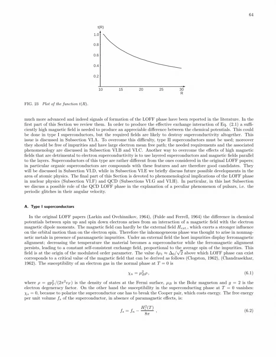
64
10 15 20 25 30
0.2
0.4
0.6
0.8
1.0
R
t(R)
FIG. 23 Plot of the function t(R).
much more advanced and indeed signals of formation of the LOFF phase have been reported in the literature. In thefirst part of this Section we review them. In order to produce the effective exchange interaction of Eq. (2.1) a suffi-ciently high magnetic field is needed to produce an appreciable difference between the chemical potentials. This couldbe done in type I superconductors, but the required fields are likely to destroy superconductivity altogether. Thisissue is discussed in Subsection VI.A. To overcome this difficulty, type II superconductors must be used; moreoverthey should be free of impurities and have large electron mean free path; the needed requirements and the associatedphenomenology are discussed in Subsection VI.B and VI.C. Another way to overcome the effects of high magneticfields that are detrimental to electron superconductivity is to use layered superconductors and magnetic fields parallelto the layers. Superconductors of this type are rather different from the ones considered in the original LOFF papers;in particular organic superconductors are compounds with these features and are therefore good candidates. Theywill be discussed in Subsection VI.D, while in Subsection VI.E we briefly discuss future possible developments in thearea of atomic physics. The final part of this Section is devoted to phenomenological implications of the LOFF phasein nuclear physics (Subsection VI.F) and QCD (Subsections VI.G and VI.H). In particular, in this last Subsectionwe discuss a possible role of the QCD LOFF phase in the explanation of a peculiar phenomenon of pulsars, i.e. theperiodic glitches in their angular velocity.
A. Type I superconductors
In the original LOFF papers (Larkin and Ovchinnikov, 1964), (Fulde and Ferrell, 1964) the difference in chemicalpotentials between spin up and spin down electrons arises from an interaction of a magnetic field with the electronmagnetic dipole moments. The magnetic field can hardly be the external field Hext., which exerts a stronger influenceon the orbital motion than on the electron spin. Therefore the inhomogeneous phase was thought to arise in nonmag-netic metals in presence of paramagnetic impurities. Under an external field the host impurities display ferromagneticalignment; decreasing the temperature the material becomes a superconductor while the ferromagnetic alignmentpersists, leading to a constant self-consistent exchange field, proportional to the average spin of the impurities. Thisfield is at the origin of the modulated order parameter. The value δµ1 ≈ ∆0/
√2 above which LOFF phase can exist
corresponds to a critical value of the magnetic field that can be derived as follows (Clogston, 1962), (Chandrasekhar,1962). The susceptibility of an electron gas in the normal phase at T = 0 is
χn = µ2Bρ , (6.1)
where ρ = gp2F /(2π
2vF ) is the density of states at the Fermi surface, µB is the Bohr magneton and g = 2 is theelectron degeneracy factor. On the other hand the susceptibility in the superconducting phase at T = 0 vanishes:χs = 0, because to polarize the superconductor one has to break the Cooper pair, which costs energy. The free energyper unit volume fs of the superconductor, in absence of paramagnetic effects, is:
fs = fn − H2c (T )
8π, (6.2)

65
where fn is the free energy of the normal phase and Hc(T ) is the critical field. Including the Pauli paramagnetismimplies adding the hamiltonian a term
− µB ψ†σ · Hψ ; (6.3)
while (6.2) becomes
fs = fn +(χn − χs)H
2
2− H2
c (T )
8π. (6.4)
Therefore the BCS superconductivity will survive at T = 0 for magnetic fields satisfying
H ≤√
H2c (0)
4πχn≡ HP (0) . (6.5)
Now H2c (0)/8π = ρ∆2
0/4 and therefore the Pauli limiting field at T = 0 is
HP (0) =∆0√
2
1
µB. (6.6)
The identification δµ1 = µBHP (0) arises by the comparison between (6.3), (6.6) and (2.1).For a type I superconductor it is difficult to reach the Pauli limit (6.6) because, while HP (0) is typically of the
order of 300 K Oe, Hc(0) is of the order 1 K Oe. Therefore superconductivity will be broken by the magnetic fieldwell before the Clogston-Chandrasekhar limit is achieved. This implies the LOFF phase is unlikely to be produced bythese materials and one has to turn to type II superconductors (Saint-James et al., 1969) because for some of thesesuperconductors the upper critical field Hc2 can be very high.
B. ”Clean” and strongly type II superconductors
To evaluate the possibility of the LOFF state one has to take into account not only Pauli paramagnetism of theelectrons but also the orbital effects (Ginzburg, 1957). Before doing that, let us first distinguish between ”clean” and”dirty” superconductors (Anderson, 1959). One calls ”clean” the superconductors in which the electron mean freepath l is much larger than the superconducting coherence length ξ0:
l ≫ ξ0 , (6.7)
while ”dirty” superconductors are characterized by the opposite condition l ≪ ξ0. In ”clean” superconductors electronsat the Fermi surface move with velocity vF , while in ”dirty” superconductors the electron motion is described by adiffusion equation. ”Dirty” superconductors are characterized by the presence of impurities, which can narrow andeven destroy the LOFF state (Aslamazov, 1969; Takada, 1970). Therefore materials with small l, e.g. PbMo6S8,should not display the LOFF phase, see e.g. (Decroux and Fischer, 1982). On the other hand the so called heavy-fermion superconductors are favored: these materials are indeed characterized by the small Fermi velocity of theirquasi particles (Rauchschwalbe, 1982); since
ξ0 =hvFπ∆
, (6.8)
for small enough vF the condition (6.7) is satisfied. For example in the heavy fermion compound UPd2Al3 thesuperconducting coherence length is ξ0 ≈ 85 A, much smaller than the electronic free mean path l = 700 A; thereforeit can be considered as a ”clean” superconductor.
To evaluate the possibility of the LOFF state in type II superconductors one has to take into account notonly Pauli paramagnetism of the electrons, but also the orbital effects. This analysis was first performed by(Gruenberg and Gunther, 1966). These authors followed the variational method of (Werthamer et al., 1966), bymaking an ansatz for the condensate. In general there is a competition between the orbital and the paramagneticeffect, the former trying to organize a structure of Abrikosov vortices and the latter a periodic LOFF structure;therefore the orbital effect reduces the possibility of the LOFF state that can exist only for sufficiently high Hc2. Thequantitative criterion at T = 0 for clean superconductors with isotropic dispersion law is as follows. The LOFF statecan persist in a type II superconductor provided
α =√
2Hc2(0)
HP (0)> 1.8 . (6.9)

66
Here α is the parameter first introduced in (Maki, 1964), Hc2(0) is the Gor’kov upper critical field at T = 0 in absenceof paramagnetic effects (Gor’kov, 1960) and HP (0) is the Pauli limiting field defined in (6.6).
In conclusion good experimental conditions to observe the LOFF state should be provided by a clean supercon-ductor with a large α value. These features are not easily found in the most common superconductors and thereforeexperimental investigations consider unconventional superconductors, e.g. heavy-fermion, organic or high Tc super-conductors. As a matter of fact many of these materials are strongly type II superconductors, which means thatthe condition (6.9) can be satisfied. Moreover they have often a layered structure, which implies that, applying themagnetic field parallel to the layers, the orbital effect is minimum and the Zeeman effect, on which the LOFF phaseis based, is dominant.
The condition of being very clean and simultaneously strong type II superconductors should be more easily realizedin d−wave superconductors like high Tc cuprate superconductors and organic superconductors like κ-(ET)2 or λ-(ET)2 salts. They will be discussed in more detail below; suffice it here to say that in d−wave superconductors theregion of the LOFF phase is much more extended than in s−wave superconductors. The analysis of (Maki and Won,1996), where this conclusion was drawn, has been extended in (Won and Maki, 2002) to the calculation of the LOFFfree energy, specific heat and magnetic susceptibility; in particular for these layered d−wave superconductors theenergetically favored structure at T = 0 is found to be
∆(x, y) ∝ cos qx + cos qy . (6.10)
Other materials where the possible existence of LOFF phase has been investigated are ferromagnetic metals oralloys (Pickett et al., 1999), (Dyugaev et al., 2001). The study of the possible coexistence of ferromagnetism andsuperconductivity was initiated by (Ginzburg, 1957) who noted that, though the two orderings can in principlecoexist, their simultaneous presence is practically impossible under ordinary conditions. As a matter of fact thepresence in ferromagnets of a spontaneous magnetization M0 produces at T = 0 an internal magnetic inductionB0 = 4πM0 even in absence of external magnetic field. For superconductivity to exist, B0 should be smaller than thelower critical field at T = 0, in absence of ferromagnetism:
B0 ≤ H0c1(0) . (6.11)
However, the induction B0 at T = 0 is of the order of 10 K Oe (e.g. 22, 18.5, 6.4, 24.8 KOe respectively for Fe,Co, Ni, Gd), while the critical field is in general much smaller, of the order of a few KOe or less. Superconductivityof ferromagnets is therefore difficult unless special conditions render the condition (6.11) possible. They might be,for example, a reduced size of the sample, with dimensions of the order of the penetration depth. The formation ofthe vortex phase in type II superconductors, however, screens locally the internal magnetic induction, and allows toavoid Ginzburg’s negative conclusion (Krey, 1973). As a matter of fact superconductivity was recently reported inthe ferromagnetic alloy RuSr2GdCu2O8 (Bernhard, 1999; Hadjiev, 1999; Pringle, 1999; Tallon, 1999). This layeredmaterial becomes first ferromagnet at T = 132 K; superconductivity appears at T = 35−40 K and finally, at T = 2.6 KGd ions acquire an antiferromagnetic order. The theoretical study of (Pickett et al., 1999) confirms these reports,but suggests that the superconducting phase is of the LOFF type, because the coupling between ferromagnetism andsuperconducting layers appears to be sufficiently weak to permit superconductivity, but strong enough to require theinhomogeneous phase. In a similar context (Dyugaev et al., 2001) consider the possibility of creating the LOFF phaseusing ferromagnetic materials instead of nonmagnetic bulks with paramagnetic impurities as in the original LOFFpapers. Since the impurities create not only an exchange interaction, but also an electromagnetic interaction, usingnuclear ferromagnetism, as they propose, would reduce the latter, since the effective field would be proportional to thenuclear magneton and not to the Bohr magneton. They show that in some metals, e.g. Rh, W, the BCS condensateimbedded in a matrix of ferromagnetically ordered nuclear spins should manifest the LOFF phase.
All the proposals we have discussed so far are rather different from the one discussed in the original LOFF papers.An extension of the LOFF analysis to these materials and unconventional superconductors is beyond the scope ofthe present review. We will therefore limit our presentation to a brief survey of the experimental results, referringthe interested reader to the specialized literature (Agterberg and Yang, 2001; Gegebwart, 1996; Murthy and Shankar,1995; Samohkin, 1997; Shimahara, 1998b; Shimahara et al., 1996; Symington, 1999; Yang, 2001).
C. Heavy fermion superconductors
The first experimental investigations on the LOFF phase used heavy-fermion compounds such as CeRu2 (Huxley,1993), UPd2Al3 (Gloos, 1993) and UBe13 (Thomas, 1996). For all these materials the conditions for the formationof the LOFF state are met. For example CeRu2 is in a metallurgically clean state; moreover it exhibits extreme typeII behavior, because the Ginzburg-Landau parameter, which discriminates between the two type of superconductors

67
(Saint-James et al., 1969), has the value κ = 16. As another example, the compound UPd2Al3 used by (Gloos,1993) is characterized by a rather large value of the parameter α in (6.9) i.e. α = 2.4, while also being a very cleansuperconductor. To quote another result, in the analysis of a high quality single crystal of UBe13 (Thomas, 1996), thevery high value Hc2(0) ≃ 140 KOe was reached. All these experimental results are however inconclusive. In a criticalanalysis of the experiment of (Gloos, 1993), (Norman, 1993) shows that the computed Gor’kov upper critical fielddoes not correspond to the experimental results reported there; for further analysis of the compound UPd2Al3 see(Yin and Maki, 1993) and (Schimanski, 1994). In the case of CeRu2, (Tenya, 1999) shows that the observed effectscan be explained by flux pinning mechanisms involving disorder. (Modler, 1996) makes a comparative study of highquality single crystals of UPd2Al3 and CeRu2 in the mixed state. The order parameter exhibits a periodic array ofnodal planes perpendicular to the Abrikosov vortex lines. In the mixed state the pinning force is very weak; howeverthe authors find, for H > 10 KOe and T < 0.9Tc, a first order transition to a state characterized by strong pinning,which might be interpreted as the formation of a LOFF state. The mechanism by which Abrikosov vortex lines intype II superconductors are pinned to the vortex cores is similar to the one that pins vortex lines to non-superfluidneutrons in a rotating superfluid within neutron stars. It will be explained in more detail in Subsection VI.H inconnection to a possible role of the QCD LOFF state in the physics of pulsars.
D. Two-dimensional, quasi-two-dimensional and organic superconductors
As we already mentioned, the paramagnetic effect can dominate if the superconducting bulk has a layered structureand the magnetic field acts parallel to it, because in this case the orbital upper critical field can be extremely high andthe breaking due to the spin interaction is most significant. The importance for two-dimensionality (2D) to favor theLOFF state was first observed in (Bulaevskii, 1973) and (Bulaevskii, 1974) where both the orbital and the spin effectwere taken into account and the upper critical field Hc2(T ) was calculated; in (Buzdin and Kulic, 1984) the analysiswas carried out near the tricritical point. For the same reason also quasi-one-dimensional (Q1D) compounds werediscussed (Buzdin and Polonski, 1987; Buzdin and Tugushev, 1983; Dupuis, 1995; Dupuis et al., 1993), even thoughthe results of (Shimahara, 1998a) indicate that the 2D structures are favored in comparison the 1D ones.
These results were generalized to arbitrary temperature and d−wave superconductivity in (Shimahara and Rainer,1997). The main result of this paper is that the critical field curve Hc2(T ) is non monotonic and consists of differentpieces corresponding to different Landau levels, characterized by n > 0. On the contrary, the Ginzburg-Landautheory would predict the pair wave function to be in the lowest energy Landau level, with n = 0 at Hc2. The paper(Shimahara, 1998a) studies the most favored structure for a 2D LOFF crystal with a cylindrical Fermi surface. First,the author finds that in general the 2D structures are favored over the 1D ones; second, it finds that the favoredcrystalline structure changes with T . For s−wave the results are as follows: at high temperature the antipodal paircondensate
∆(r) ∝ 2 cosq · r (6.12)
is favored. This was the result found by (Larkin and Ovchinnikov, 1964) in 3D at T = 0. Decreasing the temperatureother structures become favored: first the triangle, then the square and finally, at low temperatures, the hexagon.For d−wave pairing at high temperature again (6.12) is favored, while at small temperature the square dominates; onthe other hand at intermediate temperatures the phase transition should be first order. The result at T = 0 has beenconfirmed by (Won and Maki, 2002), see Eq. (6.10). As shown in (Lebed’, 1986), the quasi-2D superconductors canbe treated as essentially 2D and therefore the results of (Shimahara, 1998a) should hold also for quasi-2D compoundsprovided the external field is sufficiently strong and is kept parallel to the superconducting layer.
(Klein et al., 2000) consider a layered superconductor in a magnetic field of arbitrary orientation with respectto the conducting plane. The calculation is based on the quasi-classical Eilenberger equations (Eilenberger, 1968),(Alexander et al., 1985) and allows to elucidate the structure of the stable states below H2c minimizing the free en-ergy. The stable states are neither pure LOFF states nor pure Abrikosov vortex states, but are two-dimensionalperiodic structures or quasi-one-dimensional structures where LOFF domains are separated by vortex chains.(Barzykin and Gor’kov, 2002) address 2D surface superconductivity in presence of intense magnetic fields parallelto the surface. The spin-orbit interaction at the surface changes the properties of the LOFF state; the authors findthat strong spin-orbit interactions significantly broadens the range of parameters where the LOFF phase can existand produces periodic superconducting stripes running along the field direction on the surface.
Organic superconductors are good candidates for the formation of the LOFF state for the reasons mentioned above:i) They have narrow electron bands and therefore they are in principle clean type II superconductors; ii) due totheir low dimensionality the orbital pair-breaking effect is suppressed for magnetic fields parallel to the layers theyform. For these reasons they have been discussed by several authors, e.g. (Burkhardt and Rainer, 1994; Dupuis, 1995;Dupuis et al., 1993; Gor’kov and Lebed’, 1987; Lebed’, 1986; Shimahara, 1994, 1997). It is interesting to note that

68
in general to detect the transition from the homogeneous BCS phase to the LOFF phase thermodynamic signaturesare chosen. This however can give ambiguous results since the signatures can be produced by phase transitions ofdifferent nature. Therefore Ref. (Yang and Agterberg, 2000) proposes the use of the Josephson effect. According tothis analysis, at the Josephson junction between two superconductors, one in the BCS and the other in the LOFFphase, the Josephson current is suppressed.
As discussed in (Shimahara and Rainer, 1997), the upturn of the upper critical field d2Hc/dT2 > 0 is a common
feature in the LOFF state in quasi-2D systems and is due a Fermi surface effect. Investigations on the sensitivity of theLOFF state to the shape of the Fermi surface are in (Aoi et al., 1974; Shimahara, 1994, 1997). This upturn and a firstorder transition below the critical field have been observed in the organic compound κ-(BEDT-TTF)2Cu(NCS)2. Thisquasi-two-dimensional (Q2D) organic superconductor is examined by a number of authors (Houzet and Buzdin, 2000a;Ishiguro, 2000; Nam et al., 1999; Singleton et al., 2001, 2000; Symington et al., 2001) and, for a similar compound,(Goddard et al., 2002). These studies indicate that some evidence of the formation of the LOFF state has beenreached. For example (Singleton et al., 2000) studied resistance and magnetic behavior of single crystals of thissuperconductor in magnetic fields up to 33 T and at temperatures between 0.5 K and 11 K. When the magnetic fieldlies precisely in the Q2D planes of the material, they find evidence for a phase transition from the superconductingmixed state into a LOFF state, manifested as a change in the rigidity of the vortex system. (Manalo and Klein,2000) compare the theoretical anisotropic upper critical field Hc of a quasi-two-dimensional d-wave superconductorwith recent Hc2 data for κ-(BEDT-TTF)2Cu(NCS)2 and find agreement both with regard to the angular and thetemperature dependence of Hc. According to these authors this supports the suggestion that the LOFF phase existsin this material for exactly plane-parallel orientation of the magnetic field.
In (Uji, 2001) field induced superconductivity was reported in an organic superconductor λ−(BETS)2FeCl4(BETS=bis(ethylenedithio)tetraselenafulvalene). A possible mechanism to create field induced superconductivityis the Peter-Jaccarino effect (Jaccarino and Peter, 1962). However the upwards convex nature of the lower criticalfield as a function of the temperature casts doubts on this interpretation. Therefore some authors, e.g. (Balicas et al.,2001), have proposed that these results can be interpreted as evidence of the formation of the LOFF state. Theseresults were reviewed in (Houzet et al., 2002) and (Shimahara, 2002). In particular in the latter paper, an experi-mental phase diagram of the field-induced superconductivity in this organic compound was theoretically reproducedby a combination of the LOFF state and the Jaccarino-Peter mechanism. (Tanatar et al., 2002) discusses wetherLOFF state has been observed via thermal conductivity κ(H) in quasi-two-dimensional organic superconductor λ-(BETS)2GaCl4. For clean samples the behavior of κ(H) is similar to the one expected by a second order phasetransition and is consistent with the formation of a LOFF phase.
E. Future developments
The superconducting LOFF phase might be realized even if the difference in chemical potentials of two specieswere not generated by a magnetic field acting on electron spins. Apart from nuclear physics and pulsars, to bediscussed below, another context might be offered by ultracold quantum degenerate Fermi gas of atoms comprisingtwo hyperfine states. The experimental investigations of ultracold gases were first dedicated to the study of the Bose-Einstein condensation (Anderson, 1995; Bradley et al., 1997; Davis, 1995; Fried, 1998); subsequently these techniqueshave been extended also to magnetically trapped ultracold alkali Fermi gases or to gases with coexisting Bose-Einsteincondensate and Fermi gas (Modugno et al., 2002; Roati et al., 2002; Schreck et al., 2001). In particular two statemixtures of ultracold gases have been employed, with 40K vapors (DeMarco and Jin, 1999; DeMarco et al., 2001), or6Li (Granade, 2002; O’Hara, 2001), or a mixture of 6Li and 7Li (Mewes et al., 1999). Future developments couldlead to the observation of superconductivity and Cooper fermion pairs condensation in these systems. As discussedin (Combescot, 2000) it is quite likely that the two hyperfine states would have different atomic populations, sinceat the moment there are no known fast relaxation mechanisms to equalize the two atomic populations. Thereforesuperconductivity for two-state ultracold Fermi gases is likely to be of the LOFF type. The author of Ref. (Combescot,2000) has performed a theoretical study of 6Li under the above mentioned conditions; he considers not only s−waveinteractions, but also an anisotropic term induced by density fluctuation exchange and shows that the range wherethe LOFF phase is realized increases with the increasing role of the anisotropic term. This is an interesting theoreticaldevelopment, which adds new interest to the experimental investigations of ultracold atomic Fermi gases. It remainsto be seen, however, if such possibility is actually realized in Nature.

69
F. LOFF phase in nuclear physics
Neutron-proton pair correlations and the possibility of n−p Cooper pair condensation are presently studied in severaldifferent contexts, from heavy ion collisions to astrophysics. They have been investigated, using the BCS theory, ininfinite nuclear matter (Alm et al., 1993, 1990, 1996; Baldo et al., 1992; Sedrakian et al., 1997; Vonderfecht et al.,1991), and by mean-field effective interactions in finite nuclei. In several cases nuclear matter is highly asymmetric,with proton concentration at most 30-40% in supernova matter and 10% in neutron stars. These asymmetries aredetrimental to nucleon superconductivity; on the other hand, for weakly asymmetric states, fermion condensation isindeed possible. For example, weakly isospin asymmetric nuclear matter favors the formation of Cooper pairs in the3S1-
3D1 channel, due to the presence of a tensor force; gaps are of the order of 10 MeV. Condensation in this channelmight be relevant for low density bulk matter such as dilute nuclear matter in supernovas. On the other hand thereis no evidence of large gap isospin singlet pairing in ordinary nuclei, which might be explained by the presence ofspin orbit interaction (Goodman, 1999; Martinez-Pinedo et al., 1999). The authors (Sedrakian and Lombardo, 2000)study the dependence of the gap as a function of both the isospin asymmetry αnp = (ρn−ρp)/ρ and the temperature,using realistic nuclear interactions. For small asymmetries the gap develops a maximum at a certain intermediatetemperature; for large asymmetries the superconducting phase exists only at finite temperature, because the smearingeffect of the temperature on the Fermi surfaces favors condensation. At higher values of αnp (≃ 0.11 in their model)pairing is no longer possible.
Also in the context of isospin asymmetric nuclear matter it is possible to have a transition from the BCS state to aLOFF phase instead of the normal state (Isayev, 2002; Sedrakian, 2001; Sedrakian et al., 1997). In Ref. (Sedrakian,2001) the possibility of spatially inhomogeneous condensate in asymmetric nuclear matter is studied. Condensationis possible in different channels. The isospin triplet channels are favored for large enough asymmetries; more exactlythe channel 1S0 dominates at low densities and the channel 3P2-
3F2 (or 1P2) at high densities. For weak asymmetriesthe dominant channels are the isospin singlets 3S1-
3D1 (low densities) and 3D2 (high density). The author considersthe case of low density; as the isospin singlet 3S1-
3D1 has a strength much larger than the isospin triplet 1S0, heneglects the latter. The interaction is modelled by the Paris nucleon-nucleon potential. The gap equations are solvednumerically and have non trivial solutions for non vanishing total momentum of the pair P . The LOFF phase isfavored for αnp > 0.25 and P = 0.3pF , independent of αnp. For αnp > 0.37 pairing exists only in presence of non-vanishing P . The maximal values of αnp and P compatible with the LOFF state are 0.41 and 0.3 pF respectively (theactual values are indicative, as a refinement of the treatment of the nuclear interaction may change them by a factoras large as 3). The results are obtained at T = 3 MeV. From the BCS to the LOFF phase the phase transition is firstorder, while one passes from the LOFF to the normal state by a second order phase transition. No attempt is madeto determine the most favorite crystalline structure.
Under hypotheses similar to those of the previous paper (Isayev, 2002) studies the effect of coupling betweenthe isospin singlet and isospin triplet, since at low densities pairing between these two channels may be important(Akhiezer et al., 1999). Besides, the author goes beyond the approximation of ”bare” nucleon interaction, by using theFermi-liquid phenomenological approach (Akhiezer et al., 1994). By these changes one finds interesting peculiaritiesat T = 0. First, the triplet-singlet channel turns out to be energetically favored; second, the phase transition from theLOFF to the normal state can be of first order, depending on the nature of the nucleon interaction. While still modeldependent, these investigations of the LOFF phase in nuclear interactions are interesting as they offer, in principle,a different way to the LOFF phase. To be closer to phenomenology one should consider however more complicatedstructures such as, for example, hyperon rich matter. Alternatively the modulation of the order parameter might becaused by Pauli paramagnetism due to strong magnetic fields in highly magnetized neutron stars (magnetars). In thiscase one could have a splitting in the Fermi surfaces of a nucleon pair in the I = 1, L = 0 channel (Sedrakian, 2001).
G. Why color LOFF superconductivity could exist in pulsars
In this Subsection and in the next one we will be interested in some numerical estimates of the values of theparameters needed for the LOFF phase in pulsars to occur. In general, color superconductivity in quark matter mightbe realized in compact stars. This expectation follows from the following two facts.
First of all the BCS critical temperature is given by
Tc = 0.57∆BCS (6.13)
and in QCD ∆BCS is expected to range between 20 to 100 MeV. This estimate arises from weak coupling cal-culations (Beane and Bedaque, 2000; Beane et al., 2001; Brown et al., 2000a,b,c; Evans et al., 2000; Hong et al.,2000; Hsu and Schwetz, 2000; Pisarski and Rischke, 1999a,b, 2000a,b; Rajagopal and Shuster, 2000; Schafer, 2000;Schafer and Wilczek, 1999c; Shovkovy and Wijewardhana, 1999; Son, 1999) which are valid only at asymptotically

70
high chemical potentials µ ≫ 108 MeV (Rajagopal and Shuster, 2000), and from models with parameters ad-justed to reproduce the physics at zero densities (Alford, 2000; Alford et al., 1998, 1999b; Berges and Rajagopal,1999; Carter and Diakonov, 1999; Evans et al., 1999a,b; Rajagopal, 1999; Rapp et al., 1998, 2000; Schafer, 2001;Schafer and Wilczek, 1999b; Wilczek, 2000). None of these calculations is valid at chemical potentials around 400MeV, which correspond roughly to the density of the inner core of a neutron star, as we shall see below. However inall these cases one gets values of the gaps of the order quoted before.
The second fact has to do with the thermal history of a pulsar. The general belief is that compact stars suchas pulsars are formed in the core of a supernova explosion. The temperature at the interior of the supernova isabout 1011 K, corresponding to 10 MeV (1 MeV = 1.1065×10¹⁰ K). The star cools very rapidly by neutrino emissionwith the temperature going down to 109-1010 K in about one day. The neutrino emission is then dominating thecooling for one thousand years. In this period the temperature reaches about 106 K. After this period the star coolsdown due to X-ray and photon emission and in a few million years reaches a surface temperature around 105 K.Therefore, for the greatest part of its existence a neutron star has a temperature lower than the critical temperature,with the possibility of forming color superconducting condensates. It follows that also in this context a compact starcan be considered at zero temperature because its temperature is much smaller than the typical BCS energy gap,Tn.s./∆BCS ≈ 10−6 − 10−7.
We have seen previously that QCD favors the formation of BCS condensates in idealized cases, e.g. two or threemassless flavors of quarks. However in realistic cases the three quarks have different Fermi momenta due to the massdifference. It is interesting to have an idea of the order of magnitude of the scales involved in the description of aneutron star with a quark core. We begin with a very crude example of a free gas of three flavor quarks, taking upand down massless and the strange one with mass Ms (Alford et al., 2000). Requiring that the weak interactions arein equilibrium it is easy to determine the chemical potentials and the Fermi momenta for the quarks. We find
µu = µ− 2
3µe, puF = µu ,
µd = µ+1
3µe, pdF = µd ,
µs = µ+1
3µe, psF =
√
µ2s −M2
s , (6.14)
where µ is average chemical potential
µ =1
3(µu + µd + µs) (6.15)
and µe the chemical potential of the electrons. Notice that
∑
i=u,d,s
µiNi + µeNe = µNq − µeQ , (6.16)
where
Nq =∑
i=u,d,s
Ni, Q =2
3Nu −
1
3(Nd +Ns) −Ne . (6.17)
The chemical potential for the electrons is fixed by requiring electrical neutrality, corresponding to the followingcondition for the grand potential Ω at zero temperature
Q =∂Ω
∂µe= 0 . (6.18)
Ω is obtained from Eq. (2.60) (omitting the volume factor)
Ω =1
π2
∫ pF
0
p2(E(p) − µ)dp . (6.19)
In our case we get
Ω =3
π2
∑
i=u,d,s
∫ piF
0
p2(Ei(p) − µi)dp+1
π2
∫ µe
0
p2(p− µe)dp , (6.20)

71
where
Eu,d(p) = p, Es(p) =√
p2 +M2s . (6.21)
Although the integral is feasible its expression is algebraically involved and it is easier to do all calculations numerically.In particular the result for the chemical potential of the electrons for different values of µ as a function of Ms is givenin Fig. 24.
50 100 150 200 250 300
10
20
30
40
50
60
µe (MeV)
µ = 500 MeV
µ = 400 MeV
µ = 300 MeV
M (MeV)s
FIG. 24 The chemical potential of the electrons vs. Ms for three values of the average chemical potential.
We can get an analytical expression by performing an expansion up to the order M4s /µ
4. One gets
µe ≈M2s
4µ(6.22)
and
Ω ≈ − 3
4π2µ4 +
3
4π2M2sµ
2 − 7 − 12 log(Ms/2µ)
32π2M4s . (6.23)
The baryon density is obtained as
ρB = −1
3
∂Ω
∂µ=
1
3π2
∑
i=u,d,s
(piF )3 . (6.24)
The plot of the ratio of the baryon density to the nuclear baryon density is given in Fig. 25. The nuclear baryon densityhas been assumed as the inverse of the volume of a sphere of radius about 1.2 fm. Within the same approximation asbefore one finds
ρB ≈ µ3
π2
[
1 − 1
2
(
Ms
µ
)2]
. (6.25)
We note that densities in the core are of the order of 1015 g/cm3, corresponding to a chemical potential of the orderof 400 MeV, as shown in Fig. 25.
In particular let us discuss the range of values around 400 MeV of the average chemical potential, with a strange massof the order 200-300 MeV (the strange mass here is not the current mass but an effective density dependent mass).With Ms = 300 MeV one finds µe = 53 MeV (56 MeV from the approximate equation) with Fermi momenta
puF = 365 MeV, pdF = 418 MeV, psF = 290 MeV , (6.26)

72
50 100 150 200 250 300
2
4
6
8
10
12
M (MeV)s
n.m.ρ
Bρ___
µ= 300 MeV
µ = 500 MeV
= 400 MeVµ
FIG. 25 The ratio of the baryon density of the free quark gas to the nuclear baryon density vs. Ms, for three values of theaverage chemical potential.
and a baryon density about 4.4 times the nuclear matter density. With Ms = 200 MeV the result is µe = 24 MeV (25MeV from the approximate equation) and
puF = 384 MeV, pdF = 408 MeV, psF = 357 MeV , (6.27)
and a baryon density about 5.1 times the nuclear matter density. To go to baryon densities relevant to the centralcore of the star, i.e. densities from 6 to 8 times the nuclear matter density, one needs to go to higher values of µ andlower values of Ms where the difference among of the Fermi momenta is lower. This can be seen from Fig. 26, orusing our approximate expression for µe:
puF ≈ µ− M2s
6µ, pdF ≈ µ+
M2s
12µ, psF ≈ µ− 5M2
s
12µ, (6.28)
with
pdF − puF ≈ puF − psF ≈ M2s
4µ. (6.29)
The previous results are rather general, but in order to discuss the possible astrophysical applications we need to fixa value for ∆0. Notice that we can trade the coupling constant G (see Eq. (4.55)) for ∆0 since G is fixed once wegive the cutoff δ. On the other hand, the equation for the chiral gap (Rajagopal and Wilczek, 2001) gives a relationebetween the NJL cutoff Λ = δ + µ, the coupling G and the constituent quark mass. By taking the constituent massaround 300 − 400 MeV and fixing Λ, one has still a parameter to play around and it is possible to get values of ∆0
from about 20 MeV up to about 100 MeV. In the present case, since the typical value of δµ inside the LOFF windowis 0.7∆0 and
δµ =1
2(µd − µu) =
1
2µe , (6.30)
we can reproduce approximately the situation illustrated at the beginning of this Subsection with Ms = 300 MeV bychoosing ∆0 = 40 MeV. With this choice the LOFF grand potential at δµ = δµ1 is of the order 10−7 GeV4 which,as we shall see in Section VI.H, is of the right order of magnitude to give rise to the glitch phenomena (Alford et al.,2000). Notice also that the LOFF condensate evaluated at δµ1
∆LOFF (δµ1) ≈ 0.25∆0 = 10 MeV (6.31)
is much larger that a typical temperature of neutron stars, of the order of keVs.

73
50 100 150 200 250 300
100
200
300
400
M (MeV)s
pFs
upF
dpF
(MeV)pF
FIG. 26 The Fermi momenta of the three quarks vs. Ms.
H. Astrophysical implications of the QCD LOFF phase
While a great experimental effort is devoted to the search of the LOFF phase in condensed matter, so far nothingsimilar happens for the crystalline phase of QCD. The reason is that it is difficult to create the experimental conditionsof high density and low temperature for hadronic matter. The crystalline superconducting phase of quarks mayhowever result relevant for astrophysical dense systems, in particular in the explanation of pulsar glitches. Pulsars arerapidly rotating stellar objects, characterized by the presence of strong magnetic fields and by an almost continuousconversion of rotational energy into electromagnetic radiation. The rotation periods can vary in the range 10−3 sec upto a few seconds; these periods increase slowly and never decrease except for occasional glitches, i.e. sudden increasesof the rotational frequencies, when the pulsar spins up with a variation in frequency of the order of δΩ/Ω ≈ 10−6 orsmaller. Glitches are a typical phenomenon of the pulsars, since probably all the pulsars experience them.
Pulsars are commonly identified with neutron stars; these compact stars are characterized by a complex structurecomprising a core, an intermediate region with superfluid neutrons and a metallic crust. With a chemical potential ofthe order of 400 MeV, as we have seen, the conditions for color superconductivity in the CFL or the LOFF versionsmight be reached in the core. Before examining this possibility, let us however describe the standard explanation ofglitches, in the form originated by the papers (Alpar et al., 1984a; Anderson and Itoh, 1973). This model is based onthe idea that the sudden jumps of Ω are due to the movements outwards of rotational vortices in the neutron superfluidand their interaction with the crust. Crucial ingredients of the model are therefore the existence of a superfluid anda crystal (the metallic crust). This is one of the main reasons that allows the identification of pulsars with neutronstars, as only neutron stars are supposed to have a metallic crust. The LOFF state can be relevant in this contextbecause, if there is a LOFF phase inside the pulsar, the superfluid might interact with the LOFF crystal instead ofthe crust, thus providing an alternative or complementary mechanism for the glitches. Thus far, there is no developedmodel for the pinning of the superfluid vortices to the QCD LOFF crystals within compact stars. Therefore we limitour survey to an introduction to the subject, along the lines of (Alford, 2000; Alford et al., 2001b; Nardulli, 2002c).
Let us consider a compact star whose metallic crust rotates with angular velocity Ω. The superfluid inside thestar should not rotate because, in absence of friction, the crust cannot communicate its rotation to the superfluidcomponent. The velocity of the superfluid is vs = h∇Φ/m where Φ is the phase of the superfluid condensate wavefunction. The consequence of this formula would be
∮
γ vs · dℓ = 0. This would imply the absence of rotation in the
superfluid, which however does not correspond to the state of minimal energy (for a discussion see (Landau et al.,1980)). The correct condition is
∮
γ
vs · dℓ = 2πnκ , (6.32)
where κ is the quantum of vorticity: κ = h/m. For Eq. (6.32) to hold the curve γ must wind a singular point; theinteger n is the winding number which counts the number of times the curve goes around the singular point; the mostenergetically favorable condition is realized by n = 1. If γ is in a plane the condition (6.32) holds for any plane andthe locus of the singular points is a vortex line (v.l.). In absence of rotation there are no v.l.’s; the minimal angular

74
velocity Ωmin for the formation of the first vortex line is
Ωcrit =h
mR2lnR
a. (6.33)
Here we are assuming a cylindrical configuration with radius R; a is a cutoff of the order of the interatomic distances.By increasing Ω also the number N of vortex lines per unit area in the superfluid increases according to the formula:
N =mΩ
πh(6.34)
and one gets, instead of (6.32),∮
γ
dℓ · vs = NA2πκ , (6.35)
where A is the area encircled by γ. Eventually the v.l.’s tend to fill in all the space. As a numerical exampleone can estimate N for the pulsar in the Crab nebula. Here m = 2mN (the condensate is formed by neutralbosons: pairs of neutrons) and Ω = Ωpulsar gives N ≃ 1.9 × 105cm−2 with an average distance between vortex lines
d ∼ N−1/2 ∼ 10−2cm. If the vortex line is a straight line, vs is perpendicular both to the vortex line and to theradius joining the singular point and the point at which we compute vs. At a distance r from the singular point onehas
vs =nκ
r, (6.36)
as can be immediately seen from (6.32). More generally:
vs =κ
2
∫
v.l.
dℓ ∧ R
R3, (6.37)
where R is the distance vector from the vortex line to the point at which we compute the superfluid velocity.During the rotation the vortex lines follow the rotational motion of the vessel, which is clear because they are pinned
at the boundary of the superfluid; in particular, for rotations around an axis, the vortex lines are, by symmetry, straightlines parallel to the rotation axis. Their motion imitate the motion of the liquid as a whole and, as a consequence,also for the superfluid one can use the hydrodynamical formula
Ω =1
2∇ ∧ vs , (6.38)
which in principle would be valid only for the fluid normal component.Let now ν(r) be the number of vortices per unit area at a distance r from the rotation axis; if v = vs is the
superfluid velocity, one gets∮
γ
dℓ · v =
∫ r
0
dS · ∇ ∧ v = 2πκ
∫ r
0
2πr′ν(r′)dr′ . (6.39)
We put k = 2πκ = h/2mn and write (6.39) as follows:
2π r2 Ω(r) = k
∫ r
0
2πr′ν(r′)dr′ , (6.40)
which implies
kν(r) = 2Ω(r) + r∂Ω
∂r. (6.41)
Since the total number of v.l.’s is conserved, one has
∂ν/∂t+ ∇ · (νvr) = 0 , (6.42)
where vr is the radial component of the superfluid velocity. We write (6.40) as
2π r2 Ω(r) = k
∫ r
0
ν dS (6.43)

75
and take the time derivative, using (6.42) to get
2π r2∂Ω
∂t= −k
∫ r
0
dS∇ · (νvr) . (6.44)
Using the Gauss theorem one gets 2π r2∂Ω
∂t= −k 2πrνvr , i.e.
∂Ω
∂t= −kνvr
r= −
(
2Ω(r) + r∂Ω
∂r
)
vrr. (6.45)
Eq. (6.45) shows that the only possibility for the superfluid to change its angular velocity (Ω 6= 0) is by means of a
radial motion, i.e. vr 6= 0.Let us now consider a rotating superfluid in contact with rotating normal matter on which an external torque
is acting (Alpar et al., 1984a). We denote by Ic and Ωc the moment of inertia and angular velocity of the normalcomponents that, in a neutron star, includes the crust and possibly other normal components. The equation of motionof the normal component is
IcΩc(t) = Mext +Mint . (6.46)
Besides the external torque Mext, basically related to the spin down of the pulsar (or the steady accretion in binarypulsars), we have included the internal torque Mint due to the interaction with the superfluid:
Mint = −∫
dIp Ω(r, t) (6.47)
where dIp is the infinitesimal moment of inertia of the superfluid component. Eqs. (6.45-6.47) are the equations ofmotion for the angular velocities Ω and Ωc (superfluid and crust). The two velocities are coupled not only throughMint, but also by vr, because we will show below that vr depends on the difference Ω − Ωc. We note again thatfundamental for this model is the existence of radial motion, for, if vr = 0, then Ω = const. and only Ωc changes, dueto the external torque alone.
In the neutron star, superfluid neutrons (in Cooper pairs) coexist with nuclei of the crust. Also in the crust thereare superfluid neutrons, but they are characterized by a different (and smaller) ∆. Computing the difference in thefree energies between the two phases one obtains the difference of pressures and, consequently, the force per unitlength of vortex line. Let b be the average distance between the nuclei; b is also the average distance between twoconsecutive pinning centers. Let us assume
2ξ0 < b , (6.48)
where ξ0 is the superconducting coherence length, which also gives the dimension of the vortex core, since ξ0 is of theorder of the spatial extension of the Cooper pair. The maximum pinning force is obtained when the vortex passesthrough one layer of the lattice; therefore the maximum force per unit length of vortex line is
fp ≃δEpbξ
, (6.49)
where
δEp = Fs − Fc ∝ ρ∆2s , (6.50)
where Fs and Fc are the free energies of the superfluid neutrons and the nucleons in the crust; ∆s is the gap forsuperfluid neutrons and one can neglect ∆c, the gap of superfluid neutrons in the crust since ∆c ≪ ∆s. Eq. (6.50)implies that neutrons tend to remain in the volume V of the vortex core because they experience a force repellingthem from the superconducting phase (if neutron rich nuclei are present, the repulsion will be less important). Typicalvalues for the pinning energy per nucleus δEp at densities 3 × 10¹³ − 1.2 × 10¹⁴ g/cm3 are
δEp = 1 − 3 MeV , (6.51)
while b = 25 − 50 fm and ξ0 = 4 − 20 fm give
fp = 40 − 1200 MeV3 . (6.52)

76
On the basis of these considerations let us now sketch a possible mechanism for the formation of glitches (Alpar,1977; Alpar et al., 1984a,b; Anderson and Itoh, 1973) (for further references see below). We consider the rotatingneutron star with superfluid neutrons in its interior and a metallic crust, which is a simplified model, but adequateto our purposes. As stressed already, we distinguish between the superfluid velocity Ω and the crust velocity Ωc. Letus suppose that they are initially equal, which is a consequence of the pinning. Due to the spinning down of thestar, Ωc decreases; as long the vortex cores are pinned to the crust lattice, the neutron superfluid cannot spin down,because the radial motion is forbidden. There is therefore a relative velocity of the superfluid with respect to thepinned vortex core because Ω > Ωc:
δv = (Ω − Ωc) ∧ r . (6.53)
The interaction between the normal matter in the core of the v.l. and the rest of normal matter (nuclei in the lattice,electrons, etc.) produces a Magnus force per unit length given by
f = ρk ∧ δv , (6.54)
where the direction of k coincides with the rotation axis and its modulus is equal to the quantum of vorticity. f isthe force exerted on the vortex line; as it cannot be larger than fp there is a maximum difference of angular velocitythat the system can maintain:
ωcr = (Ω − Ωc)max =fpρkr
=Epρkξb
. (6.55)
If ω < ωcr the vortices remain pinned at the lattice sites instead of flowing with the superfluid as they generally doinside it (see discussion above). On the contrary, if ω > ωcr, the hydrodynamical forces arising from the mismatchbetween the two angular velocities ultimately break the crust and produce the conditions for the glitch. A possible wayto get it is by the observation following Eq. (6.45). If a bunch of vortex lines are unpinned and move outwards theneq. (6.45) implies that the angular velocity (and the angular momentum) of the superfluid decreases, and, therefore,the angular momentum of the crust increases, which is revealed from outside as a spin up of the star, i.e. a glitch. Anumerical analysis would imply solving the set of Eqs. (6.45-6.47), but this is outside the scope of the present review5. Let us instead discuss the possible role of the LOFF phase in this context. The QCD LOFF phase provides alattice structure independently of the crust. Therefore it meets one of the two requirements of the model for glitchesin pulsars we have outlined above, the other being the presence of a superfluid. On the other hand the only existingcalculations for the inhomogeneous phase in color superconductivity have been performed for the case of two flavors,which however, in the homogeneous case, does not present superfluidity, since there are no broken global symmetries.Superfluidity is on the other hand manifested by the CFL phase of QCD. Therefore a realistic application to QCDsuperfluid has to wait until a calculation of the LOFF phase with three flavors will be completed. For the time beingone can give some order of magnitude estimates (Alford et al., 2001b). Let us assume the following choice of theparameters: ∆2SC = 40 MeV, ∆LOFF ≈ 8 MeV, corresponding to the Fulde-Ferrel state; since q ≈ 1.2δµ ≈ 0.7∆2SC ,one would get for the average distance between nodal planes b = π/(2|q|) ≈ 9 fm and for the superconductingcoherence length ξ0 = 6 fm. From (3.28), with δµ = δµ1 and an extra factor of 4 to take into account the two flavorsand the two colors, we get the free energy per volume unit as follows6: |FLOFF | = 8× (10MeV )4 and therefore, from(6.50), the pinning energy of the vortex line is
δEp = |FLOFF | × b3 = 6 MeV . (6.56)
To get the pinning force we cannot use (6.49) since (6.48) does not hold in this case. For an order of magnitudeestimate one can use
fp ≃δEpb2
, (6.57)
giving a pinning force per unit length of the vortex of the order of
fp ≈ 3 × 10³ MeV3 . (6.58)
5 Models differ in the mechanism by which angular momentum is released; instead of performing outward movements for example v.l.’smight break the crust or rearrange it. For reviews see (Alpar, 1995; Pines and Alpar, 1985) and, more recently, (Alpar et al., 1993;Epstein and Baym, 1992; Link and Epstein, 1996; Ruderman, 1991; Ruderman et al., 1998).
6 Using the exact expression instead of (3.28), that is valid only in the weak coupling limit, one would get |FLOFF | = 5 × (10MeV )4.
77
Comparing these numerical values with Eqs. (6.51) and (6.52) one can see that these order of magnitude estimatesgive figures similar and therefore some of the glitches in neutron stars may be generated well inside the star by vorticesrelated to the LOFF phase of QCD.
As we already stated these conclusions are tentative because the analysis of the QCD LOFF phase needs extensionto the three flavor case; moreover the true ground state is likely to be different from the Fulde-Ferrel one plane wavestructure. Nevertheless they are encouraging and leave open the possibility that neutron stars might give anotherlaboratory where to study the inhomogeneous superconducting phase. It can be useful to stress that even in quarkstars, in the QCD superconducting LOFF phase, one would get a crystal structure given by a lattice characterizedby a geometric array where the gap parameter varies periodically. This would overcome the objection that pulsarscannot be strange stars. This objection is based on the following observation: If strange matter there exists, quarkstars should be rather common; however, in absence of metallic crusts, strange stars can hardly develop vortices,at least by the model we have described here. On the contrary, if the color superconductivity is able to produce acrystalline structure it could also give rise to glitches and the argument in favor of the existence of strange stars wouldbe reinforced.
VII. CONCLUSIONS
Inhomogeneous crystalline superconductivity was predicted forty years ago by Larkin, Ovchinnikov, Fulde andFerrell, but realistic conditions for its experimental investigations became available only a few years ago. In condensedmatter the existence of the LOFF phase, with its characteristic space modulation of the energy gap, still awaitscomplete confirmation. This is due to the fact that it is indeed a subtle effect. It arises when the Fermi surfaces of thetwo species participating in the Cooper pairing are different. However for large separation pairing is not possible atall and superconductivity disappears altogether. In condensed matter the separation of the Fermi surfaces is obtainedby a Zeeman splitting due to an exchange interaction due to a magnetic field. However the needed field strengthis such to destroy superconductivity due to diamagnetic effects. As we discussed in the paper, the way to avoidthe problem was to use unconventional superconductors such as organic compounds. These materials have in fact alayered structure and therefore, if the magnetic field is parallel to the layers, the orbital effects can be controlled.
New opportunities have recently arisen to detect the LOFF phase in atomic physics (ultracold atomic gases), nuclearphysics and especially quark matter. This last development is a consequence of the recent excitement generated by thestudy of QCD at high density and small temperature. Inhomogeneous crystalline superconductivity in this contextcould be generated by the difference in quark chemical potentials induced by weak interactions in the inner core ofpulsars. Their main phenomenological effect might therefore be to provide a mechanism for the explanation of glitchesin pulsars. If pulsars are neutron stars with a core made up by color superconducting matter, this mechanism wouldbe complementary to the standard models of glitches. If pulsars are strange stars, then the crystalline structure ofthe condensate would provide the possibility for pinning the superfluid vortices and eventually creating the glitches.
This paper was mainly aimed to the presentation of a unified formalism to describe the LOFF phase both incondensed and hadronic matter. The simplest way in our opinion to describe superconductivity effects, including theLOFF state, is by the effective lagrangian approach. Since they are based on the general mathematical ground of theRenormalization Group, effective lagrangians allow the conditions for this unification. The existence of a commonmathematical basis should allow experts of one side to fully appreciate and take advantage of the progresses made inthe other. We would be gratified if this paper turned out to be useful to this end.
Acknowledgments
One of us (G.N.) would like to thank CERN Theory Division for the kind hospitality offered during the completionof this paper. We would like to thank R. Gatto for his invaluable help in common work and for reading the manuscriptand E. Fabiano, and M. Mannarelli for the very pleasant scientific collaboration. We also wish to thank K. Rajagopalfor a number of useful discussions on color superconductivity and the LOFF phase. Our thanks are finally due to M.Alford, J. Bowers, M. Ciminale, R. Combescot and H. Shimahara for useful correspondence on the present review

78
APPENDIX A: Calculation of J and K
We give here an outline of the calculation of the integrals J and K appearing in the GL expansion at T = 0. Usingthe definition of J , Eq. (3.5), and K, eq. (3.6), we have
J ≡ J(q1,q2,q3,q4) = +igρ
2
∫
dw
4π
∫ +δ
−δ
dξ
∫ +∞
−∞
dE
2π
4∏
i=1
fi(E, δµ, q)
= +igρ
2
∫
dw
4π
∫ +δ
−δ
dξ
∫ +∞
−∞
dE
2π
2∏
i=1
1
E + iǫsignE + ξ − δµ+ 2w · ki
× 1
E + iǫsignE − ξ − δµ− 2w·ℓi
, (A1)
K = K(q1,q2,q3,q4,q5,q6) =igρ
2
∫
dw
4π
∫ +δ
−δ
dξ
∫ +∞
−∞
dE
2π
6∏
i=1
fi(E, δµ, q)
=igρ
2
∫
dw
4π
∫ +δ
−δ
dξ
∫ +∞
−∞
dE
2π
3∏
i=1
1
E + iǫsignE + ξ − δµ+ 2w · ki
× 1
E + iǫsignE − ξ − δµ− 2w·ℓi
, (A2)
where we have defined
k1 = 0, k2 = q1 − q2, k3 = q1 − q2 + q3 − q4 ,ℓ1 = q1, ℓ2 = q1 − q2 + q3, ℓ3 = q1 − q2 + q3 − q4 + q5 , (A3)
with the conditions q1 − q2 + q3 − q4 = 0 and q1 − q2 + q3 − q4 + q5 − q6 = 0 for J and K respectively. Weintroduce the Feynman variables xj , yj (j = 1, 2 for J and j = 1, 2, 3 for K) to form the vectors k =
∑
i xiki andℓ =
∑
i yiℓi; after rotation of the energy integration contour E → i p4 we get:
∫
dE
2π
∏
i
1
E + ξ − δµ+ 2w · ki
=
∫
idp4
2π
δ (1 −∑xk)
[ip4 + ξ − δµ+ 2w · k]2
∏
n
dxn ,
∫
dE
2π
∏
i
1
E − ξ − δµ− 2w·ℓi
=
∫
idp4
2π
δ (1 −∑ yk)
[ip4 − ξ − δµ− 2w · ℓ]2∏
n
dyn ; (A4)
next we perform the ξ integration by the residues method and the angular integration; for J the result is
J = − igρ
8
∫
dp4ǫ(p4) (δµ− ip4)
∫
[
2∏
n=1
dxndyn
]
δ (1 −∑ xk) δ (1 −∑ yk)
[(δµ− ip4)2 − v2F |k − ℓ|2]2 . (A5)
After the energy integration we remain with
J = − gρ
8
∫
[
2∏
n=1
dxndyn
]
δ(
1 −∑
xk
)
δ(
1 −∑
yk
) 1
v2F |k − ℓ|2 − δµ2
. (A6)
This expression is general; we can specialize it to the various crystal structures, as explained in the text.For K we get, instead of (A5), the result
K = −3igρ
8
∫
dp4ǫ(p4)
∫
[
3∏
n=1
dxndyn
]
δ(
1 −∑
xk
)
δ(
1 −∑
yk
)
× (δµ− ip4)(δµ− ip4)
2 + v2F |k − ℓ|2
[(δµ− ip4)2 − v2F |k − ℓ|2]4 , (A7)
which, after energy integration, becomes
K = −gρ16
∫
[
3∏
n=1
dxndyn
]
δ(
1 −∑
xk
)
δ(
1 −∑
yk
) δµ2 + 3 v2F |k − ℓ|2
[v2F |k − ℓ|2 − δµ2]
3 . (A8)

79
APPENDIX B: Expansion of Π around the tricritical point
Let us consider the expansion of Π(q) in Q = qvF , at finite T and µ, which can be obtained from Eq. (3.4) afterintroducing the Matsubara frequencies:
Π(q) = −1
2gρT
∫
dw
4π
∫ +δ
−δ
dξ
+∞∑
n=−∞
1
(iωn − δµ− ξ − 2w · qvF )(iωn − δµ+ ξ). (B1)
Expanding the first denominator in the momentum q we find
Π(q) =1
2gρT
+∞∑
n=−∞
∫
dw
4π
∫ +∞
−∞
dξ
∞∑
m=0
1
ω2n + ξ2
(2w · qvF )2m
(iωn − ξ)2m, (B2)
where, as in Eq. (2.70),
ωn = ωn + iδµ . (B3)
Notice that we have inverted the sum over the Matsubara frequencies with the integration over ξ. In this way, aswe did for the homogeneous case, we are converting the divergence in ξ into a divergence in the series, which can betreated as before by introducing a cutoff in the sum. Performing the angular integration and the integration over ξwith the help of the following integral
∫ +∞
−∞
dξ1
ω2n + ξ2
1
(iωn − ξ)2m= (−1)m
π
22mω2m+1n
, (B4)
we get eventually
Π(q) =1
2gπρT
+∞∑
n=−∞
∞∑
m=0
(−1)m
2m+ 1
Q2m
ω2m+1n
. (B5)
By using the definition of the first term in the grand potential as 1 − Π(q) multiplied by 2/g we recover easily the
expression (3.42) for α. In analogous way, to get β and γ one proceeds expanding J (see Eq. (3.5) and K (see Eq.(3.6)).
References
Abrikosov, A. A., 1957, Zh. Exsp. teor. Fiz. 32, 1442.Abrikosov, A. A., L. P. Gor’kov, and I. E. Dzyaloshinski, 1963, Methods of Quantum Field Theory in Statistical Physics (Dover,
New York).Agasian, N. O., B. O. Kerbikov, and V. I. Shevchenko, 1999, Phys. Rept. 320, 131.Agterberg, D. F., and K. Yang, 2001, J. Phys.: Condens. Matter 13, 9259.Akhiezer, A. I., A. A. Isayev, S. V. Peletminsky, and A. A. Yatsenko, 1999, Phys. Lett. B 451, 430.Akhiezer, A. I., V. V. Krasil’nikov, S. V. Peletminsky, and A. A. Yatsenko, 1994, Phys. Rep. 245, 1.Alexander, J. A. X., T. P. Orlando, D. Rainer, and P. M. Tedrow, 1985, Phys. Rev. B 31, 5811.Alexander, S., and J. McRtague, 1978, Phys. Rev. Lett. 41, 702.Alford, M. G., 2000, eprint hep-ph/0003185.Alford, M. G., 2001, Ann. Rev. Nucl. Part. Sci. 51, 131.Alford, M. G., J. Berges, and K. Rajagopal, 1999a, Nucl. Phys. B558, 219.Alford, M. G., J. Berges, and K. Rajagopal, 2000, Nucl. Phys. B571, 269.Alford, M. G., J. A. Bowers, J. M. Cheyne, and G. A. Cowan, 2003, Phys. Rev. D67, 054018.Alford, M. G., J. A. Bowers, and K. Rajagopal, 2001a, J. Phys. G27, 541.Alford, M. G., J. A. Bowers, and K. Rajagopal, 2001b, Phys. Rev. D63, 074016.Alford, M. G., K. Rajagopal, and F. Wilczek, 1998, Phys. Lett. B422, 247.Alford, M. G., K. Rajagopal, and F. Wilczek, 1999b, Nucl. Phys. B537, 443.Alm, T., B. L. Friman, G. Roepke, and H. Schulz, 1993, Nucl. Phys. A 551, 45.Alm, T., G. Roepke, and M. Schmidt, 1990, Z. Phys. A 337, 355.Alm, T., G. Roepke, A. Sedrakian, and F. Weber, 1996, Nucl. Phys. A 406, 491.Alpar, M. A., 1977, Astrophys. J. 213, 527.Alpar, M. A., 1995, in M. A. Alpar et al. eds., The Lives of Neutron Stars (Kluwer), p. 185.

80
Alpar, M. A., P. Anderson, D. Pines, and J. Shaham, 1984a, Astrophys. J. 276, 325.Alpar, M. A., P. Anderson, D. Pines, and J. Shaham, 1984b, Astrophys. J. 278, 791.Alpar, M. A., H. F. Chau, K. S. Cheng, and D. Pines, 1993, Astrophys. J. 409, 345.Anderson, M. H. et al., 1995, Science 269, 198.Anderson, P., and N. Itoh, 1973, Nature 256, 25.Anderson, P. W., 1959, J. Phys. Chem. Solids 11, 26.Aoi, K., W. Dieterich, and P. Fulde, 1974, Z. Physik B 267, 223.Aslamazov, L. G., 1969, Sov. Phys. JETP 28, 773.Bailin, D., and A. Love, 1984, Phys. Rept. 107, 325.Baldo, M., I. Bombaci, and U. Lombardo, 1992, Phys. Lett. B 283, 8.Balicas, L., J. Brooks, K. Storr, S. Uji, M. Tokumoto, H. Tanaka, H. Kobayashi, A. Kobayashi, V. Barzykin, and L. P. Gor’kov,
2001, Phys. Rev. Lett. 87, 067002.Bardeen, J., L. N. Cooper, and J. R. Schrieffer, 1957, Phys. Rev. 106, 162.Barrois, B. C., 1977, Nucl. Phys. B129, 390.Barzykin, V., and L. P. Gor’kov, 2002, Phys. Rev. Lett. 89, 22702.Beane, S. R., and P. F. Bedaque, 2000, Phys. Rev. D62, 117502.Beane, S. R., P. F. Bedaque, and M. J. Savage, 2000, Phys. Lett. B483, 131.Beane, S. R., P. F. Bedaque, and M. J. Savage, 2001, Nucl. Phys. A688, 931.Bedaque, P. F., 2002, Nucl. Phys. A697, 569.Benfatto, G., and G. Gallavotti, 1990, Phys. Rev. B42, 9967.Berges, J., and K. Rajagopal, 1999, Nucl. Phys. B538, 215.Bernhard, C. et al., 1999, Phys. Rev. B 59, 14099.Bowers, J. A., J. Kundu, K. Rajagopal, and E. Shuster, 2001, Phys. Rev. D64, 014024.Bowers, J. A., and K. Rajagopal, 2002, Phys. Rev. D66, 065002.Bradley, C. C., C. A. Sackett, and R. G. Hulet, 1997, Phys. Rev. Lett. 78, 985.Brown, W. E., J. T. Liu, and H.-c. Ren, 2000a, Phys. Rev. D62, 054013.Brown, W. E., J. T. Liu, and H.-c. Ren, 2000b, Phys. Rev. D61, 114012.Brown, W. E., J. T. Liu, and H.-c. Ren, 2000c, Phys. Rev. D62, 054016.Bulaevskii, L. N., 1973, Sov. Phys. JETP 37, 1133.Bulaevskii, L. N., 1974, Sov. Phys. JETP 38, 634.Burkhardt, H., and D. Rainer, 1994, Ann. Physik 3, 181.Buzdin, A. I., and Kachkachi, 1997, Phys. Lett. A225, 341.Buzdin, A. I., and M. L. Kulic, 1984, J. Low Temp. Phys. 54, 203.Buzdin, A. I., and S. V. Polonski, 1987, Zh. Exsp. teor. Fiz. 93, 747.Buzdin, A. I., and v. V. Tugushev, 1983, Zh. Exsp. teor. Fiz. 85, 735.Carter, G. W., and D. Diakonov, 1999, Phys. Rev. D60, 016004.Casalbuoni, R., 2001, AIP Conf. Proc. 602, 358.Casalbuoni, R., F. De Fazio, R. Gatto, G. Nardulli, and M. Ruggieri, 2002a, Phys. Lett. B547, 229.Casalbuoni, R., Z.-y. Duan, and F. Sannino, 2000, Phys. Rev. D62, 094004.Casalbuoni, R., E. Fabiano, R. Gatto, M. Mannarelli, and G. Nardulli, 2002b, Phys. Rev. D66, 094006.Casalbuoni, R., and R. Gatto, 1999, Phys. Lett. B464, 111.Casalbuoni, R., R. Gatto, M. Mannarelli, and G. Nardulli, 2001a, Phys. Lett. B511, 218.Casalbuoni, R., R. Gatto, M. Mannarelli, and G. Nardulli, 2002c, Phys. Rev. D66, 014006.Casalbuoni, R., R. Gatto, M. Mannarelli, and G. Nardulli, 2002d, Phys. Lett. B524, 144.Casalbuoni, R., R. Gatto, and G. Nardulli, 2001b, Phys. Lett. B498, 179.Casalbuoni, R., R. Gatto, and G. Nardulli, 2002e, Phys. Lett. B543, 139.Casalbuoni, R., R. Gatto, G. Nardulli, and M. Ruggieri, 2003, eprint hep-ph/0302077.Casalbuoni, R., et al., 1997, Phys. Rept. 281, 145.Chandrasekhar, B. S., 1962, App. Phys. Lett. 1, 7.Clogston, A. M., 1962, Phys. Rev. Lett. 9, 266.Collins, J. C., and M. J. Perry, 1975, Phys. Rev. Lett. 34, 1353.Combescot, R., 2000, eprint cond-mat/0007191.Combescot, R., and C. Mora, 2002, eprint cond-mat/0203031.Cooper, L. N., 1956, Phys. Rev. 104, 1189.Davis, K. B. et al., 1995, Phys. Rev. Lett. 75, 3969.Decroux, M., and Ø. Fischer, 1982, in M. B. Maple and Ø. Fischer eds., Superconductivity in Ternary Compounds, Part II
(Springer, Heidelberg), p. 57.DeMarco, B., and D. S. Jin, 1999, Science 285, 1703.DeMarco, B., S. B. Papp, and D. S. Jin, 2001, Phys. Rev. Lett 86, 5409.Deryagin, D. V., D. Y. Grigoriev, and V. A. Rubakov, 1992, Int. J. Mod. Phys. A7, 659.Dupuis, N., 1995, Phys. Rev. B 51, 9074.Dupuis, N., G. Montambaux, and C. A. R. Sa de Melo, 1993, Phys. Rev. Lett. 70, 2613.Dyugaev, A. M., I. D. Vagner, and P. Wyder, 2001, eprint cond-mat/0112286.Eichten, E., and B. Hill, 1990, Phys. Lett. B234, 511.

81
Eilenberger, G., 1968, Z. Physik 214, 195.Epstein, R. I., and G. Baym, 1992, Astrophys. J. 387, 276.Evans, N., J. Hormuzdiar, S. D. H. Hsu, and M. Schwetz, 2000, Nucl. Phys. B581, 391.Evans, N., S. D. H. Hsu, and M. Schwetz, 1999a, Nucl. Phys. B551, 275.Evans, N., S. D. H. Hsu, and M. Schwetz, 1999b, Phys. Lett. B449, 281.Frautschi, S. C., 1978, presented at Workshop on Hadronic Matter at Extreme Energy Density, Erice, Italy, Oct 13-21, 1978.Fried, D. G. et al., 1998, Phys. Rev. Lett. 81, 3811.Fulde, P., and R. A. Ferrell, 1964, Phys. Rev. 135, A550.Gegebwart, P. et al., 1996, Ann. Physik 5, 307.Georgi, H., 1990, Phys. Lett. B240, 447.Giannakis, I., J. T. Liu, and H.-c. Ren, 2002, Phys. Rev. D66, 031501.Ginzburg, L., and L. D. Landau, 1950, Zh. Exsp. teor. Fiz. 20, 1064.Ginzburg, V. L., 1957, Sov. Phys. JETP 4, 153.Gloos, K. et al., 1993, Phys. Rev. Lett. 70, 501.Goddard, P., S. Tozer, J. Singleton, A. Ardavan, A. Abate, and M. Kurmoo, 2002, J. Phys-condens mat 14, L495.Goodman, A. L., 1999, Phys. Rev. C60, 014311.Gor’kov, L. P., 1959, Zh. Exsp. teor. Fiz. 36, 1918.Gor’kov, L. P., 1960, Sov. Phys. JETP 10, 593.Gor’kov, L. P., and A. G. Lebed’, 1987, Europhys. Lett. 4, 941.Granade, S. R. et al., 2002, Phys. Rev. Lett 88, 120405.Gross, D., and F. Wilczek, 1973, Phys. Rev. Lett. 30, 1343.Gruenberg, L. W., and L. Gunther, 1966, Phys. Rev. Lett. 16, 996.Hadjiev, V. G. et al.., 1999, Phys. Status Solidi B 211, R5.Hong, D. K., 2000a, Nucl. Phys. B582, 451.Hong, D. K., 2000b, Phys. Lett. B473, 118.Hong, D. K., 2001, Acta Phys. Polon. B32, 1253.Hong, D. K., V. A. Miransky, I. A. Shovkovy, and L. C. R. Wijewardhana, 2000, Phys. Rev. D61, 056001.Houzet, M., and A. Buzdin, 2000a, Europhys. Lett. 50, 375.Houzet, M., and A. I. Buzdin, 2000b, Europhys. Lett. 50, 375.Houzet, M., A. I. Buzdin, L. Bulaevskii, and M. Maley, 2002, Phys. Rev. Lett. 88, 227001.Houzet, M., Y. Meurdesoif, O. Coste, and A. I. Buzdin, 1999, Physica C316, 89.Hsu, S. D. H., 2000, eprint hep-ph/0003140.Hsu, S. D. H., and M. Schwetz, 2000, Nucl. Phys. B572, 211.Huxley, A. D. et al., 1993, J. Phys.: Cond. Matter 5, 7709.Isayev, A. A., 2002, Phys. Rev. C65, 031302.Isgur, N., and M. B. Wise, 1989, Phys. Lett. B232, 113.Isgur, N., and M. B. Wise, 1990, Phys. Lett. B237, 527.Ishiguro, T., 2000, J. Supercond. 13, 817.Jaccarino, V., and M. Peter, 1962, Phys. Rev. Lett. 9, 290.Kamerlingh Onnes, H., 1911, Leiden Comm. 120b, 122b, 124c.Klein, U., D. Rainer, and H. Shimahara, 2000, J. Low Temp. Phys. 118, 91.Krey, U., 1973, Int. J. Magn 4, 153.Kundu, J., and K. Rajagopal, 2002, Phys. Rev. D65, 094022.Landau, L., and E. M. Lifshitz, 1996, Statistical Physics, Part I (Butterworth, Heinemann).Landau, L., E. M. Lifshitz, and L. P. Pitaevskii, 1980, Statistical Physics, Part II (Oxford: Pergamon).Larkin, A. J., and Y. N. Ovchinnikov, 1964, Zh. Exsp. teor. Fiz. 47, 1136.Le Bellac, M., 1996, Thermal Field Theory (Cambridge University Press, Cambridge, England).Lebed’, A. G., 1986, JETP Lett. 44, 114.Leibovich, A. K., K. Rajagopal, and E. Shuster, 2001, Phys. Rev. D64, 094005.Link, B., and R. I. Epstein, 1996, Astrophys. J. 457, 844.London, F., and H. London, 1935, Proc. Roy. Soc. A149, 71.Machida, K., and H. Nakanishi, 1989, Phys. Rev. B30, 122.Maki, K., 1964, Physics 1, 127.Maki, K., and H. Won, 1996, Czech. J. Phys. 46, 1035.Manalo, S., and U. Klein, 2000, J. Phys. Condens. Matter 28, L471.Manohar, A. V., and M. B. Wise, 2000, Cambridge Monogr. Part. Phys. Nucl. Phys. Cosmol. 10, 1.Martinez-Pinedo, G., K. Langanke, and P. Vogel, 1999, Nucl. Phys. A 651, 379.Matsuo, S., S. Higashitani, Y. Nagato, and K. Nagai, 1998, J. Phys. Soc. Japan 67, 280.Meissner, W., and R. Ochsenfeld, 1933, Naturwissenschaften 21, 787.Mewes, M. O., G. Ferrari, F. Schreck, A. Sinatra, and C. Salomon, 1999, Phys. Rev. A 61, 011403.Modler, R. et al., 1996, Phys. Rev. Lett. 76, 1292.Modugno, G., G. Roati, F. Riboli, F. Ferlaino, F. J. Brech, and M. Inguscio, 2002, Science 297, 2240.Murthy, G., and R. Shankar, 1995, J. Phys. Condens. Matter 7, 9155.Nam, M.-S., J. Symington, J. A. Singleton, S. J. Blundel, A. Ardavan, M. Kurmoo, and P. Day, 1999, J. Phys. Condens. Matter

82
11, L477.Nambu, Y., 1960, Phys. Rev. 117, 648.Nambu, Y., and G. Jona-Lasinio, 1961a, Phys. Rev. 122, 345.Nambu, Y., and G. Jona-Lasinio, 1961b, Phys. Rev. 124, 246.Nardulli, G., 2002a, Riv. Nuovo Cim. 25N3, 1.Nardulli, G., 2002b, eConf C010815, 104.Nardulli, G., 2002c, in Quark-gluon plasma and heavy ion collisions (World Scientific), eprint hep-ph/0206065.Neubert, M., 1994, Phys. Rept. 245, 259.Norman, M. R., 1993, Phys. Rev. Lett. 71, 3391.O’Hara, K. M. et al., 2001, Phys. Rev. Lett 85, 2092.Park, B.-Y., M. Rho, A. Wirzba, and I. Zahed, 2000, Phys. Rev. D62, 034015.Pickett, W. E., R. Weht, and A. B. Shick, 1999, Phys. Rev. Lett. 83, 3713.Pines, D., and A. Alpar, 1985, Nature 316, 27.Pisarski, R. D., and D. H. Rischke, 1999a, Phys. Rev. Lett. 83, 37.Pisarski, R. D., and D. H. Rischke, 1999b, Phys. Rev. D60, 094013.Pisarski, R. D., and D. H. Rischke, 2000a, Phys. Rev. D61, 074017.Pisarski, R. D., and D. H. Rischke, 2000b, Phys. Rev. D61, 051501.Polchinski, J., 1993, in Recent directions in particle theory: from superstrings and black holes to the standard model (TASI -
92) (World Scientific), eprint hep-th/9210046.Politzer, H. D., 1973, Phys. Rev. Lett. 30, 1346.Pringle, D. J. et al., 1999, Phys. Rev. B 59, R11679.Rajagopal, K., 1999, Nucl. Phys. A661, 150.Rajagopal, K., 2001, AIP Conf. Proc. 602, 339.Rajagopal, K., and E. Shuster, 2000, Phys. Rev. D62, 085007.Rajagopal, K., and F. Wilczek, 2001, in At the frontier of particle physics, vol. 3 (World Scientific), eprint hep-ph/0011333.Rapp, R., T. Schafer, E. V. Shuryak, and M. Velkovsky, 1998, Phys. Rev. Lett. 81, 53.Rapp, R., T. Schafer, E. V. Shuryak, and M. Velkovsky, 2000, Annals Phys. 280, 35.Rapp, R., E. V. Shuryak, and I. Zahed, 2001, Phys. Rev. D63, 034008.Rauchschwalbe, U. et al., 1982, Phys. Rev. Lett. 49, 1448.Rischke, D. H., D. T. Son, and M. A. Stephanov, 2001, Phys. Rev. Lett. 87, 062001.Roati, G., F. Riboli, G. Modugno, and M. Inguscio, 2002, Phys. Rev. Lett. 89, 140403.Ruderman, M., 1991, Astrophys. J. 382, 587.Ruderman, M., T. Zhu, and K. Chen, 1998, Astrophys. J. 492, 267.Saint-James, D., G. Sarma, and E. J. Thomas, 1969, Type II Superconductivity (Pergamon Press, Oxford).Samohkin, K. V., 1997, Physica C 274, 156.Sarma, G., 1963, J. Phys. Chem. Solids 24, 1029.Schafer, T., 2000, Nucl. Phys. B575, 269.Schafer, T., 2001, Int. J. Mod. Phys. B15, 1474.Schafer, T., and F. Wilczek, 1999a, Phys. Rev. Lett. 82, 3956.Schafer, T., and F. Wilczek, 1999b, Phys. Lett. B450, 325.Schafer, T., and F. Wilczek, 1999c, Phys. Rev. D60, 074014.Schafer, T., and F. Wilczek, 1999d, Phys. Rev. D60, 114033.Schimanski, H. et al., 1994, Physica B 199, 125.Schreck, F., L. Khaykovich, K. L. Corwin, G. Ferrari, T. Bourdel, and J. Cubizolles, 2001, Phys. Rev. Lett. 87, 080403.Sedrakian, A., 2001, Phys. Rev. C63, 025801.Sedrakian, A., T. Alm, and U. Lombardo, 1997, Phys. Rev. C 55, R582.Sedrakian, A., and U. Lombardo, 2000, Phys. Rev. Lett. 84, 602.Shankar, R., 1994, Rev. Mod. Phys. 66, 129.Shimahara, H., 1994, Phys. Rev. B 50, 12760.Shimahara, H., 1997, J. Phys. Soc. Japan 66, 541.Shimahara, H., 1998a, J. Phys. Soc. Japan 67, 736.Shimahara, H., 1998b, J. Phys. Soc. Japan 67, 1872.Shimahara, H., 2002, J. Phys. Soc. Japan. 71, 1644.Shimahara, H., S. Matsuo, and K. Nagai, 1996, Phys. Rev. B 53, 12284.Shimahara, H., and D. Rainer, 1997, J. Phys. Soc. Japan 66, 3591.Shovkovy, I. A., and L. C. R. Wijewardhana, 1999, Phys. Lett. B470, 189.Shuster, E., and D. T. Son, 2000, Nucl. Phys. B573, 434.Singleton, J., N. Harrison, C. H. Mielke, J. Schlueter, and A. M. Kini, 2001, J. Phys-condens mat 13, L899.Singleton, J., J. A. Symington, M.-S. Nam, A. Ardavan, M. Kurmoo, and P. Day, 2000, J. Phys. Condens. Matter 12, L641.Son, D. T., 1999, Phys. Rev. D59, 094019.Son, D. T., and M. A. Stephanov, 2001, Phys. Rev. Lett. 86, 592.Splittorff, K., D. T. Son, and M. A. Stephanov, 2001, Phys. Rev. D64, 016003.Symington, J. A., J. Singleton, M.-S. Nam, A. Ardavan, M. Kurmoo, and P. Day, 2001, Physica B 294-295, 418.Symington, J. A. et al., 1999, Phys. Rev. Lett. 83, 3713.

83
Takada, S., 1970, Prog. Theor. Phys. 43, 27.Takada, S., and T. Izuyama, 1969, Prog. Theor. Phys. 41, 635.Tallon, J. et al., 1999, IEEE Trans. Appl. Supercond. 9, 1696.Tanatar, M. A., T. Ishiguro, H. Tanaka, and H. Kobayashi, 2002, Phys. Rev. B66, 134503.Tenya, K. et al., 1999, Physica B 259-261, 692.Thomas, F. et al., 1996, J. Low Temp. Phys. 102, 117.Uji, S. et al., 2001, Nature 410, 908.Vonderfecht, B. E., C. G. Gearhart, W. H. Dickhoff, A. Polls, and A. Ramos, 1991, Phys. Lett. B 253, 1.Werthamer, N. R., H. Helfand, and P. C. Hohenberg, 1966, Phys. Rev. 147, 295.Wilczek, F., 2000, Nucl. Phys. A663, 257.Won, H., and K. Maki, 2002, Physica B322, 315.Yang, K., 2001, Phys. Rev. B 63, 140511.Yang, K., and D. F. Agterberg, 2000, Phys. Rev. Lett. 84, 4970.Yin, G., and K. Maki, 1993, Phys. Rev. B 48, 650.


