Embed Size (px)
Citation preview

Insertion Sort
• Insertion sort is a simple and efficient comparison sort.
• In this algorithm, each iteration removes an element from the input data and inserts it into the correct position in the list being sorted.
• The choice of the element being removed from the input is random and this process is repeated until all input elements have gone through.
Advantages • Simple implementation • Efficient for small data • Adaptive: If the input list is presorted [may not be completely] then insertions sort takes O(n + d), where d is the number of inversions • Practically more efficient than selection and bubble sorts,
even though all of them have O(n2) worst case complexity • Stable: Maintains relative order of input data if the
keys(temp variable) are same • In-place: It requires only a constant amount O(1) of
additional memory space • Online: Insertion sort can sort the list as it receives it
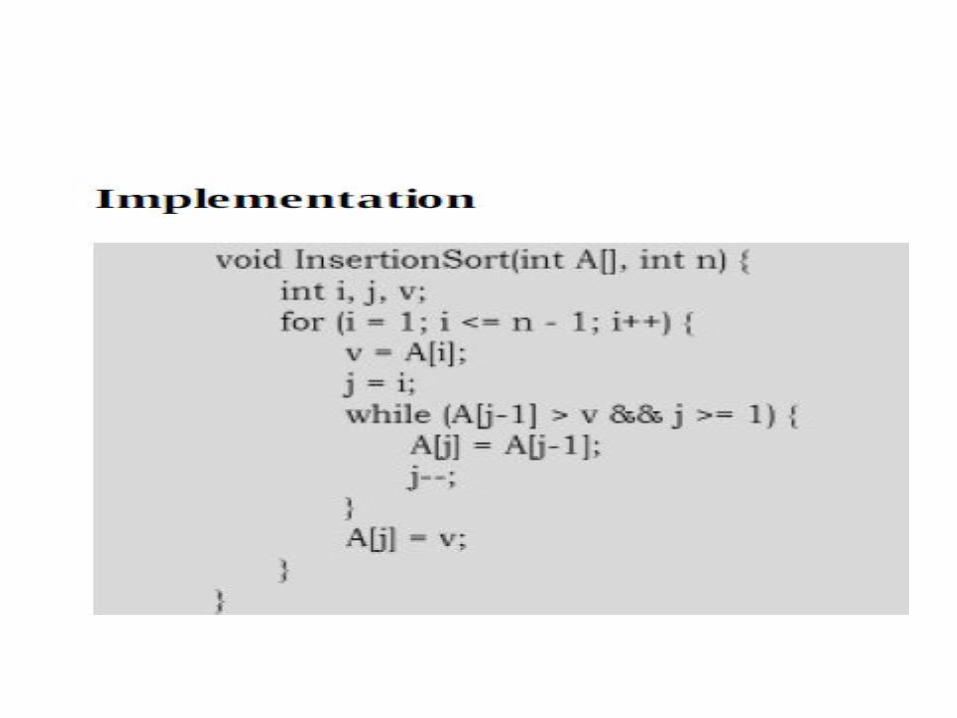
Algorithm
• Step 1 − If it is the first element, it is already sorted. return 1;
• Step 2 − Pick next element • Step 3 − Compare with all elements in the sorted
sub-list • Step 4 − Shift all the elements in the sorted sub-
list that is greater than the • value to be sorted • Step 5 − Insert the value • Step 6 − Repeat until list is sorted
• Algorithm • Every repetition of insertion sort removes an
element from the input data, and inserts it into the correct position in the already-sorted list until no input elements remain.
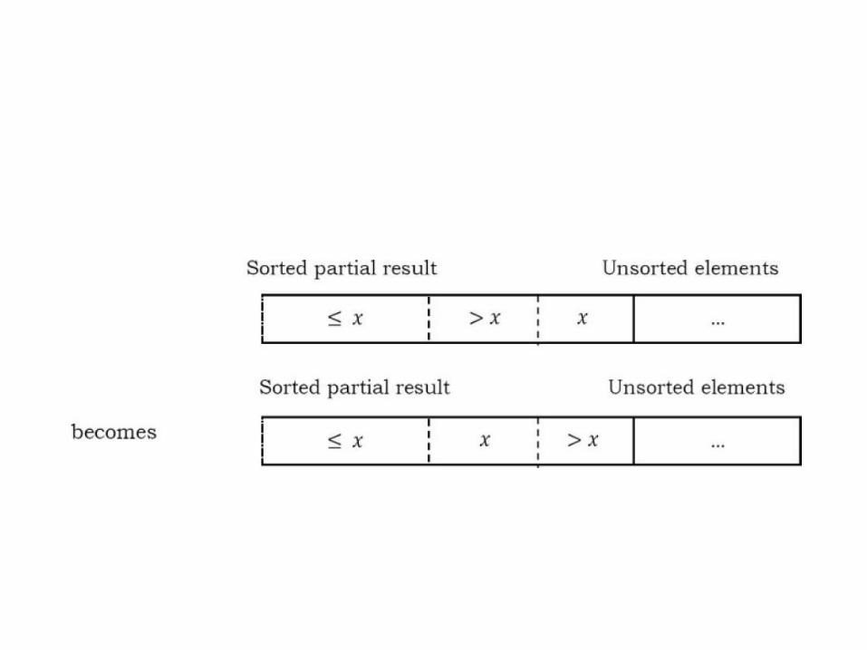
• Sorting is typically done in-place. • The resulting array after k iterations has the
property where the first k + 1 entries are sorted. • Each element greater than x is copied to the right
as it is compared against x.
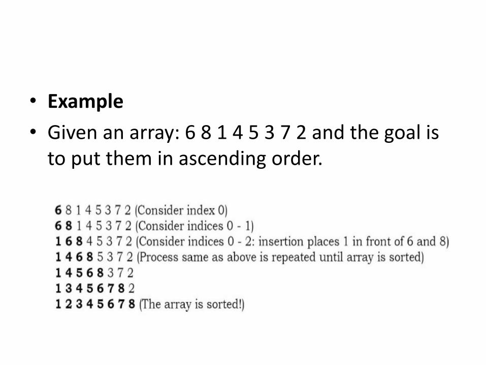
• Example
• Given an array: 6 8 1 4 5 3 7 2 and the goal is to put them in ascending order.
• Analysis
• Worst case analysis
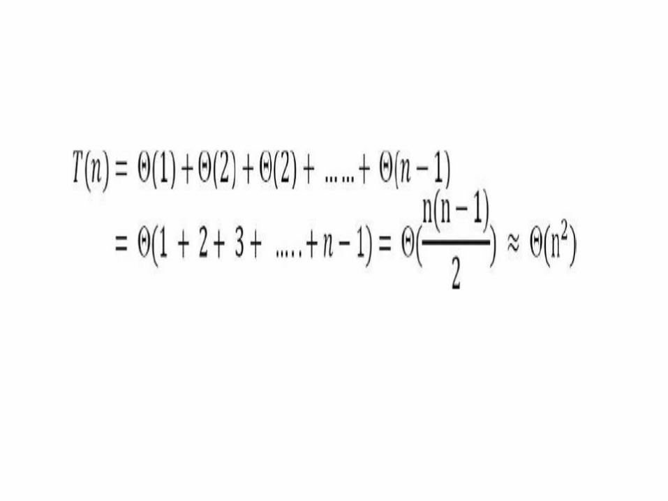
• Worst case occurs when for every i the inner loop has to move all elements A[1], . . . , A[i – 1] (which happens when A[i] = key is smaller than all of them), that takes Θ(i – 1) time.
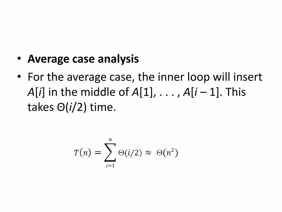
• Average case analysis
• For the average case, the inner loop will insert A[i] in the middle of A[1], . . . , A[i – 1]. This takes Θ(i/2) time.
• Performance
• If every element is greater than or equal to every element to its left, the running time of insertion sort is Θ(n).
• This situation occurs if the array starts out already sorted, and so an already-sorted array is the best case for insertion sort.
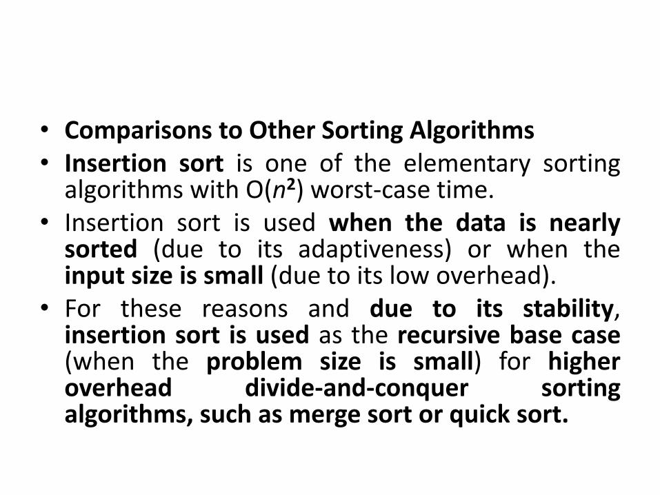
• Comparisons to Other Sorting Algorithms • Insertion sort is one of the elementary sorting
algorithms with O(n2) worst-case time. • Insertion sort is used when the data is nearly
sorted (due to its adaptiveness) or when the input size is small (due to its low overhead).
• For these reasons and due to its stability, insertion sort is used as the recursive base case (when the problem size is small) for higher overhead divide-and-conquer sorting algorithms, such as merge sort or quick sort.
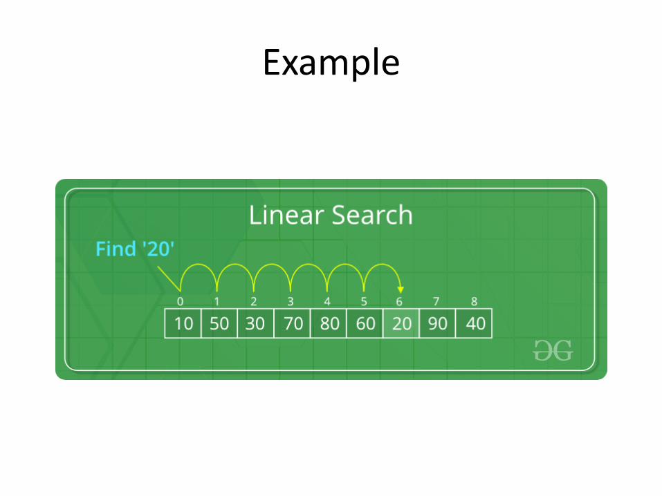
Linear Search
• Let us assume we are given an array where the order of the elements is not known.
• Means the elements of the array are not sorted.
• Here we have to scan the complete array and see if the element is there in the given list or not
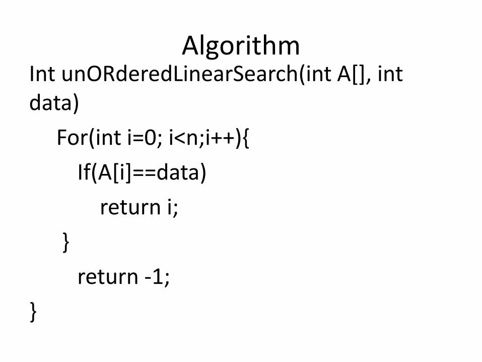
Algorithm Int unORderedLinearSearch(int A[], int data)
For(int i=0; i<n;i++){
If(A[i]==data)
return i;
}
return -1;
}
Complexity
• Time Complexity: O(n)
• In the worst case we need to scan the complete array.
• Space Complexity: O(1)

Algorithm
Int orderedLinearSearch(int A[], int n, int data){ for(int i=0; i<n ; i++){ if(A[i]==data) return i; else if(A[i] > data) return -1; } return -1; }
Example
Complexity
• Time Complexity:O(n), in worst we scan the complete array.
• Space Complexity: O(1).

Merge Sort
• Merge sort is an example of the divide and conquer strategy.
• Merging is the process of combining two sorted files to make one bigger sorted file.
• Selection is the process of dividing a file into two parts: k smallest elements and n – k largest elements.
• Selection and merging are opposite operations
– selection splits a list into two lists
–merging joins two files to make one file
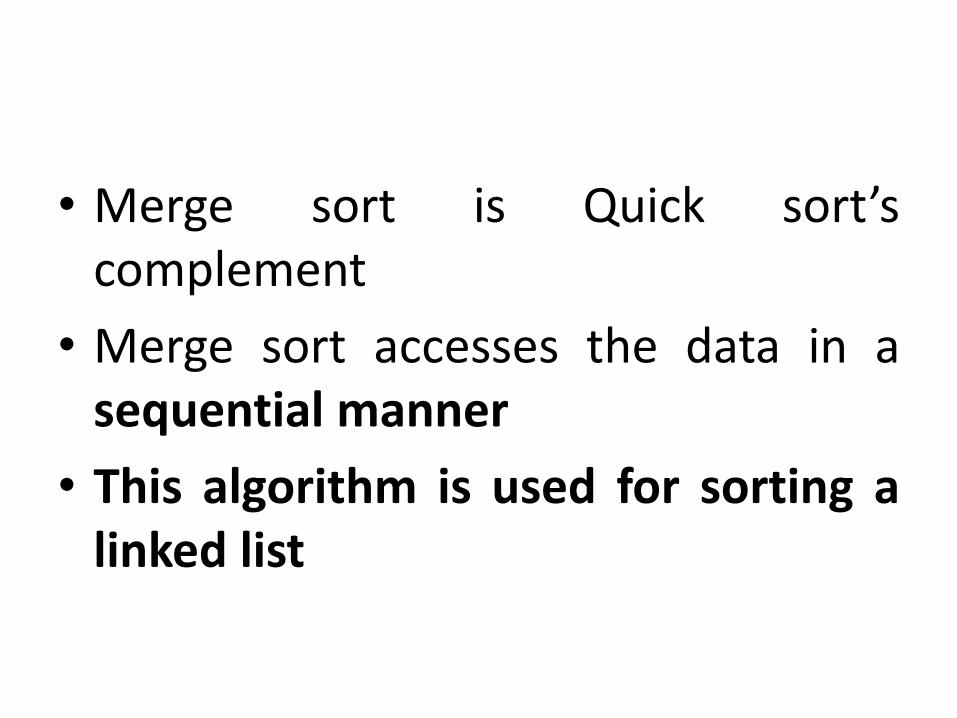
• Merge sort is Quick sort’s complement
• Merge sort accesses the data in a sequential manner
• This algorithm is used for sorting a linked list
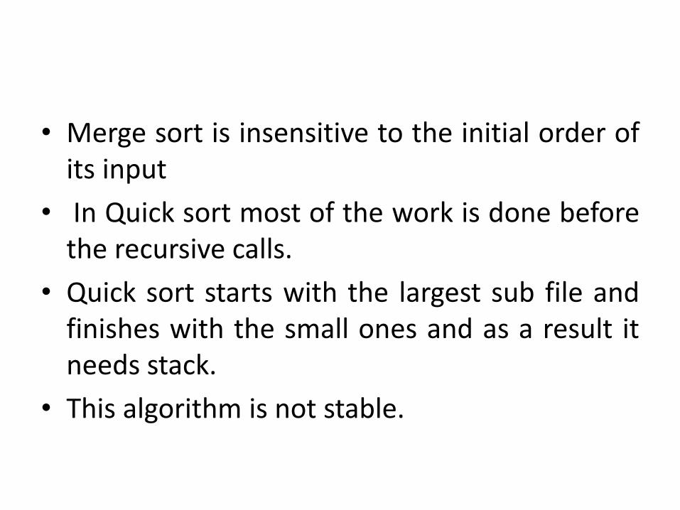
• Merge sort is insensitive to the initial order of its input
• In Quick sort most of the work is done before the recursive calls.
• Quick sort starts with the largest sub file and finishes with the small ones and as a result it needs stack.
• This algorithm is not stable.
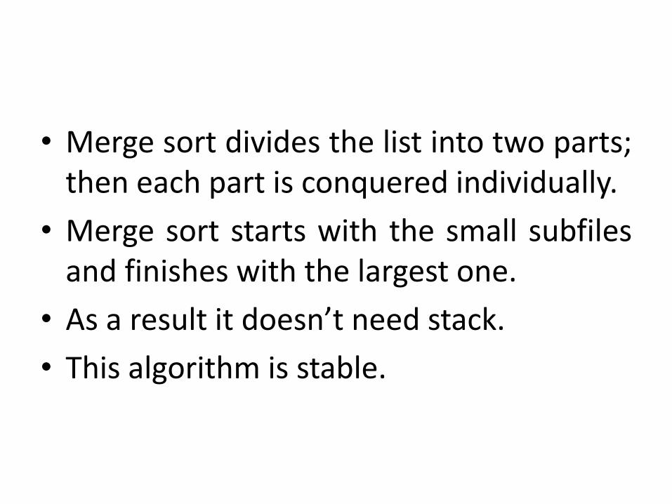
• Merge sort divides the list into two parts; then each part is conquered individually.
• Merge sort starts with the small subfiles and finishes with the largest one.
• As a result it doesn’t need stack.
• This algorithm is stable.
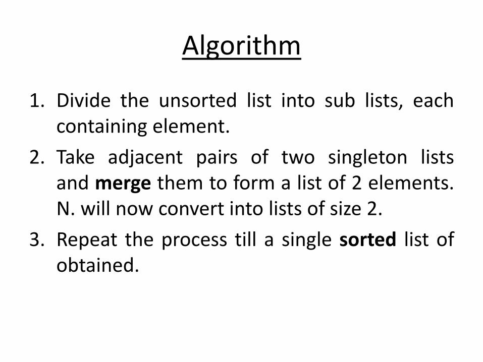
Algorithm
1. Divide the unsorted list into sub lists, each containing element.
2. Take adjacent pairs of two singleton lists and merge them to form a list of 2 elements. N. will now convert into lists of size 2.
3. Repeat the process till a single sorted list of obtained.
Algorithm
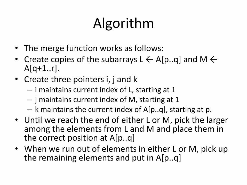
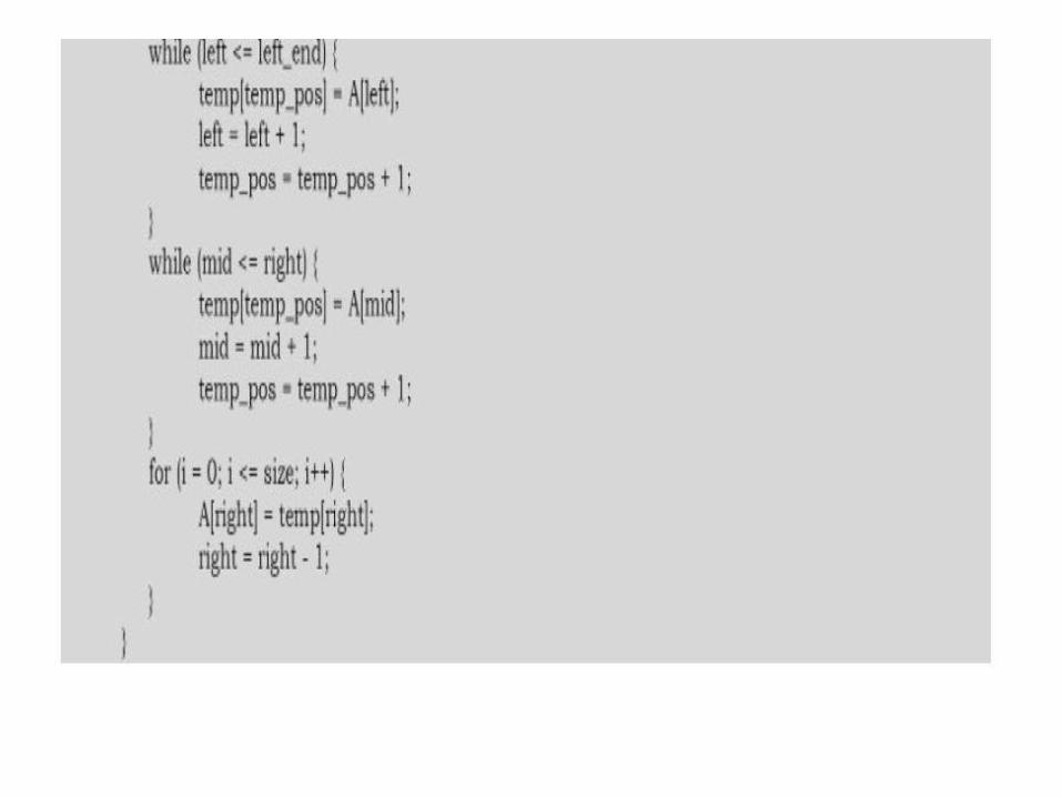
• The merge function works as follows: • Create copies of the subarrays L ← A[p..q] and M ←
A[q+1..r]. • Create three pointers i, j and k
– i maintains current index of L, starting at 1 – j maintains current index of M, starting at 1 – k maintains the current index of A[p..q], starting at p.
• Until we reach the end of either L or M, pick the larger among the elements from L and M and place them in the correct position at A[p..q]
• When we run out of elements in either L or M, pick up the remaining elements and put in A[p..q]
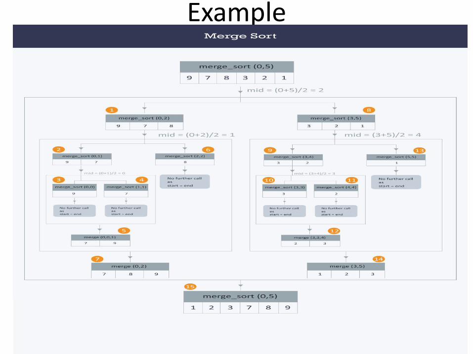
Example
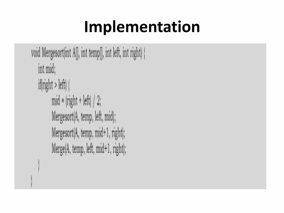
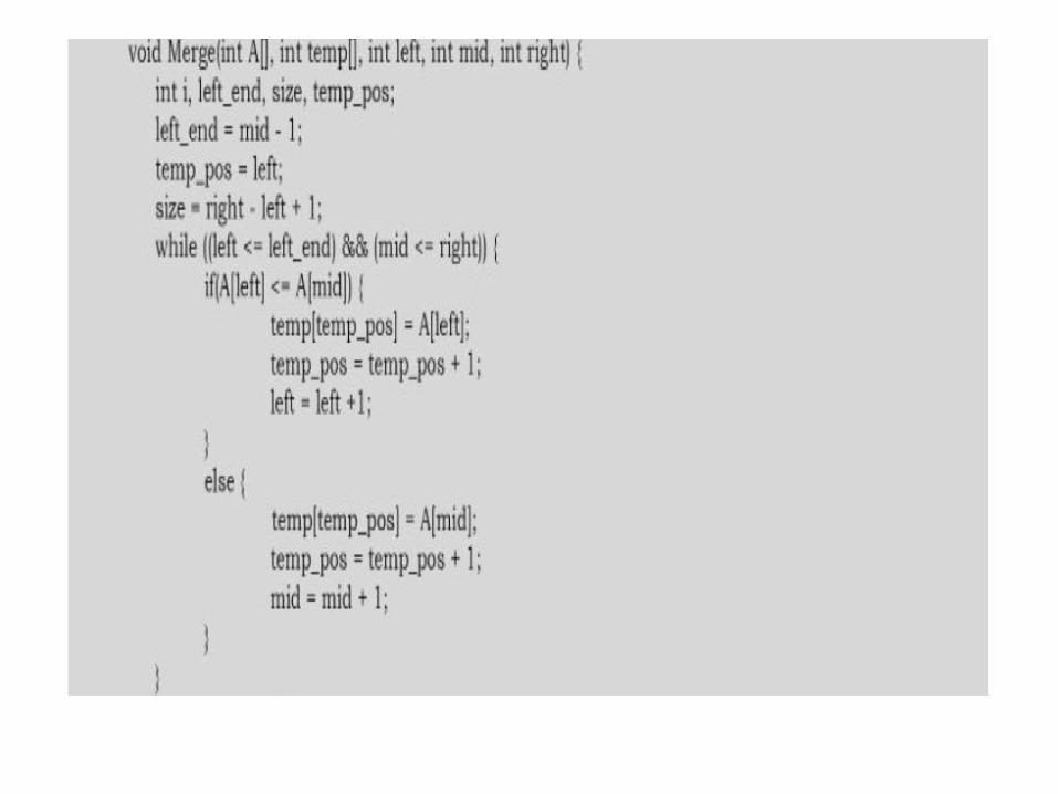
Implementation
Time Complexity
• Merge Sort is a stable sort which means that the same element in an array maintain their original positions with respect to each other.
• Overall time complexity of Merge sort is O(nLogn).
• It is more efficient as it is in worst case also the runtime is O(nlogn) The space complexity of Merge sort is O(n).
Analysis
• In Merge sort the input list is divided into two parts and these are solved recursively.
• After solving the sub problems, they are merged by scanning the resultant sub problems.
• Let us assume T(n) is the complexity of Merge sort with n elements.
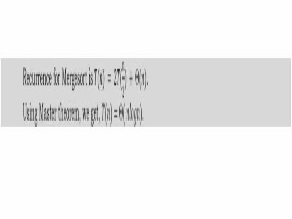
• The recurrence for the Merge Sort can be defined as:
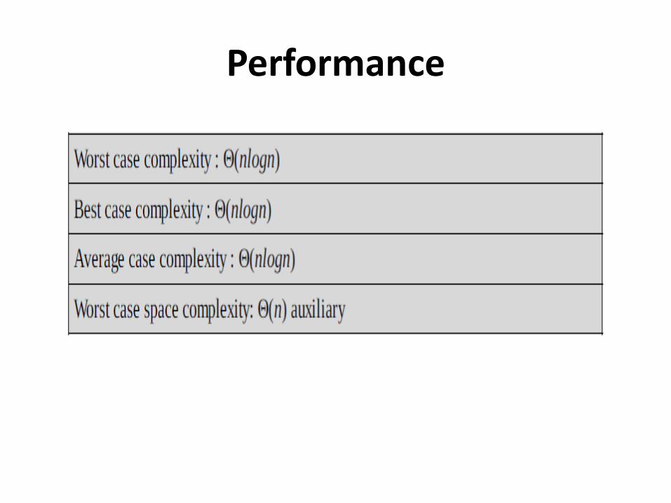
Performance

Quicksort
• Quick sort is an example of a divide-and-conquer algorithmic technique. It is also called partition exchange sort.
• It uses recursive calls for sorting the elements, and it is one of the famous algorithms among comparison-based sorting algorithms.
• Divide: The array A[low ...high] is partitioned into two non-empty sub arrays A[low ...q] and A[q + 1... high], such that each element of A[low ... high] is less than or equal to each element of A[q + 1... high].
• The index q is computed as part of this partitioning procedure.
• Conquer: The two sub arrays A[low ...q] and A[q + 1 ...high] are sorted by recursive calls to Quick sort.
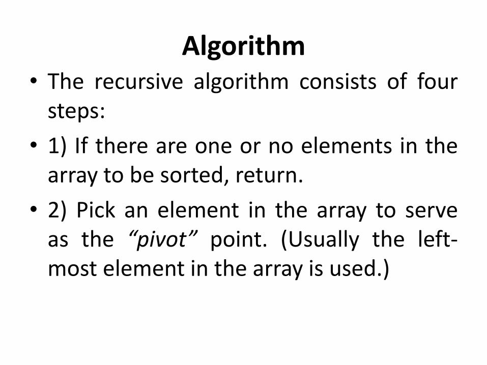
Algorithm • The recursive algorithm consists of four
steps:
• 1) If there are one or no elements in the array to be sorted, return.
• 2) Pick an element in the array to serve as the “pivot” point. (Usually the left-most element in the array is used.)
Algorithm
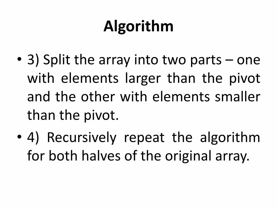
• 3) Split the array into two parts – one with elements larger than the pivot and the other with elements smaller than the pivot.
• 4) Recursively repeat the algorithm for both halves of the original array.
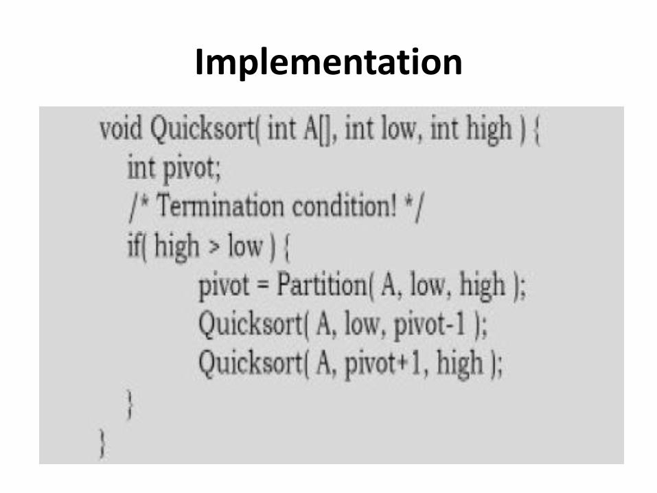
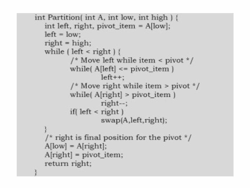
Implementation
Analysis
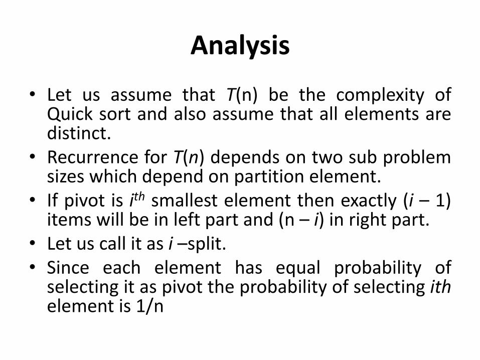
• Let us assume that T(n) be the complexity of Quick sort and also assume that all elements are distinct.
• Recurrence for T(n) depends on two sub problem sizes which depend on partition element.
• If pivot is ith smallest element then exactly (i – 1) items will be in left part and (n – i) in right part.
• Let us call it as i –split. • Since each element has equal probability of
selecting it as pivot the probability of selecting ith element is 1/n
• Best Case: Each partition splits array in halves and gives
• T(n) = 2T(n/2) + Θ(n) = Θ(nlogn), [using Divide and Conquer master theorem]
• Worst Case: Each partition gives unbalanced splits and we get
• T(n) = T(n – 1) + Θ(n) = Θ(n2)[using Subtraction and Conquer master theorem]
• The worst-case occurs when the list is already sorted and last element chosen as pivot.
• Average Case: In the average case of Quick sort, we do not know where the split happens.
• For this reason, we take all possible values of split locations, add all their complexities and divide with n to get the average case complexity.
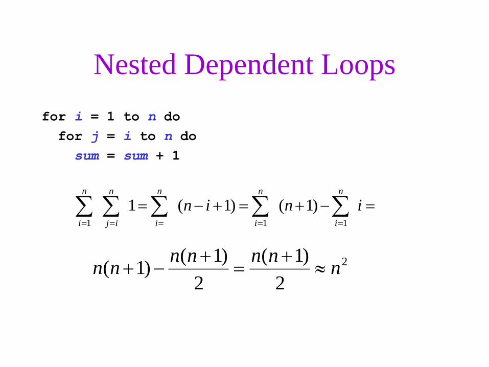
Nested Dependent Loops
for i = 1 to n do
for j = i to n do
sum = sum + 1
ininn
i
n
i
n
i
n
ij
n
i 111
)1()1(1
2
2
)1(
2
)1()1( n
nnnnnn
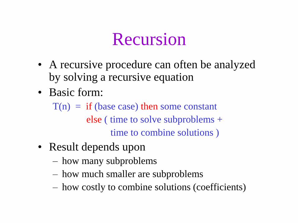
Recursion
• A recursive procedure can often be analyzed by solving a recursive equation
• Basic form:
T(n) = if (base case) then some constant
else ( time to solve subproblems +
time to combine solutions )
• Result depends upon
– how many subproblems
– how much smaller are subproblems
– how costly to combine solutions (coefficients)
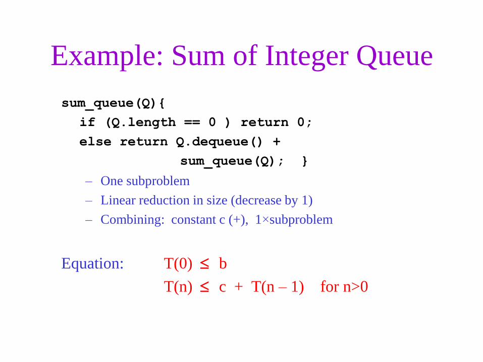
Example: Sum of Integer Queue
sum_queue(Q){
if (Q.length == 0 ) return 0;
else return Q.dequeue() +
sum_queue(Q); }
– One subproblem
– Linear reduction in size (decrease by 1)
– Combining: constant c (+), 1×subproblem
Equation: T(0) b
T(n) c + T(n – 1) for n>0
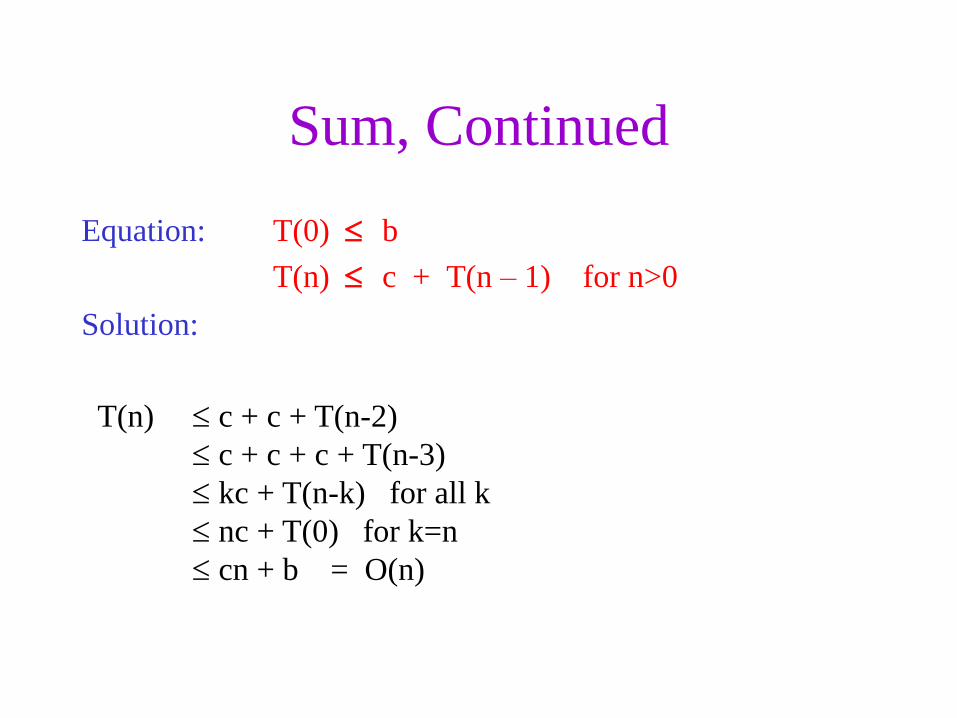
Sum, Continued
Equation: T(0) b
T(n) c + T(n – 1) for n>0
Solution:
T(n) c + c + T(n-2)
c + c + c + T(n-3)
kc + T(n-k) for all k
nc + T(0) for k=n
cn + b = O(n)
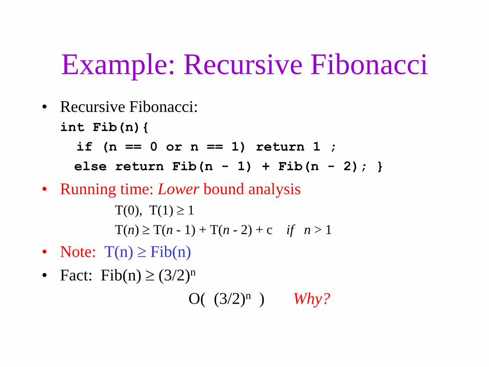
Example: Recursive Fibonacci
• Recursive Fibonacci:
int Fib(n){
if (n == 0 or n == 1) return 1 ;
else return Fib(n - 1) + Fib(n - 2); }
• Running time: Lower bound analysis
T(0), T(1) 1
T(n) T(n - 1) + T(n - 2) + c if n > 1
• Note: T(n) Fib(n)
• Fact: Fib(n) (3/2)n
O( (3/2)n ) Why?
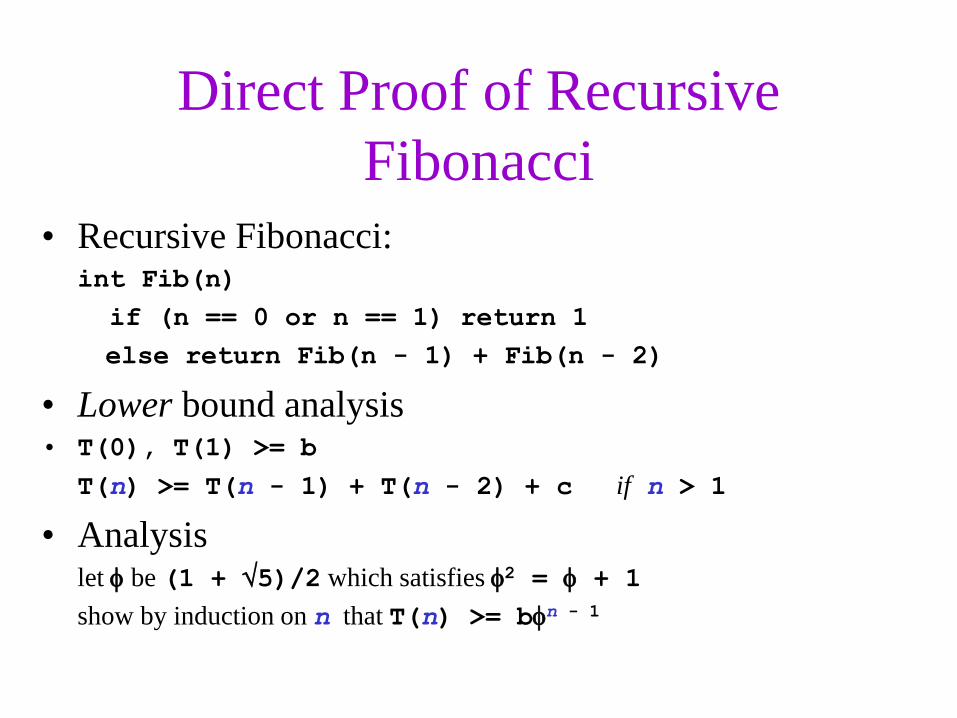
Direct Proof of Recursive
Fibonacci
• Recursive Fibonacci: int Fib(n)
if (n == 0 or n == 1) return 1
else return Fib(n - 1) + Fib(n - 2)
• Lower bound analysis • T(0), T(1) >= b
T(n) >= T(n - 1) + T(n - 2) + c if n > 1
• Analysis let be (1 + 5)/2 which satisfies 2 = + 1
show by induction on n that T(n) >= bn - 1
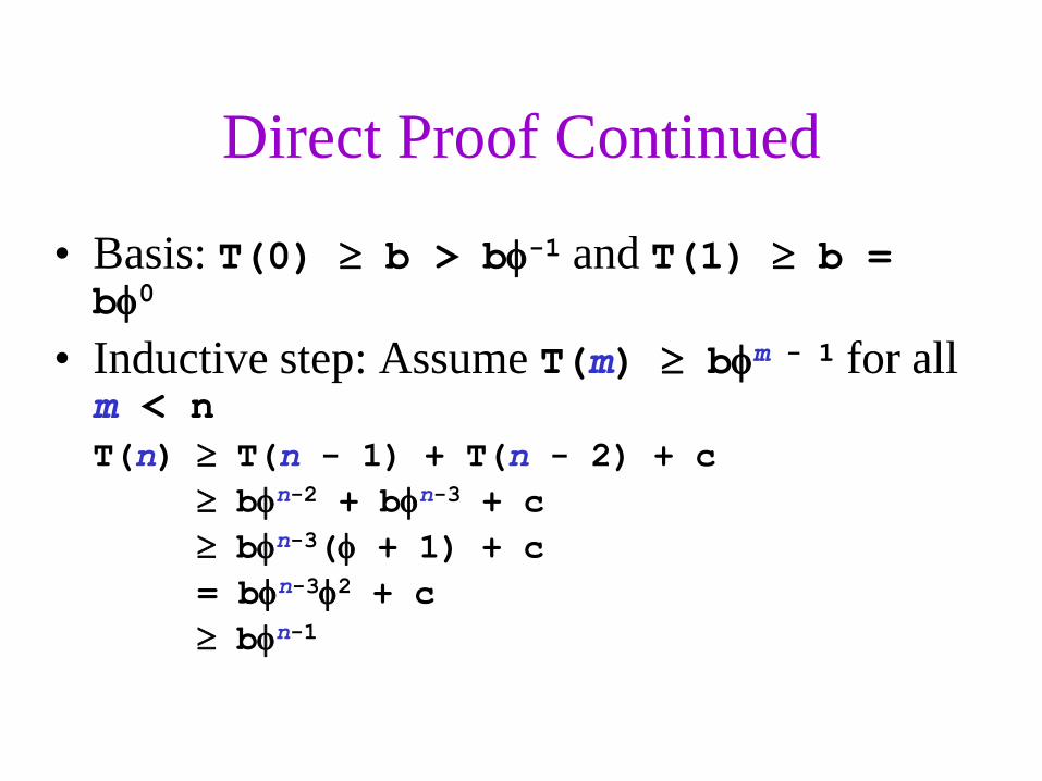
Direct Proof Continued
• Basis: T(0) b > b-1 and T(1) b = b0
• Inductive step: Assume T(m) bm - 1 for all m < n
T(n) T(n - 1) + T(n - 2) + c
bn-2 + bn-3 + c
bn-3( + 1) + c
= bn-32 + c
bn-1
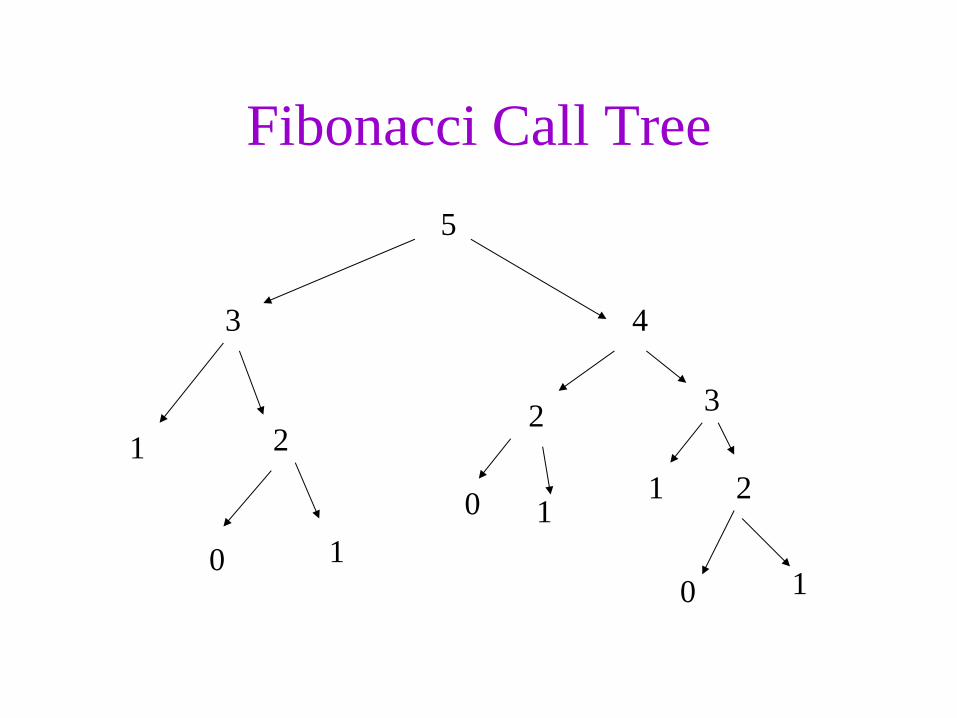
Fibonacci Call Tree
5
3
1 2
0 1
4
2
0 1
3
1 2
0 1
9
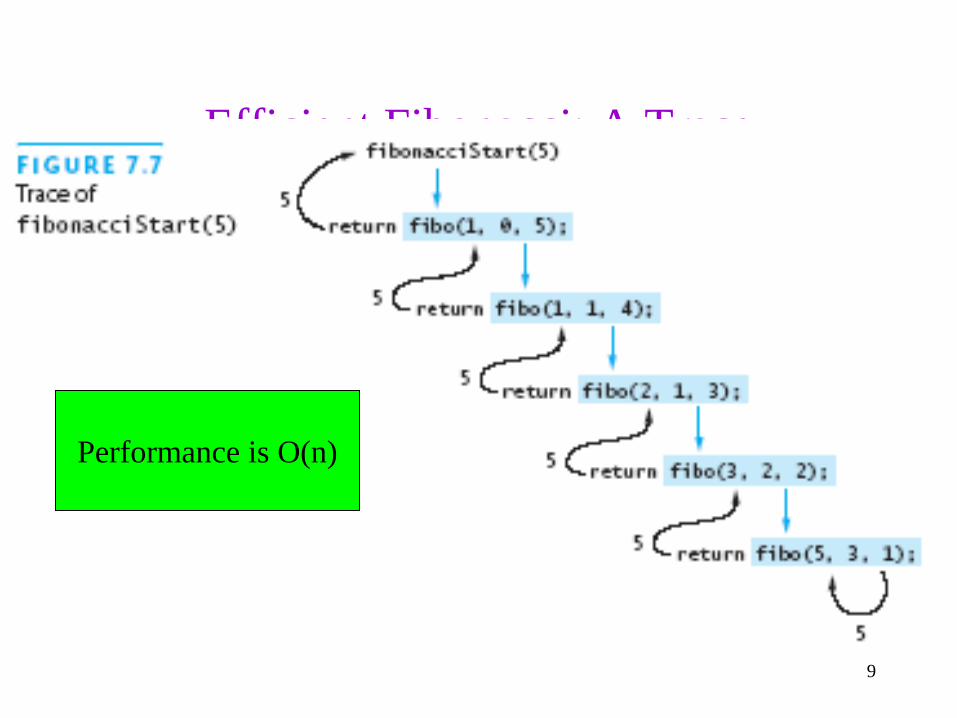
Efficient Fibonacci: A Trace
Performance is O(n)
Chapter 7: Recursion 10
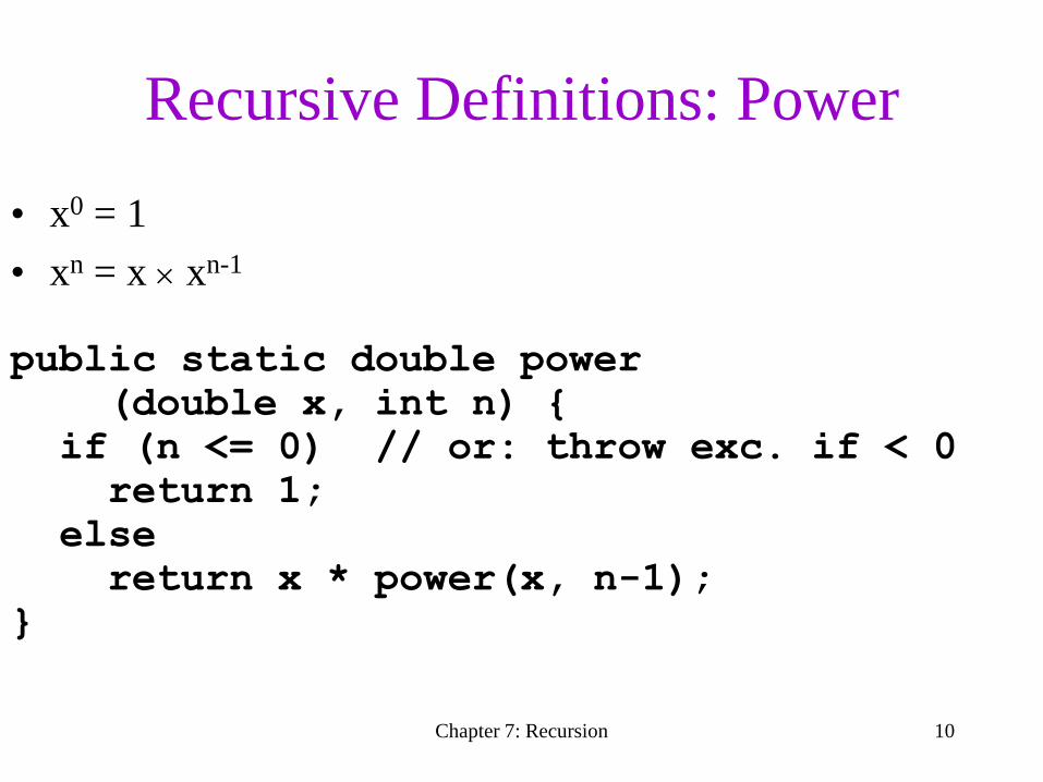
Recursive Definitions: Power
• x0 = 1
• xn = x xn-1
public static double power
(double x, int n) {
if (n <= 0) // or: throw exc. if < 0
return 1;
else
return x * power(x, n-1);
}
Chapter 7: Recursion 11
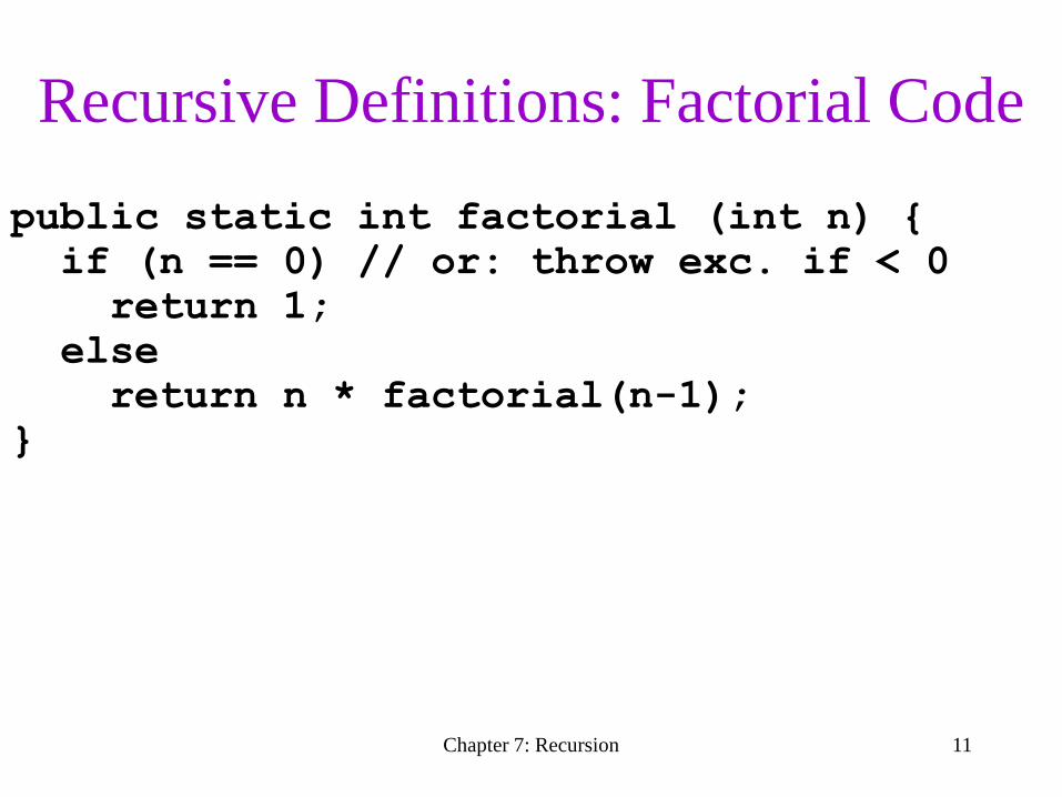
public static int factorial (int n) {
if (n == 0) // or: throw exc. if < 0
return 1;
else
return n * factorial(n-1);
}
Recursive Definitions: Factorial Code
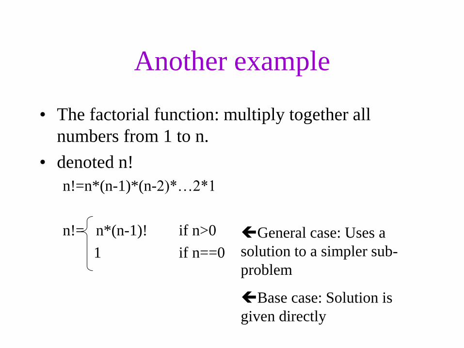
Another example
• The factorial function: multiply together all
numbers from 1 to n.
• denoted n!
n!=n*(n-1)*(n-2)*…2*1
n!= n*(n-1)! if n>0
1 if n==0
General case: Uses a
solution to a simpler sub-
problem
Base case: Solution is
given directly
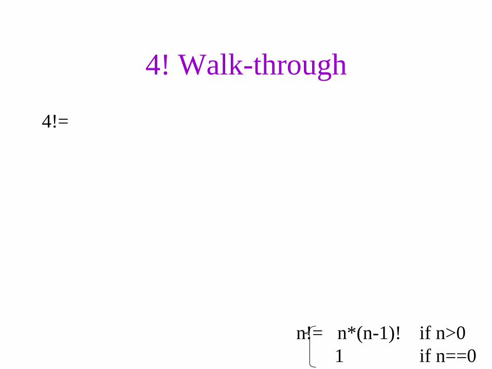
4! Walk-through
4!=
n!= n*(n-1)! if n>0
1 if n==0
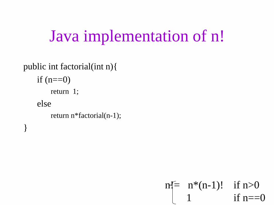
Java implementation of n!
public int factorial(int n){
if (n==0)
return 1;
else
return n*factorial(n-1);
}
n!= n*(n-1)! if n>0
1 if n==0
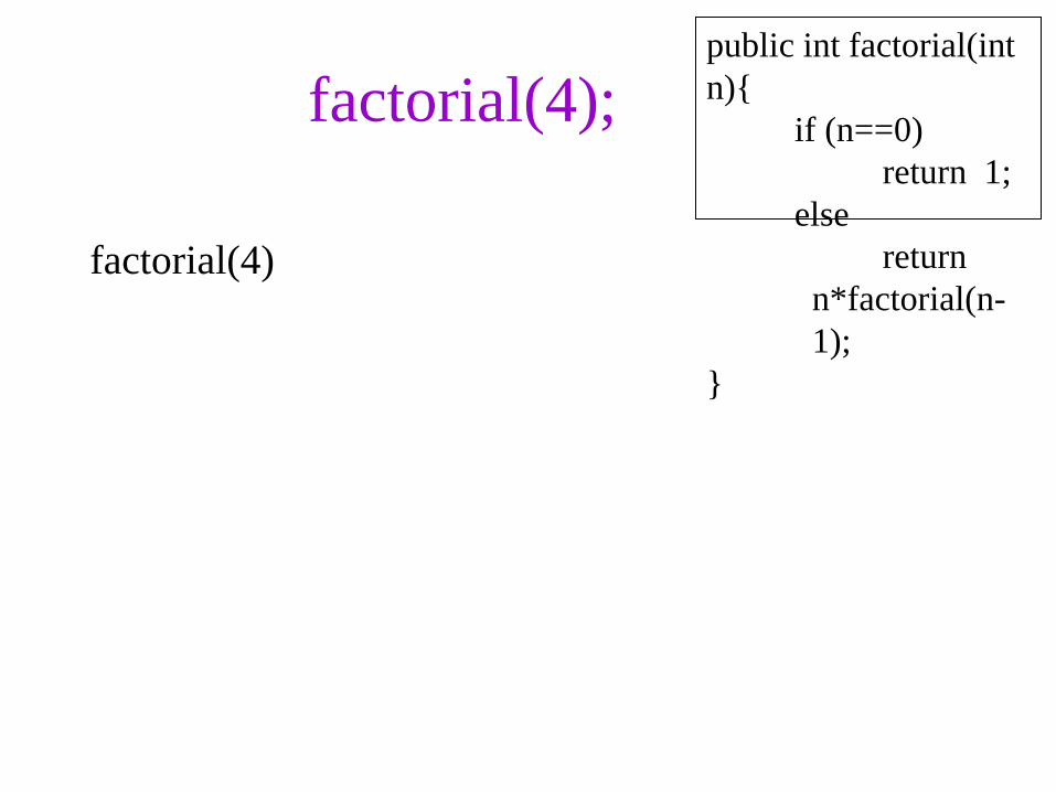
factorial(4);
factorial(4)
public int factorial(int
n){
if (n==0)
return 1;
else
return
n*factorial(n-
1);
}
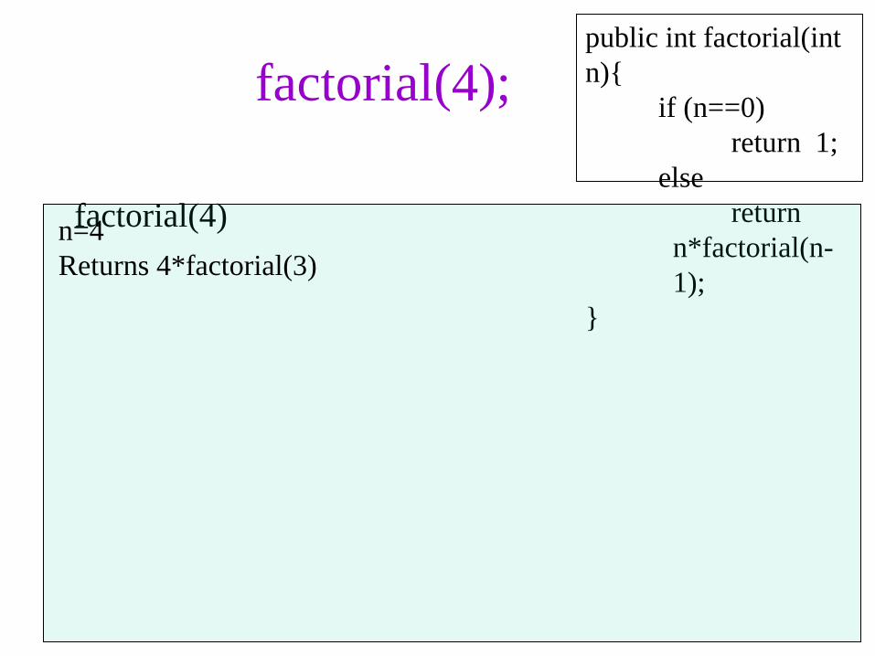
factorial(4);
factorial(4)
public int factorial(int
n){
if (n==0)
return 1;
else
return
n*factorial(n-
1);
}
n=4
Returns 4*factorial(3)
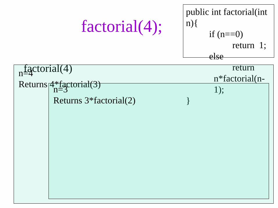
factorial(4);
factorial(4)
public int factorial(int
n){
if (n==0)
return 1;
else
return
n*factorial(n-
1);
}
n=4
Returns 4*factorial(3) n=3
Returns 3*factorial(2)

factorial(4);
factorial(4)
public int factorial(int
n){
if (n==0)
return 1;
else
return
n*factorial(n-
1);
}
n=4
Returns 4*factorial(3) n=3
Returns 3*factorial(2) n=2
Returns 2*factorial(1)
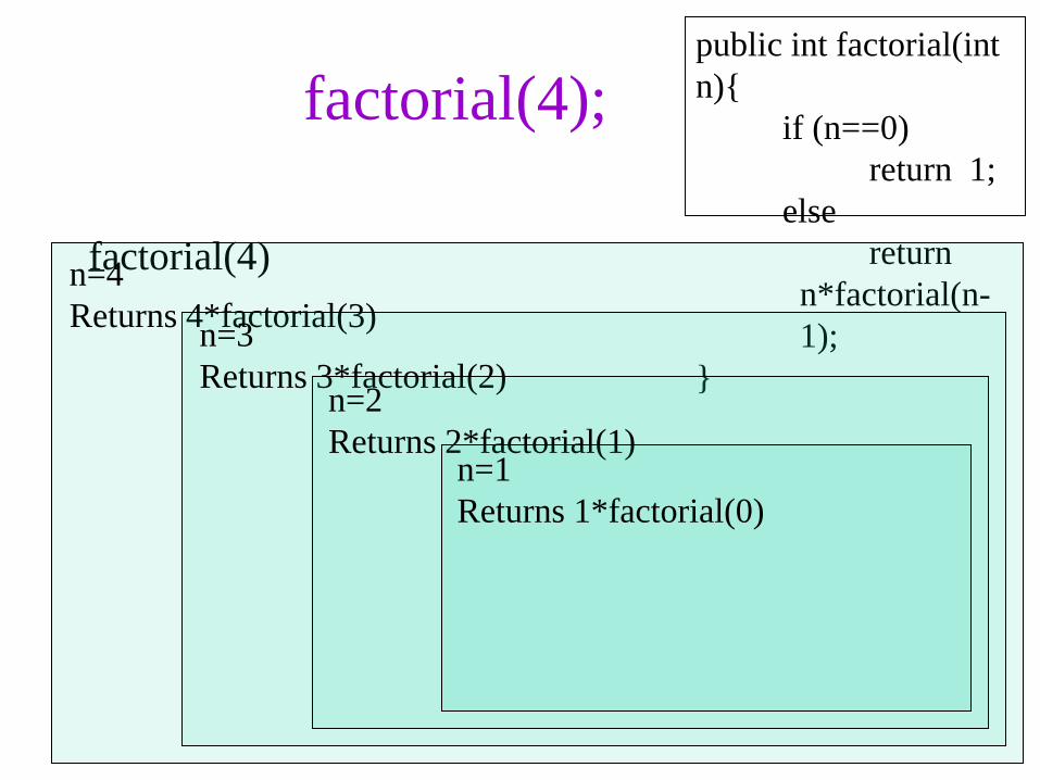
factorial(4);
factorial(4)
public int factorial(int
n){
if (n==0)
return 1;
else
return
n*factorial(n-
1);
}
n=4
Returns 4*factorial(3) n=3
Returns 3*factorial(2) n=2
Returns 2*factorial(1) n=1
Returns 1*factorial(0)
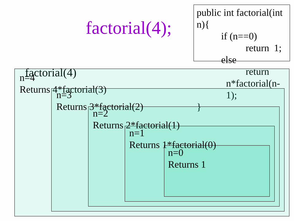
factorial(4);
factorial(4)
public int factorial(int
n){
if (n==0)
return 1;
else
return
n*factorial(n-
1);
}
n=4
Returns 4*factorial(3) n=3
Returns 3*factorial(2) n=2
Returns 2*factorial(1) n=1
Returns 1*factorial(0) n=0
Returns 1

factorial(4);
factorial(4)
public int factorial(int
n){
if (n==0)
return 1;
else
return
n*factorial(n-
1);
}
n=4
Returns 4*factorial(3) n=3
Returns 3*factorial(2) n=2
Returns 2*factorial(1) n=1
Returns 1*factorial(0) 1
factorial(4);
factorial(4)
public int factorial(int
n){
if (n==0)
return 1;
else
return
n*factorial(n-
1);
}
n=4
Returns 4*factorial(3) n=3
Returns 3*factorial(2) n=2
Returns 2*factorial(1) 1

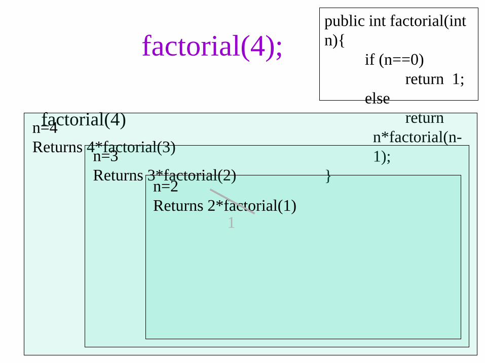
factorial(4);
factorial(4)
public int factorial(int
n){
if (n==0)
return 1;
else
return
n*factorial(n-
1);
}
n=4
Returns 4*factorial(3) n=3
Returns 3*factorial(2) 2
factorial(4);
factorial(4)
public int factorial(int
n){
if (n==0)
return 1;
else
return
n*factorial(n-
1);
}
n=4
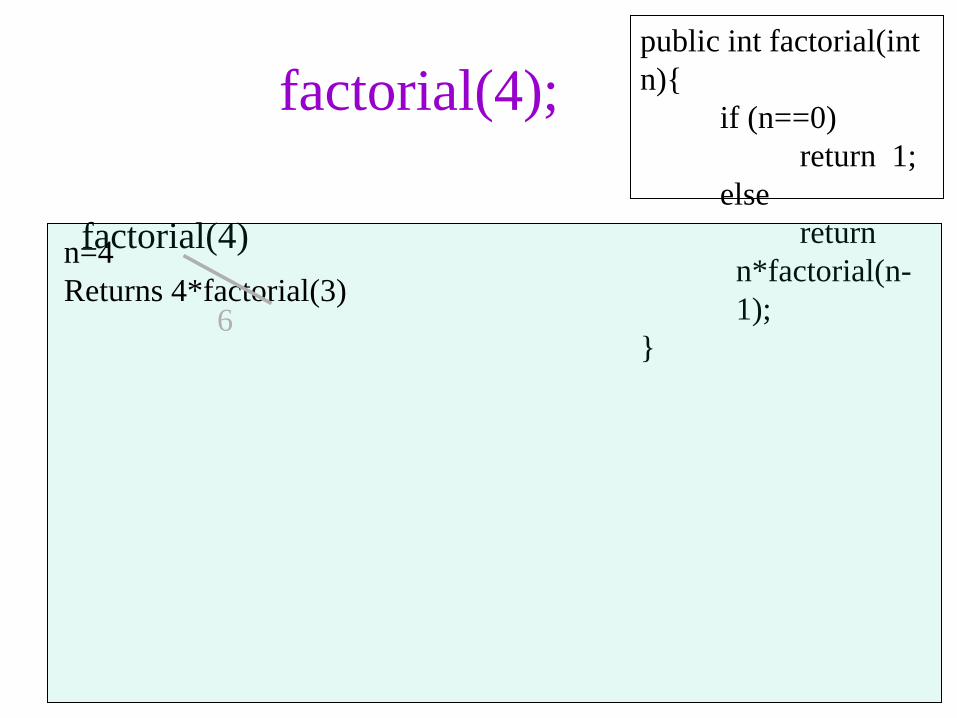
Returns 4*factorial(3) 6
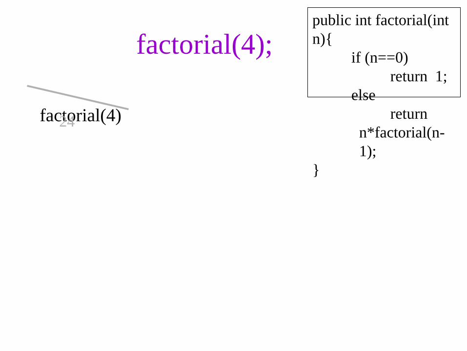
factorial(4);
factorial(4)
public int factorial(int
n){
if (n==0)
return 1;
else
return
n*factorial(n-
1);
}
24
Chapter 7: Recursion 26
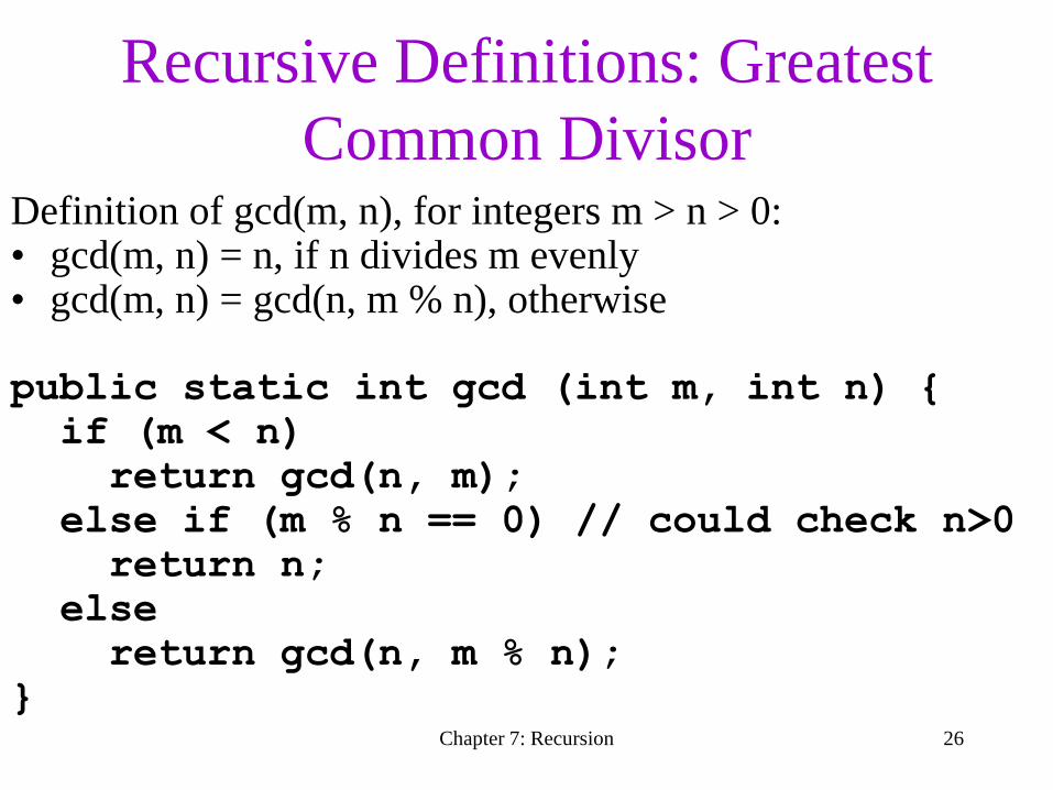
Recursive Definitions: Greatest
Common Divisor Definition of gcd(m, n), for integers m > n > 0: • gcd(m, n) = n, if n divides m evenly • gcd(m, n) = gcd(n, m % n), otherwise
public static int gcd (int m, int n) {
if (m < n)
return gcd(n, m);
else if (m % n == 0) // could check n>0
return n;
else
return gcd(n, m % n);
}
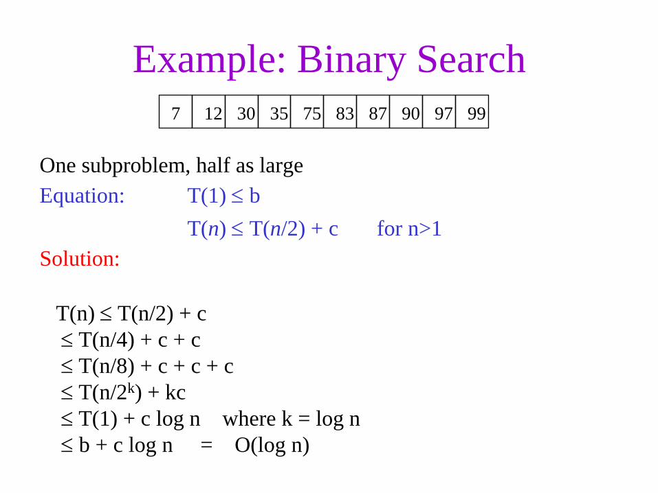
Example: Binary Search
One subproblem, half as large
Equation: T(1) b
T(n) T(n/2) + c for n>1
Solution:
7 12 30 35 75 83 87 90 97 99
T(n) T(n/2) + c
T(n/4) + c + c
T(n/8) + c + c + c
T(n/2k) + kc
T(1) + c log n where k = log n
b + c log n = O(log n)
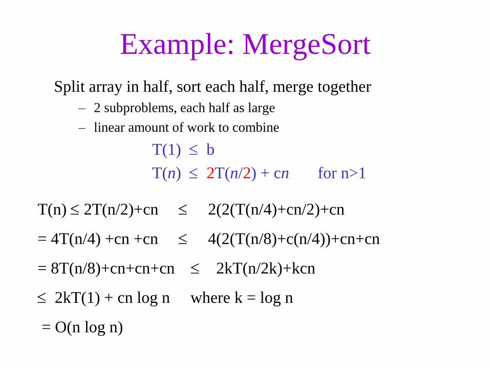
Example: MergeSort
Split array in half, sort each half, merge together
– 2 subproblems, each half as large
– linear amount of work to combine
T(1) b
T(n) 2T(n/2) + cn for n>1
T(n) 2T(n/2)+cn 2(2(T(n/4)+cn/2)+cn
= 4T(n/4) +cn +cn 4(2(T(n/8)+c(n/4))+cn+cn
= 8T(n/8)+cn+cn+cn 2kT(n/2k)+kcn
2kT(1) + cn log n where k = log n
= O(n log n)
Chapter 7: Recursion 29
Recursion Versus Iteration
• Recursion and iteration are similar
• Iteration:
– Loop repetition test determines whether to exit
• Recursion:
– Condition tests for a base case
• Can always write iterative solution to a problem solved
recursively, but:
• Recursive code often simpler than iterative
– Thus easier to write, read, and debug

Searching
Definition
• Searching is the process of finding an item with specified properties from a collection of items.
• The items may be stored as
– Records in a database
– Simple data elements in arrays
– Text in files
– Nodes in trees
Etc
Purpose of Searching
• Computers store a lot of information.
• To retrieve information proficiently searching algorithms are used.
Types of searching
• Unordered Linear Serarch
• Sorted/Ordered Linear Search
• Binary Search
Unordered Linear Search
• Let us assume we are given an array where the order of the elements is not known.
• Means the elements of the array are not sorted.
• Here we have to scan the complete array and see if the element is there in the given list or not

Algorithm Int unORderedLinearSearch(int A[], int data)
For(int i=0; i<n;i++){
If(A[i]==data)
return i;
}
return -1;
}
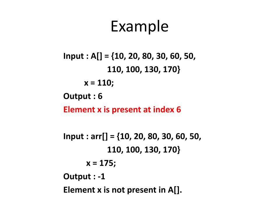
Example
Input : A[] = {10, 20, 80, 30, 60, 50,
110, 100, 130, 170}
x = 110;
Output : 6
Element x is present at index 6
Input : arr[] = {10, 20, 80, 30, 60, 50,
110, 100, 130, 170}
x = 175;
Output : -1
Element x is not present in A[].

Complexity
• Time Complexity: O(n)
• In the worst case we need to scan the complete array.
• Space Complexity: O(1)
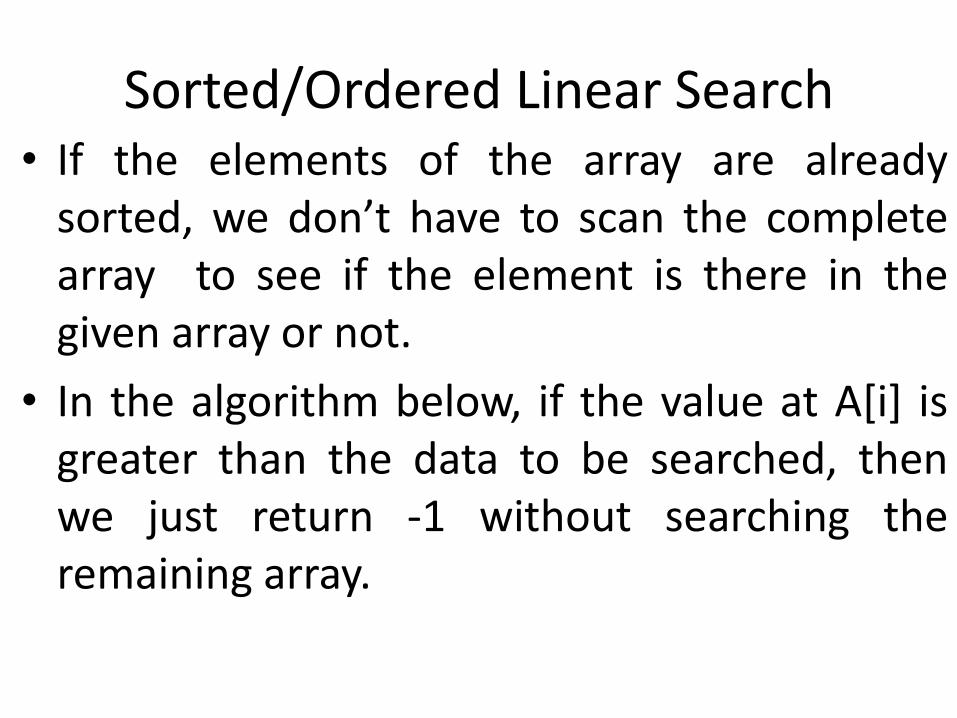
Sorted/Ordered Linear Search • If the elements of the array are already
sorted, we don’t have to scan the complete array to see if the element is there in the given array or not.
• In the algorithm below, if the value at A[i] is greater than the data to be searched, then we just return -1 without searching the remaining array.
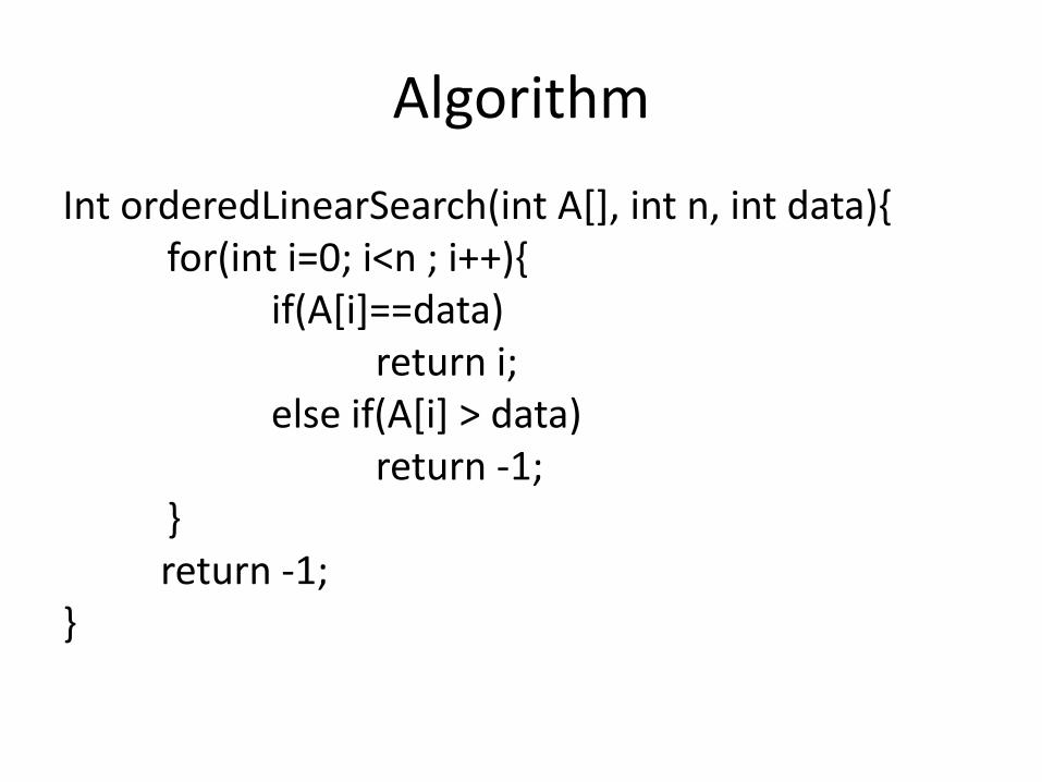
Algorithm
Int orderedLinearSearch(int A[], int n, int data){ for(int i=0; i<n ; i++){ if(A[i]==data) return i; else if(A[i] > data) return -1; } return -1; }

Example

Complexity
• Time Complexity:O(n), in worst we scan the complete array.
• Space Complexity: O(1).
Binary Search
• Let us consider the problem of searching a word in a dictionary.
• It works on the principle of divide and conquer technique.
• We go to some approximate page(say, middle page) and start searching from that point.
• If the name that we are searching is the same then the search is complete.
• If the page is before the selected pages then apply the same process for the first half; otherwise apply the same to the second half.
• Binary search also works in the same way.
• The algorithm applying such a strategy is referred to as binary search algorithm
Mid = low + (high-low)/2
or
Mid= (low+high)/2
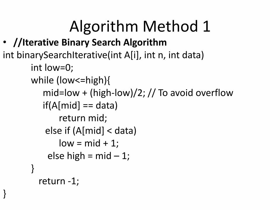
Algorithm Method 1 • //Iterative Binary Search Algorithm int binarySearchIterative(int A[i], int n, int data) int low=0; while (low<=high){ mid=low + (high-low)/2; // To avoid overflow if(A[mid] == data) return mid; else if (A[mid] < data) low = mid + 1; else high = mid – 1; } return -1; }
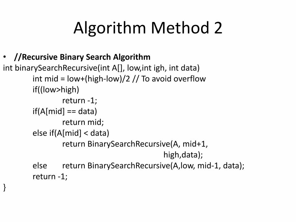
Algorithm Method 2
• //Recursive Binary Search Algorithm int binarySearchRecursive(int A[], low,int igh, int data) int mid = low+(high-low)/2 // To avoid overflow if((low>high) return -1; if(A[mid] == data) return mid; else if(A[mid] < data) return BinarySearchRecursive(A, mid+1, high,data); else return BinarySearchRecursive(A,low, mid-1, data); return -1; }
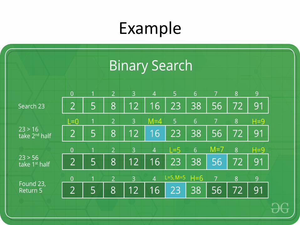
Example
Advantages & Disadvantages
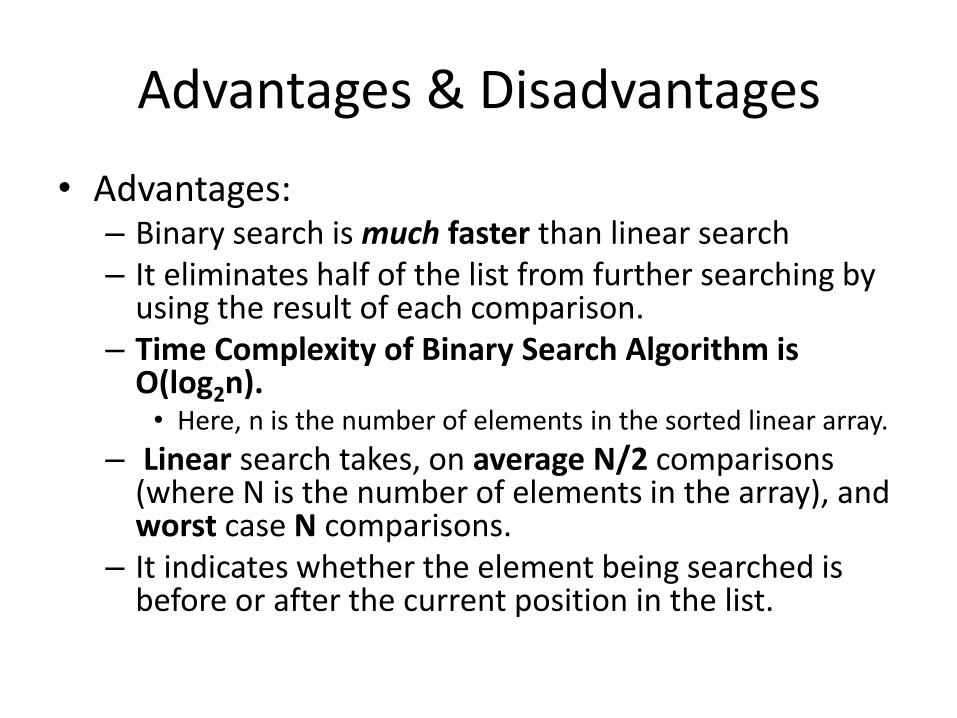
• Advantages: – Binary search is much faster than linear search – It eliminates half of the list from further searching by
using the result of each comparison. – Time Complexity of Binary Search Algorithm is
O(log2n). • Here, n is the number of elements in the sorted linear array.
– Linear search takes, on average N/2 comparisons (where N is the number of elements in the array), and worst case N comparisons.
– It indicates whether the element being searched is before or after the current position in the list.
• Disadvantages
– It works only on lists that are sorted and kept sorted.
– It works only on element types for which there exists a less-than(<) relationship.
– It employs recursive approach which requires more stack space.

Selection Sort
• Selection sort is an in-place sorting algorithm. Selection sort works well for small files.
• It is for sorting the files with very large values used and small keys.
• This is because selection is made based on keys and swaps are made only when required.
Advantages
• Easy to implement
• In-place sort (requires no additional storage space)
Disadvantages
•Doesn’t scale well: O(n2)
Algorithm
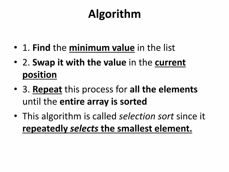
• 1. Find the minimum value in the list
• 2. Swap it with the value in the current position
• 3. Repeat this process for all the elements until the entire array is sorted
• This algorithm is called selection sort since it repeatedly selects the smallest element.
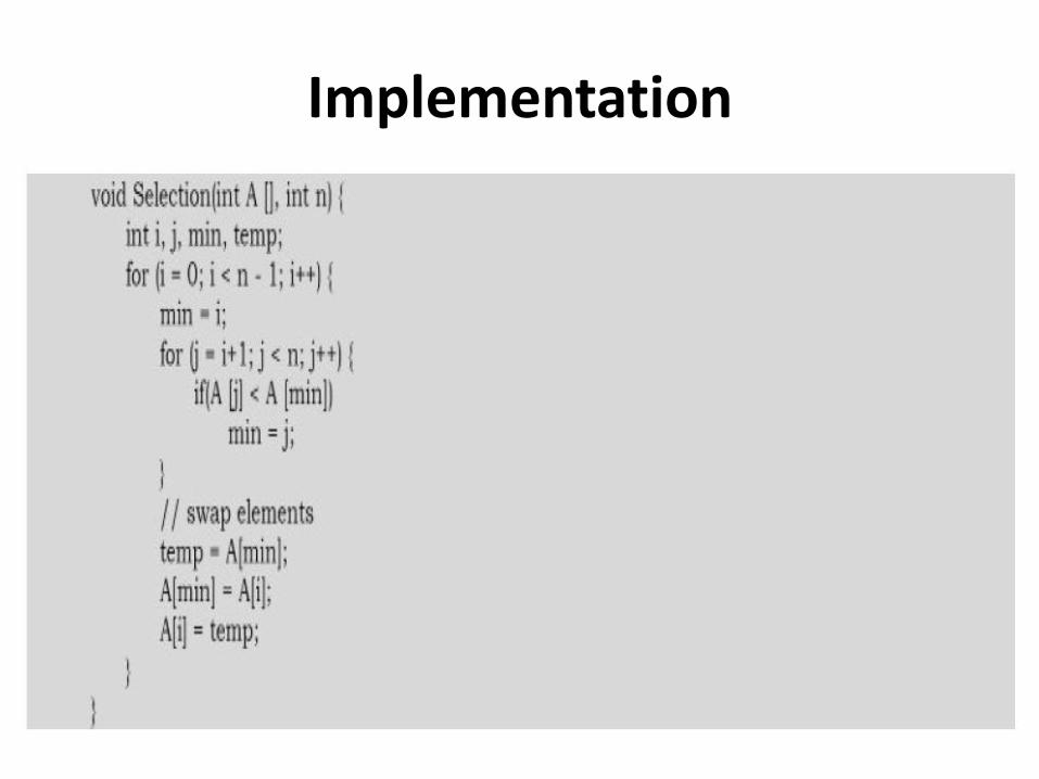
Implementation
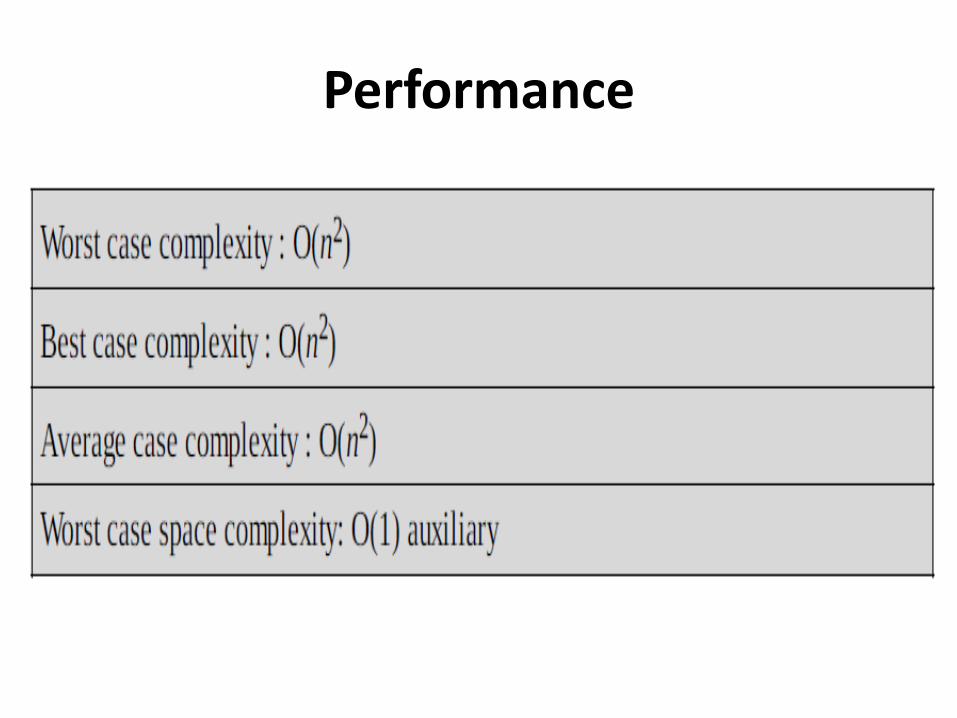
Performance

Sorting
Definition
• Sorting is an algorithm that arranges the elements of a list in a certain order [either ascending or descending].
• The output is a permutation or reordering of the input.
Why is Sorting Necessary?
• Sorting can significantly reduce the complexity of a problem.
• Used for database algorithms and searches.
Classifications
• sorting algorithms are classified into
–Internal Sort
–External Sort
Internal Sort
• Sort algorithms use main memory exclusively during the sort are called internal sorting algorithms.
• This kind of algorithm assumes high-speed random access to all memory.
• Bubble Sort.
• Insertion Sort.
• Quick Sort.
• Heap Sort.
• Radix Sort.
• Selection sort.
External Sort
• Sorting algorithms that use external memory, such as tape or disk, during the sort come under this category.
• Distribution sorting,
–which resembles quicksort,
• external merge sort,
–which resembles merge sort.
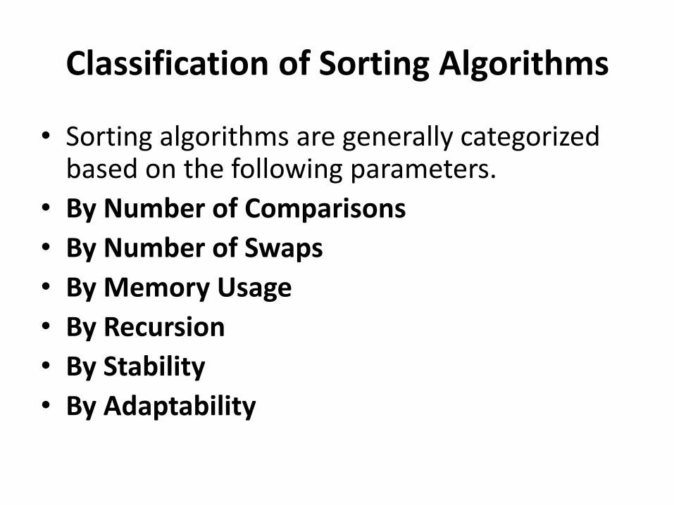
Classification of Sorting Algorithms
• Sorting algorithms are generally categorized based on the following parameters.
• By Number of Comparisons
• By Number of Swaps
• By Memory Usage
• By Recursion
• By Stability
• By Adaptability
Bubble Sort
• Bubble sort is the simplest sorting algorithm.
• It works by iterating the input array from the first element to the last, comparing each pair of elements and swapping them if needed.
• Bubble sort continues its iterations until no more swaps are needed.
• The algorithm gets its name from the way smaller elements “bubble” to the top of the list.
• The only significant advantage is that it can detect whether the input list is already sorted or not.
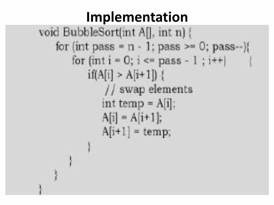
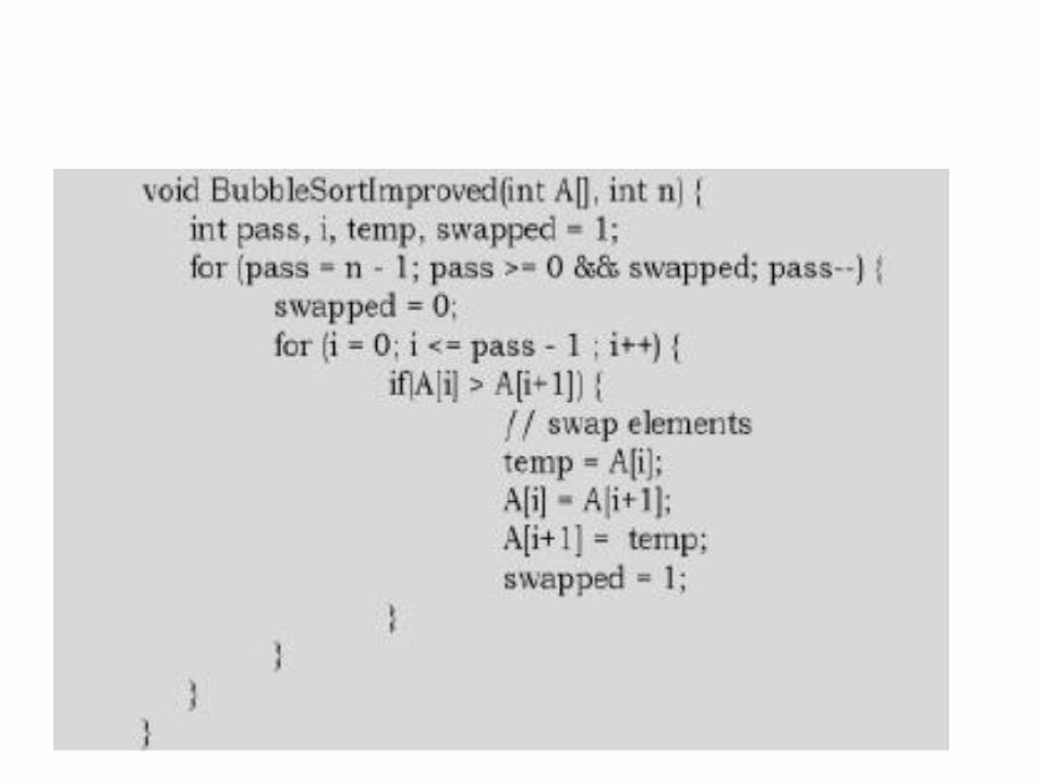
Implementation
• Algorithm takes O(n2) (even in best case).
• We can improve it by using one extra flag.
• No more swaps indicate the completion of sorting. If the list is already sorted, we can use this flag to skip the remaining passes.
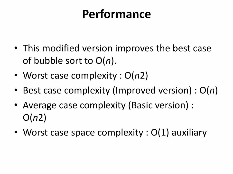
Performance
• This modified version improves the best case of bubble sort to O(n).
• Worst case complexity : O(n2)
• Best case complexity (Improved version) : O(n)
• Average case complexity (Basic version) : O(n2)
• Worst case space complexity : O(1) auxiliary


