Integer and Fractional Cointegration of Exchange Rates - The

Portuguese Case

Luis Martins¤and Vasco J. Gabriely

March 1999

Abstract

The purchasing power parity (PPP) hypothesis is examined by means of residual-based

cointegration tests. A generalized concept of cointegration is used. that is, fractional cointe-

gration. This method aims to be a complement of the Engle-Granger procedure, whose test

for cointegration assumes that the equilibrium error is strictly I(1) (nonstationary) or I(0)

(stationary). It is known and it will be shown in this work through Monte Carlo simulation,

that the unit root tests turn out to perform poorly against long memory alternatives. To

perform a test for fractional cointegration, empirical distributions are obtained through a

Monte Carlo experiment. This means that the PPP hypothesis is not con…ned to the value

of the fractional estimate. By allowing equilibrium errors to follow a fractional integrated

process, the fractional cointegration analysis capture a wider range of stationary and level

reversion behaviour. This ‡exibility is important to a proper evaluation of the exchange rate

dynamics. Two bilateral relations are studied, between Portugal as the home country and the

United Kingdom and the United States of America. We also consider the use of structural

change tests, since a long range of time is covered by the data, with periods that were a¤ected

by di¤erent policy regimes in these countries. For this century, the empirical results provide

some support for the PPP between Portugal and the two other countries. Deviations from

equilibrium can be modelled by a level-reverting fractionally integrated process. Although

short run deviations can occur, the results support the PPP as a long run phenomenon.

Keywords: Purchasing Power Parity; Fractional Integration and Cointegration; Monte

Carlo simulation

J.E.L. classi…cation: F41; C12; C15; C22; C52

¤Instituto Superior de Ciências do Trabalho e da Empresa, Lisbon (email:luis.martins@iscte.pt)yDepartment of Economics, School of Economics and Management, University of Minho (email: vj-

gabriel@eeg.uminho.pt). Partial …nancial support from the Centro de Estudos em Economia e Gestão (CEEG) is

gratefully acknowledged.

1

1 Introduction

The purchasing power parity hypothesis (PPP) is one of the most important in international

economics. This theory considers that, expressed in the same currency, goods are purchased

in two di¤erent countries by the same amount of money. To verify PPP, one has to study the

simultaneous behaviour of the nominal exchange rate and relative price index, or alternatively,

the behaviour of the real exchange rate.

The validity of PPP has always generated a great deal of controversy, intimately related to

the type of applied methodology. Traditionally, when analysing the presence of unit roots, or

cointegration, it is assumed that the processes are I(d), with integer d. The determination of the

order of integration of the variables is carried out by testing for unit roots, with the Dickey-Fuller

test being the most widely used. Using these methods, PPP has been internationally studied

by, for example, Baillie and Selover (1987), Enders (1988) and Mark (1990), with cointegration

analysis, and Corbae and Ouliaris (1988) and Nessén (1996) with univariate analysis of the real

exchange rate.

In this work, PPP is studied using two perspectives of cointegration analysis, both consti-

tuting broader concepts of cointegration. We consider cointegration under structural changes

and fractional cointegration, which will be the main focus of this paper. The cointegrating

variables and, more importantly in our case, the residuals of the cointegration model, not being

strictly represented as ARMA or ARIMA processes, may be modelled as a long memory or

fractional process, ARFIMA(p,d,q). Fractional cointegration embodies the modelling of long

memory processes, presented by Granger and Joyeux (1980) and Hosking (1981), into the con-

cept of cointegration, presented by Engle and Granger (1987). Although integer cointegration

has gained considerable relevance, mainly because Engle and Granger (1987) stressed the sim-

plest C(1; 1) case, their de…nition is valid for the general case where the processes have a real

order of integration. Integer cointegration is, therefore, a particular case of fractional cointegra-

tion. Fractional processes, besides allowing a vast range of representations where stationarity

and level revertibility are compatible, identify a broad class of low frequency dynamics.

Diebold, Husted and Rush (1991) and Wu and Crato (1995), by analysing real exchange

rate as a fractional process, and Cheung and Lai (1993), through fractional cointegration, …nd

evidence in favour of PPP. With Portuguese data, PPP was studied by Costa and Crato (1996),

with fractional analysis of the real exchange rate1. We try to present here a theoretical and

methodological motivation for the study of PPP, or any other model, using the concept of

fractional cointegration, which has not been much exploited in empirical works.1These authors concluded that the real exchange rate of the pound and the dollar have level reversibility

characteristics.

2

The …st part of the paper will survey the basic concepts, with two sections discussing integer

and fractional integration, and integer and fractional cointegration. The second part will deal

with the empirical application, comparing the di¤erent methodologies under discussion, using

Portuguese data. A …nal section concludes.

2 Integer and Fractional Integration

The …rst ideas about the existence of long memory phenomena goes back to the middle of the

century with the hydrologist Harold Hurst when observing the water levels of the river Nile. The

great persistence of the water levels (long non-periodical cycles) motivated the concept of long

memory phenomenon. In terms of economical and …nancial phenomena, the …rst long memory

models were proposed by Granger and Joyeux (1980), Granger (1980 and 1981) and Hosking

(1981).

Fractional analysis of stochastic processes allow us to circumvent some of the limitations

of integer analysis. In the spectral domain, it is known that a nonstationary process has an

in…nite pseudo-spectrum at the origin,as Granger (1966) observed for the typical spectrum of

an economic variable. Traditional analysis would suggest then to take di¤erences in the series.

However, this operation would turn the spectrum in the origin into zero, which is characteristic

of overdi¤erenced series. This led to consider the hypothesis of long memory processes, since

the spectrum analysis suggests that one should take ”half” di¤erences (for d < 1).

2.1 Fractional Integration

A process Xt is fractionally integrated of order d when this parameter assumes a non-integer

value in the di¤erence operator, (1 ¡ L)d, that is, when (1 ¡ L)dXt = ut is stationary, invertible

and with short memory2. The order of integration of Xt is now regarded as a parameter to be

estimated. Of course, integer integration means that only integer values are assumed for d.

2.1.1 ARFIMA Models

Fractionally integrated processes fXtg of the form ARFIMA(p; d; q) satisfy the di¤erence equa-

tion

Á(L)(1 ¡ L)dXt = µ(L)"t; with "t » i:i:d:(0; ¾2): (1)

The stationary solution, when it exists, is given by Xt =P1i=¡1 Ãi¢

¡d"t¡i, with Ã(z) =P1i=¡1 Ãiz

i = µ(L)=Á(L); where ¢ is the di¤erencing operator (1 ¡ L). The fractional di¤er-

20 < fu(0) <1

3

encing operator is de…ned by the binomial expression

(1 ¡ L)d =1X

i=0

µd

i

¶(¡L)i; (2)

or by (1 ¡ L)d = 1 ¡ dL + d(d¡1)2! L2 ¡ d(d¡1)(d¡2)

3! L3 + :::, for d > ¡1. Obviously, the model in

(1) generalizes the traditional ARIMA representation with real values for d.

2.1.2 Fractional Noise Process

This process was introduced by Granger and Joyeux (1980) and Hosking (1981) and may be

de…ned in the following way: fXt, t=0,1,2,...,g is a fractional noise process, ARFIMA(0,d,0), if

fXtg may be represented as

(1 ¡ L)dXt = "t; with "t » i:i:d:(0; ¾2): (3)

In order to be stationary and invertible, d 2] ¡ 0:5; 0:5[3: Stationarity and invertibility (pre-

diction ability) is guaranteed when the coe¢cients form the MA(1) (Xt =P1i=0 Ãi"t¡i) and

AR(1) (P1i=0 ¼iXt¡i = "t) representations are square summable: stationarity for d < 0:5 and

invertibility for d > ¡0:5:

2.2 Long Memory Processes: some properties

2.2.1 Time Domain

A stationary fractional process, designated as long memory, can be characterized a having a

slow, hyperbolic, decay in its ACF (Autocorrelation Function). Its expression, re‡ecting the

relative inertia of the decay and the reduced, but non-negligible, dependence among distant

observations, takes the form

j½kj s Ck2d¡1; (4)

when k ! 1, for C 6= 0 and d < 0:5. For the fractional noise, C = ¡(1¡d)¡(d) ; where ¡(:) is

the gamma function. This contrasts with integer stationary ARMA processes, or short memory

processes, where dependence tends to be dissipated geometrically with time, that is, the ACF

is geometrically bounded,

j½kj � Crjkj; with 0 < r < 1; C > 0: (5)

These are also characterized by its mean reversion, that is, its sample path frequently crosses

its mean value, meaning that shocks have a temporary e¤ect in the process. In its turn, I(1)

3The ARFIMA(p; d; q) process, with d 2] ¡ 0:5; 0:5[ is equivalent to an ARMA(p; q) process with fractional

noise: Á(L)(1¡ L)dXt = µ(L)"t , Á(L)Xt = µ(L)(1¡L)¡d"t;com "t » i:i:d:(0; ¾2):

4

processes are not mean-revertible, wherefore shocks have permanent e¤ects. Their theoretical

ACF diverges, while the empirical counterpart exhibits positive correlations, with a very slow

decay. These may be called in…nite memory processes.

2.2.2 Frequency Domain

The spectrum of a stationary ARMA process is

f(!) =

µ¾2

2¼

¶ ¯µ(e¡i!)

¯2¯Á(e¡i!)

¯2 ; (6)

so that it is …nite at the origin, and for low frequencies, f(!) » c; when ! ! 0: For I(1)

processes, the preponderance of long waves implies a divergent pseudo-spectrum at the origin

(not de…ned theoretically), that is, fX(!) » 1; f¢X(!) » c > 0; when ! ! 0. On the other

hand, the spectral function of stationary ARFIMA(p; d; q) models is

f(!) =

µ¾2

2¼

¶ ¯µ(e¡i!)

¯2¯Á(e¡i!)

¯2¯1 ¡ e¡i!

¯¡2d: (7)

By applying a linear …lter and the spectral transfer function, it is possible to de…ne (7)

through the spectrum of an ARMA process. The linear …lter is Xt = (1 ¡ L)¡dut , with

ut » I(0), Á(L)ut = µ(L)"t. Thus, the transfer function will be

fX(!) = j1 ¡ zj¡2dfu(!); para ¡ ¼ � ! � ¼; z = e¡i! ; (8)

where fu(!) = (¾2

2¼ )¯¯Á(z)µ(z)

¯¯2. In the case where Xt is a fractional noise, fu(!) = (¾

2

2¼ ). In the

lowest frequencies, the spectrum is

f(!) » c!¡2d; when ! ! 0; (9)

with c = (¾2

2¼ )hµ(1)Á(1)

i2for ARFIMA models and c = (¾

2

2¼ ) for fractional noise. For d = 0:5,

f(!) » !¡1; ! ! 0. this case is designated as ”1=f noise”: ”Xt just nonstationary”, since

”P1i=0 Ã2i just fails to converge” (see Hosking, 1981). If d = ¡0:5, f (0) = 0 and the noise is

stationary, but non-invertible.

Due to the existence of two di¤erent typologies for long memory processes, we should distin-

guish persistent (”long memory”) processes for 0 < d < 0:5, from non-persistent (”intermediate

memory”) processes for d < 0: Persistent processes are characterized by an in…nite spectrum at

the origin (f(0) = 1), that is, f(!) ! 1 when ! ! 0: Therefore, the spectral density for these

processes is concentrated in the low frequencies, re‡ecting a stationary series, but oscillating

slowly along time. The autocorrelation of the process,P1k=¡1 j½kj = 1, con…rms the proper-

ties of the spectrum at the origin. This is the relevant typology of long memory processes, since

it expresses long run persistence. Non-persistent processes (d < 0); on the contrary, have a null

spectrum at the origin (f(0) = 0), or, equivalently,P1k=¡1 ½k = 0:

5

2.2.3 Impulse-response Function

A last, but no less important property reveals that fractionally integrated processes of order

d < 1 are level-reverting (see, for example, Campbell and Mankiw, 1987) and Baillie, 1996).

The impulse-response function, with weights Ai, and equivalent to the Wold representation of

the …rst-di¤erenced series, is given by

(1 ¡ L)Xt = A(L)"t with A(L) = 1 + A1L + A2L2 + ::: (10)

A(L) = (1 ¡ L)1¡dÁ¡1(L)µ(L) = z(d ¡ 1; 1; 1;L)Á¡1(L)µ(L): In order to (1 ¡ L)Xt to be

stationary, d < 1:5:

The impact or change in Xt, in the medium term (from t to t+ k) resulting from an unitary

shock in the innovation "t; is given by 1+A1+:::+Ak. The long run impact (k ! 1) of an unitary

shock at t, or cumulative function, is given by 1+A1+A2+::: = A(1) = z(d¡1; 1; 1; 1)Á¡1(1)µ(1).

With d < 1 it can be shown, using the properties of the hypergeometrical function, that A(1) = 0,

so that in the long run the impact of the innovation on the process is null. With d = 1, A(1)

converges to a …nite, non-zero, value. With d > 1, A(1) diverges.

Thus, in a process with d < 1, although nonstationary in covariance (0:5 � d < 1), the

random shock of the innovation tends to be dissipated (it does not persist, unlike I(1) processes,

nonstationary as well). It is, therefore, possible to de…ne a set of fractional models where level

revertibility is compatible with nonstationarity.

3 Testing the Order of Integration

3.1 Real-valued Order of Integration

Relatively to ARMA models, ARFIMA(p,d,q) estimation, besides the variance ¾2 and p + q

parameters, entails the estimation of an additional parameter, d. We will present here the most

important estimation methods, well developed in Brockwell and Davis (1991) or Baillie (1996),

for example.

3.1.1 Semiparametric Estimation of d in the Frequency Domain - GPH

Geweke and Porter-Hudak (1983, henceforth GPH) suggested a semiparametric method to es-

timate d, based on the spectral analysis of the process, particularly, on its behaviour near the

origin. This procedure allows the estimation of the order of integration, independently of the

particular parameterization of the ARMA component. It may be observed that for low non-zero

frequencies, !j, the periodogram de…ned in (8) is dominated by the function j1¡ zj2: In (8), the

6

resulting spectral function is

fX(!) = [4 sin2(!=2)]¡dfu(!); with ut » ARMA(p; q): (11)

Taking logs on both sides of (11), adding and subtracting ln[fu(0)], we get

ln[fX(!)] = ln[fu(0)] ¡ d lnf[4 sin2(!=2)]g + ln[fu(!)=fu(0)]: (12)

Substituting the spectral density for the periodogram I(!); and considering negligible the last

term in (12), we have, for low frequencies, the following linear regression form

ln IX;n(!j) = a ¡ d lnf[4 sin2(!j=2)]g + vj; for j = 1; 2; :::;m; (13)

where a = ln[fu(0)]; vj = ln[fu(!)=fu(0)] with E(vj) = 0 and V ar(vj) = ¼2=6; ! = !j = 2¼j=T ,

j = 1; 2; :::; m � T=2 and m is a function of the sample size T . For this method, d corresponds to

symmetrical of the periodogram’s estimated slope, de…ned on the low frequencies. The precision

of the estimator is related to the concentration of low frequencies due to the increasing sample

size.

The estimator of d in small samples is sensitive to the spectral dimension considered. There-

fore, di¤erent suggestions have emerged in the literature for its extremes truncation, as in Geweke

and Porter-Hudak (1983), Brockwell and Davis (1991) and Cheung (1993a), inter alia, which

consider m = T 0:5. Some authors also admit truncating at the origin, in order to assure the

consistency of the GPH estimator4; Hassler and Wolters (1995) suggest that m may not be

unique. Cheung and Lai (1993) use m = T® , ® = 0:55; 0:575; 0:65.

Geweke and Porter-Hudak (1983), for d < 0; and Crato (1992), for d > 0; argue that the

spectral least squares estimator of d is consistent, although its convergence rate is smaller than

0:5=T1=2, as pointed out by Baillie (1996). Inference on d may be based on the t -ratio

dGPH ¡ dhV ar

³dGPH

´i1=2 » N(0; 1): (14)

The determination of V ar³dGPH

´is done using the usual least squares covariance matrix,

s2(X0X)¡1, noting that plim¡s2

¢= ¼2=6:

Baillie (1996), referring other studies, and Cheung (1993b), point out some situations where

this method does not work well. For example, the estimator is biased when the DGP is a

nonstationary ARFIMA (d ¸ 0:5). This suggests, in certain occasions, GPH estimation of the

4Wu and Crato (1995) use ! = T 1=3=3 as a truncation at the origin.5 If m is large, the estimate is contaminated by the medium and high frequencies; if m is small, the estimator

becomes more imprecise, because the number of degrees of freedom is reduced.

7

…rst-di¤erences, Yt = Xt ¡ Xt¡1 = ¢Xt. Very often, economic series are I(d); d < 1:5. On the

other hand, it is possible to test for the presence of a unit root. The spectral regression of the

GPH test for (1 ¡ L)Xt is given by

ln IX;n(!j) = a ¡ (d ¡ 1) lnf[4 sin2(!j=2)]g + vj; for j = 1; 2; :::;m: (15)

Here, d corresponds to the GPH estimate of (15), plus 16. In these circumstances, the bilateral

test of the nullity of d ¡ 1, for the di¤erenced series, is equivalent to a unit root test (d = 1) in

the original series. The estimation of the remaining parameters of the ARFIMA(p; d; q) process

may be accomplished using, for example, maximum likelihood after the value of d is estimated.

Fractional modelling with GPH is, therefore, realized in two steps.

Maximum Likelihood Estimation Unlike the GPH method, maximum likelihood estima-

tion is simultaneous, enabling correlation problems among estimators to be explicit, namely

those of the order of integration and of the autoregressive component. This is an important

factor in the analysis of the ACF decay, since its behaviour is in‡uenced by the size of both

types of coe¢cient.

For the series fXtg; the likelihood function, under normality and with ¹ = 0, may be written

as

L(¯¤; ¾2) =Y

i

f(Xij¯¤; ¾2) = (2¼¾2)¡T=2(r0; :::; rT¡1)¡1=2 exp

8<:¡ 1

2¾2

TX

j=1

(Xj ¡ Xj)2=rj¡1

9=; ;

(16)

where ¯¤= (d; Á1; :::; Áp; µ1; :::; µq), Xj denotes the one-step predictor and rj¡1 = ¾¡2E(Xj ¡Xj)

2; j = 1; :::; T 7. The log-likelihood is

LL(:) = ¡(T=2) log(2¼) ¡ (1=2) log j­j ¡ (1=2)X0­¡1X; (17)

where f­gij = °ji¡jj and X is the vector containing the T observations. The exact ML estimator

is the vector of parameters (¯¤;¾2)0

which maximize L(¯¤; ¾2) with respect to ¯¤ and ¾2.

Brockwell and Davis (1991) and Baillie (1996) present some results concerning this method.

It is possible to identify- the asymptotic distribution of ¯0= (d; Á1; :::; Áp; µ1; :::; µq; ¾

2) in

the case where ¹ is known or zero, as it normally happens with the residuals of the potential

cointegration model. In this case, the estimator is consistent and converges at the rate 0:5=T 1=2

to a normal distribution,

T 1=2³^ ¡ ¯

´d! N

�0; limT!1

fI(¯)=Tg¡1¸

; with I(¯) =

24 Ip;q J

J0

¼2=6

35 ; (18)

6Á(L)(1¡ L)dXt = µ(L)"t , Á(L)(1¡L)d¡1(1¡ L)Xt = µ(L)"t,7See Brockwell and Davis (1991), p. 527.

8

were Ip;q is the information matrix from the ARMA component. In the speci…c case where fXtgis a fractional noise (p = q = 0) and "t » N(0; ¾2), we have the well known result

T 1=2³d ¡ d

´d! N(0; 6=¼2): (19)

Since the exact ML estimation with large samples is extraordinarily complicated, it is usual to

resort to expressions that asymptotically approximate the likelihood function. The theoretical

background was given by Whittle, who in 1951 de…ned an approximation of the likelihood

function in the frequency domain. In general, the computational gains outweigh the (reduced)

loss in precision. Two of such estimators stand out for their good performance in practice8:

(i) Fox and Taqqu (1986), consider minimizing

¾2T (») =T¡1X

k=1

µI(2¼k=T )

f(2¼k=T; »)

¶; » = (d;Á;µ); (20)

or, in a simpler way, LL =P³

IT (!j)f (!j)

´: The consistency of » is given by

T 1=2³» ¡ »

´d! N(0; 4¼W¡1(»)); (21)

where W¡1(») is a Fourier-coe¢cients matrix.

(ii) Breidt, Crato and de Lima (1994), Crato and Ray (1996) and Costa and Crato (1996),

following Brockwell and Davis (1991), consider the minimization of

[T=2]X

j=1

µIT (!j)

f (!j)+ log f(!j)

¶: (22)

The covariance matrix is estimated using the Hessian of f(!j) on its optimum.

It can be demonstrated that, when ¹ is unknown, the asymptotic distribution is normal and

that ¹ is consistent with a convergence rate smaller that the corresponding one of ¯0. While ¹

converges at the rate T0:5¡d, the other estimators converge at the usual rate of T 0:5: When ¹ is

unknown, Cheung and Diebold (1994) concluded that the Fox-Taqqu estimator (frequency do-

main approach) is preferable to that of Sowell (1992) (exact in time domain), in the sense that it

produces a smaller bias and mean squared error. However, when ¹ is known, the Sowell estima-

tor is much more e¢cient than the Fox-Taqqu one. This results were derived for small samples,

where the estimation of the order of integration is negatively biased (d is underestimated).

Model selection for ARFIMA(p; d; q) is performed over the obtained ML estimations, for the

di¤erent models. The choice will fall on the model which minimizes an information criterion

such as AIC (Akaike information criterion) or BIC (Schwarz Bayesian information criterion).

8See, for example, Cheung and Diebold (1994) for the Fox-Taqqu approximation and Crato and Ray (1996).

9

Crato and Ray (1996) show that the …rst criterion reveals better qualities when the selection is

made over fractional models with ARMA components, that is, p; q > 0:

Like the GPH method, estimation and inference on the nullity of the order of integration in

the …rst-di¤erenced series, ¢Xt, allows testing for unit roots in the original series, H0 : d ¡ 1 =

0 , d = 1.

Integer Order of Integration Testing for integer order of integration, normally d = 1

against stationarity, implies what is called a ”knife-edged” unit root test, which means that

non-integer orders of integration will not be easily detected, that is, unit root tests will have

low power against fractional alternatives (see Diebold and Rudebusch, 1991, Cheung and Lai,

1993 and Hassler and Wolters, 1994). Besides the possibility of testing for unit roots using

GPH and ML, several other unit root tests have been proposed in the literature, Dickey-Fuller

and Phillips-Perron being the most widely used tests. Other tests consider stationarity in the

null hypothesis, with an unit root alternative, namely the Kwiatkowski-Phillips-Schmidt-Shin

(KPSS) test. Predictably, these tests will su¤er from the same problems as the unit root ones

when the true process is fractionally integrated. These tests will be used later in the empirical

analysis.

4 Cointegration

4.1 Fractional Cointegration

The de…nition of cointegration9, interpreted in a broader sense, allows us to consider a fractional

version of Engle and Granger’s (1987) original idea. In fact, assuming an integer order of

integration for some economic variables may be too restrictive, according to some empirical

evidence, so it seems natural to extend fractional analysis to long run relationships and go

beyond traditional integer analysis.

Fractional cointegration is thus de…ned for series or equilibrium errors that follow fractionally

integrated processes. Not conditioning cointegration tests to a knife-edged level, it is possible

to …t stationarity and mean reversion into a well de…ned set of fractionally integrated processes.

Notice that integer cointegration is a particular case of fractional cointegration, so from the

standard C(1; 1) case, it is possible to consider any generalization.

We may distinguish two di¤erent levels for the concept of cointegration:9Given a vector X = (X1;X2; :::;Xn), whose elements are I(d); if there is a linear combination ®0X that is

integrated of order (d¡ 1), then the elements of X are said to be cointegrated C(d; b) with cointegrating vector

®.

10

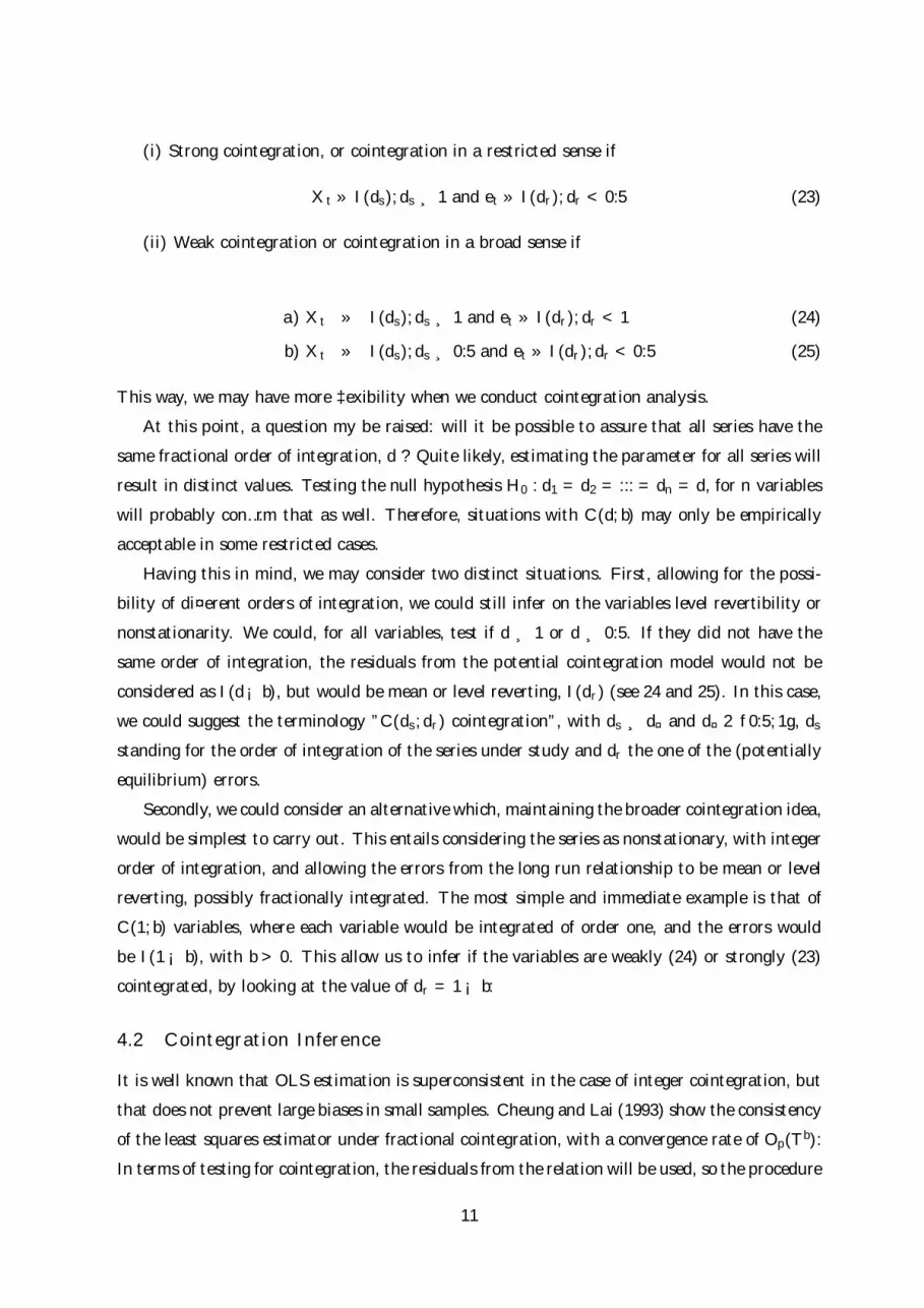
(i) Strong cointegration, or cointegration in a restricted sense if

Xt » I(ds); ds ¸ 1 and et » I(dr); dr < 0:5 (23)

(ii) Weak cointegration or cointegration in a broad sense if

a) Xt » I(ds); ds ¸ 1 and et » I(dr); dr < 1 (24)

b) Xt » I(ds); ds ¸ 0:5 and et » I(dr); dr < 0:5 (25)

This way, we may have more ‡exibility when we conduct cointegration analysis.

At this point, a question my be raised: will it be possible to assure that all series have the

same fractional order of integration, d ? Quite likely, estimating the parameter for all series will

result in distinct values. Testing the null hypothesis H0 : d1 = d2 = ::: = dn = d, for n variables

will probably con…rm that as well. Therefore, situations with C(d; b) may only be empirically

acceptable in some restricted cases.

Having this in mind, we may consider two distinct situations. First, allowing for the possi-

bility of di¤erent orders of integration, we could still infer on the variables level revertibility or

nonstationarity. We could, for all variables, test if d ¸ 1 or d ¸ 0:5. If they did not have the

same order of integration, the residuals from the potential cointegration model would not be

considered as I(d¡ b), but would be mean or level reverting, I(dr) (see 24 and 25). In this case,

we could suggest the terminology ”C(ds; dr) cointegration”, with ds ¸ d¤ and d¤ 2 f0:5; 1g, ds

standing for the order of integration of the series under study and dr the one of the (potentially

equilibrium) errors.

Secondly, we could consider an alternative which, maintaining the broader cointegration idea,

would be simplest to carry out. This entails considering the series as nonstationary, with integer

order of integration, and allowing the errors from the long run relationship to be mean or level

reverting, possibly fractionally integrated. The most simple and immediate example is that of

C(1; b) variables, where each variable would be integrated of order one, and the errors would

be I(1 ¡ b), with b > 0. This allow us to infer if the variables are weakly (24) or strongly (23)

cointegrated, by looking at the value of dr = 1 ¡ b:

4.2 Cointegration Inference

It is well known that OLS estimation is superconsistent in the case of integer cointegration, but

that does not prevent large biases in small samples. Cheung and Lai (1993) show the consistency

of the least squares estimator under fractional cointegration, with a convergence rate of Op(T b):

In terms of testing for cointegration, the residuals from the relation will be used, so the procedure

11

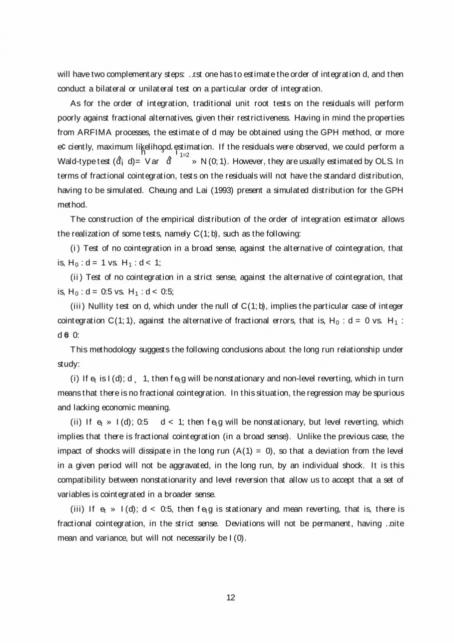
will have two complementary steps: …rst one has to estimate the order of integration d, and then

conduct a bilateral or unilateral test on a particular order of integration.

As for the order of integration, traditional unit root tests on the residuals will perform

poorly against fractional alternatives, given their restrictiveness. Having in mind the properties

from ARFIMA processes, the estimate of d may be obtained using the GPH method, or more

e¢ciently, maximum likelihood estimation. If the residuals were observed, we could perform a

Wald-type test (d¡d)=hV ar

³d´i1=2

» N(0; 1). However, they are usually estimated by OLS. In

terms of fractional cointegration, tests on the residuals will not have the standard distribution,

having to be simulated. Cheung and Lai (1993) present a simulated distribution for the GPH

method.

The construction of the empirical distribution of the order of integration estimator allows

the realization of some tests, namely C(1; b), such as the following:

(i) Test of no cointegration in a broad sense, against the alternative of cointegration, that

is, H0 : d = 1 vs. H1 : d < 1;

(ii) Test of no cointegration in a strict sense, against the alternative of cointegration, that

is, H0 : d = 0:5 vs. H1 : d < 0:5;

(iii) Nullity test on d, which under the null of C(1; b), implies the particular case of integer

cointegration C(1; 1), against the alternative of fractional errors, that is, H0 : d = 0 vs. H1 :

d 6= 0:

This methodology suggests the following conclusions about the long run relationship under

study:

(i) If et is I(d); d ¸ 1, then fetg will be nonstationary and non-level reverting, which in turn

means that there is no fractional cointegration. In this situation, the regression may be spurious

and lacking economic meaning.

(ii) If et » I(d); 0:5 � d < 1; then fetg will be nonstationary, but level reverting, which

implies that there is fractional cointegration (in a broad sense). Unlike the previous case, the

impact of shocks will dissipate in the long run (A(1) = 0), so that a deviation from the level

in a given period will not be aggravated, in the long run, by an individual shock. It is this

compatibility between nonstationarity and level reversion that allow us to accept that a set of

variables is cointegrated in a broader sense.

(iii) If et » I(d); d < 0:5, then fetg is stationary and mean reverting, that is, there is

fractional cointegration, in the strict sense. Deviations will not be permanent, having …nite

mean and variance, but will not necessarily be I(0).

12

4.2.1 Distribution and Power of the GPH and MLE Tests

We simulate, for di¤erent percentiles, the distribution of the GPH and MLE tests under the null

hypothesis of no cointegration, considering a system of two independent random walks (Table

1). In terms of cointegration testing, this distribution allows, among other things, to test the

hypothesis H0 : d = 1 vs H1 : d < 1. As expected, the distributions are negatively skewed and

having a negative mean.

Table 1: Distributions of the GPH and MLE Tests.

Perc: 0:005 0:01 0:025 0:05 0:1 0:2 0:3 0:4

GPH ¡3:606 ¡3:248 ¡2:746 ¡2:33 ¡1:902 ¡1:396 ¡1:06 ¡0:785

MLE ¡3:482 ¡3:175 ¡2:682 ¡2:3 ¡1:844 ¡1:345 ¡1:011 ¡0:733

Perc:(cont:) 0:5 0:6 0:7 0:8 0:9 0:95 0:975 0:99 0:995

GPH ¡0:537 ¡0:292 ¡0:047 0:224 0:602 0:918 1:196 1:529 1:763

MLE ¡0:485 ¡0:242 0:002 0:282 0:671 0:992 1:269 1:6 1:838

mean skewness kurtosis

GPH ¡0:601 ¡0:39 3:586

MLE ¡0:545 ¡0:345 3:378

In a second investigation, we compare the powers of these tests against the AEG test, with lag

order one, for two series. Table 2 shows the percentage of correct rejections of the null hypothesis

of no cointegration, at the 5% and 10% signi…cance levels. The true DGP is cointegrated, with

the equilibrium error assuming di¤erent values for d (fractional noise) in the revertibility and

stationarity region (between 0:95 and 0:05).

Table 2: Power of AEG, GPH and MLE tests against fractional noise alternatives

d

0:95 0:85 0:75 0:65 0:55 0:45 0:35 0:25 0:15 0:05

5% GPH 0:02 0:04 0:07 0:14 0:24 0:36 0:49 0:62 0:73 0:81

MLE 0:00 0:01 0:10 0:42 0:86 0:99 1:00 1:00 1:00 1:00

AEG 0:00 0:00 0:02 0:07 0:23 0:54 0:87 0:99 1:00 1:00

10% GPH 0:04 0:07 0:13 0:21 0:34 0:49 0:62 0:75 0:83 0:90

MLE 0:04 0:04 0:21 0:63 0:96 1:00 1:00 1:00 1:00 1:00

AEG 0:00 0:01 0:04 0:12 0:33 0:67 0:93 1:00 1:00 1:00

13

The following results worth some attention:

(i) GPH and MLE tests are more powerful than the AEG test, against fractional noise

alternatives with 1 > d ¸ 0:55.

(ii) For fractional noise alternatives, whatever the order of integration, the MLE is the most

powerful. This means that, for d between 0 and 1 (not strictly 0 or 1; as in AEG), MLE test is

the most appropriate.

(iii) The AEG test performs very poorly against fractional alternatives with d > 0:65: This

test does not recognise errors revertibility, con…rming our early comments.

The Monte Carlo procedures were written in GAUSS, considering the GPH spectral dimen-

sion !j , j = 0:1; :::; T 0:5: The simulated processes have 105 observations. The distributions were

obtained after 50 000 replications, while for the power of the tests, 20 000 replications were used.

Next, we will study the application of this methodology to a test of purchasing power parity.

5 PPP, Integer and Fractional Cointegration: the Portuguese

case

5.1 Introduction

In this section, we will discuss some of econometric issues resulting from the study of PPP

with Portuguese data. The main idea is to compare two methodologies: integer cointegration,

where structural changes are allowed for, and fractional cointegration, discussed earlier. The

PPP hypothesis is based on the relatively intuitive idea that the exchange rate between two

currencies should re‡ect, in the long run, the relationship between price levels from the respective

countries. It is usual to consider a linear version in logs, with an error term representing the short

run deviations from the PPP, re‡ecting disturbances in the economic system (real or monetary

shocks), such as

sft = ® + ¯ pn;ft + en;ft ; for t = 1; :::; T; (26)

with sf = sfn, pn;f = log PnPf

:

The variables in logs de…ne the nominal exchange rate, in escudos per unit of the foreign

currency, (Sft ) and the relative price index³PnPf

´as the ratio between the domestic price index

(Pn) and the foreign one (Pf ). PPP will hold if the variables sft and pn;ft are cointegrated.

In a restricted perspective, that is, integer cointegration, errors should be stationary, whereas

in a broader view of cointegration errors may be level revertible, despite being nonstationary.

One should also expect the hypothesis of homogeneity (meaning that the cointegrating coe¢cient

is unitary, ¯ = 1). Considering the absolute version of the PPP hypothesis, additionally ® should

14

be zero, but this may not happen in practice due to several factors, usually associated with model

misspeci…cations, the statistical procedures used or structural changes. Here we try to address

this last issue in a modest and tentative fashion, since the existence of structural breaks may

invalidate the conclusions drawn with traditional procedures, since usual tests will spuriously

indicate that there is no cointegration (see Gregory and Hansen, 1996). Notice that this model

imposes price symmetry, usual in other studies, since preliminary tests revealed that prices may

be integrated of order two.

We study this model with Portugal as the domestic country, the United Kingdom (UK) and

the United States (USA) being the foreign countries, with almost a century of annual data10

(from 1891 to 1995 for the UK and from 1900 to 1995 for the USA). The respective parity

relations are s$t = ®1 + ¯1 pn;ukt + en;ukt and s$t = ®2 + ¯2 pn;usat + en;usat :

5.2 Order of Integration

First, we have to determine the order of integration of s$t , pn;ukt , s$t , and pn;usat . Nonstationarity

will occur when, for a given variable, d ¸ 0:5, while non-revertibility implies d ¸ 1. Considering

the particular case of integer order of integration, nonstationarity will result for I(d); d = 1; 2; :::

series. The results from unit root tests may be found in Table 3, with p-values in squared

brackets and t-ratios in curved brackets underneath, and the chosen lag next to each value.

Table 3: Unit Root Tests11

Série h-Durbin BG(4) ADF(k) PP(l) KPSS d GPH

s$t ¡1:02[0:31]

3:5[0:47]

¡1:46(5) ¡4:99(4) 0:18¤ 1:09(0:53)

s$t 0:94[0:35]

8:6[0:07]

¡1:36(1) ¡5:85(3) 0:29¤ 0:95(¡0:25)

pn;ukt ¡0:52[0:60]

3:8[0:43]

¡1:82¤(4) ¡5:23(4) 0:19¤ 1:42(0:85)

pn;usa 1:01[0:32]

1:4[0:85]

¡1:54(5) ¡4:66(4) 0:32¤¤ 0:87(¡0:47)

The values of the h-Durbin and Breusch-Godfrey statistics permits us to take the residuals

from the ADF regressions as uncorrelated. The results for the GPH test are based on the

…st di¤erenced series, with spectral dimension !j, j = 0:1; :::; T 0:5: The t-ratios, which are not

signi…cant, are relative to the test of d = 1 against d 6= 1. This test supports the conclusions from10Which covers two World Wars, several economical and technological shocks, that is, structural changes that

inevitably in‡uenced the behaviour of exchange rates.11Notes to table 3: ¤- 10% signi…cant statistic; ¤¤ - 5% signi…cant statistic; ¤¤¤ - 1% signi…cant statistic; k was

chosen as the last signi…cant lag on a downward t-testing procedure; l was chosen as the last signi…cant lag from

the analysis of the ACF and PACF (also used for the KPSS test)

15

the other tests, themselves consensual, pointing to the existence of a unit root in the series12.

Even when other lags were used for the Phillips-Perron and KPSS tests, the conclusions did not

change. Although the variables may be fractionally integrated, given the results above, it is not

unreasonable to study the PPP hypothesis in the more simple framework of C(1; b) fractional

cointegration.

Figure 1 and 2 in the Appendix illustrate the behaviour of the series, where the nonstationary

nature of the variables can easily be seen. We can also identify sub-periods with di¤erent

behaviours, namely the relatively stable period from approximately 1943 to 1973, coinciding

with the Bretton Woods …xed-rates system. Despite the evident regime changes in each variable,

it is still possible that the long run relationship between prices and exchange rates held more or

less stable, with some outliers present, as can be seen in the scatter-plot.

5.3 Cointegration estimates

Estimation by least squares of a cointegration model is consistent both for integer cointegration

and fractional cointegration. The estimation results are in Table 4.

Table 4: Cointegration Vector Estimates

UK USA

Coe¢cients OLS OLS

® 4:775(207:69)

3:378(130:42)

¯ 1:053(65:24)

1:052(61:46)

Despite possible biases, OLS results are reasonably in accordance with the expected value

for ¯ under the homogeneity assumption. The estimates of ® seem to contradict absolute parity

hypothesis. In the Appendix, Figure 3 graphs the residuals from OLS estimation and Figures 4

and 5 show the periodogram and ACF, respectively.

Testing now for integer cointegration C(1; 1), we employed the ”classical” residual-based

tests, Engle-Granger (AEG) and Phillips-Ouliaris (PO), as well as tests that consider the null

hypothesis of cointegration, the Shin test and the Inf L0c of Hao (1996), this last test being

robust to possible structural breaks. The results of both types of tests are presented in table 5.

12Tests not reported here dismissed the hypothesis of the variables being I(2):

16

Table 5: Cointegration Tests13

H0 : No Cointegration H0 : Cointegration

Tests UK USA Tests UK USA

AEG (k) -2.982 (3) -2.347 (1) Shin (L0c) 0.202 0.111

PO (l) -18.565 (3) -9.932 (4) Inf L0c 0.052 0.012

As one might expect, standard tests on the residuals of the static regression do not reject the

null of no cointegration, given their properties in the presence of possible structural changes, as

mentioned before. Looking now at the tests in the second column, both agree in not rejecting

cointegration, thus contradicting the other tests.

5.4 Cointegration allowing for Regime Shifts

Gregory and Hansen (1996) generalized the usual cointegration tests (with null hypothesis of no

cointegration), allowing for a more ‡exible version of cointegration as they consider an alternative

hypothesis in which the cointegration vector su¤ers a regime shift at an unknown time. They

developed versions of the AEG tests of Engle and Granger (1987), as well as the Z ® and Z t

tests of Phillips-Ouliaris (all of these suppose invariance of the long run relationship), modifying

them according to the alternative considered. As seen before, the usual cointegration tests would

hardly indicate a result of cointegration, since the existence of breaks is almost indistinguishable

of nonstationary error terms. Therefore, the usual procedures should be modi…ed in order to

admit the hypothesis of a structural break.

Gregory and Hansen (1996) analysed four cointegration models that accommodate, under

the alternative, the possibility of changes in the cointegration vector: a level shift model (C ),

a model with a level shift and a trend (C/T ), while a more generic formulation contains a

”regime shift” (R), and to complete this class of models, a trend shift is added (R/T ) to the

previous model. In this framework, since the change point is unknown, the solution involves

the computation of the usual statistics for all possible break points and selecting the smallest

value (largest in absolute value) obtained, since they will potentially present greater evidence

against the null hypothesis of no cointegration. Therefore, it is important to observe the values

of inf Z®; inf Zt and inf AEG:

When this tests are applied14, evidence of cointegration is stronger, mainly for the UK and

with version C. For the USA, evidence less strong, but the for version C, the inf AEG still

13Notes to table 5 : Critical values at 10%, 5% and 1% are 0.231, 0.314 and 0.533 for the Shin test, 0.062, 0.076

and 0.116 for the Inf L0c and 0.361, 0.468 and 0.723 for the Lc test, respectively.14We present the results for all versions, although it would be more appropriate to consider level shifts only

(C ), that is, in the independent term.

17

rejects at the 5% level. This tests, however, only consider one break and, in this case, it is likely

that more that one break has occurred.. Moreover, the rejection points are non-informative with

respect to the break date.

Table 6: Gregory-Hansen Cointegration Tests15

UK

Tests N NT R RT

Inf Z t ¡5:107¤¤ ¡5:083¤ ¡4:948¤ ¡4:789

Inf Z® ¡44:313¤ ¡44:182 ¡39:87 ¡39:853

Inf AEG ¡5:306¤¤ ¡5:342¤ ¡5:131¤ ¡5:938

USA

Inf Z t ¡4:427 ¡4:464 ¡4:424 ¡4:625

Inf Z® ¡35:532 ¡35:533 ¡35:284 ¡36:555

Inf AEG ¡5:316¤¤ ¡5:223¤ ¡5:319¤ ¡5:037

Taking these results into account, it does not seem unreasonable to assume the existence of

cointegration and, therefore, the validity of the PPP hypothesis. In spite of this, the Gregory-

Hansen tests alert for the possibility that the relationships under study may have su¤ered regime

shifts, thus calling for the use of structural change tests. However, this line of inquiry will not

be pursued here. What we may conclude, nevertheless, is that conventional Engle-Granger

cointegration (in particular, the assumption of stability of the long run relationship) is rejected

by the data. Next, we will consider an alternative approach which we have been discussing,

fractional cointegration.

5.5 Fractional Cointegration

As before, residuals from the OLS regression will be used, but now estimation and tests of the

order of integration will be based on GPH and MLE methods. The results in table 6 are from

the …rst-di¤erenced residuals. We used the Fox-Taqqu approximation in frequency domain for

the MLE estimation, W, and exact time domain estimation, EML.

The reported t-ratios concern two tests: …rst, Ha0, in which non (fractional) cointegration

(d = 1) is tested against fractional cointegration (d < 1); secondly, Hb0, tests the null of a sta-

tionary and invertible ARMA representation against the alternative of an ARIMA or ARFIMA

model (d 6= 0).

15Notes to table 6: ¤- 10% signi…cant statistic; ¤¤ - 5% signi…cant statistic; ¤¤¤ - 1% signi…cant statistic.

18

Table 7: Fractional Cointegration Results16

Ha0 : d = 1 Hb0 : d = 0 Ha0 : d = 1 Hb0 : d = 0

dGPH t-ratio t-ratio dW t-ratio t-ratio dEML

en;ukt 0:66 ¡1:96¤ 3:82¤¤¤ 0:782 ¡2:9¤¤¤ 10:41¤¤¤ 0:74

(]0:05; 0:1[) (]0:01; 0:025[)

en;usat 0:66 ¡1:04 2:02¤¤ 0:669 ¡3:99¤¤¤ 8:07¤¤¤ 0:578

(> 30) (0)

As can be veri…ed, fractional estimates are less than unity. In its turn, testing the hypothesis

Ha0 : d = 1 produces contradictory results for the GPH and MLE methods. While inference

according to MLE supports the existence of fractional cointegration, in a broad sense, between

the exchange rates and the relative prices indexes, looking at the GPH tests we cannot reject

the null of no cointegration. On the other hand, from the test of the hypothesis Hb0 : d = 0; it is

possible to conclude that the residuals from the models do not admit an ARMA representation,

thus allowing their representation as a fractional process.

6 Concluding Remarks

From the results presented above, evidence of cointegration between prices and exchange rates

is ambiguous, that is, using di¤erent methodologies and with our data, we are unable to reach

a …rm statement about the validity of the PPP hypothesis. More speci…cally, and synthetically,

we can draw the following illations:

(i) Integer cointegration does not allow the validation of the PPP hypothesis. However, in

the line of our previous discussion, this approach has some limitations. Using tests that allow

for the presence of regime shifts, we found evidence of cointegration, although the nature of the

regime shifts was not investigated.

(ii) We con…rmed, via Monte Carlo simulation, the weaknesses of the usual cointegration

tests against fractional alternatives. For this type of alternatives, the MLE seems to be more

powerful and more adequate to the study of fractional cointegration.

(iii) The methodology we stressed in this study, fractional cointegration, presents contra-

dicting results. While GPH refuted the validity of PPP, the MLE method found some evidence

in support of the PPP. We can admit that the variables are weakly cointegrated, considering

level reverting residuals which prevent asymptotic divergence of the relationship.16Notes to table 7: ¤- 10% signi…cant statistic; ¤¤ - 5% signi…cant statistic; ¤¤¤ - 2.5% signi…cant statistic, using

the simulated distributions; p-values in brackets.

19

We tried to show in this paper the usefulness of considering more ‡exible perspectives of

cointegration. Obviously, our approach and our intention was merely illustrative, leaving some

scope for further research. One possibility could be of the simultaneous constrained estimation

of the orders of integration of the variables under study. Another line of research would be to

consider the possibility of structural changes in fractional models.

References

[1] Baillie, R. T. (1996), Long Memory Processes and Fractional Integration in Econometrics,

Journal of Econometrics, 73, pp. 5-59.

[2] Baillie, R. T. and Selover, D. D. (1987), Cointegration and Models of Exchange Rate

Determination, International Journal of Forecasting, 3, pp. 43-51.

[3] Breidt, F. J., Crato, N. and de Lima, P. (1998), On the Detection and Estimation of Long

Memory in Stochastic Volatility, Journal of Econometrics, 83, pp. 325-348.

[4] Brockwell, P. J. and Davis, R. (1991), Time Series: Theory and Methods, second edition,

New-York: Springer-Verlag.

[5] Campbell, J. Y. and Mankiw, N. G. (1987), Are Output Fluctuations Transitory ?, Quar-

terly Journal of Economics, 102, pp. 857-880.

[6] Cheung, Y.-W. (1993a), Long Memory in Foreign-Exchange Rates, Journal of Business and

Economic Statistics, 11, pp. 93-101.

[7] Cheung, Y.-W. (1993b), Tests for Fractional Integration: A Monte Carlo Investigation,

Journal of Time Series Analysis, 14, pp. 331-345.

[8] Cheung, Y-W. and Diebold, F. X. (1994), On Maximum Likelihood Estimation of the

Di¤erencing Parameter of Fractionally-Integrated Noise with Unknown Mean, Journal of

Econometrics, 62, pp. 301-316.

[9] Cheung, Y.-W. and Lai, K. S. (1993), A Fractional Cointegration Analysis of Purchasing

Power Parity, Journal of Business and Economic Statistics, 11, pp. 103-112.

[10] Corbae, D. and Ouliaris, S. (1988), Cointegration and Tests of Purchasing Power Parity,

Review of Economics and Statistics, 70, pp. 508-511.

[11] Costa, A. A. and Crato, N. (1996), A Fractional Integration Analysis of the Long-Run

versus the Short-Run Behavior of the Portuguese Real Exchange Rates, Working Paper no

2-96, Lisboa: Cemapre, ISEG, UTL.

20

[12] Crato, N. (1992), Some Misspeci…cation Problems in Long-Memory Time Series Models,

PhD. Thesis, Delaware University

[13] Crato, N. and Ray, B. K. (1996), Model Selection and Forecasting for Long-Range Depen-

dent Processes, Journal of Forecasting, 15, pp. 107-125.

[14] Diebold, F. X. and Rudebush, G. D. (1989), Long Memory and Persistence in Aggregate

Output, Journal of Monetary Economics, 24, pp. 189-209.

[15] Diebold, F. X., Husted, S. and Rush, M. (1991), Real Exchange Rates Under the Gold

Standard, Journal of Political Economy, 99, pp. 1252-1271.

[16] Enders, W. (1988), ARIMA and Cointegration Tests of PPP Under Fixed and Flexible

Exchange Rate Regimes, Review of Economics and Statistics, 70, pp. 504-508.

[17] Engle, R. F. and Granger, C. W. J. (1987), Cointegration and Error Correction : Repre-

sentation, Estimation and Testing, Econometrica, 55, pp. 251-276.

[18] Fox, R. and Taqqu, M. (1986), Large-Sample Properties of Parameter Estimates for Stron-

gly Dependent Stationary Gaussian Time Series, Annals of Statistics, 14, pp. 517-532.

[19] Geweke, J. and Porter-Hudak, S. (1983), The Estimation and Application of Long Memory

Time Series Models, Journal of Time Series Analysis, 4, pp. 221-238.

[20] Granger, C. W. J. (1966), The Typical Spectral Shape of an Economic Variable, Econo-

metrica, 34, pp. 150-161.

[21] Granger, C. W. J. (1980), Long Memory Relationships and the Aggregation of Dynamic

Models, Journal of Econometrics, 14, pp. 227-238.

[22] Granger, C. W. J. (1981), Some Properties of Time Series Data and their Use in Econo-

metric Model Speci…cation, Journal of Econometrics, 16, pp. 121-130.

[23] Granger, C. W. J. and Joyeux, R. (1980), An Introduction to Long-Memory Time Series

Models and Fractional Di¤erencing, Journal of Time Series Analysis, 1, pp. 15-39.

[24] Gregory, A. W. and Hansen, B. E. (1996), Residual-based Tests for Cointegration in Models

with Regime Shifts, Journal of Econometrics, 70, pp. 99-126.

[25] Hao, K. (1996), Testing for Structural Change in Cointegrated Regression Models: Some

Comparisons and Generalizations, Econometric Reviews, 15, pp. 401-429.

21

[26] Hassler, U. and Wolters, J. (1995), Long Memory in In‡ation Rates: International Evidence,

Journal of Business and Economic Statistics, 13, pp. 37-45.

[27] Hosking, J. R. M. (1981), Fractional Di¤erencing, Biometrika, 68, pp. 165-176.

[28] Mark, N. C. (1990), Real and Nominal Exchange Rates in the Long Run: an Empirical

Investigation, Journal of International Economics, 28, pp. 115-136.

[29] Nessén, M. (1996), Common Trends in Prices and Exchange Rates. Tests of Long-Run

Purchasing Power Parity, Empirical Economics, 21, pp. 381-400.

[30] Sowell, F. (1992), Maximum Likelihood Estimation of Stationary Univariate Fractionally

Integrated Time Series Models, Journal of Econometrics, 53, pp. 165-188.

[31] Wu, P. and Crato, N. (1995), New Tests for Stationary and Parity Reversion: Evidence on

New Zealand Real Exchange Rates, Empirical Economics, 20, pp. 599-613.

22

7 Appendix

Figure 1: Series of the UK model - a) Pound and relative prices (left), b) Scatter plot (right).

Figure 2: Series of the USA model - a) Dollar and relative prices (left), b) Scatter plot (right).

23

Figure 3: Residuals of the cointegration model - a) UK model (below), b) USA model (above)

Figure 4: Periodogram of the residuals from the cointegration model - a) UK model (below), b)

USA model (above)

24