Embed Size (px)
Citation preview
Electronic copy available at: http://ssrn.com/abstract=1945975Electronic copy available at: http://ssrn.com/abstract=1945975
INTEGRATION AND CONTAGION IN US HOUSING MARKETS
John Cotter1, Stuart Gabriel2 and Richard Roll3
ABSTRACT
This paper explores integration and contagion among US metropolitan housing markets. The analysis applies Federal Housing Finance Agency (FHFA) house price repeat sales indexes from 384 metropolitan areas to estimate a multi-factor model of U.S. housing market integration. It then identifies statistical jumps in metropolitan house price returns as well as MSA contemporaneous and lagged jump correlations. Finally, the paper evaluates contagion in housing markets via parametric assessment of MSA house price spatial dynamics. A R-squared measure reveals an upward trend in MSA housing market integration over the 2000s to approximately .83 in 2010. Among California MSAs, the trend was especially pronounced, as average integration increased from about .55 in 1997 to close to .95 in 2008! The 2000s bubble period similarly was characterized by elevated incidence of statistical jumps in housing returns. Again, jump incidence and MSA jump correlations were especially high in California. Analysis of contagion among California markets indicates that house price returns in San Francisco often led those of surrounding communities; in contrast, southern California MSA house price returns appeared to move largely in lock step. The high levels of housing market integration evidenced in the analysis suggest limited investor
opportunity to diversify away MSA-specific housing risk. Further, results suggest that macro and
policy shocks propagate through a large number of MSA housing markets. Research findings are relevant to all market participants, including institutional investors in MBS as well as those who regulate housing, the housing GSEs, mortgage lenders, and related financial institutions. This draft: October 12 2011
Keywords: integration, correlation, contagion, house price returns
JEL Classification: G10, G11, G12, G14, R12, R21
1UCD School of Business, University College Dublin, Blackrock, Co. Dublin, Ireland. Email: [email protected] and Research Fellow, Ziman Center for Real Estate, UCLA Anderson School of Management. 2Anderson School of Management, University of California, Los Angeles, 110 Westwood Plaza, Los Angeles, California 90095, [email protected] 3 Anderson School of Management, University of California, Los Angeles, 110 Westwood Plaza, Los Angeles, California 90095, [email protected]. The authors gratefully acknowledge research support from the UCLA Ziman Center for Real Estate. Cotter also acknowledges the support of Science Foundation Ireland under Grant Number 08/SRC/FM1389.

Electronic copy available at: http://ssrn.com/abstract=1945975Electronic copy available at: http://ssrn.com/abstract=1945975
2
I. Introduction
The boom and bust of house prices defined the opening decade of the 21st century. As
reported in Shiller (http://www.econ.yale.edu/shiller/data.htm)), US national house prices
recorded a decline of 31 percent over the 2006 - 2010 period, about on par with the peak-
to-trough contraction during the Great Depression. Implosion in house prices figured
importantly in the 2007 meltdown in mortgage and capital markets and the downturn in
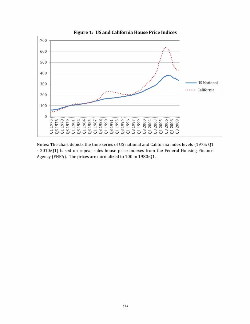
the global economy. As shown in Figure 1, the fall-off in house prices and related economic
decline were especially severe in California.
Neither analysts on Wall St., regulators in Washington, D.C., nor most academic economists
anticipated the magnitude of the house price cycle, its geographic reach, or related housing
market contagion. Indeed, while urban economists long have addressed linkages among a
system of cities (see, for example, Henderson (1977)), few studies have focused on the
spatial-temporal structure of the house price cycle. For example, little is known about the
relative exposure of MSA housing markets to fluctuations in the national economy, despite
the importance of such to investor diversification or to economic policy propagation. Also,
few analyses have provided insights as regards the metropolitan geography of house price
returns, notably including incidence of extreme (jump) returns and the directions of
contagion.
We address those questions via analyses of integration, correlation, and contagion in US
metropolitan housing markets. Those estimates are important to investors as they provide
an indication of opportunities to diversify away metropolitan-specific housing risk. For
example, high levels of MSA integration and contagion among geographically distinct
residential markets could mitigate the efficacy of geographic diversification strategies
implemented by investors in mortgage-backed securities. An improved understanding of
metropolitan housing market integration also could provide new insights regarding the
spatial incidence of national economic policy. In general, measures of integration and
contagion in housing markets provide signals for price return performance and are relevant
for the full spectrum of market participants, be they lenders, housing and mortgage
investors, homebuilders, and the like.
Following Pukthuanthong-Le and Roll (2009), we compute a simple intuitive measure of
housing market integration, based on the proportion of an MSA’s housing market returns
that can be explained by an identical set of national factors. The level of integration is
associated with the magnitude of R-Square, with higher values indicating higher levels of
integration. Two MSAs are viewed as perfectly integrated if those same national factors
fully explain housing market returns in both those areas. In that case, there would be a R-
square of 1 so there is no diversification potential between the MSAs.
Results of the analysis indicate elevated and increasing MSA housing market integration.
For the US as a whole, housing market integration trended up over the decade of the 2000s
3
to about .83 in 2010.1 In California the trend was marked; there average housing market
integration moved up from about .55 in 1997 to close to .95 in 2008! Also noteworthy,
however, was the abrupt downward adjustment in California integration, to approximately
.75, in the wake of the recent severe implosion in house prices. Further disaggregation of
California trends revealed more pronounced declines in integration among coastal markets
in the context of the housing bust. That result likely reflects special factors associated with
coastal markets (supply constraint, presence of amenities, and lack of subprime lending) in
the context of ongoing weakness in national economic and housing market fundamentals.
Using the Lee and Mykland (2008) measure to characterize extreme returns, we find that
the 2000s bubble period also was distinguished by a relatively high incidence of jumps in
housing returns. Jumps were especially evident early in the boom during 2004-2005 as
well as in 2008 in the wake of the bust in house prices, the latter likely owing to extreme
declines in returns in certain MSAs. During early stages of the boom (2003 – 2004), return
jumps in California suddenly become very prevalent with close to 70 percent of cities
having significant extreme housing returns; further, during that period, the jumps were
ubiquitous among coastal and inland California cities. In marked contrast, during the 2007-
2008 bust and among California MSAs, only inland cities witnessed extreme movements in
housing returns. Inland cities are characterized by a lack of constraint on housing supply
and, in hindsight, they had been substantially overbuilt. Further, those areas had been the
focus of substantial boom period subprime lending. As boom turned to bust, inland areas of
California quickly and largely imploded.
As would be expected, both in the US overall and in California, metropolitan return
correlations are dramatically larger than jump return correlations in both incidence and
magnitude. California, however, stands apart from the rest of the US in both returns and
extreme returns. Research findings indicate relatively high levels of housing return and
jump return correlations in California compared to the rest of the US. For example,
contemporaneous housing return correlations are generally in the range of 0.2 – 0.3 with
about 20 percent significant for MSAs outside California. In marked contrast, in excess of 92
percent of California MSA returns were significantly correlated with a mean correlation
level of about .66! Similar results are obtained for lead (one quarter ahead) MSA
correlations. Among areas outside California, less than 10 percent of lead correlations were
statistically significant with mean lead correlation levels at or below 0.20. In California,
more than three-quarters of MSAs recorded significant lead return correlations with a mean
correlation level of about .57.
California also was markedly different as regards contemporaneous and lead LM jump
correlations. Among areas outside of California, significant contemporaneous jump
correlations were small in number and in the range of only .02 – .03. Large lead jump
1 A measure of 1.0 would indicate perfectly integrated markets while zero would indicate no integration at all; hence, the observed average of 0.83 implies that U.S. housing markets are 83% integrated relative to the maximum possible level.
4
correlations outside California similarly occurred infrequently in any census division with
mean correlation coefficients (except for New England) of .04 or less. In contrast, both the
incidence and magnitude of contemporaneous and lead jump correlations were greater for
California.
Given the above aberrant nature of integration, jump incidence, and MSA jump correlations
among California MSAs, the analysis turns to parametric assessment of spatial and temporal
contagion among California cities. Regression analyses over the full sample timeframe
indicate that house price returns for Los Angeles and surrounding areas largely move in
lock-step. In contrast, findings for Bay Area regional housing markets provide some
evidence of a spatial term structure of contagion. In that region, housing returns in San
Francisco lead those of many northern California communities. Contagion findings are
robust to controls for booms and busts in California housing markets.
The plan of the paper is as follows. Section II provides assessment of integration of US MSA
house price returns. In Section III, we report on analyses of both contemporaneous and
lagged correlations and jump correlations in MSA house price returns. Section IV provides
tests of geographic-temporal contagion among MSA housing markets in California. In
section V, we provide concluding remarks.
II. Integration
Substantial research has been undertaken as regards integration of international equity
markets. The applications vary in geography of focus, as some papers address integration
in the European community (see, for example, Hardouvelis, Malliaropoulos, and Priestley
(2006), and Schotman and Zalewska (2006)), whereas others investigate emerging markets
(see, for example, Bakaert and Harvey (1995), Chamber and Gibson (2006), Bakaert,
Harvey, Lundblad and Siegel (2008)). The analyses also vary widely in methodological
approach. For instance, Carrieri, Errunza and Hogan (2007) use GARCH-in-mean methods
to assess correlation in returns and volatility between markets, whereas Longin and Solnik
(1995) use cointegration techniques. While integration is often described in terms of cross-
country correlations in stock returns (for an early study see King and Wadhwani (1990)),
such a measure is argued to be flawed. Indeed, in the case where multiple factors drive
returns, markets may be imperfectly correlated but perfectly integrated.2
2 As shown by Pukthuanthong and Roll (2009), while perfect integration implies that identical global factors fully explain index returns across countries, some countries may differ in their sensitivities to those factors and accordingly not exhibit perfect correlation. An easy intuitive example would be an energy-exporting country such as Saudi Arabia and an energy-importing country such as Hong Kong. Both countries might be positively associated with global factors such as consumer goods or financial services. Morever, both countries could be fully integrated in the global economy; yet the simple correlation between their stock market returns could be relatively small, or even negative, because higher energy price increase Saudi equity values and decrease Hong Kong equity values. As a
5
As suggested by Pukthuanthong-Le and Roll (2009), a simple intuitive measure of financial
market integration is the proportion of a country’s returns that can be explained by an
identical set of [global] factors. This measure of integration focuses on the magnitude of
country-specific residual variance in a factor model seeking to explain a broadly-defined
country equity return index.3 Clearly, to the extent global factors explain only a small
proportion of variance in a country’s returns, the country would be viewed as less
integrated (see, for example, Stulz (1981) and Errunza and Losq (1985)).4 In contrast,
markets would be viewed as highly integrated to the extent their returns are explained. We
below describe US metropolitan housing markets as highly integrated if identical US
national factors explain a large portion of the variance in MSA house price returns. To
compute US housing market integration, we regress metropolitan house price returns on an
identical set of national economic and housing market fundamentals.
Integration is viewed as important to investors, policymakers, and market participants in
general. A measure of housing market integration provides some indication of the benefits
to investor diversification among MSA markets. While there may be some benefit to
diversifying away MSA-specific housing market risk, those benefits would decline with
increases in integration. Indeed, high levels of integration may mitigate strategies of
geographic diversification among investors in mortgage-backed securities. Also, among
other things, a measure of metro housing market integration would provide national
economic policymakers with some indication of the geographic ubiquity of policy
propagation. High levels of MSA housing return integration imply that those markets
largely are driven by national factors, notably including monetary policy and other housing
fundamentals. Similarly, elevated levels of metro housing market integration imply that
macro and financial shocks will propagate through a larger number of MSA housing
markets. This will have relevance for all market participants, including institutional
investors in residential MBS as well as those who regulate housing, the housing GSEs,
mortgage lenders, and related financial institutions.
a. Model Specification and Data
MSA-specific house price returns are computed using the U.S. Federal Housing Finance
Agency (FHFA) metropolitan indices, previously known as the OFHEO house price series.
consequence, the extent to which the multi-factors drive returns is a better indication of likely diversification benefits than a correlation measure. 3 In contrast, in the presence of multiple national factors, the simple correlation between MSA house price return indexes could be a flawed measure of integration unless those MSAs have identical exposure to the national factors, e.g., unless the estimated coefficient vectors are exactly proportional across MSAs. 4 According to this definition, a country is perfectly integrated if the country-specific variance is zero after controlling for global factors. In the case of two perfectly integrated countries, market indexes would have zero residual variance. See Pukthuanthong and Roll (2009) for discussion and details.
6
The FHFA series are weighted repeat-sale price indices associated with single-family
homes. Home sales and refinancing activity included in the FHFA sample derive from
conventional home purchase mortgage loans conforming to the underwriting requirements
of the housing Government Sponsored Enterprises—the Federal National Mortgage
Association (Fannie Mae) and the Federal Home Loan Mortgage Corporation (Freddie Mac).
The FHFA data comprise the most extensive cross-sectional and time-series set of quality-
adjusted house price indices available in the United States.5 We compute house price
returns for each MSA in our sample as the log quarterly difference in its repeat home sales
price index.6 The MSA level data are quarterly from 1975:Q1 – 2010:Q1. The number of
MSAs in the database increases over time from 2 in 1975 to 380 by 1993. By the end of the
sample timeframe, there are 384 MSAs in the dataset.
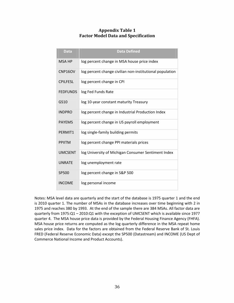
Per above, for each MSA in the sample, log percent change in the MSA-specific house price
indices is regressed on a common set of national economic, financial and housing market
factors. The specific factors and their definitions are displayed in Appendix Table 1. The
factors include measures of change in population, payroll employment, unemployment rate,
S&P500, industrial production, CPI, and PPI materials prices as well as personal income,
consumer sentiment, single-family building permits, Fed Funds rate, 10-year constant
maturity Treasury yields, and the like. All factor data are quarterly in frequency from
1975:Q1 – 2010:Q1 with the exception of consumer sentiment, which is available from
1977:Q4. Data for the factors are obtained from the Federal Reserve Bank of St. Louis FRED
(Federal Reserve Economic Data) with the exception of the S&P500 (Datastream) and
personal income (US Department of Commerce National Income and Product Accounts).
The MSA returns series are pre-whitened to remove serial correlation. A VAR(1) is
employed based on optimal AIC/BIC criteria from running the factor model on each
individual MSA. The average level of integration is measured by the R-squares from the
multi-factor model fitted for a 20-quarter moving window for the samples of MSAs (the use
of other window sizes gave the same qualitative results). The R-squares in these moving
windows indicate the corresponding levels of housing market integration.
b. Return Regressions on National Factors
Estimation results indicate that U.S. MSA housing market integration has increased over
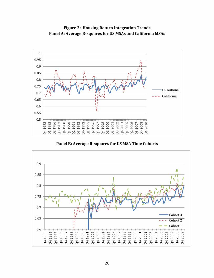
time. Figure 2 provides information on trends in housing market integration for the MSAs
in our sample. Panel A of Figure 2 shows that trend for the 1983:Q4 – 2009-Q4 period both
for the national and California samples. Very little trend in US MSA housing market
5 For a full discussion of the OFHEO house price index, see “A Comparison of House Price Measures”, Mimeo, Freddie Mac, February 28, 2008. 6 In principle, it would be desirable to model house prices at higher frequencies. Unfortunately, monthly quality-adjusted house price indices are available from OFHEO only for Census Divisions (N=18) and only for a much shorter time frame.
7
integration appeared during the decades of the 1980s and 1990s. In contrast, the 2000s
provides graphic evidence of trending up in housing market integration among US MSAs,
from about .70 in 2000 to approximately .83 by decade’s end. In California the trend in
housing market integration was even more marked moving up from about .55 in 1997 to
close to .95 in 2008! Further noteworthy, however, was the abrupt downward adjustment
in California housing market integration, to approximately .75, in the wake of the recent
severe implosion in house prices. Indeed, localized factors associated with the California
housing bust resulted in some disassociation of California metropolitan housing returns
from national economic fundamentals.
We control for potential bias in the FHFA data in terms of when an MSA was included in the
database. Regardless, the finding of increased integration still holds. Panel B of Figure 2
shows the average R-square pattern for 3 time cohorts. This categorization of MSAs into
cohorts assesses the robustness of results to the timeframe of city inclusion in the sample.
In this regard, it is possible that MSAs that entered the sample later were characterized by
lower or higher R-squares. If that were the case, averaging all MSAs together could move
the trend in the average either up or down. We plotted trends in the average level of
integration for three time-based cohorts. The cohorts included the full timeframe of
1983:Q4 – 2010:Q1 (cohort 1), 1989:Q2 – 2010:Q1 (cohort 2), and 1992:Q1 – 2010:Q1
(cohort 3). The cohorts yielded roughly similar results and indicated a longer-term trend
towards MSA housing market integration. In cohort 2, for example, the average R-square
moved up from about .65 in 1989 to almost .82 in 2010.
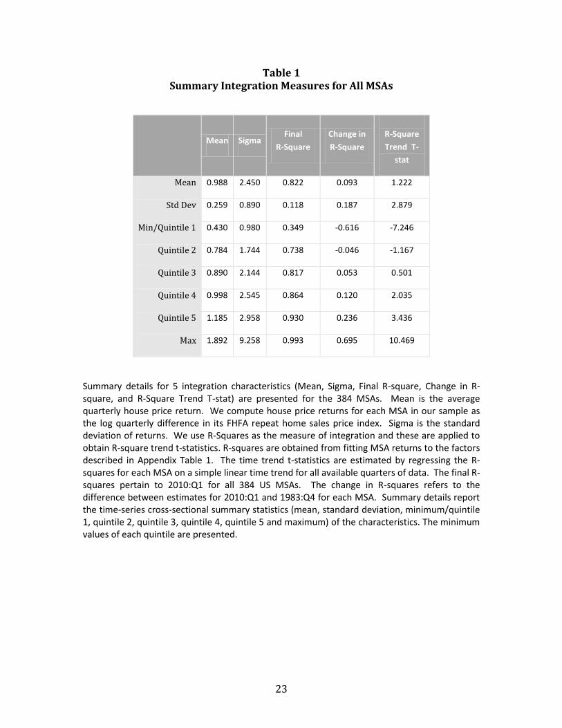
MSA housing market cross-sectional and time-series summary statistics are contained in
Table 1. For the sample of MSAs, we display mean quarterly house price returns, standard
deviation of returns (sigma), the R-square measure of integration, the change in R-square
over the timeframe of the analysis, and the associated time trend t-statistic (R-squares for
each MSA are fit to a simple linear time trend for all available quarters). Minimum values
by quintile are also presented. First, it is important to note that risk and return associated
with housing has been substantial. As shown, the average quarterly return for all MSA
housing markets in the sample is positive at almost 1% with an average deviation of about
2.5%. Moreover, we see substantial cross sectional variation in those measures; for
example, mean house price return varies from a minimum 0.43% to a sample maximum of
1.89%.
As evidenced in Table 1, the mean final period R-square of the integration model is .82,
suggesting the importance of national factors in determination of MSA house price returns.
The Table also indicates substantial temporal and cross-MSA variation in the integration
measure. On average R-squares increase by almost 10 percent from the beginning to end of
sample. In some areas, national economic and housing market fundamentals fail to explain
the majority of variation in MSA-specific house price returns (min R-squared = .35) At a
maximum, those same fundamentals explain a full 99 percent of variation in MSA-specific
house price returns. There is also substantial variation in the change in R-squared across

8
the sample with a standard deviation of .187. Appendix Table 2 contains integration details
for all 384 MSAs.7
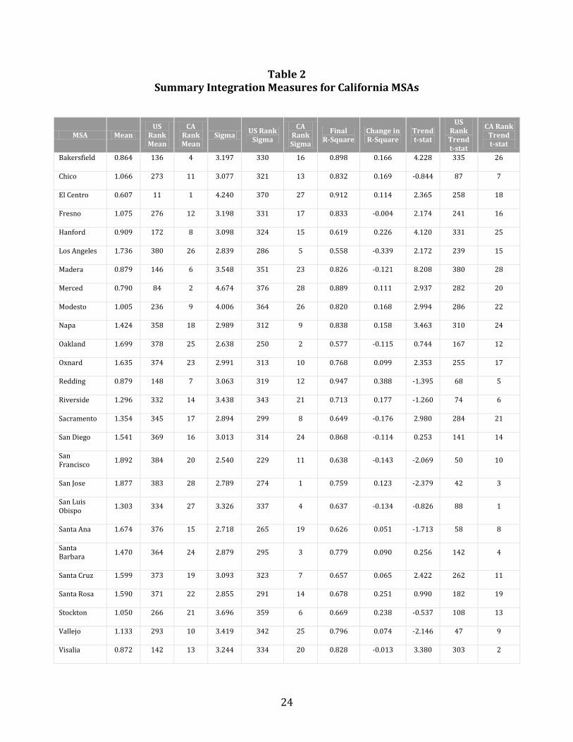
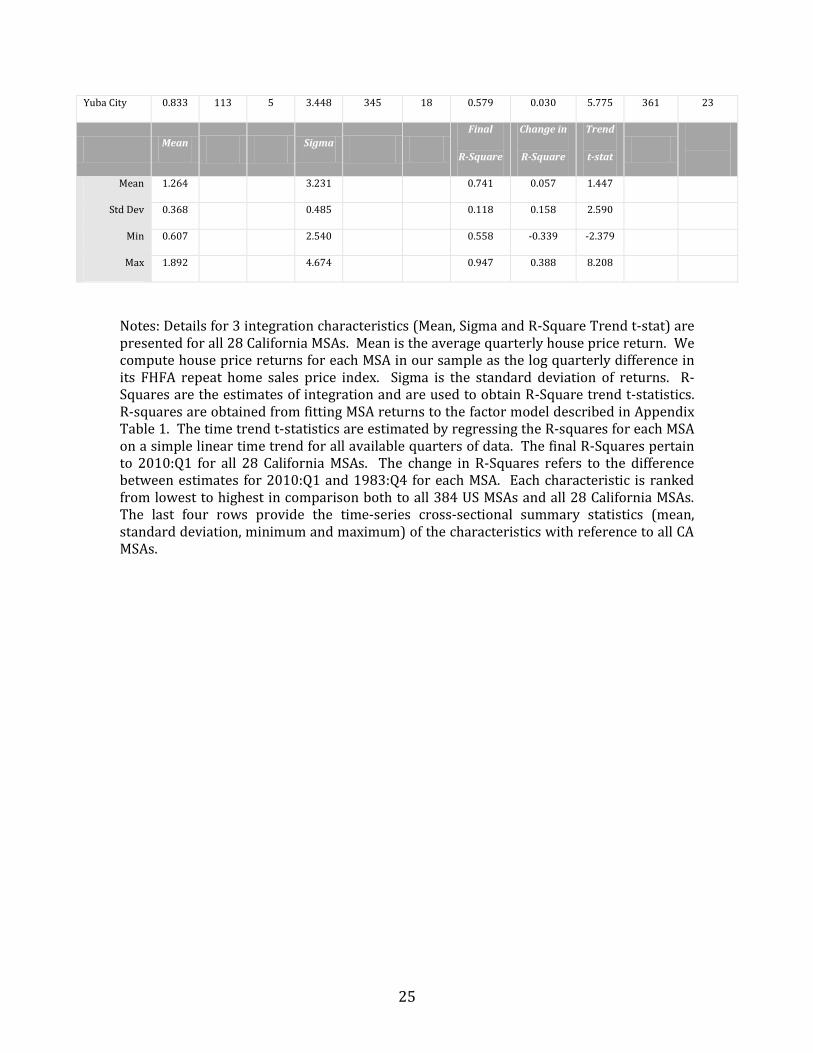
Table 2 presents integration details for the 28 California MSAs included in our dataset.
Relative to the full national sample of 384 MSAs, California metropolitan areas are
characterized by elevated mean house price returns, return volatility, and integration time
trend t-statistic. Further discernable in Table 2 are distinct coastal versus inland housing
market phenomena. Comparing coastal MSAs (see, for example, San Francisco, Oakland, San
Jose, Los Angeles, Santa Ana, and Santa Barbara) with inland MSAs (for example,
Bakersfield, Fresno, Madera, Merced, Modesto, Riverside, and Sacramento), note that the
former are roughly characterized by relatively higher mean house price returns, lower
return volatility, damped levels of integration, and lower integration trend t-statistics.
Among California coastal MSAs, mean quarterly returns averaged an elevated 1.6 percent;
further, integration R-squared averaged .69 with an insignificant time trend t-statistic. In
marked contrast, California Central Valley and Inland Empire cities displayed substantially
lower mean house price returns, elevated return volatility, higher levels of integration, and
higher integration trend t-stats. In inland areas, mean quarterly house price returns were a
damped 1 percent with an elevated sigma of 3.4 percent; further, the t-statistic on the
integration time trend was 2.2, well in excess of t-statistics for California coastal MSAs and
for the nation as a whole.
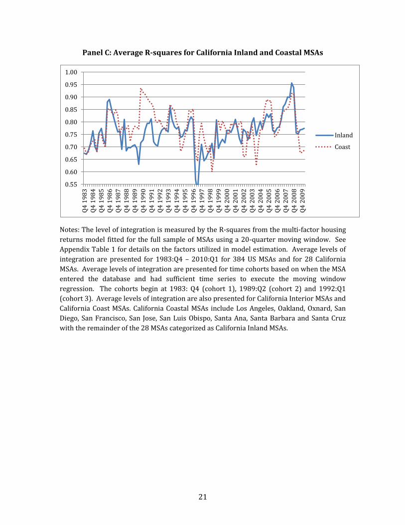
Panel C of Figure 2 shows trends in average R-square for inland and coastal MSAs in
California. As is evident, average integration for MSAs in both areas trended up over the
late-1990s through 2008 period. Striking is an up and down pattern in integration that
roughly coincided with the boom and bust in housing markets overall. While integration
levels for California MSAs moved up from about .75 to in excess of .90 in the context of the
2000s cyclical boom in housing, those same measures fell back markedly during the
subsequent bust as California housing returns became increasingly divorced from national
economic fundamentals. Further, the chart is suggestive that localized factors recently
played a substantially greater role in determination of coastal California house price
returns, as suggested in the divergence in integration between coastal and inland areas in
the context of the implosion in housing markets. That divergence likely reflected special
factors supportive of the performance of coastal markets (supply constraint, desirable
natural amenities, shorter commutes, and the like) in the context of ongoing weakness in
national economic and housing market fundamentals. As was broadly reported, Central
Valley and Inland Empire cities collectively comprised the epicentre of the 2000s boom-
bust cycle in California housing markets. Those areas were characterized by high levels of
subprime lending, elastic land and housing supply, longer commutes, and substantial
overbuilding. In many cases, the interior MSAs are outer-ring bedroom communities for
employment centers closer to the coast. The results suggest distinctions in housing return
7 The table further provides the quintile and rank (from lowest to highest) across the 384 MSAs of returns, sigma, and integration time trend t-statistic.
9
phenomena both within and between California MSAs and the nation as a whole. We return
to that below, in discussion of MSAs house price return correlations and contagion.
III. MSA Return and Jump Return Correlations
In this section, we investigate the magnitude of metropolitan house price returns,
distinguishing between common and extreme movements (jumps). Those results are
benchmarked by a discussion of contemporaneous and lagged correlations in MSA house
price returns. The analysis provides insights about temporal and geographic variations in
those measures; we pay particular attention to California MSAs.
To the extent that extreme movements in MSA house price returns are few in number or
geographically random, they would be of limited consequence to either private investors or
policymakers. On the other hand, higher levels of ubiquity in return or jump return
correlations raise concerns for mortgage or housing investors seeking to diversify risks
associated with extreme house price movements. In a similar vein, other market players
including MBS originators and investors would be similarly impacted by high correlations
in returns or jump returns among their mortgage assets. Note further that jumps or jump
correlations may be driven by economic or policy shocks at local or national levels. Jumps
in house price returns should be of interest to policymakers especially in those cases where
jumps can be traced to political events or policy perturbations.
Prior analyses have proposed alternative measures of jump test statistics (see, for example,
Barndorff-Nielson and Shepard (2006), Lee and Mykland (2008), Jiang and Oomen (2008),
and Jacod and Todorov (2009)). In a recent paper, Pukthuanthong-Le and Roll (2010)
assess the various jump statistics in application to stock return indexes for 82 countries.8
Unlike the other measures, Lee and Mykland works well with single observations (as
opposed to a sample of several observations). This is important for our application because
we have only quarterly data and hence the sample size is more limited than in the case of
equities, where daily observations are available. While results vary across alternative jump
statistics, results of of the above cited research suggest that jumps are largely idiosyncratic
in international equity indexes. We are not aware of prior analyses of jumps in metropolitan
house prices returns.
For the vast majority of sampled MSA housing markets, the most frequent quality-adjusted
house price index available to investors is quarterly. Moreover, investor rebalancing of real
estate portfolios tends to be of lower frequency relative to that of equities, and commonly is
at a quarterly interval. Consequently, we view such frequency as appropriate to investor
and policymaker market assessment and hence for the jump analysis.
8 Earlier work on extreme returns and correlation of same focused on more ad-hoc approaches (see Longin and Solnik, 2001).
10
With that in mind, we apply the Lee and Mykland (2008), (hereafter LM), method in
assessment of extreme movements in US metropolitan house price indexes. Like Barndorff-
Nielson and Shephard (2006), Lee and Mykland’s (2008) test is based on bipower variation.
Bipower variation is used to proxy the instantaneous variance of the continuous non-jump
component of prices.
To understand the test, consider the following notation:
t, subscript for quarter
Tk, the number of quarters in subperiod k
K, the total number of available subperiods
Ri,t,k, the return (log price relative) for MSA i quarter t in subperiod k
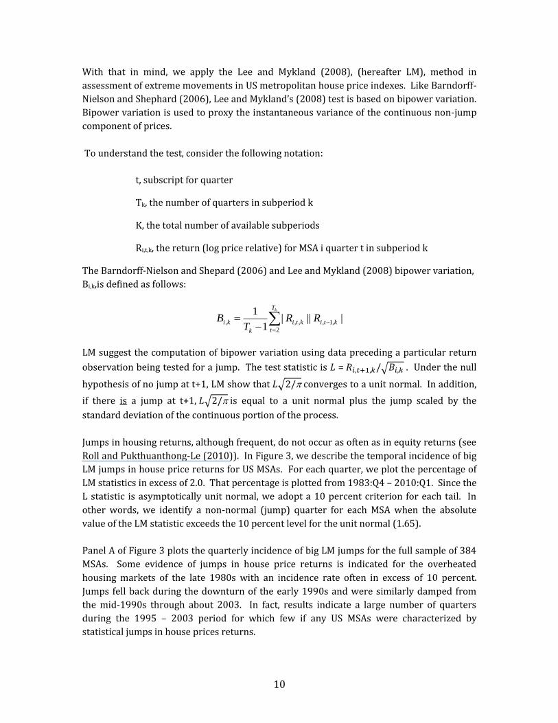
The Barndorff-Nielson and Shepard (2006) and Lee and Mykland (2008) bipower variation,
Bi,k,is defined as follows:
kT
t
ktikti
k
ki RRT
B2
,1,,,, ||||1
1
LM suggest the computation of bipower variation using data preceding a particular return
observation being tested for a jump. The test statistic is L = . Under the null
hypothesis of no jump at t+1, LM show that converges to a unit normal. In addition,
if there is a jump at t+1, is equal to a unit normal plus the jump scaled by the
standard deviation of the continuous portion of the process.
Jumps in housing returns, although frequent, do not occur as often as in equity returns (see
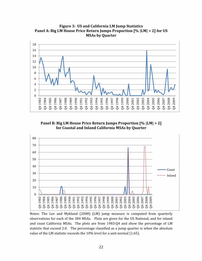
Roll and Pukthuanthong-Le (2010)). In Figure 3, we describe the temporal incidence of big
LM jumps in house price returns for US MSAs. For each quarter, we plot the percentage of
LM statistics in excess of 2.0. That percentage is plotted from 1983:Q4 – 2010:Q1. Since the
L statistic is asymptotically unit normal, we adopt a 10 percent criterion for each tail. In
other words, we identify a non-normal (jump) quarter for each MSA when the absolute
value of the LM statistic exceeds the 10 percent level for the unit normal (1.65).
Panel A of Figure 3 plots the quarterly incidence of big LM jumps for the full sample of 384
MSAs. Some evidence of jumps in house price returns is indicated for the overheated
housing markets of the late 1980s with an incidence rate often in excess of 10 percent.
Jumps fell back during the downturn of the early 1990s and were similarly damped from
the mid-1990s through about 2003. In fact, results indicate a large number of quarters
during the 1995 – 2003 period for which few if any US MSAs were characterized by
statistical jumps in house prices returns.
11
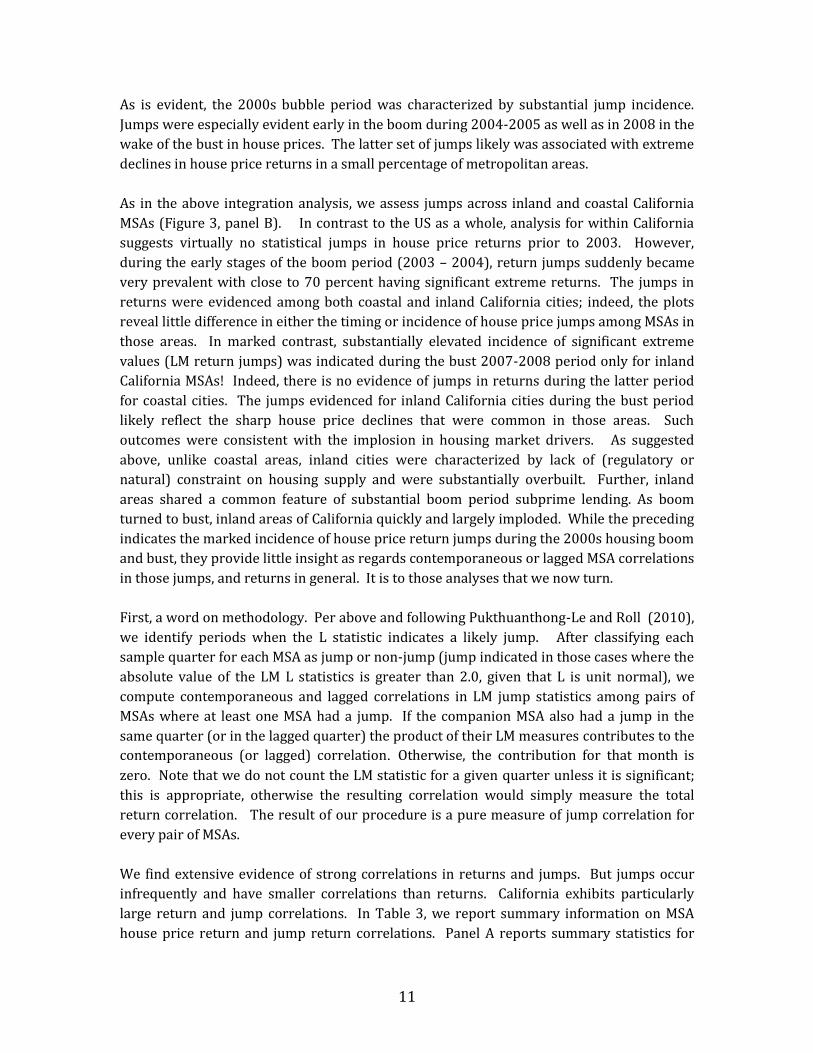
As is evident, the 2000s bubble period was characterized by substantial jump incidence.
Jumps were especially evident early in the boom during 2004-2005 as well as in 2008 in the
wake of the bust in house prices. The latter set of jumps likely was associated with extreme
declines in house price returns in a small percentage of metropolitan areas.
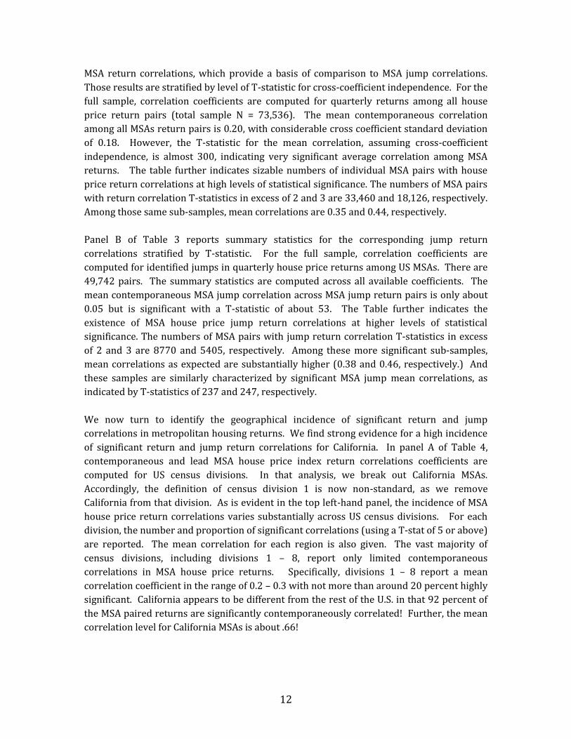
As in the above integration analysis, we assess jumps across inland and coastal California
MSAs (Figure 3, panel B). In contrast to the US as a whole, analysis for within California
suggests virtually no statistical jumps in house price returns prior to 2003. However,
during the early stages of the boom period (2003 – 2004), return jumps suddenly became
very prevalent with close to 70 percent having significant extreme returns. The jumps in
returns were evidenced among both coastal and inland California cities; indeed, the plots
reveal little difference in either the timing or incidence of house price jumps among MSAs in
those areas. In marked contrast, substantially elevated incidence of significant extreme
values (LM return jumps) was indicated during the bust 2007-2008 period only for inland
California MSAs! Indeed, there is no evidence of jumps in returns during the latter period
for coastal cities. The jumps evidenced for inland California cities during the bust period
likely reflect the sharp house price declines that were common in those areas. Such
outcomes were consistent with the implosion in housing market drivers. As suggested
above, unlike coastal areas, inland cities were characterized by lack of (regulatory or
natural) constraint on housing supply and were substantially overbuilt. Further, inland
areas shared a common feature of substantial boom period subprime lending. As boom
turned to bust, inland areas of California quickly and largely imploded. While the preceding
indicates the marked incidence of house price return jumps during the 2000s housing boom
and bust, they provide little insight as regards contemporaneous or lagged MSA correlations
in those jumps, and returns in general. It is to those analyses that we now turn.
First, a word on methodology. Per above and following Pukthuanthong-Le and Roll (2010),
we identify periods when the L statistic indicates a likely jump. After classifying each
sample quarter for each MSA as jump or non-jump (jump indicated in those cases where the
absolute value of the LM L statistics is greater than 2.0, given that L is unit normal), we
compute contemporaneous and lagged correlations in LM jump statistics among pairs of
MSAs where at least one MSA had a jump. If the companion MSA also had a jump in the
same quarter (or in the lagged quarter) the product of their LM measures contributes to the
contemporaneous (or lagged) correlation. Otherwise, the contribution for that month is
zero. Note that we do not count the LM statistic for a given quarter unless it is significant;
this is appropriate, otherwise the resulting correlation would simply measure the total
return correlation. The result of our procedure is a pure measure of jump correlation for
every pair of MSAs.
We find extensive evidence of strong correlations in returns and jumps. But jumps occur
infrequently and have smaller correlations than returns. California exhibits particularly
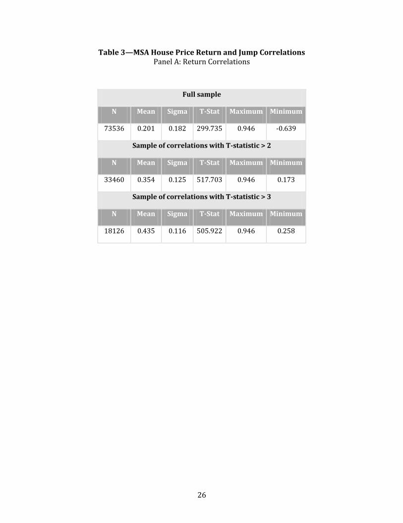
large return and jump correlations. In Table 3, we report summary information on MSA
house price return and jump return correlations. Panel A reports summary statistics for
12
MSA return correlations, which provide a basis of comparison to MSA jump correlations.
Those results are stratified by level of T-statistic for cross-coefficient independence. For the
full sample, correlation coefficients are computed for quarterly returns among all house
price return pairs (total sample N = 73,536). The mean contemporaneous correlation
among all MSAs return pairs is 0.20, with considerable cross coefficient standard deviation
of 0.18. However, the T-statistic for the mean correlation, assuming cross-coefficient
independence, is almost 300, indicating very significant average correlation among MSA
returns. The table further indicates sizable numbers of individual MSA pairs with house
price return correlations at high levels of statistical significance. The numbers of MSA pairs
with return correlation T-statistics in excess of 2 and 3 are 33,460 and 18,126, respectively.
Among those same sub-samples, mean correlations are 0.35 and 0.44, respectively.
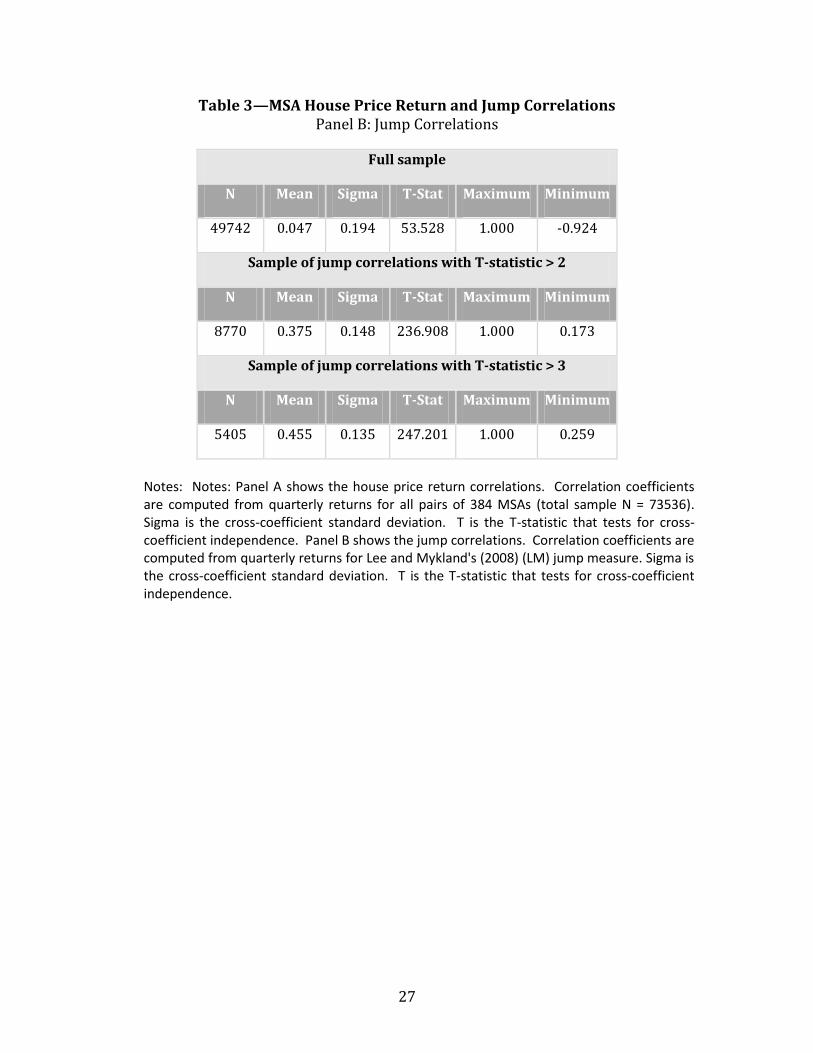
Panel B of Table 3 reports summary statistics for the corresponding jump return
correlations stratified by T-statistic. For the full sample, correlation coefficients are
computed for identified jumps in quarterly house price returns among US MSAs. There are
49,742 pairs. The summary statistics are computed across all available coefficients. The
mean contemporaneous MSA jump correlation across MSA jump return pairs is only about
0.05 but is significant with a T-statistic of about 53. The Table further indicates the
existence of MSA house price jump return correlations at higher levels of statistical
significance. The numbers of MSA pairs with jump return correlation T-statistics in excess
of 2 and 3 are 8770 and 5405, respectively. Among these more significant sub-samples,
mean correlations as expected are substantially higher (0.38 and 0.46, respectively.) And
these samples are similarly characterized by significant MSA jump mean correlations, as
indicated by T-statistics of 237 and 247, respectively.
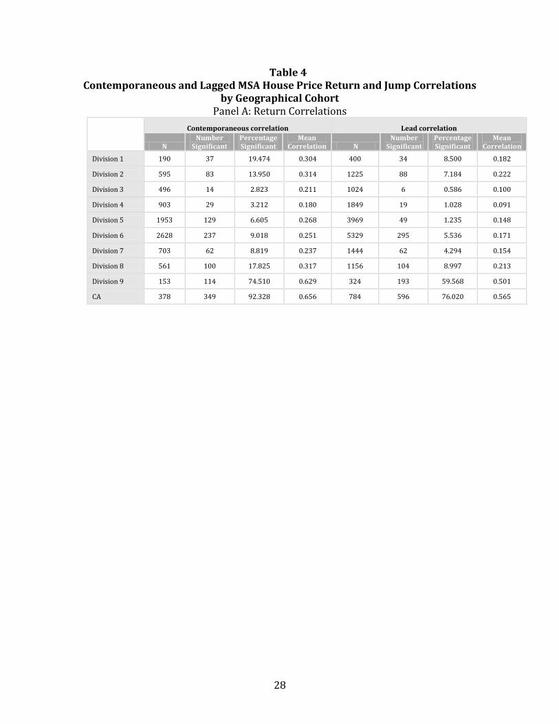
We now turn to identify the geographical incidence of significant return and jump
correlations in metropolitan housing returns. We find strong evidence for a high incidence
of significant return and jump return correlations for California. In panel A of Table 4,
contemporaneous and lead MSA house price index return correlations coefficients are
computed for US census divisions. In that analysis, we break out California MSAs.
Accordingly, the definition of census division 1 is now non-standard, as we remove
California from that division. As is evident in the top left-hand panel, the incidence of MSA
house price return correlations varies substantially across US census divisions. For each
division, the number and proportion of significant correlations (using a T-stat of 5 or above)
are reported. The mean correlation for each region is also given. The vast majority of
census divisions, including divisions 1 – 8, report only limited contemporaneous
correlations in MSA house price returns. Specifically, divisions 1 – 8 report a mean
correlation coefficient in the range of 0.2 – 0.3 with not more than around 20 percent highly
significant. California appears to be different from the rest of the U.S. in that 92 percent of
the MSA paired returns are significantly contemporaneously correlated! Further, the mean
correlation level for California MSAs is about .66!
13
As reported in the top right-hand panel of table 4, intertemporal (lead one quarter ahead)
correlations are similarly damped in most census divisions. Among divisions 1 - 8, less than
10 percent of lead correlations are statistically significant. Further, mean lead correlation
levels remain at or below .20. In marked contrast, MSAs in New England (division 9) and
California are characterized by relatively high percentages of significant and elevated lead
correlations. Again California is the outlier, as in excess of three-quarters of California MSAs
recorded significant lead return correlations with a mean correlation level of about .57.
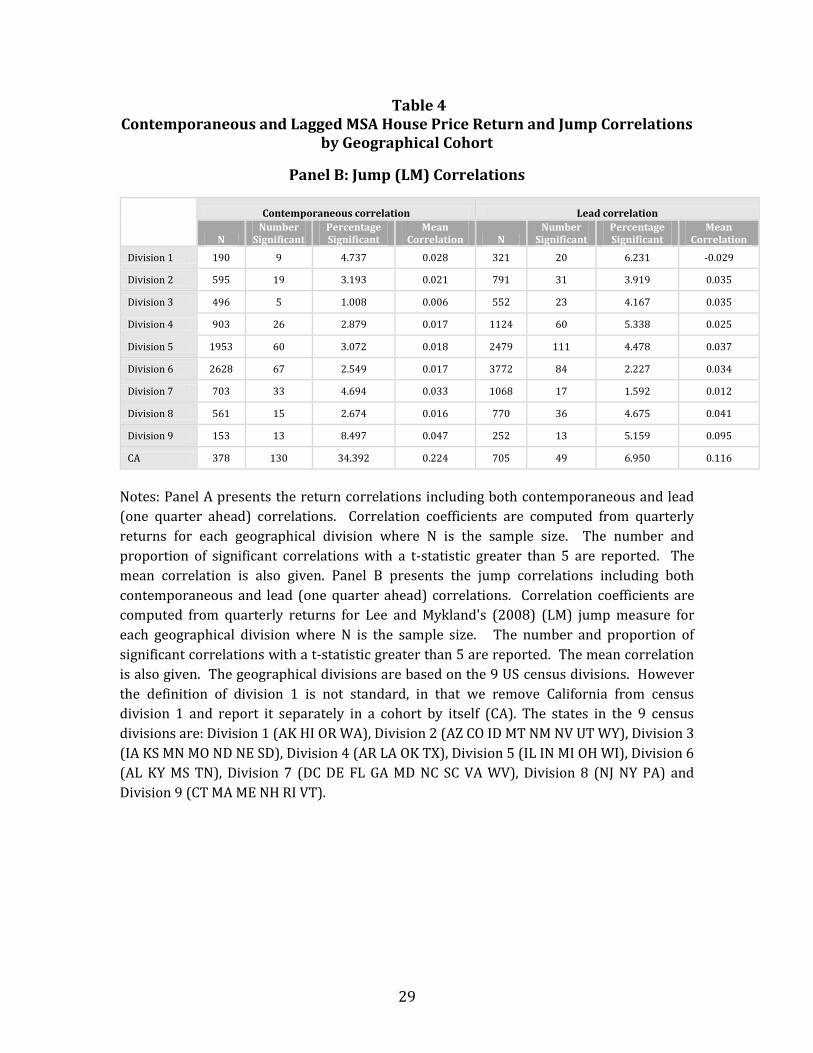
Panel B reports a similar assessment of contemporaneous and lead LM jump return
correlations among MSAs stratified by census division. As shown in the bottom panels,
California is conspicuously different from the rest of the U.S. For census divisions 1 – 8,
significant contemporaneous jump correlations are small in number (less than 10 percent
in any division) and mean correlations coefficients are in the range of only .02 – .03. In
those same areas, lead jump correlations are limited to an incidence of 6 percent or less in
any division with mean correlation coefficients (except for New England) of .04 or less. In
marked contrast, jump return contemporaneous correlations are significant among
California MSAs at an occurrence rate of 34 percent, and with much larger values, reaching
.22, substantially in excess of levels discussed above for other regions. Moreover, the mean
lead jump correlations are highest for California.
Another clear message results from the correlation analysis in US housing markets and
when broken down into geographical cohorts. The incidence of significant return
correlations far exceeds jump correlations. To illustrate, the percentage with significant t-
statistics greater than 2 is in excess of 45 percent for return correlations compared to
approximately 18 percent for jump return correlations (see Table 3). When we break out
the analysis into geographical cohorts we find that the ratio of significant t-statistics far
greater for return correlations with three exceptions, that occur in Divisions 3 through 5 for
lead values (see Table 4). The results pertaining to the magnitude of correlations across
return and jump returns are even more clear-cut. In all comparisons, we find that the
return correlations far exceed their jump counterparts, usually by a ratio of 5 or more!
In addition, analyses of contemporaneous and lead jumps in house price returns again
suggest that California is different. Also, levels of contemporaneous and lead return and
jump correlations in California were well in excess of levels recorded in other census
divisions. Given the anomalous behavior of California metropolitan housing markets thus
documented we now turn to identify further insights as regards the temporal – spatial
structure of house price return contagion in this state.
IV. Contagion in Housing Market Returns
The above analyses suggest the outlier status of California MSAs in assessment of recent
house price phenomena. Specifically, our analyses point to rising levels of integration as
well as elevated return correlation and jump return correlation, both lead and

14
contemporaneous, among California MSAs. However, the spatial dimensions of those
relationships were not specified. Below we address that issue via parametric assessment of
the spatial dynamics of housing returns among MSAs in northern and southern California.
We report some interesting findings for the metropolitan housing markets in California. In
particular, spatial return spillovers are largely efficient across MSAs, especially in Southern
California, coming from Los Angeles to surrounding areas. Results of a first set of analyses
are contained in Table 5. There we test the simple hypothesis that house price returns
among primary California coastal MSAs lead those of surrounding areas. That hypothesis is
consistent with a mechanism whereby increases in house price returns (and related
declines in affordability) in expensive, supply-constrained, coastal metropolitan areas lead
to out-migration, related demand-side pressures, and subsequent increases in returns in
more affordable inland suburbs. In our test of that hypothesis for southern California, for
example, we estimate city-specific regressions whereby we regress returns for each inner-
and outer-ring suburb of the larger LA area on contemporaneous and lead Los Angeles MSA
house price returns. We undertake identical analyses for the Bay Area and central
California using San Francisco and Santa Barbara as primary coastal cities. As shown in
Table 5, we estimate those equations over the full timeframe of the metro-specific data sets.
In each case, MSA returns are regressed on contemporaneous and 3 quarterly lags of
primary coastal MSA returns.
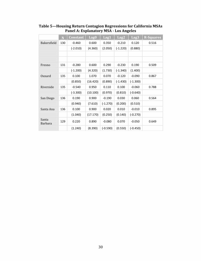
Results of the analysis for LA region MSAs are contained in the top panel of Table 5. Those
findings indicate a market efficiency in metropolitan spillover returns in that the most
significant effects are contemporaneous. Overall, the regressions are characterized by high
levels of explanatory power. In all of LA’s surrounding cities, including Bakersfield, Fresno,
Oxnard-Thousand Oaks, Riverside, San Diego, Santa Ana, and Santa Barbara, sizable and
highly significant coefficients are estimated for contemporaneous Los Angeles house price
returns. In Bakersfield and Fresno, located further from Los Angeles in California’s great
central valley, the contemporaneous coefficients on Los Angeles house price returns are
about .60 and highly significant; further, a positive and significant coefficient of about .30 is
estimated on the first quarterly lag of Los Angeles house price returns. In marked contrast,
in closer-in areas, only the contemporaneous coefficient was statistically significant.
Indeed, in those cities, the estimated coefficients on contemporaneous (quarterly) changes
in Los Angeles house price returns were close to 1! These analyses indicate a high degree
of contemporaneous correlation in house price returns among Los Angeles and its suburbs.
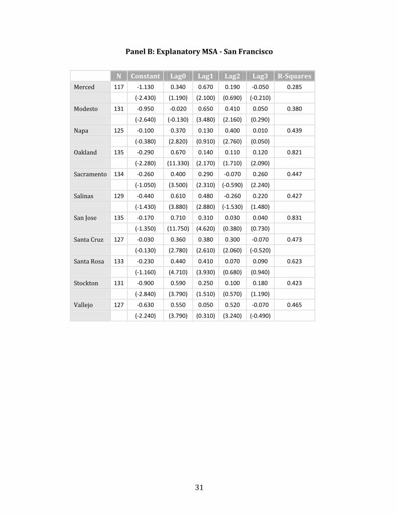
Results of the analysis diverge somewhat for San Francisco and environs where the level of
market efficiency appears to be somewhat lower. In most areas of northern California,
including Oakland, Sacramento, Salinas, San Jose, Santa Rosa, and Santa Cruz, both
contemporaneous and 1-quarter lagged San Francisco house price returns play a sizable
and significant role in determination of house price returns. In a few places, including both
Oakland and Santa Cruz, contemporaneous as well as 1- and 2-quarter lagged San Francisco
house prices returns significantly affect surrounding outcomes. San Francisco house price
15
returns lead those of the outer-ring Central Valley boom town of Modesto by 1-quarter. In
short, findings for Bay Area regional housing markets suggest a spatial term structure of
contagion, whereas results for Los Angeles indicate a southern California region where
metropolitan housing returns largely move in lock-step.
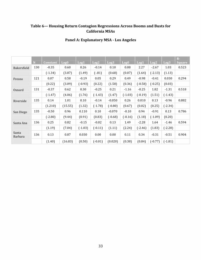
The above findings, however, may not be robust to periods of boom and bust in California
housing markets. Indeed, it is plausible that the spatial or temporal path of house price
contagion might accelerate during a boom or decelerate and even reverse during a bust. We
test for such effects in Table 6. The regression equations estimated in Table 6 are identical
to those in Table 5, except that each regression contains 4 additional terms. The additional
variables comprise interactions between the primary (explanatory) city’s return
(contemporaneous and 3 quarterly lags) and a contemporaneous residual from a time trend
fit of the log of an equal-weighted index of California house prices.
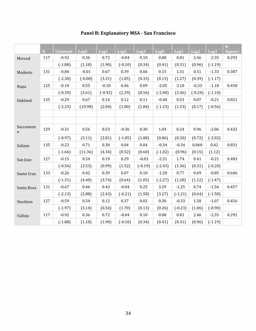
Findings contained in table 6 indicate that results of the California MSA house price
contagion analysis are largely robust to the inclusion of the boom and bust interactive
terms. In southern California, an exception is Bakersfield, where a sizable and significant
coefficient is estimated on second quarterly lagged interaction term. In northern California,
there exists little to report other than significant coefficients on contemporaneous
interactive terms for Santa Rosa and Santa Cruz. Accordingly, an explicit accounting for
boom and bust periods in California’s housing markets has little effect on conclusions
regarding the temporal path of house price contagion among California MSAs.9
V. Conclusion
This paper applies data from 384 US MSAs to examine integration and contagion among
metropolitan housing markets. The paper first examines the level and change in housing
market integration as reflected in the response of MSA house price returns to a national
multi-factor model. It then investigates the incidence of large house price return and jump
return correlations for the MSAs. Finally, as a result of the earlier integration and contagion
analysis, it isolates California and further examines contagion characteristics from leading
coastal cities to their inland neighbors.
Research findings reveal a highly integrated set of US metropolitan housing markets.
Furthermore, the susceptibility of MSA housing markets to national economic and policy
shocks trended up over time and was especially evident in the decade of the 2000s. Also,
high levels and elevated trends in housing market integration limit the efficacy of strategies
to diversify MSA-specific risk on the part of mortgage and housing investors.
9 We undertook yet another robustness check whereby we created an interaction between the explanatory’s city’s return (including four lags) and a contemporaneous residual from a time trend fit of the log of an equal-weighted California MSA (N=28) FHFA house price index. That interaction term was substituted for the primary coastal city boom and bust interaction term estimated in Table 6. Results here differed little from those reported in table 6, as the house price index for the state as a whole differed little from those for the primary coastal California cities.

16
California emerges as somewhat of an outlier, in terms of elevated trends in integration,
jumps in house price returns, and MSA contemporaneous and lagged return and jump
return correlations. In addition, high levels of short-term contagion appear endemic to
major California markets, especially in Los Angeles. Inland California MSAs appear to
behave as one and exhibit a high degree of market efficiency in the response to return
movements in the large coastal metropolitan areas.

17
References
Barndorff-Nielsen, O., Shephard, N. 2006. Econometrics of testing for jumps in financial
economics using bipower variation. Journal of Financial Econometrics 4, 1-30.
Bekaert, G., Harvey, C., 1995. “Time-Varying World Market Integration”, Journal of
Finance 50, 403-444.
Bekaert, G., Harvey, C., Lundblad, C., Siegel, S., 2008. What Segments Equity Markets? AFA 2009 Meetings Paper. Available at SSRN: http://ssrn.com/abstract=1108156.
Case, Karl., John Cotter, and Stuart Gabriel, “Housing Risk and Return: Evidence from a
Housing Asset Pricing Model”, Journal of Portfolio Management, forthcoming, 2011.
Carrieri, F., Errunza, V., Hogan, K., 2007, “Characterizing World Market Integration
Through Time. Journal of Financial and Quantitative Analysis 42, 915-940.
Chambet, A., Gibson, R., 2008, “Financial Integration, Economic Instability, and Trade
Structure in Emerging Markets”, Journal of International Money and Finance 27, 654-
675.
Hardouvelis, G., Malliaropoulos, D., Priestley, R., 2006. “EMU and European stock market
integrations” Journal of Business 79, 369-392.
Henderson, Vernon, “Economic Theory and the Cities”, Academic Press, New York, 1977.
Jacod, J., Todorov, V. 2009. Testing for common arrivals of jumps for discretely observed
multidimensional processes. The Annals of Statistics 37, 1792-1838.
Jiang, G., Oomen, R. 2008. Testing for jumps when asset prices are observed with noise –
a “swap variance” approach. Journal of Econometrics 144, 352-370.
King, Mervyn A., and Sushil Wadhwani, 1990, Transmission of volatility between stock
markets, Review of Financial Studies 3, 5-33.
Lee, S., Mykland, P., 2008. Jumps in financial markets: A new nonparametric test and
jump dynamics, Review of Financial Studies 21, 2535-2563.
Longin, F., Solnik, B., 1995. Is the correlation in international equity returns constant:
1960-1990? Journal of International Money and Finance 14, 3-26.
Longin, F. M. and Solnik, B., 2001, Extreme correlation of international equity markets,
Journal of Finance, 56: 649-676.

18
Pukthuanthong-Le, Kuntara and Richard Roll, “Global Market Integration: An
Alternative Measure and Its Application”, Journal of Financial Economics, 2009, 94(2),
214-232.
Kuntara, Pukthuanthong-Le and Richard Roll, “Internationally Correlated Jumps”,
Working Papers in Finance, UCLA Anderson School of Management, July 2010.
Schotman, P., Zalewska, A., 2006, “Non-synchronous trading and testing for market
integration in Central European emerging markets”, Journal of Empirical Finance 13,
462-494.
19
Figure 1: US and California House Price Indices
Notes: The chart depicts the time series of US national and California index levels (1975: Q1
- 2010:Q1) based on repeat sales house price indexes from the Federal Housing Finance
Agency (FHFA). The prices are normalized to 100 in 1980:Q1.
0
100
200
300
400
500
600
700
Q1
19
75
Q3
19
76
Q1
19
78
Q3
19
79
Q1
19
81
Q3
19
82
Q1
19
84
Q3
19
85
Q1
19
87
Q3
19
88
Q1
19
90
Q3
19
91
Q1
19
93
Q3
19
94
Q1
19
96
Q3
19
97
Q1
19
99
Q3
20
00
Q1
20
02
Q3
20
03
Q1
20
05
Q3
20
06
Q1
20
08
Q3
20
09
US National
California
20
Figure 2: Housing Return Integration Trends
Panel A: Average R-squares for US MSAs and California MSAs
Panel B: Average R-squares for US MSA Time Cohorts
0.5
0.55
0.6
0.65
0.7
0.75
0.8
0.85
0.9
0.95
1
Q4
19
83
Q1
19
85
Q2
19
86
Q3
19
87
Q4
19
88
Q1
19
90
Q2
19
91
Q3
19
92
Q4
19
93
Q1
19
95
Q2
19
96
Q3
19
97
Q4
19
98
Q1
20
00
Q2
20
01
Q3
20
02
Q4
20
03
Q1
20
05
Q2
20
06
Q3
20
07
Q4
20
08
Q1
20
10
US National
California
0.6
0.65
0.7
0.75
0.8
0.85
0.9
Q4
19
83
Q4
19
84
Q4
19
85
Q4
19
86
Q4
19
87
Q4
19
88
Q4
19
89
Q4
19
90
Q4
19
91
Q4
19
92
Q4
19
93
Q4
19
94
Q4
19
95
Q4
19
96
Q4
19
97
Q4
19
98
Q4
19
99
Q4
20
00
Q4
20
01
Q4
20
02
Q4
20
03
Q4
20
04
Q4
20
05
Q4
20
06
Q4
20
07
Q4
20
08
Q4
20
09
Cohort 3
Cohort 2
Cohort 1
21
Panel C: Average R-squares for California Inland and Coastal MSAs
Notes: The level of integration is measured by the R-squares from the multi-factor housing
returns model fitted for the full sample of MSAs using a 20-quarter moving window. See
Appendix Table 1 for details on the factors utilized in model estimation. Average levels of
integration are presented for 1983:Q4 – 2010:Q1 for 384 US MSAs and for 28 California
MSAs. Average levels of integration are presented for time cohorts based on when the MSA
entered the database and had sufficient time series to execute the moving window
regression. The cohorts begin at 1983: Q4 (cohort 1), 1989:Q2 (cohort 2) and 1992:Q1
(cohort 3). Average levels of integration are also presented for California Interior MSAs and
California Coast MSAs. California Coastal MSAs include Los Angeles, Oakland, Oxnard, San
Diego, San Francisco, San Jose, San Luis Obispo, Santa Ana, Santa Barbara and Santa Cruz
with the remainder of the 28 MSAs categorized as California Inland MSAs.
0.55
0.60
0.65
0.70
0.75
0.80
0.85
0.90
0.95
1.00
Q4
19
83
Q4
19
84
Q4
19
85
Q4
19
86
Q4
19
87
Q4
19
88
Q4
19
89
Q4
19
90
Q4
19
91
Q4
19
92
Q4
19
93
Q4
19
94
Q4
19
95
Q4
19
96
Q4
19
97
Q4
19
98
Q4
19
99
Q4
20
00
Q4
20
01
Q4
20
02
Q4
20
03
Q4
20
04
Q4
20
05
Q4
20
06
Q4
20
07
Q4
20
08
Q4
20
09
Inland
Coast
22
Figure 3: US and California LM Jump Statistics Panel A: Big LM House Price Return Jumps Proportion [% |LM| > 2] for US
MSAs by Quarter
Panel B: Big LM House Price Return Jumps Proportion [% |LM| > 2]
for Coastal and Inland California MSAs by Quarter
Notes: The Lee and Mykland (2008) (LM) jump measure is computed from quarterly
observations for each of the 384 MSAs. Plots are given for the US National, and for inland
and coast California MSAs. The plots are from 1983:Q4 and show the percentage of LM
statistic that exceed 2.0. The percentage classified as a jump quarter is when the absolute
value of the LM statistic exceeds the 10% level for a unit normal (1.65).
0
2
4
6
8
10
12
14
16
18
Q4
19
83
Q4
19
84
Q4
19
85
Q4
19
86
Q4
19
87
Q4
19
88
Q4
19
89
Q4
19
90
Q4
19
91
Q4
19
92
Q4
19
93
Q4
19
94
Q4
19
95
Q4
19
96
Q4
19
97
Q4
19
98
Q4
19
99
Q4
20
00
Q4
20
01
Q4
20
02
Q4
20
03
Q4
20
04
Q4
20
05
Q4
20
06
Q4
20
07
Q4
20
08
Q4
20
09
0
10
20
30
40
50
60
70
80
Q4
19
83
Q4
19
84
Q4
19
85
Q4
19
86
Q4
19
87
Q4
19
88
Q4
19
89
Q4
19
90
Q4
19
91
Q4
19
92
Q4
19
93
Q4
19
94
Q4
19
95
Q4
19
96
Q4
19
97
Q4
19
98
Q4
19
99
Q4
20
00
Q4
20
01
Q4
20
02
Q4
20
03
Q4
20
04
Q4
20
05
Q4
20
06
Q4
20
07
Q4
20
08
Q4
20
09
Coast
Inland
23
Table 1 Summary Integration Measures for All MSAs
Mean Sigma
Final
R-Square
Change in
R-Square
R-Square
Trend T-
stat
Mean 0.988 2.450 0.822 0.093 1.222
Std Dev 0.259 0.890 0.118 0.187 2.879
Min/Quintile 1 0.430 0.980 0.349 -0.616 -7.246
Quintile 2 0.784 1.744 0.738 -0.046 -1.167
Quintile 3 0.890 2.144 0.817 0.053 0.501
Quintile 4 0.998 2.545 0.864 0.120 2.035
Quintile 5 1.185 2.958 0.930 0.236 3.436
Max 1.892 9.258 0.993 0.695 10.469
Summary details for 5 integration characteristics (Mean, Sigma, Final R-square, Change in R-square, and R-Square Trend T-stat) are presented for the 384 MSAs. Mean is the average quarterly house price return. We compute house price returns for each MSA in our sample as the log quarterly difference in its FHFA repeat home sales price index. Sigma is the standard deviation of returns. We use R-Squares as the measure of integration and these are applied to obtain R-square trend t-statistics. R-squares are obtained from fitting MSA returns to the factors described in Appendix Table 1. The time trend t-statistics are estimated by regressing the R-squares for each MSA on a simple linear time trend for all available quarters of data. The final R-squares pertain to 2010:Q1 for all 384 US MSAs. The change in R-squares refers to the difference between estimates for 2010:Q1 and 1983:Q4 for each MSA. Summary details report the time-series cross-sectional summary statistics (mean, standard deviation, minimum/quintile 1, quintile 2, quintile 3, quintile 4, quintile 5 and maximum) of the characteristics. The minimum values of each quintile are presented.
24
Table 2 Summary Integration Measures for California MSAs
MSA Mean US
Rank Mean
CA Rank Mean
Sigma US Rank
Sigma
CA Rank Sigma
Final R-Square
Change in R-Square
Trend t-stat
US Rank
Trend t-stat
CA Rank Trend t-stat
Bakersfield 0.864 136 4 3.197 330 16 0.898 0.166 4.228 335 26
Chico 1.066 273 11 3.077 321 13 0.832 0.169 -0.844 87 7
El Centro 0.607 11 1 4.240 370 27 0.912 0.114 2.365 258 18
Fresno 1.075 276 12 3.198 331 17 0.833 -0.004 2.174 241 16
Hanford 0.909 172 8 3.098 324 15 0.619 0.226 4.120 331 25
Los Angeles 1.736 380 26 2.839 286 5 0.558 -0.339 2.172 239 15
Madera 0.879 146 6 3.548 351 23 0.826 -0.121 8.208 380 28
Merced 0.790 84 2 4.674 376 28 0.889 0.111 2.937 282 20
Modesto 1.005 236 9 4.006 364 26 0.820 0.168 2.994 286 22
Napa 1.424 358 18 2.989 312 9 0.838 0.158 3.463 310 24
Oakland 1.699 378 25 2.638 250 2 0.577 -0.115 0.744 167 12
Oxnard 1.635 374 23 2.991 313 10 0.768 0.099 2.353 255 17
Redding 0.879 148 7 3.063 319 12 0.947 0.388 -1.395 68 5
Riverside 1.296 332 14 3.438 343 21 0.713 0.177 -1.260 74 6
Sacramento 1.354 345 17 2.894 299 8 0.649 -0.176 2.980 284 21
San Diego 1.541 369 16 3.013 314 24 0.868 -0.114 0.253 141 14
San Francisco
1.892 384 20 2.540 229 11 0.638 -0.143 -2.069 50 10
San Jose 1.877 383 28 2.789 274 1 0.759 0.123 -2.379 42 3
San Luis Obispo
1.303 334 27 3.326 337 4 0.637 -0.134 -0.826 88 1
Santa Ana 1.674 376 15 2.718 265 19 0.626 0.051 -1.713 58 8
Santa Barbara
1.470 364 24 2.879 295 3 0.779 0.090 0.256 142 4
Santa Cruz 1.599 373 19 3.093 323 7 0.657 0.065 2.422 262 11
Santa Rosa 1.590 371 22 2.855 291 14 0.678 0.251 0.990 182 19
Stockton 1.050 266 21 3.696 359 6 0.669 0.238 -0.537 108 13
Vallejo 1.133 293 10 3.419 342 25 0.796 0.074 -2.146 47 9
Visalia 0.872 142 13 3.244 334 20 0.828 -0.013 3.380 303 2
25
Yuba City 0.833 113 5 3.448 345 18 0.579 0.030 5.775 361 23
Mean Sigma
Final
R-Square
Change in
R-Square
Trend
t-stat
Mean 1.264
3.231
0.741 0.057 1.447
Std Dev 0.368
0.485
0.118 0.158 2.590
Min 0.607
2.540
0.558 -0.339 -2.379
Max 1.892
4.674
0.947 0.388 8.208
Notes: Details for 3 integration characteristics (Mean, Sigma and R-Square Trend t-stat) are presented for all 28 California MSAs. Mean is the average quarterly house price return. We compute house price returns for each MSA in our sample as the log quarterly difference in its FHFA repeat home sales price index. Sigma is the standard deviation of returns. R-Squares are the estimates of integration and are used to obtain R-Square trend t-statistics. R-squares are obtained from fitting MSA returns to the factor model described in Appendix Table 1. The time trend t-statistics are estimated by regressing the R-squares for each MSA on a simple linear time trend for all available quarters of data. The final R-Squares pertain to 2010:Q1 for all 28 California MSAs. The change in R-Squares refers to the difference between estimates for 2010:Q1 and 1983:Q4 for each MSA. Each characteristic is ranked from lowest to highest in comparison both to all 384 US MSAs and all 28 California MSAs. The last four rows provide the time-series cross-sectional summary statistics (mean, standard deviation, minimum and maximum) of the characteristics with reference to all CA MSAs.
26
Table 3—MSA House Price Return and Jump Correlations Panel A: Return Correlations
Full sample
N Mean Sigma T-Stat Maximum Minimum
73536 0.201 0.182 299.735 0.946 -0.639
Sample of correlations with T-statistic > 2
N Mean Sigma T-Stat Maximum Minimum
33460 0.354 0.125 517.703 0.946 0.173
Sample of correlations with T-statistic > 3
N Mean Sigma T-Stat Maximum Minimum
18126 0.435 0.116 505.922 0.946 0.258
27
Table 3—MSA House Price Return and Jump Correlations Panel B: Jump Correlations
Full sample
N Mean Sigma T-Stat Maximum Minimum
49742 0.047 0.194 53.528 1.000 -0.924
Sample of jump correlations with T-statistic > 2
N Mean Sigma T-Stat Maximum Minimum
8770 0.375 0.148 236.908 1.000 0.173
Sample of jump correlations with T-statistic > 3
N Mean Sigma T-Stat Maximum Minimum
5405 0.455 0.135 247.201 1.000 0.259
Notes: Notes: Panel A shows the house price return correlations. Correlation coefficients are computed from quarterly returns for all pairs of 384 MSAs (total sample N = 73536). Sigma is the cross-coefficient standard deviation. T is the T-statistic that tests for cross-coefficient independence. Panel B shows the jump correlations. Correlation coefficients are computed from quarterly returns for Lee and Mykland's (2008) (LM) jump measure. Sigma is the cross-coefficient standard deviation. T is the T-statistic that tests for cross-coefficient independence.
28
Table 4
Contemporaneous and Lagged MSA House Price Return and Jump Correlations by Geographical Cohort
Panel A: Return Correlations
Contemporaneous correlation Lead correlation
N Number
Significant Percentage Significant
Mean Correlation N
Number Significant
Percentage Significant
Mean Correlation
Division 1 190 37 19.474 0.304 400 34 8.500 0.182
Division 2 595 83 13.950 0.314 1225 88 7.184 0.222
Division 3 496 14 2.823 0.211 1024 6 0.586 0.100
Division 4 903 29 3.212 0.180 1849 19 1.028 0.091
Division 5 1953 129 6.605 0.268 3969 49 1.235 0.148
Division 6 2628 237 9.018 0.251 5329 295 5.536 0.171
Division 7 703 62 8.819 0.237 1444 62 4.294 0.154
Division 8 561 100 17.825 0.317 1156 104 8.997 0.213
Division 9 153 114 74.510 0.629 324 193 59.568 0.501
CA 378 349 92.328 0.656 784 596 76.020 0.565
29
Table 4
Contemporaneous and Lagged MSA House Price Return and Jump Correlations by Geographical Cohort
Panel B: Jump (LM) Correlations
Contemporaneous correlation Lead correlation
N Number
Significant Percentage Significant
Mean Correlation N
Number Significant
Percentage Significant
Mean Correlation
Division 1 190 9 4.737 0.028 321 20 6.231 -0.029
Division 2 595 19 3.193 0.021 791 31 3.919 0.035
Division 3 496 5 1.008 0.006 552 23 4.167 0.035
Division 4 903 26 2.879 0.017 1124 60 5.338 0.025
Division 5 1953 60 3.072 0.018 2479 111 4.478 0.037
Division 6 2628 67 2.549 0.017 3772 84 2.227 0.034
Division 7 703 33 4.694 0.033 1068 17 1.592 0.012
Division 8 561 15 2.674 0.016 770 36 4.675 0.041
Division 9 153 13 8.497 0.047 252 13 5.159 0.095
CA 378 130 34.392 0.224 705 49 6.950 0.116
Notes: Panel A presents the return correlations including both contemporaneous and lead
(one quarter ahead) correlations. Correlation coefficients are computed from quarterly
returns for each geographical division where N is the sample size. The number and
proportion of significant correlations with a t-statistic greater than 5 are reported. The
mean correlation is also given. Panel B presents the jump correlations including both
contemporaneous and lead (one quarter ahead) correlations. Correlation coefficients are
computed from quarterly returns for Lee and Mykland's (2008) (LM) jump measure for
each geographical division where N is the sample size. The number and proportion of
significant correlations with a t-statistic greater than 5 are reported. The mean correlation
is also given. The geographical divisions are based on the 9 US census divisions. However
the definition of division 1 is not standard, in that we remove California from census
division 1 and report it separately in a cohort by itself (CA). The states in the 9 census
divisions are: Division 1 (AK HI OR WA), Division 2 (AZ CO ID MT NM NV UT WY), Division 3
(IA KS MN MO ND NE SD), Division 4 (AR LA OK TX), Division 5 (IL IN MI OH WI), Division 6
(AL KY MS TN), Division 7 (DC DE FL GA MD NC SC VA WV), Division 8 (NJ NY PA) and
Division 9 (CT MA ME NH RI VT).
30
Table 5—Housing Return Contagion Regressions for California MSAs Panel A: Explanatory MSA - Los Angeles
N Constant Lag0 Lag1 Lag2 Lag3 R-Squares
Bakersfield 130 -0.460 0.600 0.350 -0.210 0.120 0.516
(-2.010) (4.360) (2.050) (-1.220) (0.880)
Fresno 131 -0.280 0.600 0.290 -0.230 0.190 0.509
(-1.200) (4.320) (1.730) (-1.340) (1.400)
Oxnard 135 0.100 1.070 0.070 -0.120 -0.090 0.867
(0.850) (16.420) (0.890) (-1.430) (-1.300)
Riverside 135 -0.540 0.950 0.110 0.100 -0.060 0.788
(-3.300) (10.100) (0.970) (0.810) (-0.640)
San Diego 136 0.190 0.900 -0.190 0.030 0.060 0.564
(0.940) (7.610) (-1.270) (0.200) (0.510)
Santa Ana 136 0.100 0.900 0.020 0.010 -0.010 0.895
(1.040) (17.170) (0.250) (0.140) (-0.270)
Santa Barbara
129 0.220 0.890 -0.080 0.070 -0.050 0.649
(1.240) (8.390) (-0.590) (0.550) (-0.450)
31
Panel B: Explanatory MSA - San Francisco
N Constant Lag0 Lag1 Lag2 Lag3 R-Squares
Merced 117 -1.130 0.340 0.670 0.190 -0.050 0.285
(-2.430) (1.190) (2.100) (0.690) (-0.210)
Modesto 131 -0.950 -0.020 0.650 0.410 0.050 0.380
(-2.640) (-0.130) (3.480) (2.160) (0.290)
Napa 125 -0.100 0.370 0.130 0.400 0.010 0.439
(-0.380) (2.820) (0.910) (2.760) (0.050)
Oakland 135 -0.290 0.670 0.140 0.110 0.120 0.821
(-2.280) (11.330) (2.170) (1.710) (2.090)
Sacramento 134 -0.260 0.400 0.290 -0.070 0.260 0.447
(-1.050) (3.500) (2.310) (-0.590) (2.240)
Salinas 129 -0.440 0.610 0.480 -0.260 0.220 0.427
(-1.430) (3.880) (2.880) (-1.530) (1.480)
San Jose 135 -0.170 0.710 0.310 0.030 0.040 0.831
(-1.350) (11.750) (4.620) (0.380) (0.730)
Santa Cruz 127 -0.030 0.360 0.380 0.300 -0.070 0.473
(-0.130) (2.780) (2.610) (2.060) (-0.520)
Santa Rosa 133 -0.230 0.440 0.410 0.070 0.090 0.623
(-1.160) (4.710) (3.930) (0.680) (0.940)
Stockton 131 -0.900 0.590 0.250 0.100 0.180 0.423
(-2.840) (3.790) (1.510) (0.570) (1.190)
Vallejo 127 -0.630 0.550 0.050 0.520 -0.070 0.465
(-2.240) (3.790) (0.310) (3.240) (-0.490)
32
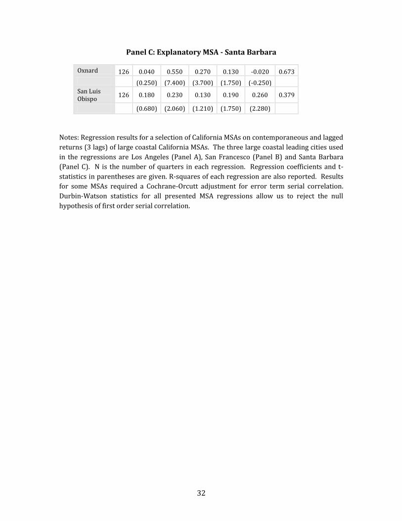
Panel C: Explanatory MSA - Santa Barbara
Notes: Regression results for a selection of California MSAs on contemporaneous and lagged
returns (3 lags) of large coastal California MSAs. The three large coastal leading cities used
in the regressions are Los Angeles (Panel A), San Francesco (Panel B) and Santa Barbara
(Panel C). N is the number of quarters in each regression. Regression coefficients and t-
statistics in parentheses are given. R-squares of each regression are also reported. Results
for some MSAs required a Cochrane-Orcutt adjustment for error term serial correlation.
Durbin-Watson statistics for all presented MSA regressions allow us to reject the null
hypothesis of first order serial correlation.
Oxnard 126 0.040 0.550 0.270 0.130 -0.020 0.673
(0.250) (7.400) (3.700) (1.750) (-0.250)
San Luis Obispo
126 0.180 0.230 0.130 0.190 0.260 0.379
(0.680) (2.060) (1.210) (1.750) (2.280)
33
Table 6— Housing Return Contagion Regressions Across Booms and Busts for
California MSAs
Panel A: Explanatory MSA - Los Angeles
N Constant Lag0 Lag1 Lag2 Lag3 Lag0 Lag1 Lag2 Lag3 R-Square
Bakersfield 130 -0.35 0.60 0.26 -0.14 0.10 0.08 2.27 -2.67 1.03 0.523
(-1.34) (3.87) (1.49) (-.81) (0.68) (0.07) (1.64) (-2.13) (1.13)
Fresno 121 0.07 0.58 -0.19 0.05 0.29 0.49 -0.98 -0.41 0.030 0.294
(0.22) (3.09) (-0.93) (0.22) (1.58) (0.36) (-0.58) (-0.25) (0.03)
Oxnard 131 -0.37 0.62 0.30 -0.25 0.21 -1.16 -0.25 1.82 -1.31 0.518
(-1.47) (4.06) (1.76) (-1.43) (1.47) (-1.03) (-0.19) (1.51) (-1.43)
Riverside 135 0.14 1.01 0.10 -0.14 -0.050 0.26 0.010 0.13 -0.96 0.882
(1.210) (15.55) (1.32) (-1.78) (-0.80) (0.67) (0.02) (0.25) (-2.34)
San Diego 135 -0.50 0.96 0.110 0.10 -0.070 -0.10 0.94 -0.91 0.13 0.786
(-2.80) (9.44) (0.91) (0.83) (-0.68) (-0.16) (1.18) (-1.09) (0.20)
Santa Ana 136 0.25 0.82 -0.15 -0.02 0.13 1.49 -2.28 1.64 -1.46 0.594
(1.19) (7.04) (-1.03) (-0.11) (1.11) (2.24) (-2.46) (1.83) (-2.28)
Santa Barbara
136 0.13 0.87 0.030 0.00 0.00 0.11 0.34 -0.31 -0.51 0.904
(1.40) (16.83) (0.50) (-0.01) (0.020) (0.38) (0.84) (-0.77) (-1.81)
34
Panel B: Explanatory MSA - San Francisco
N Constant Lag0 Lag1 Lag2 Lag3 Lag0 Lag1 Lag2 Lag3 R-Square
Merced 117 -0.92 0.36 0.72 -0.04 0.10 0.88 0.81 2.46 -2.35 0.292
(-1.88) (1.18) (1.90) (-0.10) (0.34) (0.41) (0.31) (0.96) (-1.19)
Modesto 131 -0.84 -0.01 0.67 0.39 0.06 0.15 1.51 0.51 -1.33 0.387
(-2.30) (-0.08) (3.31) (1.85) (0.33) (0.13) (1.27) (0.39) (-1.17)
Napa 125 -0.10 0.55 -0.18 0.46 0.09 -2.05 3.18 -0.33 -1.18 0.458
(-0.39) (3.61) (-0.92) (2.29) (0.56) (-2.00) (2.46) (-0.24) (-1.10)
Oakland 135 -0.29 0.67 0.14 0.12 0.11 -0.40 0.53 0.07 -0.21 0.821
(-2.23) (10.98) (2.04) (1.80) (1.84) (-1.23) (1.53) (0.17) (-0.56)
Sacramento
129 -0.31 0.56 0.53 -0.36 0.30 1.04 0.24 0.96 -2.06 0.432
(-0.97) (3.11) (2.81) (-1.85) (1.88) (0.86) (0.20) (0.72) (-2.02)
Salinas 135 -0.22 0.71 0.30 0.04 0.04 -0.34 -0.34 0.060 0.42 0.831
(-1.66) (11.36) (4.34) (0.52) (0.60) (-1.02) -(0.96) (0.15) (1.12)
San Jose 127 -0.15 0.54 0.19 0.29 -0.03 -2.51 1.74 0.41 -0.21 0.483
(-0.56) (3.53) (0.99) (1.52) (-0.19) (-2.43) (1.36) (0.31) (-0.20)
Santa Cruz 133 -0.26 0.42 0.39 0.07 0.10 -1.20 0.77 0.69 -0.85 0.646
(-1.31) (4.48) (3.74) (0.64) (1.05) (-2.27) (1.28) (1.12) (-1.47)
Santa Rosa 131 -0.67 0.46 0.43 -0.04 0.25 3.29 -1.25 0.74 -1.56 0.457
(-2.13) (2.88) (2.43) (-0.21) (1.58) (3.27) (-1.21) (0.64) (-1.58)
Stockton 127 -0.59 0.54 0.12 0.37 0.02 0.30 -0.33 1.58 -1.07 0.456
(-1.97) (3.14) (0.54) (1.70) (0.13) (0.26) (-0.23) (1.06) (-0.90)
Vallejo 117 -0.92 0.36 0.72 -0.04 0.10 0.88 0.81 2.46 -2.35 0.292
(-1.88) (1.18) (1.90) (-0.10) (0.34) (0.41) (0.31) (0.96) (-1.19)
35
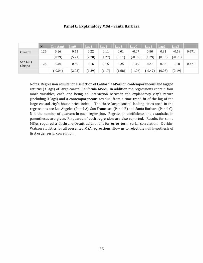
Panel C: Explanatory MSA - Santa Barbara
N Constant Lag0 Lag1 Lag2 Lag3 Lag0 Lag1 Lag2 Lag3
Oxnard 126 0.16 0.55 0.22 0.11 0.01 -0.07 0.80 0.31 -0.59 0.671
(0.79) (5.71) (2.70) (1.27) (0.11) (-0.09) (1.29) (0.53) (-0.93)
San Luis Obispo
126 -0.01 0.30 0.16 0.15 0.25 -1.19 -0.45 0.86 0.18 0.371
(-0.04) (2.03) (1.29) (1.17) (1.68) (-1.06) (-0.47) (0.95) (0.19)
Notes: Regression results for a selection of California MSAs on contemporaneous and lagged
returns (3 lags) of large coastal California MSAs. In addition the regressions contain four
more variables, each one being an interaction between the explanatory city's return
(including 3 lags) and a contemporaneous residual from a time trend fit of the log of the
large coastal city’s house price index. The three large coastal leading cities used in the
regressions are Los Angeles (Panel A), San Francesco (Panel B) and Santa Barbara (Panel C).
N is the number of quarters in each regression. Regression coefficients and t-statistics in
parentheses are given. R-squares of each regression are also reported. Results for some
MSAs required a Cochrane-Orcutt adjustment for error term serial correlation. Durbin-
Watson statistics for all presented MSA regressions allow us to reject the null hypothesis of
first order serial correlation.
36
Appendix Table 1 Factor Model Data and Specification
Data Data Defined
MSA HP log percent change in MSA house price index
CNP16OV log percent change civilian non-institutional population
CPILFESL log percent change in CPI
FEDFUNDS log Fed Funds Rate
GS10 log 10-year constant maturity Treasury
INDPRO log percent change in Industrial Production Index
PAYEMS log percent change in US payroll employment
PERMIT1 log single-family building permits
PPIITM log percent change PPI materials prices
UMCSENT log University of Michigan Consumer Sentiment Index
UNRATE log unemployment rate
SP500 log percent change in S&P 500
INCOME log personal income
Notes: MSA level data are quarterly and the start of the database is 1975 quarter 1 and the end is 2010 quarter 1. The number of MSAs in the database increases over time beginning with 2 in 1975 and reaches 380 by 1993. At the end of the sample there are 384 MSAs. All factor data are quarterly from 1975:Q1 – 2010:Q1 with the exception of UMCSENT which is available since 1977 quarter 4. The MSA house price data is provided by the Federal Housing Finance Agency (FHFA). MSA house price returns are computed as the log quarterly difference in the MSA repeat home sales price index. Data for the factors are obtained from the Federal Reserve Bank of St. Louis FRED (Federal Reserve Economic Data) except the SP500 (Datastream) and INCOME (US Dept of Commerce National Income and Product Accounts).
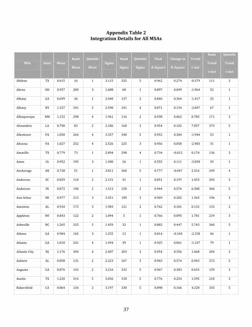
37
Appendix Table 2 Integration Details for All MSAs
MSA State Mean
Rank
Mean
Quintile
Mean
Sigma
Rank
Sigma
Quintile
Sigma
Final
R-Square
Change in
R-Square
Trend
t-stat
Rank
Trend
t-stat
Quintile
Trend
t-stat
Abilene TX 0.615 16 1 3.115 325 5 0.962 0.274 -0.379 111 2
Akron OH 0.957 200 3 1.688 68 1 0.897 0.049 -1.964 52 1
Albany GA 0.699 36 1 2.040 137 2 0.846 0.364 -1.417 32 1
Albany NY 1.337 341 5 2.590 241 4 0.871 0.134 -2.847 67 1
Albuquerque NM 1.152 298 4 1.961 116 2 0.938 0.062 0.783 171 3
Alexandria LA 0.790 83 2 2.186 160 3 0.954 0.102 7.057 373 5
Allentown PA 1.050 264 4 3.357 340 5 0.952 0.304 -1.944 53 1
Altoona PA 1.027 252 4 2.526 225 3 0.956 0.058 -2.983 31 1
Amarillo TX 0.779 73 1 2.894 298 4 0.734 -0.012 0.174 136 2
Ames IA 0.952 195 3 1.380 26 1 0.555 0.111 -3.058 29 1
Anchorage AK 0.728 51 1 3.811 360 5 0.777 -0.047 2.316 249 4
Anderson SC 0.829 110 2 2.131 41 1 0.851 0.197 1.453 203 3
Anderson IN 0.872 140 2 1.513 150 2 0.944 0.576 6.308 366 5
Ann Arbor MI 0.977 213 3 2.351 189 3 0.969 0.202 1.343 196 3
Anniston AL 0.910 173 3 1.983 121 2 0.762 0.181 0.132 133 2
Appleton WI 0.843 122 2 1.094 5 1 0.766 0.095 1.781 219 3
Asheville NC 1.265 325 5 1.459 32 1 0.882 0.447 5.743 360 5
Athens GA 0.904 165 3 1.255 12 1 0.814 -0.104 -2.158 46 1
Atlanta GA 1.010 241 4 1.494 39 1 0.925 0.061 -1.147 79 1
Atlantic City NJ 1.176 304 4 2.407 203 3 0.954 0.356 1.468 204 3
Auburn AL 0.858 131 2 2.223 167 3 0.965 0.574 6.963 372 5
Augusta GA 0.876 143 2 3.216 332 5 0.967 0.383 0.653 159 3
Austin TX 1.220 314 5 3.056 318 5 0.776 0.254 1.595 210 3
Bakersfield CA 0.864 136 2 3.197 330 5 0.898 0.166 4.228 335 5
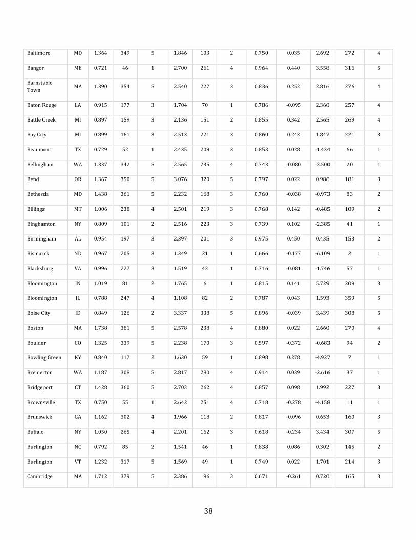
38
Baltimore MD 1.364 349 5 1.846 103 2 0.750 0.035 2.692 272 4
Bangor ME 0.721 46 1 2.700 261 4 0.964 0.440 3.558 316 5
Barnstable
Town MA 1.390 354 5 2.540 227 3 0.836 0.252 2.816 276 4
Baton Rouge LA 0.915 177 3 1.704 70 1 0.786 -0.095 2.360 257 4
Battle Creek MI 0.897 159 3 2.136 151 2 0.855 0.342 2.565 269 4
Bay City MI 0.899 161 3 2.513 221 3 0.860 0.243 1.847 221 3
Beaumont TX 0.729 52 1 2.435 209 3 0.853 0.028 -1.434 66 1
Bellingham WA 1.337 342 5 2.565 235 4 0.743 -0.080 -3.500 20 1
Bend OR 1.367 350 5 3.076 320 5 0.797 0.022 0.986 181 3
Bethesda MD 1.438 361 5 2.232 168 3 0.760 -0.038 -0.973 83 2
Billings MT 1.006 238 4 2.501 219 3 0.768 0.142 -0.485 109 2
Binghamton NY 0.809 101 2 2.516 223 3 0.739 0.102 -2.385 41 1
Birmingham AL 0.954 197 3 2.397 201 3 0.975 0.450 0.435 153 2
Bismarck ND 0.967 205 3 1.349 21 1 0.666 -0.177 -6.109 2 1
Blacksburg VA 0.996 227 3 1.519 42 1 0.716 -0.081 -1.746 57 1
Bloomington IN 1.019 81 2 1.765 6 1 0.815 0.141 5.729 209 3
Bloomington IL 0.788 247 4 1.108 82 2 0.787 0.043 1.593 359 5
Boise City ID 0.849 126 2 3.337 338 5 0.896 -0.039 3.439 308 5
Boston MA 1.738 381 5 2.578 238 4 0.880 0.022 2.660 270 4
Boulder CO 1.325 339 5 2.238 170 3 0.597 -0.372 -0.683 94 2
Bowling Green KY 0.840 117 2 1.630 59 1 0.898 0.278 -4.927 7 1
Bremerton WA 1.187 308 5 2.817 280 4 0.914 0.039 -2.616 37 1
Bridgeport CT 1.428 360 5 2.703 262 4 0.857 0.098 1.992 227 3
Brownsville TX 0.750 55 1 2.642 251 4 0.718 -0.278 -4.158 11 1
Brunswick GA 1.162 302 4 1.966 118 2 0.817 -0.096 0.653 160 3
Buffalo NY 1.050 265 4 2.201 162 3 0.618 -0.234 3.434 307 5
Burlington NC 0.792 85 2 1.541 46 1 0.838 0.086 0.302 145 2
Burlington VT 1.232 317 5 1.569 49 1 0.749 0.022 1.701 214 3
Cambridge MA 1.712 379 5 2.386 196 3 0.671 -0.261 0.720 165 3
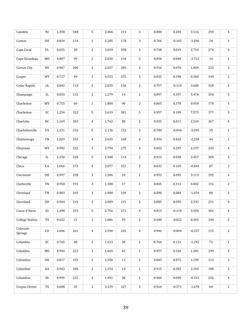
39
Camden NJ 1.358 348 5 2.466 214 3 0.800 0.204 3.116 293 4
Canton OH 0.834 114 2 2.285 178 3 0.766 -0.102 -3.296 24 1
Cape Coral FL 0.655 28 1 3.659 358 5 0.738 0.019 2.754 274 4
Cape Girardeau MO 0.807 99 2 2.030 134 2 0.856 0.040 -3.712 14 1
Carson City NV 0.967 206 3 2.827 283 4 0.916 0.078 1.869 223 3
Casper WY 0.727 49 1 4.553 375 5 0.835 0.198 0.360 149 2
Cedar Rapids IA 0.842 119 2 2.035 136 2 0.757 -0.119 3.680 320 5
Champaign IL 0.833 112 2 1.279 14 1 0.897 0.397 5.474 354 5
Charleston WV 0.755 60 1 1.800 90 2 0.865 0.378 0.954 178 3
Charleston SC 1.254 322 5 5.619 381 5 0.957 0.189 7.573 377 5
Charlotte NC 1.169 303 4 1.762 80 2 0.935 0.011 2.510 267 4
Charlottesville VA 1.231 316 5 2.136 152 2 0.700 -0.044 -3.595 19 1
Chattanooga TN 1.029 253 4 2.635 249 4 0.934 0.462 -2.258 44 1
Cheyenne WY 0.992 222 3 2.794 275 4 0.843 0.297 2.197 245 4
Chicago IL 1.250 320 5 1.948 114 2 0.913 0.038 3.457 309 5
Chico CA 1.066 273 4 3.077 321 5 0.832 0.169 -0.844 87 2
Cincinnati OH 0.997 228 3 1.206 10 1 0.953 0.695 3.113 292 4
Clarksville TN 0.950 191 3 1.308 17 1 0.845 0.311 0.402 151 2
Cleveland TN 0.983 203 3 1.900 109 2 0.898 0.084 -1.074 80 2
Cleveland OH 0.964 216 3 2.009 131 2 0.885 0.095 2.333 251 4
Coeur d'Alene ID 1.298 333 5 2.756 271 4 0.813 -0.110 3.304 301 4
College Station TX 0.632 21 1 1.806 93 2 0.448 -0.022 0.302 144 2
Colorado
Springs CO 1.046 261 4 2.590 242 4 0.946 -0.004 -0.257 115 2
Columbia SC 0.765 68 1 1.413 30 1 0.764 0.121 -1.292 72 1
Columbia MO 0.994 223 3 1.669 65 1 0.957 0.320 1.381 199 3
Columbus OH 0.817 103 2 1.258 11 1 0.845 0.072 1.199 113 2
Columbus GA 0.943 186 3 1.254 13 1 0.915 0.283 2.103 188 3
Columbus IN 0.995 225 3 1.491 38 1 0.960 0.090 -0.331 236 4
Corpus Christi TX 0.688 35 1 3.129 327 5 0.564 -0.371 -1.678 60 1
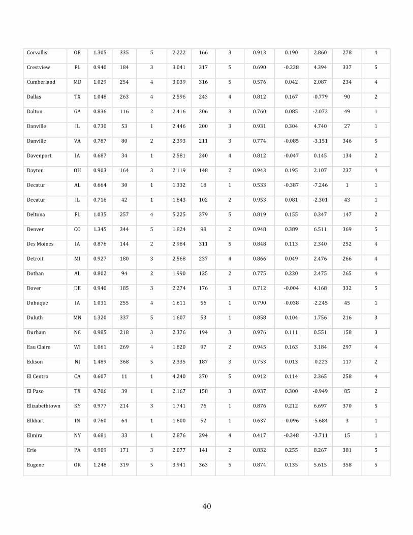
40
Corvallis OR 1.305 335 5 2.222 166 3 0.913 0.190 2.860 278 4
Crestview FL 0.940 184 3 3.041 317 5 0.690 -0.238 4.394 337 5
Cumberland MD 1.029 254 4 3.039 316 5 0.576 0.042 2.087 234 4
Dallas TX 1.048 263 4 2.596 243 4 0.812 0.167 -0.779 90 2
Dalton GA 0.836 116 2 2.416 206 3 0.760 0.085 -2.072 49 1
Danville IL 0.730 53 1 2.446 200 3 0.931 0.304 4.740 27 1
Danville VA 0.787 80 2 2.393 211 3 0.774 -0.085 -3.151 346 5
Davenport IA 0.687 34 1 2.581 240 4 0.812 -0.047 0.145 134 2
Dayton OH 0.903 164 3 2.119 148 2 0.943 0.195 2.107 237 4
Decatur AL 0.664 30 1 1.332 18 1 0.533 -0.387 -7.246 1 1
Decatur IL 0.716 42 1 1.843 102 2 0.953 0.081 -2.301 43 1
Deltona FL 1.035 257 4 5.225 379 5 0.819 0.155 0.347 147 2
Denver CO 1.345 344 5 1.824 98 2 0.948 0.389 6.511 369 5
Des Moines IA 0.876 144 2 2.984 311 5 0.848 0.113 2.340 252 4
Detroit MI 0.927 180 3 2.568 237 4 0.866 0.049 2.476 266 4
Dothan AL 0.802 94 2 1.990 125 2 0.775 0.220 2.475 265 4
Dover DE 0.940 185 3 2.274 176 3 0.712 -0.004 4.168 332 5
Dubuque IA 1.031 255 4 1.611 56 1 0.790 -0.038 -2.245 45 1
Duluth MN 1.320 337 5 1.607 53 1 0.858 0.104 1.756 216 3
Durham NC 0.985 218 3 2.376 194 3 0.976 0.111 0.551 158 3
Eau Claire WI 1.061 269 4 1.820 97 2 0.945 0.163 3.184 297 4
Edison NJ 1.489 368 5 2.335 187 3 0.753 0.013 -0.223 117 2
El Centro CA 0.607 11 1 4.240 370 5 0.912 0.114 2.365 258 4
El Paso TX 0.706 39 1 2.167 158 3 0.937 0.300 -0.949 85 2
Elizabethtown KY 0.977 214 3 1.741 76 1 0.876 0.212 6.697 370 5
Elkhart IN 0.760 64 1 1.600 52 1 0.637 -0.096 -5.684 3 1
Elmira NY 0.681 33 1 2.876 294 4 0.417 -0.348 -3.711 15 1
Erie PA 0.909 171 3 2.077 141 2 0.832 0.255 8.267 381 5
Eugene OR 1.248 319 5 3.941 363 5 0.874 0.135 5.615 358 5
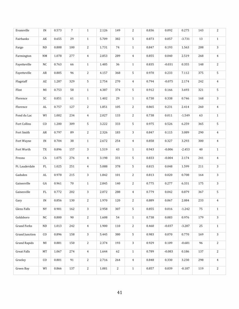
41
Evansville IN 0.573 7 1 2.126 149 2 0.836 0.092 0.275 143 2
Fairbanks AK 0.655 29 1 5.709 382 5 0.873 0.057 -3.731 13 1
Fargo ND 0.808 100 2 1.731 74 1 0.847 0.193 1.563 208 3
Farmington NM 1.078 277 4 2.853 289 4 0.855 0.040 2.519 268 4
Fayetteville NC 0.763 66 1 1.485 36 1 0.835 -0.031 0.355 148 2
Fayetteville AR 0.805 96 2 4.157 368 5 0.970 0.233 7.112 375 5
Flagstaff AZ 1.287 329 5 2.754 270 4 0.794 -0.075 2.174 242 4
Flint MI 0.753 58 1 4.387 374 5 0.912 0.166 3.693 321 5
Florence SC 0.851 61 1 1.402 29 1 0.730 0.338 0.746 168 3
Florence AL 0.757 127 2 1.851 105 2 0.865 0.231 2.414 260 4
Fond du Lac WI 1.002 234 4 2.027 133 2 0.738 0.011 -1.549 63 1
Fort Collins CO 1.200 309 5 3.222 333 5 0.975 0.526 6.259 365 5
Fort Smith AR 0.797 89 2 2.326 183 3 0.847 0.115 3.089 290 4
Fort Wayne IN 0.704 38 1 2.672 254 4 0.858 0.327 3.293 300 4
Fort Worth TX 0.896 157 3 1.519 43 1 0.943 -0.006 -2.453 40 1
Fresno CA 1.075 276 4 3.198 331 5 0.833 -0.004 2.174 241 4
Ft. Lauderdale FL 1.025 251 4 5.088 378 5 0.815 0.048 1.599 211 3
Gadsden AL 0.978 215 3 1.842 101 2 0.813 0.020 0.708 164 3
Gainesville GA 0.961 70 1 2.845 140 2 0.775 0.277 6.331 175 3
Gainesville FL 0.772 202 3 2.072 288 4 0.779 0.042 0.879 367 5
Gary IN 0.856 130 2 1.970 120 2 0.889 0.067 2.084 233 4
Glens Falls NY 0.901 162 3 2.958 307 5 0.855 0.016 -1.242 75 1
Goldsboro NC 0.800 90 2 1.608 54 1 0.738 0.083 0.976 179 3
Grand Forks ND 1.013 242 4 1.900 110 2 0.460 -0.037 -3.287 25 1
Grand Junction CO 0.896 158 3 5.445 380 5 0.983 0.070 0.770 169 3
Grand Rapids MI 0.881 150 2 2.374 193 3 0.929 0.109 -0.681 96 2
Great Falls MT 1.067 274 4 1.644 62 1 0.789 -0.083 0.186 137 2
Greeley CO 0.801 91 2 2.716 264 4 0.848 0.330 3.230 298 4
Green Bay WI 0.866 137 2 1.081 2 1 0.857 0.039 -0.187 119 2
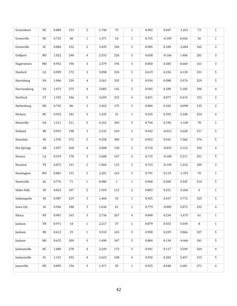
42
Greensboro NC 0.889 153 2 1.740 75 1 0.982 0.047 -1.261 73 1
Greenville NC 0.725 48 1 1.371 24 1 0.755 -0.109 0.666 36 1
Greenville SC 0.884 152 2 3.439 344 5 0.985 0.100 -2.684 162 3
Gulfport MS 1.022 248 4 2.533 226 3 0.658 -0.166 1.406 201 3
Hagerstown MD 0.952 196 3 2.379 195 3 0.850 0.285 0.660 161 3
Hanford CA 0.909 172 3 3.098 324 5 0.619 0.226 4.120 331 5
Harrisburg PA 1.006 239 4 3.261 335 5 0.934 0.588 3.974 329 5
Harrisonburg VA 1.073 275 4 2.083 142 2 0.945 0.189 3.182 296 4
Hartford CT 1.355 346 5 2.659 252 4 0.831 0.077 0.419 152 2
Hattiesburg MS 0.792 86 2 2.262 175 3 0.884 0.102 -0.090 125 2
Hickory NC 0.933 181 3 1.435 31 1 0.935 0.393 2.348 254 4
Hinesville GA 1.211 311 5 4.162 369 5 0.744 0.196 -1.160 78 1
Holland MI 0.955 198 3 2.232 169 3 0.942 -0.012 3.628 317 5
Honolulu HI 1.595 372 5 9.258 384 5 0.953 0.541 7.366 376 5
Hot Springs AR 1.057 268 4 2.008 130 2 0.718 -0.033 3.123 294 4
Houma LA 0.919 178 3 2.608 247 4 0.715 -0.100 5.211 351 5
Houston TX 0.872 141 2 1.960 115 2 0.723 -0.149 1.216 189 3
Huntington WV 0.881 151 2 2.201 163 3 0.791 0.119 -1.353 70 1
Huntsville AL 0.776 71 1 0.980 1 1 0.968 0.200 3.545 314 5
Idaho Falls ID 0.823 107 2 1.924 112 2 0.883 0.251 -5.266 6 1
Indianapolis IN 0.987 219 3 1.460 33 1 0.925 0.437 3.772 325 5
Iowa City IA 0.946 188 3 1.636 61 1 0.779 -0.005 2.072 232 4
Ithaca NY 0.901 163 3 2.736 267 4 0.848 0.234 -1.675 61 1
Jackson TN 0.971 14 1 2.217 37 1 0.879 0.553 4.549 8 1
Jackson MI 0.612 19 1 3.510 165 3 0.958 0.239 3.866 327 5
Jackson MS 0.625 209 3 1.490 347 5 0.884 0.134 -4.466 341 5
Jacksonville NC 1.080 278 4 2.249 173 3 0.941 0.117 3.549 264 4
Jacksonville FL 1.131 292 4 2.623 248 4 0.936 0.202 2.457 315 5
Janesville WI 0.895 156 3 1.471 35 1 0.925 0.448 2.681 271 4
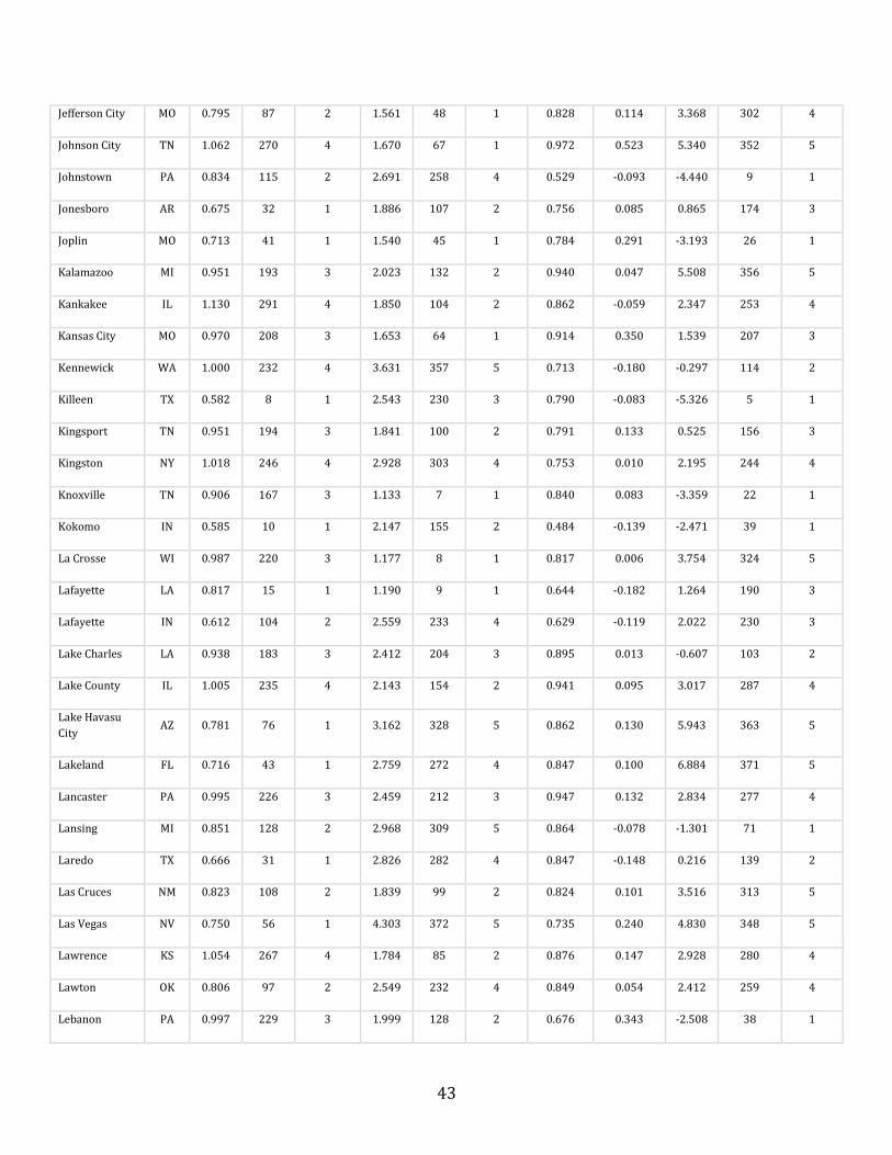
43
Jefferson City MO 0.795 87 2 1.561 48 1 0.828 0.114 3.368 302 4
Johnson City TN 1.062 270 4 1.670 67 1 0.972 0.523 5.340 352 5
Johnstown PA 0.834 115 2 2.691 258 4 0.529 -0.093 -4.440 9 1
Jonesboro AR 0.675 32 1 1.886 107 2 0.756 0.085 0.865 174 3
Joplin MO 0.713 41 1 1.540 45 1 0.784 0.291 -3.193 26 1
Kalamazoo MI 0.951 193 3 2.023 132 2 0.940 0.047 5.508 356 5
Kankakee IL 1.130 291 4 1.850 104 2 0.862 -0.059 2.347 253 4
Kansas City MO 0.970 208 3 1.653 64 1 0.914 0.350 1.539 207 3
Kennewick WA 1.000 232 4 3.631 357 5 0.713 -0.180 -0.297 114 2
Killeen TX 0.582 8 1 2.543 230 3 0.790 -0.083 -5.326 5 1
Kingsport TN 0.951 194 3 1.841 100 2 0.791 0.133 0.525 156 3
Kingston NY 1.018 246 4 2.928 303 4 0.753 0.010 2.195 244 4
Knoxville TN 0.906 167 3 1.133 7 1 0.840 0.083 -3.359 22 1
Kokomo IN 0.585 10 1 2.147 155 2 0.484 -0.139 -2.471 39 1
La Crosse WI 0.987 220 3 1.177 8 1 0.817 0.006 3.754 324 5
Lafayette LA 0.817 15 1 1.190 9 1 0.644 -0.182 1.264 190 3
Lafayette IN 0.612 104 2 2.559 233 4 0.629 -0.119 2.022 230 3
Lake Charles LA 0.938 183 3 2.412 204 3 0.895 0.013 -0.607 103 2
Lake County IL 1.005 235 4 2.143 154 2 0.941 0.095 3.017 287 4
Lake Havasu
City AZ 0.781 76 1 3.162 328 5 0.862 0.130 5.943 363 5
Lakeland FL 0.716 43 1 2.759 272 4 0.847 0.100 6.884 371 5
Lancaster PA 0.995 226 3 2.459 212 3 0.947 0.132 2.834 277 4
Lansing MI 0.851 128 2 2.968 309 5 0.864 -0.078 -1.301 71 1
Laredo TX 0.666 31 1 2.826 282 4 0.847 -0.148 0.216 139 2
Las Cruces NM 0.823 108 2 1.839 99 2 0.824 0.101 3.516 313 5
Las Vegas NV 0.750 56 1 4.303 372 5 0.735 0.240 4.830 348 5
Lawrence KS 1.054 267 4 1.784 85 2 0.876 0.147 2.928 280 4
Lawton OK 0.806 97 2 2.549 232 4 0.849 0.054 2.412 259 4
Lebanon PA 0.997 229 3 1.999 128 2 0.676 0.343 -2.508 38 1
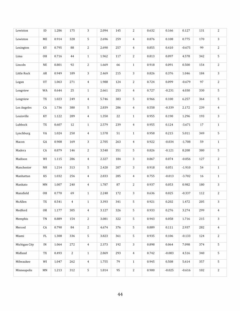
44
Lewiston ID 1.286 175 3 2.094 145 2 0.632 0.166 0.127 131 2
Lewiston ME 0.914 328 5 2.696 259 4 0.876 0.108 0.775 170 3
Lexington KY 0.795 88 2 2.690 257 4 0.855 0.410 -0.675 99 2
Lima OH 0.716 44 1 1.962 117 2 0.813 0.097 4.578 342 5
Lincoln NE 0.801 92 2 1.669 66 1 0.918 0.091 0.500 154 2
Little Rock AR 0.949 189 3 2.469 215 3 0.826 0.376 1.046 184 3
Logan UT 1.063 271 4 1.988 124 2 0.724 0.099 -0.679 97 2
Longview WA 0.644 25 1 2.661 253 4 0.727 -0.231 4.030 330 5
Longview TX 1.023 249 4 5.746 383 5 0.966 0.100 6.257 364 5
Los Angeles CA 1.736 380 5 2.839 286 4 0.558 -0.339 2.172 239 4
Louisville KY 1.122 289 4 1.350 22 1 0.955 0.190 1.296 193 3
Lubbock TX 0.607 12 1 2.579 239 4 0.955 0.124 -3.671 17 1
Lynchburg VA 1.024 250 4 1.578 51 1 0.958 0.215 5.011 349 5
Macon GA 0.908 169 3 2.705 263 4 0.922 -0.034 -1.708 59 1
Madera CA 0.879 146 2 3.548 351 5 0.826 -0.121 8.208 380 5
Madison WI 1.115 286 4 2.327 184 3 0.867 0.074 -0.056 127 2
Manchester NH 1.214 313 5 2.420 207 3 0.918 0.051 -1.910 54 1
Manhattan KS 1.032 256 4 2.833 285 4 0.755 -0.013 -3.702 16 1
Mankato MN 1.007 240 4 1.787 87 2 0.937 0.053 0.982 180 3
Mansfield OH 0.770 69 1 2.248 172 3 0.636 0.025 -0.337 112 2
McAllen TX 0.541 4 1 3.393 341 5 0.921 0.202 1.472 205 3
Medford OR 1.177 305 4 3.127 326 5 0.933 0.276 3.274 299 4
Memphis TN 0.889 154 2 3.081 322 5 0.943 0.058 1.716 215 3
Merced CA 0.790 84 2 4.674 376 5 0.889 0.111 2.937 282 4
Miami FL 1.308 336 5 3.823 361 5 0.935 0.106 -0.133 124 2
Michigan City IN 1.064 272 4 2.373 192 3 0.898 0.064 7.098 374 5
Midland TX 0.493 2 1 2.869 293 4 0.742 -0.083 4.516 340 5
Milwaukee WI 1.047 262 4 1.755 79 1 0.945 0.508 5.614 357 5
Minneapolis MN 1.213 312 5 1.814 95 2 0.900 -0.025 -0.616 102 2
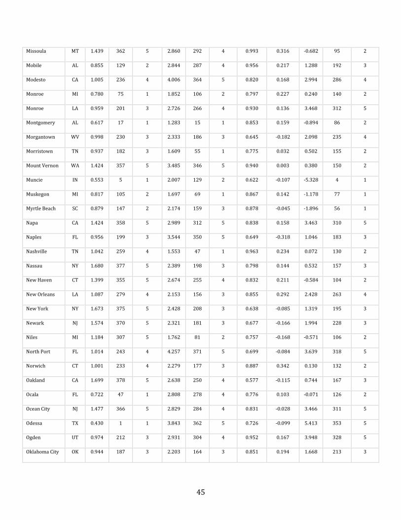
45
Missoula MT 1.439 362 5 2.860 292 4 0.993 0.316 -0.682 95 2
Mobile AL 0.855 129 2 2.844 287 4 0.956 0.217 1.288 192 3
Modesto CA 1.005 236 4 4.006 364 5 0.820 0.168 2.994 286 4
Monroe MI 0.780 75 1 1.852 106 2 0.797 0.227 0.240 140 2
Monroe LA 0.959 201 3 2.726 266 4 0.930 0.136 3.468 312 5
Montgomery AL 0.617 17 1 1.283 15 1 0.853 0.159 -0.894 86 2
Morgantown WV 0.998 230 3 2.333 186 3 0.645 -0.182 2.098 235 4
Morristown TN 0.937 182 3 1.609 55 1 0.775 0.032 0.502 155 2
Mount Vernon WA 1.424 357 5 3.485 346 5 0.940 0.003 0.380 150 2
Muncie IN 0.553 5 1 2.007 129 2 0.622 -0.107 -5.328 4 1
Muskegon MI 0.817 105 2 1.697 69 1 0.867 0.142 -1.178 77 1
Myrtle Beach SC 0.879 147 2 2.174 159 3 0.878 -0.045 -1.896 56 1
Napa CA 1.424 358 5 2.989 312 5 0.838 0.158 3.463 310 5
Naples FL 0.956 199 3 3.544 350 5 0.649 -0.318 1.046 183 3
Nashville TN 1.042 259 4 1.553 47 1 0.963 0.234 0.072 130 2
Nassau NY 1.680 377 5 2.389 198 3 0.798 0.144 0.532 157 3
New Haven CT 1.399 355 5 2.674 255 4 0.832 0.211 -0.584 104 2
New Orleans LA 1.087 279 4 2.153 156 3 0.855 0.292 2.428 263 4
New York NY 1.673 375 5 2.428 208 3 0.638 -0.085 1.319 195 3
Newark NJ 1.574 370 5 2.321 181 3 0.677 -0.166 1.994 228 3
Niles MI 1.184 307 5 1.762 81 2 0.757 -0.168 -0.571 106 2
North Port FL 1.014 243 4 4.257 371 5 0.699 -0.084 3.639 318 5
Norwich CT 1.001 233 4 2.279 177 3 0.887 0.342 0.130 132 2
Oakland CA 1.699 378 5 2.638 250 4 0.577 -0.115 0.744 167 3
Ocala FL 0.722 47 1 2.808 278 4 0.776 0.103 -0.071 126 2
Ocean City NJ 1.477 366 5 2.829 284 4 0.831 -0.028 3.466 311 5
Odessa TX 0.430 1 1 3.843 362 5 0.726 -0.099 5.413 353 5
Ogden UT 0.974 212 3 2.931 304 4 0.952 0.167 3.948 328 5
Oklahoma City OK 0.944 187 3 2.203 164 3 0.851 0.194 1.668 213 3
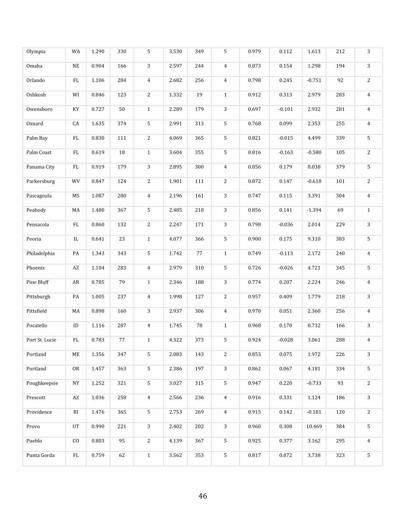
46
Olympia WA 1.290 330 5 3.530 349 5 0.979 0.112 1.613 212 3
Omaha NE 0.904 166 3 2.597 244 4 0.873 0.154 1.298 194 3
Orlando FL 1.106 284 4 2.682 256 4 0.798 0.245 -0.751 92 2
Oshkosh WI 0.846 123 2 1.332 19 1 0.912 0.313 2.979 283 4
Owensboro KY 0.727 50 1 2.289 179 3 0.697 -0.101 2.932 281 4
Oxnard CA 1.635 374 5 2.991 313 5 0.768 0.099 2.353 255 4
Palm Bay FL 0.830 111 2 4.069 365 5 0.821 -0.015 4.499 339 5
Palm Coast FL 0.619 18 1 3.604 355 5 0.816 -0.163 -0.580 105 2
Panama City FL 0.919 179 3 2.895 300 4 0.856 0.179 8.038 379 5
Parkersburg WV 0.847 124 2 1.901 111 2 0.872 0.147 -0.618 101 2
Pascagoula MS 1.087 280 4 2.196 161 3 0.747 0.115 3.391 304 4
Peabody MA 1.480 367 5 2.485 218 3 0.856 0.141 -1.394 69 1
Pensacola FL 0.860 132 2 2.247 171 3 0.798 -0.036 2.014 229 3
Peoria IL 0.641 23 1 4.077 366 5 0.900 0.175 9.310 383 5
Philadelphia PA 1.343 343 5 1.742 77 1 0.749 -0.113 2.172 240 4
Phoenix AZ 1.104 283 4 2.979 310 5 0.726 -0.026 4.721 345 5
Pine Bluff AR 0.785 79 1 2.346 188 3 0.774 0.207 2.224 246 4
Pittsburgh PA 1.005 237 4 1.998 127 2 0.957 0.409 1.779 218 3
Pittsfield MA 0.898 160 3 2.937 306 4 0.970 0.051 2.360 256 4
Pocatello ID 1.116 287 4 1.745 78 1 0.968 0.170 0.732 166 3
Port St. Lucie FL 0.783 77 1 4.322 373 5 0.924 -0.028 3.061 288 4
Portland ME 1.356 347 5 2.083 143 2 0.853 0.075 1.972 226 3
Portland OR 1.457 363 5 2.386 197 3 0.862 0.067 4.181 334 5
Poughkeepsie NY 1.252 321 5 3.027 315 5 0.947 0.220 -0.733 93 2
Prescott AZ 1.036 258 4 2.566 236 4 0.916 0.331 1.124 186 3
Providence RI 1.476 365 5 2.753 269 4 0.915 0.142 -0.181 120 2
Provo UT 0.990 221 3 2.402 202 3 0.960 0.308 10.469 384 5
Pueblo CO 0.803 95 2 4.139 367 5 0.925 0.377 3.162 295 4
Punta Gorda FL 0.759 62 1 3.562 353 5 0.817 0.072 3.738 323 5
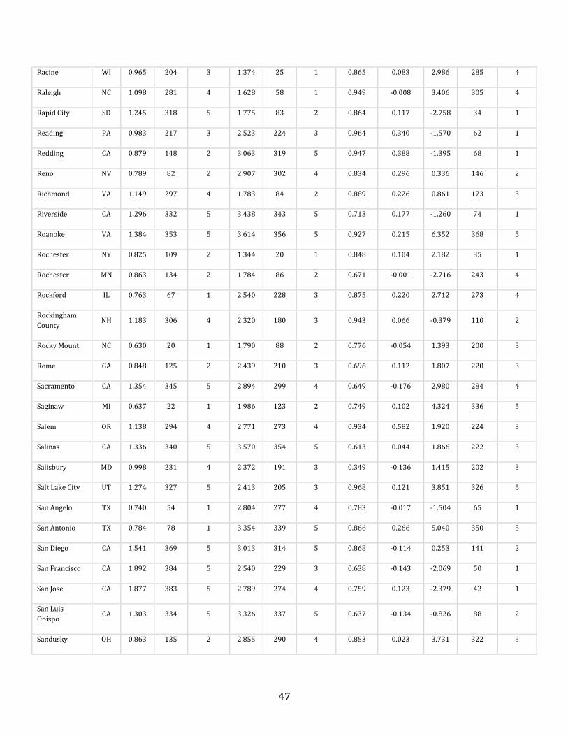
47
Racine WI 0.965 204 3 1.374 25 1 0.865 0.083 2.986 285 4
Raleigh NC 1.098 281 4 1.628 58 1 0.949 -0.008 3.406 305 4
Rapid City SD 1.245 318 5 1.775 83 2 0.864 0.117 -2.758 34 1
Reading PA 0.983 217 3 2.523 224 3 0.964 0.340 -1.570 62 1
Redding CA 0.879 148 2 3.063 319 5 0.947 0.388 -1.395 68 1
Reno NV 0.789 82 2 2.907 302 4 0.834 0.296 0.336 146 2
Richmond VA 1.149 297 4 1.783 84 2 0.889 0.226 0.861 173 3
Riverside CA 1.296 332 5 3.438 343 5 0.713 0.177 -1.260 74 1
Roanoke VA 1.384 353 5 3.614 356 5 0.927 0.215 6.352 368 5
Rochester NY 0.825 109 2 1.344 20 1 0.848 0.104 2.182 35 1
Rochester MN 0.863 134 2 1.784 86 2 0.671 -0.001 -2.716 243 4
Rockford IL 0.763 67 1 2.540 228 3 0.875 0.220 2.712 273 4
Rockingham
County NH 1.183 306 4 2.320 180 3 0.943 0.066 -0.379 110 2
Rocky Mount NC 0.630 20 1 1.790 88 2 0.776 -0.054 1.393 200 3
Rome GA 0.848 125 2 2.439 210 3 0.696 0.112 1.807 220 3
Sacramento CA 1.354 345 5 2.894 299 4 0.649 -0.176 2.980 284 4
Saginaw MI 0.637 22 1 1.986 123 2 0.749 0.102 4.324 336 5
Salem OR 1.138 294 4 2.771 273 4 0.934 0.582 1.920 224 3
Salinas CA 1.336 340 5 3.570 354 5 0.613 0.044 1.866 222 3
Salisbury MD 0.998 231 4 2.372 191 3 0.349 -0.136 1.415 202 3
Salt Lake City UT 1.274 327 5 2.413 205 3 0.968 0.121 3.851 326 5
San Angelo TX 0.740 54 1 2.804 277 4 0.783 -0.017 -1.504 65 1
San Antonio TX 0.784 78 1 3.354 339 5 0.866 0.266 5.040 350 5
San Diego CA 1.541 369 5 3.013 314 5 0.868 -0.114 0.253 141 2
San Francisco CA 1.892 384 5 2.540 229 3 0.638 -0.143 -2.069 50 1
San Jose CA 1.877 383 5 2.789 274 4 0.759 0.123 -2.379 42 1
San Luis
Obispo CA 1.303 334 5 3.326 337 5 0.637 -0.134 -0.826 88 2
Sandusky OH 0.863 135 2 2.855 290 4 0.853 0.023 3.731 322 5
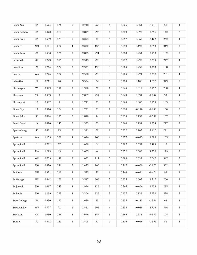
48
Santa Ana CA 1.674 376 5 2.718 265 4 0.626 0.051 -1.713 58 1
Santa Barbara CA 1.470 364 5 2.879 295 4 0.779 0.090 0.256 142 2
Santa Cruz CA 1.599 373 5 3.093 323 5 0.657 0.065 2.422 262 4
Santa Fe NM 1.101 282 4 2.032 135 2 0.819 0.195 3.650 319 5
Santa Rosa CA 1.590 371 5 2.855 291 4 0.678 0.251 0.990 182 3
Savannah GA 1.223 315 5 2.513 222 3 0.932 0.295 2.239 247 4
Scranton PA 1.264 324 5 2.351 190 3 0.885 0.252 1.373 198 3
Seattle WA 1.744 382 5 2.508 220 3 0.925 0.271 2.038 231 4
Sebastian FL 0.711 40 1 3.554 352 5 0.770 0.108 4.677 343 5
Sheboygan WI 0.949 190 3 1.390 27 1 0.845 0.019 2.152 238 4
Sherman TX 0.533 3 1 2.887 297 4 0.843 0.031 -2.842 33 1
Shreveport LA 0.582 9 1 1.711 71 1 0.865 0.006 0.159 135 2
Sioux City IA 0.910 174 3 1.721 73 1 0.618 -0.170 -0.643 100 2
Sioux Falls SD 0.894 155 2 1.810 94 2 0.834 0.152 -0.559 107 2
South Bend IN 0.876 145 2 1.353 23 1 0.866 0.194 1.774 217 3
Spartanburg SC 0.801 93 2 1.391 28 1 0.832 0.105 3.112 291 4
Spokane WA 1.159 300 4 2.696 260 4 0.877 -0.095 1.088 185 3
Springfield IL 0.702 37 1 1.089 3 1 0.897 0.057 8.489 12 1
Springfield MA 1.293 63 1 2.605 4 1 0.852 0.088 4.770 129 2
Springfield OH 0.759 138 2 1.082 217 3 0.888 0.032 0.067 347 5
Springfield MO 0.870 331 5 2.475 246 4 0.717 -0.069 -3.873 382 5
St. Cloud MN 0.971 210 3 1.575 50 1 0.748 -0.091 -0.676 98 2
St. George UT 0.842 120 2 3.517 348 5 0.835 0.005 1.517 206 3
St. Joseph MO 1.017 245 4 1.994 126 2 0.545 -0.404 1.933 225 3
St. Louis MO 1.139 295 4 3.304 336 5 0.927 0.138 7.950 378 5
State College PA 0.950 192 3 1.650 63 1 0.635 -0.113 -1.534 64 1
Steubenville WV 0.777 72 1 2.881 296 4 0.638 -0.038 4.716 344 5
Stockton CA 1.050 266 4 3.696 359 5 0.669 0.238 -0.537 108 2
Sumter SC 0.842 121 2 1.805 92 2 0.816 -0.046 -1.999 51 1
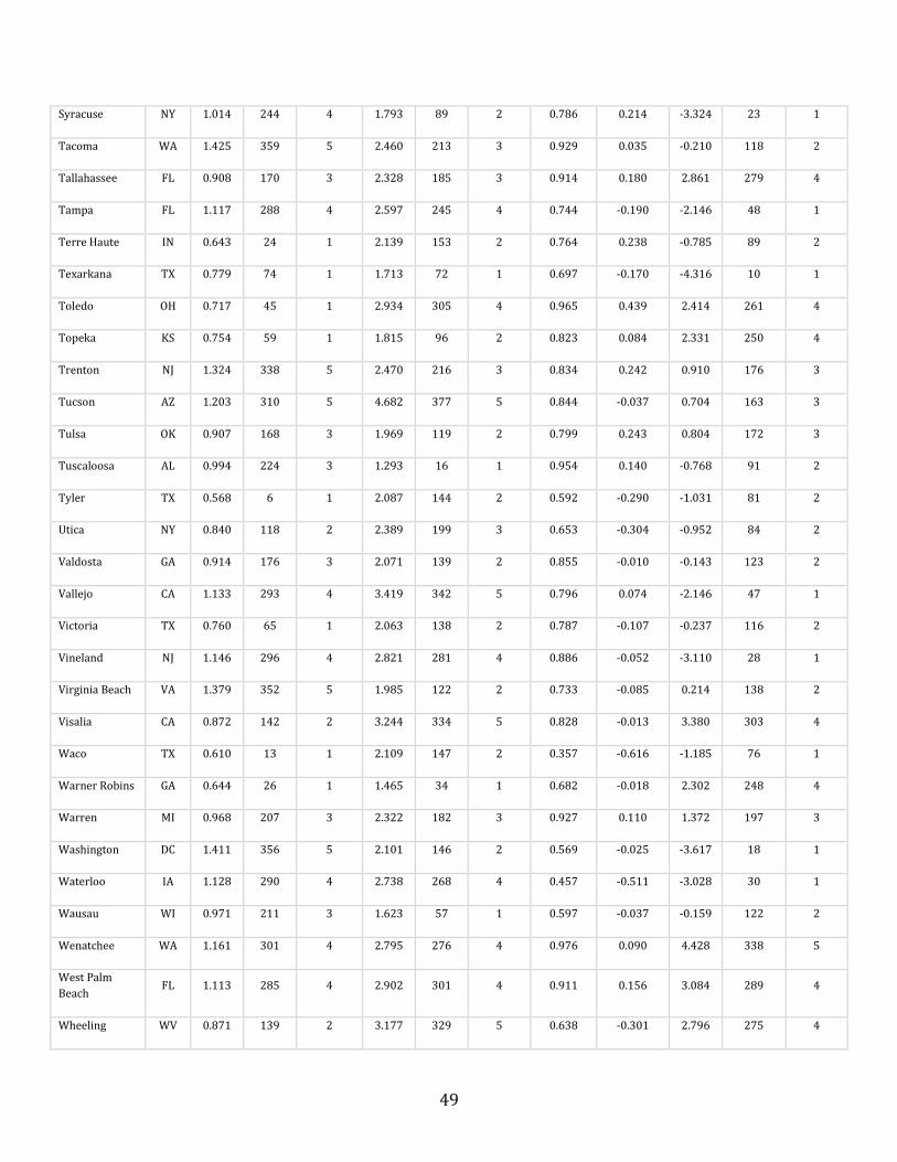
49
Syracuse NY 1.014 244 4 1.793 89 2 0.786 0.214 -3.324 23 1
Tacoma WA 1.425 359 5 2.460 213 3 0.929 0.035 -0.210 118 2
Tallahassee FL 0.908 170 3 2.328 185 3 0.914 0.180 2.861 279 4
Tampa FL 1.117 288 4 2.597 245 4 0.744 -0.190 -2.146 48 1
Terre Haute IN 0.643 24 1 2.139 153 2 0.764 0.238 -0.785 89 2
Texarkana TX 0.779 74 1 1.713 72 1 0.697 -0.170 -4.316 10 1
Toledo OH 0.717 45 1 2.934 305 4 0.965 0.439 2.414 261 4
Topeka KS 0.754 59 1 1.815 96 2 0.823 0.084 2.331 250 4
Trenton NJ 1.324 338 5 2.470 216 3 0.834 0.242 0.910 176 3
Tucson AZ 1.203 310 5 4.682 377 5 0.844 -0.037 0.704 163 3
Tulsa OK 0.907 168 3 1.969 119 2 0.799 0.243 0.804 172 3
Tuscaloosa AL 0.994 224 3 1.293 16 1 0.954 0.140 -0.768 91 2
Tyler TX 0.568 6 1 2.087 144 2 0.592 -0.290 -1.031 81 2
Utica NY 0.840 118 2 2.389 199 3 0.653 -0.304 -0.952 84 2
Valdosta GA 0.914 176 3 2.071 139 2 0.855 -0.010 -0.143 123 2
Vallejo CA 1.133 293 4 3.419 342 5 0.796 0.074 -2.146 47 1
Victoria TX 0.760 65 1 2.063 138 2 0.787 -0.107 -0.237 116 2
Vineland NJ 1.146 296 4 2.821 281 4 0.886 -0.052 -3.110 28 1
Virginia Beach VA 1.379 352 5 1.985 122 2 0.733 -0.085 0.214 138 2
Visalia CA 0.872 142 2 3.244 334 5 0.828 -0.013 3.380 303 4
Waco TX 0.610 13 1 2.109 147 2 0.357 -0.616 -1.185 76 1
Warner Robins GA 0.644 26 1 1.465 34 1 0.682 -0.018 2.302 248 4
Warren MI 0.968 207 3 2.322 182 3 0.927 0.110 1.372 197 3
Washington DC 1.411 356 5 2.101 146 2 0.569 -0.025 -3.617 18 1
Waterloo IA 1.128 290 4 2.738 268 4 0.457 -0.511 -3.028 30 1
Wausau WI 0.971 211 3 1.623 57 1 0.597 -0.037 -0.159 122 2
Wenatchee WA 1.161 301 4 2.795 276 4 0.976 0.090 4.428 338 5
West Palm
Beach FL 1.113 285 4 2.902 301 4 0.911 0.156 3.084 289 4
Wheeling WV 0.871 139 2 3.177 329 5 0.638 -0.301 2.796 275 4
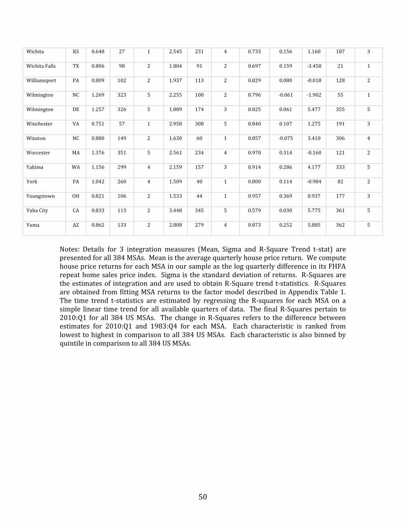
50
Wichita KS 0.648 27 1 2.545 231 4 0.733 0.156 1.160 187 3
Wichita Falls TX 0.806 98 2 1.804 91 2 0.697 0.159 -3.458 21 1
Williamsport PA 0.809 102 2 1.937 113 2 0.829 0.080 -0.018 128 2
Wilmington NC 1.269 323 5 2.255 108 2 0.796 -0.061 -1.902 55 1
Wilmington DE 1.257 326 5 1.889 174 3 0.825 0.061 5.477 355 5
Winchester VA 0.751 57 1 2.958 308 5 0.840 0.107 1.275 191 3
Winston NC 0.880 149 2 1.630 60 1 0.857 -0.075 3.410 306 4
Worcester MA 1.376 351 5 2.561 234 4 0.970 0.314 -0.160 121 2
Yakima WA 1.156 299 4 2.159 157 3 0.914 0.286 4.177 333 5
York PA 1.042 260 4 1.509 40 1 0.800 0.114 -0.984 82 2
Youngstown OH 0.821 106 2 1.533 44 1 0.957 0.369 0.937 177 3
Yuba City CA 0.833 113 2 3.448 345 5 0.579 0.030 5.775 361 5
Yuma AZ 0.862 133 2 2.808 279 4 0.873 0.252 5.885 362 5
Notes: Details for 3 integration measures (Mean, Sigma and R-Square Trend t-stat) are presented for all 384 MSAs. Mean is the average quarterly house price return. We compute house price returns for each MSA in our sample as the log quarterly difference in its FHFA repeat home sales price index. Sigma is the standard deviation of returns. R-Squares are the estimates of integration and are used to obtain R-Square trend t-statistics. R-Squares are obtained from fitting MSA returns to the factor model described in Appendix Table 1. The time trend t-statistics are estimated by regressing the R-squares for each MSA on a simple linear time trend for all available quarters of data. The final R-Squares pertain to 2010:Q1 for all 384 US MSAs. The change in R-Squares refers to the difference between estimates for 2010:Q1 and 1983:Q4 for each MSA. Each characteristic is ranked from lowest to highest in comparison to all 384 US MSAs. Each characteristic is also binned by quintile in comparison to all 384 US MSAs.


