Interethnic Wage Variation in the Helsinki Area

35

Finnish Economic Papers – Volume 17 – Number 1 – Spring 2004

INTERETHNIC WAGE VARIATION IN THE HELSINKI AREA*

JAN SAARELA

Department of Social Sciences, Åbo Akademi University,P.O. Box 311, FI-65101 Vasa, Finland

and

FJALAR FINNÄS

Institutet för Finlandssvensk Samhällsforskning, Åbo Akademi University,P.O. Box 311, FI-65101 Vasa, Finland

This paper compares wage income of Swedish-speaking and Finnish-speakingemployees in the Helsinki metropolitan area. Longitudinal data are analysed withrandom-effects tobit models. We find that Swedish-speaking males on average have17 per cent higher wages than Finnish-speaking males. Two thirds of this wagegap can be attributed to characteristics differences, particularly education andage. For females the wage difference is very small. The findings echo previousresearch in the sense that they point out a favourable labour market performanceof the Swedish-speaking minority in Finland and that differences between lan-guage groups are larger among males than among females. (JEL: J15, J31)

1. Introduction

Recent studies have shown that people of theSwedish-speaking linguistic minority in Finlandhave lower unemployment and disability retire-ment propensity than their Finnish-speakingcounterparts (Saarela and Finnäs, 2002a, 2002b,2003a, 2003b). At least in certain respects, thelabour market performance of this minority isthus better than that of the majority.

From the international literature, there areempirical evidence suggesting that populationgroups who experience relatively low unem-ployment rates also may have relatively highwages when employment is found (Blackaby etal., 1994, 1998, 2002). The purpose of thepresent paper is consequently to study whetherthere also is a wage gap between Swedish-speakers and Finnish-speakers in Finland. Nosuch systematic language-group comparisons ofwages, or of any other detailed economic indi-cators, have previously been performed.1 Offi-

* We are grateful for advice from two anonymous refe-rees, Stan Panis, Markus Jäntti, and seminar participantsat SOFI and EALE 2003.

1 Smedman (1998) and Kyyrä (1999) are two minorstudies that compare wages of the two language groups.

Finnish Economic Papers 1/2004 – Jan Saarela and Fjalar Finnäs

36

cial statistical series in Finland neither containincome measures classified by native language.

Direct involvement of Sweden in Finland canbe traced already from the twelfth century. Alsoat even earlier dates, however, Finland seems tohave had permanent settlement of Swedish-speakers. Until the beginning of the 20th cen-tury, Swedish was the official language of gov-ernment and the domestic language of the up-per social orders, but Finnish was never de-liberately suppressed. Swedish-speakers werepredominant in the tiny upper class, but bothlanguage groups consisted predominantly ofrural populations of modest social status. Alsoafter Finland’s independence from the RussianEmpire in 1917, Swedish-speakers in the coun-try benefited from existing financial resources,higher-level education and cultural life, in spiteof them having decreased in both absolute andrelative numbers due to emigration, low birthrates and intermarriage.2 Socio-economic dis-parities between the two language groups aresmaller today but do exist (Finnäs, 2003).

Nowadays, Swedish-speakers amount tobarely six per cent of the total population(whereas about two per cent has a mothertongue other than Finnish or Swedish). About95 per cent of them live concentrated at thesouthern and western coastlines of the country,in municipalities which are classified as eitherbilingual or monolingual Swedish.

Helsinki with surrounding municipalitiesconstitutes the country centre, composed of pro-fessionals and business interests, in which amajor part of the Swedish-speakers live, and inwhich they traditionally have played a majorrole in terms of professionals and business in-terests and thus decision-making and econom-ic life (Allardt and Miemois, 1979, 1982). In the

Helsinki area, which has witnessed a tremen-dous in-migration of foremost Finnish-speakersfrom other parts of the country, Swedish-speak-ers are in clear minority, in contrast with the sit-uation in most other parts of the country withSwedish-speaking settlement. Swedish-speakersamount to seven per cent of the population inthe Helsinki region, whereas about half of theSwedish-speaking population in Finland live inmunicipalities where they constitute the localmajority. There is also substantial variation inincome, education, age, industrial structure,population density, etc. within the settlementarea of the Swedish-speakers (Allardt andStarck, 1981; McRae, 1997; Finnäs, 2003). Anyattempt to analyse a larger geographical areawould therefore be confounded by these pre-conditions. In order to understand the role ofnative language in terms of a comparison ofwage income between the two language groups,a first study ever on the topic therefore obvious-ly needs to be restricted to the Helsinki metro-politan area.

A common presumption is that Swedish-speakers in Finland are over-represented amongthose well-to-do. This is also supported by pop-ulation censuses, saying that Swedish-speakers,particularly those in the Helsinki area, are pro-portionately better represented in certain high-er socio-economic categories in the work force.What is not clear from these data, however, ishow much of the socio-economic variation isexplainable in terms of factors such as level ofeducation and age structure (McRae, 1997).

It would be fairly natural to expect thatSwedish-speakers have higher wages than Finn-ish-speakers, simply because the socio-econom-ic and demographic composition favours them.Swedish-speakers are, for instance, more like-ly to have university education than Finnish-speakers (Saarela and Finnäs, 2003c). They arealso on average older.

Also some other issues may promote thewage of Swedish-speakers. One such aspect isthe ability to speak both Swedish and Finnish,which may be needed in administration as wellas in many services professions. Unfortunate-ly, there exist no recent extensive register data,which would provide information about the lan-guage skills of each population group. In spite

They come to somewhat different conclusions, probably be-cause they seem to differ in terms of how the analysed dataare geographically restricted. Saarela (2002) found thatsocial assistance propensity is lower among Swedish-speak-ing unemployed than among Finnish-speaking unemployedin a local labour market. Since social assistance is a con-ditional transfer provided to families with low income, thismay be regarded as an indication of language-group dif-ferences in the economic situation of the unemployed.

2 McRae (1997) provides a further historical back-ground.


37

of this lack of adequate data, it is evident thatSwedish-speakers to a greater extent than Finn-ish-speakers are bilingual. The 1950 census in-dicated that bilingualism is much more frequentamong the Swedish-speakers. Other featuressupporting the argument is the fact that the pro-portion of people who are the offspring ofmixed marriages is higher among the Swedish-speakers than among the Finnish-speakers, andthat in-migration of Finnish-speakers from themonolingual Finnish-speaking parts of thecountry has been very high. Being a fairly smallminority in relative numbers, Swedish-speakersin the Helsinki area also obviously need Finn-ish in much of their everyday life.

Another factor of potential importance is cul-ture, which usually includes some notion ofshared values, beliefs, expectations, customs,jargon and rituals (Lazear, 1999). Some inter-national studies (Sowell, 1981, 1983; Chiswick,1983a, 1983b; Simmons, 2003) claim that cul-tural explanations may lie behind the favoura-ble wage performance of certain minoritygroups. It is plausible that this is the case alsohere. O’Leary and Finnäs (2002) argue that in-tra-group interaction is identifiable along com-munal lines of much of the social life of Swed-ish-speakers, including the education system,media and a number of social organisations. Onthat account, the two groups are somewhat so-cially separated, which may act to promote lin-guistic solidarity among the Swedish-speakers.Some scholars also suggest that cultural endow-ments may explain why morbidity and mortali-ty rates are lower and marital stability higheramong Swedish-speakers than among Finnish-speakers (Finnäs, 1997; Hyyppä and Mäki,2001; Saarela and Finnäs, 2002a). The term cul-ture in this paper refers to such potential dif-ferences in lifestyle.

The standard interpretation of unexplainedearnings differentials, i.e. differences in wagesthat remain after having controlled for socio-economic and demographic characteristics,would be that there is discrimination (Blinder,1973; Oaxaca, 1973). This is not likely to be thecase here. Swedish-speakers and Finnish-speak-ers live intermingled and are guaranteed equalconstitutional rights, which among other thingsimply that there are two parallel education

systems up to upper secondary level, with thesame curriculum but with instructions in eachlanguage. Also in several fields at tertiary level,there are schools providing instruction inSwedish.

Due to non-existing data about languageskills and cultural related factors, and thus theimpossibility to explicitly disentangle the im-pact of these issues on the individual wage rate,this study should be seen as a first explorativeattempt to compare the wage income of thesetwo population groups. We avoid making directcomparisons with other linguistic or ethnic mi-norities, because it seems to be difficult find-ing obvious points of similarity. There is, forinstance, no linkage between linguistic and re-ligious dimensions, as is the case in Switzer-land, Belgium and Canada.3

2. Data

We will use an extract from the longitudinaldata file Työssäkäyntitilasto (Employment Sta-tistics), maintained by Statistics Finland. It con-sists of annual individual-level informationfrom the years 1987 to 1999, about basic socio-economic and demographic factors, as well asissues related to individuals’ labour market sit-uation.

Since a language variable is included in pop-ulation registers in Finland, official statisticscan be used to study language groups. The ex-tract we use has been designed to facilitate com-parisons between Swedish-speakers and Finn-ish-speakers. It is a random sample, consistingof 20 per cent of all Swedish-speakers and 5 percent of all Finnish-speakers, representing allresidents born before 1984, who live in theprovinces Uusimaa, Eastern Uusimaa, Varsi-

3 O’Leary and Finnäs (2002) propose that the Swedish-speaking minority in the Helsinki area and Protestants inDublin in the Republic of Ireland are comparable in termsof being ethnic minorities who have been historically dom-inant, with strong educational and social organisations, anda similar demographic situation. They also suggest that inthis context it is not important what people in the minorityhave in common (language or religion) but rather that theydistinguish themselves from the majority, and that they haveopportunities for contact with other members of the samegroup.


38

nais-Suomi, Pohjanmaa and the Åland Islandsat the end of one or more of the years. The geo-graphical restriction is due to the fact that prac-tically all Swedish-speakers live in this area.

The focus of the present paper is at the Hel-sinki metropolitan region, which consists of themunicipalities Helsinki, Espoo, Vantaa andKauniainen. The total population in this area isabout 900,000.

The variable of central interest is wage. To-tal annual earnings for each year are used asproxies, since explicit information about wagerates is not available. The number of months aperson has been working each year is known.We can therefore restrict the analysis to employ-ees (not self-employed and farmers) who havebeen working all twelve months of each year.This also reduces sample heterogeneity.

It is not possible to distinguish people in part-time work from those working full time. Thisshould not be a problem, because part-timework is not very common in Finland (Ilmakun-nas, 1997). We also exclude people who fallbelow the “minimum” level for full-time work-ers, which is about 60,000 FIM in 1999 prices(about 10,000 €), in order to decrease the pro-portion of potential part-time workers in thedata (cf. Kyyrä, 1997).

Statistics Finland have top-coded the earn-ings data to guarantee anonymity of the persons.This implies that wage rates for sample individ-uals found in the top decile each year are notknown.

We include a variable representing family sit-uation in order to reduce differences in annualearnings caused by variation in working hours(and/or variation in social competence). A var-iable indicating whether a person was employedfor twelve months the previous year is alsoused, to serve as a crude indicator for labourmarket experience. Data on earnings for the firstobservation year, 1987, are therefore not uti-lised in the analysis.

The data are restricted to people who are 21-59 years old, since participation rates of thosein other ages are well below 50 per cent. Thetotal number of observations is 213,177. Theyrepresent 33,373 individuals.

The standard practice to obtain real wageswould be to adjust with the consumer price in-

dex. This would, however, result in differentcensoring points for each year, and require fur-ther adjustments. Therefore, and because thefocus is not on individual earnings profiles, wehave chosen an alternative method that directlyproduces adjusted wages with the same censor-ing point for each year. 4 To achieve this, we foreach year compute Yt = (c1999/ct) · yt, where ct isthe top decile limit and yt wage income for yeart. As a consequence, we end up with “realwages” Y that are top-coded at 201,000 FIM in1999 prices.

The original top-coding was made on the ba-sis of all sample individuals, also younger andolder people, not full-time workers and thoseliving outside the Helsinki region. Since theoverall wage rate of those studied is higher thanthat of those excluded from analysis, the pro-portion of right-censored observations is high-er than in the raw data. Table 1 provides a de-scription of the real wage distribution by gen-der and native language. The proportion of peo-ple with relatively high wages is substantiallylarger among Swedish-speaking males thanamong Finnish-speaking males. For females thedifference between language groups is muchsmaller. The percentage of right-censored obser-vations, i.e. those with a wage of 201,000 FIMor higher, is 53.8 for Swedish-speaking males,39.2 for Finnish-speaking males, 16.0 for Swed-ish-speaking females, and 14.1 for Finnish-speaking females.

The statistical estimations, which will be dis-cussed in detail in the following section of thepaper, seek to explain the above depicted lan-guage-group difference in wages, i.e. if it dif-fers between socio-economic, demographic andlabour market related characteristics, and howmuch can be attributed to these characteristics.Table 2, which provides a description of thedistribution of explanatory variables to be usedby gender and native language, indicates thatthere are obvious reasons for doing such ananalysis. Swedish-speakers are on averageolder, higher educated, educated in other fields,work in different industries, have higher levelsof employment experience, and live in different

4 The results would remain practically the same no mat-ter which adjustment method is used.


39

Table 1. Some descriptive statistics of the wage distribution by gender and native language.

% with wage over (in 1,000 FIM)

100 125 150 175 200 Median n obs.

MALES Finnish 95.0 84.7 67.9 51.9 39.2 179 79,030Swedish 95.6 87.4 75.0 63.3 53.8 201 24,094

FEMALES Finnish 88.0 61.7 37.4 22.7 14.1 136 86,371Swedish 88.4 65.9 42.4 25.4 16.0 142 23,682

The percentage of observations with wages over 200,000 FIM corresponds with the percentage of right-censored obser-vations.

Table 2. Variable distributions by gender and native language (%).

MALES FEMALES

Finn. Swed. Finn. Swed.

Age, 21–24 years 5.2 3.4 4.9 3.6 25–29 14.4 10.9 12.2 10.7 30–34 17.1 13.7 14.1 11.4 35–39 15.7 13.6 14.9 11.9 40–44 15.5 16.3 16.5 15.3 45–49 14.3 17.0 16.3 17.9 50–54 11.3 15.2 13.1 17.5 55–59 6.5 9.9 7.8 11.7

Education level, Basic 24.4 22.4 27.5 27.2 Lower vocational 36.4 25.2 33.2 26.8 Upper vocational 13.1 12.9 20.0 18.4 Undergraduate 7.8 14.7 6.7 13.7 Graduate or postgraduate 18.3 24.8 12.6 13.9

Education field, Teacher, human., aesth. 2.8 3.1 7.7 7.8 Commercial, social science 15.7 27.4 25.8 32.2 Natural science 9.5 7.8 3.2 2.1 Technology 30.8 22.1 5.1 2.5 Medical and health care 1.9 2.4 11.5 12.1 Services 4.8 3.4 7.4 4.4 General or other 34.5 33.9 39.3 38.9

Industry, Manufacturing 19.5 15.9 9.9 8.6 Construction 6.6 2.7 1.2 0.5 Trade 17.4 26.2 14.9 18.7 Hotels and restaurants 1.9 1.6 3.6 1.9Transport and communications 11.9 11.2 6.5 9.2

Financial intermediation 3.9 6.2 8.7 10.0 Real estate and business services 15.6 14.7 11.2 10.5 Public administration 7.6 5.0 9.2 6.4 Education 4.8 5.6 7.7 7.7 Human health and social services 2.5 2.7 19.6 17.4 Other services 5.5 6.3 6.2 7.7 Other industry 2.7 1.9 1.4 1.5

Not employed for 12 months last year 10.1 8.3 10.7 9.8

Family type, Married, no children 14.3 16.1 14.8 17.0Married, 1 child 14.7 16.7 13.3 13.2Married, 2 children 18.9 22.1 15.0 14.7Married, 2+ children 7.7 9.9 4.7 5.5Consensual union, no children 9.5 6.9 8.7 6.7Consensual union, children 5.0 3.6 3.8 3.8Sole supporter 1.5 1.4 10.2 10.7Single 23.5 18.5 27.4 25.4Other 4.9 4.7 2.0 3.0

n observations 79,030 24,094 86,371 23,682n individuals 12,535 3,669 13,501 3,668


40

≥

<+==

τττεβ

*

**

ity

itititit

ityif

yifxyy

iitit uv +=ε .

[ ] 22uvitVar σσε += .

family compositions than Finnish-speakingmales. The differences among females aresomewhat smaller than among males.

3. Econometric methodology

Since the observed dependent variable wage,denoted by y, is right-censored, the tobit model(Tobin, 1958) that is used is specified as

(1)

where y* is the latent (or index) variable, and τis the threshold of censoring. Each individualis denoted by i, and each observation by t. Avector of explanatory variables is referred to asx, whereas β is its associated vector of coeffi-cients. The error is denoted by εit. Since wehave longitudinal data, the model used is of therandom-effects type.5 We specify

(2)

Unmeasured characteristics are thus in partspecific to each observation (vit), and in part in-dividual-specific and constant across time (ui).Both these components are assumed normallydistributed with zero means and independent ofone another, so that

(3)

The parameter σu is the standard deviation forthe error part related to unobserved individualheterogeneity. The standard deviation of vit isalso estimable, as is the case in all tobit mod-els.

If y* can be assumed normally distributed, thetobit model will provide consistent and efficientestimates of parameters. Maximum likelihoodestimation for the model involves dividing theobservations into two sets. The first set contains

5 The random-effects specification rests on the assump-tion that the distribution function of errors is independentof explanatory variables, i.e. that unobservable factors arenot correlated with explanatory variables (Arellano andHonoré, 1999). Since language group remains constant overtime, it is not possible to use fixed effects.

uncensored observations, which maximum like-lihood treats in the same way as the linear re-gression model. The second set contains cen-sored observations, for which we do not knowthe specific value of y*. One therefore proceedsby computing the probability of being censored

(4)

and using this quantity in the likelihood equa-tion. The likelihood function for both sets ofobservations is then

(5)

where ø and Φ are the probability density func-tion and the cumulative density function respec-tively, for the standard normal distribution, andσ is the standard deviation of ε.

Expected values for the latent outcome,E(y*|x) = xβ, are our primary focus.

If the wage structure is influenced by factorsaffecting whether individuals are working alltwelve months during the year, a correction forselectivity bias may improve the fit of the mod-el. We have attempted to correct for self-selec-tion in terms of “Heckman’s lambda” (Heck-man, 1979). The estimate for this parameterturned out to be positive and significant, but didnot change the results with respect to language-group differences in wages.6 Since these typesof estimates are increasingly being questioned(Nawata, 1993; Manski, 1995), we have chosento exclude this specification from the final mod-els, whose results are reported here.

The results are not sensitive for clusteringwithin individuals. There were some indicationsof heteroskedasticity, which means that the var-iance of the residual is not constant across lan-guage groups. Some tests we performed, how-ever, indicated that this departure from homo-

( )

−Φ=≥σ

τβτ xxy*Pr ,

+

−= ∑ σβφ

σxy

LUncens.

1lnln

−Φ+ ∑ στβx

Cens.

ln ,

6 For Swedish-speaking males, there was not even an im-provement of the log likelihood when Heckman’s lambdawas included.


41

skedasticity was so small in magnitude that theresults to be reported here are not severely af-fected.

As is standard in the empirical literature onbetween-group comparisons of earnings, wewill determine how much of any wage differ-ential is due to characteristics differences andhow much is due to coefficient differences (i.e.,due to differences in the returns to the charac-teristics). The latter part is often attributed todiscrimination, but it can in principle be relat-ed to anything that is not associated with ob-servable characteristics, such as for instanceculture.

The approach adopted here is the one pro-posed by Neumark (1988) and Oaxaca and Ran-som (1994). It attempts to estimate the compet-itive wage structure that would exist in the ab-sence of “discrimination” and use these esti-mates as weights in the decomposition of thewage gap. An obvious advantage of this ap-proach is that it leads to a unique solution andso avoids the index number problem associatedwith the initial methodology of Blinder (1973)and Oaxaca (1973).7

Formally, the wage gap can be decomposedas

(6)

where Y is real wage, s and f refer to Swedish-speakers and Finnish-speakers respectively, x isa row vector of characteristics, and ^ β is a vec-tor of estimated coefficients. ^ β ∗ is an estimateof the “non-discriminatory” wage structure andis derived by using the cross product matricesas weights from the wage equation such that

(7)

where Ω = (xs'xs + x f 'x f)–1xs'xs is the Oaxaca-Ransom weighting matrix. The wage structuregiven by (7) is equivalent to running a regres-sion on the pooled data.

The first term on the right-hand side of (6)represents the difference in wage that is attrib-uted to wage-related characteristics, whichproxy productivity. The second term representsthe wage differential that is due to differencesin returns to these characteristics.

Since the model is linear and the regressionline goes through the sample means of the data,the characteristic component can be further de-composed into its individual components, forinstance the proportion of the wage gap ex-plained by differences in education level. Thecoefficient component cannot be further divid-ed in this way, since individual decompositionsare arbitrary, being influenced by transforma-tions of the data and the choice of omitted var-iable categories (Jones, 1983).

Estimations have been performed with aMLversion 1.04.

4. Results

It is essential to allow the intercept as wellas the returns to each of the explanatory varia-bles to vary between language groups withingenders. We have therefore estimated separatetobit models for Finnish-speaking and Swedish-speaking males and females, respectively (theresults can be seen in Appendix 1). In order toget an overview of how each model reflects thelatent wage rate, the distribution of the predict-ed wage for the sample individuals is providedin Figure 1 for males and in Figure 2 for fe-males. The wage distribution of Swedish-speak-ing males is more skewed to the right than thatof Finnish-speaking males, as already suggest-ed by Table 1. The spread is also higher forSwedish-speakers. For females, the wage distri-bution of each language group is close to iden-tical, with a very small advantage for the Swed-ish-speakers.

The estimation results are summarised in Ta-ble 3, which reflects the percentage differencebetween Swedish-speakers and Finnish-speak-ers in the predicted wage for each characteris-

( )[ ]*ˆlnln β +−=− fsfs xxYY

( ) ( )[ ]** ˆˆˆˆ ββββ −−−+ ffss xx

( ) fs βββ ˆ1ˆˆ * Ω−+Ω= ,

7 Blackaby et al. (1998, 2002) and Simmons (2003) usethe Neumark-Oaxaca-Ransom approach, whereas Drinkwa-ter and O’Leary (1997), Trejo (1997) and Saarela andFinnäs (2002a) perform decompositions according to theBlinder-Oaxaca setting. Alternative approaches to the in-dex number problem have been proposed by Reimers (1983)and Cotton (1988).


42

tic of the explanatory variables. Each of theother variables have been set to its referencevalue (i.e., each estimate is simply added to theconstant).

For males, there is consistently a wage ad-

vantage for Swedish-speakers. There are alsosome indications that this wage gap is larger inhigher ages than in lower ages. In order to seeif this can be attributed to a cohort effect, andnot due to a pure age effect, we have tried to

0

0,02

0,04

0,06

0,08

0 50 100 150 200 250 300 350 400 450 500

wage (in 1,000 FIM)

prop

orti o

n

Finnish-speakers

Swedish-speakers

Figure 1. Distribution of predicted wage for males.

0

0,02

0,04

0,06

0,08

0,1

0,12

0,14

0 50 100 150 200 250 300

wage (in 1,000 FIM)

prop

ortio

n

Finnish-speakers

Swedish-speakers

Figure 2. Distribution of predicted wage for females.


43

include also a variable representing the decadein which the person was born. These results in-dicated that a substantial part of the above de-picted language-group difference may be due todifferences across birth cohorts. However, since

the observation period is too short to facilitateany reliable conclusions on this point, we havechosen not to outline the results of these esti-mations here.

It may also be noted that the language-groupwage gap is smallest among people with basiceducation only. This could be the case if the re-turns to underlying characteristics, such as lan-guage skills, is not equally rewarding for peo-ple with low education as it is for people withhigher levels of education. For the other char-acteristics there is no evident pattern, whichwould have suggested that factors such as bi-lingualism are particularly important in certainsocio-demographic groups.

For females, differences between languagegroups are very small. In some of the very fewcases there is any difference, they even favourthe Finnish-speakers.

Results of the decomposition are summarisedin Table 4. It shows that Swedish-speakingmales on average have 17 per cent higher wagesthan Finnish-speaking males. Two thirds of thiswage gap can be attributed to characteristics dif-ferences, whereas one third should be explainedby different returns to the characteristics. De-composing the characteristics effect tells us thatmost of this is due to differences in educationlevel and age. Unobserved individual heteroge-neity contributes negatively to the entity, say-ing that adding random effects changes the es-timated coefficients so that the predicted earn-ings gap is higher. The fit of each model im-

Table 3. Language-group difference in predicted wage.

Males Females

Age, 21–24 years + 025–29 + 030–34 ++ 035–39 +++ 040–44 +++ 045–49 +++ 050–54 +++ 055–59 +++ 0

Education level, Basic + 0Lower vocational +++ 0Upper vocational ++ 0Undergraduate +++ 0Graduate or postgraduate +++ 0

Education field, Teacher, hum., aest. + 0Commercial, social science +++ 0Natural science +++ +Technology ++ 0Medical and health care +++ –Services ++ +General or other +++ 0

Industry, Manufacturing ++ 0Construction +++ –Trade +++ 0Hotels and restaurants + 0Transport and communications +++ 0Financial intermediation +++ 0Real estate and business services ++ 0Public administration + 0Education + 0Human health and social services + 0Other services +++ 0Other industry ++ 0

Employed 12 months last year, Yes +++ 0No +++ 0

Family type, Married, no children +++ 0Married, 1 child +++ 0Married, 2 children +++ 0Married, 2+ children +++ 0Consensual union, no children ++ 0Consensual union, children +++ 0Sole supporter +++ 0Single ++ 0Other ++ 0

Percentage difference (Swedish-speakers versus Finnish-speakers) in predicted wage for each characteristic, witheach other variable set to its reference value: –10 to –5 (–);–5 to +5 (0); +5 to +10 (+); +10 to +15 (++); +15 to +20(+++).

Table 4. Decomposition of the language-group wage differ-ence, Swedish-speakers versus Finnish-speakers.

Males Females

Mean wage differential, FIM 31,900 3,300…as approximate geometric mean 0.174 0.024

Difference due to coefficients (%) 35.4 112.7

Difference due to characteristics (%) 64.6 –12.7

Components of characteristics effect (%)Age 37.9 26.3Education level 81.7 83.6Education field 4.1 22.6Industry 7.4 3.5Employed 12 months last year 0.9 0.3Family type 5.9 5.4Unobserved individual heterogeneity –37.9 –41.7


44

proves substantially when the component forunobserved individual heterogeneity is includ-ed (see Appendix 2).

From Table 4 we can also see that there is aSwedish-speaking advantage in terms of a high-er average wage also for females, but that it isonly two per cent. In contrast to what is gener-ally assumed, Swedish-speaking females areworse equipped than Finnish-speaking females,but the return to their characteristics is better.This result resembles that of Saarela and Finnäs(2002a). They compare the two languagegroups with regard to disability retirement andfind that also in terms of avoiding disability re-tirement, socio-economic and demographiccharacteristics are less favourable for Swedish-speaking females than for Finnish-speaking fe-males. The overall advantage of Swedish-speak-ing females can thus be attributed totally to dif-ferences in the returns to these characteristics.

Education level and age are, as for males,important components of the characteristics ef-fect, as well as the field of education. Addingrandom effects has the similar impact as formales.

5. Discussion and conclusions

In this paper we find that Swedish-speakingmales in the Helsinki metropolitan area on av-erage have 17 per cent higher wage income thantheir Finnish-speaking counterparts. Two thirdsof this wage gap can be explained by charac-teristics differences, foremost a more favoura-ble education and age distribution for the Swed-ish-speakers. For females the difference be-tween language groups is very small.

The reasons to why the wage gap varies be-tween genders may be several. One could bethat there is a difference in language skills be-tween Finnish-speaking females and Finnish-speaking males that drives the results, becauseit is reasonable to assume that practically everySwedish-speaker in the Helsinki region is bilin-gual. There are no indications from the data,however, that the language-group wage gap ishighest in jobs where language skills should behighly ranked, such as among people workingat hotels and restaurants. Another possibility is

that social contacts promoting wages differ be-tween genders and that they are specificallyprominent among Swedish-speaking males.

The wage gap among males may potentiallyalso be due to cultural differences. Swedish-speakers in the Helsinki area have been remark-ably successful in maintaining their relativelyhigh socio-economic position. It has thereforebeen proposed that their behaviour acts to fixsocial distances between the two groups, and tomaintain social prerogatives and support theexisting social structure (O’Leary and Finnäs,2002; Saarela and Finnäs, 2003c). In somesense this argument is supported by presentdata, which show that the language-group wagegap is smallest among those with basic educa-tion only. It should also be borne in mind thatmost of the Swedish-speakers constitute the na-tive population in this area, which may help tomaintain social status over generations. On theother hand, our data indicate that part of thewage gap could be due to a cohort effect, whichimplies that such behaviour may have becomeless important for younger generations.

It cannot be ruled out, however, that if thereis an association between social status and so-cial integration, it enhances wage discrimina-tion against the Finnish-speakers. If Swedish-speakers to a higher extent than Finnish-speak-ers work in high status occupations, which wecannot fully observe from the data, it may pro-mote linguistic solidarity and wage setting (cf.Hechter, 1978). The wage gap would then becaused by intra-group interaction in the Swed-ish-speakers’ social and cultural life.

Our findings clearly indicate that there ismuch left to explore about these issues. Onefuture approach could be to study the potentialwage gap in regions with different languagestructure, considering that previous researchsuggests that the widest language-group differ-ence in social structure is in the Helsinki region(Tunkelo, 1933; McRae, 1997; Allardt andStarck, 1981; Finnäs, 2003). Another possibili-ty could be to link intergenerational informationto the present data, in an attempt to increase ourunderstanding of the role of social and culturalheritage, or to construct and develop new dataincluding questions about language proficiencyand lifestyles.


45

References

Allardt, E., and K.J. Miemois (1979). Roots Both in theCentre and the Periphery: The Swedish-speaking Popu-lation in Finland. Research Reports No. 24. ResearchGroup for Comparative Sociology, Helsinki University.

– (1982). “A Minority in Both Centre and Periphery: AnAccount of the Swedish-speaking Finns.” EuropeanJournal of Political Research 10, 265–292.

Allardt, E., and C. Starck (1981). Språkgränser och sam-hällsstruktur: Finlandssvenskarna i ett jämförande per-spektiv. Stockholm: Almqvist and Wiksell.

Arellano, M., and B. Honoré (1999). “Panel Data Mod-els: Some Recent Developments.” In Handbook ofEconometrics, Vol. 5, 3229–3296. Eds. J.J. Heckmanand E. Leamer. Amsterdam: North-Holland.

Blackaby, D.H., K. Clark, D.G. Leslie, and P.D. Murphy(1994). “Black-white Male Earnings and EmploymentProspects in the 1970s and 1980s: Evidence for Britain.”Economics Letters 46, 273–279.

Blackaby, D.H., D.G. Leslie, P.D. Murphy, and N.C.O’Leary (1998). “The Ethnic Wage Gap and Employ-ment Differentials in the 1990s: Evidence for Britain.”Economics Letters 58, 97–103.

– (2002). “White/Ethnic Minority Earnings and Employ-ment Differentials in Britain: Evidence from the LFS.”Oxford Economic Papers 54, 270–297.

Blinder, A.S. (1973). “Wage Discrimination: Reduced Formand Structural Estimates.” Journal of Human Resources8, 436–455.

Chiswick, B.R. (1983a). “An Analysis of the Earnings andEmployment of Asian-American Men.” Journal of La-bor Economics 1, 197–214.

– (1983b). “The Earnings and Human Capital of Ameri-can Jews.” Journal of Human Resources 18, 313–336.

Cotton, J. (1988). “On the Decomposition of Wage Differ-entials.” Review of Economics and Statistics 70, 236–243.

Drinkwater, S.J., and N.C. O’Leary (1997). “Unemploy-ment in Wales: Does Language Matter?” Regional Stud-ies 31, 581–591.

Finnäs, F. (1997). “Social Integration, Heterogeneity, andDivorce: The Case of the Swedish-speaking Populationin Finland.” Acta Sociologica 40, 263–277.

– (2003). “The Swedish-speaking Population on the Finn-ish Labour Market.” Yearbook of Population Researchin Finland 39, 91–101.

Hechter, M. (1978). “Group Formation and the CulturalDivision of Labour.” American Journal of Sociology 84,293–318.

Heckman, J.J. (1979). “Sample Selection Bias as a Speci-fication Error.” Econometrica 47, 153–162.

Hyyppä, M.T., and J. Mäki (2001). “Individual-level Re-lationships between Social Capital and Self-rated Healthin a Bilingual Community.” Preventive Medicine 32,148–155.

Ilmakunnas, S. (1997). Female Labour Supply and WorkIncentives. Doctoral Dissertation. Studies No. 68. La-bour Institute for Economic Research, Helsinki.

Jones, F.L. (1983). “On Decomposing the Wage Gap: ACritical Comment on Blinder’s Method.” Journal ofHuman Resources 18, 126–130.

Kyyrä, T. (1997). Työllistyneiden alkupalkkojen määräy-tyminen. VATT-Research Reports No. 39. GovernmentInstitute for Economic Research, Helsinki.

– (1999). Post-unemployment Wages and Economic In-centives to Exit from Unemployment. VATT-ResearchReports No. 56. Government Institute for Economic Re-search, Helsinki.

Lazear, E.P. (1999). “Culture and Language.” Journal ofPolitical Economy 107, S95–S126.

Manski, C. (1995). Identification Problems in the SocialSciences. Cambridge: Harvard University Press.

McRae, K.D. (1997). Conflict and Compromise in Multi-lingual Societies: Finland. Waterloo, Ontario: WilfredLaurier University Press.

Nawata, K. (1993). “A Note on the Estimation of Modelswith Sample-selection Biases.” Economics Letters 42,15–24.

Neumark, D. (1988). “Employers’ Discriminatory Behav-iour and the Estimation of Wage Discrimination.” Jour-nal of Human Resources 23, 279–295.

Oaxaca, R. (1973). “Male-female Wage Differentials inUrban Labor Markets.” International Economic Review14, 693–709.

Oaxaca, R., and M.R. Ransom (1994). “On Discrimina-tion and the Decomposition of Wage Differentials.”Journal of Econometrics 61, 5–21.

O’Leary, R., and F. Finnäs (2002). “Education, Social In-tegration and Minority-Majority Group Intermarriage.”Sociology 36, 235–254.

Reimers, C.W. (1983). “Labour Market Discriminationagainst Hispanic and Black Men.” Review of Econom-ics and Statistics 65, 570–579.

Saarela, J. (2002). “Språkgruppsskillnader i utkomststöd-stagande.” Ekonomiska Samfundets Tidskrift 55, 89–97.

Saarela, J., and F. Finnäs (2002a). “Language-group Dif-ferences in Very Early Retirement in Finland.” Demo-graphic Research 7, 49–66.

– (2002b). “Ethnicity and Unemployment in Finland.”Ethnic Studies Review 25, 26–37.

– (2003a). “Unemployment and Native Language: TheFinnish Case.” Journal of Socio-Economics 32, 59–80.

– (2003b). “Can the Low Unemployment Rate of Swed-ish-speakers in Finland be Attributed to Language-groupand Industrial Structure?” In Essays on Labour MarketOutcomes in the Bilingual Area of Finland. J. Saarela.Doctoral Dissertation. Department of Economics andStatistics, Åbo Akademi University.

– (2003c). “Social Background and Education of Swed-ish-speakers and Finnish-speakers in Finland.” Europe-an Journal of Education 38, 445–456.

Simmons, W.O. (2002). “The Black Earnings Gap: Dis-crimination or Culture.” Journal of Socio-Economics 31,647–655.

Smedman, M. (1998). Inkomstens bestämningsfaktorer –Teoretisk bakgrund samt en empirisk undersökning avtjänstemäns inkomster på en tvåspråkig arbetsmarknad.Master’s Thesis. Department of Social Sciences, ÅboAkademi University.

Sowell, T. (1981). Markets and Minorities. Oxford: BasilBlackwell.

– (1983). The Economics and Politics of Race: An Inter-national Perspective. New York: William Morrow.

Tobin, J. (1958). “Estimation of Relationships for LimitedDependent Variables.” Econometrica 26, 24–36.

Trejo, S.J. (1997). “Why Do Mexican Americans Earn LowWages?” Journal of Political Economy 105, 1235–1268.

Tunkelo, A. (1933). “Yrke och språk.” Statistiska Översik-ter 10, 33–45.


46

Appendix 1: Estimation results of random-effects tobit models

Table A1. Results of tobit models for ln(wage/1000), males.

Finnish-speakers Swedish-speakers

Age, 21–24 years –0.2637 (0.0032) –0.3531 (0.0081)25–29 –0.1519 (0.0024) –0.2306 (0.0060)30–34 –0.0794 (0.0021) –0.1065 (0.0050)35–39 –0.0311 (0.0022) –0.0419 (0.0055)40–44 – – – –45–49 –0.0005 (0.0025) 0.0138 (0.0056)50–54 –0.0158 (0.0026) –0.0017 (0.0054)55–59 –0.0404 (0.0035) –0.0102 (0.0071)

Education level, Basic –0.0264 (0.0026) –0.1108 (0.0056)Lower vocational – – – –Upper vocational 0.0737 (0.0024) 0.0434 (0.0060)Undergraduate 0.2139 (0.0034) 0.2188 (0.0070)Graduate or postgraduate 0.3338 (0.0031) 0.3423 (0.0067)

Education field, Teacher, hum., aest. –0.0599 (0.0054) –0.1658 (0.0105)Commercial, social science – – – –Natural science 0.0665 (0.0033) 0.0712 (0.0077)Technology –0.0059 (0.0027) –0.0316 (0.0058)Medical and health care 0.0245 (0.0062) 0.0338 (0.0153)Services –0.0053 (0.0041) –0.0610 (0.0103)General or other –0.0404 (0.0033) –0.0512 (0.0071)

Industry, Manufacturing 0.0223 (0.0021) –0.0089 (0.0048)Construction 0.0164 (0.0030) 0.0227 (0.0106)Trade – – – –Hotels and restaurants –0.0560 (0.0052) –0.1582 (0.0104)Transport and communications –0.0204 (0.0023) –0.0145 (0.0052)Financial intermediation 0.0824 (0.0041) 0.1112 (0.0082)Real estate and business services –0.0236 (0.0022) –0.0604 (0.0051)Public administration –0.0372 (0.0030) –0.1224 (0.0076)Education –0.0768 (0.0035) –0.1504 (0.0074)Human health and social services –0.1034 (0.0047) –0.1669 (0.0110)Other services –0.0317 (0.0031) –0.0431 (0.0065)Other industry –0.0255 (0.0044) –0.0863 (0.0102)

Employed 12 months last year, Yes – – – – No –0.1063 (0.0021) –0.1222 (0.0051)

Family type, Married, no children –0.0328 (0.0024) –0.0468 (0.0054)Married, 1 child –0.0232 (0.0024) –0.0234 (0.0051)Married, 2 children – – – –Married, 2+ children –0.0011 (0.0029) 0.0029 (0.0066)Consensual union, no children –0.0746 (0.0026) –0.1164 (0.0063)Consensual union, children –0.0675 (0.0031) –0.0786 (0.0080)Sole supporter –0.0574 (0.0059) –0.0609 (0.0127)Other –0.1188 (0.0032) –0.1486 (0.0067)

σu 0.2087 (0.0007) 0.2508 (0.0017)

σv 0.1719 (0.0003) 0.1954 (0.0006)

Constant 5.2221 (0.0036) 5.3755 (0.0080)

Log likelihood –5,758.2975 –3,929.8789

n observations 79,030 24,094n individuals 12,535 3,669

Standard errors are in parentheses.


47

Table A2. Results of tobit models for ln(wage/1000), females.

Finnish-speakers Swedish-speakers

Age, 21–24 years –0.2641 (0.0032) –0.2917 (0.0069)25–29 –0.1812 (0.0021) –0.1799 (0.0045)30–34 –0.1070 (0.0018) –0.1228 (0.0035)35–39 –0.0434 (0.0018) –0.0490 (0.0035)40–44 – – – –45–49 –0.0012 (0.0019) 0.0069 (0.0035)50–54 –0.0282 (0.0020) –0.0146 (0.0036)55–59 –0.0694 (0.0027) –0.0455 (0.0048)

Education level, Basic –0.0548 (0.0022) –0.0330 (0.0041)Lower vocational – – – –Upper vocational 0.0616 (0.0018) 0.0464 (0.0037)Undergraduate 0.1831 (0.0030) 0.1813 (0.0048)Graduate or postgraduate 0.3300 (0.0027) 0.3051 (0.0053)

Education field, Teacher, hum., aest. –0.0658 (0.0030) –0.0549 (0.0052)Commercial, social science – – – –Natural science 0.0123 (0.0036) 0.0765 (0.0107)Technology –0.0145 (0.0031) 0.0141 (0.0083)Medical and health care 0.0277 (0.0025) –0.0225 (0.0047)Services –0.0559 (0.0029) –0.0112 (0.0069)General or other –0.0117 (0.0024) –0.0320 (0.0046)

Industry, Manufacturing 0.0491 (0.0023) 0.0410 (0.0048)Construction 0.0074 (0.0047) –0.0569 (0.0121)Trade – – – –Hotels and restaurants –0.0145 (0.0037) –0.0571 (0.0099)Transport and communications 0.0402 (0.0028) 0.0183 (0.0043)Financial intermediation 0.0806 (0.0025) 0.0679 (0.0043)Real estate and business services 0.0201 (0.0021) 0.0324 (0.0040)Public administration –0.0081 (0.0024) 0.0132 (0.0053)Education –0.0124 (0.0027) –0.0464 (0.0048)Human health and social services –0.0331 (0.0022) –0.0123 (0.0042)Other services –0.0055 (0.0026) –0.0247 (0.0046)Other industry –0.0063 (0.0042) –0.0175 (0.0091)

Employed 12 months last year, Yes – – – –No –0.0586 (0.0019) –0.0708 (0.0037)

Family type, Married, no children 0.0623 (0.0020) 0.0672 (0.0041)Married, 1 child 0.0054 (0.0019) 0.0172 (0.0039)Married, 2 children – – – –Married, 2+ children –0.0415 (0.0028) –0.0601 (0.0046)Consensual union, no children 0.0654 (0.0024) 0.0824 (0.0051)Consensual union, children –0.0310 (0.0029) –0.0350 (0.0058)Sole supporter 0.0361 (0.0022) 0.0393 (0.0043)Single 0.0779 (0.0018) 0.0823 (0.0037)Other 0.0289 (0.0039) 0.0264 (0.0066)

σu 0.1777 (0.0006) 0.1916 (0.0010)

σv 0.1633 (0.0002) 0.1696 (0.0004)

Constant 4.9091 (0.0027) 4.9102 (0.0053)

Log likelihood 9,292.5848 1,275.0031

n observations 86,371 23,682n individuals 13,501 3,668

Standard errors are in parentheses.


48

Appendix 2: Unobserved individual heterogeneity and log likelihoodimprovement

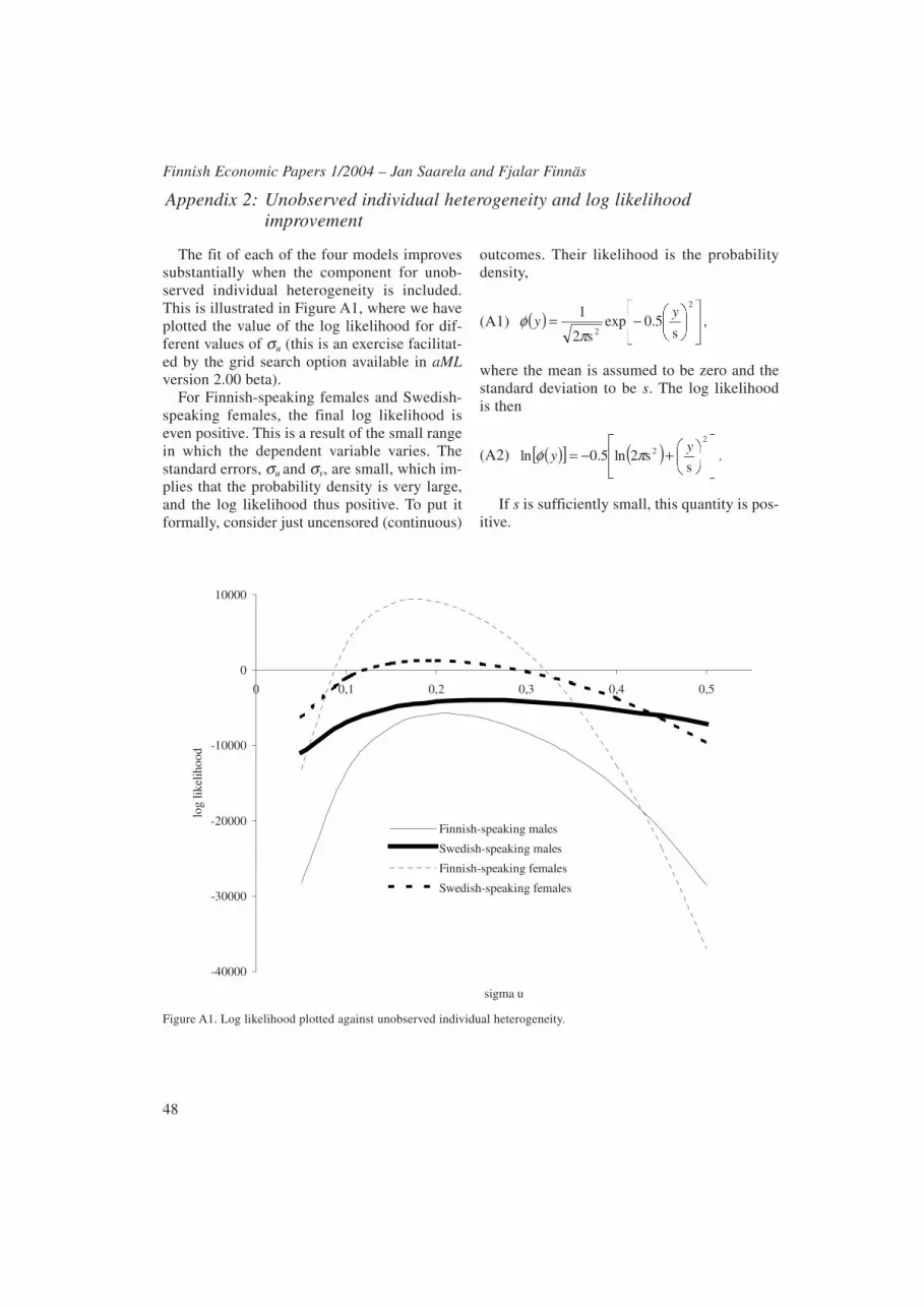
The fit of each of the four models improvessubstantially when the component for unob-served individual heterogeneity is included.This is illustrated in Figure A1, where we haveplotted the value of the log likelihood for dif-ferent values of σu (this is an exercise facilitat-ed by the grid search option available in aMLversion 2.00 beta).

For Finnish-speaking females and Swedish-speaking females, the final log likelihood iseven positive. This is a result of the small rangein which the dependent variable varies. Thestandard errors, σu and σv, are small, which im-plies that the probability density is very large,and the log likelihood thus positive. To put itformally, consider just uncensored (continuous)

outcomes. Their likelihood is the probabilitydensity,

(A1)

where the mean is assumed to be zero and thestandard deviation to be s. The log likelihoodis then

(A2)

If s is sufficiently small, this quantity is pos-itive.

-40000

-30000

-20000

-10000

0

10000

0 0,1 0,2 0,3 0,4 0,5

sigma u

log

likel

ihoo

d

Finnish-speaking males

Swedish-speaking males

Finnish-speaking females

Swedish-speaking females

( )

−=2

25.0exp

2

1

s

y

sy

πφ ,

( )[ ] ( )

+−=2

22ln5.0lns

ysy πφ .

Figure A1. Log likelihood plotted against unobserved individual heterogeneity.

Documents

Interethnic Wage Variation in the Helsinki Area