1

Intermodality and Substitution of Modes for Freight

Transportation : Computation of Price-Elasticities through a

Geographic Multimodal Transportation Network Analysis

Bart JOURQUINI, II, Michel BEUTHEI and Christian KOUL à NJANG’ HAI

I Group Transport & Mobility (GTM) Facultés Universitaires Catholiques de Mons (FUCaM), 151 Ch. de Binche, B-7000, Mons, Belgium Tel : 32-65-323211, Fax : 32-65-315691, gt&m@fucam.ac.beII Limburgs Universitair Centrum (LUC) Universitaire Campus, gebouw D, B-3590 Diepenbeek, Belgium Tel : 311-11-268600, Fax : 32-11-268700

Abstract

In order to limit the external costs caused by the use of trucks (pollution, congestion, …),multi- and intermodal transport are promoted in various ways. One way to partly shifttransport demand on trains and barges is to introduce a pricing/taxation policy which takesinto account these external costs for the different modes. The effects of such a policy areobviously dependent upon the way demand for the various modes is sensitive to variation oftariffs. There are very few estimates of direct and crossed price-elasticities available in theliterature, particularly if different markets, i.e. different categories of goods, are taken intoaccount. Moreover, existing estimates are obtained through sophisticated yet conventionalstatistical methods that do not directly cope with the topology of a given network.

This paper presents estimates which have been computed for ten different categories of goodswith a detailed multimodal network model based on a particular methodology that permits athorough analysis of intermodality and modal substitution. Assigned flows obtained withdifferent levels of relative costs for the different transportation modes are used to computedirect and cross arc-elasticities over a concrete real digitised network. The computedelasticities are then discussed and compared to previously published estimates.1 Introduction

The strong expansion of freight road transportation throughout Europe is an important

source of congestion and pollution, as well as a cause of many accidents. It is most likely that

this problem will grow worse as it is expected that freight traffic will go on increasing over the

coming years. A often proposed partial solution to this problem would be the promotion of

transportation modes which have lesser negative effects, i.e. rail and waterway, as well as

their intermodal combination with road, in order to substitute these modes to the use of direct

road transport. One way to obtain such a result would be to apply a pricing/taxation policy

which takes into account the external costs of the different modes.

2

While such a policy is worth considering in principle, because it would promote a better

allocation of collective resources, its effects are dependent upon the way demand for the

various modes reacts to tariffs’ variations. Measures of the modes’ demand direct and cross-

elasticities with respect to prices would provide some valuable information about what effect

could be expected, but very few estimates of such elasticities are available in the literature,

particularly if different markets for transportation, i.e. different categories of goods, are taken

into account. Moreover, the existing estimates, like those recently published by Abdelwahab

(1998) are obtained from sophisticated yet conventional statistical methods which do not take

explicitly into account the particularities of a real network topology, such as a convenient

accessibility at some points in space to alternative transportation modes, which depends on the

existence of specific infrastructures (rail tracks, canals, etc.).

In this paper, we present estimates of elasticities which have been obtained from a

detailed multimodal network model of freight transportation in Belgium through a set of

simulations made with different cost parameters for ten different categories of goods1. This

model of the Belgian railways, waterways and roads network embedded within the European

networks is based on the NODUS virtual network software2, which takes into account

separately each specific transport operation (loading, transiting, transhipping, etc.) and their

costs. Given the matrix of origins and destinations, it minimises the generalised cost of the

corresponding transportation task by an optimal assignment of the flows between modes,

vehicles, or their combination, and routes. Hence, it permits a thorough analysis of

intermodality and modal substitution through simulations. In this way it is possible to generate

direct and cross arc-elasticities with respect to cost variations, which fully takes into account

the spatial characteristics of the network. These network elasticities are somewhat unusual,

and their assessment requires a good understanding of their particular character compared to

the usual statistically derived elasticities.

In Section 2, the paper starts with some methodological considerations. First, section 2.1

compares network elasticities with the other more usual elasticities; then, section 2.2 explains

some basic elements of the multimodal transport model and how it was built up over the

Belgian network. Section 3 presents the elasticities obtained from a set of simulations with the

1 Part of this paper is based on the results of a research contract with the “ desTransports de la Région Wallonne”. The substantial work of building the matrix of origins and destinations wasmade by the consultant STRATEC S.A. (Brussels).2 Presented in Jourquin (1995), Jourquin and Beuthe (1996), and further developed in Deliverable D5 (1998) ofthe TERMINET Research Programme funded by the European Commission.

3

network model and compares them with those published in the litterature. A global assessment

of the results concludes the paper.

2 Methodological considerations

2.1 Elasticities in freight transport

Before explaining in some details the features of the transport model which is used to

obtain measures of transport demand elasticities, it is necessary to briefly review the different

types of price elasticities which may be found in the freight transport literature3. The first main

distinction must be made between ordinary and conditional elasticities. The former measure

the combined substitution and scale or output effect of a price change; the latter is akin to the

compensated demand elasticity in the consumer theory and is conditional on a given level of

output. In their survey Oum et al. (1992) found out that it was not always easy to identify the

type of elasticity which was presented in the literature. They propose to regard an elasticity as

conditional if the shippers’ output is included in the demand equation.

All the published measures of freight transport elasticity that we know of were obtained

from econometric estimation, either on the basis of time series or cross-section data. Cross-

section data usually do not give information about outputs, so that the corresponding estimates

are not normally of the conditional type. There are aggregate market elasticities and mode-

specific elasticities. In this paper we focus on the latter which, most often, are based on a

modal-split analysis. Such elasticities can be estimated from aggregate or disaggregate data. In

both cases, they are unable in practice to take into account the effect of a price change on the

aggregate volume of traffic and would need to be adjusted in order to obtain the regular

demand elasticity (Taplin, 1982, Quandt, 1968, and Oum et al., 1992). Elasticities obtained

with a discrete choice model from aggregate data on volume shares underestimate somewhat

the response of the shippers to price changes (Winston, 1979). Whenever possible, it is thus

preferable to proceed with disaggregate data on individual shippers’ choices. In this case, the

computed individual elasticities must be aggregated over the sample to obtain a mode’s

market demand elasticity. A recently published example of such an approach is given by

Abdelwahad (1998).

3 A very good survey of the different methodologies used to derive elasticities in the field of transportation can befound in Oum et al. (1992). See also Winston (1985) and Zlatoper and Austrian (1989).

4

Finally, we must mention the distinction between traffic and transport demand

elasticities. Björner (1999), focusing on the environmental impacts of road transports, is

somewhat more interested by the variation of traffic, i.e. kilometres realised by trucks, rather

than by transport in tons/km as it is usually the case. In effect, it is the most relevant variable

from an environmental point of view. Traffic is then taken as one of several inputs in the

shippers production of transport services, while transport demand is derived from the firms’

production of output and depends not only on transport cost per ton/km, but also on the

spatial location of transported inputs, their weight and their prices. Hence, the impacts of a

transport cost variation may vary from one commodity to another. Furthermore, since there

can be some substitution between different transport production inputs, e.g. administration,

information, capital resources, traffic, etc., the price-elasticity of traffic can be different from

the transport elasticity. Actually, it could very well be stronger, and that is what is found out

in this empirical study.

The next section will provide more details on the transport model which was used to

derive our estimates, but we can already, through its general description, define the type of

elasticity obtained with reference to the above distinctions. The model is not an econometric

one but a GIS based model of the multimodal freight network of Belgium embedded within the

trans-European network. As outlined in the introduction, given a point-to-point O-D matrix

per group of commodities, it assigns the transport flows to the cheapest combination of

modes, means and routes. After a proper calibration of the model by means of the cost

functions with respect to observed flows, sensitivity analyses applied to cost parameters allow

to assess their impacts on the mode’s market shares and to compute tons and tons/km arc-

elasticities.

Thus, since the same O-D matrixes are used for all the simulations, the computed

network arc-elasticities per group of commodities are of the conditional type for a given

transport task. The estimates are based on a “all-or-nothing” assignment procedure of the flow

between each pair of origin and destination, so that these elasticities are aggregates of

“individual” responses. They fully take into account the spatial configuration of the networks,

the specific characteristics of the different O-D matrixes, and the inventory cost of the

different commodities. In effect, the cost variations simulated in order to generate the arc-

elasticities bear upon the generalised cost of transport, which implies that they cannot be

taken as usual price elasticities but rather as “generalised cost elasticities”. This means that

these measures cumulate the effects of the factors included in the generalised cost which is

5

assumed to determine the shippers’ choice, in this case not only the monetary cost but also, to

some extent, the value of time for the shippers. On the other hand, since the variations of

costs are fully controlled through the simulations, the ceteris paribus condition is fully

respected, and these elasticities measure the impacts of a mode’s cost variation on modal

shares in the absence of any competitive adjustments by the other modes.

Another important point is that, even though the model has been calibrated on observed

data, the measures are not derived from statistically adjusted response functions but from an

optimal transport choice model. If this model approximates well enough the choice behaviour

of the shippers at least in the long run, this implies that these measures reflect, ceteris paribus,

long run responses rather than short run ones, since choice adjustments are postulated to be

made instantaneously in the simulations. The methodology allows to compute elasticities with

respect to tons/km as well as with respect to tons, hence, will allow to check Björner’s result.

Obviously, some additional comments will be given after a more detailed explanation of the

transport model and a review of the empirical results.

2.2 Inter - and multimodality in freight transport networks

A thorough analysis of freight transportation over a network, with all its alternative

solutions, requires a separate identification of the different operations in a transportation

chain. In the NODUS network model all the modes and means of transportation but also all

the loading, unloading, transhipping and transiting operations are identified and associated

with a “virtual link”. A fictitious expanded multimodal network, or “virtual network”, is

automatically generated by NODUS on the basis of the characteristics of the underlying

geographical network. In the present case, there are about 17,000 geographical links (digitised

network) from which a virtual network of about 265,000 virtual links is generated.

Appropriate cost functions (see section 2.3) are attached to each virtual link defined by

a specific transport operation. Then, given an O-D matrix, it is possible to minimise the

corresponding total generalised cost of transportation with respect to, simultaneously, the

choices of modes, means and routes, including intermodal combinations. The resulting

assignments can be taken as estimates of transport demand for the different modes and means

under two hypotheses : that the shippers are actually minimising the generalised cost of

transportation, and that the (unknown) carriers’ tariffs bear a close relationship with the

operating transport cost, at least at the margin for ‘contestable’ transports. Both hypotheses

6

can be debated. But, even if they are accepted as good approximations, the results must still

be interpreted with caution because some information, such as relative safety, reliability or

other services characterising the different transport solutions were not available and therefore

not specifically included. In order to compensate this lack of information, the model was

calibrated as far as it was possible on observed flows on main links and modal shares.

2.3 Cost functions on virtual networks

2.3.1 General framework

Various types of objective functions can be used with NODUS. In this case, the total

generalised cost of transportation on the network was minimized. This total cost, which must

be minimized with respect to the choices of modes (t), means (m), and routes (l), can be

defined as TC TC ltmmtl

= ∑∑∑ , where TCltm is the sub-total cost for the traffic on a

particular route l with mode t and mean m. TCltm is the sum of all the costs over the successive

links (or operations) of the virtual network over route l, and it is supposed that all these costs

are proportional to the total quantity transported Qltm .

Assuming further that all the costs per ton for a link j are either constant or

proportional to the distance sj , we can write :

∑∑∑ ∑∑

+=

∈∈l t m ljj

tm

lj

tmjltm sBAQTC ,

where sj is the distance over the link j. This is the total cost which must be minimised with

respect to l, t, and m. After attaching the relevant cost functions to all the links, this operation

is realised by applying Johnson’s algorithm (1973), an optimised4 version of the well known

algorithms of Moore (1957) or Dijkstra (1959), onto the virtual network.

This general framework being defined, we can now have a closer look at the various

cost functions which are used on the network: the vehicles related costs, the handling costs

and the commodities’ inventory costs. The cost data were collected through numerous

sources; they are all listed and thoroughly discussed in Jourquin (1995) .

7

2.3.2 Vehicle’s related costs

For a given link, the vehicles' costs for transporting one ton over a distance s by mode t

and mean m are taken to be a linear function of distance s : s.BA tmtm + . The constant Atm

corresponds to the fixed costs incurred for the vehicles and the crew during the (un)loading

and transhipping operations . It is based on capital annuities, insurance, maintenance costs and

wages.

The duration of the handling operations are estimated by the Deming's (1978) formula

whereby handling-time = a + b * (quantity) c, a non-linear relation between handling time and

handled quantity.

The cost of moving one ton over a distance s is proportional to that distance, as Btm,

the cost per km, is a constant. Btm includes the same parameters as those indicated above, but

is also a function of average speed, fuel consumption and loading rate. Note that the real

distance on a some links is adjusted to take into account various delays and congestion which

are usually encountered on them.

2.3.3 Other handling costs

Beside these vehicles' costs, we have taken into account the labor costs of handling the

goods at the points of origin and destination, or when the goods are transferred from one mode

or means to another. The estimation of the time needed for these operations is based on the

same formula as above. There may be also some other costs related to delays, administrative

paperwork or even congestion at some points of the network. These additional costs are

included as additional constant costs at some nodes and/or links. Some additional links in the

virtual network have also been introduced in order to take into account costs of some

particular operations, such as the crossing of a national boundary. These are simple transit

costs.

2.3.4 Opportunity cost

4 The algorithm of Johnson gives faster results on low-density networks, i.e. in which the number of links ≈ numberof nodes, as on most geographic networks.

8

It is the opportunity cost of the capital tied into the goods during transportation. This

cost is proportional to the total time needed by the transportation chain. Its importance varies

with the rate of interest and the value of the goods.

3 Reference model and calibration

The model of the actual freight flows inside and through Belgium in 1995, the

“reference scenario” was set-up in three steps:

1. First, surveys of shippers and traffic observations along the network were used, along with

aggregated published statistical data, to create detailed origin-destination matrixes for each

mode and for the ten groups of NST-R commodities. Inside Belgium the cities were used

as centroïds because information was gathered at a sufficient level of disaggregation.

Outside the country, data were only available at the aggregate level of NUTS3 or NUTS2

regions5 which contain more than one city. This problem was solved by assigning the

transport flows among the different cities by means of a Monte-Carlo procedure. The

resulting matrixes provided useful information for defining some attributes of the networks

: along the waterways, no loading and unloading operations were allowed for certain

commodities in ports where no such movements were observed; the same kind of

exclusion was introduced at some railway stations in order to forbid the handling of block

trains at some stations.

2. Through cost minimisation, all these matrixes were then assigned mode per mode over the

corresponding network and the aggregated estimated flows were compared to the counts

observed along the roads, railways and waterways. This step was very helpful for checking

the digitised networks and the attributes of the nodes and links. Speeds on some links

could for example be adjusted in order to reorient some flows and obtain a better fit

between some computed and observed flows, particularly in the periphery of large cities.

3. At that stage the matrixes relative to each freight transportation mode were merged to

obtain ten matrixes corresponding to the different groups of commodities. They were used

to assign the transport flows simultaneously to the modes, means and routes through cost

minimisation. As, in our O-D matrixes, a centroïd corresponds to a city and that on the

digitised network these centroïds are directly connected to the different transport

9

infrastructures available at the city level, i.e. roads, railways and/or inland waterways, a

last problem remained to be solved. Indeed, all the producers and customers in a city

aren’t necessarily located at the railway station or the inland port and, thus, need some

initial or final trucking to/from these facilities. To solve this, some average additional fixed

costs, used to calibrate the model, were added to the (un)loading operations in order to

reflect this additional link in the transportation chain.

As explained above, the model assigns the flows not only to a mode, but also to a

transportation means. In this application, the model performed rather well in identifying the

types of boat used (300 tons, 600 tons, 1350 tons and 2000 tons or more) on the basis of their

different cost functions, the capacity of each inland waterway and the exclusions mentioned

above. Likewise, the information about exclusions and cost functions included in the model

allowed satisfying assignments between block trains and traditional trains. Unfortunately, the

use of different cost functions for small and large trucks (7 tons and 40 tons respectively) did

not lead to correct choices between these two means, the reason being that both types of

trucks are used for long and short hauls according to the size of the shipments, and no

information that could be included in the model was available about shipment sizes. This

problem was solved by splitting total road flows between small and large trucks on the basis of

external information about the distribution of the use of small and large trucks with respect to

travel distance.

Table 1 compares the results of the assignments realised by the model with the 1995 data

on observed modal choices. Map 1 illustrates the flows on the Belgian territory, on which the

red lines correspond to truck flows, the green lines to the rail flows and the blue ones to the

waterways flows.

Map 1 : Assigned flows on the Belgian freight network (reference scenario)

5 NUTS3 data were obtained for regions nearby Belgium.

10

Another way to assess the model performance is to compute the correlation between the

observed flows and those assigned by the model at various points on the network. A

correlation coefficient of 0.92 was obtained for waterway flows, 0.86 for railways, and 0.91

for roads.

Table 1 : Assignment performance (tons)

Observed (1995) Estimated

Group Water Rail Water Rail

0-9 11.28% 8.99% 11.06% 9.05%

0 7.18% 2.24% 7.56% 1.67%

1 5.06% 2.44% 5.61% 2.13%

2 25.33% 43.51% 25.11% 43.81%

3 28.65% 6.23% 28.89% 9.08%

4 25.06% 49.07% 18.66% 50.24%

5 7.44% 26.22% 7.32% 26.77%

6 15.37% 1.74% 15.44% 1.33%

7 23.70% 5.25% 24.09% 5.39%

8 8.00% 6.56% 7.85% 6.05%

9 0.53% 11.40% 0.88% 11.35%

11

4 Model results and discussion

Once the calibrated reference scenario was obtained, a set of different simulations

could be performed in which some elements of the modes’ cost functions were modified. In

the first set, the total transportation cost for each mode separately was modified; these costs

were decreased and increased successively by 2, 5 and 10 percents of the reference level. As

three modes were involved, the first set contains 18 different assignments6. In order to

separate the impact of the direct transport costs from the other costs of handling, transhipping

and transiting, a second set of assignments was produced, in which only the “moving costs”

were reduced by 5 percent for each mode successively. A third set was made to assess the

influence of travel distances on the measured elasticities. For doing so, the O-D matrixes were

split into short and long haul transports ( > 300 km). Assignments were computed for both

types of matrixes when the total transportation costs were decreased by 5 percent for each

mode successively. On the basis of the results obtained from these simulations, the

corresponding elasticities were computed by means of the following formula, where output

can be introduced in tons (quantity) or tons/km (flow).

j2m

j2m

j1m

j1m

j1m

j1m

j2m

j2mj

2m,1m NewOutpututputReferenceO

NewCostostReferenceC*

NewCostostReferenceC

NewOutpututputReferenceO

++

−−

=ε

where:

ε : elasticity

j : group of commodities

m1 : transport mode 1

m2 : transport mode 2

Table 2 gives all the aggregate elasticities computed with respect to tons and tons/km

when costs are reduced by 5%. Table 3 gives all the ton/km elasticities per group of goods for

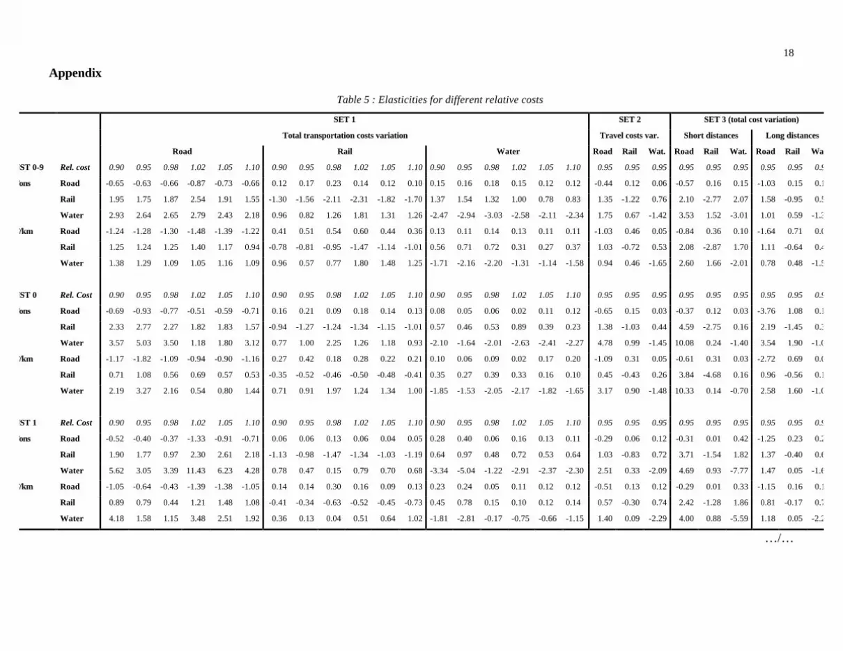
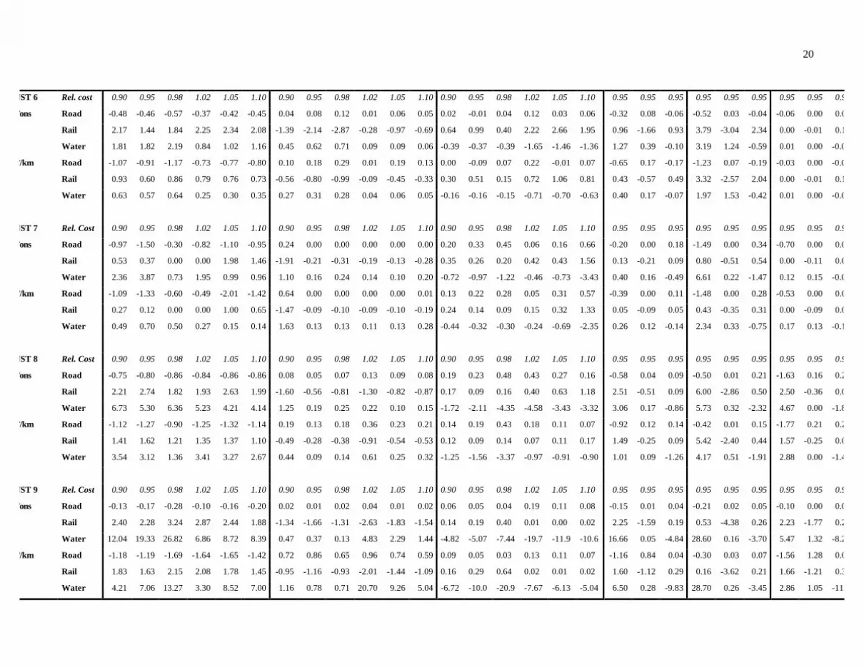
the same relative change of the costs. The extensive set of results obtained with other relative

cost variations can be found in Table 5 in the Appendix, in which some variations of

elasticities with the magnitude of the cost variation can be observed. This is inherent in this

concept of elasticity which takes into account the topology of the networks and the

localisation of activities. But, altogether, they are rather stable.

6 Note that the fixed costs introduced to simulate initial and final trucking (see step 3 of the model calibration)were kept constant.

12

Table 2: Aggregate elasticities when costs are reduced by 5%

Set 1 Set 2 Set 3 (total cost variation)

Total cost reduction Travel costs reduction Short distances Long distances

Road Rail Water Road Rail Water Road Rail Water Road Rail Water

Tons Road -0.63 0.17 0.16 -0.44 0.12 0.06 -0.57 0.16 0.15 -1.03 0.15 0.12

Rail 1.75 -1.56 1.54 1.35 -1.22 0.76 2.10 -2.77 2.07 1.58 -0.95 0.50

Water 2.64 0.82 -2.94 1.75 0.67 -1.42 3.53 1.52 -3.01 1.01 0.59 -1.30

T/km Road -1.28 0.51 0.11 -1.03 0.46 0.05 -0.84 0.36 0.10 -1.64 0.71 0.09

Rail 1.24 -0.81 0.71 1.03 -0.72 0.53 2.08 -2.87 1.70 1.11 -0.64 0.43

Water 1.29 0.57 -2.16 0.94 0.46 -1.65 2.60 1.66 -2.01 0.78 0.48 -1.59

Altogether, it can be observed that most of the obtained elasticities are of the same order

of magnitude than those which can be found in the literature. However, some of them are

definitely stronger while some others are extremely small. This can be explained by different

reasons:

• The model assigns the flows on a real network which has a particular topology with the

three transportation modes competing on most routes. Such a high density of the three

modes’ networks is an important characteristic of the studied area.

• The flows are assigned by an all-or-nothing assignment procedure that minimises the

total generalised cost. As explained in section 2, the elasticities are measured under the

ceteris paribus condition without any competitive reaction which could attenuate the

cost variation effect. Moreover, they result from assignments made under assumption

of a complete instantaneous adjustment to the new cost situation.

13

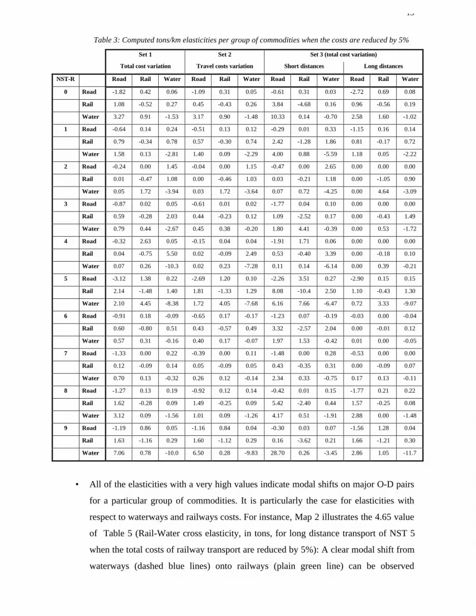
Table 3: Computed tons/km elasticities per group of commodities when the costs are reduced by 5%

Set 1 Set 2 Set 3 (total cost variation)

Total cost variation Travel costs variation Short distances Long distances

NST-R Road Rail Water Road Rail Water Road Rail Water Road Rail Water

0 Road -1.82 0.42 0.06 -1.09 0.31 0.05 -0.61 0.31 0.03 -2.72 0.69 0.08

Rail 1.08 -0.52 0.27 0.45 -0.43 0.26 3.84 -4.68 0.16 0.96 -0.56 0.19

Water 3.27 0.91 -1.53 3.17 0.90 -1.48 10.33 0.14 -0.70 2.58 1.60 -1.02

1 Road -0.64 0.14 0.24 -0.51 0.13 0.12 -0.29 0.01 0.33 -1.15 0.16 0.14

Rail 0.79 -0.34 0.78 0.57 -0.30 0.74 2.42 -1.28 1.86 0.81 -0.17 0.72

Water 1.58 0.13 -2.81 1.40 0.09 -2.29 4.00 0.88 -5.59 1.18 0.05 -2.22

2 Road -0.24 0.00 1.45 -0.04 0.00 1.15 -0.47 0.00 2.65 0.00 0.00 0.00

Rail 0.01 -0.47 1.08 0.00 -0.46 1.03 0.03 -0.21 1.18 0.00 -1.05 0.90

Water 0.05 1.72 -3.94 0.03 1.72 -3.64 0.07 0.72 -4.25 0.00 4.64 -3.09

3 Road -0.87 0.02 0.05 -0.61 0.01 0.02 -1.77 0.04 0.10 0.00 0.00 0.00

Rail 0.59 -0.28 2.03 0.44 -0.23 0.12 1.09 -2.52 0.17 0.00 -0.43 1.49

Water 0.79 0.44 -2.67 0.45 0.38 -0.20 1.80 4.41 -0.39 0.00 0.53 -1.72

4 Road -0.32 2.63 0.05 -0.15 0.04 0.04 -1.91 1.71 0.06 0.00 0.00 0.00

Rail 0.04 -0.75 5.50 0.02 -0.09 2.49 0.53 -0.40 3.39 0.00 -0.18 0.10

Water 0.07 0.26 -10.3 0.02 0.23 -7.28 0.11 0.14 -6.14 0.00 0.39 -0.21

5 Road -3.12 1.38 0.22 -2.69 1.20 0.10 -2.26 3.51 0.27 -2.90 0.15 0.15

Rail 2.14 -1.48 1.40 1.81 -1.33 1.29 8.08 -10.4 2.50 1.10 -0.43 1.30

Water 2.10 4.45 -8.38 1.72 4.05 -7.68 6.16 7.66 -6.47 0.72 3.33 -9.07

6 Road -0.91 0.18 -0.09 -0.65 0.17 -0.17 -1.23 0.07 -0.19 -0.03 0.00 -0.04

Rail 0.60 -0.80 0.51 0.43 -0.57 0.49 3.32 -2.57 2.04 0.00 -0.01 0.12

Water 0.57 0.31 -0.16 0.40 0.17 -0.07 1.97 1.53 -0.42 0.01 0.00 -0.05

7 Road -1.33 0.00 0.22 -0.39 0.00 0.11 -1.48 0.00 0.28 -0.53 0.00 0.00

Rail 0.12 -0.09 0.14 0.05 -0.09 0.05 0.43 -0.35 0.31 0.00 -0.09 0.07

Water 0.70 0.13 -0.32 0.26 0.12 -0.14 2.34 0.33 -0.75 0.17 0.13 -0.11

8 Road -1.27 0.13 0.19 -0.92 0.12 0.14 -0.42 0.01 0.15 -1.77 0.21 0.22

Rail 1.62 -0.28 0.09 1.49 -0.25 0.09 5.42 -2.40 0.44 1.57 -0.25 0.08

Water 3.12 0.09 -1.56 1.01 0.09 -1.26 4.17 0.51 -1.91 2.88 0.00 -1.48

9 Road -1.19 0.86 0.05 -1.16 0.84 0.04 -0.30 0.03 0.07 -1.56 1.28 0.04

Rail 1.63 -1.16 0.29 1.60 -1.12 0.29 0.16 -3.62 0.21 1.66 -1.21 0.30

Water 7.06 0.78 -10.0 6.50 0.28 -9.83 28.70 0.26 -3.45 2.86 1.05 -11.7

• All of the elasticities with a very high values indicate modal shifts on major O-D pairs

for a particular group of commodities. It is particularly the case for elasticities with

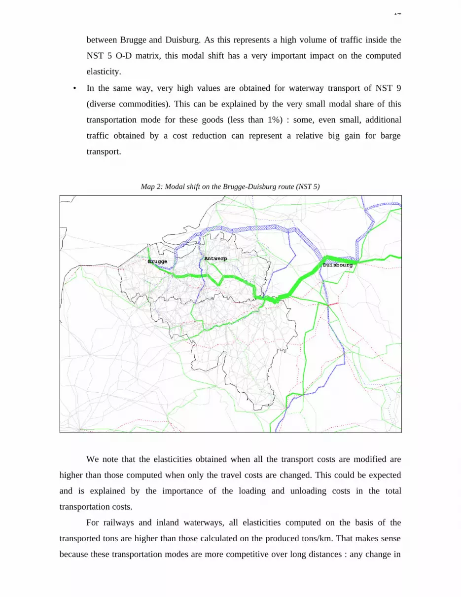
respect to waterways and railways costs. For instance, Map 2 illustrates the 4.65 value

of Table 5 (Rail-Water cross elasticity, in tons, for long distance transport of NST 5

when the total costs of railway transport are reduced by 5%): A clear modal shift from

waterways (dashed blue lines) onto railways (plain green line) can be observed

14

between Brugge and Duisburg. As this represents a high volume of traffic inside the

NST 5 O-D matrix, this modal shift has a very important impact on the computed

elasticity.

• In the same way, very high values are obtained for waterway transport of NST 9

(diverse commodities). This can be explained by the very small modal share of this

transportation mode for these goods (less than 1%) : some, even small, additional

traffic obtained by a cost reduction can represent a relative big gain for barge

transport.

Map 2: Modal shift on the Brugge-Duisburg route (NST 5)

We note that the elasticities obtained when all the transport costs are modified are

higher than those computed when only the travel costs are changed. This could be expected

and is explained by the importance of the loading and unloading costs in the total

transportation costs.

For railways and inland waterways, all elasticities computed on the basis of the

transported tons are higher than those calculated on the produced tons/km. That makes sense

because these transportation modes are more competitive over long distances : any change in

15

their transportation cost will more directly affect their market-share on shorter distances,

making the relative change in the total quantity transported more important than the relative

change in the produced tons/km. Likewise, the direct elasticities obtained for rail and water

transport are higher for short distances than for long trips. An additional reason for this is the

low market-share of these two modes on shorter hauls.

A reverse relationship is observed for road elasticities : with the exception of

elasticities with respect to waterways’ costs, the tons/km elasticities are higher than those

computed on the basis of transported tons. This outcome confirms Björner’s (1999) result who

found a “traffic” elasticity of –0.8 while the tons/km elasticity was –0.47. Like in his case

where an adjustment of mileage realised explains the stronger “traffic” elasticity, it is the

mileage adjustment which produces a stronger elasticity of tons/km when compared to the one

based on tons transported. Note also that the short distances direct road elasticities are

smaller than the long distance ones.

Table 4: Comparison with other published elasticities

STCC NST-R Elasticity Abdelwahab7 Jourquin et al.8

33: Primary metal products 5 : Metal products Truck-Truck -0.80 → -2.18 -2.13

34 : Fabricated metal products Rail-Rail -0.91 → -2.49 -3.32

Rail-Truck 0.90 → 2.42 3.72

Truck-Rail 0.93 → 2.53 1.23

Table 4 compares some of these elasticities with those published by Abdelwahab

(1998). As the categories of goods used in both papers are not directly comparable, the

comparison is limited to two groups that are more or less identical, i.e. STCC 33/34 and NST-

R 5. In this case, the values obtained in this paper appear to be slightly higher than those of

Abdelwahab (1998).

7 Elasticities were computed for different regions. This column gives the lowest and highest obtained values.8 These values are obtained with a reduction of 5% of the total transportation costs.

16

5 Conclusions

This paper has presented a whole set of direct and cross-elasticities for road, rail and

waterway freight transport computed by means of a multimodal network model applied to

different groups of goods. Section 2 gives an overview of the recent literature, and discusses

the nature of the elasticities that are computed in our simulations.

Compared to other studies, the values that are obtained are, in most cases, of the same

order of magnitude. However, the estimated values differ according to the group of goods

analysed, and some elasticities can be very high while some others are extremely low. This is

due to several factors: the strict application of the ceteris paribus condition in the simulation;

the particular topology of the region and its network of three competing modes; the different

spatial localisation of transport demand for the various categories of goods; the all-or-nothing

assignment procedure based on cost minimisation which produces “ideal” results akin to a

long run partial equilibrium outcome.

Thus, these elasticities need to be properly understood and assessed before being used

in a different regional context. Contingent on this reservation, they appear to be highly

relevant. Thus, the proposed methodology based on a multimodal spatial simulation model

has shown itself to be particularly useful in that it is able to produce complete sets of direct

and cross-elasticities for different groups of commodities and to distinguish between different

types of elasticities, i.e. between elasticities related to short and long haul transports and

according to the cost parameters which are affected.

References :

1. Abdelwahab, W.M. (1998), Elasticities of Mode Choice Probabilities and Market

Elasticities of Demand: Evidence from a Simultaneous Mode Choice/Shipment-Size

Freight Transport Model, Transportation Research E , Vol 34, No. 4, pp 257-266.

2. Björner, T.B. (1999), Environmental Benefits from Better Freight Transport

Management: Freight Traffic in a VAR Model, Transportation Research D 4, pp. 45-64.

3. Deming W.E (1978), On a Rational Relationship for Certain Costs of Handling Motor

Freight: Over the Platform, Transportation Journal 17, pp. 5-11.

4. Dijkstra E.W. (1959), A Note on Two Problems in Connection with Graphs, Numerische

Mathematik 1, pp. 269-271

17

5. Johnson D.B. (1973), A Note on Dijkstra’s Shortest Path Algorithm, Journal A.C.M. 20,

pp. 385-388

6. Jourquin B. (1995), Un outil d’analyse économique des transports de marchandises sur

des réseaux multi-modaux et multi-produits : Le réseau virtuel, concepts, méthodes et

applications, Ph.D. Thesis, Facultés Universitaires Catholiques de Mons.

7. Jourquin B. and M. Beuthe (1996) Transportation Policy Analysis with a Geographic

Information System: The Virtual Network of Freight Transportation in Europe ,

Transportation Research C, Vol. 4, No 6, pp. 359-371

8. Moore E.F. (1957) : The Shortest Path Trough a Maze, Proceedings of the International

Symposium on Theory of Switching, Part II, april 2-5, pp. 285-292, the Annals of the

computation laboratory of Harvard University 30, Harvard University Press, 1959.

9. Oum T.H., W.G. Waters II and J.S. Yong, (1992) Concepts of Price Elasticities of

Transport Demand and Recent Empirical Estimates, Journal of Transport Economics and

Policy, May, pp. 139-154.et al. (1992)

10. Quandt R.E., (1968), Estimation of Modal Splits, Transportation Research, vol. 2, pp. 41-

50.

11. Taplin J. H., (1982), Inferring Ordinary Elasticities from Choice or Mode-Split

Elasticities, Journal of Transport Economics and Policy, January, pp. 55-63.

12. TERMINET, deliverable D5 (1998) , Tool : Decision Support Tool/Model for Bundling

Layout, Transport RTD Programme of the 4th framework programme.

13. Winston C, (1979), A Disaggregated Qualitative Mode Choice Model for Intercity

Freigth Transportation, Ph.D. dissertation, University of California, Berkeley.

14. Winston C., (1985), Conceptual Developments in the Economics of Transportation: an

Interpretive Survey, Journal of Economic Literature XXIII, March, pp. 57-94.

15. Zlatoper T.J. and Z. Austrian, (1989), Freight Transportation Demand: a Survey of

Recent Econometric Studies, Transportation 16(1), pp. 27-46.

18

Appendix

Table 5 : Elasticities for different relative costs

SET 1 SET 2 SET 3 (total cost variation)

Total transportation costs variation Travel costs var. Short distances Long distances

Road Rail Water Road Rail Wat. Road Rail Wat. Road Rail Wat.

NST 0-9 Rel. cost 0.90 0.95 0.98 1.02 1.05 1.10 0.90 0.95 0.98 1.02 1.05 1.10 0.90 0.95 0.98 1.02 1.05 1.10 0.95 0.95 0.95 0.95 0.95 0.95 0.95 0.95 0.95

Tons Road -0.65 -0.63 -0.66 -0.87 -0.73 -0.66 0.12 0.17 0.23 0.14 0.12 0.10 0.15 0.16 0.18 0.15 0.12 0.12 -0.44 0.12 0.06 -0.57 0.16 0.15 -1.03 0.15 0.12

Rail 1.95 1.75 1.87 2.54 1.91 1.55 -1.30 -1.56 -2.11 -2.31 -1.82 -1.70 1.37 1.54 1.32 1.00 0.78 0.83 1.35 -1.22 0.76 2.10 -2.77 2.07 1.58 -0.95 0.50

Water 2.93 2.64 2.65 2.79 2.43 2.18 0.96 0.82 1.26 1.81 1.31 1.26 -2.47 -2.94 -3.03 -2.58 -2.11 -2.34 1.75 0.67 -1.42 3.53 1.52 -3.01 1.01 0.59 -1.30

T/km Road -1.24 -1.28 -1.30 -1.48 -1.39 -1.22 0.41 0.51 0.54 0.60 0.44 0.36 0.13 0.11 0.14 0.13 0.11 0.11 -1.03 0.46 0.05 -0.84 0.36 0.10 -1.64 0.71 0.09

Rail 1.25 1.24 1.25 1.40 1.17 0.94 -0.78 -0.81 -0.95 -1.47 -1.14 -1.01 0.56 0.71 0.72 0.31 0.27 0.37 1.03 -0.72 0.53 2.08 -2.87 1.70 1.11 -0.64 0.43

Water 1.38 1.29 1.09 1.05 1.16 1.09 0.96 0.57 0.77 1.80 1.48 1.25 -1.71 -2.16 -2.20 -1.31 -1.14 -1.58 0.94 0.46 -1.65 2.60 1.66 -2.01 0.78 0.48 -1.59

NST 0 Rel. Cost 0.90 0.95 0.98 1.02 1.05 1.10 0.90 0.95 0.98 1.02 1.05 1.10 0.90 0.95 0.98 1.02 1.05 1.10 0.95 0.95 0.95 0.95 0.95 0.95 0.95 0.95 0.95

Tons Road -0.69 -0.93 -0.77 -0.51 -0.59 -0.71 0.16 0.21 0.09 0.18 0.14 0.13 0.08 0.05 0.06 0.02 0.11 0.12 -0.65 0.15 0.03 -0.37 0.12 0.03 -3.76 1.08 0.15

Rail 2.33 2.77 2.27 1.82 1.83 1.57 -0.94 -1.27 -1.24 -1.34 -1.15 -1.01 0.57 0.46 0.53 0.89 0.39 0.23 1.38 -1.03 0.44 4.59 -2.75 0.16 2.19 -1.45 0.30

Water 3.57 5.03 3.50 1.18 1.80 3.12 0.77 1.00 2.25 1.26 1.18 0.93 -2.10 -1.64 -2.01 -2.63 -2.41 -2.27 4.78 0.99 -1.45 10.08 0.24 -1.40 3.54 1.90 -1.07

T/km Road -1.17 -1.82 -1.09 -0.94 -0.90 -1.16 0.27 0.42 0.18 0.28 0.22 0.21 0.10 0.06 0.09 0.02 0.17 0.20 -1.09 0.31 0.05 -0.61 0.31 0.03 -2.72 0.69 0.08

Rail 0.71 1.08 0.56 0.69 0.57 0.53 -0.35 -0.52 -0.46 -0.50 -0.48 -0.41 0.35 0.27 0.39 0.33 0.16 0.10 0.45 -0.43 0.26 3.84 -4.68 0.16 0.96 -0.56 0.19

Water 2.19 3.27 2.16 0.54 0.80 1.44 0.71 0.91 1.97 1.24 1.34 1.00 -1.85 -1.53 -2.05 -2.17 -1.82 -1.65 3.17 0.90 -1.48 10.33 0.14 -0.70 2.58 1.60 -1.02

NST 1 Rel. Cost 0.90 0.95 0.98 1.02 1.05 1.10 0.90 0.95 0.98 1.02 1.05 1.10 0.90 0.95 0.98 1.02 1.05 1.10 0.95 0.95 0.95 0.95 0.95 0.95 0.95 0.95 0.95

Tons Road -0.52 -0.40 -0.37 -1.33 -0.91 -0.71 0.06 0.06 0.13 0.06 0.04 0.05 0.28 0.40 0.06 0.16 0.13 0.11 -0.29 0.06 0.12 -0.31 0.01 0.42 -1.25 0.23 0.22

Rail 1.90 1.77 0.97 2.30 2.61 2.18 -1.13 -0.98 -1.47 -1.34 -1.03 -1.19 0.64 0.97 0.48 0.72 0.53 0.64 1.03 -0.83 0.72 3.71 -1.54 1.82 1.37 -0.40 0.60

Water 5.62 3.05 3.39 11.43 6.23 4.28 0.78 0.47 0.15 0.79 0.70 0.68 -3.34 -5.04 -1.22 -2.91 -2.37 -2.30 2.51 0.33 -2.09 4.69 0.93 -7.77 1.47 0.05 -1.61

T/km Road -1.05 -0.64 -0.43 -1.39 -1.38 -1.05 0.14 0.14 0.30 0.16 0.09 0.13 0.23 0.24 0.05 0.11 0.12 0.12 -0.51 0.13 0.12 -0.29 0.01 0.33 -1.15 0.16 0.14

Rail 0.89 0.79 0.44 1.21 1.48 1.08 -0.41 -0.34 -0.63 -0.52 -0.45 -0.73 0.45 0.78 0.15 0.10 0.12 0.14 0.57 -0.30 0.74 2.42 -1.28 1.86 0.81 -0.17 0.72

Water 4.18 1.58 1.15 3.48 2.51 1.92 0.36 0.13 0.04 0.51 0.64 1.02 -1.81 -2.81 -0.17 -0.75 -0.66 -1.15 1.40 0.09 -2.29 4.00 0.88 -5.59 1.18 0.05 -2.22

…/…

19

NST 2 Rel. cost 0.90 0.95 0.98 1.02 1.05 1.10 0.90 0.95 0.98 1.02 1.05 1.10 0.90 0.95 0.98 1.02 1.05 1.10 0.95 0.95 0.95 0.95 0.95 0.95 0.95 0.95 0.95

Tons Road -4.21 -1.78 -0.20 -11.4 -5.96 -3.50 0.03 0.01 0.00 0.00 0.01 0.02 2.74 5.59 11.05 0.19 1.80 0.93 -0.11 0.00 4.35 -2.07 0.01 6.23 0.00 0.00 0.00

Rail 1.10 0.02 0.01 0.02 0.03 0.05 -0.18 -0.27 -0.49 -2.20 -1.03 -1.21 2.73 1.03 2.21 0.52 0.27 0.24 0.00 -0.27 0.95 0.08 -0.20 1.04 0.00 -1.00 0.93

Water 1.95 1.30 0.13 6.63 3.30 1.83 0.34 0.53 0.97 4.00 1.85 1.99 -4.72 -4.71 -10.0 -1.15 -1.93 -1.21 0.07 0.53 -4.06 1.39 0.34 -4.74 0.00 5.31 -3.74

T/km Road -1.18 -0.24 -0.07 -2.99 -1.54 -0.83 0.01 0.00 0.00 0.00 0.00 0.01 0.72 1.45 2.93 0.07 0.22 0.12 -0.04 0.00 1.15 -0.47 0.00 2.65 0.00 0.00 0.00

Rail 0.47 0.01 0.00 0.00 0.01 0.01 -0.34 -0.47 -0.67 -1.98 -1.11 -1.16 1.89 1.08 2.01 0.66 0.44 0.37 0.00 -0.46 1.03 0.03 -0.21 1.18 0.00 -1.05 0.90

Water 0.06 0.05 0.07 3.14 1.50 0.78 1.28 1.72 2.55 4.78 2.77 2.55 -4.21 -3.94 -7.68 -2.59 -1.70 -1.42 0.03 1.72 -3.64 0.07 0.72 -4.25 0.00 4.64 -3.09

NST 3 Rel. cost 0.90 0.95 0.98 1.02 1.05 1.10 0.90 0.95 0.98 1.02 1.05 1.10 0.90 0.95 0.98 1.02 1.05 1.10 0.95 0.95 0.95 0.95 0.95 0.95 0.95 0.95 0.95

Tons Road -1.58 -1.17 -1.13 -0.36 -1.37 -1.17 0.04 0.03 0.00 0.00 0.27 0.16 0.40 0.09 0.12 0.03 0.32 0.34 -0.84 0.02 0.04 -1.32 0.03 0.10 0.00 0.00 0.00

Rail 0.98 1.21 0.44 0.36 0.45 0.63 -1.48 -0.47 -0.03 -6.08 -3.72 -2.23 1.69 2.95 6.25 0.15 0.39 1.76 0.84 -0.36 0.12 1.63 -3.29 0.33 0.00 -0.72 1.91

Water 4.77 2.16 2.80 0.61 3.00 2.15 1.88 0.46 0.03 6.12 2.91 1.69 -2.49 -3.10 -6.56 -0.26 -1.40 -3.72 1.54 0.37 -0.25 2.28 3.31 -0.53 0.00 0.77 -1.78

T/km Road -1.00 -0.87 -0.57 -0.21 -0.85 -0.69 0.03 0.02 0.00 0.00 0.30 0.17 0.28 0.05 0.07 0.02 0.16 0.18 -0.61 0.01 0.02 -1.77 0.04 0.10 0.00 0.00 0.00

Rail 0.46 0.59 0.14 0.10 0.12 0.19 -2.32 -0.28 -0.04 -3.29 -2.18 -1.50 1.17 2.03 3.45 0.21 0.25 2.58 0.44 -0.23 0.12 1.09 -2.52 0.17 0.00 -0.43 1.49

Water 1.28 0.79 0.65 0.22 1.15 0.79 7.32 0.44 0.05 3.85 2.20 1.64 -1.91 -2.67 -4.11 -0.56 -0.75 -9.09 0.45 0.38 -0.20 1.80 4.41 -0.39 0.00 0.53 -1.72

NST 4 Rel. cost 0.90 0.95 0.98 1.02 1.05 1.10 0.90 0.95 0.98 1.02 1.05 1.10 0.90 0.95 0.98 1.02 1.05 1.10 0.95 0.95 0.95 0.95 0.95 0.95 0.95 0.95 0.95

Tons Road -0.56 -0.46 -0.56 -9.64 -4.22 -3.68 1.80 3.60 0.16 0.06 0.03 0.13 0.07 0.11 0.27 0.08 0.05 0.11 -0.22 0.07 0.10 -2.14 2.04 0.12 0.00 0.00 0.00

Rail 0.11 0.13 0.23 4.16 1.79 1.43 -0.87 -1.66 -0.10 -0.09 -1.99 -3.19 4.51 5.72 0.13 0.02 0.09 0.16 0.09 -0.08 1.58 0.96 -0.90 3.99 0.00 -0.24 0.14

Water 0.58 0.33 0.19 0.43 0.24 0.16 0.22 0.17 0.08 0.18 5.15 6.03 -7.17 -11.2 -0.84 -0.21 -0.36 -0.71 0.08 0.16 -4.36 0.38 0.10 -9.61 0.00 0.39 -0.22

T/km Road -0.46 -0.32 -0.36 -6.95 -3.01 -2.45 1.31 2.63 0.10 0.06 0.02 0.08 0.03 0.05 0.11 0.07 0.04 0.09 -0.15 0.04 0.04 -1.91 1.71 0.06 0.00 0.00 0.00

Rail 0.04 0.04 0.05 1.73 0.75 0.59 -0.46 -0.75 -0.08 -0.05 -2.88 -3.00 3.45 5.50 0.14 0.05 0.12 0.22 0.02 -0.09 2.49 0.53 -0.40 3.39 0.00 -0.18 0.10

Water 0.14 0.07 0.05 0.06 0.04 0.03 0.38 0.26 0.15 0.11 7.92 5.56 -5.51 -10.3 -0.20 -0.18 -0.43 -0.72 0.02 0.23 -7.28 0.11 0.14 -6.14 0.00 0.39 -0.21

NST5 0.90 0.95 0.98 1.02 1.05 1.10 0.90 0.95 0.98 1.02 1.05 1.10 0.90 0.95 0.98 1.02 1.05 1.10 0.95 0.95 0.95 0.95 0.95 0.95 0.95 0.95 0.95

Tons Road -2.01 -2.13 -2.51 -3.59 -2.25 -1.74 0.74 1.23 2.66 1.54 0.94 0.66 0.40 0.32 0.13 0.11 0.10 0.14 -1.81 1.08 0.08 -1.34 1.81 0.32 -4.32 0.24 0.28

Rail 4.23 3.72 4.57 5.31 2.68 1.89 -2.15 -3.32 -7.25 -5.37 -3.46 -3.12 1.69 1.81 2.07 2.92 1.41 1.09 3.10 -3.03 1.44 5.86 -9.48 3.12 1.69 -0.61 1.31

Water 3.26 3.41 1.50 3.11 4.03 3.16 6.31 7.33 15.12 8.70 5.32 4.81 -6.43 -7.88 -8.84 -15.8 -8.43 -8.51 2.77 6.84 -5.58 5.02 8.96 -7.60 0.76 4.65 -8.38

T/km Road -2.65 -3.12 -3.27 -3.96 -2.38 -1.82 0.88 1.38 2.89 2.30 1.25 0.99 0.29 0.22 0.13 0.07 0.10 0.15 -2.69 1.20 0.10 -2.26 3.51 0.27 -2.90 0.15 0.15

Rail 2.05 2.14 2.20 2.27 1.23 0.84 -1.05 -1.48 -2.90 -3.44 -2.20 -2.21 1.32 1.40 1.54 1.00 0.62 0.51 1.81 -1.33 1.29 8.08 -10.4 2.50 1.10 -0.43 1.30

Water 1.82 2.10 0.63 1.91 1.68 1.52 4.23 4.45 7.16 11.04 7.29 6.46 -6.61 -8.38 -10.3 -6.90 -4.96 -4.95 1.72 4.05 -7.68 6.16 7.66 -6.47 0.72 3.33 -9.07

…/…

20

NST 6 Rel. cost 0.90 0.95 0.98 1.02 1.05 1.10 0.90 0.95 0.98 1.02 1.05 1.10 0.90 0.95 0.98 1.02 1.05 1.10 0.95 0.95 0.95 0.95 0.95 0.95 0.95 0.95 0.95

Tons Road -0.48 -0.46 -0.57 -0.37 -0.42 -0.45 0.04 0.08 0.12 0.01 0.06 0.05 0.02 -0.01 0.04 0.12 0.03 0.06 -0.32 0.08 -0.06 -0.52 0.03 -0.04 -0.06 0.00 0.00

Rail 2.17 1.44 1.84 2.25 2.34 2.08 -1.39 -2.14 -2.87 -0.28 -0.97 -0.69 0.64 0.99 0.40 2.22 2.66 1.95 0.96 -1.66 0.93 3.79 -3.04 2.34 0.00 -0.01 0.12

Water 1.81 1.82 2.19 0.84 1.02 1.16 0.45 0.62 0.71 0.09 0.09 0.06 -0.39 -0.37 -0.39 -1.65 -1.46 -1.36 1.27 0.39 -0.10 3.19 1.24 -0.59 0.01 0.00 -0.06

T/km Road -1.07 -0.91 -1.17 -0.73 -0.77 -0.80 0.10 0.18 0.29 0.01 0.19 0.13 0.00 -0.09 0.07 0.22 -0.01 0.07 -0.65 0.17 -0.17 -1.23 0.07 -0.19 -0.03 0.00 -0.04

Rail 0.93 0.60 0.86 0.79 0.76 0.73 -0.56 -0.80 -0.99 -0.09 -0.45 -0.33 0.30 0.51 0.15 0.72 1.06 0.81 0.43 -0.57 0.49 3.32 -2.57 2.04 0.00 -0.01 0.12

Water 0.63 0.57 0.64 0.25 0.30 0.35 0.27 0.31 0.28 0.04 0.06 0.05 -0.16 -0.16 -0.15 -0.71 -0.70 -0.63 0.40 0.17 -0.07 1.97 1.53 -0.42 0.01 0.00 -0.05

NST 7 Rel. Cost 0.90 0.95 0.98 1.02 1.05 1.10 0.90 0.95 0.98 1.02 1.05 1.10 0.90 0.95 0.98 1.02 1.05 1.10 0.95 0.95 0.95 0.95 0.95 0.95 0.95 0.95 0.95

Tons Road -0.97 -1.50 -0.30 -0.82 -1.10 -0.95 0.24 0.00 0.00 0.00 0.00 0.00 0.20 0.33 0.45 0.06 0.16 0.66 -0.20 0.00 0.18 -1.49 0.00 0.34 -0.70 0.00 0.00

Rail 0.53 0.37 0.00 0.00 1.98 1.46 -1.91 -0.21 -0.31 -0.19 -0.13 -0.28 0.35 0.26 0.20 0.42 0.43 1.56 0.13 -0.21 0.09 0.80 -0.51 0.54 0.00 -0.11 0.06

Water 2.36 3.87 0.73 1.95 0.99 0.96 1.10 0.16 0.24 0.14 0.10 0.20 -0.72 -0.97 -1.22 -0.46 -0.73 -3.43 0.40 0.16 -0.49 6.61 0.22 -1.47 0.12 0.15 -0.08

T/km Road -1.09 -1.33 -0.60 -0.49 -2.01 -1.42 0.64 0.00 0.00 0.00 0.00 0.01 0.13 0.22 0.28 0.05 0.31 0.57 -0.39 0.00 0.11 -1.48 0.00 0.28 -0.53 0.00 0.00

Rail 0.27 0.12 0.00 0.00 1.00 0.65 -1.47 -0.09 -0.10 -0.09 -0.10 -0.19 0.24 0.14 0.09 0.15 0.32 1.33 0.05 -0.09 0.05 0.43 -0.35 0.31 0.00 -0.09 0.07

Water 0.49 0.70 0.50 0.27 0.15 0.14 1.63 0.13 0.13 0.11 0.13 0.28 -0.44 -0.32 -0.30 -0.24 -0.69 -2.35 0.26 0.12 -0.14 2.34 0.33 -0.75 0.17 0.13 -0.11

NST 8 Rel. Cost 0.90 0.95 0.98 1.02 1.05 1.10 0.90 0.95 0.98 1.02 1.05 1.10 0.90 0.95 0.98 1.02 1.05 1.10 0.95 0.95 0.95 0.95 0.95 0.95 0.95 0.95 0.95

Tons Road -0.75 -0.80 -0.86 -0.84 -0.86 -0.86 0.08 0.05 0.07 0.13 0.09 0.08 0.19 0.23 0.48 0.43 0.27 0.16 -0.58 0.04 0.09 -0.50 0.01 0.21 -1.63 0.16 0.29

Rail 2.21 2.74 1.82 1.93 2.63 1.99 -1.60 -0.56 -0.81 -1.30 -0.82 -0.87 0.17 0.09 0.16 0.40 0.63 1.18 2.51 -0.51 0.09 6.00 -2.86 0.50 2.50 -0.36 0.05

Water 6.73 5.30 6.36 5.23 4.21 4.14 1.25 0.19 0.25 0.22 0.10 0.15 -1.72 -2.11 -4.35 -4.58 -3.43 -3.32 3.06 0.17 -0.86 5.73 0.32 -2.32 4.67 0.00 -1.80

T/km Road -1.12 -1.27 -0.90 -1.25 -1.32 -1.14 0.19 0.13 0.18 0.36 0.23 0.21 0.14 0.19 0.43 0.18 0.11 0.07 -0.92 0.12 0.14 -0.42 0.01 0.15 -1.77 0.21 0.22

Rail 1.41 1.62 1.21 1.35 1.37 1.10 -0.49 -0.28 -0.38 -0.91 -0.54 -0.53 0.12 0.09 0.14 0.07 0.11 0.17 1.49 -0.25 0.09 5.42 -2.40 0.44 1.57 -0.25 0.08

Water 3.54 3.12 1.36 3.41 3.27 2.67 0.44 0.09 0.14 0.61 0.25 0.32 -1.25 -1.56 -3.37 -0.97 -0.91 -0.90 1.01 0.09 -1.26 4.17 0.51 -1.91 2.88 0.00 -1.48

NST 9 Rel. Cost 0.90 0.95 0.98 1.02 1.05 1.10 0.90 0.95 0.98 1.02 1.05 1.10 0.90 0.95 0.98 1.02 1.05 1.10 0.95 0.95 0.95 0.95 0.95 0.95 0.95 0.95 0.95

Tons Road -0.13 -0.17 -0.28 -0.10 -0.16 -0.20 0.02 0.01 0.02 0.04 0.01 0.02 0.06 0.05 0.04 0.19 0.11 0.08 -0.15 0.01 0.04 -0.21 0.02 0.05 -0.10 0.00 0.04

Rail 2.40 2.28 3.24 2.87 2.44 1.88 -1.34 -1.66 -1.31 -2.63 -1.83 -1.54 0.14 0.19 0.40 0.01 0.00 0.02 2.25 -1.59 0.19 0.53 -4.38 0.26 2.23 -1.77 0.22

Water 12.04 19.33 26.82 6.86 8.72 8.39 0.47 0.37 0.13 4.83 2.29 1.44 -4.82 -5.07 -7.44 -19.7 -11.9 -10.6 16.66 0.05 -4.84 28.60 0.16 -3.70 5.47 1.32 -8.25

T/km Road -1.18 -1.19 -1.69 -1.64 -1.65 -1.42 0.72 0.86 0.65 0.96 0.74 0.59 0.09 0.05 0.03 0.13 0.11 0.07 -1.16 0.84 0.04 -0.30 0.03 0.07 -1.56 1.28 0.04

Rail 1.83 1.63 2.15 2.08 1.78 1.45 -0.95 -1.16 -0.93 -2.01 -1.44 -1.09 0.16 0.29 0.64 0.02 0.01 0.02 1.60 -1.12 0.29 0.16 -3.62 0.21 1.66 -1.21 0.30

Water 4.21 7.06 13.27 3.30 8.52 7.00 1.16 0.78 0.71 20.70 9.26 5.04 -6.72 -10.0 -20.9 -7.67 -6.13 -5.04 6.50 0.28 -9.83 28.70 0.26 -3.45 2.86 1.05 -11.7

21