Embed Size (px)
Citation preview

Interprocedural Dataflow Analysis via Graph Reachability
Thomas Reps,† Mooly Sagiv,‡ and Susan Horwitz†
University of Copenhagen
This paper shows how a large class of interprocedural dataflow-analysis problems can be solved precisely in polynomial time.The only restrictions are that the set of dataflow facts is a finite set, and that the dataflow functions distribute over the conflu-ence operator (either union or intersection). This class of problems includes—but is not limited to—the classical separableproblems (also known as “gen/kill” or “bit-vector” problems)—e.g., reaching definitions, available expressions, and live vari-ables. In addition, the class of problems that our techniques handle includes many non-separable problems, including truly-live variables, copy constant propagation, and possibly-uninitialized variables.
A novel aspect of our approach is that an interprocedural dataflow-analysis problem is transformed into a special kind ofgraph-reachability problem (reachability along interprocedurally realizable paths). The paper presents three polynomial-timealgorithms for the realizable-path reachability problem: an exhaustive version, a second exhaustive version that may be moreappropriate in the incremental and/or interactive context, and a demand version. The first and third of these algorithms areasymptotically faster than the best previously known realizable-path reachability algorithm.
An additional benefit of our techniques is that they lead to improved algorithms for two other kinds of interprocedural-analysis problems: interprocedural flow-sensitive side-effect problems (as studied by Callahan) and interprocedural programslicing (as studied by Horwitz, Reps, and Binkley).
CR Categories and Subject Descriptors: D.3.4 [Programming Languages]: Processors − compilers, optimization; E.1 [DataStructures] − graphs; F.2.2 [Analysis of Algorithms and Problem Complexity]: Complexity of Algorithms, NonnumericalAlgorithms and Problems − computations on discrete structures; G.2.2 [Discrete Mathematics]: Graph Theory − graph algo-rithms
General Terms: Algorithms, Theory
Additional Key Words and Phrases: demand dataflow analysis, distributive dataflow framework, flow-sensitive side-effectanalysis, function representation, graph reachability, interprocedural dataflow analysis, interprocedural program slicing, inter-procedurally realizable path, interprocedurally valid path, meet-over-all-valid-paths solution
1. Introduction
This paper shows how to find precise (i.e., meet-over-all-valid-paths) solutions to a large class of interproceduraldataflow-analysis problems in polynomial time. We giv e several efficient algorithms for solving a large subclassof interprocedural dataflow-analysis problems in the framework proposed by Sharir and Pnueli [31]. Our tech-niques also apply to the extension of the Sharir-Pnueli framework proposed by Knoop and Steffen, which coversprograms in which recursive procedures may have local variables and call-by-value parameters [21].
Our techniques apply to all problem instances in the above-mentioned interprocedural frameworks in whichthe set of dataflow facts D is a finite set, and where the dataflow functions (which are in 2D → 2D) distribute overthe confluence operator (either union or intersection, depending on the problem). This class of problems—whichwe will call the interprocedural, finite, distributive, subset problems, or IFDS problems, for short—includes, butis not limited to, the classical separable problems (also known as “gen/kill” or “bit-vector” problems)—e.g.,reaching definitions, available expressions, and live variables; however, the class also includes many non-separable problems, including truly-live variables [12], copy constant propagation [11, pp. 660], and possibly-uninitialized variables. (These problems are defined in Appendix A.)
†On sabbatical leave from the University of Wisconsin−Madison, Madison, WI, USA.‡On leave from IBM Israel, Haifa Research Laboratory.
This work was supported in part by a David and Lucile Packard Fellowship for Science and Engineering, by the National Science Foundationunder grants CCR-8958530 and CCR-9100424, by the Defense Advanced Research Projects Agency under ARPA Order No. 8856 (moni-tored by the Office of Naval Research under contract N00014-92-J-1937), by the Air Force Office of Scientific Research under grantAFOSR-91-0308, and by a grant from Xerox Corporate Research.
Authors’ address: Datalogisk Institut, University of Copenhagen, Universitetsparken 1, DK-2100 Copenhagen East, Denmark.Electronic mail: reps, sagiv, [email protected].

− 2 −
Our approach involves transforming a dataflow problem into a special kind of graph-reachability problem(reachability along interprocedurally realizable paths), which is then solved by an efficient graph algorithm. Incontrast with ordinary reachability problems in directed graphs (e.g., transitive closure), realizable-path reacha-bility problems involve some constraints on which paths are considered. A realizable path mimics the call-returnstructure of a program’s execution, and only paths in which “returns” can be matched with corresponding “calls”are considered. We show that the problem of finding a precise (i.e., meet-over-all-valid-paths) solution to aninstance of an IFDS problem can be solved by solving an instance of a realizable-path reachability problem.
The most important aspects of our work can be summarized as follows:
• In Section 3, we show that all IFDS problems can be solved precisely by transforming them to realizable-path reachability problems.
• In Sections 4, 5, and 6, we present three new polynomial-time algorithms for the realizable-path reachabilityproblem. Two of the algorithms are asymptotically faster than the best previously known algorithm for theproblem [18]. One of these algorithms permits demand interprocedural dataflow analysis to be carried out.The remaining algorithm, although asymptotically not as fast in all cases as the other two, may be the pre-ferred method in the incremental and/or interactive context (see below).
• The three realizable-path reachability algorithms are adaptive, with asymptotically better performance whenthey are applied to common kinds of problem instances that have restricted form. For example, there is anasymptotic improvement in the algorithms’ performance for the common case of “locally separable” prob-lems—the interprocedural versions of the classical separable problems.
• Imprecise answers to interprocedural dataflow-analysis problems could be obtained by treating each interpro-cedural dataflow-analysis problem as if it were essentially one large intraprocedural problem. In graph-reachability terminology, this amounts to considering all paths versus considering only the interprocedurallyrealizable paths. For the IFDS problems, we can bound the extra cost needed to obtain the more precise(realizable-path) answers. In the distributive case, the “penalty” is a factor of |D|, where D is the set under-lying the dataflow lattice 2D: the running time of our realizable-path reachability algorithm is O(E |D|3),where E is the size of the program’s control-flow graph, whereas all-paths reachability solutions can be foundin time O(E |D|2). However, in the important special case of locally separable problems, there is no penalty atall—both kinds of solutions can be obtained in time O(E |D|).
• In Section 6, we present a demand algorithm for answering individual realizable-path reachability queries.With this algorithm, information from previous queries can be accumulated and used to compute the answersto later queries, thereby further reducing the amount of work performed to answer subsequent queries. Fur-thermore, the total cost of any request sequence that poses all possible queries is no more than the cost of asingle run of the exhaustive realizable-path reachability algorithm from Section 4.
• It is possible to perform a kind of “compression transformation” that turns an IFDS problem into a com-pressed problem whose size is related to the number of call sites in the program. Compression is particularlyuseful when dealing with the incremental and/or interactive context, where the program undergoes a sequenceof small changes, after each of which dataflow information is to be reported. The advantage of the compres-sion technique stems from two factors:(i) It may be possible to solve the compressed version more efficiently than the original uncompressed
problem. The speed-up factor depends on the total number of “program points” and the total number ofcall sites.
(ii) It is possible to reuse the compressed structure for each unchanged procedure, and thus only changedprocedures need to be re-compressed. In the incremental and/or interactive context changes are ordinar-ily made to no more than a small percentage of a program’s procedures.
• Callahan has given algorithms for several “interprocedural flow-sensitive side-effect problems”[6]. As wewill see in Section 7, these problems are (from a certain technical standpoint) of a slightly different characterfrom the IFDS dataflow-analysis problems. However, with small adaptations the algorithms from Sections 4,5, and 6 can be applied to these problems. Tw o of the algorithms are asymptotically faster than the algorithmgiven by Callahan. In addition, each of our algorithms handles a natural generalization of Callahan’s prob-lems (which are locally separable problems) to a class of distributive flow-sensitive side-effect problems.
• The realizable-path reachability problem is also the heart of the problem of interprocedural program slicing,and the fastest previously known algorithm for the problem is the one given by Horwitz, Reps, and Binkley[18]. The realizable-path reachability algorithms described in this paper yield improved interprocedural-slicing algorithms—ones whose running times are asymptotically faster than the Horwitz-Reps-Binkleyalgorithm.

− 3 −
The remainder of the paper is organized as follows: Section 2 defines the IFDS framework for distributiveinterprocedural dataflow-analysis problems. Section 3 shows how the problems in the IFDS framework can beformulated as graph-reachability problems. Section 4 presents the first of our three algorithms for the realizable-path reachability problem. Section 5 discusses an alternative algorithm for the realizable-path reachability prob-lem that, while asymptotically slower than the algorithm from Section 4, may be the algorithm of choice in cer-tain situations. Section 6 discusses demand interprocedural dataflow analysis, and presents an efficient algorithmfor the problem. Section 7 describes how our techniques can be adapted to yield new algorithms for interproce-dural flow-sensitive side-effect analysis and interprocedural program slicing. Section 8 discusses related work.Appendix A defines several dataflow-analysis problems that are distributive but not separable. Appendix B pro-vides an index of the terms and notation used in the paper.
2. The IFDS Framework for Distributive Interprocedural Dataflow-Analysis Problems
The IFDS framework is a variant of Sharir and Pnueli’s “functional approach” to interprocedural dataflow analy-sis [31], with an extension similar to the one given by Knoop and Steffen in order to handle programs in whichrecursive procedures may have local variables and parameters [21]. These frameworks generalize Kildall’s con-cept of the “meet-over-all-paths” solution of an intraprocedural dataflow-analysis problem [20] to the “meet-over-all-valid-paths” solution of an interprocedural dataflow-analysis problem.
The IFDS framework is designed to be as general as possible (in particular, to support languages with proce-dure calls, parameters, and both global and local variables). Any problem that can be specified in this frameworkcan be solved efficiently using our algorithms; semantic correctness is an orthogonal issue. A problem designerwho wishes to take advantage of our results has two obligations: (i) to encode the problem so that it meets theconditions of our framework; (ii) to show that the encoding is consistent with the programming language’ssemantics.
To specify the IFDS framework, we need the following definitions of graphs used to represent programs:
Definition 2.1. Define the set G0, G1, . . . , Gk to be a collection of flow graphs, where each G p is a directedgraph corresponding to a procedure of the program, and G p = (N p, E p, s p, e p). The node sets N p,p ∈ 0, . . . , k , are pairwise disjoint, as are the edge sets E p. Node s p is the unique start node of G p; node e p isthe unique exit node of G p. Every procedure call contributes two nodes: a call node and a return-site node.Call p ⊆ N p and Ret p ⊆ N p are the sets of G p’s call and return-site nodes, respectively.
G p’s edges are divided into two disjoint subsets: E p = E0p ∪ E1
p; an edge (m, n) ∈ E0p is an ordinary control-
flow edge—it represents a direct transfer of control from one node to another; an edge (m, n) ∈ E1p iff m is a call
node and n is the corresponding return-site node. (Observe that node n is within p as well—an edge in E1p does
not run from p to the called procedure, or vice versa.) Without loss of generality, we assume that start nodeshave no incoming edges, and that a return-site node in any G p graph has exactly one incoming edge: the E1
p edgefrom the corresponding call node.
We define the super-graph G* as follows: G* = (N *, E*, smain), where N * =p ∈ 0, ..., k
∪ N p and
E* = E0 ∪ E1 ∪ E2, where E0 =p ∈ 0, ..., k
∪ E0p is the collection of all ordinary control-flow edges,
E1 =p ∈ 0, ..., k
∪ E1p is the collection of all edges linking call nodes with their respective return-site nodes, and an
edge (m, n) ∈ E2 represents either a call edge or a return edge. Edge (m, n) ∈ E2 is a call edge iff m is a callnode and n is the start node of the called procedure; edge (m, n) ∈ E2 is a return edge iff m is an exit node ofsome procedure p and n is a return-site node for a call on p. A call edge (m, s p) and return edge (eq, n) corre-spond to each other if p = q and (m, n) ∈ E1.
We identify four special classes of nodes in super-graph G*:
• Call, the set of all call nodes, defined asp ∈ 0, ..., k
∪ Call p;
• Ret, the set of all return-site nodes, defined asp ∈ 0, ..., k
∪ Ret p;
• Start, the set of all start nodes, defined as s p | p ∈ 0, . . . , k ;
• Exit, the set of all exit nodes, defined as e p | p ∈ 0, . . . , k .
Finally, we define the following functions:
• source: E* → N *, where source(m, n) =df m.
• target: E* → N *, where target(m, n) =df n.

− 4 −
• For i ∈ 0, 1, 2 , succi: N * → 2N *, where succi(m) =df n | (m, n) ∈ E i ;
• For i ∈ 0, 1, 2 , pred i: N * → 2N *, where pred i(n) =df m | (m, n) ∈ E i ;
• fg: N * → 0, . . . , k , where fg(n) =df p iff n ∈ N p;
• calledProc: Call → 0, . . . , k , where calledProc(n) =df p iff n represents a call on procedure p;
• callers: 0, . . . , k → 2Call , where callers(p) =df n | calledProc(n) = p .
Source and target map edges to their endpoints; pred and succ map nodes to their predecessors and successors,respectively; fg maps a node to the index of its corresponding flow graph; calledProc maps a call node to theindex of the called procedure; callers maps a procedure index to the set of call nodes that call that procedure.
Example. Figure 1 shows an example program and its super graph G*. Edges in E0 are shown using solidarrows; edges in E1 are shown using bold arrows; edges in E2 are shown using dotted arrows.
program mainbegindeclare x, y: integerread(x)call P(x, y)
end
procedure P(a, b: integer)beginif (a > 0) thenread(b)a : = a − bcall P(a, b)print(a, b)
fiend
ENTER P
sP
IF a > 0
n4
ENTER main
smain
READ(x)
n1
CALL P
n2
RETURNFROM P
n3
EXIT main
emain
RETURNFROM P
n8
EXIT P
eP
CALL P
n7
n6
a := a - b
n5
READ(b)
PRINT(a,b)
n9
(a) Example program (b) Its super-graph G*
Figure 1. An example program and its super-graph G*. Edges in E0 are shown using solid arrows; edges in E1 are shown us-ing bold arrows; edges in E2 are shown using dotted arrows.

− 5 −
Definition 2.2. A path of length j from node m to node n is a sequence of j edges, which will be denoted by[e1, e2, . . . , e j] (or by [m: e1, e2, . . . , e j : n] when we wish to emphasize the path’s endpoints m = source(e1) andn = target(e j)), such that for all i, 1 ≤ i ≤ j − 1, target(ei) = source(ei + 1). The empty path from m to m (oflength 0) will be denoted by [m: ε : m]. For each m, n ∈ N *, we denote the set of all paths in G* from m to n bypathG*(m, n).
The notion of an “interprocedurally valid path” captures the idea that not all paths in G* represent potentialexecution paths:
Definition 2.3. Let each call node in G* be given a unique index in the range [1 . . |Call|]. For each such indexedcall node ci , label ci’s outgoing E2 edge (ci , scalledProc(ci)) by the symbol “(i”. Label the corresponding returnedge (ecalledProc(ci), succ1(ci)) by the symbol “)i”.
For each m, n ∈ N p, we denote the set of all same-level interprocedurally valid paths in G* that lead from mto n by SLIVP(m, n). A path q ∈pathG*(m, n) is in SLIVP(m, n) iff the sequence of symbols labeling the E2
edges in the path is a string in the language of balanced parentheses generated from nonterminal matched by thefollowing context-free grammar:
matched → matched matched| (i matched )i for 1 ≤ i ≤ |Call|| ε
For each m, n ∈ N *, we denote the set of all interprocedurally valid paths in G* that lead from m to n byIVP(m, n). A path q ∈pathG*(m, n) is in IVP(m, n) iff the sequence of symbols labeling the E2 edges is a stringin the language generated from nonterminal valid in the following grammar (where matched is as definedabove):
valid → matched (i valid for 1 ≤ i ≤ |Call|| matched
We are primarily interested in IVP(smain, n), the set of interprocedurally valid paths from smain to n.
Example. In super-graph G* shown in Figure 1, the path
[(smain, n1), (n1, n2), (n2, s p), (s p, n4), (n4, e p), (e p, n3)]
is a (same-level) interprocedurally valid path; however, the path
[(smain, n1), (n1, n2), (n2, s p), (s p, n4), (n4, e p), (e p, n8)]
is not an interprocedurally valid path because the return edge (e p, n8) does not correspond to the preceding calledge (n2, s p).
In the formulation of the IFDS dataflow-analysis framework (see Definition 2.4 below), the same-level validpaths from m to n will be used to capture the transmission of effects from m to n, where m and n are in the sameprocedure, via sequences of execution steps during which the call stack may temporarily grow deeper—becauseof calls—but never shallower than its original depth, before eventually returning to its original depth. The validpaths from smain to n will be used to capture the transmission of effects from smain, the program’s start node, to nvia some sequence of execution steps. Note that, in general, such an execution sequence will end with somenumber of activation records on the call stack; these correspond to “unmatched” (i’s in a string of languageL(valid).
We now define the notion of an instance of an IFDS problem:
Definition 2.4. An instance IP of an interprocedural, finite, distributive, subset problem (or IFDS problem, forshort) is a nine-tuple:
IP = (G*, D, F , B, T , M , Tr, C, )
where
(i) G* is a super-graph as defined in Definition 2.1.
(ii) D = D0, D1, . . . , Dk is a collection of finite sets.
(iii) F = F0, F1, . . . , Fk is a collection of sets of distributive functions such that F p ⊆ 2D p → 2D p .

− 6 −
(iv) B is a positive constant that bounds the “bandwidth” for the transmission of dataflow information betweenprocedures (see clause (v)).
(v) T = Ti, j | i, j ∈ 0, . . . , k is a collection of sets of distributive functions such that T p, q ⊆ 2D p → 2Dq
and with the following further restrictions:
a. For all t ∈T p, q and x ∈ D p, |t( x ) − t(∅)| ≤ B;
b. For all t ∈T p, q and y ∈ Dq, if y ∉ t(∅) then | x | y ∈ t( x ) | ≤ B.
(vi) M : (E0 ∪ E1) →i ∈ 0, ..., k
∪ Fi is a map from G*’s E0 and E1 edges to dataflow functions, such that
(m, n) ∈ E p implies that M(m, n) ∈ F p.
(vii) Tr: E2 →i, j ∈ 0, ..., k
∪ Ti, j is a map from G*’s call and return edges to dataflow functions such that
(m, n) ∈ E2 implies that Tr(m, n) ∈T fg(m), fg(n).
(viii) C ⊆ D0 is a distinguished value associated with node smain of G*.
(ix) The meet operator is either union or intersection.
A few words of explanation to clarify Definition 2.4 are called for. One factor that complicates the definitionsof clauses (ii), (iii), (v), (vi), and (vii) is that there is potentially a different dataflow domain 2D p for each proce-dure p. Thus, for example, D is a collection of finite sets D0, D1, . . . , Dk , where each D p is associated withprocedure p. In addition,
• F is a collection of sets of functions; each F p contains the dataflow functions for procedure p.• T is also a collection of sets of functions; each T p, q contains the “transfer” functions for mapping between
the domain 2D p of procedure p and the domain 2Dq of procedure q. Typically, the functions of T p, q representbinding changes necessary for transmitting dataflow information from procedure p to procedure q.
• Map M labels each E0p and E1
p edge with a function of the appropriate type (i.e., in 2D p → 2D p ).• Map Tr labels each E2 edge with a function of the appropriate type (i.e., in 2D p → 2Dq ).
The constant B is a parameter that represents the “bandwidth” of the functions in T for mapping dataflow infor-mation between different scopes. In the worst case, B is
pmax |D p |, but it is typically a small constant, and for
many problems it is 1. For example, B is 1 when the D p are sets of variable names and the functions in T mapthe names of one scope to corresponding names of another scope. (We will postpone further discussion of B andconditions (v)a and (v)b until after Definition 3.8 in Section 3.2.)
Finally, the distinguished value C of clause (viii) represents the special dataflow value associated with the pro-gram’s start node—the dataflow facts that hold before execution begins.
Example. The super-graph from Figure 1, annotated with the dataflow functions for the “possibly-uninitialized variables” problem, is shown in Figure 2. The “possibly-uninitialized variables” problem is todetermine, for each node n ∈ N *, the set of program variables that may be uninitialized when execution reachesn. A variable x is possibly uninitialized at n either if there is an x-definition-free valid path to n or if there is avalid path to n on which the last definition of x uses some variable y that itself is possibly uninitialized. Forexample, the dataflow function associated with edge (n6, n7) shown in Figure 2 adds a to the set of possibly-uninitialized variables if either a or b is in the set of possibly-uninitialized variables before node n6. In thisproblem instance B = 1, the meet operator is union, and the special value C associated with smain is ∅. (Thedataflow function associated with edge (smain, n1) puts all variables into the possibly-uninitialized set at n1.)
Definition 2.5. Let IP = (G*, D, F , B, T , M , Tr, C, ) be an IFDS problem instance, and let q = [e1, e2, . . . , e j]be a non-empty path in pathG*(m, n). The path function that corresponds to q, denoted by pfq, is the function
pfq =df f j. . . f2 f1,
where for all i, 1 ≤ i ≤ j,
fi =
M(ei)
Tr(ei)
if ei ∈(E0 ∪ E1)
if ei ∈ E2
The path function for an empty path [m: ε : m] is the identity function, λ x . x.

− 7 −
λ S.S-x
λ S.
λ S.S
λ S.S
λ S.S
λ S.S
λ S.
λ S.S
λ S.S-b
λ S.S
ENTER P
sP
IF a > 0
n4
ENTER main
smain
READ(x)
n1
CALL P
n2
RETURNFROM P
n3
EXIT main
emain
RETURNFROM P
n8
EXIT P
eP
CALL P
n7
n6
a := a - b
n5
READ(b)
PRINT(a,b)
n9
λ S.x,y
λ S.if (a S) or (b S) then S a else S-a
Uεε
λ S.S[x <- a, y <- b]
λ S.S[a <- x, b <- y] λ S.S
λ S.S
Figure 2. The super-graph from Figure 1, annotated with the dataflow functions for the “possibly-uninitialized variables”problem. The notation S[x <- a, y <- b] denotes the set S with x renamed to a and y renamed to b.
Definition 2.6. Let IP = (G*, D, F , B, T , M , Tr, C, ) be an IFDS problem instance. The meet-over-all-valid-paths solution to IP consists of the collection of values MVPn defined as follows:
MVPn =q ∈IVP(smain, n)
pfq(C) for each n ∈ N *.
Except for Section 3.4, in the remainder of the paper we consider only IFDS problems in which the meet oper-ator is union. As discussed in Section 3.4, IFDS problems in which the meet operator is intersection can alwaysbe handled by transforming them to the complementary union problem. Informally, if the “must-be-X” problemis an intersection IFDS problem, then the “may-not-be-X” problem is a union IFDS problem. Furthermore, foreach node n ∈ N *, the solution to the “must-be-X” problem is the complement (with respect to D fg(n)) of thesolution to the “may-not-be-X” problem.
3. Interprocedural Dataflow Analysis as a Graph-Reachability Problem
3.1. Representing Distributive Functions
In this section, we show how to represent distributive functions in 2D1 → 2D2 in a compact fashion—each func-tion can be represented as a graph with at most (|D1| + 1)(|D2| + 1) edges (or, equivalently, as an adjacency matrixwith at most (|D1| + 1)(|D2| + 1) bits). Throughout this section, we assume that f and g denote functions in

− 8 −
2D1 → 2D2 and 2D2 → 2D3 , respectively, where D1, D2, and D3 are finite sets, and that f and g distribute over ∪ .
Definition 3.1. The representation relation of f, denoted by R f , is a binary relation (i.e., graph) defined as fol-lows:
R f ⊆ (D1 ∪ Λ ) × (D2 ∪ Λ )R f =df (Λ, Λ)
∪ (Λ, y) | y ∈ f (∅) ∪ (x, y) | y ∈ f ( x ) and y ∉ f (∅) .
R f can be thought of as a graph with |D1| + |D2| + 2 nodes, where each node represents an element of D1 or D2
(except for the two Λ nodes, which (roughly) stand for ∅).
Example. The identity function id: 2 a, b → 2 a, b , defined by id =df λ S . S, is represented as follows:
a
a
Λ
Λ
b
b
id
The constant function a: 2 a, b → 2 a, b , defined by a =df λ S . a , is represented as follows:
a
a
Λ
Λ
b
b
a
The function f: 2 a, b, c → 2 a, b, c , defined by f =df λ S . (S − a ) ∪ b , is represented as follows:
a
a
Λ
Λ
b
b
fc
c
Note that a consequence of Definition 3.1 is that edges in representation relations obey a kind of “subsumptionproperty”. That is, if there is an edge (Λ, y), for y ∈(D2 ∪ Λ ), there is never an edge (x, y), for any x ∈ D1.For example, in constant-function a, edge (Λ, a) subsumes the need for edges (a, a) and (b, a).
Representation relations—and, in fact, all relations in (D1 ∪ Λ ) × (D2 ∪ Λ )—can be thought of as repre-sentations of functions in 2D1 → 2D2 :
Definition 3.2. The interpretation of a relation R ⊆ (D1 ∪ Λ ) × (D2 ∪ Λ ), denoted by [[R]], is the functiondefined as follows:
[[R]]: 2D1 → 2D2
[[R]] =df λ X . ( y | ∃ x ∈ X such that (x, y) ∈ R ∪ y | (Λ, y) ∈ R ) − Λ .
Theorem 3.3.1 [[R f ]] = f .
1This is similar to Lemma 14 of Cai and Paige [4], but the notion of representation relation defined in Definition 3.1 is different from the onethat Cai and Paige use.

− 9 −
Proof. We must show that for all X ∈2D1 , [[R f ]](X) = f (X).
f (X) =x ∈ X∪ f ( x ) ∪ f (∅) by the distributivity of f
=x ∈ X∪ y | y ∈ f ( x ) ∪ y | y ∈ f (∅)
= y | ∃ x ∈ X such that y ∈ f ( x ) or y ∈ f (∅)
[[R f ]](X) = ( y | ∃ x ∈ X such that (x, y) ∈ R f ∪ y | (Λ, y) ∈ R f ) − Λ = ( y | ∃ x ∈ X such that y ∈ f ( x ) and y ∉ f (∅) ∪ y | y ∈ f (∅) ∪ Λ ) − Λ = y | (∃ x ∈ X such that y ∈ f ( x ) and y ∉ f (∅)) or y ∈ f (∅) = y | ∃ x ∈ X such that y ∈ f ( x ) or y ∈ f (∅) = f (X)
Our next task is to show how the relational composition of two representation relations R f and Rg relates tothe function composition g f .
Definition 3.4. The composition of two relations R f ⊆ S1 × S2, Rg ⊆ S2 × S3, denoted by R f ; Rg, is defined asfollows:
R f ; Rg ⊆ S1 × S3
R f ; Rg =df (x, y) ∈S1 × S3 | ∃ z ∈S2 such that (x, z) ∈ R f and (z, y) ∈ Rg .
Theorem 3.5. For all f ∈2D1 → 2D2 and g ∈2D2 → 2D3 , [[R f ; Rg]] = g f .
Proof.
R f ; Rg = (x, y) ∈(D1 ∪ Λ ) × (D3 ∪ Λ ) | ∃ z ∈(D2 ∪ Λ ) such that (x, z) ∈ R f and (z, y) ∈ Rg
= (Λ, Λ) ∪ (Λ, y) | y ∈ g(∅) ∪ (Λ, y) | ∃ z ∈(D2 ∪ Λ ) such that z ∈ f (∅) and y ∈ g( z ) and y ∉ g(∅) ∪ (x, y) | ∃ z ∈(D2 ∪ Λ ) such that z ∈ f ( x ) and z ∉ f (∅) and y ∈ g( z ) and y ∉ g(∅)
[[R f ; Rg]](X)= ( Λ
∪ y | y ∈ g(∅) ∪ y | ∃ z ∈(D2 ∪ Λ ) such that z ∈ f (∅) and y ∈ g( z ) and y ∉ g(∅) ∪ y | ∃ x ∈ X ∃ z ∈(D2 ∪ Λ ) such that z ∈ f ( x ) and z ∉ f (∅) and y ∈ g( z ) and y ∉ g(∅) ) − Λ
= y | y ∈ g(∅) ∪ y | (∃ z ∈(D2 ∪ Λ ) such that z ∈ f (∅) and y ∈ g( z )) or y ∈ g(∅) ∪ y | ∃ x ∈ X ∃ z ∈(D2 ∪ Λ ) such that z ∈ f ( x ) and z ∉ f (∅) and y ∈ g( z )
= y | y ∈ g( f (∅)) ∪ y | ∃ x ∈ X ∃ z ∈(D2 ∪ Λ ) such that z ∈ f ( x ) and z ∉ f (∅) and y ∈ g( z )
= y | (∃ x ∈ X ∃ z ∈(D2 ∪ Λ ) such that z ∈ f ( x ) and z ∉ f (∅) and y ∈ g( z )) or y ∈ g( f (∅))
= y | ∃ x ∈ X such that y ∈ g( f ( x )) or y ∈ g( f (∅))
= (g f )(X)
Corollary 3.6. For all f ∈2D1 → 2D2 and g ∈2D2 → 2D3 , [[R f ; Rg]] = [[Rg]] [[R f ]].
Proof. Follows immediately from Theorems 3.3 and 3.5.
Remark. It should be noted that Theorem 3.5 is stated in terms of [[R f ; Rg]], the interpretation of R f ; Rg. In particular,Theorem 3.5 does not claim that the following property holds:
For all f ∈2D1 → 2D2 and g ∈2D2 → 2D3 , R f ; Rg ≡ Rg f (†)
In fact, property (†) does not hold for representation relations as we have defined them. This can be seen from the followingexample:

− 10 −
Rf
Rg
Rf
Rg
;
Rg o f
a
a
Λ
Λ
b
b
a
a
Λ
Λ
b
b
a
a
Λ
Λ
b
b
a
a
Λ
Λ
b
b
Property (†) does not hold because R f ; Rg contains edge (b, b), which is not found in Rg f . Edge (b, b) does not occur inRg f because it is subsumed by edge (Λ, b).
It is not even the case that representation relations are closed under relational composition. In particular, in the aboveexample, because the edge (b, b) occurs in relation R f ; Rg, R f ; Rg is not the representation relation of any functionh ∈2 a, b → 2 a, b . There are two reasons why we do not need representation relations to be closed under relational compo-sition: (i) we have defined the notion of the interpretation of a relation for all relations in (D1 ∪ Λ ) × (D2 ∪ Λ ), not justones that are representation relations; (ii) as shown by Corollary 3.6, relational composition (;) and functional composition( ) are related by homomorphism [[ ]].
It would have been possible to work with a different definition of the “representation relation of f ” under which (i) repre-sentation relations would be closed under relational composition, and (ii) property (†) would hold. In particular, we couldhave defined R f as follows:
R f ⊆ (D1 ∪ Λ ) × (D2 ∪ Λ )R f =df (Λ, Λ)
∪ (x, Λ) | x ∈ D1 ∪ (Λ, y) | y ∈ f (∅) ∪ (x, y) | y ∈ f ( x ) .
With this definition of R f , Theorem 3.5 (i.e., f ∈2D1 → 2D2 and g ∈2D2 → 2D3 , [[R f ; Rg]] = g f ) holds as an immediatecorollary of property (†). All of the arguments that we present to demonstrate the correctness of our techniques are based onTheorem 3.5, and therefore all of our results would continue to hold if we were to use the alternative definition of R f .
One drawback of the alternative definition of R f is that it would cause R f to contain more edges than when R f is definedas in Definition 3.1, which in turn causes there to be more edges in the realizable-path problems that we construct to solveinterprocedural dataflow-analysis problems (see Definition 3.8 in Section 3.2). Using the alternative definition of representa-tion relations would not change the asymptotic complexity of our algorithms; however, it would probably degrade the actualperformance of the algorithms. Furthermore, the additional edges would add clutter to the diagrams that we present in subse-quent sections to illustrate our ideas.
Corollary 3.7. Given a collection of functions fi: 2Di → 2Di + 1 , for 1 ≤ i ≤ j,
f j f j − 1. . . f2 f1 = [[R f1
; R f2; . . . ; R f j
]].
Proof. The proof is by induction on j.
Base case. The base case, j = 1, is Theorem 3.3.
Induction step. Assume that the property holds for all j ≤ j ; we need to show that the property holds for j + 1.
f j f j − 1. . . f2 f1 = [[R f1
; R f2; . . . ; R f j
]]f j + 1 f j
. . . f2 f1 = f j + 1 [[R f1; R f2
; . . . ; R f j]]
= [[R f j + 1]] [[R f1
; R f2; . . . ; R f j
]] by Theorem 3.3= [[(R f1
; R f2; . . . ; R f j
); R f j + 1]] by Corollary 3.6
= [[R f1; R f2
; . . . ; R f j; R f j + 1
]] by the associativity of relational composition
3.2. From Dataflow-Analysis Problems to Realizable-Path Reachability Problems
In this section, we show how IFDS problems correspond to a certain kind of graph-reachability problem. In par-ticular, for each instance IP of an IFDS problem, we construct a graph G#
IP and an instance of what we call a“realizable-path” reachability problem in G#
IP . This path problem is equivalent to IP, in a well-defined sense that

− 11 −
is captured by Theorem 3.10 (dataflow-fact d holds at super-graph node n iff there is a “realizable path” from anode in G#
IP that represents a fact true at the start node of procedure main to the node in G#IP that represents fact d
at node n).
Definition 3.8. Let IP = (G*, D, F , B, T , M , Tr, C, ∪ ) be an IFDS problem instance. We define the explodedsuper-graph for IP, denoted by G#
IP , as follows:
G#IP = (N #, E#, C#), where
N # =p ∈ 0, ..., k
∪ N #p, where N #
p = N p × (D p ∪ Λ ),
E# = ((m, d1), (n, d2)) | (m, n) ∈(E0 ∪ E1) and (d1, d2) ∈ RM(m, n)
∪ ((m, d1), (n, d2)) | (m, n) ∈ E2 and (d1, d2) ∈ RTr(m, n) ,
C# = (smain, c) | c ∈(C ∪ Λ ) .
The nodes of G#IP are pairs of the form (n, d); each node n of N *
p is “exploded” into |D p | + 1 nodes of G#IP .
Each edge e of E* with dataflow function f is “exploded” into a number of edges of G#IP according to representa-
tion relation R f . Set C#, consisting of all pairs (smain, c) where c ∈(C ∪ Λ ), corresponds to the distinguishedvalue C of problem instance IP; these nodes will be the distinguished sources in the (multi-source) reachabilityproblem that corresponds to dataflow-problem IP.
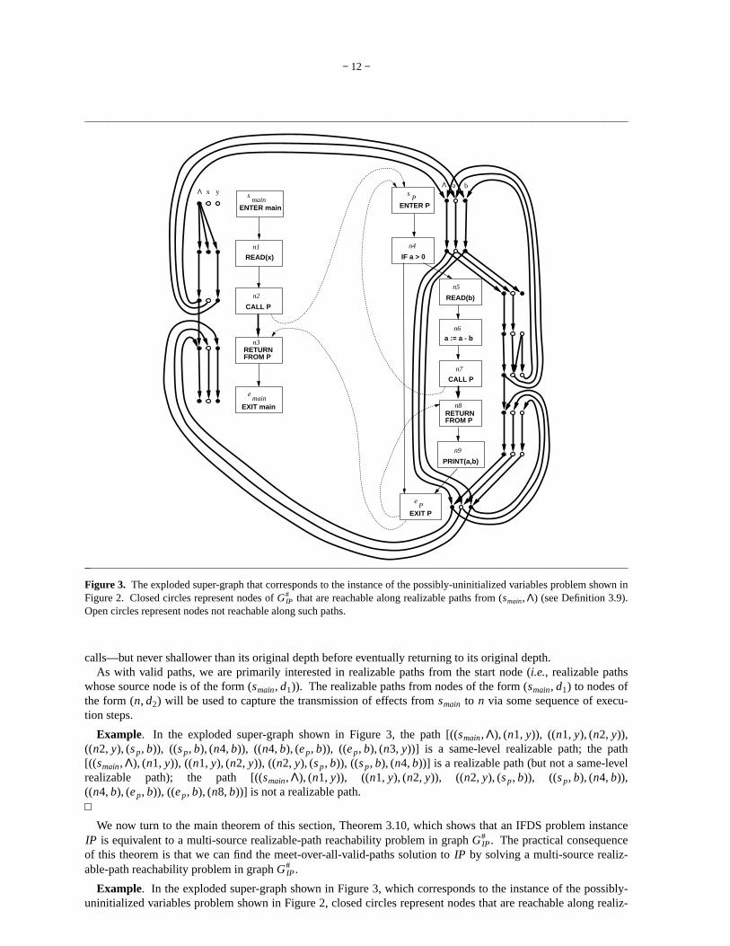
Example. The exploded super-graph that corresponds to the instance of the “possibly-uninitialized variables”problem shown in Figure 2 is shown in Figure 3.
We can now clarify the reasons for conditions (v)a and (v)b in Definition 2.4:
(v)a. For all t ∈T p, q and x ∈ D p, |t( x ) − t(∅)| ≤ B;
(v)b. For all t ∈T p, q and y ∈ Dq, if y ∉ t(∅) then | x | y ∈ t( x ) | ≤ B.
These conditions ensure that nodes in the representation relations of the transfer functions associated with E2
edges have limited indegree and outdegree. In particular, each node of the form (m, d) where m ∈(Call ∪ Exit)and d ≠ Λ, has at most B outgoing edges; each node of the form (n, d) where n ∈(Enter ∪ Ret) and d ≠ Λ, has atmost B incoming edges. (There is no restriction on the number of outgoing edges from nodes of the form (m, Λ)where m ∈(Call ∪ Exit); the definition of representation relations ensures that nodes of the form (n, Λ) wheren ∈(Enter ∪ Ret) hav e at most one incoming edge.)
These restrictions have an impact on the complexity arguments that we make in Sections 4.1, 5.1, and 6.2.They allow us to giv e more precise bounds using the parameter B rather than the worst-case parameter
pmax |D p |.
Throughout the remainder of the paper, we use the terms “realizable path” and “valid path” to refer to tworelated concepts in the super-graph and the exploded super-graph. In both cases, the idea is that not every pathcorresponds to a potential execution path: the constraints imposed on paths mimic the call-return structure of aprogram’s execution, and only paths in which “returns” can be matched with corresponding “calls” are permitted.However, the term “valid paths” will always be used in connection with paths in the super-graph, whereas theterm “realizable paths” will always be used in connection with paths in the exploded super-graph.
Definition 3.9. Let G#IP = (N #, E#, C#) be the exploded super-graph for IFDS problem instance
IP = (G*, D, F , B, T , M , Tr, C, ∪ ). Let each call node in G* be given a unique index in the range [1 . . |Call|].For each such indexed call node ci , label the edges of G#
IP that correspond to ci’s outgoing E2 edge(ci , scalledProc(ci)) (i.e., edges of the form ((ci , d1), (scalledProc(ci), d2))) by the symbol “(i”. Label the edges of G#
IP
that correspond to return edge (ecalledProc(ci), succ1(ci)) (i.e., edges of the form ((ecalledProc(ci), d3), (succ1(ci), d4)))by the symbol “)i”.
A same-level realizable path in G#IP is a path such that the sequence of symbols on the labeled edges is a string
in the language of balanced parentheses generated from nonterminal matched of Definition 2.3.A realizable path in G#
IP is a path such that the sequence of symbols on the labeled edges is a string in the lan-guage generated from nonterminal valid of Definition 2.3.
As with same-level valid paths, the same-level realizable paths from nodes of the form (m, d1) to nodes of theform (n, d2), where m and n are in the same procedure, will be used to capture the transmission of effects from mto n via sequences of execution steps during which the call stack may temporarily grow deeper—because of
− 12 −
Λ x yΛ a b
ENTER P
sP
IF a > 0
n4
ENTER main
smain
READ(x)
n1
CALL P
n2
RETURNFROM P
n3
EXIT main
emain
RETURNFROM P
n8
EXIT P
eP
CALL P
n7
n6
a := a - b
n5
READ(b)
PRINT(a,b)
n9
Figure 3. The exploded super-graph that corresponds to the instance of the possibly-uninitialized variables problem shown inFigure 2. Closed circles represent nodes of G#
IP that are reachable along realizable paths from (smain, Λ) (see Definition 3.9).Open circles represent nodes not reachable along such paths.
calls—but never shallower than its original depth before eventually returning to its original depth.As with valid paths, we are primarily interested in realizable paths from the start node (i.e., realizable paths
whose source node is of the form (smain, d1)). The realizable paths from nodes of the form (smain, d1) to nodes ofthe form (n, d2) will be used to capture the transmission of effects from smain to n via some sequence of execu-tion steps.
Example. In the exploded super-graph shown in Figure 3, the path [((smain, Λ), (n1, y)), ((n1, y), (n2, y)),((n2, y), (s p, b)), ((s p, b), (n4, b)), ((n4, b), (e p, b)), ((e p, b), (n3, y))] is a same-level realizable path; the path[((smain, Λ), (n1, y)), ((n1, y), (n2, y)), ((n2, y), (s p, b)), ((s p, b), (n4, b))] is a realizable path (but not a same-levelrealizable path); the path [((smain, Λ), (n1, y)), ((n1, y), (n2, y)), ((n2, y), (s p, b)), ((s p, b), (n4, b)),((n4, b), (e p, b)), ((e p, b), (n8, b))] is not a realizable path.
We now turn to the main theorem of this section, Theorem 3.10, which shows that an IFDS problem instanceIP is equivalent to a multi-source realizable-path reachability problem in graph G#
IP . The practical consequenceof this theorem is that we can find the meet-over-all-valid-paths solution to IP by solving a multi-source realiz-able-path reachability problem in graph G#
IP .
Example. In the exploded super-graph shown in Figure 3, which corresponds to the instance of the possibly-uninitialized variables problem shown in Figure 2, closed circles represent nodes that are reachable along realiz-

− 13 −
able paths from (smain, Λ). Open circles represent nodes not reachable along realizable paths. Note that nodes(n8, b) and (n9, b) are reachable only along non-realizable paths from (smain, Λ).
As shown in Theorem 3.10, this information indicates the nodes’ values in the meet-over-all-valid-paths solu-tion to the dataflow-analysis problem. For instance, in the meet-over-all-valid-paths solution, MVPe p
= b .(That is, variable b is the only possibly-uninitialized variable when execution reaches the exit node of procedurep.) In Figure 3, this information can be obtained by determining that there is a realizable path from (smain, Λ) to(e p, b), but not from (smain, Λ) to (e p, a).
Theorem 3.10. Let G#IP = (N #, E#, C#) be the exploded super-graph for IFDS problem instance
IP = (G*, D, F , B, T , M , Tr, C, ∪ ), and let n be a pro gram point in N *. Then d ∈ MVPn iff there is a realizablepath in graph G#
IP from one of the nodes in C# to node (n, d).
Proof. In what follows, we only need to discuss non-empty paths; empty paths arise only when n = smain, and inthat case it is easy to see that the theorem holds.
“Only if” case. Suppose d ∈ MVPn; we need to demonstrate the existence of a realizable path in graph G#IP from
one of the nodes in C# to node (n, d).
Because MVPn =r ∈IVP(smain, n)
∪ pfr (C), there must be a valid path q = [smain: (n1, n2), (n2, n3), . . .,
(n j , n j + 1): n] in G* such that d ⊆ pfq(C). For all i, 1 ≤ i ≤ j, let fi be defined as follows:
fi =
M(ni , ni + 1)
Tr(ni , ni + 1)
if (ni , ni + 1) ∈(E0 ∪ E1)
if (ni , ni + 1) ∈ E2
We hav e:
d ⊆ pfq(C)= ( f j
. . . f2 f1)(C) by Definition 2.5= [[R f j
; . . . ; R f2; R f1
]](C) by Corollary 3.7= ( y | ∃ c ∈C such that (c, y) ∈(R f j
; . . . ; R f2; R f1
) ∪ y | (Λ, y) ∈(R f j; . . . ; R f2
; R f1) ) − Λ
by Definition 3.2
Recall that edge-function f1 is associated with edge (smain, n2), and that edge-function f j is associated with edge(n j , n). Consequently, the last line in the above group of equations implies that there is a path q# in graph G#
IP ofthe following form:
q# = [(smain, c): ((n1, d1), (n2, d2)), ((n2, d2), (n3, d3)), . . . , ((n j , d j), (n j + 1, d j + 1)): (n, d)],
where c ∈(C ∪ Λ ) and for all i, 1 ≤ i ≤ j, (di , di + 1) ∈ R fi. That is, q# is a path in G#
IP from node (smain, c),one of the nodes of C#, to node (n, d). Because path q is a valid path in G*, path q# is a realizable path in G#
IP .Therefore, q# satisfies the conditions for the path whose existence we were required to demonstrate.
“If” case. Suppose that there is a realizable path q# = [c#: e#1, e#
2, . . . , e#j : (n, d)] in graph G#
IP from node c# ∈C#
to node (n, d). We need to demonstrate that d ∈ MVPn.
For all i, 1 ≤ i ≤ j, let e#i = ((ni , di), (ni + 1, di + 1)), and let fi be defined as follows:
fi =
M(ni , ni + 1)
Tr(ni , ni + 1)
if (ni , ni + 1) ∈(E0 ∪ E1)
if (ni , ni + 1) ∈ E2
Let q be the following path in G*:
q = [smain: (n1, n2), (n2, n3), . . . , (n j , n j + 1): n].
By supposition, q# is a realizable path in G#IP from node c# ∈C# to node (n, d); therefore, q must be a valid path
in G*.By the construction of G#
IP (Definition 3.8), and the supposition that q# is a realizable path in G#IP from node
c# ∈C# to node (n, d), we have:
d ∈(( y | ∃ x ∈C such that (x, y) ∈(R f j; . . . ; R f2
; R f1) ∪ y | (Λ, y) ∈(R f j
; . . . ; R f2; R f1
) ) − Λ ).
Consequently,

− 14 −
d ⊆ (( y | ∃ x ∈C such that (x, y) ∈(R f j; . . . ; R f2
; R f1) ∪ y | (Λ, y) ∈(R f j
; . . . ; R f2; R f1
) ) − Λ )= [[R f j
; . . . ; R f2; R f1
]](C) by Definition 3.2= ( f j
. . . f2 f1)(C) by Corollary 3.7= pfq(C) by Definition 2.5⊆
t ∈IVP(smain, n)∪ pft(C)
= MVPn
Therefore d ∈ MVPn, as was to be shown.
3.3. Restricted Subclasses of IFDS Problems
In this section, we define two special classes of IFDS problems: sparse problems and locally separable problems.As discussed in Sections 4.1, 5.1, and 6.2, our dataflow-analysis algorithms are more efficient when applied toproblems in these classes.
Definition 3.11. An IFDS problem instance IP = (G*, D, F , B, T , M , Tr, C, ∪ ) is h-sparse if there is a constanth such that for all F p ∈ F and f ∈ F p,
d ∈ D p
Σ | f ( d ) − f (∅)| ≤ h|D p |.
That is, in h-sparse problems, the total number of edges emanating from the non-Λ nodes in the representationrelation of an E0 or E1 edge’s function is at most h|D p |.
In general, when the nodes of the control-flow graph represent individual statements and predicates (ratherthan basic blocks) we expect most problems that are distributive to be h-sparse (with h <<
pmax |D p |): each state-
ment changes only a small portion of the execution state, and accesses only a small portion of the state as well.The dataflow functions, which are abstractions of the statements’ semantics, should therefore be “close to” theidentity function, and thus their representation relations should have roughly |D p | edges.
Definition 3.12. An IFDS problem instance IP = (G*, D, F , B, T , M , Tr, C, ∪ ) is locally separable if
(i) For all F p ∈ F , all f ∈ F p, and all x ∈ D p, f ( x ) ⊆ x ∪ f (∅);
(ii) B = 1;
(iii) If (c, sq) and (eq, r) are corresponding call and return edges then, for all x ∈ D fg(c) and y ∈ Dq,
a. If Tr(c, sq)( x ) − Tr(c, sq)(∅) = y then Tr(eq, r)( y ) − Tr(eq, r)(∅) ⊆ x .
b. If Tr(eq, r)( y ) − Tr(eq, r)(∅) = x then Tr(c, sq)( x ) − Tr(c, sq)(∅) ⊆ y .
The locally separable problems are the interprocedural versions of the classical separable problems fromintraprocedural dataflow analysis (also known as gen/kill or bit-vector problems). All locally separable problemsare 1-sparse, but not vice versa.
Clause (i) restricts the dataflow functions in F , which map dataflow information across E0 and E1 edges, tohave essentially component-wise dependences. That is, in the representation relation RM(m, n) for an edge(m, n) ∈(E0 ∪ E1), each node (n, d) can only be the target of a single edge—whose source is either of the form(m, d) or of the form (m, Λ).
Clause (ii) restricts the binding functions in T , which map dataflow information across call and return edges, tobe simple one-to-one renamings of domain elements. (However, different call sites on the same procedure maymake use of different T functions to map dataflow information across to the called procedure.)
Clause (iii) restricts the mapping Tr so that corresponding call and return edges have related binding functions.In particular, if there is an edge ((c, d1), (sq, d2)), where d1 ≠ Λ, in the representation relation of the functionTr(c, sq), then in the representation relation of the function Tr(eq, r) there is either an edge ((eq, d2), (r, d1)) or(eq, d2) has no outgoing edge. The analogous restriction holds for Tr(eq, r) with respect to Tr(c, sq).
Example. In general, an instance of the possibly-uninitialized variables problem will not be locally separable.For example, in Figure 3, a’s initialization status after the statement a : = a − b depends on that of b before thestatement. Thus, the representation relation for the dataflow function on edge (n6, n7) has an edge from node(n6, b) to (n7, a). This violates clause (i) of Definition 3.12.
However, when the nodes of the control-flow graph represent individual statements and predicates, everyinstance of the possibly-uninitialized variables problem is 2-sparse. The only non-identity dataflow functions arethose associated with assignment statements. The outdegree of every non-Λ node in the representation relation of

− 15 −
such a function is at most two: a variable’s initialization status can affect itself and at most one other variable,namely the variable assigned to.
3.4. Intersection Problems
An ∩ -distributive IFDS problem instance (with distinguished value C) can be solved by solving a ∪ -distributiveIFDS problem instance (with distinguished value C) and then complementing the answer. The problem transfor-mation is carried out merely by replacing each ∩ -distributive function f by the ∪ -distributive functionf ′ =df λ S . f (S). This transformation is justified by the following derivation:
MVPn =q ∈IVP(smain, n)
∩ pfq(C)
=q ∈IVP(smain, n)
∪ pfq(C)
=q ∈IVP(smain, n)
∪ pfq′(C) where if pfq = f j. . . f1 then pfq′ =df f j ′ . . . f1′
Thus, the solution of the original problem is the complement of the solution of the transformed problem.The functions that arise in gen/kill intersection problems are all of the form f = λ x . (x − kill) ∪ gen. It is easy
to show that f ′ = λ x . (x − gen) ∪ (kill − gen), which is also in gen/kill form. Thus, when the transformationdescribed above is used to transform an ∩ -distributive gen/kill IFDS problem into a ∪ -distributive IFDS prob-lem, every edge function satisfies clause (i) of Definition 3.12. It is reasonable to expect that every ∩ -distribu-tive gen/kill IFDS problem will also satisfy clauses (ii) and (iii) of Definition 3.12. Consequently, when an∩ -distributive gen/kill IFDS problem is transformed into a ∪ -distributive IFDS problem, the result is a locallyseparable problem.
4. An Efficient Tabulation Algorithm for the Realizable-Path Reachability Problem
In this section, we present the first of our three algorithms for the realizable-path reachability problem. The algo-rithm described in this section is a dynamic-programming algorithm that tabulates certain kinds of same-levelrealizable paths. As we show in Section 4.1, its running time is polynomial in various parameters of the problem,and the algorithm is asymptotically faster than the best previously known algorithm for the problem.
The algorithm, which we call the Tabulation Algorithm, is presented in Figure 4. The Tabulation Algorithmuses a set, named PathEdge, to record the existence of path edges, which represent a subset of the same-levelrealizable paths in graph G#
IP . In particular, the source of a path edge is always a node of the form (s p, d1) suchthat a realizable path exists from some node c# ∈C# to (s p, d1). In other words, a path edge from (s p, d1) to(n, d2) represents the suffix of a realizable path from some c# ∈C# to (n, d2).
The Tabulation Algorithm uses another set, named SummaryEdge, to record the existence of summary edges,which represent same-level realizable paths that run from nodes of the form (n, d1), where n ∈Call, to(succ1(n), d2).
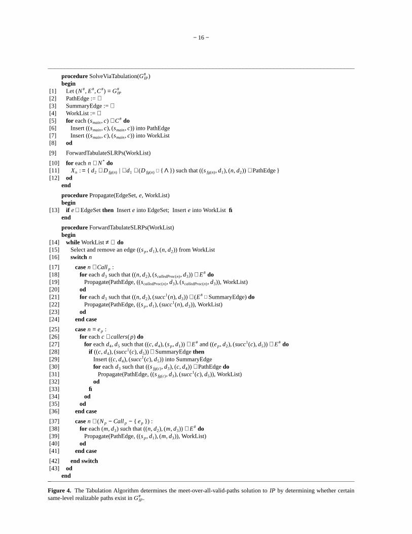
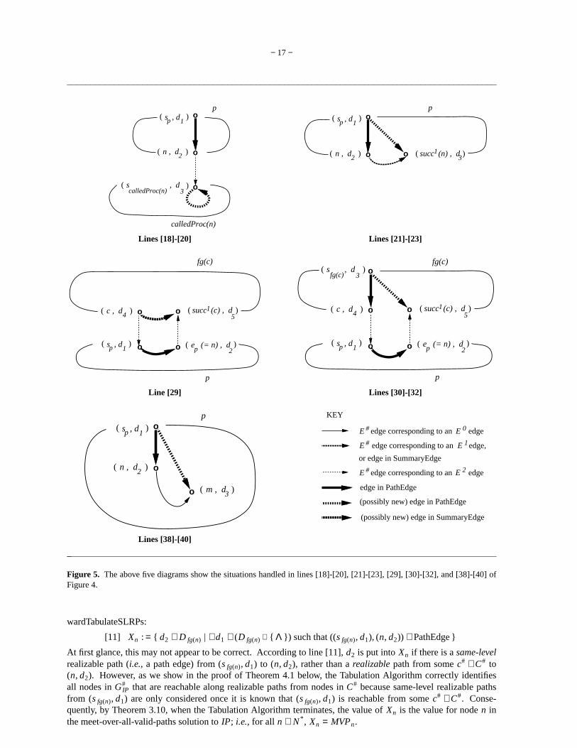
The Tabulation Algorithm is a worklist algorithm that starts with a certain set of path edges, and on each itera-tion of the main loop in procedure ForwardTabulateSLRPs (lines [14]-[43]) deduces the existence of additionalpath edges (and summary edges). The initial set of path edges corresponds to the 0-length same-level realizablepaths of the form ((smain, c), (smain, c)), for all (smain, c) ∈C# (see lines [5]-[8]). The configurations that are usedby the Tabulation Algorithm to deduce the existence of additional path edges are depicted in Figure 5; the fivediagrams of Figure 5 correspond to lines [18]-[20], [21]-[23], [29], [30]-[32], and [38]-[40] of Figure 4. In Fig-ure 5, the bold dotted arrows represent edges that are inserted into set PathEdge if they were not previously inthat set.
It is important to note the role of lines [30]-[32] of Figure 4, which are executed only when a new summaryedge is discovered:
[30] for each d3 such that ((s fg(c), d3), (c, d4)) ∈PathEdge do[31] Propagate(PathEdge, ((s fg(c), d3), (succ1(c), d5)), WorkList)[32] od
Unlike edges in E#, edges are inserted into SummaryEdge on-the-fly. The purpose of line [31] is to restart theprocessing that finds same-level realizable paths from (s fg(c), d3) as if summary edge ((c, d4), (succ1(c), d5)) hadbeen in place all along.
The final step of the Tabulation Algorithm (lines [10]-[12]) is to create values Xn, for each n ∈ N *, by gather-ing up the set of nodes associated with n in G#
IP that are targets of path edges discovered by procedure For-
− 16 −
procedure SolveViaTabulation(G#IP)
begin[1] Let (N #, E#, C#) = G#
IP
[2] PathEdge := ∅[3] SummaryEdge := ∅[4] WorkList := ∅[5] for each (smain, c) ∈C# do[6] Insert ((smain, c), (smain, c)) into PathEdge[7] Insert ((smain, c), (smain, c)) into WorkList[8] od
[9] ForwardTabulateSLRPs(WorkList)
[10] for each n ∈ N * do[11] Xn : = d2 ∈ D fg(n) | ∃ d1 ∈(D fg(n) ∪ Λ ) such that ((s fg(n), d1), (n, d2)) ∈PathEdge [12] od
end
procedure Propagate(EdgeSet, e, WorkList)begin
[13] if e ∉ EdgeSet then Insert e into EdgeSet; Insert e into WorkList fiend
procedure ForwardTabulateSLRPs(WorkList)begin
[14] while WorkList ≠ ∅ do[15] Select and remove an edge ((s p, d1), (n, d2)) from WorkList[16] switch n
[17] case n ∈Call p :[18] for each d3 such that ((n, d2), (scalledProc(n), d3)) ∈ E# do[19] Propagate(PathEdge, ((scalledProc(n), d3), (scalledProc(n), d3)), WorkList)[20] od[21] for each d3 such that ((n, d2), (succ1(n), d3)) ∈(E# ∪ SummaryEdge) do[22] Propagate(PathEdge, ((s p, d1), (succ1(n), d3)), WorkList)[23] od[24] end case
[25] case n = e p :[26] for each c ∈callers(p) do[27] for each d4, d5 such that ((c, d4), (s p, d1)) ∈ E# and ((e p, d2), (succ1(c), d5)) ∈ E# do[28] if ((c, d4), (succ1(c), d5)) ∉ SummaryEdge then[29] Insert ((c, d4), (succ1(c), d5)) into SummaryEdge[30] for each d3 such that ((s fg(c), d3), (c, d4)) ∈PathEdge do[31] Propagate(PathEdge, ((s fg(c), d3), (succ1(c), d5)), WorkList)[32] od[33] fi[34] od[35] od[36] end case
[37] case n ∈(N p − Call p − e p ) :[38] for each (m, d3) such that ((n, d2), (m, d3)) ∈ E# do[39] Propagate(PathEdge, ((s p, d1), (m, d3)), WorkList)[40] od[41] end case
[42] end switch[43] od
end
Figure 4. The Tabulation Algorithm determines the meet-over-all-valid-paths solution to IP by determining whether certainsame-level realizable paths exist in G#
IP .
− 17 −
o
o
os , dp 1( )
p
calledProc(n)
2 n , d ( )
calledProc(n) 3( )s , d
o o
os , dp 1( )
p
2 n , d ( ) succ (n) , d 13
( )
Lines [18]-[20] Lines [21]-[23]
o
o
o
os , dp 1( )
4 c , d ( ) succ (c) , d 15
( )
fg(c)
( e (= n) , d2
)p
p
o
o
o
o
o
s , dp 1( )
4 c , d ( ) succ (c) , d 15
( )
3( )s , d
fg(c)
fg(c)
( e (= n) , d2
)p
p
Line [29] Lines [30]-[32]
o
o
os , dp 1( )
p
2 n , d ( )
3 m , d ( )
KEY
edge corresponding to an edge#E E 2
# edge corresponding to an edgeE E 0
edge in PathEdge
(possibly new) edge in PathEdge
(possibly new) edge in SummaryEdge
or edge in SummaryEdge
edge corresponding to an#E edge,E 1
Lines [38]-[40]
Figure 5. The above five diagrams show the situations handled in lines [18]-[20], [21]-[23], [29], [30]-[32], and [38]-[40] ofFigure 4.
wardTabulateSLRPs:
[11] Xn : = d2 ∈ D fg(n) | ∃ d1 ∈(D fg(n) ∪ Λ ) such that ((s fg(n), d1), (n, d2)) ∈PathEdge
At first glance, this may not appear to be correct. According to line [11], d2 is put into Xn if there is a same-levelrealizable path (i.e., a path edge) from (s fg(n), d1) to (n, d2), rather than a realizable path from some c# ∈C# to(n, d2). However, as we show in the proof of Theorem 4.1 below, the Tabulation Algorithm correctly identifiesall nodes in G#
IP that are reachable along realizable paths from nodes in C# because same-level realizable pathsfrom (s fg(n), d1) are only considered once it is known that (s fg(n), d1) is reachable from some c# ∈C#. Conse-quently, by Theorem 3.10, when the Tabulation Algorithm terminates, the value of Xn is the value for node n inthe meet-over-all-valid-paths solution to IP; i.e., for all n ∈ N *, Xn = MVPn.

− 18 −
Theorem 4.1. (Correctness of the Tabulation Algorithm.) The Tabulation Algorithm always terminates, andupon termination, Xn = MVPn, for all n ∈ N *.
Proof. PathEdge is initially empty, and there are only a finite number of possible path edges. A path edge isinserted into WorkList exactly once, when it is inserted into PathEdge (see lines [6]-[7] and line [13] of Figure 4).Consequently, the outermost loop of procedure ForwardTabulateSLRPs (lines [14]-[43]) can execute at most afinite number of times, and the Tabulation Algorithm is guaranteed to halt.
To show that Xn = MVPn, for all n ∈ N *, we appeal to Theorem 3.10. Because the value of Xn is defined inline [11] of Figure 4 by the assignment:
Xn : = d2 ∈ D fg(n) | ∃ d1 ∈(D fg(n) ∪ Λ ) such that ((s fg(n), d1), (n, d2)) ∈PathEdge ,
we know from Theorem 3.10 that Xn = MVPn will hold if we can show the following:
For all d2, ∃ d1 ∈(D fg(n) ∪ Λ ) such that ((s fg(n), d1), (n, d2)) ∈ PathEdge when the Tabulation Algo-rithm terminates iff there is a realizable path in G#
IP from one of the nodes in C# to node (n, d2).
“Only if” case. Suppose ∃ d1 ∈(D fg(n) ∪ Λ ) such that ((s fg(n), d1), (n, d2)) ∈ PathEdge when the TabulationAlgorithm terminates; we need to show that there is a realizable path in G#
IP from one of the nodes in C# to node(n, d2).
This case is proven by showing that the following invariant holds for the outermost loop of procedure For-wardTabulateSLRPs:
∀ n, d1, d2, ((s fg(n), d1), (n, d2)) ∈ PathEdge =>(a) ∃ c# ∈C# such that there is a realizable path from c# to (n, d2), and(b) there is a same-level realizable path from (s fg(n), d1) to (n, d2).
PathEdge is first initialized to ∅ in line [2]. Then, in lines [5]-[8], all edge of the form ((smain, c), (smain, c)),where (smain, c) ∈C#, are inserted into PathEdge. All such edges meet the conditions of the invariant, and so theinvariant holds when ForwardTabulateSLRPs is first called.
Now assume that the invariant holds true after j iterations. Because a path edge is inserted into WorkList onlywhen it is inserted into PathEdge, when edge ((s p, d1), (n, d2)) is removed from WorkList in line [15] at thebeginning of iteration j + 1, we know that ((s p, d1), (n, d2)) ∈ PathEdge. Because it was on some previous iter-ation that ((s p, d1), (n, d2)) was inserted into PathEdge, from the invariant we know that (a) there is some c# ∈C#
such that there is a realizable path q# from c# to (n, d2), and (b) there is a same-level realizable path s# from(s p, d1) to (n, d2).
Propagate is called from four places in procedure ForwardTabulateSLRPs (lines [19], [22], [31], and [39]). Ineach case, we can demonstrate that if the call on Propagate actually does insert a new edge into PathEdge, thenthere is a realizable path q## and a same-level realizable path s## as required to re-establish the invariant. Forexample, in the call in line [39], q## is q# extended with edge ((n, d2), (m, d3)), and s## is s# extended with edge((n, d2), (m, d3)).
For the call on Propagate in line [31], the argument is more subtle. In addition to what was observed aboveabout q# and s#, we know that edge ((s fg(c), d3), (c, d4)) is in PathEdge, and hence from the invariant we knowthat there is some c# ∈C# such that there is a realizable path t# from c# to (c, d4). Thus, the realizable path q##
required by the invariant is t# extended with edge ((c, d4), (s p, d1)), same-level realizable path s#, and edge((e p, d2), (succ1(c), d5)); that is,
q## = t# || [((c, d4), (s p, d1))] || s# || [((e p, d2), (succ1(c), d5))],
where “||” denotes path concatenation. Because edges ((c, d4), (s p, d1)) and ((e p, d2), (succ1(c), d5)) are corre-sponding call and return edges, q## is a realizable path in G#
IP . Similarly, by the invariant we know that there is asame-level realizable path u# from (s fg(c), d3) to (c, d4). The same-level realizable path s## required by theinvariant is
s## = u# || [((c, d4), (s p, d1))] || s# || [((e p, d2), (succ1(c), d5))].
The arguments for the other two places where Propagate is invoked are similar and are left to the reader.Consequently, the invariant holds after iteration j + 1.
“If” case. Suppose there is a realizable path in G#IP from one of the nodes in C# to node (n, d2); we need to show
∃ d1 ∈(D fg(n) ∪ Λ ) such that ((s fg(n), d1), (n, d2)) ∈ PathEdge when the Tabulation Algorithm terminates.
This case is proven by induction on the lengths of realizable paths in G#IP . The induction hypothesis is:

− 19 −
∀ n, d2, if there is a realizable path of length j from one of the nodes in C# to node (n, d2) then ∃ d1 suchthat ((s fg(n), d1), (n, d2)) ∈ PathEdge when the Tabulation Algorithm terminates.
Base case. For the case j = 0 (realizable paths of length 0), the induction hypothesis holds because of the wayPathEdge is initialized in the loop on lines [5]-[8] of Figure 4.
Induction step. Assume that the induction hypothesis holds true for all realizable paths of length less than orequal to j . Let q## be a realizable path of length j + 1 from one of the nodes in C# to node (n, d), and supposeq## has the form
q## = [(smain, c): ((n1, d1), (n2, d2)), . . . , ((n j , d j ), (n j + 1, d j + 1)), ((n j + 1, d j + 1), (n, d))],
where c ∈(C ∪ Λ ).Let q# denote the prefix of q## of length j . Then by the induction hypothesis, we know that there exists a d ′
such that ((s fg(n j + 1), d ′), (n j + 1, d j + 1)) ∈ PathEdge. Because whenever an edge is inserted into PathEdge it isalso inserted into WorkList, we know that at some point during the execution of procedure ForwardTabu-lateSLRPs, the edge ((s fg(n j + 1), d ′), (n j + 1, d j + 1)) was the edge removed from WorkList in line [15].
There are three cases to consider, depending on the type of node n j + 1. These correspond to the three cases ofthe switch statement of procedure ForwardTabulateSLRPs. For example, if node n j + 1 is an exit node, then edge((n j + 1, d j + 1), (n, d)) must be a return edge. Because q## is a realizable path, there must be a corresponding calledge ((c, d ′′), (s fg(n j + 1), d ′)) that occurs earlier in q##. (Note that fg(c) = fg(n).) Because the prefix of q## up tothe occurrence of this edge is a realizable path of length less than j , by the induction hypothesis we know that,when the Tabulation Algorithm terminates, ((s fg(c), d ′′′), (c, d ′′)) must be in PathEdge. There are now two possi-bilities to consider:
(i) Suppose that at the time edge ((s fg(n j + 1), d ′), (n j + 1, d j + 1)) is processed, ((s fg(c), d ′′′), (c, d ′′)) ∈ PathEdge.Then there will be a call at line [31] of the form
Propagate(PathEdge, ((s fg(n), d ′′′), (n, d)), WorkList),
(ii) Suppose that at the time edge ((s fg(n j + 1), d ′), (n j + 1, d j + 1)) is processed, ((s fg(c), d ′′′), (c, d ′′)) ∉ PathEdge.Then ((c, d ′′), (n, d)) will be inserted into SummaryEdge if it is not already there, and later edge((s fg(c), d ′′′), (c, d ′′)) will be processed. (This must occur at some point during the Tabulation Algorithm,because edge ((s fg(c), d ′′′), (c, d ′′)) is inserted into WorkList when it is inserted into PathEdge. We knowthat this happens eventually.) At this point, a call is generated at line [22] of the form
Propagate(PathEdge, ((s fg(n), d ′′′), (n, d)), WorkList).
Thus, in either case, ((s fg(n), d ′′′), (n, d)) will at some point be inserted into PathEdge, which establishes theinduction hypothesis for path q##. (The arguments for the other two cases are simpler, and are again left to thereader.)
Consequently, the induction hypothesis holds true for every realizable path in G#IP .
4.1. Cost of the Tabulation Algorithm
In this section, we show that the running time of the Tabulation Algorithm is polynomial in various parameters ofa problem instance. We also show that the algorithm is asymptotically faster than the best previously knownalgorithm for the realizable-path reachability problem [18].
In this section, as well as in later sections in which we derive bounds on the running times of algorithms, weuse the name of a set to denote the set’s size. For example, we use Call, rather than |Call|, to denote the numberof call nodes in graph G*. Howev er, we make three small deviations from this convention:
(i) We use N , rather than N *, to stand for |N *|, the number of nodes in graph G*.(ii) We use E, rather than E*, to stand for |E*|, the number of edges in graph G*.(iii) Rather than distinguish between the different domains D p, for p ∈ 0, . . . , k , we will express costs in
terms of a single quantity D, where
D =dfp ∈ 0, ..., k
max |D p |.
The primary justification for this simplification is that in dataflow analysis problems all of the D p sets willshare a subset of values in common for representing information about global variables. Usually this com-mon subset dominates the size of each D p set, and thus all of the D p sets will be of roughly the same size,namely D.

− 20 −
The time bounds discussed below are derived under the following assumptions about the running times ofoperations on G#
IP’s nodes and edges, and on auxiliary edge sets SummaryEdge, PathEdge, and WorkList:
(i) An edge can be inserted into SummaryEdge, PathEdge, or WorkList in unit time.(ii) An edge can be tested for membership in SummaryEdge or in PathEdge in unit time.(iii) A random edge can be selected from WorkList in unit time.(iv) It is possible to iterate over the set of all PathEdge predecessors of an N # node in time proportional to the
size of the set.(v) It is possible to iterate over the set of all E#, SummaryEdge, or PathEdge successors of an N # node in time
proportional to the size of the set.(vi) In the case of nodes of the form (s p, d1), we make the further assumption that predecessor sets in E# are
indexed by call site. In other words, it is possible to retrieve only those predecessors that are associated witha particular call site, without having to examine all E# predecessors of (s p, d1). Similarly, in the case ofnodes of the form (e p, d2) we assume that successor sets in E# are indexed by return site. This assumptionpermits us to assume that the time required to identify the <d4, d5> pairs used in the for-loop on line [27] isproportional to the number of such pairs.
One way to satisfy assumptions (i)-(v) is to use arrays to support unit-time membership testing, and one or morelinked-lists for each N # node (to support iteration over predecessors and successors). Assumption (vi) can be sat-isfied by associating, with each N # node of the form (s p, d1) or (e p, d2), an array of linked-lists, one list for eachcall-site.
Running Time
The running time of the Tabulation Algorithm varies depending on what class of dataflow-analysis problem it isapplied to. The following table summarizes how the Tabulation Algorithm behaves (in terms of worst-caseasymptotic running time) for six different classes of problems:
Asymptotic running timeClass of functions
Graph-theoretic characterization ofthe dataflow functions’ properties Intraprocedural
problemsInterproceduralproblems
Distributive Up to O(D2) edges/rep.-relation O(ED2) O(Call B2 D2 + ED3)
h-sparse At most O(hD) edges/rep.-relation O(hED) O(Call B2 D2 + Call D3 + hED2)
(Locally) separable Component-wise dependences O(ED) O(ED)
Table 4.2. Asymptotic running time of the Tabulation Algorithm for six different classes of dataflow-analysisproblems.
Some of these bounds have been achieved previously: For intraprocedural problems, the algorithms of Hecht
[15], Kou [23], and Khedker and Dhamdhere [19] have the same time bounds as are shown in column three.2 Forlocally separable problems (both intraprocedural and interprocedural), the algorithm of Knoop and Steffen [22]also runs in time O(ED).
We now present derivations of the bounds given in Table 4.2 for the three classes of interprocedural problems.(The bounds for the three classes of intraprocedural problems follow from simplifications of the arguments givenbelow.)
Distributive Problems
For distributive problems, the representation relation for each edge e ∈(E0 ∪ E1) can contain up to O(D2) edges.Instead of calculating the worst-case cost-per-iteration of the loop on lines [14]-[43] of Figure 4 and multiplyingby the number of iterations, we break the cost of the algorithm down into three contributing aspects and bound
2The intraprocedural dataflow-analysis algorithms of Kou [23] and Khedker and Dhamdhere [19] are described as algorithms for separableproblems; however, the ideas described in Section 3.2 concerning the representation of distributive functions can be used to immediately ex-tend those algorithms to all distributive and h-sparse intraprocedural problems.

− 21 −
the total cost of the operations performed for each aspect. In particular, the cost of the Tabulation Algorithm canbe broken down into
(i) the cost of worklist manipulations,(ii) the cost of installing summary edges at call sites (lines [25]-[36] of Figure 4), and(iii) the cost of closure steps (lines [17]-[24] and [37]-[41] of Figure 4).
Because a path edge can be inserted into WorkList at most once, the cost of each worklist-manipulation opera-tion can be charged to either a summary-edge-installation step or a closure step; thus, we do not need to provide aseparate accounting of worklist-manipulation costs.
The Tabulation Algorithm can be understood as k + 1 simultaneous semi-dynamic multi-source reachabilityproblems—one per procedure of the program. For each procedure p, the sources—which we shall call anchorsites—are the D p + 1 nodes in N #
p of the form (s p, d). The edges of the multi-source reachability problem asso-ciated with p are
((m, d1), (n, d2)) ∈ E#p | (m, n) ∈(E0
p ∪ E1p) ∪ ((m, d1), (n, d2)) ∈SummaryEdge | m ∈Call p) .
In other words, the graph associated with procedure p is the “exploded flow graph” of procedure p, augmentedwith summary edges at the call sites of p. The reachability problems are semi-dynamic (insertions only) becausein the course of the algorithm, new summary edges are added, but no summary edges (or any other edges) areev er removed.
We now wish to compute a bound on the cost of installing summary edges at call sites (lines [25]-[36] of Fig-ure 4). For each summary edge ((c, d4), (succ1(c), d5)), the conditional statement on lines [28]-[33] will beexecuted some number of times (on different iterations of the loop on lines [14]-[43]). In particular, line [28] willbe executed every time the Tabulation Algorithm finds a three-edge path of the form
[((c, d4), (s p, d1)), ((s p, d1), (e p, d2)), ((e p, d2), (succ1(c), d5))] (†)
as shown in the diagram marked “Line [29]” of Figure 5.When we consider the set of all summary edges at a given call site c: ((c, d4), (succ1(c), d5)) , the executions
of line [28] can be placed in three categories:
d4 ≠ Λ and d5 ≠ ΛThere are at most D2 choices for a <d4, d5> pair, and for each such pair at most B2 possible three-edgepaths of the form (†).
d4 = Λ and d5 ≠ ΛThere are at most D choices for d5 and for each such choice at most BD possible three-edge paths of theform (†).
d4 = Λ and d5 = ΛThere is only one possible three-edge path of the form (†).
Thus, the total cost of all executions of line [28] is bounded by O(Call B2 D2).Because of the test on line [28], the code on lines [29]-[32] will be executed exactly once for each possible
summary edge. In particular, for each summary edge the cost of the loop on lines [30]-[32] is bounded by O(D).Since the total number of summary edges that can possibly be acquired by procedure p is bounded by Call p D2,the total cost of lines [29]-[32] is O(Call D3). Thus, the total cost of installing summary edges during the Tabula-tion Algorithm is bounded by O(Call B2 D2 + Call D3).
To bound the total cost of the closure steps, we use a variation on the argument used by Yellin to obtain a
bound for the running time of an algorithm for dynamic transitive closure [34].3 The essential observation is thatthere are only a certain number of “attempts” the Tabulation Algorithm makes to “acquire” a path edge((s p, d1), (n, d2)). The first attempt is successful—and ((s p, d1), (n, d2)) is inserted into PathEdge; all remainingattempts are redundant (but seem unavoidable). In particular, in the case of a node n ∉ Ret, the only way the
3The closure steps can be thought of as a variant of Yellin’s algorithm, modified as follows:
(i) Yellin’s algorithm is an algorithm for dynamic transitive closure—i.e., dynamic all-pairs reachability. The closure steps implement dy-namic multi-source reachability, where the sources in each procedure’s exploded flow graph are the anchor sites.
(ii) After a summary edge is inserted into the exploded flow graph of procedure p, rather than re-closing the graph immediately, the code inFigure 4 uses a single worklist to organize the simultaneous closure of all the exploded flow graphs.
Feature (ii) is not essential. The code could have been written to perform the closure of an exploded flow graph immediately, at the sametime accumulating pending summary edges that need to be inserted in other exploded flow graphs in an auxiliary set.

− 22 −
Tabulation Algorithm can obtain a path edge ((s p, d1), (n, d2)) is when there are one or more two-edge paths ofthe form
[((s p, d1), (m, d)), ((m, d), (n, d2))],
where ((s p, d1), (m, d)) is in PathEdge and ((m, d), (n, d2)) is in E#, as depicted below:
o o
o
o
o
s , d( )p 1
( )n, d2
( )m , d31
( )m , d42
( )m , d53
For a giv en anchor site (s p, d1), the cost of the closure steps involved in acquiring path edge ((s p, d1), (n, d2)) canbe bounded by indegree(n, d2). For such an anchor site, the total cost of acquiring all its outgoing path edges canbe bounded by
O((n, d) ∈ N #
p
and n ∉ Ret
Σ indegree(n, d)) = O(E p D2).
The accounting for the case of a node n ∈ Ret is similar. The only way the Tabulation Algorithm can obtain apath edge ((s p, d1), (n, d2)) is when there is an edge in PathEdge of the form ((s p, d1), (m, d)) and either there isan edge ((m, d), (n, d2)) in E# or an edge ((m, d), (n, d2)) in SummaryEdge. In our cost accounting, we will pes-simistically say that each node (n, d2), where n ∈ Ret, has the maximum possible number of incoming summaryedges, namely D. Because there are at most Call p D nodes of N #
p of the form (n, d2), where n ∈ Ret, for eachanchor site (s p, d1) the total cost of acquiring path edges of the form ((s p, d1), (n, d2)) is
O((n, d2) ∈ N #
p
and n ∈ Ret
Σ (indegree(n, d2) + summary-edge-indegree(n, d2))) = O(Call p D2).
Therefore we can bound the total cost of the closure steps performed by the Tabulation Algorithm as follows:
Cost of closure steps =pΣ (# anchor sites) × O(Call p D2 + E p D2)
= O(D3
pΣ (Call p + E p))
= O(D3(Call + E)).= O(ED3).
Thus, the total running time of the Tabulation Algorithm is bounded by O(Call B2 D2 + ED3).
h-Sparse Problems
The bound on the cost of the Tabulation Algorithm for h-sparse problems is obtained by an argument similar tothe one given for distributive functions, except that we modify the accounting to take into account the fact thateach representation relation can contain at most O(hD) edges.
As before, the total cost of installing summary edges is bounded by O(Call B2 D2 + Call D3). However, thebound on the total cost of closure steps is slightly different from the bound obtained in the case of distributiveproblems:
Cost of closure steps =pΣ (# anchor sites) × O(Call p D2 +
(n, d) ∈ N #p
Σ indegree(n, d))
= O(D) × O(pΣ (Call p D2 + hE p D))
= O(Call D3 + hED2).
Thus, on h-sparse problems, the total running time of the Tabulation Algorithm is bounded by

− 23 −
O(Call B2 D2 + Call D3 + hED2).
Locally Separable Problems
For locally separable problems, within a given procedure of the exploded super-graph all representation relationsfor edge functions have essentially component-wise dependences. More precisely, for all edges(m, n) ∈(E0 ∪ E1), in the representation relation RM(m, n) each node (n, d) can only be the target of a singleedge—one whose source is (m, d) or one whose source is (m, Λ).
Recall that in locally separable problems different call sites on the same procedure may make use of differentT functions to map dataflow information across to the called procedure. However, the Tabulation Algorithm tab-ulates only same-level realizable paths, and because of the additional restrictions on the binding functions in Tfor locally separable problems (see Definition 3.12), same-level realizable paths are always of the form[(m, d): . . . : (n, d)], [(m, Λ): . . . : (n, d)], or [(m, Λ): . . . : (n, Λ)]. Note that the maximum number of summaryedges in a procedure p is O(Call p D) (rather than O(Call p D2), as we have in the case of distributive and h-sparseproblems).
For locally separable problems, we can give a better bound on the number of times line [28] is executed.Again, we consider the set of all summary edges at a given call site c: ((c, d4), (succ1(c), d5)) , and place theexecutions of line [28] in three categories:
d4 ≠ Λ and d5 ≠ ΛBecause summary edges represent same-level realizable paths, it must be that d4 = d5, and thus there are atmost D choices for a <d4, d5> pair. For each such pair there is at most one possible three-edge path of theform (†).
d4 = Λ and d5 ≠ ΛThere are at most D choices for d5 and for each such choice at most three possible three-edge paths of theform (†).
d4 = Λ and d5 = ΛThere is only one possible three-edge path of the form (†).
Thus, the total number of executions of line [28] is bounded by O(Call D).Again, because of the test on line [28], the code on lines [29]-[32] will be executed exactly once for each pos-
sible summary edge, but for locally separable problems there will be at most two calls on Propagate generated atline [31]:
[31] Propagate(PathEdge, ((s fg(c), d3), (succ1(c), d5)), WorkList).
In one call, d3 = d5; in the other, d3 = Λ. Because the total number of summary edges in all procedures isbounded by O(Call D), the total cost of lines [29]-[32] is O(Call D).
Thus, the total cost of installing summary edges is bounded by O(Call D).To bound the total cost of closure steps, we use the same argument as in the distributive case, except that we
observe that for locally separable problems the indegree and summary-edge-indegree of a node can both be atmost two. Thus,
Cost of closure steps =pΣ (# anchor sites) × O(Call p + E p)
= O(Call D + ED)= O(ED).
Therefore on locally separable problems, the total running time of the Tabulation Algorithm is bounded byO(ED).
Intraprocedural Problems
Because Call = 0 for intraprocedural problems, the bounds on the Tabulation Algorithm’s running time on dis-tributive, h-sparse, and separable interprocedural problems simplify to O(ED3), O(hED2), and O(ED), respec-tively, in the intraprocedural case. In the case of distributive and h-sparse problems, we can sharpen thesebounds by observing that in the program’s one procedure, the Tabulation Algorithm uses at most C + 1 (ratherthan D) anchor sites—the C# nodes of G#
IP . Thus, it is more precise to say that the bounds for distributive and h-sparse intraprocedural problems are O(CED2) and O(hCED), respectively.
These bounds can be reduced further if we assume that C, the distinguished dataflow value associated withnode smain of the IFDS problem, has the value ∅. This assumption involves no loss of generality, because ifC ≠ ∅, the problem can always be turned into one of that form as follows: a new start node smain is added to pro-
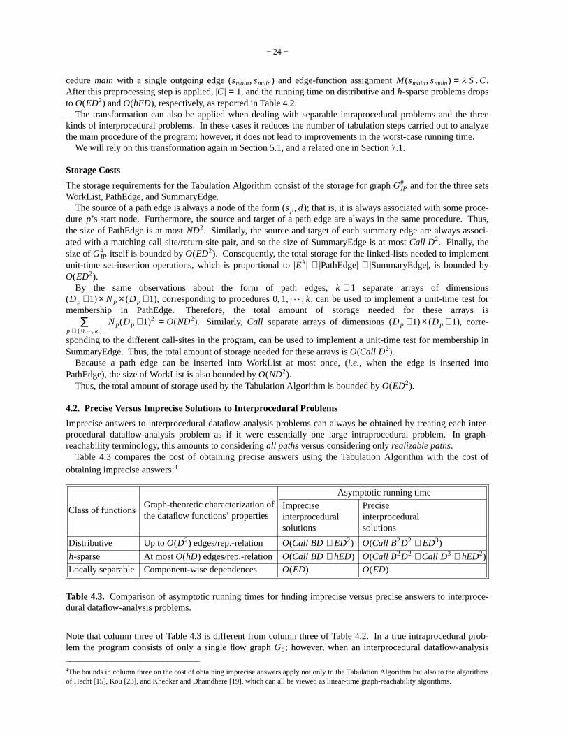
− 24 −
cedure main with a single outgoing edge (smain, smain) and edge-function assignment M(smain, smain) = λ S . C.After this preprocessing step is applied, |C | = 1, and the running time on distributive and h-sparse problems dropsto O(ED2) and O(hED), respectively, as reported in Table 4.2.
The transformation can also be applied when dealing with separable intraprocedural problems and the threekinds of interprocedural problems. In these cases it reduces the number of tabulation steps carried out to analyzethe main procedure of the program; however, it does not lead to improvements in the worst-case running time.
We will rely on this transformation again in Section 5.1, and a related one in Section 7.1.
Storage Costs
The storage requirements for the Tabulation Algorithm consist of the storage for graph G#IP and for the three sets
WorkList, PathEdge, and SummaryEdge.The source of a path edge is always a node of the form (s p, d); that is, it is always associated with some proce-
dure p’s start node. Furthermore, the source and target of a path edge are always in the same procedure. Thus,the size of PathEdge is at most ND2. Similarly, the source and target of each summary edge are always associ-ated with a matching call-site/return-site pair, and so the size of SummaryEdge is at most Call D2. Finally, thesize of G#
IP itself is bounded by O(ED2). Consequently, the total storage for the linked-lists needed to implementunit-time set-insertion operations, which is proportional to |E#| + |PathEdge| + |SummaryEdge|, is bounded byO(ED2).
By the same observations about the form of path edges, k + 1 separate arrays of dimensions(D p + 1) × N p × (D p + 1), corresponding to procedures 0, 1, . . . , k, can be used to implement a unit-time test formembership in PathEdge. Therefore, the total amount of storage needed for these arrays is
p ∈ 0, ..., k Σ N p(D p + 1)2 = O(ND2). Similarly, Call separate arrays of dimensions (D p + 1) × (D p + 1), corre-
sponding to the different call-sites in the program, can be used to implement a unit-time test for membership inSummaryEdge. Thus, the total amount of storage needed for these arrays is O(Call D2).
Because a path edge can be inserted into WorkList at most once, (i.e., when the edge is inserted intoPathEdge), the size of WorkList is also bounded by O(ND2).
Thus, the total amount of storage used by the Tabulation Algorithm is bounded by O(ED2).
4.2. Precise Versus Imprecise Solutions to Interprocedural Problems
Imprecise answers to interprocedural dataflow-analysis problems can always be obtained by treating each inter-procedural dataflow-analysis problem as if it were essentially one large intraprocedural problem. In graph-reachability terminology, this amounts to considering all paths versus considering only realizable paths.
Table 4.3 compares the cost of obtaining precise answers using the Tabulation Algorithm with the cost of
obtaining imprecise answers:4
Asymptotic running time
Class of functionsGraph-theoretic characterization ofthe dataflow functions’ properties
Impreciseinterproceduralsolutions
Preciseinterproceduralsolutions
Distributive Up to O(D2) edges/rep.-relation O(Call BD + ED2) O(Call B2 D2 + ED3)
h-sparse At most O(hD) edges/rep.-relation O(Call BD + hED) O(Call B2 D2 + Call D3 + hED2)
Locally separable Component-wise dependences O(ED) O(ED)
Table 4.3. Comparison of asymptotic running times for finding imprecise versus precise answers to interproce-dural dataflow-analysis problems.
Note that column three of Table 4.3 is different from column three of Table 4.2. In a true intraprocedural prob-lem the program consists of only a single flow graph G0; howev er, when an interprocedural dataflow-analysis
4The bounds in column three on the cost of obtaining imprecise answers apply not only to the Tabulation Algorithm but also to the algorithmsof Hecht [15], Kou [23], and Khedker and Dhamdhere [19], which can all be viewed as linear-time graph-reachability algorithms.

− 25 −
problem is treated as if it were one large intraprocedural problem, the “flow graph” is the super-graph, whichconsists of multiple flow graphs connected by edges from set E2. In the case of general distributive and h-sparseproblems, the edges from E2 contribute O(Call BD) edges to the exploded flow graph of the “intraprocedural”problem.
When a locally separable interprocedural problem is treated as if it were one large intraprocedural problem,the problem may not be separable. Although within each procedure all representation relations for edge func-tions have essentially component-wise dependences, this may not be the case at procedure-call boundaries. How-ev er, the problem is always 1-sparse (since B = 1 in locally separable problems), so the asymptotic running timeis bounded by O(ED).
Because the quantity B is typically a small constant, and in many cases is simply 1, it is instructive also to con-sider these cost expressions after factors of B are dropped:
Asymptotic running time
Class of functionsGraph-theoretic characterization ofthe dataflow functions’ properties
Impreciseinterproceduralsolutions
Preciseinterproceduralsolutions
Distributive Up to O(D2) edges/rep.-relation O(ED2) O(ED3)
h-sparse At most O(hD) edges/rep.-relation O(hED) O(Call D3 + hED2)
Locally separable Component-wise dependences O(ED) O(ED)
Table 4.4. Comparison of asymptotic running times for finding imprecise versus precise answers to interproce-dural dataflow-analysis problems, neglecting factors of B.
Table 4.4 lets us get a feel for the extra cost involved in obtaining the more precise (realizable-path) answers. Inthe case of general distributive problems, the “penalty” is a factor of D. In the case of locally separable prob-lems, there is no penalty at all—both kinds of solutions can be obtained in time O(ED).
The fact that there is no penalty for finding the more precise answers for locally separable problems wasobserved by Knoop and Steffen [22]. What we have shown is that this can also be achieved by an algorithm thathandles the more general distributive and h-sparse problem classes; when applied to locally separable problems,the algorithm “adapts” to exhibit O(ED) behavior. No extra code is needed to handle the locally separable prob-lems as a special case.
5. Compression
In this section, we present an alternative tabulation-based approach that involves transforming the original prob-lem into a compressed problem whose size is related to the number of call sites in the program. This “compres-sion step” is similar to the kind of problem transformations implicit in the creation of the “program summarygraph” that is used by Callahan for solving flow-sensitive side-effect problems [6] and the “system dependencegraph” that is used by Horwitz, Reps, and Binkley for interprocedural program slicing [18].
As we shall see, for a “one-shot” solution of a dataflow-analysis problem, the compression-based algorithm isprobably not the algorithm of choice since the cost of the initial compression step could be more expensive thanthe cost of the best algorithm for solving the problem. However, as pointed out by Callahan in his work on flow-sensitive side-effect problems, compression may be useful when dealing with the incremental and/or interactivecontext, where the program undergoes a sequence of small changes, after each of which dataflow information isto be reported. It is possible to reuse the compressed structure for each unchanged procedure; one only has to re-compress procedures that have been changed, which is ordinarily no more than a small percentage of the entireprogram. The compressed version can then be solved more efficiently than the original uncompressed problem.(The factor saved depends on the ratio between the total number of “program points” and the total number of callsites.)
The Compressed-Tabulation Algorithm is presented in Figures 6 and 7. It carries out three steps:
Compress: Compress the Problem (lines [1], [7]-[24])The first step is to transform the original problem to one that deals only with the original program’s start, exit,call, and return-site nodes. Procedure Compress is a worklist algorithm that solves a collection of purelyintraprocedural reachability problems. Compress follows only the edges of E# that correspond to E0 edges

− 26 −
procedure SolveViaCompression(G#IP)
begin[1] G := Compress(G#
IP)
[2] SolveViaTabulation(G)
[3] RealizablePath := FindRealizablePaths()
[4] /* Values for Xn, for all n ∈(Start ∪ Exit ∪ Call ∪ Ret) hav e already been determined by SolveViaTabulation */[5] for m ∈ N * − (Start ∪ Exit ∪ Call ∪ Ret) do[6] Xm : = d ∈ D fg(m) | ∃ c such that ((smain, c), (m, d)) ∈RealizablePath [7] od
end
function Compress(G#IP) returns exploded super-graph
begin[8] Let (N #, E#, C#) = G#
IP
[9] CompressedEdges := ∅[10] WorkList := ∅[11] for each p ∈ 0, . . . , k and d ∈(D p ∪ Λ) do[12] Insert ((s p, d), (s p, d)) into CompressedEdges; Insert ((s p, d), (s p, d)) into WorkList[13] for each m ∈ Ret p do[14] Insert ((m, d), (m, d)) into CompressedEdges; Insert ((m, d), (m, d)) into WorkList[15] od[16] od
[17] while WorkList ≠ ∅ do[18] Select and remove an edge ((a, d1), (n, d2)) from WorkList[19] for each (m, d3) ∈ N #
fg(a) such that (n, m) ∈ E0fg(a) and ((n, d2), (m, d3)) ∈ E# do
[20] Propagate(CompressedEdges, ((a, d1), (m, d3)), WorkList)[21] od[22] od[23] N := (n, d) ∈ N # | n ∈(Start ∪ Exit ∪ Call ∪ Ret) [24] E := ((m, d1), (n, d2)) | m, n ∈(Start ∪ Exit ∪ Call ∪ Ret) and ((m, d1), (n, d2)) ∈CompressedEdges
∪ ((m, d1), (n, d2)) ∈ E# | (m, n) ∈(E1 ∪ E2) [25] return(N , E, C#)
end
Figure 6. The compression phase transforms the original problem to one that deals only with the original program’s start, ex-it, call, and return-site nodes. The compressed problem is solved by the Tabulation Algorithm, which gives answers for thestart, exit, call, and return-site nodes. From these, answers for the nodes of the full problem are determined. (See also Figure7.)

− 27 −
function FindRealizablePaths() returns set of edgesbegin
[26] RealizablePath := ∅[27] WorkList := ∅[28] for each (smain, c) ∈C# do[29] Insert ((smain, c), (smain, c)) into RealizablePath[30] Insert ((smain, c), (smain, c)) into WorkList[31] od[32] while WorkList ≠ ∅ do[33] Select and remove an edge ((smain, c), (n, d1)) from WorkList[34] switch n
[35] case n ∈Call p :[36] for each d2 such that ((n, d1), (scalledProc(n), d2)) ∈ E# do[37] Propagate(RealizablePath, ((smain, c), (scalledProc(n), d2)), WorkList)[38] od[39] for each d2 such that ((n, d1), (succ1(n), d2)) ∈(E# ∪ SummaryEdge) do[40] Propagate(RealizablePath, ((smain, c), (succ1(n), d2)), WorkList)[41] od[42] end case
[43] case n ∈(N p − Call p − e p ) :[44] for each (m, d2) such that ((n, d1), (m, d2)) ∈ E# do[45] Propagate(RealizablePath, ((smain, c), (m, d2)), WorkList)[46] od[47] end case
[48] end switch[49] od[50] return(RealizablePath)
end
Figure 7. Function FindRealizablePaths determines which nodes in G#IP are reachable from a node in C# via a realizable
path. (See also Figure 6.)
of the super-graph (cf. line [18]), and returns a compressed version of exploded super-graph G#IP .
Solve: Solve the Compressed Problem (line [2])The second phase is to solve the compressed problem by invoking the Tabulation Algorithm on the com-pressed graph.
Extend: Determine Values for the Nodes of the Full Problem (lines [4]-[7] of Figure 6, lines [26]-[50] of Figure7)As noted in the comment on line [4], at the end of Step 2 values in the meet-over-all-valid-paths solution ofthe dataflow-analysis problem are already known for the original program’s start, exit, call, and return-sitenodes. The third and final step is to determine solution values for all other nodes of the super-graph.
Function FindRealizablePaths (Figure 7) is also a worklist algorithm. On each iteration of its main loop itdeduces the existence of realizable paths from the nodes of C#. This is in contrast to the other algorithmspresented in the paper so far, which tabulate only same-level realizable paths. These paths are recorded in setRealizablePath. The configurations that are used by FindRealizablePaths to deduce the existence of addi-tional realizable paths from (smain, c) are depicted in Figure 8.
We leave it to the reader to convince himself of the algorithm’s correctness: when the Compressed-TabulationAlgorithm terminates, the value of Xn is the value for node n in the meet-over-all-valid-paths solution to IP.
5.1. Cost of the Compressed-Tabulation Algorithm
Table 5.1 compares the asymptotic running times of the the Tabulation Algorithm, the Compressed-Tabulation

− 28 −
on , d1
( )
s , cmain( ) o
oscalledProc(n)( ), d
2
main
on , d1
( )
s , cmain( ) o
o
main
succ (n), d1( )2
Lines [36]-[38] Lines [39]-[41]
on , d1
( )
s , cmain( ) omain
o m, d( )2
KEY
edge corresponding to an edge,# EE 1
edge corresponding to an edge# EE 0
(possibly new) edge in RealizablePath
edge corresponding to an edge# EE 2
or edge in SummaryEdge
edge in RealizablePath
Lines [44]-[46]
Figure 8. The above three diagrams show the situations handled in lines [36]-[38], [39]-[41], and [44]-[46] of Figure 7.
Algorithm, and the Horwitz-Reps-Binkley algorithm.5
5The Horwitz-Reps-Binkley algorithm is presented in [18] as an algorithm for interprocedural slicing. To use it for interprocedural dataflowanalysis, only minor changes are necessary. Graph G#
IP takes the place of the “system dependence graph” (before “characteristic-graphedges” are added). Problem instance IP is then solved as follows:
(i) Create the “linkage grammar” for G#IP , compute its characteristic-graph edges, and add them to G#
IP .(ii) Perform a forward slice of the augmented graph starting from the C# nodes.(iii) For each n ∈ N *, set Xn to be d ∈ D fg(n) | (n, d) was reached in the forward slice .

− 29 −
Asymptotic running timeClass offunctions
Phase ofalgorithm Tabulation Algorithm Compressed-Tabulation
AlgorithmHorwitz-Reps-Binkley Algorithm
Compress O(D3
pΣCall p E p) O(D3
pΣCall p E p)
Solve O(Call B2 D2 + ED3) O(Call B2 D2 + D3
pΣCall2
p) O(B2 D4
pΣCall3
p)
Extend O(ED2) O(ED2)
Distributive
Compress O(hD2
pΣCall p E p) O(hD2
pΣCall p E p)
Solve O(Call B2 D2 + Call D3 + hED2) O(Call B2 D2 + D3
pΣCall2
p) O(B2 D4
pΣCall3
p)
Extend O(Call D2 + hED) O(Call D2 + hED)
h-sparse
Compress O(DpΣCall p E p) O(D
pΣCall p E p)
Solve O(ED) O(DpΣCall2
p) O(DpΣCall3
p)
Extend O(ED) O(ED)
Locallyseparable
Table 5.1. Comparison of the asymptotic running times of the Tabulation Algorithm, the Compressed-TabulationAlgorithm, and the Horwitz-Reps-Binkley Algorithm for three different classes of interprocedural dataflow-analysis problems.
The arguments used to obtain the bounds for the Compressed-Tabulation Algorithm and the Horwitz-Reps-Binkley Algorithm are similar to the indegree-counting arguments given in Section 4.1. The bounds for theSolve steps in columns four and five reflect the fact that the Compress step can cause a quadratic explosion ofedges to occur. For example, in the case of distributive problems, the compressed exploded flow graph of a pro-cedure p can have Ω(Call2
p D2) edges. Thus, for distributive problems, the quantity “E” in Table 4.2 has to betaken to be
pΣ Call2
p.
There is also a subtle point involved in showing that the the worst-case running time of the Extend Step of theCompressed-Tabulation Algorithm (i.e., function FindRealizablePaths and lines [4]-[7] of Figure 6) meets thebounds claimed in Table 5.1. As presented in Figure 7, FindRealizablePaths tabulates realizable paths from allnodes of the form (smain, c) ∈C#. This means that there are C + 1 anchor sites, and so—by the kind of indegree-counting arguments used in Section 4.1—one obtains bounds of O(CED2), O(Call CD2 + hCED), and O(CED)for distributive, h-sparse, and locally separable problems, respectively, which is a factor of C greater thanclaimed. Fortunately, we can fall back on the problem transformation described at the end of Section 4.1 andassume that C, the distinguished dataflow value associated with node smain of the IFDS problem, has the value ∅.This involves no loss of generality, and for problems in this form C = 1, so the bounds on the running time matchthe ones reported in Table 5.1.
The Horwitz-Reps-Binkley algorithm is also a compression algorithm; in particular, the step of constructingthe “linkage grammar” is similar to the compression step of the Compressed-Tabulation Algorithm: Both stepssolve a collection of purely local reachability problems to turn a realizable-path reachability problem into a com-pressed problem whose size is related to the number of call sites in the program. The bounds given in Table 5.1for the Compressed-Tabulation Algorithm are better than the corresponding bounds for the Horwitz-Reps-Binkley algorithm, and suggest that the Compressed-Tabulation Algorithm is likely to outperform the Horwitz-Reps-Binkley algorithm. In fact, the Compressed-Tabulation Algorithm is an asymptotically faster algorithmthan the Horwitz-Reps-Binkley algorithm: there is a family of examples on which the Horwitz-Reps-Binkleyalgorithm actually takes the number of steps shown in Table 5.1. (In other words, this is not just a case of beingable to give a better bound for the Tabulation Algorithm because of better analysis techniques.)
Surprisingly, due to the cost of the compression step (Step 1) the asymptotic running times of the Compressed-Tabulation Algorithm and the Horwitz-Reps-Binkley algorithm may actually be worse than the running time ofthe Tabulation Algorithm. However, as argued earlier, in the incremental and/or interactive context, where theprogram undergoes a sequence of small changes, after each of which dataflow information is to be reported, analgorithm that uses compression may outperform one that does not.
In the incremental/interactive contexts only the changed procedures need to be re-compressed, and thereforethe cost of the re-compression step is not likely to be the dominant cost. However, in the case of distributive

− 30 −
problems and h-sparse problems, it is not possible to say that the Compressed-Tabulation Algorithm is asymptot-ically superior to the Tabulation Algorithm or vice versa. In both cases, the expressions for the bounds on therunning time have incomparable terms: D3
pΣ Call2
p versus ED3 in the case of distributive problems, and
D3
pΣ Call2
p versus hED2 in the case of h-sparse problems.
In the case of locally separable problems, the bound on the running time for the Tabulation Algorithm is notcomparable to the bound for the Solve step of the Compressed-Tabulation Algorithm (O(ED) versusO(D
pΣ Call2
p)), but matches the bound for the Extend step. (Because there is a family of examples on which the
Compressed-Tabulation Algorithm actually takes the number of steps shown in Table 5.1, outside the incremen-tal/interactive context—when the Compress step comes into play—we can say that the Tabulation Algorithm isan asymptotically faster algorithm than the Compressed-Tabulation Algorithm.)
It would be fair to say that this analysis of the Compressed-Tabulation Algorithm is inconclusive: experimentalevaluation of the algorithm is necessary to determine whether in practice it will outperform the Tabulation Algo-rithm in the interactive/incremental context.
6. Demand Interprocedural Dataflow Analysis
This section concerns the solution of demand versions of interprocedural dataflow-analysis problems. In demandproblems, dataflow information is to be reported only for a single program element of interest (or a small numberof elements of interest).
Because the dataflow information at one program point typically depends on dataflow information from otherpoints, a demand algorithm must minimize the number of other points for which (transient) summary informa-tion is computed and/or the amount of information computed at those points. Because multiple demands may beissued, another important goal is to maximize reuse of intermediate results computed in the course of answeringprevious queries. Algorithms that are able to do this we call caching demand algorithms.
There are several reasons why it is desirable to solve the demand versions of interprocedural analysis prob-lems.
• Narrowing the focus to specific flow-graph nodes of interest. In program optimization, most of the gains areobtained from making improvements at a program’s “hot spots”—in particular, its innermost loops. Althoughthe optimization phases during which transformations are applied can be organized to concentrate on hotspots, there is typically an earlier phase to determine dataflow facts during which an exhaustive algorithm forinterprocedural dataflow analysis is used. Although it will not change the worst-case asymptotic cost of per-forming dataflow analysis, there is good reason to believe that a demand algorithm will greatly reduce theamount of extraneous information computed.
• Narrowing the focus to specific dataflow facts of interest. Even when dataflow information is desired forev ery flow-graph node n, the full set of dataflow facts at n may not be required. For example, the solution tothe possibly-uninitialized variables problem is usually used to report the places in a program where uninitial-ized variables are used. Although only certain variables are used at each program point, the possibly-uninitialized variables problem associates the full set of uninitialized variables with each program point.Therefore it may be advantageous to use a demand algorithm for dataflow analysis (without changing the def-inition of the problem to be solved) and for each program point n and variable v used at n issue the query “Isv in the set of possibly-uninitialized variables at n?”
• Sidestepping incremental-updating problems. An optimizing transformation performed at one point in theprogram can invalidate previously computed dataflow information at other points in the program. In somecases, the old information at such points is not a “safe” summary of the possible execution states that canarise there; the dataflow information needs to be updated before it is possible to perform optimizing transfor-mations at such points. However, no good incremental algorithms for interprocedural dataflow analysis arecurrently known.
An alternative is to use an algorithm for the demand version of the dataflow-analysis problem and have theoptimizer place appropriate demands. With each demand, the algorithm would be invoked on the currentprogram. (As indicated above, any information cached from previous queries would be discarded wheneverthe program is modified.)
• Demand analysis as a user-level operation. It is desirable to have program-development tools in which theuser can interactively ask questions about various aspects of a program [26,33,25,16]. Such tools are particu-larly useful when debugging, when trying to understand complicated code, or when trying to transform a pro-gram to execute efficiently on a parallel machine.

− 31 −
Because we have been able to formulate interprocedural dataflow-analysis problems as realizable-path reacha-bility problems, an algorithm for demand interprocedural dataflow analysis can be obtained by finding a demandalgorithm for the single-sink realizable-path reachability problem. This problem asks “What are all the points q
for which there exists a realizable path from q to a given point p?”.6 Although the Horwitz-Reps-Binkley algo-rithm (for “backward slicing”) can be applied to the single-sink realizable-path reachability problem, asdescribed in [18] that algorithm has a phase in which certain auxiliary information is computed by a preliminaryexhaustive algorithm. In other words, although the single-sink realizable-path reachability problem is a demandproblem the Horwitz-Reps-Binkley algorithm is not a true demand algorithm for that problem.
One way to obtain an improved demand algorithm for the single-sink realizable-path reachability problem hasbeen described by Reps [27]. Another demand algorithm for this problem has been developed by Rosay [30].The next section presents a third demand algorithm. Because Reps’s and Rosay’s algorithms are based on theHorwitz-Reps-Binkley algorithm, their running times are asymptotically worse than the running time of the algo-rithm presented in Section 6.1.
6.1. A Demand-Tabulation Algorithm for Realizable-Path Reachability Queries
We now present the Demand-Tabulation Algorithm, which permits solving a sequence of demands for dataflowinformation. The top-level function of the algorithm is called IsMemberOfSolution, and is presented in Figure11. Each call IsMemberOfSolution(x, d1) returns true iff d1 ∈ MVP x , where MVP x is the value for node x inthe meet-over-all-valid-paths solution to the dataflow problem. It is assumed below that sets PathEdge and Sum-maryEdge have been initialized to ∅ before the first call on function IsMemberOfSolution is performed.
IsMemberOfSolution includes a call to procedure BackwardTabulateSLRPs, shown in Figure 9.The two procedures of the Demand-Tabulation Algorithm, when viewed in the right way, can be seen as the
duals of procedures we have seen before in the Tabulation and Compressed-Tabulation Algorithms. In particular,IsMemberOfSolution is essentially the dual of procedure FindRealizablePaths of Figure 7; that is, it works in theopposite direction to FindRealizablePaths—counter to the direction of the edges in G#
IP . Similarly, Back-wardTabulateSLRPs is the dual of procedure ForwardTabulateSLRPs of Figure 4.
Procedure BackwardTabulateSLRPs is a worklist algorithm that starts with a certain set of path edges, and oneach iteration of the main loop deduces the existence of additional path edges (and summary edges). In this case,“path edges” refers to the subset of the same-level realizable paths of G#
IP whose targets are nodes of the form(e p, d1). The configurations that are used by BackwardTabulateSLRPs to deduce the existence of additional pathedges are depicted in Figure 10; the five diagrams of Figure 10 correspond to lines [5]-[7], [8]-[10], [16],[17]-[19], and [25]-[27] of Figure 9. In Figure 10, the bold dotted arrows represent edges that are inserted intoset PathEdge if they were not previously in that set.
Function IsMemberOfSolution (Figure 11) is also a worklist algorithm that on each iteration of the main loopdeduces the existence of additional realizable paths to node (x, d1). These paths are recorded in RealizablePath.
The configurations that are used by IsMemberOfSolution to deduce the existence of additional realizable pathsto (x, d1) are depicted in Figure 12. Lines [37]-[41] of Figure 11, where IsMemberOfSolution initializes Work-List and calls BackwardTabulateSLRPs, play a key role. When a node of the form (n, d2), where n ∈ Ret, is pro-cessed by IsMemberOfSolution, BackwardTabulateSLRPs is used to find the summary edges from nodes of G#
IP
associated with n’s corresponding call node. BackwardTabulateSLRPs adds additional edges to SummaryEdge.Note that if these summary edges have previously been computed, BackwardTabulateSLRPs will not perform anyiterations of the loop in lines [1]-[30] of Figure 9 because the call on Propagate in line [39] of Figure 11 onlyadds an edge to WorkList if it is not already in PathEdge.
The Demand-Tabulation Algorithm is a caching demand algorithm: On all calls after the first call to IsMem-berOfSolution, edges in PathEdge and SummaryEdge that have been inserted during earlier calls on IsMem-berOfSolution are used to avoid redoing work that has been previously performed. Edges in those two sets signalthat a previous call on IsMemberOfSolution had occasion to deduce the existence of a same-level realizable pathin G#
IP , and this work is not repeated. The use of such saved, previously computed information can reduce thecost of responding to demands when there is a sequence of demands in between program modifications. (Theaccumulation of information can go on until such time as the program is modified, whereupon all previousresults—which may no longer be safe—must be discarded.)
6The demand interprocedural dataflow-analysis problem is actually a single-source-single-sink realizable-path reachability problem: “Is therea realizable path from a given point q to a given point p?” However, it is not known how to solve such problems more efficiently than thesingle-sink realizable-path reachability problem.

− 32 −
procedure BackwardTabulateSLRPs(WorkList)begin
[1] while WorkList ≠ ∅ do[2] Select and remove an edge ((n, d2), (e p, d1)) from WorkList[3] switch n
[4] case n ∈ Ret p :[5] for each d3 such that ((ecalledProc(pred1(n)), d3), (n, d2)) ∈ E# do[6] Propagate(PathEdge, ((ecalledProc(pred1(n)), d3), (ecalledProc(pred1(n)), d3)), WorkList)[7] od[8] for each d3 such that ((pred1(n), d3), (n, d2)) ∈(E# ∪ SummaryEdge) do[9] Propagate(PathEdge, (( pred1(n), d3), (e p, d1)), WorkList)[10] od[11] end case
[12] case n = s p :[13] for each c ∈callers(p) do[14] for each d4, d5 such that ((c, d5), (s p, d2)) ∈ E# and ((e p, d1), (succ1(c), d4)) ∈ E# do[15] if ((c, d5), (succ1(c), d4)) ∉ SummaryEdge then[16] Insert ((c, d5), (succ1(c), d4)) into SummaryEdge[17] for each d3 such that ((succ1(c), d4), (e fg(c), d3)) ∈PathEdge do[18] Propagate(PathEdge, ((c, d5), (e fg(c), d3)), WorkList)[19] od[20] fi[21] od[22] od[23] end case
[24] case n ∈(N p − Ret p − s p ) :[25] for each (m, d3) such that ((m, d3), (n, d2)) ∈ E# do[26] Propagate(PathEdge, ((m, d3), (e p, d1)), WorkList)[27] od[28] end case
[29] end switch[30] od
end
Figure 9. Procedure BackwardTabulateSLRPs determines all same-level realizable paths to targets of the form (e p, d1) takenfrom WorkList. All summary edges found are accumulated in set SummaryEdge. (See also Figure 11.)

− 33 −
o
o
o e , dp 1( )
p
2 n , d ( )
calledProc(pred (n))1
e3
( )calledProc(pred (n))1 , d
oo
o e , dp 1( )
p
2 n , d ( ) pred (n) , d 13
( )
Lines [5]-[7] Lines [8]-[10]
o
o
o
os (= n) , dp 2
( )
5 c , d ( ) succ (c) , d 14
( )
fg(c)
( e , d 1
)p
p
o
o
o
o
o
s (= n) , dp 2
( )
5 c , d ( ) succ (c) , d 14
( )
3( )e , d
fg(c)
fg(c)
( e , d 1
)p
p
Line [16] Lines [17]-[19]
o
o
o e , dp 1( )p
2 n , d ( )
3 m , d ( )
KEY
edge corresponding to an edge#E E 2
# edge corresponding to an edgeE E 0
edge in PathEdge
(possibly new) edge in PathEdge
(possibly new) edge in SummaryEdge
or edge in SummaryEdge
edge corresponding to an#E edge,E 1
Lines [25]-[27]
Figure 10. The above five diagrams show the situations handled in lines [5]-[7], [8]-[10], [16], [17]-[19], and [25]-[27] ofFigure 9.

− 34 −
function IsMemberOfSolution(x, d1) returns Booleanbegin
[31] RealizablePath := ((x, d1), (x, d1)) [32] RPWorkList := ((x, d1), (x, d1)) [33] while RPWorkList ≠ ∅ do[34] Select and remove an edge ((n, d2), (x, d1)) from RPWorkList[35] switch n
[36] case n ∈ Ret p :[37] WorkList := ∅[38] for each d3 such that ((ecalledProc(pred1(n)), d3), (n, d2)) ∈ E# do[39] Propagate(PathEdge, ((ecalledProc(pred1(n)), d3), (ecalledProc(pred1(n)), d3)), WorkList)[40] od[41] BackwardTabulateSLRPs(WorkList)[42] for each d3 such that ((pred1(n), d3), (n, d2)) ∈(E# ∪ SummaryEdge) do[43] Propagate(RealizablePath, (( pred1(n), d3), (x, d1)), RPWorkList)[44] od[45] end case
[46] case n = s p :[47] for each c ∈callers(p) do[48] for each d3 such that ((c, d3), (s p, d2)) ∈ E# do[49] Propagate(RealizablePath, ((c, d3), (x, d1)), RPWorkList)[50] od[51] od[52] end case
[53] case n ∈(N p − Ret p − s p ) :[54] for each (m, d3) such that ((m, d3), (n, d2)) ∈ E# do[55] Propagate(RealizablePath, ((m, d3), (x, d1)), RPWorkList)[56] od[57] end case
[58] end switch[59] od[60] return(∃ (smain, c) ∈C# such that ((smain, c), (x, d1)) ∈RealizablePath)
end
Figure 11. The Demand-Tabulation Algorithm performs a kind of “reverse tabulation” to determine whether d1 ∈ MVP x ,where MVP x is the value for node x in the meet-over-all-valid-paths solution to the dataflow problem. (See also Figure 9.)

− 35 −
o
fg(n)
o
fg(x)
opred (n), d3
1( ) n, d2
( )
x, d( )1
o s (= n) , dp 2( )
o
fg(c)
c , d3
( )
p
o
fg(x)
x, d( )1
Lines [42]-[44] Lines [48]-[50]
m , d3
( )
o
fg(x)
o
fg(n)
o 2n , d( )
x, d( )1
KEY
edge corresponding to an edge,# EE 1
edge corresponding to an edge# EE 0
(possibly new) edge in RealizablePath
edge corresponding to an edge# EE 2
or edge in SummaryEdge
edge in RealizablePath
Lines [54]-[56]
Figure 12. The above three diagrams show the situations handled in lines [42]-[44], [48]-[50], and [54]-[56] of Figure 11.
6.2. Cost of the Demand-Tabulation Algorithm
The arguments used to obtain the bounds for the Demand-Tabulation Algorithm are similar to the indegree-counting arguments given in Section 4.1 for the Tabulation Algorithm. The worst-case running time of IsMem-berOfSolution is the same as that of FindRealizablePaths, whereas the worst-case running time of BackwardTab-ulateSLRPs is the same as that of ForwardTabulateSLRPs. Thus, the cost of BackwardTabulateSLRPs dominatesthe cost of the Demand-Tabulation Algorithm.
The following table shows how the Demand-Tabulation Algorithm behaves (in terms of worst-case asymptoticrunning time) for six different classes of problems:

− 36 −
Asymptotic running timeClass of functions
Graph-theoretic characterization ofthe dataflow functions’ properties Intraprocedural
problemsInterproceduralproblems
Distributive Up to O(D2) edges/rep.-relation O(ED2) O(Call B2 D3 + ED3)
h-sparse At most O(hD) edges/rep.-relation O(hED) O(Call B2 D3 + hED2)
(Locally) separable Component-wise dependences O(E) (†) O(ED)
Table 6.1. Asymptotic running time of the Demand-Tabulation Algorithm (for answering a single query).
The only entry in Table 6.1 that differs from the corresponding entry in Table 4.2 is the entry for separableintraprocedural problems, marked above with (†), where the cost drops from O(ED) to O(E). The reason for thisis that in a separable intraprocedural problem, the algorithm works backwards from a single anchor site (x, d1).The algorithm will only visit nodes in G#
IP of the form (n, d1) or (n, Λ), and thus at most O(E) work will be per-formed.
For the three classes of interprocedural problems, the worst-case performance of the Demand-Tabulation Algo-rithm is the same as that of the Tabulation Algorithm. However, in practice the Demand-Tabulation Algorithmshould outperform the Tabulation Algorithm when there are only a small number of program elements at whichdataflow information is to be reported.
As we observed earlier, the Demand-Tabulation Algorithm is a caching demand algorithm: it saves path edgesand summary edges computed on previous queries in order to reduce the amount of work performed on subse-quent queries. A desirable property for a demand algorithm to have is the same-total-cost property, which wedefine as follows:
Definition 6.2. A demand algorithm has the same-total-cost property with respect to an exhaustive algorithm Aif, for every input G#
IP , the total cost of any request sequence that places demands on all possible nodes of G#IP is
proportional to the cost of a single run of algorithm A on G#IP .
When we compare the cost of calling IsMemberOfSolution ND times to satisfy a request sequence that placesdemands on all nodes of G#
IP to the cost of calling SolveViaTabulation once, we find that the total time spent inBackwardTabulateSLRPs is proportional to the time spent in the one call on ForwardTabulateSLRPs made fromprocedure SolveViaTabulation. However, the version of IsMemberOfSolution presented in Figure 11 does nothave the same-total-cost property with respect to the Tabulation Algorithm because a sequence of ND demandsmay perform multiple traversals of the edges of G#
IP (in IsMemberOfSolution itself). For example, for distribu-tive problems, the time spent in IsMemberOfSolution proper can be Ω(NED3).
We now describe how to modify IsMemberOfSolution so that, over a request sequence that places demands onall possible nodes of G#
IP , each edge in G#IP is explored (by IsMemberOfSolution proper) exactly once. With this
change, the Demand-Tabulation Algorithm has the same-total-cost property with respect to the Tabulation Algo-rithm. The modified version of IsMemberOfSolution is presented in Figure 13. The lines changed from Figure11 are marked with “*”.
The key idea is to maintain one of three possible marks on each node (m, d) of G#IP , with the following mean-
ings:
ReachableA realizable path from a C# node to (m, d) definitely exists.
NotReachableA realizable path from a C# node to (m, d) definitely does not exist.
UnknownIt has not been established yet whether there is a realizable path from a C# node to (m, d).
At the end of a given inv ocation of IsMemberOfSolution, all nodes visited during that invocation are markedeither “Reachable” or “NotReachable”. When any of these nodes are encountered on a subsequent invocation ofIsMemberOfSolution, their reachability status is already known, and therefore it is unnecessary to explore theirpredecessors.
Before the first call on IsMemberOfSolution is performed, the C# nodes are marked “Reachable”, all nodeswith no predecessors are marked “NotReachable”, and all other nodes are marked “Unknown”.

− 37 −
function IsMemberOfSolution(x, d1) returns Booleanbegin
[1] RealizablePath := ((x, d1), (x, d1)) [2] RPWorkList := ((x, d1), (x, d1)) [3]* ReachableNodes := ∅; UnreachableNodes := ∅[4]* VisitedNodes := ∅; VisitedEdges := ∅[5] while RPWorkList ≠ ∅ do[6] Select and remove an edge ((n, d2), (x, d1)) from RPWorkList[7]* Insert (n, d2) into VisitedNodes[8]* if (n, d2) is marked “Reachable” then Insert (n, d2) into ReachableNodes[9]* else if (n, d2) is marked “NotReachable” then Insert (n, d2) into UnreachableNodes[10]* else /* (n, d2) is marked “Unknown” */[11] switch n
[12] case n ∈ Ret p :[13] WorkList := ∅[14] for each d3 such that ((ecalledProc(pred1(n)), d3), (n, d2)) ∈ E# do[15] Propagate(PathEdge, ((ecalledProc(pred1(n)), d3), (ecalledProc(pred1(n)), d3)), WorkList)[16] od[17] BackwardTabulateSLRPs(WorkList)[18] for each d3 such that ((pred1(n), d3), (n, d2)) ∈(E# ∪ SummaryEdge) do[19]* Insert ((pred1(n), d3), (n, d2)) into VisitedEdges[20] Propagate(RealizablePath, (( pred1(n), d3), (x, d1)), RPWorkList)[21] od[22] end case[23] case n = s p :[24] for each c ∈callers(p) do[25] for each d3 such that ((c, d3), (s p, d2)) ∈ E# do[26]* Insert ((c, d3), (s p, d2)) into VisitedEdges[27] Propagate(RealizablePath, ((c, d3), (x, d1)), RPWorkList)[28] od[29] od[30] end case[31] case n ∈(N p − Ret p − s p ) :[32] for each (m, d3) such that ((m, d3), (n, d2)) ∈ E# do[33]* Insert ((m, d3), (n, d2)) into VisitedEdges[34] Propagate(RealizablePath, ((m, d3), (x, d1)), RPWorkList)[35] od[36] end case[37] end switch[38]* fi[39] od[40]* /* Find all reachable nodes that are reachable along visited edges */[41]* WorkList := ReachableNodes[42]* while WorkList ≠ ∅ do[43]* Select and remove a node (m, d) from WorkList[44]* for each successor (n, d ′) of (m, d) such that ((m, d), (n, d ′)) ∈VisitedEdges do[45]* if (n, d ′) is marked “Unknown” then[46]* Mark (n, d ′) “Reachable”; Insert (n, d ′) into WorkList[47]* Insert (n, d ′) into ReachableNodes[48]* fi[49]* od[50]* od[51]* for each node (m, d) ∈(VisitedNodes − ReachableNodes) do Mark (m, d) “NotReachable” od[52]* return(ReachableNodes ≠ ∅)
end
Figure 13. A version of IsMemberOfSolution that has the same-total-cost property with respect to the Tabulation Algorithm.The lines changed from Figure 11 are marked with “*”.

− 38 −
During a given inv ocation of IsMemberOfSolution, the algorithm uses the sets VisitedNodes and VisitedEdgesto keep track of all nodes and edges visited by IsMemberOfSolution itself (see lines [4], [7], [19], [26], and [33]).(Nodes and edges visited by BackwardTabulateSLRPs are not recorded in these sets; as pointed out above, it isnot the time spent in BackwardTabulateSLRPs that prevents the Demand-Tabulation Algorithm from having thesame-total-cost property with respect to the Tabulation Algorithm.) IsMemberOfSolution also collects the set ofvisited nodes that are already marked “Reachable” and “NotReachable” in sets ReachableNodes and Unreach-ableNodes. New code at the beginning of the loop (lines [8]-[9]) tests whether the mark on node (n, d2) is either“Reachable” or “NotReachable”; if so, the node’s predecessors are not explored.
Before IsMemberOfSolution returns, the sets VisitedNodes, VisitedEdges, ReachableNodes, and Unreach-ableNodes are used in a new phase of the algorithm—a forward traversal of G#
IP , during which the marks on vis-ited nodes are changed from “Unknown” to either “Reachable” or “NotReachable” (see lines [40]-[51]). Anynode that has a predecessor with the mark “Reachable” is marked “Reachable”; any node for which all predeces-sors have the mark “NotReachable” is marked “NotReachable”. (Because this phase of the algorithm only tra-verses edges visited in the earlier phase (lines [1]-[39]), this causes no increase in the asymptotic cost of the algo-rithm when it is used for answering a single query.)
Finally, the return condition is changed to:
[52] return(ReachableNodes ≠ ∅)
In this version of the Demand-Tabulation Algorithm, for a request sequence that places demands on all possi-ble nodes of G#
IP , a given edge in G#IP is traversed (in IsMemberOfSolution proper) during exactly one of the
invocations of IsMemberOfSolution. Thus, the total amount of work performed (in IsMemberOfSolution proper)is proportional to the total number of edges in G#
IP . This is O(ED2), O(hED), and O(ED), for distributive, h-sparse, and locally separable problems, respectively.
7. Applications to Other Interprocedural Analysis Problems
In this section, we describe adaptations of our techniques that allow them to be used for solving two other kindsof interprocedural analysis problems: interprocedural flow-sensitive side-effect analysis and interprocedural pro-gram slicing. In both cases, the algorithms we give are asymptotically faster than ones given previously in the lit-erature. We also describe how to obtain demand algorithms for the two problems, which have no analog in previ-ous papers on these problems.
7.1. Flow-Sensitive Side-Effect Analysis
Callahan gav e algorithms for solving two flow-sensitive side-effect problems: must-modify and may-use [6]. Themust-modify problem is to identify, for each procedure p, which variables must be modified during a call on p;the may-use problem is to identify, for each procedure p, which variables may be used before being modifiedduring a call on p. Callahan’s method involves building a program summary graph, which consists of a collec-tion of graphs, each of which represents a subset of the intraprocedural reaching-definitions information, togetherwith interprocedural linkage information.
Although the problems examined by Callahan are not IFDS problems as defined in Definition 2.4, they areclosely related to them. The basic difference between IFDS problems and Callahan’s problems is that the formersummarize what must be true at a program point in all calling contexts, while the latter summarize the effects of aprocedure isolated from its calling contexts. Consequently, Callahan’s problems involve valid paths from theindividual procedures’ start nodes rather than just the start node of the main procedure. The must-modify prob-lem has a further difference: it is a “same-level-valid-path” problem rather than a “valid-path” problem. Themust-modify value for each procedure involves only the same-level valid paths from the procedure’s start node toits exit node.
When looked at in these terms, Callahan’s two problems can be thought of as specific examples of problems intwo general classes of problems: one class can be posed as realizable-path problems in an exploded super-graph;the other can be posed as same-level realizable-path problems. As we now show, slight modifications to the algo-rithms of Sections 4, 5, and 6 can be used to solve the problems in these classes. Furthermore, the algorithms wegive can solve distributive and h-sparse problem instances, not just locally separable ones such as must-modifyand may-use.
Same-Level Realizable-Path Problems
To solve same-level realizable-path problems, which include (the complement of) the must-modify problem, onlytwo modifications to the Tabulation Algorithm are needed:

− 39 −
(i) Initialize PathEdge by inserting all edges of the form ((s p, d), (s p, d))) for all p ∈ 0, . . . , k andd ∈(D p ∪ Λ ).
(ii) Determine the answer from the set of edges of the form ((sq, d1), (eq, d2)) that are in the final value ofPathEdge.
Procedure ForwardTabulateSLRPs is unchanged. The modified version of the Tabulation Algorithm, calledSolveViaSLRPTabulation, is presented in Figure 14.
Realizable-Path Problems
In the realizable-path problems, which include the may-use problem, we are interested in realizable paths fromeach node of the form (s p, d) to some distinguished set X# of nodes of G#
IP . For example, in the may-use prob-lem X# is the set of all nodes of the form (n, v) where flow-graph node n uses program-variable v.
To solve the realizable-path problems, we first apply a transformation to the exploded super-graph similar tothe one described at the end of Section 4.1: We add a new node dummy to G#
IP , and add edges from all of thenodes in X# to dummy. We then make use of a function, called ReachedFromViaRealizablePath, which is identi-cal to function IsMemberOfSolution of Figure 11 except that it initializes PathEdge and SummaryEdge to ∅, andit returns a set of exploded super-graph nodes rather than a Boolean:
[60] return( (n, d2) | ((n, d2), (x, d1)) ∈RealizablePath )
Finally, for each procedure p, the solution X p is obtained as follows:
X p : = d ∈ D p | (s p, d) ∈ReachedFromViaRealizablePath(dummy) .
Costs of the Realizable-Path Algorithms
Callahan gav e two algorithms—one for the must-modify problem and one for the may-use problem. Surpris-ingly, in each case, when the total cost is considered—the cost of constructing the program summary graph, plusthe cost of solving the problem on the program summary graph—Callahan’s algorithms are less efficient than the
procedure SolveViaSLRPTabulation(G#IP)
begin[1] ForwardTabulateAllSLRPs(G#
IP)[2] for each p ∈ 0, . . . , k do[3] X p : = (d1, d2) ∈((D p ∪ Λ ) × (D p ∪ Λ )) | ((s p, d1), (e p, d2)) ∈PathEdge [4] od
end
procedure ForwardTabulateAllSLRPs(G#IP)
begin[5] Let (N #, E#, C#) = G#
IP
[6] PathEdge := ∅[7] SummaryEdge := ∅[8] WorkList := ∅[9] for each p ∈ 0, . . . , k and d ∈(D p ∪ Λ ) do[10] Insert ((s p, d), (s p, d)) into PathEdge[11] Insert ((s p, d), (s p, d)) into WorkList[12] od[13] ForwardTabulateSLRPs(WorkList)
end
Figure 14. Procedure SolveViaSLRPTabulation determines the solution to flow-sensitive side-effect analysis problems likemust-modify by determining whether certain same-level realizable paths exist in G#
IP .

− 40 −
algorithms given above!7 The cost of Callahan’s approach has two parts:
(i) The cost of doing the dataflow analysis (computing “reaches information”) needed to construct the programsummary graph, which in the worst case is O(D
pΣ Call p E p).
(ii) The cost of solving the problem on the program summary graph, which in the worst case is O(DpΣ Call2
p).
In contrast, SolveViaSLRPTabulation and ReachedFromViaRealizablePath have the same asymptotic runningtime as the Tabulation Algorithm. In particular, for locally separable problems the running time is O(ED).
Table 7.1 compares the costs of three strategies for solving flow-sensitive side-effect problems.8
Asymptotic running timeClass offunctions
Phase ofalgorithm
Variants of Tabulation(SolveViaSLRPTabulation andReachedFromViaRealizablePath)
Variants ofCompressed-Tabulation(not given in the paper)
Callahan’sAlgorithm
Compress O(D3
pΣCall p E p)
Solve O(Call B2 D2 + ED3) O(Call B2 D2 + D3
pΣCall2
p)Distributive Not applicable
Compress O(hD2
pΣCall p E p)
Solve O(Call B2 D2 + Call D3 + hED2) O(Call B2 D2 + D3
pΣCall2
p)h-sparse Not applicable
Compress O(DpΣCall p E p) O(D
pΣCall p E p)
Solve O(ED) O(DpΣCall2
p) O(DpΣCall2
p)Locallyseparable
Table 7.1. Comparison of the asymptotic running times of three strategies for solving flow-sensitive side-effectanalysis problems.
With minor changes, procedures FindRealizablePaths of Figure 7 (modified to call ForwardTabulateSLRPssimilarly to the way that IsMemberOfSolution calls BackwardTabulateSLRPs) and BackwardTabulateSLRPs ofFigure 9 yield algorithms that have no analog in Callahan’s work—demand algorithms for, respectively, realiz-able-path and same-level realizable-path flow-sensitive side-effect problems.
7.2. Interprocedural Program Slicing
The realizable-path reachability problem is also the heart of the problem of interprocedural program slicing. Thefastest previously known algorithm for the problem is the one given by Horwitz, Reps, and Binkley; in this sec-tion, we assume familiarity with the terminology used in the paper that describes that algorithm [18].
7On reflection, this is less surprising: The step of constructing the program summary graph corresponds to the step of compression in the al-gorithm presented in Section 5. We hav e already seen in Section 5 how compression leads to algorithms that, in the worst case, are less effi-cient than algorithms that do not use compression.8From a historical standpoint, it is interesting to consider a fourth strategy for solving these problems: one based on the Horwitz-Reps-Binkley interprocedural-slicing algorithm. By coincidence, the original paper describing the Horwitz-Reps-Binkley slicing algorithm [17].and the paper by Callahan describing how the “program summary graph” could be used to solve flow-sensitive side-effect analysis problems[6] were published back-to-back in the Proceedings of the 1988 Conference on Programming Language Design and Implementation. While itwas thought at that time that the techniques presented in the two papers must be related, it was not entirely clear what the relationship was.The framework of the present paper allows us to clarify the relationship between the two papers:
• One of the subroutines of the Horwitz-Reps-Binkley algorithm is an algorithm for the same-level realizable-path reachability problem,and this can now be seen as an algorithm for solving the same-level-valid-path flow-sensitive side-effect problems. The slicing algorithmitself can be used as an algorithm for solving the valid-path flow-sensitive side-effect problems. Unlike Callahan’s algorithm, the algo-rithms based on the Horwitz-Reps-Binkley algorithm can handle distributive and h-sparse, as well as locally separable problems. Howev-er, they are not as efficient as the algorithms described in the present paper. Furthermore, on the locally separable problems they are notas efficient as Callahan’s algorithm.
• Comparing in the other direction, Callahan did not give a fully general algorithm for either the realizable-path reachability problem or thesame-level realizable-path reachability problem, and so his techniques do not directly solve the interprocedural-slicing problem.

− 41 −
The methods that have been described in earlier sections of the present paper carry over to the interprocedural-slicing problem by using them not as operations on the exploded super-graph of an IFDS problem, but as opera-tions on the program’s “system dependence graph”, or SDG, (but before the “characteristic-graph edges” havebeen added to the SDG). Given an SDG (without characteristic-graph edges), interprocedural slicing can be per-formed by the following method:
(i) Run procedure ForwardTabulateAllSLRPs of Figure 14.9
(ii) When ForwardTabulateAllSLRPs terminates, SummaryEdge contains all the characteristic-graph edgesneeded to complete the construction of the SDG. Add these edges to the SDG.
(iii) Perform the actual slicing operations as usual (i.e., using the backward-slicing algorithm of Figure 9 of ref-erence [18]).
A bound on the cost of the Horwitz-Reps-Binkley algorithm for interprocedural slicing can be expressed interms of k (the number of procedures in the program), Call p, Call, and the following additional parameters:
Emax the largest number of edges in any procedure’s dependence graphParams the largest number of formal parameters in any procedureGlobals the number of global variables in the programX Globals + ParamsCallmax
pmax Call p
In [18], it is shown that the cost of the Horwitz-Reps-Binkley algorithm is bounded byO(Call XEmax + Call Call2
max X4). In contrast, it can be shown that when the algorithm outlined above is used forinterprocedural slicing, the cost is bounded by O(kXEmax + Call X3). Note that it is reasonable to assume that k,the number of procedures, is strictly less than Call, the total number of call sites. Because there is a family ofexamples on which the Horwitz-Reps-Binkley algorithm actually performs Ω(Call XEmax + Call Call2
max X4)steps, the new method is an asymptotically faster algorithm.
As discussed in Section 6, neither the Horwitz-Reps-Binkley backward-slicing algorithm nor the slicing algo-rithm presented above is a true demand algorithm, since they both compute all characteristic graph edges beforecomputing a slice. A demand algorithm can be obtained from function ReachedFromViaRealizablePath,described in Section 7.1. When ReachedFromViaRealizablePath is called with an SDG node n as its argument, itreturns the set of SDG nodes that are identified by Pass 1 of the Horwitz-Reps-Binkley backward-slicing algo-rithm (Figure 9 of reference [18]). The full slice set can be obtained as follows:
ReachedFromViaRealizablePath(n) ∪ m | ∃ x such that (m, x) ∈PathEdge
When used for program slicing, the worst-case running time of ReachedFromViaRealizablePath is alsobounded by O(kXEmax + Call X3), so in the worst case its running time is the same as that of the algorithm basedon ForwardTabulateAllSLRPs. However, because the modified ReachedFromViaRealizablePath only computescharacteristic-graph edges as needed, it is reasonable to expect it to outperform the algorithm based on For-wardTabulateAllSLRPs.
Because ReachedFromViaRealizablePath re-initializes PathEdge and SummaryEdge to ∅, the algorithmdescribed above is not a caching demand algorithm for interprocedural slicing. Because the answer slice set isdetermined from the edges in PathEdge, it is important to re-initialize PathEdge to ∅. Howev er, the Summa-ryEdge set can be reused, and by extending the notion of summary edge to include path edges of the form((s p, d1), (e p, d2)), it is possible to create a caching demand algorithm that eliminates the cost of installing a sum-mary edge that has already been computed during a previous demand.
Algorithms for forward slicing are obtained merely by applying the algorithms described above to the SDGwith all edges reversed in direction.
8. Related Work
This paper has defined a natural and quite general framework for interprocedural dataflow analysis, which wehave termed the IFDS framework. It has shown how problems in this framework can be solved by finding thesolution to a realizable-path reachability problem. Three polynomial-time algorithms for realizable-path reacha-
9For the purposes of this section, we assume that in the algorithms of this paper all references to nodes of exploded super-graph G#IP—that is,
pairs of the form (n, d)—are changed to refer to nodes of the SDG.

− 42 −
bility problems have been presented: the Tabulation Algorithm, the Compressed-Tabulation Algorithm, and theDemand-Tabulation Algorithm. The Tabulation and Demand-Tabulation Algorithms are asymptotically fasterthan the best previously known algorithm for the realizable-path reachability problem.
In the remainder of this section, we summarize how these ideas relate to previous work.
Previous Interprocedural Dataflow-Analysis Frameworks
The IFDS framework is based on earlier interprocedural dataflow-analysis frameworks defined by Sharir andPnueli [31] and Knoop and Steffen [21]. It is basically the Sharir-Pnueli framework with three modifications:
(i) The dataflow functions are restricted to be distributive functions;(ii) The dataflow domain is restricted to be a subset domain 2D, where D is a finite set;(iii) There are allowed to be dataflow functions on the E1 edges.
Conditions (i) and (ii) are restrictions that make the IFDS framework less general than the full Sharir-Pnueliframework. Condition (iii), however, generalizes the Sharir-Pnueli framework and permits it to cover program-ming languages in which recursive procedures have local variables and parameters (which the Sharir-Pnueliframework does not).
It can be shown that for distributive problems, condition (iii) is a generalization of a previous extension—byKnoop and Steffen—to the Sharir-Pnueli framework in order to permit it to cover programming languages inwhich recursive procedures have local variables and call-by-value parameters [21]. (Knoop and Steffen observedthat the summary function for a return-site node must combine the dataflow information that holds at the corre-sponding call node with the dataflow information that holds at the exit node of the called procedure. Intuitively,the dataflow information that holds at the return-site node is a combination of the information about local vari-ables that holds at the corresponding call—those variables are not visible to the called procedure and thereforecannot be affected by the call—with the information about global variables that holds at the end of the called pro-cedure.)
The IFDS problems can be solved by a number of previous algorithms, including the “elimination”, iterative,and “call-strings” algorithms given by Sharir and Pnueli [31]. However, for general IFDS problems both the iter-ative and call-strings algorithms can take exponential time in the worst case. Knoop and Steffen give an algo-rithm similar to Sharir and Pnueli’s “elimination” algorithm [21]. The efficiencies of the Sharir-Pnueli andKnoop-Steffen elimination algorithms depend, among other things, on the way functions are represented. Norepresentations are discussed in [31] and [21]. However, even if representation relations (as defined in Section3.1) are used, because the Sharir-Pnueli and Knoop-Steffen algorithms manipulate functions as a whole, ratherthan element-wise, for distributive and h-sparse problems, they are not as efficient as the algorithms given in Sec-tions 4 and 6.
The Tabulation Algorithm can be thought of as a specialization for IFDS problems of the Sharir-Pnueli itera-tive algorithm. The main differences introduced in the Tabulation Algorithm are:
• The use of representation relations as a compact way of representing functions.• “Point-wise” tabulation, rather than tabulation on the basis of set-valued arguments. That is, PathEdge is a
subset of N # × N #; the Sharir-Pnueli iterative algorithm tabulates a subset of N * × 2D × 2D.• Summary edges are introduced to avoid redundant work at call sites when path edges of the form
((s p, d1), (e p, d2)) are discovered.
When compared with the algorithms of Callahan and Horwitz-Reps-Binkley, the key feature that causes our algo-rithms to have better worst-case running times is the idea (in “forward algorithms”, such as the Tabulation Algo-rithm) that the only anchor sites are nodes in G#
IP of the form (s p, d). This idea falls out naturally from the algo-rithms of Sharir and Pnueli.
Logic-Programming Implementations of Interprocedural Dataflow-Analysis Algorithms
The work described in the present paper was originally motivated by the desire to generalize to a broader class ofdataflow-analysis problems the ideas described by Reps in [28]. Reps’s paper shows how locally separable prob-lems in the Sharir-Pnueli framework can be encoded so that they can be solved by evaluating a program with abottom-up logic-programming system. (With a slight extension, locally separable problems in the Knoop-Steffenframework can be handled, as well.) By making use of the “Magic-sets” transformation [29,2,3], demanddataflow-analysis algorithms are obtained automatically.
In the present paper we have not made use of logic-programming terminology, nor have we stated explicitlyhow the techniques developed in the present paper generalize the approach taken in Reps’s paper. Suffice it tosay that, using the transformation of IFDS problems to realizable-path reachability problems described in Section

− 43 −
3.2, the algorithms from Sections 4, 5, 6, and 7 have implementations as logic programs similar to the algorithmsgiven in [28]. Thus, the work reported in this paper shows how to extend the logic-programming-based approachto implementing dataflow-analysis algorithms to all IFDS problems.
One advantage of the approach adopted in the present paper is that it makes our results more accessible to peo-ple who implement in imperative programming languages. All of the algorithms in the paper are given in a stylethat permits straightforward implementation in an imperative language. In particular, our description of theDemand-Tabulation Algorithm is far simpler than the demand algorithm that results from applying the Magic-sets transformation to a logic program that implements the Tabulation Algorithm.
Dataflow Analysis and Graph-Reachability Problems
Many dataflow-analysis algorithms can be classified as either iterative algorithms [32,20], elimination algorithms[7,13], or reachability algorithms [8,9,6]. Sharir and Pnueli presented two iterative algorithms for the problemsin their framework [31]. Our work shows that a large subclass of the problems in the Sharir-Pnueli and Knoop-Steffen frameworks can also be posed as graph-reachability problems.
Other work on solving dataflow-analysis problems by reducing them to reachability problems has been doneby Kou [23] and Cooper and Kennedy [8,9]. In each case a dataflow-analysis problem is solved by first buildinga graph—derived from the program’s flow graph and the dataflow functions to be solved—and then performing areachability analysis on the graph by propagating simple marks. (This contrasts with standard iterative tech-niques, which propagate sets of values over the flow graph.)
Kou’s paper addresses the intraprocedural live-variable problem [23], although his ideas immediately carryover to all the intraprocedural separable problems.
Cooper and Kennedy showed how certain flow-insensitive interprocedural dataflow-analysis problems could beconverted to reachability problems [9,8]. Because they deal only with flow-insensitive problems, the solutionmethod involves ordinary reachability rather than the more difficult question of reachability along realizablepaths.
Demand Dataflow Analysis
With the exception of the paper by Reps discussed above [28], previous work on demand-driven dataflow analy-sis has dealt only with the intraprocedural case [1,35].
The work reported in the present paper complements previous work on the intraprocedural case in the sensethat our approach to obtaining algorithms for demand-driven dataflow-analysis problems applies equally well tointraprocedural dataflow analysis. However, in intraprocedural dataflow analysis all paths in the flow graph are(statically) valid paths; for this reason, previous work on demand-driven intraprocedural dataflow analysis doesnot extend well to the interprocedural case, where the notion of valid paths is important.
A recent paper by Duesterwald, Gupta, and Soffa discusses a very different approach to (intraprocedural)demand dataflow analysis [10]. For each query of the form “Is fact d in the solution set at node x?”, a set ofdataflow equations is set up on the flow graph (but as if all edges were reversed). The flow functions on thereverse graph are the (approximate) inverses of the original forward functions. (A special function—derivedfrom the query—is used for the reversed flow function of node x.) These equations are then solved using ademand-driven fixed-point finding procedure to obtain a value for the start node. The answer to the query (trueor false) is determined from the value so obtained.
In one way, the Duesterwald-Gupta-Soffa approach is more general than ours because they handle distributivefunctions on arbitrary domains, while we handle only finite power-set domains. However, Duesterwald, Gupta,and Soffa only briefly discuss how their technique might be extended to handle interprocedural dataflow-analysisproblems, and it is not really clear from the extensions they outline for the interprocedural case whether the algo-rithm obtained will properly account for valid paths.
Although the formal framework used by Duesterwald, Gupta, and Soffa and the one developed in the presentpaper are very different (Galois connections versus realizable-path reachability problems), there is a natural cor-respondence between the reversal of representation relations and the approximate inverses used in their work.This connection is beyond the scope of this paper. Howev er, we believe that the Demand-Tabulation Algorithmprovides (in graph-reachability terms) the appropriate extension of their work to the interprocedural case in a waythat properly takes into account valid paths.
Another point of contrast between their work and ours is that we have giv en a caching demand algorithm,while their (intraprocedural) method does not appear to permit information to be accumulated over successivequeries. The reason is that the equations for a given query are tailored to that particular query and are slightlydifferent from the equations for all other queries. As a consequence, answers and intermediate values previously

− 44 −
computed for other queries cannot be reused.A final point of contrast has to do with the “early-cut-off” optimization proposed by Duesterwald, Gupta, and
Soffa. Their algorithm stops—and returns false—whenever a certain distinguished value (“double- ”) arises.Similarly, it would be possible to halt the Demand-Tabulation Algorithm and return true if the source of an edgein RealizablePath or PathEdge is ever of the form (m, Λ), because if this happens there must be a realizable pathfrom (smain, Λ) to query-node (x, d1). However, this optimization would preclude reuse of information because itleaves the PathEdge and SummaryEdge sets in an inconsistent state; reusing the sets could cause the wronganswer to be reported on a subsequent query.
Nevertheless, the modifications to the Demand-Tabulation Algorithm described in Section 6.2 do introduce aform of early cut-off that is compatible with the reuse of information: The algorithm does not explore the prede-cessors of a node already marked Reachable or NotReachable. This feature of the algorithm is, in fact, vitallyimportant; it is the feature that enables the Demand-Tabulation Algorithm to have the same-total-cost propertywith respect to the Tabulation Algorithm.
Constant Propagation
Several different algorithms for interprocedural constant propagation were presented by Callahan, Cooper,Kennedy, and Torczon in [5]. It is interesting to compare the accuracy and costs of their methods with the con-
stant-propagation problems that fit into the IFDS framework.10
The most powerful method considered in [5], symbolic interpretation, does not fit into the IFDS framework,both because the functions are not distributive, and because the domain is infinite. Their next best method ispass-through constant propagation enhanced with “return jump functions”[14]. This method is of particularinterest because experimental evidence indicates that pass-through constant propagation may be as good as sym-bolic interpretation in practice [14]. A similar—but slightly more accurate—problem can be expressed as alocally separable IFDS problem. (The IFDS version is also more general because it handles recursion. Because[5,14] were working with Fortran programs, they were able to assume that the programs were non-recursive, andtheir method for computing return jump functions relied on that fact.) The cost of performing pass-through con-stant propagation using the method proposed in [5,14]—including the cost of building jump functions—isO(ED). Because the IFDS version is locally separable, the cost of our method is also O(ED).
Another kind of constant propagation, copy constant propagation (discussed in Appendix A) falls in betweenpass-through constant propagation and symbolic interpretation in accuracy. Although copy constant propagationis not locally separable, it is 1-sparse, and parameter B equals 1. Therefore the cost is O(Call D3 + ED2). Thecost can be specified more precisely by observing that the propagation of one literal is independent of the propa-gation of all other literals. Thus, the Tabulation Algorithm acts as if it were solving Literal independent prob-lems, where Literal is the number of distinct literals that appear in the program text. Letting Varsmax be the max-imum number of variables visible in any procedure, the total cost for copy constant propagation is bounded byO(Literals (Call Vars3
max + E Vars2max)).
Extensions and Other Contexts
Finally, we note two other contexts in which the ideas developed in this paper should prove useful:
(i) In elimination-based dataflow techniques it is necessary to have an efficient representation for the composi-tions of functions [7,13]. Thus, the representation described in Section 3.1 also has applications for repre-senting distributive functions in conjunction with standard elimination algorithms.
(ii) Recently, Khedker and Dhamdhere [19] have put forward a theory of bidirectional dataflow-analysis prob-lems. In bidirectional problems, information is permitted to flow both forwards and backwards along flow-graph edges. Khedker and Dhamdhere confine their attention to intraprocedural separable bidirectional prob-lems. Although Khedker and Dhamdhere do not use graph-reachability terminology, their worklist algorithmcan be considered as such (i.e., their value TOP corresponds to “not reachable”; BOT corresponds to “reach-able”).
Although (in our terminology) Khedker and Dhamdhere generate their graph-reachability problem by, in asense, treating the underlying flow graph as an undirected graph, this is probably an inessential detail. Ouralgorithms can be applied whenever a correspondence between solutions to bidirectional dataflow-analysisproblems and realizable-path reachability problems can be established. Once a realizable-path reachability
10There is no discussion of aliasing in [5], and in this comparison, we will assume that programs are alias-free.

− 45 −
problem is in hand, the Tabulation, Compressed-Tabulation, and Demand-Tabulation algorithms (or perhapsslight notational variants of them) can be used to solve it. Consequently, we expect that the ideas developedin this paper will permit defining a natural class of interprocedural bidirectional problems that can be solvedefficiently using our techniques.

− 46 −
Appendix A: Distributive but Non-Separable Dataflow-Analysis Problems
In this appendix we define several dataflow problems that are ∪ -distributive (and h-sparse) but not separable. Ineach case we give a brief description of the problem, we specify the problem domain D, and the problem direc-tion (forward or backward). We also describe the dataflow functions that would be associated with E1 edges(edges from a call to the corresponding return-site), the transfer functions T (the functions that map dataflow val-ues across call and return edges), and say what the constants B and h are for each problem instance. For simplic-ity, our definitions are formulated for call-by-value or call-by-value-result parameter passing. Finally, we giv ethe dataflow functions that would be associated with some example program statements, as well as the graph rep-resentations of the functions. In each case, the functions could be associated with either the incoming or the out-going edges of the nodes that represent the statements; in the former case, the meet-over-all-valid-paths solutionfor node n would be the information true after n executes, while in the latter case it would be the information truebefore n executes. (For backward problems, we assume that the edges of the program’s flowgraph are reversed,and that the roles of the procedures’ start and exit nodes, as well as the roles of the call and return-site nodes, arealso reversed. Thus, the outgoing edges of node n for a backward problem are the incoming edges for a forwardproblem.)
Truly-Live Variables
The truly-live variables problem is a variation on the standard live-variables problem; every truly-live variable isalso live, but not vice versa [12]. Variable x is considered to be truly-live at flowgraph node n if there is a pathfrom n to the end of the program on which x is used before being defined, and the use is either in a predicate, inan output statement, or in an assignment statement that defines a truly-live variable.
For each procedure p, domain D p is the set of variables visible in p; the direction is backward. An E1 edgefunction is the identity function restricted to the variables that are not visible in the called procedure (becausethose variables’ liveness status cannot be affected by the call). The transfer functions for both calls and returnsmap global variables to themselves, and map actuals to formals and vice versa depending on their parameter-passing modes (for example, for call-by-value parameters, actuals will be mapped to formals but not vice versa).B is the maximum number of times the same actual parameter appears in a single call (for example, for the callP(x, y, x), B = 2). Because the indegree of every node in an edge function’s representation relation is at most 2,ev ery problem instance is 2-sparse.
statement output(x) x : = y + z if (x < y)
function λ S. S ∪ x λ S. if x ∈S then(S − x ) ∪ y, z
else S
λ S. S ∪ x, y
graphrepresentation Λ x y z
o ooo
o ooo
Λ x y z
o ooo
o ooo
Λ x y zo ooo
o ooo
Copy Constant Propagation
Copy constant propagation is a simple kind of constant propagation in which no expressions are evaluated.Therefore, a variable is only discovered to be constant if it is assigned a literal value, or it is assigned the value ofanother variable that is known to be constant [11, pp. 660].
The natural way to specify the problem is to use intersection as the meet operator (the “must-be-constant”problem). To solve the problem using the algorithms described in this paper, it must be transformed into the cor-responding ∪ -distributive problem: the may-not-be-constant problem. The information given below is for thetransformed version of the problem.
For each procedure p, domain D p is the set of pairs of the form: <x, v>, for all visible variables x and all liter-als v that occur in the program. The direction is forward. The E1 edge functions and the transfer functions aresimilar to those described above for the truly-live variable problem: information about variables that are not visi-ble to the called procedure is “copied” across the E1 edge; information about globals is “passed” across call andreturn edges, as is appropriate information about parameters. Again, B is the maximum number of times the

− 47 −
same actual parameter appears in a single call. Because the indegree of every node in an edge function’s repre-sentation relation is at most 1, every problem instance is 1-sparse.
In the functions given below, we use the notation “< x, * >” to mean all pairs with x as the first component.
statement x : = 5 x : = y x : = y + 1
function λ S. (S ∪ < x, * > )− < x, 5 >
λ S. (S − < x, * > )∪ < x, v > | < y, v > ∈S
λ S. S ∪ < x, * >
graphrepresentation Λ x,1 x,5 y,1 y,5
o o o o o
o o o o o
Λ x,1 x,5 y,1 y,5
o o o o o
o o o o o
Λ x,1 x,5 y,1 y,5
o o o o o
o o o o o
May-Alias Pairs
A pair of expressions < e1, e2 > (interpreted as r-values) may be aliased at flowgraph node n if there is some pathto n that causes e1 and e2 to be aliases.
We only know how to express the may-alias-pairs problem in the IFDS framework for a language limited to
one-level pointers and procedures with no local variables or parameters.11 In this case, the (single) domain D isthe set of pairs of the form <a, b>, for all pointer variables a and b of the same type, or of the form <a, &x>, forall pointer variables a and scalar variables x of the type pointed to by a. (For simplicity, we assume that the pairsare unordered, so if e1 and e2 are aliased, this is denoted either by <e1, e2> or by <e2, e1>.) The direction is for-ward. Every E1 edge function is the constant function λ S. ∅ (since there are only global variables, all alias pairscan be affected by the call), and every transfer function is the identity function λ S. S. For every probleminstance, B = 1 and h = 1.
In the functions given below, variables a and b are pointers to some type t, and variable x is a scalar of type t.We use the notation “< e, * >” to mean all pairs that include e as one component.
statement a : = b a : = &x
function λ S. ((S − < a, * > )∪ < a, b > )∪ < a, v > | < b, v > ∈S and v ≠ a
λ S. ((S − < a, * > )∪ < a, &x > )∪ < a, v > | < &x, v > ∈S and v ≠ a
graphrepresentation Λ a,b a,&x b,&x
o o o o
o o o o
Λ a,b a,&x b,&x
o o o o
o o o o
Must-Alias Pairs
The must-alias-pairs problem is the same as the may-alias-pairs problem except that an alias must hold on allpaths. The table given below is for the ∪ -distributive version of the problem (the may-not-be-aliased problem).The E1 edge functions, the transfer functions, and the constants B and h are the same as for the may-alias-pairsproblem.
11Landi and Ryder [24] gav e an algorithm to find the meet-over-all-valid-paths solution to the may-alias-pairs problem in the presence of localvariables and parameters; however, their solution involves non-distributive functions, and thus does not fit into the IFDS framework.

− 48 −
statement a : = b a : = &x
function λ S. (S − < a, * > )∪ < a, v > | < b, v > ∈S and v ≠ a
λ S. (S − < a, * > )∪ < a, v > | < &x, v > ∈S and v ≠ a
graphrepresentation Λ a,b a,&x b,&x
o o o o
o o o o
Λ a,b a,&x b,&x
o o o o
o o o o

− 49 −
Appendix B: Index of Terms and Notation
[[R]] Definition 3.2anchor site Section 4.1B Definition 2.4BackwardTabulateSLRPs Figure 9C Definition 2.4C# Definition 3.8caching demand algorithm Section 6Call Definition 2.1call edge Definition 2.1call node Definition 2.1calledProc Definition 2.1callers Definition 2.1composition, of two relations Definition 3.4Compress Figure 6CompressedEdges Figure 6Compressed-Tabulation Algorithm Figure 6corresponding (call and
return edges) Definition 2.1demand algorithm Section 6Demand-Tabulation Algorithm Figures 9 and 11D Definition 2.4D p Definition 2.4E Section 4.1E0
p Definition 2.1E1
p Definition 2.1e p Definition 2.1E p Definition 2.1E# Definition 3.8E* Definition 2.1E0 Definition 2.1E1 Definition 2.1E2 Definition 2.1edge set Definition 2.1empty path Definition 2.2endpoints, of path Definition 2.2Exit Definition 2.1exit node Definition 2.1exploded super-graph Definition 3.8F Definition 2.4fg Definition 2.1flow graph Definition 2.1ForwardTabulateAllSLRPs Figure 14ForwardTabulateSLRPs Figure 4G p Definition 2.1G#
IP Definition 3.8G* Definition 2.1h-sparse problem Definition 3.11IFDS problem Definition 2.4interpretation, of a relation Definition 3.2interprocedural, finite, distributive,
subset problem Definition 2.4
interprocedurally valid path Definition 2.3IP Definition 2.4IsMemberOfSolution Figure 11IVP Definition 2.3k Definition 2.1locally separable problem Definition 3.12M Definition 2.4meet-over-all-valid-paths solution Definition 2.6MVPn Definition 2.6N Section 4.1N p Definition 2.1N # Definition 3.8N * Definition 2.1node set Definition 2.1path Definition 2.2path edge Section 4PathEdge Figures 4 and 9path function Definition 2.5pred0,1,2 Definition 2.1Propagate Figure 4R f Definition 3.1ReachedFromViaRealizablePath Section 7.1realizable path Definition 3.9RealizablePath Figures 7 and 11representation relation Definition 3.1Ret Definition 2.1return edge Definition 2.1return-site node Definition 2.1s p Definition 2.1same-level valid path Definition 2.3same-level realizable path Definition 3.9same-total-cost property Definition 6.2SLIVP Definition 2.3SolveViaCompression Figure 6SolveViaTabulation Figure 4source Definition 2.1sparse Definition 3.11Start Definition 2.1start node Definition 2.1succ0,1,2 Definition 2.1summary edge Section 4SummaryEdge Figures 4 and 9super-graph Definition 2.1T Definition 2.4Tabulation Algorithm Figure 4target Definition 2.1Tr Definition 2.4valid path Definition 2.3

− 50 −
References1. Babich, W.A. and Jazayeri, M., “The method of attributes for data flow analysis: Part II. Demand analysis,” Acta Informatica 10(3) pp.
265-272 (October 1978).
2. Bancilhon, F., Maier, D., Sagiv, Y., and Ullman, J., “Magic sets and other strange ways to implement logic programs,” in Proceedings ofthe Fifth ACM Symposium on Principles of Database Systems, (1986).
3. Beeri, C. and Ramakrishnan, R., “On the power of magic,” pp. 269-293 in Proceedings of the Sixth ACM Symposium on Principles ofDatabase Systems, (San Diego, CA, March 1987), (1987).
4. Cai, J. and Paige, R., “Program derivation by fixed point computation,” Science of Computer Programming 11 pp. 197-261 (1988/89).
5. Callahan, D., Cooper, K.D., Kennedy, K., and Torczon, L., “Interprocedural constant propagation,” Proceedings of the SIGPLAN 86Symposium on Compiler Construction, (Palo Alto, CA, June 25-27, 1986), ACM SIGPLAN Notices 21(7) pp. 152-161 (July 1986).
6. Callahan, D., “The program summary graph and flow-sensitive interprocedural data flow analysis,” Proceedings of the ACM SIGPLAN88 Conference on Programming Language Design and Implementation, (Atlanta, GA, June 22-24, 1988), ACM SIGPLAN Notices23(7) pp. 47-56 (July 1988).
7. Cocke, J., “Global common subexpression elimination,” ACM SIGPLAN Notices 5(7) pp. 20-24 (1970).
8. Cooper, K.D. and Kennedy, K., “Interprocedural side-effect analysis in linear time,” Proceedings of the ACM SIGPLAN 88 Conferenceon Programming Language Design and Implementation, (Atlanta, GA, June 22-24, 1988), ACM SIGPLAN Notices 23(7) pp. 57-66 (July1988).
9. Cooper, K.D. and Kennedy, K., “Fast interprocedural alias analysis,” pp. 49-59 in Conference Record of the Sixteenth ACM Symposiumon Principles of Programming Languages, (Austin, TX, Jan. 11-13, 1989), ACM, New York, NY (1989).
10. Duesterwald, E., Gupta, R., and Soffa, M.L., “Demand-driven program analysis,” Technical Report TR-93-15, Department of ComputerScience, University of Pittsburgh, Pittsburgh, PA (October 1993).
11. Fischer, C.N. and LeBlanc, R.J., Crafting a Compiler, Benjamin/Cummings Publishing Company, Inc., Menlo Park, CA (1988).
12. Giegerich, R., Moncke, U., and Wilhelm, R., “Invariance of approximative semantics with respect to program transformation,” pp. 1-10in Informatik-Fachberichte 50, Springer-Verlag, New York, NY (1981).
13. Graham, S.L. and Wegman, M., “A fast and usually linear algorithm for global data flow analysis,” J. ACM 23(1) pp. 172-202 (1976).
14. Grove, D. and Torczon, L., “Interprocedural constant propagation: A study of jump function implementation,” pp. 90-99 in Proceedingsof the ACM SIGPLAN 93 Conference on Programming Language Design and Implementation, (Albuquerque, NM, June 23-25, 1993),ACM, New York, NY (1989).
15. Hecht, M.S., Flow Analysis of Computer Programs, North-Holland, New York, NY (1977).
16. Horwitz, S. and Teitelbaum, T., “Generating editing environments based on relations and attributes,” ACM Trans. Program. Lang. Syst.8(4) pp. 577-608 (October 1986).
17. Horwitz, S., Reps, T., and Binkley, D., “Interprocedural slicing using dependence graphs,” Proceedings of the ACM SIGPLAN 88 Con-ference on Programming Language Design and Implementation, (Atlanta, GA, June 22-24, 1988), ACM SIGPLAN Notices 23(7) pp.35-46 (July 1988).
18. Horwitz, S., Reps, T., and Binkley, D., “Interprocedural slicing using dependence graphs,” ACM Trans. Program. Lang. Syst. 12(1) pp.26-60 (January 1990).
19. Khedker, U.P. and Dhamdhere, D.M., “A generalized theory of data flow analysis,” ACM Trans. Program. Lang. Syst., (). (To appear.)
20. Kildall, G., “A unified approach to global program optimization,” pp. 194-206 in Conference Record of the First ACM Symposium onPrinciples of Programming Languages, ACM, New York, NY (1973).
21. Knoop, J. and Steffen, B., “The interprocedural coincidence theorem,” pp. 125-140 in Proceedings of the Fourth International Confer-ence on Compiler Construction, (Paderborn, FRG, October 5-7, 1992), Lecture Notes in Computer Science, Vol. 641, ed. U. Kastens andP. Pfahler, Springer-Verlag, New York, NY (1992).
22. Knoop, J. and Steffen, B., “Efficient and optimal bit-vector data flow analyses: A uniform interprocedural framework,” Bericht Nr. 9309,Institut fuer Informatik und Praktische Mathematik, Christian-Albrechts-Universitaet zu Kiel, Kiel, Germany (April 1993).
23. Kou, L.T., “On live-dead analysis for global data flow problems,” Journal of the ACM 24(3) pp. 473-483 (July 1977).
24. Landi, W. and Ryder, B.G., “Pointer-induced aliasing: A problem classification,” pp. 93-103 in Conference Record of the EighteenthACM Symposium on Principles of Programming Languages, (Orlando, FL, January 1991), ACM, New York, NY (1991).
25. Linton, M.A., “Implementing relational views of programs,” Proceedings of the ACM SIGSOFT/SIGPLAN Software Engineering Sym-posium on Practical Software Development Environments, (Pittsburgh, PA, Apr. 23-25, 1984), ACM SIGPLAN Notices 19(5) pp.132-140 (May 1984).
26. Masinter, L.M., “Global program analysis in an interactive environment,” Tech. Rep. SSL-80-1, Xerox Palo Alto Research Center, PaloAlto, CA (January 1980).
27. Reps, T., “Solving demand versions of interprocedural analysis problems,” Unpublished report, Datalogisk Institut, University of Copen-hagen, Copenhagen, Denmark (October 1993).
28. Reps, T., “Solving demand versions of interprocedural analysis problems,” pp. 389-403 in Proceedings of the Fifth International Confer-ence on Compiler Construction, (Edinburgh, Scotland, April 7-9, 1994), Lecture Notes in Computer Science, Vol. 786, ed. P. Fritzson,Springer-Verlag, New York, NY (1994).
29. Rohmer, R., Lescoeur, R., and Kersit, J.-M., “The Alexander method, a technique for the processing of recursive axioms in deductivedatabases,” New Generation Computing 4(3) pp. 273-285 (1986).
30. Rosay, G., Personal communication. October 1993.
31. Sharir, M. and Pnueli, A., “Two approaches to interprocedural data flow analysis,” pp. 189-233 in Program Flow Analysis: Theory andApplications, ed. S.S. Muchnick and N.D. Jones, Prentice-Hall, Englewood Cliffs, NJ (1981).
32. Vyssotsky, V. and Wegner, P., “A graph theoretical Fortran source language analyzer,” Unpublished report, AT&T Bell Laboratories,Murray Hill, NJ (1963). (As cited in Aho, Sethi, and Ullman, Compilers: Principles, Techniques, and Tools, Addison-Wesley, Reading,

− 51 −
MA, 1986.)
33. Weiser, M., “Program slicing,” IEEE Transactions on Software Engineering SE-10(4) pp. 352-357 (July 1984).
34. Yellin, D.M., “Speeding up dynamic transitive closure for bounded degree graphs,” Acta Informatica 30 pp. 369-384 (1993).
35. Zadeck, F.K., “Incremental data flow analysis in a structured program editor,” Proceedings of the SIGPLAN 84 Symposium on CompilerConstruction, (Montreal, Can., June 20-22, 1984), ACM SIGPLAN Notices 19(6) pp. 132-143 (June 1984).


