Turku Centre for Computer Science

TUCS DissertationsNo 181, August 2014

Johan Ersfolk

Scheduling Dynamic Dataflow Graphs with Model Checking

Scheduling Dynamic DataflowGraphs with Model Checking

Johan Ersfolk

To be presented, with the permission of the Department of InformationTechnologies at Abo Akademi University, for public criticism in

Auditorium Gamma on August 15, 2014, at 12 noon.

Abo Akademi UniversityDepartment of Information Technologies

Joukahainengatan 3-5 A

2014

Supervisor

Professor Johan LiliusDepartment of Information TechnologiesAbo Akademi UniversityJoukahaisengatan 3-5, FI-20520 AboFinland

Reviewers

Associate Professor Stavros TripakisDepartment of Information and Computer ScienceAalto UniversityPO Box 15400, FI-00076 AaltoFinland

Docent Johan EkerEricsson ResearchLundSweden

Opponent

Associate Professor Stavros TripakisDepartment of Information and Computer ScienceAalto UniversityPO Box 15400, FI-00076 AaltoFinland

ISBN 978-952-12-3091-2ISSN 1239-1883

Abstract

With the shift towards many-core computer architectures, dataflow pro-gramming has been proposed as one potential solution for producing soft-ware that scales to a varying number of processor cores. Programmingfor parallel architectures is considered difficult as the current popular pro-gramming languages are inherently sequential and introducing parallelism istypically up to the programmer. Dataflow, however, is inherently parallel,describing an application as a directed graph, where nodes represent calcu-lations and edges represent a data dependency in form of a queue. Thesequeues are the only allowed communication between the nodes, making thedependencies between the nodes explicit and thereby also the parallelism.Once a node have the sufficient inputs available, the node can, independentlyof any other node, perform calculations, consume inputs, and produce out-puts.

Dataflow models have existed for several decades and have become pop-ular for describing signal processing applications as the graph representationis a very natural representation within this field. Digital filters are typicallydescribed with boxes and arrows also in textbooks. Dataflow is also be-coming more interesting in other domains, and in principle, any applicationworking on an information stream fits the dataflow paradigm. Such applica-tions are, among others, network protocols, cryptography, and multimediaapplications. As an example, the MPEG group standardized a dataflowlanguage called RVC-CAL to be use within reconfigurable video coding.Describing a video coder as a dataflow network instead of with conventionalprogramming languages, makes the coder more readable as it describes howthe video data flows through the different coding tools.

While dataflow provides an intuitive representation for many applica-tions, it also introduces some new problems that need to be solved in orderfor dataflow to be more widely used. The explicit parallelism of a dataflowprogram is descriptive and enables an improved utilization of available pro-cessing units, however, the independent nodes also implies that some kind ofscheduling is required. The need for efficient scheduling becomes even moreevident when the number of nodes is larger than the number of process-ing units and several nodes are running concurrently on one processor core.

i

There exist several dataflow models of computation, with different trade-offsbetween expressiveness and analyzability. These vary from rather restrictedbut statically schedulable, with minimal scheduling overhead, to dynamicwhere each firing requires a firing rule to evaluated. The model used in thiswork, namely RVC-CAL, is a very expressive language, and in the generalcase it requires dynamic scheduling, however, the strong encapsulation ofdataflow nodes enables analysis and the scheduling overhead can be reducedby using quasi-static, or piecewise static, scheduling techniques.

The scheduling problem is concerned with finding the few schedulingdecisions that must be run-time, while most decisions are pre-calculated.The result is then an, as small as possible, set of static schedules that aredynamically scheduled. To identify these dynamic decisions and to find theconcrete schedules, this thesis shows how quasi-static scheduling can be rep-resented as a model checking problem. This involves identifying the relevantinformation to generate a minimal but complete model to be used for modelchecking. The model must describe everything that may affect scheduling ofthe application while omitting everything else in order to avoid state spaceexplosion. This kind of simplification is necessary to make the state spaceanalysis feasible. For the model checker to find the actual schedules, a setof scheduling strategies are defined which are able to produce quasi-staticschedulers for a wide range of applications.

The results of this work show that actor composition with quasi-staticscheduling can be used to transform dataflow programs to fit many differ-ent computer architecture with different type and number of cores. Thisin turn, enables dataflow to provide a more platform independent represen-tation as one application can be fitted to a specific processor architecturewithout changing the actual program representation. Instead, the programrepresentation is in the context of design space exploration optimized by thedevelopment tools to fit the target platform. This work focuses on repre-senting the dataflow scheduling problem as a model checking problem andis implemented as part of a compiler infrastructure. The thesis also presentsexperimental results as evidence of the usefulness of the approach.

ii

Sammandrag

Under det senaste decenniet har vi sett en overgang fran allt snabbareenkarniga processorer mot datorarkitekturer med ett okande antal proces-sorkarnor. Orsaken till den har utvecklingen ar att gransen har natts fornar varje hojning av hastigheten pa en processor orsakar en betydligt storrehojning av energiforbrukningen, vilket betyder dyrare berakningar och sam-tidigt problem med att processorer varms upp for mycket. Medan utvecklin-gen inom halvledarteknologi fortfarande erbjuder en okning av antalet tran-sistorer som ryms pa en viss yta, och darigenom erbjuder en motsvarandeokning av berakningskapasitet som tidigare, ar trenden nu att anvanda dessatill att oka pa antalet processorkarnor. Det har har i sin tur lett till attdet blivit svarare for programmerare att konstruerar program som effektivtanvander den berakningskapacitet som finns tillganglig pa moderna proces-sorer.

Programmering av parallella arkitekturer anses i allmanhet svart efter-som nuvarande populara programmeringssprak i grunden ar sekventiellamedan parallelismen ofta ar nagot som programmeraren sjalv infor. Data-flodes programmering har foreslagits som en mojlig losning for att produceraprogram som skalar till ett varierande antal processorkarnor. Dataflodesbeskrivningen ar till sin natur parallel och beskriver ett program som enriktad graf dar noderna representerar berakningar och kanter representerarett databeroende i form av en ko. Dessa koer ar den enda tillatna kom-munikation mellan noderna vilket gor databeroenden mellan noderna ochdarigenom ocksa parallelismen explicit. Genast en nod har sin behovdaindata tillganglig kan noden, oberoende av nagon annan nod, utfora sinaberakningar, konsumera indata och producera utdata.

Dataflodesprogrammering har varit intressant inom forskning i flera de-cennier och har mera allmant blivit populart for att beskriva signalbe-handlingsapplikationer eftersom grafrepresentationen ar en mycket naturligrepresentation inom detta omrade. Digitala filter, till exempel, beskrivsvanligtvis med rektanglar och pilar, motsvarande berakningar och signaler,ocksa i larobocker. Dataflode blir ocksa allt mer intressant pa andra omraden,och i princip ar alla program som arbetar pa en informationsstrom lampligaett beskrivas med dataflodes paradigmen. Sadana applikationer ar bland an-

iii

nat natverksprotokoll, kryptografi- och multimediaprogram. Som ett exem-pel har MPEG-gruppen standardiserat ett dataflodessprak som kallas RVC-CAL for att anvands inom omkonfigurerbar videokodning for att beskrivavideokodnings kompnenter medan kommunikationen mellan dessa kompo-nenter beskrivs som datakoer. Att beskriva en video kodare som ett dataflodesnatverk i stallet for med konventionella programmeringssprak gor program-met mera lattlast eftersom den beskriver hur videodatan flodar genom deolika kodningsverktygen.

Medan dataflode ger en intuitiv representation for manga tillampningar,uppstar ocksa en del nya problem som maste losas for att dataflode skakunna anvandas i storre utstrackning. Den uttryckliga parallellism i ettdataflodesprogram ar beskrivande och mojliggor ett forbattrat utnyttjandeav tillgangliga berakningsenheter, men att ett program bestar av ett antaloberoende noder innebar ocksa att nagon form av schemalaggning behovs.Speciellt nar antalet noder ar storre an antalet berakningsenheter, vilketbetyder att flera noder turvis kors pa en processorkarna, blir behovet av eneffektiv schemalaggning uppenbart. Det finns flera dataflodes beraknings-modeller med olika kompromisser mellan uttrycksfullhet och analysbarhet.Dessa varierar fran ganska begransade men statiskt schemalaggningsbara,med minimal schemalaggningskostnad under korningen av programmet, tilldynamiska dar varje uppgift kraver att ett villkor utvarderas under korningenav programmet. Den berakningsmodell som anvands i det har arbetet,namligen DPN (dataflow process network), som ocksa spraket RVC-CALbygger pa, ar en mycket uttrycksfull modell som i det allmanna fallet kraverdynamisk schemalaggning under programmets korning. Lyckligtvis mojliggordock den starka inkapslingen av dataflodesnoder kraftfull analys vilket goratt man kan identifiera delar av ett program som styckvis kan schemalaggasi forvag vilket leder till minskad schemalaggningskostnad under korningenav programmet.

Schemalaggnings problemet bestar i att hitta de fa schemalaggningsbeslutsom maste tas medan programmet ar aktivt, medan de flesta beslutenkan beraknas i design skedet. Resultatet blir da en, sa liten som mojlig,uppsattning av statiska scheman dar endast valet av schema utfors underprogrammets korning. For att identifiera dessa dynamiska beslut och foratt hitta konkreta scheman, presenterar den har avhandling hur styckvis-statisk schemalaggning kan representeras som ett modellgransknings (modelchecking) problem. Det har handlar i huvudsak om att identifiera den rel-evanta informationen som behovs for att generera en liten men fullstandigmodell som kan anvandas for att undersoka tillstandsrymden av program-met. Modellen ska beskriva allt som kan paverka schemalaggningen mengomma alla andra detaljer for att undvika att kombinatorisk explosion avtillstandsrymden. Denna typ av forenkling ar nodvandig for att gora analy-sen av tillstandsrymden genomforbar. For att identifiera de konkreta sche-

iv

man i tillstandsrymden behovs en uppsattning schemalaggnings strategiersom ger en partiell beskrivning en mangd tillstand som upprepat besoksmedan programmet kors och darigenom kan lankas ihop av nagra statiskashcheman. Pa det har sattet kan man gora en uppskattning av de sche-mans som behovs for att programmet ska fungera korrekt och beskriva dempartiellt sa att man kan soka dem i tillstandsrymden.

Resultatet av detta arbete visar att komposition av dataflodesnodermed styckvis-staticka schemalaggningsmetoder kan anvandas for att anpassadataflodesprogram for en mangd olika datorarkitekturer med olika egen-skaper och ett varierande antal processorkarnor. Detta mojliggor i sin turatt dataflode kan anvandas som en mer plattformsoberoende representationeftersom en applikation kan monteras pa en specifik processorarkitektur utanatt andra sjalva programrepresentationen. Istallet modifieras programrepre-sentation av olika utvecklingsverktyg for att passa malplattformen. Arbetetar inriktat pa hur man kan representera dataflodesschemalaggningsproblemetsom ett modellgranskningsproblem och de verktyg som behovs for att visaatt metoden fungerar har konstruerats som en del av en befintlig kompila-torinfrastruktur. Slutligen presenterar avhandlingen nagra fallstudier medexperiment som visar att metoden ar anvandbar och kan anvandas for attgora program effektivare.

v

vi

Acknowledgements

One may have a blast working on a dissertation if the work environment isright and the needed support is available. Many-many people and organi-zations have contributed to this thesis, be it with moral support, technicalsupport, financial support, or pure cooperation.

First of all, I would like to thank my supervisor, Johan Lilius, forthe opportunity to pursue doctoral studies and to work at the EmbeddedSystems Lab. for all these years. Speaking of which, I am also grateful forthe patience and the appropriate pushing-in-the-right-direction that finallyresulted in this thesis. I am also grateful to Stavros Tripakis and JohanEker for reviewing this thesis and for providing useful feedback regardingpossible improvements to the contents. A special thanks also to ReamBarclay who not did not only check the language of the thesis but alsohelped and instructed me regarding how improve the language of the thesis;after correcting hundreds of issues, the text is already in a readable shape.

The research work related to this thesis including the collection of paperswhich is part of this thesis, is a result of several peoples’ ideas and efforts.I am especially grateful to all the co-authors of these papers, and these aremany: Ghislain Roquire, Marco Mattavelli, Jani Boutellier, Aman-ullah Ghazi, Olli Silven, Fareed Jokhio, Wictor Lund, and JohanLilius. Also, I would like to thank everyone behind the efforts related to theOrcc project and the large number of CAL applications that are available,as this has been essential for this work to be possible. In particular, I wouldlike to mention Herve Yviquel, Mathieu Wipliez, Antoine Lorence,and Mickael Raulet, who have always been ready to answer questionsrelated to Orcc and assist with any problems related to the implementationwork.

The ESLab has been a great place to work; even if the set of people inthe lab has changed during these years and the lab has increased in size,the atmosphere and the working philosophy is still the same as in the olddays. It is always refreshing to visit the offices of Stefan Gronroos andDag Agren and check-out their latest gadgets. Then with the addition ofJerker Bjorkquist and Wictor Lund, the future of technology can notstay unchanged. For the uncountable hours spent discussing the ideas that

vii

now are the contributions of this thesis a huge thanks goes to AndreasDahlin and Sebastien Lafond.

There are a large number of issues that are not directly related to re-search but are needed in order to get the research done. One needs to travelto conferences, get the computers to work, print the dissertation, etc. Whilethe thanks belong to the whole department, I would like to mention the fewI personally have felt free to consult at any time, these are especially: ToveOsterroos, Nina Rytkonen, Christel Engblom, Pia Kallio, JoachimStorrank, Niklas Gronblom, Karl Ronnholm, and Marat Vagapov.I would also like to thank Tomi Mantyla for all the help with getting thisthesis printed.

I would also like to thank IT-department, TUCS, and Tekniikanedistamissaatio for funding the my research.

Let us now consider the sequence of events that resulted in this thesis.It all started in 2001 somewhere in the deep forests between Myrkky andPerala; the names, by the way, mean poison and behind. After roller skatingabout the kilometers on a gravel road, Richard Westerback convinced methat I should join him to Abo Akademi. So, this we did. Several years later,when it was time to do my masters thesis, again, the same guy, convinced meto join him and do the master’s thesis at the Embedded Systems Laboratory.So, an enormous thanks to Richard Westerback who is responsible for medoing all the right decisions regarding work related questions.

Finally, a big thanks to my family. Being a student for more than twodecades requires a lot of patience from everybody around you. First of allI am grateful for all the support from my parents, Berit and Borje: ”heha it failast naa” and to Mikael, Reetta, Tanja, Abdullah, Yasmine,and Jacob: ”ni ha heija oap bra”. Also to my wife Tabita and my family-in-law Riitta, Mauri, Tomi, and Aili: ”kiitos kaikesta tuesta”. And last,not least, but definitely the smallest, the finest of all dogs, Ruben, who’scontribution to this thesis cannot be described with words.

Abo, June 17th 2014

viii

List of Original Publications

1. Johan Ersfolk, Ghislain Roquier, Fareed Jokhio, Johan Lilius, andMarco Mattavelli. Scheduling of dynamic dataflow programs withmodel checking. In IEEE International Workshop on Signal Process-ing Systems (SiPS), 2011. Beirut, Lebanon.

2. Johan Ersfolk, Ghislain Roquier, Johan Lilius, and Marco Mattavelli.Scheduling of dynamic dataflow programs based on state space analy-sis. In Acoustics, Speech and Signal Processing (ICASSP), 2012 IEEEInternational Conference on, pages 1661 –1664, march 2012. Kyoto,Japan.

3. J. Ersfolk, G. Roquier, W. Lund, M. Mattavelli, and J. Lilius. Staticand quasi-static compositions of stream processing applications fromdynamic dataflow programs. In Acoustics, Speech and Signal Process-ing (ICASSP), 2013 IEEE International Conference on, pages 2620–2624, 2013. Vancouver, Canada.

4. J. Ersfolk, G. Roquier, J. Lilius, and M. Mattavelli. Modeling controltokens for composition of cal actors. In Design and Architecturesfor Signal and Image Processing (DASIP), 2013 Conference on, pages71–78, 2013. Cagliari, Italy.

5. J. Boutellier, A. Ghazi, O. Silven, and J. Ersfolk. High-performanceprograms by source-level merging of rvc-cal dataflow actors. In SignalProcessing Systems (SiPS), 2013 IEEE Workshop on, pages 360–365,2013. Taipei, Taiwan.

ix

x

Contents

I Research Summary 1

1 Introduction 3

1.1 Recent Developments . . . . . . . . . . . . . . . . . . . . . . . 4

1.2 Programming Many-Core Systems . . . . . . . . . . . . . . . 7

1.2.1 Current State of the Art . . . . . . . . . . . . . . . . . 8

1.2.2 Dataflow programming . . . . . . . . . . . . . . . . . . 10

1.3 The Problem Statement . . . . . . . . . . . . . . . . . . . . . 11

1.4 Contribution of the Thesis . . . . . . . . . . . . . . . . . . . . 12

1.4.1 Constructed Artifacts . . . . . . . . . . . . . . . . . . 14

1.5 Research Methods in this Thesis . . . . . . . . . . . . . . . . 16

1.5.1 Design-science research . . . . . . . . . . . . . . . . . 16

1.5.2 Experiments and Measurements . . . . . . . . . . . . 20

1.6 Structure of Thesis . . . . . . . . . . . . . . . . . . . . . . . . 22

2 Some Background Regarding Dataflow Models 25

2.1 Processes, Actors, and Dataflow Models . . . . . . . . . . . . 26

2.2 Dataflow Models of Computation . . . . . . . . . . . . . . . . 30

2.3 The Cal Actor Language . . . . . . . . . . . . . . . . . . . . . 36

2.3.1 Relevant Language Constructs . . . . . . . . . . . . . 38

2.3.2 Scheduling and Code Generation . . . . . . . . . . . . 41

3 The Scheduling Problem 43

3.1 Specifying Dynamism . . . . . . . . . . . . . . . . . . . . . . 44

3.2 Scheduling Based on Partition Input . . . . . . . . . . . . . . 46

3.2.1 Choices and Redundant Choices . . . . . . . . . . . . 47

3.2.2 Control Token Paths and Guard Strength . . . . . . . 48

3.2.3 Variable Dependency Graph . . . . . . . . . . . . . . . 50

3.2.4 A Few Complex or Many Simple Guards? . . . . . . . 53

3.3 Nondeterminism and Time-dependent Actors . . . . . . . . . 54

3.3.1 Introduction of Time-dependency by Composition . . 55

3.3.2 Analyzing Independent Data Paths . . . . . . . . . . . 57

3.4 Correctness of Scheduling Models . . . . . . . . . . . . . . . . 60

xi

3.4.1 Boundedness of Nondeterminism . . . . . . . . . . . . 613.4.2 Valid Partitions . . . . . . . . . . . . . . . . . . . . . . 62

4 Analysis of an Actor in Isolation 634.1 A Simplified Actor Scheduler . . . . . . . . . . . . . . . . . . 654.2 A First Approximation . . . . . . . . . . . . . . . . . . . . . . 664.3 Concrete Schedules . . . . . . . . . . . . . . . . . . . . . . . . 684.4 Validation of Action Sequences . . . . . . . . . . . . . . . . . 704.5 Describing the Actor State More Precisely . . . . . . . . . . . 734.6 The Results of the Analysis . . . . . . . . . . . . . . . . . . . 744.7 Related Work . . . . . . . . . . . . . . . . . . . . . . . . . . . 76

5 Analysis of Actor Partitions 815.1 The Scheduling Model Format . . . . . . . . . . . . . . . . . 825.2 Correctness of Scheduling Model . . . . . . . . . . . . . . . . 845.3 Schedule Construction . . . . . . . . . . . . . . . . . . . . . . 905.4 Scheduling Strategies . . . . . . . . . . . . . . . . . . . . . . . 965.5 Actor Composition . . . . . . . . . . . . . . . . . . . . . . . . 975.6 Related Work . . . . . . . . . . . . . . . . . . . . . . . . . . . 99

6 Discussion on Efficiency and Implementation 1056.1 Design Parameters . . . . . . . . . . . . . . . . . . . . . . . . 1066.2 Performance . . . . . . . . . . . . . . . . . . . . . . . . . . . . 1086.3 Efficient Code Generation . . . . . . . . . . . . . . . . . . . . 1116.4 Related Work . . . . . . . . . . . . . . . . . . . . . . . . . . . 112

7 Some Scheduling Case Studies 1177.1 Case I – FIR Filter . . . . . . . . . . . . . . . . . . . . . . . . 1187.2 Case II – IIR Filter . . . . . . . . . . . . . . . . . . . . . . . . 1207.3 Case III – Zigbee Transmitter . . . . . . . . . . . . . . . . . . 1237.4 Case IV – MPEG-4 Decoder (Coarse Gained) . . . . . . . . . 1307.5 Case V – MPEG-4 Decoder (Fine Grained) . . . . . . . . . . 134

8 Vision of the Future 1438.1 Identified Problems . . . . . . . . . . . . . . . . . . . . . . . . 1438.2 Preciser Specification . . . . . . . . . . . . . . . . . . . . . . . 1468.3 Specification Verification . . . . . . . . . . . . . . . . . . . . . 1498.4 Related Work . . . . . . . . . . . . . . . . . . . . . . . . . . . 150

9 Overview of the Original Publications 1559.1 Paper I: Scheduling of Dynamic Dataflow Programs with Model

Checking . . . . . . . . . . . . . . . . . . . . . . . . . . . . . 155

9.2 Paper II: Scheduling of Dynamic Dataflow Programs Basedon State Space Analysis . . . . . . . . . . . . . . . . . . . . . 157

xii

9.3 Paper III: Static and Quasi-Static Composition of StreamProcessing Applications from Dynamic Dataflow Programs . 158

9.4 Paper IV: Modeling Control Tokens for Composition of CALActors . . . . . . . . . . . . . . . . . . . . . . . . . . . . . . . 159

9.5 Paper V: High-Performance Programs by Source-Level Merg-ing of RVC-CAL Dataflow Actors . . . . . . . . . . . . . . . . 160

9.6 Positioning the Papers . . . . . . . . . . . . . . . . . . . . . . 161

10 Conclusions 16310.1 Retrospective – Goals versus Approach . . . . . . . . . . . . . 16410.2 This Research in Perspective . . . . . . . . . . . . . . . . . . 166

II Original Publications 181

xiii

xiv

Part I

Research Summary

1

Chapter 1

Introduction

Programming languages and methods are constantly evolving to further im-prove programmer productivity and make large software projects manage-able. This development is driven by the advances in semiconductor designwhich provide processors and systems with more and more processing ca-pacity, which in turn enable more complex software. Software developersinvent new applications that utilize the increasing processing capacity ofnew hardware, introducing new services that simply were not possible ear-lier. To enable programmers to develop increasingly complex systems, moreadvanced tools and methods are developed.

For many years, the main difference between two generations of a pro-cessor, for a programmer, was that the uni-processor speed, including theclock rate, doubled every 18 months [12, 96]. Raising the speed of a processormainly resulted in that the software, without modifications, would run twiceas fast on the new processor allowing the developer to add more features toutilize the increased processing capacity. To handle more complex softwareprojects and improve programmer productivity, this development mainlyresulted in raising the abstraction level of the programming languages byadding one more level of language constructs on top of the existing ones.In the early history of computers, programming was performed by directlyusing the instruction-set of the processor; programming using such assemblylanguages became tedious as the processors gained more processing capacityand the abstraction level was raised to languages where the focus was moreon the level of the algorithm than on which instructions to use. Imperativelanguages, such as C, which have their roots in ALGOL which was intro-duced in the mid-1950s [15, 101], could be considered to be such languagesas the specific instruction set of the processor is not anymore important forthe programmer, but the program still reflects a general processor design asevery programming construct has a counterpart in the processor instructionset. Such languages are in principle processor independent as the compiler

3

translates the program into the appropriate processor instructions.

To further raise the abstraction level, introduction of new programmingconcepts, such as objects, that, instead of being based on processor architec-tures are abstractions of the concepts programmers typically describe, wasstudied already in the 1960s, but only became mainstream as late as in the1990s; partly as a result of the growing popularity of graphical user interfacesfor which this kind of abstractions was well suited. This next generation oflanguages, improved on reusability by collecting functionality and data in anatural way. Object oriented programming has significantly improved pro-ductivity and reusability [88], and provides a really intuitive description forsome applications, such as, graphical user interfaces, where inheriting thebasic functionality, while adding new functionality, hides the less interest-ing details from the programmer while making it easy to add new features.Further improvements on methods for designing object oriented programshave increased the productivity of the programmer. A natural next step forobject oriented methods was to introduce design patterns, that is, more orless, agreed upon general designs that are used to implement certain typessoftware components [92]. All these methods improve the productivity andmake large projects manageable, however, they are platform independentonly as long as one processor is assumed and do not scale on systems withmore processors.

1.1 Recent Developments

Currently, processor clock rates have reached the limit of what is practicalwith the technology available today and instead of raising the clock rate, theincreasing number of transistors on a chip is used to build parallel executionunits or processor cores. The reason for this is that while the number oftransistors on a chip and the density of transistors continue to increase, thepower density on the chip will limit which ones can be turned on at thesame time and also the clock rate at which the processor core runs [12]. Itcan easily be seen that the clock rate of a processor reaches a wall when thefrequency and consequently the voltage is increased for a specific technology,by inspecting the switching power of a CMOS transistor P = α×C×f×v2.For different applications or devices, the power is limited for various reasons.For hand-held devises, it is obvious that battery time is a limiting factor,but, also the power dissipation plays a role as it will heat up the device.As an example, in [111, 98], it is said that, the power dissipation for a cellphone, should be kept under 3 W. As a contrast, in data centers, the powerconsumption directly translates into a cost, when both the power to run thesystems and to cool the systems results in enormous electricity bills [90].

This development, while still providing the same increase in processor

4

capacity, has created an enormous problem for programmer productivitywith the current methods for programming and has forced programmers torethink how to design applications that can utilize many-core systems. Mostof the current methods for programming systems with several cores dependon the programmer to make the decision of what to run where, and how thesynchronization is handled. The problem with such approaches is that, in-stead of describing the algorithm, the programmer also needs to think abouthow to distribute and manage the program on the available system. Fur-thermore, if the current development continues as predicted, transistors arebecoming comparably inexpensive and it will not be possible to use all partsof a chip simultaneously [126, 71]. This means that architectures, alreadynow, but even more in the future, will contain accelerators and specializedhardware of which most parts normally are turned off. As an example, theOMAP 4 platform includes a dual-core general purpose processor, two addi-tional low-power cores, a digital signal processor, a graphics processor, andmultimedia accelerators. Using hardware accelerators allows the GPP torun at a lower clock frequency reducing the power consumption [94]. Forthe programmer, this means that parallelization is not the only problem,but also heterogeneous platforms and the synchronization of the variousprocessing elements need to be handled in an efficient manner.

The potential overheads related to synchronizing complex systems withaccelerators can be illustrated by examining the study of the developmentin energy efficiency of mobile communication equipment between the years1995 and 2003, presented in [111]. The study in [111] shows that the usagetime of such equipment had not improved despite improvements in siliconprocesses. The development of the hardware had enabled improved function-ality and new features to be supported, and with improved energy efficiency.As the complexity of the DSPs and the number of accelerators had grown,the software has become more difficult to manage. In 1995, the softwareon the phones was still scheduled by the developers in a static manner.This approach was efficient and predictable, the accelerators had determin-istic latencies and were used without interrupts and introduced almost nooverhead. The more recent models were more complex systems developedby larger teams, and in order to make the development manageable thesoftware was divided into layers and the accelerators were synchronized byinterrupts and the scheduling was performed by a preemptive operating sys-tem. The ordinary operation of a hardware accelerator is to interrupt theprocessor when it has finished its task. This interrupt will make the sys-tem switch tasks, run interrupt handlers and other parts of the operatingsystem and then switch back to the program using the accelerator. Thesecontext switches caused by the interrupts introduce an overhead. Experi-ments reveal that the impact the context switches have on cache-hit ratessignificantly affects the overall performance of the system [111]. The per-

5

formance is further affected by the communication between the processingunits introducing an overhead every time an accelerator is used. In orderto improve the efficiency, the cache-hit ratios should be increased and thenumber of context switches kept low. Due to multitasking and sporadicevents, static scheduling is not an option. It is impossible to return to sys-tems scheduled by the developers as the systems have grown in complexity.In order to acquire a system with better performance and with less overheadthe compilers should have knowledge, not only of the processor, but also ofthe whole system including the accelerators.

The other direction of hardware development is to make the proces-sor cores more complex and use a number of functional units to utilizeinstruction-level parallelism (ILP) to increase the parallel operation a pro-gram performs when running a sequential program [57]. ILP is a measureof how many operations can be executed in parallel in a computer program.A processor taking advantage of ILP is called superscalar and has multiplefunctional units executing instructions simultaneously. To be able to exploitILP, superscalar processors are performing dynamic scheduling of instruc-tions during execution. As the number of simultaneously issued instructionsincreases, the cost from logic gates required to handle the instructions andcheck dependencies at run time at the CPUs clock rate increases rapidly.Even if there are no real dependencies between a set of instructions the pro-cessor must check for dependencies. In practice there is a limited amount ofinstruction-level parallelism in programs [119].

One attempt to reduce the overhead of the processors, related to dynamicscheduling, is to move this complexity from the hardware to the compiler;this is called static scheduling [38]. The advantage of static compile-timescheduling is that a compiler has several orders of magnitude more timeto make sophisticated scheduling decisions than a dynamic run-time sched-uler. Static scheduling performed by the compiler implies that no specialhardware is required to analyze dependencies; the result is reduced manu-facturing costs and power consumption. The Very Long Instruction Word(VLIW) processors are using this approach, one VLIW instruction encodesmultiple operations to be executed in parallel on different functional unitsof the device. VLIW instructions have as many operation fields as thereare functional units on the processor and each field specifies what operationshould be executed on the corresponding unit. The compiler examines thedependencies in a sequence of instructions and encodes the operations intoinstructions containing several operations. To handle the communicationinside the processor VLIWs have a forwarding network. The forwardingnetwork is used for bypassing operands from one functional unit to anotheror for writing operands to a register file. This network becomes complexwhen the number of functional units grows, and an attempt to further movecomplexity from the hardware to the compiler is the Transport Triggered

6

Architecture (TTA) [38, 53], where the program instructions describe howoperands are passed between the functional units and register files.

For the programmer, this kind of parallelism is transparent, as it is thecompiler or the hardware that finds the parallelism and exploits it. Thelevel of IPL is, however, limited and does not scale to systems with manyprocessor cores. Also, as the number of cores is growing, IPL is reallydifficult to utilize on several cores as the delays of communicating betweencores is big compared to the time it takes to run an instruction. Instead, itis necessary for a programmer to describe larger parts of the program thatcan be executed in parallel; this again, forces the programmer to constructprograms in a different fashion than before.

1.2 Programming Many-Core Systems

Parallel programming has existed for several decades already, and the targetof the language constructs has slightly varied with the available platforms,however, the high-level concepts are still rather unchanged. Parallel pro-grams either utilize data parallelism, task parallelism, or a combination ofthese. Data parallelism can be seen as having many independent data el-ements for which the computations can be performed concurrently, whiletask parallelism can be seen as a series of tasks that can be performed in apipelined fashion. A simple example from the real world should make thisclear. If we have a box full of oranges, data parallelism would be to haveseveral people pealing oranges in parallel while task parallelism would be tohave one person pealing oranges while another is cutting the oranges intopieces, and a third removes the seeds.

The difficulty with parallel programming is that it does not conformto the real world. If two persons reach for the same orange, it will beclear from the result which one acquired it; with a memory object in acomputer program, if two parallel parts of the program grab it, they willboth acquire it and when they update it, the result may be a combinationof what both of them did, leading to inconsistent or corrupted data. Toassure correct behavior, shared data structures must be locked while beingmodified, however, locking results in waiting and potentially deadlocks. Afurther problem is that errors may occur sporadically when a program isexecuted as threads may be interleaved differently each run. Programmingwith locks is difficult, and requires the programmer to keep track of whichlock corresponds to which data; this kind of disciplined work it better suitedfor a tool than a human being [114].

7

1.2.1 Current State of the Art

Current parallel programs typically depend on multi-threading as the ba-sis for parallel execution, with the drawback that it is the programmer whoneeds to express the execution platform (threads) as a part of the implemen-tation. Threads create an illusion of shared memory, however, it is up tothe programmer to protect the data against the nondeterministic behaviorof using threads as the abstraction for concurrency [84]. As it is up to theprogrammer to choose when to spawn parallel tasks and when shared datamust be locked to prevent race conditions, while it is up to the operatingsystem to choose in which order the threads are interleaved, the program-ming becomes difficult, error prone, platform dependent, and simply painfulto have anything to do with.

One significant drawback with this kind of an approach, is that, the pro-grammer writes the application to fit the parallelism of the target platform.As an example, if the target platform is a quad-core processor, it wouldseem to make sense to implement a program with four threads co-operatingto finish the task. On the other hand, this implementation would not effi-ciently utilize a new platform with eight cores, as the implementation hasbeen tailored for the previous processor. The other problem is, leaving thesynchronization to be solved by the programmer. This is in general verydifficult for a human being to get correct. Instead, high-level constructsthat describe communication and synchronization, should be available for aprogrammer, while mutexes and locks should be generated by the tools.

There are extensions to popular programming languages which add prim-itives for parallel operations. One such implementation of multi-threadingis OpenMP, which of a set of compiler directives, library routines, and en-vironment variables, which lets the programmer mark the parts of the codethat are meant to run in parallel, while the framework takes care of thethread creation and synchronization. [36]

Methods that have started to gain more interest let the programmerexpress parallel tasks that can be distributed on the threads/cores by arun-time system. OpenCL (Open Computing Language), for example, isa standard for cross-platform parallel computing. An OpenCL program istypically a program written in a language like C, but with some part of theprogram, that can run on a separate device, like a graphics processing unitor a digital signal processor, constructed as OpenCL kernels, which are func-tions written in a flavor of C/C++. The OpenCL kernels are controlled bythe host through an application programming interface (API) that are usedto define and then control the platforms. [97] OpenCL enables programmersto program heterogeneous platforms without binding the program to muchto the platform.

Another problem with using sequential programming languages and adding

8

parallelism with glued-on-top solutions is that the benefit from having morecores is limited by the sequential parts of the program. Amdahl’s law [8],describes this relationship as

S =1

B + 1n(1−B)

where n is the number of cores, B is the fraction of strictly sequential code,and S is the speedup. This gives an upper bound for how much speedup ispossible for a program with a certain amount of parallelism, it also gives thepoint after which, adding more cores does not improve the speedup anymore.

To avoid unnecessary limitations on the parallelism, a program shouldbe described as parallel as possible; it is not enough that a programmer addsthe parallelism needed for one target platform and hopes that it will scalein the future. A number of technologies are available, where the compu-tations are described with explicit dependencies between the calculations.A calculation, then, may, when it completes, enable other calculations thatdepend on it. The parallelism of the program is then a dynamic propertywhich changes while the program executes, and typically a run-time sys-tem is needed to schedule the parallel calculations such that the system isutilized. Such a run-time system typically uses a thread pool to which itdistributes parallel tasks, usually by using some kind of dispatch queues.

One implementation of this is the Grand Central Dispatch (GCD) whichis a technology by Apple Inc. [9], to enable concurrent execution of parallelparts of a program. The parallel tasks which are either functions or a smallerunit which is introduced called blocks, are enqueued and executed on thethread pool of the GCD.

Another example, which also extends the programming model from C/C++is the Cilk [24] run-time system. With Cilk, a programmer can easily createparallel tasks (called threads in Cilk) which the run-time system distributeson the available processor cores. Cilk is especially good for describing re-cursive algorithms and a dependency graph is constructed at run-time as aconsequence of (recursive) function calls in the program code. This graph,which is a directed acyclic graph, describes the dependencies between thetasks of the application. A newer version of Cilk called Cilk Plus is currentlypart of Intel Parallel Studio, which is a toolkit by Intel Inc. for parallel pro-gramming.

For other types of applications such as multimedia and signal processingalgorithms the dependency graph is more static and can therefore be de-scribed statically as a dataflow network, where the dataflow nodes describetasks and the edges data dependencies.

9

1.2.2 Dataflow programming

Dataflow has been proposed as one solution for how to represent parallelismof an application. A dataflow program consists of independent computa-tional nodes only connected by communication queues. As such the nodescan run in parallel as long as there is enough input and enough space on theoutput queue. Dataflow programs explicitly express the parallelism of theprogram and the nodes can easily be distributed to many processor cores.This is guaranteed by the strong encapsulation of dataflow actors as the ac-tors are not allowed to share state but only communicate through directedconnections. [21]

Dataflow programs provide a parallelism which resembles task paral-lelism, as actor firings can be seen as tasks that can execute in parallel.The programmer describes firings, the operations that should happen, theinput and output rates, and possibly a condition enabling a firing to takeplace. A dataflow program scales to platforms with different degrees of par-allelism, with some restrictions, depending on how fine grained the dataflowimplementation is. While dataflow programs provide a flexible parallel im-plementation, this does not automatically mean that the program will beefficient. As the control flow is not explicitly described, but instead theconcurrency is specified, scheduling is required when several actors shares aprocessor.

Dataflow programming has proved itself useful in signal processing ap-plications as it maps nicely to the mathematical representations used withinthis field. It is common praxis to represent filters and transforms as boxesconnected with data queues and many tools used for modeling use a dataflowrepresentation, e.g. Simulink and Labview. However, for dataflow program-ming to be useful for a wider range of applications, the programming meth-ods and tool support need to improve.

For the type of applications, for which dataflow typically is used, perfor-mance of the generated program is important for how useful the applicationwill be. For dataflow programs, a central aspect that has a significant im-pact on the performance of the program is the scheduling of the dataflownodes. On a theoretical platform with more cores that dataflow nodes andno communication overheads, a dataflow program does not need schedulingas every node simply occupies one core and waits for input to arrive. Ona real platform there are usually more dataflow nodes than processor coresand, in the case there actually are more processor cores, the communicationoverheads between the cores make it necessary to map several nodes to thesame processor core. This means that scheduling, that is, deciding what torun next, is required.

10

1.3 The Problem Statement

Dataflow programming can be used to highlight the parallelism of an appli-cation. A dataflow program is a directed graph, where arcs represent datadependencies between the computational nodes; as any other communica-tion is forbidden, the communication and dependencies between the nodesare explicitly described. For a dataflow program to be truly platform inde-pendent, it should adapt to both platforms with massive parallelism as wellas to single processor systems, but it should also be possible to tune it forsystems with different cache sizes and for processors with varying penaltiesfor branch instructions. This means that the size of the computational nodes(actors) must adapt to the target platform, either by merging smaller nodesinto larger or by splitting larger nodes into a set of smaller; these operationsaffect the scheduling of the nodes but also the size of data a node works onduring one firing.

The approach chosen for this work requests the programmer to constructan as fine-grained as possible design, which then is transformed by actorcomposition in to something that is efficient on the specific target platform.The composition implies a joint scheduling of the actors, which can be madeefficient by removing some generality from the composition by removingsome of the scheduling decisions. Such a simplified composed actor, again,needs to be proven correct in that it still accepts every possible input streamthat the original actors did. Also, deadlock freeness must be proven for aprogram after composition of actors.

This thesis discusses approaches for choosing appropriate program parti-tions for composition, such that it is possible to reason about the efficiencyand correctness of the scheduler of the composition. The thesis includesdiscussion about the different aspects of a scheduling model that relates tothe correctness of the model and shows how the complexity of a schedulercan be approximated. A full prototype tool chain, that takes a CAL pro-gram, performs partitioning, scheduler composition, and actor merging, ispresented.

As some of the definitions used in this work may have different meaningsin other contexts, it is necessary to define what is intended with some of thecentral concepts discussed in this thesis.

Composition Actor composition is used to transform a set of actors intoone single larger actor with less scheduling overhead. In this context, com-position means that the action schedulers of a set of actors are composed into a single scheduler. The goal with the composition is to allow a simplifiedaction scheduler and the composed scheduler is not required to allow all thedifferent firing sequences that was allowed by the original program, however,it is required to produce identical outputs for an input sequence.

11

Scheduling The composed scheduler is simplified by having as many ofthe scheduling decisions as possible done at compile-time. The scheduling isabout finding the sequences of action firings that always follow each other.The composed scheduler runs such sequences, called static schedules, insteadof single actions. In practice this means that the scheduling sequentializesa set of actors. Scheduling may also refer to the run-time scheduling whichincludes choosing and running one of the composed schedulers, however, itshould be clear from the context which type of scheduling is discussed.

Merging The actual process of creating a new actor from the composedactor scheduler and the functionality of the actors that has been jointlyscheduled is called actor merging. The actor merging decides how the func-tionality and data channels of the different actors are put in to a single actor,and how the composed scheduler is integrated in the actor. The result ofthe merging is then a new actor that can be code generated instead of theoriginal actors.

1.4 Contribution of the Thesis

The problem of scheduling dynamic dataflow programs is manifold and canbe explored from several angles. Starting from a choice between differentmodels of computations, which restricts or enriches the model with extrainformation, to approaches which try to fit parts of a program in to morestatic descriptions, and by this, extract static schedules. The approachinvestigated in this thesis, starts from an expressive model, which is allowedto describe dataflow actors with any behavior. These actors are analyzedand a model describing the behavior of an actor partition, with a limitedstate space only including scheduling related information, is constructed.Then the state space is analyzed, and static schedules that link some ofthe reoccurring states of the program are extracted and used to generate aquasi-static scheduler. The problems discussed in this thesis are differentaspects of how this analysis is made feasible.

The first thing that is needed to even make a state space analysis of adataflow program feasible is to reduce the state space to only include the in-formation essential for the scheduling analysis. A CAL program, essentially,is a set of dataflow actors which can be described as state machines withvariables, and which are connected by data channels. One of the main pointsin the thesis is therefore to show how to describe the state space ofa program, with the minimal information such that the programcan be scheduled correctly. This property is a central requirement in thework presented and is therefore discussed throughout the thesis, but mainlyin Papers 2 and 4, and in Chapters 3, 4, and 5.

12

A related issue, which is important for constructing a set of guards for acomposition of actors, relates to the set of firing rules that are used by thequasi-static scheduler, and how these can be chosen. The related researchproblem is how one can show that a set of guards are strong enough todescribe the behavior of a partition, and how control values shouldbe modeled in order to choose suitable partitions for composition.This is on a more abstract level discussed in Chapter 3 and with some moredetails in Paper 4; then in Chapter 5, more concrete examples are given ofhow this issue can be handled.

With a model that efficiently describes the state space of the programand correctly gives an adequate set of guards that describes the operationsof a dataflow program, or part of one, the next problem is to actually extractboth the static schedules and a scheduler which describes how the schedulesshould be fired based on the set of guards provided. The thesis, therefore,also presents a number of strategies that can be used to find staticschedules out of the state space of a program partition by using amodel checker. The initial work related to this issue is presented in Paper1, however, a more in depth discussion is provided in Chapter 5, while somecase studies are presented in Chapter 7.

With the composition and partial compile-time scheduling of the actorpartitions successfully completed, one would hope that the transformed pro-gram in every sense performs better than the original program where eachactor is individually scheduled at run-time. Now, this is unfortunately notsimply a software issue, as the processor architecture plays a crucial role indeciding how a composition and a specific schedule impacts on the perfor-mance. For this reason, the thesis contributes with measurements andconclusions regarding how partitioning, scheduling, and composi-tion affect the performance of a program. Measurements are mainlypresented in Papers 3 and 5, while Chapter 6 provides a more general dis-cussion of this topic.

The work done related to this thesis shows that this type of methods canbe used to schedule CAL actors for composition. However, to enable moreautomatized and successful scheduling of CAL program, some improvementsregarding specification of programs could be useful for a future tool set toallow easier verification of properties related to scheduling, but potentiallyalso others. The case studies in Chapter 7 highlights some constructs thatmake the scheduling difficult, some possible solutions on how to implementdataflow programs or how specifications could be added to a program isdiscussed in Chapter 8.

13

Orcc

C Backend Promela Backend

Scheduling Tool

RVC-CAL Prog

Missing Schedules

C code

Scheduler

Promela Code

Input Sequences

Actor Schdules

Merger

Partitions

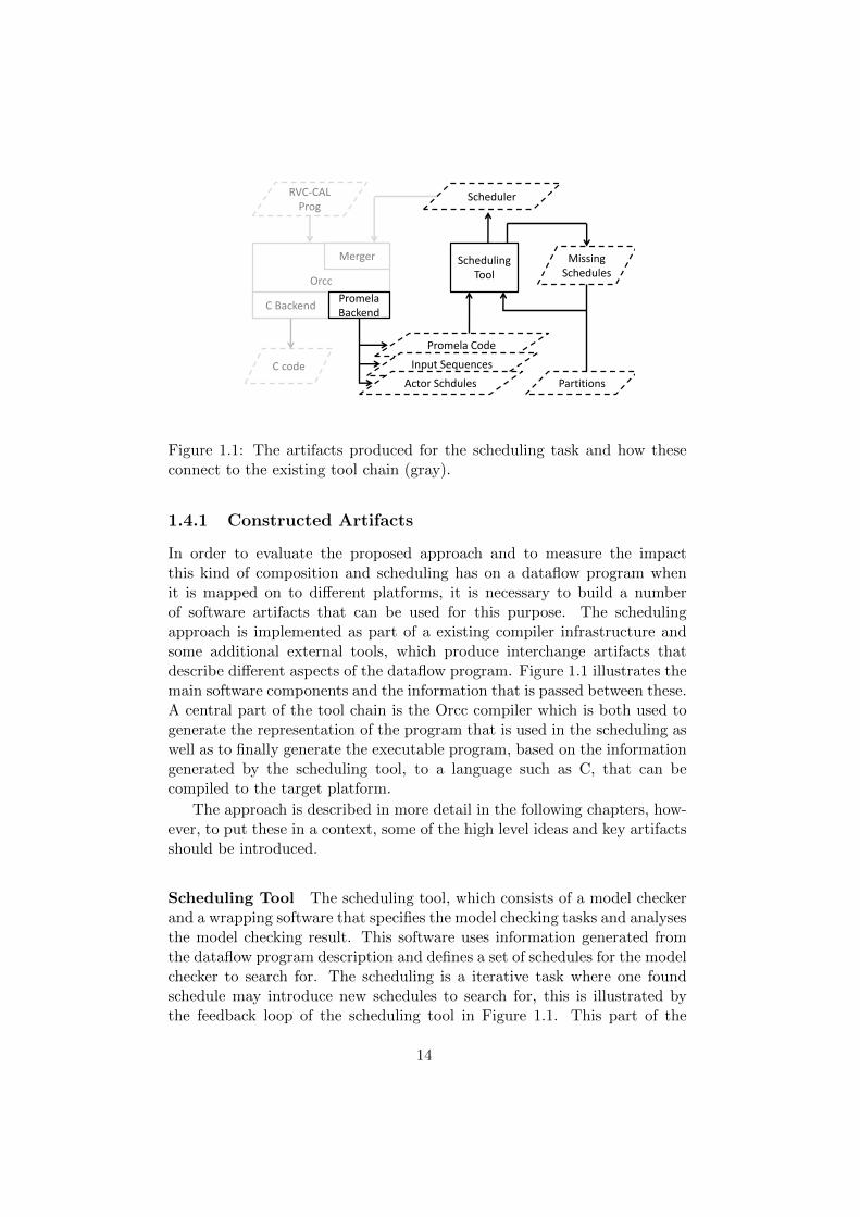
Figure 1.1: The artifacts produced for the scheduling task and how theseconnect to the existing tool chain (gray).

1.4.1 Constructed Artifacts

In order to evaluate the proposed approach and to measure the impactthis kind of composition and scheduling has on a dataflow program whenit is mapped on to different platforms, it is necessary to build a numberof software artifacts that can be used for this purpose. The schedulingapproach is implemented as part of a existing compiler infrastructure andsome additional external tools, which produce interchange artifacts thatdescribe different aspects of the dataflow program. Figure 1.1 illustrates themain software components and the information that is passed between these.A central part of the tool chain is the Orcc compiler which is both used togenerate the representation of the program that is used in the scheduling aswell as to finally generate the executable program, based on the informationgenerated by the scheduling tool, to a language such as C, that can becompiled to the target platform.

The approach is described in more detail in the following chapters, how-ever, to put these in a context, some of the high level ideas and key artifactsshould be introduced.

Scheduling Tool The scheduling tool, which consists of a model checkerand a wrapping software that specifies the model checking tasks and analysesthe model checking result. This software uses information generated fromthe dataflow program description and defines a set of schedules for the modelchecker to search for. The scheduling is a iterative task where one foundschedule may introduce new schedules to search for, this is illustrated bythe feedback loop of the scheduling tool in Figure 1.1. This part of the

14

scheduling approach is mainly described in Chapter 5.

Partition The set of actors that are to be composed and thereby ana-lyzed for scheduling is called a partition. A partition may correspond to thewhole dataflow program but usually partitions are chosen, by the designer,to minimize the scheduling overhead by grouping together actors with re-lated behavior, and to improve run-time performance by choosing partitionsizes that fit the target platform. Partitioning is only described in this thesisfrom the point of view of correctness, where correctness means that a modeldescribing the scheduling of a partition must include all the necessary in-formation, while the performance aspect is left for an external design spaceexploration. The required properties of a partition is discussed in Chapter 3,which presents the different types of dynamic behavior a partition of actorscan have.

Schedules The task of the scheduling framework is to produces staticschedules, that is, sequences of firings that, once chosen for execution, thewhole schedule can be guaranteed to run to completion without the need forevaluating guard expressions. When several schedules are need to describethe behavior of a partition, the choice of schedule is performed by a schedulerat run-time. The scheduler produces, the schedules and the firing rules forthese, is then the artifact that is the end result of the scheduling tool andis used by the compiler to merge actors before the code is generated forthe target platform. The construction of a set of static schedules for apartition together with a scheduler that corresponds to the firing rules ofthe schedules, is mainly discussed in Chapter 5.

To construct and initialize the model checker for one scheduling task afew pieces of information, either automatically generated from the dataflowprogram or provided by the developer, is need.

Promela Code The behavior of the dataflow program is translated to thelanguage used by the model checker, in this case Promela. For this purposea backend producing Promela code is constructed for the Orcc compiler.The generation of the Promela code not as such interesting in this context,and is only briefly described in Chapter 5 and Paper 1, instead finding therelevant information to generate code from is more relevant. An additionto generating the Promela code, the backed runs a set of analysis passeswhich are used to simplify the program description to only include schedulinginformation as well as producing additional information which is used bythe scheduling tool, this involves information regarding static schedules andtheir corresponding input sequences of individual actors.

15

Actor Schedules Simplifying of the individual actors to only include in-put dependent firing rules, while firing sequences that can be resolved fromthe program text of the actor are described as static schedules, gives a goodstaring point for the actual scheduling task. Generating a set of static sched-ules that describe the possible firing sequences of the actor, gives a predic-tions of what the static schedules, of a partition, that are to be searched forby the model checker should look like. Similarly, it also gives the data ratesand the needed input sequences that are consumed by the correspondingschedules.

Input Sequences A final artifact that is produced as an input for themodel checking task, is the set of input sequences an actor accepts. Theseinput sequences correspond to the per actor static schedules described above,and describe the number of data tokens a schedule consumes and, if it canbe resolved, the value of a control token that enables the schedule. Thisinformation is used to initialize the model checking tasks as well as to de-cide when a schedule has finished based on the number of tokens it hasconsumed. The construction of the actor schedules and the correspondinginput sequences is discussed in Chapter 4.

1.5 Research Methods in this Thesis

This thesis presents research related to the scheduling problem of dynamicdataflow programs, where the dataflow programs in practice are programsimplemented using the Cal Actor Language (CAL) [46]. The research startsfrom an idea that the dataflow program can be modeled as a set of commu-nicating finite state machines (FSM), for which a state space analysis cangive the set of schedules that describes the behavior of the program. Apartfrom building tools and prototypes for evaluating the ideas, the research alsoincludes performing measurements evaluating the impacts of the approachand algebraic analysis of the correctness of the models.

To narrow down the discussion on research methods, the discussion isbased on the book On Research Methods [74] by P. Jarvinen, and the indi-vidual parts of the research work is compared to the methods presented inthis book.

1.5.1 Design-science research

A great part of the work presented in this thesis relates to tools and ar-tifacts that have been built to solve the problems of scheduling dataflowapplications. This kind of a research problem fits well with design-science,which describes a methodology for research where the target is to create newinnovative artifacts for a specific problem domain, and, while this method

16

has not strictly been followed, it is relevant to compare the presented workwith the main points of this research method.

According to March and Smith (1995) [91], design-science has two ba-sic activities, build and evaluate, and four types of products or artifacts,constructs, models, methods, and instantiations.

The build activity corresponds to building tools and methods for solv-ing a specific problem, and the build activity is performed to construct aprototype that shows that the proposed idea is feasible and enables a evalu-ation of the proposed approach. What separate design-science research fromengineering is that the construction does not follow what is best praxis inthe field, but instead, the purpose of building an artifact is to create newknowledge and to enable an evaluation of a new idea. It is therefore impor-tant in design-science that research resources are not used to build artifactswhich are based on already known and evaluated ideas. [91, 74]

A constructed artifact then needs to be evaluated in order to answerthe question regarding if the artifact contributes to the progress of the field.The questions that needs to be asked are: How well does the artifact performthe task? How does it compare to previous work? To be able to evaluatethe artifact, some criteria for success and metrics need to be defined, suchthat results are comparable. Of course, if no previous methods have beenable to achieve the same goals, the feasibility of constructing the artifact isalready a valid result. [91, 74]

The building process related to this thesis, includes extending a codegeneration tool chain with a set of analysis and transformation operations.To evaluate how well the artifacts work, some metrics that can be comparedare: how fast the generated code is when run on different platforms, howusable the tool is regarding how large parts of a program can be transformedin to something more efficient, and finally, how usable the tool is for adeveloper, where usable means how difficult the tool is to use and howmuch time it requires. These metrics can then be compared to previouswork, however, some criteria for success are also needed to define what canbe regarded as success. In this case, it is not required that the usabilityimproves, but instead, it is a trade-off with the other metrics.

Design-science research must produce an artifact, according to the defi-nitions of March and Smith, we have the four types of artifacts as follows.

The first one, Constructs, provides the language in which problemsand solutions are defined and forms a vocabulary for the domain [91, 74].According to March the evaluation of constructs typically involve complete-ness, simplicity, elegance, understandability, and ease of use. In the dataflowdomain, which is rather mature, the constructs have been developed overseveral decades and for this reason adding new constructs can typically beavoided. In this work, existing constructs are used to keep the discussionsimple and not introduce overlapping constructs; instead, the focus is on

17

other types of artifacts.Models are built as a set of proposition or statements describing rela-

tionships between the constructs and are used to improve the understandingof the problem and solution and ties the approach to the real world problems.According to March the models are evaluated in terms of their fidelity withreal world phenomena, completeness, level of detail, robustness, and internalconsistency. In this work, several models are constructed which each high-lights one property of the dataflow program that is being analyzed. Thesemethods are for this reason presented formally to demonstrate the proper-ties related to completeness and consistency, as an incomplete model in thecontext of code analysis and transformation, is worthless. The evaluation ofthe models is presented in Paper 4, and Chapter 3.

The methods are algorithms or guidelines that describe how a specificproblem should be solved, or more applicable in the context of this the-sis, how to search the solution space. According to March the evaluationof methods mainly regards their efficiency, generality, and ease of use. Inthe work of this thesis, this relates mainly to strategies related to schedul-ing, how the information from the models is used to perform the actualscheduling. The evaluation of methods is mainly presented as case studiesin Chapter 7 of this thesis.

Instantiations are the actual tools constructed to demonstrate the ap-proach and show that constructs, models, or methods can be implemented ina working system. The instantiations are the artifacts that link researchersto the real world and show how the artifacts react to it and how users reactto the artifact. According to March the evaluation of instantiations relatesto the efficiency of the artifact and what impact it has on the environmentand users. For the tools produced within this work, this would mean that anumber of developers should be able to use the tools and feel that it helpsthem achieve some of their goals.

Evaluation of the Work The research work behind this thesis was notdirectly based on design science, but because of many similarities regardingthe goals of the research and the kind of experiments needed, it is relevantto evaluate this work as a design science research problem. This can be doneby analyzing the seven guidelines, regarding design science research, givenby Hevner et al. in [65].

The first one, Guideline 1: Design as an Artifact, is obviously followedas described above according to the definitions of March and Smith. Thesecond guideline, Guideline 2: Problem Relevance, states that these arti-facts should provide solutions to important and relevant business problems.In this context, this means that the problem that is solved has a value inindustrial applications and that it aids to the development in the field. Therelevance cannot be evaluated from the research work but instead from the

18

problem statement motivating the research. The relevance of the schedul-ing problem comes from the fact that, using dataflow in many industrialapplications is avoided due to the lack of methods for generating efficientcode.

Guideline 3: Design Evaluation. It is crucial that the resulting artifactsare evaluated with proper metrics and sufficient experimental data. Withinthis context, when the artifact is part of a design tool chain, the relevantproperties are related both to the usability of the artifact from the point ofview of the user of the artifact, but also regarding how the artifact affectsthe performance of the dataflow program which is transformed by the arti-fact. For the user, the question is how much manual labor and additionalexpertise is needed to use the artifact and how much time the user mustwait for the tool to finish. These properties are evaluated in Chapter 7which provides a set of case studies where the artifact is used to constructschedulers for composed actors. While several of the studied examples areautomatically transformed by the artifact, the ones that are not are also im-portant for giving an improved understanding of the research problem. Forthe second part, regarding the performance of the actors that are composedby the artifact, the evaluation requires numerous experiments including dif-ferent configurations and target platforms. Experimental data is presentedin Chapter 6 and in several of the original publication, however, what iseven more important than being able to show promising numbers is thatthe experiments are properly performed. We will get back to evaluating themeasurements shortly, after discussing the other guidelines by Hevner et al.

Guideline 4: Research Contributions. Following the discussion on de-sign evaluation, a more general evaluation is defining clear and verifiablecontributions of the work. According to Hevner et al. the contributioncan be the design artifact itself or contributions related to foundations andmethodologies if the area of the design artifact. While much of the work pre-sented in this thesis evaluate experimental strategies for building schedulingmodels and deriving schedules for composed actors, the design artifact bothshows that such methods are implementable but also enables an evaluationof methods presented. The following guideline, Guideline 5: Research Rigor,relates to the research contributions by requesting rigorous methods in boththe construction and evaluation of the design artifact [65]. In the contextof this work, rigor relates to the set of dataflow programs that are used todesign and evaluate the artifact such that the artifact can be shown to solvea general problem and not only a special case. Similarly, rigor can be relatedto the data sets that are used to perform experiments and evaluation of theartifact; rigorous experiments make the knowledge acquired from the exper-iments more general. Furthermore, to show that the presented methods arecomplete, with respect to the possible inputs to the artifact, the methodsneed to be described mathematically based on an formal description of the

19

dataflow program.

The next guideline, Guideline 6: Design as a Search Process, definesthe research as an iterative process, where available means, which are re-sources available to construct a solution, are used to reach desired ends,representing goals or constraints on the solution, while satisfying laws inthe problem environment [65]. For complex problems, the first version of anartifact typically requires simplifications of the problem space or decompo-sition in to subproblems. While such an artifact hardly can be expected toas such be usable, it enables an improved understanding of the problem andraises relevant questions. The last guideline, Guideline 7: Communicationof Research, elaborates this idea by highlighting the communication of theresearch results to the relevant audience. The important result of the workis then not the artifact itself but the knowledge acquired from constructingthe artifact and by conducting the experiments enabled by the artifact.

1.5.2 Experiments and Measurements

One aspect of evaluating the approach is to construct experiments and per-form measurements. In the context of CAL, relevant experiments are mul-timedia applications such as video decoders and various signal processingapplications like network protocols and digital filters.

For measurements to make sense, it is essential to plan what is actuallymeasured and what parameters may affect the measurement. To draw moregeneral conclusions from the measurements, it is also important that theexperiments are repeated for several application, input sequences, compilersettings, and hardware configurations. In Paper 3, where a larger set ofexperiments is presented, it is obvious from the results that, had the ex-periments been done for only a part of the chosen experiments, the resultswould not have given a realistic view of the impact of the presented programtransformations. The reason is that the same configurations give, not onlydifferent, but contradicting results on different platforms that were used inthe experiment. Instead of simply concluding that a transformation of aprogram is good or not, it is then possible to find how platform parame-ters such as cache size, has an impact on how the transformation affectsthe program performance. To be able to make a conclusion, it is thereforeimportant to have a large enough set of test cases.

Measurement Errors and Variation Performing measurements on acomputer system is made complicated by operating systems, caches, andadvanced processor features. In general, it is hard to know if a specific mea-surement is a result of the feature being investigated or if it is a coincidenceof a combination of features that are not taken into account in the measure-ment setup. Further, the same experiment may give varying results for every

20

run; and in some cases, already by touching the mouse of the computer, thesamples measured during that interval may be quite far from the average.To make the results valid, basic statistical methods, such as calculating aconfidence interval, can be used. This way, it is possible to say if a result isstatistically significant or not.

What we are interested in when measuring the performance of the dataflowprograms after composition, is the speedup compared to the original pro-gram or other configurations. The speedup can be defined as the differencebetween the time it takes to run a program to completion, or in case the pro-gram does not run to completion, the difference between the rate at whichthe programs complete a tasks e.g. the frame rate of a video application.

A useful measure of the speedup of an application is the mean valueaccompanied by an confidence interval. The confidence interval gives an in-terval within which a sample will reside with a given probability (e.g. 95%).When measuring two configurations of a system, if the confidence inter-vals of the two configurations do not overlap, the measured difference canbe considered to be significant. In order to calculate a confidence interval,however, the measurements, and the variation of these, must be assumed tofollow a normal distribution. Measuring a computer system, there are manypossible sources of both systematic and unexpected errors. In the measure-ment related to this work, measurements were performed according to theguidelines by Lilja in [86].

Especially some errors in the measurements are more difficult to handle,as an example, if the operating system decides to run a task during one ofthe measurements; this measurement may then be completely useless andmisleading. For this reason, the samples that clearly are outliers should beremoved from the measurements to assure that the samples have a normaldistribution. The removal of outliers, however, must be justified. Outliers onthe sample set of the measurements of the speed of a program typically aresingle values with much worse results than the other samples which residein a comparably small interval.

When the measurements are properly handled and the different config-urations can be compared, the next important thing is to be able to drawconclusions from the result, or more importantly, to draw correct conclu-sions.

Generalizability of Results A property we are interested in is the gen-eralizability, which refers to how useful a theoretical construct is outside thelimited set of observations from which it has been constructed [74]. It wouldbe tempting to state, based on the experiments, that actor composition re-sults in faster code, however, does the set of example programs, the set ofplatforms, the different configurations, and the measurements themselves,justify this generalization? Fortunately, the experiments already show that

21

this is not the case; instead it can be concluded that composition is a usefulpart of design space exploration.

1.6 Structure of Thesis

This thesis is constructed as a collection of peer-reviewed conference paperswhich are accompanied by a more general introduction to the field and anoverview of the topics presented in the papers. The two parts of the thesis areto some extent overlapping, with the difference that the first part attemptsto explain the concepts and background in a more general fashion while, inthe second part, the papers are more technical and concentrate on narrowersubjects within the research. As a result, the two parts are also independentand part one gives an understanding of the research work without the needto study the more detailed papers.

The first two chapters of the thesis is an introduction to parallel pro-gramming and dataflow, and the purpose of these is to motivate why theresearch is needed and describe the relevant concepts that the later chap-ters depend on. In the second chapter, work regarding dataflow and processmodels is presented, introducing the problems related to scheduling andproperties such as boundedness. Chapter 2 also presents the CAL ActorLanguage, which is used as the programming language to implement thedynamic dataflow programs that are studied.

Chapter 3 is a discussion of the dynamism that can be implemented byCAL actors and the point with the chapter is to show what a real dynamicscheduling decision is and which scheduling decisions can be resolved byanalyzing the context of the actor. The chapter discusses properties suchas input dependency, non-determinism, and monotonicity. Methods for rea-soning about such properties is then presented; this is partly based on Paper4 [49] with some additions of previously unpublished work.

The following two chapters present actual scheduling methods. First,Chapter 4 presents the scheduling of a single actor by removing schedulingdecisions that can be resolved from the information in the actor programtext. Then Chapter 5 presents how the scheduling can be further resolvedby analyzing a partition of actors such that some dynamic behavior becomesstatic when the context of the actor is known. Chapter 5 is partly basedon Paper 1 [51] and Paper 2 [52], when it comes to generating the actualschedules, and Paper 4 [49] regarding the analysis of the actor partitions.Furthermore, Chapter 4, contains work that has been implemented andis needed by the methods presented in the following chapter, but has notpreviously been published.

Finally, Chapters 6 and 7, evaluate the result and draw some conclusionregarding the presented approach. Chapter 6 presents measurement results,

22

partly published in Papers 3 [50] and 5 [26], and then discusses these resultsand what further steps, regarding design of languages and tools would beneeded to achieve better results and possibilities for analysis and verification.Chapter 9 then presents the papers and some final conclusions are presentedin Chapter 10.

23

24

Chapter 2

Some Background RegardingDataflow Models

Ideally, a computer program describes an algorithm or a set of computa-tions without making any assumptions about the underlying hardware andwithout imposing unnecessary restrictions on how, or in which order, thecomputations are to be performed. It is instead the compiler’s job to makethe appropriate choices that are needed for the program to run efficientlyon the desired hardware, but without altering the results computed by theprogram. With parallel programming, this becomes even more relevant asunnecessary restrictions, imposed by the programmer over specifying theprogram, limits the available parallelism.

For this reason, many computational models for describing concurrentcomputational entities, have been proposed and have to some extent beenused in industrial strength tools. In digital signal processing, programs areoften described as directed graphs where edges describe streams of datasamples and nodes describe calculations performed on these samples. Thiskind of applications are typically represented with a visual syntax to specifythe graphs, e.g. Ptolemy from the University of California at Berkeley [29]and MATLAB from MathWorks with its visual interface SIMULINK, whichmakes the description intuitive for humans to read or use readymade compo-nents to build models. While a graphical representation is of no consequencefor a compiler, the graph representation explicitly describes the parallelismof the program.

Programming models based on the dataflow paradigm have a long historystarting with work form the early 1960’s. One of the early languages, waspresented by Dennis in 1974 [42]. This dataflow language describes programfunctionality as a bipartite directed graph with two types of node, namelylinks and actors. A number of actors are provided, which either operateon control or data values (tokens) or perform a conditional operation on

25

some data values depending on a control value, and links which are onetoken queues and distribute the token to one or more other nodes. For asoftware engineer, the language presented resembles logic gates schematics,however, the nodes implement firing rules which means that the semanticscompared to a Boolean function is quite different. In Dennis’s language linksare also called nodes as these also have firing rules, e.g. links that distributeone input token to several nodes. In this thesis, however, when a node ismentioned it corresponds to an actor, links on the other hand are referredto as the edges of a dataflow graph.

In addition to Dennis’s dataflow language, early work was done by Petriwho presented Petri nets 1962 [102], Estrin and Turn who presented adataflow model in 1963 [54], Karp and Miller who presented computationgraphs in 1966 [77, 78], Chamberlain who presented a single assignmentdataflow language in 1971 [35], Kahn who presented a process language in1974 [76], and in 1977 Arvind and Gostelow [10, 11], and Gurd and Wat-son [63] presented their separate works on tagged token dataflow models.But also more recently, dataflow languages have started to attract moreinterest and languages such as StreamIT [117] and CAL [46], has been pre-sented. Also, much work has been put into developing different computa-tional models with a trade-off between expressiveness and predictability, andmany of these will be presented later in this chapter.

Many programming languages and models for describing this type ofapplications exist, and have been developed for the last half century; athorough survey is given by Johnston et al. in [75]. Many contemporarydataflow tools and languages have their roots in, or at least much in commonwith, Process Calculi [56, 118, 95, 64], the Actor Model [66, 13, 37], and/orData Flow Models [42, 82]. While these models have much in common, andcan be seen as concurrent processes exchanging messages, still, the differentmodels have some fundamental differences and provide different primitivesfor concurrent processing. The languages typically consist of a host languagedescribing the behavior of the nodes and a coordination language describingthe interaction between nodes [83]. What primitives are allowed in eachof the models and which model a languages depends on inherently decidewhat can be expressed by the language and which properties the resultingprogram has regarding predictability and determinism. Before going intomore specific scheduling approaches, it will be appropriate to present someof the basic models and the properties of these.

2.1 Processes, Actors, and Dataflow Models

Communication between processes has been studied for quite some time,and in a more general context than only streaming applications. Some of

26

the significant initial work on Cooperating sequential processes was done byDijkstra in 1968 [44], where synchronization primitives such as semaphoresare presented. For dataflow (or related) models, the abstraction level israised to deal with communication on the level of massages and queues,and primitives such as semaphores, monitors, threads, etc. which may beused to implement the program in practice, are hidden for the programmerwithin higher level constructs. This is perhaps the most significant com-monality the models of interest share on a practical level, but of course, theexact primitives available and the semantics of these is also what makes thedifference between these models.

In the following, some more general models, which are of consequencefor this thesis, are presented. Then in the following sections, more special-ized dataflow models of computation and the properties these provide arepresented, and finally the CAL actor language is presented.

Communicating Sequential Processes Hoare presented in 1978, Com-municating Sequential Processes (CSP) [69], which adds a set of primitivesfor managing creation of and communication between concurrent processesand combines this with Dijkstra’s Guarded Commands [45] to describe thebehavior of the processes. CSP has been useful especially for verification ofconcurrent properties of different systems [17], and has significantly evolvedduring the years since it was presented. For a more contemporary versionsee [70], however, here we concentrate on the language presented in theoriginal work.

CSP provides a parallel statement for starting concurrent processes,where each process starts simultaneously and where the parallel statementends when each process has terminated. The behavior of the processes isdescribed using repetitive and alternative commands based on Dijkstra’sGuarded Commands [45], and allows non-determinism as the guarded com-mands does not need to be mutually exclusive. The processes are onlyallowed to communicate by updating variables through the communicationprimitives. Originally CSP did not include any automatic buffered commu-nication, instead, communication in CSP was synchronous and involved arendezvous between the processes sending and receiving the message, thismeans that both sending and receiving are blocking operations. Bufferingis left out because the rendezvous communication can be used to constructbuffered communications by constructing a FIFO process where both leftand right sides have synchronous communication. In later versions of CSP,however, explicit channels for message passing are added.

The communication in CSP simply names the process to communicatewith and the variable to send or receive. As an example producer?data;would receive a value for the variable data from a process named producerwhile receiver!data; would send the content of the variable data to the

27

process named receiver. The communication only takes place if the twovariables have a matching type.

CSP is of special interest as the Spin Model Checker [72] uses a CSP-likelanguage to describe the process network that is analyzed. This language,called Promela (PRocess MEta LAnguage), is briefly presented in Chapter 5as part of the discussion of how the model checker can be used to extractstatic schedules from a dataflow program.

Kahn Process Network A simple language for describing parallel pro-gramming was presented by Kahn in 1974 [76]. Compared to CSP, theprocesses in Kahn’s model are deterministic, have communication queueswith automatic buffering of infinite size, and the processes are designed torun forever. The Kahn Process Network (KPN) achieves these propertiesby adding some simple commands, for describing how processes relates toeach other, to the program description, where the processes are describedas an Algol program with the addition of communication primitives.

The communication between processes in KPN is implemented with ablocking receive and a non blocking read. The blocking receive implies thatKPN is deterministic, that is, processes cannot check for input, or absence ofinput [76]. The processes, which are declared similar to a procedure, are runstatement by statement until a wait primitive is reached, which indicatesthe read of an input channel. The only way to get input is to use the waitprimitive, which simply waits until input is available. With output, on theother hand, the nonblocking send primitive is used. With the combinationof infinite buffers and nonblocking send operations, sending output is anoperations that is always successful.

A KPN is monotonic, which means that more inputs only will result inmore outputs and future inputs only concerns future outputs [76, 83]. Moreformally monotonicity means that X1 v X2 implies that f(X1) v f(X2),which means that if a sequence X1 is a prefix to a sequence X2, then theresulting sequences of these are also ordered in a corresponding prefix order.In KPN monotonicity is guaranteed by blocking reads, which means thatthere is only one possible order to read the inputs. A Khan process networkis also continuous which means that a process cannot decide to send outputonly after an infinite number of inputs has been received [76]. These areimportant properties for the scheduling problem; for models which can havenon-monotonic actors, it also implies that the actors are nondeterminate,which makes the scheduling more challenging. As an example, with a non-monotonic actor, a schedule that is correctly generated for a specific input,may be incorrect when more inputs are available.

28

Dataflow Process Networks Lee et al. presents Dataflow Process Net-works (DPN) [83] as a special case of Kahn process networks, where theprocesses, called actors, consist of repeated firings. The DPN model of com-putation is highly relevant to this thesis as the Cal Actor Language (CAL)is based on DPN. Compared to KPN, DPN adds the principle of firings asproposed by Dennis, which is useful for describing dataflow applications. [85]

The introduction of firings provides a quantum for scheduling calcula-tions that map input tokens to output tokens. The behavior of an actoris then described as pairs of firing rules and firings, where the firing ruledefines a precondition for an actor firing, while the firing itself consumes afixed number of tokens on input streams and produces tokens on the out-put streams. A scheduler then interleaves actor firings according to a setof firing rules which may depend on inputs or the state of the actor. Thefiring rules are a set of expressions, describing some properties regarding theinput sequences and the actor state that are required for an actor firing tobe eligible. The actor firings in DPN can to some extent be compared toDijkstra’s Guarded Commands [45] and the firing rules do not need to bemutually exclusive implying that an actor can be non-deterministic. Con-sequently, non-deterministic actors must be identified, and non-monotonicbehavior needs to be identified in order to produce correct scheduling.

DPN is a rather expressive model of computation, which can be usedto implement applications that could be implemented with more restrictedmodels of computations. While this means that any dataflow program, orpart of a dataflow program, can be implemented with DPN, the imple-mentation in DPN does not automatically provide some of the conveniencethat more restricted models of computation would provide concerning pre-dictability or static scheduling. Instead, these properties need to be iden-tified by analyzing the actors of the whole program, and, in one way oranother, fit the actors in to more restricted models of computation thathave the desired properties. In the next section different dataflow modelsof computation, with different trade-offs between expressiveness and pre-dictability are presented in order to show what kind of properties we wantto identify in DPN programs.

The Actor Model In order to avoid unnecessary confusion, a related butstill different model, namely the actor model should be briefly mentioned.In dataflow models, a computational node is often called an actor. This is,however, not to be confused with the actor model, which is a separate modelof computation.

The actor model was designed as a model of concurrent computation,and was created as a new theory of an inherently concurrent model [37].Compared to the process networks and data flow networks already discussedin this chapter which have a fixed network topology, in the actor model

29

the communication topology is dynamically changing. The Actor modelallows actors to dynamically create actors, send messages to other actors,and respond to messages received from other actors. The fixed topologyof dataflow programs is beneficial for analysis, as the connections betweenactors are static, the dynamic topology of the actor model, on the otherhand, allows more dynamic application models. Which model is better willof course depend on the application that is being implemented, and for manysignal processing applications, a static topology is adequate.

The actor model was presented by Hewitt et al. in 1973 [67], and furtherdevelopments and reading can be found in Hewitt et al. from 1977 [66, 13],Clinger from 1981 [37], Agha from 1986 [6], and many others. To not getoff topic too much, the actor model will not further be discussed in thisthesis, instead we will move on to discussing more specific dataflow modelsof computation.

2.2 Dataflow Models of Computation

The behavior of a dataflow program is defined by the Model of Computation(MoC) of the dataflow network, which defines in which order and how thenodes are to be executed. Several MoCs have been presented, each describinga different trade-off between expressiveness and compile-time predictability.The simplest one is Synchronous Data Flow (SDF) which is a staticallyschedulable MoC [81], while e.g. dataflow process networks are dynamicallyscheduled, that is, scheduling decisions are taken at run-time [83].

In this context we are particularly interested in compile-time analysisand scheduling of dataflow programs in an SDF like manner but withoutsacrificing expressiveness of models like DPN. Depending on the MoC whichdefine the operations an actor is allowed to perform, some properties areinherent to more restricted models while for less restrictive models theseproperties may be more difficult to verify. The properties of a dataflowactor that can be resolved at compile-time depend on either what behavioris allowed by the MoC of the actor or which of the allowed properties areused. In other words, either some properties are implied by the restrictionsof the programming model or these properties need to be identified from theimplementation. Dataflow models are often used to model and implementsignal processing systems which in many cases work on never ending datastreams. For this reasons it is important to analyze properties such as,if the program can run using bounded memory, whether or not there existschedules of finite length that bring the program back to its initial state, andif the programs are guaranteed to be deadlock free. Each of these problemsare related to the main problem addressed in this thesis, that is, how togenerate a set of static schedules that can describe the different operations

30

of the dynamic dataflow program.

Numerous computational models have been proposed to find a comfort-able trade-off between expressiveness and predictability in the range betweenfully static models such as SDF and dynamic models such as DPN. There arebenefits with requiring the user to specify and stick to a specific restrictedMoC, by this the programmer is forced to think and specify the intended be-havior, but in many cases it is more beneficial to allow a less restricted MoCand let the compiler try to resolve the properties of the program. Dataflowprograms can be divided into different MoCs depending on how token ratesand firing rules are specified. Several MoCs, which levels of predictabilityand expressiveness, reside between static dataflow (synchronous data flow)and dynamic dataflow, exist. With static data flow, every scheduling deci-sion is compile-time predictable while with dynamic data flow, scheduling isin general a run-time operation. Typically, each dynamic dataflow programincludes portions that are static, and therefore compile-time predictable, andfor this reason, dynamic dataflow programs or parts of these, will usuallybelong to more restricted MoCs with better compile-time predictability.

The work in this thesis focuses on one of the more expressive MoCsnamely Dataflow Process Networks (DPN) which is the model used in CAL.It is necessary to present some of the other models as much of the workon analyzing CAL can be compared to fitting a CAL program in to a morerestricted MoC in that sense that finding that some language constructs arenot used allows more precise analysis of the program. In the next section wewill go through a set of MoCs from the fully static models to more dynamicmodels, and then we will present related approaches on how to analyze andschedule dynamic dataflow programs.

Generally speaking, a node in a dataflow application may correspondto anything between a simple arithmetic operation to a larger subprogram.For any type of platform, a dataflow program requires scheduling, and thelarger the number of actors allocated to a specific processor core is, thelarger the impact of efficient scheduling becomes. When several actors aremapped to the same processor, the size of nodes should be adapted to fitthe target architecture by clustering, and the scheduling of the nodes shouldbe optimized to minimize the scheduling overhead. To achieve an efficientimplementation on a multi-core system, the compiler should resolve as muchas possible of unspecified decisions while leaving balancing for the run-time.Now, we must decide what can be decided at run-time. In theory, all alter-native paths of a program can be derived at compile-time, although it maynot always be practical. Hoare describes computer programming as an exactscience in [68] as ”all properties of a program and all the consequences of ex-ecuting it in any given environment can, in principle, be found out from thetext of the program itself by means of purely deductive reasoning”. In prac-tice this means that, if the program is known, we can calculate the outputs

31

for every possible input. If we look strictly at which parts or statements of aprogram are executed, we can deduce a set of sequences of statements thatare sufficient to process every possible input of the program. To create effi-cient dataflow programs, different programming models have been proposedthat guarantee different properties, by construction of a program accordingto that MoC. Many of these provide programs that allow static scheduling,unbounded buffers, or deadlock freeness.

Dynamic Data Flow A dataflow program where the computations aredescribed with a set of firing rules, depending on variables or data tokensthat are evaluated at run-time, belongs to a MoC called Dynamic Data Flow(DDF). The concept of DDF is loosely defined in literature, and seems to inmany cases describe a model that does not correspond to any of the morerestricted MoCs. In this text the simple definition of DDF used in [122] willbe used to describe applications where no scheduling information is givenfor the program. In a DDF program, an actor has a set of firing rules whichcan be any Boolean expression and the tokens rates can be undefined or bedefined as a range [122]. A DDF program can also be non-deterministic byallowing more than one firing rules to be enabled at once. According to thisdefinition, DPN can also be considered to belong to DDF.

With DDF scheduling is a run-time operation; some or all schedulingdecisions can however be predicted at compile-time by either describing theprogram with a more restricted MoC or by analyzing the program to find ifparts of it can be described with more restricted MoCs. This operation canbe seen as a classification of one MoC to a more restricted MoC, and canbe described as identifying if a program implemented with a less restrictiveMoC fulfills the requirements of a more restrictive MoC.

Synchronous Data Flow One approach to solve the scheduling problemis to use a restricted MoC which enables static scheduling. Many signal pro-cessing algorithms, such as a filter, can be described as a dataflow programwhere each node has constant data rates. Such programs can be modeled asSynchronous Dataflow (SDF) which can be statically scheduled and are opti-mal as no scheduling decisions are needed at run-time. The static schedulingof SDF programs is presented by Lee in [81], and the conditions for the ex-istence of a valid static schedule has been extended for many of the otherMoCs we will review as well.

The number of times the nodes in an SDF graph must be triggered inorder to form a periodic sequential schedule is found by solving the balanceequation Γq = 0, where the (i, j)th element in Γ represents the number oftokens node j will produce on arc i; in case the node consumes tokens theentry will be a negative number. If the equation has a non-trivial solution,

32

that is, a non-zero positive solution, there exist a schedule that will take thenetwork back to it initial state. A necessary condition for the existence ofsuch a schedule is that rank[Γ] = s−1, where s is the number of nodes [82].

The program is said to be consistent if the consumption and produc-tion rates of each edge match in the long run [79]. Consistency does notmean that it is possible to construct a periodic admissible schedule. As anexample, every cycle in the dataflow graph with an initially empty bufferis deadlocked. By inserting the appropriate initial tokens (delay tokens)b(n) = b(0) + nΓq it will be possible to create a schedule that runs oneperiod without consuming tokens from any empty FIFOs. [82, 81]

For an SDF graph, some important properties can be proved. If thetoken rates are consistent, the program can be run, also in the long run,with static FIFO sizes (bounded memory). This is an important propertyfor static scheduling as inconsistent token rates can lead to accumulation ontokens which imply either unbounded memory requirements or deadlock.

Composition of two adjacent nodes is not always possible without intro-ducing deadlock. Pino et al. [105] presents an SDF composition theoremfor testing if a composition (or clustering) is valid and does not introducedeadlock. Generally speaking, an SDF graph does not deadlock if and only ifit has an acyclic precedence graph [105]. The composition theorem includesfour criteria that prevent cycles in the precedence graph of the composedactors.

Not every application can be modeled as SDF and for this reason thereexist several almost SDF MoCs. These typically have a deterministic behav-ior but are somewhat more complex than SDF and the MoCs are designedto allow some flexibility to describe algorithms with some specific behavior.

Cyclo-Static Dataflow One extension of SDF is Cyclo-Static Dataflow(CSDF) which allows the dataflow network to have different data-rates fordifferent firings as long as these are periodic. This is useful for applicationswith cyclically changing behavior, for example, one node in the dataflownetwork have different data-rate every other time it is executed. The result-ing application can still be scheduled statically at compile-time by using anextended version of the methods for scheduling SDF. [23]

At first glance, CSDF may seem more like a convenient representationfor some SDF programs as an CSDF actor can be described as SDF if thecycles are merged. However, the CSDF representation offers some benefitsover the SDF representation as the SDF model may introduce deadlock ina dataflow graph where it could be avoided with the functionally equivalentCSDF actor. The CSDF MoC also enables reduced buffering requirementsand network delay by allowing actors to fire partial firings which, if fired atonce, would correspond to an SDF actor with higher token rates.

33

Token Flow Model Another type of extension needed in many programsis the ability to describe conditional execution or a choice between severalalternatives. A basic model for this, called the token flow model, is presentedby Buck in [31]. In this model special nodes, which are called Switch andSelect, has an special input which carry a Boolean value deciding whichinput/output is active at that specific time. An extension of the token flowmodel allowing integer values instead of only Boolean values is presentedin [30], the integer value can be used to either specify the number of tokensthat are produced or consumed, or to enable/disable an arc depending onthe value of the token.

To determine if a graph is consistent the balance equation is required tohave a nontrivial solution. When the dataflow graph has dynamic actors, thetopology matrix will have entries with pi corresponding to the proportionsof tokens with a special value. The graph is called strongly consistent if thebalance equation has a nontrivial solution for any value of pi and weaklyconsistent if the solutions only exist for some values. A graph with strongconsistency will have bounded buffer requirements while a graph with weakconsistency only for the right proportions of the control values.

For both the Boolean and integer dataflow models, it is possible to findif the graph is consistent and can be scheduled with bounded memory. Thisalso means that a set of static schedules which can be chosen based on thecontrol values, can be derived. If a dataflow graph is strongly consistentdepends in its topology and how the special control actors are used. Aslightly different approach is to restrict the usage of control actors such thata design always will have the desired properties.

Well-Behaved Dataflow Gao et al [58] proposed well-behaved dataflow,where the dataflow graph is built from actors corresponding to the actorsin the token flow model, but allowing only structured use of Switch andMerge (Select) actors. Well-behaved graphs only allows the dynamic actorsin the conditional schema and the loop schema which enables compile-timepredictability of the storage requirement [58].

A MoC which somewhat combines the benefits of both CSDF and BDFis the Cyclo-dynamic Dataflow model.

Cyclo-dynamic Dataflow Cyclo-dynamic dataflow model (CDDF) ex-tends cyclo-static dataflow [122] such that it can cover all BDF and CSDFgraphs. The CDDF model extends the CSDF model and keeps the prop-erties related to analyzability and compile-time scheduling, but introducesdata dependent choices similar to those of Boolean dataflow.

What is interesting with CDDF is that it gives the designer the opportu-nity to express additional scheduling related information that is not possible

34

in the other models. A token rate of a port of an actor can, for example,be described as a sequence of rates, like in CSDF, or as a function of aninput value. In this way, the dynamic behavior of these actors is explicitlydescribed and the model can be said to tie the output of one actor to the cor-responding action in the other actor when these expressions are combined.For dynamic dataflow models, compile-time scheduling often requires thisinformation to be derived from the implementation in order to predict thebehavior of the model.

Some MoCs handle the control or dynamic behavior on a higher level.

Parameterized Synchronous Dataflow The Parameterized SynchronousDataflow (PSDF) is presented as a meta-modeling technique in [20]. PSDFallows parameterization of sub-systems where parameters can control func-tional behavior and also token flow behavior of the dataflow graph. A pa-rameterized graph behaves like a graph in the underlying dataflow model,during each of its invocations, but can assume different configurations acrossinvocations [20]. The PSDF model assumes SDF as the underlying model,however, any underlying dataflow model which has a notion of a graph it-eration can be used. For example, the concept of periodic schedules oriterations exists in SDF, CSDF, Multi Dimensional SDF [80] etc.

A PSDF specification Φ consist of three graphs, namely, the init graphΦi, the subinit graph Φs, and the body graph Φb. The body graph representsthe dataflow program while the init and subinit graphs are used to configurethe parameters of the body graph.

With the PSDF model, a subsystem, say the texture coding part of avideo decoder, could have two behaviors, for decoding macro blocks (MB)with or without intra prediction. For each MB processed, the texture codingsubsystem is configured to process the next block type. Further, the param-eterization could be implemented by a data input from another subsystem,which is read and used to reconfigure the dataflow graph between the invo-cations. This kind of scheduling resembles the type of scheduling which isthe goal of the methods presented in this thesis when the subinit graph Φs

is seen as the choice of schedule and the body graph Φb in the CAL programhas different token rates as a result of a different schedule being fired.

A MoC with a somewhat similar reconfigurability, but where the controlpart is more integrated in the MoC, is the Scenario-aware Dataflow model.

Scenario-Aware Data Flow A dataflow MoC which also handles controltokens or dynamic behavior is the Scenario-Aware Data Flow (SADF) [116,113]. Here, the dynamic behavior is viewed as a set of scenarios occurring insome possible order, modeling the behavior of each scenario as an SDF graphwhile the dynamic behavior is modeled as a set of possible scenarios [113].

35

An SADF graph can be viewed as an SDF graph where some of the tokenrates are indicated as a variable instead of a constant as in SDF. The actorsin an SADF graph are of two types: kernels which are the data processingpart of the program, and detectors which models the control part of theapplication. When a detector fires, it sends control tokens indicating thedetected scenario and fixing the values for the parameterized tokens rates ofthe receiving kernels [116]. SADF enables a pipelined execution of scenariosas the control tokens are part of the model. The SADF model has beendesigned to allow efficient performance analysis, however, only the MoC isrelevant for this thesis.

A restricted form of the SADF model adds a finite state machine (FSM)to represent the possible order in which the scenarios can occur [113]. Thismodel, called an FSM-based SADF graph, resembles to some extent the typeof dataflow scheduler that is generated from dynamic dataflow applicationswith the approach presented in this thesis.

Points of Interest The different MoC presented in this section providesdifferent restrictions or descriptions of relevant information that makes thedataflow program analyzable. In the context of this thesis, this is interestingas scheduling of a CAL program is about identifying properties, similarto these presented in the various MoCs. On a high level, the interestinginformation relates to how the token rates of an actor firing can be predicted,and how the tokens that carry information that will affect scheduling isdescribed in the MoCs that allow data dependent firing rules. In the lastsection of this chapter, the CAL actor language is presented with focus onthe different constructs that are relevant for scheduling.

2.3 The Cal Actor Language

The Cal Actor Language (CAL) is presented by Eker and Janneck in [46]as an actor language which is part of the Ptolemy project [29, 1], at theUC at Berkeley. CAL is a very expressive language for describing dataflowactors, and can implement the DPN model, which in practice means thatany dataflow program can be implemented with CAL.

Since the introduction of the language, CAL has gained interest alsowithin other contexts than Ptolemy, applications within signal processing,cryptography, and multimedia, has been implemented using the CAL lan-guage. The perhaps greatest achievement so far is that a subset of CALnamed RVC-CAL, has been standardized by ISO/IEC MPEG [2, 93], forthe Reconfigurable Video Coding (RVC) initiative. In MPEG RVC a videodecoder is described by a network configuration of RVC-CAL actors instan-tiated from a standardized library. This decoder description is associated

36

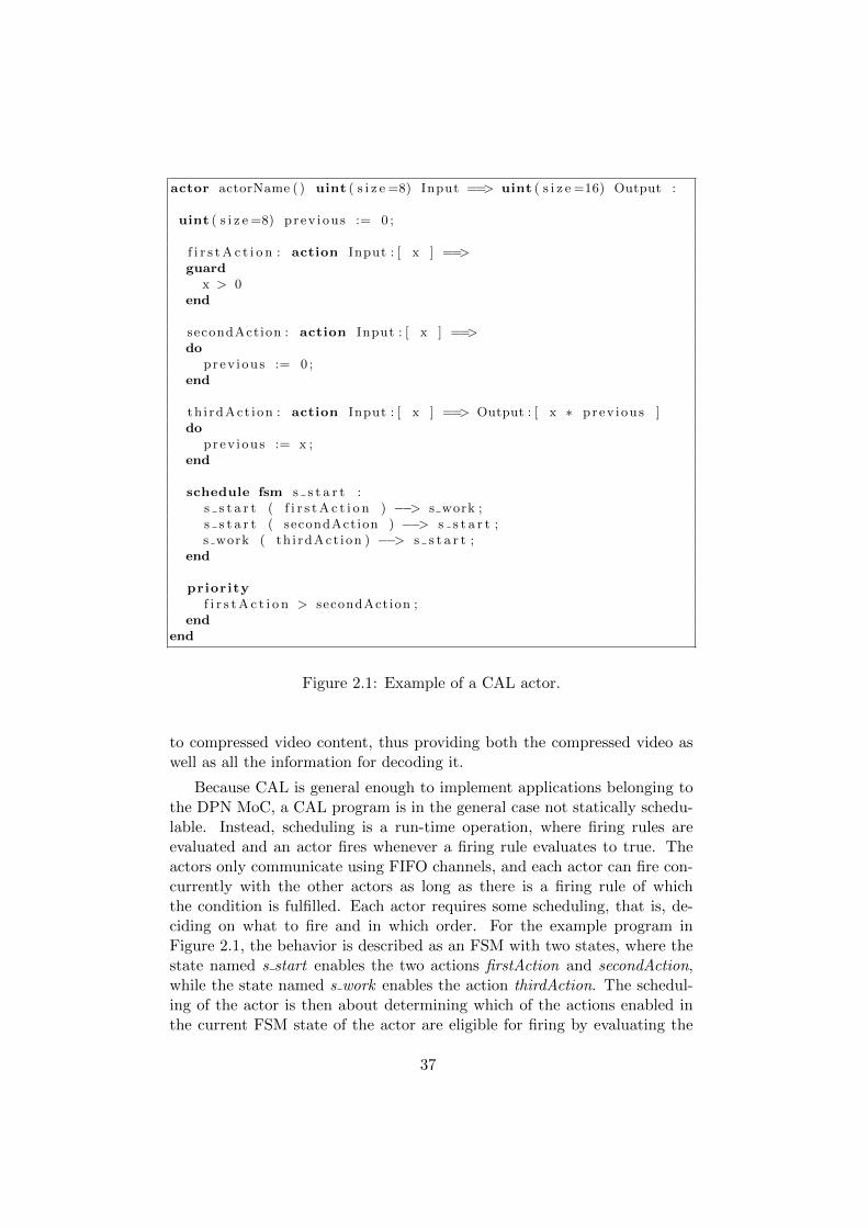
actor actorName ( ) uint ( s i z e =8) Input ==> uint ( s i z e =16) Output :

uint ( s i z e =8) prev ious := 0 ;

f i r s t A c t i o n : action Input : [ x ] ==>guard

x > 0end

secondAction : action Input : [ x ] ==>do

prev ious := 0 ;end

th i rdAct ion : action Input : [ x ] ==> Output : [ x ∗ prev ious ]do

prev ious := x ;end

schedule fsm s s t a r t :s s t a r t ( f i r s t A c t i o n ) −−> s work ;s s t a r t ( secondAction ) −−> s s t a r t ;s work ( th i rdAct ion ) −−> s s t a r t ;

end

priorityf i r s t A c t i o n > secondAction ;

endend

Figure 2.1: Example of a CAL actor.

to compressed video content, thus providing both the compressed video aswell as all the information for decoding it.

Because CAL is general enough to implement applications belonging tothe DPN MoC, a CAL program is in the general case not statically schedu-lable. Instead, scheduling is a run-time operation, where firing rules areevaluated and an actor fires whenever a firing rule evaluates to true. Theactors only communicate using FIFO channels, and each actor can fire con-currently with the other actors as long as there is a firing rule of whichthe condition is fulfilled. Each actor requires some scheduling, that is, de-ciding on what to fire and in which order. For the example program inFigure 2.1, the behavior is described as an FSM with two states, where thestate named s start enables the two actions firstAction and secondAction,while the state named s work enables the action thirdAction. The schedul-ing of the actor is then about determining which of the actions enabled inthe current FSM state of the actor are eligible for firing by evaluating the

37

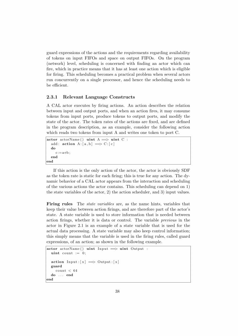
guard expressions of the actions and the requirements regarding availabilityof tokens on input FIFOs and space on output FIFOs. On the program(network) level, scheduling is concerned with finding an actor which canfire, which in practice means that it has at least one action which is eligiblefor firing. This scheduling becomes a practical problem when several actorsrun concurrently on a single processor, and hence the scheduling needs tobe efficient.

2.3.1 Relevant Language Constructs

A CAL actor executes by firing actions. An action describes the relationbetween input and output ports, and when an action fires, it may consumetokens from input ports, produce tokens to output ports, and modify thestate of the actor. The token rates of the actions are fixed, and are definedin the program description, as an example, consider the following actionwhich reads two tokens from input A and writes one token to port C.

actor actorName ( ) uint A ==> uint C :add : action A : [ a , b ] ==> C : [ c ]do

c :=a+b ;end

end

If this action is the only action of the actor, the actor is obviously SDFas the token rate is static for each firing; this is true for any action. The dy-namic behavior of a CAL actor appears from the interaction and schedulingof the various actions the actor contains. This scheduling can depend on 1)the state variables of the actor, 2) the action scheduler, and 3) input values.

Firing rules The state variables are, as the name hints, variables thatkeep their value between action firings, and are therefore part of the actor’sstate. A state variable is used to store information that is needed betweenaction firings, whether it is data or control. The variable previous in theactor in Figure 2.1 is an example of a state variable that is used for theactual data processing. A state variable may also keep control information;this simply means that the variable is used in the firing rules, called guardexpressions, of an action; as shown in the following example.

actor actorName ( ) uint Input ==> uint Output :uint count := 0 ;

action Input : [ x ] ==> Output : [ x ]guard

count < 64do . . . end

end

38

The other part of the actor state is described by the action scheduler.This construct, if present, is (typically) a Finite State Machine (FSM) whichrestricts when action may fire. The FSM describes a set of states and thetransitions between these states correspond to actions; only actions corre-sponding to outgoing transitions of a specific state may fire in that state.The FSM, as such, already describes the order in which actions may fireand also shows the states where a scheduling decision based on a guard isneeded, as such states have more than one outgoing transitions. While theFSM also could be implemented using state variables, from a schedulingpoint of view, the FSM is more practical as it describes the intention of theprogrammer. An example of the FSM scheduler can be seen in Figure 2.1.

Except for the actor state, the scheduling of actions may depend on theinputs of an actor. An action guard may directly refer to a value on aninput port, which means that the token is read but only removed from thequeue if the guard evaluates to true and the action fires. This is called apeek and can be used to implement behavior where the appropriate actionis schedules based on the value of an input token. Consider the followingactions as an example.

actor actorName ( ) uint A, uint B ==> uint C :d iv id e : action A : [ x ] , B : [ y ] ==> C : [ x/y ]guard

y != 0end

sk ip : action A : [ x ] , B : [ y ] ==>guard

y = 0end

end

This simple actor, divides a stream of values by two, but avoids divisionby zero, by skipping the pairs where the denominator has a zero value. Aguard may also depend on an input value that is first read to a state variable,technically, the guard simply uses the value of the state variable, but froma scheduling point of view, the value of the state variable is now much moredifficult to predict.

The guard expression is the explicit part of the firing rules. For anaction to fire, the guard expression must be evaluated to true, but theremust also be a sufficient number of input tokens available, and in a practicalimplementation with limited buffer sizes, enough space on the output queues.As the actions have fixed token rates, it is trivial to extend the firing ruleswith the check for available inputs and output buffer space.

Special properties So far, the discussion has concerned the basic con-structs and firing rules of a CAL actor. Depending on how a CAL actor is

39

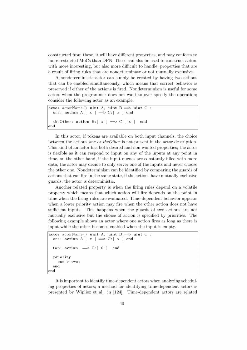
constructed from these, it will have different properties, and may conform tomore restricted MoCs than DPN. These can also be used to construct actorswith more interesting, but also more difficult to handle, properties that area result of firing rules that are nondeterminate or not mutually exclusive.

A nondeterministic actor can simply be created by having two actionsthat can be enabled simultaneously, which means that correct behavior ispreserved if either of the actions is fired. Nondeterminism is useful for someactors when the programmer does not want to over specify the operation;consider the following actor as an example.

actor actorName ( ) uint A, uint B ==> uint C :one : action A : [ x ] ==> C : [ x ] end

theOther : action B : [ x ] ==> C : [ x ] endend

In this actor, if tokens are available on both input channels, the choicebetween the actions one or theOther is not present in the actor description.This kind of an actor has both desired and non wanted properties; the actoris flexible as it can respond to input on any of the inputs at any point intime, on the other hand, if the input queues are constantly filled with moredata, the actor may decide to only server one of the inputs and never choosethe other one. Nondeterminism can be identified by comparing the guards ofactions that can fire in the same state, if the actions have mutually exclusiveguards, the actor is deterministic.

Another related property is when the firing rules depend on a volatileproperty which means that which action will fire depends on the point intime when the firing rules are evaluated. Time-dependent behavior appearswhen a lower priority action may fire when the other action does not havesufficient inputs. This happens when the guards of two actions are notmutually exclusive but the choice of action is specified by priorities. Thefollowing example shows an actor where one action fires as long as there isinput while the other becomes enabled when the input is empty.

actor actorName ( ) uint A, uint B ==> uint C :one : action A : [ x ] ==> C : [ x ] end

two : action ==> C : [ 0 ] end

priorityone > two ;

endend

It is important to identify time-dependent actors when analyzing schedul-ing properties of actors; a method for identifying time-dependent actors ispresented by Wipliez et al. in [124]. Time-dependent actors are related

40

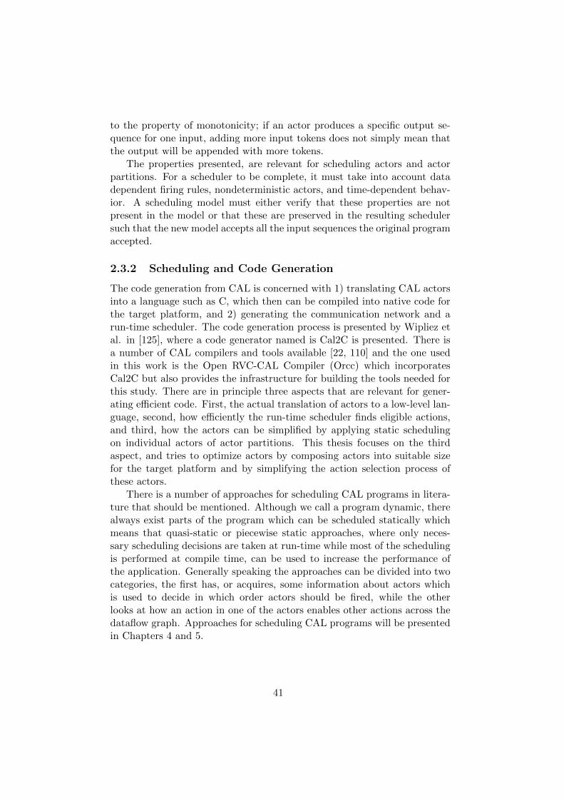
to the property of monotonicity; if an actor produces a specific output se-quence for one input, adding more input tokens does not simply mean thatthe output will be appended with more tokens.

The properties presented, are relevant for scheduling actors and actorpartitions. For a scheduler to be complete, it must take into account datadependent firing rules, nondeterministic actors, and time-dependent behav-ior. A scheduling model must either verify that these properties are notpresent in the model or that these are preserved in the resulting schedulersuch that the new model accepts all the input sequences the original programaccepted.

2.3.2 Scheduling and Code Generation

The code generation from CAL is concerned with 1) translating CAL actorsinto a language such as C, which then can be compiled into native code forthe target platform, and 2) generating the communication network and arun-time scheduler. The code generation process is presented by Wipliez etal. in [125], where a code generator named is Cal2C is presented. There isa number of CAL compilers and tools available [22, 110] and the one usedin this work is the Open RVC-CAL Compiler (Orcc) which incorporatesCal2C but also provides the infrastructure for building the tools needed forthis study. There are in principle three aspects that are relevant for gener-ating efficient code. First, the actual translation of actors to a low-level lan-guage, second, how efficiently the run-time scheduler finds eligible actions,and third, how the actors can be simplified by applying static schedulingon individual actors of actor partitions. This thesis focuses on the thirdaspect, and tries to optimize actors by composing actors into suitable sizefor the target platform and by simplifying the action selection process ofthese actors.

There is a number of approaches for scheduling CAL programs in litera-ture that should be mentioned. Although we call a program dynamic, therealways exist parts of the program which can be scheduled statically whichmeans that quasi-static or piecewise static approaches, where only neces-sary scheduling decisions are taken at run-time while most of the schedulingis performed at compile time, can be used to increase the performance ofthe application. Generally speaking the approaches can be divided into twocategories, the first has, or acquires, some information about actors whichis used to decide in which order actors should be fired, while the otherlooks at how an action in one of the actors enables other actions across thedataflow graph. Approaches for scheduling CAL programs will be presentedin Chapters 4 and 5.

41

42

Chapter 3

The Scheduling Problem

Every dynamic dataflow program can be scheduled with a finite set of staticschedules. On the one extreme, a static schedule is a single action and ascheduling decision is made between each action firing; on the other extreme,a static schedule is identified for each combination of program state andinput sequence of finite length. Somewhere between these two ridiculousextremes, we can find more practical trade-offs that will affect differentproperties of the program such as the number of conditional branches aprogram will have or the cache behavior of that program.

The scheduling of a dataflow program is not a trivial task when perfor-mance, measured in whatever sense, is the goal. As will be further discussedin Chapter 6 (and shown by the results in Paper III), it is not always theconfiguration with the least run-time scheduling decisions, and the largestactor compositions, that will give the best results, but instead the schedul-ing should be tuned to fit the chosen hardware architecture. As a result,scheduling should be performed in smaller steps where the first steps areplatform independent and are used to transform the program in to a repre-sentation that can be used to produce schedules according to the propertiesof the platform. In practice, this means that a program or part of a programfirst should be translated into a representation similar to a partial order fromwhich actual schedules can be generated.

Consequently, scheduling can be viewed as the following operations.First conditions that are definitely compile-time are identified; these areguard evaluations that can be decided from within the actor at compile-time. Next, inter action dependencies are analyzed and based on this, theconditions are found to be either static or dynamic depending on how actorsare composed. Last, the actors are composed according to these dependen-cies such that the platform decides the size of the compositions.

The scheduling problem can in simple words be described as, resolvinghow parts of a dynamic dataflow program can be identified to belong to

43

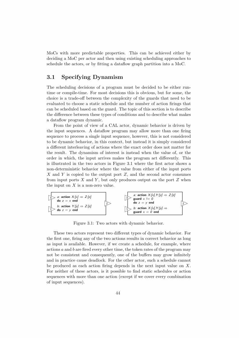
MoCs with more predictable properties. This can be achieved either bydeciding a MoC per actor and then using existing scheduling approaches toschedule the actors, or by fitting a dataflow graph partition into a MoC.

3.1 Specifying Dynamism

The scheduling decisions of a program must be decided to be either run-time or compile-time. For most decisions this is obvious, but for some, thechoice is a trade-off between the complexity of the guards that need to beevaluated to choose a static schedule and the number of action firings thatcan be scheduled based on the guard. The topic of this section is to describethe difference between these types of conditions and to describe what makesa dataflow program dynamic.

From the point of view of a CAL actor, dynamic behavior is driven bythe input sequences. A dataflow program may allow more than one firingsequence to process a single input sequence, however, this is not consideredto be dynamic behavior, in this context, but instead it is simply considereda different interleaving of actions where the exact order does not matter forthe result. The dynamism of interest is instead when the value of, or theorder in which, the input arrives makes the program act differently. Thisis illustrated in the two actors in Figure 3.1 where the first actor shows anon-deterministic behavior where the value from either of the input portsX and Y is copied to the output port Z, and the second actor consumesfrom input ports X and Y , but only produces output on the port Z whenthe input on X is a non-zero value.

a: action X:[x] ⇒ Z:[z]do z = x end

b: action Y:[y] ⇒ Z:[z]do z = y end

X

Y

Z

a: action X:[x],Y:[y] ⇒ Z:[z]guard x != 0do z = y end

b: action X:[x],Y:[y] ⇒guard x = 0 end

X

Y

Z

Figure 3.1: Two actors with dynamic behavior.

These two actors represent two different types of dynamic behavior. Forthe first one, firing any of the two actions results in correct behavior as longas input is available. However, if we create a schedule, for example, whereactions a and b are fired every other time, the token rates of the program maynot be consistent and consequently, one of the buffers may grow infinitelyand in practice cause deadlock. For the other actor, such a schedule cannotbe produced as each action firing depends in the next input value on X.For neither of these actors, is it possible to find static schedules or actionsequences with more than one action (except if we cover every combinationof input sequences).

44

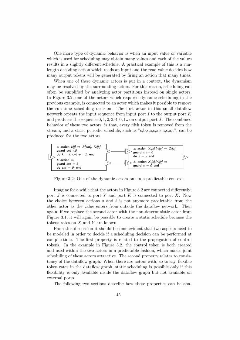
One more type of dynamic behavior is when an input value or variablewhich is used for scheduling may obtain many values and each of the valuesresults in a slightly different schedule. A practical example of this is a run-length decoding action which reads an input and the read value decides howmany output tokens will be generated by firing an action that many times.

When one of these dynamic actors is put in a context, the dynamismmay be resolved by the surrounding actors. For this reason, scheduling canoften be simplified by analyzing actor partitions instead on single actors.In Figure 3.2, one of the actors which required dynamic scheduling in theprevious example, is connected to an actor which makes it possible to removethe run-time scheduling decision. The first actor in this small dataflownetwork repeats the input sequence from input port I to the output port Kand produces the sequence 0, 1, 2, 3, 4, 0, 1.. on output port J . The combinedbehavior of these two actors, is that, every fifth token is removed from thestream, and a static periodic schedule, such as ”s,b,s,a,s,a,s,a,s,a,t”, can beproduced for the two actors.

s: action I:[i] ⇒ J:[cnt], K:[k]guard cnt <5do k = i; cnt += 1; end

t: action ⇒guard cnt = 5do cnt = 0; end

J

K

I

a: action X:[x],Y:[y] ⇒ Z:[z]guard x != 0do z = y end

b: action X:[x],Y:[y] ⇒guard x = 0 end

X

Y

Z

Figure 3.2: One of the dynamic actors put in a predictable context.

Imagine for a while that the actors in Figure 3.2 are connected differently;port J is connected to port Y and port K is connected to port X. Nowthe choice between actions a and b is not anymore predictable from theother actor as the value enters from outside the dataflow network. Thenagain, if we replace the second actor with the non-deterministic actor fromFigure 3.1, it will again be possible to create a static schedule because thetokens rates on X and Y are known.

From this discussion it should become evident that two aspects need tobe modeled in order to decide if a scheduling decision can be performed atcompile-time. The first property is related to the propagation of controltokens. In the example in Figure 3.2, the control token is both createdand used within the two actors in a predictable fashion, which makes jointscheduling of these actors attractive. The second property relates to consis-tency of the dataflow graph. When there are actors with, so to say, flexibletoken rates in the dataflow graph, static scheduling is possible only if thisflexibility is only available inside the dataflow graph but not available onexternal ports.

The following two sections describe how these properties can be ana-

45

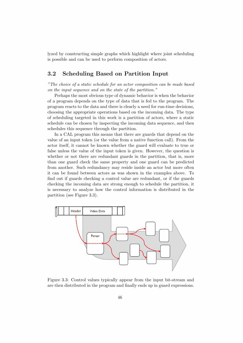
lyzed by constructing simple graphs which highlight where joint schedulingis possible and can be used to perform composition of actors.

3.2 Scheduling Based on Partition Input

”The choice of a static schedule for an actor composition can be made basedon the input sequence and on the state of the partition.”

Perhaps the most obvious type of dynamic behavior is when the behaviorof a program depends on the type of data that is fed to the program. Theprogram reacts to the data and there is clearly a need for run-time decisions,choosing the appropriate operations based on the incoming data. The typeof scheduling targeted in this work is a partition of actors, where a staticschedule can be chosen by inspecting the incoming data sequence, and thenschedules this sequence through the partition.

In a CAL program this means that there are guards that depend on thevalue of an input token (or the value from a native function call). From theactor itself, it cannot be known whether the guard will evaluate to true orfalse unless the value of the input token is given. However, the question iswhether or not there are redundant guards in the partition, that is, morethan one guard check the same property and one guard can be predictedfrom another. Such redundancy may reside inside an actor but more oftenit can be found between actors as was shown in the examples above. Tofind out if guards checking a control value are redundant, or if the guardschecking the incoming data are strong enough to schedule the partition, itis necessary to analyze how the control information is distributed in thepartition (see Figure 3.3).

Figure 3.3: Control values typically appear from the input bit-stream andare then distributed in the program and finally ends up in guard expressions.

46

Scheduling a partition of actors based on the input sequences to thepartition requires some properties to hold regarding firing rules and how theinformation propagates in the partition. Before discussing these properties,some definitions are needed.

Definition 3.1. Variable Dependency Graph. The internal behavior of theactors is described as a directed graph GR = (V,R) where V is the set ofvariables and the edges are described by the binary relation R ⊆ V ×V suchthat (v1, v2) ∈ R indicates that 1) v1 is assigned a value based on variablev2, or 2) v1 is associated to an input port which is connected to an outputport associated to v2.

Definition 3.2. Control Token Path. A control token is a value on a FIFOthat eventually ends up in a guard expression. This means that, for eachvariable directly used in a guard, each node reachable in GR is part of thecontrol token path.

Definition 3.3. Guard Strength. A set of guards are sufficient (strongenough) for scheduling a partition when these describe every scenario of thecontrol token paths of the partition.

3.2.1 Choices and Redundant Choices

”Efficient scheduling means that once a property is checked when data entersthe partition, it should not be checked again inside the same partition.”

To understand why redundancy can be expected in a CAL program, itis necessary to pay some attention to why dynamic behavior typically isintroduced in a program. There are mainly two sources of dynamic behav-ior. The main driving factor is the input-stream which, depending on itscontents, requires the program to act differently. The second factor is theimplementation choices, that is, how the algorithms have been implemented;this also includes how the information from the input-stream is describedand distributed in the dataflow network.

To begin with, the input-stream, as such, defines how much of thescheduling must be performed at run-time. If there is a part of the in-put bit-stream that can hold one of several types of content, the applicationmust also have the corresponding check to choose the appropriate function-ality for the content at run-time. A stream parser, most usually, makes thischeck but also the other actors that depend on this check typically receivesthis information as a control value on which they make a check. As an ex-ample consider a video decoder application where a parser reads the inputstream and produces blocks which are distributed to the different codingtools; see Figure 3.3. A block can be represented by motion vectors (MV)and the 64 coefficients representing the block, but, it is also necessary to

47

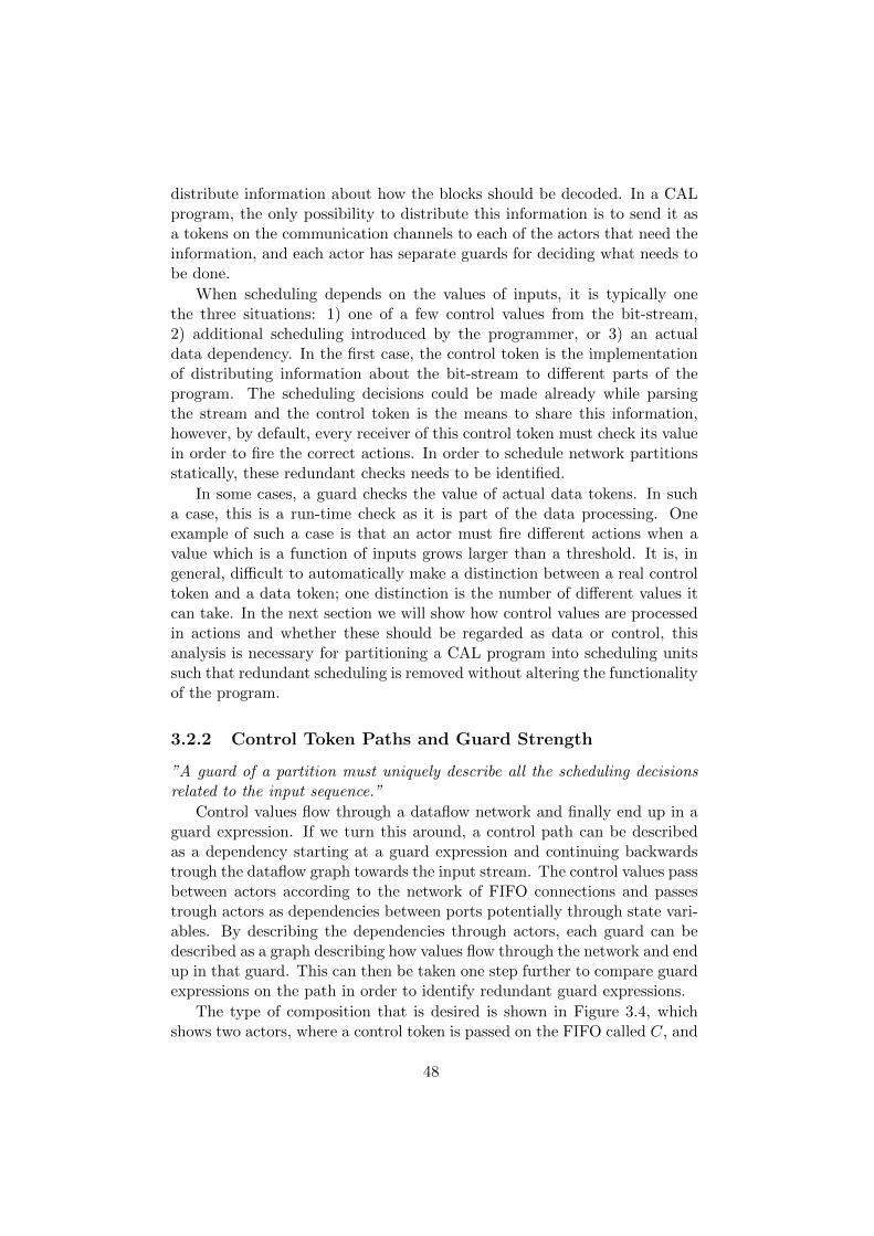
distribute information about how the blocks should be decoded. In a CALprogram, the only possibility to distribute this information is to send it asa tokens on the communication channels to each of the actors that need theinformation, and each actor has separate guards for deciding what needs tobe done.

When scheduling depends on the values of inputs, it is typically onethe three situations: 1) one of a few control values from the bit-stream,2) additional scheduling introduced by the programmer, or 3) an actualdata dependency. In the first case, the control token is the implementationof distributing information about the bit-stream to different parts of theprogram. The scheduling decisions could be made already while parsingthe stream and the control token is the means to share this information,however, by default, every receiver of this control token must check its valuein order to fire the correct actions. In order to schedule network partitionsstatically, these redundant checks needs to be identified.

In some cases, a guard checks the value of actual data tokens. In sucha case, this is a run-time check as it is part of the data processing. Oneexample of such a case is that an actor must fire different actions when avalue which is a function of inputs grows larger than a threshold. It is, ingeneral, difficult to automatically make a distinction between a real controltoken and a data token; one distinction is the number of different values itcan take. In the next section we will show how control values are processedin actions and whether these should be regarded as data or control, thisanalysis is necessary for partitioning a CAL program into scheduling unitssuch that redundant scheduling is removed without altering the functionalityof the program.

3.2.2 Control Token Paths and Guard Strength

”A guard of a partition must uniquely describe all the scheduling decisionsrelated to the input sequence.”

Control values flow through a dataflow network and finally end up in aguard expression. If we turn this around, a control path can be describedas a dependency starting at a guard expression and continuing backwardstrough the dataflow graph towards the input stream. The control values passbetween actors according to the network of FIFO connections and passestrough actors as dependencies between ports potentially through state vari-ables. By describing the dependencies through actors, each guard can bedescribed as a graph describing how values flow through the network and endup in that guard. This can then be taken one step further to compare guardexpressions on the path in order to identify redundant guard expressions.

The type of composition that is desired is shown in Figure 3.4, whichshows two actors, where a control token is passed on the FIFO called C, and

48

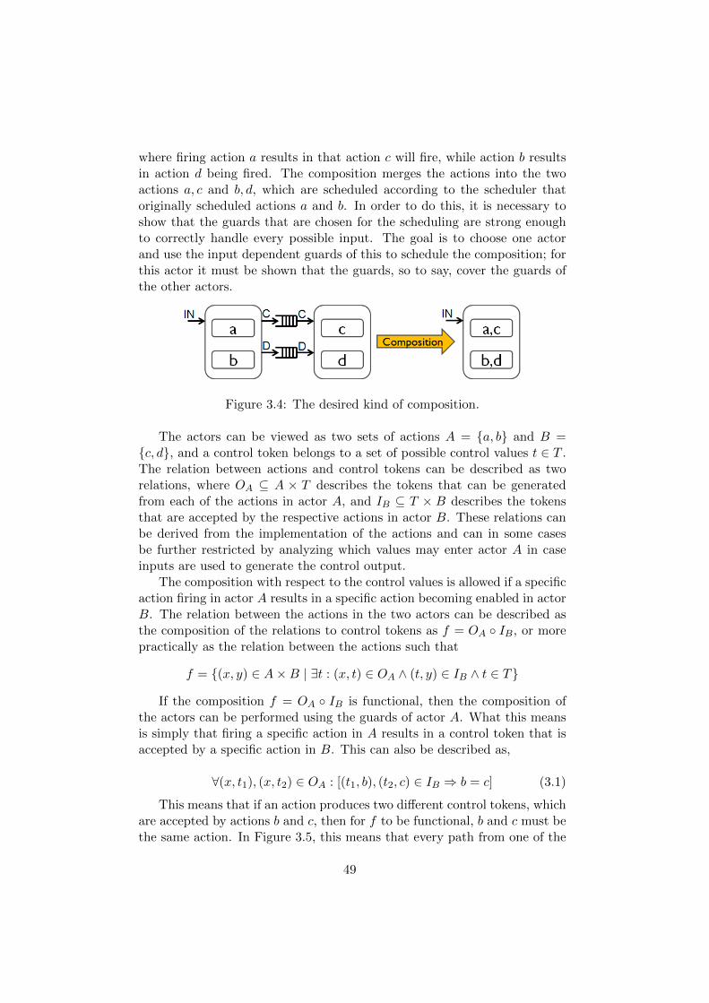
where firing action a results in that action c will fire, while action b resultsin action d being fired. The composition merges the actions into the twoactions a, c and b, d, which are scheduled according to the scheduler thatoriginally scheduled actions a and b. In order to do this, it is necessary toshow that the guards that are chosen for the scheduling are strong enoughto correctly handle every possible input. The goal is to choose one actorand use the input dependent guards of this to schedule the composition; forthis actor it must be shown that the guards, so to say, cover the guards ofthe other actors.

Figure 3.4: The desired kind of composition.

The actors can be viewed as two sets of actions A = {a, b} and B ={c, d}, and a control token belongs to a set of possible control values t ∈ T .The relation between actions and control tokens can be described as tworelations, where OA ⊆ A × T describes the tokens that can be generatedfrom each of the actions in actor A, and IB ⊆ T × B describes the tokensthat are accepted by the respective actions in actor B. These relations canbe derived from the implementation of the actions and can in some casesbe further restricted by analyzing which values may enter actor A in caseinputs are used to generate the control output.

The composition with respect to the control values is allowed if a specificaction firing in actor A results in a specific action becoming enabled in actorB. The relation between the actions in the two actors can be described asthe composition of the relations to control tokens as f = OA ◦ IB, or morepractically as the relation between the actions such that

f = {(x, y) ∈ A×B | ∃t : (x, t) ∈ OA ∧ (t, y) ∈ IB ∧ t ∈ T}

If the composition f = OA ◦ IB is functional, then the composition ofthe actors can be performed using the guards of actor A. What this meansis simply that firing a specific action in A results in a control token that isaccepted by a specific action in B. This can also be described as,

∀(x, t1), (x, t2) ∈ OA : [(t1, b), (t2, c) ∈ IB ⇒ b = c] (3.1)

This means that if an action produces two different control tokens, whichare accepted by actions b and c, then for f to be functional, b and c must bethe same action. In Figure 3.5, this means that every path from one of the

49

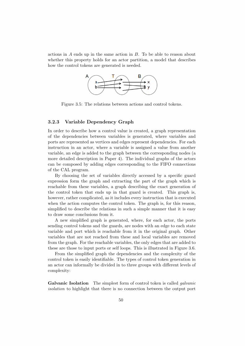
actions in A ends up in the same action in B. To be able to reason aboutwhether this property holds for an actor partition, a model that describeshow the control tokens are generated is needed.

Figure 3.5: The relations between actions and control tokens.

3.2.3 Variable Dependency Graph

In order to describe how a control value is created, a graph representationof the dependencies between variables is generated, where variables andports are represented as vertices and edges represent dependencies. For eachinstruction in an actor, where a variable is assigned a value from anothervariable, an edge is added to the graph between the corresponding nodes (amore detailed description in Paper 4). The individual graphs of the actorscan be composed by adding edges corresponding to the FIFO connectionsof the CAL program.

By choosing the set of variables directly accessed by a specific guardexpression form the graph and extracting the part of the graph which isreachable from these variables, a graph describing the exact generation ofthe control token that ends up in that guard is created. This graph is,however, rather complicated, as it includes every instruction that is executedwhen the action computes the control token. The graph is, for this reason,simplified to describe the relations in such a simple manner that it is easyto draw some conclusions from it.

A new simplified graph is generated, where, for each actor, the portssending control tokens and the guards, are nodes with an edge to each statevariable and port which is reachable from it in the original graph. Othervariables that are not reached from these and local variables are removedfrom the graph. For the reachable variables, the only edges that are added tothese are those to input ports or self loops. This is illustrated in Figure 3.6.

From the simplified graph the dependencies and the complexity of thecontrol token is easily identifiable. The types of control token generation inan actor can informally be divided in to three groups with different levels ofcomplexity:

Galvanic Isolation The simplest form of control token is called galvanicisolation to highlight that there is no connection between the output port

50

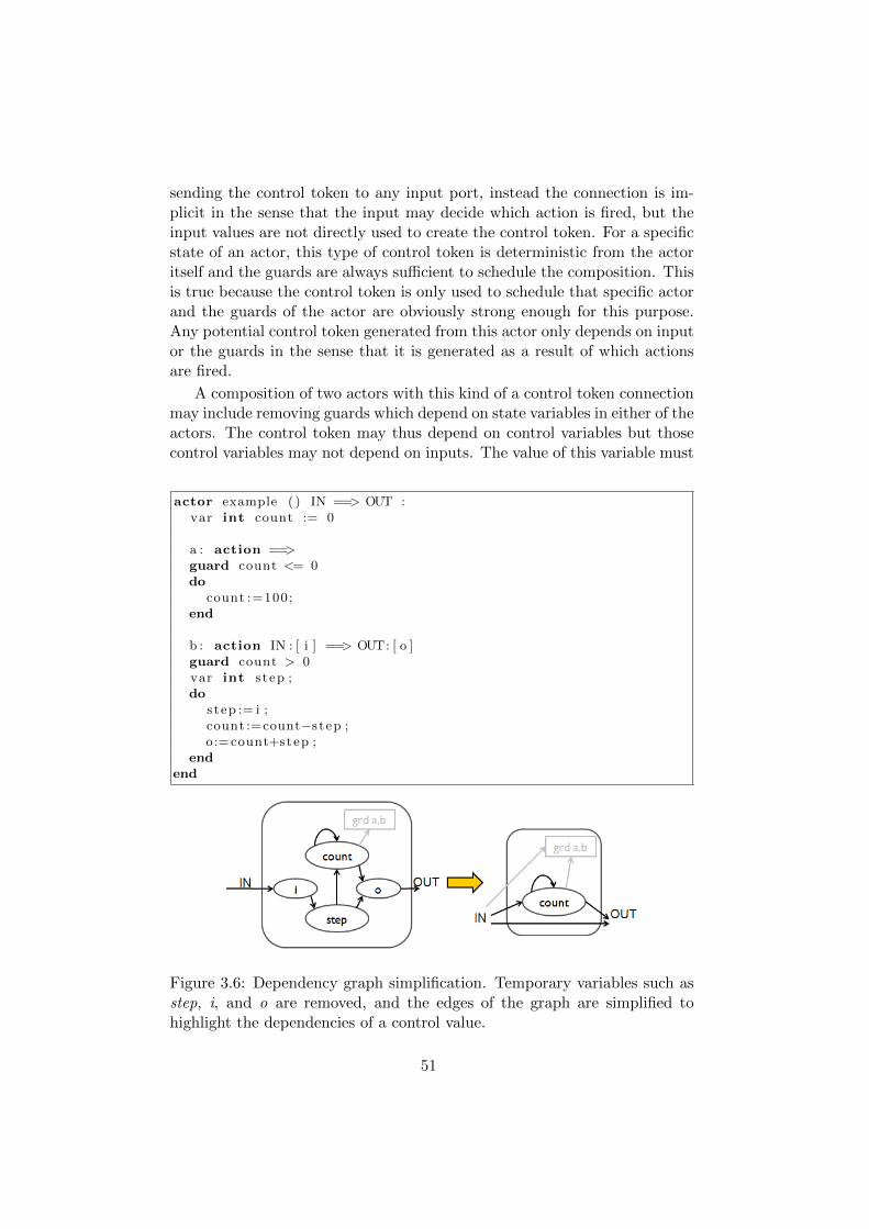
sending the control token to any input port, instead the connection is im-plicit in the sense that the input may decide which action is fired, but theinput values are not directly used to create the control token. For a specificstate of an actor, this type of control token is deterministic from the actoritself and the guards are always sufficient to schedule the composition. Thisis true because the control token is only used to schedule that specific actorand the guards of the actor are obviously strong enough for this purpose.Any potential control token generated from this actor only depends on inputor the guards in the sense that it is generated as a result of which actionsare fired.

A composition of two actors with this kind of a control token connectionmay include removing guards which depend on state variables in either of theactors. The control token may thus depend on control variables but thosecontrol variables may not depend on inputs. The value of this variable must

actor example ( ) IN ==> OUT :var int count := 0

a : action ==>guard count <= 0do

count :=100;end

b : action IN : [ i ] ==> OUT: [ o ]guard count > 0var int s tep ;do

s tep := i ;count :=count−s tep ;o:= count+step ;

endend

Figure 3.6: Dependency graph simplification. Temporary variables such asstep, i, and o are removed, and the edges of the graph are simplified tohighlight the dependencies of a control value.

51

then be used to describe the state of the partition when the scheduling isperformed.

Actors with this kind of control token dependency, can from the pointof view of control tokens, always be composed. The obvious reason for thisis that the control tokens entering a partition are directly used in guardexpressions after which they are never used for scheduling again. Any otherguard is only indirectly depending on the control token and may becomeenable as a result of which action was fired. For scheduling, this is a goodsituation, as the dependencies inside a partition are between action firingsand not input values.

Shared Property A slightly more complicated type of control token prop-agation is when there is an actual connection between a control token enter-ing the actor and the control token leaving the actor, but the generation ofthe control token is instant and completely done within an action firing. Thecontrol token may depend on input ports, but not on variables dependingon input ports. This restriction has two benefits, first, the relation betweenthe input value, the guard, and the output value, is simple. Second, theoutput control token only depends on the inputs read in that firing but noton inputs from previous firings.

The implication of this type of control tokes is that the guards checkingthe inputs of a composition must be proved to cover all the properties thataffect the actors of the composition. Fortunately, the restrictions regardinghow the control tokens are generated makes the verification simple. As thereis no history of control tokens used, there is no need to verify properties ofinput sequences but only on individual control tokens. This fits well withformula (3.1) which can be verified for every pair of possible input values;this will be more closely discussed in Chapter 5.

Shared Information Path The third type of control information pathdoes not have any of the restriction of the two previous types. In the generalcase, it is difficult to analyze this kind of control tokens, as the value of thetoken may be a result of the history of inputs. By allowing the controlpath to include state variables, the propagation of control tokens throughan actor is not necessarily purely the firing on an action, but the value of aninput may reside in the actor between actor firings and be used at a laterpoint to produce the output control token.

The main problem with this, is, that it is not anymore enough to ana-lyze single input tokens, but instead, sequences of inputs may be required.Composition of actors with this type of control token propagation is notperformed, in the general case, as the control is more close to being partof the computations than simply propagating information. In some cases,

52

however, it is possible to transform the actor to correspond to the previoustype, e.g. by merging actions that always fire in sequence and replacing statevariables by local variables. In other cases, when a state variable with anunpredictable behavior is used to produce a control value, the state variableitself could be viewed as an input port, which then would move the behaviorof the variable outside the analysis.

While some automation of the verification of the guard strengths regard-ing control tokens and transformations of the actors to allow this verificationshould be possible, it is outside the scope of this thesis. Instead this thesisfocuses on showing what is needed to obtain correct models, and how thiscan be used to allow efficient composition of actors.

3.2.4 A Few Complex or Many Simple Guards?

”A few more simple guards may be less of an effort than a few complexguards.”

The process of building the scheduling models is concerned with findinga trade-off between, on the one hand, complex guards and a large numberof guards to choose from but large partitions with long static sequencesof action firings, and on the other hand, simple guards and scheduler butshorter schedules and smaller partitions. The basic idea in the approach wehave used in this work, is to avoid making the guards more complex butinstead choose a set of actors such that the actor with the strongest guards,in that sense that a guard being evaluated to true in that actor implies aspecific behavior in the other actors, makes the evaluation of the guards ofthe other actors redundant.

The reason is evident from the combinatorics of the guard conditions.An actor with n guarded actions needs, with an even distribution of inputvalues matching the different guards, on average to evaluate cn = 1

n

∑nk=1(k)

guard expressions 1. If two such actors have either identical guards or theguards check the same property of the input, then the number of checks forthe two actors can be reduced from 2cn to cn. If the guards does not checkthe same property of the input, the combination of the guards would meanthat the number of guards is n2 where each guard consists of one condition

from each actor, this would result in an average of cn×n = 2n2

∑n2

k=1(k) whichis larger than cn when n > 1.

There are, of course, special cases where guards partially overlap and thenumber of needed guards would be larger than n and smaller than n2, but asthe trade-off in such cases would be platform dependent, the choice must beleft for the designer. An example of this can be found in Chapter 7, where

1One could argue that only n−1 guard evaluations are needed for n actions as the lastguard obviously must be true if the previous was not, in any case, this would not affectthe result

53

one of the case studies is constructed from guards which partially overlap.The problem, however, is that it is not trivial to construct the guards, as isthe case when the guards of a single actor is used.

3.3 Nondeterminism and Time-dependent Actors

The other type of dynamic behavior is when an actor is nondeterministic.In many popular programming languages, there is no such thing as non-determinism, and, nondeterminism does introduce some problems, as tworuns of the program may produce different results but still be correct. Inan imperative programming language, for example, an alternative statementhas a defined order in which expressions are evaluated. The statement

if E_1 then S_1

else is E_2 then S_2

will only evaluate the guard represented by E2 if E1 is evaluated to false.This means that there is an implicit negation of E1 in E2, which makes thetwo alternatives mutually exclusive. In a guarded command based language,such as Promela, however, the statement

if

:: E1 -> S1

:: E2 -> S2

fi;

is nondeterministic if the guard expressions are not mutually exclusive. Insuch a case, the language does not define which of the commands should beexecuted, instead, either choice is correct.

The introduction of nondeterminism in a programming language mayintroduce some confusion for a programmer, at the same time, it enablesthe programmer to not specify the program to much. Dijkstra includednondeterminism in guarded commands, after stating that he ”had to over-come a considerable mental resistance before [he] found [himself] willing toconsider nondeterministic programs seriously” [45]. However, he added thathe ”could never have discovered the calculus before having taken that hur-dle: the simplicity and elegance of the above would have been destroyed byrequiring the derivation of deterministic programs only”.

How, and if the nondeterminism is removed in a final implementationwas left to circumstances.

Lee and Parks list five methods in which nondeterminism can be addedto Kahn networks. The first two methods, which are available in CAL, areby 1) allowing processes to test input channels for emptiness, and 2) allowingprocesses to be internally nondeterminate. Methods three and four are to

54

allow more than one process to write to respectively consume data from achannel. And last, by allowing processes to share variables. [83]

As mentioned, the nondeterminism we deal with in CAL is the firsttwo methods. That is, 1) one action may become enabled if an actionwith higher priority is waiting for input, or 2) two actions may be enabledsimultaneously. We distinguish these two kinds of nondeterminism from eachother as the first is only nondeterministic in the sense that it has differentbehavior depending on when input arrives while the other one is internallynondeterministic.

Definition 3.4. Time-Dependent Actor. An actor is time-dependent whena lower priority action requires fewer tokens than a higher priority actionand their guard expressions are not mutually exclusive; hence, the behaviordepends on the time when the tokens are available [124].

From a scheduling point of view, looking at one actor, we may find acorrect schedule for the actor which may not be correct in a certain context.Then again, a nondeterministic actor may in composition with another actorproduce a deterministic composed actor. The scheduling problem, hence, isto determine which actors can be composed to deterministic actors such thatthe nondeterminism and scheduling decision are resolved at design time.

For many-core implementations, it may not always desirable to removenondeterminism. Instead, this can be used for improving load balancingas an actor can work in one mode as long as input is available but switchat another mode, and do some low priority work, when there is no inputavailable. In any case, the goal here is to remove as much nondeterminismas possible, and where it cannot be removed, e.g. where it is used to handlevariable data rates, it will be kept as it is.

3.3.1 Introduction of Time-dependency by Composition

”A composition of time-independent actors cannot be allowed to becometime-dependent.”

A composition of two actors can incorrectly become time-dependent ifthe guards chosen for the composition are not strong enough. Consider theexample in Figure 3.7, which shows two actors which have input dependentguards. According to the analysis presented so far these two actors can becomposed and jointly scheduled, as the actor to the left decides which actionwill fire in the actor to the right; and this is true. There is, however, oneproblem, when we consider the two schedules for a potential composition:(s, a) and (t, b), which can be chosen based on the guards of the left actor.The composed actor (see Figure 3.8a) now has two input ports: I and Y ,which means that the lower priority action has less input dependencies than

55

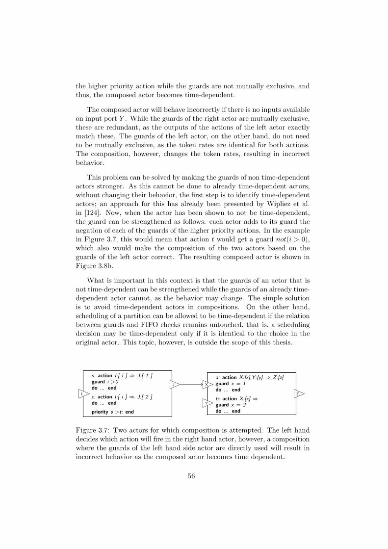
the higher priority action while the guards are not mutually exclusive, andthus, the composed actor becomes time-dependent.

The composed actor will behave incorrectly if there is no inputs availableon input port Y . While the guards of the right actor are mutually exclusive,these are redundant, as the outputs of the actions of the left actor exactlymatch these. The guards of the left actor, on the other hand, do not needto be mutually exclusive, as the token rates are identical for both actions.The composition, however, changes the token rates, resulting in incorrectbehavior.

This problem can be solved by making the guards of non time-dependentactors stronger. As this cannot be done to already time-dependent actors,without changing their behavior, the first step is to identify time-dependentactors; an approach for this has already been presented by Wipliez et al.in [124]. Now, when the actor has been shown to not be time-dependent,the guard can be strengthened as follows: each actor adds to its guard thenegation of each of the guards of the higher priority actions. In the examplein Figure 3.7, this would mean that action t would get a guard not(i > 0),which also would make the composition of the two actors based on theguards of the left actor correct. The resulting composed actor is shown inFigure 3.8b.

What is important in this context is that the guards of an actor that isnot time-dependent can be strengthened while the guards of an already time-dependent actor cannot, as the behavior may change. The simple solutionis to avoid time-dependent actors in compositions. On the other hand,scheduling of a partition can be allowed to be time-dependent if the relationbetween guards and FIFO checks remains untouched, that is, a schedulingdecision may be time-dependent only if it is identical to the choice in theoriginal actor. This topic, however, is outside the scope of this thesis.

s: action I:[ i ] ⇒ J:[ 1 ]guard i >0do ... end

t: action I:[ i ] ⇒ J:[ 2 ]do ... end

priority s >t; end

J

I

a: action X:[x],Y:[y] ⇒ Z:[z]guard x = 1do ... end

b: action X:[x] ⇒guard x = 2do ... end

X

Y

Z

Figure 3.7: Two actors for which composition is attempted. The left handdecides which action will fire in the right hand actor, however, a compositionwhere the guards of the left hand side actor are directly used will result inincorrect behavior as the composed actor becomes time dependent.

56

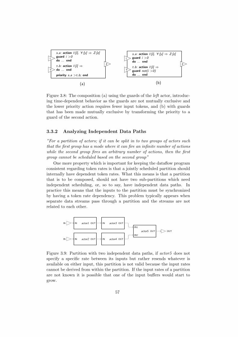
s a: action I:[i], Y:[y] ⇒ Z:[z]guard i >0do ... end

t b: action I:[i] ⇒do ... end

priority s a >t b; end

I

Z

Y

(a)

s a: action I:[i], Y:[y] ⇒ Z:[z]guard i >0do ... end

t b: action I:[i] ⇒guard not(i >0)do ... end

I

Z

Y

(b)

Figure 3.8: The composition (a) using the guards of the left actor, introduc-ing time-dependent behavior as the guards are not mutually exclusive andthe lower priority action requires fewer input tokens, and (b) with guardsthat has been made mutually exclusive by transforming the priority to aguard of the second action.

3.3.2 Analyzing Independent Data Paths

”For a partition of actors; if it can be split in to two groups of actors suchthat the first group has a mode where it can fire an infinite number of actionswhile the second group fires an arbitrary number of actions, then the firstgroup cannot be scheduled based on the second group”

One more property which is important for keeping the dataflow programconsistent regarding token rates is that a jointly scheduled partition shouldinternally have dependent token rates. What this means is that a partitionthat is to be composed, should not have two sub-partitions which needindependent scheduling, or, so to say, have independent data paths. Inpractice this means that the inputs to the partition must be synchronizedby having a token rate dependency. This problem typically appears whenseparate data streams pass through a partition and the streams are notrelated to each other.

actor1IN OUT

actor2IN OUT

actor3IN OUT

actor4IN OUT

actor5

IN1

IN2

OUT

IN

OUT

IN

Figure 3.9: Partition with two independent data paths, if actor5 does notspecify a specific rate between its inputs but rather resends whatever isavailable on either input, this partition is not valid because the input ratescannot be derived from within the partition. If the input rates of a partitionare not known it is possible that one of the input buffers would start togrow.

57

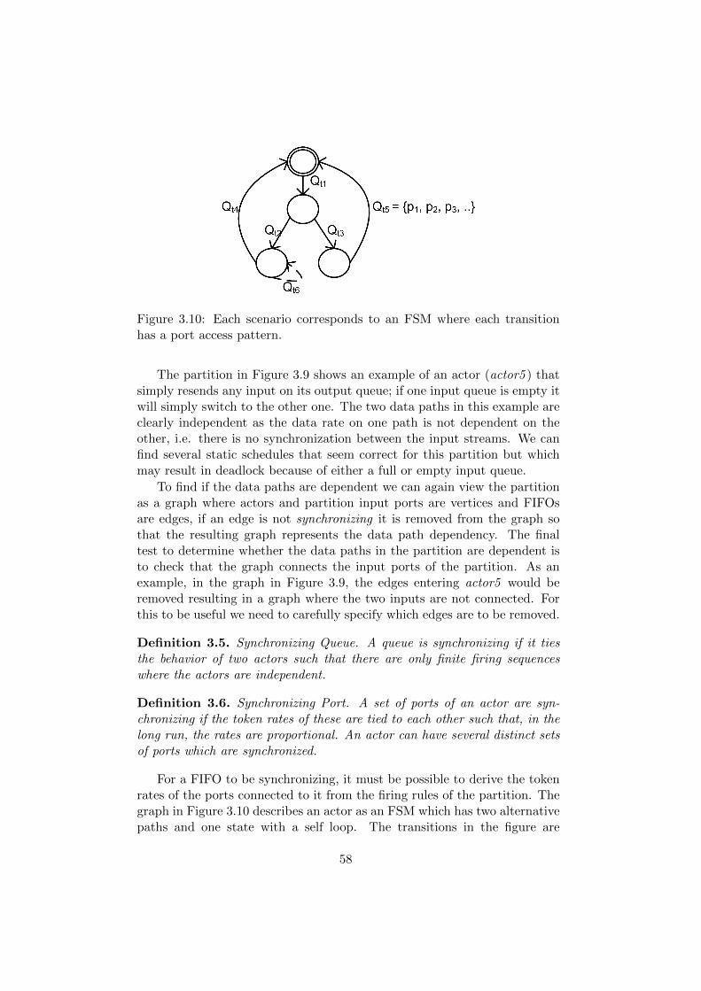
Figure 3.10: Each scenario corresponds to an FSM where each transitionhas a port access pattern.

The partition in Figure 3.9 shows an example of an actor (actor5 ) thatsimply resends any input on its output queue; if one input queue is empty itwill simply switch to the other one. The two data paths in this example areclearly independent as the data rate on one path is not dependent on theother, i.e. there is no synchronization between the input streams. We canfind several static schedules that seem correct for this partition but whichmay result in deadlock because of either a full or empty input queue.

To find if the data paths are dependent we can again view the partitionas a graph where actors and partition input ports are vertices and FIFOsare edges, if an edge is not synchronizing it is removed from the graph sothat the resulting graph represents the data path dependency. The finaltest to determine whether the data paths in the partition are dependent isto check that the graph connects the input ports of the partition. As anexample, in the graph in Figure 3.9, the edges entering actor5 would beremoved resulting in a graph where the two inputs are not connected. Forthis to be useful we need to carefully specify which edges are to be removed.

Definition 3.5. Synchronizing Queue. A queue is synchronizing if it tiesthe behavior of two actors such that there are only finite firing sequenceswhere the actors are independent.

Definition 3.6. Synchronizing Port. A set of ports of an actor are syn-chronizing if the token rates of these are tied to each other such that, in thelong run, the rates are proportional. An actor can have several distinct setsof ports which are synchronized.

For a FIFO to be synchronizing, it must be possible to derive the tokenrates of the ports connected to it from the firing rules of the partition. Thegraph in Figure 3.10 describes an actor as an FSM which has two alternativepaths and one state with a self loop. The transitions in the figure are

58

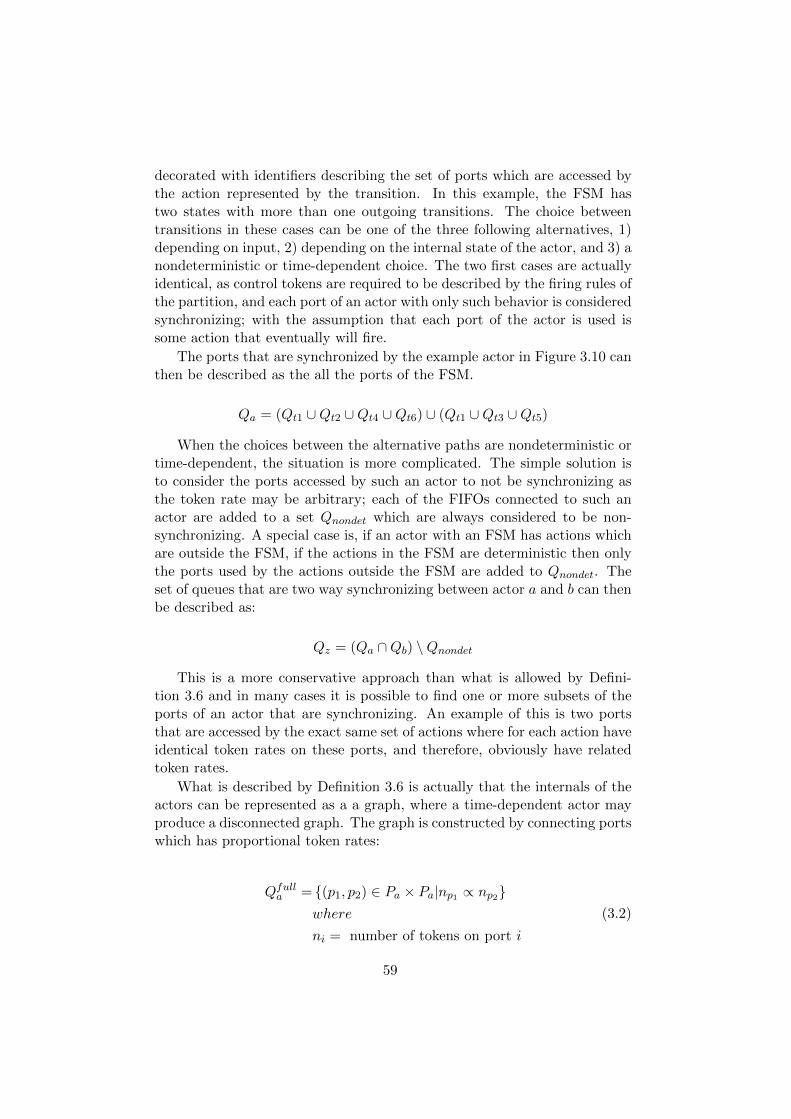
decorated with identifiers describing the set of ports which are accessed bythe action represented by the transition. In this example, the FSM hastwo states with more than one outgoing transitions. The choice betweentransitions in these cases can be one of the three following alternatives, 1)depending on input, 2) depending on the internal state of the actor, and 3) anondeterministic or time-dependent choice. The two first cases are actuallyidentical, as control tokens are required to be described by the firing rules ofthe partition, and each port of an actor with only such behavior is consideredsynchronizing; with the assumption that each port of the actor is used issome action that eventually will fire.

The ports that are synchronized by the example actor in Figure 3.10 canthen be described as the all the ports of the FSM.

Qa = (Qt1 ∪Qt2 ∪Qt4 ∪Qt6) ∪ (Qt1 ∪Qt3 ∪Qt5)

When the choices between the alternative paths are nondeterministic ortime-dependent, the situation is more complicated. The simple solution isto consider the ports accessed by such an actor to not be synchronizing asthe token rate may be arbitrary; each of the FIFOs connected to such anactor are added to a set Qnondet which are always considered to be non-synchronizing. A special case is, if an actor with an FSM has actions whichare outside the FSM, if the actions in the FSM are deterministic then onlythe ports used by the actions outside the FSM are added to Qnondet. Theset of queues that are two way synchronizing between actor a and b can thenbe described as:

Qz = (Qa ∩Qb) \Qnondet

This is a more conservative approach than what is allowed by Defini-tion 3.6 and in many cases it is possible to find one or more subsets of theports of an actor that are synchronizing. An example of this is two portsthat are accessed by the exact same set of actions where for each action haveidentical token rates on these ports, and therefore, obviously have relatedtoken rates.

What is described by Definition 3.6 is actually that the internals of theactors can be represented as a a graph, where a time-dependent actor mayproduce a disconnected graph. The graph is constructed by connecting portswhich has proportional token rates:

Qfulla = {(p1, p2) ∈ Pa × Pa|np1 ∝ np2}

where

ni = number of tokens on port i

(3.2)

59

������ �����

������

�� ���� ��� � �

���

��

�����

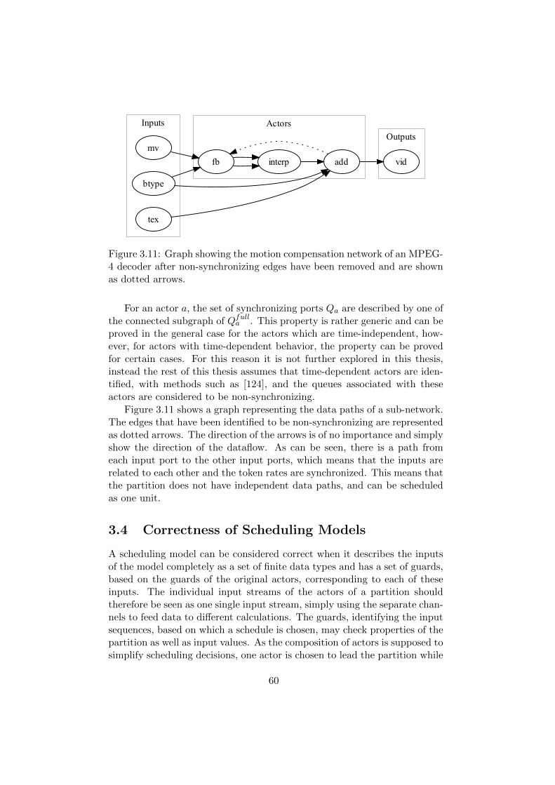
Figure 3.11: Graph showing the motion compensation network of an MPEG-4 decoder after non-synchronizing edges have been removed and are shownas dotted arrows.

For an actor a, the set of synchronizing ports Qa are described by one ofthe connected subgraph of Qfull

a . This property is rather generic and can beproved in the general case for the actors which are time-independent, how-ever, for actors with time-dependent behavior, the property can be provedfor certain cases. For this reason it is not further explored in this thesis,instead the rest of this thesis assumes that time-dependent actors are iden-tified, with methods such as [124], and the queues associated with theseactors are considered to be non-synchronizing.

Figure 3.11 shows a graph representing the data paths of a sub-network.The edges that have been identified to be non-synchronizing are representedas dotted arrows. The direction of the arrows is of no importance and simplyshow the direction of the dataflow. As can be seen, there is a path fromeach input port to the other input ports, which means that the inputs arerelated to each other and the token rates are synchronized. This means thatthe partition does not have independent data paths, and can be scheduledas one unit.

3.4 Correctness of Scheduling Models

A scheduling model can be considered correct when it describes the inputsof the model completely as a set of finite data types and has a set of guards,based on the guards of the original actors, corresponding to each of theseinputs. The individual input streams of the actors of a partition shouldtherefore be seen as one single input stream, simply using the separate chan-nels to feed data to different calculations. The guards, identifying the inputsequences, based on which a schedule is chosen, may check properties of thepartition as well as input values. As the composition of actors is supposed tosimplify scheduling decisions, one actor is chosen to lead the partition while

60

the other actors are forced to follow. This results in that some propertiesmust hold, regarding the leader actor and the rest of the partition, for thescheduling to be successful.

This results in the following type of compositions: 1) Checking inputvalues is only allowed for one actor per partition – the partition leader.Other actors may only use control tokens indirectly by reacting to actionfirings in the leader action. 2) The leader actor must enforce static tokenrates on the other actors’ external inputs. It cannot allow another actor torun an arbitrary number of times without causing buffers to overflow. 3)The partition may work with more data at the time compared to the originalprogram – a schedule instead of an action firing. However, the partitioningis not allowed to introduce time-dependency.

3.4.1 Boundedness of Nondeterminism

There can be two variants of nondeterminism in an actor partition. Thefirst one, which was already discussed earlier in this chapter, adds flexibilityto the order in which actions fire or to the token rates of the actors. Forthis, it is enough to show that the partition does not have less flexibility onits inputs that the original program. The other type of nondeterminism, theone of interest in this section, is not related to what sequences a partitionaccepts or if the partition is deadlock free or not, instead it is more relatedto the semantics of the programming model.

As an example, consider an actor which has a low priority action al whichis used to optimize some parameter of the actor. This action have neitherinputs nor outputs but simply performs some calculations to tune the actor,but does not change the state of anything in the actor related to scheduling.Now, when the actor performs one iteration, it fires a sequence of actionse.g. a1, a2, a3, consumes an input sequence SIN and produces an outputsequence SOUT . Such an iteration may include the action al but it is alsocorrect behavior if it is not fired. Now, if the firing sequence can be firedrepeatedly for any possible input, one simple SDF schedule can be used toschedule this actor, however, and this is the question: is it correct behaviorwhen such a schedule implies that al will either fire once per iteration (if itis included in the schedule) or never (if it is not included in the schedule)?

Technically speaking, the scheduling model does not guarantee unboundnondeterminism. The reason should be obvious; the purpose with schedulingis to choose a minimal number of firing sequences from the great number ofpossible alternatives for interleaving actions that are possible. This in turn,means that a more regular firing pattern is enforced which in turn meansthat nondeterministic behavior becomes deterministic.

61

3.4.2 Valid Partitions

Finally, for a partitioning to be valid, the actors in the partition must be al-lowed to fire without requiring actors outside the partition to be interleaved.When a scheduling model is constructed from an actor partition, it is as-sumed that the required inputs to the partition will become available simplyby waiting for other actors outside the partition to fire enough times. Theproblem arises when the actor that is supposed to produce an input waitsfor tokens from an actor inside the partition. As the scheduling model is re-quired to completely describe the behavior of the partition, we cannot allowthis type of behavior as the required interaction between the partition andthe surrounding actors affects how the partition must be scheduled.

We need something similar to the composition theorem by Pino et al. [105],which states that an SDF composition is valid if it has an acyclic precedencegraph. While this perhaps is unnecessarily strict for a CAL composition, wecan use a variant of it to guarantee correct partitioning. Consider a simpleCAL program with the four actors a, b, c and d. Actor a has a channelto both b and c, while actor d receives tokens from b and c. Based on thetopology, a preorder can be described as {(a ≤ b), (a ≤ c), (b ≤ d), (c ≤ d)}.If a partition, pabd, including the actions a, b, d is proposed, the precedencewill become {(pabd ≤ c), (c ≤ pabd)}, indicating that action c both precedesand succeeds the partition. If the partition is scheduled with the connec-tions to the actor c as simply inputs and outputs to the partition, there isno guarantee that the schedule will be correct.

In order to construct correct partitions, partitions must be constructedsuch that actors outside the partition either precede or succeed the partition,or are independent. This approach is conservative as it omits the actualbehavior of the actions and simply uses the actors and connections to decideif a specific partitioning can be allowed. There will certainly be cases wherethis rule is to strict and will forbid partitions that would work correctly.The goal here is instead to give a sufficient (but not necessary) condition forthat a correct scheduling model can be constructed for a partition.

62

Chapter 4

Analysis of an Actor inIsolation

Even though the target is actor composition, much useful information canbe extracted by analyzing single actors in isolation. The scheduler of asingle actor can often be simplified which as such can improve the generatedcode, but, of course, the goal is to simplify the actors before attempting tocompose the actors. The actor schedulers typically have similar constructsas the control flow of an imperative programming language, however, moreexplicitly described. Consequently, transformations resembling what is usualin most compilers, such as loop unrolling [7], can be performed on the actorscheduler as well. Actor-level scheduling is useful for the scheduling modelsas it groups single input tokens into groups that are to be processed together.A schedule thereby gives the token rates of the actor and is represented asa pair consisting of a guard expression and a sequence of action firings.For a network partition, the schedules of the front-edge actors drive thescheduling by defining the portions of data that can be processed together,then, typically, it is possible to calculate balance equations between theschedules in order to derive the inputs of the partition.

The actor scheduler can always be seen as an FSM, with guards on someof the transitions, and where the transitions (in form of actions) modify thestate of the actor 1. The first thought on analyzing the action scheduler isto identify transitions that are input dependent and to identify loops. Onsecond thoughts, while simple loops are easy to identify from an FSM, formore complex schedulers it is more difficult do define what a loop actuallyis. Consider as an example the FSMs in Figure 4.1; in the first example(a) there are two clear loops, the self loop in the state σ3 and the loopcovering the whole FSM, in the second example (b) the loops are not that

1Actors without an explicit action scheduler are simply seen as an FSM with a singlestate

63

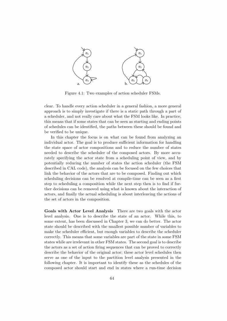
σ2

σ1

σ3 σ4

σ2

σ1

σ3

a. b.

Figure 4.1: Two examples of action scheduler FSMs.

clear. To handle every action scheduler in a general fashion, a more generalapproach is to simply investigate if there is a static path through a part ofa scheduler, and not really care about what the FSM looks like. In practice,this means that if some states that can be seen as starting and ending pointsof schedules can be identified, the paths between these should be found andbe verified to be unique.

In this chapter the focus is on what can be found from analyzing anindividual actor. The goal is to produce sufficient information for handlingthe state space of actor compositions and to reduce the number of statesneeded to describe the scheduler of the composed actors. By more accu-rately specifying the actor state from a scheduling point of view, and bypotentially reducing the number of states the action scheduler (the FSMdescribed in CAL code), the analysis can be focused on the few choices thatlink the behavior of the actors that are to be composed. Finding out whichscheduling decisions can be resolved at compile-time can be seen as a firststep to scheduling a composition while the next step then is to find if fur-ther decisions can be removed using what is known about the interaction ofactors, and finally the actual scheduling is about interleaving the actions ofthe set of actors in the composition.

Goals with Actor Level Analysis There are two goals with the actorlevel analysis. One is to describe the state of an actor. While this, tosome extent, has been discussed in Chapter 3, we can do better. The actorstate should be described with the smallest possible number of variables tomake the scheduler efficient, but enough variables to describe the schedulercorrectly. This means that some variables are part of the state in some FSMstates while are irrelevant in other FSM states. The second goal is to describethe actors as a set of action firing sequences that can be proved to correctlydescribe the behavior of the original actor; these actor level schedules thenserve as one of the input to the partition level analysis presented in thefollowing chapter. It is important to identify these as the schedules of thecomposed actor should start and end in states where a run-time decision

64

is needed; the actor level schedules are for this reason used to predict thescheduler of the partition. As these two goals are strongly related, thefollowing sections will jointly discuss both topics and the approaches thatcan be used to generate this information.

4.1 A Simplified Actor Scheduler

The presented approach can loosely be described as three steps that canbe repeated until a valid model is found; the following steps can be iden-tified: 1) Create a high level description of which schedules optimisticallyare expected to exist, 2) Generate the concrete action sequences represent-ing these schedules, 3 validate that the schedules are unique or if necessarysplit the schedules that are not unique and redo the steps. The approachused resembles abstract interpretation [99, 124], but technically, the modelis restructured before the interpretation to not include any code that woulduse variables with unknown values, but only values that may not be unique.

The starting point is an actor, which is viewed as an FSM where tran-sitions withe guards that depend on a value from outside the actor aremarked as an input dependent transition. A guard is considered to be in-put dependent if a input port (or a value that is returned from a nativefunction) is reachable from the guard in the variable dependency graph.These transitions are considered as dynamic scheduling decisions, and are,as in the example in Figure 4.2, marked with a question mark, indicating apoint where a synchronization with another actor is needed. Before startingthe actor level scheduling stage, the actor is simplified to only include theinstructions and variables that are related to scheduling. This is done sim-ply by removing variables and instructions that are not reachable from anyguard in the actor partition. As a result, the actor will look like the FSMin Figure 4.2 (left), only including a few variables, in this case the variablenamed x.

The idea needs some clarification before continuing with more details.Consider what using abstract interpretation means for analyzing schedulingof a CAL actor; in practice it means that input tokens produces unknownvalues in the actor, which if used in calculations are fine but if used in guardsmeans that it is not possible to know which action to fire next. What is thegoal here is, that, when a state where the guards use such an unknown valueis found, each of the outgoing transitions are examined. It could be thoughtof as, if this guard would evaluate to true, then this would happen. Whena guard is, so to say, forced to evaluate to true, even if the values usedin the guard are unknown, every variable used by that guard must be setto unknown in order to not enable some impossible behavior further on inthe interpretation. How this is actually done in the implementation of this

65

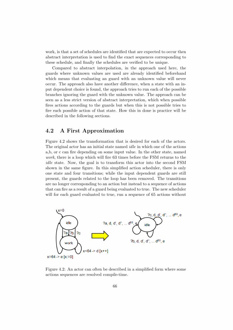
work, is that a set of schedules are identified that are expected to occur thenabstract interpretation is used to find the exact sequences corresponding tothese schedule, and finally the schedules are verified to be unique.

Compared to abstract interpolation, in the approach used here, theguards where unknown values are used are already identified beforehandwhich means that evaluating an guard with an unknown value will neveroccur. The approach also have another difference, when a state with an in-put dependent choice is found, the approach tries to run each of the possiblebranches ignoring the guard with the unknown value. The approach can beseen as a less strict version of abstract interpretation, which when possiblefires actions according to the guards but when this is not possible tries tofire each possible action of that state. How this in done is practice will bedescribed in the following sections.

4.2 A First Approximation

Figure 4.2 shows the transformation that is desired for each of the actors.The original actor has an initial state named idle in which one of the actionsa,b, or c can fire depending on some input value. In the other state, namedwork, there is a loop which will fire 63 times before the FSM returns to theidle state. Now, the goal is to transform this actor into the second FSMshown in the same figure. In this simplified action scheduler, there is onlyone state and four transitions; while the input dependent guards are stillpresent, the guards related to the loop has been removed. The transitionsare no longer corresponding to an action but instead to a sequence of actionsthat can fire as a result of a guard being evaluated to true. The new schedulerwill for each guard evaluated to true, run a sequence of 65 actions without

Figure 4.2: An actor can often be described in a simplified form where someactions sequences are resolved compile-time.

66

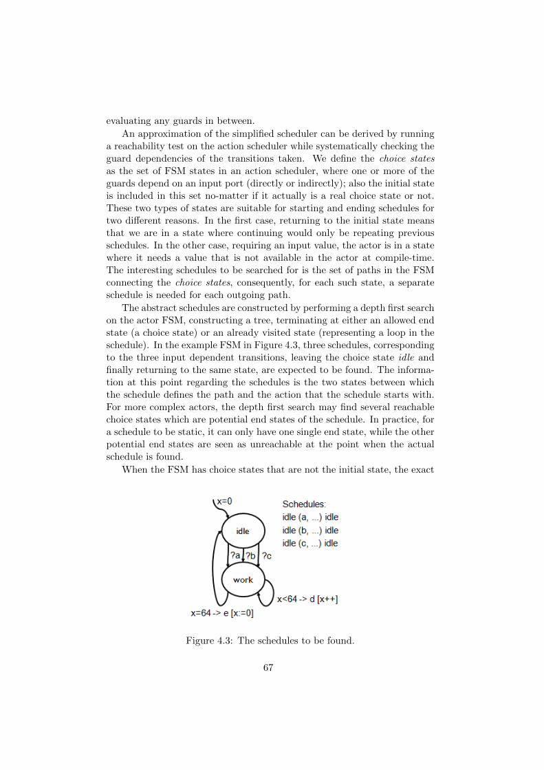
evaluating any guards in between.

An approximation of the simplified scheduler can be derived by runninga reachability test on the action scheduler while systematically checking theguard dependencies of the transitions taken. We define the choice statesas the set of FSM states in an action scheduler, where one or more of theguards depend on an input port (directly or indirectly); also the initial stateis included in this set no-matter if it actually is a real choice state or not.These two types of states are suitable for starting and ending schedules fortwo different reasons. In the first case, returning to the initial state meansthat we are in a state where continuing would only be repeating previousschedules. In the other case, requiring an input value, the actor is in a statewhere it needs a value that is not available in the actor at compile-time.The interesting schedules to be searched for is the set of paths in the FSMconnecting the choice states, consequently, for each such state, a separateschedule is needed for each outgoing path.

The abstract schedules are constructed by performing a depth first searchon the actor FSM, constructing a tree, terminating at either an allowed endstate (a choice state) or an already visited state (representing a loop in theschedule). In the example FSM in Figure 4.3, three schedules, correspondingto the three input dependent transitions, leaving the choice state idle andfinally returning to the same state, are expected to be found. The informa-tion at this point regarding the schedules is the two states between whichthe schedule defines the path and the action that the schedule starts with.For more complex actors, the depth first search may find several reachablechoice states which are potential end states of the schedule. In practice, fora schedule to be static, it can only have one single end state, while the otherpotential end states are seen as unreachable at the point when the actualschedule is found.

When the FSM has choice states that are not the initial state, the exact

Figure 4.3: The schedules to be found.

67

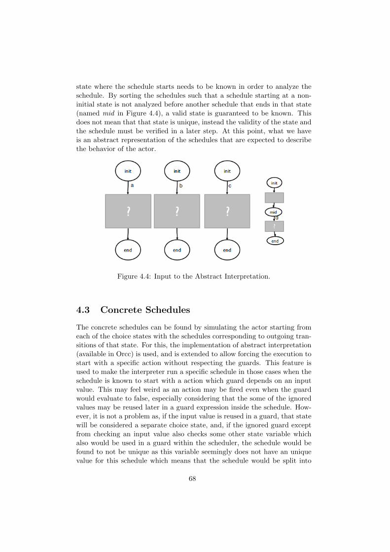
state where the schedule starts needs to be known in order to analyze theschedule. By sorting the schedules such that a schedule starting at a non-initial state is not analyzed before another schedule that ends in that state(named mid in Figure 4.4), a valid state is guaranteed to be known. Thisdoes not mean that that state is unique, instead the validity of the state andthe schedule must be verified in a later step. At this point, what we haveis an abstract representation of the schedules that are expected to describethe behavior of the actor.

Figure 4.4: Input to the Abstract Interpretation.

4.3 Concrete Schedules

The concrete schedules can be found by simulating the actor starting fromeach of the choice states with the schedules corresponding to outgoing tran-sitions of that state. For this, the implementation of abstract interpretation(available in Orcc) is used, and is extended to allow forcing the execution tostart with a specific action without respecting the guards. This feature isused to make the interpreter run a specific schedule in those cases when theschedule is known to start with a action which guard depends on an inputvalue. This may feel weird as an action may be fired even when the guardwould evaluate to false, especially considering that the some of the ignoredvalues may be reused later in a guard expression inside the schedule. How-ever, it is not a problem as, if the input value is reused in a guard, that statewill be considered a separate choice state, and, if the ignored guard exceptfrom checking an input value also checks some other state variable whichalso would be used in a guard within the scheduler, the schedule would befound to not be unique as this variable seemingly does not have an uniquevalue for this schedule which means that the schedule would be split into

68

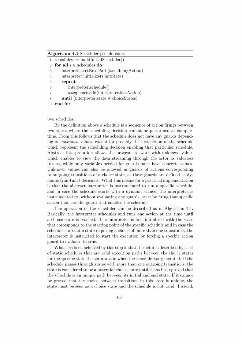
Algorithm 4.1 Scheduler pseudo code.

1: schedules := buildInitialScheduler()2: for all s ∈ schedules do3: interpreter.setNextPath(s.enablingAction)4: interpreter.initialize(s.initState)5: repeat6: interpreter.schedule()7: s.sequence.add(interpreter.lastAction)8: until (interpreter.state ∈ choiceStates)9: end for

two schedules.

By the definition above a schedule is a sequence of action firings betweentwo states where the scheduling decision cannot be performed at compile-time. From this follows that the schedule does not have any guards depend-ing on unknown values, except for possibly the first action of the schedulewhich represent the scheduling decision enabling that particular schedule.Abstract interpretation allows the program to work with unknown valueswhich enables to view the data streaming through the actor as valuelesstokens, while only variables needed for guards must have concrete values.Unknown values can also be allowed in guards of actions correspondingto outgoing transitions of a choice state, as these guards are defined as dy-namic (run-time) decisions. What this means for a practical implementationis that the abstract interpreter is instrumented to run a specific schedule,and in case the schedule starts with a dynamic choice, the interpreter isinstrumented to, without evaluating any guards, start by firing that specificaction that has the guard that enables the schedule.

The operation of the scheduler can be described as in Algorithm 4.1.Basically, the interpreter schedules and runs one action at the time untila choice state is reached. The interpreter is first initialized with the statethat corresponds to the starting point of the specific schedule and in case theschedule starts at a state requiring a choice of more than one transitions, theinterpreter is instructed to start the execution by forcing a specific actionguard to evaluate to true.

What has been achieved by this step is that the actor is described by a setof static schedules that are valid execution paths between the choice statesfor the specific state the actor was in when the schedule was generated. If theschedule passes through states with more than one outgoing transitions, thestate is considered to be a potential choice state until it has been proved thatthe schedule is an unique path between its initial and end state. If it cannotbe proved that the choice between transitions in this state is unique, thestate must be seen as a choice state and the schedule is not valid. Instead,

69

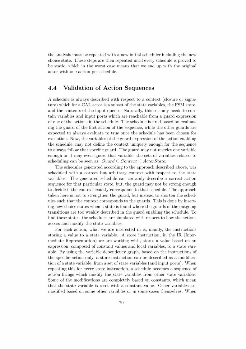
the analysis must be repeated with a new initial scheduler including the newchoice state. These steps are then repeated until every schedule is proved tobe static, which in the worst case means that we end up with the originalactor with one action per schedule.

4.4 Validation of Action Sequences

A schedule is always described with respect to a context (closure or signa-ture) which for a CAL actor is a subset of the state variables, the FSM state,and the contents of the input queues. Naturally, this set only needs to con-tain variables and input ports which are reachable from a guard expressionof one of the actions in the schedule. The schedule is fired based on evaluat-ing the guard of the first action of the sequence, while the other guards areexpected to always evaluate to true once the schedule has been chosen forexecution. Now, the variables of the guard expression of the action enablingthe schedule, may not define the context uniquely enough for the sequenceto always follow that specific guard. The guard may not restrict one variableenough or it may even ignore that variable; the sets of variables related toscheduling can be seen as: Guard ⊆ Context ⊆ ActorState.

The schedules generated according to the approach described above, wasscheduled with a correct but arbitrary context with respect to the statevariables. The generated schedule can certainly describe a correct actionsequence for that particular state, but, the guard may not be strong enoughto decide if the context exactly corresponds to that schedule. The approachtaken here is not to strengthen the guard, but instead to shorten the sched-ules such that the context corresponds to the guards. This is done by insert-ing new choice states when a state is found where the guards of the outgoingtransitions are too weakly described in the guard enabling the schedule. Tofind these states, the schedules are simulated with respect to how the actionsaccess and modify the state variables.

For each action, what we are interested in is, mainly, the instructionsstoring a value to a state variable. A store instruction, in the IR (Inter-mediate Representation) we are working with, stores a value based on anexpression, composed of constant values and local variables, to a state vari-able. By using the variable dependency graph, based on the instructions ofthe specific action only, a store instruction can be described as a modifica-tion of a state variable, from a set of state variables (and input ports). Whenrepeating this for every store instruction, a schedule becomes a sequence ofaction firings which modify the state variables from other state variables.Some of the modifications are completely based on constants, which meanthat the state variable is reset with a constant value. Other variables aremodified based on some other variables or in some cases themselves. When

70

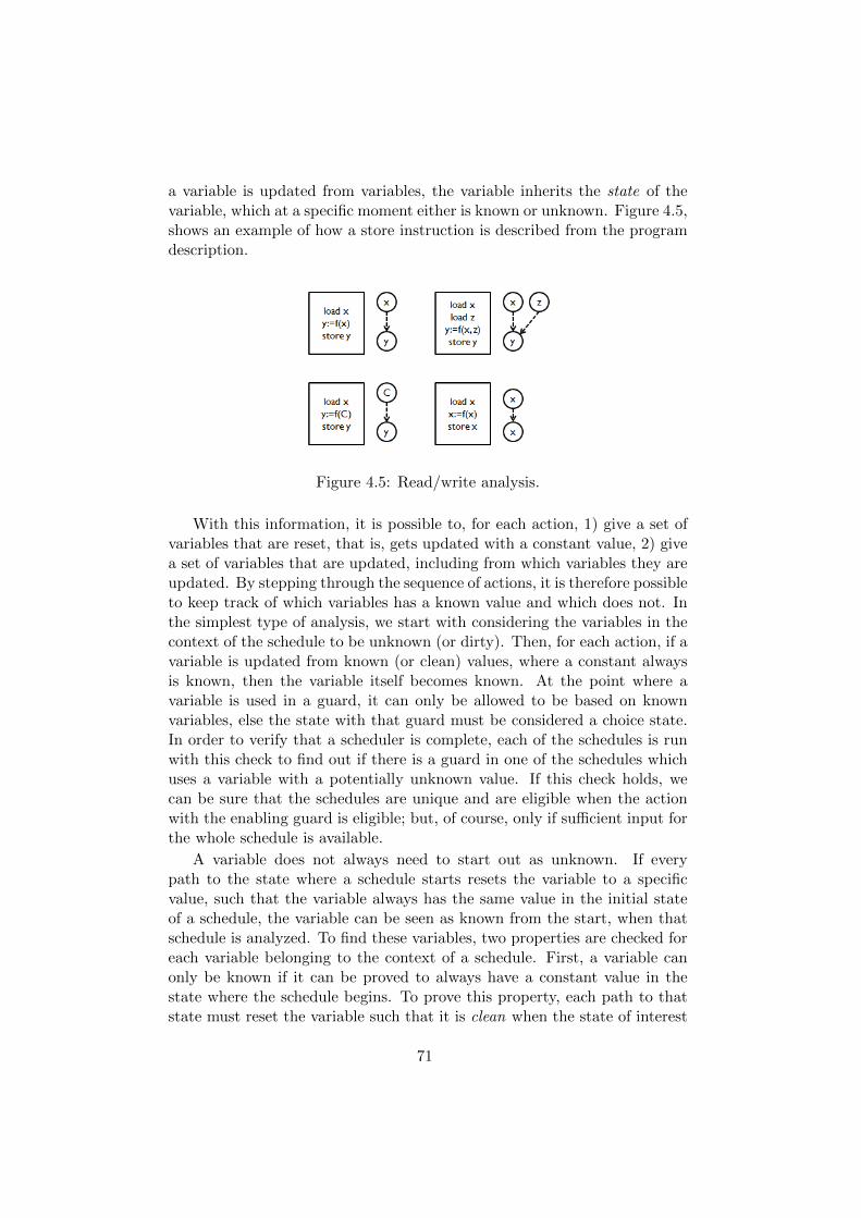
a variable is updated from variables, the variable inherits the state of thevariable, which at a specific moment either is known or unknown. Figure 4.5,shows an example of how a store instruction is described from the programdescription.

Figure 4.5: Read/write analysis.

With this information, it is possible to, for each action, 1) give a set ofvariables that are reset, that is, gets updated with a constant value, 2) givea set of variables that are updated, including from which variables they areupdated. By stepping through the sequence of actions, it is therefore possibleto keep track of which variables has a known value and which does not. Inthe simplest type of analysis, we start with considering the variables in thecontext of the schedule to be unknown (or dirty). Then, for each action, if avariable is updated from known (or clean) values, where a constant alwaysis known, then the variable itself becomes known. At the point where avariable is used in a guard, it can only be allowed to be based on knownvariables, else the state with that guard must be considered a choice state.In order to verify that a scheduler is complete, each of the schedules is runwith this check to find out if there is a guard in one of the schedules whichuses a variable with a potentially unknown value. If this check holds, wecan be sure that the schedules are unique and are eligible when the actionwith the enabling guard is eligible; but, of course, only if sufficient input forthe whole schedule is available.

A variable does not always need to start out as unknown. If everypath to the state where a schedule starts resets the variable to a specificvalue, such that the variable always has the same value in the initial stateof a schedule, the variable can be seen as known from the start, when thatschedule is analyzed. To find these variables, two properties are checked foreach variable belonging to the context of a schedule. First, a variable canonly be known if it can be proved to always have a constant value in thestate where the schedule begins. To prove this property, each path to thatstate must reset the variable such that it is clean when the state of interest

71

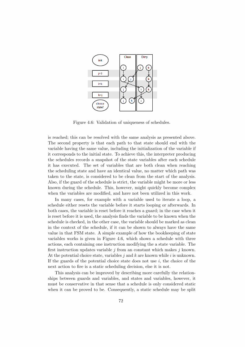
Figure 4.6: Validation of uniqueness of schedules.

is reached; this can be resolved with the same analysis as presented above.The second property is that each path to that state should end with thevariable having the same value, including the initialization of the variable ifit corresponds to the initial state. To achieve this, the interpreter producingthe schedules records a snapshot of the state variables after each scheduleit has executed. The set of variables that are both clean when reachingthe scheduling state and have an identical value, no matter which path wastaken to the state, is considered to be clean from the start of the analysis.Also, if the guard of the schedule is strict, the variable might be more or lessknown during the schedule. This, however, might quickly become complexwhen the variables are modified, and have not been utilized in this work.

In many cases, for example with a variable used to iterate a loop, aschedule either resets the variable before it starts looping or afterwards. Inboth cases, the variable is reset before it reaches a guard; in the case when itis reset before it is used, the analysis finds the variable to be known when theschedule is checked, in the other case, the variable should be marked as cleanin the context of the schedule, if it can be shown to always have the samevalue in that FSM state. A simple example of how the bookkeeping of statevariables works is given in Figure 4.6, which shows a schedule with threeactions, each containing one instruction modifying the a state variable. Thefirst instruction updates variable j from an constant which makes j known.At the potential choice state, variables j and k are known while i is unknown.If the guards of the potential choice state does not use i, the choice of thenext action to fire is a static scheduling decision, else it is not.

This analysis can be improved by describing more carefully the relation-ships between guards and variables, and states and variables, however, itmust be conservative in that sense that a schedule is only considered staticwhen it can be proved to be. Consequently, a static schedule may be split

72

into several schedules, because it could not be proven to be unique. Theresulting scheduler, after this step, describes the behavior of an actor with asimplified scheduler where the scheduling decisions that can be resolved atcompile-time have been removed and replaced with sequences action firings.If the action sequences are composed in to bigger actions (super actions),the new scheduler causes the actor to work on larger chunks of data, whichmay cause problems especially if the program includes feedback loops. Thisis similar to the known problem that deadlock-freedom, for models such asSDF, is not closed under composition. Instead, composing two adjacentactors may introduce deadlock, and deadlock-freedom needs to be provedaccording to composition conditions such as those presented in [105].

The conclusion from this is that while the schedules are correct, for acomposition to be deadlock-free, it may be unavoidable to interleave actionsof two schedules from two different actions. This is exactly what the compo-sition presented in the next chapter is about, and the composition presentedthere does guarantee that a composition is deadlock-free, however, it doesnot guarantee the program to be deadlock-free globally.

4.5 Describing the Actor State More Precisely

When an actor is described as a set of static schedules, the accesses andmodifications of state variables become easier to analyze. For the differentchoice states, a subset of the state variables represent the context of theschedule. When the value of a variable cannot reach any of the guards in aschedule, typically because the variable is reset before being used or becauseit is not used at all in the guards of the schedule, these variables should notbe used for describing the state of the actor in that specific FSM state. Inother words, when the actor is in a specific FSM state, the actual state ofthe actor is described by the FSM state and the state variables, however,only the variables that affect the choice of the next schedule, in that FSMstate, should be used in order to avoid introducing unnecessary states.

What should be resolved is which variables are relevant in each particularFSM state that corresponds to a choice state. The benefit from describinga state more precisely will become more evident in the next chapter, whena scheduler for a partition is generated. Then it is essential that any state isnot duplicated in the scheduler as every new state, results in a more complexscheduler. When there are two states, where the future action firings willbe identical, the two states should be considered the same state. To findthe variables that are relevant for a state, and to remove those which arenot, an analysis similar to the check of uniqueness of schedules is performed.The difference is that it is required to verify the value reachability beyondthe schedules only. Furthermore, with composition, it is not only required

73

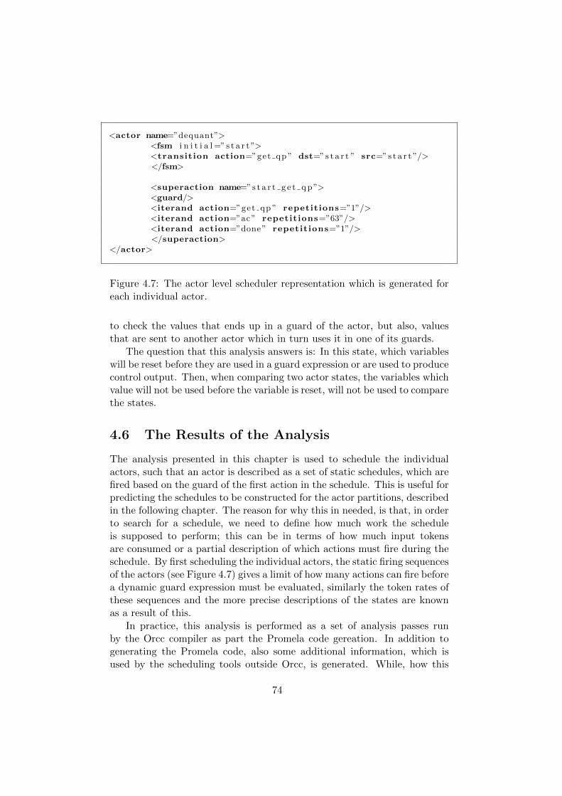
<actor name=”dequant”><fsm i n i t i a l =”s t a r t ”><transition action=”get qp ” dst=”s t a r t ” src=”s t a r t ”/></fsm>

<superaction name=”s t a r t g e t q p”><guard/><iterand action=”get qp ” repetitions=”1”/><iterand action=”ac” repetitions=”63”/><iterand action=”done” repetitions=”1”/></superaction>

</actor>

Figure 4.7: The actor level scheduler representation which is generated foreach individual actor.

to check the values that ends up in a guard of the actor, but also, valuesthat are sent to another actor which in turn uses it in one of its guards.

The question that this analysis answers is: In this state, which variableswill be reset before they are used in a guard expression or are used to producecontrol output. Then, when comparing two actor states, the variables whichvalue will not be used before the variable is reset, will not be used to comparethe states.

4.6 The Results of the Analysis

The analysis presented in this chapter is used to schedule the individualactors, such that an actor is described as a set of static schedules, which arefired based on the guard of the first action in the schedule. This is useful forpredicting the schedules to be constructed for the actor partitions, describedin the following chapter. The reason for why this in needed, is that, in orderto search for a schedule, we need to define how much work the scheduleis supposed to perform; this can be in terms of how much input tokensare consumed or a partial description of which actions must fire during theschedule. By first scheduling the individual actors, the static firing sequencesof the actors (see Figure 4.7) gives a limit of how many actions can fire beforea dynamic guard expression must be evaluated, similarly the token rates ofthese sequences and the more precise descriptions of the states are knownas a result of this.

In practice, this analysis is performed as a set of analysis passes runby the Orcc compiler as part the Promela code gereation. In addition togenerating the Promela code, also some additional information, which isused by the scheduling tools outside Orcc, is generated. While, how this

74

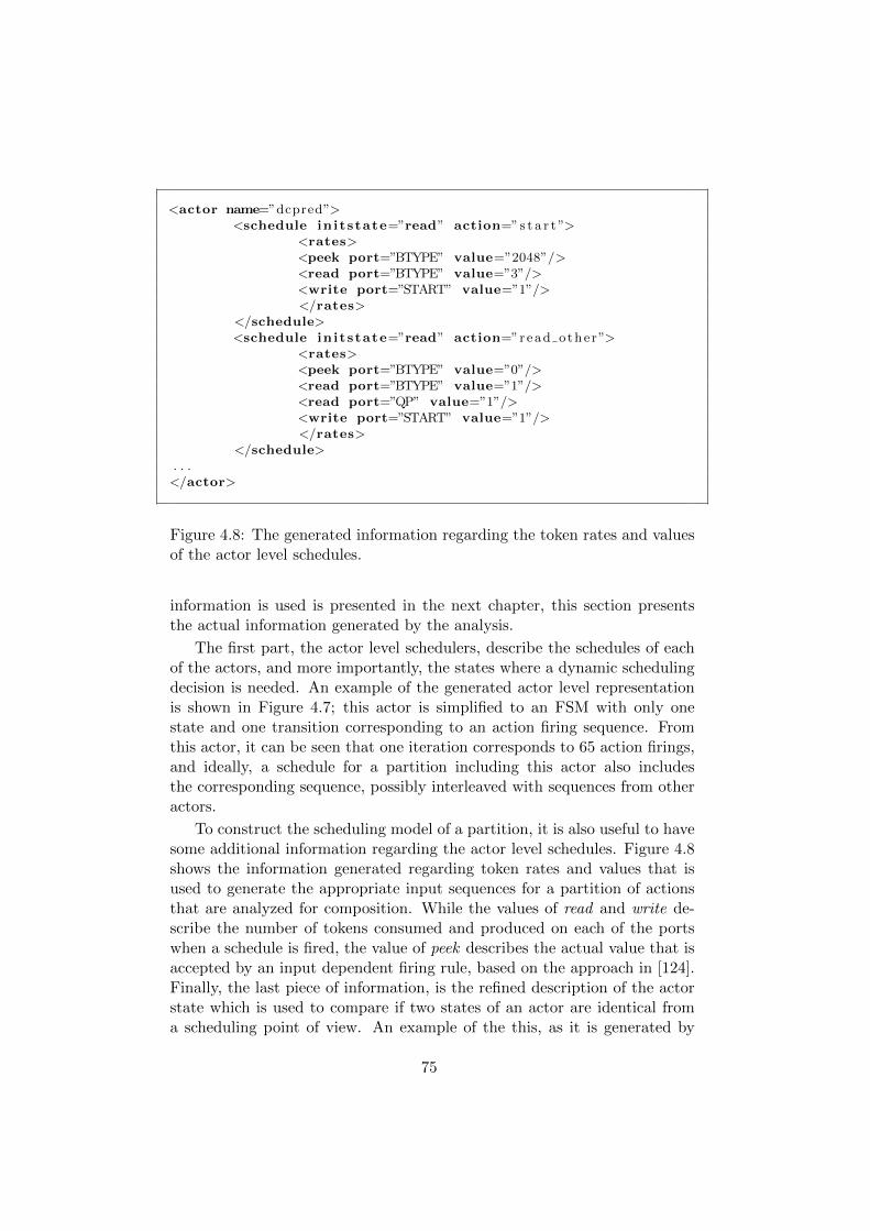
<actor name=”dcpred”><schedule initstate=”read” action=”s t a r t”>

<rates><peek port=”BTYPE” value=”2048”/><read port=”BTYPE” value=”3”/><write port=”START” value=”1”/></rates>

</schedule><schedule initstate=”read” action=”read othe r”>

<rates><peek port=”BTYPE” value=”0”/><read port=”BTYPE” value=”1”/><read port=”QP” value=”1”/><write port=”START” value=”1”/></rates>

</schedule>. . .</actor>

Figure 4.8: The generated information regarding the token rates and valuesof the actor level schedules.

information is used is presented in the next chapter, this section presentsthe actual information generated by the analysis.

The first part, the actor level schedulers, describe the schedules of eachof the actors, and more importantly, the states where a dynamic schedulingdecision is needed. An example of the generated actor level representationis shown in Figure 4.7; this actor is simplified to an FSM with only onestate and one transition corresponding to an action firing sequence. Fromthis actor, it can be seen that one iteration corresponds to 65 action firings,and ideally, a schedule for a partition including this actor also includesthe corresponding sequence, possibly interleaved with sequences from otheractors.

To construct the scheduling model of a partition, it is also useful to havesome additional information regarding the actor level schedules. Figure 4.8shows the information generated regarding token rates and values that isused to generate the appropriate input sequences for a partition of actionsthat are analyzed for composition. While the values of read and write de-scribe the number of tokens consumed and produced on each of the portswhen a schedule is fired, the value of peek describes the actual value that isaccepted by an input dependent firing rule, based on the approach in [124].Finally, the last piece of information, is the refined description of the actorstate which is used to compare if two states of an actor are identical froma scheduling point of view. An example of the this, as it is generated by

75

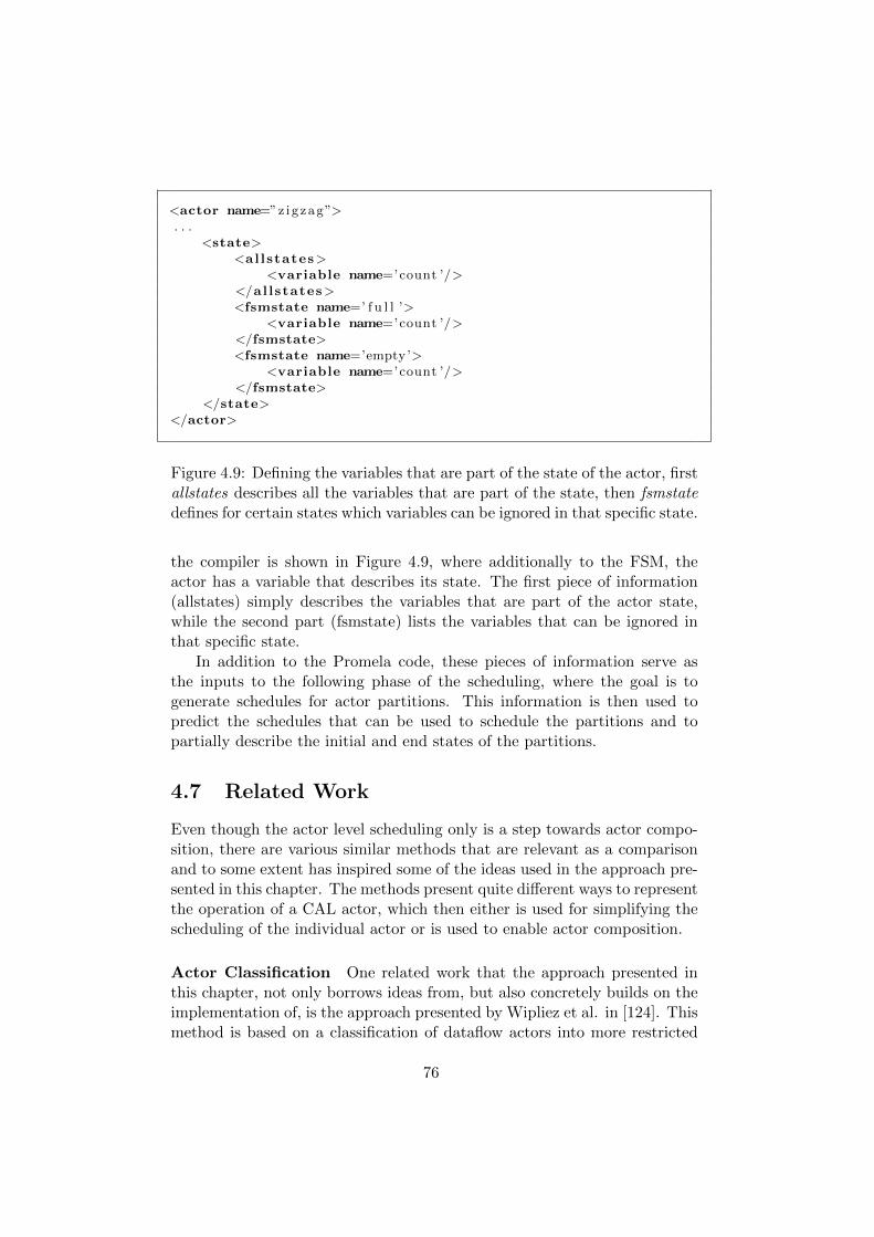
<actor name=”z igzag”>. . .

<state><al lstates>

<variable name=’count ’/></al lstates><fsmstate name=’ f u l l ’>

<variable name=’count ’/></fsmstate><fsmstate name=’empty’>

<variable name=’count ’/></fsmstate>

</state></actor>

Figure 4.9: Defining the variables that are part of the state of the actor, firstallstates describes all the variables that are part of the state, then fsmstatedefines for certain states which variables can be ignored in that specific state.

the compiler is shown in Figure 4.9, where additionally to the FSM, theactor has a variable that describes its state. The first piece of information(allstates) simply describes the variables that are part of the actor state,while the second part (fsmstate) lists the variables that can be ignored inthat specific state.

In addition to the Promela code, these pieces of information serve asthe inputs to the following phase of the scheduling, where the goal is togenerate schedules for actor partitions. This information is then used topredict the schedules that can be used to schedule the partitions and topartially describe the initial and end states of the partitions.

4.7 Related Work

Even though the actor level scheduling only is a step towards actor compo-sition, there are various similar methods that are relevant as a comparisonand to some extent has inspired some of the ideas used in the approach pre-sented in this chapter. The methods present quite different ways to representthe operation of a CAL actor, which then either is used for simplifying thescheduling of the individual actor or is used to enable actor composition.

Actor Classification One related work that the approach presented inthis chapter, not only borrows ideas from, but also concretely builds on theimplementation of, is the approach presented by Wipliez et al. in [124]. Thismethod is based on a classification of dataflow actors into more restricted

76

but easier to schedule MoCs, such as SDF, CSDF, and PSDF. The approachin [124] is based on abstract interpretation and satisfiability, where a morerestricted MoC is decided for one actor at the time and the internal schedul-ing of the actor is made minimal. The classified actors can then also, on thelevel of the program, be more efficiently scheduled according to the schedul-ing principles available for the different MoCs. This means that for a partof a program where every actor can be classified to a statically schedulableMoC, the run-time overhead will be minimal as all scheduling decisions canbe done at compile-time [81].

The classification approach uses abstract interpretation to find whichscheduling conditions can be resolved from the actor itself and satisfiabilityto find the different configurations for an actor which fires differently de-pending on an input value. The abstract interpretation can be describedinformally like this: the actor is initialized and starts to fire actions basedon evaluating the guards of the actions. Variables may have concrete valuesor unknown values, for example, as a result of a read from an input channel.For the calculations in an action, if the variables used in the calculationare known, then the result from the value is a concrete value, else it is anunknown value. Unknown values are not a problem as long as no guard usesa variable with such a value, which would mean that it cannot be known ifthe guard will evaluate to true or false.

The approach in [124] uses abstract interpretation as follows. If the actorcan be run, from its initial state, back to that state, without evaluating anyunknown guard expressions, the actor can be classified as SDF. The actorstate here means, the state of the FSM and the state variables that areused in guards. The intuition here is that, for one iteration of the actor, nounknown values reached any guards, and as the initial state is found, thenext iteration will be identical, which means that the actor repeatedly willfire this same sequence of actions. When it takes a few iterations of theFSM to reach the initial state, the actor is instead classified as CSDF.

Actors that are input dependent can still have static behavior if depend-ing on the control input, one static schedule can be chosen. Such actors areclassified as quasi-static, which in this approach resembles PSDF. The quasi-static actors are considered to have a set of configurations, which maps acontrol input to a sequence of actions, which themselves can be classified asSDF or CSDF. The control tokens corresponding to the configurations andthat are feed to the abstract interpreter needs to be found such that abstractinterpretation can be performed for the different configurations. In [124],an approach using Satisfiability Modulo Theories (SMT), which is used tofind an unique value that is accepted by a specific guard, but not by anyhigher priority guard. This method for finding the control values, includingthe implementation of it, is also used in the work presented in this thesis tofind control tokens for guards expressions that references an input queue (a

77

peek). However, this topic is more relevant for the next chapter, so we canlet i rest for a while.

Another property which is handled in the classification approach is time-dependent behavior. CAL allows actors to be time-dependent in the sensethat a different action may fire if more input tokens are available, whichmeans that triggering the actor at a later moment may lead to a differentbehavior. In practice this means that an action requires fewer tokens fromthe input ports than a higher priority action while the guards of both ac-tions are evaluated to true. In the abstract interpretation, the inputs areconsidered to always have enough inputs which means that time-dependentbehavior is not allowed as the resulting scheduler will loose this behavior. Inthe variant presented in this chapter, time-dependent behavior should notbe a problem as long as the state with this behavior is identified and thechoice between the actions is considered a run-time decision. To identifythe time-dependent choices, the approach from [124] is directly used as it isavailable in the Orcc compiler.

Dynamic Code Analysis The actor level schedules are to some extentinspired by what is called actor chains in the work by Boutellier et al. [27].In this work, dynamic code analysis, which means that the program codeis instrumented with operations gathering information about the programwhen to program is executed, is used to extract static schedules. Staticschedules are extracted both on the level of individual actors and on parti-tions consisting of several actors. In the context of this chapter, we are onlyinteresting in the scheduling on actor level, but we will get back to moredetails regarding this work in the next chapter.

An actor chain is defined as a sequence of actions that always follow eachother. In [27], action chains are obtained by executing actors in isolationaccording to FIFO traces, which has been recorded from executing the pro-gram with training data. The execution traces then, ideally, if the trainingdata is sufficient, covers every possible action sequence that can occur. Thedetection of action chains is based on data dependent actions, FSM states,or state variable values.

Compared to the analysis presented in this chapter, the detection of actorchains in [27], have the same goal, and constructs action sequences based onvery similar conditions. The most significant difference is that dynamic codeanalysis is based on real execution traces while the approach presented hereis based on abstract interpretation. Verification of uniqueness of schedulesis, for this reason also different, as in dynamic code analysis, it is based onthe nonexistence or alternative schedules, while in the presented approachit is verified based on an approach that can be compared with an analysisof the reachability of variable definitions [99].

Both methods also use the actor level scheduling as an initial step that

78

enables the scheduling of actor partitions. It seems like both methods foractor level scheduling, ideally, should give identical results. However, themethod presented by Boutellier et al., may be less conservative and mayfind chains that are not detected by the presented method; on the otherhand, the method based on dynamic code analysis depends on sufficienttraining data and would obviously give overoptimistic results if the trainingdata is not sufficient. This said, it seems both methods have their benefits,and the presented approach could still borrow some more ideas from thisapproach in order to more efficiently detect action chains.

Actor Machines Another way to represent the scheduling decisions of anactor is presented by Janneck in [73]. This model, called actor machines,is an automation that implements the behavior of the actor and encapsu-lates the action selection mechanism in an action machine controller, whichconsists of controller states and test-, execute-, and wait- instructions. Eachof the controller states keeps the information regarding which conditionsare satisfied, which are not, and which are unknown in that state while theinstructions make the automaton proceed to the next state by executingactions, checking conditions, or waiting for input.

The controller states are mapped to a set of conditions that, in thatspecific state belong to the set {true, false, unknown}, which means that,the controller states state which conditions are known in that state. The testinstruction then, which based on some conditions, proceeds to one of twostates, is only needed if the condition tests a condition that is unknown inthe state preceding the test instruction. Furthermore, as the test instructiontests one of the conditions, that condition is known in the state reached afterthe test instruction. This means that the same condition does not need tobe retested again after it once has been determined [33]. On the other hand,some conditions cannot only be tested once; consider for example a conditionthat tests if input is available. For this purpose the wait instruction is usedto erase the information about a volatile condition [73], which if at onemoment evaluated to false may at the next instant be evaluated to true, asinput data may become available.

An actor machine seems to be a practical description of the schedulingprocess of an actor, and seems to encapsulate the same information as theactor scheduler description that is described in this chapter. The actor ma-chine model, however, includes slightly different information, as it describesmore specifically the conditions that are known in different states. Fromthis point of view, the actor machine model might be a good alternative todescribing the simplified actor schedulers produced in this chapter to possi-bly make the action selection process more efficient. The difficulty in bothmodels, however, is to create the model from the original CAL actors.

In [33], Cedersjo and Janneck present a number of translators from CAL

79

to actor machines, with different properties. The more advanced generatorspresented allows that actor machine to memorize tests such that tests wherethe result cannot change are not repeatedly performed. This is then usedto generate more efficient schedulers for the actors. The actor machinescan further be reduced by removing choices where more than one action isavailable in a controller state. As an example, a controller state may besucceeded by two test instructions that both are mutually exclusive, now,in this case it is unnecessary to keep both test instructions; instead theautomation can be reduced.

The benefit from using actor machines in code generation is that theprocess of choosing the next action to fire can be simplified as the sequenceof conditions to be tested is not constructed by chance but is based onknowledge about the actors. By this, it is always known what conditionsmake sense to check and conditions that are known are not rechecked. Thisresult is to some extent similar to what we achieve with the analysis in thischapter, that is, which conditions are known at which state. This said, theactor machine model could be one alternative representation for performingthe operations presented in this chapter.

Actor machines are also used to classify actors as deterministic, prefixmonotonic, Kahn processes, CSDF, and SDF [34]. This analysis could easilybe extended to identify the simplified schedulers presented in this chapter,with the added value of a more efficient description of the action selectionprocess providing information regarding which values are known at whichstates.

80

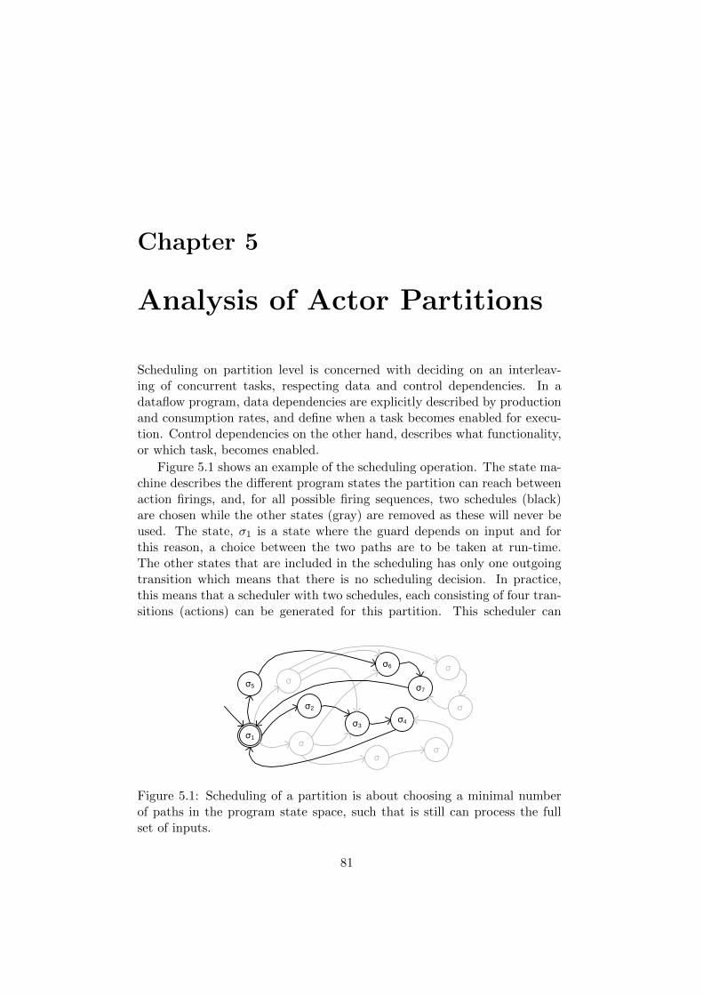
Chapter 5

Analysis of Actor Partitions

Scheduling on partition level is concerned with deciding on an interleav-ing of concurrent tasks, respecting data and control dependencies. In adataflow program, data dependencies are explicitly described by productionand consumption rates, and define when a task becomes enabled for execu-tion. Control dependencies on the other hand, describes what functionality,or which task, becomes enabled.

Figure 5.1 shows an example of the scheduling operation. The state ma-chine describes the different program states the partition can reach betweenaction firings, and, for all possible firing sequences, two schedules (black)are chosen while the other states (gray) are removed as these will never beused. The state, σ1 is a state where the guard depends on input and forthis reason, a choice between the two paths are to be taken at run-time.The other states that are included in the scheduling has only one outgoingtransition which means that there is no scheduling decision. In practice,this means that a scheduler with two schedules, each consisting of four tran-sitions (actions) can be generated for this partition. This scheduler can

σ1

σ2

σ5

σ4

σ7

σ3

σ6

σ

σ

σσ

σ

σ

σ1

Figure 5.1: Scheduling of a partition is about choosing a minimal numberof paths in the program state space, such that is still can process the fullset of inputs.

81

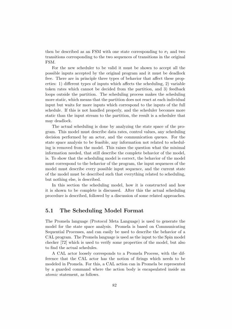
then be described as an FSM with one state corresponding to σ1 and twotransitions corresponding to the two sequences of transitions in the originalFSM.

For the new scheduler to be valid it must be shown to accept all thepossible inputs accepted by the original program and it must be deadlockfree. There are in principle three types of behavior that affect these prop-erties: 1) different types of inputs which affects the scheduling, 2) variabletoken rates which cannot be decided from the partition, and 3) feedbackloops outside the partition. The scheduling process makes the schedulingmore static, which means that the partition does not react at each individualinput but waits for more inputs which correspond to the inputs of the fullschedule. If this is not handled properly, and the scheduler becomes morestatic than the input stream to the partition, the result is a scheduler thatmay deadlock.

The actual scheduling is done by analyzing the state space of the pro-gram. This model must describe data rates, control values, any schedulingdecision performed by an actor, and the communication queues. For thestate space analysis to be feasible, any information not related to schedul-ing is removed from the model. This raises the question what the minimalinformation needed, that still describe the complete behavior of the model,is. To show that the scheduling model is correct, the behavior of the modelmust correspond to the behavior of the program, the input sequences of themodel must describe every possible input sequence, and the current stateof the model must be described such that everything related to scheduling,but nothing else, is described.

In this section the scheduling model, how it is constructed and howit is shown to be complete is discussed. After this the actual schedulingprocedure is described, followed by a discussion of some related approaches.

5.1 The Scheduling Model Format

The Promela language (Protocol Meta Language) is used to generate themodel for the state space analysis. Promela is based on CommunicatingSequential Processes, and can easily be used to describe the behavior of aCAL program. The Promela language is used as the input to the Spin modelchecker [72] which is used to verify some properties of the model, but alsoto find the actual schedules.

A CAL actor loosely corresponds to a Promela Process, with the dif-ference that the CAL actor has the notion of firings which needs to bemodeled in Promela. For this, a CAL action can in Promela be representedby a guarded command where the action body is encapsulated inside anatomic statement, as follows.

82

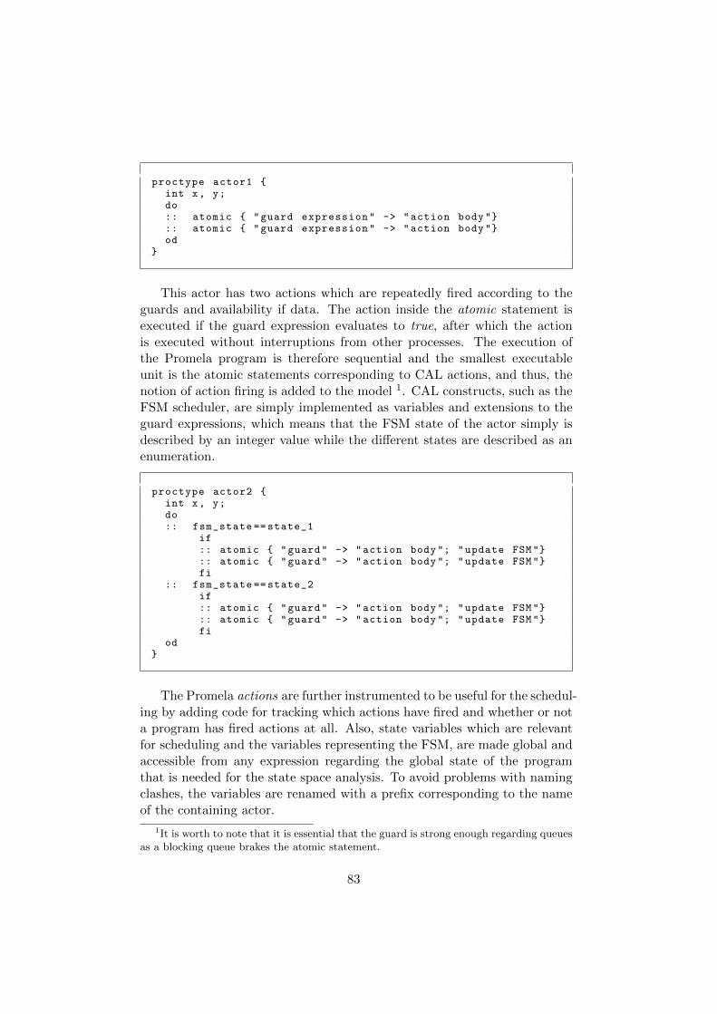
proctype actor1 {int x, y;do:: atomic { "guard expression" -> "action body"}:: atomic { "guard expression" -> "action body"}od

}

This actor has two actions which are repeatedly fired according to theguards and availability if data. The action inside the atomic statement isexecuted if the guard expression evaluates to true, after which the actionis executed without interruptions from other processes. The execution ofthe Promela program is therefore sequential and the smallest executableunit is the atomic statements corresponding to CAL actions, and thus, thenotion of action firing is added to the model 1. CAL constructs, such as theFSM scheduler, are simply implemented as variables and extensions to theguard expressions, which means that the FSM state of the actor simply isdescribed by an integer value while the different states are described as anenumeration.

proctype actor2 {int x, y;do:: fsm_state == state_1

if:: atomic { "guard" -> "action body"; "update FSM"}:: atomic { "guard" -> "action body"; "update FSM"}fi

:: fsm_state == state_2if:: atomic { "guard" -> "action body"; "update FSM"}:: atomic { "guard" -> "action body"; "update FSM"}fi

od}

The Promela actions are further instrumented to be useful for the schedul-ing by adding code for tracking which actions have fired and whether or nota program has fired actions at all. Also, state variables which are relevantfor scheduling and the variables representing the FSM, are made global andaccessible from any expression regarding the global state of the programthat is needed for the state space analysis. To avoid problems with namingclashes, the variables are renamed with a prefix corresponding to the nameof the containing actor.

1It is worth to note that it is essential that the guard is strong enough regarding queuesas a blocking queue brakes the atomic statement.

83

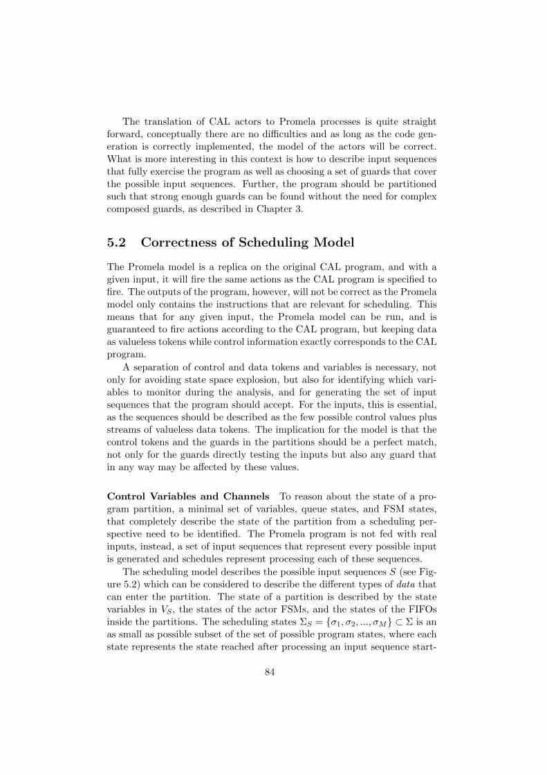
The translation of CAL actors to Promela processes is quite straightforward, conceptually there are no difficulties and as long as the code gen-eration is correctly implemented, the model of the actors will be correct.What is more interesting in this context is how to describe input sequencesthat fully exercise the program as well as choosing a set of guards that coverthe possible input sequences. Further, the program should be partitionedsuch that strong enough guards can be found without the need for complexcomposed guards, as described in Chapter 3.

5.2 Correctness of Scheduling Model

The Promela model is a replica on the original CAL program, and with agiven input, it will fire the same actions as the CAL program is specified tofire. The outputs of the program, however, will not be correct as the Promelamodel only contains the instructions that are relevant for scheduling. Thismeans that for any given input, the Promela model can be run, and isguaranteed to fire actions according to the CAL program, but keeping dataas valueless tokens while control information exactly corresponds to the CALprogram.

A separation of control and data tokens and variables is necessary, notonly for avoiding state space explosion, but also for identifying which vari-ables to monitor during the analysis, and for generating the set of inputsequences that the program should accept. For the inputs, this is essential,as the sequences should be described as the few possible control values plusstreams of valueless data tokens. The implication for the model is that thecontrol tokens and the guards in the partitions should be a perfect match,not only for the guards directly testing the inputs but also any guard thatin any way may be affected by these values.

Control Variables and Channels To reason about the state of a pro-gram partition, a minimal set of variables, queue states, and FSM states,that completely describe the state of the partition from a scheduling per-spective need to be identified. The Promela program is not fed with realinputs, instead, a set of input sequences that represent every possible inputis generated and schedules represent processing each of these sequences.

The scheduling model describes the possible input sequences S (see Fig-ure 5.2) which can be considered to describe the different types of data thatcan enter the partition. The state of a partition is described by the statevariables in VS , the states of the actor FSMs, and the states of the FIFOsinside the partitions. The scheduling states ΣS = {σ1, σ2, ..., σM} ⊂ Σ is anas small as possible subset of the set of possible program states, where eachstate represents the state reached after processing an input sequence start-

84

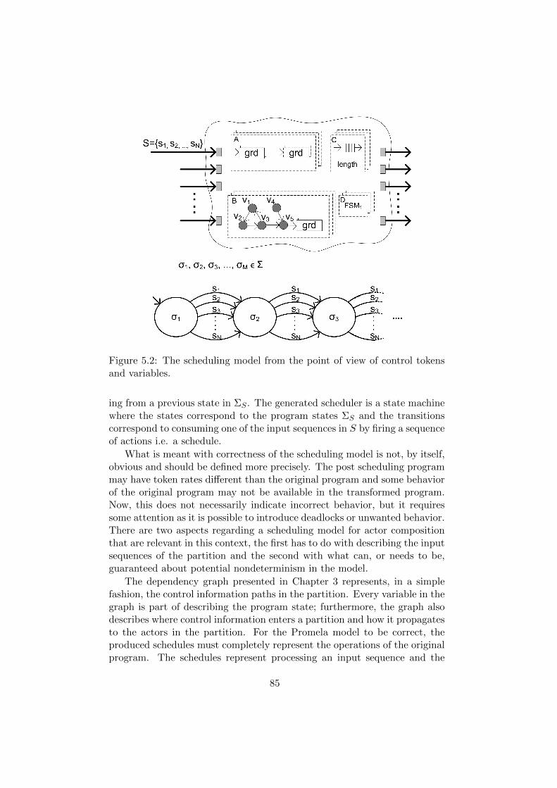
Figure 5.2: The scheduling model from the point of view of control tokensand variables.

ing from a previous state in ΣS . The generated scheduler is a state machinewhere the states correspond to the program states ΣS and the transitionscorrespond to consuming one of the input sequences in S by firing a sequenceof actions i.e. a schedule.

What is meant with correctness of the scheduling model is not, by itself,obvious and should be defined more precisely. The post scheduling programmay have token rates different than the original program and some behaviorof the original program may not be available in the transformed program.Now, this does not necessarily indicate incorrect behavior, but it requiressome attention as it is possible to introduce deadlocks or unwanted behavior.There are two aspects regarding a scheduling model for actor compositionthat are relevant in this context, the first has to do with describing the inputsequences of the partition and the second with what can, or needs to be,guaranteed about potential nondeterminism in the model.

The dependency graph presented in Chapter 3 represents, in a simplefashion, the control information paths in the partition. Every variable in thegraph is part of describing the program state; furthermore, the graph alsodescribes where control information enters a partition and how it propagatesto the actors in the partition. For the Promela model to be correct, theproduced schedules must completely represent the operations of the originalprogram. The schedules represent processing an input sequence and the

85

choice of schedules is to be made by checking the type of the input and thestate of the program. For this reason, a set of guards that are strong enoughmust be identified.

Identify the Guards and Input Sequences For an input sequence, theguards that check a property of the input may be located in more than oneof the actors of the partition. In practice, this means that the scheduling isdistributed and decisions are made at different times during the processingof an input sequence. To be able to choose a static schedule based on thedata waiting at the input ports of the partition, a set of guards coveringall these other guards is needed. This can be achieved either by choosingproper partitions or by composing a set of stronger guards from the guardsof the partition.

The relationship between input sequences, guards, and the scheduler isillustrated in Figure 5.2. The section of the partition description labeled A,shows a set of guards directly reading the input sequence and another set ofguards (connected by a dashed lines) which at some later point checks someproperty of the input. This latter set of actions should be covered by theguards in the first set, such that evaluating the guards checking the inputprovides the information that predicts the evaluation of the other guards.

In this work, the preferred approach is to choose partitions such thatthere is one actor with strong enough guards to schedule the rest of thepartition. This approach restricts the sizes of partitions as some actorshave guards that are not compatible, however, it also guaranties that thescheduling overhead is never increased as guards are removed but neveradded. Further, it also enforces a partitioning where the processing is relatedto the same properties of the data as the guards must be overlapping. Ofcourse, there will certainly be cases where creating new guards will give somebenefits and it would make sense to explore this optimization problem, butit is left outside the scope of this thesis.

The input sequences for the actors in a partition are generated accordingto the actor level scheduling presented in the previous chapter. Controlvalues are resolved using the SMT solver approach presented in [124] whiledata values simply are a number of valueless (in practice zero value) tokens.When these are put on the input channels to a partition, the model checkeris ready to run as soon as it has been verified that the guards are strongenough to identify every different input sequence that requires a differentschedule.

Verify Guard Strength The guard strengths are analyzed according tothe types of control value propagation presented in Section 3.2.2. In thecases where the propagated control value is not a function of the input, the

86

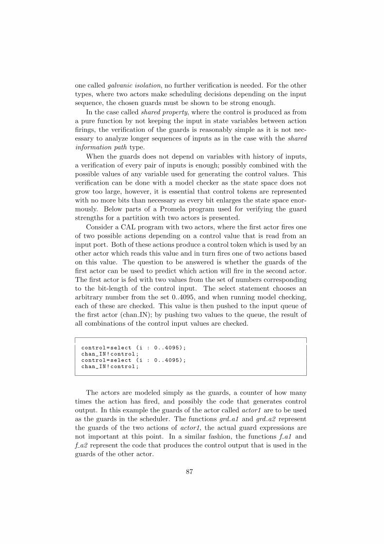
one called galvanic isolation, no further verification is needed. For the othertypes, where two actors make scheduling decisions depending on the inputsequence, the chosen guards must be shown to be strong enough.

In the case called shared property, where the control is produced as froma pure function by not keeping the input in state variables between actionfirings, the verification of the guards is reasonably simple as it is not nec-essary to analyze longer sequences of inputs as in the case with the sharedinformation path type.

When the guards does not depend on variables with history of inputs,a verification of every pair of inputs is enough; possibly combined with thepossible values of any variable used for generating the control values. Thisverification can be done with a model checker as the state space does notgrow too large, however, it is essential that control tokens are representedwith no more bits than necessary as every bit enlarges the state space enor-mously. Below parts of a Promela program used for verifying the guardstrengths for a partition with two actors is presented.

Consider a CAL program with two actors, where the first actor fires oneof two possible actions depending on a control value that is read from aninput port. Both of these actions produce a control token which is used by another actor which reads this value and in turn fires one of two actions basedon this value. The question to be answered is whether the guards of thefirst actor can be used to predict which action will fire in the second actor.The first actor is fed with two values from the set of numbers correspondingto the bit-length of the control input. The select statement chooses anarbitrary number from the set 0..4095, and when running model checking,each of these are checked. This value is then pushed to the input queue ofthe first actor (chan IN); by pushing two values to the queue, the result ofall combinations of the control input values are checked.

control=select (i : 0..4095);chan_IN!control;control=select (i : 0..4095);chan_IN!control;

The actors are modeled simply as the guards, a counter of how manytimes the action has fired, and possibly the code that generates controloutput. In this example the guards of the actor called actor1 are to be usedas the guards in the scheduler. The functions grd a1 and grd a2 representthe guards of the two actions of actor1, the actual guard expressions arenot important at this point. In a similar fashion, the functions f a1 andf a2 represent the code that produces the control output that is used in theguards of the other actor.

87

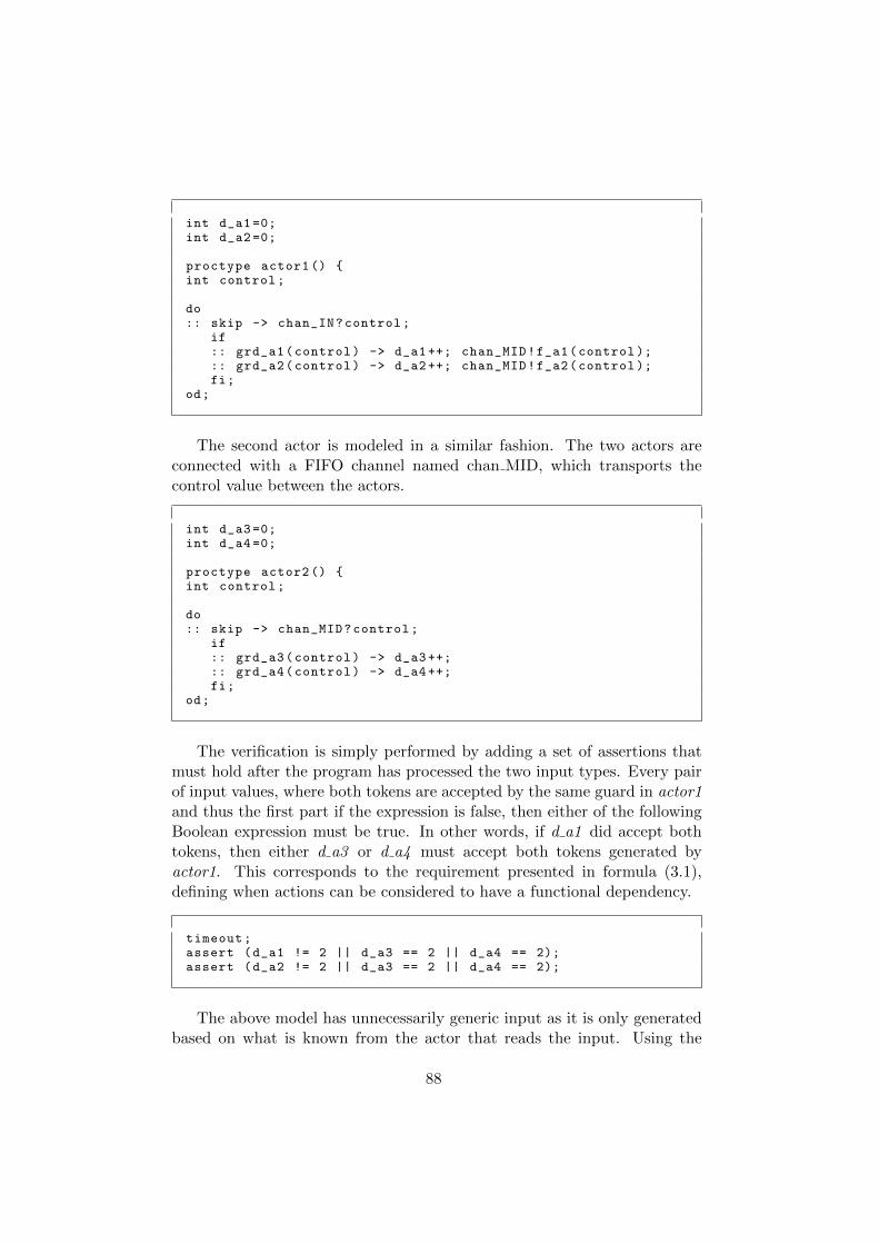
int d_a1 =0;int d_a2 =0;

proctype actor1 () {int control;

do:: skip -> chan_IN?control;

if:: grd_a1(control) -> d_a1 ++; chan_MID!f_a1(control );:: grd_a2(control) -> d_a2 ++; chan_MID!f_a2(control );fi;

od;

The second actor is modeled in a similar fashion. The two actors areconnected with a FIFO channel named chan MID, which transports thecontrol value between the actors.

int d_a3 =0;int d_a4 =0;

proctype actor2 () {int control;

do:: skip -> chan_MID?control;

if:: grd_a3(control) -> d_a3 ++;:: grd_a4(control) -> d_a4 ++;fi;

od;

The verification is simply performed by adding a set of assertions thatmust hold after the program has processed the two input types. Every pairof input values, where both tokens are accepted by the same guard in actor1and thus the first part if the expression is false, then either of the followingBoolean expression must be true. In other words, if d a1 did accept bothtokens, then either d a3 or d a4 must accept both tokens generated byactor1. This corresponds to the requirement presented in formula (3.1),defining when actions can be considered to have a functional dependency.

timeout;assert (d_a1 != 2 || d_a3 == 2 || d_a4 == 2);assert (d_a2 != 2 || d_a3 == 2 || d_a4 == 2);

The above model has unnecessarily generic input as it is only generatedbased on what is known from the actor that reads the input. Using the

88

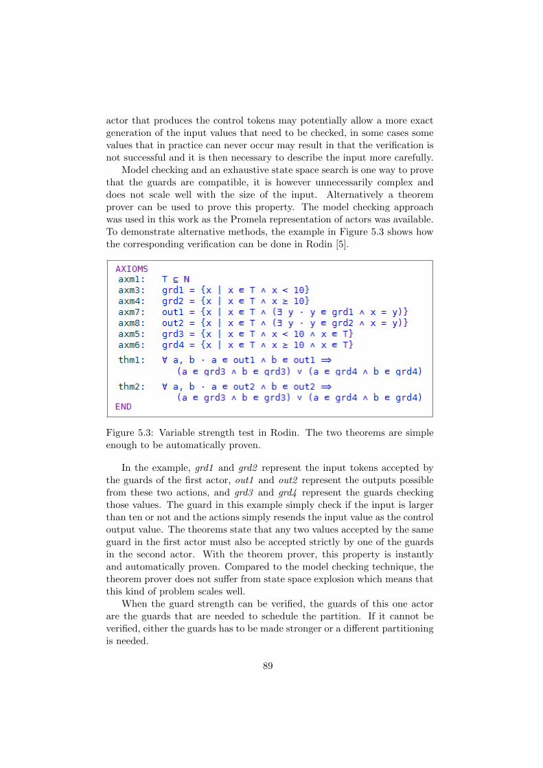
actor that produces the control tokens may potentially allow a more exactgeneration of the input values that need to be checked, in some cases somevalues that in practice can never occur may result in that the verification isnot successful and it is then necessary to describe the input more carefully.

Model checking and an exhaustive state space search is one way to provethat the guards are compatible, it is however unnecessarily complex anddoes not scale well with the size of the input. Alternatively a theoremprover can be used to prove this property. The model checking approachwas used in this work as the Promela representation of actors was available.To demonstrate alternative methods, the example in Figure 5.3 shows howthe corresponding verification can be done in Rodin [5].

Figure 5.3: Variable strength test in Rodin. The two theorems are simpleenough to be automatically proven.

In the example, grd1 and grd2 represent the input tokens accepted bythe guards of the first actor, out1 and out2 represent the outputs possiblefrom these two actions, and grd3 and grd4 represent the guards checkingthose values. The guard in this example simply check if the input is largerthan ten or not and the actions simply resends the input value as the controloutput value. The theorems state that any two values accepted by the sameguard in the first actor must also be accepted strictly by one of the guardsin the second actor. With the theorem prover, this property is instantlyand automatically proven. Compared to the model checking technique, thetheorem prover does not suffer from state space explosion which means thatthis kind of problem scales well.

When the guard strength can be verified, the guards of this one actorare the guards that are needed to schedule the partition. If it cannot beverified, either the guards has to be made stronger or a different partitioningis needed.

89

Variable Token Rates Finally, to show that the scheduling model iscomplete, it is essential to show that the token rates of the different inputsare synchronized. Following the approach presented above, one actor is cho-sen for providing the guards of the partition scheduler. In a similar fashion,this same actor should also decide on the consumption and production ratesof the other actors in the partition. This means that the other actors shouldnot be allowed to make a choice depending on input, be it based on inputvalue or input availability, except if that choice can be decided from theactor on which the scheduling is based.

In a partition, therefore, there should only be one actor which can makeindependent scheduling decisions based on the available input. All the otheractors must depend on this choice and follow the first actor.

This property must be identified for a partition. By showing that oneactor has enough strong guards to schedule the other actors, this also meansthat there are no independent scheduling decisions based on input values inthe partition. The other type of independency comes from actors that havenondeterministic or time-dependent behavior. The classification presentedby Wipliez et al. in [124] can be used to identify such actors, and an actorthat is classified to belong to KPN or a more restricted MoC is known tonot have such a behavior. However, an actor with this type of behavior canstill be allowed to be part of a partition as long as it can be shown that thisbehavior is only available inside the partition but not available on the inputports of the partition. The simple rule, therefore, is that all input ports tothe partition should belong to actors which completely depend on the actorwhich the scheduling is based on.

In principle, there is no limitation for the actor which the schedulingis based on to have nondeterministic of time-dependent behavior, this issimply a scheduling decision as any other scheduling decision. However, thegoal with the scheduling is to work on larger units of input, this again maybe in conflict with basing the scheduling on a time-dependent actor as theamount of input then affects the scheduling. For this reason, it is avoidedto have time-dependent actors connected to the input ports of the partition.Now, when this actor which scheduling decisions decide the token rates andbehavior of the other actors in the partition has been identified, the nextstep is to search for the actual schedules of the partition.

5.3 Schedule Construction

The actual scheduling is a composition of the actor state machines whichin this case are represented by Promela processes. The composed schedulerdescribes a set of reoccurring program states which are linked by a set ofschedules, representing processing the possible inputs of the program. This

90

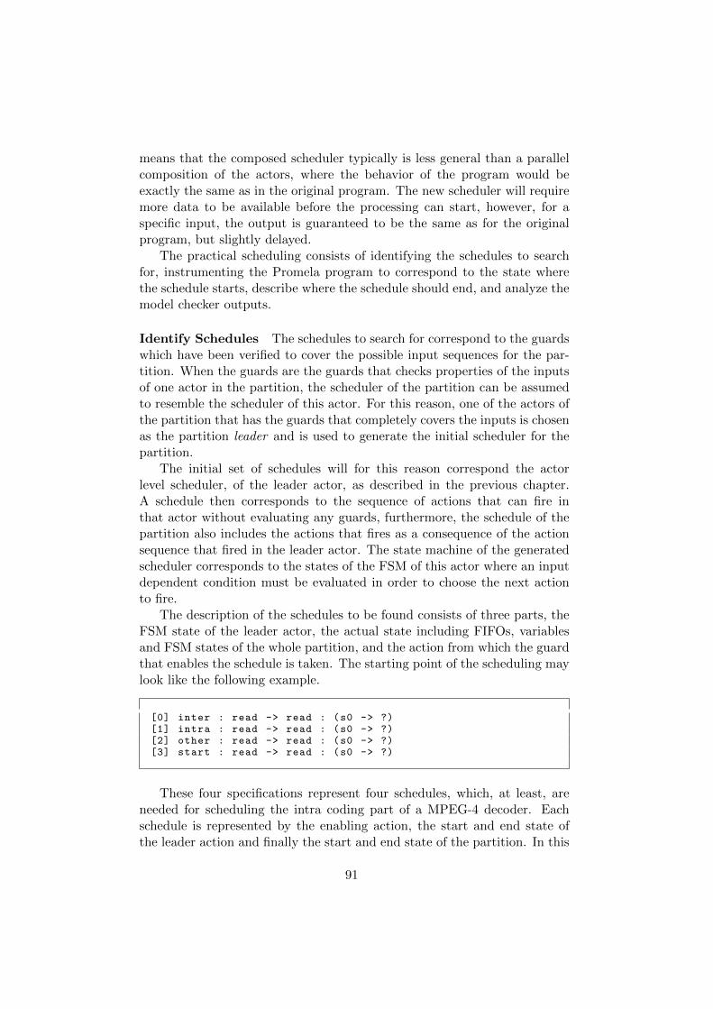
means that the composed scheduler typically is less general than a parallelcomposition of the actors, where the behavior of the program would beexactly the same as in the original program. The new scheduler will requiremore data to be available before the processing can start, however, for aspecific input, the output is guaranteed to be the same as for the originalprogram, but slightly delayed.

The practical scheduling consists of identifying the schedules to searchfor, instrumenting the Promela program to correspond to the state wherethe schedule starts, describe where the schedule should end, and analyze themodel checker outputs.

Identify Schedules The schedules to search for correspond to the guardswhich have been verified to cover the possible input sequences for the par-tition. When the guards are the guards that checks properties of the inputsof one actor in the partition, the scheduler of the partition can be assumedto resemble the scheduler of this actor. For this reason, one of the actors ofthe partition that has the guards that completely covers the inputs is chosenas the partition leader and is used to generate the initial scheduler for thepartition.

The initial set of schedules will for this reason correspond the actorlevel scheduler, of the leader actor, as described in the previous chapter.A schedule then corresponds to the sequence of actions that can fire inthat actor without evaluating any guards, furthermore, the schedule of thepartition also includes the actions that fires as a consequence of the actionsequence that fired in the leader actor. The state machine of the generatedscheduler corresponds to the states of the FSM of this actor where an inputdependent condition must be evaluated in order to choose the next actionto fire.

The description of the schedules to be found consists of three parts, theFSM state of the leader actor, the actual state including FIFOs, variablesand FSM states of the whole partition, and the action from which the guardthat enables the schedule is taken. The starting point of the scheduling maylook like the following example.

[0] inter : read -> read : (s0 -> ?)[1] intra : read -> read : (s0 -> ?)[2] other : read -> read : (s0 -> ?)[3] start : read -> read : (s0 -> ?)

These four specifications represent four schedules, which, at least, areneeded for scheduling the intra coding part of a MPEG-4 decoder. Eachschedule is represented by the enabling action, the start and end state ofthe leader action and finally the start and end state of the partition. In this

91

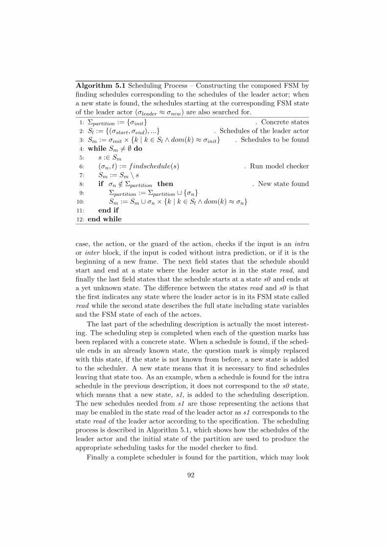
Algorithm 5.1 Scheduling Process – Constructing the composed FSM byfinding schedules corresponding to the schedules of the leader actor; whena new state is found, the schedules starting at the corresponding FSM stateof the leader actor (σleader ≈ σnew) are also searched for.

1: Σpartition := {σinit} . Concrete states2: Sl := {(σstart, σend), ...} . Schedules of the leader actor3: Sm := σinit × {k | k ∈ Sl ∧ dom(k) ≈ σinit} . Schedules to be found4: while Sm 6= ∅ do5: s :∈ Sm6: (σn, t) := findschedule(s) . Run model checker7: Sm := Sm \ s8: if σn /∈ Σpartition then . New state found9: Σpartition := Σpartition ∪ {σn}

10: Sm := Sm ∪ σn × {k | k ∈ Sl ∧ dom(k) ≈ σn}11: end if12: end while

case, the action, or the guard of the action, checks if the input is an intraor inter block, if the input is coded without intra prediction, or if it is thebeginning of a new frame. The next field states that the schedule shouldstart and end at a state where the leader actor is in the state read, andfinally the last field states that the schedule starts at a state s0 and ends ata yet unknown state. The difference between the states read and s0 is thatthe first indicates any state where the leader actor is in its FSM state calledread while the second state describes the full state including state variablesand the FSM state of each of the actors.

The last part of the scheduling description is actually the most interest-ing. The scheduling step is completed when each of the question marks hasbeen replaced with a concrete state. When a schedule is found, if the sched-ule ends in an already known state, the question mark is simply replacedwith this state, if the state is not known from before, a new state is addedto the scheduler. A new state means that it is necessary to find schedulesleaving that state too. As an example, when a schedule is found for the intraschedule in the previous description, it does not correspond to the s0 state,which means that a new state, s1, is added to the scheduling description.The new schedules needed from s1 are those representing the actions thatmay be enabled in the state read of the leader actor as s1 corresponds to thestate read of the leader actor according to the specification. The schedulingprocess is described in Algorithm 5.1, which shows how the schedules of theleader actor and the initial state of the partition are used to produce theappropriate scheduling tasks for the model checker to find.

Finally a complete scheduler is found for the partition, which may look

92

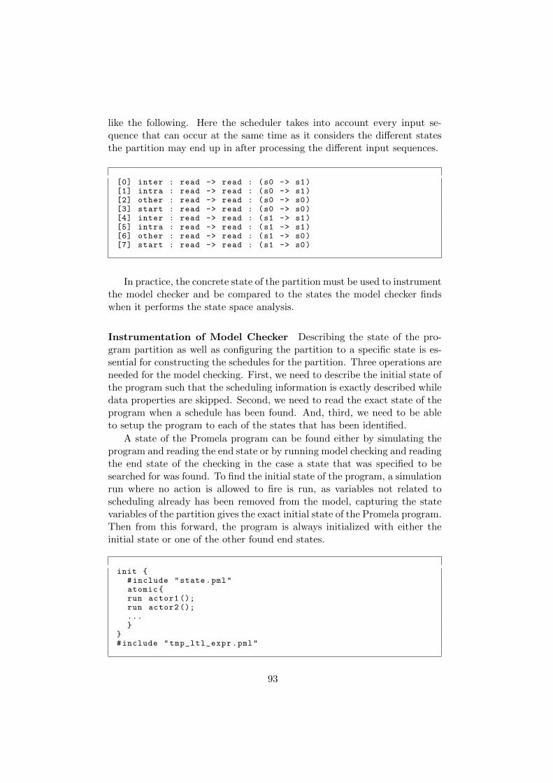
like the following. Here the scheduler takes into account every input se-quence that can occur at the same time as it considers the different statesthe partition may end up in after processing the different input sequences.

[0] inter : read -> read : (s0 -> s1)[1] intra : read -> read : (s0 -> s1)[2] other : read -> read : (s0 -> s0)[3] start : read -> read : (s0 -> s0)[4] inter : read -> read : (s1 -> s1)[5] intra : read -> read : (s1 -> s1)[6] other : read -> read : (s1 -> s0)[7] start : read -> read : (s1 -> s0)

In practice, the concrete state of the partition must be used to instrumentthe model checker and be compared to the states the model checker findswhen it performs the state space analysis.

Instrumentation of Model Checker Describing the state of the pro-gram partition as well as configuring the partition to a specific state is es-sential for constructing the schedules for the partition. Three operations areneeded for the model checking. First, we need to describe the initial state ofthe program such that the scheduling information is exactly described whiledata properties are skipped. Second, we need to read the exact state of theprogram when a schedule has been found. And, third, we need to be ableto setup the program to each of the states that has been identified.

A state of the Promela program can be found either by simulating theprogram and reading the end state or by running model checking and readingthe end state of the checking in the case a state that was specified to besearched for was found. To find the initial state of the program, a simulationrun where no action is allowed to fire is run, as variables not related toscheduling already has been removed from the model, capturing the statevariables of the partition gives the exact initial state of the Promela program.Then from this forward, the program is always initialized with either theinitial state or one of the other found end states.

init {#include "state.pml"atomic{run actor1 ();run actor2 ();...}

}#include "tmp_ltl_expr.pml"

93

Search for Schedules The last piece of the model checking puzzle is thedescription of the state to look for. Now, model checkers are typically meantfor verifying correctness of programs, thus correctness properties that shouldhold for the program are described and errors are reported by the modelchecker when a violation is found. Typically an error state or a sequence ofstates that should never occur are described with linear-time temporal logicwhich enables reasoning about the order in which things happen.

In the search for schedules, we are interested in finding specific states inthe program state space and the sequence of action firings that leads to thatstate from the state to which the model checker was initialized. To makethe model checker to search for a specific state and report that the state isreachable providing the path (the trace) to this state, the state needs to bedescribed as an unwanted error state. This kind of (miss-) using the modelchecker is needed when a general model checker that is designed to verifycorrectness and not schedule existence is used for this purpose.

The state to be found can simply be described as a linear-time temporallogic formula, as is shown in Formula 5.1, which simply says that for everystate (the square), there should not be a state where the program has madeprogress, by firing at-least one action, and where the FSM of actor1 is inthe state named state1, and the data of the FIFOs of the partition has beenconsumed. What is actually described here is that, first of all, a schedulerequires that something has been done, else the schedule is useless. Second, apartial specification of the state to be found is described typically describinghow one of the actors should be run during this schedule, and last, somedescription of how the other actors have synchronized with the tokens thathas been produced by getting to the specified state.

ltl �! (hasProgress ∧ FSMactor1 == state1 ∧ emptyBuffers) (5.1)

The spin model checker generates an automaton, based on this formula,that is executed in lock-steps with the program that is model checked. Theautomaton describes a sequence that should never occur and it is an errorwhen the automaton terminates; the generated trace to the error can thenbe used in combination with the simulator to run the program according tothe schedule that ends up in the specified state [72]. The simulator can thenbe instrumented to generate the information that is needed to both get theschedule and the state that is needed to decide on how the new schedulerneeds to be updated to correspond to the information gained from runningthe model checker.

Model Checking Results The output from the model checker, when thedescribed state is found, is the sequence of action firings that lead to that

94

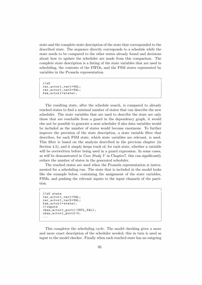
state and the complete state description of the state that corresponded to thedescribed state. The sequence directly corresponds to a schedule while thestate needs to be compared to the other states already found and decisionsabout how to update the scheduler are made from this comparison. Thecomplete state description is a listing of the state variables that are used inscheduling, the contents of the FIFOs, and the FSM states represented byvariables in the Promela representation.

//s0var_actor1_var1=VAL;var_actor1_var2=VAL;fsm_actor1=state1;

The resulting state, after the schedule search, is compared to alreadyreached states to find a minimal number of states that can describe the newscheduler. The state variables that are used to describe the state are onlythose that are reachable from a guard in the dependency graph, it wouldelse not be possible to generate a neat scheduler if also data variables wouldbe included as the number of states would become enormous. To furtherimprove the precision of the state description, a state variable filter thatdescribes, for each FSM state, which state variables are relevant, is used.This filter is based on the analysis described in the previous chapter (inSection 4.5), and it simply keeps track of, for each state, whether a variablewill be overwritten before being used in a guard expression. In some cases,as will be demonstrated in Case Study V in Chapter7, this can significantlyreduce the number of states in the generated scheduler.

The reached states are used when the Promela representation is instru-mented for a scheduling run. The state that is included in the model lookslike the example below, containing the assignment of the state variables,FSMs, and pushing the relevant inputs to the input channels of the parti-tion.

//s0 statevar_actor1_var1=VAL;var_actor1_var2=VAL;fsm_actor1=state1;// inputschan_actor1_port1!CNTL_VAL1;chan_actor1_port2 !0;...

This completes the scheduling cycle. The model checking gives a moreand more exact description of the scheduler needed; this in turn is used asinput to the model checker. Finally when each reached state has an outgoing

95

transition (schedule) for each type of input that is accepted in that state,the scheduling is completed.

5.4 Scheduling Strategies

With the vast number of behaviors that can be implemented in a dataflownetwork, it is no surprise that one scheduling strategy will not be sufficientfor every program. Luckily, a few variation of the one strategy presentedabove, covers the majority of programs. The key point is to decide whichthe states to search for are, as the other parts of the scheduling is generaland corresponds to the behavior of the dataflow program. The descriptionof the end state of a schedule, however, is either a state that can be reachedor not. The problem then is, how to describe a state which is reachable, butat the same time results in a proper scheduler.

The initial scheduler is often given by one of the actors’ simplified FSMs,from which the input sequences that should the processed by the schedulesare defined. When there are no data dependences, the choice of initialscheduler is arbitrary and could be omitted, and a schedule could correspondto processing all the available data. In general, what can be used to describethe state of a partition when searching for a schedule is: FSM states ofactors, state variables of actors, FIFO channel contents, and progress of theactors. The problem is that, if the state is described to exactly, it may notbe found, and, if it is described to loosely, the scheduler will probably havemany unnecessary intermediate states. The only property that is alwaysrequired is progress as, a schedule does not make sense if it does not fireany actions, however, different trade-offs between the other properties areneeded.

One FSM Plus Empty Buffers A strategy that works for many actorpartitions is to define a schedule to be finished when every internal FIFOof the partition is empty and the inputs of the leader actor have been con-sumed. The state description then contains the FSM state of one of theactors, the requirement that the FIFOs are empty, and of course the re-quirement of progress; this is the strategy presented throughout this chap-ter. The state variables are completely outside the description, however,they are considered when constructing the scheduler. The requirement ofhaving every FIFO empty between the schedules is not always possible, anda variation of the strategy is needed to handle these cases.

Allowing Delay Tokens Programs with feedback loops may often beimplemented to, once initialized, never reach a state with empty buffers. Asimple solution to this problem is to simply remove some of the FIFOs from

96

the requirement of emptiness, and by this allow the program to leave some(valueless data) tokens in the partition between the schedules. These tokensnow need to be part of the state description, and need to be replaced whenthe program is initialized to that state the next time.

There are a couple of alternatives for how to choose which FIFOs to allowto keep tokes, based on how delay tokes usually are used. Often delay tokensare needed together with feedback loops, which makes the feedback FIFOsa natural position where to leave the delay tokes. Another possibility is toconsider how delay tokens are generated in CAL. A delay token is generatedonce, meaning that there probably is an actor which has an action thatcan only run once, after which the actor continues in its normal executionloop. These actors can be identified, and the potential FIFO for keeping thedelay token is the one where it initially is produced. However, identificationof delay tokens is outside the scope if this work and is instead left for thedeveloper to decide on and inform the scheduling framework.

All FSMs Specified Sometimes a specific strategy can be used to forcethe scheduler to use an already known state, if it is reachable. This is usefulwhen the partition contains actions which does not affect the state of theFIFOs inside the partition, typically by having an action that changes theFSM state of an actor but does not communicate with ports. In this case,the state that is searched for can be described more exactly by specifyingthe required states of each FSM according to an already known state. Bydoing this, the final scheduler becomes smaller.

5.5 Actor Composition

Schedules are created to be executed. A schedule can be seen as a list ofactions that will fire in sequence and can be glued in to the C programgenerated from the CAL program as a list of function calls to functions rep-resenting the actions. It is, of course, more practical to be able to transformthe CAL program according to the new scheduler and allow code generationfrom the transformed CAL program. The scheduler created by the approachpresented in this chapter consists of an FSM scheduler, a set of guards basedon the guards of the original actors, and sequences of action firings repre-senting transitions of the FSM. This obviously resembles a CAL actor, andcan be seen as a composition of the original actors.

In practice, the FSM from the generated scheduler becomes the FSM ofthe composed actor, the schedules become actions, the needed guards areadded to the actions, and the token rates are calculated from the schedules.With actor composition, the composed actor is more predictable than theset of original actors. The communication between the actors is known at

97

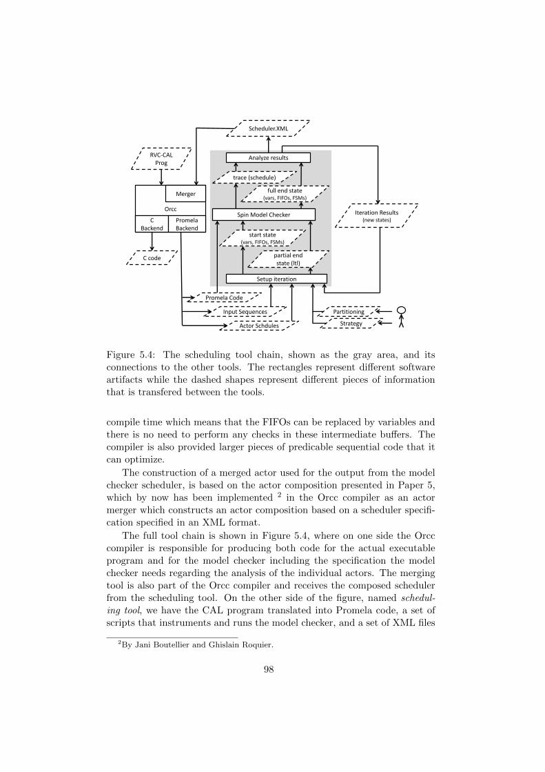
Orcc

C Backend

Promela Backend

Setup iteration

RVC-CAL Prog

C code

Scheduler.XML

Promela Code

Input Sequences

Actor Schdules

Merger

Spin Model Checker

start state (vars, FIFOs, FSMs)

partial end state (ltl)

trace (schedule)

full end state (vars, FIFOs, FSMs)

Analyze results

Iteration Results (new states)

Partitioning

Strategy

Figure 5.4: The scheduling tool chain, shown as the gray area, and itsconnections to the other tools. The rectangles represent different softwareartifacts while the dashed shapes represent different pieces of informationthat is transfered between the tools.

compile time which means that the FIFOs can be replaced by variables andthere is no need to perform any checks in these intermediate buffers. Thecompiler is also provided larger pieces of predicable sequential code that itcan optimize.

The construction of a merged actor used for the output from the modelchecker scheduler, is based on the actor composition presented in Paper 5,which by now has been implemented 2 in the Orcc compiler as an actormerger which constructs an actor composition based on a scheduler specifi-cation specified in an XML format.

The full tool chain is shown in Figure 5.4, where on one side the Orcccompiler is responsible for producing both code for the actual executableprogram and for the model checker including the specification the modelchecker needs regarding the analysis of the individual actors. The mergingtool is also part of the Orcc compiler and receives the composed schedulerfrom the scheduling tool. On the other side of the figure, named schedul-ing tool, we have the CAL program translated into Promela code, a set ofscripts that instruments and runs the model checker, and a set of XML files

2By Jani Boutellier and Ghislain Roquier.

98

including partial schedules, scheduling information about individual actors,and information about input sequences.

5.6 Related Work

Scheduling of dataflow programs is far from a new problem and it has beeninvestigated for several decades. The scheduling problem can be dividedin to two categories, 1) designing dataflow programs where actors have re-stricted behavior according to a MoC which guaranties a certain level ofpredictability, or 2) designing the program with a very expressive languageand attempt to fit parts of it in to more restricted MoCs. For the firstapproach many MoCs with a different trade-off between predictability andexpressiveness has been proposed and several of these were presented inChapter 2. For the second, the scheduling can be viewed as fitting actorsto more restricted models which can be statically scheduled, as presentedin the last chapter, or by scheduling a part (or partition) of a program aspresented in this chapter. There are several approaches that are relevant tobe compared to the scheduling approach presented in this chapter.

Dynamic Code Analysis The scheduling approach that resembles theapproach presented in this chapter the most is dynamic analysis presented byBoutellier et al. in [28]. Here, the executable code generated from the CALcode is instrumented to collect the needed information from the programwhile the program is executing. The approach is called dynamic as theinformation is collected during program runs with real input; this means thatthe program is analyzed during normal execution, however, it also meansthat the inputs must cover all types of possible inputs for the generatedschedules to make sense.

A quasi-static scheduled actor network is defined as a set of actors wherea control value entering the partition on a FIFO, decides which operatingmode (or schedule) to be fired. This definition matches the behavior ofPSDF [20], by seeing the control token as the parameter that controls theoperation of the partition. This also, of course, requires that the controltoken has total control over the actor partition [28]. This is similar to therestrictions we have on control tokens in the approach presented in thisthesis, the difference is how this property is verified. Compared to theanalytic approach presented earlier in this chapter, in [28], the program isinstrumented with token gates, which are added to FIFOs that carry controlinformation. A token gate is a construct that has two objectives: first, itcontrols when the control tokens can enter the network and by this can delaythe next control token until all the computations related to the previous onehas finished, and second, it observes the control tokens passing through in

99

order to use these as parameters [28].The dynamic analysis then collects, for each actor, action chains, which

consist of a sequence of action firings and a corresponding signature whichdescribes the parameters that made the actor run that specific sequence.Further, on the network level, the values of the control tokens are mappedto sequences of actors that are invoked for that specific value. These se-quences are called strands, where a slot corresponds to an actor and cancontain a number of action chains. The result is then a set of actor strandscorresponding to control values and a set of action chains corresponding tothe set of signatures for the actors. [28]

Boutellier et al. presented a further improved version of this approachin [27], with improvements mainly regarding the segmentation and the gen-eration of quasi-static schedules. We can for the purposes of this chaptersee the production of action chains to be similar to the one presented in [28]as it is also discussed in Chapter 4 related to the actor level scheduling.The concepts of actor strands and token gates, are however dropped hereand the network level scheduling is made more general by constructing thesegments according to a set of rules regarding the behavior of the actor andthe scheduling is constructed by expanding the concept of signatures to thelevel of segments.

The approach in [28] has to some extent been used as inspiration whendeveloping the approach presented in this thesis. The model checking ap-proach has some advantages over the dynamic code analysis. First, with amodel checker, it is possible to search for a specific state, while when run-ning a program, it is, in some cases, difficult to accidentally get the programto interleave the action such that the wanted state is reached. Second, theinputs should be proved to be complete, how this can be done has beendemonstrated in this chapter, and could probably be extended to the ap-proach in [28, 27].

Statically Schedulable Regions Another approach, presented by Gu etal. [60] identifies SDF like regions in CAL programs which can be sched-uled statically. The end result is a quasi-static scheduler, where groups ofcomputations across several actors can be statically scheduled while thesegroups are dynamically scheduled. The idea is to identify statically schedu-lable regions, which can be seen as a set of ports from several actors, whichare connected by one of several possible relations. The identification of stat-ically schedulable regions mainly consists of constructing a graph describingthe association between ports after which various transforms are performedon the graph.

The initial partitioning of ports, which is performed per actor, is basedon the interaction between the ports. If two ports either are used in thesame action, or one port is used in a state changing-action while the other

100

port is used in a state-guarded action, then the two ports are in the samepartition and are called coupled ports. Then, a coupling relationship graphis constructed by extending the partitioning to span over several actors byusing the information about how the queues connect the ports in the CALprogram. The partitioning so far describes how the ports directly dependson each other; to make something useful out of this, the next step is toidentify coupled groups, which are the weakly connected components of thecoupling relationship graph.

The next step is to extract from each coupled group a subset of ports intostatically related groups. These ports are static rate ports, which means thateach action using that port has the same rate for that port. Furthermore,the subset of ports, must be such that any action of the actor, either haseach of these ports or none. This means that, for each action firing of thatactor, either, each of these ports will consume/produce a static number oftokens, or nothing. This property is related to the ports, the actions usingthese ports can still include dynamic ports, however, these ports have astatic relationship regarding token rates.

By connecting the statically related groups according to the CAL net-work, and by this constructing a graph, statically schedulable regions canbe constructed by taking the weakly connected components form this graph.The statically schedulable regions are then a set of ports across the dataflownetwork which acts like an SDF graph. Due to the partitioning, these arealso independent, as ports related by state modification are in the samepartition or outside the partitions. This means that the static regions canbe extracted as separate actors, where the ports connecting the staticallyrelated groups disappear inside the actor, while the other ports remain asthe ports of the new actor.

This work is quite different from the presented approach which searchesfor schedules by analyzing and identifying the dynamic behavior, while thisapproach identifies the static behavior. It is not completely clear how theapproaches could be used together, one possibility is to first identify stati-cally schedulable regions and extract these as separate actors, then use thepresented approach to schedule the dynamic parts possibly including thestatic regions.

Analysis of Actors with SMT The actor classification approach, whichwas already discussed in the previous chapter, presented by Wipliez etal. [124], involves analyzing the guards of each actor with an SMT solver(Satisfiability Modulo Theories). This involves finding the parameter thatexclusively satisfies the input dependent guards when an actor is classifiedas quasi-static, but also to identify time-dependent behavior. For the dis-cussion in this chapter, the approach for comparing whether guards arecompatible or not, is interesting as is relates to the problem of checking the

101

guard strengths. It would make sense to investigate whether an extendedversion of this work could be used to check the compatibility between guardsof separate actors, that is, to find if the guards of one actor are strong enoughfor scheduling a partition. Furthermore, parts of this work are directly usedfor generating the model checker information.

In generating the Promela program as presented above, the guard solveris directly reused to produce the concrete control tokens. This is only avail-able for control tokens that are peeked, so far, but could be extended to allowother types of input values; the problem being that if the control value ismodified before reaching the guard, the analysis becomes more complex, andif the guard does not purely depend on that input, it may be impossible.Also, the functionality to identify if an actor has time-dependent behavioris used to find the actors that must be placed in actor partitions such thatthe actor can be scheduled correctly.

Generalized Dataflow Scheduling A different but related schedulingapproach was presented by Plishker et al. in [107]. This scheduling approachis based on a dataflow MoC called Core Functional Data Flow (CFDF) [106],which describes a dataflow actor as a set of modes which have static tokenrates. The dynamic behavior of an actor is described by invoking one modewhich gives the next valid modes; the modes and transition between thesecould simply be described as an FSM. SFDF can easily be used to describeMoCs such as SDF by having only one mode, CSDF by having a set ofmodes that are cyclically enabled, and BDF by having one mode checkingthe Boolean value and enabling one of the two modes corresponding to theBoolean values True and False.

The modes of the actors in CFDF have static token rates, like actions inCAL, and the scheduling of the modes is a result of a mode being invoked,resembling the action scheduling in CAL. So, it is obvious that this approachis applicable to CAL.

The idea in the scheduling approach is that, while an actor may havedynamic behavior, the modes are static and may be statically composed withmodes from the other actors. These compositions, then, are static dataflowgraphs which interactions can be scheduled dynamically. The result is aquasi-static scheduler, which dynamically searches for a static graph thatcan be invoked.

A Rule-Based Quasi-Static Scheduling Approach In many cases, adataflow program may consist of many static actors while a few dynamicactors are needed to take care of any dynamic property. In such cases, com-position of static actors that are mapped to the same processor core impliesimproved performance of the program. Falk et al. presented a rule-based

102

quasi-static scheduling approach in [55], where static actors are clusteredtogether to form composite actors such that the quasi-static schedule of thecomposite actors guarantee deadlock-freedom.

The work by Falk et al. is more explicit, compared to this work, regard-ing how the schedules should be produced such that deadlock-freedom canbe guaranteed globally. As we know, deadlock-freedom is not closed undercomposition for models such as SDF; for this reason the composition is per-formed according to a set of rules which produces a quasi-static schedulerfor the static actors such that deadlocks are avoided. This is similar to howa CSDF actor can avoid deadlock, by splitting the firing in to phases, wherean SDF actor would cause deadlock. The scheduler in this model, however,is more flexible and is described as an FSM.

What this approach has in common with the approach presented in thisthesis, is that there is a set of rules for when actors can be composed,and then there is one or more strategies for performing the compositionand scheduling. The difference is that this approach in general producescomposite actors by adding dynamism to the original static actors, while thepresented approach only removes dynamism. A scheduling strategy whichadds dynamism for avoiding deadlocks would be useful for the approachpresented in this thesis, as it would enable more options for constructingpartition for actor composition.

Model Checking Dataflow Applications While model checking typi-cally is used to verify that a design behaves correctly, using model checkersfor finding a better solution to various problems has also been used to someextent. In [109] Ruys presents how the Spin model checker can be usedto find optimal solutions for problems like traveling sales man, which tosome extent resembles the problem of scheduling a dataflow program. Herethe guarded commands includes cost functions, that is, depending on whichchoice is made, a different penalty is added to the total cost. Every time abetter solution is found, that is, with a lower cost, Spin emits a trail withthe schedule of the traveling sales man.

The traveling salesman problem is to some extent similar to the CALscheduling problem, as soon as a complete model has been generated for apartition of a CAL program. An interesting idea, would be to use a similarapproach as presented in [109] to define cost for the order of actions to notonly search for a schedule, but to, for example, search for a schedule withbetter data locality.

Using model checking for analyzing and optimizing dataflow applica-tions is not a completely new idea either. In [115] Theelen et al. presentresults of analyzing scenario-aware dataflow with the CADP model checker,to formally verify functional and performance properties of the dataflowmodel. Also some work related to scheduling of dataflow has been pre-

103

sented; scheduling of SDF with the goal of minimal buffer sizes has beenpresented by Geilen et al. [59], Liu et al. [87], and Guan et al. [62], and withextensions to CSDF, MD-SDF, and BDF, by Gu et al. [61].

104

Chapter 6

Discussion on Efficiency andImplementation

Actor composition and scheduling is not the goal, in itself, but are meansto transform the program into a more efficient format to better fit a targetplatform. To improve the performance of a program, several design choicesaffect the end result and depending on the target platform and what ac-tually is meant with performance, some choices are more adequate thanothers. The goal with this chapter is to present some experimental resultsregarding actor composition and draw some conclusions from these to betterunderstand how a dataflow program should be designed and transformed,such that efficient code can be generated.

From the scheduling perspective, the performance is affected by the com-plexity of the scheduling, meaning that the number of guard evaluation andthe complexity of these, decide how much work is spent on scheduling. Thepartition sizes also play a role here as the number of partitions decides onhow many partitions must be scheduled by a run-time scheduler choosingthe actor partition to schedule next. At the same time, the partition sizesalso affect the memory footprint of the program which affects cache behav-ior. This means that a longer static schedule, while requiring fewer guardevaluations per action firing, also requires more memory when running.

If composition is a method to increase the size of the actors and therebyto improve the performance of a program, one could imagine that it wouldbe easier to directly design the program with large enough actors in thefirst place. And, this is true; the performance of a program that has beentailored to fit a platform is difficult to achieve by transforming another pro-gram. However, implementing a program for one specific platform is notvery interesting, instead, a program should be portable and a decent andpredictable performance should be achievable, on many different platforms,by applying a set of transformations and optimizations. The approach cho-

105

sen here for this problem is to design fine grained programs and use compo-sition to achieve coarser grained designs when needed; the opposite, that is,splitting actors, could also be possible but is not investigated here.

Ideally, a dataflow program designed for an FPGA should be designedon the level of adders and multipliers, producing a program with a maximalnumber of simple parallel actors. The scheduling of each of the actors isnot a problem in this case, since each of the actors have dedicated hardwareand there is no software interleaving of the actors. It does not make senseto compose and schedule, and thereby sequentialize such an application.On the other hand, when an application is designed for a general purposeprocessor, the scheduling and interleaving of the program on the level ofadders and multipliers would introduce a huge overhead and the programneeds to be implemented on the level of larger functional blocks in orderto be efficient. It is this kind of fitting applications to processors which isthe main purpose with the work presented in this thesis, the difficulty is,however, to decide what a program should look like in order to fit a specificplatform.

6.1 Design Parameters

The main goal with composition of actors is to enable more efficient schedul-ing. First of all, the scheduling of actors, that is, the task to find an actorwith an enabled action becomes simpler when there are fewer actors toschedule. Simultaneously, the number of guards that needs to be evaluatedper action fired is reduced as one guard can enable a sequence of actions thatcan fire. These improvements of a program are, as such, platform indepen-dent, as they simplify the action selection process and by this only reducethe number of calculations that are needed in order to run the program.The results of actor composition, however, are not platform independent;instead the schedules affect the size of the work units and thereby also thememory usage. Sometimes, these properties have an opposite effect on theprogram performance; a composition of two actors may reduce the schedul-ing overhead while causing worse cache behavior. Which of the propertieshave a stronger result on the performance depends on the architecture ofthe target processor.

Considering a single processor, the number of actors that works well onthe processor depends on a few things. To begin with, the program itselfgives the first indication of how many partitions it is efficient to composethe program to. For more complex programs, it is often difficult to findsimple schedulers for the whole program and instead unrelated parts of theprogram should be placed in different partitions. This is then a trade-offbetween the complexity of the actor scheduler and the action schedulers.

106

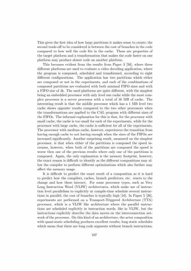
This gives the first idea of how large partitions it makes sense to create; thesecond trade-off to be considered is between the cost of branches in the codecompared to how well the code fits in the cache. These are properties ofthe target platform and a transformation that makes the code faster on oneplatform may produce slower code on another platform.

This becomes evident from the results from Paper 3 [50], where threedifferent platforms are used to evaluate a video decoding application, wherethe program is composed, scheduled and transformed, according to eightdifferent configurations. The application has two partitions which eitherare composed or not in the experiments, and each of the combinations ofcomposed partitions are evaluated with both minimal FIFO sizes and witha FIFO size of 4k. The used platforms are quite different, with the simplestbeing an embedded processor with only level one cache while the most com-plex processor is a server processor with a total of 16 MB of cache. Theinteresting result is that the middle processor which has a 1 MB level twocache shows opposite results compared to the two other processors whenthe transformations are applied to the CAL program with different sizes ofthe FIFOs. The informal explanation for this is that, for the processor withsmall cache, the cache is too small for each of the experiments, while for theprocessor with large cache, the cache is sufficient for all of the experiments.The processor with medium cache, however, experiences the transition fromhaving enough cache to not having enough when the sizes of the FIFOs areincreased significantly. Another surprising result, measured on the simplestprocessor, is that when either of the partitions is composed the speed in-creases, however, when both of the partitions are composed the speed isworse then one of the previous results where only one of the partitions iscomposed. Again, the only explanation is the memory footprint, however,the exact reason is difficult to identify as the different compositions may al-low the compiler to perform different optimizations which also further mayaffect the memory usage.

It is difficult to predict the exact result of a composition as it is hardto predict how the compilers, caches, branch predictors, etc. reacts to thechange and how these interact. For some processor types, such as VeryLong Instruction Word (VLIW) architectures, which make use of instruc-tion level parallelism to explicitly at compile-time schedule several instruc-tions in parallel, the cost of branches is typically high [16]. In Paper 5 [26],experiments are performed on a Transport-Triggered Architecture (TTA)processor, which is a VLIW like architecture where the parallel instruc-tions are scheduled explicitly in instruction words, like in VLIW, but theinstructions explicitly describe the data moves on the interconnection net-work of the processor. On this kind of an architecture, the actor compositionwith quasi-static scheduling produces excellent results; long static scheduleswhich mean that there are long code segments without branch instructions,

107

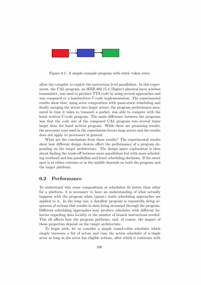
Figure 6.1: A simple example program with static token rates.

allow the compiler to exploit the instruction level parallelism. In this exper-iment, the CAL program, an IEEE 802.15.4 (Zigbee) physical layer wirelesstransmitter, was used to produce TTA code by using several approaches andwas compared to a handwritten C-code implementation. The experimentalresults show that, using actor composition with quasi-static scheduling andfinally merging the actors into larger actors, the program performance mea-sured in time it takes to transmit a packet, was able to compete with thehand written C-code program. The main difference between the programswas that the code size of the composed CAL program was several timeslarger than the hand written program. While these are promising results,the processor type used in the experiments favors large actors and the resultsdoes not apply to processors in general.

What are the conclusions from these results? The experimental resultsshow how different design choices affect the performance of a program de-pending on the target architecture. The design space exploration is thenabout finding the trade-off between more parallelism but with more schedul-ing overhead and less parallelism and fewer scheduling decisions. If the sweetspot is at either extreme or in the middle depends on both the program andthe target platform.

6.2 Performance

To understand why some compositions or schedulers fit better than otherfor a platform, it is necessary to have an understanding of what actuallyhappens with the program when (quasi-) static scheduling approaches areapplied to it. In the long run, a dataflow program is repeatedly firing se-quences of actions that results in data being streamed through the program.Different scheduling approaches may produce schedules with different be-havior regarding data locality or the number of branch instructions needed.This all affects how the program performs, and, of course, the impact ofthese properties depend on the target architecture.

To begin with, let us consider a simple round-robin scheduler whichsimply traverses a list of actors and runs the action scheduler of a singleactor as long as the actor has eligible actions, after which it continues with

108

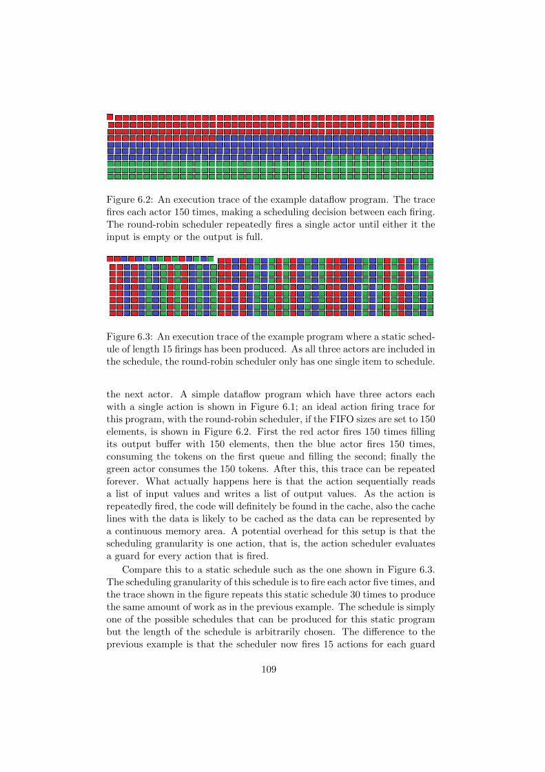
Figure 6.2: An execution trace of the example dataflow program. The tracefires each actor 150 times, making a scheduling decision between each firing.The round-robin scheduler repeatedly fires a single actor until either it theinput is empty or the output is full.

Figure 6.3: An execution trace of the example program where a static sched-ule of length 15 firings has been produced. As all three actors are included inthe schedule, the round-robin scheduler only has one single item to schedule.

the next actor. A simple dataflow program which have three actors eachwith a single action is shown in Figure 6.1; an ideal action firing trace forthis program, with the round-robin scheduler, if the FIFO sizes are set to 150elements, is shown in Figure 6.2. First the red actor fires 150 times fillingits output buffer with 150 elements, then the blue actor fires 150 times,consuming the tokens on the first queue and filling the second; finally thegreen actor consumes the 150 tokens. After this, this trace can be repeatedforever. What actually happens here is that the action sequentially readsa list of input values and writes a list of output values. As the action isrepeatedly fired, the code will definitely be found in the cache, also the cachelines with the data is likely to be cached as the data can be represented bya continuous memory area. A potential overhead for this setup is that thescheduling granularity is one action, that is, the action scheduler evaluatesa guard for every action that is fired.

Compare this to a static schedule such as the one shown in Figure 6.3.The scheduling granularity of this schedule is to fire each actor five times, andthe trace shown in the figure repeats this static schedule 30 times to producethe same amount of work as in the previous example. The schedule is simplyone of the possible schedules that can be produced for this static programbut the length of the schedule is arbitrarily chosen. The difference to theprevious example is that the scheduler now fires 15 actions for each guard

109

evaluation; at the same time, within a schedule, code from three differentactors are fired and both FIFOs are accessed. This puts more pressure onthe cache. Which of these two schedulers performs better depends on howwell the schedules fit in the cache, regarding both instructions and data, andhow expensive the guard evaluation is.

Multi-core Performance While this work focuses on composition, andthereby on improving the performance of a single processor core, the goalwith the work is to enable efficient solutions for platforms with more thanone cores. The approach for composing and scheduling actors is directlyusable of many-core systems as the only thing it does is to reduce the num-ber of actors that must be scheduled at run-time. For the performance ofone of the single cores, the same balancing between reducing schedulingoverheads and improving cache behavior as above applies, however, the in-teraction between several cores makes the performance even more difficultto predict. Communication between actors mapped to several cores intro-duces performance limitations for example as a result of concurrent memoryaccesses [89].

The execution of a CAL program on a platform with several cores canin principle be done in two different ways. One way is to leave the schedul-ing of the actors to the operating system and let each actor be run on aseparate thread. The problem with this approach is that the operating sys-tem does not have enough information about the dataflow program to beable to schedule it efficiently [127]. Another approach is to have one threadper core, where the thread has a number of actors that are mapped to thiscore to schedule. This kind of a scheduler for multi-core scheduling of CALprograms was presented by Hyviquel et al. in [127], where a distributedscheduler, based on a combination of a round-robin and a demand drivenscheduling strategy, implementing the distributed scheduler by using lock-free communication channels for exchanging scheduling information, wasused. With the first approach, mapping an actor to a thread, compositionmakes the task of the thread scheduler easier as the number of actors canbe matched to the number of cores. By this, the scheduling of threads thatanyway cannot fire anything is not an as big problem. When a dataflowprogram is run on a platform with many cores, one of the problems is tobalance the load of the cores. Load-balancing can be performed by movingthe execution of one actor to another core. With composition, the granular-ity of the load balancing is coarser which implies more coarse grained loadbalancing.

Considering multi-core architectures, and especially heterogeneous multi-core architectures, it is often more sufficient to use design space explorationto, at design time, come up with an appropriate mapping. With such astatic mapping, the need for actor composition becomes clearer as the com-

110

position problem now is performed per core. As an example, each of thedesign space exploration approaches for dataflow to multi core architecturesin [89, 108, 19, 32, 100], present a step where actors either are composedor split. The work presented in this thesis can be seen as that part ofthe design space exploration where the actors mapped on to the same coreare optimized for better single processor performance. This still does not re-move the potential problems with the communication between the processorcores; however, this issue has been addressed by, among others, Roquier etat. in [108], where the communication between the actors are handled andscheduled by adding additional vertices or actors to handle the inter-corecommunication.

As can be seen, the performance of a program, especially on multi-core,depends on several different details of the implementation, and, schedulingand composition, by them selves, does not guarantee efficient code. On theother hand, by using the appropriate design space explorations methods,to identify the parts of the program where composition will be adequate,different scheduling and composition approaches will make a difference inhow the generated program performs.

6.3 Efficient Code Generation

The quasi-static scheduling of an actor partition enables the actors to bemerged into one larger actor which has a predictable behavior internally.A composed actor includes the FIFOs connecting the actors in the parti-tion, all the state variables of the actors, and all the actions of the actors.The interaction between these is after composition more predictable as thebehavior of the actor is described by a set of static schedules. To allowefficient code generation it makes a difference how the actor is merged andtransformed before code generation.

Typically the code generation, from high-level descriptions such as data-flow, targets other programming languages (e.g. C/C++) which alreadyhave a wide support for code generation for various processor architectures.This in turn, means that part of how efficient a program is depends on howwell the low level compiler is able to optimize the code. Several trade-offs,that should be considered in the code generation is discussed by Battacharyaet al. in [18], and in addition to transformations related to high-levelconcepts such as clustering and scheduling, also code generation aspectssuch as a potential negative interaction between e.g. inlining and registerallocation. While the work in this thesis is concerned with scheduling andcomposition, it will make a difference how the merged actors are constructed.For the tool chain, this means two things: first, the transformation should bemade on a close to algorithmic level as low level optimizations are provided

111

by the low level compiler and all possible options should be kept open forthe optimizations. Second, optimizations related to the information specificfor a dataflow program, should be used to minimize the needed calculationsof the program as the low level compiler does not have this information.

The actor merging approach presented in Paper 5 [26] is an example ofthis. The quasi-static scheduler provided for an actor partition is imple-mented such that there is a minimal loss of information. The actions ofthe original actors are made into procedures, the schedules of the composedactor becomes actions which sequentially fire the action procedures, and theFSM and guard of the compound scheduler are directly used. This kind ofa structure enables the code generator to inline these procedures (action) ifit is useful, or to iterate sequences of repeated actions either in a loop oras a sequence of procedure calls. The point is that it is up to the low levelcompiler to decide what is the most adequate code for the target platform.

The actor composition enables the actor merger to remove all internalbuffers of a composition as the quasi-static scheduler of such a compositioncan be used to predict the read and write behavior of the buffers. As aresult, FIFO channels can be replaced with simple data structures such asarrays.

What should be handled by the dataflow code generator, however, is any-thing related to removing scheduling decisions, removing redundant schedul-ing information such as FIFOs or state variables, and anything related tosequentializing parts of the code. This type of transformations may not bepossible for a low level compiler to perform as it cannot know about therestrictions a dataflow program has regarding data locality etc. This meansthat is would make sense for the tool to remove state variables and FIFOsthat cannot affect the outputs of the partition that has been merged to oneactor.

With the composed actors, the last step which affects the performancein the actual code generator. There exists a number of code generations forCAL, and there is a lot of development around such tools as Orcc. As thesecode generators are constantly improved, it is important that the, in thiscase external, scheduling tools have the ability to use the code generators ofthese.

6.4 Related Work

This chapter is mainly based on the experimental results that has been ob-tained from the evaluation of the scheduling approaches presented. Thereexists a number of publications which present scheduling approaches andeach of these present, in one way or another, experimental results whichcould be compared to the results in this work. While it to some extent is

112

hard to directly compare measurements such as speedup, some experimen-tal results should be compared to show, on a more general level, that thepresented results and conclusions hold.

Some other Experiments To get more broad results regarding the po-tentials of efficient scheduling and actor composition, some of the approachespresented earlier should be compared regarding the performance improve-ment reported.

Wipliez et al. presented actor classification in [124, 123], where thescheduling is performed based on the classes of MoCs that the actors aredetermined to belong to. This kind of an approach can provide very efficientscheduling when the actors belong to static MoCs, which also is shown bythe results is Paper 3 [50] where this classification approach was used toschedule one of the partitions. When the actors of a partition belong tostatically schedulable classes, it is difficult to improve on the speedup of thistype of approaches. With the actor classification, the speedup of the MPEG-4 decoder that was used as an example in [123] was about 20%. However,the results in paper Paper 3 [50] shows, for a different platform, that thespeedup of an MPEG-4 decoder is up to 53% using the actor compositionbased on the classification presented in [124].

Boutellier et al. presented an scheduling approach based on dynamiccode analysis in [27]. The dynamic code analysis resembles the work pre-sented in this thesis, with the exception of how the input sequences of aprogram are generated and how the actual schedules are searched for. Else,the type of composition is quite similar as it is based on the traces of howactions of several actors are fired. The results presented in [27] show aspeedup of up to 58% for an MPEG-4 decoder running on a Intel Core 2Duo E8500 processor. The produced schedules, with the dynamic code anal-ysis approach, result in schedules that resembles the schedules produced bythe model checking approach. For this reason, the resulting performancecan be expected to reside in the same range, however, the partitioning ismore closely specified in the dynamic code analysis approach.

Gu et al. presented using static regions for enabling static schedulingof parts of a dataflow program in [60]. This approach, while being elegant,only performs well when the application is enough static. The approach wasevaluated on the IDCT network of a CAL implementation of an MPEG-4 decoder and showed a speedup of about 10% regarding the frame rate.Again, it is difficult to compare the results, however, it shows on improve-ment when the dataflow network is appropriately restructured. What isinteresting in this approach, although it was not the case in this example,is that the restructuring not necessarily is a pure composition but also mayinvolve splitting actors, or ending up with a completely new set of actors.

Plishker et al. presented in [107] a generalized scheduling approach, which

113

is based on the CFDF model of computation. The experimental resultspresented show a reduction of execution time of up to almost 85% for somesignal processing applications, compared to a simple round-robin scheduler.However, for one of the test programs, the run-time increased; this resultcorresponds to the findings presented in this chapter regarding the trade-offbetween different overheads.

Falk et al. presented a rule-based qusi-static scheduling approach in [55],where sets of static actors were clustered together and were quasi-staticallyscheduled such that deadlocks were avoided when the composite actors in-teracted with the surrounding including dynamic actor. Falk et al. presentssome experimental results with the proposed clustering algorithms where,among other results, the performance of a Motion JPEG decoder was im-proved by 40%, when the (fine grained) IDCT network was clustered withthe proposed algorithm. Another experiment showed that the speedup of acoarser grained mp3 decoder was was about 6%. This is another example ofthat clustering, or composition, is only useful up to a specific point wherethe program reaches a sweet spot, which again depends on the platform.

Each of these works show on an improvement of the speed of an dataflowprogram in the (quite wide) range of 10-85% depending on the platform andthe application that was used in the experiment. These results correspondto the experiments performed in this work, and therefore shows that actorcomposition and scheduling is an important part of the tools that are neededfor fitting dataflow applications onto various processor architectures. Theother property that will be of interest to evaluate based on relevant literatureis the scalability of dataflow program onto multi-core architectures.

Scalability to Many-Core The main reason for that dataflow is inter-esting for software development is that is scales well to many-core architec-tures. Now, while it is easy to see that the explicit parallelism of a dataflowprogram at least in theory scales to as many cores as there are actors, astatement like this needs some evidence taking into account the potentialoverheads of a realistic platform.

CAL is in principle platform independent and the same implementationshould run on anything between an FPGA and a single processor archi-tecture. Eker et al. presents in [47] an overview of results where CAL isused to target both hardware and software. One of the results show that aMPEG-4 decoder scales, almost linearly, at least up to four cores withoutmodification. Of course, the program can be made to scale even better ifthe appropriate transformations are performed on the actor network.

To know which transformation to perform, some knowledge regarding theprogram is needed. Casale-Brunet et al. presented a tool called TURNUSin [32], which performs a profiled simulation on CAL dataflow programs.The tool records causation traces and analyses properties such as compu-

114

tational load, optimal buffer sizes, critical path measurements, etc. Theanalysis provided by TURNUS is used to decide how the program is to berefactored to achieve the requirements. [32, 3]

With the appropriate design space exploration for identifying the trans-formations needed for a program to efficiently run on a program, dataflowprograms will provide a scalable implementation of many algorithms. Thescalability to many-core, of course, is still limited by the size of the programand the communication overheads between cores.

115

116

Chapter 7

Some Scheduling CaseStudies

The scheduling methods should be general enough to produce a schedulerfor any program, or at least reproduce the original actor if it cannot producea better one. At the same time, the scheduler should use specific propertiesof the program to be able to identify more clever schedules for the program.This is a difficult trade-off; in the work by Wipliez et al. [124], for example,the actors must conform to one of a few statically schedulable MoCs. Theschedules produced are very efficient but it also requires the actors to beimplemented such that these can be scheduled according the one of thegiven MoCs. In this work, the target is something more general, which isenough to identify the schedules to be searched for. In practice, the questionis how to ask the model checker the right questions regarding the state tosearch for. This was already described in Chapter 5, and worked for the kindof applications that were used as examples, but it is still relevant to evaluatethe methods with some more applications and types of applications.

In this chapter some relevant applications 1 for the signal processingand multimedia domain are used to show how different properties of theprogram affect the scheduling approach. The idea is to from this drawsome conclusions about the generality of the approach and what kind ofproblems may arise. The two first cases are basic digital filters, where thescheduling can be expected to be static, however, the implementation maycause some difficulties with the scheduling. The following case is a networkprotocol application, which also may be expected to have static scheduling,but the size of the packets is variable. The last cases are a couple of videodecoding implementations, representing larger applications than the other

1The applications are available at https://github.com/orcc/orc-apps and I would liketo thank all the authors for their work as non of this work would have been possiblewithout their contributions

117

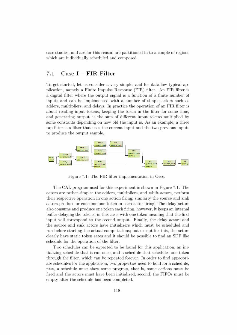
case studies, and are for this reason are partitioned in to a couple of regionswhich are individually scheduled and composed.

7.1 Case I – FIR Filter

To get started, let us consider a very simple, and for dataflow typical ap-plication, namely a Finite Impulse Response (FIR) filter. An FIR filter isa digital filter where the output signal is a function of a finite number ofinputs and can be implemented with a number of simple actors such asadders, multipliers, and delays. In practice the operation of an FIR filter isabout reading input tokens, keeping the token in the filter for some time,and generating output as the sum of different input tokens multiplied bysome constants depending on how old the input is. As an example, a threetap filter is a filter that uses the current input and the two previous inputsto produce the output sample.

Figure 7.1: The FIR filter implementation in Orcc.

The CAL program used for this experiment is shown in Figure 7.1. Theactors are rather simple: the adders, multipliers, and rshift actors, performtheir respective operation in one action firing; similarly the source and sinkactors produce or consume one token in each actor firing. The delay actorsalso consume and produce one token each firing, however, it keeps an internalbuffer delaying the tokens, in this case, with one token meaning that the firstinput will correspond to the second output. Finally, the delay actors andthe source and sink actors have initializers which must be scheduled andrun before starting the actual computations; but except for this, the actorsclearly have static token rates and it should be possible to find an SDF likeschedule for the operation of the filter.

Two schedules can be expected to be found for this application, an ini-tializing schedule that is run once, and a schedule that schedules one tokenthrough the filter, which can be repeated forever. In order to find appropri-ate schedules for the application, two properties need to hold for a schedule,first, a schedule must show some progress, that is, some actions must befired and the actors must have been initialized, second, the FIFOs must beempty after the schedule has been completed.

118

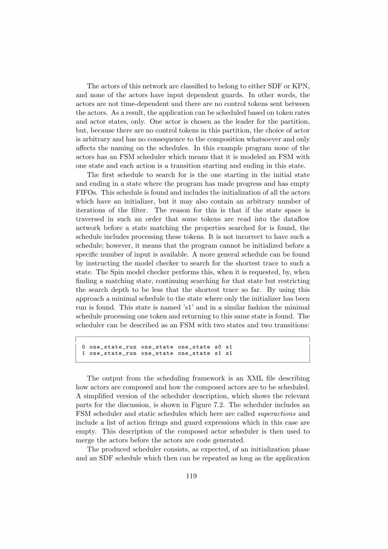
The actors of this network are classified to belong to either SDF or KPN,and none of the actors have input dependent guards. In other words, theactors are not time-dependent and there are no control tokens sent betweenthe actors. As a result, the application can be scheduled based on token ratesand actor states, only. One actor is chosen as the leader for the partition,but, because there are no control tokens in this partition, the choice of actoris arbitrary and has no consequence to the composition whatsoever and onlyaffects the naming on the schedules. In this example program none of theactors has an FSM scheduler which means that it is modeled an FSM withone state and each action is a transition starting and ending in this state.

The first schedule to search for is the one starting in the initial stateand ending in a state where the program has made progress and has emptyFIFOs. This schedule is found and includes the initialization of all the actorswhich have an initializer, but it may also contain an arbitrary number ofiterations of the filter. The reason for this is that if the state space istraversed in such an order that some tokens are read into the dataflownetwork before a state matching the properties searched for is found, theschedule includes processing these tokens. It is not incorrect to have such aschedule; however, it means that the program cannot be initialized before aspecific number of input is available. A more general schedule can be foundby instructing the model checker to search for the shortest trace to such astate. The Spin model checker performs this, when it is requested, by, whenfinding a matching state, continuing searching for that state but restrictingthe search depth to be less that the shortest trace so far. By using thisapproach a minimal schedule to the state where only the initializer has beenrun is found. This state is named ’s1’ and in a similar fashion the minimalschedule processing one token and returning to this same state is found. Thescheduler can be described as an FSM with two states and two transitions:

0 one_state_run one_state one_state s0 s11 one_state_run one_state one_state s1 s1

The output from the scheduling framework is an XML file describinghow actors are composed and how the composed actors are to be scheduled.A simplified version of the scheduler description, which shows the relevantparts for the discussion, is shown in Figure 7.2. The scheduler includes anFSM scheduler and static schedules which here are called superactions andinclude a list of action firings and guard expressions which in this case areempty. This description of the composed actor scheduler is then used tomerge the actors before the actors are code generated.

The produced scheduler consists, as expected, of an initialization phaseand an SDF schedule which then can be repeated as long as the application

119

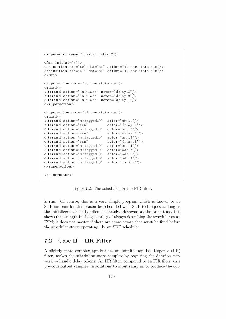
<superactor name=”c l u s t e r d e l a y 2 ”>

<fsm i n i t i a l =”s0”><transition src=”s0 ” dst=”s1 ” action=”s 0 o n e s t a t e r u n ”/><transition src=”s1 ” dst=”s1 ” action=”s 1 o n e s t a t e r u n ”/></fsm>

<superaction name=”s 0 o n e s t a t e r u n”><guard/><iterand action=” i n i t a c t ” actor=”de lay 3”/><iterand action=” i n i t a c t ” actor=”de lay 2”/><iterand action=” i n i t a c t ” actor=”de lay 1”/></superaction>

<superaction name=”s 1 o n e s t a t e r u n”><guard/><iterand action=”untagged 0 ” actor=”mul 1”/><iterand action=”run” actor=”de lay 1”/><iterand action=”untagged 0 ” actor=”mul 2”/><iterand action=”run” actor=”de lay 2”/><iterand action=”untagged 0 ” actor=”mul 3”/><iterand action=”run” actor=”de lay 3”/><iterand action=”untagged 0 ” actor=”mul 4”/><iterand action=”untagged 0 ” actor=”add 2”/><iterand action=”untagged 0 ” actor=”add 1”/><iterand action=”untagged 0 ” actor=”add 3”/><iterand action=”untagged 0 ” actor=” r s h i f t ”/></superaction>

</superactor>

Figure 7.2: The scheduler for the FIR filter.

is run. Of course, this is a very simple program which is known to beSDF and can for this reason be scheduled with SDF techniques as long asthe initializers can be handled separately. However, at the same time, thisshows the strength in the generality of always describing the scheduler as anFSM; it does not matter if there are some actors that must be fired beforethe scheduler starts operating like an SDF scheduler.

7.2 Case II – IIR Filter

A slightly more complex application, an Infinite Impulse Response (IIR)filter, makes the scheduling more complex by requiring the dataflow net-work to handle delay tokens. An IIR filter, compared to an FIR filter, usesprevious output samples, in additions to input samples, to produce the out-

120

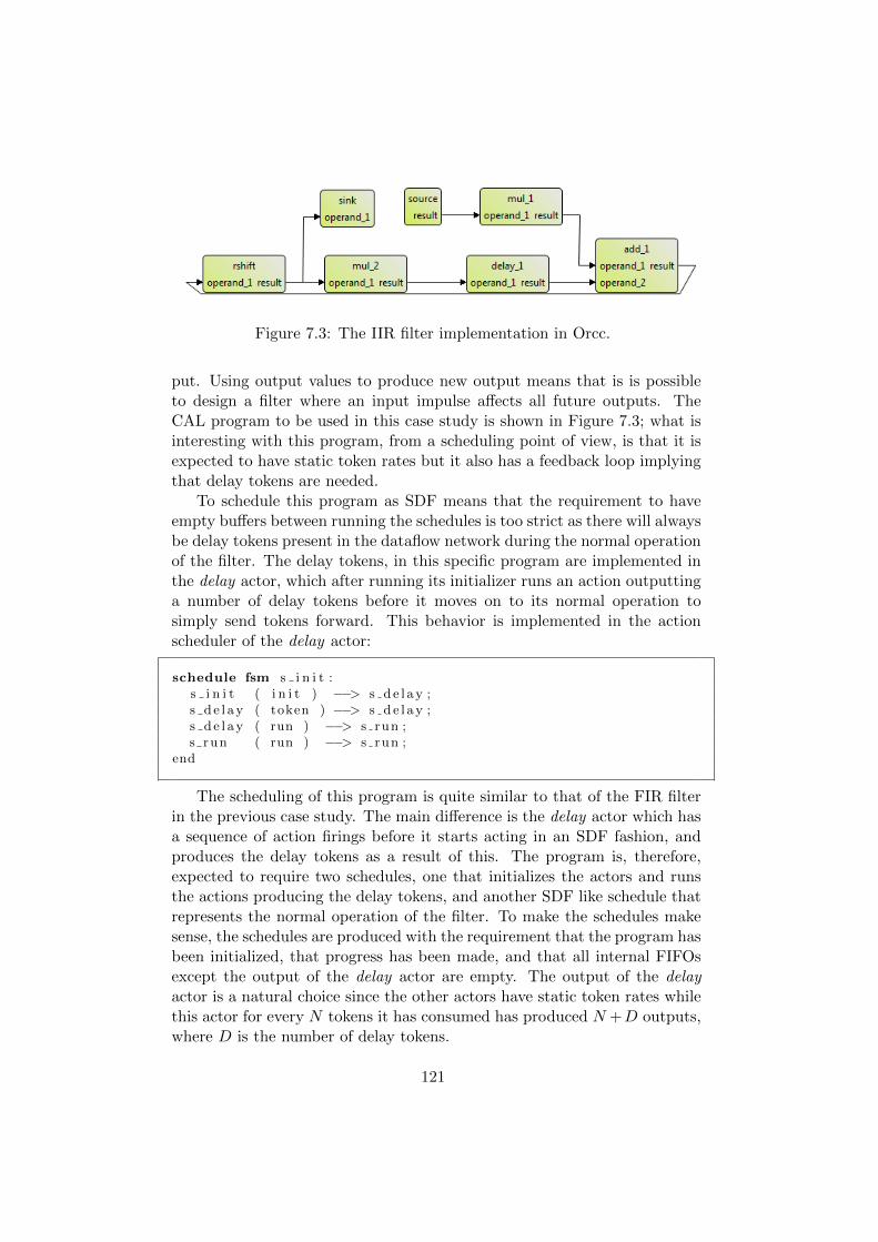
Figure 7.3: The IIR filter implementation in Orcc.

put. Using output values to produce new output means that is is possibleto design a filter where an input impulse affects all future outputs. TheCAL program to be used in this case study is shown in Figure 7.3; what isinteresting with this program, from a scheduling point of view, is that it isexpected to have static token rates but it also has a feedback loop implyingthat delay tokens are needed.

To schedule this program as SDF means that the requirement to haveempty buffers between running the schedules is too strict as there will alwaysbe delay tokens present in the dataflow network during the normal operationof the filter. The delay tokens, in this specific program are implemented inthe delay actor, which after running its initializer runs an action outputtinga number of delay tokens before it moves on to its normal operation tosimply send tokens forward. This behavior is implemented in the actionscheduler of the delay actor:

schedule fsm s i n i t :s i n i t ( i n i t ) −−> s d e l a y ;s d e l a y ( token ) −−> s d e l a y ;s d e l a y ( run ) −−> s run ;s run ( run ) −−> s run ;

end

The scheduling of this program is quite similar to that of the FIR filterin the previous case study. The main difference is the delay actor which hasa sequence of action firings before it starts acting in an SDF fashion, andproduces the delay tokens as a result of this. The program is, therefore,expected to require two schedules, one that initializes the actors and runsthe actions producing the delay tokens, and another SDF like schedule thatrepresents the normal operation of the filter. To make the schedules makesense, the schedules are produced with the requirement that the program hasbeen initialized, that progress has been made, and that all internal FIFOsexcept the output of the delay actor are empty. The output of the delayactor is a natural choice since the other actors have static token rates whilethis actor for every N tokens it has consumed has produced N +D outputs,where D is the number of delay tokens.

121

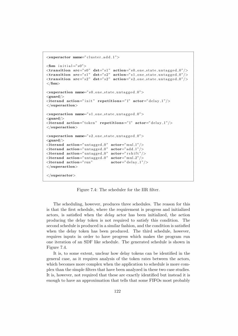
<superactor name=”c l u s t e r a d d 1”>

<fsm i n i t i a l =”s0”><transition src=”s0 ” dst=”s1 ” action=”s 0 o n e s t a t e u n t a g g e d 0 ”/><transition src=”s1 ” dst=”s2 ” action=”s 1 o n e s t a t e u n t a g g e d 0 ”/><transition src=”s2 ” dst=”s2 ” action=”s 2 o n e s t a t e u n t a g g e d 0 ”/></fsm>

<superaction name=”s 0 o n e s t a t e u n t a g g e d 0”><guard/><iterand action=” i n i t ” repetitions=”1” actor=”de lay 1”/></superaction>

<superaction name=”s 1 o n e s t a t e u n t a g g e d 0”><guard/><iterand action=”token ” repetitions=”1” actor=”de lay 1”/></superaction>

<superaction name=”s 2 o n e s t a t e u n t a g g e d 0”><guard/><iterand action=”untagged 0 ” actor=”mul 1”/><iterand action=”untagged 0 ” actor=”add 1”/><iterand action=”untagged 0 ” actor=” r s h i f t ”/><iterand action=”untagged 0 ” actor=”mul 2”/><iterand action=”run” actor=”de lay 1”/></superaction>

</superactor>

Figure 7.4: The scheduler for the IIR filter.

The scheduling, however, produces three schedules. The reason for thisis that the first schedule, where the requirement is progress and initializedactors, is satisfied when the delay actor has been initialized, the actionproducing the delay token is not required to satisfy this condition. Thesecond schedule is produced in a similar fashion, and the condition is satisfiedwhen the delay token has been produced. The third schedule, however,requires inputs in order to have progress which makes the program runone iteration of an SDF like schedule. The generated schedule is shown inFigure 7.4.

It is, to some extent, unclear how delay tokens can be identified in thegeneral case, as it requires analysis of the token rates between the actors,which becomes more complex when the application to schedule is more com-plex than the simple filters that have been analyzed in these two case studies.It is, however, not required that these are exactly identified but instead it isenough to have an approximation that tells that some FIFOs most probably

122

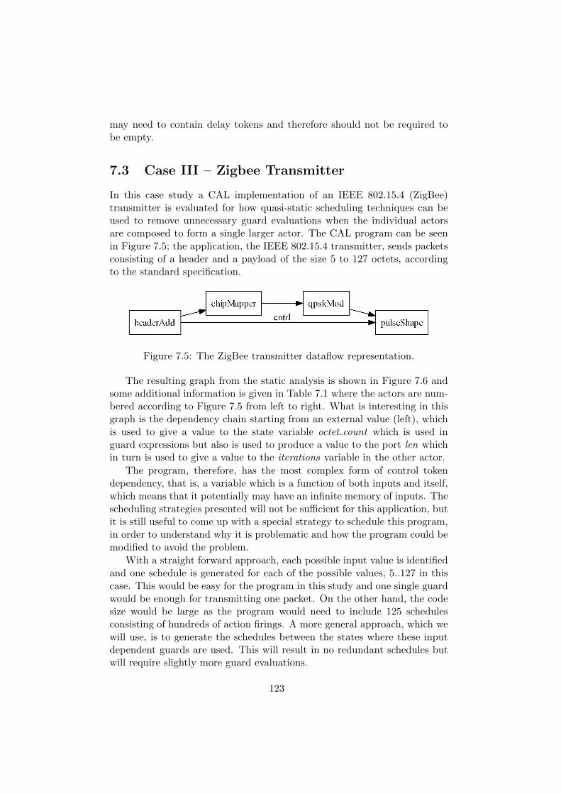
may need to contain delay tokens and therefore should not be required tobe empty.

7.3 Case III – Zigbee Transmitter

In this case study a CAL implementation of an IEEE 802.15.4 (ZigBee)transmitter is evaluated for how quasi-static scheduling techniques can beused to remove unnecessary guard evaluations when the individual actorsare composed to form a single larger actor. The CAL program can be seenin Figure 7.5; the application, the IEEE 802.15.4 transmitter, sends packetsconsisting of a header and a payload of the size 5 to 127 octets, accordingto the standard specification.

Figure 7.5: The ZigBee transmitter dataflow representation.

The resulting graph from the static analysis is shown in Figure 7.6 andsome additional information is given in Table 7.1 where the actors are num-bered according to Figure 7.5 from left to right. What is interesting in thisgraph is the dependency chain starting from an external value (left), whichis used to give a value to the state variable octet count which is used inguard expressions but also is used to produce a value to the port len whichin turn is used to give a value to the iterations variable in the other actor.

The program, therefore, has the most complex form of control tokendependency, that is, a variable which is a function of both inputs and itself,which means that it potentially may have an infinite memory of inputs. Thescheduling strategies presented will not be sufficient for this application, butit is still useful to come up with a special strategy to schedule this program,in order to understand why it is problematic and how the program could bemodified to avoid the problem.

With a straight forward approach, each possible input value is identifiedand one schedule is generated for each of the possible values, 5..127 in thiscase. This would be easy for the program in this study and one single guardwould be enough for transmitting one packet. On the other hand, the codesize would be large as the program would need to include 125 schedulesconsisting of hundreds of action firings. A more general approach, which wewill use, is to generate the schedules between the states where these inputdependent guards are used. This will result in no redundant schedules butwill require slightly more guard evaluations.

123

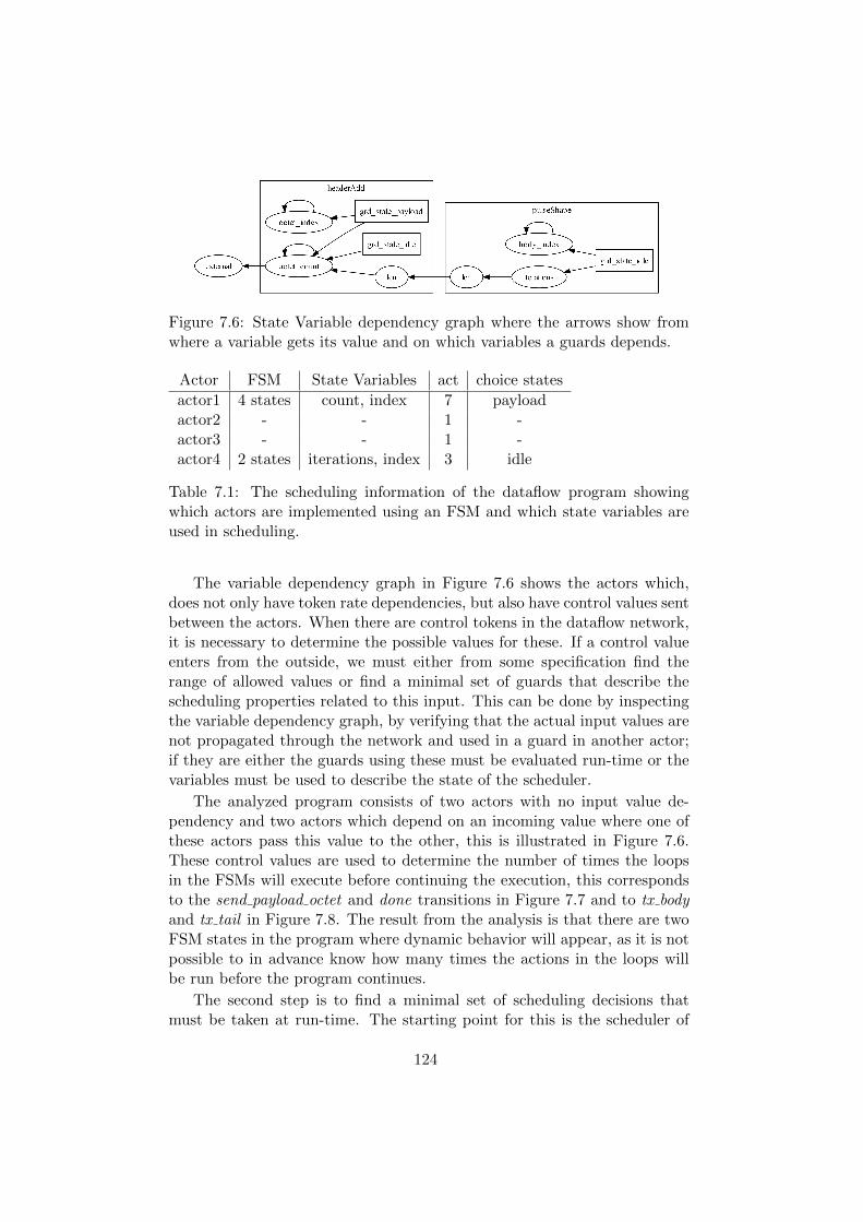
Figure 7.6: State Variable dependency graph where the arrows show fromwhere a variable gets its value and on which variables a guards depends.

Actor FSM State Variables act choice states

actor1 4 states count, index 7 payloadactor2 - - 1 -actor3 - - 1 -actor4 2 states iterations, index 3 idle

Table 7.1: The scheduling information of the dataflow program showingwhich actors are implemented using an FSM and which state variables areused in scheduling.

The variable dependency graph in Figure 7.6 shows the actors which,does not only have token rate dependencies, but also have control values sentbetween the actors. When there are control tokens in the dataflow network,it is necessary to determine the possible values for these. If a control valueenters from the outside, we must either from some specification find therange of allowed values or find a minimal set of guards that describe thescheduling properties related to this input. This can be done by inspectingthe variable dependency graph, by verifying that the actual input values arenot propagated through the network and used in a guard in another actor;if they are either the guards using these must be evaluated run-time or thevariables must be used to describe the state of the scheduler.

The analyzed program consists of two actors with no input value de-pendency and two actors which depend on an incoming value where one ofthese actors pass this value to the other, this is illustrated in Figure 7.6.These control values are used to determine the number of times the loopsin the FSMs will execute before continuing the execution, this correspondsto the send payload octet and done transitions in Figure 7.7 and to tx bodyand tx tail in Figure 7.8. The result from the analysis is that there are twoFSM states in the program where dynamic behavior will appear, as it is notpossible to in advance know how many times the actions in the loops willbe run before the program continues.

The second step is to find a minimal set of scheduling decisions thatmust be taken at run-time. The starting point for this is the scheduler of

124

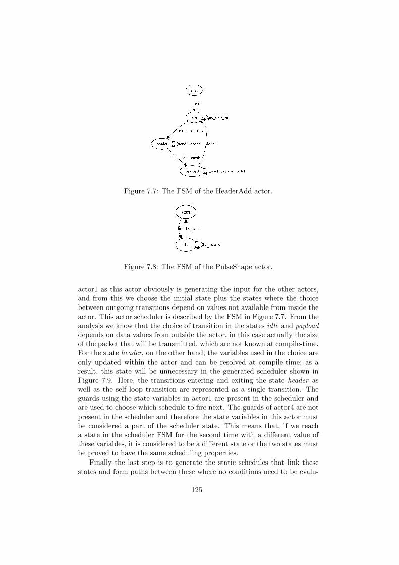
Figure 7.7: The FSM of the HeaderAdd actor.

Figure 7.8: The FSM of the PulseShape actor.

actor1 as this actor obviously is generating the input for the other actors,and from this we choose the initial state plus the states where the choicebetween outgoing transitions depend on values not available from inside theactor. This actor scheduler is described by the FSM in Figure 7.7. From theanalysis we know that the choice of transition in the states idle and payloaddepends on data values from outside the actor, in this case actually the sizeof the packet that will be transmitted, which are not known at compile-time.For the state header, on the other hand, the variables used in the choice areonly updated within the actor and can be resolved at compile-time; as aresult, this state will be unnecessary in the generated scheduler shown inFigure 7.9. Here, the transitions entering and exiting the state header aswell as the self loop transition are represented as a single transition. Theguards using the state variables in actor1 are present in the scheduler andare used to choose which schedule to fire next. The guards of actor4 are notpresent in the scheduler and therefore the state variables in this actor mustbe considered a part of the scheduler state. This means that, if we reacha state in the scheduler FSM for the second time with a different value ofthese variables, it is considered to be a different state or the two states mustbe proved to have the same scheduling properties.

Finally the last step is to generate the static schedules that link thesestates and form paths between these where no conditions need to be evalu-

125

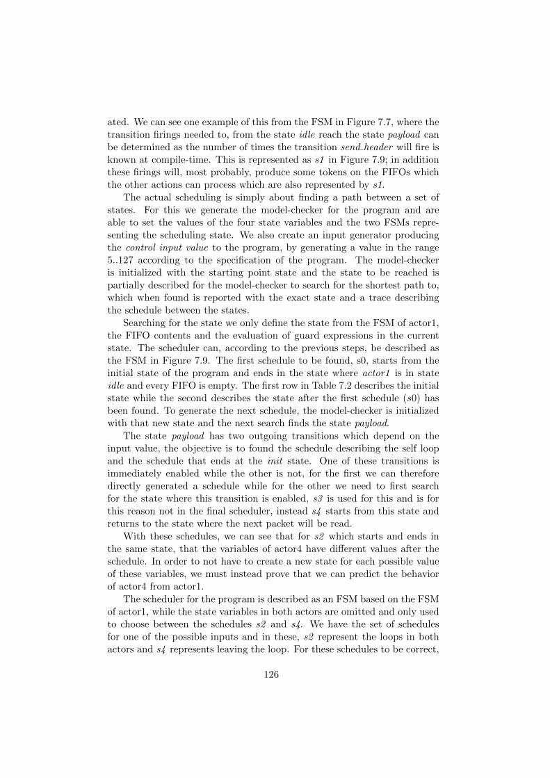
ated. We can see one example of this from the FSM in Figure 7.7, where thetransition firings needed to, from the state idle reach the state payload canbe determined as the number of times the transition send header will fire isknown at compile-time. This is represented as s1 in Figure 7.9; in additionthese firings will, most probably, produce some tokens on the FIFOs whichthe other actions can process which are also represented by s1.

The actual scheduling is simply about finding a path between a set ofstates. For this we generate the model-checker for the program and areable to set the values of the four state variables and the two FSMs repre-senting the scheduling state. We also create an input generator producingthe control input value to the program, by generating a value in the range5..127 according to the specification of the program. The model-checkeris initialized with the starting point state and the state to be reached ispartially described for the model-checker to search for the shortest path to,which when found is reported with the exact state and a trace describingthe schedule between the states.

Searching for the state we only define the state from the FSM of actor1,the FIFO contents and the evaluation of guard expressions in the currentstate. The scheduler can, according to the previous steps, be described asthe FSM in Figure 7.9. The first schedule to be found, s0, starts from theinitial state of the program and ends in the state where actor1 is in stateidle and every FIFO is empty. The first row in Table 7.2 describes the initialstate while the second describes the state after the first schedule (s0) hasbeen found. To generate the next schedule, the model-checker is initializedwith that new state and the next search finds the state payload.

The state payload has two outgoing transitions which depend on theinput value, the objective is to found the schedule describing the self loopand the schedule that ends at the init state. One of these transitions isimmediately enabled while the other is not, for the first we can thereforedirectly generated a schedule while for the other we need to first searchfor the state where this transition is enabled, s3 is used for this and is forthis reason not in the final scheduler, instead s4 starts from this state andreturns to the state where the next packet will be read.

With these schedules, we can see that for s2 which starts and ends inthe same state, that the variables of actor4 have different values after theschedule. In order to not have to create a new state for each possible valueof these variables, we must instead prove that we can predict the behaviorof actor4 from actor1.

The scheduler for the program is described as an FSM based on the FSMof actor1, while the state variables in both actors are omitted and only usedto choose between the schedules s2 and s4. We have the set of schedulesfor one of the possible inputs and in these, s2 represent the loops in bothactors and s4 represents leaving the loop. For these schedules to be correct,

126

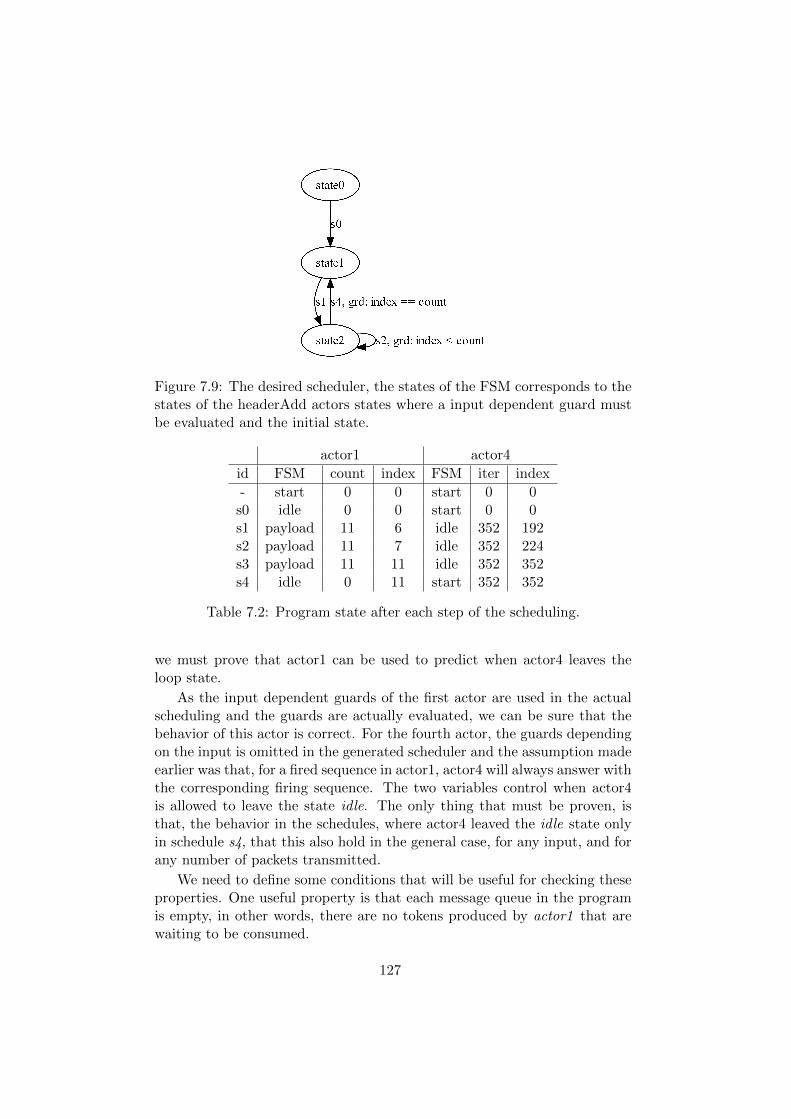
Figure 7.9: The desired scheduler, the states of the FSM corresponds to thestates of the headerAdd actors states where a input dependent guard mustbe evaluated and the initial state.

actor1 actor4

id FSM count index FSM iter index

- start 0 0 start 0 0s0 idle 0 0 start 0 0s1 payload 11 6 idle 352 192s2 payload 11 7 idle 352 224s3 payload 11 11 idle 352 352s4 idle 0 11 start 352 352

Table 7.2: Program state after each step of the scheduling.

we must prove that actor1 can be used to predict when actor4 leaves theloop state.

As the input dependent guards of the first actor are used in the actualscheduling and the guards are actually evaluated, we can be sure that thebehavior of this actor is correct. For the fourth actor, the guards dependingon the input is omitted in the generated scheduler and the assumption madeearlier was that, for a fired sequence in actor1, actor4 will always answer withthe corresponding firing sequence. The two variables control when actor4is allowed to leave the state idle. The only thing that must be proven, isthat, the behavior in the schedules, where actor4 leaved the idle state onlyin schedule s4, that this also hold in the general case, for any input, and forany number of packets transmitted.

We need to define some conditions that will be useful for checking theseproperties. One useful property is that each message queue in the programis empty, in other words, there are no tokens produced by actor1 that arewaiting to be consumed.

127

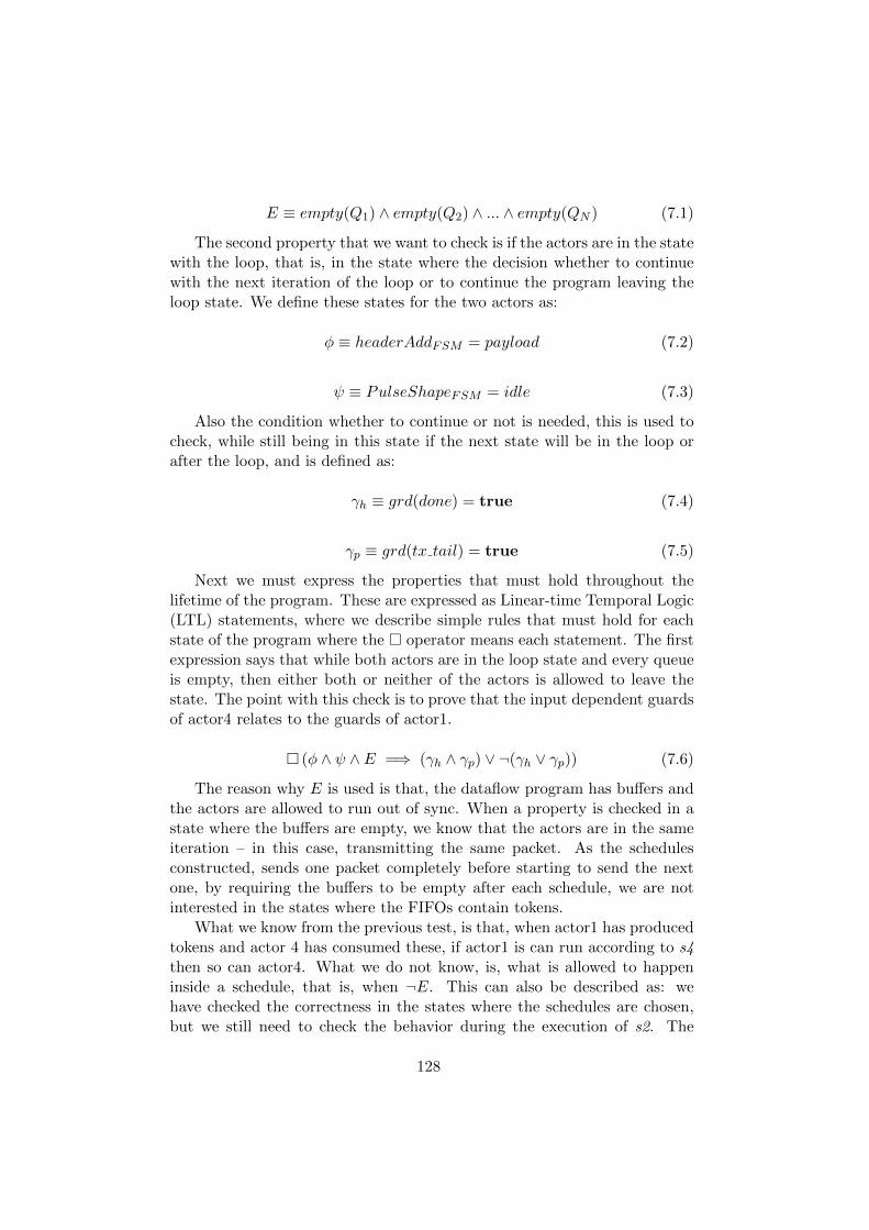
E ≡ empty(Q1) ∧ empty(Q2) ∧ ... ∧ empty(QN ) (7.1)

The second property that we want to check is if the actors are in the statewith the loop, that is, in the state where the decision whether to continuewith the next iteration of the loop or to continue the program leaving theloop state. We define these states for the two actors as:

φ ≡ headerAddFSM = payload (7.2)

ψ ≡ PulseShapeFSM = idle (7.3)

Also the condition whether to continue or not is needed, this is used tocheck, while still being in this state if the next state will be in the loop orafter the loop, and is defined as:

γh ≡ grd(done) = true (7.4)

γp ≡ grd(tx tail) = true (7.5)

Next we must express the properties that must hold throughout thelifetime of the program. These are expressed as Linear-time Temporal Logic(LTL) statements, where we describe simple rules that must hold for eachstate of the program where the � operator means each statement. The firstexpression says that while both actors are in the loop state and every queueis empty, then either both or neither of the actors is allowed to leave thestate. The point with this check is to prove that the input dependent guardsof actor4 relates to the guards of actor1.

� (φ ∧ ψ ∧ E =⇒ (γh ∧ γp) ∨ ¬(γh ∨ γp)) (7.6)

The reason why E is used is that, the dataflow program has buffers andthe actors are allowed to run out of sync. When a property is checked in astate where the buffers are empty, we know that the actors are in the sameiteration – in this case, transmitting the same packet. As the schedulesconstructed, sends one packet completely before starting to send the nextone, by requiring the buffers to be empty after each schedule, we are notinterested in the states where the FIFOs contain tokens.

What we know from the previous test, is that, when actor1 has producedtokens and actor 4 has consumed these, if actor1 is can run according to s4then so can actor4. What we do not know, is, what is allowed to happeninside a schedule, that is, when ¬E. This can also be described as: wehave checked the correctness in the states where the schedules are chosen,but we still need to check the behavior during the execution of s2. The

128

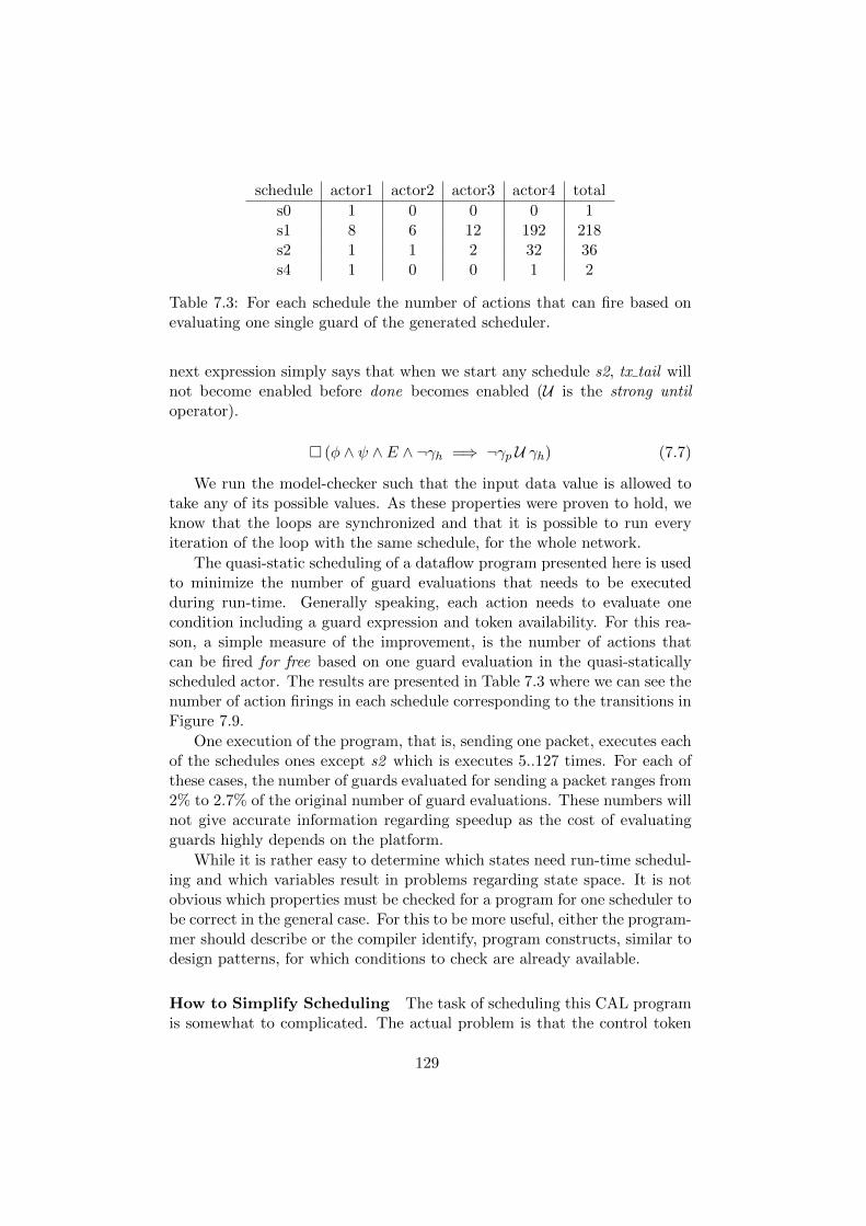
schedule actor1 actor2 actor3 actor4 total

s0 1 0 0 0 1s1 8 6 12 192 218s2 1 1 2 32 36s4 1 0 0 1 2

Table 7.3: For each schedule the number of actions that can fire based onevaluating one single guard of the generated scheduler.

next expression simply says that when we start any schedule s2, tx tail willnot become enabled before done becomes enabled (U is the strong untiloperator).

� (φ ∧ ψ ∧ E ∧ ¬γh =⇒ ¬γp U γh) (7.7)

We run the model-checker such that the input data value is allowed totake any of its possible values. As these properties were proven to hold, weknow that the loops are synchronized and that it is possible to run everyiteration of the loop with the same schedule, for the whole network.

The quasi-static scheduling of a dataflow program presented here is usedto minimize the number of guard evaluations that needs to be executedduring run-time. Generally speaking, each action needs to evaluate onecondition including a guard expression and token availability. For this rea-son, a simple measure of the improvement, is the number of actions thatcan be fired for free based on one guard evaluation in the quasi-staticallyscheduled actor. The results are presented in Table 7.3 where we can see thenumber of action firings in each schedule corresponding to the transitions inFigure 7.9.

One execution of the program, that is, sending one packet, executes eachof the schedules ones except s2 which is executes 5..127 times. For each ofthese cases, the number of guards evaluated for sending a packet ranges from2% to 2.7% of the original number of guard evaluations. These numbers willnot give accurate information regarding speedup as the cost of evaluatingguards highly depends on the platform.

While it is rather easy to determine which states need run-time schedul-ing and which variables result in problems regarding state space. It is notobvious which properties must be checked for a program for one scheduler tobe correct in the general case. For this to be more useful, either the program-mer should describe or the compiler identify, program constructs, similar todesign patterns, for which conditions to check are already available.

How to Simplify Scheduling The task of scheduling this CAL programis somewhat to complicated. The actual problem is that the control token

129

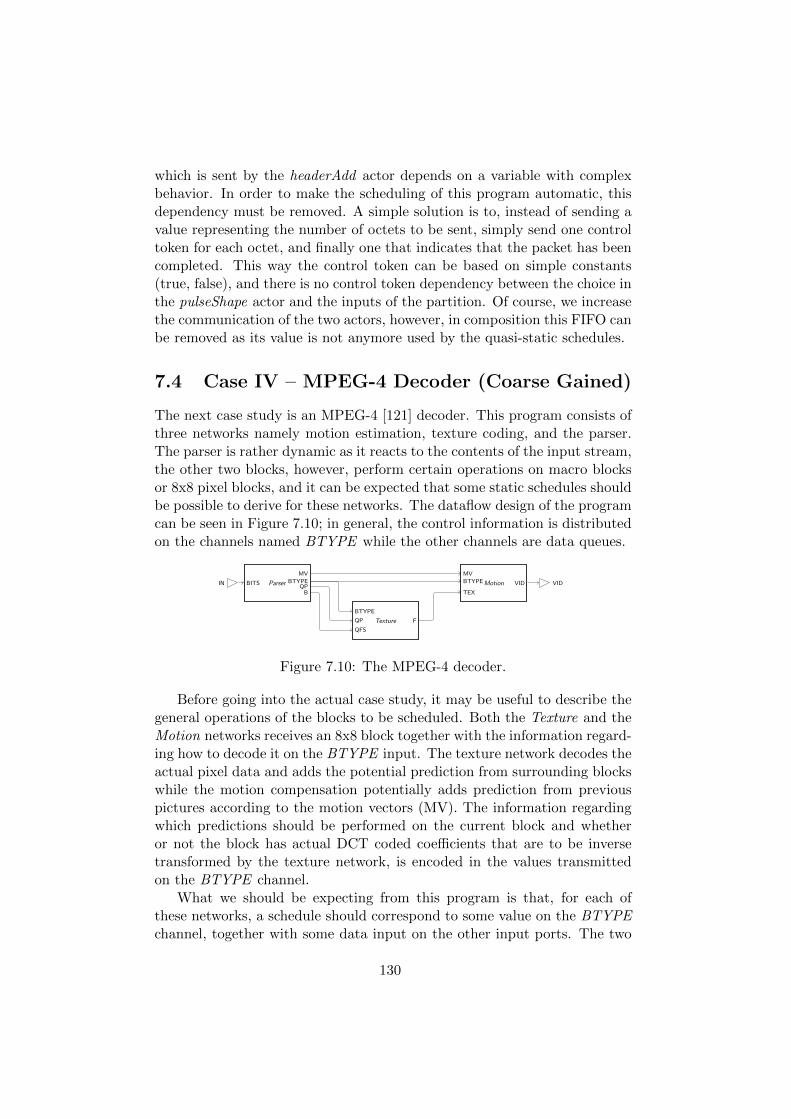
which is sent by the headerAdd actor depends on a variable with complexbehavior. In order to make the scheduling of this program automatic, thisdependency must be removed. A simple solution is to, instead of sending avalue representing the number of octets to be sent, simply send one controltoken for each octet, and finally one that indicates that the packet has beencompleted. This way the control token can be based on simple constants(true, false), and there is no control token dependency between the choice inthe pulseShape actor and the inputs of the partition. Of course, we increasethe communication of the two actors, however, in composition this FIFO canbe removed as its value is not anymore used by the quasi-static schedules.

7.4 Case IV – MPEG-4 Decoder (Coarse Gained)

The next case study is an MPEG-4 [121] decoder. This program consists ofthree networks namely motion estimation, texture coding, and the parser.The parser is rather dynamic as it reacts to the contents of the input stream,the other two blocks, however, perform certain operations on macro blocksor 8x8 pixel blocks, and it can be expected that some static schedules shouldbe possible to derive for these networks. The dataflow design of the programcan be seen in Figure 7.10; in general, the control information is distributedon the channels named BTYPE while the other channels are data queues.

ParserBITS

MV

BTYPEQPB

Texture

BTYPE

QFS

QP F

Motion

MV

BTYPE

TEX

VIDIN VID

Figure 7.10: The MPEG-4 decoder.

Before going into the actual case study, it may be useful to describe thegeneral operations of the blocks to be scheduled. Both the Texture and theMotion networks receives an 8x8 block together with the information regard-ing how to decode it on the BTYPE input. The texture network decodes theactual pixel data and adds the potential prediction from surrounding blockswhile the motion compensation potentially adds prediction from previouspictures according to the motion vectors (MV). The information regardingwhich predictions should be performed on the current block and whetheror not the block has actual DCT coded coefficients that are to be inversetransformed by the texture network, is encoded in the values transmittedon the BTYPE channel.

What we should be expecting from this program is that, for each ofthese networks, a schedule should correspond to some value on the BTYPEchannel, together with some data input on the other input ports. The two

130

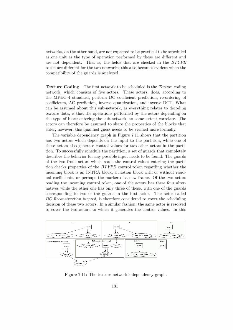
networks, on the other hand, are not expected to be practical to be scheduledas one unit as the type of operation performed by these are different andare not dependent. That is, the fields that are checked in the BTYPEtoken are different for the two networks; this also becomes evident when thecompatibility of the guards is analyzed.

Texture Coding The first network to be scheduled is the Texture codingnetwork, which consists of five actors. These actors, does, according tothe MPEG-4 standard, perform DC coefficient prediction, re-ordering ofcoefficients, AC prediction, inverse quantization, and inverse DCT. Whatcan be assumed about this sub-network, as everything relates to decodingtexture data, is that the operations performed by the actors depending onthe type of block entering the sub-network, to some extent correlate. Theactors can therefore be assumed to share the properties of the blocks thatenter, however, this qualified guess needs to be verified more formally.

The variable dependency graph in Figure 7.11 shows that the partitionhas two actors which depends on the input to the partition, while one ofthese actors also generate control values for two other actors in the parti-tion. To successfully schedule the partition, a set of guards that completelydescribes the behavior for any possible input needs to be found. The guardsof the two front actors which reads the control values entering the parti-tion checks properties of the BTYPE control token regarding whether theincoming block is an INTRA block, a motion block with or without resid-ual coefficients, or perhaps the marker of a new frame. Of the two actorsreading the incoming control token, one of the actors has these four alter-natives while the other one has only three of these, with one of the guardscorresponding to two of the guards in the first actor. The actor calledDC Reconstruction invpred, is therefore considered to cover the schedulingdecision of these two actors. In a similar fashion, the same actor is resolvedto cover the two actors to which it generates the control values. In this

Figure 7.11: The texture network’s dependency graph.

131

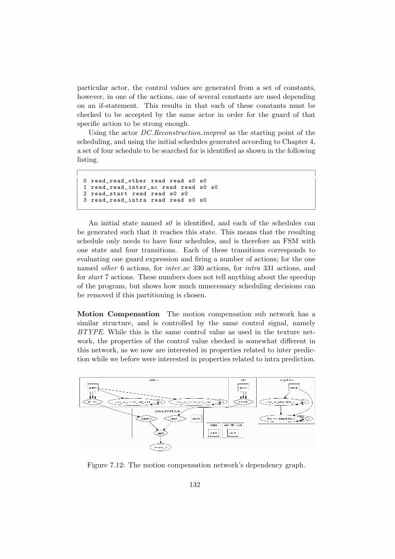
particular actor, the control values are generated from a set of constants,however, in one of the actions, one of several constants are used dependingon an if-statement. This results in that each of these constants must bechecked to be accepted by the same actor in order for the guard of thatspecific action to be strong enough.

Using the actor DC Reconstruction invpred as the starting point of thescheduling, and using the initial schedules generated according to Chapter 4,a set of four schedule to be searched for is identified as shown in the followinglisting.

0 read_read_other read read s0 s01 read_read_inter_ac read read s0 s02 read_start read read s0 s03 read_read_intra read read s0 s0

An initial state named s0 is identified, and each of the schedules canbe generated such that it reaches this state. This means that the resultingschedule only needs to have four schedules, and is therefore an FSM withone state and four transitions. Each of these transitions corresponds toevaluating one guard expression and firing a number of actions; for the onenamed other 6 actions, for inter ac 330 actions, for intra 331 actions, andfor start 7 actions. These numbers does not tell anything about the speedupof the program, but shows how much unnecessary scheduling decisions canbe removed if this partitioning is chosen.

Motion Compensation The motion compensation sub network has asimilar structure, and is controlled by the same control signal, namelyBTYPE. While this is the same control value as used in the texture net-work, the properties of the control value checked is somewhat different inthis network, as we now are interested in properties related to inter predic-tion while we before were interested in properties related to intra prediction.

Figure 7.12: The motion compensation network’s dependency graph.

132

For this reason, these networks are chosen to be scheduled separately, al-though it would not be impossible to schedule them together either, onlythe scheduler would become more complex.

More complex guards than what is available in any single actor willalready be needed to schedule this partition. The reason for this is thatthe two actors sharing the input control token does not have compatibleguards. In Figure 7.12, one can see that the incoming control token is usedby the actors address and add. While both of these actors have four guardschecking this token, both of them have two separate guards that may beenabled simultaneously with two guards of the other actor. Consequently,in order to find strong enough guards for the partition, a set of new guards,corresponding to the different possible combinations of guards of these twoactors, must be generated.

Considering two sets of guards Gadd and Gaddress, the needed guardscorresponds to the Cartesian product of these sets, that is,

Gpartition = Gadd ×Gaddress

where the contents of these sets are

Gadd = {nvop, texture,motion, both}

andGaddress = {nvop, no motion,motion, neither}

The guards needed to schedule the partition is then defined as all thesecombinations except the ones that cannot be accepted simultaneously.

Gscheduler = Gpartition \Gimpossible

Where the impossible combinations are those, for example, requiring a blockto be both intra and inter block simultaneously.

Gscheduler = {(nvop, nvop), (texture, no motion),

(motion,motion), (motion, neither),

(both,motion), (both, neither)}

The obvious problem is that no tool could ever know which of thesecombinations are impossible, unless the programmer adds this information.The set of guards of an actor describes the conditions that are sufficient tofire actions, but this information is based on assumption the programmerhas made and is not visible in the guards. Some hints may be possible toderive from how a control token is generated but this is not always possibleeither. For this reason, the only way to succeed with the scheduling of thispartition, such that the scheduler does not include impossible schedules, is

133

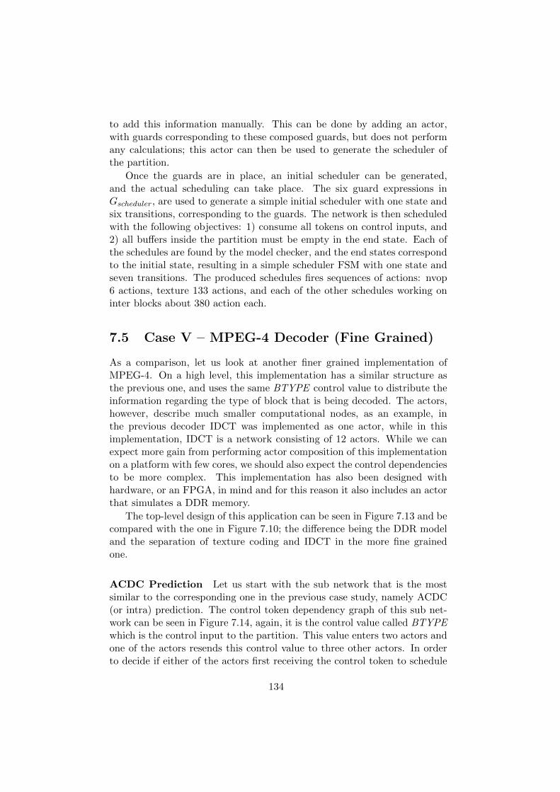
to add this information manually. This can be done by adding an actor,with guards corresponding to these composed guards, but does not performany calculations; this actor can then be used to generate the scheduler ofthe partition.

Once the guards are in place, an initial scheduler can be generated,and the actual scheduling can take place. The six guard expressions inGscheduler, are used to generate a simple initial scheduler with one state andsix transitions, corresponding to the guards. The network is then scheduledwith the following objectives: 1) consume all tokens on control inputs, and2) all buffers inside the partition must be empty in the end state. Each ofthe schedules are found by the model checker, and the end states correspondto the initial state, resulting in a simple scheduler FSM with one state andseven transitions. The produced schedules fires sequences of actions: nvop6 actions, texture 133 actions, and each of the other schedules working oninter blocks about 380 action each.

7.5 Case V – MPEG-4 Decoder (Fine Grained)

As a comparison, let us look at another finer grained implementation ofMPEG-4. On a high level, this implementation has a similar structure asthe previous one, and uses the same BTYPE control value to distribute theinformation regarding the type of block that is being decoded. The actors,however, describe much smaller computational nodes, as an example, inthe previous decoder IDCT was implemented as one actor, while in thisimplementation, IDCT is a network consisting of 12 actors. While we canexpect more gain from performing actor composition of this implementationon a platform with few cores, we should also expect the control dependenciesto be more complex. This implementation has also been designed withhardware, or an FPGA, in mind and for this reason it also includes an actorthat simulates a DDR memory.

The top-level design of this application can be seen in Figure 7.13 and becompared with the one in Figure 7.10; the difference being the DDR modeland the separation of texture coding and IDCT in the more fine grainedone.

ACDC Prediction Let us start with the sub network that is the mostsimilar to the corresponding one in the previous case study, namely ACDC(or intra) prediction. The control token dependency graph of this sub net-work can be seen in Figure 7.14, again, it is the control value called BTYPEwhich is the control input to the partition. This value enters two actors andone of the actors resends this control value to three other actors. In orderto decide if either of the actors first receiving the control token to schedule

134

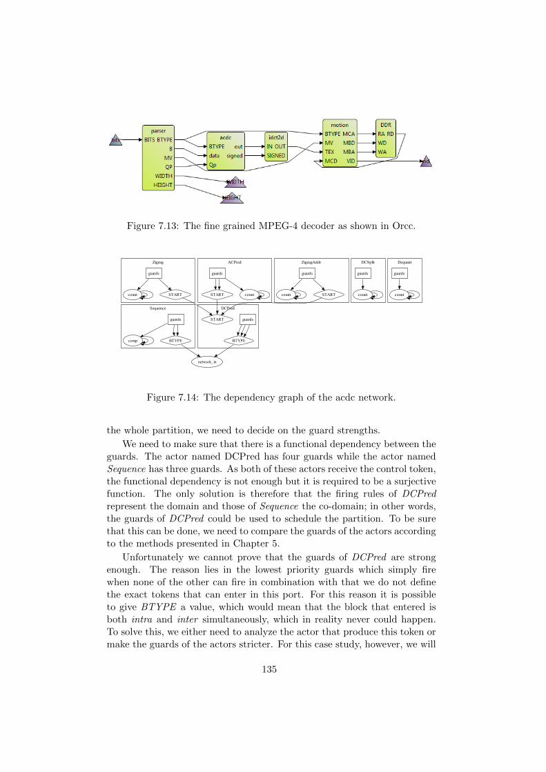
Figure 7.13: The fine grained MPEG-4 decoder as shown in Orcc.

������

���� ������ ��� ����������� ������

��������

�����

�����

����������

�����

�����

����� �����

�����

����� �����

�����

�����

�����

����� �����

�����

�����

�����

��� �����

Figure 7.14: The dependency graph of the acdc network.

the whole partition, we need to decide on the guard strengths.

We need to make sure that there is a functional dependency between theguards. The actor named DCPred has four guards while the actor namedSequence has three guards. As both of these actors receive the control token,the functional dependency is not enough but it is required to be a surjectivefunction. The only solution is therefore that the firing rules of DCPredrepresent the domain and those of Sequence the co-domain; in other words,the guards of DCPred could be used to schedule the partition. To be surethat this can be done, we need to compare the guards of the actors accordingto the methods presented in Chapter 5.

Unfortunately we cannot prove that the guards of DCPred are strongenough. The reason lies in the lowest priority guards which simply firewhen none of the other can fire in combination with that we do not definethe exact tokens that can enter in this port. For this reason it is possibleto give BTYPE a value, which would mean that the block that entered isboth intra and inter simultaneously, which in reality never could happen.To solve this, we either need to analyze the actor that produce this token ormake the guards of the actors stricter. For this case study, however, we will

135

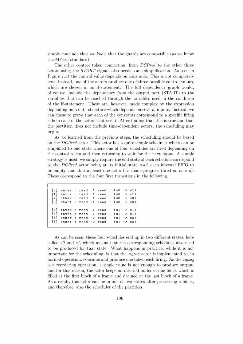
simply conclude that we know that the guards are compatible (as we knowthe MPEG standard).

The other control token connection, from DCPred to the other threeactors using the START signal, also needs some simplification. As seen inFigure 7.14 the control value depends on constants. This is not completelytrue, instead, one of the actors produce one of three possible control values,which are chosen in an if-statement. The full dependency graph would,of course, include the dependency from the output port (START) to thevariables that can be reached through the variables used in the conditionof the if-statement. These are, however, made complex by the expressiondepending on a data structure which depends on several inputs. Instead, wecan chose to prove that each of the constants correspond to a specific firingrule in each of the actors that use it. After finding that this is true and thatthe partition does not include time-dependent actors, the scheduling maybegin.

As we learned from the previous steps, the scheduling should be basedon the DCPred actor. This actor has a quite simple scheduler which can besimplified to one state where one of four schedules are fired depending onthe control token and then returning to wait for the next input. A simplestrategy is used, we simply require the end state of each schedule correspondto the DCPred actor being at its initial state read, each internal FIFO tobe empty, and that at least one actor has made progress (fired an action).These correspond to the four first transitions in the following.

[0] inter : read -> read : (s0 -> s1)[1] intra : read -> read : (s0 -> s1)[2] other : read -> read : (s0 -> s0)[3] start : read -> read : (s0 -> s0)-------------------------------------[4] inter : read -> read : (s1 -> s1)[5] intra : read -> read : (s1 -> s1)[6] other : read -> read : (s1 -> s0)[7] start : read -> read : (s1 -> s0)

As can be seen, these four schedules end up in two different states, herecalled s0 and s1, which means that the corresponding schedules also needto be produced for that state. What happens in practice, while it is notimportant for the scheduling, is that the zigzag actor is implemented to, innormal operation, consume and produce one token each firing. As the zigzagis a reordering operation, a single value is not enough to produce output,and for this reason, the actor keeps an internal buffer of one block which isfilled at the first block of a frame and drained at the last block of a frame.As a result, this actor can be in one of two states after processing a block,and therefore, also the scheduler of the partition.

136

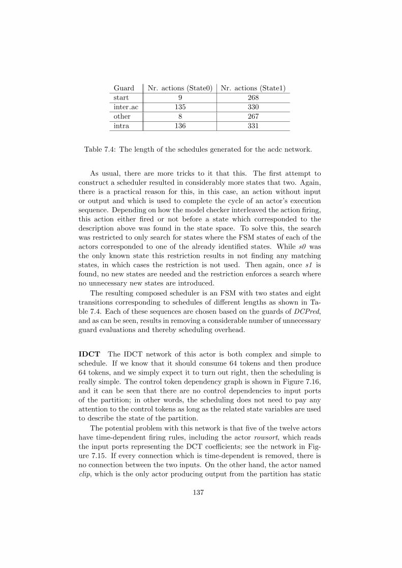
Guard Nr. actions (State0) Nr. actions (State1)

start 9 268

inter ac 135 330

other 8 267

intra 136 331

Table 7.4: The length of the schedules generated for the acdc network.

As usual, there are more tricks to it that this. The first attempt toconstruct a scheduler resulted in considerably more states that two. Again,there is a practical reason for this, in this case, an action without inputor output and which is used to complete the cycle of an actor’s executionsequence. Depending on how the model checker interleaved the action firing,this action either fired or not before a state which corresponded to thedescription above was found in the state space. To solve this, the searchwas restricted to only search for states where the FSM states of each of theactors corresponded to one of the already identified states. While s0 wasthe only known state this restriction results in not finding any matchingstates, in which cases the restriction is not used. Then again, once s1 isfound, no new states are needed and the restriction enforces a search whereno unnecessary new states are introduced.

The resulting composed scheduler is an FSM with two states and eighttransitions corresponding to schedules of different lengths as shown in Ta-ble 7.4. Each of these sequences are chosen based on the guards of DCPred,and as can be seen, results in removing a considerable number of unnecessaryguard evaluations and thereby scheduling overhead.

IDCT The IDCT network of this actor is both complex and simple toschedule. If we know that it should consume 64 tokens and then produce64 tokens, and we simply expect it to turn out right, then the scheduling isreally simple. The control token dependency graph is shown in Figure 7.16,and it can be seen that there are no control dependencies to input portsof the partition; in other words, the scheduling does not need to pay anyattention to the control tokens as long as the related state variables are usedto describe the state of the partition.

The potential problem with this network is that five of the twelve actorshave time-dependent firing rules, including the actor rowsort, which readsthe input ports representing the DCT coefficients; see the network in Fig-ure 7.15. If every connection which is time-dependent is removed, there isno connection between the two inputs. On the other hand, the actor namedclip, which is the only actor producing output from the partition has static

137

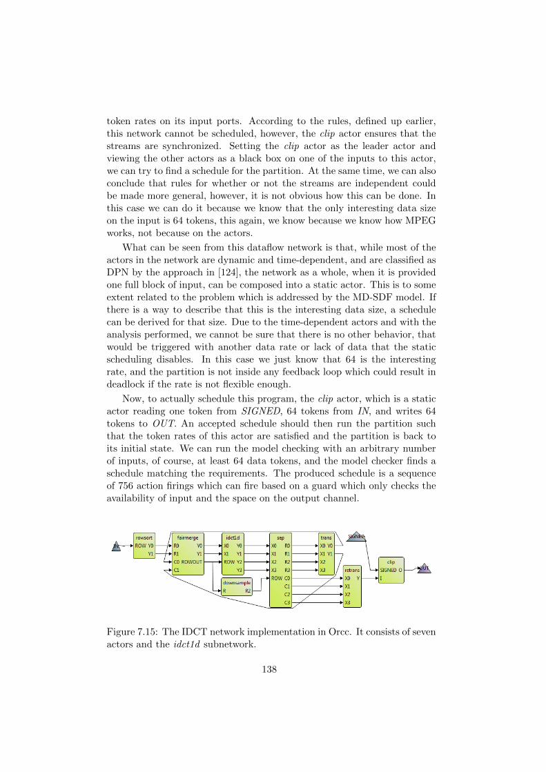
token rates on its input ports. According to the rules, defined up earlier,this network cannot be scheduled, however, the clip actor ensures that thestreams are synchronized. Setting the clip actor as the leader actor andviewing the other actors as a black box on one of the inputs to this actor,we can try to find a schedule for the partition. At the same time, we can alsoconclude that rules for whether or not the streams are independent couldbe made more general, however, it is not obvious how this can be done. Inthis case we can do it because we know that the only interesting data sizeon the input is 64 tokens, this again, we know because we know how MPEGworks, not because on the actors.

What can be seen from this dataflow network is that, while most of theactors in the network are dynamic and time-dependent, and are classified asDPN by the approach in [124], the network as a whole, when it is providedone full block of input, can be composed into a static actor. This is to someextent related to the problem which is addressed by the MD-SDF model. Ifthere is a way to describe that this is the interesting data size, a schedulecan be derived for that size. Due to the time-dependent actors and with theanalysis performed, we cannot be sure that there is no other behavior, thatwould be triggered with another data rate or lack of data that the staticscheduling disables. In this case we just know that 64 is the interestingrate, and the partition is not inside any feedback loop which could result indeadlock if the rate is not flexible enough.

Now, to actually schedule this program, the clip actor, which is a staticactor reading one token from SIGNED, 64 tokens from IN, and writes 64tokens to OUT. An accepted schedule should then run the partition suchthat the token rates of this actor are satisfied and the partition is back toits initial state. We can run the model checking with an arbitrary numberof inputs, of course, at least 64 data tokens, and the model checker finds aschedule matching the requirements. The produced schedule is a sequenceof 756 action firings which can fire based on a guard which only checks theavailability of input and the space on the output channel.

Figure 7.15: The IDCT network implementation in Orcc. It consists of sevenactors and the idct1d subnetwork.

138

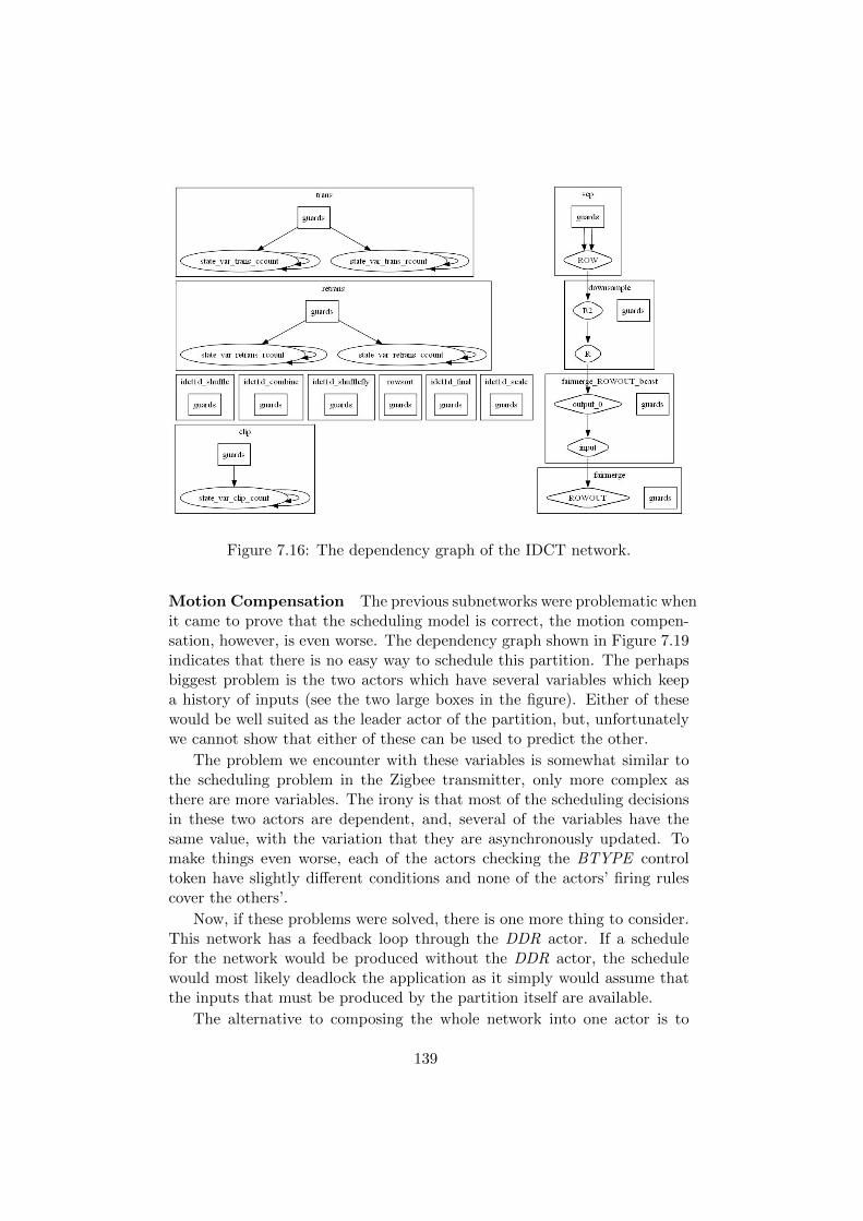
Figure 7.16: The dependency graph of the IDCT network.

Motion Compensation The previous subnetworks were problematic whenit came to prove that the scheduling model is correct, the motion compen-sation, however, is even worse. The dependency graph shown in Figure 7.19indicates that there is no easy way to schedule this partition. The perhapsbiggest problem is the two actors which have several variables which keepa history of inputs (see the two large boxes in the figure). Either of thesewould be well suited as the leader actor of the partition, but, unfortunatelywe cannot show that either of these can be used to predict the other.

The problem we encounter with these variables is somewhat similar tothe scheduling problem in the Zigbee transmitter, only more complex asthere are more variables. The irony is that most of the scheduling decisionsin these two actors are dependent, and, several of the variables have thesame value, with the variation that they are asynchronously updated. Tomake things even worse, each of the actors checking the BTYPE controltoken have slightly different conditions and none of the actors’ firing rulescover the others’.

Now, if these problems were solved, there is one more thing to consider.This network has a feedback loop through the DDR actor. If a schedulefor the network would be produced without the DDR actor, the schedulewould most likely deadlock the application as it simply would assume thatthe inputs that must be produced by the partition itself are available.

The alternative to composing the whole network into one actor is to

139

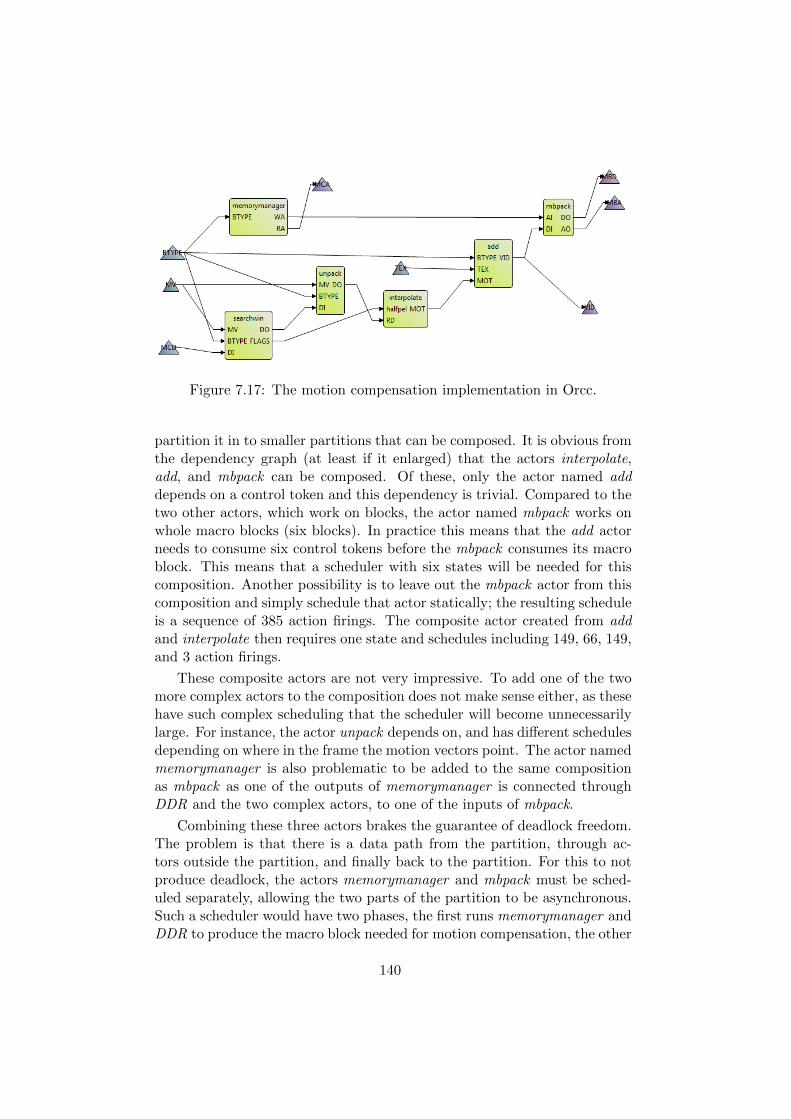
Figure 7.17: The motion compensation implementation in Orcc.

partition it in to smaller partitions that can be composed. It is obvious fromthe dependency graph (at least if it enlarged) that the actors interpolate,add, and mbpack can be composed. Of these, only the actor named adddepends on a control token and this dependency is trivial. Compared to thetwo other actors, which work on blocks, the actor named mbpack works onwhole macro blocks (six blocks). In practice this means that the add actorneeds to consume six control tokens before the mbpack consumes its macroblock. This means that a scheduler with six states will be needed for thiscomposition. Another possibility is to leave out the mbpack actor from thiscomposition and simply schedule that actor statically; the resulting scheduleis a sequence of 385 action firings. The composite actor created from addand interpolate then requires one state and schedules including 149, 66, 149,and 3 action firings.

These composite actors are not very impressive. To add one of the twomore complex actors to the composition does not make sense either, as thesehave such complex scheduling that the scheduler will become unnecessarilylarge. For instance, the actor unpack depends on, and has different schedulesdepending on where in the frame the motion vectors point. The actor namedmemorymanager is also problematic to be added to the same compositionas mbpack as one of the outputs of memorymanager is connected throughDDR and the two complex actors, to one of the inputs of mbpack.

Combining these three actors brakes the guarantee of deadlock freedom.The problem is that there is a data path from the partition, through ac-tors outside the partition, and finally back to the partition. For this to notproduce deadlock, the actors memorymanager and mbpack must be sched-uled separately, allowing the two parts of the partition to be asynchronous.Such a scheduler would have two phases, the first runs memorymanager andDDR to produce the macro block needed for motion compensation, the other

140

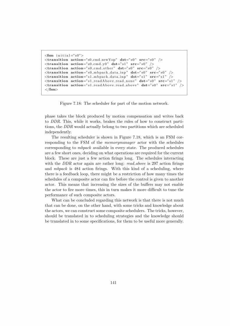
<fsm i n i t i a l =”s0”><transition action=”s0 cmd newVop” dst=”s0 ” src=”s0 ” /><transition action=”s0 cmd y0 ” dst=”s1 ” src=”s0 ” /><transition action=”s0 cmd other ” dst=”s0 ” src=”s0 ” /><transition action=”s0 mbpack data inp ” dst=”s0 ” src=”s0 ” /><transition action=”s1 mbpack data inp ” dst=”s1 ” src=”s1 ” /><transition action=”s1 readAbove read none ” dst=”s0 ” src=”s1 ” /><transition action=”s1 readAbove read above ” dst=”s0 ” src=”s1 ” /></fsm>

Figure 7.18: The scheduler for part of the motion network.

phase takes the block produced by motion compensation and writes backto DDR. This, while it works, brakes the rules of how to construct parti-tions, the DDR would actually belong to two partitions which are scheduledindependently.

The resulting scheduler is shown in Figure 7.18, which is an FSM cor-responding to the FSM of the memorymanager actor with the schedulescorresponding to mbpack available in every state. The produced schedulesare a few short ones, deciding on what operations are required for the currentblock. These are just a few action firings long. The schedules interactingwith the DDR actor again are rather long: read above is 297 action firingsand mbpack is 484 action firings. With this kind of a scheduling, wherethere is a feedback loop, there might be a restriction of how many times theschedules of a composite actor can fire before the control is given to anotheractor. This means that increasing the sizes of the buffers may not enablethe actor to fire more times, this in turn makes it more difficult to tune theperformance of such composite actors.

What can be concluded regarding this network is that there is not muchthat can be done, on the other hand, with some tricks and knowledge aboutthe actors, we can construct some composite schedulers. The tricks, however,should be translated in to scheduling strategies and the knowledge shouldbe translated in to some specifications, for them to be useful more generally.

141

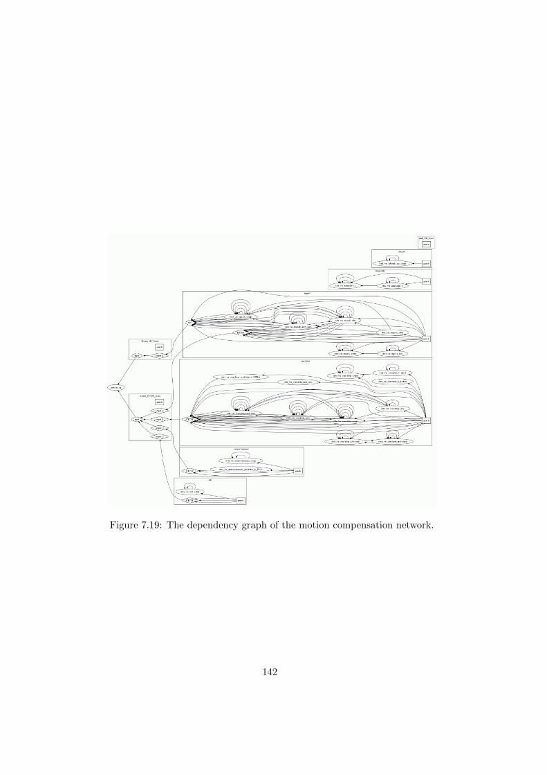
Figure 7.19: The dependency graph of the motion compensation network.

142

Chapter 8

Vision of the Future

The work done related to this thesis, has, to some extent shown what ispossible to do and what is worth to do, and of course also what is practicalto do when searching for a quasi-static scheduler for a dataflow application.Some of the experiments show how the efficiency of a program relates tothe scheduling of the program, while some show what is required in orderto construct a correct scheduling model of a program partition. For allthese ideas, transformations, model checking, and analysis, to be practical,the tool support should be improved considerably. The purpose of thischapter is to discuss what improvements, beyond what has been presentedin this thesis, would be required in order to allow any developer to use theapproaches presented when developing a dataflow program with CAL.

It is my contention that the developer should describe his or her intentionfor the tools to be able to do something very useful. The benefit from thisis twofold, fist, a well defined intention describes what should be done andgives the schedules that should be searched for, and second, by explicitlydescribing the intention, the tools can check if the program or part of theprogram does what it is supposed to do.

8.1 Identified Problems

While the purpose with this research is to show how the scheduling andcomposition of CAL actors can be performed using the approach presented,it is almost equally important to identify the situations where the approachwas not sufficient. There are then two alternative solutions, either the meth-ods must be improved, or the application description must be improved toinclude more information. Improving the description of a program does notnecessarily mean that the programming language is changed, but may alsosimply be guidelines for how an application is described in the dataflowlanguage.

143

Too Loose Specifications Many of the problems related to schedulingcome from situations where the program is not specified exactly enough forthe analysis to be able to draw the needed conclusions. In many cases, fora human, it would seem obvious that a guard checking if a video frame isan I-frame, that another guard checking if it is a P-frame, must be mutu-ally exclusive, however, an analysis tool does not have the option to checkthe MPEG standard and can therefore not know that there are no I-framesthat are also P-frames (see case study - Case V). This becomes a real prob-lem when comparing the guards of several actors, as the intention of theprogrammer is not anymore available.

The source of this problem is that it seems unnatural for a programmerto overstate conditions, as an example, it would seem strange to write:

if (x > 0) then ...

else if (x <= 0) then ...

where the second condition obviously is redundant, as it can be shown thatthe two conditions are mutually exclusive. For a programmer, the examplewith the type of video frames would seem to be the same situation, however,in the case study the two properties corresponded to two different bits whicheither are set of not, and in that case, it cannot be known that both bitscannot be set simultaneously.

Mixed Data and Control Another related problem appears when a pro-grammer does not clearly separate control from data. In CAL, everything istokens, and there is no separation of control values and data values, exceptfor the action scheduler which is strictly control. Now, consider an actorwhich has two actions, each producing a positive integer value. A secondactor receives this value and if it was produced by action a in the first ac-tor, it should be consumed by action a in the second actor, and if it wasproduced by action b it should be consumed by action b. The question ishow to achieve this behavior. A clever way is to encode it in the token, e.g.action a sends the value as it is while b negates it, then the guards of thesecond actor can check if the input token is positive or negative. This is anexample of mixing control and data, and when the control token is analyzedit is unnecessarily complex. Another alternative is to add a separate FIFOwhere the two actions send different constant, while the actions in the sec-ond actor has corresponding guards. This makes the analysis trivial and theFIFO can be removed in case the actors are merged.

What this is all about is, keeping the intention visible by describing con-trol tokens with as simple constructs as possible. This improves readabilityfor both the developer and the tools.

144

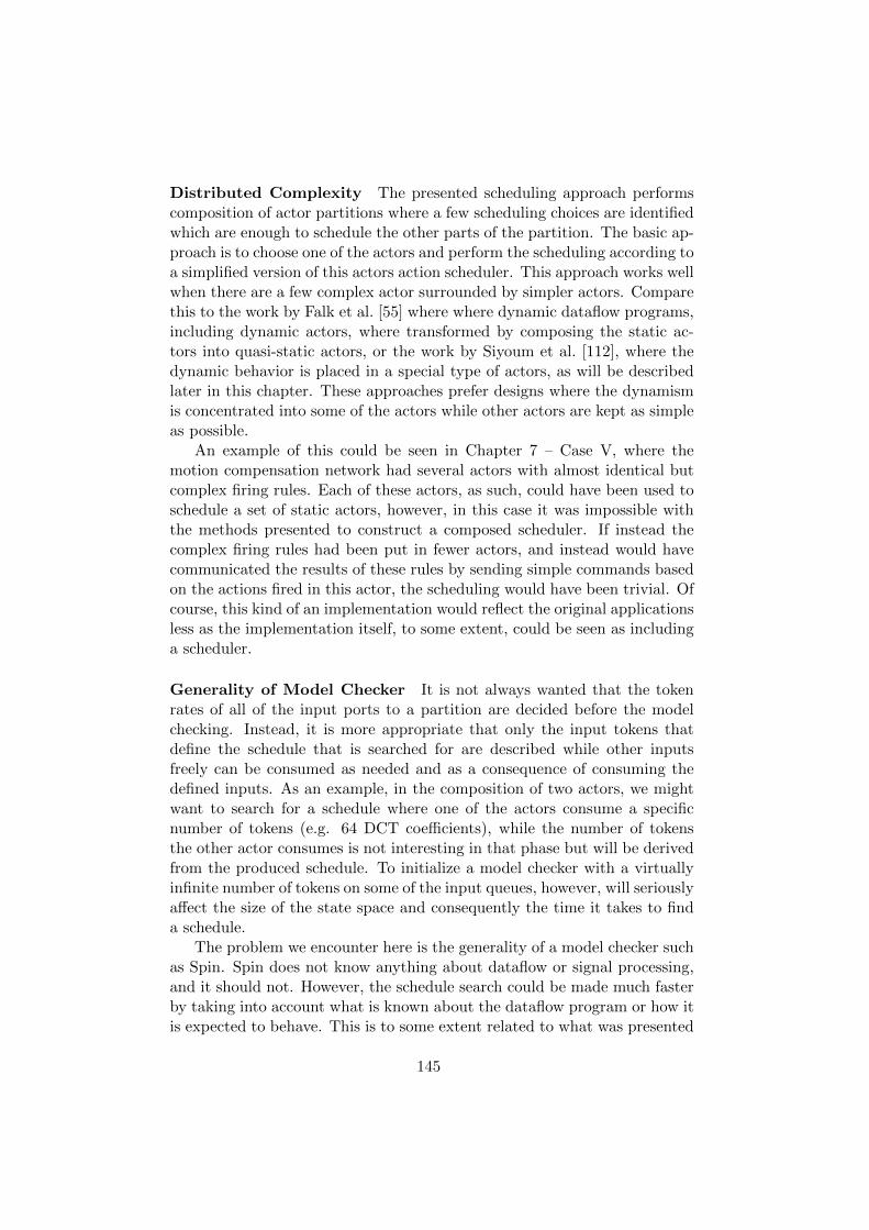
Distributed Complexity The presented scheduling approach performscomposition of actor partitions where a few scheduling choices are identifiedwhich are enough to schedule the other parts of the partition. The basic ap-proach is to choose one of the actors and perform the scheduling according toa simplified version of this actors action scheduler. This approach works wellwhen there are a few complex actor surrounded by simpler actors. Comparethis to the work by Falk et al. [55] where where dynamic dataflow programs,including dynamic actors, where transformed by composing the static ac-tors into quasi-static actors, or the work by Siyoum et al. [112], where thedynamic behavior is placed in a special type of actors, as will be describedlater in this chapter. These approaches prefer designs where the dynamismis concentrated into some of the actors while other actors are kept as simpleas possible.

An example of this could be seen in Chapter 7 – Case V, where themotion compensation network had several actors with almost identical butcomplex firing rules. Each of these actors, as such, could have been used toschedule a set of static actors, however, in this case it was impossible withthe methods presented to construct a composed scheduler. If instead thecomplex firing rules had been put in fewer actors, and instead would havecommunicated the results of these rules by sending simple commands basedon the actions fired in this actor, the scheduling would have been trivial. Ofcourse, this kind of an implementation would reflect the original applicationsless as the implementation itself, to some extent, could be seen as includinga scheduler.

Generality of Model Checker It is not always wanted that the tokenrates of all of the input ports to a partition are decided before the modelchecking. Instead, it is more appropriate that only the input tokens thatdefine the schedule that is searched for are described while other inputsfreely can be consumed as needed and as a consequence of consuming thedefined inputs. As an example, in the composition of two actors, we mightwant to search for a schedule where one of the actors consume a specificnumber of tokens (e.g. 64 DCT coefficients), while the number of tokensthe other actor consumes is not interesting in that phase but will be derivedfrom the produced schedule. To initialize a model checker with a virtuallyinfinite number of tokens on some of the input queues, however, will seriouslyaffect the size of the state space and consequently the time it takes to finda schedule.

The problem we encounter here is the generality of a model checker suchas Spin. Spin does not know anything about dataflow or signal processing,and it should not. However, the schedule search could be made much fasterby taking into account what is known about the dataflow program or how itis expected to behave. This is to some extent related to what was presented

145

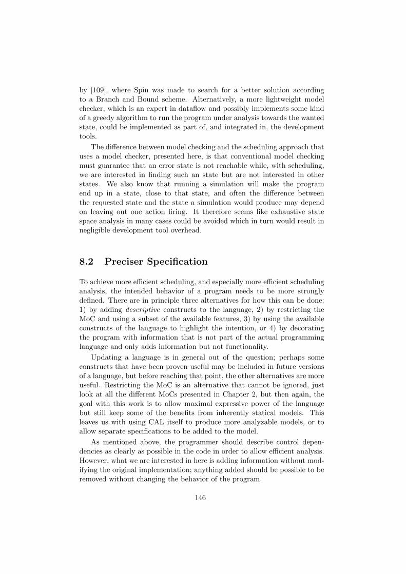
by [109], where Spin was made to search for a better solution accordingto a Branch and Bound scheme. Alternatively, a more lightweight modelchecker, which is an expert in dataflow and possibly implements some kindof a greedy algorithm to run the program under analysis towards the wantedstate, could be implemented as part of, and integrated in, the developmenttools.

The difference between model checking and the scheduling approach thatuses a model checker, presented here, is that conventional model checkingmust guarantee that an error state is not reachable while, with scheduling,we are interested in finding such an state but are not interested in otherstates. We also know that running a simulation will make the programend up in a state, close to that state, and often the difference betweenthe requested state and the state a simulation would produce may dependon leaving out one action firing. It therefore seems like exhaustive statespace analysis in many cases could be avoided which in turn would result innegligible development tool overhead.

8.2 Preciser Specification

To achieve more efficient scheduling, and especially more efficient schedulinganalysis, the intended behavior of a program needs to be more stronglydefined. There are in principle three alternatives for how this can be done:1) by adding descriptive constructs to the language, 2) by restricting theMoC and using a subset of the available features, 3) by using the availableconstructs of the language to highlight the intention, or 4) by decoratingthe program with information that is not part of the actual programminglanguage and only adds information but not functionality.

Updating a language is in general out of the question; perhaps someconstructs that have been proven useful may be included in future versionsof a language, but before reaching that point, the other alternatives are moreuseful. Restricting the MoC is an alternative that cannot be ignored, justlook at all the different MoCs presented in Chapter 2, but then again, thegoal with this work is to allow maximal expressive power of the languagebut still keep some of the benefits from inherently statical models. Thisleaves us with using CAL itself to produce more analyzable models, or toallow separate specifications to be added to the model.

As mentioned above, the programmer should describe control depen-dencies as clearly as possible in the code in order to allow efficient analysis.However, what we are interested in here is adding information without mod-ifying the original implementation; anything added should be possible to beremoved without changing the behavior of the program.

146

seqBTYPE

A

B

Cdcpred

A

B

C

BTYPE

QP

IN

OUT

PTR

QUANT

SIGNED

START

dcsplitINDC

AC

SpecBT

BTYPE

data

QP

Figure 8.1: Adding an actor to strengthen the guards of the actors scheduledbased on the input BTYPE.

seqBTYPE

A

B

Cdcpred

A

B

C

BTYPE

QP

IN

OUT

PTR

QUANT

SIGNED

START

dcsplitINDC

AC

Spec

BT

QP

DT

BT

QP

DT

BTYPE

data

QP

Figure 8.2: Adding an actor to define the scheduling of the rest of thepartition.

Adding Scheduler Actors Let us play with the idea that we add ac-tors that does nothing else than introduce stronger guards into a partition.An appropriate example where stronger guards could be useful is the acdcnetwork in Case Study V, where there are two actors which guards are func-tionally dependent but this cannot be proved as it is possible to come upwith input tokes that never will occur in practice (e.g. a frame is neverboth I and P), but that will cause the unwanted behavior. In this example,the network has one control input which is connected to two actors, namelyDCPred and Sequence. These actors receives identical copies of the samecontrol value and it is known that the four firing rules of DCPred can beused to decide which firing rule will be enabled in Sequence, however, withthe given guards this cannot be proved.

An additional actor, which gives stronger guards regarding these controltokens, can be added either in parallel or in sequence with the other actorsthat use this control value, as shown in Figures 8.1 and 8.2 respectively.Neither of these structures add any new behavior to the dataflow program;instead they introduce a sequence of firing rules that should be strong enoughto define the scheduling of the other actors. To do this the actors mightinclude an FSM and a set of actions defining strong guards. The idea isthen that, when a the scheduling model is generated, these actors can bechosen as the actors that the scheduling is based on as the firing rules havebeen constructed such that a functional dependency can be proved.

The first alternative, the one presented in Figure 8.1, adds the specifica-

147

tion actors as a listener, that is, it is tapped to the channel carrying controlinformation and consumes these values. Now the question is, if this actorshould be treated as any actor or if the tools should assume that this isa specific actor that specifies how the other actors work. This potentiallybecomes a problem if it is desired that the actor adds more informationregarding, for example, the sequence in which inputs may arrive. Whilethis type of specification actor adds a minimal modification to the dataflownetwork, the sequential alternative will have control over how informationflows in to the partition.

The second alternative, shown in Figure 8.2, the actor connected insequence actually resends every token that is received at the inputs of thepartition. Except from defining stronger firing rules in form of guards, thisversion also makes it possible to add more specific firing sequences as itfully can control how the tokens are streamed in to the partition. Withthis construct, it is easy to specify the exact scenarios that the partitionis supposed to perform. Furthermore, in this example the control tokendescribed the type of one 64-coefficient block in an MPEG-4 decoder, and itmight be desired to describe that if a block is either an I-block or a P-block,the next five blocks will be of the same type. This is easy to describe usingthe FSM of the specification actor as this actor controls what is allowed toenter the partition.

While these actors are rather simple, it might be easier to describe thebehavior of these in some other representation than CAL. A more high-levelrepresentation, from which these simple actors can be generated, could bemore appropriate. Such representations could also easily be used to decoratethe model with information that cannot be expressed in CAL.

Adding Information Software systems are often tested for correctnessby adding additional statements which are only used for testing or verifyingthat the program works according to the specifications. Typically asser-tions or invariants, pre- and post- conditions, are defined which describewhich properties should hold and when. The format of these specificationare often a more mathematical format than the language the application isimplemented in provides, e.g. the Spin model checker accepts linear-timetemporal logic statements to describe the correct behavior of the Promelaprogram being verified.

If we return to the example discussed above, where the problem wasthat the tools cannot know that a I-block cannot be a P-block, it wouldbe practical to add a few statements like btype ∈ I ∪ P ∪ Nvop and I ∩P = ∅, where I and P represent the sets of possible values that belongto these types of blocks. This actually would add a new dimension to thepossibilities of specifying the program, first of all, scheduling becomes easier,but second, it is also possible to verify that the program acts according to

148

the specifications.

8.3 Specification Verification

The point with adding a layer of specifications on top of a dataflow programis to more carefully state the intention of the programmer without the needto make the actual program too explicit or strict. The idea is then that anyof these specifications should be removable without the program loosing anyfunctionality. We could actually see such specifications as a description ofwhat is possible in the input stream while the program itself is a descriptionof how the input stream is processed. However, specifications are desiredin other places than on the input stream of the program, and if the devel-oper could specify what values are expected on a FIFO or even on a statevariable, it would open the possibility of verifying that the implementationcorresponds to the intention.

Describing the values that are possible on a FIFO does not seem likea good idea, instead this information belong to the ports connected to theFIFO. This would enable checking if two connected ports are compatible,and either we can trust this information or prove it from the actor representa-tion, then the actors are analyzed for composition. This kind of specificationis already used in the Cyclo-Static Dataflow model presented by Wauterset al. in [122]. While this kind of information should not be required forimplementing a program, it would introduce interfaces of the actors thatfirst can be verified for the individual actors and then at composition beused to construct an efficient description.

Actor interface compatibility leads us to an approach called CountingInterface Automata (CIA), which was presented by Wandeler et al. [120].CIA is designed to be a lightweight formalism which can be used to provebehavioral type compatibility between actors of a composition. This is doneby capturing the behavior of a CAL program and from this generating anautomaton for each actor and one for the framework, meaning the MoC andinterconnects of the model. The CIA does in principle describe automatawith labeled transitions, where a transition can be an input, output or in-ternal action. The automaton, furthermore, has variables which representquantitative aspects, which can be used in guards to describe when a tran-sition is enabled. The CIA is used for actor composition, however, with thegoal of analyzing the compatibility of actors and not, as in this thesis toremove unnecessary scheduling overheads.

The reason why CIA is mentioned here is that, while this automaton isderived from the CAL representation, it to some extent shows what kindof information we are interested in but, even more importantly, it is anexample of a formalism which would be composable with the specifications

149

of an actor. While this is only speculation of what would be an appropriaterepresentation of additional specification of a dataflow model, the followingsection is a comparison of some models which have taken different directionsto solve related problems. In other words, these are not comparisons of workthat is related to the main contributions of this thesis, but a comparison ofwork that is related to the direction this work should take in the future.

8.4 Related Work

In this chapter, the discussion is more philosophical and for this reasonthe discussion on related work has to be on the level of the goals and onthe ideas of other projects or tools that have a solution or have chosendifferent direction to solve the problems identified here. For this reason, thecomparison of approaches is less technical, and the goal is to highlight thedifferent direction of research within the problem domain.

Canals Part of the scheduling process is to identify how tokens belong to-gether and form larger data units that should be processed together. Such adata unit is then associated with a schedule which triggers the appropriatebehavior. Another approach is taken in a dataflow programming languagecalled Canals which was presented by Dahlin et al. in [39]. With Canalsscheduling is expressed in the language itself in special, per dataflow sub-network elements, called schedulers. Both networks and computational ker-nels are limited to only have one input and one output queue, and instead,the input tokens are grouped into more complex data types. When there isan actual need for several inputs or outputs, special elements called scattersand gathers are used, which define how data types are split or composedbetween the channels.

In Canals, much of the complexity of the dataflow network is movedto the data types. A network then, when a data token enters, can assignthe appropriate schedule for that data type. Also the scheduler is definedin the language, and this means that the developer can create a customscheduler for a network, or use a more generic scheduler such as a roundrobin scheduler. If we compare this to CAL, the scheduling in CAL is definedin the actors but not at all on network level while Canals does the oppositeby concentrating on the scheduling on network level. For this reason, ina comparison of how to translate CAL actor into Canals, the CAL actorswere compared to networks in Canals while CAL actions were comparedto kernels [40]; however, it would in that case seem natural to implementthe Canals program more coarse grained as the data dependencies betweenkernels else would result in a massive interconnect.

What seems relevant from Canals in this context is the mapping between

150

data types and schedules. Even though CAL handles data types on thelevel of individual numbers (integers etc.), and more complex data typesin most cases can be derived for the inputs to a partition, a more explicitrepresentation, at least on specification level would be useful.

PREESM Another direction of the research is to restrict the expressive-ness of CAL, to only include statically schedulable actors, in order to allowefficient scheduling on multiprocessor architectures. An example of this isPREESM which is presented by Piat et al. in [104], which uses a restrictedversion of CAL where actors are implemented according to rules such thateach action of an actor must consume and produce an equal amount of to-kens on all of the ports. As a result, the CAL network can be translated into an SDF graph and a balance equation, which then can be used by thePREESM scheduler to, at compile-time generated a multiprocessor schedule.

While SDF is efficient for compile-time scheduling om multiprocessor ar-chitectures, SDF does by definition not provide any flexibility and for thisreason SDF is not sufficient for many applications. This can to some ex-tent be taken care of by considering the different scenarios, that is, a setof parameters and constraints which specify the conditions under which theapplication will run [100]. To enable reasoning about scenarios, PREESMuses the Parameterized and Interfaced SDF (πSDF) MoC which was pre-sented by Desnos et al. in [43]. This model extends the SDF model withconcepts from PSDF and a MoC called interface-based datalow [103], andintroduces explicit parameters and a parameter dependency tree.

The πSDF model includes special elements which are used to explicitlydescribe the configuration of the model. Such elements are configuration ac-tors, configurable parameters, configuration input/output ports, and config-uration interfaces. These elements make the parameterization of the modelexplicit, also through hierarchical levels, and the semantics of πSDF definesthe exact behavior and the order in which the steps related to configurationtakes place. [43]

This kind of a modeling highlights the control structures by modelingthe program as a set of configurable SDF subparts. While the goal of thework related to this thesis is to provide the programmer with a maximalexpressiveness, it is certainly relevant to compare these constructs to thecontrol information we try to derive from CAL programs. Also, the con-ceptual specification actors presented above in Figures 8.1 and 8.2 can becompared to the configuration actors.

CAL as Disciplined Dataflow for Analysis as SADF In [112], Siy-oum et al. presents an approach where CAL programs are implementedaccording to the Disciplined Dataflow Network (DDN) MoC, which enables

151

automatic extraction of scenario sequences which are comparable to thestatic schedules presented in this thesis. The approach identifies all thepossible scenarios of a DDN and extracts the SDF graphs corresponding tothe scenarios. This enables analysis of the dataflow program, for propertiessuch as deadlock-freedom and boundedness, with known methods. The ap-proach in [112] takes the design of an CAL program in the same directionas was proposed in this chapter by forcing the programs to be implementedaccording to a set of construction rules making the CAL program conformto DDN.

For a CAL program to conform to DDN, control values, either as inputtokens or state variables, must be such that these can only assume a finitenumber of integer values. DDN uses two types of actors which has differentconstruction rules. The detector actors control kernel actors by providingthe control tokens that decide the firing sequence of the kernel actor. Thus,any control input of a kernel actor must be connected to the output of adetector actor. These control tokens – the output of the detector actors –must be restricted to a finite set of integers. The end result here is rathersimilar to the scheduling technique presented in Chapter 5; the detectoractors correspond to the leader actor of a partition, and, the restrictions ofthe control values have a similar effect in both works.

The choice to mention this work in this chapter, and not in the chap-ters related to scheduling, is due to the fact that this approach is based onspecifying the program such that the analysis becomes simple. From thepoint of view of the discussion in this chapter, this work takes the designof a CAL program in the direction where the intention of the designer ismore obvious for the design tools. The difference is that the detector actorsactually are part of the program and not simply specifications. However, aCAL program constructed according to DDN, is still simply a CAL program,but with some very useful features. For this reason, a CAL program imple-mented as DDN should directly by schedulable with the methods presentedin this thesis.

Ptolemy It is at this point appropriate to return to the roots of CAL,namely the Ptolemy project [46, 1]. Ptolemy provides a framework for mod-eling and simulating heterogeneous models, that is, different parts of themodel may belong to different MoCs such as SDF or continuous time. Dif-ferent models are composed with a hierarchically heterogeneous approach,which means that the model is hierarchically structured such that a modelcan include components with another MoC internally. A Ptolemy model isbuilt from actors, hence the name actor in CAL, which can be atomic orcomposite, depending on if they are built from other actors or if they are atthe bottom of the hierarchy. [48]

In the context of dataflow, CAL uses FIFOs for the communication be-

152

tween the actors, in Ptolemy, however, there are different types of com-munication, such as mailboxes and rendezvous points, and this is definedby the domain of the composite actor. The domain includes an director,which is concerned with the scheduling of the actors, and receivers, whichare concerned with the different types of communication.

We are not, in this context, interested in MoCs such as continuous time,however, Ptolemy also interfaces and specifies different dataflow MoCs, andimplements how these different models are composed. It therefore, showsone more way to describe the intention, that is, how the actors are supposedto be fired. Also, the compatibility of these can be checked as already wasdiscussed earlier in this chapter regarding counting interface automata aspresented in [120]. This is the essence of what is requested in this chapter,a description of the intended behavior of the domain, a description of thebehavior of the actors, and a method for how these can be checked forcompatibility.

The three approaches presented above all provide the needed schedul-ing information by adding special elements to the dataflow network, whichdescribes how the scheduling is supposed or intended to work. It is usuallyuseful to follow research is different communities, and for this we will lookat one more work from the world of formal methods.

Rodin and Event-B Rodin is a tool for formal modeling in Event-B,which is a language and a proof method influenced by the B Method [4]and Action Systems [14]. Event-B uses the structure of guarded actionswhich operate on state variables from Action Systems to describe systembehavior, while it uses typed set theory as the mathematical language fordefining state structures and events [5]. Compared to CAL, a program ineither language is a set of guarded actions, called events in Event-B, whichexecute as atomic statements and operate on the state variables. The onlydifference, as CAL is used in dataflow, is that is explicitly defines ports, andthe surroundings of the actors describe how these are connected with theFIFOs.

The modeling in Event-B begins from the opposite direction compared tohow a CAL program would be implemented. In Event-B the development, orperhaps more correctly, the modeling, starts from more abstract models ofthe system which describe the intuition regarding what the system shoulddo and what it is allowed to do. The modeling proceeds with somethingcalled stepwise refinement, that is, more details are added to the model andthe correctness of the refinement, that the refined model does not violatethe previous model, is proved by solving some required proof obligations.The proof obligations are automatically generated and often automaticallyproven. [5]

An Event-B model consists of contexts which describe the static part of

153

the model such as constants and axioms, and machines which describe thedynamic part of the model such as state variables and events. The statevariables are constrained by invariants which always must hold. The cor-rectness between models and refined models can be proved with the relationbetween different invariants and axioms, and the proof obligations are gener-ated for this purpose. For the scheduling work presented in this thesis, whilethe machines resemble the actors, there is nothing similar to the invariantsor the contexts in CAL. This is solved in work related to scheduling CALby using external tools such as model checkers [51] or SMT solvers [124], asdiscussed in Chapter 5, to prove some properties needed for deciding on howan actor or partition can be scheduled. This again related to the discussionof how specifications could be added to a CAL program.

This makes it easy to describe guards and to prove that these have thespecified properties, in Event-B. However, with Event-B, like with CAL, theproblem of efficient scheduling or efficient sequentialization is not solved bythis, instead it simply helps to prove the completeness of a scheduler. Workregarding scheduling of Event-B has been presented by Bostrom in [25] andby Degerlund in [41], partly by providing scheduling patterns with theirproof obligations, and by allowing processes to fire, up to a maximal numberof times before the state variables are updated to the global state. In anycase, the scheduling of Event-B resembles the scheduling of CAL, and forthis reason it will make sense to more carefully compare the work from bothcamps.

154

Chapter 9

Overview of the OriginalPublications

The second part of this thesis is a collection of pair reviewed publishedpapers that focus on different aspects of the dataflow scheduling problem.The papers are more focused on solving specific problems than the moregeneral first part of the thesis and go more in to detail. The purpose ofthis chapter is to give an overview of each of the papers and highlight thecontribution the papers give to the topic of this thesis. Then for each of thepapers, the contribution of the author is also explained.

The papers are presented in chronological order, as they have been pub-lished. As can be expected, the first papers present the high level ideasregarding how the scheduling approach can be used and shows some initialproof of concept. The following papers then refine the scheduling approachand evaluates the approach by providing more experimental results. Finallya paper which shows on how the approach can be integrated in a larger toochain is presented.

9.1 Paper I: Scheduling of Dynamic Dataflow Pro-grams with Model Checking

The idea of using a model checker for scheduling a dynamic dataflow pro-gram written in CAL originates from the idea that a CAL program simplyis a set of communicating state machines. The Promela programming lan-guage, which is the input to the Spin model checker, and which basicallydescribes a process network, can then be used to mimic a CAL programand to generate a model checker to analyze the state space of the program.When considering the state space of a program, a schedule is then a pathbetween two program states, while a static schedule is a path between twostates that, is always valid when some precondition, in form of a guard ex-

155

pression, holds. The scheduling is the about identifying these reoccurringstates, the guards enabling static schedules, and the actual schedules thatlink these states.

The main contribution of this paper is to show how the scheduling prob-lem can be expressed as a model checking program. This consists of twoparts, first, it is shown how the CAL representation can be translated intoPromela, which is the input to the Spin model checker, and an implemen-tation of the Promela code generation that was implemented in the Orcccompiler is presented. Second, the ideas how the schedules are searchedfor is presented. This includes how the model checker is initialized withan appropriate input sequence corresponding to a type of inputs the pro-gram partition accepts, and how to define the state to be searched for as aLinear-time Temporal Logic (LTL) expression, which defines a state wherethe model checker reports an error if it is found. The concept of usingthe model checker to produce a trace to such an error state, and using thereported trace to describe a schedule is presented in this paper.

This paper presents the initial ideas related to how scheduling of a CALprogram can be performed using a model checker. The idea in this paper isthat the developer has some knowledge about the application to be scheduledand is able to describe to the model checker what kind of schedules tosearch for. This is a manual process, where the inputs to a network andthe objectives of the schedule search are given by the developer. While thescheduling process mainly is a manual process, this paper shows that theconcept works and also, to some extent, what kind of information is neededin order to specify the objective of a model checking schedule search.

The resulting schedule is, already in this paper, described as an FSM,which is important for the future developments as this is a natural wayto describe the scheduler of a CAL actor, which is the result of merging apartition after the scheduling stage. The resulting scheduler is, however, notused to merge the actors, but instead, the model checker is used to generate asequence of C-function calls, that are glued in to the C-code generated fromOrcc. This code is then executed and gives some promise of a potentialspeedup, however, there is only a limited number of experiments.

Author’s Contribution: The background and high level idea to thiswork started from the co-authors of the paper, while the author of thisthesis was given the task to realize the idea in a concrete implementation.The task of the author was then to plan what the translation from CALto Promela should look like, which is described in Section 3, to find outhow this can be used to generate schedules, which is described in Section 4,and to implement this in the Orcc compiler. The implementation work, andlater the experiments for the paper, was done in cooperation with GhislainRouquier. Regarding the paper writing, the author wrote the first draft of

156

the paper after which the co-authors contributed with improvements andadditions.

9.2 Paper II: Scheduling of Dynamic Dataflow Pro-grams Based on State Space Analysis

For the state space exploration to be feasible and hence the model checkingof a network of CAL actors, the state of the actors and the actor partitionshould be described with the minimal information that is required to cor-rectly schedule the program. For an actor, the state is described by theFSM scheduler and the state variables. To reduce the state space, only thestate variables relevant for scheduling should be used to describe the actorstate. For this, not only the variables that are directly used in a guard areneeded but also any variable that are in any sense used to give the value toa variable that is used in a guard. Furthermore, on the level of a networkof actors, the cross actor dependencies, that is, every variable inside any ofthe actions in the partition that is used to produce a value that ends up ina guard in any of the other actors in the partition must also be included.

The main contribution in this second paper is the more careful descrip-tion of how the model checker is constructed, and which information fromthe actors is included in the generated Promela code. The paper presentssome simple rules for how to create the graph that describes the depen-dencies between variables in a network of actors. This information bothsimplifies the description of the actor but also describes the state of a par-tition such that it can be used for searching for schedules. In practice, theactor is simplified by removing the code that is not relevant, before the codegeneration. This effects the state space in two ways, first, the variables thatsimply process data are removed and does not contribute to the state space,second, the code that produces data output is removed which means thatdata written to queues is always zero valued and only contributes to thestate space with the number of tokens. The second benefit from this is thatthe states of the actors can be described from a pure scheduling point ofview, this in turn is important when the schedules to be searched for are tobe defined.

Except for this, the paper also present some fresh results from exper-iments on an MPEG-4 decoder, where the scheduling approach is appliedto schedule the motion compensation, IDCT, and texture coding networksindependently. The paper then provides results regarding the reduction ofguard evaluations needed to schedule the partitions and some measurementsof the performance (frame rate) of the program, after manually applying theschedules extracted by the model checker.

157

Author’s Contribution: This paper was a natural continuation of theprevious paper, with some of the ideas more clearly defined and with moreexperiments. The contribution of the author regarding the work for this pa-per was to develop the rules for describing the partition state more carefullywhich is presented in Section 3 in the paper and to refine the model checkingapproach as presented in Section 4.

9.3 Paper III: Static and Quasi-Static Composi-tion of Stream Processing Applications fromDynamic Dataflow Programs

The purpose with any code transformation or optimization is always to im-prove the run-time performance of an application, be it with respect to speed(frame rate), memory usage, energy consumption, or some other metric. Thescheduling and composition of a partition of actors implies that the memoryfootprint of the program changes and the locality of the code and data willalso change. This means that a single metric such as the number of guardsneeded, is not sufficient for predicting how the performance will change asa result of the composition. Instead, the many parameters regarding thehardware, such as memory architecture, decides how a specific compositionwill affect the run-time performance.

This paper presents how different types of actors can be composed usingdifferent methods, depending on how dynamic the actor is. Different partsof a program are then composed in to larger actors, either using a staticcomposition, if the actors are classified to SDF or CSDF, or a quasi-staticcomposition in the other cases. The classification and static compositionis here based on [124] while the quasi-static scheduling is performed usingthe model checking approach. The different configurations of an MPEG-4 decoder program, with different compositions applied and different sizesof the FIFOs between the actors, are used to run experiments on differentprocessors with a set of different videos.

The main contribution of this paper is in the experimental results, whichseemingly shows contradicting results but which can be linked to how wellthe program fits in the cache of the different processors. The paper, com-pares various aspects of scheduling and composition, and presents resultsthat on the one hand show how different aspects may affect the performancebut on the other hand shows the importance of extensive experiments whenevaluating an approach like this. The lesson learned from this work is thatthe platform and perhaps more specifically the cache size and structure,should be used to decide what the schedules should look like and how largethe actor compositions should be. In practice it may be hard to directly de-cide on such parameters from a hardware description, however, these aspects

158

can still be considered in the design space exploration.

Author’s Contribution: This paper presents work related to two schedul-ing approaches of which the author only has contributed to the other. Thecontribution of the author in this paper was to write the parts of Sections 3and 4 related to quasi-static scheduling as well as to plan the experimentsand to write the results section (Section 5).

9.4 Paper IV: Modeling Control Tokens for Com-position of CAL Actors

A partition scheduler is an FSM where transitions correspond to sequencesof actions i.e. schedules. The scheduling decision, that is, the choice betweenthe outgoing transitions in a state is represented as guards of the transitions,where a guard can depend on state variables and input ports. These guardsneed to be generated or reused from the original actors, and these must bestrong enough to correctly schedule the partition. To successfully produce ascheduler for a partition which receives control information from outside thepartition, it is essential to have means for reasoning about how the controltokens propagate in the partition in order to decide on whether a set ofguards are strong enough to schedule the partition.

This paper presents a different view point of a CAL program, that is,from the point of view of the control tokens. The ideas how to describe thestate of a partition presented in Paper 2, are taken further and are formal-ized, and the resulting dependency graph is simplified to a point when thetoken propagation of an actor only can have one of a few forms. This makesit easier to reason about control tokens of a partition and to decide whattype of proofs are needed in order to show that a set of guards are sufficientfor the partition. The different forms of how an actor propagates the controltokens imply different complexity of the verification of the strength of theguards. While in the most simple form, sufficient strength is implied, othertypes varies from requiring simple proofs to requiring the actor to be trans-formed. The main idea is that, depending on the constructed dependencygraph, the requirements for verification can easily be derived.

The contribution of this paper is that it formally shows how the de-pendencies of an actor partition is constructed and analyzed. The, almosttoo, formal description of how to build graphs form a CAL program, showshow each program construct is taken into account. This gives some level ofguarantee regarding the completeness of the approach presented.

Author’s Contribution: This work was initiated by the author to solve aproblem that was identified while working with scheduling of different CAL

159

programs. The paper is a continuation of the work started in the previouspaper, and formalizes the way to view how control information propagatesin the program. The first draft was written by the author after which theco-authors contributed with improvements and additions.

9.5 Paper V: High-Performance Programs by Source-Level Merging of RVC-CAL Dataflow Actors

A set of schedules is hardly useful as such, instead, only once the scheduledescription is used to generate efficient code or to transform a program intoa more efficient representation, can some improvement be achieved. Thepresented scheduling approach produces a scheduler, and a set of schedulesin a textual format. This representation then needs to be used to transformthe corresponding CAL program according to the composed actors and theschedule describing the execution of this actor composition. We refer to thisoperation, to create a super actor from a set of actors and the composedactor scheduler, as actor merging. After the actor merging step, a superactor is an actor which has actions corresponding to the sequences of actionfirings of each schedule, an FSM scheduler corresponding to the FSM thatdescribes the scheduler of the composition, and the ports that communicatewith the surrounding actors.

This paper presents source-level actor merging, which means that themerging operation is performed on the level of CAL code. The tools pre-sented takes as input CAL code and a schedule description, and producesa transformed CAL program as output. The difficulty in merging actorsis on the one hand to achieve correctness regarding how guards and actorschedulers are generated, and on the other hand, to generate the mergedactor such that efficient code can be generated from it. This paper presentsformally how the actors are merged and how the different parts of the actorsare handled in order to guarantee a correct super actor.

The work in this paper is the basis for the actor merging mentionedin Chapter 7, and which is used to import the scheduler generated by themodel checker to the Orcc compiler. The main contribution of this paperwith respect to this thesis is that it provides the missing part namely theconcrete merging operation, by doing this, it also provides an description ofwhich information needs to be produced by the scheduling framework.

The paper also presents experimental results from a case study of aZigBee transmitter, run through the full tool chain, including: scheduling,merging, code generation, and running the code on a TTA processor. Theexperiments show promising results regarding efficient code generation, atleast for the class of applications and processors that are studied in this pa-per. These results show that, using dataflow to describe some applications

160

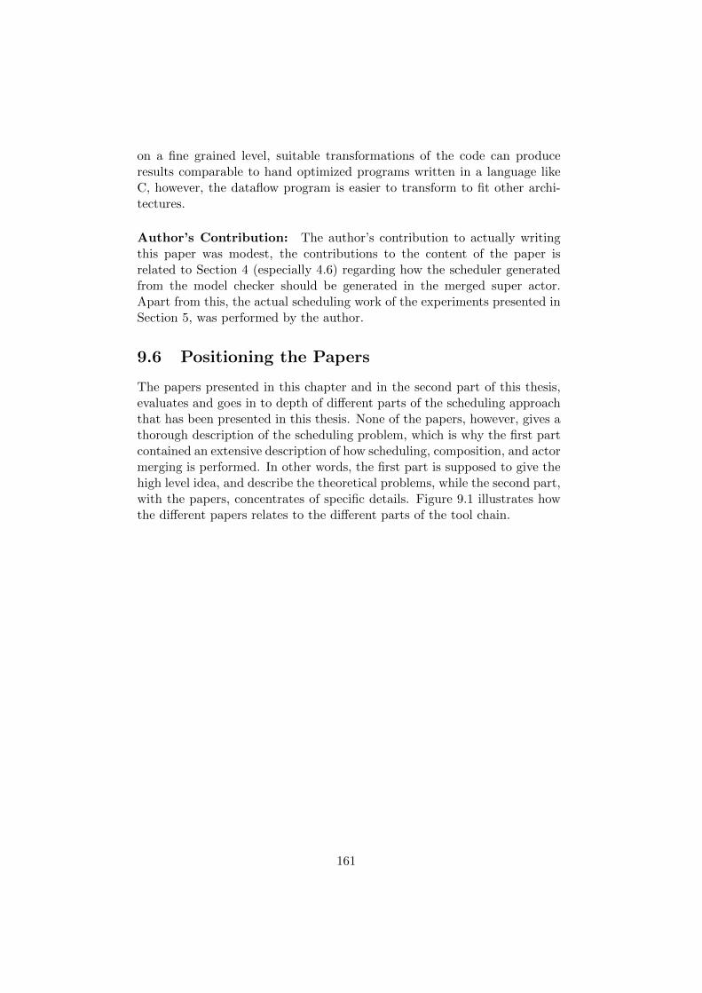
on a fine grained level, suitable transformations of the code can produceresults comparable to hand optimized programs written in a language likeC, however, the dataflow program is easier to transform to fit other archi-tectures.

Author’s Contribution: The author’s contribution to actually writingthis paper was modest, the contributions to the content of the paper isrelated to Section 4 (especially 4.6) regarding how the scheduler generatedfrom the model checker should be generated in the merged super actor.Apart from this, the actual scheduling work of the experiments presented inSection 5, was performed by the author.

9.6 Positioning the Papers

The papers presented in this chapter and in the second part of this thesis,evaluates and goes in to depth of different parts of the scheduling approachthat has been presented in this thesis. None of the papers, however, gives athorough description of the scheduling problem, which is why the first partcontained an extensive description of how scheduling, composition, and actormerging is performed. In other words, the first part is supposed to give thehigh level idea, and describe the theoretical problems, while the second part,with the papers, concentrates of specific details. Figure 9.1 illustrates howthe different papers relates to the different parts of the tool chain.

161

Orcc

C Backend Promela Backend

Scheduling Tool

RVC-CAL Prog

Missing Schedules

C code

Scheduler.XML

Promela Code

Input Sequences

Actor Schdules

Merger

Exprimental Results

Paper 1

Paper 2 Paper 5

Paper 3

Paper 4

Figure 9.1: Illustration of how the papers correspond to the different partsof the scheduling tool chain.

162

Chapter 10

Conclusions

This thesis addresses quasi-static actor composition and scheduling, andpresents how the scheduling problem can be expressed as a model checkingproblem. For this to be possible, the actors that form a composite actorare required to be simplified such that a state space analysis is feasible butthe behavior is preserved. The presented approach starts from a part of aCAL program which is analyzed and transformed to include only relevantinformation, and a model checker is produced from this representation. Thena strategy for the scheduling is chosen, typically based on one of the actors inthe partition, and the state space is searched in order to find paths betweenstates that partially have been identified at the previous step. Finally, whenall necessary paths or schedules have been found, these are translated into aformat (based on XML) which is used to transform the CAL program whichthen is ready for code generation.

The usefulness of the approach depends of the trade-off between potentialgain in form of program performance, the effort required from the developerin form of knowledge and time, and simply how well the approach can handletypical actor partitions. Then these properties should be compared to otherrelated approaches in order to find whether the approach excels in any ofthese directions. Another aspect is how the approach, or perhaps parts ofit, has potential to be further developed, and what can be learned from theusefulness of the tool chain that has been constructed for the purpose. Thiswork gives a proof of concept of that this kind of a method is possible toimplement and use in a datalow context. This is shown regarding severalsub problems, such as, feasibility of state space analysis, identification ofcontrol structures, the practical scheduling, and experimental results.

163

10.1 Retrospective – Goals versus Approach

It is Feasible to Perform State Space Analysis One of the potentialproblems with using a model checker to analyze a problem for scheduling isthe potential size of the state space. In a dataflow program, the state space,if the whole behavior of the program is taken into account, is enormous.If the model would include the data on the FIFOs and the state of theactors, including possible internal data structures of the actors, the statespace would not be possible to analyze efficiently. Furthermore, it would beimpossible to find a relatively small scheduler if data values also would bepart of the state. In the present approach, the state space is significantlyreduced both by removing variables which do not affect the scheduling andby treating tokens which carry pure data as simple valueless tokens.

It was shown in the case studies in Chapter 7 that the approach can beused on reasonable large applications, such as a video decoder. However,the efficiency of the scheduling could be significantly improved by methodsfor finding the minimal buffer sizes (e.g. TURNUS [32]) and by limiting theamount of data that is available on the input queues according to some kindof an approximated balance equation. This tried out manually shows, forthe applications in the case studies, that the time spent running the modelchecker was a few seconds instead of, in the worst case, several minutes whenthe buffers and inputs were not properly adjusted.

It is, of course, not enough that the program can be simplified such thatthe state space is manageable. The generated scheduling model must alsoinclude enough information such that a complete scheduler can be generated.

Completeness can be verified regarding Guard Strength The cor-rectness of the model is guaranteed by identifying all the required inputsequences that result in different schedules and the guards that uniquelycorresponds to these. There are two properties that require special atten-tion, the first one is control tokens and the second is independent data paths.Both of these properties are viewed from the point of one actor, which isseen as the leader of the scheduling, and it is then shown that all the otheractors in a partition depends on this actor, both regarding token rates andcontrol values.

The control token dependencies can be viewed as a graph describinghow control values flow between and through the actors. The graph is thenused to decide whether further properties must be proved or if the controlstructure already is sufficient. The graph also helps the developer to visualizeand understand the control structures of an application and, based on this,choose sufficient partitions or in some cases to change the implementationto simplify the control dependencies. In Chapter 5 it was also demonstratedhow theorem provers (and model checkers) can be used to further analyze

164

the control dependencies by proving that the required properties hold forthe actors.

In a similar fashion, the token rate dependencies between actors washandled such that it can be shown that the one leader actor can be used todecide the token rates of any other actor that reads inputs of the partition.This is important as else the partition may start to accumulate inputs onone or more of the input ports. This is resolved by constructing a graphof the connections which have deterministic token rates with respect to theleader action, and verify that all inputs depend on the execution of thisactor. While this ensures that the partition does not accumulate tokens andby this cause deadlock, this does not guarantee deadlock-freedom. If thepartition is part of a feedback loop, deadlock-freedom needs to be verifiedglobally on the schedules of the partition; this is however not discussed inthis thesis.

The scheduling decisions are by this a set of firing rules which in turnare guaranteed to decide the behavior of the full partition. With this spec-ification, each firing rule describes a partial input stream and possibly anorder in which decisions are to be taken; the complete input streams and thecorresponding schedules are searched for in the state space of the partition.

A Few Scheduling Strategies takes us Quite Far The scheduling isbased on the possible input sequences and the states the actors may reachprocessing these. The schedules then are paths between a few of these statessuch that the schedules can be fired to correspond to any input stream. Ascheduling strategy then describes how to identify these states. Often, it isappropriate to describe these states partially, that is, describing some of theproperties that should hold in that state. A few strategies were presentedin Chapter 5, and these were successfully used to schedule most of the casestudies in Chapter 7. It was also shown that the scheduling was automatic,in the sense that the user simply needed to chose the next schedule to searchfor, for most of the applications, while the once that were not, it could beidentified from the analysis of the actor partition that the dependencies willcause problems.

It is difficult to speculate whether the strategies work well because oftheir generality or because they have been developed with knowledge of thespecific case studies. However, choosing one actor to base the schedulingon, and surrounding it with actors which scheduling depends on this actor,basing the scheduling on this actor seems to be an obvious match. Theonly problem, except from it being difficult to predict the number of statesthat will be needed for the scheduling, is then predicting which FIFOs mayrequire to store tokens between the schedule firings. This has in this workbeen left for the developer to decide and can be seen as the potential weak-ness of the scheduling strategies. The work of the developer could, however,

165

be simplified by providing an approximation of potential delay tokens or ifone input sequence can be predicted to not produce enough tokens for someof the actors during one schedule firing.

The Experimental Results Show Evidence of Usefulness To showthe usefulness of quasi-static actor composition techniques, rigorous experi-ments with different applications, configurations, and platforms, are neededto show that the measured improvements can be generalized. The experi-mental results presented in this thesis in combination to the results in relatedapproaches show that composition as such is not a guarantee for improvedperformance, but instead, performance depends on how well the actors fitthe target platform. This also shows that designing larger actors to be-gin with does not make composition unnecessary as different actor sizes arerequired for portable performance on different platforms.

10.2 This Research in Perspective

Actor composition, possibly together with actor splitting, is essential fordataflow applications to be portable to various platforms regarding perfor-mance. While composition only is one step of the design space exploration,it is the one step that enables fitting an application to an architecture witha specific number of cores or with a specific memory hierarchy. As the com-position step involves composition of the scheduler, it also decides how muchscheduling overhead a program will have.

Another important question is how this approach compares to otherapproaches for scheduling dynamic dataflow applications. It is quite difficultto compare, and for networks with static actors, it is difficult to competewith approaches such as the classification approach presented by Wipliezet al. in [124] as was shown by the results in Paper 3 [50]. Neither is itfair to compare the exact experimental results with the other approachesthat were mentioned before as this would require identical configuration inorder to be valid. What, on the other hand, can be compared is the effortit requires from the user to produce the composite scheduler. In the otherapproaches, the partitioning and scheduling is an automatic step, which doeswhatever it can before code generation. In the presented approach, however,the developer is part of the process and chooses the partitions, the leaderactor, and a strategy for searching for the schedules.

As this approach is more interactive than the others presented, it shouldbe seen more as a part of design space exploration than a compiler op-timization. It would, from this point of view, also make sense to use anextended version of the approach to provide the developer with feedbackregarding guard strengths and potential partitioning. To take this one step

166

further, the developer could even provide a library of composition recipesfor composite schedulers.

The other alternative to scheduling, as has already been discussed, is touse more restrictive MoCs which provide more predictable scheduling. Inany case, even if the MoC provides adequate primitives for describing thecontrol mechanisms, scheduling is still required and similar methods may berequired to produce the static schedules for such dynamic actor partitions.

The potential benefit of this work is that it may highlight various designpatterns, or perhaps scheduling patterns, which is typically used in dynamicdataflow programs. Simultaneously, it describes the control structures andthe potential problems which scheduling some designs. The best way tomake use of this contribution is within designing tools that aid the designereither by highlighting dependencies in the design or by allowing the devel-oper to express higher level intentions of the program which can be verifiedfor the actors.

167

168

Bibliography

[1] The Ptolemy Project. Department EECS, University of California atBerkeley, (http://ptolemy.eecs.berkeley.edu).

[2] ISO/IEC 23001-4:2009. Information technology - MPEG systems tech-nologies - Part 4: Codec configuration representation, 2009.

[3] A.A.-H. Ab Rahman, S. Casale Brunet, C. Alberti, and M. Mattavelli.Dataflow program analysis and refactoring techniques for design spaceexploration: Mpeg-4 avc/h.264 decoder implementation case study. InDesign and Architectures for Signal and Image Processing (DASIP),2013 Conference on, pages 63–70, 2013.

[4] J.-R. Abrial. The B-book: Assigning Programs to Meanings. Cam-bridge University Press, New York, NY, USA, 1996.

[5] Jean-Raymond Abrial, Michael Butler, Stefan Hallerstede, Thai SonHoang, Farhad Mehta, and Laurent Voisin. Rodin: An open toolsetfor modelling and reasoning in event-b. Int. J. Softw. Tools Technol.Transf., 12(6):447–466, November 2010.

[6] Gul Agha. Actors: A Model of Concurrent Computation in DistributedSystems. MIT Press, Cambridge, MA, USA, 1986.

[7] Alfred V. Aho, Ravi Sethi, and Jeffrey D. Ullman. Compilers: Prin-ciles, Techniques, and Tools. Addison-Wesley, 1986.

[8] Gene M. Amdahl. Validity of the single processor approach to achiev-ing large scale computing capabilities. In Proceedings of the April18-20, 1967, spring joint computer conference, AFIPS ’67 (Spring),pages 483–485, New York, NY, USA, 1967. ACM.

[9] Apple. Grand Central Dispatch. Technical report, 2009.

[10] Arvind and K. P. Gostelow. Some relationships between asynchronousinterpreters of a data flow language. In Formalization of ProgrammingConcepts, 1977.

169

[11] Arvind, Kim P. Gostelow, and Wil Plouffe. Indeterminacy, monitors,and dataflow. SIGOPS Oper. Syst. Rev., 11(5):159–169, November1977.

[12] Krste Asanovic et al. The landscape of parallel computing research:A view from berkeley. Technical Report UCB/EECS-2006-183, EECSDepartment, University of California, Berkeley, Dec 2006.

[13] Russell Atkinson and Carl Hewitt. Synchronization in actor systems.In Proceedings of the 4th ACM SIGACT-SIGPLAN symposium onPrinciples of programming languages, POPL ’77, pages 267–280, NewYork, NY, USA, 1977. ACM.

[14] R.J.R. Back. Refinement calculus, part ii: Parallel and reactive pro-grams. In J.W. Bakker, W.-P. Roever, and G. Rozenberg, editors,Stepwise Refinement of Distributed Systems Models, Formalisms, Cor-rectness, volume 430 of Lecture Notes in Computer Science, pages 67–93. Springer Berlin Heidelberg, 1990.

[15] J. W. Backus, F. L. Bauer, J. Green, C. Katz, J. McCarthy, A. J.Perlis, H. Rutishauser, K. Samelson, B. Vauquois, J. H. Wegstein,A. van Wijngaarden, and M. Woodger. Report on the algorithmiclanguage algol 60. Commun. ACM, 3(5):299–314, May 1960.

[16] Lidan Bao, Hongmei Wang, Tiejun Zhang, Donghui Wang, and Chao-huan Hou. Improvement on branch scheduling for vliw architecture. InASIC (ASICON), 2011 IEEE 9th International Conference on, pages723–726, 2011.

[17] Geoff Barrett. Model checking in practice: the t9000 virtual channelprocessor. Software Engineering, IEEE Transactions on, 21(2):69–78,1995.

[18] Shuvra S. Battacharyya, Edward A. Lee, and Praveen K. Murthy. Soft-ware Synthesis from Dataflow Graphs. Kluwer Academic Publishers,Norwell, MA, USA, 1996.

[19] Endri Bezati, Richard Thavot, Ghislain Roquier, and Marco Mat-tavelli. High-level dataflow design of signal processing systems for re-configurable and multicore heterogeneous platforms. Journal of Real-Time Image Processing, pages 1–12, 2013.

[20] B. Bhattacharya and S.S. Bhattacharyya. Parameterized dataflowmodeling of dsp systems. In Acoustics, Speech, and Signal Processing,2000. ICASSP ’00. Proceedings. 2000 IEEE International Conferenceon, volume 6, pages 3362–3365 vol.6.

170

[21] S. S. Bhattacharyya, G. Brebner, J. Eker, J. W. Janneck, M. Mat-tavelli, and M. Raulet. How to make stream processing more main-stream. In Proceedings of the Workshop on Streaming Systems, LakeComo, Italy, November 2008. 3 pages.

[22] Shuvra S. Bhattacharyya, Gordon Brebner, Jorn W. Janneck, JohanEker, Carl von Platen, Marco Mattavelli, and Mickael Raulet. Opendf:a dataflow toolset for reconfigurable hardware and multicore systems.SIGARCH Comput. Archit. News, 36(5):29–35, June 2009.

[23] G. Bilsen, M. Engels, R. Lauwereins, and J.A. Peperstraete. Cyclo-static data flow. In Acoustics, Speech, and Signal Processing, 1995.ICASSP-95., 1995 International Conference on, volume 5, pages3255–3258 vol.5, May.

[24] Robert D. Blumofe et al. Cilk: An efficient multithreaded runtimesystem. In PPoPP, pages 207–216, July 1995.

[25] Pontus Bostrom, Fredrik Degerlund, Kaisa Sere, and Marina Walden.Concurrent scheduling of event-b models. In John Derrick, Eerke A.Boiten, and Steve Reeves, editors, Proceedings 15th International Re-finement Workshop, volume 55 of Electronic Proceedings in TheoreticalComputer Science, page 166–182. Open Publishing Association, 2011.

[26] J. Boutellier, A. Ghazi, O. Silven, and J. Ersfolk. High-performanceprograms by source-level merging of rvc-cal dataflow actors. In SignalProcessing Systems (SiPS), 2013 IEEE Workshop on, pages 360–365,2013.

[27] Jani Boutellier, Mickael Raulet, and Olli Silven. Automatic hierar-chical discovery of quasi-static schedules of rvc-cal dataflow programs.Journal of Signal Processing Systems, 71(1):35–40, 2013.

[28] Jani Boutellier, Olli Silven, and Mickael Raulet. Scheduling of calactor networks based on dynamic code analysis. In ICASSP, pages1609–1612, 2011.

[29] Joseph Buck, Soonhoi Ha, Edward A. Lee, and David G. Messer-schmitt. Readings in hardware/software co-design. chapter Ptolemy:a framework for simulating and prototyping heterogeneous systems,pages 527–543. Kluwer Academic Publishers, Norwell, MA, USA,2002.

[30] J.T. Buck. Static scheduling and code generation from dynamicdataflow graphs with integer-valued control streams. In Signals, Sys-tems and Computers, 1994. 1994 Conference Record of the Twenty-

171

Eighth Asilomar Conference on, volume 1, pages 508–513 vol.1, Oct-2Nov.

[31] J.T. Buck and E.A. Lee. Scheduling dynamic dataflow graphs withbounded memory using the token flow model. In Acoustics, Speech,and Signal Processing, 1993. ICASSP-93., 1993 IEEE InternationalConference on, volume 1, pages 429–432 vol.1, April.

[32] S. Casale-Brunet, C. Alberti, M. Mattavelli, and J.W. Janneck. Tur-nus: A unified dataflow design space exploration framework for hetero-geneous parallel systems. In Design and Architectures for Signal andImage Processing (DASIP), 2013 Conference on, pages 47–54, 2013.

[33] G. Cedersjo and J.W. Janneck. Toward efficient execution of dataflowactors. In Signals, Systems and Computers (ASILOMAR), 2012 Con-ference Record of the Forty Sixth Asilomar Conference on, pages 1465–1469, 2012.

[34] Gustav Cedersjo and Jorn Janneck. Actor Classification using ActorMachines. In Signals, Systems and Computers (ASILOMAR), 2013Conference Record of the Forty Seventh Asilomar Conference on, 2013.

[35] Donald D. Chamberlin. The ”single-assignment” approach to parallelprocessing. In Proceedings of the November 16-18, 1971, Fall JointComputer Conference, AFIPS ’71 (Fall), pages 263–269, New York,NY, USA, 1971. ACM.

[36] Barbara Chapman, Gabriele Jost, and Ruud van der Pas. UsingOpenMP: Portable Shared Memory Parallel Programming (Scientificand Engineering Computation). The MIT Press, 2007.

[37] W. D. Clinger. Foundations of Actor Semantics. PhD thesis, Mas-sachusetts Institute of Technology, Dept. of Mathematics.

[38] Henk Corporaal. Microprocessor Architectures from VLIW to TTA.John Wiley and Sons Ltd, Baffins Lane, Chichester.

[39] A. Dahlin et al. The canals language and its compiler. SCOPES 2009,pages 43–52. ACM.

[40] A. Dahlin, F. Jokhio, J. Lilius, J. Gorin, and M. Raulet. Interfacingand scheduling legacy code within the canals framework. In Design andArchitectures for Signal and Image Processing (DASIP), 2011 Confer-ence on, pages 1–8, Nov 2011.

[41] Fredrik Degerlund. Scheduling of Guarded Command Based Models.PhD thesis, 2012.

172

[42] JackB. Dennis. First version of a data flow procedure language. InB. Robinet, editor, Programming Symposium, volume 19 of LectureNotes in Computer Science, pages 362–376. Springer Berlin Heidel-berg, 1974.

[43] K. Desnos, M. Pelcat, J.-F. Nezan, S.S. Bhattacharyya, and S. Aridhi.Pimm: Parameterized and interfaced dataflow meta-model for mpsocsruntime reconfiguration. In Embedded Computer Systems: Architec-tures, Modeling, and Simulation (SAMOS XIII), 2013 InternationalConference on, pages 41–48, July 2013.

[44] Edsger W. Dijkstra. Cooperating sequential processes. In F. Genuys,editor, Programming Languages, pages 43–112. Academic Press, 1968.

[45] Edsger W. Dijkstra. Guarded commands, nondeterminacy and formalderivation of programs. Commun. ACM, 18(8):453–457, August 1975.

[46] J. Eker and J. Janneck. CAL Language Report. Technical ReportERL Technical Memo UCB/ERL M03/48, University of California atBerkeley, December 2003.

[47] J. Eker and J.W. Janneck. Dataflow programming in cal — balancingexpressiveness, analyzability, and implementability. In Signals, Sys-tems and Computers (ASILOMAR), 2012 Conference Record of theForty Sixth Asilomar Conference on, pages 1120–1124, 2012.

[48] J. Eker, J.W. Janneck, E.A. Lee, Jie Liu, Xiaojun Liu, J. Ludvig,S. Neuendorffer, S. Sachs, and Yuhong Xiong. Taming heterogeneity- the ptolemy approach. Proceedings of the IEEE, 91(1):127 – 144,January 2003.

[49] J. Ersfolk, G. Roquier, J. Lilius, and M. Mattavelli. Modeling controltokens for composition of cal actors. In Design and Architectures forSignal and Image Processing (DASIP), 2013 Conference on, pages 71–78, 2013.

[50] J. Ersfolk, G. Roquier, W. Lund, M. Mattavelli, and J. Lilius. Staticand quasi-static compositions of stream processing applications fromdynamic dataflow programs. In Acoustics, Speech and Signal Process-ing (ICASSP), 2013 IEEE International Conference on, pages 2620–2624, 2013.

[51] Johan Ersfolk, Ghislain Roquier, Fareed Jokhio, Johan Lilius, andMarco Mattavelli. Scheduling of dynamic dataflow programs withmodel checking. In IEEE International Workshop on Signal ProcessingSystems (SiPS), 2011.

173

[52] Johan Ersfolk, Ghislain Roquier, Johan Lilius, and Marco Mattavelli.Scheduling of dynamic dataflow programs based on state space analy-sis. In Acoustics, Speech and Signal Processing (ICASSP), 2012 IEEEInternational Conference on, pages 1661 –1664, march 2012.

[53] Otto Esko, Pekka Jaaskelainen, Pablo Huerta, Carlos S. de La Lama,Jarmo Takala, and Jose Ignacio Martinez. Customized exposed dat-apath soft-core design flow with compiler support. In Proceedings ofthe 2010 International Conference on Field Programmable Logic andApplications, FPL ’10, pages 217–222, Washington, DC, USA, 2010.IEEE Computer Society.

[54] G. Estrin and R. Turn. Automatic assignment of computations ina variable structure computer system. Electronic Computers, IEEETransactions on, EC-12(6):755–773, 1963.

[55] Joachim Falk, Christian Zebelein, Christian Haubelt, and Jurgen Te-ich. A rule-based quasi-static scheduling approach for static islandsin dynamic dataflow graphs. ACM Trans. Embed. Comput. Syst.,12(3):74:1–74:31, April 2013.

[56] Wan Fokkink. Introduction to Process Algebra. Springer-Verlag NewYork, Inc., Secaucus, NJ, USA, 1st edition, 2000.

[57] Martti Forsell. Analysis of transport triggered architectures in generalpurpose computing. In Proceedings of the 21st IEEE Norchip Confer-ence., Nov 2003.

[58] G.R. Gao, R. Govindarajan, and P. Panangaden. Well-behaveddataflow programs for dsp computation. In Acoustics, Speech, andSignal Processing, 1992. ICASSP-92., 1992 IEEE International Con-ference on, volume 5, pages 561–564 vol.5, 1992.

[59] Marc Geilen, Twan Basten, and Sander Stuijk. Minimising bufferrequirements of synchronous dataflow graphs with model checking. InDAC ’05, 2005.

[60] R. Gu, J. Janneck, M. Raulet, and S. Bhattacharyya. Exploitingstatically schedulable regions in dataflow programs. Journal of SignalProcessing Systems, 63:129–142, 2011.

[61] Zonghua Gu et al. Static scheduling and software synthesis fordataflow graphs with symbolic model-checking. In RTSS ’07, 2007.

[62] Nan Guan et al. Improving scalability of model-checking for minimiz-ing buffer requirements of synchronous dataflow graphs. In ASP-DAC’09, 2009.

174

[63] J. R Gurd, C. C Kirkham, and I. Watson. The manchester prototypedataflow computer. Commun. ACM, 28(1):34–52, January 1985.

[64] Matthew Hennessy. Algebraic Theory of Processes. The MIT Press,Cambridge, Mass., 1988.

[65] Alan R. Hevner, Salvatore T. March, Jinsoo Park, and Sudha Ram.Design science in information systems research. MIS Q., 28(1):75–105,March 2004.

[66] Carl Hewitt and Henry G. Baker. Laws for communicating parallelprocesses. In IFIP Congress, pages 987–992, 1977.

[67] Carl Hewitt, Peter Bishop, and Richard Steiger. A universal modularactor formalism for artificial intelligence. In Proceedings of the 3rdInternational Joint Conference on Artificial Intelligence, IJCAI’73,pages 235–245, San Francisco, CA, USA, 1973. Morgan KaufmannPublishers Inc.

[68] C. A. R. Hoare. An axiomatic basis for computer programming. Com-mun. ACM, 12(10):576–580, October 1969.

[69] C. A. R. Hoare. Communicating sequential processes. Commun. ACM,21(8):666–677, August 1978.

[70] Tony Hoare. Communicating Sequential Processes. 2004.

[71] Simon Holmbacka, Wictor Lund, Sebastien Lafond, and Johan Lilius.Task migration for dynamic power and performance characteristics onmany-core distributed operating systems. In Peter Kilpatrick, PeterMilligan, and Rainer Stotzka, editors, Proceedings of the 21st Inter-national Euromicro Conference on Parallel, Distributed and Network-based Processing, page 310–317. IEEE Computer society, 2013.

[72] Gerard Holzmann. Spin model checker, the: primer and referencemanual. Addison-Wesley Professional, first edition, 2003.

[73] J.W. Janneck. A machine model for dataflow actors and its applica-tions. In Signals, Systems and Computers (ASILOMAR), 2011 Con-ference Record of the Forty Fifth Asilomar Conference on, pages 756–760, nov. 2011.

[74] P. Jarvinen. On research methods. Opinpaja, 2004.

[75] Wesley M. Johnston, J. R. Paul Hanna, and Richard J. Millar. Ad-vances in dataflow programming languages. ACM Comput. Surv.,36(1):1–34, March 2004.

175

[76] G. Kahn. The semantics of a simple language for parallel program-ming. In J. L. Rosenfeld, editor, Information processing, pages 471–475, Stockholm, Sweden, Aug 1974. North Holland, Amsterdam.

[77] Richard M. Karp and Raymond E. Miller. Properties of a model forparallel computations: Determinancy, termination, queueing. SIAMJournal on Applied Mathematics, 14(6):pp. 1390–1411, 1966.

[78] Richard M. Karp and Raymond E. Miller. Parallel program schemata:A mathematical model for parallel computation. In SWAT (FOCS),pages 55–61, 1967.

[79] E. Lee. Consistency in dataflow graphs. Parallel and Distributed Sys-tems, IEEE Transactions on, 2(2):223–235, Apr.

[80] E.A. Lee. Representing and exploiting data parallelism using mul-tidimensional dataflow diagrams. In Acoustics, Speech, and SignalProcessing, 1993. ICASSP-93., 1993 IEEE International Conferenceon, volume 1, pages 453–456 vol.1, April.

[81] E.A. Lee and D.G. Messerschmitt. Static scheduling of synchronousdata flow programs for digital signal processing. Computers, IEEETransactions on, C-36(1):24 –35, January 1987.

[82] E.A. Lee and D.G. Messerschmitt. Synchronous data flow. Proceedingsof the IEEE, 75(9):1235–1245, 1987.

[83] E.A. Lee and T.M. Parks. Dataflow process networks. Proceedings ofthe IEEE, 83(5):773 –801, May 1995.

[84] Edward A. Lee. The problem with threads. Computer, 39(5):33–42,May 2006.

[85] Edward A. Lee and Eleftherios Matsikoudis. A denotational seman-tics for dataflow with firing. In Memorandum UCB/ERL M97/ 3,Electronics Research, 1997.

[86] David J. Lilja. Measuring Computer Performance: A Practitioner’sGuide. Cambridge University Press, September 2005.

[87] Weichen Liu et al. An efficient technique for analysis of minimal bufferrequirements of synchronous dataflow graphs with model checking. InCODES+ISSS ’09, 2009.

[88] G. Low and S. Huan. Impact of object oriented development on soft-ware quality. In Software Technology and Engineering Practice, 1999.STEP ’99. Proceedings, pages 3–11, 1999.

176

[89] Christophe Lucarz, Ghislain Roquier, and Marco Mattavelli. Highlevel design space exploration of RVC codec specifications for multi-core heterogeneous platforms. In Conference on Design and Architec-tures for Signal and Image Processing, DASIP, 2010.

[90] T. Malkamaki and S.J. Ovaska. Data centers and energy balance infinland. In Green Computing Conference (IGCC), 2012 International,pages 1–6, 2012.

[91] Salvatore T. March and Gerald F. Smith. Design and natural scienceresearch on information technology. Decis. Support Syst., 15(4):251–266, December 1995.

[92] R.C. Martin. Agile Software Development: Principles, Patterns, andPractices. Alan Apt Series. Prentice Hall/Pearson Education, 2003.

[93] Marco Mattavelli, Ihab Amer, and Mickael Raulet. The reconfigurablevideo coding standard. IEEE Signal Processing Magazine, 27(3):157–167, 2010.

[94] Tiffany M. Mintz and James P. Davis. Low-power tradeoffs for mobilecomputing applications: embedded processors versus custom comput-ing kernels. In ACM-SE 45: Proceedings of the 45th annual southeastregional conference, pages 144–149, New York, NY, USA, 2007. ACMPress.

[95] Andrew M. Mironov. Theory of processes. CoRR, abs/1009.2259,2010.

[96] Gordon E. Moore. Cramming more components onto integrated cir-cuits. Electronics, 38(8), April 1965.

[97] A. Munshi. OpenCL - Introduction and Overview, 2011.

[98] Y. Neuvo. Cellular phones as embedded systems. In Solid-StateCircuits Conference, 2004. Digest of Technical Papers. ISSCC. 2004IEEE International, pages 32–37 Vol.1, 2004.

[99] Flemming Nielson, Hanne R. Nielson, and Chris Hankin. Principlesof Program Analysis. Springer-Verlag New York, Inc., Secaucus, NJ,USA, 1999.

[100] M. Pelcat, P. Menuet, S. Aridhi, and J. F Nezan. Scalable compile-time scheduler for multi-core architectures. In Design, AutomationTest in Europe Conference Exhibition, 2009. DATE ’09., pages 1552–1555, April 2009.

177

[101] R. Petersen. Introductory C With C++. Surfing Turtle Press, 2006.

[102] Carl Adam Petri. Kommunikation mit Automaten. PhD thesis, Darm-stadt University of Technology, Germany, 1962.

[103] J. Piat, S.S. Bhattacharyya, and M. Raulet. Interface-based hierarchyfor synchronous data-flow graphs. In Signal Processing Systems, 2009.SiPS 2009. IEEE Workshop on, pages 145–150, Oct 2009.

[104] J. Piat, M. Raulet, M. Pelcat, Pengcheng Mu, and O. Deforges. Anextensible framework for fast prototyping of multiprocessor dataflowapplications. In Design and Test Workshop, 2008. IDT 2008. 3rdInternational, pages 215–220, Dec 2008.

[105] J.L. Pino, S.S. Bhattacharyya, and E.A. Lee. A hierarchical multipro-cessor scheduling system for dsp applications. In Twenty-Ninth Asilo-mar Conference on Signals, Systems and Computers, 1995., pages122–126, 1995.

[106] W. Plishker, N. Sane, M. Kiemb, K. Anand, and S.S. Bhattacharyya.Functional dif for rapid prototyping. In Rapid System Prototyping,2008. RSP ’08. The 19th IEEE/IFIP International Symposium on,pages 17–23, June 2008.

[107] William Plishker, Nimish Sane, and Shuvra S. Bhattacharyya. A gen-eralized scheduling approach for dynamic dataflow applications. InProceedings of the Conference on Design, Automation and Test inEurope, DATE ’09, pages 111–116, 3001 Leuven, Belgium, Belgium,2009. European Design and Automation Association.

[108] Ghislain Roquier, Endri Bezati, and Marco Mattavelli. Hardware andsoftware synthesis of heterogeneous systems from dataflow programs.JECE, 2012:2:2–2:2, January 2012.

[109] Theo C. Ruys. Optimal scheduling using branch and bound with spin4.0. In Thomas Ball and Sriram K. Rajamani, editors, SPIN, vol-ume 2648 of Lecture Notes in Computer Science, pages 1–17. Springer,2003.

[110] Chung-Ching Shen, Shenpei Wu, N. Sane, Hsiang-Huang Wu,W. Plishker, and S.S. Bhattacharyya. Design and synthesis for multi-media systems using the targeted dataflow interchange format. Mul-timedia, IEEE Transactions on, 14(3):630–640, June.

[111] Olli Silven and Kari Jyrkka. Observations on power-efficiency trendsin mobile communication devices. In SAMOS, pages 142–151, 2005.

178

[112] F. Siyoum, M. Geilen, J. Eker, C. von Platen, and H. Corporaal. Auto-mated extraction of scenario sequences from disciplined dataflow net-works. In Formal Methods and Models for Codesign (MEMOCODE),2013 Eleventh IEEE/ACM International Conference on, pages 47–56,2013.

[113] S. Stuijk, M. Geilen, B. Theelen, and T. Basten. Scenario-awaredataflow: Modeling, analysis and implementation of dynamic applica-tions. In Embedded Computer Systems (SAMOS), 2011 InternationalConference on, pages 404–411, July.

[114] Herb Sutter and James Larus. Software and the concurrency revolu-tion. Queue, 3(7), Sep 2005.

[115] B. Theelen, J. Katoen, and Hao Wu. Model checking of scenario-awaredataflow with cadp. In Design, Automation Test in Europe ConferenceExhibition (DATE), 2012, pages 653–658, March.

[116] B.D. Theelen, M. C W Geilen, T. Basten, J. P M Voeten, S. V. Ghe-orghita, and S. Stuijk. A scenario-aware data flow model for com-bined long-run average and worst-case performance analysis. In For-mal Methods and Models for Co-Design, 2006. MEMOCODE ’06. Pro-ceedings. Fourth ACM and IEEE International Conference on, pages185–194, July.

[117] William Thies, Michal Karczmarek, and Saman P. Amarasinghe.Streamit: A language for streaming applications. In CC ’02, 2002.

[118] Rob van Glabbeek and Ursula Goltz. Partial Order Semantics forRefinement of Actions — Neither Necessary nor Always Sufficient butAppropriate when Used with Care. Centre for Mathematics and Com-puter Science Note CS-N8901, Amsterdam, The Netherlands, 1989.NewsletterInfo: 36.

[119] D. W. Wall. Limits of instruction-level parallelism. In Proceedingsof the 4th International Conference on Architectural Support for Pro-gramming Languages and Operating System (ASPLOS), volume 26,pages 176–189, New York, NY, 1991. ACM Press.

[120] Ernesto Wandeler, Jorn W. Janneck, Edward A. Lee, and LotharThiele. Counting interface automata and their application in staticanalysis of actor models. In Proceedings of the Third IEEE Inter-national Conference on Software Engineering and Formal Methods,SEFM ’05, pages 106–116, Washington, DC, USA, 2005. IEEE Com-puter Society.

179

[121] John Watkinson. MPEG Handbook. Butterworth-Heinemann, New-ton, MA, USA, 2001.

[122] P. Wauters, M. Engels, R. Lauwereins, and J.A. Peperstraete. Cyclo-dynamic dataflow. In Parallel and Distributed Processing, 1996. PDP’96. Proceedings of the Fourth Euromicro Workshop on, pages 319–326, Jan.

[123] M. Wipliez and M. Raulet. Classification and transformation of dy-namic dataflow programs. In Design and Architectures for Signal andImage Processing (DASIP), 2010 Conference on, pages 303–310, Oct2010.

[124] Matthieu Wipliez and Mickael Raulet. Classification of dataflow actorswith satisfiability and abstract interpretation. IJERTCS, 3(1):49–69,2012.

[125] Matthieu Wipliez, Ghislain Roquier, and Jean-Francois Nezan. Soft-ware code generation for the rvc-cal language. Journal of Signal Pro-cessing Systems, 2009.

[126] Dong Hyuk Woo and H.-H.S. Lee. Extending amdahl’s law for energy-efficient computing in the many-core era. Computer, 41(12):24–31,2008.

[127] Herve Yviquel, Emmanuel Casseau, Matthieu Wipliez, and MickaelRaulet. Efficient multicore scheduling of dataflow process networks.In Signal Processing Systems (SiPS), 2011 IEEE Workshop on, pages198 – 203, Liban, December 2011.

180

Part II

Original Publications

181

Paper I

Scheduling of Dynamic Dataflow Pro-grams with Model Checking

Johan Ersfolk, Ghislain Roquier, Fareed Jokhio, Johan Lil-ius, Marco Mattavelli

Originally published 2011 IEEE Workshop on Signal Processing Sys-tems (SiPS). IEEE. October 2011, Beirut, Lebanon.

Paper II

Scheduling of Dynamic Dataflow Pro-grams Based on State Space Analy-sis

Johan Ersfolk, Ghislain Roquier, Johan Lilius, Marco Mat-tavelli

Originally published Proceedings of the IEEE International Conferenceon Acoustics, Speech and Signal Processing. IEEE. 2012. pages 1661–1664. Kyoto, Japan.

Paper III

Static and Quasi-Static Compositionof Stream Processing Applications fromDynamic Dataflow Programs

Johan Ersfolk, Ghislain Roquier, Wictor Lund, Marco Mat-tavelli, Johan Lilius

Originally published Proceedings of the IEEE International Conferenceon Acoustics, Speech and Signal Processing. IEEE. 2013. Vancouver,Canada.

Paper IV

Modeling Control Tokens for Com-position of CAL Actors

Johan Ersfolk, Ghislain Roquier, Marco Mattavelli, JohanLilius

Originally published DASIP. ECSI. 2013. Cagliari Italy

c©2013 ECSI. Reprinted with permission of ECSI.

Modeling Control Tokens for Composition of CALActors

Johan Ersfolk1,3, Ghislain Roquier2, Johan Lilius1, Marco Mattavelli21Abo Akademi University, Finland

2Ecole Polytechnique Federale de Lausanne, Switzerland3Turku Centre for Computer Science, Finland

Abstract—Dataflow programming is typically used as an in-tuitive representation for describing multimedia and signal pro-cessing applications as computation nodes which communicatethrough FIFO queues. To run a dataflow network, consistingof several nodes, either run-time or compile-time schedulingis required. Compile-time scheduling techniques are typicallybased on token rates between nodes and for languages such asCAL, which are expressive enough to describe an actor withany behavior, run-time scheduling is needed in the general case,introducing an overhead. However, the well defined structure ofdataflow programs enables analysis of the dependencies of theprogram and partitions with piecewise static schedules can bederived. In this paper we describe how actor partitions withcontrol tokens can be modeled such that a correct scheduler,where most scheduling decisions are taken at compile-time, canbe derived for the resulting composed actor.

Index Terms—Dataflow programming, actor composition,MPEG-4 decoder

I. INTRODUCTION

The typical applications for dataflow programming arefrom the domain of multimedia and signal processing. Signalprocessing algorithms can often be described as functionalmappings between the inputs and the outputs and can beimplemented with static token rates. Multimedia applicationson the contrary, use various coding tools (i.e. algorithmicblocks) and allow different combinations of coding tools to beused for the processing. When implementing such applicationsas dataflow programs, this means that, while many coding toolssuch as various transforms can be implemented as synchronousdataflow (SDF) [1], a well-known static dataflow model, theprograms implementing multimedia applications will includechoices that must be taken at run-time. These choices are aresult of the need to choose the appropriate coding tools butalso, in some cases, a result of implementation choices in thedataflow program.

The RVC-CAL actor language has been standardized asthe language to be used to describe the different codingtools of the MPEG Reconfigurable Video Coding (RVC)standard [2]. RVC-CAL provides the expressiveness that isneeded to describe the various coding tools. The coding tools,represented by RVC-CAL actors, are assembled into a programby connecting the actors with unidirectional order preservingqueues. The actors are allowed to execute in parallel and definetheir internal scheduling depending on the actors inputs and/orinternal state. As a consequence, compile-time scheduling of

an RVC-CAL program, consisting of a network of connectedactors, is not a trivial task. Scheduling in an SDF like mannerbased on token rates at compile-time is in general not anoption as the actors does not have static token rates, instead thetoken rates may depend on the input values of the actor or onthe current state of the actor. Dynamic (run-time) schedulingintroduces significant overhead from evaluating guards at run-time, for this reason, quasi-static scheduling methods, wherepiecewise static schedules are identified at compile-time whilea minimum number of scheduling decisions are left for run-time, have been proposed [3], [4], [5].

Dynamic scheduling is needed when actors have inputdependent conditions and consequently, some of the queuescarry control tokens between the actors. The actors in turncan retransmit control tokens by defining how an outputport depends on an input port. In this paper we focus onconstructing models that capture this essential informationwhich is needed for scheduling and also to decide on how topartition a network such that the scheduling becomes efficient.The abstract model of the control token propagation enablesreasoning about whether a partition after a composition stillaccepts every input sequence allowed in the original program.The problem is related to the actual control values enteringthe partition and thereby also describes the guards requiredto perform the scheduling. When the models are in place,approaches such as [5] can be used to find the actual schedules.

II. BACKGROUND AND RELATED WORK

A CAL program consist of a set of actors exchangingdata tokens through First-In First-Out queues (FIFOs). Theactors execute the program by firing eligible actions. Actionsare eligible depending on the availability of input tokens,the values of the input tokens, and the internal state of theactor (inside guard statements). Each action may consumeand/or produce tokens from one or more input or output portsconnected to the FIFO channels; an action may also have noinput or output.

The execution of a CAL dataflow program is asynchronous(i.e. it abstracts from time) and each actor can fire inde-pendently from all the others as far as one of its actionsis eligible. However, sometimes the number of processingelements is lower than the number of actors. In that case, actorsassigned on the same processing element must be scheduledby an external scheduler. An actor can fire an action only

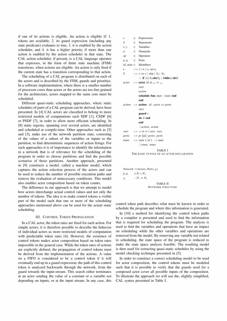
if one of its actions is eligible. An action is eligible if: 1.tokens are available, 2. its guard expression (including anystate predicate) evaluates to true, 3. it is enabled by the actionscheduler, and 4. it has a higher priority if more than oneaction is enabled by the action scheduler in that state. TheCAL action scheduler, if present, is a CAL language operatorthat expresses, in the form of finite state machine (FSM)transitions, when actions are eligible. An action is only fired ifthe current state has a transition corresponding to that action.

The scheduling of a CAL program is distributed on each ofthe actors and is described by the FSM, guards and priorities.In a software implementation, where there is a smaller numberof processor cores than actors or the actors are too fine grainedfor the architecture, actors mapped to the same core must bescheduled.

Different quasi-static scheduling approaches, where staticschedules of parts of a CAL program can be derived, have beenpresented. In [4] CAL actors are classified to belong to morerestricted models of computations such SDF [1], CSDF [6]or PSDF [7], in order to allow more efficient scheduling. In[8] static regions, spanning over several actors, are identifiedand scheduled at compile-time. Other approaches such as [5]and [3], make use of the network partition state, consistingof the values of a subset of the variables or inputs to thepartition, to find deterministic sequences of action firings. Forsuch approaches it is of importance to identify the informationin a network that is of relevance for the scheduling of theprogram in order to choose partitions and find the possiblescenarios of those partitions. Another approach, presentedin [9] constructs a model, called a machine model, whichcaptures the action selection process of the actors and canbe used to reduce the number of possible execution paths andremove the evaluation of unnecessary conditions. This modelalso enables actor composition based on token counts.

The difference in our approach is that we attempt to modelhow actors interchange actual control values and not only thenumber of tokens. The idea is to make control tokens a visiblepart of the model such that one or more of the schedulingapproaches mentioned above can be used for the actual staticscheduling.

III. CONTROL TOKEN PROPAGATION

In a CAL actor, the token rates are fixed for each action. Forsimple actors, it is therefore possible to describe the behaviorof individual actors as more restricted models of computationwith predictable token rates [4]. However, the existence ofcontrol tokens makes actor composition based on token ratesimpossible in the general case. While the token rates of actionsare explicitly defined, the propagation of control tokens mustbe derived from the implementation of the actions. A valueon a FIFO is considered to be a control token if it willeventually end up in a guard expression; the path of this controltoken is analyzed backwards through the network, from theguard towards the input-stream. This search either terminatesat an actor sending the value of a constant or a variable notdepending on inputs, or at the input stream. In any case, this

e ∈ ExpressionsS ∈ Statementsx, y ∈ Variablesn ∈ Numeralsop ∈ Operatorsp, q ∈ Portsid, state ∈ Identifierse ::= x | n | e1 op e2S ::= x := e | skip | S1; S2

| if (e) S1elseS2 | while(e)doS

actor ::= actor id () ... ⇒ ...vars

action

schedule fsm state : trans endend

action ::= action : id : ports ⇒ ports

vars

guard e

do S endend| action; action

vars ::= x := n | vars; vars

ports ::= p: [x] | ports; ports

trans ::= state ( id ) → state

| trans; trans

TABLE ITHE BASIC SYNTAX OF AN ACTOR DECLARATION

Network =(Actors,Ports, χ)

p, q ∈Pi ∪ Po

χ : Pi �→ Po

TABLE IINETWORK STRUCTURE

control token path describes what must be known in order toschedule the program and where this information is generated.

In [10] a method for identifying the control token pathsby a compiler is presented and used to find the informationthat is required for scheduling the program. The analysis isused to find the variables and operations that have an impacton scheduling while the other variables and operations areremoved from the model. By removing any variable not relatedto scheduling, the state space of the program is reduced tomake the state space analysis feasible. The resulting modelis then used for extracting quasi-static schedules by using themodel checking technique presented in [5].

In order to construct a correct scheduling model to be usedfor actor composition, the control tokens must be modeledsuch that it is possible to verify that the guards used for acomposed actor cover all possible inputs of the composition.To illustrate the approach we will use the, slightly simplified,CAL syntax presented in Table I.

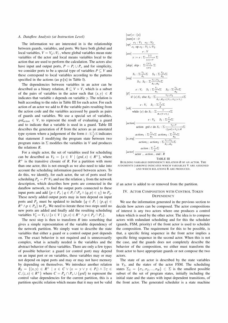
A. Dataflow Analysis (at Instruction Level)

The information we are interested in is the relationshipbetween guards, variables, and ports. We have both global andlocal variables, V = Vg∪Vl , where global variables mean statevariables of the actor and local means variables local to theaction that are used to perform the calculation. The actors alsohave input and output ports, P = Pi ∪ Po and for simplicity,we consider ports to be a special type of variables P ⊆ V andthese correspond to local variables according to the patternsspecified in the actions (as p:[x] in Table I).

The dependencies between variables in an actor can bedescribed as a binary relation, R ⊆ V × V , which is a subsetof the pairs of variables in the actor such that (x, y) ∈ Rindicates that variable x depends on variable y. The relation isbuilt according to the rules in Table III for each actor. For eachaction of an actor we add to R the variable pairs resulting fromthe action code and the variables accessed by guards as pairsof guards and variables. We use a special set of variables,grdaction ∈ V , to represent the result of evaluating a guardand to indicate that a variable is used in a guard. Table IIIdescribes the generation of R from the actors as an annotatedtype system where a judgement of the form S : Σ

V−→RΣ indicates

that statement S modifying the program state between twoprogram states in Σ modifies the variables in V and producesthe relations R.

For a single actor, the set of variables used for schedulingcan be described as VS = {x ∈ V | (grd, x) ∈ R+}, whereR+ is the transitive closure of R. For a partition with morethan one actor, this is not enough as we also need to take intoaccount the scheduling information passed between actors. Todo this, we identify, for each actor, the set of ports used forscheduling Pg = P∩VS and use the relation χ from the networkdescription, which describes how ports are connected in thedataflow network, to find the output ports connected to theseinput ports and add {p ∈ Po | q ∈ Pi ∩Pg ∧ (q, p) ∈ χ} to Pg.These newly added output ports may in turn depend on inputports and Pg must be updated to include {q ∈ Pi | (p, q) ∈R+∧p ∈ Pg} to Pg. We need to iterate these two steps until nonew ports are added and finally add the resulting schedulingvariables V ′

S = VS ∪ {x ∈ V | (p, x) ∈ R+ ∧ p ∈ Pg ∩ Po}.The next step is then to transform R into something that

gives a simple representation of the variable dependency ofthe network partition. We simply want to describe the statevariables that either a guard or a control output port dependson. The exact behavior is not required and is unnecessarilycomplex, what is actually needed is the variables and theabstract behavior of these variables. There are only a few typesof possible behavior: a guard (or control port) may dependon an input port or on variables, these variables may or maynot depend on input ports and may or may not have memoryby depending on themselves. We introduce another relationRS = {(x, y) ∈ R+ | x ∈ C ∨ (x = y ∨ y ∈ Pi) ∧ ∃ z ∈C, (z, x) ∈ R+} where C = Pg ∩ Po ∪ {grd} to represent thecontrol value dependencies for the current partition, this is apartition specific relation which means that it may not be valid

[var] x : {x}[num] n : ∅

[op]e1 : V1 e2 : V2

e1 op e2 : V1 ∪ V2

[ass]e : V

x := e : Σ{x}−−−−→

{x}×VΣ

[skip] skip : Σ{∅}−−−→{∅}

Σ

[seq]S1 : Σ

V1−−→R1

Σ S2 : ΣV2−−→R2

Σ

S1; S2 : ΣV1∪V2−−−−→R1∪R2

Σ

[if ]e : Vc S1 : Σ

V1−−→R1

Σ S2 : ΣV2−−→R2

Σ

if (e) S1 else S2 : ΣV1∪V2−−−−−−−−−−−−−−−→

R1∪R2∪((V1∪V2)×Vc)Σ

[wh]e : Vc S1 : Σ

V−→RΣ

while (e) do S1 : ΣV−−−−−−→

R∪(V×Vc)Σ

[action]e : Vg S1 : Σ

V−→RΣ

action grd e do S1 : ΣVg∪V−−−−−−−−−→

({grd}×Vg)∪RΣ

[a seq]action1 : Σ

V1−−→R1

Σ action2 : ΣV2−−→R2

Σ

action1; action2 : ΣV1∪V2−−−−→R1∪R2

Σ

[actor]action : Σ

V−→RΣ

actor ... action... end : R

TABLE IIIBUILDING VARIABLE DEPENDENCY RELATION R OF AN ACTOR. THE

JUDGMENTS (ARROWS) INDICATES WHICH VARIABLES V ARE ASSIGNEDAND WHICH RELATIONS R ARE PRODUCED.

if an actor is added to or removed from the partition.

IV. ACTOR COMPOSITION WITH CONTROL TOKENDEPENDENCY

We use the information generated in the previous section todecide how actors can be composed. The actor compositionsof interest is any two actors where one produces a controltoken which is used by the other actor. The idea is to composeactors with redundant scheduling and for this the scheduler(guards, FSM, priority) of the front actor is used to schedulethe composition. The requirement for this to be possible, isthat, a specific firing sequence in the front actor implies aspecific firing sequence in the second actor. When this is notthe case, and the guards does not completely describe thebehavior of the composition, we either must transform thefront actor to have appropriate guards or not compose the twoactors.

The state of an actor is described by the state variablesin VS, and the states of the actor FSM. The schedulingstates ΣS = {σ1, σ2, ..., σM} ⊂ Σ is the smallest possiblesubset of the set of program states, initially including theinitial state and the states with input dependent transitions, ofthe front actor. The generated scheduler is a state machine

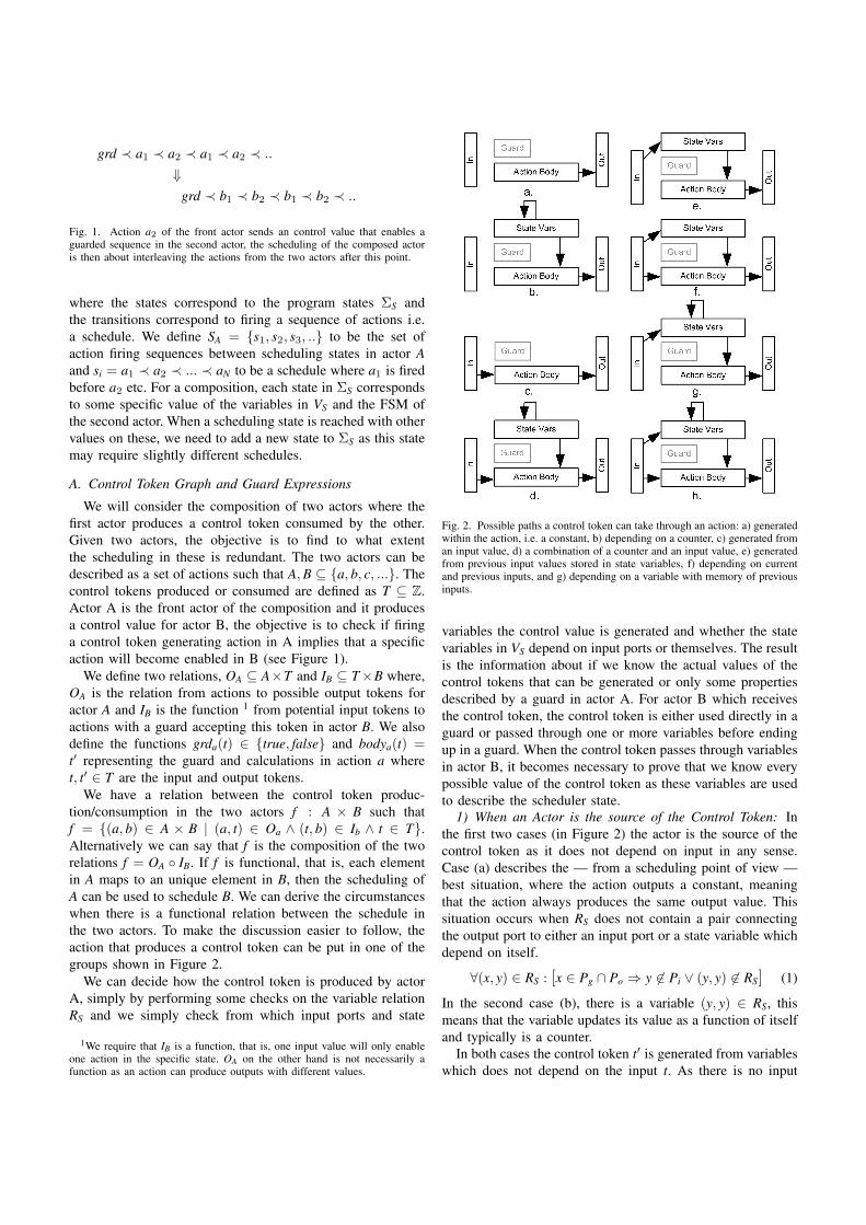
grd ≺ a1 ≺ a2 ≺ a1 ≺ a2 ≺ ..

⇓grd ≺ b1 ≺ b2 ≺ b1 ≺ b2 ≺ ..

Fig. 1. Action a2 of the front actor sends an control value that enables aguarded sequence in the second actor, the scheduling of the composed actoris then about interleaving the actions from the two actors after this point.

where the states correspond to the program states ΣS andthe transitions correspond to firing a sequence of actions i.e.a schedule. We define SA = {s1, s2, s3, ..} to be the set ofaction firing sequences between scheduling states in actor Aand si = a1 ≺ a2 ≺ ... ≺ aN to be a schedule where a1 is firedbefore a2 etc. For a composition, each state in ΣS correspondsto some specific value of the variables in VS and the FSM ofthe second actor. When a scheduling state is reached with othervalues on these, we need to add a new state to ΣS as this statemay require slightly different schedules.

A. Control Token Graph and Guard Expressions

We will consider the composition of two actors where thefirst actor produces a control token consumed by the other.Given two actors, the objective is to find to what extentthe scheduling in these is redundant. The two actors can bedescribed as a set of actions such that A,B ⊆ {a, b, c, ...}. Thecontrol tokens produced or consumed are defined as T ⊆ Z.Actor A is the front actor of the composition and it producesa control value for actor B, the objective is to check if firinga control token generating action in A implies that a specificaction will become enabled in B (see Figure 1).

We define two relations, OA ⊆ A×T and IB ⊆ T×B where,OA is the relation from actions to possible output tokens foractor A and IB is the function 1 from potential input tokens toactions with a guard accepting this token in actor B. We alsodefine the functions grda(t) ∈ {true, false} and bodya(t) =t′ representing the guard and calculations in action a wheret, t′ ∈ T are the input and output tokens.

We have a relation between the control token produc-tion/consumption in the two actors f : A × B such thatf = {(a, b) ∈ A × B | (a, t) ∈ Oa ∧ (t, b) ∈ Ib ∧ t ∈ T}.Alternatively we can say that f is the composition of the tworelations f = OA ◦ IB. If f is functional, that is, each elementin A maps to an unique element in B, then the scheduling ofA can be used to schedule B. We can derive the circumstanceswhen there is a functional relation between the schedule inthe two actors. To make the discussion easier to follow, theaction that produces a control token can be put in one of thegroups shown in Figure 2.

We can decide how the control token is produced by actorA, simply by performing some checks on the variable relationRS and we simply check from which input ports and state

1We require that IB is a function, that is, one input value will only enableone action in the specific state. OA on the other hand is not necessarily afunction as an action can produce outputs with different values.

Fig. 2. Possible paths a control token can take through an action: a) generatedwithin the action, i.e. a constant, b) depending on a counter, c) generated froman input value, d) a combination of a counter and an input value, e) generatedfrom previous input values stored in state variables, f) depending on currentand previous inputs, and g) depending on a variable with memory of previousinputs.

variables the control value is generated and whether the statevariables in VS depend on input ports or themselves. The resultis the information about if we know the actual values of thecontrol tokens that can be generated or only some propertiesdescribed by a guard in actor A. For actor B which receivesthe control token, the control token is either used directly in aguard or passed through one or more variables before endingup in a guard. When the control token passes through variablesin actor B, it becomes necessary to prove that we know everypossible value of the control token as these variables are usedto describe the scheduler state.

1) When an Actor is the source of the Control Token: Inthe first two cases (in Figure 2) the actor is the source of thecontrol token as it does not depend on input in any sense.Case (a) describes the — from a scheduling point of view —best situation, where the action outputs a constant, meaningthat the action always produces the same output value. Thissituation occurs when RS does not contain a pair connectingthe output port to either an input port or a state variable whichdepend on itself.

∀(x, y) ∈ RS : [x ∈ Pg ∩ Po ⇒ y �∈ Pi ∨ (y, y) �∈ RS] (1)

In the second case (b), there is a variable (y, y) ∈ RS, thismeans that the variable updates its value as a function of itselfand typically is a counter.

In both cases the control token t′ is generated from variableswhich does not depend on the input t. As there is no input

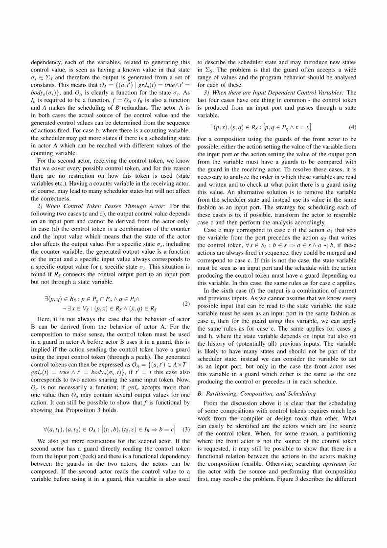
dependency, each of the variables, related to generating thiscontrol value, is seen as having a known value in that stateσs ∈ ΣS and therefore the output is generated from a set ofconstants. This means that OA = {(a, t′) | grda(t) = true∧t′ =bodya(σs)}, and OA is clearly a function for the state σs. AsIb is required to be a function, f = OA ◦ IB is also a functionand A makes the scheduling of B redundant. The actor A isin both cases the actual source of the control value and thegenerated control values can be determined from the sequenceof actions fired. For case b, where there is a counting variable,the scheduler may get more states if there is a scheduling statein actor A which can be reached with different values of thecounting variable.

For the second actor, receiving the control token, we knowthat we cover every possible control token, and for this reasonthere are no restriction on how this token is used (statevariables etc.). Having a counter variable in the receiving actor,of course, may lead to many scheduler states but will not affectthe correctness.

2) When Control Token Passes Through Actor: For thefollowing two cases (c and d), the output control value dependson an input port and cannot be derived from the actor only.In case (d) the control token is a combination of the counterand the input value which means that the state of the actoralso affects the output value. For a specific state σs, includingthe counter variable, the generated output value is a functionof the input and a specific input value always corresponds toa specific output value for a specific state σs. This situation isfound if RS connects the control output port to an input portbut not through a state variable.

∃(p, q) ∈ RS : p ∈ Pg ∩ Po ∧ q ∈ Pi∧¬∃ x ∈ VS : (p, x) ∈ RS ∧ (x, q) ∈ RS

(2)

Here, it is not always the case that the behavior of actorB can be derived from the behavior of actor A. For thecomposition to make sense, the control token must be usedin a guard in actor A before actor B uses it in a guard, this isimplied if the action sending the control token have a guardusing the input control token (through a peek). The generatedcontrol tokens can then be expressed as OA = {(a, t′) ∈ A×T |grda(t) = true ∧ t′ = bodya(σs, t)}, if t′ = t this case alsocorresponds to two actors sharing the same input token. Now,Oa is not necessarily a function; if grda accepts more thanone value then Oa may contain several output values for oneaction. It can still be possible to show that f is functional byshowing that Proposition 3 holds.

∀(a, t1), (a, t2) ∈ OA : [(t1, b), (t2, c) ∈ IB ⇒ b = c] (3)

We also get more restrictions for the second actor. If thesecond actor has a guard directly reading the control tokenfrom the input port (peek) and there is a functional dependencybetween the guards in the two actors, the actors can becomposed. If the second actor reads the control value to avariable before using it in a guard, this variable is also used

to describe the scheduler state and may introduce new statesin ΣS. The problem is that the guard often accepts a widerange of values and the program behavior should be analysedfor each of these.

3) When there are Input Dependent Control Variables: Thelast four cases have one thing in common - the control tokenis produced from an input port and passes through a statevariable.

∃(p, x), (y, q) ∈ RS : [p, q ∈ Pg ∧ x = y] (4)

For a composition using the guards of the front actor to bepossible, either the action setting the value of the variable fromthe input port or the action setting the value of the output portfrom the variable must have a guards to be compared withthe guard in the receiving actor. To resolve these cases, it isnecessary to analyze the order in which these variables are readand written and to check at what point there is a guard usingthis value. An alternative solution is to remove the variablefrom the scheduler state and instead use its value in the samefashion as an input port. The strategy for scheduling each ofthese cases is to, if possible, transform the actor to resemblecase c and then perform the analysis accordingly.

Case e may correspond to case c if the action a1 that setsthe variable from the port precedes the action a2 that writesthe control token, ∀ s ∈ SA : b ∈ s ⇒ a ∈ s ∧ a ≺ b, if theseactions are always fired in sequence, they could be merged andcorrespond to case c. If this is not the case, the state variablemust be seen as an input port and the schedule with the actionproducing the control token must have a guard depending onthis variable. In this case, the same rules as for case c applies.

In the sixth case (f) the output is a combination of currentand previous inputs. As we cannot assume that we know everypossible input that can be read to the state variable, the statevariable must be seen as an input port in the same fashion ascase e, then for the guard using this variable, we can applythe same rules as for case c. The same applies for cases gand h, where the state variable depends on input but also onthe history of (potentially all) previous inputs. The variableis likely to have many states and should not be part of thescheduler state, instead we can consider the variable to actas an input port, but only in the case the front actor usesthis variable in a guard which either is the same as the oneproducing the control or precedes it in each schedule.

B. Partitioning, Composition, and Scheduling

From the discussion above it is clear that the schedulingof some compositions with control tokens requires much lesswork from the compiler or design tools than other. Whatcan easily be identified are the actors which are the sourceof the control token. When, for some reason, a partitioningwhere the front actor is not the source of the control tokenis requested, it may still be possible to show that there is afunctional relation between the actions in the actors makingthe composition feasible. Otherwise, searching upstream forthe actor with the source and performing that compositionfirst, may resolve the problem. Figure 3 describes the different

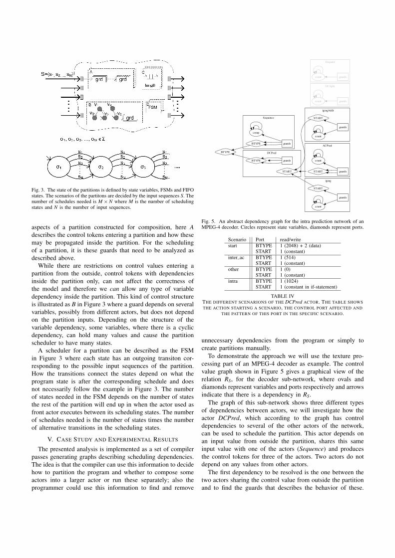
Fig. 3. The state of the partitions is defined by state variables, FSMs and FIFOstates. The scenarios of the partitons are decided by the input sequences S. Thenumber of schedules needed is M × N where M is the number of schedulingstates and N is the number of input sequences.

aspects of a partition constructed for composition, here Adescribes the control tokens entering a partition and how thesemay be propagated inside the partition. For the schedulingof a partition, it is these guards that need to be analyzed asdescribed above.

While there are restrictions on control values entering apartition from the outside, control tokens with dependenciesinside the partition only, can not affect the correctness ofthe model and therefore we can allow any type of variabledependency inside the partition. This kind of control structureis illustrated as B in Figure 3 where a guard depends on severalvariables, possibly from different actors, but does not dependon the partition inputs. Depending on the structure of thevariable dependency, some variables, where there is a cyclicdependency, can hold many values and cause the partitionscheduler to have many states.

A scheduler for a partiton can be described as the FSMin Figure 3 where each state has an outgoing transiton cor-responding to the possible input sequences of the partition.How the transitions connect the states depend on what theprogram state is after the corresponding schedule and doesnot necessarily follow the example in Figure 3. The numberof states needed in the FSM depends on the number of statesthe rest of the partition will end up in when the actor used asfront actor executes between its scheduling states. The numberof schedules needed is the number of states times the numberof alternative transitions in the scheduling states.

V. CASE STUDY AND EXPERIMENTAL RESULTS

The presented analysis is implemented as a set of compilerpasses generating graphs describing scheduling dependencies.The idea is that the compiler can use this information to decidehow to partition the program and whether to compose someactors into a larger actor or run these separately; also theprogrammer could use this information to find and remove

�

�

Fig. 5. An abstract dependency graph for the intra prediction network of anMPEG-4 decoder. Circles represent state variables, diamonds represent ports.

Scenario Port read/writestart BTYPE 1 (2048) + 2 (data)

START 1 (constant)inter ac BTYPE 1 (514)

START 1 (constant)other BTYPE 1 (0)

START 1 (constant)intra BTYPE 1 (1024)

START 1 (constant in if-statement)

TABLE IVTHE DIFFERENT SCENARIONS OF THE DCPred ACTOR. THE TABLE SHOWSTHE ACTION STARTING A SCENARIO, THE CONTROL PORT AFFECTED AND

THE PATTERN OF THIS PORT IN THE SPECIFIC SCENARIO.

unnecessary dependencies from the program or simply tocreate partitions manually.

To demonstrate the approach we will use the texture pro-cessing part of an MPEG-4 decoder as example. The controlvalue graph shown in Figure 5 gives a graphical view of therelation RS, for the decoder sub-network, where ovals anddiamonds represent variables and ports respectively and arrowsindicate that there is a dependency in RS.

The graph of this sub-network shows three different typesof dependencies between actors, we will investigate how theactor DCPred, which according to the graph has controldependencies to several of the other actors of the network,can be used to schedule the partition. This actor depends onan input value from outside the partition, shares this sameinput value with one of the actors (Sequence) and producesthe control tokens for three of the actors. Two actors do notdepend on any values from other actors.

The first dependency to be resolved is the one between thetwo actors sharing the control value from outside the partitionand to find the guards that describes the behavior of these.

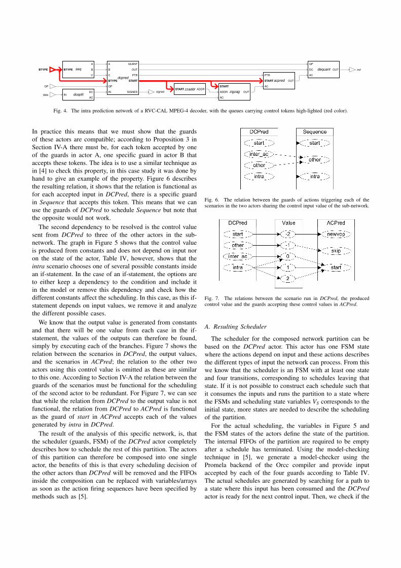
seqBTYPE

A

B

Cdcpred

A

B

C

BTYPE

QP

IN

OUT

PTR

QUANT

SIGNED

START

dcsplitINDC

AC

zzaddrSTART ADDRzigzag

START

ADDR

AC

OUT

acpredSTART

AC

PTR

OUT

dequant

AC

DC

QP

OUTBTYPE

data

QP

out

signed

Fig. 4. The intra prediction network of a RVC-CAL MPEG-4 decoder, with the queues carrying control tokens high-lighted (red color).

In practice this means that we must show that the guardsof these actors are compatible; according to Proposition 3 inSection IV-A there must be, for each token accepted by oneof the guards in actor A, one specific guard in actor B thataccepts these tokens. The idea is to use a similar technique asin [4] to check this property, in this case study it was done byhand to give an example of the property. Figure 6 describesthe resulting relation, it shows that the relation is functional asfor each accepted input in DCPred, there is a specific guardin Sequence that accepts this token. This means that we canuse the guards of DCPred to schedule Sequence but note thatthe opposite would not work.

The second dependency to be resolved is the control valuesent from DCPred to three of the other actors in the sub-network. The graph in Figure 5 shows that the control valueis produced from constants and does not depend on input noron the state of the actor, Table IV, however, shows that theintra scenario chooses one of several possible constants insidean if-statement. In the case of an if-statement, the options areto either keep a dependency to the condition and include itin the model or remove this dependency and check how thedifferent constants affect the scheduling. In this case, as this if-statement depends on input values, we remove it and analyzethe different possible cases.

We know that the output value is generated from constantsand that there will be one value from each case in the if-statement, the values of the outputs can therefore be found,simply by executing each of the branches. Figure 7 shows therelation between the scenarios in DCPred, the output values,and the scenarios in ACPred; the relation to the other twoactors using this control value is omitted as these are similarto this one. According to Section IV-A the relation between theguards of the scenarios must be functional for the schedulingof the second actor to be redundant. For Figure 7, we can seethat while the relation from DCPred to the output value is notfunctional, the relation from DCPred to ACPred is functionalas the guard of start in ACPred accepts each of the valuesgenerated by intra in DCPred.

The result of the analysis of this specific network, is, thatthe scheduler (guards, FSM) of the DCPred actor completelydescribes how to schedule the rest of this partition. The actorsof this partition can therefore be composed into one singleactor, the benefits of this is that every scheduling decision ofthe other actors than DCPred will be removed and the FIFOsinside the composition can be replaced with variables/arraysas soon as the action firing sequences have been specified bymethods such as [5].

Fig. 6. The relation between the guards of actions triggering each of thescenarios in the two actors sharing the control input value of the sub-network.

Fig. 7. The relations between the scenario run in DCPred, the producedcontrol value and the guards accepting these control values in ACPred.

A. Resulting Scheduler

The scheduler for the composed network partition can bebased on the DCPred actor. This actor has one FSM statewhere the actions depend on input and these actions describesthe different types of input the network can process. From thiswe know that the scheduler is an FSM with at least one stateand four transitions, corresponding to schedules leaving thatstate. If it is not possible to construct each schedule such thatit consumes the inputs and runs the partition to a state wherethe FSMs and scheduling state variables VS corresponds to theinitial state, more states are needed to describe the schedulingof the partition.

For the actual scheduling, the variables in Figure 5 andthe FSM states of the actors define the state of the partition.The internal FIFOs of the partition are required to be emptyafter a schedule has terminated. Using the model-checkingtechnique in [5], we generate a model-checker using thePromela backend of the Orcc compiler and provide inputaccepted by each of the four guards according to Table IV.The actual schedules are generated by searching for a path toa state where this input has been consumed and the DCPredactor is ready for the next control input. Then, we check if the

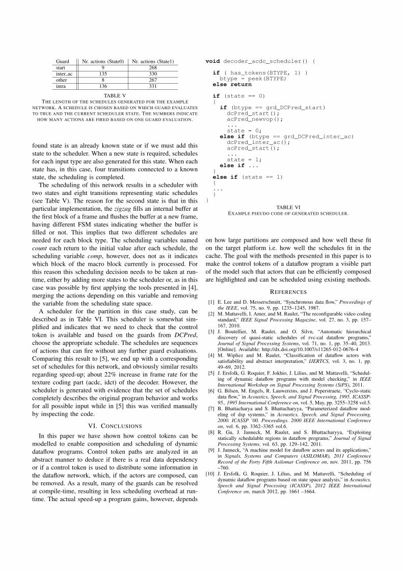
Guard Nr. actions (State0) Nr. actions (State1)start 9 268inter ac 135 330other 8 267intra 136 331

TABLE VTHE LENGTH OF THE SCHEDULES GENERATED FOR THE EXAMPLE

NETWORK. A SCHEDULE IS CHOSEN BASED ON WHICH GUARD EVALUATESTO TRUE AND THE CURRENT SCHEDULER STATE. THE NUMBERS INDICATE

HOW MANY ACTIONS ARE FIRED BASED ON ONE GUARD EVALUATION.

found state is an already known state or if we must add thisstate to the scheduler. When a new state is required, schedulesfor each input type are also generated for this state. When eachstate has, in this case, four transitions connected to a knownstate, the scheduling is completed.

The scheduling of this network results in a scheduler withtwo states and eight transitions representing static schedules(see Table V). The reason for the second state is that in thisparticular implementation, the zigzag fills an internal buffer atthe first block of a frame and flushes the buffer at a new frame,having different FSM states indicating whether the buffer isfilled or not. This implies that two different schedules areneeded for each block type. The scheduling variables namedcount each return to the initial value after each schedule, thescheduling variable comp, however, does not as it indicateswhich block of the macro block currently is processed. Forthis reason this scheduling decision needs to be taken at run-time, either by adding more states to the scheduler or, as in thiscase was possible by first applying the tools presented in [4],merging the actions depending on this variable and removingthe variable from the scheduling state space.

A scheduler for the partition in this case study, can bedescribed as in Table VI. This scheduler is somewhat sim-plified and indicates that we need to check that the controltoken is available and based on the guards from DCPred,choose the appropriate schedule. The schedules are sequencesof actions that can fire without any further guard evaluations.Comparing this result to [5], we end up with a correspondingset of schedules for this network, and obviously similar resultsregarding speed-up; about 22% increase in frame rate for thetexture coding part (acdc, idct) of the decoder. However, thescheduler is generated with evidence that the set of schedulescompletely describes the original program behavior and worksfor all possible input while in [5] this was verified manuallyby inspecting the code.

VI. CONCLUSIONS

In this paper we have shown how control tokens can bemodelled to enable composition and scheduling of dynamicdataflow programs. Control token paths are analyzed in anabstract manner to deduce if there is a real data dependencyor if a control token is used to distribute some information inthe dataflow network, which, if the actors are composed, canbe removed. As a result, many of the guards can be resolvedat compile-time, resulting in less scheduling overhead at run-time. The actual speed-up a program gains, however, depends

void decoder_acdc_scheduler() {

if ( has_tokens(BTYPE, 1) )btype = peek(BTYPE)

else return

if (state == 0){if (btype == grd_DCPred_start)dcPred_start();acPred_newvop();...state = 0;

else if (btype == grd_DCPred_inter_ac)dcPred_inter_ac();acPred_start();...state = 1;

else if ...}else if (state == 1){...}

}TABLE VI

EXAMPLE PSEUDO CODE OF GENERATED SCHEDULER.

on how large partitions are composed and how well these fiton the target platform i.e. how well the schedules fit in thecache. The goal with the methods presented in this paper is tomake the control tokens of a dataflow program a visible partof the model such that actors that can be efficiently composedare highlighted and can be scheduled using existing methods.

REFERENCES

[1] E. Lee and D. Messerschmitt, “Synchronous data flow,” Proceedings ofthe IEEE, vol. 75, no. 9, pp. 1235–1245, 1987.

[2] M. Mattavelli, I. Amer, and M. Raulet, “The reconfigurable video codingstandard,” IEEE Signal Processing Magazine, vol. 27, no. 3, pp. 157–167, 2010.

[3] J. Boutellier, M. Raulet, and O. Silvn, “Automatic hierarchicaldiscovery of quasi-static schedules of rvc-cal dataflow programs,”Journal of Signal Processing Systems, vol. 71, no. 1, pp. 35–40, 2013.[Online]. Available: http://dx.doi.org/10.1007/s11265-012-0676-4

[4] M. Wipliez and M. Raulet, “Classification of dataflow actors withsatisfiability and abstract interpretation,” IJERTCS, vol. 3, no. 1, pp.49–69, 2012.

[5] J. Ersfolk, G. Roquier, F. Jokhio, J. Lilius, and M. Mattavelli, “Schedul-ing of dynamic dataflow programs with model checking,” in IEEEInternational Workshop on Signal Processing Systems (SiPS), 2011.

[6] G. Bilsen, M. Engels, R. Lauwereins, and J. Peperstraete, “Cyclo-staticdata flow,” in Acoustics, Speech, and Signal Processing, 1995. ICASSP-95., 1995 International Conference on, vol. 5, May, pp. 3255–3258 vol.5.

[7] B. Bhattacharya and S. Bhattacharyya, “Parameterized dataflow mod-eling of dsp systems,” in Acoustics, Speech, and Signal Processing,2000. ICASSP ’00. Proceedings. 2000 IEEE International Conferenceon, vol. 6, pp. 3362–3365 vol.6.

[8] R. Gu, J. Janneck, M. Raulet, and S. Bhattacharyya, “Exploitingstatically schedulable regions in dataflow programs,” Journal of SignalProcessing Systems, vol. 63, pp. 129–142, 2011.

[9] J. Janneck, “A machine model for dataflow actors and its applications,”in Signals, Systems and Computers (ASILOMAR), 2011 ConferenceRecord of the Forty Fifth Asilomar Conference on, nov. 2011, pp. 756–760.

[10] J. Ersfolk, G. Roquier, J. Lilius, and M. Mattavelli, “Scheduling ofdynamic dataflow programs based on state space analysis,” in Acoustics,Speech and Signal Processing (ICASSP), 2012 IEEE InternationalConference on, march 2012, pp. 1661 –1664.

Paper V

High-Performance Programs by Source-Level Merging of RVC-CAL DataflowActors

Jani Boutellier, Amanullah Ghazi, Olli Silven, Johan Ers-folk

Originally published 2013 IEEE Workshop on Signal Processing Sys-tems (SiPS). IEEE. October 2013, Taipei, Taiwan.

Turku Centre for Computer Science

TUCS Dissertations 1. Marjo Lipponen, On Primitive Solutions of the Post Correspondence Problem 2. Timo Käkölä, Dual Information Systems in Hyperknowledge Organizations 3. Ville Leppänen, Studies on the Realization of PRAM 4. Cunsheng Ding, Cryptographic Counter Generators 5. Sami Viitanen, Some New Global Optimization Algorithms 6. Tapio Salakoski, Representative Classification of Protein Structures 7. Thomas Långbacka, An Interactive Environment Supporting the Development of

Formally Correct Programs 8. Thomas Finne, A Decision Support System for Improving Information Security 9. Valeria Mihalache, Cooperation, Communication, Control. Investigations on

Grammar Systems. 10. Marina Waldén, Formal Reasoning About Distributed Algorithms 11. Tero Laihonen, Estimates on the Covering Radius When the Dual Distance is

Known 12. Lucian Ilie, Decision Problems on Orders of Words 13. Jukkapekka Hekanaho, An Evolutionary Approach to Concept Learning 14. Jouni Järvinen, Knowledge Representation and Rough Sets 15. Tomi Pasanen, In-Place Algorithms for Sorting Problems 16. Mika Johnsson, Operational and Tactical Level Optimization in Printed Circuit

Board Assembly 17. Mats Aspnäs, Multiprocessor Architecture and Programming: The Hathi-2 System 18. Anna Mikhajlova, Ensuring Correctness of Object and Component Systems 19. Vesa Torvinen, Construction and Evaluation of the Labour Game Method 20. Jorma Boberg, Cluster Analysis. A Mathematical Approach with Applications to

Protein Structures 21. Leonid Mikhajlov, Software Reuse Mechanisms and Techniques: Safety Versus

Flexibility 22. Timo Kaukoranta, Iterative and Hierarchical Methods for Codebook Generation in

Vector Quantization 23. Gábor Magyar, On Solution Approaches for Some Industrially Motivated

Combinatorial Optimization Problems 24. Linas Laibinis, Mechanised Formal Reasoning About Modular Programs 25. Shuhua Liu, Improving Executive Support in Strategic Scanning with Software

Agent Systems 26. Jaakko Järvi, New Techniques in Generic Programming – C++ is more Intentional

than Intended 27. Jan-Christian Lehtinen, Reproducing Kernel Splines in the Analysis of Medical

Data 28. Martin Büchi, Safe Language Mechanisms for Modularization and Concurrency 29. Elena Troubitsyna, Stepwise Development of Dependable Systems 30. Janne Näppi, Computer-Assisted Diagnosis of Breast Calcifications 31. Jianming Liang, Dynamic Chest Images Analysis 32. Tiberiu Seceleanu, Systematic Design of Synchronous Digital Circuits 33. Tero Aittokallio, Characterization and Modelling of the Cardiorespiratory System

in Sleep-Disordered Breathing 34. Ivan Porres, Modeling and Analyzing Software Behavior in UML 35. Mauno Rönkkö, Stepwise Development of Hybrid Systems 36. Jouni Smed, Production Planning in Printed Circuit Board Assembly 37. Vesa Halava, The Post Correspondence Problem for Market Morphisms 38. Ion Petre, Commutation Problems on Sets of Words and Formal Power Series 39. Vladimir Kvassov, Information Technology and the Productivity of Managerial

Work 40. Frank Tétard, Managers, Fragmentation of Working Time, and Information

Systems

41. Jan Manuch, Defect Theorems and Infinite Words 42. Kalle Ranto, Z4-Goethals Codes, Decoding and Designs 43. Arto Lepistö, On Relations Between Local and Global Periodicity 44. Mika Hirvensalo, Studies on Boolean Functions Related to Quantum Computing 45. Pentti Virtanen, Measuring and Improving Component-Based Software

Development 46. Adekunle Okunoye, Knowledge Management and Global Diversity – A Framework

to Support Organisations in Developing Countries 47. Antonina Kloptchenko, Text Mining Based on the Prototype Matching Method 48. Juha Kivijärvi, Optimization Methods for Clustering 49. Rimvydas Rukšėnas, Formal Development of Concurrent Components 50. Dirk Nowotka, Periodicity and Unbordered Factors of Words 51. Attila Gyenesei, Discovering Frequent Fuzzy Patterns in Relations of Quantitative

Attributes 52. Petteri Kaitovaara, Packaging of IT Services – Conceptual and Empirical Studies 53. Petri Rosendahl, Niho Type Cross-Correlation Functions and Related Equations 54. Péter Majlender, A Normative Approach to Possibility Theory and Soft Decision

Support 55. Seppo Virtanen, A Framework for Rapid Design and Evaluation of Protocol

Processors 56. Tomas Eklund, The Self-Organizing Map in Financial Benchmarking 57. Mikael Collan, Giga-Investments: Modelling the Valuation of Very Large Industrial

Real Investments 58. Dag Björklund, A Kernel Language for Unified Code Synthesis 59. Shengnan Han, Understanding User Adoption of Mobile Technology: Focusing on

Physicians in Finland 60. Irina Georgescu, Rational Choice and Revealed Preference: A Fuzzy Approach 61. Ping Yan, Limit Cycles for Generalized Liénard-Type and Lotka-Volterra Systems 62. Joonas Lehtinen, Coding of Wavelet-Transformed Images 63. Tommi Meskanen, On the NTRU Cryptosystem 64. Saeed Salehi, Varieties of Tree Languages 65. Jukka Arvo, Efficient Algorithms for Hardware-Accelerated Shadow Computation 66. Mika Hirvikorpi, On the Tactical Level Production Planning in Flexible

Manufacturing Systems 67. Adrian Costea, Computational Intelligence Methods for Quantitative Data Mining 68. Cristina Seceleanu, A Methodology for Constructing Correct Reactive Systems 69. Luigia Petre, Modeling with Action Systems 70. Lu Yan, Systematic Design of Ubiquitous Systems 71. Mehran Gomari, On the Generalization Ability of Bayesian Neural Networks 72. Ville Harkke, Knowledge Freedom for Medical Professionals – An Evaluation Study

of a Mobile Information System for Physicians in Finland 73. Marius Cosmin Codrea, Pattern Analysis of Chlorophyll Fluorescence Signals 74. Aiying Rong, Cogeneration Planning Under the Deregulated Power Market and

Emissions Trading Scheme 75. Chihab BenMoussa, Supporting the Sales Force through Mobile Information and

Communication Technologies: Focusing on the Pharmaceutical Sales Force 76. Jussi Salmi, Improving Data Analysis in Proteomics 77. Orieta Celiku, Mechanized Reasoning for Dually-Nondeterministic and

Probabilistic Programs 78. Kaj-Mikael Björk, Supply Chain Efficiency with Some Forest Industry

Improvements 79. Viorel Preoteasa, Program Variables – The Core of Mechanical Reasoning about

Imperative Programs 80. Jonne Poikonen, Absolute Value Extraction and Order Statistic Filtering for a

Mixed-Mode Array Image Processor 81. Luka Milovanov, Agile Software Development in an Academic Environment 82. Francisco Augusto Alcaraz Garcia, Real Options, Default Risk and Soft

Applications 83. Kai K. Kimppa, Problems with the Justification of Intellectual Property Rights in

Relation to Software and Other Digitally Distributable Media 84. Dragoş Truşcan, Model Driven Development of Programmable Architectures 85. Eugen Czeizler, The Inverse Neighborhood Problem and Applications of Welch

Sets in Automata Theory

86. Sanna Ranto, Identifying and Locating-Dominating Codes in Binary Hamming Spaces

87. Tuomas Hakkarainen, On the Computation of the Class Numbers of Real Abelian Fields

88. Elena Czeizler, Intricacies of Word Equations 89. Marcus Alanen, A Metamodeling Framework for Software Engineering 90. Filip Ginter, Towards Information Extraction in the Biomedical Domain: Methods

and Resources 91. Jarkko Paavola, Signature Ensembles and Receiver Structures for Oversaturated

Synchronous DS-CDMA Systems 92. Arho Virkki, The Human Respiratory System: Modelling, Analysis and Control 93. Olli Luoma, Efficient Methods for Storing and Querying XML Data with Relational

Databases 94. Dubravka Ilić, Formal Reasoning about Dependability in Model-Driven

Development 95. Kim Solin, Abstract Algebra of Program Refinement 96. Tomi Westerlund, Time Aware Modelling and Analysis of Systems-on-Chip 97. Kalle Saari, On the Frequency and Periodicity of Infinite Words 98. Tomi Kärki, Similarity Relations on Words: Relational Codes and Periods 99. Markus M. Mäkelä, Essays on Software Product Development: A Strategic

Management Viewpoint 100. Roope Vehkalahti, Class Field Theoretic Methods in the Design of Lattice Signal

Constellations 101. Anne-Maria Ernvall-Hytönen, On Short Exponential Sums Involving Fourier

Coefficients of Holomorphic Cusp Forms 102. Chang Li, Parallelism and Complexity in Gene Assembly 103. Tapio Pahikkala, New Kernel Functions and Learning Methods for Text and Data

Mining 104. Denis Shestakov, Search Interfaces on the Web: Querying and Characterizing 105. Sampo Pyysalo, A Dependency Parsing Approach to Biomedical Text Mining 106. Anna Sell, Mobile Digital Calendars in Knowledge Work 107. Dorina Marghescu, Evaluating Multidimensional Visualization Techniques in Data

Mining Tasks 108. Tero Säntti, A Co-Processor Approach for Efficient Java Execution in Embedded

Systems 109. Kari Salonen, Setup Optimization in High-Mix Surface Mount PCB Assembly 110. Pontus Boström, Formal Design and Verification of Systems Using Domain-

Specific Languages 111. Camilla J. Hollanti, Order-Theoretic Mehtods for Space-Time Coding: Symmetric

and Asymmetric Designs 112. Heidi Himmanen, On Transmission System Design for Wireless Broadcasting 113. Sébastien Lafond, Simulation of Embedded Systems for Energy Consumption

Estimation 114. Evgeni Tsivtsivadze, Learning Preferences with Kernel-Based Methods 115. Petri Salmela, On Commutation and Conjugacy of Rational Languages and the

Fixed Point Method 116. Siamak Taati, Conservation Laws in Cellular Automata 117. Vladimir Rogojin, Gene Assembly in Stichotrichous Ciliates: Elementary

Operations, Parallelism and Computation 118. Alexey Dudkov, Chip and Signature Interleaving in DS CDMA Systems 119. Janne Savela, Role of Selected Spectral Attributes in the Perception of Synthetic

Vowels 120. Kristian Nybom, Low-Density Parity-Check Codes for Wireless Datacast Networks 121. Johanna Tuominen, Formal Power Analysis of Systems-on-Chip 122. Teijo Lehtonen, On Fault Tolerance Methods for Networks-on-Chip 123. Eeva Suvitie, On Inner Products Involving Holomorphic Cusp Forms and Maass

Forms 124. Linda Mannila, Teaching Mathematics and Programming – New Approaches with

Empirical Evaluation 125. Hanna Suominen, Machine Learning and Clinical Text: Supporting Health

Information Flow 126. Tuomo Saarni, Segmental Durations of Speech 127. Johannes Eriksson, Tool-Supported Invariant-Based Programming

128. Tero Jokela, Design and Analysis of Forward Error Control Coding and Signaling for Guaranteeing QoS in Wireless Broadcast Systems

129. Ville Lukkarila, On Undecidable Dynamical Properties of Reversible One-Dimensional Cellular Automata

130. Qaisar Ahmad Malik, Combining Model-Based Testing and Stepwise Formal Development

131. Mikko-Jussi Laakso, Promoting Programming Learning: Engagement, Automatic Assessment with Immediate Feedback in Visualizations

132. Riikka Vuokko, A Practice Perspective on Organizational Implementation of Information Technology

133. Jeanette Heidenberg, Towards Increased Productivity and Quality in Software Development Using Agile, Lean and Collaborative Approaches

134. Yong Liu, Solving the Puzzle of Mobile Learning Adoption 135. Stina Ojala, Towards an Integrative Information Society: Studies on Individuality

in Speech and Sign 136. Matteo Brunelli, Some Advances in Mathematical Models for Preference Relations 137. Ville Junnila, On Identifying and Locating-Dominating Codes 138. Andrzej Mizera, Methods for Construction and Analysis of Computational Models

in Systems Biology. Applications to the Modelling of the Heat Shock Response and the Self-Assembly of Intermediate Filaments.

139. Csaba Ráduly-Baka, Algorithmic Solutions for Combinatorial Problems in Resource Management of Manufacturing Environments

140. Jari Kyngäs, Solving Challenging Real-World Scheduling Problems 141. Arho Suominen, Notes on Emerging Technologies 142. József Mezei, A Quantitative View on Fuzzy Numbers 143. Marta Olszewska, On the Impact of Rigorous Approaches on the Quality of

Development 144. Antti Airola, Kernel-Based Ranking: Methods for Learning and Performace

Estimation 145. Aleksi Saarela, Word Equations and Related Topics: Independence, Decidability

and Characterizations 146. Lasse Bergroth, Kahden merkkijonon pisimmän yhteisen alijonon ongelma ja sen

ratkaiseminen 147. Thomas Canhao Xu, Hardware/Software Co-Design for Multicore Architectures 148. Tuomas Mäkilä, Software Development Process Modeling – Developers

Perspective to Contemporary Modeling Techniques 149. Shahrokh Nikou, Opening the Black-Box of IT Artifacts: Looking into Mobile

Service Characteristics and Individual Perception 150. Alessandro Buoni, Fraud Detection in the Banking Sector: A Multi-Agent

Approach 151. Mats Neovius, Trustworthy Context Dependency in Ubiquitous Systems 152. Fredrik Degerlund, Scheduling of Guarded Command Based Models 153. Amir-Mohammad Rahmani-Sane, Exploration and Design of Power-Efficient

Networked Many-Core Systems 154. Ville Rantala, On Dynamic Monitoring Methods for Networks-on-Chip 155. Mikko Pelto, On Identifying and Locating-Dominating Codes in the Infinite King

Grid 156. Anton Tarasyuk, Formal Development and Quantitative Verification of

Dependable Systems 157. Muhammad Mohsin Saleemi, Towards Combining Interactive Mobile TV and

Smart Spaces: Architectures, Tools and Application Development 158. Tommi J. M. Lehtinen, Numbers and Languages 159. Peter Sarlin, Mapping Financial Stability 160. Alexander Wei Yin, On Energy Efficient Computing Platforms 161. Mikołaj Olszewski, Scaling Up Stepwise Feature Introduction to Construction of

Large Software Systems 162. Maryam Kamali, Reusable Formal Architectures for Networked Systems 163. Zhiyuan Yao, Visual Customer Segmentation and Behavior Analysis – A SOM-

Based Approach 164. Timo Jolivet, Combinatorics of Pisot Substitutions 165. Rajeev Kumar Kanth, Analysis and Life Cycle Assessment of Printed Antennas for

Sustainable Wireless Systems 166. Khalid Latif, Design Space Exploration for MPSoC Architectures

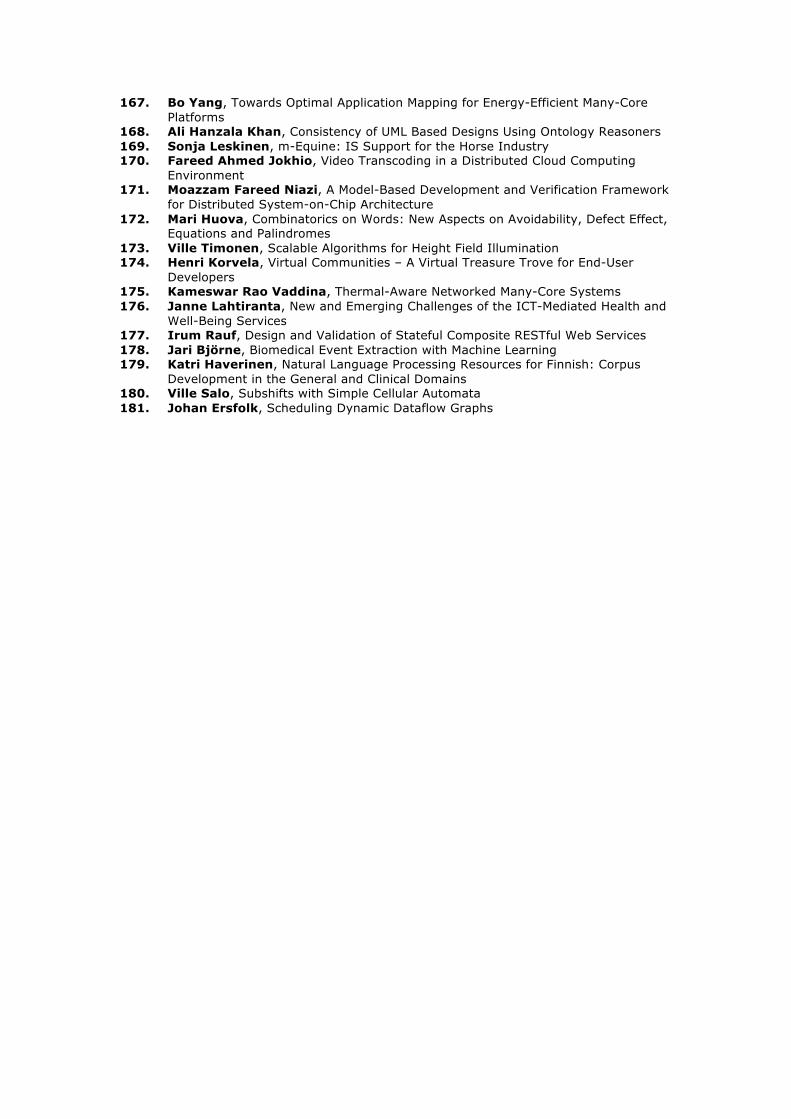
167. Bo Yang, Towards Optimal Application Mapping for Energy-Efficient Many-Core Platforms

168. Ali Hanzala Khan, Consistency of UML Based Designs Using Ontology Reasoners 169. Sonja Leskinen, m-Equine: IS Support for the Horse Industry 170. Fareed Ahmed Jokhio, Video Transcoding in a Distributed Cloud Computing

Environment 171. Moazzam Fareed Niazi, A Model-Based Development and Verification Framework

for Distributed System-on-Chip Architecture 172. Mari Huova, Combinatorics on Words: New Aspects on Avoidability, Defect Effect,

Equations and Palindromes 173. Ville Timonen, Scalable Algorithms for Height Field Illumination 174. Henri Korvela, Virtual Communities – A Virtual Treasure Trove for End-User

Developers 175. Kameswar Rao Vaddina, Thermal-Aware Networked Many-Core Systems 176. Janne Lahtiranta, New and Emerging Challenges of the ICT-Mediated Health and

Well-Being Services 177. Irum Rauf, Design and Validation of Stateful Composite RESTful Web Services 178. Jari Björne, Biomedical Event Extraction with Machine Learning 179. Katri Haverinen, Natural Language Processing Resources for Finnish: Corpus

Development in the General and Clinical Domains 180. Ville Salo, Subshifts with Simple Cellular Automata 181. Johan Ersfolk, Scheduling Dynamic Dataflow Graphs

Joukahaisenkatu 3-5 B, 20520 Turku, Finland | www. tucs.fi

TurkuCentre forComputerScience

University of TurkuFaculty of Mathematics and Natural Sciences • Department of Information Technology • Department of Mathematics and StatisticsTurku School of Economics • Institute of Information Systems Science

Åbo Akademi UniversityDivision for Natural Sciences and Technology • Department of Information Technologies

ISBN 978-952-12-3091-2ISSN 1239-1883

Johan Ersfolk

Johan ErsfolkScheduling D

ynamic D

ataflow w

ith Model C

hecking

Scheduling D

ynamic D

ataflow G

raphs with M

odel Checking