Intertemporal Poverty Measurement: Tradeoffs andPolicy Options∗

Catherine Porter†

Natalie Naıri Quinn‡

August 18, 2008

Abstract

This paper makes three contributions to the literature on intertemporal povertymeasurement, in particular the aggregation of a measure of wellbeing over time andacross people. Firstly we conduct an exhaustive analysis of properties of intertem-poral poverty measures, identifying relationships between the functional form andproperties of ITPMs and identifying the tradeoffs and compatibilities that exist be-tween the properties. We link this to the normative choices a poverty analyst mustmake when measuring intertemporal poverty. We also determine a ‘recipe’ whichmay be used to construct poverty measures with properties desired by the povertyanalyst. Second, we apply the recipe to construct a new family of intertemporalpoverty measures with the desired property of increasing compensation, a propertythat has thus far not been discussed in the literature. Third, we calculate measuresfrom the new family and compare them to other measures recently proposed in theliterature, to evaluate poverty in rural Ethiopia in the period 1994 - 2004.

∗This research constitutes part of the doctoral research of both authors, supported by ESRC researchtraining studentships. We would like to thank Stefan Dercon, Maria Ana Lugo, Christine Valente,Michael Griebe, Wanwiphang Manachotphong, Meg Meyer, James Foster and seminar participants atOxford University (Gorman Workshop), the CSAE conference Economic Development in Africa 2008and the Brooks World Poverty Institute/IPD Advanced Graduate Workshop 2008 for helpful comments.All errors are our own.

†St Antony’s College, University of Oxford; catherine.porter@economics.ox.ac.uk‡Balliol College, University of Oxford; natalie.quinn@economics.ox.ac.uk

1

CSAE WPS/2008-21

Contents

1 Introduction 3

2 Analysis of Intertemporal Poverty Measures and their Properties 62.1 Notation and Definitions . . . . . . . . . . . . . . . . . . . . . . . . . . . . 62.2 Induced Orderings and Functional Structure . . . . . . . . . . . . . . . . . 92.3 A Recipe for Construction of Intertemporal Poverty Measures . . . . . . . 122.4 Properties of the Trajectory Ordering . . . . . . . . . . . . . . . . . . . . . 122.5 Properties of the Trajectory-Distribution Ordering . . . . . . . . . . . . . . 212.6 Cardinal Properties of the Intertemporal Poverty Measure . . . . . . . . . 25

3 A New Family of Intertemporal Poverty Measures with Increasing Com-pensation Property 273.1 Construction . . . . . . . . . . . . . . . . . . . . . . . . . . . . . . . . . . 273.2 Generalisation . . . . . . . . . . . . . . . . . . . . . . . . . . . . . . . . . . 32

4 An empirical application: poverty in rural Ethiopia 334.1 Data . . . . . . . . . . . . . . . . . . . . . . . . . . . . . . . . . . . . . . . 334.2 Annual poverty measures and transition matrices . . . . . . . . . . . . . . 344.3 Introducing a time dimension to poverty measures . . . . . . . . . . . . . . 344.4 Extensions and sensitivity analysis . . . . . . . . . . . . . . . . . . . . . . 37

5 Conclusions 38

A Tables 39

2

1 Introduction

Quantitative measurement of poverty began with Rowntree (1901)’s innovative study ofpoor householders in York. Following the seminal contribution of Sen (1976), the quantita-tive unidimensional poverty measures developed in this literature aggregate cross-sectionor ‘snapshot’ data on a measure of wellbeing1 across those members of a sample of indi-viduals or households identified as poor. Economists have now reached a reasonable levelof consensus on what the desirable properties of such a measure should be, including howto identify the poor and aggregate the data, incorporating depth of poverty and distri-bution amongst the poor appropriately into the measure (see Atkinson (1987), Ravallion(1996) and Dercon (2006) for progressive reviews). Measures satisfying these propertiesinclude those suggested by Chakravarty (1983) and Foster, Greer, and Thorbecke (1984)(subsequently FGT), although the headcount measure – which does not satisfy Sen’smonotonicity or transfer properties – still finds frequent application in policy work.

Both economists and non-economists studying the lives of the poor have criticised thisapproach, observing that poverty is a multidimensional state, characterised by lack ofassets, feelings of insecurity or vulnerability, and deprivation in many dimensions and overextended durations2. Whilst much research has agreed in principle with this critique, inpractice many challenges arise when attempting to be true to the broader definition ofpoverty using economic tools and the available empirical data.

Data on many dimensions have been included in policy-relevant analysis, for example,the Human Development Index (UNDP3). The theoretical challenges that arise when ag-gregating data across dimensions of deprivation are analysed in the growing literature onmultidimensional poverty measurement, see the review by Atkinson (2003) as an intro-duction as well as and Bourguignon and Chakravarty (2003) and more recent work byFoster and Alkire (2007).

In this paper, though, we focus on the challenges that arise when attempting to takeinto account the time dimension. Time-relevant facets of poverty include duration orchronicity, systematic changes, variation and risk or vunerability. Chronicity can be seenas a key hardship for a number of reasons, firstly, intrinsically and intuitively: we mightpostulate that longer is simply worse when you are in a difficult situation. Secondly,it may be that being longer in poverty reduces the chances of being able to climb outof poverty; possible mechanisms are that assets are depleted (including body mass) andmorale is lower (Narayan-Parker, Patel, Schaff, Rademacher, and Koch-Schulte, 2000).Alternatively, it may be argued that periods in poverty can be compensated for if futurewelfare improves.

The absence of panel data meant that until recently such propositions could not be testedempirically, but when more than one time period of data is available the possibilities foranalysis increase, and it is possible to research questions around poverty dynamics. Ifsomeone is observed as poor in a particular survey how representative is that of their

1Typically income or consumption.2On policy, see Bank (2001) and Narayan-Parker, Patel, Schaff, Rademacher, and Koch-Schulte (2000).

For philosophical perspectives see Nussbaum and Sen (1999) and the various writings of Amartya Sen(1982), (1997), (2001).

3Various years, see http://hdr.undp.org/en/

3

lifetime welfare? If we have poverty measures from two cross sections at the beginningand end of a time period, what percentage of the poor are included in both of these sets?

One strand of empirical literature, mainly in developed countries has analysed poverty‘spells’, for example estimating the probability of entering or exiting poverty over time(Bane and Ellwood (1986), Stevens (1999)), confirming empirically that longer time spentin poverty increases the probability of being poor in the future4. As data became availableon two time periods for developing countries, economists calculated transition matrices5 toconclude that much of observed poverty is transient (see Baulch and Hoddinott (2000) foran overview). The literature further broadened in the 1990’s into analyses of vulnerability,“churning” and transient poverty, and the conceptual analysis of chronic poverty (seeHulme and Shepherd (2003), McCulloch and Calandrino (2003), McKay and Lawson(2003), Chaudhuri and Ravallion (1994) and CPRC (2004) for analysis and empiricalapplications).

Another strand of the literature on the intertemporal facets of poverty is that of norma-tive poverty measurement, a direct extension of the quantitative poverty measurementdiscussed above, to the intertemporal case. Several authors have proposed methods tocharacterise poverty over time, usually into a single number or composite poverty in-dex, generally termed a ‘chronic poverty’ measure. The approach proposed by Jalan andRavallion (2000) involves decomposing an FGT-style intertemporal poverty measure into‘chronic’ and ‘transient’ components, where the ‘chronic’ component – which has beenmost widely adoped and applied in the empirical literature – focuses on those who arepoor on average during the period under scrutiny. This approach implicitly assumes per-fect substitutability of wellbeing across time, both above and below the poverty line. Incontrast, the measure proposed by Foster (2007) has its basis in the ‘spells’ or countingapproach described above, weighting the depth of poverty experienced by those therebyidentified as chronically poor according to an FGT-style transformation before aggregat-ing over time and individuals. Calvo and Dercon (2007) generalise a particular case ofthis approach and show that it can also be discounted over time. Foster (2007)’s andCalvo and Dercon (2007)’s measures allow some degree of substitution between wellbe-ings in different periods provided they are all below the poverty line, but none acrossit. The measure proposed by Foster and Santos (2006) takes an approach intermediatebetween this and Jalan and Ravallion (2000)’s approach, allowing imperfect substitutionboth below and across the poverty line.

The current paper builds on this normative poverty measurement literature, contributinga systematic analysis of the properties of intertemporal poverty measures, including anumber of key observations on the complementarities and potential tradeoffs betweencertain desirable properties of the measures. In any application, the properties of thechosen measure must reflect the particular facet(s) of intertemporal poverty the povertyanalyst is attempting to capture, and the existence of tradeoffs between properties meanthat a measure appropriate for one facet will not necessarily possess properties makingit appropriate for another; this perhaps accounts for the current lack of consensus inthe literature. We build on the formal analysis to suggest a recipe for construction of

4This has parallels in the unemployment literature, which has shown that longer duration can oftensend negative signals to employers (thus duration can increase duration even further).

5The transition matrix cross-tabulates categories, usually “poor” and “non poor” for both surveyperiods to analyse what percent of the observations fall into each category

4

intertemporal poverty measures with desired properties, and apply the recipe to constructa new class of measures which possess an increasing-compensation property. Finally, weapply our new measure, together with others suggested in the recent literature, to theanalysis of poverty in rural Ethiopia between 1994 and 2004, using the Ethiopian RuralHousehold Survey.

Overview

Section 2 contains a systematic analysis of potential properties of intertemporal povertymeasures, and the restrictions they impose on the functional form of the measure. Weshow that mild and intuitively acceptable properties impose a great deal of structure,within which there are flexible components. The choice of these allows the poverty analystto determine the ordinal and cardinal properties of the measure, which we assert sheshould do according to the context of application and the facets of intertemporal povertyshe wishes to capture.

Importantly we distinguish groups of properties among which there is no conflict or trade-off (for example, increasing cost of hardship and intertemporal transfer, andgroups among which there must be a tradeoff (for example, duration sensitivity andintertemporal transfer). These results will inform the choice of measures whichare appropriate to apply to measurement of a particular facet of intertemporal poverty,for example measurement of the degree of chronic poverty. In fact, we show that severalmeasures previously suggested as appropriate for the measurement of ‘chronic poverty’do not in fact capture chronicity, but rather, other facets of intertemporal poverty.

The analysis in section 2 provides a method for construction of intertemporal povertymeasures with desired properties, and in section 3 we apply this method to construct anew class of measures satisfying the increasing compensation property.

In section 4 we apply our results to the analysis of poverty in some villages in ruralEthiopia between 1994 and 2004, using the Ethiopian Rural Household Survey panel dataset and some descriptive logit regressions. We find that the assumptions (both explicitand implicit) in the duration-adjusted poverty measures make a considerable differenceto the identification of the poorest households in the sample. In terms of individualcharacteristics, it appears that agricultural shocks (such as crop failure through pestsand trampling) as well as illness are correlated with higher poverty. Similar findingsto the static poverty literature are larger household size, less educated household headsand low initial assets. There are, however, a number of econometric challenges that arepresented if one wishes to attempt any kind of modelling of this kind of duration-adjustedpoverty measure; studies of consumption using panel data usually control for householdfixed-effects or unobservables correlated with the average level of consumption over time.When we study duration poverty we are trying to understand exactly those characteristics,and we have only one observation for each household in the ten year period. This is oneof our challenges for further analytic work.

Section 5 concludes and notes possibilities for further work.

5

2 Analysis of Intertemporal Poverty Measures and

their Properties

In this section we discuss properties of an intertemporal poverty measure, some of whichhave been suggested in the recent literature and others which we introduce. Taking certainof these properties as fundamental and axiomatic, we are able to restrict significantlythe space of possible intertemporal poverty measures, as well as providing a frameworkin which a poverty analyst may construct a measure with properties that she regardsas necessary for applied context in which she is working. In particular we show howthe properties of the trajectory ordering, trajectory-distribution ordering and cardinalproperties may be determined recursively by the composition of suitable functions.

To put this in the context of the extant literature on intertemporal poverty measures, Jalanand Ravallion (1998) do not discuss the properties of their chronic or transient povertymeasures. Foster and Santos (2006) and Foster (2007) do determine and discuss manyof the properties satisfied by their measures. Calvo and Dercon (2007) make a broaderdiscussion of possible properties and their connection with the functional form of themeasure; however, without formal justification they restrict attention to certain functionalstructures (thus excluding the possibility of achieving some desirable properties) and theiranalysis is informal. This paper presents the first general and rigorous discussion, in theintertemporal context, of the connections between properties and the form of the measure.We follow a similar approach to that taken by, for example Foster and Shorrocks (1991)in the context of static poverty measures.

We shall illustrate the analysis by reference to the intertemporal poverty measures pro-posed and favoured by the above authors.

2.1 Notation and Definitions

For the purpose of our theoretical analysis, we assume the availability of data x ∈ R+

on a cardinal, interpersonally and intertemporally comparable indicator of wellbeing6 foreach of a set of N ∈ N homogeneous individuals7 labelled i = 1, 2, . . . , N in each of a setof T ∈ N time-periods labelled t = 1, 2, . . . , T . We thus have an (N × T ) matrix of data

6We will never have a perfect measure of wellbeing, but in practice must use a proxy. It may beargued that value of consumption is typically the best indicator of achieved wellbeing available, certainlybetter than income which may be subject to intertemporal smoothing. This is discussed further insection 4 in the context of poverty in rural Ethiopia. Of course, the arguments made in the literatureon multidimensional poverty measurement, for example ? and Bourguignon and Chakravarty (2003)will apply here, and so x may itself be a multidimensional index. However, the introduction of severaldimensions raises issues that are not dealt with in this paper, for example the order of intertemporal,multidimensional and social aggregation.

7Though data may be available just at the household level; in practice, in order to maintain compa-rability (for example between households of different composition, or between individuals with differentcharacteristics) the data may need to be transformed. These issues are discussed further in section 4.

6

points,

X =

⎛⎜⎜⎜⎝

x11 x12 · · · x1T

x21 x22 · · · x2T...

.... . .

...xN1 xN2 · · · xNT

⎞⎟⎟⎟⎠ . (2.1)

(We are operating in a world of certainty, with a fixed number of individuals, whosewellbeings are observed in every time period of interest.) The data matrix X is anelement of the set

XNT = RN×T+ . (2.2)

Our aim will be to compute from the wellbeing data X a real-valued measure or indexP which represents information about the poverty experienced by the population of in-dividuals whose wellbeing is measured. We may be interested in comparing populationsof different sizes, or for which data is available for a different number of time periods, sothe domain of the index function must be

X =∞⋃

N=1

∞⋃T=1

XNT .

Definition 1. An Intertemporal Poverty Measure (ITPM) is a function

P : X → R such that P : X �→ P (X) (2.3)

whose properties, as defined and discussed below, are congruent with the intertemporalmeasurement of poverty.

We shall abuse notation, letting N represent the set {1, 2, . . . , N} ⊂ N and T representthe set {1, 2, . . . , T} ⊂ N.

We may wish to refer to the trajectory of wellbeings experienced by a particular in-dividual i ∈ N , that is, a row of the data matrix, for which we shall use the notationxi = (xi1, xi2, . . . , xiT ).

We may then think of a data matrix X ∈ X as representing a distribution of trajec-tories. The set X represents all possible distributions of trajectories.

We may wish to refer to the distribution of wellbeings experienced by the populationin a particular time period t ∈ T , that is, a column of the data matrix, for which we shalluse the notation Xt = (x1t, x2t, . . . , xNt)

′.

We shall also be interested in families of intertemporal poverty measures, indexed by aparticular level8 of wellbeing z ∈ R+.

Definition 2. A wellbeing-indexed ITPM is a function

P : X × R+ → R such that P : (X, z) �→ P (X; z) (2.4)

whose properties, as defined and discussed below, are congruent with the intertemporalmeasurement of poverty.

8z typically has the interpretation of a ‘poverty line’ though that need not be the case.

7

Intertemporal Poverty Measures in the Literature

We shall refer to a number of intertemporal poverty measures suggested in the recentliterature; for clarity we write these measures following the notational convention definedabove.

Jalan and Ravallion (2000)’s ‘total poverty’ measure PJRT is essentially FGT-2 (squaredpoverty gap) aggregated over time periods as well as individuals,

PJRT (X; z) =1

NT

N∑i=1

T∑t=1

(1− xit

z

)2

I(xit ≤ z) =1

NT

N∑i=1

T∑t=1

(max

[0, 1− xit

z

])2

(2.5)

while their ‘chronic poverty’ measure PJRC is FGT-2 applied to each individual’s meanwellbeing,

PJRC(X; z) =1

N

N∑i=1

(1− xi

z

)2

I(xi ≤ z) =1

N

N∑i=1

(max

[0,

1

T

T∑t=1

(1− xit

z

)])2

. (2.6)

Foster (2007)’s measure is similar to PJRT , but he incorporates a ‘poverty line’ τ in thetime dimension so that a household’s wellbeings only enter if that household is below thewellbeing poverty line z in a proportion of periods greater than τ . (He also permits aflexible power parameter α; for comparability, and because it yields attractive properties,we shall take α = 2; in our empirical section we take τ = 0.5.)

PF (X; z) =1

NT

N∑i=1

T∑t=1

(1− xit

z

)α

I(xit ≤ z)I

(T∑

t=1

I(xit ≤ z) ≥ τT

)(2.7)

Calvo and Dercon (2007) analyse a great variety of individual poverty measures, obtainedby permuting three operations applied to the wellbeing data: focus, convex decreasingtransformation, and linear aggregation over time. They discuss the properties of themeasures thus generated, and prefer that obtained by the sequence focus, transformation,aggregation. As a representative measure they apply this with an FGT transformation toobtain (incorporating linear social aggregation),

PCD(X; z) =1

NT

N∑i=1

T∑t=1

βT−t(1− xit

z

)α

I(xit ≤ z) (2.8)

=1

NT

N∑i=1

T∑t=1

βT−t(max

[0, 1− xit

z

])α

, (2.9)

equivalent to Jalan and Ravallion (2000)’s total poverty measure, generalised from α = 2and by the inclusion of the discount factor. In our empirical analysis we restrict attention

8

to the case with α = 2 and β = 1, identical to PJRT . Calvo and Dercon (2007) alsoconsider measures which are not additively separable over time.

The approach taken by Foster and Santos (2006) is somewhat different from the above; ageneralised mean or constant elasticity of substitution aggregation over time yields theirfamily of measures,

PFS(X; z) =

⎧⎪⎪⎨⎪⎪⎩

1β

1n

1T

∑ni=1 max

[0,∑T

t=1

(1− ( xit

z

)β)]for β ≤ 1; β = 0,

1β

1T

∑ni=1 max

[0,∑T

t=1(ln z − ln x)]

for β = 0.

(2.10)

All of the above measures (except Jalan and Ravallion (2000)’s ‘total poverty’ measure) arereferred to by their authors as ‘chronic poverty’ measures; as we shall discuss below, theirproperties enable them to capture particular intertemporal aspects of poverty, though notnecessarily chronicity per se.

2.2 Induced Orderings and Functional Structure

An intertemporal poverty measure P (2.3) is a real-valued function and thus induces anatural total preorder9 � on its domain set X , such that

Definition 3 (Induced Trajectory-Distribution Ordering). For any X, Y ∈ X ,

X � Y if and only if P (X) ≤ P (Y ). (2.11)

As elements of X are distributions of trajectories, and P is an intertemporal povertymeasure, X � Y should be read ‘distribution Y contains at least as much intertemporalpoverty as distribution X’. What ‘intertemporal poverty’ means in this context will ofcourse depend on the properties of P as discussed below.

Given N and T , an individual i ∈ N and trajectories wj for each j = i, an ITPM Pinduces a total preorder of the trajectory space R

T+:

Definition 4 (Induced Trajectory Ordering iNTX). Given N , T , i ∈ N and X¬i =[wj]j �=i, for any x,y ∈ R

T+,

x �iNTX y if and only if P (X) ≤ P (Y ). (2.12)

where

• [X]it = xt and [Y ]it = yt for each t ∈ T , and

• [X]jt = [Y ]jt = [wj]t for each j = i and each t ∈ T .

9A total preorder is a total (complete) transitive binary relation.

9

Definition 5. Given N , T and i ∈ N , say that P is separable10 in i given N and T ifthe induced trajectory ordering iNTX is independent of the wj. In that case the inducedtrajectory ordering may be represented by �iNT .

Definition 6. [Separability] An ITPM P is separable if, given N andT , it is separable in each i ∈ N .

Proposition 1. Given N and T , any separable ITPM may be written in the form

P (X) = A(p1(x1), p2(x2), . . . , pN(xN)) (2.13)

where A :⋃

N∈NR

N → R is strictly increasing in each of its arguments, and each pi :R

T+ → R. Conversely, any function of the form (2.13) is separable.

Proof. Converse: the function pi establishes the ordering �iNT , which is preserved in Pby monotonicity of A.

Separability is a natural regularity or independence property; given that an ITPMreflects an ordering over trajectories for each individual in the distribution, we requirethat ordering to be invariant to changes in the other individuals’ trajectories. That is,if trajectory x experienced by individual i is ‘no poorer than’ trajectory y, this orderingshould not be reversed if there are changes in the trajectories experienced by individualsother than i.

We now strengthen this property to introduce symmetry across individuals in the tra-jectory ordering; if trajectory x is ‘no poorer than’ trajectory y for some individual i, xshould be ‘no poorer than’ trajectory y for any other individual j.

Definition 7. [Trajectory-Ordering] An ITPM P is trajectory-ordering

if it is separable and, given T , the induced trajectory orderings �iNT areidentical for each N ∈ N and each i ∈ N .

Notation: we represent the trajectory orderings induced by a trajectory-ordering

ITPM by �T .

For x,y ∈ RT+, we interpret x �T y as ‘y is at least as poor as x’. For each T ∈ N we

may define two derived relations on RT+:

• x ∼T y if x �T y and y �T x, ‘y is equally as poor as x’.

• x ≺T y if x �T y and y �T x, ‘y is strictly poorer than x’.

All intertemporal poverty measures suggested in the literature are trajectory-ordering,although the property has not previously been stated explicitly.11 Our motivation for in-troducing the trajectory-ordering property is to elucidate the relationship betweenthe functional form of the measure and its properties.

10In the sense of Gorman (1968).11Note that it is not equivalent to the ubiquitous property of anonymity or symmetry across individ-

uals; that does not restrict interactions between individuals whereby orderings may change according totrajectories experienced by others. Also it is purely an ordinal property while full symmetry is cardinal.However, we shall later impose symmetry as well.

10

Proposition 2. 1. Given T , any trajectory-ordering ITPM may be written inthe form

P (T )(X) = A(T )(p(T )(x1), p(T )(x2), . . . , p

(T )(xN)) (2.14)

where A(T ) :⋃

N∈NR

N → R is strictly increasing in each of its arguments, andp(T ) : R

T+ → R.

2. The ordering induced by p(T ) on RT+ is the trajectory ordering �T .

Proof. 1. Separability yields form as above, trajectory-ordering yields p1 = p2 =. . . = pN = p(T ).

2. Follows directly from A strictly increasing in all arguments.

Corollary 3. Without loss of generality, any trajectory-ordering ITPM may bewritten in the form

P (X) = A(p(x1), p(x2), . . . , p(xN)) (2.15)

where A :⋃

N∈NR

N → R is strictly increasing in each of its arguments, and p :⋃

T∈NR

T+ →

R.

Proof. P (X) is trajectory ordering and therefore for each T has a representation (2.14).The A(T ) are increasing functions of each of their arguments, and trajectory orderingsare preserved under increasing transformations, therefore any differences in A(T ) acrossT may be captured by making appropriate transformations of the p(T ), which, collectedover T , form p.

We have thus extended the trajectory ordering to⋃

T∈NR

T+.

Note that the function A need not be symmetric in each of its arguments, consistent withour observation above that trajectory-ordering does not entail full symmetry. Notealso that each of the ITPMs suggested in the literature are trajectory-ordering andthus may be represented in this form. In fact, their representations above (2.5) – (2.10)are all of this form.

Corollary 4. Any trajectory-ordering ITPM may be written in the form

P (X) = G(S(p(x1), p(x2), . . . , p(xN))) (2.16)

where G : R → R is strictly increasing and S :⋃

N∈NR

N → R induces the same trajectory-distribution ordering as A.

Proof. Without loss of generality, write A = G(S) for appropriate functions G : R → R

and S :⋃

N∈NR

N → R. Existence is trivial; we may take G(x) = x and S = A.

11

2.3 A Recipe for Construction of Intertemporal Poverty Mea-sures

The above results enable us to suggest a simple recipe for construction of intertemporalpoverty measures with desirable properties:

• Step 1: Choose a function p which induces a trajectory ordering with the desiredproperties.

• Step 2: Choose a social aggregation function S to aggregate over individuals in away that yields an ordering of distributions of trajectories with desired properties.

• Step 3: If necessary, choose a transformation function G to yield a poverty measurewith the desired cardinal properties.

Of course, in practice things may not be so simple, as application of this recipe requiresthe existence (and discovery) of suitable functions p, S and G. In section 3 below we applythis recipe to construct a new class of intertemporal poverty measures with an increasingcompensation property of the trajectory ordering.

Decomposing P in this way enables us to distinguish clearly between the different types ofproperties: properties of the trajectory ordering, properties of the distribution ordering,and cardinal properties of the measure. This will facilitate our analysis greatly, enablingus to clarify tradeoffs and compatibilities between different properties, in a more completeand coherent way than has yet appeared in the literature.

This section continues with an analysis of these three classes of properties. Some proper-ties, which we believe are justified in all circumstances and thus take as axiomatic, enableus to make restrictions on the classes of functions suitable for p, S and G. Other prop-erties will depend on the particular information which the poverty measure is intendedto represent; in some cases we are able to show how the functions may be chosen toincorporate the chosen properties.

2.4 Properties of the Trajectory Ordering

Through most of this section we take T as fixed, and discuss possible properties of thetrajectory orderings �T . As the properties of �T are entirely determined by the functionp we also analyse the relationships between the form of p and these properties. This willfacilitate the choice of suitable functions p to yield intertemporal poverty measures withdesired properties. The function p of course determines an ordering over the entire tra-jectory space

⋃∞T=1 R

T+ and so we conclude the section by briefly discussing the properties

of the ordering in this dimension.

The first property we consider is continuity of the trajectory ordering.

Definition 8. [Continuity] Given T , �T is continuous on RT+ if, for any

trajectory x ∈ RT+ and sequence of trajectories ys ∈ R

T+ with limit y ∈ R

T+

such that x �T ys for each s ∈ N, x �T y.

12

Proposition 5. Given T , �T is continuous on RT+ if and only if p is a continuous function

on RT+.

Proof. Topological argument (see Debreu (1960).

Continuity is essentially a regularity property, required for a ‘well-behaved’ trajectoryordering. An important argument in its favour is that a non-continuous poverty measurewould be excessively sensitive to measurement error at any point of discontinuity. Wetherefore restrict attention to measures satisfying continuity. Of the ITPMs suggestedin the literature, all satisfy continuity except PF .

It will prove useful to note here a standard result about continuous total preorders on atopological space:

Lemma 6. If �T is continuous on RT+ then the ‘indifference’ sets I(x) = {y ∈ R

T+ : y ∼T

x} are connected.

Sensitivity to Wellbeing: Monotonicity, Focus and Identification

We now consider properties of the trajectory ordering in relation to changes in wellbeing,primarily in a single time period.

We start with a property which is fundamental to the concept of poverty measurement andis ubiquitous in the poverty measurement literature. All other things equal, an increasein wellbeing of one individual in one time period should not increase the intertemporalmeasure of poverty P . In the context of the trajectory ordering, a trajectory x whichdiffers from a trajectory y only by having greater wellbeing in a single time period shouldbe ordered as weakly less poor than y.

Definition 9. [Weak Monotonicity] Given T , �T satisfies weak mono-

tonicity if, for any x,y ∈ RT+ such that xt > yt for some t ∈ T and xτ = yτ

for all τ = t, x �T y.

Proposition 7. �T satisfies weak monotonicity if and only if p is a weakly decreasingfunction of each of its arguments at each point in R

T+.

Proof. ‘If’: weakly decreasing p yields weakly monotone �T . ‘Only if’: any p consistentwith weakly monotone �T must be weakly decreasing throughout R

T+.

It will prove useful to note here that trajectory-ordering, continuity and weak

monotonicity together enable us to identify, for every trajectory, a constant-wellbeingequivalent12 trajectory.

Definition 10 (Constant-Wellbeing Trajectories). Given T ∈ N, define the set of constant-wellbeing trajectories CT ⊂ R

T+ as CT = {c|c ∈ R

T+, c1 = c2 = . . . = cT}.

12A similar approach is taken in, for example, ?, though in the context of populations rather thantrajectories.

13

Note that CT is the T -dimensional generalisation of the familiar ‘45-degree line’. It has anatural total order ≤ where for c,d ∈ CT , vecc ≤ d if and only if c1 ≤R d1 where ≤R isthe usual total order of the reals.

Definition 11 (Constant-Wellbeing Equivalent of a Trajectory). Given an ITPM P sat-isfying trajectory-ordering, continuity and weak monotonicity with inducedtrajectory orderings {�T}, define the constant-wellbeing equivalent of a trajectoryx ∈ R

T+ as c(x) where c : R

T+ → CT such that c(x) = min{c ∈ CT |c ∼T x}. (Minimum

under the natural total order of CT defined above.)

Proposition 8. For all x ∈ RT+, c(x) exists.

Proof. CT is totally ordered and therefore if {c ∈ CT |c ∼T x} has a minimal elementthat minimal element is unique and is thus the minimum. Weak monotonicity andcontinuity are sufficient for {c ∈ CT |c ∼T x} to be non-empty; continuity may beinvoked again to show that if non-empty, {c ∈ CT |c ∼T x} has a minimal element.

Weak monotonicity is satisfied by all poverty measures suggested in the literature, andis essentially equivalent to, for example, Bourguignon and Chakravarty (2003)’s ‘axiom’MN. However, it is a weak property and does not ensure any sensitivity of the measureto lack of wellbeing. One remedy would be simply to strengthen the property, requiringx ≺T y rather than x �T y. However, this would yield a ‘poverty measure’ that wassensitive to the wellbeings of all individuals, even those who are consistently very well-off.

Following Sen (1976) it is conventional in the poverty measurement literature to distin-guish between identification of the poor among the population being studied, and aggre-gation of information available about those identified as poor to construct the index ofpoverty. It follows that the index should not be sensitive to the level of wellbeing of thosenot identified as poor (the ‘focus principle’). This makes intuitive sense; we are unlikelyto want our measure of poverty to decrease if, all other things equal, an already well-offperson becomes better off. This principle may be formalised as a focus property.

For static, unidimensional measures it is conventional to choose a poverty line z, anddemand that the measure is not sensitive to wellbeings x which lie above this line.13 It isnot entirely straightforward to extend this concept to several dimensions or multiple timeperiods. Bourguignon and Chakravarty (2003) define two possibilities for the multidimen-sional context, whose analogues in the intertemporal context, expressed as properties ofthe trajectory ordering,14 we give here:

13If z is chosen independently of the observed distribution of wellbeings, this corresponds to the conceptof absolute rather than relative poverty, an approach that we shall maintain throughout the paper. Notethat identification could, in principle, be based on information different from that incorporated in thepoverty measure. We shall ignore this possibility; if such data were available and informative aboutpoverty, we maintain that it should be incorporated in the wellbeing measure.

14Bourguignon and Chakravarty (2003) state the properties as properties of the poverty measure itself,the direct analogues being Strong Focus: The trajectory-indexed ITPM P satisfies strong focus

relative to the set of trajectories Z if, for any N and T , for any i ∈ N and t ∈ T , and for any X, Y ∈ XNT

such that

• xit > yit and yit > zTt ,

• xiτ = yiτ for all τ = t, and

14

Definition 12. [Strong Focus] Given T , �T satisfies strong focus rel-ative to z ∈ R+ if, for any x,y ∈ R

T+ such that xt > yt > z for some t ∈ T

and xτ = yτ for all τ = t, x ∼T y.

Definition 13. [Weak Focus] Given T , �T satisfies weak focus relativeto z ∈ R+ if, for any x,y ∈ R

T+ such that xt > yt > z for some t ∈ T and

xτ = yτ > z for all τ = t, x ∼T y.

Note that strong focus entails weak focus.

It follows directly from the definitions that if �T satisfies strong focus relative toz ∈ R+ then for any x,y ∈ R

T+ such that xt > yt > z for some t ∈ T and xτ = yτ for

all τ = t, p(x) = p(y). If �T satisfies weak focus relative to z ∈ R+ then, for anyx,y ∈ R

T+ such that xt > yt > z for some t ∈ T and xτ = yτ > z for all τ = t, p(x) = p(y).

Intuitively, under weak focus, the function p (and thus the intertemporal poverty mea-sure P ) are not sensitive to changes in the wellbeing in any period, for an individual whoselevel of wellbeing lies above a ‘poverty line’ z in every period. Under strong focus, thisproperty is strengthened, so that p (and thus P ) are not sensitive to changes in wellbeingin any period above the poverty line, for any individual (even if that individual’s wellbeinglies below the poverty line in other periods).

We note here that all of the intertemporal poverty measures suggested in the literaturesatisfy weak focus, while PF and PCD additionally satisfy strong focus.

These alternative focus properties do not ensure sensitivity, but simply restrict it. Inorder to define a property that ensures sensitivity of the measure to poverty or lack ofwellbeing, we must return to the idea of identification. In the intertemporal context, wetake this to mean identification of trajectories of wellbeings as ‘intertemporally poor’.

Given the concept of the trajectory ordering, we have a natural way to identify poor andnon-poor trajectories.

Definition 14. �T identifies the trajectory x ∈ RT+ as non-poor if x ∼T y where yt is

arbitrarily large for each t ∈ T .

Definition 15. �T identifies the trajectory x ∈ RT+ as poor if y ≺T x where y is any

non-poor trajectory.

• xjτ = yjτ for all j = i and all τ ∈ T ,

P (X) = P (Y ), and Weak Focus: The trajectory-indexed ITPM P satisfies weak focus relative tothe set of trajectories Z if, for any N and T , for any i ∈ N and t ∈ T , and for any X,Y ∈ XNT such that

• xit > yit and yit > zTt ,

• xiτ = yiτ and yiτ > zTτ for all τ = t, and

• xjτ = yjτ for all j = i and all τ ∈ T ,

P (X) = P (Y ).

15

Weak monotonicity yields considerable structure: if x is non-poor under the weakly

monotone trajectory ordering �T then any trajectory y with wellbeings yt ≥ xt in eachperiod t ∈ T must also be non-poor. Similarly, if x is poor under the weakly monotone

trajectory ordering �T then any trajectory y with wellbeings yt ≤ xt in each period t ∈ Tmust also be poor.

It will be convenient to label the space of trajectories identified as poor; let ΦT = {x ∈R

T+ : x is poor under �T} ⊂ R

T+.

We are now able to strengthen the monotonicity property in a fairly general way thatdoes not conflict with the focus principle:

Definition 16. [Strict Monotonicity] Given T , �T satisfies strict

monotonicity if, for any x,y ∈ ΦT such that xt > yt for all t ∈ T , x ≺T y.

A stronger monotonicity property satisfied by Jalan and Ravallion (2000)’s and Foster andSantos (2006)’s measures though not by Calvo and Dercon (2007)’s nor Foster (2007)’sis:

Definition 17. [Strong Monotonicity] Given T , �T satisfies strong

monotonicity if, for any x,y ∈ ΦT such that xt > yt for some t ∈ T ,x ≺T y.

We can also define a general focus property:

Definition 18. [Focus] Given T , �T satisfies focus if ΦT = ∅ and thereexists a non-poor trajectory xT ∈ R

T+ comprising finite wellbeings in every

period.

Each of the intertemporal poverty measures suggested in the literature satisfy strict

monotonicity and focus(though the ‘headcount’ version of Foster’s measure does notsatisfy strict monotonicity.

We now seek a more practical approach to identification.

Proposition 9. Given T and a trajectory ordering �T which satisfies continuity,strict monotonicity and focus, there exists a hypersurface (connected space of di-mension T − 1) Z of trajectories x ∈ R

T+ bounding ΦT ; this is intersected exactly once

by the space of constant-wellbeing trajectories, and thus may be labelled by that wellbeingz ∈ R

T+ such that z = (z, z, . . . , z) ∈ Z. Without loss of generality we may represent �T

with a function p where p(z) = 0; then p(x) > 0 for all poor trajectories x and p(x) = 0for all non-poor trajectories.

Proof. Topological argument.

16

The wellbeing level z represents that constant level of wellbeing which is on the marginof being regarded as ‘intertemporally poor’. It is important to be clear that it is notdirectly analogous to the poverty line in static, unidimensional poverty measurement; abetter analogue for the poverty line is the entire space of marginally poor trajectories Z.

It is helpful to consider the shape of Z for the measures suggested in the literature. ForPJRC it is the simplex passing through z, for PCD it is an extended L-shape, while forPFS it is an isoquant of the CES function on which the measure is based. As PF is notin general continuous, Z may not be connected; its shape is very complex and does notintuitively correspond to an idea of ‘marginally poor’ trajectories.

Intertemporal Intrapersonal Transfer

We now consider the sensitivity of the poverty measure to changes in wellbeing in morethan one time period. We shall see that the choices made here are central to the conceptof intertemporal poverty measurement, and lead to strong restrictions on the form ofthe function p. We identify desirable but incompatible properties, between which thepoverty analyst must make a normative or empirical choice, according to the context ofapplication.

To what extent can a relatively high level of welfare in one period compensate for lowwelfare in another? This is a crucial consideration in the choice of intertemporal povertymeasure, and one in which there is no consensus as yet in the literature. As we noted inthe introduction, Jalan and Ravallion (2000)’s measure averages wellbeings across timeand thus allows perfect compensation between periods while both Foster (2007) and Calvoand Dercon (2007) only allow (imperfect) compensation between periods both below thepoverty line; Foster and Santos (2006)’s measure does allow imperfect compensation bothbelow and across the poverty line.

The intertemporal analogue of Sen (1976)’s transfer axiom, applied to the trajectoryordering, is as follows.

Definition 19. [Intertemporal Transfer]15 Given T ≥ 2, �T satisfies

intertemporal transfer if, for any δ > 0, x,y ∈ ΦT such that xt > xs,yt = xt + δ, ys = xs− δ for some t, s ∈ T and xτ = yτ for all τ = t, s, x ≺T y.

Intuitively, intertemporal transfer reflects the idea that a period of elevated well-being cannot fully compensate for a period of depressed wellbeing. It would seem anappropriate normative choice when the poverty analyst aims to capture the total burdenof poverty over time. It is also closely related to the concept of fluctuation or varianceaversion, which is natural if the measure is to reflect preferences for smoothing of wellbe-ing.

15This is similar to Foster (2007)’s transfer property which requires chronic poverty to decrease givena smoothing of incomes among those identified as chronically poor. (Foster does not distinguish betweensmoothing over time and over people.) Note that the measures suggested by Foster (2007) do not ingeneral satisfy the property. Calvo and Dercon (2007)’s first, dismissed, suggestion for ‘increasing costof hardship’ is essentially the same.

17

Trajectory aa Trajectory bb

We may extend this concept, recognising that the resistance to compensation will bestronger, the lower the level of wellbeing experienced.16 That is, we should allow a greater(or at least, not lesser) marginal rate of compensation between a pair of periods whenwellbeing is greater in both.

Definition 20. [Non-Decreasing Compensation] The marginal rate ofintertemporal compensation between an individual’s welfare in two periodsshould not decrease, as the period wellbeings increase in proportion. Equiva-lently, the elasticity of compensation should not decrease as wellbeing increases.

We may require a stronger version of this property:

Definition 21. [Increasing Compensation] The marginal rate of intertem-poral compensation between an individual’s welfare in two periods should in-crease, as the period wellbeings increase in proportion, given that their trajec-tory is identified as ‘poor’. Equivalently, the elasticity of compensation shouldnot decrease as wellbeings increase in proportion.

Proposition 10. 1. Strong focus and increasing compensation are incompat-ible properties.

2. The only trajectory ordering satisfying strong focus and non-decreasing com-

pensation is the ‘Rawlsian’ ordering.

Proof. 1. Assume that p(x) satisfies strong focus. Consider poor trajectories x andαx, α > 1, such that all elements of x are strictly less than z while at least oneelement of αx is strictly greater than z. Elasticity of compensation at αx is zero andat x is greater than or equal to zero, therefore P (X) does not satisfy increasing

compensation.

2. Consider p(x) that induces the ‘Rawlsian’ ordering and thus satisfies strong fo-

cus. Consider poor trajectories x and αx, α > 1, such that all elements of xare strictly less than z while at least one element of αx is strictly greater thanz. Elasticity of compensation at αx is zero and at x is zero, therefore P (X) doesnot satisfy increasing compensation. The ‘Rawlsian’ ordering is the uniqueordering satisfying this for all x.

16This is intuitively desirable but of course is an empirically testable proposition; we are not aware ofa study which has established this.

18

Proposition 11. If (and only if) p satisfies increasing compensation its lines ofconstant MRC diverge faster than homothetic.

This provides us with a simple condition to test whether a function p(x) satisfies theproperty.

Permutations of Wellbeings over Time

We consider here the impact on the trajectory ordering of permutations of wellbeingsbetween different time periods.

The simplest approach, which has been taken (implicitly or explicitly) by most authorsin this literature, is to impose perfect time symmetry.

Definition 22. [Time symmetry] Given T , �T satisfies time symmetry

if, for any x,y ∈ RT+ such that x = My for some permutation matrix M ,

x ∼T y.

Proposition 12. �T satisfies time symmetry if and only if p is a symmetric functionof the component wellbeings.

Of course, imposing such a property does not allow for various aspects of intertemporalpoverty which the poverty analyst might want to capture, including systematic changes(for example a trajectory with a systematic downward trend might be considered ‘worse’than an equivalent trajectory with an upward trend) or asymmetric transfer properties(for example the elasticity of compensation may be greater between successive periodsthan between those separated by a considerable time). This is an especially importantconsideration when the intervals between data periods are not regular.

Calvo and Dercon (2007) apply discount factors to incorporate sensitivity to trend in theirmeasures. This is an important contribution which may be used as an alternative to time

symmetry if demanded by the context of application.

Duration or Chronicity of Poverty

We now return to one of the motivating concepts for the measurement of intertemporalpoverty; the attempt to capture information about chronicity in a quantitative measure.Our main result here is that it is difficult to do this whilst maintaining the transferproperties discussed above. In fact the poverty analyst must make a normative choiceamong these properties, according to the context in which she applies the measure, andwhether she aims to measure the total burden of poverty experienced, or chronicity ofpoverty.

Most of the discussion in the policy literature (CPRC, 2004), and in much of the eco-nomic literature (Calvo and Dercon, 2007) has focused around the concept of chronicityof poverty: prolonged periods below the poverty line must be thought of as worse than

19

shorter, other things equal. The fundamental idea is that prolonged periods of low well-being may have an adverse effect over and above that due to the depth of poverty alone.We attempt to reflect this in a duration-sensitivity property.17

Definition 23. [Duration Sensitivity] Given T and trajectories x,y withidentical average wellbeing, but with strictly more periods in x spent below thepoverty line, p(x) > p(y).

Proposition 13. No p satisfies both intertemporal transfer and duration sen-

sitivity.

Proof. Consider x,y with identical wellbeings in all periods except t = 1 and t = 2, wherex1 = z + δ, y1 = z − δ, x2 = z/2 − δ and y2 = z/2 + δ where δ ∈ (0, z/4). If p satisfiesduration sensitivity (1) then p(x) < p(y). If p satisfies intertemporal transfer

then p(x) ≥ p(y), a contradiction. Therefore no function p satisfies both intertemporal

transfer and duration sensitivity.

The tradeoff between intertemporal transfer and duration sensitivity meansthat the poverty analyst must choose between them when choosing an intertemporalpoverty measure. In fact the only measures proposed thus far in the literature that dosatisfy duration sensitivity is the duration extended headcount measures (special cases ofthe poverty measure proposed by Foster (2007) with α = 0 and τ < 1 in the intertem-poral FGT framework). Thus, whilst the concept of chronic poverty in the sense of longduration may be intuitive, in fact imposing this property precludes some other desirableproperties.18

Temporal Homogeneity

Given a trajectory-ordering ITPM P (X) = A(p(x1), p(x2), . . . , p(xN)) the trajec-tory function p :

⋃T∈N

RT+ → R induces a total preorder on

⋃∞T=1 R

T+, the space of

trajectories of different durations. The properties discussed in detail above all relate tothe orderings over the spaces of same-duration trajectories R

T+. We now consider how

these are connected; a natural approach is to require the constant-wellbeing trajectoriesto be equivalent across trajectory lengths.19

Definition 24. [Timespan Comparability] � satisfies timespan com-

parability if, for all wellbeings x ∈ R+ and all T1, T2 ∈ N, (x, x, . . . , xT1) ∼(x, x, . . . , xT2).

17For clarity, although Foster (2007)’s time monotonicity is motivated in a similar way, it does notcapture this idea but is a consequence of strong monotonicity.

18There is an analogy here to the static literature in which the intuitive proposition ‘A population witha greater proportion of poor people is worse off than one with a lesser proportion of poor people’ conflictswith sensitivity to inequality among the poor, or the transfer principle.

19Whilst it is possible to think of contexts in which this property would not be desired, perhaps if thegreater information in a longer series of observations is in itself informative, such exceptional situationsseem quite contrived.

20

Proposition 14. � satisfies timespan comparability if and only if for all wellbeingsx ∈ R+ and all T1, T2 ∈ N, p(x(1), x(2), . . . , x(T1)) = p(x(1), x(2), . . . , x(T2)).

Proof. Trivial.

With the assumption of timespan comparability we are now able to prove a resultwhich will be useful in the subsequent analysis.

Lemma 15. Given a function p which satisfies continuity, weak monotonicity andtimespan comparability, there exists for every x ∈ ⋃∞T=1 R

T+ an equivalent constant

wellbeing c(x) such that p(c(x)) = p(x).

Proof. Topological argument.

Note that the equivalent constant wellbeing may not be unique. However, we may define afunction c :

⋃∞T=1 R

T+ → R+ by taking c to be the minimum equivalent constant wellbeing

for each x.

Conclusion

We have conducted a fairly exhaustive analysis of fundamental and desirable propertiesof the trajectory ordering, and provided results which enable these properties to be rep-resented by a function p. Construction of a suitable p is the first stage of our recipe forconstruction of an intertemporal poverty measure; we now turn to the subsequent stages.

We note here that although some of the properties are fundamental and will subsequentlybe taken as axiomatic, others are the choice of the poverty analyst and must be chosen toreflect those facets of intertemporal poverty that she wishes her measure to capture. Howshe makes this choice will depend on the application, and may be driven by normativeconsiderations. Alternatively a more welfarist approach may be taken, and she mayattempt to determine empirically the preferences over trajectories of wellbeings held bythe subjects of her study. This approach would raise many practical challenges which weshall not explore further in the present paper.

We will note briefly, however, that the precise specification of the properties of the measureshould in either case reflect the observed variable which is being used to proxy for wellbe-ing. For example, if income were used, the poverty analyst should impose a higher degreeof intertemporal substitution than if consumption were used, to allow for intertemporalconsumption smoothing.

2.5 Properties of the Trajectory-Distribution Ordering

Having discussed and analysed properties of the trajectory ordering induced by a tra-

jectory ordering intertemporal poverty measure P we now turn to properties of theordering it induces on X , that is, the ordering of distributions of trajectories.

21

Throughout this section we assume that the poverty analyst has chosen the properties ofthe trajectory ordering, subject to the restrictions discussed above, and has found a suit-able function p which embodies her chosen properties. We assume also that the propertieschosen include weak monotonicity, continuity and timespan independence sothat by Lemma 15 for every trajectory x ∈ ⋃T∈N

RT+ there exists an equivalent constant

wellbeing c(x).

This greatly simplifies the analysis, as we are thus able to focus entirely on the proper-ties of the ordering of constant-wellbeing trajectories induced by the ITPM. Intuitively,the ITPM ’treats’ any trajectory x in exactly the same way as its equivalent constant-wellbeing trajectory c(x). 20 Drawing the obvious analogy between constant-wellbeingtrajectories and individual wellbeings in the context of static poverty measurement en-ables us to draw directly on that mature literature for properties and results. In particularwe make use of Foster and Shorrocks (1991)’s results which invoke Gorman (1968) to char-acterise the class of subgroup-consistent poverty indices.

As the literature on static, unidimensional poverty measurement has reached a broadconsensus on the desirable properties of such a measure, we shall not discuss alterna-tive properties in any detail here, but simply establish the appropriate analogy with theintertemporal case.

Analogy with Static, Unidimensional Poverty Measurement

We shall let ci = c(xi) and regard this, the individual’s equivalent constant wellbeing,as analogous to the individual wellbeing21 in the static, unidimensional case, notatedxi in Foster and Shorrocks (1991). A distribution of equivalent constant wellbeings c =(c1, c2, . . . , cn) ∈ ⋃∞N=1 R

N+ is then analogous to Foster and Shorrocks (1991)’s distribution

x. We take Foster and Shorrocks (1991)’s distribution space D to be the image of X underc, that is, the space of all vectors of equivalent constant wellbeings under P . (The structureof this space is consistent with the definition of D given by Foster and Shorrocks (1991);if P satisfies focus then D = [0, z] while if P does not satisfy focus D = [0,∞).)

We start with the ‘basic properties’ listed by Foster and Shorrocks (1991), stating themin the context of equivalent constant wellbeings and clarifying their relationship to moregeneral properties of intertemporal poverty measures. Some are equivalent to propertiesthat we shall impose on the trajectory-distribution ordering, while others follow directlyfrom properties already established of the trajectory ordering. We note that for Fosterand Shorrocks (1991) an index P is in sections 2 and 3 a family of poverty measuresindexed by poverty lines z ∈ D while in section 4 it is a particular poverty measure.For clarity, consistency with the rest of our paper and because their main results are notdependent on their assumption of the focus property we follow the latter, dropping theargument z in our statement of their properties.

20In fact, we may go further than this; the existence of equivalent constant wellbeings c(x) enables us tocompare trajectories of different durations and thus distributions of trajectories of a variety of durations;in practice this will be useful and straightforward to implement but the formal analysis would require anextension of the foundations so we set the task aside for now.

21The literature typically refers to ‘income’ or ‘consumption’; see our discussion above and in section4.

22

Definition 25. [FS1-Symmetry] P satisfies FS-symmetry if P (c) = P (d)whenever c ∈ D is obtained from d ∈ D by a permutation.

The natural symmetry property for intertemporal poverty measures, a property of thetrajectory-distribution ordering, is as follows:

Definition 26. [Population Symmetry] P (X) = P (Y ) whenever X ∈ Xis obtained from Y ∈ X by a permutation of trajectories across individuals,that is, X = ΠY where Π is an N × N matrix of ones and zeros, each rowand each column summing to one.

This kind of anonymity or symmetry property is standard in the social welfare literature;in the context of intertemporal poverty measurement the only information about eachindividual that impacts on the intertemporal poverty measure P should be the trajectoryof measured wellbeings. It is straightforward to show that if P satisfies population

symmetry it also satisfies FS1-symmetry.

Definition 27. [FS2-Replication Invariance] P (c) = P (d) wheneverc ∈ D is obtained from d ∈ D by a replication.

This is essentially homogeneity of degree zero in population size. If P is to measurethe per-capita impact22 of intertemporal poverty, then it must satisfy this kind of homo-geneity property. That is, applying the measure to a different population with the samedistribution of wellbeing trajectories, should yield the same result. This property may beformalised as follows for the intertemporal case:

Definition 28. [Population-Size Invariance] P satisfies population-

size invariance if for any N1, N2 and T and for any X ∈ XN1T , Y ∈ XN2T

such that X and Y represent an identical distribution of trajectories, P (X) =P (Y ).

Again, it is straightforward to show that if P satisfies population-size invariance italso satisfies FS2-replication invariance.

Definition 29. [FS3-Monotonicity] P (c) ≤ P (d) whenever c ∈ D is ob-tained from d ∈ D by an increment to a poor person.

This property follows directly from weak monotonicity which we have assumed P tosatisfy.

Definition 30. [FS4-Focus] P (c) = P (d) whenever c ∈ D is obtained fromd ∈ D by an increment to a nonpoor person.

22The poverty analyst may, of course, in some applications wish to measure the total rather than per-capita burden of poverty in a population, necessitating a measure which is homogeneous of degree 1 inpopulation size. Such measures will be directly related to the class of decomposable measures.

23

This property would follow directly from focus; we have not imposed focus on thetrajectory ordering, though of course P may satisfy it; we note however that Foster andShorrocks (1991)’s main results do not depend upon the assumption of this property.

Definition 31. [FS5-Restricted Continuity] P (c) is continuous as afunction of ci on [0, z] where z is the poverty line.

This follows directly from contunity which we have assumed P to satisfy; in fact con-

tinuity is stronger and will allow us to apply those results of Foster and Shorrocks (1991)which depend on their stronger continuity property. 23

The main result in Foster and Shorrocks (1991) establishes a general functional formfor poverty measures satisfying a subgroup consistency property, which we shall wish toextend to the intertemporal case. This property requires that if the level of poverty risesin any subset of a population whilst remaining fixed in the complementary subset, theoverall level of poverty shall rise. In the context of equivalent constant wellbeings theproperty is:

Definition 32. [FS-Subgroup Consistency] A poverty index P is FS-

subgroup consistent if, for any N1, N2 ∈ N, c, c′ ∈ DN1 and d, d′ ∈ DN2,P (c, d) > P (c′, d′) whenever P (c) > P (c′) and P (d) = P (d′).

The natural equivalent in the intertemporal case is:

Definition 33. [Population Subgroup Consistency] A poverty indexP is population subgroup consistent if, for any T ∈ N, N1, N2 ∈ N,X, X ′ ∈ XN1T and Y, Y ′ ∈ XN2T , P (X, Y ) > P (X ′, Y ′) whenever P (X) >P (X ′) and P (Y ) = P (Y ′).

P is population subgroup consistent if and only if it satisfies FS-subgroup con-

sistency and so we are able to apply the results of Foster and Shorrocks (1991) to de-termine a general form for population subgroup consistent intertemporal povertyindices.

Proposition 16. Let P : X → R satisfy trajectory-ordering, weak monotonic-

ity, continuity and timespan invariance. Then P satisfies population symme-

try, population-size invariance and population subgroup consistency if andonly if there exist functions φ : D → R and F : φ(D) → R such that

P (X) = F

⎡⎣ 1

N(X)

N(X)∑i=1

φ(ci)

⎤⎦ (2.17)

where F is continuous and increasing, φ is continuous and non-increasing, and ci = c(xi)where c is the equivalent constant wellbeing from Lemma ?? above.

23Our continuity property is weaker than Foster and Shorrocks (1991)’s stronger continuity property,however it is strong enough for their results still to hold.

24

Proof. Follows directly from Lemma ?? above and Foster and Shorrocks (1991) Proposi-tion 1, relaxing the assumption of focus.

We note that the ordinal properties of P are independent of the function F , which es-tablishes the cardinal properties of the poverty measure; we discuss these further below.Of course there may be other properties of the trajectory-distribution ordering that thepoverty analyst wishes P to satisfy; these must be established by choice of the functionφ if we are to retain the properties listed above.

In particular, a property that we have not yet discussed is interpersonal transfer

or sensitivity to inequality among the poor; following Sen (1976) this is conventionallyadopted in the static, unidimensional poverty measurement literature. Informally, itsanalogue in the intertemporal context can be ensured by convexity of the function φ.24

2.6 Cardinal Properties of the Intertemporal Poverty Measure

If the poverty analyst wishes to assign an interpretation to the numerical value taken byher poverty measure (rather than just using it for comparison) she must choose its cardinalproperties to reflect the interpretation she wishes to assign. We assume that she has foundsuitable functions to construct a poverty measure P ′ with the ordinal properties she desires(as discussed above) and note that any strictly increasing transformation f : R → R yieldsa poverty measure P = f(P ′) with the same ordinal properties. The final task is thereforeto find a transformation f which yields the desired cardinal properties.

The particular form of f will depend on the cardinal properties desired as well as thecardinal properties of the preliminary intertemporal poverty measure P ′.

An important cardinality property is that of decomposability, under which the povertymeasure is a population-weighted average of the poverties of the components of any dis-joint decomposition of the population. This was introduced to the static, unidimensionalpoverty measure literature by Foster, Greer, and Thorbecke (1984), and may be statedfor an intertemporal poverty measure as follows:

Definition 34. [Population Subgroup Decomposability] A povertyindex P is population subgroup decomposable if, for any T ∈ N,N1, N2 ∈ N, X ∈ XN1T and Y ∈ XN2T ,

P (X, Y ) =N1

N1 + N2

P (X) +N2

N1 + N2

P (Y ). (2.18)

(This definition may, by repeated application, be shown to be equivalent to the definitionof decomposability used by Foster and Shorrocks (1991).)

Population subgroup decomposability entails population subgroup consis-

tency and yields a very simple form of population-aggregation for the intertemporalpoverty measure. In particular, maintaining the properties taken as axiomatic above,Corollary 1 of Foster and Shorrocks (1991) gives us:

24Compare Calvo and Dercon (2007)’s increasing cost of hardship (second definition). Note that thereis in fact no conflict with intertemporal transfer which is established independently as a property of thetrajectory ordering.

25

Corollary 17. Let P : X → R satisfy trajectory-ordering, weak monotonicity,continuity and timespan invariance. Then P satisfies population symmetry,population-size invariance and population subgroup decomposability if andonly if there exists a function φ : D → R such that

P (X) =1

N(X)

N(X)∑i=1

φ(ci) (2.19)

where φ is continuous and non-increasing and ci = c(xi) where c is the equivalent constantwellbeing from Lemma ?? above.

(Without loss of generality we may drop their constant c, as we have not imposed focus.)

In some applications the poverty analyst may wish to measure the total rather than per-capita burden of intertemporal poverty; in that case given the distribution of trajectories,the measure should be homogeneous of degree one in population size.

Definition 35. [Population-Size Homogeneity] P satisfies population-

size homogeneity if for any N1, N2 and T and for any X ∈ XN1T , Y ∈XN2T such that X and Y represent an identical distribution of trajectories,P (X) = N1

N2P (Y ).

Any population subgroup decomposable measure may be converted into a population-

size homogeneous measure simply by multiplying through by N(X).

We finally briefly consider normalisation. Some authors have sought to normalise povertymeasures such that, for example, if Y is a matrix of zeros, P (Y ) = 1. In general givena measure P ′ with desired ordinal properties, it will be possible to find a transformationfunction f such that P (Y ) = f(P ′(Y )) = 1. However in some cases it will not be possibleto achieve normalisation together with other desired cardinal properties; for example, ifP ′(Y ) is not finite it may not be possible to achieve decomposability as well as normali-sation. This is the case with the poverty measure introduced in the subsequent section,which we do not attempt to normalise.

26

3 A New Family of Intertemporal Poverty Measures

with Increasing Compensation Property

We construct in this section a new family of intertemporal poverty measures which possessthe increasing compensation property, that is, they allow a lower degree of compen-sation for periods of extreme poverty than for mild poverty.

This reflects the idea that it is less easy to compensate for periods of extremely lowwellbeing than for periods of less low wellbeing. That is, persistence or path-dependence.In practical terms, this may arise through long-term effects of severe malnutrition, forexample.

3.1 Construction

In section 2.4 we suggested a new property of the trajectory ordering, increasing com-

pensation. This reflects the idea that it is very hard to compensate for periods ofextremely low wellbeing, but that it may be easier to compensate for periods of lesslow wellbeing. Alternatively and equivalently, fluctuations in wellbeing have a greaternegative impact, the poorer the individual.

None of the intertemporal poverty measures suggested in the literature have this property;Bourguignon and Chakravarty (2003) attempt to construct a multidimensional povertymeasure (their equation 22) with a similar characteristic, but are hampered by their com-mitment to strong focus. The properties possessed by their suggested measure, whichis expressed only in implicit form, are not clear; it certainly does not satisfy increasing

compensation throughout the space of trajectories identified as poor.

To construct our poverty measure, we follow the steps of the recipe suggested in section2.

• Step 1: Choose a function p which induces a trajectory ordering with thedesired properties.

We have seen (proposition 11) that such a function will have (in the poor domain),increasingly diverging lines of constant marginal rate of compensation (MRC). This rulesout any homothetic function; however, we observe that a linear combination of CESfunctions will yield the required increasing elasticity of substitution if the lower-elasticityfunction dominates for poorer trajectories, and the higher-elasticity function dominatesfor less-poor trajectories. For example, the function

f(x) =1

T

T∑t=1

(xt + ln(xt)) (3.1)

27

illustrated here for the T = 2, z = 1 case:

has marginal rate of compensation

MRCts = −xs + xtxs

xt + xtxs

(3.2)

whose isoMRCs diverge as required:

This function is strictly increasing and has no focus property, so it must be transformedto achieve other desirable properties of the trajectory ordering.

28

Proposition 18. The function

p(x) = max[0, 1− f

(x

z

)]= max

[0,

1

T

T∑t=1

(1− xt

z− ln

(xt

z

))](3.3)

yields, for all T > 1, a trajectory ordering with the properties continuity, weak mono-

tonicity, timespan invariance, focus, strong monotonicity, intertemporal

transfer and increasing compensation.

Proof. 1. Continuity p is a continuous function on RT+ for each T .

2. Weak and strong monotonicity p is weakly decreasing in each xt and strictlydecreasing wherever p > 0.

3. Timespan invariance If c is a constant-wellbeing trajectory of any duration Tthen p(c) = max

[0,(1− c

z− ln

(cz

))]which is independent of T .

4. Focus p = 0 for all trajectories such that 1T

∑Tt=1

(1− xt

z− ln

(xt

z

))< 0 and p > 0

for all others.

5. Intertemporal transfer Elasticity of compensation is finite for all x identifiedas poor.

6. Increasing compensation Lines of constant MRC diverge relative to homotheticcase.

We may illustrate p in the case of two time periods. As required for increasing compen-sation, the lines of constant marginal rate of compensation diverge:

29

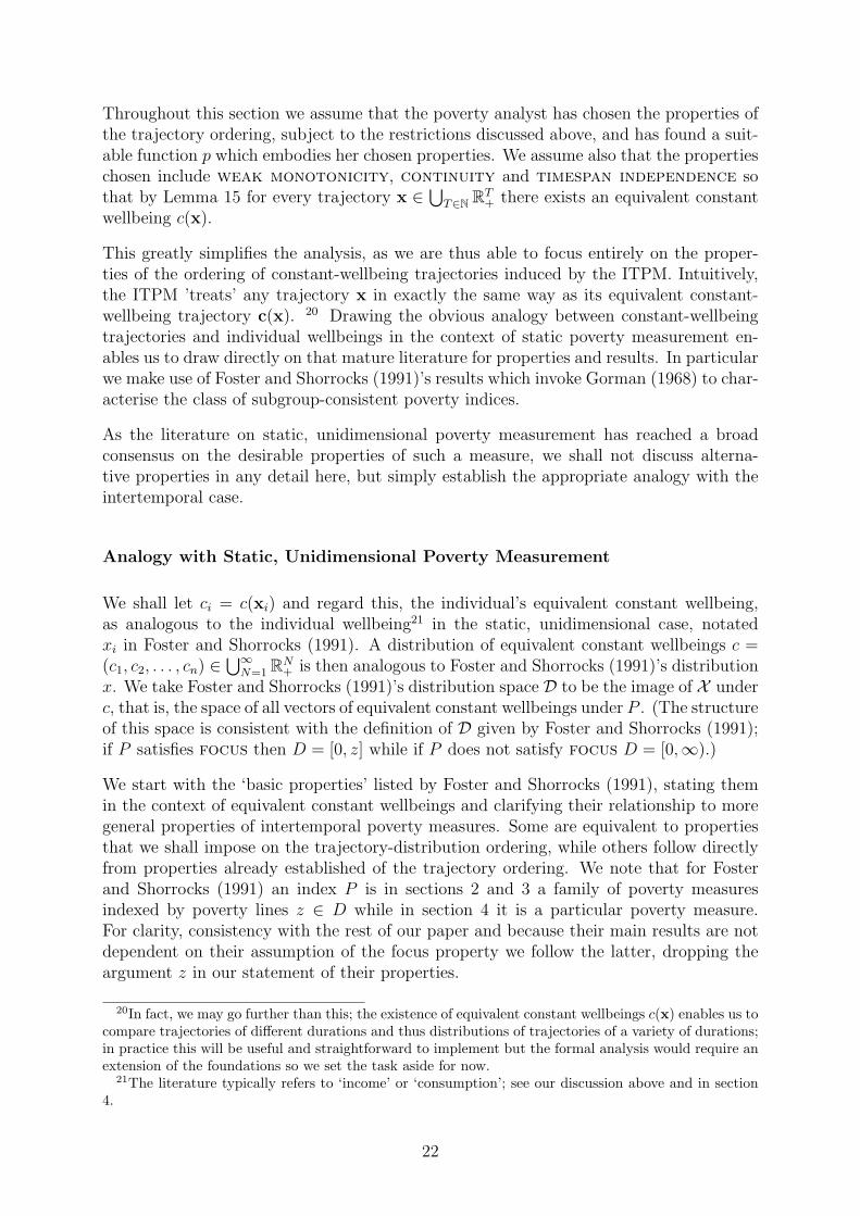
Isoquants of p:

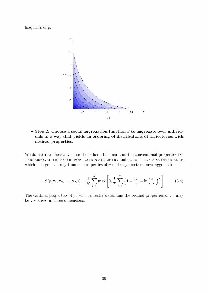
• Step 2: Choose a social aggregation function S to aggregate over individ-uals in a way that yields an ordering of distributions of trajectories withdesired properties.

We do not introduce any innovations here, but maintain the conventional properties in-

terpersonal transfer, population symmetry and population-size invariance

which emerge naturally from the properties of p under symmetric linear aggregation:

S(p(x1,x2, . . . ,xN)) =1

N

N∑i=1

max

[0,

1

T

T∑t=1

(1− xit

z− ln

(xit

z

))](3.4)

The cardinal properties of p, which directly determine the ordinal properties of P , maybe visualised in three dimensions:

30

• Step 3: If necessary, choose a transformation function G to yield a povertymeasure with the desired cardinal properties.

The important cardinal properties are already achieved; we simply introduce a normali-sation 1

2to yield, to some extent, cardinal comparability with the measures proposed by

Foster and Santos (2006). The poverty measure is thus

P (X) = G(S(p(x1,x2, . . . ,xN))) =1

N

N∑i=1

max

[0,

1

2T

T∑t=1

(1− xit

z− ln

(xit

z

))]. (3.5)

For distributions of constant-wellbeing trajectories (abstracting from the different transferproperties), P converges to the Foster-Santos measure as x → z.

We may summarise the properties of the aggregate measure P (X) by noting that it sat-isfies all the conditions for Corollary 17 and therefore has the properties population

symmetry, population-size invariance and population subgroup decompos-

ability.

31

3.2 Generalisation

The analysis above may be generalised to a whole family of poverty measures by takinglinear combinations of different CES functions, for example:

P (X) =1

N

N∑i=1

max

[0,

1

2T

T∑t=1

(z

xit

+ ln

(z

xit

)− 1

)](3.6)

and

P (X) =1

N

N∑i=1

max

[0,

1

3T

T∑t=1

((z

xit

)2

+ ln

(z

xit

)− 1

)]. (3.7)

These measures have the same properties as (3.5) but in fact allow for a lower degree ofintertemporal compensation, as illustrated by the isoquants of (3.7):

More generally, for some k ∈ N,

P (X) =1

N

N∑i=1

max

[0,

1

(k + 1)T

T∑t=1

((z

xit

)k

+ ln

(z

xit

)− 1

)]. (3.8)

The degree of intertemporal compensation decreases as k increases.

32

4 An empirical application: poverty in rural Ethiopia

In this section we provide an empirical application using data from the Ethiopian Ru-ral Household Survey (ERHS). We firstly provide static measures of consumption basedpoverty, followed by transition matrices and finally the set of duration-adjusted povertymeasures proposed in the literature and discussed in the analytical section above. Weexamine which households remain classified as poor and the proportion of the householdsthat are classified as poor when the methodology changes. We shall use real household(per adult equivalent) average consumption (defined below) as our measure of welfare.

4.1 Data

Data are from the Ethiopian Rural Household Survey (ERHS) collected by the Universityof Addis Ababa and the Centre for the Study of African Economies (CSAE) at the Uni-versity of Oxford, as well as the International Food Policy Research Institute (IFPRI).Data are available from fifteen districts25 in several regions. Seven villages were originallyincluded in IFPRI’s survey of 1989, which were chosen primarily because they had suf-fered hardships in the period 1984–89 (the 1984–85 famine). For a detailed descriptionsee Webb, von Braun, and Yohannes (1992). In 1994, 360 of the households in six vil-lages were retraced and the sample frame was expanded to 1477 households. The nineadditional communities were selected to account for the diversity in the farming systemsin the country. Within each village, random sampling was used. The households wereresurveyed again in 1994 and 1995, and subsequently in 1997 and 1999. The sixth andlatest round of the survey was completed in 2004. The attrition rate is low, less than oneper cent per annum (annualised, or 12.1% in total between 1994 and 2004). Since thethree surveys in 1994-1995 are within eighteen months of each other, we drop the secondround of 1994, in order to use five rounds of the data for our subsequent analysis.

The dependent variable or welfare measure chosen is real household monthly consumptionper adult-equivalent. This is comparable with other studies of consumption and povertythat have been conducted on the dataset, and other studies of poverty. In the ERHS,detailed information is also available on household income and assets. At the individuallevel, there is information on height and weight though not for all individuals and not forall rounds. Data on monthly consumption of food, purchased food and non-investmentnon-food items (excluding durables, as well as health and education expenditure) basedon purchased items, gifts in cash and in kind, and a diary of consumption from ownproduction from a two-week recall period was divided by adult equivalent units based onWorld Health Organisation (WHO) guidelines. This was deflated by a food price indexconstructed from data collected for each village at the same time as the household survey.For a detailed discussion on the construction of the consumption indicator, see Derconand Krishnan (1998). Food represents around eighty per cent of the consumption basket.We use a consumption poverty line calculated by Dercon and Krishnan (1998) which isvillage specific (according to local prices) and averages 44.3 Birr per adult equivalent per

25 These communities are called Woredas, the equivalent of a county in the UK. They are furtherdivided into Peasant Associations (PAs), the equivalent of a village, and consist of up to several villages(e.g. the ERHS comprises 15 Woredas, and 18 PAs). The administrative system of the PAs was createdin 1974 after the revolution.

33

month (all prices are specified in 1994 real terms). It is based on the monthly cost of thediet to achieve 2100 Kcal per day per adult, using the food consumed by the poorer half ofthe sample, and minimum ‘essential non-food’ expenditure.26 For analytical convenience,we include only households in the analysis that have nonmissing values of consumption foreach available round, restricting the sample to 1168 households. We also ignore changes inhousehold composition, apart from in the calculation of consumption per adult equivalent,and therefore abstract somewhat from measuring individual welfare. In the ERHS, theonly possibility to examine individual wellbeing would be through an anthropometricmeasure, which is a focus for future work.

4.2 Annual poverty measures and transition matrices

Table 2 shows the standard Foster-Greer-Thorbecke (FGT) poverty indices for the fiveyears. We observe a decline in poverty as measured by all three indices, by around similarmagnitudes – the percentage of poor falling from almost 40% poor to 26%. Althoughthe headcount falls, the mean consumption of the poor only grows by around 1.5% perannum (or 12.5% in total between the first and last rounds). Table 3 breaks this downby village, and shows that whilst a number of villages have had relatively low poverty inall time periods (e.g. Debre Birhan villages), some villages have experienced high povertyrates for most of the time (e.g. Gara Godo, Imdibir, Adado). Other villages had veryhigh poverty in 1994, but have shown a substantial reduction in poverty rates by 2004(e.g. Geblen, Domaa, Korodegaga).

Table 4 shows that of the households who were classified as poor in 1994, a third were stillpoor in 2004, 10% of all households. Table 5 breaks this down further and looks at relativepositions in the consumption distribution keeping quintile cutoffs fixed at the 1994 level.Whilst the diagonal (no movement between quintiles) is the most populous quadrant, thetable does show that upward mobility is happening, with more than proportional numbersending up in the top three quintiles. However, just over 22% of households do remain inthe two bottom quintiles in both time periods.

4.3 Introducing a time dimension to poverty measures

Poverty duration

Table 2 showed that 24–39% of the households were below the poverty line in each round,and in cross-sectional analysis the aggregate rate is all that can be shown. It also calcu-lated the average consumption of the households under the poverty line, but it was notpossible to say anything about the poverty experiences of individual households. Table 6

26Dercon and Krishnan (1998) show the calculations in depth. Also note that the household wasconsidered the same between rounds if the head of the household was unchanged, while if the headhad died or left the household, the household was considered the same if the current household headacknowledged that the household (in the local meaning of the term) was the same as in the previousround. In 1994 the exchange rate of the Ethiopian Birr (ETB) with the USD, corrected for purchasingpower parity was 0.21875. One PPP dollar is worth 1.75 its equivalent in USD [World Bank (2000)],and the exchange rate was 8 ETB to 1 USD. Therefore the Dollar a Day poverty line (1.08) would becalculated as approximately 148 Birr per adult per month, around three times that which we use here.

34

shows in fact that only very few (twenty four, or just over 2%) of households are actuallyclassified as poor in all five time periods. However, nine per cent are poor in at least fourout of five periods. A substantial majority (just under 65%) of households have falleninto poverty at least once in the ten years, showing that many are vulnerable to povertydespite having consumption above the poverty line.

Comparing intertemporal poverty measures

In this section, we compare the measures found in the recent intertemporal poverty mea-surement literature that were analysed above. All of these measures satisfy differentproperties, and we discussed table 1 showing the variety of properties satisfied by themeasures. We calculate the measures of Calvo and Dercon (2007); Jalan and Ravallion(2000); Foster and Santos (2006); Foster (2007) as well as the new measure proposedabove and show how altering the policy parameters can affect the classification of whichhouseholds are poor, and how the aggregates change, firstly by village, and then by someother characteristics that are often cited as correlates of poverty. As noted above, weare using average household consumption per adult equivalent as the welfare measure.A large literature (see Fafchamps (2003) or Dercon (2004) for an overview) shows thatincomes in developing countries can be highly erratic and that risk is central to economicdecision making. There is also considerable evidence that households who are faced withrisk use all available methods to ‘smooth’ their consumption, on a daily and seasonalbasis, and also in the face of a negative shock (such as crop failure, or household illness).We therefore assume that households have smoothed their consumption to the best oftheir ability (for other work on evidence for this in the ERHS dataset see Dercon andKrishnan (2000), Dercon, Hoddinott, and Woldehanna (2005). The measure by Fosterand Santos (2006) allows us to choose a (constant) degree of intertemporal substitution,and therefore we make it relatively low, setting β = −1 in equation 2.10 above. Wechoose the measure outlined above that has a similar elasticity of intertemporal welfareto that of Foster and Santos (2006) close to the poverty line, but reduces the elasticityof substitution as the poverty gap gets larger (to extremely low levels at extremely highpoverty), or setting k = 2.

Table 7 shows what proportion of households are classified as ‘poor’ by the measuresproposed in the literature.27 Foster (2007) has a flexible duration poverty line, whichalters the proportion of poor households considerably, as can be understood from table6: just under ten percent of households are poor for four or five periods, rising to 21.5%if we include households that are poor three or more periods. Calvo and Dercon (2007)generalise Foster (2007), and propose no duration cutoff. Their measure is thereforenon-zero for any household experiencing any poverty during the decade. Hence, almost67% of households are classified as poor by this definition. Foster and Santos (2006)define as chronic poor those households with a generalised mean below the poverty line.In this case we choose β = −1 for the choice parameter, the harmonic mean.28 Justunder 30% are classified poor by this method. Jalan and Ravallion (2000) set the chronicpoverty identification step as those households whose arithmetic mean consumption is

27None of the authors of the papers recommend using this quasi-headcount for policy or analysis,however we consider it useful for illustration to compare the populations covered by each measure.

28The authors (Foster and Santos, 2006) provide an illustration of choice of β.

35

below the poverty line, which is 13.4% of households. Finally the measure as proposedabove classifies 31.2% of households as below the poverty line.29

In table 8 the correlations between the calculated poverty measures is shown. As expected,all are positive and significant at 1%. The highest correlation is between the two measureswith similar structure, those of Calvo and Dercon, and Foster (2007). The Porter-Quinnmeasure and Foster-Santos measure are also highly correlated, as the two have very similarproperties (diverging mainly at extreme levels of poverty and very close to the povertyline).

In table 9 we compare the measures of duration adjusted poverty discussed above forthe fifteen ERHS villages, by showing the share of total poverty as defined by the mea-sure,30 allowing us to make comparisons despite the measures having different scales andinterpretations. One village, Gara Godo dominates with a share of poverty from 29%(Calvo-Dercon) to 50% (Jalan-Ravallion), with a population share of only 8%. This isnot necessarily easily predicted from the static poverty estimates (as shown in table 3):Gara Godo is amongst the poorer villages, but Imdibir for example appears to have similarpoverty rates taking all periods together. The measures appear to rank similarly, thoughthere are a number of differences. Poverty is more evenly spread using the Calvo-Derconmeasure, due to the higher proportion of the population that enter the reference group.Porter-Quinn weights Trurufe Ketchema more heavily than other measures, due to someextremely poor households.

Table 10 provides a more general poverty profile based on household and head of householdcharacteristics in 1994. Given these characteristics, would any of them correlate withfuture higher poverty in the next decade? None of the measures shows differential inpoverty between male and female headed households. All of the measures however showthat households with heads that are unable to read make up a more than proportionateshare of intertemporal poverty, in particular as measured by Porter-Quinn and Foster-Santos (indicating that these households may suffer episodes of extreme povetry). Assetholdings appear to matter too, with land- and livestock-poor households (defined as havingrespective asset holdings below the median) accounting more than proportionately forintertemporal poverty. Only Jalan-Ravallion shows that large households are more thanproportionately poor.

In table 11 we present some descriptive logits to analyse correlates of poverty as measuredwith depth and duration over the ten year period and present marginal effects. Thenumbers classified as poor and non-poor can be taken from tables 2 and 7. We startwith correlates of static poverty at the beginning and end of the period (e.g. in 1994and 2004 respectively). We find a strong correlation between initial assets and initialpoverty, with few other significant factors (apart from male children). End-period povertyis also correlated with lower livestock holdings, and also higher household size in 2004.The descriptive logit for the intertemporal measure shows more correlates. Livestockis again a good predictor of poverty experienced over the decade. Similarly a largerhousehold size and uneducated household head increases the probability of being classified

29For ease of reading, we now abbreviate the measures to the names of the lead authors, with Jalan andRavallion (2000) as Jalan-Ravallion, Foster (2007) as Foster (D3) since we adopt the three period cutofffor that measure, Foster and Santos (2006) as Foster-Santos, Calvo and Dercon (2007) as Calvo-Dercon,and our measure as Porter-Quinn.

30Here we take the value of the measure, not the headcount as in table 7.

36

in poverty over the period. We include measures of shocks in the regressions and find thatwhilst agricultural shocks are not significant, illness does increase the probability of beingclassified as poor. Having a high share of crop income in total income in the first periodalso substantially decreases the probability of being classified as poor, though this maybe proxying for land holdings (which we exclude as 100 households have missing valuesfor land).

4.4 Extensions and sensitivity analysis

Measurement error is a problem in many household surveys (see Deaton (1991) for acomprehensive treatment) and has been widely dealt with in the static context. Theissue of measurement error could become a more difficult problem if we had reason tosuspect serial correlation in the measurement error, or that the direction/magnitude issomehow correlated with the household fixed-effect. Downward measurement error at thelower end of the consumption distribution would probably increase the poverty estimates.We note also that measurement error can cause an over-estimate in mobility betweenrounds, however, measures that allow a degree of intertemporal compensation may averageout some of the measurement error. Sensitivity to extremely low levels of welfare is avery desirable attribute of a poverty measure, but if the low levels are due to downwardmeasurement error then we will over-estimate poverty.

Censoring at both sides of the distribution may cause changes in measures downwardthat do allow intertemporal compensation of welfare above the poverty line. On the otherhand, measures that have a high degree of intertemporal compensation may have less biaswith respect to downward measurement error, but may lead to under-counting in the caseof upward measurement error. We recalculated the poverty shares by village as shownin table 9 but with consumption per adult censored to the 5th and 95th percentiles, inorder to examine the changes. Porter-Quinn and Foster-Santos showed some sensitivityto this change, probably due to the highly sensitive nature of the measures to extremelevels of poverty. Data reliability should be a consideration when choosing the amount ofintertemporal compensation that is required in the measure.

We may also wish to examine sensitivity to the choice of poverty line, since it is alsofairly arbitrary. We recalculated the village-level poverty rates as in table 9, but with thepoverty line augmented by 20%. The distribution did not change for our measure. 31

The previous analyses have taken real household consumption per adult equivalent asthe welfare measure upon which to base calculations of welfare underlying the povertymeasures. As outlined in the theory section, it is impossible to have a direct measureof wellbeing. We are assuming in the analysis that the consumption and whatever wemean by ‘wellbeing’ or welfare are monotonically related (Sen, 1976). This will not hold,for example, in the case where public goods provisioning changes over time, and there isan implicit assumption in the measures that when we compare across villages that thesethings change at a constant rate across all regions. In principle, it would be possibleto calculate the intertemporal measures based on some kind of multidimensional welfaremeasure, though this is beyond the scope of this chapter. Aside from the criticism of

31There were not many major differences in the distribution of poverty for the other measures, with theexception of the Foster(D3) measure, which is perhaps due to the discontinuity inherent in the measure.

37

consumption as a restrictive welfare measure, we also contend with the argument that ahousehold measure does not capture the welfare of the individuals: it ignores intrahouse-hold distribution of welfare. In order to be able to compare directly between householdswe calculate consumption per adult equivalent. Deflating the consumption basket to real1994 Birr allows us to assert that the welfare measure is directly comparable across timeperiods. In summary, we are assuming inter-household and intertemporal comparabilityof the poverty measures.

In summary, the poverty measure should be chosen on the basis of desirable theoreticalproperties, but also on the basis of empirical considerations that may feed into the theo-retical properties. There may be other empirical considerations: do we need to define asub-group of the poor for policy purposes, or calculate the total burden of poverty in theeconomy? If the data quality is expected to be very poor, a measure that averages moreacross time may be theoretically less appealing but may be less sensitive to measurementerror. Finally, as noted above, the measure used in practice may depend on intuitiveunderstanding rather than desirable properties.

5 Conclusions

The approach to poverty analysis that we have taken in this paper builds firm foundationsfor the understanding of poverty profiles, and adds considerable depth to the debate onpoverty measurement. The empirical section has applied the new measures of chronicpoverty to a sample of Ethiopian rural households. We find that the assumptions (bothexplicit and implicit) in the duration-adjusted poverty measures make a considerabledifference to the identification of the poorest households in the sample. We also find thatinitial characteristics, especially low levels of education, and risk and shocks increase theprobability of low welfare over the time period in question.

The analysis in this paper provides a more rigorous foundation for the construction ofintertemporal poverty measures that enables clarity regarding their properties and thus,we hope, greater clarity in the interpretation and conclusions that may be drawn whenthey are applied to empirical or policy analysis.

The method we develop for construction of intertemporal poverty measures requires onlymild restrictions on the properties they possess, and the space of measures that may bedeveloped within this framework remains to be further explored. Although a consensushas been reached in the poverty measurement literature regarding desirable propertiesof the population-distribution ordering, a similar consensus has not been achieved in theintertemporal context for the properties of the trajectory ordering. In fact, as we discussabove, different properties will be necessary in different contexts of application. Themeasures suggested in the recent literature and the new family of measures proposedin this paper certainly do not exhaust the possibilities. We hope that the analyticalframework developed in this paper will prove useful for the development of measures withdifferent trajectory ordering properties. In particular, we believe that there remains aneed for a measure that appropriately captures chronicity of poverty.

38

A Tables

39

Tab

le1:

Pro

per

ties

ofin

tert

empor

alpov

erty

mea

sure

sTra

ject

ory

ord

eri

ng

Jala

n-R

avallio

nFost

er

Calv

o-D

erc

on

Fost

er-

Santo

sPort

er-

Quin

n

Con

tinuity

��

��

�

Wea

km

onot

onic

ity

��

��

�

Str

ict

mon

oton

icity

��

a�

b�

�Focu

spro

pert

ies

Wea

kfo

cus

��

��

�

Focu

s�

��

��

Tem

pora

lP

ropert

ies

Tim

esy

mm

etry

��

(�)

��

Sen

siti

vity

totr

end

��

�c

��

Inte

rtem

por

altr

ansf

er�

(�)

(�)

��

Non

-dec

reas

ing

com

pen

sati

on�

��

��

Incr

easi

ng

com

pen

sati

on�

��

��

Dura

tion

Sen

siti

vity

(1)

��

�d

��

Dura

tion

Sen

siti

vity

(2)

��

�e

��

Not

es:

The

tabl

esh

ows

prop

erti

esof

the

traj

ecto

ryor

deri

ngp

asou

tlin

edin

anal

ysis

sect

ion.

Form

ulae

for

the

mea

sure

sca

nal

sobe

foun

din

this

sect

ion.

()de

note

sm

easu

reha

sth

epr

oper

tybe

low

the

pove

rty

line

only

.

aIf

α>

0bIf

α>

0cIf

disc

ount

rate

appl

ied

dIf

α>

0eIn

one

spec

ifica

tion

40

Table 2: Standard poverty measures, by roundYear Headcount Poverty Gap Sq-Poverty Gap Mean cons.

F-G-T (0) F-G-T (1) F-G-T (2) of poor (Birr)1994 0.39 0.16 0.09 26.841995 0.44 0.19 0.10 25.721997 0.24 0.08 0.04 30.311999 0.28 0.09 0.04 31.132004 0.22 0.07 0.03 30.29

Notes: Source is ERHS data, own calculations. Poverty line is 44.3 Birr per adult, per month on average(though varies by village ). Number of observations is 1168. Measures are weighted by household size.

Table 3: Headcount poverty, by village and roundPeasant association 1994 1995 1997 1999 2004

Haresaw 0.34 0.56 0.25 0.17 0.28Geblen 0.79 0.76 0.24 0.38 0.28Dinki 0.52 0.62 0.49 0.38 0.24Yetemen 0.07 0.21 0.08 0.27 0.15Shumsheha 0.08 0.06 0.09 0.01 0.02Sirbana Godeti 0.15 0.07 0.11 0 0.02Adele Keke 0.13 0.07 0.02 0.26 0.24Korodegaga 0.68 0.56 0.31 0.15 0.26Trurufe Ketchema 0.23 0.32 0.3 0.15 0.19Imdibir 0.55 0.85 0.4 0.48 0.61Aze Deboa 0.3 0.65 0.28 0.76 0.23Adado 0.32 0.56 0.2 0.31 0.49Gara Godo 0.89 0.89 0.64 0.54 0.42Domaa 0.62 0.33 0.35 0.19 0.11Db-milki 0.31 0.26 0.03 0.04 0.02Db-kormargefia 0.2 0.24 0.05 0.13 0.03Db-karafino 0.23 0.29 0.03 0.06 0.14Db-faji bokafia 0.09 0.26 0 0.12 0

Notes: Poverty line as above, headcount measure.

Table 4: Transition Matrix, Households over ten yearsStatus in 2004

Status in 1994 Poor Non-poorPoor 11.76% 27.22% 38.98%Non-poor 10.10% 50.92% 61.02%

21.86% 78.14%

41

Table 5: Transition Matrix, consumption quintiles, holding quintile cutoff constant at1994 level

1994Quintile in 2004 1 2 3 4 5 totals

1 8.53 2.81 1.56 1.27 0.67 14.832 3.82 7.12 2.88 2.18 1.57 17.573 3.25 3.63 7.76 3.60 3.33 21.574 2.17 2.72 3.52 7.69 3.53 19.625 2.24 3.72 4.28 5.27 10.91 26.41

20.00 20.00 20.00 20.00 20.00 100.00

Table shows transition

matrix between quintiles fixed at the 1994 levels as shown in table ??, showing absolute rather thanrelative movement.

Table 6: Poverty Duration (Nr times hh classified as poor)Counted poor Nr households Percent Cum. Percent

Never 424 36.30 100Once 297 25.43 63.70Twice 202 17.29 38.27Thrice 138 11.82 20.98Four times 77 6.59 9.16In every period 30 2.57 2.57

Total 1,168 100.00 100.00Notes: Cumulative percent works backwards: i.e. the number of households// poor in at least n periods

Table 7: Duration adjusted poverty measures ‘headcount’Measure % households ‘poor’ DefinitionFoster (2007) 9.7 xht < z for 4 or more periodsFoster (2007) 21.5 xht < z for 3 or more periodsCalvo-Dercon (2007) 63.7 xht < z for more than 0 periodsFoster-Santos (2006) 29.4 general (harmonic) mean xh < zJalan-Ravallion (2000) 13.4 arithmetic mean xh < zPorter-Quinn (2008) 31.2 utility below ‘equivalent constant’ z

Notes: Equations showing the poverty measures are outlined in section ?? of the text. The authors of thepapers do not recommend using the headcount for policy purposes, this table is simply for illustration sothat we can compare what proportion of the population make up the relevant study population for eachmeasure. Note that Foster (2007) and Foster-Santos(2006) have flexible parameters which can change theproportion of households classified as poor. We note as an illustration above the Foster(2007) measurewith the duration poverty line set at 3 periods and 2 periods respectively.

42

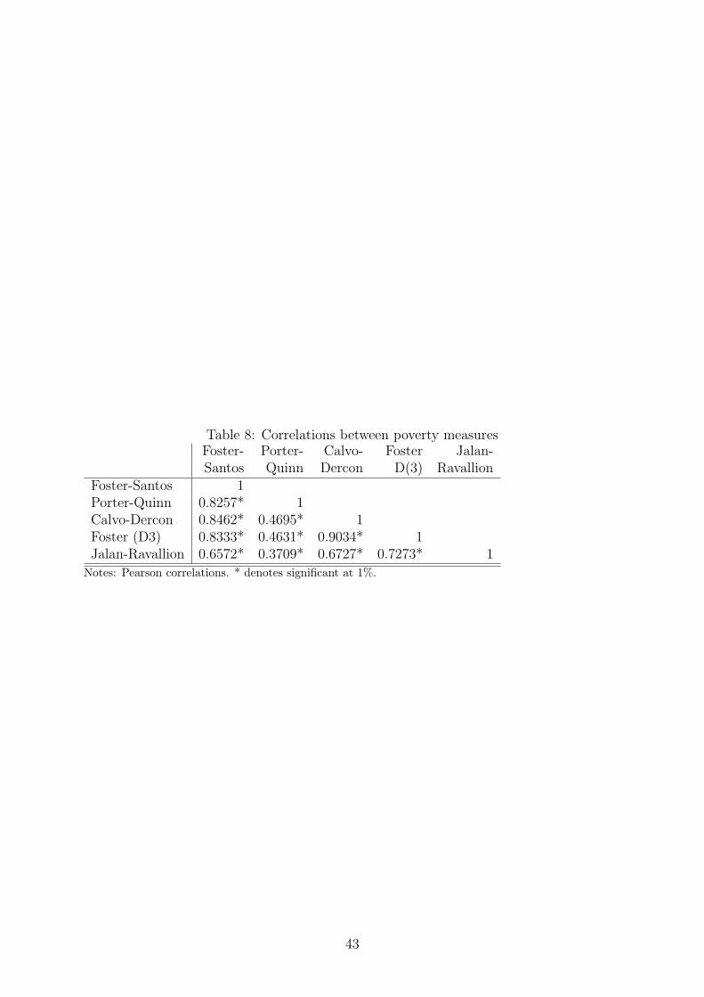
Table 8: Correlations between poverty measuresFoster- Porter- Calvo- Foster Jalan-Santos Quinn Dercon D(3) Ravallion

Foster-Santos 1Porter-Quinn 0.8257* 1Calvo-Dercon 0.8462* 0.4695* 1Foster (D3) 0.8333* 0.4631* 0.9034* 1Jalan-Ravallion 0.6572* 0.3709* 0.6727* 0.7273* 1

Notes: Pearson correlations. * denotes significant at 1%.

43

Table 9: Duration adjusted poverty measures by villagePeasant Porter- Jalan- Foster Calvo- Foster- PopulationAssociation Quinn Ravallion (D3) Dercon Santos contribution

Haresaw 0.04 0.01 0.03 0.05 0.04 0.06Geblen 0.09 0.09 0.11 0.10 0.11 0.04Dinki 0.02 0.06 0.06 0.05 0.04 0.06Yetemen 0.00 0.00 0.00 0.01 0.00 0.04Shumsheha 0.00 0.00 0.00 0.01 0.00 0.08Sirbana Godeti 0.00 0.00 0.00 0.00 0.00 0.06Adele Keke 0.03 0.00 0.01 0.04 0.02 0.07Korodegaga 0.05 0.04 0.09 0.09 0.07 0.08Trurufe Ketchema 0.18 0.03 0.02 0.03 0.06 0.07Imdibir 0.04 0.11 0.08 0.08 0.07 0.06Aze Deboa 0.01 0.01 0.05 0.05 0.02 0.05Adado 0.02 0.03 0.04 0.05 0.03 0.07Gara Godo 0.34 0.50 0.39 0.29 0.38 0.08Domaa 0.15 0.13 0.11 0.11 0.14 0.05Db-milki 0.00 0.00 0.00 0.02 0.01 0.05Db-kormargefia 0.00 0.00 0.01 0.02 0.00 0.05Db-karafino 0.00 0.00 0.00 0.01 0.00 0.03Db-faji bokafia 0.00 0.00 0.00 0.00 0.00 0.02

Notes: Measures defined as in table 7 above. ‘Foster’ refers to Foster’s (2007) chronic poverty measure,with duration cutoff 3/5 time periods. Foster-Santos sets β = −1. Porter-Quinn sets k = 2.

44

Table 10: Poverty by household characteristicsHousehold (Head) Porter Jalan Foster Calvo Foster Population

Characteristics -Quinn -Ravallion (D3) -Dercon -Santos contributionFemale 0.26 0.22 0.24 0.27 0.27 0.27

Male 0.72 0.72 0.72 0.71 0.71 0.73

Unable to read 0.84 0.72 0.78 0.76 0.81 0.62Able to read 0.16 0.28 0.22 0.24 0.19 0.38

Small HH 0.62 0.49 0.53 0.57 0.56 0.62Large HH 0.38 0.51 0.47 0.43 0.44 0.38

Land Poor 1994 0.62 0.52 0.54 0.53 0.57 0.53Land Rich 1994 0.29 0.37 0.37 0.37 0.34 0.47

Livestock Poor 1994 0.67 0.59 0.56 0.58 0.60 0.49Livestock Rich 1994 0.33 0.41 0.44 0.42 0.40 0.51

Notes: In the rows for land poor and land rich, n=999 due to missing data on land holdings, hencepercentages do not sum to 100. n for other rows is 1089.

45

Table 11: Descriptive Poverty Logits

Pov 94 Pov 04 Port-QuinnMarg-FX Marg-FX Marg-FX

Livestock 94 -.028* -.031*** -.043**Sex hh head 94 (d) -0.023 0.001 -0.056Head schooling (d) -.109* -0.027 -.107**Female adults 94 .047* .020* .062***Male children 94 0.045 0.009 0.029Female children 94 0.037 0.003 .092***Male 5-15 94 .082*** .028* .104***Female 5-15 94 0.028 -0.003 0.058Female elderly 94 -0.013 0.014 0.009Male elderly 94 (d) -0.026 -0.038 0.003Crop Share Income -0.163 -0.071 -.230**Ill adults 94 0.047Crop shock 94 0.105Rainfall quintile 94 -0.034CV village rainfall 0.003 0.001 0.005Average ill adults 94-04 0.016 .151*Average crop shock 94-04 -0.026 -0.357Rain 94-97 .000** .000*Rain 98-04 0 0HH size 2004 .023*** 0.005Village road improved 0.002 -0.03

Notes: The dependent variable is the poverty headcount in 1994 and 2004 respectively, based on con-sumption per adult equivalent being below the poverty line, and a binary variable based being poor asdefined by the Porter-Quinn measure.

46

References

Atkinson, A. B. (1987): “On the Measurement of Poverty,” Econometrica, 55(4), 749–764.

(2003): “Multidimensional Deprivation: Contrasting Social Welfare and Count-ing Approaches,” Journal of Economic Inequality, 1(1), 51.

Bane, M. J., and D. T. Ellwood (1986): “Slipping Into and Out of Poverty: theDynamics of Spells,” Journal of Human Resources, 21(1), 1–23.

Bank, W. (2001): World Development Report 2000/2001.

Baulch, B., and J. Hoddinott (2000): “Economic Mobility and Poverty Dynamicsin Developing Countries,” Journal of Development Studies, 36(6), 1.

Bourguignon, F., and S. R. Chakravarty (2003): “The Measurement of Multidi-mensional Poverty,” Journal of Economic Inequality, 1(1), 25.

Calvo, C., and S. Dercon (2007): “Chronic Poverty and All That: the Measurementof Poverty over Time,” Discussion paper, Centre for the Study of African Economies,University of Oxford.

Chakravarty, S. R. (1983): “A New Index of Poverty,” Mathematical Social Sciences,6, 307–313.

Chaudhuri, S., and M. Ravallion (1994): “How well do static indicators identify thechronically poor?,” Journal of Public Economics, 53(3), 367–394.

CPRC (2004): “The Chronic Poverty Report 2004-05,” Discussion paper, ChronicPoverty Research Centre.

Deaton, A. (1991): Household saving in LDC’s : credit markets, insurance and wel-fare. Research Program in Development Studies Woodrow Wilson School PrincetonUniversity, Princeton, N.J.

Dercon, S. (2004): Insurance against poverty, Studies in development economics. OxfordUniversity Press, Oxford.

(2006): “Poverty Measurement,” in The Elgar Companion to Development Stud-ies, ed. by D. A. Clark. Edward Elgar.

Dercon, S., J. Hoddinott, and T. Woldehanna (2005): “Shocks and Consumptionin 15 Ethiopian Villages, 19992004,” Journal of African Economies, 14(Number 4).

Dercon, S., and P. Krishnan (1998): “Changes in Poverty in Rural Ethiopia 1989-1995: Measurement, Robustness Tests and Decomposition,” Discussion Paper WPS/98-7, Centre for the Study of African Economies.

(2000): “In Sickness and in Health: Risk Sharing within Households in RuralEthiopia,” Journal of Political Economy, 108(4), 688.

Fafchamps, M. (2003): Rural poverty, risk and development. Edward Elgar, Chel-tenham.

47

Foster, J., J. Greer, and E. Thorbecke (1984): “A Class of Decomposable PovertyMeasures,” Econometrica, 52(3), 761–766.

Foster, J., and M. E. Santos (2006): “Measuring Chronic Poverty,” .

Foster, J. E. (2007): “A class of chronic poverty measures,” Discussion paper, Depart-ment of Economics, Vanderbilt University.

Foster, J. E., and A. F. Shorrocks (1991): “Subgroup Consistent Poverty Indices,”Econometrica, 59(3), 687–709.

Gorman, T. (1968): “The Structure of Utility Functions,” The Review of EconomicStudies, 35(4), 367–390.

Hulme, D., and A. Shepherd (2003): “Conceptualizing Chronic Poverty,” WorldDevelopment, 31(3), 403–423.

Jalan, J., and M. Ravallion (1998): “Behavioral responses to risk in rural China,”Discussion paper, World Bank Development Research Group Poverty and Human Re-sources, Jyotsna Jalan and Martin Ravallion. 28 cm. ”September 1998”–Cover.

(2000): “Is Transient Poverty Different? Evidence for Rural China,” Journal ofDevelopment Studies, 36(6), 82.

McCulloch, N., and M. Calandrino (2003): “Vulnerability and Chronic Poverty inRural Sichuan,” World Development, 31(3), 611–628.

McKay, A., and D. Lawson (2003): “Assessing the Extent and Nature of ChronicPoverty in Low Income Countries: Issues and Evidence,” World Development, 31(3),425–439.

Narayan-Parker, D., R. Patel, K. Schaff, A. Rademacher, and S. Koch-

Schulte (2000): Voices of the poor : can anyone hear us?, vol. 1 of Voices of the poor.Oxford University Press for the World Bank, Oxford.

Nussbaum, M. C., and A. K. Sen (1999): The quality of life, Studies in developmenteconomics. Oxford University Press, New Delhi.

Ravallion, M. (1996): “Issues in measuring and modelling poverty,” Economic Journal,106(438), 1328–1343.

Rowntree, B. S. (1901): Poverty : a study of town life. Macmillan, London.

Sen, A. K. (1976): “Poverty: An Ordinal Approach to Measurement,” Econometrica,44(2), 219–231.

(1982): Choice, welfare and measurement. Basil Blackwell, Oxford.

(1997): Choice, welfare and measurement. Harvard University Press, Cambridge,Mass. ; London.

(2001): Development as freedom. Oxford University Press, Oxford.

Stevens, A. H. (1999): “Climbing out of poverty, falling back in: measuring the persis-tence of poverty over multiple spells,” Journal of Human Resources, 34, 557–588.

48

Webb, P., J. von Braun, and Y. Yohannes (1992): “Famine in Ethiopia: PolicyImplications of Coping Failure at National and Household Levels,” Discussion Paper 92,International Food Policy Research Institute (IFPRI).

49