IntroductionGeneral ConsiderationsQuantitative structure–activity relationships(QSARs) are mathematical models approxi-mating the often complex relationshipsbetween chemical properties and biologicalactivities of compounds. Common objectivesof such models are a) to allow prediction ofbiological activity of untested and sometimesyet unavailable compounds and b) to extractclues of which chemical properties of com-pounds are likely determinants for their bio-logical activities. It is convenient to distinguishbetween QSARs and SARs: QSARs are typi-cally quantitative in nature, producing categor-ical or continuous prediction scales; SARs arequalitative in nature, often occurring in theform of structural alerts that include molecularsubstructures or fragment counts related to thepresence or absence of biological activity.

In this article, we review QSARs. Themost common techniques for establishingQSARs are based on regression analysis, neuralnets, and classification approaches. Among theregression-based approaches, the methods ofmultiple linear regression (MLR) and partialleast squares (PLS) regression are prime exam-ples. Examples of classification methodsinvolve, for example, discriminant analysis anddecision trees. It is important to observe thatclassification is a central concept also in regres-sion-based QSARs. A molecule that is not sat-isfactorily classified in a model—that is, it doesnot “fit” the model—should be handled withcare, and the model’s predictions should beconsidered with some skepticism. Hence,methods and tools for classification are ubiqui-tous in QSARs, regardless of the final form ofthe “equation.”

QSARs are increasingly used by authorities,industries, and other institutions for assessingthe risks of chemicals released to the environ-ment (Anonymous 1995, 1999). An impor-tant reason for this is the increasing awarenessthat completing even the most basic biologicaltesting of compounds of concern would takedecades. Therefore, predictive models (PMs)such as QSARs are necessary for aiding inchemicals management because they may con-siderably reduce costs, avoid animal testing,and speed up managerial decisions. In addi-tion, safety of new chemicals, often already inthe preproduction phase, can be assessed viaQSARs (Anonymous 1995, 1999; Wahlström1988). This may guide the design of com-pounds with fewer unwanted side effects byoptimizing their relevant properties. However,these potential benefits of QSARs can be ful-filled only if QSAR results are accepted at theregulatory level. The decision to accept QSARresults relies on assessing the reliability anduncertainty of the predictions as well asassessing the applicable domain of a QSAR.

Analogy ModelsThe goal in any QSAR modeling is to obtainthe mathematical expression that best portraysthe relationship between chemistry and biol-ogy. To adequately describe the often complexnature of such phenomena, it is often necessaryto use a battery of relevant and consistentchemical descriptors (Dunn 1989; Eriksson etal. 2001; Wold and Dunn 1983). Theassumption, or expectation, is then that thefactors governing the events in a biological testsystem are represented in the multitude ofdescriptors characterizing the compounds. Inother words, within a series of compounds—in

which biological activity is expressed via thesame mechanism—it is anticipated that a smallchange in chemical structure will be accompa-nied by a proportionally small shift in biologi-cal activity, and that the set of descriptors willreveal these analogies. Hence, QSARs aresometimes referred to as analogy models(Eriksson et al. 2001; Wold and Dunn 1983).

Analogy models can be regarded as lin-earizations of the real, complicated SARs.Wold and Dunn (1983) have shown that suchanalogy models normally have local validityonly, that is, can embrace only compoundswith similar chemical and biological data. It isnoted, however, that the substances must bedisparate enough to cause some systematicchange in biological activity.

The nature of the biological responsevariable under study has a strong impact onthe degree of chemical diversity that can beaccommodated by a QSAR model; that is,there is a trade-off between chemical diversityin the training set and complexity of the bio-logical response variable (Wold and Dunn1983; Eriksson et al. 2001). For an endpointvariable where measured data involve a specificand selective mechanism, it is expected that theresulting QSAR model cannot tolerate toomuch structural diversity in chemicals(Anonymous 1995, 1999). On the other hand,in less complicated cases, dealing with less“demanding” biological response variables, forexample, acute toxicity of narcotics to aquaticorganisms, QSAR models are usually possiblefor a much broader and more diverse set ofchemical structures.

The Role of Pattern Recognition in QSARsPattern recognition (PARC) is often describedas a procedure for formulating rules of classi-fication (Albano et al. 1978; Wold et al.1983) in multivariate data. PARC has beenused in a wide variety of applications such as

Environmental Health Perspectives • VOLUME 111 | NUMBER 10 | August 2003 1361

Methods for Reliability and Uncertainty Assessment and for ApplicabilityEvaluations of Classification- and Regression-Based QSARs

Lennart Eriksson,1 Joanna Jaworska,2 Andrew P. Worth,3 Mark T.D. Cronin,4 Robert M. McDowell,5

and Paola Gramatica6

1Umetrics, Umeå, Sweden; 2Procter & Gamble Eurocor, Central Product Safety, Strombeek-Bever, Belgium; 3European ChemicalsBureau, Institute for Health & Consumer Protection, Joint Research Centre, European Commission, Ispra, Italy; 4School of Pharmacy andChemistry, Liverpool John Moores University, Liverpool, United Kingdom; 5U.S. Department of Agriculture, Animal and Plant HealthInspection Service, Risk Analysis Systems, Riverdale, Maryland, USA; 6QSAR and Environmental Chemistry Research Unit, Departmentof Structural and Functional Biology, Insubria University, Varese, Italy

This article is part of the mini-monograph“Regulatory Acceptance of (Q)SARs for HumanHealth and Environmental Endpoints.”

Address correspondence to L. Eriksson, UmetricsAB, POB 7960, 907 19 Umeå, Sweden. Telephone:46-90-184852. Fax: 46-90-184899. E-mail:lennart.eriksson@umetrics.com

The authors declare they have no conflict of interest.Received 2 May 2002; accepted 3 February 2003.

This article provides an overview of methods for reliability assessment of quantitative structure–activ-ity relationship (QSAR) models in the context of regulatory acceptance of human health and environ-mental QSARs. Useful diagnostic tools and data analytical approaches are highlighted andexemplified. Particular emphasis is given to the question of how to define the applicability borders ofa QSAR and how to estimate parameter and prediction uncertainty. The article ends with a discussionregarding QSAR acceptability criteria. This discussion contains a list of recommended acceptabilitycriteria, and we give reference values for important QSAR performance statistics. Finally, we empha-size that rigorous and independent validation of QSARs is an essential step toward their regulatoryacceptance and implementation. Key words: QSAR acceptability criteria, QSAR applicability domain,QSAR reliability, QSAR uncertainty estimation, QSAR validation. Environ Health Perspect111:1361–1375 (2003). doi:10.1289/ehp.5758 available via http://dx.doi.org/ [Online 5 February 2003]

Regulatory Acceptance of (Q)SARs | Mini-Monograph

analytical chemistry, food research, andprocess monitoring in manufacturing. PARCmethods are useful also in QSARs (Wold andDunn 1983). Based on a set of given classes,each of which contains a number of observa-tions (in QSARs, compounds) mapped by amultitude of variables, guidelines, and rules aredeveloped that make it possible to classify newobservations (compounds) as similar or dis-similar to the members of the existing classes.

Experience shows that nature often seems toorganize itself in a clustered, rather discontinu-ous way. Inside a class or a cluster, the observa-tions (compounds) are rather similar to eachother, so if we know the class membership of anobservation, we can potentially infer a great dealabout it. The similarity among observationswithin each class is considerably greater thanamong observations of different classes. This isthe basis for the principle of analogy. If we knowthat a compound is a hydrocarbon, for instance,we can confidently predict how the compoundreacts or fails to react with various “reagents”because we know from experience that almostall hydrocarbons behave similarly, analogously,when subjected to various “treatments.”

It is therefore often practical to formulate aQSAR problem in terms of similarities andclasses. One tries to find a battery of easilyaccessible properties (variables) that can be usedto predict the class of an unknown observation(compound). One then infers that all observa-tions within a class behave similarly and thatthere are no outliers or further subclusteringendangering the foundation of the class model.Once such information is known, it is also pos-sible to determine which among existing—per-haps competing—QSAR models will bestaccommodate a candidate chemical for whichprediction of biological and environmental datais sought.

Scope of ReviewThe objective of this article is to review existingmethods for assessing the reliability and uncer-tainty of QSARs, particularly regarding predic-tive power and applicability domain. In sodoing, the objective is also to distill some indi-cators that can be used as acceptability criteria.In the section, “Conditions for Applicabilityand Validity of QSARs,” we outline basic con-ditions for the applicability of QSARs. In”Modeling Techniques” we review commonmodeling techniques in QSARs, with emphasison regression-based methods. In “Assessing/Enhancing Model Reliability, Interpretability,and Predictive Power,” we describe varioustools that aid the development and use ofQSARs. In “Bayesian Methods for ReliabilityTesting,” we consider Bayesian approaches andtheir applicability in QSAR reliability assess-ment, and, last, in the “Discussion,” weprovide concluding remarks with recommen-dations for acceptability criteria.

We make very clear that we are addressingimportant matters of QSARs from a statisticalperspective. Thus, the main focus lies on dis-cussing methods, procedures, and diagnostictools—mostly statistical in nature—aiding usin developing statistically and informationallysound QSARs. However, this very strongemphasis on data analytical aspects of QSARsdoes not mean that we refrain entirely fromtouching upon related and important itemsthat deal with, for example, compilation ofchemical and biological data, configuration ofdata tables, and so forth. It should be empha-sized, however, that we do not intend to delvedeep into detailed and practical issues regard-ing procedures for gathering the necessarychemical, biological, and toxicologic data.

Conditions for Applicability and Validity of QSARs

Homogeneity

Any data analysis, including QSAR modeling,is based on an assumption of homogeneity andabsence of influential outliers (Wold et al.1993; Eriksson and Johansson 1996). Thismeans that the investigated system, that is,series of compounds, must be in a similar“state”—have rather similar properties—throughout the investigation, and the mecha-nism of influence of X on Y must be the same.This, in turn, corresponds to having some lim-its on the variability and diversity of X and Y.These limits may be wide if the biologicalactivity is unspecific (e.g., acute toxicity to fishfor narcotic chemicals), or narrow if the biolog-ical endpoint involves a very specific mecha-nism of action (e.g., binding of substrates tothe active site of an enzyme).

Hence, it is essential that the data analysisprovide diagnostics about how well theseassumptions indeed are fulfilled. Much of therecent progress in applied statistics has con-cerned diagnostics, and many of these diagnos-tics can be used also in QSAR modeling asdiscussed later.

In many cases, QSAR modeling in riskassessment involves large databases of clusteredcompounds. Here the term “clustered” corre-sponds to a data set in which several classes ofchemical compounds are encountered. Theseclasses may be partially overlapped, barely sepa-rated, or completely resolved in the chemicaldescriptor (X-) space and/or biological property(Y-) space of the compounds in question. Toconduct proper QSAR modeling, it is impor-tant to understand the nature of the clusteringthat occurs.

The extent to which data are clustered willbe a function of the compounds and descriptorschosen, and can be checked by simply plottingthe data and/or model parameters. In the idealcase, compounds will have an even spread insuch plots. Moreover, there should be no

influential outliers or strong clustering. If thereis strong clustering in the data, it is often notrealistic to fit only one model. Such a modelwould be able to describe only systematic varia-tion among the groups and would be unable toresolve what is happening within a group. Wealso note that, from a modeling point of view,too, severe clustering will violate the assump-tion of homogeneity; that is, if a data set is clus-tered with large separation between groups, itno longer has a homogeneous distribution.

Therefore, with selective and specificbiological or environmental responses, and astrongly clustered data set—a chemical prop-erty space containing several dense regions(clusters) of compounds with empty spacebetween—it is often appropriate to treat eachcluster/class independently and make separateQSAR models for each homogeneous cluster(Andersson et al. 2000; Eriksson et al. 2000a).

However, with nonspecific responses, oftenresulting from measurement in aquatic environ-ments and with less strong clustering in thechemical properties, that is, clusters that are par-tially overlapped or barely resolved from oneanother in chemical space, the approach is a bitmore complicated. Although a single QSARmodel is still conceivable, care must be exercisedto assure all chemical classes are represented inthe training set (Andersson et al. 2000; Erikssonet al. 2000a). Otherwise, there is an apparentrisk that small clusters with few members willnot be represented in the final training set.

RepresentativityAs should be apparent from the discussionabove, the selection of the training set is cru-cially important in QSAR analysis. A represen-tative selection of compounds that well spanthe chemical domain of interest should beincluded in this set. One way to accomplish arepresentative training set is through multivari-ate design (Wold et al. 1986). This methodol-ogy is also frequently used in medicinalchemistry and combinatorial approaches and isknown as statistical molecular design (SMD).It results in a test series of compounds in whichall major structural and chemical properties aresystematically varied at the same time (Giraudet al. 2000; Linusson et al. 2000).

A point of some controversy is how todefine the chemical space appropriately. This isnot a trivial issue. Because it is often difficult toknow beforehand exactly which type and com-bination of chemical descriptors will be founduseful in the QSAR modeling, the generaladvice given is to include a broad and stable setof descriptors.

The ensuing data analysis will then revealwhether the data set contains groups, outliers,and so forth, and care must then be exercisedto modify the data set accordingly. Moreover,QSAR practitioners are sometimes anxiousregarding the consequences of forgetting to

Mini-Monograph | Eriksson et al.

1362 VOLUME 111 | NUMBER 10 | August 2003 • Environmental Health Perspectives

include important chemical descriptors whencompiling the initial set of descriptors.Frequently, however, this is not a big problem.If extra variables are added to the data set dur-ing the QSAR analysis, and if these are fewcompared with the total number of descriptorsused, the structure of the training set in termsof its latent variables usually is little affected.

Moreover, it is important to understandthe range of validity of the QSAR model-to-be,both in terms of the range of biologicalresponse data within which it will predict reli-ably, and also in terms of the type of chemicalstructure on which it is based. Diagnostic toolsaiding us in the assessment of such modelvalidity ranges are discussed.

Demands on the X-Data (ChemicalDescriptors) andY-Data (BiologicalResponses)The intuitive belief of many environmentalchemists and toxicologists is that measuringmany variables provides more informationabout the chemical and biological properties ofcompounds than measuring just a few vari-ables. Indeed, a rich description of chemicalproperties of compounds will facilitate thedetection of groups (classes) of compoundswith markedly different properties and help inunraveling chemical outliers. Outliers are com-pounds that do not fit a QSAR. It is importantnot to simply mechanically delete such com-pounds from a data set; rather, they should beanalyzed carefully because their existence mightlead to new, unexpected discoveries.

The compilation of data for use in QSARsrequires consideration of some importantaspects. First of all, because all our QSAR mod-eling efforts rest critically on the assumption ofchemical similarity and biological homogeneityof compounds, we must analyze data that arerich enough to allow an adequate testing of thisimportant assumption. This means that wemust use chemical descriptors that are mean-ingful, interpretable, and reversible.

Descriptors that are often found useful inQSARs mirror fundamental physicochemicalfactors that in some way relate to the biologicalendpoint(s) under study. Examples of suchmolecular properties are hydrophobicity, stericand electronic properties, molecular weight,pKa , and so forth. These descriptors providevaluable insight into plausible mechanisticproperties. It is also desirable that the chemicaldescription be reversible. It must be possible toconvert model information into understand-able chemical properties. For a deeper treat-ment of chemical descriptors and their use inQSARs, the reader is advised to consult theliterature (e.g., Andersson et al. 2000; Croninand Schultz 2003).

Furthermore, as emphasized by Croninand Schultz (2003), knowledge about the bio-logical data is essential in QSARs:

Reliable data are required to build reliable predictivemodels. In terms of biological activities, such datashould ideally be measured by a single protocol, ide-ally even the same laboratory and by the same work-ers. High quality biological data will have lowerexperimental error associated with them. Biologicaldata should ideally be from well standardized assays,with a clear and unambiguous endpoint.

The article of Cronin and Schultz (2003) alsodiscusses in depth the importance of appreciat-ing the quality of biological data and of know-ing the uncertainty with which the biologicaldata were measured.

Interestingly, QSAR analysis may involvemodeling of more than one endpoint, that is, amatrix (Y) of several end points. This will leadto the determination of biological responseprofiles of compounds (Nendza and Müller2000). Measurement of multivariate biologicaldata leads to statistically beneficial properties ofthe QSAR and improved possibilities ofexploring the biological similarity of the stud-ied substances. The absence of outliers in mul-tivariate biological data is a very valuableindication of homogeneity of the biologicalresponse profiles among the compounds(Eriksson et al. 2001, 2002).

The use of multiple endpoints is becomingincreasingly widespread in QSARs, in bothdrug design and environmental sciences(Deneer et al. 1987, 1989; Nendza and Müller2000; Sjöström et al. 1997; Verhaar et al.1994). And, as discussed above, a multitude ofchemical descriptors is often favorable andtends to stabilize the description of the chemicalproperties of the compounds.

Modeling Techniques

Multiple Linear Regression

MLR is the classical approach to regressionproblems in QSARs. MLR assumes the pre-dictor variables, normally called X, to bemathematically independent (orthogonal).Mathematical independence means that therank of X is K (the number of X-variables).

A limitation of MLR is the sensitivity tocorrelated descriptors. One practical work-around is to use long and lean data matrices—matrices where the number of compoundssubstantially exceeds the number of chemicaldescriptors—where interrelatedness amongvariables usually drops. It has been recom-mended that the ratio of compounds to vari-ables should be at least 5 (Topliss and Edwards1979). We note that one way to introduceorthogonality or near-orthogonality among theX-variables is through SMD.

MLR is satisfactorily applied in QSARstudies if the main problem of the selection ofvariables is faced and solved.

MLR is usually used to fit the regressionmodel (Equation 1), which models a responsevariable, y, as a linear combination of the

X-variables, with the coefficients b. Thedeviations between the data (y) and the model(Xb) are called residuals, and are denoted by e:

y = Xb + e [1]

For many response variables (columns in theresponse matrix Y), regression normally formsone model for each of the M y-variables, thatis, M separate models.

If MLR is applied to data sets exhibitingcollinearities among the X-variables, the calcu-lated regression coefficients get unstable andtheir interpretability breaks down (Draper andSmith 1981; Lindgren 1994; Topliss andEdwards 1979). For example, certain co-efficients may be much larger than expected, orthey may even have the wrong sign (Erikssonet al. 1995; Lindgren 1994; Mullet 1976).

Another key feature of MLR is that itexhausts the X-matrix, that is, uses all (100%)of its variance (i.e., there will be no X-matrixerror term in the regression model). Hence, it isassumed that the X-variables are exact and com-pletely (100%) relevant for the modeling of Y.

Other ApproachesMultivariate projection methods such asprincipal component analysis (PCA), principalcomponent regression (PCR), and PLS areother approaches that are increasingly used inQSAR analysis in the environmental sciences(Langer 1994; Sjöström et al. 1997; Tosato etal. 1992; Tysklind et al. 1995; Verhaar et al.1994). These methods are particularly aptwhen the number of variables equals or exceedsthe number of compounds. This is becauseprojections to latent variables in multivariatespace tend to become more distinct and stableas more variables are involved (Eriksson et al.2001; Höskuldsson 1996; Lindgren 1994;Wold et al. 1993).

Geometrically, PCA, PCR, PLS, and similarmethods can be seen as the projection of theobservation points (compounds) in variablespace down on an A-dimensional hyperplane.The positions of the observation points on thishyperplane are given by the scores, and the ori-entation of the plane in relation to the originalvariables is indicated by the loadings. In contrastto MLR, PLS and similar approaches do notexhaust the X-matrix; that is, they do notassume that the X-variables are exact and 100%relevant for modeling of Y.

Some other methods are canonicalcorrespondence analysis (CCA), correspon-dence analysis scaling (for discrete data),redundancy analysis, and ridge regression(Jackson 1991; Jongman et al. 1987).

MLR, PLS, and the other methodsdiscussed above are usually applied to data setswhere a linear relationship between X and Y isanticipated. However, there are also many othermethods that are used in the analysis of non-linear QSAR data, for example, neural

Mini-Monograph | Methods for validation of QSARs

Environmental Health Perspectives • VOLUME 111 | NUMBER 10 | August 2003 1363

networks (Burden et al. 1997), nonlinearversions of genetic algorithms (Vankeerberghenet al. 1995), and nonlinear extensions of PLS(Eriksson et al. 2000a; Martin et al. 1995;Wold 1992). All these methods contain moreadjustable model parameters than do linearmodeling techniques. As a consequence, non-linear modeling methods are usually very flexi-ble and adapt to almost anything, includingoutliers, inhomogeneities, discontinuities, andother anomalies in the data. Because of the highdegree of flexibility of such methods, very manyobservations (compounds) are required forthese techniques to work reliably and producestable models.

A recent article by Worth and Cronin(2003) describes the use of alternative tech-niques in QSARs, such as discriminant analy-sis, logistic regression, and classification treeanalysis. The reader is referred to this articlefor a more in-depth discussion of the classifi-cation problem and how to categorize com-pounds as active/inactive or potent/nonpotentusing these approaches.

Assessing/Enhancing ModelReliability, Interpretability, and Predictive PowerA QSAR analyst must master many elementsof data analysis. There are many tools anddiagnostics available that will give better, morereliable, and more useful PMs. In this sectionwe provide an overview of some of these toolsand diagnostics.

Preprocessing TechniquesScaling and centering. Pretreatment ofmeasured data is carried out to reshape (“trans-form”) the data to facilitate data analysis andmodel interpretation. The two most commonpreprocessing procedures are centering andscaling (Eriksson et al. 2001). Subtracting themean (mean-centering) facilitates model inter-pretation and may in certain situations alsoremove some numerical instability.

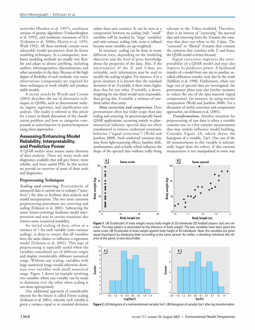
An initial scaling of data, often to avariance of 1 for each variable (unit-variancescaling), is done to ensure that all variableshave the same chance to influence a regressionmodel (Eriksson et al. 2001). This type ofpreprocessing is especially useful when thevariables considered are of different originand display considerably different numericalrange. Without any scaling, variables withlarge numerical range would otherwise domi-nate over variables with small numericalrange. Figure 1 shows an example involvingtwo variables where one variable can be madeto dominate over the other when scaling isnot done appropriately.

One additional approach of considerableinterest for the future is called Pareto scaling(Eriksson et al. 2001), whereby each variable isgiven a variance equal to its standard deviation

rather than unit variance. It can be seen as acompromise between no scaling (risk: “small”variables will be masked by “large” variables)and unit-variance scaling (risk: noise is inflatedbecause noisy variables are up-weighted).

In summary, scaling can be done in manydifferent ways, depending on the modelingobjectives and the level of prior knowledgeabout the properties of the data. Also, if theuncertainties of the X- and Y-data areestimable, such information may be used tomodify the scaling weights. For instance, if in agiven situation it is known that the standarddeviation of an X-variable is three times higherthan that for any other X-variable, a down-weighting by one-third would seem reasonable,thus giving this X-variable a variance of one-third rather than unity.

Data correction and compression. Datapretreatment often has wider scope than justscaling and centering. In spectroscopically basedQSAR applications, occurring mainly in phar-maceutical industry, spectral data are oftentransformed to remove undesired systematicbehavior (“signal correction”) (Wold andJosefson 2000). Such undesired variation mayarise from light-scattering effects, baseline drift,nonlinearities, and so forth, which influence theshape of the spectral data without really being

relevant to the Y-data modeled. Therefore,there is an interest of “correcting” the spectraldata and removing from the X-matrix the varia-tion that does not relate to the Y-data. The“corrected” or “filtered” X-matrix then containsthe variation that correlate with Y, and hencethe QSAR model is better focused.

Signal correction improves the inter-pretability of a QSAR model and may alsoimprove its predictive power. A facilitatedtransfer of a model from one site to another, so-called calibration transfer, may also be the result(Sjöblom et al. 1998). Furthermore, when verylarge sets of spectral data are investigated, thepretreatment phase may also involve measuresto reduce the size of the data material (signalcompression), for instance, by using waveletcompression (Wold and Josefson 2000). For adiscussion of useful correction and compressionapproaches, see Eriksson et al. (2001).

Transformations. Another situation forpreprocessing of raw data is when a variablecontains one or a few extreme measurementsthat may unduly influence model building.Consider Figure 2A, which shows thehistogram of a variable, Var1. One out of the40 measurements in this variable is substan-tially larger than the others. If this extrememeasurement is not manipulated in some way

Mini-Monograph | Eriksson et al.

1364 VOLUME 111 | NUMBER 10 | August 2003 • Environmental Health Perspectives

Figure 1. (A) Scatterplot of body weight versus body height of 23 individuals (22 football players and one ref-eree). The data pattern is dominated by the influence of body weight. The two variables have been given thesame scale. (B) Scatterplot of body weight against body height of 23 individuals. Now, the variables are givenequal importance by displaying them according to the same spread. An outlier, a deviating individual, the ref-eree of the game, is now discernible.

Figure 2. (A) Histogram of a nontransformed variable Var1. (B) Histogram of variable Var1 after log transformation.

◆◆

◆◆◆◆◆◆

◆◆

◆◆◆◆◆◆◆◆

◆◆

◆◆◆◆◆◆

◆◆◆◆◆◆◆◆

100

90

80

700 10 20 30

Same scale

Body height (m)

Bod

y w

eigh

t (kg

)

◆◆

◆◆◆◆

◆◆

◆◆

◆◆

◆◆

◆◆◆◆

◆◆◆◆◆◆

◆◆

◆◆

◆◆◆◆

◆◆◆◆

◆◆

◆◆

◆◆

◆◆◆◆

100

90

80

70

Same spread

Body height (m)

Bod

y w

eigh

t (kg

)

1.6 1.7 1.8 1.9 2

BA

Log(Var1)

A

Coun

ts

11

10

9

8

7

6

5

4

3

2

1

0

8

6

4

2

0

Coun

ts

–2.0 –1.6 –1.2 –0.9 –0.5 –0.1 0.3 0.7 1.0 1.4VarTr1

B

–2.0 –1.5 –1.0 –0.5 0.0 0.5 1.0 1.5

before the data analysis, it will exert a largeinfluence (have high leverage) on the modeland dominate over the other measurements. Asimple logarithmic transformation will in thiscase remedy the situation (Figure 2B). If thetransformation does not increase the model’sgoodness of prediction, it should be avoided.

Informative Model ParametersDepending on the data analytical techniqueused, QSAR analysis will result in a set ofmodel parameters that is useful in the interpre-tation phase. With straightforward MLR, aregression equation consisting of coefficients isproduced. These coefficients have an intu-itively simple and therefore appealing meaning.But, one should be aware that—depending onthe choice of regression method—there are

other model parameters and diagnosticsavailable that also deserve attention when inter-preting a QSAR model. Our goal in this sub-section is to highlight a few of these parametersand diagnostics. In so doing, we will use twodata sets drawn from the literature.

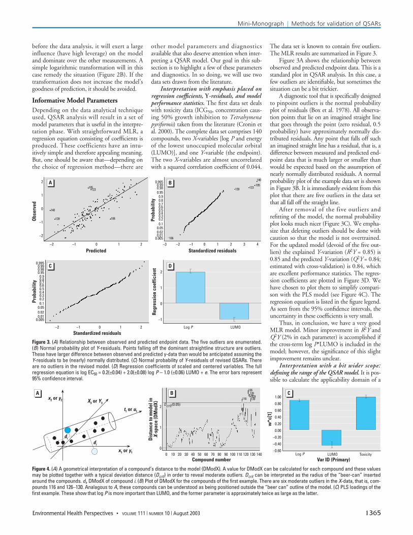
Interpretation with emphasis placed onregression coefficients, Y-residuals, and modelperformance statistics. The first data set dealswith toxicity data (ICG50, concentration caus-ing 50% growth inhibition to Tetrahymenapyriformis) taken from the literature (Cronin etal. 2000). The complete data set comprises 140compounds, two X-variables [log P and energyof the lowest unoccupied molecular orbital(LUMO)], and one Y-variable (the endpoint).The two X-variables are almost uncorrelatedwith a squared correlation coefficient of 0.044.

The data set is known to contain five outliers.The MLR results are summarized in Figure 3.

Figure 3A shows the relationship betweenobserved and predicted endpoint data. This is astandard plot in QSAR analysis. In this case, afew outliers are identifiable, but sometimes thesituation can be a bit trickier.

A diagnostic tool that is specifically designedto pinpoint outliers is the normal probabilityplot of residuals (Box et al. 1978). All observa-tion points that lie on an imagined straight linethat goes through the point (zero residual, 0.5probability) have approximately normally dis-tributed residuals. Any point that falls off suchan imagined straight line has a residual, that is, adifference between measured and predicted end-point data that is much larger or smaller thanwould be expected based on the assumption ofnearly normally distributed residuals. A normalprobability plot of the example data set is shownin Figure 3B. It is immediately evident from thisplot that there are five outliers in the data setthat all fall off the straight line.

After removal of the five outliers andrefitting of the model, the normal probabilityplot looks much nicer (Figure 3C). We empha-size that deleting outliers should be done withcaution so that the model is not overtrained.For the updated model (devoid of the five out-liers) the explained Y-variation (R2Y = 0.85) is0.85 and the predicted Y-variation (Q2Y = 0.84;estimated with cross-validation) is 0.84, whichare excellent performance statistics. The regres-sion coefficients are plotted in Figure 3D. Wehave chosen to plot them to simplify compari-son with the PLS model (see Figure 4C). Theregression equation is listed in the figure legend.As seen from the 95% confidence intervals, theuncertainty in these coefficients is very small.

Thus, in conclusion, we have a very goodMLR model. Minor improvement in R2Y andQ2Y (2% in each parameter) is accomplished ifthe cross-term log P*LUMO is included in themodel; however, the significance of this slightimprovement remains unclear.

Interpretation with a bit wider scope:defining the range of the QSAR model. It is pos-sible to calculate the applicability domain of a

Mini-Monograph | Methods for validation of QSARs

Environmental Health Perspectives • VOLUME 111 | NUMBER 10 | August 2003 1365

Figure 3. (A) Relationship between observed and predicted endpoint data. The five outliers are enumerated.(B) Normal probability plot of Y-residuals. Points falling off the dominant straightline structure are outliers.These have larger difference between observed and predicted y-data than would be anticipated assuming theY-residuals to be (nearly) normally distributed. (C) Normal probability of Y-residuals of revised QSARs. Thereare no outliers in the revised model. (D) Regression coefficients of scaled and centered variables. The fullregression equation is log EC50 = 0.2(±0.04) + 2.0(±0.08) log P – 1.0 (±0.06) LUMO + e. The error bars represent95% confidence interval.

2

1

0

–1

Standardized residualsLog P LUMO

Prob

abili

ty

0.9950.990.980.950.90.80.70.60.50.40.30.20.1

0.050.020.01

0.005

Prob

abili

ty

Standardized residuals

–2 –1 0 1 2

–2 –1 0 1 2

Predicted

Obs

erve

d

2

1

0

–1

–2

D

–2 –1 0 1 2 3 4–3

A139 123

105140

B

C

140

139

105123

106

106

0.9950.990.980.950.90.80.70.60.50.40.30.20.1

0.050.020.01

0.005

Regr

essi

on c

oeffi

cien

t

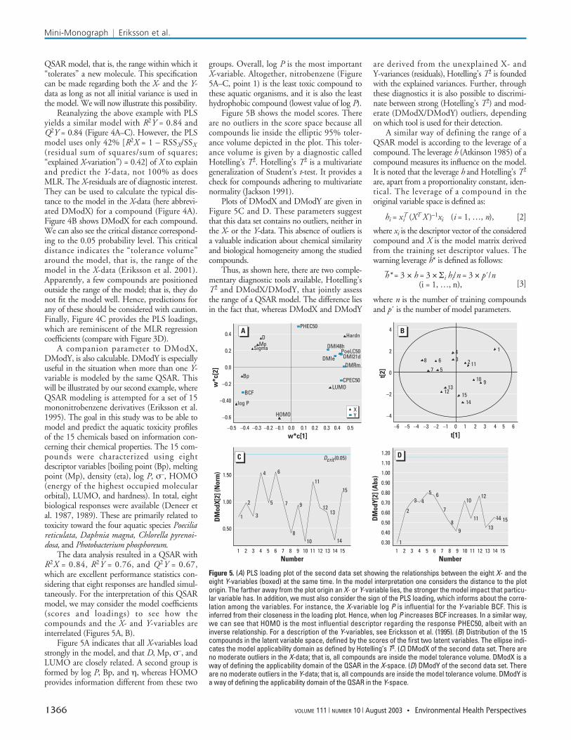
Figure 4. (A) A geometrical interpretation of a compound’s distance to the model (DModX). A value for DModX can be calculated for each compound and these valuesmay be plotted together with a typical deviation distance (Dcrit) in order to reveal moderate outliers. Dcrit can be interpreted as the radius of the “beer-can” insertedaround the compounds. di, DModX of compound i. (B) Plot of DModX for the compounds of the first example. There are six moderate outliers in the X-data, that is, com-pounds 116 and 126–130. Analagous to A, these compounds can be understood as being positioned outside the “beer can” outline of the model. (C) PLS loadings of thefirst example. These show that log P is more important than LUMO, and the former parameter is approximately twice as large as the latter.

x2 or y2 X3 or Y3

t1 or u1

di

x1 or y1

A C

Var ID (Primary)

1.00

0.80

0.60

0.40

0.20

0.00

–0.20

–0.40

–0.60

w*c

[1]

Log P LUMO Toxicity

di

B

0 10 20 30 40 50 60 70 80 90 100 110 120 130 140Compound number

116

126128

129130

127

2

1

0

Dcrit (0.05)

Dis

tanc

e to

mod

el in

X-sp

ace

(DM

odX)

Mini-Monograph | Eriksson et al.

QSAR model, that is, the range within which it“tolerates” a new molecule. This specificationcan be made regarding both the X- and the Y-data as long as not all initial variance is used inthe model. We will now illustrate this possibility.

Reanalyzing the above example with PLSyields a similar model with R2Y = 0.84 andQ2Y = 0.84 (Figure 4A–C). However, the PLSmodel uses only 42% [R2X = 1 – RSSX/SSX(residual sum of squares/sum of squares;“explained X-variation”) = 0.42] of X to explainand predict the Y-data, not 100% as doesMLR. The X-residuals are of diagnostic interest.They can be used to calculate the typical dis-tance to the model in the X-data (here abbrevi-ated DModX) for a compound (Figure 4A).Figure 4B shows DModX for each compound.We can also see the critical distance correspond-ing to the 0.05 probability level. This criticaldistance indicates the “tolerance volume”around the model, that is, the range of themodel in the X-data (Eriksson et al. 2001).Apparently, a few compounds are positionedoutside the range of the model; that is, they donot fit the model well. Hence, predictions forany of these should be considered with caution.Finally, Figure 4C provides the PLS loadings,which are reminiscent of the MLR regressioncoefficients (compare with Figure 3D).

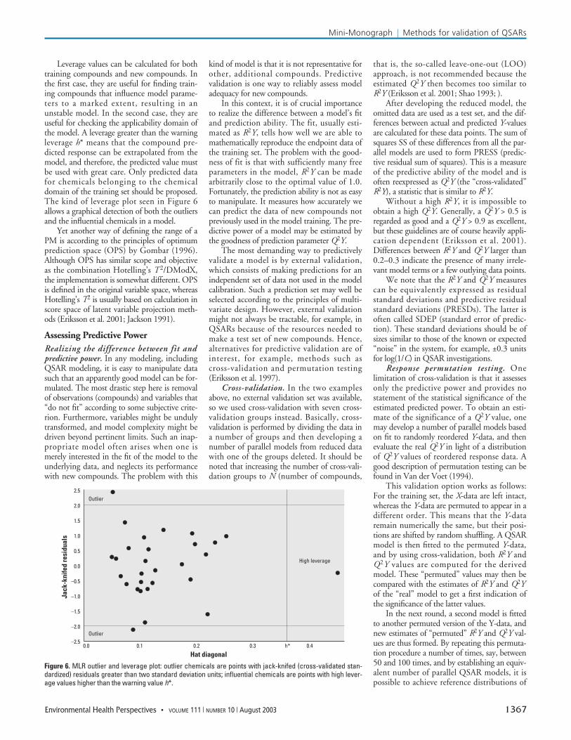
A companion parameter to DModX,DModY, is also calculable. DModY is especiallyuseful in the situation when more than one Y-variable is modeled by the same QSAR. Thiswill be illustrated by our second example, whereQSAR modeling is attempted for a set of 15mononitrobenzene derivatives (Eriksson et al.1995). The goal in this study was to be able tomodel and predict the aquatic toxicity profilesof the 15 chemicals based on information con-cerning their chemical properties. The 15 com-pounds were characterized using eightdescriptor variables [boiling point (Bp), meltingpoint (Mp), density (eta), log P, σ–, HOMO(energy of the highest occupied molecularorbital), LUMO, and hardness). In total, eightbiological responses were available (Deneer etal. 1987, 1989). These are primarily related totoxicity toward the four aquatic species Poeciliareticulata, Daphnia magna, Chlorella pyrenoi-dosa, and Photobacterium phosphoreum.

The data analysis resulted in a QSAR withR2X = 0.84, R2Y = 0.76, and Q2Y = 0.67,which are excellent performance statistics con-sidering that eight responses are handled simul-taneously. For the interpretation of this QSARmodel, we may consider the model coefficients(scores and loadings) to see how thecompounds and the X- and Y-variables areinterrelated (Figures 5A, B).

Figure 5A indicates that all X-variables loadstrongly in the model, and that D, Mp, σ–, andLUMO are closely related. A second group isformed by log P, Bp, and η, whereas HOMOprovides information different from these two

groups. Overall, log P is the most importantX-variable. Altogether, nitrobenzene (Figure5A–C, point 1) is the least toxic compound tothese aquatic organisms, and it is also the leasthydrophobic compound (lowest value of log P).

Figure 5B shows the model scores. Thereare no outliers in the score space because allcompounds lie inside the elliptic 95% toler-ance volume depicted in the plot. This toler-ance volume is given by a diagnostic calledHotelling’s T2. Hotelling’s T2 is a multivariategeneralization of Student’s t-test. It provides acheck for compounds adhering to multivariatenormality (Jackson 1991).

Plots of DModX and DModY are given inFigure 5C and D. These parameters suggestthat this data set contains no outliers, neither inthe X- or the Y-data. This absence of outliers isa valuable indication about chemical similarityand biological homogeneity among the studiedcompounds.

Thus, as shown here, there are two comple-mentary diagnostic tools available, Hotelling’sT2 and DModX/DModY, that jointly assessthe range of a QSAR model. The difference liesin the fact that, whereas DModX and DModY

are derived from the unexplained X- andY-variances (residuals), Hotelling’s T2 is foundedwith the explained variances. Further, throughthese diagnostics it is also possible to discrimi-nate between strong (Hotelling’s T2) and mod-erate (DModX/DModY) outliers, dependingon which tool is used for their detection.

A similar way of defining the range of aQSAR model is according to the leverage of acompound. The leverage h (Atkinson 1985) of acompound measures its influence on the model.It is noted that the leverage h and Hotelling’s T2

are, apart from a proportionality constant, iden-tical. The leverage of a compound in theoriginal variable space is defined as:

hi = xiT (XT X )–1xi (i = 1, …, n), [2]

where xi is the descriptor vector of the consideredcompound and X is the model matrix derivedfrom the training set descriptor values. Thewarning leverage h* is defined as follows:

–h* = 3 × h = 3 × Σi hi/n = 3 × p´/n(i = 1, …, n), [3]

where n is the number of training compoundsand p´ is the number of model parameters.

1366 VOLUME 111 | NUMBER 10 | August 2003 • Environmental Health Perspectives

Figure 5. (A) PLS loading plot of the second data set showing the relationships between the eight X- and theeight Y-variables (boxed) at the same time. In the model interpretation one considers the distance to the plotorigin. The farther away from the plot origin an X- or Y-variable lies, the stronger the model impact that particu-lar variable has. In addition, we must also consider the sign of the PLS loading, which informs about the corre-lation among the variables. For instance, the X-variable log P is influential for the Y-variable BCF. This isinferred from their closeness in the loading plot. Hence, when log P increases BCF increases. In a similar way,we can see that HOMO is the most influential descriptor regarding the response PHEC50, albeit with aninverse relationship. For a description of the Y-variables, see Ericksson et al. (1995). (B) Distribution of the 15compounds in the latent variable space, defined by the scores of the first two latent variables. The ellipse indi-cates the model applicability domain as defined by Hotelling’s T2. (C) DModX of the second data set. There areno moderate outliers in the X-data; that is, all compounds are inside the model tolerance volume. DModX is away of defining the applicability domain of the QSAR in the X-space. (D) DModY of the second data set. Thereare no moderate outliers in the Y-data; that is, all compounds are inside the model tolerance volume. DModY isa way of defining the applicability domain of the QSAR in the Y-space.

1

112

10 913

12 1514

4368

7 5

1513

12

11

10

98

7

65

43

2

1

141

2

3

4

5

6

7

8

9

10

11

1213

14

15

4

2

0

–2

–4

t[2]

t[1]

1.20

1.10

1.00

0.90

0.80

0.70

0.60

0.50

0.40

0.30

DM

odY[

2] (A

bs)

Number

1.50

1.00

0.50

C D

BD

MpSigma

Bp

log P

BCF

PHEC50

Hardn

LUMOCPEC50

0.4

0.2

0.0

–0.2

–0.40

–0.6

w*c

[2]

Number

DM

odX[

2] (N

orm

)

w*c[1]

A

XYHOMO

–0.5 –0.4 –0.3 –0.2 –0.1 0.0 0.1 0.2 0.3 0.4 –6 –5 –4 –3 –2 –1 0 1 2 3 4 5 60.5

DMIe

DMI48hPoeLC50DMI21dDMRm

1 151312111098765432 141 151312111098765432 14

Dcrit (0.05)

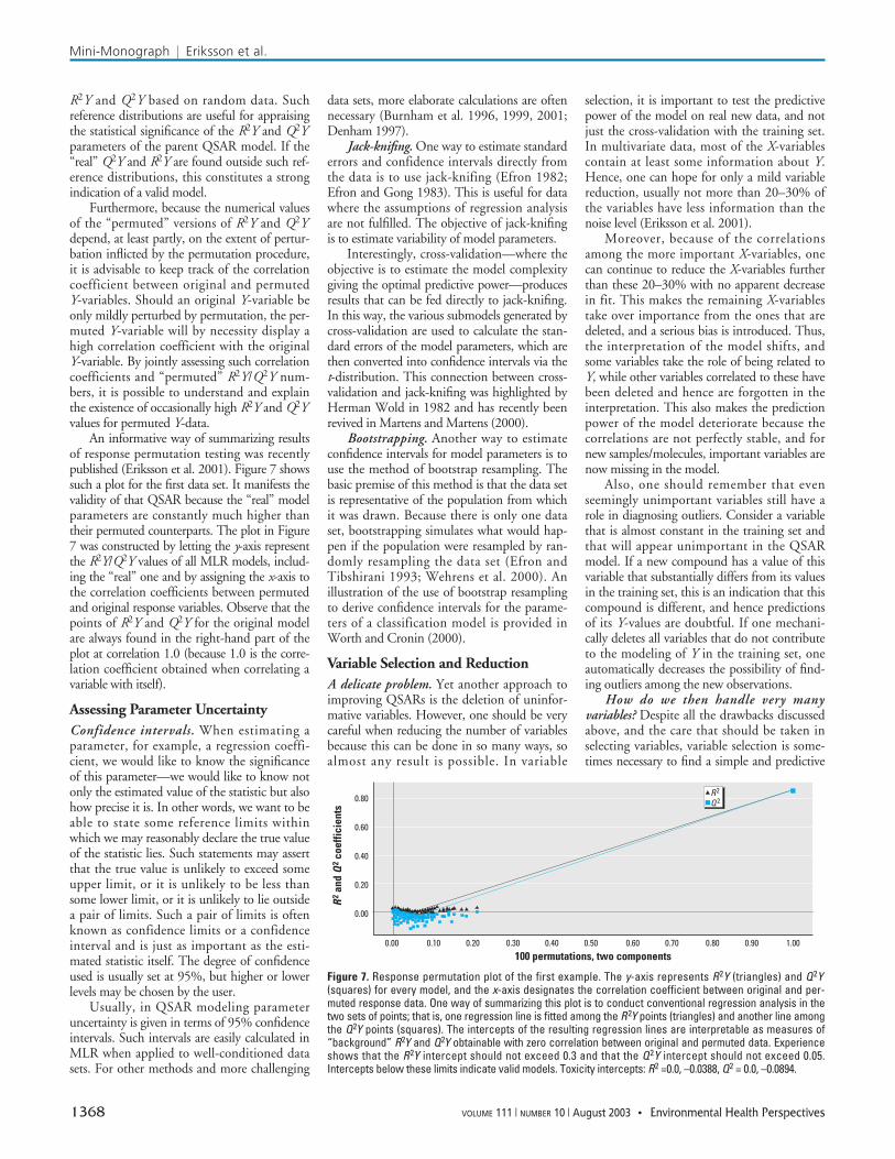
Leverage values can be calculated for bothtraining compounds and new compounds. Inthe first case, they are useful for finding train-ing compounds that influence model parame-ters to a marked extent, resulting in anunstable model. In the second case, they areuseful for checking the applicability domain ofthe model. A leverage greater than the warningleverage h* means that the compound pre-dicted response can be extrapolated from themodel, and therefore, the predicted value mustbe used with great care. Only predicted datafor chemicals belonging to the chemicaldomain of the training set should be proposed.The kind of leverage plot seen in Figure 6allows a graphical detection of both the outliersand the influential chemicals in a model.

Yet another way of defining the range of aPM is according to the principles of optimumprediction space (OPS) by Gombar (1996).Although OPS has similar scope and objectiveas the combination Hotelling’s T2/DModX,the implementation is somewhat different. OPSis defined in the original variable space, whereasHotelling’s T2 is usually based on calculation inscore space of latent variable projection meth-ods (Eriksson et al. 2001; Jackson 1991).

Assessing Predictive PowerRealizing the difference between fit andpredictive power. In any modeling, includingQSAR modeling, it is easy to manipulate datasuch that an apparently good model can be for-mulated. The most drastic step here is removalof observations (compounds) and variables that“do not fit” according to some subjective crite-rion. Furthermore, variables might be undulytransformed, and model complexity might bedriven beyond pertinent limits. Such an inap-propriate model often arises when one ismerely interested in the fit of the model to theunderlying data, and neglects its performancewith new compounds. The problem with this

kind of model is that it is not representative forother, additional compounds. Predictivevalidation is one way to reliably assess modeladequacy for new compounds.

In this context, it is of crucial importanceto realize the difference between a model’s fitand prediction ability. The fit, usually esti-mated as R2Y, tells how well we are able tomathematically reproduce the endpoint data ofthe training set. The problem with the good-ness of fit is that with sufficiently many freeparameters in the model, R2Y can be madearbitrarily close to the optimal value of 1.0.Fortunately, the prediction ability is not as easyto manipulate. It measures how accurately wecan predict the data of new compounds notpreviously used in the model training. The pre-dictive power of a model may be estimated bythe goodness of prediction parameter Q2Y.

The most demanding way to predictivelyvalidate a model is by external validation,which consists of making predictions for anindependent set of data not used in the modelcalibration. Such a prediction set may well beselected according to the principles of multi-variate design. However, external validationmight not always be tractable, for example, inQSARs because of the resources needed tomake a test set of new compounds. Hence,alternatives for predictive validation are ofinterest, for example, methods such ascross-validation and permutation testing(Eriksson et al. 1997).

Cross-validation. In the two examplesabove, no external validation set was available,so we used cross-validation with seven cross-validation groups instead. Basically, cross-validation is performed by dividing the data ina number of groups and then developing anumber of parallel models from reduced datawith one of the groups deleted. It should benoted that increasing the number of cross-vali-dation groups to N (number of compounds,

that is, the so-called leave-one-out (LOO)approach, is not recommended because theestimated Q2Y then becomes too similar toR2Y (Eriksson et al. 2001; Shao 1993; ).

After developing the reduced model, theomitted data are used as a test set, and the dif-ferences between actual and predicted Y-valuesare calculated for these data points. The sum ofsquares SS of these differences from all the par-allel models are used to form PRESS (predic-tive residual sum of squares). This is a measureof the predictive ability of the model and isoften reexpressed as Q2Y (the “cross-validated”R2Y), a statistic that is similar to R2Y.

Without a high R2Y, it is impossible toobtain a high Q2Y. Generally, a Q2Y > 0.5 isregarded as good and a Q2Y > 0.9 as excellent,but these guidelines are of course heavily appli-cation dependent (Eriksson et al. 2001).Differences between R2Y and Q2Y larger than0.2–0.3 indicate the presence of many irrele-vant model terms or a few outlying data points.

We note that the R2Y and Q2Y measurescan be equivalently expressed as residualstandard deviations and predictive residualstandard deviations (PRESDs). The latter isoften called SDEP (standard error of predic-tion). These standard deviations should be ofsizes similar to those of the known or expected“noise” in the system, for example, ±0.3 unitsfor log(1/C) in QSAR investigations.

Response permutation testing. Onelimitation of cross-validation is that it assessesonly the predictive power and provides nostatement of the statistical significance of theestimated predicted power. To obtain an esti-mate of the significance of a Q2Y value, onemay develop a number of parallel models basedon fit to randomly reordered Y-data, and thenevaluate the real Q2Y in light of a distributionof Q2Y values of reordered response data. Agood description of permutation testing can befound in Van der Voet (1994).

This validation option works as follows:For the training set, the X-data are left intact,whereas the Y-data are permuted to appear in adifferent order. This means that the Y-dataremain numerically the same, but their posi-tions are shifted by random shuffling. A QSARmodel is then fitted to the permuted Y-data,and by using cross-validation, both R2Y andQ2Y values are computed for the derivedmodel. These “permuted” values may then becompared with the estimates of R2Y and Q2Yof the “real” model to get a first indication ofthe significance of the latter values.

In the next round, a second model is fittedto another permuted version of the Y-data, andnew estimates of “permuted” R2Y and Q2Y val-ues are thus formed. By repeating this permuta-tion procedure a number of times, say, between50 and 100 times, and by establishing an equiv-alent number of parallel QSAR models, it ispossible to achieve reference distributions of

Mini-Monograph | Methods for validation of QSARs

Environmental Health Perspectives • VOLUME 111 | NUMBER 10 | August 2003 1367

Figure 6. MLR outlier and leverage plot: outlier chemicals are points with jack-knifed (cross-validated stan-dardized) residuals greater than two standard deviation units; influential chemicals are points with high lever-age values higher than the warning value h*.

●●

●●

●●

●●●●

●●

●●

●●

●●

●●●● ●●

●●

●●

●●

●●

●●

●●

●●

●●

●●

●●

●●

●●

●●

●●

●●●●

●●

Outlier

Outlier

High leverage

2.5

2.0

1.5

1.0

0.5

0.0

–0.5

–1.0

–1.5

–2.0

–2.5

Hat diagonal

Jack

-kni

fed

resi

dual

s

0.0 0.1 0.2 0.3 h* 0.4

R2Y and Q2Y based on random data. Suchreference distributions are useful for appraisingthe statistical significance of the R2Y and Q2Yparameters of the parent QSAR model. If the“real” Q2Y and R2Y are found outside such ref-erence distributions, this constitutes a strongindication of a valid model.

Furthermore, because the numerical valuesof the “permuted” versions of R2Y and Q2Ydepend, at least partly, on the extent of pertur-bation inflicted by the permutation procedure,it is advisable to keep track of the correlationcoefficient between original and permutedY-variables. Should an original Y-variable beonly mildly perturbed by permutation, the per-muted Y-variable will by necessity display ahigh correlation coefficient with the originalY-variable. By jointly assessing such correlationcoefficients and “permuted” R2Y/Q2Y num-bers, it is possible to understand and explainthe existence of occasionally high R2Y and Q2Yvalues for permuted Y-data.

An informative way of summarizing resultsof response permutation testing was recentlypublished (Eriksson et al. 2001). Figure 7 showssuch a plot for the first data set. It manifests thevalidity of that QSAR because the “real” modelparameters are constantly much higher thantheir permuted counterparts. The plot in Figure7 was constructed by letting the y-axis representthe R2Y/Q2Y values of all MLR models, includ-ing the “real” one and by assigning the x-axis tothe correlation coefficients between permutedand original response variables. Observe that thepoints of R2Y and Q2Y for the original modelare always found in the right-hand part of theplot at correlation 1.0 (because 1.0 is the corre-lation coefficient obtained when correlating avariable with itself).

Assessing Parameter UncertaintyConfidence intervals. When estimating aparameter, for example, a regression coeffi-cient, we would like to know the significanceof this parameter—we would like to know notonly the estimated value of the statistic but alsohow precise it is. In other words, we want to beable to state some reference limits withinwhich we may reasonably declare the true valueof the statistic lies. Such statements may assertthat the true value is unlikely to exceed someupper limit, or it is unlikely to be less thansome lower limit, or it is unlikely to lie outsidea pair of limits. Such a pair of limits is oftenknown as confidence limits or a confidenceinterval and is just as important as the esti-mated statistic itself. The degree of confidenceused is usually set at 95%, but higher or lowerlevels may be chosen by the user.

Usually, in QSAR modeling parameteruncertainty is given in terms of 95% confidenceintervals. Such intervals are easily calculated inMLR when applied to well-conditioned datasets. For other methods and more challenging

data sets, more elaborate calculations are oftennecessary (Burnham et al. 1996, 1999, 2001;Denham 1997).

Jack-knifing. One way to estimate standarderrors and confidence intervals directly fromthe data is to use jack-knifing (Efron 1982;Efron and Gong 1983). This is useful for datawhere the assumptions of regression analysisare not fulfilled. The objective of jack-knifingis to estimate variability of model parameters.

Interestingly, cross-validation—where theobjective is to estimate the model complexitygiving the optimal predictive power—producesresults that can be fed directly to jack-knifing.In this way, the various submodels generated bycross-validation are used to calculate the stan-dard errors of the model parameters, which arethen converted into confidence intervals via thet-distribution. This connection between cross-validation and jack-knifing was highlighted byHerman Wold in 1982 and has recently beenrevived in Martens and Martens (2000).

Bootstrapping. Another way to estimateconfidence intervals for model parameters is touse the method of bootstrap resampling. Thebasic premise of this method is that the data setis representative of the population from whichit was drawn. Because there is only one dataset, bootstrapping simulates what would hap-pen if the population were resampled by ran-domly resampling the data set (Efron andTibshirani 1993; Wehrens et al. 2000). Anillustration of the use of bootstrap resamplingto derive confidence intervals for the parame-ters of a classification model is provided inWorth and Cronin (2000).

Variable Selection and ReductionA delicate problem. Yet another approach toimproving QSARs is the deletion of uninfor-mative variables. However, one should be verycareful when reducing the number of variablesbecause this can be done in so many ways, soalmost any result is possible. In variable

selection, it is important to test the predictivepower of the model on real new data, and notjust the cross-validation with the training set.In multivariate data, most of the X-variablescontain at least some information about Y.Hence, one can hope for only a mild variablereduction, usually not more than 20–30% ofthe variables have less information than thenoise level (Eriksson et al. 2001).

Moreover, because of the correlationsamong the more important X-variables, onecan continue to reduce the X-variables furtherthan these 20–30% with no apparent decreasein fit. This makes the remaining X-variablestake over importance from the ones that aredeleted, and a serious bias is introduced. Thus,the interpretation of the model shifts, andsome variables take the role of being related toY, while other variables correlated to these havebeen deleted and hence are forgotten in theinterpretation. This also makes the predictionpower of the model deteriorate because thecorrelations are not perfectly stable, and fornew samples/molecules, important variables arenow missing in the model.

Also, one should remember that evenseemingly unimportant variables still have arole in diagnosing outliers. Consider a variablethat is almost constant in the training set andthat will appear unimportant in the QSARmodel. If a new compound has a value of thisvariable that substantially differs from its valuesin the training set, this is an indication that thiscompound is different, and hence predictionsof its Y-values are doubtful. If one mechani-cally deletes all variables that do not contributeto the modeling of Y in the training set, oneautomatically decreases the possibility of find-ing outliers among the new observations.

How do we then handle very manyvariables? Despite all the drawbacks discussedabove, and the care that should be taken inselecting variables, variable selection is some-times necessary to find a simple and predictive

Mini-Monograph | Eriksson et al.

1368 VOLUME 111 | NUMBER 10 | August 2003 • Environmental Health Perspectives

Figure 7. Response permutation plot of the first example. The y-axis represents R2Y (triangles) and Q2Y(squares) for every model, and the x-axis designates the correlation coefficient between original and per-muted response data. One way of summarizing this plot is to conduct conventional regression analysis in thetwo sets of points; that is, one regression line is fitted among the R2Y points (triangles) and another line amongthe Q2Y points (squares). The intercepts of the resulting regression lines are interpretable as measures of“background” R2Y and Q2Y obtainable with zero correlation between original and permuted data. Experienceshows that the R2Y intercept should not exceed 0.3 and that the Q2Y intercept should not exceed 0.05.Intercepts below these limits indicate valid models. Toxicity intercepts: R2 =0.0, –0.0388, Q2 = 0.0, –0.0894.

0.80

0.60

0.40

0.20

0.00

0.00 0.10 0.20 0.30 0.40 0.50 0.60 0.70 0.80 0.90 1.00

100 permutations, two components

R 2

Q 2

R2 a

nd Q

2 coe

ffici

ents

QSAR model. Nowadays it is becoming quitecommon to use a wide set of moleculardescriptors of different kinds (experimentaland/or theoretical) able to capture all the struc-tural information possibly related to theY-response. A recent survey of this was pub-lished by Livingstone (2000). Many softwareprograms calculate wide sets of different theo-retical descriptors, from SMILES (simplifiedmolecular input line entry specification), two-dimensional graphs, and three-dimensionalx,y,z-coordinates. Only some of the more com-plete are mentioned here: ADAPT (Jurs 2002;Stuper and Jurs 1976), OASIS (Mekenyan andBonchev 1986), CODESSA (Katritzky et al.1994), and DRAGON (Todeschini et al.2001). It has been estimated that more than3,000 molecular descriptors are now available,and most of them are summarized andexplained in recently published books (Devillersand Balaban 1999; Karelson 2000; Todeschiniand Consonni 2000). The great advantage oftheoretical descriptors is that they are calcula-ble for not yet synthesized chemicals.

There are two main steps in QSARmodeling by variable selection: first, statisticallyvalidated and robust regression models must befound, and second, the model variables mustbe interpretable. In principle, all the differentpossible variable combinations of the X-vari-ables should be investigated to find the mostpredictive QSAR model. However, this may bequite taxing, mainly for reasons of time. Thus,first, various types of rapid prescreens (discard-ing constant values, pair-correlated variables,etc.) are often implemented to sort out a lim-ited set of descriptors among which the selec-tion of those really related to the response, notonly in fitting but most importantly in predic-tion, is then performed by alternative variableselection methods.

Several strategies for variable subsetselection have been applied in QSARs (amongthose most widely applied: stepwise regressions,forward selection, backward elimination, simu-lated annealing, and evolutionary and geneticalgorithms). A recent comparison (Xu andZhang 2001) of these methods has given ademonstration of the advantages and success ofgenetic algorithms as a variable selection proce-dure for QSAR studies. Below, we discussgenetic algorithms and a few alternatives.

Genetic algorithm strategy for variableselection. Genetic algorithms are a particularkind of evolutionary algorithm shown to beable to solve complex optimization problemsin a number of fields, including chemistry(Davis 1991; Goldberg 1989; Hibbert 1993;Wehrens and Buydens 1998). The naturalprinciples of the evolution of species in the bio-logical world are applied: the assumption thatconditions that lead to better results willprevail over poorer ones, and that improve-ment can be obtained by different kinds of

recombination of independent variables, thatis, reproduction, mutation, and crossover.The goodness of the selected solution is meas-ured by a response function that has to beoptimized.

Genetic algorithms, first proposed as astrategy for variable subset selection in multi-variate analysis by Leardi et al. (1992), are nowwidely and successfully applied in QSARapproaches where there are many moleculardescriptors as X-variables in various modifiedversions, depending on the way to performreproduction, crossover, mutation, and soforth (Devillers 1996; GFA of Rogers andHopfinger 1994; Leardi 1994; MUSEUM ofKubinyi 1994a, 1994b; MOBY-DIGS ofTodeschini 1997).

In variable selection for QSAR studies,each variable (molecular descriptor) is denotedby a bit equal to 1 if present in the regressionmodel or to 0 if excluded. A population consti-tuted by a number of 0/1 bit strings (each oflength equal to the total number of variables) isevolved following genetic algorithm rules, max-imizing the predictive power of the models(explained variance in prediction, Q2Y, or rootmean squared error of prediction). Only themodels producing the highest predictive powerare finally retained and further analyzed.

Whereas revolutionary algorithms searchfor the global optimum and end up with onlyone or very few results (Kubinyi 1994a, 1994b,1996), genetic algorithms simultaneously cre-ate many different results of comparable qual-ity in larger populations of models. Within agiven population, the selected models can dif-fer in number and kind of variables.

Different rules can be adopted to select thefinal “best” models. Todeschini, Gramatica,and colleagues (Gramatica et al. 1998, 1999,2000; Gramatica and Papa 2003; Todeschiniand Gramatica 1997) use the QUIK rule (Qunder influence of K) (Todeschini et al. 1999)to avoid multicollinearity without predictionpower or “apparent” prediction power (chancecorrelation). According to this rule, only mod-els with a K multivariate correlation calculatedon the X + Y-block that is at least 5% greaterthan the K correlation of the X-block are con-sidered statistically significant. Alternatively,one may use the approach of Hopfinger(discussed in a later section).

Model validation is always used to avoid“overfitted” models, that is, models where toomany variables have been selected, and to avoidselecting variables randomly correlated withthe dependent response. Particular care mustbe taken against overfitting; therefore, subsetswith fewer variables are favored, even thoughthe chance of finding “acceptable” modelsincreases with increasing the selected variables.The proportion of random variables selectedby chance correlation could also increase(Jouan-Rimbaud et al. 1996).

The collinearity in the original set ofmolecular descriptors results in many similarmodels yielding more or less the same predic-tive power. Therefore, after having selected aset of similar PMs, model validation proceedsvia leave-more-out cross-validation, responsepermutation testing (Y-scrambling), bootstrap-ping (Efron 1982), or other resampling tech-niques. This is done to avoid overestimation ofthe model predictive power by Q2

LOO(Golbraikh and Tropsha 2002; Shao 1993), toverify model predictivity stability, and to selectthe “best” model. Finally, for the strongestevaluation of model applicability for predictionin new chemicals, external validation (verifiedby Q2

EXT) of all the models is also recom-mended, depending on whether the data set islarge enough to permit an independent exter-nal validation set. The best splitting of theoriginal data set into a representative trainingset and a validation set can be obtained byapplying experimental design (Eriksson et al.2000b; Marengo and Todeschini 1992).

If after several different runs of geneticalgorithms the same subsets of variables havebeen selected, and if the obtained models passall the validation procedures above (cross-vali-dation), external testing, Y-scrambling, boot-strapping), there is a reasonable certainty thatthe models are robust and applicable for predic-tion. Good predictive properties is also an indi-cation that chance correlation has been avoided.

Because genetic algorithms simultaneouslycreate many different good models in a popula-tion, the user can choose the “best model”according to need: the interpretability of theselected molecular descriptors, the possibility ofhaving reliable predictions for some chemicalsrather than others, the highlighting of differentoutliers, and so forth. The need for inter-pretability depends on the application, as a val-idated mathematical model relating a targetproperty to chemical features may, in somecases, be all that is necessary, though it is obvi-ously desirable to attempt some explanation ofthe ‘mechanism’ in chemical terms, but it isoften not necessary, per se (Livingstone 2000).This type of QSAR model follows a path thatstarts with a statistical validation and furtherinterpretation for their biological andmechanistic meaning (Tropsha et al. 2003).Therefore, their application domain is mainlyrelated to the production of predicted data,verified for their reliability.

Assessing model uniqueness. Hopfinger andcolleagues advocate a related approach aimingat defining the best QSAR model. Thisapproach is based on some of the elementsdescribed above, notably, cross-validation,response permutation testing, and variableselection (Kulkarni et al. 2001). They strive tomaximize Q2Y through elimination ofunimportant X-variables. Several differentmodel versions are derived using genetic

Mini-Monograph | Methods for validation of QSARs

Environmental Health Perspectives • VOLUME 111 | NUMBER 10 | August 2003 1369

algorithms and the ones producing the highestQ2Y are retained. In the next step cross-correlation analysis of the modeling residualsfrom the set of best models is used to deter-mine how many unique models have beenobtained. A unique model will have low corre-lations of its residuals of fit to those of thealternative top-ranked models.

After having selected a set of unique modelswith highest possible Q2Y, model validationproceeds via response permutation testingand/or external predictive validation, depend-ing on whether the data set is large enough topermit an independent external prediction set.In some cases when there is thought to be con-siderable noise in the Y-data, the approach ofHopfinger and colleagues also involves studyingthe stability of the resultant QSAR models as afunction of increasing simulated error amongthe X-variables. The objective with this latterexercise is to investigate whether stable QSARswith respect to the inherent error of the data sethave been obtained (Hopfinger AJ andJaworska J. Personal communication).

GOLPE (generating optimal linear PLSestimations). About a decade ago an advancedvariable selection procedure called GOLPE wasintroduced by Sergio Clementi and colleagues(Baroni et al. 1993) and has found widespreaduse in three-dimensional QSARs. The objec-tive of this approach is to obtain PLS regres-sion models with the highest prediction ability.The key steps of this approach involve a firstpreliminary variable selection by means of aD-optimal (determinant optimal) design in theloading space, and an iterative evaluation of theeffects of the individual variables on the modelpredictivity. This is accomplished based on thevalidation of a number of partial submodelsusing many combinations of the descriptorvariables as dictated by a fractional factorialdesign strategy. Cruciani and Watson (1994)show the utility of GOLPE in generatingthree-dimensional QSAR models with goodpredictive power.

Hierarchical modeling for easier modelinterpretation and as an alternative to variableselection. In two- and three-dimensional QSARmodeling involving many variables, plots andlists of coefficients, loadings, and so forth,rapidly become messy, and results are thereforedifficult to interpret. As discussed above, theremay then be a strong temptation to eliminatevariables to obtain a smaller data set. Such a

reduction of variables, however, often removesinformation and makes the modeling effortsless reliable. Model interpretation may be mis-leading, and predictive power may deteriorate.

As reported by Berglund et al. (1997), aninteresting alternative is to partition the vari-ables into blocks of logically related variablesand apply hierarchical data analysis. All suchblocks may be analyzed individually. Thismodeling forms the base level of the hierarchi-cal modeling setup (Eriksson et al. 2002). Thescore vectors, often called “super variables,”formed on the base level may be concatenatedin new matrices amenable for analysis on thetop level. On the top level, superficial relation-ships between the X- and the Y-data are investi-gated. On the base level, in-depth informationis extracted for the different blocks.

Bayesian Methods forReliability TestingBayesian-based methods have been heavilyused in reliability engineering and diagnosticmedicine where models are used for decisionmaking. These methods are perfectly suitableto evaluating QSARs and have been intro-duced to the field but still are not used broadly(McDowell and Jaworska 2002; Pet-Edwardset al. 1989). One characteristic of Bayesian-based procedures is that they allow both priorinformation (including expert judgment) andsampling information to be combined in theweighting scheme inherent in Bayes’ formula.The second characteristic of Bayesian-basedmethods is they can be formulated in a recur-sive form. This means Bayesian methods allowsuccessive updating of battery interpretation asadditional tests results are obtained, which isparticularly useful if sequential testing proce-dures are being considered.

The most common and simple applicationof Bayes’ approach is found in evaluating per-formance statistics for two-way categorical clas-sifications. It uses as inputs sensitivity andspecificity. Sensitivity is the fraction of activechemicals that are predicted to be active by themodel (α i

+); and specificity is defined as thefraction of nonactive chemicals the model pre-dicts nonactive (α i

–). Sensitivity can also beexpressed as Pr(P+|S+), the conditional proba-bility a model predicts a chemical to be active(P+) given that the true state is active (S+).Similarly, specificity is defined as Pr(P–|S–),the conditional probability the model predicts

a chemical nonactive (P–) given the true stateis nonactive (S–).

We then can use Bayes’ formula

[4]

to obtain Pr(Si|Tj), the posterior probability ofcondition Si prevailing given we have test resultj from a) the prior probability of Si, Pr(Si), andb) Pr(Tj |Si), the likelihood of jth test resultgiven true state is Si.

It is important to note the likelihood value(sensitivity or specificity), Pr(Tj |Si), is condi-tional on Si (not known to the observer or ana-lyst), whereas the posterior probability isconditional on the observed result or predictionTj. The posterior probability or predictive valueis the appropriate statistic for inferring from testresults the probability the modeled chemicalhas condition Si. Posterior probabilities are sta-tistically precise statements of the likelihood achemical has a particular state or attribute, con-ditional on the test evidence obtained.

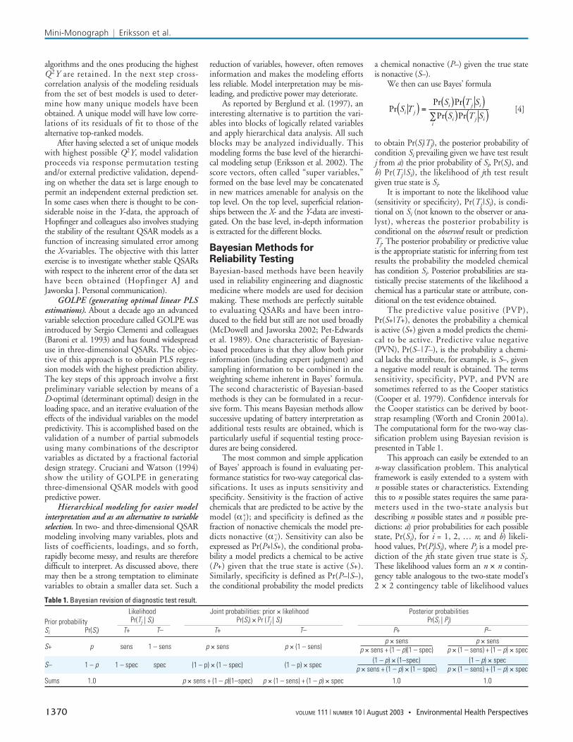
The predictive value positive (PVP),Pr(S+|T+), denotes the probability a chemicalis active (S+) given a model predicts the chemi-cal to be active. Predictive value negative(PVN), Pr(S–|T–), is the probability a chemi-cal lacks the attribute, for example, is S–, givena negative model result is obtained. The termssensitivity, specificity, PVP, and PVN aresometimes referred to as the Cooper statistics(Cooper et al. 1979). Confidence intervals forthe Cooper statistics can be derived by boot-strap resampling (Worth and Cronin 2001a).The computational form for the two-way clas-sification problem using Bayesian revision ispresented in Table 1.

This approach can easily be extended to ann-way classification problem. This analyticalframework is easily extended to a system withn possible states or characteristics. Extendingthis to n possible states requires the same para-meters used in the two-state analysis butdescribing n possible states and n possible pre-dictions: a) prior probabilities for each possiblestate, Pr(Si), for i = 1, 2, … n; and b) likeli-hood values, Pr(Pj|Si), where Pj is a model pre-diction of the jth state given true state is Si.These likelihood values form an n × n contin-gency table analogous to the two-state model’s2 × 2 contingency table of likelihood values

PrPr Pr

Pr PrS T

S T S

S T Si ji j i

i j ii

( ) =( ) ( )( ) ( )∑

Mini-Monograph | Eriksson et al.

1370 VOLUME 111 | NUMBER 10 | August 2003 • Environmental Health Perspectives

Table 1. Bayesian revision of diagnostic test result.Likelihood Joint probabilities: prior × likelihood Posterior probabilities

Prior probability Pr(Tj | Si) Pr(Si) × Pr (Tj | Si) Pr(Si | Pj)Si Pr(Si) T+ T– T+ T– P+ P–

S+ p sens 1 – sens p × sens p × (1 – sens)p × sens p × sens

p × sens + (1 – p)(1 – spec) p × (1 – sens) + (1 – p) × spec

S– 1 – p 1 – spec spec (1 – p) × (1 – spec) (1 – p) × spec(1 – p) × (1–spec) (1 – p) × spec

p × sens + (1 – p) × (1 – spec) p × (1 – sens) + (1 – p) × spec

Sums 1.0 p × sens + (1 – p)(1–spec) p × (1 – sens) + (1 – p) × spec 1.0 1.0

comprised sensitivity, specificity, and theircomplements.

The application of Bayes’ formula to an n-state model is identical to the two-state case(Equation 4) and the same conditions that holdfor the two-state case apply to the n-state case:

Σi

Pr(Si) = 1.0, Σi

Pr(P|Si) = 1.0 [5]

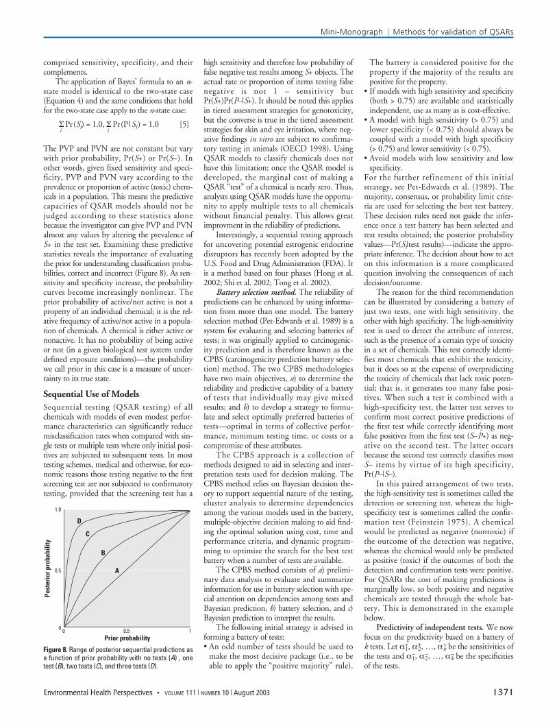
The PVP and PVN are not constant but varywith prior probability, Pr(S+) or Pr(S–). Inother words, given fixed sensitivity and speci-ficity, PVP and PVN vary according to theprevalence or proportion of active (toxic) chem-icals in a population. This means the predictivecapacities of QSAR models should not bejudged according to these statistics alonebecause the investigator can give PVP and PVNalmost any values by altering the prevalence ofS+ in the test set. Examining these predictivestatistics reveals the importance of evaluatingthe prior for understanding classification proba-bilities, correct and incorrect (Figure 8). As sen-sitivity and specificity increase, the probabilitycurves become increasingly nonlinear. Theprior probability of active/not active is not aproperty of an individual chemical; it is the rel-ative frequency of active/not active in a popula-tion of chemicals. A chemical is either active ornonactive. It has no probability of being activeor not (in a given biological test system underdefined exposure conditions)—the probabilitywe call prior in this case is a measure of uncer-tainty to its true state.

Sequential Use of ModelsSequential testing (QSAR testing) of allchemicals with models of even modest perfor-mance characteristics can significantly reducemisclassification rates when compared with sin-gle tests or multiple tests where only initial posi-tives are subjected to subsequent tests. In mosttesting schemes, medical and otherwise, for eco-nomic reasons those testing negative to the firstscreening test are not subjected to confirmatorytesting, provided that the screening test has a

high sensitivity and therefore low probability offalse negative test results among S+ objects. Theactual rate or proportion of items testing falsenegative is not 1 – sensitivity butPr(S+)Pr(P–|S+). It should be noted this appliesin tiered assessment strategies for genotoxicity,but the converse is true in the tiered assessmentstrategies for skin and eye irritation, where neg-ative findings in vitro are subject to confirma-tory testing in animals (OECD 1998). UsingQSAR models to classify chemicals does nothave this limitation; once the QSAR model isdeveloped, the marginal cost of making aQSAR “test” of a chemical is nearly zero. Thus,analysts using QSAR models have the opportu-nity to apply multiple tests to all chemicalswithout financial penalty. This allows greatimprovment in the reliability of predictions.

Interestingly, a sequential testing approachfor uncovering potential estrogenic endocrinedisruptors has recently been adopted by theU.S. Food and Drug Administration (FDA). Itis a method based on four phases (Hong et al.2002; Shi et al. 2002; Tong et al. 2002).

Battery selection method. The reliability ofpredictions can be enhanced by using informa-tion from more than one model. The batteryselection method (Pet-Edwards et al. 1989) is asystem for evaluating and selecting batteries oftests; it was originally applied to carcinogenic-ity prediction and is therefore known as theCPBS (carcinogenicity prediction battery selec-tion) method. The two CPBS methodologieshave two main objectives, a) to determine thereliability and predictive capability of a batteryof tests that individually may give mixedresults; and b) to develop a strategy to formu-late and select optimally preferred batteries oftests—optimal in terms of collective perfor-mance, minimum testing time, or costs or acompromise of these attributes.

The CPBS approach is a collection ofmethods designed to aid in selecting and inter-pretation tests used for decision making. TheCPBS method relies on Bayesian decision the-ory to support sequential nature of the testing,cluster analysis to determine dependenciesamong the various models used in the battery,multiple-objective decision making to aid find-ing the optimal solution using cost, time andperformance criteria, and dynamic program-ming to optimize the search for the best testbattery when a number of tests are available.

The CPBS method consists of a) prelimi-nary data analysis to evaluate and summarizeinformation for use in battery selection with spe-cial attention on dependencies among tests andBayesian prediction, b) battery selection, and c)Bayesian prediction to interpret the results.

The following initial strategy is advised informing a battery of tests:• An odd number of tests should be used to

make the most decisive package (i.e., to beable to apply the “positive majority” rule).

The battery is considered positive for theproperty if the majority of the results arepositive for the property.

• If models with high sensitivity and specificity(both > 0.75) are available and statisticallyindependent, use as many as is cost-effective.

• A model with high sensitivity (> 0.75) andlower specificity (< 0.75) should always becoupled with a model with high specificity(> 0.75) and lower sensitivity (< 0.75).

• Avoid models with low sensitivity and lowspecificity.

For the further refinement of this initialstrategy, see Pet-Edwards et al. (1989). Themajority, consensus, or probability limit crite-ria are used for selecting the best test battery.These decision rules need not guide the infer-ence once a test battery has been selected andtest results obtained; the posterior probabilityvalues—Pr(Si|test results)—indicate the appro-priate inference. The decision about how to acton this information is a more complicatedquestion involving the consequences of eachdecision/outcome.

The reason for the third recommendationcan be illustrated by considering a battery ofjust two tests, one with high sensitivity, theother with high specificity. The high-sensitivitytest is used to detect the attribute of interest,such as the presence of a certain type of toxicityin a set of chemicals. This test correctly identi-fies most chemicals that exhibit the toxicity,but it does so at the expense of overpredictingthe toxicity of chemicals that lack toxic poten-tial; that is, it generates too many false posi-tives. When such a test is combined with ahigh-specificity test, the latter test serves toconfirm most correct positive predictions ofthe first test while correctly identifying mostfalse positives from the first test (S–P+) as neg-ative on the second test. The latter occursbecause the second test correctly classifies mostS– items by virtue of its high specificity,Pr(P–|S–).

In this paired arrangement of two tests,the high-sensitivity test is sometimes called thedetection or screening test, whereas the high-specificity test is sometimes called the confir-mation test (Feinstein 1975). A chemicalwould be predicted as negative (nontoxic) ifthe outcome of the detection was negative,whereas the chemical would only be predictedas positive (toxic) if the outcomes of both thedetection and confirmation tests were positive.For QSARs the cost of making predictions ismarginally low, so both positive and negativechemicals are tested through the whole bat-tery. This is demonstrated in the examplebelow.

Predictivity of independent tests. We nowfocus on the predictivity based on a battery ofk tests. Let α1

+, α2+, …, αk

+ be the sensitivities ofthe tests and α1

–, α2–, …, αk

– be the specificitiesof the tests.

Mini-Monograph | Methods for validation of QSARs

Environmental Health Perspectives • VOLUME 111 | NUMBER 10 | August 2003 1371

Figure 8. Range of posterior sequential predictions asa function of prior probability with no tests (A) , onetest (B), two tests (C), and three tests (D).

1.0

0.5

0 0 0.5 1Prior probability

Post

erio

r pro

babi

lity

D

C

B

A

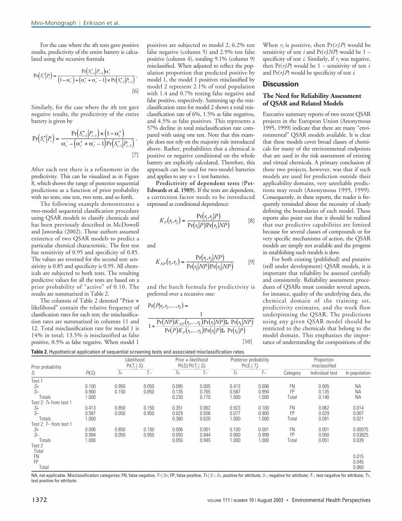
For the case where the ith tests gave positiveresults, predictivity of the entire battery is calcu-lated using the recursive formula

[6]

Similarly, for the case where the ith test gavenegative results, the predictivity of the entirebattery is given by

[7]

After each test there is a refinement in thepredictivity. This can be visualized as in Figure8, which shows the range of posterior sequentialpredictions as a function of prior probabilitywith no tests, one test, two tests, and so forth.

The following example demonstrates atwo-model sequential classification procedureusing QSAR models to classify chemicals andhas been previously described in McDowelland Jaworska (2002). Those authors assumedexistence of two QSAR models to predict aparticular chemical characteristic. The first testhas sensitivity of 0.95 and specificity of 0.85.The values are reversed for the second test: sen-sitivity is 0.85 and specificity is 0.95. All chem-icals are subjected to both tests. The resultingpredictive values for all the tests are based on aprior probability of “active” of 0.10. Theresults are summarized in Table 2.

The columns of Table 2 denoted “Prior ×likelihood” contain the relative frequency ofclassification rates for each test; the misclassifica-tion rates are summarized in columns 11 and12. Total misclassification rate for model 1 is14% in total; 13.5% is misclassified as falsepositive, 0.5% as false negative. When model 1

positives are subjected to model 2, 6.2% testfalse negative (column 5) and 2.9% test falsepositive (column 4), totaling 9.1% (column 9)misclassified. When adjusted to reflect the pop-ulation proportion that predicted positive bymodel 1, the model 1 positives misclassified bymodel 2 represent 2.1% of total populationwith 1.4 and 0.7% testing false negative andfalse positive, respectively. Summing up the mis-classification rates for model 2 shows a total mis-classification rate of 6%, 1.5% as false negatives,and 4.5% as false positives. This represents a57% decline in total misclassification rate com-pared with using one test. Note that this exam-ple does not rely on the majority rule introducedabove. Rather, probabilities that a chemical ispositive or negative conditional on the wholebattery are explicitly calculated. Therefore, thisapproach can be used for two-model batteriesand applies to any n > 1 test batteries.

Predictivity of dependent tests (Pet-Edwards et al. 1989). If the tests are dependent,a correction factor needs to be introducedexpressed as conditional dependence:

[8]

and

[9]

and the batch formula for predictivity ispreferred over a recursive one:

[10]

When ri is positive, then Pr(ri|P) would besensitivity of test i and Pr(ri|NP) would be 1 –specificity of test i. Similarly, if ri was negative,then Pr(ri|P) would be 1 – sensitivity of test iand Pr(ri|P) would be specificity of test i.

Discussion

The Need for Reliability Assessment of QSAR and Related Models

Executive summary reports of two recent QSARprojects in the European Union (Anonymous1995, 1999) indicate that there are many “envi-ronmental” QSAR models available. It is clearthat these models cover broad classes of chemi-cals for many of the environmental endpointsthat are used in the risk assessment of existingand virtual chemicals. A primary conclusion ofthese two projects, however, was that if suchmodels are used for prediction outside theirapplicability domains, very unreliable predic-tions may result (Anonymous 1995, 1999).Consequently, in these reports, the reader is fre-quently reminded about the necessity of clearlydefining the boundaries of each model. Thesereports also point out that it should be realizedthat our predictive capabilities are limitedbecause for several classes of compounds or forvery specific mechanisms of action, the QSARmodels are simply not available and the progressin establishing such models is slow.

For both existing (published) and putative(still under development) QSAR models, it isimportant that reliability be assessed carefullyand consistently. Reliability assessment proce-dures of QSARs must consider several aspects,for instance, quality of the underlying data, thechemical domain of the training set,predictivity estimates, and the work flowunderpinning the QSAR. The predictionsusing any given QSAR model should berestricted to the chemicals that belong to themodel domain. This emphasizes the impor-tance of understanding the compositions of the

Pr , , ,

Pr , Pr Pr

Pr , Pr Pr

P r r r

NP K r r r NP r NPP K r r r P r P

k

NP k k

P k k

1 2

1 1

1 1

1

1

…( ) =

+( ) …( ) ( ) ( )

( ) …( ) ( ) ( )L

L

K r r

r r NP

r NP r NPNP 1 21 2

1 2

,Pr ,

Pr Pr( ) =

( )( ) ( )

K r rr r P

r P r NPP 1 21 2

1 2

,Pr ,

Pr Pr( ) =

( )( ) ( )

PrPr

– – Pr.

– ––

S PS P

S Pi ii– i– i

i i i i i–

++ +

+ +( ) =( ) × −( )

+( ) ( )1 1

1 1

1

1

α

α α α

PrPr

– Pr.

– ––

S PS P

S Pi ii– i– i

i i i i i–

++ +

+ +( ) =( )

−( ) + +( ) × ( )1 1

1 11 1

α

α α α

Mini-Monograph | Eriksson et al.

1372 VOLUME 111 | NUMBER 10 | August 2003 • Environmental Health Perspectives

Table 2. Hypothetical application of sequential screening tests and associated misclassification rates. Likelihood Prior × likelihood Posterior probability Proportion

Prior probability Pr(Tj | Si) Pr(Si) Pr(Tj | Si) Pr(Si | Tj) misclassifiedSi Pr(Si) T+ T– T+ T– T+ T– Category Individual test In population

Test 1S+ 0.100 0.950 0.050 0.095 0.005 0.413 0.006 FN 0.005 NAS– 0.900 0.150 0.850 0.135 0.765 0.587 0.994 FP 0.135 NA

Totals 1.000 0.230 0.770 1.000 1.000 Total 0.140 NATest 2: T+ from test 1

S+ 0.413 0.850 0.150 0.351 0.062 0.923 0.100 FN 0.062 0.014S– 0.587 0.050 0.950 0.029 0.558 0.077 0.900 FP 0.029 0.007

Totals 1.000 0.380 0.620 1.000 1.000 Total 0.091 0.021Test 2: T– from test 1

S+ 0.006 0.850 0.150 0.006 0.001 0.100 0.001 FN 0.001 0.00075S– 0.994 0.050 0.950 0.050 0.944 0.900 0.999 FP 0.050 0.03825

Totals 1.000 0.055 0.945 1.000 1.000 Total 0.051 0.039Test 2

TotalFN 0.015FP 0.045

Total 0.060NA, not applicable. Misclassification categories: FN, false negative, T–| S+; FP, false positive, T+| S–; S+, positive for attribute; S–, negative for attribute; T–, test negative for attribute; T+,test positive for attribute.

intended prediction and validation sets. Tohave faith in model results, analysts must con-sider the model and the chemicals tested todetermine if they are appropriately matched.

QSAR models based on the mechanism ofaction approach tend to rely on expert judg-ment to define the domain. QSAR modelsbased on chemometric or statistical approachestend to use similarity analysis tools where thedecision is made based on formally definedsimilarity of chemicals in the prediction set tothe chemicals in the training set. Similarity ismeasured as the multidimensional distance inthe molecular descriptors space used as para-meters of the evaluated QSAR model or bymatching fragments. If the results of the simi-larity analysis indicate that the given QSARmodel is applicable to the chemicals in the pre-diction set, then and only then the statisticalreliability should be evaluated.

Furthermore, as described by Cronin et al.(2003a, 2003b), national and international val-idation centers have been established in theEuropean Union and in the United States tovalidate alternative (nonanimal) methods. Inthis context, validation is seen as the process bywhich the relevance and reliability of a methodfor a particular purpose undergo independentassessment (Balls et al. 1995). Alternativemethods include not only physicochemical andin vitro tests but also QSAR models and othercomputer-based systems for predicting toxicity.An alternative test based on physicochemical orin vitro data can be regarded as the combina-tion of a test system that generates experimen-tal data and a PM that provides an objectivemeans of extrapolating the data to an expres-sion of toxicity at the in vivo level (Worth andBalls 2001). Thus, a PM is analogous to aQSAR for an in vivo endpoint: the former isbased on experimental physicochemical or invitro data, whereas the latter is based on physic-ochemical descriptors. Criteria for the accept-ability of PMs, which can also be applied toQSARs, are summarized below.

Acceptability CriteriaAs should be evident from the discussionabove, the specification of reasonable accept-ability criteria for the use of QSARs in riskassessment is a multifaceted task. We try todeal with this task by grouping such criteriaaccording to three uniting principles: a) basicmodeling conditions, b) procedural steps, andc) reference values of performance parameters.

Basic QSAR-modeling conditions. Earlier weoutlined basic modeling conditions for applica-bility of QSARs. Checking data for homogene-ity and representativity is easily overlooked.

Homogeneity. Homogeneity means thatthe investigated series of compounds must haverather similar chemical and biological proper-ties, and the mechanism of influence of X on Ymust be the same. Sometimes the data

set/database in question may contain manyclasses of compounds. These classes may bepartially overlapping, barely separated, or com-pletely resolved in the chemical descriptor (X-)space and/or biological property (Y-) space ofthe compounds in question. Because verystrong clustering violates the assumption ofhomogeneity, we recommend that any QSARmodeling be commenced by studying how thecompounds are clustered. PARC methods andcluster analysis techniques are ideally suited forthis. For instance, a plot of the scores of thefirst few summary latent variables will rapidlyreveal groups, trends, discontinuities, outliers,and other anomalies in the data.

Representativity. The composition of thetraining set and the prediction set is of crucialimportance. A representative selection of com-pounds that well span the chemical domain ofinterest should be included in these sets. Oneway to accomplish a representative selection ofcompounds is through SMD (Wold et al.1986). With this approach, test series of com-pounds are defined in which all major struc-tural and chemical properties are systematicallyvaried at the same time.

Taking into account properties of X- andY-data. Earlier we discussed several aspects thatrelate to the nature and quality of the X- and theY-data. It is of utmost importance that anyknowledge about measurement noise be used inthe model-building process. Any estimated“noise” in response data can be beneficially com-pared with the predictive power of the model.For example, if the known or expected noise is±0.3 units for log(1/C), then the PRESD of Yshould be of similar size. Also, if uncertaintyestimates of many variables are available, thisinformation can be used in the scaling of data.

Procedural steps. Before a PM/QSAR isrecommended for regulatory use, it should bemandatory to carry out model validation. First,it is important to make clear what we mean bya valid model. We mean that it predicts muchbetter than chance. In addition, it should havemodel coefficients that have the correct signand with size that is proportional to their sig-nificance to the modeled process. Finally, itshould be consistent with fundamental chemi-cal, biological, and toxicologic knowledge.

To facilitate the handling of real-worlddata sets, a PM/QSAR should a) be associatedwith a defined endpoint that it serves to pre-dict; b) take the form of an unambiguous andeasily applicable algorithm for predicting apharmacotoxicologic endpoint; c) ideally havea clear mechanistic basis; d) be accompanied bya definition of the domain of its applicability—for example, the physicochemical classes ofchemicals for which it is applicable; e) be asso-ciated with a measure of its goodness of fit andinternal goodness of prediction estimated withcross-validation or similar method to a trainingset of data; and f) be assessed in terms of its

predictive power by using data that were notused in the development of the model (externalvalidation).

In the framework of alternative tests, it isconsidered essential that the validation processbe managed under the auspices of an organiza-tion such as the European Centre for theValidation of Alternative Methods (ECVAM)in the European Union that is independent oftest method developers, who have vested inter-ests in their own methods. Organizations suchas ECVAM provide independent advice to theregulatory authorities, who have the responsi-bility for deciding on modifications to existinglegislation (including the addition of new testmethods). Additional criteria have also beendeveloped that relate to the experimental proto-cols of alternative methods (Balls et al. 1995).

Reference values of performance parame-ters for continuous models. A third part in thecompilation of acceptability criteria involvesthe specification of recommended values formodel performance statistics such as R2Y. Thevalues given below must be regarded as a ruleof thumb, and it might be necessary, on acase-by-case basis, to reconsider these, takinginto account the purpose of the model and thevariability of the underlying X- and Y-data(which place limitations on the predictivecapacity). However, it is important that themodel parameter criteria be defined inadvance of the experimental phase of the vali-dation study by the management team of thestudy. This circumvents the possibility thatthe criteria could be weakened, with theimproper aim of “successfully” validating themethod.

Proposed reference values. • R2Y : This limit is conditional on the Q2Y

value.• Q2Y: Q2Y > 0.5 is generally regarded as good,

and Q2Y > 0.9 as excellent. These limits arehighly application dependent.

• R2Y – Q2Y: This difference ought not toexceed 0.3. A substantially larger differenceindicates a) an overfitted model (i.e., a modelmodeling noise); b) presence of irrelevant X-variables, or c) outliers in the data.

• “Background” R2Y and Q2Y: This consists ofthe intercepts of the regression lines of theresponse permutation testing. Results shouldbe R2Y < 0.3 and Q2Y < 0.05 to indicate avalid model. These intercepts can be under-stood as indicating the level of “background”R2Y and Q2Y obtainable with random data.

Condition Number. The conditionnumber is defined as the ratio of the largest tothe smallest singular value of the X-matrix.When this ratio exceeds 10, this indicates thatthe X-variables are significantly correlated, andthe user should refrain from using MLR. It hasbeen recommended to use a ratio 5:1 (com-pounds: X-variables) to diminish the risk ofmulticollinearities among the X-variables.

Mini-Monograph | Methods for validation of QSARs

Environmental Health Perspectives • VOLUME 111 | NUMBER 10 | August 2003 1373

SDEP/PRESD. The SDEP should besimilar to the experimental variability of anendpoint; or, for example, if the known noiseis ±0.3 units for log(1/C), then the SDEP (alsocalled PRESD) of Y should be of similar size.Alternatively, if for instance the variability inthe Y-data is 20% (in variance-metric), then itseems unlikely that R2Y and Q2Y can exceed80% (0.8).

Reference values of performance parametersfor classification models. Similar considerationsapply to the Cooper statistics that are oftenused to assess the predictive performance oftwo-group classification models; that is, fixedacceptability criteria for the sensitivity, speci-ficity, and accuracy (concordance) cannot bedefined for all types of classification modelsbecause the maximal predictive performanceachievable will depend on the quality of thepredictor and response data. Thus, the accep-tance criteria need to be established on a case-by-case basis in advance of the experimentalwork conducted to test the classification model.

Furthermore, the criteria should takeaccount of the purpose of the model. Forexample, if the model is intended to serve as astand-alone test, that is, a complete replace-ment of an animal test, then, as a minimumrequirement, the Cooper statistics should besignificantly greater than 50% (for a two-groupmodel) to ensure that the model is producingpredictions that are significantly better thanchance (Worth and Cronin 2001b). An exam-ple is provided by an ECVAM validation studyin which classification models based on in vitrodata were assessed for their capacity to predictskin corrosion potential (Fentem et al. 1998).In this study, one of the acceptability criteriawas that the sensitivity of each test be greaterthan 70%.

However, if a classification model is beingused in a battery of tests, for example, to iden-tify toxic chemicals that act by a certain mecha-nism of action, the acceptance criteria are likelyto be different. For example, classification mod-els for predicting skin corrosion potential canalso be based on pH data because chemicalsthat are acidic or alkaline in solution areexpected to be corrosive (Worth and Cronin2001b). However, not all corrosive chemicalsexert their toxic action by a pH-dependentmechanism. Thus, a model based on pH datamay therefore detect a small percentage ofknown corrosives in a given test set (i.e., themodel could have a sensitivity less than 50%),but of those chemicals it does identify as corro-sive, there is a high probability of actual corro-sivity [i.e., the model would have a highpositive predictive value, Pr(S+|P+)]. Tests withlow specificity can generate high PVP results inonly two ways: a) the test also has very highspecificity, thus generating very few false posi-tives regardless of prevalence of S– items in thetested population; and b) a high S+ prevalence

(thus low S-prevalence) will also produce fewfalse positives because there are few negatives inthe tested population. This kind of perfor-mance could be regarded as acceptable becauseit is understood the pH model is not a stand-alone model but is used as one component in abattery of models. Such a model is being usedto identify toxic chemicals with a high degree ofcertainty, but it makes no predictions aboutnontoxic chemicals (which would need to beidentified by another test in the battery).

Concluding RemarksTo increase regulatory acceptance and use ofQSARs, and to enhance confidence of QSARpredictions, it is necessary to develop guidanceand acceptability criteria that are not only reli-able but also easy to understand and apply.This has been the intention of this article. Atfirst sight this may seem an overly ambitiousgoal, particularly because many of the criteriaput forward are originally statistical in natureand may therefore have a discouraging effecton the user. However, because we believe sostrongly in the future use of QSARs for chemi-cals management, we have tried to compose abasic set of acceptability criteria so “user-friendly” in nature that each and every QSARanalyst may benefit from them.

In summary, we emphasize the value ofpredictive QSAR models in future chemicalsmanagement, including priority setting, riskassessment, and classification and labeling.These models can be seen as simplifications(approximations) of complicated functionalrelationships that often prevail between chemi-cal and biological properties of compounds.Provided that QSARs are applied with careand common sense and are developed by ful-filling the basic acceptability criteria outlined-here, they constitute an important andpowerful tool definitely deserving a slot in therisk assessor’s toolbox.

REFERENCES

Albano C, Dunn WG III, Edlund U, Johansson E, Nordén B,Sjöström M, et al. 1978. Four levels of pattern recognition.Anal Chem Acta 103:429–443.

Andersson PM, Sjöström M, Wold S, Lundstedt T. 2000.Comparison between physicochemical and calculated mole-cular descriptors. J Chemomr 14:629–642.

[Anonymous]. 1995. QSAR for prediction of fate and effects ofchemicals in the environment. Environmental TechnologiesRTD Programme (DGXII/D-1). Contract EV5V-CT92-0211.Brussels:Commission of the European Union.

———. 1999. Fate and activity modeling of environmental pollu-tants using structure-activity relationships (FAME). Contractnumber ENV4-CT96-0221. Brussels:Environment and ClimateProgramme of the European Union.

Atkinson AC. 1985. Plots, Transformations and Regression.Oxford:Clarendon Press.

Balls M, Blaauboer BJ, Fentem JH, Bruner L, Combes RD, EkwallB, et al. 1995. Practical aspects of the validation of toxicitytest procedures. The report and recommendations ofECVAM workshop 5. Altern Lab Anim 23:129–147.

Baroni M, Costatino G, Cruciani G, Riganelli D, Valigi R, ClementiS. 1993. Generating optimal linear PLS estimations (GOLPE):an advanced chemometric tool for handling 3D-QSAR prob-lems. Quant Struct-Act Rel 12:9–20.

Berglund A, De Rosa MC, Wold S. 1997. Alignment of flexible mol-ecules at their receptor site using 3D descriptors and Hi-PCA. J Comput Aid Mol Des 11:601–612.

Blum DJW, Speece RE. 1990. Determining chemical toxicity toaquatic species. Environ Sci Technol 24:284–293.

Box GEP, Hunter WG, Hunter JS. 1978. Statistics forExperimenter. New York:Wiley.

Burden FR, Rosewarne BR, Winkler DA. 1997. Predicting maxi-mum bioactivity by effective inversion of neural networksusing genetic algorithms. Chemomr Intell Lab 38:127–137.

Burnham AJ, MacGregor JF, Viveros R. 1999. A statistical frame-work for multivariate latent variable regression methodsbased on maximum likelihood. J Chemomr 13: 49–65.

———. 2001. Interpretation of regression coefficients under alatent variable regression model. J Chemomr 15:265–284.

Burnham AJ, Viveros R, MacGregor JF. 1996. Frameworks forlatent variable multivariate regression. J Chemomr 10:31–45.

Cooper JA, Saracci R, Cole P. 1979. Describing the validity of car-cinogen screening tests. Br J Cancer 39:87–89.

Cronin MTD, Jaworska J, Walker JD, Comber M, Watts CD,Worth AP. 2003b. Use of QSARs in international decision-making frameworks to predict ecologic effects and environ-mental fate of chemical substances. Environ HealthPerspect 111:1391–1401.

Cronin MTD, Schultz TW. 2003. Pitfalls in QSAR. J Mol Struct633:39–51.

Cronin MTD, Sinks GD, Schultz TW. 2000. Modeling of toxicity tothe ciliate tetrahymena pyriformis: the aliphatic carbonyldomain. In: Forecasting the Environmental Fate and Effectsof Chemicals (Rainbow PS, Hopkins SP, Crane M, eds).Chichester, UK:Wiley, 113–124.

Cronin MTD, Walker JD, Jaworska J, Comber M, Watts CD, WorthAP. 2003a. Use of QSAR relationships in international deci-sion-making frameworks to predict health effects of chemicalsubstances. Environ Health Perspect 111:1376–1390.

Cruciani G, Watson KA. 1994. Comparative molecular field analy-sis using GRID force-field and GOLPE variable selectionmethods in a study of inhibitors of glycogenphosphorylase b. J Med Chem 37:2589–2601.

Davis L. 1991. Handbook of Genetic Algorithms. New York:VanNostrand Reinhold.

Deneer JW, Sinnige TL, Seinen W, Hermens JLM. 1987.Quantitative structure-activity relationships for the toxicityand bioconcentration factor of nitrobenzene derivativestowards the guppy. Aquat Toxicol 10:115–129.

Deneer JW, van Leeuwen CJ, Seinen W, Maas-Diepeveen JL,Hermens JLM. 1989. QSAR study of the toxicity to nitroben-zene derivatives towards Daphnia magna, Chlorella pyrenoi-dosa and Photobacterium phosphoreum. Aquat Toxicol15:83–97.

Denham MC. 1997. Prediction intervals in partial least squares. JChemomr 11:39–52.

Devillers J. 1996. Genetic algorithms in computer-aided molecu-lar design. In: Genetic Algorithms in Molecular Modeling(Devillers J, ed). London:Academic Press, 131–157.

Devillers J, Balaban AT. 1999. Topological Indices and RelatedDescriptors in QSAR and QSPR. Amsterdam:Gordon BreachScientific Publishers, 811.

Draper NR, Smith H. 1981. Applied Regression Analysis. NewYork:Wiley and Sons.

Dunn WJ III. 1989. Quantitative structural-activity relationships.Chemomr Intell Lab 6:181–189.

Efron B. 1982. The Jackknife, the Bootstrap and Other ResamplingPlanes. Philadelphia:Society for Industrial and AppliedMathematics.

Efron B, Gong G. 1983. A leisurely look at the bootstrap, the jack-knife, and cross-validation. Am Stat 37:36–48.

Efron B, Tibshirani RJ. 1993. An Introduction to the Bootstrap.London:Chapman & Hall.

Eriksson L, Hermens JLM, Johansson E, Verhaar HJM, Wold S.1995. Multivariate analysis of aquatic toxicity data with PLS.Aquat Sci 57:217–241.

Eriksson L, Johansson E. 1996. Multivariate design and modelingin QSAR. Chemomr Intell Lab 34:1–19.

Eriksson L, Johansson E, Kettaneh-Wold N, Wikström C, Wold S.2000b. Design of Experiments—Principles and Applications.Umea, Sweden:Umetrics AB.

Eriksson L, Johansson E, Kettaneh-Wold N, Wold S. 2001. Multi-and Megavariate Data Analysis—Principles andApplications. Umea, Sweden:Umetrics AB.

Eriksson L, Johansson E, Lindgren F, Sjöström M, Wold S. 2002.Megavariate analysis of hierarchical QSAR data. J Comp AidMol Des 16:711–726.

Eriksson L, Johansson E, Lindgren F, Wold S. 2000. GIFI-PLS:modeling of non-linearities and discontinuities in QSAR.Quant Struct-Act Rel 19:345–355.

Mini-Monograph | Eriksson et al.

1374 VOLUME 111 | NUMBER 10 | August 2003 • Environmental Health Perspectives

Eriksson L, Johansson E, Müller M, Wold S. 2000a. On the selec-tion of training set in environmental QSAR when compoundsare clustered. J Chemomr 14:599–616.

Eriksson L, Johansson E, Wold S. 1997. QSAR model validation. In:Quantitative Structure-Activity Relationships inEnvironmental Sciences—VII (Chen F, Schüürmann G, eds).Proceedings of the 7th International Workshop on QSAR inEnvironmental Sciences, 24–28 June 1996, Elsinore,Denmark. Pensacola, FL:SETAC Press, 381–397.

Feinstein AR. 1975. Clinical biostatistics XXXI. On the sensitivity,specificity, and discrimination of diagnostic tests. ClinPharmacol Ther 17:104–116.

Fentem JH, Archer GEB, Balls M, Botham PA, Curren RD, Earl LK,et al. 1998. The ECVAM international validation study on invitro tests for skin corrosivity. 2. Results and evaluation bythe management team. Toxicol In Vitro 12:483–524.

Giraud E, Luttman C, Lavelle F, Riou JF, Mailliet P, Laoui A. 2000.Multivariate data analysis using D-optimal designs, PLS andRSM. A directional approach for the analysis of farnesyl-transferase inhibitors. J Med Chem 43:1807–1816.

Golbraikh A, Tropsha A. 2002. Beware of q2! J Mol Graph Model20:269–276.

Goldberg D.E. 1989. Genetic Algorithms in Search, Optimization &Machine Learning. New York:Addison-Wesley.

Gombar V. 1996. U.S. Patent 6 036 349. Method and apparatus forvalidation of model-based predictions.

Gramatica P, Consonni V, Todeschini R. 1999. QSAR study of thetropospheric degradation of organic compounds.Chemosphere 38:1371–1378.

Gramatica P, Corradi M, Consonni V. 2000. Modeling and predic-tion of soil sorption coefficients of non-ionic organic pesti-cides by different sets of molecular descriptors.Chemosphere 41:763–777.

Gramatica P, Navas N, Todeschini R. 1998. 3D-modelling and pre-diction by WHIM descriptors. Part 9. Chromatographic rela-tive retention time and physico-chemical properties ofpolychlorinated biphenyls (PCBs). Chemomr Intell Lab40:53–63.

Gramatica P, Papa E. 2003. QSAR modeling of bioconcentrationfactor by theoretical molecular descriptors. Quant Struct-Act Rel 22:374–385.

Hibbert DB. 1993. Genetic algorithms in chemistry. ChemomrIntell Lab 19:277–293.

Hong H, Tong W, Fang H, Shi L, Qian X, Wu J, et al. 2002.Prediction of estrogen receptor binding for 58,000 chemicalsusing an integrated computational approach. Environ HealthPerspect 110:29–36.

Höskuldsson A. 1996. Prediction Methods in Science andTechnology. Copenhagen:Thor Publishing.

Jackson JE. 1991. A User’s Guide to Principal Components. NewYork:John Wiley.

Jongman RGH, ter Braak CJF, van Tongeren OFR. 1987. DataAnalysis in Community and Landscape Ecology.Wageningen, the Netherlands:Pudoc.

Jouan-Rimbaud D, Massart DL, de Noord OE. 1996. Random cor-relation in variable selection for multivariate calibration witha genetic algorithm. Chemomr Intell Lab 35:213–220.

Jurs PC. 2002. ADAPT—Automated Data Analysis and PatternRecognition Toolkit. University Park, PA:Pennsylvania StateUniversity. Available: http://research.chem.psu.edu/pcjgroup/ADAPT.html [accessed 23 April 2002].

Karelson M. 2000. Molecular Descriptors in QSAR/QSPR. NewYork:Wiley-InterScience.

Katritzky AR, Lobanov VS, Karelson M. 1994. CODESSA,Reference Manual. Gainesville, FLUniversity of Florida.Available: http://www.semichem.com/codessarefs.html[accessed 19 April 2002].

Kubinyi H. 1994a. Variable selection in QSAR studies. I. An evolu-tionary algorithm. Quant Struct-Act Rel 13:285–294.

———. 1994b. Variable selection in QSAR Studies. II. A highlyefficient combination of systematic search and evolution.Quant Struct-Act Rel 13:393–401.

———. 1996. Evolutionary variable selection in regression andPLS analyses. J Chemomr 10:119–133.

Kulkarni A, Hopfinger AJ, Osborne R, Bruner LH, Thompson ED.2001. Prediction of eye irritation of organic chemicals usingmembrane-interaction QSAR analysis. Toxicol Sci59:335–345.

Langer T. 1994. Molecular similarity determination of heteroaro-matics using CoMFA and multivariate data analysis. QuantStruct-Act Rel 13:402–405.

Leardi R. 1994. Application of a genetic algorithm to feature

selection under full validation conditions and to outlierdetection. J Chemomr 8:65–79.

Leardi R, Boggia R, Terrile M. 1992. Genetic algorithms as a strat-egy for feature selection. J Chemomr 6:267–281.

Lindgren F. 1994. Third Generation PLS—Some Elements andApplications [PhD Thesis]. Umeå, Sweden:Umeå University.

Linusson A, Gottfries J, Lindgren F, Wold S. 2000. Statistical mole-cular design of building blocks for combinatorial chemistry.J Med Chem 43:1320–1328.

Livingstone DJ. 2000. The characterization of chemical structuresusing molecular properties. A survey. J Chem Inf Comput Sci40:195–209.

Marengo E, Todeschini, R. 1992. A new algorithm for optimal, dis-tance—based experimental design. Chemomr Intell Lab16:37–44.

Martens H, Martens M. 2000. Modified jack-knife estimation ofparameter uncertainty in bilinear modeling (PLSR). FoodQual Prefer 11:5–16.

Martin YC, Lin CT, Hetti C, DeLazzer J. 1995. PLS analysis ofdistance matrices to detect nonlinear relationships betweenbiological potency and molecular properties. J Med Chem38:3009–3015.

McDowell RM, Jaworska J. 2002. Bayesian analysis and infer-ence of QSAR predictive model results. SAR QSAR EnvironRes 13:111–125.

Mekenyan O, Bonchev D. 1986. OASIS method for predicting bio-logical activity of chemical compounds. Acta Pharm Jugosl36:225–237.

Mullet GM. 1976. Why regression coefficients have the wrongsign. J Qual Technol 8:121–126.

Nendza M, Müller M. 2000. Discriminating toxicant classes bymode of action: 2. Physico-chemical descriptors. QuantStruct-Act Rel 19:581–598.

OECD. 1998. Harmonized Integrated Hazard Classification Systemfor Human Health and Environmental Effects of ChemicalSubstances. Paris:Organisation for Economic Cooperationand Development.

Pet-Edwards J, Haimes Y, Chankong V, Rosenkranz H, Ennever F.1989. Risk Assessment and Decision Making Using TestsResults—The Carcinogenicity Prediction and BatterySelection Approach. New York:Plenum Press, 211.

Rogers D, Hopfinger AJ. 1994. Application of genetic functionapproximation to quantitative structure-activity relationshipsand quantitative structure-property relationships. J Chem InfComput Sci 34:854–866.

Shao J. 1993. Linear model selection by cross-validation. J AmStat Assoc 88:486–494.

Shi LM, Tong W, Fang H, Perkins R, Wu J, Tu M, et al. 2002. Anintegrated “four-phase” approach for priority setting ofendocrine disruptors—phase I and II for prediction of poten-tial estrogenic endocrine disruptor. SAR/QSAR Environ Res13(1):69–88.

Sjöblom J, Svensson O, Josefson M, Kullberg H, Wold S. 1998. Anevaluation of orthogonal signal correction applied to calibra-tion transfer of near infrared spectra. Chemomr Intell Lab 44:229–244.

Sjöström M, Lindgren Å, Uppgård L. 1997. Joint multivariate quan-titative structure-property and structure-activity relation-ships for a series of technical nonionic surfactants. In:Quantitative Structure-Activity Relationships inEnvironmental Sciences—VII (Schüürmann G, Chen F, eds).Proceedings of the 7th International Workshop on QSAR inEnvironmental Sciences, 24–28 June 1996, Elsinore,Denmark. Pensacola, FL:SETAC Press, 435–449.

Stuper AJ, Jurs PC. 1976. ADAPT: A computer system for auto-mated data analysis using pattern recognition techniques. JChem Inf Comput Sci 16:99–105.

Todeschini R. 1997. MOBY DIGS—Software for MultilinearRegression Analysis and Variable Subset Selection byGenetic Algorithm. Release 2.1 for Windows. Milan:Talete Srl.

Todeschini R, Consonni V. 2000. Handbook of MolecularDescriptors. Weinheim:Wiley-VCH.

Todeschini R, Consonni V, Pavan M. 2001. DRAGON—Softwarefor the Calculation of Molecular Descriptors. Release 1.12for Windows. Available: http://www.disat.unimib/chm[accessed 25 March 2002].

Todeschini R, Gramatica P. 1997. 3D-modelling and prediction byWHIM descriptors. Part 6. Applications of WHIM descriptorsin QSAR studies. Quant Struct-Act Rel 16:120–125.

Todeschini R, Maiocchi A, Consonni V. 1999. The K correlationindex: theory development and its application in chemo-metrics. Chemomr Intell Lab 46:13–29.

Tong W, Perkins R, Fang H, Hong H, Xie Q, Branham W, et al. 2002.Development of quantitative structure-activity relationships(QSARs) and their use for priority setting in testing strategy ofendocrine disruptors. Regul Res Perspect 1(3):1–16.

Topliss JG, Edwards RP. 1979. Chance factors in studies of quan-titative structure-activity relationships. J Med Chem22:1238–1244.

Tosato ML, Piazza R, Chiorboli C, Passerini L, Pino A, Cruciani G,et al. 1992. Application of chemometrics to the screening ofhazardous chemicals. Chemomr Intell Lab 16:155–167.

Tropsha A, Gramatica P, Gombar VJ. 2003. The importance ofbeing earnest: validation is the absolute essential for suc-cessful application and interpretation of QSPR models.Quant Struct-Act Rel 22:69–77.

Tysklind M, Andersson P, Haglund P, Van Bavel B, Rappe C. 1995.Selection of polychlorinated biphenyls for use in quantitativestructure-activity relationships. SAR QSAR Environ Res4:11–19.

Van der Voet H. 1994. Comparing the predictive accuracy of mod-els using a simple randomization test. Chemomr Intell Lab25:313–323.

Vankeerberghen P, Smeyers-Verbeke J, Leardi R, Karr CL,Massart DL. 1995. Robust regression and outlier detectionfor non-linear models using genetic algorithms. ChemomrIntell Lab 28:73–87.

Verhaar HJM, Eriksson L, Sjöström M, Schüürmann G, Seinen W,Hermens JLM. 1994. Modeling the toxicity of organophos-phates: a comparison of the multiple linear regression andPLS regression methods. Quant Struct-Act Rel 13:133–143.

Wahlström B. 1988. The need for new strategies—the OECDexisting chemicals program. In: The Use of QSAR forChemicals Screening—Limitations and Possibilities. Report8/1988. Stockholm:National Chemicals Inspectorate, 1–17.

Wehrens R, Buydens, LMC. 1998. Evolutionary optimization: atutorial. Trends Analyt Chem 17:193–203.

Wehrens R, Putter H, Buydens LMC. 2000. The bootstrap: a tutor-ial. Chemomr Intell Lab 54:35–52.

Wold H. 1982. Soft modeling. The basic design and some exten-sions. In: Systems under Indirect Observation, Vols I, II(Jöreskog KG, Wold H, eds). Amsterdam:North-Holland,18–34.

Wold S. 1992. Nonlinear partial least squares modeling. II. Splineinner relation. Chemomr Intell Lab 14:71–84.

Wold S, Albano C, Dunn WJ III, Esbensen K, Hellberg S,Johansson E, et al. 1983. Pattern recognition: finding andusing regularities in multivariate data. In: Food Research andData Analysis (Martens H, Russwurm H, eds). Essex, UK:Applied Science Publishers, 147–188.

Wold S, Dunn WJ III. 1983. Multivariate quantitative structure-activity relationships (QSAR): conditions for their applicabil-ity. J Chem Inf Comput Sci 23:6–13.

Wold S, Johansson E, Cocchi M. 1993. PLS—partial least squaresprojections to latent structures. In: 3D-QSAR in Drug Design,Theory, Methods, and Applications (Kubinyi H, ed).Leiden:ESCOM Science Publishers, 523–550.

Wold S, Josefson M. 2000. Multivariate calibration of analyticaldata. In: Encyclopedia of Analytical Chemistry (Meyers RA,ed). Chichester, UK:John Wiley & Sons, 9710–9736.

Wold S, Sjöström M, Carlson R, Lundstedt T, Hellberg S,Skagerberg B, et al. 1986. Multivariate design. Anal ChemActa 191:17–32.

Worth AP, Balls M. 2001. The importance of the prediction modelin the development and validation of alternative tests. AlternLab Anim 29:135–143.

Worth AP, Cronin MTD. 2000. Embedded cluster modeling: anovel QSAR method for generating elliptic models of biologi-cal activity. In: Progress in the Reduction, Refinement andReplacement of Animal Experimentation (Balls M, van ZellerA-M, Halder ME, eds). Amsterdam:Elsevier Science,479–491.

———. 2001a. The use of bootstrap resampling to assess theuncertainty of Cooper statistics. Altern Lab Anim 29: 447–459.

———. 2001b. The use of pH measurements to predict thepotential of chemicals to cause acute dermal and ocular tox-icity. Toxicology 169:119–131.

———. In press. The use of discriminant analysis, logistic regres-sion and classification tree analysis in the devlopment ofclassification models for human health effects. J Mol Struct.

Xu L, Zhang WJ. 2001. Comparison of different methods for vari-able selection. Anal Chim Acta 446:477–483.

Mini-Monograph | Methods for validation of QSARs

Environmental Health Perspectives • VOLUME 111 | NUMBER 10 | August 2003 1375